1

Production planning and control of closed-loop supply chains

Karl InderfurthOtto-von-Guericke University Magdeburg, Faculty of Economics and Management,P.O.Box 4120, 39016 Magdeburg, Germany, inderfurth@ww.uni-magdeburg.de

Ruud H. TeunterErasmus University Rotterdam, Econometric Institute, P.O.Box 1738, 3000 DRRotterdam, The Netherland, teunter@few.eur.nl

Econometric Institute Report EI 2001 - 39

1. Introduction

Closed-loop supply chains are characterized by the recovery of returned products. Inmost of these chains (e.g. glass, metal, paper, computers, copiers), used products (alsoknown as cores) are returned by or collected from customers. But returned productscan also come from production facilities within the supply chain (productiondefectives, by-products. In cases with internal returns, recovery is often referred to asrework.

There are two main types of recovery: remanufacturing (product/part recovery) andrecycling (material recovery). Energy recovery via incineration could be consideredas a third type. Combinations of different recovery types are also possible. It is oftennot easy to decide what the best product recovery strategy is. Moreover, for a numberof reasons, it is difficult to plan and control operations in closed-loop supply chains.

Based on a literature review, [Guide 2000] lists the following complicatingcharacteristics for planning and controlling a supply chain with remanufacturing ofexternal returns:1. The requirement for a reverse logistics network2. The uncertain timing and quality of cores3. The disassembly of cores4. The uncertainly in materials recovered from cores5. The problems of stochastic routings for materials and highly variable processing

times.6. The complication of material matching restrictions7. The need to balance returns of cores with demands for remanufactured products.

Many of these complicating issues also characterize the planning and control of asupply chain with remanufacturing of internal returns, though often to a lesser degree.We discuss each of the seven complicating characteristics separately, and alsomention an additional one.

The first three complicating characteristics concern closed-loop supply chains withexternal returns in general (with remanufacturing, recycling, incineration, orcombinations of these recovery options). Cores have to be collected from end-usersbefore they can be recovered. This requires decisions on the number of collectionpoints (take-back centers), incentives for core returns, and transportation methods

brought to you by COREView metadata, citation and similar papers at core.ac.uk

provided by Erasmus University Digital Repository

2

from the collection points to recovery facilities (characteristic 1). The timing of areturn depends on the uncertain life of a product, and the quality of a return isinfluenced by the uncertain intensity of use. These uncertainties complicate capacityplanning and inventory control for recovery operations (characteristic 2). A core canoften be disassembled in many different ways. This requires decisions on the type ofdisassembly, e.g. partial or complete, destructive or non-destructive (characteristic 3).

The remaining characteristics only concern remanufacturing systems. Due to theuncertain quality of cores, there is uncertainty about the possibility to remanufactureparts/materials (characteristic 4). The uncertain quality of cores also causes stochasticroutings for materials and highly variable processing times (characteristic 5). In someindustries (e.g. aviation), it is required that a product/component is remanufacturedusing the original 'serial-number-specific' parts (characteristic 6). Finally, there is aneed to balance core returns and demands for remanufactured products (characteristic7). Imperfect correlation between demands and returns may lead to excess stocks ofrepaired/remanufactured products/components. This holds especially if there aredifferent needs for components/parts of the same product, since thosecomponents/parts are normally disassembled at the same time.

We want to mention an additional complicating characteristic for supply chains whereproducts are manufactured as well as remanufactured, i.e., closed-loop supply chainsof original equipment manufacturers (OEMs). In such chains, the manufacturing andremanufacturing operations have to be coordinated (characteristic 8) to preventcapacity shortages and excess stocks.

The planning and control of supply chains with internal returns also suffers frommany of the above mentioned characteristics (2-5,7,8). Often this is to a lesser degree,due to reduced uncertainties. But on the other hand, returns are immediate and hencejointly planning and controlling production and rework operations can be even morecrucial. Moreover, production and rework operations often share the same resourcesand produced/reworked products compete for the same storage space.

Due to all these complicating characteristics, planning and controlling a closed-loopsupply chain is a complex task. Well-known concepts and techniques forplanning/controlling supply chains are not always (directly) useful for closed-loopsupply chains. Researchers have therefore developed new techniques or proposedmodifications of existing techniques. In this chapter, we will discuss some of theirfindings. We remark that only the, in our view, most practical findings will bediscussed. We refer interested readers to [Gungor and Gupta 1999] for a recent andcomplete overview of all the findings in this research area.

The remainder of the chapter is organized as follows. In Section 2 we restrict ourfocus on disassembly and recovery operations in closed-loop supply chains. Wediscuss methods for finding all possible disassembly/recovery strategies, forcomparing those strategies, for picking the best one, and for scheduling thedisassembly/recovery operations. In Sections 3 and 4 we consider the whole closed-loop supply chain, with respectively external and internal returns. In those sections,we discuss methods for jointly planning and controlling disassembly, recovery,assembly, and (for OEMs) manufacturing operations. We end with some concludingremarks in Section 5.

3

2. Disassembly and recovery

Disassembly may be defined as a systematic method for separating a product into itsconstituent modules, parts, etc. (all to be called assemblies from now on) [Gupta andVeerakamolmal 1994]. Disassembly plays an important role in product recovery[Jovane et al. 1993]. Obviously, assemblies have to be disassembled before they canbe recovered. But even products that are recovered as a whole, e.g. copier machinesthat are sold on a secondary market, often require partial or complete disassembly,followed by cleaning, testing, and possible repair/replacement of assemblies, beforethey can be reassembled. Exceptions are products that can be re-used directly, e.g.containers and unopened commercial returns. Many companies, e.g. Air France,Lufthansa, BMW, Volkswagen, Daimler-Chrysler, Nissan, Océ, Xerox and Philips,operate large-scale disassembly plants.

In many cases disassembly is not simply the reverse of assembly. The operationalaspects of disassembly are quite different from those of assembly systems [Brennan etal. 1994, Lambert 1999]. Some of the key aspects of disassembly systems are thefollowing:• There is uncertainty about the timing and number of core returns.• There is uncertainty about the quality of cores (and their assemblies).• Cores may not need to be disassembled completely.• One can choose between disassembly processes (destructive, non-destructive),

depending on the type of recovery that is aimed for.• There is a large number of demand sources (one for each assembly) and a

corresponding need for multiple demand forecasts.

Due to these complicating aspects, a disassembly system is difficult to control.Below, we will present a list of steps that can be used as a guideline for the control ofa disassembly system. Afterwards, these steps will be discussed in detail. Ideally, allsteps should be considered in the listed order. We remark that product design issues(design for recovery (DFR), design for disassembly (DFD)) are considered to beoutside the scope of this chapter, and are therefore not included in the list. We referinterested readers to [Moyer and Gupta 1997] for a review of DFR and DFD in theelectronics industries. The list of steps is as follows:

1. (for each type of core) Based on technical and environmental restrictions, identifyall possible/efficient disassembly strategies. A disassembly strategy ischaracterized by the disassembly set (the set of assemblies that are disassembled),by the disassembly processes, and by the disassembly sequence. Note that therecan be multiple disassembly strategies with the same disassembly set, but withdifferent disassembly processes and/or a different disassembly sequence. Weremark that the possibilities for disassembling a core can depend on its quality. Ifso, then each disassembly strategy is actually a collection of disassemblystrategies for every possible state of the core. The quality can be assessed throughinitial testing of the core and/or testing of assemblies at a later stage.

2. (for each disassembly strategy of each type of core) Identify the recovery options(e.g. remanufacturing, recycling, incineration) for each of the assemblies in the

4

disassembly set. We remark that the availability of a recovery option for adisassembled assembly can depend on the disassembly processes. For instance,remanufacturing an assembly might be an option after carefully removing it froma core (non-destructive disassembly), but not after tearing it from the core by bruteforce (destructive disassembly). We further remark that the availability of arecovery option for an assembly can depend on its quality (see the first step). Wewill call the combination of a disassembly strategy and of a recovery option foreach of the assemblies in the disassembly set, a disassembly/recovery strategy.

3. (for each disassembly/recovery strategy of each type of core) Determine the netprofit of a strategy, by adding the net profits associated with recovery,disassembly and disposal. That is, add the net recovery revenues for all assembliesin the disassembly set, and subtract all disassembly costs and disposal costs.

4. (for each type of core) Based on a comparison of the net profits ofdisassembly/recovery strategies (and possibly also based on environmentallegislation and/or on a comparison of the environmental impact of strategies),choose the best disassembly/recovery strategy.

5. (for all types of cores together, given the disassembly/recovery strategy for eachtype of core that has been chosen in the previous step) Forecast demands for allassemblies that are in the disassembly set of one or more types of cores, and usethose forecasts to schedule the disassembly operations (disassembly scheduling).Note that an assembly might be in the disassembly set of multiple types of cores,i.e. there can be 'component commonality'. Furthermore, disassembly operationsfor different types of cores might share the same equipment. Hence, schedulingthe disassembly operations for all types of cores together is a complex task.

To the best of our knowledge, no researchers have addressed all these steps. However,many authors discussed one or more of the steps and proposed/tested methods thatcan aid in performing those steps. In the remainder of this section, we will discuss andsometimes modify some of their findings. This is done for Steps 1 and 2 in Section2.1, for Steps 3 and 4 in Section 2.2, and for Step 5 in Section 2.3.

2.1. Steps 1 and 2: Identifying/comparing all possible disassembly strategiesand the associated recovery optionsIn identifying all possible/efficient disassembly strategies for a core, the key role isplayed by the geometrical structure, though mechanical factors such as force andfriction are also relevant [Chen et al. 1997, Dutta and Woo 1995]. The feasibility ofrecovery options associated with a disassembly strategy depends on technical,commercial, and ecological feasibility criteria [Krikke et al. 1998]. We will notdiscuss these technical issues in detail here, since our focus is on the optimal controlof a disassembly system. We shall simply assume that the set of possible/efficientdisassembly strategies and the associated recovery options are given, and focus oncomparing the strategies in that set. For ease of presentation, we first assume thatthere are no variations in the quality of assemblies or uncertainties about disassemblyyields. At the end of this section, however, we will discuss situations where theseassumptions do not hold.

The easiest way to compare disassembly strategies is by representing them in adisassembly graph/tree, based on the geometrical structure of the product [Arai et al.1995, Chen et al. 1997, Dutta and Woo 1995, Johnson and Wang 1998, Krikke et al.

5

1998, Lambert 1997 1999, Penev and de Ron 1996, Pnueli and Zussman 1997,Spengler et al. 1997, Veerakamolmal et al. 1998a, Yan and Gu 1994, Zussman et al.1994]. Recall from the previous section, that the availability of a recovery option for acertain assembly can depend on the processes that are used to disassemble it. Thisholds especially for the remanufacturing option, which is only available if anassembly is obtained via non-destructive disassembly. Hence, it seems best tocompare strategies in a disassembly graph that indicates the availability of recoveryoptions. Furthermore, this graph should allow multiple disassembly strategies with thesame disassembly set, but with different disassembly operations and/or a differentdisassembly sequence (see also the previous section).

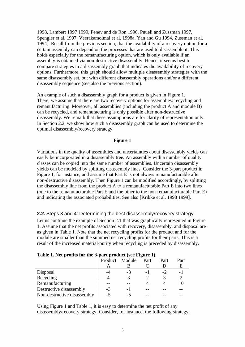
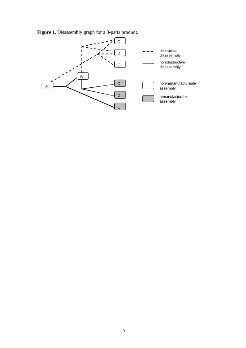
An example of such a disassembly graph for a product is given in Figure 1.There, we assume that there are two recovery options for assemblies: recycling andremanufacturing. Moreover, all assemblies (including the product A and module B)can be recycled, and remanufacturing is only possible after non-destructivedisassembly. We remark that these assumptions are for clarity of representation only.In Section 2.2, we show how such a disassembly graph can be used to determine theoptimal disassembly/recovery strategy.

Figure 1

Variations in the quality of assemblies and uncertainties about disassembly yields caneasily be incorporated in a disassembly tree. An assembly with a number of qualityclasses can be copied into the same number of assemblies. Uncertain disassemblyyields can be modeled by splitting disassembly lines. Consider the 3-part product inFigure 1, for instance, and assume that Part E is not always remanufacturable afternon-destructive disassembly. Then Figure 1 can be modified accordingly, by splittingthe disassembly line from the product A to a remanufacturable Part E into two lines(one to the remanufacturable Part E and the other to the non-remanufacturable Part E)and indicating the associated probabilities. See also [Krikke et al. 1998 1999].

2.2. Steps 3 and 4: Determining the best disassembly/recovery strategyLet us continue the example of Section 2.1 that was graphically represented in Figure1. Assume that the net profits associated with recovery, disassembly, and disposal areas given in Table 1. Note that the net recycling profits for the product and for themodule are smaller than the summed net recycling profits for their parts. This is aresult of the increased material-purity when recycling is preceded by disassembly.

Table 1. Net profits for the 3-part product (see Figure 1).Product

AModule

BPartC

PartD

PartE

Disposal -4 -3 -1 -2 -1Recycling 4 3 2 3 2Remanufacturing -- -- 4 4 10Destructive disassembly -3 -1 -- -- --Non-destructive disassembly -5 -5 -- -- --

Using Figure 1 and Table 1, it is easy to determine the net profit of anydisassembly/recovery strategy. Consider, for instance, the following strategy:

6

disassemble a core in a destructive way, and recycle all three parts. The net profit ofthis policy is –3+2+3+2=4. By comparing the net profits of all possibledisassembly/recovery strategies, the best strategy can be determined. For thisexample, the optimal strategy is: disassemble a core in a non-destructive way,remanufacture Part E, disassemble module B in a destructive way, and recycle Parts Cand D. The associated net profit is –5+10-1+2+3=9.

Of course, for products with many modules/parts, the number of possibledisassembly/recovery strategies can be enormous. Fortunately, the disassembly tree-structure can be exploited to determine the best (profit maximizing) strategy in anefficient way using either dynamic programming (DP) [Krikke et al. 1998 1999,Penev and de Ron 1996] or mixed-integer linear programming (MILP) [Johnson andWang 1998, Lambert 1999, Spengler et al. 1997]. In our view, DP is the easiest andmost insightful approach, and hence we will illustrate its use for the product depictedin Figure 1.

The DP algorithm first considers decisions for the lowest level items (Parts C, D andE in Figure 1) and then 'moves up' in the tree until it reaches the root level (theproduct itself). So we first consider the three parts. Based on the net profits given inTable 1, it is easy to see that (for all parts) recycling is the best available recoveryoption after destructive disassembly, and that remanufacturing is the best option afternon-destructive disassembly. Next consider Module B. The net profits associated withdestructive and non-destructive disassembly are respectively –1+2+3=4 and –5+4+4=3. So Module B should be disassembled in a destructive way, after whichParts C and D should be recycled. Finally consider the product A. The net profitsassociated with destructive and non-destructive disassembly are respectively –3+2+3+2=4 and –5+(-1+2+3)+10=9. So the best strategy is as mentioned before.

The DP algorithm can also be used if assemblies vary in quality and if disassemblyyields are uncertain. Recall from the previous section, that the disassembly tree shouldbe modified in those cases by introducing multiple quality copies of assemblies andby splitting disassembly lines. To illustrate that DP still works, consider the product inFigure 1 again, but assume that Part E is remanufacturable after non-destructivedisassembly in only 80 per cent of the cases (no quality variations or other yielduncertainties). Then the net profits associated with destructive and non-destructivedisassembly of the product are respectively –3+2+3+2=4 and–5+(-1+2+3)+(0.8*10+0.2*2)=7.4. So the best strategy remains unchanged, thoughthe associated net profit is lower.

We end this section with a remark on the net profits for recovery options. Weassumed throughout this section that the profit for recovering an assembly is fixed andhence independent of the number of assemblies that are recovered. As a result, allassemblies of a certain type are recovered in the same (best) way. This seemsreasonable for assemblies that are recycled, since demand for the resulting rawmaterials is (almost) unlimited. But the limited demand/need for remanufacturedassemblies might make it unprofitable to remanufacture all the available assemblies.In such cases, different recovery strategies should be used for cores, depending on thedemand for remanufactured assemblies in various markets. This issue of limiteddemand is also relevant for disassembly scheduling, which will be discussed in thenext section.

7

2.3. Step 5: Disassembly schedulingAfter completing Steps 1 to 4, the disassembly strategy for each type of core is fixed.What remains is to schedule the disassembly operations for all types of cores. This isa complex task. Compared to assembly scheduling in a traditional assemblyenvironment, there are two important complicating factors. First, there is a separatedemand source for each assembly that is in the disassembly set of one or more typesof cores. Second, there is uncertainty about the timing and numbers of core returns.

Researchers [Gupta and Veerakamolmal 1994, Veerakamolmal and Gupta 1998b,Taleb et al. 1997ab] on disassembly scheduling have circumvented thesecomplications. They focus on a planning horizon for which demands are fixed andknown. They further assume that unlimited numbers of cores are available, and thatall disassembly lead times are fixed. Under these strict assumptions, the problem offinding the best disassembly schedule is still tractable.

In fact, under the above restrictions, the optimal disassembly schedule can bedetermined using integer programming (IP) [Veerakamolmal and Gupta 1998b].However, as is remarked in [Taleb and Gupta 1997b], the computational complexityof IP is considerable for large systems. Alternatively, one can use a heuristicprocedure to find a reasonable, though not necessarily optimal, disassembly schedule.We end this section with a summary of the heuristic approach that is proposed in[Taleb and Gupta 1997b]. This approach is only valid under the previously mentionedassumptions, but it does allow for the existence of common parts and/or materials indifferent products.

In the first step of the heuristic approach [Taleb and Gupta 1997b], the 'core'algorithm ignores the timing of the demands for assemblies, and determines a feasible(satisfying all demands over the entire planning horizon) set of cores that have to bedisassembled. In building that feasible set of cores, cores are added sequentially basedon the associated profit and on the remaining demands for assemblies. After a feasibleset has been determined, the 'allocation' algorithm then determines the exact times atwhich the disassembly of cores in the set should start.

8

3. Closed-loop supply chains with external returns

3.1. Planning and Scheduling IssuesIn Section 2, we discussed methods for comparing product disassembly and recoverystrategies. In this section, we will discuss planning and scheduling issues for closed-loop supply chains with external returns if a remanufacturing strategy is chosen. Sowe consider cases where either whole cores or certain assemblies of cores areremanufactured. Recall from Section 1 that these are the most complicated cases froma production planning and control (PPC) point of view. Tasks like demandmanagement, master production scheduling, capacity planning, materialsrequirements planning and production scheduling have to cope with manycomplicating characteristics.

Demand management has to tackle the problem of balancing demands forremanufactured products with returns of remanufacturable cores. Sinceremanufacturing capabilities are restricted by the inflow of cores, demand planningdepends on the degree of knowledge a firm has about the inflow process. Typically,this degree is low. Due to the occurrence of major uncertainties it is very difficult topredict the number of remanufacturable products that will become available in futuretime intervals. Main sources of uncertainty result from limited predictability ofquantity and timing of core returns as well as of core quality and material recoveryrates. Suitable forecasting procedures [e.g. Goh and Varaprasad 1986, Krupp 1992]and core sourcing activities [e.g. Krupp 1993] are measures to limit majoruncertainties. Thus it is obvious that in a remanufacturing environment an integrateddemand and returns management is necessary.

Material and capacity requirements planning faces uncertain processing operationsand uncertain material requirements caused by variations in the quality of usedproducts. This requires restructuring of both the bill of material (BOM) and the bill ofresources (BOR) as well as adjustments in planned lead times. Integrated disassemblyand assembly BOMs and specific (quality-dependent) BOMs for differentdisassembly and remanufacturing options have been suggested [Krupp 1993, Flapper1994]. Yield and leadtime adjustments have to protect against major uncertainties inrecovery rates and processing times. Material matching faces specific challenges insituations where core suppliers stay owners of the products and require that the sameunits be returned [Guide and Srivastava 1998].

Uncertainties in routings and material processing times require modified BORapproaches for both rough-cut capacity planning and capacity requirements planning[Dowlatshahi 2000]. [Guide and Spencer 1997a] propose to modify the BORcalculations using empirical (and regularly updated) occurrence factors for variableroutings and material recovery rate factors for probabilistic recovery yields. Theyshow that modified rough-cut capacity planning BOR techniques outperform thestandard approaches [Guide et al. 1997].

For all these PPC tasks, it is most of all the high level and variety of uncertainties thatrequire modifications in PPC systems for remanufacturing environments. In thisrespect, it is important to distinguish between companies that are only engaged in theremanufacturing business and those that also manufacture original products orcomponents, i.e. OEMs.

9

Uncertainty in the remanufacturing environment may be smaller for OEMs. Betterknowledge of original products and their markets, potential application of leasecontracts, higher efforts in design for remanufacturing and other factors allow forhigher predictability of returns and more standardization and stability in theremanufacturing processes. Thus planning and scheduling tasks are confronted withless complexity. On the other hand, for materials planning there is the additionalproblem of coordinating manufacturing and remanufacturing activities (see Section1). This challenging coordination problem will be treated in more detail in thefollowing section.

3.2. Materials Planning for OEMsMaterials planning in a hybrid manufacturing/remanufacturing environment isconcerned with both disassembly and reassembly stages, in order to take the materialimpact from remanufacturing fully into account. Thus a large number of differentoptions in materials treatment including the option to dispose of parts, components oreven cores has to be integrated in the planning system. Even if uncertainties do notplay a major role, this complex task cannot be fulfilled by simple MRP-basedapproaches, but has to be tackled by advanced planning methods. In [Clegg et al.1995] and [Uzsoy and Venkatachalam 1998] linear programming (LP) models aresuggested for optimal decision support in such difficult materials planning situations.In a more practical-oriented approach, the problem is simplified by separating thedisassembly part from the combined reassembly and manufacturing part. Disassemblyplanning is carried out as described in Section 1 leading to standard options, whichare chosen mainly depending on the quality of returned products. Thus given orexpected return volumes of remanufacturable components or products are availablefor coordinated materials planning for manufacturing and remanufacturing processes.

Under the separation described above, it will be shown how the standard MRPapproach can be extended to incorporate return flows and availability of componentsor products after disassembly and remanufacturing operations in a hybrid system. Weremark that there is widespread use of standard PPC systems, including MRP systemsfor material procurement [Panisset 1988], in the remanufacturing business. This holdsespecially for firms employing a make-to-stock strategy [Guide 2000].

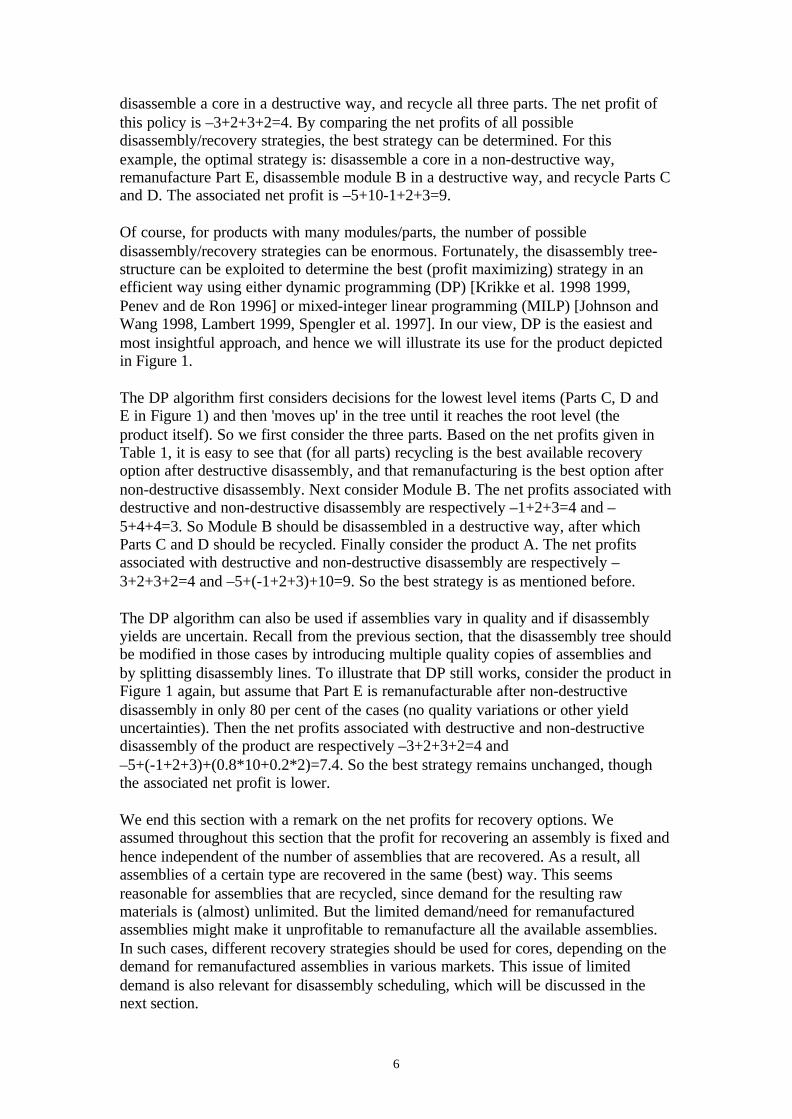
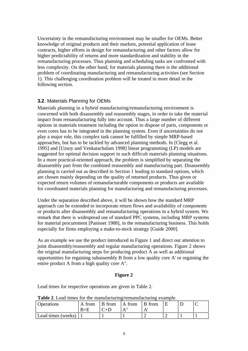
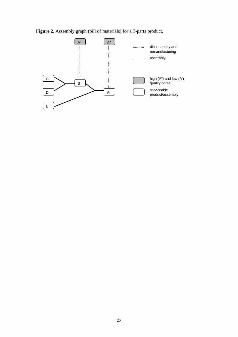
As an example we use the product introduced in Figure 1 and direct our attention tojoint disassembly/reassembly and regular manufacturing operations. Figure 2 showsthe original manufacturing steps for producing product A as well as additionalopportunities for regaining subassembly B from a low quality core A' or regaining theentire product A from a high quality core A".

Figure 2

Lead times for respective operations are given in Table 2.

Table 2. Lead times for the manufacturing/remanufacturing example.Operations A from

B+EB fromC+D

A fromA"

B fromA'

E D C

Lead times (weeks) 1 1 1 2 2 1 1

10

As for systems without remanufacturing options, MRP can be applied in a level-by-level procedure performing the standard steps like exploding the BOM, netting grossrequirements, lotsizing and offsetting order releases. The coordination problem arisesfor those components that can be remanufactured as well as manufactured. In order todemonstrate the MRP extensions necessary for coping with the coordination task, wewill demonstrate the respective MRP calculations for subassembly B which can eitherbe produced from parts C and D or regained from used core A'.

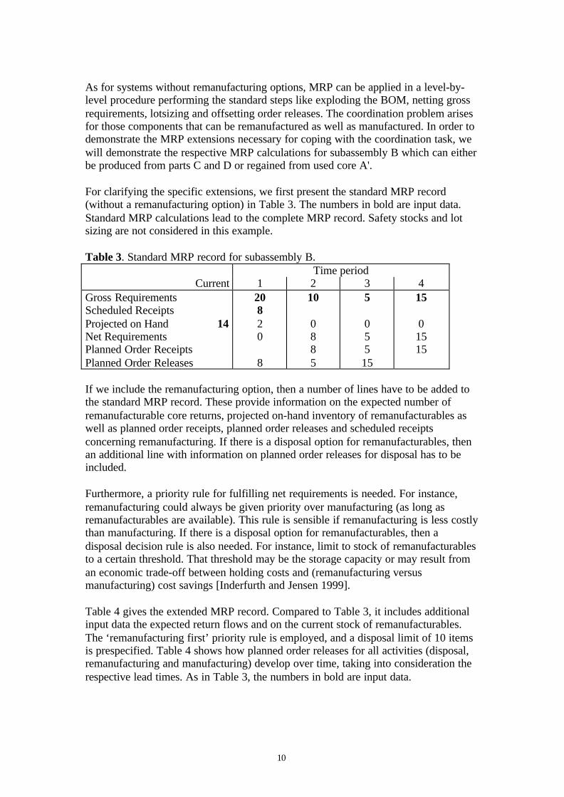
For clarifying the specific extensions, we first present the standard MRP record(without a remanufacturing option) in Table 3. The numbers in bold are input data.Standard MRP calculations lead to the complete MRP record. Safety stocks and lotsizing are not considered in this example.

Table 3. Standard MRP record for subassembly B.Time period

Current 1 2 3 4Gross RequirementsScheduled ReceiptsProjected on Hand 14Net RequirementsPlanned Order ReceiptsPlanned Order Releases

20820

8

10

0885

5

05515

15

01515

If we include the remanufacturing option, then a number of lines have to be added tothe standard MRP record. These provide information on the expected number ofremanufacturable core returns, projected on-hand inventory of remanufacturables aswell as planned order receipts, planned order releases and scheduled receiptsconcerning remanufacturing. If there is a disposal option for remanufacturables, thenan additional line with information on planned order releases for disposal has to beincluded.

Furthermore, a priority rule for fulfilling net requirements is needed. For instance,remanufacturing could always be given priority over manufacturing (as long asremanufacturables are available). This rule is sensible if remanufacturing is less costlythan manufacturing. If there is a disposal option for remanufacturables, then adisposal decision rule is also needed. For instance, limit to stock of remanufacturablesto a certain threshold. That threshold may be the storage capacity or may result froman economic trade-off between holding costs and (remanufacturing versusmanufacturing) cost savings [Inderfurth and Jensen 1999].

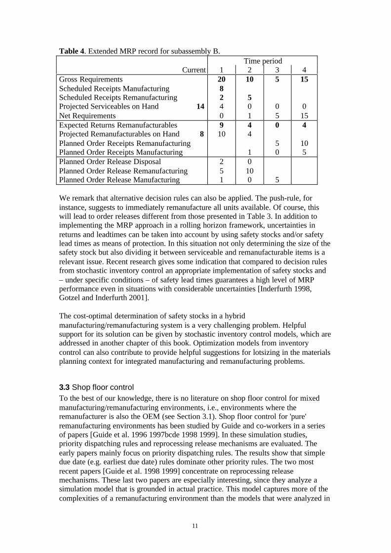
Table 4 gives the extended MRP record. Compared to Table 3, it includes additionalinput data the expected return flows and on the current stock of remanufacturables.The ‘remanufacturing first’ priority rule is employed, and a disposal limit of 10 itemsis prespecified. Table 4 shows how planned order releases for all activities (disposal,remanufacturing and manufacturing) develop over time, taking into consideration therespective lead times. As in Table 3, the numbers in bold are input data.

11

Table 4. Extended MRP record for subassembly B.Time period

Current 1 2 3 4Gross RequirementsScheduled Receipts ManufacturingScheduled Receipts RemanufacturingProjected Serviceables on Hand 14Net Requirements

208240

10

501

5

05

15

015

Expected Returns RemanufacturablesProjected Remanufacturables on Hand 8Planned Order Receipts RemanufacturingPlanned Order Receipts Manufacturing

910

44

1

0

50

4

105

Planned Order Release DisposalPlanned Order Release RemanufacturingPlanned Order Release Manufacturing

251

0100 5

We remark that alternative decision rules can also be applied. The push-rule, forinstance, suggests to immediately remanufacture all units available. Of course, thiswill lead to order releases different from those presented in Table 3. In addition toimplementing the MRP approach in a rolling horizon framework, uncertainties inreturns and leadtimes can be taken into account by using safety stocks and/or safetylead times as means of protection. In this situation not only determining the size of thesafety stock but also dividing it between serviceable and remanufacturable items is arelevant issue. Recent research gives some indication that compared to decision rulesfrom stochastic inventory control an appropriate implementation of safety stocks and– under specific conditions – of safety lead times guarantees a high level of MRPperformance even in situations with considerable uncertainties [Inderfurth 1998,Gotzel and Inderfurth 2001].

The cost-optimal determination of safety stocks in a hybridmanufacturing/remanufacturing system is a very challenging problem. Helpfulsupport for its solution can be given by stochastic inventory control models, which areaddressed in another chapter of this book. Optimization models from inventorycontrol can also contribute to provide helpful suggestions for lotsizing in the materialsplanning context for integrated manufacturing and remanufacturing problems.

3.3 Shop floor controlTo the best of our knowledge, there is no literature on shop floor control for mixedmanufacturing/remanufacturing environments, i.e., environments where theremanufacturer is also the OEM (see Section 3.1). Shop floor control for 'pure'remanufacturing environments has been studied by Guide and co-workers in a seriesof papers [Guide et al. 1996 1997bcde 1998 1999]. In these simulation studies,priority dispatching rules and reprocessing release mechanisms are evaluated. Theearly papers mainly focus on priority dispatching rules. The results show that simpledue date (e.g. earliest due date) rules dominate other priority rules. The two mostrecent papers [Guide et al. 1998 1999] concentrate on reprocessing releasemechanisms. These last two papers are especially interesting, since they analyze asimulation model that is grounded in actual practice. This model captures more of thecomplexities of a remanufacturing environment than the models that were analyzed in

12

earlier studies. We will describe the model below and summarize the results of [Guideet al. 1998 1999].

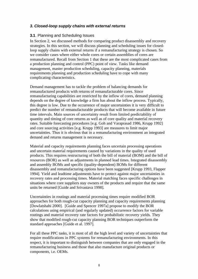
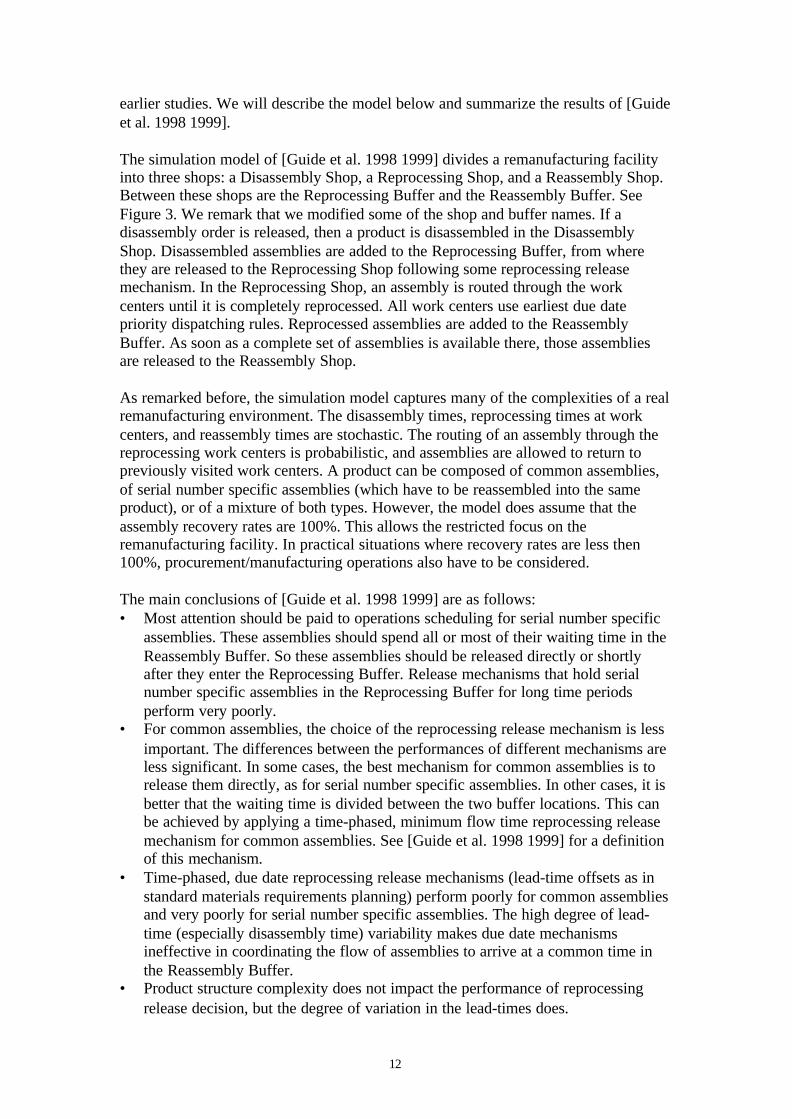
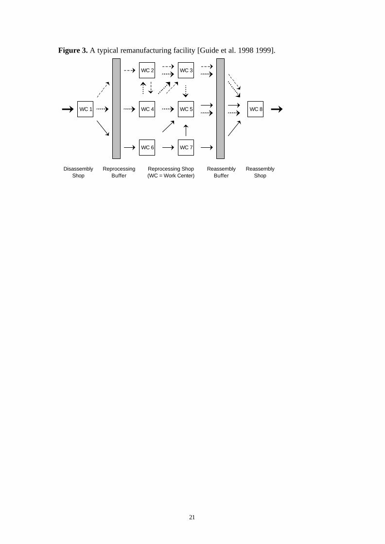
The simulation model of [Guide et al. 1998 1999] divides a remanufacturing facilityinto three shops: a Disassembly Shop, a Reprocessing Shop, and a Reassembly Shop.Between these shops are the Reprocessing Buffer and the Reassembly Buffer. SeeFigure 3. We remark that we modified some of the shop and buffer names. If adisassembly order is released, then a product is disassembled in the DisassemblyShop. Disassembled assemblies are added to the Reprocessing Buffer, from wherethey are released to the Reprocessing Shop following some reprocessing releasemechanism. In the Reprocessing Shop, an assembly is routed through the workcenters until it is completely reprocessed. All work centers use earliest due datepriority dispatching rules. Reprocessed assemblies are added to the ReassemblyBuffer. As soon as a complete set of assemblies is available there, those assembliesare released to the Reassembly Shop.

As remarked before, the simulation model captures many of the complexities of a realremanufacturing environment. The disassembly times, reprocessing times at workcenters, and reassembly times are stochastic. The routing of an assembly through thereprocessing work centers is probabilistic, and assemblies are allowed to return topreviously visited work centers. A product can be composed of common assemblies,of serial number specific assemblies (which have to be reassembled into the sameproduct), or of a mixture of both types. However, the model does assume that theassembly recovery rates are 100%. This allows the restricted focus on theremanufacturing facility. In practical situations where recovery rates are less then100%, procurement/manufacturing operations also have to be considered.

The main conclusions of [Guide et al. 1998 1999] are as follows:• Most attention should be paid to operations scheduling for serial number specific

assemblies. These assemblies should spend all or most of their waiting time in theReassembly Buffer. So these assemblies should be released directly or shortlyafter they enter the Reprocessing Buffer. Release mechanisms that hold serialnumber specific assemblies in the Reprocessing Buffer for long time periodsperform very poorly.

• For common assemblies, the choice of the reprocessing release mechanism is lessimportant. The differences between the performances of different mechanisms areless significant. In some cases, the best mechanism for common assemblies is torelease them directly, as for serial number specific assemblies. In other cases, it isbetter that the waiting time is divided between the two buffer locations. This canbe achieved by applying a time-phased, minimum flow time reprocessing releasemechanism for common assemblies. See [Guide et al. 1998 1999] for a definitionof this mechanism.

• Time-phased, due date reprocessing release mechanisms (lead-time offsets as instandard materials requirements planning) perform poorly for common assembliesand very poorly for serial number specific assemblies. The high degree of lead-time (especially disassembly time) variability makes due date mechanismsineffective in coordinating the flow of assemblies to arrive at a common time inthe Reassembly Buffer.

• Product structure complexity does not impact the performance of reprocessingrelease decision, but the degree of variation in the lead-times does.

13

4 Closed-loop supply chains with internal returns (rework)

A specific situation in the context of closed-loop supply chains is given if returns ofproducts do not come from external customers but from internal production facilities.This occurs when manufacturing not only results in good products, but also inreworkable production rejects. Rework is not only an issue in poor-qualitymanufacturing companies. In some industries, like the semiconductor or the chemicalindustry, production processes are simply not completely controllable. In the latter weoften find production output in the form of by-products, which can be used as inputsagain in the same or related production processes. Rework can be described as the setof all activities that are necessary to bring product rejects into a state that fulfillsprespecified, usually as-good-as-new, qualifications. Thus rework more or lessresembles remanufacturing since it is connected with activities like testing,disassembly, cleaning, processing, and reassembly [Gupta and Chakraborty 1984].However, systems with rework have some specific properties that have to be takeninto consideration for production planning and control.

1. Production decisions immediately influence the return flow of reworkableproducts. Since rework operations replace future production, it is therefore essentialthat production and rework operations are jointly planned. In [Inderfurth and Jensen1999] it is shown how the adjusted MRP approach for materials planning in hybridmanufacturing/remanufacturing systems, described in Section 3.2, can also beextended to systems with rework.

2. The inbound character of rework often is connected with a sharing of the sameresources for production and rework operations. This creates a further need forintegrating production planning and scheduling of both production and rework. Amajor task is setting up priority rules for scheduling rework operations in order tocoordinate production and rework orders in a most cost and/or time-effective way[e.g. Jewkes 1994 1995].

3. Additional complexity in rework situations often arises from storage space andtime restrictions, from perishability of reworkable products and from the existence ofpreset technical lot sizes. Conditions of these kinds are typical for food and chemicalproduction and are widespread in the process industry in general. They ask foradjusted production planning and control systems that still have to be developed insome areas [Flapper et al. 2001]. The most advanced planning systems have been setup in the pharmaceutical and fine chemicals industries, where in-line rework inconnection with a multi-stage batch production creates highly complex planning andcontrol problems. In these cases mixed-integer programming approaches are appliedfor integrated production, materials and capacity planning [Kallrath 1999, Teunter etal. 2000].

4. The return process usually is under closer control for rework systems.Nevertheless, product rejects or by-products normally result from unreliableproduction processes that are characterized by a variable and uncertain yield. Thusuncertainty is also a major issue in production planning and control of rework, even if

14

it may not be as dominant as in the remanufacturing environment. Although there is alot of research addressing production planning under stochastic yields [e.g. Yano andLee 1995], only few contributions consider production systems with rework options.Most consider the problem of buffer stock sizing as a means of protection againstuncertainties in stochastic rework systems [e.g. Robinson et al. 1990, Denardo andLee 1996].

Summarizing we can state that, even though systems with rework resemble closed-loop materials supply systems with external returns in many respects, there are somedifferences which ask for specific production planning and control procedures. Acomprehensive overview of research contributions on rework is given in [Flapper andJensen 2001].

5 Conclusions

More and more supply chains emerge that include a return flow of materials. Manyoriginal equipment manufacturers are nowadays engaged in the remanufacturingbusiness. In many process industries, production defectives and by-products arereworked. These closed-loop supply chains deserve special attention. Productionplanning and control in such hybrid systems is a real challenge, especially due toincreased uncertainties. Even companies that are engaged in remanufacturingoperations only, face more complicated planning situations than traditionalmanufacturing companies.

We pointed out the main complicating characteristics in closed-loop systems withboth remanufacturing and rework, and indicated the need for new ormodified/extended production planning and control approaches. An overview of theexisting scientific contributions was given. But it appeared that we only stand at thebeginning of this line of research, and that many more contributions are needed andexpected in the future.

ReferencesArai E., Uchiyama N. and Igoshi M. (1995) 'Disassembly path generation to verify theassemblability of mechanical products' JSME International Journal – Series C 38(4):805-810.

Brennan L., Gupta S.M. and Taleb K.N. (1994) 'Operations planning issues in anassembly/disassembly environment' International Journal of Operations andProduction Management 14(9): 57-67.

Chen S.F., Oliver J.H., Chou S.Y. and Chen L.L. (1997) 'Parallel disassembly byonion peeling' Journal of Mechanical Design 119(2): 267-274.

Clegg A.J., Williams D.J. and Uzsoy R. (1995) 'Production planning for companieswith remanufacturing capability' Proceedings of the 1995 IEEE Symposium onElectronics and the Environment, IEEE, Orlando FL, 186-191.

15

Denardo, E.V. and Lee, T.Y.S. (1996) ‘Managing uncertainty in a serial productionline’ Operations Research 44: 382-392, 1996.

Dowlatshahi S. (2000) 'Developing a theory of reverse logistics' Interfaces 30(3):143-155.

Dutta D. and Woo T.C. (1995) 'Algorithm for multiple disassembly and parallelassemblies' Journal of Engineering for Industry 117(1): 102-109.

Flapper S.D.P. (1994) 'On the logistics aspects of integrating procurement, productionand recycling by lean and agile-wise manufacturing companies' Proceedings 27th

ISATA International Dedicated Conference on Lean/Agile Manufacturing in theAutomotive Industries, Aachen, Germany, 749-756.

Flapper, S.D.P. and Jensen,T. (2001) ‘Planning and control of rework: a review’International Journal of Production Research, to be published in 2001.

Flapper, S.D.P., Fransoo, J.C., Broekmeulen, R.A.C.M. and Inderfurth, K. (2001)‘Planning and control of rework in the process industries: a review’ ProductionPlanning & Control, to be published in 2001.

Gotzel C. and Inderfurth K. (2001) 'Performance of MRP in product recovery systemswith demand, return and leadtime uncertainties' Preprint 6/2001, Faculty ofEconomics and Management, University of Magdeburg, Germany.

Guide Jr. V.D.R. (2000) 'Production planning and control for remanufacturing:industry practice and research needs' Journal of Operations Management 18(4): 467-483.

Guide Jr. V.D.R. (1996) 'Scheduling using drum-buffer-rope in a remanufacturingenvironment' International Journal of Production Research 34(4): 1081-1091.

Guide Jr. V.D.R., Jayaraman V. and Srivastava R. (1999) 'The effect of lead timevariation on the performance of reprocessing release mechanisms' Computer &Industrial Engineering 36(4): 759-779.

Guide Jr. V.D.R. and Spencer M.S. (1997a) 'Rough-cut capacity planning forremanufacturing firms' Production Planning and Control 8(3): 237-244.

Guide Jr. V.D.R. and Srivastava R. (1997b) 'An evaluation of order release strategiesin a remanufacturing environment' Computers and Operations Research 24(1): 37-47.

Guide Jr. V.D.R. and Srivastava R. (1998) 'Inventory buffers in recoverablemanufacturing' Journal of Operations Management 16(5): 551-568.

Guide Jr. V.D.R., Srivastava R. and Kraus M.E. (1997c) 'Product structure complexityand scheduling of operations in recoverable manufacturing' International Journal ofProduction Research 35(11): 3179-3199.

16

Guide Jr. V.D.R., Srivastava R. and Kraus M.E. (1997d) 'Scheduling policies forremanufacturing' International Journal of Production Economics 48(2): 187-204.

Guide Jr. V.D.R., Srivastava R. and Spencer M.S. (1997e) 'An evaluation of capacityplanning techniques in a remanufacturing environment' International Journal ofProduction Research 35(1): 67-82.

Goh T.N. and Varaprasad N. (1986) 'A statistical methodology for the analysis of thelife-cycle of reusable containers' IIE Transactions 18(1): 42-47, 1986.

Gungor A. and Gupta S.M. (1999) 'Issues in environmentally consciousmanufacturing and product recovery: a survey' Computer & Industrial Engineering36(4): 811-853.

Gupta, T. and Chakraborty, S. (1984) ‘Looping in a multistage production system’International Journal of production research 22: 299-311, 1984.

Gupta S.M. and Veerakamolmal P. (1994) 'Scheduling disassembly' InternationalJournal of Production Research 32(8): 1857-1866.

Inderfurth K. (1998) 'The performance of simple MRP driven policies for a productrecovery system with lead-times' Preprint 32/1998, Faculty of Economics andManagement, University of Magdeburg, Germany.

Inderfurth K. and Jensen T. (1999) 'Analysis of MRP policies with recovery options'in Modelling and Decisions in Economics (ed. by Leopold-Wildburger U. et al.),Heidelberg-New York, 189-228.

Jewkes, E. M. (1994) ‘A queueing analysis of priority-based scheduling rules for asingle-stage manufacturing system with repair’ IIE Transactions 26: 80-86, 1994.

Jewkes, E. M. (1995) ‘Optimal inspection effort and scheduling for a manufacturingprocess with repair’ European Journal of Operational Research 85: 340-351, 1995.

Johnson M.R. and Wang M.H. (1998) 'Economic evaluation of disassemblyoperations for recycling, remanufacturing and reuse' International Journal ofProduction Research 36(12): 3227-3252.

Jovane F., Alting L., Armillotta A., Eversheim W., Feldmann K. and Seliger G.(1993) 'A key issue in product life cycle: disassembly' Annals of the CIRP 42(2): 640-672.

Kallrath, J. (1999) ‘Mixed-integer nonlinear programming applications’ OperationalResearch in Industry (ed. by Ciriani, S. et al.) London , 59-67, 1999.

Krikke H.R., van Harten A. and Schuur P.C. (1998) 'On a medium term productrecovery and disposal strategy for durable assembly products' International Journal ofProduction Research 36(1): 111-139.

17

Krikke H.R., van Harten A. and Schuur P.C. (1999) 'Business case Roteb: recoverystrategies for monitors' Computers & Industrial Engineering 36(4): 739-757.

Krupp J.A.G. (1992) 'Core obsolescence forecasting in remanufacturing' Productionand Inventory Management Journal 33(2): 12-17.

Krupp J.A.G. (1993) 'Structuring bills of material for automotive remanufacturing'Production and Inventory Management Journal 34(4): 46-52.

Lambert A.J.D. (1997) 'Optimal disassembly of complex products' InternationalJournal of Production Research 35(9): 2509-2523.

Lambert A.J.D. (1999) 'Linear programming in disassembly/clustering sequencegeneration' Computer & Industrial Engineering 36(4): 723-738.

Moyer L.K. and Gupta S.M. (1997) 'Environmental concerns andrecycling/disassembly efforts in the electronics industry' Journal of ElectronicsManufacturing 7(1): 1-22.

Panisset B.D. (1988) 'MRP II for repair/refurbish industries' Production and InventoryManagement Journal 29(4): 12-15.

Penev K.D. and de Ron A.J. (1996) 'Determination of a disassembly strategy'International Journal of Production Research 34(2): 495-506.

Pnueli Y. and Zussman E. (1997) 'Evaluating the end-of-life value of a product andimproving it by redesign' International Journal of Production Research 35(4): 921-942.

Robinson, L.W., McClain, J.O. and Thomas. L.J. (1990) ‘The good, the bad and theugly: quality on an assembly line’ International Journal of Production Research 28:963-980, 1990.

Spengler T., Pueckert H., Penkuhn T. and Rentz O. (1997) 'Environmentalintegrated production and recycling management' European Journal of OperationalResearch 97(2): 308-326.

Taleb K.N., Gupta S.M. and Brennan L. (1997a) 'Disassembly of complex productstructures with parts and materials commonality' Production Planning & Control8(3): 255-269.

Taleb K.N. and Gupta S.M. (1997b) 'Disassembly of multiple product structures'Computer & Industrial Engineering 32(4): 949-961.

Teunter, R., Inderfurth, K., Minner, S. and Kleber, R. (2000) ‘Reverse logistics in apharmaceutical company: a case study’ Preprint 15/2000, Faculty of Management andEconomics, University of Magdeburg, Germany, 2000.

18

Uzsoy R. and Venkatachalam G. (1998) 'Supply chain management for companieswith product recovery and remanufacturing capability' International Journal ofEnvironmentally Conscious Design & Manufacturing 7: 59-72.

Veerakamolmal P. and Gupta S.M. (1998a) 'High-mix/low-volume batch of electronicequipment disassembly' Computer & Industrial Engineering 35(1-2): 65-68.

Veerakamolmal P. and Gupta S.M. (1998b) 'Optimal analysis of lot-size balancing formultiproducts selective disassembly', International Journal of Flexible Automationand Integrated Manufacturing 6(3&4): 245-269.

Yan X. and Gu P. (1994) 'A graph based heuristic approach to automated assemblyplanning' Flexible Assembly Systems 73:97-106.

Zussman E., Kriwet A. and Seliger G. (1994) 'Disassembly-oriented assessmentmethodology to support design for recycling' Annals of the CIRP 43(1): 9-14.

19

Figure 1. Disassembly graph for a 3-parts produc t.

A

B

E

C

D

E

C

D

destructive disassembly

non-destructive disassembly

non-remanufacturable assembly

remanufacturable assembly

20

Figure 2. Assembly graph (bill of materials) for a 3-parts product.

A

B

A’

A”

E

C

D

assembly

high (A”) and low (A’) quality cores

serviceable product/assembly

disassembly and remanufacturing

21

Figure 3. A typical remanufacturing facility [Guide et al. 1998 1999].

WC 1

WC 2

WC 4

WC 6

WC 5

WC 7

WC 3

WC 8

Disassembly Shop

Reprocessing Buffer

Reprocessing Shop (WC = Work Center)

Reassembly Buffer

Reassembly Shop