A Model of Flow in a Closed-Loop Thermosyphon Including

J. E. Hart Department of Astrophysical, Planetary

and Atmospheric Sciences, University of Colorado,

Boulder, CO 80309

A Model of Flow in a Closed-Loop Thermosyphon Including the Soret Effect . This theoretical study addresses the nature of convective motions in a toroidal loop of binary fluid oriented in the vertical plane and heated from below. The boundaries of the loop are impermeable, but gradients of the solute can be set up by Soret diffusion in the direction around the loop. The existence and stability of steady solutions are discussed over the Rayleigh number-Soret coefficient parameter plane. When the Soret coefficient is negative, periodic and chaotic oscillations analogous to those of thermohaline convection are predicted. When the Soret coefficient is positive, relaxation oscillations and low Rayleigh number chaotic motions are found. Both sets of phenomena are predicted to occur for realistic thermosyphon parameters.

1 Introduction There has recently been considerable interest in double

diffusive convection phenomena. Much theoretical work has been done on motion between parallel plates maintained at different temperatures and solute concentrations. In practice it is very difficult to create a constant salinity boundary condition in the laboratory, so many of the theories using this assumed boundary condition cannot be checked. However, Soret diffusion, where a molecular flux of a solute is generated by an internal temperature gradient, can generate gradients of solute in a fluid, even with impermeable boundaries. The problem of Soret convection between isothermal plates has been investigated by a number of authors (e.g. [1, 2]) and the theoretically predicted double diffusive instability has been observed in experiments. The Soret-induced instabilities can be either monotonic or overstable. The oscillatory ones were found to compete with a direct thermally driven convection instability, and hysteresis effects have been observed and predicted [3].

This paper addresses the question of whether or not substantial Soret effects might occur in a closed-loop toroidal thermosyphon containing a two-component fluid mixture. Simple one-dimensional models have been proposed for motion in a fluid loop heated from below (Malkus [4]), in a fluid loop driven by thermal and solute boundary conditions (Seigmann and Rubenfeld [5]), and in a thermosyphon driven by angularly displaced nonvertical heating (Hart [6]). The fluid loop models derived in these papers are relatively simple, yet in some instances do very well in describing motions observed in the laboratory. For example, such models yield qualitatively favorable comparisons with the experiments of Creveling et al. [7] and Damerell and Schoenhals [8]. In addition, Gorman et al. [9] have observed chaotic oscillations in a laboratory thermosyphon that seem to be reasonably well described by the loop model even though the motion in the thermosyphon is highly supercritical (in the sense that the thermal stress far exceeds the critical level required for the onset of motion by instability.

Except for the Seigmann and Rubenfeld [5] model, previous work has dealt primarily with a one-component fluid. In [5] the boundary condition of specified solute concentration on the tube wall cannot be realized experimentally. However, since one might naturally want to run a thermosyphon with a two-component fluid (water and antifreeze for example), it

Contributed by the Heat Transfer Division for publication in the JOURNAL OF HEAT TRANSFER. Manuscript received by the Heat Transfer Division August 8, 1984.

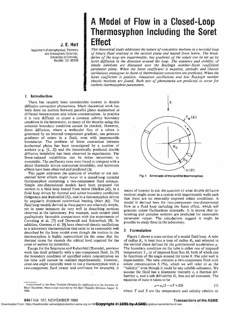
Fig. 1 Schematic of the toroidal thermosyphon

seems of interest to ask the question of what double diffusive motions might occur in a system with impermeable walls such that there are no externally imposed solute conditions. A model is derived here for two-component one-dimensional flow in a fluid loop including the Soret effect, which will generate solute fluctuations internally. It is shown that interesting and complex motions are predicted for reasonable parameter values. The calculations suggest it might be possible to study these in the laboratory.

2 Formulation

Figure 1 shows a cross section of a model fluid loop. A tube of radius Rp is bent into a loop of radius R0 and oriented in the vertical plane defined by the gravitational acceleration g. The boundary condition on the tube is either one of imposed temperature Tw or of imposed heat flux H, both of which can be functions of the angle around the torus 0. The tube wall is impermeable. The tube contains a two-component fluid with solute concentration S (%), which we will refer to as the "salinity" even though it could be any soluble substance. We assume the fluid has a kinematic viscosity v, a thermal dif-fusivity K, and a salt diffusivity Ds that are all constants. The equation of state is taken to be

p = p0(l-ar+/3S) (1)

where T and S are the temperature and salinity relative to

840/ Vol. 107, NOVEMBER 1985 Transactions of the ASME Copyright © 1985 by ASME

Downloaded From: https://heattransfer.asmedigitalcollection.asme.org on 06/30/2019 Terms of Use: http://www.asme.org/about-asme/terms-of-use

ambient values, a is the coefficient of thermal expansion, and /? is the volumetric expansion coefficient (constant).

As discussed in Hurle and Jakeman [2] the molecular flux of salinity Fs in a nonisothermal fluid is given by

FS=DS[T*S(.1-S)\7T-VS] (2)

where F* is the Soret coefficient for the fluid. Since the product DST* is small, the fluctuations of salinity will be small compared to the average value. It is thus customary to consider T = r*S0(l - S0) a constant and write

F,=JDs[rvr-vs] (3) where S0 is now the ambient salinity and S the fluctuation from the mean.

The model equations are derived by averaging the azimuthal momentum equation, the thermodynamic (heat balance) equation, and the salt conservation equation over the diameter of the tube Rp. One assumption is used, that the variables can be replaced by their cross-sectional averages, and in particular that the terms describing the azimuthal advection of heat and salt can be replaced by the advection of the averaged quantities by the cross-sectional average velocity v. This assumption and the generation of one-dimensional models has been discussed in much detail previously (see the discussion and papers referenced in [6]). It is an ad hoc assumption at this point, justified in part by the success of previous models in describing experimental results. The momentum equation is further averaged around the loop (in 8) to form a circulation equation. One then obtains the following equations for the cross-sectionally averaged quantities, which we now call v, T, and S.

dv = gpa r * / 2TT J -IT V

c o s (61) T-a

i (8)S) dd-2jx

Rn (4)

dT {dT S) = -2W^+ /W<5)

dS

~dt

dS

Tt v

R~„

dS

Ro2

d2S

Je1 DST dT

Rn> "W (6)

Here Cp is the specific heat at constant pressure, / the time, h the heat transfer coefficient from the wall to the fluid, and ix the wall stress. In generating the right-hand side of (6) the boundary condition that Fs = 0 at the impermeable wall has been used. However, since there are no wall fluxes of solute,

axial diffusion must be retained as the dominant molecular transport process for the solute. Equation (4) says that the average circulation is generated by the net buoyancy torque exerted by both salinity and temperature, and is retarded by viscous drag at the wall. In equation (5) heat is advected azimuthally by the velocity v, and diffuses in and out of the boundary with transfer coefficient h. As discussed below axial diffusion of heat can be lumped into h for the problem under consideration. Salinity varies along the wall, but there is no salt flux through it. In equation (6) a salt fluctuation is advected azimuthally, and can be generated by Soret diffusion and reduced by molecular diffusion in the azimuthal direction.

Hart [6] discusses various forms of equations (4) and (5) with applied boundary conditions that involve odd symmetry in 6 and a general direction of gravity in the plane of the torus, as well as a heat transfer coefficient that varies in 6 (although when h is not constant that model is only approximate). In order to focus on the Soret-driven component in this problem we will consider h to be constant, H to be zero, and Tw(6) to be an odd function of 6, but even in each half plane 6^0 about 0=±7r /2 . This last requirement means that it is possible to represent Tw(6) as a sine series (as in equation (11)). In addition we take a linear drag law fx = CdVv where Cd

is the drag coefficient and V=2HR0/p0RpCp is a velocity scale. We also use the scale AT=2V2Cd/gcdip for temperature, the scale ATa/f3 for salinity, and the scale R0/Vfor time. With this nondimensionalization equations (4)-(6) become:

dv

~dt = ?\\-v+-V cos (d)(T-S)dd\

dT dT +V =

dt de •T+RaTd(6)

dS dS d2S d2T

v+vTe = -TW+QR*W

(7)

(8)

(9)

Here we have introduced a nondimensional thermal driving function Td with scale ATd, such that T„ = ATd'Td. The parameter T=DJ VR0 is a Lewis number. It is the ratio of the time for a signal to propagate around the loop by advection to the time it takes to do so by molecular diffusion. Pr = R0Cd/Rp is essentially a Prandtl number, and Ra = ATd/AT

A

B C

cd cP

D Ds

E Fs

g h

H

n

Pr Q

Ra

= a stability region defined in Fig. 3

= defined in Fig. 3 = defined in Fig. 3 = drag coefficient = specific heat at constant

pressure = defined in Fig. 3 = solute diffusivity = defined in Fig. 3 = molecular solute flux,

equation (2) = gravitational acceleration = wall heat transfer coef

ficient = wall or internal heating

function, see Fig. 1 = index for Fourier ex

pansion = Prandtl number = R0Cd/Rp

= Soret parameter = Tfi/a = Rayleigh number ATd/AT

Ro

RP

s

So

t T

Td

T„

U,U„

V

V

w,wn

X Y Y

= radius of toroidal loop, Fig. 1

= radius of fluid pipe, Fig. 1 = solute or salinity fluc

tuation = background or ambient

salinity = time = temperature fluctuation = nondimensional thermal

boundary forcing function = d imens iona l t he rma l

forcing function, Fig. 1 = salinity amplitude func

tions, equation (13) = azimuthal velocity = azimuthal velocity scale =

2hR0/RpC„ = salinity amplitude func

tions, equation (13) = nondimensional circulation = temperature amplitude

functions, equation (12)

7 7

a

0 AT

&Tdn

V

r K

X

/* V

p Pa

e T

= temperature amplitude functions, equation (12)

= coefficient of thermal expansion

= volumetric expansivity = temperature scale =

2V2Cd/gaRp

= thermal forcing amplitudes, equation (11), ATd = ATdl

= Soret coefficient = r*s0(i-s0) = thermal conductivity = growth rate for linear

perturbations = wall stress = kinematic viscosity = density = density at ambient con

ditions = azimuthal angle, Fig. 1 = Lewis number - DJ VR0

Journal of Heat Transfer NOVEMBER 1985, Vol. 107/841 Downloaded From: https://heattransfer.asmedigitalcollection.asme.org on 06/30/2019 Terms of Use: http://www.asme.org/about-asme/terms-of-use

is a Rayleigh number (Hart, [6]). The Soret effect enters through the parameter

e ^ W a (10)

With the symmetry arguments imposed on the driving function Tdt it can be represented as

Td= 2J -ATd„sm(nff) (11)

The problem can then be decomposed into Fourier harmonics. Writing

T= Yt Yn cos (nd) + 2„ sin (nd) - Ra sin (6) (12)

S= £ ] U„ cos (nd) + ff„ sin (nd) + QRa sin (6) (13) « = i

and setting v = X(/), and ATd = ATdv equations (8)-(10) reduce to a five-component master problem for the modes X=Xi,Y=Yt, Z=ZX,U=Ui, W= Wx:

dX = Pr[-X+Y-U] dt

dY — = -XZ-Y+R&X dt

dZ

Tt =XY-Z

dU ~di

= -XW- TU- QRSLX- TQY

dW

~dl : --XU-TW-TQZ

(14)

(15)

(16)

(17)

(18)

There is in addition, if ATdn is nonzero for n > 1, an infinite set of slaved modes for n > 1 governed by:

dY„ -~=-Y„-nXZ„ (19)

dZ„ ATJ„ —^ = ~Z„ +nXY„ +Ra — * ctf Arrf

and

tft/„ dt

dWn

dt

• = -TU„-XW-TQYH

= -TWH+XU„-TQZB

(20)

(21)

(22)

In what follows we shall concentrate on the master problem, since the motion X(t) is completely determined by equations (14)—(18). If ATd„ is nonzero for « > 1 , the slaved modes will contribute to the temperature and salinity fields in the loop, but will not affect the dynamics. It is worth mentioning here that as far as the dynamics are concerned, one can simply include axial diffusion of heat in this problem by rewriting h -~ h + KRP/2RQ2. Normally this correction will be of order Rp

2/R02 < < 1.

Note that if Ra is positive, the loop thermal boundary condition has an azimuthal wavenumber 1 component, and the bottom is hotter. Also, the dimensionless Soret parameter Q can be of either sign, since for some mixtures like isopropanol in water the Soret coefficient V* is indeed multisigned depending on the percentage of alcohol in the mixture.

Before proceeding to analyze the master problem, it is useful to estimate the magnitude of the various non-dimensional parameters for a typical physical realization of this problem. The following values are taken from Hurle and Jakeman [2] for an alcohol-water mixture: Ds = 10 "5cm2s _ ' , a = 2 x l O - 4 o C - \ 0 = 0.1, and T* =0.001 "CT1. Assuming the flows will be slow, an estimate of the transfer coefficient using thermal conduction as the dominant transfer mode gives h/pCp = K/Rp = 0.001 cm/s for a 1-cm pipe. Pr = CdVRp/K = V/K using viscous drag CdV — v/Rp. Thus Pr scales with the normal molecular Prandtl number for slow flow in the loop, and thus for typical liquid like water is about 7. The velocity scale Kis then about 0.00lRo/Rp ~ 0.01 cm/s for a 1-cm tube radius and a 10-cm loop radius. For this case the Lewis number r is of order 1 0 - 4 . In many of the numerical integrations described below we use r = 0.001 to save com-

o . i -

Ro°

-O.I -O.I

—

A

^ f 5 ^

B vl \ l

i y i« , v

B

-^ jc£_ I 1

A

1 0 Q

Fig. 2 Stability curves at small Ra and Q for values of r as labeled; Pr = 6.7; (A) origin only real root and is stable; (S) origin monotonically unstable, Soret root exists and is stable

842 / Vol. 107, NOVEMBER 1985 Transactions of the ASME Downloaded From: https://heattransfer.asmedigitalcollection.asme.org on 06/30/2019 Terms of Use: http://www.asme.org/about-asme/terms-of-use

10.0

Ra 1.0

0.1

\ G

A y ^ ^ ^ ^ \ F

E \ ^

A

1

G-

D

^ ^ ^ ^ C

X

B

1 -2.0 -1.0

(B) 0 Q

i.o (A)

Fig. 3 Regime diagram for Pr = 6.7, T = 0.001; (A) and (B) as in Fig. 2; (C) origin monotonicaily unstable, Soret root exists but is unstable; (D) origin monotonicaily unstable, Lorenz root stable; (E) origin and Lorenz root stable, Soret root monotonicaily unstable; (F) origin overstable, Lorenz root stable, Soret root monotonicaily unstable; (G) all roots exist but are unstable; * curve's angle with vertical axis x 10

I0.0

R,

I.O 0 (B) Q

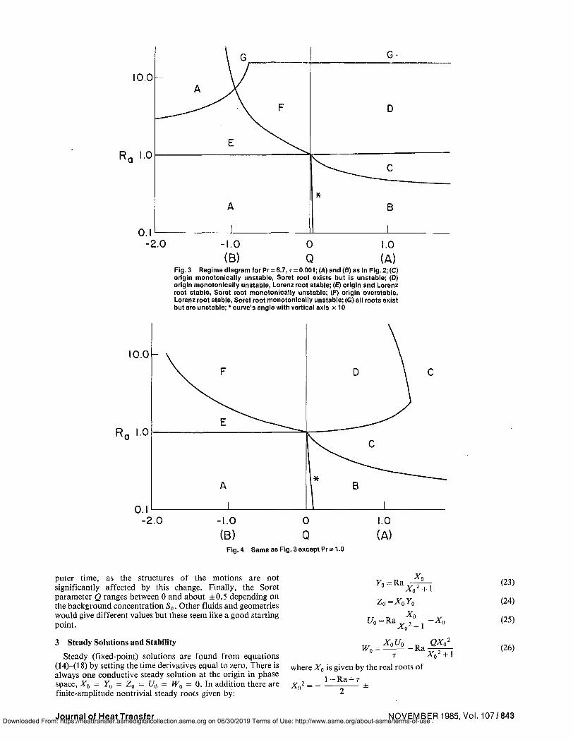
Fig. 4 Same as Fig. 3 except Pr = 1.0

I.O

(A)

puter time, as the structures of the motions are not significantly affected by this change. Finally, the Soret parameter Q ranges between 0 and about ±0.5 depending on the background concentration S0. Other fluids and geometries would give different values but these seem like a good starting point.

3 Steady Solutions and Stability

Steady (fixed-point) solutions are found from equations (14)-(18) by setting the time derivatives equal to zero. There is always one conductive steady solution at the origin in phase space, X0 = Y0 = Z0 = U0 = Wa = 0. In addition there are finite-amplitude nontrivial steady roots given by:

7 n = R a

U0 = Ra ' •O + 1

-Xn

wn = X0U0 „_ QX0

2

- R a X0

2 + l

(23)

(24)

(25)

(26)

where X0 is given by the real roots of

1 - R a + T


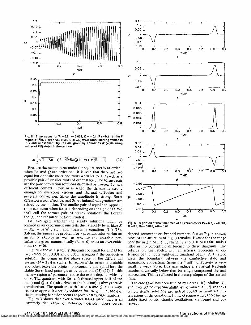
Fig. 5 Time traces for Pr = 6.7, T = 0.001, Q = - 0.1, Ra = 0.11 in the F region of Fig. 3: (a) X(0) = 0.0001, (b) X(0) = 0.3; other starting values in this and subsequent figures are given by equations (23)-(26) using values of X(0) stated in the caption

-V(l-Ra + r)2+4(TRaf2(l + T) + T2(Ra-l) (27)

Because the second term under the square root is of order T when Ra and Q are order one, it is seen that there are two equal but opposite order one roots when Ra > 1, as well as a possible pair of smaller roots of order RaQ-r. The former pair are the pure convection solutions discussed by Lorenz [10] in a different context. They arise when the driving is strong enough to overcome viscous and thermal diffusion and generate convection. Since the amplitude is strong, Soret diffusion is not effective, and Soret-induced salt gradients are stirred by the motion. The smaller pair of equal and opposite roots can occur when Ra < 1 depending on the sign of Q. We shall call the former pair of steady solutions the Lorenz root(s), and the latter the Soret root(s).

To investigate whether the steady solutions might be realized in an experiment one tests their stability by writing X = X0 + X'eXl, etc., and linearizing equations (14)-(18). Solving the eigenvalue problem for X provides information on instability (Xr>0) as well as whether the unstable perturbations grow monotonically (X, = 0) or as an overstable mode (X, * 0).

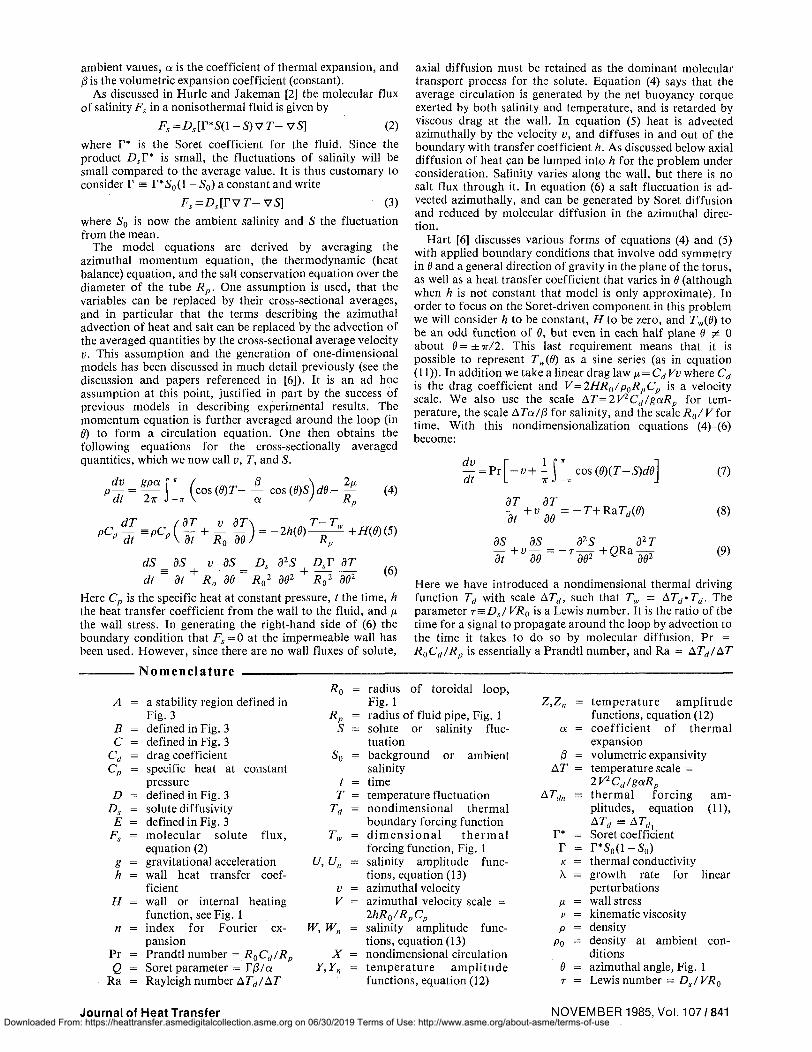
Figure 2 shows a stability diagram for small Ra and Q for two values of T, 0.001 and 0.0001. In region A the conductive solution [the origin in the phase space of the differential system (14)-(18)] is stable. In region B the origin is unstable and orbits leave the origin monotonically and spiral into the stable Soret fixed point given by equations (23)-(27). In this narrow region of parameter space the orbits depend critically on T. The quadrant with Ra < 0 (heated upper half of the loop) and Q > 0 (salt driven to the bottom) is always stable (conductive). The quadrant with Ra < 0 and Q < 0 always seems to approach a steady solution for Ra > - 15. Most of the interesting behavior occurs at positive Rayleigh numbers.

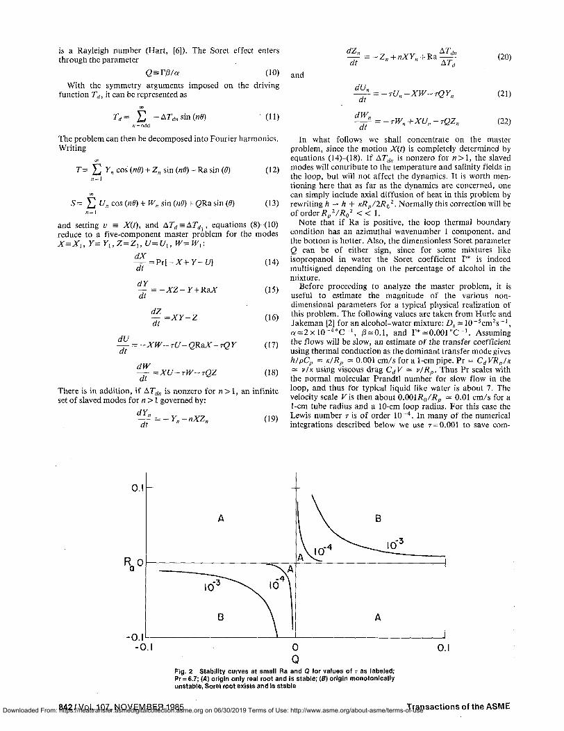
Figure 3 shows that over a wider Ra-Q space there is an extremely rich range of behavior possible. These curves

o.i

0.05

o

- 0 . 0 5

- 0 . 1

^ , / u

- 0 . 0 7

- 0 . 0 8

-0 .09

-0 .1

-0 .11

I 1 1

i i i

1 — 1 •••• - \

• " " ' \

\ \^*~

i i i

0 0.1 0.2 0.3 0.4 0.5 0.6 0.7

TIME e

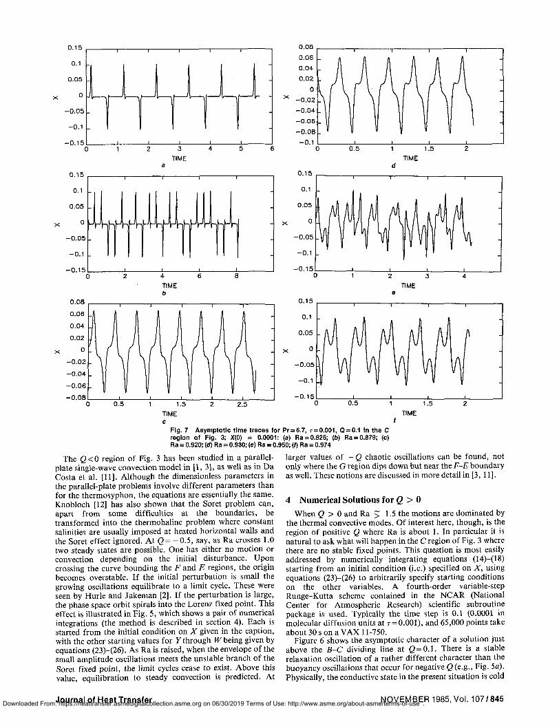
Fig. 6 A portion of the time trace of all variables for Pr = 6.7, T = 0.001, Q = 0.1, Ra = 0.825, X(0) = 0.01

depend somewhat on Prandtl number. But as Fig. 4 shows, most of the structure of Fig. 3 remains. Except for the range near the origin of Fig. 3, changing r to 0.01 or 0.0001 makes little or no perceptible difference to these diagrams. The bifurcation line labeled with an asterisk represents an extension of the upper right-hand quadrant of Fig. 2. This line gives the boundary between the conductive state and monotonic convection. Since the "salt" diffusivity is very small, a weak Soret flux can reduce the critical Rayleigh number drastically below that for single-component thermal convection. This is reflected in the steep slopes of the starred lines.

The case Q = 0 has been studied by Lorenz [10], Malkus [4], and investigated experimentally by Gorman et al. [9]. In the/? region steady solutions are indeed found in numerical integrations of the equations. In the G region where there are no stable fixed points, chaotic oscillations are found and observed.

844/Vol. 107, NOVEMBER 1985 Transactions of the ASM E Downloaded From: https://heattransfer.asmedigitalcollection.asme.org on 06/30/2019 Terms of Use: http://www.asme.org/about-asme/terms-of-use

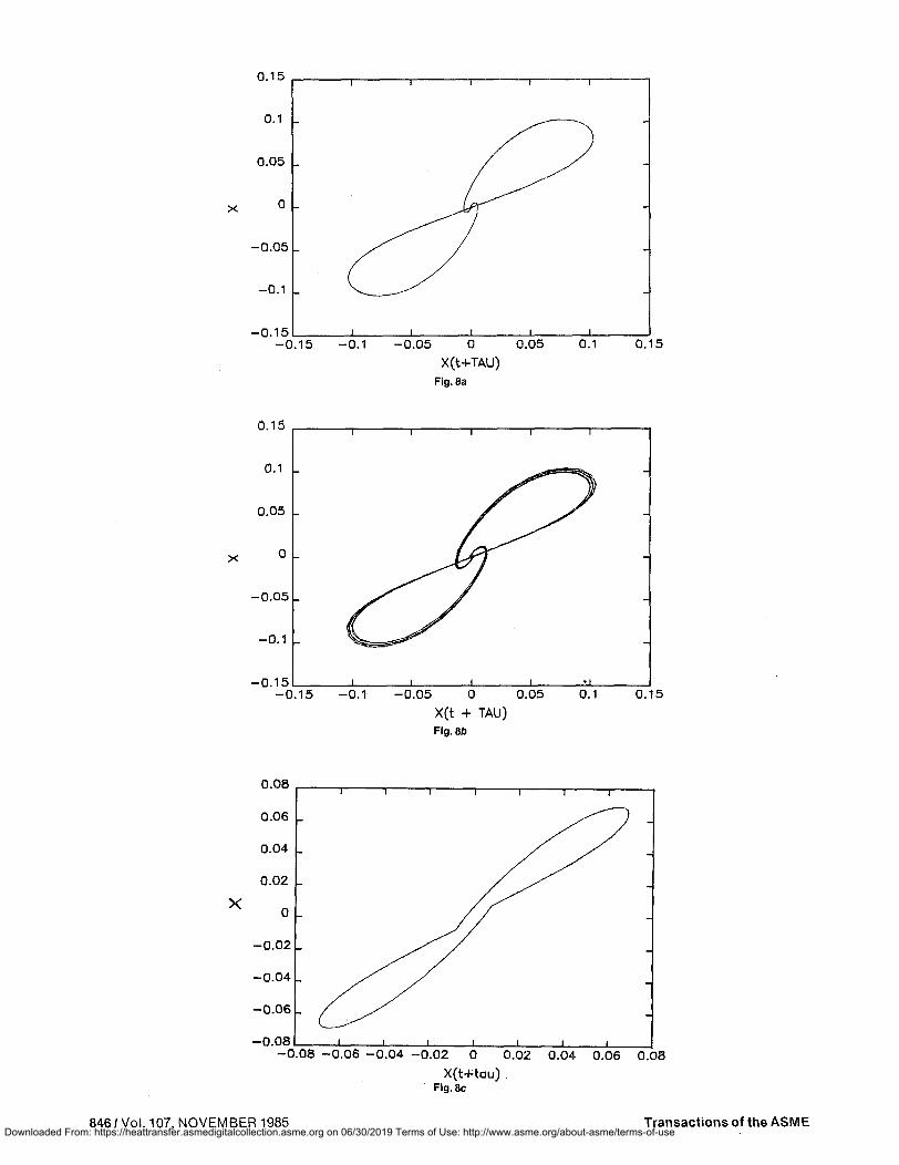
TIME c

Fig. 7 Asymptotic time traces for Pr = 6.7, T = 0.001, Q = 0.1 in the C region of Fig. 3; X(0) = 0.0001: (a) Ra = 0.825; (b) Ra = 0.879; (c) Ra = 0.920; (d) Ra = 0.930; (e) Ra = 0.950; (f) Ra = 0.974

TIME

The Q<0 region of Fig. 3 has been studied in a parallel-plate single-wave convection model in [1, 3], as well as in Da Costa et al. [11]. Although the dimensionless parameters in the parallel-plate problems involve different parameters than for the thermosyphon, the equations are essentially the same. Knobloch [12] has also shown that the Soret problem can, apart from some difficulties at the boundaries, be transformed into the thermohaline problem where constant salinities are usually imposed at heated horizontal walls and the Soret effect ignored. At Q= -0.5, say, as Ra crosses 1.0 two steady states are possible. One has either no motion or convection depending on the initial disturbance. Upon crossing the curve bounding the F and E regions, the origin becomes overstable. If the initial perturbation is small the growing oscillations equilibrate to a limit cycle. These were seen by Hurle and Jakeman [2]. If the perturbation is large, the phase space orbit spirals into the Lorenz fixed point. This effect is illustrated in Fig. 5, which shows a pair of numerical integrations (the method is described in section 4). Each is started from the initial condition on X given in the caption, with the other starting values for Y through W being given by equations (23)-(26). As Ra is raised, when the envelope of the small amplitude oscillations meets the unstable branch of the Soret fixed point, the limit cycles cease to exist. Above this value, equilibration to steady convection is predicted. At

larger values of - Q chaotic oscillations can be found, not only where the G region dips down but near the F-E boundary as well. These notions are discussed in more detail in [3, 11].

4 Numerical Solutions for Q > 0

When Q > 0 and Ra > 1.5 the motions are dominated by the thermal convective modes. Of interest here, though, is the region of positive Q where Ra is about 1. In particular it is natural to ask what will happen in the C region of Fig. 3 where there are no stable fixed points. This question is most easily addressed by numerically integrating equations (14)-(18) starting from an initial condition (i.e.) specified on X, using equations (23)-(26) to arbitrarily specify starting conditions on the other variables. A fourth-order variable-step Runge-Kutta scheme contained in the NCAR (National Center for Atmospheric Research) scientific subroutine package is used. Typically the time step is 0.1 (0.0001 in molecular diffusion units at T = 0.001), and 65,000 points take about 30 s on a VAX 11-750.

Figure 6 shows the asymptotic character of a solution just above the B-C dividing line at £> = 0.1. There is a stable relaxation oscillation of a rather different character than the buoyancy oscillations that occur for negative Q (e.g., Fig. 5a). Physically, the conductive state in the present situation is cold


0.15

0.05 .

-0 .05

-0.1

-0 .15 -0.15 -0.1 -0.05 0 0.05

X(t+TAU) Fig. 8a

0.15

0.1S

0.1 _

0.05 .

-0.05

-0.1

-0 .15 -0.15 -0 .1

X(t + TAU) Fig. 8b

0.15

-0 .08 -0.08 -0.06 -0.04 -0.02 0 0.02 0.04 0.06 0.08

X(t+tau) Fig. 8c

846/ Vol. 107, NOVEMBER 1985 Transactions of the ASME Downloaded From: https://heattransfer.asmedigitalcollection.asme.org on 06/30/2019 Terms of Use: http://www.asme.org/about-asme/terms-of-use

-0 .08 -0.08 -0 .06 -0 .04 -0 .02 0 0.02 0.04 0.06 0.08

x X(t+tau) Fig. 8d

0.15

0.1

0.05

0

-0 .05

-0 .1

-0 .15

I I

i i

1 i

/%%zSz^^

$f /

-

-

1 1 -0.15 -0 .1 -0.05 0 0.05

X(t+tau) Fig. 8e

0.1 0.15

0.15

0.1

0.05

-0 .05 .

-0 .1 .

-0 .15 -0.15 -0 .1 -0.05 0.05

X(t+tau) Fig. 8f

0.15


-0.098

- 0 . 1 - 0 . 0 9 8 - 0 . 0 9 6 - 0 . 0 9 4 - 0 . 0 9 2 - 0 . 0 9 - 0 . 0 8 8 - 0 . 0 8 6

W(t+tau) Fig. 8g

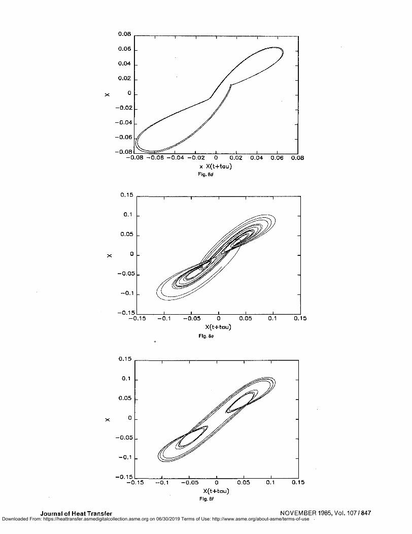
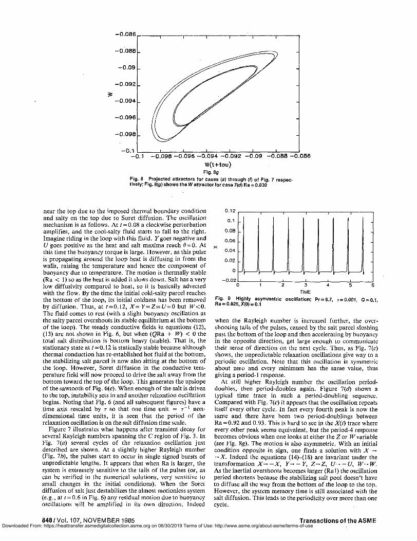
Fig. 8 Projected attractors for cases (a) through (r) ot Fig. 7 respectively; Fig. 8(g) shows the W attractor for case 7(d) Ra = 0.930

near the top due to the imposed thermal boundary condition and salty on the top due to Soret diffusion. The oscillation mechanism is as follows. At / = 0.08 a clockwise perturbation amplifies, and the cool-salty fluid starts to fall to the right. Imagine riding in the loop with this fluid. Fgoes negative and U goes positive as the heat and salt maxima reach 6 = 0. At this time the buoyancy torque is large. However, as this pulse is propagating around the loop heat is diffusing in from the walls, raising the temperature and hence the component of buoyancy due to temperature. The motion is thermally stable (Ra < 1) so as the heat is added it slows down. Salt has a very low diffusivity compared to heat, so it is basically advected with the flow. By the time the initial cold-salty parcel reaches the bottom of the loop, its initial coldness has been removed by diffusion. Thus, at f = 0.12, X= Y=Z= t/=0 but W<0. The fluid comes to rest (with a slight buoyancy oscillation as the salty parcel overshoots its stable equilibrium at the bottom of the loop). The steady conductive fields in equations (12), (13) are not shown in Fig. 6, but when (QRa + W) < 0 the total salt distribution is bottom heavy (stable). That is, the stationary state at (=0.12 is statically stable because although thermal conduction has re-established hot fluid at the bottom, the stabilizing salt parcel is now also sitting at the bottom of the loop. However, Soret diffusion in the conductive temperature field will now proceed to drive the salt away from the bottom toward the top of the loop. This generates the upslope of the sawtooth of Fig. 6(e). When enough of the salt is driven to the top, instability sets in and another relaxation oscillation begins. Noting that Fig. 6 (and all subsequent figures) have a time axis rescaled by T SO that one time unit = T~! non-dimensional time units, it is seen that the period of the relaxation oscillation is on the salt diffusion time scale.

Figure 7 illustrates what happens after transient decay for several Rayleigh numbers spanning the C region of Fig. 3. In Fig. 1(a) several cycles of the relaxation oscillation just described are shown. At a slightly higher Rayleigh number (Fig. lb), the pulses start to occur in single signed bursts of unpredictable lengths. It appears that when Ra is larger, the system is extremely sensitive to the tails of the pulses (or, as can be verified in the numerical solutions, very sensitive to small changes in the initial conditions). When the Soret diffusion of salt just destabilizes the almost motionless system (e.g., at / = 0.6 in Fig. 6) any residual motion due to buoyancy oscillations will be amplified in its own direction. Indeed

0.12

0.1

0.08

0.06

0.04

0.02

0

-0.02

-

-

i i i

,

i

j

1

_

---

-

i r i r r r i i i i i

0 1 2 3 4 5 6 TIME

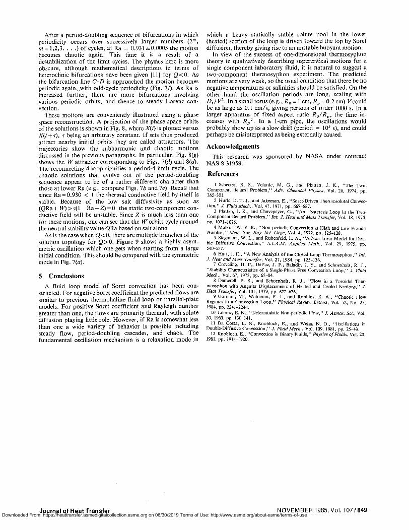
Fig. 9 Highly asymmetric oscillation; Pr = 6.7, T = 0.001, Q = 0 1 Ra = 0.825, X(0) = 0.1

when the Rayleigh number is increased further, the overshooting tails of the pulses, caused by the salt parcel sloshing past the bottom of the loop and then accelerating by buoyancy in the opposite direction, get large enough to communicate their sense of direction on the next cycle. Thus, as Fig. 7(c) shows, the unpredictable relaxation oscillations give way to a periodic oscillation. Note that this oscillation is symmetric about zero and every minimum has the same value, thus giving a period-1 response.

At still higher Rayleigh number the oscillation period-doubles, then period-doubles again. Figure 1(d) shows a typical time trace in such a period-doubling sequence. Compared with Fig. 1(c) it appears that the oscillation repeats itself every other cycle. In fact every fourth peak is now the same and there have been two period-doublings between Ra = 0.92 and 0.93. This is hard to see in the X(t) trace where every other peak seems equivalent, but the period-4 response becomes obvious when one looks at either the Z or W variable (see Fig. 8g). The motion is also asymmetric. With an initial condition opposite in sign, one finds a solution with X — —X. Indeed the equations (14)-(18) are invariant under the transformation X- -X, Y--Y, Z~Z, U- - U, W-* W. As the inertial overshoots becomes larger (Rat) the oscillation period shortens because the stabilizing salt pool doesn't have to diffuse all the way from the bottom of the loop to the top. However, the system memory time is still associated with the salt diffusion. This leads to the periodicity over more than one cycle.

848/Vol. 107, NOVEMBER 1985 Transactions of the ASME Downloaded From: https://heattransfer.asmedigitalcollection.asme.org on 06/30/2019 Terms of Use: http://www.asme.org/about-asme/terms-of-use

After a period-doubling sequence of bifurcations in which periodicity occurs over successively larger numbers (2"\ m = 1,2,3. . . .) of cycles, at Ra = 0.931 ±0.0005 the motion becomes chaotic again. This time it is a result of a destabilization of the limit cycles. The physics here is more obscure, although mathematical descriptions in terms of heteroclinic bifurcations have been given [11] for Q<0. As the bifurcation line C-D is approached the motion becomes periodic again, with odd-cycle periodicity (Fig. If). As Ra is increased further, there are more bifurcations involving various periodic orbits, and thence to steady Lorenz convection.

These motions are conveniently illustrated using a phase space reconstruction. A projection of the phase space orbits of the solutions is shown in Fig. 8, where X(f) is plotted versus X(t+r), 7 being an arbitrary constant. If sets thus produced attract nearby initial orbits they are called attractors. The trajectories show the subharmonic and chaotic motions discussed in the previous paragraphs. In particular, Fig. 8(g) shows the Wattractor corresponding to Figs. 1(d) and 8(e0-The reconnecting 4-loop signifies a period-4 limit cycle. The chaotic solutions that evolve out of the period-doubling sequence appear to be of a rather different character than those at lower Ra (e.g., compare Figs, lb and le). Recall that since Ra = 0.930 < 1 the thermal conductive field by itself is stable. Because of the low salt diffusivity as soon as (QRa + W) > 7<1 - Ra - Z) = 0 the static two-component conductive field will be unstable. Since Z is much less than one for these motions, one can see that the W orbits cycle around the neutral stability value QRa based on salt alone.

As is the case when Q<0, there are multiple branches of the solution topology for Q>0. Figure 9 shows a highly asymmetric oscillation which one gets when starting from a large initial condition. This should be compared with the symmetric mode in Fig. 7(a).

5 Conclusions A fluid loop model of Soret convection has been con

structed. For negative Soret coefficient the predicted flows are similar to previous thermohaline fluid loop or parallel-plate models. For positive Soret coefficient and Rayleigh number greater than one, the flows are primarily thermal, with solute diffusion playing little role. However, if Ra is somewhat less than one a wide variety of behavior is possible including steady flow, period-doubling cascades, and chaos. The fundamental oscillation mechanism is a relaxation mode in

which a heavy statically stable solute pool in the lower (heated) section of the loop is driven toward the top by Soret diffusion, thereby giving rise to an unstable buoyant motion.

In view cf the success of one-dimensional thermosyphon theory in qualitatively describing supercritical motions for a single component laboratory fluid, it is natural to suggest a two-component thermosyphon experiment. The predicted motions are very weak, so the usual condition that there be no negative temperatures or salinities should be satisfied. On the other hand the oscillation periods are long, scaling with DJV2. In a small torus (e.g., i?0 = l cm, ̂ p =0.2 cm) F could be as large as 0.1 cm/s, giving periods of order 1000 s. In a larger apparatus of fixed aspect ratio R0/Rp, the time increases with Rp

2. In a 1-cm pipe, the oscillations would probably show up as a slow drift (period = 105 s), and could perhaps be misinterpreted as being externally caused.

Acknowledgments

This research was sponsored by NASA under contract NAS-8-31958.

References

1 Schecter, R. S., Velarde, M. O., and Platten, J. K., "The Two-Component Benard Problem," Adv. Chemical Physics, Vol. 26, 1974, pp. 265-301.

2 Hurle, D. T. J., and Jakeman, E., "Soret-Driven Thermosolutal Convection," J. Fluid Mech., Vol. 47, 1971, pp. 667-687.

3 Platten, J. K., and Chavepeyer, G., "An Hysteresis Loop in the Two-Component Benard Problem," Int. J. Heat and Mass Transfer, Vol. 18, 1975, pp. 1071-1075.

4 Malkus, W. V. R., "Non-periodic Convection at High and Low Prandtl Number," Mem. Soc. Roy. Sci. Liege, Vol. 4, 1972, pp. 125-128.

5 Siegmann, W. L., and Rubenfeld, L. A., "A Non-linear Model for Double Diffusive Convection," S.I.A.M. Applied Math., Vol. 29, 1975, pp. 540-557.

6 Hart, J. E., "A New Analysis of the Closed Loop Thermosyphon," Int. J. Heat and Mass Transfer, Vol. 27, 1984, pp. 125-136.

7 Creveling, H. F., DePaz, J. F., Baladir, J. Y., and Schoenhals, R. J., "Stability Characteristics of a Single-Phase Free Convection Loop," J. Fluid Mech., Vol. 67, 1975, pp. 65-84.

8 Damerell, P. S., and Schoenhals, R. J., "Flow in a Toroidal Thermosyphon with Angular Displacements of Heated and Cooled Sections," J. Heat Transfer, Vol. 101, 1979, pp. 672-676.

9 Gorman, M., Widmann, P. J., and Robbins, K. A., "Chaotic Flow Regimes in a Convection Loop," Physical Review Letters, Vol. 52, No. 25, 1984, pp. 2241-2244.

10 Lorenz, E. N., "Deterministic Non-periodic Flow," J. Atmos. Sci., Vol. 20, 1963, pp. 130-141.

11 Da Costa, L. N., Knobloch, E., and Weiss, N. O., "Oscillations in Double-Diffusive Convection," J. Fluid Mech., Vol. 109, 1981, pp. 25-43.

12 Knobloch, E., "Convection in Binary Fluids," Physics of Fluids, Vol. 23, 1981, pp. 1918-1920.


Documents

A Model of Flow in a Closed-Loop Thermosyphon Including