Embed Size (px)
Citation preview
arX
iv:1
110.
2210
v1 [
cs.C
V]
10
Oct
201
1Journal of Artificial Intelligence Research 28 (2007) 349–391 Submitted 06/06; published 03/07
Closed-Loop Learning of Visual Control Policies
Sebastien Jodogne [email protected]
Justus H. Piater [email protected]
Montefiore Institute (B28)
University of Liege, B-4000 Liege, Belgium
Abstract
In this paper we present a general, flexible framework for learning mappings from im-ages to actions by interacting with the environment. The basic idea is to introduce afeature-based image classifier in front of a reinforcement learning algorithm. The classifierpartitions the visual space according to the presence or absence of few highly informa-tive local descriptors that are incrementally selected in a sequence of attempts to removeperceptual aliasing. We also address the problem of fighting overfitting in such a greedyalgorithm. Finally, we show how high-level visual features can be generated when thepower of local descriptors is insufficient for completely disambiguating the aliased states.This is done by building a hierarchy of composite features that consist of recursive spatialcombinations of visual features. We demonstrate the efficacy of our algorithms by solvingthree visual navigation tasks and a visual version of the classical “Car on the Hill” controlproblem.
1. Introduction
Designing robotic controllers quickly becomes a challenging problem. Indeed, such con-trollers face a huge number of possible inputs that can be noisy, must select actions among acontinuous set, and should be able to automatically adapt themselves to evolving or stochas-tic environmental conditions. Although a real-world robotic task can often be solved bydirectly connecting the perceptual space to the action space through a given computationalmechanism, such mappings are usually hard to derive by hand, especially when the percep-tual space contains images. Evidently, automatic methods for generating such mappingsare highly desirable, because many robots are nowadays equipped with CCD sensors.
In this paper, we are interested in reactive systems that learn to couple visual perceptionsand actions inside a dynamic world so as to act reasonably. This coupling is known as avisual (control) policy . This wide category of problems will be called vision-for-action tasks(or simply visual tasks). Despite about fifty years years of active research in artificialintelligence, robotic agents are still largely unable to solve many real-world visuomotortasks that are easily performed by humans and even by animals. Such vision-for-actiontasks notably include grasping, vision-guided navigation and manipulation of objects so asto achieve a goal. This article introduces a general framework that is suitable for buildingimage-to-action mappings using a fully automatic and flexible learning protocol.
1.1 Vision-for-Action and Reinforcement Learning
Strong neuropsychological evidence suggests that human beings learn to extract useful infor-mation from visual data in an interactive fashion, without any external supervisor (Gibson
c©2007 AI Access Foundation. All rights reserved.
Jodogne & Piater
& Spelke, 1983). By evaluating the consequence of our actions on the environment, welearn to pay attention to visual cues that are behaviorally important for solving the task.This way, as we interact with the outside world, we gain more and more expertise on ourtasks (Tarr & Cheng, 2003). Obviously, this process is task driven, since different tasks donot necessarily need to make the same distinctions (Schyns & Rodet, 1997).
A breakthrough in modern artificial intelligence would be to design an artificial systemthat would acquire object or scene recognition skills based only on its experience withthe surrounding environment. To state it in more general terms, an important researchdirection would be to design a robotic agent that could autonomously acquire visual skillsfrom its interactions with an uncommitted environment in order to achieve some set ofgoals. Learning new visual skills in a dynamic, task-driven fashion so as to complete an apriori unknown visual task is known as the purposive vision paradigm (Aloimonos, 1990).
One plausible framework to learn image-to-action mappings according to purposive vi-sion is Reinforcement Learning (RL) (Bertsekas & Tsitsiklis, 1996; Kaelbling, Littman,& Moore, 1996; Sutton & Barto, 1998). Reinforcement learning is a biologically-inspiredcomputational framework that can generate nearly optimal control policies in an automaticway, by interacting with the environment. RL is founded on the analysis of a so-calledreinforcement signal . Whenever the agent takes a decision, it receives as feedback a realnumber that evaluates the relevance of this decision. From a biological perspective, whenthis signal becomes positive, the agent experiences pleasure, and we can talk about a reward .Conversely, a negative reinforcement implies a sensation of pain, which corresponds to apunishment . The reinforcement signal can be arbitrarily delayed from the actions whichare responsible for it. Now, RL algorithms are able to map every possible perception to anaction that maximizes the reinforcement signal over time. In this framework, the agent isnever told what the optimal action is when facing a given percept, nor whether one of itsdecisions was optimal. Rather, the agent has to discover by itself what the most promisingactions are by constituting a representative database of interactions, and by understand-ing the influence of its decisions on future reinforcements. Schematically, RL lies betweensupervised learning (where an external teacher gives the correct action to the agent) andunsupervised learning (in which no clue about the goodness of the action is given).
RL has had successful applications, for example turning a computer into an excellentBackgammon player (Tesauro, 1995), solving the Acrobot control problem (Yoshimoto,Ishii, & Sato, 1999), making a quadruped robot learn progressively to walk without anyhuman intervention (Huber & Grupen, 1998; Kimura, Yamashita, & Kobayashi, 2001; Kohl& Stone, 2004), riding a bicycle (Randløv & Alstrøm, 1998; Lagoudakis & Parr, 2003) orcontrolling a helicopter (Bagnell & Schneider, 2001; Ng, Coates, Diel, Ganapathi, Schulte,Tse, Berger, & Liang, 2004). The major advantages of the RL protocol are that it is fullyautomatic, and that it imposes very weak constraints on the environment.
Unfortunately, standard RL algorithms are highly sensitive to the number of distinctpercepts as well as to the noise that results from the sensing process. This general problemis often referred to as the Bellman curse of dimensionality (Bellman, 1957). Thus, the highdimensionality and the noise that is inherent to images forbid the use of basic RL algorithmsfor direct closed-loop learning of image-to-action mappings according to purposive vision.
350

Closed-Loop Learning of Visual Control Policies
1.2 Achieving Purposive Vision through Reinforcement Learning
There exists a variety of work in RL on specific robotic problems involving a perceptualspace that contains images. For instance, Schaal (1997) uses visual feedback to solve apole-balancing task. RL has been used to control a vision-guided underwater robotic ve-hicle (Wettergreen, Gaskett, & Zelinsky, 1999). More recently, Kwok and Fox (2004) havedemonstrated the applicability of RL to learning sensing strategies using Aibo robots.Reinforcement learning can also be used to learn strategies for view selection (Paletta &Pinz, 2000) and sequential attention models (Paletta, Fritz, & Seifert, 2005). Let us alsomention the use of reinforcement learning in other vision-guided tasks such as ball kick-ing (Asada, Noda, Tawaratsumida, & Hosoda, 1994), ball acquisition (Takahashi, Takeda,& Asada, 1999), visual servoing (Gaskett, Fletcher, & Zelinsky, 2000), robot docking (We-ber, Wermter, & Zochios, 2004; Martınez-Marın & Duckett, 2005) and obstacle avoid-ance (Michels, Saxena, & Ng, 2005). Interestingly, RL is also used as a way of tun-ing the high-level parameters of image-processing applications. For example, Peng andBhanu (1998) introduce RL algorithms for image segmentation, whereas Yin (2002) pro-poses algorithms for multilevel image thresholding, and uses entropy as a reinforcementsignal.
All of these applications preprocess the images to extract some high-level informationabout the observed scene that is directly relevant to the task to be solved and that feeds theRL algorithm. This requires prior assumptions about the images perceived by the sensorsof the agent, and about the physical structure of the task itself. The preprocessing stepis task specific and is coded by hand. This contrasts with our objectives, which consist inintroducing algorithms able to learn how to directly connect the visual space to the actionspace, without using manually written code and without relying on prior knowledge aboutthe task to be solved. Our aim is to develop general algorithms that are applicable to anyvisual task that can be formulated in the RL framework.
A noticeable exception is the work by Iida et al. (2002) who apply RL to seek and reachtargets, and to push boxes (Shibata & Iida, 2003) with real robots. In this work, raw visualsignals directly feed a neural network that is trained by an actor-critic architecture. In theseexamples, the visual signal is downscaled and averaged into a monochrome (i.e. two-color)image of 64 × 24 = 1536 pixels. The output of four infrared sensors are also added to thisperceptual input. While this approach is effective for the specific tasks, this process canonly be used in a highly controlled environment. Real-world images are much richer andcould not undergo such a strong reduction in size.
1.3 Local-Appearance Paradigm
In this paper, we propose algorithms that rely on the extraction of visual features as away to achieve more compact state spaces that can be used as an input to traditional RLalgorithms. Indeed, buried in the noise and in the confusion of visual cues, images containhints of regularity. Such regularities are captured by the important notion of visual features.Loosely speaking, a visual feature is a representation of some aspect of local appearance,e.g. a corner formed by two intensity edges, a spatially localized texture signature, or acolor. Therefore, to analyze images, it is often sufficient for a computer program to extractonly useful information from the visual signal, by focusing its attention on robust and highly
351

Jodogne & Piater
percepts
Image Classifier Reinforcement Learningdetected visual class
reinforcements
informative visual features
actions
Figure 1: The structure of Reinforcement Learning of Visual Classes.
informative patterns in the percepts. The program should thereafter seek the characteristicappearance of the observed scenes or objects.
This is actually the basic postulate behind local-appearance methods that have hadmuch success in computer vision applications such as image matching, image retrieval andobject recognition (Schmid & Mohr, 1997; Lowe, 2004). They rely on the detection ofdiscontinuities in the visual signal thanks to interest point detectors (Schmid, Mohr, &Bauckhage, 2000). Similarities in images are thereafter identified using a local descriptionof the neighborhood around the interest points (Mikolajczyk & Schmid, 2003): If two imagesshare a sufficient number of matching local descriptors, they are considered to belong tothe same visual class.
Local-appearance techniques are at the same time powerful and flexible, as they arerobust to partial occlusions, and do not require segmentation or 3D models of the scenes.It seems therefore promising to introduce, in front of the RL algorithm, a feature-basedimage classifier that partitions the visual space into a finite set of distinct visual classesaccording to the local-appearance paradigm, by focusing the attention of the agent onhighly distinctive local descriptors located at interest points of the visual stimuli. Thesymbol corresponding to the detected visual class could then be given as the input of aclassical, embedded RL algorithm, as shown in Figure 1.
This preprocessing step is intended to reduce the size of the input domain, thus en-hancing the rate of convergence, the generalization capabilities as well as the robustnessof RL to noise in visual domains. Importantly, the same family of visual features can beapplied to a wide variety of visual tasks, thus the preprocessing step is essentially generaland task-independent. The central difficulty is the dynamic selection of the discriminativevisual features. This selection process should group images that share similar, task-specificproperties together in the same visual class.
1.4 Contributions
The key technical contribution of this paper consists in the introduction of reinforcementlearning algorithms that can be used when the perceptual space contains images. Thedeveloped algorithms do not rely on a task-specific pre-treatment. As a consequence, theycan be used in any vision-for-action task that can be formalized as a Markov DecisionProblem. We now review the three major contributions that are discussed in this paper.
352

Closed-Loop Learning of Visual Control Policies
1.4.1 Adaptive Discretization of a Visual Space
Our first contribution is to propose a new algorithm called Reinforcement Learning of VisualClasses (RLVC) that combines the aforementioned ideas. RLVC is an iterative algorithmthat is suitable for learning direct image-to-action mappings by taking advantage of thelocal-appearance paradigm. It consists of two simultaneous, interleaved learning processes:Reinforcement learning of a mapping from visual classes to actions, and incremental buildingof a feature-based image classifier.
Initially, the image classifier contains one single visual class, so that all images aremapped to this class. Of course, this introduces a kind of perceptual aliasing (or hiddenstate) (Whitehead & Ballard, 1991): The optimal decisions cannot always be made, sincepercepts requiring different reactions are associated with the same class. The agent thenisolates the aliased classes. Since there is no external supervisor, the agent can only rely ona statistical analysis of the earned reinforcements. For each detected aliased class, the agentdynamically selects a new visual feature that is distinctive, i.e. that best disambiguates thealiased percepts. The extracted local descriptor is used to refine the classifier. This way,at each stage of the algorithm, the number of visual classes in the classifier grows. Newvisual features are learned until perceptual aliasing vanishes. The resulting image classifieris finally used to control the system.
Our approach is primarily motivated by strong positive results of McCallum’s U-Treealgorithm (McCallum, 1996). In essence, RLVC is an adaptation of U-Tree to visual spaces,though the internals of the algorithms are different. The originality of RLVC lies in itsexploitation of successful local-appearance features. RLVC selects a subset of such highlyrelevant features in a fully closed-loop, purposive learning process. We show that thisalgorithm is of practical interest, as it can be successfully applied to several simulatedvisual navigation tasks.
1.4.2 Compacting Visual Policies
Because of its greedy nature, RLVC is prone to overfitting. Splitting one visual class canpotentially improve the control policy for all the visual classes. Therefore, the splittingstrategy can get stuck in local minima: Once a split is made that subsequently provesuseless, it cannot be undone in the original description of RLVC. Our second contributionis to provide RLVC with the possibility of aggregating visual classes that share similarproperties. Doing so has at least three potential benefits:
1. Useless features are discarded, which enhances generalization capabilities;
2. RLVC can reset the search for good features; and
3. the number of samples that the embedded RL algorithm has at its disposal for eachvisual class is increased, which results in better visual control policies.
Experiments indeed show an improvement in the generalization abilities, as well as a reduc-tion of the number of visual classes and selected features.
353
Jodogne & Piater
1.4.3 Spatial Combinations of Visual Features
Finally, the efficacy of RLVC clearly depends on the discriminative power of the visualfeatures. If their power is insufficient, the algorithm will not be able to completely removethe aliasing, which will produce sub-optimal control policies. Practical experiments onsimulated visual navigation tasks exhibit this deficiency, as soon as the number of detectedvisual features is reduced or as features are made more similar by using a less sensitivemetric. Now, most objects encountered in the world are composed of a number of distinctconstituent parts (e.g. a face contains a nose and two eyes, a phone possesses a keypad).These parts are themselves recursively composed of other sub-parts (e.g. an eye contains aniris and eyelashes, a keypad is composed of buttons). Such a hierarchical physical structurecertainly imposes strong constraints on the spatial disposition of the visual features.
Our third contribution is to show how highly informative spatial combinations of visualfeatures can be iteratively constructed in the framework of RLVC. This result is promisingfor it permits the construction of features at increasingly higher levels of discriminativepower, enabling us to tackle visual tasks that are unsolvable using individual point featuresalone. To the best of our knowledge, this extension to RLVC appears to be the veryfirst attempt to build visual feature hierarchies in a closed-loop, interactive and purposivelearning process.
2. An Overview of Reinforcement Learning
Our framework relies on the theory of RL, which is introduced in this section. In RL, theenvironment is traditionally modeled as a Markov Decision Process (MDP). An MDP isa tuple 〈S,A,T ,R〉, where S is a finite set of states, A is a finite set of actions, T is aprobabilistic transition function from S × A to S, and R is a reinforcement function fromS × A to R. An MDP obeys the following discrete-time dynamics: If at time t, the agenttakes the action at while the environment lies in a state st, the agent perceives a numericalreinforcement rt+1 = R(st, at), then reaches some state st+1 with probability T (st, at, st+1).Thus, from the point of view of the agent, an interaction with the environment is definedas a quadruple 〈st, at, rt+1, st+1〉. Note that the definition of Markov decision processesassumes the full observability of the state space, which means that the agent is able todistinguish between the states of the environment using only its sensors. This allows us totalk indifferently about states and percepts. In visual tasks, S is a set of images.
A percept-to-action mapping is a fixed probabilistic function π : S 7→ A from states toactions. A percept-to-action mapping tells the agent the probability with which it shouldchoose an action when faced with some percept. In RL terminology, such a mapping is calleda stationary Markovian control policy . For an infinite sequence of interactions starting in astate st, the discounted return is
Rt =
∞∑
i=0
γirt+i+1, (1)
where γ ∈ [0, 1[ is the discount factor that gives the current value of the future reinforce-ments. TheMarkov decision problem for a given MDP is to find an optimal percept-to-actionmapping that maximizes the expected discounted return, whatever the starting state is. It is
354
Closed-Loop Learning of Visual Control Policies
possible to prove that this problem is well-defined, in that such an optimal percept-to-actionmapping always exists (Bellman, 1957).
Markov decision problems can be solved using Dynamic Programming (DP) algorithms(Howard, 1960; Derman, 1970). Let π be a percept-to-action mapping. Let us call thestate-action value function Qπ(s, a) of π, the function giving for each state s ∈ S and eachaction a ∈ A the expected discounted return obtained by starting from state s, taking actiona, and thereafter following the mapping π:
Qπ(s, a) = Eπ {Rt | st = s, at = a} , (2)
where Eπ denotes the expected value if the agent follows the mapping π. Let us also definethe H transform from Q functions to Q functions as
(HQ)(s, a) = R(s, a) + γ∑
s′∈S
T (s, a, s′)maxa′∈A
Q(s′, a′), (3)
for all s ∈ S and a ∈ A. Note that the H transform is equally referred to as the Bellmanbackup operator for state-action value functions. All the optimal mappings for a given MDPshare the same Q function, denoted Q∗ and called the optimal state-action value function,that always exists and that satisfies Bellman’s so-called optimality equation (Bellman, 1957)
HQ∗ = Q∗. (4)
Once the optimal state-action value function Q∗ is known, an optimal deterministic percept-to-action mapping π∗ is easily derived by choosing
π∗(s) = argmaxa∈A
Q∗(s, a), (5)
for each s ∈ S. Another very useful concept from the DP theory is that of optimal valuefunction V ∗. For each state s ∈ S, V ∗(s) corresponds to the expected discounted returnwhen the agent always chooses the optimal action in each encountered state, i.e.
V ∗(s) = maxa∈A
Q∗(s, a). (6)
Dynamic Programming includes the well-known Value Iteration (Bellman, 1957), Pol-icy Iteration (Howard, 1960) and Modified Policy Iteration (Puterman & Shin, 1978) algo-rithms. Value Iteration learns the optimal state-action value function Q∗, whereas PolicyIteration and Modified Policy Iteration directly learn an optimal percept-to-action mapping.
RL is a set of algorithmic methods for solving Markov decision problems when theunderlying MDP is not known (Bertsekas & Tsitsiklis, 1996; Kaelbling et al., 1996; Sutton& Barto, 1998). Precisely, RL algorithms do not assume the knowledge of T and R. Theinput of RL algorithms is basically a sequence of interactions 〈st, at, rt+1, st+1〉 of the agentwith its environment. RL techniques are often divided in two categories:
1. Model-based methods that first build an estimate of the underlying MDP (e.g. bycomputing the relative frequencies that appear in the sequence of interactions), andthen use classical DP algorithms such as Value or Policy Iteration;
2. Model-free methods such as SARSA (Rummery & Niranjan, 1994), TD(λ) (Barto,Sutton, & Anderson, 1983; Sutton, 1988), and the popular Q-learning (Watkins,1989), that do not compute such an estimate.
355
Jodogne & Piater
3. Reinforcement Learning of Visual Classes
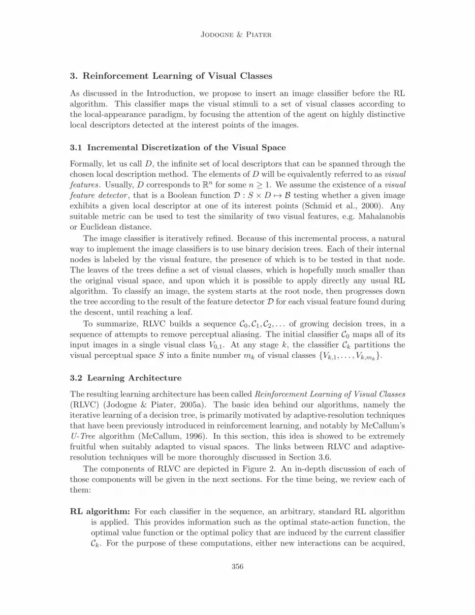
As discussed in the Introduction, we propose to insert an image classifier before the RLalgorithm. This classifier maps the visual stimuli to a set of visual classes according tothe local-appearance paradigm, by focusing the attention of the agent on highly distinctivelocal descriptors detected at the interest points of the images.
3.1 Incremental Discretization of the Visual Space
Formally, let us call D, the infinite set of local descriptors that can be spanned through thechosen local description method. The elements of D will be equivalently referred to as visualfeatures. Usually, D corresponds to R
n for some n ≥ 1. We assume the existence of a visualfeature detector , that is a Boolean function D : S ×D 7→ B testing whether a given imageexhibits a given local descriptor at one of its interest points (Schmid et al., 2000). Anysuitable metric can be used to test the similarity of two visual features, e.g. Mahalanobisor Euclidean distance.
The image classifier is iteratively refined. Because of this incremental process, a naturalway to implement the image classifiers is to use binary decision trees. Each of their internalnodes is labeled by the visual feature, the presence of which is to be tested in that node.The leaves of the trees define a set of visual classes, which is hopefully much smaller thanthe original visual space, and upon which it is possible to apply directly any usual RLalgorithm. To classify an image, the system starts at the root node, then progresses downthe tree according to the result of the feature detector D for each visual feature found duringthe descent, until reaching a leaf.
To summarize, RLVC builds a sequence C0, C1, C2, . . . of growing decision trees, in asequence of attempts to remove perceptual aliasing. The initial classifier C0 maps all of itsinput images in a single visual class V0,1. At any stage k, the classifier Ck partitions thevisual perceptual space S into a finite number mk of visual classes {Vk,1, . . . , Vk,mk
}.
3.2 Learning Architecture
The resulting learning architecture has been called Reinforcement Learning of Visual Classes(RLVC) (Jodogne & Piater, 2005a). The basic idea behind our algorithms, namely theiterative learning of a decision tree, is primarily motivated by adaptive-resolution techniquesthat have been previously introduced in reinforcement learning, and notably by McCallum’sU-Tree algorithm (McCallum, 1996). In this section, this idea is showed to be extremelyfruitful when suitably adapted to visual spaces. The links between RLVC and adaptive-resolution techniques will be more thoroughly discussed in Section 3.6.
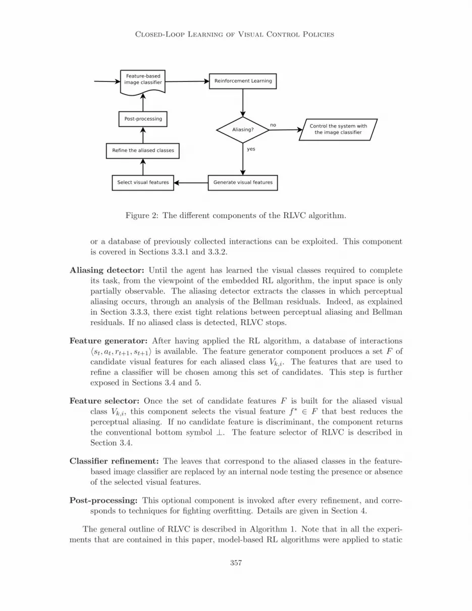
The components of RLVC are depicted in Figure 2. An in-depth discussion of each ofthose components will be given in the next sections. For the time being, we review each ofthem:
RL algorithm: For each classifier in the sequence, an arbitrary, standard RL algorithmis applied. This provides information such as the optimal state-action function, theoptimal value function or the optimal policy that are induced by the current classifierCk. For the purpose of these computations, either new interactions can be acquired,
356
Closed-Loop Learning of Visual Control Policies
Figure 2: The different components of the RLVC algorithm.
or a database of previously collected interactions can be exploited. This componentis covered in Sections 3.3.1 and 3.3.2.
Aliasing detector: Until the agent has learned the visual classes required to completeits task, from the viewpoint of the embedded RL algorithm, the input space is onlypartially observable. The aliasing detector extracts the classes in which perceptualaliasing occurs, through an analysis of the Bellman residuals. Indeed, as explainedin Section 3.3.3, there exist tight relations between perceptual aliasing and Bellmanresiduals. If no aliased class is detected, RLVC stops.
Feature generator: After having applied the RL algorithm, a database of interactions〈st, at, rt+1, st+1〉 is available. The feature generator component produces a set F ofcandidate visual features for each aliased class Vk,i. The features that are used torefine a classifier will be chosen among this set of candidates. This step is furtherexposed in Sections 3.4 and 5.
Feature selector: Once the set of candidate features F is built for the aliased visualclass Vk,i, this component selects the visual feature f∗ ∈ F that best reduces theperceptual aliasing. If no candidate feature is discriminant, the component returnsthe conventional bottom symbol ⊥. The feature selector of RLVC is described inSection 3.4.
Classifier refinement: The leaves that correspond to the aliased classes in the feature-based image classifier are replaced by an internal node testing the presence or absenceof the selected visual features.
Post-processing: This optional component is invoked after every refinement, and corre-sponds to techniques for fighting overfitting. Details are given in Section 4.
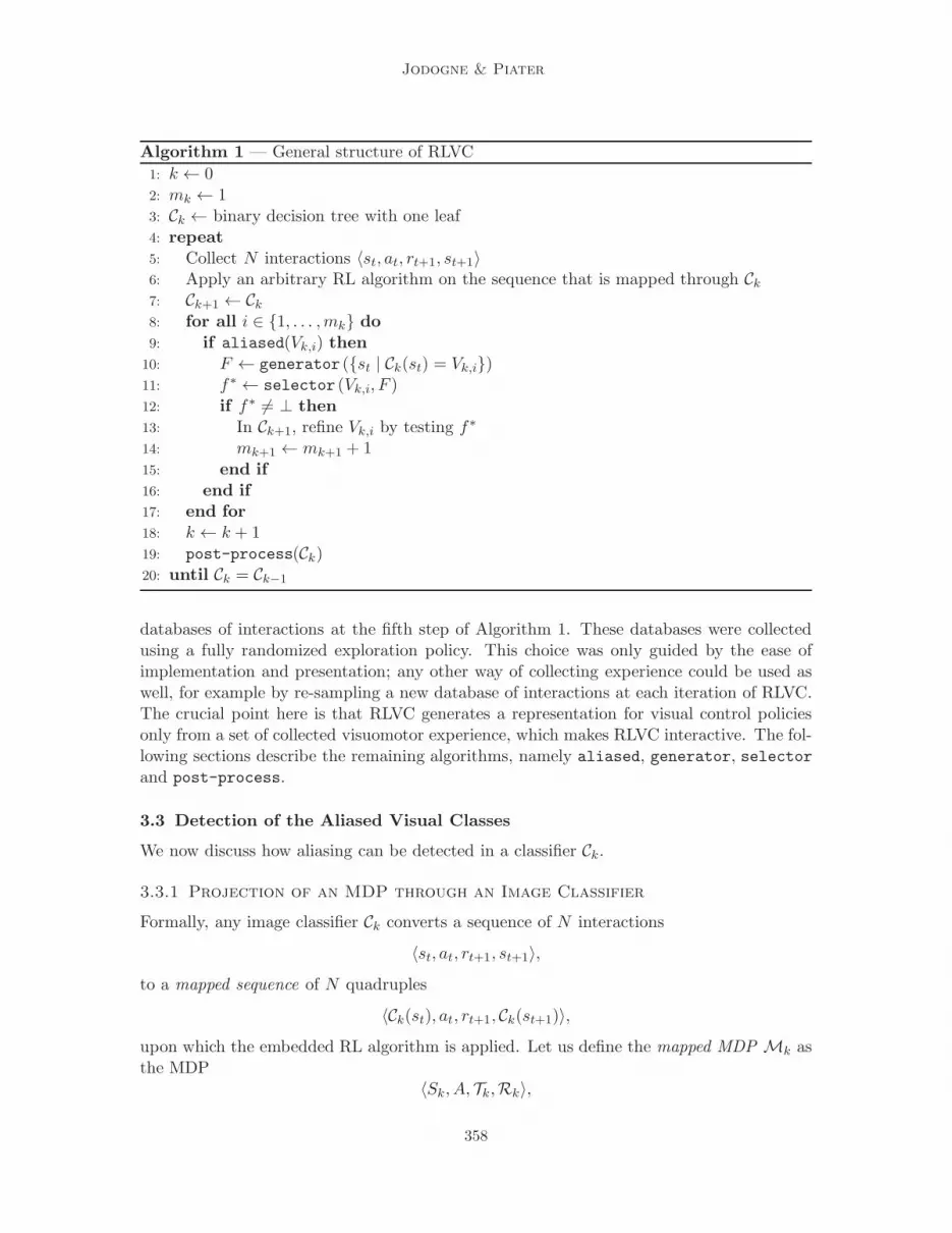
The general outline of RLVC is described in Algorithm 1. Note that in all the experi-ments that are contained in this paper, model-based RL algorithms were applied to static
357
Jodogne & Piater
Algorithm 1 — General structure of RLVC
1: k ← 02: mk ← 13: Ck ← binary decision tree with one leaf4: repeat
5: Collect N interactions 〈st, at, rt+1, st+1〉6: Apply an arbitrary RL algorithm on the sequence that is mapped through Ck7: Ck+1 ← Ck8: for all i ∈ {1, . . . ,mk} do9: if aliased(Vk,i) then
10: F ← generator ({st | Ck(st) = Vk,i})11: f∗ ← selector (Vk,i, F )12: if f∗ 6= ⊥ then
13: In Ck+1, refine Vk,i by testing f∗
14: mk+1 ← mk+1 + 115: end if
16: end if
17: end for
18: k ← k + 119: post-process(Ck)20: until Ck = Ck−1
databases of interactions at the fifth step of Algorithm 1. These databases were collectedusing a fully randomized exploration policy. This choice was only guided by the ease ofimplementation and presentation; any other way of collecting experience could be used aswell, for example by re-sampling a new database of interactions at each iteration of RLVC.The crucial point here is that RLVC generates a representation for visual control policiesonly from a set of collected visuomotor experience, which makes RLVC interactive. The fol-lowing sections describe the remaining algorithms, namely aliased, generator, selectorand post-process.
3.3 Detection of the Aliased Visual Classes
We now discuss how aliasing can be detected in a classifier Ck.
3.3.1 Projection of an MDP through an Image Classifier
Formally, any image classifier Ck converts a sequence of N interactions
〈st, at, rt+1, st+1〉,
to a mapped sequence of N quadruples
〈Ck(st), at, rt+1, Ck(st+1)〉,
upon which the embedded RL algorithm is applied. Let us define the mapped MDP Mk asthe MDP
〈Sk, A,Tk,Rk〉,
358
Closed-Loop Learning of Visual Control Policies
that is obtained from the mapped sequence, where Sk is the set of visual classes that areknown to Ck, and where Tk and Rk have been computed using the relative frequencies inthe mapped sequence, as follows.
Consider two visual classes V, V ′ ∈ {Vk,1, . . . , Vk,mk} and one action a ∈ A. We define
the following functions:
• δt(V, a) equals 1 if Ck(st) = V and at = a, and 0 otherwise;
• δt (V, a, V′) equals 1 if Ck(st) = V , Ck(st+1) = V ′ and at = a, and 0 otherwise;
• η(V, a) is the number of t’s such that δt(V, a) = 1.
Using this notation, we can write:
• Sk = {Vk,1, . . . , Vk,mk};
• Tk (V, a, V′) =
∑Nt=1 δt (V, a, V
′) /η(V, a);
• Rk(V, a) =∑N
t=1 rtδt(V, a)/η(V, a).
3.3.2 Optimal Q Function for a Mapped MDP
Each mapped MDPMk induces an optimal Q function on the domain Sk ×A that will bedenoted Q′∗
k . Computing Q′∗k can be difficult: In general, there may exist no MDP defined
on the state space Sk and on the action space A that can generate a given mapped sequence,since the latter is not necessarily Markovian anymore. Thus, if some RL algorithm is runon the mapped sequence, it might not converge toward Q′∗
k , or not even converge at all.However, when applied on a mapped sequence, any model-based RL method (cf. Section 2)can be used to compute Q′∗
k ifMk is used as the underlying model. Under some conditions,Q-learning also converges to the optimal Q function of the mapped MDP (Singh, Jaakkola,& Jordan, 1995).
In turn, the function Q′∗k induces another Q function on the initial domain S×A through
the relation:Q∗
k(s, a) = Q′∗k (Ck(s), a) , (7)
In the absence of aliasing, the agent would perform optimally, and Q∗k would correspond to
Q∗, according to Bellman theorem that states the uniqueness of the optimal Q function (cf.Section 2). By Equation 4, the function
Bk(s, a) = (HQ∗k)(s, a) −Q∗
k(s, a) (8)
is therefore a measure of the aliasing induced by the image classifier Ck. In RL terminology,Bk is Bellman residual of the function Q∗
k (Sutton, 1988). The basic idea behind RLVC isto refine the states that have a non-zero Bellman residual.
3.3.3 Measuring Aliasing
Consider a time stamp t in a database of interactions 〈st, at, rt+1, st+1〉. According toEquation 8, the Bellman residual that corresponds to the state-action pair (st, at) equals
Bk(st, at) = R(st, at) + γ∑
s′∈S
T (st, at, s′)max
a′∈AQ∗
k(s′, a′)−Q∗
k(st, at). (9)
359
Jodogne & Piater
Algorithm 2 — Aliasing Criterion
1: aliased(Vk,i) :–2: for all a ∈ A do
3: ∆← {∆t | Ck(st) = Vk,i ∧ at = a}4: if σ2(∆) > τ then
5: return true6: end if
7: end for
8: return false
Unfortunately, the RL agent does not have access to the transition probabilities T and tothe reinforcement function R of the MDP modeling the environment. Therefore, Equa-tion 9 cannot be directly evaluated. A similar problem arises in the Q-learning (Watkins,1989) and the Fitted Q Iteration (Ernst, Geurts, & Wehenkel, 2005) algorithms. Thesealgorithms solve this problem by considering the stochastic version of the time differencethat is described by Equation 9: The value
∑
s′∈S
T (st, at, s′)max
a′∈AQ∗
k(s′, a′) (10)
can indeed be estimated asmaxa′∈A
Q∗k(s
′, a′), (11)
if the successor s′ is chosen with probability T (st, at, s′). But following the transitions of
the environment ensures making a transition from st to st+1 with probability T (st, at, st+1).Thus
∆t = rt+1 + γmaxa′∈A
Q∗k(st+1, a
′)−Q∗k(st, at) (12)
= rt+1 + γmaxa′∈A
Q′∗k
(
Ck (st+1) , a′)
−Q′∗k (Ck(st), a) (13)
is an unbiased estimate of the Bellman residual for the state-action pair (st, at) (Jaakkola,Jordan, & Singh, 1994).1 Very importantly, if the system is deterministic and in the absenceof perceptual aliasing, these estimates are equal to zero. Therefore, a nonzero ∆t potentiallyindicates the presence of perceptual aliasing in the visual class Vt = Ck(st) with respect toaction at. Our criterion for detecting the aliased classes consists in computing the Q′∗
k
function, then in sweeping again all the interactions 〈st, at, rt+1, st+1〉 to identify nonzero∆t. In practice, we assert the presence of aliasing if the variance of the ∆t exceeds a giventhreshold τ . This is summarized in Algorithm 2, where σ2(·) denotes the variance of a setof samples.
3.4 Generation and Selection of Distinctive Visual Features
Once aliasing has been detected in some visual class Vk,i ∈ Sk with respect to an action a,we need to select a local descriptor that best explains the variations in the set of ∆t values
1. It is worth noticing that αt∆t corresponds to the updates that would be applied by Q-learning, whereαt is known as the learning rate at time t.
360
Closed-Loop Learning of Visual Control Policies
Algorithm 3 — Canonical feature generator
1: generator({s1, . . . , sn}) :–2: F ← {}3: for all i ∈ {1, . . . , n} do4: for all (x, y) such that (x, y) is an interest point of si do5: F ← F ∪ {symbol(descriptor(si, x, y))}6: end for
7: end for
8: return F
corresponding to Vk,i and a. This local descriptor is to be chosen among a set of candidatevisual features F .
3.4.1 Extraction of Candidate Features
Informally, the canonical way of building F for a visual class Vk,i consists in:
1. identifying all collected visual percepts st such that Ck(st) = Vk,i,
2. locating all the interest points in all the selected images st, then
3. adding to F the local descriptor of all those interest points.
The corresponding feature generator is detailed in Algorithm 3. In the latter algorithm,descriptor(s, x, y) returns the local description of the point at location (x, y) in the image s,and symbol(d) returns the symbol that corresponds to the local descriptor d ∈ F accordingto the used metric. However, more complex strategies for generating the visual features canbe used. Such a strategy that builds spatial combinations of individual point features willbe presented in Section 5.
3.4.2 Selection of Candidate Features
The problem of choosing the candidate feature that most reduces the variations in a set ofreal-valued Bellman residuals is a regression problem, for which we suggest an adaptation ofa popular splitting rule used in the CART algorithm for building regression trees (Breiman,Friedman, & Stone, 1984).2
In CART, variance is used as an impurity indicator: The split that is selected to refinea particular node is the one that leads to the greatest reduction in the sum of the squareddifferences between the response values for the learning samples corresponding to the nodeand their mean. More formally, let S = {〈xi, yi〉} be a set of learning samples, where xi ∈ R
n
are input vectors of real numbers, and where yi ∈ R are real-valued outputs. CART selectsthe following candidate feature:
f∗ = argminv∈F
(
pv⊕ · σ2(
Sv⊕
)
+ pv⊖ · σ2(
Sv⊖
))
, (14)
2. Note that in our previous work, we used a splitting rule that is borrowed from the building of classificationtrees (Quinlan, 1993; Jodogne & Piater, 2005a).
361

Jodogne & Piater
Algorithm 4 — Feature Selection
1: selector(Vk,i, F ) :–2: f∗ ← ⊥ {Best feature found so far}3: r∗ ← +∞ {Variance reduction induced by f∗}4: for all a ∈ A do
5: T ← {t | Ck(st) = Vk,i and at = a}6: for all visual feature f ∈ F do
7: S⊕ ← {∆t | t ∈ T and st exhibits f}8: S⊖ ← {∆t | t ∈ T and st does not exhibit f}9: s⊕ ← |S⊕|/|T |
10: s⊖ ← |S⊖|/|T |11: r ← s⊕ · σ
2 (S⊕) + s⊖ · σ2 (S⊖)
12: if r < r∗ and the distributions (S⊕, S⊖) are significantly different then13: f∗ ← f14: r∗ ← s15: end if
16: end for
17: end for
18: return f∗
where pv⊕ (resp. pv⊖) is the proportion of samples that exhibit (resp. do not exhibit) thefeature v, and where Sv
⊕ (resp. Sv⊖) is the set of samples that exhibit (resp. do not exhibit)
the feature v. This idea can be directly transferred in our framework, if the set of xi
corresponds to the set of interactions 〈st, at, rt+1, st+1〉, and if the set of yi corresponds tothe set of ∆t. This is written explicitly in Algorithm 4.
Our algorithms exploit the stochastic version of Bellman residuals. Of course, real envi-ronments are in general non-deterministic, which generates variations in Bellman residualsthat are not a consequence of perceptual aliasing. RLVC can be made somewhat robust tosuch a variability by introducing a statistical hypothesis test: For each candidate feature,a Student’s t−test is used to decide whether the two sub-distributions the feature inducesare significantly different. This approach is also used in U-Tree (McCallum, 1996).
3.5 Illustration on a Simple Navigation Task
We have evaluated our system on an abstract task that closely parallels a real-world scenariowhile avoiding any unnecessary complexity. As a consequence, the sensor model we use mayseem unrealistic; a better visual sensor model will be exploited in Section 4.4.
RLVC has succeeded at solving the continuous, noisy visual navigation task depictedin Figure 3. The goal of the agent is to reach as fast as possible one of the two exits ofthe maze. The set of possible locations is continuous. At each location, the agent has fourpossible actions: Go up, right, down, or left. Every move is altered by a Gaussian noise,the standard deviation of which is 2% the size of the maze. Glass walls are present in themaze. Whenever a move would take the agent into a wall or outside the maze, its locationis not changed.
362
Closed-Loop Learning of Visual Control Policies
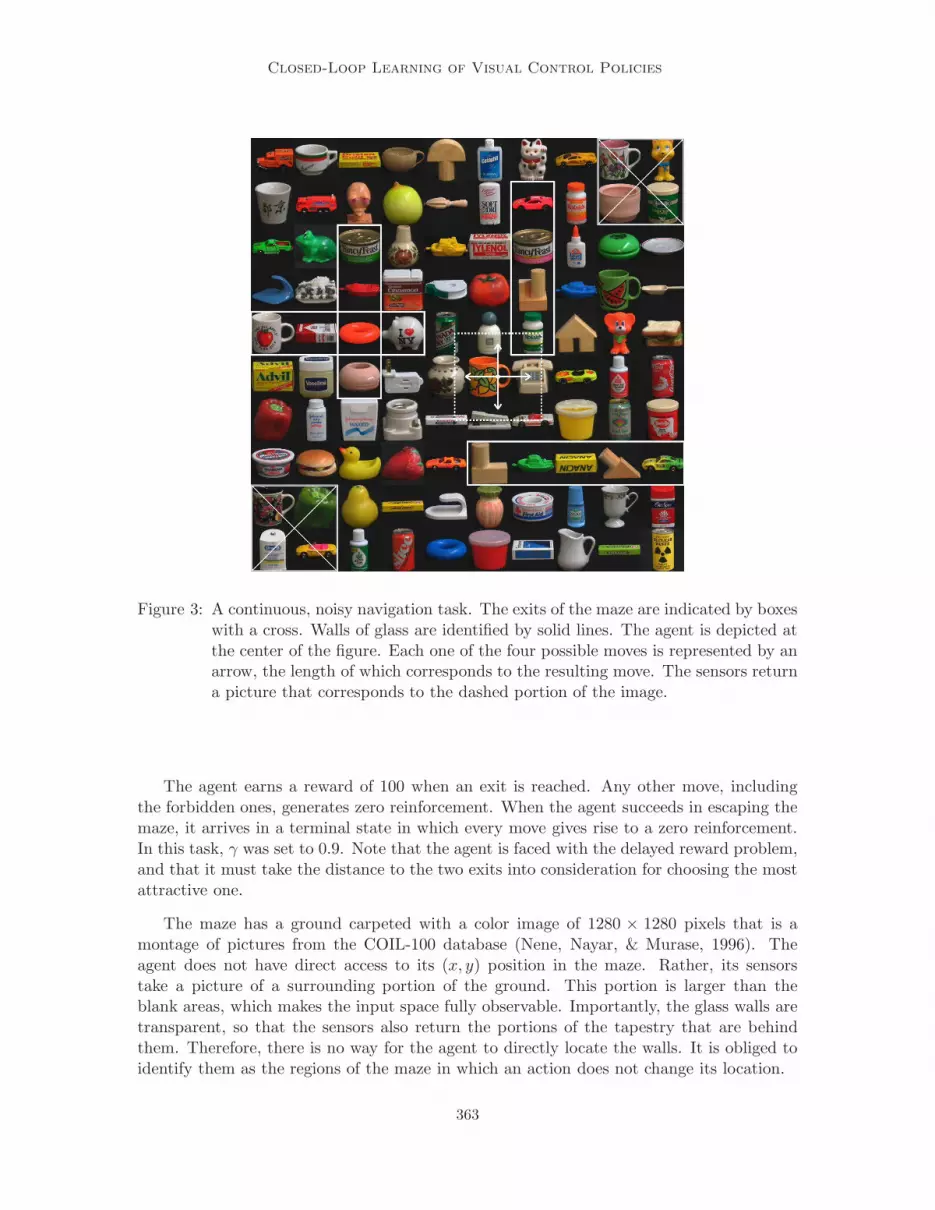
Figure 3: A continuous, noisy navigation task. The exits of the maze are indicated by boxeswith a cross. Walls of glass are identified by solid lines. The agent is depicted atthe center of the figure. Each one of the four possible moves is represented by anarrow, the length of which corresponds to the resulting move. The sensors returna picture that corresponds to the dashed portion of the image.
The agent earns a reward of 100 when an exit is reached. Any other move, includingthe forbidden ones, generates zero reinforcement. When the agent succeeds in escaping themaze, it arrives in a terminal state in which every move gives rise to a zero reinforcement.In this task, γ was set to 0.9. Note that the agent is faced with the delayed reward problem,and that it must take the distance to the two exits into consideration for choosing the mostattractive one.
The maze has a ground carpeted with a color image of 1280 × 1280 pixels that is amontage of pictures from the COIL-100 database (Nene, Nayar, & Murase, 1996). Theagent does not have direct access to its (x, y) position in the maze. Rather, its sensorstake a picture of a surrounding portion of the ground. This portion is larger than theblank areas, which makes the input space fully observable. Importantly, the glass walls aretransparent, so that the sensors also return the portions of the tapestry that are behindthem. Therefore, there is no way for the agent to directly locate the walls. It is obliged toidentify them as the regions of the maze in which an action does not change its location.
363

Jodogne & Piater
Figure 4: The deterministic image-to-action mapping that results from RLVC, sampled atregularly-spaced points. It manages to choose the correct action at each location.
In this experiment, we have used color differential invariants as visual features (Gouet& Boujemaa, 2001). The entire tapestry includes 2298 different visual features. RLVCselected 200 features, corresponding to a ratio of 9% of the entire set of possible features.The computation stopped after the generation of 84 image classifiers (i.e. when k reached84), which took 35 minutes on a 2.4GHz Pentium IV using databases of 10,000 interactions.205 visual classes were identified. This is a small number, compared to the number ofperceptual classes that would be generated by a discretization of the maze when the agentknows its (x, y) position. For example, a reasonably sized 20×20 grid leads to 400 perceptualclasses.
Figure 4 shows the optimal, deterministic image-to-action mapping that results fromthe last obtained image classifier Ck:
π∗(s) = argmaxa∈A
Q∗k(s, a) = Q′∗
k (Ck(s), a) . (15)
364
Closed-Loop Learning of Visual Control Policies
(a) (b)
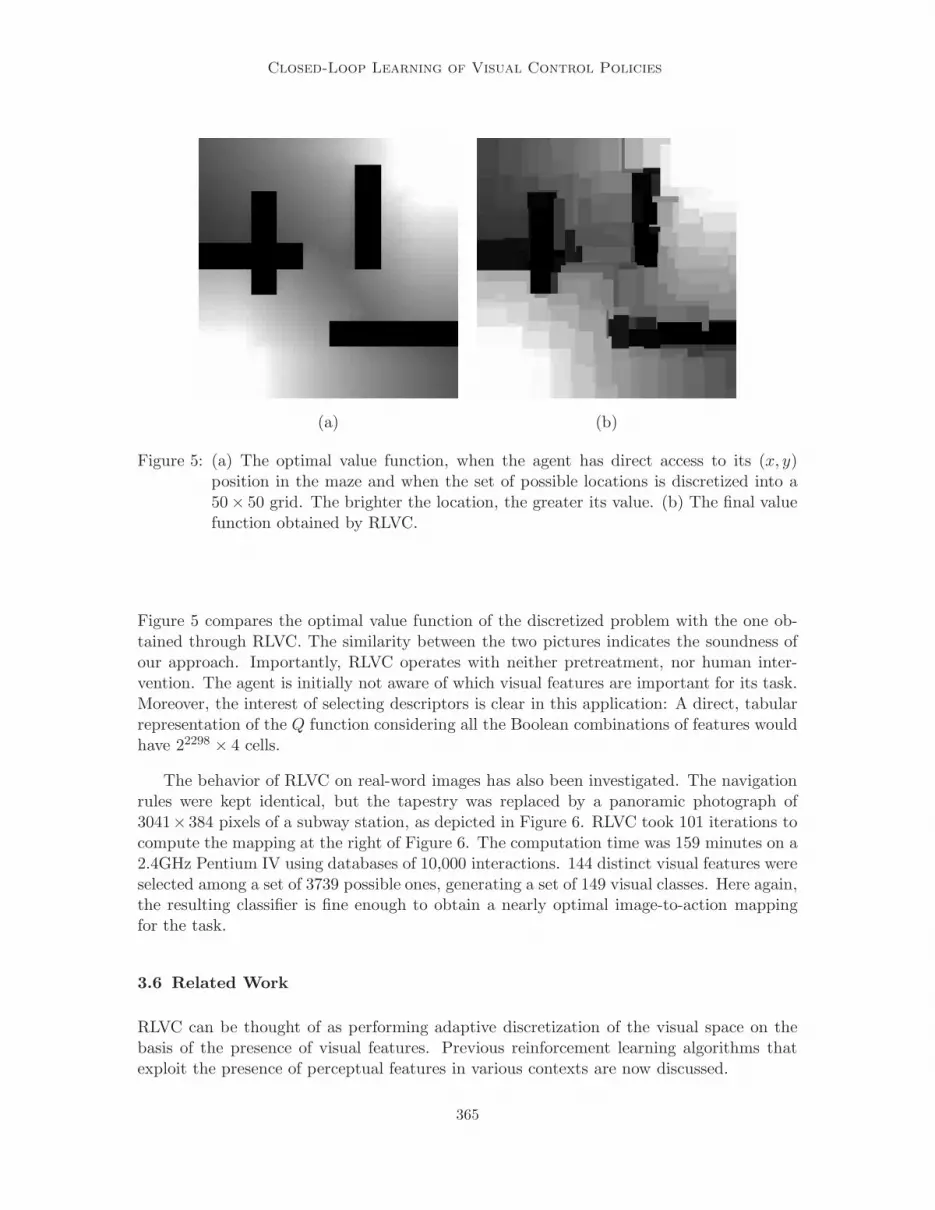
Figure 5: (a) The optimal value function, when the agent has direct access to its (x, y)position in the maze and when the set of possible locations is discretized into a50× 50 grid. The brighter the location, the greater its value. (b) The final valuefunction obtained by RLVC.
Figure 5 compares the optimal value function of the discretized problem with the one ob-tained through RLVC. The similarity between the two pictures indicates the soundness ofour approach. Importantly, RLVC operates with neither pretreatment, nor human inter-vention. The agent is initially not aware of which visual features are important for its task.Moreover, the interest of selecting descriptors is clear in this application: A direct, tabularrepresentation of the Q function considering all the Boolean combinations of features wouldhave 22298 × 4 cells.
The behavior of RLVC on real-word images has also been investigated. The navigationrules were kept identical, but the tapestry was replaced by a panoramic photograph of3041× 384 pixels of a subway station, as depicted in Figure 6. RLVC took 101 iterations tocompute the mapping at the right of Figure 6. The computation time was 159 minutes on a2.4GHz Pentium IV using databases of 10,000 interactions. 144 distinct visual features wereselected among a set of 3739 possible ones, generating a set of 149 visual classes. Here again,the resulting classifier is fine enough to obtain a nearly optimal image-to-action mappingfor the task.
3.6 Related Work
RLVC can be thought of as performing adaptive discretization of the visual space on thebasis of the presence of visual features. Previous reinforcement learning algorithms thatexploit the presence of perceptual features in various contexts are now discussed.
365

Jodogne & Piater
(a) (b)
Figure 6: (a) A navigation task with a real-world image, using the same conventions thanFigure 3. (b) The deterministic image-to-action mapping computed by RLVC.
366
Closed-Loop Learning of Visual Control Policies
3.6.1 Perceptual Aliasing
As explained above, the incremental selection of a set of informative visual features neces-sarily leads to temporary perceptual aliasing, which RLVC tries to remove. More generally,perceptual aliasing occurs whenever an agent cannot always take the right on the basis ofits percepts.
Early work in reinforcement learning has tackled this general problem in two distinctways: Either the agent identifies and then avoids states where perceptual aliasing occurs(as in the Lion algorithm, see Whitehead & Ballard, 1991), or it tries to build a short-termmemory that will allow it to remove the ambiguities on its percepts (as in the predictivedistinctions approach, see Chrisman, 1992). Very sketchily, these two algorithms detect thepresence of perceptual aliasing through an analysis of the sign of Q-learning updates. Thepossibility of managing a short-term memory has led to the development of the PartiallyObservable Markov Decision Processes (POMDP) theory (Kaelbling, Littman, & Cassandra,1998), in which the current state is a random variable of the percepts.
Although these approaches are closely related to the perceptual aliasing RLVC tem-porarily introduces, they do not consider the exploitation of perceptual features. Indeed,they tackle a structural problem in a given control task, and, as such, they assume thatperceptual aliasing cannot be removed. As a consequence, these approaches are orthogonalto our research interest, since the ambiguities RLVC generates can be removed by furtherrefining the image classifier. In fact, the techniques above tackle a lack of information in-herent to the used sensors, whereas our goal is to handle a surplus of information relatedto the high redundancy of visual representations.
3.6.2 Adaptive Resolution in Finite Perceptual Spaces
RLVC performs an adaptive discretization of the perceptual space through an autonomous,task-driven, purposive selection of visual features. Work in RL that incrementally partitionsa large (either discrete or continuous) perceptual space into a piecewise constant valuefunction is usually referred to as adaptive-resolution techniques. Ideally, regions of theperceptual space with a high granularity should only be present where they are needed,while a lower resolution should be used elsewhere. RLVC is such an adaptive-resolutionalgorithm. We now review several adaptive-resolution methods that have been previouslyproposed for finite perceptual spaces.
The idea of adaptive-resolution techniques in reinforcement learning goes back to theG Algorithm (Chapman & Kaelbling, 1991), and has inspired the other approaches thatare discussed below. The G Algorithm considers perceptual spaces that are made up offixed-length binary numbers. It learns a decision tree that tests the presence of informativebits in the percepts. This algorithm uses a Student’s t-test to determine if there is some bitb in the percepts that is mapped to a given leaf, such that the state-action utilities of statesin which b is set are significantly different from the state-action utilities of states in whichb is unset. If such a bit is found, the corresponding leaf is split. The process is repeatedfor each leaf. This method is able to learn compact representations, even though there isa large number of irrelevant bits in the percepts. Unfortunately, when a region is split,all the information associated with that region is lost, which makes for very slow learning.
367

Jodogne & Piater
Concretely, the G Algorithm can solve a task whose perceptual space contains 2100 distinctpercepts, which corresponds to the set of binary numbers with a length of 100 bits.
McCallum’s U-Tree algorithm builds upon this idea by combining a “selective attention”mechanism inspired by the G Algorithm with a short-term memory that enables the agentto deal with partially observable environments (McCallum, 1996). Therefore, McCallum’salgorithms are a keystone in reinforcement learning, as they unify the G Algorithm (Chap-man & Kaelbling, 1991) with Chrisman’s predictive distinctions (Chrisman, 1992).
U-Tree incrementally grows a decision tree through Kolmogorov-Smirnov tests. It hassucceeded at learning behaviors in a driving simulator. In this simulator, a percept consistsof a set of 8 discrete variables whose variation domains contain between 2 and 6 values,leading to a perceptual space with 2, 592 possible percepts. Thus, the size of the perceptualspace is much smaller than a visual space. However, this task is difficult because the“physical” state space is only partially observable through the perceptual space: The drivingtask contains 21, 216 physical states, which means that several physical states requiringdifferent reactions can be mapped to the same percept through the sensors of the agent.U-Tree resolves such ambiguities on the percepts by testing the presence of perceptualfeatures in the percepts that have been encountered previously in the history of the system.To this end, U-Tree manages a short-term memory. In this paper, partially observableenvironments are not considered. Our challenge is rather to deal with huge visual spaces,without hand-tuned pre-processing, which is in itself a difficult, novel research direction.
3.6.3 Adaptive Resolution in Continuous Perceptual Spaces
It is important to notice that all the methods for adaptive resolution in large-scale, finiteperceptual spaces use a fixed set of perceptual features that is hard-wired. This has to bedistinguished from RLVC that samples visual features from a possibly infinite visual featurespace (e.g. the set of visual features is infinite), and that makes no prior assumptionsabout the maximum number of useful features. From this point of view, RLVC is closer toadaptive-resolution techniques for continuous perceptual spaces. Indeed, these techniquesdynamically select new relevant features from a whole continuum.
The first adaptive-resolution algorithm for continuous perceptual spaces is the Dar-
ling algorithm (Salganicoff, 1993). This algorithm, just like all the current algorithmsfor continuous adaptive resolution, splits the perceptual space using thresholds. For thispurpose, Darling builds a hybrid decision tree that assigns a label to each point in theperceptual space. Darling is a fully on-line and incremental algorithm that is equippedwith a forgetting mechanism that deletes outdated interactions. It is however limited tobinary reinforcement signals, and it only takes immediate reinforcements into account, sothat Darling is much closer to supervised learning than to reinforcement learning.
The Parti-Game algorithm (Moore & Atkeson, 1995) produces goal-directed behaviors incontinuous perceptual spaces. Parti-Game also splits regions where it deems it important,using a game-theoretic approach. Moore and Atkeson show that Parti-Game can learncompetent behavior in a variety of continuous domains. Unfortunately, the approach iscurrently limited to deterministic domains where the agent has a greedy controller andwhere the goal state is known. Moreover, this algorithm searches for any solution to agiven task, and does not try to find the optimal one.
368
Closed-Loop Learning of Visual Control Policies
The Continuous U-Tree algorithm is an extension of U-Tree that is adapted to contin-uous perceptual spaces (Uther & Veloso, 1998). Just like Darling, Continuous U-Treeincrementally builds a decision tree that splits the perceptual space into a finite set of hy-percubes, by testing thresholds. Kolmogorov-Smirnov and sum-of-squared-errors are usedto determine when to split a node in the decision tree. Pyeatt and Howe (2001) analyzethe performance of several splitting criteria for a variation of Continuous U-Tree. Theyconclude that Student’s t-test leads to the best performance, which motivates the use ofthis statistical test in RLVC (cf. Section 3.4).
Munos and Moore (2002) have proposed Variable Resolution Grids. Their algorithmassumes that the perceptual space is a compact subset of Euclidean space, and begins witha coarse, grid-based discretization of the state space. In contrast with the other abstractalgorithms in this section, the value function and policy vary linearly within each region.Munos and Moore use Kuhn triangulation as an efficient way to interpolate the value func-tion within regions. The algorithm refines its approximation by refining cells according toa splitting criterion. Munos and Moore explore several local heuristic measures of the im-portance of splitting a cell including the average of corner-value differences, the variance ofcorner-value differences, and policy disagreement. They also explore global heuristic mea-sures involving the influence and variance of the approximated system. Variable ResolutionGrids are probably the most advanced adaptive-resolution algorithm available so far.
3.6.4 Discussion
To summarize, several algorithms that are similar in spirit to RLVC have been proposedover the years. Nevertheless, our work appears to be the first that can learn direct image-to-action mappings through reinforcement learning. Indeed, none of the reinforcement learningmethods above combines all the following desirable properties of RLVC: (1) The set of rel-evant perceptual features is not chosen a priori by hand, as the selection process is fullyautomatic and does not require any human intervention; (2) visual perceptual spaces are ex-plicitly considered through appearance-based visual features; and (3) the highly informativeperceptual features can be drawn out of a possibly infinite set.
These advantages of RLVC are essentially due to the fact that the candidate visualfeatures are not selected only because they are informative: They are also ranked accordingto an information-theoretic measure inspired by decision tree induction (Breiman et al.,1984). Such a ranking is required, as vision-for-action tasks induce a large number of visualfeatures (a typical image contains about a thousand of them). This kind of criterion thatranks features, though already considered in Variable Resolution Grids (Munos & Moore,2002), seems to be new in discrete perceptual spaces.
RLVC is defined independently of any fixed RL algorithm, which is similar in spirit toContinuous U-Tree (Uther & Veloso, 1998), with the major exception that RLVC deals withBoolean features, whereas Continuous U-Tree works in a continuous input space. Further-more, the version of RLVC presented in this paper uses a variance-reduction criterion forranking the visual features. This criterion, though already considered in Variable ResolutionGrids, seems to be new in discrete perceptual spaces.
369
Jodogne & Piater
4. Compacting Visual Policies
As written in Section 1.4.2, this original version of RLVC is subject to overfitting (Jodogne &Piater, 2005b). A simple heuristic to avoid the creation of too many visual classes is simplyto bound the number of visual classes that can be refined at each stage of the algorithm,since splitting one visual class potentially has an impact on the Bellman residuals of all thevisual classes. In practice, we first try to split the classes that have the most samples beforeconsidering the others, since there is more evidence of variance reduction for the first. Inour tests, we systematically apply this heuristics. However, it is often insufficient if takenalone.
4.1 Equivalence Relations in Markov Decision Processes
Since we apply an embedded RL algorithm at each stage k of RLVC, properties like theoptimal value function V ∗
k (·), the optimal state-action value functionQ∗k(·, ·) and the optimal
control policy π∗k(·) are known for each mapped MDPMk. Using those properties, it is easy
to define a whole range of equivalence relations between the visual classes. For instance,given a threshold ε ∈ R
+, we list hereunder three possible equivalence relations for a pairof visual classes (V, V ′):
Optimal Value Equivalence:
|V ∗k (V )− V ∗
k (V′)| ≤ ε.
Optimal Policy Equivalence:
|V ∗k (V )−Q∗
k(V′, π∗
k(V ))| ≤ ε ∧|V ∗
k (V′)−Q∗
k(V, π∗k(V
′))| ≤ ε.
Optimal State-Action Value Equivalence:
(∀a ∈ A) |Q∗k(V, a)−Q∗
k(V′, a)| ≤ ε.
We therefore propose to modify RLVC so that, periodically, visual classes that areequivalent with respect to one of those criteria are merged together. We have experimentallyobserved that the conjunction of the first two criteria tends to lead to the best performance.This way, RLVC alternatively splits and merges visual classes. The compaction phase shouldnot be done too often, in order to allow exploration. To the best of our knowledge, thispossibility has not been investigated yet in the framework of adaptive-resolution methodsin reinforcement learning.
In the original version of RLVC, the visual classes correspond to the leaves of a decisiontree. When using decision trees, the aggregation of visual classes can only be achieved bystarting from the bottom of the tree and recursively collapsing leaves, until dissimilar leavesare found. This operation is very close to post-pruning in the framework of decision treesfor machine learning (Breiman et al., 1984). In practice, this means that classes that havesimilar properties, but that can only be reached from one another by making a number ofhops upwards then downwards, are extremely unlikely to be matched. This greatly reducesthe interest of exploiting the equivalence relations.
This drawback is due to the rather limited expressiveness of decision trees. In a decisiontree, each visual class corresponds to a conjunction of visual feature literals, which defines a
370
Closed-Loop Learning of Visual Control Policies
path from the root of the decision tree to one leaf. To take full advantage of the equivalencerelations, it is necessary to associate, to each visual class, an arbitrary union of conjunctionsof visual features. Indeed, when exploiting the equivalence relations, the visual classes arethe result of a sequence of conjunctions (splitting) and disjunctions (aggregation). Thus, amore expressive data structure that would be able to represent general, arbitrary Booleancombinations of visual features is required. Such a data structure is introduced in the nextsection.
4.2 Using Binary Decision Diagrams
The problem of representing general Boolean functions has been extensively studied in thefield of computer-aided verification, since they can abstract the behavior of logical electronicdevices. In fact, a whole range of methods for representing the state space of richer andricher domains have been developed over the last few years, such as Binary Decision Diagram(BDD) (Bryant, 1992), Number and Queue Decision Diagrams (Boigelot, 1999), UpwardClosed Sets (Delzanno & Raskin, 2000) and Real Vector Automata (Boigelot, Jodogne, &Wolper, 2005).
In our framework, BDD is a particularly well-suited tool. It is a acyclic graph-basedsymbolic representation for encoding arbitrary Boolean functions, and has had much suc-cess in the field of computer-aided verification (Bryant, 1992). A BDD is unique when theordering of its variables is fixed, but different variable orderings can lead to different sizesof the BDD, since some variables can be discarded by the reordering process. Although theproblem of finding the optimal variable ordering is coNP-complete (Bryant, 1986), auto-matic heuristics can in practice find orderings that are close to optimal. This is interestingin our case, since reducing the size of the BDD potentially discards irrelevant variables,which correspond to removing useless visual features.
4.3 Modifications to RLVC
To summarize, this extension to RLVC does not use decision trees anymore, but assignsone BDD to each visual class. Two modifications are to be applied to Algorithm 1:
1. The operation of refining, with a visual feature f , a visual class V that is labeled bythe BDD B(V ), consists in replacing V by two new visual classes V1 and V2 such thatB(V1) = B(V ) ∧ f and B(V2) = B(V ) ∧ ¬f .
2. Given an equivalence relation, the post-process(Ck) operation consists in mergingthe equivalent visual classes. To merge a pair of visual classes (V1, V2), V1 and V2 aredeleted, and a new visual class V such that B(V ) = B(V1) ∨ B(V2) is added. Everytime a merging operation takes place, it is advised to carry on variable reordering, tominimize the memory requirements.
4.4 Experiments
We have applied the modified version of RLVC to another simulated navigation task. Inthis task, the agent moves between 11 spots of the campus of the University of Liege (cf.Figure 7). Every time the agent is at one of the 11 locations, its body can aim at four possible
371
Jodogne & Piater
N
(c) Google Map
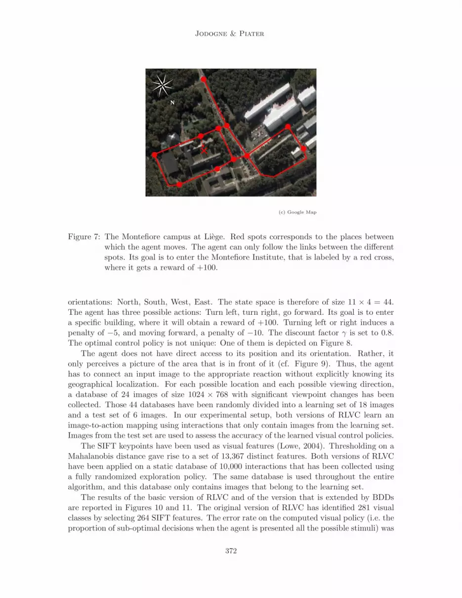
Figure 7: The Montefiore campus at Liege. Red spots corresponds to the places betweenwhich the agent moves. The agent can only follow the links between the differentspots. Its goal is to enter the Montefiore Institute, that is labeled by a red cross,where it gets a reward of +100.
orientations: North, South, West, East. The state space is therefore of size 11 × 4 = 44.The agent has three possible actions: Turn left, turn right, go forward. Its goal is to entera specific building, where it will obtain a reward of +100. Turning left or right induces apenalty of −5, and moving forward, a penalty of −10. The discount factor γ is set to 0.8.The optimal control policy is not unique: One of them is depicted on Figure 8.
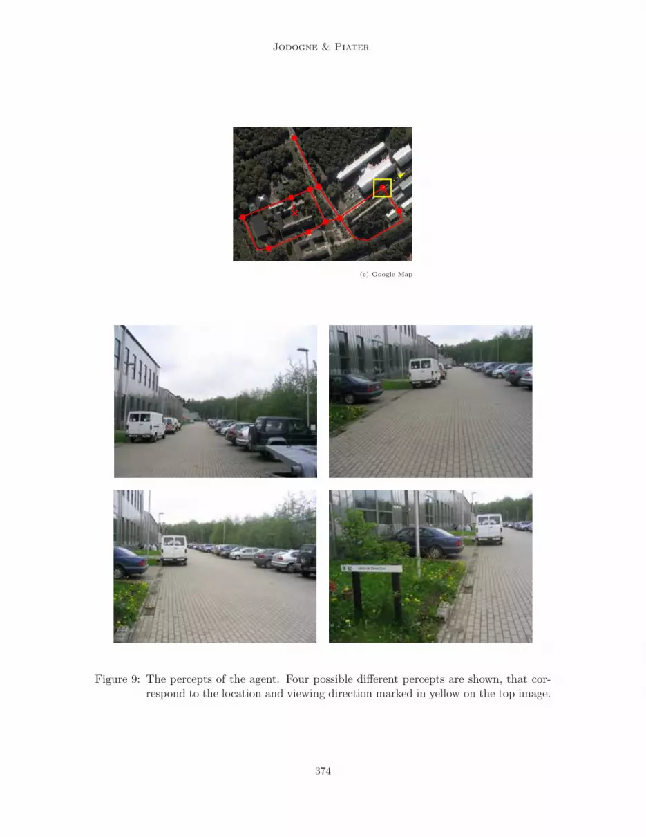
The agent does not have direct access to its position and its orientation. Rather, itonly perceives a picture of the area that is in front of it (cf. Figure 9). Thus, the agenthas to connect an input image to the appropriate reaction without explicitly knowing itsgeographical localization. For each possible location and each possible viewing direction,a database of 24 images of size 1024 × 768 with significant viewpoint changes has beencollected. Those 44 databases have been randomly divided into a learning set of 18 imagesand a test set of 6 images. In our experimental setup, both versions of RLVC learn animage-to-action mapping using interactions that only contain images from the learning set.Images from the test set are used to assess the accuracy of the learned visual control policies.
The SIFT keypoints have been used as visual features (Lowe, 2004). Thresholding on aMahalanobis distance gave rise to a set of 13,367 distinct features. Both versions of RLVChave been applied on a static database of 10,000 interactions that has been collected usinga fully randomized exploration policy. The same database is used throughout the entirealgorithm, and this database only contains images that belong to the learning set.
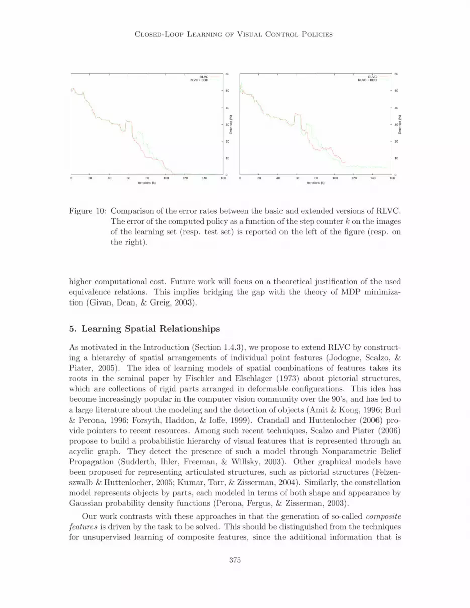
The results of the basic version of RLVC and of the version that is extended by BDDsare reported in Figures 10 and 11. The original version of RLVC has identified 281 visualclasses by selecting 264 SIFT features. The error rate on the computed visual policy (i.e. theproportion of sub-optimal decisions when the agent is presented all the possible stimuli) was
372
Closed-Loop Learning of Visual Control Policies
(c) Google Map
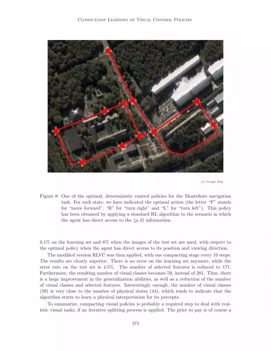
Figure 8: One of the optimal, deterministic control policies for the Montefiore navigationtask. For each state, we have indicated the optimal action (the letter “F” standsfor “move forward”, “R” for “turn right” and “L” for “turn left”). This policyhas been obtained by applying a standard RL algorithm to the scenario in whichthe agent has direct access to the (p, d) information.
0.1% on the learning set and 8% when the images of the test set are used, with respect tothe optimal policy when the agent has direct access to its position and viewing direction.
The modified version RLVC was then applied, with one compacting stage every 10 steps.The results are clearly superior. There is no error on the learning set anymore, while theerror rate on the test set is 4.5%. The number of selected features is reduced to 171.Furthermore, the resulting number of visual classes becomes 59, instead of 281. Thus, thereis a large improvement in the generalization abilities, as well as a reduction of the numberof visual classes and selected features. Interestingly enough, the number of visual classes(59) is very close to the number of physical states (44), which tends to indicate that thealgorithm starts to learn a physical interpretation for its percepts.
To summarize, compacting visual policies is probably a required step to deal with real-istic visual tasks, if an iterative splitting process is applied. The price to pay is of course a
373
Jodogne & Piater
(c) Google Map
Figure 9: The percepts of the agent. Four possible different percepts are shown, that cor-respond to the location and viewing direction marked in yellow on the top image.
374
Closed-Loop Learning of Visual Control Policies
0 20 40 60 80 100 120 140 160 0
10
20
30
40
50
60
Err
or r
ate
(%)
Iterations (k)
RLVCRLVC + BDD
0 20 40 60 80 100 120 140 160 0
10
20
30
40
50
60
Err
or r
ate
(%)
Iterations (k)
RLVCRLVC + BDD
Figure 10: Comparison of the error rates between the basic and extended versions of RLVC.The error of the computed policy as a function of the step counter k on the imagesof the learning set (resp. test set) is reported on the left of the figure (resp. onthe right).
higher computational cost. Future work will focus on a theoretical justification of the usedequivalence relations. This implies bridging the gap with the theory of MDP minimiza-tion (Givan, Dean, & Greig, 2003).
5. Learning Spatial Relationships
As motivated in the Introduction (Section 1.4.3), we propose to extend RLVC by construct-ing a hierarchy of spatial arrangements of individual point features (Jodogne, Scalzo, &Piater, 2005). The idea of learning models of spatial combinations of features takes itsroots in the seminal paper by Fischler and Elschlager (1973) about pictorial structures,which are collections of rigid parts arranged in deformable configurations. This idea hasbecome increasingly popular in the computer vision community over the 90’s, and has led toa large literature about the modeling and the detection of objects (Amit & Kong, 1996; Burl& Perona, 1996; Forsyth, Haddon, & Ioffe, 1999). Crandall and Huttenlocher (2006) pro-vide pointers to recent resources. Among such recent techniques, Scalzo and Piater (2006)propose to build a probabilistic hierarchy of visual features that is represented through anacyclic graph. They detect the presence of such a model through Nonparametric BeliefPropagation (Sudderth, Ihler, Freeman, & Willsky, 2003). Other graphical models havebeen proposed for representing articulated structures, such as pictorial structures (Felzen-szwalb & Huttenlocher, 2005; Kumar, Torr, & Zisserman, 2004). Similarly, the constellationmodel represents objects by parts, each modeled in terms of both shape and appearance byGaussian probability density functions (Perona, Fergus, & Zisserman, 2003).
Our work contrasts with these approaches in that the generation of so-called compositefeatures is driven by the task to be solved. This should be distinguished from the techniquesfor unsupervised learning of composite features, since the additional information that is
375
Jodogne & Piater
0 20 40 60 80 100 120 140 160 0
50
100
150
200
250
300
Num
ber
of c
lass
es
Iterations (k)
RLVCRLVC + BDD
0 20 40 60 80 100 120 140 160 0
50
100
150
200
250
300
Num
ber
of s
elec
ted
feat
ures
Iterations (k)
RLVCRLVC + BDD
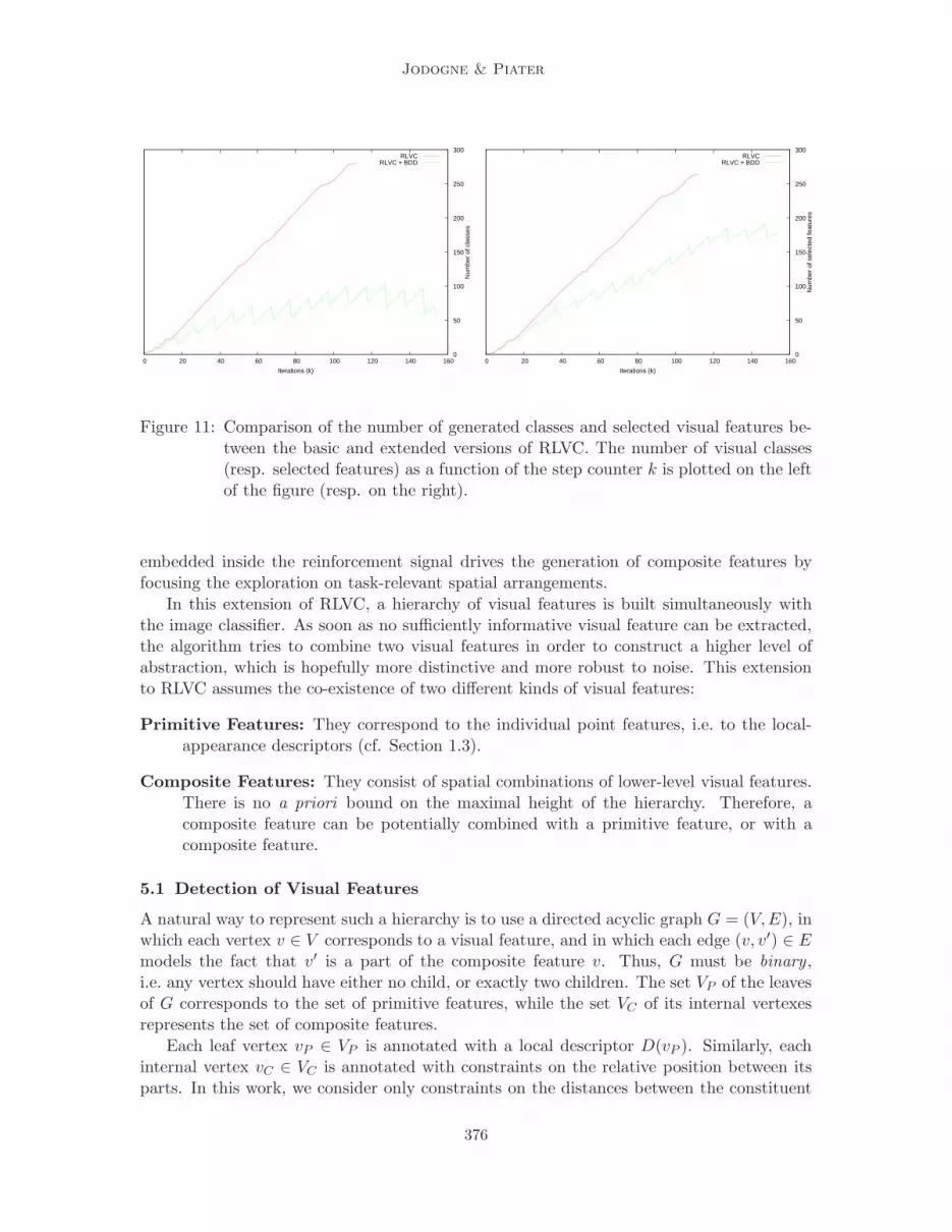
Figure 11: Comparison of the number of generated classes and selected visual features be-tween the basic and extended versions of RLVC. The number of visual classes(resp. selected features) as a function of the step counter k is plotted on the leftof the figure (resp. on the right).
embedded inside the reinforcement signal drives the generation of composite features byfocusing the exploration on task-relevant spatial arrangements.
In this extension of RLVC, a hierarchy of visual features is built simultaneously withthe image classifier. As soon as no sufficiently informative visual feature can be extracted,the algorithm tries to combine two visual features in order to construct a higher level ofabstraction, which is hopefully more distinctive and more robust to noise. This extensionto RLVC assumes the co-existence of two different kinds of visual features:
Primitive Features: They correspond to the individual point features, i.e. to the local-appearance descriptors (cf. Section 1.3).
Composite Features: They consist of spatial combinations of lower-level visual features.There is no a priori bound on the maximal height of the hierarchy. Therefore, acomposite feature can be potentially combined with a primitive feature, or with acomposite feature.
5.1 Detection of Visual Features
A natural way to represent such a hierarchy is to use a directed acyclic graph G = (V,E), inwhich each vertex v ∈ V corresponds to a visual feature, and in which each edge (v, v′) ∈ Emodels the fact that v′ is a part of the composite feature v. Thus, G must be binary ,i.e. any vertex should have either no child, or exactly two children. The set VP of the leavesof G corresponds to the set of primitive features, while the set VC of its internal vertexesrepresents the set of composite features.
Each leaf vertex vP ∈ VP is annotated with a local descriptor D(vP ). Similarly, eachinternal vertex vC ∈ VC is annotated with constraints on the relative position between itsparts. In this work, we consider only constraints on the distances between the constituent
376
Closed-Loop Learning of Visual Control Policies
visual features of the composite features, and we assume that they should be distributedaccording to a Gaussian law G(µ, σ) of mean µ and standard deviation σ. Evidently, richerconstraints could be used, such as taking the relative orientation or the scaling factor be-tween the constituent features into consideration, which would require the use of multivari-ate Gaussians.
More precisely, let vC be a composite feature, the parts of which are v1 and v2. In orderto trigger the detection of vC in an image s, there should be an occurrence of v1 and anoccurrence of v2 in s such that their relative Euclidean distance has a sufficient likelihood νof being generated by a Gaussian of mean µ(vC) and standard deviation σ(vC). To ensuresymmetry, the location of the composite feature is then taken as the midpoint between thelocations of v1 and v2.
The occurrences of a visual feature v in a percept s can be found using the recursiveAlgorithm 5. Of course, at steps 6 and 7 of Algorithm 4, the test “does st exhibit v?” canbe rewritten as a function of Algorithm 5, by checking if occurrences(v, st) 6= ∅.
5.2 Generation of Composite Features
The cornerstone of this extension to RLVC is the way of generating composite features.The general idea behind our algorithm is to accumulate statistical evidence from the relativepositions of the detected visual features in order to find “conspicuous coincidences” of visualfeatures. This is done by providing a more evolved implementation of generator(s1, . . . , sn)than the one of Algorithm 3.
5.2.1 Identifying Spatial Relations
We first extract the set F of all the (primitive or composite) features that occur within theset of provided images {s1, . . . , sn}:
F = {v ∈ V | (∃i) si exhibits v} . (16)
We identify the pairs of visual features the occurrences of which are highly correlated withinthe set of provided images {s1, . . . , sn}. This simply amounts to counting the number ofco-occurrences for each pair of features in F , then only keeping the pairs the correspondingcount of which exceeds a fixed threshold.
Let now v1 and v2 be two features that are highly correlated. A search for a meaningfulspatial relationship between v1 and v2 is then carried out in the images {s1, . . . , sn} thatcontain occurrences of both v1 and v2. For each such co-occurrence, we accumulate in a setΛ the distances between the corresponding occurrences of v1 and v2. Finally, a clusteringalgorithm is applied on the distribution Λ in order to detect typical distances between v1and v2. For the purpose of our experiments, we have used hierarchical clustering (Jain,Murty, & Flynn, 1999). For each cluster, a Gaussian is fitted by estimating a mean valueµ and a standard deviation σ. Finally, a new composite feature vC is introduced in thefeature hierarchy, that has v1 and v2 as parts and such that µ(vC) = µ and σ(vC) = σ.
In summary, in Algorithm 1, we replace the call to Algorithm 3 by a call to Algorithm 6.
377

Jodogne & Piater
Algorithm 5 — Detecting Composite Features
1: occurrences(v, s) :–2: if v is primitive then
3: return {(x, y) | (x, y) is an interest point of s, the local descriptor of which corre-sponds to D(v)}
4: else
5: O ← {}6: O1 ← occurrences(subfeature1(v), s)7: O2 ← occurrences(subfeature2(v), s)8: for all (x1, y1) ∈ O1 and (x2, y2) ∈ O2 do
9: d←√
(x2 − x1)2 + (y2 − y1)2
10: if G(d − µ(v), σ(v)) ≥ ν then
11: O ← O ∪ {((x1 + x2)/2, (y1 + y2)/2)}12: end if
13: end for
14: return O15: end if
Algorithm 6 — Generation of Composite Features
1: generator({s1, . . . , sn}) :–2: F = {v ∈ V | (∃i) si exhibits v}3: F ′ = {}4: for all (v1, v2) ∈ F × F do
5: if enough co-occurrences of v1 and v2 in {s1, . . . , sn} then6: Λ← {}7: for all i ∈ {1, . . . , n} do8: for all occurrences (x1, y1) of v1 in si do9: for all occurrences (x2, y2) of v2 in si do
10: Λ← Λ ∪ {√
(x2 − x1)2 + (y2 − y1)2}11: end for
12: end for
13: end for
14: Apply a clustering algorithm on Λ15: for each cluster C = {d1, . . . dm} in Λ do
16: µ = mean(C)17: σ = stddev(C)18: Add to F ′ a composite feature vC composed of v1 and v2, annotated with a
mean µ and a standard deviation σ19: end for
20: end if
21: end for
22: return F ′
378
Closed-Loop Learning of Visual Control Policies
−.5−1 .5 1
mg
u
p
N
0.2
0.4
−0.2
H(p)
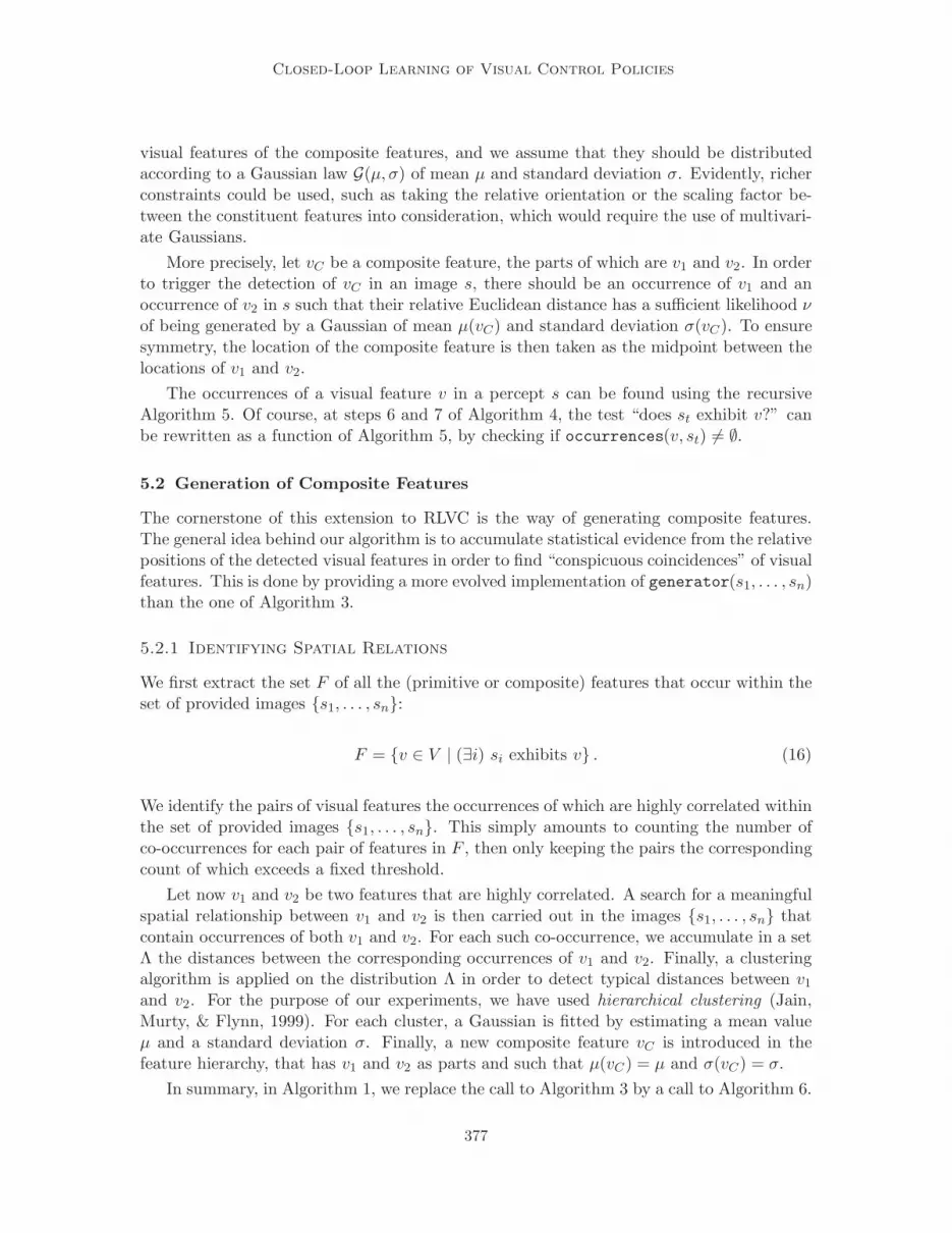
Figure 12: The “Car on the Hill” control problem.
5.2.2 Feature Validation
Algorithm 6 can generate several composite features for a given visual class Vk,i. However,at the end of Algorithm 4, at most one generated composite feature is to be kept. It isimportant to notice that the performance of the clustering method is not critical for ourpurpose. Indeed, irrelevant spatial combinations are automatically discarded, thanks to thevariance-reduction criterion of the feature selection component. In fact, the reinforcementsignal helps to direct the search for a good feature, which is an advantage over unsupervisedmethods of building feature hierarchies.
5.3 Experiments
We demonstrate the efficacy of our algorithms on a version of the classical “Car on the Hill”control problem (Moore & Atkeson, 1995), where the position and velocity information ispresented to the agent visually.
In this episodic task, a car (modeled by a mass point) is riding without friction on ahill, the shape of which is defined by the function:
H(p) =
{
p2 + p if p < 0,
p/√
1 + 5p2 if p ≥ 0.
The goal of the agent is to reach as fast as possible the top of the hill, i.e. a location suchthat p ≥ 1. At the top of the hill, the agent obtains a reward of 100. The car can thrust leftor right with an acceleration of ±4 Newtons. However, because of gravity, this accelerationis insufficient for the agent to reach the top of the hill by always thrusting toward the right.Rather, the agent has to go left for while, hence acquiring potential energy by going up theleft side of the hill, before thrusting rightward. There are two more constraints: The agentis not allowed to reach locations such that p < −1, and a velocity greater than 3 in absolutevalue leads to the destruction of the car.
379

Jodogne & Piater
5.3.1 Formal Definition of the Task
Formally, the set of possible actions is A = {−4, 4}, while the state space is S = {(p, s) ||p| ≤ 1 ∧ |s| ≤ 3}. The system has the following continuous-time dynamics:
p = s
s =a
M√
1 +H ′(p)2−
gH ′(p)
1 +H ′(p)2,
where a ∈ A is the thrust acceleration, H ′(p) is the first derivative of H(p), M = 1 is themass of the car, and g = 9.81 is the acceleration due to gravity. These continuous-timedynamics are approximated by the following discrete-time state update rule:
st+1 = st + hpt + h2st/2
st+1 = pt + hst,
where h = 0.1 is the integration time step. The reinforcement signal is defined through thisexpression:
R((st, st), a) =
{
100 if st+1 ≥ 1 ∧ |st+1| ≤ 3,0 otherwise.
In our setup, the discount factor γ was set to 0.75.
This definition is actually a mix of two coexistent formulations of the “Car on the Hill”task (Ernst, Geurts, & Wehenkel, 2003; Moore & Atkeson, 1995). The major differenceswith the initial formulation of the problem (Moore & Atkeson, 1995) is that the set ofpossible actions is discrete, and that the goal is at the top of the hill (rather than on a givenarea of the hill), just like in the definition from Ernst et al. (2003). To ensure the existenceof an interesting solution, the velocity is required to remain less than 3 (instead of 2), andthe integration time step is set to h = 0.1 (instead of 0.01).
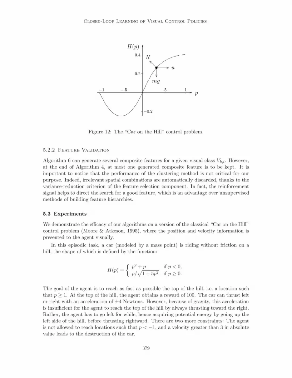
5.3.2 Inputs of the Agent
In previous work (Moore & Atkeson, 1995; Ernst et al., 2003), the agent was always assumedto have direct access to a numerical measure of its position and velocity. The only exceptionis Gordon’s work in which a visual, low-resolution representation of the global scene is givento the agent (Gordon, 1995). In our experimental setup, the agent is provided with twocameras, one looking at the ground underneath, the second at a velocity gauge. This way,the agent cannot directly know its current position and velocity, but has to suitably interpretits visual inputs to derive them.
Some examples of the pictures the sensors can return are presented in Figure 13. Theground is carpeted with a color image of 1280 × 128 pixels that is a montage of picturesfrom the COIL-100 database (Nene et al., 1996). It is very important to notice that usingindividual point features is insufficient for solving this task, since the set of features in thepictures of the velocity gauge are always the same. To know its velocity, the agent has togenerate composite features sensitive to the distance of the primitive features on the cursorwith respect to the primitive features on the digits.
380
Closed-Loop Learning of Visual Control Policies
(a)
(b)
Figure 13: (a) Visual percepts corresponding to pictures of the velocity gauge when s = −3,s = 0.5 and s = 1.5. (b) Visual percepts returned by the position sensor. Theregion framed with a white rectangle corresponds to the portion of the groundthat is returned by the sensor when p = 0.1. This portion slides back and forthas the agent moves.
5.3.3 Results
In this experimental setup, we used color differential invariants (Gouet & Boujemaa, 2001)as primitive features. Among all the possible visual inputs (both for the position and thevelocity sensors), there were 88 different primitive features. The entire image of the groundincludes 142 interest points, whereas the images of the velocity gauge include about 20interest points.
The output of RLVC is a decision tree that defines 157 visual classes. Each internalnode of this tree tests the presence of one visual feature, taken from a set of 91 distinct,highly discriminant features selected by RLVC. Among the 91 selected visual features, therewere 56 primitive and 26 composite features. Two examples of composites features thatwere selected by RLVC are depicted in Figure 15. The computation stopped after k = 38refinement steps in Algorithm 1.
To show the efficacy of our method, we compare its performance with the scenario inwhich the agent has a direct perception of its current (p, s) state. In the latter scenario, thestate space was discretized in a grid of 13 × 13 cells. The number 13 was chosen since itapproximately corresponds to the square root of 157, the number of visual classes that wereproduced by RLVC. This way, RL is provided an equivalent number of perceptual classes inthe two scenarios. Figure 14 compares the optimal value function of the direct-perception
381
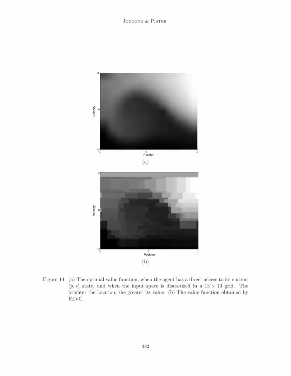
Jodogne & Piater
Position
Vel
ocity
−1 0 1
3
0
−3
(a)
Position
Vel
ocity
−1 0 1
3
0
−3
(b)
Figure 14: (a) The optimal value function, when the agent has a direct access to its current(p, s) state, and when the input space is discretized in a 13 × 13 grid. Thebrighter the location, the greater its value. (b) The value function obtained byRLVC.
382
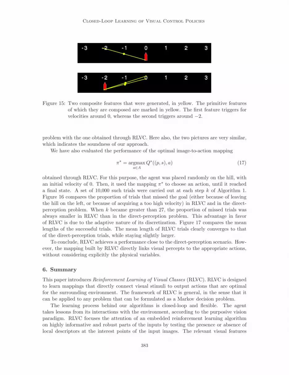
Closed-Loop Learning of Visual Control Policies
Figure 15: Two composite features that were generated, in yellow. The primitive featuresof which they are composed are marked in yellow. The first feature triggers forvelocities around 0, whereas the second triggers around −2.
problem with the one obtained through RLVC. Here also, the two pictures are very similar,which indicates the soundness of our approach.
We have also evaluated the performance of the optimal image-to-action mapping
π∗ = argmaxa∈A
Q∗((p, s), a) (17)
obtained through RLVC. For this purpose, the agent was placed randomly on the hill, withan initial velocity of 0. Then, it used the mapping π∗ to choose an action, until it reacheda final state. A set of 10,000 such trials were carried out at each step k of Algorithm 1.Figure 16 compares the proportion of trials that missed the goal (either because of leavingthe hill on the left, or because of acquiring a too high velocity) in RLVC and in the direct-perception problem. When k became greater than 27, the proportion of missed trials wasalways smaller in RLVC than in the direct-perception problem. This advantage in favorof RLVC is due to the adaptive nature of its discretization. Figure 17 compares the meanlengths of the successful trials. The mean length of RLVC trials clearly converges to thatof the direct-perception trials, while staying slightly larger.
To conclude, RLVC achieves a performance close to the direct-perception scenario. How-ever, the mapping built by RLVC directly links visual percepts to the appropriate actions,without considering explicitly the physical variables.
6. Summary
This paper introduces Reinforcement Learning of Visual Classes (RLVC). RLVC is designedto learn mappings that directly connect visual stimuli to output actions that are optimalfor the surrounding environment. The framework of RLVC is general, in the sense that itcan be applied to any problem that can be formulated as a Markov decision problem.
The learning process behind our algorithms is closed-loop and flexible. The agenttakes lessons from its interactions with the environment, according to the purposive visionparadigm. RLVC focuses the attention of an embedded reinforcement learning algorithmon highly informative and robust parts of the inputs by testing the presence or absence oflocal descriptors at the interest points of the input images. The relevant visual features
383
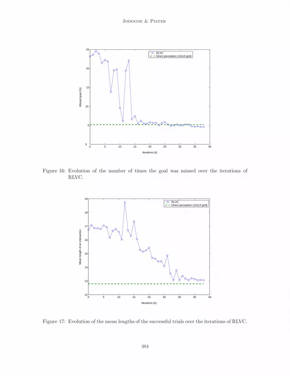
Jodogne & Piater
0 5 10 15 20 25 30 35 400
5
10
15
20
25
Iterations (k)
Mis
sed
goal
(%
)
RLVCDirect perception (13x13 grid)
Figure 16: Evolution of the number of times the goal was missed over the iterations ofRLVC.
0 5 10 15 20 25 30 35 4012
13
14
15
16
17
18
19
Iterations (k)
Mea
n le
ngth
of a
n in
tera
ctio
n
RLVCDirect perception (13x13 grid)
Figure 17: Evolution of the mean lengths of the successful trials over the iterations of RLVC.
384
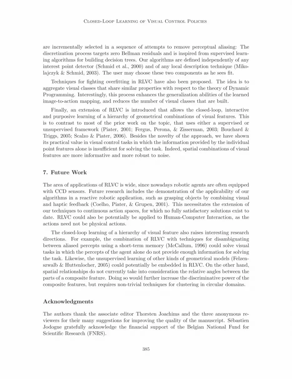
Closed-Loop Learning of Visual Control Policies
are incrementally selected in a sequence of attempts to remove perceptual aliasing: Thediscretization process targets zero Bellman residuals and is inspired from supervised learn-ing algorithms for building decision trees. Our algorithms are defined independently of anyinterest point detector (Schmid et al., 2000) and of any local description technique (Miko-lajczyk & Schmid, 2003). The user may choose these two components as he sees fit.
Techniques for fighting overfitting in RLVC have also been proposed. The idea is toaggregate visual classes that share similar properties with respect to the theory of DynamicProgramming. Interestingly, this process enhances the generalization abilities of the learnedimage-to-action mapping, and reduces the number of visual classes that are built.
Finally, an extension of RLVC is introduced that allows the closed-loop, interactiveand purposive learning of a hierarchy of geometrical combinations of visual features. Thisis to contrast to most of the prior work on the topic, that uses either a supervised orunsupervised framework (Piater, 2001; Fergus, Perona, & Zisserman, 2003; Bouchard &Triggs, 2005; Scalzo & Piater, 2006). Besides the novelty of the approach, we have shownits practical value in visual control tasks in which the information provided by the individualpoint features alone is insufficient for solving the task. Indeed, spatial combinations of visualfeatures are more informative and more robust to noise.
7. Future Work
The area of applications of RLVC is wide, since nowadays robotic agents are often equippedwith CCD sensors. Future research includes the demonstration of the applicability of ouralgorithms in a reactive robotic application, such as grasping objects by combining visualand haptic feedback (Coelho, Piater, & Grupen, 2001). This necessitates the extension ofour techniques to continuous action spaces, for which no fully satisfactory solutions exist todate. RLVC could also be potentially be applied to Human-Computer Interaction, as theactions need not be physical actions.
The closed-loop learning of a hierarchy of visual feature also raises interesting researchdirections. For example, the combination of RLVC with techniques for disambiguatingbetween aliased percepts using a short-term memory (McCallum, 1996) could solve visualtasks in which the percepts of the agent alone do not provide enough information for solvingthe task. Likewise, the unsupervised learning of other kinds of geometrical models (Felzen-szwalb & Huttenlocher, 2005) could potentially be embedded in RLVC. On the other hand,spatial relationships do not currently take into consideration the relative angles between theparts of a composite feature. Doing so would further increase the discriminative power of thecomposite features, but requires non-trivial techniques for clustering in circular domains.
Acknowledgments
The authors thank the associate editor Thorsten Joachims and the three anonymous re-viewers for their many suggestions for improving the quality of the manuscript. SebastienJodogne gratefully acknowledge the financial support of the Belgian National Fund forScientific Research (FNRS).
385
Jodogne & Piater
References
Aloimonos, Y. (1990). Purposive and qualitative active vision. In Proc. of the 10th Inter-national Conference on Pattern Recognition, pp. 436–460.
Amit, Y., & Kong, A. (1996). Graphical templates for model registration. IEEE Transac-tions on Pattern Analysis and Machine Intelligence, 18 (3), 225–236.
Asada, M., Noda, S., Tawaratsumida, S., & Hosoda, K. (1994). Vision-based behavior acqui-sition for a shooting robot by using a reinforcement learning. In Proc. of IAPR/IEEEWorkshop on Visual Behaviors, pp. 112–118.
Bagnell, J., & Schneider, J. (2001). Autonomous helicopter control using reinforcementlearning policy search methods. In Proc. of the International Conference on Roboticsand Automation. IEEE.
Barto, A., Sutton, R., & Anderson, C. (1983). Neuronlike adaptive elements that cansolve difficult learning control problems. IEEE Transactions on Systems, Man andCybernetics, 13 (5), 835–846.
Bellman, R. (1957). Dynamic Programming. Princeton University Press.
Bertsekas, D., & Tsitsiklis, J. (1996). Neuro-Dynamic Programming. Athena Scientific.
Boigelot, B. (1999). Symbolic Methods for Exploring Infinite State Spaces. Ph.D. thesis,University of Liege, Liege (Belgium).
Boigelot, B., Jodogne, S., & Wolper, P. (2005). An effective decision procedure for lineararithmetic with integer and real variables. ACM Transactions on Computational Logic(TOCL), 6 (3), 614–633.
Bouchard, G., & Triggs, B. (2005). Hierarchical part-based visual object categorization. InIEEE Conference on Computer Vision and Pattern Recognition, Vol. 1, pp. 710–715,San Diego (CA, USA).
Breiman, L., Friedman, J., & Stone, C. (1984). Classification and Regression Trees.Wadsworth International Group.
Bryant, R. (1986). Graph-based algorithms for boolean function manipulation. IEEE Trans-actions in Computers, 8 (35), 677–691.
Bryant, R. (1992). Symbolic boolean manipulation with ordered binary decision diagrams.ACM Computing Surveys, 24 (3), 293–318.
Burl, M., & Perona, P. (1996). Recognition of planar object classes. In Proc. of the IEEEConference on Computer Vision and Pattern Recognition, pp. 223–230, San Francisco(CA, USA).
Chapman, D., & Kaelbling, L. (1991). Input generalization in delayed reinforcement learn-ing: An algorithm and performance comparisons. In Proc. of the 12th InternationalJoint Conference on Artificial Intelligence (IJCAI), pp. 726–731, Sydney.
Chrisman, L. (1992). Reinforcement learning with perceptual aliasing: The perceptualdistinctions approach. In National Conference on Artificial Intelligence, pp. 183–188.
386
Closed-Loop Learning of Visual Control Policies
Coelho, J., Piater, J., & Grupen, R. (2001). Developing haptic and visual perceptual cat-egories for reaching and grasping with a humanoid robot. Robotics and AutonomousSystems, special issue on Humanoid Robots, 37 (2–3), 195–218.
Crandall, D., & Huttenlocher, D. (2006). Weakly supervised learning of part-based spatialmodels for visual object recognition. In Proc. of the 9th European Conference onComputer Vision.
Delzanno, G., & Raskin, J.-F. (2000). Symbolic representation of upward closed sets. InTools and Algorithms for the Construction and Analysis of Systems, Lecture Notes inComputer Science, pp. 426–440, Berlin (Germany).
Derman, C. (1970). Finite State Markovian Decision Processes. Academic Press, New York.
Ernst, D., Geurts, P., & Wehenkel, L. (2003). Iteratively extending time horizon reinforce-ment learning. In Proc. of the 14th European Conference on Machine Learning, pp.96–107, Dubrovnik (Croatia).
Ernst, D., Geurts, P., &Wehenkel, L. (2005). Tree-based batch mode reinforcement learning.Journal of Machine Learning Research, 6, 503–556.
Felzenszwalb, P., & Huttenlocher, D. (2005). Pictorial structures for object recognition.International Journal of Computer Vision, 61 (1), 55–79.
Fergus, R., Perona, P., & Zisserman, A. (2003). Object class recognition by unsupervisedscale-invariant learning. In IEEE Conference on Computer Vision and Pattern Recog-nition, Vol. 2, pp. 264–271, Madison (WI, USA).
Fischler, M., & Elschlager, R. (1973). The representation and matching of pictorial struc-tures. IEEE Transactions on Computers, 22 (1), 67–92.
Forsyth, D., Haddon, J., & Ioffe, S. (1999). Finding objects by grouping primitives. In Shape,Contour and Grouping in Computer Vision, pp. 302–318, London (UK). Springer-Verlag.
Gaskett, C., Fletcher, L., & Zelinsky, A. (2000). Reinforcement learning for visual servoingof a mobile robot. In Proc. of the Australian Conference on Robotics and Automation,Melbourne (Australia).
Gibson, E., & Spelke, E. (1983). The development of perception. In Flavell, J. H., & Mark-man, E. M. (Eds.), Handbook of Child Psychology Vol. III: Cognitive Development(4th edition)., chap. 1, pp. 2–76. Wiley.
Givan, R., Dean, T., & Greig, M. (2003). Equivalence notions and model minimization inmarkov decision processes. Artificial Intelligence, 147 (1–2), 163–223.
Gordon, G. (1995). Stable function approximation in dynamic programming. In Proc. ofthe International Conference on Machine Learning, pp. 261–268.
Gouet, V., & Boujemaa, N. (2001). Object-based queries using color points of interest. InIEEE Workshop on Content-Based Access of Image and Video Libraries, pp. 30–36,Kauai (HI, USA).
Howard, R. (1960). Dynamic Programming and Markov Processes. Technology Press andWiley, Cambridge (MA) and New York.
387
Jodogne & Piater
Huber, M., & Grupen, R. (1998). A control structure for learning locomotion gaits. In 7thInt. Symposium on Robotics and Applications, Anchorage (AK, USA). TSI Press.
Iida, M., Sugisaka, M., & Shibata, K. (2002). Direct-vision-based reinforcement learningto a real mobile robot. In Proc. of International Conference of Neural InformationProcessing Systems, Vol. 5, pp. 2556–2560.
Jaakkola, T., Jordan, M., & Singh, S. (1994). Convergence of stochastic iterative dynamicprogramming algorithms. In Cowan, J. D., Tesauro, G., & Alspector, J. (Eds.), Ad-vances in Neural Information Processing Systems, Vol. 6, pp. 703–710. Morgan Kauf-mann Publishers.
Jain, A. K., Murty, M. N., & Flynn, P. J. (1999). Data clustering: A review. ACM ComputingSurveys, 31 (3), 264–323.
Jodogne, S., & Piater, J. (2005a). Interactive learning of mappings from visual perceptsto actions. In De Raedt, L., & Wrobel, S. (Eds.), Proc. of the 22nd InternationalConference on Machine Learning (ICML), pp. 393–400, Bonn (Germany). ACM.
Jodogne, S., & Piater, J. (2005b). Learning, then compacting visual policies (extended ab-stract). In Proc. of the 7th European Workshop on Reinforcement Learning (EWRL),pp. 8–10, Napoli (Italy).
Jodogne, S., Scalzo, F., & Piater, J. (2005). Task-driven learning of spatial combinationsof visual features. In Proc. of the IEEE Workshop on Learning in Computer Visionand Pattern Recognition, San Diego (CA, USA). IEEE.
Kaelbling, L., Littman, M., & Cassandra, A. (1998). Planning and acting in partiallyobservable stochastic domains. Artificial Intelligence, 101 (1-2), 99–134.
Kaelbling, L., Littman, M., & Moore, A. (1996). Reinforcement learning: A survey. Journalof Artificial Intelligence Research, 4, 237–285.
Kimura, H., Yamashita, T., & Kobayashi, S. (2001). Reinforcement learning of walkingbehavior for a four-legged robot. In Proc. of the 40th IEEE Conference on Decisionand Control, Orlando (FL, USA).
Kohl, N., & Stone, P. (2004). Policy gradient reinforcement learning for fast quadrupedallocomotion. In Proc. of the IEEE International Conference on Robotics and Automa-tion, pp. 2619–2624, New Orleans.
Kumar, M., Torr, P., & Zisserman, A. (2004). Extending pictorial structures for objectrecognition. In Proc. of the British Machine Vision Conference.
Kwok, C., & Fox, D. (2004). Reinforcement learning for sensing strategies. In Proc. of theIEEE International Conference on Intelligent Robots and Systems.
Lagoudakis, M., & Parr, R. (2003). Least-squares policy iteration. Journal of MachineLearning Research, 4, 1107–1149.
Lowe, D. (2004). Distinctive image features from scale-invariant keypoints. InternationalJournal of Computer Vision, 60 (2), 91–110.
Martınez-Marın, T., & Duckett, T. (2005). Fast reinforcement learning for vision-guidedmobile robots. In Proc. of the IEEE International Conference on Robotics and Au-tomation, pp. 18–22, Barcelona (Spain).
388
Closed-Loop Learning of Visual Control Policies
McCallum, R. (1996). Reinforcement Learning with Selective Perception and Hidden State.Ph.D. thesis, University of Rochester, New York.
Michels, J., Saxena, A., & Ng, A. (2005). High speed obstacle avoidance using monocularvision and reinforcement learning. In Proc. of the 22nd International Conference inMachine Learning, pp. 593–600, Bonn (Germany).
Mikolajczyk, K., & Schmid, C. (2003). A performance evaluation of local descriptors. InProc. of the IEEE Conference on Computer Vision and Pattern Recognition, Vol. 2,pp. 257–263, Madison (WI, USA).
Moore, A., & Atkeson, C. (1995). The parti-game algorithm for variable resolution rein-forcement learning in multidimensional state-spaces. Machine Learning, 21.
Munos, R., & Moore, A. (2002). Variable resolution discretization in optimal control. Ma-chine Learning, 49, 291–323.
Nene, S., Nayar, S., & Murase, H. (1996). Columbia object image library (COIL-100). Tech.rep. CUCS-006-96, Columbia University, New York.
Ng, A., Coates, A., Diel, M., Ganapathi, V., Schulte, J., Tse, B., Berger, B., & Liang, E.(2004). Inverted autonomous helicopter flight via reinforcement learning. In Proc. ofthe International Symposium on Experimental Robotics.
Paletta, L., Fritz, G., & Seifert, C. (2005). Q-learning of sequential attention for visual objectrecognition from informative local descriptors.. In Proc. of the 22nd InternationalConference on Machine Learning (ICML), pp. 649–656, Bonn (Germany).
Paletta, L., & Pinz, A. (2000). Active object recognition by view integration and reinforce-ment learning. Robotics and Autonomous Systems, 31 (1–2), 71–86.
Peng, J., & Bhanu, B. (1998). Closed-loop object recognition using reinforcement learning.IEEE Transactions on Pattern Analysis and Machine Intelligence, 20 (2), 139–154.
Perona, P., Fergus, R., & Zisserman, A. (2003). Object class recognition by unsupervisedscale-invariant learning. In Conference on Computer Vision and Pattern Recognition,Vol. 2, p. 264.
Piater, J. (2001). Visual Feature Learning. Ph.D. thesis, University of Massachusetts,Computer Science Department, Amherst (MA, USA).
Puterman, M., & Shin, M. (1978). Modified policy iteration algorithms for discountedMarkov decision problems. Management Science, 24, 1127–1137.
Pyeatt, L., & Howe, A. (2001). Decision tree function approximation in reinforcementlearning. In Proc. of the Third International Symposium on Adaptive Systems, pp.70–77, Havana, Cuba.
Quinlan, J. (1993). C4.5: Programs for Machine Learning. Morgan Kaufmann PublishersInc., San Francisco (CA, USA).
Randløv, J., & Alstrøm, P. (1998). Learning to drive a bicycle using reinforcement learningand shaping. In Proc. of the 15th International Conference on Machine Learning, pp.463–471, Madison (WI, USA). Morgan Kaufmann.
389
Jodogne & Piater
Rummery, G., & Niranjan, M. (1994). On-line Q-learning using connectionist sytems. Tech.rep. CUED/F-INFENG-TR 166, Cambridge University.
Salganicoff, M. (1993). Density-adaptive learning and forgetting. In Proc. of the 10thInternational Conference on Machine Learning, pp. 276–283, Amherst (MA, USA).Morgan Kaufmann Publishers.
Scalzo, F., & Piater, J. (2006). Unsupervised learning of dense hierarchical appearancerepresentations. In Proc. of the 18th International Conference on Pattern Recognition,Hong-Kong.
Schaal, S. (1997). Learning from demonstration. In Mozer, M. C., Jordan, M., & Petsche,T. (Eds.), Advances in Neural Information Processing Systems, Vol. 9, pp. 1040–1046.Cambridge, MA, MIT Press.
Schmid, C., & Mohr, R. (1997). Local greyvalue invariants for image retrieval. IEEETransactions on Pattern Analysis and Machine Intelligence, 19 (5), 530–535.
Schmid, C., Mohr, R., & Bauckhage, C. (2000). Evaluation of interest point detectors.International Journal of Computer Vision, 37 (2), 151–172.
Schyns, P., & Rodet, L. (1997). Categorization creates functional features. Journal ofExperimental Psychology: Learning, Memory and Cognition, 23 (3), 681–696.
Shibata, K., & Iida, M. (2003). Acquisition of box pushing by direct-vision-based reinforce-ment learning. In Proc. of the Society of Instrument and Control Engineers AnnualConference, p. 6.
Singh, S., Jaakkola, T., & Jordan, M. (1995). Reinforcement learning with soft state aggre-gation. In Advances in Neural Information Processing Systems, Vol. 7, pp. 361–368.MIT Press.
Sudderth, E., Ihler, A., Freeman, W., & Willsky, A. (2003). Nonparametric belief propaga-tion. In Proc. of the IEEE Conference on Computer Vision and Pattern Recognition,pp. 605–612.
Sutton, R. (1988). Learning to predict by the methods of temporal differences. MachineLearning, 3 (1), 9–44.
Sutton, R., & Barto, A. (1998). Reinforcement Learning, an Introduction. MIT Press.
Takahashi, Y., Takeda, M., & Asada, M. (1999). Continuous valued Q-learning for vision-guided behavior acquisition. In Proc. of the International Conference on MultisensorFusion and Integration for Intelligent Systems, pp. 255–260.
Tarr, M., & Cheng, Y. (2003). Learning to see faces and objects. Trends in CognitiveSciences, 7 (1), 23–30.
Tesauro, G. (1995). Temporal difference learning and TD-Gammon. Communications ofthe ACM, 38 (3), 58–68.
Uther, W., & Veloso, M. (1998). Tree based discretization for continuous state space rein-forcement learning. In Proc. of the 15th National Conference on Artificial Intelligence(AAAI), pp. 769–774, Madison (WI, USA).
390
Closed-Loop Learning of Visual Control Policies
Watkins, C. (1989). Learning From Delayed Rewards. Ph.D. thesis, King’s College, Cam-bridge (UK).
Weber, C., Wermter, S., & Zochios, A. (2004). Robot docking with neural vision andreinforcement. Knowledge-Based Systems, 17 (2–4), 165–172.
Wettergreen, D., Gaskett, C., & Zelinsky, A. (1999). Autonomous guidance and control foran underwater robotic vehicle. In Proc. of the International Conference on Field andService Robotics, Pittsburgh (USA).
Whitehead, S., & Ballard, D. (1991). Learning to perceive and act by trial and error.Machine Learning, 7, 45–83.
Yin, P.-Y. (2002). Maximum entropy-based optimal threshold selection using deterministicreinforcement learning with controlled randomization. Signal Processing, 82, 993–1006.
Yoshimoto, J., Ishii, S., & Sato, M. (1999). Application of reinforcement learning to bal-ancing acrobot. In Proc. of the 1999 IEEE International Conference on Systems,Man and Cybernetics, pp. 516–521.
391