Embed Size (px)
Citation preview

J. Fluid Mech. (2012), vol. 703, pp. 326–362. c© Cambridge University Press 2012 326doi:10.1017/jfm.2012.223
Closed-loop control of unsteadiness over arounded backward-facing step
Alexandre Barbagallo1,2, Gregory Dergham3, Denis Sipp1, Peter J. Schmid2†and Jean-Christophe Robinet3
1 ONERA – The French Aerospace Lab, 8 rue des Vertugadins, 92190 Meudon, France2 Laboratoire d’Hydrodynamique (LadHyX), CNRS – Ecole Polytechnique, 91128 Palaiseau, France3 DynFluid Laboratory, Arts et Metiers ParisTech, 151 Boulevard de l’Hopital, 75013 Paris, France
(Received 22 October 2010; revised 8 March 2012; accepted 8 May 2012;first published online 12 June 2012)
The two-dimensional, incompressible flow over a rounded backward-facing step atReynolds number Re = 600 is characterized by a detachment of the flow close tothe step followed by a recirculation zone. Even though the flow is globally stable,perturbations are amplified as they are convected along the shear layer, and thepresence of upstream random noise renders the flow unsteady, leading to a broadbandspectrum of excited frequencies. This paper is aimed at suppressing this unsteadinessusing a controller that converts a shear-stress measurement taken from a wall-mountedsensor into a control law that is supplied to an actuator. A comprehensive studyof various components of closed-loop control design – covering sensor placement,choice and influence of the cost functional, accuracy of the reduced-order model,compensator stability and performance – shows that successful control of this flowrequires a judicious balance between estimation speed and estimation accuracy, andbetween stability limits and performance requirements. The inherent amplificationbehaviour of the flow can be reduced by an order of magnitude if the above-mentionedconstraints are observed. In particular, to achieve superior controller performance, theestimation sensor should be placed upstream near the actuator to ensure sufficientestimation speed. Also, if high-performance compensators are sought, a very accuratereduced-order model is required, especially for the dynamics between the actuator andthe estimation sensor; otherwise, very minute errors even at low energies and highfrequencies may render the large-scale compensated linearized simulation unstable.Finally, coupling the linear compensator to nonlinear simulations shows a gradualdeterioration in control performance as the amplitude of the noise increases.
Key words: boundary layer control, control theory, separated flows
1. IntroductionMany industrial fluid devices are afflicted by undesirable flow behaviour – such
as unsteadiness, separation, instabilities and transition to turbulence – which limitsperformance, endangers safe operation or is detrimental to structural components. Flowcontrol is quickly becoming a key technology in engineering design to overcome
† Email address for correspondence: [email protected]

Closed-loop control of unsteadiness over a rounded backward-facing step 327
inherent limitations, to advance into unexplored parameter regimes, to extend safetymargins and to ensure operation under optimal conditions. A prototypical and much-studied example is the compressible flow over a cavity, which is characterized byinstabilities that manifest themselves in a buffeting motion, in induced drag (Gharib& Roshko 1987) and in intense noise emission (see Rossiter 1964). In the air intakesof aircraft engines, separated flow can act as an amplifier for incoming perturbations,causing unsteadiness, which in turn results in loss of performance and material fatigue.Transitional and turbulent boundary layers have long attracted the attention of theflow control community (see e.g. Joslin 1998; Kim 2003; Saric, Reed & White 2003;Archambaud et al. 2008; Boiko, Dovgal & Hein 2008), mainly as a result of theirubiquity in vehicle aerodynamics and their central role as the source of skin friction.For all three examples, flow control techniques that effectively eliminate instabilities,efficiently reduce noise amplification or successfully diminish drag are essential inmaintaining the desired flow conditions.
The design procedure of flow control laws critically depends on the nature of theflow to be controlled. Oscillator-type flows, which are defined by a global instabilityresulting in self-sustained oscillatory fluid behaviour, are more easily controlled, sincethe flow is dominated by a limited number of structures of well-defined frequencies.Sensitivity to noise is comparatively low, and the estimator and controller can simplyreconstruct the flow state from measurements and act upon it according to thecontrol objective. A second type of flow behaviour, referred to as noise amplifiers,is substantially more challenging to control. This type of flow is globally stable butis characterized by a strong propensity to amplify noise and a broadband spectrumof responsive frequencies. These characteristics make the flow and the controlperformance highly sensitive, not only to physical noise sources and uncertainties,but also to the methodological approximations, modelling inaccuracies and truncationerrors that inevitably arise during estimator and control design. The propagation ofsmall perturbations, whether of physical or computational origin, is appropriatelytracked and quantified by frequency-based transfer functions, which reveal preferredfrequencies or confirm the successful reduction of the flow’s amplification potential.
Optimal flow control techniques have been widely applied for active controlpurposes. In particular, the linear quadratic Gaussian (LQG) framework has beenadopted for the control of small-amplitude perturbations in oscillator and amplifierflows. Examples of oscillator flows include, among others, supercritical flow over ashallow or deep cavity (Akervik et al. 2007; Barbagallo, Sipp & Schmid 2009), flowover a shallow bump (Ehrenstein, Passaggia & Gallaire 2010) and flow past a flatplate (Ahuja & Rowley 2010). In all cases, stabilization of the flow by feedbackcontrol strategies could be accomplished. Amplifier flows are dominated by convectiveand transient processes, and successful control is defined by a marked reduction ofthe flow’s inherent amplification potential. Control of amplifier flows using LQGtechniques was first attempted for very idealized geometries (see e.g. Joshi, Speyer& Kim 1997; Bewley & Liu 1998; Chevalier et al. 2007), namely, in simple, one-dimensional configurations. For more complex and higher-dimensional flows, directapplication of the LQG framework becomes prohibitively expensive, and reduced-ordermodels have to be introduced for the practical design of the compensator. LQG-based compensators using reduced-order models have been applied by Bagheri, Brandt& Henningson (2009) to control the amplification of perturbations in a spatiallydeveloping boundary layer and by Ilak & Rowley (2008) to control transitionalchannel flow. In Bagheri & Henningson (2011), strong emphasis has been placedon the model reduction technology; in particular, it has been demonstrated that the

328 A. Barbagallo, G. Dergham, D. Sipp, P. J. Schmid and J.-C. Robinet
reduced-order model (ROM) had to capture accurately the input–output behaviourbetween actuators and sensors to ensure a positive compensator performance (Kim& Bewley 2007). Despite the first successful attempts at applying LQG-feedbackcontrol to amplifier flows, many questions remain open about the design and practicalimplementation of compensators for this type of flow. Owing to the flow’s tendency toamplify perturbations transiently, sensitivity becomes the key concept in the design andperformance evaluation of compensators: sensitivity to sensor and actuator placement,to the accuracy of the ROM and to nonlinear effects. Some of these issues have beenaddressed using an idealized (parallel base flow) model problem in Ilak (2009); acomprehensive analysis of closed-loop control for amplifier flows, however, is missing.
The goal of the present study is an identification of the various environmental andprocedural factors and the assessment of their influence on the performance of thecompensator for a specific amplifier flow: the case of a two-dimensional, laminarflow over a rounded backward-facing step (see Blackburn, Barkley & Sherwin 2008;Marquet et al. 2008; Dergham et al. 2011). This configuration is characterized by adetachment of the flow close to the step, followed by a recirculation zone; even thoughthe flow is globally stable, perturbations are amplified as they are convected alongthe shear layer. This is due to a Kelvin–Helmholtz type of instability, which createsa convectively unstable region, extending approximately from the detachment to thereattachment point. If upstream residual noise is present, for example white, Gaussiannoise, the flow will be unsteady, with a broadband spectrum in the bubble. Ourcontrol objective consists in suppressing this unsteadiness using an optimal controller,which converts a measurement signal obtained from a wall-mounted sensor into acontrol law that is subsequently supplied to an actuator. We believe that the resultsobtained for this specific configuration also hold, at least qualitatively, for otherconvectively unstable flows, such as, for example, a supercritical boundary layerdeveloping over a flat plate subject to Tollmien–Schlichting instabilities. A discussionabout the similarities of and differences between these two configurations is postponedto § 2.
The present study is structured as follows. After a brief description of the flowconfiguration, its noise amplification behaviour and the basic principles of LQGcontrol and model reduction (§ 2), we start by considering the estimation problem(§ 3) and address sensor placement and estimation speed. In § 4 the controller willbe introduced, performance limitations of the compensator will be discussed and theinfluence of the choice of control objective will be assessed. Section 5 will presentthe application of the LQG controller to linearized numerical simulations; specifically,the sensitivity to model inaccuracies and its relation to stability margins for thecompensated system will be treated, based on both classical stability concepts andworst-case optimization. In § 6 we apply linear control to a nonlinear simulationand discuss the validity range of the linear compensator. A summary of results andconclusions are given in § 7.
2. Configuration and mathematical model2.1. Flow configuration and governing equations
We study the laminar and incompressible flow over a two-dimensional roundedbackward-facing step, which is sketched in figure 1, together with the geometricmeasures, the base flow stream-function and the set-up of control inputs and sensoroutputs. Only a reduced part of the computational domain is shown. The step height hand the inflow velocity U∞ are chosen as the characteristic length and velocity scales

Closed-loop control of unsteadiness over a rounded backward-facing step 329
1.000.50
0–0.03–0.01
0 5 10
Inputs
Outputs
0
1
2
FIGURE 1. Sketch of the geometry for flow over a rounded backward-facing step, showingthe stream-function of the base flow at Re = 600 (dashed values refer to negative values).The stream-function is set to zero at the lower boundary of the computational domain. Theupstream, downstream and top boundaries are respectively located at x = −20, x = 100 andy = 20. A typical mesh yields n = 400 775 degrees of freedom from 88 181 triangles. Thepositions of the input (B1,2) and output (C1,2,3,4,p) devices are also shown.
of the problem. The rounded part of the step consists of a circular arc extendingfrom (x = 0, y = 1) to (x = 2, y = 0). The flow enters the computational domain fromthe left (at x = −20) with a constant streamwise velocity. A free-slip condition isimposed on the upstream part of the lower boundary (−20 6 x 6 −2, y = 1), beyondwhich a laminar boundary layer starts to develop; no-slip conditions are enforcedon the remaining lower boundary given by −2 6 x 6 100. On the top part ofthe computational domain, at y = 20, a symmetry condition is implemented, and astandard outflow condition is prescribed at the outlet (x = 100). The symmetry andoutflow boundary conditions have been placed far from the backward-facing step toensure negligible influence of the choice of boundary conditions on the inherent flowdynamics.
The Reynolds number based on the step height and inflow velocity is chosen asRe = 600 and held constant throughout our study. For this Reynolds number, theflow separates at x ≈ 0.6 and reattaches at x ≈ 11, forming an elongated recirculationbubble. The displacement thickness of the incoming boundary layer at x = 0 is equalto δ∗ ≈ 0.082, which yields a Reynolds number based on the displacement thickness ofReδ∗ ≈ 49.2. The base flow, a solution of the nonlinear steady Navier–Stokes equations,is visualized by iso-contours of its stream-function in figure 1.
Flow over a rounded backward-facing step is a prototypical example for an amplifierflow since small upstream perturbations may be selectively amplified in the shearlayer due to a Kelvin–Helmholtz instability (see next section for details). Characteristicunsteadiness arises from low-level noise via a linear amplification mechanism, whichsubsequently saturates nonlinearly once sufficiently high amplitudes have been reached.It is the goal of this paper to devise and assess an active feedback control strategythat decreases the convective amplification of random perturbations. We will considersmall-amplitude noise; the dynamics of the perturbations is thus linear, which justifiesusing the Navier–Stokes equations linearized about the base flow as a mathematicalmodel. The governing equations are spatially discretized using finite elements ofTaylor–Hood type (P2–P2–P1) and implemented using the FreeFem++ software (seeHecht et al. 2005). In matrix form, these read
QdXdt= AX, (2.1)
where X denotes the state vector containing the velocity and pressure fields, Arepresents the Navier–Stokes operator linearized around the base flow (shown in

330 A. Barbagallo, G. Dergham, D. Sipp, P. J. Schmid and J.-C. Robinet
–4 0 4 8 12 16 20 24 28 32 36 400 1 2 3 4
102
103
2
–4 0 4 8 12 16 20 24 28 32 36 40
2
(b)(a)
(c)
0
4
0
4
FIGURE 2. (a) Optimal energy response of the linear system to a harmonic forcingof frequency ω. (b) Optimal forcing visualized by contours of the streamwise velocity.(c) Optimal response visualized by contours of the streamwise velocity.
figure 1) and Q stands for the mass matrix, which simultaneously defines theperturbation kinetic energy according to E = X∗QX .
2.2. Noise amplification behaviourFor the chosen Reynolds number of Re = 600, the flow is globally stable and thematrix A does not show any unstable eigenvalues. Yet, sustained unsteadiness mayarise from the continuous excitation of the flow by upstream noise. This noiseamplifier behaviour can be analysed and quantified in terms of the optimal harmonicforcing and its response in the frequency domain (see Alizard, Cherubini & Robinet2009; Sipp et al. 2010). For a given frequency ω, a periodic forcing of the formFω exp(iωt) yields a corresponding response Xω exp(iωt), where Xω is given byXω = (iωQ − A)−1 QFω. The optimal forcing is defined as the forcing Fω of unitenergy (i.e. F∗ωQFω = 1) that maximizes the energy of the response. The correspondingresponse Xω is referred to as the optimal response; its energy X∗ωQXω is the optimalenergy gain due to external forcing at a prescribed frequency ω. We will use thesubscript ω to indicate quantities defined in the frequency domain.
In figure 2(a), the optimal energy gain is presented as a function of the forcingfrequency. The semi-logarithmic graph shows a parabolic curve, with the highestresponse to forcing around a frequency of ω = 0.8. For frequencies above ω ≈ 2, theenergy gain decays monotonically. In figure 2(b,c), the spatial shapes of the optimalforcing and response (real part only) taken at the highest energy gain are visualized bycontours of the streamwise component. In accordance with the convective nature of theflow, we observe that the optimal forcing is concentrated upstream near the step, whilethe associated response is located further downstream. Hence, a noise source situatednear the rounded step (mimicking an upstream, stochastic disturbance environment)can efficiently trigger perturbations whose maximum amplitudes are attained nearx ≈ 12. Based on this result, we model the noise as a Gaussian-shaped momentumforcing located at (x=−1, y= 1) with a width of 0.6. After discretization, this forcingappears in form of the matrix B1 in the linear system
QdXdt= AX + QB1w(t), (2.2)
with w(t) describing the temporal behaviour of the noise. For the sake of simplicity,the noise will be taken as white in time with zero mean 〈w〉 = 0 and variance 〈w2〉
Closed-loop control of unsteadiness over a rounded backward-facing step 331
denoted by W2. We have chosen a compact source of disturbances located upstreamin accordance with the physical conditions of advection-dominated flows. Even thoughan alternative global forcing by noise is conceivable, this particular set-up, besidesrunning counter to the principal physical mechanisms, would not be amenable toeffective flow control strategies owing to a poor sensing and estimation process. Inaddition, we assume that a linear model is sufficient in describing the flow behaviour;in this sense, we restrict ourselves to small-amplitude processes, as mentioned above.
In continuing to set up our flow control problem, an appropriate objective or costfunctional has to be specified. To this end, two quantities will be considered. The firstquantity consists of the shear stress measured at the wall and is computed followingmp = CpX =
∫ x=11.6x=11 ∂yu′ dx. The placement of this sensor has been motivated by the
location of maximum response of the flow to harmonic excitation (see figure 2c).For higher frequencies (ω > 2), the optimal response moves upstream towards thedetachment point and is no longer observable by the sensor Cp; for lower frequencies,the spatial support of the optimal response extends both upstream and downstream(with the most energetic region remaining near the reattachment point). Hence, sensorCp will detect all perturbation frequencies with ω 6 2. The second quantity of interestis the total kinetic perturbation energy contained in the entire domain; it is given byE = X∗QX . The control to be designed will aim at diminishing either mp or E. It isinteresting to note that, under random forcing, the two quantities of interest, mp and E,display a frequency response strikingly similar to that given in figure 2(a); the spatialstructure of the stochastic response resembles that given in figure 2(c) (the reader isreferred to figure 9 for verification).
2.3. Linear quadratic Gaussian (LQG) controlA closed-loop control strategy is considered in order to weaken or suppress theamplification of perturbations. In contrast to open-loop control strategies, this methodextracts information from the system via measurements, which is then processed toapply real-time actuation. This technique allows flow manipulation with rather lowexpended energy and permits the application and adaptation of control laws to avariety of flow situations, provided the model is representative of and robust tophysical and parametric changes. The approach taken in our study is based on acompensator designed within the linear quadratic Gaussian (LQG) control framework(see Burl 1999). The actuator through which control efforts are exerted on the flowconsists of a body force acting on the vertical momentum component; the location,shape and type of the actuator is summarized in the matrix B2 (see figure 1). Thecontrol law u(t) that describes the temporal behaviour of the actuator is based onreal-time measurements of the flow from sensors, which extract shear stresses andare located at various positions along the wall. The governing system of equations,including the actuators and sensors, can be cast into the familiar state-space form
QdXdt= AX + QB1w+ QB2u, m= CX + g(t), (2.3)
where g(t) is a zero-mean measurement noise of variance G2, which contaminatesthe measure m. The link between the measurement signal m and the actuation lawu is provided by the compensator. Figure 3 presents a sketch of a typical LQGcontrol set-up, including the system to be controlled as well as the two componentsof the compensator: the estimator and the controller. The module labelled ‘Plant’represents our fluid system whose flow characteristics we wish to modify; it is givenmathematically by (2.3). The plant depends on the initial condition X(t0), the noise

332 A. Barbagallo, G. Dergham, D. Sipp, P. J. Schmid and J.-C. Robinet
Plant
Controller Estimator
Compensator
Y (t)
FIGURE 3. Sketch of a typical LQG control set-up.
input w(t) and the control law u(t), and provides as an output the state vector X . Ameasurement signal m can be extracted at all times from the state vector, which is thenpassed to the compensator. In a first step, the estimator will reconstruct an estimatedstate Y(t) from the measurement m, which is, in a second step, used by the controllerto compute the control law u(t). More details about the design of the estimator and thecontroller will be given below.
It is important to stress that the placement of the actuator and sensor is criticalfor the success of closed-loop control. In our case, the actuator is positioned nearthe separation point (see control input B2 in figure 1), which corresponds to thelocation where the optimal forcing structures are most prominent, independent of thefrequency (see figure 2b, which illustrates the case for ω = 0.8). This placementoptimally exploits the sensitivity of the flow to external forcing and suggests that low-amplitude control at this location may exert sufficient influence on the flow behaviourto accomplish our control objective. In other words, the chosen actuator locationshould ensure low control gains.
Analogously, the placement of the sensor requires care and thought. Commonly,measurements are taken at locations where the flow feature we wish to suppressis particularly prevalent. Recalling the spatial structure of the most amplified flowresponse to optimal forcing (see figure 2c), this would suggest a sensor placementdownstream of the reattachment point near x ≈ 12. Nevertheless, we will demonstratethat this particular choice does not yield an efficient and effective closed-loop control,and we will methodically explore the estimator performance based on sensors placedfurther upstream in the recirculation bubble (see figure 1). In particular, four discretesensor locations, denoted by C1,2,3,4, will be assessed; these are distinct from theperformance sensor Cp.
More generally, to ensure low control gains and a physically relevant controlobjective, the actuator should be placed at the transition location from the stableto the convectively unstable flow regime (branch I) and the performance sensor Cp atthe transition location from convectively unstable to the stable flow regime (branch II).Indeed, in a convectively unstable flow, the instability is cumulative in the downstreamdirection: branch I is the point where an action has largest effect on the perturbation,while branch II is the point where the perturbation is strongest. The locations ofbranches I and II usually depend on the frequency of the perturbation; in the present

Closed-loop control of unsteadiness over a rounded backward-facing step 333
flow over a backward-facing step, however, branches I and II are located for allfrequencies near the flow separation and reattachment points (not shown here). Hence,a single actuator and a single performance sensor (plus one estimation sensor) aresufficient to stabilize the flow for all frequencies. In the case of a convectively unstableboundary layer developing over a flat plate, the locations of branches I and II stronglydepend on the perturbation frequency. Hence, multiple input–output triplets (eachconsisting of actuator, performance sensor and estimation sensor) are necessary, whereeach triplet is designed to stabilize the flow in a bounded area in the downstreamdirection and in a restricted frequency band.
2.4. Reduced-order model based on proper orthogonal decompositionThe design of the estimator and controller involves the numerical solution of twoRiccati equations for the Kalman and control gain, respectively. The numerical effortis proportional to the dimension of the system matrix A, which makes the directsolution of the Riccati equation excessively expensive or even impossible. It is thusnecessary and common practice to substitute the full system by an equivalent systemof considerably smaller dimensions and to compute the two gains based on this ROMof the flow. A standard technique to arrive at a ROM of the flow uses a Galerkinprojection of the governing equations onto proper orthogonal decomposition (POD)modes (see Sirovich 1987). This method proves to be efficient (see Bagheri et al.2009; Barbagallo et al. 2009; Bagheri & Henningson 2011) in capturing the maincharacteristics of the original system required for closed-loop control, namely thedynamics between the inputs (given by B1 and B2) and the outputs (given by C1,2,3,4
and the control objectives E and Cp). The governing equation for the ROM is similarto (2.3) and is given by
dXdt= AX + B1w+ B2u, m= CX, (2.4)
where the superscript ‘hat’ indicates reduced quantities. The energy of the state E is
simply given by ‖X‖2 = X∗X , since the projection basis is orthonormal with respect to
the energy inner product. The use of a ROM decreases the dimension of our systemfrom O(106) to ∼150 degrees of freedom and thus allows the application of standarddirect algorithms for LQG control design. The choice of POD modes as a projectionbasis has essentially been motivated by the requirement for capturing the energyoutput. A standard balanced-truncation technique (see Bagheri et al. 2009; Barbagalloet al. 2009; Ahuja & Rowley 2010) is not able to cope with large-dimensional outputs,unless the ‘output projection technique’ is used (Rowley 2005); this technique howeveris beyond the scope of this study. Accounting for disturbances in the entire flowdomain would require a ROM capturing the entire input space. Since our goal is totarget the kinetic energy of the perturbations, we need to represent the full outputspace accurately. This choice prohibits the consideration of disturbances in the entireflow domain, since standard model-reduction techniques are not capable of dealingwith both large-scale input and large-scale output spaces. A comparison between thetransfer function from u to m1 of the linearized direct numerical simulation (DNS)and the ROM based on 150 POD modes is displayed in figure 4(a). It showsexcellent agreement for frequencies in the range 0 6 ω 6 4. For larger frequencies,small discrepancies appear; the absolute error, however, remains below 3 × 10⁻³. It isnoteworthy that the maximum absolute error occurs at a frequency of ω ≈ 1, ratherthan at higher frequencies. In appendix A, we show that all transfer functions from

334 A. Barbagallo, G. Dergham, D. Sipp, P. J. Schmid and J.-C. Robinet
108642010–4
10–3
10–2
10–1
100LDNSROMAbs. error
LDNSROM2Abs. error
108642010–4
10–3
10–2
10–1
100(a) (b)
FIGURE 4. (Colour online available at journals.cambridge.org/flm) (a) Transfer functionsfrom u to m1 of the linearized DNS and the ROM based on 150 POD modes versus frequencyω. The absolute error between the two transfer functions is included as the dashed line.(b) Same for a ROM based on 550 POD modes.
w and u to m1,2,3,4,p and E(t) can be captured with an H2 error of less than 1 %.This error seems quite small, which, at first glance, should ensure that a study ofcompensated systems with the ‘ROM as a plant’ is representative of compensatedsystems with the ‘linearized DNS as a plant’. This point of view is taken in § 3 forthe estimation problem and in § 4 for the complete estimation–control problem. Theabove-mentioned error of 1 % is nonetheless appreciable, and § 5 is thus devoted to thequestion whether this 1 % error between the linearized simulation and the POD modelis sufficiently small to guarantee in all cases the equivalence between a ROM-basedand a linearized DNS-based study of the compensated system. In fact, one of theobjectives of the present paper is to assess quantitatively the performance robustnessof the compensator. Such issues become even more pertinent under more realisticconditions (e.g. in experimental realizations), as errors inevitably corrupt the quality ofa ROM. It is essential to understand the minimum requirements on the quality of theROM for acceptable or required control performance; it is equally essential to knowhow the compensated system will fail if these requirements are not met. In addition,should specific inputs and/or outputs be more accurately captured than others? In whatfollows we will try to address some of these points.
2.5. Validation of the reduced-order modelSince the objective of this paper is a study of performance robustness with respectto sensor placement, signal-to-noise ratios and control-cost parameters – all of whichis accomplished based on a ROM – it is important to eliminate influences stemmingfrom the truncation of the expansion basis for the underlying ROM. To this end,we have computed a ROM model using 550, rather than 150, POD modes. Thisextended model is able to capture accurately the exact input–output behaviour beyondthe above-mentioned frequency of ω ≈ 4 with an absolute error below 10−3 for ω > 3.The transfer function from u to m1 for this extended model is shown in figure 4(b).Higher frequencies are more accurately represented, compared to the 150-mode model,with a reduced absolute error. Each of the performance analyses that follow in thesubsequent sections of this paper (with the exception of the internal stability marginsin figure 14; the internal stability margins have only been recomputed for specific

Closed-loop control of unsteadiness over a rounded backward-facing step 335
parameters, cases 1–4, see below) have been recomputed to ensure results that areindependent of the ROM’s truncation error and to confirm the conclusions drawn inthe text. This exercise proved that our working model (based on 150 POD modes,as described above) is more than adequate to yield converged results and to provideconfidence in our conclusions.
3. Estimation and sensor placementAs a first step of the full control design and performance evaluation process, we
concentrate on the estimator, in particular its performance with respect to the locationof the sensors. We would like to reiterate that our analysis is based on the ROMintroduced in the previous section.
3.1. Presentation of the estimatorIn general, the estimator’s task is the approximate reconstruction of the full statevector using only limited information from the measurement. This approximate statevector will then be used by the controller to determine a control strategy thataccomplishes our objective. The estimated state Y is assumed to satisfy a set ofequations similar to that governing the original system (2.4). We have
dYdt= AY + B2u(t)− L(m− CY), (3.1)
where the original noise term B1w(t) has been replaced by the forcing term−L(m − CY). The latter term represents the difference between the true measurementsignal m(t) = CX and the estimated measurement signal CY and is applied as aforcing term premultiplied by L. This term is to drive the estimated state Y towardsthe true state X . In the forcing term, the so-called Kalman gain L can be computedfrom an optimization problem in which the cost functional is taken as the errorbetween the full and estimated states, i.e. Z = X − Y , and is subsequently minimized.The resulting optimality condition yields a Riccati equation, from which the Kalmangain L follows (see Burl 1999). Commonly, the energy of the estimation error isformulated in the time domain; it will prove advantageous in our case, though, torecast the energy in the frequency domain. Using Parseval’s theorem we obtain for theobjective functional
Z=∫ ∞−∞‖Zω‖2
dω, (3.2)
where Zω denotes the Fourier transform of the error Z. Two sources of noise – bothassumed as white in time – are taken into account in the derivation and solution ofthe Riccati equation: a plant noise w(t) of variance W2 driving the dynamics of theoriginal system (2.4) and a measurement noise g(t) with variance G2 contaminatingthe measurement m(t). The ratio of the two standard deviations, i.e. G/W, can betaken as a parameter that governs the speed of the estimation process, but can alsobe interpreted as the noise-to-signal ratio of the sensor. For example, considering aconstant standard deviation W of the plant noise, the parameter G/W represents aquality measure of the sensor. Large values of G/W indicate that the measurementnoise g(t) is too high to ensure a correct signal; the corresponding Kalman gain Ltends to zero. Consequently, the forcing term in (3.1) has a negligible effect on the

336 A. Barbagallo, G. Dergham, D. Sipp, P. J. Schmid and J.-C. Robinet
system, which, in turn, leads to a poorly performing estimator. This parameter regimeis referred to as the small-gain limit (SGL). Contrary to the small-gain limit, forG/W 1 the corruption of the measurement signal by noise is low compared to thestochasticity arising from the system itself. As a consequence, the estimation processbecomes highly effective owing to the substantial Kalman gains. This parameterregime, referred to as the large-gain limit (LGL), comprises the most performingestimators for a given configuration.
By construction, the performance of the estimator crucially depends on detailsrelated to the measurement signal, and the type of sensor (in terms of its noise-to-signal ratio) as well as its location have to be chosen judiciously if overall success ofthe closed-loop control effort is to be expected. In what follows, we will consider foursensors C1,2,3,4 that are identical in type but placed at four different positions withinthe recirculation bubble, and assess their capability of efficiently estimating the flowstate.
3.2. Performance of the estimator
In this section, we further elaborate on estimating the flow state X governed by (2.4).The estimation problem is decoupled from the control problem (see Burl 1999). Forthis reason, we can set the control law to zero (u(t) = 0) without loss of generalityand continue our study of the estimation problem without actuation. The system isdriven by white noise represented by w(t); but, owing to the linearity of (2.4), theperformance of the estimator can equivalently be studied by considering harmonicforcings w(t) = exp(iωt) of a given frequency ω. It is then convenient to reformulatethe coupled plant–estimator system in the frequency domain and state the governingequations for the harmonic response as(
Xω
Yω
)=(
iωI − A 0
LC iωI − (A+ LC)
)−1(B1
0
), (3.3)
where, as before, the subscript ω indicates variables defined in the frequency domain.The estimation error in frequency space is given as Zω = Xω − Yω.
In figure 5(a) the frequency dependence of the estimation error ‖Zω‖2is displayed
for the shear-stress sensor placed at C1 (see figure 1) and for selected values ofthe noise-to-signal parameter G/W. For comparison, the norm of the state vector
‖Xω‖2, which is similar to figure 2(a), is included as a dashed line. In the small-gain
limit (red line), the estimator, as expected, does not succeed in identifying the state,producing an error as large as the norm of the original state. As the parameter G/Wdecreases though, the estimation process improves due to a less contaminated inputfrom the sensors, and the estimation error is reduced – mainly at frequencies wherethe system reacts strongly to external excitations. As the parameter G/W approachesthe large-gain limit (blue lines), the error curve eventually converges to the lowestpossible value. This curve then defines the best attainable performance for sensor C1.
This general behaviour is observable for each of the four sensors (not shown here).The final errors in the large-gain limit, however, are not identical for all sensors: thebest performance is achieved by sensor C1. As the location of the sensor is movedfurther downstream in the separation bubble (considering successively the sensors C1,C2, C3 and C4), the frequencies that are naturally amplified by the system are less wellpredicted.

Closed-loop control of unsteadiness over a rounded backward-facing step 337
65431 2010–3
10–2
10–1
100
10–2
10–1
100
101
102
10–410–6 10–2 100 102 104
103(a) (b)
FIGURE 5. Performance of the estimator versus frequency using four different sensors andselected values of the estimation (noise-to-signal) parameter G/W. (a) Sensor C1; normalizedperformance of the estimator, integrated over all frequencies, versus the estimation parameterG/W for four different sensor locations. (b) Measuring shear stress.
An instructive way of assessing the performance of an estimator over all frequenciesis to directly compute the cost functional Z (see (3.2)) normalized by the energy of the
state. We thus introduce√Z/E0, with E0 =
∫∞−∞ ‖Xω‖2
dω and Xω = (iωI − A)−1
B1.
When this quantity is close to 1, the estimation process has failed with a 100 %estimation error; the smaller the value, the better performing the estimator. Thisquantity is displayed in figure 5(b) versus the estimation parameter G/W for eachof the four sensors. The red curve represents the estimator performance basedon sensor C1. For this sensor location and for noise-to-signal ratios above 1, thesensor noise prohibits a correct estimation, resulting in an estimation error of 100 %.As the noise-to-signal ratio diminishes further, the performance of the estimatorprogressively increases until it reaches the large-gain limit for values of G/W lessthan approximately 10−2. Below this value of G/W, the estimator performs at itsoptimum. Similar behaviour can be observed for the remaining sensor locations givenby C2, C3 and C4: the small-gain limit regime is clearly detectable at high values ofG/W. However, the exact values for which the estimator reaches the large-gain limitbecome less sharply defined as the sensor location is moved further downstream inthe separation bubble. Comparing the performance of estimators based on differentsensors, we conclude, in agreement with figure 5, that the performance in the large-gain limit is best for the sensor C1 and decreases as the sensor is moved furtherdownstream. It is surprising, though, that the estimator based on C4, which performsworst in the large-gain limit, shows better performance at high values of the noise-to-signal ratio G/W. For example, if we consider the value G/W = 100, the estimatorbased on C4 displays a relative error of 20 % while the estimator based on C1 stillshows an error of 100 %. If a constant noise level of the system-generated signalis assumed (W = const.), this implies that the estimator based on C4 can cope withhigher levels of measurement noise than the estimator based on C1. In practice, thismeans that lower-quality sensors can be used as long as they are placed furtherdownstream; this point will be discussed further in the next section.

338 A. Barbagallo, G. Dergham, D. Sipp, P. J. Schmid and J.-C. Robinet
Sensor W ′/W G/W|SGL G/W|MGL G/W ′|SGL G/W ′|MGL
1 0.14 1.25 0.21 8.9 1.52 0.31 6.4 1 10.5 1.643 1.87 21 3.5 11.2 1.874 4 52 7 13 1.75
TABLE 1. Estimation parameters G/W and true noise-to-signal ratios G/W ′ for the foursensors C1,2,3,4 in the small-gain limit (SGL) and medium-gain limit (MGL). The criticalvalues for the small-gain limit are based on
√Z/E0 = 0.95; the critical values for the
medium-gain limit are based on√
Z/E0 = 0.5. Values for W ′/W may be obtained byinspection of the impulse responses (see figure 7).
It seems fitting to mention here that, although the term G/W parametrizes theperformance quantities via the governing equations, a more intuitive and physicallyrelevant quantity is the ratio of the sensor noise variance G to a measure of the noisecovariance localized near the sensor location. Denoting the actual amplitude of thesignal detected by the sensor by W ′, we can define the true noise-to-signal ratio G/W ′.Values for all four sensors are presented in the second column of table 1. We proceedby introducing the small-gain limit (SGL) at a threshold value of
√Z/E0 = 0.95 and
a medium-gain limit (MGL) at a threshold value of√Z/E0 = 0.5 and determine, for
all four sensors, critical values of the true noise-to-signal ratio G/W ′ for the estimationprocess using G/W ′ = (G/W)/(W ′/W). Values for W ′/W can be determined byanalysing the maximum measurement amplitudes m from a simulation starting withan impulse at B1 (see figure 7 for example). Referring back to figure 5(b) for resultson sensor C1, we observe that estimation becomes effective for G/W < 1.25, whichcorresponds to G/W ′ < 8.9. Analogous results for the other sensors are reported intable 1. It appears that the estimation process for each of the four sensors startsbeing efficient for values of the true noise-to-signal ratio G/W ′ ≈ 10, i.e. when themagnitude of the signal from the plant (measured by W ′) is 10 times smaller thanthe noise intrinsic to the sensor (measured by G). If G/W ′ is of order one (see sixthcolumn of table 1), the estimation process performs significantly better: the estimationperformance parameter in figure 5(b) has reached the mean value between the small-gain limit performance (unity for all sensors) and the large-gain limit performance (e.g.0.02 for sensor C1). Optimal performance is obtained for true noise-to-signal ratiosG/W ′ of the order of 10−2.
To conclude, the estimation errors are rather small (<10−1) for all sensors in thelarge-gain limit. Yet, the estimator based on C1 is most efficient, with a performancemeasure of 2× 10⁻², while the estimator based on C4 only reaches a value of 10−1 inthe large-gain limit. At first glance, this difference in performance may seem small andinsignificant, but it will be shown below (§ 4) that it nonetheless has a strong influenceon the efficiency of the compensator. But first, the next section will offer a physicalexplanation for the observed loss of estimation performance by analysing the aboveresults in the time domain rather than the frequency domain.
3.3. Interpretation in the time domainEven though a formulation of the estimation problem in the frequency domain isthe proper choice for designing closed-loop control strategies for open flows, it

Closed-loop control of unsteadiness over a rounded backward-facing step 339
0 10 20 30t
40 50
5–1 1510 21 26
10–5
10–4
10–3
10–2
10–1
100
101
FIGURE 6. Temporal evolution of the energy of the error vector ‖Z‖2for four different sensor
locations C1,2,3,4, and energy of the (uncontrolled) state ‖X‖2(in grey).
nevertheless remains challenging to attach physical meaning to the frequency-basedresults; an interpretation of our findings in the time domain seems more intuitive.The main result – the estimator’s performance deteriorates as the sensor is graduallymoved from the upstream C1 to the downstream C4 position – suggests that the traveltime of a perturbation, before it is detected by the sensor, plays a critical role. Tovalidate this proposition, we start by rewriting the estimation performance parameter in
the time domain using Parseval’s theorem. We obtain∫∞−∞ ‖Zω‖
2dω = 2π
∫∞0 ‖Z‖
2dt,
with Z= X − Y , and X and Y satisfying the following system of equations in the timedomain:
ddt
(XY
)=(
A 0−LC A+ LC
)(XY
),
(XY
)t=0
=(
B1
0
). (3.4)
The above system determines an impulse response triggered by the noise term B1:the initial condition X t=0 = B1 is advected downstream while being amplified along
the shear layer of the recirculation bubble. The energy ‖X‖2of this perturbation is
displayed versus time by the thick grey line in figure 6. In addition to the timeaxis, a second axis is displayed at the top of the figure where the location ofthe advected wave packet, evaluated by the energy-weighted x centroid xc definedas xc(t) =
∫xk′(x, y, t) dx dy /
∫k′(x, y, t) dx dy with k′(x, y, t) = (u′ 2 + v′ 2
)/2 as thepointwise kinetic energy at time t, is shown. The initial condition is associated with
the non-zero state energy ‖X‖2 = ‖B1‖2at t = 0. The energy then decreases for
0 < t . 1.5 as the perturbation traverses the stable region of the flow between thenoise location and the separation point. Beyond the separation point of the shearlayer, the wave packet enters the convectively unstable region and its energy growsuntil the perturbation reaches the attachment point. At time t ≈ 19 the energy reachesa maximum; the corresponding energy-weighted x centroid xc is located at x ≈ 9.5.The perturbation continues through a convectively stable region and the state energy

340 A. Barbagallo, G. Dergham, D. Sipp, P. J. Schmid and J.-C. Robinet
Shea
rst
ress
Shea
rst
ress
0 10 20t
30
0 10 20 30
–4
0
4
–0.1
0
0.1(a)
(b)
FIGURE 7. (Colour online) Measured impulse response at the four sensor locations, C1,4 (topto bottom). The solid grey (blue online) vertical lines correspond to the times when the curves
in figure 6 deviate from ‖X‖2. The solid black vertical lines indicate the times when the
energy-based x centroid of the wave packet xc reaches the sensor. The dashed black verticallines give the times when xc ± σ reaches the sensor, with σ denoting the standard deviation ofthe wave packet.
decreases accordingly. During this advective process, the estimator tries, in real time,to reconstruct the actual state from the information provided by one sensor, andthe estimation performance parameter is given by the integral in time of the actualestimation error Z. In the following analysis, all estimators (C1 to C4) will operateat their respective large-gain limit, which ensures the best attainable performance foreach estimator.
In figure 6 the thin solid lines display the energy of the estimation error ‖Z‖2
as a function of time for all four sensors. The red curve traces the estimation errorassociated with sensor C1. For short times (0 < t . 3), the estimation error energy iscomparable to the state energy, indicating a relative estimation error of 100 %. Startingat t ≈ 3, the error drops abruptly by one order of magnitude before a more gradualdecrease sets in for t ' 6. The estimator becomes effective as soon as the error curveclearly detaches from the state energy curve (thick grey solid line); the state is hencewell estimated beyond t ≈ 4 using sensor C1. The estimation error curves (green,blue and black curves) for the remaining sensors C2,3,4 display a similar behaviour:a relative estimation error of 100 % for early times, followed by a pronounced dropafter a critical time and finally a gradual decay. The abrupt decline in the estimationerror energy, however, occurs considerably later than for sensor C1, and this delayincreases steadily as the sensor location is moved further downstream. Nevertheless, inall cases the estimation error ultimately decreases, and the flow state appears to bewell estimated for large times. We thus conclude that the principal difference betweenthe estimators is the time at which they start to become effective: sensor C1, locatedfurthest upstream, yields the earliest accurate estimates of the state, followed by C2, C3
and finally C4.
More insight is gained by displaying the measurements from the different sensorsfor the above impulse-response simulation (see figure 7). For sensor C1 (figure 7a)we observe a quiet phase (0 < t . 4), after which a sinusoidal signal, the footprintof the wave packet travelling downstream in the shear layer above the sensor, isdetected. The measurement returns to zero for t ' 16. Similar features can be observedfor the other three sensors and in particular for sensor C4 (figure 7b). However, the

Closed-loop control of unsteadiness over a rounded backward-facing step 341
time of first detection is delayed and the amplitude of the signal is substantiallyincreased (by nearly 40 times between C1 and C4) as we move the sensor locationfurther downstream. The time delay in detecting the wave packet is closely linkedto the overall performance of the four estimators: early detection yields better results.The detection times in figure 7 (blue vertical bars) correspond to the critical timesin figure 6. After the wave packet has been captured by the sensor, the estimationproceeds rapidly due to the large Kalman gains (large-gain limit). If noise is generatedat B1, the C4 estimator, for example, is able to identify the associated response in theregion x > 5 but is incapable of detecting any response in the region −1 < x < 5.The performance of the estimator is thus determined less by the quality of thereconstructed state – all energy curves in figure 6 tend to zero – than by its reactiontime, which translates into a spatial range where state responses to noise are detectable.It is this distinction that will have a marked impact on the performance of closed-loopcontrol (see § 4) and will reveal the effectiveness of seemingly performing estimatorswhen incorporated into a compensator.
Larger amplitudes are detected at sensors located further downstream, which stemsfrom the amplification of the wave packet due to a convective instability along theshear layer of the separation bubble; the four sensors C1,2,3,4 capture the wave packetat various stages of this instability. This difference in amplitude also explains somefeatures observed in figure 5(b). Comparing the curves associated with the differentsensors C1,2,3,4, we note that the estimation process becomes effective for differentvalues of the noise-to-signal ratio G/W. For example, sensor C1 starts to perform wellfor G/W < 1.25, while sensor C4 only requires G/W < 52, which leads us to concludethat higher-quality sensors are required when one plans to place them further upstreamwhere signals are generally weaker.
In summary, two competing mechanisms have been isolated in the estimationprocess for flow over a backward-facing step: (i) for an effective estimator, thesensor has to be located sufficiently upstream to allow a rapid identification ofthe perturbation; and (ii) on the other hand, the noise-to-signal ratio G/W has tobe sufficiently small to enable an accurate estimate, thus favouring or forcing theplacement of noisy sensors further downstream where the signal amplitudes are higher.In short, a balance between speed and accuracy of the estimation process has to bestruck. Whereas the upstream placement of the sensors runs somewhat counter to theintuitive placement of the sensor near the reattachment line, it will be shown that,for our prototypical configuration, the speed of estimation appears more critical for asuccessful compensator performance than the capture of highly accurate measurements.
4. Closed-loop control based on reduced-order model
After our analysis of the estimator and its performance, we now direct our attentionto the complete compensator. After a brief presentation of the controller and its designsteps, we investigate the performance of the compensator built on the four sensorsC1,2,3,4. Two objective functionals for the controller will be studied: (i) the square ofthe measurement based on Cp and integrated over time; and (ii) the time integral ofthe entire perturbation energy. Within this section, the plant is modelled by the ROMintroduced in § 2.

342 A. Barbagallo, G. Dergham, D. Sipp, P. J. Schmid and J.-C. Robinet
4.1. Presentation of the controller
We will aim at suppressing perturbations in our fluid system by employing an optimalcontrol strategy, which will be designed to minimize a predefined cost functional. Inmathematical terms, a control law of the form u(t) = K X will be assumed, wherethe control gain K arises from the solution of a Riccati equation (see Burl 1999).Traditionally, the cost functional is related to a quantity measuring the energy of thestate, but also takes into account the control effort in terms of its expended energy.
In our study, two measures of the state will be considered in the minimizationprocess: the energy contained in the measurement extracted at location Cp (seefigure 1), yielding a cost functional of the form
Jm =∫ ∞
0(X∗C∗pCpX + l2u2) dt, (4.1)
or the perturbation energy contained in the entire domain, leading to a cost functionalof the form
Je =∫ ∞
0(X∗X + l2u2) dt. (4.2)
The parameter l appears in either choice and is referred to as the cost of control,as it quantifies the user-specified weighting of the control energy compared to thequantity to be minimized. Similar to the estimator, a small-gain limit (respectively,large-gain limit) parameter regime exists where the controller exerts nearly no action(respectively, maximum action) on the flow. Invoking the separation principle (seeBurl 1999), the controller design can be carried out independently of the estimatordesign.
The performance assessment of the compensator will follow the frequency-basedframework outlined in §§ 2 and 3. Considering the state-space system (2.4) drivenby a harmonic excitation w(t) = exp(iωt), the response of the compensated systemreads (
Xω
Yω
)=(
iωI − A −B2K
LC iωI − (A+ B2K + LC)
)−1(B1
0
). (4.3)
The above equation will form the basis for our performance analysis of thecompensated system, where we will focus on the influence of controllers designedwith Jm or Je as well as on the impact of the control cost l and the noise-to-signalratio G/W.
4.2. Performance of the compensator using a cost functional based on the measurement
We start by considering a compensator whose controller has been designed using thecost functional Jm, i.e. the state is measured by the energy output of the sensor Cp andthe resulting controller aims at minimizing the energy of the measurement mp = CpX .
4.2.1. Effect on the perturbation measure mp
Figure 8(a,b) shows the performance of the compensator designed to minimizethe measurement using, respectively, sensors C1 and C4 for the estimator. Resultsrelated to sensors C2 and C3 display intermediate results and are not shown here. The

Closed-loop control of unsteadiness over a rounded backward-facing step 343
–5 –4 –3 –2 –1 0 1 2
Case 1
Case 2
Case 3
Case 4
Case 1
Case 2
Case 3
Case 4
Case 1
Case 2
Case 3
Case 4
Case 1
Case 2
Case 3
Case 4
–5
–4
–3
–2
–1
0
1
2
3
4
50.1 0.3 0.5 0.7 0.9
–5 –4 –3 –2 –1 0 1 2–5
–4
–3
–2
–1
0
1
2
3
4
5
–5 –4 –3 –2 –1 0 1 2–5
–4
–3
–2
–1
0
1
2
3
4
5
–5 –4 –3 –2 –1 0 1 2–5
–4
–3
–2
–1
0
1
2
3
4
5
0.1 0.3 0.5 0.7 0.9
0.1 0.3 0.5 0.7 0.90.1 0.3 0.5 0.7 0.9
(a) (b)
(c) (d)
FIGURE 8. Contours of the performance measures Pm and Pe as a function of noise-to-signalratio G/W and control cost parameter l: (a) Pm|cf :m using estimation sensor C1; (b) Pm|cf :musing C4; (c) Pe|cf :m using C1; and (d) Pe|cf :e using C1.
measurement-based performance Pm of the compensator is defined as
Pm =
∫ +∞−∞|CpXω|2 dω
m20
1/2
, (4.4)
where Xω is given by (4.3) and m20 is the measurement energy related to the
uncontrolled case. Each plot shows iso-contours of Pm in the (G/W, l)-plane. Contourswith ‘hot’ colours (red) indicate parameter combinations where the control hasbeen ineffective in reducing the measurement energy; contours with ‘cold’ colours(blue) point to values of (G/W, l) where the perturbation measure has been reducedsuccessfully. The convergence of the performance Pm towards one (ineffective closed-loop control) is common to all sensor configurations as either the control cost lor the noise-to-signal ratio G/W exceeds a critical value. This parameter regime

344 A. Barbagallo, G. Dergham, D. Sipp, P. J. Schmid and J.-C. Robinet
Case l G/W Pm|cf :m Pe|cf :m Pm|cf :e Pe|cf :e
1 103 101 1.000 1.000 1.000 1.0002 101 10−1 0.566 0.574 0.784 0.7073 100 10−2 0.135 0.254 0.292 0.1574 10−3 10−4 0.026 1.084 0.037 0.005
TABLE 2. Performance measures based on measurement energy (subscript m) or globalperturbation energy (subscript e). The compensator has been designed using a costfunctional based on measurement energy (subscript cf : m) or on global perturbation energy(subscript cf : e). Four selected cases, ranging from the small-gain limit to the large-gainlimit, are presented.
corresponds to small-gain limit situations where either the control gain K or theKalman gain L approach zero. For small noise-to-signal ratios G/W and small controlparameters l (inexpensive control), the estimator provides an accurate approximationof the state, which is subsequently multiplied by a non-zero control gain to obtaina positive action on the perturbation. As a result, the performance measure Pm israther small in this parameter regime since both the estimator and the controller reachtheir large-gain limit and behave at their best. The compensator based on sensor C1
is, by a considerable margin, the most efficient, with a performance parameter Pm
equal to 0.026 in the large-gain limit; this means that only 2.6 % of the uncontrolledmeasurement energy remains after control is applied. As the sensor location for theestimator is moved further downstream, though, the performance parameter Pm risessubstantially in the large-gain region: 17, 36 or 71 % of the uncontrolled measurementenergy could not be removed by the compensator using sensors C2, C3 or C4,
respectively. This exercise clearly demonstrates that an actuator placed near the edgeof the step requires a sensor located in its vicinity, if satisfactory performance of thecompensator is to be expected. In what follows, we will concentrate on sensor C1 andfurther probe its performance behaviour and limitations.
More physical insight into the compensated system can be gained by computingthe transfer function between the noise w and the performance measurement mp.
Four cases, labelled accordingly in figure 8(a), are analysed in detail: case 1 isrepresentative of an ineffective compensator in the small-gain limit, both cases 2and 3 characterize a system with average performance, while case 4 corresponds toa compensator operating in the large-gain limit. As we shall see later, case 4 hasbeen included to probe the edge of performance robustness and the characteristicsof its breakdown beyond this limit. The governing parameters, i.e. the noise-to-signalratio and control cost, for theses cases are summarized in table 2 (second and thirdcolumns) together with values of various performance measures.
In figure 9(a) the magnitude of the transfer function from w(t) to mp(t) for eachof the four cases is displayed, and results pertaining to the uncontrolled system areoverlaid in black symbols. As expected, the compensator operating in the small-gainlimit (case 1, shown in red) does not act on the flow and the transfer functionis identical to the uncontrolled one. By progressively reducing the noise-to-signalratio and the control parameter (light blue and dark blue curves), the most amplifiedfrequencies are considerably reduced and the compensator becomes effective overa wider range of frequencies, even though frequencies above ω ≈ 1.5 are slightlymore amplified compared to the uncontrolled case. This tendency continues until the

Closed-loop control of unsteadiness over a rounded backward-facing step 345
0 1 2 3 4 5 6 7 8 9 10
Case 1Case 2Case 3Case 4No controlFSC
10–3
10–2
10–1
100
101
102
103(a)
0 1 2 3 4 5 6 7 8 9 10
(b)
10–4
10–3
10–2
10–1
100
101
102
103
FIGURE 9. (a) Magnitude of the transfer function |mpw| for four different (G/W, l) parametersettings, as well as the uncontrolled case. (b) Transfer function between noise and globalenergy for the same four parameter settings. The full-state control (FSC) transfer function hasbeen obtained for l= 10−3 (large-gain limit).
large-gain limit (in green) is reached: the low frequencies (ω < 2), which would benaturally amplified by the uncontrolled system, have been successfully suppressed,which explains the very good performance of the compensator with Pm = 0.026 (seetable 2, fourth column).
The results above confirm the successful manipulation of the inherent amplificationbehaviour (see figure 2a) of the uncontrolled flow: the pronounced response to lowfrequencies has been strongly reduced by the compensator.
4.2.2. Response in the frequency domain: effect on the perturbation energyEven though the controller is designed based on the measurement mp only, the
performance of the compensator can also be evaluated by the reduction of theperturbation energy in the entire domain. This is possible in the present case sinceour ROM is based on POD modes, and therefore accurately captures the energy of theoriginal system. This point has particular implications for experimental control set-upswhere reduced-order models are typically obtained by identification techniques basedon input and output data. By construction, such models cannot express or capture stateinformation, and the question arises whether targeting the measurement energy in thecost functional produces commensurate reductions in the entire perturbation energy.While the control gain is still based on the measurement-based cost functional Jm, wetherefore evaluate the global energy performance measure
Pe =
∫ +∞−∞‖Xω‖2
dω
E0, (4.5)
with Xω from (4.3) and E0 as the energy based on the uncontrolled system. The ratioPe of the perturbation energy for the compensated case to the perturbation energy forthe uncontrolled case is depicted in the (G/W, l)-plane in figure 8(c). This plot showssimilar characteristics to figure 8(a) but also displays important differences. For largevalues of G/W and l (the small-gain limit for estimator and controller), the controlaction is negligible and no reduction in the perturbation energy is achieved (Pe = 1).

346 A. Barbagallo, G. Dergham, D. Sipp, P. J. Schmid and J.-C. Robinet
For moderate estimation and control cost parameters, the performance parameter Pe
decreases, and it appears that a reduction in measurement energy (measured by Pm)brings about a proportional reduction in the overall perturbation energy. However, asthe large-gain limit is approached (case 4), the value of Pe increases again, even aboveone, indicating that the perturbation energy of the controlled case exceeds the energyof the uncontrolled case. The measurement energy, however, is efficiently reduced, asby design.
As before, the transfer function between the noise and the energy in the domain
‖Xω‖2provides more details of the observed behaviour (see figure 9b). Case 1 (in
red) represents the small-gain limit, and the transfer function coincides with that forthe uncontrolled flow since no control action is exerted on the flow. As G/W and lare reduced (light blue curve), the dominant, inherently amplified frequencies aroundω = 1 are reduced by the compensator but higher frequencies appear near ω = 1.8.Nonetheless, the energy in the entire domain diminishes (Pe = 0.458) – see values intable 2 (fifth column). This trend continues as the governing parameters are furtherdecreased (dark blue curve). Finally, in the large-gain limit (green curve), the dominantfrequencies of the uncontrolled system (ω ≈ 1) have been reduced by four decades,while the energy in higher frequencies (ω > 2) has been amplified by four orders ofmagnitude. This amplification outweighs the control effort on the lower frequencies,thereby leading to an increase in the overall energy of the system (Pe = 1.085) anda failure of the compensator when measured in the global energy norm. The reasonfor this behaviour may stem from the location of the spatial support of the optimalresponse at high frequencies. As mentioned in § 2.2, this support is upstream ofsensor Cp for ω > 2. Hence, mp cannot capture the naturally amplified perturbations(the optimal response) in this frequency range. This may explain the failure of thecompensator to stabilize the energy in high frequencies, since the objective functionalof the compensator is precisely the measurement energy based on mp.
4.3. Performance of the compensator using a cost functional based on the energy
We conclude by basing the controller design on the cost functional Je and by directlytargeting the perturbation energy in the entire domain. In figure 8(d), we show in the(G/W, l)-plane the performance parameter Pe. We observe that in the large-gain limit(small values of G/W and l), the compensator now efficiently reduces the perturbationenergy Pe = 0.005. From table 2 (column 6), we also note that the perturbationmeasurement is significantly reduced, i.e. Pm = 0.037.
5. Closed-loop control using linearized Navier–Stokes simulationsIn the last section, we have studied the performance of the designed compensator
with the reduced-order model ROM150 as the plant. We will now assess theperformance of this compensator in the case of the large-scale LDNS, i.e. the full,unreduced model for flow over a rounded backward-facing step, as the plant. In manyflow control studies, this represents the essential performance test of the compensator.As the ROM reproduces all input–output dynamics from the LDNS with an error lessthan 1 %, we expect that the results of the study presented in §§ 3 and 4 remainvalid for the case of the compensated LDNS. We will see that this is indeed truefor the case of small and medium gains (§§ 5.1 and 5.2) but, for larger gains (§ 5.3),instabilities arise in the compensated system.

Closed-loop control of unsteadiness over a rounded backward-facing step 347
0 500 1000 1500
No controlControl
No controlControl
1200 1400 1600 1800t
10–3
–4
–2
0
2
4
10–2
10–1
100(a)
(b)
FIGURE 10. (Colour online) Temporal evolution of the energy based on an LDNScontinuously forced by random noise. The compensator has been designed under linearassumptions (case 3). (a) Perturbation energy for the uncontrolled (grey/red online) andcontrolled (black) cases. (b) Measurement energy for the uncontrolled (grey/red online) andcontrolled (black) cases.
5.1. Analysis of case 3 (l= 100 and G/W = 10−2)
We first consider the medium-gain case (case 3 with l = 100 and G/W = 10−2) anduse the cost-functional Je as our objective for the controller. We choose again thebest-performing estimator based on sensor C1, which will be referred to by C inwhat follows. The plant is given by the discretized system of (2.3); a second-orderscheme is used for the time integration. A white Gaussian noise is supplied to w(t),and a statistically steady state is obtained after some time. The performance measuresPm and Pe defined in (4.4) and (4.5) may be evaluated in the simulations by timeaveraging |CpX |2 and X∗QX, respectively. The results should be comparable to thoseof the ROM study (§ 4) since the simulation has been given a white Gaussian noise intime, which statistically feeds all frequencies by an equal amount.
Figure 10(a) juxtaposes the temporal evolution of energy for the uncontrolledsimulation (in grey/red online) and the evolution of energy for the compensatedsimulation (in black), where the same excitation sequence w(t) has been used to ensurea fair comparison. Starting from a zero initial state, a transient phase is observedthat quickly evolves into a statistically stationary state. The time for a particle tobe convected from the actuator location B2 to the reattachment point (sensor Cp)is approximately 20 time units. The total simulation time T = 1800 is almost 100times larger, thus ensuring adequate convergence of the statistical properties of theflow. At t = 200 the compensator is switched on (black curve). The energy rapidlydecreases to levels nearly one decade smaller than in the uncontrolled simulation.For completeness, the measurement signal mp(t) is displayed in figure 10(b) for theuncontrolled (grey/red online) and compensated (black) simulation. Again, a distinctreduction in variance of the signal can be observed.

348 A. Barbagallo, G. Dergham, D. Sipp, P. J. Schmid and J.-C. Robinet
0 5 10 15 20
0.0040
0.0040
0
1
2(b)
0
1
2(a)
FIGURE 11. Pointwise mean perturbation kinetic energy k′/W2 of simulations with randomforcing: (a) uncontrolled LDNS; (b) compensated LDNS (case 3).
ROM LDNS DNS DNS DNS(W = 1) (W = 0.1) (W = 1) (W =√10)
Pe 0.157 0.17 0.17 0.41 0.63Pm 0.292 0.30 0.31 0.64 0.84
k′max/U2∞ (%) 0.42 0.0042 0.31 1.96
k′max |c/U2∞ (%) 0.07 0.0007 0.12 1.34
k′max |c/k′max 0.16 0.16 0.37 0.69
TABLE 3. Performance evaluation of linear and nonlinear simulations: column 2, based onthe ROM (§ 4); column 3, based on LDNS with random noise (§ 5); and columns 4–6,based on DNS with random noise with W = 0.1, W = 1 and W =√10 (§ 6).
The third column of table 3 contains the performance measures Pe and Pm
corresponding to the above simulation. The values are nearly identical to thoseobtained for the ROM (the numbers from table 2 have been reproduced in the secondcolumn). It is evident that the overall perturbation energy Pe and the perturbationmeasurement energy Pm have been reduced by a factor of 0.17 and 0.30, respectively.These results underline the validity of the overall procedure followed within this paper.
Finally, figure 11 displays contours of the pointwise perturbation mean kineticenergy (normalized by the variance of the input noise) k′/W2 for the uncontrolled(figure 11a) and controlled (figure 11b) simulations. The pointwise kinetic energy ofthe perturbation is taken as k′(x, y, t) = (u′ 2 + v′ 2
)/2, and the overline designatesthe time average. The perturbation energy increases along the shear layer due toa convective instability; its maximum is reached near x = 10. This pointwise meankinetic energy distribution for the uncontrolled case is closely related to the optimalresponse given in figure 2(c). The mean kinetic energy contours for the controlledsimulation deviate significantly, as the effectiveness of the compensator is clearlydemonstrated by the greatly reduced energy levels in the shear-layer region. Table 3(column 3) shows that the maximum (over space) perturbation mean kinetic energy is

Closed-loop control of unsteadiness over a rounded backward-facing step 349
lowered by a factor of 1/0.16 ≈ 6. Figure 11 is of interest to experimental studies offlow control, as it provides a direct comparison of local turbulence levels throughoutthe recirculation bubble for the uncontrolled and controlled case.
5.2. Analysis of control costWe will next assess the characteristics of the control cost. We first note that thepenalization term u2, appearing in the objective functionals Jm and Je introducedin § 4, is not representative of the true energy expended by the user for control.We therefore resort to an analysis of the energy budget: evaluate the user-suppliedpower to the system associated with u(t) and compare it to a physical quantity thatdescribes the realized gain by controlling the flow. To this end, we recall the linearizedNavier–Stokes equations (2.3) in continuous form,
∂tv′ + V ·∇v′ + v′ ·∇V =−∇p′ + Re−1∇2v′ + w(t)b1 + u(t)b2, ∇ ·v′ = 0, (5.1)
where v′ is the perturbation velocity and V the base flow. Taking the inner product ofthis equation with v′, averaging over time and integrating in space over a domain Ω(which includes the spatial support of b2, but excludes that of b1) yields∫
∂Ω
(k′V ·n+ p′v′ ·n− 2Re−1D ′ ·v′ ·n) ds
=∫∫
Ω
(u(t)b2 ·v′ −R ′ :D − 2Re−1D ′ : D ′
)dΩ (5.2)
where : denotes the contraction operator or Frobenius inner product, defined asA : B =∑ijAijBij = trace(A∗B). This equation governs the flux of the mean kineticperturbation energy k′ across the boundary ∂Ω, given by
∫∂Ω
k′V · n ds. It is written inconservative form, and various volume source terms appear on the right-hand side ofthe equation that contribute to this flux. The mean external power u(t)b2 ·v′ representsthe mean power supplied by the user during the control effort. The production term−R ′ : D involves the Reynolds stress tensor R ′ and the strain-rate tensor D of thebase flow. In the case of an amplifier flow, this term will supply the main power(drawn from the base flow V ), which in turn will trigger high values of the meanfluctuating kinetic energy flux. Even though this term may be positive or negative, inthe case of an amplifier flow it should be predominantly and strongly positive. Thedissipation term 2Re−1D ′ : D ′ contains the strain-rate tensor D ′ of the perturbationsand accounts for the mean power lost due to viscous stresses. Lastly, not only thepower supplied to the system enters the mean fluctuating kinetic energy flux, there aretwo other terms: the mean velocity–pressure correlation
∫∂Ω
p′v′ · n ds and the viscousdiffusion term
∫∂Ω−2Re−1D ′ ·v′ ·n ds.
We have evaluated the various integrals appearing in (5.2) for the case described in§ 5.1. For Ω we chose the domain −0.1 6 x 6 11.3. The left boundary at x = −0.1is downstream of b1, but upstream of b2, such that the domain Ω comprises theactuator b2 and extends downstream beyond the reattachment point. The line integralsalong the wall and in the far field yield zero contributions, and we are thus leftonly with contributions from the line integrals at x = −0.1 and x = 11.3. In table 4,the numerical values of the non-zero line integrals at x = −0.1 and x = 11.3 as wellas the various source terms in −0.1 6 x 6 11.3 are listed for the uncontrolled andcontrolled simulations. For the uncontrolled case, we identify the kinetic energy fluxat the boundaries as the dominant term among the line integrals, with a pronouncedincrease between the inlet (x = −0.1) and the outlet (x = 11.3). This feature is linked

350 A. Barbagallo, G. Dergham, D. Sipp, P. J. Schmid and J.-C. Robinet
–6 –4 -2 0–6
–4
–2
0
2
FIGURE 12. (Colour online) Instabilities in the compensated linearized numerical simulation.The grey (red online) squares (respectively, black squares) represent unstable (respectively,stable) results. The circles refer to the ‘medium-gain’ and ‘large-gain’ cases studied in depthin § 5.3.2.
Control At x=−0.1 At x= 11.3 Sources in−0.1 6 x 6 11.3
k′V p′v′ Visc. k′V p′v′ Visc. Power Prod. Dissip.
Off −0.0058 −0.000 82 −0.000 025 1.5 0.69 0.0017 0 3.8 −1.7On −0.0058 −0.000 79 −0.000 025 0.16 0.068 0.0023 0.004 0.56 −0.34
TABLE 4. Evaluation of the control cost in the linearized simulations. All values are tobe multiplied by 10−3. The compensator has been designed for l = 100 and G/W = 10−2
(case 3).
to the convective Kelvin–Helmholtz instability, which gives rise to strong disturbancegrowth along the shear layer of the separation bubble. Closer inspection of the sourceterms shows that this growth in kinetic energy flux is mainly due to the productionterm, which is more than twice the dissipation term in magnitude (while the powerterm is zero due to the absent control input). The production term is the ‘engine’of the instability, located along the shear layer of the separation bubble. Clearly,any effective control effort should target this term in order to reduce the amountof unsteadiness in the flow. For the controlled simulation, similar features can beobserved; yet the increase in kinetic energy flux between the boundaries of the domainΩ is significantly smaller (by a factor of 10, as shown in column 5 of table 4). Thesource terms (columns 8–10) show that the production and dissipation terms havedecreased accordingly, while the user-supplied power term from the control effortremains negligible in the process. For a minute cost of control (for our case, a valueof 0.004) we have attained a substantial reduction of kinetic energy flux between theuncontrolled and controlled simulation (in our case, 1.50 − 0.16 = 1.34) – indeed ahighly efficient effort. Of course, this efficiency is due to the fact that we control aninstability, i.e. the strong convective instability as the source of unsteadiness is takenadvantage of to actively suppress it.
5.3. Behaviour of compensated systems for larger gains – robustness and sensitivityThis section is devoted to a performance evaluation of the compensator for thecase of larger gains. Simulations with the randomly forced, linearized Navier–Stokesequations for a range of control costs l and noise-to-signal ratios G/W have shownthat strong instabilities can arise in the compensated system. Figure 12 reports stable

Closed-loop control of unsteadiness over a rounded backward-facing step 351
FIGURE 13. Block diagram for the robustness and internal stability analysis, showing theplant and compensator transfer function as well as relevant input and output signals.
(black symbols) and unstable (grey symbols, red online) parameter combinations. Forsufficiently large l or G/W (black symbols), the response behaviour of the linearizedsimulation is close to the response of model ROM150 (as observed in the medium-gaincase in § 5.1). The linearized DNS then reaches the same performance measures asthe ones displayed in figure 8(d). Cases 1–3, studied in §§ 3 and 4, belong to thiscategory as well, with equivalent performances of the linearized DNS. On the otherhand, we also encountered cases in which the linearized DNS exhibited instabilitiesas a compensator was applied (indicated by grey symbols (red online) in figure 12).These cases concentrate at the large-gain limit in the (G/W, l)-plane; case 4, studiedin §§ 3 and 4, falls into this category. This instability phenomenon should not comeas a surprise, since it is well known from the control literature (see Doyle 1978) that,although stability bounds for the LQR problem can be stated, the same is not true forthe LQG problem. In the latter cases, a case-by-case sensitivity analysis will detectand quantify the presence of an instability in the compensated system.
A discrepancy between the model of the plant on which a compensator is based andthe model of the plant the compensator is intended to ultimately control can causea decline in compensator performance or, in more severe cases, an instability in thecompensated system. In what follows, we will address robustness and sensitivity issuesdue to uncertainties in the model.
It is worth mentioning that for our case a robustness study is necessary and relevant,since the estimation sensor has been placed downstream of the control location, and,consequently, the influence of the control u on the measurement m may render thefeedback loop unstable. An analysis of the stability margins of the compensatedsystem, as presented below, is thus sensible. The work of Bagheri et al. (2009) alsotreats convectively unstable flows (boundary layers), but, in contrast, the estimationsensor is invariably located upstream of the controller. This configuration is thus inpure feed-forward mode, and the compensated systems are never unstable. For thisreason, the issue of robustness for boundary layer studies did not have to be raised.
Robustness analysis for compensated systems is closely linked to the concept ofinternal stability. It is based on the feedback loop consisting of the plant andthe compensator, which is externally driven by either measurement noise g or theexternal noise environment w (see figure 13). Two transfer functions, describing thedynamics between w and measurement m and the dynamics between g and m, haveto be analysed as to their amplification characteristics. Physically, the external noiseenvironment w is an essential component of any amplifier flow since it drives its
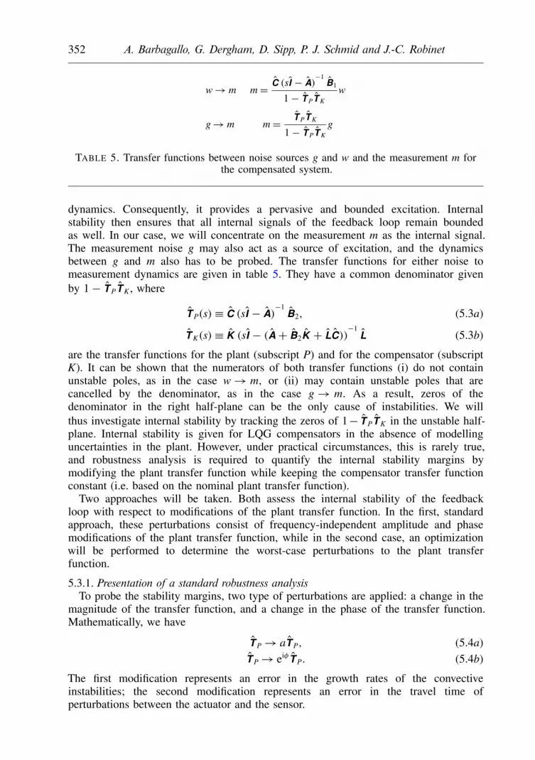
352 A. Barbagallo, G. Dergham, D. Sipp, P. J. Schmid and J.-C. Robinet
w→ m m= C (sI − A)−1
B1
1− T PT K
w
g→ m m= T PT K
1− T PT K
g
TABLE 5. Transfer functions between noise sources g and w and the measurement m forthe compensated system.
dynamics. Consequently, it provides a pervasive and bounded excitation. Internalstability then ensures that all internal signals of the feedback loop remain boundedas well. In our case, we will concentrate on the measurement m as the internal signal.The measurement noise g may also act as a source of excitation, and the dynamicsbetween g and m also has to be probed. The transfer functions for either noise tomeasurement dynamics are given in table 5. They have a common denominator givenby 1− T PT K , where
T P(s)≡ C (sI − A)−1
B2, (5.3a)
T K(s)≡ K (sI − (A+ B2K + LC))−1
L (5.3b)
are the transfer functions for the plant (subscript P) and for the compensator (subscriptK). It can be shown that the numerators of both transfer functions (i) do not containunstable poles, as in the case w→ m, or (ii) may contain unstable poles that arecancelled by the denominator, as in the case g→ m. As a result, zeros of thedenominator in the right half-plane can be the only cause of instabilities. We willthus investigate internal stability by tracking the zeros of 1− T PT K in the unstable half-plane. Internal stability is given for LQG compensators in the absence of modellinguncertainties in the plant. However, under practical circumstances, this is rarely true,and robustness analysis is required to quantify the internal stability margins bymodifying the plant transfer function while keeping the compensator transfer functionconstant (i.e. based on the nominal plant transfer function).
Two approaches will be taken. Both assess the internal stability of the feedbackloop with respect to modifications of the plant transfer function. In the first, standardapproach, these perturbations consist of frequency-independent amplitude and phasemodifications of the plant transfer function, while in the second case, an optimizationwill be performed to determine the worst-case perturbations to the plant transferfunction.
5.3.1. Presentation of a standard robustness analysisTo probe the stability margins, two type of perturbations are applied: a change in the
magnitude of the transfer function, and a change in the phase of the transfer function.Mathematically, we have
T P→ aT P, (5.4a)T P→ eiφT P. (5.4b)
The first modification represents an error in the growth rates of the convectiveinstabilities; the second modification represents an error in the travel time ofperturbations between the actuator and the sensor.

Closed-loop control of unsteadiness over a rounded backward-facing step 353
We define the minimum gain margin GM+ as the minimum value of the amplitudea, greater than one, that achieves marginal stability in the transfer functions w→ mor g→ m. For this we seek a which ensures that 1 − aT PT K has one zero withzero real part while all other zeros are located in the left half-plane. The maximumgain margin GM− is defined analogously: it corresponds to the maximum value ofamplitude a, less than one, that achieves marginal stability. Lastly, the phase marginPM is the minimum positive value of φ such that 1 − eiφT pT K exhibits a marginalzero (i.e. with zero real part). More formally, if we define a function of the amplitudea as f (a) = maxk Resk(a) | 1 − aT P(s)T K(s) = 0, the minimum gain margin GM+ isthe smallest zero of f greater than one, while the maximum gain margin GM− isthe largest zero of f less than one. If we define a function of the phase angle φ asg(φ) = maxk Resk(φ) | 1 − eiφT P(s)T K(s) = 0, the phase margin PM is the smallestpositive zero of g.
The robustness analysis described above has been applied to our compensatedsystem, and results are given in figure 14, which displays iso-contours of the variousinternal stability margins as a function of control cost l and noise-to-signal ratioG/W. The coloured contours are overlaid by black contours showing the performancemeasure Pe. In addition, symbols have been added to the (G/W, l)-plane to indicatestable (black circles) or unstable (white circles) compensated simulations. In the limitof small gains and low noise-to-signal ratio, we observe significant internal stabilitymargins and thus good robustness, with gain margins of more than 6 dB for theamplitude and 60 for the phase angle. In contrast, for large gains the stabilitymargins are substantially reduced, in both gain and phase margin. Case 3, whichresults in an efficient compensated DNS, is characterized by internal stability marginsof GM+ = 1.91 dB, GM− =−9.41 dB and PM = 14.1. For only slightly larger gains,GM+, 1/GM− and PM drop off rather precipitously since case 3 is located in aparameter regime distinguished by large gradients for GM+, GM− and PM. For case4, we obtain GM+ = 0.047 dB, GM− = −0.138 dB and PM = 0.68, which amountsto exceedingly small stability margins. This explains the observed (in)stability of thecompensated DNS.
5.3.2. Presentation of a worst-case sensitivity analysisA technique that is more common in fluid dynamics aims at determining the
worst-case scenario for internal instability. For this analysis, we consider generalperturbations to all components of the plant transfer function and write
T P→ T P = C (sI − A)−1 B2, (5.5)
where A, B2 and C deviate from the nominal system matrices A, B2 and C. Thestability condition based on the zeros of 1 − T PT K translates into finding the unstableeigenvalues of the matrix
M =(
A B2K
−LC A+ B2 + LC
). (5.6)
We look for A, B2 and C that lead to marginal stability of the matrix M, with agiven eigenvalue displaying a zero amplification rate. To constrain the optimization, weintroduce an error measure that describes the disparity between the transfer function of

354 A. Barbagallo, G. Dergham, D. Sipp, P. J. Schmid and J.-C. Robinet
0.1
0.9
0.30.50.7
0.1
0.9
0.30.50.7
0.1
0.9
0.30.50.7
Case 1
Case 2
Case 3
Case 4
Case 1
Case 2
Case 3
Case 4
Case 1
Case 2
Case 3
Case 4
Case l
1 103 100
2 101
3 100
4 10–3 10–4
10–2
10–1
–5 –4 –3 –2 –1 0 1 2–5
–4
–3
–2
–1
0
1
2
3
4
5
–5 –4 –3 –2 –1 0 1 2–5
–4
–3
–2
–1
0
1
2
3
4
5
–5 –4 –3 –2 –1 0 1 2–5
–4
–3
–2
–1
0
1
2
3
4
50.5 1.5 2.5 3.5 4.5 5.5 –6 –5 –4 –3 –2 –1
5 15 25 35 45
(a)
(c)
(b)
FIGURE 14. (a) Iso-contours of gain margin as a function of noise-to-signal ratio G/W andcontrol cost l. (b) Same as (a) for the downside gain margin. (c) Same as (a) for the phasemargin. Superimposed on the plots (in black) are contours of the performance measure Pe.Furthermore, the black symbols indicate stable compensated numerical simulations, whilewhite symbols mark unstable compensated simulations.
the original plant model and of the nominal plant. We have
err(A,B2,C)=
∫ i∞
−i∞|T P − T P|2 ds∫ i∞
−i∞|T P|2 ds
1/2
, (5.7)
with T P = C (sI − A)−1
B2 and T P = C (sI − A)−1 B2. We will then determine theminimal distance to instability of M by adjusting the components A, B2 and C of theplant model (taken as matrices of size 150 × 150, 150 × 1 and 1 × 150, respectively)while maintaining a given error err between the respective transfer functions. Detailsof the optimization procedure are given in appendix B.

Closed-loop control of unsteadiness over a rounded backward-facing step 355
InitAfter optim
–0.4 –0.2 0
3 4 5 6
InitAfter optim medium-gain caseAfter optim large-gain case
0
2
4
–0.4 –0.2 0
0
2
4
10–2
10–1
100
0 2 4 6 8
0.010
0.015
0.025
0.0350.040
0.030
0.020
(a)
(b)
(c)
FIGURE 15. (Colour online) Example from the sensitivity analysis. (a,b) Spectra of plant Aand compensated system M for the medium-gain case. The circles indicate the plant basedon (A, B2, C) while the grey (red online) squares indicate the plant governed by the optimal(A,B2,C) found by the optimization algorithm. (c) Modulus of the transfer functions T Pand T P for the medium-gain case (l = 100, G/W = 10−2, err = 0.003 75, ωopt = 3.3) and thelarge-gain case (l= 10−1, G/W = 10−2, err = 0.001 25, ωopt = 3.3).
Figure 15 shows a typical example from our sensitivity analysis where thecompensated system becomes unstable for a particularly small error err of the transferfunction. For the medium-gain case, the optimization process, performed for ωopt = 3.3and err = 0.003 75, yields a nearly unmodified spectrum for A (figure 15a) but strongmodifications of the compensated spectrum for M (figure 15b). In both panels, thecircles represent the spectrum of the plant based on (A, B2, C) while the grey squares(red online) pertain to a plant governed by the optimal (A,B2,C) determined bythe optimization algorithm. The compensated system clearly displays a marginaleigenvalue at the optimization frequency ωopt = 3.3 (see figure 15b), which is inaccordance with the high value of λω = 7.5 × 10⁴ found for the singular value ofR−1. Further insight can be gained from a comparison of the transfer functions T P
and T P; the modulus of the respective transfer functions is depicted in figure 15(c).It is evident that the response behaviour u→ m for the optimized plant (dark greyline, red online) exhibits a small error near the optimization frequency ωopt = 3.3.For comparison, the transfer function modulus for the large-gain case, obtained forωopt = 3.3 and err = 0.001 25, is also displayed (in grey, green online). The large-gain transfer function is even closer to the original transfer function (black curve)but, nonetheless, displays a very high value for the largest singular value of R−1,namely, λω = 2 × 10⁴. This latter finding corroborates, for the large-gain case, thehigh sensitivity of the compensated system to minute variations in the transfer functionu→ m in the frequency band ω ≈ 2.6–6. The sensitivity is less pronounced for themedium-gain case.
It may appear that, in certain parameter ranges, the LQG design is particularlysensitive to modelling errors; one should keep in mind, however, that the abovesensitivity analysis is based on worst-case scenarios, and that under realistic conditionsthe observed sensitivity may be less severe.

356 A. Barbagallo, G. Dergham, D. Sipp, P. J. Schmid and J.-C. Robinet
No controlControlLin no controlLin control
1200 1400 1600 1800t
10–3
10–2
10–1
100
FIGURE 16. (Colour online) Temporal evolution of the mean perturbation energy based ona DNS continuously forced by finite-amplitude noise W = √10. The compensator has beendesigned under linear assumptions (case 3). The linear case has been added in dashed linesand scaled to the initial energy of the nonlinear simulations.
6. Nonlinear effectsThe controller has been designed for perturbations governed by linear dynamics.
With nonlinear governing equations, this situation is recovered if the amplitude ofthe perturbations is and remains very small over the entire domain, which may beachieved using very small amplitude for the upstream noise, i.e. W 1. In theprevious section, we have seen that small-amplitude noise may be suppressed by acontroller designed under the assumption of a linear governing equation. In the presentsection, we will gradually increase the amplitude W of the incoming perturbations;nonlinear effects will progressively be introduced and their impact on the overallperformance of the linear compensator under off-design conditions can be studied. Asimilar test has been conducted by Ilak (2009) for impulsive initial conditions.
We have tested three different amplitudes: W = 0.1 (see the supplementary movieavailable at journals.cambridge.org/flm), W = 1 and W = √10. The performancemeasures Pe and Pm corresponding to the three cases are reported in table 3 (columns4–6). The simulations have been run up to t = 1800, as in the linear simulation of § 5.The random noise sequence from the linear case has been used, which allows a directcomparison with the linear results (reported in column 3). In table 3, the maximumpointwise mean kinetic energy of the uncontrolled and controlled (indicated by |c)simulations are listed together with their ratio. For a small noise amplitude W = 0.1,the evolution of the uncontrolled perturbation is quasi-linear, and the performance ofthe compensator is nearly the same as in the linear case (compare columns 3 and 4 oftable 3). The performance measures Pe and Pm, however, gradually deteriorate as thenoise amplitude W increases (compare columns 4–6 of table 3).
In figure 16, the temporal evolution of the mean perturbation energy is displayed forthe large-amplitude case W =√10; the uncontrolled simulation is shown in grey (redonline), the compensated one in black. The oscillations of the energy curves for thenonlinear case (solid curve) are less pronounced than in the linear case (dashed line).The same observation can be made for the compensated simulation. It is seen thatthe mean energy level of the perturbation is reduced by the linear compensator, but anoticeable loss in performance is apparent.
As before, the pointwise perturbation mean kinetic energy k′/W2 gives furtherinsight into the temporal evolution of the energy as the disturbances advect along theshear layer. In figure 17(a,b) the pointwise perturbation mean kinetic energy from the

Closed-loop control of unsteadiness over a rounded backward-facing step 357
0 5 10 15 20
0
1
2(b)
0
1
2(a)0.0040
0.0040
FIGURE 17. Pointwise perturbation mean kinetic energy k′/W2 of simulations with randomforcing for W =√10: (a) uncontrolled DNS; and (b) compensated DNS (case 3).
nonlinear simulation with random noise is displayed for the case with W =√10. Thecolour map has been adjusted to permit direct comparison with the equivalent linearresults given in figure 11; significant differences from the linear case can be observed.Figure 17(a), illustrating the uncontrolled case, displays saturation effects causedby nonlinearities; the overall shape of the maximum energy contours are, however,similar to the linear case – concentrating on the dynamics in the shear layer and thereattachment area. For the compensated case (figure 17b), the energy is maximal in theshear layer but is, again, lower than in the uncontrolled case; in contrast, the energyis higher than in the linear case for x > 10, indicating the appearance of nonlinearstructures, which are more difficult to control. We notice that the energy could be lessattenuated by control efforts than in the linear case: in table 3 (column 6), a maximumperturbation mean kinetic energy of 1.96 % is observed in the uncontrolled simulation,which reduces to 1.34 % as the compensator is switched on. The perturbation meankinetic energy is thus diminished by a modest factor of 1/0.69 ≈ 1.5 (compared toa factor of 1/0.17 ≈ 6 for the small-amplitude simulation with W = 0.1, see column4). As stronger nonlinearities set in, the linear-based compensator becomes ever lesseffective.
7. Summary and conclusionsTwo-dimensional incompressible flow over a rounded backward-facing step, a
canonical configuration showing noise-amplifying behaviour, has been controlled byfeedback control strategies. Specifically, the LQG framework has been employed inconjunction with POD-based reduced-order models for the plant. Similar techniqueshave previously been studied (see Ilak & Rowley 2008; Bagheri & Henningson 2011),but with the main emphasis on model reduction aspects. Important issues related to thepractical implementation of feedback control laws for amplifier flows have been leftunaddressed, which motivated this present investigation.
The analysis of the feedback control set-up first concentrated on the estimationprocess. A placement of sensors throughout the convectively unstable region of theflow revealed a distinct advantage of measurement input from the most upstreamsensor. It further showed that the speed of estimation is more important than the

358 A. Barbagallo, G. Dergham, D. Sipp, P. J. Schmid and J.-C. Robinet
accuracy of the estimation, while keeping in mind that upstream sensor measurementsare more easily corrupted by noise since the signal has not yet been amplified andfiltered by the flow. Low-quality sensors should be placed further downstream wherethe amplitude of the detected signal prevails over the added inherent measurementnoise; the resulting delay in estimation, however, will ultimately cause a loss incompensator performance. The noise-to-signal ratio of the sensor thus plays animportant role and has been linked to the estimation parameter for the computationof the Kalman gain.
Continuing with the best (most upstream) sensor, the performance of thecompensated system has been studied under the idealistic assumptions that the ROMaccurately mimics the plant. The noise-to-signal ratio (or estimation parameter) G/Wand the cost-of-control parameter l have been varied to cover a range of controlscenarios from the small-gain limit (SGL), where the compensator is ineffective, to thelarge-gain limit (LGL), where the compensator operates at its maximal performance.An excess total energy can be observed when the measurement energy is taken as thecontrol objective; this phenomenon may be linked to the inability of the sensor Cp
to detect optimal responses with high frequency (ω > 2). However, this shortcomingcan be overcome by basing the cost functional for the controller design on the totalenergy Je.
A compensator designed with Je has then been applied to the full, linearizedNavier–Stokes equations driven by continuous stochastic forcing. In the case ofmedium gains, the compensated system reacted as predicted by the ROM-based modelstudy, and a substantial reduction in perturbation energy could be accomplished. Adetailed, term-by-term analysis of contributions to the energy budget showed thatthe control action was extremely efficient: a very weak user-supplied actuationpower generated a substantial (order one) gain in the kinetic energy flux near thereattachment location. For compensators designed with larger gains, instabilities inthe compensated linearized Navier–Stokes equations arose: even if the compensatoris stable for the model it was designed for, its stability can no longer be impliedor assured when applied to a slightly different plant. This loss of stability has beenanalysed using two approaches, one based on classical Nyquist analysis, the other ona worst-case analysis, which is more common to fluid dynamical applications. Bothanalyses showed a reduction in internal stability margins as the large-gain limit isapproached. This established that the POD model was particularly sensitive to highfrequencies (around ω ≈ 3–6). Hence, for a compensator to work efficiently with largegains (in order to achieve maximal performance), the ROM (based upon which thecompensator was designed) is required to be very precise also at low energies and highfrequencies.
Nonlinear effects have been reintroduced to the closed-loop control problemby applying the compensator, designed under linear assumptions, to the nonlinearNavier–Stokes equations and attempting to suppress continuous noise sources ofprogressively higher amplitude W. Minor deviations have been detected for small-amplitude noise; in the large-amplitude case, however, the compensator performancedeteriorated owing to the appearance of nonlinearly triggered structures.
It can be concluded from our study that designing closed-loop control strategiesfor amplifier flows is significantly more involved than the equivalent design foroscillator flows. While in this latter case instabilities are generally narrow-band infrequency and thus more easily detectable/controllable, a noise amplifier producesmore broadband signals and magnifies physical and non-physical perturbations alike.For this latter reason, a comprehensive study of the sensitivity of the compensator

Closed-loop control of unsteadiness over a rounded backward-facing step 359
C1 C2 C3 C4 Cp E
B1 0.99 0.60 0.62 0.66 0.74 0.77B2 0.61 0.34 0.33 0.32 0.30 0.28
TABLE 6. The relative H2-errors (in %) for the various input–output combinations.The error on the energy has been evaluated using the following expression:∫ +∞−∞ [(X∗ωXω)
1/2 − (X∗ωQXω)1/2]2 dω /
∫ +∞−∞ X∗ωQXω dω1/2.
performance with respect to various noise sources is imperative for a successful closed-loop control design. Transfer functions, i.e. frequency-based input–output relations, areparticularly helpful in pinpointing strong sensitivities, in placing sensors efficiently,and in avoiding undesirable parameter regimes. It is hope that the present study hasintroduced and demonstrated effective tools that – despite the inherent challenges – aidin the design of effective closed-loop control strategies for amplifier flows.
Supplementary movies are available at journals.cambridge.org/flm.
Appendix A. Reduced-order modelIn view of our control objectives, the ROM should be able to capture accurately
the dynamic response of the output variables (C1,2,3,4,p given by sensors and theperturbation energy E(t)) to forcings by the two input variables (B1,2). We choosea model reduction technique based on standard POD, which transforms flow-statesnapshots, arising from harmonic forcings introduced via the terms B1 and B2, intoa finite-dimensional orthogonal basis onto which the full flow equations are projected.An analysis of the ROM confirmed a satisfactory balance between accuracy and size.Details of this type of analysis are given in Dergham et al. (2011) for the samebackward-facing step configuration using a single input B2.
In our case, a ROM based on a Galerkin projection of the full system onto the first150 POD modes has been selected owing to its good performance and comparativelysmall size. The transfer functions of the full system have been computed by Fourier-transforming signals from the impulse responses of the linearized DNS. The errorsbetween the transfer functions of the reduced-order models and the linearized DNShave been measured using the H2-norm. Table 6 presents these errors for differentcombinations of input triggering and output sensing. We note that the impulseresponses triggered by B2 are more accurately captured than those triggered by B1.
All errors are below 1 %.
Appendix B. Sensitivity analysisThe worst-case sensitivity analysis outlined in § 5.3.2 proceeds in the following
manner. We first note that a marginal eigenvalue s = iω of the matrix M is equivalentto the largest singular value λω of the resolvent matrix tending to infinity. Theresolvent matrix corresponds to the matrix R−1 with R = iωI − M. Formulating anoptimization problem, we will try to maximize, for a given frequency ω, the functionalλ2ω(A,B2,C) as a function of A, B2 and C. The optimum will be sought under the
constraint that the transfer function error err(A,B2,C) maintains a prescribed error ε.The constrained optimization problem is transformed into an unconstrained problem

360 A. Barbagallo, G. Dergham, D. Sipp, P. J. Schmid and J.-C. Robinet
via a penalization technique, and a Polak–Ribiere conjugate-gradient method coupledto a line-search algorithm is used to determine the optimum.
More specifically, we denote by λω the largest singular value of R−1 whereR = iωI − M and M is the matrix defined in (5.6). We furthermore introduce (F,G)T
and (X,Y)T as the principal right and left singular vectors associated with λω, whichsatisfy
R−1∗R−1
(FG
)= λ2
ω
(FG
),
(XY
)= R−1
(FG
). (B 1)
The sensitivity analysis is formulated as an optimization problem for determining theminimal stability margin for a specified discrepancy between two transfer functions.We begin with the following Lagrangian:
L= λ2ω −
(YX
)∗ [R
(XY
)−(FG
)]−(FG
)∗ [λ2ωR∗
(FG
)−(XY
)]. (B 2)
Rendering this Lagrangian stationary with respect to the variables (F,G)T, (X,Y)T
and λ2ω yields the following expressions for the Lagrange multipliers (denoted by an
over-tilde): (FG
)= R−1
(FG
),
(YX
)= λ2
ω
(FG
),
(FG
)∗(FG
)= 1. (B 3)
Setting the first variation of the Lagrangian with respect to the control variableR to zero results in an expression for the variation of the squared singular valuegiven by
δλ2ω =−2λ2
ω Re
[(FG
)∗δR
(XY
)]. (B 4)
Using (5.6), this expression for δλ2ω may be expressed in terms of variations in the
matrices A, B2 and C. We obtain
δλ2ω = 2λ2
ω Re(FX∗) : δA+ 2λ2ω Re(FY ∗K
∗) : δB − 2λ2
ω Re(XG∗L) : δC∗, (B 5)
where : denotes the contraction operator or Frobenius inner product, defined asA : B =∑ijAijBij = trace(A∗B).
The constraint of a user-prescribed error γ (measured in the H2-norm) betweenthe full and reduced transfer function may be approximated in the followingmanner:
µγ (A,B2,C)=−γ 2 +∑
j
|C (iωjI − A)−1 B − C (iωjI − A)−1
B︸ ︷︷ ︸φj
|21ωj. (B 6)
In the above expression 1ωj are quadrature coefficients. In our case, we chosea simple first-order approximation of the integral with 1ωj = 0.02 and integration

Closed-loop control of unsteadiness over a rounded backward-facing step 361
limits ωmin =−10, ωmax = 10. The first variation of this functional reads
δµγ =(
2∑
j
Re[φj (−iωjI − A∗)−1 C∗B∗ (−iωjI − A∗)−1]
1ωj
): δA
+(
2∑
j
Re[φj (−iωjI − A∗)−1 C∗
]1ωj
): δB
+(
2∑
j
Re[φ∗j (iωjI − A)−1 B
]1ωj
): δC∗. (B 7)
Lastly, we combine the above expressions and consider the unconstrainedminimization problem
Jω,γ (A,B2,C)=− arctan(ln(λ2ω)/α)+ βµ2
γ + arctan(ln(ν2ω)/α), (B 8)
with β as the penalty coefficient. In our computations, we used α = 10 and103 6 β 6 1010. Note that the third term in (B 8) penalizes the largest singularvalue νω of S−1 where S = iωI − A. This is simply to avoid convergence of theoptimization algorithm towards solutions where s= iω is an eigenvalue of A, which isan undesirable solution. With H and Z as the principal right and left singular vectorsof S corresponding to νω and satisfying S∗SH = ν2
ωH and Z= SH with H∗H = 1, wecan express the first variation of ν2
ω in the form δν2ω = 2ν2
ω Re(HZ∗) : δA.
R E F E R E N C E S
AHUJA, S. & ROWLEY, C. W. 2010 Feedback control of unstable steady states of flow past a flatplate using reduced-order estimators. J. Fluid Mech. 645, 447–478.
AKERVIK, E., HŒPFFNER, J., EHRENSTEIN, U. & HENNINGSON, D. S. 2007 Optimal growth,model reduction and control in a separated boundary-layer flow using global modes. J. FluidMech. 579, 305–314.
ALIZARD, F., CHERUBINI, S. & ROBINET, J.-C. 2009 Sensitivity and optimal forcing response inseparated boundary layer flows. Phys. Fluids 21, 064108.
ARCHAMBAUD, J. P., ARNAL, D., HEIN, S., MELO DE SOUZA, J., HANIFI, A., GODDARD, J. L.,KRIER, J. & DONELLI, R. 2008 Use of laminar flow technologies for supersonic dragreduction – results of FP project SUPERTRAC. In Proceedings of the 5th European Congresson Computational Methods in Applied Sciences and Engineering (ECCOMAS), Venice, Italy.
BAGHERI, S., BRANDT, L. & HENNINGSON, D. S. 2009 Input–output analysis, model reduction andcontrol of the flat-plate boundary layer. J. Fluid Mech. 620, 263–298.
BAGHERI, S. & HENNINGSON, D. S. 2011 Transition delay using control theory. Phil. Trans. R.Soc. A 369, 1365–1381.
BARBAGALLO, A., SIPP, D. & SCHMID, P. J. 2009 Closed-loop control of an open cavity flowusing reduced-order models. J. Fluid Mech. 641, 1–50.
BEWLEY, T. R. & LIU, S. 1998 Optimal and robust control and estimation of linear paths totransition. J. Fluid Mech. 365, 305–349.
BLACKBURN, H. M., BARKLEY, D. & SHERWIN, S. J. 2008 Convective instability and transientgrowth in flow over a backward-facing step. J. Fluid Mech. 603, 271–304.
BOIKO, A. V., DOVGAL, A. V. & HEIN, S. 2008 Control of a laminar separating boundary layer byinduced stationary perturbations. Eur. J. Mech. (B/Fluids) 27 (4), 466–476.
BURL, J. B. 1999 Linear Optimal Control. H∈ and H∞ Methods. Addison-Wesley.CHEVALIER, M., HŒPFFNER, J., AKERVIK, E. & HENNINGSON, D. S. 2007 Linear feedback
control and estimation applied to instabilities in spatially developing boundary layers. J. FluidMech. 588, 163–187.
362 A. Barbagallo, G. Dergham, D. Sipp, P. J. Schmid and J.-C. Robinet
DERGHAM, G., SIPP, D., ROBINET, J.-C. & BARBAGALLO, A. 2011 Model reduction for fluidsusing frequential snapshots. Phys. Fluids 23, 064101.
DOYLE, J. 1978 Guaranteed margins for LQG regulators. IEEE Trans. Autom. Control 23 (4),756–757.
EHRENSTEIN, U., PASSAGGIA, P.-Y. & GALLAIRE, F. 2011 Control of a separated boundary layer:reduced-order modeling using global modes revisited. Theor. Comput. Fluid Dyn. 25 (1–4),195–207.
GHARIB, M. & ROSHKO, A. 1987 The effect of flow oscillations on cavity drag. J. Fluid Mech.177, 501–530.
HECHT, F., PIRONNEAU, O., HYARIC, A. LE & OHTSUKA, K. 2005 Freefem++, 3rd edition,version 3.19, http://www.freefem.org/ff++, Universite Pierre et Marie Curie Paris, LaboratoireJacques-Louis Lions.
ILAK, M. 2009 Model reduction and feedback control of transitional channel flow. PhD thesis,Princeton University, Mechanical and Aerospace Engineering.
ILAK, M. & ROWLEY, C. W. 2008 Modeling of transitional channel flow using balanced properorthogonal decomposition. Phys. Fluids 20, 034103.
JOSHI, S. S., SPEYER, J. L. & KIM, J. 1997 A systems theory approach to the feedbackstabilization of infinitesimal and finite-amplitude disturbances in plane Poiseuille flow. J. FluidMech. 332, 157–184.
JOSLIN, R. D. 1998 Overview of laminar flow control. NASA Rep. TP 208705.KIM, J. 2003 Control of turbulent boundary layers. Phys. Fluids 15, 1093–1105.KIM, J. & BEWLEY, T. R. 2007 A linear systems approach to flow control. Annu. Rev. Fluid Mech.
39, 383–417.MARQUET, O., SIPP, D., CHOMAZ, J.-M. & JACQUIN, L. 2008 Amplifier and resonator dynamics
of a low-Reynolds number recirculation bubble in a global framework. J. Fluid Mech. 605,429–443.
ROSSITER, J. E. 1964 Wind tunnel experiments on the flow over rectangular cavities at subsonic andtransonic speeds. Aero. Res. Counc. R&M 3438.
ROWLEY, C. W. 2005 Model reduction for fluids using balanced proper orthogonal decomposition.Intl J. Bifurcation Chaos 15, 997–1013.
SARIC, W. S., REED, H. L. & WHITE, E. B. 2003 Stability and transition of three-dimensionalboundary layers. Annu. Rev. Fluid Mech. 35, 413–440.
SIPP, D., MARQUET, O., MELIGA, P. & BARBAGALLO, A. 2010 Dynamics and control of globalinstabilities in open flows: a linearized approach. Appl. Mech. Rev. 63, 030801.
SIROVICH, L. 1987 Turbulence and the dynamics of coherent structures. Q. Appl. Maths 45,561–590.


