Computers & Fluids 112 (2015) 1–18

Contents lists available at ScienceDirect

Computers & Fluids

journal homepage: www.elsevier .com/ locate /compfluid

A fully implicit combined field scheme for freely vibrating squarecylinders with sharp and rounded corners

http://dx.doi.org/10.1016/j.compfluid.2015.02.0020045-7930/� 2015 Elsevier Ltd. All rights reserved.

⇑ Corresponding author.E-mail address: mperkj@nus.edu.sg (R.K. Jaiman).

Rajeev K. Jaiman ⇑, Subhankar Sen, Pardha S. GurugubelliDepartment of Mechanical Engineering, National University of Singapore, Singapore 119077, Singapore

a r t i c l e i n f o

Article history:Received 28 September 2014Received in revised form 25 January 2015Accepted 4 February 2015Available online 14 February 2015

Keywords:Fully implicit combined fieldPetrov–GalerkinRounded squareLateral edge separationALEFree vibrationGalloping

a b s t r a c t

We present a fully implicit combined field scheme based on Petrov–Galerkin formulation for fluid–bodyinteraction problems. The motion of the fluid domain is accounted by an arbitrary Lagrangian–Eulerian(ALE) strategy. The combined field scheme is more efficient than conventional monolithic schemes asit decouples the computation of ALE mesh position from the fluid–body variables. The effect of cornerrounding is studied in two-dimensions for stationary as well as freely vibrating square cylinders. Thecylinder shapes considered are: square with sharp corners, circle and four intermediate rounded squaresgenerated by varying a single rounding parameter. Rounding of the corners delays the primary separationoriginating from the cylinder base. The secondary separation, seen solely for the basic square along itslateral edges, initiates at a Reynolds number, Re between 95 and 100. Imposition of blockage lowersthe critical Re marking the onset of secondary separation. For free vibrations without damping, Re rangeis 100–200 and mass ratio, m� of each cylinder is 10. The rounded cylinders undergo vortex-inducedmotion alone whereas motion of the basic square is vortex-induced at low Re and galloping at high Re.The flow is periodic for vortex-induced motion and quasi-periodic for galloping. The lower branch anddesynchronization characterize the response of rounded cylinders. For the square cylinder, the compo-nents of response are the lower branch, desynchronization and galloping. Removal of the sharp cornersof square cylinder drastically alters the flow and vibration characteristics.

� 2015 Elsevier Ltd. All rights reserved.

1. Introduction

The analysis of flow around a single body or multiple bluff bod-ies continues to attract the attention of the research community.The primary motivation behind the present work concerning anisolated obstacle stems from the need to optimize multi-columnoffshore structures subjected to ocean currents. In particular, thereis a growing demand to reduce or control the vortex-inducedmotions of multi-column structures. Motion of such offshore struc-tures can be minimized by suitably altering the spacing betweenthe columns and also by selecting appropriate column shapes suchas circular, and square with sharp/rounded corners.

The presence of sharp corners on a square cylinder largely altersthe flow characteristics as compared to the ones with circular/el-liptical section having smooth contours. Besides the angle of inci-dence, the sharp corners appear as a major influencing factor inthe body geometry, that affect the flow separation. The locationof the separation points strongly depends on the body shape whichin turn governs the wake dynamics and fluid loading. Removal of

the sharp corners of a square cylinder and gradual transition tothe circle through intermediate rounded squares generate cross-sections, that might be competitive both for a stationary andvibrating cylinder in various mechanical and civil engineeringapplications. It is therefore important to study the effect ofgradually rounding the corners of a square cylinder at zero inci-dence on the flow till the circular section is reached.

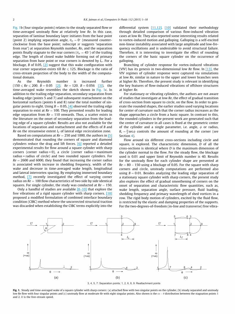
In correspondence with a steady or time-averaged flow, exis-tence of an even number of zero vorticity points on the surfaceof a symmetric or asymmetric obstacle was earlier suggested in[1]. For a separated flow, these singular points are alternate pointsof attachment and separation. In terms of streamlines, theschematics in Fig. 1 (upper row) illustrate various wake configura-tions of a square cylinder with sharp corners in low to moderateReynolds number regime (Re 6 150). Also shown is the corre-sponding vorticity, x distribution along half the circumference ofthe cylinder. Here, h is the circumferential angle measured coun-terclockwise from the forward stagnation point. Points 1, 2, 6, 8and 9 denote locations of attachment while 3, 4, 5 and 7 denotelocations of separation. An attached laminar boundary layer asobserved at very low Re, is represented by Fig. 1a where formationof wake does not take place. The wake configuration depicted by

2 R.K. Jaiman et al. / Computers & Fluids 112 (2015) 1–18

Fig. 1b (four singular points) relates to the steady separated flow ortime-averaged unsteady flow at relatively low Re. In this case,separation of laminar boundary layer initiates from the base point(point 2) implying separation angle, hsr ¼ 0� (measured counter-clockwise from the base point; subscript sr suggests ‘separationfrom rear’) at separation Reynolds number, Res and the separationpoints finally stagnate to the rear corners (hsr ¼ 45�) of the trailingedge. The length of closed wake bubble forming out of primaryseparation from base point or rear corners is denoted by Lr . For ablockage, B of 0.05, [2] suggest that this wake configuration withrear corner separation exists till Re 6 125. Blockage is the ratio ofcross-stream projection of the body to the width of the computa-tional domain.

As the Reynolds number is increased further(150 6 Re 6 200; B ¼ 0:05 [2]; Re ¼ 120; B ¼ 0:056 [3]), thetime-averaged wake resembles the sketch shown in Fig. 1c. Inaddition to the trailing edge separation, secondary separation fromleading edge (points 5 and 7) and subsequent reattachment on thehorizontal surfaces (points 6 and 8) raise the total number of sin-gular points to eight. Using B ¼ 0:05, [4] observed the trailing edgeseparation to exist at Re ¼ 100. They presented results for leadingedge separation from Re ¼ 110 onwards. Thus, a scatter exists inthe literature on the onset of secondary separation from the lead-ing edge of a square cylinder. Results are also not available for thelocations of separation and reattachment and the effects of B andRe on the streamwise extent Lf of lateral edge recirculation zone.

Based on computations at Re ¼ 250 and 1000, the authors in [5]demonstrated that rounding the corners of square and diamondcylinders reduce the drag and lift forces. [6] reported a detailedexperimental results for flow around a square cylinder with sharpcorners (corner radius = 0), a circle (corner radius = maximumradius = radius of circle) and two rounded square cylinders. ForRe ¼ 2600 and 6000, they found that increasing the corner radiusis associated with increase in shedding frequency, width of thewake and decrease in time-averaged wake length, longitudinaland lateral intervortex spacing. By employing immersed boundarymethod, [7] recently investigated the effect of varying cornerradius on Re ¼ 100 flow characteristics of two side by side identicalsquares. For single cylinder, the study was conducted at Re ¼ 150.

Only a handful of studies are available [8–10] that explore thefree vibrations of a rigid square cylinder with sharp corners. [10]proposed a modified formulation of combined interface boundarycondition (CIBC) method where the uncorrected structural tractionwas discarded when establishing the CIBC terms explicitly into the

Fig. 1. Steady and time-averaged wake of a square cylinder with sharp corners: (a) attachlow Re flow with four singular points and (c) unsteady flow at moderate Re with eight siand 2. U is the free-stream speed.

differential system [11,12]. [10] validated their methodologythrough detailed comparison of various flow-induced vibrationcases at low Re. They also reported some interesting results relatedto vortex-induced motion and galloping. Galloping is a self-excitednon-linear instability associated with large amplitude and low-fre-quency oscillations and is undesirable to avoid structural failure.Therefore, it is interesting to investigate the effect of roundingthe corners of the basic square cylinder on the occurrence ofgalloping.

Branching of cylinder response for vortex-induced vibrations(VIV) has its genesis in two-dimensional low Re flow. In [13], theVIV regimes of cylinder response were captured via simulationsat low Re, similar in nature to the upper and lower branches seenat higher Re. Therefore, the present study is relevant in identifyingthe key features of flow-induced vibrations of offshore structuresat higher Re.

For stationary or vibrating cylinders, the authors are not awareof studies that investigate at low Re, the effect of gradual transitionof cross-section from square to circle, on the flow. In order to gen-erate the rounded shapes, the earlier studies used varying locationsfor center of curvature such that the corner radius increases as theshape approaches a circle from a basic square. In contrast to this,the rounded cylinders in the present work are generated such thatthe center of curvature in all cases is fixed at the geometric centerof the cylinder and a single parameter, i.e. angle, / or radius,Rc ¼ D

2 sec/ controls the amount of rounding at the corner (seeSection 4).

Flow around six different cross-sections including circle andsquare, is explored. The characteristic dimension, D of all thecross-sections is identical where D is the maximum dimension ofthe cylinder normal to the flow. For the steady flow, the blockageused is 0.01 and upper limit of Reynolds number is 40. Resultsfor the unsteady flow for each cylinder shape are presented atRe ¼ 80� 150 using a blockage of 0.05. For the square with sharpcorners and circle, unsteady computations are performed alsousing B ¼ 0:01. Besides analyzing the leading edge separation ofa stationary square cylinder with sharp corners, the present studyalso explores the effect of gradual smoothening of corners on theonset of separation and characteristic flow quantities, such as,wake length, separation angle, surface pressure, fluid loading,shedding frequency and primary wavelength of shed vortices in arow. The rigid body motion of cylinders, excited by the fluid flow,is restricted by the elastic and damping properties of the supports.For the two-degrees-of-freedom (in-line and transverse) free vibra-

ed flow with two singular points on the cylinder, (b) steady separated and unsteadyngular points. Also shown is the x� h distribution between the stagnation points 1

R.K. Jaiman et al. / Computers & Fluids 112 (2015) 1–18 3

tions of rigid cylinders, the parameters used are: Re ¼ 100� 200;mass ratio, m� ¼ 10; damping coefficient, f ¼ 0 and B ¼ 0:05. Thequantities studied are the frequency, lock-in, response, fluid load-ing, modes of vortex formation and phase between transverse forceand displacement.

A solver employing a standard stabilized finite-element formu-lation [14,15] and semi-discrete time stepping has been developedto investigate the two-dimensional incompressible flow character-istics of stationary and freely oscillating cylinders. This methodmay be considered as a Galerkin/least square stabilization tech-nique [16] in the context of linear finite-element interpolation.To account for the coupled fluid–body interactions, we extendthe combined field with explicit interface (CFEI) to fully implicitcombined field (FICF) formulation for rigid-body coupling. Throughthis fully implicit scheme, we achieve the coupled fluid–body sta-bility not only for low structure-to-fluid mass ratio but also for alarge time step size. In both of these formulations, we predict theposition of the structure at the start of each time step, whichdecouples the arbitrary Lagrangian–Eulerian (ALE) mesh from thecoupled fluid–body solver. In [17], an explicit Adam–Bashforthscheme is employed to predict the rigid-body position, whereasthe present formulation employs the implicit predictor-multi cor-rector iterations. A detailed stability proof for the combined fieldformulation using the energy estimate is provided in [17].

For the steady flow, the blockage used is 0.01 and upper limit ofReynolds number is 40. Results for the unsteady flow for eachcylinder shape are presented at Re ¼ 80� 150 using a blockageof 0.05. For the square with sharp corners and circle, unsteadycomputations are performed also using B ¼ 0:01. The rigid bodymotion of cylinders, excited by the fluid flow, is restricted by theelastic and damping properties of the supports. For the two-de-grees-of-freedom free vibration of rigid cylinders, the parametersused are: Re ¼ 100� 200; m� ¼ 10; f ¼ 0 and B ¼ 0:05.

The outline of the rest of the article is as follows. The governingequations of fluid–body system are discussed in Section 2. In Sec-tion 3, we present our numerical formulation of the coupled fluid–body system using the stabilized finite-element and the fullyimplicit combined field procedures. Section 4 provides the problemdefinition, geometry and mesh description. Accuracy of the compu-tations and convergence of results are presented in Section 5. Themain results for stationary cylinder in steady flow, unsteady flowand moving cylinders are presented and discussed in Sections 6–8, respectively. Finally, in Section 9, a few concluding remarksare made.

2. Governing equations for flow and rigid body motion

The Navier–Stokes equations governing an incompressible flowin an arbitrary Lagrangian–Eulerian reference frame are

q f @u f

@tþ q f u f �w

� �� $u f ¼ $ � r f þ b f on X f ðtÞ; ð1Þ

$ � u f ¼ 0 on X f ðtÞ; ð2Þ

where u f and w represent the fluid and mesh velocities, respective-

ly, b f is the body force applied on the fluid and r f is the Cauchystress tensor for a Newtonian fluid, written as

r f ¼ �pI þ l f $u f þ $u f� �T

� �; ð3Þ

where p denotes fluid pressure and l f is the dynamic viscosity ofthe fluid.

An immersed rigid body experiences unsteady forces and whenmounted elastically, may undergo rigid body motion. The equationof motion of the body is

m � @us

@tþ c � us þ k � us z0; tð Þ � z0ð Þ ¼ Fs þ bs on Xs; ð4Þ

where m; c and k denote the mass, damping and stiffness vectorsper unit length for the translational degrees of freedom, Xs denotesthe rigid body, us tð Þ represents the rigid-body velocity at time t andC is the interface between the fluid and the rigid-body at t ¼ 0; Fs

and bs are the fluid traction and body forces acting on the rigidbody, respectively, us is the function mapping the initial positionz0 to its position at time t.

The coupled system requires to satisfy the no-slip andtraction continuity conditions at the fluid–body interface C asfollows

u f usðz0; tÞ; tð Þ ¼ us z0; tð Þ 8 z 2 C; ð5ÞZuðc;tÞ

r f x; tð Þ � n f dCþZ

cFsdC ¼ 0 8 c 2 C; ð6Þ

where n f and ns are respectively the outer normals to the fluid andthe solid and /s is the function that maps each structural node fromits initial position z to its deformed position at time t. Here, c is anyedge on the interface C. We next present the fully implicit com-bined field (FICF) formulation for the coupled fluid–body system.

3. Numerical formulation

3.1. Coupled fluid rigid-body system

The weak form of the Navier–Stokes Eqs. (1) and (2) can bewritten asZ

X f ðtÞq f @tu f þ u f �w

� �� $u f

� �� / f ðxÞdXþ

ZX f ðtÞ

r f

: $/ f ðxÞdX

¼Z

X f ðtÞb f � / f ðxÞdXþ

ZC f

hðtÞ

h f � / f ðxÞdC

þZ

C tð Þr f ðx; tÞ � n f� �

� / f ðxÞdC; ð7Þ

ZX f ðtÞ

$ � u f qðxÞdX ¼ 0: ð8Þ

Here @t denotes partial time derivative operator @ �ð Þ=@t;/ f and qare test functions for the fluid velocity and pressure, respectively.

C fhðtÞ represents the non-interface Neumann boundary along

which r f ðx; tÞ � n f ¼ h f . The weak form for the rigid-body Eq.(4) isZ

Xsm � @tus þ c � us þ k � us z0; tð Þ � z0ð Þ½ � � /sdX

¼Z

CFs � /sdCþ

ZXs

bs � /sdX; ð9Þ

where /s is the test function for the rigid-body velocity, which is aconstant for any point on the body. Similarly, we can write the weakform for the traction boundary condition as

Zuðc;tÞ

r f ðx; tÞ � n f� �

� / f dCþZ

cFs � /sdC ¼ 0 8c 2 C: ð10Þ

In the above equation, the condition / f ¼ /s can be enforced byconsidering a conforming mesh along the interface C. We nextenforce the traction continuity condition (10) to combine the fluidand structural weak forms in (8), (7), (9) to construct a single weakform for the combined system

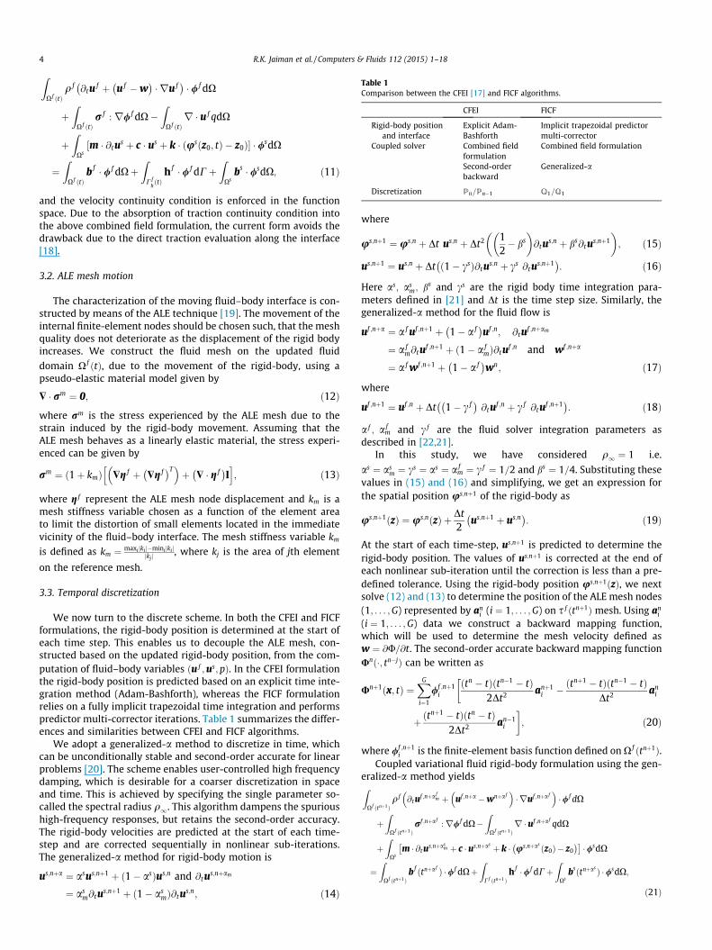
Table 1Comparison between the CFEI [17] and FICF algorithms.

CFEI FICF

Rigid-body positionand interface

Explicit Adam-Bashforth

Implicit trapezoidal predictormulti-corrector

Coupled solver Combined fieldformulation

Combined field formulation

Second-orderbackward

Generalized-a

Discretization Pn=Pn�1 Q1=Q1

4 R.K. Jaiman et al. / Computers & Fluids 112 (2015) 1–18

ZX f ðtÞ

q f @tu f þ u f �w� �

� ru f� �

� / f dX

þZ

X f ðtÞr f : r/ f dX�

ZX f ðtÞr � u f qdX

þZ

Xsm � @tus þ c � us þ k � us z0; tð Þ � z0ð Þ½ � � /sdX

¼Z

X f ðtÞb f � / f dXþ

ZC f

hðtÞ

h f � / f dCþZ

Xsbs � /sdX; ð11Þ

and the velocity continuity condition is enforced in the functionspace. Due to the absorption of traction continuity condition intothe above combined field formulation, the current form avoids thedrawback due to the direct traction evaluation along the interface[18].

3.2. ALE mesh motion

The characterization of the moving fluid–body interface is con-structed by means of the ALE technique [19]. The movement of theinternal finite-element nodes should be chosen such, that the meshquality does not deteriorate as the displacement of the rigid bodyincreases. We construct the fluid mesh on the updated fluid

domain X f ðtÞ, due to the movement of the rigid-body, using apseudo-elastic material model given by

$ � rm ¼ 0; ð12Þ

where rm is the stress experienced by the ALE mesh due to thestrain induced by the rigid-body movement. Assuming that theALE mesh behaves as a linearly elastic material, the stress experi-enced can be given by

rm ¼ ð1þ kmÞ $g f þ $g f� �T

� �þ $ � g f� �

Ih i

; ð13Þ

where g f represent the ALE mesh node displacement and km is amesh stiffness variable chosen as a function of the element areato limit the distortion of small elements located in the immediatevicinity of the fluid–body interface. The mesh stiffness variable km

is defined as km ¼ maxi jki j�mini jki jjkj j

, where kj is the area of jth element

on the reference mesh.

3.3. Temporal discretization

We now turn to the discrete scheme. In both the CFEI and FICFformulations, the rigid-body position is determined at the start ofeach time step. This enables us to decouple the ALE mesh, con-structed based on the updated rigid-body position, from the com-putation of fluid–body variables ðu f ;us; pÞ. In the CFEI formulationthe rigid-body position is predicted based on an explicit time inte-gration method (Adam-Bashforth), whereas the FICF formulationrelies on a fully implicit trapezoidal time integration and performspredictor multi-corrector iterations. Table 1 summarizes the differ-ences and similarities between CFEI and FICF algorithms.

We adopt a generalized-a method to discretize in time, whichcan be unconditionally stable and second-order accurate for linearproblems [20]. The scheme enables user-controlled high frequencydamping, which is desirable for a coarser discretization in spaceand time. This is achieved by specifying the single parameter so-called the spectral radius q1. This algorithm dampens the spurioushigh-frequency responses, but retains the second-order accuracy.The rigid-body velocities are predicted at the start of each time-step and are corrected sequentially in nonlinear sub-iterations.The generalized-a method for rigid-body motion is

us;nþa ¼ asus;nþ1 þ 1� asð Þus;n and @tus;nþam

¼ asm@tus;nþ1 þ ð1� as

mÞ@tus;n; ð14Þ

where

us;nþ1 ¼ us;n þ Dt us;n þ Dt2 12� bs

� �@tus;n þ bs@tus;nþ1

� �; ð15Þ

us;nþ1 ¼ us;n þ Dt 1� csð Þ@tus;n þ cs @tus;nþ1� �: ð16Þ

Here as; asm; bs and cs are the rigid body time integration para-

meters defined in [21] and Dt is the time step size. Similarly, thegeneralized-a method for the fluid flow is

uf ;nþa ¼ a f uf ;nþ1 þ 1� a f� �

uf ;n; @tuf ;nþam

¼ a fm@tuf ;nþ1 þ ð1� a f

mÞ@tuf ;n and wf ;nþa

¼ a f wf ;nþ1 þ 1� a f� �

wn; ð17Þ

where

uf ;nþ1 ¼ uf ;n þ Dt 1� c f� �

@tuf ;n þ c f @tuf ;nþ1� �: ð18Þ

a f ; a fm and c f are the fluid solver integration parameters as

described in [22,21].In this study, we have considered q1 ¼ 1 i.e.

as ¼ asm ¼ cs ¼ as ¼ a f

m ¼ c f ¼ 1=2 and bs ¼ 1=4. Substituting thesevalues in (15) and (16) and simplifying, we get an expression forthe spatial position us;nþ1 of the rigid-body as

us;nþ1ðzÞ ¼ us;nðzÞ þ Dt2

us;nþ1 þ us;n� �

: ð19Þ

At the start of each time-step, us;nþ1 is predicted to determine therigid-body position. The values of us;nþ1 is corrected at the end ofeach nonlinear sub-iteration until the correction is less than a pre-defined tolerance. Using the rigid-body position us;nþ1ðzÞ, we nextsolve (12) and (13) to determine the position of the ALE mesh nodes(1; . . . ;G) represented by an

i (i ¼ 1; . . . ;G) on s f ðtnþ1Þ mesh. Using ani

(i ¼ 1; . . . ;G) data we construct a backward mapping function,which will be used to determine the mesh velocity defined asw ¼ @U=@t. The second-order accurate backward mapping functionUnð�; tn�jÞ can be written as

Unþ1ðx; tÞ ¼XG

i¼1

/f ;nþ1i

ðtn � tÞðtn�1 � tÞ2Dt2 anþ1

i � ðtnþ1 � tÞðtn�1 � tÞ

Dt2 ani

�

þðtnþ1 � tÞðtn � tÞ

2Dt2 an�1i

; ð20Þ

where /f ;nþ1i is the finite-element basis function defined on X f ðtnþ1Þ.

Coupled variational fluid rigid-body formulation using the gen-eralized-a method yieldsZ

X f ðtnþ1Þq f @tuf ;nþa f

m þ uf ;nþa �wnþa f� �

� ruf ;nþa f� �

�/ f dX

þZ

X f ðtnþ1Þrf ;nþa f

:r/ f dX�Z

X f ðtnþ1Þr �uf ;nþa f

qdX

þZ

Xsm � @tus;nþas

m þ c �us;nþas þk � us;nþasz0ð Þ � z0

� � ��/sdX

¼Z

X f ðtnþ1Þb f ðtnþa f Þ �/ f dXþ

ZC f ðtnþ1Þ

h f �/ f dCþZ

Xsbsðtnþas Þ �/sdX;

ð21Þ

R.K. Jaiman et al. / Computers & Fluids 112 (2015) 1–18 5

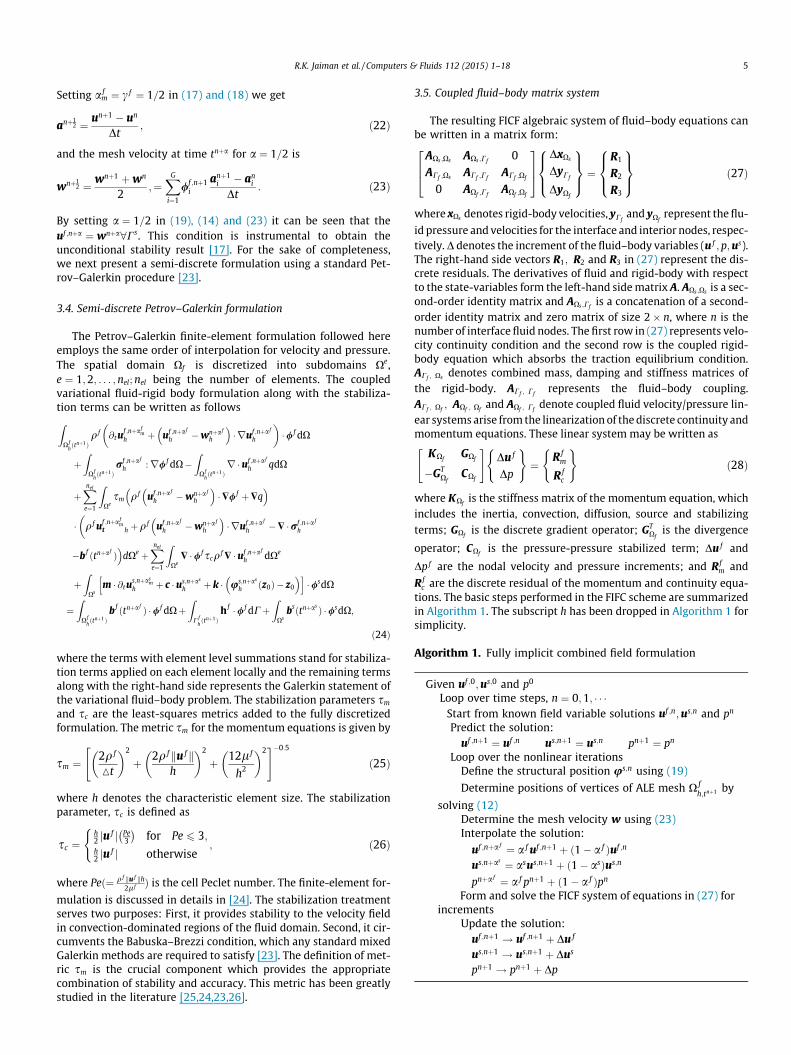
Setting a fm ¼ c f ¼ 1=2 in (17) and (18) we get

anþ12 ¼ unþ1 � un

Dt; ð22Þ

and the mesh velocity at time tnþa for a ¼ 1=2 is

wnþ12 ¼ wnþ1 þwn

2;¼XG

i¼1

/f ;nþ1i

anþ1i � an

i

Dt: ð23Þ

By setting a ¼ 1=2 in (19), (14) and (23) it can be seen that theuf ;nþa ¼ wnþa8Cs. This condition is instrumental to obtain theunconditional stability result [17]. For the sake of completeness,we next present a semi-discrete formulation using a standard Pet-rov–Galerkin procedure [23].

3.4. Semi-discrete Petrov–Galerkin formulation

The Petrov–Galerkin finite-element formulation followed hereemploys the same order of interpolation for velocity and pressure.The spatial domain Xf is discretized into subdomains Xe,e ¼ 1;2; . . . ;nel; nel being the number of elements. The coupledvariational fluid-rigid body formulation along with the stabiliza-tion terms can be written as followsZ

X fhðtnþ1Þ

q f @tuf ;nþa f

mh þ uf ;nþa f

h �wnþa f

h

� �� ruf ;nþa f

h

� ��/ f dX

þZ

X fhðtnþ1Þ

rf ;nþa f

h :r/ f dX�Z

X fhðtnþ1Þr �uf ;nþa f

h qdX

þXnel

e¼1

ZXe

sm q f uf ;nþa f

h �wnþa f

h

� ��$/ f þ$q

� �

� q f uf ;nþa fm

t h þq f uf ;nþa f

h �wnþa f

h

� �� ruf ;nþa f

h �$ �rf ;nþa f

h

�

�b f ðtnþa f Þ�

dXe þXnel

e¼1

ZXe

$ �/ f scq f $ �uf ;nþa f

h dXe

þZ

Xsm � @tu

s;nþasm

h þ c �us;nþas

h þ k � us;nþas

h z0ð Þ � z0

� �h i�/sdX

¼Z

X fhðtnþ1Þ

b f ðtnþa f Þ �/ f dXþZ

C fhðtnþ1Þ

h f �/ f dCþZ

Xsbsðtnþas Þ �/sdX;

ð24Þ

where the terms with element level summations stand for stabiliza-tion terms applied on each element locally and the remaining termsalong with the right-hand side represents the Galerkin statement ofthe variational fluid–body problem. The stabilization parameters sm

and sc are the least-squares metrics added to the fully discretizedformulation. The metric sm for the momentum equations is given by

sm ¼2q f

Mt

� �2

þ 2q f ku f kh

� �2

þ 12l f

h2

� �2" #�0:5

ð25Þ

where h denotes the characteristic element size. The stabilizationparameter, sc is defined as

sc ¼h2 ju f j Pe

3

� �for Pe 6 3;

h2 ju f j otherwise

(; ð26Þ

where Peð¼ q f ku f kh2l f Þ is the cell Peclet number. The finite-element for-

mulation is discussed in details in [24]. The stabilization treatmentserves two purposes: First, it provides stability to the velocity fieldin convection-dominated regions of the fluid domain. Second, it cir-cumvents the Babuska–Brezzi condition, which any standard mixedGalerkin methods are required to satisfy [23]. The definition of met-ric sm is the crucial component which provides the appropriatecombination of stability and accuracy. This metric has been greatlystudied in the literature [25,24,23,26].

3.5. Coupled fluid–body matrix system

The resulting FICF algebraic system of fluid–body equations canbe written in a matrix form:

AXs ;Xs AXs ;Cf0

ACf ;Xs ACf ;CfACf ;Xf

0 AXf ;CfAXf ;Xf

264

375

DxXs

DyCf

DyXf

8><>:

9>=>; ¼

R1

R2

R3

8><>:

9>=>; ð27Þ

where xXs denotes rigid-body velocities, yCfand yXf

represent the flu-

id pressure and velocities for the interface and interior nodes, respec-tively. D denotes the increment of the fluid–body variables (u f ;p;us).The right-hand side vectors R1; R2 and R3 in (27) represent the dis-crete residuals. The derivatives of fluid and rigid-body with respectto the state-variables form the left-hand side matrix A. AXs ;Xs is a sec-ond-order identity matrix and AXs ;Cf

is a concatenation of a second-order identity matrix and zero matrix of size 2� n, where n is thenumber of interface fluid nodes. The first row in (27) represents velo-city continuity condition and the second row is the coupled rigid-body equation which absorbs the traction equilibrium condition.ACf ; Xs denotes combined mass, damping and stiffness matrices ofthe rigid-body. ACf ; Cf

represents the fluid–body coupling.ACf ; Xf

; AXf ; Xfand AXf ; Cf

denote coupled fluid velocity/pressure lin-ear systems arise from the linearization of the discrete continuity andmomentum equations. These linear system may be written as

KXfGXf

�GTXf

CXf

" #Du f

Dp

( )¼

R fm

R fc

( )ð28Þ

where KXfis the stiffness matrix of the momentum equation, which

includes the inertia, convection, diffusion, source and stabilizingterms; GXf

is the discrete gradient operator; GTXf

is the divergence

operator; CXfis the pressure-pressure stabilized term; Du f and

Dp f are the nodal velocity and pressure increments; and R fm and

R fc are the discrete residual of the momentum and continuity equa-

tions. The basic steps performed in the FIFC scheme are summarizedin Algorithm 1. The subscript h has been dropped in Algorithm 1 forsimplicity.

Algorithm 1. Fully implicit combined field formulation

Given uf ;0;us;0 and p0

Loop over time steps, n ¼ 0;1; � � �Start from known field variable solutions uf ;n;us;n and pn

Predict the solution:uf ;nþ1 ¼ uf ;n us;nþ1 ¼ us;n pnþ1 ¼ pn

Loop over the nonlinear iterationsDefine the structural position us;n using (19)

Determine positions of vertices of ALE mesh X fh;tnþ1 by

solving (12)Determine the mesh velocity w using (23)Interpolate the solution:

uf ;nþa f ¼ a f uf ;nþ1 þ ð1� a f Þuf ;n

us;nþas ¼ asus;nþ1 þ ð1� asÞus;n

pnþa f ¼ a f pnþ1 þ ð1� a f Þpn

Form and solve the FICF system of equations in (27) forincrements

Update the solution:uf ;nþ1 ! uf ;nþ1 þ Du f

us;nþ1 ! us;nþ1 þ Dus

pnþ1 ! pnþ1 þ Dp

6 R.K. Jaiman et al. / Computers & Fluids 112 (2015) 1–18

Since the kinematic compatibility at the interface is achieved byconstruction, there is a reduction in the size of the linear system tobe solved per iteration. Unlike the monolithic scheme presented in[27,28], the algebraic system in (27) does not contain the equationfor the ALE mesh motion. In contrast to the CIBC scheme based onpartitioned staggered scheme [10,11] where the explicit tractionand acceleration terms are added to the right-hand side force vec-tor, the combined field scheme directly absorbs the traction equi-librium condition in a monolithic manner.

The incremental velocity and pressure are computed via thematrix-free implementation of the restarted Generalized MinimalRESidual (GMRES) solver proposed in [29]. The GMRES uses a Kry-lov space of 30 orthonormal vectors. In contrast to the CFEI formu-lation, we perform Newton–Raphson type iterations to minimizesthe linearization errors per time step. Once an equilibrium stateis reached, not only kinematic compatibility in terms of equivalentvelocities but also the equilibrium in terms of equivalent tractionson both sides of the interface is satisfied exactly. In combinationwith the implicit scheme, the FICF scheme achieves unconditionalstability and a second-order accuracy for very low mass ratios.

4. Problem description

Fig. 2a schematically depicts the problem statement for two-di-mensional incompressible flow around a rigid square cylinder withrounded corners held at zero incidence. The origin of the Cartesiancoordinate system coincides with the center of the cylinder whenit is stationary. Edge length of an equivalent square cylinder withsharp corners is denoted by D. A characteristic angle, / and radius,Rc (Fig. 2b) are used to define the geometry of the rounded square./ is subtended by half the straight portion of an edge at the originand Rc , the characteristic radius (different from corner radius) mea-sured from the center of cylinder, is defined as Rc ¼ D

2 sec/. The char-acteristic radius here is the radius of a circle concentric with thebasic square and intersects the basic square at angle /. The rounded-ness thus defined differs from conventional rounding and can beconsidered as a combination of rounding and chamfering. Six differ-ent cross-sections with same geometric center and D are consideredsuch that / = 45� (basic square), 40�, 30�, 20�, 10� and 0� (circle).This results in Rc¼0:7071D; 0:6527D; 0:5774D; 0:5321D; 0:5077Dand 0:5000D, respectively. Outer boundary of the computationaldomain containing the cylinder is rectangular. Vertical distance Hbetween the sidewalls of this rectangle equals 100D for B ¼ 0:01and 40D for B ¼ 0:05 computations. Relative to the origin, theupstream and downstream boundaries are located at distancesof 40D and 80D, respectively. Same set of boundary conditions isused for the stationary and vibrating cylinders. Free-streamcondition on velocity is applied at the inlet. At the sidewalls, thestress component in flow direction and normal component ofvelocity attain a zero value. Stress-free condition is imposed atthe domain exit. No-slip condition on velocity is applied at thecylinder surface. The Reynolds number of flow is based on the char-acteristic dimension, kinematic viscosity of fluid and free-streamspeed, U. For the unsteady computations on stationary cylinder, anon-dimensional time step size, MtU=D of 0.005 is used. For thefreely vibrating cylinders, X and Y, respectively denote the in-lineand transverse displacements of the cylinder measured from theorigin of the coordinate system.

A structured, non-uniform and multi-block finite-element meshis used for domain discretization. A representative mesh for/ ¼ 30� and B ¼ 0:01 is shown in Fig. 3. Also shown is a close-upof the mesh near the cylinder. The mesh consists of 93,206 nodesand 92,480 bilinear quadrilateral elements. A central square blockof size 4D� 4D and four rectangular blocks surrounding it consti-tute the mesh. The central block is non-uniform and accommo-

dates the cylinder. The number of nodes on the cylinder surface,Nt equals 384. The radial distance between the cylinder and itsimmediate next circumferential grid line, hr

1 is 0.0005D. Meshingin the remaining four blocks is done through non-uniformly spacedCartesian grid lines.

In order to implement the ALE technique for vibrating cylinders,the cylinder is considered to be integral to the central block andthis system undergoes identical rigid body motion. Since the outerrectangular boundary is fixed, this motion causes deformation (dis-placement) of nodes pertaining to the remaining four blocks. Fig. 4in close-up shows the deformed mesh for the basic square cylinderexecuting galloping at Re ¼ 200.

The fluid loading is computed by integrating the surface trac-tion considering the first layer of elements located on the cylindersurface. The instantaneous force coefficients are defined as

Cd ¼1

12 q f U2D

ZCðr f :nÞ:nxdC: ð29Þ

Cl ¼1

12 q f U2D

ZCðr f :nÞ:nydC; ð30Þ

Here nx and ny are the Cartesian components of the unit normal, n.In the present study, Cd and Cl are calculated as derived quantitiesusing direct evaluation of the Cauchy stress on the boundary. Thus,computation of these coefficients is not linked to the coupled fluid–body formulation.

5. Assessment of method and convergence of results

5.1. Verification of accuracy

To establish validity of the numerical method and accuracy ofcomputations, characteristic flow quantities such as, time-aver-aged drag coefficient, Cd; r.m.s. drag coefficient, Cdrms; r.m.s. liftcoefficient, Cdrms ; forward stagnation pressure coefficient, Cp0; basesuction coefficient, �Cpb and Strouhal frequency, St of a stationarysquare cylinder with sharp corners have been compared with thoseavailable in the literature for Re ¼ 100 and 150 (see Table 2). TheRe ¼ 150 results in [2] correspond to B ¼ 0:025. Apart from this,the blockage is 0.05 for the remaining cases. In general, the presentresults compare favourably with the existing results for fluid forcesand shedding frequency. Underprediction of Clrms and discrepancyof the predicted pressure coefficients with those obtained in [2] arequite apparent. The key factors influencing the accuracy of numer-ical solution are Nt ;h

r1; Ld;Mt, etc. Higher Nt; Ld and lower hr

1;Mt aredesirable to ensure solutions of high accuracy. A better choice ofthese mesh parameters and time step size in the current work thanthe ones employed in [2] might explain the discrepancies in someparameters (see Table 2).

5.2. Mesh convergence

To examine mesh independence of the computed results, theRe ¼ 40 and B ¼ 0:01 steady flow around the / ¼ 30� stationarysquare cylinder is computed on several meshes. Among thesemeshes, Table 3 lists the details of three meshes M1, M2 and M3and also summarizes the results of the test. Starting from M1, sub-sequent finer meshes M2 and M3 are generated such that the totalnumber of nodes and elements in M2 are approximately twice theones for M1 and so on. No significant difference is observed in thevalues of flow quantities obtained from M2 and M3. Based on thistest, mesh M2 with 93,206 nodes and 92,480 bilinear quadrilateralelements is therefore used for most of the computations for sta-tionary cylinders in the present work.

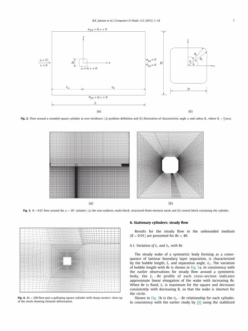
Fig. 2. Flow around a rounded square cylinder at zero incidence: (a) problem definition and (b) illustration of characteristic angle / and radius Rc , where Rc ¼ D2 sec/.

Fig. 3. B ¼ 0:01 flow around the / ¼ 30� cylinder: (a) the non-uniform, multi-block, structured finite-element mesh and (b) central block containing the cylinder.

Fig. 4. Re ¼ 200 flow past a galloping square cylinder with sharp corners: close-upof the mesh showing element deformation.

R.K. Jaiman et al. / Computers & Fluids 112 (2015) 1–18 7

6. Stationary cylinders: steady flow

Results for the steady flow in the unbounded medium(B ¼ 0:01) are presented for Re 6 40.

6.1. Variation of Lr and hsr with Re

The steady wake of a symmetric body forming as a conse-quence of laminar boundary layer separation, is characterizedby the bubble length, Lr and separation angle, hsr . The variationof bubble length with Re is shown in Fig. 5a. In consistency withthe earlier observations for steady flow around a symmetricbody, the Lr � Re profile of each cross-section indicatesapproximate linear elongation of the wake with increasing Re.When Re is fixed, Lr is maximum for the square and decreasesconsistently with decreasing Rc so that the wake is shortest forthe circle.

Shown in Fig. 5b is the hsr � Re relationship for each cylinder.In consistency with the earlier study by [9] using the stabilized

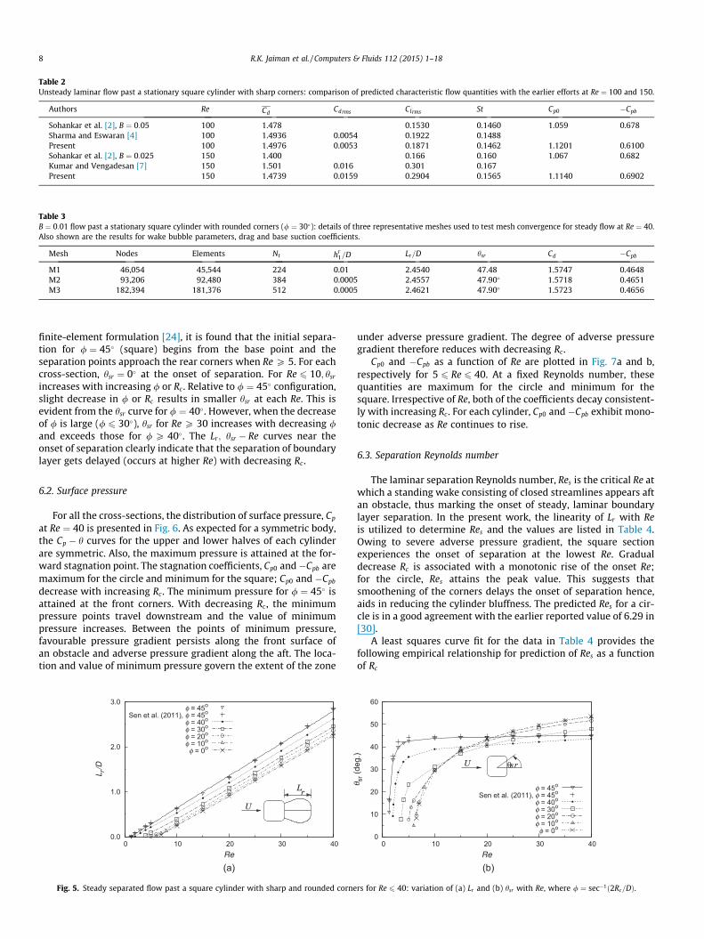
Table 2Unsteady laminar flow past a stationary square cylinder with sharp corners: comparison of predicted characteristic flow quantities with the earlier efforts at Re ¼ 100 and 150.

Authors Re Cd Cdrms Clrms St Cp0 �Cpb

Sohankar et al. [2], B ¼ 0:05 100 1.478 0.1530 0.1460 1.059 0.678Sharma and Eswaran [4] 100 1.4936 0.0054 0.1922 0.1488Present 100 1.4976 0.0053 0.1871 0.1462 1.1201 0.6100Sohankar et al. [2], B ¼ 0:025 150 1.400 0.166 0.160 1.067 0.682Kumar and Vengadesan [7] 150 1.501 0.016 0.301 0.167Present 150 1.4739 0.0159 0.2904 0.1565 1.1140 0.6902

Table 3B ¼ 0:01 flow past a stationary square cylinder with rounded corners (/ ¼ 30�): details of three representative meshes used to test mesh convergence for steady flow at Re ¼ 40.Also shown are the results for wake bubble parameters, drag and base suction coefficients.

Mesh Nodes Elements Nt hr1=D Lr=D hsr Cd �Cpb

M1 46,054 45,544 224 0.01 2.4540 47.48 1.5747 0.4648M2 93,206 92,480 384 0.0005 2.4557 47.90� 1.5718 0.4651M3 182,394 181,376 512 0.0005 2.4621 47.90� 1.5723 0.4656

8 R.K. Jaiman et al. / Computers & Fluids 112 (2015) 1–18

finite-element formulation [24], it is found that the initial separa-tion for / ¼ 45� (square) begins from the base point and theseparation points approach the rear corners when Re P 5. For eachcross-section, hsr ¼ 0� at the onset of separation. For Re 6 10; hsr

increases with increasing / or Rc . Relative to / ¼ 45� configuration,slight decrease in / or Rc results in smaller hsr at each Re. This isevident from the hsr curve for / ¼ 40�. However, when the decreaseof / is large (/ 6 30�), hsr for Re P 30 increases with decreasing /and exceeds those for / P 40�. The Lr ; hsr � Re curves near theonset of separation clearly indicate that the separation of boundarylayer gets delayed (occurs at higher Re) with decreasing Rc .

6.2. Surface pressure

For all the cross-sections, the distribution of surface pressure, Cp

at Re ¼ 40 is presented in Fig. 6. As expected for a symmetric body,the Cp � h curves for the upper and lower halves of each cylinderare symmetric. Also, the maximum pressure is attained at the for-ward stagnation point. The stagnation coefficients, Cp0 and�Cpb aremaximum for the circle and minimum for the square; Cp0 and �Cpb

decrease with increasing Rc . The minimum pressure for / ¼ 45� isattained at the front corners. With decreasing Rc , the minimumpressure points travel downstream and the value of minimumpressure increases. Between the points of minimum pressure,favourable pressure gradient persists along the front surface ofan obstacle and adverse pressure gradient along the aft. The loca-tion and value of minimum pressure govern the extent of the zone

Fig. 5. Steady separated flow past a square cylinder with sharp and rounded corne

under adverse pressure gradient. The degree of adverse pressuregradient therefore reduces with decreasing Rc.

Cp0 and �Cpb as a function of Re are plotted in Fig. 7a and b,respectively for 5 6 Re 6 40. At a fixed Reynolds number, thesequantities are maximum for the circle and minimum for thesquare. Irrespective of Re, both of the coefficients decay consistent-ly with increasing Rc . For each cylinder, Cp0 and �Cpb exhibit mono-tonic decrease as Re continues to rise.

6.3. Separation Reynolds number

The laminar separation Reynolds number, Res is the critical Re atwhich a standing wake consisting of closed streamlines appears aftan obstacle, thus marking the onset of steady, laminar boundarylayer separation. In the present work, the linearity of Lr with Reis utilized to determine Res and the values are listed in Table 4.Owing to severe adverse pressure gradient, the square sectionexperiences the onset of separation at the lowest Re. Gradualdecrease Rc is associated with a monotonic rise of the onset Re;for the circle, Res attains the peak value. This suggests thatsmoothening of the corners delays the onset of separation hence,aids in reducing the cylinder bluffness. The predicted Res for a cir-cle is in a good agreement with the earlier reported value of 6.29 in[30].

A least squares curve fit for the data in Table 4 provides thefollowing empirical relationship for prediction of Res as a functionof Rc

rs for Re 6 40: variation of (a) Lr and (b) hsr with Re, where / ¼ sec�1ð2Rc=DÞ.

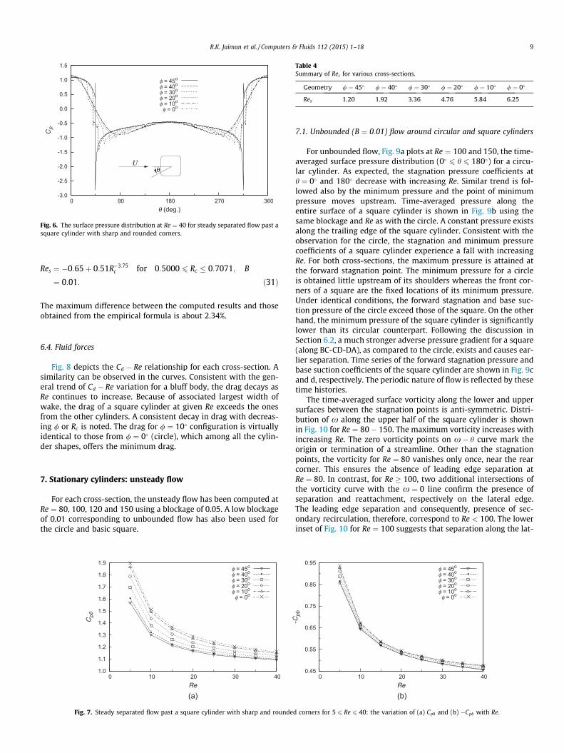
Fig. 6. The surface pressure distribution at Re ¼ 40 for steady separated flow past asquare cylinder with sharp and rounded corners.

Table 4Summary of Res for various cross-sections.

Geometry / ¼ 45� / ¼ 40� / ¼ 30� / ¼ 20� / ¼ 10� / ¼ 0�

Res 1.20 1.92 3.36 4.76 5.84 6.25

R.K. Jaiman et al. / Computers & Fluids 112 (2015) 1–18 9

Res ¼ �0:65þ 0:51R�3:75c for 0:5000 6 Rc � 0:7071; B

¼ 0:01: ð31Þ

The maximum difference between the computed results and thoseobtained from the empirical formula is about 2.34%.

6.4. Fluid forces

Fig. 8 depicts the Cd � Re relationship for each cross-section. Asimilarity can be observed in the curves. Consistent with the gen-eral trend of Cd � Re variation for a bluff body, the drag decays asRe continues to increase. Because of associated largest width ofwake, the drag of a square cylinder at given Re exceeds the onesfrom the other cylinders. A consistent decay in drag with decreas-ing / or Rc is noted. The drag for / ¼ 10� configuration is virtuallyidentical to those from / ¼ 0� (circle), which among all the cylin-der shapes, offers the minimum drag.

7. Stationary cylinders: unsteady flow

For each cross-section, the unsteady flow has been computed atRe ¼ 80, 100, 120 and 150 using a blockage of 0.05. A low blockageof 0.01 corresponding to unbounded flow has also been used forthe circle and basic square.

Fig. 7. Steady separated flow past a square cylinder with sharp and rounde

7.1. Unbounded (B ¼ 0:01) flow around circular and square cylinders

For unbounded flow, Fig. 9a plots at Re ¼ 100 and 150, the time-averaged surface pressure distribution (0� 6 h 6 180�) for a circu-lar cylinder. As expected, the stagnation pressure coefficients ath ¼ 0� and 180� decrease with increasing Re. Similar trend is fol-lowed also by the minimum pressure and the point of minimumpressure moves upstream. Time-averaged pressure along theentire surface of a square cylinder is shown in Fig. 9b using thesame blockage and Re as with the circle. A constant pressure existsalong the trailing edge of the square cylinder. Consistent with theobservation for the circle, the stagnation and minimum pressurecoefficients of a square cylinder experience a fall with increasingRe. For both cross-sections, the maximum pressure is attained atthe forward stagnation point. The minimum pressure for a circleis obtained little upstream of its shoulders whereas the front cor-ners of a square are the fixed locations of its minimum pressure.Under identical conditions, the forward stagnation and base suc-tion pressure of the circle exceed those of the square. On the otherhand, the minimum pressure of the square cylinder is significantlylower than its circular counterpart. Following the discussion inSection 6.2, a much stronger adverse pressure gradient for a square(along BC-CD-DA), as compared to the circle, exists and causes ear-lier separation. Time series of the forward stagnation pressure andbase suction coefficients of the square cylinder are shown in Fig. 9cand d, respectively. The periodic nature of flow is reflected by thesetime histories.

The time-averaged surface vorticity along the lower and uppersurfaces between the stagnation points is anti-symmetric. Distri-bution of x along the upper half of the square cylinder is shownin Fig. 10 for Re ¼ 80� 150. The maximum vorticity increases withincreasing Re. The zero vorticity points on x� h curve mark theorigin or termination of a streamline. Other than the stagnationpoints, the vorticity for Re ¼ 80 vanishes only once, near the rearcorner. This ensures the absence of leading edge separation atRe ¼ 80. In contrast, for Re 100, two additional intersections ofthe vorticity curve with the x ¼ 0 line confirm the presence ofseparation and reattachment, respectively on the lateral edge.The leading edge separation and consequently, presence of sec-ondary recirculation, therefore, correspond to Re < 100. The lowerinset of Fig. 10 for Re ¼ 100 suggests that separation along the lat-

d corners for 5 6 Re 6 40: the variation of (a) Cp0 and (b) �Cpb with Re.

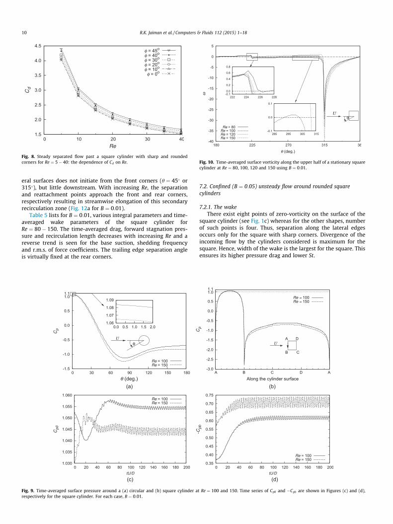
Fig. 8. Steady separated flow past a square cylinder with sharp and roundedcorners for Re ¼ 5� 40: the dependence of Cd on Re. Fig. 10. Time-averaged surface vorticity along the upper half of a stationary square

cylinder at Re ¼ 80, 100, 120 and 150 using B ¼ 0:01.

10 R.K. Jaiman et al. / Computers & Fluids 112 (2015) 1–18

eral surfaces does not initiate from the front corners (h ¼ 45� or315�), but little downstream. With increasing Re, the separationand reattachment points approach the front and rear corners,respectively resulting in streamwise elongation of this secondaryrecirculation zone (Fig. 12a for B ¼ 0:01).

Table 5 lists for B ¼ 0:01, various integral parameters and time-averaged wake parameters of the square cylinder forRe ¼ 80� 150. The time-averaged drag, forward stagnation pres-sure and recirculation length decreases with increasing Re and areverse trend is seen for the base suction, shedding frequencyand r.m.s. of force coefficients. The trailing edge separation angleis virtually fixed at the rear corners.

Fig. 9. Time-averaged surface pressure around a (a) circular and (b) square cylinder arespectively for the square cylinder. For each case, B ¼ 0:01.

7.2. Confined (B ¼ 0:05) unsteady flow around rounded squarecylinders

7.2.1. The wakeThere exist eight points of zero-vorticity on the surface of the

square cylinder (see Fig. 1c) whereas for the other shapes, numberof such points is four. Thus, separation along the lateral edgesoccurs only for the square with sharp corners. Divergence of theincoming flow by the cylinders considered is maximum for thesquare. Hence, width of the wake is the largest for the square. Thisensures its higher pressure drag and lower St.

t Re ¼ 100 and 150. Time series of Cp0 and �Cpb are shown in Figures (c) and (d),

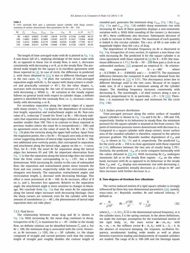
Table 5B ¼ 0:01 unsteady flow past a stationary square cylinder with sharp corners:summary of various characteristic flow parameters for Re ¼ 80� 150.

Re Cd Cdrms Clrms Cp0 �Cpb St Lr=D hsr (�)

80 1.4823 0.0025 0.1401 1.0618 0.5758 0.1338 2.1688 44.74100 1.4483 0.0051 0.1809 1.0543 0.6179 0.1427 1.9364 44.89120 1.4312 0.0084 0.2179 1.0490 0.6556 0.1489 1.7785 45.17150 1.4284 0.0151 0.2796 1.0440 0.7093 0.1538 1.6074 45.95

R.K. Jaiman et al. / Computers & Fluids 112 (2015) 1–18 11

The length of time-averaged wake with Re is plotted in Fig. 11a.A non-linear fall of Lr implying shrinkage of the mean wake withRe, as opposed to linear rise in steady flow, is seen. Lr decreasesconsistently with decreasing / or Rc as in the steady flow. The pre-dicted wake length for the square is in excellent agreement withthose reported in [4]. In case of circle, the difference in predictedLr with those obtained in [31] is due to different blockages usedin the two cases. Fig. 11b plots the variation of time-averagedseparation angle with Re. hsr for square with sharp corners is small-est and practically constant (= 45�). For the other shapes, hsr

increases with increasing Re; the rate of increase of hsr increaseswith decreasing /. While hsr � Re variation in the steady regimefollows no general trend with respect to cylinder shape, a definitepattern is identified for the unsteady flow, i.e. hsr increases consis-tently with decreasing / or Rc .

For secondary separation along the lateral edges of a squarewith sharp corners, Fig. 12a depicts the dependence of recircula-tion length, separation and reattachment angles on Re. Non-zerovalue of Lf (subscript ‘f’ stands for ‘front’) at Re ¼ 100 clearly indi-cates that separation along the lateral edges initiates at a Reynoldsnumber smaller than 100. This is in contrast to those reported inprevious studies where the onset Re is overpredicted (> 100) andno agreement exists on the value of onset Re. For 80 6 Re 6 150,Fig. 12b plots the vorticity along the upper half surface. Apart fromthe stagnation points, the x for Re ¼ 95 equals zero only at the rearcorner suggesting absence of lateral edge separation. For Re P 100,two additional zero-vorticity points, that correspond to separationand attachment along the lateral edge, appear on the x� h curve.Thus, for B ¼ 0:05, the onset Re for separation along the lateraledges lies between 95 and 100. An important observation fromFig. 12 is that the separation along the lateral edge does not initiatefrom the front corner corresponding to hsf ¼ 135�, but a littledownstream. With increasing Re, similar to the case of unboundedflow, the separation and reattachment points move towards thefront and rear corners, respectively while the recirculation zoneelongates non-linearly. The separation, reattachment angles andrecirculation length, Lf decrease with decreasing blockage. Thiseffect is most prominent at Re ¼ 100. As Re increases, effect of Bon hsf and Lf becomes less apparent. Relative to the separationangle, the attachment angle is more sensitive to changes in block-age. We conclude from Fig. 12a that the onset Re for separationalong the lateral edges increases with decreasing blockage. Oncethe sharp corners are removed, even for the cylinder with leastamount of roundedness (/ ¼ 40�), the phenomenon of lateral edgeseparation does not take place.

7.2.2. Fluid forcesThe relationship between mean drag and Re is shown in

Fig. 13a. With increasing Re, the mean drag continues to decay.Irrespective of Re;Cd is maximum for / ¼ 45�. Unlike in the steadyflow, no definite relation can be identified between Cd and /. ForRe 6 100, the minimum drag is associated with the circle. Howev-er, as Re increases (P 120), the / ¼ 30� cylinder, i.e. the shapecomposed of straight and curved portions such that the contourlength of straight part roughly doubles the contour length of

rounded part, generates the minimum drag. Cdrms (Fig. 13b), Clmax

(Fig. 13)c and Clrms (Fig. 13d) exhibit sharp monotonic rise withincreasing Re. Each of these quantities displays a non-monotonicvariation with /. With little rounding of the corners (/ decreasesto 40�), these coefficients also decrease. Subsequent decrease of/ leads to increase in their values. The maximum of each quantityis linked to the circular cylinder. The r.m.s. of lift is one order ofmagnitude higher than the r.m.s. of drag.

The dependence of Strouhal frequency on Re is illustrated inFig. 14a. Irrespective of cross-section, St registers a non-linear risewith increasing Re. The predicted St for the square cylinder is inclose agreement with those reported in [4] for B ¼ 0:05 (the max-imum difference is 1.7%). For Re ¼ 50� 250 flow past a circle in anunbounded medium, [32] proposed an empirical St � Re relation-ship expressed as St ¼ aþ bRec wherea ¼ 0:278484; b ¼ �0:896502 and c ¼ �0:445775. The maximumdifference between the computed St and those obtained from theempirical formula in [32] is 3.5%. This discrepancy arises due todifferent blockage used in the two cases. Because of its largestwake size, St of a square is minimum among all the cylindershapes. The shedding frequency increases consistently withdecreasing Rc. The wavelength, k of shed vortices along a row isinversely proportional to St, in particular, k=D ¼ 1=St [33]. There-fore, k is maximum for the square and minimum for the circle(Fig. 14b).

7.2.3. Surface pressure distributionTime-averaged pressure along the entire surface of rounded

square cylinders is shown in Fig. 15a and b for Re ¼ 100 and 150,respectively. Similar to its behaviour in steady flow, the minimumpressure for the square cylinder is attained at the front corners. Thepoint of minimum pressure moves downstream with decrease in /.Compared to a square cylinder with sharp corners, lesser surfacearea of the rounded cylinders is therefore, exposed to the adversepressure gradient. The Reynolds number dependence of Cp0 and�Cpb is shown in Fig. 15c and d, respectively. The predicted Cp0

for the circle at Re ¼ 150 is in close agreement with those reportedin [34]; difference between the two sets of results being 1.79%.Similarly, the predicted �Cpb of a circle compares favourably withthe values obtained in [35,34]. With increasing Re;Cp0 undergoesmonotonic fall as in the steady flow regime. �Cpb on the otherhand, increases with Re as opposed to its behaviour in the steadyflow. Cp0 and �Cpb display non-monotonic rise with decreasing /.Each of these quantities initially decreases as / drops to 40� andthen increases with further decrease in /.

8. Two-degrees-of-freedom free vibrations

The vortex-induced motion of a rigid square cylinder is stronglyinfluenced by three key non-dimensional parameters [36], namely,mass-ratio, m�; Reynolds number, Re and reduced velocity, U�

defined as

m� ¼ m

q f D2 ; Re ¼ q f UDl f

; U� ¼ Uf ND

: ð32Þ

where f N ¼ ð1=2pÞffiffiffiffiffiffiffiffiffiffik=m

pis the dimensional natural frequency, m is

the cylinder mass, k is the spring constant. In the above definitions,we make the isotropic assumption for the translational motion ofthe rigid body, i.e., the mass vector m ¼ ðmx;myÞ withmx ¼ my ¼ m, the stiffness vector k ¼ ðkx; kyÞ with kx ¼ ky ¼ k. Inthe absence of structural damping, the response, oscillation fre-quency, aerodynamic loading, wake modes as well as phasebetween transverse loading and displacement of rounded cylindersare studied. The range of Re is 100–200 and the blockage equals

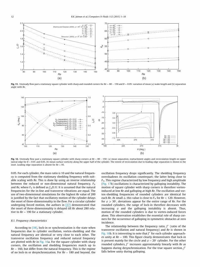
Fig. 11. Unsteady flow past a stationary square cylinder with sharp and rounded corners for Re ¼ 80� 150 and B ¼ 0:05: variation of mean (a) wake length and (b) separationangle with Re.

Fig. 12. Unsteady flow past a stationary square cylinder with sharp corners at Re ¼ 80� 150: (a) mean separation, reattachment angles and recirculation length on upperlateral edge for B ¼ 0:01 and 0.05, (b) mean surface vorticity along the upper half of the cylinder. The extent of recirculation due to leading edge separation is shown in theinset. Leading edge separation is absent for Re 6 95.

12 R.K. Jaiman et al. / Computers & Fluids 112 (2015) 1–18

0.05. For each cylinder, the mass ratio is 10 and the natural frequen-cy is computed from the stationary shedding frequency with suit-able scaling with Re. This is done by using an inverse relationshipbetween the reduced or non-dimensional natural frequency, FN

and Re, where FN is defined as f ND=U. It is assumed that the naturalfrequencies for the in-line and transverse vibrations are equal. Theuse of two-dimensional simulations for the highest Re value of 200is justified by the fact that oscillatory motion of the cylinder delaysthe onset of three-dimensionality in the flow. For a circular cylinderundergoing forced motion, the authors in [37] demonstrated thatthe onset of three-dimensionality is delayed till Re about 280 rela-tive to Re ¼ 190 for a stationary cylinder.

8.1. Frequency characteristics

According to [38], lock-in or synchronization is the state whenfrequencies due to cylinder oscillation, vortex-shedding and thenatural frequency are identical or very close to each other. Thetransverse oscillation frequency and reduced natural frequencyare plotted with Re in Fig. 16a. For the square cylinder with sharpcorners, the oscillation and shedding frequencies match up toRe ¼ 160, but differ from the natural frequency. This is the regimeof no lock-in or desynchronization. For Re ¼ 180 and beyond, the

oscillation frequency drops significantly. The shedding frequencyovershadows its oscillation counterpart; the latter being close toFN . This regime characterized by low frequency and high amplitude(Fig. 17b) oscillations is characterized by galloping instability. Themotion of square cylinder with sharp corners is therefore vortex-induced at low Re and galloping at high Re. The oscillation and vor-tex-shedding frequencies of rounded cylinders are identical foreach Re. At small /, this value is close to FN for Re 6 120. However,for / P 30�, deviations appear for the entire range of Re. For therounded cylinders, the range of lock-in therefore decreases withincreasing / and the galloping instability is absent. Thus,motion of the rounded cylinders is due to vortex-induced forcesalone. This observation establishes the essential role of sharp cor-ners for the occurrence of galloping in symmetric obstacles at zeroincidence.

The relationship between the frequency ratio, f � (ratio of thetransverse oscillation and natural frequency) and Re is shown inFig. 16b. It is interesting to note that f � for each cylinder approach-es unity at Re ¼ 100. This figure clearly demonstrates that lock-inis present mainly for the circle and / ¼ 20� cylinder. For the otherrounded cylinders, f � increases approximately linearly with Re ashappens during desynchronization. For the true square section, f �

falls below unity during galloping.

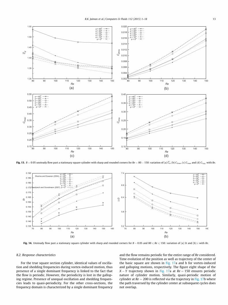
Fig. 13. B ¼ 0:05 unsteady flow past a stationary square cylinder with sharp and rounded corners for Re ¼ 80� 150: variation of (a) Cd , (b) Cd rms , (c) Clmax and (d) Clrms with Re.

Fig. 14. Unsteady flow past a stationary square cylinder with sharp and rounded corners for B ¼ 0:05 and 80 6 Re 6 150: variation of (a) St and (b) k with Re.

R.K. Jaiman et al. / Computers & Fluids 112 (2015) 1–18 13

8.2. Response characteristics

For the true square section cylinder, identical values of oscilla-tion and shedding frequencies during vortex-induced motion, thuspresence of a single dominant frequency is linked to the fact thatthe flow is periodic. However, the periodicity is lost in the gallop-ing regime. Presence of unequal oscillation and shedding frequen-cies leads to quasi-periodicity. For the other cross-sections, thefrequency domain is characterized by a single dominant frequency

and the flow remains periodic for the entire range of Re considered.Time evolution of the position as well as trajectory of the center ofthe basic square are shown in Fig. 17a and b for vortex-inducedand galloping motions, respectively. The figure eight shape of theX � Y trajectory shown in Fig. 17a at Re ¼ 150 ensures periodicnature of cylinder motion. Similarly, quasi-periodic motion ofcylinder at Re ¼ 200 is reflected via the trajectory in Fig. 17b wherethe path traversed by the cylinder center at subsequent cycles doesnot overlap.

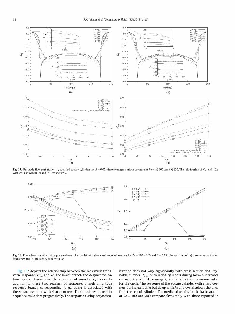
Fig. 15. Unsteady flow past stationary rounded square cylinders for B ¼ 0:05: time-averaged surface pressure at Re = (a) 100 and (b) 150. The relationship of Cp0 and �Cpb

with Re is shown in (c) and (d), respectively.

Fig. 16. Free vibrations of a rigid square cylinder of m� ¼ 10 with sharp and rounded corners for Re ¼ 100� 200 and B ¼ 0:05: the variation of (a) transverse oscillationfrequency and (b) frequency ratio with Re.

14 R.K. Jaiman et al. / Computers & Fluids 112 (2015) 1–18

Fig. 18a depicts the relationship between the maximum trans-verse response, Ymax and Re. The lower branch and desynchroniza-tion regime characterize the response of rounded cylinders. Inaddition to these two regimes of response, a high amplituderesponse branch corresponding to galloping is associated withthe square cylinder with sharp corners. These regimes appear insequence as Re rises progressively. The response during desynchro-

nization does not vary significantly with cross-section and Rey-nolds number. Ymax of rounded cylinders during lock-in increasesconsistently with decreasing Rc and attains the maximum valuefor the circle. The response of the square cylinder with sharp cor-ners during galloping builds up with Re and overshadows the onesfrom the rest of cylinders. The predicted results for the basic squareat Re ¼ 180 and 200 compare favourably with those reported in

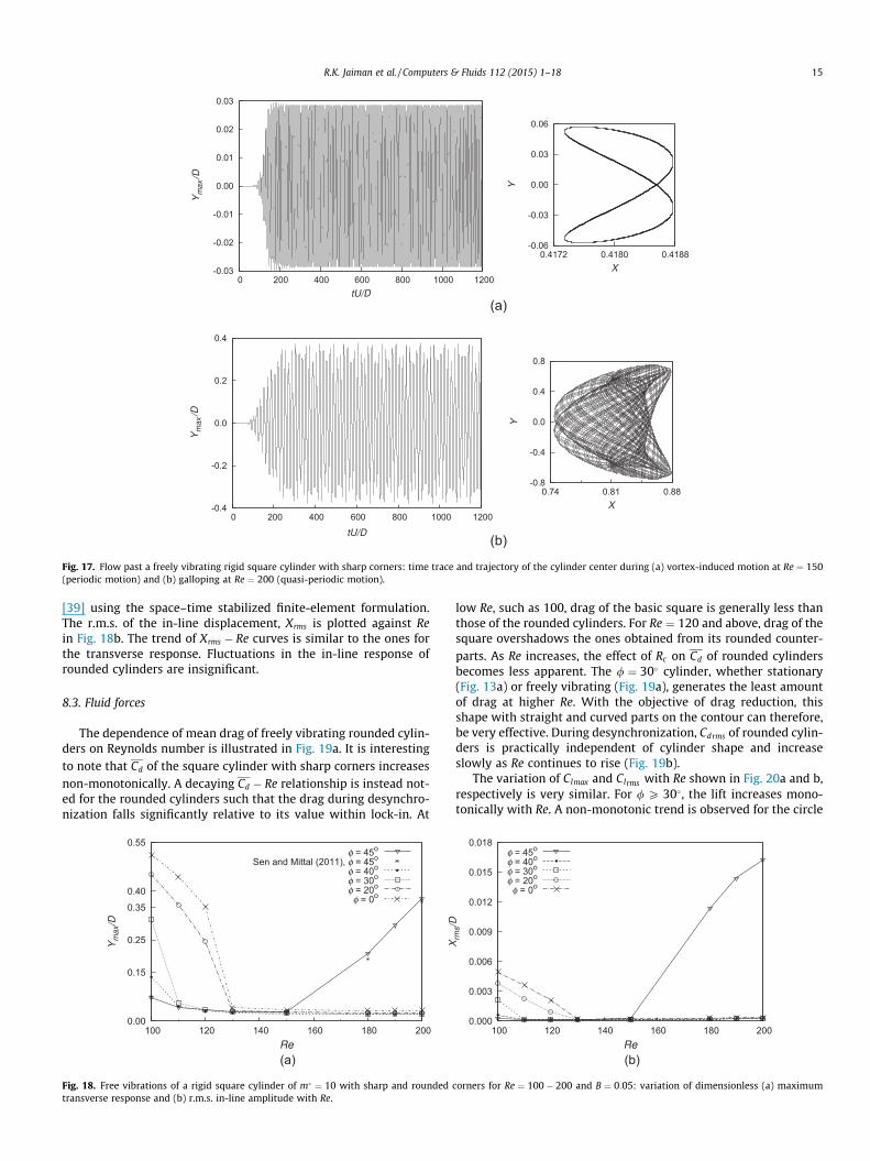
Fig. 17. Flow past a freely vibrating rigid square cylinder with sharp corners: time trace and trajectory of the cylinder center during (a) vortex-induced motion at Re ¼ 150(periodic motion) and (b) galloping at Re ¼ 200 (quasi-periodic motion).

R.K. Jaiman et al. / Computers & Fluids 112 (2015) 1–18 15

[39] using the space–time stabilized finite-element formulation.The r.m.s. of the in-line displacement, Xrms is plotted against Rein Fig. 18b. The trend of Xrms � Re curves is similar to the ones forthe transverse response. Fluctuations in the in-line response ofrounded cylinders are insignificant.

8.3. Fluid forces

The dependence of mean drag of freely vibrating rounded cylin-ders on Reynolds number is illustrated in Fig. 19a. It is interestingto note that Cd of the square cylinder with sharp corners increasesnon-monotonically. A decaying Cd � Re relationship is instead not-ed for the rounded cylinders such that the drag during desynchro-nization falls significantly relative to its value within lock-in. At

Fig. 18. Free vibrations of a rigid square cylinder of m� ¼ 10 with sharp and roundedtransverse response and (b) r.m.s. in-line amplitude with Re.

low Re, such as 100, drag of the basic square is generally less thanthose of the rounded cylinders. For Re ¼ 120 and above, drag of thesquare overshadows the ones obtained from its rounded counter-parts. As Re increases, the effect of Rc on Cd of rounded cylindersbecomes less apparent. The / ¼ 30� cylinder, whether stationary(Fig. 13a) or freely vibrating (Fig. 19a), generates the least amountof drag at higher Re. With the objective of drag reduction, thisshape with straight and curved parts on the contour can therefore,be very effective. During desynchronization, Cdrms of rounded cylin-ders is practically independent of cylinder shape and increaseslowly as Re continues to rise (Fig. 19b).

The variation of Clmax and Clrms with Re shown in Fig. 20a and b,respectively is very similar. For / P 30�, the lift increases mono-tonically with Re. A non-monotonic trend is observed for the circle

corners for Re ¼ 100� 200 and B ¼ 0:05: variation of dimensionless (a) maximum

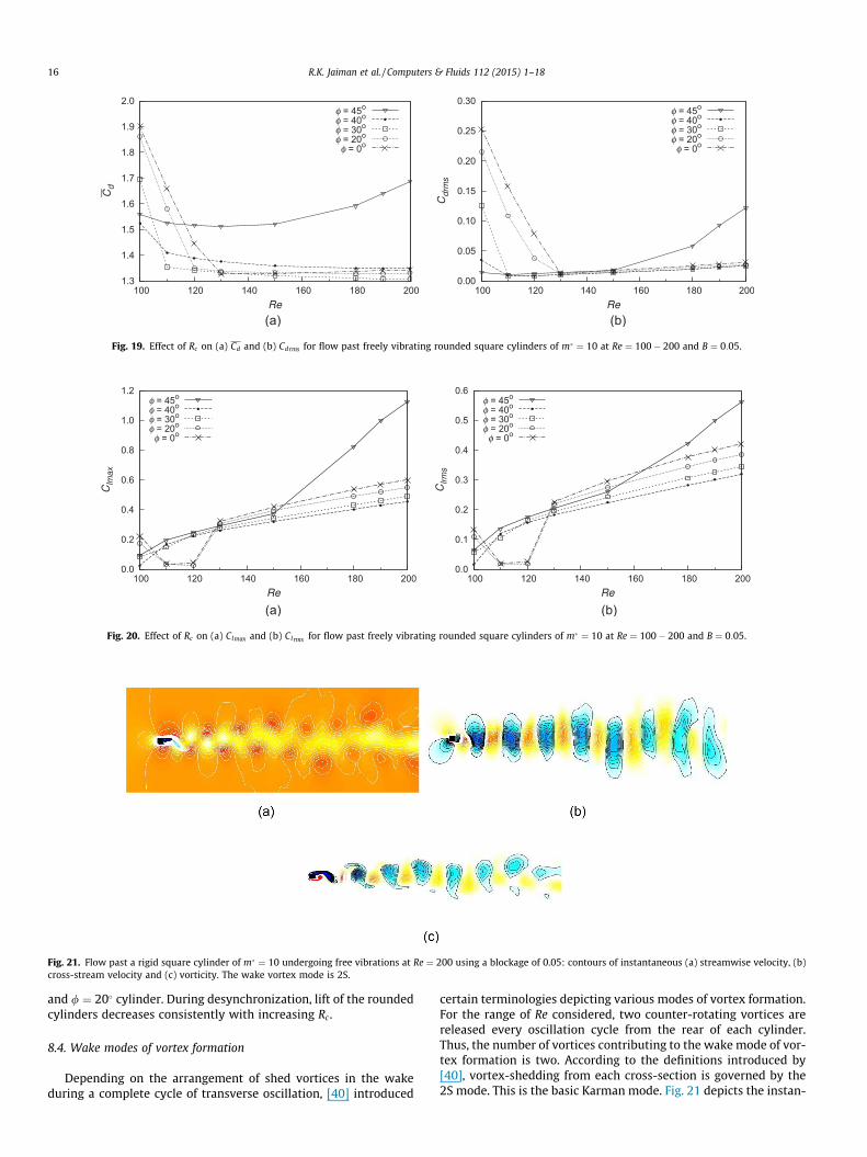
Fig. 19. Effect of Rc on (a) Cd and (b) Cd rms for flow past freely vibrating rounded square cylinders of m� ¼ 10 at Re ¼ 100� 200 and B ¼ 0:05.

Fig. 20. Effect of Rc on (a) Clmax and (b) Clrms for flow past freely vibrating rounded square cylinders of m� ¼ 10 at Re ¼ 100� 200 and B ¼ 0:05.

Fig. 21. Flow past a rigid square cylinder of m� ¼ 10 undergoing free vibrations at Re ¼ 200 using a blockage of 0.05: contours of instantaneous (a) streamwise velocity, (b)cross-stream velocity and (c) vorticity. The wake vortex mode is 2S.

16 R.K. Jaiman et al. / Computers & Fluids 112 (2015) 1–18

and / ¼ 20� cylinder. During desynchronization, lift of the roundedcylinders decreases consistently with increasing Rc .

8.4. Wake modes of vortex formation

Depending on the arrangement of shed vortices in the wakeduring a complete cycle of transverse oscillation, [40] introduced

certain terminologies depicting various modes of vortex formation.For the range of Re considered, two counter-rotating vortices arereleased every oscillation cycle from the rear of each cylinder.Thus, the number of vortices contributing to the wake mode of vor-tex formation is two. According to the definitions introduced by[40], vortex-shedding from each cross-section is governed by the2S mode. This is the basic Karman mode. Fig. 21 depicts the instan-

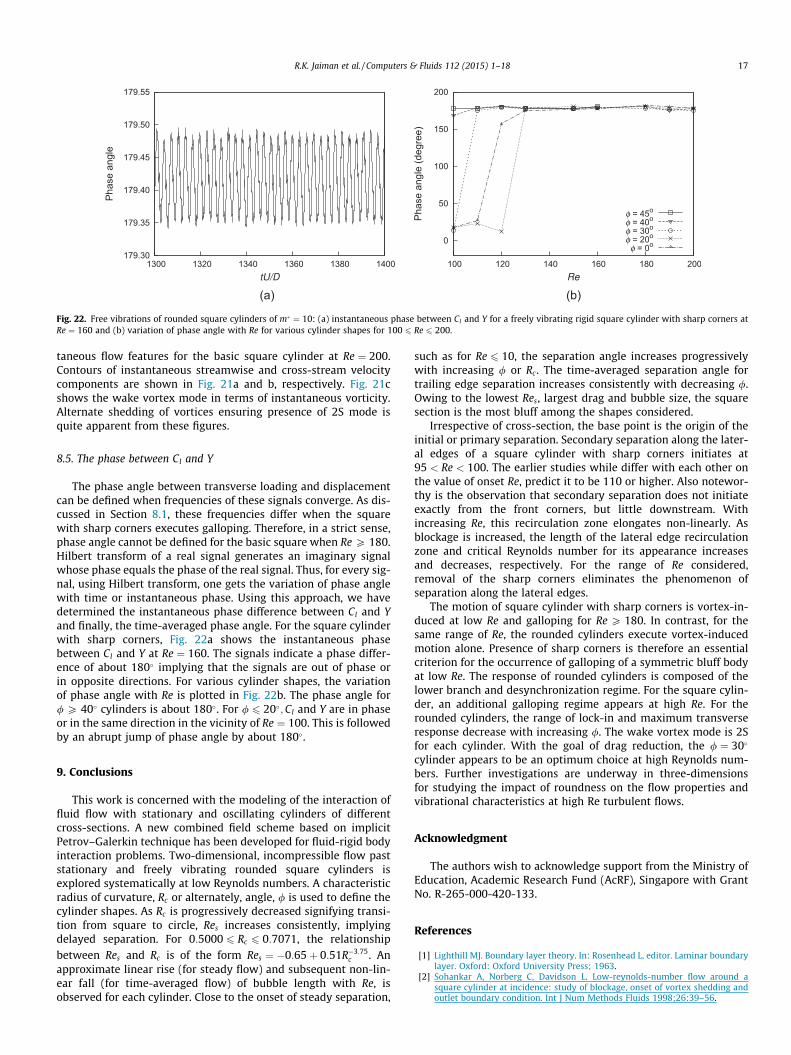
Fig. 22. Free vibrations of rounded square cylinders of m� ¼ 10: (a) instantaneous phase between Cl and Y for a freely vibrating rigid square cylinder with sharp corners atRe ¼ 160 and (b) variation of phase angle with Re for various cylinder shapes for 100 6 Re 6 200.

R.K. Jaiman et al. / Computers & Fluids 112 (2015) 1–18 17

taneous flow features for the basic square cylinder at Re ¼ 200.Contours of instantaneous streamwise and cross-stream velocitycomponents are shown in Fig. 21a and b, respectively. Fig. 21cshows the wake vortex mode in terms of instantaneous vorticity.Alternate shedding of vortices ensuring presence of 2S mode isquite apparent from these figures.

8.5. The phase between Cl and Y

The phase angle between transverse loading and displacementcan be defined when frequencies of these signals converge. As dis-cussed in Section 8.1, these frequencies differ when the squarewith sharp corners executes galloping. Therefore, in a strict sense,phase angle cannot be defined for the basic square when Re P 180.Hilbert transform of a real signal generates an imaginary signalwhose phase equals the phase of the real signal. Thus, for every sig-nal, using Hilbert transform, one gets the variation of phase anglewith time or instantaneous phase. Using this approach, we havedetermined the instantaneous phase difference between Cl and Yand finally, the time-averaged phase angle. For the square cylinderwith sharp corners, Fig. 22a shows the instantaneous phasebetween Cl and Y at Re ¼ 160. The signals indicate a phase differ-ence of about 180� implying that the signals are out of phase orin opposite directions. For various cylinder shapes, the variationof phase angle with Re is plotted in Fig. 22b. The phase angle for/ P 40� cylinders is about 180�. For / 6 20�;Cl and Y are in phaseor in the same direction in the vicinity of Re ¼ 100. This is followedby an abrupt jump of phase angle by about 180�.

9. Conclusions

This work is concerned with the modeling of the interaction offluid flow with stationary and oscillating cylinders of differentcross-sections. A new combined field scheme based on implicitPetrov–Galerkin technique has been developed for fluid-rigid bodyinteraction problems. Two-dimensional, incompressible flow paststationary and freely vibrating rounded square cylinders isexplored systematically at low Reynolds numbers. A characteristicradius of curvature, Rc or alternately, angle, / is used to define thecylinder shapes. As Rc is progressively decreased signifying transi-tion from square to circle, Res increases consistently, implyingdelayed separation. For 0:5000 6 Rc 6 0:7071, the relationshipbetween Res and Rc is of the form Res ¼ �0:65þ 0:51R�3:75

c . Anapproximate linear rise (for steady flow) and subsequent non-lin-ear fall (for time-averaged flow) of bubble length with Re, isobserved for each cylinder. Close to the onset of steady separation,

such as for Re 6 10, the separation angle increases progressivelywith increasing / or Rc. The time-averaged separation angle fortrailing edge separation increases consistently with decreasing /.Owing to the lowest Res, largest drag and bubble size, the squaresection is the most bluff among the shapes considered.

Irrespective of cross-section, the base point is the origin of theinitial or primary separation. Secondary separation along the later-al edges of a square cylinder with sharp corners initiates at95 < Re < 100. The earlier studies while differ with each other onthe value of onset Re, predict it to be 110 or higher. Also notewor-thy is the observation that secondary separation does not initiateexactly from the front corners, but little downstream. Withincreasing Re, this recirculation zone elongates non-linearly. Asblockage is increased, the length of the lateral edge recirculationzone and critical Reynolds number for its appearance increasesand decreases, respectively. For the range of Re considered,removal of the sharp corners eliminates the phenomenon ofseparation along the lateral edges.

The motion of square cylinder with sharp corners is vortex-in-duced at low Re and galloping for Re P 180. In contrast, for thesame range of Re, the rounded cylinders execute vortex-inducedmotion alone. Presence of sharp corners is therefore an essentialcriterion for the occurrence of galloping of a symmetric bluff bodyat low Re. The response of rounded cylinders is composed of thelower branch and desynchronization regime. For the square cylin-der, an additional galloping regime appears at high Re. For therounded cylinders, the range of lock-in and maximum transverseresponse decrease with increasing /. The wake vortex mode is 2Sfor each cylinder. With the goal of drag reduction, the / ¼ 30�

cylinder appears to be an optimum choice at high Reynolds num-bers. Further investigations are underway in three-dimensionsfor studying the impact of roundness on the flow properties andvibrational characteristics at high Re turbulent flows.

Acknowledgment

The authors wish to acknowledge support from the Ministry ofEducation, Academic Research Fund (AcRF), Singapore with GrantNo. R-265-000-420-133.

References

[1] Lighthill MJ. Boundary layer theory. In: Rosenhead L, editor. Laminar boundarylayer. Oxford: Oxford University Press; 1963.

[2] Sohankar A, Norberg C, Davidson L. Low-reynolds-number flow around asquare cylinder at incidence: study of blockage, onset of vortex shedding andoutlet boundary condition. Int J Num Methods Fluids 1998;26:39–56.

18 R.K. Jaiman et al. / Computers & Fluids 112 (2015) 1–18

[3] Robichaux J, Balachandar S, Vanka SP. Three-dimensional floquet instability ofthe wake of square cylinder. Phys Fluids 1999;11:560–78.

[4] Sharma A, Eswaran V. Heat and fluid flow across a square cylinder in the two-dimensional laminar flow regime. Num Heat Trans 2004;45:247–69.

[5] Dalton C, Zheng W. Numerical simulations of a viscous uniform approach flowpast square and diamond cylinders. J Fluids Struct 2003;18:455–65.

[6] Hu JC, Zhou Y, Dalton C. Effects of the corner radius on the near wake of asquare prism. Exp Fluids 2006;40:106–18.

[7] Kumar MBS, Vengadesan S. Influence of rounded corners on flow interferencedue to square cylinders using immersed boundary method. ASME J Fl Eng2012;134:091203-1–3-3.

[8] Amandolese X, Hemon P. Vortex-induced vibration of square cylinder in windtunnel. Comptes Rendus Mecanique 2010;338:12–7.

[9] Sen S, Mittal S, Biswas G. Flow past a square cylinder at low reynolds numbers.Int J Num Methods Fluids 2011;67:1160–74.

[10] He T, Zhou D, Bao Y. Combined interface boundary condition method for fluid-rigid body interaction. Comput Methods Appl Mechan Eng 2012:81–102.

[11] Jaiman R, Geubelle P, Loth E, Jiao X. Combined interface boundary conditionsmethod for unsteady fluid-structure interaction. Comput Meth Appl Mech Eng2011;200:27–39.

[12] Jaiman R, Geubelle P, Loth E, Jiao X. Transient fluid-structure interaction withnon-matching spatial and temporal discretizations. Comput Fluids2011;50:120–35.

[13] S Leontini J, Thompson MC, Hourigan K. The begining of branching behaviourof vortex-induced vibration during two-dimensional flow. J Fluids Struct2006;73:857–64.

[14] Hughes TJR, Brooks AN. A multi-dimensional upwind scheme with nocrosswind diffusion. Finite Element Methods Convect 1979:19–35.

[15] Brooks AN, Hughes TJR. Streamline upwind/Petrov–Galerkin formulation forconvection dominated flows with particular emphasis on the incompressibleNavier–Stokes equations. Comput Methods Appl Mech Eng 1982;32:199–259.

[16] Hughes TJR, Franca LP, Hulbert GM. A new finite element formulation forcomputational fluid dynamics: Viii. the galerkin/least-squares method foradvective–diffusive equations. Comput Methods Appl Mech Eng1989;73:173–89.

[17] Liu J, Jaiman RK, Gurugubelli PS. A stable second-order scheme for fluid-structure interaction with strong added-mass effects. J Comput Phy2014;270:687–710.

[18] van Brummelen EH, van der Zee KG, Garg VV, Prudhomme S. Flux evaluation inprimal and dual boundary-coupled problems. J Appl Mech 2011;79.

[19] Hughes TJR, Liu WK, Zimmerman TK. Lagrangian–Eulerian finite elementformulation for incompressible viscous flows. Comput Meth Appl Mech Eng1981;29:329–49.

[20] Chung J, Hulbert GM. A time integration algorithm for structural dynamicswith improved numerical dissipation: the generalized-a method. J Appl Mech1993;60:370–5.

[21] Dettmer W, Peric. A computational framework for fluid-rigid body interaction:finite element formulation and applications. Comput Methods Appl Mech Eng2006;195:1633–66.

[22] Bazilevs Y, Takizawa K, Tezduar TE. Computational fluid–structure interaction:methods and applications. Wiley; 2013.

[23] Johnson C. Numerical solutions of partial differential equations by the finiteelement method. Cambridge University Press; 1987.

[24] Tezduyar T, Mittal S, Ray SE, Shih R. Incompressible flow computations withstabilized bilinear and linear equal-order- interpolation velocity–pressureelements. Comput Meth Appl Mech Eng 1992;95:221–42.

[25] Hughes TJR, Franca LP, Balestra M. A new finite element formulation forcomputational fluid dynamics: V. circumventing the babuška-brezzicondition: a stable Petrov–Galerkin formulation of the Stokes problemaccommodating equal-order interpolations. Comput Methods Appl Mech Eng1986;59:85–99.

[26] Tezduyar TE. Finite elements in fluids: stabilized formulations and movingboundaries and interfaces. Comput Fluids 2007;36:191–206.

[27] Hron J, Turek S. A monolithic FEM/Multigrid solver for an ALE formulation offluid–structure interaction with applications in Biomechanics. Springer; 2006.

[28] Wick T. Solving monolithic fluid–structure interaction problems in arbitrarylagrangian eulerian coordinates with the deal. ii library. Arch Numer Software2013;1(1):1–19.

[29] Saad Y, Schultz MH. GMRES: a generalized minimal residual algorithm forsolving non-symmetric linear systems. SIAM J Sci Stat Comput 1986;7.

[30] Sen S, Mittal S, Biswas G. Steady separated flow past a circular cylinder at lowreynolds numbers. J Fluid Mech 2009;620:89–119.

[31] Lima E Silva ALF, Silveira-Neto A, Damasceno JJR. Numerical simulation of two-dimensional flows over a circular cylinder using the immersed boundarymethod. J Comput Phy 2003;189:351–70.

[32] Posdziech O, Grundmann R. A systematic approach to the numericalcalculation of fundamental quantities of the two-dimensional flow over acircular cylinder. J Fluids Struct 2007;23:479–99.

[33] Vorobieff P, Georgiev D, Ingber MS. Onset of the second wake: dependence onthe reynolds number. Phys Fluids 2002;14:L53–6.

[34] Farhoud RK, Amiralaie S, Jabbari G, Amiralaie S. Numerical study of unsteadylaminar flow around a circular cylinder. J Civil Eng Urban 2012;2:63–7.

[35] Lin PT, Baker TJ, Martinelli L, Jameson A. Two-dimensional implicit time-dependent calculations on adaptive unstructured meshes with time evolvingboundaries. Int J Num Methods Fluids 2006;50:199–218.

[36] Sarpkaya T. A critical review of the intrinsic nature of vortex-inducedvibrations. J Fluids Struct 2004;19:389–447.

[37] S Leontini J, Thompson MC, Hourigan K. Three-dimensional transition in thewake of a transversely oscillating cylinder. J Fluid Mech 2007;577:79–104.

[38] Williamson CHK, Govardhan R. Vortex induced vibration. Ann Rev FluidMechan 2004;36:413–55.

[39] Sen S, Mittal S. Free vibration of a square cylinder at low reynolds numbers. JFluids Struct 2011;27:875–84.

[40] Williamson CHK, Roshko A. Vortex formation in the wake of an oscillatingcylinder. J Fluids Struct 1988;2:355–81.