Finding the Minimum-Cost Path Without Cutting Corners

Finding the Minimum-Cost Path WithoutCutting Corners

R. Joop van Heekeren, Frank G.A. Faas, and Lucas J. van Vliet

Quantitative Imaging Group, Delft University of Technology, The [email protected]

Abstract. Applying a minimum-cost path algorithm to find the paththrough the bottom of a curvilinear valley yields a biased path throughthe inside of a corner. DNA molecules, blood vessels, and neurite tracksare examples of string-like (network) structures, whose minimum-costpath is cutting through corners and is less flexible than the underlyingcenterline. Hence, the path is too short and its shape too stiff, whichhampers quantitative analysis. We developed a method which solves thisproblem and results in a path whose distance to the true centerline ismore than an order of magnitude smaller in areas of high curvature. Wefirst compute an initial path. The principle behind our iterative algorithmis to deform the image space, using the current path in such a way thatcurved string-like objects are straightened before calculating a new path.A damping term in the deformation is needed to guarantee convergenceof the method.

1 Introduction

Algorithms for computing the minimum-cost path have played an important rolein various fields of science and engineering. These algorithms try to find the pathconnecting a selected start and end point that minimizes the integrated costs. Inoptics, light rays travel along a minimum-cost path from source to destination. Awave front of light propagates with a speed that depends inversely proportionalon the refractive index of the medium. A space varying velocity map suggeststhat the path with the shortest arrival time will in general be longer than theEuclidean distance between the start and end points. If you consider the localcost as the inverse of the local speed, then calculating the minimum integratedcost corresponds to calculating the smallest possible arrival time from a startpoint to all points in the domain.

In many fields of science and engineering we encounter images of string-likestructures in which the centerline conveys important information about the un-derlying objects. Examples are DNA-strands (cf. Fig. 1), blood vessels, or neu-rite tracks. The tracking results as depicted in [5] display exactly the problemsthat we are addressing in this paper. The minimum-cost path does not follow thecurvilinear valley of the cost function, but is biased towards the inside of corners.In general, the minimum-cost path is cutting corners, and is therefore shorterand stiffer than the underlying centerline of the cost valley. Quantification of the

B.K. Ersbøll and K.S. Pedersen (Eds.): SCIA 2007, LNCS 4522, pp. 263–272, 2007.c© Springer-Verlag Berlin Heidelberg 2007

264 R.J. van Heekeren, F.G.A. Faas, and L.J. van Vliet

Fig. 1. DNA molecules labeled with uranyl acetate and visualized by transmission elec-tron microscopy. The images are kindly provided by Dr. Dmitry Cherny, PhD, Dr. Sc.

bending energy of DNA plays a key role in understanding cellular processes. Toverify the competing models and measure the so-called persistence length, anaccurate path through these structures is required. The key to quantifying thelength and shape of these objects is to find the centerline of these objects. Aminimum-cost path guarantees a connected path that approximates this center-line even if the curvilinear object contains small gaps and is corrupted by noise(cf. Fig. 1). Solving the bias problem of minimum-cost path algorithms will beof utmost importance in many fields of science and engineering.A typical implementation of such a standard minimum-cost path approach con-sists of the following steps:

– Define one start point in the image domain. Having an end point is notmandatory, but may assist in defining an early stopping criterion.

– Compute the minimum integrated cost from the starting point to all pointsin the domain, or until the pre-defined end point has been reached.

– Descend along the opposite gradient direction of the integrated cost imagefrom the end point to the start point. Due to the smoothness of the inte-grated cost images one can obtain sub-pixel accuracy in the location of theminimum-cost path.

Finding the Minimum-Cost Path Without Cutting Corners 265

The minimum integrated cost T is given as the minimum cumulative cost alongall possible paths P connecting the start point S with any end point E in ourdomain. Or mathematically:

T = min∀P SE

∫ E

S

I(P SE(l))dl (1)

with P SE(l) = (x(l), y(l)). This is equivalent to solving the Eikonal equation [2]

|∇u(x, y)| = I(x, y) (2)

in which I(x, y) denotes the local cost function and u(x, y) the local arrival time.For uniform costs, the solution of the Eikonal equation is identical to the resultgiven by the (domain constrained) Euclidean distance transform. For space vari-ant costs we have the gray-weighted distance transform (GDT) [9,7,6,4] and fastmarching (FM) algorithms [1,3,8]. Both methods are based on wave front propa-gation. The GDT constructs a path using a superposition of cost-weighted basisvectors, thereby quantizing the local path direction to the directions of a set ofbasis vectors in a 3x3 (or 5x5) neighborhood. The FM algorithm models the wavefront by a straight front, which does not restrict the propagation direction toa limited set of discrete directions. Both methods produce an image containingthe minimum integrated cost from a starting point to all points in the domain.

The minimum-cost path can be obtained by a steepest descend (from the endpoint back to the start point) along the opposite gradient direction of the inte-grated cost map created by the aforementioned methods. Since the cost functionis usually smooth, the integrated cost function is even smoother. This permitssub-pixel accuracy in computing the steps taken during the steepest descend.Due to the finite step size and approximation errors in the aforementioned al-gorithms, the path will not end exactly at the starting point but in very close(sub-pixel) proximity.

In section 2 we quantify the cutting corner problem for circular arcs with aGaussian line profile and present our iterative algorithm to solve it. In section3 we present quantitative results on the displacement error as a function of thenumber of iterations and qualitative results on TEM images of uranyl acetatelabeled DNA. Section 4 presents the conclusions of our work.

2 Method

A correct implementation of a minimum-cost path algorithm applied to curvedlinear structures will always result in a path that is shorter and stiffer (lessbending energy) than the centerline of the underlying linear structure. Especiallyin highly curved areas the minimum-cost path is cutting corners. The minimum-cost path does not follow the path through the minimum of the cost functionin curved areas. To illustrate this we consider a circular path with a Gaussiancross-section

I(r, σ, c) = 1 + c (1 − exp(− (r − Rc)2

2σ2 )) (3)


Rp/R

c

Rc (Pixel)

c = 10, σ = 1c = 10, σ = 3c = 2, σ = 1c = 2, σ = 3

0.90

0.70

0.80

0.75

0.85

0.95

1.00

4 6 8 10 12

Fig. 2. The relative radius (Rp/Rc) of the minimum-cost path for the Gaussian profileas a function of centerline radius Rc

with the cost contrast c = cb−cp

cp, in which cb and cp are respectively the cost

values of the background and the path, and Rc the radius of curvature of thecenterline. The integrated cost of a circular path with radius r around such acircle is

T (r) = 2πr I(r, σ, c) = 2πr (1 + c (1 − exp(−(r − Rc)2

2σ2 ))) (4)

To find the minimum-cost path, we calculated the radius Rp for which T (r)is minimized, Rp = argmin T (r). Fig. 2 shows the relative radius Rp/Rc ofthe minimum-cost paths for different values of line width σ and contrast c.The results suggest that increasing the contrast or decreasing the line width(for example by scaling the cost function: I(r) → Iα(r), α > 1)) of the costfunction will reduce the bias in the minimum-cost path. In practice the biaswill be reduced by these measures to some extent, but will never produce thedesired smooth centerline path. This is shown by considering the limit (c → ∞or α → ∞), this will reduce the problem to a binary problem discarding all thegray value information and therefore produce a rough, binary skeleton type pathinstead of smooth centerline path. This skeleton path will also be hampered andpossibly even interrupted due to the presence of noise in the original image. Weclaim to have developed an algorithm not based on increasing the contrast ordecreasing the line width which solves the bias problem and still finds a smoothpath, approximating the true centerline, through this class of objects.

Algorithm

Our method is based on the idea that a standard minimum-cost path algorithmsuch as FM will only give the correct centerline path for straight string-likeobjects (assuming the start and end points are located on the centerline). Hence,the principle behind our algorithm is to deform the image space in such a way


(a) (b) (c)

Fig. 3. (a) The red line is the path extracted by a classical minimum-cost path algo-rithm, the green line is the path after the first iteration and the blue line is the truecenterline of the object. (b) Zoomed in version of (a). (c) Deformed image obtainedby equi-distant sampling perpendicular to the initial (red) path. The green path is theminimum cost path formed in the deformed image.

that a curvilinear object becomes straight. After an initial path through theobject is extracted using a standard minimum-cost path algorithm, two cubicsplines are defined through the data points found by a steepest descend; onefor the x-values and one for y-values of the data points, using the distancefrom the end points along the path as the running variable. Using cubic splinesguarantees that the path is continuous up to the second derivative. As shownin Fig. 3(a-b), lines perpendicular to the splines separated by a distance of onepixel are defined. A new image Fig. 3(c) is sampled using cubic interpolation onequi-distant points along these perpendicular lines. A new minimum-cost pathis calculated in the deformed space (the green line in Fig. 3(c)). This new pathis again represented by two splines. Next, the perpendicular distance betweenthe centerline of the deformed image and the splines is calculated. By definingpoints on the perpendicular lines in the original image with the same distancefrom the original path, the new path is transferred back to the original imagespace. Two new splines are fitted through the coordinates of these points toproduce a new path. As shown in Fig. 3(a), this path is already much closer tothe desired centerline. Repeating the process described above yields a path thatconverges to the true centerline of the object.

3 Results

We first tested our algorithm on synthetic data, allowing us to measure its per-formance by comparing the results with a ground truth. Later we used imagesof DNA-strands made using an electron microscope to examine its real worldperformance qualitatively.


(a) (b)

Fig. 4. (a) A low contrast (c = 1) image depicting the path converging to the truecenterline of the object. (b) A High contrast (c = 10) image depicting the oscillationeffect causing the path to lie alternately on either side of the true centerline of theobject. In both images the true centerline is denoted by the red dotted line.

3.1 Synthetic Data

As synthetic data we used images of curved Gaussian line profiles, with a ninetydegrees change in orientation and a curvature radius Rc (Fig. 3(a)). The crosssection of this profile is defined as in Eq. 3. The algorithm was tested for differentcenterline radii Rc, noise levels and contrast ratios c. As shown in Fig. 4(a) the firstiteration already results in a path which is significantly closer to the centerline. Wemeasured the performance by looking at the distance between the centerline ofthe object and the path found using our algorithm. We computed the root-mean-square (RMS) of the perpendicular distance between the path and the groundtruth at ten points separated by a pixel in the middle of the curve.

Initially this RMS error decreases for all the settings. However, after a num-ber of iterations (one to three for the high contrast images and about six forthe low contrast images) it starts to increase for certain values of radius Rc andcontrast level c. This is due to an oscillation effect, which results in the pathslying alternately on either side of the centerline of the object between successiveiterations. The effect is depicted in the close up of Fig. 4(b). We suspect it orig-inates from the two fundamentally different ways to cut a corner. In Fig. 5 thetwo possible ways are shown. On the left side the radius of the path Rp whichcuts the corner is larger than the radius of the centerline Rc of the object. Incontrast to the situation on the right where the radius of the path is smaller. Dueto this sharper bend, we overcompensate for the bending and hence change signof the curvature in the deformed space. In cases with a bend which is less sharpthan the true centerline, we only partially compensate and hence do not changethe sign of the curvature. Therefore, the oscillating effect is only observed when


Rc

Rp

(a)

Rc

Rp

(b)

Fig. 5. (a) The first way to cut a corner. Notice the radius of the path (Rp) beinglarger than the radius of the centerlineA (Rc). (b) The second way to cut a corner.Notice the radius of the path (Rp) being smaller than the radius of the centerline (Rc).

an intermediate path has a sharper bend than the true centerline of the objectand significantly cuts the corner.

To counteract this effect we introduced a damping term at the transitionof the path from the deformed space to the original image space. The damp-ing is being reduced exponentially. After N iterations the distance between thelast and the new path in the nth iteration is multiplied by a damping factorD(n−N) (D < 1). This damping assures stable results. Elaborate testing hasshowed us that D = 0.7 is either the optimal or near optimal over a wide rangeof values for c and Rc. Only very low contrast settings require less damping toallow the path to reach the centerline.

In Fig. 6 the mean of the RMS distance of twenty realizations is plotted as afunction of the number of iterations with low (c = 1) and high (c = 10) contrastsettings and no noise added. The plots show that the RMS error decreases dra-matically in comparison with standard minimum-cost path algorithms (the 0th

iteration) for all radii and contrast levels. The damping is switched on after thefourth iteration. We observed that the damping decreased the RMS distance onall high contrast images, but on the low contrast images only for the curves witha large radius.

Fig. 7 shows the mean RMS distance for images with 5 percent Gaussian noiseadded. The RMS distance slightly increases after a number of iterations. This isnot due to oscillating behavior but caused by the fact that the path also adaptto the noise pattern. For medium to high SNR’s the path corrections in the firstiterations are dominated by the signal. The iterative procedure should stop whenthe noise becomes the dominant factor.

3.2 Real Data

The proposed algorithm has been extensively tested on transmission electron mi-croscope images of DNA-strands labeled with uranyl acetate to quantify theirshape. Empirically we deduced that twenty-five iterations were sufficient to reacha stable result on all of the images. Because no oscillating behavior was observed,


0 2 4 6 8 100

0.5

1

1.5

2

Number of iterations

RM

S di

stan

ce (

pixe

l)

Results for low contrast images (c = 1)

R = 4, D = 1R = 4, D = 0.7R = 12, D = 1R = 12, D = 0.7

0 2 4 6 8 100

0.1

0.2

0.3

0.4Results for high contrast images (c = 10)


RM

S di

stan

ce (

pixe

l)

R = 4, D = 1R = 4, D = 0.7R = 12, D = 1R = 12, D = 0.7

Fig. 6. The mean of the RMS distance for twenty realizations as a function of thenumber of iterations using low (c = 1) and high (c = 10) contrast and line widthσ = 2.5. For the cases with D = 0.7 the damping is switched on after four iterations.

0 2 4 6 8 100

0.5

1

1.5

2


RM

S di

stan

ce (

pixe

l)

Results for low contrast images (c = 1)with 5% Gaussian noise

R = 4, D = 1R = 4, D = 0.7R = 12, D = 1R = 12, D = 0.7

0 2 4 6 8 100

0.1

0.2

0.3

0.4

0.5

0.6


RM

S di

stan

ce (

pixe

l)

Results for high contrast images (c = 10)with 5% Gaussian noise.

R = 4, D = 1R = 4, D = 0.7R = 12, D = 1R = 12, D = 0.7

Fig. 7. The mean of the RMS distance for twenty realizations as a function of thenumber of iterations using low (c = 1) and high (c = 10) contrast and line widthσ = 2.5. 5% Gaussian noise is added to the images. For the cases with D = 0.7 thedamping is switched on after four iterations.

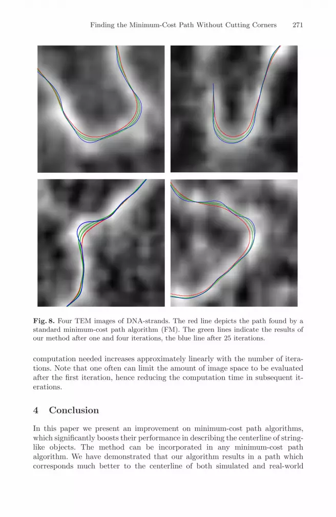
no exponential damping was used. Fig. 8 shows four typical results from the morethan thousand molecules that were processed. The red line is depicting the pathfound by the fast marching algorithm, the blue indicates the final result aftertwenty-five iterations, the green lines in between are the results after respectivelyone and four iterations. Note that the final results describe the centerline of theobject much better, especially in regions with high curvature. The blue line fol-lows the local minimum of the cost function without cutting corners. This workpermits the computation of the persistence length of DNA with much greater ac-curacy, especially over small distances. Earlier results always overestimated thepersistence length in this regime due to the stiffness of the minimum-cost path.

3.3 Computational Speed

The time needed for one iteration is comparable to the time needed to calcu-late a classical minimal-cost path. Therefore, it is evident that the amount of


Fig. 8. Four TEM images of DNA-strands. The red line depicts the path found by astandard minimum-cost path algorithm (FM). The green lines indicate the results ofour method after one and four iterations, the blue line after 25 iterations.

computation needed increases approximately linearly with the number of itera-tions. Note that one often can limit the amount of image space to be evaluatedafter the first iteration, hence reducing the computation time in subsequent it-erations.

4 Conclusion

In this paper we present an improvement on minimum-cost path algorithms,which significantly boosts their performance in describing the centerline of string-like objects. The method can be incorporated in any minimum-cost pathalgorithm. We have demonstrated that our algorithm results in a path whichcorresponds much better to the centerline of both simulated and real-world


string-like objects. The RMS displacement error decreases more then a factor often, especially in highly curved areas. Displacement errors of several pixels canbe repaired. The behavior depends on conditions such as contrast, noise leveland line width. Under certain conditions, such as high contrast, the methodonly converges after incorporating a damping term. Ten to twenty-five iterationsare needed, using an exponentially reducing damping term after several itera-tions. The method has been successfully applied to several thousands of DNAmolecules in high-resolution images obtained by TEM and AFM. The paths weobtained on the images of DNA-strands follow the valley through the cost func-tion without cutting corners. Hence the length measurement remains unbiasedand the curvature is no longer underestimated. This is of utmost importance formeasuring the bending energy of DNA-strands on a nanometer scale.

References

1. Adalsteinsson, D., Sethian, J.A.: A fast level set method for propagating interfaces.Journal of Computational Physics 118(2), 269–277 (1995)

2. Born, M., Wolf, E.: Principles of Optics, 6th edn. 1977 Pergamon Press, London(1980)

3. Danielsson, P.-E., Lin, Q.: A modified fast marching method. In: Bigun, J., Gus-tavsson, T. (eds.) SCIA 2003. LNCS, vol. 2749, pp. 1154–1161. Springer, Heidelberg(2003)

4. Fouard, C., Gedda, M.: An objective comparison between gray weighted distancetransforms and distance transforms on curved spaces. In: Kuba, A., Nyul, L.G.,Palagyi, K. (eds.) DGCI 2006. LNCS, vol. 4245, pp. 259–270. Springer, Heidelberg(2006)

5. Meijering, E., Jacob, M., Sarria, J.-C.F., Steiner, P., Hirling, H., Unser, M.: Designand validation of a tool for neurite tracing and analysis in fluorescence microscopyimages. Cytometry 58A(2), 167–176 (2004)

6. Saha, P.K., Wehrli, F.W., Gomberg, B.R.: Fuzzy distance transform: Theory, algo-rithms, and applications. Computer Vision and Image Understanding 86(3), 171–190(2002)

7. Toivanen, P.J.: New geodesic distance transforms for gray-scale images. PatternRecognition Letters 17(5), 437–450 (1996)

8. Tsitsiklis, J.N.: Efficient algorithms for globally optimal trajectories. IEEE Trans-actions on Automatic Control 40(9), 1528–1538 (1995)

9. Verbeek, P.W., Verwer, B.J.H.: Shading from shape, the eikonal equation solved bygrey-weighted distance transform. Pattern Recognition Letters 11, 681–690 (1990)

Documents

Finding the Minimum-Cost Path Without Cutting Corners