Nonlinearity and unsteadiness in rivermeandering: a review of progress in theoryand modellingMichele Bolla Pittaluga and Giovanni Seminara*DICAT, Department of Civil, Environmental and Architectural Engineering, University of Genoa, Italy

Received 7 May 2009; Revised 30 July 2010; Accepted 17 August 2010

*Correspondence to: Giovanni Seminara, Department of Civil, Environmental and Architectural Engineering, University of Genova, Via Montallegro 1, 16145 Genoa,Italy. E-mail: sem@dicat.unige.it

ABSTRACT: River meandering has been extensively investigated. Two fundamental features to be explored in order to make furtherprogress are nonlinearity and unsteadiness. Linear steady models have played an important role in the development of the subjectbut suffer from a number of limits. Moreover, rivers are not steady systems; rather their states respond to hydrologic forcing subjectto seasonal oscillations, punctuated by the occurrence of flood events. We first derive a classification of river bends based on asystematic assessment of the various physical mechanisms affecting their morphodynamic equilibrium and their evolution inresponse to variations of hydrodynamic forcing. Using the database by Lagasse et al. (2004) we also show that natural meanders aretypically mildly curved and long, i.e. such that both the centrifugal and the topographic secondary flows are weak, but they arealmost invariably nonlinear. We then review some recent developments which allow us to treat analytically the flow and bedtopography of mildly curved and long nonlinear bends subject to steady forcing, taking advantage of the fact that flow and bedtopography in mildly curved long bends are slowly varying. Results show that nonlinearity has a number of consequences: mostnotably damping of the morphodynamic response and upstream shifting of the location of the nonlinear peak of the flow speed.Next we extend the latter model to the case of unsteady forcing. Results are found to depend crucially on the ratio between the floodduration and a morphodynamic timescale. It turns out that, in a channel subject to a repeated sequence of floods, the systemreaches a dynamic equilibrium. We conclude the paper discussing how the present assessment relates to the debate on meandermodelling of the late 1980s and suggesting what we see as promising lines of future developments. Copyright © 2010 John Wiley& Sons, Ltd.

KEYWORDS: river meandering; morphodynamics; modelling; sediment transport

Introduction

In the recent past, river meandering has been extensivelyinvestigated. The subject might then be considered as fairlymature and its theoretical basis has indeed been recently andless recently reviewed (e.g. Ikeda and Parker, 1989; Seminara,2006; Camporeale et al., 2007). What new goals are thenpursued in this contribution?

In order to answer this question it is important to note that,for reasons related to the complexity of the problem, researchhas mainly focused (with few exceptions) on the developmentof linear steady models. In other words, in spite of their majorimportance, the roles of nonlinearity and unsteadiness have sofar been vastly disregarded. Linear steady models have playeda major role in the development of the subject, disclosing avariety of features of the meandering phenomenon: the behav-iour of meanders as linear resonators displaying ideal resonantconditions for particular values of meander wavelength andaspect ratio of the channel; the distinct behaviour of subreso-nant meanders, which migrate downstream and undergo

dominant downstream influence, from the opposite behaviourof super-resonant meanders which migrate upstream andundergo dominant upstream influence; the tendency of mean-ders to develop upstream (downstream) skewness as well asmultiple loops; the inability of meander evolution to reach astable equilibrium pattern, the final fate of alluvial meandersbeing their annihilation due to the occurrence of neck cutoffs;the long-term tendency of meander plan forms to reach anasymptotic state characterized by some asymptotic averagevalue of channel sinuosity subject to small fluctuations.

Having stated some of their merits, it is, however, importantto recognize that linear models suffer from restrictions whichmake them inadequate to fully capture and model the inter-action between meandering rivers and their floodplains, withthe related processes of bank collapse and chute cutoffs. Themost severe of these limits is the assumption that perturbationsof bed elevation should be small with respect to the unper-turbed flow depth, a constraint which is generally not met innature. The rationale behind this assumption was the recogni-tion that, most often, the forcing effect of curvature is weak in

EARTH SURFACE PROCESSES AND LANDFORMSEarth Surf. Process. Landforms 36, 20–38 (2011)Copyright © 2010 John Wiley & Sons, Ltd.Published online 28 September 2010 in Wiley Online Library(wileyonlinelibrary.com) DOI: 10.1002/esp.2089

some sense; below we will clarify this concept, introducingthe definition of mildly curved bends. The assumed implica-tion was then that a weak forcing must produce weak effects.On a more careful examination, however, this implicationturns out to be incorrect and the process displays its subtleties.Essentially, weak curvature-driven secondary flows give rise tobottom perturbations characterized by weak (lateral as well aslongitudinal) slopes, but weak slopes may build up finite-amplitude perturbations as long as they act on sufficientlylarge distances, i.e. provided the channel width is sufficientlylarge. Once such finite perturbations are established, second-ary flows are enhanced by a topographic contribution drivenby simple continuity requirements and depending on meanderlength. The problem then turns out to be intrinsically nonlin-ear. This notwithstanding, some progress can still be madeanalytically if one recognizes that, under conditions of weakforcing, flow and bed topography may be treated as slowlyvarying. Below we will review the recent analysis of BollaPittaluga et al. (2009), which removes the linear constraint in aslowly varying context.

A second major restriction of classical models is theassumption of steady flow. In fact, rivers are not steadysystems: their states respond to hydrologic forcing subject toseasonal oscillations, punctuated by the occurrence of floodevents. This feature raises a number of important morphologi-cal questions. In particular, how is the pattern of bottom topog-raphy that we observe after a flood event (when the stream ispossibly no longer active) related to the characteristics of thatevent? Is the morphodynamic evolution so slow that we mayreasonably assume that the bed keeps in equilibrium with theinstantaneous hydrodynamic conditions (quasi-steady mor-phodynamics)? If the process cannot be treated as quasi steady,does the system tend to reach some asymptotic state ofdynamic equilibrium? And, finally, based on a morphody-namic model accounting for unsteady effects, can we definean effective steady discharge morphologically equivalent to aperiodic forcing? The concept that, despite flow variability, onesingular discharge, the dominant discharge, might be heldresponsible for determining river channel morphology was putforward by Wolman and Miller (1960). They emphasized that,given near steady-state conditions over moderate timescales,the most significant discharge influencing alluvial channelcapacity through morphological adjustment was that whichtransported most bed sediment for its given frequency ofoccurrence. The concept was then extended defining the geo-morphic effectiveness as the ability of an event or combinationof events to affect the shape or form of the landscape (Wolmanand Gerson, 1978). Conversely, it has also been hypothesizedthat the structure of many river channels and their floodplainzones may largely represent legacies of past catastrophic dis-turbances, not a state in quasi-equilibrium with the annualflood regime (Graf, 1979). The approach employed herein willattempt to provide a mechanistic answer to the above questionusing an approach somewhat similar to that put forward byTubino (1991), who investigated the parallel problem ofunsteady alternate bars on the basis of a morphodynamicmodel accounting for unsteady effects.

In the present contribution we wish to assess recent progressin addressing the issue of nonlinearity and present an attemptto investigate some of the features of the process brought up byunsteadiness. We attempt to set up a fairly general framework.Hence we first derive a classification of river bends based ona systematic assessment of the various physical mechanismsaffecting their morphodynamic equilibrium and their evolu-tion in response to variations of hydrodynamic forcing. Thiswill lead us to clarify what dimensionless parameters controlthe different mechanisms and will allow us to provide physi-

cally based definitions (next section) of mildly curved versussharp, long versus short, linear versus nonlinear, narrow versuswide bends. Next we use the established classification toclarify (third section) for which class of meandering channelsthe classical linear approach is indeed appropriate. We thenbriefly summarize what we have learned from linear models.In the fourth section we move to the issue of nonlinearity andreview recent developments which allow us to treat analyti-cally the flow and bed topography of mildly curved and longnonlinear bends subject to steady forcing (Bolla Pittalugaet al., 2009). The improvement achieved over linear models isdemonstrated via comparison with the results of controlledexperiments. The last issue, namely the morphodynamicresponse of fluvial channels to unsteady forcing, is tackledthrough an extension of the latter model (fifth section). Inparticular, we investigate the dependence of the unsteadyresponse on the ratio between the flood duration and themorphodynamic timescale analysing a channel subject to arepeated sequence of floods to ascertain whether the systemdoes tend to reach some asymptotic state of dynamic equilib-rium. An as yet unexplored phenomenon, here termed tempo-ral overshooting, will emerge.

We complete the paper (sixth section) with a discussion onhow the present assessment relates to the debate on meandermodelling raised in the late 1980s and some indications onwhat we see as promising lines of future developments.

A Mechanistic Classification of River Bends

To provide a rational classification of river bends, we firstneed to examine the dimensionless form of the governingequations for flow and bed topography in meandering chan-nels. The framework classically employed relies on theassumption that the presence of sediment transported asbedload or suspended load does not affect significantly themotion of the fluid phase. This is justified provided the sus-pension is dilute, i.e. the concentration of the solid phasemust be sufficiently small. A thorough analysis of the mecha-nistic basis of the latter definition is presented in early classi-cal papers (e.g. Batchelor, 1970; Lumley, 1978). For presentpurposes it suffices to note that, for a suspension to be dilute,the volume fraction of suspended particles should not exceedvalues around 10-3.

With the latter assumption, the mathematical formulation ofthe problem requires the following tools: the continuity andmomentum (Reynolds) equations for the fluid phase, the massconservation equation for the solid phase governing the evo-lution of the bed interface and some closure relationship forsediment transport which replaces, in a bulk form, the momen-tum equations for the solid phase. In the following sections webriefly review these tools.

Scales and coordinates

Let us first clarify the matter of scales. Consider a sinuouschannel with a cohesionless bed and refer it to intrinsic lon-gitudinal, lateral and vertical coordinates (s, n and z, respec-tively). Let Bu denote a reference width (say half the averagechannel width, defined at bankfull stage), L a referencemeander intrinsic length (typically of the order of a fewchannel widths) and Du a reference flow depth, the index ureferring to properties of uniform flow in a straight channelwith the given flow discharge and average bed slope S. Twoscales arise naturally for the longitudinal coordinate, namely

NONLINEARITY AND UNSTEADINESS 21

Copyright © 2010 John Wiley & Sons, Ltd. Earth Surf. Process. Landforms, Vol. 36, 20–38 (2011)

the spatial scale (S

S sd d⎛⎝⎜

⎞⎠⎟

) over which the uniform flow varies

and the meander length L. The former scale is often muchlarger than the latter: hence meander flow is superimposed ona basic state which varies much more slowly. As for the lateraland vertical coordinates, the natural scales are the referencewidth (2Bu) and the reference flow depth Du, with the latterscale also appropriate for the flow depth D. Let us finallydenote by T an externally imposed flow timescale (say a char-acteristic flood period) and introduce the following dimen-sionless variables:

ssL

nnB

z Dz DD

ttTu u

* * * * *= = ( ) = ( ) =, , ,,

, (1)

The reader should note that s is a curvilinear coordinatedefined along the axis of a channel characterized by a spatialdistribution of curvature radius r(s) = c-1(s). The fact that ifone walks in the longitudinal direction along a coordinateline, the distance travelled increases as the lateral coordinateincreases and is mathematically accounted for through theso-called metric coefficient N. This quantity measuresthe ratio r(s)/(r(s) + n) between the longitudinal arclength atthe channel axis and the corresponding length at the lateralcoordinate n.

Let Uu denote the scale for the local mean velocity averagedover turbulence. The natural scale for the perturbations of freesurface elevation h is then F Dr u

2 , where Fr is the Froudenumber:

FUgD

ru

u

22

= (2)

where g is gravity. The latter statement simply reproduces theknown fact that perturbations of the free surface in subcriticalflows are typically much weaker than corresponding perturba-tions experienced in supercritical flows. It is then appropriateto scale the horizontal components of the flow velocity vectoru = (u, v, w) and the free surface elevation as follows:

u vu vU

hF hDu

r

u

* * *,,

,( ) = ( ) =2

(3)

As for the vertical component of velocity w, its scale isdetermined by flow continuity. Ignoring the boundary layersadjacent to the side banks, the lateral derivative of the lateralvelocity must balance the vertical derivative of the verticalvelocity; hence it is convenient to write

ww

Uu

u

* = β (4)

with bu reference aspect ratio of the channel:

βuu

u

BD

= (5)

Finally, the eddy viscosity vT is naturally scaled by theproduct of the local value of the friction velocity and the localflow depth, while the sediment flux per unit width (qs,qn) isnaturally scaled by the classical Einstein scale. We then write

ν νT

T

fu u us n

s n

pC U Dq q

q q

s gd* , ( *, *)

( , )

( )= =

−1 3 (6)

where sp is the relative particle density (= rs/r, with r and rs

water and particle density, respectively), d is the particle diam-eter (taken to be uniform) and Cfu is the reference frictioncoefficient.

Dimensionless formulation andgoverning parameters

The fluid phaseLet us start with the vertical component of the momentumequation: taking advantage of the hydrostatic approximation,which applies when the horizontal scale of the relevant hydro-dynamic processes largely exceeds the flow depth, this equa-tion simply states that pressure is hydrostatically distributed inthe vertical direction. This allows us to remove pressure fromthe Reynolds equations, where the pressure gradient isreplaced by the slope of the free surface. The turbulent flow ofwater in a channel characterized by a spatial distribution ofchannel curvature c(s) is then governed by the longitudinal andlateral components of the Reynolds equations, along with thecontinuity equation for the fluid phase. Recalling the definitionof metric coefficient we may write

c s r c s N n c s* * *( ) = ( ) = + ( )−0

101, ν (7)

with r0 some typical radius of curvature of the channel axis, sayits minimum value, and v0 a curvature ratio defined as

ν00

= Br

u

Note that we employ the curvature ratio Bu/r0, extensivelyused in theoretical models, rather than the ratio r0/Bu usuallyemployed in geomorphological literature. The reader willappreciate that the dimensionless forms of channel curvaturec(s) and metric coefficient N defined above are O(1) quantities.Hereafter, the asterisks denoting dimensionless quantities aredropped for the sake of simplicity. The continuity equation indimensionless form then reads

Nus

vn

wz

N c s vλ ν∂∂+ ∂∂+ ∂∂

= − ( )0 (8)

where l-1 is the dimensionless intrinsic meander wavelength,defined as

λ = BLu

The parameter l measures the slowly varying character ofthe flow field. In fact, as l→ 0, the adaptation length, requiredfor the flow to adjust to the varying curvature, becomes neg-ligible relative to the spatial scale over which variations occur,namely the meander wavelength L.

Next, let us write the longitudinal component of themomentum equation in dimensionless form for the generalcase of unsteady forcing. It reads

M. BOLLA PITTALUGA AND G. SEMINARA22

Copyright © 2010 John Wiley & Sons, Ltd. Earth Surf. Process. Landforms, Vol. 36, 20–38 (2011)

∂∂

∂∂( ) = − + ∂

∂+ ∂

∂⎡⎣⎢

+ ∂∂+ ∂

∂⎤⎦⎥+

zuz

NR CC

ut

N uus

vun

wuz

T fuu fu

νβ

σ λ01

δδNc s uv( )(9)

This equation involves three dimensionless parameters. Thefirst, s, measures the importance of local inertia relative tolateral convection. The second, l, measures the importance oflongitudinal convection of longitudinal momentum relative tolateral convection. The third, d, measures the intensity of cen-trifugal effects relative to dissipation. Also note that the drivinggravity force is corrected relative to the uniform state throughthe coefficient R0. These parameters read

δ σ λβ

= = = − ∂∂

Dr C

BU T

RC

hs

u

fu

u

u u fu00 1, , (10)

Note that the size of s is typically very small; in fact, with atypical width falling in the range 100–1000 m and a corre-sponding flood period in the range 105–106 s one finds that s~ O(10-3), a value much smaller than the typical values of theparameter d observed in nature (see Figure 2a). Conversely, thesize of l varies considerably throughout the process ofmeander evolution. In fact, we may write

λβ

δλu fuC

= ′ (11)

with l′ a dimensionless parameter which reads r0/L; hence thesize of l varies from ‘much larger than’ to ‘an order of mag-nitude smaller than’ d as meanders grow in amplitude (seeFigure 2f).

The lateral component of the momentum equation can bewritten in a similar form:

∂∂

∂∂( ) − ∂

∂+ ( ) =

∂∂+

∂∂+

∂∂+

zvz C

hn

N c s u

Cvt

N uvs

vvn

Tu fu

u fu

νβ

δ

βσ λ

1

1

2

wwvz∂∂

⎡⎣⎢

⎤⎦⎥

(12)

showing the important role played by the centripetal accelera-tion, as well as by the lateral slope of the free surface as majorfactors controlling the intensity of secondary flow.

Equations (8), (9) and (12) must be supplemented withappropriate boundary conditions. In dimensionless form, theformer set of conditions, imposing no slip at the conventionalreference level z0, reads

u v w z z= = = =( )0 0 (13)

The second condition imposes the requirement that the freesurface must be a material surface:

w Fht

N uhs

vhn

z F hr r= ∂∂+ ∂

∂+ ∂

∂⎡⎣⎢

⎤⎦⎥

=( )2 2σ λ (14)

The third set imposes the condition of no stress at the freesurface; hence

ν νT T ruz

vz

z F h∂∂= ∂

∂= =( )0 2 (15)

Finally, a no-flux condition must be imposed at the banks.For a narrow cross-section, this constraint must be imposed

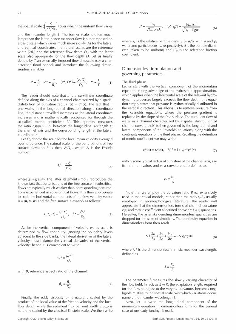
requiring that the component of the flow velocity in the direc-tion normal to the banks must vanish. For a wide cross-sectionit is more convenient to follow a simpler approximate proce-dure, which we now clarify. Consider the boundary layer ofthickness O(Du) adjacent to the outer bank and impose massbalance in a control volume, confined laterally by the interfaceboundary layer core flow and by the outer bank; longitudinallyby two vertical sections of the boundary layer; and verticallyby the free surface (Figure 1).

It is then easy to show that the depth-averaged lateral com-ponent of the flow velocity at the interface boundary layer–core, say <v>|n=1, is O(DuUu|n=1/L). Since the quantity (Du/L) istypically small (say less than 10-2), it is then convenient toreplace the condition at the bank by the condition of vanishing<v>|n=1, i.e.

v z nz

F hr

d = = ±( )∫ 0 10

2

(16)

Note that the latter constraint does allow for a lateral com-ponent of velocity at the boundary layer–core interface, albeitwith vanishing depth average. Inside the boundary layer thesecondary flow is closed by a vertical component of velocitywhich flow continuity suggests to be of the same order ofmagnitude as the lateral component v.

A closure relationship is finally needed for the eddy viscosityvT. We leave aside this issue at this stage: it will be seen belowthat closure is readily achieved under the conditions typicallyencountered in nature, which are slowly varying both in spaceand time.

The solid phaseThe continuity equation for the solid phase takes the form of anExner equation and can be written as follows:

∂∂+ ∂

∂+ ∂∂

+ ( )⎡⎣⎢

⎤⎦⎥=η ω λ ν

tN

qs

qn

N c s qs nn0 0

(17)

where η = −( )F h Dr2 is the dimensionless bed elevation,

w is a dimensionless parameter measuring the ratiobetween the externally forced hydrodynamic timescale (T)and a morphodynamic timescale associated with pro-cesses occurring at the scale of channel width defined as

T p B D s gdu u u p031 1= −( )[ ] −( )⎡⎣ ⎤⎦Φ ; hence

Figure 1. Sketch of the boundary layer adjacent to the outer bank.

NONLINEARITY AND UNSTEADINESS 23

Copyright © 2010 John Wiley & Sons, Ltd. Earth Surf. Process. Landforms, Vol. 36, 20–38 (2011)

0

20

40

60

80

100

2 0.01 0.1 1

0

5

10

15

20

25

Cum

ula

tive %

Ni/N

TO

T%

δ

(a)

Median=0.180

St. Dev.=0.190

CumulativeNi/NTOT

0

20

40

60

80

100

0.02 0.05 0.2 0.3 0.4 0.5 0.1

0

5

10

15

20

25

Cum

ula

tive %

Ni/N

TO

T%

4λ

(b)

Median=0.124

St. Dev.=0.070

CumulativeNi/NTOT

0

20

40

60

80

100

0.1 1 10

0

5

10

15

20

25

Cum

ula

tive %

Ni/N

TO

T%

γ

(c)

Median=2.243

St. Dev.=1.698

CumulativeNi/NTOT

0

20

40

60

80

100

0.03 0.1 1

0

5

10

15

20

25

Cum

ula

tive %

Ni/N

TO

T%

ν0

(d)

Median=0.192

St. Dev.=0.090

CumulativeNi/NTOT

0

20

40

60

80

100

2 31

0

5

10

15

20

25

Cum

ula

tive %

Ni/N

TO

T%

Sinuosity σ

(e)

Median=1.690

St. Dev.=0.399

CumulativeNi/NTOT

0

20

40

60

80

100

20 0.1 1 10

0

5

10

15

20

25

Cu

mu

lative

%

Ni/N

TO

T%

4λ/δ

(f)

Median=0.668

St. Dev.=1.330

CumulativeNi/NTOT

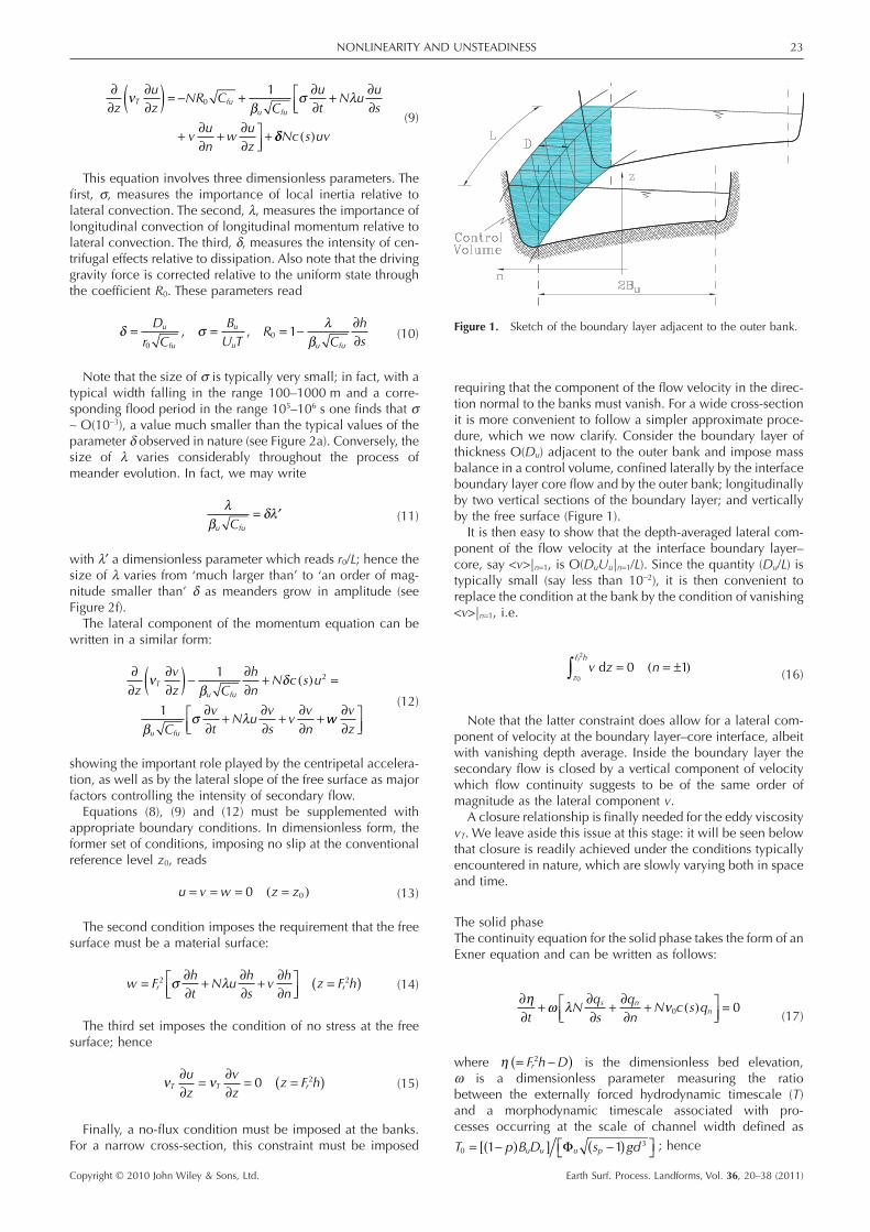
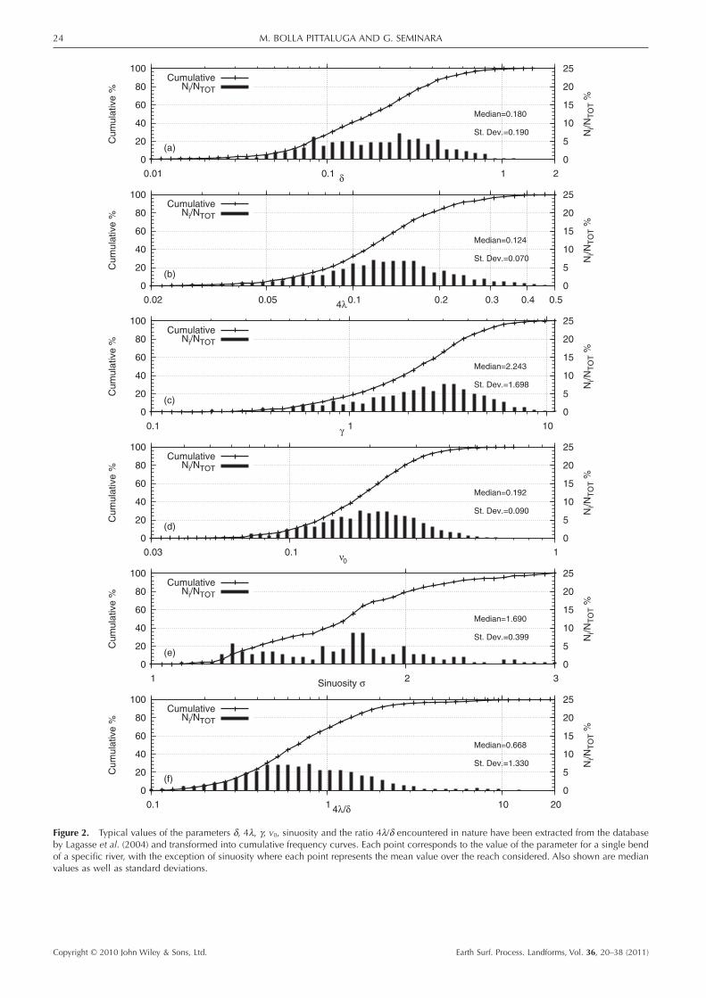
Figure 2. Typical values of the parameters d, 4l, g, v0, sinuosity and the ratio 4l/d encountered in nature have been extracted from the databaseby Lagasse et al. (2004) and transformed into cumulative frequency curves. Each point corresponds to the value of the parameter for a single bendof a specific river, with the exception of sinuosity where each point represents the mean value over the reach considered. Also shown are medianvalues as well as standard deviations.

M. BOLLA PITTALUGA AND G. SEMINARA24

Copyright © 2010 John Wiley & Sons, Ltd. Earth Surf. Process. Landforms, Vol. 36, 20–38 (2011)

ω = TT0

(18)

The parameter w is typically an O(1) quantity; i.e. morpho-dynamic processes occurring at the scale of channel widthhave timescale comparable with that of the externally forcedhydrodynamic process. However, since the meander scale istypically one order of magnitude greater than channel width,morphodynamic processes occurring at the scale of meandersare slower than the externally forced hydrodynamic process,i.e. typically a flood event. This is the basis for the decoupledapproach employed below (’The Response of Bed Topographyto Unsteady Forcing’).

Closure relationships are obviously needed for the sedimentflux per unit width q. Here, we restrict ourselves to thecase of dominant bed load. A well-established approach ofsemi-empirical nature appropriate to weakly sloping beds(Engelund, 1974; Parker, 1984) then allows us to write

q ;= −( ) − ∂∂

⎛⎝

⎞⎠Φ θ θ η

c pR Rn

tt

n (19)

where F is a monotonically increasing function of the excessShields stress (q - qc) for given particle Reynolds number Rp, nis the unit vector in the lateral direction and t is the tangentialshear stress vector at the bottom. With vf kinematic viscosity ofthe fluid, the Shields stress q (Shields, 1936) and Rp read

θ =−( )

= −( )tρ ρs

pp

fgdR

s gd,

1 3

ν(20)

The function F can be estimated through well-known empiri-cal relationships. Note that equation (19) essentially states thatbedload is aligned with the bottom stress except for the effect ofgravity on particle motion, which drives some deviation ofparticle trajectories. Below we only account for the prevailinglateral component of gravity and write (Parker, 1984)

Rrc

u

=β θ (21)

rc being an empirical constant with a value of about 0·56(Talmon et al., 1995).

The reader should note that Equation (19) fails close to sharpfronts (for the case of arbitrarily sloping beds see Seminaraet al. (2002)).

Finally, the problem formulated above is subject to twointegral constraints stipulating that flow and sediment supplyare assigned at the initial cross-section; hence

D u z n t z n Q tz

h n; , ,

,0

0

0

1

1( ) = ( )

( )

−

+

∫∫ d d (22)

Φ θ 01

1, n n Q ts( )[ ] = ( )

−

+

∫ d (23)

where Q(t) and Qs(t) are the assigned flow and sediment dis-charges, respectively.

Classification of river bends

Having formulated the morphodynamic problem in a fairlygeneral dimensionless form, we now classify bends on the

basis of the range of values attained by the various dimension-less parameters introduced above. We also provide typicalvalues of the parameters encountered in nature referring to thedatabase by Lagasse et al. (2004). The latter contains datareferring to roughly 1500 meander bends on 139 rivers in theUSA. The data for each meander site include general informa-tion compiled from various sources: namely, an aerial photoshowing the site and the meander bends, as well as detailedhistorical data for each bend. In some cases, there is alsoinformation on the mean daily and annual peak discharge forthe gage nearest to the site. Starting from the original datareported in the dataset, we have calculated the values of thevarious dimensionless parameters for each meander bend andwe have determined the cumulative frequency curves reportedin Figure 2. To construct such curves, the range spanned by thevalues attained by each parameter was divided into a numberof subranges. The number of times the parameter value wasfound to fall within each subrange was then determined basedon the data. The numbers pertaining to each subrange werethen cumulated and each cumulative curve was normalized bythe total number of occurrences of the record. The resultantquotient represents the percentage of times a given parameteris not exceeded or equalled in the entire dataset. The resultinghistograms are plotted in Figure 2. In each panel we have alsoreported the median value of the parameter (equalled orexceeded 50% of the time) as well as its standard deviation.

Mildly curved versus sharp bends: the d parameterThe parameter d plays a central role in the lateral momentumequation (Equation (12)), where it multiplies the centripetalacceleration term; in fact, it has long been known that asecondary flow directed outward close to the free surface andinward close to the bed develops in bends to compensate forthe inability of the lateral pressure gradient driven by thelateral slope of the free surface to balance the centripetal forcerequired for fluid particles to move along purely longitudinaltrajectories. Since the quantities c(s) and N (recall Equation (7))as well as u (recall Equation (3)) are O(1) quantities, theintensity of this centrifugally driven secondary flow is O(d). Theimportant role of this parameter was recognized long ago(Kalkwijk and de Vriend, 1980). We then define a bend asmildly curved provided d << 1 and sharp if d ~ O(1).

Hence a mildly curved (sharp) bend is a bend which gen-erates a fairly weak (strong) centrifugally induced secondaryflow. Mildly curved bends are fairly common, as shown inFigure 2a. The latter figure shows that 50% of the meanderbends analysed in that set are characterized by a value of theparameter d below 0·18.

However, note that in a mildly curved bend the perturba-tions of bed topography driven by the action of secondary flowon a cohesionless bed are by no means necessarily smallrelative to the average flow depth; in fact, a second topo-graphic component of the secondary flow is driven by thedevelopment of bottom perturbations. Moreover, even whenboth the centrifugal and topographic contributions to second-ary flows are small, the implication is simply that the lateralbottom slope is indeed small. But a small lateral slope maybuild up a finite perturbation of bed elevation in a sufficientlywide bend: hence mildly curved bends are not necessarilylinear bends.

Long versus short bends: the l parameterThe erodible character of the bed makes the secondary flowtransport sediment towards the inner bank where point barsbuild up, while pools develop at the outer bank. The bar-poolpattern then drives a further, topographical, component of thesecondary flow. The importance of this fundamental mecha-

NONLINEARITY AND UNSTEADINESS 25

Copyright © 2010 John Wiley & Sons, Ltd. Earth Surf. Process. Landforms, Vol. 36, 20–38 (2011)

nism was pointed out by Dietrich and Smith (1983). To esti-mate the intensity of this topographic steering we note that, fora sine-generated meander, forcing is proportional to cos(2ps).Moreover, the lateral distribution of the transverse velocity

behaves roughly like cosπn2( ). Equation (8) then suggests that

the size of the topographic component of the secondary flowis O(4l). The presence of the factor 4 is readily understood: infact, the lateral velocity vanishes at the banks and peaksroughly at the channel centreline, and hence lateral variationsoccur on the scale of half channel width Bu; on the other hand,the longitudinal derivative of a harmonic perturbation of thelongitudinal velocity scales with the ratio between the ampli-tude of the latter and a quarter meander wavelength.

Hence a long (short) bend is a bend which generates a fairlyweak (strong) topographically induced secondary flow. Longbends are also fairly common, as shown in Figure 2b, where itturns out that the median value of the parameter 4l is roughlyequal to 0·124. However, an argument identical to that pro-posed above suggests that in a long bend the perturbations ofbed topography driven by the action of secondary flow on acohesionless bed are not necessarily small relative to theaverage flow depth. In other words, long bends are also notnecessarily linear bends.

Linear versus nonlinear bends: the g parameterThe amplitude of perturbations of bed elevation is controlledby a parameter denoted by g which can be derived consideringthe fully developed flow in constant curvature channels.Under these conditions, the lateral component of the sedimentflux qn vanishes identically; hence from Equation (19) itfollows that

∂∂

⎛⎝

⎞⎠

η β θ τn

un~ Ot (24)

The relative amplitude of bed perturbations is then propor-tional to the ratio of the lateral component of bottom stress toits modulus, i.e. to the ratio between intensity of the secondaryflow and intensity of the main flow. In a fully developedconstant curvature channel secondary flow is purely centrifu-gal. However, if we extend the estimate of Equation (24) to thegeneral case, then the above ratio is the sum of two contribu-tions of O(d) and O(l) respectively. Hence

γ β θ δ λ~ ,O u ( )( ) (25)

This result clarifies our previous statement: g can be an O(1)parameter even for mildly curved (d << 1), long (l << 1) bends,as long as the aspect ratio of the channel is sufficiently large(bu >> 1) and the Shields stress is not too small. Note that theimportance of this parameter was pointed out by Seminara andSolari (1998) in the context of an investigation on fully devel-oped flow and bed topography in constant curvature channels,where the only component of secondary flow is the centrifugalone. Finite values of g are most common in nature, as shownin Figure 2c, where it turns out that the median value of g isroughly equal to 2·2, including meandering rivers which aretypically characterized by mildly curved (median value of dequal to 0·180) and long bends (median value of 4l equal to0·124).

Narrow versus wide bends: the v0 parameterWide bends are defined by the condition v0 << 1, whichimplies that the role of metric effects is large. The metric effect

is essentially a ‘free vortex’ effect, whereby flow at the innerbank accelerates initially relative to the outer bank; proceed-ing downstream, momentum is convected towards the outerbank by the secondary flow and the thread of high velocityprogressively moves from the inner to the outer part of thebend. The intensity of the free vortex mechanism depends onthe parameter v0; hence, for given channel curvature, metriceffects increase with channel width; conversely, for a givenchannel width, they are enhanced as curvature increases.Typical values of v0 found in nature are shown in Figure 2d,where it turns out that 50% of the meander bends analysed inthat set are characterized by a value of the parameter v0 below0·192.

The reader should not confuse the definition of a wide bendwith the definition of a wide cross-section. The latter requiresthat the aspect ratio of the channel cross-section must be largeenough (say bu > 10). This condition allows one to distinguishbetween a central flow region and side wall boundary layersrequired for the flow to satisfy the no-slip condition at thebanks. In fluvial morphodynamics channels are usually fairlywide and the role of the side wall boundary layers is assumedto be hydrodynamically passive; hence it is usually ignored.

Linear Models: What Have We Learned?

A significant body of research has been produced on linearmodels of meandering channels (e.g. Ikeda et al., 1981; Johan-nesson and Parker, 1989a; Zolezzi and Seminara, 2001).Essentially, a linear model consists of the solution of theproblem of morphodynamics for a sinuous channel under theassumption that perturbations of flow and bed topography aresmall relative to the characteristics of flow in a straight channelwith the same longitudinal slope, subject to the same flow andsediment discharges. The reader unaware of previous reviewswith a mechanistic emphasis on this subject may find it usefulto refer to a sequence of recent and less recent works: inparticular, Ikeda and Parker (1989) and Seminara (2006). Adetailed comparison of the performance of different linearmodels has also been presented by Camporeale et al. (2007)and further pursued by Frascati and Lanzoni (2009). Here, wesimply wish to recall briefly some merits of linear models andemphasize their restrictions, in order to motivate the reader tothe need for pursuing the development of nonlinear models.

The first merit of linear models has been to allow for theconstruction of a rational theoretical framework able toexplain the mechanism of meander formation. It is somewhatsurprising to read that the process of meander formation inalluvial rivers is not yet understood and that novel paradigmswould be needed to make progress. Meanders form because astraight channel configuration is intrinsically unstable, pro-vided the banks are erodible. The so-called bend theoryreviewed in Seminara (2006) clarifies that both meandergrowth and meander migration arise from the occurrence of aphase lag between bank erosion and channel curvature. Thetheory also shows that: (i) a range of not too short meanders isunstable, while meander wavelengths being less than somethreshold value (ranging around 10Bu) are stable; (ii) in theunstable range a most unstable wavelength exists and is theone selected by the instability process.

The reader should appreciate the fact that the initial pertur-bation causing meander formation may vary widely and iden-tifying the precise cause in each case is irrelevant from theconceptual viewpoint. In fact, the so called convective natureof meander instability (Lanzoni and Seminara, 2006) ensuresthat meanders will form whenever some persistent small per-turbation is forced at some initial cross-section. In laboratory

M. BOLLA PITTALUGA AND G. SEMINARA26

Copyright © 2010 John Wiley & Sons, Ltd. Earth Surf. Process. Landforms, Vol. 36, 20–38 (2011)

experiments with a cohesionless floodplain a sequence ofevents is observed to generate a temporary meandering pattern(e.g. Federici and Paola, 2003) but the ultimate mechanismfrom which initial perturbations of channel alignment are trig-gered is the development of initially migrating alternate bars.Braudrick et al. (2009) found that elevated bank strength (pro-vided by alfalfa sprouts) relative to the cohesionless bed mate-rial and the blocking of troughs (chutes) in the lee of point barsvia suspended sediment deposition were the necessary ingre-dients to successful meandering. In experiments with cohesive(Smith, 1998) and vegetated (Braudrick et al., 2009) flood-plains the formation of migrating bars is not observed and yetmeanders do form, confirming the distinction between bar andbend instabilities pointed out by Blondeaux and Seminara(1985); in the latter case, the initial perturbation may simply bea deviation of channel alignment from the valley direction.

A second fundamental issue, which we have called theproblem of morphodynamic influence (see the review paper ofLanzoni et al., 2006), was clarified through the use of linearmodels. In open channel flows with cohesionless bed andcohesionless banks, information about perturbations ofchannel morphology is propagated through waves arising fromthe erodible nature of the boundaries and the ability of thestream to transport sediment. A natural question then arises: inwhich direction is information propagated? This problem wasraised by de Vries (1965), who showed that, in the case ofone-dimensional (long) bottom perturbations, information ispropagated downstream (upstream) under sub- (super-)criticalconditions. A number of additional features arise when pertur-bations are examined in the strongly nonlinear regime and areallowed to develop sharp fronts (Lanzoni et al., 2006). Whenthe latter analysis is extended to large-scale two-dimensionalbed forms or perturbations of channel alignment, it turns out(Seminara et al., 2001) that the role played by the Froudenumber is somewhat overtaken by the aspect ratio of thechannel. In particular, it is found that for b < bR (sub-resonantregime) meanders migrate downstream, while for b > bR (super-resonant regime) meanders migrate upstream, the thresholdvalue bR identifying the ‘resonant’ conditions discovered byBlondeaux and Seminara (1985).

A third major merit of (hydrodynamically) linear models hasbeen the construction of a rational framework able to explaina number of features of the planform evolution of meanderingrivers, namely: (i) the development of a Kinoshita pattern start-ing from a sine-generated curve (hence the process of meanderskewing); (ii) the continuous deceleration of meandersthroughout their development; (iii) their continuous lengthen-ing; (iv) their lateral amplification increasing up to a peak andthen decreasing; (v) the formation of multiple loops; (vi) theeventual occurrence of neck cutoff. Note that, in spite of thelinear nature of the hydrodynamic model employed, all thesefeatures result from the intrinsic geometric nonlinearity of thedeformation process, which is accounted for in the nonlinearintegro-differential nature of the equation describing the evo-lution of channel alignment.

Finally, numerical simulations based on the use of linearmodels, due to their relative simplicity, have been extended forvery large prototype times, of the order of centuries (e.g.Howard, 1992; Zolezzi and Seminara, 2001; Sun et al., 2001;Frascati and Lanzoni, 2009). These simulations have been usedessentially to explore the existence of a long-term statisticallyuniversal behaviour of meandering rivers.

The reader may have realized at this stage that the popularityenjoyed by linear models is well deserved. This notwithstand-ing, these models have serious restrictions which have beenpointed out in the previous section and call for the need fornonlinear developments. Below, we review an analytical

framework recently developed by the present authors toaccount for nonlinearity in mildly curved and long bends.

Flow in Mildly Curved Nonlinear BendsSubject to Steady Forcing

Figure 2 suggests that it is worth attempting to formulate atheoretical approach suitable to model meanders which arefairly mildly curved and long. In fact, as already pointed out,the dataset of Lagasse et al. (2004) shows that 50 (73)% ofbends analysed are characterized by a value of the d parameterless or equal to 0·18 (0·3). Similarly, the dimensionless param-eter (4l) of 50 (85)% of meander bends turns out to be smallerthan 0·124 (0·2). The main consequence of the latter estimatesis that, for the above class of bends, flow and bottom topog-raphy can be treated as slowly varying in both longitudinal andlateral directions.

The approach employed by Bolla Pittaluga et al. (2009) toremove the linear constraint and account for finite-amplitudebed deformations in mildly curved nonlinear bends understeady forcing takes advantage of this character of flow andbottom topography. Essentially, the idea is to realize that thelocal flow depth is ultimately the scale of the basic uniformflow perturbed by the effects of curvature. This scale varies inthe lateral direction on the scale of channel width, which istypically much larger than the average flow depth; in thelongitudinal direction it varies with meander length, which ismuch larger than channel width.

An equilibrium solution for the flow and topography fieldsmay then be sought, expanding it in a neighbourhood of thebasic solution for locally uniform flow in a straight channelwith an unknown shape of the cross-section. The latter isdescribed by a slowly varying function D(n,s) of the longitu-dinal and lateral coordinates. Bolla Pittaluga et al. (2009) thenwrite

u v w h D u n s h s D n s

u v w h Dm m m m m

, , , , ; , , , , , ,

, , , ,

( ) = ( ) ( ) ( )[ ] +

(

0 0 00 0ξ δ

))∞

∑ δm

1

(26)

where the free surface elevation at leading order is taken to bea function of the coordinate s, in order to account for the slowvariations of the longitudinal free surface slope associated withchannel curvature.

Substituting from the latter expansion into the governingdifferential problem (Equations (8)–(17)) and equating likewisepowers of d, Bolla Pittaluga et al. (2009) derived a sequence ofdifferential problems which were then solved in terms of theunknown functions D and ∂h/∂s. Below we simply recall thestructure of the solution.

At the leading order of approximation, the longitudinalcomponent of the Reynolds equations reduces to a locallyuniform balance between gravity and friction in a channelwith unknown distribution of flow depth D0(n,s) and localslope of the free surface (-∂h0/∂s); hence

u D n s R s F n s0 01 2

01 2

0= ( ) ( ) ( ), ; ,ξ (27)

where F0 is the classical logarithmic law and x is a normalizedvertical coordinate attaining values in the range x0 � x � 1,with x0 a normalized reference level (strictly, a slow functionof the longitudinal and lateral coordinates, assumed to beconstant).

NONLINEARITY AND UNSTEADINESS 27

Copyright © 2010 John Wiley & Sons, Ltd. Earth Surf. Process. Landforms, Vol. 36, 20–38 (2011)

At first order, the lateral component of the Reynolds equa-tions reduces to a balance between the lateral component ofgravity, centripetal inertia and lateral friction in the channelwith known slowly varying distribution of channel curvaturec(s) and unknown flow depth D0(n,s) and free surface slope(-∂h0/∂s). The solution for the lateral velocity can be decom-posed in the form

v s n v s n F v s n1 10 0 1, , , , ,ξ ξ ξ( ) = ( ) + ( ) < ( ) > (28)

where v10 is the centrifugally induced secondary flow withvanishing depth average and <> denotes depth-averaged quan-tities. Moreover:

v D R c s a F G10 03 2

01 2

10 0 12= ( ) +( ) (29)

< > = − ∂∂

< >( )−∫vD s

D u no

n

10

01

1λδ

d (30)

with a10 a constant and G12 a function which was determined

analytically. Note that the ratioλδ

λ δ∂∂

( )s

~ O 4 is here

assumed to be an O(1) quantity. This is a reasonable assump-tion as confirmed from Figure 2f, which is based on the datasetreported by Lagasse et al. (2004).

Finally, the sediment continuity equation (Equation (17))with the help of the closure relationship for q (Equations(19)–(21)) at O(d) reduces to a nonlinear partial differential

equation for the unknown functions D0(n; s) and∂∂( )h

ss0 ,

which reads

∂∂

= −

∂∂∂∂

+ ∂∂

⎡

⎣

⎢⎢⎢⎢

⎤

⎦

⎥⎥⎥⎥

−∫Dn r

v

u q sq n

c ss

n0 0

10

00

00

1

1γ ξξ

ξξ

λδ

d (31)

where γ δβ θ0 0= u . Equation (31), with the appropriateboundary conditions imposing vanishing sediment fluxthrough the side walls and the integral constraints (Equation(22)), was solved numerically, marching in n at each crosssection. This allowed us to determine the unknown functionsD0(n, s) and ∂h0/∂s(s) by a trial-and-error procedure. The readerwill note that, according to Equation (31), the size of ∂D0/∂n isprecisely of O(g0), as discussed above.

Proceeding at the second order of approximation, convec-tive terms were also considered in the equations of motion(Equations (9) and (12)) and, following a procedure similar tothe one discussed above, we ended up with a similar differ-ential equation for the flow depth correction D1(s, n), whichwas again solved with the appropriate boundary conditions bya trial-and-error procedure.

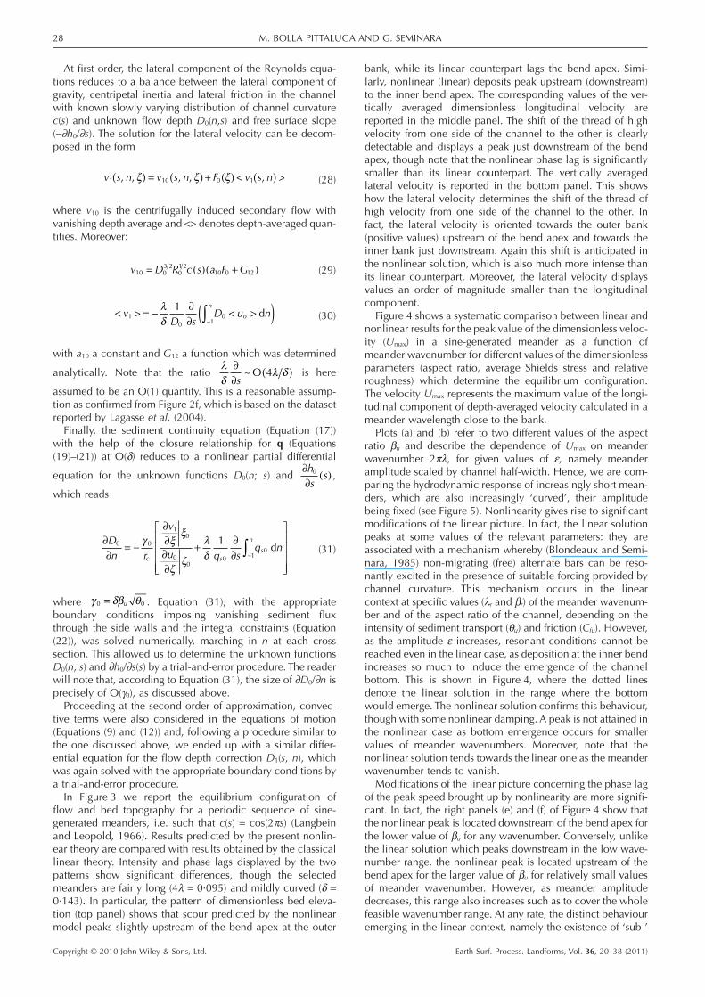
In Figure 3 we report the equilibrium configuration offlow and bed topography for a periodic sequence of sine-generated meanders, i.e. such that c(s) = cos(2ps) (Langbeinand Leopold, 1966). Results predicted by the present nonlin-ear theory are compared with results obtained by the classicallinear theory. Intensity and phase lags displayed by the twopatterns show significant differences, though the selectedmeanders are fairly long (4l = 0·095) and mildly curved (d =0·143). In particular, the pattern of dimensionless bed eleva-tion (top panel) shows that scour predicted by the nonlinearmodel peaks slightly upstream of the bend apex at the outer

bank, while its linear counterpart lags the bend apex. Simi-larly, nonlinear (linear) deposits peak upstream (downstream)to the inner bend apex. The corresponding values of the ver-tically averaged dimensionless longitudinal velocity arereported in the middle panel. The shift of the thread of highvelocity from one side of the channel to the other is clearlydetectable and displays a peak just downstream of the bendapex, though note that the nonlinear phase lag is significantlysmaller than its linear counterpart. The vertically averagedlateral velocity is reported in the bottom panel. This showshow the lateral velocity determines the shift of the thread ofhigh velocity from one side of the channel to the other. Infact, the lateral velocity is oriented towards the outer bank(positive values) upstream of the bend apex and towards theinner bank just downstream. Again this shift is anticipated inthe nonlinear solution, which is also much more intense thanits linear counterpart. Moreover, the lateral velocity displaysvalues an order of magnitude smaller than the longitudinalcomponent.

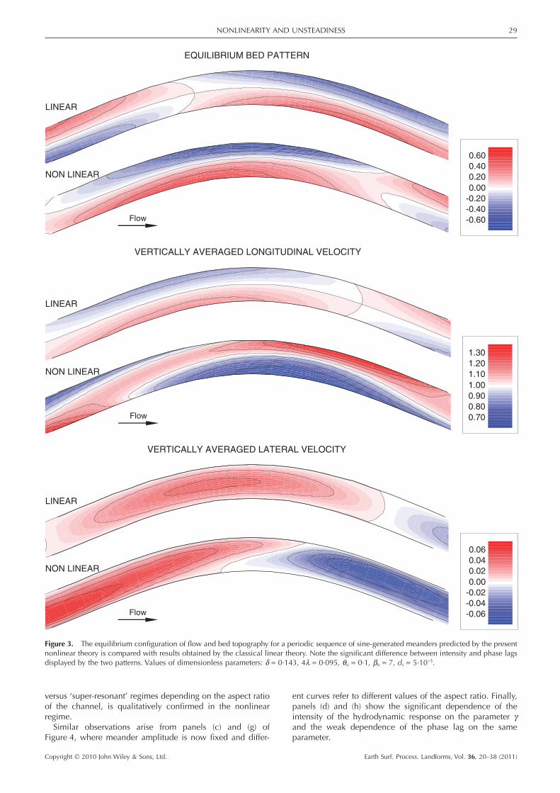
Figure 4 shows a systematic comparison between linear andnonlinear results for the peak value of the dimensionless veloc-ity (Umax) in a sine-generated meander as a function ofmeander wavenumber for different values of the dimensionlessparameters (aspect ratio, average Shields stress and relativeroughness) which determine the equilibrium configuration.The velocity Umax represents the maximum value of the longi-tudinal component of depth-averaged velocity calculated in ameander wavelength close to the bank.

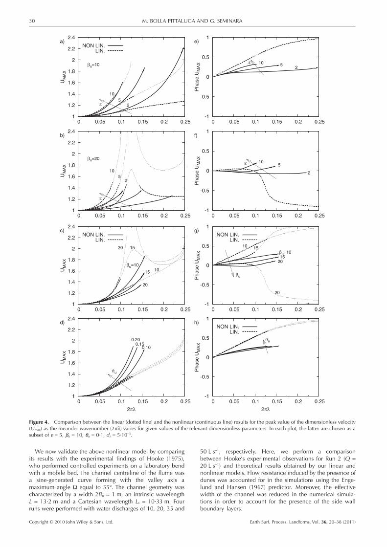
Plots (a) and (b) refer to two different values of the aspectratio bu and describe the dependence of Umax on meanderwavenumber 2pl, for given values of e, namely meanderamplitude scaled by channel half-width. Hence, we are com-paring the hydrodynamic response of increasingly short mean-ders, which are also increasingly ‘curved’, their amplitudebeing fixed (see Figure 5). Nonlinearity gives rise to significantmodifications of the linear picture. In fact, the linear solutionpeaks at some values of the relevant parameters: they areassociated with a mechanism whereby (Blondeaux and Semi-nara, 1985) non-migrating (free) alternate bars can be reso-nantly excited in the presence of suitable forcing provided bychannel curvature. This mechanism occurs in the linearcontext at specific values (lr and br) of the meander wavenum-ber and of the aspect ratio of the channel, depending on theintensity of sediment transport (qu) and friction (Cfu). However,as the amplitude e increases, resonant conditions cannot bereached even in the linear case, as deposition at the inner bendincreases so much to induce the emergence of the channelbottom. This is shown in Figure 4, where the dotted linesdenote the linear solution in the range where the bottomwould emerge. The nonlinear solution confirms this behaviour,though with some nonlinear damping. A peak is not attained inthe nonlinear case as bottom emergence occurs for smallervalues of meander wavenumbers. Moreover, note that thenonlinear solution tends towards the linear one as the meanderwavenumber tends to vanish.

Modifications of the linear picture concerning the phase lagof the peak speed brought up by nonlinearity are more signifi-cant. In fact, the right panels (e) and (f) of Figure 4 show thatthe nonlinear peak is located downstream of the bend apex forthe lower value of bu for any wavenumber. Conversely, unlikethe linear solution which peaks downstream in the low wave-number range, the nonlinear peak is located upstream of thebend apex for the larger value of bu for relatively small valuesof meander wavenumber. However, as meander amplitudedecreases, this range also increases such as to cover the wholefeasible wavenumber range. At any rate, the distinct behaviouremerging in the linear context, namely the existence of ‘sub-’

M. BOLLA PITTALUGA AND G. SEMINARA28

Copyright © 2010 John Wiley & Sons, Ltd. Earth Surf. Process. Landforms, Vol. 36, 20–38 (2011)

versus ‘super-resonant’ regimes depending on the aspect ratioof the channel, is qualitatively confirmed in the nonlinearregime.

Similar observations arise from panels (c) and (g) ofFigure 4, where meander amplitude is now fixed and differ-

ent curves refer to different values of the aspect ratio. Finally,panels (d) and (h) show the significant dependence of theintensity of the hydrodynamic response on the parameter gand the weak dependence of the phase lag on the sameparameter.

-0.06

-0.04

-0.02

0.00

0.02

0.04

0.06

Flow

NON LINEAR

LINEAR

VERTICALLY AVERAGED LATERAL VELOCITY

0.70

0.80

0.90

1.00

1.10

1.20

1.30

Flow

NON LINEAR

LINEAR

VERTICALLY AVERAGED LONGITUDINAL VELOCITY

-0.60

-0.40

-0.20

0.00

0.20

0.40

0.60

Flow

NON LINEAR

LINEAR

EQUILIBRIUM BED PATTERN

Figure 3. The equilibrium configuration of flow and bed topography for a periodic sequence of sine-generated meanders predicted by the presentnonlinear theory is compared with results obtained by the classical linear theory. Note the significant difference between intensity and phase lagsdisplayed by the two patterns. Values of dimensionless parameters: d = 0·143, 4l = 0·095, qu = 0·1, bu = 7, ds = 5·10-3.

NONLINEARITY AND UNSTEADINESS 29

Copyright © 2010 John Wiley & Sons, Ltd. Earth Surf. Process. Landforms, Vol. 36, 20–38 (2011)

We now validate the above nonlinear model by comparingits results with the experimental findings of Hooke (1975),who performed controlled experiments on a laboratory bendwith a mobile bed. The channel centreline of the flume wasa sine-generated curve forming with the valley axis amaximum angle W equal to 55°. The channel geometry wascharacterized by a width 2Bu = 1 m, an intrinsic wavelengthL = 13·2 m and a Cartesian wavelength Lx = 10·33 m. Fourruns were performed with water discharges of 10, 20, 35 and

50 L s-1, respectively. Here, we perform a comparisonbetween Hooke’s experimental observations for Run 2 (Q =20 L s-1) and theoretical results obtained by our linear andnonlinear models. Flow resistance induced by the presence ofdunes was accounted for in the simulations using the Enge-lund and Hansen (1967) predictor. Moreover, the effectivewidth of the channel was reduced in the numerical simula-tions in order to account for the presence of the side wallboundary layers.

1

1.2

1.4

1.6

1.8

2

2.2

2.4

0 0.05 0.1 0.15 0.2 0.25

UM

AX

ε

a)

βu=10

25

10

NON LIN.LIN.

1

1.2

1.4

1.6

1.8

2

2.2

2.4

0 0.05 0.1 0.15 0.2 0.25

UM

AX

b)

ε

βu=20

25

10

-1

-0.5

0

0.5

1

0 0.05 0.1 0.15 0.2 0.25

Phase U

MA

X

e)

ε2

510

-1

-0.5

0

0.5

1

0 0.05 0.1 0.15 0.2 0.25

Phase U

MA

X

f)

ε

2

510

1

1.2

1.4

1.6

1.8

2

2.2

2.4

0 0.05 0.1 0.15 0.2 0.25

UM

AX

c)

10

1520

βu=10

15

20

NON LIN.LIN.

1

1.2

1.4

1.6

1.8

2

2.2

2.4

0 0.05 0.1 0.15 0.2 0.25

UM

AX

2πλ

d)

ϑu

0.100.15

0.20

-1

-0.5

0

0.5

1

0 0.05 0.1 0.15 0.2 0.25

Phase U

MA

X

g)

βu

10 15

20

βu=1015

20

NON LIN.LIN.

-1

-0.5

0

0.5

1

0 0.05 0.1 0.15 0.2 0.25

Phase U

MA

X

2πλ

h)

ϑu

NON LIN.LIN.

Figure 4. Comparison between the linear (dotted line) and the nonlinear (continuous line) results for the peak value of the dimensionless velocity(Umax) as the meander wavenumber (2pl) varies for given values of the relevant dimensionless parameters. In each plot, the latter are chosen as asubset of e = 5, bu = 10, qu = 0·1, ds = 5·10-3.

M. BOLLA PITTALUGA AND G. SEMINARA30

Copyright © 2010 John Wiley & Sons, Ltd. Earth Surf. Process. Landforms, Vol. 36, 20–38 (2011)

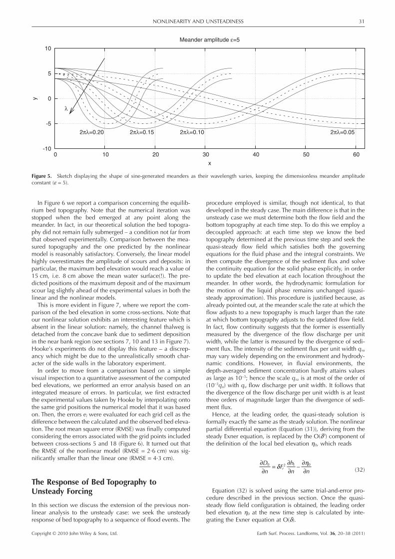
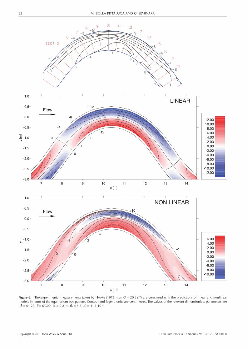
In Figure 6 we report a comparison concerning the equilib-rium bed topography. Note that the numerical iteration wasstopped when the bed emerged at any point along themeander. In fact, in our theoretical solution the bed topogra-phy did not remain fully submerged – a condition not far fromthat observed experimentally. Comparison between the mea-sured topography and the one predicted by the nonlinearmodel is reasonably satisfactory. Conversely, the linear modelhighly overestimates the amplitude of scours and deposits: inparticular, the maximum bed elevation would reach a value of15 cm, i.e. 8 cm above the mean water surface(!). The pre-dicted positions of the maximum deposit and of the maximumscour lag slightly ahead of the experimental values in both thelinear and the nonlinear models.

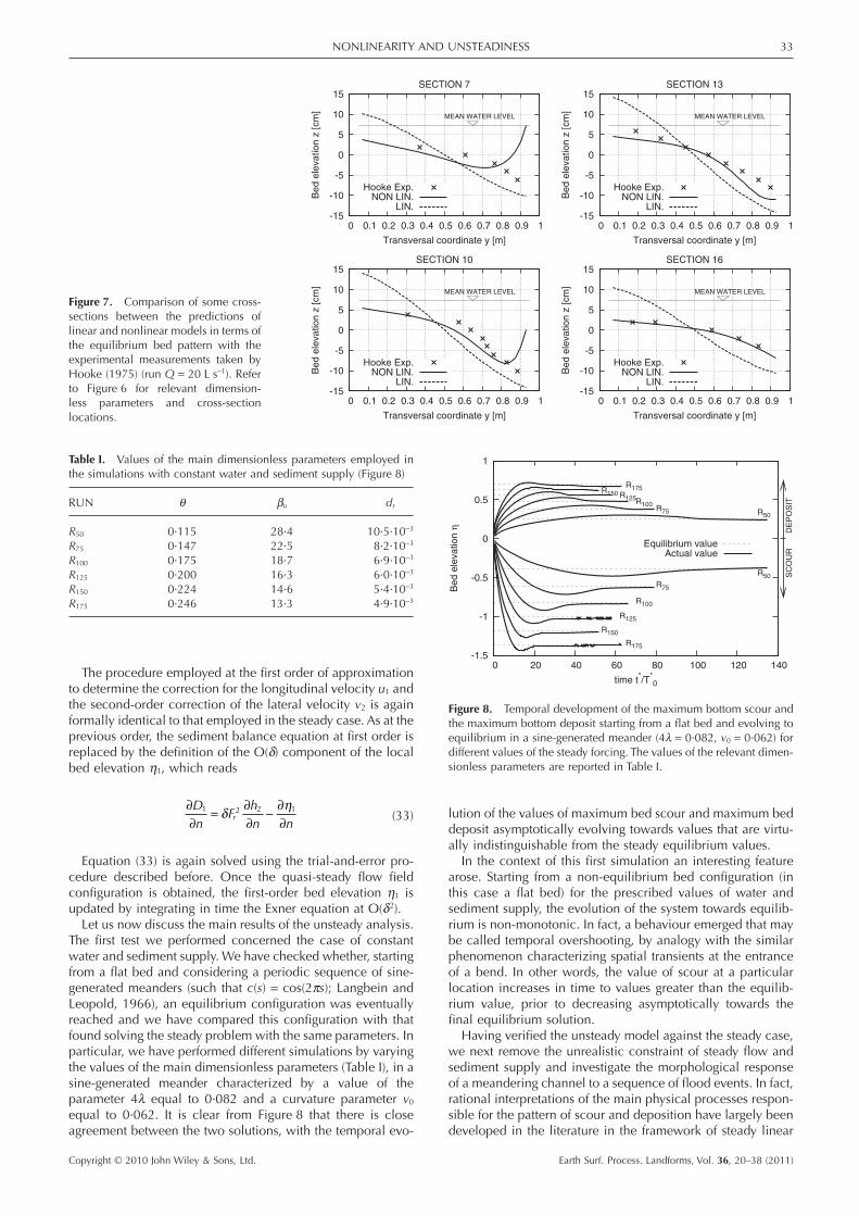
This is more evident in Figure 7, where we report the com-parison of the bed elevation in some cross-sections. Note thatour nonlinear solution exhibits an interesting feature which isabsent in the linear solution: namely, the channel thalweg isdetached from the concave bank due to sediment depositionin the near bank region (see sections 7, 10 and 13 in Figure 7).Hooke’s experiments do not display this feature – a discrep-ancy which might be due to the unrealistically smooth char-acter of the side walls in the laboratory experiment.

In order to move from a comparison based on a simplevisual inspection to a quantitative assessment of the computedbed elevations, we performed an error analysis based on anintegrated measure of errors. In particular, we first extractedthe experimental values taken by Hooke by interpolating ontothe same grid positions the numerical model that it was basedon. Then, the errors ei were evaluated for each grid cell as thedifference between the calculated and the observed bed eleva-tion. The root mean square error (RMSE) was finally computedconsidering the errors associated with the grid points includedbetween cross-sections 5 and 18 (Figure 6). It turned out thatthe RMSE of the nonlinear model (RMSE = 2·6 cm) was sig-nificantly smaller than the linear one (RMSE = 4·3 cm).

The Response of Bed Topography toUnsteady Forcing

In this section we discuss the extension of the previous non-linear analysis to the unsteady case: we seek the unsteadyresponse of bed topography to a sequence of flood events. The

procedure employed is similar, though not identical, to thatdeveloped in the steady case. The main difference is that in theunsteady case we must determine both the flow field and thebottom topography at each time step. To do this we employ adecoupled approach: at each time step we know the bedtopography determined at the previous time step and seek thequasi-steady flow field which satisfies both the governingequations for the fluid phase and the integral constraints. Wethen compute the divergence of the sediment flux and solvethe continuity equation for the solid phase explicitly, in orderto update the bed elevation at each location throughout themeander. In other words, the hydrodynamic formulation forthe motion of the liquid phase remains unchanged (quasi-steady approximation). This procedure is justified because, asalready pointed out, at the meander scale the rate at which theflow adjusts to a new topography is much larger than the rateat which bottom topography adjusts to the updated flow field.In fact, flow continuity suggests that the former is essentiallymeasured by the divergence of the flow discharge per unitwidth, while the latter is measured by the divergence of sedi-ment flux. The intensity of the sediment flux per unit width qsu

may vary widely depending on the environment and hydrody-namic conditions. However, in fluvial environments, thedepth-averaged sediment concentration hardly attains valuesas large as 10-3; hence the scale qsu is at most of the order of(10-3qu) with qu flow discharge per unit width. It follows thatthe divergence of the flow discharge per unit width is at leastthree orders of magnitude larger than the divergence of sedi-ment flux.

Hence, at the leading order, the quasi-steady solution isformally exactly the same as the steady solution. The nonlinearpartial differential equation (Equation (31)), deriving from thesteady Exner equation, is replaced by the O(d0) component ofthe definition of the local bed elevation h0, which reads

∂∂

= ∂∂

− ∂∂

Dn

Fhn n

r0 2 1 0δ η

(32)

Equation (32) is solved using the same trial-and-error pro-cedure described in the previous section. Once the quasi-steady flow field configuration is obtained, the leading orderbed elevation h0 at the new time step is calculated by inte-grating the Exner equation at O(d).

-10

-5

0

5

10

0 10 20 30 40 50 60

y

x

Meander amplitude ε=5

λ

2πλ=0.20 2πλ=0.15 2πλ=0.10 2πλ=0.05

Figure 5. Sketch displaying the shape of sine-generated meanders as their wavelength varies, keeping the dimensionless meander amplitudeconstant (e = 5).

NONLINEARITY AND UNSTEADINESS 31

Copyright © 2010 John Wiley & Sons, Ltd. Earth Surf. Process. Landforms, Vol. 36, 20–38 (2011)

7 8 9 10 11 12 13 14

x [m]

-3.0

-2.5

-2.0

-1.5

-1.0

-0.5

0.0

0.5

1.0

y [m

]

-12.00

-10.00

-8.00

-6.00

-4.00

-2.00

0.00

2.00

4.00

6.00

8.00

10.00

12.00

Flow

LINEAR

12

8

4

-8

0

-4

-12

0

7 8 9 10 11 12 13 14

x [m]

-3.0

-2.5

-2.0

-1.5

-1.0

-0.5

0.0

0.5

1.0

y [

m]

-10.00

-8.00

-6.00

-4.00

-2.00

0.00

2.00

4.00

6.00

Flow

NON LINEAR

4

2

00

-10

-2

-2

Figure 6. The experimental measurements taken by Hooke (1975) (run Q = 20 L s-1) are compared with the predictions of linear and nonlinearmodels in terms of the equilibrium bed pattern. Contour and legend units are centimetres. The values of the relevant dimensionless parameters are4l = 0·129, d = 0·300, qu = 0·214, bu = 5·8, ds = 4·11·10-3.

M. BOLLA PITTALUGA AND G. SEMINARA32

Copyright © 2010 John Wiley & Sons, Ltd. Earth Surf. Process. Landforms, Vol. 36, 20–38 (2011)

The procedure employed at the first order of approximationto determine the correction for the longitudinal velocity u1 andthe second-order correction of the lateral velocity v2 is againformally identical to that employed in the steady case. As at theprevious order, the sediment balance equation at first order isreplaced by the definition of the O(d) component of the localbed elevation h1, which reads

∂∂

= ∂∂

− ∂∂

Dn

Fhn n

r1 2 2 1δ η

(33)

Equation (33) is again solved using the trial-and-error pro-cedure described before. Once the quasi-steady flow fieldconfiguration is obtained, the first-order bed elevation h1 isupdated by integrating in time the Exner equation at O(d2).

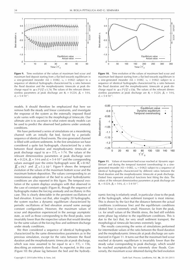
Let us now discuss the main results of the unsteady analysis.The first test we performed concerned the case of constantwater and sediment supply. We have checked whether, startingfrom a flat bed and considering a periodic sequence of sine-generated meanders (such that c(s) = cos(2ps); Langbein andLeopold, 1966), an equilibrium configuration was eventuallyreached and we have compared this configuration with thatfound solving the steady problem with the same parameters. Inparticular, we have performed different simulations by varyingthe values of the main dimensionless parameters (Table I), in asine-generated meander characterized by a value of theparameter 4l equal to 0·082 and a curvature parameter v0

equal to 0·062. It is clear from Figure 8 that there is closeagreement between the two solutions, with the temporal evo-

lution of the values of maximum bed scour and maximum beddeposit asymptotically evolving towards values that are virtu-ally indistinguishable from the steady equilibrium values.

In the context of this first simulation an interesting featurearose. Starting from a non-equilibrium bed configuration (inthis case a flat bed) for the prescribed values of water andsediment supply, the evolution of the system towards equilib-rium is non-monotonic. In fact, a behaviour emerged that maybe called temporal overshooting, by analogy with the similarphenomenon characterizing spatial transients at the entranceof a bend. In other words, the value of scour at a particularlocation increases in time to values greater than the equilib-rium value, prior to decreasing asymptotically towards thefinal equilibrium solution.

Having verified the unsteady model against the steady case,we next remove the unrealistic constraint of steady flow andsediment supply and investigate the morphological responseof a meandering channel to a sequence of flood events. In fact,rational interpretations of the main physical processes respon-sible for the pattern of scour and deposition have largely beendeveloped in the literature in the framework of steady linear

-15

-10

-5

0

5

10

15

0 0.1 0.2 0.3 0.4 0.5 0.6 0.7 0.8 0.9 1

Be

d e

leva

tio

n z

[cm

]

Transversal coordinate y [m]

SECTION 7

Hooke Exp.NON LIN.

LIN.

MEAN WATER LEVEL

-15

-10

-5

0

5

10

15

0 0.1 0.2 0.3 0.4 0.5 0.6 0.7 0.8 0.9 1

Be

d e

leva

tio

n z

[cm

]

Transversal coordinate y [m]

SECTION 10

Hooke Exp.NON LIN.

LIN.

MEAN WATER LEVEL

-15

-10

-5

0

5

10

15

0 0.1 0.2 0.3 0.4 0.5 0.6 0.7 0.8 0.9 1

Be

d e

leva

tio

n z

[cm

]

Transversal coordinate y [m]

SECTION 13

Hooke Exp.NON LIN.

LIN.

MEAN WATER LEVEL

-15

-10

-5

0

5

10

15

0 0.1 0.2 0.3 0.4 0.5 0.6 0.7 0.8 0.9 1

Be

d e

leva

tio

n z

[cm

]

Transversal coordinate y [m]

SECTION 16

Hooke Exp.NON LIN.

LIN.

MEAN WATER LEVEL

Figure 7. Comparison of some cross-sections between the predictions oflinear and nonlinear models in terms ofthe equilibrium bed pattern with theexperimental measurements taken byHooke (1975) (run Q = 20 L s-1). Referto Figure 6 for relevant dimension-less parameters and cross-sectionlocations.

Table I. Values of the main dimensionless parameters employed inthe simulations with constant water and sediment supply (Figure 8)

RUN q bu ds

R50 0·115 28·4 10·5·10-3

R75 0·147 22·5 8·2·10-3

R100 0·175 18·7 6·9·10-3

R125 0·200 16·3 6·0·10-3

R150 0·224 14·6 5·4·10-3

R175 0·246 13·3 4·9·10-3

-1.5

-1

-0.5

0

0.5

1

0 20 40 60 80 100 120 140

Bed e

levation η

time t*/T

*0

DE

PO

SIT

SC

OU

R

R50

R50

R75

R75

R100

R100

R125

R125

R150

R150

R175

R175

Equilibrium valueActual value

Figure 8. Temporal development of the maximum bottom scour andthe maximum bottom deposit starting from a flat bed and evolving toequilibrium in a sine-generated meander (4l = 0·082, v0 = 0·062) fordifferent values of the steady forcing. The values of the relevant dimen-sionless parameters are reported in Table I.

NONLINEARITY AND UNSTEADINESS 33

Copyright © 2010 John Wiley & Sons, Ltd. Earth Surf. Process. Landforms, Vol. 36, 20–38 (2011)

models. It should therefore be emphasized that here weremove both the steady and linear constraints, and investigatethe response of the system as the externally imposed floodscale varies with respect to the morphological timescale. Ourultimate aim is to ascertain to what extent steady models canbe used to predict the observed bed patterns under unsteadyconditions.

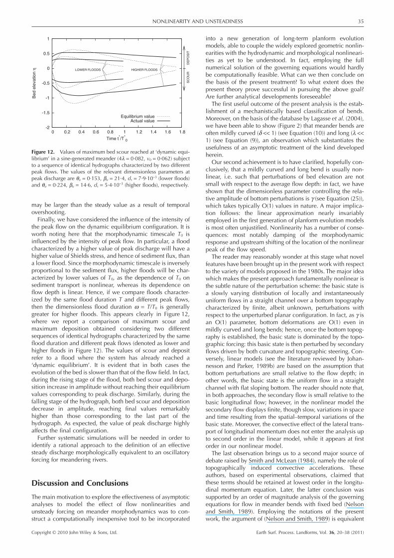
We have performed a series of simulations on a meanderingchannel with an initially flat bed, forced by a periodicsequence of identical flood events. The sine-generated channelis filled with uniform sediments. In the first simulation we haveconsidered a quite fast hydrograph, characterized by a ratiobetween flood duration and morphodynamic timescale atpeak discharge equal to w = T/T0 = 1·74. The values of therelevant dimensionless parameters at peak discharge werequ = 0·224, bu = 14·6 and ds = 5·4·10-3 and the correspondingvalues averaged over the entire hydrograph were θu = 0 167. ,βu = 19 7. and ds = ⋅ −7 3 10 3. . Figure 9 shows the temporalevolution of the values of the maximum bottom scour and themaximum bottom deposition. The values corresponding to aninstantaneous adaptation of the bed to actual hydrodynamicconditions are also reported in this figure. The temporal evo-lution of the system displays analogies with that observed inthe case of constant supply (Figure 8), though the sequence ofhydrographs makes the forcing unsteady and oscillatory in thiscase. This is clearly detectable in the persistent oscillations ofbed elevation. It turns out that, after roughly 20 hydrographs,the system reaches a dynamic equilibrium characterized byperiodic oscillations of bed elevation around some averageconstant configuration. However, the maximum values ofscour and deposition experienced in the average asymptoticstate, as well as those corresponding to the flood peaks, wereinvariably lower than the respective values that would developfor the same values of the forcing flow and sediment dischargeunder steady conditions.

We then considered a sequence of identical hydrographscharacterized by the same dimensionless parameters as in theprevious simulation, except for the ratio between the floodduration and the morphodynamic timescale at peak discharge,which was now assumed to be equal to w = T/T0 = 156,describing an extremely slow flood. As expected, in this case(Figure 10) the phase lag between the bed and the hydrody-

namic forcing is relatively small, in particular close to the peakof the hydrograph, when sediment transport is most intense.This is shown by the fact that the distance between the actualconditions (continuous line) and the equilibrium conditions(dotted line) is extremely small. However, far from the peak,i.e. for small values of the Shields stress, the bed still exhibitssome phase lag relative to the equilibrium conditions. This isdue to the fact that, for very small sediment transport, themorphological timescale becomes extremely large.

The results concerning the series of simulations performedfor intermediate values of the ratio between the flood durationand the morphodynamic timescale at peak discharge are sum-marized in Figure 11. It turns out that the maximum bed scourreached at dynamic equilibrium is invariably lower than thesteady value corresponding to peak discharge, which wouldbe reached asymptotically for extremely slow floods. Con-versely, the maximum scour obtained during the bed evolution

-2

-1.5

-1

-0.5

0

0.5

1

0 10 20 30 40 50 60

Be

d e

leva

tio

n η

Time t*/T

*0

DE

PO

SIT

SC

OU

R

Equilibrium valueActual value

Figure 9. Time evolution of the values of maximum bed scour andmaximum bed deposit starting from a flat bed towards equilibrium ina sine-generated meander (4l = 0·082, v0 = 0·062) subject to asequence of identical hydrographs characterized by a ratio betweenthe flood duration and the morphodynamic timescale at peak dis-charge equal to ω = =T T* 0 1 74* . . The values of the relevant dimen-sionless parameters at peak discharge are qu = 0·224, bu = 14·6,ds = 5·4·10-3.

-2

-1.5

-1

-0.5

0

0.5

1

0 50 100 150 200 250 300 350

Be

d e

leva

tio

n η

Time t*/T

*0

DE

PO

SIT

SC

OU

R

Equilibrium valueActual value

Figure 10. Time evolution of the values of maximum bed scour andmaximum bed deposit starting from a flat bed towards equilibrium ina sine-generated meander (4l = 0·082, v0 = 0·062) subject to asequence of identical hydrographs characterized by a ratio betweenthe flood duration and the morphodynamic timescale at peak dis-charge equal to ω = =T T* 0 156* . The values of the relevant dimen-sionless parameters at peak discharge are qu = 0·224, bu = 14·6,ds = 5·4·10-3.

-1.25

-1.2

-1.15

-1.1

-1.05

-1

-0.95

-0.9

-0.85

0 20 40 60 80 100 120 140 160

Bed e

levation η

T*/T

*0

Equilibrium valueDynamic equilibrium

Temporal overshooting

Figure 11. Values of maximum bed scour reached at ‘dynamic equi-librium’ and during the temporal transient (overshooting) in a sine-generated meander (4l = 0·082, v0 = 0·062) subject to a sequence ofidentical hydrographs characterized by different ratios between theflood duration and the morphodynamic timescale at peak discharge.Dotted lines represent analytical functions best fitting the data. Thevalues of the relevant dimensionless parameters at peak discharge arequ = 0·224, bu = 14·6, ds = 5·4·10-3.

M. BOLLA PITTALUGA AND G. SEMINARA34

Copyright © 2010 John Wiley & Sons, Ltd. Earth Surf. Process. Landforms, Vol. 36, 20–38 (2011)

may be larger than the steady value as a result of temporalovershooting.

Finally, we have considered the influence of the intensity ofthe peak flow on the dynamic equilibrium configuration. It isworth noting here that the morphodynamic timescale T0 isinfluenced by the intensity of peak flow. In particular, a floodcharacterized by a higher value of peak discharge will have ahigher value of Shields stress, and hence of sediment flux, thana lower flood. Since the morphodynamic timescale is inverselyproportional to the sediment flux, higher floods will be char-acterized by lower values of T0, as the dependence of T0 onsediment transport is nonlinear, whereas its dependence onflow depth is linear. Hence, if we compare floods character-ized by the same flood duration T and different peak flows,then the dimensionless flood duration w = T/T0 is generallygreater for higher floods. This appears clearly in Figure 12,where we report a comparison of maximum scour andmaximum deposition obtained considering two differentsequences of identical hydrographs characterized by the sameflood duration and different peak flows (denoted as lower andhigher floods in Figure 12). The values of scour and depositrefer to a flood where the system has already reached a‘dynamic equilibrium’. It is evident that in both cases theevolution of the bed is slower than that of the flow field. In fact,during the rising stage of the flood, both bed scour and depo-sition increase in amplitude without reaching their equilibriumvalues corresponding to peak discharge. Similarly, during thefalling stage of the hydrograph, both bed scour and depositiondecrease in amplitude, reaching final values remarkablyhigher than those corresponding to the last part of thehydrograph. As expected, the value of peak discharge highlyaffects the final configuration.

Further systematic simulations will be needed in order toidentify a rational approach to the definition of an effectivesteady discharge morphologically equivalent to an oscillatoryforcing for meandering rivers.

Discussion and Conclusions

The main motivation to explore the effectiveness of asymptoticanalyses to model the effect of flow nonlinearities andunsteady forcing on meander morphodynamics was to con-struct a computationally inexpensive tool to be incorporated

into a new generation of long-term planform evolutionmodels, able to couple the widely explored geometric nonlin-earities with the hydrodynamic and morphological nonlineari-ties as yet to be understood. In fact, employing the fullnumerical solution of the governing equations would hardlybe computationally feasible. What can we then conclude onthe basis of the present treatment? To what extent does thepresent theory prove successful in pursuing the above goal?Are further analytical developments foreseeable?

The first useful outcome of the present analysis is the estab-lishment of a mechanistically based classification of bends.Moreover, on the basis of the database by Lagasse et al. (2004),we have been able to show (Figure 2) that meander bends areoften mildly curved (d << 1) (see Equation (10)) and long (l <<1) (see Equation (9)), an observation which substantiates theusefulness of an asymptotic treatment of the kind developedherein.

Our second achievement is to have clarified, hopefully con-clusively, that a mildly curved and long bend is usually non-linear, i.e. such that perturbations of bed elevation are notsmall with respect to the average flow depth: in fact, we haveshown that the dimensionless parameter controlling the rela-tive amplitude of bottom perturbations is g (see Equation (25)),which takes typically O(1) values in nature. A major implica-tion follows: the linear approximation nearly invariablyemployed in the first generation of planform evolution modelsis most often unjustified. Nonlinearity has a number of conse-quences: most notably damping of the morphodynamicresponse and upstream shifting of the location of the nonlinearpeak of the flow speed.

The reader may reasonably wonder at this stage what novelfeatures have been brought up in the present work with respectto the variety of models proposed in the 1980s. The major ideawhich makes the present approach fundamentally nonlinear isthe subtle nature of the perturbation scheme: the basic state isa slowly varying distribution of locally and instantaneouslyuniform flows in a straight channel over a bottom topographycharacterized by finite, albeit unknown, perturbations withrespect to the unperturbed planar configuration. In fact, as g isan O(1) parameter, bottom deformations are O(1) even inmildly curved and long bends; hence, once the bottom topog-raphy is established, the basic state is dominated by the topo-graphic forcing: this basic state is then perturbed by secondaryflows driven by both curvature and topographic steering. Con-versely, linear models (see the literature reviewed by Johan-nesson and Parker, 1989b) are based on the assumption thatbottom perturbations are small relative to the flow depth; inother words, the basic state is the uniform flow in a straightchannel with flat sloping bottom. The reader should note that,in both approaches, the secondary flow is small relative to thebasic longitudinal flow; however, in the nonlinear model thesecondary flow displays finite, though slow, variations in spaceand time resulting from the spatial–temporal variations of thebasic state. Moreover, the convective effect of the lateral trans-port of longitudinal momentum does not enter the analysis upto second order in the linear model, while it appears at firstorder in our nonlinear model.

The last observation brings us to a second major source ofdebate raised by Smith and McLean (1984), namely the role oftopographically induced convective accelerations. Theseauthors, based on experimental observations, claimed thatthese terms should be retained at lowest order in the longitu-dinal momentum equation. Later, the latter conclusion wassupported by an order of magnitude analysis of the governingequations for flow in meander bends with fixed bed (Nelsonand Smith, 1989). Employing the notations of the presentwork, the argument of (Nelson and Smith, 1989) is equivalent

-2

-1.5

-1

-0.5

0

0.5

1

0 0.2 0.4 0.6 0.8 1 1.2 1.4 1.6 1.8

Be

d e

leva

tio

n η

Time t*/T

*0

DE

PO

SIT

SC

OU

R

HIGHER FLOODSLOWER FLOODS

Equilibrium valueActual value

Figure 12. Values of maximum bed scour reached at ‘dynamic equi-librium’ in a sine-generated meander (4l = 0·082, v0 = 0·062) subjectto a sequence of identical hydrographs characterized by two differentpeak flows. The values of the relevant dimensionless parameters atpeak discharge are qu = 0·153, bu = 21·4, ds = 7·9·10-3 (lower floods)and qu = 0·224, bu = 14·6, ds = 5·4·10-3 (higher floods), respectively.

NONLINEARITY AND UNSTEADINESS 35

Copyright © 2010 John Wiley & Sons, Ltd. Earth Surf. Process. Landforms, Vol. 36, 20–38 (2011)

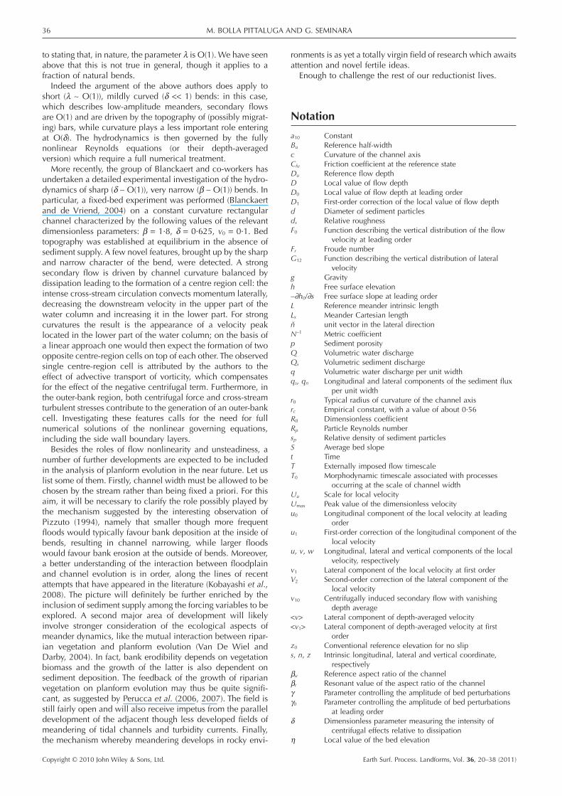
to stating that, in nature, the parameter l is O(1). We have seenabove that this is not true in general, though it applies to afraction of natural bends.

Indeed the argument of the above authors does apply toshort (l ~ O(1)), mildly curved (d << 1) bends: in this case,which describes low-amplitude meanders, secondary flowsare O(1) and are driven by the topography of (possibly migrat-ing) bars, while curvature plays a less important role enteringat O(d). The hydrodynamics is then governed by the fullynonlinear Reynolds equations (or their depth-averagedversion) which require a full numerical treatment.

More recently, the group of Blanckaert and co-workers hasundertaken a detailed experimental investigation of the hydro-dynamics of sharp (d ~ O(1)), very narrow (b ~ O(1)) bends. Inparticular, a fixed-bed experiment was performed (Blanckaertand de Vriend, 2004) on a constant curvature rectangularchannel characterized by the following values of the relevantdimensionless parameters: b = 1·8, d = 0·625, v0 = 0·1. Bedtopography was established at equilibrium in the absence ofsediment supply. A few novel features, brought up by the sharpand narrow character of the bend, were detected. A strongsecondary flow is driven by channel curvature balanced bydissipation leading to the formation of a centre region cell: theintense cross-stream circulation convects momentum laterally,decreasing the downstream velocity in the upper part of thewater column and increasing it in the lower part. For strongcurvatures the result is the appearance of a velocity peaklocated in the lower part of the water column; on the basis ofa linear approach one would then expect the formation of twoopposite centre-region cells on top of each other. The observedsingle centre-region cell is attributed by the authors to theeffect of advective transport of vorticity, which compensatesfor the effect of the negative centrifugal term. Furthermore, inthe outer-bank region, both centrifugal force and cross-streamturbulent stresses contribute to the generation of an outer-bankcell. Investigating these features calls for the need for fullnumerical solutions of the nonlinear governing equations,including the side wall boundary layers.

Besides the roles of flow nonlinearity and unsteadiness, anumber of further developments are expected to be includedin the analysis of planform evolution in the near future. Let uslist some of them. Firstly, channel width must be allowed to bechosen by the stream rather than being fixed a priori. For thisaim, it will be necessary to clarify the role possibly played bythe mechanism suggested by the interesting observation ofPizzuto (1994), namely that smaller though more frequentfloods would typically favour bank deposition at the inside ofbends, resulting in channel narrowing, while larger floodswould favour bank erosion at the outside of bends. Moreover,a better understanding of the interaction between floodplainand channel evolution is in order, along the lines of recentattempts that have appeared in the literature (Kobayashi et al.,2008). The picture will definitely be further enriched by theinclusion of sediment supply among the forcing variables to beexplored. A second major area of development will likelyinvolve stronger consideration of the ecological aspects ofmeander dynamics, like the mutual interaction between ripar-ian vegetation and planform evolution (Van De Wiel andDarby, 2004). In fact, bank erodibility depends on vegetationbiomass and the growth of the latter is also dependent onsediment deposition. The feedback of the growth of riparianvegetation on planform evolution may thus be quite signifi-cant, as suggested by Perucca et al. (2006, 2007). The field isstill fairly open and will also receive impetus from the paralleldevelopment of the adjacent though less developed fields ofmeandering of tidal channels and turbidity currents. Finally,the mechanism whereby meandering develops in rocky envi-

ronments is as yet a totally virgin field of research which awaitsattention and novel fertile ideas.

Enough to challenge the rest of our reductionist lives.

Notation

a10 ConstantBu Reference half-widthc Curvature of the channel axisCfu Friction coefficient at the reference stateDu Reference flow depthD Local value of flow depthD0 Local value of flow depth at leading orderD1 First-order correction of the local value of flow depthd Diameter of sediment particlesds Relative roughnessF0 Function describing the vertical distribution of the flow

velocity at leading orderFr Froude numberG12 Function describing the vertical distribution of lateral

velocityg Gravityh Free surface elevation-∂h0/∂s Free surface slope at leading orderL Reference meander intrinsic lengthLx Meander Cartesian lengthn unit vector in the lateral directionN-1 Metric coefficientp Sediment porosityQ Volumetric water dischargeQs Volumetric sediment dischargeq Volumetric water discharge per unit widthqs, qn Longitudinal and lateral components of the sediment flux

per unit widthr0 Typical radius of curvature of the channel axisrc Empirical constant, with a value of about 0·56R0 Dimensionless coefficientRp Particle Reynolds numbersp Relative density of sediment particlesS Average bed slopet TimeT Externally imposed flow timescaleT0 Morphodynamic timescale associated with processes

occurring at the scale of channel widthUu Scale for local velocityUmax Peak value of the dimensionless velocityu0 Longitudinal component of the local velocity at leading

orderu1 First-order correction of the longitudinal component of the

local velocityu, v, w Longitudinal, lateral and vertical components of the local

velocity, respectivelyv1 Lateral component of the local velocity at first orderV2 Second-order correction of the lateral component of the

local velocityv10 Centrifugally induced secondary flow with vanishing

depth average<v> Lateral component of depth-averaged velocity<v1> Lateral component of depth-averaged velocity at first

orderz0 Conventional reference elevation for no slips, n, z Intrinsic longitudinal, lateral and vertical coordinate,

respectivelybu Reference aspect ratio of the channelbr Resonant value of the aspect ratio of the channelg Parameter controlling the amplitude of bed perturbationsg0 Parameter controlling the amplitude of bed perturbations

at leading orderd Dimensionless parameter measuring the intensity of

centrifugal effects relative to dissipationh Local value of the bed elevation

M. BOLLA PITTALUGA AND G. SEMINARA36

Copyright © 2010 John Wiley & Sons, Ltd. Earth Surf. Process. Landforms, Vol. 36, 20–38 (2011)

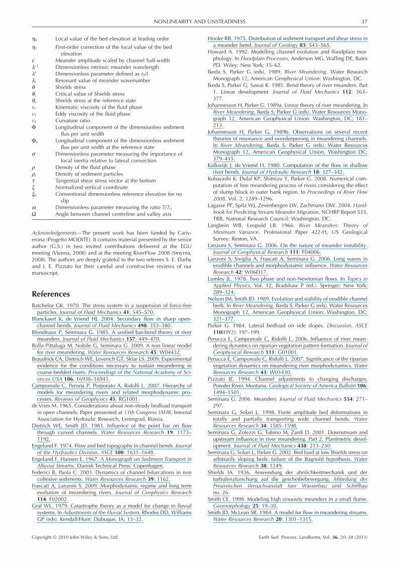
h0 Local value of the bed elevation at leading order

h1 First-order correction of the local value of the bedelevation

e Meander amplitude scaled by channel half-widthl-1 Dimensionless intrinsic meander wavelengthl′ Dimensionless parameter defined as r0/Llr Resonant value of meander wavenumberq Shields stressqc Critical value of Shields stressqu Shields stress at the reference statevf Kinematic viscosity of the fluid phasevT Eddy viscosity of the fluid phasev0 Curvature ratioF Longitudinal component of the dimensionless sediment

flux per unit widthFu Longitudinal component of the dimensionless sediment

flux per unit width at the reference states Dimensionless parameter measuring the importance of

local inertia relative to lateral convectionr Density of the fluid phasers Density of sediment particlest Tangential shear stress vector at the bottomx Normalized vertical coordinatex0 Conventional dimensionless reference elevation for no

slipw Dimensionless parameter measuring the ratio T/T0

W Angle between channel centreline and valley axis

Acknowledgements—The present work has been funded by Cariv-erona (Progetto MODITE). It contains material presented by the seniorauthor (G.S.) in two invited contributions delivered at the EGUmeeting (Vienna, 2008) and at the meeting RiverFlow 2008 (Smyrna,2008). The authors are deeply grateful to the two referees S. E. Darbyand J. E. Pizzuto for their careful and constructive reviews of ourmanuscript.

ReferencesBatchelor GK. 1970. The stress system in a suspension of force-free

particles. Journal of Fluid Mechanics 41: 545–570.Blanckaert K, de Vriend HJ. 2004. Secondary flow in sharp open-

channel bends. Journal of Fluid Mechanics 498: 353–380.Blondeaux P, Seminara G. 1985. A unified bar-bend theory of river

meanders. Journal of Fluid Mechanics 157: 449–470.Bolla Pittaluga M, Nobile G, Seminara G. 2009. A non linear model

for river meandering. Water Resources Research 45: W04432.Braudrick CA, Dietrich WE, Leverich GT, Sklar LS. 2009. Experimental

evidence for the conditions necessary to sustain meandering incoarse-bedded rivers. Proceedings of the National Academy of Sci-ences USA 106: 16936–16941.

Camporeale C, Perona P, Porporato A, Ridolfi L. 2007. Hierarchy ofmodels for meandering rivers and related morphodynamic pro-cesses. Reviews of Geophysics 45: RG1001.

de Vries M. 1965. Considerations about non-steady bedload transportin open channels. Paper presented at 11th Congress IAHR, InternalAssociation for Hydraulic Research, Leningrad, Russia.

Dietrich WE, Smith JD. 1983. Influence of the point bar on flowthrough curved channels. Water Resources Research 19: 1173–1192.

Engelund F. 1974. Flow and bed topography in channel bends. Journalof the Hydraulics Division, ASCE 100: 1631–1648.

Engelund F, Hansen E. 1967. A Monograph on Sediment Transport inAlluvial Streams. Danish Technical Press: Copenhagen.

Federici B, Paola C. 2003. Dynamics of channel bifurcations in noncohesive sediments. Water Resources Research 39: 1162.

Frascati A, Lanzoni S. 2009. Morphodynamic regime and long termevolution of meandering rivers. Journal of Geophysics Research114: F02002.

Graf WL. 1979. Catastrophe theory as a model for change in fluvialsystems. In Adjustments of the Fluvial System, Rhodes DD, WilliamsGP (eds). Kendall/Hunt: Dubuque, IA; 13–32.

Hooke RB. 1975. Distribution of sediment transport and shear stress ina meander bend. Journal of Geology 83: 543–565.

Howard A. 1992. Modelling channel evolution and floodplain mor-phology. In Floodplain Processes, Anderson MG, Walling DE, BatesPD. Wiley: New York; 15–62.

Ikeda S, Parker G (eds). 1989. River Meandering. Water ResearchMonograph 12, American Geophysical Union: Washington, DC.

Ikeda S, Parker G, Sawai K. 1981. Bend theory of river meanders. Part1. Linear development. Journal of Fluid Mechanics 112: 363–377.

Johannesson H, Parker G. 1989a. Linear theory of river meandering. InRiver Meandering, Ikeda S, Parker G (eds). Water Resources Mono-graph 12, American Geophysical Union: Washington, DC; 181–213.

Johannesson H, Parker G. 1989b. Observations on several recenttheories of resonance and overdeepening in meandering channels.In River Meandering, Ikeda S, Parker G (eds). Water ResourcesMonograph 12, American Geophysical Union, Washington DC;379–415.

Kalkwijk J, de Vriend H. 1980. Computation of the flow in shallowriver bends. Journal of Hydraulic Research 18: 327–342.

Kobayashi K, Dulal KP, Shimizu Y, Parker G. 2008. Numerical com-putation of free meandering process of rivers considering the effectof slump block in outer bank region. In Proceedings of River Flow2008, Vol. 2; 1289–1296.

Lagasse PF, Spitz WJ, Zevenbergen LW, Zachmann DW. 2004. Hand-book for Predicting Stream Meander Migration. NCHRP Report 533,TRB, National Research Council: Washington, DC.

Langbein WB, Leopold LB. 1966. River Meanders: Theory ofMinimum Variance. Professional Paper 422-H, US GeologicalSurvey: Reston, VA.

Lanzoni S, Seminara G. 2006. On the nature of meander instability.Journal of Geophysical Research 111: F04006.

Lanzoni S, Siviglia A, Frascati A, Seminara G. 2006. Long waves inerodible channels and morphodynamic influence. Water ResourcesResearch 42: W06D17.

Lumley JL. 1978. Two phase and non-Newtonian flows. In Topics inApplied Physics, Vol. 12, Bradshaw P (ed.). Springer: New York;289–324.

Nelson JM, Smith JD. 1989. Evolution and stability of erodible channelbeds. In River Meandering, Ikeda S, Parker G (eds). Water ResourcesMonograph 12, American Geophysical Union: Washington, DC;321–377.

Parker G. 1984. Lateral bedload on side slopes. Discussion, ASCE110(HY2): 197–199.

Perucca E, Camporeale C, Ridolfi L. 2006. Influence of river mean-dering dynamics on riparian vegetation pattern formation. Journal ofGeophysical Research 111: G01001.

Perucca E, Camporeale C, Ridolfi L. 2007. Significance of the riparianvegetation dynamics on meandering river morphodynamics. WaterResources Research 43: W03430.

Pizzuto JE. 1994. Channel adjustments to changing discharges,Powder River, Montana. Geological Society of America Bulletin 106:1494–1501.

Seminara G. 2006. Meanders. Journal of Fluid Mechanics 554: 271–297.

Seminara G, Solari L. 1998. Finite amplitude bed deformations intotally and partially transporting wide channel bends. WaterResources Research 34: 1585–1598.

Seminara G, Zolezzi G, Tubino M, Zardi D. 2001. Downstream andupstream influence in river meandering. Part 2. Planimetric devel-opment. Journal of Fluid Mechanics 438: 213–230.

Seminara G, Solari L, Parker G. 2002. Bed load at low Shields stress onarbitrarily sloping beds: failure of the Bagnold hypothesis. WaterResources Research 38: 1249.

Shields IA. 1936. Anwendung der ahnlichkeitmechanik und derturbulenzforschung auf die gescheibebewegung. Mitteilung derPreussischen Versuchsanstalt fuer Wasserbau und Schiffbauno. 26.

Smith CE. 1998. Modeling high sinuosity meanders in a small flume.Geomorphology 25: 19–30.

Smith JD, McLean SR. 1984. A model for flow in meandering streams.Water Resources Research 20: 1301–1315.

NONLINEARITY AND UNSTEADINESS 37

Copyright © 2010 John Wiley & Sons, Ltd. Earth Surf. Process. Landforms, Vol. 36, 20–38 (2011)

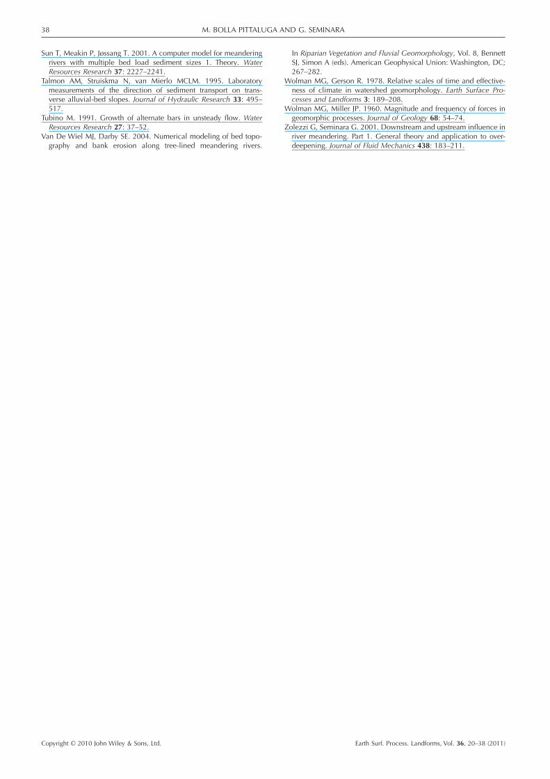
Sun T, Meakin P, Jøssang T. 2001. A computer model for meanderingrivers with multiple bed load sediment sizes 1. Theory. WaterResources Research 37: 2227–2241.

Talmon AM, Struiskma N, van Mierlo MCLM. 1995. Laboratorymeasurements of the direction of sediment transport on trans-verse alluvial-bed slopes. Journal of Hydraulic Research 33: 495–517.

Tubino M. 1991. Growth of alternate bars in unsteady flow. WaterResources Research 27: 37–52.

Van De Wiel MJ, Darby SE. 2004. Numerical modeling of bed topo-graphy and bank erosion along tree-lined meandering rivers.

In Riparian Vegetation and Fluvial Geomorphology, Vol. 8, BennettSJ, Simon A (eds). American Geophysical Union: Washington, DC;267–282.

Wolman MG, Gerson R. 1978. Relative scales of time and effective-ness of climate in watershed geomorphology. Earth Surface Pro-cesses and Landforms 3: 189–208.

Wolman MG, Miller JP. 1960. Magnitude and frequency of forces ingeomorphic processes. Journal of Geology 68: 54–74.

Zolezzi G, Seminara G. 2001. Downstream and upstream influence inriver meandering. Part 1. General theory and application to over-deepening. Journal of Fluid Mechanics 438: 183–211.

M. BOLLA PITTALUGA AND G. SEMINARA38

Copyright © 2010 John Wiley & Sons, Ltd. Earth Surf. Process. Landforms, Vol. 36, 20–38 (2011)