Spatial width oscillations in meandering rivers at equilibrium

Spatial width oscillations in meandering rivers at equilibrium

R. Luchi,1 M. Bolla Pittaluga,1 and G. Seminara1

Received 1 July 2011; revised 5 April 2012; accepted 10 April 2012; published 31 May 2012.

[1] In canaliform rivers channel width at bankfull stage is fairly uniform though, at bendapexes, it is typically smaller than at crossings. Conversely, in sinuous point bar riversbankfull width peaks at bend apexes. Why? Is there any mechanistic constraint that forcesthis different behavior? We provide an answer to these questions investigating how bankfullwidth must vary in a sequence of sine-generated meanders in order for the constraints ofequilibrium (constant flow discharge and sediment flux) to be satisfied. With the help ofa 3-D fully nonlinear analytical model of flow and bed topography in meandering riverswith variable width, we show that, in a meandering channel characterized by a constantlongitudinal free-surface slope, the equilibrium width thus obtained oscillates with afrequency twice the frequency of channel curvature and experiences the maximum widthclose to inflection points. This pattern is typically observed in canaliform rivers. We thenshow that a similar pattern is observed in sinuous point bar rivers, provided thehydrodynamic width (width of the free surface) is replaced by the active width, namely thewidth of the portion of the cross section where transport occurs at formative conditions.Theoretical results are substantiated by a satisfactory comparison with field observationsreferring to the Mississippi River (United States) and to the Bollin River (United Kingdom).

Citation: Luchi, R., M. Bolla Pittaluga, and G. Seminara (2012), Spatial width oscillations in meandering rivers at equilibrium, WaterResour. Res., 48, W05551, doi:10.1029/2011WR011117.

1. Introduction[2] It is a common observation that actively migrating

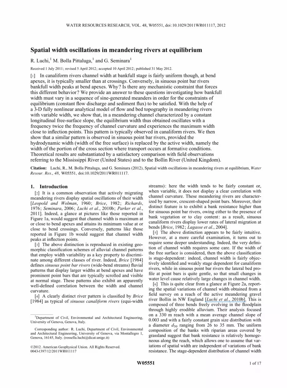
meandering rivers display spatial oscillations of their width[Leopold and Wolman, 1960; Brice, 1982; Richards,1976; Seminara, 2006; Luchi et al., 2010b; Parker et al.,2011]. Indeed, a glance at pictures like those reported inFigure 1a, would suggest that channel width is maximum ator close to bend apexes and attains its minimum value at orclose to bend crossings. Conversely, patterns like thosereported in Figure 1b would suggest that channel widthpeaks at inflection points.

[3] The above distinction is reproduced in existing geo-morphic classification schemes of alluvial channel patternsthat employ width variability as a key property to discrimi-nate among different classes of river. Indeed, Brice [1984]defines sinuous point bar rivers (wide-bend streams) fluvialpatterns that display larger widths at bend apexes and haveprominent point bars that are typically scrolled and visibleat normal stage. These patterns also exhibit an apparentlywell-defined correlation between the width and channelcurvature.

[4] A clearly distinct river pattern is classified by Brice[1984] as typical of sinuous canaliform rivers (equi-width

streams): here the width tends to be fairly constant or,when variable, it does not display a clear correlation withchannel curvature. These meandering rivers are character-ized by narrow, crescent-shaped point bars. Moreover, theirdistinct feature is to exhibit a bank resistance higher thanfor sinuous point bar rivers, owing either to the presence ofbank vegetation or to clay content : as a result, sinuouscanaliform rivers display lower rates of lateral migration atbends [Brice, 1982; Lagasse et al., 2004].

[5] The above distinction appears to be fairly intuitive.However, at a more careful examination, it turns out torequire some deeper understanding. Indeed, the very defini-tion of channel width requires some care. If the width ofthe free surface is considered, then the above classificationis stage-dependent: indeed, channel width is fairly objec-tively identified and weakly stage dependent for canaliformrivers, while in sinuous point bar rivers the lateral bed pro-file at point bars is quite gentle, so that small changes inwater level cause relatively large changes in channel width.

[6] This is quite clear from a glance at Figure 2a, report-ing the spatial variations of channel width obtained from afield survey on a reach of the active meandering gravelriver Bollin in NW England [Luchi et al., 2010b]. This iscomposed of three bends freely evolving in the floodplainthrough highly erodible alluvium. Their analysis focusedon a 330 m reach with a mean average channel slope of0.003 and with a fairly constant grain size distribution witha diameter d50 ranging from 26 to 35 mm. The uniformcomposition of the banks with riparian areas covered bygrassland suggest that bank resistance is relatively homoge-neous along the reach, which allows one to assume that var-iations of spatial width are independent of variations of bankresistance. The stage-dependent distribution of channel width

1Department of Civil, Environmental and Architectural Engineering,University of Genova, Genova, Italy.

Corresponding author: R. Luchi, Department of Civil, Environmentaland Architectural Engineering, University of Genova, via Montallegro 1,Genova, 16145, Italy. ([email protected])

©2012. American Geophysical Union. All Rights Reserved.0043-1397/12/2011WR011117

W05551 1 of 17

WATER RESOURCES RESEARCH, VOL. 48, W05551, doi:10.1029/2011WR011117, 2012

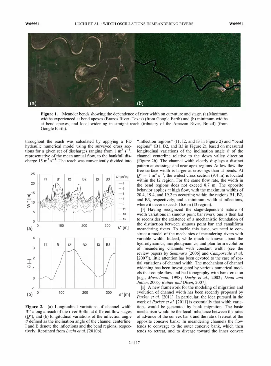
http://dx.doi.org/10.1029/2011WR011117

https://www.researchgate.net/publication/248513567_Width_variations_and_mid-channel_bar_inception_in_meanders_River_Bollin_UK?el=1_x_8&enrichId=rgreq-a0427a2b-6873-495c-922b-25ad2acca5ce&enrichSource=Y292ZXJQYWdlOzIzMDcwMTQ1ODtBUzoxMDQ1NTYyMDU3MDcyNzJAMTQwMTkzOTU1MDY5Mw==

throughout the reach was calculated by applying a 1-Dhydraulic numerical model using the surveyed cross sec-tions for a given set of discharges ranging from 1 m3 s�1,representative of the mean annual flow, to the bankfull dis-charge 15 m3 s�1. The reach was conveniently divided into

‘‘inflection regions’’ (I1, I2, and I3 in Figure 2) and ‘‘bendregions’’ (B1, B2, and B3 in Figure 2), based on measuredlongitudinal variations of the inclination angle # of thechannel centerline relative to the down valley direction(Figure 2b). The channel width clearly displays a distinctpattern at crossings and near-apex regions. At low flow, thefree surface width is larger at crossings than at bends. AtQ� ¼ 1 m3 s�1, the widest cross section (9.4 m) is locatedwithin the I2 region. For the same flow rate, the width inthe bend regions does not exceed 8.7 m. The oppositebehavior applies at high flow, with the maximum widths of20.4, 19.4, and 19.2 m occurring within the regions B1, B2,and B3, respectively, and a minimum width at inflections,where it never exceeds 16.6 m (I3 region).

[7] Having recognized the stage-dependent nature ofwidth variations in sinuous point bar rivers, one is then ledto reconsider the existence of a mechanistic foundation ofthe distinction between sinuous point bar and canaliformmeandering rivers. To tackle this issue, we need to con-struct a model of the mechanics of meandering rivers withvariable width. Indeed, while much is known about thehydrodynamics, morphodynamics, and plan form evolutionof meandering channels with constant width (see thereview papers by Seminara [2006] and Camporeale et al.[2007]), little attention has been devoted to the case of spa-tial variations of channel width. The mechanism of channelwidening has been investigated by various numerical mod-els that couple flow and bed topography with bank erosion[e.g., Mosselman, 1998; Darby et al., 2002; Duan andJulien, 2005; Ruther and Olsen, 2007].

[8] A new framework for the modeling of migration andevolution of channel width has been recently proposed byParker et al. [2011]. In particular, the idea pursued in thework of Parker et al. [2011] is essentially that width varia-tions would be generated by bank migration. The basicmechanism would be the local imbalance between the ratesof advance of the convex bank and the rate of retreat of theopposite concave bank: In meandering channels the flowtends to converge to the outer concave bank, which thentends to retreat, and to diverge toward the inner convex

Figure 2. (a) Longitudinal variations of channel widthW � along a reach of the river Bollin at different flow stages(Q�), and (b) longitudinal variations of the inflection angle# defined as the inclination angle of the channel centerline.I and B denote the inflections and the bend regions, respec-tively. Reprinted from Luchi et al. [2010b].

Figure 1. Meander bends showing the dependence of river width on curvature and stage. (a) Maximumwidths experienced at bend apexes (Brazos River, Texas) (from Google Earth) and (b) minimum widthsat bend apexes, and local widening in straight reach (tributary of the Amazon River, Brazil) (fromGoogle Earth).

W05551 LUCHI ET AL.: WIDTH OSCILLATIONS IN MEANDERING RIVERS W05551

2 of 17

bank, which consequently accretes [Nanson and Hickin,1983]. As outer erosion is faster than inner accretion thechannel tends to widen locally. The above idea was mod-eled originally by Mosselman et al. [2000] in a simplifiedmodel of bank stabilization on anabranches of braider riv-ers. Parker et al. [2011] have extended this idea to mean-dering rivers. This allowed the latter authors to relax theassumption employed in most meander evolution models,where the river width is kept spatially and temporally con-stant throughout the evolution process. The latter assump-tion is equivalent to stipulating that the outer bank retreatrate is equal to the inner bank advance rate. As a result,inner deposition does not need to be treated explicitly andthe channel centerline is simply shifted laterally at a rateequal to the rate of outer bank retreat. Note that thisassumption has been justified as a long-term requirementfor meandering rivers and has received some support[Pizzuto and Meckelnburg, 1989] from field observationson rivers with fairly uniform cohesive banks. In the Parkeret al. [2011] model separate relations for the migrationrates of the eroding and depositing banks are assumed andtied to a standard morphodynamic model for flow and sedi-ment transport in the central region of the channel. Thebanks interact dynamically with each other to determinethe evolution of channel width.

[9] An alternative mechanism for the generation ofwidth variations in sinuous rivers has been correlated withthe presence of mid-channel bars. Indeed, characteristiccycles for the development of mid-channel bars and longi-tudinal widening-narrowing sequences in single-threadmeandering streams have been documented in the field[Knighton, 1972; Richards, 1976; Hooke, 1986; Hookeand Yorke, 2011], while other studies mainly focused onsingle anabranches of braided rivers [e.g., Ashworth, 1996;Klaassen et al., 1993], where bed and banks evolve at compa-rable timescales [Bertoldi and Tubino, 2005]. Recently, usinga mathematical model based on a perturbation approach,Luchi et al. [2010a] showed that mid-channel bars can de-velop in meanders also in the absence of width variations,due to nonlinear effects forced by curvature. As a result, theflow is forced to diverge against both banks thus inducing lat-erally symmetrical bank erosion and channel widening. Inturn, the presence of width variations promotes the develop-ment of mid-channel bars [Repetto et al., 2002] and affectsthe process of meander growth [Luchi et al., 2011].

[10] Width variations may also occur as a result of heter-ogeneous bank erodibility though they are unlikely to besystematic [Richards, 1976]. Indeed, locally resistant banksblock channel migration in such a way that very sharpbends arise. Sharp bends display a number of hydrody-namic features (flow impingement, downwelling, horizon-tal outer-bank eddies), which are excluded from the presentanalysis that applies to the more common case of gentlebends. The interested reader is referred to Ferguson et al.[2003], Parsons et al. [2004], and Vermeulen et al. [2011].

[11] The question tackled in this paper is somehow com-plementary to the above works. Indeed, in order to ascer-tain the existence of a mechanistic foundation of thedistinction between sinuous point bar and canaliform mean-dering rivers, we assume morphodynamic equilibrium andinvestigate how bankfull width must vary in a sequence ofsine-generated meanders in order for the constraints of

equilibrium to be satisfied. We show that, because of thenonlinear dependence of bed load transport on bottomstress, in order for a curved channel to exhibit a uniformtransport capacity at any cross section, its width must oscil-late in response to the local values of channel curvature[Solari and Seminara, 2005]. In general, we find that thewidth attains its maximum close to the inflection points andits minimum close to the bend apex. We then clarify howthis result, which fits clearly the canaliform pattern, alsoapplies to sinuous point bar rivers. This will lead us torevisit the very definition of channel width to show that, inthe context of morphological investigations, the appropriatenotion of channel width differs from the width of the freesurface: rather, a morphologically active width has to bedefined. We then show that the distinction between canali-form and sinuous point bar rivers is not tied with differentpatterns of variations of their active width.

[12] Our analysis is based on an extension of the nonlin-ear approach to the morphodynamics of meandering riversproposed by Bolla Pittaluga et al. [2009]. The presentextension is required in order to allow for spatial variationsof channel width. Indeed, in the work of Bolla Pittalugaet al. [2009] the banks were fixed and the overall sedimentflux was forced to attain a constant value allowing for spa-tial variations of the free-surface slope in the curved reach.Here we argue that, provided the banks are not fixed, thestream may achieve the goal to meet the constant sedimentflux constraint by simply allowing the width to vary. Themain assumption required for the present model to be rationalis that flow and bottom topography must be ‘‘slowly vary-ing’’ in both longitudinal and lateral directions; these condi-tions imply that the channel must be ‘‘wide’’ enough and itswidth and channel alignment must vary on a longitudinalscale much larger than channel width. These conditions aretypically (though not always) met in actual rivers but neitherof them implies that perturbations of bottom topography arenecessarily ‘‘small.’’ Taking advantage of the slowly varyingassumption, we do not need to assume linearity and suc-ceed in developing an analytical approach able to accountfor finite amplitude perturbations of flow and bed topogra-phy driven by both curvature and slow spatial variations ofchannel width.

[13] The remainder of the paper is then organized as fol-lows. In section 2 we formulate a 3-D nonlinear model offlow and bed topography in meandering rivers allowing forspatial variations of channel width. In section 3 we derivean analytical solution of the above problem based on theassumption that both channel curvature and channel widthvary slowly in the longitudinal direction. Section 4 isdevoted to clarifying the mechanism whereby the con-straint of constant sediment flux does lead to the need forchannel width to vary in space. Results are presented anddiscussed in sections 5 and 6. Concluding remarks followin section 7.

2. A 3-D Nonlinear Model of Meandering RiversWith Variable Width: Formulation

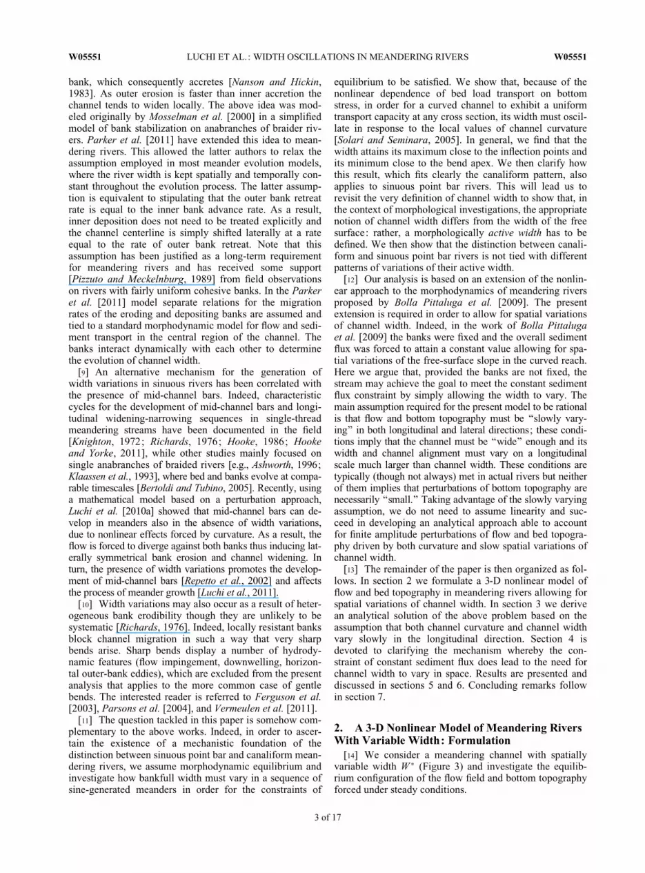
[14] We consider a meandering channel with spatiallyvariable width W � (Figure 3) and investigate the equilib-rium configuration of the flow field and bottom topographyforced under steady conditions.


3 of 17

https://www.researchgate.net/publication/251425739_Evaluation_of_a_Linear_Bank_Erosion_Equation?el=1_x_8&enrichId=rgreq-a0427a2b-6873-495c-922b-25ad2acca5ce&enrichSource=Y292ZXJQYWdlOzIzMDcwMTQ1ODtBUzoxMDQ1NTYyMDU3MDcyNzJAMTQwMTkzOTU1MDY5Mw==

https://www.researchgate.net/publication/232004999_Bend_theory_of_river_meanders_with_spatial_width_variations?el=1_x_8&enrichId=rgreq-a0427a2b-6873-495c-922b-25ad2acca5ce&enrichSource=Y292ZXJQYWdlOzIzMDcwMTQ1ODtBUzoxMDQ1NTYyMDU3MDcyNzJAMTQwMTkzOTU1MDY5Mw==

https://www.researchgate.net/publication/231819140_Planimetric_instability_of_channels_with_variable_width?el=1_x_8&enrichId=rgreq-a0427a2b-6873-495c-922b-25ad2acca5ce&enrichSource=Y292ZXJQYWdlOzIzMDcwMTQ1ODtBUzoxMDQ1NTYyMDU3MDcyNzJAMTQwMTkzOTU1MDY5Mw==

https://www.researchgate.net/publication/249525048_Channel_width_and_riffle-pool_sequence?el=1_x_8&enrichId=rgreq-a0427a2b-6873-495c-922b-25ad2acca5ce&enrichSource=Y292ZXJQYWdlOzIzMDcwMTQ1ODtBUzoxMDQ1NTYyMDU3MDcyNzJAMTQwMTkzOTU1MDY5Mw==

[15] Following a well-established approach, we assumethe channel width sufficiently large for the sidewall bound-ary layers to play a passive role. We then focus on the cen-tral flow region. The mathematical formulation of theproblem relies on the continuity and momentum equationsfor the fluid phase, the mass conservation equation for thesolid phase governing the evolution of the bed interface,and some closure relationship for sediment transport. Theformulation then follows the lines of the theory proposedby Bolla Pittaluga et al. [2009] and Bolla Pittaluga andSeminara [2011]. Here we simply recall the key ingredientsof the above formulation and underlie the additional fea-tures required in order to account for the effects of spatialvariations of channel width. For the full details of the origi-nal model the reader is referred to Bolla Pittaluga et al.[2009] and Bolla Pittaluga and Seminara [2011].

[16] We refer the flow to intrinsic longitudinal, lateral,and vertical coordinates (s�, n�, and z�, respectively, with astar hereafter denoting dimensional quantities). We thenselect some characteristic scales for the latter variables andwrite the problem in dimensionless form. It is convenientto transform the physical domain introducing the dimen-sionless coordinates ð�; n; zÞ as follows:

ðs�; n�; z�Þ ¼ ðr�0�;B�n;D�uzÞ; (1)

where r�0 is a typical radius of curvature of the channelaxis, B� is the local half channel width, while D� is thelocal flow depth, and the index subscript u refers to the ba-sic uniform flow of the given flow discharge in a straightchannel with some ‘‘average’’ channel width and the aver-age channel slope S. Note that in the Bolla Pittaluga et al.[2009] model the lateral coordinate was scaled by the con-stant value of the channel width (B�u), whereas here theemployed scale is the local value of channel width B�(s�).We also scale the flow depth D�, the free surface elevationh�, the velocity vector (averaged over turbulence)(u�; v�;w�), the eddy viscosity ��T , and the sediment fluxper unit width ðq��; q�nÞ as follows:

ðD�; h�Þ ¼ D�uðD;F2r hÞ; (2a)

ðu�; v�Þ ¼ U�u ðu; vÞ; (2b)

w� ¼ U�u w

�; (2c)

��T ¼ffiffiffiffiffiffiffiCfu

pU�u D�u

� ��T ; (2d)

ðq��; q�nÞ ¼ffiffiffiffiffiffiffiffiffiffiffiffiffiffiffiffiffiffiffiffiffiffiffiffiffiðsp � 1Þgd�3

qðq�; qnÞ ; (2e)

where the average aspect ratio � and the average Froudenumber Fr have been defined in the form:

� ¼ B�uD�u

; (3a)

F2r ¼

U�2u

gD�u: (3b)

[17] Moreover, sp ¼ �s=� is the relative particle density,with � and �s the water and particle density, respectively,d� is the particle diameter (taken to be uniform), g is grav-ity, and Cfu is an average friction coefficient.

[18] We now focus on the central flow region and writethe governing equations, namely the longitudinal and trans-verse 3-D Reynolds equations and the continuity equationsfor the fluid and solid phase. Indeed, the vertical compo-nent of the Reynolds equation simply implies that pressureis hydrostatically distributed. The above equations take thefollowing dimensionless form:

Nuð� u;� � nb�u;nÞ þ b�1vu;n þ wu;z þ � NCuv

¼ �Nð� h;� � nb�h;nÞ þ N�Cfu þ �ffiffiffiffiffiffiffiCfu

pð�T u;zÞ;z;

(4)

Nuð� v;� � nb�v;nÞ þ b�1vv;n þ wv;z � � NCu2

¼ �b�1h;n þ �ffiffiffiffiffiffiffiCfu

pð�T v;zÞ;z;

(5)

Nð� u;� � nb�u;nÞ þ b�1v;n þ � NCvþ w;z ¼ 0; (6)

Nð� q�;� � nb�q�;nÞ þ b�1qn;n þ � NCqn ¼ 0; (7)

where b is the local value of the half channel width scaledby its reference value B�u, N is the metric coefficient of

Figure 3. Sketch illustrating the meandering channel; notations are explained in the notation section atthe end of the text.


4 of 17

the curvilinear coordinate system, in the form N�1 ¼½1þ �nbð�ÞCð�Þ�, and a Boussinesq-type closure has beenused to link Reynolds stresses to the mean strain rate (as iscommon in large-scale morphodynamics). Moreover, � is acurvature parameter such that:

� ¼ B�ur�0: (8)

[19] Note that the channel width is a slowly varyingfunction of the longitudinal coordinate, hence we assumethat b ¼ bð�Þ. Moreover, recalling (1), the following trans-formations for the spatial derivatives have been used:

@

@s�! 1

B�u�@

@�� nb�

@

@n

� �;

@

@n�! 1

B�u

1

bð�Þ@

@n

� �;

b� ¼�

bð�Þ@b

@�:

(9)

[20] Finally, we assume that channel curvature is also aslowly varying function of the longitudinal coordinate,hence we write C ¼ Cð�Þ.

[21] The governing system (4)–(7) requires the followingboundary conditions:

u ¼ v ¼ w ¼ 0 z ¼ z0; (10)

u;z ¼ v;z ¼ w� NuF2r �

@h

@�� nb�

@h

@n

� �� vF2

r b�1; (11a)

@h

@n¼ 0;

(11b)

z ¼ F2r h; (11c)

Z F2r h

z0

ðu � n̂bÞdz ¼ ðq � n̂bÞ ¼ 0 (12a)

n ¼ 61: (12b)

[22] The equations (10) impose no slip at the conven-tional reference level z0; the equations (11) impose the con-ditions of no stress at the free surface and the requirementthat the latter must be a material surface; finally, the condi-tions (12) impose the constraints that both water and sedi-ment fluxes must vanish at the banks, denoted by n̂b, theunit vector normal to the banks, by u the velocity vector(u; v;w), and by q the sediment flux per unit width (q�; qn).

[23] The closure for the bed load flux per unit width q ona weakly sloping bottom may be given the general form[Seminara, 1998]:

q ¼ �ð�� c; RpÞs�

js�j þG � rh�

!;

(13)

where s� is the tangential component of the stress vectoracting on the bed, Rp is the particle Reynolds number, and� is the Shields stress which reads:

� ¼ js�jð�s � �Þgd�

: (14)

[24] Moreover, � ð¼F2r h� DÞ is the dimensionless bed

elevation, rh is ðN�@=@�; @=@nÞ, while G is a (2 � 2) ma-trix dependent on �, �c, and the angle of repose of the sedi-ment. The longitudinal component of the dimensionlesssediment flux per unit width � can be estimated throughwell-known empirical relationships. In the following weuse the relation proposed by Parker [1990], unless other-wise specified. Below, we only account for the prevailinglateral effect of gravity on the lateral particle motion andwrite [Parker, 1984]:

G��¼G�n¼Gn�¼ 0 ; (15a)

Gnn¼�R ; (15b)

R¼ rc

�ffiffiffi�p ; (15c)

rc being an empirical constant ranging �0.56 [Talmonet al., 1995].

[25] The problem formulated above is also subject to twointegral constraints stipulating that flow and sediment dis-charges must be constant at any cross section, such that wemay write:

b

Z þ1

�1

Z F2r h

z0

uðz; n;�Þ dz dn ¼ constant; (16)

b

Z þ1

�1�½�ðn; �Þ� dn ¼ constant: (17)

3. Analytic Solution for Slowly Varying Channels[26] We follow the basic idea of Bolla Pittaluga et al.

[2009] and expand the solution in a neighborhood of theslowly varying uniform flow in a straight channel withunknown shape of the cross section described by theunknown function Dð�; nÞ. Denoted by bð�Þ, the dimension-less width of the free surface (a slowly varying function ofthe longitudinal coordinate), the appropriate extension of theBolla Pittaluga et al. [2009] expansion suitable to accountfor the effects of width variations, reads:

ðu; v;w; h;D; bÞ ¼ ½u0ð�; n; �Þ; 0; 0; h0ð�Þ=;D0ð�; nÞ; b0ð�Þ�

þX1m¼1

ðum; vm;wm; hm;Dm; bmÞðÞm :

(18)

[27] Note that in (18), is the small parameterð�=�

ffiffiffiffiffiffiffiCfu

pÞ, which measures the intensity of centrifugal

effects relative to dissipation [Bolla Pittaluga and Semi-nara, 2011] and plays a crucial role in the present analysis.Also, � is a normalized vertical coordinate which reads:

� ¼ z� ½F2r hðn; �Þ � Dðn; �Þ�

Dðn; �Þ ; (19)

with �0 normalized reference level, treated as a constant,though strictly it is a slow function of the longitudinal andlateral coordinates.


5 of 17

[28] Using the database by Lagasse et al. [2004], BollaPittaluga and Seminara [2011] have shown that the param-eter and the dimensionless wave number ¼ 2�B�u=L�,with L� the intrinsic meander wavelength, can be used toclassify meander bends. They have shown that meanderbends are often mildly curved ( << 1) and long ( << 1),an observation which substantiates the usefulness of thepresent asymptotic treatment.

[29] Substituting from the expansion (18) into the gov-erning differential problem (4)–(7) and equating likewisepowers of , we obtain a sequence of differential systemsfor the coefficients of the perturbation expansion. We thenfollow the approach proposed by Bolla Pittaluga et al.[2009] to solve the sequence of differential problems, witha major difference though: the unknown functions in thepresent analysis are D and b rather than D and h;�, as weare seeking to determine the longitudinal distribution ofchannel width required in order for the integral constraintsto be satisfied. Below we simply recall the structure of thevarious solutions leaving out details which are given inAppendix A.

[30] At the leading order of approximation, the longitudi-nal component of the Reynolds equations reduces to alocally uniform balance between gravity and friction in achannel with unknown distribution of flow depth D0ð�; nÞ,hence:

u0 ¼ D1=20 ð�; nÞF0ð�Þ ; (20)

where F0 is the classical logarithmic law.[31] At first order, the lateral component of the Reynolds

equations reduces to a balance between a lateral componentof gravity, centripetal inertia, and lateral friction in a chan-nel with known slowly varying distribution of channel cur-vature Cð�Þ and unknown flow depth D0ðn; �Þ and widthb0. It is then convenient to split the solution for the lateralvelocity v1 into a centrifugally induced secondary flowwith vanishing depth average v10 and a depth-averagedcontribution < v1ð�; nÞ > with <> denoting the depthaveraging operation. We then write:

v1ð�; n; �Þ ¼ v10ð�; n; �Þ þ F0 < v1ð�; nÞ >; (21)

h1;n ¼ �ffiffiffiffiffiffiffiCfu

pa1b0D0Cð�Þ; (22)

where a1ð�; nÞ is a function reported in Appendix A.[32] Moreover, the differential problem for v10 and flow

continuity suggest the following structure for the solution:

v10 ¼ D3=20 Cð�Þða10G11 þ G12Þ; (23)

< v1 >¼��


pD0

@

@�b0

Z n

�1D0 < u0 > dn

� ��nD0 < u0 > b0;�

� �;

(24)

with a10 a constant, and G11 and G12 functions to be deter-mined analytically.

[33] Proceeding at the first order of approximation, con-vective terms appear in the longitudinal component of theequations of motion providing the value of u1:

u1 ¼ D1=20 ð�; nÞF1ðn; �; �Þ ; (25)

with F1 a function to be determined analytically.[34] Finally, the lateral component of the Reynolds equa-

tions at the second order of approximation includes manyeffects that correct the secondary flow. Following a proce-dure similar to that employed for the component v1, wethen write:

v2ð�; n; �Þ ¼ v20ð�; n; �Þ þ F0 < v2ð�; nÞ >; (26)

and

v20 ¼ D3=20 Cð�Þða20G11 þgG22Þ; (27)

where a20, G11, and gG22 can be determined analytically.[35] The sediment continuity equation (7), with the help

of the closure relationship (13), for q, evaluated at OðÞand Oð2Þ, reduces to two nonlinear partial differentialequations for the unknown functions D0ð�; nÞ;D1ð�; nÞ;b0ð�Þ; b1ð�Þ, which read:

D0;n ¼ �b0

ffiffiffiffiffiffiD0p

R=

v1;�j�0

u0;�j�0

þ�


pqs0

@

@�b0

Z n

�1qs0 dn

� ��(

�nqs0b0;�

�);

(28)

D1;n ¼ �b0


R=

v2;�j�0

u0;�j�0

þ�


pqs0

@

@�b0

Z n

�1qs1 dn

��(

þ b1

Z n

�1qs0 dn

�� nðqs1b0;� þ qs0b1;�Þ

�þ qn1

qs0�


pb0nCð�Þ þ qs1

qs0� u1;�j;�0

u0;�j;�0

� �)þF2

r h1;n þb1

b0D0;n:

(29)

[36] The equations (28) and (29), with the appropriateboundary conditions imposing vanishing sediment fluxthrough the side walls and the integral constraints (16) and(17) were solved numerically at each n coordinate for everycross section with the help of a trial and error procedure.The output of the above analysis was then the evaluation offlow, bed topography, and width variations in equilibriumwith the imposed flow and sediment fluxes.

[37] Noteworthy is that the nonlinear model for sinuouschannels with the constant width of Bolla Pittaluga et al.[2009] did indeed show that an equilibrium configurationof flow and bed topography exists for the given flow dis-charge and associated sediment flux. However, in order foran equilibrium solution to be obtained with channel widthforced to be constant, one has to allow for spatial variations ofthe longitudinal free-surface slope. In the present development


6 of 17

of the above work, where we allow the channel width toundergo spatial oscillations, we show that the system mayindeed accommodate prescribed values of flow and sedimentdischarges with the longitudinal free-surface slope keptconstant.

4. Simple Physical Interpretation of theMechanisms Which Control Width Variations

[38] Before we present results obtained on the basis ofthe theory formulated in section 3, it proves instructive toattempt to provide, with the help of a simple model, a phys-ical interpretation of why the constraints of constant flowand sediment fluxes at equilibrium imply that the channelwidth must undergo spatial oscillations associated withchannel curvature.

[39] The idea we pursue below can be summarized as fol-lows. We consider the flow in a constant curvature channeland investigate the flow and bottom configuration attainedsufficiently downstream from the bend entrance for the flowto be fully developed, i.e., it is no longer dependent on thelongitudinal coordinate. Moreover, we assume that the bot-tom at equilibrium can be approximated as linear, with theuniform flat bed configuration perturbed by the effects of thecurvature of the channel axis. We then assume the followingstructure for the dimensionless flow depth D :

D ¼ 1þ l þ kn; (30)

where the slope of the bed surface k is an Oð1Þ quantity. Inreal cases this quantity is obtained from the full theory pre-sented above and is correlated with channel curvature.Herein, we assume k to be known bearing in mind, how-ever, that the dependence of our outcomes on the value of kmust be interpreted as a dependence on channel curvature.Also note that in (30) we have allowed for a correction l ofthe average dimensionless flow depth. This parameter,along with the dimensionless width b, will have to be cho-sen such that the constraints of constant flow and sedimentflux are satisfied.

[40] Since, the above constraints must be imposed ateach order of approximation in our perturbation solution, itis also convenient to expand l in powers of in the form:

l ¼ l0 þ l1 þOð2Þ: (31)

Hence, we immediately find:

D ¼ D0 þ D1 þOð2Þ; (32)

with

D0 ¼ 1þ l0 þ kn; D1 ¼ l1: (33)

The knowledge of bed topography allows us to evaluate theflow field based on the theory presented in section 3, withD given the form (30). Once we know the flow field we canreadily determine the Shields stress, which is found toread:

� ¼ �0ð1þ �1 þO½2�Þ; (34)

where the quantities �0 and �1 can be expressed in terms ofthe leading and first order components of the longitudinalcomponent of the flow velocity as follows:

�0 ¼ �uD0; �1 ¼ 2u1;�

u0;�j�¼�0

: (35)

Note that, under the simplified conditions consideredherein, the Shields stress varies at leading order only due tobed deformation, while, at first order, besides the effect ofthe OðÞ bed deformation, the convective effect of the lat-eral transport of longitudinal momentum is felt through theOðÞ correction of the longitudinal velocity u1 which drivesan OðÞ correction of the bottom stress Tzs. We show belowthat the latter effect plays a crucial role in determining thevariation of channel width. Indeed, recalling the solutionsof (20) and (25), the constraints of constant fluid flux (16)and constant sediment flux (17) to be imposed under steadyconditions, become:

b

Z þ1

�1DIudn ¼ 2IF0 ; (36)

b

Z þ1

�1ð�� cÞ3=2dn ¼ 2ð�u � �cÞ3=2: (37)

Notice that we have denoted by I the integralR 1�0

d�, assum-ing dominant bed load transport calculated by a classical 3/2-power predictor. For any given value of k (i.e., channelcurvature), we wish to determine the values of l0, l1, b0,and b1 able to satisfy the above constraints at O (0) and O(1). This requires some tedious algebra, the details ofwhich are given in Appendix B. It suffices here to describeour results.

[41] The value of b0 is found to be invariably larger thanone, although by a very small amount which increasesas k increases (Figure 4); physically, this implies that adeformed cross section is able to carry the same liquid andsolid discharge carried by a straight channel with a horizon-tal bed and the same channel slope, as long as the channelwidth increases slightly.

[42] Proceeding to OðÞ, the picture changes signifi-cantly: the value of b1 is found to be invariably smallerthan 1, the more so as k increases. This contribution is dom-inant giving rise to a value of b smaller than 1 (Figure 5)

Figure 4. Value of the dimensionless width at the leadingorder of approximation (b0) as a function of the Shields pa-rameter �u for different values of the parameter k.


7 of 17

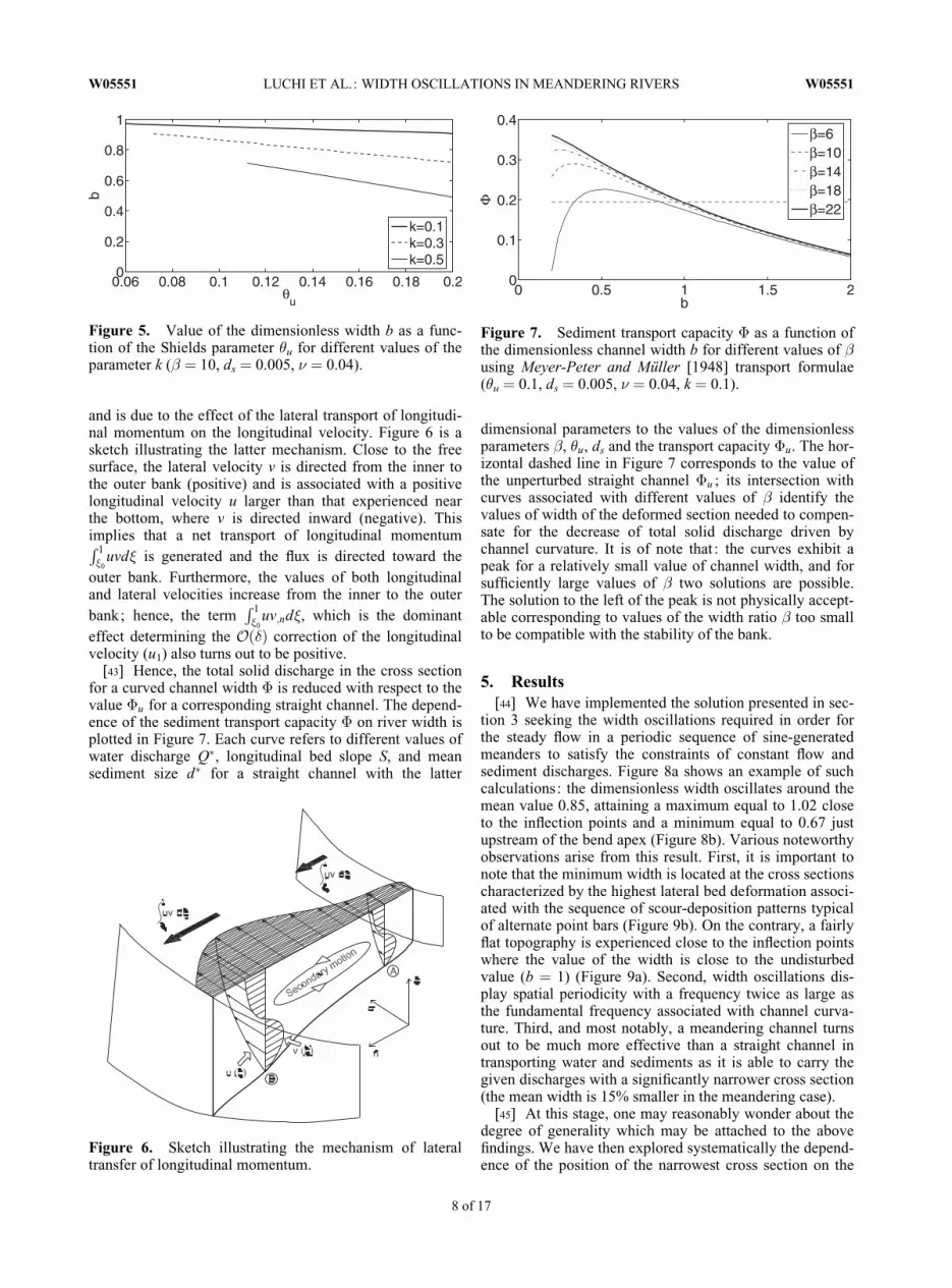
and is due to the effect of the lateral transport of longitudi-nal momentum on the longitudinal velocity. Figure 6 is asketch illustrating the latter mechanism. Close to the freesurface, the lateral velocity v is directed from the inner tothe outer bank (positive) and is associated with a positivelongitudinal velocity u larger than that experienced nearthe bottom, where v is directed inward (negative). Thisimplies that a net transport of longitudinal momentumR 1�0

uvd� is generated and the flux is directed toward the

outer bank. Furthermore, the values of both longitudinaland lateral velocities increase from the inner to the outer

bank; hence, the termR 1�0

uv;nd�, which is the dominant

effect determining the OðÞ correction of the longitudinalvelocity (u1) also turns out to be positive.

[43] Hence, the total solid discharge in the cross sectionfor a curved channel width � is reduced with respect to thevalue �u for a corresponding straight channel. The depend-ence of the sediment transport capacity � on river width isplotted in Figure 7. Each curve refers to different values ofwater discharge Q�, longitudinal bed slope S, and meansediment size d� for a straight channel with the latter

dimensional parameters to the values of the dimensionlessparameters �, �u, ds and the transport capacity �u. The hor-izontal dashed line in Figure 7 corresponds to the value ofthe unperturbed straight channel �u ; its intersection withcurves associated with different values of � identify thevalues of width of the deformed section needed to compen-sate for the decrease of total solid discharge driven bychannel curvature. It is of note that : the curves exhibit apeak for a relatively small value of channel width, and forsufficiently large values of � two solutions are possible.The solution to the left of the peak is not physically accept-able corresponding to values of the width ratio � too smallto be compatible with the stability of the bank.

5. Results[44] We have implemented the solution presented in sec-

tion 3 seeking the width oscillations required in order forthe steady flow in a periodic sequence of sine-generatedmeanders to satisfy the constraints of constant flow andsediment discharges. Figure 8a shows an example of suchcalculations: the dimensionless width oscillates around themean value 0.85, attaining a maximum equal to 1.02 closeto the inflection points and a minimum equal to 0.67 justupstream of the bend apex (Figure 8b). Various noteworthyobservations arise from this result. First, it is important tonote that the minimum width is located at the cross sectionscharacterized by the highest lateral bed deformation associ-ated with the sequence of scour-deposition patterns typicalof alternate point bars (Figure 9b). On the contrary, a fairlyflat topography is experienced close to the inflection pointswhere the value of the width is close to the undisturbedvalue (b ¼ 1) (Figure 9a). Second, width oscillations dis-play spatial periodicity with a frequency twice as large asthe fundamental frequency associated with channel curva-ture. Third, and most notably, a meandering channel turnsout to be much more effective than a straight channel intransporting water and sediments as it is able to carry thegiven discharges with a significantly narrower cross section(the mean width is 15% smaller in the meandering case).

[45] At this stage, one may reasonably wonder about thedegree of generality which may be attached to the abovefindings. We have then explored systematically the depend-ence of the position of the narrowest cross section on the

Figure 5. Value of the dimensionless width b as a func-tion of the Shields parameter �u for different values of theparameter k (� ¼ 10, ds ¼ 0.005, � ¼ 0.04).

Figure 6. Sketch illustrating the mechanism of lateraltransfer of longitudinal momentum.

Figure 7. Sediment transport capacity � as a function ofthe dimensionless channel width b for different values of �using Meyer-Peter and Müller [1948] transport formulae(�u ¼ 0.1, ds ¼ 0.005, � ¼ 0.04, k ¼ 0.1).


8 of 17

average aspect ratio of the channel � and on dimensionlessmeander wave number . Results of this investigation arereported in Figure 10a. The quantity � is the phase lagbetween the curvature peak and the narrowest cross sec-tion; hence, either � vanishes or it takes the value –1 if thenarrowest cross section is located at one of the bendapexes; it is equal to 60:5 if the narrowest cross section islocated at the inflection point. The four curves refer toincreasing values of the average aspect ratio � and showthat the minimum width is invariably experienced close tothe bend apex, shifting from upstream to downstream atsome threshold value of meander wavelength dependent onthe value of �. Figure 10b shows that, except for very long

and narrow meanders, the deepest cross section is invaria-bly located upstream of the bend apex, the more so thewider the channel. Finally, Figure 11 shows that the mini-mum width decreases as the meander wavelength increasesand the channel narrows; correspondingly, the amplitudeof the width variations increases.

[46] In order to interpret the above findings it is instruc-tive to examine the role played by convective terms. Acomparison between Figure 12a, based on the leading ordercomponent of the present solution and Figure 10a, whichincludes the effect of the lateral transfer of longitudinal mo-mentum accounted for by the convective terms appearingat first order, shows clearly that, as a result of the latter

Figure 8. (a) Dimensionless bed elevation relative to the undisturbed bed in a sequence of sine generatedmeanders and (b) associated spatial oscillations of the dimensionless channel width b (� ¼ 7, �u ¼ 0.09,ds ¼ 0.005, ¼ 0.11, � ¼ 0.06). Flow is from left to right.

Figure 9. Isocontours of dimensionless downstream velocity (a) at crossing and (b) at the bend apex ofthe sine-generated meander of Figure 8 (� ¼ 7, �u ¼ 0.09, ds ¼ 0.005, ¼ 0.11, � ¼ 0.06). Vectorsshowing the secondary motion are also represented.


9 of 17

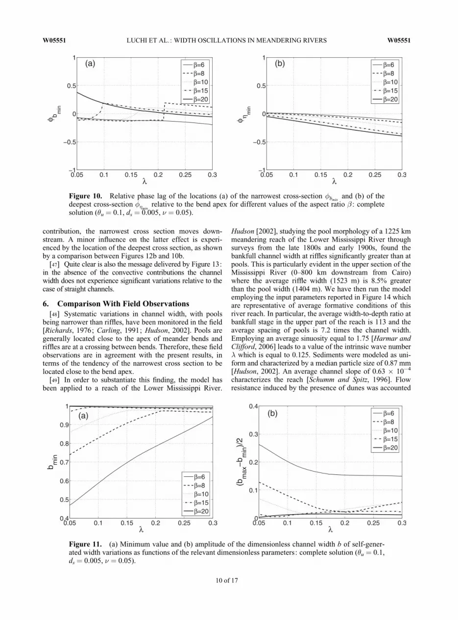
contribution, the narrowest cross section moves down-stream. A minor influence on the latter effect is experi-enced by the location of the deepest cross section, as shownby a comparison between Figures 12b and 10b.

[47] Quite clear is also the message delivered by Figure 13:in the absence of the convective contributions the channelwidth does not experience significant variations relative to thecase of straight channels.

6. Comparison With Field Observations[48] Systematic variations in channel width, with pools

being narrower than riffles, have been monitored in the field[Richards, 1976; Carling, 1991; Hudson, 2002]. Pools aregenerally located close to the apex of meander bends andriffles are at a crossing between bends. Therefore, these fieldobservations are in agreement with the present results, interms of the tendency of the narrowest cross section to belocated close to the bend apex.

[49] In order to substantiate this finding, the model hasbeen applied to a reach of the Lower Mississippi River.

Hudson [2002], studying the pool morphology of a 1225 kmmeandering reach of the Lower Mississippi River throughsurveys from the late 1800s and early 1900s, found thebankfull channel width at riffles significantly greater than atpools. This is particularly evident in the upper section of theMississippi River (0–800 km downstream from Cairo)where the average riffle width (1523 m) is 8.5% greaterthan the pool width (1404 m). We have then run the modelemploying the input parameters reported in Figure 14 whichare representative of average formative conditions of thisriver reach. In particular, the average width-to-depth ratio atbankfull stage in the upper part of the reach is 113 and theaverage spacing of pools is 7.2 times the channel width.Employing an average sinuosity equal to 1.75 [Harmar andClifford, 2006] leads to a value of the intrinsic wave number which is equal to 0.125. Sediments were modeled as uni-form and characterized by a median particle size of 0.87 mm[Hudson, 2002]. An average channel slope of 0.63 � 10�4

characterizes the reach [Schumm and Spitz, 1996]. Flowresistance induced by the presence of dunes was accounted

Figure 10. Relative phase lag of the locations (a) of the narrowest cross-section �bminand (b) of the

deepest cross-section ��minrelative to the bend apex for different values of the aspect ratio � : complete

solution (�u ¼ 0.1, ds ¼ 0.005, � ¼ 0.05).

Figure 11. (a) Minimum value and (b) amplitude of the dimensionless channel width b of self-gener-ated width variations as functions of the relevant dimensionless parameters: complete solution (�u ¼ 0.1,ds ¼ 0.005, � ¼ 0.05).


10 of 17

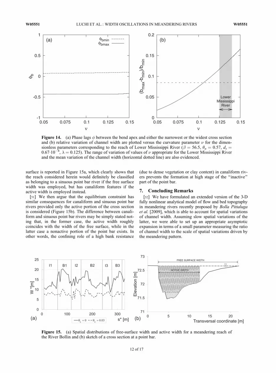
for in the simulations using the Engelund and Hansen[1967] predictor. In Figure 14a the phase lags betweenthe bend apex and either the narrowest or the widest crosssection are reported as a function of the curvature parame-ter �. This figure shows that the minimum width is invariablyexperienced just downstream from the bend apex and themaximum width downstream from the inflection point. More-over, the relative variation of the channel width increases asthe curvature parameter � increases (Figure 14b). For typicalaverage values of � between 0.125 and 0.14, calculated forvarious subset of meanders of the Lower Mississippi River byHarmar and Clifford [2006], the predicted maximum width isbetween 12% and 14.5% greater than the minimum predictedwidth. These values are slightly greater than those observed inthe field (8.5%).

[50] The picture emerging from our results unambigu-ously suggests that width variations driven by the constraint

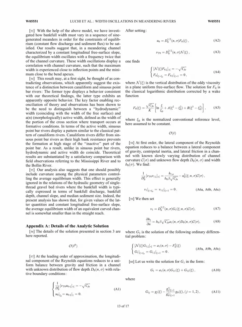
of morphodynamic equilibrium cannot be set at the basis ofthe distinction between canaliform and sinuous point barmeandering rivers. Is this surprising? Does it contradictobservations? In order to answer these questions we mustpreliminarily note that the equilibrium constraint does notinvolve the entire cross section, but rather the portion ofthe cross section where transport occurs at formative condi-tions, the width of which will be referred to as active width.This quantity has been recently recognized as a crucial pa-rameter by Ashmore et al. [2011] to describe the morphol-ogy and the dynamics of braiding rivers. If we assume thatthe latter conditions correspond to bankfull discharge andadopt a value for the critical Shields stress (here taken to beequal to 0.03), we readily obtain the spatial distribution ofthe active width at bankfull conditions for the reach of theBollin River discussed above. A comparison between thespatial distributions of active width and width of the free

Figure 12. Relative phase lag of the locations (a) of the narrowest cross-section �b0 minand (b) of the

deepest cross-section ��0 minrelative to the bend apex for different values of the aspect ratio � : leading

order of approximation (�u ¼ 0.1, ds ¼ 0.005, � ¼ 0.05). Note that at this order of approximation theeffect of the lateral transfer of longitudinal momentum accounted for by the convective terms does notappear.

Figure 13. (a) Minimum value and (b) amplitude of the dimensionless channel width b0 of self-generatedwidth variations as functions of the relevant dimensionless parameters: leading order of approximation(�u ¼ 0.1, ds ¼ 0.005, � ¼ 0.05).


11 of 17

surface is reported in Figure 15a, which clearly shows thatthe reach considered herein would definitely be classifiedas belonging to a sinuous point bar river if the free surfacewidth was employed, but has canaliform features if theactive width is employed instead.

[51] We then argue that the equilibrium constraint hassimilar consequences for canaliform and sinuous point barrivers provided only the active portion of the cross sectionis considered (Figure 15b). The difference between canali-form and sinuous point bar rivers may be simply stated not-ing that, in the former case, the active width roughlycoincides with the width of the free surface, while in thelatter case a nonactive portion of the point bar exists. Inother words, the confining role of a high bank resistance

(due to dense vegetation or clay content) in canaliform riv-ers prevents the formation at high stage of the ‘‘inactive’’part of the point bar.

7. Concluding Remarks[52] We have formulated an extended version of the 3-D

fully nonlinear analytical model of flow and bed topographyin meandering rivers recently proposed by Bolla Pittalugaet al. [2009], which is able to account for spatial variationsof channel width. Assuming slow spatial variations of thelatter, we were able to set up an appropriate asymptoticexpansion in terms of a small parameter measuring the ratioof channel width to the scale of spatial variations driven bythe meandering pattern.

Figure 14. (a) Phase lags � between the bend apex and either the narrowest or the widest cross sectionand (b) relative variation of channel width are plotted versus the curvature parameter � for the dimen-sionless parameters corresponding to the reach of Lower Mississippi River (� ¼ 56.5, �u ¼ 0.57, ds ¼0.67�10�4, ¼ 0.125). The range of variation of values of � appropriate for the Lower Mississippi Riverand the mean variation of the channel width (horizontal dotted line) are also evidenced.

Figure 15. (a) Spatial distributions of free-surface width and active width for a meandering reach ofthe River Bollin and (b) sketch of a cross section at a point bar.


12 of 17

[53] With the help of the above model, we have investi-gated how bankfull width must vary in a sequence of sine-generated meanders in order for the constraints of equilib-rium (constant flow discharge and sediment flux) to be sat-isfied. Our results suggest that, in a meandering channelcharacterized by a constant longitudinal free-surface slope,the equilibrium width oscillates with a frequency twice thatof the channel curvature. These width oscillations display acorrelation with channel curvature, such that the maximumwidth is experienced close to inflection points and the mini-mum close to the bend apexes.

[54] This result may, at a first sight, be thought of as con-tradicting observations, which apparently suggest the exis-tence of a distinction between canaliform and sinuous pointbar rivers: The former type displays a behavior consistentwith our theoretical findings, the latter type exhibits anapparently opposite behavior. The key factor enabling rec-onciliation of theory and observations has been shown tobe the need to distinguish between a ‘‘hydrodynamic’’width (coinciding with the width of the free surface) anda(n) (morphologically) active width, defined as the width ofthe portion of the cross section where transport occurs atformative conditions. In terms of the active width, sinuouspoint bar rivers display a pattern similar to the classical pat-tern of canaliform rivers. Canaliform rivers differ from sin-uous point bar rivers as their high bank resistance preventsthe formation at high stage of the ‘‘inactive’’ part of thepoint bar. As a result, unlike in sinuous point bar rivers,hydrodynamic and active width do coincide. Theoreticalresults are substantiated by a satisfactory comparison withfield observations referring to the Mississippi River and tothe Bollin River.

[55] Our analysis also suggests that one should possiblyinclude curvature among the physical parameters control-ling the average equilibrium width. This effect is generallyignored in the relations of the hydraulic geometry of single-thread gravel bed rivers where the bankfull width is typi-cally expressed in terms of bankfull discharge, bankfulldepth, channel slope, and median sediment size. Indeed, thepresent analysis has shown that, for given values of the lat-ter quantities and constant longitudinal free-surface slope,the average equilibrium width of an equivalent curved chan-nel is somewhat smaller than in the straight reach.

Appendix A: Details of the Analytic Solution[56] The details of the solution presented in section 3 are

here reported.

Oð0Þ

[57] At the leading order of approximation, the longitudi-nal component of the Reynolds equations reduces to a uni-form balance between gravity and friction in a channelwith unknown distribution of flow depth D0ðn; �Þ with rela-tive boundary conditions:

1

D20

½�T0u0;��;� ¼ �ffiffiffiffiffiffiffiCfu

pu0j�0¼ u0;�j1 ¼ 0:

8><>: (A1)

After setting:

u0 ¼ D1=20 ðn; �ÞF0ð�Þ ; (A2)

�T0 ¼ D3=20 ðn; �ÞN ð�Þ ; (A3)

one finds

½N ð�ÞF0;��;� ¼ �ffiffiffiffiffiffiffiCfu

pF0j�¼�0

¼ F0;�j�¼1 ¼ 0 ;

((A4)

where Nð�Þ is the vertical distribution of the eddy viscosityin a plane uniform free-surface flow. The solution for F0 isthe classical logarithmic distribution corrected by a wakefunction

F0ð�Þ ¼ffiffiffiffiffiffiffiCfu

pK

ln�

�0

þ Að�2 � �20Þ þ Bð�3 � �3

0Þ� �

; (A5)

where �0 is the normalized conventional reference level,here assumed to be constant.

OðÞ

[58] At first order, the lateral component of the Reynoldsequation reduces to a balance between a lateral componentof gravity, centripetal inertia, and lateral friction in a chan-nel with known slowly varying distribution of channelcurvature Cð�Þ and unknown flow depth D0ðn; �Þ and widthb0ð�Þ. We find:

1

D20

½�T0v1;��;� ¼h1;n

b0�ffiffiffiffiffiffiffiCfu

p � u20ð�; n; �ÞCð�Þ ;

v1j�¼�0¼ v1;�j�¼1 ¼ 0 : (A6a, A6b, A6c)

[59] We then set

v1 ¼ D3=20 ðn; �ÞG1ð�; n; �ÞCð�Þ; (A7)

@h1

@n¼ b0�


pa1ðn; �ÞD0ðn; �ÞCð�Þ; (A8)

where G1 is the solution of the following ordinary differen-tial problem:

½N ð�ÞG1;��;� ¼ a1ðn; �Þ � F20ð�Þ

G1j�¼�0¼ G1;�j�¼1 ¼ 0 :

((A9a, A9b, A9c)

[60] Let us write the solution for G1 in the form:

G1 ¼ a1ðn; �ÞG11ð�Þ þ G12ð�Þ ; (A10)

where

G1j ¼ gjð�Þ �g0jj�¼1

g00j�¼1

g0ð�Þ; ð j ¼ 1; 2Þ ; (A11)


13 of 17

and gjð j ¼ 0; 1; 2Þ solutions of ordinary differential prob-lems identical with those solved by Seminara and Solari[1998] (equations (26) and (27) of that paper). Note thatsystem (A9) has been solved analytically but the solutionis not reported here for the sake of brevity. We may thenproceed to determine the function a1ðn; �Þ by first inte-grating the continuity equation (6) over the flow depth, atOðÞ, with the use of the kinematic boundary condition(11c), and second integrating over the cross section, withthe use of the boundary condition (12) at the sidewallto get

a1ðn;�Þ ¼ a10�a11

Cð�ÞD5=20

@

@�ðb0

Z n

�1D3=2

0 IF0 dnÞ�D3=20 IF0 b0;� n

�;

�(A12)

where

a10 ¼ �IG12

IG11

; a11 ¼�


pIG11

; (A13)

and If ð f ¼ F0;G11;G12Þ is the integral ðR 1�0

f d�Þ. By sub-stituting equations (A12) and (A10) into equations (A7)and (A8) one gets the expression (21) for secondary flow.

[61] Let us finally come to the sediment continuity equa-tion (7). At OðÞ, in the rescaled coordinates, it reads:

qs0;� �b0;�b0

nqs0;n þ1


p qn1;n ¼ 0 : (A14)

With the help of the closure relationship for q (equations(13)–(15)) rewritten in terms of the rescaled coordinatesand expanded in powers of and with boundary conditionsforcing the normal component of sediment flux to vanish atthe side walls (12), the equation (A14) can be reduced to anonlinear partial differential equation for the unknownfunctions D0ð�; nÞ and b0ð�Þ. We find:

D0;n¼�b0


R=

v1;�j�0

u0;�j�0

þ�


pqs0

@

@�b0

Z n

�1qs0 dn

� ��nqs0b0;�

� �( ):

(A15)

[62] Proceeding at the first order of approximation, con-vective terms appear in the longitudinal component of theequations of motion (4). After setting:

u1 ¼ D1=20 ðn; �ÞF1ð�; n; �Þ; (A16)

some algebra allows us to derive the problem for F1 whichtakes the form:

½N ð�ÞF1;��;� ¼ R1þ1

2R2½F2

0 �þ1

2R3½F0G1�

�3

2R4

�F0;�

Z �

�0

F0 d�

��5

2R5

�F0;�

Z �

�0

G1 d�

�F1j�¼�0

¼F1;�j�¼1¼ 0;

8>>>>>><>>>>>>:(A17)

with Rjð j¼1;5Þ coefficients depending on � and n havingthe form:

R1 ¼ �ffiffiffiffiffiffiffiCfu

p D1

D0�u1;�

u0;�

�0

� �þb0nCð�Þ�Cfu

R2 ¼ R4¼D0;��b0;�b0

nD0;n

R3 ¼ R5¼1


p Cð�ÞD0D0;n;

(A18)

the solution for F1 can be given the form:

F1¼R1F11�1

2R2F12�

1

2R3F13�

3

2R4F14�

5

2R5F15; (A19)

where

F1j¼ fjð�Þ�f 0jj�¼1

f 00j�¼1

f0ð�Þðj¼1;5Þ (A20)

and fj ðj¼0;5Þ are solutions of ordinary differential prob-lems identical with those solved by Bolla Pittaluga et al.[2009] (equations (43) and (44) of that paper).

Oð2Þ

[63] The lateral component of the Reynolds equations atorder Oð2Þ includes many second-order effects that cor-rect the secondary flow. After setting

v2¼D3=20 ðn;�ÞG2ð�;n;�ÞCð�Þ; (A21)

some algebra allows us to derive the differential system forG2 which takes the form:

½N ð�ÞG2;��;� ¼ a2þR8 a1þR6½F20 �þR7½F0G1�þ

3

2R3½G1�2

�2½F0F1��3

2R4

"G1;�

Z �

�0

F0 d�

#

�5

2R3

"G1;�

Z �

�0

G1 d�

#G2j�0

¼ G2;�j1¼ 0;

8>>>>>>>>>>>>><>>>>>>>>>>>>>:(A22)

with Rjð j¼6;8Þ coefficients depending on � and n havingthe form:

R6 ¼ �D1

D0�u1;�

u0;�

�0

� �þb0nCð�Þ�


p;

R7 ¼3

2D0;��

b0;�b0

nD0;nþ2

3

D0

Cð�ÞC;��

;

R8 ¼D1

D0�u1;�

u0;�

�0

� �� b1

b0;

(A23)

and the function a2ðn;�Þ determined first integrating thecontinuity equation (6) over the flow depth, at Oð2Þ, withthe use of the kinematic boundary condition (11c), and sec-ond integrating over the cross section, with the use of theboundary condition (12) at the sidewall. The system (A22)


14 of 17

has been solved analytically but the solution is not reportedhere for the sake of brevity.

[64] Following a procedure similar to the one reported forthe previous order the sediment continuity equation atO (2) leads to the following differential equation:

D1;n ¼ �b0


R=

v2;�j�0

u0;�j�0

þ�


pqs0

@

@�b0

Z n

�1qs1 dn

��(

þ b1

Z n

�1qs0 dn

�� nðqs1b0;� þ qs0b1;�Þ

�

þ qn1

qs0�


pb0nCð�Þ þ qs1

qs0� u1;�j;�0

u0;�j;�0

� �

þF2r h1;n þ

b1

b0D0;n ;

(A24)

to be solved with similar boundary conditions as forequation (A15).

Appendix B: Details of the Physical Interpretation[65] Let us derive the forms taken by the constraints (36),

(37) at O (0) and O (1). We then substitute (32), (34) into(36) and (37) and equate likewise powers of to find thefollowing relationships:

Oð0Þ

b0

Z þ1

�1D

3=20 IF0 dn ¼ 2IF0 ; (B1)

b0

Z þ1

�1ð�uD0 � �cÞ3=2dn ¼ 2ð�u � �cÞ3=2: (B2)

[66] Next we use (31), (33), (35) to express D0 in terms ofthe parameters l and k. The above constraints then take theform:

2b0

5k½ð1þ l0 þ kÞ5=2 � ð1þ l0 � kÞ5=2� ¼ 2; (B3)

2b0

5kT½ð1þ l0T þ kTÞ5=2 � ð1þ l0T � kTÞ5=2� ¼ 2; (B4)

where

T ¼ �u

ð�u � �cÞ: (B5)

[67] The equations (B3) and (B4) have been solved forthe parameters b0 and l0 for given values for the parametersk and �u.

OðÞ

At the next order of approximation (36) and (37) take theform:

2IF0

b1

b0þ b0

Z þ1

�1ðD1D1=2

0 IF0 þ IF1 D3=20 Þdn ¼ 0; (B6)

b1

b0ð�u � �cÞ3=2 þ 3

2b0�u

Z þ1

�1ðD0f Þð�uD0 � �cÞ1=2dn ¼ 0; (B7)

where f ¼ F1;�

F0;�j�¼�0

. Next we use (33) to express D1 in terms

of the parameter l1 and perform the integrations to find:

1

2ðUb E7=2

� þ Zb E3=2� þ Ua E7=2

þ þ Za E3=2þ Þb0 þ b1 ¼ 0; (B8)

SaG3=2� þ SbG3=2

þ þ b1 ¼ 0; (B9)

where the functions Eþ, E�, Ua, Ub, Za, Zb, Sa, Sb read:

Ua ¼3

7

Cfu �� 1

7

Z 1

0F13d�

�ffiffiffiffiffiffiffiCfu

p � 5

7

Z 1

0F15d�


p ;

Ub ¼ �3

7

Cfu�þ 1

7

Z 1

0F13d�


p þ 5

7

Z 1

0F15d�


p ;

Za ¼ þ1

35

Eþ ð2 l0 þ 2� 5 kÞ� b20


pk2

þ b0 l1

k;

Zb ¼ �1

35

ð2 l0 þ 5 k þ 2ÞE� �b20


pk2

� b0 l1

k;

Eþ ¼ 1þ k þ l0; E� ¼ 1� k þ l0;

Sa ¼3

70

b0ðA� T 2 þ Pþ T þ 8Þ T 2�Cfu

�

þ 1

70

ðS� T2 þ Lþ T þ 8Þb30


p�

T2k2� 1

2

b20l1k

�;

Sb ¼ � 3

70

b0ðAþ T2 þ P� T þ 8Þ T 2�Cfu

�

� 1

70

ðSþ T 2 þ L� T þ 8Þb03ffiffiffiffiffiffiffiCfu

p�

T 2k2þ 1

2

b02l1k

�;

(B10)

and ¼R 1�0

F0G1d� represents the depth averaged contribu-tion of the convective term uv;n. Note that �0 has beenassumed equal to zero and that we have employed the fol-lowing notations:

Sþ ¼ �6 l20 þ ð9 k � 14Þl0 þ 15 k2 þ 21 k;

S� ¼ �6 l20 þ ð�9 k � 14Þl0 þ 15 k2 � 21 k;

Lþ ¼ 2 l0 þ 12 k � 14;L� ¼ 2 l0 � 12 k � 14;

Aþ ¼ 15 l20 þ ð30 k þ 42Þl0 þ 42 k þ 15 k2 þ 35;

A� ¼ 15 l20 þ ð�30 k þ 42Þl0 � 42 k þ 15 k2 þ 35;

Pþ ¼ �28þ 12 k � 12 l0;P� ¼ �28� 12 k � 12 l0;

Gþ ¼ Tk þ 1þ Tl0;G� ¼ �Tk þ 1þ Tl0: (B11)


15 of 17

[68] The equations (B8) and (B9) have been solved forthe parameters b1 and l1 for given values of the parametersk and �u.

Notation

a1 Function (equation (22))a10 Constant (equation (23))a20 Constant (equation (27))

B Local value of half channel widthBu Reference half channel widthb Local value of half channel width

scaled by the reference half channelwidth

b0; b1; bm Local value of half channel widthscaled by the reference half channelwidth at leading order, first-order, andm-order of approximation, respectively

b� Function (equation (9))C Curvature of the channel axis

Cfu Friction coefficient at the referencestate

D Local value of flow depthDu Reference flow depth

D0;D1;Dm Local value of flow depth at leadingorder, first-order, and m-order ofapproximation, respectively

d Diameter of sediment particlesds Relative roughnessFr Froude numberF0 Function describing the vertical

distribution of the flow velocity atleading order

F1 Function (equation (25))G (2 � 2) matrix

Gnn;Gn�;G�n;G�� Elements of GG11;G12 Functions (equation (23))gG22

Function (equation (27))g Gravityh Free-surface elevation

h0; h1; hm Free-surface elevation at leadingorder, first-order, and m-order ofapproximation, respectively

I IntegralR 1�0

d�k Transversal slope of the bed surfaceL Intrinsic meander wavelengthl Correction of the average

dimensionless flow depthl0; l1 Correction of the average dimension-

less flow depth at leading orderand first order of approximation,respectively

N Metric coefficientn̂b Unit vector normal to the banksQ Flow dischargeq Sediment flux per unit width

qn1 Lateral component of the sedimentflux per unit width at first order

qs0; qs1 Longitudinal component of the sedi-ment flux per unit width at leadingorder and first order of approximation,respectively

q�; qn Longitudinal and lateral componentsof the sediment flux per unit width

R Dimensionless coefficientRp Particle Reynolds numberrc Empirical constant, with a value of�0.56

r0 Typical radius of curvature of thechannel axis

S Average channel slopes; n; z Intrinsic longitudinal, lateral, and

vertical coordinate, respectivelysp Relative particle density

Tzs Bottom stressUu Scale for local velocity

u Velocity vectoru0; u1; um Longitudinal component of the local

velocity at leading order, first-order, andm-order of approximation, respectively

u; v;w Longitudinal, lateral and vertical compo-nents of the local velocity, respectively

v1; v2; vm Lateral component of the local veloc-ity at first order, second order, andm-order of approximation, respectively

< v1 >;< v2 > Lateral component of depth-averagedvelocity at first order and secondorder of approximation, respectively

v10; v20 Centrifugally induced secondary flowwith vanishing depth average at firstorder and second order of approxima-tion, respectively

W Local value of channel widthwm Vertical component of the local ve-

locity at the m-order of approximationz0 Conventional reference elevation for

no slip� Reference aspect ratio of the channel Perturbation parameter� Local value of the bed elevation Intrinsic meander wave number� Curvature parameter�T Eddy viscosity of the fluid phase� Longitudinal component of the dimen-

sionless sediment flux per unit width�u Longitudinal component of the

dimensionless sediment flux per unitwidth at the reference state

�0 Longitudinal component of the dimen-sionless sediment flux per unit width atleading order of approximation

� Phase lag between curvature peak andnarrowest or widest cross section

� Density of the fluid phase�s Density of sediment particles� Rescaled intrinsic longitudinal coordi-

nate ss� Tangential component of the stress

vector acting on the bed� Shields stress�c Critical value of shields stress�u Shields stress at the reference state

�0; �1 Shields stress at leading order and firstorder of approximation, respectively


16 of 17

# Inflection angle� Normalized vertical coordinate�0 Conventional dimensionless reference

elevation for no slip

[69] Acknowledgments. This work has been developed within theframework of the National Project cofunded by the Italian Ministry of Uni-versity and of Scientific and Technological Research ‘‘Ecomorphodynam-ics of tidal environments and climate change’’ (PRIN 2008). Partialsupport has also come from Fondazione Cassa di Risparmio di Verona,Vicenza, Belluno ed Ancona (Progetto RIMOF).We thank the AssociateEditor, Erik Mosselman, and an anonymous reviewer for providing helpfulcomments on this paper.

ReferencesAshmore, P., W. Bertoldi, and J. Tobias Gardner (2011), Active width of

gravel-bed braided rivers, Earth Surf. Processes Landforms, 36(11),1510–1521, doi:10.1002/esp.2182.

Ashworth, P. J. (1996), Mid-channel bar growth and its relationship to localflow strength and direction, Earth Surf. Processes Landforms, 21(2),103–123.

Bertoldi, W., and M. Tubino (2005), Bed and bank evolution of bifurcatingchannels, Water Resour. Res., 41, W07001, doi:10.1029/2004WR003333.

Bolla Pittaluga, M., and G. Seminara (2011), Nonlinearity and unsteadinessin river meandering: a review of progress in theory and modelling, EarthSurf. Processes Land., 36, 20–38. doi:10.1002/esp.2089.

Bolla Pittaluga, M., G. Nobile, and G. Seminara (2009), A nonlinear modelfor river meandering, Water Resour. Res., 45, W04432, doi:10.1029/2008WR007298.

Brice, J. C. (1982), Stream channel stability assessment, Federal HighwayAdministration, Rep. FHWA-RD-82-021, January, U.S. Dep. of Trans-portation, Washington, D. C., 42 pp.

Brice, J. C. (1984), Planform properties of meandering rivers, Keynotepaper, in River Meandering, Proceedings of the Conference Rivers, ’83New Orleans, LA, 24–26 October 1983, edited by C. M. Elliott, pp. 1–15,American Society of Civil Engineers, N. Y.

Camporeale, C., P. Perona, A. Porporato, and L. Ridolfi (2007), Hierarchyof models for meandering rivers and related morphodynamic processes,Rev. Geophys., 45, RG1001, doi:10.1029/2005RG000185.

Carling, P. A. (1991), An appraisal of the velocity-reversal hypothesis forstable pool-riffle sequences in the river Severn, England, Earth Surf.Processes Landforms, 16(1), 19–31.

Darby, S. E., A. M. Alabyan, and M. J. Van de Wiel (2002), Numerical sim-ulation of bank erosion and channel migration in meandering rivers,Water Resour. Res., 38(9), 1163, doi:10.1029/2001WR000602.

Duan, J. G., and P. Y. Julien (2005), Numerical simulation of the inception ofchannel meandering, Earth Surf. Processes Landforms, 30, 1093–1110.

Engelund, F., and E. Hansen (1967), A Monograph on Sediment Transportin Alluvial Streams, Danish Technical Press, Copenhagen, Denmark.

Ferguson, R. I., D. R. Parsons, S. N. Lane, and R. J. Hardy (2003), Flow inmeander bends with recirculation at the inner bank, Water Resour. Res.,39(11), 1322, doi:10.1029/2003WR001965.

Harmar, O. P., and N. J. Clifford (2006), Planform dynamics of the LowerMississippi River, Earth Surf. Processes Landforms, 31(7), 825–843,doi:10.1002/esp.1294.

Hooke, J. M. (1986), The significance of mid-channel bars in an activemeandering river, Sedimentology, 33(6), 839–850.

Hooke, J. M., and L. Yorke (2011), Channel bar dynamics on multi-decadaltimescales in an active meandering river, Earth Surf. Processes Land-forms, 36(14), 1910–1928, doi:10.1002/esp.2214.

Hudson, P. F. (2002), Pool-riffle morphology in an actively migratingalluvial channel: The Lower Mississippi River, Phys. Geogr., 23(2),154–169.

Klaassen, G. J., E. Mosselman, and H. Brühl (1993), On the prediction ofplanform changes in braided sand-bed rivers, in Advances in Hydro-Science

Engineering, edited by S. S. Y. Wang, pp. 134–146, Univ. of Mississippi,Oxford, Miss.

Knighton, A. (1972), Changes in a braided reach, Geol. Soc. Am. Bull., 83,3813–3822.

Lagasse, P. F., W. J. Spitz, L. W. Zevenbergen, and D. W. Zachmann(2004), Handbook for predicting stream ameander migration, NCHRPRep. 533, TRB, National Research Council, Washington, D. C.

Leopold, L. B., and M. G. Wolman (1960), River Meanders, Geol. Soc. Am.Bull., 71(6), 769–793.

Luchi, R., G. Zolezzi, and M. Tubino (2010a), Modelling mid-channel barsin meandering channels, Earth Surf. Process. Landforms, 35(8), 902–917.

Luchi, R., J. M. Hooke, G. Zolezzi, and W. Bertoldi (2010b), Width varia-tions and mid-channel bar inception in meanders: River Bollin (UK),Geomorphology, 119(1–2), 1–8, doi:10.1016/j.geomorph.2010.01.010.

Luchi, R., G. Zolezzi, and M. Tubino (2011), Bend theory of river meanderswith spatial width variations, J. Fluid Mech., 681, 311–339, doi:10.1017/jfm.2011.200.

Meyer-Peter, E., and R. Müller (1948), Formulas for bed load transport, inProceedings of the 2nd Int. Congress, Int. Association for HydraulicResearch, vol. 2, 39–64; Int. Assoc. for Hydraul. Res., Stockholm,Sweden.

Mosselman, E. (1998), Morphological modeling of rivers with erodiblebanks, Hydrol. Processes, 12, 1357–1370.

Mosselman, E., T. Shishikura, and G. J. Klaassen (2000), Effect of bank sta-bilization on bend scour in anabranches of braided rivers, Phys. Chem.Earth, 25(7–8), 699–704.

Nanson, G. C., and E. J. Hickin (1983), Channel migration and incision onthe Beatton River, J. Hydraul. Eng., 109(3), 327–337.

Parker, G. (1984), Lateral bed load transport on side slopes, J. Hydraul.Engng. ASCE, 110(2), 197–199.

Parker, G. (1990), Surface-based bedload transport relation for gravel riv-ers, J. Hydraul. Res., 28(4), 417–436.

Parker, G., Y. Shimizu, G. V. Wilkerson, E. C. Eke, J. D. Abad, J. W.Lauer, C., Paola, W. E. Dietrich, and V. R. Voller (2011), A new frame-work for modeling the migration of meandering rivers, Earth Surf. Pro-cess. Landforms, 36(1), 70–86.

Parsons, D., Ferguson, R. I., Lane, S. N., and R. J. Hardy (2004), Flow struc-tures in meander bends with recirculation zones: implications for bendmovements, in Proceedings River Flow 2004, vol. 1, edited by M. Greco,A. Carravetta, and R. D. Morte, pp. 49–59, Balkema, London, U. K.

Pizzuto, E. J., and J. S. Meckelnburg (1989), Evaluation of a linear bankerosion equation, Water Resour. Res., 25, 1005–1013.

Repetto, R., M. Tubino, and C. Paola (2002), Planimetric instability ofchannels with variable width, J. Fluid Mech., 457, 79–109.

Richards, K. (1976), Channel width and the riffle-pool sequence, Geol. Soc.Am. Bull., 87, 883–890.

Rüther, N., and N. R. B. Olsen (2007), Modelling free-forming meanderevolution in a laboratory channel using three-dimensional computationalfluid dynamics, Geomorphology, 89(34), 308–319.

Schumm, S. A., and W. J. Spitz (1996), Geological influences on the LowerMississippi River and its alluvial valley, Eng. Geol., 45(14), 245–261.

Seminara, G. (1998), Stability and morphodynamics, Meccanica, 33, 59–99.Seminara, G. (2006), Meanders, J. Fluid Mech., 554, 271–297.Seminara, G., and L. Solari (1998), Finite amplitude bed deformations in

totally and partially transporting wide channel bends, Water Resour.Res., 34(6), 1585–1598.

Solari, L., and G. Seminara (2005), On width variations in meanderingrivers, in Proc. 4th IAHR Symp. on River, Coastal and Estuarine Mor-phodynamics, RCEM 2005, 4–7 October, Urbana, Illinois, USA, editedby G. Parker and M. H. Garcia, vol. 2, 745–751, Taylor & Francis, Phila-delphia, Pa.

Talmon, A. M., N. Struiksma, and M. C. L. M. Van Mierlo (1995), Labora-tory measurements of the sediment transport on transverse alluvial-bedslopes, J. Hydraul. Res., 33, 495–517.

Vermeulen, B., S. W. Van Berkum, B. W. H. De Vries, and A. J. F. Hoitink(2011), Morphology of sharp bends in the Mahakam River, Proc. 7thIAHR Symp. on River, Coastal and Estuarine Morphodynamics, RCEM2011, 6–8 September, Tsinghua Univ. Press, Beijing, China.


17 of 17

Documents

Spatial width oscillations in meandering rivers at equilibrium