A nonlinear model for river meandering

A nonlinear model for river meandering

M. Bolla Pittaluga,1 G. Nobile,1 and G. Seminara1

Received 18 July 2008; revised 9 January 2009; accepted 6 February 2009; published 30 April 2009.

[1] We develop a nonlinear asymptotic theory of flow and bed topography in meanderingchannels able to describe finite amplitude perturbations of bottom topography and accountfor arbitrary, yet slow, variations of channel curvature. This approach then allows us toformulate a nonlinear bend instability theory, which predicts several characteristic featuresof the actual meandering process and extends results obtained by classical linear bendtheories. In particular, in agreement with previous weakly nonlinear findings andconsistently with field observations, the bend growth rate is found to peak at some valueof the meander wave number, reminiscent of the resonant value of linear stabilitytheory. Moreover, a feature typical of nonlinear waves arises: the selected wave numberdepends on the amplitude of the initial perturbation (for given values of the relevantdimensionless parameters), and in particular, larger wavelengths are associated with largeramplitudes. Meanders are found to migrate preferentially downstream, though upstreammigration is found to be possible for relatively large values of the aspect ratio of thechannel, a finding in agreement with the picture provided by linear theory. Meanders arefound to slow down as their amplitude increases, again a feature typical of nonlinearwaves, driven in the present case by flow rather than geometric nonlinearities. The modelis substantiated by comparing predictions with field observations obtained for a test case.The potential use of the present approach to investigate a number of as yet unexploredaspects of meander evolution (e.g., chute cutoff) is finally discussed.

Citation: Bolla Pittaluga, M., G. Nobile, and G. Seminara (2009), A nonlinear model for river meandering, Water Resour. Res., 45,

W04432, doi:10.1029/2008WR007298.

1. Introduction

[2] River meandering is a major topic in the field ofmorphodynamics. It has been the subject of extensiveinvestigations in the recent past. The review paper ofSeminara [2006], to which the reader is referred for a broadoverview of the subject, has outlined the main stepswhereby progress has been made in this field.[3] Let us briefly recall them. The attention was initially

focused on understanding the mechanism of meander for-mation starting from a straight channel configuration. Lin-ear stability analyses (so-called ‘‘bend’’ theories) wereemployed, hence linear models were developed to deter-mine flow and bed topography in weakly curved channels.The physical implications of the linearity assumption can beappreciated recalling the main ingredients of the processwhereby the pattern of bed topography develops in asinuous channel. The first feature is the establishment of acentrifugal secondary flow directed outwards close to thefree surface and inward close to the bed: it arises becausethe lateral pressure gradient driven by the lateral slope of thefree surface established in a bend is unable to provide thecentripetal force required for fluid particles to move alongpurely longitudinal trajectories. If the bed is nonerodible, a

‘‘free vortex’’ effect prevails initially, longitudinal trajecto-ries in the inner part of the bend being shorter than in theouter part. As a result, flow at the inner bend acceleratesrelative to the outer bend. This is a purely metric effectwhich is accounted for also in linear models. Proceedingdownstream, a net transfer of momentum toward the outerbend is driven by the secondary flow (the outward transferoccurring in the upper layer prevailing on the inwardtransfer occurring in the lower layer), hence the thread ofhigh velocity progressively moves from the inner to theouter bend. In the context of perturbation approaches wherethe basic state is laterally uniform, this is a second-ordereffect hence it is not accounted for in the context of linearmodels. The picture changes considerably when the bed iserodible. Under the latter conditions, secondary flow alsoaffects the motion of grain particles: they deviate from thelongitudinal direction, hence sediments are transportedtoward the inner bends where a sequence of so-called pointbars are built up while pools develop at the outer bends. Thebar-pool pattern then drives a topographical component ofthe secondary flow and an additional contribution to sedi-ment transport which further modifies the bed topography.Linear theories are indeed able to generate this topograph-ical effect, though the important role of the lateral transfer ofmomentum driven by the topographical secondary flow isagain neglected, formally appearing still at second order.The need to relax the linear constraint was recognized in theengineering literature, where a large effort was made toconstruct a rational framework, amenable to numericaltreatment, in order to predict flow and bed topography in

1Department of Civil, Environmental and Architectural Engineering,University of Genova, Genova, Italy.

Copyright 2009 by the American Geophysical Union.0043-1397/09/2008WR007298

W04432

WATER RESOURCES RESEARCH, VOL. 45, W04432, doi:10.1029/2008WR007298, 2009

1 of 22

meandering channels with finite curvature and arbitrarywidth variations. These models serve the interests of riverengineering, being fairly successful when applied to rela-tively short reaches of alluvial rivers and fairly short events.[4] However, a more general interest toward the con-

struction of sound analytical nonlinear models arises in thecontext of the fundamental research on the subject. In fact,the availability of such a model is potentially suitable toinvestigate a number of important processes observed inmeander evolution, which still await to be understood. Letus list some of these processes, which did motivate ourpresent work.[5] An inspection of the patterns of meandering rivers

(e.g., Figure 1) reveals that the river width, defined as thewidth of the stream free surface, undergoes typically spatialoscillations which display a distinct correlation with channelcurvature. The river width may peak at bend apexes, reach-ing a minimum at inflection points (Figure 1a) or viceversa(Figure 1b). Note that this issue bears both a conceptual anda practical relevance. In fact, we know from the seminalcontributions of Parker [1978a, 1978b] that the averagewidth of straight channels in equilibrium is ultimatelycontrolled by requirements of bank stability. We also knowthat meandering does not alter such equilibrium in the mean.Why and how? An attempt at clarifying the latter points hasbeen recently proposed by Parker and Shimizu [2008].However, provided the river is free to erode and deposit,i.e., it is able to choose its own width, then curvature makesthe stream unable to keep a constant width. Why? And towhat extent channel widening at the bend apexes modifiesthe scour pattern typically observed at the outer banks, thusaffecting the lateral migration of meanders?[6] A further reason of interest is related to a second

observation: it is not uncommon to detect the formation ofan island at bends of meandering channels (Figure 2). Thepresence of the island then forces the stream to bifurcateinto an outer and an inner branch. In natural settings this isnot a stable configuration: sooner or later, the stream willcut through and abandon the outer branch. The latter wellknown process is described as chute cutoff and occurstypically in wide bends with fairly large curvatures, highdischarges, poorly cohesive unvegetated banks and high

slope [Howard and Knutson, 1984]. Though some recentnumerical investigations [Jager, 2003, and references there-in] have attempted to model the latter process, it is notunfair to state that the occurrence of chute cutoff is aproblem yet awaiting to be understood. The availability ofan analytical nonlinear model of river meanders wouldallow to approach the latter problem. In fact, the processof widening is known [Repetto et al., 2002] to promote theformation of steady central bars in straight channels: it isthen natural to wonder whether the formation of bendislands is similarly related to a bottom instability drivenby widening of a curved channel. The next step would thenconsist of modeling the tendency of the central bar to forcethe stream to bifurcate into an outer and an inner branchleading to the occurrence of chute cutoff.[7] A third motivation to develop an analytical approach

to nonlinear meanders is related to the fundamental interestof a nonlinear theory of bend instability. In fact, lineartheories display the occurrence of a resonance mechanismwhich controls the selection of the preferred wavelength forbend instability [Blondeaux and Seminara, 1985]. Reso-nance is obviously damped by nonlinear effects, as shownby the weakly nonlinear theory of Seminara and Tubino[1992]. However, no fully nonlinear theory has been pro-posed so far, though the role of nonlinearity is known toaffect the flow field, hence the selection mechanism, con-siderably. In the present work, we do develop a nonlineartheory of bend instability, based on the nonlinear asymptoticsolution of flow and bed topography in meandering riversdeveloped herein.[8] Finally an analytical approach to nonlinear meanders

involving a sufficiently modest computational effort, willhopefully allow us to investigate the long-term morphody-namic evolution of meandering rivers, a topic which hasattracted the attention of both geomorphologists [Sun et al.,1996] and engineers [Camporeale et al., 2007]. For suchapplications, numerical solutions of the full 3-D governingequations or their shallow water version [e.g., Mosselman,1991; Shimizu, 2002] are not appropriate tools as thecomputational effort they require would be prohibitive.Researchers have then been forced to employ analyticallinear models for flow and bed topography, allowing only

Figure 1. Meander bends showing the dependence of river width on curvature and stage. (a) Maximumwidths experienced at bend apexes (Eel River, California) (from Google Earth) and (b) minimum widthsat bend apexes, and local widening in straight reach (tributary of the Amazon River, Brazil) (from GoogleEarth).

2 of 22

W04432 BOLLA PITTALUGA ET AL.: A NONLINEAR MODEL FOR RIVER MEANDERING W04432

for geometric nonlinearities arising from planform evolu-tion. The present model removes the latter restriction.[9] This idea is pursued by resorting to the use of

perturbation methods. We set up an appropriate perturbationexpansion for the solution of the problem of morphody-namics, valid in the general case of rivers with arbitrarydistributions of channel curvature, the only constraint beingthat flow and bottom topography must be ‘‘slowly varying’’in both longitudinal and lateral directions and channelcurvature must be ‘‘sufficiently small’’. The former assump-tion requires the channel to be ‘‘wide’’ with channelalignment varying on a longitudinal scale much larger thanchannel width, while the latter assumption is satisfiedprovided the radius of curvature of channel axis is largecompared with channel width. Both conditions are typicallymet in actual rivers but, in spite of the popularity enjoyed bylinear models, neither of them implies that perturbations ofbottom topography are necessarily ‘‘small’’. It may beuseful at this stage to clarify the latter statement by pointingout the fundamental distinction between the notion oflinearity and the notion of slow variation. The former isbased on the assumption that the amplitude of perturbationsof bed topography driven by channel curvature must besmall. The latter is based on the assumption that perturba-tions of bed topography must vary slowly in space. In orderto further clarify this concept, let us consider the simplestpossible case: a meander with channel axis defined inCartesian coordinates as follows:

y ¼ � cos wt � lxð Þ c ¼ y00 ¼ ��l2 cos wt � lxð Þ

with � meander amplitude, l(= 2p/L) meander wavenumber, L meander intrinsic length, w angular frequencyand c meander curvature. The above relationships showvarious obvious facts: (1) channel curvature c can be smallwith meander amplitude � ‘‘large’’ as long as the meanderis ‘‘long’’ enough (l � 1) (i.e., slowly varying), and(2) conversely, a meander bend can be ‘‘sharp’’ (largecurvature) even if its amplitude � is small, provided themeander is ‘‘short’’ enough (l � 1). In this paper we areonly interested in the former case.

[10] Taking advantage of the slowly varying assumption,a suitable extension of the approach developed by Seminaraand Solari [1998] to investigate bed deformations in con-stant curvature channels with constant width can be devel-oped. The latter approach allows for slow, yet finite,perturbations of flow and bed topography relative to a basicstate consisting of a gradually varying sequence of locallyuniform flow, slowly varying in both the lateral andlongitudinal directions. The only unknowns left for numer-ical computation are then flow depth, a slow function oflongitudinal and lateral coordinates, and variation of thelongitudinal free surface slope satisfying a strongly nonlineardifferential equation subject to continuity constraints.[11] The content of the paper is then organized as follows.

In chapter 2 we formulate the 3D problem of flow in sinuousalluvial channels with a noncohesive bed. In the analysis, thedirect effect of secondary flow on the transverse distributionof the main flow, leading to lateral transfer of longitudinalmomentum is accounted for. This effect, which has beenargued to be important by many authors [e.g., Nelson andSmith, 1989; Imran and Parker, 1999], appears at the firstorder of approximation in the present scheme. Section 3 isthen devoted to ascertaining the role of flow nonlinearity on‘‘bend instability theory’’ by coupling the morphodynamicmodel with a bank erosion law, expressing the dependenceof erosion intensity on the flow field. We are then able topredict the wavelength selected by bend instability as well asthe meander wave speed in a nonlinear context. The modelpredictions are then tested by a direct application to a testcase (a reach of the Cecina River, Italy) for which accuratedata obtained by recent detailed monitoring are available(section 4). Predictions of both the equilibrium configurationand of the wave number selected in the meandering processdo support the soundness of the present nonlinear approach.Finally, some discussion of future developments concludesthe paper.

2. Nonlinear Theory of Slowly Varying Meanders

[12] River morphodynamics deals with the turbulent freesurface flow of a low-concentration two-phase mixture of

Figure 2. A meander showing the formation of an island close to the bend apex (Finke River, Australia,courtesy of Aberdeen University, Geoff Pickup).

W04432 BOLLA PITTALUGA ET AL.: A NONLINEAR MODEL FOR RIVER MEANDERING

3 of 22

W04432

water and sediment particles bounded by a granular mediumconsisting of still sediment particles packed at their highestconcentration: in river morphodynamics one ultimatelywishes to determine the configuration of the bed interface.In other words, the mathematical problem of river morpho-dynamics is essentially a free boundary problem. Let usformulate it.

2.1. Formulation of the Problem

[13] Let us consider a sinuous alluvial channel with anoncohesive bed and refer it to the intrinsic coordinatessketched in Figure 3 (s*, n* and z* representing the longitu-dinal, lateral and vertical coordinates, respectively). In the caseof channels with constant width, say 2Bu*, the appropriatescaling for the intrinsic coordinates, the local mean velocityaveraged over turbulence u* = (u*, v*, w*)T, the flow depthD*, the free surface elevation h*, the eddy viscosity nT* and thesediment flux per unit width (qs*, qn*)

T reads:

s*; n*ð Þ ¼ B*u s; nð Þ; z*;D*; h*ð Þ ¼ D*u z;D;F2r h

� �;

u*; v*;w*ð Þ ¼ Uu* u; v;w=buð Þ; nT* ¼ffiffiffiffiffiffiffiCfu

pUu*Du*

� �nT ;

qs*; qn*ð Þ ¼ffiffiffiffiffiffiffiffiffiffiffiffiffiffiffiffiffiffiffiffiffiffiffiffiffiffisp � 1� �

gd*3q

qs; qnð Þ;

ð1Þ

where a star denotes dimensional quantities. Moreover, sp isthe relative particle density (= rs/r, with r and rs water andparticle density respectively), d* is the particle diameter (takento be uniform), Cfu is the friction coefficient, bu is the aspectratio of the channel, Fr is the Froude number and the index u

refers to properties of uniform flow in a straight channel withthe same flow discharge and the average channel slope S. Twoparameters arise, namely:

bu ¼Bu*

D*u; F2

r ¼ Uu*2

gDu*: ð2Þ

[14] We then consider a sinuous channel characterized bya slowly varying distribution of curvature c*(s) of thechannel axis. Flow and bottom topography are thenassumed to be slowly varying in both longitudinal andlateral directions. The above assumptions do not implythat perturbations of flow and bottom topography arenecessarily small. It is then appropriate to rescale thelongitudinal coordinate s as follows:

s ¼ s*

r0*¼ n0s: ð3Þ

We also take advantage of the hydrostatic approximation,which applies when the spatial scale of the relevanthydrodynamic processes largely exceeds the flow depth.Under these circumstances the vertical component ofReynolds equations simply states that pressure is hydro-statically distributed in the vertical direction. The steadyturbulent flow of water in a channel characterized by aslowly varying spatial distribution of channel curvature isthen governed by the longitudinal and lateral components ofReynolds equations, along with the continuity equations forthe fluid and solid phases. In dimensionless form, they read:

r u ¼ �h�1s n0c sð Þv ; ð4Þ

u rð Þuþ h�1s h;s � bu

ffiffiffiffiffiffiffiCfu

pnTu;zð Þ;z ¼ h�1

s buCfu � n0c sð Þuv� �

;

ð5Þ

u rð Þvþ h;n � bu


pnT v;zð Þ;z ¼ h�1

s n0c sð Þu2; ð6Þ

h�1s qs;s þ qn;n ¼ �h�1

s n0c sð Þqn; ð7Þ

where r is defined by (hs�1n0@/@s, @/@n, @/@z). Moreover

n0 is a curvature parameter, c(s) is dimensionless curvatureand hs is a metric coefficient, such that:

n0 ¼Bu*

r*0; c sð Þ ¼ r0*c* sð Þ ; hs ¼ 1þ n0nc sð Þ ; ð8Þ

where r0* is some typical radius of curvature of the channelaxis. In the lateral component of the momentum equationappear the main factors controlling the intensity ofsecondary flow, i.e., centripetal acceleration and the lateralslope of the free surface. The equations (4)–(7) must besupplemented with boundary conditions which may bewritten in the dimensionless form:

u ¼ v ¼ w ¼ 0 z ¼ z0; ð9Þ

u;z ¼ v;z ¼ w� h�1s n0uF2

r h;s � vF2r h;n ¼ 0 z ¼ F2

r h; ð10Þ

Z F2r h

z0

v dz ¼ qn ¼ 0 n ¼ �1: ð11Þ

Figure 3. Sketch illustrating the meandering channel and notations.

4 of 22


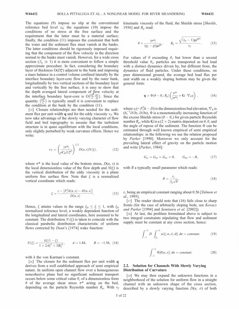
The equations (9) impose no slip at the conventionalreference bed level z0; the equations (10) impose theconditions of no stress at the free surface and therequirement that the latter must be a material surface;finally, the condition (11) imposes the constraint that boththe water and the sediment flux must vanish at the banks.The latter conditions should be rigorously imposed requir-ing that the component of the flow velocity in the directionnormal to the banks must vanish. However, for a wide crosssection (bu � 1) it is more convenient to follow a simpleapproximate procedure. In fact, considering the boundarylayer of thickness O(Du*) adjacent to the bank and imposinga mass balance in a control volume confined laterally by theinterface boundary layer-core flow and by the outer bank,longitudinally by two vertical sections of the boundary layerand vertically by the free surface, it is easy to show thatthe depth averaged lateral component of flow velocity at

the interface boundary layer-core is O�Du*L

@U@s

�. Since the

quantity�Du*L

�is typically small it is convenient to replace

the condition at the bank by the condition (11).[15] Closure relationships are then needed for the sedi-

ment flux per unit width q and for the eddy viscosity vT. Wenow take advantage of the slowly varying character of flowfield and bed topography to assume that the turbulentstructure is in quasi equilibrium with the local conditions,only slightly perturbed by weak curvature effects. Hence wewrite:

nT ¼ jt*jrCfuUu*

2

!1=2

Dðn; sÞNðxÞ; ð12Þ

where t* is the local value of the bottom stress, D(n, s) isthe local dimensionless value of the flow depth and N(x) isthe vertical distribution of the eddy viscosity in a planeuniform free surface flow. Note that x is a normalizedvertical coordinate which reads:

x ¼z� F2

r hðn; sÞ � Dðn; sÞ� �

Dðn; sÞ : ð13Þ

Hence, x attains values in the range x0 x 1, with x0normalized reference level, a weakly dependent function ofthe longitudinal and lateral coordinates, here assumed to beconstant. The distribution N (x) is taken to coincide with theclassical parabolic distribution characteristic of uniformflows corrected by Dean’s [1974] wake function:

NðxÞ ¼ kxð1� xÞ1þ 2Ax2 þ 3Bx3

; A ¼ 1:84; B ¼ �1:56; ð14Þ

with k the von Karman’s constant.[16] The closure for the sediment flux per unit width q

derives from a well established approach of semi empiricalnature. In uniform open channel flow over a homogeneousnoncohesive plane bed no significant sediment transportoccurs below some critical value qc of a dimensionless formq of the average shear stress t* acting on the bed,depending on the particle Reynolds number Rp. With vf

kinematic viscosity of the fluid, the Shields stress [Shields,1936] and Rp read:

q ¼ jt*jð|s � |Þgd* ; Rp ¼

ffiffiffiffiffiffiffiffiffiffiffiffiffiffiffiffiffiffiffiffiffiffiffiffiffiffiðsp � 1Þgd*3

qnf

: ð15Þ

For values of q exceeding qc but lower than a secondthreshold value qs, particles are transported as bed loadwith a distinct dynamics driven by, but different from, thedynamics of fluid particles. Under these conditions, onpure dimensional ground, the average bed load flux perunit width on a weakly sloping bottom may be given thegeneral form:

q ¼ Fðq� qc;RpÞt*jt*j þG rhh� �

; ð16Þ

where h (= Fr2h�D) is the dimensionless bed elevation,rh is

(hs�1@/@s, @/@n), F is a monotonically increasing function of

the excess Shields stress (q� qc) for given particle Reynoldsnumber Rp, whileG is a (2� 2) matrix dependent on q, qc andthe angle of repose of the sediment. The function F can beestimated through well known empirical of semi empiricalrelationships: in the following we use the relation proposedby Parker [1990]. Moreover we only account for theprevailing lateral effect of gravity on the particle motionand write [Parker, 1984]:

Gss ¼ Gsn ¼ Gns ¼ 0; Gnn ¼ �R; ð17Þ

with R a typically small parameter which reads:

R ¼ rc

bu

ffiffiffiq

p ; ð18Þ

rc being an empirical constant ranging about 0.56 [Talmon etal., 1995].[17] The reader should note that (16) fails close to sharp

fronts (for the case of arbitrarily sloping beds, see Kovacsand Parker [1994] and Seminara et al. [2002]).[18] At last, the problem formulated above is subject to

two integral constraints stipulating that flow and sedimentsupply must be constant at any cross section, hence:

Z þ1

�1

D

Z þ1

x0

uðx; n; sÞ dx dn ¼ constant; ð19Þ

Z þ1

�1

F qðn; sÞ½ � dn ¼ constant: ð20Þ

2.2. Solution for Channels With Slowly VaryingDistribution of Curvature

[19] We may then expand the unknown functions in aneighborhood of the solution for uniform flow in a straightchannel with an unknown shape of the cross section,described by a slowly varying function D(n, s) of both


5 of 22

W04432

the longitudinal and lateral coordinates. We can then expandthe solution in the form:

ðu; v;w; h;DÞ ¼ u0ðx; n; sÞ; 0; 0; h0ðsÞ=d;D0ðn;sÞ½ �þP11

ðum; vm;wm; hm;DmÞðdÞm; ð21Þ

where d is the small parameter (v0/bu


p). Note that, in

order to account for the small variations of the longitudinalfree surface slope associated with channel curvature, thefree surface elevation is divided by d. This allows the latterterm to be an order one quantity.[20] The latter expansion is then substituted into the

governing differential problem (4)–(7), conveniently rewrit-ten in terms of the transformed variables s, n and x usingthe chain rules:

@

@z! 1

D

@

@x;

@

@n! @

@nþ ð1� xÞD;n �F2

r h;nD

� �@

@x; ð22Þ

@

@s! @

@sþ ð1� xÞD;s �F2

r h;sD

� �@

@x: ð23Þ

[21] By substituting into the Reynolds equation the ex-pression for the vertical component of velocity derived fromintegrating the continuity equation of the liquid phase in thevertical direction, we derive the final form of the integro-differential equations, which are reported in Appendix A.[22] We then equate likewise powers of d to obtain a

sequence of differential problems, to be solved in terms ofthe unknown functions D and h,s.

Oðd0Þ

[23] At the leading order of approximation, the longi-tudinal component of the Reynolds equations reduces to auniform balance between gravity and friction in a channelwith unknown distribution of flow depth D0(n, s) andfree surface slope (�h0,s(s)) with relative boundaryconditions:

1

D20

½nT0u0;x �;x ¼ h0;s �ffiffiffiffiffiffiffiCfu

pu0 jx0 ¼ u0;x j1 ¼ 0:

8><>: ð24Þ

After setting:

u0 ¼ D1=20 ðn;sÞR1=2

0 ðsÞF0ðx; n;sÞ; ð25Þ

nT0 ¼ D3=20 ðn;sÞR1=2

0 ðsÞNðxÞ; ð26Þ

with R0 = 1 � h0,s/ffiffiffiffiffiffiffiCfu

p, one finds

½NðxÞF0;x�;x ¼ �ffiffiffiffiffiffiffiCfu

pF0jx¼x0

¼ F0;xjx¼1 ¼ 0;

8<: ð27Þ

The solution for F0 is the classical logarithmic distributioncorrected by a wake function

F0ðxÞ ¼ffiffiffiffiffiffiffiCfu

pk

lnxx0

þ Aðx2 � x20Þ þ Bðx3 � x30Þ� �

; ð28Þ

where x0 is the normalized conventional reference level,here assumed to be constant.

Oðd1Þ

[24] At first order, the lateral component of the Reynoldsequations reduces to a balance between lateral componentof gravity, centripetal inertia and lateral friction in a channelwith unknown, yet slowly varying, distributions of flowdepth D0(n, s) and free surface slope (�h0,s) as well asgiven slowly varying distribution of channel curvature c(s).We find:

1

D20

½nT0v1;x�;x ¼h1;n

bu


p � u20ðx; n;sÞcðsÞ;

v1jx¼x0¼ v1;xjx¼1 ¼ 0: ð29Þ

[25] We then set

v1 ¼ D3=20 ðn;sÞR1=2

0 ðsÞG1ðx; n;sÞcðsÞ; ð30Þ

@h1@n

¼ bu


pa1ðn;sÞD0ðn;sÞR0ðsÞcðsÞ; ð31Þ

whereG1 is the solution of the following ordinary differentialproblem:

½NðxÞG1;x�;x ¼ a1ðn; sÞ � F20 ðxÞ;

G1jx¼x0¼ G1;xjx¼1 ¼ 0:

8<: ð32Þ

[26] Let us write the solution for G1 in the form:

G1 ¼ a1ðn; sÞG11ðxÞ þ G12ðxÞ; ð33Þ

where

G1j ¼ gjðxÞ �g0j jx¼1

g00jx¼1

g0ðxÞ; ðj ¼ 1; 2Þ; ð34Þ

and gj( j = 0, 1, 2) solutions of ordinary differentialproblems identical with those solved by Seminara andSolari [1998, equations 26 and 27]. Note that system (32)has been solved analytically but the solution is not reportedhere for the sake of brevity. We may then proceed todetermine the function a1(n, s) first integrating thecontinuity equation (4) over the flow depth, at O(d), withthe use of the kinematic boundary condition (10), and

6 of 22


secondly integrating over the cross section, with the use ofthe boundary condition (11) at the sidewall to get

a1ðn; sÞ ¼ a10 �a11

cðsÞD5=20 R

1=20 IF0

@

@s

Z n

�1

D3=20 R

1=20 IF0

dn

� �;

ð35Þ

where

a10 ¼ � IG12

IG11

; a11 ¼IF0

IG11

bu


p: ð36Þ

and If (f = F0, G11, G12) is the integral (Rx01 fdx).

[27] Let us finally come to the sediment continuityequation (7). At O(d), in the rescaled coordinates, it reads:

bu


pqs0;s þqn1;n ¼ 0: ð37Þ

With the help of the closure relationship for q (equations(16)–(18)) rewritten in terms of the rescaled coordinatesand expanded in powers of d and with boundary conditionsforcing the normal component of sediment flux to vanish atthe sidewalls (11), the equation (37) can be reduced to anonlinear partial differential equation for the unknownfunctions D0(n,s) and h0,s (s). We find:

D0;n ¼ �ffiffiffiffiffiffiffiffiffiffiffiD0R0

p

R=d

v1;x jx0u0;x jx0

þbu


pqs0

@

@s

Z n

�1

qs0 dn

" #: ð38Þ

Note that the slowly varying character of the lateraldistribution of flow depth ensures that the value assumedby the ratio R/d appearing in equation (38) is an O(1)parameter. The reader will easily check that this is verifiedprovided the Shields stress attains values smaller than a fewunits. Equation (38) is to be solved with integral constraints(19) whereby the flow and sediment discharges must keepconstant in the longitudinal direction. The above differentialproblem can be solved numerically, marching in n for everysingle cross section. In particular, at each cross section j, westart with a set of trial values of flow depth at the bank D0j j,0and free surface slope correction h0,sj j. We then solve theequations (38) numerically in the whole domain. Thedifferences between the values of the liquid and the soliddischarges associated with the computed solution and theassigned values are then computed and the trial initialvalues are modified correspondingly until residual errorsreduce below some chosen value. This trial and errorprocedure allows us to determine the unknown functionsD0 (n, s) and h0,s(s). We have also checked whetherdistinct solutions of the above system of equations mightexist, possibly depending on the inability of part of the crosssection to transport sediments. The numerical tests we haveperformed suggest that this is not the case, provided theentire cross section transports sediments and the channelwidth is given.[28] Proceeding at the first order of approximation, con-

vective terms appear in the longitudinal component of theequations of motion (5). After setting:

u1 ¼ D1=20 ðn;sÞR1=2

0 ðsÞF1ðx; n;sÞ ð39Þ

some algebra allows us to derive the problem for F1 whichtakes the form:

NðxÞF1;x� �

;x ¼ R1 þ1

2R2½F2

0 � þ1

2R3½F0G1�

� 3

2R4 F0;x

Z x

x0

F0 dx

" #� 5

2R5 F0;x

Z x

x0

G1 dx

" #

F1jx¼x0¼ F1;xjx¼1 ¼ 0

8>>>>>><>>>>>>:

ð40Þ

with Rj( j = 1, 5) coefficients depending on s and n reportedin Appendix B. The solution for F1 can be given the form:

F1 ¼ R1F11 �1

2R2F12 �

1

2R3F13 �

3

2R4F14 �

5

2R5F15 ð41Þ

where:

F1j ¼ fjðxÞ �f 0j jx¼1

f 00 jx¼1

f0ðxÞ ð j ¼ 1; 5Þ ð42Þ

and fj ( j = 0, 5) are solutions of the following ordinarydifferential systems:

NðxÞ fj;x� �

;x ¼ difjjx0 ¼ 0

fj;xjx0 ¼ 1

8<: ð43Þ

where:

d0 ¼ 0 d1 ¼ 1 d2 ¼ �F20

d3 ¼ �F0G1 d4 ¼ F0;xR xx0F0 dx d5 ¼ F0;x

R xx0G1 dx

ð44Þ

Again system (43) has been solved analytically and thesolution is not reported here for the sake of brevity.

Oðd2Þ

[29] The lateral component of the Reynolds equations atorder O(d2) includes many second-order effects whichcorrect the secondary flow. After setting

v2 ¼ D3=20 ðn;sÞR1=2

0 ðsÞG2ðx; n;sÞcðsÞ ð45Þ

some algebra allows us to derive the differential system forG2 which takes the form:

NðxÞG2;x� �

;x ¼ a2 þ R8 a1 þ R6½F20 � þ R7½F0G1� þ

3

2R3½G1�2

�2½F0F1� �3

2R4 G1;x

Z x

x0

F0 dx

" #

� 5

2R3 G1;x

Z x

x0

G1 dx

" #

G2jx0 ¼ G2;xj1 ¼ 0

8>>>>>>>>>>>><>>>>>>>>>>>>:

ð46Þ

with Rj( j = 1, 8) coefficients depending on s and n andreported in the appendix. The system 46 has been solvedanalytically but the solution is not reported here for the sakeof brevity.


7 of 22

W04432

Figure 4. (a, b) Dimensionless bed elevation relative to the undisturbed bed and (c, d) dimensionlessvalue of the vertically averaged longitudinal velocity predicted by the present theory for two periodicsequences of sine generated meanders, characterized by different dimensionless wave numbers (l = 0.07(Figure 4a), l = 0.185 (Figure 4b), l = 0.07 (Figure 4c), and l = 0.185 (Figure 4d)). The values of therelevant dimensionless parameters are ds = 5 10�3, n0 = 0.04, Ju = 0.1, and bu = 7. Green arrows showthe locations of maximum scour and maximum velocity.

8 of 22


[30] Following a procedure similar to the one reported forthe previous order the sediment continuity equation at O(d2)leads to the following differential equation:

D1;n ¼ �ffiffiffiffiffiffiffiffiffiffiffiD0R0

p

R=d

v2;x jx0u0;x jx0

þbu


pqs0

@

@s

Z n

�1

qs1 dn

(

þ qn1

qs0bu


pncðsÞ þ qs1

qs0�u1;x j;x0u0;x j;x0

� �)þ F2

r h1;n ; ð47Þ

to be solved with similar boundary conditions as forequation (38). Again, the above differential problem issolved numerically, marching in n for every cross sectionand it allows us to determine the unknown functionsD1(n, s) and h1,s(n, s) by a trial and error procedure.

3. Results

[31] Results are reported in Figure 4, for two periodicsequences of sine generated meanders such that c(s) =cos(ls) [Langbein and Leopold, 1966], characterized bydifferent dimensionless wave numbers l (quite small inFigure 4a, fairly large in Figure 4b). The latter measures thedegree to which the longitudinal variations of the flow fieldmay be considered as slowly varying. In fact, for very longmeanders the spatial scale over which variations occur,namely the meander wavelength, become much greater thanthe adaptation length required for the flow to adjust to thevarying curvature. As expected, the phase lag of bed

topography relative to channel curvature is fairly smallwhen convective effects play a negligible role, i.e., for smallwave numbers. As the latter increases, the location ofmaximum scour moves from downstream to upstream of thebend apex and the pattern of scour and deposits displaysoscillations larger than those found for smaller wavenumbers. Note that hereinafter results represent our solutiontruncated at second order of approximation, i.e., O(d) for theReynolds equation along the longitudinal direction andO(d2) for the remaining equations.[32] The corresponding values of the vertically averaged

longitudinal velocity predicted in the previous meanderconfigurations are reported in Figures 4c and 4d. In bothcases, the high-velocity core (greater for smaller wave-lengths), which shifts from one side to the other side ofthe channel with distance through the meander, displays apeak just downstream to the bend apex.[33] The complete flow field calculated in four cross

sections located at different positions along the shortermeander (l = 0.185) are also reported in Figure 5. Herethe contour lines represent the values of the dimensionlessdownstream velocity and are plotted together with thevectors showing the secondary flow and the projection ofsome streamlines on the cross section. At the inflectionpoint (Figure 5a) the secondary flow is nearly uniform in thecross section and is directed from the left to the right bankexcept for regions close to the sidewalls where a secondaryflow cell is found. However, note that, at the banks, the

Figure 5. Isocontours of dimensionless downstream velocity at different cross sections of the sine-generated meander of Figure 4b (l = 0.185). Vectors showing the secondary motion and the projection ofsome streamlines on the cross section are also represented ((a) sl/p = 0.5, (b) sl/p = 0.75, (c) sl/p = 1,and (d) sl/p = 1.25). The values of the relevant dimensionless parameters are ds = 5 10�3, n0 = 0.04,Ju = 0.1, and bu = 7.


9 of 22

W04432

transverse flow rate has vanishing depth average as requiredby the boundary conditions. Moving downstream, thesecondary flow driven by streamline curvature and topo-graphic effects is initially enhanced near the bottom andclose to the outer bank (Figure 5b). Further downstream itoccupies the outer part of the cross section (Figure 5c). Inthe shallower portion of the cross section, flow is toward theleft bank except for the region close to the sidewall wherethe secondary flow with vanishing depth average does againprevail. Downstream of the bend apex (Figure 5d) the bedelevation is nearly uniform in the transverse direction andthe secondary flow is driven by convective effects. Alsonote that the values of the secondary flow velocity aretypically one order of magnitude smaller than those of thelongitudinal motion. On the online version of the paper,the complete flow field calculated in 144 cross sectionslocated at different positions along the shorter meander(l = 0.185) is also reported (Animation S1).1 Note thatin our computations we have always employed suffi-ciently wide channels in order to avoid the formation of‘‘turbulence-driven secondary flow’’ which are clearly notaccounted for by our simple turbulence closures. FollowingCallander [1978], a single helix in each bend is formedprovided bu > 5.

[34] The Figure 6 reports the peak value (Figure 6a) andrelative phase lag (Figure 6b) of the minimum bed elevationrelative to the undisturbed bed calculated in a sine generatedmeander characterized by a given amplitude parameter v0for different values of bu. Note that, for increasing values ofbu, the curvature parameter v0 being kept constant, theperturbation parameter d decreases, hence smaller values ofthe maximum scour (�hmin) are experienced.[35] Moreover, for small values of bu, the location of the

cross section where the maximum scour is experiencedmoves from downstream to upstream the bend apex as thewave number increases. For larger values of bu the trend issimilar but the maximum scour is located upstream the bendapex even for small wave numbers. The same tendency isshown by the phase lag of the peak value of velocitycalculated along the meander (Figure 6d). Also note that, forgiven value of bu, the curves representing the maximumvalue of velocity (Figure 6c) exhibit a peak. In the case ofbu = 5, the curve is interrupted because the value of theShields stress falls below the threshold of motion some-where along the meander.[36] A comparison with the solution truncated at leading

order is reported in Figure 7, where it appears that the first-order correction generally contributes to increasing thevalues of maximum scour and maximum velocity and toshifting the latter peaks downstream. These correctionsincrease their importance as bu decreases.

Figure 6. (a) Peak value and (b) relative phase lag (ls/p) of the minimum bed elevation relative to theundisturbed bed for different values of bu. (c) Peak values and (d) relative phase lag of verticallyaveraged velocity for different values of bu (ds = 5 10�3, n0 = 0.04, and Ju = 0.1).

1Auxiliary materials are available in the HTML. doi:10.1029/2008WR007298.

10 of 22


[37] Also note that the ratio between the free surfaceslope if, averaged along the entire meander, and thereference uniform flow slope ifu, is slightly different andinvariably smaller than one at leading order d0 (Figure 8a).On the contrary, at the first order of approximation d1,convective terms appear and, for small values of bu, theylead to an increased value of the mean free surface slope(Figure 8b). The value of the correction decreases as theaspect ratio bu increases. The latter effect is strictly relatedto the lateral transfer of longitudinal momentum.

4. Nonlinear Bend Stability Theory for RiverMeanders

[38] The model presented above is suitable for the for-mulation of a non linear bend instability theory. In order topursue the latter goal one needs to associate a bank erosionequation to the governing equation for flow and bedtopography.[39] The detailed mechanics of bank erosion, both the

continuous process of particle removal of small particlesfrom the bank surface and the intermittent process of bankcollapse occurring typically during the decaying stage offlood events, depends on several factors, namely scour atthe bank toe, bank cohesion, wetting and drying of banks,its rate being ultimately controlled by the ability of thestream to remove sediments accumulated at the bank foot.However, for long-term investigations, rather than attempt-ing to investigate in detail the mechanics of single events, it

is more appropriate to resort to some integrated formulation:in other words, one simply locates the region of the outerbank where erosion is expected to occur on the basis of theknowledge of the hydrodynamic field and simply modelsthe actual intermittent mechanism as effectively continuousand such to reproduce the averaged effects of the actualprocess. Long ago Ikeda et al. [1981] proposed that a simplerule accomplishing the latter task is to assume that bankerosion is linearly proportional to an excess flow speed atthe outer bank while bank deposition is conversely linearlyrelated to a defect of flow speed at the inner bank. In otherwords, Ikeda et al. [1981] proposed the following expres-sion for the lateral migration speed:

zðsÞ ¼ E U jn¼1 � U jn¼�1

� �ð48Þ

where both the lateral migration speed z(s) and the depthaveraged longitudinal velocity U are scaled by somereference speed Uu* and E is a dimensionless long-termerosion coefficient. The above linear rule has beenemployed by virtually all researchers who have investigatedthe planform development of meandering rivers [Sun et al.,2001a, 2001b; Edwards and Smith, 2002; Camporeale etal., 2007; Lanzoni and Seminara, 2006; Lanzoni et al.,2006]. Its actual suitability has so far been tested [Pizzutoand Meckelnburg, 1989] by field observations on riverswith fairly uniform cohesive banks. Note that the rule (48)is such that channel width is preserved throughout theprocess of meander development.

Figure 7. Same as Figure 6; solution is truncated at leading order.


11 of 22

W04432

[40] We then follow a classical normal mode analysis andassume that the channel axis follows a sinusoidal curve inthe (x, y) plane, denoting by k its Cartesian wave numberand by � its amplitude, having normalized both quantities byhalf the channel width Bu*. One then readily finds thefollowing relation:

n0 ¼ �k2 ð49Þ

In the present nonlinear context it is then convenient todefine an average measure of the migration vector (�zx, �zy)integrating the local values of z(s) given by the equation (48)along the intrinsic coordinate s, between two consecutiveinflection points. The x and y Cartesian components of theabove vector provide measures of the meander wave speedand meander growth rate, respectively: a positive (negative)value of �zx corresponding to downstream (upstream) mean-der migration while positive (negative) values of �zycorresponding to meander amplification (attenuation). Infact, from the average migration vector one readily derivesthe following forms for the meander migration speed c andmeander growth rate (�,t/�):

c ¼ �zx2

�2kl�;t�¼ �zy

p2�

k

lð50Þ

[41] The Figures 9a and 9b show the growth rate andwave speed, respectively, as functions of the wave numberl for different values of the amplitude �. Results of lineartheory are also reported and it is evident that for small wavenumbers, i.e., for meanders characterized by very slowlongitudinal variations, nonlinear terms are negligible,hence all the curves tend to collapse. On the contrary, asthe wave number increases, the solution strongly dependson the amplitude of the perturbation � due to the increasingimportance of convective terms. It is worth noting that

O(�zx/E) � v02 = �2l4 and O(�zy/E) � v0 = �l2 hence the

quantities c and {�,t/�} keep bounded even in the limits of� ! 0 and l ! 0.[42] The curves obtained by the present nonlinear model

are interrupted when the value of the Shields stress fallsbelow the threshold of motion somewhere along the mean-der. Clearly, within the linear context, neither amplificationnor migration rates are affected by the amplitude of theinitial perturbation �. However, note that the linear solutionfor flow field and bed topography depends on the valueattained by the small parameter v0, related to both � and lthrough (49). Hence, for example, in the case of � = 15 thebed emerges in the linear case for a value of l = 0.079, thelatter value increasing as � decreases.[43] In Figure 10 we plot the nonlinear (Figure 10a) and

linear (Figure 10b) values of the meander amplification rate�,t/� (scaled by the erosion coefficient E) as a function of themeander wave number l for a given value of the amplitude�. Note that, for different values of bu, the nonlinear solutionis characterized by a peak which corresponds to the value ofthe critical wave number selected in the meanderingprocess. The location of the peak, i.e., the wave numberselected, increases monotonically as bu increases. On theother hand, the linear solution is highly influenced by thefact that the amplification rate tends to infinity for values ofbu and l close to the resonant values (bR = 18.25, lR =0.123). Close to resonance the linear solution is plotted withdotted lines when the bed emerges (Figure 10b, bu = 20).[44] The wave numbers corresponding to the maximum

bend amplification are plotted versus bu in Figure 11 fordifferent values of the amplitude �. Note that the selectedwave number depends on the amplitude of the initialperturbation and in particular larger wavelengths (smallerwave numbers) are associated with larger amplitudes �.Decreasing the relative roughness (compare Figures 11band 11a) also has a minor influence, which leads to a decreaseof the wave number selected. A similar trend has been

Figure 8. Ratio between the mean free surface slope if and the reference uniform flow slope ifu (a) atleading order and (b) at first order of approximation.

12 of 22


observed increasing the reference Shield stress. The valuescorresponding to the linear theory of Blondeaux andSeminara [1985] are also reported in Figures 11a and 11band show a peak close to the resonant values (bR, lR). Itturns out that, for small values of bu, the nonlinear modeltypically selects a larger wave number, i.e., shorterwavelengths. The situation is reversed increasing bedfriction (Figure 11b), independently of the value attained

by the aspect ratio bu. Also note that the perturbationparameter d in these cases attains values that are alwayssmaller than 0.15.[45] In Figure 12 the values of the meander wave speed c

selectedbybend instability (scaledby the erosion coefficientE)are plotted versus the aspect ratio bu for different valuesof the amplitude �. The wave speed corresponding to thelinear theory is also reported and shows the well-known

Figure 9. (a) Meander amplification rate �,t/� and (b) wave speed c (scaled by the erosion coefficient E)are reported versus the wave number in the case of a meander following a sinusoidal planimetric patternwith different values of amplitude �. Values corresponding to the linear theory are also reported (ds = 5 10�3, Ju = 0.1, and bu = 10).

Figure 10. (a) Nonlinear and (b) linear solutions for the meander amplification rate �,t/� (scaled by theerosion coefficient E) are plotted versus the meander wave number for different values of bu in the case ofa meander following a sinusoidal pattern with amplitude � = 10 (ds = 5 10�3 and Ju = 0.1).


13 of 22

W04432

feature of linear resonators [Kevorkian and Cole, 1981],whereby the phase of the response changes quadrant oncrossing the resonant conditions. Note that, in the linearcase, the wave speed is strongly affected by resonance for awide range of values of bu leading to results markedlydifferent from those obtained in the nonlinear case.However, an important feature of linear theory is preserved:

the resonant value still distinguishes between upstream anddownstream migration (Figures 12a and 12b). Note alsothat the meander wave speed grows as the meanderamplitude decreases, the Shield stress increases and frictiondecreases (compare Figures 12b and 12a). Moreover, foreach given meander amplitude �, a threshold value of theaspect ratio bu exists above which the model predicts

Figure 11. The selected wave numbers for bend instability are reported for different values of theamplitude � and compared with the linear theory for (a) ds = 5 10�3, Ju = 0.1 and (b) ds = 0.1, Ju = 0.1.

Figure 12. The values of meander wave speed c (scaled by the erosion coefficient E) selected by bendinstability are plotted versus the aspect ratio bu for different values of the amplitude � and compared withthe values obtained by the linear theory: (a) ds = 5 10�3, Ju = 0.1 and (b) ds = 0.1, Ju = 0.1.

14 of 22


upstream migration, a finding which confirms the pictureobtained in the context of the linear model of Zolezzi andSeminara [2001].[46] The meander amplification rates are finally reported

in Figure 13 for the values of meander wave numbers

selected by bend instability and different values of theamplitude �. Unlike predictions by the linear model, ampli-fication rates are only slightly affected by the aspect ratio bu

for a given amplitude �. Similarly to wave speed, themeander amplification rate grows as the meander amplitude

Figure 13. The values of the meander amplification rate �,t/� (scaled by the erosion coefficient E)corresponding to the wave numbers selected by bend instability are plotted versus the aspect ratio bu fordifferent values of the amplitude � and compared with the values obtained in the context of the lineartheory: (a) ds = 5 10�3, Ju = 0.1 and (b) ds = 0.1, Ju = 0.1.

Figure 14. The reach of the Cecina River showing the formation of a meander from a nearly straightconfiguration. Flow is from right to left.


15 of 22

W04432

Figure

15.

(a)Theequilibrium

configurationofthebed

topographyand(b)longitudinal

velocity

simulatedin

theCecina

River

extrapolatingtheplanform

shapeofthechannelaxisfrom

a1978aerialpicture.Thebed

elevations(inmeters)represent

thedeviationfrom

themeanlongitudinalslope.Velocities

areexpressed

inmeters/second.Green

arrowsshowthelocationsof

maxim

um

scourandmaxim

um

velocity.Thevalues

oftherelevantdim

ensionless

param

eter

aren 0

’0.062,l’

0.129,bu’

15,Ju’

0.210,andds’

0.005.

16 of 22


decreases, the Shield stress increases and friction decreases(compare Figures 13b and 13a).

5. Comparison With Field Observations for aTest Case

[47] We now attempt to substantiate the soundness of thepresent model by applying it to a short reach of the CecinaRiver (Tuscany, Italy), a gravel bed river with activelymigrating outer banks [Rossi Romanelli et al., 2004].[48] The Cecina River Basin is located in central Italy and

comprises a basin surface area of approximately 900 km2

with a total length of about 79 km. The study site is locateda few kilometers upstream from the confluence between thetributary Sterza and the main course. The criteria guidingthe selection of this site were the availability of aerialphotographs taken at different years (1954, 1978, 1986,and 2004) showing the formation of a meander from anearly straight reach (Figure 14). Data for the flow dis-charge were also available from a gauging station, locatedjust downstream of the study site, at Ponte di Monterufoli.Grain size distributions were measured at the site and madeavailable to the Authors (M. Rinaldi, personal communica-tion, 2008). The study reach is about 1000 m long and ischaracterized by an average slope of about 0.002.[49] The first group of numerical simulations was per-

formed for a set of data obtained by extrapolating theplanform shape of the channel axis from a 1978 aerial picture.The shape turned out to follow closely a sine generated curve[Langbein and Leopold, 1966], characterized by a minimumradius of curvature r0* ’ 325 m, an intrinsic wavelengthLs* ’ 970 m and a channel width 2Bu* ’ 40 m, taken to

keep constant throughout the reach. The water dischargewith a return period of 1 year, Qu* ’ 140 m3/s, was usedin the simulations, corresponding to a uniform flow depthof Du* ’ 1.3 m. Sediments were modeled as uniform andcharacterized by d* = 7.4 mm.[50] The values of the relevant dimensionless parameters

could then be calculated to give:

bu ’ 15 Ju ’ 0:210 ds ¼d*

Du*’ 0:005

n0 ’ 0:062 l ’ 0:129:

ð51Þ

With the latter values, the model was then run to predict theequilibrium bed topography and the associated flow field.The former is plotted in Figure 15a and shows that the valueof the maximum scour depth relative to the mean bedelevation is slightly larger than the uniform flow depth andis roughly located at the bend apex. On the contrary, theposition of the forced bars is upstream the bend apex andshows a value of bed elevation which does not lead to baremergence. The corresponding values of the verticallyaveraged longitudinal velocity predicted for this configura-tion are reported in Figure 15b. Note that the high-velocitycore shifts from one side to the other side of the channelwith distance along the meander, displaying a peak justdownstream the bend apex. The value of the maximumvelocity is slightly smaller than 4 m/s.[51] We next investigated whether the nonlinear bend

instability theory is able to predict the wavelength selectedin the meandering process. From the first aerial pictureavailable (see Figure 14, year 1954) it can be easily noted

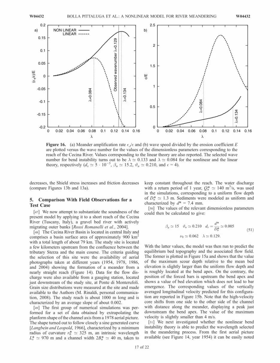
Figure 16. (a) Meander amplification rate �,t/� and (b) wave speed divided by the erosion coefficient Eare plotted versus the wave number for the values of the dimensionless parameters corresponding to thereach of the Cecina River. Values corresponding to the linear theory are also reported. The selected wavenumber for bend instability turns out to be l ’ 0.133 and l ’ 0.084 for the nonlinear and the lineartheory, respectively (ds ’ 5 10�3, bu ’ 15.2, Ju ’ 0.210, and � = 4).


17 of 22

W04432

that two parallel straight reaches, probably rectified byhuman intervention, are joined together by an obliquestretch. The distance between the two parallel straightreaches is roughly equal to two channel widths. The aerialpicture of 1978 already shows the evidence of a meanderingprocess taking place downstream to the connection betweenthe oblique and straight reaches. The intrinsic wavelengthLs* of the incipient meander can be estimated at 970 m(corresponding to an intrinsic dimensionless wave numberl = 0.129). The most recent pictures then clearly reveal theprocesses of meander amplification and downstreammigration occurred in the following years.[52] In Figure 16a the meander amplification rate �,t/�

(scaled by the erosion coefficient E) is plotted versus themeander wave number for the values of the dimensionlessparameters corresponding to the reach of the Cecina Riverconsidered as test case. The predicted value of the wavenumber selected by bend instability turns out to be l’ 0.133and corresponds to an intrinsic wavelength Ls* ’ 945 m,very close to the value estimated from the aerial pictures.[53] In order to investigate the sensitivity of the wave

number selected to the value chosen for the formativedischarge, we evaluated the meander amplification rate byvarying the latter within a range of ±50%. Results arereported in Figure 17, where the ranges of selected wave

numbers for bend instability corresponding to the linear andnonlinear theory are also evidenced and compared with thevalue observed in the field.[54] Finally, a comparison was performed between the

bed topography predicted by the present model and thevalues obtained during a topographic survey of the site ofinterest undertaken in July 2007 (Figure 14). In particularour attention was focused on the second bend, proceedingdownstream, where a deep scour was located close to theouter bank, just upstream of the apex. In order to analyzethe results, it proved appropriate to reinterpret data in termsof variations of bottom elevation relative to an inclinedplane characterized by the average channel slope. The latterslope was computed through best fitting of the acquired databy a plane inclined in the down valley direction. The locallongitudinal Cartesian slope of the river corresponding tothe slope of the floodplain turned out to be ix = 0.0023. Theaverage width of the reach was estimated by making use ofboth the topographical survey and the aerial picture of 2007.In particular, in the straight reach just upstream the site ofinterest we estimated an average width of 20 m, slightlysmaller than the value we best estimated in the curved reach,being roughly equal to 2Bu* = 25 m. We then used the lattervalue for the simulation. The correct elevation of theinclined plane was evaluated by making sure that the

Figure 17. Meander amplification rate �,t/� divided by the erosion coefficient E is plotted versus thewave number for different values of formative discharge relative to the reach of the Cecina River. Valuescorresponding to the linear theory are also reported. The ranges of selected wave numbers for bendinstability corresponding to the linear and nonlinear theory are also evidenced (� = 4).

18 of 22


Figure

18.

Comparisonbetween(a)measuredvalues

ofbottom

elevation(inmeters)

intheCecinaRiver

andthevalues

obtained

using(b)thepresentnonlinearand(c)linearmodelsforthe2007planim

etricconfiguration.Flowisfrom

rightto

left.Thegreen

arrow

showsthelocationofmaxim

um

scour.


19 of 22

W04432

intersection of the latter with measured data generated anaverage free surface width of the channel equal to 2Bu* and,consequently, the point bar nearly emerged. The planformshape of the reach did not strictly follow a sine generatedcurve, but was approximately close to such a shape, with adimensionless intrinsic wave number l ’ 0.1085 and acurvature parameter v0 ’ 0.12. To perform a simulation offlow and bed topography in the surveyed bend, an estimateof the formative discharge Qu* was also needed. This waschosen such as to generate in the model a nearly emergingpoint bar and turned out to be Qu* ’ 45 m3/s. The followingvalues of the relevant dimensionless parameters wereobtained:

bu ’ 12:6 Ju ’ 0:128 ds ’ 0:0077 ifu ’ 0:00164 ð52Þ

In Figure 18 we show the comparison between the observeddeviations of bed elevations relative to the inclined planeand the results obtained by the nonlinear and the linearmodels, respectively. We find that, consistently withmeasured data, the nonlinear theory predicts a maximum(minimum) scour at the outer bank (inner bank) located justdownstream (upstream) the bend apex. On the contrary, inthe linear case, although the intensity is quite similar, thelocation of both the maximum and minimum scour isshifted far downstream relative to the bend apex. Also notethat the nonlinear model is able to predict the presence of achute channel in the downstream part of the bend, a featureclearly observed in the field data. Finally, as shown inFigure 19, the thread of high velocity is consistently locatedat the outer bank just downstream the bend apex. On thecontrary, the maximum velocity predicted by the linearmodel is located close to the inflection point and the threadof high velocity is very elongated, and shifts from the innerto the outer bank quite sharply close to the apex.

6. Discussion and Conclusions

[55] A nonlinear asymptotic theory of flow and bedtopography in meandering channels able to describe finiteamplitude perturbations of bottom topography and accountfor arbitrary, yet slow, variations of channel curvature hasbeen developed. This model appears to be a potentiallyuseful and powerful tool for many purposes. In the presentpaper we have been able to formulate a nonlinear bendinstability theory, which predicts several characteristic fea-tures of the actual meandering process and extends resultsobtained by classical linear bend theories. In particular, wehave found the following: (1) for given values of therelevant physical parameters, the bend growth rate peaksat some value of the meander wavelength, reminiscent of(but typically smaller than) the resonant value of linearstability theory, a result confirming the weakly nonlinearresults of Seminara and Tubino [1992], consistent with fieldobservations that show that the wavelength selected bytraditional linear theories is typically slightly larger thanobserved values; (2) the selected wavelength depends on theamplitude of the initial perturbation (for a given value of therelevant dimensionless parameters) and, in particular, largerwavelengths (smaller wave numbers) are associated withlarger amplitudes �, a feature typical of nonlinear waves;(3) the infinite peak in the linear response at resonance isdamped by nonlinearity, a result again confirming its weakly

Figure

19.

Comparisonbetweenthevalues

oflongitudinal

averagevelocity

(inmeters/second)obtained

usingthe(a)

presentnonlinearand(b)linearmodelsforthe2007planim

etricconfiguration.Flow

isfrom

rightto

left.Thegreen

arrow

showsthelocationofmaxim

um

near-bankvelocity.


20 of 22

W04432

nonlinear counterpart; (4) meanders are found to migratepreferentially downstream, though upstream migration isalso possible, at least in principle, for relatively large valuesof the aspect ratio of the channel, a finding in agreement withthe picture provided by the linear theory of Zolezzi andSeminara [2001]; and (5) meanders slow down as theiramplitude increases (for a given value of the relevantdimensionless parameters), again a feature typical of non-linear waves, driven in the present case by flow rather thangeometric nonlinearities.[56] In conclusion, the picture offered by results obtained

through the present theory seems satisfactory and consistentwith field observations as well as previous theoretical findings.Further substantiation of the model has been achieved bycomparing predictions obtained for a test case (a reach of theCecina River, Italy) with field observations, though admit-tedly, the nonuniform bank erodibility associated with thegrowth of vegetation as well as other anthropogenic effectsmake the significance of the latter validation only qualitative.[57] A number of interesting future developments of the

present model are called for as discussed in section 1. Theseinclude also the need to allow for slow temporal variationsof flow and sediment supply such that the morphologicalresponse of the channel to a sequence of flood events. Suchan investigation will help to provide a rational interpretationof the as yet loosely defined notion of ‘‘formative dischargeof an alluvial river’’.

Appendix A: Equations

[58] Here we report the final form of the Reynoldsequations and of the continuity equation for the liquid andsolid phases written in coordinate (s, n, x):

dh�1s uu;s �

u;xD

@

@sD

Z x

x0

u dx

" # !

þ 1

bu


p vu;n �u;xD

@

@nD

Z x

x0

v dx

" # !

þ dch�1s uv� u;x

Z x

x0

v dx

!

¼ �dh�1s h;s þ h�1

s


pþ 1

D2ðnTu;x Þ;x ðA1Þ

dh�1s uv;s �

v;xD

@

@sD

Z x

x0

u dx

" # !

þ 1

bu


p vv;n �v;xD

@

@nD

Z x

x0

v dx

" # !

� dch�1s u2 þ v;x

Z x

x0

v dx

!¼ ðA2Þ

� h;n

bu


p þ 1

D2nT v;x� �

;x ðA3Þ

dh�1s

@

@sD

Z 1

x0

u dx

" #þ 1

bu


p @

@nD

Z 1

x0

v dx

" #

þ dh�1s c D

Z 1

x0

v dx

" #¼ 0 ðA4Þ

dh�1s qs;s þ

1

bu


p qn;n þ dh�1s cqn ¼ 0 ðA5Þ

Appendix B: Coefficients

[59] Here we report the coefficients Rj(j = 1, 8) appearingin equations (40) and (46):

R1 ¼ �ffiffiffiffiffiffiffiCfu

p D1

D0

� u1;xu0;x

jx0

� �þ ncðsÞbuCfu þ

h1;sR0

R2 ¼ D0;s þD0

R0

R0;s

R3 ¼ 1

bu


p cðsÞD0D0;n

R4 ¼ D0;s þD0

3R0

R0;s

R5 ¼ R3

R6 ¼ � D1

D0

� u1;xu0;x

jx0

� �þ ncðsÞbu


pR7 ¼ 3

2D0;s þ

D0

3R0

R0;s þ2

3

D0

cðsÞ c;s� �

R8 ¼ D1

D0

� u1;xu0;x

jx0

� �

ðB1Þ

[60] Acknowledgments. M. Rinaldi is kindly acknowledged for pro-viding the aerial picture and the data of the Cecina River. The present workhas been funded by Cariverona (Progetto MODITE). Partial support hasalso come from the Italian Ministry of University and of Scientific andTechnological Research in the framework of the National Project ‘‘Evolu-zione morfodinamica di ambienti lagunari’’ (PRIN 2006) cofunded by theUniversity of Genova.

ReferencesBlondeaux, P., and G. Seminara (1985), A unified bar-bend theory of rivermeanders, J. Fluid Mech., 157, 449–470.

Callander, R. A. (1978), River meandering, Annu. Rev. Fluid Mech., 10,129–158.

Camporeale, C., P. Perona, A. Porporato, and L. Ridolfi (2007), Hierarchyof models for meandering rivers and related morphodynamic processes,Rev. Geophys., 45, RG1001, doi:10.1029/2005RG000185.

Dean, R. B. (1974), Reynolds number dependence on skin friction in twodimensional rectangular duct flow and a discussion on the law of theWake, AERO Rep. 74-11, Imperial Coll., London.

Edwards, B. F., and D. H. Smith (2002), River meandering dynamics, Phys.Rev. E, 65, 046303, doi:10.1103/PhysRevE.65.046303.

Howard, A. D., and T. R. Knutson (1984), Sufficient conditions for rivermeandering: A simulation approach,Water Resour. Res., 20, 1659–1667.

Ikeda, S., G. Parker, and K. Sawai (1981), Bend theory of river meanders.Part 1. Linear development, J. Fluid Mech., 112, 363–377.

Imran, J., and G. Parker (1999), A nonlinear model of flow in meanderingsubmarine and subaerial channels, J. Fluid Mech., 400, 295–331.

Jager, H. R. A. (2003), Modelling planform changes of braided rivers,Ph.D. thesis, Univ. of Twente, Enschede, Netherlands.

Kevorkian, J., and J. D. Cole (1981), Perturbation Methods in AppliedMathematics, Springer, Berlin.

Kovacs, A., and G. Parker (1994), A new vectorial bedload formulation andits application to the time evolution of straight river channels, J. FluidMech., 267, 153–183.

Langbein, W. B., and L. B. Leopold (1966), River meanders: Theory ofminimum variance, U.S. Geol. Surv. Prof. Pap., 422-H.

Lanzoni, S., and G. Seminara (2006), On the nature of meander instability,J. Geophys. Res., 111, F04006, doi:10.1029/2005JF000416.

Lanzoni, S., A. Siviglia, A. Frascati, and G. Seminara (2006), Long wavesin erodible channels and morphodynamic influence, Water Resour. Res.,42, W06D17, doi:10.1029/2006WR004916.


21 of 22

W04432

Mosselman, E. (1991), Modelling of river morphology with non-orthogonalhorizontal curvilinear coordinates, in Communications on Hydraulic andGeotechnical Engineering, Rep. 91-1, Delft Univ. of Technol., Delft,Netherlands.

Nelson, J. M., and J. D. Smith (1989), Evolution and stability oferodible channel beds, in River Meandering, Water Resour. Monogr.,vol. 12, edited by S. Ikeda and G. Parker, pp. 321–377, AGU,Washington, D.C.

Parker, G. (1978a), Self-formed straight rivers with equilibrium banks andmobile bed. Part 1. The sand-silt river, J. Fluid Mech., 89, 109–125.

Parker, G. (1978b), Self-formed straight rivers with equilibrium banks andmobile bed. Part 2. The gravel river, J. Fluid Mech., 89, 127–146.

Parker, G. (1984), Lateral bed load transport on side slopes, J. Hydraul.Eng. Am. Soc. Civ. Eng., 110, 197–199.

Parker, G. (1990), Surface-based bedload transport relation for gravelrivers, J. Hydraul. Res., 28, 417–436.

Parker, G., and Y. Shimizu (2008), Framework for a new model of themigration of meandering rivers, Geophys. Res. Abstr., 10, AbstractEGU2008-A-04840.

Pizzuto, E. J., and J. S. Meckelnburg (1989), Evaluation of a linear bankerosion equation, Water Resour. Res., 25, 1005–1013.

Repetto, R., M. Tubino, and C. Paola (2002), Planimetric instability ofchannels with variable width, J. Fluid. Mech., 457, 79–109.

Rossi Romanelli, L., M. Rinaldi, S. E. Darby, L. Luppi, and L. Nardi(2004), Monitoring and modelling river bank processes: A new metho-dological approach, in River Flow 2004, vol. 2, edited by M. Greco,A. Carravetta, and R. Dalla Morte, pp. 993–998, Taylor and Francis,London.

Seminara, G. (2006), Meanders, J. Fluid Mech., 554, 271–297.Seminara, G., and L. Solari (1998), Finite amplitude bed deformations intotally and partially transporting wide chanel bends, Water Resour. Res.,34, 1585–1598.

Seminara, G., and M. Tubino (1992), Weakly nonlinear theory of regularmeanders, J. Fluid Mech., 244, 257–288.

Seminara, G., L. Solari, and G. Parker (2002), Bed load at low Shieldsstress on arbitrarily sloping beds: Failure of the Bagnold hypothesis,Water Resour. Res., 38(11), 1249, doi:10.1029/2001WR000681.

Shields, I. A. (1936), Anwendung der ahnlichkeitmechanik und der turbu-lenzforschung auf die gescheibebewegung, Mitt. Preuss. Versuchsanst.,26, 5–24.

Shimizu, Y. (2002), A method for simultaneous computation of bed andbank deformation of a river, in River Flow 2002, vol. 2, edited byD. Bousmar and Y. Zech, pp. 793–801, Taylor and Francis, London.

Sun, T., P. Meakin, T. Jøssang, and K. Schwarz (1996), A simulation modelfor meandering rivers, Water Resour. Res., 32, 2937–2954.

Sun, T., P. Meakin, and T. Jøssang (2001a), A computer model for mean-dering rivers with multiple bed load sediment sizes: 1. Theory, WaterResour. Res., 37, 2227–2242.

Sun, T., P. Meakin, and T. Jøssang (2001b), A computer model for mean-dering rivers with multiple bed load sediment sizes: 2. Computer simula-tions, Water Resour. Res., 37, 2243–2258.

Talmon, A. M., N. Struiksma, and M. C. L. M. Van Mierlo (1995),Laboratory measurements of the sediment transport on transversealluvial-bed slopes, J. Hydraul. Res., 33, 495–517.

Zolezzi, G., and G. Seminara (2001), Downstream and upstream influencein river meandering. Part 1. General theory and application to overdee-pening, J. Fluid Mech., 438, 183–211.

��M. Bolla Pittaluga, G. Nobile, and G. Seminara, Department of Civil,

Environmental and Architectural Engineering, University of Genova, ViaMontallegro 1, I-16145 Genova, Italy. ([email protected])

22 of 22


Documents

A nonlinear model for river meandering