Embed Size (px)
Citation preview

SPE Golden Gate Section, 8 December 2010 1
Closed-loop reservoir management
Jan-Dirk Jansen
Delft University of TechnologyDepartment of Geotechnology
Cox visiting professorStanford UniversityDepartment of Energy Resources Engineering
SPE Golden Gate Section, 8 December 2010 2
Closed-loop reservoir management a.k.a. Smart Fields, i-Fields, e-Fields, etc.
Jan-Dirk Jansen
Delft University of TechnologyDepartment of Geotechnology
Cox visiting professorStanford UniversityDepartment of Energy Resources Engineering

SPE Golden Gate Section, 8 December 2010 3
Delft University of Technology
Founded 184216000 students2700 scientific staff250 PhDs/yr8 faculties
Faculty of Civil Engineering and Geosciences – Department of Geotechnology
SPE Golden Gate Section, 8 December 2010 4
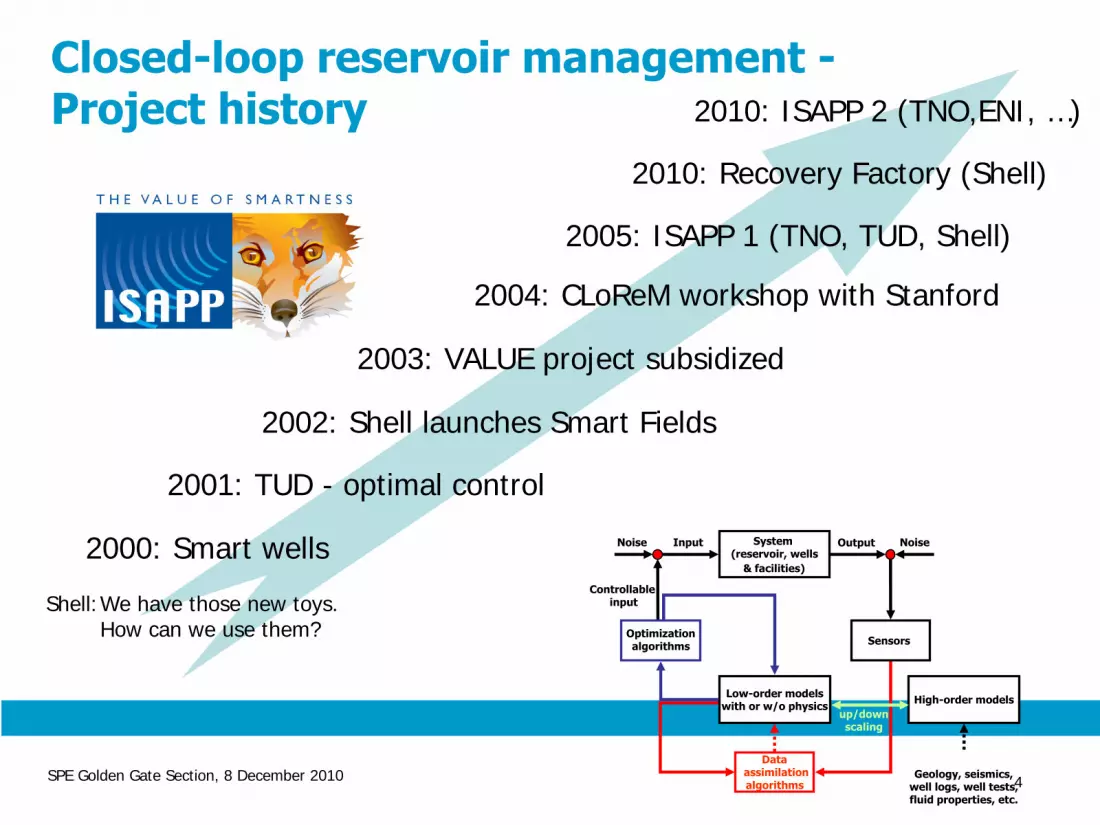
Closed-loop reservoir management - Project history
Controllable
input
Data
assimilationalgorithms
Low-order modelswith or w/o physics High-order
modelsup/downscaling
Geology, seismics,well logs, well tests,fluid properties, etc.
Noise OutputInput NoiseSystem (reservoir, wells
& facilities)
Optimizationalgorithms Sensors
2000: Smart wells
Shell:We have those new toys. How can we use them?
2001: TUD - optimal control
2004: CLoReM workshop with Stanford
2010: Recovery FFactory (Shell)
2005: ISAPP 1 (TNO, TUD, Shell)
2003: VALUE project subsidized
2002: Shell launches Smart Fields
2010: ISAPP 2 (TNO,ENI, …)

SPE Golden Gate Section, 8 December 2010 5
Closed-loop reservoir management
• Hypothesis: recovery can be significantly increased by changing reservoir management from a ‘batch-type’ to a near-continuous model-based controlled activity
• Key elements:• Optimization under physical constraints and
geological uncertainties• Data assimilation aimed at continuous updating of
system models
• Inspiration:• Measurement and control theory• Meteorology and oceanography

SPE Golden Gate Section, 8 December 2010 6
Closed-loop reservoir management
Dataassimilationalgorithms
Noise OutputInput NoiseSystem (reservoir, wells
& facilities)
Optimizationalgorithms Sensors
System models
Predicted output Measured output
Controllableinput
Geology, seismics,well logs, well tests,fluid properties, etc.
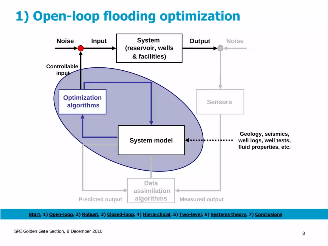
Start, 1) Open-loop, 2) Robust, 3) Closed-loop, 4) Hierarchical, 5) Two-level, 6) Systems theory, 7) Conclusions
SPE Golden Gate Section, 8 December 2010 7
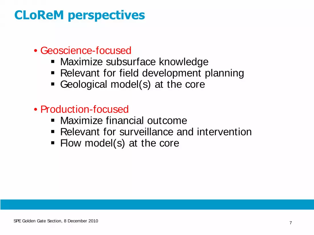
CLoReM
perspectives
• Geoscience-focused Maximize subsurface knowledgeRelevant for field development planningGeological model(s) at the core
• Production-focusedMaximize financial outcomeRelevant for surveillance and interventionFlow model(s) at the core
SPE Golden Gate Section, 8 December 2010 8
Dataassimilationalgorithms
Noise OutputInput NoiseSystem (reservoir, wells
& facilities)
Optimizationalgorithms Sensors
System model
Predicted output Measured output
Controllableinput
Geology, seismics,well logs, well tests,fluid properties, etc.
1) Open-loop flooding optimization
Start, 1) Open-loop, 2) Robust, 3) Closed-loop, 4) Hierarchical, 5) Two-level, 6) Systems theory, 7) Conclusions

SPE Golden Gate Section, 8 December 2010 9
Optimization techniques
• Global versus local• Gradient-based versus gradient-free• Constrained versus non-constrained• ‘Classical’ versus ‘non-classical’ (genetic algorithms,
simulated annealing)
• We use ‘optimal control theory’ – local, gradient-based• Has been proposed for history matching (Chen et al.
1974, Chavent et al. 1975, Li, Reynolds and Oliver 2003 ) and for flooding optimization (Ramirez 1987, Asheim 1988, Virnovski 1991, Zakirov et al. 1996, Sudaryanto and Yortsos, 1998, Brouwer et al. 2002, Sarma et al. 2004)
SPE Golden Gate Section, 8 December 2010 10
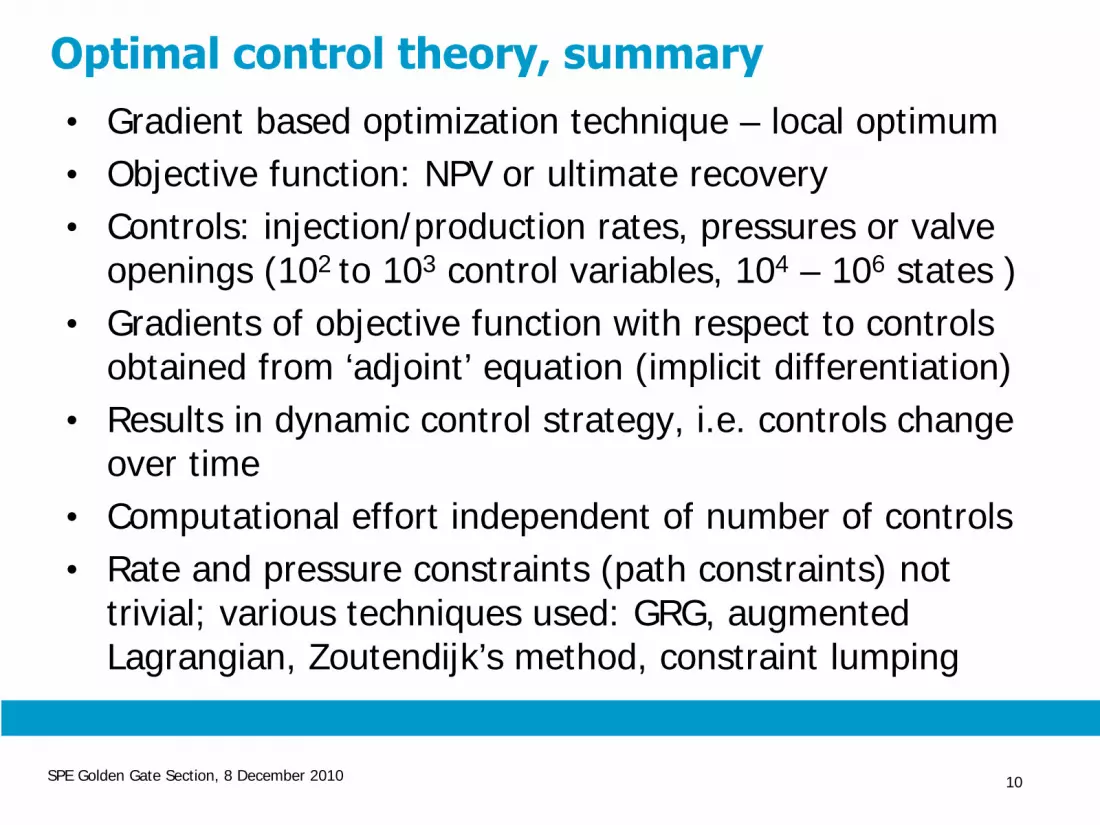
Optimal control theory, summary• Gradient based optimization technique – local optimum• Objective function: NPV or ultimate recovery• Controls: injection/production rates, pressures or valve
openings (102 to 103 control variables, 104 – 106 states )• Gradients of objective function with respect to controls
obtained from ‘adjoint’ equation (implicit differentiation) • Results in dynamic control strategy, i.e. controls change
over time• Computational effort independent of number of controls• Rate and pressure constraints (path constraints) not
trivial; various techniques used: GRG, augmented Lagrangian, Zoutendijk’s method, constraint lumping

SPE Golden Gate Section, 8 December 2010 11
12-well example
• 3D reservoir• High-permeability channels• 8 injectors, rate-controlled• 4 producers, BHP-controlled• Production period of 10 years• 12 wells x 10 x 12 time steps gives 1440 optimization parameters
• Optimization of monetary value Van Essen et al., 2006
( ) ( ) ( )
( )
, , ,1 1
1 1
inj prod
k
N N
wi wi i wp wp j o o jK k k ki j
k ktk
r u r y r yJ J t
b τ
= =
=
⎧ ⎫⎡ ⎤× + × + ×⎪ ⎪⎣ ⎦⎪ ⎪= Δ⎨ ⎬⎪ ⎪+⎪ ⎪⎩ ⎭
∑ ∑∑

SPE Golden Gate Section, 8 December 2010 12
Run animation 1
SPE Golden Gate Section, 8 December 2010 13
Why this wouldn’t work
• Real wells are sparse and far apart• Real wells have more complicated constraints• Field management is usually production-focused• Long-term optimization may jeopardize short-term profit• Production engineers don’t trust reservoir models anyway
• We do not know the reservoir!

SPE Golden Gate Section, 8 December 2010 14
2) Robust open-loop flooding optimization
Dataassimilationalgorithms
Noise OutputInput NoiseSystem (reservoir, wells
& facilities)
Optimizationalgorithms Sensors
System models
Predicted output Measured output
Controllableinput
Geology, seismics,well logs, well tests,fluid properties, etc.
Start, 1) Open-loop, 2) Robust, 3) Closed-loop, 4) Hierarchical, 5) Two-level, 6) Systems theory, 7) Conclusions

SPE Golden Gate Section, 8 December 2010 15
Robust optimization example
• 100 realizations• Optimize expectation of objective function
Van Essen et al., 2006
( )1:
1: 1:1
1max , ,r
K
Ni
K K iir
JN =∑u
y u θ

SPE Golden Gate Section, 8 December 2010 16
Robust optimization results
3 control strategies applied to set of 100 realizations:reactive control, nominal optimization, robust optimization
Van Essen et al., 2006
SPE Golden Gate Section, 8 December 2010 17
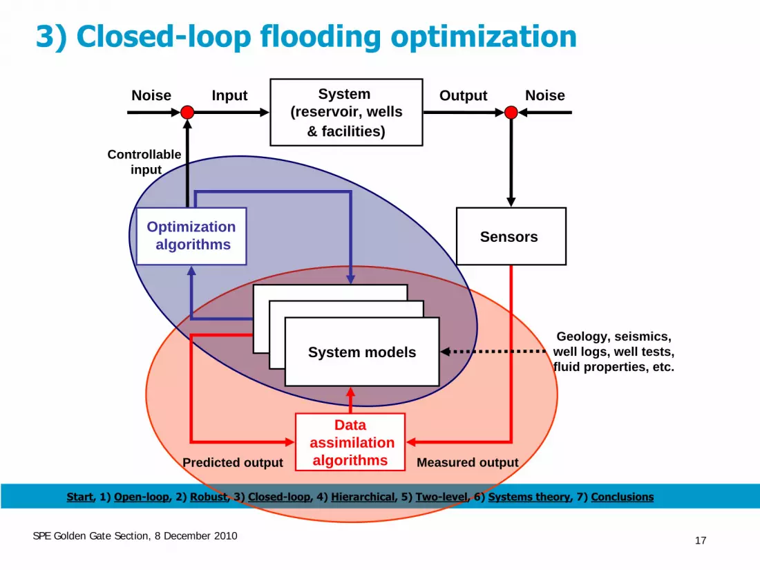
3) Closed-loop flooding optimization
Dataassimilationalgorithms
Noise OutputInput NoiseSystem (reservoir, wells
& facilities)
Optimizationalgorithms Sensors
System models
Predicted output Measured output
Controllableinput
Geology, seismics,well logs, well tests,fluid properties, etc.
Start, 1) Open-loop, 2) Robust, 3) Closed-loop, 4) Hierarchical, 5) Two-level, 6) Systems theory, 7) Conclusions

SPE Golden Gate Section, 8 December 2010 18
Computer-assisted history matching (data assimilation, parameter estimation)
• Very ill-posed problem: many parameters, little info
• Variational methods – minimization of mismatch
• Ensemble Kalman filtering – sequential methods
• Reservoir-specific methodsStreamline-based sensitivitiesGradual deformation Probability perturbation
• ‘Non-classical’ methods – simulated annealing, GAs, …
• Monte Carlo methods – MCMC with proxies
• We use Ensemble Kalman filtering (sequential assimilation)

SPE Golden Gate Section, 8 December 2010 19
Closed-loop –
example 1 Ensemble updates at different times
SPE Golden Gate Section, 8 December 2010 20
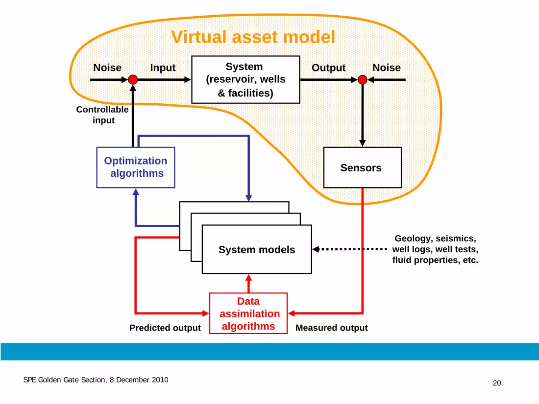
Virtual asset model
Dataassimilationalgorithms
Noise OutputInput NoiseSystem (reservoir, wells
& facilities)
Optimizationalgorithms Sensors
System models
Predicted output Measured output
Controllableinput
Geology, seismics,well logs, well tests,fluid properties, etc.

SPE Golden Gate Section, 8 December 2010 21
Closed-loop –
example 1 NPV and contributions from water & oil production
1 2 3 4 5 68.5
9
9.5
10
10.5x 10⁷
NPV, $
1 2 3 4 5 6-2
-1.5
-1.0
-0.5
0
Dis
coun
ted
wat
er c
osts
, $
1 2 3 4 5 68.5
9
9.5
10
10.5x 10⁷
Dis
coun
ted
oil r
even
ues,
$
reactive
open-loop
1 month 1 year 2 years 4 years
SPE Golden Gate Section, 8 December 2010 22
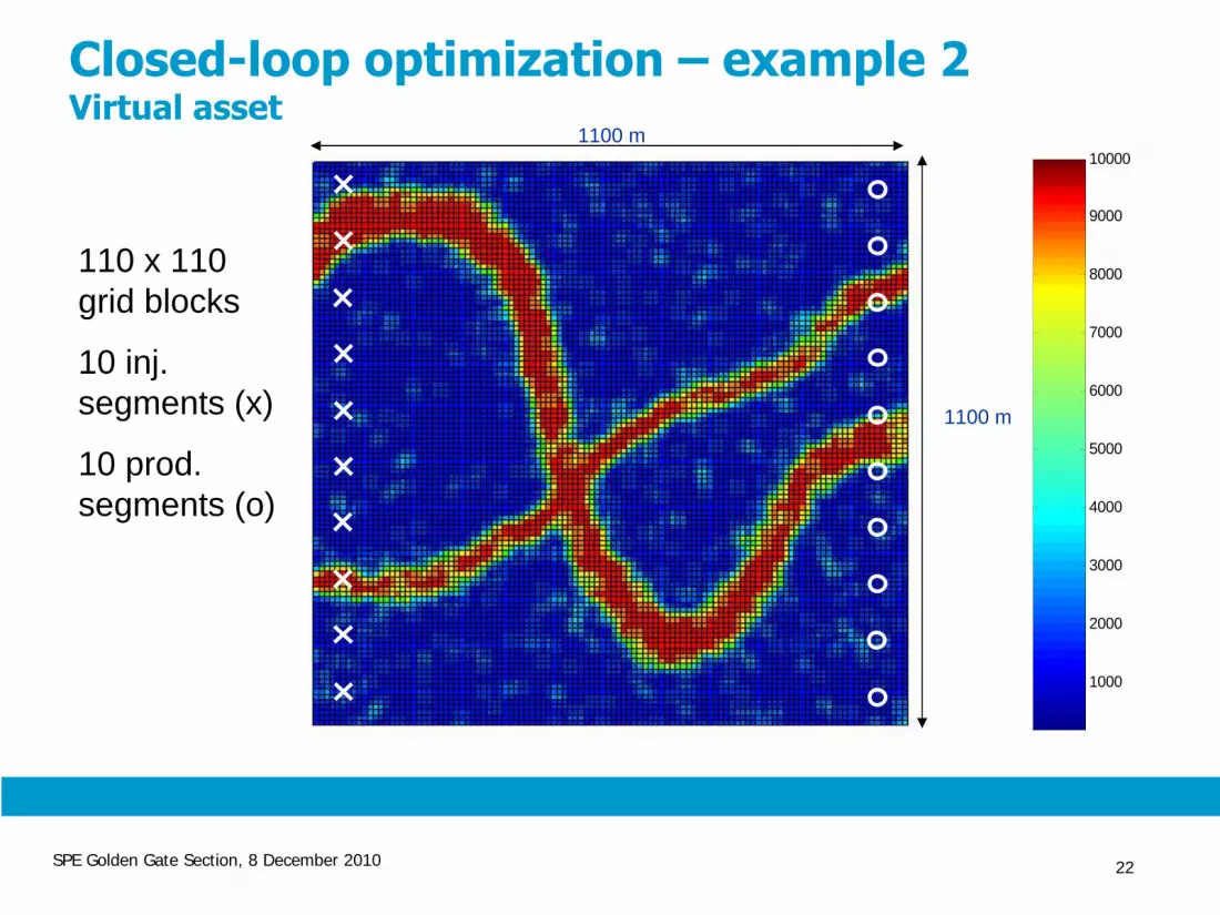
110 x 110 grid blocks
10 inj. segments (x)
10 prod. segments (o)
1100 m
1100 m
1000
2000
3000
4000
5000
6000
7000
8000
9000
10000
Closed-loop optimization –
example 2 Virtual asset
SPE Golden Gate Section, 8 December 2010 23
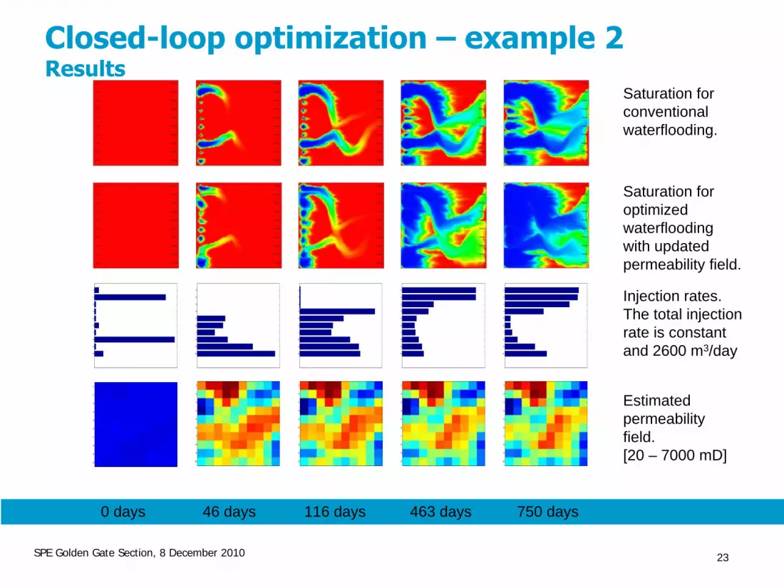
Closed-loop optimization –
example 2 Results
Saturation for conventional waterflooding.
Saturation for optimized waterflooding with updated permeability field.
Estimated permeability field. [20 – 7000 mD]
Injection rates. The total injection rate is constant and 2600 m3/day
46 days
1
2
3
4
5
6
7
8
9
10
1
2
3
4
5
6
7
8
9
10
116 days
1
2
3
4
5
6
7
8
9
10
1
2
3
4
5
6
7
8
9
10
463 days
1
2
3
4
5
6
7
8
9
10
1
2
3
4
5
6
7
8
9
10
750 days
1
2
3
4
5
6
7
8
9
10
1
2
3
4
5
6
7
8
9
10
0 days
1
2
3
4
5
6
7
8
9
10
1
2
3
4
5
6
7
8
9
10
SPE Golden Gate Section, 8 December 2010 24
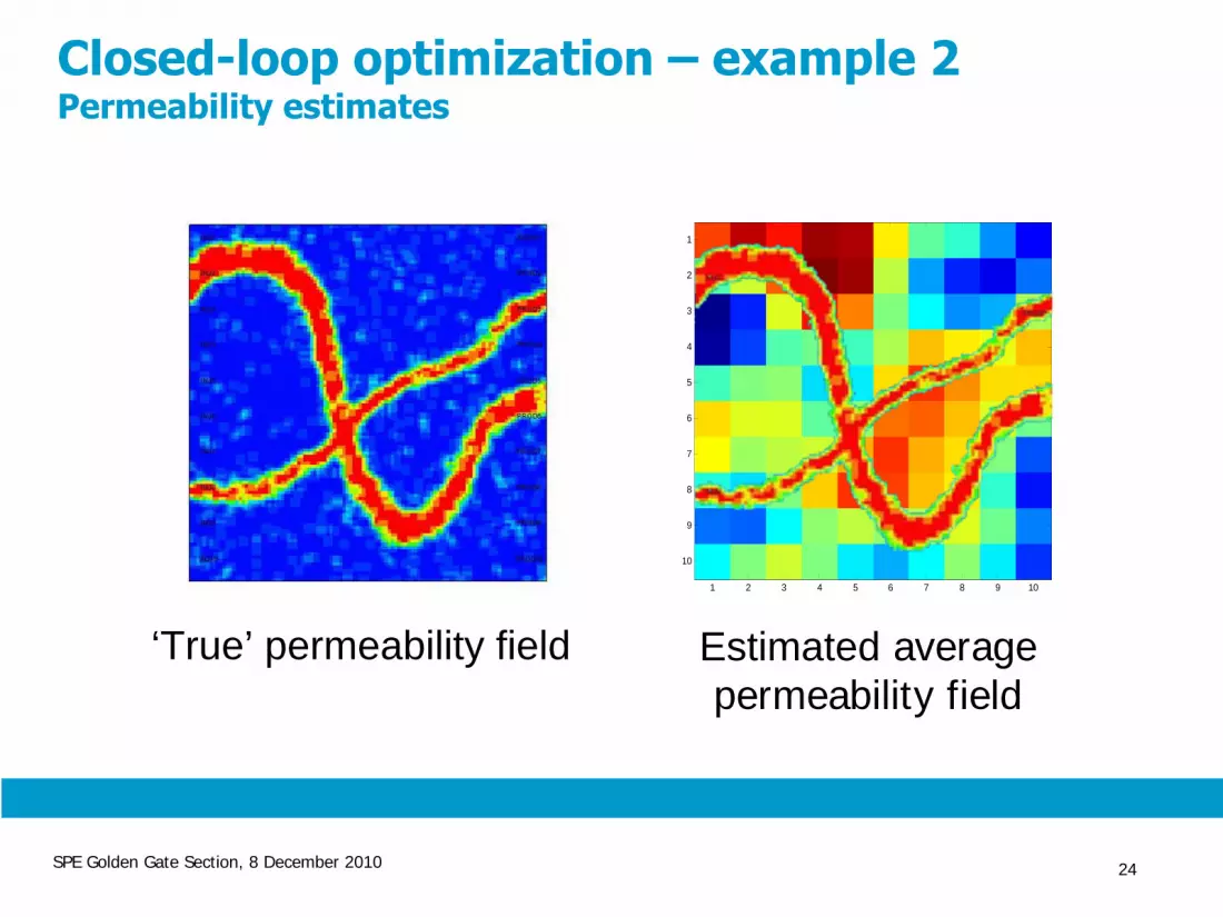
Closed-loop optimization –
example 2 Permeability estimates
1 2 3 4 5 6 7 8 9 10
1
2
3
4
5
6
7
8
9
10
‘True’ permeability field Estimated average permeability field
SPE Golden Gate Section, 8 December 2010 25
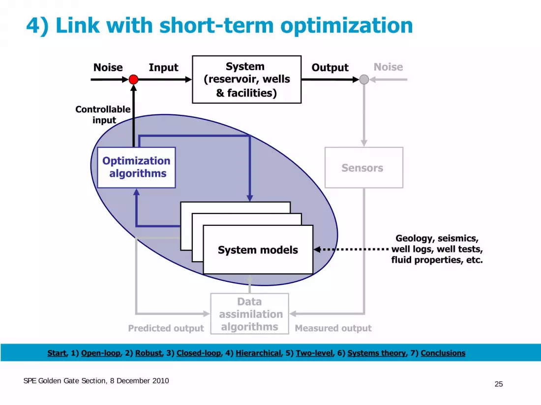
4) Link with short-term optimization
Dataassimilationalgorithms
Noise OutputInput NoiseSystem (reservoir, wells
& facilities)
Optimizationalgorithms Sensors
System models
Predicted output Measured output
Controllableinput
Geology, seismics,well logs, well tests,fluid properties, etc.
Start, 1) Open-loop, 2) Robust, 3) Closed-loop, 4) Hierarchical, 5) Two-level, 6) Systems theory, 7) Conclusions

SPE Golden Gate Section, 8 December 2010 26
Run animation 2

SPE Golden Gate Section, 8 December 2010 27
Hierarchical optimization
• Take production objectives into account by incorporating them as additional optimization criteria:
• Formal solution:• Order objectives according to importance• Optimize objectives sequentially• Optimality of upper objective constrains optimization of
lower one
• Only possible if there are redundant degrees of freedom in input parameters after meeting primary objective

SPE Golden Gate Section, 8 December 2010 28
Objective function with ridges
SPE Golden Gate Section, 8 December 2010 29
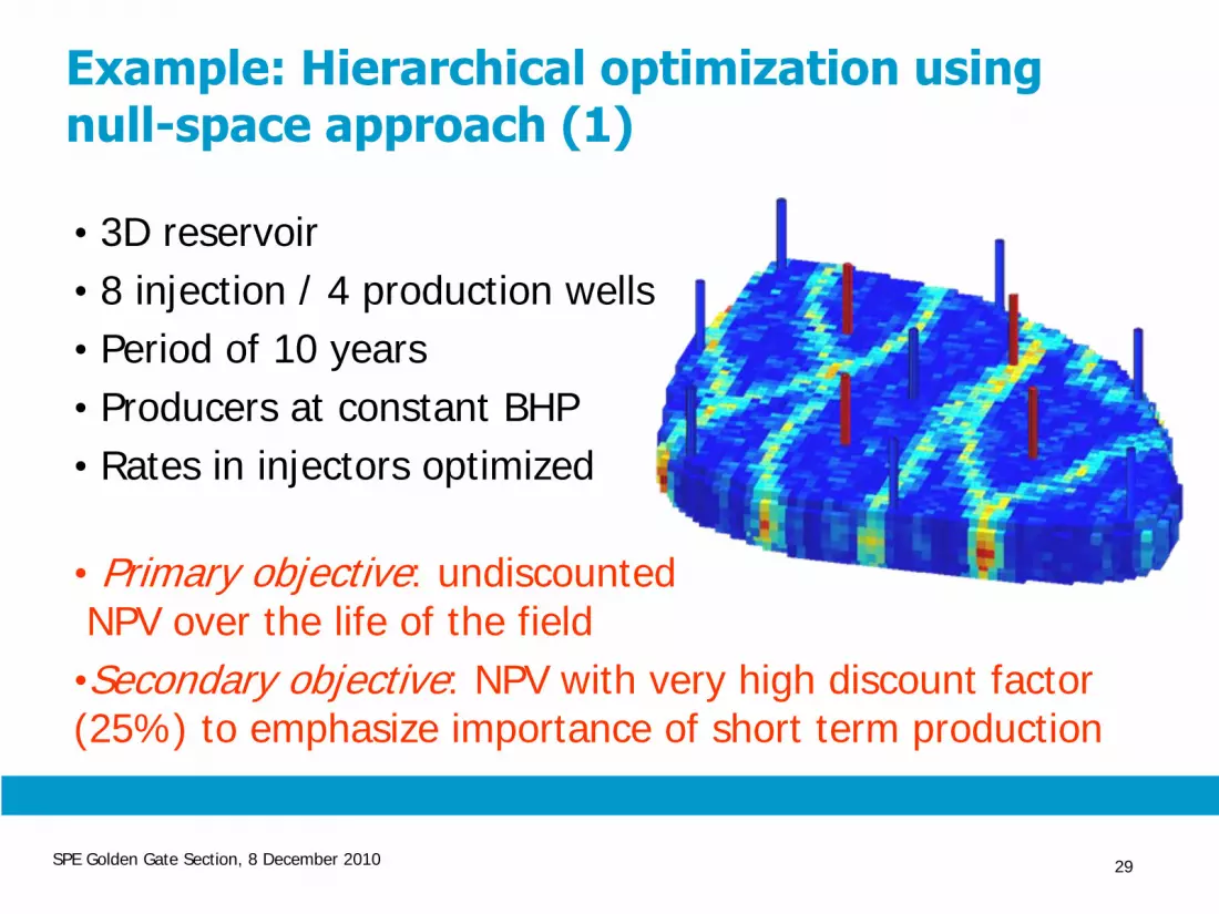
Example: Hierarchical optimization using null-space approach (1)
• 3D reservoir• 8 injection / 4 production wells• Period of 10 years • Producers at constant BHP• Rates in injectors optimized
• Primary objective: undiscounted NPV over the life of the field
•Secondary objective: NPV with very high discount factor (25%) to emphasize importance of short term production
SPE Golden Gate Section, 8 December 2010 30
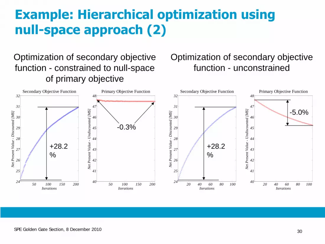
Example: Hierarchical optimization using null-space approach (2)
20 40 60 80 10024
25
26
27
28
29
30
31
32
Iterations
Net P
rese
nt V
alue
- D
iscou
nted
[M$]
Secondary Objective Function
20 40 60 80 10040
41
42
43
44
45
46
47
48
Iterations
Net
Pre
sent
Val
ue -
Und
iscou
nted
[M$]
Primary Objective Function
50 100 150 20024
25
26
27
28
29
30
31
32
Iterations
Net P
rese
nt V
alue
- D
iscou
nted
[M$]
Secondary Objective Function
50 100 150 20040
41
42
43
44
45
46
47
48
Iterations
Net
Pre
sent
Val
ue -
Und
iscou
nted
[M$]
Primary Objective Function
Optimization of secondary objective function - constrained to null-space
of primary objective
Optimization of secondary objective function - unconstrained
+28.2 %
+28.2 %
-0.3%
-5.0%
SPE Golden Gate Section, 8 December 2010 31
0 900 1800 2700 36000
5
10
15
20
25
30
35
40
45
50
time [days]
NPV
ove
r Ti
me
- Und
isco
unte
d [1
0 6 $
]
~~
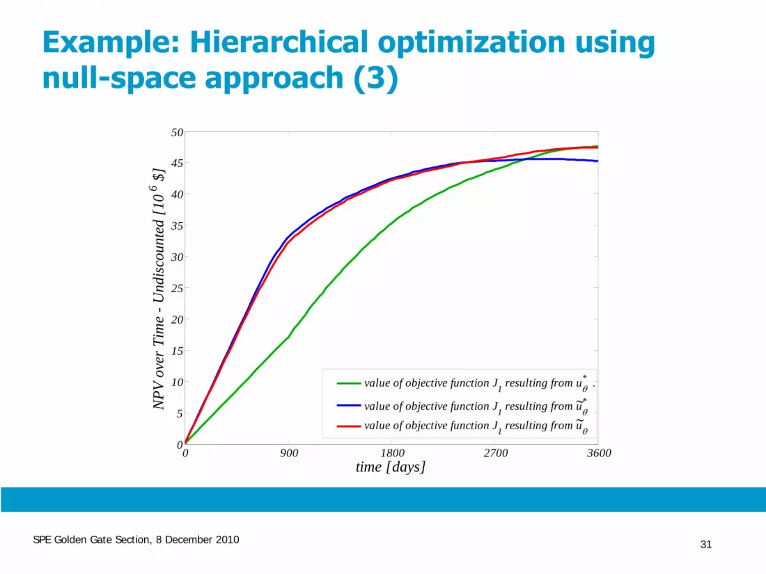
value of objective function J1 resulting from uθ* .
value of objective function J1 resulting from uθ*
value of objective function J1 resulting from uθ
Example: Hierarchical optimization using null-space approach (3)
SPE Golden Gate Section, 8 December 2010 32
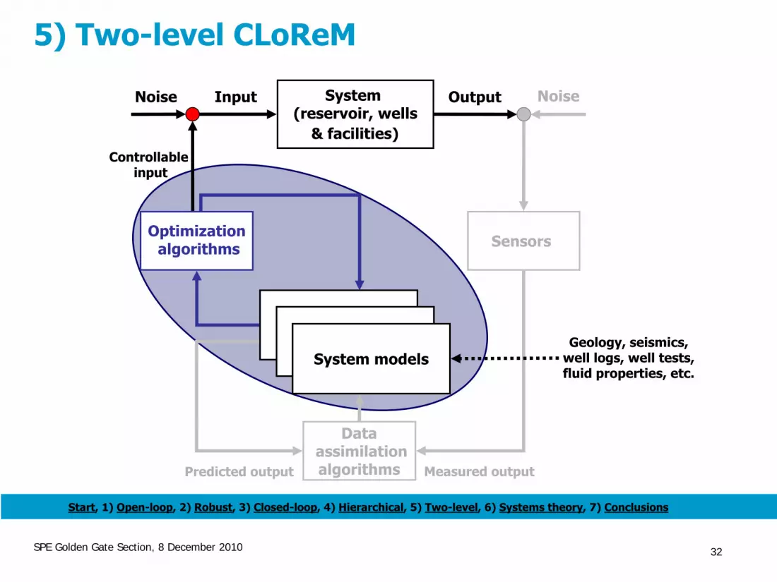
5) Two-level CLoReM
Dataassimilationalgorithms
Noise OutputInput NoiseSystem (reservoir, wells
& facilities)
Optimizationalgorithms Sensors
System models
Predicted output Measured output
Controllableinput
Geology, seismics,well logs, well tests,fluid properties, etc.
Start, 1) Open-loop, 2) Robust, 3) Closed-loop, 4) Hierarchical, 5) Two-level, 6) Systems theory, 7) Conclusions

SPE Golden Gate Section, 8 December 2010 33
• Full cycle of assisted history matching and robust optimization too labor-intensive to apply frequently
• Poor short-term prediction quality of large-scale reservoir model (poor near-well bore modeling)
• Optimal inputs may be difficult to implement in practice• Cultural barriers to use reservoir simulation as a basis
for production-related decisions• Proposed solution: two-level control strategy
• Outer loop to determine optimal ouput trajectory (life-cycle horizon, periodically updated)
• Inner loop to stay close to optimal output (short- term horizon, frequently updated)
• Can be interpreted as ‘disturbance rejection’
Two-level CLoReM
–
motivation & idea

SPE Golden Gate Section, 8 December 2010 34
Two-level CLoReM
–
elements
• Model-predictive controller (MPC) to track optimal output
• Data-driven low-order system model
• State estimator (observer)
• Short-term objective function: mismatch between optimal and actual (estimated) output
Dataassimilationalgorithms
Optimizationalgorithms
High-ordersystem models
Predicted output Measured output
Noise OutputInput NoiseSystem (reservoir, wells
& facilities)
Sensors Low-order
system model
MPCcontroller
Observer
J = |(yopt* - ylo )|2
J = NPV
States & parameters
Statesyopt
ylo
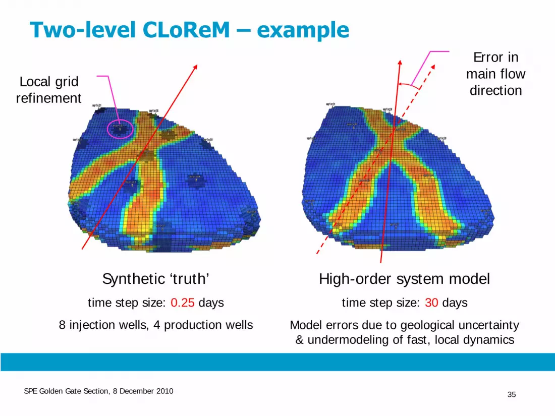
SPE Golden Gate Section, 8 December 2010 35
Local grid refinement
Error in main flow direction
Synthetic ‘truth’time step size: 0.25 days
8 injection wells, 4 production wells
High-order system modeltime step size: 30 days
Model errors due to geological uncertainty & undermodeling of fast, local dynamics
Two-level CLoReM
–
example

SPE Golden Gate Section, 8 December 2010 36
Low-order modeling (system identification)
Persistently exciting inputs
= Injection rates
&Producer
BHP’s
Virtual asset
System Identification
Subspace model
Liquid production flow
rates

SPE Golden Gate Section, 8 December 2010 37
Two-level CLoReM
–
results
500 1000 1500 2000 2500 3000 3500 40000
2000
4000
6000
8000
10000
12000
14000
producer 1
time [days]
liqui
d flo
w ra
te [b
bl/d
ay] reference
open-loopMPC controlled
500 1000 1500 2000 2500 3000 3500 40000
0.5
1
1.5
2
2.5
3
3.5x 10⁴ producer 2
time [days]
liqui
d flo
w ra
te [b
bl/d
ay] reference
open-loopMPC controlled
Small tracking error due to bottom-hole pressure constraint
Small tracking error due to water
break-through in producer 2
Van Essen et al., 2010

SPE Golden Gate Section, 8 December 2010 38
6) System-theoretical aspects
Dataassimilationalgorithms
Noise OutputInput NoiseSystem (reservoir, wells
& facilities)
Optimizationalgorithms Sensors
Low-ordersystem models
Predicted output Measured output
Controllableinput
Geology, seismics,well logs, well tests,fluid properties, etc.
up/downscaling
High-ordersystem models
Start, 1) Open-loop, 2) Robust, 3) Closed-loop, 4) Hierarchical, 5) Two-level, 6) Systems theory, 7) Conclusions

SPE Golden Gate Section, 8 December 2010 39
1 2 3 4 5 6 7 8 9 10
1
2
3
4
5
6
7
8
9
10
Why do such crude models sometimes work so well?
System-theoretical aspects

SPE Golden Gate Section, 8 December 2010 40
Observability, controllability, identifiability
Controllability of a dynamic system is the ability to influence the states through manipulation of the inputs.
Observability of a dynamic system is the ability to determine the states through observation of the outputs.
Identifiablity of a dynamic system is the ability to determine the parameters from the input-output behavior.
See Zandvliet et al., Computational Geosciences, 2008, 12
(4) 808-822.
System model
state (p,S)parameters (k,φ,…)
output (pwf ,qw ,qo )input (pwf ,qt )

SPE Golden Gate Section, 8 December 2010 41
System-theoretical aspects
For our system the (few) identifiable parameter patterns correspond just to the (few) controllable state patterns
Reservoir dynamics ‘lives’ in a state space of a much smaller dimension than the number of model grid blocks
=> Large scope for reduced-order modeling to speed up iterative optimization, history matching

SPE Golden Gate Section, 8 December 2010 42
Control-relevant grid-coarsening
• one layer of SPE 10 model Vakili 2010
• 0.0001 < k < 17000 mD• 60 x 220 = 13200 gridblocks• Dominant nr. of Hankel singular values: O(100)
1
2
1
1
2
1

SPE Golden Gate Section, 8 December 2010 43
Do we still need geology?
System-theoretical aspects
For our system the (few) identifiable parameter patterns correspond just to the (few) controllable state patterns
Reservoir dynamics ‘lives’ in a state space of a much smaller dimension than the number of model grid blocks
=> Large scope for reduced-order modeling to speed up iterative optimization, history matching

SPE Golden Gate Section, 8 December 2010 44
System-theoretical aspects
Yes, we do need geology!
• Interpreting the history match results requires geological insight
• Well location-optimization requires a geological model
• However, we need to focus on the relevant geology:
Which geological features are identifiable?
Which geological features influence controllability?

SPE Golden Gate Section, 8 December 2010 45
CLoReM
–
conclusions so far
• Size of the prize still unknown (open-loop and closed-loop) • Adjoint based-optimization techniques work well; constraints,
regularization, storage, efficiency, still to be improved• Specific data assimilation methods less important than
workflow & human interpretation of results• Many history matching efforts too much focused on history &
models, not on forecast and decisions • Field acceptance of closed-loop approach will require
combination with short-term production optimization• Reservoir dynamics lives in low-order space. Wide scope for
reduced-order, control-relevant modeling
Start, 1) Open-loop, 2) Robust, 3) Closed-loop, 4) Hierarchical, 5) Two-level, 6) Systems theory, 7) Conclusions

SPE Golden Gate Section, 8 December 2010 46
CLoReM
–
current focus areas• Develop workflows for geoscience- and production-focused
CLoReM• Develop means for joint assimilation (production data, 4D
seismics, passive, EM, gravity, etc. • Quantify flow/control/decision-relevant aspects of geology• Continue reduced-order modeling of reservoir flow• Address computational aspects: HPC (infrastructure, multi
run) and physics-based pre-conditioning (link to ROM)• Develop multi-level optimization methods to reconcile
production optimization and reservoir management• Extend to EOR applications (Recovery Factory program)• Develop tools and apply to field cases (ISAPP 2 program)
SPE Golden Gate Section, 8 December 2010 47
AcknowledgmentsOkko
Bosgra2
Paul van den Hof2
Arnold Heemink3
Roald Brouwer5
Sippe
Douma5
Marielba
Rojas3
Hans Kraaijevanger5 Rob Arts1,6
Remus
Hanea1,6
Renato
Markovinivić1
Joris
Rommelse1,3
Maarten Zandvliet1,2
Jorn
van Doren1,2
Gijs
van Essen1,2
Justyna
Przybysz1,4
Ali Vakili1
Gosia
Kaleta1,2
Gerben
de Jager1
Maryia
Krymskaya1,2
Mario Trani1
Victoria Lawniczak1,2
1)
TUD –
Geotechnology 2)
TUD –
Delft Institute for Measurement and Control3)
TUD –
Delft Institute for Applied Mathematics4)
TUD –
Applied Physics5
)
Shell International Exploration & Production6)
TNO –
Built Environment and GeosciencesSponsors:• VALUE & ISAPP 1 –
TNO & Shell , ISAPP 2 –
TNO & ENI• Recovery Factory –
Shell• Delphi consortium –
BGP, BP, CGG-Veritas, Chevron, Conoco Phillips, ExxonMobil, Fugro
Jason, Petrobras, Petronas, PGS,
Saudi Aramco, Shell, Statoil, TNO, WesternGeco
SPE Golden Gate Section, 8 December 2010 48
www.citg.tudelft.nl/smart
Questions?