Capacity of Generalized UTRA FDD Closed-Loop Transmit Diversity Modes

Wireless Pers Commun (2010) 54:467–484DOI 10.1007/s11277-009-9735-y

Capacity of Generalized UTRA FDD Closed-LoopTransmit Diversity Modes

Jyri Hämäläinen · Risto Wichman ·Alexis A. Dowhuszko · Graciela Corral-Briones

Published online: 27 May 2009© Springer Science+Business Media, LLC. 2009

Abstract Transmit diversity techniques have received a lot of attention recently, andopen-loop and closed-loop downlink transmit diversity modes for two transmit antennaehave been included into universal terrestrial radio access (UTRA) frequency divisionduplex (FDD) specification. Closed-loop modes provide larger system capacity than open-loop modes, but they need additional side information of the downlink channel in the trans-mitter. In FDD systems this requires a separate feedback channel. Quantization of channelstate information (CSI) in closed-loop transmit diversity schemes decreases the performancewhen compared to a closed-loop system where the transmitter has access to complete CSI. Inthis paper, we analyze the effect of quantization of CSI and deduce approximate capacity for-mulae for closed-loop transmit diversity schemes that are generalizations of the closed-loopschemes included in UTRA FDD specification. Moreover, we calculate approximation errorand show by simulations that our approximation is tight for flat Rayleigh fading environmentswith and without fast transmit power control.

Keywords Transmit diversity · Imperfect channel feedback · UTRA FDD

J. Hämäläinen · R. Wichman (B)Helsinki University of Technology, P.O. Box 3000, 02015 Espoo, Finlande-mail: [email protected]

J. Hämäläinene-mail: [email protected]

A. A. Dowhuszko · G. Corral-BrionesDigital Communications Research Laboratory, National University of Cordoba (UNC) – CONICET,Avenida Velez Sarsfield 1611, X5016GCA Cordoba, Argentinae-mail: [email protected]

G. Corral-Brionese-mail: [email protected]

123

468 J. Hämäläinen et al.

1 Introduction

Universal terrestrial radio access (UTRA) frequency division duplex (FDD) specificationhas adopted open-loop and closed-loop transmit diversity techniques for two transmit anten-nae [1]. Closed-loop transmit diversity techniques can provide full diversity and increase thereceived SNR without space-time coding. However, closed-loop modes require a separatefeedback channel to pass channel state information (CSI) to the transmitter, and the perfor-mance of closed-loop schemes depends on feedback latency, errors in the feedback channels,and quantization of CSI.

The two closed-loop modes in UTRA FDD, defined for two transmit antennae, come withslightly different trade-offs in effective constellation resolution and signaling robustness. InMode 1, the length of the feedback word is one bit and the base station interpolates betweentwo consecutive feedback words, making the transmit weight to resemble a time-varyingQPSK constellation and maintaining equal power transmission from both antennae. On theother hand, in Mode 2 the feedback word consists of four bits, where three bits are assignedto phase and one bit to gain. With Mode 2, the antennae transmit with different powers so thatthe stronger channel is assigned 6 dB more power than the weaker one. Feedback overheadin both modes is 1,500 bps. Based on this, Mode 2 is more sensitive to mobile speed thanMode 1, because the former has a longer feedback word. A detailed description of frame andslot structures can be found in [1].

The capacity of the feedback channel is limited so that it is not possible to pass completeCSI to the transmitter. To cope with this, the design of CSI should simultaneously meet twogoals: minimize the overhead of uplink signaling, and optimize some performance measurein the receiver (e.g., bit error probability, pair-wise error probability, mutual information,SNR gain) at the same time. In UTRA FDD, quantization of CSI is coarse and the capacity ofthe finite-rate feedback channel is defined explicitly. Without feedback errors, the signalingof CSI is deterministic and the performance is characterized by the codebook used in thequantization of CSI.

Different finite-rate quantization strategies for the feedback message that use SNR gain asperformance measure have been studied in [2–4]. In these suboptimal quantization methods,amplitude and phase differences of transmit weights are independently adjusted with respectto a reference antenna. In [5,6], the authors developed a criterion for quantization design thatis based on the minimization of maximum correlation between any pair of codewords in thecodebook. Codebooks complying with the design criterion are then determined by computersearch. On the other hand, a codebook design based on Fourier transform [7] performs rea-sonably well and avoids exhaustive computer search to determine the codebook. It is worthnoticing that in these codebooks both complex transmit weights of the different transmitantennae are quantized jointly. Thus, their performance is not easy to analyze in closed-form. Lower bounds for symbol error rate for the codebook design [5,6] have been presentedin [8]. On the other hand, assuming that codewords are drawn randomly from the uniform dis-tribution on unit sphere, facilitates the performance analysis of closed-loop schemes [9,10].This approach, based on random vector quantization, was shown to be asymptotically optimalin multiple-input single-output systems when the number of transmit antennae and feedbackbits approach infinity [10].

In contrast to random codebooks, we provide capacity analysis for practical closed-looptransmit diversity modes that are generalizations for UTRA FDD modes. Although UTRAclosed-loop modes are not optimal codebook designs, the performance loss is minor with fewtransmit antennae and small codebook sizes when compared to the designs according to [5,6].The performance loss is then compensated by straightforward implementation. In [3,4] SNR

123

Capacity of Generalized UTRA FDD Closed-Loop Transmit Diversity Modes 469

gains and bit error probabilities [11] of UTRA FDD closed-loop modes have been calculated,but corresponding capacity expressions have not been derived so far.

The calculations are presented for a single path Rayleigh fading environment with andwithout fast transmit power control (TPC), where TPC is assumed to be able to invert thechannel so that received SNR remains constant. In multipath channels, UTRA FDD closed-loop modes provide less SNR gain than in flat fading environments [12]. Thus, a study in aflat fading scenario would provide information on the upper bound of obtainable gains whenclosed-loop techniques are applied. In this context, transmit antenna selection performanceis used as a baseline to illustrate the capacities that can be achieved by these generalizedclosed-loop modes.

The paper is organized as follows: Section 2 introduces system model and generalizedclosed-loop transmit diversity algorithms, along with their corresponding SNR distributions.In Sect. 3, the calculation of SNR gain for the generalized closed-loop modes is outlined, andfading figures are determined. Section 4 presents link capacity approximations for generalizedclosed-loop modes with and without fast TPC, along with their corresponding approximationerrors. Finally, concluding remarks are drawn in Sect. 5.

2 System Model and Distribution of SNR

2.1 System Model and Algorithms

The transmission system is illustrated in Fig. 1. Receiver encodes CSI to the feedback messagethat is transmitted using the feedback indicator (FBI) field in the uplink channel. Similarly,fast TPC commands are passed in the TPC field. Note that the fast TPC is used for serviceswith strict latency requirements like voice communication, while those data services usinghigh-speed downlink packet access (HSDPA) extension of UTRA FDD do not employ TPC.

We assume that all channels remain constant during each block of transmitted symbols.Transmitted codewords span multiple independent fading blocks and when the number ofblocks is large, the system will achieve non-zero ergodic capacity. Another way to approachchannel capacity, used in HSDPA, is to adapt coding and modulation to the channel state ofeach block. It has been shown in [13] that when channel variation satisfies a compatibilityconstraint both approaches result in the same capacity. Furthermore, we assume that:

1. There are M antennae at the transmitter and a single-element antenna at the receiver,2. Components hm = √

γm e jψm (m = 1, . . . ,M) of channel vector h are independent andidentically distributed zero-mean complex Gaussian random variables,

Fig. 1 General system structure for UTRA FDD downlink

123


3. Channel vector is perfectly known at the receiver side, and4. Feedback words are composed of short-term CSI that is available at the transmitter side

without errors or latency.

The effects of feedback errors and feedback latency to the performance of closed-looptransmit diversity have been previously studied in [14–16]. However, the focus of this paperis to evaluate the upper bound of the available gains of closed-loop transmit diversity schemesand therefore latency and feedback errors, which reduce the gains, are not considered here.

In case of closed-loop transmit diversity, the received signal in the mobile station is of theform

r = (h · w)s + n =(

M∑m=1

wmhm

)s + n, (1)

where s is the transmitted symbol, n refers to zero-mean complex additive white Gauss-ian noise, and vector w ∈ W refers to the codebook of complex transmit weights such that||w|| = 1. Given received signal (1) and quantization set W, the weight w that maximizesSNR in reception can be found after evaluating (1) for all weight vectors. In this paper, wewill compare the following three sub-optimal closed-loop transmit diversity algorithms:

2.1.1 Transmitter Selection Combining (TSC)

Quantization consists of M vectors of the form w = (0, . . . , 0, 1, 0, . . . , 0), where the non-zero component indicates the best channel in terms of the received power. Hence,

|h · w| = max{|hm | : 1 ≤ m ≤ M}.Quantization set has M vectors; therefore, only �log2(M)� feedback bits are required,

where �x� denotes the smallest integer not less than x . The main benefit of TSC is the smallfeedback overhead making the algorithm attractive from practical implementation point ofview. However, the performance of TSC is inferior to more sophisticated closed-loop algo-rithms, and the scheme is sensitive to feedback errors [14].

2.1.2 Generalized Mode 1 (g-mode 1)

This mode adjusts phase differences between the signals from different antennae [3] withrespect to a reference antenna. This special form of co-phasing algorithm was previouslyaddressed in [2,17], where it was assumed that a feedback word of length (M − 1) bitsis provided to the base station having M antenna elements. The feedback word consists ofinformation on the state of each relative phase between the reference antenna and all the other(M − 1) antennae. Feedback bits are determined independently. A generalization utilizingNrp feedback bits per relative phase is given by

|h1 + vmhm | = max{|h1 + vmhm | : vm = e j2πn/2Nrp }, (2)

where 0 ≤ n ≤ 2Nrp − 1, and the components of the transmit weight w are of the form

wm = 1√M

{1 m = 1vm m > 1

.

123


That is, each phase is adjusted independently against the phase of the first channel. Sinceg-mode 1 applies only phase adjustments, transmit antennae are power balanced, which canbe advantageous in practical systems.

A natural generalization to the above scheme is to weight transmit amplitudes in additionto adjusting phase differences, giving rise to generalized Mode 2 transmit diversity algorithm.

2.1.3 Generalized Mode 2 (g-mode 2)

In this algorithm [3], receiver ranks some or all channel gains {|hm |}Mm=1 and selects the

phase feedback by applying g-mode 1. Order and phase difference information is signaledto the transmitter which then chooses appropriate amplitude and phase weights from a finitequantization set. Selection of amplitude weight is discussed briefly in Sect. 3.

In Sect. 4 it will be observed that g-mode 2 provides capacity that is close to optimal atthe expense of a rapid increase in required amplitude information. When using full ordersignaling, the length of the feedback word in g-mode 2 is �log2(M !)� order bits in addition to(M − 1)Nrp phase bits. Yet, it is interesting to highlight that even the simple design criteriaof g-mode 2 are able to provide a codebook with good performance.

We remark that in case of M = 2, g-mode 1 with Nrp = 2 and g-mode 2 with Nrp = 3resemble UTRA FDD closed-loop transmit diversity Mode 1 and 2, respectively [1]. Note thatlater on, Mode 2 was removed from UTRA FDD specification together with several other fea-tures to simplify the standard. However, g-mode 2 is also included in comparisons to illustratethe performance of the transmit diversity algorithm that adjusts both, gain and phase.

Finally, we note that our analysis of TSC, g-mode 1 and g-mode 2 can be extended to thecase of multiple receive antennae provided that maximal ratio combining or antenna selec-tion is applied over receiver antennae. Yet, to avoid complexity in analytical treatment, wehave concentrated on single receive antenna case that is still the most feasible assumptionfor handheld terminals.

2.2 SNR Distributions

In order to calculate link capacities for closed-loop algorithms, we need the correspondingdistributions for received SNR. In case of TSC the distribution of SNR is well-known, seee.g. [18]. For g-mode 1 and g-mode 2, we have that

|h · w|2 =∣∣∣∣∣

M∑m=1

um√γm e jφm

∣∣∣∣∣2

, γm = |hm |2, (3)

where φ1 = 0 and adjusted phases φm (m = 2, 3, . . . ,M) are uniformly distributed on theinterval (−π/2Nrp , π/2Nrp). Moreover, um refers to the amplitude weight of antenna m. Wenote in the following that distributions are scaled such that E{γm} = 1. In general, the dis-tribution of |h · w|2 is difficult to deduce and therefore we need an approximation. Whileselecting an appropriate approximation we consider the following aspects:

1. In case of ideal feedback when the transmitter is equipped with complete CSI, thenw = h/||h||, and |h · w|2 = ||h||2 follows the χ2 distribution with 2M degrees offreedom,

f (z) = 1

�(M)zM−1e−z, (4)

where �(·) denotes the Gamma function.

123


2. In case of pure diversity without coherent combining gain, the SNR distribution isgiven by

f (z) = 1

�(M)M M zM−1e−Mz . (5)

This is the case when using, e.g., orthogonal space-time codes.3. Nakagami distribution [19] is given by

f (z) = 1

�(κ)

(κ

G

)κzκ−1e−κz/G . (6)

In case of the closed-loop modes, G is the gain in SNR and κ is the fading figure [19],

G = E{|h · w|2}, κ = E2{|h · w|2}E{(|h · w|2 − E{|h · w|2})2} . (7)

The SNR gain provides information on the coherent combining gain due to transmitweights, whereas the fading figure indicates the degree of signal variation.

By comparing (4), (5), and (6), we find that:

– In case of perfect CSI, G = κ = M .– For pure diversity, G = 1 and κ = M .– Without CSI in the transmitter, the amplitude of the sum channel in (1) follows Ray-

leigh distribution, while in case of partial CSI, 1 ≤ G ≤ M and 1 ≤ κ ≤ M hold.Based on these considerations, it is expected that Nakagami distribution may offer a goodapproximation.

In Sect. 3 we will compute SNR gains and fading figures for g-mode 1 and g-mode 2.Results show that fading figure for both g-modes is close to M , which leads us to use thedistribution (6) with κ = M . Then, the SNR gain G reflects the impact of incomplete CSI.We note that this approximation shows a good match with simulation results. A similar tech-nique was used previously in [11] to calculate bit error probabilities by scaling Nakagamidistribution by asymptotic gain in bit errors. A different approach to approximate symbolerror probabilities for the codebooks [5,6] was taken in [8] bounding the SNR distributionof these codebooks.

3 Computation of SNR Gain and Fading Figure

3.1 SNR Gains for g-mode 1 and 2

We first recall the SNR gain for g-mode 1 and 2. Originally, these SNR calculations werepresented in [3] and also in [2] for g-mode 1 in case of Nrp = 1. When phase differences areadjusted according to (2), the SNR gain for g-mode 1 becomes

G = 1 + M − 1

2M

(1 + M − 2

2· cNrp

)· π cNrp , cNrp = 2Nrp

πsin

π

2Nrp, (8)

where we used the fact that the phase difference between the first and the m-th signal replica(m = 2, 3, . . . ,M) is uniformly distributed on (−π/2Nrp , π/2Nrp). We note that accordingto (8) the SNR gain of g-mode 1 is proportional to the number of transmit antennae, while itis known that SNR gain from TSC is proportional to loge(M) [20].

123


Table 1 SNR gains and fading figures for g-mode 1 and 2 when Nrp = 3

G / g-mode 1 (dB) G / g-mode 2 (dB) κ / g-mode 1 κ / g-mode 2

M = 2 2.52 2.86 1.91 1.99

M = 4 5.26 5.79 3.73 3.97

M = 8 8.13 8.80 7.37 7.96

In case of g-mode 2, the amplitude weights are designed based on the covariance matrixRfb that is given by

(Rfb)m,k = E{√γ(m)γ(k)} cm,k = m,k cm,k .

Here, γ(m) refers to the SNR of the ordered sample such that γ(m) ≥ γ(k) when m > k.Moreover, m,k is the correlation due to the order statistics, and cm,k is the correlation dueto the phase adjustment, where cm,k = cNrp if k = 1 and cm,k = c2

Nrpotherwise. Both,

phase and order information jointly impose long-term signal statistics that defines amplitudeweight quantization through the eigenvectors of Rfb. Closed-form expressions for m,k forflat Rayleigh fading channels are given in [3] based on results presented in [21].

The SNR gains of g-mode 1 and 2 in case Nrp = 3 are given in Table 1. These resultsshow that the gains for both g-modes are quite close to the optimal value 10 · log10(M) dB.However, the use of full order information is practically viable only if the number of anten-nae is small, because signaling overhead in g-mode 2 increases rapidly with the number ofantennae. The overhead can be decreased by applying a reduced order information strategy,where only the order of few best channels are signaled to the base station [3].

3.2 Fading Figures for g-mode 1 and 2

In this part we compute the fading figure when M = 2. Fading figures for M > 2 are obtainedthrough computer simulations.

Assume that M = 2. Then, the second moment of SNR for g-mode 1 and 2 can be computedfrom

E{|h · w|2} = E{| u1

√γ(1) + u2

√γ(2) e jφ | 4

}. (9)

For g-mode 1 we have u1 = u2 = 1/√

2, while closed-form expression for weights ofg-mode 2 can be found from [3], Eq. 5. Hence, we need to deduce formulae for expectations

E{cosφ}, E{cos2φ}, E{γ 2−δ(1) γ

δ(2)} δ ∈ {0, 1/2, 1, 3/2, 2}. (10)

The first expectation in (10) is known from (8), because cNrp = E{cosφ}, whereφ is uniformlydistributed on (−π/2Nrp , π/2Nrp). For the second expectation in (10),

E{cos2φ} = 2Nrp

π

π/2Nrp∫−π/2Nrp

1

2(1 + cos 2φ) dφ

= 1

2· (1 + cNrp−1) (11)

123


holds. Computation of correlations between different amplitudes of component signals isstraightforward: We have that

E{γ 2−δ(1) γ

δ(2)} =

∞∫0

γ1∫0

γ 2−δ1 γ δ2 e−(γ1+γ2) dγ2 dγ1

=∞∫

0

γ 2−δ1 e−γ1ϒ(δ + 1, γ1) dγ1,

where ϒ(a, x) is the incomplete gamma function, see Eq. 6.5.2 of [22]. By using the inte-gration formula (6.455.2) of [23] we obtain

E{γ 2−δ(1) γ

δ(2)} = 3

8(δ + 1)2F1(1, 4; δ + 2; 1/2), (12)

where 2F1 is the hypergeometric function, see [22], (15.1.1). Fading figure in case M = 2is obtained using definition (7), weights u1 and u2, previously computed SNR gains (seeSect. 3.1), and second order moments are obtained from (9), (11) and (12).

Table 1 shows that the fading figures of g-mode 1 and 2 are close to M (i.e., the value thatis achieved when full CSI is available). Therefore, it is justified to adopt approximation (6)with κ = M as a starting point to carry out capacity analysis. In connection with capacitycomputations, we will see that the selected approach provides accurate approximation. FromTable 1 we also see that the impact of amplitude weights is relatively small. Hence, most ofthe gain is already reaped through co-phasing of signal replicas from the different antennae.

4 Link Capacity

4.1 Constant Transmit Power

With constant transmit power, receiver CSI only, and flat fading channels, link capacity is ofthe form

Cctp(γ ) = W · E{log2(1 + γ |h · w|2)}, (13)

where W [Hz] is the channel bandwidth, γ is the mean SNR in individual channels and|h · w|2 refers to the instantaneous received SNR [24]. In the computation of (13) we needto know the joint distribution of random vectors

γ = (γ1, γ2, . . . , γM ), φ = (φ1, φ2, . . . , φM ).

Since channel coefficients are uncorrelated, and phases and amplitudes are adjusted inde-pendently, we have that

f (γ, ψ) = f (γ )M∏

m=2

U (φm),

where U refers to the uniform distribution function corresponding to φm , resulting from Nrp-bit phase adjustments. The distribution of γ depends on the amplitude information. In caseof g-mode 1 there is no such information; therefore, f (γ ) = e−|γ | with |γ | = ∑M

i=1 γi . On

123


the other hand, order information is available in case of g-mode 2, and f (γ ) is equivalent tothe joint distribution of M ordered exponentially distributed random variables.

Capacity (13) is now written in the form

Cctp(γ ) = W∫

log2(1 + γ · |h · w|2) f (γ, φ) dγ dφ, (14)

where |h·w|2 depends on γ andφ according to (3), dγ = dγ1 dγ2 . . . dγM and dφ= dφ2 . . .

dφM . In the following we introduce approximation which greatly simplifies the computationof (14). By using the basic properties of the logarithm we find that

log2(1 + γ · |h · w|2) = log2

(1 + γ · G|γ |

M

)+ log2(1 + ρ), (15)

where ρ is given by

ρ = γ · |h · w|2 − G|γ |/M

1 + γ · G|γ |/M. (16)

Using the decomposition (15) we obtain the approximation

Cctp(γ ) = Cctp(γ )+ ε, (17)

where ε represents the error. Simulations will show that ε is small. Yet, we also carry out abrief error analysis later in this section.

According to (17), our capacity approximation is of the form

Cctp(γ ) = W∫

log2

(1 + γ · G|γ |

M

)f (γ ) dγ. (18)

We note that in (18) the applied phase and amplitude information is embedded into the SNRgain G. Then, the integrand is independent of the phases and order, and f (γ ) is given by (4).Furthermore, we note that if G = 1 then Cctp represents the link capacity for pure diver-sity obtained, e.g., by an orthogonal design such as rate one space-time block code. Such acode would provide full diversity benefit but no coherent combining gain. If complete CSI isavailable at the transmitter side, then G = M and Cctp gives the exact capacity of transmittermaximal ratio combining in an M-antenna system setting.

Let us now compute (18). Closed-form expressions for maximal ratio combining linkcapacity were first deduced in [18]. Here, we use a different expression that is obtained byusing the result of Appendix, i.e.,

Cctp(γ ) = W

∞∫0

log2

(1 + Gγ

Mz

)zM−1

�(M)e−z dz

= W log2(e) · M · eMGγ

M∑m=1

Em

(M

Gγ

), (19)

where Em(z) refer to the exponential integral function of order m defined by

Em(z) =∞∫

1

e−z·t

tmdt m = 0, 1, . . . ; z > 0,

123


1 2 3 4 5 6 7 82.5

3

3.5

4

4.5

5

5.5

6

6.5

Number of Antennas

Cap

acity

[bits

/s/H

z]

Fig. 2 Link capacity for g-mode 1 (‘x’) and g-mode 2 (‘o’) as a function of the number of transmit antennaewhen Nrp = 3, SNR is 10 dB, and transmission power is constant. Dashed curve refers to the capacity givenby TSC, while dashed-dotted curve indicates the capacity in case of complete CSI

see Eq. 5.1.1 of [22]. The introduced approximation reduces link capacity calculation tothe computation of SNR gain, which is a more straightforward operation that can be doneanalytically (see Sect. 3.1).

Figure 2 shows the increase in link capacity of TSC, g-mode 1, and g-mode 2, as a functionof M when Nrp = 3 and SNR = 10 dB. Discrete values (‘x’) and (‘o’) were simulated byusing 5·105 samples. From this figure it is possible to observe that the gain that both g-mode 1and g-mode 2 provide against TSC increases as the number of transmit antennae grows. Weemphasize that different closed-loop algorithms require different feedback overheads, andthe curves depict achievable capacities given that the system is able to support correspondingsignaling overheads. Note that the capacity of g-mode 2 is close to that of complete CSIalso for large M . Even though capacity gain due to amplitude weights is visible, the gain isrelatively small. Since signaling overhead regarding to amplitude weights increases rapidlywith the number of transmit antennae, we conclude that it is not necessarily justified to feedback the whole order information to the transmitter.

Figure 3 depicts the link capacity as a function of mean SNR for two-antenna g-mode 1(Nrp = 2) and g-mode 2 (Nrp = 3). Results show that g-mode 1 and 2 provide better capacitythan TSC while the performance difference between g-mode 1 and 2 is small. The perfor-mance difference between g-mode 2 and ideal case is very small as well. For single-antennasystem, TSC and ideal case the exact closed-form expressions are applied and for g-mode 1and 2 the approximation (17) is employed. Discrete values (‘x’) and (‘o’) were simulated byusing 5 · 105 samples. The approximation error is small in the whole SNR range.

Table 2 presents the approximation errors for g-mode 1 and 2 when Nrp = 3 and SNR =10 dB. From this table it is straightforward to conclude that approximation error is small.We also note that in (16) the difference is getting smaller when accuracy of the feedback is

123


−5 0 5 10 15 200

1

2

3

4

5

6

7

8

SNR [dB]

Cap

acity

[bits

/s/H

z]

Fig. 3 Link capacity for g-mode 1 (‘x’, Nrp = 2) and g-mode 2 (‘o’, Nrp = 3) as a function of SNR whenM = 2 and transmission power is constant. Dotted curve refers to the capacity of single-antenna transmission,dashed curve refers to the capacity given by TSC, and dashed-dotted curve indicates the capacity in case ofcomplete CSI

Table 2 Approximation errors for the capacities of g-mode 1 and 2 when assuming constant transmit powerand Nrp = 3

M = 2 M = 4 M = 8

g-mode 1 (bps/Hz) 0.0111 (0.29%) 0.0117 (0.24%) 0.0068 (0.12%)

g-mode 2 (bps/Hz) 0.0021 (0.05%) 0.0019 (0.04%) 0.0005 (0.01%)

increasing. Hence, the approximation error is decreasing with additional phase bits. Further-more, the error admits a fixed upper bound that does not increase with SNR. In order to backup this claim we let γ → ∞ and denote

ρ∞ = limγ→∞ ρ = M |h · w|2 − G|γ |

G|γ | .

After applying the inequality

|h · w|2 ≤ ||h||2 · ||w||2 = |γ | (20)

we find that

ε∞ = W∫

log2

(1 + M |h · w|2 − G|γ |

G|γ |)

f (γ, φ) dγ dφ ≤ W log2

(M

G

).

Although this bound is rough, it shows that the error remains small also when SNR isgrowing without limit. For example, according to results of Table 1, we have that the bound

123


for g-mode 1 and 2 when M = 8 and Nrp = 3 are equal to ε∞ /W ≤ 0.299 bps/Hz andε∞ /W ≤ 0.077 bps/Hz, respectively.

Before closing this section we consider the asymptotic behavior of the capacity. As areference we use the pure transmit diversity scheme, for which the capacity Cdiv

ctp (γ ) is givenby (19) with G = 1. For this purpose, we recall that

E1(z) ≈ −e0 − loge(z) z � 1, limz→0+ Em(z) = 0 m > 1, (21)

where e0 = 0.5772 . . . is the Eulers’ constant, see equations (5.1.11) and (5.1.12) of [22].If γ is large, by using (21) we get

Cctp(γ )− Cdivctp (γ ) ≈ W log2(e)

[−e0 − loge

(M

Gγ

)+ e0 + loge

(M

γ

)]= W log2(G).

Hence, if mean SNR is large, then gain from g-mode 1 and 2 against pure diversity is definedby SNR gain G.

4.2 Fast Transmit Power Control

In systems that apply fast transmit power control, a suitable form for capacity is given by

Cfpc(γ ) = W · log2(1 + γ /E{1/|h · w|2}), (22)

that is valid when transmitter adapts its power to maintain a constant SNR at the receiver [24].Thus, channel encoder and decoder become independent of fading statistics and they can bedesigned for AWGN channel. In addition to fast TPC, alternative power allocation schemes fortransmit diversity systems have been designed that utilize different antenna branches [25,26].

The expectation in (22) represents the power that is required to compensate the fading.For this expectation we use approximation

E

{1

|h · w|2}

= M

G E

{1

|γ |}

− ε ≈ M

G E

{1

|γ |}, (23)

where ε is the corresponding approximation error. Random variable |γ | in (23) follows aχ2-distribution with 2 M degrees of freedom; therefore, using a similar procedure to the onepresented in [18] we find that

E{1/|γ |} = 1/(M − 1). (24)

The approximation Cfpc is then given by

Cfpc = W · log2

(1 + (M − 1)G

M· γ

). (25)

We note that when G = 1, expression (25) provides the capacity of a pure diversity scheme(i.e., orthogonal rate one space-time block code).

Capacity formula for TSC is also recalled in this section for comparison purposes. Accord-ing to [18], it is known that

E

{1

γ(1)

}= limω→0+ M

M−1∑m=0

(−1)m(

M − 1

m

)E1 ((1 + m) ω),

123


where(a

b

)is the binomial coefficient of a and b, and ω is an auxiliary variable that is added

due to the value of exponential integral function approaches −∞ when input argument tendsto zero. Yet, we have shown in the following that the limit ω → 0+ of the above for-mula exists, and somewhat simpler expression for E{1/γ(1)} can be obtained. According tobinomial theorem, it holds that

M−1∑m=0

(−1)m(

M − 1

m

)= (1 − 1)M−1 = 0.

On the other hand, by using (21) when ω is small, it is observed that

E1[(1 + m) ω] ≈ −e0 − loge ω − loge(1 + m).

Hence, terms that contain ω vanish and we find that

E

{1

γ(1)

}= M

M−1∑m=0

(−1)m+1(

M − 1

m

)loge(1 + m)

=M∑

m=1

(−1)m(

M

m

)m loge(m),

where the latter equality is obtained after changing the summation index.Figure 4 shows the capacity of TSC, g-mode 1, and g-mode 2, as a function of the number

of transmit antennae. By comparing Figs. 2 and 4 we observe that transmit diversity methodsprovide a slightly worse performance in terms of capacity when fast power control is applied.It is also found that g-mode 1 and 2 provide clearly better performance than TSC. We notethat in Fig. 4 the approximation error is visible in case of g-mode 1. However, from the valuespresented in Table 3, it is also possible to conclude that numerical values for approximationerrors are still negligible for both g-modes when fast power control is applied.

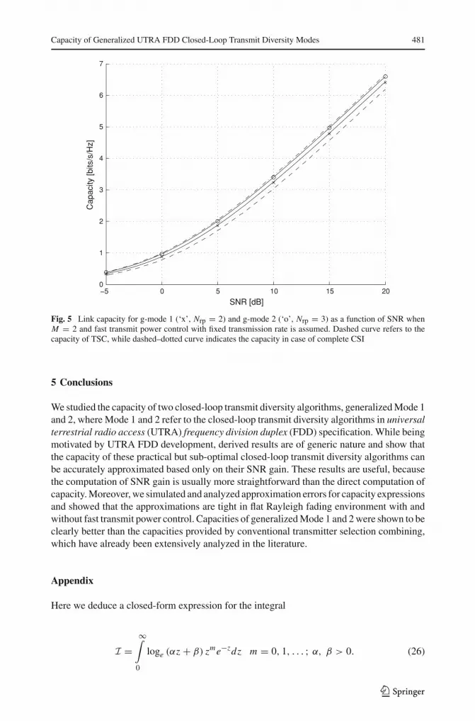
Figure 5 shows capacity for two-antenna g-mode 1 (Nrp = 2) and g-mode 2 (Nrp = 3).The corresponding discrete values (‘x’) and (‘o’) were simulated by using 5 · 105 samples.Results show that the closed-loop modes provide better capacity than TSC also in case of fastpower control and fixed-rate modulation and coding. The gap between g-mode 2 and idealcase is small.

At this stage we shortly analyze the error for approximations (23) and (25). Following theinequality (20) and formula (24) we obtain

E

{1

|h · w|2}

≥ E

{1

|γ |}

= 1

M − 1.

After applying this inequality to the error formula of ε we find the bound

ε = M

G E

{1

|γ |}

− E

{1

|h · w|2}

≤ M − G(M − 1)G .

Thus, ε is decreasing with the number of transmit diversity antennae. We also note that|h · w|2 approaches G|γ |/M when accuracy of the transmit weight increases. Thus, error isdecreasing when Nrp increases.

123


2 3 4 5 6 7 83

3.5

4

4.5

5

5.5

6

6.5

Number of Antennas

Cap

acity

[bits

/s/H

z]

Fig. 4 Link capacity for g-mode 1 (‘x’) and g-mode 2 (‘o’) as a function of the number of transmit antennaewhen Nrp = 3, SNR is 10 dB, and assuming fast transmit power control with fixed transmission rate. Dashedcurve refers to the capacity of TSC, while dashed–dotted curve indicates the capacity in case of complete CSI

Table 3 Approximation errors for the capacities of g-mode 1 and 2 when assuming fast power control, fixedtransmission rate, and Nrp = 3

M = 2 M = 4 M = 8

g-mode 1 (bps/Hz) 0.0288 (0.74%) 0.0230 (0.47%) 0.0138 (0.23%)

g-mode 2 (bps/Hz) 0.0059 (0.15%) 0.0023 (0.05%) 0.0007 (0.01%)

If SNR is large, then the error of the capacity approximation (25) admits the same boundas in case of fixed transmission power, i.e.,

ε∞ = limγ→∞ W log2

(1 + γ /E{1/|h · w|2}1 + (M − 1)G γ /M

)

= W log2

(M

(M − 1)G E{1/|h · w|2})

≤ W log2

(M

G

).

Finally, we highlight that in case of fast power control, capacity gain in the asymptoticSNR region for both g-mode 1 and 2 is the same as with fixed transmission power, i.e.,

limγ→∞

[Cfpc − Cdiv

fpc(γ )]

= limγ→∞ W log2

[1 + (M − 1)G γ /M

1 + (M − 1) γ /M

]= W log2(G).

Thus, we conclude that also in this case the SNR gain defines the asymptotic differencebetween a pure diversity scheme and both g-modes.

123


−5 0 5 10 15 200

1

2

3

4

5

6

7

SNR [dB]

Cap

acity

[bits

/s/H

z]

Fig. 5 Link capacity for g-mode 1 (‘x’, Nrp = 2) and g-mode 2 (‘o’, Nrp = 3) as a function of SNR whenM = 2 and fast transmit power control with fixed transmission rate is assumed. Dashed curve refers to thecapacity of TSC, while dashed–dotted curve indicates the capacity in case of complete CSI

5 Conclusions

We studied the capacity of two closed-loop transmit diversity algorithms, generalized Mode 1and 2, where Mode 1 and 2 refer to the closed-loop transmit diversity algorithms in universalterrestrial radio access (UTRA) frequency division duplex (FDD) specification. While beingmotivated by UTRA FDD development, derived results are of generic nature and show thatthe capacity of these practical but sub-optimal closed-loop transmit diversity algorithms canbe accurately approximated based only on their SNR gain. These results are useful, becausethe computation of SNR gain is usually more straightforward than the direct computation ofcapacity. Moreover, we simulated and analyzed approximation errors for capacity expressionsand showed that the approximations are tight in flat Rayleigh fading environment with andwithout fast transmit power control. Capacities of generalized Mode 1 and 2 were shown to beclearly better than the capacities provided by conventional transmitter selection combining,which have already been extensively analyzed in the literature.

Appendix

Here we deduce a closed-form expression for the integral

I =∞∫

0

loge (αz + β) zme−zdz m = 0, 1, . . . ; α, β > 0. (26)

123


Let us use formula (8.356.4) of [23] and integrate (26) by parts. Then we find that

I = m! loge (β)+ α

∞∫0

� (m + 1, z)

αz + βdz,

where �(m, z) is the incomplete gamma function defined by (8.350.2) of [23]. Furthermore,by formulae (6.5.3), (6.5.2), (6.5.13), and (6.5.11) of [22] we obtain

∞∫0

� (m + 1, z)

αz + βdz = m!

m∑k=0

1

k!∞∫

0

zke−z

αz + βdz.

Then, by using (3.383.10) of [23] and (6.5.9) of [22] we get

∞∫0

zke−z

αz + βdz = k! e

βα Ek+1

(β

α

).

After combining the last three formulae we reach the desired result:

I = m![

loge (β)+ eβα

m∑k=0

Ek+1

(β

α

)].

References

1. 3GPP. (2004). Physical layer procedures (FDD), 3GPP technical specification, TS 25.214, Ver. 6.4.0.2. Narula, A., Lopez, M., Trott, M., & Wornell, G. (1998). Efficient use of side information in multiple-

antenna data transmission over fading channels. IEEE Journal of Selected Areas on Communications,16(8), 1423–1436.

3. Hämäläinen, J., & Wichman, R. (2000). Closed-loop transmit diversity for FDD WCDMA systems. InProceedings of Asilomar conference on signals, systems and computers (Vol. 1, pp. 111–115).

4. Hämäläinen, J., & Wichman, R. (2002). On the performance of FDD WCDMA closed-loop transmitdiversity modes in Nakagami and Ricean fading channels. In Proceedings of the IEEE internationalsymposium on spread spectrum techniques and applications (Vol. 1, pp. 24–28).

5. Mukkavilli, K., Sabharwal, A., Erkip, E., & Aazhang, B. (2003). On beamforming with finite rate feedbackin multiple-antenna systems. IEEE Transactions on Information Theory, 49(10), 2562–2579.

6. Love, D., Heath, R., & Strohmer, T. (2003). Grassmannian beamforming for multiple-input multiple-output wireless systems IEEE Transactions on Information Theory, 49(10), 2735–2747.

7. Hochwald, B., Marzetta, T., Richardson, T., Sweldens, W., & Urbanke, R. (2000). Systematic design ofunitary space-time constellations. IEEE Transactions on Information Theory, 46(6), 1962–1973.

8. Zhou, S., Wang, Z., & Giannakis, G. (2005). Quantifying the power loss when transmit beamformingrelies on finite-rate feedback. IEEE Transactions on Wireless Communication, 4(4), 1948–1957.

9. Au-Yeung, C., & Love, D. (2007). On the performance of random vector quantization limited feedbackbeamforming in a MISO system. IEEE Transactions on Wireless Communication, 6(2), 458–462.

10. Santipach, W., & Honig, M. (2009). Capacity of a multiple-antenna fading channel with a quantizedprecoding matrix. IEEE Transactions on Information Theory, 55(3), 1218–1234.

11. Hämäläinen, J., & Wichman, R. (2002). Asymptotic bit error probabilities of some closed-loop trans-mit diversity schemes. In Proceedings of the IEEE global telecommunications conference (Vol. 1,pp. 360–364).

12. Hämäläinen, J., & Wichman, R. (2001). Feedback schemes for FDD WCDMA systems in multipathenvironments. In Proceedings of the IEEE vehicular technology conference (Vol. 1, pp. 238–242).

13. McEliece, R., & Stark, W. (1984). Channels with block interference. IEEE Transactions on InformationTheory, 30(1), 44–53.

14. Hämäläinen, J., & Wichman, R. (2002). Performance analysis of closed-loop transmit diversity in thepresence of feedback errors. In Proceedings of the IEEE international symposium on personal, indoorand mobile radio communications (Vol. 5, pp. 2297–2301).

123


15. Onggosanusi, E., Gatherer, A., Dabak, A., & Hosur, S. (2001). Performance analysis of closed-looptransmit diversity in the presence of feedback delay. IEEE Transactions on Communications, 49(9),1618–1630.

16. Choi, J. (2002). Performance analysis for transmit antenna diversity with/without channel information.IEEE Transactions on Vehicular Technology, 51(1), 101–113.

17. Heath, R., Jr., & Paulraj, A. (1998). A simple scheme for transmit diversity using partial channel feedback.In Proceedings of asilomar conference on signals, systems and computers, 2, 1073–1078.

18. Alouini, M.-S., & Goldsmith, A. (1999).Capacity of rayleigh fading channels under different adaptivetransmission and diversity-combining techniques. IEEE Transactions on Vehicular Technology, 48(4),1165–1181.

19. Nakagami, M. (1958). The m-distribution—A general formula for intensity distribution of rapid fading.Statistical methods in radio wave propagation (pp. 581–635). New York, NTY, USA: McGraw-Hill.

20. Jakes, W. (Ed.). (1974). Microwave mobile communications. New York: Wiley.21. Lieblein, J. (1955). On moments of order statistics from the weibull distribution. Annals of Mathematical

Statistics, 26(2), 330–333.22. Abramowitz, M., & Stegun, I. (1970). Handbook of mathematical functions. Washington, D.C.: National

Bureau of Standards.23. Gradshteyn, I., & Ryzhik, I. (1965). Tables of integrals, series and products. New York: Academic Press.24. Goldsmith, A., & Varaiya, P. (1997). Capacity of fading channels with channel side information. IEEE

Transactions on Information Theory, 43(6), 1986–1992.25. Cavers, J. (1999). Optimized use of diversity modes in transmitter diversity systems. In Proceedings of

the IEEE vehicular technology conference (Vol. 3, pp. 1768–1773).26. Michalopoulos, D., Lioumpas, A., & Karagiannidis, G. (2008). Increasing power efficiency in transmitter

diversity systems under error performance constraints. IEEE Transactions on Communications, 56(12),2025–2029.

Author Biographies

Jyri Hämäläinen received his M.Sc. and Ph.D. degrees from Univer-sity of Oulu, Oulu, Finland, in 1992 and 1998, respectively, in app-lied mathematics. From 1999 to 2007 he was with Nokia, where hehas worked on various aspects of mobile telecommunications systems.Since 2008 he has been a professor in Department of Communicationsand Networking, Helsinki University of Techonology. His current res-earch interests include multi-antenna transmission and reception tech-niques, design and analysis of wireless networks.

Risto Wichman received his M.Sc. and D.Sc. (Tech) degrees inDigital Signal Processing from Tampere University of Technology,Tampere, Finland, in 1990 and 1995, respectively. From 1995 to 2001,he worked at Nokia Research Center as a senior research engineer. In2002, he joined Department of Signal Processing and Acoustics, Fac-ulty of Electronics, Communications and Automation, Helsinki Univer-sity of Technology, where he is a professor since 2003. His researchinterests include physical layer analysis and design for 3G-4G wirelesscommunication systems.

123


Alexis A. Dowhuszko was born in San Nicolas, Argentina, in 1978.He received the telecommunications engineer degree in 2002 from theBlas Pascal University, Cordoba, Argentina. In 2006, he received a fel-lowship from CONICET, the National Research Council of Argentina,to carry out his studies in the area of MIMO wireless communications.He is currently pursuing his research towards a Doctor of Science de-gree at the Digital Communications Research Laboratory, Departmentof Electronics, National University of Cordoba. His research interestslie in the area of MIMO wireless and include spatial multiplexing,multiuser diversity, and opportunistic beamforming.

Graciela Corral-Briones received the electrical and electronicengineer degree in 1991, and the Ph.D. degree in 2007, both from theNational University of Cordoba, Cordoba, Argentina. From 1991 to1993, she was with the Center for Research in Materials, Cordoba,Argentina, as a Research Fellow. From 1993 to 1996, she receiveda fellowship from CONICOR (Scientific and Technological ResearchCouncil of Cordoba) to develop analyzers for communication proto-cols. Since March 1996, she has been with the Digital CommunicationsResearch Laboratory, Department of Electronic Engineering, NationalUniversity of Cordoba. Her research interests lie in the areas of wire-less communications and signal processing, including multiuser detec-tion, channel coding, and MIMO systems.

123

Documents

Capacity of Generalized UTRA FDD Closed-Loop Transmit Diversity Modes