CLOSED-LOOP TURBULENCE CONTROL - UW Faculty Web

CLOSED-LOOP TURBULENCE CONTROL:PROGRESS AND CHALLENGESSteven L. Brunton1 and Bernd R. Noack2,3

1 Department of Mechanical Engineering & eScience Institute, University of Washington, Seattle, WA 98195, United States2 Institut PPRIME, CNRS – Universite de Poitiers – ENSMA, UPR 3346, Department Fluides, Thermique, Combustion,F-86036 Poiters CEDEX, France3 Institut fur Stromungsmechanik, Technische Universitat Braunschweig, D-38108 Braunschweig, Germany

AbstractClosed-loop turbulence control is a critical enabler of aero-dynamic drag reduction, lift increase, mixing enhancement,and noise reduction. Current and future applications haveepic proportion: cars, trucks, trains, airplanes, wind turbines,medical devices, combustion, chemical reactors, just to namea few. Methods to adaptively adjust open-loop parametersare continually improving towards shorter response times.However, control design for in-time response is challengedby strong nonlinearity, by high-dimensionality and by time-delays. Recent advances in the field of model identificationand system reduction, coupled with advances in control the-ory (robust, adaptive, and nonlinear) are driving significantprogress in adaptive and in-time closed-loop control of fluidturbulence. In this review, we provide an overview of criticaltheoretical developments, highlighted by compelling exper-imental success stories. We also point to challenging openproblems and propose potentially disruptive technologies ofmachine learning and compressive sensing.

Contents1 Introduction 2

2 Turbulence control problem 32.1 The flow control plant and associated goals . 42.2 Linear dynamics . . . . . . . . . . . . . . . . . 52.3 Turbulence control mechanisms . . . . . . . . 62.4 Actuators and sensors . . . . . . . . . . . . . . 72.5 Achievable performance . . . . . . . . . . . . 7

3 Black-box, gray-box, and white-box models 83.1 State-space models . . . . . . . . . . . . . . . . 83.2 Kinematics: employed state spaces . . . . . . 9

3.2.1 Full-resolution description (white-box) 93.2.2 Modal representation (gray-box) . . . . 93.2.3 Input–output (black-box) . . . . . . . . 11

3.3 Dynamics: classification by system resolution 113.3.1 White-box models . . . . . . . . . . . . 113.3.2 Gray-box models . . . . . . . . . . . . 113.3.3 Black-box models . . . . . . . . . . . . 123.3.4 Model-free approaches . . . . . . . . . 12

4 Linear model-based control 124.1 Linearized input–output dynamics . . . . . . 134.2 Model-based open-loop control . . . . . . . . 134.3 Dynamic closed-loop feedback control . . . . 14

4.3.1 Controllability, observability, andGramians . . . . . . . . . . . . . . . . . 14

4.3.2 Linear quadratic Gaussian . . . . . . . 154.4 Robust control . . . . . . . . . . . . . . . . . . 16

4.4.1 Sensitivity, complementary sensitivity,and robustness . . . . . . . . . . . . . . 16

4.4.2 H∞ robust control design . . . . . . . 174.4.3 Fundamental limitations with implica-

tions for turbulence control . . . . . . . 184.4.4 Two degrees of freedom control . . . . 19

4.5 Balanced model reduction . . . . . . . . . . . 194.5.1 Discrete-time systems and Gramians . 204.5.2 Goal of model reduction . . . . . . . . 204.5.3 Balanced proper orthogonal decompo-

sition . . . . . . . . . . . . . . . . . . . 204.5.4 Eigensystem realization algorithm . . 214.5.5 Observer/Kalman filter identification . 22

4.6 Case study: Transition delay in a boundarylayer and stabilizing steady states . . . . . . . 224.6.1 Early work . . . . . . . . . . . . . . . . 224.6.2 Use of reduced-order models . . . . . 23

4.7 Case study: Wall turbulence control and skin-friction reduction . . . . . . . . . . . . . . . . 23

4.8 Case study: Cavity flow control . . . . . . . . 234.9 Potential impact and challenges . . . . . . . . 24

5 Prototypes for linear and nonlinear dynamics 245.1 Galerkin model . . . . . . . . . . . . . . . . . 255.2 Linear dynamics . . . . . . . . . . . . . . . . . 25

5.2.1 Oscillator model . . . . . . . . . . . . . 255.2.2 Energy-based control design . . . . . . 26

5.3 Weakly nonlinear dynamics . . . . . . . . . . 265.3.1 Mean-field model . . . . . . . . . . . . 275.3.2 Nonlinear control design . . . . . . . . 27

5.4 Moderately nonlinear dynamics . . . . . . . . 275.4.1 Generalized mean-field model . . . . . 285.4.2 Nonlinear control design . . . . . . . . 29

5.5 Strongly nonlinear dynamics . . . . . . . . . . 305.5.1 Examples of strongly nonlinear dynamics 305.5.2 Nonlinear control design . . . . . . . . 30

5.6 Enablers and challenges of nonlinear model-based control . . . . . . . . . . . . . . . . . . . 31

1

6 Model-free control 326.1 Open-loop forcing . . . . . . . . . . . . . . . . 336.2 Adaptive control . . . . . . . . . . . . . . . . . 33

6.2.1 Extremum-seeking control methodology 336.2.2 Examples of adaptive control in turbu-

lence . . . . . . . . . . . . . . . . . . . 356.3 In-time control . . . . . . . . . . . . . . . . . . 35

6.3.1 Control law parameterizations andtuning methodologies . . . . . . . . . . 35

6.3.2 Case study: opposition control in wallturbulence . . . . . . . . . . . . . . . . 36

6.4 Neural network based control . . . . . . . . . 366.5 Genetic algorithm based control . . . . . . . . 376.6 Genetic programming control . . . . . . . . . 38

7 Conclusions 417.1 Historical perspective . . . . . . . . . . . . . . 417.2 Current practices . . . . . . . . . . . . . . . . . 42

7.2.1 Linear control and transition . . . . . . 427.2.2 Nonlinear control and separation . . . 427.2.3 Model-free control and mixing . . . . . 43

7.3 Industrial applications . . . . . . . . . . . . . 44

8 Future developments beyond control theory 448.1 Bio-inspired sensing and actuation . . . . . . 44

8.1.1 Cheap hardware and local computations 458.1.2 Sensor and actuator placement . . . . . 45

8.2 Data-driven modeling and control . . . . . . . 468.2.1 Compressive sensing . . . . . . . . . . 468.2.2 Machine learning . . . . . . . . . . . . 468.2.3 Uncertainty quantification and

equation-free methods . . . . . . . . . 478.2.4 Design of experiments . . . . . . . . . 48

8.3 Advanced nonlinear models, controllers andclosures . . . . . . . . . . . . . . . . . . . . . . 488.3.1 Graph-theoretic flow control . . . . . . 488.3.2 Markov model-based control . . . . . . 49

1 IntroductionTaming turbulence for engineering goals is one of the old-est and most fruitful academic and technological challenges.One of the earliest examples are the feathers at the tail of anarrow invented several thousand years ago. These feathersstabilize the orientation of the arrow and make the trajectorymore predictable and increase its range. Meanwhile, mod-ern turbulence control has applications of epic proportion.Examples include drag reduction of road vehicles, airbornetransport, ships and submarines, drag reduction in pipes andair-conditioning systems, lift increase of airfoils, efficiency in-crease of harvesting wind and water energy, of heat transferand of chemical and combustion processes — just to name afew examples.

Animal motion has inspired numerous technical ad-vances in engineering flows [1]. The shape of sharks, dol-phins and whales, for instance, yields a low drag per volume[2]. It is not an accident that zeppelins and airplanes havesimilar shapes. Dolphins are speculated to delay boundary

layer transition by a compliant skin. This form of transitiondelay has been applied to submarines and is under active in-vestigation. Under magnification, the skin of sharks exhibitriblets [3]. Riblets have been found to reduce drag by up to11 % in the laboratory [4]. In-flight tests of riblets on an Air-bus passenger airplane have reduced fuel consumption by 2-3 %. Some sharks decrease drag by ejecting lubricants duringhigh-speed chases of their pray. A similar skin-friction reduc-tion is used in oil pipelines: one added polymer per 1 millionoil molecules reduces the drag by about 40 %. Eagles andother birds have 5 feathers at the tip of their wings. Thesefeathers increase the lift by reducing the pressure short-cutbetween the low pressure upper side and the higher pressurelower side. Most modern passenger airplanes have wingletsfor the same reason.

The environmental benefit of turbulence control can beillustrated with an everyday example: automotive trans-port. Today, the annual global CO2 emissions from cars ex-ceed 22 billion tons and are expected to increase by 57% by2030. A large portion of this emission is due to aerodynamicdrag [5, 6]. At a speed of 50 km/h the aerodynamic dragaccounts for 50% of the total resistance reaching 80% at 130km/h. A drag reduction of around 25% is currently achiev-able by active flow control [7]. Ad a speed of 120km/h, thiswould reduce consumption by about 1.8 liter and would re-duce CO2 by almost 2 kg per 100 km. In normal traffic, thecorresponding reductions are 0.15 liter in fuel and 0.73 kg inCO2. For Europe, this drag reduction would mean a reduc-tion of 23 million tonnes of CO2 emission in one year. Tomitigate pollution, the European government imposes strictnorms to car manufacturers. By 2020, the mean CO2 emis-sion per vehicle must not exceed 95 gCO2/km. By 2025, thelimit is 75 gCO2/km.

Among the countless technologies that will benefit fromturbulence control, we highlight the potential benefits for en-ergy and transportation. Increased lift and reduced drag dueto separation control and transition delay would result inincreased payloads and decreased runway requirements foraircraft and improved efficiency in nearly all vehicles. Con-sidering that transportation accounts for approximately 20%of global energy consumption, a small improvement wouldhave a dramatic effect [8, 9, 10]. Active separation controlwould also improve the safety of cargo trucks and trains instrong cross-winds [11, 12, 13]. Hypersonic vehicles stand tobenefit from active control to prevent the undesirable ejectionof flames out of the combustion chamber, and subsequentquenching. Finally, reducing the amount of turbulent fluctu-ations on rotor blades would reduce vibration and improvethe life of rotor hubs on wind turbines and rotorcraft.

Strategies to control laminar and turbulent flow are clas-sified in three categories [14]: aerodynamic shape optimiza-tion, passive and active control. The first approach for in-creasing flow performance is the optimization of the aerody-namic shape. Potential flow theory, invented about 150 yearsago, provides a simple mathematical foundation. Meanwhileadjoint-based shape optimization can be numerically per-formed for the full Navier-Stokes equations. As a secondstep, passive actuators may improve the performance. Sucha device represents a small change of the original configura-

2

tion. One example are the turbulators on wings of passen-ger airplanes to delay separation. Such passive devices maycome with the penalty of parasitic drag. An alternative areactive control devices, like fluidic vortex generators, whichmay be turned on and off but require energy for their opera-tion. One advantage is a large dynamic bandwidth, e.g. theexcitation of particular frequencies. Active control may beperformed in a predetermined open-loop manner, e.g. peri-odic blowing and suction, independent of the flow state. Thelargest gains are, of course, realized in a closed-loop mannerwhen the actuation is informed by the sensors recording theflow state.

Up to the 1990’s, manufacturers have often seen ac-tive control as a remedy for a flawed aerodynamic design[15]. Hence, industrial interest has been correspondinglylow. Meanwhile, aerodynamic design and passive devicesare considered as maturely developed and active control ispursued to further increase the performance, particularly foroff-design conditions. Three trends foster closed-loop con-trol. First, the power and reliability of actuators and sensorshave dramatically increased, while the price is decreasing.Second, a sophisticated control logic can be performed un-der real-world conditions with increasing computer powerand the advancement of mathematical theories. Thirdly, theexperimental demonstrations of the benefits of closed-loopover open-loop forcing has become overwhelming [see, e.g.,16, 17].

Most literature on closed-loop flow control falls in oneof three categories: stabilization of laminar flow, adaptivecontrol of turbulence and model-free tuning of control laws.For the first category, there exists a mature theory for thestabilization of laminar flows with in-time closed-loop con-trol. Early experimental examples are described in [18, 19]while most studies are based on Direct Navier-Stokes (DNS)solutions [see, e.g., 20, 21]. ’In-time’ means that the actua-tion responds on a time-scale much smaller than the naturaltime-scale. Most corresponding publications are based on alinearization of the evolution equation. The employed evolu-tion equation may be a white-box model, e.g. DNS discretiza-tion, resolving all features of the flows, a gray-box model,e.g. POD models, just describing the coherent structures, ora black-box model, e.g. transfer functions, representing onlythe input-output behavior. The control logic based on whitebox models are the most accurate. Gray-box and black-boxmodels are less accurate but allow online-capable control so-lutions for experiments.

The second category is adaptive control of turbulenceusually based on a manipulation of periodic forcing. Mostexperimental success stories belong to this class. ’Adaptive’means that the change of the actuation parameter, like am-plitude or frequency, is slow compared to the natural time-scale. The third group consists of in-time control of turbulentflows, for instance by tuning simple laws, e.g. opposition orPID control [22]. The inherent nonlinearities of turbulencepose a challenge for model-based in-time control.

Closed-loop control requires decisions on the hardware,like the kind, number, location, and dynamic bandwidth ofactuators and sensors. Such decisions may be guided bymodern adjoint-based techniques for linearized equations,

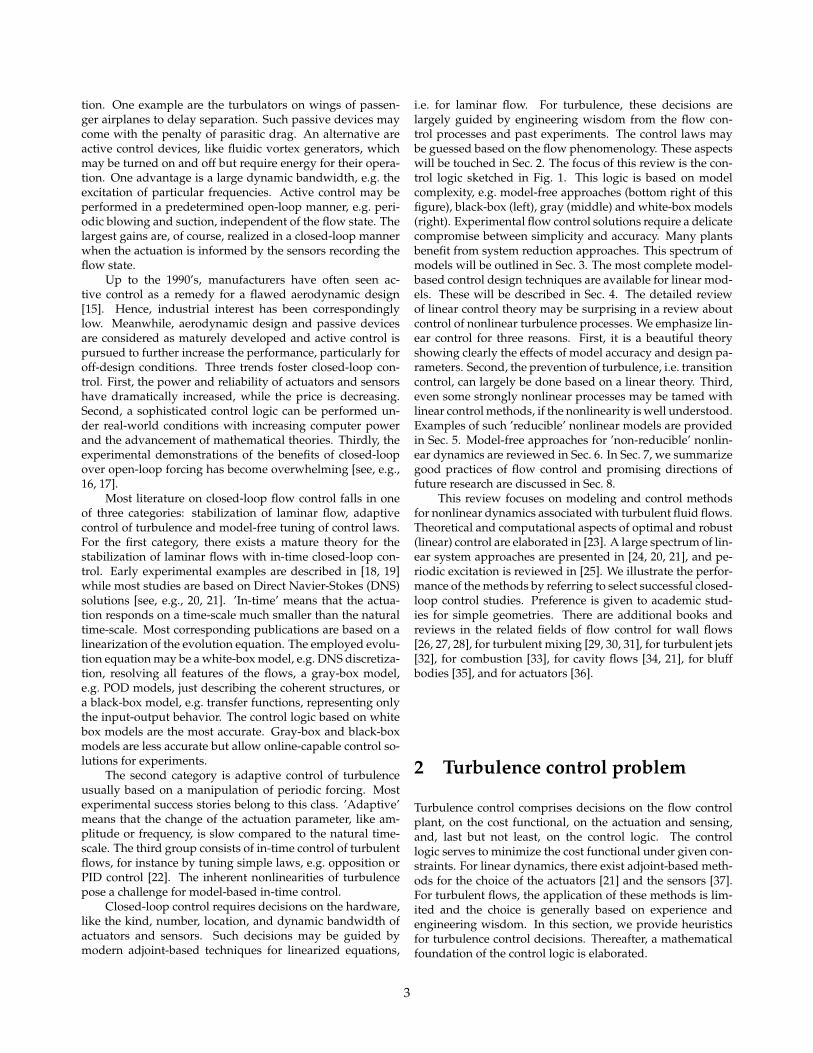
i.e. for laminar flow. For turbulence, these decisions arelargely guided by engineering wisdom from the flow con-trol processes and past experiments. The control laws maybe guessed based on the flow phenomenology. These aspectswill be touched in Sec. 2. The focus of this review is the con-trol logic sketched in Fig. 1. This logic is based on modelcomplexity, e.g. model-free approaches (bottom right of thisfigure), black-box (left), gray (middle) and white-box models(right). Experimental flow control solutions require a delicatecompromise between simplicity and accuracy. Many plantsbenefit from system reduction approaches. This spectrum ofmodels will be outlined in Sec. 3. The most complete model-based control design techniques are available for linear mod-els. These will be described in Sec. 4. The detailed reviewof linear control theory may be surprising in a review aboutcontrol of nonlinear turbulence processes. We emphasize lin-ear control for three reasons. First, it is a beautiful theoryshowing clearly the effects of model accuracy and design pa-rameters. Second, the prevention of turbulence, i.e. transitioncontrol, can largely be done based on a linear theory. Third,even some strongly nonlinear processes may be tamed withlinear control methods, if the nonlinearity is well understood.Examples of such ’reducible’ nonlinear models are providedin Sec. 5. Model-free approaches for ’non-reducible’ nonlin-ear dynamics are reviewed in Sec. 6. In Sec. 7, we summarizegood practices of flow control and promising directions offuture research are discussed in Sec. 8.

This review focuses on modeling and control methodsfor nonlinear dynamics associated with turbulent fluid flows.Theoretical and computational aspects of optimal and robust(linear) control are elaborated in [23]. A large spectrum of lin-ear system approaches are presented in [24, 20, 21], and pe-riodic excitation is reviewed in [25]. We illustrate the perfor-mance of the methods by referring to select successful closed-loop control studies. Preference is given to academic stud-ies for simple geometries. There are additional books andreviews in the related fields of flow control for wall flows[26, 27, 28], for turbulent mixing [29, 30, 31], for turbulent jets[32], for combustion [33], for cavity flows [34, 21], for bluffbodies [35], and for actuators [36].

2 Turbulence control problem

Turbulence control comprises decisions on the flow controlplant, on the cost functional, on the actuation and sensing,and, last but not least, on the control logic. The controllogic serves to minimize the cost functional under given con-straints. For linear dynamics, there exist adjoint-based meth-ods for the choice of the actuators [21] and the sensors [37].For turbulent flows, the application of these methods is lim-ited and the choice is generally based on experience andengineering wisdom. In this section, we provide heuristicsfor turbulence control decisions. Thereafter, a mathematicalfoundation of the control logic is elaborated.

3

Black-box model based control design

Parameter tuning(heuristic)

MLC(unsupervised)

Adaptive control(quasi-steady)

Optim

al adjoint based control

Galerkin projection

Time-delay coordinates

Model identification

LQR, LQG, ...(optimal)

Weakly nonlinear

Moderately nonlinear

Linear Strongly nonlinear

Linear control design

Model-free control design

Knowledge of the plant

Kinematics

Dynamics

Empirical Physical Mathematical

Flow data Navier-Stokes equations

Input/output data

Plant model

Control design

Action mechanisms

Modes

Controllers

fact, the gain in towing power corrected by the actuation en-ergy is less efficient than for complete stabilization. A fourthhighly successful drag reduction strategy consist of an aero-dynamic shaping of the dead-water region, so that the bluffbody and the wake are more streamlined [7].

For high-lift configurations, the potential solution can beconjectured to yield the maximum achievable lift. Similarly,the maximum achievable pressure recovery in diffusers canalso be estimated from the potential solution. Summarizing,the hypothesis on achievable performance has not only a the-oretical value. The answer may also guide the control strat-egy.

Finally, we mention mixing enhancement and noise re-duction problems in which the cost function explicitely de-pends on the history of the fluid motion. For such La-grangian control tasks, an intuition about achievable maxi-mum mixing or the minimum noise emission is still in itsinfancy.

3 Black-box, gray-box, and white-box models

Regardless of the modeling strategy employed below, we as-sume that we are able to actuate the flow with some inputvariables b 2 RNb and we are able to measure features of theflow with some output variables s 2 RNs . Once the inputsand outputs are set, there are many choices for the modelthat links them. For example, we may consider the full dis-cretized Navier-Stokes equations as a high-dimensional non-linear set of ordinary differential equations. Alternatively,we may relate inputs to outputs through either a statisti-cal description or a set of empirical basis functions. Recentadvances in dimensionality reduction techniques and turbu-lence closures also have exciting implications for the futureof turbulence modeling and control.

The choice of model affects nearly every downstreamcontrol decision. There are many factors and tradeoffs thatmust be balanced when deciding on a modeling strategy.These include the accuracy of the model, execution time,generality in other parameter regimes, spatial-temporal res-olution relative to disturbances, and the up-front cost to ac-quire such a model. For example, direct numerical simula-tion (DNS) is unparalleled at descriptive resolution, general-ity, and accuracy, but current computational capabilities aredecades away from real-time execution for in-time controlstrategies. Reduced-order models based on data from DNSor experiments provide real-time capable models, but thesemodels are expensive to create and may only work for a smallrange of training parameters. Fortunately, it may be possibleto leverage physical intuition about the structure of the un-derlying modes, often in terms of linear combinations of fullflow fields, to modify the models with addit ional terms andextend their predictive range. Black-box models based oninput–output data are typically faster to generate and requireless measured data, but they lack the physical interpretationthat goes with having an underlying modal representation.

Figure 4 outlines a model hierarchy for control design,

Bla

ck

box

Data

Navier-Stokes equations

Gra

y bo

xW

hite

bo

xU

ltra

whi

teM

odel

fr

ee

I/O

Controllers

ROM

CFD

Figure 4: Model hierarchy for control design based on [74].

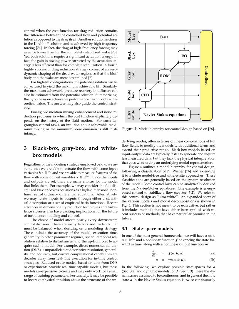
following a classification of N. Wiener [74] and extending itto include model-free approaches. These classifications aregenerally based on the system resolution of the model. Somecontrol laws can be analytically derived from the Navier-Stokes equations. One example is energy-based control tostabilize a flow (see Sec. 5.2). We refer to this control-designas “ultra-white”. An expanded view of the various modelsand modal decompositions is shown in Fig. 5. This section isnot meant to be exhaustive, but rather include methods thathave either been applied with recent success or methods thathave particular promise in the future.

3.1 State-space modelsIn one of the most general frameworks, we will have a statea 2 RNa and a nonlinear function f advancing the state for-ward in time, along with a nonlinear output function m:

a = f(a, b; µ), (2a)

s = m(a, b; µ). (2b)

In the following, we explore possible state-spaces for a(Sec. 3.2) and dynamic models for f (Sec. 3.3). Here the dy-namics are assumed to be continuous, and in general the flowstate a in the Navier-Stokes equation is twice continuouslydifferentiable in space and once continuously differentiablein time. The bifurcation parameters µ may change the qual-itative nature of the solutions, and the flow field may notalways be continuously differentiable in µ. These parame-ters include the Reynolds number and Mach number, amongothers.

The nonlinear dynamics in Eq. (2) may be linearized ata steady fixed point as, where f(as,0; µ) = 0, away from

8

Figure 1: Turbulence control roadmap. For details, see text and the coming sections.

2.1 The flow control plant and associatedgoals

In the sequel, flow is assumed to be within or around a steadyboundary with small unsteady actuators and sensors. Aca-demic flow control configurations strive at geometric sim-plicity for enhanced reproducibility and for ’clean’ under-standable physical mechanisms. Examples include free shearflows from a bluff body, a mixing layer or a jet and wall-bounded flows in a channel or over a flat plate. Cavity noise,suppression of aeroelastic oscillation and flame-holder com-bustion serve as examples for multi-physics flows.

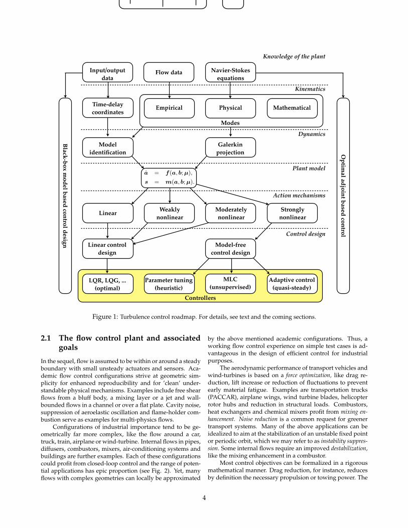
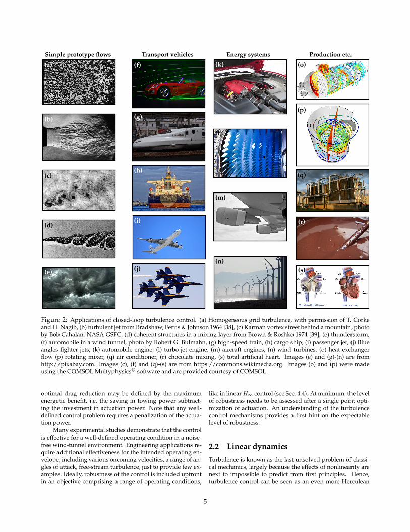
Configurations of industrial importance tend to be ge-ometrically far more complex, like the flow around a car,truck, train, airplane or wind-turbine. Internal flows in pipes,diffusers, combustors, mixers, air-conditioning systems andbuildings are further examples. Each of these configurationscould profit from closed-loop control and the range of poten-tial applications has epic proportion (see Fig. 2). Yet, manyflows with complex geometries can locally be approximated

by the above mentioned academic configurations. Thus, aworking flow control experience on simple test cases is ad-vantageous in the design of efficient control for industrialpurposes.

The aerodynamic performance of transport vehicles andwind-turbines is based on a force optimization, like drag re-duction, lift increase or reduction of fluctuations to preventearly material fatigue. Examples are transportation trucks(PACCAR), airplane wings, wind turbine blades, helicopterrotor hubs and reduction in structural loads. Combustors,heat exchangers and chemical mixers profit from mixing en-hancement. Noise reduction is a common request for greenertransport systems. Many of the above applications can beidealized to aim at the stabilization of an unstable fixed pointor periodic orbit, which we may refer to as instability suppres-sion. Some internal flows require an improved destabilization,like the mixing enhancement in a combustor.

Most control objectives can be formalized in a rigorousmathematical manner. Drag reduction, for instance, reducesby definition the necessary propulsion or towing power. The

4

Simple prototype flows Transport vehicles Energy systems Production etc.

(a)

(b)

(c)

(d)

(e)

(f)

(g)

(h)

(i)

(j)

(k)

(l)

(m)

(n)

(o)

(p)

(q)

(r)

(s)

Figure 2: Applications of closed-loop turbulence control. (a) Homogeneous grid turbulence, with permission of T. Corkeand H. Nagib, (b) turbulent jet from Bradshaw, Ferris & Johnson 1964 [38], (c) Karman vortex street behind a mountain, photoby Bob Cahalan, NASA GSFC, (d) coherent structures in a mixing layer from Brown & Roshko 1974 [39], (e) thunderstorm,(f) automobile in a wind tunnel, photo by Robert G. Bulmahn, (g) high-speed train, (h) cargo ship, (i) passenger jet, (j) Blueangles fighter jets, (k) automobile engine, (l) turbo jet engine, (m) aircraft engines, (n) wind turbines, (o) heat exchangerflow (p) rotating mixer, (q) air conditioner, (r) chocolate mixing, (s) total artificial heart. Images (e) and (g)-(n) are fromhttp://pixabay.com. Images (c), (f) and (q)-(s) are from https://commons.wikimedia.org. Images (o) and (p) were madeusing the COMSOL Multyphysicsr software and are provided courtesy of COMSOL.

optimal drag reduction may be defined by the maximumenergetic benefit, i.e. the saving in towing power subtract-ing the investment in actuation power. Note that any well-defined control problem requires a penalization of the actua-tion power.

Many experimental studies demonstrate that the controlis effective for a well-defined operating condition in a noise-free wind-tunnel environment. Engineering applications re-quire additional effectiveness for the intended operating en-velope, including various oncoming velocities, a range of an-gles of attack, free-stream turbulence, just to provide few ex-amples. Ideally, robustness of the control is included upfrontin an objective comprising a range of operating conditions,

like in linearH∞ control (see Sec. 4.4). At minimum, the levelof robustness needs to be assessed after a single point opti-mization of actuation. An understanding of the turbulencecontrol mechanisms provides a first hint on the expectablelevel of robustness.

2.2 Linear dynamics

Turbulence is known as the last unsolved problem of classi-cal mechanics, largely because the effects of nonlinearity arenext to impossible to predict from first principles. Hence,turbulence control can be seen as an even more Herculean

5

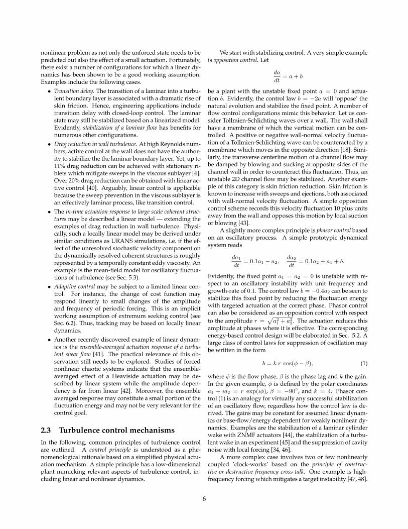
nonlinear problem as not only the unforced state needs to bepredicted but also the effect of a small actuation. Fortunately,there exist a number of configurations for which a linear dy-namics has been shown to be a good working assumption.Examples include the following cases.• Transition delay. The transition of a laminar into a turbu-

lent boundary layer is associated with a dramatic rise ofskin friction. Hence, engineering applications includetransition delay with closed-loop control. The laminarstate may still be stabilized based on a linearized model.Evidently, stabilization of a laminar flow has benefits fornumerous other configurations.

• Drag reduction in wall turbulence. At high Reynolds num-bers, active control at the wall does not have the author-ity to stabilize the the laminar boundary layer. Yet, up to11% drag reduction can be achieved with stationary ri-blets which mitigate sweeps in the viscous sublayer [4].Over 20% drag reduction can be obtained with linear ac-tive control [40]. Arguably, linear control is applicablebecause the sweep prevention in the viscous sublayer isan effectively laminar process, like transition control.

• The in-time actuation response to large scale coherent struc-tures may be described a linear model — extending theexamples of drag reduction in wall turbulence. Physi-cally, such a locally linear model may be derived undersimilar conditions as URANS simulations, i.e. if the ef-fect of the unresolved stochastic velocity component onthe dynamically resolved coherent structures is roughlyrepresented by a temporally constant eddy viscosity. Anexample is the mean-field model for oscillatory fluctua-tions of turbulence (see Sec. 5.3).

• Adaptive control may be subject to a limited linear con-trol. For instance, the change of cost function mayrespond linearly to small changes of the amplitudeand frequency of periodic forcing. This is an implicitworking assumption of extremum seeking control (seeSec. 6.2). Thus, tracking may be based on locally lineardynamics.

• Another recently discovered example of linear dynam-ics is the ensemble-averaged actuation response of a turbu-lent shear flow [41]. The practical relevance of this ob-servation still needs to be explored. Studies of forcednonlinear chaotic systems indicate that the ensemble-averaged effect of a Heaviside actuation may be de-scribed by linear system while the amplitude depen-dency is far from linear [42]. Moreover, the ensembleaveraged response may constitute a small portion of thefluctuation energy and may not be very relevant for thecontrol goal.

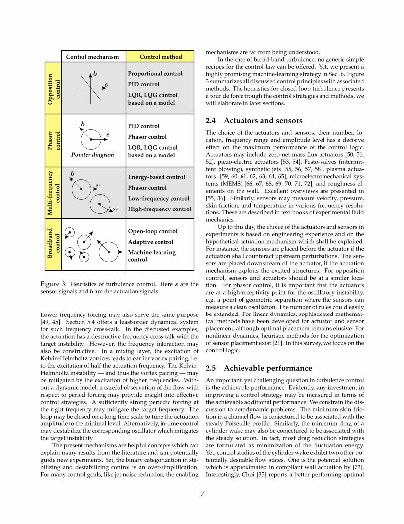
2.3 Turbulence control mechanismsIn the following, common principles of turbulence controlare outlined. A control principle is understood as a phe-nomenological rationale based on a simplified physical actu-ation mechanism. A simple principle has a low-dimensionalplant mimicking relevant aspects of turbulence control, in-cluding linear and nonlinear dynamics.

We start with stabilizing control. A very simple exampleis opposition control. Let

da

dt= a+ b

be a plant with the unstable fixed point a = 0 and actua-tion b. Evidently, the control law b = −2a will ’oppose’ thenatural evolution and stabilize the fixed point. A number offlow control configurations mimic this behavior. Let us con-sider Tollmien-Schlichting waves over a wall. The wall shallhave a membrane of which the vertical motion can be con-trolled. A positive or negative wall-normal velocity fluctua-tion of a Tollmien-Schlichting wave can be counteracted by amembrane which moves in the opposite direction [18]. Simi-larly, the transverse centerline motion of a channel flow maybe damped by blowing and sucking at opposite sides of thechannel wall in order to counteract this fluctuation. Thus, anunstable 2D channel flow may be stabilized. Another exam-ple of this category is skin friction reduction. Skin friction isknown to increase with sweeps and ejections, both associatedwith wall-normal velocity fluctuation. A simple oppositioncontrol scheme records this velocity fluctuation 10 plus unitsaway from the wall and opposes this motion by local suctionor blowing [43].

A slightly more complex principle is phasor control basedon an oscillatory process. A simple prototypic dynamicalsystem reads

da1

dt= 0.1a1 − a2,

da2

dt= 0.1a2 + a1 + b.

Evidently, the fixed point a1 = a2 = 0 is unstable with re-spect to an oscillatory instability with unit frequency andgrowth-rate of 0.1. The control law b = −0.4a2 can be seen tostabilize this fixed point by reducing the fluctuation energywith targeted actuation at the correct phase. Phasor controlcan also be considered as an opposition control with respectto the amplitude r =

√a2

1 + a22. The actuation reduces this

amplitude at phases where it is effective. The correspondingenergy-based control design will be elaborated in Sec. 5.2. Alarge class of control laws for suppression of oscillation maybe written in the form

b = k r cos(φ− β), (1)

where φ is the flow phase, β is the phase lag and k the gain.In the given example, φ is defined by the polar coordinatesa1 + ıa2 = r exp(ıφ), β = −90, and k = 4. Phasor con-trol (1) is an analogy for virtually any successful stabilizationof an oscillatory flow, regardless how the control law is de-rived. The gains may be constant for assumed linear dynam-ics or base-flow/energy dependent for weakly nonlinear dy-namics. Examples are the stabilization of a laminar cylinderwake with ZNMF actuators [44], the stabilization of a turbu-lent wake in an experiment [45] and the suppression of cavitynoise with local forcing [34, 46].

A more complex case involves two or few nonlinearlycoupled ’clock-works’ based on the principle of construc-tive or destructive frequency cross-talk. One example is high-frequency forcing which mitigates a target instability [47, 48].

6

Opp

ositi

on

cont

rol

Mul

ti-fr

eque

ncy

cont

rol

Phas

or

cont

rol

Broa

dban

d co

ntro

lControl mechanism Control method

Bro

ad

ba

nd

dy

na

mic

sco

ntr

ol

Ph

aso

r co

ntr

ol

Op

po

siti

on

con

tro

l

b

s

s

s

b

b

s

1

2

Control mechanism

Proportional control

PID control

LQR, LQG controlbased on a model


PID control

Adaptive control

Machine learning c.

Open−loop control

Phasor control

High−frequency c.

Low−frequency c.

Phasor control

Energy−based c.

pointer diagram

Mu

lti−

freq

uen

cy

Control method

Figure 3: Heuristics of turbulence control

turbulence presents a tour de force trough the control strate-gies and methods, we will elaborate in later sections.

2.3 Actuators and sensorsThe choice of the actuators and sensors, their number, lo-cation, frequency range and amplitude level has a decisiveeffect on the maximum performance of the control logic.Actuators may include zero-net mass flux actuators, piezo-electric actuators, Festo-valves (intermittent blowing), syn-thetic jets [17], plasma actuators, and roughness elements onthe wall. [13] offers an excellent summary. Similarly, sensorsmay measure velocity, pressure, skin-friction, temperature invarious frequency resolutions.

Up to this day, the choice of the actuators and sensors inexperiments is based on engineering experience and on thehypothetical actuation mechanism which shall be exploited.For instance, the sensors are placed before the actuator ofthe actuator shall counteract upstream perturbations. Thesensors are placed downstream of the actuator, if actuationmechanism exploits the excited structures. For oppositioncontrol, sensors and actuators should be at a similar loca-tion. For phasor control, it is important that the actuatorsare at a high-receptitivity point for the oscillatory instability,e.g. a point of geometric separation and the sensors can mea-sure a clean oscillation. The number of rules could easily be

extended. For linear dynamics, sophisticated mathematicalmethods have been developed for actuator and sensor place-ment. For nonlinear dynamics, heuristic methods for the op-timization of sensor placement exist [? ]. In this survey, wefocus on the control logic.

5

Bro

ad

ban

dd

yn

am

ics

con

trol

Ph

aso

r co

ntr

ol

Op

posi

tion

con

trol

b

s

s

s

b

b

s

1

2

Control mechanism


PID control



PID control

Adaptive control

Machine learning c.

Open−loop control

Phasor control

High−frequency c.

Low−frequency c.

Phasor control

Energy−based c.

pointer diagram

Mu

lti−

freq

uen

cyControl method






5

4.4.1 Balanced model reduction

4.5 H1 robust vs. H2 optimal control

Now that we have established conditions enablingarbitrary pole placement of the closed-loop system,we must now decide on where to place them.

4.5.1 H2 optimal control: Linear quadratic Gaus-sian (LQG)

We may often modify Eq. (2) with the addition ofwhite noise disturbance wd and measurement noisewn:

d

dta = Aa + Bb + wd, (14a)

s = Ca + Db + wn. (14b)

Each of these noise inputs has a different co-variance matrix: E(wdw

Td ) = Vd and E(wnwT

n ) =Vn, where E(·) is the expectation value. [This isnot precise enough... really need E(wd(t)wd()T ) =Vd(t ).]

Linear-quadratic regulator (LQR):

J =

Z 1

0aT Qa + bT Rb dt. (15a)

The optimal control law is b = Kra, where Kr =R1BT X and X is the unique solution to the alge-braic Riccati equation:

AT X + XA XBR1BT X + Q = 0. (16a)

A dual Riccati equation is solved for the observergain Kf = Y CT Vn:

Y AT + AY Y CT V 1n CY + Vd = 0. (17a)

The so-called Kalman filter Kf is chosen to mini-

mize E(a a)T (a a)

given known covariance

Vd and Vn.[Note: Kalman published his famous Kalman

filter in a journal of Fluid Engineering.][Decent stability margins for LQR, but no guar-

anteed stability margins for LQG (famous Doyle pa-per)].

4.5.2 Sensitivity, Complementary Sensitivity,and Robustness

• S() - sensitivity function

• T () - complementary sensitivity function

• wr - reference tracking

4.5.3 H1 robust control

We will often set C = Kr and D = 0, whereKr is a linear-quadratic-regulator (LQR) gain ma-trix. We may also choose A and B according to theKalman filter, resulting in a combined estimation-based controller known as the linear-quadratic-Gaussian (LQG). Because of the separation principlefor linear systems, it is possible to design an optimalfeedback control gain Kr and an optimal observerseparately, and they will be both stable and optimalwhen combined.

The resulting controller, known more generallyas a H2 controller, optimally balances the effect ofGaussian measurement noise with process distur-bances. However, these controllers are known tohave arbitrarily poor robustness margins. Instead,H1 robust controllers are used when robustness isimportant.

Figure 4 shows the most general schematic forclosed loop feedback control, encompassing H2 andH1 optimal control strategies. There are a numberof excellent books expanding on this theory [39, 40].

Here we discuss important theoretical results re-garding the various types of optimal control: H1robust control, and H2 LQG.

• Often times turbulence is considered a distur-bance term in a slower dynamical system, suchas the rigid body equations of an aircraft, spaceshuttle, or rocket. In this case, turbulent fluc-tuations may be seen as inevitable and oper-ating on a time scale that is faster than con-troller bandwidth. Instead of trying to changethe nature of the turbulence itself, the controllermay be designed to obtain some other objectivewhile robustly managing the uncertain turbu-lent disturbance.

• H2 is by far the more popular control paradigmbecause of its simple mathematical formula-

11






d


s = Ca + Db + wn. (14b)





J =

Z 1



AT X + XA XBR1BT X + Q = 0. (16a)




mize E(a a)T (a a)
















11

Bro

ad

ba

nd

dy

na

mic

sco

ntr

ol

Ph

aso

r co

ntr

ol

Op

po

siti

on

con

tro

l

b

s

s

s

b

b

s

1

2

Control mechanism


PID control



PID control

Adaptive control

Machine learning c.

Open−loop control

Phasor control

High−frequency c.

Low−frequency c.

Phasor control

Energy−based c.

pointer diagram

Mu

lti−

freq

uen

cyControl method






5






d


s = Ca + Db + wn. (14b)





J =

Z 1



AT X + XA XBR1BT X + Q = 0. (16a)




mize E(a a)T (a a)
















11






d


s = Ca + Db + wn. (14b)





J =

Z 1



AT X + XA XBR1BT X + Q = 0. (16a)




mize E(a a)T (a a)
















11

Pointer diagram

Bro

ad

ban

dd

yn

am

ics

con

trol

Ph

aso

r co

ntr

ol

Op

posi

tion

con

trol

b

s

s

s

b

b

s

1

2

Control mechanism


PID control



PID control

Adaptive control

Machine learning c.

Open−loop control

Phasor control

High−frequency c.

Low−frequency c.

Phasor control

Energy−based c.

pointer diagram

Mu

lti−

freq

uen

cy

Control method






5






d


s = Ca + Db + wn. (14b)





J =

Z 1



AT X + XA XBR1BT X + Q = 0. (16a)




mize E(a a)T (a a)
















11

s1

s2


PID control

LQR, LQG control based on a model

PID control

Phasor control

LQR, LQG control based on a model

Energy-based control

Phasor control

Low-frequency control

High-frequency control

Open-loop control

Adaptive control

Machine learning control

Figure 3: Heuristics of turbulence control. Here s are thesensor signals and b are the actuation signals.

Lower frequency forcing may also serve the same purpose[49, 45]. Section 5.4 offers a least-order dynamical systemfor such frequency cross-talk. In the discussed examples,the actuation has a destructive frequency cross-talk with thetarget instability. However, the frequency interaction mayalso be constructive. In a mixing layer, the excitation ofKelvin-Helmholtz vortices leads to earlier vortex pairing, i.e.to the excitation of half the actuation frequency. The Kelvin-Helmholtz instability — and thus the vortex pairing — maybe mitigated by the excitation of higher frequencies. With-out a dynamic model, a careful observation of the flow withrespect to period forcing may provide insight into effectivecontrol strategies. A sufficiently strong periodic forcing atthe right frequency may mitigate the target frequency. Theloop may be closed on a long time scale to tune the actuationamplitude to the minimal level. Alternatively, in-time controlmay destabilize the corresponding oscillator which mitigatesthe target instability.

The present mechanisms are helpful concepts which canexplain many results from the literature and can potentiallyguide new experiments. Yet, the binary categorization in sta-bilizing and destabilizing control is an over-simplification.For many control goals, like jet noise reduction, the enabling

mechanisms are far from being understood.In the case of broad-band turbulence, no generic simple

recipes for the control law can be offered. Yet, we present ahighly promising machine-learning strategy in Sec. 6. Figure3 summarizes all discussed control principles with associatedmethods. The heuristics for closed-loop turbulence presentsa tour de force trough the control strategies and methods, wewill elaborate in later sections.

2.4 Actuators and sensorsThe choice of the actuators and sensors, their number, lo-cation, frequency range and amplitude level has a decisiveeffect on the maximum performance of the control logic.Actuators may include zero-net mass flux actuators [50, 51,52], piezo-electric actuators [53, 54], Festo-valves (intermit-tent blowing), synthetic jets [55, 56, 57, 58], plasma actua-tors [59, 60, 61, 62, 63, 64, 65], microelectromechanical sys-tems (MEMS) [66, 67, 68, 69, 70, 71, 72], and roughness el-ements on the wall. Excellent overviews are presented in[55, 36]. Similarly, sensors may measure velocity, pressure,skin-friction, and temperature in various frequency resolu-tions. These are described in text books of experimental fluidmechanics.

Up to this day, the choice of the actuators and sensors inexperiments is based on engineering experience and on thehypothetical actuation mechanism which shall be exploited.For instance, the sensors are placed before the actuator if theactuation shall counteract upstream perturbations. The sen-sors are placed downstream of the actuator, if the actuationmechanism exploits the excited structures. For oppositioncontrol, sensors and actuators should be at a similar loca-tion. For phasor control, it is important that the actuatorsare at a high-receptivity point for the oscillatory instability,e.g. a point of geometric separation where the sensors canmeasure a clean oscillation. The number of rules could easilybe extended. For linear dynamics, sophisticated mathemat-ical methods have been developed for actuator and sensorplacement, although optimal placement remains elusive. Fornonlinear dynamics, heuristic methods for the optimizationof sensor placement exist [21]. In this survey, we focus on thecontrol logic.

2.5 Achievable performanceAn important, yet challenging question in turbulence controlis the achievable performance. Evidently, any investment inimproving a control strategy may be measured in terms ofthe achievable additional performance. We constrain the dis-cussion to aerodynamic problems. The minimum skin fric-tion in a channel flow is conjectured to be associated with thesteady Poiseuille profile. Similarly, the minimum drag of acylinder wake may also be conjectured to be associated withthe steady solution. In fact, most drag reduction strategiesare formulated as minimization of the fluctuation energy.Yet, control studies of the cylinder wake exhibit two other po-tentially desirable flow states. One is the potential solutionwhich is approximated in compliant wall actuation by [73].Interestingly, Choi [35] reports a better performing optimal

7

control when the cost function for drag reduction containsthe difference between the controlled flow and potential so-lution as opposed to the drag itself. Another solution is closerto the Kirchhoff solution and is achieved by high-frequencyforcing [74]. In fact, the drag of high-frequency forcing mayeven be lower than for the completely stabilized wake [75].Yet, both solutions require a significant actuation energy. Infact, the gain in towing power corrected by the actuation en-ergy is less efficient than for complete stabilization. A fourthhighly successful drag reduction strategy consist of an aero-dynamic shaping of the dead-water region, so that the bluffbody and the wake are more streamlined [7].

For high-lift configurations, the potential solution can beconjectured to yield the maximum achievable lift. Similarly,the maximum achievable pressure recovery in diffusers canalso be estimated from the potential solution. Summarizing,the hypothesis on achievable performance has not only a the-oretical value. The answer may also guide the control strat-egy.

Finally, we mention mixing enhancement and noise re-duction problems in which the cost function explicitely de-pends on the history of the fluid motion. For such La-grangian control tasks, an intuition about achievable maxi-mum mixing or the minimum noise emission is still in itsinfancy.

3 Black-box, gray-box, and white-box models

Regardless of the modeling strategy employed below, we as-sume that we are able to actuate the flow with some inputvariables b ∈ RNb and we are able to measure features of theflow with some output variables s ∈ RNs . Once the inputsand outputs are set, there are many choices for the modelthat links them. For example, we may consider the full dis-cretized Navier-Stokes equations as a high-dimensional non-linear set of ordinary differential equations. Alternatively,we may relate inputs to outputs through either a statisti-cal description or a set of empirical basis functions. Recentadvances in dimensionality reduction techniques and turbu-lence closures also have exciting implications for the futureof turbulence modeling and control.

The choice of model affects nearly every downstreamcontrol decision. There are many factors and tradeoffs thatmust be balanced when deciding on a modeling strategy.These include the accuracy of the model, execution time,generality in other parameter regimes, spatial-temporal res-olution relative to disturbances, and the up-front cost to ac-quire such a model. For example, direct numerical simula-tion (DNS) is unparalleled at descriptive resolution, general-ity, and accuracy, but current computational capabilities aredecades away from real-time execution for in-time controlstrategies. Reduced-order models based on data from DNSor experiments provide real-time capable models, but thesemodels are expensive to create and may only work for a smallrange of training parameters. Fortunately, it may be possibleto leverage physical intuition about the structure of the un-

Blac

k bo

x

Data


Gra

y bo

xW

hite

bo

xU

ltra

whi

teM

odel

fr

ee

I/O

Controllers

ROM

CFD

Figure 4: Model hierarchy for control design based on [76].

derlying modes, often in terms of linear combinations of fullflow fields, to modify the models with additional terms andextend their predictive range. Black-box models based oninput–output data are typically faster to generate and requireless measured data, but they lack the physical interpretationthat goes with having an underlying modal representation.

Figure 4 outlines a model hierarchy for control design,following a classification of N. Wiener [76] and extendingit to include model-free and ultra-white approaches. Theseclassifications are generally based on the system resolutionof the model. Some control laws can be analytically derivedfrom the Navier-Stokes equations. One example is energy-based control to stabilize a flow (see Sec. 5.2). We refer tothis control-design as “ultra-white”. An expanded view ofthe various models and modal decompositions is shown inFig. 5. This section is not meant to be exhaustive, but ratherit includes methods that have either been applied with re-cent success or methods that have particular promise in thefuture.

3.1 State-space modelsIn one of the most general frameworks, we will have a statea ∈ RNa and a nonlinear function f advancing the state for-ward in time, along with a nonlinear output functionm:

d

dta = f(a, b;µ), (2a)

s = m(a, b;µ). (2b)

In the following, we explore possible state-spaces for a(Sec. 3.2) and dynamic models for f (Sec. 3.3). Here the dy-namics are assumed to be continuous, and in general the flowstate a in the Navier-Stokes equation is twice continuously

8

differentiable in space and once continuously differentiablein time. The bifurcation parameters µ may change the qual-itative nature of the solutions, and the flow field may notalways be continuously differentiable in µ. These parame-ters include the Reynolds number and Mach number, amongothers.

The nonlinear dynamics in Eq. (2) may be linearized ata steady fixed point as, where f(as,0;µ) = 0, away fromcritical values of the bifurcation parameters. The linearizedmodel may also be converted into a frequency domain repre-sentation, as explored in Sec. 4.

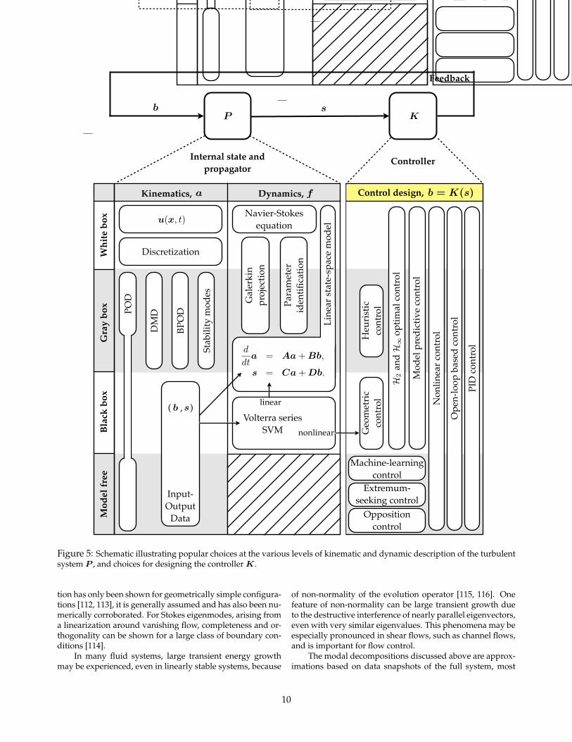
3.2 Kinematics: employed state spacesThere are numerous choices for the underlying state space inEq. (2), some of which are shown in the ’Kinematics’ columnof Fig. 5. This choice depends strongly on the availabilityof measurements and the desired model resolution; more-over, it should be considered whether or not the method isdata-driven or if it requires knowledge of the governing equa-tions. The following represents a non-exhaustive set of pos-sible state-spaces, defining a in Eq. (2). Note that many ofthese state-spaces may be used in model-free approaches.

3.2.1 Full-resolution description (white-box)

A full description of a fluid flow may include a high-resolution spatial or spectral discretization of the velocityfield

a = Du(x, t).

Here, D is a discretization operator, resulting in a high-dimensional state vector representation of a continuous field.Such descriptions are the basis of white-box models, whichdescribe every relevant feature of the flow. These represen-tations are typically very high dimensional, sometimes ex-ceeding the capacity of computer memory. For example, ahigh Reynolds number three-dimensional unsteady flow willexhibit important spatial structures that span many ordersof magnitude in scale. The Reynolds number can be esti-mated from the ratio between the largest-scale structures tothe smallest structures in the flow. Thus, for a generic ge-ometry, the state dimension will scale with Re9/4, along withthe memory cost [77, 78, 79]. The computational cost willscale with Re3 because of the addition of multiple temporalscales, which generally scale with Re3/4. For a channel flow,the scaling may even be worse with Reynolds number, as Re3

in space and Re4 in space and time [80, 81]. If a spatial dis-cretization is required with 1000 elements in each direction,then a three-dimensional simulation will contain 109 statesfor every flow variable (velocity, pressure, etc.).

The highest-order fully-resolved simulation to date isa wall-bounded turbulent channel flow with Reτ = 5200(Reynolds number based on the friction velocity), containing2.4×1011 states [81]. This simulation is about 3.5 times largerthan the previous record holder [82], and it uses slightly over3/4 of a million processors in parallel. Even with Moore’slaw, it will take nearly 40 years for this type of computa-tion to become a lightweight ’laptop’ computation [83], and

decades longer before being useful for in-time control, sincethe parallel code takes 7 real seconds per simulated time-step, as benchmarked in [81]. However impressive and use-ful for design and optimization, it is unclear that this level ofresolution is even necessary for many control applications.

3.2.2 Modal representation (gray-box)

Instead of resolving every detail of the flow field at all scales,it is often possible to represent most of the relevant flow fea-tures in terms of a much lower dimensional state. This staterepresents the amplitudes of modes, or coherent structuresthat are likely to be found in the flow of interest. Galerkinmodels based on modal expansions constitute one class ofgray-box models, which resolve the coherent structures ofthe white-box models while accounting for small scale fluc-tuations with sub-scale closures.

The proper orthogonal decomposition (POD) is one ofthe earliest and most successful modal representations usedin fluids [84, 85], resulting in dominant spatially coher-ent structures. POD benefits from a physical interpretationwhere modes are ordered hierarchically in terms of the en-ergy content that they capture in the flow. There are numer-ous methods to compute POD, and the snapshot POD [86]is efficient when a limited number of well-resolved full-state measurements are available from simulations or exper-iments. Snapshot POD is based on the singular value de-composition (SVD) [87, 88, 89, 90], which is both numericallystable and efficient. POD is known under other names: Prin-cipal components analysis (PCA) [91], the Hotelling transfor-mation [92], Karhunen–Loeve decomposition [93], and em-pirical orthogonal func tions [94]. POD has been widely usedfor flow control, as in the case of using proportional feed-back control to reduce turbulent fluctuations around a turretfor aero-optic applications [95]. Extensions of POD specif-ically designed for closed-loop feedback control, known asbalanced proper orthogonal decomposition (BPOD) [96, 97],will be discussed in Sec. 4.5.3.

A recent technique, known as dynamic mode decompo-sition (DMD) combines features of the POD and the discreteFourier transform (DFT). The resulting spatial-temporal co-herent structures oscillate in time at fixed frequencies, pos-sibly with growth or decay [98, 99, 100, 101]. Like POD,DMD is a snapshot based method, making it appealing forsimulations and experiments alike. DMD requires time-resolved snapshots of the same quality as needed for aFourier transform, although recent methods have investi-gated sub-Nyquist sampled DMD [102]. Finally, DMD hasa strong connection to the Koopman operator, which is an in-finite dimensional linear operator describing the evolution ofan observable function of a nonlinear dynamical system on amanifold [103, 104, 105, 100, 106, 107].

It is also possible to construct a modal representationof growing and decaying features in the flow based on sta-bility modes of the linearized Navier-Stokes equation andlinearized adjoint equations [108, 109, 110, 111]. The leastdamped part of the spectrum determines the coherent struc-tures and their transient dynamics. Although completenessof the stability modes of the linearized Navier-Stokes equa-

9

wn:

d


s = Ca + Db + wn. (14b)





J =

Z 1



AT X + XA XBR1BT X + Q = 0. (16a)




mize E(a a)T (a a)









We will often set C = Kr and D = 0, whereKr is a linear-quadratic-regulator (LQR) gain ma-trix. We may also choose A and B according to theKalman filter, resulting in a combined estimation-based controller known as the linear-quadratic-Gaussian (LQG). Because of the separation principle

TurbulentSystem

FeedbackController

w J

b s

Figure 2: General framework for feedback control.The input to the controller are the system measure-ments s, and the controller outputs an actuation sig-nal b. The exogenous inputs w may refer to a refer-ence state r, disturbances d or sensor noise n. Theoutput cost function z may measure any cost associ-ated with inaccuracy of reference tracking, expenseof control, etc.

for linear systems, it is possible to design an optimalfeedback control gain Kr and an optimal observerseparately, and they will be both stable and optimalwhen combined.




• Often times turbulence is considered a distur-bance term in a slower dynamical system, suchas the rigid body equations of an aircraft, spaceshuttle, or rocket. In this case, turbulent fluc-tuations may be seen as inevitable and oper-ating on a time scale that is faster than con-troller bandwidth. Instead of trying to changethe nature of the turbulence itself, the controller

8

wn:

d


s = Ca + Db + wn. (14b)





J =

Z 1



AT X + XA XBR1BT X + Q = 0. (16a)




mize E(a a)T (a a)










TurbulentSystem

FeedbackController

w J

b s







8

4 Linear model-based control

Many results in closed-loop turbulence control arespecific to linear systems. For example, one may sta-bilize an unstable steady-state and delay the transi-tion to turbulence, as in the boundary layer or chan-nel flow. In this case, the laminar solution becomesunstable for post-critical Reynolds numbers, but itmay be stabilized by feedback control.

Such work has encompassed a significant mod-eling effort (see Sec. 3) to describe the relevant low-order fluid mechanisms. Performance issues such asbandwidth, disturbance rejection, and noise atten-uation must be balanced with robustness to modeluncertainty and time-delays. For this reason, therehas been a recent push to move away from H2 op-timal control techniques (LQR, Kalman estimation,LQG, etc.) to the robust H1 controllers [32, 33, 34,35]. These controllers penalize the worse-case sce-nario error and provide robust performance. In addi-tion, significant effort has gone into the design andmodeling of sensor and actuators, along with theirplacement in the flow.

There are many instances when linear controlstrategies may have significant and direct impact fornonlinear turbulent flows, even away from laminarfixed-point solutions:

1. In mean-field models, exciting one oscillatorymode with linear control may kill other oscilla-tory modes [36, 37],

2. ensemble averages of turbulent flow responsesmay be linear, as in Colonius’s experimental jetnoise study ,

3. Dusek’s jet simulation at Re=100,

4. transient control of separation for fully turbu-lent boundary layer [38].

4.1 Linearized input–output dynamics

Often, we are interested in linearizing Eq. (1) abouta steady fixed point as or periodic orbit, leading toa linear system of equations:

d

dta = Aa + Bb, (2a)

s = Ca + Db. (2b)

where each of the (A, B, C, D) depend on the lin-earization point as and bifurcation parameter .This approximation will be approximately validnear fixed points and away from critical values ofthe bifurcation parameter where det df/d = 0.

It is possible to represent the state-space modelin Eq. (2) as a transfer function P () in the frequencydomain (in terms of a Laplace variable ):

P () = C (I A)1 B + D. (3a)

4.2 Model-based open loop control

• What it would look like to design the ideal sys-tem, invert plant dynamics, etc.

• Why this would be a terrible idea (in manycases)...

4.3 Dynamic feedback controllers

Given linear dynamics of the form in Eq. (2), we of-ten want a feedback controller based on full-statefeedback: b = Kra. For example, if the system iscontrollable, then the poles of the closed-loop systemmay be placed arbitrarily by choice of Kr.

d

dta = Aa BKra (4a)

= (A BKr) a. (4b)

However, full-state measurements of a are ei-ther infeasible or prohibitively expensive, and so anestimate a may be obtained from measurements s.This is of course, only if the system of equations (2)is observable. An observer dynamical system may beconstructed as follows:

d

dta = Aa + Bb + Kf (s s), (5a)

s = Ca + Db (5b)

[(typically D = 0 for this problem...)] which leadsto

d

dta = (A KfC) a + Kfs + (B KfD) b.(6a)

The full-state estimate a will converge to an esti-mate of the true state a if the eigenvalues of A KfC are stable.

6

Whi

te b

oxB

lack

box

Gra

y bo

xM

odel

fre

e

Internal state and propagator

Discretization

Ope

n-lo

op b

ased

cont

rol

Oppositioncontrol

Navier-Stokes equation

Non

linea

r con

trol

Machine-learningcontrol

Extremum- seeking control

3 Black, grey, and white-box models

Regardless of the modeling strategy below, we as-sume that we are able to actuate the flow with someinput variables b 2 Rp and we are able to measurefeatures of the flow with some output variables s 2Rq. Once the inputs and outputs are set, there aremany choices for the model that links them. For ex-ample, we may consider the full discretized Navier-Stokes equations as a high-dimensional nonlinearset of ordinary differential equations. Alternatively,we may relate inputs to outputs through either a sta-tistical description or a set of empirical basis func-tions. Recent advances in dimensionality reductiontechniques and turbulence closures have excitingimplications for the future of turbulence control.

3.1 State-space models

In the most general framework, we will have a statea 2 RNa and a nonlinear function advancing thestate forward in time, along with a nonlinear outputfunction:

a = f(a, b;), (1a)s = g(a, b). (1b)

Here we have assumed continuous dynamics, andin general the Navier-Stokes equation is twice con-tinuously differentiable in space and once continu-ously differentiable in time. Notice that there is a setof parameters that may change the qualitative na-ture of solutions; we call these bifurcation parameters.

3.2 Employed state spaces

1. Velocity field (a = u(x, t)),

2. modal coefficients of a Galerkin expansion,

3. sensor signals a = s,

4. sensor signals + time delay coordinates, ideallywith given by C() = 0, where C is the auto-correlation function,

5. sensor signals + derivatives (a = (s, s)).

I/Omodel

MIM

O c

on

fig

.

con

tro

l d

esig

n

e.g. structureidentification

e.g. parameteridentification

CFD

ROM

controllaws

White−box modelling

Model−free approaches

Black−box modelling

Grey−box modelling

Navier−Stokes equation

Data driven methods

Figure 1: Model hierarchy for control design.

3.3 Phenomenological classification

3.3.1 Classification based on system resolution

Figure ?? outlines a model hierarchy for control de-sign, following a classification of N. Wiener [15] andextending it by model-free approaches.

1. White-box models, e.g. a Navier-Stokes dis-cretization resolve all flow physics and nonlin-earities. Problems for real-time implementa-tions are the computational load and full stateestimation.

2. Grey-box models, e.g. reduced-order modelsfor coherent structure dynamics, may enable areal-time control in experiments and state esti-mation. However, acceptable accuracy is onlyachieved for one of few dominant frequenciesand few known nonlinear mechanisms.

3. Black-box models, e.g. transfer functions, havesimilar dynamic bandwidth as grey-box mod-els. A black-box model may be derived forgrey-box models and vice versa. One ad-vantage of black-box models are easy experi-mental identification, particularly for weakly-nonlinear dynamics.

4. Model-free approaches, e.g. based on qualita-tive steady state maps, are generally restrictedto existing one or few-parametric open-loopcontrol.

3.4 Approaches to system reduction (grey-box models)

1. Response surfaces (on the level of black-boxmodels are model-free approaches).

4











d

dta = Aa + Bb, (2a)

s = Ca + Db. (2b)


It is possible to represent the state-space modelin Eq. (2) as a transfer function G() in the fre-quency domain (in terms of a Laplace variable ):

G() = C (I A)1 B + D. (3a)






d

dta = Aa BKra (4a)

= (A BKr) a. (4b)


d


s = Ca + Db (5b)


d



6

Volterra seriesSVM

linear

nonlinear

POD

Line

ar st

ate-

spac

e m

odel

DM

D

BPO

D

Stab

ility

mod

es

Input-Output

Data

Gal

erki

n pr

ojec

tion

Para

met

er

iden

tifica

tion

Mod

el p

redi

ctiv

e co

ntro

l

wn

:

d dta

=A

a+

Bb

+w

d,

(14a

)

s=

Ca

+D

b+

wn.

(14b

)

Each

ofth

ese

nois

ein

puts

has

adi

ffer

ent

co-

vari

ance

mat

rix:

E(w

dw

T d)

=V

dan

dE

(wnw

T n)

=V

n,

whe

reE

(·)is

the

expe

ctat

ion

valu

e.[T

his

isno

tpre

cise

enou

gh...

real

lyne

edE

(wd(t

)wd(

)T)

=V

d(

t

).

]Li

near

-qua

drat

icre

gula

tor

(LQ

R):

J=

Z1

0a

TQ

a+

bTR

bdt.

(15a

)

The

optim

alco

ntro

llaw

isb

=K

ra

,whe

reK

r=

R

1B

TX

and

Xis

the

uniq

ueso

lutio

nto

the

alge

-br

aic

Ric

cati

equa

tion:

ATX

+X

A

XB

R

1B

TX

+Q

=0.

(16a

)

Adu

alR

icca

tieq

uatio

nis

solv

edfo

rth

eob

serv

erga

inK

f=

YC

TV

n:

YA

T+

AY

Y

CTV

1

nC

Y+

Vd

=0.

(17a

)

The

so-c

alle

dK

alm

anfil

ter

Kf

isch

osen

tom

ini-

miz

eE (a

a)T

(a

a)

give

nkn

own

cova

rian

ceV

dan

dV

n.

[Not

e:K

alm

anpu

blis

hed

his

fam

ous

Kal

man

filte

rin

ajo

urna

lofF

luid

Engi

neer

ing.

][D

ecen

tsta

bilit

ym

argi

nsfo

rLQ

R,b

utno

guar

-an

teed

stab

ility

mar

gins

forL

QG

(fam

ous

Doy

lepa

-pe

r)].

4.5.

2Se

nsit

ivit

y,C

ompl

emen

tary

Sens

itiv

ity,

and

Rob

ustn

ess

•S

()

-sen

sitiv

ityfu

nctio

n

•T

()

-com

plem

enta

ryse

nsiti

vity

func

tion

4.5.

3H

1ro

bust

cont

rol

We

will

ofte

nse

tC

=K

ran

dD

=0

,w

here

Kr

isa

linea

r-qu

adra

tic-r

egul

ator

(LQ

R)

gain

ma-

trix

.We

may

also

choo

seA

and

Bac

cord

ing

toth

eK

alm

anfil

ter,

resu

lting

ina

com

bine

des

timat

ion-

base

dco

ntro

ller

know

nas

the

linea

r-qu

adra

tic-

Gau

ssia

n(L

QG

).Be

caus

eof

the

sepa

ratio

npr

inci

ple

Turb

ulen

tSy

stem

Feed

back

Con

trol

ler

wJ

bs

Figu

re2:

Gen

eral

fram

ewor

kfo

rfe

edba

ckco

ntro

l.Th

ein

putt

oth

eco

ntro

ller

are

the

syst

emm

easu

re-

men

tss

,and

the

cont

rolle

rout

puts

anac

tuat

ion

sig-

nalb

.The

exog

enou

sin

puts

wm

ayre

fer

toa

refe

r-en

cest

ate

r,d

istu

rban

ces

dor

sens

orno

ise

n.

The

outp

utco

stfu

nctio

nz

may

mea

sure

any

cost

asso

ci-

ated

with

inac

cura

cyof

refe

renc

etr

acki

ng,e

xpen

seof

cont

rol,

etc.

forl

inea

rsys

tem

s,it

ispo

ssib

leto

desi

gnan

optim

alfe

edba

ckco

ntro

lgai

nK

ran

dan

optim

alob

serv

erse

para

tely

,and

they

will

bebo

thst

able

and

optim

alw

hen

com

bine

d.Th

ere

sulti

ngco

ntro

ller,

know

nm

ore

gene

rally

asa

H2

cont

rolle

r,op

timal

lyba

lanc

esth

eef

fect

ofG

auss

ian

mea

sure

men

tno

ise

with

proc

ess

dist

ur-

banc

es.

How

ever

,th

ese

cont

rolle

rsar

ekn

own

toha

vear

bitr

arily

poor

robu

stne

ssm

argi

ns.

Inst

ead,

H1

robu

stco

ntro

llers

are

used

whe

nro

bust

ness

isim

port

ant.

Figu

re2

show

sth

em

ost

gene

ral

sche

mat

icfo

rcl

osed

loop

feed

back

cont

rol,

enco

mpa

ssin

gH

2an

dH

1op

timal

cont

rols

trat

egie

s.Th

ere

are

anu

mbe

rof

exce

llent

book

sex

pand

ing

onth

isth

eory

[39,

40].

Her

ew

edi

scus

sim

port

antt

heor

etic

alre

sults

re-

gard

ing

the

vari

ous

type

sof

optim

alco

ntro

l:H

1ro

bust

cont

rol,

and

H2

LQG

.

•O

ften

times

turb

ulen

ceis

cons

ider

eda

dist

ur-

banc

ete

rmin

asl

ower

dyna

mic

alsy

stem

,suc

has

the

rigi

dbo

dyeq

uatio

nsof

anai

rcra

ft,s

pace

shut

tle,o

rro

cket

.In

this

case

,tur

bule

ntflu

c-tu

atio

nsm

aybe

seen

asin

evita

ble

and

oper

-at

ing

ona

time

scal

eth

atis

fast

erth

anco

n-tr

olle

rba

ndw

idth

.In

stea

dof

tryi

ngto

chan

geth

ena

ture

ofth

etu

rbul

ence

itsel

f,th

eco

ntro

ller

8

Com

bine

dw

ith

full-

stat

efe

edba

ckb

=

Kra

,th

isre

sult

sin

ady

nam

ical

syst

emfo

rth

eco

ntro

ller:

d dta

=(A

K

fC

B

Kr+

KfD

Kr)a

+K

fs,

(7a)

b=

K

ra.

(7b)

Not

eth

atth

ein

put

toth

eco

ntro

ller

isth

ese

nsor

sign

als

,th

eou

tput

isth

eac

tuat

ion

sign

alb

,an

dth

est

ate

aes

tim

ates

the

full-

stat

eof

the

linea

rsy

s-te

min

Eq.(

2).

The

sepa

rati

onpr

inci

ple

stat

esth

atK

ran

dK

fm

aybe

desi

gned

sepa

rate

lyto

dete

r-m

ine

the

stab

ility

ofth

est

ate

dyna

mic

sfo

ra

and

a,

resp

ecti

vely

,an

dth

ecl

osed

-loo

psy

stem

will

have

pole

sgi

ven

byth

epo

les

ofA

B

Kr

and

A

KfC

.Th

em

ostg

ener

alob

serv

erdy

nam

ical

syst

emis

give

nby

:

d dta

=A

a+

Bs,

(8a)

b=

Ca

+D

s.

(8b)

The

gene

ralc

ontr

olle

rw

illbe

deno

ted

byK

()

inth

efr

eque

ncy

dom

ain.

4.4

Con

trol

labi

lity

,O

bser

vabi

lity

,an

dG

ram

ians

The

abili

tyto

plac

epo

les

ofth

ecl

osed

-loo

psy

stem

arbi

trar

ilyw

ith

choi

ceof

Kr

relie

son

the

cont

rolla

-bi

lity

ofth

esy

stem

inEq

.(2)

.The

syst

emis

cont

rol-

labl

eif

the

follo

win

gm

atri

x:

C=

BA

BA

2B

···

AN

a

1B

(9a)

has

full

rank

Na.

Con

trol

labi

lity

impl

ies

that

the

syst

emm

aybe

stee

red

toan

arbi

trar

yst

ate

aw

ith

suit

able

tim

e-hi

stor

yof

the

cont

roli

nput

b.

Sim

ilarl

y,th

efu

llst

ate

isob

serv

able

ifth

eob

serv

-ab

ility

mat

rix

isfu

llra

nk:

O=

2 6 6 6 6 6 4

C CA

CA

2

. . .C

AN

a

1

3 7 7 7 7 7 5.

(10a

)

This

mea

nsth

atan

yst

ate

am

aybe

esti

mat

edw

ith

asu

itab

leti

me-

hist

ory

ofth

em

easu

rem

ents

s.

Alt

houg

hth

ede

finit

ions

ofco

ntro

llabi

lity

and

obse

rvab

ility

abov

ear

ebi

nary

,th

ere

are

degr

ees

ofco

ntro

llabi

lity

and

obse

rvab

ility

,bas

edon

how

dif-

ficul

titi

sto

cont

rolo

rest

imat

ea

stat

ea

.The

degr

eeof

cont

rolla

bilit

yan

dob

serv

abili

tyof

agi

ven

stat

eis

quan

tifie

dby

eige

nval

ues

and

eige

nvec

tors

ofth

eco

ntro

llabi

lity

Gra

mia

n

Wc

=

Z1

0eA

t BB

eA

tdt

(11a

)

1 X k=

0

eA

tkB

B eA

t k

(11b

)

and

obse

rvab

ility

Gra

mia

n:

Wo

=

Z1

0eA

tC

CeA

t dt

(12a

)

1 X k=

0

eA

t kC

C eA

t

k.

(12b

)

Thes

em

aybe

appr

oxim

ated

byfu

ll-st

ate

mea

-su

rem

ents

ofth

edi

rect

syst

emin

Eq.(

2)an

dad

join

tsy

stem

:

Wc

W

e c=

CC ,

(13a

)W

o

We o

=O

O .

(13b

)

[Dec

ide

onno

tati

onfo

rco

ntin

uous

vs.

disc

rete

tim

eA

...em

p.G

ram

ians

are

slig

htly

wro

ng,s

ince

they

use

Ad]

[Men

tion

SVD

and

sym

met

ric

mat

rix,

degr

ees

ofco

ntro

llabi

lity.

..][M

enti

onba

lanc

edm

odel

redu

ctio

n:BT

,BPO

D,

ERA

]

4.4.

1B

alan

ced

mod

elre

duct

ion

4.5

H1

robu

stvs

.H2

opti

mal

cont

rol

Now

that

we

have

esta

blis

hed

cond

itio

nsen

ablin

gar

bitr

ary

pole

plac

emen

toft

hecl

osed

-loo

psy

stem

,w

em

ustn

owde

cide

onw

here

topl

ace

them

.

4.5.

1H

2op

tim

alco

ntro

l:Li

near

quad

rati

cG

aus-

sian

(LQ

G)

We

may

ofte

nm

odif

yEq

.(2

)w

ith

the

addi

tion

ofw

hite

nois

edi

stur

banc

ew

dan

dm

easu

rem

entn

oise

7

and

opt

imal

cont

rol

Geo

met

ricco

ntro

lH

euris

ticco

ntro

l

( , )

wn:

d


s = Ca + Db + wn. (14b)





J =

Z 1



AT X + XA XBR1BT X + Q = 0. (16a)




mize E(a a)T (a a)










TurbulentSystem

FeedbackController

w J

b s







8

wn:

d


s = Ca + Db + wn. (14b)





J =

Z 1



AT X + XA XBR1BT X + Q = 0. (16a)




mize E(a a)T (a a)










TurbulentSystem

FeedbackController

w J

b s







8

PID

cont

rol

Dynamics,

3 Black-box, grey-box, and white-box models

Regardless of the modeling strategy employed below, we as-sume that we are able to actuate the flow with some inputvariables b 2 RNb and we are able to measure features of theflow with some output variables s 2 RNs . Once the inputsand outputs are set, there are many choices for the modelthat links them. For example, we may consider the full dis-cretized Navier-Stokes equations as a high-dimensional non-linear set of ordinary differential equations. Alternatively,we may relate inputs to outputs through either a statisti-cal description or a set of empirical basis functions. Recentadvances in dimensionality reduction techniques and turbu-lence closures have exciting implications for the future of tur-bulence modeling and control.

The choice of model affects nearly every downstreamcontrol decision. There are many factors and tradeoffs thatmust be balanced when deciding on a modeling strategy.These include the accuracy of the model, execution time,generality in other parameter regimes, spatial-temporal res-olution relative to disturbances, and the up-front cost to ac-quire such a model. For example, direct numerical simula-tion (DNS) is unparalleled at descriptive resolution, general-ity, and accuracy, but current computational capabilities aredecades away from real-time execution for in-time controlstrategies. Reduced-order models based on data from DNSor experiments provide real-time capable models, but thesemodels are expensive to create and may only work for a smallrange of training parameters. Fortunately, it may be possi-ble to leverage physical intuition about the structure of theunderlying modes, often in terms of linear combinations offull flow fields, to modify the models with additional termsto extend their predictive range. Black-box models based oninput–output data are typically faster to generate and requireless measured data, but they lack the physical interpretationthat goes with having an underlying modal representation.

Figure 4 outlines a model hierarchy for control design,following a classification of N. Wiener [18] and extending itto include model-free approaches. These classifications aregenerally based on the system resolution of the model. Anexpanded view of the various models and modal decompo-sitions is shown in Fig. 5. These methods are not meant to beexhaustive, but rather include methods that have either beenapplied with recent success or methods that have particularpromise in the future.

3.1 State-space modelsIn one of the most general frameworks, we will have a statea 2 RNa and a nonlinear function f advancing the state for-ward in time, along with a nonlinear output function g:

a = f(a, b; µ), (2a)

s = g(a, b). (2b)

Here the dynamics are assumed to be continuous, and ingeneral the flow state a in the Navier-Stokes equation is

Blac

k bo

x

Data


Gra

y bo

xW

hite

bo

xU

ltra

whi

teM

odel

fr

ee

I/O

Controllers

ROM

CFD

Figure 4: Model hierarchy for control design, basedon [18].

twice continuously differentiable in space and once contin-uously differentiable in time. The bifurcation parameters µmay change the qualitative nature of the solutions, and theflow field is not necessarily continuously differentiable in µ.These parameters include the Reynolds number and Machnumber, among others.

The nonlinear dynamics in Eq. (2) may be linearized ata steady fixed point as, where f(as,0; µ) = 0, away fromcritical values of the bifurcation parameters. The linearizedmodel may also be converted into a frequency domain repre-sentation, as explored in Sec. 4.

3.2 Kinematics: employed state spacesThere are numerous choices for the underlying state space inEq. (2), some of which are shown in the “Kinematics” columnof Fig. 5. This choice depends strongly on the availabilityof measurements and the desired model resolution; more-over, it should be considered whether or not the method isdata-driven or if it requires knowledge of the governing equa-tions. The following represents a non-exhaustive set of pos-sible state-spaces, defining a in Eq. (2). Note that many ofthese state-spaces may be used in model-free approaches.


A full description of a fluid flow may include a high-resolution spatial or spectral discretization of either the ve-locity field (a = u(x, t)) or the vorticity field (a = !(x, t) ,ru(x, t)). Such descriptions are the basis of white-box mod-els, which describe every relevant feature of the flow. These

8

Kinematics,






a = f(a, b; µ), (2a)

s = g(a, b). (2b)


Blac

k bo

x

Data


Gra

y bo

xW

hite

bo

xU

ltra

whi

teM

odel

fr

ee

I/O

Controllers

ROM

CFD







8

Controller

K

wn:

d


s = Ca + Db + wn. (14b)





J =



AT X + XA XBR1BT X + Q = 0. (16a)




mize E(a a)T (a a)








4.5.3 H robust control


TurbulentSystem

FeedbackController

w J

b s



The resulting controller, known more generallyas a H2 controller, optimally balances the effect ofGaussian measurement noise with process distur-bances. However, these controllers are known tohave arbitrarily poor robustness margins. Instead,H robust controllers are used when robustness isimportant.

Figure 2 shows the most general schematic forclosed loop feedback control, encompassing H2 andH optimal control strategies. There are a numberof excellent books expanding on this theory [39, 40].

Here we discuss important theoretical results re-garding the various types of optimal control: Hrobust control, and H2 LQG.


8

wn:

d


s = Ca + Db + wn. (14b)





J =



AT X + XA XBR1BT X + Q = 0. (16a)




mize E(a a)T (a a)










TurbulentSystem

FeedbackController

w J

b s







8



Such work has encompassed a significant mod-eling effort (see Sec. 3) to describe the relevant low-order fluid mechanisms. Performance issues such asbandwidth, disturbance rejection, and noise atten-uation must be balanced with robustness to modeluncertainty and time-delays. For this reason, therehas been a recent push to move away from H2 op-timal control techniques (LQR, Kalman estimation,LQG, etc.) to the robust H controllers [32, 33, 34,35]. These controllers penalize the worse-case sce-nario error and provide robust performance. In addi-tion, significant effort has gone into the design andmodeling of sensor and actuators, along with theirplacement in the flow.








d

dta = Aa + Bb, (2a)

s = Ca + Db. (2b)



P () = C (I A)1 B + D. (3a)






d

dta = Aa BKra (4a)

= (A BKr) a. (4b)


d


s = Ca + Db (5b)


d



6W

hite

box

Bla

ck b

oxG

ray

box

Mod

el f

ree

Control design

Internal state and propagator

Discretization

Ope

n lo

op b

ased

cont

rol

Oppositioncontrol

Navier-Stokes equation

Non

linea

r con

trol

Machine learningcontrol

Extremum seeking control

3 Black, grey, and white-box models

Regardless of the modeling strategy below, we as-sume that we are able to actuate the flow with someinput variables b Rp and we are able to measurefeatures of the flow with some output variables s Rq. Once the inputs and outputs are set, there aremany choices for the model that links them. For ex-ample, we may consider the full discretized Navier-Stokes equations as a high-dimensional nonlinearset of ordinary differential equations. Alternatively,we may relate inputs to outputs through either a sta-tistical description or a set of empirical basis func-tions. Recent advances in dimensionality reductiontechniques and turbulence closures have excitingimplications for the future of turbulence control.

3.1 State-space models

In the most general framework, we will have a statea RNa and a nonlinear function advancing thestate forward in time, along with a nonlinear outputfunction:

a = f(a, b;), (1a)s = g(a, b). (1b)

Here we have assumed continuous dynamics, andin general the Navier-Stokes equation is twice con-tinuously differentiable in space and once continu-ously differentiable in time. Notice that there is a setof parameters that may change the qualitative na-ture of solutions; we call these bifurcation parameters.

3.2 Employed state spaces

1. Velocity field (a = u(x, t)),

2. modal coefficients of a Galerkin expansion,

3. sensor signals a = s,

4. sensor signals + time delay coordinates, ideallywith given by C() = 0, where C is the auto-correlation function,

5. sensor signals + derivatives (a = (s, s)).

I/Omodel

MIM

O c

onfi

g.

contr

ol

des

ign

e.g. structureidentification

e.g. parameteridentification

CFD

ROM

controllaws

White−box modelling

Model−free approaches

Black−box modelling

Grey−box modelling

Navier−Stokes equation

Data driven methods

Figure 1: Model hierarchy for control design.

3.3 Phenomenological classification

3.3.1 Classification based on system resolution

Figure ?? outlines a model hierarchy for control de-sign, following a classification of N. Wiener [15] andextending it by model-free approaches.

1. White-box models, e.g. a Navier-Stokes dis-cretization resolve all flow physics and nonlin-earities. Problems for real-time implementa-tions are the computational load and full stateestimation.

2. Grey-box models, e.g. reduced-order modelsfor coherent structure dynamics, may enable areal-time control in experiments and state esti-mation. However, acceptable accuracy is onlyachieved for one of few dominant frequenciesand few known nonlinear mechanisms.

3. Black-box models, e.g. transfer functions, havesimilar dynamic bandwidth as grey-box mod-els. A black-box model may be derived forgrey-box models and vice versa. One ad-vantage of black-box models are easy experi-mental identification, particularly for weakly-nonlinear dynamics.

4. Model-free approaches, e.g. based on qualita-tive steady state maps, are generally restrictedto existing one or few-parametric open-loopcontrol.

3.4 Approaches to system reduction (grey-box models)

1. Response surfaces (on the level of black-boxmodels are model-free approaches).

4



Such work has encompassed a significant mod-eling effort (see Sec. 3) to describe the relevant low-order fluid mechanisms. Performance issues such asbandwidth, disturbance rejection, and noise atten-uation must be balanced with robustness to modeluncertainty and time-delays. For this reason, therehas been a recent push to move away from H2 op-timal control techniques (LQR, Kalman estimation,LQG, etc.) to the robust H controllers [32, 33, 34,35]. These controllers penalize the worse-case sce-nario error and provide robust performance. In addi-tion, significant effort has gone into the design andmodeling of sensor and actuators, along with theirplacement in the flow.








d

dta = Aa + Bb, (2a)

s = Ca + Db. (2b)


It is possible to represent the state-space modelin Eq. (2) as a transfer function G() in the fre-quency domain (in terms of a Laplace variable ):

G() = C (I A)1 B + D. (3a)






d

dta = Aa BKra (4a)

= (A BKr) a. (4b)


d


s = Ca + Db (5b)


d



6

Volterra seriesSVM

linear

nonlinear

POD

Line

ar st

ate-

spac

e m

odel

DM

D

BPO

D

Stab

ility

mod

es

InputOutput

Data

Gal

erki

n pr

ojec

tion

Para

met

er

iden

tifica

tion

Mod

el p

redi

ctiv

e co

ntro

l

wn

:

d dta

=A

a+

Bb

+w

d,

(14a

)

s=

Ca

+D

b+

wn.

(14b

)

Each

ofth

ese

nois

ein

puts

has

adi

ffer

ent

co-

vari

ance

mat

rix:

E(w

dw

T d)

=V

dan

dE

(wnw

T n)

=V

n,

whe

reE

(·)is

the

expe

ctat

ion

valu

e.[T

his

isno

tpre

cise

enou

gh...

real

lyne

edE

(wd(t

)wd(

)T)

=V

d(

t

).]

Line

ar-q

uadr

atic

regu

lato

r(L

QR

):

J=

0a

TQ

a+

bTR

bdt

.(1

5a)

The

optim

alco

ntro

llaw

isb

=K

ra

,whe

reK

r=

R

1B

TX

and

Xis

the

uniq

ueso

lutio

nto

the

alge

-br

aic

Ric

cati

equa

tion:

ATX

+X

A

XB

R

1B

TX

+Q

=0.

(16a

)

Adu

alR

icca

tieq

uatio

nis

solv

edfo

rth

eob

serv

erga

inK

f=

YC

TV

n:

YA

T+

AY

Y

CTV

1

nC

Y+

Vd

=0.

(17a

)

The

so-c

alle

dK

alm

anfil

ter

Kf

isch

osen

tom

ini-

miz

eE (a

a)T

(a

a) gi

ven

know

nco

vari

ance

Vd

and

Vn

.[N

ote:

Kal

man

publ

ishe

dhi

sfa

mou

sK

alm

anfil

ter

ina

jour

nalo

fFlu

idEn

gine

erin

g.]

[Dec

ents

tabi

lity

mar

gins

for

LQR

,but

nogu

ar-

ante

edst

abili

tym

argi

nsfo

rLQ

G(f

amou

sDoy

lepa

-pe

r)].

4.5.

2Se

nsit

ivit

y,C

ompl

emen

tary

Sens

itiv

ity,

and

Rob

ustn

ess

•S

()

-sen

sitiv

ityfu

nctio

n

•T

()

-com

plem

enta

ryse

nsiti

vity

func

tion

4.5.

3H

ro

bust

cont

rol

We

will

ofte

nse

tC

=K

ran

dD

=0

,w

here

Kr

isa

linea

r-qu

adra

tic-r

egul

ator

(LQ

R)

gain

ma-

trix

.We

may

also

choo

seA

and

Bac

cord

ing

toth

eK

alm

anfil

ter,

resu

lting

ina

com

bine

des

timat

ion-

base

dco

ntro

ller

know

nas

the

linea

r-qu

adra

tic-

Gau

ssia

n(L

QG

).Be

caus

eof

the

sepa

ratio

npr

inci

ple

Turb

ulen

tSy

stem

Feed

back

Con

trol

ler

wJ

bs

Figu

re2:

Gen

eral

fram

ewor

kfo

rfe

edba

ckco

ntro

l.Th

ein

putt

oth

eco

ntro

ller

are

the

syst

emm

easu

re-

men

tss

,and

the

cont

rolle

rout

puts

anac

tuat

ion

sig-

nalb

.The

exog

enou

sin

puts

wm

ayre

fer

toa

refe

r-en

cest

ate

r,d

istu

rban

ces

dor

sens

orno

ise

n.

The

outp

utco

stfu

nctio

nz

may

mea

sure

any

cost

asso

ci-

ated

with

inac

cura

cyof

refe

renc

etr

acki

ng,e

xpen

seof

cont

rol,

etc.

forl

inea

rsys

tem

s,it

ispo

ssib

leto

desi

gnan

optim

alfe

edba

ckco

ntro

lgai

nK

ran

dan

optim

alob

serv

erse

para

tely

,and

they

will

bebo

thst

able

and

optim

alw

hen

com

bine

d.Th

ere

sulti

ngco

ntro

ller,

know

nm

ore

gene

rally

asa

H2

cont

rolle

r,op

timal

lyba

lanc

esth

eef

fect

ofG

auss

ian

mea

sure

men

tno

ise

with

proc

ess

dist

ur-

banc

es.

How

ever

,th

ese

cont

rolle

rsar

ekn

own

toha

vear

bitr

arily

poor

robu

stne

ssm

argi

ns.

Inst

ead,

H

robu

stco

ntro

llers

are

used

whe

nro

bust

ness

isim

port

ant.

Figu

re2

show

sth

em

ost

gene

rals

chem

atic

for

clos

edlo

opfe

edba

ckco

ntro

l,en

com

pass

ing

H2

and

H

optim

alco

ntro

lstr

ateg

ies.

Ther

ear

ea

num

ber

ofex

celle

ntbo

oks

expa

ndin

gon

this

theo

ry[3

9,40

].H

ere

we

disc

ussi

mpo

rtan

tthe

oret

ical

resu

ltsre

-ga

rdin

gth

eva

riou

sty

pes

ofop

timal

cont

rol:

H

robu

stco

ntro

l,an

dH

2LQ

G.

•O

ften

times

turb

ulen

ceis

cons

ider

eda

dist

ur-

banc

ete

rmin

asl

ower

dyna

mic

alsy

stem

,suc

has

the

rigi

dbo

dyeq

uatio

nsof

anai

rcra

ft,s

pace

shut

tle,o

rro

cket

.In

this

case

,tur

bule

ntflu

c-tu

atio

nsm

aybe

seen

asin

evita

ble

and

oper

-at

ing

ona

time

scal

eth

atis

fast

erth

anco

n-tr

olle

rba

ndw

idth

.In

stea

dof

tryi

ngto

chan

geth

ena

ture

ofth

etu

rbul

ence

itsel

f,th

eco

ntro

ller

8

Com

bine

dw

ithfu

ll-st

ate

feed

back

b=

Kra

,th

isre

sults

ina

dyna

mic

alsy

stem

for

the

cont

rolle

r:

d dta

=(A

K

fC

B

Kr+

KfD

Kr)a

+K

fs,

(7a)

b=

Kra.

(7b)

Not

eth

atth

ein

put

toth

eco

ntro

ller

isth

ese

nsor

sign

als

,th

eou

tput

isth

eac

tuat

ion

sign

alb

,an

dth

est

ate

aes

timat

esth

efu

ll-st

ate

ofth

elin

ear

sys-

tem

inEq

.(2)

.Th

ese

para

tion

prin

cipl

est

ates

that

Kr

and

Kf

may

bede

sign

edse

para

tely

tode

ter-

min

eth

est

abili

tyof

the

stat

edy

nam

ics

fora

and

a,

resp

ectiv

ely,

and

the

clos

ed-lo

opsy

stem

will

have

pole

sgi

ven

byth

epo

les

ofA

B

Kr

and

A

KfC

.Th

em

ostg

ener

alob

serv

erdy

nam

ical

syst

emis

give

nby

:

d dta

=A

a+

Bs,

(8a)

b=

Ca

+D

s.

(8b)

The

gene

ralc

ontr

olle

rw

illbe

deno

ted

byK

()

inth

efr

eque

ncy

dom

ain.

4.4

Con

trol

labi

lity

,O

bser

vabi

lity

,an

dG

ram

ians

The

abili

tyto

plac

epo

les

ofth

ecl

osed

-loop

syst

emar

bitr

arily

with

choi

ceof

Kr

relie

son

the

cont

rolla

-bi

lity

ofth

esy

stem

inEq

.(2)

.The

syst

emis

cont

rol-

labl

eif

the

follo

win

gm

atri

x:

C=

BA

BA

2B

···

AN

a

1B

(9a)

has

full

rank

Na.

Con

trol

labi

lity

impl

ies

that

the

syst

emm

aybe

stee

red

toan

arbi

trar

yst

ate

aw

ithsu

itabl

etim

e-hi

stor

yof

the

cont

roli

nput

b.

Sim

ilarl

y,th

efu

llst

ate

isob

serv

able

ifth

eob

serv

-ab

ility

mat

rix

isfu

llra

nk:

O=

C CA

CA

2

. . .C

AN

a

1

.

(10a

)

This

mea

nsth

atan

yst

ate

am

aybe

estim

ated

with

asu

itabl

etim

e-hi

stor

yof

the

mea

sure

men

tss

.

Alth

ough

the

defin

ition

sof

cont

rolla

bilit

yan

dob

serv

abili

tyab

ove

are

bina

ry,

ther

ear

ede

gree

sof

cont

rolla

bilit

yan

dob

serv

abili

ty,b

ased

onho

wdi

f-fic

ulti

tis

toco

ntro

lore

stim

ate

ast

ate

a.T

hede

gree

ofco

ntro

llabi

lity

and

obse

rvab

ility

ofa

give

nst

ate

isqu

antifi

edby

eige

nval

ues

and

eige

nvec

tors

ofth

eco

ntro

llabi

lity

Gra

mia

n

Wc

=

0eA

t BB

eA

tdt

(11a

)

k=

0

eA

t kB

B eA

t k

(11b

)

and

obse

rvab

ility

Gra

mia

n:

Wo

=

0eA

tC

CeA

t dt

(12a

)

k=

0

eA

t kC

C eA

t k

.(1

2b)

Thes

em

aybe

appr

oxim

ated

byfu

ll-st

ate

mea

-su

rem

ents

ofth

edi

rect

syst

emin

Eq.(

2)an

dad

join

tsy

stem

:

Wc

W

e c=

CC ,

(13a

)W

o

We o

=O

O .

(13b

)

[Dec

ide

onno

tatio

nfo

rco

ntin

uous

vs.

disc

rete

time

A...

emp.

Gra

mia

nsar

esl

ight

lyw

rong

,sin

ceth

eyus

eA

d]

[Men

tion

SVD

and

sym

met

ric

mat

rix,

degr

eeso

fco

ntro

llabi

lity.

..][M

entio

nba

lanc

edm

odel

redu

ctio

n:BT

,BPO

D,

ERA

]

4.4.

1B

alan

ced

mod

elre

duct

ion

4.5

H

robu

stvs

.H2

opti

mal

cont

rol

Now

that

we

have

esta

blis

hed

cond

ition

sen

ablin

gar

bitr

ary

pole

plac

emen

toft

hecl

osed

-loop

syst

em,

we

mus

tnow

deci

deon

whe

reto

plac

eth

em.

4.5.

1H

2op

tim

alco

ntro

l:Li

near

quad

rati

cG

aus-

sian

(LQ

G)

We

may

ofte

nm

odify

Eq.(

2)w

ithth

ead

ditio

nof

whi

teno

ise

dist

urba

nce

wd

and

mea

sure

men

tnoi

se

7

and

opt

imal

cont

rol

Geo

met

ricco

ntro

lH

euris

ticco

ntro

l

( , )

wn:

d


s = Ca + Db + wn. (14b)





J =



AT X + XA XBR1BT X + Q = 0. (16a)




mize E(a a)T (a a)










TurbulentSystem

FeedbackController

w J

b s







8

wn:

d


s = Ca + Db + wn. (14b)





J =



AT X + XA XBR1BT X + Q = 0. (16a)




mize E(a a)T (a a)










TurbulentSystem

FeedbackController

w J

b s







8

PID

cont

rol

Dynamics,






a = f(a, b; µ), (2a)

s = g(a, b). (2b)


Blac

k bo

x

Data


Gra

y bo

xW

hite

bo

xU

ltra

whi

teM

odel

fr

ee

I/O

Controllers

ROM

CFD







8

Kinematics,






a = f(a, b; µ), (2a)

s = g(a, b). (2b)


Blac

k bo

x

Data


Gra

y bo

xW

hite

bo

xU

ltra

whi

teM

odel

fr

ee

I/O

Controllers

ROM

CFD







8

Controller

Figure 5: Schematic illustrating popular choices at the various levels of kinematic and dynamic description ofthe turbulent system P , and choices for designing the controller K.

or the vorticity field

a = D!(x, t) , Dr u(x, t).

Here, D is a discretization operator, resulting in a high-dimensional state vector representation of a continuous field.Such descriptions are the basis of white-box models, whichdescribe every relevant feature of the flow. These representa-tions are typically very high dimensional, sometimes exceed-ing the capacity of computer memory. For example, a highReynolds number three-dimensional unsteady flow will ex-

hibit important spatial structures that span many orders ofmagnitude in scale. The Reynolds number is, roughly speak-ing, the ratio of the largest-scale structures to the smalleststructures in the flow. Thus, for a generic geometry, the statedimension will scale with Re3, along with the memory cost.The computational cost will scale with Re4 because of the ad-dition of multiple temporal scales [21, 22]. If a spatial dis-cretization is required with 1000 elements in each direction,then a three-dimensional simulation will contain 109 statesfor every flow variable (velocity, pressure, etc.).

8

Feedback

Control design, b = K(s)

Figure 5: Schematic illustrating popular choices at the various levels of kinematic and dynamic description of the turbulentsystem P , and choices for designing the controllerK.

tion has only been shown for geometrically simple configura-tions [112, 113], it is generally assumed and has also been nu-merically corroborated. For Stokes eigenmodes, arising froma linearization around vanishing flow, completeness and or-thogonality can be shown for a large class of boundary con-ditions [114].

In many fluid systems, large transient energy growthmay be experienced, even in linearly stable systems, because

of non-normality of the evolution operator [115, 116]. Onefeature of non-normality can be large transient growth dueto the destructive interference of nearly parallel eigenvectors,even with very similar eigenvalues. This phenomena may beespecially pronounced in shear flows, such as channel flows,and is important for flow control.

The modal decompositions discussed above are approx-imations based on data snapshots of the full system, most

10

likely from a white-box model or experiments. We thenhave many of the same problems as in the white-box models:since the data may be exceedingly large, even simple taskssuch as computing the inner product of velocity fields arecumbersome. Fortunately, the expense to compute a modaldecomposition is a one-time upfront cost during the train-ing phase, and resulting reduced-order models are generallymuch faster in the execution phase. There is a new softwarepackage in Python, called modred from ’model reduction’,that efficiently computes various modal decompositions andreduced-order models for systems with large data [117].

The oldest class of gray-box models are based on vor-tex representations starting with Helmholtz’s vortex laws in1869. Von Karman’s kinematic model [118] of the vortexstreet is one famous example. Some of these vortex modelshave been used for control applications. The Foppl (1906)vortex model of the cylinder wake has, for instance, beenused to design a controller stabilizing the wake [119]. Suh’svortex model [120] of a recirculation zone has been used forflatness-based control targeting mixing enhancement [121].Most vortex models, however, are of hybrid nature, i.e. vor-tices are continually produced, merged or removed. Thisimplies that the dimension of the state space as well as themeaning of the coordinates continually changes. Such hy-brid models are a challenge for almost all control methods.We shall not pause to elaborate these Lagrangian gray boxmodels as there exist excellent textbooks on the topic [see,e.g., 122, 123, 124] and the control applications are sparse.

3.2.3 Input–output (black-box)

Models that are built purely on input–output data are re-ferred to as black-box models because they are opaque withrespect to the underlying structure of the fluid. However,what black-box models lack in flow resolution, they makeup for in rapid identification and low-overhead implementa-tion. These models may be based on a state space comprisedof the sensor and actuator signals

a =[sT , bT

]T,

a time-history of sensor signals using time-delay coordinates

a =[s(t)T , s(t− τ)T , s(t− 2τ)T , · · · , b(t)T , · · ·

]T,

or these signals and their derivatives

a =

[sT , bT ,

d

dtsT ,

d

dtbT , · · ·

]T.

3.3 Dynamics: classification by system res-olution

Some of the modal representations above are fundamentallylinked to a dynamic model. For instance, DMD results inspatial-temporal coherent structures along with a low-ordermodel for how these modes oscillate and/or grow or decay.Likewise, BPOD results in a balanced linear model. For otherrepresentations, it is necessary to build a model on top of

the data separately. The various methods to determine f inEq. (2) are illustrated in Fig. 5 under the ’Dynamics’ column.

3.3.1 White-box models

For white-box models, the discretized Navier-Stokes equa-tions are used to resolve all flow physics and nonlineari-ties. When appropriate, e.g. near a fixed point or periodicorbit, the linearized Navier-Stokes equations may be used.As discussed earlier, there are significant hurdles to real-time implementation of these models based on the compu-tational load. In addition, full-state estimation may be re-quired when using a white-box model to control an exper-iment where measurements are limited. Estimation may bestatistical, such as linear stochastic estimation (LSE) [125, 126,127, 128, 129, 130, 131, 132], or dynamic, as in the Kalman fil-ter [133, 134, 135, 136]. However, these models are able toaccurately capture important dynamic events, such as bifur-cations, which define the phenomenological landscape.

There are a variety of methods in computational fluiddynamics (CFD), including the finite element method, spec-tral elements, finite volumes, finite differences, immersedboundaries, point-vortex methods, and many more. As theReynolds number increases, DNS becomes prohibitively ex-pensive, and it is necessary to use turbulence models forsmaller scale fluctuations. Finding turbulence closures tothese models is an active field of research, and commonmethods include Reynolds averaged Navier-Stokes (RANS)and large eddy simulations (LES). These may be thought ofas off-white box models, since they still resolve many ordersof magnitude in scale. However, these models must be usedwith caution and experience.

3.3.2 Gray-box models

Reduced-order models may be obtained in terms of the dy-namic interaction of coherent structures, such as those ob-tained through POD, BPOD, DMD, or global stability analy-sis. The resulting models enable real-time control in exper-iments since the computational burden is limited and stateestimation is often feasible based on limited measurements.However, acceptable accuracy is typically only achievednear the training parameters, for one or a few dominantfrequencies, and for a few known nonlinear mechanisms.More robust mathematical reduced-order models may be ob-tained for simple geometries from Hilbert space considera-tions without advance data, but at the price of a significantlyincreased dimension [137, 138].

Galerkin projection of the Navier-Stokes equations ontoa modal basis is a common technique to obtain non-linear reduced-order models. The ’traditional’ Galerkinmethod [139] requests the same orthogonal modes for theexpansion and as test functions for the projection. POD-Galerkin models are the most prominent corresponding ex-ample in fluid mechanics [140]. Although BPOD has an as-sociated linear model, it is possible to use BPOD modes for anonlinear Galerkin projection. Gray-box models will be dis-cussed in more detail in Secs. 4 and 5.

11

3.3.3 Black-box models

Transfer functions and state-space models identified purelyfrom input–output data (i.e. measurements of the sensor andactuation history) are black-box models. They have similardynamic bandwidth as gray-box models, and in fact mayhave identical input–output characteristics. However, resultsand predictions lack the clear interpretation available whenmodel states represent modal amplitudes, as is the case withgray-box models. A black-box model may be derived froma gray-box model, and the opposite may also be true if ad-ditional snapshot information is available. For example, itmay be possible to relate the internal model states with linearcombinations of the flow snapshots, resulting in a gray-boxmodel. A major advantage of black-box models is easy ex-perimental identification, particularly for linear and weakly-nonlinear dynamics.

There are many techniques available to obtain black-box models, and a full exploration is outside the scope ofthis review. However, the eigensystem realization algorithm(ERA) [141, 142] is a promising algorithm that produces bal-anced models from input–output data. Other methods arediscussed in [143, 144].

The ERA, discussed more in Sec. 4.5.4, results in a linearstate-space model based on impulse response data; i.e. sen-sor measurements in response to an impulsive delta functioninput in the actuation. The impulse response of a multiple-input, multiple-output (MIMO) system will be given by h(t),a function of time with Ns rows and Nb columns. It is possi-ble to predict the sensor measurements s(t) in response to anarbitrary input signal b(t) for linear systems by convolutionof the actuation signal with the impulse response:

s(t) = s(0) +

∫ t

0

h(t− τ)b(τ)dτ. (3)

The notion of convolution may be extended for generic non-linear systems, such as in Eq. (2), by a Volterra series [145,146, 147]. To simplify notation, we consider a single-input,single-output (SISO) system:

s(t) = s(0) +

N∑

k=1

∫ t

0

· · ·∫ t

0

hk(t− τ1, · · · , t− τk) (4)

×b(τ1) · · · b(τk)dτ1 · · · dτk.

The functions hk are called Volterra kernels, and there areexistence and uniqueness theorems for a large class of non-linear systems [148]. There are also uses of Volterra series ingeometric control theory [149]. Notice that the first integralin Eq. (4) for k = 1 is the linear impulse response from Eq. (3).

As a simple example to demonstrate Volterra series, con-sider a SISO system with linear dynamics and a quadraticoutput nonlinearity1:

d

dta = Aa+Bb

s = (Ca)2 .

1This example was adapted from notes by Nicholas R. Gamroth.

The output s(t) is the square of the convolution in Eq. (3):

s(t) = s(0) +

(∫ t

0

h1(t− τ)b(τ)dτ

)2

,

= s(0) +

∫ t

0

∫ t

0

h1(t− τ1)h1(t− τ2)b(τ1)b(τ2)dτ1dτ2,

= s(0) +

∫ t

0

∫ t

0

h2(t− τ1, t− τ2)b(τ1)b(τ2)dτ1dτ2.

Here, h2(t − τ1, t − τ2) = h1(t − τ1)h1(t − τ2), so that staticoutput nonlinearities have simple higher order kernels.

Volterra series have been used with back-stepping andboundary control of PDEs for fluid flow control [150]. Theyhave also been used for general fluid modeling [151], to cap-ture aerodynamic and aeroelastic phenomena [152, 153, 154],and to model and control plasma turbulence [155, 156, 157].

Support vector machines (SVMs) [158, 159, 160] area new class of supervised nonlinear models that have atremendous amount of potential for the control of complexdynamical systems. SVMs are supervised models that takeinput data into a high-dimensional nonlinear feature space,which may then be mapped back down to inputs. They arerelated to the Volterra series above. Knowledge of the kernelis a central part of the algorithm, and in practice, a suite ofkernels may be tested to optimize model performance. SVMshave not penetrated the turbulence control literature signifi-cantly, but we expect this method to become more prominentin fluids in the future.

3.3.4 Model-free approaches

Model-free approaches do not rely on any underlying modeldescription relating inputs to outputs. Instead, these ap-proaches are often based on qualitative steady state mapsand are generally restricted to existing one or few-parameteropen-loop control. Steady-state maps typically assumeworking periodic control and the maps relate input param-eters to outcomes in some objective function. However, re-cent methods allow the identification of controllers using ma-chine learning and adaptive control.

4 Linear model-based controlMany results in closed-loop turbulence control are specificto linear systems. For example, one may stabilize an un-stable steady-state and delay the transition to turbulence inthe boundary layer or channel flow. In this case, the steady(laminar) solution, which becomes unstable for post-criticalReynolds numbers, may be stabilized by feedback control.

Such work has encompassed a significant modeling ef-fort (see Sec. 3) to describe the relevant low-order flow mech-anisms to be suppressed or utilized. Performance issues suchas bandwidth, disturbance rejection, and noise attenuationmust be balanced with robustness to model uncertainty andtime-delays in sensing, actuation, or computation. For thisreason, there has been a recent push to move away fromH2 optimal control techniques (LQR, Kalman estimation,LQG, etc.) to the robust H∞ controllers [161, 162, 163, 164].

12

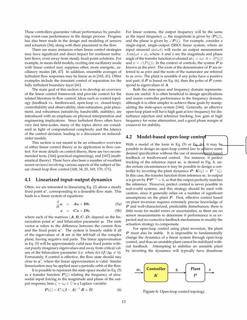
These controllers guarantee robust performance by penaliz-ing worst-case performance in the design process. Progresshas also been made in the design and modeling of sensorsand actuators [36], along with their placement in the flow.

There are many instances when linear control strategiesmay have significant and direct impact for nonlinear turbu-lent flows, even away from steady fixed-point solutions. Forexample, in mean-field models, exciting one oscillatory modewith linear control may suppress other, more energetic, os-cillatory modes [48, 47]. In addition, ensemble averages ofturbulent flow responses may be linear as in [165, 41]. Otherexamples include the transient control of separation for thefully turbulent boundary layer [41].

The main goal of this section is to develop an overviewof the linear control framework and provide context for therelated literature in flow control. Ideas such as control topol-ogy (feedback vs. feedforward, open-loop vs. closed-loop),controllability and observability, state estimation, pole place-ment, and robustness (sensitivity, bandwidth, stability), areintroduced with an emphasis on physical interpretation andengineering implications. Since turbulent flows often havevery fast time-scales, many of the topics above are consid-ered in light of computational complexity and the latencyof the control decision, leading to a discussion on reduced-order models.

This section is not meant to be an exhaustive overviewof either linear control theory or its application in flow con-trol. For more details on control theory, there are two recom-mended texts, [166] (practical engineering), and [167] (math-ematical theory). There have also been a number of excellentrecent reviews involving various aspects of the subject of lin-ear closed-loop flow control [168, 34, 20, 169, 170, 171].

4.1 Linearized input–output dynamicsOften, we are interested in linearizing Eq. (2) about a steadyfixed point as, corresponding to a desirable flow state. Thisleads to a linear system of equations:

d

dta = Aa+Bb, (5a)

s = Ca+Db, (5b)

where each of the matrices (A,B,C,D) depend on the lin-earization point as and bifurcation parameter µ. The statevector a refers to the difference between the current flowand the fixed point as. The system is linearly stable if allof the eigenvalues of A are in the left-half of the complexplane, having negative real parts. The linear approximationin Eq. (5) will be approximately valid near fixed points with-out purely imaginary eigenvalues and away from critical val-ues of the bifurcation parameter (i.e. when det df/dµ 6= 0).Fortunately, if control is effective, the flow state should stayclose to as, where the linear approximation is valid. Similarlinearization may be applied near a periodic orbit of the flow.

It is possible to represent the state-space model in Eq. (5)as a transfer function P (ζ) relating the frequency of sinu-soidal input forcing to the magnitude and phase of the out-put response; here ζ = iω ∈ C is a Laplace variable:

P (ζ) = C (ζI −A)−1B +D. (6)

For linear systems, the output frequency will be the sameas the input frequency ω, the magnitude is given by |P (ζ)|,and the phase is given by ∠P (ζ). For example, consider asingle-input, single-output (SISO) linear system, where aninput sinusoid sin(ωt) will excite an output measurementA sin(ωt + φ), where A and φ are the magnitude and phaseangle of the transfer function evaluated at ζ = iω: A = |P (ζ)|and φ = ∠(P (ζ)). In the context of controls, the system P isknown as the plant. The roots of the denominator ofP are re-ferred to as poles and the roots of the numerator are referredto as zeros. The plant is unstable if any poles have a positivereal part; if P is based on Eq. (6), then the poles of P corre-spond to eigenvalues ofA.

Both the state-space and frequency domain representa-tions are useful. It is often beneficial to design specificationsand assess controller performance in the frequency domain,although it is often simpler to achieve these goals by manip-ulating the state-space system [166]. Generally, an effectiveopen-loop plant will have high gain at low frequency for dis-turbance rejection and reference tracking, low gain at highfrequency for noise attenuation, and a good phase margin atcrossover for stability.

4.2 Model-based open-loop controlWith a model of the form in Eq. (5) or Eq. (6), it may bepossible to design an open-loop control law to achieve somedesired specification without the use of measurement-basedfeedback or feedforward control. For instance, if perfecttracking of the reference input wr is desired in Fig. 6, un-der certain circumstances it may be possible to design a con-troller by inverting the plant dynamics P : K(ζ) = P−1(ζ).In this case, the transfer function from referencewr to outputs is given byPP−1 = 1, so that the output perfectly matchesthe reference. However, perfect control is never possible inreal-world systems, and this strategy should be used withcaution, since it generally relies on a number of significantassumptions on the plant P . First, effective control basedon plant inversion requires extremely precise knowledge ofP and well-characterized, predictable disturbances; there islittle room for model errors or uncertainties, as there are nosensor measurements to determine if performance is as ex-pected and no corrective feedback mechanisms to modify theactuation strategy to compensate.

For open-loop control using plant inversion, the plantP must also be stable. It is impossible to fundamentallychange the dynamics of a linear system through open-loopcontrol, and thus an unstable plant cannot be stabilized with-out feedback. Attempting to stabilize an unstable plantby inverting the dynamics will typically have disastrous

PlantController


d



Combined with full-state feedback b = Kra,this results in a dynamical system for the controller:

d

dta = (A KfC BKr + KfDKr) a + Kfs,(7a)

b = Kra. (7b)

Note that the input to the controller is the sensorsignal s, the output is the actuation signal b, andthe state a estimates the full-state of the linear sys-tem in Eq. (2). The separation principle states thatKr and Kf may be designed separately to deter-mine the stability of the state dynamics for a and a,respectively, and the closed-loop system will havepoles given by the poles of ABKr and AKfC.

The most general observer dynamical system isgiven by:

d

dta = Aa + Bs, (8a)

b = Ca + Ds. (8b)

The general controller will be denoted by K()in the frequency domain.

4.4 Controllability, Observability, andGramians

The ability to place poles of the closed-loop systemarbitrarily with choice of Kr relies on the controlla-bility of the system in Eq. (2). The system is control-lable if the following matrix:

C =B AB A2B · · · ANa1B

(9a)

has full rank Na. Controllability implies that thesystem may be steered to an arbitrary state a withsuitable time-history of the control input b.

Similarly, the full state is observable if the observ-ability matrix is full rank:

O =

2666664

CCACA2

...CANa1

3777775

. (10a)

This means that any state a may be estimated witha suitable time-history of the measurements s.

Although the definitions of controllability andobservability above are binary, there are degrees ofcontrollability and observability, based on how dif-ficult it is to control or estimate a state a. The degreeof controllability and observability of a given stateis quantified by eigenvalues and eigenvectors of thecontrollability Gramian

Wc =

Z 1

0eAtBBeAtdt (11a)

1X

k=0

eAt

kBB

eAt

k(11b)

and observability Gramian:

Wo =

Z 1

0eAtCCeAtdt (12a)

1X

k=0

eAt

kCC

eAt

k. (12b)

These may be approximated by full-state mea-surements of the direct system in Eq. (2) and adjointsystem:

Wc W ec = CC, (13a)

Wo W eo = OO. (13b)

[Decide on notation for continuous vs. discretetime A... emp. Gramians are slightly wrong, sincethey use Ad]

[Mention SVD and symmetric matrix, degrees ofcontrollability...]

[Mention balanced model reduction: BT, BPOD,ERA]

10






d


s = Ca + Db + wn. (14b)





J =

Z 1



AT X + XA XBR1BT X + Q = 0. (16a)




mize E(a a)T (a a)
















11






d


s = Ca + Db + wn. (14b)





J =

Z 1



AT X + XA XBR1BT X + Q = 0. (16a)




mize E(a a)T (a a)
















11






d


s = Ca + Db + wn. (14b)





J =

Z 1



AT X + XA XBR1BT X + Q = 0. (16a)




mize E(a a)T (a a)
















11











d

dta = Aa + Bb, (2a)

s = Ca + Db. (2b)

Open-loop control

PlantController

Figure 3: Open-loop control topology.



P () = C (I A)1 B + D. (3a)




• P



d

dta = Aa BKra (4a)

= (A BKr) a. (4b)

However, full-state measurements of a are ei-ther infeasible or prohibitively expensive, and so anestimate a may be obtained from measurements s.This is of course, only if the system of equations (2)

9


13

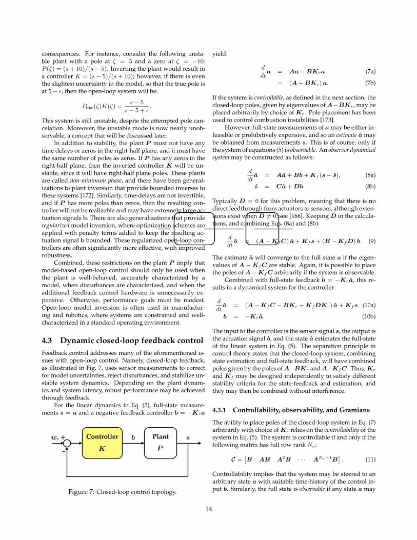
consequences. For instance, consider the following unsta-ble plant with a pole at ζ = 5 and a zero at ζ = −10:P (ζ) = (s+ 10)/(s− 5). Inverting the plant would result ina controller K = (s− 5)/(s+ 10); however, if there is eventhe slightest uncertainty in the model, so that the true pole isat 5− ε, then the open-loop system will be:

Ptrue(ζ)K(ζ) =s− 5

s− 5 + ε.

This system is still unstable, despite the attempted pole can-celation. Moreover, the unstable mode is now nearly unob-servable, a concept that will be discussed later.

In addition to stability, the plant P must not have anytime delays or zeros in the right-half plane, and it must havethe same number of poles as zeros. If P has any zeros in theright-half plane, then the inverted controller K will be un-stable, since it will have right-half plane poles. These plantsare called non-minimum phase, and there have been general-izations to plant inversion that provide bounded inverses tothese systems [172]. Similarly, time-delays are not invertible,and if P has more poles than zeros, then the resulting con-troller will not be realizable and may have extremely large ac-tuation signals b. There are also generalizations that provideregularized model inversion, where optimization schemes areapplied with penalty terms added to keep the resulting ac-tuation signal b bounded. These regularized open-loop con-trollers are often significantly more effective, with improvedrobustness.

Combined, these restrictions on the plant P imply thatmodel-based open-loop control should only be used whenthe plant is well-behaved, accurately characterized by amodel, when disturbances are characterized, and when theadditional feedback control hardware is unnecessarily ex-pensive. Otherwise, performance goals must be modest.Open-loop model inversion is often used in manufactur-ing and robotics, where systems are constrained and well-characterized in a standard operating environment.

4.3 Dynamic closed-loop feedback controlFeedback control addresses many of the aforementioned is-sues with open-loop control. Namely, closed-loop feedback,as illustrated in Fig. 7, uses sensor measurements to correctfor model uncertainties, reject disturbances, and stabilize un-stable system dynamics. Depending on the plant dynam-ics and system latency, robust performance may be achievedthrough feedback.

For the linear dynamics in Eq. (5), full-state measure-ments s = a and a negative feedback controller b = −Kra

PlantController+-


d




d


b = Kra. (7b)



d

dta = Aa + Bs, (8a)

b = Ca + Ds. (8b)





(9a)



O =

2666664

CCACA2

...CANa1

3777775

. (10a)



Wc =

Z 1

0eAtBBeAtdt (11a)

1X

k=0

eAt

kBB

eAt

k(11b)


Wo =

Z 1

0eAtCCeAtdt (12a)

1X

k=0

eAt

kCC

eAt

k. (12b)


Wc W ec = CC, (13a)

Wo W eo = OO. (13b)




10






d


s = Ca + Db + wn. (14b)





J =

Z 1



AT X + XA XBR1BT X + Q = 0. (16a)




mize E(a a)T (a a)
















11






d


s = Ca + Db + wn. (14b)





J =

Z 1



AT X + XA XBR1BT X + Q = 0. (16a)




mize E(a a)T (a a)
















11






d


s = Ca + Db + wn. (14b)





J =

Z 1



AT X + XA XBR1BT X + Q = 0. (16a)




mize E(a a)T (a a)
















11











d

dta = Aa + Bb, (2a)

s = Ca + Db. (2b)

Open-loop control

PlantController




P () = C (I A)1 B + D. (3a)




• P



d

dta = Aa BKra (4a)

= (A BKr) a. (4b)


9

Figure 7: Closed-loop control topology.

yield:

d

dta = Aa−BKra, (7a)

= (A−BKr)a. (7b)

If the system is controllable, as defined in the next section, theclosed-loop poles, given by eigenvalues ofA−BKr , may beplaced arbitrarily by choice of Kr . Pole placement has beenused to control combustion instabilities [173].

However, full-state measurements of amay be either in-feasible or prohibitively expensive, and so an estimate a maybe obtained from measurements s. This is of course, only ifthe system of equations (5) is observable. An observer dynamicalsystem may be constructed as follows:

d

dta = Aa+Bb+Kf (s− s), (8a)

s = Ca+Db. (8b)

Typically D = 0 for this problem, meaning that there is nodirect feedthrough from actuators to sensors, although exten-sions exist whenD 6= 0; see [166]. KeepingD in the calcula-tions, and combining Eqs. (8a) and (8b):

d

dta = (A−KfC) a+Kfs+ (B −KfD) b. (9)

The estimate a will converge to the full state a if the eigen-values of A −KfC are stable. Again, it is possible to placethe poles ofA−KfC arbitrarily if the system is observable.

Combined with full-state feedback b = −Kra, this re-sults in a dynamical system for the controller:

d

dta = (A−KfC −BKr +KfDKr) a+Kfs, (10a)

b = −Kra. (10b)

The input to the controller is the sensor signal s, the output isthe actuation signal b, and the state a estimates the full-stateof the linear system in Eq. (5). The separation principle incontrol theory states that the closed-loop system, combiningstate estimation and full-state feedback, will have combinedpoles given by the poles ofA−BKr andA−KfC. Thus,Kr

and Kf may be designed independently to satisfy differentstability criteria for the state-feedback and estimation, andthey may then be combined without interference.

4.3.1 Controllability, observability, and Gramians

The ability to place poles of the closed-loop system in Eq. (7)arbitrarily with choice ofKr relies on the controllability of thesystem in Eq. (5). The system is controllable if and only if thefollowing matrix has full row rank Na:

C =[B AB A2B · · · ANa−1B

]. (11)

Controllability implies that the system may be steered to anarbitrary state a with suitable time-history of the control in-put b. Similarly, the full state is observable if any state a may

14

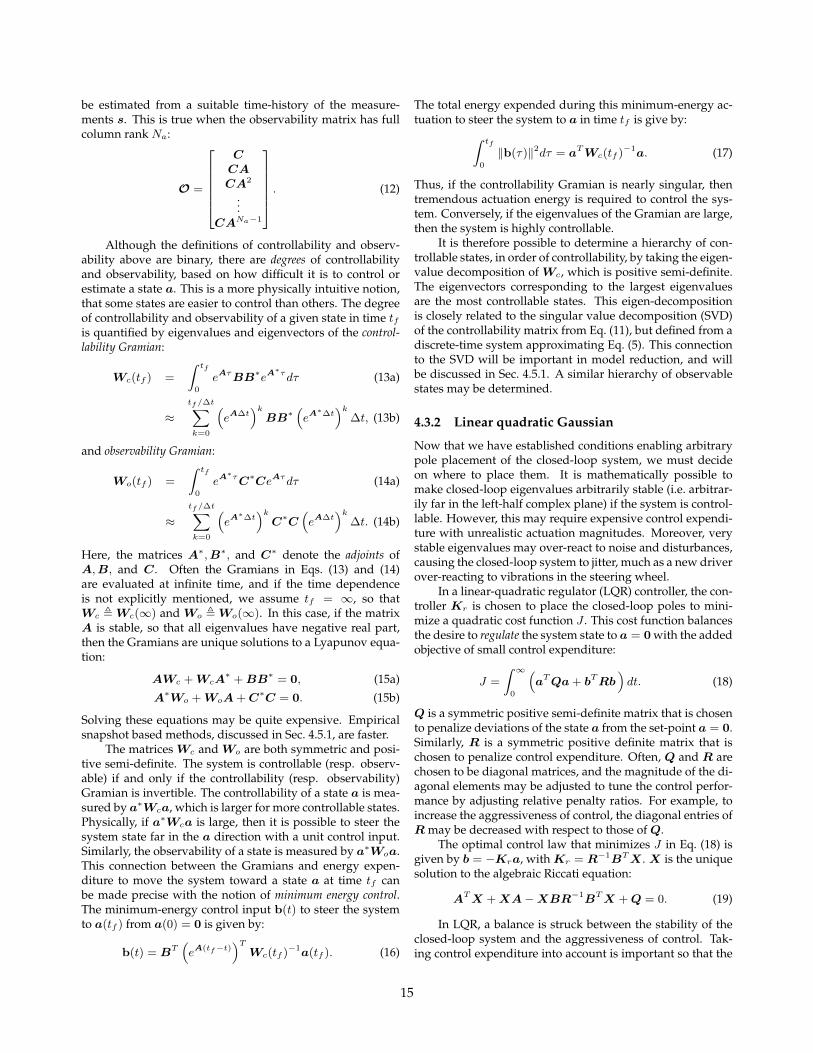
be estimated from a suitable time-history of the measure-ments s. This is true when the observability matrix has fullcolumn rank Na:

O =

CCACA2

...CANa−1

. (12)

Although the definitions of controllability and observ-ability above are binary, there are degrees of controllabilityand observability, based on how difficult it is to control orestimate a state a. This is a more physically intuitive notion,that some states are easier to control than others. The degreeof controllability and observability of a given state in time tfis quantified by eigenvalues and eigenvectors of the control-lability Gramian:

Wc(tf ) =

∫ tf

0

eAτBB∗eA∗τdτ (13a)

≈tf/∆t∑

k=0

(eA∆t

)kBB∗

(eA∗∆t)k

∆t, (13b)


Wo(tf ) =

∫ tf

0

eA∗τC∗CeAτdτ (14a)

≈tf/∆t∑

k=0

(eA∗∆t)kC∗C

(eA∆t

)k∆t. (14b)

Here, the matrices A∗,B∗, and C∗ denote the adjoints ofA,B, and C. Often the Gramians in Eqs. (13) and (14)are evaluated at infinite time, and if the time dependenceis not explicitly mentioned, we assume tf = ∞, so thatWc ,Wc(∞) and Wo ,Wo(∞). In this case, if the matrixA is stable, so that all eigenvalues have negative real part,then the Gramians are unique solutions to a Lyapunov equa-tion:

AWc +WcA∗ +BB∗ = 0, (15a)

A∗Wo +WoA+C∗C = 0. (15b)

Solving these equations may be quite expensive. Empiricalsnapshot based methods, discussed in Sec. 4.5.1, are faster.

The matrices Wc and Wo are both symmetric and posi-tive semi-definite. The system is controllable (resp. observ-able) if and only if the controllability (resp. observability)Gramian is invertible. The controllability of a state a is mea-sured by a∗Wca, which is larger for more controllable states.Physically, if a∗Wca is large, then it is possible to steer thesystem state far in the a direction with a unit control input.Similarly, the observability of a state is measured by a∗Woa.This connection between the Gramians and energy expen-diture to move the system toward a state a at time tf canbe made precise with the notion of minimum energy control.The minimum-energy control input b(t) to steer the systemto a(tf ) from a(0) = 0 is given by:

b(t) = BT(eA(tf−t)

)TWc(tf )−1a(tf ). (16)

The total energy expended during this minimum-energy ac-tuation to steer the system to a in time tf is give by:

∫ tf

0

‖b(τ)‖2dτ = aTWc(tf )−1a. (17)

Thus, if the controllability Gramian is nearly singular, thentremendous actuation energy is required to control the sys-tem. Conversely, if the eigenvalues of the Gramian are large,then the system is highly controllable.

It is therefore possible to determine a hierarchy of con-trollable states, in order of controllability, by taking the eigen-value decomposition of Wc, which is positive semi-definite.The eigenvectors corresponding to the largest eigenvaluesare the most controllable states. This eigen-decompositionis closely related to the singular value decomposition (SVD)of the controllability matrix from Eq. (11), but defined from adiscrete-time system approximating Eq. (5). This connectionto the SVD will be important in model reduction, and willbe discussed in Sec. 4.5.1. A similar hierarchy of observablestates may be determined.

4.3.2 Linear quadratic Gaussian

Now that we have established conditions enabling arbitrarypole placement of the closed-loop system, we must decideon where to place them. It is mathematically possible tomake closed-loop eigenvalues arbitrarily stable (i.e. arbitrar-ily far in the left-half complex plane) if the system is control-lable. However, this may require expensive control expendi-ture with unrealistic actuation magnitudes. Moreover, verystable eigenvalues may over-react to noise and disturbances,causing the closed-loop system to jitter, much as a new driverover-reacting to vibrations in the steering wheel.

In a linear-quadratic regulator (LQR) controller, the con-troller Kr is chosen to place the closed-loop poles to mini-mize a quadratic cost function J . This cost function balancesthe desire to regulate the system state to a = 0 with the addedobjective of small control expenditure:

J =

∫ ∞

0

(aTQa+ bTRb

)dt. (18)

Q is a symmetric positive semi-definite matrix that is chosento penalize deviations of the state a from the set-point a = 0.Similarly, R is a symmetric positive definite matrix that ischosen to penalize control expenditure. Often, Q and R arechosen to be diagonal matrices, and the magnitude of the di-agonal elements may be adjusted to tune the control perfor-mance by adjusting relative penalty ratios. For example, toincrease the aggressiveness of control, the diagonal entries ofRmay be decreased with respect to those ofQ.

The optimal control law that minimizes J in Eq. (18) isgiven by b = −Kra, withKr = R−1BTX . X is the uniquesolution to the algebraic Riccati equation:

ATX +XA−XBR−1BTX +Q = 0. (19)

In LQR, a balance is struck between the stability of theclosed-loop system and the aggressiveness of control. Tak-ing control expenditure into account is important so that the

15

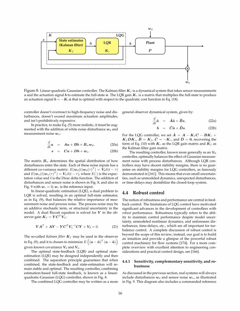
LQR PlantState estimator (Kalman filter)

+

LQG











d

dta = Aa + Bb, (2a)

s = Ca + Db. (2b)

Open-loop control

PlantController




P () = C (I A)1 B + D. (3a)






d

dta = Aa BKra (4a)

= (A BKr) a. (4b)


d


s = Ca + Db (5b)

9


d




d


b = Kra. (7b)



d

dta = Aa + Bs, (8a)

b = Ca + Ds. (8b)





(9a)



O =

2666664

CCACA2

...CANa1

3777775

. (10a)



Wc =

Z 1

0eAtBBeAtdt (11a)

1X

k=0

eAt

kBB

eAt

k(11b)


Wo =

Z 1

0eAtCCeAtdt (12a)

1X

k=0

eAt

kCC

eAt

k. (12b)


Wc W ec = CC, (13a)

Wo W eo = OO. (13b)




10


d




d


b = Kra. (7b)



d

dta = Aa + Bs, (8a)

b = Ca + Ds. (8b)





(9a)



O =

2666664

CCACA2

...CANa1

3777775

. (10a)



Wc =

Z 1

0eAtBBeAtdt (11a)

1X

k=0

eAt

kBB

eAt

k(11b)


Wo =

Z 1

0eAtCCeAtdt (12a)

1X

k=0

eAt

kCC

eAt

k. (12b)


Wc W ec = CC, (13a)

Wo W eo = OO. (13b)




10






d


s = Ca + Db + wn. (14b)





J =

Z 1



AT X + XA XBR1BT X + Q = 0. (16a)




mize E(a a)T (a a)
















11






d


s = Ca + Db + wn. (14b)





J =

Z 1



AT X + XA XBR1BT X + Q = 0. (16a)




mize E(a a)T (a a)
















11






d


s = Ca + Db + wn. (14b)





J =

Z 1



AT X + XA XBR1BT X + Q = 0. (16a)




mize E(a a)T (a a)
















11






d


s = Ca + Db + wn. (14b)





J =

Z 1



AT X + XA XBR1BT X + Q = 0. (16a)




mize E(a a)T (a a)
















11











d

dta = Aa + Bb, (2a)

s = Ca + Db. (2b)

Open-loop control

PlantController




P () = C (I A)1 B + D. (3a)




• P



d

dta = Aa BKra (4a)

= (A BKr) a. (4b)


9

estimate a may be obtained from measurements s.This is of course, only if the system of equations (2)is observable. An observer dynamical system may beconstructed as follows:

d


s = Ca + Db (5b)


d




d


b = Kra. (7b)



d

dta = Aa + Bs, (8a)

b = Ca + Ds. (8b)





(9a)



O =

2666664

CCACA2

...CANa1

3777775

. (10a)



Wc =

Z 1

0eAtBBeAtdt (11a)

1X

k=0

eAt

kBB

eAt

k(11b)


Wo =

Z 1

0eAtCCeAtdt (12a)

1X

k=0

eAt

kCC

eAt

k. (12b)


Wc W ec = CC, (13a)

Wo W eo = OO. (13b)

[Decide on notation for continuous vs. discrete timeA... emp. Gramians are slightly wrong, since theyuse Ad]



11

Figure 8: Linear-quadratic Gaussian controller. The Kalman filterKf is a dynamical system that takes sensor measurementss and the actuation signal b to estimate the full-state a. The LQR gainKr is a matrix that multiplies the full-state to producean actuation signal b = −Kra that is optimal with respect to the quadratic cost function in Eq. (18).

controller doesn’t overreact to high-frequency noise and dis-turbances, doesn’t exceed maximum actuation amplitudes,and isn’t prohibitively expensive.

In practice, to make Eq. (5) more realistic, it must be aug-mented with the addition of white noise disturbancewd andmeasurement noisewn:

d

dta = Aa+Bb+Bwwd, (20a)

s = Ca+Db+wn. (20b)

The matrix Bw determines the spatial distribution of howdisturbances enter the state. Each of these noise inputs has adifferent co-variance matrix: E(wd(t)wd(τ)T ) = Vdδ(t − τ)and E(wn(t)wn(τ)T ) = Vnδ(t− τ), where E(·) is the expec-tation value and δ is the Dirac delta function. The addition ofdisturbances and sensor noise is shown in Fig. 8, and also inFig. 9 withwr = 0;wr is the reference input.

In linear-quadratic estimation (LQE), a dual problem toLQR is solved, resulting in an optimal full-state estimator,as in Eq. (9), that balances the relative importance of mea-surement noise and process noise. The process noise may bean additive stochastic term, or structural uncertainty in themodel. A dual Riccati equation is solved for Y in the ob-server gainKf = Y CTVn:

Y AT +AY − Y CTV −1n CY + Vd = 0. (21)

The so-called Kalman filter Kf may be used in the observer

in Eq. (9), and it is chosen to minimize E(

(a− a)T (a− a))

given known covariance Vd and Vn.The optimal state-feedback (LQR) and optimal state-

estimation (LQE) may be designed independently and thencombined. The separation principle guarantees that whencombined, the state-feedback and state-estimation will re-main stable and optimal. The resulting controller, combiningestimation-based full-state feedback, is known as a linear-quadratic-Gaussian (LQG) controller, shown in Fig. 8.

The combined LQG controller may be written as a more

general observer dynamical system, given by:

d

dta = Aa+ Bs, (22a)

b = Ca+ Ds. (22b)

For the LQG controller, we set A = A − KfC − BKr +KfDKr , B = Kf , C = −Kr , and D = 0, recovering theform of Eq. (10) with Kr as the LQR gain matrix and Kf asthe Kalman filter gain matrix.

The resulting controller, known more generally as anH2

controller, optimally balances the effect of Gaussian measure-ment noise with process disturbances. Although LQR con-trollers may have decent stability margins, there is no guar-antee on stability margins for LQG controllers, as famouslydemonstrated in [161]. This means that even small uncertain-ties, such as unmodeled dynamics, unexpected disturbances,or time-delays may destabilize the closed-loop system.

4.4 Robust controlThe notion of robustness and performance are central in feed-back control. The limitations of LQG control have motivatedsignificant advances in the development of controllers withrobust performance. Robustness typically refers to the abil-ity to maintain control performance despite model uncer-tainty, unmodeled nonlinear dynamics, and unforeseen dis-turbances, time-delays, etc., which are all important for tur-bulence control. A complete discussion of robust control isbeyond the scope of this review; instead, our goal is to buildan intuition and provide a glimpse of the powerful robustcontrol machinery for flow systems [174]. For a more com-plete overview with excellent attention to engineering con-siderations and practical control design, see [166].

4.4.1 Sensitivity, complementary sensitivity, and ro-bustness

As discussed in the previous section, real systems will alwaysinclude disturbances wd and sensor noise wn, as illustratedin Fig. 9. This diagram also includes a commanded reference

16

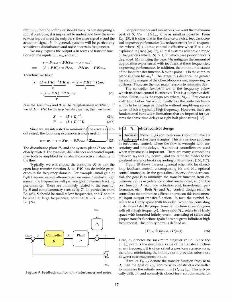
inputwr , that the controller should track. When designing arobust controller, it is important to understand how these ex-ogenous inputs affect the outputs s, the error signal e, and theactuation signal, b. In general, systems will be particularlysensitive to disturbances and noise at certain frequencies.

We may express the output s in terms of transfer func-tions on the inputswr ,wd, andwn:

s = Pdwd + PK(wr − s−wn),

=⇒ (I + PK)s = Pdwd + PKwr − PKwn.

Therefore, we have:

s = (I + PK)−1PK︸︷︷︸T

wr + (I + PK)−1

︸︷︷︸S

Pdwd

− (I + PK)−1PK︸︷︷︸T

wn. (23)

S is the sensitivity and T is the complementary sensitivity. Ifwe let L = PK be the loop transfer function, then we have:

S = (I +L)−1, (24a)

T = (I +L)−1L. (24b)

Since we are interested in minimizing the error e (with-out noise), the following expression is more useful:

e = wr − s = Swr − SPdwd + Twn. (25)

The disturbance plant Pd and the system plant P are oftenclosely related. For example, disturbances and control inputsmay both be amplified by a natural convective instability inthe flow.

Typically, we will choose the controller K so that theopen-loop transfer function L = PK has desirable prop-erties in the frequency domain. For example, small gain athigh frequencies will attenuate sensor noise. Similarly, highgain at low frequencies will provide good reference trackingperformance. These are intimately related to the sensitiv-ity S and complementary sensitivity T . In particular, fromEq. (25), S should be small at low frequencies, and T shouldbe small at large frequencies; note that S + T = I , fromEq. (24).

PlantController+

-


d




d


b = Kra. (7b)



d

dta = Aa + Bs, (8a)

b = Ca + Ds. (8b)





(9a)



O =

2666664

CCACA2

...CANa1

3777775

. (10a)



Wc =

Z 1

0eAtBBeAtdt (11a)

1X

k=0

eAt

kBB

eAt

k(11b)


Wo =

Z 1

0eAtCCeAtdt (12a)

1X

k=0

eAt

kCC

eAt

k. (12b)


Wc W ec = CC, (13a)

Wo W eo = OO. (13b)




10











d

dta = Aa + Bb, (2a)

s = Ca + Db. (2b)

Open-loop control

PlantController




P () = C (I A)1 B + D. (3a)




• P



d

dta = Aa BKra (4a)

= (A BKr) a. (4b)


9

The most general observer dynamical system is givenby:

d

dta = Aa + Bs, (8a)

b = Ca + Ds. (8b)

The general controller will be denoted by K() in thefrequency domain.

4.3.1 Controllability, Observability, and Gramians

The ability to place poles of the closed-loop system arbitrarilywith choice of Kr relies on the controllability of the system inEq. (2). The system is controllable if the following matrix:


(9a)

has full rank Na. Controllability implies that the system maybe steered to an arbitrary state a with suitable time-historyof the control input b.

Similarly, the full state is observable if the observabilitymatrix is full rank:

O =

2666664

CCACA2

...CANa1

3777775

. (10a)

This means that any state a may be estimated with a suitabletime-history of the measurements s.

Although the definitions of controllability and observ-ability above are binary, there are degrees of controllabilityand observability, based on how difficult it is to control orestimate a state a. The degree of controllability and observ-ability of a given state is quantified by eigenvalues and eigen-vectors of the controllability Gramian

Wc =

Z 1

0

eAtBBeAtdt (11a)

1X

k=0

eAt

k

BBeAt

k

(11b)


Wo =

Z 1

0

eAtCCeAtdt (12a)

1X

k=0

eAt

k

CCeAt

k

. (12b)

[Mention SVD and symmetric matrix, degrees of con-trollability...]

Eigenvalues and eigenvectors of Wc are left singularvectors of Cd

4.4 H1 robust vs. H2 optimal controlNow that we have established conditions enabling arbitrarypole placement of the closed-loop system, we must now de-cide on where to place them.

4.4.1 H2 optimal control: Linear quadratic Gaussian(LQG)

[Decide on notation for continuous vs. discrete time A...emp. Gramians are slightly wrong, since they use Ad]

We may often modify Eq. (2) with the addition of whitenoise disturbance wd and measurement noise wn:

d


s = Ca + Db + wn. (13b)

Each of these noise inputs has a different co-variance matrix:E(wdwT

d ) = Vd and E(wnwTn ) = Vn, where E(·) is the ex-

pectation value. [This is not precise enough... really needE(wd(t)wd()T ) = Vd(t ).]


J =

Z 1

0

aT Qa + bT Rb dt. (14a)

The optimal control law is b = Kra, where Kr =R1BT X and X is the unique solution to the algebraic Ric-cati equation [Expensive!!]:

AT X + XA XBR1BT X + Q = 0. (15a)

A dual Riccati equation is solved for the observer gain Kf =Y CT Vn:


The so-called Kalman filter Kf is chosen to minimize

E(a a)T (a a)

given known covariance Vd and Vn.

[Note: Kalman published his famous Kalman filter in ajournal of Fluid Engineering.]

We will often set C = Kr and D = 0 in Eq. (8), whereKr is a linear-quadratic-regulator (LQR) gain matrix. Wemay also choose A and B according to the Kalman filter,resulting in a combined estimation-based controller knownas the linear-quadratic-Gaussian (LQG). Because of the sepa-ration principle for linear systems, it is possible to design anoptimal feedback control gain Kr and an optimal observerseparately, and they will be both stable and optimal whencombined.

The resulting controller, known more generally as a H2

controller, optimally balances the effect of Gaussian measure-ment noise with process disturbances. Although LQR con-trollers may have decent stability margins, there is no guar-antee on stability margins for LQG controllers, as famouslydemonstrated in [32].

4.4.2 [Sensitivity, Complementary Sensitivity, andRobustness]

• Pd

• n d




• Time delays

10

++

++

wr e b

wd

wn

s

Figure 9: Feedback control with disturbances and noise.

For performance and robustness, we want the maximumpeak of S, MS = ‖S‖∞, to be as small as possible. FromEq. (25), it is clear that in the absence of noise, feedback con-trol improves performance (i.e. reduces error) for all frequen-cies where |S| < 1; thus control is effective when T ≈ 1. Asexplained in [166] (pg. 37), all real systems will have a rangeof frequencies where |S| > 1, in which case performance isdegraded. Minimizing the peak MS mitigates the amount ofdegradation experienced with feedback at these frequencies,improving performance. In addition, the minimum distanceof the loop transfer functionL to the point−1 in the complexplane is given by M−1

S . The larger this distance, the greaterthe stability margin of the closed-loop system, improving ro-bustness. These are the two major reasons to minimize MS .

The controller bandwidth ωB is the frequency belowwhich feedback control is effective. This is a subjective defi-nition. Often, ωB is the frequency where |S(jω)| first crosses-3 dB from below. We would ideally like the controller band-width to be as large as possible without amplifying sensornoise, which is typically high frequency. However, there arefundamental bandwidth limitations that are imposed for sys-tems that have time delays or right half plane zeros [166].

4.4.2 H∞ robust control design

As discussed above, LQG controllers are known to have ar-bitrarily poor robustness margins. This is a serious problemin turbulence control, where the flow is wrought with un-certainty and time-delays. H∞ robust controllers are usedwhen robustness is important. There are many connectionsbetween H2 and H∞ control, and we refer the reader to theexcellent reference books expanding on this theory [166, 167].

Figure 10 shows the most general schematic for closed-loop feedback control, encompassing H2 and H∞ optimalcontrol strategies. In the generalized theory of modern con-trol, the goal is to minimize the transfer function from ex-ogenous inputsw (reference, disturbances, noise, etc.) to thecost function J (accuracy, actuation cost, time-domain per-formance, etc.). Both H2 and H∞ control design result incontrollers that minimize different norms on this fundamen-tal input–output transfer function. In fact, the symbol H2

refers to a Hardy space with bounded two-norm, consistingof stable and strictly proper transfer functions (meaning gainrolls off at high frequency). The symbolH∞ refers to a Hardyspace with bounded infinity-norm, consisting of stable andproper transfer functions (gain does not grow infinite at highfrequencies). The infinity norm is defined as:

‖P ‖∞ , maxω

σ1 (P (iω)) . (26)

Here, σ1 denotes the maximum singular value. Since the‖ · ‖∞ norm is the maximum value of the transfer functionat any frequency, it is often called a worst-case scenario norm;therefore, minimizing the infinity norm provides robustnessto worst-case exogenous inputs.

If we let Pw→J denote the transfer function from w toJ , then the goal of H∞ control is to construct a controllerto minimize the infinity norm: min ‖Pw→J‖∞. This is typi-cally difficult, and no analytic closed-form solution exists for

17

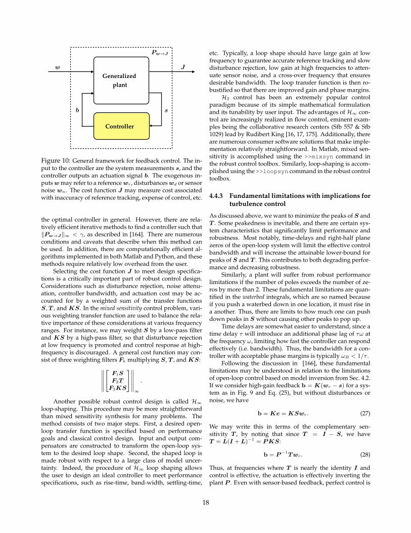
Generalizedplant

Controller

w J

b s

Pw→J

Figure 10: General framework for feedback control. The in-put to the controller are the system measurements s, and thecontroller outputs an actuation signal b. The exogenous in-putswmay refer to a referencewr , disturbanceswd or sensornoise wn. The cost function J may measure cost associatedwith inaccuracy of reference tracking, expense of control, etc.

the optimal controller in general. However, there are rela-tively efficient iterative methods to find a controller such that‖Pw→J‖∞ < γ, as described in [164]. There are numerousconditions and caveats that describe when this method canbe used. In addition, there are computationally efficient al-gorithms implemented in both Matlab and Python, and thesemethods require relatively low overhead from the user.

Selecting the cost function J to meet design specifica-tions is a critically important part of robust control design.Considerations such as disturbance rejection, noise attenu-ation, controller bandwidth, and actuation cost may be ac-counted for by a weighted sum of the transfer functionsS,T , and KS. In the mixed sensitivity control problem, vari-ous weighting transfer function are used to balance the rela-tive importance of these considerations at various frequencyranges. For instance, we may weight S by a low-pass filterand KS by a high-pass filter, so that disturbance rejectionat low frequency is promoted and control response at high-frequency is discouraged. A general cost function may con-sist of three weighting filters Fk multiplying S, T , andKS:

∥∥∥∥∥∥

F1SF2TF3KS

∥∥∥∥∥∥∞

.

Another possible robust control design is called H∞loop-shaping. This procedure may be more straightforwardthan mixed sensitivity synthesis for many problems. Themethod consists of two major steps. First, a desired open-loop transfer function is specified based on performancegoals and classical control design. Input and output com-pensators are constructed to transform the open-loop sys-tem to the desired loop shape. Second, the shaped loop ismade robust with respect to a large class of model uncer-tainty. Indeed, the procedure of H∞ loop shaping allowsthe user to design an ideal controller to meet performancespecifications, such as rise-time, band-width, settling-time,

etc. Typically, a loop shape should have large gain at lowfrequency to guarantee accurate reference tracking and slowdisturbance rejection, low gain at high frequencies to atten-uate sensor noise, and a cross-over frequency that ensuresdesirable bandwidth. The loop transfer function is then ro-bustified so that there are improved gain and phase margins.H2 control has been an extremely popular control

paradigm because of its simple mathematical formulationand its tunability by user input. The advantages of H∞ con-trol are increasingly realized in flow control, eminent exam-ples being the collaborative research centers (Sfb 557 & Sfb1029) lead by Rudibert King [16, 17, 175]. Additionally, thereare numerous consumer software solutions that make imple-mentation relatively straightforward. In Matlab, mixed sen-sitivity is accomplished using the >>mixsyn command inthe robust control toolbox. Similarly, loop-shaping is accom-plished using the >>loopsyn command in the robust controltoolbox.

4.4.3 Fundamental limitations with implications forturbulence control

As discussed above, we want to minimize the peaks of S andT . Some peakedness is inevitable, and there are certain sys-tem characteristics that significantly limit performance androbustness. Most notably, time-delays and right-half planezeros of the open-loop system will limit the effective controlbandwidth and will increase the attainable lower-bound forpeaks of S and T . This contributes to both degrading perfor-mance and decreasing robustness.

Similarly, a plant will suffer from robust performancelimitations if the number of poles exceeds the number of ze-ros by more than 2. These fundamental limitations are quan-tified in the waterbed integrals, which are so named becauseif you push a waterbed down in one location, it must rise ina another. Thus, there are limits to how much one can pushdown peaks in S without causing other peaks to pop up.

Time delays are somewhat easier to understand, since atime delay τ will introduce an additional phase lag of τω atthe frequency ω, limiting how fast the controller can respondeffectively (i.e. bandwidth). Thus, the bandwidth for a con-troller with acceptable phase margins is typically ωB < 1/τ .

Following the discussion in [166], these fundamentallimitations may be understood in relation to the limitationsof open-loop control based on model inversion from Sec. 4.2.If we consider high-gain feedback b = K(wr − s) for a sys-tem as in Fig. 9 and Eq. (25), but without disturbances ornoise, we have

b = Ke = KSwr. (27)

We may write this in terms of the complementary sen-sitivity T , by noting that since T = I − S, we haveT = L(I +L)−1 = PKS:

b = P−1Twr. (28)

Thus, at frequencies where T is nearly the identity I andcontrol is effective, the actuation is effectively inverting theplant P . Even with sensor-based feedback, perfect control is

18

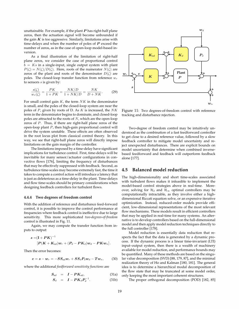
unattainable. For example, if the plantP has right-half planezeros, then the actuation signal will become unbounded ifthe gainK is too aggressive. Similarly, limitations arise withtime-delays and when the number of poles of P exceed thenumber of zeros, as in the case of open-loop model-based in-version.

As a final illustration of the limitation of right-halfplane zeros, we consider the case of proportional controlb = Ks in a single-input, single output system with plantP (ζ) = N(ζ)/D(ζ). Here, roots of the numerator N(ζ) arezeros of the plant and roots of the denominator D(ζ) arepoles. The closed-loop transfer function from reference wrto sensors s is given by:

s(ζ)

wr(ζ)=

PK

1 + PK=

NK/D

1 +NK/D=

NK

D +NK. (29)

For small control gain K, the term NK in the denominatoris small, and the poles of the closed-loop system are near thepoles of P , given by roots of D. As K is increased, the NKterm in the denominator begins to dominate, and closed-looppoles are attracted to the roots of N , which are the open-loopzeros of P . Thus, if there are right-half plane zeros of theopen-loop plant P , then high-gain proportional control willdrive the system unstable. These effects are often observedin the root locus plot from classical control theory. In thisway, we see that right-half plane zeros will directly imposelimitations on the gain margin of the controller.

The limitations imposed by a time-delay have significantimplications for turbulence control. First, time-delays will beinevitable for many sensor/actuator configurations in con-vective flows [176], limiting the frequency of disturbancesthat may be effectively suppressed with feedback. Second, asturbulence time-scales may become extremely fast, the time ittakes to compute a control action will introduce a latency thatis just as deleterious as a time-delay in the plant. Time-delaysand flow time-scales should be primary considerations whendesigning feedback controllers for turbulent flows.

4.4.4 Two degrees of freedom control

With the addition of reference and disturbance feed-forwardcontrol, it is possible to improve the control performance atfrequencies where feedback control is ineffective due to largesensitivity. This more sophisticated two-degrees-of-freedomcontrol is illustrated in Fig. 11.

Again, we may compute the transfer function from in-puts to output:

s =(I + PK)−1

[P (K +Kref)wr + (Pd − PKd)wd − PKwn] .

Then the error becomes:

e = s−wr = −SSrefwr + SSdPdwd − Twn, (30)

where the additional feedforward sensitivity functions are

Sref = I − PKref, (31a)

Sd = I − PKdP−1d . (31b)

Plant+- +

+

++

+ +

++

wr e

Kref

K

Kd

P

Pd

wd

wn

s

Figure 11: Two degrees-of-freedom control with referencetracking and disturbance rejection.

Two-degree of freedom control may be intuitively un-derstood as the combination of a fast feedforward controllerto get close to a desired reference value, followed by a slowfeedback controller to mitigate model uncertainty and re-ject unexpected disturbances. There are explicit bounds onmodel uncertainty that determine when combined inverse-based feedforward and feedback will outperform feedbackalone [177].

4.5 Balanced model reductionThe high-dimensionality and short time-scales associatedwith turbulent flows makes it infeasible to implement themodel-based control strategies above in real-time. More-over, solving for H2 and H∞ optimal controllers may becomputationally intractable, as they involve either a high-dimensional Riccati equation solve, or an expensive iterativeoptimization. Instead, reduced-order models provide effi-cient, low-dimensional representations of the most relevantflow mechanisms. These models result in efficient controllersthat may be applied in real-time for many systems. An alter-native is to develop controllers based on the full-dimensionalmodel and then apply model reduction techniques directly tothe full controller [178].

Model reduction is essentially data reduction that re-spects the fact that the data is generated by a dynamic pro-cess. If the dynamic process is a linear time-invariant (LTI)input–output system, then there is a wealth of machineryavailable for model reduction, and performance bounds maybe quantified. Many of these methods are based on the singu-lar value decomposition (SVD) [88, 179, 87], and the minimalrealization theory of Ho and Kalman [180, 181]. The generalidea is to determine a hierarchical modal decomposition ofthe flow state that may be truncated at some model order,only keeping the most important coherent structures.

The proper orthogonal decomposition (POD) [182, 85]

19

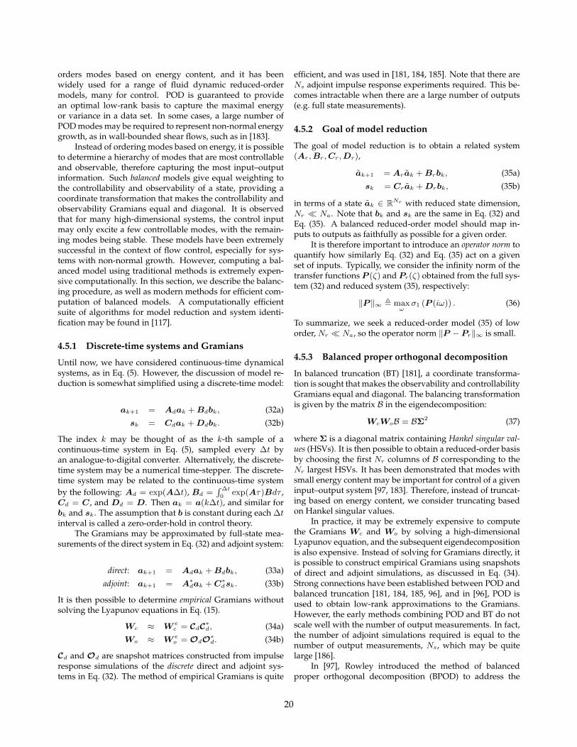
orders modes based on energy content, and it has beenwidely used for a range of fluid dynamic reduced-ordermodels, many for control. POD is guaranteed to providean optimal low-rank basis to capture the maximal energyor variance in a data set. In some cases, a large number ofPOD modes may be required to represent non-normal energygrowth, as in wall-bounded shear flows, such as in [183].

Instead of ordering modes based on energy, it is possibleto determine a hierarchy of modes that are most controllableand observable, therefore capturing the most input–outputinformation. Such balanced models give equal weighting tothe controllability and observability of a state, providing acoordinate transformation that makes the controllability andobservability Gramians equal and diagonal. It is observedthat for many high-dimensional systems, the control inputmay only excite a few controllable modes, with the remain-ing modes being stable. These models have been extremelysuccessful in the context of flow control, especially for sys-tems with non-normal growth. However, computing a bal-anced model using traditional methods is extremely expen-sive computationally. In this section, we describe the balanc-ing procedure, as well as modern methods for efficient com-putation of balanced models. A computationally efficientsuite of algorithms for model reduction and system identi-fication may be found in [117].

4.5.1 Discrete-time systems and Gramians

Until now, we have considered continuous-time dynamicalsystems, as in Eq. (5). However, the discussion of model re-duction is somewhat simplified using a discrete-time model:

ak+1 = Adak +Bdbk, (32a)

sk = Cdak +Ddbk. (32b)

The index k may be thought of as the k-th sample of acontinuous-time system in Eq. (5), sampled every ∆t byan analogue-to-digital converter. Alternatively, the discrete-time system may be a numerical time-stepper. The discrete-time system may be related to the continuous-time systemby the following: Ad = exp(A∆t), Bd =

∫∆t

0exp(Aτ)Bdτ ,

Cd = C, and Dd = D. Then ak = a(k∆t), and similar forbk and sk. The assumption that b is constant during each ∆tinterval is called a zero-order-hold in control theory.

The Gramians may be approximated by full-state mea-surements of the direct system in Eq. (32) and adjoint system:

direct: ak+1 = Adak +Bdbk, (33a)

adjoint: ak+1 = A∗dak +C∗dsk. (33b)

It is then possible to determine empirical Gramians withoutsolving the Lyapunov equations in Eq. (15).

Wc ≈ W ec = CdC∗d, (34a)

Wo ≈ W eo = OdO∗d. (34b)

Cd and Od are snapshot matrices constructed from impulseresponse simulations of the discrete direct and adjoint sys-tems in Eq. (32). The method of empirical Gramians is quite

efficient, and was used in [181, 184, 185]. Note that there areNs adjoint impulse response experiments required. This be-comes intractable when there are a large number of outputs(e.g. full state measurements).

4.5.2 Goal of model reduction

The goal of model reduction is to obtain a related system(Ar,Br,Cr,Dr),

ak+1 = Arak +Brbk, (35a)

sk = Crak +Drbk, (35b)

in terms of a state ak ∈ RNr with reduced state dimension,Nr Na. Note that bk and sk are the same in Eq. (32) andEq. (35). A balanced reduced-order model should map in-puts to outputs as faithfully as possible for a given order.

It is therefore important to introduce an operator norm toquantify how similarly Eq. (32) and Eq. (35) act on a givenset of inputs. Typically, we consider the infinity norm of thetransfer functions P (ζ) and Pr(ζ) obtained from the full sys-tem (32) and reduced system (35), respectively:

‖P ‖∞ , maxω

σ1 (P (iω)) . (36)

To summarize, we seek a reduced-order model (35) of loworder, Nr Na, so the operator norm ‖P − Pr‖∞ is small.

4.5.3 Balanced proper orthogonal decomposition

In balanced truncation (BT) [181], a coordinate transforma-tion is sought that makes the observability and controllabilityGramians equal and diagonal. The balancing transformationis given by the matrix B in the eigendecomposition:

WcWoB = BΣ2 (37)

where Σ is a diagonal matrix containing Hankel singular val-ues (HSVs). It is then possible to obtain a reduced-order basisby choosing the first Nr columns of B corresponding to theNr largest HSVs. It has been demonstrated that modes withsmall energy content may be important for control of a giveninput–output system [97, 183]. Therefore, instead of truncat-ing based on energy content, we consider truncating basedon Hankel singular values.

In practice, it may be extremely expensive to computethe Gramians Wc and Wo by solving a high-dimensionalLyapunov equation, and the subsequent eigendecompositionis also expensive. Instead of solving for Gramians directly, itis possible to construct empirical Gramians using snapshotsof direct and adjoint simulations, as discussed in Eq. (34).Strong connections have been established between POD andbalanced truncation [181, 184, 185, 96], and in [96], POD isused to obtain low-rank approximations to the Gramians.However, the early methods combining POD and BT do notscale well with the number of output measurements. In fact,the number of adjoint simulations required is equal to thenumber of output measurements, Ns, which may be quitelarge [186].

In [97], Rowley introduced the method of balancedproper orthogonal decomposition (BPOD) to address the

20

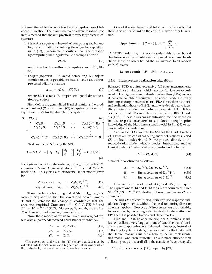
aforementioned issues associated with snapshot based bal-anced truncation. There are two major advances introducedin this method that make it practical to very large dynamicalsystems:

1. Method of snapshots – Instead of computing the balanc-ing transformation by solving the eigendecompositionin Eq. (37), it is possible to construct the transformationby computing the singular value decomposition of

OdCd, (38)

reminiscent of the method of snapshots from [187, 188,86].

2. Output projection – To avoid computing Ns adjointsimulations, it is possible instead to solve an output-projected adjoint equation:

ak+1 = A∗dak +C∗dUrs (39)

where Ur is a rank-Nr proper orthogonal decomposi-tion truncation.

First, define the generalized Hankel matrix as the prod-uct of the direct (Cd) and adjoint (O∗d) snapshot matrices fromEq. (11) and (12), for the discrete-time system:

H = OdCd (40)

=

CdBd CdAdBd · · · CdAmc−1d Bd

CdAdBd CdA2dBd · · · CdA

mcd Bd

......

. . ....

CdAmo−1d Bd CdA

mod Bd · · · CdA

mc+mo−2d Bd

.

Next, we factorH2 using the SVD:

H = UΣV ∗ =[U1 U2

] [Σ1 00 0

] [V ∗1V ∗2

]= U1Σ1V

∗1 .

(41)

For a given desired model order Nr Na, only the first Nrcolumns of U and V are kept, along with the first Nr × Nrblock of Σ. This yields a bi-orthogonal set of modes givenby:

direct modes: Φr = CdVrΣ−1/2r , (42a)

adjoint modes: Ψr = O∗dUrΣ−1/2r . (42b)

These modes are bi-orthogonal, Ψ∗rΦr = INr×Nr , andRowley [97] showed that the direct and adjoint modes,Φ and Ψ, establish the change of coordinates that bal-ance the empirical Gramians: B = Φ , CdV Σ−1/2 andB−1 = Ψ∗ , Σ−1/2U∗Od. Moreover, Φr and Ψr are the firstNr-columns of the balancing transformation.

Now, these modes allow us to project our original sys-tem onto a (balanced) reduced-order model or order Nr :

Ar = Ψ∗rAdΦr, (43a)

Br = Ψ∗rBd, (43b)

Cr = CdΦr. (43c)

2The powers mc and mo in Eq. (40) signify that data must becollected until the matrices Cd and O∗d become full rank, after whichthe controllable/observable subspaces have been sampled.

One of the key benefits of balanced truncation is thatthere is an upper bound on the error of a given order trunca-tion:

Upper bound: ‖P − Pr‖∞ < 2

n∑

j=Nr+1

σj .

A BPOD model may not exactly satisfy this upper bounddue to errors in the calculation of empirical Gramians. In ad-dition, there is a lower bound that is universal to all modelswith Nr states:

Lower bound: ‖P − Pr‖∞ > σNr+1.

4.5.4 Eigensystem realization algorithm

Balanced POD requires expensive full-state measurementsand adjoint simulations, which are not feasible for experi-ments. The eigensystem realization algorithm (ERA) makesit possible to obtain equivalent balanced models directlyfrom input–output measurements. ERA is based on the mini-mal realization theory of [180], and it was developed to iden-tify structural models for various spacecraft [141]. It hasbeen shown that ERA models are equivalent to BPOD mod-els [189]. ERA is a system identification method based onimpulse response measurements and does not require priorknowledge of the high-dimensional model in Eq. (32) or ac-cess to adjoint simulations.

Similar to BPOD, we take the SVD of the Hankel matrixH . However, instead of collecting snapshot matrices Cd andO∗d to obtain modes Φ and Ψ, we proceed directly to thereduced-order model, without modes. Introducing anotherHankel matrixH ′ advanced one time-step in the future

H ′ = OdAdCd, (44)

a model is constructed as follows:

Ar = Σ−1/2r U∗rH

′VrΣ−1/2r , (45a)

Br = first p columns of Σ1/2r V ∗, (45b)

Cr = first q columns of UΣ1/2r . (45c)

It is simple to verify that (43a) and (45a) are equal.The expressions (43b) and (45b) for Br are equivalent, sinceΣ−1/2r U∗rH = Σ

1/2r V ∗r . Similarly, the expressions forCr are

equivalent.H and H ′ are constructed from impulse response sim-

ulations/experiments, without the need for storing direct oradjoint snapshots. However, if direct snapshots are available,for example, by collecting velocity fields in simulations orPIV, then it is possible to construct direct modes.

ERA and BPOD balance the empirical Gramians, so un-less we collect a very large amount of data, the true Grami-ans are only approximately balanced. However, instead ofcollecting long tails of data, it is possible to collect data untilthe Hankel matrix is full rank, balance the full-rank identi-fied model, and then truncate. This is more efficient thancollecting snapshots until all of the transients have decayed3.

3This idea is developed in [190], inspired by [191].

21

4.5.5 Observer/Kalman filter identification

Observer/Kalman filter identification (OKID) was devel-oped to compliment the ERA for lightly damped experimen-tal systems with noise [192, 193, 194, 142]. This methodaddresses the general problem of identifying an approxi-mate impulse response (i.e. Markov parameters) from arbi-trary, noisy input–output data. Typically, one would ob-tain reduced-order models according to the following gen-eral procedure:

1. Collect output response to a pseudo-random input

2. This information is then passed through the OKID algo-rithm to obtain the linear impulse response,

3. The impulse response is passed through the ERA to ob-tain a reduced-order state-space system.

The OKID method identifies an approximation to theimpulse response of a system from noisy input–output datausing an asymptotically stable Kalman filter. Although thismethod is quite powerful, it has not been broadly adoptedbecause of the algorithmic complexity as well as nonintuitivetheoretical elements. However, a recent method extendingdynamic mode decomposition (DMD) to systems with con-trol inputs provides similar models as ERA/OKID, but witha more intuitive and computationally simple algorithm [195].This follows recent results that DMD and ERA may be seenas equivalent, up to a coordinate transformation, for certaintypes of input–output data [101].

4.6 Case study: Transition delay in aboundary layer and stabilizing steadystates

For many canonical flows, such as pipe flow or Couetteflow, the underlying laminar steady solution is stable for allReynolds numbers [196, 197, 198], and turbulent fluctuationsarise as transient events due to perturbations and wall rough-ness. However, many fully turbulent flows are character-ized by saturated nonlinear dynamics, and the existence ofa desirable underlying unstable fixed point or periodic or-bit. For example, in the laminar-to-turbulent transition of aflat plate boundary layer or channel flow, the unstable fixedpoint corresponds to steady, laminar flow with significantlydecreased drag. The existence of these remnant unstablesteady-states is consistent with the Hopf-bifurcation route toturbulence [199]. In addition, linearization may also work inthe viscous sublayer in wall turbulence.

Linear control is ideal for such systems, because success-ful regulators keep the system in a state that is near the fixedpoint, where the linear assumption remains valid. Therefore,linear control has largely been applied to transition delay andstabilizing unstable steady-states. It is also possible to desta-bilize a system to enhance mixing by reversing the sign ofa stabilizing controller [200]. It is worth noting that thereare numerous examples where linear model-based controlhas been successfully applied to flows that are in a nonlinearregime. Often times turbulence is considered a disturbanceterm in a slower dynamical system, such as the rigid body

equations of an aircraft, space shuttle, or rocket. In this case,turbulent fluctuations may be seen as inevitable and operat-ing on a time scale that is faster than controller bandwidth.Instead of trying to change the nature of the turbulence itself,the controller may be designed to obtain some other objec-tive while robustly managing the uncertain turbulent distur-bance. Here, we consider the problem of actively controllingthe turbulent dynamical system.

The field of linear model-based flow control has expe-rienced exceptional growth, largely due to the close align-ment of challenges in engineering fluid dynamics with thesophisticated machinery in model reduction and control the-ory. There are a number of excellent reviews of linear flowcontrol [20], for transition delay in spatially developing wall-bounded flows [170, 201, 171], and for the control of cavityoscillations [34]. A good overview of drag reduction by con-trol of turbulence boundary layers is also found in [10], witha quantification of potential fuel savings in transportation.The discussion here is not meant to be complete, but ratheris designed to clarify the choices and historical progress oflinear model-based flow control, especially in turbulence.

4.6.1 Early work

Early progress in model-based flow control is closely tied toadvances in computational resources, enabling the simula-tion of large-scale dynamical systems, such as in fluid dy-namics. Currently, the majority of model-based flow controlemploying H2 and H∞ techniques are applied to numericalsimulations. In [202], gradient-based optimal control tech-niques were introduced to control the flow in a channel usingboundary condition control. Adjoint methods have also beenused extensively for aerodynamic shape optimization basedon CFD [203, 204, 205, 206].

A suboptimal control approximation was introduced byChoi et al in 1993 [207] using a very short time horizon thatallowed convective terms to be neglected, resulting in a con-troller based on a Stokes flow model. This method was thenapplied to a turbulent channel flow by Bewley and Moinin 1994 [208], resulting in a 17% drag reduction. Subop-timal control with more physically realizable measurementwas analyzed for a turbulent channel flow in [209]. Withoutthe suboptimal approximation, a model-predictive control(MPC) framework may be used for receding-horizon optimalcontrol, although this is computationally intensive. MPC hasbeen used in [210] and [211], and is discussed in more detailin a recent review [171].

In Bewley and Liu [212], both H2 and H∞ controllerswere developed and applied to single wavenumber pairs ina plane channel flow with three dimensional perturbations.In [213], robust control was applied to the extended prob-lem of 2D multi-wavenumber control with localized actua-tion and sensing in plane Poiseuille flow. Hogberg et al [214]extended the analysis of [212] to include multiple wavenum-bers and state estimation using a Kalman filter based on wallmeasurements. Their three-dimensional DNS used bound-ary condition forcing, and it was shown that state-estimationwas not as effective as full-state feedback.

Hogberg and Henningson [215] demonstrated the effec-

22

tiveness of linear H2 optimal control in spatially developingboundary layers, even with moderately strong nonlinearitiespresent. In a follow-up work [216], they extended this analy-sis to include full-state estimation based on a number of wallmeasurements, similar to [214].

4.6.2 Use of reduced-order models

As discussed earlier, the development of controllers for high-dimensional linear systems may be extremely computation-ally intensive since they depend on the solution to Riccatiequations, involving O(N3

a ) operations, or expensive itera-tions. Further, once a high-dimensional controller has beendesigned, it is expensive to compute the resulting control ac-tion, introducing unwanted latency in the control loop. Thislatency significantly limits control bandwidth and may pre-vent real-time control of high-dimensional systems with fasttime-scales. These issues are especially pronounced in flowcontrol.

In the timely work of Akervik et al [218], reduced-ordermodels were developed by using a few non-normal globaleigenmodes of the linearized Navier-Stokes equations as abasis for Galerkin projection. Based on the reduced-ordermodel, an LQG controller is able to attenuate global oscilla-tions in a separated boundary layer. The use of non-normalglobal modes has been important to capture the transientenergy growth associated with wall-bounded shear flows.Yet, these approaches have limited applicability to unstableadvection-dominated flows. Transient growth implies a sen-sitivity issue: a small difference in the initial condition or asmall perturbation in the system can give rise to significantlydifferent solutions. Hence, unavoidable truncation errorsof reduced-order models based on global modes may causesimilar differences in the solutions. The sensitivity problemis less pronounced at lower Reynolds numbers or for weaklyunstable flows.

After the seminal work of Rowley [97], introducinga computationally efficient method to compute balancedreduced-order models, the use of balanced models has be-come a mainstay in model-based linear flow control. The re-sulting models are able to capture transient energy growthwith significantly fewer modes than POD, as demonstratedin [183] on the transitional channel flow. BPOD was alsoshown to outperform standard POD/Galerkin methods forthe separation control of an airfoil at low Reynolds num-ber [219], using an immersed-boundary method [220, 221].

The paper of Bagheri, Brandt, and Henningson [222]provides one of the most complete and clearly presented nar-ratives on closed-loop control based on balanced models. Inthis work, they develop models using snapshot-based bal-anced truncation. Snapshot based methods are necessarywhen the state dimension Na is large, since the A matrixis size N2

a , which may not be representable in system mem-ory. The matrix-free methods advocated in [222] use the CFDtime-stepper to find the next flow state, rather than explic-itly computing a large A matrix. These methods may beused to solve large eigenvalue problems, for instance usingArnoldi iteration, thus bypassing the creation and factoriza-tion of a large matrix. In this paper, H2 control is developed

to suppress two-dimensional boundary layer perturbations.[223] presents a three-dimensional generalization of [222] us-ing LQG to delay transition in a boundary layer.

As described in Sec. 4.5.4, the eigensystem realization al-gorithm (ERA) produces balanced models that are equivalentto BPOD, but without the need for adjoint simulations [189].ERA has been rapidly adopted in flow control because of thefact that it is based purely on input–output data, making it asystem identification method, rather than a model reductionmethod. ERA was used to study and control cavity flow os-cillations and combustion oscillations [224, 225]. In Semeraroet al [217], ERA models were used to develop LQG control tosuppress three-dimensional Tollmien-Schlichting (TS) wavesin a transitional boundary layer using a volume force actua-tion. This paper is well-written and thought provoking, andan illustration of the closed-loop control topology is shown inFig. 12. Interestingly, one of the earliest experimental demon-strations of active feedback suppression of turbulence wasapplied to cancel TS waves using a downstream heating el-ement and a phase shifted measurement feedback, resultingin an increase in the transition Reynolds number [18].

4.7 Case study: Wall turbulence controland skin-friction reduction

There is a tremendous industrial motivation to reduce tur-bulent skin-friction drag. This problem has thus receivedsignificant attention, and corresponding progress has beenmade [40, 10]. Reduced-order models for control based onLQG and the robustifying loop-transfer recovery were usedto reduce skin-friction drag in a a channel flow [226, 227], re-sulting in eventual relaminarization of the flow. Reduced-order models were also used with blowing/suction at thewall to reduce skin friction in simulations [228], and reduced-order Kalman filters were developed based on balanced trun-cation models [133].

In addition to the mechanisms and techniques dis-cussed, there have been many efforts to reduce turbulentskin friction drag [229, 230, 231, 232, 233] using various tech-niques such as traveling-wave-like actuation including blow-ing/suction and wall deformation. Increasing heat trans-fer while decreasing drag is also an important area of re-search [234]. In addition, system identification and controlwere used for the linear feed-forward control of turbulentboundary layer fluctuations by exploiting coherent struc-tures and predicting their behavior downstream [235]. Thesame reduction in turbulent boundary layer fluctuations wasexplored using model-based control in an experiment usingan array of synthetic jet actuators [236].

4.8 Case study: Cavity flow controlThe work surrounding the control of open cavity flows rep-resents one of the most complete and compelling successstories in active flow control [237]. Cavity flow control hasmany applications, such as the suppression of oscillations inweapons bays in high-speed flight [238], which is an inher-ently high Reynolds number phenomena. A more complete

23

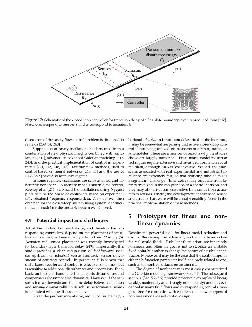
Transition delay in a boundary layer flow using active control 293

DisturbanceB1

SensorsC2

ActuatorsB2

Domain to minimize disturbance energy

C1

z(t)

Controller

FIGURE 2. (Colour online) Sketch of the control configuration. The disturbance (B1) consistsof an optimal initial condition. A low-order LQG controller is designed; based on the outputextracted by a spanwise row of sensors (C2), the controller computes the control signalsfeeding a row of actuators (B2). The objective of the controller is to minimize the disturbanceenergy in the region marked with the grey colour. The inset figure shows that all of thesensors are wired to all of the actuators (so-called centralized control, see Appendix).

The optimal, localized initial condition triggers a wavepacket of TS waves(Monokrousos et al. 2010). The temporal behaviour described by the signal w(t) 2 Ris the disturbance signal excitation, assumed as a unit-variance white noise process.The matrix B2 2 Rnm represents the spatial distribution of the actuators, located in aspanwise array of m elements and modelled as volume forcing localized close to thewalls. The control signal is represented by (t) 2 Rm.

The output signals (t) 2 Rp in (2.2b) are extracted by the array of p localizedsensors C2 2 Rpn, which are placed a short distance upstream of the actuators.The noise contamination of the signal is modelled by the unit-variance white noiseg(t) 2 Rp, whose level is set by the constant . A large value of introduces highlevels of noise corruption on the measurements (t), while a small value indicateshigh fidelity of the information extracted by the sensors C2.

The output signal z(t) 2 Rk in (2.2c) is used to assess the performance of thecontroller. Output projection is performed (Rowley 2005): the signal is obtained byprojecting the velocity field on a sequence of k = 10 proper orthogonal decomposition(POD) modes, capturing 93 % of the perturbation energy. The modes are generatedby a dataset of snapshots collected from the impulse response to the initial conditionB1 and are represented by the rows of C1 2 Rkn. By adopting this approach, thesignal z(t) 2 Rk represents an approximation of the energy content of the system;based on the output z(t), a fictitious output is defined as

z(t)0 ="

C1

0

#u(t)0 +

"0

R1/2

#(t), (2.3)

where the diagonal entries of the matrix R 2 Rmm correspond to the control penaltyl2. Thus, the first term is related to the energy of the system through the projectionperformed on the POD basis, while the second term is related to the control effort.

Figure 12: Schematic of the closed-loop controller for transition delay of a flat plate boundary layer, reproduced from [217].Here, ψ correspond to sensors s and ϕ correspond to actuators b.

discussion of the cavity flow control problem is discussed inreviews [239, 34, 240].

Suppression of cavity oscillations has benefited from acombination of new physical insights combined with simu-lations [241], advances in advanced Galerkin modeling [242,243], and the practical implementation of control in experi-ments [244, 245, 246, 247]. Exciting new methods, such ascontrol based on neural networks [248, 46] and the use ofERA [225] have also been investigated.

In some regimes, oscillations are self-sustained and in-herently nonlinear. To identify models suitable for control,Rowley et al [244] stabilized the oscillations using Nyquistplots to tune the phase of controllers based on experimen-tally obtained frequency response data. A model was thenobtained for the closed-loop system using system identifica-tion, and model for the unstable system was derived.

4.9 Potential impact and challengesAll of the models discussed above, and therefore the cor-responding controllers, depend on the placement of actua-tors and sensors, as these directly effect B and C in Eq. (5).Actuator and sensor placement was recently investigatedfor boundary layer transition delay [249]. Importantly, thisstudy provides a clear comparison of feedforward (sen-sor upstream of actuator) versus feedback (sensor down-stream of actuator) control. In particular, it is shown thatdisturbance-feedforward control is effective sometimes, butis sensitive to additional disturbances and uncertainty. Feed-back, on the other hand, effectively rejects disturbances andcompensates for unmodeled dynamics. However, if the sen-sor is too far downstream, the time-delay between actuationand sensing dramatically limits robust performance, whichis consistent with the discussion above.

Given the performance of drag reduction, in the neigh-

borhood of 20%, and transition delay cited in the literature,it may be somewhat surprising that active closed-loop con-trol is not being utilized on mainstream aircraft, trains, orautomobiles. There are a number of reasons why the studiesabove are largely numerical. First, many model-reductiontechniques require extensive and invasive information aboutthe plant, although ERA is less invasive. Second, the time-scales associated with real experimental and industrial tur-bulence are extremely fast, so that reducing time delays isa significant challenge. Time delays may originate from la-tency involved in the computation of a control decision, andthey may also arise from convective time scales from actua-tors to sensors. Finally, the development of advanced sensorand actuator hardware will be a major enabling factor in thepractical implementation of these methods.

5 Prototypes for linear and non-linear dynamics

Despite the powerful tools for linear model reduction andcontrol, the assumption of linearity is often overly restrictivefor real-world fluids. Turbulent fluctuations are inherentlynonlinear, and often the goal is not to stabilize an unstablefixed point but rather to change the nature of a turbulent at-tractor. Moreover, it may be the case that the control input iseither a bifurcation parameter itself, or closely related to one,such as the control surfaces on an aircraft.

The degree of nonlinearity is most easily characterizedin a Galerkin modeling framework (Sec. 5.1). The subsequentsections (Sec. 5.2–5.5) provide prototypic examples of linear,weakly, moderately and strongly nonlinear dynamics as evi-denced in many fluid flows and corresponding control strate-gies. Sec. 5.6 concludes with enablers and show-stoppers ofnonlinear model-based control design.

24

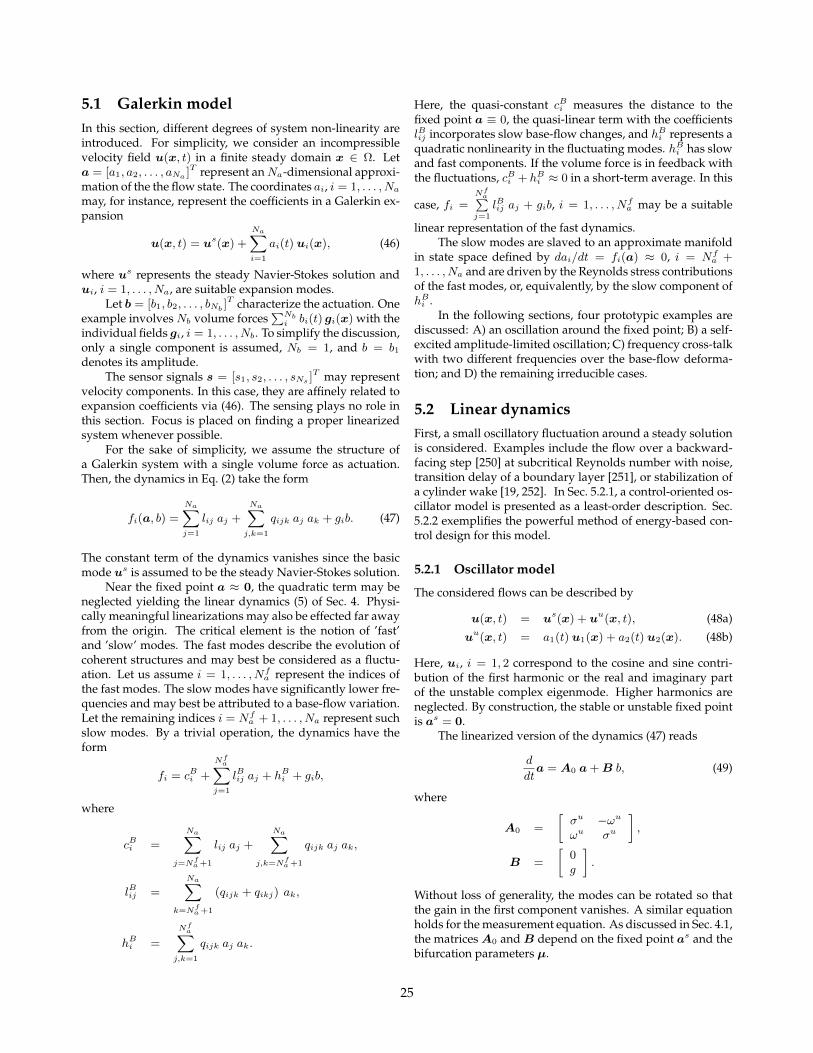
5.1 Galerkin modelIn this section, different degrees of system non-linearity areintroduced. For simplicity, we consider an incompressiblevelocity field u(x, t) in a finite steady domain x ∈ Ω. Leta = [a1, a2, . . . , aNa ]T represent anNa-dimensional approxi-mation of the the flow state. The coordinates ai, i = 1, . . . , Namay, for instance, represent the coefficients in a Galerkin ex-pansion

u(x, t) = us(x) +

Na∑

i=1

ai(t) ui(x), (46)

where us represents the steady Navier-Stokes solution andui, i = 1, . . . , Na, are suitable expansion modes.

Let b = [b1, b2, . . . , bNb ]T characterize the actuation. Oneexample involves Nb volume forces

∑Nbi bi(t) gi(x) with the

individual fields gi, i = 1, . . . , Nb. To simplify the discussion,only a single component is assumed, Nb = 1, and b = b1denotes its amplitude.

The sensor signals s = [s1, s2, . . . , sNs ]T may representvelocity components. In this case, they are affinely related toexpansion coefficients via (46). The sensing plays no role inthis section. Focus is placed on finding a proper linearizedsystem whenever possible.

For the sake of simplicity, we assume the structure ofa Galerkin system with a single volume force as actuation.Then, the dynamics in Eq. (2) take the form

fi(a, b) =

Na∑

j=1

lij aj +

Na∑

j,k=1

qijk aj ak + gib. (47)

The constant term of the dynamics vanishes since the basicmode us is assumed to be the steady Navier-Stokes solution.

Near the fixed point a ≈ 0, the quadratic term may beneglected yielding the linear dynamics (5) of Sec. 4. Physi-cally meaningful linearizations may also be effected far awayfrom the origin. The critical element is the notion of ’fast’and ’slow’ modes. The fast modes describe the evolution ofcoherent structures and may best be considered as a fluctu-ation. Let us assume i = 1, . . . , Nf

a represent the indices ofthe fast modes. The slow modes have significantly lower fre-quencies and may best be attributed to a base-flow variation.Let the remaining indices i = Nf

a + 1, . . . , Na represent suchslow modes. By a trivial operation, the dynamics have theform

fi = cBi +

Nfa∑

j=1

lBij aj + hBi + gib,

where

cBi =

Na∑

j=Nfa +1

lij aj +

Na∑

j,k=Nfa +1

qijk aj ak,

lBij =

Na∑

k=Nfa +1

(qijk + qikj) ak,

hBi =

Nfa∑

j,k=1

qijk aj ak.

Here, the quasi-constant cBi measures the distance to thefixed point a ≡ 0, the quasi-linear term with the coefficientslBij incorporates slow base-flow changes, and hBi represents aquadratic nonlinearity in the fluctuating modes. hBi has slowand fast components. If the volume force is in feedback withthe fluctuations, cBi + hBi ≈ 0 in a short-term average. In this

case, fi =Nf

a∑j=1

lBij aj + gib, i = 1, . . . , Nfa may be a suitable

linear representation of the fast dynamics.The slow modes are slaved to an approximate manifold

in state space defined by dai/dt = fi(a) ≈ 0, i = Nfa +

1, . . . , Na and are driven by the Reynolds stress contributionsof the fast modes, or, equivalently, by the slow component ofhBi .

In the following sections, four prototypic examples arediscussed: A) an oscillation around the fixed point; B) a self-excited amplitude-limited oscillation; C) frequency cross-talkwith two different frequencies over the base-flow deforma-tion; and D) the remaining irreducible cases.

5.2 Linear dynamicsFirst, a small oscillatory fluctuation around a steady solutionis considered. Examples include the flow over a backward-facing step [250] at subcritical Reynolds number with noise,transition delay of a boundary layer [251], or stabilization ofa cylinder wake [19, 252]. In Sec. 5.2.1, a control-oriented os-cillator model is presented as a least-order description. Sec.5.2.2 exemplifies the powerful method of energy-based con-trol design for this model.

5.2.1 Oscillator model

The considered flows can be described by

u(x, t) = us(x) + uu(x, t), (48a)

uu(x, t) = a1(t) u1(x) + a2(t) u2(x). (48b)

Here, ui, i = 1, 2 correspond to the cosine and sine contri-bution of the first harmonic or the real and imaginary partof the unstable complex eigenmode. Higher harmonics areneglected. By construction, the stable or unstable fixed pointis as = 0.

The linearized version of the dynamics (47) reads

d

dta = A0 a+B b, (49)

where

A0 =

[σu −ωuωu σu

],

B =

[0g

].

Without loss of generality, the modes can be rotated so thatthe gain in the first component vanishes. A similar equationholds for the measurement equation. As discussed in Sec. 4.1,the matricesA0 andB depend on the fixed point as and thebifurcation parameters µ.

25

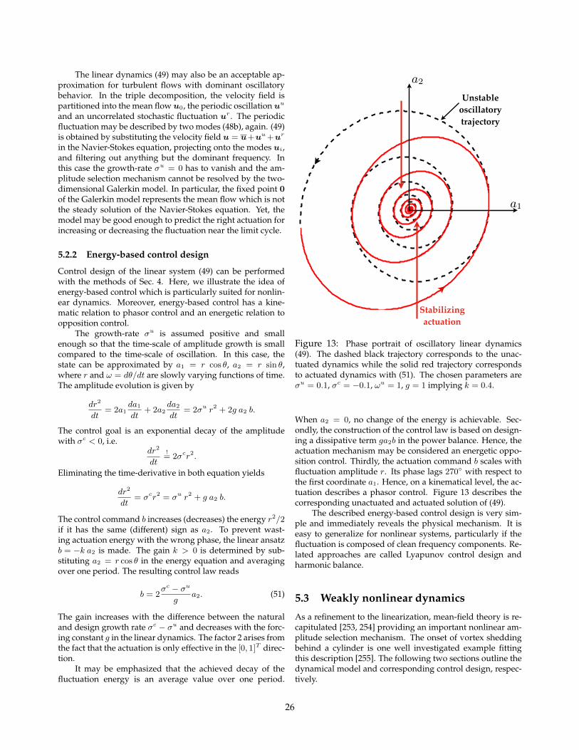
The linear dynamics (49) may also be an acceptable ap-proximation for turbulent flows with dominant oscillatorybehavior. In the triple decomposition, the velocity field ispartitioned into the mean flow u0, the periodic oscillation uu

and an uncorrelated stochastic fluctuation ur . The periodicfluctuation may be described by two modes (48b), again. (49)is obtained by substituting the velocity field u = u+uu+ur

in the Navier-Stokes equation, projecting onto the modes ui,and filtering out anything but the dominant frequency. Inthis case the growth-rate σu = 0 has to vanish and the am-plitude selection mechanism cannot be resolved by the two-dimensional Galerkin model. In particular, the fixed point 0of the Galerkin model represents the mean flow which is notthe steady solution of the Navier-Stokes equation. Yet, themodel may be good enough to predict the right actuation forincreasing or decreasing the fluctuation near the limit cycle.

5.2.2 Energy-based control design

Control design of the linear system (49) can be performedwith the methods of Sec. 4. Here, we illustrate the idea ofenergy-based control which is particularly suited for nonlin-ear dynamics. Moreover, energy-based control has a kine-matic relation to phasor control and an energetic relation toopposition control.

The growth-rate σu is assumed positive and smallenough so that the time-scale of amplitude growth is smallcompared to the time-scale of oscillation. In this case, thestate can be approximated by a1 = r cos θ, a2 = r sin θ,where r and ω = dθ/dt are slowly varying functions of time.The amplitude evolution is given by

dr2

dt= 2a1

da1

dt+ 2a2

da2

dt= 2σu r2 + 2g a2 b.

The control goal is an exponential decay of the amplitudewith σc < 0, i.e.

dr2

dt

!= 2σcr2.

Eliminating the time-derivative in both equation yields

dr2

dt= σcr2 = σu r2 + g a2 b.

The control command b increases (decreases) the energy r2/2if it has the same (different) sign as a2. To prevent wast-ing actuation energy with the wrong phase, the linear ansatzb = −k a2 is made. The gain k > 0 is determined by sub-stituting a2 = r cos θ in the energy equation and averagingover one period. The resulting control law reads

b = 2σc − σu

ga2. (51)

The gain increases with the difference between the naturaland design growth rate σc − σu and decreases with the forc-ing constant g in the linear dynamics. The factor 2 arises fromthe fact that the actuation is only effective in the [0, 1]T direc-tion.

It may be emphasized that the achieved decay of thefluctuation energy is an average value over one period.

a

a1

a

Inertial manifold

Limit cycle3

2

Figure 12: Phase portrait of weakly nonlinear dynam-ics (24).

were

A(a3) = A0 + a3A3

A0 =

u !u

!u u

A3 =

u u

u u

B =

0g

References [58] & [59].

5.4 Moderately nonlinear dynamics

Ansatz:

u(x, t) = us(x) + uu(x, t) + ua(x, t) + u(x, t),(25a)

uu(x, t) = a1(t) u1(x) + a2(t) u2(x), (25b)

ua(x, t) = a3(t) u3(x) + a4(t) u4(x), (25c)

u(x, t) = a5(t) u5(x) + a6(t) u6(x). (25d)

Evolution equation:

d

dt

0BB@

a1

a2

a3

a4

1CCA = A(a5, a6)

0BB@

a1

a2

a3

a4

1CCA + Bb (26a)

a5 = cu a21 + a2

2

(26b)

a6 = ca a23 + a2

4

(26c)

where

A(a5, a6) = A0 + a5A5 + a6A6

A0 =

0BB@

u !u 0 0!u u 0 00 0 a !a

0 0 !u u

1CCA

A5 =

0BB@

uu uu 0 0uu uu 0 00 0 au au

0 0 au au

1CCA

A6 =

0BB@

ua ua 0 0ua ua 0 00 0 aa aa

0 0 aa aa

1CCA

B =

0BB@

000g

1CCA

These may be described by a linear parameter varying sys-tem (LPV). Like weakly nonlinear dynamics, but now the fre-quency cross talk is key to the control goal. A prominent ex-ample is high-frequency forcing to mitigate vortex shedding.

A11 = u uucu a21 + a2

2

uaca a2

3 + a24

(28)

Reference: [60], [36, 61].

5.5 Strongly nonlinear dynamicsA simple version of strongly nonlinear dynamics is describedby (??), but with

A = A0 +NX

i=1

ai Ai. (29)

Now, the quadratic nonlinear gives rise to an energy cascade,i.e. non-trivial frequency cross talk.

This classification is based on a spectrum of periodicprocesses (clock-works). There exist an analogue classifica-tion for event-based control.

• Turbulent jet-noise control [62].

5.6 Implications for control

12

a

a1

a

Inertial manifold

Limit cycle3

2


were

A(a3) = A0 + a3A3

A0 =

u !u

!u u

A3 =

u u

u u

B =

0g



Ansatz:


uu(x, t) = a1(t) u1(x) + a2(t) u2(x), (25b)

ua(x, t) = a3(t) u3(x) + a4(t) u4(x), (25c)

u(x, t) = a5(t) u5(x) + a6(t) u6(x). (25d)

Evolution equation:

d

dt

0BB@

a1

a2

a3

a4

1CCA = A(a5, a6)

0BB@

a1

a2

a3

a4

1CCA + Bb (26a)

a5 = cu a21 + a2

2

(26b)

a6 = ca a23 + a2

4

(26c)

where

A(a5, a6) = A0 + a5A5 + a6A6

A0 =

0BB@

u !u 0 0!u u 0 00 0 a !a

0 0 !u u

1CCA

A5 =

0BB@


0 0 au au

1CCA

A6 =

0BB@


0 0 aa aa

1CCA

B =

0BB@

000g

1CCA


A11 = u uucu a21 + a2

2

uaca a2

3 + a24

(28)

Reference: [60], [36, 61].


A = A0 +NX

i=1

ai Ai. (29)





12

Unstable oscillatory trajectory

Stabilizing actuation

Figure 13: Phase portrait of oscillatory linear dynamics(49). The dashed black trajectory corresponds to the unac-tuated dynamics while the solid red trajectory correspondsto actuated dynamics with (51). The chosen parameters areσu = 0.1, σc = −0.1, ωu = 1, g = 1 implying k = 0.4.

When a2 = 0, no change of the energy is achievable. Sec-ondly, the construction of the control law is based on design-ing a dissipative term ga2b in the power balance. Hence, theactuation mechanism may be considered an energetic oppo-sition control. Thirdly, the actuation command b scales withfluctuation amplitude r. Its phase lags 270 with respect tothe first coordinate a1. Hence, on a kinematical level, the ac-tuation describes a phasor control. Figure 13 describes thecorresponding unactuated and actuated solution of (49).

The described energy-based control design is very sim-ple and immediately reveals the physical mechanism. It iseasy to generalize for nonlinear systems, particularly if thefluctuation is composed of clean frequency components. Re-lated approaches are called Lyapunov control design andharmonic balance.

5.3 Weakly nonlinear dynamics

As a refinement to the linearization, mean-field theory is re-capitulated [253, 254] providing an important nonlinear am-plitude selection mechanism. The onset of vortex sheddingbehind a cylinder is one well investigated example fittingthis description [255]. The following two sections outline thedynamical model and corresponding control design, respec-tively.

26

5.3.1 Mean-field model

Qualitatively, mean-field theory describes the feedbackmechanism between the fluctuations and the base flow. Thefluctuation gives rise to a Reynolds stress which changes thebase flow. The base-flow deformation generally reduces theproduction of fluctuation energy with increasing fluctuationlevel until an equilibrium is reached. The resulting evolutionequations are also referred to as weakly nonlinear dynamics,as they describe a mild form of nonlinearity.

The fluctuation has the same representation as inSec. 5.2. However, the base flow is allowed to vary by an-other mode u3, called the 0-th, base-deformation or shiftmode. This mode can be derived from the (linearized)Reynolds equation and it is assumed to be slaved to the fluc-tuation level. The resulting velocity field ansatz reads

u(x, t) = us(x) + uu(x, t) + u∆(x, t), (52a)

uu(x, t) = a1(t) u1(x) + a2(t) u2(x), (52b)

u∆(x, t) = a3(t) u3(x). (52c)

The evolution equation is given by

d

dt

[a1

a2

]= A(a3)

[a1

a2

]+B b (53a)

a3 = αu(a2

1 + a22

), (53b)

where

A(a3) = A0 + a3A3,

A0 =

[σu −ωuωu σu

],

A3 =

[−βu −γuγu −βu

],

B =

[0g

].

Without loss of generality, αu > 0. Otherwise, the sign of themodeu3 must be changed. A nonlinear amplitude saturationrequires the Landau constant to be positive βu > 0.

For a3 ≡ 0, (53) is equivalent to (49). However, (53) hasa globally stable limit cycle with radius r∞ =

√σu/αuβu in

the plane a3 = a∞3 = σu/βu, and with center [0, 0, a∞3 ].In the framework of weakly nonlinear stability the-

ory, the growth-rate is considered a linear function of theReynolds number σu = κ(Re−Rec), whereRec correspondsto its critical value. The other parameters are considered tobe constant. This yields the famous Landau equation forthe amplitude dr/dt = σur − βr3, β = αuβu and a corre-sponding equation for the frequency. In particular, the Lan-dau equation explains the famous square-root amplitude lawr ∝

√Re−Rec for supercritical Reynolds numbers assum-

ing a soft bifurcation. We refer to the literature for a discus-sion of the hard subcritical bifurcation with quintic nonlin-earity [254].

Mean-field theory explains the stabilizing feedbackmechanism between the harmonic oscillatory structure andthe mean-field deformation. A refined weakly nonlinear ex-pansion also takes higher harmonics into account. The first

harmonic, via the quadratic Navier-Stokes term, generatesnot only a mean-flow deformation but also a second har-monic which changes, in turn, the mean flow. The nonlin-ear interaction of the first and second harmonics produces athird harmonic, etc. Dusek et al. [256] derive a correspondingharmonic expansion from the Navier-Stokes equation in theneighborhood of a supercritical Hopf bifurcation. Let ε > 0be the small amplitude of the first harmonic, then n-th har-monics are shown to scale in geometric progression i.e. withεn. Hence, higher harmonics may be neglected near the onsetof fluctuations. Even for periodic flow far beyond the onset,the second harmonic is observed to be one order of magni-tude smaller than the corresponding harmonic component.A similar observation holds for turbulent flow with domi-nant periodicity.

Intriguingly, even turbulent flows with dominant peri-odic coherent structures may be described by (53). One ex-ample is the wake behind a finite cylinder [257]. In this case,the rationale is the velocity decomposition with an added un-correlated stochastic fluctuationur : u = us+a3u3+uu+ur .In this case, (53) remains valid ifur scales with the oscillatoryfluctuation level and the base flow deformation is slaved tothis level as well.

5.3.2 Nonlinear control design

The mean-field model and variants thereof have been suc-cessfully used for the model-based stabilization of the cylin-der wake at Re = 100 [44, 258, 259]. In these studies, anenergy based control design as discussed in Sec. 5.2 has beenused to prescribe a fixed decay rate of the model. Figure 14illustrates an unactuated and actuated transient.

It may be noted that (53) can be considered a linear pa-rameter varying (LPV) model with the shift-mode amplitudea3, or, equivalently, with the fluctuation level r2 as the pa-rameter. Thus, the linear control design of Sec. 4 is immedi-ately applicable for the linear system corresponding to the ac-tual value of this parameter. King et al. [260] elaborate othernonlinear control design techniques for the mean-field modelemploying input-output-linearization, Lyapunov-based syn-thesis and backstepping. The mean-field model has also beenthe basis for optimal control of the Navier-Stokes equation[261], using the simulation to improve the model and themodel as a surrogate plant for control design.

5.4 Moderately nonlinear dynamicsSome oscillatory flows may be tamed by direct mitigationwith models and methods described in the previous section.Not all plants, particularly turbulent flows, have the actu-ation authority for such a stabilization. However, periodicforcing at high frequency has mitigated periodic oscillationsin a number of experiments. Examples are the wake stabiliza-tion with a oscillatory cylinder rotation [74], suppression ofKelvin-Helmholtz vortices in transitional shear layers [262],reduction of the separation zone in a high-lift configuration[48], and elongation of the dead-water region behind a back-ward facing step [47]. Also a periodic frequency at 60–70%of the dominant shedding frequency may substantially delay

27

Limit cycle

Inertial manifold

a

a1

a

Inertial manifold

Limit cycle3

2


were

A(a3) = A0 + a3A3

A0 =

u !u

!u u

A3 =

u u

u u

B =

0g



Ansatz:


uu(x, t) = a1(t) u1(x) + a2(t) u2(x), (25b)

ua(x, t) = a3(t) u3(x) + a4(t) u4(x), (25c)

u(x, t) = a5(t) u5(x) + a6(t) u6(x). (25d)

Evolution equation:

d

dt

0BB@

a1

a2

a3

a4

1CCA = A(a5, a6)

0BB@

a1

a2

a3

a4

1CCA + Bb (26a)

a5 = cu a21 + a2

2

(26b)

a6 = ca a23 + a2

4

(26c)

where

A(a5, a6) = A0 + a5A5 + a6A6

A0 =

0BB@

u !u 0 0!u u 0 00 0 a !a

0 0 !u u

1CCA

A5 =

0BB@


0 0 au au

1CCA

A6 =

0BB@


0 0 aa aa

1CCA

B =

0BB@

000g

1CCA


A11 = u uucu a21 + a2

2

uaca a2

3 + a24

(28)

Reference: [60], [36, 61].


A = A0 +

NX

i=1

ai Ai. (29)





12

a

a1

a

Inertial manifold

Limit cycle3

2


were

A(a3) = A0 + a3A3

A0 =

u !u

!u u

A3 =

u u

u u

B =

0g



Ansatz:


uu(x, t) = a1(t) u1(x) + a2(t) u2(x), (25b)

ua(x, t) = a3(t) u3(x) + a4(t) u4(x), (25c)

u(x, t) = a5(t) u5(x) + a6(t) u6(x). (25d)

Evolution equation:

d

dt

0BB@

a1

a2

a3

a4

1CCA = A(a5, a6)

0BB@

a1

a2

a3

a4

1CCA + Bb (26a)

a5 = cu a21 + a2

2

(26b)

a6 = ca a23 + a2

4

(26c)

where

A(a5, a6) = A0 + a5A5 + a6A6

A0 =

0BB@

u !u 0 0!u u 0 00 0 a !a

0 0 !u u

1CCA

A5 =

0BB@


0 0 au au

1CCA

A6 =

0BB@


0 0 aa aa

1CCA

B =

0BB@

000g

1CCA


A11 = u uucu a21 + a2

2

uaca a2

3 + a24

(28)

Reference: [60], [36, 61].


A = A0 +NX

i=1

ai Ai. (29)





12

a

a1

a

Inertial manifold

Limit cycle3

2


were

A(a3) = A0 + a3A3

A0 =

u !u

!u u

A3 =

u u

u u

B =

0g



Ansatz:


uu(x, t) = a1(t) u1(x) + a2(t) u2(x), (25b)

ua(x, t) = a3(t) u3(x) + a4(t) u4(x), (25c)

u(x, t) = a5(t) u5(x) + a6(t) u6(x). (25d)

Evolution equation:

d

dt

0BB@

a1

a2

a3

a4

1CCA = A(a5, a6)

0BB@

a1

a2

a3

a4

1CCA + Bb (26a)

a5 = cu a21 + a2

2

(26b)

a6 = ca a23 + a2

4

(26c)

where

A(a5, a6) = A0 + a5A5 + a6A6

A0 =

0BB@

u !u 0 0!u u 0 00 0 a !a

0 0 !u u

1CCA

A5 =

0BB@


0 0 au au

1CCA

A6 =

0BB@


0 0 aa aa

1CCA

B =

0BB@

000g

1CCA


A11 = u uucu a21 + a2

2

uaca a2

3 + a24

(28)

Reference: [60], [36, 61].


A = A0 +NX

i=1

ai Ai. (29)





12

Figure 14: Phase portrait of weakly nonlinear dynamics.The dashed black trajectory corresponds to the unactuateddynamics while the solid red trajectory corresponds to actu-ated dynamics. The chosen parameters of (53) are σu = 0.1,ωu = 1, αu = 1, βu = 1, γu = 0 and the forced decayrate σc = −0.1. The globally stable limit cycle lies on theparabolic inertial manifold, shown in gray.

the vortex formation in wall-bounded shear-layers [49] andD-shaped cylinders [45]. The following two sections outlinea corresponding modeling and control strategy.

5.4.1 Generalized mean-field model

Here, a generalized mean-field model for such frequency-cross talk phenomena is reviewed from [48]. Let uu denotethe natural self-amplified oscillation represented by two os-cillatory modes u1, u2. Analogously, the actuated oscillatoryfluctuation ua is described by two modes u3, u4. The base-flow deformation due to the unstable natural frequency ωu

and stable actuation frequency ωa is described by the shift-modes u5 and u6 respectively. The resulting velocity decom-position reads

u(x, t) = us(x) + u∆(x, t)

+uu(x, t) + ua(x, t), (54a)

uu(x, t) = a1(t) u1(x) + a2(t) u2(x), (54b)

ua(x, t) = a3(t) u3(x) + a4(t) u4(x), (54c)

u∆(x, t) = a5(t) u5(x) + a6(t) u6(x). (54d)

Generalized mean-field arguments yield the following

evolution equation:

d

dt

a1

a2

a3

a4

= A(a5, a6)

a1

a2

a3

a4

+B b, (55a)

a5 = αu(a2

1 + a22

), (55b)

a6 = αa(a2

3 + a24

), (55c)

where

A(a5, a6) = A0 + a5A5 + a6A6,

A0 =

σu −ωu 0 0ωu σu 0 00 0 σa −ωa0 0 ωu σu

,

A5 =

−βuu −γuu 0 0γuu −βuu 0 00 0 −βau −γau0 0 γau −βau

,

A6 =

−βua −γua 0 0γua −βua 0 00 0 −βaa −γaa0 0 γaa −βaa

,

B =

000g

.

It should be noted that a vanishing actuation impliesa3 = a4 = a6 = 0 and yields the mean-field model of (53)modulo index numbering. In the sequel, we assume thatthe fixed point is unstable (σu > 0) and the limit cycle isstable (βuu > 0). Similarly, a vanishing natural fluctuationa1 = a2 = a5 yields another mean-field model, again mod-ulo index numbering. In the sequel, we assume that the ac-tuated structures vanish after the end of actuation, implyingσaa < 0 and βaa > 0 in the model.

An interesting aspect of (55) is the frequency cross-talk.The effective growth-rate for the natural oscillation reads

A11 = σu − βuuαu(a2

1 + a22

)− βuaαa

(a2

3 + a24

). (57)

The forcing stabilizes the natural instability if and only ifβua > 0. Complete stabilization implies A11 ≤ 0. From(57), such complete stabilization is achieved with a thresholdfluctuation level at the forcing frequency

a23 + a2

4 ≥σu

αaβua.

Thus, increasing the forcing at higher or lower frequency candecrease the natural frequency.

The generalized mean-field model has been fitted to nu-merical URANS simulation data of a high-lift configuration[48] with high-frequency forcing. This model also accuratelydescribes the experimental turbulent wake data with a stabi-lizing low-frequency forcing [263] as shown in Fig. 15.

28

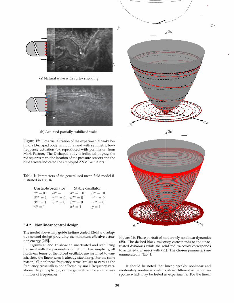
(a) Natural wake with vortex shedding

(b) Actuated partially stabilized wake

Figure 15: Flow visualization of the experimental wake be-hind a D-shaped body without (a) and with symmetric low-frequency actuation (b), reproduced with permission fromMark Pastoor. The D-shaped body is indicated in gray, thered squares mark the location of the pressure sensors and theblue arrows indicated the employed ZNMF actuators.

Table 1: Parameters of the generalized mean-field model il-lustrated in Fig. 16.

Unstable oscillator Stable oscillatorσu = 0.1 ωu = 1 σa = −0.1 ωa = 10βuu = 1 γuu = 0 βau = 0 γau = 0βua = 1 γua = 0 βaa = 0 γaa = 0αu = 1 αa = 1 g = 1


The model above may guide in-time control [264] and adap-tive control design providing the minimum effective actua-tion energy [265].

Figures 16 and 17 show an unactuated and stabilizingtransient with the parameters of Tab. 1. For simplicity, allnonlinear terms of the forced oscillator are assumed to van-ish, since the linear term is already stabilizing. For the samereason, all nonlinear frequency terms are set to zero as thefrequency cross-talk is not affected by small frequency vari-ations. In principle, (55) can be generalized for an arbitrarynumber of frequencies.

a

a1

a

Inertial manifold

Limit cycle3

2


were

A(a3) = A0 + a3A3

A0 =

u !u

!u u

A3 =

u u

u u

B =

0g



Ansatz:


uu(x, t) = a1(t) u1(x) + a2(t) u2(x), (25b)

ua(x, t) = a3(t) u3(x) + a4(t) u4(x), (25c)

u(x, t) = a5(t) u5(x) + a6(t) u6(x). (25d)

Evolution equation:

d

dt

0BB@

a1

a2

a3

a4

1CCA = A(a5, a6)

0BB@

a1

a2

a3

a4

1CCA + Bb (26a)

a5 = cu a21 + a2

2

(26b)

a6 = ca a23 + a2

4

(26c)

where

A(a5, a6) = A0 + a5A5 + a6A6

A0 =

0BB@

u !u 0 0!u u 0 00 0 a !a

0 0 !u u

1CCA

A5 =

0BB@


0 0 au au

1CCA

A6 =

0BB@


0 0 aa aa

1CCA

B =

0BB@

000g

1CCA


A11 = u uucu a21 + a2

2

uaca a2

3 + a24

(28)

Reference: [60], [36, 61].


A = A0 +NX

i=1

ai Ai. (29)





12

a

a1

a

Inertial manifold

Limit cycle3

2


were

A(a3) = A0 + a3A3

A0 =

u !u

!u u

A3 =

u u

u u

B =

0g



Ansatz:


uu(x, t) = a1(t) u1(x) + a2(t) u2(x), (25b)

ua(x, t) = a3(t) u3(x) + a4(t) u4(x), (25c)

u(x, t) = a5(t) u5(x) + a6(t) u6(x). (25d)

Evolution equation:

d

dt

0BB@

a1

a2

a3

a4

1CCA = A(a5, a6)

0BB@

a1

a2

a3

a4

1CCA + Bb (26a)

a5 = cu a21 + a2

2

(26b)

a6 = ca a23 + a2

4

(26c)

where

A(a5, a6) = A0 + a5A5 + a6A6

A0 =

0BB@

u !u 0 0!u u 0 00 0 a !a

0 0 !u u

1CCA

A5 =

0BB@


0 0 au au

1CCA

A6 =

0BB@


0 0 aa aa

1CCA

B =

0BB@

000g

1CCA


A11 = u uucu a21 + a2

2

uaca a2

3 + a24

(28)

Reference: [60], [36, 61].


A = A0 +NX

i=1

ai Ai. (29)





12

Limit cycle

Inertial manifold

a

a1

a

Inertial manifold

Limit cycle3

2


were

A(a3) = A0 + a3A3

A0 =

u !u

!u u

A3 =

u u

u u

B =

0g



Ansatz:


uu(x, t) = a1(t) u1(x) + a2(t) u2(x), (25b)

ua(x, t) = a3(t) u3(x) + a4(t) u4(x), (25c)

u(x, t) = a5(t) u5(x) + a6(t) u6(x). (25d)

Evolution equation:

d

dt

0BB@

a1

a2

a3

a4

1CCA = A(a5, a6)

0BB@

a1

a2

a3

a4

1CCA + Bb (26a)

a5 = cu a21 + a2

2

(26b)

a6 = ca a23 + a2

4

(26c)

where

A(a5, a6) = A0 + a5A5 + a6A6

A0 =

0BB@

u !u 0 0!u u 0 00 0 a !a

0 0 !u u

1CCA

A5 =

0BB@


0 0 au au

1CCA

A6 =

0BB@


0 0 aa aa

1CCA

B =

0BB@

000g

1CCA


A11 = u uucu a21 + a2

2

uaca a2

3 + a24

(28)

Reference: [60], [36, 61].


A = A0 +NX

i=1

ai Ai. (29)





12

a

a1

a

Inertial manifold

Limit cycle3

2


were

A(a3) = A0 + a3A3

A0 =

u !u

!u u

A3 =

u u

u u

B =

0g



Ansatz:


uu(x, t) = a1(t) u1(x) + a2(t) u2(x), (25b)

ua(x, t) = a3(t) u3(x) + a4(t) u4(x), (25c)

u(x, t) = a5(t) u5(x) + a6(t) u6(x). (25d)

Evolution equation:

d

dt

0BB@

a1

a2

a3

a4

1CCA = A(a5, a6)

0BB@

a1

a2

a3

a4

1CCA + Bb (26a)

a5 = cu a21 + a2

2

(26b)

a6 = ca a23 + a2

4

(26c)

where

A(a5, a6) = A0 + a5A5 + a6A6

A0 =

0BB@

u !u 0 0!u u 0 00 0 a !a

0 0 !u u

1CCA

A5 =

0BB@


0 0 au au

1CCA

A6 =

0BB@


0 0 aa aa

1CCA

B =

0BB@

000g

1CCA


A11 = u uucu a21 + a2

2

uaca a2

3 + a24

(28)

Reference: [60], [36, 61].


A = A0 +NX

i=1

ai Ai. (29)





12

a

a1

a

Inertial manifold

Limit cycle3

2


were

A(a3) = A0 + a3A3

A0 =

u !u

!u u

A3 =

u u

u u

B =

0g



Ansatz:


uu(x, t) = a1(t) u1(x) + a2(t) u2(x), (25b)

ua(x, t) = a3(t) u3(x) + a4(t) u4(x), (25c)

u(x, t) = a5(t) u5(x) + a6(t) u6(x). (25d)

Evolution equation:

d

dt

0BB@

a1

a2

a3

a4

1CCA = A(a5, a6)

0BB@

a1

a2

a3

a4

1CCA + Bb (26a)

a5 = cu a21 + a2

2

(26b)

a6 = ca a23 + a2

4

(26c)

where

A(a5, a6) = A0 + a5A5 + a6A6

A0 =

0BB@

u !u 0 0!u u 0 00 0 a !a

0 0 !u u

1CCA

A5 =

0BB@


0 0 au au

1CCA

A6 =

0BB@


0 0 aa aa

1CCA

B =

0BB@

000g

1CCA


A11 = u uucu a21 + a2

2

uaca a2

3 + a24

(28)

Reference: [60], [36, 61].


A = A0 +NX

i=1

ai Ai. (29)





12


were

A(a3) = A0 + a3A3

A0 =

u !u

!u u

A3 =

u u

u u

B =

0g


5.4 Moderately nonlinear dynamicsAnsatz:


uu(x, t) = a1(t) u1(x) + a2(t) u2(x), (25b)

ua(x, t) = a3(t) u3(x) + a4(t) u4(x), (25c)

u(x, t) = a5(t) u5(x) + a6(t) u6(x). (25d)

Evolution equation:

d

dt

0BB@

a1

a2

a3

a4

1CCA = A(a5, a6)

0BB@

a1

a2

a3

a4

1CCA + Bb (26a)

a5 = cu a21 + a2

2

(26b)

a6 = ca a23 + a2

4

(26c)

where

A(a5, a6) = A0 + a5A5 + a6A6

A0 =

0BB@

u !u 0 0!u u 0 00 0 a !a

0 0 !u u

1CCA

A5 =

0BB@


0 0 au au

1CCA

A6 =

0BB@


0 0 aa aa

1CCA

B =

0BB@

000g

1CCA


A11 = u uucu a21 + a2

2

uaca a2

3 + a24

(28)

Reference: [60], [36, 61].


A = A0 +NX

i=1

ai Ai. (29)





12

Limit cycle

Inertial manifold

a

a1

a

Inertial manifold

Limit cycle3

2


were

A(a3) = A0 + a3A3

A0 =

u !u

!u u

A3 =

u u

u u

B =

0g



Ansatz:


uu(x, t) = a1(t) u1(x) + a2(t) u2(x), (25b)

ua(x, t) = a3(t) u3(x) + a4(t) u4(x), (25c)

u(x, t) = a5(t) u5(x) + a6(t) u6(x). (25d)

Evolution equation:

d

dt

0BB@

a1

a2

a3

a4

1CCA = A(a5, a6)

0BB@

a1

a2

a3

a4

1CCA + Bb (26a)

a5 = cu a21 + a2

2

(26b)

a6 = ca a23 + a2

4

(26c)

where

A(a5, a6) = A0 + a5A5 + a6A6

A0 =

0BB@

u !u 0 0!u u 0 00 0 a !a

0 0 !u u

1CCA

A5 =

0BB@


0 0 au au

1CCA

A6 =

0BB@


0 0 aa aa

1CCA

B =

0BB@

000g

1CCA


A11 = u uucu a21 + a2

2

uaca a2

3 + a24

(28)

Reference: [60], [36, 61].


A = A0 +NX

i=1

ai Ai. (29)





12

a

a1

a

Inertial manifold

Limit cycle3

2


were

A(a3) = A0 + a3A3

A0 =

u !u

!u u

A3 =

u u

u u

B =

0g



Ansatz:


uu(x, t) = a1(t) u1(x) + a2(t) u2(x), (25b)

ua(x, t) = a3(t) u3(x) + a4(t) u4(x), (25c)

u(x, t) = a5(t) u5(x) + a6(t) u6(x). (25d)

Evolution equation:

d

dt

0BB@

a1

a2

a3

a4

1CCA = A(a5, a6)

0BB@

a1

a2

a3

a4

1CCA + Bb (26a)

a5 = cu a21 + a2

2

(26b)

a6 = ca a23 + a2

4

(26c)

where

A(a5, a6) = A0 + a5A5 + a6A6

A0 =

0BB@

u !u 0 0!u u 0 00 0 a !a

0 0 !u u

1CCA

A5 =

0BB@


0 0 au au

1CCA

A6 =

0BB@


0 0 aa aa

1CCA

B =

0BB@

000g

1CCA


A11 = u uucu a21 + a2

2

uaca a2

3 + a24

(28)

Reference: [60], [36, 61].


A = A0 +NX

i=1

ai Ai. (29)





12

a

a1

a

Inertial manifold

Limit cycle3

2


were

A(a3) = A0 + a3A3

A0 =

u !u

!u u

A3 =

u u

u u

B =

0g



Ansatz:


uu(x, t) = a1(t) u1(x) + a2(t) u2(x), (25b)

ua(x, t) = a3(t) u3(x) + a4(t) u4(x), (25c)

u(x, t) = a5(t) u5(x) + a6(t) u6(x). (25d)

Evolution equation:

d

dt

0BB@

a1

a2

a3

a4

1CCA = A(a5, a6)

0BB@

a1

a2

a3

a4

1CCA + Bb (26a)

a5 = cu a21 + a2

2

(26b)

a6 = ca a23 + a2

4

(26c)

where

A(a5, a6) = A0 + a5A5 + a6A6

A0 =

0BB@

u !u 0 0!u u 0 00 0 a !a

0 0 !u u

1CCA

A5 =

0BB@


0 0 au au

1CCA

A6 =

0BB@


0 0 aa aa

1CCA

B =

0BB@

000g

1CCA


A11 = u uucu a21 + a2

2

uaca a2

3 + a24

(28)

Reference: [60], [36, 61].


A = A0 +NX

i=1

ai Ai. (29)





12


were

A(a3) = A0 + a3A3

A0 =

u !u

!u u

A3 =

u u

u u

B =

0g




uu(x, t) = a1(t) u1(x) + a2(t) u2(x), (25b)

ua(x, t) = a3(t) u3(x) + a4(t) u4(x), (25c)

u(x, t) = a5(t) u5(x) + a6(t) u6(x). (25d)

Evolution equation:

d

dt

0BB@

a1

a2

a3

a4

1CCA = A(a5, a6)

0BB@

a1

a2

a3

a4

1CCA + Bb (26a)

a5 = cu a21 + a2

2

(26b)

a6 = ca a23 + a2

4

(26c)

where

A(a5, a6) = A0 + a5A5 + a6A6

A0 =

0BB@

u !u 0 0!u u 0 00 0 a !a

0 0 !u u

1CCA

A5 =

0BB@


0 0 au au

1CCA

A6 =

0BB@


0 0 aa aa

1CCA

B =

0BB@

000g

1CCA


A11 = u uucu a21 + a2

2

uaca a2

3 + a24

(28)

Reference: [60], [36, 61].


A = A0 +NX

i=1

ai Ai. (29)





12

Limit cycle

Inertial manifold

a

a1

a

Inertial manifold

Limit cycle3

2


were

A(a3) = A0 + a3A3

A0 =

u !u

!u u

A3 =

u u

u u

B =

0g



Ansatz:


uu(x, t) = a1(t) u1(x) + a2(t) u2(x), (25b)

ua(x, t) = a3(t) u3(x) + a4(t) u4(x), (25c)

u(x, t) = a5(t) u5(x) + a6(t) u6(x). (25d)

Evolution equation:

d

dt

0BB@

a1

a2

a3

a4

1CCA = A(a5, a6)

0BB@

a1

a2

a3

a4

1CCA + Bb (26a)

a5 = cu a21 + a2

2

(26b)

a6 = ca a23 + a2

4

(26c)

where

A(a5, a6) = A0 + a5A5 + a6A6

A0 =

0BB@

u !u 0 0!u u 0 00 0 a !a

0 0 !u u

1CCA

A5 =

0BB@


0 0 au au

1CCA

A6 =

0BB@


0 0 aa aa

1CCA

B =

0BB@

000g

1CCA


A11 = u uucu a21 + a2

2

uaca a2

3 + a24

(28)

Reference: [60], [36, 61].


A = A0 +NX

i=1

ai Ai. (29)





12

a

a1

a

Inertial manifold

Limit cycle3

2


were

A(a3) = A0 + a3A3

A0 =

u !u

!u u

A3 =

u u

u u

B =

0g



Ansatz:


uu(x, t) = a1(t) u1(x) + a2(t) u2(x), (25b)

ua(x, t) = a3(t) u3(x) + a4(t) u4(x), (25c)

u(x, t) = a5(t) u5(x) + a6(t) u6(x). (25d)

Evolution equation:

d

dt

0BB@

a1

a2

a3

a4

1CCA = A(a5, a6)

0BB@

a1

a2

a3

a4

1CCA + Bb (26a)

a5 = cu a21 + a2

2

(26b)

a6 = ca a23 + a2

4

(26c)

where

A(a5, a6) = A0 + a5A5 + a6A6

A0 =

0BB@

u !u 0 0!u u 0 00 0 a !a

0 0 !u u

1CCA

A5 =

0BB@


0 0 au au

1CCA

A6 =

0BB@


0 0 aa aa

1CCA

B =

0BB@

000g

1CCA


A11 = u uucu a21 + a2

2

uaca a2

3 + a24

(28)

Reference: [60], [36, 61].


A = A0 +NX

i=1

ai Ai. (29)





12

a

a1

a

Inertial manifold

Limit cycle3

2


were

A(a3) = A0 + a3A3

A0 =

u !u

!u u

A3 =

u u

u u

B =

0g



Ansatz:


uu(x, t) = a1(t) u1(x) + a2(t) u2(x), (25b)

ua(x, t) = a3(t) u3(x) + a4(t) u4(x), (25c)

u(x, t) = a5(t) u5(x) + a6(t) u6(x). (25d)

Evolution equation:

d

dt

0BB@

a1

a2

a3

a4

1CCA = A(a5, a6)

0BB@

a1

a2

a3

a4

1CCA + Bb (26a)

a5 = cu a21 + a2

2

(26b)

a6 = ca a23 + a2

4

(26c)

where

A(a5, a6) = A0 + a5A5 + a6A6

A0 =

0BB@

u !u 0 0!u u 0 00 0 a !a

0 0 !u u

1CCA

A5 =

0BB@


0 0 au au

1CCA

A6 =

0BB@


0 0 aa aa

1CCA

B =

0BB@

000g

1CCA


A11 = u uucu a21 + a2

2

uaca a2

3 + a24

(28)

Reference: [60], [36, 61].


A = A0 +NX

i=1

ai Ai. (29)





12


were

A(a3) = A0 + a3A3

A0 =

u !u

!u u

A3 =

u u

u u

B =

0g




uu(x, t) = a1(t) u1(x) + a2(t) u2(x), (25b)

ua(x, t) = a3(t) u3(x) + a4(t) u4(x), (25c)

u(x, t) = a5(t) u5(x) + a6(t) u6(x). (25d)

Evolution equation:

d

dt

0BB@

a1

a2

a3

a4

1CCA = A(a5, a6)

0BB@

a1

a2

a3

a4

1CCA + Bb (26a)

a5 = cu a21 + a2

2

(26b)

a6 = ca a23 + a2

4

(26c)

where

A(a5, a6) = A0 + a5A5 + a6A6

A0 =

0BB@

u !u 0 0!u u 0 00 0 a !a

0 0 !u u

1CCA

A5 =

0BB@


0 0 au au

1CCA

A6 =

0BB@


0 0 aa aa

1CCA

B =

0BB@

000g

1CCA


A11 = u uucu a21 + a2

2

uaca a2

3 + a24

(28)

Reference: [60], [36, 61].


A = A0 +NX

i=1

ai Ai. (29)





12

a

a1

a

Inertial manifold

Limit cycle3

2


were

A(a3) = A0 + a3A3

A0 =

u !u

!u u

A3 =

u u

u u

B =

0g



Ansatz:


uu(x, t) = a1(t) u1(x) + a2(t) u2(x), (25b)

ua(x, t) = a3(t) u3(x) + a4(t) u4(x), (25c)

u(x, t) = a5(t) u5(x) + a6(t) u6(x). (25d)

Evolution equation:

d

dt

0BB@

a1

a2

a3

a4

1CCA = A(a5, a6)

0BB@

a1

a2

a3

a4

1CCA + Bb (26a)

a5 = cu a21 + a2

2

(26b)

a6 = ca a23 + a2

4

(26c)

where

A(a5, a6) = A0 + a5A5 + a6A6

A0 =

0BB@

u !u 0 0!u u 0 00 0 a !a

0 0 !u u

1CCA

A5 =

0BB@


0 0 au au

1CCA

A6 =

0BB@


0 0 aa aa

1CCA

B =

0BB@

000g

1CCA


A11 = u uucu a21 + a2

2

uaca a2

3 + a24

(28)

Reference: [60], [36, 61].


A = A0 +NX

i=1

ai Ai. (29)





12

Figure 16: Phase portrait of moderately nonlinear dynamics(55). The dashed black trajectory corresponds to the unac-tuated dynamics while the solid red trajectory correspondsto actuated dynamics with (51). The chosen parameters areenumerated in Tab. 1.

It should be noted that linear, weakly nonlinear andmoderately nonlinear systems show different actuation re-sponse which may be tested in experiments. For the linear

29

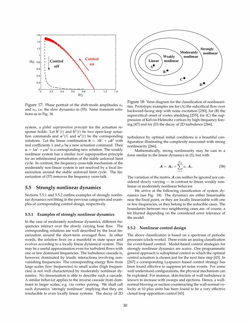
0 0.2 0.4 0.6 0.8 1 1.2 1.40

0.2

0.4

0.6

0.8

1

1.2

1.4

1.6

Limit cycle

Inertial manifold

a

a1

a

Inertial manifold

Limit cycle3

2


were

A(a3) = A0 + a3A3

A0 =

u !u

!u u

A3 =

u u

u u

B =

0g



Ansatz:


uu(x, t) = a1(t) u1(x) + a2(t) u2(x), (25b)

ua(x, t) = a3(t) u3(x) + a4(t) u4(x), (25c)

u(x, t) = a5(t) u5(x) + a6(t) u6(x). (25d)

Evolution equation:

d

dt

0BB@

a1

a2

a3

a4

1CCA = A(a5, a6)

0BB@

a1

a2

a3

a4

1CCA + Bb (26a)

a5 = cu a21 + a2

2

(26b)

a6 = ca a23 + a2

4

(26c)

where

A(a5, a6) = A0 + a5A5 + a6A6

A0 =

0BB@

u !u 0 0!u u 0 00 0 a !a

0 0 !u u

1CCA

A5 =

0BB@


0 0 au au

1CCA

A6 =

0BB@


0 0 aa aa

1CCA

B =

0BB@

000g

1CCA


A11 = u uucu a21 + a2

2

uaca a2

3 + a24

(28)

Reference: [60], [36, 61].


A = A0 +NX

i=1

ai Ai. (29)





12

a

a1

a

Inertial manifold

Limit cycle3

2


were

A(a3) = A0 + a3A3

A0 =

u !u

!u u

A3 =

u u

u u

B =

0g



Ansatz:


uu(x, t) = a1(t) u1(x) + a2(t) u2(x), (25b)

ua(x, t) = a3(t) u3(x) + a4(t) u4(x), (25c)

u(x, t) = a5(t) u5(x) + a6(t) u6(x). (25d)

Evolution equation:

d

dt

0BB@

a1

a2

a3

a4

1CCA = A(a5, a6)

0BB@

a1

a2

a3

a4

1CCA + Bb (26a)

a5 = cu a21 + a2

2

(26b)

a6 = ca a23 + a2

4

(26c)

where

A(a5, a6) = A0 + a5A5 + a6A6

A0 =

0BB@

u !u 0 0!u u 0 00 0 a !a

0 0 !u u

1CCA

A5 =

0BB@


0 0 au au

1CCA

A6 =

0BB@


0 0 aa aa

1CCA

B =

0BB@

000g

1CCA


A11 = u uucu a21 + a2

2

uaca a2

3 + a24

(28)

Reference: [60], [36, 61].


A = A0 +NX

i=1

ai Ai. (29)





12

a

a1

a

Inertial manifold

Limit cycle3

2


were

A(a3) = A0 + a3A3

A0 =

u !u

!u u

A3 =

u u

u u

B =

0g



Ansatz:


uu(x, t) = a1(t) u1(x) + a2(t) u2(x), (25b)

ua(x, t) = a3(t) u3(x) + a4(t) u4(x), (25c)

u(x, t) = a5(t) u5(x) + a6(t) u6(x). (25d)

Evolution equation:

d

dt

0BB@

a1

a2

a3

a4

1CCA = A(a5, a6)

0BB@

a1

a2

a3

a4

1CCA + Bb (26a)

a5 = cu a21 + a2

2

(26b)

a6 = ca a23 + a2

4

(26c)

where

A(a5, a6) = A0 + a5A5 + a6A6

A0 =

0BB@

u !u 0 0!u u 0 00 0 a !a

0 0 !u u

1CCA

A5 =

0BB@


0 0 au au

1CCA

A6 =

0BB@


0 0 aa aa

1CCA

B =

0BB@

000g

1CCA


A11 = u uucu a21 + a2

2

uaca a2

3 + a24

(28)

Reference: [60], [36, 61].


A = A0 +NX

i=1

ai Ai. (29)





12


were

A(a3) = A0 + a3A3

A0 =

u !u

!u u

A3 =

u u

u u

B =

0g




uu(x, t) = a1(t) u1(x) + a2(t) u2(x), (25b)

ua(x, t) = a3(t) u3(x) + a4(t) u4(x), (25c)

u(x, t) = a5(t) u5(x) + a6(t) u6(x). (25d)

Evolution equation:

d

dt

0BB@

a1

a2

a3

a4

1CCA = A(a5, a6)

0BB@

a1

a2

a3

a4

1CCA + Bb (26a)

a5 = cu a21 + a2

2

(26b)

a6 = ca a23 + a2

4

(26c)

where

A(a5, a6) = A0 + a5A5 + a6A6

A0 =

0BB@

u !u 0 0!u u 0 00 0 a !a

0 0 !u u

1CCA

A5 =

0BB@


0 0 au au

1CCA

A6 =

0BB@


0 0 aa aa

1CCA

B =

0BB@

000g

1CCA


A11 = u uucu a21 + a2

2

uaca a2

3 + a24

(28)

Reference: [60], [36, 61].


A = A0 +NX

i=1

ai Ai. (29)





12

Control off

Control on

Limit cycle

Inertial manifold

a

a1

a

Inertial manifold

Limit cycle3

2


were

A(a3) = A0 + a3A3

A0 =

u !u

!u u

A3 =

u u

u u

B =

0g



Ansatz:


uu(x, t) = a1(t) u1(x) + a2(t) u2(x), (25b)

ua(x, t) = a3(t) u3(x) + a4(t) u4(x), (25c)

u(x, t) = a5(t) u5(x) + a6(t) u6(x). (25d)

Evolution equation:

d

dt

0BB@

a1

a2

a3

a4

1CCA = A(a5, a6)

0BB@

a1

a2

a3

a4

1CCA + Bb (26a)

a5 = cu a21 + a2

2

(26b)

a6 = ca a23 + a2

4

(26c)

where

A(a5, a6) = A0 + a5A5 + a6A6

A0 =

0BB@

u !u 0 0!u u 0 00 0 a !a

0 0 !u u

1CCA

A5 =

0BB@


0 0 au au

1CCA

A6 =

0BB@


0 0 aa aa

1CCA

B =

0BB@

000g

1CCA


A11 = u uucu a21 + a2

2

uaca a2

3 + a24

(28)

Reference: [60], [36, 61].


A = A0 +NX

i=1

ai Ai. (29)





12

a

a1

a

Inertial manifold

Limit cycle3

2


were

A(a3) = A0 + a3A3

A0 =

u !u

!u u

A3 =

u u

u u

B =

0g



Ansatz:


uu(x, t) = a1(t) u1(x) + a2(t) u2(x), (25b)

ua(x, t) = a3(t) u3(x) + a4(t) u4(x), (25c)

u(x, t) = a5(t) u5(x) + a6(t) u6(x). (25d)

Evolution equation:

d

dt

0BB@

a1

a2

a3

a4

1CCA = A(a5, a6)

0BB@

a1

a2

a3

a4

1CCA + Bb (26a)

a5 = cu a21 + a2

2

(26b)

a6 = ca a23 + a2

4

(26c)

where

A(a5, a6) = A0 + a5A5 + a6A6

A0 =

0BB@

u !u 0 0!u u 0 00 0 a !a

0 0 !u u

1CCA

A5 =

0BB@


0 0 au au

1CCA

A6 =

0BB@


0 0 aa aa

1CCA

B =

0BB@

000g

1CCA


A11 = u uucu a21 + a2

2

uaca a2

3 + a24

(28)

Reference: [60], [36, 61].


A = A0 +NX

i=1

ai Ai. (29)





12

a

a1

a

Inertial manifold

Limit cycle3

2


were

A(a3) = A0 + a3A3

A0 =

u !u

!u u

A3 =

u u

u u

B =

0g



Ansatz:


uu(x, t) = a1(t) u1(x) + a2(t) u2(x), (25b)

ua(x, t) = a3(t) u3(x) + a4(t) u4(x), (25c)

u(x, t) = a5(t) u5(x) + a6(t) u6(x). (25d)

Evolution equation:

d

dt

0BB@

a1

a2

a3

a4

1CCA = A(a5, a6)

0BB@

a1

a2

a3

a4

1CCA + Bb (26a)

a5 = cu a21 + a2

2

(26b)

a6 = ca a23 + a2

4

(26c)

where

A(a5, a6) = A0 + a5A5 + a6A6

A0 =

0BB@

u !u 0 0!u u 0 00 0 a !a

0 0 !u u

1CCA

A5 =

0BB@


0 0 au au

1CCA

A6 =

0BB@


0 0 aa aa

1CCA

B =

0BB@

000g

1CCA


A11 = u uucu a21 + a2

2

uaca a2

3 + a24

(28)

Reference: [60], [36, 61].


A = A0 +NX

i=1

ai Ai. (29)





12


were

A(a3) = A0 + a3A3

A0 =

u !u

!u u

A3 =

u u

u u

B =

0g




uu(x, t) = a1(t) u1(x) + a2(t) u2(x), (25b)

ua(x, t) = a3(t) u3(x) + a4(t) u4(x), (25c)

u(x, t) = a5(t) u5(x) + a6(t) u6(x). (25d)

Evolution equation:

d

dt

0BB@

a1

a2

a3

a4

1CCA = A(a5, a6)

0BB@

a1

a2

a3

a4

1CCA + Bb (26a)

a5 = cu a21 + a2

2

(26b)

a6 = ca a23 + a2

4

(26c)

where

A(a5, a6) = A0 + a5A5 + a6A6

A0 =

0BB@

u !u 0 0!u u 0 00 0 a !a

0 0 !u u

1CCA

A5 =

0BB@


0 0 au au

1CCA

A6 =

0BB@


0 0 aa aa

1CCA

B =

0BB@

000g

1CCA


A11 = u uucu a21 + a2

2

uaca a2

3 + a24

(28)

Reference: [60], [36, 61].


A = A0 +NX

i=1

ai Ai. (29)





12

Figure 17: Phase portrait of the shift-mode amplitudes a5

and a6, i.e. the slow dynamics in (55). Same transient solu-tions as in Fig. 16.

system, a global superposition principle for the actuation re-sponse holds: Let b1(t) and b2(t) be two open-loop actua-tion commands and a1(t) and a2(t) be the correspondingsolutions. Let the linear combination b = λb1 + µb2 withreal coefficients λ and µ be a new actuation command. Thena = λa1 + µa2 is a corresponding new solution. The weaklynonlinear system has a similar local superposition principlefor an infinitesimal perturbation of the stable unforced limitcycle. In contrast, the frequency cross-talk mechanism of themoderately non-linear system is not resolved by a local lin-earization around the stable unforced limit cycle. The lin-earization of (57) removes the frequency cross-talk.

5.5 Strongly nonlinear dynamicsSections 5.5.1 and 5.5.2 outline examples of strongly nonlin-ear dynamics not fitting in the previous categories and exam-ples of corresponding control design, respectively.

5.5.1 Examples of strongly nonlinear dynamics

In the case of moderately nonlinear dynamics, different fre-quencies interact over the slowly varying base flow. Thecorresponding solutions are well described by the local lin-earization around the short-term averaged flow. In otherwords, the solution lives on a manifold in state space andevolves according to a locally linear dynamical system. Thismay be a useful approximation even for turbulent flows withone or few dominant frequencies. The turbulence cascade is,however, dominated by triadic interactions involving non-vanishing frequencies. The corresponding energy flow fromlarge scales (low frequencies) to small scales (high frequen-cies) is not well characterized by moderately nonlinear dy-namics. No linearization is able to describe such a cascade.A similar behavior applies to the inverse cascade from dom-inant to larger scales, e.g. via vortex pairing. We shall callsuch dynamics ’strongly nonlinear’ implying that they areirreducible to even locally linear systems. The decay of 2D

nonlinear

Moderately

Weakly

nonlinearLinear

nonlinear

Strongly

A

B

C

D

Figure 18: Venn diagram for the classification of nonlineari-ties. Prototypic examples are for (A) the subcritical flow overbackward-facing step with noise excitation [250], for (B) thesupercritical onset of vortex shedding [255], for (C) the sup-pression of Kelvin-Helmoltz vortices by high-frequency forc-ing [47] and for (D) the decay of 2D turbulence [266].

turbulence by optimal initial conditions is a beautiful con-figuration illustrating the complexity associated with strongnonlinearity [266].

Mathematically, strong nonlinearity may be cast in aform similar to the linear dynamics in (5), but with

A = A0 +

Na∑

i=1

ai Ai. (58)

The variation of the matrixA can neither be ignored nor con-sidered slowly varying — in contrast to linear, weakly non-linear or moderately nonlinear behavior.

We arrive at the following classification of system dy-namics (see Fig. 18). The dynamics are either linearizablenear the fixed point, or they are locally linearizable with oneor few frequencies, or they belong to the reducible cases. Theboundaries between two neighboring cases are, of course, abit blurred depending on the considered error tolerance ofthe model.


The above classification is based on a spectrum of periodicprocesses (clock-works). There exists an analog classificationfor event-based control. Model-based control strategies forstrongly nonlinear dynamics are scarce. One programmaticgeneral approach is suboptimal control in which the optimalcontrol actuation is chosen just for the next time step [43]. In[267] a corresponding Lyapunov-based control strategy hasbeen found effective to suppress jet noise events. For somewell understood configurations, the physical mechanism canbe exploited. For instance, skin-friction of wall turbulence isknown to increase with sweeps and ejections. Hence, a wall-normal blowing or suction counteracting the wall-normal ve-locity at 10 plus units has been found to be a very effectiveclosed-loop opposition control [43].

30

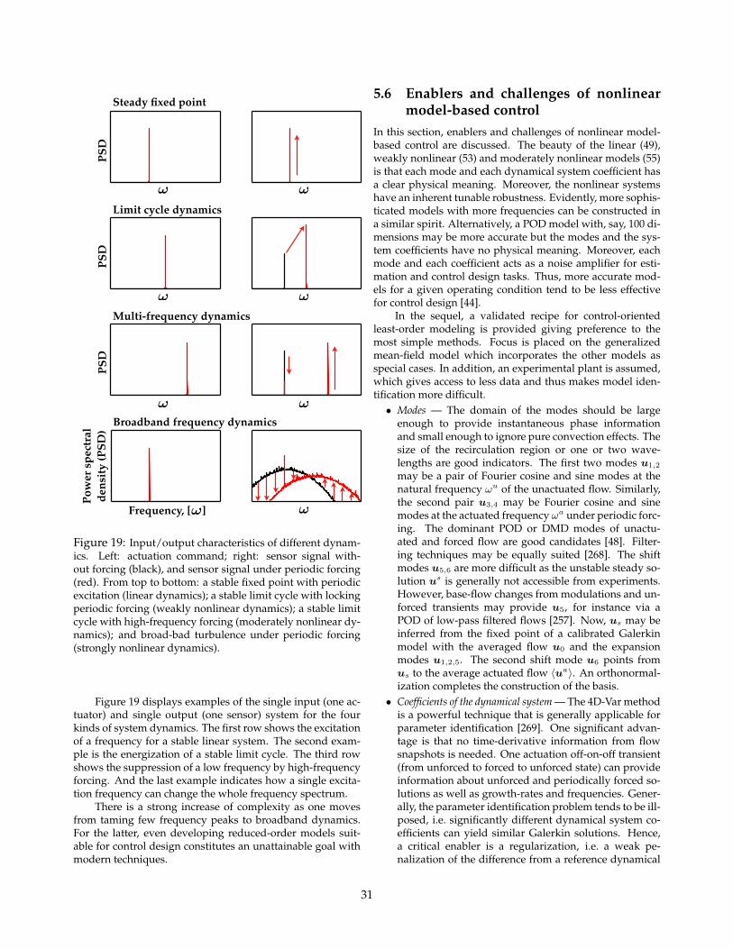
Pow

er s

pect

ral

dens

ity

(PSD

)

Frequency, [ ]!

PSD

PSD

PSD

!

Broadband frequency dynamics

Multi-frequency dynamics

Limit cycle dynamics

Steady fixed point

!

!

!

!

!

!

Figure 19: Input/output characteristics of different dynam-ics. Left: actuation command; right: sensor signal with-out forcing (black), and sensor signal under periodic forcing(red). From top to bottom: a stable fixed point with periodicexcitation (linear dynamics); a stable limit cycle with lockingperiodic forcing (weakly nonlinear dynamics); a stable limitcycle with high-frequency forcing (moderately nonlinear dy-namics); and broad-bad turbulence under periodic forcing(strongly nonlinear dynamics).

Figure 19 displays examples of the single input (one ac-tuator) and single output (one sensor) system for the fourkinds of system dynamics. The first row shows the excitationof a frequency for a stable linear system. The second exam-ple is the energization of a stable limit cycle. The third rowshows the suppression of a low frequency by high-frequencyforcing. And the last example indicates how a single excita-tion frequency can change the whole frequency spectrum.

There is a strong increase of complexity as one movesfrom taming few frequency peaks to broadband dynamics.For the latter, even developing reduced-order models suit-able for control design constitutes an unattainable goal withmodern techniques.

5.6 Enablers and challenges of nonlinearmodel-based control

In this section, enablers and challenges of nonlinear model-based control are discussed. The beauty of the linear (49),weakly nonlinear (53) and moderately nonlinear models (55)is that each mode and each dynamical system coefficient hasa clear physical meaning. Moreover, the nonlinear systemshave an inherent tunable robustness. Evidently, more sophis-ticated models with more frequencies can be constructed ina similar spirit. Alternatively, a POD model with, say, 100 di-mensions may be more accurate but the modes and the sys-tem coefficients have no physical meaning. Moreover, eachmode and each coefficient acts as a noise amplifier for esti-mation and control design tasks. Thus, more accurate mod-els for a given operating condition tend to be less effectivefor control design [44].

In the sequel, a validated recipe for control-orientedleast-order modeling is provided giving preference to themost simple methods. Focus is placed on the generalizedmean-field model which incorporates the other models asspecial cases. In addition, an experimental plant is assumed,which gives access to less data and thus makes model iden-tification more difficult.• Modes — The domain of the modes should be large

enough to provide instantaneous phase informationand small enough to ignore pure convection effects. Thesize of the recirculation region or one or two wave-lengths are good indicators. The first two modes u1,2

may be a pair of Fourier cosine and sine modes at thenatural frequency ωu of the unactuated flow. Similarly,the second pair u3,4 may be Fourier cosine and sinemodes at the actuated frequency ωa under periodic forc-ing. The dominant POD or DMD modes of unactu-ated and forced flow are good candidates [48]. Filter-ing techniques may be equally suited [268]. The shiftmodes u5,6 are more difficult as the unstable steady so-lution us is generally not accessible from experiments.However, base-flow changes from modulations and un-forced transients may provide u5, for instance via aPOD of low-pass filtered flows [257]. Now, us may beinferred from the fixed point of a calibrated Galerkinmodel with the averaged flow u0 and the expansionmodes u1,2,5. The second shift mode u6 points fromus to the average actuated flow 〈ua〉. An orthonormal-ization completes the construction of the basis.

• Coefficients of the dynamical system — The 4D-Var methodis a powerful technique that is generally applicable forparameter identification [269]. One significant advan-tage is that no time-derivative information from flowsnapshots is needed. One actuation off-on-off transient(from unforced to forced to unforced state) can provideinformation about unforced and periodically forced so-lutions as well as growth-rates and frequencies. Gener-ally, the parameter identification problem tends to be ill-posed, i.e. significantly different dynamical system co-efficients can yield similar Galerkin solutions. Hence,a critical enabler is a regularization, i.e. a weak pe-nalization of the difference from a reference dynamical

31

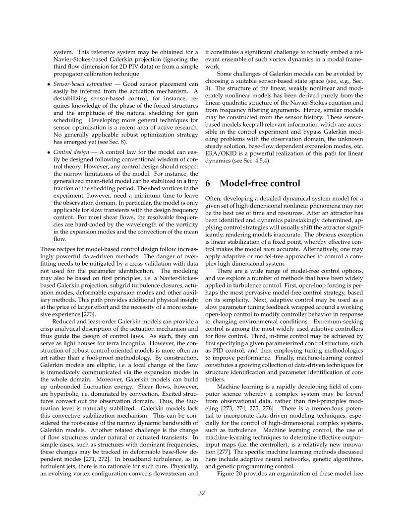
system. This reference system may be obtained for aNavier-Stokes-based Galerkin projection (ignoring thethird flow dimension for 2D PIV data) or from a simplepropagator calibration technique.

• Sensor-based estimation — Good sensor placement caneasily be inferred from the actuation mechanism. Adestabilizing sensor-based control, for instance, re-quires knowledge of the phase of the forced structuresand the amplitude of the natural shedding for gainscheduling. Developing more general techniques forsensor optimization is a recent area of active research.No generally applicable robust optimization strategyhas emerged yet (see Sec. 8).

• Control design — A control law for the model can eas-ily be designed following conventional wisdom of con-trol theory. However, any control design should respectthe narrow limitations of the model. For instance, thegeneralized mean-field model can be stabilized in a tinyfraction of the shedding period. The shed vortices in theexperiment, however, need a minimum time to leavethe observation domain. In particular, the model is onlyapplicable for slow transients with the design frequencycontent. For most shear flows, the resolvable frequen-cies are hard-coded by the wavelength of the vorticityin the expansion modes and the convection of the meanflow.

These recipes for model-based control design follow increas-ingly powerful data-driven methods. The danger of over-fitting needs to be mitigated by a cross-validation with datanot used for the parameter identification. The modelingmay also be based on first principles, i.e. a Navier-Stokes-based Galerkin projection, subgrid turbulence closures, actu-ation modes, deformable expansion modes and other auxil-iary methods. This path provides additional physical insightat the price of larger effort and the necessity of a more exten-sive experience [270].

Reduced and least-order Galerkin models can provide acrisp analytical description of the actuation mechanism andthus guide the design of control laws. As such, they canserve as light houses for terra incognita. However, the con-struction of robust control-oriented models is more often anart rather than a fool-proof methodology. By construction,Galerkin models are elliptic, i.e. a local change of the flowis immediately communicated via the expansion modes inthe whole domain. Moreover, Galerkin models can buildup unbounded fluctuation energy. Shear flows, however,are hyperbolic, i.e. dominated by convection. Excited struc-tures convect out the observation domain. Thus, the fluc-tuation level is naturally stabilized. Galerkin models lackthis convective stabilization mechanism. This can be con-sidered the root-cause of the narrow dynamic bandwidth ofGalerkin models. Another related challenge is the changeof flow structures under natural or actuated transients. Insimple cases, such as structures with dominant frequencies,these changes may be tracked in deformable base-flow de-pendent modes [271, 272]. In broadband turbulence, as inturbulent jets, there is no rationale for such cure. Physically,an evolving vortex configuration convects downstream and

it constitutes a significant challenge to robustly embed a rel-evant ensemble of such vortex dynamics in a modal frame-work.

Some challenges of Galerkin models can be avoided bychoosing a suitable sensor-based state space (see, e.g., Sec.3). The structure of the linear, weakly nonlinear and mod-erately nonlinear models has been derived purely from thelinear-quadratic structure of the Navier-Stokes equation andfrom frequency filtering arguments. Hence, similar modelsmay be constructed from the sensor history. These sensor-based models keep all relevant information which are acces-sible in the control experiment and bypass Galerkin mod-eling problems with the observation domain, the unknownsteady solution, base-flow dependent expansion modes, etc.ERA/OKID is a powerful realization of this path for lineardynamics (see Sec. 4.5.4).

6 Model-free controlOften, developing a detailed dynamical system model for agiven set of high-dimensional nonlinear phenomena may notbe the best use of time and resources. After an attractor hasbeen identified and dynamics painstakingly determined, ap-plying control strategies will usually shift the attractor signif-icantly, rendering models inaccurate. The obvious exceptionis linear stabilization of a fixed point, whereby effective con-trol makes the model more accurate. Alternatively, one mayapply adaptive or model-free approaches to control a com-plex high-dimensional system.

There are a wide range of model-free control options,and we explore a number of methods that have been widelyapplied in turbulence control. First, open-loop forcing is per-haps the most pervasive model-free control strategy, basedon its simplicity. Next, adaptive control may be used as aslow parameter tuning feedback wrapped around a workingopen-loop control to modify controller behavior in responseto changing environmental conditions. Extremum-seekingcontrol is among the most widely used adaptive controllersfor flow control. Third, in-time control may be achieved byfirst specifying a given parameterized control structure, suchas PID control, and then employing tuning methodologiesto improve performance. Finally, machine-learning controlconstitutes a growing collection of data-driven techniques forstructure identification and parameter identification of con-trollers.

Machine learning is a rapidly developing field of com-puter science whereby a complex system may be learnedfrom observational data, rather than first-principles mod-eling [273, 274, 275, 276]. There is a tremendous poten-tial to incorporate data-driven modeling techniques, espe-cially for the control of high-dimensional complex systems,such as turbulence. Machine learning control, the use ofmachine-learning techniques to determine effective output–input maps (i.e. the controller), is a relatively new innova-tion [277]. The specific machine learning methods discussedhere include adaptive neural networks, genetic algorithms,and genetic programming control.

Figure 20 provides an organization of these model-free

32

+

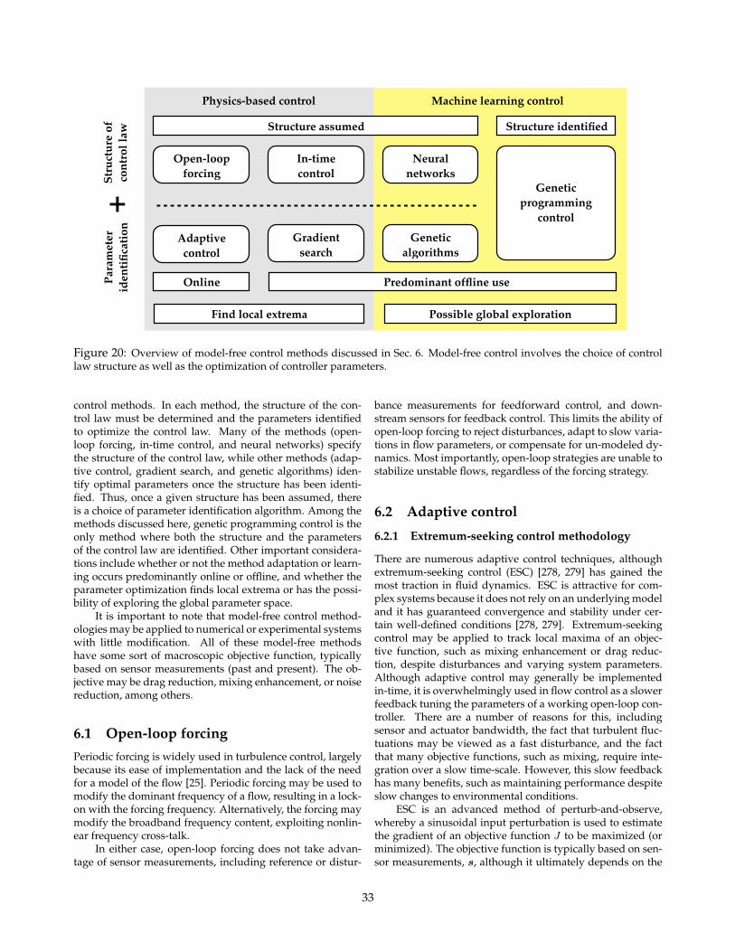
Open-loopforcing

In-time control

Adaptive control

Gradient search

Neural networks

Genetic algorithms

Stru

ctur

e of

co

ntro

l law

Para

met

er

iden

tifica

tion

Online Predominant offline use

Structure assumed Structure identified

Physics-based control Machine learning control

Find local extrema Possible global exploration

Genetic programming

control

Figure 20: Overview of model-free control methods discussed in Sec. 6. Model-free control involves the choice of controllaw structure as well as the optimization of controller parameters.

control methods. In each method, the structure of the con-trol law must be determined and the parameters identifiedto optimize the control law. Many of the methods (open-loop forcing, in-time control, and neural networks) specifythe structure of the control law, while other methods (adap-tive control, gradient search, and genetic algorithms) iden-tify optimal parameters once the structure has been identi-fied. Thus, once a given structure has been assumed, thereis a choice of parameter identification algorithm. Among themethods discussed here, genetic programming control is theonly method where both the structure and the parametersof the control law are identified. Other important considera-tions include whether or not the method adaptation or learn-ing occurs predominantly online or offline, and whether theparameter optimization finds local extrema or has the possi-bility of exploring the global parameter space.

It is important to note that model-free control method-ologies may be applied to numerical or experimental systemswith little modification. All of these model-free methodshave some sort of macroscopic objective function, typicallybased on sensor measurements (past and present). The ob-jective may be drag reduction, mixing enhancement, or noisereduction, among others.

6.1 Open-loop forcingPeriodic forcing is widely used in turbulence control, largelybecause its ease of implementation and the lack of the needfor a model of the flow [25]. Periodic forcing may be used tomodify the dominant frequency of a flow, resulting in a lock-on with the forcing frequency. Alternatively, the forcing maymodify the broadband frequency content, exploiting nonlin-ear frequency cross-talk.

In either case, open-loop forcing does not take advan-tage of sensor measurements, including reference or distur-

bance measurements for feedforward control, and down-stream sensors for feedback control. This limits the ability ofopen-loop forcing to reject disturbances, adapt to slow varia-tions in flow parameters, or compensate for un-modeled dy-namics. Most importantly, open-loop strategies are unable tostabilize unstable flows, regardless of the forcing strategy.

6.2 Adaptive control

6.2.1 Extremum-seeking control methodology

There are numerous adaptive control techniques, althoughextremum-seeking control (ESC) [278, 279] has gained themost traction in fluid dynamics. ESC is attractive for com-plex systems because it does not rely on an underlying modeland it has guaranteed convergence and stability under cer-tain well-defined conditions [278, 279]. Extremum-seekingcontrol may be applied to track local maxima of an objec-tive function, such as mixing enhancement or drag reduc-tion, despite disturbances and varying system parameters.Although adaptive control may generally be implementedin-time, it is overwhelmingly used in flow control as a slowerfeedback tuning the parameters of a working open-loop con-troller. There are a number of reasons for this, includingsensor and actuator bandwidth, the fact that turbulent fluc-tuations may be viewed as a fast disturbance, and the factthat many objective functions, such as mixing, require inte-gration over a slow time-scale. However, this slow feedbackhas many benefits, such as maintaining performance despiteslow changes to environmental conditions.

ESC is an advanced method of perturb-and-observe,whereby a sinusoidal input perturbation is used to estimatethe gradient of an objective function J to be maximized (orminimized). The objective function is typically based on sen-sor measurements, s, although it ultimately depends on the

33

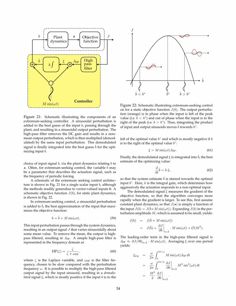
+ +k∫ High

passfilter

Plantdynamics

sb JObjectivefunction

Controller

b ξ JHP

M sin(ωt)

Figure 21: Schematic illustrating the components of anextremum-seeking controller. A sinusoidal perturbation isadded to the best guess of the input b, passing through theplant, and resulting in a sinusoidal output perturbation. Thehigh-pass filter removes the DC gain and results in a zero-mean output perturbation, which is then multiplied (demod-ulated) by the same input perturbation. This demodulatedsignal is finally integrated into the best guess b for the opti-mizing input b.

choice of input signal b, via the plant dynamics relating b tos. Often, for extremum-seeking control, the variable b maybe a parameter that describes the actuation signal, such asthe frequency of periodic forcing.

A schematic of the extremum seeking control architec-ture is shown in Fig. 21 for a single scalar input b, althoughthe methods readily generalize to vector-valued inputs b. Aschematic objective function J(b), for static plant dynamics,is shown in Fig. 22.

In extremum-seeking control, a sinusoidal perturbationis added to b, the best approximation of the input that maxi-mizes the objective function:

b = b+M sin(ωt). (59)

This input perturbation passes through the system dynamics,resulting in an output signal J that varies sinusoidally aboutsome mean value. To remove the mean, the output is high-pass filtered, resulting in JHP. A simple high-pass filter isrepresented in the frequency domain as

HP(ζ) =ζ

ζ + ωHP, (60)

where ζ is the Laplace variable, and ωHP is the filter fre-quency, chosen to be slow compared with the perturbationfrequency ω. It is possible to multiply the high-pass filteredoutput signal by the input sinusoid, resulting in a demodu-lated signal ξ, which is mostly positive if the input b is to the

b

J

b < b∗ b∗ b > b∗

Figure 22: Schematic illustrating extremum-seeking controlon for a static objective function J(b). The output perturba-tion (orange) is in phase when the input is left of the peakvalue (i.e. b < b∗) and out of phase when the input is to theright of the peak (i.e. b > b∗). Thus, integrating the productof input and output sinusoids moves b towards b∗.

left of the optimal value b∗ and which is mostly negative if bis to the right of the optimal value b∗:

ξ = M sin(ωt)JHP. (61)

Finally, the demodulated signal ξ is integrated into b, the bestestimate of the optimizing value:

d

dtb = k ξ, (62)

so that the system estimate b is steered towards the optimalinput b∗. Here, k is the integral gain, which determines howaggressively the actuation responds to a non-optimal input.

The demodulated signal ξ measures the gradient of theobjective function, so that the algorithm converges morerapidly when the gradient is larger. To see this, first assumeconstant plant dynamics, so that J(s) is simply a function ofthe input J(b) = J(b+M sin(ωt)). Expanding J(b) in the per-turbation amplitudeM , which is assumed to be small, yields:

J(b) = J(b+M sin(ωt))

= J(b) +∂J

∂b

∣∣∣∣b=b

·M sin(ωt) +O(M2).

The leading-order term in the high-pass filtered signal isJHP ≈ ∂J/∂b|b=b ·M sin(ωt). Averaging ξ over one periodyields:

ξavg =ω

2π

∫ 2π/ω

0

M sin(ωt)JHP dt

=ω

2π

∫ 2π/2

0

∂J

∂b

∣∣∣∣b=b

M2 sin2(ωt) dt

=M2

2

∂J

∂b

∣∣∣∣b=b

.

34

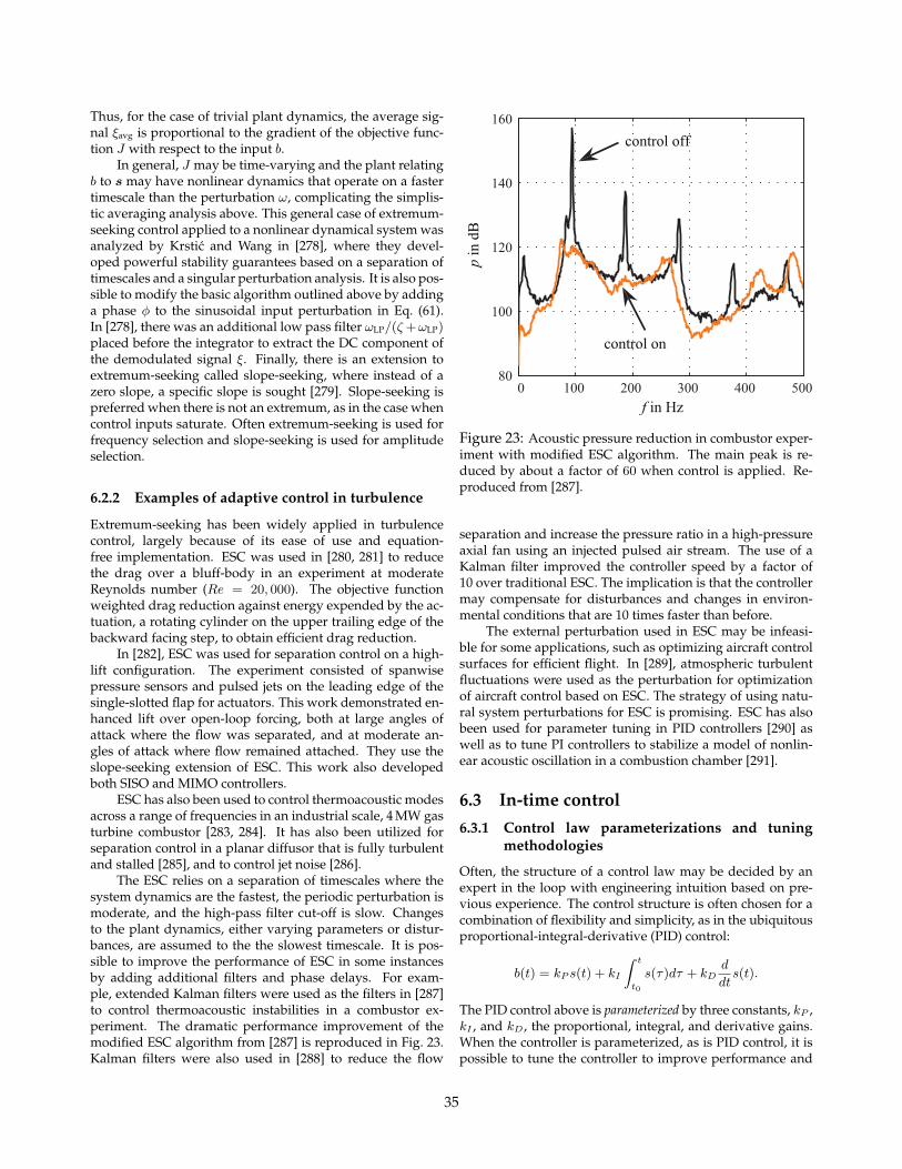
Thus, for the case of trivial plant dynamics, the average sig-nal ξavg is proportional to the gradient of the objective func-tion J with respect to the input b.

In general, J may be time-varying and the plant relatingb to s may have nonlinear dynamics that operate on a fastertimescale than the perturbation ω, complicating the simplis-tic averaging analysis above. This general case of extremum-seeking control applied to a nonlinear dynamical system wasanalyzed by Krstic and Wang in [278], where they devel-oped powerful stability guarantees based on a separation oftimescales and a singular perturbation analysis. It is also pos-sible to modify the basic algorithm outlined above by addinga phase φ to the sinusoidal input perturbation in Eq. (61).In [278], there was an additional low pass filter ωLP/(ζ+ωLP)placed before the integrator to extract the DC component ofthe demodulated signal ξ. Finally, there is an extension toextremum-seeking called slope-seeking, where instead of azero slope, a specific slope is sought [279]. Slope-seeking ispreferred when there is not an extremum, as in the case whencontrol inputs saturate. Often extremum-seeking is used forfrequency selection and slope-seeking is used for amplitudeselection.

6.2.2 Examples of adaptive control in turbulence

Extremum-seeking has been widely applied in turbulencecontrol, largely because of its ease of use and equation-free implementation. ESC was used in [280, 281] to reducethe drag over a bluff-body in an experiment at moderateReynolds number (Re = 20, 000). The objective functionweighted drag reduction against energy expended by the ac-tuation, a rotating cylinder on the upper trailing edge of thebackward facing step, to obtain efficient drag reduction.

In [282], ESC was used for separation control on a high-lift configuration. The experiment consisted of spanwisepressure sensors and pulsed jets on the leading edge of thesingle-slotted flap for actuators. This work demonstrated en-hanced lift over open-loop forcing, both at large angles ofattack where the flow was separated, and at moderate an-gles of attack where flow remained attached. They use theslope-seeking extension of ESC. This work also developedboth SISO and MIMO controllers.

ESC has also been used to control thermoacoustic modesacross a range of frequencies in an industrial scale, 4 MW gasturbine combustor [283, 284]. It has also been utilized forseparation control in a planar diffusor that is fully turbulentand stalled [285], and to control jet noise [286].

The ESC relies on a separation of timescales where thesystem dynamics are the fastest, the periodic perturbation ismoderate, and the high-pass filter cut-off is slow. Changesto the plant dynamics, either varying parameters or distur-bances, are assumed to the the slowest timescale. It is pos-sible to improve the performance of ESC in some instancesby adding additional filters and phase delays. For exam-ple, extended Kalman filters were used as the filters in [287]to control thermoacoustic instabilities in a combustor ex-periment. The dramatic performance improvement of themodified ESC algorithm from [287] is reproduced in Fig. 23.Kalman filters were also used in [288] to reduce the flow

708 G. Gelbert et al. / Journal of Process Control 22 (2012) 700– 709

0 50 100 150 200 250

−202

0 50 100 150 200 2500

1

0 50 100 150 200 250

−1

0

1

0 50 100 150 200 2502468

pin

kPa

Kls

F(K

,τ)

τin

ms

t in s

Fig. 9. Experimental results from an ESC with combined EKF. Topmost frame:pressure measured in the combustion chamber; second frame: map output andcontroller index – (1) for on and (0) for off; third frame: loudspeaker gain; bottom:delay time.

0 100 200 300 400 50080

100

120

140

160

f in Hz

p in

dB

control on

control off

Fig. 10. Spectra of acoustic pressure for the uncontrolled and the controlled case.

converges towards a second minimum at Kls = − 1.2 and ! = 8 ms.Not surprisingly, the difference between the two optimal timedelays corresponds to half the period of the fundamental frequencyof the instability (1/2 · 94 Hz = 5.3 ms). At t = 170 s, the ESC also startsfrom !0 = 6 ms, and at t = 225 s, it starts once again from !0 = 5 ms,thus, converging towards the first minimum.

Fig. 10 shows the spectrum of the acoustic pressure for theuncontrolled and the controlled case. In the uncontrolled case dis-tinct peaks at 94 Hz and higher harmonics can be seen. The peakamplitude at 94 Hz is 157 dB. In the controlled case, this amplitudeis reduced by 35 dB. Due to the complete stabilization of the systemthe higher harmonics also disappear.

6. Conclusion and outlook

The convergence speed of ESC can be improved by a more accu-rate estimation of the local gradients. In this contribution no plantdynamics were considered – the convergence was sped up by a

better gradient estimation of the plants static map only. The clas-sical algorithm uses a combination of high and low-pass filters forgradient estimation. Here, extended Kalman filters were exploitedinstead. In the SISO case, an EKF was employed to fit a tangentialline to the map of the plant. It was shown that for a correct esti-mation of the gradients, the complete control input instead of theperturbation signal should be used. By analyzing the observabilitymatrix of the EKF, an exact measure for the choice of the delay timein the EKF was found.

In the DISO case the EKF estimated the parameters of a tangentialplane that was fitted to the map. In this way, the coupling of theoutput to both inputs was incorporated and a clearly more accurateestimate of the gradients was obtained. In simulation it was shownthat

• the ESC that uses this EKF converges faster than the classicalalgorithm when the same gain k is used in the integrators;

• the gain factor k can be increased to much larger values withoutcausing instability.

Using the EKF, a 50% reduction of the convergence time compartedto the classical algorithm was achieved.

In the simulations the influence of measurement noise was notconsidered. A systematic examination would be interesting. It isassumed that Kalman filter based ESC would again outperform theclassical algorithm.

As this contribution introduces the basic idea of an advancedalgorithm for gradient estimation in extremum seeking control, arigorous and lengthy proof of stability is omitted here. It will bepublished elsewhere. However, the application of the algorithmin a combustor test rig presented Section 5 and in other technicalsetups (results not shown) corroborate a stable operation.

As stated in Section 3, the presented concept for gradient esti-mation could easily be extended to multiple-input single-output(MISO) and multiple-input multiple-output (MIMO) cases. Also,higher order derivatives could be estimated using extended Kalmanfilters. In the same way as presented, this could be accomplishedby fitting quadratic or higher order functions to the map. With sucha gradient estimator, for example, the performance of algorithmsthat use the second derivative for an adaptation of the perturbationamplitude and integrator gain [14] could be improved. Further-more, approaches for a compensation of the plants dynamic asdescribed in Section 2.1 could be combined with the presentedmethod for gradient estimation. Finally, advanced control algo-rithms that use ESC on a higher hierarchal layer for the computationof optimal operational points of a lower layer control structure [15],might also benefit from the proposed gradient estimator.

Acknowledgement

Financial support from the German Research Foundationthrough the collaborative research center Control of complex tur-bulent shear flows (SFB 557) is gratefully acknowledged.

Appendix A. Parameters of the filters

All EKFs were run with a sampling time of "t = 10−3s. "t = "t/sis the non-dimensional sampling time.

Section 2:Classical algorithm: high- and low-pass filters of first order with

a corner frequency off fc = 0.5 Hz.

GHP(s) = ss + 2#fc

GLP(s) = 11/(2#fc)s + 1

Figure 23: Acoustic pressure reduction in combustor exper-iment with modified ESC algorithm. The main peak is re-duced by about a factor of 60 when control is applied. Re-produced from [287].

separation and increase the pressure ratio in a high-pressureaxial fan using an injected pulsed air stream. The use of aKalman filter improved the controller speed by a factor of10 over traditional ESC. The implication is that the controllermay compensate for disturbances and changes in environ-mental conditions that are 10 times faster than before.

The external perturbation used in ESC may be infeasi-ble for some applications, such as optimizing aircraft controlsurfaces for efficient flight. In [289], atmospheric turbulentfluctuations were used as the perturbation for optimizationof aircraft control based on ESC. The strategy of using natu-ral system perturbations for ESC is promising. ESC has alsobeen used for parameter tuning in PID controllers [290] aswell as to tune PI controllers to stabilize a model of nonlin-ear acoustic oscillation in a combustion chamber [291].

6.3 In-time control6.3.1 Control law parameterizations and tuning

methodologies

Often, the structure of a control law may be decided by anexpert in the loop with engineering intuition based on pre-vious experience. The control structure is often chosen for acombination of flexibility and simplicity, as in the ubiquitousproportional-integral-derivative (PID) control:

b(t) = kP s(t) + kI

∫ t

t0

s(τ)dτ + kDd

dts(t).

The PID control above is parameterized by three constants, kP ,kI , and kD , the proportional, integral, and derivative gains.When the controller is parameterized, as is PID control, it ispossible to tune the controller to improve performance and

35

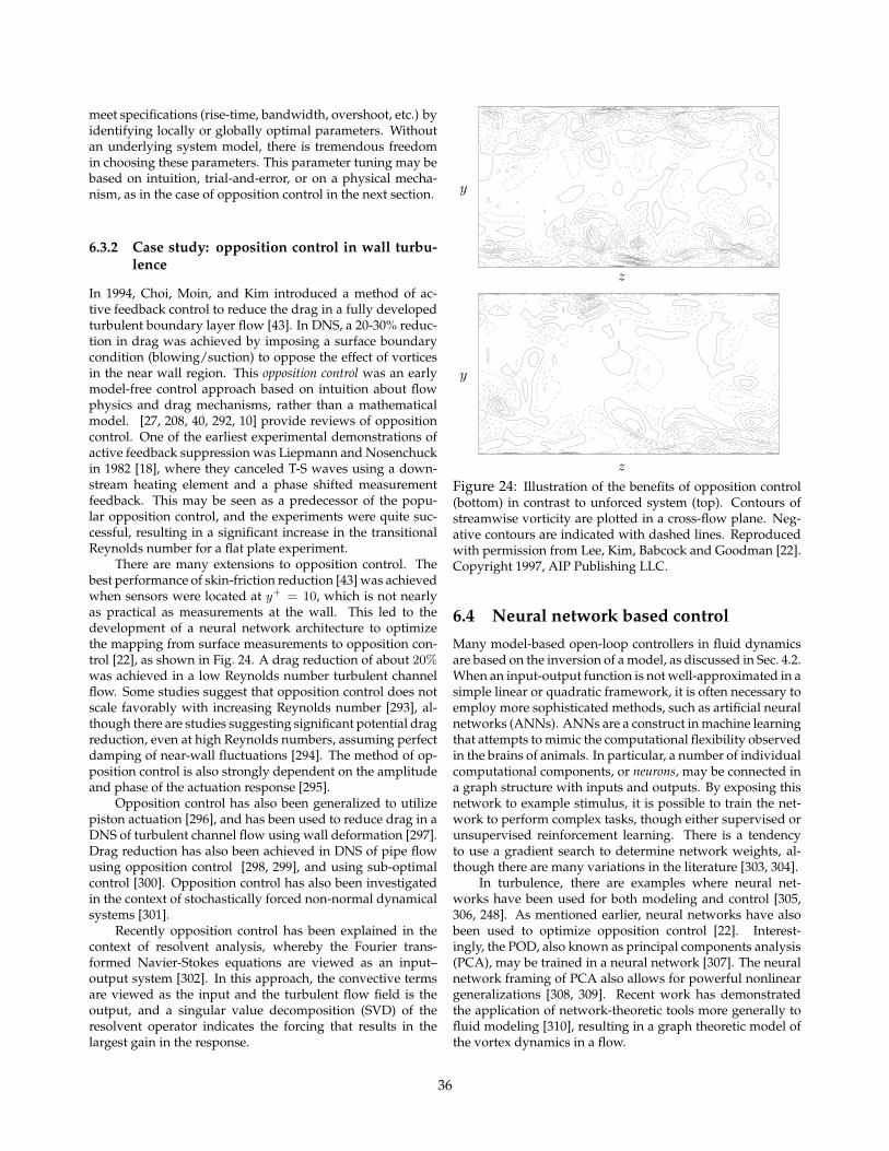
meet specifications (rise-time, bandwidth, overshoot, etc.) byidentifying locally or globally optimal parameters. Withoutan underlying system model, there is tremendous freedomin choosing these parameters. This parameter tuning may bebased on intuition, trial-and-error, or on a physical mecha-nism, as in the case of opposition control in the next section.

6.3.2 Case study: opposition control in wall turbu-lence

In 1994, Choi, Moin, and Kim introduced a method of ac-tive feedback control to reduce the drag in a fully developedturbulent boundary layer flow [43]. In DNS, a 20-30% reduc-tion in drag was achieved by imposing a surface boundarycondition (blowing/suction) to oppose the effect of vorticesin the near wall region. This opposition control was an earlymodel-free control approach based on intuition about flowphysics and drag mechanisms, rather than a mathematicalmodel. [27, 208, 40, 292, 10] provide reviews of oppositioncontrol. One of the earliest experimental demonstrations ofactive feedback suppression was Liepmann and Nosenchuckin 1982 [18], where they canceled T-S waves using a down-stream heating element and a phase shifted measurementfeedback. This may be seen as a predecessor of the popu-lar opposition control, and the experiments were quite suc-cessful, resulting in a significant increase in the transitionalReynolds number for a flat plate experiment.

There are many extensions to opposition control. Thebest performance of skin-friction reduction [43] was achievedwhen sensors were located at y+ = 10, which is not nearlyas practical as measurements at the wall. This led to thedevelopment of a neural network architecture to optimizethe mapping from surface measurements to opposition con-trol [22], as shown in Fig. 24. A drag reduction of about 20%was achieved in a low Reynolds number turbulent channelflow. Some studies suggest that opposition control does notscale favorably with increasing Reynolds number [293], al-though there are studies suggesting significant potential dragreduction, even at high Reynolds numbers, assuming perfectdamping of near-wall fluctuations [294]. The method of op-position control is also strongly dependent on the amplitudeand phase of the actuation response [295].

Opposition control has also been generalized to utilizepiston actuation [296], and has been used to reduce drag in aDNS of turbulent channel flow using wall deformation [297].Drag reduction has also been achieved in DNS of pipe flowusing opposition control [298, 299], and using sub-optimalcontrol [300]. Opposition control has also been investigatedin the context of stochastically forced non-normal dynamicalsystems [301].

Recently opposition control has been explained in thecontext of resolvent analysis, whereby the Fourier trans-formed Navier-Stokes equations are viewed as an input–output system [302]. In this approach, the convective termsare viewed as the input and the turbulent flow field is theoutput, and a singular value decomposition (SVD) of theresolvent operator indicates the forcing that results in thelargest gain in the response.

y

y

z

z

Figure 24: Illustration of the benefits of opposition control(bottom) in contrast to unforced system (top). Contours ofstreamwise vorticity are plotted in a cross-flow plane. Neg-ative contours are indicated with dashed lines. Reproducedwith permission from Lee, Kim, Babcock and Goodman [22].Copyright 1997, AIP Publishing LLC.

6.4 Neural network based controlMany model-based open-loop controllers in fluid dynamicsare based on the inversion of a model, as discussed in Sec. 4.2.When an input-output function is not well-approximated in asimple linear or quadratic framework, it is often necessary toemploy more sophisticated methods, such as artificial neuralnetworks (ANNs). ANNs are a construct in machine learningthat attempts to mimic the computational flexibility observedin the brains of animals. In particular, a number of individualcomputational components, or neurons, may be connected ina graph structure with inputs and outputs. By exposing thisnetwork to example stimulus, it is possible to train the net-work to perform complex tasks, though either supervised orunsupervised reinforcement learning. There is a tendencyto use a gradient search to determine network weights, al-though there are many variations in the literature [303, 304].

In turbulence, there are examples where neural net-works have been used for both modeling and control [305,306, 248]. As mentioned earlier, neural networks have alsobeen used to optimize opposition control [22]. Interest-ingly, the POD, also known as principal components analysis(PCA), may be trained in a neural network [307]. The neuralnetwork framing of PCA also allows for powerful nonlineargeneralizations [308, 309]. Recent work has demonstratedthe application of network-theoretic tools more generally tofluid modeling [310], resulting in a graph theoretic model ofthe vortex dynamics in a flow.

36

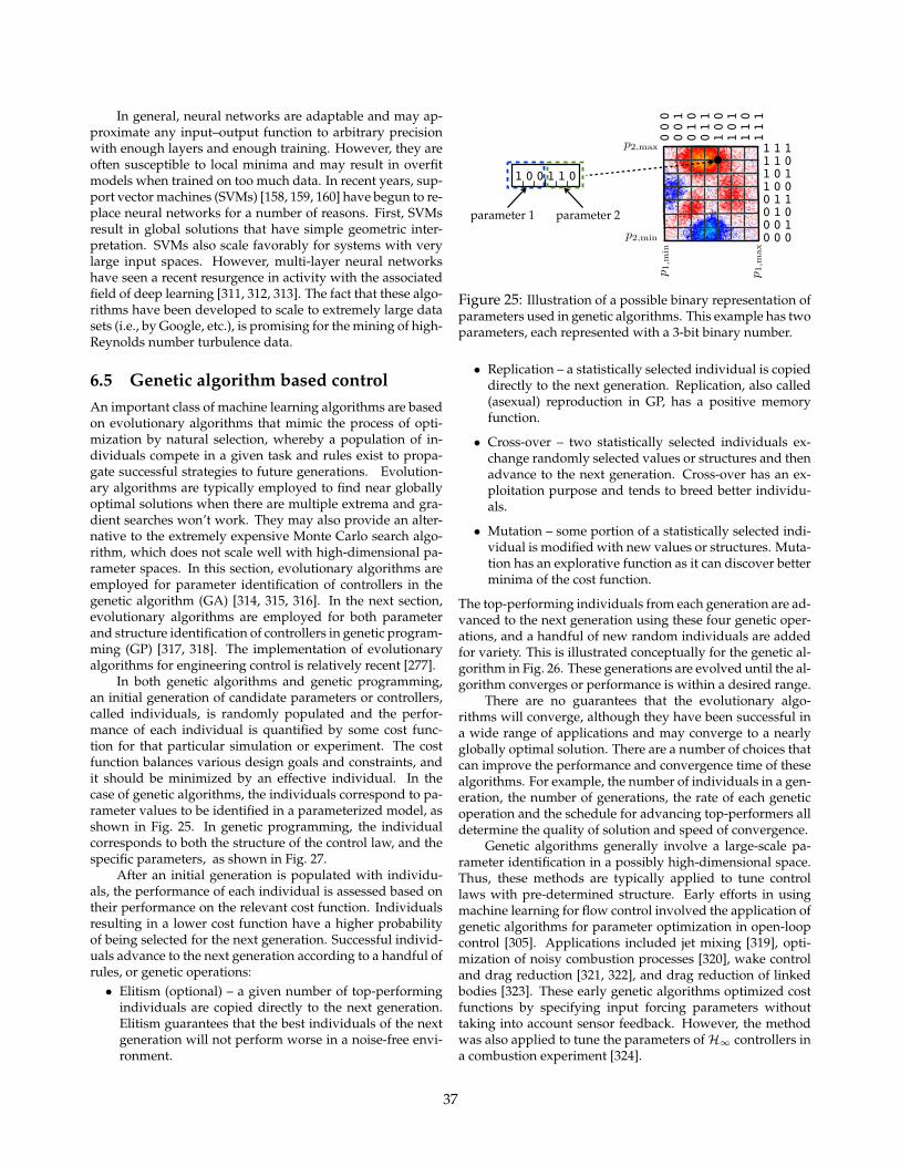
In general, neural networks are adaptable and may ap-proximate any input–output function to arbitrary precisionwith enough layers and enough training. However, they areoften susceptible to local minima and may result in overfitmodels when trained on too much data. In recent years, sup-port vector machines (SVMs) [158, 159, 160] have begun to re-place neural networks for a number of reasons. First, SVMsresult in global solutions that have simple geometric inter-pretation. SVMs also scale favorably for systems with verylarge input spaces. However, multi-layer neural networkshave seen a recent resurgence in activity with the associatedfield of deep learning [311, 312, 313]. The fact that these algo-rithms have been developed to scale to extremely large datasets (i.e., by Google, etc.), is promising for the mining of high-Reynolds number turbulence data.

6.5 Genetic algorithm based controlAn important class of machine learning algorithms are basedon evolutionary algorithms that mimic the process of opti-mization by natural selection, whereby a population of in-dividuals compete in a given task and rules exist to propa-gate successful strategies to future generations. Evolution-ary algorithms are typically employed to find near globallyoptimal solutions when there are multiple extrema and gra-dient searches won’t work. They may also provide an alter-native to the extremely expensive Monte Carlo search algo-rithm, which does not scale well with high-dimensional pa-rameter spaces. In this section, evolutionary algorithms areemployed for parameter identification of controllers in thegenetic algorithm (GA) [314, 315, 316]. In the next section,evolutionary algorithms are employed for both parameterand structure identification of controllers in genetic program-ming (GP) [317, 318]. The implementation of evolutionaryalgorithms for engineering control is relatively recent [277].

In both genetic algorithms and genetic programming,an initial generation of candidate parameters or controllers,called individuals, is randomly populated and the perfor-mance of each individual is quantified by some cost func-tion for that particular simulation or experiment. The costfunction balances various design goals and constraints, andit should be minimized by an effective individual. In thecase of genetic algorithms, the individuals correspond to pa-rameter values to be identified in a parameterized model, asshown in Fig. 25. In genetic programming, the individualcorresponds to both the structure of the control law, and thespecific parameters, as shown in Fig. 27.

After an initial generation is populated with individu-als, the performance of each individual is assessed based ontheir performance on the relevant cost function. Individualsresulting in a lower cost function have a higher probabilityof being selected for the next generation. Successful individ-uals advance to the next generation according to a handful ofrules, or genetic operations:• Elitism (optional) – a given number of top-performing

individuals are copied directly to the next generation.Elitism guarantees that the best individuals of the nextgeneration will not perform worse in a noise-free envi-ronment.

p1,m

in

p2,min

p2,max

p1,m

ax

parameter 1 parameter 2

1 0 0 1 1 0

000

001

010

011

100

101

110

111

0 0 00 0 10 1 00 1 11 0 01 0 11 1 01 1 1

Figure 25: Illustration of a possible binary representation ofparameters used in genetic algorithms. This example has twoparameters, each represented with a 3-bit binary number.

• Replication – a statistically selected individual is copieddirectly to the next generation. Replication, also called(asexual) reproduction in GP, has a positive memoryfunction.

• Cross-over – two statistically selected individuals ex-change randomly selected values or structures and thenadvance to the next generation. Cross-over has an ex-ploitation purpose and tends to breed better individu-als.

• Mutation – some portion of a statistically selected indi-vidual is modified with new values or structures. Muta-tion has an explorative function as it can discover betterminima of the cost function.

The top-performing individuals from each generation are ad-vanced to the next generation using these four genetic oper-ations, and a handful of new random individuals are addedfor variety. This is illustrated conceptually for the genetic al-gorithm in Fig. 26. These generations are evolved until the al-gorithm converges or performance is within a desired range.

There are no guarantees that the evolutionary algo-rithms will converge, although they have been successful ina wide range of applications and may converge to a nearlyglobally optimal solution. There are a number of choices thatcan improve the performance and convergence time of thesealgorithms. For example, the number of individuals in a gen-eration, the number of generations, the rate of each geneticoperation and the schedule for advancing top-performers alldetermine the quality of solution and speed of convergence.

Genetic algorithms generally involve a large-scale pa-rameter identification in a possibly high-dimensional space.Thus, these methods are typically applied to tune controllaws with pre-determined structure. Early efforts in usingmachine learning for flow control involved the application ofgenetic algorithms for parameter optimization in open-loopcontrol [305]. Applications included jet mixing [319], opti-mization of noisy combustion processes [320], wake controland drag reduction [321, 322], and drag reduction of linkedbodies [323]. These early genetic algorithms optimized costfunctions by specifying input forcing parameters withouttaking into account sensor feedback. However, the methodwas also applied to tune the parameters ofH∞ controllers ina combustion experiment [324].

37

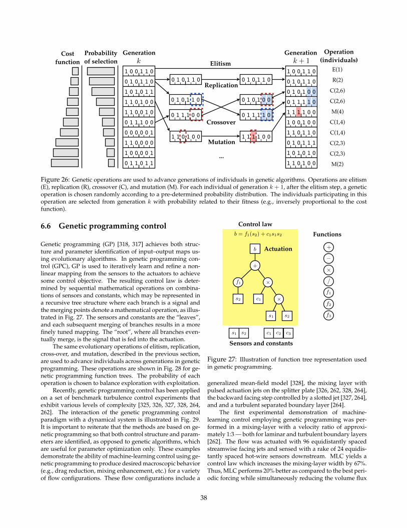
1 0 0 1 1 00 1 0 1 1 01 0 1 0 1 11 1 0 1 0 01 1 0 0 1 00 1 1 1 0 00 0 0 0 0 11 1 0 0 0 01 0 0 0 0 10 1 1 0 1 1

GenerationProbability of selection

Cost function

1 0 0 1 1 00 1 0 1 1 0

1 0 0 1 0 01 1 0 1 1 00 1 0 1 1 11 0 1 0 1 01 1 0 1 0 0

Generation Operation(individuals)

E(1)

R(2)

C(2,6)

C(2,6)

M(4)

C(1,4)

C(1,4)

C(2,3)

C(2,3)

M(2)

Elitism

Replication0 1 0 1 1 0 0 1 0 1 1 0

0 1 0 1 1 0

0 1 1 1 0 0Crossover

1 1 0 1 0 0Mutation

...

0 1 0 1 0 00 1 1 1 1 01 1 1 1 0 0

0 1 0 1 0 0

0 1 1 1 1 0

k k + 1

1 1 1 1 0 0

Figure 26: Genetic operations are used to advance generations of individuals in genetic algorithms. Operations are elitism(E), replication (R), crossover (C), and mutation (M). For each individual of generation k + 1, after the elitism step, a geneticoperation is chosen randomly according to a pre-determined probability distribution. The individuals participating in thisoperation are selected from generation k with probability related to their fitness (e.g., inversely proportional to the costfunction).

6.6 Genetic programming control

Genetic programming (GP) [318, 317] achieves both struc-ture and parameter identification of input–output maps us-ing evolutionary algorithms. In genetic programming con-trol (GPC), GP is used to iteratively learn and refine a non-linear mapping from the sensors to the actuators to achievesome control objective. The resulting control law is deter-mined by sequential mathematical operations on combina-tions of sensors and constants, which may be represented ina recursive tree structure where each branch is a signal andthe merging points denote a mathematical operation, as illus-trated in Fig. 27. The sensors and constants are the “leaves”,and each subsequent merging of branches results in a morefinely tuned mapping. The “root”, where all branches even-tually merge, is the signal that is fed into the actuation.

The same evolutionary operations of elitism, replication,cross-over, and mutation, described in the previous section,are used to advance individuals across generations in geneticprogramming. These operations are shown in Fig. 28 for ge-netic programming function trees. The probability of eachoperation is chosen to balance exploration with exploitation.

Recently, genetic programming control has been appliedon a set of benchmark turbulence control experiments thatexhibit various levels of complexity [325, 326, 327, 328, 264,262]. The interaction of the genetic programming controlparadigm with a dynamical system is illustrated in Fig. 29.It is important to reiterate that the methods are based on ge-netic programming so that both control structure and param-eters are identified, as opposed to genetic algorithms, whichare useful for parameter optimization only. These examplesdemonstrate the ability of machine-learning control using ge-netic programming to produce desired macroscopic behavior(e.g., drag reduction, mixing enhancement, etc.) for a varietyof flow configurations. These flow configurations include a

Other References• APS DFD 2008, DMD[443]

• compressed DMD (Mathelin) [444]

• Willcox [445, 446, 447, 448, 449]

• K. Breuer [450, 451, 452, 453, 454]

• Videler et al (science and nature bio-flight) [455]

• Daniel [456] and Spohnberg

• Moss bat [338, 337]

• Dickinson [333] [335, 327? ? ] , [326]

• Wang [328]

• [330], [331]

Network theory references:

• Sam and Aditya [457]

• Eurika and Bernd [379]

• Network control refs[458, 459, 460, 461, 462? , 463]

• More refs [464, 465, 466, 467, 468, 469]

• Mesbahi work [470]

• Network science in general

– Small-world networks [471], Scale-free net-works [472, 473], Universality of networks [474]

– Network review paper [475]

– All scale-free networks are sparse [476]

There have been many powerful advances in network con-trol theory surrounding multi-agent systems in the past twodecades. In particular, networks are often characterized by alarge collection of individuals (represented by nodes), thateach execute their own set of local protocols in responseto external stimulus. This analogy holds quite well for anumber of large graph dynamical systems, including ani-mals flocking [458, 477], multi-robotic cooperative controlsystems [469], sensor networks [467, 463], biological regula-tory networks [478, 479], and the internet [462, 460], to namea few. Similarly, in a fluid we may view packets of vor-ticity as nodes in a graph that move collectively accordingto global rules (i.e., governing physical equations) based onlocal rules (diffusion, etc.) as well as their external inputssummed across the entire network (i.e., convection due to in-duced velocity from the Biot–Savart law).

In these large multi-agent systems, it is often possible tomanipulate the large-scale behavior with leader nodes thatenact a larger supervisory control protocol to create a system-wide minima that is favorable [458, 470, 480]. The fact thatbirds and fish often act as local flows with large-scale coher-ence, and that leaders can strongly influence and manipulatethe large-scale coherent motion [458, 477], is promising whenconsidering network-based fluid flow control.

There have been recent advances in understandingwhen such a network is controllable and with how manyleader or “driver” nodes in the system [480]. A key observa-tion in this line of research is that large, sparse networks with

heterogeneous degree distributions4 (such as sparse, scale-free turbulence networks), are especially difficult to control.In particular, the number of driver nodes (or leaders) may bequite large for these systems, as compared with a regular orrandom graph with more homogeneous degree distribution.

Degree to which network is controllable [481]

Extremum-seeking mathematics

b = b + M sin(!t) (55)

Then, this signal passes through the system, and the out-put J(s) also has a sinusoidal perturbation at frequency !.To remove the DC component of this signal, the output issent through a high-pass filter of the form h() = /( +!f ),where !f is the cutoff frequency.

Finally, the high-pass filtered signal is multiplied by theoriginal perturbation sin(!t + ) with a possible additionalphase to demodulate the signal. The result is a signal thatis either mostly positive when b is left of the optimum pointb and a signal that is mostly negative when b is to the rightof the optimum point. This demodulated signal is then inte-grated into our best estimate b of b, driving the input signaltowards the optimal value.

The theory is relatively straightforward to analyze in thecase of no dynamics and a quadratic cost function. To extendthis to systems with nonlinear dynamics, Wang and Krsticleveraged singular perturbation theory and a separation oftime-scales argument.

b = f1(s2) + c1s1s2 (56)

(57)

b = s1 (c2 + f2(s2)) (58)

(59)

b = f1(s2) + c1f2(s2) (60)

(61)

b = s1(c2 + s1s2) (62)

(63)

b = f1(s2) + f3(c3 + s2) (64)

(65)

c1 c2 c3 c4 (66)

(67)

s1 s2 s3 s4 (68)

(69)

f1 f2 f3 f4 (70)

(71)

+ (72)

4The degree distribution of a network is the distribution of howmany other nodes each node is connected to; this is often visualizedas a histogram. Recent results indicate that all scale-free networksare inherently sparse, with heterogeneous degree distribution.

43



• Willcox [445, 446, 447, 448, 449]

• K. Breuer [450, 451, 452, 453, 454]



• Moss bat [338, 337]

• Dickinson [333] [335, 327? ? ] , [326]

• Wang [328]

• [330], [331]





• More refs [464, 465, 466, 467, 468, 469]












b = b + M sin(!t) (55)




b = f1(s2) + c1s1s2 (56)

(57)

b = s1 (c2 + f2(s2)) (58)

(59)

b = f1(s2) + c1f2(s2) (60)

(61)

b = s1(c2 + s1s2) (62)

(63)

b = f1(s2) + f3(c3 + s2) (64)

(65)

c1 c2 c3 c4 (66)

(67)

s1 s2 s3 s4 (68)

(69)

f1 f2 f3 f4 (70)

(71)

+ (72)


43



• Willcox [445, 446, 447, 448, 449]

• K. Breuer [450, 451, 452, 453, 454]



• Moss bat [338, 337]

• Dickinson [333] [335, 327? ? ] , [326]

• Wang [328]

• [330], [331]





• More refs [464, 465, 466, 467, 468, 469]












b = b + M sin(!t) (55)




b = f1(s2) + c1s1s2 (56)

(57)

b = s1 (c2 + f2(s2)) (58)

(59)

b = f1(s2) + c1f2(s2) (60)

(61)

b = s1(c2 + s1s2) (62)

(63)

b = f1(s2) + f3(c3 + s2) (64)

(65)

c1 c2 c3 c4 (66)

(67)

s1 s2 s3 s4 (68)

(69)

f1 f2 f3 f4 (70)

(71)

+ (72)


43



• Willcox [445, 446, 447, 448, 449]

• K. Breuer [450, 451, 452, 453, 454]



• Moss bat [338, 337]

• Dickinson [333] [335, 327? ? ] , [326]

• Wang [328]

• [330], [331]





• More refs [464, 465, 466, 467, 468, 469]












b = b + M sin(!t) (55)




b = f1(s2) + c1s1s2 (56)

(57)

b = s1 (c2 + f2(s2)) (58)

(59)

b = f1(s2) + c1f2(s2) (60)

(61)

b = s1(c2 + s1s2) (62)

(63)

b = f1(s2) + f3(c3 + s2) (64)

(65)

c1 c2 c3 c4 (66)

(67)

s1 s2 s3 s4 (68)

(69)

f1 f2 f3 f4 (70)

(71)

+ (72)


43



• Willcox [445, 446, 447, 448, 449]

• K. Breuer [450, 451, 452, 453, 454]



• Moss bat [338, 337]

• Dickinson [333] [335, 327? ? ] , [326]

• Wang [328]

• [330], [331]





• More refs [464, 465, 466, 467, 468, 469]












b = b + M sin(!t) (55)




b = f1(s2) + c1s1s2 (56)

(57)

b = s1 (c2 + f2(s2)) (58)

(59)

b = f1(s2) + c1f2(s2) (60)

(61)

b = s1(c2 + s1s2) (62)

(63)

b = f1(s2) + f3(c3 + s2) (64)

(65)

c1 c2 c3 c4 (66)

(67)

s1 s2 s3 s4 (68)

(69)

f1 f2 f3 f4 (70)

(71)

+ (72)


43



• Willcox [445, 446, 447, 448, 449]

• K. Breuer [450, 451, 452, 453, 454]



• Moss bat [338, 337]

• Dickinson [333] [335, 327? ? ] , [326]

• Wang [328]

• [330], [331]





• More refs [464, 465, 466, 467, 468, 469]












b = b + M sin(!t) (55)




b = f1(s2) + c1s1s2 (56)

(57)

b = s1 (c2 + f2(s2)) (58)

(59)

b = f1(s2) + c1f2(s2) (60)

(61)

b = s1(c2 + s1s2) (62)

(63)

b = f1(s2) + f3(c3 + s2) (64)

(65)

c1 c2 c3 c4 (66)

(67)

s1 s2 s3 s4 (68)

(69)

f1 f2 f3 f4 (70)

(71)

+ (72)


43



• Willcox [445, 446, 447, 448, 449]

• K. Breuer [450, 451, 452, 453, 454]



• Moss bat [338, 337]

• Dickinson [333] [335, 327? ? ] , [326]

• Wang [328]

• [330], [331]





• More refs [464, 465, 466, 467, 468, 469]












b = b + M sin(!t) (55)




b = f1(s2) + c1s1s2 (56)

(57)

b = s1 (c2 + f2(s2)) (58)

(59)

b = f1(s2) + c1f2(s2) (60)

(61)

b = s1(c2 + s1s2) (62)

(63)

b = f1(s2) + f3(c3 + s2) (64)

(65)

c1 c2 c3 c4 (66)

(67)

s1 s2 s3 s4 (68)

(69)

f1 f2 f3 f4 (70)

(71)

+ (72)


43



• Willcox [445, 446, 447, 448, 449]

• K. Breuer [450, 451, 452, 453, 454]



• Moss bat [338, 337]

• Dickinson [333] [335, 327? ? ] , [326]

• Wang [328]

• [330], [331]





• More refs [464, 465, 466, 467, 468, 469]












b = b + M sin(!t) (55)




b = f1(s2) + c1s1s2 (56)

(57)

b = s1 (c2 + f2(s2)) (58)

(59)

b = f1(s2) + c1f2(s2) (60)

(61)

b = s1(c2 + s1s2) (62)

(63)

b = f1(s2) + f3(c3 + s2) (64)

(65)

c1 c2 c3 c4 (66)

(67)

s1 s2 s3 s4 (68)

(69)

f1 f2 f3 f4 (70)

(71)

+ (72)


43



• Willcox [445, 446, 447, 448, 449]

• K. Breuer [450, 451, 452, 453, 454]



• Moss bat [338, 337]

• Dickinson [333] [335, 327? ? ] , [326]

• Wang [328]

• [330], [331]





• More refs [464, 465, 466, 467, 468, 469]












b = b + M sin(!t) (55)




b = f1(s2) + c1s1s2 (56)

(57)

b = s1 (c2 + f2(s2)) (58)

(59)

b = f1(s2) + c1f2(s2) (60)

(61)

b = s1(c2 + s1s2) (62)

(63)

b = f1(s2) + f3(c3 + s2) (64)

(65)

c1 c2 c3 c4 (66)

(67)

s1 s2 s3 s4 (68)

(69)

f1 f2 f3 f4 (70)

(71)

+ (72)


43



• Willcox [445, 446, 447, 448, 449]

• K. Breuer [450, 451, 452, 453, 454]



• Moss bat [338, 337]

• Dickinson [333] [335, 327? ? ] , [326]

• Wang [328]

• [330], [331]





• More refs [464, 465, 466, 467, 468, 469]












b = b + M sin(!t) (55)




b = f1(s2) + c1s1s2 (56)

(57)

b = s1 (c2 + f2(s2)) (58)

(59)

b = f1(s2) + c1f2(s2) (60)

(61)

b = s1(c2 + s1s2) (62)

(63)

b = f1(s2) + f3(c3 + s2) (64)

(65)

c1 c2 c3 c4 (66)

(67)

s1 s2 s3 s4 (68)

(69)

f1 f2 f3 f4 (70)

(71)

+ (72)


43

Control law

Sensors and constants

Functions



• Willcox [445, 446, 447, 448, 449]

• K. Breuer [450, 451, 452, 453, 454]



• Moss bat [338, 337]

• Dickinson [333] [335, 327? ? ] , [326]

• Wang [328]

• [330], [331]





• More refs [464, 465, 466, 467, 468, 469]












b = b + M sin(!t) (55)




b = f1(s2) + c1s1s2 (56)

(57)

b = s1 (c2 + f2(s2)) (58)

(59)

b = f1(s2) + c1f2(s2) (60)

(61)

b = s1(c2 + s1s2) (62)

(63)

b = f1(s2) + f3(c3 + s2) (64)

(65)

c1 c2 c3 c4 (66)

(67)

s1 s2 s3 s4 (68)

(69)

f1 f2 f3 f4 (70)

(71)

+ (72)


43



• Willcox [445, 446, 447, 448, 449]

• K. Breuer [450, 451, 452, 453, 454]



• Moss bat [338, 337]

• Dickinson [333] [335, 327? ? ] , [326]

• Wang [328]

• [330], [331]





• More refs [464, 465, 466, 467, 468, 469]












b = b + M sin(!t) (55)




b = f1(s2) + c1s1s2 (56)

(57)

b = s1 (c2 + f2(s2)) (58)

(59)

b = f1(s2) + c1f2(s2) (60)

(61)

b = s1(c2 + s1s2) (62)

(63)

b = f1(s2) + f3(c3 + s2) (64)

(65)

c1 c2 c3 c4 (66)

(67)

s1 s2 s3 s4 (68)

(69)

f1 f2 f3 f4 (70)

(71)

+ (72)


43



• Willcox [445, 446, 447, 448, 449]

• K. Breuer [450, 451, 452, 453, 454]



• Moss bat [338, 337]

• Dickinson [333] [335, 327? ? ] , [326]

• Wang [328]

• [330], [331]





• More refs [464, 465, 466, 467, 468, 469]












b = b + M sin(!t) (55)




b = f1(s2) + c1s1s2 (56)

(57)

b = s1 (c2 + f2(s2)) (58)

(59)

b = f1(s2) + c1f2(s2) (60)

(61)

b = s1(c2 + s1s2) (62)

(63)

b = f1(s2) + f3(c3 + s2) (64)

(65)

c1 c2 c3 c4 (66)

(67)

s1 s2 s3 s4 (68)

(69)

f1 f2 f3 f4 (70)

(71)

+ (72)


43



• Willcox [445, 446, 447, 448, 449]

• K. Breuer [450, 451, 452, 453, 454]



• Moss bat [338, 337]

• Dickinson [333] [335, 327? ? ] , [326]

• Wang [328]

• [330], [331]





• More refs [464, 465, 466, 467, 468, 469]












b = b + M sin(!t) (55)




b = f1(s2) + c1s1s2 (56)

(57)

b = s1 (c2 + f2(s2)) (58)

(59)

b = f1(s2) + c1f2(s2) (60)

(61)

b = s1(c2 + s1s2) (62)

(63)

b = f1(s2) + f3(c3 + s2) (64)

(65)

c1 c2 c3 c4 (66)

(67)

s1 s2 s3 s4 (68)

(69)

f1 f2 f3 f4 (70)

(71)

+ (72)


43



• Willcox [445, 446, 447, 448, 449]

• K. Breuer [450, 451, 452, 453, 454]



• Moss bat [338, 337]

• Dickinson [333] [335, 327? ? ] , [326]

• Wang [328]

• [330], [331]





• More refs [464, 465, 466, 467, 468, 469]












b = b + M sin(!t) (55)




b = f1(s2) + c1s1s2 (56)

(57)

b = s1 (c2 + f2(s2)) (58)

(59)

b = f1(s2) + c1f2(s2) (60)

(61)

b = s1(c2 + s1s2) (62)

(63)

b = f1(s2) + f3(c3 + s2) (64)

(65)

c1 c2 c3 c4 (66)

(67)

s1 s2 s3 s4 (68)

(69)

f1 f2 f3 f4 (70)

(71)

+ (72)


43



• Willcox [445, 446, 447, 448, 449]

• K. Breuer [450, 451, 452, 453, 454]



• Moss bat [338, 337]

• Dickinson [333] [335, 327? ? ] , [326]

• Wang [328]

• [330], [331]





• More refs [464, 465, 466, 467, 468, 469]












b = b + M sin(!t) (55)




b = f1(s2) + c1s1s2 (56)

(57)

b = s1 (c2 + f2(s2)) (58)

(59)

b = f1(s2) + c1f2(s2) (60)

(61)

b = s1(c2 + s1s2) (62)

(63)

b = f1(s2) + f3(c3 + s2) (64)

(65)

c1 c2 c3 c4 (66)

(67)

s1 s2 s3 s4 (68)

(69)

f1 f2 f3 f4 (70)

(71)

+ (72)


43



• Willcox [445, 446, 447, 448, 449]

• K. Breuer [450, 451, 452, 453, 454]



• Moss bat [338, 337]

• Dickinson [333] [335, 327? ? ] , [326]

• Wang [328]

• [330], [331]





• More refs [464, 465, 466, 467, 468, 469]












b = b + M sin(!t) (55)




b = f1(s2) + c1s1s2 (56)

(57)

b = s1 (c2 + f2(s2)) (58)

(59)

b = f1(s2) + c1f2(s2) (60)

(61)

b = s1(c2 + s1s2) (62)

(63)

b = f1(s2) + f3(c3 + s2) (64)

(65)

c1 c2 c3 c4 (66)

(67)

s1 s2 s3 s4 (68)

(69)

f1 f2 f3 f4 (70)

(71)

+ (72)


43



• Willcox [445, 446, 447, 448, 449]

• K. Breuer [450, 451, 452, 453, 454]



• Moss bat [338, 337]

• Dickinson [333] [335, 327? ? ] , [326]

• Wang [328]

• [330], [331]





• More refs [464, 465, 466, 467, 468, 469]












b = b + M sin(!t) (55)




b = f1(s2) + c1s1s2 (56)

(57)

b = s1 (c2 + f2(s2)) (58)

(59)

b = f1(s2) + c1f2(s2) (60)

(61)

b = s1(c2 + s1s2) (62)

(63)

b = f1(s2) + f3(c3 + s2) (64)

(65)

c1 c2 c3 c4 (66)

(67)

s1 s2 s3 s4 (68)

(69)

f1 f2 f3 f4 (70)

(71)

+ (72)


43



• Willcox [445, 446, 447, 448, 449]

• K. Breuer [450, 451, 452, 453, 454]



• Moss bat [338, 337]

• Dickinson [333] [335, 327? ? ] , [326]

• Wang [328]

• [330], [331]





• More refs [464, 465, 466, 467, 468, 469]












b = b + M sin(!t) (55)




b = f1(s2) + c1s1s2 (56)

(57)

b = s1 (c2 + f2(s2)) (58)

(59)

b = f1(s2) + c1f2(s2) (60)

(61)

b = s1(c2 + s1s2) (62)

(63)

b = f1(s2) + f3(c3 + s2) (64)

(65)

c1 c2 c3 c4 (66)

(67)

s1 s2 s3 s4 (68)

(69)

f1 f2 f3 f4 (70)

(71)

+ (72)


43

/

Actuation

Figure 27: Illustration of function tree representation usedin genetic programming.

generalized mean-field model [328], the mixing layer withpulsed actuation jets on the splitter plate [326, 262, 328, 264],the backward facing step controlled by a slotted jet [327, 264],and and a turbulent separated boundary layer [264].

The first experimental demonstration of machine-learning control employing genetic programming was per-formed in a mixing-layer with a velocity ratio of approxi-mately 1:3 — both for laminar and turbulent boundary layers[262]. The flow was actuated with 96 equidistantly spacedstreamwise facing jets and sensed with a rake of 24 equidis-tantly spaced hot-wire sensors downstream. MLC yields acontrol law which increases the mixing-layer width by 67%.Thus, MLC performs 20% better as compared to the best peri-odic forcing while simultaneously reducing the volume flux

38

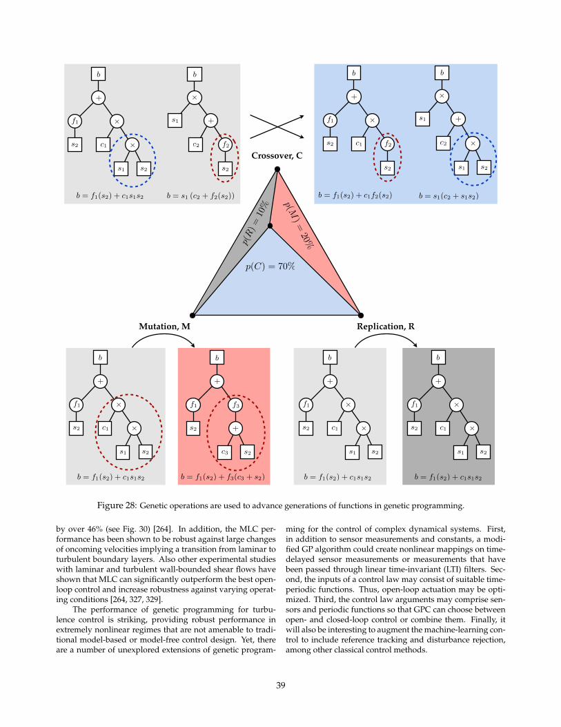
Crossover, C

Replication, RMutation, M



• Willcox [445, 446, 447, 448, 449]

• K. Breuer [450, 451, 452, 453, 454]



• Moss bat [338, 337]

• Dickinson [333] [335, 327? ? ] , [326]

• Wang [328]

• [330], [331]





• More refs [464, 465, 466, 467, 468, 469]












b = b + M sin(!t) (55)




b = f1(s2) + c1s1s2 (56)

(57)

b = s1 (c2 + f2(s2)) (58)

(59)

b = f1(s2) + c1f2(s2) (60)

(61)

b = s1(c2 + s1s2) (62)

(63)

b = f1(s2) + f3(c3 + s2) (64)

(65)

c1 c2 c3 c4 (66)

(67)

s1 s2 s3 s4 (68)

(69)

f1 f2 f3 f4 (70)

(71)

+ (72)


43



• Willcox [445, 446, 447, 448, 449]

• K. Breuer [450, 451, 452, 453, 454]



• Moss bat [338, 337]

• Dickinson [333] [335, 327? ? ] , [326]

• Wang [328]

• [330], [331]





• More refs [464, 465, 466, 467, 468, 469]












b = b + M sin(!t) (55)




b = f1(s2) + c1s1s2 (56)

(57)

b = s1 (c2 + f2(s2)) (58)

(59)

b = f1(s2) + c1f2(s2) (60)

(61)

b = s1(c2 + s1s2) (62)

(63)

b = f1(s2) + f3(c3 + s2) (64)

(65)

c1 c2 c3 c4 (66)

(67)

s1 s2 s3 s4 (68)

(69)

f1 f2 f3 f4 (70)

(71)

+ (72)


43



• Willcox [445, 446, 447, 448, 449]

• K. Breuer [450, 451, 452, 453, 454]



• Moss bat [338, 337]

• Dickinson [333] [335, 327? ? ] , [326]

• Wang [328]

• [330], [331]





• More refs [464, 465, 466, 467, 468, 469]












b = b + M sin(!t) (55)




b = f1(s2) + c1s1s2 (56)

(57)

b = s1 (c2 + f2(s2)) (58)

(59)

b = f1(s2) + c1f2(s2) (60)

(61)

b = s1(c2 + s1s2) (62)

(63)

b = f1(s2) + f3(c3 + s2) (64)

(65)

c1 c2 c3 c4 (66)

(67)

s1 s2 s3 s4 (68)

(69)

f1 f2 f3 f4 (70)

(71)

+ (72)


43



• Willcox [445, 446, 447, 448, 449]

• K. Breuer [450, 451, 452, 453, 454]



• Moss bat [338, 337]

• Dickinson [333] [335, 327? ? ] , [326]

• Wang [328]

• [330], [331]





• More refs [464, 465, 466, 467, 468, 469]












b = b + M sin(!t) (55)




b = f1(s2) + c1s1s2 (56)

(57)

b = s1 (c2 + f2(s2)) (58)

(59)

b = f1(s2) + c1f2(s2) (60)

(61)

b = s1(c2 + s1s2) (62)

(63)

b = f1(s2) + f3(c3 + s2) (64)

(65)

c1 c2 c3 c4 (66)

(67)

s1 s2 s3 s4 (68)

(69)

f1 f2 f3 f4 (70)

(71)

+ (72)


43



• Willcox [445, 446, 447, 448, 449]

• K. Breuer [450, 451, 452, 453, 454]



• Moss bat [338, 337]

• Dickinson [333] [335, 327? ? ] , [326]

• Wang [328]

• [330], [331]





• More refs [464, 465, 466, 467, 468, 469]












b = b + M sin(!t) (55)




b = f1(s2) + c1s1s2 (56)

(57)

b = s1 (c2 + f2(s2)) (58)

(59)

b = f1(s2) + c1f2(s2) (60)

(61)

b = s1(c2 + s1s2) (62)

(63)

b = f1(s2) + f3(c3 + s2) (64)

(65)

c1 c2 c3 c4 (66)

(67)

s1 s2 s3 s4 (68)

(69)

f1 f2 f3 f4 (70)

(71)

+ (72)


43



• Willcox [445, 446, 447, 448, 449]

• K. Breuer [450, 451, 452, 453, 454]



• Moss bat [338, 337]

• Dickinson [333] [335, 327? ? ] , [326]

• Wang [328]

• [330], [331]





• More refs [464, 465, 466, 467, 468, 469]












b = b + M sin(!t) (55)




b = f1(s2) + c1s1s2 (56)

(57)

b = s1 (c2 + f2(s2)) (58)

(59)

b = f1(s2) + c1f2(s2) (60)

(61)

b = s1(c2 + s1s2) (62)

(63)

b = f1(s2) + f3(c3 + s2) (64)

(65)

c1 c2 c3 c4 (66)

(67)

s1 s2 s3 s4 (68)

(69)

f1 f2 f3 f4 (70)

(71)

+ (72)


43



• Willcox [445, 446, 447, 448, 449]

• K. Breuer [450, 451, 452, 453, 454]



• Moss bat [338, 337]

• Dickinson [333] [335, 327? ? ] , [326]

• Wang [328]

• [330], [331]





• More refs [464, 465, 466, 467, 468, 469]












b = b + M sin(!t) (55)




b = f1(s2) + c1s1s2 (56)

(57)

b = s1 (c2 + f2(s2)) (58)

(59)

b = f1(s2) + c1f2(s2) (60)

(61)

b = s1(c2 + s1s2) (62)

(63)

b = f1(s2) + f3(c3 + s2) (64)

(65)

c1 c2 c3 c4 (66)

(67)

s1 s2 s3 s4 (68)

(69)

f1 f2 f3 f4 (70)

(71)

+ (72)


43



• Willcox [445, 446, 447, 448, 449]

• K. Breuer [450, 451, 452, 453, 454]



• Moss bat [338, 337]

• Dickinson [333] [335, 327? ? ] , [326]

• Wang [328]

• [330], [331]





• More refs [464, 465, 466, 467, 468, 469]












b = b + M sin(!t) (55)




b = f1(s2) + c1s1s2 (56)

(57)

b = s1 (c2 + f2(s2)) (58)

(59)

b = f1(s2) + c1f2(s2) (60)

(61)

b = s1(c2 + s1s2) (62)

(63)

b = f1(s2) + f3(c3 + s2) (64)

(65)

c1 c2 c3 c4 (66)

(67)

s1 s2 s3 s4 (68)

(69)

f1 f2 f3 f4 (70)

(71)

+ (72)


43



• Willcox [445, 446, 447, 448, 449]

• K. Breuer [450, 451, 452, 453, 454]



• Moss bat [338, 337]

• Dickinson [333] [335, 327? ? ] , [326]

• Wang [328]

• [330], [331]





• More refs [464, 465, 466, 467, 468, 469]












b = b + M sin(!t) (55)




b = f1(s2) + c1s1s2 (56)

(57)

b = s1 (c2 + f2(s2)) (58)

(59)

b = f1(s2) + c1f2(s2) (60)

(61)

b = s1(c2 + s1s2) (62)

(63)

b = f1(s2) + f3(c3 + s2) (64)

(65)

c1 c2 c3 c4 (66)

(67)

s1 s2 s3 s4 (68)

(69)

f1 f2 f3 f4 (70)

(71)

+ (72)


43



• Willcox [445, 446, 447, 448, 449]

• K. Breuer [450, 451, 452, 453, 454]



• Moss bat [338, 337]

• Dickinson [333] [335, 327? ? ] , [326]

• Wang [328]

• [330], [331]





• More refs [464, 465, 466, 467, 468, 469]












b = b + M sin(!t) (55)




b = f1(s2) + c1s1s2 (56)

(57)

b = s1 (c2 + f2(s2)) (58)

(59)

b = f1(s2) + c1f2(s2) (60)

(61)

b = s1(c2 + s1s2) (62)

(63)

b = f1(s2) + f3(c3 + s2) (64)

(65)

c1 c2 c3 c4 (66)

(67)

s1 s2 s3 s4 (68)

(69)

f1 f2 f3 f4 (70)

(71)

+ (72)


43



• Willcox [445, 446, 447, 448, 449]

• K. Breuer [450, 451, 452, 453, 454]



• Moss bat [338, 337]

• Dickinson [333] [335, 327? ? ] , [326]

• Wang [328]

• [330], [331]





• More refs [464, 465, 466, 467, 468, 469]












b = b + M sin(!t) (55)




b = f1(s2) + c1s1s2 (56)

(57)

b = s1 (c2 + f2(s2)) (58)

(59)

b = f1(s2) + c1f2(s2) (60)

(61)

b = s1(c2 + s1s2) (62)

(63)

b = f1(s2) + f3(c3 + s2) (64)

(65)

c1 c2 c3 c4 (66)

(67)

s1 s2 s3 s4 (68)

(69)

f1 f2 f3 f4 (70)

(71)

+ (72)


43



• Willcox [445, 446, 447, 448, 449]

• K. Breuer [450, 451, 452, 453, 454]



• Moss bat [338, 337]

• Dickinson [333] [335, 327? ? ] , [326]

• Wang [328]

• [330], [331]





• More refs [464, 465, 466, 467, 468, 469]












b = b + M sin(!t) (55)




b = f1(s2) + c1s1s2 (56)

(57)

b = s1 (c2 + f2(s2)) (58)

(59)

b = f1(s2) + c1f2(s2) (60)

(61)

b = s1(c2 + s1s2) (62)

(63)

b = f1(s2) + f3(c3 + s2) (64)

(65)

c1 c2 c3 c4 (66)

(67)

s1 s2 s3 s4 (68)

(69)

f1 f2 f3 f4 (70)

(71)

+ (72)


43



• Willcox [445, 446, 447, 448, 449]

• K. Breuer [450, 451, 452, 453, 454]



• Moss bat [338, 337]

• Dickinson [333] [335, 327? ? ] , [326]

• Wang [328]

• [330], [331]





• More refs [464, 465, 466, 467, 468, 469]












b = b + M sin(!t) (55)




b = f1(s2) + c1s1s2 (56)

(57)

b = s1 (c2 + f2(s2)) (58)

(59)

b = f1(s2) + c1f2(s2) (60)

(61)

b = s1(c2 + s1s2) (62)

(63)

b = f1(s2) + f3(c3 + s2) (64)

(65)

c1 c2 c3 c4 (66)

(67)

s1 s2 s3 s4 (68)

(69)

f1 f2 f3 f4 (70)

(71)

+ (72)


43



• Willcox [445, 446, 447, 448, 449]

• K. Breuer [450, 451, 452, 453, 454]



• Moss bat [338, 337]

• Dickinson [333] [335, 327? ? ] , [326]

• Wang [328]

• [330], [331]





• More refs [464, 465, 466, 467, 468, 469]












b = b + M sin(!t) (55)




b = f1(s2) + c1s1s2 (56)

(57)

b = s1 (c2 + f2(s2)) (58)

(59)

b = f1(s2) + c1f2(s2) (60)

(61)

b = s1(c2 + s1s2) (62)

(63)

b = f1(s2) + f3(c3 + s2) (64)

(65)

c1 c2 c3 c4 (66)

(67)

s1 s2 s3 s4 (68)

(69)

f1 f2 f3 f4 (70)

(71)

+ (72)


43



• Willcox [445, 446, 447, 448, 449]

• K. Breuer [450, 451, 452, 453, 454]



• Moss bat [338, 337]

• Dickinson [333] [335, 327? ? ] , [326]

• Wang [328]

• [330], [331]





• More refs [464, 465, 466, 467, 468, 469]












b = b + M sin(!t) (55)




b = f1(s2) + c1s1s2 (56)

(57)

b = s1 (c2 + f2(s2)) (58)

(59)

b = f1(s2) + c1f2(s2) (60)

(61)

b = s1(c2 + s1s2) (62)

(63)

b = f1(s2) + f3(c3 + s2) (64)

(65)

c1 c2 c3 c4 (66)

(67)

s1 s2 s3 s4 (68)

(69)

f1 f2 f3 f4 (70)

(71)

+ (72)


43



• Willcox [445, 446, 447, 448, 449]

• K. Breuer [450, 451, 452, 453, 454]



• Moss bat [338, 337]

• Dickinson [333] [335, 327? ? ] , [326]

• Wang [328]

• [330], [331]





• More refs [464, 465, 466, 467, 468, 469]












b = b + M sin(!t) (55)




b = f1(s2) + c1s1s2 (56)

(57)

b = s1 (c2 + f2(s2)) (58)

(59)

b = f1(s2) + c1f2(s2) (60)

(61)

b = s1(c2 + s1s2) (62)

(63)

b = f1(s2) + f3(c3 + s2) (64)

(65)

c1 c2 c3 c4 (66)

(67)

s1 s2 s3 s4 (68)

(69)

f1 f2 f3 f4 (70)

(71)

+ (72)


43



• Willcox [445, 446, 447, 448, 449]

• K. Breuer [450, 451, 452, 453, 454]



• Moss bat [338, 337]

• Dickinson [333] [335, 327? ? ] , [326]

• Wang [328]

• [330], [331]





• More refs [464, 465, 466, 467, 468, 469]












b = b + M sin(!t) (55)




b = f1(s2) + c1s1s2 (56)

(57)

b = s1 (c2 + f2(s2)) (58)

(59)

b = f1(s2) + c1f2(s2) (60)

(61)

b = s1(c2 + s1s2) (62)

(63)

b = f1(s2) + f3(c3 + s2) (64)

(65)

c1 c2 c3 c4 (66)

(67)

s1 s2 s3 s4 (68)

(69)

f1 f2 f3 f4 (70)

(71)

+ (72)


43



• Willcox [445, 446, 447, 448, 449]

• K. Breuer [450, 451, 452, 453, 454]



• Moss bat [338, 337]

• Dickinson [333] [335, 327? ? ] , [326]

• Wang [328]

• [330], [331]





• More refs [464, 465, 466, 467, 468, 469]












b = b + M sin(!t) (55)




b = f1(s2) + c1s1s2 (56)

(57)

b = s1 (c2 + f2(s2)) (58)

(59)

b = f1(s2) + c1f2(s2) (60)

(61)

b = s1(c2 + s1s2) (62)

(63)

b = f1(s2) + f3(c3 + s2) (64)

(65)

c1 c2 c3 c4 (66)

(67)

s1 s2 s3 s4 (68)

(69)

f1 f2 f3 f4 (70)

(71)

+ (72)


43



• Willcox [445, 446, 447, 448, 449]

• K. Breuer [450, 451, 452, 453, 454]



• Moss bat [338, 337]

• Dickinson [333] [335, 327? ? ] , [326]

• Wang [328]

• [330], [331]





• More refs [464, 465, 466, 467, 468, 469]












b = b + M sin(!t) (55)




b = f1(s2) + c1s1s2 (56)

(57)

b = s1 (c2 + f2(s2)) (58)

(59)

b = f1(s2) + c1f2(s2) (60)

(61)

b = s1(c2 + s1s2) (62)

(63)

b = f1(s2) + f3(c3 + s2) (64)

(65)

c1 c2 c3 c4 (66)

(67)

s1 s2 s3 s4 (68)

(69)

f1 f2 f3 f4 (70)

(71)

+ (72)


43



• Willcox [445, 446, 447, 448, 449]

• K. Breuer [450, 451, 452, 453, 454]



• Moss bat [338, 337]

• Dickinson [333] [335, 327? ? ] , [326]

• Wang [328]

• [330], [331]





• More refs [464, 465, 466, 467, 468, 469]












b = b + M sin(!t) (55)




b = f1(s2) + c1s1s2 (56)

(57)

b = s1 (c2 + f2(s2)) (58)

(59)

b = f1(s2) + c1f2(s2) (60)

(61)

b = s1(c2 + s1s2) (62)

(63)

b = f1(s2) + f3(c3 + s2) (64)

(65)

c1 c2 c3 c4 (66)

(67)

s1 s2 s3 s4 (68)

(69)

f1 f2 f3 f4 (70)

(71)

+ (72)


43



• Willcox [445, 446, 447, 448, 449]

• K. Breuer [450, 451, 452, 453, 454]



• Moss bat [338, 337]

• Dickinson [333] [335, 327? ? ] , [326]

• Wang [328]

• [330], [331]





• More refs [464, 465, 466, 467, 468, 469]












b = b + M sin(!t) (55)




b = f1(s2) + c1s1s2 (56)

(57)

b = s1 (c2 + f2(s2)) (58)

(59)

b = f1(s2) + c1f2(s2) (60)

(61)

b = s1(c2 + s1s2) (62)

(63)

b = f1(s2) + f3(c3 + s2) (64)

(65)

c1 c2 c3 c4 (66)

(67)

s1 s2 s3 s4 (68)

(69)

f1 f2 f3 f4 (70)

(71)

+ (72)


43



• Willcox [445, 446, 447, 448, 449]

• K. Breuer [450, 451, 452, 453, 454]



• Moss bat [338, 337]

• Dickinson [333] [335, 327? ? ] , [326]

• Wang [328]

• [330], [331]





• More refs [464, 465, 466, 467, 468, 469]












b = b + M sin(!t) (55)




b = f1(s2) + c1s1s2 (56)

(57)

b = s1 (c2 + f2(s2)) (58)

(59)

b = f1(s2) + c1f2(s2) (60)

(61)

b = s1(c2 + s1s2) (62)

(63)

b = f1(s2) + f3(c3 + s2) (64)

(65)

c1 c2 c3 c4 (66)

(67)

s1 s2 s3 s4 (68)

(69)

f1 f2 f3 f4 (70)

(71)

+ (72)


43



• Willcox [445, 446, 447, 448, 449]

• K. Breuer [450, 451, 452, 453, 454]



• Moss bat [338, 337]

• Dickinson [333] [335, 327? ? ] , [326]

• Wang [328]

• [330], [331]





• More refs [464, 465, 466, 467, 468, 469]












b = b + M sin(!t) (55)




b = f1(s2) + c1s1s2 (56)

(57)

b = s1 (c2 + f2(s2)) (58)

(59)

b = f1(s2) + c1f2(s2) (60)

(61)

b = s1(c2 + s1s2) (62)

(63)

b = f1(s2) + f3(c3 + s2) (64)

(65)

c1 c2 c3 c4 (66)

(67)

s1 s2 s3 s4 (68)

(69)

f1 f2 f3 f4 (70)

(71)

+ (72)


43



• Willcox [445, 446, 447, 448, 449]

• K. Breuer [450, 451, 452, 453, 454]



• Moss bat [338, 337]

• Dickinson [333] [335, 327? ? ] , [326]

• Wang [328]

• [330], [331]





• More refs [464, 465, 466, 467, 468, 469]












b = b + M sin(!t) (55)




b = f1(s2) + c1s1s2 (56)

(57)

b = s1 (c2 + f2(s2)) (58)

(59)

b = f1(s2) + c1f2(s2) (60)

(61)

b = s1(c2 + s1s2) (62)

(63)

b = f1(s2) + f3(c3 + s2) (64)

(65)

c1 c2 c3 c4 (66)

(67)

s1 s2 s3 s4 (68)

(69)

f1 f2 f3 f4 (70)

(71)

+ (72)


43



• Willcox [445, 446, 447, 448, 449]

• K. Breuer [450, 451, 452, 453, 454]



• Moss bat [338, 337]

• Dickinson [333] [335, 327? ? ] , [326]

• Wang [328]

• [330], [331]





• More refs [464, 465, 466, 467, 468, 469]












b = b + M sin(!t) (55)




b = f1(s2) + c1s1s2 (56)

(57)

b = s1 (c2 + f2(s2)) (58)

(59)

b = f1(s2) + c1f2(s2) (60)

(61)

b = s1(c2 + s1s2) (62)

(63)

b = f1(s2) + f3(c3 + s2) (64)

(65)

c1 c2 c3 c4 (66)

(67)

s1 s2 s3 s4 (68)

(69)

f1 f2 f3 f4 (70)

(71)

+ (72)


43



• Willcox [445, 446, 447, 448, 449]

• K. Breuer [450, 451, 452, 453, 454]



• Moss bat [338, 337]

• Dickinson [333] [335, 327? ? ] , [326]

• Wang [328]

• [330], [331]





• More refs [464, 465, 466, 467, 468, 469]












b = b + M sin(!t) (55)




b = f1(s2) + c1s1s2 (56)

(57)

b = s1 (c2 + f2(s2)) (58)

(59)

b = f1(s2) + c1f2(s2) (60)

(61)

b = s1(c2 + s1s2) (62)

(63)

b = f1(s2) + f3(c3 + s2) (64)

(65)

c1 c2 c3 c4 (66)

(67)

s1 s2 s3 s4 (68)

(69)

f1 f2 f3 f4 (70)

(71)

+ (72)


43



• Willcox [445, 446, 447, 448, 449]

• K. Breuer [450, 451, 452, 453, 454]



• Moss bat [338, 337]

• Dickinson [333] [335, 327? ? ] , [326]

• Wang [328]

• [330], [331]





• More refs [464, 465, 466, 467, 468, 469]












b = b + M sin(!t) (55)




b = f1(s2) + c1s1s2 (56)

(57)

b = s1 (c2 + f2(s2)) (58)

(59)

b = f1(s2) + c1f2(s2) (60)

(61)

b = s1(c2 + s1s2) (62)

(63)

b = f1(s2) + f3(c3 + s2) (64)

(65)

c1 c2 c3 c4 (66)

(67)

s1 s2 s3 s4 (68)

(69)

f1 f2 f3 f4 (70)

(71)

+ (72)


43



• Willcox [445, 446, 447, 448, 449]

• K. Breuer [450, 451, 452, 453, 454]



• Moss bat [338, 337]

• Dickinson [333] [335, 327? ? ] , [326]

• Wang [328]

• [330], [331]





• More refs [464, 465, 466, 467, 468, 469]












b = b + M sin(!t) (55)




b = f1(s2) + c1s1s2 (56)

(57)

b = s1 (c2 + f2(s2)) (58)

(59)

b = f1(s2) + c1f2(s2) (60)

(61)

b = s1(c2 + s1s2) (62)

(63)

b = f1(s2) + f3(c3 + s2) (64)

(65)

c1 c2 c3 c4 (66)

(67)

s1 s2 s3 s4 (68)

(69)

f1 f2 f3 f4 (70)

(71)

+ (72)


43



• Willcox [445, 446, 447, 448, 449]

• K. Breuer [450, 451, 452, 453, 454]



• Moss bat [338, 337]

• Dickinson [333] [335, 327? ? ] , [326]

• Wang [328]

• [330], [331]





• More refs [464, 465, 466, 467, 468, 469]












b = b + M sin(!t) (55)




b = f1(s2) + c1s1s2 (56)

(57)

b = s1 (c2 + f2(s2)) (58)

(59)

b = f1(s2) + c1f2(s2) (60)

(61)

b = s1(c2 + s1s2) (62)

(63)

b = f1(s2) + f3(c3 + s2) (64)

(65)

c1 c2 c3 c4 (66)

(67)

s1 s2 s3 s4 (68)

(69)

f1 f2 f3 f4 (70)

(71)

+ (72)


43



• Willcox [445, 446, 447, 448, 449]

• K. Breuer [450, 451, 452, 453, 454]



• Moss bat [338, 337]

• Dickinson [333] [335, 327? ? ] , [326]

• Wang [328]

• [330], [331]





• More refs [464, 465, 466, 467, 468, 469]












b = b + M sin(!t) (55)




b = f1(s2) + c1s1s2 (56)

(57)

b = s1 (c2 + f2(s2)) (58)

(59)

b = f1(s2) + c1f2(s2) (60)

(61)

b = s1(c2 + s1s2) (62)

(63)

b = f1(s2) + f3(c3 + s2) (64)

(65)

c1 c2 c3 c4 (66)

(67)

s1 s2 s3 s4 (68)

(69)

f1 f2 f3 f4 (70)

(71)

+ (72)


43



• Willcox [445, 446, 447, 448, 449]

• K. Breuer [450, 451, 452, 453, 454]



• Moss bat [338, 337]

• Dickinson [333] [335, 327? ? ] , [326]

• Wang [328]

• [330], [331]





• More refs [464, 465, 466, 467, 468, 469]












b = b + M sin(!t) (55)




b = f1(s2) + c1s1s2 (56)

(57)

b = s1 (c2 + f2(s2)) (58)

(59)

b = f1(s2) + c1f2(s2) (60)

(61)

b = s1(c2 + s1s2) (62)

(63)

b = f1(s2) + f3(c3 + s2) (64)

(65)

c1 c2 c3 c4 (66)

(67)

s1 s2 s3 s4 (68)

(69)

f1 f2 f3 f4 (70)

(71)

+ (72)


43



• Willcox [445, 446, 447, 448, 449]

• K. Breuer [450, 451, 452, 453, 454]



• Moss bat [338, 337]

• Dickinson [333] [335, 327? ? ] , [326]

• Wang [328]

• [330], [331]





• More refs [464, 465, 466, 467, 468, 469]












b = b + M sin(!t) (55)




b = f1(s2) + c1s1s2 (56)

(57)

b = s1 (c2 + f2(s2)) (58)

(59)

b = f1(s2) + c1f2(s2) (60)

(61)

b = s1(c2 + s1s2) (62)

(63)

b = f1(s2) + f3(c3 + s2) (64)

(65)

c1 c2 c3 c4 (66)

(67)

s1 s2 s3 s4 (68)

(69)

f1 f2 f3 f4 (70)

(71)

+ (72)


43



• Willcox [445, 446, 447, 448, 449]

• K. Breuer [450, 451, 452, 453, 454]



• Moss bat [338, 337]

• Dickinson [333] [335, 327? ? ] , [326]

• Wang [328]

• [330], [331]





• More refs [464, 465, 466, 467, 468, 469]












b = b + M sin(!t) (55)




b = f1(s2) + c1s1s2 (56)

(57)

b = s1 (c2 + f2(s2)) (58)

(59)

b = f1(s2) + c1f2(s2) (60)

(61)

b = s1(c2 + s1s2) (62)

(63)

b = f1(s2) + f3(c3 + s2) (64)

(65)

c1 c2 c3 c4 (66)

(67)

s1 s2 s3 s4 (68)

(69)

f1 f2 f3 f4 (70)

(71)

+ (72)


43



• Willcox [445, 446, 447, 448, 449]

• K. Breuer [450, 451, 452, 453, 454]



• Moss bat [338, 337]

• Dickinson [333] [335, 327? ? ] , [326]

• Wang [328]

• [330], [331]





• More refs [464, 465, 466, 467, 468, 469]












b = b + M sin(!t) (55)




b = f1(s2) + c1s1s2 (56)

(57)

b = s1 (c2 + f2(s2)) (58)

(59)

b = f1(s2) + c1f2(s2) (60)

(61)

b = s1(c2 + s1s2) (62)

(63)

b = f1(s2) + f3(c3 + s2) (64)

(65)

c1 c2 c3 c4 (66)

(67)

s1 s2 s3 s4 (68)

(69)

f1 f2 f3 f4 (70)

(71)

+ (72)


43



• Willcox [445, 446, 447, 448, 449]

• K. Breuer [450, 451, 452, 453, 454]



• Moss bat [338, 337]

• Dickinson [333] [335, 327? ? ] , [326]

• Wang [328]

• [330], [331]





• More refs [464, 465, 466, 467, 468, 469]












b = b + M sin(!t) (55)




b = f1(s2) + c1s1s2 (56)

(57)

b = s1 (c2 + f2(s2)) (58)

(59)

b = f1(s2) + c1f2(s2) (60)

(61)

b = s1(c2 + s1s2) (62)

(63)

b = f1(s2) + f3(c3 + s2) (64)

(65)

c1 c2 c3 c4 (66)

(67)

s1 s2 s3 s4 (68)

(69)

f1 f2 f3 f4 (70)

(71)

+ (72)


43



• Willcox [445, 446, 447, 448, 449]

• K. Breuer [450, 451, 452, 453, 454]



• Moss bat [338, 337]

• Dickinson [333] [335, 327? ? ] , [326]

• Wang [328]

• [330], [331]





• More refs [464, 465, 466, 467, 468, 469]












b = b + M sin(!t) (55)




b = f1(s2) + c1s1s2 (56)

(57)

b = s1 (c2 + f2(s2)) (58)

(59)

b = f1(s2) + c1f2(s2) (60)

(61)

b = s1(c2 + s1s2) (62)

(63)

b = f1(s2) + f3(c3 + s2) (64)

(65)

c1 c2 c3 c4 (66)

(67)

s1 s2 s3 s4 (68)

(69)

f1 f2 f3 f4 (70)

(71)

+ (72)


43



• Willcox [445, 446, 447, 448, 449]

• K. Breuer [450, 451, 452, 453, 454]



• Moss bat [338, 337]

• Dickinson [333] [335, 327? ? ] , [326]

• Wang [328]

• [330], [331]





• More refs [464, 465, 466, 467, 468, 469]












b = b + M sin(!t) (55)




b = f1(s2) + c1s1s2 (56)

(57)

b = s1 (c2 + f2(s2)) (58)

(59)

b = f1(s2) + c1f2(s2) (60)

(61)

b = s1(c2 + s1s2) (62)

(63)

b = f1(s2) + f3(c3 + s2) (64)

(65)

c1 c2 c3 c4 (66)

(67)

s1 s2 s3 s4 (68)

(69)

f1 f2 f3 f4 (70)

(71)

+ (72)


43



• Willcox [445, 446, 447, 448, 449]

• K. Breuer [450, 451, 452, 453, 454]



• Moss bat [338, 337]

• Dickinson [333] [335, 327? ? ] , [326]

• Wang [328]

• [330], [331]





• More refs [464, 465, 466, 467, 468, 469]












b = b + M sin(!t) (55)




b = f1(s2) + c1s1s2 (56)

(57)

b = s1 (c2 + f2(s2)) (58)

(59)

b = f1(s2) + c1f2(s2) (60)

(61)

b = s1(c2 + s1s2) (62)

(63)

b = f1(s2) + f3(c3 + s2) (64)

(65)

c1 c2 c3 c4 (66)

(67)

s1 s2 s3 s4 (68)

(69)

f1 f2 f3 f4 (70)

(71)

+ (72)


43



• Willcox [445, 446, 447, 448, 449]

• K. Breuer [450, 451, 452, 453, 454]



• Moss bat [338, 337]

• Dickinson [333] [335, 327? ? ] , [326]

• Wang [328]

• [330], [331]





• More refs [464, 465, 466, 467, 468, 469]












b = b + M sin(!t) (55)




b = f1(s2) + c1s1s2 (56)

(57)

b = s1 (c2 + f2(s2)) (58)

(59)

b = f1(s2) + c1f2(s2) (60)

(61)

b = s1(c2 + s1s2) (62)

(63)

b = f1(s2) + f3(c3 + s2) (64)

(65)

c1 c2 c3 c4 (66)

(67)

s1 s2 s3 s4 (68)

(69)

f1 f2 f3 f4 (70)

(71)

+ (72)


43



• Willcox [445, 446, 447, 448, 449]

• K. Breuer [450, 451, 452, 453, 454]



• Moss bat [338, 337]

• Dickinson [333] [335, 327? ? ] , [326]

• Wang [328]

• [330], [331]





• More refs [464, 465, 466, 467, 468, 469]












b = b + M sin(!t) (55)




b = f1(s2) + c1s1s2 (56)

(57)

b = s1 (c2 + f2(s2)) (58)

(59)

b = f1(s2) + c1f2(s2) (60)

(61)

b = s1(c2 + s1s2) (62)

(63)

b = f1(s2) + f3(c3 + s2) (64)

(65)

c1 c2 c3 c4 (66)

(67)

s1 s2 s3 s4 (68)

(69)

f1 f2 f3 f4 (70)

(71)

+ (72)


43



• Willcox [445, 446, 447, 448, 449]

• K. Breuer [450, 451, 452, 453, 454]



• Moss bat [338, 337]

• Dickinson [333] [335, 327? ? ] , [326]

• Wang [328]

• [330], [331]





• More refs [464, 465, 466, 467, 468, 469]












b = b + M sin(!t) (55)




b = f1(s2) + c1s1s2 (56)

(57)

b = s1 (c2 + f2(s2)) (58)

(59)

b = f1(s2) + c1f2(s2) (60)

(61)

b = s1(c2 + s1s2) (62)

(63)

b = f1(s2) + f3(c3 + s2) (64)

(65)

c1 c2 c3 c4 (66)

(67)

s1 s2 s3 s4 (68)

(69)

f1 f2 f3 f4 (70)

(71)

+ (72)


43



• Willcox [445, 446, 447, 448, 449]

• K. Breuer [450, 451, 452, 453, 454]



• Moss bat [338, 337]

• Dickinson [333] [335, 327? ? ] , [326]

• Wang [328]

• [330], [331]





• More refs [464, 465, 466, 467, 468, 469]












b = b + M sin(!t) (55)




b = f1(s2) + c1s1s2 (56)

(57)

b = s1 (c2 + f2(s2)) (58)

(59)

b = f1(s2) + c1f2(s2) (60)

(61)

b = s1(c2 + s1s2) (62)

(63)

b = f1(s2) + f3(c3 + s2) (64)

(65)

c1 c2 c3 c4 (66)

(67)

s1 s2 s3 s4 (68)

(69)

f1 f2 f3 f4 (70)

(71)

+ (72)


43



• Willcox [445, 446, 447, 448, 449]

• K. Breuer [450, 451, 452, 453, 454]



• Moss bat [338, 337]

• Dickinson [333] [335, 327? ? ] , [326]

• Wang [328]

• [330], [331]





• More refs [464, 465, 466, 467, 468, 469]












b = b + M sin(!t) (55)




b = f1(s2) + c1s1s2 (56)

(57)

b = s1 (c2 + f2(s2)) (58)

(59)

b = f1(s2) + c1f2(s2) (60)

(61)

b = s1(c2 + s1s2) (62)

(63)

b = f1(s2) + f3(c3 + s2) (64)

(65)

c1 c2 c3 c4 (66)

(67)

s1 s2 s3 s4 (68)

(69)

f1 f2 f3 f4 (70)

(71)

+ (72)


43



• Willcox [445, 446, 447, 448, 449]

• K. Breuer [450, 451, 452, 453, 454]



• Moss bat [338, 337]

• Dickinson [333] [335, 327? ? ] , [326]

• Wang [328]

• [330], [331]





• More refs [464, 465, 466, 467, 468, 469]












b = b + M sin(!t) (55)




b = f1(s2) + c1s1s2 (56)

(57)

b = s1 (c2 + f2(s2)) (58)

(59)

b = f1(s2) + c1f2(s2) (60)

(61)

b = s1(c2 + s1s2) (62)

(63)

b = f1(s2) + f3(c3 + s2) (64)

(65)

c1 c2 c3 c4 (66)

(67)

s1 s2 s3 s4 (68)

(69)

f1 f2 f3 f4 (70)

(71)

+ (72)


43



• Willcox [445, 446, 447, 448, 449]

• K. Breuer [450, 451, 452, 453, 454]



• Moss bat [338, 337]

• Dickinson [333] [335, 327? ? ] , [326]

• Wang [328]

• [330], [331]





• More refs [464, 465, 466, 467, 468, 469]












b = b + M sin(!t) (55)




b = f1(s2) + c1s1s2 (56)

(57)

b = s1 (c2 + f2(s2)) (58)

(59)

b = f1(s2) + c1f2(s2) (60)

(61)

b = s1(c2 + s1s2) (62)

(63)

b = f1(s2) + f3(c3 + s2) (64)

(65)

c1 c2 c3 c4 (66)

(67)

s1 s2 s3 s4 (68)

(69)

f1 f2 f3 f4 (70)

(71)

+ (72)


43



• Willcox [445, 446, 447, 448, 449]

• K. Breuer [450, 451, 452, 453, 454]



• Moss bat [338, 337]

• Dickinson [333] [335, 327? ? ] , [326]

• Wang [328]

• [330], [331]





• More refs [464, 465, 466, 467, 468, 469]












b = b + M sin(!t) (55)




b = f1(s2) + c1s1s2 (56)

(57)

b = s1 (c2 + f2(s2)) (58)

(59)

b = f1(s2) + c1f2(s2) (60)

(61)

b = s1(c2 + s1s2) (62)

(63)

b = f1(s2) + f3(c3 + s2) (64)

(65)

c1 c2 c3 c4 (66)

(67)

s1 s2 s3 s4 (68)

(69)

f1 f2 f3 f4 (70)

(71)

+ (72)


43



• Willcox [445, 446, 447, 448, 449]

• K. Breuer [450, 451, 452, 453, 454]



• Moss bat [338, 337]

• Dickinson [333] [335, 327? ? ] , [326]

• Wang [328]

• [330], [331]





• More refs [464, 465, 466, 467, 468, 469]












b = b + M sin(!t) (55)




b = f1(s2) + c1s1s2 (56)

(57)

b = s1 (c2 + f2(s2)) (58)

(59)

b = f1(s2) + c1f2(s2) (60)

(61)

b = s1(c2 + s1s2) (62)

(63)

b = f1(s2) + f3(c3 + s2) (64)

(65)

c1 c2 c3 c4 (66)

(67)

s1 s2 s3 s4 (68)

(69)

f1 f2 f3 f4 (70)

(71)

+ (72)


43



• Willcox [445, 446, 447, 448, 449]

• K. Breuer [450, 451, 452, 453, 454]



• Moss bat [338, 337]

• Dickinson [333] [335, 327? ? ] , [326]

• Wang [328]

• [330], [331]





• More refs [464, 465, 466, 467, 468, 469]












b = b + M sin(!t) (55)




b = f1(s2) + c1s1s2 (56)

(57)

b = s1 (c2 + f2(s2)) (58)

(59)

b = f1(s2) + c1f2(s2) (60)

(61)

b = s1(c2 + s1s2) (62)

(63)

b = f1(s2) + f3(c3 + s2) (64)

(65)

c1 c2 c3 c4 (66)

(67)

s1 s2 s3 s4 (68)

(69)

f1 f2 f3 f4 (70)

(71)

+ (72)


43



• Willcox [445, 446, 447, 448, 449]

• K. Breuer [450, 451, 452, 453, 454]



• Moss bat [338, 337]

• Dickinson [333] [335, 327? ? ] , [326]

• Wang [328]

• [330], [331]





• More refs [464, 465, 466, 467, 468, 469]












b = b + M sin(!t) (55)




b = f1(s2) + c1s1s2 (56)

(57)

b = s1 (c2 + f2(s2)) (58)

(59)

b = f1(s2) + c1f2(s2) (60)

(61)

b = s1(c2 + s1s2) (62)

(63)

b = f1(s2) + f3(c3 + s2) (64)

(65)

c1 c2 c3 c4 (66)

(67)

s1 s2 s3 s4 (68)

(69)

f1 f2 f3 f4 (70)

(71)

+ (72)


43



• Willcox [445, 446, 447, 448, 449]

• K. Breuer [450, 451, 452, 453, 454]



• Moss bat [338, 337]

• Dickinson [333] [335, 327? ? ] , [326]

• Wang [328]

• [330], [331]





• More refs [464, 465, 466, 467, 468, 469]












b = b + M sin(!t) (55)




b = f1(s2) + c1s1s2 (56)

(57)

b = s1 (c2 + f2(s2)) (58)

(59)

b = f1(s2) + c1f2(s2) (60)

(61)

b = s1(c2 + s1s2) (62)

(63)

b = f1(s2) + f3(c3 + s2) (64)

(65)

c1 c2 c3 c4 (66)

(67)

s1 s2 s3 s4 (68)

(69)

f1 f2 f3 f4 (70)

(71)

+ (72)


43



• Willcox [445, 446, 447, 448, 449]

• K. Breuer [450, 451, 452, 453, 454]



• Moss bat [338, 337]

• Dickinson [333] [335, 327? ? ] , [326]

• Wang [328]

• [330], [331]





• More refs [464, 465, 466, 467, 468, 469]












b = b + M sin(!t) (55)




b = f1(s2) + c1s1s2 (56)

(57)

b = s1 (c2 + f2(s2)) (58)

(59)

b = f1(s2) + c1f2(s2) (60)

(61)

b = s1(c2 + s1s2) (62)

(63)

b = f1(s2) + f3(c3 + s2) (64)

(65)

c1 c2 c3 c4 (66)

(67)

s1 s2 s3 s4 (68)

(69)

f1 f2 f3 f4 (70)

(71)

+ (72)


43



• Willcox [445, 446, 447, 448, 449]

• K. Breuer [450, 451, 452, 453, 454]



• Moss bat [338, 337]

• Dickinson [333] [335, 327? ? ] , [326]

• Wang [328]

• [330], [331]





• More refs [464, 465, 466, 467, 468, 469]












b = b + M sin(!t) (55)




b = f1(s2) + c1s1s2 (56)

(57)

b = s1 (c2 + f2(s2)) (58)

(59)

b = f1(s2) + c1f2(s2) (60)

(61)

b = s1(c2 + s1s2) (62)

(63)

b = f1(s2) + f3(c3 + s2) (64)

(65)

c1 c2 c3 c4 (66)

(67)

s1 s2 s3 s4 (68)

(69)

f1 f2 f3 f4 (70)

(71)

+ (72)


43



• Willcox [445, 446, 447, 448, 449]

• K. Breuer [450, 451, 452, 453, 454]



• Moss bat [338, 337]

• Dickinson [333] [335, 327? ? ] , [326]

• Wang [328]

• [330], [331]





• More refs [464, 465, 466, 467, 468, 469]












b = b + M sin(!t) (55)




b = f1(s2) + c1s1s2 (56)

(57)

b = s1 (c2 + f2(s2)) (58)

(59)

b = f1(s2) + c1f2(s2) (60)

(61)

b = s1(c2 + s1s2) (62)

(63)

b = f1(s2) + f3(c3 + s2) (64)

(65)

c1 c2 c3 c4 (66)

(67)

s1 s2 s3 s4 (68)

(69)

f1 f2 f3 f4 (70)

(71)

+ (72)


43



• Willcox [445, 446, 447, 448, 449]

• K. Breuer [450, 451, 452, 453, 454]



• Moss bat [338, 337]

• Dickinson [333] [335, 327? ? ] , [326]

• Wang [328]

• [330], [331]





• More refs [464, 465, 466, 467, 468, 469]












b = b + M sin(!t) (55)




b = f1(s2) + c1s1s2 (56)

(57)

b = s1 (c2 + f2(s2)) (58)

(59)

b = f1(s2) + c1f2(s2) (60)

(61)

b = s1(c2 + s1s2) (62)

(63)

b = f1(s2) + f3(c3 + s2) (64)

(65)

c1 c2 c3 c4 (66)

(67)

s1 s2 s3 s4 (68)

(69)

f1 f2 f3 f4 (70)

(71)

+ (72)


43



• Willcox [445, 446, 447, 448, 449]

• K. Breuer [450, 451, 452, 453, 454]



• Moss bat [338, 337]

• Dickinson [333] [335, 327? ? ] , [326]

• Wang [328]

• [330], [331]





• More refs [464, 465, 466, 467, 468, 469]












b = b + M sin(!t) (55)




b = f1(s2) + c1s1s2 (56)

(57)

b = s1 (c2 + f2(s2)) (58)

(59)

b = f1(s2) + c1f2(s2) (60)

(61)

b = s1(c2 + s1s2) (62)

(63)

b = f1(s2) + f3(c3 + s2) (64)

(65)

c1 c2 c3 c4 (66)

(67)

s1 s2 s3 s4 (68)

(69)

f1 f2 f3 f4 (70)

(71)

+ (72)


43



• Willcox [445, 446, 447, 448, 449]

• K. Breuer [450, 451, 452, 453, 454]



• Moss bat [338, 337]

• Dickinson [333] [335, 327? ? ] , [326]

• Wang [328]

• [330], [331]





• More refs [464, 465, 466, 467, 468, 469]












b = b + M sin(!t) (55)




b = f1(s2) + c1s1s2 (56)

(57)

b = s1 (c2 + f2(s2)) (58)

(59)

b = f1(s2) + c1f2(s2) (60)

(61)

b = s1(c2 + s1s2) (62)

(63)

b = f1(s2) + f3(c3 + s2) (64)

(65)

c1 c2 c3 c4 (66)

(67)

s1 s2 s3 s4 (68)

(69)

f1 f2 f3 f4 (70)

(71)

+ (72)


43



• Willcox [445, 446, 447, 448, 449]

• K. Breuer [450, 451, 452, 453, 454]



• Moss bat [338, 337]

• Dickinson [333] [335, 327? ? ] , [326]

• Wang [328]

• [330], [331]





• More refs [464, 465, 466, 467, 468, 469]












b = b + M sin(!t) (55)




b = f1(s2) + c1s1s2 (56)

(57)

b = s1 (c2 + f2(s2)) (58)

(59)

b = f1(s2) + c1f2(s2) (60)

(61)

b = s1(c2 + s1s2) (62)

(63)

b = f1(s2) + f3(c3 + s2) (64)

(65)

c1 c2 c3 c4 (66)

(67)

s1 s2 s3 s4 (68)

(69)

f1 f2 f3 f4 (70)

(71)

+ (72)


43



• Willcox [445, 446, 447, 448, 449]

• K. Breuer [450, 451, 452, 453, 454]



• Moss bat [338, 337]

• Dickinson [333] [335, 327? ? ] , [326]

• Wang [328]

• [330], [331]





• More refs [464, 465, 466, 467, 468, 469]












b = b + M sin(!t) (55)




b = f1(s2) + c1s1s2 (56)

(57)

b = s1 (c2 + f2(s2)) (58)

(59)

b = f1(s2) + c1f2(s2) (60)

(61)

b = s1(c2 + s1s2) (62)

(63)

b = f1(s2) + f3(c3 + s2) (64)

(65)

c1 c2 c3 c4 (66)

(67)

s1 s2 s3 s4 (68)

(69)

f1 f2 f3 f4 (70)

(71)

+ (72)


43



• Willcox [445, 446, 447, 448, 449]

• K. Breuer [450, 451, 452, 453, 454]



• Moss bat [338, 337]

• Dickinson [333] [335, 327? ? ] , [326]

• Wang [328]

• [330], [331]





• More refs [464, 465, 466, 467, 468, 469]












b = b + M sin(!t) (55)




b = f1(s2) + c1s1s2 (56)

(57)

b = s1 (c2 + f2(s2)) (58)

(59)

b = f1(s2) + c1f2(s2) (60)

(61)

b = s1(c2 + s1s2) (62)

(63)

b = f1(s2) + f3(c3 + s2) (64)

(65)

c1 c2 c3 c4 (66)

(67)

s1 s2 s3 s4 (68)

(69)

f1 f2 f3 f4 (70)

(71)

+ (72)


43



• Willcox [445, 446, 447, 448, 449]

• K. Breuer [450, 451, 452, 453, 454]



• Moss bat [338, 337]

• Dickinson [333] [335, 327? ? ] , [326]

• Wang [328]

• [330], [331]





• More refs [464, 465, 466, 467, 468, 469]












b = b + M sin(!t) (55)




b = f1(s2) + c1s1s2 (56)

(57)

b = s1 (c2 + f2(s2)) (58)

(59)

b = f1(s2) + c1f2(s2) (60)

(61)

b = s1(c2 + s1s2) (62)

(63)

b = f1(s2) + f3(c3 + s2) (64)

(65)

c1 c2 c3 c4 (66)

(67)

s1 s2 s3 s4 (68)

(69)

f1 f2 f3 f4 (70)

(71)

+ (72)


43



• Willcox [445, 446, 447, 448, 449]

• K. Breuer [450, 451, 452, 453, 454]



• Moss bat [338, 337]

• Dickinson [333] [335, 327? ? ] , [326]

• Wang [328]

• [330], [331]





• More refs [464, 465, 466, 467, 468, 469]












b = b + M sin(!t) (55)




b = f1(s2) + c1s1s2 (56)

(57)

b = s1 (c2 + f2(s2)) (58)

(59)

b = f1(s2) + c1f2(s2) (60)

(61)

b = s1(c2 + s1s2) (62)

(63)

b = f1(s2) + f3(c3 + s2) (64)

(65)

c1 c2 c3 c4 (66)

(67)

s1 s2 s3 s4 (68)

(69)

f1 f2 f3 f4 (70)

(71)

+ (72)


43



• Willcox [445, 446, 447, 448, 449]

• K. Breuer [450, 451, 452, 453, 454]



• Moss bat [338, 337]

• Dickinson [333] [335, 327? ? ] , [326]

• Wang [328]

• [330], [331]





• More refs [464, 465, 466, 467, 468, 469]












b = b + M sin(!t) (55)




b = f1(s2) + c1s1s2 (56)

(57)

b = s1 (c2 + f2(s2)) (58)

(59)

b = f1(s2) + c1f2(s2) (60)

(61)

b = s1(c2 + s1s2) (62)

(63)

b = f1(s2) + f3(c3 + s2) (64)

(65)

c1 c2 c3 c4 (66)

(67)

s1 s2 s3 s4 (68)

(69)

f1 f2 f3 f4 (70)

(71)

+ (72)


43



• Willcox [445, 446, 447, 448, 449]

• K. Breuer [450, 451, 452, 453, 454]



• Moss bat [338, 337]

• Dickinson [333] [335, 327? ? ] , [326]

• Wang [328]

• [330], [331]





• More refs [464, 465, 466, 467, 468, 469]












b = b + M sin(!t) (55)




b = f1(s2) + c1s1s2 (56)

(57)

b = s1 (c2 + f2(s2)) (58)

(59)

b = f1(s2) + c1f2(s2) (60)

(61)

b = s1(c2 + s1s2) (62)

(63)

b = f1(s2) + f3(c3 + s2) (64)

(65)

c1 c2 c3 c4 (66)

(67)

s1 s2 s3 s4 (68)

(69)

f1 f2 f3 f4 (70)

(71)

+ (72)


43



• Willcox [445, 446, 447, 448, 449]

• K. Breuer [450, 451, 452, 453, 454]



• Moss bat [338, 337]

• Dickinson [333] [335, 327? ? ] , [326]

• Wang [328]

• [330], [331]





• More refs [464, 465, 466, 467, 468, 469]












b = b + M sin(!t) (55)




b = f1(s2) + c1s1s2 (56)

(57)

b = s1 (c2 + f2(s2)) (58)

(59)

b = f1(s2) + c1f2(s2) (60)

(61)

b = s1(c2 + s1s2) (62)

(63)

b = f1(s2) + f3(c3 + s2) (64)

(65)

c1 c2 c3 c4 (66)

(67)

s1 s2 s3 s4 (68)

(69)

f1 f2 f3 f4 (70)

(71)

+ (72)


43



• Willcox [445, 446, 447, 448, 449]

• K. Breuer [450, 451, 452, 453, 454]



• Moss bat [338, 337]

• Dickinson [333] [335, 327? ? ] , [326]

• Wang [328]

• [330], [331]





• More refs [464, 465, 466, 467, 468, 469]












b = b + M sin(!t) (55)




b = f1(s2) + c1s1s2 (56)

(57)

b = s1 (c2 + f2(s2)) (58)

(59)

b = f1(s2) + c1f2(s2) (60)

(61)

b = s1(c2 + s1s2) (62)

(63)

b = f1(s2) + f3(c3 + s2) (64)

(65)

c1 c2 c3 c4 (66)

(67)

s1 s2 s3 s4 (68)

(69)

f1 f2 f3 f4 (70)

(71)

+ (72)


43



• Willcox [445, 446, 447, 448, 449]

• K. Breuer [450, 451, 452, 453, 454]



• Moss bat [338, 337]

• Dickinson [333] [335, 327? ? ] , [326]

• Wang [328]

• [330], [331]





• More refs [464, 465, 466, 467, 468, 469]












b = b + M sin(!t) (55)




b = f1(s2) + c1s1s2 (56)

(57)

b = s1 (c2 + f2(s2)) (58)

(59)

b = f1(s2) + c1f2(s2) (60)

(61)

b = s1(c2 + s1s2) (62)

(63)

b = f1(s2) + f3(c3 + s2) (64)

(65)

c1 c2 c3 c4 (66)

(67)

s1 s2 s3 s4 (68)

(69)

f1 f2 f3 f4 (70)

(71)

+ (72)


43



• Willcox [445, 446, 447, 448, 449]

• K. Breuer [450, 451, 452, 453, 454]



• Moss bat [338, 337]

• Dickinson [333] [335, 327? ? ] , [326]

• Wang [328]

• [330], [331]





• More refs [464, 465, 466, 467, 468, 469]












b = b + M sin(!t) (55)




b = f1(s2) + c1s1s2 (56)

(57)

b = s1 (c2 + f2(s2)) (58)

(59)

b = f1(s2) + c1f2(s2) (60)

(61)

b = s1(c2 + s1s2) (62)

(63)

b = f1(s2) + f3(c3 + s2) (64)

(65)

c1 c2 c3 c4 (66)

(67)

s1 s2 s3 s4 (68)

(69)

f1 f2 f3 f4 (70)

(71)

+ (72)


43



• Willcox [445, 446, 447, 448, 449]

• K. Breuer [450, 451, 452, 453, 454]



• Moss bat [338, 337]

• Dickinson [333] [335, 327? ? ] , [326]

• Wang [328]

• [330], [331]





• More refs [464, 465, 466, 467, 468, 469]












b = b + M sin(!t) (55)




b = f1(s2) + c1s1s2 (56)

(57)

b = s1 (c2 + f2(s2)) (58)

(59)

b = f1(s2) + c1f2(s2) (60)

(61)

b = s1(c2 + s1s2) (62)

(63)

b = f1(s2) + f3(c3 + s2) (64)

(65)

c1 c2 c3 c4 (66)

(67)

s1 s2 s3 s4 (68)

(69)

f1 f2 f3 f4 (70)

(71)

+ (72)


43



• Willcox [445, 446, 447, 448, 449]

• K. Breuer [450, 451, 452, 453, 454]



• Moss bat [338, 337]

• Dickinson [333] [335, 327? ? ] , [326]

• Wang [328]

• [330], [331]





• More refs [464, 465, 466, 467, 468, 469]












b = b + M sin(!t) (55)




b = f1(s2) + c1s1s2 (56)

(57)

b = s1 (c2 + f2(s2)) (58)

(59)

b = f1(s2) + c1f2(s2) (60)

(61)

b = s1(c2 + s1s2) (62)

(63)

b = f1(s2) + f3(c3 + s2) (64)

(65)

c1 c2 c3 c4 (66)

(67)

s1 s2 s3 s4 (68)

(69)

f1 f2 f3 f4 (70)

(71)

+ (72)


43



• Willcox [445, 446, 447, 448, 449]

• K. Breuer [450, 451, 452, 453, 454]



• Moss bat [338, 337]

• Dickinson [333] [335, 327? ? ] , [326]

• Wang [328]

• [330], [331]





• More refs [464, 465, 466, 467, 468, 469]












b = b + M sin(!t) (55)




b = f1(s2) + c1s1s2 (56)

(57)

b = s1 (c2 + f2(s2)) (58)

(59)

b = f1(s2) + c1f2(s2) (60)

(61)

b = s1(c2 + s1s2) (62)

(63)

b = f1(s2) + f3(c3 + s2) (64)

(65)

c1 c2 c3 c4 (66)

(67)

s1 s2 s3 s4 (68)

(69)

f1 f2 f3 f4 (70)

(71)

+ (72)


43



• Willcox [445, 446, 447, 448, 449]

• K. Breuer [450, 451, 452, 453, 454]



• Moss bat [338, 337]

• Dickinson [333] [335, 327? ? ] , [326]

• Wang [328]

• [330], [331]





• More refs [464, 465, 466, 467, 468, 469]












b = b + M sin(!t) (55)




b = f1(s2) + c1s1s2 (56)

(57)

b = s1 (c2 + f2(s2)) (58)

(59)

b = f1(s2) + c1f2(s2) (60)

(61)

b = s1(c2 + s1s2) (62)

(63)

b = f1(s2) + f3(c3 + s2) (64)

(65)

c1 c2 c3 c4 (66)

(67)

s1 s2 s3 s4 (68)

(69)

f1 f2 f3 f4 (70)

(71)

+ (72)


43



• Willcox [445, 446, 447, 448, 449]

• K. Breuer [450, 451, 452, 453, 454]



• Moss bat [338, 337]

• Dickinson [333] [335, 327? ? ] , [326]

• Wang [328]

• [330], [331]





• More refs [464, 465, 466, 467, 468, 469]












b = b + M sin(!t) (55)




b = f1(s2) + c1s1s2 (56)

(57)

b = s1 (c2 + f2(s2)) (58)

(59)

b = f1(s2) + c1f2(s2) (60)

(61)

b = s1(c2 + s1s2) (62)

(63)

b = f1(s2) + f3(c3 + s2) (64)

(65)

c1 c2 c3 c4 (66)

(67)

s1 s2 s3 s4 (68)

(69)

f1 f2 f3 f4 (70)

(71)

+ (72)


43



• Willcox [445, 446, 447, 448, 449]

• K. Breuer [450, 451, 452, 453, 454]



• Moss bat [338, 337]

• Dickinson [333] [335, 327? ? ] , [326]

• Wang [328]

• [330], [331]





• More refs [464, 465, 466, 467, 468, 469]












b = b + M sin(!t) (55)




b = f1(s2) + c1s1s2 (56)

(57)

b = s1 (c2 + f2(s2)) (58)

(59)

b = f1(s2) + c1f2(s2) (60)

(61)

b = s1(c2 + s1s2) (62)

(63)

b = f1(s2) + f3(c3 + s2) (64)

(65)

c1 c2 c3 c4 (66)

(67)

s1 s2 s3 s4 (68)

(69)

f1 f2 f3 f4 (70)

(71)

+ (72)


43



• Willcox [445, 446, 447, 448, 449]

• K. Breuer [450, 451, 452, 453, 454]



• Moss bat [338, 337]

• Dickinson [333] [335, 327? ? ] , [326]

• Wang [328]

• [330], [331]





• More refs [464, 465, 466, 467, 468, 469]












b = b + M sin(!t) (55)




b = f1(s2) + c1s1s2 (56)

(57)

b = s1 (c2 + f2(s2)) (58)

(59)

b = f1(s2) + c1f2(s2) (60)

(61)

b = s1(c2 + s1s2) (62)

(63)

b = f1(s2) + f3(c3 + s2) (64)

(65)

c1 c2 c3 c4 (66)

(67)

s1 s2 s3 s4 (68)

(69)

f1 f2 f3 f4 (70)

(71)

+ (72)


43



• Willcox [445, 446, 447, 448, 449]

• K. Breuer [450, 451, 452, 453, 454]



• Moss bat [338, 337]

• Dickinson [333] [335, 327? ? ] , [326]

• Wang [328]

• [330], [331]





• More refs [464, 465, 466, 467, 468, 469]












b = b + M sin(!t) (55)




b = f1(s2) + c1s1s2 (56)

(57)

b = s1 (c2 + f2(s2)) (58)

(59)

b = f1(s2) + c1f2(s2) (60)

(61)

b = s1(c2 + s1s2) (62)

(63)

b = f1(s2) + f3(c3 + s2) (64)

(65)

c1 c2 c3 c4 (66)

(67)

s1 s2 s3 s4 (68)

(69)

f1 f2 f3 f4 (70)

(71)

+ (72)


43

p(C) = 70%p(M

)=

20%p(R

)=

10%

Figure 28: Genetic operations are used to advance generations of functions in genetic programming.

by over 46% (see Fig. 30) [264]. In addition, the MLC per-formance has been shown to be robust against large changesof oncoming velocities implying a transition from laminar toturbulent boundary layers. Also other experimental studieswith laminar and turbulent wall-bounded shear flows haveshown that MLC can significantly outperform the best open-loop control and increase robustness against varying operat-ing conditions [264, 327, 329].

The performance of genetic programming for turbu-lence control is striking, providing robust performance inextremely nonlinear regimes that are not amenable to tradi-tional model-based or model-free control design. Yet, thereare a number of unexplored extensions of genetic program-

ming for the control of complex dynamical systems. First,in addition to sensor measurements and constants, a modi-fied GP algorithm could create nonlinear mappings on time-delayed sensor measurements or measurements that havebeen passed through linear time-invariant (LTI) filters. Sec-ond, the inputs of a control law may consist of suitable time-periodic functions. Thus, open-loop actuation may be opti-mized. Third, the control law arguments may comprise sen-sors and periodic functions so that GPC can choose betweenopen- and closed-loop control or combine them. Finally, itwill also be interesting to augment the machine-learning con-trol to include reference tracking and disturbance rejection,among other classical control methods.

39

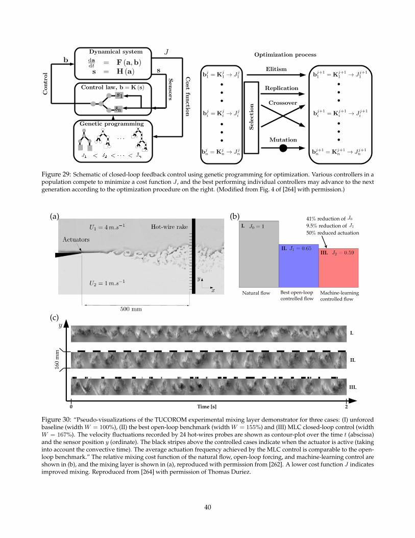
Figure 29: Schematic of closed-loop feedback control using genetic programming for optimization. Various controllers in apopulation compete to minimize a cost function J , and the best performing individual controllers may advance to the nextgeneration according to the optimization procedure on the right. (Modified from Fig. 4 of [264] with permission.)

Time [s]

I.

II.

III.

I.

II.III.

41% reduction of 9.5% reduction of 50% reduced actuation

J0

J1

y

Natural flow Best open-loop controlled flow

Machine-learning controlled flow

160

mm

0 2

(a)

(c)

(b)

Figure 30: “Pseudo-visualizations of the TUCOROM experimental mixing layer demonstrator for three cases: (I) unforcedbaseline (width W = 100%), (II) the best open-loop benchmark (width W = 155%) and (III) MLC closed-loop control (widthW = 167%). The velocity fluctuations recorded by 24 hot-wires probes are shown as contour-plot over the time t (abscissa)and the sensor position y (ordinate). The black stripes above the controlled cases indicate when the actuator is active (takinginto account the convective time). The average actuation frequency achieved by the MLC control is comparable to the open-loop benchmark.” The relative mixing cost function of the natural flow, open-loop forcing, and machine-learning control areshown in (b), and the mixing layer is shown in (a), reproduced with permission from [262]. A lower cost function J indicatesimproved mixing. Reproduced from [264] with permission of Thomas Duriez.

40

7 ConclusionsUnderstanding turbulence has been a central engineeringchallenge of the past century, with the clear goal of pas-sively manipulating and eventually actively controlling tur-bulence. Many advances in improved turbulence modelshave resulted in devices that enable passive manipulation.The focus has rapidly shifted from passive control of tur-bulence to actively controlling it, and this will surely be acentral focus of engineering efforts during the present cen-tury. Put simply, our ability to control and manipulate tur-bulence will be a deciding factor in our ability to advancekey technologies, addressing challenges in energy, security,transportation, medicine, and many other endeavors.

Our goal throughout this review has been to explorethe possibilities associated with turbulence control in variouscontexts and for different problems. We have emphasized as-pects of model complexity and resolution as well as controllogic and design objectives. In the current section, we sum-marize this review from three perspectives: historical, prac-tical, and industrial. In the next section, we point towardsexciting future directions that we believe will be particularlyimpactful for closed-loop turbulence control.

As discussed throughout this review, there is not onesingle method of turbulence control, just as there is not a sin-gle type of turbulence. Fortunately, as difficult as it has beento develop improved models of turbulence, control strategiesmay be quite robust to model imperfections and uncertain-ties. It was pointed out in [20] that models suitable for con-trol may not be suitable for accurate prediction. Hopefully,controlling turbulence will prove to be a more manageabletask than understanding it.

7.1 Historical perspectiveProgress and challenges in turbulence control may be un-derstood more clearly in a historical context. The story ofturbulence control is one of the oldest and richest chap-ters in humans’ engineering history, marking great techno-logical and theoretical strides along with ongoing struggles.An in-depth treatment of this fascinating history is beyondthe scope of this review, although there are other excellentsources [330, 331].

The first chapter of quantitative research in flow controlcan be considered to be shape optimization. While Lilien-thal optimized the wings of his gliders purely based on care-ful experiments in the 1880’s, airfoil design has profited im-mensely from potential flow theory around 1900. Joukowskiformulated his famous lift theorem for two-dimensional air-foils in 1906 after visiting Lilienthal and observing his ex-periments. Prandtl generalized the lift theory for finitewings with his famous lifting line theory in 1923. Furtherprogress in quantitative shape optimization using potentialtheory is associated with the names of Betz, von Karman andTheodorsen, to name a few. More recently, these achieve-ments have been generalized for use in adjoint-based shapeoptimization using the full Navier-Stokes equations.

The discovery of boundary-layer theory by Prandtl in1904 has stimulated active control, as suction and blow-

ing were rapidly realized to change important boundary-layer properties. The first experimental demonstrations in-cluded stabilization of boundary layers with steady suction.These efforts have enjoyed a thorough mathematical treat-ment entering Schlichting’s famous book on boundary-layertheory [332]. In the past century, many other forms of actua-tors have been invented with continually increasing author-ity and dynamic bandwidth [36]. Destabilizing control us-ing unsteady periodic forcing was considered later for mix-ing enhancements of shear flows [333].

In the 1940’s, the foundations of modern turbulencetheory were laid by Kolmogorov, Landau, Millionshtchikov,Monin, von Neumann, Obhukov and Yaglom, to name onlya few [see, e.g., 334, 335]. Neither the energy cascade nor themathematical closure approaches have entered main-streamflow control methodologies until now. Yet, the need for clo-sures in nonlinear control design is increasingly realized asan important grand challenge problem.

Around 1950, passive actuators were explored and opti-mized. The vortex generator [336] for separation mitigationis one prominent example. These developments are contin-ued — hydrophobe surfaces for ships, riblets for airplanesand spoilers on cars serving as prominent examples.

In the 1980’s, chaos theory has stimulated fluid mechan-ics toward the search for universal transition scenarios, forlow-dimensional strange attractors [337] and for chaos con-trol [338, 339]. The success of quantitative nonlinear dynam-ics methods for turbulent flows has been limited. Yet, nonlin-ear dynamics has entered fluid dynamics thinking with thequalitative notions of strange attractors, domains of attrac-tion, edge states, and bifurcations, just to name a few.

In the same period, the first closed-loop control experi-ments were performed for the suppression of boundary layerinstabilities [18], for wake stabilization [19], for skin fric-tion reduction of turbulent boundary layers [43], etc. Thefirst control designs were based on heuristic considerations,like superposition of traveling waves and opposition control.Rapidly, control theory has entered fluid mechanics [27, 212]and is providing a solid foundation for model identificationand control design. Even the nomenclature, like ’plant’ foractuated flow and ’order’ for the model dimension, is largelyborrowed from control theory.

In the late 1980’s, the foundation of many currentreduced-order models for flow control has been laid by thepioneering POD model of wall turbulence [340], the snap-shot method for POD [86, 188, 187], and other early workon coherent structures [341, 342, 343]. This development ofcontrol-oriented reduced-order models is attracting increas-ingly many researchers with numerical and experimentalcontrol demonstrations. At the same time, the challenges ofPOD models are becoming more obvious. A minimum re-quirement and challenge for model-based control design isthat the model describes unactuated and actuated states aswell as the transients between both. A more comprehensivepresentation is provided in [270].

Starting around 2000, the technological development ofmicroelectromechanical systems (MEMS) with actuators andsensors of increasing performance [69] has stimulated the de-velopment of more complex hierarchical control laws, based

41

on globally coupled local sensing and control units. This areais undergoing rapid development. The complexity of turbu-lent dynamics has been partially addressed by a novel formof model-free control design. The control laws have been castin the form of artificial neural networks with the pioneeringcomputational demonstrations in wall turbulence [22]. Cur-rently many other machine-learning methods are enteringfluid mechanics for an increasing number of analysis, mod-eling and control tasks.

There are two common and recurring themes in this his-torical perspective on turbulence control. First, advances intheory drive progress in control design. These theoreticaladvances may involve first-principles understanding of in-stabilities and turbulence itself. Additionally, theoretical ad-vances in external fields, such as linear systems, control the-ory, and dynamical systems, have all had a transformativeimpact on the direction and progress of flow control efforts.

The next general rule is that whatever is possible on theexisting hardware will be fully exploited by the software.Physical demonstrations of flow control have been necessar-ily tied to advances in sensor and actuator hardware and togrowth in computational capabilities. With recent develop-ments in micro manufacturing techniques, including MEMS,many industrial applications of closed-loop flow control arebecoming increasingly feasible.

7.2 Current practicesHere we attempt to summarize some of the current “bestpractices” gathered from success stories in the literature. Be-cause of the mercurial nature of the field, this discussion maybe viewed as a work in progress. The specific control strat-egy will vary depending on whether the goal is to minimizeor maximize a cost function, track a reference value of somequantity, or stabilize an unstable steady state and reject dis-turbances.

It is reasonable to start by assessing whether or not su-perposition holds. If so, then it is possible to develop bal-anced linear input–output models, either gray-box or black-box, and then design optimal linear feedback controllers.These controllers may be optimal in the sense of minimizingthe control expenditure, attenuating sensor noise, and reject-ing disturbances while minimizing the error of the state tosome reference value. Alternatively, if model uncertainty islarge and stability margins are critical, then it is possible tooptimize the controller for robust performance. Linear con-trol has been especially successful in delaying the transitionto turbulence, which involves stabilizing an unstable steadystate.

If superposition doesn’t hold, then the flow may bedominated by oscillatory components. If there are a fewdominant frequencies in the flow, then it is possible to de-velop a mean-field model and resulting nonlinear controllaw. This strategy has been proven effective in suppressingshedding behind bluff bodies.

If there are not strong, isolated oscillatory components,but rather there is broad-band frequency cross-talk, thenopen-loop control may be able to modify the spectrum to-ward desirable specifications. It may be necessary to explore

the input parameter space to identify the most effective com-bination of inputs for open-loop actuation. Once these inputdirections are identified, an adaptive control algorithm, suchas extremum-seeking, may be applied to find a locally op-timal open-loop forcing. Effective open-loop strategies maythen be emulated in closed-loop with added robustness.

A very general approach, including open- and closed-loop control, is enabled by machine-learning methods.Machine-learning control can be configured to yield eitheropen-loop or closed-loop control, depending on the choiceof inputs. Although the resulting controllers may approachglobally minimizing values of the cost function, there is noguaranteed convergence, and depending on the dimensionof the input space, convergence may be slow. More workis needed to extend MLC to include two-degree of freedomreference tracking control to suppress disturbances via feed-back.

The progress in turbulence control, both passive and ac-tive, has been significant, as evidenced by the ability to re-laminarize flows and reduce drag, to control separation, andto modulate mixing. However, each of these three canoni-cal flow control problems present unique challenges to largescale industrial implementation, which in turn motivate newopportunities for research. Note that the association of thefollowing three flows with corresponding control method-ologies is not inclusive, but instead covers a large portion ofthe cases in the literature.

7.2.1 Linear control and transition

Linear feedback flow control benefits from the most well-developed theoretical foundations and a set of clear goals.For instance, it is often used to stabilize unstable laminarsteady states and delay the transition to turbulence, reducingdrag. These techniques amount to a systematic approach toidentify and suppress unstable structures and disturbancesin the flow utilizing sensors and actuators. Many feedfor-ward techniques in the optimal linear control of turbulentboundary layers closely resemble opposition control, exceptthat future model predictions of disturbances are used tocancel flow structures after they have been deformed andconvected with the flow. Feedback control offers betterrobustness to unmodeled dynamics and disturbances,although it is sensitive to time-delays which are inevitable inconvective flows, as it takes time for the effect of actuation toreach downstream sensors. The limitations imposed by timedelays motivate the need for a denser array of sensors andactuators for more complex convective flows, which in turnmotivate bio-inspired sensing and actuation along with localcomputations.

7.2.2 Nonlinear control and separation

Nonlinear control presents a significant opportunity tomanipulate flows that are not close enough to a fixed pointfor linear flow control. For example, massively separatedflows are in a fully nonlinear regime, and manipulationof coherent structures requires an understanding of their

42

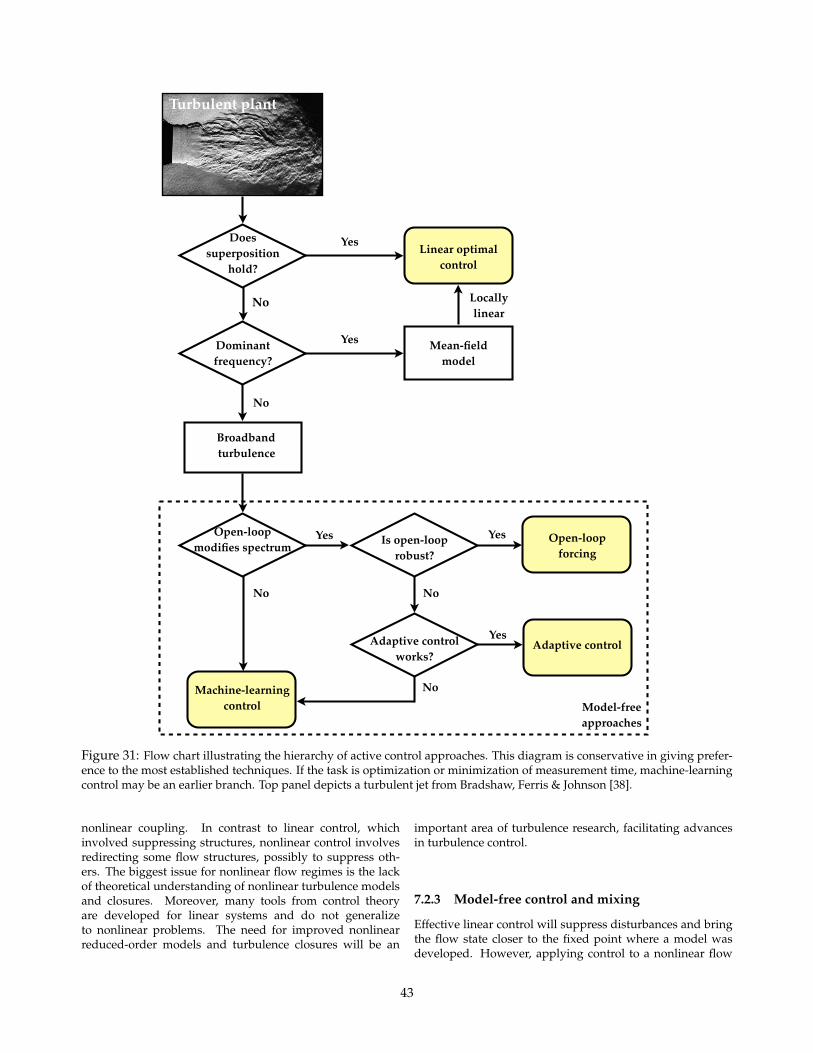
No

Turbulent plant

Does superposition

hold?

Yes

Dominant frequency?

Yes

No

Broadband turbulence

Open-loop modifies spectrum

Yes

Linear optimal control

Mean-field model

Locallylinear

No

Is open-loop robust?

Yes Open-loop forcing

Adaptive control

Machine-learning control Model-free

approaches

Adaptive control works?

No

Yes

No

Figure 31: Flow chart illustrating the hierarchy of active control approaches. This diagram is conservative in giving prefer-ence to the most established techniques. If the task is optimization or minimization of measurement time, machine-learningcontrol may be an earlier branch. Top panel depicts a turbulent jet from Bradshaw, Ferris & Johnson [38].

nonlinear coupling. In contrast to linear control, whichinvolved suppressing structures, nonlinear control involvesredirecting some flow structures, possibly to suppress oth-ers. The biggest issue for nonlinear flow regimes is the lackof theoretical understanding of nonlinear turbulence modelsand closures. Moreover, many tools from control theoryare developed for linear systems and do not generalizeto nonlinear problems. The need for improved nonlinearreduced-order models and turbulence closures will be an

important area of turbulence research, facilitating advancesin turbulence control.

7.2.3 Model-free control and mixing

Effective linear control will suppress disturbances and bringthe flow state closer to the fixed point where a model wasdeveloped. However, applying control to a nonlinear flow

43

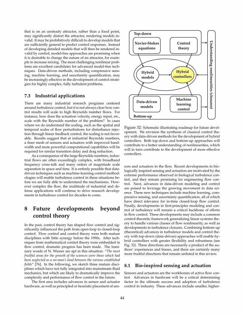
that is on an unsteady attractor, rather than a fixed point,may significantly distort the attractor, rendering models in-valid. It may be prohibitively difficult to develop models thatare sufficiently general to predict control responses. Insteadof developing detailed models that will then be rendered in-valid by control, model-free approaches are promising whenit is desirable to change the nature of an attractor, for exam-ple to increase mixing. The most challenging nonlinear prob-lems are excellent candidates for advanced model-free tech-niques. Data-driven methods, including compressive sens-ing, machine learning, and uncertainty quantification, maybe increasingly effective in the development of control strate-gies for highly complex, fully turbulent problems.

7.3 Industrial applicationsThere are many industrial research programs centeredaround turbulence control, but it is not always clear how con-trol results will scale to high Reynolds number flows. Forinstance, how does the actuation velocity, energy input, etc.,scale with the Reynolds number of the problem? In caseswhere we do understand the scaling, such as the spatial andtemporal scales of flow perturbations for disturbance rejec-tion through linear feedback control, the scaling is not favor-able. Results suggest that at industrial Reynolds numbers,a finer mesh of sensors and actuators with improved band-width and more powerful computational capabilities will berequired for similar transition delay and drag reduction.

As a consequence of the large Reynolds numbers, indus-trial flows are often exceedingly complex, with broadbandfrequency cross-talk and many orders of magnitude scaleseparation in space and time. It is entirely possible that data-driven techniques such as machine-learning control method-ologies will enable turbulence control in these situations be-fore we are fully able to understand the mechanisms. How-ever complex the flow, the multitude of industrial and de-fense applications will continue to drive research develop-ments in turbulence control for decades to come.

8 Future developments beyondcontrol theory

In the past, control theory has shaped flow control and sig-nificantly influenced the path from open-loop to closed-loopcontrol. Flow control and control theory were both maturedisciplines with little synergy before the 1990s. After tech-niques from mathematical control theory were embedded inflow control, dramatic progress has been made. The lumi-nary words of N. Wiener are apt in this situation: “The mostfruitful areas for the growth of the sciences were those which hadbeen neglected as a no-man’s land between the various establishedfields” [76]. In the following, we sketch three mature disci-plines which have not fully integrated into mainstream fluidmechanics, but which are likely to dramatically improve thecomplexity and performance of flow control in the future.

The first area includes advances in sensor and actuatorhardware, as well as principled or heuristic placement of sen-

Understanding nonlinearities (closures)

Machine learningcontrol

Data-drivenmodels

Control theory


Hybridcontrollers

Hybridmodels

Bottom-up

Top-down

Figure 32: Schematic illustrating roadmap for future devel-opment. We envision the synthesis of classical control the-ory with data-driven methods for the development of hybridcontrollers. Both top-down and bottom-up approaches willcontribute to a better understanding of nonlinearities, whichwill in turn contribute to the development of more effectivecontrollers.

sors and actuators in the flow. Recent developments in bio-logically inspired sensing and actuation are motivated by theextreme performance observed in biological turbulence con-trol, and they remain promising for engineering flow con-trol. Next, advances in data-driven modeling and controlare poised to leverage the growing movement in data sci-ence. These new techniques include machine learning, com-pressive sensing, and uncertainty quantification, all of whichhave direct relevance for in-time closed-loop flow control.Finally, developments in first-principles modeling and con-trol of turbulence will remain a critical backbone of effortsin flow control. These developments may include a commoncontrol-theoretic framework generalizing linear systems the-ory to handle various classes of flow nonlinearity, as well asdevelopments in turbulence closures. Combining bottom-up(theoretical) advances in turbulence models and control the-ory with top-down (data-driven) approaches will enable hy-brid controllers with greater flexibility and robustness (seeFig. 32). These directions are necessarily a product of the au-thors’ experiences and biases, and there are certainly manymore fruitful directions that remain unlisted in this review.

8.1 Bio-inspired sensing and actuationSensors and actuators are the workhorses of active flow con-trol. Advances in hardware will be a critical determiningfactor in the ultimate success and adoption of turbulencecontrol in industry. These advances include smaller, higher-

44

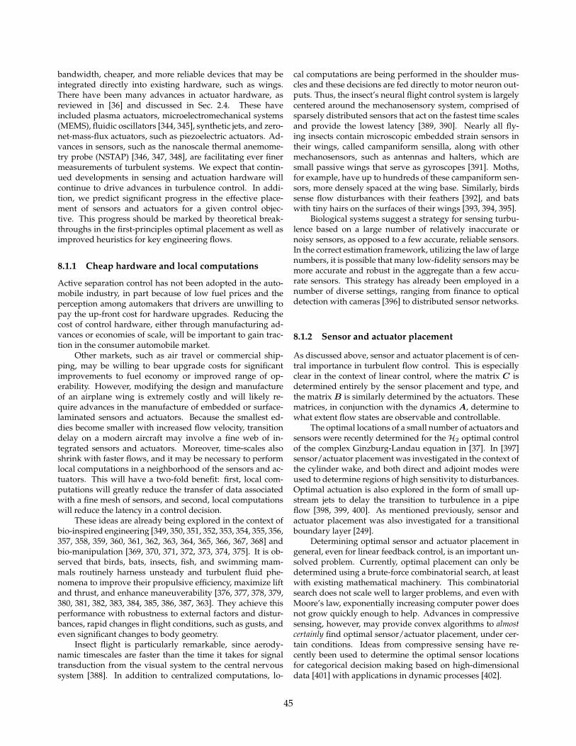
bandwidth, cheaper, and more reliable devices that may beintegrated directly into existing hardware, such as wings.There have been many advances in actuator hardware, asreviewed in [36] and discussed in Sec. 2.4. These haveincluded plasma actuators, microelectromechanical systems(MEMS), fluidic oscillators [344, 345], synthetic jets, and zero-net-mass-flux actuators, such as piezoelectric actuators. Ad-vances in sensors, such as the nanoscale thermal anemome-try probe (NSTAP) [346, 347, 348], are facilitating ever finermeasurements of turbulent systems. We expect that contin-ued developments in sensing and actuation hardware willcontinue to drive advances in turbulence control. In addi-tion, we predict significant progress in the effective place-ment of sensors and actuators for a given control objec-tive. This progress should be marked by theoretical break-throughs in the first-principles optimal placement as well asimproved heuristics for key engineering flows.

8.1.1 Cheap hardware and local computations

Active separation control has not been adopted in the auto-mobile industry, in part because of low fuel prices and theperception among automakers that drivers are unwilling topay the up-front cost for hardware upgrades. Reducing thecost of control hardware, either through manufacturing ad-vances or economies of scale, will be important to gain trac-tion in the consumer automobile market.

Other markets, such as air travel or commercial ship-ping, may be willing to bear upgrade costs for significantimprovements to fuel economy or improved range of op-erability. However, modifying the design and manufactureof an airplane wing is extremely costly and will likely re-quire advances in the manufacture of embedded or surface-laminated sensors and actuators. Because the smallest ed-dies become smaller with increased flow velocity, transitiondelay on a modern aircraft may involve a fine web of in-tegrated sensors and actuators. Moreover, time-scales alsoshrink with faster flows, and it may be necessary to performlocal computations in a neighborhood of the sensors and ac-tuators. This will have a two-fold benefit: first, local com-putations will greatly reduce the transfer of data associatedwith a fine mesh of sensors, and second, local computationswill reduce the latency in a control decision.

These ideas are already being explored in the context ofbio-inspired engineering [349, 350, 351, 352, 353, 354, 355, 356,357, 358, 359, 360, 361, 362, 363, 364, 365, 366, 367, 368] andbio-manipulation [369, 370, 371, 372, 373, 374, 375]. It is ob-served that birds, bats, insects, fish, and swimming mam-mals routinely harness unsteady and turbulent fluid phe-nomena to improve their propulsive efficiency, maximize liftand thrust, and enhance maneuverability [376, 377, 378, 379,380, 381, 382, 383, 384, 385, 386, 387, 363]. They achieve thisperformance with robustness to external factors and distur-bances, rapid changes in flight conditions, such as gusts, andeven significant changes to body geometry.

Insect flight is particularly remarkable, since aerody-namic timescales are faster than the time it takes for signaltransduction from the visual system to the central nervoussystem [388]. In addition to centralized computations, lo-

cal computations are being performed in the shoulder mus-cles and these decisions are fed directly to motor neuron out-puts. Thus, the insect’s neural flight control system is largelycentered around the mechanosensory system, comprised ofsparsely distributed sensors that act on the fastest time scalesand provide the lowest latency [389, 390]. Nearly all fly-ing insects contain microscopic embedded strain sensors intheir wings, called campaniform sensilla, along with othermechanosensors, such as antennas and halters, which aresmall passive wings that serve as gyroscopes [391]. Moths,for example, have up to hundreds of these campaniform sen-sors, more densely spaced at the wing base. Similarly, birdssense flow disturbances with their feathers [392], and batswith tiny hairs on the surfaces of their wings [393, 394, 395].

Biological systems suggest a strategy for sensing turbu-lence based on a large number of relatively inaccurate ornoisy sensors, as opposed to a few accurate, reliable sensors.In the correct estimation framework, utilizing the law of largenumbers, it is possible that many low-fidelity sensors may bemore accurate and robust in the aggregate than a few accu-rate sensors. This strategy has already been employed in anumber of diverse settings, ranging from finance to opticaldetection with cameras [396] to distributed sensor networks.

8.1.2 Sensor and actuator placement

As discussed above, sensor and actuator placement is of cen-tral importance in turbulent flow control. This is especiallyclear in the context of linear control, where the matrix C isdetermined entirely by the sensor placement and type, andthe matrixB is similarly determined by the actuators. Thesematrices, in conjunction with the dynamics A, determine towhat extent flow states are observable and controllable.

The optimal locations of a small number of actuators andsensors were recently determined for theH2 optimal controlof the complex Ginzburg-Landau equation in [37]. In [397]sensor/actuator placement was investigated in the context ofthe cylinder wake, and both direct and adjoint modes wereused to determine regions of high sensitivity to disturbances.Optimal actuation is also explored in the form of small up-stream jets to delay the transition to turbulence in a pipeflow [398, 399, 400]. As mentioned previously, sensor andactuator placement was also investigated for a transitionalboundary layer [249].

Determining optimal sensor and actuator placement ingeneral, even for linear feedback control, is an important un-solved problem. Currently, optimal placement can only bedetermined using a brute-force combinatorial search, at leastwith existing mathematical machinery. This combinatorialsearch does not scale well to larger problems, and even withMoore’s law, exponentially increasing computer power doesnot grow quickly enough to help. Advances in compressivesensing, however, may provide convex algorithms to almostcertainly find optimal sensor/actuator placement, under cer-tain conditions. Ideas from compressive sensing have re-cently been used to determine the optimal sensor locationsfor categorical decision making based on high-dimensionaldata [401] with applications in dynamic processes [402].

45

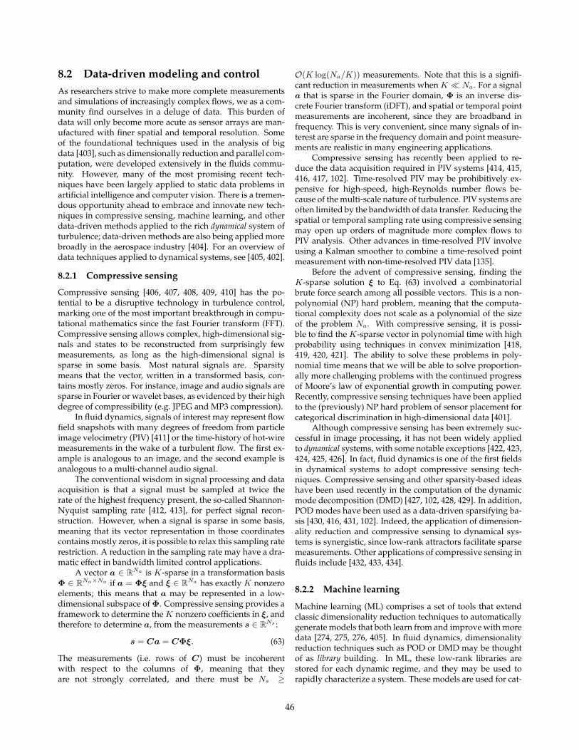
8.2 Data-driven modeling and controlAs researchers strive to make more complete measurementsand simulations of increasingly complex flows, we as a com-munity find ourselves in a deluge of data. This burden ofdata will only become more acute as sensor arrays are man-ufactured with finer spatial and temporal resolution. Someof the foundational techniques used in the analysis of bigdata [403], such as dimensionally reduction and parallel com-putation, were developed extensively in the fluids commu-nity. However, many of the most promising recent tech-niques have been largely applied to static data problems inartificial intelligence and computer vision. There is a tremen-dous opportunity ahead to embrace and innovate new tech-niques in compressive sensing, machine learning, and otherdata-driven methods applied to the rich dynamical system ofturbulence; data-driven methods are also being applied morebroadly in the aerospace industry [404]. For an overview ofdata techniques applied to dynamical systems, see [405, 402].

8.2.1 Compressive sensing

Compressive sensing [406, 407, 408, 409, 410] has the po-tential to be a disruptive technology in turbulence control,marking one of the most important breakthrough in compu-tational mathematics since the fast Fourier transform (FFT).Compressive sensing allows complex, high-dimensional sig-nals and states to be reconstructed from surprisingly fewmeasurements, as long as the high-dimensional signal issparse in some basis. Most natural signals are. Sparsitymeans that the vector, written in a transformed basis, con-tains mostly zeros. For instance, image and audio signals aresparse in Fourier or wavelet bases, as evidenced by their highdegree of compressibility (e.g. JPEG and MP3 compression).

In fluid dynamics, signals of interest may represent flowfield snapshots with many degrees of freedom from particleimage velocimetry (PIV) [411] or the time-history of hot-wiremeasurements in the wake of a turbulent flow. The first ex-ample is analogous to an image, and the second example isanalogous to a multi-channel audio signal.

The conventional wisdom in signal processing and dataacquisition is that a signal must be sampled at twice therate of the highest frequency present, the so-called Shannon-Nyquist sampling rate [412, 413], for perfect signal recon-struction. However, when a signal is sparse in some basis,meaning that its vector representation in those coordinatescontains mostly zeros, it is possible to relax this sampling raterestriction. A reduction in the sampling rate may have a dra-matic effect in bandwidth limited control applications.

A vector a ∈ RNa is K-sparse in a transformation basisΦ ∈ RNa×Na if a = Φξ and ξ ∈ RNa has exactly K nonzeroelements; this means that a may be represented in a low-dimensional subspace of Φ. Compressive sensing provides aframework to determine the K nonzero coefficients in ξ, andtherefore to determine a, from the measurements s ∈ RNs :

s = Ca = CΦξ. (63)

The measurements (i.e. rows of C) must be incoherentwith respect to the columns of Φ, meaning that theyare not strongly correlated, and there must be Ns ≥

O(K log(Na/K)) measurements. Note that this is a signifi-cant reduction in measurements when K Na. For a signala that is sparse in the Fourier domain, Φ is an inverse dis-crete Fourier transform (iDFT), and spatial or temporal pointmeasurements are incoherent, since they are broadband infrequency. This is very convenient, since many signals of in-terest are sparse in the frequency domain and point measure-ments are realistic in many engineering applications.

Compressive sensing has recently been applied to re-duce the data acquisition required in PIV systems [414, 415,416, 417, 102]. Time-resolved PIV may be prohibitively ex-pensive for high-speed, high-Reynolds number flows be-cause of the multi-scale nature of turbulence. PIV systems areoften limited by the bandwidth of data transfer. Reducing thespatial or temporal sampling rate using compressive sensingmay open up orders of magnitude more complex flows toPIV analysis. Other advances in time-resolved PIV involveusing a Kalman smoother to combine a time-resolved pointmeasurement with non-time-resolved PIV data [135].

Before the advent of compressive sensing, finding theK-sparse solution ξ to Eq. (63) involved a combinatorialbrute force search among all possible vectors. This is a non-polynomial (NP) hard problem, meaning that the computa-tional complexity does not scale as a polynomial of the sizeof the problem Na. With compressive sensing, it is possi-ble to find the K-sparse vector in polynomial time with highprobability using techniques in convex minimization [418,419, 420, 421]. The ability to solve these problems in poly-nomial time means that we will be able to solve proportion-ally more challenging problems with the continued progressof Moore’s law of exponential growth in computing power.Recently, compressive sensing techniques have been appliedto the (previously) NP hard problem of sensor placement forcategorical discrimination in high-dimensional data [401].

Although compressive sensing has been extremely suc-cessful in image processing, it has not been widely appliedto dynamical systems, with some notable exceptions [422, 423,424, 425, 426]. In fact, fluid dynamics is one of the first fieldsin dynamical systems to adopt compressive sensing tech-niques. Compressive sensing and other sparsity-based ideashave been used recently in the computation of the dynamicmode decomposition (DMD) [427, 102, 428, 429]. In addition,POD modes have been used as a data-driven sparsifying ba-sis [430, 416, 431, 102]. Indeed, the application of dimension-ality reduction and compressive sensing to dynamical sys-tems is synergistic, since low-rank attractors facilitate sparsemeasurements. Other applications of compressive sensing influids include [432, 433, 434].

8.2.2 Machine learning

Machine learning (ML) comprises a set of tools that extendclassic dimensionality reduction techniques to automaticallygenerate models that both learn from and improve with moredata [274, 275, 276, 405]. In fluid dynamics, dimensionalityreduction techniques such as POD or DMD may be thoughtof as library building. In ML, these low-rank libraries arestored for each dynamic regime, and they may be used torapidly characterize a system. These models are used for cat-

46

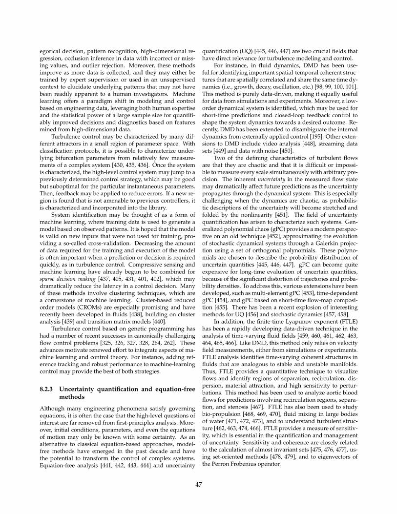
egorical decision, pattern recognition, high-dimensional re-gression, occlusion inference in data with incorrect or miss-ing values, and outlier rejection. Moreover, these methodsimprove as more data is collected, and they may either betrained by expert supervision or used in an unsupervisedcontext to elucidate underlying patterns that may not havebeen readily apparent to a human investigators. Machinelearning offers a paradigm shift in modeling and controlbased on engineering data, leveraging both human expertiseand the statistical power of a large sample size for quantifi-ably improved decisions and diagnostics based on featuresmined from high-dimensional data.

Turbulence control may be characterized by many dif-ferent attractors in a small region of parameter space. Withclassification protocols, it is possible to characterize under-lying bifurcation parameters from relatively few measure-ments of a complex system [430, 435, 436]. Once the systemis characterized, the high-level control system may jump to apreviously determined control strategy, which may be goodbut suboptimal for the particular instantaneous parameters.Then, feedback may be applied to reduce errors. If a new re-gion is found that is not amenable to previous controllers, itis characterized and incorporated into the library.

System identification may be thought of as a form ofmachine learning, where training data is used to generate amodel based on observed patterns. It is hoped that the modelis valid on new inputs that were not used for training, pro-viding a so-called cross-validation. Decreasing the amountof data required for the training and execution of the modelis often important when a prediction or decision is requiredquickly, as in turbulence control. Compressive sensing andmachine learning have already begun to be combined forsparse decision making [437, 405, 431, 401, 402], which maydramatically reduce the latency in a control decision. Manyof these methods involve clustering techniques, which area cornerstone of machine learning. Cluster-based reducedorder models (CROMs) are especially promising and haverecently been developed in fluids [438], building on clusteranalysis [439] and transition matrix models [440].

Turbulence control based on genetic programming hashad a number of recent successes in canonically challengingflow control problems [325, 326, 327, 328, 264, 262]. Theseadvances motivate renewed effort to integrate aspects of ma-chine learning and control theory. For instance, adding ref-erence tracking and robust performance to machine-learningcontrol may provide the best of both strategies.

8.2.3 Uncertainty quantification and equation-freemethods

Although many engineering phenomena satisfy governingequations, it is often the case that the high-level questions ofinterest are far removed from first-principles analysis. More-over, initial conditions, parameters, and even the equationsof motion may only be known with some certainty. As analternative to classical equation-based approaches, model-free methods have emerged in the past decade and havethe potential to transform the control of complex systems.Equation-free analysis [441, 442, 443, 444] and uncertainty

quantification (UQ) [445, 446, 447] are two crucial fields thathave direct relevance for turbulence modeling and control.

For instance, in fluid dynamics, DMD has been use-ful for identifying important spatial-temporal coherent struc-tures that are spatially correlated and share the same time dy-namics (i.e., growth, decay, oscillation, etc.) [98, 99, 100, 101].This method is purely data-driven, making it equally usefulfor data from simulations and experiments. Moreover, a low-order dynamical system is identified, which may be used forshort-time predictions and closed-loop feedback control toshape the system dynamics towards a desired outcome. Re-cently, DMD has been extended to disambiguate the internaldynamics from externally applied control [195]. Other exten-sions to DMD include video analysis [448], streaming datasets [449] and data with noise [450].

Two of the defining characteristics of turbulent flowsare that they are chaotic and that it is difficult or impossi-ble to measure every scale simultaneously with arbitrary pre-cision. The inherent uncertainty in the measured flow statemay dramatically affect future predictions as the uncertaintypropagates through the dynamical system. This is especiallychallenging when the dynamics are chaotic, as probabilis-tic descriptions of the uncertainty will become stretched andfolded by the nonlinearity [451]. The field of uncertaintyquantification has arisen to characterize such systems. Gen-eralized polynomial chaos (gPC) provides a modern perspec-tive on an old technique [452], approximating the evolutionof stochastic dynamical systems through a Galerkin projec-tion using a set of orthogonal polynomials. These polyno-mials are chosen to describe the probability distribution ofuncertain quantities [445, 446, 447]. gPC can become quiteexpensive for long-time evaluation of uncertain quantities,because of the significant distortion of trajectories and proba-bility densities. To address this, various extensions have beendeveloped, such as multi-element gPC [453], time-dependentgPC [454], and gPC based on short-time flow-map composi-tion [455]. There has been a recent explosion of interestingmethods for UQ [456] and stochastic dynamics [457, 458].

In addition, the finite-time Lyapunov exponent (FTLE)has been a rapidly developing data-driven technique in theanalysis of time-varying fluid fields [459, 460, 461, 462, 463,464, 465, 466]. Like DMD, this method only relies on velocityfield measurements, either from simulations or experiments.FTLE analysis identifies time-varying coherent structures influids that are analogous to stable and unstable manifolds.Thus, FTLE provides a quantitative technique to visualizeflows and identify regions of separation, recirculation, dis-persion, material attraction, and high sensitivity to pertur-bations. This method has been used to analyze aortic bloodflows for predictions involving recirculation regions, separa-tion, and stenosis [467]. FTLE has also been used to studybio-propulsion [468, 469, 470], fluid mixing in large bodiesof water [471, 472, 473], and to understand turbulent struc-ture [462, 463, 474, 466]. FTLE provides a measure of sensitiv-ity, which is essential in the quantification and managementof uncertainty. Sensitivity and coherence are closely relatedto the calculation of almost invariant sets [475, 476, 477], us-ing set-oriented methods [478, 479], and to eigenvectors ofthe Perron Frobenius operator.

47

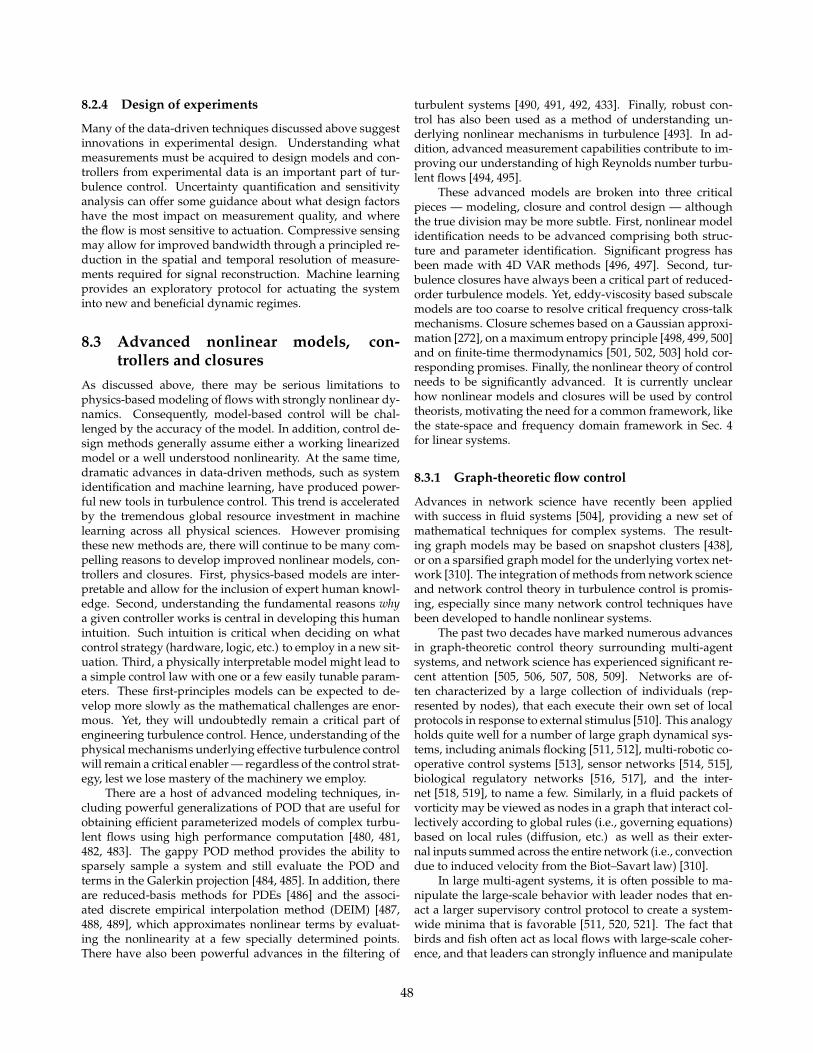
8.2.4 Design of experiments

Many of the data-driven techniques discussed above suggestinnovations in experimental design. Understanding whatmeasurements must be acquired to design models and con-trollers from experimental data is an important part of tur-bulence control. Uncertainty quantification and sensitivityanalysis can offer some guidance about what design factorshave the most impact on measurement quality, and wherethe flow is most sensitive to actuation. Compressive sensingmay allow for improved bandwidth through a principled re-duction in the spatial and temporal resolution of measure-ments required for signal reconstruction. Machine learningprovides an exploratory protocol for actuating the systeminto new and beneficial dynamic regimes.

8.3 Advanced nonlinear models, con-trollers and closures

As discussed above, there may be serious limitations tophysics-based modeling of flows with strongly nonlinear dy-namics. Consequently, model-based control will be chal-lenged by the accuracy of the model. In addition, control de-sign methods generally assume either a working linearizedmodel or a well understood nonlinearity. At the same time,dramatic advances in data-driven methods, such as systemidentification and machine learning, have produced power-ful new tools in turbulence control. This trend is acceleratedby the tremendous global resource investment in machinelearning across all physical sciences. However promisingthese new methods are, there will continue to be many com-pelling reasons to develop improved nonlinear models, con-trollers and closures. First, physics-based models are inter-pretable and allow for the inclusion of expert human knowl-edge. Second, understanding the fundamental reasons whya given controller works is central in developing this humanintuition. Such intuition is critical when deciding on whatcontrol strategy (hardware, logic, etc.) to employ in a new sit-uation. Third, a physically interpretable model might lead toa simple control law with one or a few easily tunable param-eters. These first-principles models can be expected to de-velop more slowly as the mathematical challenges are enor-mous. Yet, they will undoubtedly remain a critical part ofengineering turbulence control. Hence, understanding of thephysical mechanisms underlying effective turbulence controlwill remain a critical enabler — regardless of the control strat-egy, lest we lose mastery of the machinery we employ.

There are a host of advanced modeling techniques, in-cluding powerful generalizations of POD that are useful forobtaining efficient parameterized models of complex turbu-lent flows using high performance computation [480, 481,482, 483]. The gappy POD method provides the ability tosparsely sample a system and still evaluate the POD andterms in the Galerkin projection [484, 485]. In addition, thereare reduced-basis methods for PDEs [486] and the associ-ated discrete empirical interpolation method (DEIM) [487,488, 489], which approximates nonlinear terms by evaluat-ing the nonlinearity at a few specially determined points.There have also been powerful advances in the filtering of

turbulent systems [490, 491, 492, 433]. Finally, robust con-trol has also been used as a method of understanding un-derlying nonlinear mechanisms in turbulence [493]. In ad-dition, advanced measurement capabilities contribute to im-proving our understanding of high Reynolds number turbu-lent flows [494, 495].

These advanced models are broken into three criticalpieces — modeling, closure and control design — althoughthe true division may be more subtle. First, nonlinear modelidentification needs to be advanced comprising both struc-ture and parameter identification. Significant progress hasbeen made with 4D VAR methods [496, 497]. Second, tur-bulence closures have always been a critical part of reduced-order turbulence models. Yet, eddy-viscosity based subscalemodels are too coarse to resolve critical frequency cross-talkmechanisms. Closure schemes based on a Gaussian approxi-mation [272], on a maximum entropy principle [498, 499, 500]and on finite-time thermodynamics [501, 502, 503] hold cor-responding promises. Finally, the nonlinear theory of controlneeds to be significantly advanced. It is currently unclearhow nonlinear models and closures will be used by controltheorists, motivating the need for a common framework, likethe state-space and frequency domain framework in Sec. 4for linear systems.

8.3.1 Graph-theoretic flow control

Advances in network science have recently been appliedwith success in fluid systems [504], providing a new set ofmathematical techniques for complex systems. The result-ing graph models may be based on snapshot clusters [438],or on a sparsified graph model for the underlying vortex net-work [310]. The integration of methods from network scienceand network control theory in turbulence control is promis-ing, especially since many network control techniques havebeen developed to handle nonlinear systems.

The past two decades have marked numerous advancesin graph-theoretic control theory surrounding multi-agentsystems, and network science has experienced significant re-cent attention [505, 506, 507, 508, 509]. Networks are of-ten characterized by a large collection of individuals (rep-resented by nodes), that each execute their own set of localprotocols in response to external stimulus [510]. This analogyholds quite well for a number of large graph dynamical sys-tems, including animals flocking [511, 512], multi-robotic co-operative control systems [513], sensor networks [514, 515],biological regulatory networks [516, 517], and the inter-net [518, 519], to name a few. Similarly, in a fluid packets ofvorticity may be viewed as nodes in a graph that interact col-lectively according to global rules (i.e., governing equations)based on local rules (diffusion, etc.) as well as their exter-nal inputs summed across the entire network (i.e., convectiondue to induced velocity from the Biot–Savart law) [310].

In large multi-agent systems, it is often possible to ma-nipulate the large-scale behavior with leader nodes that en-act a larger supervisory control protocol to create a system-wide minima that is favorable [511, 520, 521]. The fact thatbirds and fish often act as local flows with large-scale coher-ence, and that leaders can strongly influence and manipulate

48

the large-scale coherent motion [511, 512], is promising whenconsidering network-based fluid flow control. Based on thenetwork-control methodology used to analyze schooling fishand flocking birds [511, 512], there is an appealing goal ofschooling turbulence by collecting and harnessing distributedmulti-scale eddies into a collective organization, or commu-nity, with favorable large-scale properties.

Recent work investigating the number of leader nodesrequired for structural controllability of a network [521] sug-gests that large, sparse networks with heterogenous degreedistributions4,such as scale-free turbulence networks, are es-pecially difficult to control. In particular, the number ofdriver nodes may be quite large for these systems, as com-pared with a regular or random graph with more homoge-neous degree distribution. However, full structural control-lability of a turbulent vortex network is not necessarily a rea-sonable or desirable goal. In fact, these results are consistentwith physical intuition that controlling every single turbu-lent eddy would require immense control authority with dis-tributed actuation over a number of spatial locations.

In flow control, especially for turbulent fluids, the goalis not necessarily to control every minor eddy in the flow,but rather to manipulate the base flow and large-scale coher-ent structures that mediate quantities of interest (lift, drag,etc.). In addition, practically, we are more interested in thedegree of controllability [522], rather than structural controlla-bility, of large-scale vortical structures in order to manipulatethe base flow. Even with the goal of increasing mixing, whichinvolves increasing the level of turbulence, individual eddiesneed not be controlled, but rather control should manipulatethe statistical distribution of eddies that determine dominantenergy balances in the fluid.

8.3.2 Markov model-based control

One elegant strategy comprising modeling, closures andcontrol design starts with the Liouville equation for the prob-ability distribution [523]. The probability density p(a, t) ofEq. (2a) evolves according to the Liouville equation

∂tp(a, t) +∇a · [f(a, b) p(a, t)] = 0,

where ∇a is the Nabla operator in the state space. The ele-gance lies in the fact that this evolution equation is a linearconservation equation for the probability distribution andthus allows to take advantage of the sophisticated linear con-trol design methods for nonlinear dynamics. In addition, theprobability distribution gives immediate access to engineer-ing goals, like average drag, average lift or level of fluctua-tion. Such averages are not provided by linear(ized) mod-els. However, the challenge is that the Liouville equationof the Navier-Stokes equation [524] is a functional equationand thus computationally far more demanding than the orig-inal equation. Yet, a suitable cluster-based phase-space dis-cretization may reduce this Liouville equation down to alow-dimensional linear Markov model [439, 438] providing

4The degree distribution of a network is the distribution of howmany other nodes each node is connected to. All scale-free networksare inherently sparse, with heterogeneous degree distribution [508].

easy access to linear control design. Intriguingly, the adjointof the Liouville equation is related to the Koopman operator[438, 525, 526]. This deep relation still waits to be exploited inprobability control. In summary, there are plenty of promis-ing opportunities advancing nonlinear model-based control.

AcknowledgementsWe have benefited tremendously from many fruitful dis-cussions on machine learning, compressive sensing, andcontrol of complex dynamical systems with Nathan Kutz,Josh Proctor, and Bing Brunton. We acknowledge highlystimulating discussions with the local TUCOROM team(Jean-Paul Bonnet, Laurent Cordier, Joel Delville, ThomasDuriez, Eurika Kaiser, Kai von Krbek, Jean-Charles Lau-rentie, Vladimir Parezanovic and Andreas Spohn), withthe OpenLab PPRIME/PSA team (Diogo Barros, Cecile Li,Jacques Boree and Tony Ruiz), with the SepaCoDe teammanaged by Azeddine Kourta, Andreas Spohn and MichelStanislas, with Ambrosys (Markus W. Abel, Marc Segond),with the SFB 880, in particular Rolf Radespiel, Peter Scholzand Richard Semaan, with the ARC team (Robert Niven andSteven Waldrip), and with our close visitors and collabo-rators Jean-Luc Aider, Shervin Bagheri, Maciej Balajewicz,Zacharias Berger, Jason Bourgeois, Helmut Eckelmann, Nico-las Gautiers, Mark Glauser, Hans-Christian Hege, Jens Kas-ten, Sinisa Krajnovic, Jacques Lewalle, Kervin Low, RobertMartinuzzi, Marek Morzynski, Christian Nayeri, Jan Osth,Oliver Paschereit, Brian Polagye, Bartosz Protas, MichaelSchlegel, Tamir Shaqarin, Sam Taira, Jonathan Tu, and DaveWilliams.

SLB would also like to gratefully acknowledge andthank Clancy Rowley, Richard Murray, Rob Stengel, andNaomi Leonard, who each found unique ways to make con-trol theory come to life. SLB has also had the pleasure oflearning about bio-inspired fluids from Tom Daniel and tur-bulence from Lex Smits, Jim Riley, and Gigi Martinelli. SLBwas generously supported by the University of Washing-ton departments of Mechanical Engineering and as a DataScience Fellow in the eScience Institute (NSF, Moore-SloanFoundation, Washington Research Foundation), as well asthe Department of Energy and Boeing.

BRN is deeply indebted to his turbulence control men-tors Andrzej Banaszuk, Andreas Dillmann, Helmut Eckel-mann, Rudibert King and William K. George who shared andfueled the passion for the field. BRN acknowledges generousfunding from the French Agence Nationale de la Recherche(ANR) via the Senior Chair of Excellence TUCOROM andthe SepaCoDe project, from the OpenLab PPRIME/PSA byPeugeot-Citroen, from the region Poitou-Charentes, from theGerman Science Foundation via the Collaborative ResearchCenter SFB 880, from the Rector-Funded Visiting Professor-ship of the UNSW, Canberra, Australia, from the US NationalResearch Foundatiation via the PIRE grant OISE-0968313from Ambrosys GmbH, Potsdam, Germany and from BerndNoack Cybernetics Foundation.

We are deeply indebted to both anonymous referees forproviding valuable suggestions regarding many technical as-pects of the manuscript.

49

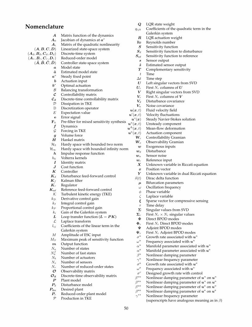
NomenclatureA Matrix function of the dynamicsA0 Jacobian of dynamics at as

Ai Matrix of the quadratic nonlinearity(A,B,C,D) Linearized state-space system

(Ad,Bd,Cd,Dd) Discrete-time system(Ar,Br,Cr,Dr) Reduced-order model

(A, B, C, D) Controller state-space systema Model statea Estimated model stateas Steady fixed pointb Actuation inputb∗ Optimal actuationB Balancing transformationC Controllability matrix

Cd Discrete-time controllability matrixD Dissipation in TKED Discretization operatorE Expectation valuee Error signal

Fk Pre-filter for mixed sensitivity synthesisf DynamicsG Forcing in TKEg Volume forceH Hankel matrixH2 Hardy space with bounded two normH∞ Hardy space with bounded infinity normh Impulse response functionhk Volterra kernelsI Identity matrixJ Cost functionK ControllerKd Disturbance feed-forward controlKf Kalman filterKr RegulatorKref Reference feed-forward controlK Turbulent kinetic energy (TKE)kD Derivative control gainkI Integral control gainkP Proportional control gainki Gain of the Galerkin systemL Loop transfer function (L = PK)L Laplace transformlij Coefficients of the linear term in the

Galerkin systemM Amplitude of ESC inputMS Maximum peak of sensitivity functionm Output functionNa Number of statesNfa Number of fast statesNb Number of actuatorsNs Number of sensorsNr Number of reduced-order statesO Observability matrix

Od Discrete-time observability matrixP Plant modelPd Disturbance modelPdes Desired plantPr Reduced-order plant modelP Production in TKE

Q LQR state weightqijk Coefficients of the quadratic term in the

Galerkin systemR LQR actuation weightRe Reynolds numberS Sensitivity functionSd Sensitivity function to disturbanceSref Sensitivity function to references Sensor outputs Estimated sensor outputT Complementary sensitivityt Time

∆t Time stepU Left singular vectors from SVDUr First Nr columns of UV Right singular vectors from SVDVr First Nr columns of VVd Disturbance covarianceVn Noise covariance

u(x, t) Fluid velocity fieldu′(x, t) Velocity fluctuationsus(x) Steady Navier-Stokes solution

uu(x, t) Unsteady componentu∆(x, t) Mean-flow deformationua(x, t) Actuation component

Wc Controllability GramianWo Observability Gramianw Exogenous inputswd Disturbancewn Sensor noisewr Reference inputX Unknown variable in Riccati equationx Position vectorY Unknown variable in dual Riccati equation

δ(t) Dirac delta functionµ Bifurcation parametersω Oscillation frequencyφ Phase variableζ Laplace variableξ Sparse vector for compressive sensingτ Time delayΣ Singular values from SVD

Σr First Nr ×Nr singular valuesΦ Direct BPOD modes

Φr First Nr Direct BPOD modesΨ Adjoint BPOD modes

Ψr First Nr Adjoint BPOD modesσu Growth rate associated with uu

ωu Frequency associated with uu

αu Manifold parameter associated with uu

αa Manifold parameter associated with ua

βu Nonlinear damping parameterγu Nonlinear frequency parameterσa Growth rate associated with ua

ωa Frequency associated with ua

σc Designed growth rate with controlβuu Nonlinear damping parameter of uu on uu

βau Nonlinear damping parameter of uu on ua

βua Nonlinear damping parameter of ua on uu

βaa Nonlinear damping parameter of ua on ua

γ∗∗ Nonlinear frequency parameter(superscripts have analogous meaning as in β)

50

References

[1] Fish, F. E. and Lauder, G. V. Passive and active flow control by swim-ming fishes and mammals. Annual Review of Fluid Mechanics, 38:193–224,2006.

[2] Ahlborn, B. K. Zoological Physics. Springer-Verlag, 2004.[3] Dean, B. and Bhushan, B. Shark-skin surfaces for fluid-drag reduction

in turbulent flow: a review. Philosophical Transactions of the Royal SocietyA: Mathematical, Physical and Engineering Sciences, 368(1929):4775–4806,2010.

[4] Bechert, D. W., Bruse, M., Hage, W., van der Hoeven, J. G. T., andHoppe, G. Experiments on drag-reducing surfaces and their optimiza-tion with an adjustable geometry. Journal of Fluid Mechanics, 338:59–87,1997.

[5] Gillieron, P. and Kourta, A. Aerodynamic drag reduction by verticalsplitter plates. Experiments in Fluids, 48(1):1–16, 2010.

[6] Grandemange, M., Ricot, D., Vartanian, C., Ruiz, T., and Cadot, O. Char-acterisation of the flow past real road vehicles with blunt afterbodies.International Journal of Aerodynamics, 4(1):24–42, 2014.

[7] Pfeiffer, J. and King, R. Multivariable closed-loop flow control of dragand yaw moment for a 3d bluff body. In 6th AIAA Flow Control Confer-ence, pages 1–14, Atlanta, Georgia, USA, 2012.

[8] Gad-el Hak, M. Flow control. Applied mechanics reviews, 42(10):261–293,1989.

[9] Gad-el Hak, M. and Tsai, H. M. Transition and turbulence control, vol-ume 8. World Scientific, 2006.

[10] Kim, J. Physics and control of wall turbulence for drag reduction. Philo-sophical Transactions of the Royal Society A: Mathematical, Physical and En-gineering Sciences, 369(1940):1396–1411, 2011.

[11] Baker, C., Jones, J., Lopez-Calleja, F., and Munday, J. Measurements ofthe cross wind forces on trains. Journal of Wind Engineering and IndustrialAerodynamics, 92(7):547–563, 2004.

[12] Baker, C. The flow around high speed trains. Journal of Wind Engineeringand Industrial Aerodynamics, 98(6):277–298, 2010.

[13] Schetz, J. A. Aerodynamics of high-speed trains. Annual Review of FluidMechanics, 33(1):371–414, 2001.

[14] Gad-el Hak, M. Modern developments in flow control. Appl. Mech. Rev.,49:365–379, 1996.

[15] Barber, T. J. Private communication, 1999.[16] King, R., editor. Active Flow Control, number 95 in Notes on Numeri-

cal Fluid Mechanics and Interdisciplinary Design, Berlin, 2007. SpringerVerlag.

[17] King, R., editor. Active Flow Control II, number 108 in Notes on Nu-merical Fluid Mechanics and Interdisciplinary Design, Berlin, 2010.Springer-Verlag.

[18] Liepmann, H. and Nosenchuck, D. Active control of laminar-turbulenttransition. Journal of Fluid Mechanics, 118:201–204, 1982.

[19] Roussopoulos, K. Feedback control of vortex shedding at low Reynoldsnumbers. Journal of Fluid Mechanics, 248:267–296, 1993.

[20] Kim, J. and Bewley, T. A linear systems approach to flow control. AnnualReview of Fluid Mechanics, 39:383–417, 2007.

[21] Sipp, D., Marquet, O., Meliga, P., and Barbagallo, A. Dynamics and con-trol of global instabilities in open-flows: a linearized approach. AppliedMechanics Reviews, 63:251–276, 2010.

[22] Lee, C., Kim, J., Babcock, D., and Goodman, R. Application of neu-ral networks to turbulence control for drag reduction. Physics of Fluids,9(6):1740–1747, 1997.

[23] Medjo, T. T., Temam, R., and Ziane, M. Optimal and robust control offluid flows: Some theoretical and computational aspects. Applied Me-chanics Reviews, 61(1):010801, 2008.

[24] Bewley, T. R. Flow control: new challenges for a new renaissance.Progress in Aerospace sciences, 37(1):21–58, 2001.

[25] Greenblatt, D. and Wygnanski, I. J. The control of flow separation byperiodic excitation. Progress in Aerospace Sciences, 36(7):487–545, 2000.

[26] Bushnell, D. M. and McGinley, C. B. Turbulence control in wall flows.Annual Review of Fluid Mechanics, 21:1–20, 1989.

[27] Moin, P. and Bewley, T. Feedback control of turbulence. Applied Mechan-ics Reviews, 47(6S):S3–S13, 1994.

[28] Lumley, J. and Blossey, P. Control of turbulence. Annual Review of FluidMechanics, 30:311–327, 1998.

[29] Gutmark, E. J., Schadow, K. C., and Yu, K. H. Methods for enhancedturbulence mixing in supersonic shear flows. Applied Mechanics Reviews,47(6S):S188–S192, 1994.

[30] Aamo, O. M. and Krstic, M. Flow control by feedback: stabilization andmixing. Springer, 2002.

[31] Dimotakis, P. E. Turbulent mixing. Annual Review of Fluid Mechanics,37:329–356, 2005.

[32] Mankbadi, R. R. Dynamics and control of coherent structures in turbu-lent jets. Applied Mechanics Reviews, 45(6):219–248, 1992.

[33] Dowling, A. P. and Morgans, A. S. Feedback control of combustion os-cillations. Annual Review of Fluid Mechanics, 37(151–182), 2005.

[34] Rowley, C. and Williams, D. Dynamics and control of high-Reynoldsnumber flows over open cavities. Annual Review of Fluid Mechanics,38:251–276, 2006.

[35] Choi, H., Jeon, W.-P., and Kim, J. Control of flow over a bluff body.Annual Review of Fluid Mechanics, 40:113–139, 2008.

[36] Cattafesta, L. Actuators for active flow control. Annual Review of FluidMechanics, 43:247–272, 2011.

[37] Chen, K. K. and Rowley, C. W. H2 optimal actuator and sensor place-ment in the linearised complex Ginzburg-Landau system. Journal ofFluid Mechanics, 681:241–260, 2011.

[38] Bradshaw, P., Ferriss, D. H., and Johnson, R. Turbulence in the noise-producing region of a circular jet. Journal of Fluid Mechanics, 19(04):591–624, 1964.

[39] Brown, G. L. and Roshko, A. On density effects and large structure inturbulent mixing layers. Journal of Fluid Mechanics, 64:775–816, 1974.

[40] Kim, J. Control of turbulent boundary layers. Physics of Fluids,15(5):1093–1105, 2003.

[41] Siauw, W., Bonnet, J.-P., Tensi, J., Cordier, L., Noack, B. R., andCattafesta, L. I. Transient dynamics of the flow around a NACA0015airfoil using fluid vortex generators. International Journal Heat and FluidFlow, 31:450–459, 2010.

[42] Private communication with Tamir Shaqarin, 2014.[43] Choi, H., Moin, P., and Kim, J. Active turbulence control for drag re-

duction in wall-bounded flows. Journal of Fluid Mechanics, 262:75–110,1994.

[44] Gerhard, J., Pastoor, M., King, R., Noack, B. R., Dillmann, A., Morzynski,M., and Tadmor, G. Model-based control of vortex shedding using low-dimensional Galerkin models. In 33rd AIAA Fluids Conference and Ex-hibit, Orlando, Florida, USA, June 23–26, 2003, 2003. Paper 2003-4262.

[45] Pastoor, M., Henning, L., Noack, B. R., King, R., and Tadmor, G. Feed-back shear layer control for bluff body drag reduction. Journal of FluidMechanics, 608:161–196, 2008.

[46] Samimy, M., Debiasi, M., Caraballo, E., Serrani, A., Yuan, X., Little, J.,and Myatt., J. Feedback control of subsonic cavity flows using reduced-order models. Journal of Fluid Mechanics, 579:315–346, 2007.

[47] Vukasinovic, B., Rusak, Z., and Glezer, A. Dissipative, small-scale ac-tuation of a turbulent shear layer. Journal of Fluid Mechanics, 656:51–81,2010.

[48] Luchtenburg, D. M., Gunter, B., Noack, B. R., King, R., and Tadmor, G. Ageneralized mean-field model of the natural and actuated flows arounda high-lift configuration. Journal of Fluid Mechanics, 623:283–316, 2009.

[49] Aider, J.-L. Private communication, 2014.[50] Gordon, M. and Soria, J. PIV measurements of a zero-net-mass-flux jet

in cross flow. Experiments in Fluids, 33(6):863–872, 2002.[51] Cater, J. E. and Soria, J. The evolution of round zero-net-mass-flux jets.

Journal of Fluid Mechanics, 472:167–200, 2002.[52] Zhang, P., Wang, J., and Feng, L. Review of zero-net-mass-flux jet and

its application in separation flow control. Science in China Series E: Tech-nological Sciences, 51(9):1315–1344, 2008.

[53] Cattafesta, L. N., Garg, S., and Shukla, D. Development of piezoelectricactuators for active flow control. AIAA journal, 39(8):1562–1568, 2001.

[54] Gallas, Q., Holman, R., Nishida, T., Carroll, B., Sheplak, M., andCattafesta, L. Lumped element modeling of piezoelectric-driven syn-thetic jet actuators. AIAA journal, 41(2):240–247, 2003.

[55] Glezer, A. and Amitay, M. Synthetic jets. Annual Review of Fluid Mechan-ics, 34:503–529, 2002.

[56] Smith, B. L. and Glezer, A. The formation and evolution of syntheticjets. Physics of Fluids, 10(9):2281–2297, 1998.

[57] Holman, R., Utturkar, Y., Mittal, R., Smith, B. L., and Cattafesta, L. For-mation criterion for synthetic jets. AIAA journal, 43(10):2110–2116, 2005.

[58] You, D. and Moin, P. Active control of flow separation over an airfoil us-ing synthetic jets. Journal of Fluids and Structures, 24(8):1349–1357, 2008.

[59] Moreau, E. Airflow control by non-thermal plasma actuators. Journal ofPhysics D: Applied Physics, 40(3):605, 2007.

[60] Hanson, R. E., Lavoie, P., and Naguib, A. M. Effect of plasma actuator

51

excitation for controlling bypass transition in boundary layers. AIAAPaper 2010-1091, 2010.

[61] Hanson, R. E., Bade, K. M., Belson, B. A., Lavoie, P., Naguib, A. M., andRowley, C. W. Feedback control of slowly-varying transient growth byan array of plasma actuators. Physics of Fluids, 26(2):024102, 2014.

[62] Huang, J., Corke, T. C., and Thomas, F. O. Plasma actuators for separa-tion control of low-pressure turbine blades. AIAA journal, 44(1):51–57,2006.

[63] Roth, J. R., Sherman, D. M., and Wilkinson, S. P. Electrohydrody-namic flow control with a glow-discharge surface plasma. AIAA journal,38(7):1166–1172, 2000.

[64] Post, M. L. and Corke, T. C. Separation control on high angle of attackairfoil using plasma actuators. AIAA journal, 42(11):2177–2184, 2004.

[65] Hanson, R. E., Lavoie, P., Naguib, A. M., and Morrison, J. F. Transientgrowth instability cancelation by a plasma actuator array. Experimentsin fluids, 49(6):1339–1348, 2010.

[66] Ho, C.-M. and Tai, Y.-C. Review: MEMS and its applications for flowcontrol. Journal of Fluids Engineering, 118(3):437–447, 1996.

[67] Ho, C.-M. and Tai, Y.-C. Micro-electro-mechanical systems (MEMS) andfluid flows. Annual Review of Fluid Mechanics, 1998.

[68] Naguib, A., Christophorou, C., Alnajjar, E., Nagib, H., Huang, C., andNajafi, K. Arrays of MEMS-based actuators for control of supersonic jetscreech. In AIAA Summer Fluid Mechanics Meeting, pages 1–9, 1997.

[69] Lofdahl, L. & Gad-el-Hak, M. Mems applications in turbulence andflow control. Progr. Aeronaut. Sci., 35:101–203, 1999.

[70] Huang, C., Christophorou, C., Najafi, K., Naguib, A., and Nagib, H. M.An electrostatic microactuator system for application in high-speed jets.Microelectromechanical Systems, Journal of, 11(3):222–235, 2002.

[71] Suzuki, H., Kasagi, N., and Suzuki, Y. Active control of an axisymmetricjet with distributed electromagnetic flap actuators. Experiments in Fluids,36(3):498–509, 2004.

[72] Kasagi, N., Suzuki, Y., and Fukagata, K. Microelectromechanicalsystems-based feedback control of turbulence for skin friction reduc-tion. Annual Review of Fluid Mechanics, 41:231–251, 2009.

[73] Wu, J., Wang, L., and Tadmor, J. Suppression of the von Karman vor-tex street behind a circular cylinder by a traveling wave generated by aflexible surface. Journal of Fluid Mechanics, 574:365–391, 2007.

[74] Thiria, B., Goujon-Durand, S., and Wesfreid, J. E. The wake of a cylinderperforming rotary oscillations. Journal of Fluid Mechanics, 560:123–147,2006.

[75] Bergmann, M., Cordier, L., and Brancher, J.-P. Optimal rotary controlof the cylinder wake using proper orthogonal decomposition reducedorder model. Physics of Fluids, 17:097101–1–21, 2005.

[76] Wiener, N. Cybernetics or Control and Communication in the Animal and theMachine. MIT Press, Boston, 1st edition, 1948.

[77] Kolmogorov, A. The local structure of turbulence in incompressible vis-cous fluid for very large Reynolds number. Dokl. Akad. Nauk SSSR, 30:9–13, 1941. (translated and reprinted 1991 in Proceedings of the RoyalSociety A 434, 9–13).

[78] Kolmogorov, A. On degeneration (decay) of isotropic turbulence. Dokl.Akad. Nauk SSSR, 31:538–540, 1941.

[79] Landau, L. D. and Lifshitz, E. M. Fluid Mechanics. Number Vol. 6 inCourse of Theoretical Physics. Pergamon Press, Oxford, 2nd engl. edi-tion, 1987.

[80] Pope, S. Turbulent Flows. Cambridge University Press, Cambridge, UK,1st edition, 2000.

[81] Lee, M., Malaya, N., and Moser, R. D. Petascale direct numerical sim-ulation of turbulent channel flow on up to 786k cores. In Proceedings ofSC13: International Conference for High Performance Computing, Network-ing, Storage and Analysis, page 61. ACM, 2013.

[82] Kaneda, Y., Ishihara, T., Yokokawa, M., Itakura, K., and Uno, A. En-ergy dissipation rate and energy spectrum in high resolution direct nu-merical simulations of turbulence in a periodic box. Physics of Fluids,15(2):L21–L24, 2003.

[83] Moore, G. E. et al. Cramming more components onto integrated circuits.Electronics, 38(8):114–117, 1965.

[84] Lumley, J. Stochastic Tools in Turbulence. Academic Press, New York,1970.

[85] Holmes, P., Lumley, J. L., Berkooz, G., and Rowley, C. W. Turbulence,Coherent Structures, Dynamical Systems and Symmetry. Cambridge Uni-versity Press, Cambridge, 2nd paperback edition, 2012.

[86] Sirovich, L. Turbulence and the dynamics of coherent structures, PartI: Coherent structures. Quarterly of Applied Mathematics, XLV:561–571,1987.

[87] Golub, G. H. and Reinsch, C. Singular value decomposition and leastsquares solutions. Numerical Mathematics, 14:403–420, 1970.

[88] Golub, G. and Kahan, W. Calculating the singular values and pseudo-inverse of a matrix. Journal of the Society for Industrial & Applied Mathe-matics, Series B: Numerical Analysis, 2(2):205–224, 1965.

[89] Trefethen, L. N. and Bau III, D. Numerical linear algebra, volume 50. Siam,1997.

[90] Antoulas, A. C. Approximation of Large-Scale Dynamical Systems. SIAM,Philadelphia, 2005.

[91] Pearson, K. On lines and planes of closest fit to systems of points inspace. Philosophical Magazine, 2(7–12):559–572, 1901.

[92] Hotelling, H. Analysis of a complex of statistical variables into principalcomponents. Journal of Educational Psychology, 24:417–441, September1933.

[93] Karhunen, K. Zur Spektraltheorie stochastischer Prozesse. Ann. Acad.Sci., Fennicae, Ser. A. I., Math.-Phys., 37:1–79, 1946.

[94] Lorenz, E. Empirical orthogonal functions and statistical weather pre-diction. Technical report, Technical report, MIT, Department of Meteo-rology, Statistical Forecasting Project, 1956.

[95] Andino, M. Y., Wallace, R. D., Glauser, M. N., Camphouse, R. C., Schmit,R. F., and Myatt, J. H. Boundary feedback flow control: proportionalcontrol with potential application to aero-optics. AIAA journal, 49(1):32–40, 2011.

[96] Willcox, K. and Peraire, J. Balanced model reduction via the properorthogonal decomposition. AIAA Journal, 40(11):2323–2330, 2002.

[97] Rowley, C. Model reduction for fluids using balanced proper orthogo-nal decomposition. International Journal Bifurcation and Chaos, 15(3):997–1013, 2005.

[98] Schmid, P. J. and Sesterhenn, J. Dynamic mode decomposition of nu-merical and experimental data. In 61st Annual Meeting of the APS Divi-sion of Fluid Dynamics. American Physical Society, November 2008.

[99] Schmid, P. J. Dynamic mode decomposition for numerical and experi-mental data. Journal of Fluid Mechanics, 656:5–28, 2010.

[100] Rowley, C. W., Mezic, I., Bagheri, S., Schlatter, P., and Henningson, D.Spectral analysis of nonlinear flows. Journal of Fluid Mechanics, 645:115–127, 2009.

[101] Tu, J. H., Rowley, C. W., Luchtenburg, D. M., Brunton, S. L., and Kutz,J. N. On dynamic mode decomposition: theory and applications. Journalof Computational Dynamics, 1(2):391–421, 2014.

[102] Tu, J. H., Rowley, C. W., Kutz, J. N., and Shang, J. K. Spectral analysisof fluid flows using sub-Nyquist-rate PIV data. Experiments in Fluids,55(9):1–13, 2014.

[103] Koopman, B. O. Hamiltonian systems and transformation in Hilbertspace. Proceedings of the National Academy of Sciences, 17(5):315–318, 1931.

[104] Mezic, I. and Banaszuk, A. Comparison of systems with complex be-havior. Physica D: Nonlinear Phenomena, 197(1):101–133, 2004.

[105] Mezic, I. Spectral properties of dynamical systems, model reductionand decompositions. Nonlinear Dynamics, 41(1-3):309–325, 2005.

[106] Budisic, M., Mohr, R., and Mezic, I. Applied Koopmanism a). Chaos: AnInterdisciplinary Journal of Nonlinear Science, 22(4):047510, 2012.

[107] Mezic, I. Analysis of fluid flows via spectral properties of the Koopmanoperator. Annual Review of Fluid Mechanics, 45:357–378, 2013.

[108] Schmid, P. J. and Hennigson, D. S. Stability and Transition in Shear Flows.Springer-Verlag, New York, 2001.

[109] Schmid, P. J. Nonmodal stability theory. Annual Review of Fluid Mechan-ics, 39:129–162, 2007.

[110] Theofilis, V. Global linear instability. Annual Review of Fluid Mechanics,43:319–352, 2011.

[111] Schmid, P. J. and Brandt, L. Analysis of fluid systems: stability, recep-tivity, sensitivity. Applied Mechanics Reviews, 2014.

[112] Grosch, C. E. and Salwen, H. The continuous spectrum of the Orr-Sommerfeld equation. Part I. The spectrum and the eigenfunctions. Jour-nal of Fluid Mechanics, 87:33–54, 1978.

[113] Salwen, H. and Grosch, C. E. The continuous spectrum of the Orr-Sommerfeld equation. Part 2. Eigenfunction expansions. Journal of FluidMechanics, 104:445–465, 1981.

[114] Joseph, D. D. Stability of Fluid Motions I & II. Springer Tracts in NaturalPhilosophy - Vol. 26 & 27. Springer, Berlin, Heidelberg, New York, 1976.

[115] Boberg, L. and Brosa, U. Onset of turbulence in a pipe. Z. Naturforsch.,43a:697–726, 1988.

[116] Trefethen, L. N., Trefethen, A. E., Reddy, S. C., and Driscoll, T. A. Hy-drodynamic stability without eigenvalues. Science, 261(5121):578–584,1993.

52

[117] Belson, B. A., Tu, J. H., and Rowley, C. W. Algorithm 945: modred—aparallelized model reduction library. ACM Transactions on MathematicalSoftware, 40(4):30, 2014.

[118] von Karman, T. uber den Mechanismus des Widerstands, den ein be-wegter Korper in einer Flussigkeit erfahrt. Gottinger Nachrichten, Math.Phys. Kl., pages 547–556, 1912.

[119] Protas, B. Linear feedback stabilization of laminar vortex sheddingbased on a point vortex model. Physics of Fluids, 16(12):4473–4488, 2004.

[120] Suh, Y. Periodic motion of a point vortex in a corner subject to a poten-tial flow. J. Phys. Soc. Jap., 62:3441–3445, 1993.

[121] Noack, B. R., Mezic, I., Tadmor, G., and Banaszuk, A. Optimal mixingin recirculation zones. Physics of Fluids, 16(4):867–888, 2004.

[122] Lugt, H. Introduction to Vortex Theory. Vortex Flow Press, Potomac(Maryland, U.S.A.), 1996.

[123] Cottet, G. H. and Koumoutsakos, P. Vortex Methods — Theory and Prac-tice. Cambridge University Press, Cambridge, 2000.

[124] Wu, J.-Z., Ma, H.-Y., and Zhou, M.-D. Vorticity and Vortex Dynamics.Springer-Verlag, Berlin, 1st edition, 2006.

[125] Adrian, R. and Moin, P. Stochastic estimation of organized turbulentstructure: homogeneous shear flow. Journal of Fluid Mechanics, 190:531–559, 1988.

[126] Nicoud, F., Baggett, J., Moin, P., and Cabot, W. Large eddy simulationwall-modeling based on suboptimal control theory and linear stochasticestimation. Physics of Fluids, 13(10):2968–2984, 2001.

[127] Bonnet, J.-P., Cole, D., Delville, J., Glauser, M. N., and Ukeiley, L. S.Stochastic estimation and proper orthogonal decomposition — com-plementary techniques for identying structure. Experiments in Fluids,17:307–314, 1998.

[128] Glauser, M. N., Higuchi, H., Ausseur, J., and Pinier, J. Feedback controlof separated flows. In 2nd AIAA Flow Control of Separated Flows, June 28– 1 July, 2004, Portland, Oregon, USA, 2004. AIAA Paper 2004-2521.

[129] Ausseur, J. M., Pinier, J. T., Glauser, M. N., Higuchi, H., and Carlson, H.Experimental development of a reduced-order model for flow separa-tion control. AIAA paper, 1251, 2006.

[130] Tinney, C., Coiffet, F., Delville, J., Hall, A., Jordan, P., and Glauser, M. Onspectral linear stochastic estimation. Experiments in Fluids, 41:763–775,2006.

[131] Hudy, L. M., Naguib, A., and Humphreys, W. M. Stochastic estima-tion of a separated-flow field using wall-pressure-array measurements.Physics of Fluids, 19(2):024103, 2007.

[132] Pinier, J. T., Ausseur, J. M., Glauser, M. N., and Higuchi, H. Propor-tional closed-loop feedback control of flow separation. AIAA journal,45(1):181–190, 2007.

[133] Farrell, B. F. and Ioannou, P. J. State estimation using a reduced-orderKalman filter. Journal of the Atmospheric Sciences, 58(23):3666–3680, 2001.

[134] King, R. and Gilles, E. Multiple Kalman filters for early detection ofhazardous states. In Proc. 1. Int. Conf. Ind. Process Modelling and Control,pages 130–138, Hangzhou, China, 1985.

[135] Tu, J. H., Griffin, J., Hart, A., Rowley, C. W., III, L. N. C., and Ukeiley,L. S. Integration of non-time-resolved PIV and time-resolved velocitypoint sensors for dynamic estimation of velocity fields. Experiments inFluids, 54(1429):1–20, 2013.

[136] Welch, G. and Bishop, G. An introduction to the Kalman filter, 1995.[137] Busse, F. H. Numerical analysis of secondary and tertiary states of fluid

flow and their stability properties. Applied Science Research, 48:341–351,1991.

[138] Noack, B. R. and Eckelmann, H. A global stability analysis of the steadyand periodic cylinder wake. Journal of Fluid Mechanics, 270:297–330,1994.

[139] Fletcher, C. A. J. Computational Galerkin Methods. Springer, New York,1st edition, 1984.

[140] Holmes, P., Lumley, J. L., and Berkooz, G. Turbulence, Coherent Struc-tures, Dynamical Systems and Symmetry. Cambridge University Press,Cambridge, 1st paperback edition, 1998.

[141] Juang, J. N. and Pappa, R. S. An eigensystem realization algorithm formodal parameter identification and model reduction. Journal of Guid-ance, Control, and Dynamics, 8(5):620–627, 1985.

[142] Juang, J. N. Applied System Identification. Prentice Hall PTR, Upper Sad-dle River, New Jersey, 1994.

[143] Ljung, L. Black-box models from input-output measurements. In Proc.IEEE Instrumentation and Measurement Technology Conf., Budapest, pages138–146, 2001.

[144] Ljung, L. System Identification: Theory for the User. Prentice Hall, 1999.[145] Crouch, P. Dynamical realizations of finite Volterra series. SIAM Journal

on Control and Optimization, 19(2):177–202, 1981.[146] Boyd, S., Chua, L. O., and Desoer, C. A. Analytical foundations of

Volterra series. IMA Journal of Mathematical Control and Information,1(3):243–282, 1984.

[147] Boyd, S. and Chua, L. O. Fading memory and the problem of approx-imating nonlinear operators with Volterra series. Circuits and Systems,IEEE Transactions on, 32(11):1150–1161, 1985.

[148] Lesiak, C. and Krener, A. J. The existence and uniqueness of Volterraseries for nonlinear systems. Automatic Control, IEEE Transactions on,23(6):1090–1095, 1978.

[149] Brockett, R. W. Volterra series and geometric control theory. Automatica,12(2):167–176, 1976.

[150] Krstic, M., Smyshlyaev, A., and Vazquez, R. Boundary control of PDEsand applications to turbulent flows and flexible structures. In ControlConference, 2006. CCC 2006. Chinese, pages PL–4. IEEE, 2006.

[151] Floriani, E., de Wit, T. D., and Le Gal, P. Nonlinear interactions in a ro-tating disk flow: From a Volterra model to the Ginzburg–Landau equa-tion. Chaos: An Interdisciplinary Journal of Nonlinear Science, 10(4):834–847, 2000.

[152] Tromp, J. C. and Jenkins, J. E. A Volterra kernel identification schemeapplied to aerodynamic reactions. AIAA Paper 90-2803, AtmosphericFlight Mechanics Conference, August 1990.

[153] Prazenica, R. J., Reisenthel, P. H., Kurdila, A. J., and Brenner, M. J.Volterra kernel extrapolation for modeling nonlinear aeroelastic sys-tems at novel flight conditions. Journal of Aircraft, 44(1):149–162, 2007.

[154] Balajewicz, M. and Dowell, E. Reduced-order modeling of flutter andlimit-cycle oscillations using the sparse Volterra series. Journal of Air-craft, 49(6):1803–1812, 2012.

[155] Balikhin, M., Bates, I., and Walker, S. Identification of linear and non-linear processes in space plasma turbulence data. Advances in Space Re-search, 28(5):787–800, 2001.

[156] Vazquez, R. and Krstic, M. Control of Turbulent and MagnetohydrodynamicChannel Flows: Boundary Stabilization and State Estimation. Springer, 2007.

[157] Estrada, T., Happel, T., Hidalgo, C., Ascasibar, E., and Blanco, E. Ex-perimental observation of coupling between turbulence and shearedflows during lh transitions in a toroidal plasma. Europhysics Letters,92(3):35001, 2010.

[158] Smola, A. J. and Scholkopf, B. A tutorial on support vector regression.Statistics and computing, 14(3):199–222, 2004.

[159] Scholkopf, B. and Smola, A. J. Learning with kernels: support vector ma-chines, regularization, optimization, and beyond. MIT press, 2002.

[160] Suykens, J. A. and Vandewalle, J. Least squares support vector machineclassifiers. Neural processing letters, 9(3):293–300, 1999.

[161] Doyle, J. C. Guaranteed margins for LQG regulators. IEEE Transactionson Automatic Control, 23(4):756–757, 1978.

[162] Doyle, J. C. and Stein, G. Multivariable feedback design: concepts fora classical/modern synthesis. IEEE Transactions on Automatic Control,26(1):4–16, 1981.

[163] Glover, K. and Doyle, J. C. State-space formulae for all stabilizing con-trollers that satisfy an H∞-norm bound and relations to risk sensitivity.Systems & Control Letters, 11:167–172, 1988.

[164] Doyle, J. C., Glover, K., Khargonekar, P. P., and Francis, B. A. State-spacesolutions to standard H2 and H∞ control problems. IEEE Transactionson Automatic Control, 34(8):831–847, 1989.

[165] Schlinker, R., Simonich, J., Shannon, D., Reba, R., Colonius, T., Gud-mundsson, K., and Ladeinde, F. Supersonic jet noise from round andchevron nozzles: experimental studies. In 30th AIAA Aeroacoustics Con-ference, AIAA, volume 3257, 2009.

[166] Skogestad, S. and Postlethwaite, I. Multivariable feedback control. Wiley,Chichester, 1996.

[167] Dullerud, G. E. and Paganini, F. A course in robust control theory: A convexapproach. Texts in Applied Mathematics. Springer, Berlin, Heidelberg,2000.

[168] Scott Collis, S., Joslin, R. D., Seifert, A., and Theofilis, V. Issues in activeflow control: theory, control, simulation, and experiment. Progress inAerospace Sciences, 40(4):237–289, 2004.

[169] Rowley, C. W. and Batten, B. A. Dynamic and closed-loop control. Fun-damentals and Applications of Modern Flow Control, 231:40, 2008.

[170] Bagheri, S., Hoepffner, J., Schmid, P. J., and Henningson, D. S. Input-output analysis and control design applied to a linear model of spatiallydeveloping flows. Applied Mechanics Reviews, 62(2):020803–1–020803–27,2009.

[171] Fabbiane, N., Semeraro, O., Bagheri, S., and Henningson, D. S. Adaptiveand model-based control theory applied to convectively unstable flows.

53

Applied Mechanics Reviews, 66(6):060801–1–060801–20, 2014.[172] Devasia, S., Chen, D., and Paden, B. Nonlinear inversion-based output

tracking. Automatic Control, IEEE Transactions on, 41(7):930–942, 1996.[173] Krstic, M. and Banaszuk, A. Multivariable adaptive control of instabil-

ities arising in jet engines. Control Engineering Practice, 14(7):833–842,2006.

[174] Bewley, T. R., Temam, R., and Ziane, M. A general framework for robustcontrol in fluid mechanics. Physica D, 138:360–392, 2000.

[175] King, R. Active Flow and Combustion Control 2014, volume 127. Springer,2014.

[176] Kerstens, W., Pfeiffer, J., Williams, D., King, R., and Colonius, T. Closed-loop control of lift for longitudinal gust suppression at low Reynoldsnumbers. AIAA Journal, 49(8):1721–1728, 2011.

[177] Devasia, S. Should model-based inverse inputs be used as feedfor-ward under plant uncertainty? Automatic Control, IEEE Transactions on,47(11):1865–1871, 2002.

[178] Chen, K. K. and Rowley, C. W. Normalized coprime robust stabilityand performance guarantees for reduced-order controllers. IEEE Trans-actions on Automatic Control, 58(4):1068–1073, 2013.

[179] Businger, P. A. and Golub, G. H. Algorithm 358: singular value de-composition of a complex matrix [f1, 4, 5]. Communications of the ACM,12(10):564–565, 1969.

[180] Ho, B. L. and Kalman, R. E. Effective construction of linear state-variablemodels from input/output data. In Proceedings of the 3rd Annual AllertonConference on Circuit and System Theory, pages 449–459, 1965.

[181] Moore, B. C. Principal component analysis in linear systems: Control-lability, observability, and model reduction. IEEE Transactions on Auto-matic Control, AC-26(1):17–32, 1981.

[182] Berkooz, G., Holmes, P., and Lumley, J. The proper orthogonal decom-position in the analysis of turbulent flows. Annual Review of Fluid Me-chanics, 25:539–575, 1993.

[183] Ilak, M. and Rowley, C. W. Modeling of transitional channel flow usingbalanced proper orthogonal decomposition. Physics of Fluids, 20:034103,2008.

[184] Lall, S., Marsden, J. E., and Glavaski, S. Empirical model reduction ofcontrolled nonlinear systems. In IFAC World Congress, volume F, pages473–478. International Federation of Automatic Control, 1999.

[185] Lall, S., Marsden, J. E., and Glavaski, S. A subspace approach to bal-anced truncation for model reduction of nonlinear control systems. In-ternational Journal of Robust and Nonlinear Control, 12(6):519–535, 2002.

[186] Laub, A. J., Heath, M. T., Paige, C., and Ward, R. Computation ofsystem balancing transformations and other applications of simultane-ous diagonalization algorithms. Automatic Control, IEEE Transactions on,32(2):115–122, 1987.

[187] Sirovich, L. Turbulence and the dynamics of coherent structures, PartIII: Dynamics and scaling. Quarterly of Applied Mathematics, XLV:583–590, 1987.

[188] Sirovich, L. Turbulence and the dynamics of coherent structures, PartII: Symmetries and transformations. Quarterly of Applied Mathematics,XLV:573–582, 1987.

[189] Ma, Z., Ahuja, S., and Rowley, C. W. Reduced order models for controlof fluids using the eigensystem realization algorithm. Theoretical andComputational Fluid Dynamics, 25(1):233–247, 2011.

[190] Luchtenburg, D. M. and Rowley, C. W. Model reduction using snapshot-based realizations. Bulletin of the American Physical Society, 56, 2011.

[191] Tu, J. H. and Rowley, C. W. An improved algorithm for balanced PODthrough an analytic treatment of impulse response tails. Journal of Com-putational Physics, 231(16):5317–5333, 2012.

[192] Juang, J. N., Phan, M., Horta, L. G., and Longman, R. W. Identification ofobserver/Kalman filter Markov parameters: Theory and experiments.Technical Memorandum 104069, NASA, 1991.

[193] Phan, M., Juang, J. N., and Longman, R. W. Identification of linear-multivariable systems by identification of observers with assigned realeigenvalues. The Journal of the Astronautical Sciences, 40(2):261–279, 1992.

[194] Phan, M., Horta, L. G., Juang, J. N., and Longman, R. W. Linear systemidentification via an asymptotically stable observer. Journal of Optimiza-tion Theory and Applications, 79:59–86, 1993.

[195] Proctor, J. L., Brunton, S. L., and Kutz, J. N. Dynamic mode decomposi-tion with control: Using state and input snapshots to discover dynam-ics. arXiv preprint arXiv:1409.6358, 2014.

[196] Barkley, D. and Tuckerman, L. S. Stability analysis of perturbed planecouette flow. Physics of Fluids (1994-present), 11(5):1187–1195, 1999.

[197] Bayly, B. J., Orszag, S. A., and Herbert, T. Instability mechanisms inshear-flow transition. Annual review of fluid mechanics, 20(1):359–391,

1988.[198] Orszag, S. A. and Patera, A. T. Secondary instability of wall-bounded

shear flows. Journal of Fluid Mechanics, 128:347–385, 1983.[199] Ruelle, D. and Takens, F. On the nature of turbulence. Comm. Math.

Phys., 20:167–192, 1971.[200] Aamo, O. M., Krstic, M., and Bewley, T. R. Control of mixing by bound-

ary feedback in 2D channel flow. Automatica, 39:1597–1606, 2003.[201] Bagheri, S. and Henningson, D. S. Transition delay using control the-

ory. Philosophical Transactions of the Royal Society A, 369(1940):1365–1381,2011.

[202] Abergel, F. and Temam, R. On some control problems in fluid mechan-ics. Theoretical and Computational Fluid Dynamics, 1(6):303–325, 1990.

[203] Jameson, A. Aerodynamic shape optimization using the adjointmethod. Lectures at the Von Karman Institute, Brussels, 2003.

[204] Reuther, J. J., Jameson, A., Alonso, J. J., Rimlinger, M. J., and Saunders,D. Constrained multipoint aerodynamic shape optimization using anadjoint formulation and parallel computers, part 1. Journal of Aircraft,36(1):51–60, 1999.

[205] Jameson, A., Martinelli, L., and Pierce, N. Optimum aerodynamic de-sign using the Navier–Stokes equations. Theoretical and computationalfluid dynamics, 10(1-4):213–237, 1998.

[206] Reuther, J., Jameson, A., Farmer, J., Martinelli, L., and Saunders, D. Aero-dynamic shape optimization of complex aircraft configurations via an adjointformulation. Research Institute for Advanced Computer Science, NASAAmes Research Center, 1996.

[207] Choi, H., Temam, R., Moin, P., and Kim, J. Feedback control for un-steady flow and its application to the stochastic Burgers equation. Jour-nal of Fluid Mechanics, 253:509–543, 1993.

[208] Bewley, T. and Moin, P. Optimal control of turbulent channel flows.Active Control of Vibration and Noise, 75:221–227, 1994.

[209] Lee, C., Kim, J., and Choi, H. Suboptimal control of turbulent channelflow for drag reduction. Journal of Fluid Mechanics, 358:245–258, 1998.

[210] Bewley, T. R., Moin, P., and Temam, R. DNS-based predictive control ofturbulence: an optimal benchmark for feedback algorithms. Journal ofFluid Mechanics, 447:179–225, 2001.

[211] Collis, S. S., Chang, Y., Kellogg, S., and Prabhu, R. Large eddy simula-tion and turbulence control. AIAA paper, 2564:2000, 2000.

[212] Bewley, T. and Liu, S. Optimal and robust control and estimation oflinear paths to transition. Journal of Fluid Mechanics, 365:305–349, 1998.

[213] Baramov, L., Tutty, O. R., and Rogers, E. Robust control of planePoiseuille flow. AIAA Paper 2000-2684, 2000.

[214] Hogberg, M., Bewley, T. R., and Henningson, D. S. Linear feedbackcontrol and estimation of transition in plane channel flow. Journal ofFluid Mechanics, 481:149–175, 2003.

[215] Hogberg, M. and Henningson, D. S. Linear optimal control applied toinstabilities in spatially developing boundary layers. Journal of FluidMechanics, 470:151–179, 2002.

[216] Chevalier, M., Hœpffner, J., Akervik, E., and Henningson, D. Linearfeedback control and estimation applied to instabilities in spatially de-veloping boundary layers. Journal of Fluid Mechanics, 588:163–187, 2007.

[217] Semeraro, O., Bagheri, S., Brandt, L., and Henningson, D. S. Transitiondelay in a boundary layer flow using active control. Journal of FluidMechanics, 731:288–311, 2013.

[218] Akervik, E., Hœpffner, J., Ehrenstein, U., and Henningson, D. S. Opti-mal growth, model reduction and control in separated boundary-layerflow using global eigenmodes. Journal of Fluid Mechanics, 579:305–314,2007.

[219] Ahuja, S., Rowley, C. W., Kevrekidis, I. G., Wei, M., Colonius, T., andTadmor, G. Low-dimensional models for control of leading-edge vor-tices: Equilibria and linearized models. AIAA Paper 2007-709, 45thAerospace Sciences Meeting, January 2007.

[220] Colonius, T. and Taira, K. A fast immersed boundary method usinga nullspace approach and multi-domain far-field boundary conditions.Computer Methods in Applied Mechanics and Engineering, 197:2131–2146,2008.

[221] Taira, K. and Colonius, T. The immersed boundary method: a projectionapproach. Journal of Computational Physics, 225(2):2118–2137, 2007.

[222] Bagheri, S., Brandt, L., and Henningson, D. Input-output analysis,model reduction and control of the flat-plate boundary layer. Journalof Fluid Mechanics, 620:263–298, 2009.

[223] Semeraro, O., Bagheri, S., Brandt, L., and Henningson, D. S. Feedbackcontrol of three-dimensional optimal disturbances using reduced-ordermodels. Journal of Fluid Mechanics, 677:63–102, 2011.

[224] Illingworth, S. J., Morgans, A. S., and Rowley, C. W. Feedback control of

54

flow resonances using balanced reduced-order models. Journal of Soundand Vibration, 330(8):1567–1581, 2010.

[225] Illingworth, S. J., Morgans, A. S., and Rowley, C. W. Feedback controlof cavity flow oscillations using simple linear models. Journal of FluidMechanics, 709:223–248, 2012.

[226] Cortelezzi, L., Lee, K., Kim, J., and Speyer, J. Skin-friction drag reductionvia robust reduced-order linear feedback control. International Journal ofComputational Fluid Dynamics, 11(1-2):79–92, 1998.

[227] Cortelezzi, L. and Speyer, J. Robust reduced-order controller of laminarboundary layer transitions. Physical Review E, 58(2):1906, 1998.

[228] Lee, K. H., Cortelezzi, L., Kim, J., and Speyer, J. Application of reduced-order controller to turbulent flows for drag reduction. Physics of Fluids,13(5):1321–1330, 2001.

[229] Kasagi, N., Hasegawa, Y., and Fukagata, K. Toward cost-effective con-trol of wall turbulence for skin friction drag reduction. In Advances inTurbulence XII, pages 189–200. Springer, 2009.

[230] Fukagata, K., Kobayashi, M., and Kasagi, N. On the friction drag re-duction effect by a control of large-scale turbulent structures. Journal ofFluid Science and Technology, 5(3):574–584, 2010.

[231] Mamori, H., Fukagata, K., and Hoepffner, J. Phase relationship in lami-nar channel flow controlled by traveling-wave-like blowing or suction.Physical Review E, 81(4):046304, 2010.

[232] Kametani, Y. and Fukagata, K. Direct numerical simulation of spatiallydeveloping turbulent boundary layers with uniform blowing or suction.Journal of Fluid Mechanics, 681:154–172, 2011.

[233] Nakanishi, R., Mamori, H., and Fukagata, K. Relaminarization of tur-bulent channel flow using traveling wave-like wall deformation. Inter-national Journal of Heat and Fluid Flow, 35:152–159, 2012.

[234] Kasagi, N., Hasegawa, Y., Fukagata, K., and Iwamoto, K. Control ofturbulent transport: Less friction and more heat transfer. Journal of HeatTransfer, 134(3):031009, 2012.

[235] Rathnasingham, R. and Breuer, K. S. System identification and controlof a turbulent boundary layer. Physics of Fluids (1994-present), 9(7):1867–1869, 1997.

[236] Rathnasingham, R. and Breuer, K. S. Active control of turbulent bound-ary layers. Journal of Fluid Mechanics, 495:209–233, 2003.

[237] Rowley, C. W. Modeling, simulation, and control of cavity flow oscillations.PhD thesis, California Institute of Technology, 2002.

[238] Cattafesta, L., Shukla, D., Garg, S., and Ross, J. Development of an adap-tive weapons-bay suppression system. AIAA paper, 1901:1999, 1999.

[239] Cattafesta, L., Williams, D., Rowley, C., and Alvi, F. Review of activecontrol of flow-induced cavity resonance. AIAA paper, 3567:2003, 2003.

[240] Cattafesta III, L. N., Song, Q., Williams, D. R., Rowley, C. W., and Alvi,F. S. Active control of flow-induced cavity oscillations. Progress inAerospace Sciences, 44(7):479–502, 2008.

[241] Rowley, C. W., Colonius, T., and Basu, A. J. On self-sustained oscilla-tions in two-dimensional compressible flow over rectangular cavities.Journal of Fluid Mechanics, 455:315–346, 2002.

[242] Rowley, C. W., Colonius, T., and Murray, R. M. POD based models ofself-sustained oscillations in the flow past an open cavity. AIAA Paper2000-1969, 2000.

[243] Rowley, C., Colonius, T., and Murray, R. Model reduction for compress-ible flows using POD and Galerkin projection. Physica D, 189:115–129,2004.

[244] Rowley, C. W., Williams, D. R., Colonius, T., Murray, R. M., MacMartin,D. G., and Fabris, D. Model-based control of cavity oscillations part ii:System identification and analysis. AIAA paper, 972:2002, 2002.

[245] Samimy, M., Debiasi, M., Caraballo, E., Malone, J., Little, J., Ozbay, H.,Efe, M., Yan, X., Yuan, X., DeBonis, J., Myatt, J., and Camphouse, R. Ex-ploring strategies for closed-loop cavity flow control. In 42nd AerospaceSciences Meeting and Exhibit, Reno, Nevada, January 5–8, 2004, 2004.AIAA Paper 2004-0576.

[246] Rowley, C. W., Williams, D. R., Colonius, T., Murray, R. M., andMacmynowski, D. G. Linear models for control of cavity flow oscil-lations. Journal of Fluid Mechanics, 547:317–330, 2006.

[247] Samimy, M., Debiasi, M., Caraballo, E., Serrani, A., Yuan, X., and Little,J. Reduced-order model-based feedback control of subsonic cavity flows- an experimental approach. In Notes on Numerical Fluid Mechanics andMultidisciplinary Design (NNFM), pages 211–230, Springer Berlin, 2007.vol 25.

[248] Efe, M., Debiasi, M., Yan, P., Ozbay, H., and Samimy, M. Control ofsubsonic cavity flows by neural networks-analytical models and exper-imental validation. AIAA Paper, 294:2005, 2005.

[249] Belson, B. A., Semeraro, O., Rowley, C. W., and Henningson, D. S. Feed-

back control of instabilities in the two-dimensional Blasius boundarylayer: The role of sensors and actuators. Physics of Fluids, 25:054106–1–054106–17, 2013.

[250] Herve, A., Sipp, D., Schmid, P. J., and Samuelides, M. A physics-basedapproach to flow control using system identification. Journal of FluidMechanics, 702:26–58, 2012.

[251] Semeraro, O., Pralits, J. O., Rowley, C. W., and Henningson, D. S.Riccati-less approach for optimal control and estimation: an applica-tion to two-dimensional boundary layers. Journal of Fluid Mechanics,731:394–417, 2013.

[252] Weller, J., Camarri, S., and Iollo, A. Feedback control by low-order mod-elling of the laminar flow past a bluff body. Journal of Fluid Mechanics,634:405–418, 2009.

[253] Stuart, J. On the non-linear mechanics of hydrodynamic stability. Journalof Fluid Mechanics, 4:1–21, 1958.

[254] Stuart, J. Nonlinear stability theory. Annual Review of Fluid Mechanics,3:347–370, 1971.

[255] Schumm, M., Berger, E., and Monkewitz, P. Self-excited oscillations inthe wake of two-dimensional bluff bodies and their control. Journal ofFluid Mechanics, 271:17–53, 1994.

[256] Dusek, J., Le Gal, P., and Fraunie, P. A numerical and theoretical study ofthe first Hopf bifurcation in a cylinder wake. Journal of Fluid Mechanics,264:59–80, 1994.

[257] Bourgeois, J. A., Martinuzzi, R. J., and Noack, B. R. Generalised phaseaverage with applications to sensor-based flow estimation of the wall-mounted square cylinder wake. Journal of Fluid Mechanics, 736:316–350,2013.

[258] Lehmann, O., Noack, B. R., King, R., Morzynski, M., and Tadmor, G.Parameterized pod models for wake stabilization. In 3rd AIAA FlowControl Conference, San Francisco, Ca, USA, 5-8 June 2006, 2006. InvitedAIAA-Paper 2006-XXXX.

[259] Tadmor, G., Lehmann, O., Noack, B. R., Cordier, L., Delville, J., Bonnet,J.-P., and Morzynski, M. Reduced order models for closed-loop wakecontrol. Philosophical Transactions of the Royal Society A, 369(1940):1513–1523, 2010.

[260] King, R., Seibold, M., Lehmann, O., Noack, B. R., Morzynski, M., andTadmor, G. Nonlinear flow control based on a low dimensional modelof fluid flow. In Meurer, T., Graichen, K., and Gilles, E., editors, Controland Observer Design for Nonlinear Finite and Infinite Dimensional Systems,LNCIS 322, pages 369–386. Springer, 2005.

[261] Bergmann, M. and Cordier, L. Optimal control of the cylinder wake inthe laminar regime by Trust-Region methods and POD Reduced OrderModels. Journal of Computational Physics, 227:7813–7840, 2008.

[262] Parezanovic, V., Laurentie, J.-C., Duriez, T., Fourment, C., Delville, J.,Bonnet, J.-P., Cordier, L., Noack, B. R., Segond, M., Abel, M., Shaqarin,T., and Brunton, S. L. Mixing layer manipulation experiment – fromperiodic forcing to machine learning closed-loop control. Journal FlowTurbulence and Combustion, 94(1):155–173, 2015.

[263] Aleksic, K., Luchtenburg, D. M., King, R., Noack, B. R., and Pfeiffer,J. Robust nonlinear control versus linear model predictive control of abluff body wake. In 5th AIAA Flow Control Conference, pages 1–18, June28 – July 1, 2010, Chicago, USA, 2010. AIAA-Paper 2010-4833.

[264] Duriez, T., Parezanovic, V., Laurentie, J.-C., Fourment, C., Delville, J.,Bonnet, J.-P., Cordier, L., Noack, B. R., Segond, M., Abel, M., Gautier,N., Aider, J.-L., Raibaudo, C., Cuvier, C., Stanislas, M., and Brunton,S. L. Closed-loop control of experimental shear flows using machinelearning. AIAA Paper 2014-2219, 7th Flow Control Conference, 2014.

[265] Luchtenburg, D. M., Schlegel, M., Noack, B. R., Aleksic, K., King, R.,Tadmor, G., and Gunther, B. Turbulence control based on reduced-order models and nonlinear control design. In King, R., editor, ActiveFlow Control II, volume 108 of Notes on Numerical Fluid Mechanics andMultidisciplinary Design, pages 341–356, Berlin, 26-28 May 2010, 2010.Springer-Verlag.

[266] Farazmand, M. M., Kevlahan, N. K.-R., and Protas, B. Controlling thedual cascade of two-dimensional turbulence. Journal of Fluid Mechanics,668:1–21, 2011.

[267] Schlegel, M., Noack, B. R., Comte, P., Kolomenskiy, D., Schneider, K.,Farge, M., Scouten, J., Luchtenburg, D. M., and Tadmor, G. Reduced-order modelling of turbulent jets for noise control. In Numerical Simula-tion of Turbulent Flows and Noise Generation: Results of the DFG/CNRS Re-searcg Groups FOR 507 and FOR 508, Notes on Numerical Fluid Mechan-ics and Multidisciplinary Design (NNFM), pages 3–27. Springer-Verlag,2009.

[268] John, C., Noack, B. R., Schlegel, M., Troltzsch, F., and Wachsmuth, D.Optimal boundary control problems related to high lift configurations.In King, R. e., editor, Active Flow Control II, volume ?? of Notes on Numer-

55

ical Fluid Mechanics and Multidisciplinary Design, pages ???–???, Berlin,26-28 May 2010, 2010. Springer-Verlag.

[269] Cordier, L., Noack, B. R., Daviller, G., Delvile, J., Lehnasch, G., Tissot,G., Balajewicz, M., and Niven, R. Control-oriented model identificationstrategy. Experiments in Fluids, (submitted):???–???, 2013.

[270] Noack, B. R., Morzynski, M., and Tadmor, G. e. Reduced-Order Modellingfor Flow Control. Number 528 in CISM Courses and Lectures. Springer-Verlag, Berlin, 2011.

[271] Morzynski, M., Stankiewicz, W., Noack, B. R., Thiele, F., and Tadmor, G.Generalized mean-field model for flow control using continuous modeinterpolation. In 3rd AIAA Flow Control Conference, San Francisco, Ca,USA, 5-8 June 2006, 2006. Invited AIAA-Paper 2006-3488.

[272] Sapsis, T. P. and Majda, A. Statistically accurate low-order models foruncertainty quantification in turbulent dynamical systems. Proceedingsof the National Academy of Sciences, 110:13705–13710, 2013.

[273] Mitchell, T. M. Machine Learning. McGraw Hill, 1997.[274] Duda, R. O., Hart, P. E., and Stork, D. G. Pattern Classification. Wiley-

Interscience, 2000.[275] Bishop, C. M. et al. Pattern recognition and machine learning, volume 1.

springer New York, 2006.[276] Murphy, K. P. Machine learning: a probabilistic perspective. MIT press,

2012.[277] Fleming, P. J. and Purshouse, R. C. Evolutionary algorithms in control

systems engineering: a survey. Control Engineering Practice, 10:1223–1241, 2002.

[278] Krstic, M. and Wang, H. Stability of extremum seeking feedback forgeneral nonlinear dynamic systems. Automatica, 36:595–601, 2000.

[279] Ariyur, K. B. and Krstic, M. Real-Time Optimization by Extremum-SeekingControl. Wiley, Hoboken, New Jersey, 2003.

[280] Beaudoin, J., Cadot, O., Aider, J., and Wesfreid, J. E. Bluff-body dragreduction by extremum-seeking control. Journal of Fluids and Structures,22(6):973–978, 2006.

[281] Beaudoin, J.-F., Cadot, O., Aider, J.-L., and Wesfreid, J.-E. Drag reduc-tion of a bluff body using adaptive control methods. Physics of Fluids,18(8):085107, 2006.

[282] Becker, R., King, R., Petz, R., and Nitsche, W. Adaptive closed-loop con-trol on a high-lift configuration using extremum seeking. AIAA Journal,45(6):1382–92, 2007.

[283] Banaszuk, A., Zhang, Y., and Jacobson, C. A. Adaptive control of com-bustion instability using extremum-seeking. In American Control Confer-ence, 2000. Proceedings of the 2000, volume 1, pages 416–422. IEEE, 2000.

[284] Banaszuk, A., Ariyur, K. B., Krstic, M., and Jacobson, C. A. An adaptivealgorithm for control of combustion instability. Automatica, 40(11):1965–1972, 2004.

[285] Banaszuk, A., Narayanan, S., and Zhang, Y. Adaptive control of flowseparation in a planar diffuser. AIAA paper, 617:2003, 2003.

[286] Maury, R., Keonig, M., Cattafesta, L., Jordan, P., and Delville, J.Extremum-seeking control of jet noise. Aeroacoustics, 11(3&4):459–474,2012.

[287] Gelbert, G., Moeck, J. P., Paschereit, C. O., and King, R. Advanced al-gorithms for gradient estimation in one-and two-parameter extremumseeking controllers. Journal of Process Control, 22(4):700–709, 2012.

[288] Wiederhold, O., King, R., Noack, B. R., Neuhaus, L., Neise, W. an En-ghard, L., and Swoboda, M. Extensions of extremum-seeking controlto improve the aerodynamic performance of axial turbomachines. In39th AIAA Fluid Dynamics Conference, pages 1–19, San Antonio, TX, USA,2009. AIAA-Paper 092407.

[289] Krieger, J. P. and Krstic, M. Extremum seeking based on atmosphericturbulence for aircraft endurance. Journal of Guidance, Control, and Dy-namics, 34(6):1876–1885, 2011.

[290] Killingsworth, N. J. and Krstic, M. PID tuning using extremum seek-ing: online, model-free performance optimization. IEEE Control SystemsMagazine, February:70–79, 2006.

[291] Krstic, M., Krupadanam, A., and Jacobson, C. Self-tuning control of anonlinear model of combustion instabilities. IEEE Tr. Contr. Syst. Tech-nol., 7(4):424–436, 1999.

[292] Koumoutsakos, P. Active control of turbulent channel flow. Center forturbulence research annual research briefs, C, 1997.

[293] Pamies, M., Garnier, E., Merlen, A., and Sagaut, P. Response of a spa-tially developing turbulent boundary layer to active control strategiesin the framework of opposition control. Physics of Fluids, 19(10):108102,2007.

[294] Iwamoto, K., Fukagata, K., Kasagi, N., and Suzuki, Y. Friction dragreduction achievable by near-wall turbulence manipulation at high

Reynolds numbers. Physics of Fluids, 17(1):011702–011702, 2005.[295] Chung, Y. M. and Talha, T. Effectiveness of active flow control for tur-

bulent skin friction drag reduction. Physics of Fluids, 23(2):025102, 2011.[296] Rebbeck, H. and Choi, K.-S. Opposition control of near-wall turbulence

with a piston-type actuator. Physics of Fluids, 13(8):2142–2145, 2001.[297] Endo, T., Kasagi, N., and Suzuki, Y. Feedback control of wall turbu-

lence with wall deformation. International Journal of Heat and Fluid Flow,21(5):568–575, 2000.

[298] Fukagata, K. and Kasagi, N. Active control for drag reduction in tur-bulent pipe flow. In Proceedings of the 3rd Symposium on Smart Control ofTurbulence, 2002.

[299] Fukagata, K. and Kasagi, N. Drag reduction in turbulent pipe flow withfeedback control applied partially to wall. International Journal of Heatand Fluid Flow, 24(4):480–490, 2003.

[300] Fukagata, K. and Kasagi, N. Suboptimal control for drag reduction viasuppression of near-wall Reynolds shear stress. International Journal ofHeat and Fluid Flow, 25(3):341–350, 2004.

[301] Farrell, B. F. and Ioannou, P. J. Turbulence suppression by active control.Physics of Fluids, 8(5):1257–1268, 1996.

[302] Luhar, M., Sharma, A. S., and McKeon, B. J. Opposition control withinthe resolvent analysis framework. Journal of Fluid Mechanics, 749:597–626, 2014.

[303] Cheng, B. and Titterington, D. M. Neural networks: A review from astatistical perspective. Statistical science, pages 2–30, 1994.

[304] Haykin, S. Neural Networks: A Comprehensive Foundation. Prentice Hall,Upper Saddle River, New Jersey, 2004.

[305] Muller, S., Milano, M., and Koumoutsakos, P. Application of machinelearning algorithms to flow modeling and optimization. Annual ResearchBriefs, pages 169–178, 1999.

[306] Milano, M. and Koumoutsakos, P. Neural network modeling for nearwall turbulent flow. Journal of Computational Physics, 182(1):1–26, 2002.

[307] Oja, E. Principal components, minor components, and linear neuralnetworks. Neural Networks, 5(6):927–935, 1992.

[308] Oja, E. The nonlinear PCA learning rule in independent componentanalysis. Neurocomputing, 17(1):25–45, 1997.

[309] Karhunen, J. and Joutsensalo, J. Representation and separation of sig-nals using nonlinear PCA type learning. Neural networks, 7(1):113–127,1994.

[310] Nair, A. G. and Taira, K. Network-theoretic approach to sparsified dis-crete vortex dynamics. Journal of Fluid Mechanics, 768:549–571, 2015.

[311] Ciresan, D., Meier, U., and Schmidhuber, J. Multi-column deep neuralnetworks for image classification. In Computer Vision and Pattern Recog-nition (CVPR), 2012 IEEE Conference on, pages 3642–3649. IEEE, 2012.

[312] Dean, J., Corrado, G., Monga, R., Chen, K., Devin, M., Mao, M., Senior,A., Tucker, P., Yang, K., Le, Q. V., et al. Large scale distributed deepnetworks. In Advances in Neural Information Processing Systems, pages1223–1231, 2012.

[313] Hinton, G., Deng, L., Yu, D., Dahl, G. E., Mohamed, A.-r., Jaitly, N.,Senior, A., Vanhoucke, V., Nguyen, P., Sainath, T. N., et al. Deep neuralnetworks for acoustic modeling in speech recognition: The shared viewsof four research groups. Signal Processing Magazine, IEEE, 29(6):82–97,2012.

[314] Holland, J. H. Adaptation in natural and artificial systems: An introductoryanalysis with applications to biology, control, and artificial intelligence. UMichigan Press, 1975.

[315] Davis, L. et al. Handbook of genetic algorithms, volume 115. Van NostrandReinhold New York, 1991.

[316] Goldberg, D. E. Genetic algorithms. Pearson Education India, 2006.[317] Koza, J. R. Genetic programming: on the programming of computers by means

of natural selection, volume 1. MIT press, 1992.[318] Koza, J. R., Bennett III, F. H., and Stiffelman, O. Genetic programming as

a darwinian invention machine. In Genetic Programming, pages 93–108.Springer, 1999.

[319] Koumoutsakos, P., Freund, J., and Parekh, D. Evolution strategies forautomatic optimization of jet mixing. AIAA journal, 39(5):967–969, 2001.

[320] Buche, D., Stoll, P., Dornberger, R., and Koumoutsakos, P. Multiobjec-tive evolutionary algorithm for the optimization of noisy combustionprocesses. Systems, Man, and Cybernetics, Part C: Applications and Re-views, IEEE Transactions on, 32(4):460–473, 2002.

[321] Poncet, P., Cottet, G.-H., and Koumoutsakos, P. Control of three-dimensional wakes using evolution strategies. Comptes RendusMecanique, 333(1):65–77, 2005.

[322] Fukagata, K., Kern, S., Chatelain, P., Koumoutsakos, P., and Kasagi, N.Evolutionary optimization of an anisotropic compliant surface for tur-

56

bulent friction drag reduction. Journal of Turbulence, 9(35):1–17, 2008.[323] Gazzola, M., Vasilyev, O. V., and Koumoutsakos, P. Shape optimization

for drag reduction in linked bodies using evolution strategies. Comput-ers & Structures, 89(11):1224–1231, 2011.

[324] Hansen, N., Niederberger, A. S., Guzzella, L., and Koumoutsakos, P.A method for handling uncertainty in evolutionary optimization withan application to feedback control of combustion. IEEE Transactions onEvolutionary Computation, 13(1):180–197, 2009.

[325] Noack, B. R., Duriez, T., Cordier, L., Segond, M., Abel, M., Brunton,S. L., Morzynski, M., Laurentie, J.-C., Parezanovic, V., and Bonnet, J.-P.Closed-loop turbulence control with machine learning methods. Bul-letin Am. Phys. Soc., 58(18):M25.0009, p. 418, 2013.

[326] Parezanovic, V., Duriez, T., Cordier, L., Noack, B. R., Delville, J., Bonnet,J.-P., Segond, M., Abel, M., and Brunton, S. L. Closed-loop control ofan experimental mixing layer using machine learning control. arXivpreprint arXiv:1408.3259, 2014.

[327] Gautier, N., Aider, J.-L., Duriez, T., Noack, B. R., Segond, M., and Abel,M. Closed-loop separation control using machine learning. Journal ofFluid Mechanics, 2014. Submitted.

[328] Duriez, T., Parezanovic, V., Cordier, L., Noack, B. R., Delville, J., Bonnet,J.-P., Segond, M., and Abel, M. Closed-loop turbulence control usingmachine learning. arXiv preprint arXiv:1404.4589, 2014.

[329] Gautier, N. Flow Control Using Optical Sensors. PhD thesis, Ecole doc-torale: Sciences Mecaniques, Acoustique, Electronique & Robotique(UPMC), ESPCI, Laboratoire PMMH, 2014.

[330] Gunzburger, M. D. Perspectives in flow control and optimization, volume 5.Siam, 2003.

[331] Williams, D. and MacMynowski, D. Brief history of flow control. Chap-ter 1. Fundamentals and Applications of Modern Flow Control, Edited by R.Joslin and D. Miller, 231:1–20, 2009.

[332] Schlichting, H. Boundary-Layer Theory. McGraw-Hill, New York, 7thedition, 1979.

[333] Fiedler, H. & Fernholz, H.-H. On the management and control of turbu-lent shear flows. Progress in Aeronautical Sciences, 27:305–387, 1990.

[334] McComb, D. The Physics of Fluid Turbulence. Clarendon Press, Oxford,1st edition, 1991.

[335] Frisch, U. Turbulence. Cambridge University Press, Cambridge, 1st edi-tion, 1995.

[336] Taylor, H. The elimination of diffuser separation by vortex generators.Technical report, United Aircraft Corporation, 1947. Report No. R.4012-3.

[337] Lorenz, E. N. Deterministic nonperiodic flow. J. Atm. Sci., 20:130–141,1963.

[338] Ott, E., Grebogi, C., and Yorke, J. A. Controlling chaos. Physical ReviewLetters, 64(11):1196, 1990.

[339] Scholl, E. and Schuster, H. G. Handbook of Chaos Control. Wiley-VCH,Weinheim, 2007.

[340] Aubry, N., Holmes, P., Lumley, J. L., and Stone, E. The dynamics ofcoherent structures in the wall region of a turbulent boundary layer.Journal of Fluid Mechanics, 192:115–173, 1988.

[341] Glauser, M. N., Leib, S. J., and George, W. K. Coherent structures in theaxisymmetric turbulent jet mixing layer. Springer, 1987.

[342] George, W. K. Insight into the dynamics of coherent structures from aproper orthogonal decomposition. 1988.

[343] Glauser, M. N. and George, W. K. Application of multipoint measure-ments for flow characterization. Experimental Thermal and Fluid Science,5(5):617–632, 1992.

[344] Guyot, D., Paschereit, C. O., and Raghu, S. Active combustion controlusing a fluidic oscillator for asymmetric fuel flow modulation. Interna-tional Journal of Flow Control, 1(2):155–166, 2009.

[345] Bobusch, B. C., Woszidlo, R., Bergada, J., Nayeri, C. N., and Paschereit,C. O. Experimental study of the internal flow structures inside a fluidicoscillator. Experiments in fluids, 54(6):1–12, 2013.

[346] Vallikivi, M., Hultmark, M., Bailey, S., and Smits, A. Turbulence mea-surements in pipe flow using a nano-scale thermal anemometry probe.Experiments in fluids, 51(6):1521–1527, 2011.

[347] Bailey, S. C., Kunkel, G. J., Hultmark, M., Vallikivi, M., Hill, J. P., Meyer,K. A., Tsay, C., Arnold, C. B., and Smits, A. J. Turbulence measurementsusing a nanoscale thermal anemometry probe. Journal of Fluid Mechanics,663:160–179, 2010.

[348] Hultmark, M., Vallikivi, M., Bailey, S., and Smits, A. Turbulent pipeflow at extreme Reynolds numbers. Physical review letters, 108(9):094501,2012.

[349] Daniel, T. L. Forward flapping flight from flexible fins. Canadian journal

of zoology, 66(3):630–638, 1988.[350] Anderson, J. M., Streitlien, K., Barrett, D. S., and Triantafyllou, M. S.

Oscillating foils of high propulsive efficiency. Journal of Fluid Mechanics,360:41–72, 1998.

[351] Triantafyllou, M. S. and Triantafyllou, G. S. An efficient swimming ma-chine. Scientific american, 272(3):64–71, 1995.

[352] Allen, J. J. and Smits, A. J. Energy harvesting eel. Journal of Fluids andStructures, 15:629–640, 2001.

[353] Combes, S. A. and Daniel, T. L. Shape, flapping and flexion: wingand fin design for forward flight. The Journal of Experimental Biology,204:2073–2085, 2001.

[354] Clark, R. P. and Smits, A. J. Thrust production and wake structure ofa batoid-inspired oscillating fin. Journal of Fluid Mechanics, 562:415–429,2006.

[355] Buchholz, J. H. and Smits, A. J. The wake structure and thrust perfor-mance of a rigid low-aspect-ratio pitching panel. Journal of Fluid Me-chanics, 603:331–365, 2008.

[356] Song, A., Tian, X., Israeli, E., Galvao, R., Bishop, K., Swartz, S., andBreuer, K. Aeromechanics of membrane wings with implications foranimal flight. AIAA journal, 46(8):2096–2106, 2008.

[357] Taira, K. and Colonius, T. Effect of tip vortices in low-Reynolds-numberpoststall flow control. AIAA Journal, 47(3):749–756, 2008.

[358] Taira, K. and Colonius, T. Three-dimensional flows around low-aspect-ratio flat-plate wings at low Reynolds numbers. Journal of Fluid Mechan-ics, 623:187–207, 2009.

[359] Whittlesey, R. W., Liska, S. C., and Dabiri, J. O. Fish schooling as a basisfor vertical-axis wind turbine farm design. Bioinspiration and Biomimet-ics, 5:035005, 2010.

[360] Faruque, I. and Humbert, J. S. Dipteran insect flight dynamics.part 1 longitudinal motion about hover. Journal of Theoretical Biology,264(2):538–552, 2010.

[361] Faruque, I. and Humbert, J. S. Dipteran insect flight dynamics. part2: lateral–directional motion about hover. Journal of Theoretical Biology,265(3):306–313, 2010.

[362] Humbert, J. S. and Hyslop, A. M. Bioinspired visuomotor convergence.Robotics, IEEE Transactions on, 26(1):121–130, 2010.

[363] Shelley, M. J. and Zhang, J. Flapping and bending bodies interactingwith fluid flows. Annual Review of Fluid Mechanics, 43:449–465, 2011.

[364] Leftwich, M. C., Tytell, E. D., Cohen, A. H., and Smits, A. J. Wake struc-tures behind a swimming robotic lamprey with a passively flexible tail.The Journal of Experimental Biology, 215(3):416–425, 2012.

[365] Dewey, P. A., Carriou, A., and Smits, A. J. On the relationship betweenefficiency and wake structure of a batoid-inspired oscillating fin. Journalof Fluid Mechanics, 691:245–266, 2012.

[366] Nawroth, J. C., Lee, H., Feinberg, A. W., Ripplinger, C. M., McCain,M. L., Grosberg, A., Dabiri, J. O., and Parker, K. K. A tissue-engineeredjellyfish with biomimetic propulsion. Nature Biotechnology, 30:792–797,2012.

[367] Roth, E., Sponberg, S., and Cowan, N. A comparative approach toclosed-loop computation. Current opinion in neurobiology, 25:54–62, 2014.

[368] Cowan, N. J., Ankarali, M. M., Dyhr, J. P., Madhav, M. S., Roth, E., Sefati,S., Sponberg, S., Stamper, S. A., Fortune, E. S., and Daniel, T. L. Feedbackcontrol as a framework for understanding tradeoffs in biology. Integra-tive and Comparative Biology, page icu050, 2014.

[369] Dickinson, M. H. and G otz, K. G. The wake dynamics and flight forcesof the fruit fly Drosophila melanogaster. The Journal of Experimental Biology,199:2085–2104, 1996.

[370] Sane, S. P. and Dickinson, M. H. The control of flight force by a flap-ping wing: lift and drag production. The Journal of Experimental Biology,204:2607–2626, 2001.

[371] Frye, M. A. and Dickinson, M. H. Fly flight: a model for the neuralcontrol of complex behavior. Neuron, 32:385–388, 2001.

[372] Ghose, K., Horiuchi, T. K., Krishnaprasad, P., and Moss, C. F. Echolo-cating bats use a nearly time-optimal strategy to intercept prey. PLoSbiology, 4(5):e108, 2006.

[373] Hedenstrom, A., Johansson, L., Wolf, M., Von Busse, R., Winter, Y., andSpedding, G. Bat flight generates complex aerodynamic tracks. Science,316(5826):894–897, 2007.

[374] Riskin, D. K., Willis, D. J., Iriarte-Dıaz, J., Hedrick, T. L., Kostandov,M., Chen, J., Laidlaw, D. H., Breuer, K. S., and Swartz, S. M. Quantify-ing the complexity of bat wing kinematics. Journal of Theoretical Biology,254(3):604–615, 2008.

[375] Hubel, T. Y., Hristov, N. I., Swartz, S. M., and Breuer, K. S. Time-resolved wake structure and kinematics of bat flight. Experiments in

57

Fluids, 46(5):933–943, 2009.[376] Fish, F. E. and Hui, C. A. Dolphin swimming–a review. Mammal Review,

21(4):181–195, 1991.[377] Fish, F. E. Transitions from drag-based to lift-based propulsion in mam-

malian swimming. American Zoologist, 36(6):628–641, 1996.[378] Dickinson, M. H., Lehmann, F. O., and Sane, S. P. Wing rotation and the

aerodynamic basis of insect flight. Science, 284(5422):1954–1960, 1999.[379] Birch, J. and Dickinson, M. Spanwise flow and the attachment of the

leading-edge vortex on insect wings. Nature, 412:729–733, 2001.[380] Sane, S. P. The aerodynamics of insect flight. The Journal of Experimental

Biology, 206(23):4191–4208, 2003.[381] Liao, J. C., Beal, D. N., Lauder, G. V., and Triantafyllou, M. S. Fish ex-

ploiting vortices decrease muscle activity. Science, 302(5650):1566–1569,2003.

[382] Tytell, E. D. and Lauder, G. V. The hydrodynamics of eel swimming i.wake structure. The Journal of Experimental Biology, 207:1825–1841, 2004.

[383] Lauder, G. V. and Tytell, E. D. Hydrodynamics of undulatory propul-sion. Fish physiology, 23:425–468, 2005.

[384] Videler, J. J., Samhuis, E. J., and Povel, G. D. E. Leading-edge vortex liftsswifts. Science, 306:1960–1962, 2004.

[385] Wang, Z. J. Dissecting insect flight. Annual Review of Fluid Mechanics,37:183–210, 2005.

[386] Dabiri, J. O. Optimal vortex formation as a unifying principle in biolog-ical propulsion. Annual Review of Fluid Mechanics, 41:17–33, 2009.

[387] Wu, T. Y. Fish swimming and bird/insect flight. Annual Review of FluidMechanics, 43:25–58, 2011.

[388] Collett, T. S. and Land, M. F. Visual control of flight behaviour in thehoverfly Syritta pipiens L. Journal of Comparative Physiology A, 99(1):1–66,1975.

[389] Fayyazuddin, A. and Dickinson, M. H. Haltere afferents provide direct,electronic input to a steering motor neuron in the blowfly, Calliphora.The Journal of Neuroscience, 16(16):5225–5232, 1996.

[390] Fox, J. L. and Daniel, T. L. A neural basis for gyroscopic force measure-ment in the halteres of Holorusia. Journal of Comparative Physiology A,194:887–897, 2008.

[391] Sane, S. P., Dieudonne, A., Willis, M. A., and Daniel, T. L. Antennalmechanosensors mediate flight control in moths. Science, 315:863–866,2007.

[392] Brown, R. E. and Fedde, M. R. Airflow sensors in the avian wing. Journalof Experimental Biology, 179(1):13–30, 1993.

[393] Sterbing-D’Angelo, S. J. and Moss, C. F. Air flow sensing in bats. In FlowSensing in Air and Water, pages 197–213. Springer, 2014.

[394] Sterbing-D’Angelo, S., Chadha, M., Chiu, C., Falk, B., Xian, W., Barcelo,J., Zook, J. M., and Moss, C. F. Bat wing sensors support flight control.Proceedings of the National Academy of Sciences, 108(27):11291–11296, 2011.

[395] Dickinson, B. Hair receptor sensitivity to changes in laminar boundarylayer shape. Bioinspiration & biomimetics, 5(1):016002, 2010.

[396] Massey, T., Kapur, R., Dabiri, F., Vu, L. N., and Sarrafzadeh, M. Localiza-tion using low-resolution optical sensors. In IEEE Internatonal Conferenceon Mobile Adhoc and Sensor Systems, 2007, pages 1–9. IEEE, 2007.

[397] Giannetti, F. and Luchini, P. Structural sensitivity of the first instabilityof the cylinder wake. Journal of Fluid Mechanics, 581:167–197, 2007.

[398] Hof, B., de Lozar, A., Avila, M., Tu, X., and Schneider, T. M. Eliminatingturbulence in spatially intermittent flows. Science, 327(5972):1491–1494,2010.

[399] McKeon, B. J. Controlling turbulence. Science, 327(1462–1463), 2010.[400] Avila, K., Moxey, D., de Lozar, A., Avila, M., Barkley, D., and Hof, B.

The onset of turbulence in pipe flow. Science, 333(6039):192–196, 2011.[401] Brunton, B. W., Brunton, S. L., Proctor, J. L., and Kutz, J. N. Optimal

sensor placement and enhanced sparsity for classification. arXiv preprintarXiv:1310.4217, 2013.

[402] Proctor, J. L., Brunton, S. L., Brunton, B. W., and Kutz, J. N. Exploitingsparsity and equation-free architectures in complex systems (invited re-view). The European Physical Journal Special Topics, 223(13):2665–2684,2014.

[403] Hey, A. J., Tansley, S., Tolle, K. M., et al. The fourth paradigm: data-intensive scientific discovery. Microsoft Research Redmond, WA, 2009.

[404] Allaire, D., Biros, G., Chambers, J., Ghattas, O., Kordonowy, D., andWillcox, K. Dynamic data driven methods for self-aware aerospace ve-hicles. Procedia Computer Science, 9:1206–1210, 2012.

[405] Kutz, J. N. Data-Driven Modeling & Scientific Computation: Methods forComplex Systems & Big Data. Oxford University Press, 2013.

[406] Candes, E. J. Compressive sensing. Proceedings of the International

Congress of Mathematics, 2006.[407] Donoho, D. L. Compressed sensing. IEEE Transactions on Information

Theory, 52(4):1289–1306, 2006.[408] Baraniuk, R. G. Compressive sensing. IEEE Signal Processing Magazine,

24(4):118–120, 2007.[409] Tropp, J. A. and Gilbert, A. C. Signal recovery from random measure-

ments via orthogonal matching pursuit. IEEE Transactions on InformationTheory, 53(12):4655–4666, 2007.

[410] Candes, E. J. and Wakin, M. B. An introduction to compressive sam-pling. IEEE Signal Processing Magazine, pages 21–30, 2008.

[411] Willert, C. E. and Gharib, M. Digital particle image velocimetry. Experi-ments in Fluids, 10(4):181–193, 1991.

[412] Nyquist, H. Certain topics in telegraph transmission theory. Transactionsof the A. I. E. E., pages 617–644, FEB 1928.

[413] Shannon, C. E. A mathematical theory of communication. Bell SystemTechnical Journal, 27(3):379–423, 1948.

[414] Petra, S. and Schnorr, C. TomoPIV meets compressed sensing. PureMathematics and Applications, 20(1-2):49–76, 2009.

[415] Becker, F., Wieneke, B., Petra, S., Schroder, A., and Schnorr, C. Varia-tional adaptive correlation method for flow estimation. IEEE Transac-tions on Image Processing, 21(6):3053–3065, 2012.

[416] Bai, Z., Wimalajeewa, T., Berger, Z., Wang, G., Glauser, M., and Varsh-ney, P. K. Physics based compressive sensing approach applied to airfoildata collection and analysis. AIAA Paper 2013-0772, 51st Aerospace Sci-ences Meeting, January 2013.

[417] Bai, Z., Wimalajeewa, T., Berger, Z., Wang, G., Glauser, M., and Varsh-ney, P. K. Low-dimensional approach for reconstruction of airfoil datavia compressive sensing. AIAA Journal, 53(4):920–933, 2014.

[418] Candes, E. J., Romberg, J., and Tao, T. Robust uncertainty principles:exact signal reconstruction from highly incomplete frequency informa-tion. IEEE Transactions on Information Theory, 52(2):489–509, 2006.

[419] Candes, E. J., Romberg, J., and Tao, T. Stable signal recovery from in-complete and inaccurate measurements. Communications in Pure and Ap-plied Mathematics, 8(1207–1223), 59.

[420] Candes, E. J. and Tao, T. Near optimal signal recovery from random pro-jections: Universal encoding strategies? IEEE Transactions on InformationTheory, 52(12):5406–5425, 2006.

[421] Boyd, S. and Vandenberghe, L. Convex optimization. Cambridge univer-sity press, 2009.

[422] Mathelin, L. and Gallivan, K. A. A Compressed Sensing Approach forPartial Differential Equations with Random Input Data. Communicationsin Computational Physics, x(x):1–36, 2012.

[423] Schaeffer, H., Caflisch, R., Hauck, C. D., and Osher, S. Sparse dynamicsfor partial differential equations. Proceedings of the National Academy ofSciences USA, 110(17):6634–6639, 2013.

[424] Mackey, A., Schaeffer, H., and Osher, S. On the compressive spectralmethod. submitted for publication, 2014.

[425] Tran, G., Schaeffer, H., Feldman, W. M., and Osher, S. J. An L1 penaltymethod for general obstacle problems. arXiv preprint arXiv:1404.1370,2014.

[426] Shi, J. V., Yin, W., Sankaranarayanan, A. C., and Baraniuk, R. G. Videocompressive sensing for dynamic MRI. submitted for publication, 2013.

[427] Jovanovic, M. R., Schmid, P. J., and Nichols, J. W. Sparsity-promotingdynamic mode decomposition. Physics of Fluids, 26(2):024103, 2014.

[428] Brunton, S. L., Proctor, J. L., and Kutz, J. N. Compressive sampling anddynamic mode decomposition. Submitted for publication, 2013.

[429] Gueniat, F., Mathelin, L., and Pastur, L. A dynamic mode decompositionapproach for large and arbitrarily sampled systems. Physics of Fluids,27(2):025113, 2015.

[430] Bright, I., Lin, G., and Kutz, J. N. Compressive sensing and machinelearning strategies for characterizing the flow around a cylinder withlimited pressure measurements. Physics of Fluids, 25:127102–1–127102–15, 2013.

[431] Brunton, S. L., Tu, J. H., Bright, I., and Kutz, J. N. Compressive sensingand low-rank libraries for classification of bifurcation regimes in non-linear dynamical systems. SIAM Journal on Applied Dynamical Systems,13(4):1716–1732, 2014.

[432] Tayler, A. B., Holland, D. J., Sederman, A. J., and Gladden, L. F. Ex-ploring the origins of turbulence in multiphase flow using compressedsensing mri. Physical Review Letters, 108(26):264505–1–264505–5, 2012.

[433] Branicki, M. and Majda, A. J. Quantifying Bayesian filter performancefor turbulent dynamical systems through information theory. Commu-nications in Mathematical Sciences, 12(5):901–978, 2014.

[434] Bourguignon, J.-L., Tropp, J., Sharma, A., and McKeon, B. Compact rep-

58

resentation of wall-bounded turbulence using compressive sampling.Physics of Fluids, 26(1):015109, 2014.

[435] Fu, X., Brunton, S. L., and Kutz, J. N. Classification of birefringence inmode-locked fiber lasers using machine learning and sparse represen-tation. Optics Express, 22(7):8585–8597, 2014.

[436] Brunton, S. L., Fu, X., and Kutz, J. N. Self-tuning fiber lasers. IEEEJournal of Selected Topics in Quantum Electronics, 20(5), 2014.

[437] Wright, J., Yang, A., Ganesh, A., Sastry, S., and Ma, Y. Robust face recog-nition via sparse representation. IEEE Transactions on Pattern Analysisand Machine Intelligence (PAMI), 31(2):210–227, 2009.

[438] Kaiser, E., Noack, B. R., Cordier, L., Spohn, A., Segond, M., Abel, M.,Daviller, G., and Niven, R. K. Cluster-based reduced-order modellingof a mixing layer. Journal of Fluid Mechanics, 754:365–414, 2014.

[439] Burkardt, J., Gunzburger, M., and Lee, H.-C. Centroidal VoronoiTessellation-Based Reduced-Order Modeling of Complex Systems.Technical report, Florida State University, 2004.

[440] Schneider, T. M., Eckhardt, B., and Vollmer, J. Statistical analysis of co-herent structures in transitional pipe flow. Physical Review E, 75:66–313,2007.

[441] Gear, C. W., Kevrekidis, I. G., and Theodoropoulos, C. ‘coarse’ integra-tion/bifurcation analysis via microscopic simulators: micro-Galerkinmethods. Computers & Chemical Engineering, 26(7-8):941–963, 2002.

[442] Gorban, A., Kazantzis, N. K., Kevrekidis, I. G., Ottinger, H., andTheodoropoulos, C., editors. Model Reduction and Coarse-Graining Ap-proaches for Multiscale Phenomena. Springer-Verlag, 2006.

[443] Kevrekidis, I. G., Gear, C. W., Hyman, J. M., Kevrekidis, P. G., Runborg,O., and Theodoropoulos, C. Equation-free, coarse-grained multiscalecomputation: Enabling microscopic simulators to perform system-levelanalysis. Communications in Mathematical Science, 1(4):715–762, 2003.

[444] Sirisup, S., Karniadakis, G. E., Xiu, D., and Kevrekidis, I. G. Equation-free/Galerkin-free POD-assisted computation of incompressible flows.Journal of Computational Physics, 207:568–587, 2005.

[445] Xiu, D. and Karniadakis, G. E. The Wiener-Askey Polynomial Chaos forStochastic Differential Equations. SIAM Journal of Scientific Computing,24(2):619–644, 2002.

[446] Xiu, D. and Karniadakis, G. E. Modeling uncertainty in flow simula-tions via generalized polynomial chaos. Journal of Computational Physics,187(1):137–167, May 2003.

[447] Xiu, D. Numerical Methods for Stochastic Computations: A Spectral MethodApproach. Princeton University Press, 2010.

[448] Grosek, J. and Kutz, J. N. Dynamic mode decomposition for real-time background/foreground separation in video. arXiv preprintarXiv:1404.7592, 2014.

[449] Hemati, M. S., Williams, M. O., and Rowley, C. W. Dynamicmode decomposition for large and streaming datasets. arXiv preprintarXiv:1406.7187, 2014.

[450] Dawson, S., Hemati, M., Williams, M., and Rowley, C. Characterizingand correcting for the effect of sensor noise in the dynamic mode de-composition. Bulletin of the American Physical Society, 59, 2014.

[451] Aref, H. Stirring by chaotic advection. Journal of Fluid Mechanics, 143:1–21, April 1984.

[452] Wiener, N. The Homogeneous Chaos. American Journal of Mathematics,60(4):897–936, 1938.

[453] Wan, X. and Karniadakis, G. E. An adaptive multi-element generalizedpolynomial chaos method for stochastic differential equations. Journalof Computational Physics, 209(2):617–642, November 2005.

[454] Gerritsma, M., van der Steen, J.-B., Vos, P. E. J., and Karniadakis, G. E.Time-dependent generalized polynomial chaos. Journal of ComputationalPhysics, 229(22):8333–8363, November 2010.

[455] Luchtenburg, D. M., Brunton, S. L., and Rowley, C. W. Long-time uncer-tainty propagation using generalized polynomial chaos and flow mapcomposition. Journal of Computational Physics, 274:783–802, 2014.

[456] Le Maıtre, O. P. and Knio, O. M. Spectral Methods for Uncertainty Quan-tification. Springer, 2010.

[457] Sapsis, T. P. and Lermusiaux, P. F. Dynamically orthogonal field equa-tions for continuous stochastic dynamical systems. Physica D: NonlinearPhenomena, 238(23-24):2347–2360, December 2009.

[458] Sapsis, T. P. and Lermusiaux, P. F. Dynamical criteria for the evolutionof the stochastic dimensionality in flows with uncertainty. Physica D:Nonlinear Phenomena, 241(1):60–76, January 2012.

[459] Haller, G. Distinguished material surfaces and coherent structures inthree-dimensional fluid flows. Physica D, 149:248–277, 2001.

[460] Haller, G. Lagrangian coherent structures from approximate velocitydata. Physics of Fluids, 14(6):1851–1861, June 2002.

[461] Shadden, S. C., Lekien, F., and Marsden, J. E. Definition and propertiesof Lagrangian coherent structures from finite-time Lyapunov exponentsin two-dimensional aperiodic flows. Physica D, 212:271–304, 2005.

[462] Green, M. A., Rowley, C. W., and Haller, G. Detection of Lagrangiancoherent structures in 3D turbulence. Journal of Fluid Mechanics, 572:111–120, 2007.

[463] Mathur, M., Haller, G., Peacock, T., Ruppert-Felsot, J. E., and Swinney,H. L. Uncovering the Lagrangian skeleton of turbulence. Physical ReviewLetters, 98:144502–1–144502–4, 2007.

[464] Brunton, S. L. and Rowley, C. W. Fast computation of FTLE fields forunsteady flows: a comparison of methods. Chaos, 20:017503, 2010.

[465] Farazmand, M. and Haller, G. Computing Lagrangian coherent struc-tures from their variational theory. Chaos, 22(013128):013128–1–013128–12, 2012.

[466] Kafiabad, H. A., Chan, P. W., and Haller, G. Lagrangian detection ofaerial turbulence for landing aircraft. Journal of Applied Meteorology andClimatology, 2012.

[467] Shadden, S. C., Astorino, M., and Gerbeau, J. F. Computational anal-ysis of an aortic valve jet with Lagrangian coherent structures. Chaos,20:017512–1–017512–11, 2010.

[468] Wilson, M. M., Peng, J., Dabiri, J. O., and Eldredge, J. D. Lagrangian co-herent structures in low Reynolds number swimming. Journal of Physics:Condensed Matter, 21(20):204105, 2009.

[469] Green, M. A., Rowley, C. W., and Smits, A. J. The unsteady three-dimensional wake produced by a trapezoidal pitching panel. Journalof Fluid Mechanics, 685:117–145, 2011.

[470] Peng, J. and Dabiri, J. O. The ‘upstream wake’ of swimming and fly-ing animals and its correlation with propulsive efficiency. The Journal ofExperimental Biology, 211:2669–2677, 2008.

[471] Bollt, E. M., Luttman, A., Kramer, S., and Basnayake, R. Measurabledynamics analysis of transport in the Gulf of Mexico during the oil spill.International Journal of Bifurcation and Chaos, 22(3):1230012, 2012.

[472] Lekien, F., Coulliette, C., Mariano, A. J., Ryan, E. H., Shay, L. K., Haller,G., and Marsden, J. E. Pollution release tied to invariant manifolds: acase study for the coast of Florida. Physica D, 210:1–20, 2005.

[473] Mezic, I., Loire, S., Fonoberov, V. A., and Hogan, P. A new mixing diag-nostic and gulf oil spill movement. Science, 330:486–489, 2010.

[474] Padberg, K., Hauff, T., Jenko, F., and Junge, O. Lagrangian structuresand transport in turbulent magnetized plasmas. New Journal of Physics,9:400, 2007.

[475] Froyland, G. and Padberg, K. Almost-invariant sets and invariant man-ifolds – connecting probabilistic and geometric descriptions of coherentstructures in flows. Physica D, 238:1507–1523, 2009.

[476] Froyland, G., Santitissadeekorn, N., and Monahan, A. Transport intime-dependent dynamical systems: Finite-time coherent sets. Chaos,20(4):043116–1–043116–16, 2010.

[477] Tallapragada, P. and Ross, S. D. A set oriented definition of finite-timeLyapunov exponents and coherent sets. Communications in NonlinearScience and Numerical Simulation, 18(5):1106–1126, May 2013.

[478] Dellnitz, M., Froyland, G., and Junge, O. The algorithms behind gaio—set oriented numerical methods for dynamical systems. In Ergodic the-ory, analysis, and efficient simulation of dynamical systems, pages 145–174.Springer, 2001.

[479] Dellnitz, M. and Junge, O. Set oriented numerical methods for dynami-cal systems. Handbook of dynamical systems, 2:221–264, 2002.

[480] Carlberg, K., Bou-Mosleh, C., and Farhat, C. Efficient non-linear modelreduction via a least-squares Petrov–Galerkin projection and compres-sive tensor approximations. International Journal for Numerical Methodsin Engineering, 86(2):155–181, 2011.

[481] Avellaneda, M. and Majda, A. J. Mathematical models with exactrenormalization for turbulent transport. Communications in Mathemat-ical Physics, 131(2):381–429, 1990.

[482] Amsallem, D., Zahr, M. J., and Farhat, C. Nonlinear model order reduc-tion based on local reduced-order bases. International Journal for Numer-ical Methods in Engineering, 92(10):891–916, 2012.

[483] Carlberg, K., Farhat, C., Cortial, J., and Amsallem, D. The GNATmethod for nonlinear model reduction: effective implementation andapplication to computational fluid dynamics and turbulent flows. Jour-nal of Computational Physics, 242:623–647, 2013.

[484] Everson, R. and Sirovich, L. Karhunen–loeve procedure for gappy data.JOSA A, 12(8):1657–1664, 1995.

[485] Willcox, K. Unsteady flow sensing and estimation via the gappy properorthogonal decomposition. Computers & fluids, 35(2):208–226, 2006.

[486] Barrault, M., Maday, Y., Nguyen, N. C., and Patera, A. T. An ‘em-

59

pirical interpolation’method: application to efficient reduced-basis dis-cretization of partial differential equations. Comptes Rendus Mathema-tique, 339(9):667–672, 2004.

[487] Chaturantabut, S. and Sorensen, D. C. Nonlinear model reduction viadiscrete empirical interpolation. SIAM Journal on Scientific Computing,32(5):2737–2764, 2010.

[488] Chaturantabut, S. and Sorensen, D. C. A state space error estimate forpod-deim nonlinear model reduction. SIAM Journal on numerical analy-sis, 50(1):46–63, 2012.

[489] Peherstorfer, B., Butnaru, D., Willcox, K., and Bungartz, H.-J. Localizeddiscrete empirical interpolation method. SIAM Journal on Scientific Com-puting, 36(1):A168–A192, 2014.

[490] Majda, A. J. and Kramer, P. R. Simplified models for turbulent diffusion:theory, numerical modelling, and physical phenomena. Physics reports,314(4):237–574, 1999.

[491] Majda, A. J., Harlim, J., and Gershgorin, B. Mathematical strategies forfiltering turbulent dynamical systems. Discrete and Continuous Dynami-cal Systems, 27(2):441–486, 2010.

[492] Majda, A. J. and Harlim, J. Filtering complex turbulent systems. Cam-bridge University Press, 2012.

[493] Maynard Gayme, D. A robust control approach to understanding nonlinearmechanisms in shear flow turbulence. PhD thesis, California Institute ofTechnology, 2010.

[494] Marusic, I. and Hutchins, N. Experimental study of wall turbulence:implications for control. Transition and turbulence control, pages 207–246,2005.

[495] Smits, A. J., McKeon, B. J., and Marusic, I. High-Reynolds number wallturbulence. Annual Review of Fluid Mechanics, 43:353–375, 2011.

[496] Cacuci, D. G., Navon, I. M., and Ionescu-Bujor, M. Computational Meth-ods for Data Evaluation and Assimilation. Chapman & Hall, Oxford, UK,2013.

[497] Cordier, L., Abou El Majd, B., and Favier, J. Calibration of PODReduced-Order Models using Tikhonov regularization. InternationalJournal for Numerical Methods in Fluids, 63(2):269–296, 2010.

[498] Kapur, J. N. and Kevasan, H. K. Entropy Optimization Principles withApplications. Academic Press, Boston, 1st edition, 1992.

[499] Noack, B. R. and Niven, R. K. Maximum-entropy closure for a Galerkinsystem of incompressible shear flow. Journal of Fluid Mechanics, 700:187–213, 2012.

[500] Noack, B. R. and Niven, R. K. A hierarchy of maximum-entropy clo-sures for Galerkin systems of incompressible flows. Computers and Math-ematics with Applications, 65:1558–1574, 2013.

[501] Andresen, B. Finite-Time Thermodynamics. Physics Laboratory II, Uni-versity of Copenhagen, Copenhagen, 1st edition, 1983.

[502] Noack, B. R., Schlegel, M., Ahlborn, B., Mutschke, G., Morzynski, M.,Comte, P., and Tadmor, G. A finite-time thermodynamics of unsteadyfluid flows. J. Non-Equilibr. Thermodyn., 33:103–148, 2008.

[503] Noack, B. R., Schlegel, M., Morzynski, M., and Tadmor, G. System re-duction strategy for Galerkin models of fluid flows. International Journalfor Numerical Methods in Fluids, 63(2):231–248, 2010.

[504] Private communication with Kunihiko Taira, 2015.[505] Watts, D. J. and Strogatz, S. H. Collective dynamics of ’small-world’

networks. Nature, 393(6684):440–442, June 1998.[506] Barabasi, A.-L. and Albert, R. Emergence of scaling in random net-

works. science, 286(5439):509–512, 1999.[507] Barabasi, A.-L. et al. Scale-free networks: a decade and beyond. science,

325(5939):412, 2009.[508] Del Genio, C. I., Gross, T., and Bassler, K. E. All scale-free networks are

sparse. Physical review letters, 107(17):178701, 2011.[509] Barzel, B. and Barabasi, A.-L. Universality in network dynamics. Nature

physics, 9(10):673–681, 2013.[510] Newman, M. E. The structure and function of complex networks. SIAM

review, 45(2):167–256, 2003.[511] Leonard, N. E. and Fiorelli, E. Virtual leaders, artificial potentials and

coordinated control of groups. In Decision and Control, 2001. Proceedingsof the 40th IEEE Conference on, volume 3, pages 2968–2973. IEEE, 2001.

[512] Olfati-Saber, R. Flocking for multi-agent dynamic systems: Algorithmsand theory. Automatic Control, IEEE Transactions on, 51(3):401–420, 2006.

[513] Balch, T. and Arkin, R. C. Behavior-based formation control for mul-tirobot teams. Robotics and Automation, IEEE Transactions on, 14(6):926–939, 1998.

[514] Cortes, J., Martinez, S., Karatas, T., and Bullo, F. Coverage control formobile sensing networks. In Robotics and Automation, 2002. Proceedings.ICRA’02. IEEE International Conference on, volume 2, pages 1327–1332.

IEEE, 2002.[515] Leonard, N. E., Paley, D. A., Lekien, F., Sepulchre, R., Fratantoni, D. M.,

and Davis, R. E. Collective motion, sensor networks, and ocean sam-pling. Proceedings of the IEEE, 95(1):48–74, 2007.

[516] Milo, R., Shen-Orr, S., Itzkovitz, S., Kashtan, N., Chklovskii, D., andAlon, U. Network motifs: simple building blocks of complex networks.Science, 298(5594):824–827, 2002.

[517] Luscombe, N. M., Babu, M. M., Yu, H., Snyder, M., Teichmann, S. A.,and Gerstein, M. Genomic analysis of regulatory network dynamicsreveals large topological changes. Nature, 431(7006):308–312, 2004.

[518] Low, S. H., Paganini, F., and Doyle, J. C. Internet congestion control.Control Systems, IEEE, 22(1):28–43, 2002.

[519] Doyle, J. C., Alderson, D. L., Li, L., Low, S., Roughan, M., Shalunov,S., Tanaka, R., and Willinger, W. The “robust yet fragile” nature of theinternet. Proceedings of the National Academy of Sciences of the United Statesof America, 102(41):14497–14502, 2005.

[520] Rahmani, A., Ji, M., Mesbahi, M., and Egerstedt, M. Controllabilityof multi-agent systems from a graph-theoretic perspective. SIAM J. onControl and Optimization, 48(1):162–186, 2009.

[521] Liu, Y.-Y., Slotine, J.-J., and Barabasi, A.-L. Controllability of complexnetworks. Nature, 473:167–173, 2011.

[522] Cowan, N. J., Chastain, E. J., Vilhena, D. A., Freudenberg, J. S., andBergstrom, C. T. Nodal dynamics, not degree distributions, determinethe structural controllability of complex networks. PloS one, 7(6):e38398,2012.

[523] Brockett, R. Notes on the control of the Liouville equation: Cetraro, italy2010. In Alabau-Boussouira, F., Brockett, R., Glass, O., Le Rousseau, J.,and Zuazua, E., editors, Control of Partial Differential Equations, volume2048 of Lecture Notes in Mathematics, pages 101–130, Heidelberg, Dor-drecht, London, New York, 2012.

[524] Hopf, E. Statistical hydromechanics and functional analysis. Journal ofRational Mechanics and Analysis, 1:87–123, 1951.

[525] Bagheri, S. Koopman-mode decomposition of the cylinder wake. J. FluidMechanics, 726:596–623, 2013.

[526] Bagheri, S. Effects of weak noise on oscillating flows: Linking qualityfactor, floquet modes and koopman spectrum. Phys. Fluids, 26(articlenumber 094104):1–17, 2014.

60

Documents

CLOSED-LOOP TURBULENCE CONTROL - UW Faculty Web