Embed Size (px)
Citation preview
Biol Cybern (2010) 103:255–271DOI 10.1007/s00422-010-0396-4
ORIGINAL PAPER
Behavioral analysis of differential hebbian learningin closed-loop systems
Tomas Kulvicius · Christoph Kolodziejski ·Minija Tamosiunaite · Bernd Porr ·Florentin Wörgötter
Received: 23 March 2010 / Accepted: 31 May 2010 / Published online: 17 June 2010© The Author(s) 2010. This article is published with open access at Springerlink.com
Abstract Understanding closed loop behavioral systems isa non-trivial problem, especially when they change duringlearning. Descriptions of closed loop systems in terms ofinformation theory date back to the 1950s, however, therehave been only a few attempts which take into account learn-ing, mostly measuring information of inputs. In this study weanalyze a specific type of closed loop system by looking atthe input as well as the output space. For this, we investigatesimulated agents that perform differential Hebbian learning(STDP). In the first part we show that analytical solutionscan be found for the temporal development of such systemsfor relatively simple cases. In the second part of this studywe try to answer the following question: How can we pre-dict which system from a given class would be the best for aparticular scenario? This question is addressed using energy,input/output ratio and entropy measures and investigating
Tomas Kulvicius and Christoph Kolodziejski have contributed equallyto this work.
T. Kulvicius (B) · C. Kolodziejski · F. WörgötterBernstein Center for Computational Neuroscience, Departmentfor Computational Neuroscience, III Physikalisches Institut -Biophysik, Georg-August-Universität Göttingen, Friedrich-HundPlatz 1, 37077 Göttingen, Germanye-mail: [email protected]
C. Kolodziejskie-mail: [email protected]
M. TamosiunaiteDepartment of Informatics, Vytautas Magnus University,Vileikos g. 8, Kaunas, Lithuaniae-mail: [email protected]
B. PorrDepartment of Electronics & Electrical Engineering, Universityof Glasgow, Glasgow, GT12 8LT, Scotlande-mail: [email protected]
their development during learning. This way we can showthat within well-specified scenarios there are indeed agentswhich are optimal with respect to their structure and adaptiveproperties.
Keywords Adaptive systems · Sensorimotor loop ·Learning and plasticity · Entropy · Input/output ratio ·Energy · Optimal agents
1 Introduction
Behaving systems form a closed loop with their environmentwhere sensor inputs influence motor output, which, in turn,will create different sensations. Simple systems of this kindare reflex-based agents which react in a stereotyped way tosensory stimulation, either by a retraction or an attractionreflex (Braitenberg Vehicles, Braitenberg, 1986). If the envi-ronment is not too complex, one can describe (linear) sys-tems of this kind also in the closed loop case by methodsfrom systems theory. For this, the transfer functions of agentand environment need to be known and the characteristics ofthe control-loop also needs to be taken into account.
The situation becomes much more complicated as soon asone allows the controller to adapt, for example by learning.Now the transfer function of the agent changes over timeand thereby its interaction with the world, which not onlyinfluences its behavior but also the learning, resulting in anongoing change of the behavior. It is exceedingly difficult todescribe such non-stationary situations.
Two very general questions arise here. (1) To what degreeis it possible to describe the temporal development of suchadaptive systems using only knowledge about their ini-tial configuration, their learning mechanism and knowledgeabout the structure of the world? and (2) Given a certain
123

256 Biol Cybern (2010) 103:255–271
complexity of the world can we predict which system from agiven class would be the best (in some well defined sense)?
Clearly these questions are too general to be answeredwithout constraining “system” and “world” much more. Buteven when doing so, the problem remains intricate due to thenon-stationary closed loop configuration.
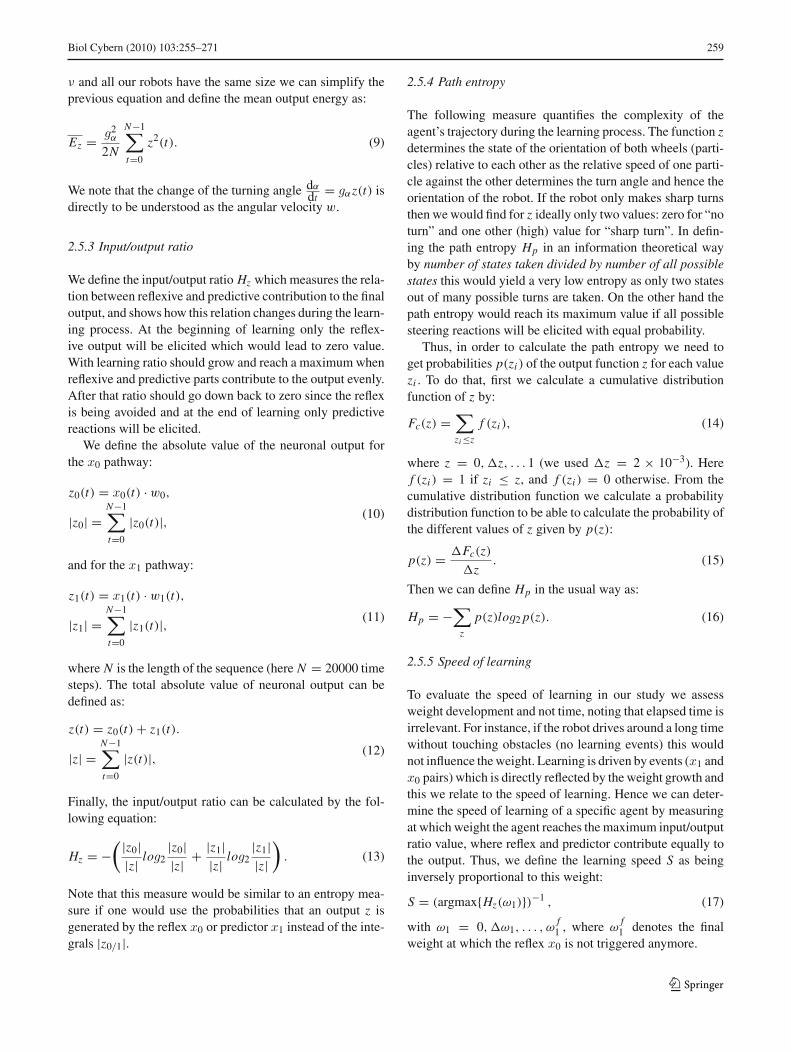
In this study, we will focus on systems that perform differ-ential hebbian learning (Hebb 1949; Sutton and Barto 1981;Kosco 1986; Klopf 1988), related to spike-timing dependentplasticity (Markram et al. 1997; Saudargiene et al. 2004,2005), for the learning of temporal sequences of paired sen-sor events. Temporal sequences of sensor events are commonfor animals and humans and exist as soon as the same eventis registered first by a “far-sensor” (e.g., eye, ear, nose) andlater by a “near-sensor” (e.g., touch-sensor, taste-bud). Oursystems are initially built as reflex loops and the learning goalis to avoid this reflex. A simple example, also used here, isa robot that learns to avoid obstacles. Such a machine canstart—like a Braitenberg Vehicle—with a touch-triggered(signal x0, Fig. 1a) retraction reflex and learn to use a far-sensor (i.e., infrared signal x1) to turn earlier and stop runninginto obstructions thereby avoiding the reflex (Porr andWörgötter 2003a). Fig. 1a shows the general control diagramfor such systems, discussed in several previous articles (Porrand Wörgötter 2003a,b, 2006; Kulvicius et al. 2007). Inputsarise from the system’s own behavior and can be understoodas disturbance-events D that enter the inner loop via the trans-fer function P0 of the world and become a sensor event atsensor x0. This sensor is the near-sensor and triggers thereflex motor action z. The far-sensor x1 has received thesame disturbance already earlier (via transfer function P1)leading to a stimulation sequence: first x1 then x0 (Fig. 1b).This is depicted by the delay variable τ between inner andouter loop. During learning the influence of x1 onto outputz will grow via weight ω1 leading to an earlier motor actionand, thus, to the avoidance of the reflex.
Previous studies (Porr and Wörgötter 2003a,b, 2006;Kulvicius et al. 2007) have derived stability conditions forenvironments where the transfer functions were constant.However, while the agent interacts with its environment thesetransfer functions change. For example, the question ariseswhether the delay τ between the predicting event x1 andthe reflex trigger x0 would change while learning to avoidobstacles. Thinking of an obstacle-avoiding robot, intuitivelyone would expect τ to get longer as the growing influenceof x1 should lead to a later and later triggering (by x0) ofthe reflex until it is finally fully eliminated. This is shown inFig. 1b trajectory (1) versus trajectory (2), where the robotbeetle depicted uses two sets of antennas (short and long)for near (x0) and far (x1) sensing, respectively. The intui-tion of a growing τ is alluring, but just shows how even inthe simplest cases our understanding of such adaptive sys-tems can go astray. Because, as shown below and contrary
Z(t)
z
=1
=1
(t)
0
0
X (t)0
X0
1
1
X (t)1
X1
Agent
Environment
DP
P
P0
1
A B
C+
(t) dx /dt0 x
t
= t - tx x0 1
H
Antennae withspring-like properties
30o
(2)
(1)
wheeled robotwith sensors x and x0 1
x0
x0
x0
x1
x1
x1
Fig. 1 a Schematic diagram of the closed-loop learning system withinputs x0 and x1, connection weights ω0 and ω1 and neuronal output z.P0 and P1 denote the reflexive and the predictive pathway, respectively.D defines the disturbance, where τ is the time difference between inputsx0 and x1 as shown in c. b Robot setup with short antennas (reflex-ive inputs, x0) and long antennas (predictive inputs, x1). The diagramshows a situation with an increase of the time difference between far-and near-sensor events during learning process (τ2 > τ1), depicted bythe respective distance between the little (solid) triggering lines x0,1from trajectory (dashed) to wall. c Schematic diagram of the input cor-relation learning rule and the signal structure (ICO, Porr and Wörgötter2006; Kulvicius et al. 2007)
to our naive intuition, such systems are better described bya τ which first grows and then shrinks again back to essen-tially its starting value. A deeper look into the development ofthese systems allows understanding why this happens and wecan even derive an analytical approximation for the weightdevelopment in these cases.
In the second part of the study we define energy,input/output ratio and entropy measures for these systems andmeasure them in environments of different complexity. Usingthese measures we will first show that learning equalizes theenergy uptake across agents and worlds. Strong differenceswhich initially exist are being leveled out during learning.However, when judging learning speed and complexity ofthe resulting behavior one finds a trade-off and some agentswill be better than others in the different worlds tested.
The analysis of closed-loop systems is a well establishedfield in the engineering sciences, which also investigates“adaptive controllers”. Very little, however, is known aboutadaptive controllers which interact with their environment byshaping non-stationary dynamics through their own learning(see Sect. 4). It had been shown that Shanon’s InformationTheory (Shannon 1948) can be applied for perception-actionloops (Ashby 1956; Tishby et al. 1999; Touchette and Lloyd2000). Few other studies exist that try to analyze closed loopsystems from an agent-perspective asking about the informa-tion processing properties of such system in the context ofwhat would be beneficial for the agent itself (Klyubin et al.2007, 2008; Lungarella et al. 2005; Lungarella and Sporns
123
Biol Cybern (2010) 103:255–271 257
2006; Prokopenko et al. 2006). Even fewer attempts exist thatconsider learning (Lungarella and Sporns 2006; Porr et al.2006). This study is, to our knowledge, one of the few whichtries to address these issues in closed-loop learning systems.While our scenarios have strong constrains, the newly intro-duced information measures can be applied to a wide rangeof adaptive predictive controllers independent on the systemsetup.
The article is organized in the following way. First off allwe will describe the environment and the adaptive control-ler of our system and define several system measures. Thenwe will present results from single experiments to demon-strate the basic behavior of the system and provide an ana-lytical solution of its temporal development. Afterwards wewill show results for the different system measures showinga statistical analysis for different agents and different envi-ronments. Finally we will discuss the question of “optimalrobots” and will conclude our study with Sect. 4 relating ourwork to other approaches.
2 Methods
Note, all spatial measures in the following are given in arbi-trary “size units” (short “units”), time is measured in “steps”.
2.1 Agent
The structure of the simulated agent used for these simula-tions is shown in Fig. 1b. It is a Braitenberg Vehicle of diam-eter 40 units with two lateral wheels. It operates in a squarearena of 400 × 400 units or a circular arena with diameterof 400 units, which can be empty (“simple world”) or con-tain different numbers of obstacles (“complex worlds”). Bydefault, the agent drives straight forward (dashed arrow) withspeed ν = 1 units per time step. It has two sensor-pairs, near-sensors and far-sensors, at the front; each sensor resembling abeetle’s antenna, albeit here with ideal spring-like properties.Short near-sensors elicit the reflex signal x0 and long far-sensors the predictive signal x1. Triggering of a sensor willhappen as soon as the agent gets close enough to an obstacle.Then the sensor signal x will be elicited according to:
x(t) = βx(t − 1) + (1 − β)λt
�, (1)
where λt is the part of the antenna bent by an obstacleat time point t and � is the length of the antenna. Theconstant β = 0.6 defines the decay rate of the first orderlow pass implemented by the feedback x(t − 1). We usea fixed reflex antenna length of �0 = 10 units and dif-ferent antenna lengths for the predictive sensor of �1 =40, 50, 60, 70, 80, 100, 120, 150, 200. In the following wewill use the antenna ratio �1
�0to specify different robots.
To compute the agents’s output z we use a linear summa-tion neuron with an added-on winner-takes-all mechanism inorder to prevent the robot from getting stuck in the corner orfrom oscillatory movements in case sensors on the left andright side are triggered at the same time. If sensors are trig-gered at the same time but one sensor is triggered more thanthe other (xR
0,1 �= xL0,1) then z will follow strongest of the
left and right sensor signals:
b0,1 = sign(xR
0,1 − xL0,1
),
z = ω0b0max{xR
0 ,xL0
}+ ω1b1max
{xR
1 ,xL1
}, (2)
where xL ,R0,1 are sensory inputs from the left and right side
obtained by Eq. 1 above.In case xR
0,1 = xL0,1 we use a bias for the right side and
calculate output by z = ω0xR0 + ω1x
R1 .
Note that winner-takes-all mechanism does not keepinputs from canceling out but creates lateral inhibition whichmeans that, for instance, if the input on the right side is trig-gered stronger than that on the left side then the input fromthe left side will be ignored (inhibited) and the robot willturn to the left side until at some point sensors on the rightand the left side will be triggered equally. If sensors are trig-gered equally then we use a bias for the right side (input fromthe left side is ignored) and as a consequence the robot willcontinue turning to the left until the obstacle is completelyavoided. Thus, the winner-takes-all mechanism (lateral inhi-bition) together with built in bias helps preventing the robotfrom getting stuck in corners or from oscillatory movements.
Signal z is then directly used to change the robot’s drivingangle α. For the remainder of this study it is important toremember that z directly corresponds to the change of theturning angle dα/dt :
dα
dt= gαz(t), (3)
where gα is the steering gain. Positive output (z > 0) leads toa positive change of the turning angle dα/dt , thus the robotwould steer to the left, whereas negative output (z < 0)
leads to a negative change of the turning angle dα/dt andcorresponds to a rightward steering. From this the change ofthe robot position can be calculated for each time step andas a result of this setup the agent will avoid obstacles whenmoving through its arena.
We keep the weight w0 fixed (w0 = 1) and let only w1
develop where initially we set w1 = 0.
2.2 Learning rule
For learning we use the ICO (input correlation) rule (Porrand Wörgötter 2006), because of its intrinsic stability, givenby (Fig. 1c):
123
258 Biol Cybern (2010) 103:255–271
dω1
dt= μx1
dx0
dt(4)
Note, that the typical low pass filtering of the input signalsfor ICO learning (Porr and Wörgötter 2006) is performed bythe environment itself and by Eq. 1.
2.3 Closed-loop system
The general structure of the closed loop has been presentedin Fig. 1a and was discussed in the introduction so that onlya few explanations need to be added here.
In general we denote the transfer function of the agent byH and those of the environment by P . In Fig. 1a we haveadded the time variable t to all those components of whichthe temporal development is of interest in the context of thisstudy: x0,x1, z, τ and ω1. The other synaptic weight ω0 iskept constant at 1.0.
2.4 Experimental procedure
We tested nine simulated robots with different antenna ratio�1/�0 = [4, 5, 6, 7, 8, 10, 12, 15, 20] in four environmentsof different complexity. We used a circular environment witha diameter of 400 units where complexity was defined bythe number of obstacles (3, 7, 14, or 21). We used squareshaped obstacles of size 20 × 20 units that were placed atrandom positions in a circular manner at the perimeter ofthree imaginary circles with radii of 50, 120, and 190 points.This way we avoid deadlock situations and assure a freepath along the whole circular arena. Several examples of thesimplest and the most complex environments are shown inFig. 2.
Two different types of experiments are being made. (1)Normal learning experiments where the robots actually learnwhile driving and (2) steady state experiments (called weightfreezing), where we keep ω1 for some time at a preset valuefor measuring the currently queried parameter(s) in a steadystate situation. Then ω1 will be increased and parameter(s)will be measured again and so on until we are reaching thefinal weight ω
f1 at which the reflex is not triggered any-
more.We used the following procedure for this. We set the
weight ω1 to specific values (0,ω1, 2ω1, . . . ωf1 , where
ω1 = 10−3) and, for each ω1, let the robot run forN = 20000 time steps without learning.
Such a procedure is motivated by the fact that the actualruntime is irrelevant (as explained above). Thus, by settingweights we can probe the robot’s behavior for a longer periodin a steady state situation in order to get more data for theanalysis.
2.5 System measures
In the following we will present different measures used toevaluate temporal development and success of learning, andto find the optimal robot for a specific environment.
2.5.1 Temporal development
To analyze the temporal development we measure how thetemporal difference τ between inputs x1 and x0 changeson average during learning. As events in these systems arevery noisy we need to adopt a method by which the time-difference between two subsequent x1,x0 events is reliablymeasured. For this we use the weight freezing procedure andkeep ω1 = const for N time steps. We use a threshold withvalue θ = 0.02 only for the x0 signal to determine the time tkwhen the signal x0 reaches the threshold (x0 > θ). Finally,we place a window cw = 300 steps around these tk values(cw ≤ tk < N − cw, N = 20,000) and calculate the cross-correlation between x1 and x0 only inside this time window,with a window size related to STDP windows as reported inthe literature (Markram et al. 1997; Bi and Poo 1998). Thisis given by:
Ck(t) =T =+cw∑T =−cw
x1(tk) · x0(tk + T ), (5)
We determine the peak location of the cross-correlation as:
τk = argmax{Ck(t)}. (6)
Finally, we calculate the mean value of the obtained differ-ent time differences τk for the whole frozen time section(N steps) according to:
τ = 1
M
M∑k=1
τk, (7)
where M is the number of found threshold crossings. Afterincreasing ω1, this procedure is repeated until ω
f1 .
2.5.2 Energy
We measure how much energy the robot uses for a giventask during the learning process. In physics the total kineticenergy of an extended object is defined as the sum of thetranslational kinetic energy of the center of mass and therotational kinetic energy about the center of mass:
Ek = 1
2mν2 + 1
2Iω2, (8)
where m is the mass (translational inertia), I is the moment ofinertia (rotational inertia), ν and ω are the velocity and angu-lar velocity, respectively. As we use a constant basic speed
123
Biol Cybern (2010) 103:255–271 259
ν and all our robots have the same size we can simplify theprevious equation and define the mean output energy as:
Ez = g2α
2N
N−1∑t=0
z2(t). (9)
We note that the change of the turning angle dα
dt= gαz(t) is
directly to be understood as the angular velocity w.
2.5.3 Input/output ratio
We define the input/output ratio Hz which measures the rela-tion between reflexive and predictive contribution to the finaloutput, and shows how this relation changes during the learn-ing process. At the beginning of learning only the reflex-ive output will be elicited which would lead to zero value.With learning ratio should grow and reach a maximum whenreflexive and predictive parts contribute to the output evenly.After that ratio should go down back to zero since the reflexis being avoided and at the end of learning only predictivereactions will be elicited.
We define the absolute value of the neuronal output forthe x0 pathway:
z0(t) = x0(t) · w0,
|z0| =N−1∑t=0
|z0(t)|, (10)
and for the x1 pathway:
z1(t) = x1(t) · w1(t),
|z1| =N−1∑t=0
|z1(t)|, (11)
where N is the length of the sequence (here N = 20000 timesteps). The total absolute value of neuronal output can bedefined as:
z(t) = z0(t) + z1(t).
|z| =N−1∑t=0
|z(t)|, (12)
Finally, the input/output ratio can be calculated by the fol-lowing equation:
Hz = −( |z0|
|z| log2|z0||z| + |z1|
|z| log2|z1||z|
). (13)
Note that this measure would be similar to an entropy mea-sure if one would use the probabilities that an output z isgenerated by the reflex x0 or predictor x1 instead of the inte-grals |z0/1|.
2.5.4 Path entropy
The following measure quantifies the complexity of theagent’s trajectory during the learning process. The function zdetermines the state of the orientation of both wheels (parti-cles) relative to each other as the relative speed of one parti-cle against the other determines the turn angle and hence theorientation of the robot. If the robot only makes sharp turnsthen we would find for z ideally only two values: zero for “noturn” and one other (high) value for “sharp turn”. In defin-ing the path entropy Hp in an information theoretical wayby number of states taken divided by number of all possiblestates this would yield a very low entropy as only two statesout of many possible turns are taken. On the other hand thepath entropy would reach its maximum value if all possiblesteering reactions will be elicited with equal probability.
Thus, in order to calculate the path entropy we need toget probabilities p(zi ) of the output function z for each valuezi . To do that, first we calculate a cumulative distributionfunction of z by:
Fc(z) =∑zi ≤z
f (zi ), (14)
where z = 0,z, . . . 1 (we used z = 2 × 10⁻³). Heref (zi ) = 1 if zi ≤ z, and f (zi ) = 0 otherwise. From thecumulative distribution function we calculate a probabilitydistribution function to be able to calculate the probability ofthe different values of z given by p(z):
p(z) = Fc(z)
z. (15)
Then we can define Hp in the usual way as:
Hp = −∑
z
p(z)log2 p(z). (16)
2.5.5 Speed of learning
To evaluate the speed of learning in our study we assessweight development and not time, noting that elapsed time isirrelevant. For instance, if the robot drives around a long timewithout touching obstacles (no learning events) this wouldnot influence the weight. Learning is driven by events (x1 andx0 pairs) which is directly reflected by the weight growth andthis we relate to the speed of learning. Hence we can deter-mine the speed of learning of a specific agent by measuringat which weight the agent reaches the maximum input/outputratio value, where reflex and predictor contribute equally tothe output. Thus, we define the learning speed S as beinginversely proportional to this weight:
S = (argmax{Hz(ω1)})−1 , (17)
with ω1 = 0,ω1, . . . , ωf1 , where ω
f1 denotes the final
weight at which the reflex x0 is not triggered anymore.
123

260 Biol Cybern (2010) 103:255–271
Note in a given environment one finds that learning eventscan occur more or less often depending on the sensitivity ofthe reflex. In this case—to compare architectures at the reflexlevel—one would indeed want to measure time as such. Weare, however, in the current study not concerned with this.
2.5.6 Optimality
In order to find an optimal robot for a specific environment weused an averaged optimality measure O which is a productof the speed of learning S and the final path entropy Hp(ω
f1 ):
O = S · Hp(ωf1 ). (18)
Note that we normalized values of S and Hp(ωf1 ) between
zero and one before calculating the product in Eq. 18. Thismeasure is based on the heuristic assumption that an “opti-mal robot” should be one which requires least learning timeand still “makes the most of it” in the sense of producingthe most complex paths. Therefore, we used the quotientof these two measures to define “optimal”. In general opti-mality measures used to quantify behavior in engineered orself-organizing systems as well as in animals-observation arealways in the eyes of beholder where combination of differ-ent features can be taken into account to describe what isdeemed to be “optimal behavior” and this depends also onthe specific task.
3 Results
3.1 Basic behavior of the system
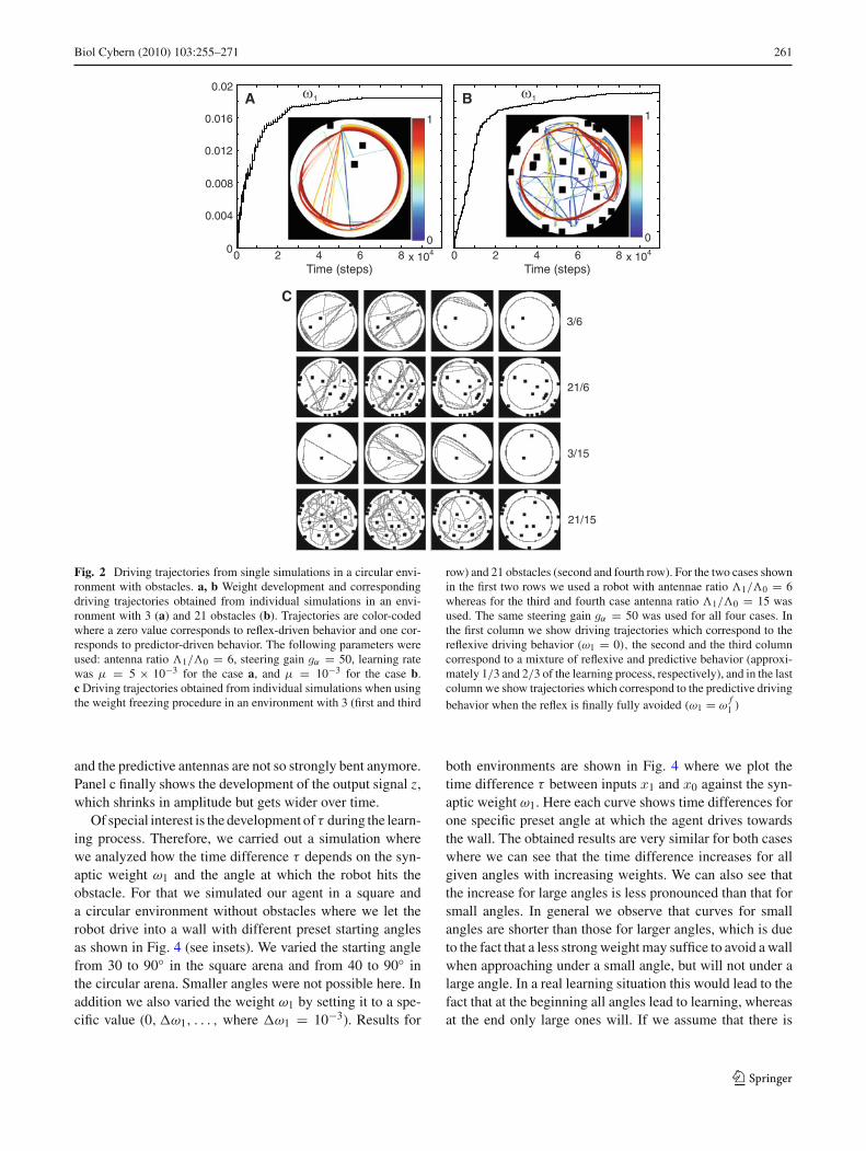
The basic behavior of the obstacle avoidance agent is pre-sented in Fig. 2 where we show simulation results for a cir-cular environment with 3 and 21 obstacles. In panels a andb, we show weight development and corresponding drivingtrajectories (see insets) for the case where the robot was actu-ally learning (no weight freezing here). The resulting weightcurves for both cases are similar and we observe relativelyrapid weight growth at the beginning of the learning and thenslow saturation till the reflex is avoided and weights finallystabilize. Corresponding trajectories are color-coded wherethe blue color corresponds to reflex-driven behavior and thered color corresponds to predictor-driven behavior. Valuesfor the color-coding were calculated by a contrast measuregiven in Appendix A.1. From the driving trajectories we cansee that at the beginning the robots make sharp turns becauseof the initially built in strong reflex reaction whereby, as aconsequence, the robot explores more or less the whole envi-ronment. With learning the predictor takes over which at theend leads to wall following behavior since learned steeringactions are much weaker but are elicited earlier compared to
the initially strong and late reflex reactions. Note that for therobots to learn wall-following behavior is not a desired nav-igational strategy. The learning goal of the robots is to learnavoiding obstacles without triggering the reflex (x0, reflexavoidance learning). Since the robots do not have any addi-tional “motivation” or “drive” function implemented, theirbehavior will be equilibrated (and, thus, not change anymore)as soon as they navigate in the environment without trigger-ing the reflex. To avoid reflexes they learn reacting to earlystimuli (x1) but with much weaker steering reactions com-pared to the initial reflex (x0) which as a consequence turnsinto wall following behavior. By reacting earlier the robotscan use much less energy compared to late reflex reactions.The strategy of “reflex-avoidance” learning is known fromneurons in the Cerebellum (Wolpert et al. 1998; Hofstötteret al. 2002).
Simulation results for the case where we used the weightfreezing procedure are shown in Fig. 2c. This way we can, fordifferent weights, show longer trajectories to better assess therobots’ behavior. Here we plot selected trajectories for twodifferent environments (3 and 21 obstacles) and for two dif-ferent robots (antenna ratio 6 and 15). Trajectories for eachcase are presented in rows where the first trajectory corre-sponds to the reflexive driving behavior (ω1 = 0), the secondand the third trajectory correspond to a mixture of reflexiveand predictive behavior, and the last trajectory correspondsto the predictive driving trajectory when the reflex is finallyfully avoided (ω1 = ω
f1 ). Here we obtained similar driving
behavior as in the examples presented above. In general weobserved that late, strong, and abrupt reflex reactions turninto early, weak and smooth predictive reactions whereby, asa consequence, a bouncing driving behavior turns into a wallfollowing behavior.
3.2 Characterizing the temporal development
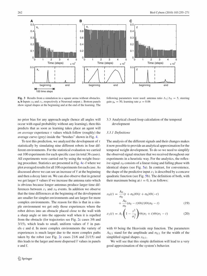
Figure 3 shows the results from one obstacle avoidance exper-iment in our standard empty square arena. Panels a andb show the development of the reflex (x0) and predictor(x1) signals over time (top panels), where the bottom pan-els show magnifications for the beginning and the end of thelearning. As expected, x0 shrinks substantially during learn-ing, because the reflex signal is better and better avoided.It would finally fully vanish as theory predicts, leading tothe stabilization of weights (Porr and Wörgötter 2006), onlyhere—to be able to show how small x0 signals look like—wehave stopped the learning process before this final equilib-rium had been reached (see Fig. 2a for a completed pro-cess).
The predictor signal in panel b also gets smaller which isdue to the fact that at the beginning of learning the predictiveantennas are bent all the way until the reflex antennas finallyalso hit the wall whereas after learning the reflex is avoided
123
Biol Cybern (2010) 103:255–271 261
0 00 2 442 66 88 x 104 x 104
0.004
0.008
0.012
0.016
0.02
0
1
0
1A B
Time (steps) Time (steps)
1 1
C
3/6
21/6
3/15
21/15
Fig. 2 Driving trajectories from single simulations in a circular envi-ronment with obstacles. a, b Weight development and correspondingdriving trajectories obtained from individual simulations in an envi-ronment with 3 (a) and 21 obstacles (b). Trajectories are color-codedwhere a zero value corresponds to reflex-driven behavior and one cor-responds to predictor-driven behavior. The following parameters wereused: antenna ratio �1/�0 = 6, steering gain gα = 50, learning ratewas μ = 5 × 10⁻³ for the case a, and μ = 10−3 for the case b.c Driving trajectories obtained from individual simulations when usingthe weight freezing procedure in an environment with 3 (first and third
row) and 21 obstacles (second and fourth row). For the two cases shownin the first two rows we used a robot with antennae ratio �1/�0 = 6whereas for the third and fourth case antenna ratio �1/�0 = 15 wasused. The same steering gain gα = 50 was used for all four cases. Inthe first column we show driving trajectories which correspond to thereflexive driving behavior (ω1 = 0), the second and the third columncorrespond to a mixture of reflexive and predictive behavior (approxi-mately 1/3 and 2/3 of the learning process, respectively), and in the lastcolumn we show trajectories which correspond to the predictive drivingbehavior when the reflex is finally fully avoided (ω1 = ω
f1 )
and the predictive antennas are not so strongly bent anymore.Panel c finally shows the development of the output signal z,which shrinks in amplitude but gets wider over time.
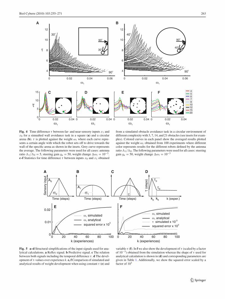
Of special interest is the development of τ during the learn-ing process. Therefore, we carried out a simulation wherewe analyzed how the time difference τ depends on the syn-aptic weight ω1 and the angle at which the robot hits theobstacle. For that we simulated our agent in a square anda circular environment without obstacles where we let therobot drive into a wall with different preset starting anglesas shown in Fig. 4 (see insets). We varied the starting anglefrom 30 to 90◦ in the square arena and from 40 to 90◦ inthe circular arena. Smaller angles were not possible here. Inaddition we also varied the weight ω1 by setting it to a spe-cific value (0,ω1, . . . , where ω1 = 10−3). Results for
both environments are shown in Fig. 4 where we plot thetime difference τ between inputs x1 and x0 against the syn-aptic weight ω1. Here each curve shows time differences forone specific preset angle at which the agent drives towardsthe wall. The obtained results are very similar for both caseswhere we can see that the time difference increases for allgiven angles with increasing weights. We can also see thatthe increase for large angles is less pronounced than that forsmall angles. In general we observe that curves for smallangles are shorter than those for larger angles, which is dueto the fact that a less strong weight may suffice to avoid a wallwhen approaching under a small angle, but will not under alarge angle. In a real learning situation this would lead to thefact that at the beginning all angles lead to learning, whereasat the end only large ones will. If we assume that there is
123
262 Biol Cybern (2010) 103:255–271
A B
Time (steps)
z
z
C
x0
Time (steps)Time (steps)
x1
0 1 2 3 4 5
x 104
0
0.1
0.2
0.3
0.4
0.5
0 1 2 3 4 5
x 104
0
0.2
0.4
0.6
0.8
1
0 1 2 3 4 5
x 104
0
0.1
0.2
0.3
0.4
0.5
0
1x1
beginning beginningend end00
0.5 0.5x0
beginning end
100 time steps
Fig. 3 Results from a simulation in a square arena without obstacles.a, b Inputs x0 and x1, respectively. c Neuronal output z. Bottom panelsshow signal shapes at the beginning and at the end of the learning. The
following parameters were used: antenna ratio �1/�0 = 5, steeringgain gα = 50, learning rate μ = 0.06
no prior bias for any approach-angle (hence all angles willoccur with equal probability without any learning), then thispredicts that as soon as learning takes place an agent willon average experience τ values which follow (roughly) theaverage curve (grey) inside the “brushes” shown in Fig. 4.
To test this prediction, we analyzed the development of τ
statistically by simulating nine different robots in four dif-ferent environments. For the statistical evaluation we carriedout 100 experiments for each specific case (in total 36 cases).All experiments were carried out by using the weight freez-ing procedure. Statistics are presented in Fig. 4c–f where weplot averaged results for all 100 experiments for each case. Asdiscussed above we can see an increase of τ at the beginningand then a decay later on. We can also observe that in generalwe get larger τ values if we increase the antenna ratio whichis obvious because longer antennas produce larger time dif-ferences between x1 and x0 events. In addition we observethat the time differences at the beginning of the developmentare smaller for simpler environments and are larger for morecomplex environments. The reason for this is that in a sim-ple environment we get only those experiences where therobot drives into an obstacle placed close to the wall witha sharp angle or into the opposite wall when it is repelledfrom the obstacle (for trajectories see Fig. 2c cases 3/6 and3/15), which leads to small, uniform values of τ in pan-els c and d. In more complex environments the variety ofexperiences is much larger due to the more complex pathstaken by the robot (see Fig. 2c cases 21/6 and 21/15) andthis leads to the larger and more dispersed τ values in panelse and f.
3.3 Analytical closed-loop calculation of the temporaldevelopment
3.3.1 Definitions
The analysis of the different signals and their changes makesit now possible to provide an analytical approximation for thetemporal weight development. To do so we need to simplifythe observed signal structure that we received throughout ourexperiments in a heuristic way. For the analytics, the reflex-ive signal x0 consists of a linear rising and falling phase withidentical slopes (see Fig. 5a). In contrast, for convenience,the shape of the predictive input x1 is described by a concavequadratic function (see Fig. 5b). The definition of both, withtheir maximum being at t = 0, is as follows:
x0(t) = A0
σ0(t + σ0)�(t + σ0)�(−t)
+ A0
σ0(σ0 − t)�(t)�(σ0 − t) (19)
x1(t) = A1
(1 − t2
σ 21
)�(σ1 + t)�(σ1 − t) (20)
with � being the Heaviside step function. The parametersA0/1 stand for the amplitude and σ0/1 for the width of thesimplified signal shapes x0/1.
We will see that this simple definition will lead to a verygood approximation of the system’s behavior.
123
Biol Cybern (2010) 103:255–271 263
40o
90o
30o 40o
90o
90o
30o
90o
1 1
0 0.02 0.04 0.06
4
6
8
10
12
0 0.02 0.04 0.06
4
6
8
10
12
C D
BA
E F
1 1 1 1
0 0.02 0.040 0.02 0.040 0.02 0.040
5
10
15
0 0.02 0.04
4567810121520
Fig. 4 Time difference τ between far- and near-sensory inputs x1 andx0 for a simualted wall avoidance task in a square (a) and a circulararena (b). τ is plotted against the weight ω1 where each curve repre-sents a certain angle with which the robot sets off to drive towards thewall of the specific arena as shown in the insets. Grey curve representsthe average. The following parameters were used for all cases: antennaratio �1/�0 = 5, steering gain gα = 50, weight change ω1 = 10−3.c–f Statistics for time difference τ between inputs x0 and x1 obtained
from a simulated obstacle avoidance task in a circular environment ofdifferent complexity with 3, 7, 14, and 21 obstacles (see insets for exam-ples). Colored curves in each panel show the averaged results plottedagainst the weight ω1 obtained from 100 experiments where differentcolor represents results for the different robots defined by the antennaratio �1/�0. The following parameters were used for all cases: steeringgain gα = 50, weight change ω1 = 10−3
Sen
sory
inpu
t
Time (steps) Time (steps) Time (steps) k (exper.)
(ste
ps)
C D
A0
A1
p
b
kp kb
0 1
k (experiences) k (experiences)
A B
E F0.02
0.01
000 20 2040 4060 6080 80100 100
1 simulated 1 simulated
1 analytical 1 analytical
squared error x 103
squared error x 103simulated x 10-3
Fig. 5 a–d Structural simplifications of the input signals used for ana-lytical calculations. a Reflex signal. b Predictive signal. c The relationbetween both signals including the temporal difference τ . d The devel-opment of τ -values over experience k. e, f Comparison of simulated andanalytical results of weight development when using constant τ (e) and
variable τ (f). In f we also show the development of τ (scaled by a factorof 10−3) obtained from the simulation whereas the shape of τ used foranalytical calculation is shown in (d) and corresponding parameters aregiven in Table 1. Additionally, we show the squared error scaled by afactor of 103
123
264 Biol Cybern (2010) 103:255–271
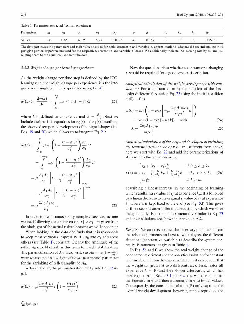
Table 1 Parameters extracted from an experiment
Parameters a0 A1 σ0 σ1 ω f τb μ1 τp kb kp μ2
Values 0.6 0.85 43.75 5.75 0.0223 4 0.073 12 13 9 0.0523
The first part states the parameters and their values needed for both, constant-τ and variable-τ , approximations, whereas the second and the thirdpart give particular parameters used for the respective, constant-τ and variable-τ , cases. We additionally indicate the learning rate by μ1 and μ2,relating them to the equation used to fit the data
3.3.2 Weight change per learning experience
As the weight change per time step is defined by the ICO-learning rule, the weight change per experience k is the inte-gral over a single x1 − x0 experience using Eq. 4:
ω′(k) := dω(k)
dk=
σ1∫
−σ1
μx1(t)x0(t − τ) dt (21)
where k is defined as experience and x = dxdt
. Next weinclude the heuristic equations for x0(t) and x1(t) describingthe observed temporal development of the signal shapes (i.e.,Eqs. 19 and 20) which allows us to integrate Eq. 21:
ω′(k) =τ∫
τ−σ0
μA1
(1 − (t − σ1)
2
σ 21
)A0
σ0dt
−τ+σ0∫
τ
μA1
(1 − (t − σ1)
2
σ 21
)A0
σ0dt
= μA1 A0
σ0
[t − 1
3
(t − σ1)3
σ 21
]τ
τ−σ0
−μA1 A0
σ0
[t − 1
3
(t − σ1)3
σ 21
]τ+σ0
τ
= μ2A0 A1σ0
σ 21
τ. (22)
In order to avoid unnecessary complex case distinctionswe used following constraints on τ : |τ | < σ1−σ0 given fromthe hindsight of the actual τ development we will encounter.
When looking at the data one finds that it is reasonableto keep most variables, especially A1, σ0 and σ1 and someothers (see Table 1), constant. Clearly the amplitude of thereflex A0 should shrink as this leads to weight stabilization.The parametrization of A0, thus, writes as A0 = a0(1− ω
ω f),
were we use the final weight value ω f as a control parameterfor the shrinking of reflex amplitude A0.
After including the parametrization of A0 into Eq. 22 weget:
ω′(k) = μ2a0 A1σ0
σ 21
τ
(1 − ω(k)
ω f
)(23)
Now the question arises whether a constant or a changingτ would be required for a good system description.
Analytical calculation of the weight development with con-stant τ : For a constant τ = τb the solution of the first-order differential equation Eq. 23 using the initial conditionω(0) = 0 is
ω(k) = ω f
(1 − exp
[−μ
2a0 A1σ0τb
ω f σ21
k
])
= ω f (1 − exp [−μλk]) with (24)
λ = 2a0 A1σ0τb
ω f σ21
(25)
Analytical calculation of the temporal development includingthe temporal dependence of τ on k: Different from above,here we start with Eq. 22 and add the parameterizations ofA0 and τ to this equation using:
τ(k) =
⎧⎪⎪⎨⎪⎪⎩
τb + (τp − τb)k
kpif 0 ≤ k ≤ kp
τp − τp−τbkp−kb
kp + τp−τbkp−kb
k if kp < k ≤ kb
τbk
k fif k > kb
(26)
describing a linear increase in the beginning of learningwhich results in a τ -value of τp at experience kp . It is followedby a linear decrease to the original τ -value of τb at experiencekb where it is kept fixed to the end (see Fig. 5d). This givesus three second-order differential equations, which we solveindependently. Equations are structurally similar to Eq. 23and their solutions are shown in Appendix A.2.
Results: We can now extract the necessary parameters fromthe robot experiments and test to what degree the differentsituations (constant vs. variable τ ) describe the system cor-rectly. Parameters are given in Table 1.
In Fig. 5e and f, we show the real weight change of theconducted experiment and the analytical solution for constantand variable τ . From the experimental data it can be seen thatthe weight ω1 grows at two different rates. First, faster tillexperience k = 10 and then slower afterwards, which hasbeen explained in Sects. 3.1 and 3.2, and was due to an ini-tial increase in τ and then a decrease in τ to initial values.Consequently, the constant-τ solution (E) only captures theoverall weight development, however, cannot reproduce the
123
Biol Cybern (2010) 103:255–271 265
45678
10121520
I/Ora
tioP
ath
entr
opy
Out
pute
nerg
y A
0
0.5
1
1.5
2
E
0
0.2
0.4
0.6
0.8
1
I
0 0.02 0.040
1
2
3
4
B
0
1
2
3
F
0
0.2
0.4
0.6
0.8
1
J
0 0.02 0.040
1
2
3
4
5
C
0
1
2
3
4
5
G
0
0.2
0.4
0.6
0.8
1
K
0 0.020
2
4
6
0.04
L
0
0.2
0.4
0.6
0.8
1
0 0.02 0.040
2
4
6
D
H
0
2
4
6
1 1 1 1
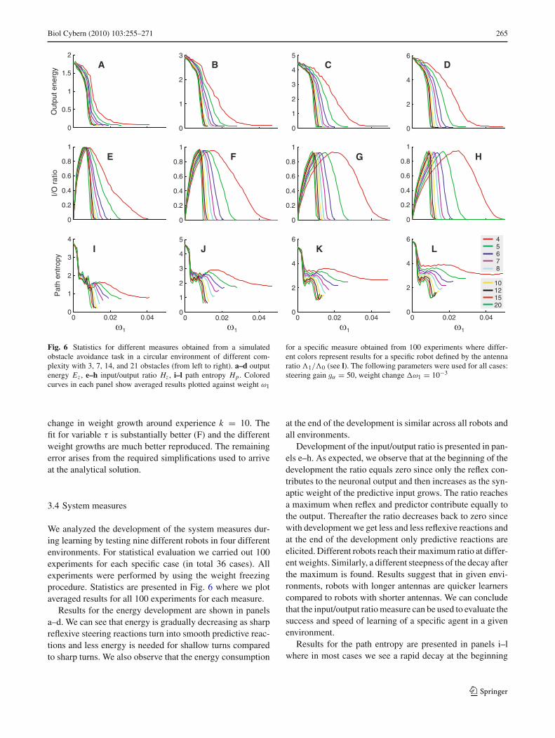
Fig. 6 Statistics for different measures obtained from a simulatedobstacle avoidance task in a circular environment of different com-plexity with 3, 7, 14, and 21 obstacles (from left to right). a–d outputenergy Ez , e–h input/output ratio Hz , i–l path entropy Hp . Coloredcurves in each panel show averaged results plotted against weight ω1
for a specific measure obtained from 100 experiments where differ-ent colors represent results for a specific robot defined by the antennaratio �1/�0 (see l). The following parameters were used for all cases:steering gain gα = 50, weight change ω1 = 10−3
change in weight growth around experience k = 10. Thefit for variable τ is substantially better (F) and the differentweight growths are much better reproduced. The remainingerror arises from the required simplifications used to arriveat the analytical solution.
3.4 System measures
We analyzed the development of the system measures dur-ing learning by testing nine different robots in four differentenvironments. For statistical evaluation we carried out 100experiments for each specific case (in total 36 cases). Allexperiments were performed by using the weight freezingprocedure. Statistics are presented in Fig. 6 where we plotaveraged results for all 100 experiments for each measure.
Results for the energy development are shown in panelsa–d. We can see that energy is gradually decreasing as sharpreflexive steering reactions turn into smooth predictive reac-tions and less energy is needed for shallow turns comparedto sharp turns. We also observe that the energy consumption
at the end of the development is similar across all robots andall environments.
Development of the input/output ratio is presented in pan-els e–h. As expected, we observe that at the beginning of thedevelopment the ratio equals zero since only the reflex con-tributes to the neuronal output and then increases as the syn-aptic weight of the predictive input grows. The ratio reachesa maximum when reflex and predictor contribute equally tothe output. Thereafter the ratio decreases back to zero sincewith development we get less and less reflexive reactions andat the end of the development only predictive reactions areelicited. Different robots reach their maximum ratio at differ-ent weights. Similarly, a different steepness of the decay afterthe maximum is found. Results suggest that in given envi-ronments, robots with longer antennas are quicker learnerscompared to robots with shorter antennas. We can concludethat the input/output ratio measure can be used to evaluate thesuccess and speed of learning of a specific agent in a givenenvironment.
Results for the path entropy are presented in panels i–lwhere in most cases we see a rapid decay at the beginning
123
266 Biol Cybern (2010) 103:255–271
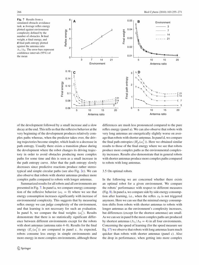
Fig. 7 Results from asimulated obstacle avoidancetask. a Average reflex energyplotted against environmentcomplexity defined by thenumber of obstacles. b finalweight, c final energy, andd final path entropy plottedagainst the antenna ratio�1/�0. The error-bars representconfidence intervals (95%) ofthe mean
Fin
alw
eigh
t
Antenna ratio
Antenna ratioAntenna ratio
Fin
alpa
then
trop
y
EnvironmentF
inal
ener
gyR
efle
xen
ergy
3
7
14
21
0.01
0.02
0.03
0.04
0.05
0
1
2
3
5 10 15 02
5 10 15 205 10 15 200.06
0.08
0.1
0.12
0.14
0.16
73 14 210
2
4
6
8EnvironmentBA
C D
3 37
7
14
1421
21
of the development followed by a small increase and a slowdecay at the end. This tells us that the reflexive behavior at thevery beginning of the development produces relatively com-plex paths whereas, when the predictor takes over, the driv-ing trajectories become simpler, which leads to a decrease inpath entropy. Usually there exists a transition phase duringthe development where the robot changes its driving trajec-tory in order to avoid obstacles producing more complexpaths for some time and this is seen as a small increase inthe path entropy curve. After that the path entropy slowlydecreases since predictive reactions produce rather stereo-typical and simple circular paths (see also Fig. 2c). We canalso observe that robots with shorter antennas produce morecomplex paths compared to robots with longer antennas.
Summarized results for all robots and all environments arepresented in Fig. 7. In panel a, we compare energy consump-tion of the reflexive behavior (ω1 = 0) where we see thatenergy consumption increases significantly with increase ofenvironmental complexity. This suggests that by measuringreflex energy we can judge complexity of the environment,and that learning is not necessary for such an evaluation.In panel b, we compare the final weights (ω
f1 ). Results
demonstrate that there is no statistically significant differ-ence between different environments except for the robotswith short antennas (antenna ratio 4–8). Results for the finalenergy (Ez(ω
f1 )) are compared in panel c. As expected,
robots consume less energy in simple environments andmore energy in more complex environments, although those
differences are mush less pronounced compared to the purereflex energy (panel a). We can also observe that robots withvery long antennas are energetically slightly worse on aver-age than robots with shorter antennas. In panel d, we comparethe final path entropies (Hp(ω
f1 )). Here we obtained similar
results to those of the final energy where we see that robotsproduce more complex paths as the environmental complex-ity increases. Results also demonstrate that in general robotswith shorter antennas produce more complex paths comparedto robots with long antennas.
3.5 On optimal robots
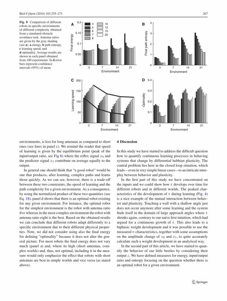
In the following we are concerned whether there existsan optimal robot for a given environment. We comparethe robots’ performance with respect to different measures(Fig. 8). In panel a, we compare side by side energy consump-tion after learning, i.e., when the reflex x0 is not triggeredanymore. Here we can see that the minimal energy consump-tion shifts from robots with shorter antennas to robots withlonger antennas as the environment’s complexity increases,but differences (except for the shortest antennas) are small.As we can see in panel b the most complex paths are producedby shortest antennas (�1/�0 = 4) in all four environments.Concerning the speed of learning (for the speed measure seeEq. 17) we observe that robots with long antennas learn muchquicker than robots with shorter antennas (panel c). Alsothe drop in performance, when getting into more complex
123
Biol Cybern (2010) 103:255–271 267
Fig. 8 Comparison of differentrobots in specific environmentsof different complexity obtainedfrom a simulated obstacleavoidance task. Antenna ratiosare given by the gray shading(see a). a energy, b path entropy,c learning speed, andd optimality. Average results areshown in each panel obtainedfrom 100 experiments. In d errorbars represent confidenceintervals (95%) of mean
Environment14 21
0
1
2
3
4
Fin
alpa
then
trop
y
Environment14 21
Lear
ning
spee
d
0
50
100
150
200
Environment
Opt
imal
ity
14 210
0.1
0.2
0.3
0.4
EnvironmentF
inal
ener
gy3 7
3 7 3 7
3 7 14 210
0.05
0.1
0.15
0.2 45678
10121520
A B
C D
environments, is less for long antennas as compared to shortones (see lines in panel c). We remind the reader that speedof learning is given by the equilibrium point (peak of theinput/output ratio, see Fig 6) where the reflex signal x0 andthe predictor signal x1 contribute on average equally to theoutput.
In general one should think that “a good robot” would beone that produces, after learning, complex paths and learnsthose quickly. As we can see, however, there is a trade-offbetween these two constraints, the speed of learning and thepath complexity for a given environment. As a consequence,by using the normalized product of these two quantities (seeEq. 18), panel d shows that there is an optimal robot existingfor any given environment. For instance, the optimal robotfor the simplest environment is the robot with antenna ratiofive whereas in the most complex environment the robot withantenna ratio eight is the best. Based on the obtained resultswe can conclude that different robots adapt differently to aspecific environment due to their different physical proper-ties. Note, we did not consider using also the final energyfor defining “optimality” because it does not alter the gen-eral picture. For most robots the final energy does not varymuch (panel a) and, where its high (short antennas, com-plex worlds) and, thus, not optimal, including it in the mea-sure would only emphasize the effect that robots with shortantennas are best in simple worlds and vice versa (as statedabove).
4 Discussion
In this study we have started to address the difficult questionhow to quantify continuous learning processes in behavingsystems that change by differential hebbian plasticity. Thecentral problem lies here in the closed loop situation, whichleads—even in very simple linear cases—to an intricate inter-play between behavior and plasticity.
In the first part of this study we have concentrated onthe inputs and we could show how τ develops over time fordifferent robots and in different worlds. The peaked char-acteristics of the development of τ during learning (Fig. 4)is a nice example of the mutual interaction between behav-ior and plasticity. Touching a wall with a shallow angle justdoes not occur anymore after some learning and the systemfinds itself in the domain of large approach angles where τ
shrinks again, contrary to our naive first intuition, which hadargued for a continuous growth of τ . This also leads to abiphasic weight development and it was possible to use themeasured τ -characteristics, together with some assumptionson the amplitude change of x0 and x1, to quite accuratelycalculate such a weight development in an analytical way.
In the second part of this article, we have started to quan-tify the behavior of our little beetles by considering theiroutput z. We have defined measures for energy, input/outputratio and entropy focusing on the question whether there isan optimal robot for a given environment.
123
268 Biol Cybern (2010) 103:255–271
4.1 The system identification problem in adaptiveclosed-loop systems
Several methods are known from the literature to address themodel identification issue in a broader context. For exampleone can use a [Non-linear] Auto-Regressive Moving Averageapproach with or without exogeneous inputs ([N]ARMA[X],Box et al. (1994)) to arrive at a general model of behavingrobot systems (Iglesias et al. 2008; Kyriacou et al. 2008), butthese models contain many parameters for fitting and param-eters do not have any direct physical meaning. Our attemptsstop short of a complete model identification approach, whichdoes not seem to be required for our system. Instead, herewe could use a rather limited model with quite a reductionistset of equations (see Sect. 3.3), which was to some degreeunexpected given the complexity of the closed loop behaviorof our robots (Fig. 2).
We observed that signal shapes and timings change in adifficult way influencing the learning. As a consequence, it isnot easy to find an appropriate description and the right mea-sures for capturing such non-stationary situations. Fig. 1ashows the structure of our closed loops system and this dia-gram has been used in earlier studies for convergence ana-lyzes (Porr and Wörgötter 2003a,b, 2006; Kulvicius et al.2007). From this diagram it becomes clear that τ, z as wellas x0,1 are the relevant variables in our system. While learn-ing is defined by the relation between inputs x0,1 and, hence,τ ; behavior is defined by output z.
Interestingly one finds in the first place that learning acts“equalizing”. Robots with different initial (reflex) energy(Fig. 7a) become very similar after learning (Fig 7b, notethe different scales in panel a and b). This finding canbe understood from some older studies on closed-loopdifferential hebbian (ISO, ICO) learning. Fig. 1a showsthat these systems will learn avoiding the reflex and thatlearning will stop once this goal has “just” been reachedleading to an asymptotic equilibrium situation (Porr andWörgötter 2003b). Furthermore, the systems investigatedhere are linear, hence all of them will in the end essen-tially require the same total effort for performing the avoid-ance reaction. These two facts explain why their energyis very similar in the end. The fact that robots are differ-ent, however, does surface when looking at the paths theychoose after learning. Robots with long predictive anten-nas can never make sharp turns anymore and their pathsare dominated by performing the same shallow turns againand again leading to little path variability and hence toa small final path entropy (Fig. 7d). On the other hand,these same long-antenna robots learn their task much fasterthan their short-antenna fellows: for the former, the equi-librium point between reflex and predictor (peak in theinput/output ratio) is reached faster than for the latter(Fig. 6e–h).
This leads to a trade-off and by using the normalized prod-uct of learning speed times path entropy we found that fordifferent environments different robots are optimal (Fig. 8d).Clearly, this type of optimality is to some degree just in theeyes of the beholder and one might choose to weigh the twoaspects (learning speed and path complexity) differently bywhich other robots would be valued more than those cur-rently called “optimal”. Nonetheless, also with a differentweighing one will observe that some robots would be betterthan others in the different worlds.
4.2 Information flow in adaptive closed-loop systems
In general the second part of the study relates to work focus-ing on information flow in closed-loop systems. There havebeen a few contributions to this topic. Tishby et al. (1999)introduced an Information-Bottleneck (IB) framework thatfinds concise representations for a system’s input that are asrelevant as possible for its output, i.e., concise descriptionthat preserves the relevant essence of the data. The relevantinformation in one signal with respect to the other is definedas the mutual information that the signal provides about theother. Although, the Information-Bottleneck framework wassuccessfully applied in various applications, like data clus-tering (Slonim and Tishby 2000; Slonim et al. 2001), featureselection (Slonim and Tishby 2001), POMDPs (Poupart andBoutilier 2002), it conceptually differs from our study, sincewe are interested in the dynamics of sensory-motor systemsduring the learning process.
In the study of Klyubin et al. (2004, 2005, 2007, 2008) theauthors used a Bayesian network to model perception-actionloops. In their approach a perception-action loop is inter-preted in terms of a communication channel-like model. Theyshow that maximization of information flow can evolve intoa meaningful sensorimotor structure (Klyubin et al. 2004,2007). In Klyubin et al. (2005, 2008) the authors presenta universal agent-centric measure, called “empowerment”,which is defined as the information-theoretic capacity of anagent’s actuation channel (the maximum mutual informationfor the channel over all possible distributions of the trans-mitted signal). The empowerment is zero when the agenthas no control over its sensory input, and it is higher whenthe agent can control what it is sensing. In these studies itcould be demonstrated that maximization of empowermentcan be used for control tasks (such as pole balancing) aswell as for an evolution of the sensorimotor system or evento construct contexts which can assign semantic “meaning”to the robot’s actions (Klyubin et al. 2005, 2008). Similarto the work of Klyubin et al. (2004, 2005, 2007, 2008) inthe study of Prokopenko et al. (2006) the authors used twomeasures called generalized correlation entropy and gener-alized excess entropy to alter the locomotion of a simulatedmodular robotic system (snake-like robot) by an evolution
123
Biol Cybern (2010) 103:255–271 269
process. The mentioned studies differ from our approach,since in these works information measures had been used todrive a sensorimotor adaptation on a relatively large timescales (simulating evolution by using genetic algorithms)whereas in our approach we use information measures toinvestigate the behavior of closed-loop system during on-linelearning on relatively short time scales.
Lungarella et al. (2005) have shown that coordinatedand coupled sensorimotor activity decreases the entropy andincreases the mutual information within specific regions ofthe sensory space. In contrast to our study they analyzedinformation flow only on the sensory inputs whereas weconsider inputs as well as outputs (input/output ratio, pathentropy, energy). Also, different from our attempt, theseauthors analyzed the system in a reflex-based closed-loopscenario where no learning had been applied. Ay et al. (2008)and Der et al. (2008) used a predictive information measure(PI, mutual information between past and future sensor val-ues) to evaluate behavioral complexity of agents and to usePI as an objective function for the agents’ adaptation, how-ever, similar to Lungarella et al. (2005), only looking at theinput space.
An earlier study of Lungarella and Sporns (2006) has dem-onstrated that learning can affect information flow (transferentropy) of the sensorimotor network of a behaving agent.In this study transfer entropy was used to analyze the causalstructure of the loop, i.e., causal effects of sensory inputs onmotor states and vice versa, whereas in our study we usesystem measures to analyze the system dynamics duringlearning with respect to the speed of learning and behavioralperformance of an agent. Also differently from our approachLungarella and Sporns (2006) used incremental reward basedlearning, which belongs to a different class of learningalgorithms.
Our approach more closely relates to the study of Porret al. (2006). They define the information value (called pre-dictive information) only by the weights of the ISO learn-ing rule (Porr and Wörgötter 2003b), where, different fromour approach (see Eq. 13), sensory inputs and outputs arenot included in this measure. In Porr et al. (2006) weightsreflect the predictive power of their corresponding inputs:the larger the weights the higher the predictive informa-tion. Essentially this measure shows which inputs are morepredictive in relation to the signal at x0, whereas in ourapproach the measures of input/output ratio, path entropyand energy reflect the general behavior of the system, forexample the contribution of reflex and predictor to the sys-tem’s output.
Our measures, similar to those in Porr et al. (2006),are developed within the framework of predictive correla-tion based learning (specifically using the ICO-rule here).Nevertheless, these measures can be also used for otherlearning rules as long as the reflex and the predictive
inputs can be identified. The previously discussed empow-erment measure (Klyubin et al. 2005, 2008) is indepen-dent of the specific learning rule and can treat the systemas a black box. As mentioned before empowerment isdefined as channel capacity, which is the maximum mutualinformation over all possible distributions of the transmit-ted signal. This quantity is difficult to calculate and mayrequire using a “detachable” world model that allows exactrepetitions of certain behaviors in a particular situation(Klyubin et al. 2008). This means that it is not straightfor-ward to use empowerment for analyzing on-line behavioralsystems.
Here we used input/output ratio in order to see how theinfluence of predictor and reflex on the system output changesover time. This measure could be also used to investigatethe dynamics of systems with many different inputs (alsowithout defining predictive and reflexive inputs and inde-pendent on system setup) in order to analyze the contribu-tion of different inputs to the performance during learning.For this, one would need to calculate input/output ratio ofeach sensory input independently. Note that the output-sig-nal based measures used by us, for example our path entropymeasure, can also be applied independently of the learn-ing rule and the actual behavioral pattern. They could, thus,be used also in other systems, quantifying their (possiblyentirely different) behavior and its variability. The proposedsystem measures could be also used for an analysis of thesystem dynamics with multiple subtasks, i.e., obstacle avoid-ance (negative tropism) and food retrieval (positive tropism),or multiple agent systems, for investigation of cooperativebehavior.
In summary, in the current study we have analyzedclosed loop behavioral systems which change by differentialHebbian learning. We were surprised to find that even thesevery simple systems are already too complex to fully deductthe system’s behavior from the initial setup of system andworld. Only together with some information on the generalstructure of the development of their descriptive parame-ters, analytical solutions can be still found for their tem-poral development. By using energy, input/output ratio andentropy measures and investigating their development duringlearning we have shown that within well-specified scenariosthere are indeed agents which are optimal with respect totheir structure and adaptive properties. As a consequence,this study may help leading to better understanding ofthe complex dynamics of learning&behaving systems. Thefact that with learning optimal agents will exist (probablyunder any measure of optimality!) may make it necessaryto reconsider evolutionary approaches as cited above(Klyubin et al. 2007, 2008; Prokopenko et al. 2006) in light ofa different fitness function, which also takes the learning intoaccount (Baldwin Effect, Baldwin 1896; Hinton and Nowlan1987).
123
270 Biol Cybern (2010) 103:255–271
Acknowledgements This research was supported by the Europeanfunded PACO-PLUS project as well as by BMBF (Federal Ministry ofEducation and Research), BCCN (Bernstein Center for ComputationalNeuroscience)—Göttingen project W3 and BFNT project 3a
Open Access This article is distributed under the terms of the CreativeCommons Attribution Noncommercial License which permits anynoncommercial use, distribution, and reproduction in any medium,provided the original author(s) and source are credited.
Appendix
A.1 Contrast measure
We obtained values for the color-coding in Fig. 2 as follows:
Z0(k) =k+cw−1∑
t=k
|ω0(t) · x0(t)|,
Z1(k) =k+cw−1∑
t=k
|ω1(t) · x1(t)|,
R(k) = Z1(k) − Z0(k)
Z1(k) + Z0(k),
(27)
where k = 0 . . . N − wr , N = 105 is the length of the inputsequence, and cw = 5 × 10³ is the size of the sliding timewindow. Note that we normalized values of R between zeroand one.
A.2 Analytical calculation of the temporal developmentincluding the temporal dependence of τ on k
From Eqs. 22 and 26 we derive three second-order differen-tial equations, which we solve independently:
if 0 ≤ k ≤ kp
ω′(k) = μ2a0 A1σ0
σ 21
(τb + (τp − τb)
k
kp
)
×(
1 − ω(k)
ω f
), (28)
if kp < k ≤ kb
ω′(k) = μ2a0 A1σ0
σ 21
(τp − τp − τb
kp − kbkp + τp − τb
kp − kbk
)
×(
1 − ω(k)
ω f
), (29)
if k > kb
ω′(k) = μ2a0 A1σ0
σ 21
(τb
k
kb
) (1 − ω(k)
ω f
). (30)
The solution of these differential equations are as follows:
if k ≤ kp
ω(k) = ω f
(1 − exp
[−μλ
2kpτb + k(τp − τb)
2kpk
]), (31)
if kp < k ≤ kb
ω(k) = ω f − ω f exp
[−μλ
(k2 − 2kpk + kpkb)τb
2(kb − kp)
]
× exp
[μλ
(k2 − 2kkb + kpkb)τp
2(kb − kp)
], (32)
if k > kb
ω(k) = ω f
(1 − exp
[−μλ
2kτb + kb(τb − τb)
2
]), (33)
where λ = λ/τ (see Eq. 25).
References
Ashby WR (1956) An introduction to cybernetics. Chapmann and HallLtd., London
Ay N, Bertschinger N, Der R, Güttler F, Olbrich E (2008) Predictiveinformation and explorative behavior of autonomous robots. EurPhys J B 63:329–339
Baldwin JM (1896) A new factor in evolution. Am Nat 30:441–451Bi GQ, Poo MM (1998) Synaptic modifications in cultured hippocam-
pal neurons: dependence on spike timing, synaptic strength, andpostsynaptic cell type. J. Neurosci. 18:10464–10472
Box G, Jenkins GM, Reinsel GC (1994) Time series analysis: forecast-ing and control. Prentice-Hall, Englewood Cliffs, NJ
Braitenberg V (1986) Vehicles: experiments in synthetic psychology.The MIT Press, Cambridge, MA
Der R, Güttler F, Ay N (2008) Predictive information and emergentcooperativity in a chain of mobile robots. In: Bullock S, Noble J,Watson R, Bedau MA, (eds) Artificial life XI: proceedings of theeleventh international conference on the simulation and synthesisof living systems. MIT Press, Cambridge, MA, pp 166–172
Hebb DO (1949) The organization of behavior. Wiley, New YorkHinton GE, Nowlan SJ (1987) How learning guides evolution. Complex
Syst 1:495–502Hofstötter C, Mintz M, Verschure PF (2002) The cerebellum in action:
a simulation and robotics study. Eur J Neurosci 16:1361–1376Iglesias R, Nehmzow U, Billings SA (2008) Model identification and
model analysis in robot training. Robot Auton Syst 56:1061–1067Klopf AH (1988) A neuronal model of classical conditioning. Psycho-
biology 16(2):85–123Klyubin AS, Polani D, Nehaniv CL (2004) Organization of the informa-
tion flow in the perception-action loop of evolved agents. In: 2004NASA/DoD conference on evolvable hardware. IEEE ComputerSociety, pp 177–180
Klyubin AS, Polani D, Nehaniv CL (2005) Empowerment: a universalagent-centric measure of control. In: IEEE congress on evolution-ary computation (CEC 2005), pp 128–135
Klyubin AS, Polani D, Nehaniv CL (2007) Representations of spaceand time in the maximization of information flow in the percep-tion-action loop. Neural Comput 19:2387–2432
Klyubin AS, Polani D, Nehaniv CL (2008) Keep your options open:an information-based driving principle for sensorimotor systems.PLoS ONE 3:e4018
Kosco B (1986) Differential Hebbian learning. In: Denker JS (ed) Neu-ral networks for computing: AIP conference proceedings, vol 151.American Institute of Physics, New York
Kulvicius T, Porr B, Wörgötter F (2007) Chained learning architecturesin a simple closed-loop behavioural context. Biol Cybern 97:363–378
123
Biol Cybern (2010) 103:255–271 271
Kyriacou T, Nehmzow U, Iglesias R, Billings SA (2008) Accuraterobot simulation through system identification. Robot Auton Syst56:1082–1093
Lungarella M, Pegors T, Bulwinkle D, Sporns O (2005) Methods forquantifying the informational structure of sensory and motor data.Neuroinformatics 3:243–262
Lungarella M, Sporns O (2006) Mapping information flow in sensori-motor networks. PLoS Comput Biol 2:e144
Markram H, Lübke J, Frotscher M, Sakmann B (1997) Regulation ofsynaptic efficacy by coincidence of postsynaptic APs and EPSPs.Science 275:213–215
Porr B, Wörgötter F (2003a) Isotropic sequence order learning. NeuralComput 15:831–864
Porr B, Wörgötter F (2003b) Isotropic-sequence-order learning in aclosed-loop behavioural system. Philos Transact A Math Phys EngSci 361:2225–2244
Porr B, Wörgötter F (2006) Strongly improved stability and faster con-vergence of temporal sequence learning by using input correlationsonly. Neural Comput 18:1380–1412
Porr B, Egerton A, Wörgötter F (2006) Towards closed loop informa-tion: Predictive information. Constr Found 1(2):83–90
Poupart P, Boutilier C (2002) Value-directed compression of POMDPs.In: Becker STS, Obermayer K (eds) Advances in neural informa-tion processing systems, vol 15. pp 1547–1554
Prokopenko M, Gerasimov V, Tanev I (2006) Evolving spatiotempo-ral coordination in a modular robotic system. In: SAB 2006. pp558–569
Saudargiene A, Porr B, Wörgötter F (2004) How the shape of pre- andpostsynaptic signals can influence STDP: a biophysical model.Neural Comput 16:595–625
Saudargiene A, Porr B, Wörgötter F (2005) Synaptic modificationsdepend on synapse location and activity: a biophysical model ofSTDP. BioSystems 79:3–10
Shannon CE (1948) A mathematical theory of communication. BellSyst Tech J 27:379–423
Slonim N, Tishby N (2000) Document clustering using word clustersvia the information bottleneck method. In: Proceedings of the 23rdannual international acm-sigir conference on research and devel-opment in information retrieval
Slonim N, Tishby N (2001) The power of word clustering for text clas-sification. In: Proceedings of the 23rd European colloquium oninformation retrieval research
Slonim N, Somerville R, Tishby N, Lahav O (2001) Objective classifi-cation of galaxy spectra using the information bottleneck method.Mon Notes R Astron Soc 323:270–284
Sutton RS, Barto AG (1981) Toward a modern theory of adaptive net-works: expectation and prediction. Psychol Rev 88:135–170
Tishby N, Pereira FC, Bialek W (1999) The information bottleneckmethod. In: Proceedings of the 37-th annual allerton conferenceon communication, control and computing. pp 368–377
Touchette H, Lloyd S (2000) Information-theoretic approach to thestudy of control systems. Physica A 331:140–172
Wolpert DM, Miall RC, Kawato M (1998) Internal models in the cere-bellum. Trends Cogn Sci 2:338–347
123