Closed-Loop Design of Brain-Machine Interface Systems

by

Amy Leigh Orsborn

A dissertation submitted in partial satisfaction of the

requirements for the degree of

Joint Doctor of Philosophy with University of California, San Francisco

in

Bioengineering

in the

Graduate Division

of the

University of California, Berkeley

Committee in charge:

Professor Jose M. Carmena, Chair Professor Richard Ivry

Professor Philip N. Sabes Professor Claire Tomlin

Fall 2013

  

© 2013 Copyright, Amy Orsborn All Rights Reserved

1  

Abstract

Closed-Loop Design of Brain-Machine Interface Systems

by

Amy L. Orsborn

Doctor of Philosophy in Bioengineering

University of California, Berkeley

Professor Jose M. Carmena, Chair

Brain-machine interface (BMI) systems show great promise for restoring motor function to patients with motor disabilities, but significant improvements in performance are needed before they will be clinically viable. Moreover, BMIs must ultimately provide long-term performance that can be used in a variety of settings. One key challenge is to improve performance such that it can be maintained for long-term use in the varied activities of daily life. Leveraging the closed-loop, co-adaptive nature of BMI systems may be particularly beneficial for meeting these challenges. BMI creates an artificial, closed-loop control system, where the subject actively contributes to performance by volitional modulation of neural activity. In this work, we explore closed-loop design methods for BMI, which exploit the closed-loop and adaptive properties of BMI to improve performance and reliability. We use a non-human primate model system, where subjects controlled 2-dimensional virtual cursors using spiking activity recorded from chronic electrode arrays implanted in motor cortex. We first explore closed-loop decoder adaptation (CLDA), which adapts the decoding algorithm as the user controls the BMI to improve performance. We present a CLDA algorithm that can rapidly and reliably improve performance regardless of the initial decoding algorithm, which may be particularly useful for clinical applications with paralyzed patients. We then demonstrate that CLDA can be combined with neural adaptation, and that leveraging both forms of adaptation may be useful for producing high-performance BMIs that can be maintained long-term. We also show that neural adaptation may be important for BMIs used in multiple contexts by exploring simultaneous motor and BMI control. We also show that both the selection of the neural signals for control will influence BMI operation. Finally, we explore neural representations of movement dynamics to explore alternative control signals for BMI. All together, this work shows the power of closed-loop engineering of BMI systems for motor neuroprostheses.

i  

Acknowledgements I entered graduate school with little-to-no experience in neural engineering or neuroscience. But I had heard about brain-machine interfaces and they sounded exciting. Intellectually, I was intrigued by the intersection of basic science and engineering at the core of BMI, and that there were far more open questions than answers. Personally, there was the potential to develop devices that could improve people’s lives within my lifetime. So when I had the opportunity to join Jose M. Carmena’s Brain-Machine Interfaces lab, I was thrilled. Like all graduate students, I’ve had a long, work-filled road through my Ph.D. with many ups and downs. But after coming to the end, I can (and will) still talk people’s ears off about how exciting BMIs are. This continued infatuation, even after the many roadblocks and stumbles along the way to my Ph.D., says more about my colleagues, friends, and family than I could ever articulate in these acknowledgements. Enthusiasm can’t survive in a vacuum. I would be telling a different story if not for the support and encouragement, both personally and scientifically, of so very many people. UC Berkeley and UCSF have outstanding neural engineering and neuroscience communities that I feel lucky to have been a part of. It’s been a fantastic experience where my vague (uninformed) excitement about BMIs flourished into gradually growing expertise and a life-long passion. I am forever grateful. First and foremost, I have to thank my mentor Jose M. Carmena. Jose’s enthusiasm and passion for science is infectious, and his insights and ideas are inspiring. The many (many) hours spent in his office brainstorming and planning were a real treat—something I always looked forward to, and will miss! He gave me incredible freedom to pursue my interests and shape the research, which has been an invaluable experience for developing into an independent researcher. (And he was always there with advice when I invariably painted myself into a corner with said freedom.) His words of encouragement, and company for celebratory or sympathy rounds of beer when needed, helped keep me going through good times and bad. It’s been a true pleasure. Many faculty members at UC Berkeley and UCSF have played an important role in my graduate career. I am greatly appreciative for the guidance of my thesis committee members Philip Sabes, Richard Ivry, and Claire Tomlin. Your input, interest, and support have been instrumental to the completion of this work. I would also like to thank Steve Lehman, who was a member of my qualifying exam committee and my teaching mentor. Before my qualifying exam, he effectively volunteered to give me a personal mini-course on the spinal cord that was both fascinating and extremely useful. His passion for teaching is inspiring, and teaching with him was a fantastic learning experience in how to develop innovative inquiry-based classes. I’ve had the great fortune to work with many extraordinarily talented colleagues during my tenure in the Carmena lab. I owe several people very sincere thanks for directly contributing to the work presented in this thesis. Siddharth Dangi and I collaborated on the closed-loop decoder adaptation work (Chapters 3 and 4). Sid and Kelvin So also lead the work applying decoder adaptation algorithms to local field potential BMIs, which allowed me to explore the influence of signal selection (Chapter 6). Finally, Helene Moorman and Simon Overduin gave me a tremendous amount of help with experimental work throughout this thesis. My time in the Carmena lab has been both personally and professionally edifying. Thank you to everyone in the lab—both past and present—for creating a fantastic community for both science and fun. To my predecessors, John Long and Subbu Venkatramaniam, thank you

ii  

for the sage wisdom and for the always-available listening ear. John once told me “you haven’t earned your Ph.D. until you’ve wanted to quit at least twice,” which was always somehow comforting to me in the rockier times. Thank you to Karunesh Ganguly for his patience in training me on experimental procedures, and for his constant support. Maryam Shanechi, it has been fantastic collaborating with you on new experiments and really appreciate the new perspectives and ideas you’ve brought to the lab. I never would have survived my many years down in the basement trenches without the company and support of Helene Moorman and Aaron Koralek. You are both fantastic friends and scientists, and I feel so lucky to have been able to work with you both. Aaron, by my estimates we’ve sent on the order of 500 “no-subject” email threads over the last 5 years. I’m hoping we hit quadruple digits by the next five! Helene, I will so miss our TV- and movie-watching sessions, and having you down the hall to pester for advice. I am so grateful to my family and friends for their dependable support. Jen Sloan, Erin Rich, Alejandra Dominguez, Kirstie Whitaker, Rikky Muller, Naomi Kort, and Chris Rodgers, thank you for always being on-call for much-needed de-stressing sessions. I owe a huge debt of gratitude to my partner, Matthew Smith. You are forever understanding and patient. Your support and love is unfailing. You keep me sane (and well-fed), and I often doubt whether I could be a fully-functional human being without you. I am so happy to have you in my life, and cannot wait to embark on our new adventure together. Thank you to my sister, Robin, for her encouragement and love. And last but not least, thank you to my parents. You’ve always believed in me, and gave me the freedom to pursue my passions. Thank you for instilling in me the value of education and the importance of hard work. I cannot imagine making it to UC Berkeley – UCSF without you all.

iii  

Contents  

1 Introduction 1

1.1 Closed-loop brain-machine interface systems 2 1.1.1 Relationship between BMI control and the natural motor system 3 1.1.2 The importance of feedback 3

1.2 Open- vs. Closed-loop BMI design 4 1.3 Closed-loop BMI design strategies 5

1.3.1 Neural adaptation 5 1.3.2 Closed-loop decoder adaptation 6 1.3.3 Closed-loop system design 9

1.4 Chapter previews 9

2 BMI decoding and closed-loop decoder adaptation algorithms 11 2.1 The Kalman filter 12 2.2 Experimental implementation of the Kalman filter 13 2.3 Closed-loop decoder adaptation 14 2.3.1 Batch maximum likelihood estimation 15 2.3.2 Adaptive Kalman filter 15 2.3.3 SmoothBatch 16 3 Designing closed-loop decoder adaptation algorithms to improve

BMI performance independent of initialization 18 3.1 Introduction 18 3.2 Methods 19 3.2.1 Electrophysiology 19 3.2.2 Behavioral task 19 3.2.3 BMI decoder and implementation 20 3.2.4 Decoder seeding 21 3.2.5 Closed-loop decoder adaptation algorithm: SmoothBatch 21 3.2.6 Data analysis 22 3.2.6.1 Behavioral performance metrics 22 3.2.6.2 Decoder metrics 23 3.2.6.3 Offline seed decoder prediction power 23 3.3 Results 24 3.3.1 SmoothBatch BMI performance improvements 24 3.3.2 Kalman filter decoder evolution during SmoothBatch 26 3.3.3 Performance improvement’s dependence on decoder seeding 27 3.4 Discussion 28

iv  

4 Design considerations for closed-loop decoder adaptation algorithms 32

4.1 Introduction 32 4.2 Methods 34 4.2.1 Experimental procedures 34 4.2.2 BMI decoding and CLDA algorithms 36 4.3 CLDA design principles 36 4.3.1 Time-scale of adaptation 37 4.3.2 Selective parameter adaptation 39 4.3.3 Smooth decoder updates 41 4.3.4 Intuitive CLDA parameters 43 4.4 Convergence analysis 44 4.4.1 Proposed convergence measures 44 4.4.2 Case study: SmoothBatch algorithm 46 4.4.3 Time evolution of SmoothBatch’s MSE 47 4.4.4 Rate of convergence 48 4.4.5 CLDA parameter trade-offs 49 4.4.6 Effect of decoder seeding 49 4.4.7 Improving the SmoothBatch Algorithm 50 4.4.8 Experimental validation 52 4.5 Discussion 53 5 Combining neural and decoder adaptation to provide skillful,

robust BMI performance 58 5.1 Introduction 58 5.2 Methods 60 5.2.1 Surgical procedures 60 5.2.2 Electrophysiology 62 5.2.3 Behavioral tasks and training 62 5.2.3.1 Center-out task 62 5.2.3.2 BMI-force simultaneous control (BMI-SC) 63 5.2.4 BMI algorithms 63 5.2.5 Decoder training and CLDA algorithms 65 5.2.6 Data analysis 66 5.2.6.1 Behavioral metrics 66 5.2.6.2 Directional tuning 66 5.2.6.3 Quantifying learning-related changes 67 5.2.6.4 Ensemble tuning maps 67 5.2.6.5 Neural timing analyses 68 5.2.6.6 Decoder tuning parameters 68 5.3 Results 68 5.3.1 Skilled performance with non-stationary neural activity and two-learners 68 5.3.2 Importance of decoder stability and specificity of learning 70 5.3.3 Neural adaptation and map formation in a two-learner BMI 70

v  

5.3.4 Neural adaptation varies with amount of performance improvements 72 5.3.5 Neural adaptation is shaped by decoder properties 78 5.3.6 Refinement of neural activity temporal recruitment 79 5.3.7 Neural adaptation reduces interference from native motor networks 80 5.4 Discussion 83

5.4.1 Relationship between decoder stability and neural adaptation 83 5.4.2 Neural adaptation mechanisms in BMI 84 5.4.3 BMI network formation and resistance to interference from native motor

networks 84 5.4.4 Implications for neuroprostheses 85

6 Exploring signal sources for closed-loop BMI: local field potentials

versus spiking activity 87 6.1 Introduction 87 6.2 Methods 88 6.2.1 Electrophysiology 88 6.2.2 Behavioral task 88 6.2.3 BMI implementation 89 6.2.4 Data sets 89 6.2.5 Data analysis 90 6.3 Results 90 6.3.1 Behavioral performance 90 6.3.2 Spiking activity 90 6.3.3 LFP activity 91 6.3.4 Direct comparisons 92 6.4 Discussion 95 7 Exploring alternative control signals: local field potentials

modulate with movement dynamics 97 7.1 Introduction 97 7.2 Methods 99 7.2.1 Electrophysiology 99 7.2.2 Behavioral task 99 7.2.3 Electromyography recording 101 7.2.4 Data analysis 101 7.2.4.1 Behavioral metrics 101 7.2.4.2 LFP analysis 101 7.3 Results 102 7.3.1 Behavior 102 7.3.2 LFP 104 7.4 Discussion 107  

vi  

8 Conclusions and open questions 111 8.1 Summary of contributions 111 8.2 Open questions and future directions 113 8.2.1 Adaptation and learning in BMI 114 8.2.2 Optimizing BMI systems 115 8.3 Conclusion 115  

vii  

Publications resulting from this thesis Closed-loop decoder adaptation (Chapters 3 and 4)

Journal articles and peer-reviewed conference proceedings Dangi, S.*, Orsborn, A. L.*, Moorman, H. G., and Carmena, J. M. (2013). Design and

analysis of closed-loop decoder adaptation algorithms for brain-machine interfaces. Neural Computation 25, 1693–1731.

Orsborn, A.L., Dangi, S., Moorman, H.G., and Carmena, J.M. (2012). Closed-Loop Decoder Adaptation on Intermediate Time-Scales Facilitates Rapid BMI Performance Improvements Independent of Decoder Initialization Conditions. IEEE Transactions on Neural and Systems Rehabilitation Engineering, 20, 468–477.

Orsborn, A. L.*, Dangi, S.*, Moorman, H. G., and Carmena, J. M. (2011). Exploring timescales of closed-loop decoder adaptation in brain-machine interfaces. In Proceedings of the 33rd Annual International Conference of the IEEE EMBS, pp. 5436–5439.

Conference abstracts Orsborn, A. L. and Carmena, J. M., (2013). Characterization of neural tuning properties

during BMI control with closed-loop decoder adaptation. Society for Neuroscience annual meeting, San Diego, CA, November 2013.

Orsborn, A. L., Dangi, S., Moorman, H. G., and Carmena, J. M. (2011). Closed-loop decoder adaptation on intermediate time-scales facilitates rapid BMI performance improvements independent of decoder initialization. Society for Neuroscience annual meeting, Washington, D.C., November 2011.

Combined neural and decoder adaptation (Chapter 5)

Journal articles and peer-reviewed conference proceedings Orsborn, A. L., Moorman, H. G., Overduin, S. A., Shanechi, M., Dimitrov, D., and

Carmena, J.M. (in submission). Closed-loop decoder adaptation shapes neural plasticity for skillful neuroprosthetic control.

Conference abstracts Orsborn, A.L. and Carmena, J. M. (2013) Neural and decoder adaptation in BMI reduces

interference from native motor networks. Translational and Computational Motor Control meeting, San Diego, CA, November 2013.

                                                            * authors contributed equally

viii  

Orsborn, A.L., Dangi, S., Moorman, H. G., and Carmena, J. M. (2012). Combining neural and decoder adaptation to improve brain-machine interface performance. Society for Neuroscience annual meeting, New Orleans, LA, October 2012.

Orsborn, A.L., Dangi, S., Moorman, H. G. and Carmena, J.M. (2012). Co-adaptive BMIs: Combining Neural and Decoder Plasticity. 4th annual Conference on Research in Encoding and Decoding Neural Ensembles (AREADNE), Santorini, Greece, June 2012.

Local field potential BMIs (Chapter 6)

Journal articles and peer-reviewed conference proceedings So, K.*, Dangi, S.*, Orsborn, A.L., Gastpar, M.C., and Carmena, J.M. (in submission).

Subject-specific modulation of local field potential spectral power during brain-machine interface control in primates.

Orsborn, A. L., So, K., Dangi, S., and Carmena, J.M. (2013) Comparison of neural activity during closed-loop control of spike- or LFP-based brain-machine interfaces. In the Proceedings of the 6th Annual International Conference of the IEEE EMBS on Neural Engineering.

Dangi, S.*, So, K.*, Orsborn, A.L., Gastpar, M.C., and Carmena, J.M. (2013). Brain-machine interface control using broadband spectral power from local field potentials. In Proceedings of the 35th Annual International Conference of the IEEE EMBS, pp. 285–288.

Conference abstracts So, K., Orsborn, A. L., Dangi, S., Gastpar, M. C., and Carmena, J. M. (2012). Implementing

closed-loop decoder adaptation algorithms for ECoG-based brain-machine interfaces. Society for Neuroscience annual meeting, New Orleans, LA, October 2012.

Towards limb dynamics control in BMIs (Chapter 7)

Journal articles and peer-reviewed conference proceedings Héliot, R., Orsborn, A. L., Ganguly, K., and Carmena, J. M. (2010). System architecture for

stiffness control in brain-machine interfaces. IEEE Transactions on Systems, Man and Cybernetics, part A 40(4), 732 – 742.

Héliot, R., Orsborn, A. L., and Carmena, J. M., (2008) Stiffness control of 2-DOF exoskeleton for brain-machine interfaces. In Proceedings of the 2nd IEEE RAS / EMBS International Conference on Biomedical Robotics and Biomechatronics, Scottsdale, AZ.

                                                            * authors contributed equally

ix  

Conference abstracts Orsborn, A. L. and Carmena, J. M. (2009). Neural correlates of dynamic limb stiffness

modulation in an accuracy constraint task. Society for Neuroscience annual meeting, Chicago, IL, October 2009.

Others

Review articles and book chapters Orsborn, A.L. and Carmena, J. M. (2013) Cortical Control of Limb Prosthesis. In: D.

Jaeger, R. Jung (Ed.) Encyclopedia of Computational Neuroscience: Springer Reference. Springer-Verlag Berlin Heidelberg.

Orsborn, A.L., and Carmena, J.M. (2013). Creating new functional circuits for action via brain-machine interfaces. Frontiers in Computational Neuroscience, 7, doi: 10.3389/fncom.2013.00157.

Journal articles and peer-reviewed conference proceedings Gowda, S., Orsborn, A. L., and Carmena, J. M. (in submission). Parameter estimation for

maximizing controllability of linear brain-machine interfaces.

Gowda, S., Orsborn, A. L., and Carmena, J. M. (2012). Parameter estimation for maximizing controllability in brain-machine interfaces. In the Proceedings of the 34th Annual International Conference of the IEEE EMBS, pp. 1314-1317.

Ganguly, K., Secundo, L., Ranade, G., Orsborn, A., Chang, E.F., Dimitrov, D.F., Wallis, J.D., Barbaro, N.M., Knight, R.T., and Carmena, J.M. (2009). Cortical Representation of Ipsilateral Arm Movements in Monkey and Man. Journal of Neuroscience 29, 12948–12956.

Conference abstracts Shanechi, M.*, Orsborn, A. L.*, Gowda, S., and Carmena, J. M. (2013) Proficient BMI

Control Enabled by Closed-Loop Adaptation of an Optimal Feedback-Controlled Point Process Decoder. Translational and Computational Motor Control meeting, San Diego, CA, 2013.

Overduin, S. A., Chang, Y.-H., Chen, M., Gowda, S., Orsborn, A.L., So, K., Bizzi, E., Tomlin, C., Carmena, J. M. (2012). Detection of submovement primatives for neuroprosthetic motor control. Society for Neuroscience annual meeting, New Orleans, LA, October 2012.

                                                            * authors contributed equally

1  

Chapter 1:

Introduction Recent technological advances have made it possible to directly connect brains with machines. Recorded neural activity can be used to control external devices in real-time, and neural stimulation can be applied based on external events to convey information into the brain. These brain-machine interfaces (BMIs) have a wide range of potential applications, including rehabilitative and restorative therapies for patients with neurological deficits. Cochlear implants, for instance, are widely used to restore hearing to patients with severe hearing loss. Recently, there have been demonstrations of BMIs used to restore movement in paralyzed humans by using neural signals to control external devices (Hochberg et al., 2006, 2012; Collinger et al., 2012). Much as there are many potential applications for BMI technology, there are a variety of possible implementations. BMIs can be used to replace motor or sensory systems, or both simultaneously. Motor (efferent) BMIs use recorded neural activity to control external devices, while sensory (afferent) BMIs use neural stimulation to transmit information to the brain. Many different types of neural signals can be used for efferent control including electroencephalography (EEG), electrocorticography (ECoG), local-field potentials (LFPs), or single- and multi-unit action potentials. Neural activity has been successfully used to control a variety of devices in real time, including virtual objects (Serruya et al., 2002; Taylor et al., 2002; Carmena et al., 2003; Leuthardt et al., 2004; Wolpaw and McFarland, 2004; Hochberg et al., 2006; Schalk et al., 2008; Kim et al., 2008; Jarosiewicz et al., 2008; Ganguly and Carmena, 2009; Suminski et al., 2010; O’Doherty et al., 2011; Gilja et al., 2012; Dangi et al., 2013b; Engelhard et al., 2013; Rouse et al., 2013; Wander et al., 2013) robots (Chapin et al., 1999; Carmena et al., 2003; Taylor et al., 2003; Millán et al., 2004; Velliste et al., 2008; Hochberg et al., 2012; Collinger et al., 2012), wheelchairs (Millán et al., 2009), or to drive movements of the user's body via muscle stimulation (Moritz et al., 2008; Ethier et al., 2012). Similarly, neural stimulation for sensory BMIs can be implemented using electrical approaches, such as intra-cortical microelectrode stimulation (ICMS), or via optogenetic methods. Stimulation at different levels of the CNS has been used to convey auditory (Wilson et al., 1991), visual (Weiland and Humayun, 2008; Tehovnik et al., 2009), tactile (Romo et al., 2000; Venkatraman and Carmena, 2011; O’Doherty et al., 2011; Berg et al., 2013), and proprioceptive (London et al., 2008) feedback to users. Recent work also shows that sensory and motor BMIs can be combined (O’Doherty et al., 2011), which holds great promise for restoring function to paralyzed individuals lacking somatosensory feedback. This thesis focuses on BMI technology for the recovery of motor function using invasively recorded neural signals (single- and multi-unit action potentials, and LFP). The ultimate goal of these systems is to use neural activity recorded from intact areas of the central nervous system to restore function to patients with motor disabilities. BMIs could be used to restore motor function for patients with complete paralysis (e.g. due to spinal cord injury or amyotrophic lateral sclerosis), provide control for new end-effectors (e.g. for amputees), or facilitate motor rehabilitation for patients with severe damage to the motor system (e.g. due to stroke). The strong potential for BMIs for motor restoration is evidenced by the myriad of demonstrations of rats (Chapin et al., 1999; Koralek et al., 2012; 2013), non-human primates

2  

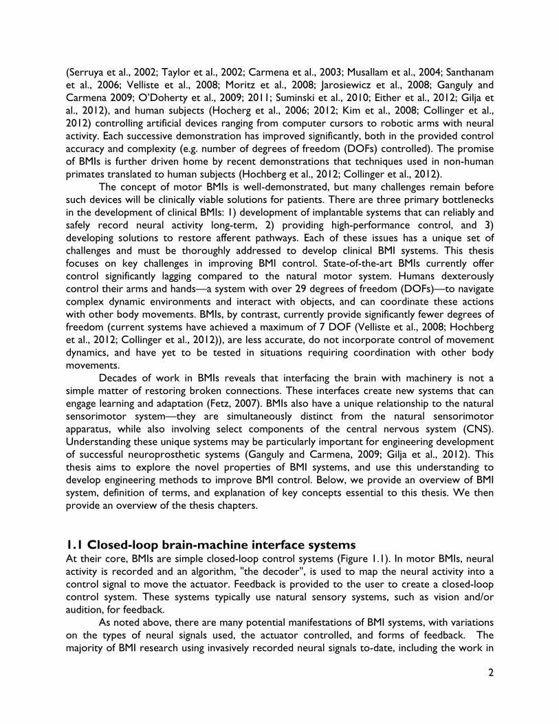
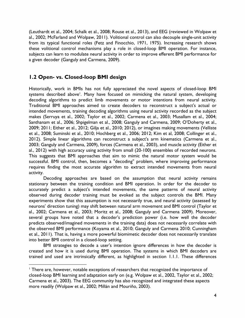
(Serruya et al., 2002; Taylor et al., 2002; Carmena et al., 2003; Musallam et al., 2004; Santhanam et al., 2006; Velliste et al., 2008; Moritz et al., 2008; Jarosiewicz et al., 2008; Ganguly and Carmena 2009; O’Doherty et al., 2009; 2011; Suminski et al., 2010; Either et al., 2012; Gilja et al., 2012), and human subjects (Hocherg et al., 2006; 2012; Kim et al., 2008; Collinger et al., 2012) controlling artificial devices ranging from computer cursors to robotic arms with neural activity. Each successive demonstration has improved significantly, both in the provided control accuracy and complexity (e.g. number of degrees of freedom (DOFs) controlled). The promise of BMIs is further driven home by recent demonstrations that techniques used in non-human primates translated to human subjects (Hochberg et al., 2012; Collinger et al., 2012). The concept of motor BMIs is well-demonstrated, but many challenges remain before such devices will be clinically viable solutions for patients. There are three primary bottlenecks in the development of clinical BMIs: 1) development of implantable systems that can reliably and safely record neural activity long-term, 2) providing high-performance control, and 3) developing solutions to restore afferent pathways. Each of these issues has a unique set of challenges and must be thoroughly addressed to develop clinical BMI systems. This thesis focuses on key challenges in improving BMI control. State-of-the-art BMIs currently offer control significantly lagging compared to the natural motor system. Humans dexterously control their arms and hands—a system with over 29 degrees of freedom (DOFs)—to navigate complex dynamic environments and interact with objects, and can coordinate these actions with other body movements. BMIs, by contrast, currently provide significantly fewer degrees of freedom (current systems have achieved a maximum of 7 DOF (Velliste et al., 2008; Hochberg et al., 2012; Collinger et al., 2012)), are less accurate, do not incorporate control of movement dynamics, and have yet to be tested in situations requiring coordination with other body movements. Decades of work in BMIs reveals that interfacing the brain with machinery is not a simple matter of restoring broken connections. These interfaces create new systems that can engage learning and adaptation (Fetz, 2007). BMIs also have a unique relationship to the natural sensorimotor system—they are simultaneously distinct from the natural sensorimotor apparatus, while also involving select components of the central nervous system (CNS). Understanding these unique systems may be particularly important for engineering development of successful neuroprosthetic systems (Ganguly and Carmena, 2009; Gilja et al., 2012). This thesis aims to explore the novel properties of BMI systems, and use this understanding to develop engineering methods to improve BMI control. Below, we provide an overview of BMI system, definition of terms, and explanation of key concepts essential to this thesis. We then provide an overview of the thesis chapters. 1.1 Closed-loop brain-machine interface systems At their core, BMIs are simple closed-loop control systems (Figure 1.1). In motor BMIs, neural activity is recorded and an algorithm, "the decoder", is used to map the neural activity into a control signal to move the actuator. Feedback is provided to the user to create a closed-loop control system. These systems typically use natural sensory systems, such as vision and/or audition, for feedback. As noted above, there are many potential manifestations of BMI systems, with variations on the types of neural signals used, the actuator controlled, and forms of feedback. The majority of BMI research using invasively recorded neural signals to-date, including the work in

3  

this thesis, explores BMI control of a 2-dimensional cursor using action-potential signals recorded from motor cortices (e.g. primary- and pre-motor cortex), with visual feedback. For illustrative purposes, all examples discussed below refer to this example system. 1.1.1 Relationship between BMI control and the natural motor system Natural arm movements are orchestrated by a host of brain areas, the spinal cord, and limb biomechanics; and somatosensory, proprioceptive and visual feedback play critical roles in the control. In BMI, subjects control an artificial device via visual observation alone, whose movements are governed by the activity of only a small subset of neurons in motor cortical areas. While BMIs can engage other cortical and subcortical areas (Ganguly et al., 2011; Koralek et al., 2012; Wander et al., 2013), the relationship between movement and neural activity imposed in BMI differs significantly from that of natural movements. The actuators controlled in BMI—e.g. virtual cursors and robotic arms—also differ dramatically from the complex biomechanical properties of the musculoskeletal system. These BMI systems may be able to replace motor function, but do so by creating a new control system that is distinct from natural arm movements (Carmena, 2013). Yet, this novel system still incorporates elements of the natural system. For instance, a BMI controlled with primary motor cortex and arm movements both engage motor cortical areas. The control of BMI systems may, then, share key similarities to the control of natural movements. Research does suggest strong connections between natural motor learning and BMI control (Green and Kalaska, 2011; Jackson and Fetz, 2011). BMI systems are separate from, but parallel to, the native functions they imitate. 1.1.2 The importance of feedback The closed-loop nature of BMI systems is essential to their operation. Feedback in BMI systems allows users to modify their behavior to achieve desired goals. Many studies show that rats, non-human primates and humans can learn to volitionally control neural activity using biofeedback at the level of single-unit action-potentials (Fetz, 1969; Fetz and Finocchio, 1971, 1975; Chapin et al., 1999; Gage et al., 2005; Fetz, 2007; Cerf et al., 2010; Moritz and Fetz, 2011; Koralek et al., 2012), local field potentials (Engelhard et al., 2013; Flint et al., 2013), ECoG

  

Figure 1.1 Schematic representations of motor (efferent) BMI systems. In BMI, recorded neural activity is mapped into control signals for a device via a decoding algorithm. These systems typically use natural sensory systems, such as vision, to provide feedback to the user, creating a closed-loop system.

4  

(Leuthardt et al., 2004; Schalk et al., 2008; Rouse et al., 2013), and EEG (reviewed in Wolpaw et al., 2002; McFarland and Wolpaw, 2011). Volitional control can also decouple single-unit activity from its typical functional roles (Fetz and Finocchio, 1971, 1975). Increasing research shows these volitional control mechanisms play a role in closed-loop BMI operation. For instance, subjects can learn to modulate neural activity in order to improve efferent BMI performance for a given decoder (Ganguly and Carmena, 2009). 1.2 Open- vs. Closed-loop BMI design Historically, work in BMIs has not fully appreciated the novel aspects of closed-loop BMI systems described above1. Many have focused on mimicking the natural system, developing decoding algorithms to predict limb movements or motor intentions from neural activity. Traditional BMI approaches aimed to create decoders to reconstruct a subject's actual or intended movements, training decoding algorithms using neural activity recorded as the subject makes (Serruya et al., 2002; Taylor et al., 2002; Carmena et al., 2003; Musallam et al., 2004; Santhanam et al., 2006; Shpigelman et al., 2008; Ganguly and Carmena, 2009; O’Doherty et al., 2009; 2011; Either et al., 2012; Gilja et al., 2010; 2012), or imagines making movements (Velliste et al., 2008; Suminski et al., 2010; Hochberg et al., 2006; 2012; Kim et al, 2008; Collinger et al., 2012). Simple linear algorithms can reconstruct a subject's arm kinematics (Carmena et al., 2003; Ganguly and Carmena, 2009), forces (Carmena et al., 2003), and muscle activity (Either et al., 2012) with high accuracy using activity from small (20-100) ensembles of recorded neurons. This suggests that BMI approaches that aim to mimic the natural motor system would be successful. BMI control, then, becomes a "decoding" problem, where improving performance requires finding the most accurate algorithm to extract intended movements from neural activity. Decoding approaches are based on the assumption that neural activity remains stationary between the training condition and BMI operation. In order for the decoder to accurately predict a subject's intended movements, the same patterns of neural activity observed during decoder training must be evoked as the subject controls the BMI. Many experiments show that this assumption is not necessarily true, and neural activity (assessed by neurons' direction tuning) may shift between natural arm movement and BMI control (Taylor et al., 2002; Carmena et al., 2003; Moritz et al., 2008; Ganguly and Carmena 2009). Moreover, several groups have noted that a decoder's prediction power (i.e. how well the decoder predicts observed/imagined movements in the training data) does not necessarily correlate with the observed BMI performance (Koyama et al., 2010; Ganguly and Carmena 2010; Cunningham et al., 2011). That is, having a more powerful biomimetic decoder does not necessarily translate into better BMI control in a closed-loop setting. BMI strategies to decode a user's intention ignore differences in how the decoder is created and how it is used during BMI operation. The systems in which BMI decoders are trained and used are intrinsically different, as highlighted in section 1.1.1. These differences

                                                            1 There are, however, notable exceptions of researchers that recognized the importance of closed-loop BMI learning and adaptation early on (e.g. Wolpaw et al., 2002, Taylor et al., 2002; Carmena et al., 2003). The EEG community has also recognized and integrated these aspects more readily (Wolpaw et al., 2002; Millán and Mouriño, 2003).

5  

contribute to decoder inaccuracies, and thus reduce prediction performance in BMI. While some of these differences might be overcome with technological advances—modeling to mimic limb biomechanics, neural stimulation shows promise to restore proprioceptive and tactile feedback (London et al., 2008; O’Doherty et al., 2009; 2011; Venkatraman and Carmena, 2011; Berg et al., 2013), improved neural recording technologies can increase the amount of brain areas recorded—it may be infeasible to create a BMI that completely mimics the motor system. What's more, it is unclear if and how biomimetic-based approaches can translate to patients with motor disabilities. Motor imagery can be used to evoke neural activity in motor-related areas (Tkach et al., 2007; Truccolo et al., 2008; Suminski et al., 2009) but if and how the motor system changes in response to injury is not fully understood. Decoding-based approaches and related techniques are "open-loop design" methods. The user has no knowledge of the predictions during training, thus creating an "open" feedback loop. Similarly, they neglect information about the new closed-loop control system created in BMI (see Section 1.1). BMI creates a novel, closed-loop system with a myriad of differences from the natural motor system. Increasing evidence suggests that decoding-based strategies alone may be insufficient for producing high-performance BMIs. BMIs do not accurately mimic the sensorimotor experience of natural limb movements, making the translation of decoding strategies from one context to another unclear. And most importantly, closed-loop BMI operation allows the subject to actively contribute to BMI performance (section 1.1.2). In closed-loop, BMI performance is determined by a collaboration of the user and the decoder. Thus, improving BMI performance may not be a matter of finding the optimal offline, open-loop decoder to "read-out" a user's intended movements. Instead, it is essential to understand the novel system created by closed-loop BMI and how to leverage its properties to design robust, high-performance BMIs. That is, BMI systems must be designed in closed-loop. 1.3 Closed-loop BMI design strategies This thesis explores closed-loop design of BMI systems. Designing “in closed-loop” refers to strategies informed by the view of BMIs as adaptive feedback systems (described in 1.1.2). Key considerations for closed-loop design include: 1) system adaptation (of the brain and/or decoder), 2) interactions between the brain and decoder, and 3) selection of system components (neural signals, control signals, actuator, feedback modalities). Recent work has begun to explore these factors, how they influence BMI performance, and how they may be used for providing high-performance neuroprostheses. 1.3.1 Neural adaptation A key feature of closed-loop BMI control is that the subject can actively contribute to performance by volitionally modulating neural activity (Fetz et al., 2007; Green and Kalaska 2011). Several studies suggest that subjects can learn to evoke new patterns of neural activity to facilitate BMI control (Moritz et al., 2008; Jarosiewicz et al., 2008; Ganguly and Carmena, 2009; Koralek et al., 2012; Chase et al., 2012). Recent findings suggest that harnessing this volitional control may be critical for creating high-performance, robust, and natural BMIs. When subjects are allowed to practice with a stable BMI "circuit"—including both the decoding algorithm mapping neural activity into control signals and the recorded neural activity input to the decoder—they learn a neural representation of the decoder that facilitates successful BMI

6  

control (Ganguly and Carmena, 2009). This learning allowed for significant performance improvements. Perhaps more importantly, this type of neural adaptation has been shown to facilitate consolidation of a “neuroprosthetic skill”. Much like natural motor skill learning, when practicing with a stable BMI circuit, subjects showed intra- and intersession learning, rapid recall of skill across days, and performance was robust to interference like learning new BMI decoders (Ganguly and Carmena, 2009). Skill consolidation resulted in the formation of a stable neural representation that was specific to the learned decoder that could be rapidly recalled.

BMI skill learning may also utilize similar neural mechanisms as natural motor learning, such as the corticostriatal system. Using rats controlling an auditory BMI, Koralek et al. (2012; 2013) found that the dorsolateral striatum is involved in and necessary for BMI learning. This was true even though subjects were controlling the BMI irrespective of physical movements (Koralek et al., 2012).

Neural adaptation may also facilitate creation of unique neural networks specialized for BMI control. Learning-related changes in cortical (Ganguly et al., 2011) and corticostriatal plasticity (Koralek et al., 2013) show specificity for BMI control neurons. The development of skilled BMI control has also been associated with reduced cognitive effort, linked to the formation of a control network distributed broadly across cortex (Wander et al., 2013).

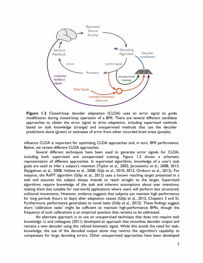
Together, these results suggest neural adaptation may be useful for both improving BMI performance and creating interfaces with desirable properties. BMIs that incorporate neural plasticity and skill consolidation may become more natural and intuitive for users to control. Skill consolidation and neural ensemble formation may also make BMIs more resistant to external perturbations, which is critical for creating BMIs that can be used in many different contexts and coordinated with other movements. In Chapter 5, we explore the potential utility of neural plasticity for creating BMIs that are robust to changes in context. 1.3.2 Closed-loop decoder adaptation Closed-loop decoder adaptation (CLDA) is another emerging approach to improve BMI performance motivated from a closed-loop perspective. Open-loop predictions may not accurately reflect the user's neural activity in closed-loop BMI, and closed-loop behavior cannot necessarily be predicted a priori. CLDA aims to combat these challenges by modify the decoder during closed-loop BMI operation. CLDA uses an error signal, derived in some way from the subject's performance during closed-loop BMI operation, to update the decoding algorithm (Figure 1.2). This concept has many different potential applications. For instance, CLDA has been successfully used to boost BMI performance by compensating for differences between open- and closed-loop decoders (Taylor et al., 2002; Jarosiewicz et al., 2008; 2013; Shpigelman et al., 2008; Velliste et al., 2008; Gilja et al., 2010; 2012; Collinger et al., 2012; Hochberg et al., 2012; Orsborn et al., 2012). As we explore in Chapter 3, it can also be used to compensate for a lack of available information to initialize a decoder, which may be particularly useful in clinical settings with paralyzed patients (Orsborn et al., 2012). CLDA may also be useful for maintaining high-performance BMIs in the presence of non-stationary neural recordings (Héliot et al., 2010b; Wu et al., 2008; Li et al., 2011). The basic CLDA approach can be implemented in a variety of ways. At the heart of every CLDA algorithm are methods to 1) estimate an error signal, and 2) update the decoder based on these signals. Many different CLDA approaches have been successfully developed. However, the structure of these algorithms will influence their ultimate utility, and the uses for which they are best suited. Fully understanding these algorithms and how design choices

7  

influence CLDA is important for optimizing CLDA approaches and, in turn, BMI performance. Below, we review different CLDA approaches.

Several different techniques have been used to generate error signals for CLDA, including both supervised and unsupervised training. Figure 1.2 shows a schematic representation of different approaches. In supervised algorithms, knowledge of a user's task goals are used to infer a subject's intention (Taylor et al., 2002; Jarosiewicz et al., 2008; 2013; Shpigelman et al., 2008; Velliste et al., 2008; Gilja et al., 2010; 2012; Orsborn et al., 2012). For instance, the ReFIT algorithm (Gilja et al., 2012) uses a known reaching target presented in a task and assumes the subject always intends to reach straight to the target. Supervised algorithms require knowledge of the task and inherent assumptions about user intentions, making them less suitable for real-world applications where users will perform less structured, volitional movements. However, evidence suggests that subjects can maintain high performance for long periods (hours to days) after adaptation ceases (Gilja et al., 2012; Chapters 3 and 5). Furthermore, performance generalizes to novel tasks (Gilja et al., 2012). These findings suggest short 'calibration tasks' might be sufficient to maintain high-performance BMIs, though the frequency of such calibrations is an empirical question that remains to be addressed. An alternate approach is to use an unsupervised technique that does not require task knowledge. Li and colleagues (2011) developed an approach that smoothes decoder output and retrains a new decoder using this refined kinematic signal. While this avoids the need for task-knowledge, the use of the decoded output alone may restrict the algorithm's capability to compensate for large decoding errors. Other unsupervised approaches have been developed

  

Figure 1.2 Closed-loop decoder adaptation (CLDA) uses an error signal to guide modification during closed-loop operation of a BMI. There are several different candidate approaches to obtain the error signal to drive adaptation, including supervised methods based on task knowledge (orange) and unsupervised methods that use the decoder predictions alone (green) or estimates of error from other recorded brain areas (purple).

8  

that use models of user cost-functions to detect deviations from optimal control, which was able to compensate for large errors in simulation studies (Gürel and Mehring, 2012). However, such methods still do not avoid inherent assumptions about a user's intentions and may increase algorithmic complexity. Another unsupervised approach is to use neural-derived error signals. Mahmoudi and Sanchez (2011) demonstrated an actor-critic CLDA algorithm where basal ganglia output, known to relate to motor error-evaluation, was used as a decoder training signal. It may also be fruitful to combine unsupervised approaches based on task performance with neural-based error signals (Gürel and Mehring, 2012). The necessity to record additional neural signals, possibly requiring implantation in more brain areas, could be prohibitive in clinical settings. Additional work is also needed to understand the best methods for deriving error signals from neural activity. The other key component to CLDA algorithms is a method to update the decoder given an error signal. This step involves several different design choices, including 1) the time-scale of decoder adaptation, 2) the structure of the update rules, and 3) what parameters to update. Each design element will ultimately influence the algorithm's performance, particularly in closed-loop operation where decoder adaptation interacts with the user. The time-scale of adaptation determines both the amount of data used for decoder updates and the rate at which the user experiences shifts in the decoder, which will both critically influence CLDA performance. As we show in Chapters 3 and 4, in situations where initial decoders have severely limited performance, providing the subject with feedback (in the form of a new decoder and modified closed-loop performance) in a timely manner may be critical. The structure of the update rules can also contribute significantly to CLDA algorithm performance. For instance, algorithms designed to make smooth, gradual updates to decoder parameters (e.g. (Taylor et al., 2002; Shpigelman et al., 2008; Dangi et al., 2011; Orsborn et al., 2012)) may be more robust to unreliable training data than algorithms that overwrite parameters. Finally, it is also important to assess what parameters within a decoder to adapt. The primary goal of CLDA is to adapt the mapping between neural activity and controlled kinematics. Decoders such as the Kalman filter, for example, include parameters that govern the underlying kinematics of the controlled system. Adapting these parameters could be equivalent to modifying the controlled actuator, and could have unwanted consequences (Gowda et al., 2012). We explore these CLDA design choices in Chapter 4. CLDA algorithm design choices all have intrinsic trade-offs, and may be more useful for different applications. For instance, supervised methods may be most fruitful for initial decoder training, while unsupervised approaches could be employed to maintain performance in the presence of neural instability. Similarly, the design choices of each CLDA component are not entirely independent. The best update rules for an algorithm will be informed by the time-scale of adaptation. Further study is needed to fully understand how these algorithm design choices influence CLDA algorithm performance. Mathematical analyses (Dangi et al., 2013a) or closed-loop simulators (Cunningham et al., 2011) may be particularly useful tools to facilitate preliminary design and parameter-space exploration. However, CLDA algorithm testing must ultimately be conducted in closed-loop BMI experiments to incorporate the subject interactions inherent in the process. Finally, CLDA design should not be considered in isolation of the full BMI system design. For instance, constant decoder adaptation may be detrimental to long-term BMI performance, as it could obfuscate neural adaptation and skill consolidation. Little is known, however, about how neural and decoder adaptation might interact. We explore these issues in Chapter 5.

9  

1.3.3 Closed-loop system design Viewing BMIs as closed-loop systems can also be used to inform the development and design of the BMI system. Much as the spinal cord organization and limb biomechanics contribute to natural movements, the structure of decoding algorithms and dynamics the controlled actuators will play important roles in closed-loop BMI performance. Indeed, studies have shown that closed-loop BMI performance changes significantly when neural activity is used to control a cursor versus a robot (Carmena et al., 2003; Taylor et al., 2003). Because closed-loop control involves interplay between the user and decoder, the decoder design cannot be done in isolation. Traditional approaches for decoder creation and optimization have been done in open-loop, where the sole goal is to maximize the decoder's prediction power. However open-loop prediction power does not necessarily translate to improved closed-loop BMI performance due to fundamental system differences (see section 1.2). What's more, the requirements of a closed-loop decoder may differ significantly due to subject-interaction. That is, closed-loop decoders not only need to be able to extract user intention, they must also be readily controlled by the subject in the presence of feedback. Increasing evidence suggests that decoders optimized for extracting information in open-loop may not be optimal in the closed-loop setting. For instance, Kalman filters created using maximum-likelihood methods can have undesirable control-properties that hinder closed-loop performance (Gowda et al., 2012). The optimal bin-width for linear filter decoders also differs significantly between open- and closed-loop settings (Cunningham et al., 2011). These findings suggest that decoder design and development must incorporate a closed-loop perspective of BMIs. The neural input selected for a decoder may also significantly influence performance. Traditional open-loop approaches only focus on maximizing decoded information. This might suggest that increasing the number of neural inputs (e.g. the number of neurons) into the decoder. However, closed-loop performance can often be improved by selecting a small subset of neurons that the subjects can readily modulate in closed-loop control, rather than using all available neurons (Wahoun et al., 2006). This suggests that optimizing BMI performance requires identifying neural signals that are most informative in closed-loop and that subjects can easily learn to control. A related question is what control variables are optimal for closed-loop control. Research with humans controlling a simulated BMI with arm movements suggest that performance strongly depends on the controlled kinematic variables (Marathe and Taylor, 2011). These questions become increasingly important in considering how to transition to BMIs that operate in real-world environments, where dynamics play a crucial role.

These studies clearly illustrate that the dynamics and structure of a decoder and the controlled actuator play key roles in closed-loop performance. Additional work is needed to both develop frameworks for studying closed-loop decoder optimization and explore the influence of decoder dynamics on control. 1.4 Chapter previews In Chapter 2, we present an overview of the BMI decoding and closed-loop decoder adaptation methods used throughout this thesis.

10  

In Chapters 3 and 4, we explore the design and analysis of CLDA algorithms. Chapter 3 presents a novel algorithm (SmoothBatch) that is designed to improve performance regardless of the initial decoder. This is particularly important for clinical applications, where there is limited information to train an initial decoder. Chapter 4 carefully explores important design considerations inherent in designing CLDA algorithms: the time-scale of adaptation and structure of the decoder update rules. This chapter carefully examines the SmoothBatch algorithm as a case study. We also present a mathematical framework to analyze CLDA algorithms that can facilitate engineering design and algorithm development. Having developed a robust CLDA algorithm, in Chapter 5, we explore how decoder adaptation can be combined with neural adaptation to improve BMI performance. We explore using decoder adaptation to shape neuroplasticity in two scenarios relevant for real-world neuroprostheses: non-stationary recordings of neural activity, and changes in control context. We show that beneficial neuroplasticity can occur alongside decoder adaptation, yielding performance improvements, skill retention, and resistance to interference from native motor networks. These results highlight the importance of neuroplasticity for real-world neuroprostheses. In Chapter 6, we explore how the neural signals used for control may influence closed-loop BMIs. While BMIs have been implemented with a variety of neural signals (spiking activity, local field potentials, ECoG) across different brain areas, little is known about how subjects control these different neural signals. The relationship between these neural signals in closed-loop BMI is also poorly understood. Because biofeedback in BMI facilitates neural adaptation (see sections 1.1.2 and 1.2.1), the signal used for control may influence neural control strategies in closed-loop. In this chapter, we examine the neural strategies used by subjects operating a BMI with spiking or LFP activity. Better understanding the relationship between neural signals in closed-loop BMI could inform the design of future systems. Finally, in Chapter 7 we explore how neural activity in the natural motor system depends on the dynamics of movement. To date, BMIs have focused on controlling movement kinematics. Pure motion control, however, lacks the information required for interaction with real objects. In real-world environments, dynamic interactions—forces and torques between the hand and the environment—will be critical for robust performance. Little is known, however, about how the central nervous system controls limb dynamics. Deeper understanding of how the highly distributed natural motor system controls limb dynamics may provide insights into how to incorporate dynamics control into neuroprostheses. In this study, we ask if neural activity within the primary and pre-motor cortices varies with movements in different dynamic environments, focusing on local-field potential activity.

11  

Chapter 2:

BMI decoding and closed-loop decoder adaptation methods Many different decoding algorithms have been developed for Brain-Machine Interfaces (BMIs). The decoding algorithm maps recorded neural activity into a control signal for the actuator (see section 1.1). As reviewed in the introduction (and Chapter 6), the types of neural and control signals used can be varied. Similarly, the structure of the decoding algorithm is an important design consideration for developing cortical prostheses. The BMI system architecture—particularly the controlled actuator and neural signal properties—will shape the type of algorithms used.

BMI algorithms can be grouped into several different classes: continuous variable versus discrete movement prediction, generative versus discriminative approaches, and linear versus non-linear methods. Continuous variable prediction uses neural activity to estimate a continuous-valued movement variable (e.g. end-point velocity), while discrete movement prediction maps neural activity to one of a limited set of movement options (e.g. one of 8 target positions). Generative (or inference-based) methods aim to model the relationship between neural activity and movement parameters, which then allows for prediction. Discriminative methods, instead, establish relationships between observed neural activity and movement parameters without learning an underlying model. That is, they perform pattern-recognition. Discriminative algorithms, then, are most commonly used for discrete predictions where a limited number of patterns must be learned. Finally, linear decoders use a mapping between neural activity and movement parameters that is linear, while non-linear decoders use non-linear mappings.

The design of decoding algorithms to maximize closed-loop BMI performance is an important question. In this thesis, however, we focus on other closed-loop design considerations related to system adaptation (Chapters 3-5), and neural (Chapter 6) and control (Chapter 7) signal selection. Therefore, BMI work presented in this thesis uses a single decoding approach. We focus on linear decoding algorithms for continuous movement control, which are most commonly used in intra-cortical BMI applications. Specifically, we use the Kalman filter (KF) to implement position-velocity control of a cursor. Continuous control BMI systems are particularly interesting because the subject has constant control and feedback of the device, facilitating dynamic adaptive processes (see Chapter 1).

Similarly, there are many candidate methods for closed-loop decoder adaptation (CLDA) (see Section 1.3.2 and Chapter 4). One key focus of this thesis is better understanding CLDA algorithms and the design principles that influence their performance. In this thesis, we restrict our study of CLDA algorithms to supervised-training methods, focusing primarily on how to update the decoder given a particular training signal. As discussed in Chapters 1 and 4, further study is needed to understand the best ways to obtain the training signals for particular CLDA applications.

In this chapter, we provide an overview of the KF, its implementation for BMI, and relevant CLDA algorithms that are used throughout the work presented in this thesis.

12  

2.1 The Kalman filter The Kalman filter (KF) is a linear filter that predicts an unobservable "hidden" state of a system by modeling the underlying dynamics of the hidden state and their relationship to observable variables (Hayes, 1996; Haykin, 2002). In BMI applications, the KF is used to predict unknown movement variables (hidden state) based on observed neural activity (observable variables) (Wu et al., 2003; Kim et al., 2008; Gilja et al., 2012; Orsborn et al., 2012). The filter models the underlying dynamics of movement (e.g. given a particular end-point position at time t, what is the most likely end-point position at t+1). It also models the relationship between measured neural activity and movement. The filter uses a combination of estimates based on the dynamics model and neural activity measurements to predict movements. The KF assumes jointly Gaussian linear state evolution (2.1) and observation models (2.2):

1t t tx Ax w (2.1)

t t ty Cx q (2.2) where 1k

tyR represents the observed measurements (e.g. firing rates of k neurons) at time

t. 1ptx

R denotes the hidden state (e.g. p movement variables) recorded neural activity at time t. wt ~ N(0, W) and qt ~ N(0, Q) are Gaussian additive noise terms. The filter is thus specified by the matrices p pA R , p pW R , k pC R , and k kQ R .

Based on these models, the KF recursively estimates the current movement variables xt based on both the past observed movements (xt-1, …x0) and currently observed neural activity yt. The recursive estimation scheme is as follows:

1) Estimate of movement variables based solely on state-evolution model (a priori estimate):

| 1 1ˆt t tx Ax (2.3)

2) Estimate the covariance (uncertainty) of the a priori estimate:

T

| 1 1t t tP AP A W (2.4)

3) Compute the expected neural activity corresponding to the a priori estimated movement,

and the difference between the expected and observed neural activity (measurement residual):

| 1ˆt t t ty y Cx (2.5)

4) Compute the covariance (uncertainty) of this measurement residual:

T

| 1t t tS CP C Q (2.6)

13  

5) Compute an estimate of kinematics incorporating the recorded neural activity (a posteriori estimate):

| 1ˆ ˆt t t tx x Ky (2.7) T 1

| 1t t tK P C S (2.8)

6) Compute the covariance (uncertainty) of the a posteriori estimate:

| 1( )t t t tP I K C P (2.9)

Because the KF is recursive, it is an infinite-length filter—that is, observations at a given

time can influence all future predictions. However, in practice the influence of a given observation decays relatively quickly over (on the order of 0.5-1 second in typical BMIs presented in this thesis). The KF is well-suited to predictions of continuous movement variables in BMI because it is designed to incorporate temporal dynamics. For instance, the filter can be designed to capture the natural physical relationships between dynamically-linked variables like position and velocity. 2.2 Experimental implementation of the Kalman filter BMI control in this thesis used a position-velocity KF operating in end-point coordinates. The state variable was defined to include cursor position (p) and velocity (v) in Cartesian space:

T[ 1]horiz vert horiz vertt t t t tx p p v v (2.10)

where horiz and vert indicate the horizontal and vertical directions, respectively. The constant 1 term was used to compensate for non-zero-mean firing rates.

The state-transition model (A and W matrices, describing cursor dynamics) were defined to model the system physics, with position components set as the integral of velocity, as in (Gilja et al., 2010; 2012):

1 0 0 0

0 1 0 0

0 0 0

0 0 0

0 0 0 0 1

xx xyv vyx yyv v

dt

dt

A a a

a a

(2.11)

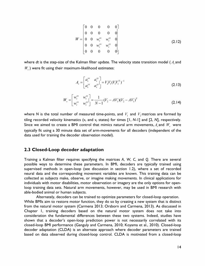
14  

0 0 0 0 0

0 0 0 0 0

0 0 0

0 0 0

0 0 0 0 0

xx xyv vyx yyv v

W w w

w w

(2.12)

where dt is the step-size of the Kalman filter update. The velocity state transition model ( vA and

vW ) were fit using their maximum-likelihood estimates:

T 12 1 1 1( )

xx xyv v

v yx yyv v

a aA V V VV

a a

(2.13)

T2 1 2 1

1( )( )

1

xx xyv v

v yx yyv v

w wW V AV V AV

Nw w

(2.14)

where N is the total number of measured time-points, and 1V and 2V matrices are formed by tiling recorded velocity kinematics (vx and vy states) for times [1, N-1] and [2, N], respectively. Since we aimed to create a BMI control that mimics natural arm movements, vA and vW were typically fit using a 30 minute data set of arm-movements for all decoders (independent of the data used for training the decoder observation model). 2.3 Closed-Loop decoder adaptation Training a Kalman filter requires specifying the matrices A, W, C, and Q. There are several possible ways to determine these parameters. In BMI, decoders are typically trained using supervised methods in open-loop (see discussion in section 1.2), where a set of recorded neural data and the corresponding movement variables are known. This training data can be collected as subjects make, observe, or imagine making movements. In clinical applications for individuals with motor disabilities, motor observation or imagery are the only options for open-loop training data sets. Natural arm movements, however, may be used in BMI research with able-bodied animal or human subjects.

Alternately, decoders can be trained to optimize parameters for closed-loop operation. While BMIs aim to restore motor function, they do so by creating a new system that is distinct from the natural motor system (Carmena 2013; Orsborn and Carmena, 2013). As discussed in Chapter 1, training decoders based on the natural motor system does not take into consideration the fundamental differences between these two systems. Indeed, studies have shown that a decoder’s open-loop prediction power is not necessarily correlated with its closed-loop BMI performance (Ganguly and Carmena, 2010; Koyama et al., 2010). Closed-loop decoder adaptation (CLDA) is an alternate approach where decoder parameters are trained based on data observed during closed-loop control. CLDA is motivated from a closed-loop

15  

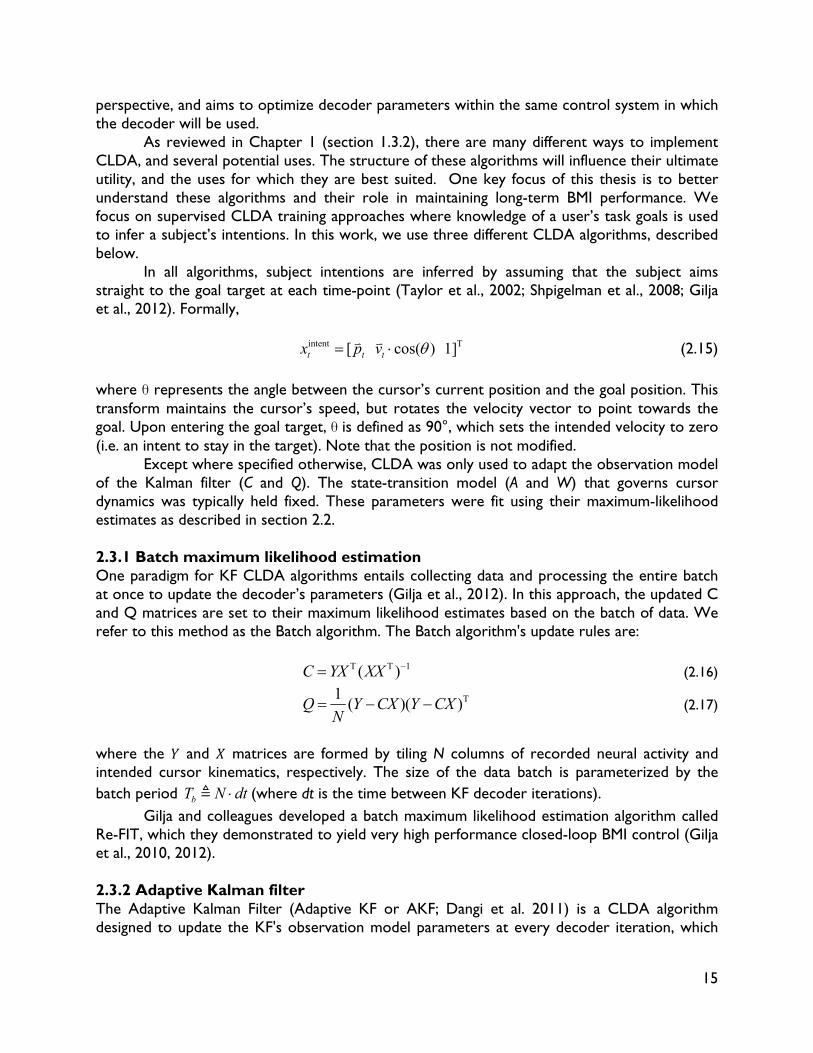
perspective, and aims to optimize decoder parameters within the same control system in which the decoder will be used. As reviewed in Chapter 1 (section 1.3.2), there are many different ways to implement CLDA, and several potential uses. The structure of these algorithms will influence their ultimate utility, and the uses for which they are best suited. One key focus of this thesis is to better understand these algorithms and their role in maintaining long-term BMI performance. We focus on supervised CLDA training approaches where knowledge of a user’s task goals is used to infer a subject’s intentions. In this work, we use three different CLDA algorithms, described below.

In all algorithms, subject intentions are inferred by assuming that the subject aims straight to the goal target at each time-point (Taylor et al., 2002; Shpigelman et al., 2008; Gilja et al., 2012). Formally,

intent T[ cos( ) 1]t t tx p v (2.15)

where θ represents the angle between the cursor’s current position and the goal position. This transform maintains the cursor’s speed, but rotates the velocity vector to point towards the goal. Upon entering the goal target, θ is defined as 90°, which sets the intended velocity to zero (i.e. an intent to stay in the target). Note that the position is not modified. Except where specified otherwise, CLDA was only used to adapt the observation model of the Kalman filter (C and Q). The state-transition model (A and W) that governs cursor dynamics was typically held fixed. These parameters were fit using their maximum-likelihood estimates as described in section 2.2. 2.3.1 Batch maximum likelihood estimation One paradigm for KF CLDA algorithms entails collecting data and processing the entire batch at once to update the decoder’s parameters (Gilja et al., 2012). In this approach, the updated C and Q matrices are set to their maximum likelihood estimates based on the batch of data. We refer to this method as the Batch algorithm. The Batch algorithm's update rules are:

T T 1( )C YX XX (2.16)

T1( )( )Q Y CX Y CX

N

(2.17)

where the and matrices are formed by tiling N columns of recorded neural activity and intended cursor kinematics, respectively. The size of the data batch is parameterized by the batch period bT N dt (where dt is the time between KF decoder iterations).

Gilja and colleagues developed a batch maximum likelihood estimation algorithm called Re-FIT, which they demonstrated to yield very high performance closed-loop BMI control (Gilja et al., 2010, 2012). 2.3.2 Adaptive Kalman filter The Adaptive Kalman Filter (Adaptive KF or AKF; Dangi et al. 2011) is a CLDA algorithm designed to update the KF's observation model parameters at every decoder iteration, which

16  

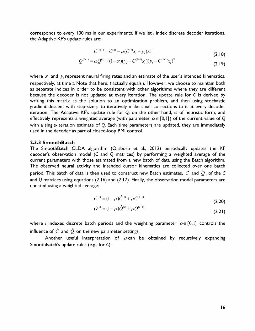
corresponds to every 100 ms in our experiments. If we let i index discrete decoder iterations, the Adaptive KF's update rules are:

( 1) ( ) ( ) T( )i i it t tC C C x y x (2.18)

( 1) ( ) ( 1) ( 1) T(1 )( )( )i i i it t t tQ Q y C x y C x

(2.19) where tx and ty represent neural firing rates and an estimate of the user's intended kinematics, respectively, at time t. Note that here, t actually equals i. However, we choose to maintain both as separate indices in order to be consistent with other algorithms where they are different because the decoder is not updated at every iteration. The update rule for C is derived by writing this matrix as the solution to an optimization problem, and then using stochastic gradient descent with step-size μ to iteratively make small corrections to it at every decoder iteration. The Adaptive KF's update rule for Q, on the other hand, is of heuristic form, and effectively represents a weighted average (with parameter [0,1] ) of the current value of Q with a single-iteration estimate of Q. Each time parameters are updated, they are immediately used in the decoder as part of closed-loop BMI control. 2.3.3 SmoothBatch The SmoothBatch CLDA algorithm (Orsborn et al., 2012) periodically updates the KF decoder's observation model (C and Q matrices) by performing a weighted average of the current parameters with those estimated from a new batch of data using the Batch algorithm. The observed neural activity and intended cursor kinematics are collected over one batch period. This batch of data is then used to construct new Batch estimates, C

and Q , of the C

and Q matrices using equations (2.16) and (2.17). Finally, the observation model parameters are updated using a weighted average:

( ) ( ) ( 1)ˆ(1 )i i iC C C (2.20)

( ) ( ) ( 1)ˆ(1 )i i iQ Q Q (2.21)

where i indexes discrete batch periods and the weighting parameter [0,1]

controls the

influence of C and Q on the new parameter settings.

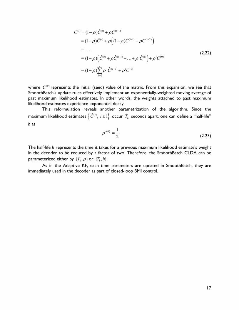
Another useful interpretation of can be obtained by recursively expanding SmoothBatch's update rules (e.g., for C):

17  

( ) ( ) ( 1)

( ) ( 1) ( 2)

( ) ( 1) (1) (0)

( ) (0)

0

ˆ(1 )

ˆ ˆ (1 ) (1 )

=

ˆ ˆ ˆ = (1 )

ˆ = (1 )

i i i

i i i

i i i i

ij i j i

j

C C C

C C C

C C C C

C C

(2.22)

where (0)C represents the initial (seed) value of the matrix. From this expansion, we see that SmoothBatch's update rules effectively implement an exponentially-weighted moving average of past maximum likelihood estimates. In other words, the weights attached to past maximum likelihood estimates experience exponential decay.

This reformulation reveals another parametrization of the algorithm. Since the

maximum likelihood estimates ( )ˆ , 1iC i occur bT seconds apart, one can define a “half-life”

h as / 1

2bh T

(2.23) The half-life h represents the time it takes for a previous maximum likelihood estimate's weight in the decoder to be reduced by a factor of two. Therefore, the SmoothBatch CLDA can be parameterized either by { , }bT or { , }bT h .

As in the Adaptive KF, each time parameters are updated in SmoothBatch, they are immediately used in the decoder as part of closed-loop BMI control.

18  

Chapter 3:

Designing closed-loop decoder adaptation algorithms to improve BMI performance independent of initialization Significant improvements in reliability (lifetime usability of the interface) and performance (achieving control and dexterity comparable to natural movements) are needed (Millán and Carmena, 2010; Gilja et al., 2011) to make BMIs a clinically viable therapeutic option for paralyzed individuals. One critical challenge is in understanding how to improve BMI performance using techniques that can tolerate variability and non-ideal conditions. In this chapter, we take steps towards this long-term goal by developing a novel closed-loop decoder adaptation (CLDA; see Chapters 1 and 2) algorithm that is robust to varying initialization. This work was done in collaboration with Siddharth Dangi, Helene Moorman and Jose M. Carmena, and was published in IEEE Transactions on Neural Systems and Rehabilitation Engineering (Orsborn et al., 2012). 3.1 Introduction BMI systems use an algorithm (the "decoder") to translate recorded neural activity (e.g. spike trains) into a control signal (e.g. position) for an external actuator such as a computer cursor. The BMI user receives performance feedback, typically in the form of visual observation, creating a closed feedback system. Thus, BMIs allow a user to modulate their neural activity to achieve a desired goal. BMI decoders are usually created in open-loop by first recording neural activity as a subject makes movements (Serruya et al., 2002; Taylor et al., 2002; Carmena et al., 2003; Musallam et al., 2004; Santhanam et al., 2006; Shpigelman et al., 2008; Ganguly and Carmena, 2009; O’Doherty et al., 2009; Gilja et al., 2010; 2012), or imagines moving (Hochberg et al., 2006; 2012; Kim et al., 2008; Velliste et al., 2008; Suminski et al., 2010), and then training a decoder to predict these movements from the neural activity. However, open-loop decoder prediction power does not directly correlate with closed-loop performance (Koyama et al., 2010; Ganguly and Carmena, 2010), suggesting that improvements in BMI performance cannot be achieved solely by finding an optimal open-loop decoding algorithm. Instead, recent work shows that significant improvements in performance can come from insights into the closed-loop BMI system, in which brain and machine adaptation play pivotal roles. For instance, Ganguly and Carmena (2009) showed that when subjects practiced BMI control with a fixed decoder, they learned a stable neural representation of the decoder, and the development of these stable representations paralleled improvements in control. In other words, the brain can adapt to improve performance. Other researchers have taken the opposite approach, investigating methods of closed-loop decoder adaptation (CLDA) to improve performance (Taylor et al., 2002; Gage et al., 2005; Shpigelman et al., 2008; Gilja et al., 2010; Mahmoudi and Sanchez, 2011; Gilja et al., 2010; 2012). These studies show that closed-loop BMI performance can be significantly improved by using known or inferred task goals, or evaluative feedback, during closed-loop BMI control to modify the decoder. CLDA algorithms typically have two components: 1) a method to infer a subject's intended movement goals during closed-loop control, and 2) a rule to update the decoder's

19  

parameters. One particularly interesting aspect of candidate decoder update algorithms is the time-scale on which they update the decoder. Gilja et al. (2010, 2012) used a batch-based algorithm that applies one discrete decoder update 10-15 minutes after the initial seeding, while Shpigelman et al. (2008) used a real-time update rule that adjusts the decoder at every decoder iteration. Given that closed-loop BMI performance involves an inherent interplay between the subject and the decoder, the rate at which the decoder changes will likely influence performance and the algorithm's ability to improve control. Moreover, this time-scale of adaptation may be paramount in situations where initial closed-loop performance may be severely limited, such as clinical applications for patients that cannot enact natural movement because of spinal cord injury or other neurological disorders. It is thus worthwhile to identify the most appropriate time-scale of decoder adaptation to yield efficient CLDA algorithms that rapidly and robustly improve BMI performance regardless of initial closed-loop performance. Here, we present a new CLDA algorithm called SmoothBatch, which updates the decoder on an intermediate (1-2 minute) timescale. This algorithm implements a sliding average of decoder parameters estimated on small batches of data. SmoothBatch uses the method developed by Gilja et al. (2010, 2012) to infer the subject's intended kinematics in a center-out task. We present experimental validation using data from one non-human primate subject. We also explore the algorithm's ability to improve closed-loop BMI performance independent of the initial decoder performance (seed) by comparing SmoothBatch's performance using four different decoder seeding methods: 1) visual observation of cursor movement, 2) ipsilateral arm movement, 3) neural activity during quiet sitting, and 4) arbitrary weights. 3.2 Methods 3.2.1 Electrophysiology One adult male rhesus macaque (macaca mulatta) was used in this study. The subject was chronically implanted with microwire electrode arrays for neural recording. One array of 128 Teflon-coated tungsten electrodes (35 μm diameter, 500 μm wire spacing, 8 x 16 array configuration; Innovative Neurophysiology, Durham, NC) was implanted in each brain hemisphere, targeting the arm areas of primary motor cortex (M1) and dorsal premotor cortex (PMd). Localization was performed using stereotactic coordinates from rhesus brain anatomy (Paxinos, 2000). Each array was positioned targeting M1, and due to the size of the array, extended rostrally into PMd. All procedures were conducted in compliance with the National Institutes of Health Guide for Care and Use of Laboratory Animals and were approved by the University of California, Berkeley Institutional Animal Care and Use Committee.

Unit activity was recorded using a combination of two 128-channel MAP and OmniPlex recording systems (Plexon Inc., Dallas, TX). Single and multi-unit activity was sorted using an online sorting application (Plexon, Inc., Dallas, TX), and only neural activity with well-identified waveforms were used for BMI control (see below). 3.2.2 Behavioral task The subject was trained to perform a self-paced delayed 2D center-out reaching task to 8 targets (1.7cm radius) uniformly spaced about a 14cm diameter circle. The animal sat in a primate chair, head restrained, and observed reach targets displayed via a computer monitor projecting to a semi-transparent mirror parallel to the floor. Figure 3.1 shows an illustration of

20  

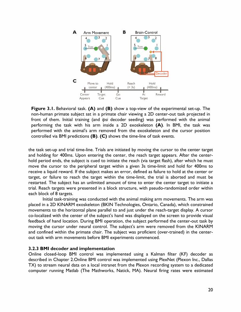
Figure 3.1. Behavioral task. (A) and (B) show a top-view of the experimental set-up. The non-human primate subject sat in a primate chair viewing a 2D center-out task projected in front of them. Initial training (and ipsi decoder seeding) was performed with the animal performing the task with his arm inside a 2D exoskeleton (A). In BMI, the task was performed with the animal's arm removed from the exoskeleton and the cursor position controlled via BMI predictions (B). (C) shows the time-line of task events.

the task set-up and trial time-line. Trials are initiated by moving the cursor to the center target and holding for 400ms. Upon entering the center, the reach target appears. After the center-hold period ends, the subject is cued to initiate the reach (via target flash), after which he must move the cursor to the peripheral target within a given 3s time-limit and hold for 400ms to receive a liquid reward. If the subject makes an error, defined as failure to hold at the center or target, or failure to reach the target within the time-limit, the trial is aborted and must be restarted. The subject has an unlimited amount of time to enter the center target to initiate a trial. Reach targets were presented in a block structure, with pseudo-randomized order within each block of 8 targets. Initial task-training was conducted with the animal making arm movements. The arm was placed in a 2D KINARM exoskeleton (BKIN Technologies, Ontario, Canada), which constrained movements to the horizontal plane parallel to and just under the reach-target display. A cursor co-localized with the center of the subject's hand was displayed on the screen to provide visual feedback of hand location. During BMI operation, the subject performed the center-out task by moving the cursor under neural control. The subject's arm were removed from the KINARM and confined within the primate chair. The subject was proficient (over-trained) in the center-out task with arm movements before BMI experiments commenced. 3.2.3 BMI decoder and implementation Online closed-loop BMI control was implemented using a Kalman filter (KF) decoder as described in Chapter 2.Online BMI control was implemented using PlexNet (Plexon Inc., Dallas TX) to stream neural data on a local intranet from the Plexon recording system to a dedicated computer running Matlab (The Mathworks, Natick, MA). Neural firing rates were estimated

21  

with a 100ms bin width. Neural ensembles of 16-36 (26.5 ± 4.45; mean ± STD) neurons were used. Units were selected only based on waveform quality. 3.2.4 Decoder seeding Decoders were initialized in four ways: 1) using neural activity recorded as the subject passively viewed a cursor moving through the center-out task (visual feedback; VFB; n = 20), 2) using neural activity recorded during ipsilateral arm movements (ipsi; n = 8), 3) using neural activity recorded during quiet sitting (baseline; n = 17), and 4) arbitrary seeding by shuffling weights of past (SmoothBatch-adapted) decoder weights (shuffled; n = 11). The state-transition model (A and W matrices in equation (2.1), describing cursor dynamics) were defined to model the system physics, with position components set as the integral of velocity, as in (Gilja et al., 2010; 2012) and as described in Chapter 2. Since we aimed to create a BMI control that mimics natural arm movements, and (see equations (2.13) and (2.14)) were fit using a 30 minute data set of arm-movements from the center-out task for all seeds.

For seeding methods 1-3, the observation model (C and Q matrices in equation (2.2). describing neural activity's relation to cursor movement) were fit using their maximum-likelihood estimate:

T T 1( )C YX XX (3.1)

T1( )( )Q Y CX Y CX

N (3.1)

where the Y and X matrices are formed by tiling recorded neural activity and kinematics (full state vector), respectively. Neural and kinematic data were collected for 8 minutes. For VFB seeding, a visual cursor was moved through artificially generated trajectories (straight trajectories, Gaussian speed profiles, 800ms reach duration) to perform the center-out task. The subject viewed the cursor movement while seated in the primate chair, receiving pseudo-random rewards on 25% of all trials. While no effort was made to constrain subject behavior, the animal typically sat quietly and looked at the display. Recorded neural activity and the artificially generated cursor kinematics were used for decoder estimation. Baseline seeding was performed using the same protocol as VFB, but with the display turned off so that the subject did not see anything. Ipsi decoder seeds were created with neural data ipsilateral to the arm kinematics recorded as the subject performed the center-out task with his arm. For shuffled seeds, the observation models were constructed by taking the weights of an existing decoder (previously optimized using SmoothBatch CLDA; see below) from prior experimental sessions and shuffling the weight assignments for each unit. 3.2.5 Closed-loop decoder adaptation algorithm: SmoothBatch Once a seed decoder was created, CLDA was used to improve performance. The algorithm used, SmoothBatch, updates the decoder on an intermediate (1-2 minute) time-scale. The subject performed the center-out task under BMI control as the algorithm updated the decoder. The subject's intended kinematics were inferred from the observed BMI performance using the technique developed by Gilja et al. (2010, 2012), which assumed that the subjects intends to reach straight to the target at all times and rotates observed cursor velocities to

22  

point towards the current task target. The observed neural activity and intended kinematics were collected for a short (1-2 minutes) interval. Each batch of data was used to construct a new estimate of the C and Q matrices (using equations (3.1) and (3.2)), and , and these batch estimates were averaged over time to update the decoder parameters. The SmoothBatch algorithm equations and a detailed description can be found in Chapter 2. Here, we parameterize the SmoothBatch algorithm by the batch-size (Tb) and half-life (h), as described in Chapter 2. To avoid conducting a vast parameter search of both batch-size and half-life experimentally, SmoothBatch was first implemented in a BMI simulator that utilizes an empirically verified model of the user’s learning process during closed-loop BMI operation (Héliot et al., 2010a). Preliminary results from the simulator allowed were used to narrow down the search space, which was then explored in experiments. Batch sizes of 40 - 100s and C and Q half-lives of 90 - 300s were tested experimentally. Rough optimization showed that batch sizes of 60 - 100s and half-lives of 90 - 210s produced the most rapid performance improvements. All presented data use parameters within this range; the majority (n = 46) use 80s batches and 120s half-lives. In all cases, C and Q half-lives were set to be equal so that these matrices were updated at the same time. Also note that the A and W matrices (which parameterize the cursor dynamics model) were held fixed. As soon as a new decoder update was calculated, it was used for subsequent BMI predictions. 3.2.6 Data analysis 3.2.6.1 Behavioral performance metrics Only successfully initiated trials (i.e. entering the center and successfully holding until the go-cue) were considered for analysis, allowing for 3 possible outcomes: a successful reach, a target-hold error, or a reach time-out. The subject would typically leave the center early (a false-alarm) on approximately 10% of all attempts to initiate a reach, both during neural and arm control. The task structure did not penalize these errors, likely leading to the high false-alarm rate. Thus, they were excluded from analysis. Task behavior was quantified by analyzing trial outcomes both by percentage and event rates. The success, reach time-out, and error percentages over time were calculated using a sliding average (75 trial window) to estimate the evolution of performance within the session. The corresponding rates for these different trial outcomes were quantified by binning the event times (60 sec wide, non-overlapping bins). The event percentage metric provides an estimate of overall task performance, while the event rates provide more temporal information about task performance (e.g. periods of inactivity when the subject is unable to initiate a trial will not be reflected in the trial-based percentage). A threshold of 8 successes/min was used to assess SmoothBatch's improvement time. The task required the subject to hit each presented reach target before moving to the next target. Therefore, achieving 8 successes/min typically corresponds to the subject successfully acquiring all targets, demonstrating control across the entire workspace. Reach times were quantified as the time between the cursor leaving the center target and entering the peripheral target or occurrence of a time-out error. Evolution of trajectory quality was estimated using metrics adopted from literature for pointing device evaluation (Mackenzie et al., 2001) and previously used to evaluate BMIs (Kim et al., 2008). Average movement error (ME) and movement variability (MV) around the task-relevant axis (i.e. perpendicular to the reach target) were quantified. ME and MV are defined as:

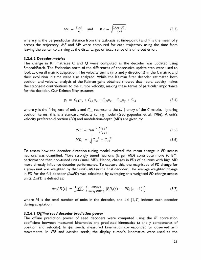
23  

∑| |

. and ∑

(3.3)

where yi is the perpendicular distance from the task-axis at time-point i and is the mean of y across the trajectory. ME and MV were computed for each trajectory using the time from leaving the center to arriving at the distal target or occurrence of a time-out error. 3.2.6.2 Decoder metrics The change in KF matrices C and Q were computed as the decoder was updated using SmoothBatch. The Frobenius norm of the differences of consecutive update step were used to look at overall matrix adaptation. The velocity terms (in x and y directions) in the C matrix and their evolution in time were also analyzed. While the Kalman filter decoder estimated both position and velocity, analysis of the Kalman gains obtained showed that neural activity makes the strongest contributions to the cursor velocity, making these terms of particular importance for the decoder. Our Kalman filter assumes:

, , , , , (3.4) where yi is the firing rate of unit i, and , represents the (i,1) entry of the C matrix. Ignoring position terms, this is a standard velocity tuning model (Georgopoulos et al, 1986). A unit's velocity preferred-direction (PD) and modulation-depth (MD) are given by:

tan ,

, (3.5)

, , (3.6)

To assess how the decoder direction-tuning model evolved, the mean change in PD across neurons was quantified. More strongly tuned neurons (larger MD) contribute more to BMI performance than non-tuned units (small MD). Hence, changes in PDs of neurons with high MD more directly influence decoder performance. To capture this, the magnitude of PD change for a given unit was weighted by that unit's MD in the final decoder. The average weighted change in PD for the full decoder (∆wPD) was calculated by averaging this weighted PD change across units. ∆wPD is defined as:

∆ ∑ | 1 | (3.7)

where M is the total number of units in the decoder, and ∈ 1, indexes each decoder during adaptation. 3.2.6.3 Offline seed decoder prediction power The offline prediction power of seed decoders were computed using the R2 correlation coefficient between measured kinematics and predicted kinematics (x and y components of position and velocity). In ipsi seeds, measured kinematics corresponded to observed arm movements. In VFB and baseline seeds, the display cursor's kinematics were used as the

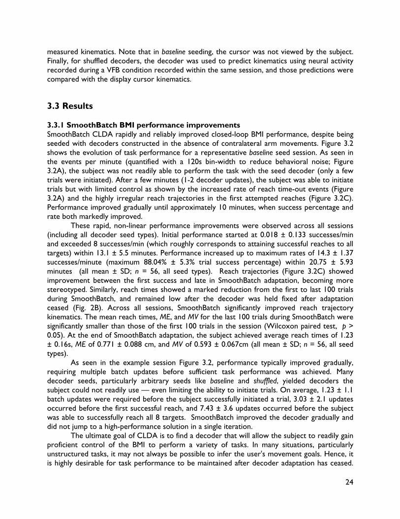
24  

measured kinematics. Note that in baseline seeding, the cursor was not viewed by the subject. Finally, for shuffled decoders, the decoder was used to predict kinematics using neural activity recorded during a VFB condition recorded within the same session, and those predictions were compared with the display cursor kinematics. 3.3 Results 3.3.1 SmoothBatch BMI performance improvements SmoothBatch CLDA rapidly and reliably improved closed-loop BMI performance, despite being seeded with decoders constructed in the absence of contralateral arm movements. Figure 3.2 shows the evolution of task performance for a representative baseline seed session. As seen in the events per minute (quantified with a 120s bin-width to reduce behavioral noise; Figure 3.2A), the subject was not readily able to perform the task with the seed decoder (only a few trials were initiated). After a few minutes (1-2 decoder updates), the subject was able to initiate trials but with limited control as shown by the increased rate of reach time-out events (Figure 3.2A) and the highly irregular reach trajectories in the first attempted reaches (Figure 3.2C). Performance improved gradually until approximately 10 minutes, when success percentage and rate both markedly improved. These rapid, non-linear performance improvements were observed across all sessions (including all decoder seed types). Initial performance started at 0.018 ± 0.133 successes/min and exceeded 8 successes/min (which roughly corresponds to attaining successful reaches to all targets) within 13.1 ± 5.5 minutes. Performance increased up to maximum rates of 14.3 ± 1.37 successes/minute (maximum 88.04% ± 5.3% trial success percentage) within 20.75 ± 5.93 minutes (all mean ± SD; n = 56, all seed types). Reach trajectories (Figure 3.2C) showed improvement between the first success and late in SmoothBatch adaptation, becoming more stereotyped. Similarly, reach times showed a marked reduction from the first to last 100 trials during SmoothBatch, and remained low after the decoder was held fixed after adaptation ceased (Fig. 2B). Across all sessions, SmoothBatch significantly improved reach trajectory kinematics. The mean reach times, ME, and MV for the last 100 trials during SmoothBatch were significantly smaller than those of the first 100 trials in the session (Wilcoxon paired test, p > 0.05). At the end of SmoothBatch adaptation, the subject achieved average reach times of 1.23 ± 0.16s, ME of 0.771 ± 0.088 cm, and MV of 0.593 ± 0.067cm (all mean ± SD; n = 56, all seed types). As seen in the example session Figure 3.2, performance typically improved gradually, requiring multiple batch updates before sufficient task performance was achieved. Many decoder seeds, particularly arbitrary seeds like baseline and shuffled, yielded decoders the subject could not readily use — even limiting the ability to initiate trials. On average, 1.23 ± 1.1 batch updates were required before the subject successfully initiated a trial, 3.03 ± 2.1 updates occurred before the first successful reach, and 7.43 ± 3.6 updates occurred before the subject was able to successfully reach all 8 targets. SmoothBatch improved the decoder gradually and did not jump to a high-performance solution in a single iteration. The ultimate goal of CLDA is to find a decoder that will allow the subject to readily gain proficient control of the BMI to perform a variety of tasks. In many situations, particularly unstructured tasks, it may not always be possible to infer the user's movement goals. Hence, it is highly desirable for task performance to be maintained after decoder adaptation has ceased.

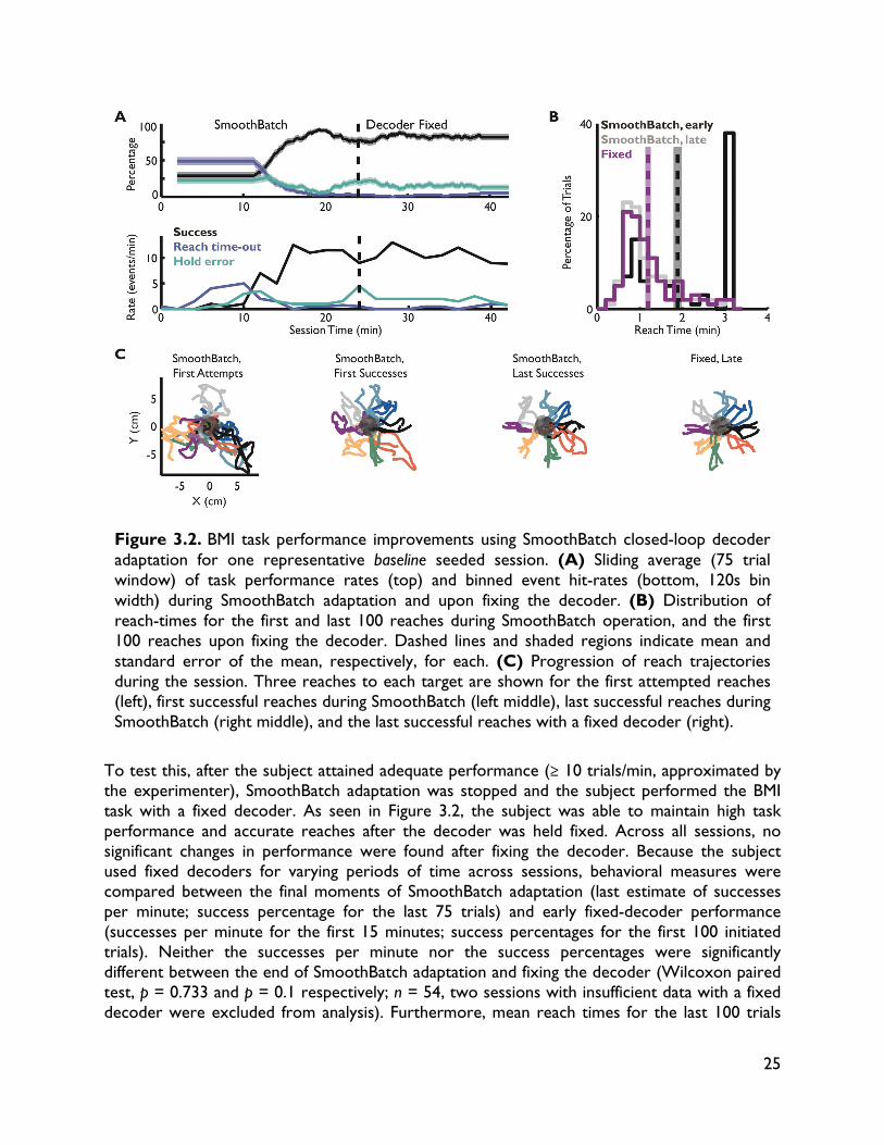
25  

To test this, after the subject attained adequate performance (≥ 10 trials/min, approximated by the experimenter), SmoothBatch adaptation was stopped and the subject performed the BMI task with a fixed decoder. As seen in Figure 3.2, the subject was able to maintain high task performance and accurate reaches after the decoder was held fixed. Across all sessions, no significant changes in performance were found after fixing the decoder. Because the subject used fixed decoders for varying periods of time across sessions, behavioral measures were compared between the final moments of SmoothBatch adaptation (last estimate of successes per minute; success percentage for the last 75 trials) and early fixed-decoder performance (successes per minute for the first 15 minutes; success percentages for the first 100 initiated trials). Neither the successes per minute nor the success percentages were significantly different between the end of SmoothBatch adaptation and fixing the decoder (Wilcoxon paired test, p = 0.733 and p = 0.1 respectively; n = 54, two sessions with insufficient data with a fixed decoder were excluded from analysis). Furthermore, mean reach times for the last 100 trials

Figure 3.2. BMI task performance improvements using SmoothBatch closed-loop decoder adaptation for one representative baseline seeded session. (A) Sliding average (75 trial window) of task performance rates (top) and binned event hit-rates (bottom, 120s bin width) during SmoothBatch adaptation and upon fixing the decoder. (B) Distribution of reach-times for the first and last 100 reaches during SmoothBatch operation, and the first 100 reaches upon fixing the decoder. Dashed lines and shaded regions indicate mean and standard error of the mean, respectively, for each. (C) Progression of reach trajectories during the session. Three reaches to each target are shown for the first attempted reaches (left), first successful reaches during SmoothBatch (left middle), last successful reaches during SmoothBatch (right middle), and the last successful reaches with a fixed decoder (right).

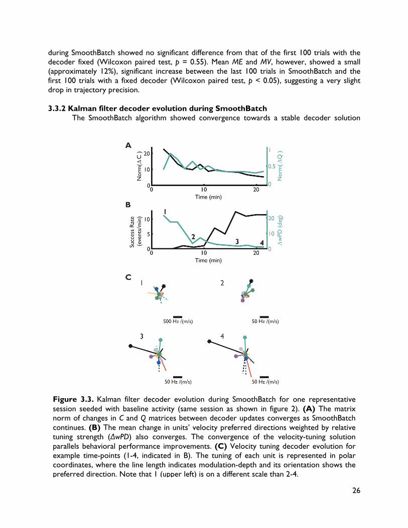
26  

during SmoothBatch showed no significant difference from that of the first 100 trials with the decoder fixed (Wilcoxon paired test, p = 0.55). Mean ME and MV, however, showed a small (approximately 12%), significant increase between the last 100 trials in SmoothBatch and the first 100 trials with a fixed decoder (Wilcoxon paired test, p < 0.05), suggesting a very slight drop in trajectory precision. 3.3.2 Kalman filter decoder evolution during SmoothBatch The SmoothBatch algorithm showed convergence towards a stable decoder solution

Figure 3.3.  Kalman filter decoder evolution during SmoothBatch for one representative session seeded with baseline activity (same session as shown in figure 2). (A) The matrix norm of changes in C and Q matrices between decoder updates converges as SmoothBatch continues. (B) The mean change in units’ velocity preferred directions weighted by relative tuning strength (∆wPD) also converges. The convergence of the velocity-tuning solution parallels behavioral performance improvements. (C) Velocity tuning decoder evolution for example time-points (1-4, indicated in B). The tuning of each unit is represented in polar coordinates, where the line length indicates modulation-depth and its orientation shows the preferred direction. Note that 1 (upper left) is on a different scale than 2-4.

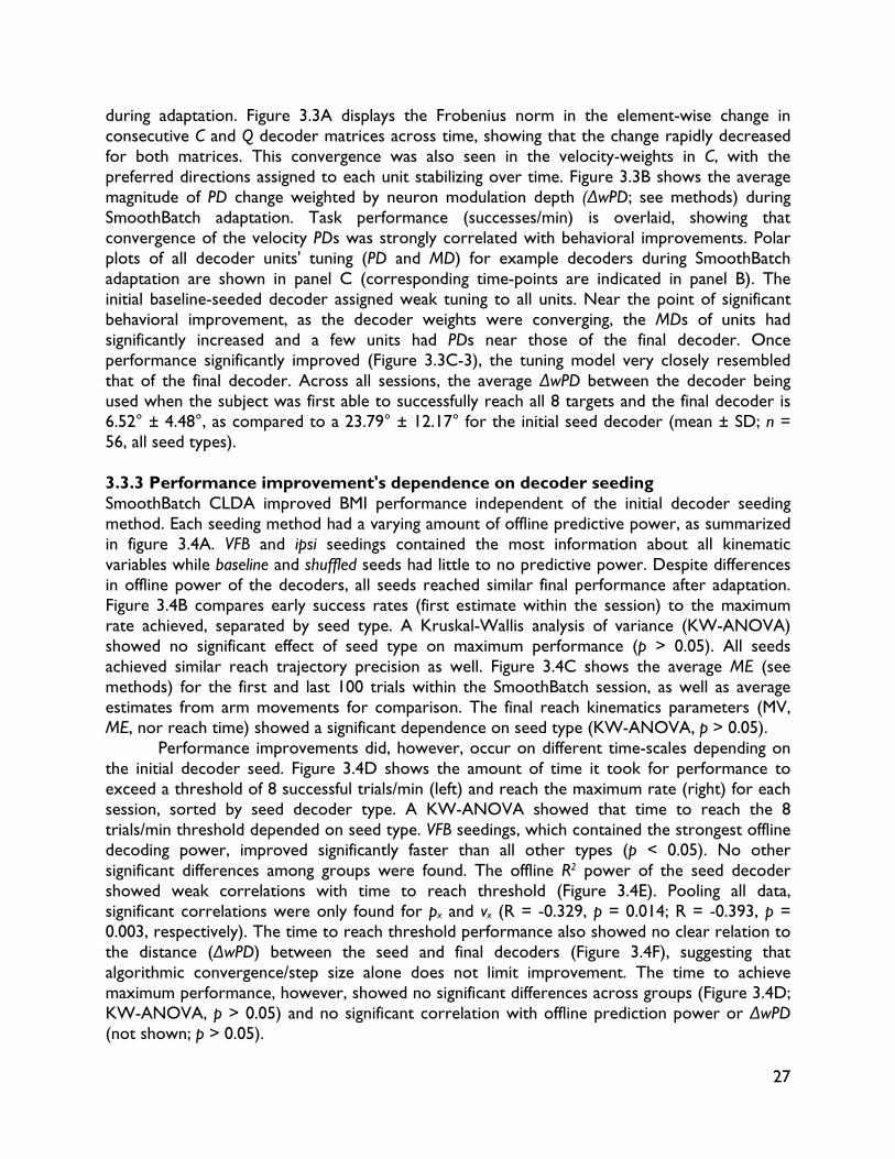
27  

during adaptation. Figure 3.3A displays the Frobenius norm in the element-wise change in consecutive C and Q decoder matrices across time, showing that the change rapidly decreased for both matrices. This convergence was also seen in the velocity-weights in C, with the preferred directions assigned to each unit stabilizing over time. Figure 3.3B shows the average magnitude of PD change weighted by neuron modulation depth (∆wPD; see methods) during SmoothBatch adaptation. Task performance (successes/min) is overlaid, showing that convergence of the velocity PDs was strongly correlated with behavioral improvements. Polar plots of all decoder units' tuning (PD and MD) for example decoders during SmoothBatch adaptation are shown in panel C (corresponding time-points are indicated in panel B). The initial baseline-seeded decoder assigned weak tuning to all units. Near the point of significant behavioral improvement, as the decoder weights were converging, the MDs of units had significantly increased and a few units had PDs near those of the final decoder. Once performance significantly improved (Figure 3.3C-3), the tuning model very closely resembled that of the final decoder. Across all sessions, the average ∆wPD between the decoder being used when the subject was first able to successfully reach all 8 targets and the final decoder is 6.52° ± 4.48°, as compared to a 23.79° ± 12.17° for the initial seed decoder (mean ± SD; n = 56, all seed types). 3.3.3 Performance improvement's dependence on decoder seeding SmoothBatch CLDA improved BMI performance independent of the initial decoder seeding method. Each seeding method had a varying amount of offline predictive power, as summarized in figure 3.4A. VFB and ipsi seedings contained the most information about all kinematic variables while baseline and shuffled seeds had little to no predictive power. Despite differences in offline power of the decoders, all seeds reached similar final performance after adaptation. Figure 3.4B compares early success rates (first estimate within the session) to the maximum rate achieved, separated by seed type. A Kruskal-Wallis analysis of variance (KW-ANOVA) showed no significant effect of seed type on maximum performance (p > 0.05). All seeds achieved similar reach trajectory precision as well. Figure 3.4C shows the average ME (see methods) for the first and last 100 trials within the SmoothBatch session, as well as average estimates from arm movements for comparison. The final reach kinematics parameters (MV, ME, nor reach time) showed a significant dependence on seed type (KW-ANOVA, p > 0.05). Performance improvements did, however, occur on different time-scales depending on the initial decoder seed. Figure 3.4D shows the amount of time it took for performance to exceed a threshold of 8 successful trials/min (left) and reach the maximum rate (right) for each session, sorted by seed decoder type. A KW-ANOVA showed that time to reach the 8 trials/min threshold depended on seed type. VFB seedings, which contained the strongest offline decoding power, improved significantly faster than all other types (p < 0.05). No other significant differences among groups were found. The offline R2 power of the seed decoder showed weak correlations with time to reach threshold (Figure 3.4E). Pooling all data, significant correlations were only found for px and vx (R = -0.329, p = 0.014; R = -0.393, p = 0.003, respectively). The time to reach threshold performance also showed no clear relation to the distance (∆wPD) between the seed and final decoders (Figure 3.4F), suggesting that algorithmic convergence/step size alone does not limit improvement. The time to achieve maximum performance, however, showed no significant differences across groups (Figure 3.4D; KW-ANOVA, p > 0.05) and no significant correlation with offline prediction power or ∆wPD (not shown; p > 0.05).

28  

As seen by the wide spread in ∆wPD in Figure 3.4F, few initial seed decoders, even ones that contained significant offline decoding power, had velocity PD assignments close to those of the final SmoothBatch solution (note that on average, significant performance improvements were not seen until ∆wPD < 6.52° ± 4.48°). A KW-ANOVA showed that ∆wPDs were significantly larger for baseline seeds than VFB (p < 0.05); no other groups showed statistically significant differences. 3.4 Discussion We found that the SmoothBatch CLDA algorithm, which updates on an intermediate timescale (1-2 minutes), was able to improve closed-loop BMI performance rapidly and robustly, independent of initial decoder seeding. The subject was readily able to achieve proficient

Figure 3.4.  SmoothBatch performance improvement across different decoder seeding types. (A) Offline decoder prediction power for end-point position and velocity (x and y components) for all decoder seed types. Bars indicate mean across all performed sessions, error bars show standard error of the mean. (B) Initial and maximum performance rates of SmoothBatch sessions, separated by seed types. Points show individual sessions; bars and error bars show mean and standard error of the mean, respectively. (C) Average movement error (ME, see methods) for the first (early) and last (late) 100 trials during SmoothBatch adaptation, separated by seed condition. Average ME across 8 arm movement sessions (arm) are shown at right for comparison. Format as in panel C. (D) SmoothBatch performance improvement times (time for successes per minute to exceed 8 trials/min) and time to achieve the maximum performance rate for all sessions and all decoder seed types. Format as in panel C. (E) Relationship between seed decoder predictive power (R2 for x-component of position) and time to reach threshold performance. Points are individual sessions, color-coded by seed type, and line shows linear regression (R = -0.329, p < 0.05). (F) Relationship between relative distance between seed decoder and final decoder’s velocity tuning models (∆wPD; see methods) and time to reach threshold performance. Points are individual sessions, color-coded by seed type, and line shows linear regression (not significant).

29  

center-out task performance (88.04 ± 5.3% success rate, 1.23 ± 0.16s reach times, 0.771 ± 0.088 cm ME, and 0.593 ± 0.067cm MV) across 56 experimental sessions. Importantly, improvements were rapid (success rates exceeding 8 trials/min in an average of 13.1 ± 5.5 minutes), and occurred reliably in all sessions despite decoders being seeded using four different methods. Performance was also maintained upon ceasing adaptation and holding the decoder fixed, with no drop in task performance or reach times, and only slight (12%) increases in ME and MV. Comparison across BMI studies is a current challenge in the field (Gilja et al., 2011). Studies use incongruous task designs and different types of neural activity, obscuring direct comparisons. The use of different animal models (e.g. animals with arms free to move versus partial or full movement restriction) across studies may further confound cross-study comparisons (Nuyujukian et al., 2011). Furthermore, the field has not established standard metrics for performance evaluation, limiting the ability to quantitatively compare results. In an effort to make this work more readily comparable to future studies, we report performance metrics commonly used to evaluate pointing-devices like computer mice (MV and ME, see methods) (Mackenzie et al., 2001). Comparisons to one human BMI study (not explicitly utilizing CLDA or across-session learning) reporting MV and ME metrics shows that SmoothBatch has markedly reduced mean ME and MV relative to their best results ((Kim et al., 2008) MV: 1.2cm, SmoothBatch 0.587cm; (Kim et al., 2008) ME: 2.3cm, SmoothBatch: 0.759cm). Moreover, MV and ME results for SmoothBatch approach those of natural movements (MV: 0.35 ± 0.17cm, ME: 0.44 ± 0.20cm; mean ± SD across 2,025 trials in 8 arm movement session). The success of SmoothBatch is a clear testament to the power of the CLDA principle (Taylor et al., 2002; Gage et al., 2005; Shpigelman et al., 2008; Gilja et al., 2010; 2012; Mahmoudi and Sanchez, 2011). In the limit of long batch sizes and ρ = 0 (see Chapters 2 and 4), Gilja et al.'s batch algorithm is a special case of SmoothBatch. The longer data batches used by Gilja et al. allow for more accurate parameter estimation, eliminating the need for averaging. However, waiting to collect sufficient data for a single model update greatly reduces the update frequency, thus reducing the rate at which the user sees performance improvements. In Gilja et al.'s work, using decoders seeded from contralateral arm movements and BMI performed during overt arm movements, their subjects were able to attain > 90% task performance with the seed decoder before any CLDA intervention (Gilja et al., 2010, 2012). This initial high level of performance allows for a significant improvement in reach kinematics after a single batch-based decoder update (Gilja et al., 2010, 2012). We further explore key differences in CLDA algorithms in Chapter 4. SmoothBatch, however, is ideally suited to address a different problem—how can we use CLDA to generate a high-performance BMI given an initial decoder with severely limited closed-loop performance? CLDA may be a particularly useful tool in clinical applications, where many factors could limit initial closed-loop performance (see below). In these applications, collecting sufficient data for a batch-based decoder update is challenging. Furthermore, the slow update rates may reduce subject motivation, since subjects were required to use poorly performing decoders for 8-10 minutes (see Chapter 4). Though SmoothBatch sacrifices accuracy in each parameter estimation step due to a smaller batch-size than the Gilja et al algorithm, the increased decoder update frequency provides the user with more rapid feedback and may facilitate faster improvement. The progress of improvements seen in SmoothBatch also further suggest that using CLDA may involve a bootstrapping or co-adaptation process between the brain and decoder

30  

when starting from limited closed-loop BMI performance. SmoothBatch required multiple decoder update steps before performance improved significantly, progressing to gradually let the subject initiate trials, then reach a few targets, and finally reach all targets. This progression may be due in part to the exponentially weighted averaging and short data-batches used. However, the batch-sizes and half-lives used here correspond to relatively aggressive adaptation rates (ρ ∈ 0.54, 0.77 , see Chapter 2) and on average, more than one half-life's worth of updates occurred before adequate performance was achieved. This suggests that creating an optimal decoder in a single update step may be highly infeasible when starting from severely limited closed-loop performance. Instead, intermediate adaptation time-scale algorithms like SmoothBatch provide the subject with more rapid feedback and gradually adapt the decoder, facilitating a co-adaptation process and yielding rapid performance improvements.

SmoothBatch uses a sliding average of model parameter estimates based on small amounts of data, which is similar to the approach used by Taylor et al. (2002). They also show that their co-adaptive algorithm is able to yield proficient closed-loop BMI control when seeded with randomly initialize parameters. This suggests that an intermediate time-scale adaptation approach may ideal for such applications. The idea of CLDA involving a co-adaptation between the subject and decoder is further implied by the fact that SmoothBatch's improvement rate depended upon the initial decoder seed. While SmoothBatch was able to improve performance regardless of the seed, decoders seeded with neural activity during VFB improved more rapidly than arbitrary (baseline and shuffled) or ipsilateral arm-movement (ipsi) seeds. VFB seeds had the highest level of offline decoding power, consistent with observations that imagined/viewed movements evoke motor cortex activity (Tkach et al., 2007; Truccolo et al., 2008; Suminski et al., 2009). Times to achieve a threshold of 8 successful trials/min were weakly correlated with the decoder's offline prediction power, suggesting that the algorithm can more readily improve performance if initiated with decoder with some movement decoding power.

However, our results also suggest that offline prediction power is not the sole factor in how quickly SmoothBatch can improve performance. Ipsi decoder seeds had moderate offline prediction power, greater than that of baseline and shuffled seeds, consistent with findings of population-level representations of ipsilateral arm movements in motor cortex (Ganguly et al., 2009). Yet, no statistically significant differences in improvement times were detected between ipsi, baseline or shuffled seeds. Furthermore, the times to achieve maximum performance rates were uncorrelated with offline prediction power. This is consistent with Taylor et al.'s finding that the speed of adaptation did not differ when their co-adaptive population vector algorithm was initialized with PD estimates from arm movements or with random assignments (Taylor et al. 2002). Interestingly, we also found that on average the velocity tuning models for all seeds were 'far' from that of the final decoder, despite containing varying degrees of offline prediction (Figure 3.4D; only baseline seeds had significantly larger ∆wPD than VFB). This combined with the observation that offline prediction power alone is not indicative of SmoothBatch improvement rates, is consistent with the emerging notion that closed-loop BMI performance is not necessarily related to open-loop predictions (Koyama et al., 2010; Ganguly and Carmena, 2010). The many differences between BMI and natural movement—for instance congruent proprioceptive feedback is absent during BMI—may significantly alter the neural activity of the motor networks (Suminski et al., 2009; 2010). Performance improvements in SmoothBatch did not appear to be limited by relative distance between initial and final decoders (Figure 3.4D).

31  

However, the difference between the subject's evoked neural activity between arm movements and closed-loop control would influence his performance in BMI, possibly affecting this co-adaptation process by influencing user strategy (e.g. causing frustration). We did see noticeable variability in improvement times across all decoder seed types, which could be related to subject strategies/motivation and the co-adaptation process. Additional work is needed to explore the exact mechanisms underlying performance improvements and the aspects of a seed decoder that influence final improvement. Such insights could yield further reduction in performance improvement times. We return to this question in Chapter 4, exploring if and how decoder seeding influence the adaptation process in SmoothBatch.

One concern in using an adaptive algorithm is convergence. Here, we show preliminary analysis showing that decoder parameters rapidly converge with SmoothBatch CLDA (Figure 3.3). The subject was also readily able to maintain task performance after decoder adaptation ceased, suggesting that the algorithm converged towards a general task solution and avoided overfitting. C and Q matrices did exhibit small fluctuations (i.e. changes did not fully converge to zero, see Fig. 3), however these did not noticeably affect task performance, suggesting they may only be driven by behavioral and neural variability. It may also be possible to optimize batch size and half-life parameters to further improve convergence. For instance, increasing the batch size as a function of task performance could allow the algorithm to take large, rapid steps while the decoder is 'far' from a high-performance decoder, and smaller steps to fine-tune the model as it nears the final solution. In Chapter 4, we study the convergence properties of SmoothBatch, and how to optimize the algorithm’s performance. In conclusion, here we show that SmoothBatch can readily improve performance in a relatively short time, even with ill-conditioned seed decoders. Additional work to explore SmoothBatch's operation—the influence of adaptation parameters and the subject-decoder co-adaptation process—could also further improve the algorithm's operation. The ability quickly and robustly generate high-performance BMIs independent of the subject's initial closed-loop BMI performance could be useful for clinical applications. For paralyzed patients, seeding decoders with arm movements is not feasible. Many patients will also lack proprioceptive feedback during closed-loop BMI operation, potentially limiting their performance (Suminski et al., 2010). Furthermore, non-invasive human BMI studies have shown significant inter-subject variability in the ability to volitionally modulate neural activity, which greatly impacts their ability to operate BMIs (Blankertz et al., 2010). All of the decoder seeding methods presented here are compatible with many patient populations: VFB, baseline, and shuffled decoders could be created for any patient regardless of motor disability, and ipsi seedings could be used for unilaterally paralyzed patients such as stroke victims. Our work shows that SmoothBatch CLDA, an algorithm that updates the decoder on an intermediate time-scale during closed-loop operation, can reliably improve BMI performance in all of these cases.

32  

Chapter 4:

Design considerations for closed-loop decoder adaptation algorithms In Chapter 3, we presented a novel CLDA algorithm that can readily improve performance independent of the initial decoder. Algorithms like SmoothBatch that are robust to system variability may be particularly important for clinical applications, where subjects will have a wide range of motor deficits. The development of this algorithm, however, involved many engineering design choices that shape performance and the suitability of the algorithm to particular applications. For instance, as discussed in Chapter 3, the time-scale of decoder adaptation in SmoothBatch may be essential for improving performance from a poorly performing initial decoder. In this chapter, we now turn to exploring the design choices for CLDA algorithms and present a mathematical framework to facilitate algorithm development. This work was a joint effort with Siddharth Dangi, with collaboration from Helene Moorman and Jose M. Carmena, and was published in Neural Computation (Dangi et al., 2013). 4.1 Introduction A fundamental component of any BMI is the decoding algorithm, or “decoder”, that translates recorded neural activity into control signals for a prosthetic device. Decoders are often initialized offline by recording neural activity while a subject performs real movements (Serruya et al., 2002; Taylor et al., 2002; Carmena et al., 2003; Musallam et al., 2004; Santhanam et al., 2006) or observes/imagines movements (Hochberg et al., 2006; 2012; Wahoun et al., 2006; Kim et al., 2008; Velliste et al., 2008; Suminski et al., 2010), and fitting a decoder to predict these movements from the neural activity. However, BMIs are fundamentally closed-loop systems, since BMI users receive performance feedback (e.g. by visual observation of the prosthetic's movements). Recent research shows that the prediction power of decoders trained offline does not directly correlate with closed-loop performance, perhaps due to the inherent feedback-related differences between open- and closed-loop systems (Ganguly and Carmena, 2010; Koyama et al., 2010). These results suggest that performance improvements cannot be achieved solely by finding an optimal open-loop decoding algorithm, and therefore highlight the importance of treating BMIs as closed-loop systems.

In the closed-loop regime, two mechanisms can be used to achieve high performance BMI systems. The first mechanism, neural plasticity or brain adaptation, is the ability of neurons to adapt their receptive fields and tuning properties to facilitate performance improvements. For instance, previous work from Ganguly and Carmena demonstrated that when monkeys practiced BMI control with a “stable circuit” consisting of a fixed decoder and stable neurons, they developed a stable neural “map” of the decoder that enabled performance improvements, was readily recalled across days, and was robust to interference from a second learned map (Ganguly and Carmena, 2009). The second mechanism, Closed-Loop Decoder Adaptation (CLDA), is the process of adapting or updating the decoder's parameters during closed-loop BMI operation, i.e., while the subject is using the BMI (see Figure 4.1D). The goal of CLDA is to

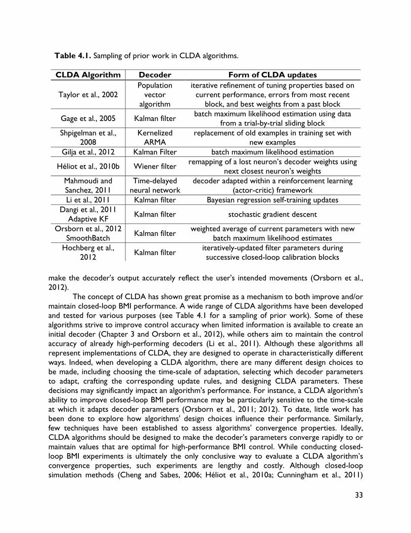
33  

make the decoder's output accurately reflect the user's intended movements (Orsborn et al., 2012).

The concept of CLDA has shown great promise as a mechanism to both improve and/or maintain closed-loop BMI performance. A wide range of CLDA algorithms have been developed and tested for various purposes (see Table 4.1 for a sampling of prior work). Some of these algorithms strive to improve control accuracy when limited information is available to create an initial decoder (Chapter 3 and Orsborn et al., 2012), while others aim to maintain the control accuracy of already high-performing decoders (Li et al., 2011). Although these algorithms all represent implementations of CLDA, they are designed to operate in characteristically different ways. Indeed, when developing a CLDA algorithm, there are many different design choices to be made, including choosing the time-scale of adaptation, selecting which decoder parameters to adapt, crafting the corresponding update rules, and designing CLDA parameters. These decisions may significantly impact an algorithm's performance. For instance, a CLDA algorithm's ability to improve closed-loop BMI performance may be particularly sensitive to the time-scale at which it adapts decoder parameters (Orsborn et al., 2011; 2012). To date, little work has been done to explore how algorithms' design choices influence their performance. Similarly, few techniques have been established to assess algorithms' convergence properties. Ideally, CLDA algorithms should be designed to make the decoder’s parameters converge rapidly to or maintain values that are optimal for high-performance BMI control. While conducting closed-loop BMI experiments is ultimately the only conclusive way to evaluate a CLDA algorithm’s convergence properties, such experiments are lengthy and costly. Although closed-loop simulation methods (Cheng and Sabes, 2006; Héliot et al., 2010a; Cunningham et al., 2011)

Table 4.1. Sampling of prior work in CLDA algorithms. CLDA Algorithm Decoder Form of CLDA updates

Taylor et al., 2002 Population

vector algorithm

iterative refinement of tuning properties based on current performance, errors from most recent

block, and best weights from a past block

Gage et al., 2005 Kalman filter batch maximum likelihood estimation using data from a trial-by-trial sliding block

Shpigelman et al., 2008

Kernelized ARMA

replacement of old examples in training set with new examples

Gilja et al., 2012 Kalman Filter batch maximum likelihood estimation

Héliot et al., 2010b Wiener filter remapping of a lost neuron’s decoder weights using next closest neuron’s weights

Mahmoudi and Sanchez, 2011

Time-delayed neural network

decoder adapted within a reinforcement learning (actor-critic) framework

Li et al., 2011 Kalman filter Bayesian regression self-training updates Dangi et al., 2011

Adaptive KF Kalman filter stochastic gradient descent

Orsborn et al., 2012 SmoothBatch Kalman filter weighted average of current parameters with new

batch maximum likelihood estimates Hochberg et al.,

2012 Kalman filter iteratively-updated filter parameters during successive closed-loop calibration blocks

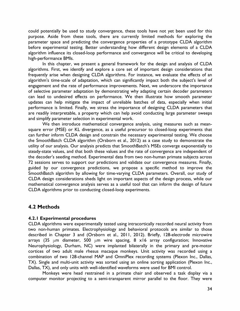
34  

could potentially be used to study convergence, these tools have not yet been used for this purpose. Aside from these tools, there are currently limited methods for exploring the parameter space and predicting the convergence properties of a prototype CLDA algorithm before experimental testing. Better understanding how different design elements of a CLDA algorithm influence its closed-loop performance and convergence will be critical to developing high-performance BMIs.

In this chapter, we present a general framework for the design and analysis of CLDA algorithms. First, we identify and explore a core set of important design considerations that frequently arise when designing CLDA algorithms. For instance, we evaluate the effects of an algorithm's time-scale of adaptation, which can significantly impact both the subject's level of engagement and the rate of performance improvements. Next, we underscore the importance of selective parameter adaptation by demonstrating why adapting certain decoder parameters can lead to undesired effects on performance. We then illustrate how smooth parameter updates can help mitigate the impact of unreliable batches of data, especially when initial performance is limited. Finally, we stress the importance of designing CLDA parameters that are readily interpretable, a property which can help avoid conducting large parameter sweeps and simplify parameter selection in experimental work.

We then introduce mathematical convergence analysis, using measures such as mean-square error (MSE) or KL divergence, as a useful precursor to closed-loop experiments that can further inform CLDA design and constrain the necessary experimental testing. We choose the SmoothBatch CLDA algorithm (Orsborn et al., 2012) as a case study to demonstrate the utility of our analysis. Our analysis predicts that SmoothBatch's MSEs converge exponentially to steady-state values, and that both these values and the rate of convergence are independent of the decoder's seeding method. Experimental data from two non-human primate subjects across 72 sessions serves to support our predictions and validate our convergence measures. Finally, guided by our convergence predictions, we propose a specific method to improve the SmoothBatch algorithm by allowing for time-varying CLDA parameters. Overall, our study of CLDA design considerations sheds light on important aspects of the design process, while our mathematical convergence analysis serves as a useful tool that can inform the design of future CLDA algorithms prior to conducting closed-loop experiments. 4.2 Methods 4.2.1 Experimental procedures CLDA algorithms were experimentally tested using intracortically recorded neural activity from two non-human primates. Electrophysiology and behavioral protocols are similar to those described in Chapter 3 and (Orsborn et al., 2011, 2012). Briefly, 128-electrode microwire arrays (35 μm diameter, 500 μm wire spacing, 8 x16 array configuration; Innovative Neurophysiology, Durham, NC) were implanted bilaterally in the primary and pre-motor cortices of two adult male rhesus macaque monkeys. Unit activity was recorded using a combination of two 128-channel MAP and OmniPlex recording systems (Plexon Inc., Dallas, TX). Single and multi-unit activity was sorted using an online sorting application (Plexon Inc., Dallas, TX), and only units with well-identified waveforms were used for BMI control.

Monkeys were head restrained in a primate chair and observed a task display via a computer monitor projecting to a semi-transparent mirror parallel to the floor. They were

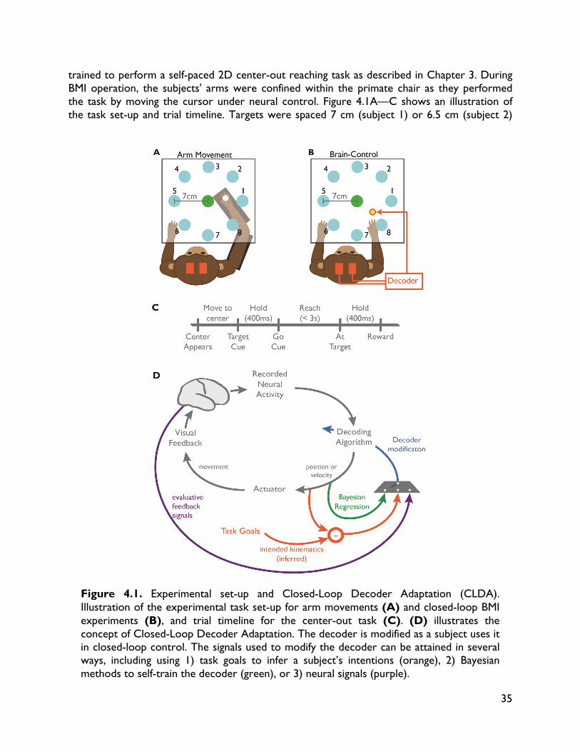
35  

trained to perform a self-paced 2D center-out reaching task as described in Chapter 3. During BMI operation, the subjects' arms were confined within the primate chair as they performed the task by moving the cursor under neural control. Figure 4.1A—C shows an illustration of the task set-up and trial timeline. Targets were spaced 7 cm (subject 1) or 6.5 cm (subject 2)

Figure 4.1. Experimental set-up and Closed-Loop Decoder Adaptation (CLDA). Illustration of the experimental task set-up for arm movements (A) and closed-loop BMI experiments (B), and trial timeline for the center-out task (C). (D) illustrates the concept of Closed-Loop Decoder Adaptation. The decoder is modified as a subject uses it in closed-loop control. The signals used to modify the decoder can be attained in several ways, including using 1) task goals to infer a subject’s intentions (orange), 2) Bayesian methods to self-train the decoder (green), or 3) neural signals (purple).

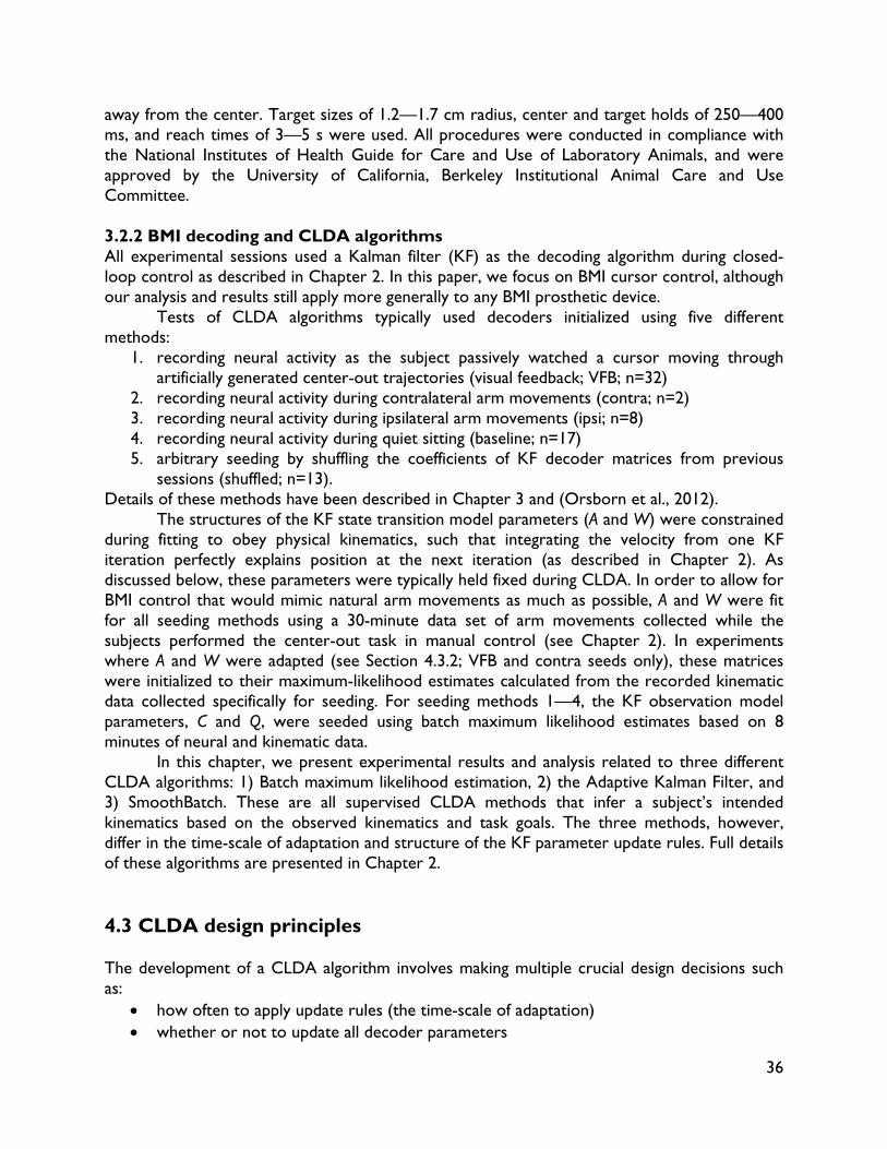
36  

away from the center. Target sizes of 1.2—1.7 cm radius, center and target holds of 250—400 ms, and reach times of 3—5 s were used. All procedures were conducted in compliance with the National Institutes of Health Guide for Care and Use of Laboratory Animals, and were approved by the University of California, Berkeley Institutional Animal Care and Use Committee.

3.2.2 BMI decoding and CLDA algorithms All experimental sessions used a Kalman filter (KF) as the decoding algorithm during closed-loop control as described in Chapter 2. In this paper, we focus on BMI cursor control, although our analysis and results still apply more generally to any BMI prosthetic device.

Tests of CLDA algorithms typically used decoders initialized using five different methods:

1. recording neural activity as the subject passively watched a cursor moving through artificially generated center-out trajectories (visual feedback; VFB; n=32)

2. recording neural activity during contralateral arm movements (contra; n=2) 3. recording neural activity during ipsilateral arm movements (ipsi; n=8) 4. recording neural activity during quiet sitting (baseline; n=17) 5. arbitrary seeding by shuffling the coefficients of KF decoder matrices from previous

sessions (shuffled; n=13). Details of these methods have been described in Chapter 3 and (Orsborn et al., 2012).

The structures of the KF state transition model parameters (A and W) were constrained during fitting to obey physical kinematics, such that integrating the velocity from one KF iteration perfectly explains position at the next iteration (as described in Chapter 2). As discussed below, these parameters were typically held fixed during CLDA. In order to allow for BMI control that would mimic natural arm movements as much as possible, A and W were fit for all seeding methods using a 30-minute data set of arm movements collected while the subjects performed the center-out task in manual control (see Chapter 2). In experiments where A and W were adapted (see Section 4.3.2; VFB and contra seeds only), these matrices were initialized to their maximum-likelihood estimates calculated from the recorded kinematic data collected specifically for seeding. For seeding methods 1—4, the KF observation model parameters, C and Q, were seeded using batch maximum likelihood estimates based on 8 minutes of neural and kinematic data. In this chapter, we present experimental results and analysis related to three different CLDA algorithms: 1) Batch maximum likelihood estimation, 2) the Adaptive Kalman Filter, and 3) SmoothBatch. These are all supervised CLDA methods that infer a subject’s intended kinematics based on the observed kinematics and task goals. The three methods, however, differ in the time-scale of adaptation and structure of the KF parameter update rules. Full details of these algorithms are presented in Chapter 2. 4.3 CLDA design principles The development of a CLDA algorithm involves making multiple crucial design decisions such as:

how often to apply update rules (the time-scale of adaptation) whether or not to update all decoder parameters

37  

how to update decoder parameters (the actual parameter update formulas or “update rules”)

how to set CLDA algorithmic parameters (e.g., step-sizes or learning rates)

Ideally, these design choices should enable a CLDA algorithm to make the decoder’s parameters converge rapidly to or maintain values that are optimal for high-performance BMI control. In the following sections, we explore these design choices by examining various aspects of the Batch, Adaptive KF, and SmoothBatch CLDA algorithms. We focus primarily on SmoothBatch, which has been demonstrated to improve BMI control accuracy even when initial performance is severely limited due to an unfavorable seeding (Chapter 3 and Orsborn et al., 2012). For instance, with patients such as paralyzed individuals or amputees that would be likely clinical targets of BMI technology, seeding methods involving overt movements wouldn't be feasible, and therefore other methods that typically result in a lower level of initial performance would need to be used. Despite our focus on SmoothBatch, however, we will see that many of its design properties are likely to be shared by other CLDA algorithms, even when their underlying purpose is characteristically different. 4.3.1 Time-scale of adaptation A CLDA algorithm's time-scale of adaptation refers to the frequency with which its update rules are applied to adapt the decoder's parameters. In a clinical setting with paralyzed patients, initial closed-loop BMI performance may be limited. As such, it is critical to develop CLDA algorithms capable of rapidly improving control accuracy regardless of initial performance. Given the subject-decoder interactions inherent in closed-loop BMI systems, the time-scale of adaptation may be particularly important in these situations. In Chapter 3, we showed that the SmoothBatch algorithm, when operating on an intermediate time-scale (1-2 minutes), successfully and robustly improves performance independent of the initial decoder (Orsborn et al., 2012). Here, we extend these results by comparing experimental data from the Batch, AKF, and SmoothBatch algorithms to highlight the role of the adaptation time-scale.

All three CLDA algorithms were experimentally tested with one non-human primate subject1, starting from limited task performance (Batch and AKF using VFB seeds, n=7 and n=2, respectively; SmoothBatch using VFB, Ipsi, Baseline, and Shuffled seeds, n=64). For all algorithms, the state transition model (A and W) was held fixed. Sessions selected for comparison had comparable task settings and neural ensemble sizes. Figure 4.2 A—C shows examples of the Batch, AKF, and SmoothBatch algorithms' performance in representative sessions. The evolution of task performance is illustrated with both moving averages (75 trial window) of percentages of trial outcomes (i.e. success, reach-error, or hold error; upper panels) and rates of each task event (estimated via binning events in 120 s non-overlapping bins; lower panels). Each CLDA algorithm was able to improve performance, as evidenced by increases in success percentages and rates, and corresponding decreases in errors during adaptation. However, the algorithms differ significantly in how well the subject is able to maintain performance after adaptation ceases (i.e., when using a fixed decoder). For both the Batch and SmoothBatch algorithms, the subject readily maintained performance upon fixing the

                                                            1 The Batch and AKF algorithms were not tested in the second subject. Two SmoothBatch sessions in subject 1 did not have sufficient data with the fixed decoder to assess the post-CLDA maintenance of performance, and thus were excluded from our analysis. 

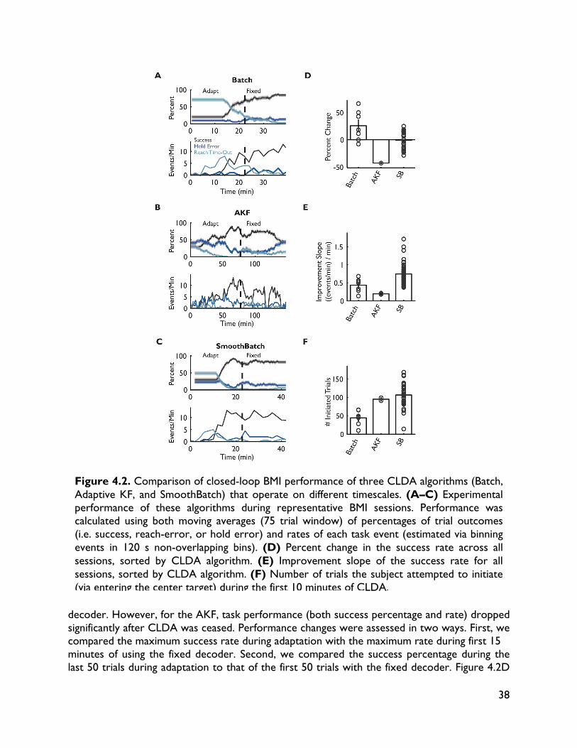
38  

decoder. However, for the AKF, task performance (both success percentage and rate) dropped significantly after CLDA was ceased. Performance changes were assessed in two ways. First, we compared the maximum success rate during adaptation with the maximum rate during first 15 minutes of using the fixed decoder. Second, we compared the success percentage during the last 50 trials during adaptation to that of the first 50 trials with the fixed decoder. Figure 4.2D

  

Figure 4.2. Comparison of closed-loop BMI performance of three CLDA algorithms (Batch, Adaptive KF, and SmoothBatch) that operate on different timescales. (A–C) Experimental performance of these algorithms during representative BMI sessions. Performance was calculated using both moving averages (75 trial window) of percentages of trial outcomes (i.e. success, reach-error, or hold error) and rates of each task event (estimated via binning events in 120 s non-overlapping bins). (D) Percent change in the success rate across all sessions, sorted by CLDA algorithm. (E) Improvement slope of the success rate for all sessions, sorted by CLDA algorithm. (F) Number of trials the subject attempted to initiate (via entering the center target) during the first 10 minutes of CLDA.

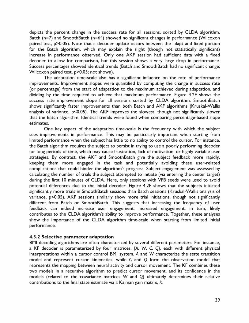
39  

depicts the percent change in the success rate for all sessions, sorted by CLDA algorithm. Batch (n=7) and SmoothBatch (n=64) showed no significant changes in performance (Wilcoxon paired test, p>0.05). Note that a decoder update occurs between the adapt and fixed portion for the Batch algorithm, which may explain the slight (though not statistically significant) increase in performance observed. Only one AKF session had sufficient data with a fixed decoder to allow for comparison, but this session shows a very large drop in performance. Success percentages showed identical trends (Batch and SmoothBatch had no significant change; Wilcoxon paired test, p>0.05; not shown).

The adaptation time-scale also has a significant influence on the rate of performance improvements. Improvement slopes were quantified by computing the change in success rate (or percentage) from the start of adaptation to the maximum achieved during adaptation, and dividing by the time required to achieve that maximum performance. Figure 4.2E shows the success rate improvement slope for all sessions sorted by CLDA algorithm. SmoothBatch shows significantly faster improvements than both Batch and AKF algorithms (Kruskal-Wallis analysis of variance, p<0.05). The AKF improves the slowest, though not significantly slower that the Batch algorithm. Identical trends were found when comparing percentage-based slope estimates.

One key aspect of the adaptation time-scale is the frequency with which the subject sees improvements in performance. This may be particularly important when starting from limited performance when the subject has little to no ability to control the cursor. For instance, the Batch algorithm requires the subject to persist in trying to use a poorly performing decoder for long periods of time, which may cause frustration, lack of motivation, or highly variable user strategies. By contrast, the AKF and SmoothBatch give the subject feedback more rapidly, keeping them more engaged in the task and potentially avoiding these user-related complications that could hinder the algorithm's progress. Subject engagement was assessed by calculating the number of trials the subject attempted to initiate (via entering the center target) during the first 10 minutes of CLDA. Here, only sessions with VFB seeds were used to avoid potential differences due to the initial decoder. Figure 4.2F shows that the subjects initiated significantly more trials in SmoothBatch sessions than Batch sessions (Kruskal-Wallis analysis of variance, p<0.05). AKF sessions similarly show more trial initiations, though not significantly different from Batch or SmoothBatch. This suggests that increasing the frequency of user feedback can indeed increase user engagement. Increased engagement, in turn, likely contributes to the CLDA algorithm's ability to improve performance. Together, these analyses show the importance of the CLDA algorithm time-scale when starting from limited initial performance. 4.3.2 Selective parameter adaptation BMI decoding algorithms are often characterized by several different parameters. For instance, a KF decoder is parameterized by four matrices, {A, W, C, Q}, each with different physical interpretations within a cursor control BMI system. A and W characterize the state transition model and represent cursor kinematics, while C and Q form the observation model that represents the mapping between neural activity and cursor movement. The KF combines these two models in a recursive algorithm to predict cursor movement, and its confidence in the models (related to the covariance matrices W and Q) ultimately determines their relative contributions to the final state estimate via a Kalman gain matrix, K.

40  

A priori, a KF CLDA algorithm should adapt all four matrices since they all contribute to the final observed cursor movement. Indeed, previous work with Batch-based KF CLDA updated all KF parameters (Gilja et al., 2010; Gilja et al., 2012). However, experimental evidence reveals that repeated adaptation (as is often needed when starting from limited initial performance) of the full KF model can have negative consequences. In particular, decoded cursor speed shows marked decreases with each successive update of KF parameters. Analysis of the matrices across consecutive CLDA updates reveals a clear explanation for this phenomenon. Figure 4.3A shows the changes (relative to their initial values) in the cursor speed and norms of the Kalman gain (top), and norms of the KF matrices (transition model, middle; observation model, bottom) across Batch CLDA sessions where all KF parameters are adapted. Thick lines show the mean across all sessions (n=9; 4 VFB seeds, 5 Contra seeds), and shading shows standard error. (Note that not all sessions contained the same number of Batch CLDA updates.) The mean predicted cursor speed decreased significantly with each CLDA update. Interestingly, the Kalman gain shows a parallel decrease in amplitude (estimated via the matrix norm). Inspecting the KF matrices reveals large and rapid decreases in W (by an order of magnitude over the course of CLDA) and significant increases in C. A and Q matrices, by

Figure 4.3. Advantages of CLDA with selective parameter adaptation for a Kalman filter decoder. Changes (relative to their initial values) in mean cursor speed and norm of the Kalman gain (top row), and KF model matrices (middle and bottom rows) across Batch CLDA sessions. (A) Adaptation of all KF parameters {A, W, C, Q} leads to dramatic decreases in cursor speed. (B) Selective adaptation of only the KF state observation model parameters {C, Q} avoids undesirable decreases in cursor speed.

41  

contrast show no clear trends. As noted above, the covariance matrix W plays a crucial role in determining the relative

contributions of the state and observation models. Smaller W matrices indicate that the KF is more confident in its linear state transition model, and thus will give less weight to the neural data when forming a prediction (reflected by a smaller Kalman gain). We see that the A matrix of the state transition model does not change significantly, but rather that the confidence in this model increases with each CLDA update. State transition models in BMIs (and models of natural arm movements) typically have damped velocity dynamics (Gilja et al., 2010; Gilja et al., 2012). Thus, decreasing the weight on the system input—the neural data—inherently reduces cursor speed. As such, the observed decreases in W likely contribute significantly to the cursor slowing that occurs when all KF parameters are updated.

To test this hypothesis, consecutive Batch updates were performed while holding the state transition model (A and W) fixed. The speed, Kalman gain, and KF matrices for these sessions are shown in figure 4.3B (formatting identical to 4.3A; n=19, all VFB seeds). Here, we see that fixing A and W eliminated cursor slowing. In fact, cursor speeds show a slight increase, accompanied by small increase in the Kalman gain. Changes in the observation model are similar to changes in sessions where all matrices were adapted. This selective adaptation improved performance more successfully than full adaptation because it did not inherently limit cursor speed.

While all KF matrices contribute to cursor movement, and thus are candidates for adaptation, it is important to consider their physical interpretations and the system as a whole before selecting what parameters to adapt. Given that the state transition model represents cursor kinematics, intuition suggests that the model should not change dramatically. In fact, the A matrices show little to no change, as expected. However, the cursor movements used for decoder parameter updates are themselves generated by a KF with kinematics specified by the decoder. Thus, the KF becomes increasingly confident in its model of cursor movement, driving decreases in W and corresponding decreases in cursor speed. If we instead interpret the KF as having a fixed model of cursor kinematics, and only adapt the mapping between the subject's neural activity and cursor movement, we avoid this problem of recursively refitting a kinematics model on itself. For this reason, SmoothBatch only modifies the C and Q matrices of the KF. Similarly, other CLDA algorithms for the KF update only these parameters as well (Li et al., 2011).

BMI decoders typically contain multiple parameters, and therefore deciding which parameters to update is an essential design choice for CLDA algorithms. Our experiments have demonstrated that CLDA algorithms for KF decoders should not adapt the state transition model parameters, as this leads to reductions in cursor speed and other undesirable effects. More generally, these results may suggest that it is undesirable to update any decoder parameters that represent a prior model on movement. Instead, CLDA algorithms should primarily focus on adapting parameters that represent the mapping between the subject's neural activity and their intended movements. 4.3.3 Smooth decoder updates CLDA algorithms typically collect and process real-time data, such as the user's neural activity and BMI cursor movements, to form parameter updates that will improve performance. However, occasionally an algorithm may encounter unreliable data that, if not properly addressed, can have a negative impact on performance. For instance, if the BMI user is

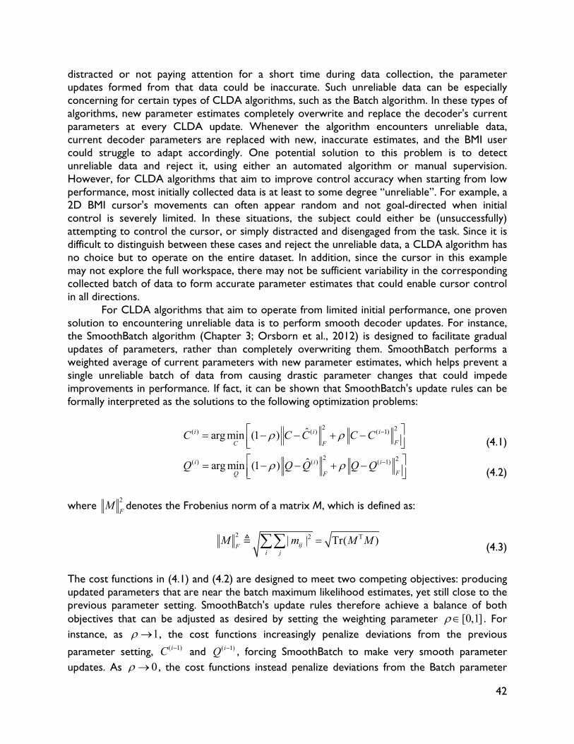
42  

distracted or not paying attention for a short time during data collection, the parameter updates formed from that data could be inaccurate. Such unreliable data can be especially concerning for certain types of CLDA algorithms, such as the Batch algorithm. In these types of algorithms, new parameter estimates completely overwrite and replace the decoder's current parameters at every CLDA update. Whenever the algorithm encounters unreliable data, current decoder parameters are replaced with new, inaccurate estimates, and the BMI user could struggle to adapt accordingly. One potential solution to this problem is to detect unreliable data and reject it, using either an automated algorithm or manual supervision. However, for CLDA algorithms that aim to improve control accuracy when starting from low performance, most initially collected data is at least to some degree “unreliable”. For example, a 2D BMI cursor's movements can often appear random and not goal-directed when initial control is severely limited. In these situations, the subject could either be (unsuccessfully) attempting to control the cursor, or simply distracted and disengaged from the task. Since it is difficult to distinguish between these cases and reject the unreliable data, a CLDA algorithm has no choice but to operate on the entire dataset. In addition, since the cursor in this example may not explore the full workspace, there may not be sufficient variability in the corresponding collected batch of data to form accurate parameter estimates that could enable cursor control in all directions.

For CLDA algorithms that aim to operate from limited initial performance, one proven solution to encountering unreliable data is to perform smooth decoder updates. For instance, the SmoothBatch algorithm (Chapter 3; Orsborn et al., 2012) is designed to facilitate gradual updates of parameters, rather than completely overwriting them. SmoothBatch performs a weighted average of current parameters with new parameter estimates, which helps prevent a single unreliable batch of data from causing drastic parameter changes that could impede improvements in performance. If fact, it can be shown that SmoothBatch's update rules can be formally interpreted as the solutions to the following optimization problems:

2 2( ) ( ) ( 1)ˆarg min (1 )i i i

FC FC C C C C (4.1)

2 2( ) ( ) ( 1)ˆarg min (1 )i i i

FQ FQ Q Q Q Q (4.2)

where 2

FM denotes the Frobenius norm of a matrix M, which is defined as:

2 2 T| | Tr( )ijF

i j

M m M M (4.3)

The cost functions in (4.1) and (4.2) are designed to meet two competing objectives: producing updated parameters that are near the batch maximum likelihood estimates, yet still close to the previous parameter setting. SmoothBatch's update rules therefore achieve a balance of both objectives that can be adjusted as desired by setting the weighting parameter [0,1] . For instance, as 1 , the cost functions increasingly penalize deviations from the previous

parameter setting, ( 1)iC and ( 1)iQ , forcing SmoothBatch to make very smooth parameter updates. As 0 , the cost functions instead penalize deviations from the Batch parameter

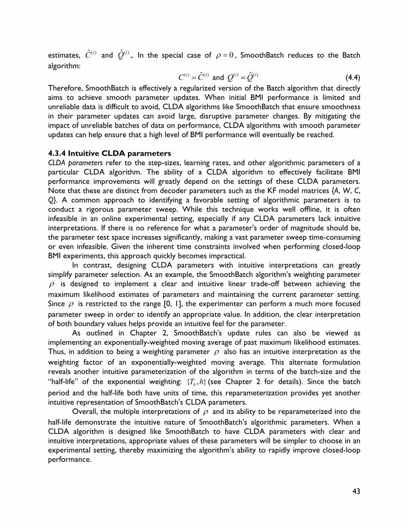
43  

estimates, ( )ˆ iC and ( )ˆ iQ ,. In the special case of 0 , SmoothBatch reduces to the Batch algorithm:

( ) ( )ˆi iC C and ( ) ( )ˆi iQ Q

(4.4)

Therefore, SmoothBatch is effectively a regularized version of the Batch algorithm that directly aims to achieve smooth parameter updates. When initial BMI performance is limited and unreliable data is difficult to avoid, CLDA algorithms like SmoothBatch that ensure smoothness in their parameter updates can avoid large, disruptive parameter changes. By mitigating the impact of unreliable batches of data on performance, CLDA algorithms with smooth parameter updates can help ensure that a high level of BMI performance will eventually be reached.

4.3.4 Intuitive CLDA parameters CLDA parameters refer to the step-sizes, learning rates, and other algorithmic parameters of a particular CLDA algorithm. The ability of a CLDA algorithm to effectively facilitate BMI performance improvements will greatly depend on the settings of these CLDA parameters. Note that these are distinct from decoder parameters such as the KF model matrices {A, W, C, Q}. A common approach to identifying a favorable setting of algorithmic parameters is to conduct a rigorous parameter sweep. While this technique works well offline, it is often infeasible in an online experimental setting, especially if any CLDA parameters lack intuitive interpretations. If there is no reference for what a parameter's order of magnitude should be, the parameter test space increases significantly, making a vast parameter sweep time-consuming or even infeasible. Given the inherent time constraints involved when performing closed-loop BMI experiments, this approach quickly becomes impractical.

In contrast, designing CLDA parameters with intuitive interpretations can greatly simplify parameter selection. As an example, the SmoothBatch algorithm's weighting parameter is designed to implement a clear and intuitive linear trade-off between achieving the maximum likelihood estimates of parameters and maintaining the current parameter setting. Since is restricted to the range [0, 1], the experimenter can perform a much more focused parameter sweep in order to identify an appropriate value. In addition, the clear interpretation of both boundary values helps provide an intuitive feel for the parameter.

As outlined in Chapter 2, SmoothBatch's update rules can also be viewed as implementing an exponentially-weighted moving average of past maximum likelihood estimates. Thus, in addition to being a weighting parameter also has an intuitive interpretation as the weighting factor of an exponentially-weighted moving average. This alternate formulation reveals another intuitive parameterization of the algorithm in terms of the batch-size and the “half-life” of the exponential weighting: { , }bT h (see Chapter 2 for details). Since the batch period and the half-life both have units of time, this reparameterization provides yet another intuitive representation of SmoothBatch's CLDA parameters.

Overall, the multiple interpretations of and its ability to be reparameterized into the half-life demonstrate the intuitive nature of SmoothBatch's algorithmic parameters. When a CLDA algorithm is designed like SmoothBatch to have CLDA parameters with clear and intuitive interpretations, appropriate values of these parameters will be simpler to choose in an experimental setting, thereby maximizing the algorithm's ability to rapidly improve closed-loop performance.

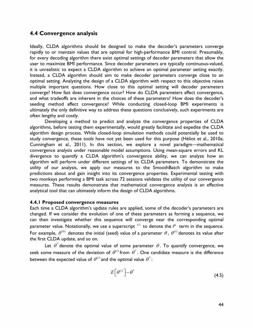
44  

4.4 Convergence analysis Ideally, CLDA algorithms should be designed to make the decoder’s parameters converge rapidly to or maintain values that are optimal for high-performance BMI control. Presumably, for every decoding algorithm there exist optimal settings of decoder parameters that allow the user to maximize BMI performance. Since decoder parameters are typically continuous-valued, it is unrealistic to expect a CLDA algorithm to achieve an optimal parameter setting exactly. Instead, a CLDA algorithm should aim to make decoder parameters converge close to an optimal setting. Analyzing the design of a CLDA algorithm with respect to this objective raises multiple important questions. How close to this optimal setting will decoder parameters converge? How fast does convergence occur? How do CLDA parameters affect convergence, and what tradeoffs are inherent in the choices of these parameters? How does the decoder's seeding method affect convergence? While conducting closed-loop BMI experiments is ultimately the only definitive way to address these questions conclusively, such experiments are often lengthy and costly.

Developing a method to predict and analyze the convergence properties of CLDA algorithms, before testing them experimentally, would greatly facilitate and expedite the CLDA algorithm design process. While closed-loop simulation methods could potentially be used to study convergence, these tools have not yet been used for this purpose (Héliot et al., 2010a; Cunningham et al., 2011). In this section, we explore a novel paradigm—mathematical convergence analysis under reasonable model assumptions. Using mean-square errors and KL divergence to quantify a CLDA algorithm's convergence ability, we can analyze how an algorithm will perform under different settings of its CLDA parameters. To demonstrate the utility of our analysis, we apply our measures to the SmoothBatch algorithm to make predictions about and gain insight into its convergence properties. Experimental testing with two monkeys performing a BMI task across 72 sessions validates the utility of our convergence measures. These results demonstrate that mathematical convergence analysis is an effective analytical tool that can ultimately inform the design of CLDA algorithms. 4.4.1 Proposed convergence measures Each time a CLDA algorithm's update rules are applied, some of the decoder's parameters are changed. If we consider the evolution of one of these parameters as forming a sequence, we can then investigate whether this sequence will converge near the corresponding optimal parameter value. Notationally, we use a superscript ( )i to denote the ith term in the sequence. For example, (0) denotes the initial (seed) value of a parameter , (1) denotes its value after the first CLDA update, and so on.

Let * denote the optimal value of some parameter . To quantify convergence, we seek some measure of the deviation of ( )i from * . One candidate measure is the difference between the expected value of ( )i and the optimal value * :

( ) *iE (4.5)

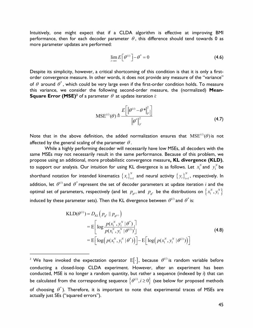
45  

Intuitively, one might expect that if a CLDA algorithm is effective at improving BMI performance, then for each decoder parameter , this difference should tend towards 0 as more parameter updates are performed:

( ) *lim 0i

tE

(4.6)

Despite its simplicity, however, a critical shortcoming of this condition is that it is only a first-order convergence measure. In other words, it does not provide any measure of the “variance” of around * , which could be very large even if the first-order condition holds. To measure this variance, we consider the following second-order measure, the (normalized) Mean-Square Error (MSE)2 of a parameter at update iteration i:

2( )

( )2*

*MSE ( )

i

Fi

F

E

(4.7)

Note that in the above definition, the added normalization ensures that ( )MSE ( )i is not affected by the general scaling of the parameter .

While a highly performing decoder will necessarily have low MSEs, all decoders with the same MSEs may not necessarily result in the same performance. Because of this problem, we propose using an additional, more probabilistic convergence measure, KL divergence (KLD), to support our analysis. Our intuition for using KL divergence is as follows. Let 1

Nx and 1Ny be

shorthand notation for intended kinematics 1

N

t tx

and neural activity

1

N

t ty

, respectively. In

addition, let ( )i and * represent the set of decoder parameters at update iteration i and the

optimal set of parameters, respectively (and let ( )ip and *p be the distributions on 1 1,N Nx y

induced by these parameter sets). Then the KL divergence between ( )i and * is:

* ( )

( )

*1 1

( )1 1

* ( )1 1 1 1

KLD( ) ||

( , | ) = E log

( , | )

= E log ( , | ) E log ( , | )

i

iKL

N N

N N i

N N N N i

D p p

p x y

p x y

p x y p x y

(4.8)

                                                            2  We have invoked the expectation operator , because ( )i is random variable before

conducting a closed-loop CLDA experiment. However, after an experiment has been conducted, MSE is no longer a random quantity, but rather a sequence (indexed by i) that can

be calculated from the corresponding sequence ( ) , 0i i (see below for proposed methods

of choosing * ). Therefore, it is important to note that experimental traces of MSEs are actually just SEs (“squared errors”). 

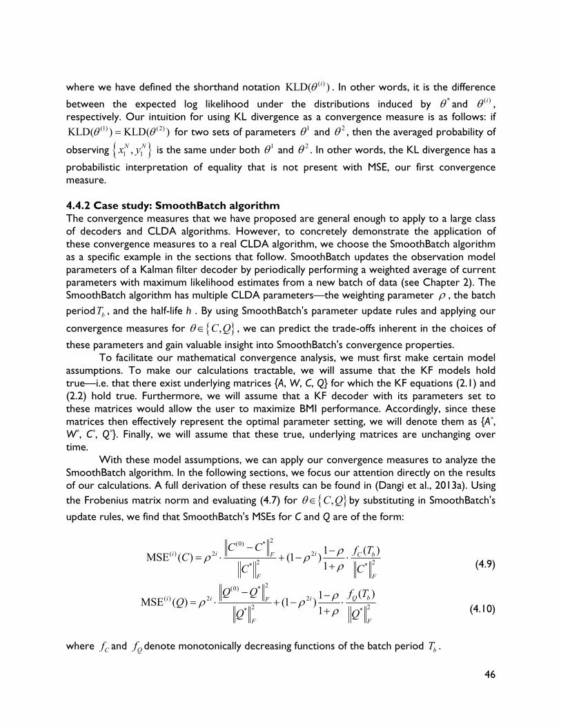
46  

where we have defined the shorthand notation ( )KLD( )i . In other words, it is the difference

between the expected log likelihood under the distributions induced by * and ( )i , respectively. Our intuition for using KL divergence as a convergence measure is as follows: if

(1) (2)KLD( ) KLD( ) for two sets of parameters 1 and 2 , then the averaged probability of

observing 1 1,N Nx y is the same under both 1 and 2 . In other words, the KL divergence has a

probabilistic interpretation of equality that is not present with MSE, our first convergence measure. 4.4.2 Case study: SmoothBatch algorithm The convergence measures that we have proposed are general enough to apply to a large class of decoders and CLDA algorithms. However, to concretely demonstrate the application of these convergence measures to a real CLDA algorithm, we choose the SmoothBatch algorithm as a specific example in the sections that follow. SmoothBatch updates the observation model parameters of a Kalman filter decoder by periodically performing a weighted average of current parameters with maximum likelihood estimates from a new batch of data (see Chapter 2). The SmoothBatch algorithm has multiple CLDA parameters—the weighting parameter , the batch period bT , and the half-life h . By using SmoothBatch's parameter update rules and applying our

convergence measures for ,C Q , we can predict the trade-offs inherent in the choices of

these parameters and gain valuable insight into SmoothBatch's convergence properties. To facilitate our mathematical convergence analysis, we must first make certain model

assumptions. To make our calculations tractable, we will assume that the KF models hold true—i.e. that there exist underlying matrices {A, W, C, Q} for which the KF equations (2.1) and (2.2) hold true. Furthermore, we will assume that a KF decoder with its parameters set to these matrices would allow the user to maximize BMI performance. Accordingly, since these matrices then effectively represent the optimal parameter setting, we will denote them as {A*, W*, C*, Q*}. Finally, we will assume that these true, underlying matrices are unchanging over time.

With these model assumptions, we can apply our convergence measures to analyze the SmoothBatch algorithm. In the following sections, we focus our attention directly on the results of our calculations. A full derivation of these results can be found in (Dangi et al., 2013a). Using the Frobenius matrix norm and evaluating (4.7) for ,C Q by substituting in SmoothBatch's

update rules, we find that SmoothBatch's MSEs for C and Q are of the form:

2(0) *

( ) 2 22 2* *

( )1MSE ( ) (1 )

1i i i C bF

F F

C C f TC

C C

(4.9)

2(0) *

( ) 2 22 2* *

( )1MSE ( ) (1 )

1Q bi i iF

F F

Q Q f TQ

Q Q

(4.10)

where Cf and Qf denote monotonically decreasing functions of the batch period bT .

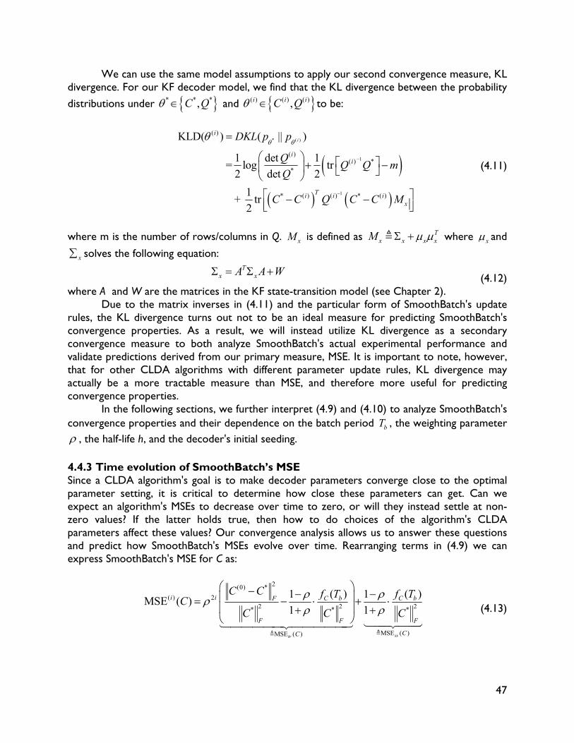
47  

We can use the same model assumptions to apply our second convergence measure, KL divergence. For our KF decoder model, we find that the KL divergence between the probability

distributions under * * *,C Q and ( ) ( ) ( ),i i iC Q to be:

* ( )

1

1

( )

( )( ) *

*

* ( ) ( ) * ( )

KLD( ) ( || )

1 det 1 = log tr

2 det 2

1 + tr

2

i

i

ii

Ti i ix

DKL p p

QQ Q m

Q

C C Q C C M

(4.11)

where m is the number of rows/columns in Q. xM is defined as

T

x x x xM where x and

x solves the following equation: T

x xA A W (4.12)

where A and W are the matrices in the KF state-transition model (see Chapter 2). Due to the matrix inverses in (4.11) and the particular form of SmoothBatch's update

rules, the KL divergence turns out not to be an ideal measure for predicting SmoothBatch's convergence properties. As a result, we will instead utilize KL divergence as a secondary convergence measure to both analyze SmoothBatch's actual experimental performance and validate predictions derived from our primary measure, MSE. It is important to note, however, that for other CLDA algorithms with different parameter update rules, KL divergence may actually be a more tractable measure than MSE, and therefore more useful for predicting convergence properties.

In the following sections, we further interpret (4.9) and (4.10) to analyze SmoothBatch's convergence properties and their dependence on the batch period bT , the weighting parameter , the half-life h, and the decoder's initial seeding. 4.4.3 Time evolution of SmoothBatch’s MSE Since a CLDA algorithm's goal is to make decoder parameters converge close to the optimal parameter setting, it is critical to determine how close these parameters can get. Can we expect an algorithm's MSEs to decrease over time to zero, or will they instead settle at non-zero values? If the latter holds true, then how to do choices of the algorithm's CLDA parameters affect these values? Our convergence analysis allows us to answer these questions and predict how SmoothBatch's MSEs evolve over time. Rearranging terms in (4.9) we can express SmoothBatch's MSE for C as:

2(0) *

( ) 22 2 2* * *

MSE ( )MSE ( )

( ) ( )1 1MSE ( )

1 1

sstr

i i C b C bF

F F F

CC

C C f T f TC

C C C

(4.13)

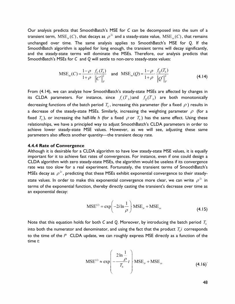
48  

Our analysis predicts that SmoothBatch's MSE for C can be decomposed into the sum of a transient term, MSE ( )tr C , that decays as 2i and a steady-state value, MSE ( )ss C , that remains unchanged over time. The same analysis applies to SmoothBatch's MSE for Q. If the SmoothBatch algorithm is applied for long enough, the transient terms will decay significantly, and the steady-state terms will dominate the MSEs. Therefore, our analysis predicts that SmoothBatch's MSEs for C and Q will settle to non-zero steady-state values:

ss 2*

( )1MSE ( )

1C b

F

f TC

C

and ss 2*

( )1MSE ( )

1Q b

F

f TQ

Q

(4.14)

From (4.14), we can analyze how SmoothBatch's steady-state MSEs are affected by changes in its CLDA parameters. For instance, since ( )c bf T and ( )Q bf T

are both monotonically

decreasing functions of the batch period bT , increasing this parameter (for a fixed ) results in a decrease of the steady-state MSEs. Similarly, increasing the weighting parameter (for a fixed bT ), or increasing the half-life h (for a fixed or bT ) has the same effect. Using these relationships, we have a principled way to adjust SmoothBatch's CLDA parameters in order to achieve lower steady-state MSE values. However, as we will see, adjusting these same parameters also affects another quantity—the transient decay rate. 4.4.4 Rate of Convergence Although it is desirable for a CLDA algorithm to have low steady-state MSE values, it is equally important for it to achieve fast rates of convergences. For instance, even if one could design a CLDA algorithm with zero steady-state MSEs, the algorithm would be useless if its convergence rate was too slow for a real experiment. Fortunately, the transient terms of SmoothBatch's MSEs decay as 2i , predicting that these MSEs exhibit exponential convergence to their steady-

state values. In order to make this exponential convergence more clear, we can write 2i in terms of the exponential function, thereby directly casting the transient's decrease over time as an exponential decay:

( ) 1MSE exp 2 ln MSE MSEi

tr ssi

(4.15)

Note that this equation holds for both C and Q. Moreover, by introducing the batch period bT

into both the numerator and denominator, and using the fact that the product bT i corresponds to the time of the ith CLDA update, we can roughly express MSE directly as a function of the time t:

( )

12ln

MSE exp MSE MSEitr ss

b

tT

(4.16).

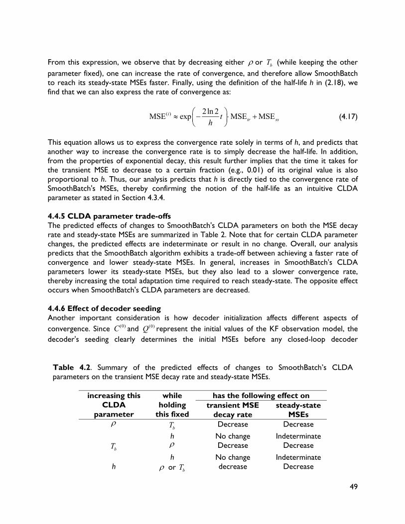
49  

From this expression, we observe that by decreasing either or bT (while keeping the other parameter fixed), one can increase the rate of convergence, and therefore allow SmoothBatch to reach its steady-state MSEs faster. Finally, using the definition of the half-life h in (2.18), we find that we can also express the rate of convergence as:

( ) 2 ln 2MSE exp MSE MSEi

tr ssth

(4.17)

This equation allows us to express the convergence rate solely in terms of h, and predicts that another way to increase the convergence rate is to simply decrease the half-life. In addition, from the properties of exponential decay, this result further implies that the time it takes for the transient MSE to decrease to a certain fraction (e.g., 0.01) of its original value is also proportional to h. Thus, our analysis predicts that h is directly tied to the convergence rate of SmoothBatch's MSEs, thereby confirming the notion of the half-life as an intuitive CLDA parameter as stated in Section 4.3.4. 4.4.5 CLDA parameter trade-offs The predicted effects of changes to SmoothBatch's CLDA parameters on both the MSE decay rate and steady-state MSEs are summarized in Table 2. Note that for certain CLDA parameter changes, the predicted effects are indeterminate or result in no change. Overall, our analysis predicts that the SmoothBatch algorithm exhibits a trade-off between achieving a faster rate of convergence and lower steady-state MSEs. In general, increases in SmoothBatch's CLDA parameters lower its steady-state MSEs, but they also lead to a slower convergence rate, thereby increasing the total adaptation time required to reach steady-state. The opposite effect occurs when SmoothBatch's CLDA parameters are decreased. 4.4.6 Effect of decoder seeding Another important consideration is how decoder initialization affects different aspects of convergence. Since (0)C and (0)Q represent the initial values of the KF observation model, the decoder's seeding clearly determines the initial MSEs before any closed-loop decoder

Table 4.2. Summary of the predicted effects of changes to SmoothBatch’s CLDA parameters on the transient MSE decay rate and steady-state MSEs.

increasing this CLDA

parameter

while holding

this fixed

has the following effect on transient MSE

decay rate steady-state

MSEs

bT Decrease Decrease

h No change Indeterminate

bT Decrease Decrease

h No change Indeterminate h or bT decrease Decrease

50  

adaptation has been performed:

2(0) *

(0)2*

MSE ( ) F

F

C CC

C

and

2(0) *

(0)2*

MSE ( ) F

F

Q QQ

Q

(4.18)

However, (0)C and (0)Q do not appear in any of our expressions for either the rate of convergence or the steady-state MSEs. Therefore our analysis predicts that the decoder's seeding method does not affect either of these two quantities3. Since the steady-state MSE is a measure of the deviation of parameters from the optimal parameter setting—which in turn relates directly to performance—our convergence analysis predicts that the decoder's initial seeding should not affect the level of performance achievable using the SmoothBatch algorithm. 4.4.7 Improving the SmoothBatch algorithm Our analysis of the SmoothBatch algorithm has predicted a key trade-off between the convergence rate and the steady-state MSEs. However, with our new understanding of how SmoothBatch's CLDA parameters affect its convergence properties, we may be able to re-engineer the algorithm to overcome this seemingly fundamental limitation, and further improve the algorithm's performance. Specifically, we would like to modify SmoothBatch to achieve lower steady-state MSEs without significantly sacrificing the convergence rate. We propose allowing CLDA parameters to vary in time. Since the seed decoder's parameters may initially be far from their optimal setting, one could perform aggressive adaptation early to make large parameter updates that bring the parameters into the right “ballpark”. However, as decoder parameters near their optimal values, more fine-tuned adaptation could be used to avoid potentially disruptive large parameter updates.

We propose using a time-varying version of SmoothBatch's parameter, where ( ) 1i as i increases so that parameter updates become smoother as time progresses. Letting

(1) and choosing a decay factor 1 , our proposed method for increasing ( )i over time

is to make ( )(1 )i decay exponentially as i increases:

( ) 11 (1 )i i

(4.19) Rearranging terms, we therefore propose the following systematic method for increasing ( )iover time:

( ) 11 (1 ), 1i i

(4.20)

                                                            3  Note that the seeding method can still affect the total time to achieve convergence—for example, the time required for the transient MSEs to decay below a certain level—but our analysis predicts that it will not affect the rate at which the transient MSEs decay. 

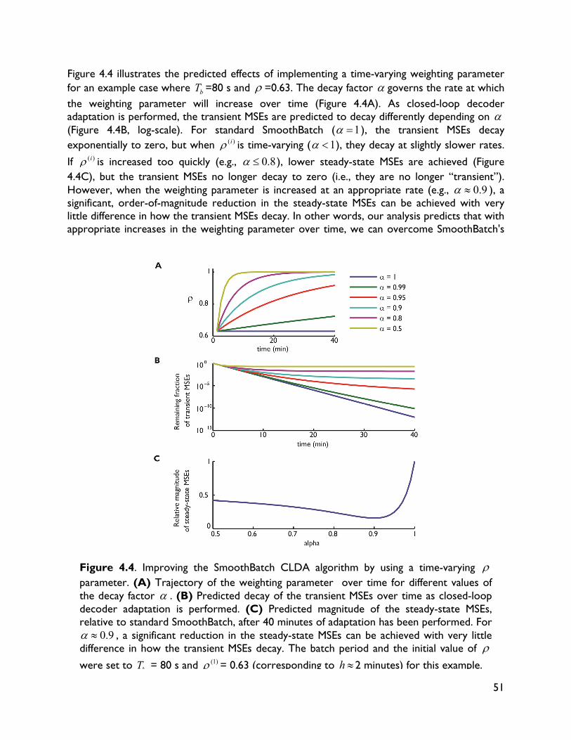
51  

Figure 4.4 illustrates the predicted effects of implementing a time-varying weighting parameter for an example case where bT =80 s and =0.63. The decay factor governs the rate at which the weighting parameter will increase over time (Figure 4.4A). As closed-loop decoder adaptation is performed, the transient MSEs are predicted to decay differently depending on

(Figure 4.4B, log-scale). For standard SmoothBatch ( 1 ), the transient MSEs decay exponentially to zero, but when ( )i is time-varying ( 1 ), they decay at slightly slower rates.

If ( )i is increased too quickly (e.g., 0.8 ), lower steady-state MSEs are achieved (Figure 4.4C), but the transient MSEs no longer decay to zero (i.e., they are no longer “transient”). However, when the weighting parameter is increased at an appropriate rate (e.g., 0.9 ), a significant, order-of-magnitude reduction in the steady-state MSEs can be achieved with very little difference in how the transient MSEs decay. In other words, our analysis predicts that with appropriate increases in the weighting parameter over time, we can overcome SmoothBatch's

Figure 4.4. Improving the SmoothBatch CLDA algorithm by using a time-varying parameter. (A) Trajectory of the weighting parameter over time for different values of the decay factor . (B) Predicted decay of the transient MSEs over time as closed-loop decoder adaptation is performed. (C) Predicted magnitude of the steady-state MSEs, relative to standard SmoothBatch, after 40 minutes of adaptation has been performed. For

0.9 , a significant reduction in the steady-state MSEs can be achieved with very little difference in how the transient MSEs decay. The batch period and the initial value of were set to bT = 80 s and (1) = 0.63 (corresponding to h 2 minutes) for this example.

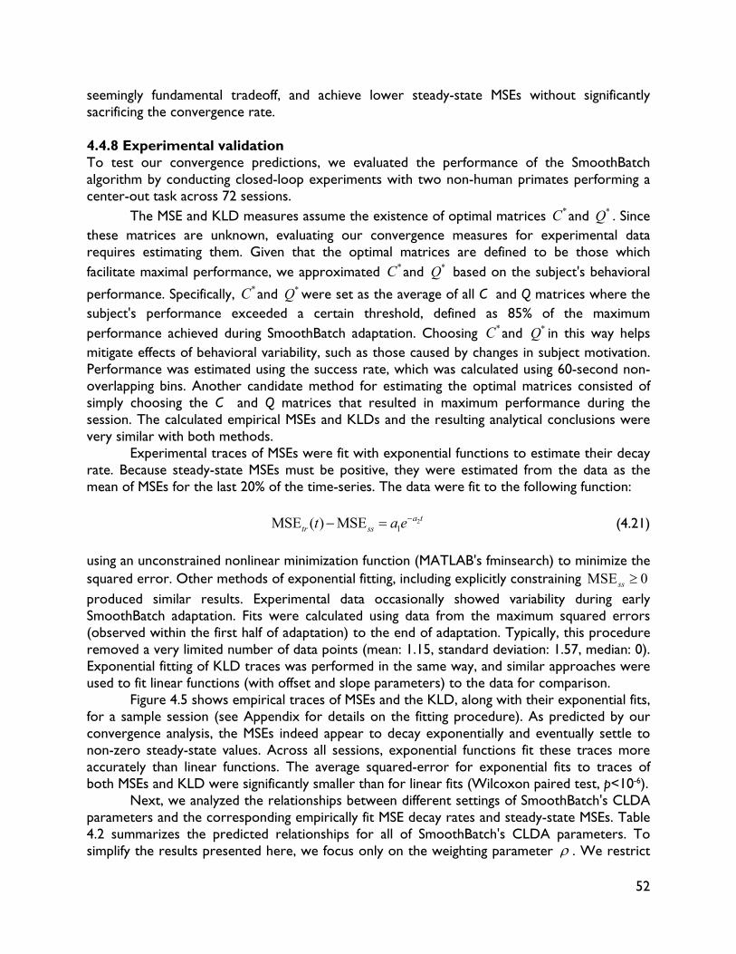
52  

seemingly fundamental tradeoff, and achieve lower steady-state MSEs without significantly sacrificing the convergence rate. 4.4.8 Experimental validation To test our convergence predictions, we evaluated the performance of the SmoothBatch algorithm by conducting closed-loop experiments with two non-human primates performing a center-out task across 72 sessions.

The MSE and KLD measures assume the existence of optimal matrices *C and *Q . Since these matrices are unknown, evaluating our convergence measures for experimental data requires estimating them. Given that the optimal matrices are defined to be those which facilitate maximal performance, we approximated *C and *Q

based on the subject's behavioral

performance. Specifically, *C and *Q were set as the average of all C and Q matrices where the subject's performance exceeded a certain threshold, defined as 85% of the maximum performance achieved during SmoothBatch adaptation. Choosing *C and *Q in this way helps mitigate effects of behavioral variability, such as those caused by changes in subject motivation. Performance was estimated using the success rate, which was calculated using 60-second non-overlapping bins. Another candidate method for estimating the optimal matrices consisted of simply choosing the C and Q matrices that resulted in maximum performance during the session. The calculated empirical MSEs and KLDs and the resulting analytical conclusions were very similar with both methods.

Experimental traces of MSEs were fit with exponential functions to estimate their decay rate. Because steady-state MSEs must be positive, they were estimated from the data as the mean of MSEs for the last 20% of the time-series. The data were fit to the following function:

2

1MSE ( ) MSE a ttr sst a e

(4.21)

using an unconstrained nonlinear minimization function (MATLAB's fminsearch) to minimize the squared error. Other methods of exponential fitting, including explicitly constraining MSE 0ss produced similar results. Experimental data occasionally showed variability during early SmoothBatch adaptation. Fits were calculated using data from the maximum squared errors (observed within the first half of adaptation) to the end of adaptation. Typically, this procedure removed a very limited number of data points (mean: 1.15, standard deviation: 1.57, median: 0). Exponential fitting of KLD traces was performed in the same way, and similar approaches were used to fit linear functions (with offset and slope parameters) to the data for comparison.

Figure 4.5 shows empirical traces of MSEs and the KLD, along with their exponential fits, for a sample session (see Appendix for details on the fitting procedure). As predicted by our convergence analysis, the MSEs indeed appear to decay exponentially and eventually settle to non-zero steady-state values. Across all sessions, exponential functions fit these traces more accurately than linear functions. The average squared-error for exponential fits to traces of both MSEs and KLD were significantly smaller than for linear fits (Wilcoxon paired test, p<10-6).

Next, we analyzed the relationships between different settings of SmoothBatch's CLDA parameters and the corresponding empirically fit MSE decay rates and steady-state MSEs. Table 4.2 summarizes the predicted relationships for all of SmoothBatch's CLDA parameters. To simplify the results presented here, we focus only on the weighting parameter . We restrict

53  

our analysis to sessions with 1) more than one data point for a given and with 2) the same seeding condition (VFB), to isolate effects caused only (n = 29). As predicted by our convergence analysis, MSE decay rates are negatively correlated with for both C (r = -0.37; p < 0.05) and Q (r = -0.27; p = 0.15) (Figure 4.6A—B). In addition, steady-state MSE values are negatively correlated with for both C (r = -0.50; p < 0.05) and Q (r = -0.33; p = 0.08), further confirming the predictions derived from our convergence analysis (Figure 4.6D—E). Decay rates and steady-state values of KLDs showed similar correlations with as MSEs (Figure 4.6C, F).

Finally, we tested the prediction that the decoder's initial seeding method should not affect either the MSE decay rate or the steady-state MSEs. Figure 4.7 shows the decay rates (top row) and steady-state values (bottom row) for MSE( )C (left) and MSE( )Q

(middle), and

KLD (right), separated by seeding condition. We restrict our analysis to sessions with the same value of to isolate effects of initialization (60 sessions total; VFB, n = 22; Baseline, n = 17; Shuffled, n = 11; Ipsi, n = 8; Contra, n = 2). Bars indicate the mean, error bars show standard error of the mean, and points show individual session data. A Kruskal-Wallis analysis of variance reveals some statistically significant differences (indicated on the figure) in decay rates and steady-state values. However, no seeding conditions show consistent differences across any of the KF measures or convergence properties. Consistent with this result, our work in Chapter 3 comparing behavioral improvements across seeding conditions revealed no significant differences across seeding conditions. Specifically, all sessions reached similar final performance, and the time required to achieve maximum performance did not depend on the decoder's initialization. 4.5 Discussion Closed-loop decoder adaptation is a powerful paradigm for rapidly improving online BMI performance. In this chapter, we have established a general framework for the design and analysis of CLDA algorithms. We first identified a core set of design considerations that frequently arise when designing CLDA algorithms. We explored the consequences of choosing different time-scales of adaptation, motivated the idea of selective parameter adaptation, illustrated the need for performing smooth parameter updates, and stressed the importance of

Figure 4.5. Exponential decay of transient MSEs. Experimental traces of MSEs (A and B) and KLD (C), along with their exponential fits, for a session in which SmoothBatch was performed after VFB seeding.

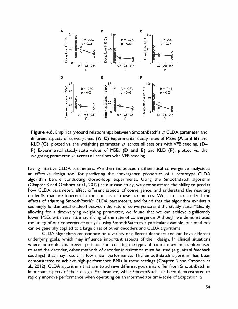
54  

having intuitive CLDA parameters. We then introduced mathematical convergence analysis as an effective design tool for predicting the convergence properties of a prototype CLDA algorithm before conducting closed-loop experiments. Using the SmoothBatch algorithm (Chapter 3 and Orsborn et al., 2012) as our case study, we demonstrated the ability to predict how CLDA parameters affect different aspects of convergence, and understand the resulting tradeoffs that are inherent in the choices of these parameters. We also characterized the effects of adjusting SmoothBatch's CLDA parameters, and found that the algorithm exhibits a seemingly fundamental tradeoff between the rate of convergence and the steady-state MSEs. By allowing for a time-varying weighting parameter, we found that we can achieve significantly lower MSEs with very little sacrificing of the rate of convergence. Although we demonstrated the utility of our convergence analysis using SmoothBatch as a particular example, our methods can be generally applied to a large class of other decoders and CLDA algorithms.

CLDA algorithms can operate on a variety of different decoders and can have different underlying goals, which may influence important aspects of their design. In clinical situations where motor deficits prevent patients from enacting the types of natural movements often used to seed the decoder, other methods of decoder initialization must be used (e.g., visual feedback seedings) that may result in low initial performance. The SmoothBatch algorithm has been demonstrated to achieve high-performance BMIs in these settings (Chapter 3 and Orsborn et al., 2012). CLDA algorithms that aim to achieve different goals may differ from SmoothBatch in important aspects of their design. For instance, while SmoothBatch has been demonstrated to rapidly improve performance when operating on an intermediate time-scale of adaptation, a

Figure 4.6. Empirically-found relationships between SmoothBatch’s CLDA parameter and different aspects of convergence. (A–C) Experimental decay rates of MSEs (A and B) and KLD (C), plotted vs. the weighting parameter across all sessions with VFB seeding. (D–F) Experimental steady-state values of MSEs (D and E) and KLD (F), plotted vs. the weighting parameter across all sessions with VFB seeding.

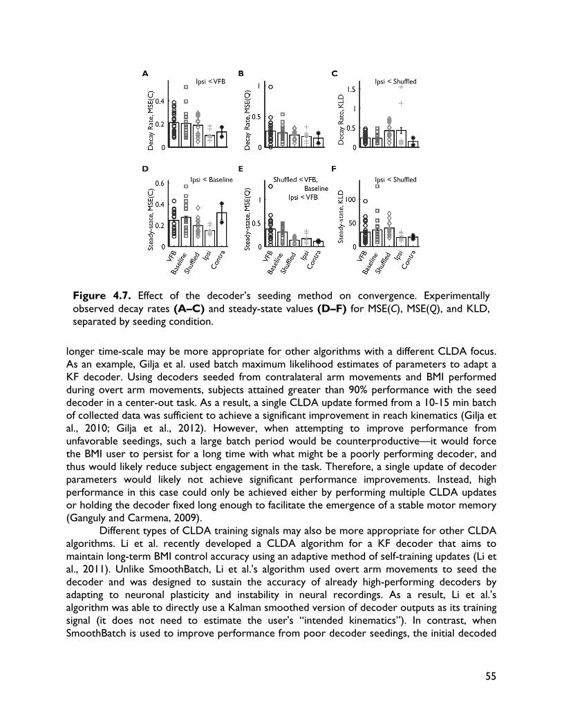
55  

longer time-scale may be more appropriate for other algorithms with a different CLDA focus. As an example, Gilja et al. used batch maximum likelihood estimates of parameters to adapt a KF decoder. Using decoders seeded from contralateral arm movements and BMI performed during overt arm movements, subjects attained greater than 90% performance with the seed decoder in a center-out task. As a result, a single CLDA update formed from a 10-15 min batch of collected data was sufficient to achieve a significant improvement in reach kinematics (Gilja et al., 2010; Gilja et al., 2012). However, when attempting to improve performance from unfavorable seedings, such a large batch period would be counterproductive—it would force the BMI user to persist for a long time with what might be a poorly performing decoder, and thus would likely reduce subject engagement in the task. Therefore, a single update of decoder parameters would likely not achieve significant performance improvements. Instead, high performance in this case could only be achieved either by performing multiple CLDA updates or holding the decoder fixed long enough to facilitate the emergence of a stable motor memory (Ganguly and Carmena, 2009).

Different types of CLDA training signals may also be more appropriate for other CLDA algorithms. Li et al. recently developed a CLDA algorithm for a KF decoder that aims to maintain long-term BMI control accuracy using an adaptive method of self-training updates (Li et al., 2011). Unlike SmoothBatch, Li et al.'s algorithm used overt arm movements to seed the decoder and was designed to sustain the accuracy of already high-performing decoders by adapting to neuronal plasticity and instability in neural recordings. As a result, Li et al.'s algorithm was able to directly use a Kalman smoothed version of decoder outputs as its training signal (it does not need to estimate the user's “intended kinematics”). In contrast, when SmoothBatch is used to improve performance from poor decoder seedings, the initial decoded

Figure 4.7. Effect of the decoder’s seeding method on convergence. Experimentally observed decay rates (A–C) and steady-state values (D–F) for MSE(C), MSE(Q), and KLD, separated by seeding condition.

56  

cursor outputs are naturally a poor reflection of the user's intended kinematics, and therefore Kalman smoothing would not be an effective training signal4.

Despite differences in the operation and goals of CLDA algorithms, some design elements are still likely to be shared in common by many CLDA algorithms. For example, despite its vastly different purpose, Li et al.'s algorithm maintains the property of selective decoder adaptation like SmoothBatch and does not adapt the KF's transition model parameters. Many algorithms are also designed in one way or another to have smooth decoder updates. Taylor et al. developed a CLDA algorithm for a PVA decoder in which the next set of decoder weights was determined from a corrected version of the current weights along with past weights that resulted in good performance (Taylor et al., 2002). Gage et al. estimated new KF parameters using a trial-by-trial sliding block of data, thus naturally allowing for smoothness across successive estimates (Gage et al., 2005). Li et al.’s algorithm also achieved smooth updates, albeit in a characteristically different way, by endowing decoder parameters with probability distributions and updating them using Bayesian regression updates.

Closed-loop decoder adaptation should synergize well with previous results that have demonstrated the importance of neural plasticity in the BMI learning process (Taylor et al., 2002; Carmena et al., 2003; Jarosiewicz et al., 2008; Ganguly and Carmena, 2009; Ganguly et al., 2011; Koralek et al., 2012). With respect to the learning and retention of neuroprosthetic skill, a study by Ganguly and Carmena demonstrated the importance of a stable neural map (Ganguly and Carmena, 2009). Some studies may have misinterpreted these results—for instance, contrary to Li et al.'s representation of these results, Ganguly and Carmena did not assert that a fixed decoder may be sufficient for long-term control accuracy (Li et al., 2011). Rather, they showed that a “stable circuit”, consisting of a fixed decoder and stable neurons, can facilitate the development of a stable neural map of the decoder that enables performance improvements, can be readily recalled across days, and is robust to interference from a second learned map. However, even if CLDA is used to achieve initial rapid gains in performance, it is likely that subsequent fixing of decoder parameters could still allow the formation of such a stable map. We explore the possibility of leveraging CLDA and neural adaptation in Chapter 5.

While our convergence predictions are consistent with our experimental results, we still find some variability in our results that is not accounted for by our analysis. For instance, calculating convergence measures from experimental data requires explicit assumptions that could introduce variability. As an example, the true underlying mapping between the observed neural firing rates ty and the kinematic state tx of the cursor is unlikely to be exactly linear with additive Gaussian noise. Existing work does suggest that incorporating nonlinearities into the KF could be beneficial (Li et al., 2009), and that CLDA can be successfully used with this decoding framework (Li et al., 2011). Exploring system nonlinearities may, then, be a fruitful avenue for future research. However, we feel the design principles highlighted in this study of linear decoders will likely translate to nonlinear applications. Indeed, our findings regarding selective adaptation of KF matrices are consistent with the approach used by Li et al. using a non-linear KF.

Despite the aforementioned variability, all of our data show clear trends consistent with our convergence analysis predictions (e.g., the signs of all calculated correlations are consistent with our predictions). Indeed, the goal of our convergence analysis is not to predict the exact                                                             4  In experiments using SmoothBatch, we instead used Gilja et al.'s method for estimating intended cursor kinematics (Gilja et al., 2010; Gilja et al., 2012). 

57  

value of the MSEs of different decoder parameters. Instead, what we are more interested in is finding the general form of the MSEs, in order to understand both how they evolve over time and how they are affected by CLDA parameters (like SmoothBatch's , bT , and h). Furthermore, our methods should not only be able to evaluate a wide range of existing CLDA algorithms, but also provide insights into ways of improving these algorithms. Our convergence analysis techniques accomplish these goals, thus demonstrating that they can be an effective analytical tool for evaluating and informing CLDA algorithm design.

Overall, our CLDA design principles and convergence analysis techniques will help us design the next generation of CLDA algorithms for BMI systems. Combined with neural plasticity, closed-loop decoder adaptation will serve as a powerful paradigm for rapidly achieving reliable and proficient neuroprosthetic control.

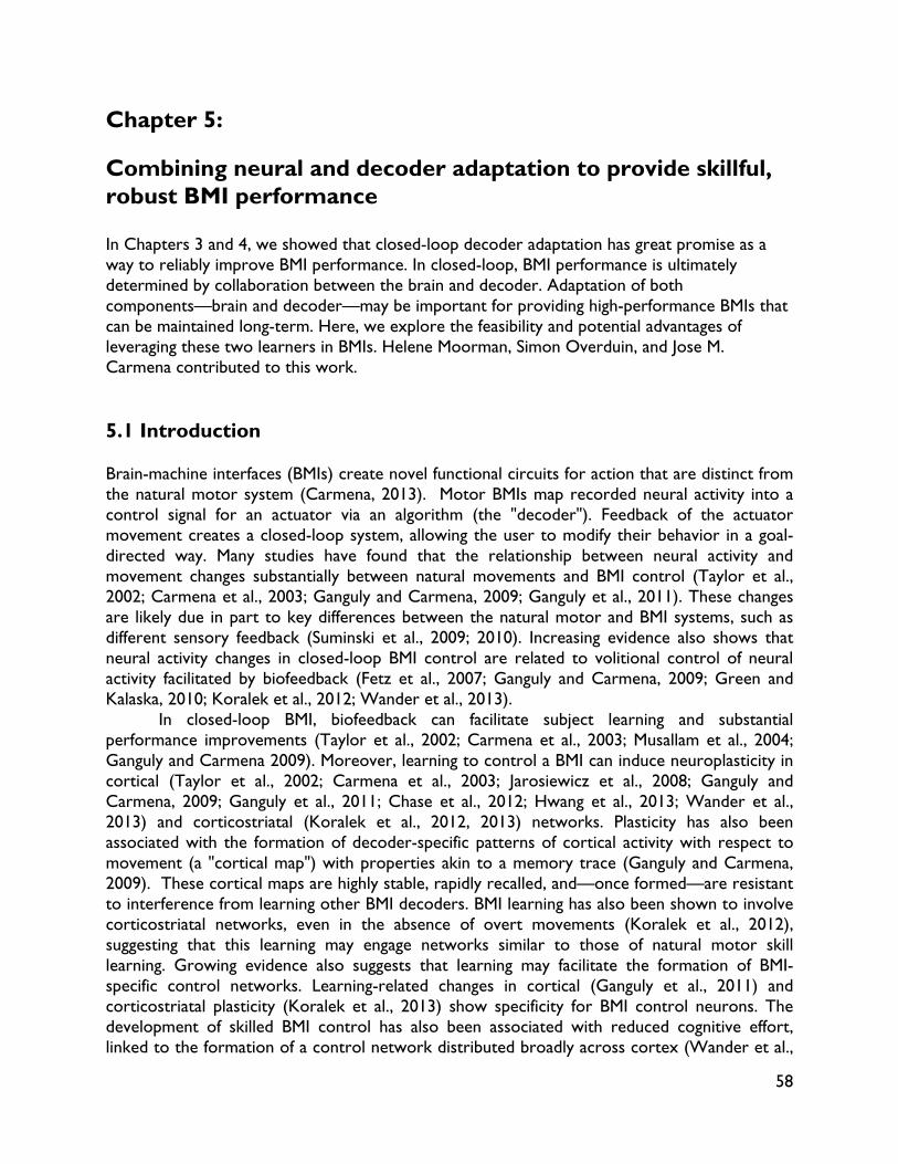
58  

Chapter 5:

Combining neural and decoder adaptation to provide skillful, robust BMI performance In Chapters 3 and 4, we showed that closed-loop decoder adaptation has great promise as a way to reliably improve BMI performance. In closed-loop, BMI performance is ultimately determined by collaboration between the brain and decoder. Adaptation of both components—brain and decoder—may be important for providing high-performance BMIs that can be maintained long-term. Here, we explore the feasibility and potential advantages of leveraging these two learners in BMIs. Helene Moorman, Simon Overduin, and Jose M. Carmena contributed to this work. 5.1 Introduction Brain-machine interfaces (BMIs) create novel functional circuits for action that are distinct from the natural motor system (Carmena, 2013). Motor BMIs map recorded neural activity into a control signal for an actuator via an algorithm (the "decoder"). Feedback of the actuator movement creates a closed-loop system, allowing the user to modify their behavior in a goal-directed way. Many studies have found that the relationship between neural activity and movement changes substantially between natural movements and BMI control (Taylor et al., 2002; Carmena et al., 2003; Ganguly and Carmena, 2009; Ganguly et al., 2011). These changes are likely due in part to key differences between the natural motor and BMI systems, such as different sensory feedback (Suminski et al., 2009; 2010). Increasing evidence also shows that neural activity changes in closed-loop BMI control are related to volitional control of neural activity facilitated by biofeedback (Fetz et al., 2007; Ganguly and Carmena, 2009; Green and Kalaska, 2010; Koralek et al., 2012; Wander et al., 2013).

In closed-loop BMI, biofeedback can facilitate subject learning and substantial performance improvements (Taylor et al., 2002; Carmena et al., 2003; Musallam et al., 2004; Ganguly and Carmena 2009). Moreover, learning to control a BMI can induce neuroplasticity in cortical (Taylor et al., 2002; Carmena et al., 2003; Jarosiewicz et al., 2008; Ganguly and Carmena, 2009; Ganguly et al., 2011; Chase et al., 2012; Hwang et al., 2013; Wander et al., 2013) and corticostriatal (Koralek et al., 2012, 2013) networks. Plasticity has also been associated with the formation of decoder-specific patterns of cortical activity with respect to movement (a "cortical map") with properties akin to a memory trace (Ganguly and Carmena, 2009). These cortical maps are highly stable, rapidly recalled, and—once formed—are resistant to interference from learning other BMI decoders. BMI learning has also been shown to involve corticostriatal networks, even in the absence of overt movements (Koralek et al., 2012), suggesting that this learning may engage networks similar to those of natural motor skill learning. Growing evidence also suggests that learning may facilitate the formation of BMI-specific control networks. Learning-related changes in cortical (Ganguly et al., 2011) and corticostriatal plasticity (Koralek et al., 2013) show specificity for BMI control neurons. The development of skilled BMI control has also been associated with reduced cognitive effort, linked to the formation of a control network distributed broadly across cortex (Wander et al.,

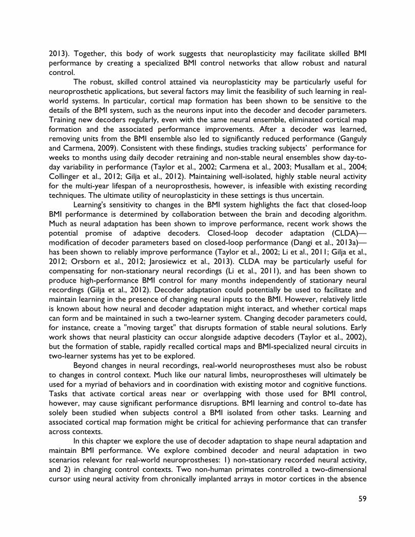
59  

2013). Together, this body of work suggests that neuroplasticity may facilitate skilled BMI performance by creating a specialized BMI control networks that allow robust and natural control.

The robust, skilled control attained via neuroplasticity may be particularly useful for neuroprosthetic applications, but several factors may limit the feasibility of such learning in real-world systems. In particular, cortical map formation has been shown to be sensitive to the details of the BMI system, such as the neurons input into the decoder and decoder parameters. Training new decoders regularly, even with the same neural ensemble, eliminated cortical map formation and the associated performance improvements. After a decoder was learned, removing units from the BMI ensemble also led to significantly reduced performance (Ganguly and Carmena, 2009). Consistent with these findings, studies tracking subjects’ performance for weeks to months using daily decoder retraining and non-stable neural ensembles show day-to-day variability in performance (Taylor et al., 2002; Carmena et al., 2003; Musallam et al., 2004; Collinger et al., 2012; Gilja et al., 2012). Maintaining well-isolated, highly stable neural activity for the multi-year lifespan of a neuroprosthesis, however, is infeasible with existing recording techniques. The ultimate utility of neuroplasticity in these settings is thus uncertain.

Learning's sensitivity to changes in the BMI system highlights the fact that closed-loop BMI performance is determined by collaboration between the brain and decoding algorithm. Much as neural adaptation has been shown to improve performance, recent work shows the potential promise of adaptive decoders. Closed-loop decoder adaptation (CLDA)—modification of decoder parameters based on closed-loop performance (Dangi et al., 2013a)—has been shown to reliably improve performance (Taylor et al., 2002; Li et al., 2011; Gilja et al., 2012; Orsborn et al., 2012; Jarosiewicz et al., 2013). CLDA may be particularly useful for compensating for non-stationary neural recordings (Li et al., 2011), and has been shown to produce high-performance BMI control for many months independently of stationary neural recordings (Gilja et al., 2012). Decoder adaptation could potentially be used to facilitate and maintain learning in the presence of changing neural inputs to the BMI. However, relatively little is known about how neural and decoder adaptation might interact, and whether cortical maps can form and be maintained in such a two-learner system. Changing decoder parameters could, for instance, create a "moving target" that disrupts formation of stable neural solutions. Early work shows that neural plasticity can occur alongside adaptive decoders (Taylor et al., 2002), but the formation of stable, rapidly recalled cortical maps and BMI-specialized neural circuits in two-learner systems has yet to be explored.

Beyond changes in neural recordings, real-world neuroprostheses must also be robust to changes in control context. Much like our natural limbs, neuroprostheses will ultimately be used for a myriad of behaviors and in coordination with existing motor and cognitive functions. Tasks that activate cortical areas near or overlapping with those used for BMI control, however, may cause significant performance disruptions. BMI learning and control to-date has solely been studied when subjects control a BMI isolated from other tasks. Learning and associated cortical map formation might be critical for achieving performance that can transfer across contexts.

In this chapter we explore the use of decoder adaptation to shape neural adaptation and maintain BMI performance. We explore combined decoder and neural adaptation in two scenarios relevant for real-world neuroprostheses: 1) non-stationary recorded neural activity, and 2) in changing control contexts. Two non-human primates controlled a two-dimensional cursor using neural activity from chronically implanted arrays in motor cortices in the absence

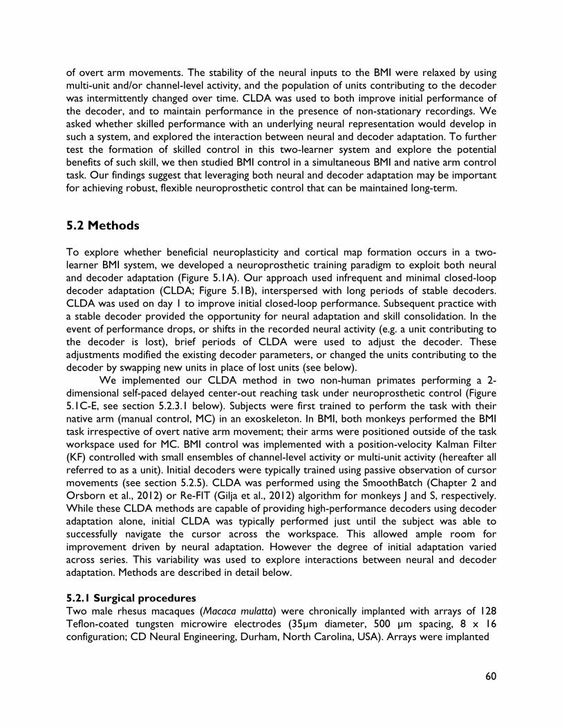
60  

of overt arm movements. The stability of the neural inputs to the BMI were relaxed by using multi-unit and/or channel-level activity, and the population of units contributing to the decoder was intermittently changed over time. CLDA was used to both improve initial performance of the decoder, and to maintain performance in the presence of non-stationary recordings. We asked whether skilled performance with an underlying neural representation would develop in such a system, and explored the interaction between neural and decoder adaptation. To further test the formation of skilled control in this two-learner system and explore the potential benefits of such skill, we then studied BMI control in a simultaneous BMI and native arm control task. Our findings suggest that leveraging both neural and decoder adaptation may be important for achieving robust, flexible neuroprosthetic control that can be maintained long-term. 5.2 Methods To explore whether beneficial neuroplasticity and cortical map formation occurs in a two-learner BMI system, we developed a neuroprosthetic training paradigm to exploit both neural and decoder adaptation (Figure 5.1A). Our approach used infrequent and minimal closed-loop decoder adaptation (CLDA; Figure 5.1B), interspersed with long periods of stable decoders. CLDA was used on day 1 to improve initial closed-loop performance. Subsequent practice with a stable decoder provided the opportunity for neural adaptation and skill consolidation. In the event of performance drops, or shifts in the recorded neural activity (e.g. a unit contributing to the decoder is lost), brief periods of CLDA were used to adjust the decoder. These adjustments modified the existing decoder parameters, or changed the units contributing to the decoder by swapping new units in place of lost units (see below).

We implemented our CLDA method in two non-human primates performing a 2-dimensional self-paced delayed center-out reaching task under neuroprosthetic control (Figure 5.1C-E, see section 5.2.3.1 below). Subjects were first trained to perform the task with their native arm (manual control, MC) in an exoskeleton. In BMI, both monkeys performed the BMI task irrespective of overt native arm movement; their arms were positioned outside of the task workspace used for MC. BMI control was implemented with a position-velocity Kalman Filter (KF) controlled with small ensembles of channel-level activity or multi-unit activity (hereafter all referred to as a unit). Initial decoders were typically trained using passive observation of cursor movements (see section 5.2.5). CLDA was performed using the SmoothBatch (Chapter 2 and Orsborn et al., 2012) or Re-FIT (Gilja et al., 2012) algorithm for monkeys J and S, respectively. While these CLDA methods are capable of providing high-performance decoders using decoder adaptation alone, initial CLDA was typically performed just until the subject was able to successfully navigate the cursor across the workspace. This allowed ample room for improvement driven by neural adaptation. However the degree of initial adaptation varied across series. This variability was used to explore interactions between neural and decoder adaptation. Methods are described in detail below. 5.2.1 Surgical procedures Two male rhesus macaques (Macaca mulatta) were chronically implanted with arrays of 128 Teflon-coated tungsten microwire electrodes (35μm diameter, 500 μm spacing, 8 x 16 configuration; CD Neural Engineering, Durham, North Carolina, USA). Arrays were implanted

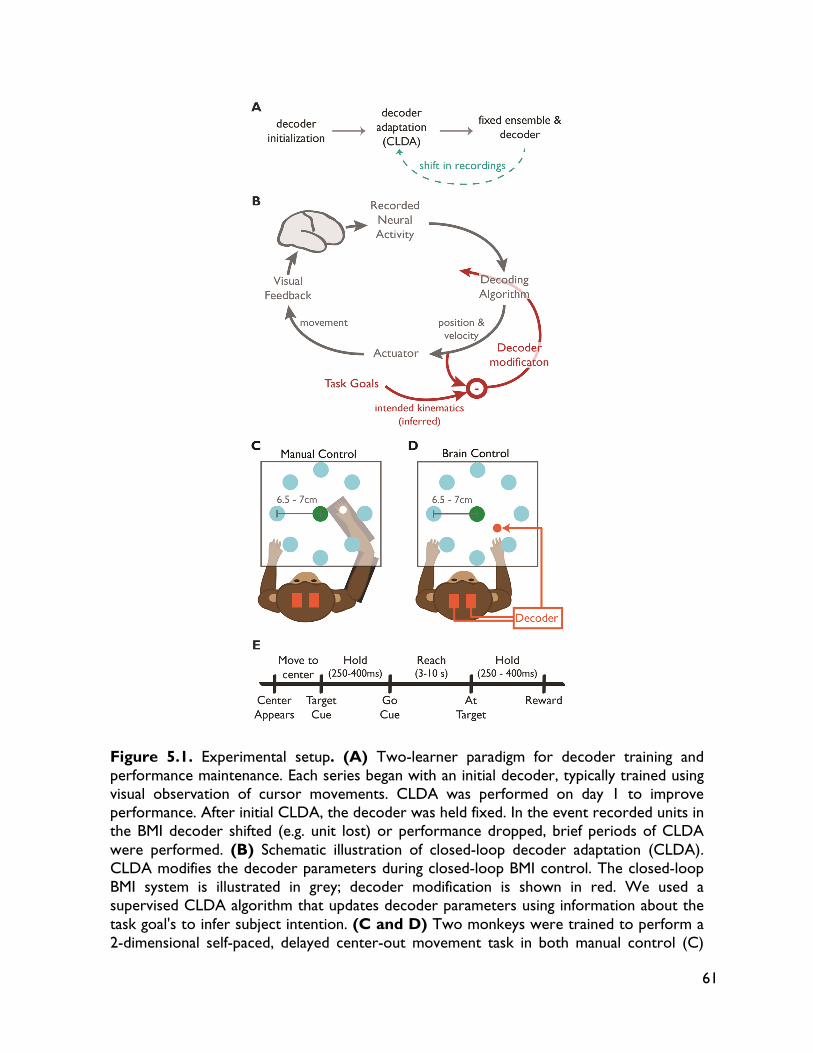
61  

Figure 5.1. Experimental setup. (A) Two-learner paradigm for decoder training and performance maintenance. Each series began with an initial decoder, typically trained using visual observation of cursor movements. CLDA was performed on day 1 to improve performance. After initial CLDA, the decoder was held fixed. In the event recorded units in the BMI decoder shifted (e.g. unit lost) or performance dropped, brief periods of CLDA were performed. (B) Schematic illustration of closed-loop decoder adaptation (CLDA). CLDA modifies the decoder parameters during closed-loop BMI control. The closed-loop BMI system is illustrated in grey; decoder modification is shown in red. We used a supervised CLDA algorithm that updates decoder parameters using information about the task goal's to infer subject intention. (C and D) Two monkeys were trained to perform a 2-dimensional self-paced, delayed center-out movement task in both manual control (C)

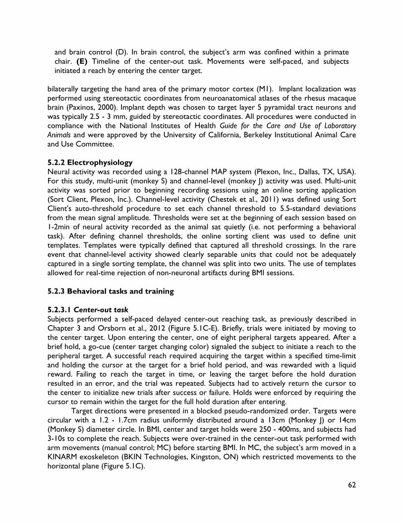
62  

and brain control (D). In brain control, the subject’s arm was confined within a primate chair. (E) Timeline of the center-out task. Movements were self-paced, and subjects initiated a reach by entering the center target.

bilaterally targeting the hand area of the primary motor cortex (M1). Implant localization was performed using stereotactic coordinates from neuroanatomical atlases of the rhesus macaque brain (Paxinos, 2000). Implant depth was chosen to target layer 5 pyramidal tract neurons and was typically 2.5 - 3 mm, guided by stereotactic coordinates. All procedures were conducted in compliance with the National Institutes of Health Guide for the Care and Use of Laboratory Animals and were approved by the University of California, Berkeley Institutional Animal Care and Use Committee. 5.2.2 Electrophysiology Neural activity was recorded using a 128-channel MAP system (Plexon, Inc., Dallas, TX, USA). For this study, multi-unit (monkey S) and channel-level (monkey J) activity was used. Multi-unit activity was sorted prior to beginning recording sessions using an online sorting application (Sort Client, Plexon, Inc.). Channel-level activity (Chestek et al., 2011) was defined using Sort Client's auto-threshold procedure to set each channel threshold to 5.5-standard deviations from the mean signal amplitude. Thresholds were set at the beginning of each session based on 1-2min of neural activity recorded as the animal sat quietly (i.e. not performing a behavioral task). After defining channel thresholds, the online sorting client was used to define unit templates. Templates were typically defined that captured all threshold crossings. In the rare event that channel-level activity showed clearly separable units that could not be adequately captured in a single sorting template, the channel was split into two units. The use of templates allowed for real-time rejection of non-neuronal artifacts during BMI sessions. 5.2.3 Behavioral tasks and training 5.2.3.1 Center-out task Subjects performed a self-paced delayed center-out reaching task, as previously described in Chapter 3 and Orsborn et al., 2012 (Figure 5.1C-E). Briefly, trials were initiated by moving to the center target. Upon entering the center, one of eight peripheral targets appeared. After a brief hold, a go-cue (center target changing color) signaled the subject to initiate a reach to the peripheral target. A successful reach required acquiring the target within a specified time-limit and holding the cursor at the target for a brief hold period, and was rewarded with a liquid reward. Failing to reach the target in time, or leaving the target before the hold duration resulted in an error, and the trial was repeated. Subjects had to actively return the cursor to the center to initialize new trials after success or failure. Holds were enforced by requiring the cursor to remain within the target for the full hold duration after entering.

Target directions were presented in a blocked pseudo-randomized order. Targets were circular with a 1.2 - 1.7cm radius uniformly distributed around a 13cm (Monkey J) or 14cm (Monkey S) diameter circle. In BMI, center and target holds were 250 - 400ms, and subjects had 3-10s to complete the reach. Subjects were over-trained in the center-out task performed with arm movements (manual control; MC) before starting BMI. In MC, the subject’s arm moved in a KINARM exoskeleton (BKIN Technologies, Kingston, ON) which restricted movements to the horizontal plane (Figure 5.1C).

63  

5.2.3.2 BMI-force simultaneous control (BMI-SC) The simultaneous control task (Figure 5.8 A-B) required monkey J to perform an isometric force generation task with his arm at the same time as performing a center-out task under BMI control. A force sensor (Measurement Specialties, Inc., Hampton, VA) was placed within the primate behavioral chair near the hand's natural resting position. The force registered by the sensor was mapped to the size of a circular cursor on the display ("force cursor"), such that larger applied forces increased the diameter of the cursor. The thickness of the ring denoted an acceptable range of applied force. A trial began with the appearance of a circular ring (the "force target"), signaling the magnitude of force to apply. The subject then initiated trials by acquiring the force target. Upon entering the force target, the BMI cursor and center target appeared, allowing the subject to initialize a center-out reach with the BMI cursor (as described above). If at any time the subject applied forces outside of the target range, an error occurred, causing the BMI cursor and task to disappear and the trail to be repeated. This enforced that the subject simultaneously control both the applied force and BMI cursor. The force target and cursor were co-localized with the center target, as illustrated in Figure 5.8A. One force target (2N +/- 1N) was used. Due to the task difficulty, center-out task difficulty was reduced, using targets of 1.4cm radius, and trials with 100ms hold times and 10s reach time-limits. Because hold settings can influence cursor kinematics in BMI (see for instance Gilja et al., 2012 supplemental materials), we focus primarily on comparison of task-level metrics (percent correct trials and success rate; see section 5.2.6 below) between BMI-only and BMI-SC performance.

One subject (monkey J) performed the BMI-SC task. He was initially trained to perform the isometric force generation task in isolation, and was well-trained in this task before beginning BMI-SC. He also performed blocks of interleaved force-only and BMI-only for training purposes prior to beginning BMI-SC sessions. BMI-SC was tested intermittently throughout the course of BMI-only learning series (i.e. practice in BMI-only with a particular decoder or CLDA-modifications thereof). On days when BMI-SC was tested, the subject typically performed BMI-only and BMI-SC in a block structure (A-B-A). Monkey J performed the force task with his right arm. BMI decoders for BMI-SC sessions were driven by neural activity primarily from the contralateral (left) hemisphere (15 - 16 units contralateral, of 16-17 units; 4 of 5 series included a single ipsilateral unit, while one series comprised entirely contralateral units). 5.2.4 BMI algorithms Real-time BMI control was implemented using a position-velocity Kalman Filter as described in Chapter 2. Neural input to the KF (yt) was defined as the firing rate of BMI units, estimated in non-overlapping 100ms bins. BMI ensembles typically included tens of units (range: 11-23, mean and mode: 16).

For monkey J who performed BMI with channel-level activity, channel firing rates were scaled (mean subtracted, multiplied by a scaling factor) before input into the KF to compensate for day-to-day variability in channels' statistical properties (see below). As described in section 5.2.2, channel-level activity was defined as all activity crossing a threshold. The thresholds for each channel were set on a daily basis to account for possible changes in channels over time. This procedure, however, may also introduce variability in the categorization of neural activity. For instance, even if a channel's recordings remained highly stable, small differences in threshold over days (due to variability inherent in estimating channel statistics) would result in slightly different firing statistics each day. Indeed, while channel-level activity was often quite stable in

64  

waveforms and tuning properties (see Figure 5.5), we found that many channels exhibited day-to-day variability in mean firing rates.

This variability can severely impact BMI performance with a fixed decoder. The KF models units' baseline firing rates (via the offset state in equation (2.10)) and modulation depths. If a unit’s baseline firing rate changes, it results in an "offset" cursor velocity and position in BMI control. That is, a unit resting at baseline produces cursor movement, rather than mapping to no movements. These offset velocities and/or positions can be very difficult for subjects to overcome, and often produce cursors that cannot effectively navigate across the workspace.

We developed a normalization procedure to compensate for day-to-day variability in the firing rate statistics at the channel level. This procedure operates under the assumption that the underlying neural activity has similar directional tuning properties over days, and that variability in the firing rate statistics (mean and standard deviation) are caused by fluctuations in channel thresholds and/or the distribution of neurons contributing to the channel activity. Thus, the goal was to scale the channel firing rates such that they maintained similar statistics each day. This scaling was performed on firing rates before they were input to the KF. The scaling is defined as:

(5.1)

Where represents the channel's firing rate (a function of time t) on day d, and is the scaled firing rate. and represent the firing rate mean and standard-deviation, estimated on day d, and is the standard-deviation estimated on day 1. This transform scales the firing rates such that they are approximately zero-mean, and have a standard deviation of each day (though see below).

Transform parameters { , } were estimated on day 1 using data collected for decoder initialization. Each day, { , } was estimated during an initial block of the same type. For instance, in series where the initial decoder was trained using visual observation of cursor movement (VFB; see below and Chapter 3), channel means and standard deviations were estimated each day with a block of VFB performed before BMI operation. Blocks for parameter estimation were typically 7-10min long. Note that many units often changed their baseline firing rates between the conditions used for initialization and in BMI control. This transform, however, can still effectively compensate for constant shifts in firing rate properties. Hence, even if this transform produces non-zero-mean inputs to the KF, it is designed to maintain the input means near this non-zero value over days. While this transform is susceptible to variability in parameter estimation, we found that it significantly improved transfer of BMI performance over days. Note, however, that this transform cannot compensate for changes in channel preferred directions.

All neural analysis for monkey J (see below) was performed on the transformed neural activity. That is, we analyzed the same neural data that were input to the decoder. This ensures that all changes in modulation depths observed are not due solely to fluctuations in channel statistics over time (see also Figure 5.5). Results calculated from the recorded (non-transformed) neural activity did not qualitatively differ, suggesting that day-to-day variability in channel-level statistics was not sufficient to remove the observed effects.

65  

5.2.5 Decoder training and CLDA algorithms Initial decoder parameters were trained via maximum-likelihood (ML) estimation methods similar to those described in Chapters 3. Full details and equations for ML estimates of the KF matrices can be found in there and in Orsborn et al., 2012. Initial decoders were typically trained using neural data collected during a visual feedback (VFB) protocol. Subjects passively observed a cursor move through the center-out task with artificially generated trajectories. A small number of series used alternative methods for creating an initial decoder including: manual control (n = 3, monkey J; n = 1, monkey S), shuffled manual control (n = 1, monkey J), and baseline neural activity (n = 2, monkey J). Manual control decoders were trained with neural activity and arm kinematics recorded as the subject performed the center-out task with his arm. Shuffled manual control decoders were created by training a decoder on arm movements and randomly shuffling the relationship between units and decoder weights. Finally, baseline neural activity training was the same as the VFB protocol except that the subject did not view cursor trajectories. No qualitative behavioral or neural differences were found across series with different initialization methods. In Chapters 2 and 3, we showed that CLDA convergence and final performance are not significantly impacted by the initial seed (Orsborn et al., 2012; Dangi et al., 2013a). Moreover, the termination of CLDA in initial adaptation was based on the experimenter’s assessment of behavioral performance, rather than the duration of adaptation, further reducing the potential influence of the initial decoder. Hence, all analyses do not distinguish between series with different initializations.

CLDA was performed using the SmoothBatch (Orsborn et al., 2012) and Re-FIT1 (Gilja et al., 2012) algorithms for monkey J and S, respectively. These algorithms use knowledge of the task goals (i.e. reaching targets) to infer the subject's intended kinematics. The intended kinematics and observed neural activity during closed-loop BMI are used to re-estimate the KF parameters. In the SmoothBatch algorithm, only the observation model of the KF (matrices C and Q) was re-estimated, and updates were constrained to enforce smooth, gradual updates (Dangi et al., 2013a). Re-FIT re-calculated all KF parameters. Algorithm details are presented in Chapter 2, and in Orsborn et al., 2012 and Gilja et al., 2012.

In the two-learner paradigm, CLDA was used for two primary purposes: 1) to improve initial closed-loop performance from the initial decoder, and 2) to maintain performance in the event of shifts in neural activity (e.g. loss of a unit within the BMI ensemble). Initial CLDA was typically run for 5-15 min, to provide the subject with adequate performance to allow successful reaches to all eight targets. Mid-series CLDA was performed if units were lost, or a drop in performance was observed (typically due to instability in the recorded BMI ensemble). In this instance, CLDA was run for a very brief time (3-5 minutes, corresponding to1 batch in Re-FIT and 1-2 updates in SmoothBatch). The goal was to compensate for neural activity changes to restore performance, not to substantially improve BMI performance.

During a decoder series, the subjects performed BMI with a single decoder (or CLDA-updated versions thereof). For monkey J, daily sessions typically consisted of blocks of manual control, visual feedback, and BMI. Monkey S typically only performed BMI, with occasional blocks of manual control or visual observation. Subjects were typically given 1-2 days break, or sessions with other behavioral tasks, in between decoder series.

                                                            1 Recall that Re-FIT is a batch maximum likelihood estimation CLDA approach as discussed in Chapters 2 and 4. 

66  

For daily re-training sessions (Figure 5.3), SmoothBatch CLDA was used to train a new decoder starting from different initial decoders using different (but overlapping) neural ensembles each day. Initial decoders were created using MC, VFB, baseline, and shuffled decoders. CLDA was run until behavioral performance began to saturate (i.e. aiming to improving performance as much as possible). Full details of the methods and data set for monkey S were presented in Chapter 3 and Orsborn et al., 2012. 5.2.6 Data analysis Decoder series had varying lengths, initial performance, and final performance. As such, all comparisons focus on changes within-series. To quantify behavioral changes over time, all series (monkey S: 6, monkey J: 13) were used. Note that 5 of the series from monkey J overlap with data presented for the BMI-SC task. For analysis of neural changes associated with learning, we restricted our analysis to series lasting three or more days where the subject used the same decoder for two days or more with no CLDA (monkey S: 4, monkey J: 10). This allowed us to better isolate changes in performance linked to neural adaptation, as opposed to CLDA. Inclusion of all series in neural analyses did not change any reported trends. 5.2.6.1 Behavioral metrics Behavior was quantified using both task-performance metrics and measures of trajectory kinematics. Task performance was quantified by the percentage of trials that were correctly completed ("percent correct"), and the rate of successful trial completion ("success rate"). Percent correct was calculated using successfully initiated trials (i.e. those where the subject successfully held at the center target). The center-out task design used did not directly penalize hold errors at the center target, and subjects typically made more hold-errors at the center compared to peripheral targets, even in arm movements (Chapter 3 and Orsborn et al., 2012). As such, these errors were excluded from analyses. Success rates were estimated using non-overlapping 120s windows. Because the task was self-paced, success rate and percent correct provide related, but different information about task proficiency. Reach kinematics were quantified by calculating the average movement error of trajectories (from leaving the central target to arrival at the peripheral target). Movement error for each trajectory was defined as the average trajectory deviation perpendicular to the straight line path between targets (as defined in Chapter 3, equation (3.3)).

To control for variability in the number of trials completed each day, and motivation changes across sessions, behavioral metrics were calculated using the first 300 trials performed within a day. Analysis using all trials completed in a series did not qualitatively change any reported results. 5.2.6.2 Directional tuning Unit directional tuning was computed by relating the mean firing rate with movement direction (Georgopoulos et al., 1986). Each unit's firing rate (f) was fit to a cosine direction-tuning function:

(5.2) where θ represents the reaching angle, and B1, B2, and B3 are linear constants. A unit's modulation depth ( ) and preferred direction ( ) are then defined as

67  

and arctan / , resolved to the correct quadrant. We use the superscript “U” to denote tuning properties for units, to differentiate from tuning of the decoder (see below). Unit firing rates were estimated using non-overlapping 100ms bins (to match the decoding bin width). Tuning parameters were estimated using the average firing rate immediately surrounding the go-cue (100ms prior, to 200ms after) to capture the firing associated with reach initiations. Reach angle was determined by the reach target location. Selecting different time-windows for firing rate estimation had no qualitative change on the presented results. Tuning parameters and their 95% confidence intervals were estimated via linear regression in Matlab. All successfully initiated trials were used for tuning estimation. Units were said to be significantly direction tuned if the linear regression was statistically significant (p <0.05). For non-tuned units, was defined as zero, and was said to be undefined. 5.2.6.3 Quantifying learning-related changes To assess learning-related changes in neural activity, series were divided into "early", "middle", and "late" periods based on behavioral criteria. Behavior was quantified using three metrics: task percent correct, task success rate, and movement error. "Late" learning was characterized by performance within 20% of the best performance achieved during the series. "Early" learning periods were defined as all days prior to the onset of the “late” phase where performance was within 20% of the performance on day 1. These thresholds had to be satisfied for all three behavioral metrics. Mid-learning were all days in between early and late. In the rare event no days satisfied the late criterion, late days were defined as those days where the majority of behavior metrics met the "late" criteria. In typical series, "early" was day 1 only, and "late" was the last 2-3 days.

Changes in neural activity during a series were quantified by comparing unit tuning parameters ( and ) early and late in a series. For units that were not initially significantly tuned, or joined the BMI ensemble mid-series (thus having ill-defined tuning parameters),changes were calculated relative to the first day a unit was significantly tuned and part of the BMI ensemble. For units that left the BMI ensemble mid-series, "late" was the last day they were in the ensemble. Changes in and were said to be significant if the 95% confidence interval estimates of the two parameters did not overlap. For MD, both absolute and relative change (∆ = 100( , - , ) / , ), the latter reducing the dependence on absolute firing rates of units, were calculated. 5.2.6.4 Ensemble tuning maps Ensemble-level changes in directional tuning were also quantified by comparing tuning "maps" over the series. A map consists of the fitted tuning curves for the BMI ensemble on a given day. To isolate changes in and , the baseline firing rate was subtracted from tuning curve fits. Pair-wise correlations of daily maps allowed us to assess the similarity of ensemble tuning over time. Because the BMI ensemble periodically changed, maps were computed using only units that were part of the ensemble across the entire series. The average similarity of a given day's map to all others (excluding self-comparison) was used to visualize the time-course of map changes (e.g. Figure 5.4F). The average correlation of the initial map with all others was also computed, and captures the magnitude of change—in both and tuning parameters—occurring during the series (Figure 5.6A, B).

68  

5.2.6.5 Neural timing analyses To assess changes in neural recruitment timing, we quantified the time at which neurons became directionally tuned. Firing rates were estimated using 25ms non-overlapping bins. Tuning curves were fit using the firing rate of single bins, starting at 250ms prior to and 500ms after the go-cue. The onset time of tuning was defined as the first time when 4 consecutive bins produced statistically-significant directional tuning fits (p < 0.05). Similar results were found with different criteria (number of consecutive bins, significance threshold). 5.2.6.6 Decoder tuning parameters To assess differences between decoder parameters and neural activity, we quantified the directional tuning of the decoder. The KF observation model assumes neural activity of unit i (yi) is a linearly related to cursor state:

, , , , , (5.3)

where Ci,1 indicates the (i,1)th entry of the C observation-model matrix (equation (2.2)). The KF, then, can be viewed as defining position- and velocity-based cosine-tuning models for each unit. We used the decoder parameters in C to compute the position- and velocity-based MD and PD for each unit, defining both properties in the same way as for units (e.g. , , , where the Cv superscript denotes the decoder’s velocity-based tuning). Full details and equations can be found in Chapter 3 and Orsborn et al., 2012.

Decoder and unit tuning properties were compared to assess whether decoder properties influenced neural adaptation. PD mismatch between units and the decoder was quantified by computing the difference between the decoder's PD and the unit's PD (estimated via neural activity) on day 1 of a series. Relationships between decoder and unit MDs were assessed using a unit's average MD across all decoders used in a series. 5.3 Results 5.3.1 Skilled performance with non-stationary neural activity and two-learners Task performance showed clear improvements across days in both monkeys (Figure 5.2A), with increases in task success and the rate of successful trials. Cursor trajectories were also refined, with a reduction in the average movement error (Figure 5.2A, bottom and Figure 5.2B). CLDA on day 1 substantially improved performance from the initial decoder. Performance continued to improve after the decoder was held fixed on subsequent days. Intermittent CLDA was able to compensate for performance drops and changes in the neural ensemble, and performance improvements continued after mid-series modifications. Subjects also showed intra-day learning that was retained across days (Figure 5.2C). That is, there was little to no re-learning on days when the decoder was held static with a stable neural ensemble. These trends held across multiple series performed with both subjects (Figure 5.2D). Comparing performance on day 1 (after initial adaptation; "Early") with the maximum performance achieved during the series ("Late") showed significant improvements in all measures (one-sided Wilcoxon signed rank test; p < 0.05).

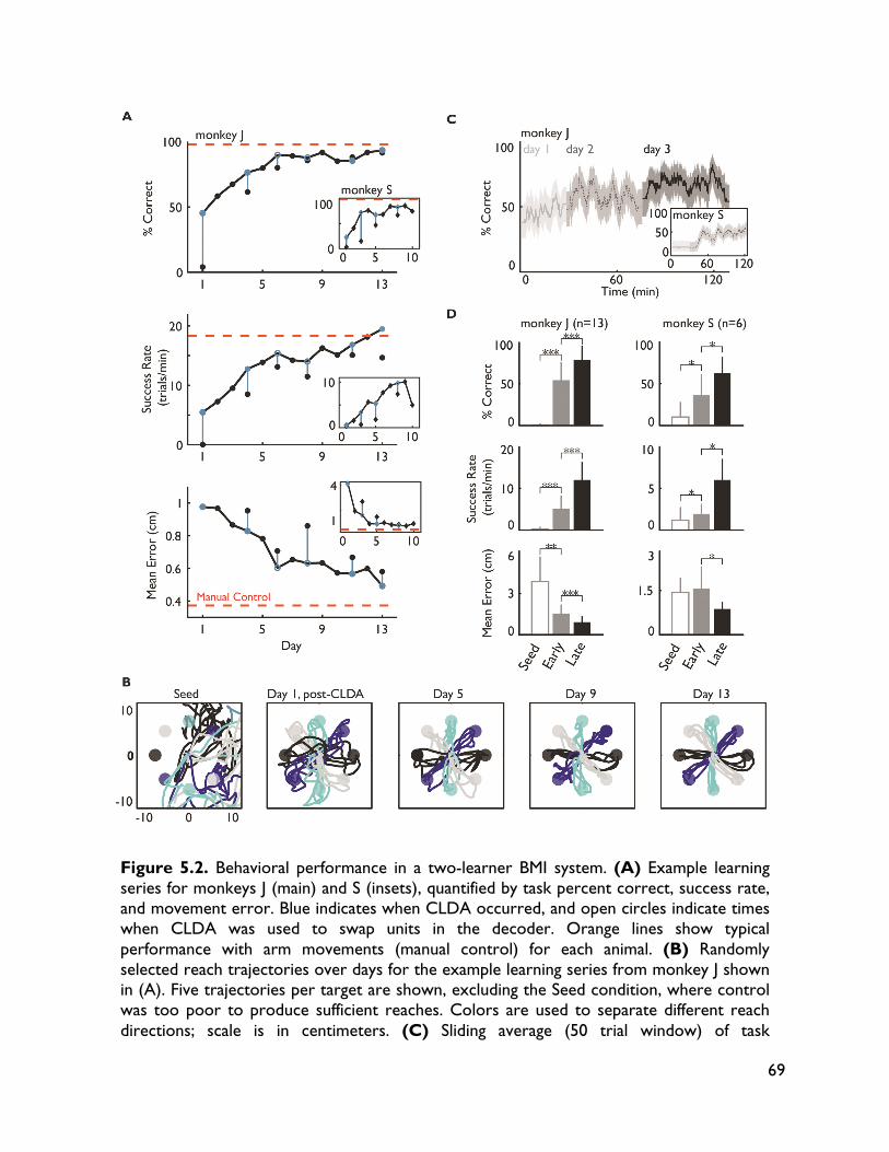
69  

Figure 5.2. Behavioral performance in a two-learner BMI system. (A) Example learning series for monkeys J (main) and S (insets), quantified by task percent correct, success rate, and movement error. Blue indicates when CLDA occurred, and open circles indicate times when CLDA was used to swap units in the decoder. Orange lines show typical performance with arm movements (manual control) for each animal. (B) Randomly selected reach trajectories over days for the example learning series from monkey J shown in (A). Five trajectories per target are shown, excluding the Seed condition, where control was too poor to produce sufficient reaches. Colors are used to separate different reach directions; scale is in centimeters. (C) Sliding average (50 trial window) of task

70  

performance for days 1-3 (monkey J) and 1-2 (monkey S) in the example series shown in (A). Shading indicates 95% confidence-intervals (Agresti-Coull binomial confidence interval). The decoder was held fixed over these days, after initial CLDA on day 1. Note that sliding averages were done separately for each day. (D) Average improvement over all learning series (n = 13, monkey J; n = 6, monkey S) for task percent correct, success rate, and movement error. “Seed” shows the performance with the initial decoder. “Early” corresponds to performance on day 1 following CLDA. Late corresponds to the best performance achieved after day 1. Bars show means; error bars indicate standard deviation. * = p< 0.05; ** = p< 0.01; *** = p < 0.001, one-sided, paired Wilcoxon sign-rank test.

5.3.2 Importance of decoder stability and specificity of learning Subjects showed gradual refinement of cursor control, with movement errors and success rates showing continued improvements even after task performance (percent correct) reached a plateau (Figure 5.2A). This refinement was absent when CLDA was used each day to maximize performance from varying initial decoders. While CLDA could achieve high task performance, movement kinematics showed no improvements (Figure 5.3). Moreover, daily performance showed variability that was not present when using a two-learner paradigm.

To verify that learning was decoder-specific, we also tested performance with novel decoders with monkey J. Novel decoders were trained using neural activity during native arm movements or visual observation of cursor movements on the day of the test. Closed-loop performance dropped significantly when using unpracticed test decoders (Figure 5.3D). Similar to previous studies (Ganguly and Carmena, 2009), these perturbations were reversible and performance quickly returned when learned decoders were reinstated. 5.3.3 Neural adaptation and map formation in a two-learner BMI We next explored the neural activity underlying the development of skilled task performance in our two-learner BMI paradigm. The directional-tuning of units contributing to the BMI cursor was assessed each day within learning series (see section 5.2.6.2) to determine how the relationship between cursor movement and neural activity changed over time. Figure 5.4A-C shows cosine tuning curve fits for three example units for four days within a learning series. Unit tuning properties (modulation depth and preferred direction; subsequently denoted as

and , respectively) changed gradually over the course of a series for the majority of units within the ensemble (Figure 5.4D).

To quantify learning-related neural tuning changes at the population level, we performed a direction-tuning map analysis similar to Ganguly and Carmena, 2009. The fitted tuning curves for the BMI ensemble for each day form a cortical map. We performed pair-wise correlations among the daily maps within a learning series (see section 5.2.6.4). Maps were more strongly correlated to one another late in learning, showing the stabilization of a neural representation (Figure 5.4E). The average correlation of each day's map with all others, which reflects the degree of map stability, increased late in learning, with a time-course very similar to the task performance improvements (Figure 5.4F). Both performance improvements and cortical map formation were not sensitive to changes in the BMI ensemble. Recorded units were only partially stationary, showing slight variability in waveforms and firing properties during native arm movements (Figure 5.5). Cortical maps computed in arm movement and visual observation tasks did not show stabilization trends for

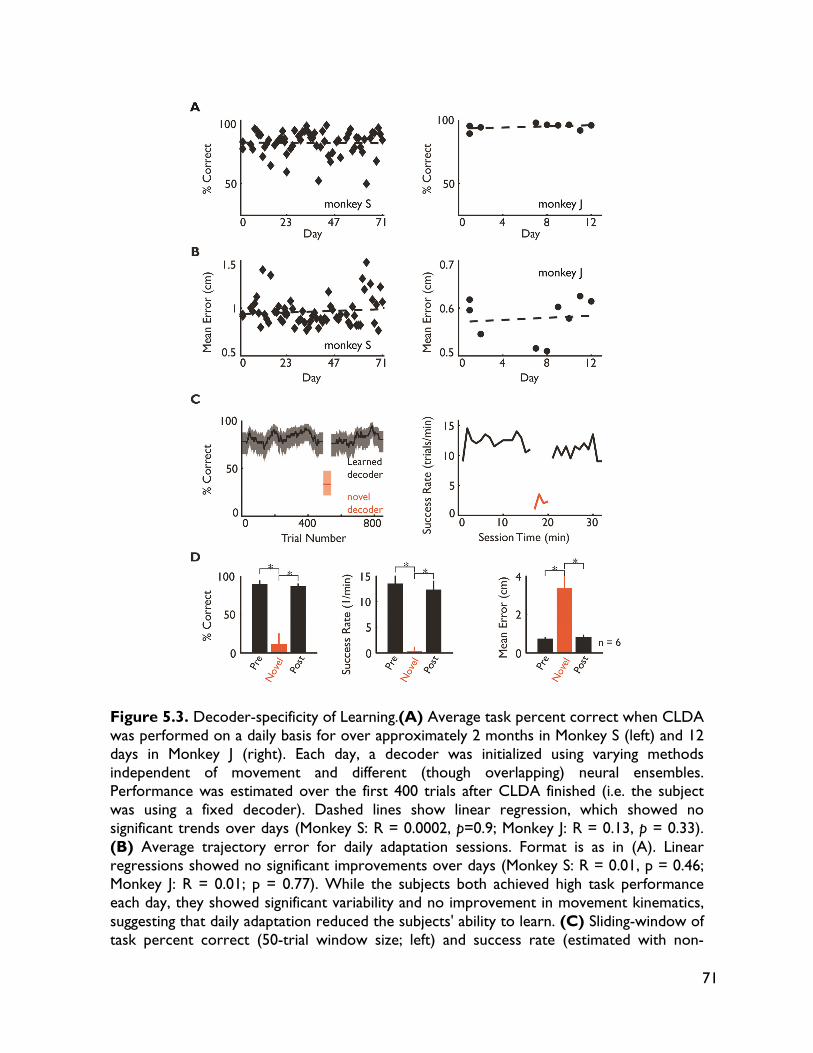
71  

Figure 5.3. Decoder-specificity of Learning.(A) Average task percent correct when CLDA was performed on a daily basis for over approximately 2 months in Monkey S (left) and 12 days in Monkey J (right). Each day, a decoder was initialized using varying methods independent of movement and different (though overlapping) neural ensembles. Performance was estimated over the first 400 trials after CLDA finished (i.e. the subject was using a fixed decoder). Dashed lines show linear regression, which showed no significant trends over days (Monkey S: R = 0.0002, p=0.9; Monkey J: R = 0.13, p = 0.33). (B) Average trajectory error for daily adaptation sessions. Format is as in (A). Linear regressions showed no significant improvements over days (Monkey S: R = 0.01, p = 0.46; Monkey J: R = 0.01; p = 0.77). While the subjects both achieved high task performance each day, they showed significant variability and no improvement in movement kinematics, suggesting that daily adaptation reduced the subjects' ability to learn. (C) Sliding-window of task percent correct (50-trial window size; left) and success rate (estimated with non-

72  

overlapping 2 minute windows; right) for an example decoder-swap session where a learned decoder was replaced with a novel decoder trained that day. Performance with the learned decoder is shown in black; performance for the test decoder is shown in orange. Lines indicate the mean. Shading indicates 95% confidence intervals for the percent correct estimates (Agresti-Coull interval). Swapping the novel decoder for the learned decoder resulted in a significant and reversible drop in performance. (D) Average performance disruption for decoder swaps across 6 sessions with Monkey J. Performance was assessed using task percent correct (left), success rate (middle), and mean trajectory error (right). All metrics were calculated as the average across trials within each block (pre-swap; novel decoder (“novel”); and post-swap). Bars represent mean, and error bars denote standard deviations. Across all metrics, performance dropped significantly between the learned decoder (both pre- and post-perturbation) and biomimetic decoder (one-sided Wilcoxon paired sign-test, * denotes p < 0.05). No significant difference was found between performance with the learned decoder pre- and post-perturbation (one-sided Wilcoxon paired sign-test, p > 0.05).

monkey J (Figure 5.5 A-C), suggesting that the emergence of a stable map in BMI cannot be attributed to this recording variability.

Furthermore, cortical map stability and behavioral improvements were not impeded by ensemble membership changes (Figure 5.5H). CLDA was also used to change membership of the BMI ensemble. In the event a recorded unit contributing to the decoder was lost, it was deleted or replaced with another unit using CLDA. For each session in which the BMI ensemble changed, we examined behavioral performance and ensemble-level neural stability (similarity of that day’s tuning map with all others) before swapping, on the day of the swap, and the following day. Task performance continued to improve over days, even with unit swaps. Ensemble tuning maps were not disrupted by ensemble changes, with no significant drop in the average map correlation measure across swaps. Note that maps were computed only using units that were part of the BMI ensemble throughout the series. This measure thus suggests that changes in BMI ensemble membership did not disrupt directional tuning of other units in the ensemble. Analyzing changes in decoder parameters across series revealed similar trends. CLDA made the largest changes in initial adaptation, with mid-series updates making only minor adjustments (Figure 5.5 I-J). Together, these behavioral and neural results show that beneficial neuroplasticity can occur with semi-stationary BMI circuits. 5.3.4 Neural adaptation varies with amount of performance improvements Little is known about how distributed learning might occur in a two-learner BMI system. Given the observations of beneficial neuroplasticity occurring alongside decoder adaptation, we next examined the relationship between neural and decoder adaptation. We hypothesized that stable neural representations would form regardless of the initial amount of CLDA, but that the degree to which the subject improved performance after initial CLDA would influence the degree of neural adaptation. As previously noted, the amount of initial improvements from CLDA varied across series. Figure 5.6A shows example map correlations for different series in which initial CLDA improved performance by different amounts, or no CLDA was used. Series with low initial performance showed gradual improvement and retention, while those with high performance achieved via CLDA on day 1 was readily maintained. Interestingly, neural maps

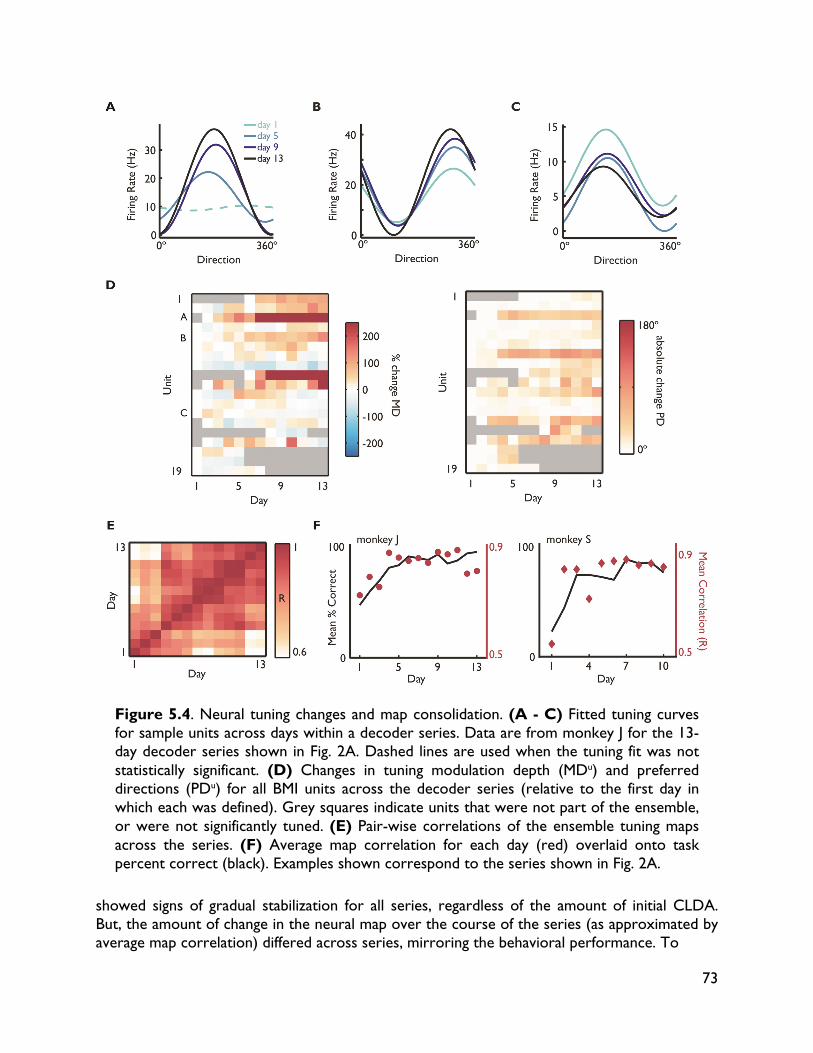
73  

showed signs of gradual stabilization for all series, regardless of the amount of initial CLDA. But, the amount of change in the neural map over the course of the series (as approximated by average map correlation) differed across series, mirroring the behavioral performance. To

Figure 5.4. Neural tuning changes and map consolidation. (A - C) Fitted tuning curves for sample units across days within a decoder series. Data are from monkey J for the 13-day decoder series shown in Fig. 2A. Dashed lines are used when the tuning fit was not statistically significant. (D) Changes in tuning modulation depth (MDu) and preferred directions (PDu) for all BMI units across the decoder series (relative to the first day in which each was defined). Grey squares indicate units that were not part of the ensemble, or were not significantly tuned. (E) Pair-wise correlations of the ensemble tuning maps across the series. (F) Average map correlation for each day (red) overlaid onto task percent correct (black). Examples shown correspond to the series shown in Fig. 2A.

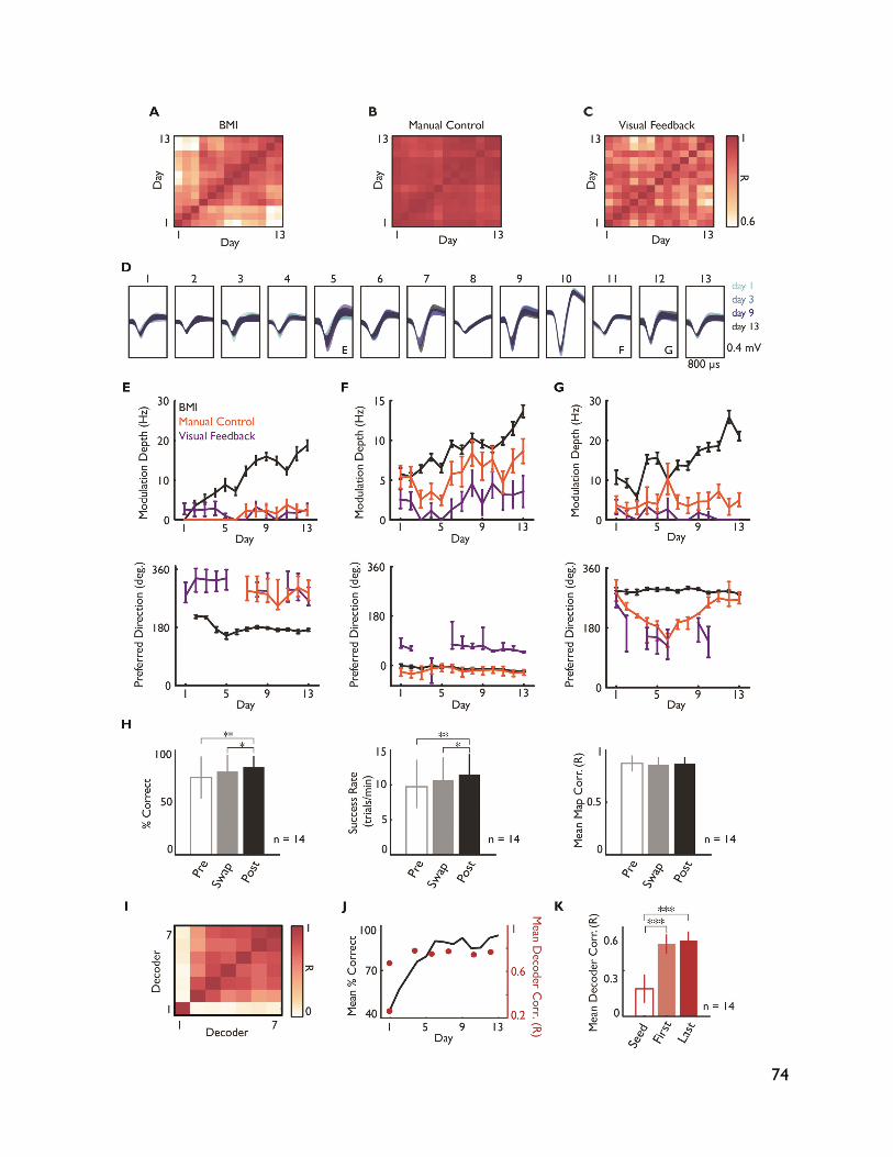
74  

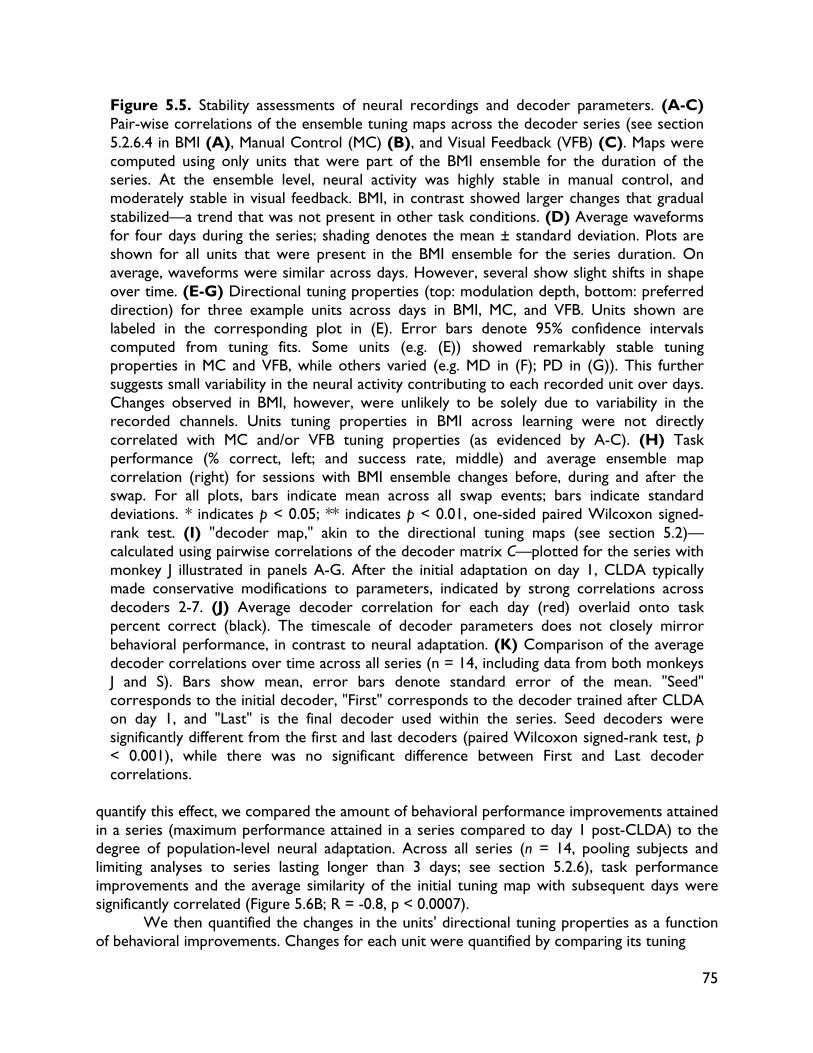
75  

Figure 5.5. Stability assessments of neural recordings and decoder parameters. (A-C) Pair-wise correlations of the ensemble tuning maps across the decoder series (see section 5.2.6.4 in BMI (A), Manual Control (MC) (B), and Visual Feedback (VFB) (C). Maps were computed using only units that were part of the BMI ensemble for the duration of the series. At the ensemble level, neural activity was highly stable in manual control, and moderately stable in visual feedback. BMI, in contrast showed larger changes that gradual stabilized—a trend that was not present in other task conditions. (D) Average waveforms for four days during the series; shading denotes the mean ± standard deviation. Plots are shown for all units that were present in the BMI ensemble for the series duration. On average, waveforms were similar across days. However, several show slight shifts in shape over time. (E-G) Directional tuning properties (top: modulation depth, bottom: preferred direction) for three example units across days in BMI, MC, and VFB. Units shown are labeled in the corresponding plot in (E). Error bars denote 95% confidence intervals computed from tuning fits. Some units (e.g. (E)) showed remarkably stable tuning properties in MC and VFB, while others varied (e.g. MD in (F); PD in (G)). This further suggests small variability in the neural activity contributing to each recorded unit over days. Changes observed in BMI, however, were unlikely to be solely due to variability in the recorded channels. Units tuning properties in BMI across learning were not directly correlated with MC and/or VFB tuning properties (as evidenced by A-C). (H) Task performance (% correct, left; and success rate, middle) and average ensemble map correlation (right) for sessions with BMI ensemble changes before, during and after the swap. For all plots, bars indicate mean across all swap events; bars indicate standard deviations. * indicates p < 0.05; ** indicates p < 0.01, one-sided paired Wilcoxon signed-rank test. (I) "decoder map," akin to the directional tuning maps (see section 5.2)—calculated using pairwise correlations of the decoder matrix C—plotted for the series with monkey J illustrated in panels A-G. After the initial adaptation on day 1, CLDA typically made conservative modifications to parameters, indicated by strong correlations across decoders 2-7. (J) Average decoder correlation for each day (red) overlaid onto task percent correct (black). The timescale of decoder parameters does not closely mirror behavioral performance, in contrast to neural adaptation. (K) Comparison of the average decoder correlations over time across all series (n = 14, including data from both monkeys J and S). Bars show mean, error bars denote standard error of the mean. "Seed" corresponds to the initial decoder, "First" corresponds to the decoder trained after CLDA on day 1, and "Last" is the final decoder used within the series. Seed decoders were significantly different from the first and last decoders (paired Wilcoxon signed-rank test, p < 0.001), while there was no significant difference between First and Last decoder correlations.

quantify this effect, we compared the amount of behavioral performance improvements attained in a series (maximum performance attained in a series compared to day 1 post-CLDA) to the degree of population-level neural adaptation. Across all series (n = 14, pooling subjects and limiting analyses to series lasting longer than 3 days; see section 5.2.6), task performance improvements and the average similarity of the initial tuning map with subsequent days were significantly correlated (Figure 5.6B; R = -0.8, p < 0.0007).

We then quantified the changes in the units' directional tuning properties as a function of behavioral improvements. Changes for each unit were quantified by comparing its tuning

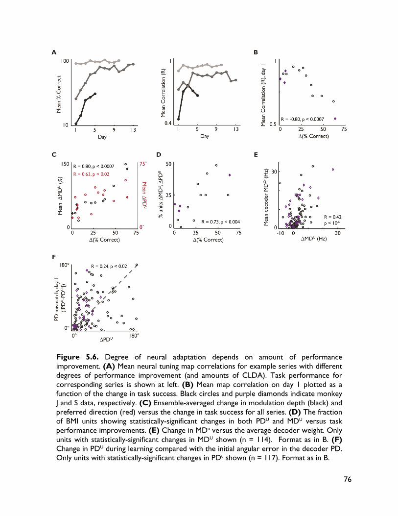
76  

Figure 5.6. Degree of neural adaptation depends on amount of performance improvement. (A) Mean neural tuning map correlations for example series with different degrees of performance improvement (and amounts of CLDA). Task performance for corresponding series is shown at left. (B) Mean map correlation on day 1 plotted as a function of the change in task success. Black circles and purple diamonds indicate monkey J and S data, respectively. (C) Ensemble-averaged change in modulation depth (black) and preferred direction (red) versus the change in task success for all series. (D) The fraction of BMI units showing statistically-significant changes in both PDU and MDU versus task performance improvements. (E) Change in MDu versus the average decoder weight. Only units with statistically-significant changes in MDU shown (n = 114). Format as in B. (F) Change in PDU during learning compared with the initial angular error in the decoder PD. Only units with statistically-significant changes in PDu shown (n = 117). Format as in B.

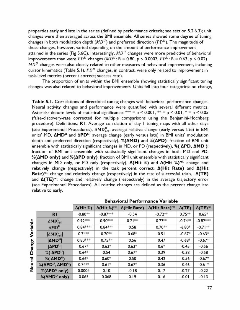
77  

properties early and late in the series (defined by performance criteria; see section 5.2.6.3); unit changes were then averaged across the BMI ensemble. All series showed some degree of tuning changes in both modulation depth ( ) and preferred direction ( ). The magnitude of these changes, however, varied depending on the amount of performance improvement attained in the series (Fig 5.6C). Interestingly, changes were more predictive of behavioral improvements than were changes ( : R = 0.80, p < 0.0007; : R = 0.63, p < 0.02).

changes were also closely related to other measures of behavioral improvement, including cursor kinematics (Table 5.1). changes, in contrast, were only related to improvement in task-level metrics (percent correct; success rate).

The proportion of units within the BMI ensemble showing statistically significant tuning changes was also related to behavioral improvements. Units fell into four categories: no change,

Table 5.1. Correlations of directional tuning changes with behavioral performance changes. Neural activity changes and performance were quantified with several different metrics. Asterisks denote levels of statistical significance: *** = p < 0.001, ** = p < 0.01, * = p < 0.05 (false-discovery-rate corrected for multiple comparisons using the Benjamini-Hochberg procedure). Definitions: R1: Average correlation of day 1 tuning maps with all other days (see Experimental Procedures), ∆ : average relative change (early versus late) in BMI units' MD, ∆MDU and ∆PDU: average change (early versus late) in BMI units' modulation depth and preferred direction (respectively), %(∆MD) and %(∆PD): fraction of BMI unit ensemble with statistically significant changes in MD, or PD (respectively), %( ∆PD, ∆MD ): fraction of BMI unit ensemble with statistically significant changes in both MD and PD, %(∆MD only) and %(∆PD only): fraction of BMI unit ensemble with statistically significant changes in MD only, or PD only (respectively), ∆(Hit %) and ∆(Hit %)rel: change and relatively change (respectively) in the task percent correct, ∆(Hit Rate) and ∆(Hit Rate)rel: change and relatively change (respectively) in the rate of successful trials, ∆(TE) and ∆(TE)rel: change and relatively change (respectively) in the average trajectory error (see Experimental Procedures). All relative changes are defined as the percent change late relative to early.

Behavioral Performance Variable

∆(Hit %) ∆(Hit %)rel ∆(Hit Rate) ∆(Hit Rate)rel ∆(TE) ∆(TE)rel

Neu

ral C

hang

e V

aria

ble

R1 -0.80** -0.87*** -0.54 -0.72** 0.75** 0.65*

∆ 0.92*** 0.90*** 0.71** 0.77** -0.74** -0.82***

∆ 0.84*** 0.84*** 0.58 0.70** -6.80* -0.71**

|∆ | 0.74** 0.70** 0.68* 0.51 -0.67* -0.63*

|∆MDU| 0.80*** 0.75** 0.56 0.47 -0.68* -0.67* |∆PDU| 0.67* 0.63* 0.63* 0.6* -0.45 -0.56

%( ∆PDU) 0.64* 0.54 0.67* 0.39 -0.38 -0.58 %( ∆MDU) 0.66* 0.60* 0.50 0.42 -0.56 -0.67*

%(∆PDU, ∆MDU) 0.74** 0.61* 0.67* 0.36 -0.46 -0.61* %(∆PDU only) 0.0004 0.10 -0.18 0.17 -0.27 -0.22 %(∆MDU only) 0.065 0.068 0.19 0.16 -0.01 -0.13

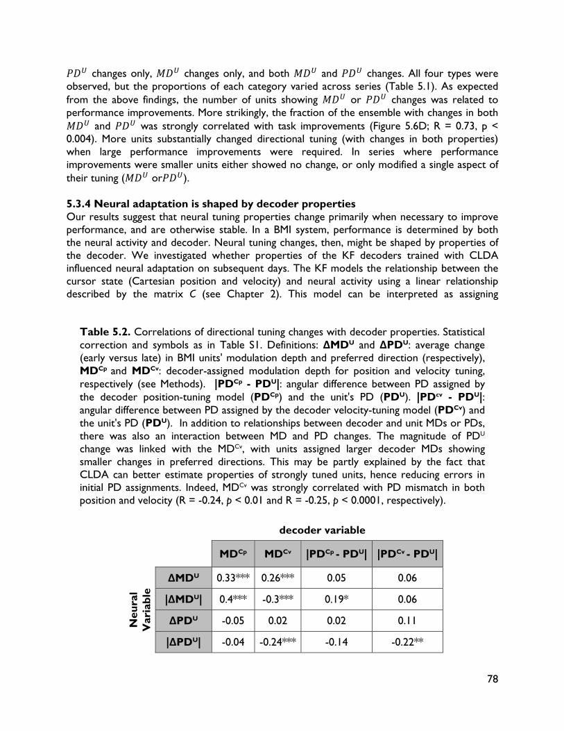
78  

changes only, changes only, and both and changes. All four types were observed, but the proportions of each category varied across series (Table 5.1). As expected from the above findings, the number of units showing or changes was related to performance improvements. More strikingly, the fraction of the ensemble with changes in both

and was strongly correlated with task improvements (Figure 5.6D; R = 0.73, p < 0.004). More units substantially changed directional tuning (with changes in both properties) when large performance improvements were required. In series where performance improvements were smaller units either showed no change, or only modified a single aspect of their tuning ( or ). 5.3.4 Neural adaptation is shaped by decoder properties Our results suggest that neural tuning properties change primarily when necessary to improve performance, and are otherwise stable. In a BMI system, performance is determined by both the neural activity and decoder. Neural tuning changes, then, might be shaped by properties of the decoder. We investigated whether properties of the KF decoders trained with CLDA influenced neural adaptation on subsequent days. The KF models the relationship between the cursor state (Cartesian position and velocity) and neural activity using a linear relationship described by the matrix C (see Chapter 2). This model can be interpreted as assigning

Table 5.2. Correlations of directional tuning changes with decoder properties. Statistical correction and symbols as in Table S1. Definitions: ∆MDU and ∆PDU: average change (early versus late) in BMI units' modulation depth and preferred direction (respectively), MDCp and MDCv: decoder-assigned modulation depth for position and velocity tuning, respectively (see Methods). |PDCp - PDU|: angular difference between PD assigned by the decoder position-tuning model (PDCp) and the unit's PD (PDU). |PDcv - PDU|: angular difference between PD assigned by the decoder velocity-tuning model (PDCv) and the unit's PD (PDU). In addition to relationships between decoder and unit MDs or PDs, there was also an interaction between MD and PD changes. The magnitude of PDU change was linked with the MDCv, with units assigned larger decoder MDs showing smaller changes in preferred directions. This may be partly explained by the fact that CLDA can better estimate properties of strongly tuned units, hence reducing errors in initial PD assignments. Indeed, MDCv was strongly correlated with PD mismatch in both position and velocity (R = -0.24, p < 0.01 and R = -0.25, p < 0.0001, respectively).

decoder variable

MDCp MDCv |PDCp

- PDU| |PDCv - PDU|

Neu

ral

Var

iabl

e

∆MDU 0.33*** 0.26*** 0.05 0.06

|∆MDU| 0.4*** -0.3*** 0.19* 0.06

∆PDU -0.05 0.02 0.02 0.11

|∆PDU| -0.04 -0.24*** -0.14 -0.22**

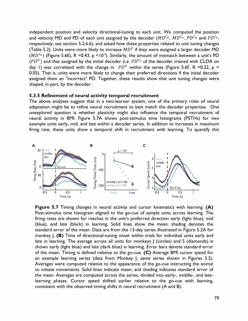
79  

independent position and velocity directional-tuning to each unit. We computed the position and velocity MD and PD of each unit assigned by the decoder ( , , and , respectively; see section 5.2.6.6), and asked how these properties related to unit tuning changes (Table 5.2). Units were more likely to increase if they were assigned a larger decoder MD ( (Figure 5.6E), R =0.43, p <10-5). Similarly, the amount of mismatch between a unit's PD ( and that assigned by the initial decoder (i.e. of the decoder trained with CLDA on day 1) was correlated with the change in within the series (Figure 5.6F, R =0.22, p < 0.05). That is, units were more likely to change their preferred directions if the initial decoder assigned them an "incorrect" PD. Together, these results show that unit tuning changes were shaped, in part, by the decoder. 5.3.5 Refinement of neural activity temporal recruitment The above analyses suggest that in a two-learner system, one of the primary roles of neural adaptation might be to refine neural recruitment to best match the decoder properties. One unexplored question is whether plasticity might also influence the temporal recruitment of neural activity in BMI. Figure 5.7A shows post-stimulus time histograms (PSTHs) for two example units early, mid, and late within a decoder series. In addition to increases in maximum firing rate, these units show a temporal shift in recruitment with learning. To quantify this

Figure 5.7 Timing changes in neural activity and cursor kinematics with learning. (A) Post-stimulus time histogram aligned to the go-cue of sample units across learning. The firing rates are shown for reaches in the unit’s preferred direction early (light blue), mid (blue), and late (black) in learning. Solid lines show the mean; shading denotes the standard error of the mean. Data are from the 13-day series illustrated in Figure 5.2A for monkey J. (B) Time of directional-tuning onset within trials for individual units early and late in learning. The average across all units for monkeys J (circles) and S (diamonds) is shown early (light blue) and late (dark blue) in learning. Error bars denote standard error of the mean. Timing is defined relative to the go-cue. (C) Average BMI cursor speed for an example learning series (data from Monkey J, same series shown in Figures 5.2). Averages were computed relative to the appearance of the go-cue instructing the animal to initiate movements. Solid lines indicate mean, and shading indicates standard error of the mean. Averages are computed across the series, divided into early-, middle-, and late-learning phases. Cursor speed shifted earlier relative to the go-cue with learning, consistent with the observed timing shifts in neural recruitment (A and B).

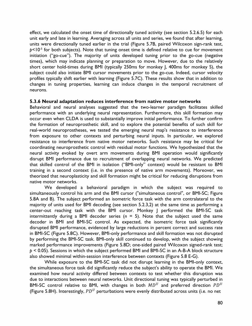
80  

effect, we calculated the onset time of directionally tuned activity (see section 5.2.6.5) for each unit early and late in learning. Averaging across all units and series, we found that after learning, units were directionally tuned earlier in the trial (Figure 5.7B, paired Wilcoxon sign-rank test, p<10-5 for both subjects). Note that tuning onset time is defined relative to cue for movement initiation (“go-cue”). The majority of units developed tuning prior to the go-cue (negative times), which may indicate planning or preparation to move. However, due to the relatively short center hold-times during BMI (typically 250ms for monkey J, 400ms for monkey S), the subject could also initiate BMI cursor movements prior to the go-cue. Indeed, cursor velocity profiles typically shift earlier with learning (Figure 5.7C). These results show that in addition to changes in tuning properties, learning can induce changes in the temporal recruitment of neurons. 5.3.6 Neural adaptation reduces interference from native motor networks Behavioral and neural analyses suggested that the two-learner paradigm facilitates skilled performance with an underlying neural representation. Furthermore, this skill formation may occur even when CLDA is used to substantially improve initial performance. To further confirm the formation of neuroprosthetic skill, and to explore the potential benefits of such skill for real-world neuroprostheses, we tested the emerging neural map's resistance to interference from exposure to other contexts and perturbing neural inputs. In particular, we explored resistance to interference from native motor networks. Such resistance may be critical for coordinating neuroprosthetic control with residual motor functions. We hypothesized that the neural activity evoked by overt arm movements during BMI operation would significantly disrupt BMI performance due to recruitment of overlapping neural networks. We predicted that skilled control of the BMI in isolation (“BMI-only” context) would be resistant to BMI training in a second context (i.e. in the presence of native arm movements). Moreover, we theorized that neuroplasticity and skill formation might be critical for reducing disruptions from native motor networks. We developed a behavioral paradigm in which the subject was required to simultaneously control his arm and the BMI cursor ("simultaneous control", or BMI-SC; Figure 5.8A and B). The subject performed an isometric force task with the arm contralateral to the majority of units used for BMI decoding (see section 5.2.3,2) at the same time as performing a center-out reaching task with the BMI cursor. Monkey J performed the BMI-SC task intermittently during a BMI decoder series (n = 5). Note that the subject used the same decoder in BMI and BMI-SC control. As expected, the isometric force task significantly disrupted BMI performance, evidenced by large reductions in percent correct and success rate in BMI-SC (Figure 5.8C). However, BMI-only performance and skill formation was not disrupted by performing the BMI-SC task. BMI-only skill continued to develop, with the subject showing marked performance improvements (Figure 5.8D; one-sided paired Wilcoxon signed-rank test; p < 0.05). Sessions in which the subject performed BMI and BMI-SC in an A-B-A block structure also showed minimal within-session interference between contexts (Figure 5.8 E-G).

While exposure to the BMI-SC task did not disrupt learning in the BMI-only context, the simultaneous force task did significantly reduce the subject's ability to operate the BMI. We examined how neural activity differed between contexts to test whether this disruption was due to interactions between neural networks. Unit directional tuning was typically perturbed in BMI-SC control relative to BMI, with changes in both and preferred direction (Figure 5.8H). Interestingly, perturbations were evenly distributed across units (i.e. no net

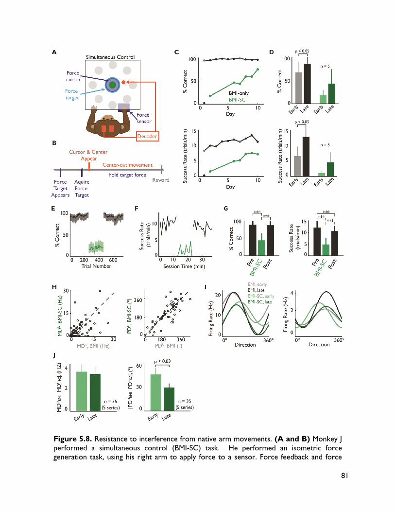
81  

Figure 5.8. Resistance to interference from native arm movements. (A and B) Monkey J performed a simultaneous control (BMI-SC) task. He performed an isometric force generation task, using his right arm to apply force to a sensor. Force feedback and force

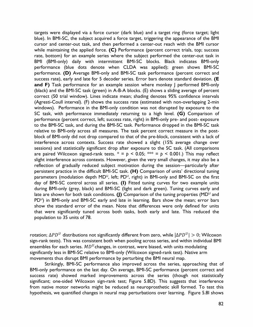
82  

targets were displayed via a force cursor (dark blue) and a target ring (force target; light blue). In BMI-SC, the subject acquired a force target, triggering the appearance of the BMI cursor and center-out task, and then performed a center-out reach with the BMI cursor while maintaining the applied force. (C) Performance (percent correct trials, top; success rate, bottom) for an example series where the subject performed the center-out task in BMI (BMI-only) daily with intermittent BMI-SC blocks. Black indicates BMI-only performance (blue dots denote when CLDA was applied); green shows BMI-SC performance. (D) Average BMI-only and BMI-SC task performance (percent correct and success rate), early and late for 5 decoder series. Error bars denote standard deviation. (E and F) Task performance for an example session where monkey J performed BMI-only (black) and the BMI-SC task (green) in A-B-A blocks. (E) shows a sliding average of percent correct (50 trial window). Lines indicate mean; shading denotes 95% confidence intervals (Agresti-Coull interval). (F) shows the success rate (estimated with non-overlapping 2-min windows). Performance in the BMI-only condition was not disrupted by exposure to the SC task, with performance immediately returning to a high level. (G) Comparison of performance (percent correct, left; success rate, right) in BMI-only pre- and post- exposure to the BMI-SC task, and during the BMI-SC task. Performance dropped in the BMI-SC task relative to BMI-only across all measures. The task percent correct measure in the post-block of BMI-only did not drop compared to that of the pre-block, consistent with a lack of interference across contexts. Success rate showed a slight (15% average change over sessions) and statistically significant drop after exposure to the SC task. (All comparisons are paired Wilcoxon signed-rank tests. * = p < 0.05; *** = p < 0.001.) This may reflect slight interference across contexts. However, given the very small changes, it may also be a reflection of gradually reduced subject motivation during the session—particularly after persistent practice in the difficult BMI-SC task. (H) Comparison of units’ directional tuning parameters (modulation depth MDU, left; PDU, right) in BMI-only and BMI-SC on the first day of BMI-SC control across all series. (I) Fitted tuning curves for two example units during BMI-only (grey, black) and BMI-SC (light and dark green). Tuning curves early and late are shown for both task conditions. (J) Comparison of the tuning properties (MDU and PDU) in BMI-only and BMI-SC early and late in learning. Bars show the mean; error bars show the standard error of the mean. Note that differences were only defined for units that were significantly tuned across both tasks, both early and late. This reduced the population to 35 units of 78.

rotation; ∆ distributions not significantly different from zero, while |∆ | 0; Wilcoxon sign-rank tests). This was consistent both when pooling across series, and within individual BMI ensembles for each series. changes, in contrast, were biased, with units modulating significantly less in BMI-SC relative to BMI-only (Wilcoxon signed-rank test). Native arm movements thus disrupt BMI performance by perturbing the BMI neural map.

Strikingly, BMI-SC performance also improved across the series, approaching that of BMI-only performance on the last day. On average, BMI-SC performance (percent correct and success rate) showed marked improvements across the series (though not statistically significant; one-sided Wilcoxon sign-rank test; Figure 5.8D). This suggests that interference from native motor networks might be reduced as neuroprosthetic skill formed. To test this hypothesis, we quantified changes in neural map perturbations over learning. Figure 5.8I shows

83  

fitted tuning curves for two example units during BMI-only and BMI-SC early and late in learning. Tuning in BMI-SC late in learning often changed to shift closer to that of BMI-only. We quantified this effect at a population level by computing the difference in a unit's and in BMI-only and BMI-SC each day. Comparing the difference in tuning properties early and late in learning, we found a significant reduction in perturbations (paired Wilcoxon signed-rank test, p < 0.03), but no significant change in the magnitude of perturbations (Figure 5.8J). 5.4 Discussion Together, these results show that decoder and neural adaptation can be combined to produce robust, skilled neuroprosthetic performance that can be maintained despite non-stationary neural inputs and changes in context. Behavioral skill was accompanied by the formation of stable cortical maps, and performance improvements were driven by changes in units' relationship to cursor movement. Relationships between neural and decoder adaptation also suggest that CLDA might help shape neural activity during closed-loop BMI control and learning. Our results suggest that neural and decoder adaptation can collaborate to achieve high performance. Critically, skilled performance and stable neural representations developed even when the majority of performance improvements were achieved via initial decoder adaptation. This skill development showed resistance to interference from practicing BMI in other contexts, and may also increase the BMI ensemble's resistance to perturbing inputs. 5.4.1 Relationship between decoder stability and neural adaptation Previous results suggest that neural adaptation and skill formation are strongly tied to stability of the BMI decoder and ensemble (Ganguly and Carmena, 2009). Our results expand this finding to suggest that skill formation can still occur in the presence of gradually changing decoder parameters and ensembles. The smooth, gradual, and intermittent nature of our decoder and ensemble changes may be critical for facilitating skill formation. Exploration of co-adaptive learning in human-machine interfaces suggests that machine learning algorithms that make more gradual decoder modifications may be easier for subjects to learn (Danzinger et al., 2009). The same may be true in BMI. Though the decoder was allowed to adapt in our paradigm, we found that after initial CLDA training, decoder adaptation produced relatively conservative changes in parameters over the course of a series (Figure 5.5 I-K). Indeed, as we found in Chapter 4, the SmoothBatch algorithm used for monkey J explicitly constrains decoder retraining to impose smoothness (Dangi et al., 2013a). Moreover, changes in the BMI ensemble were made gradually, with approximately 10% of the ensemble (1-2 units) changing at a time, and relatively infrequently within the series. The importance of gradual decoder adaptation for skill formation is further supported by the varied learning rates found in studies with daily decoder re-training, with or without CLDA, where decoder properties and BMI ensembles are more abruptly changed (Figure 5.3, also Taylor et al., 2002; Carmena et al., 2003; Musallam et al., 2004; Gilja et al., 2012; Collinger et al., 2012). This finding may be particularly important for designs of new CLDA algorithms, relevant to Chapter 4 (Dangi et al., 2013a). Our results also suggest that it may be both feasible and highly advantageous to leverage neural adaptation in neuroprosthetic applications.

84  

5.4.2 Neural adaptation mechanisms in BMI Our results show that a two-learner system can facilitate skill formation, and involves changes in the BMI ensemble units' firing properties. We observed changes in units' modulation depth and preferred directions, consistent with previous findings (Taylor et al., 2002; Carmena et al., 2003; Jarosiewicz et al., 2008; Ganguly and Carmena, 2009; Ganguly et al., 2011; Chase et al., 2012; Hwang et al., 2013). Interestingly, we find that these properties may be somewhat independent of one another, with many units showing either changes in MD or PD alone. Both MD and PD changes were linked to the decoder properties (Figures 5.6E, F). These results suggest that MD changes may be driven by “credit-assignment” processes to increase modulation of units most strongly linked to cursor movements, while PD changes are driven by mismatch between the cursor movement and the subject's intent. These findings are consistent with previous evidence that BMI skill learning gradually shapes network activity by selectively modulating BMI units (Ganguly et al., 2011), and that subjects can selectively rotate PDs of individual units within the BMI ensemble (Jarosiewicz et al., 2008; Chase et al., 2012).

Importantly, the amount of neural adaptation observed showed a clear interaction with decoder adaptation (Figure 5.6). This provides further evidence that neural adaptation is shaped by errors provided during closed-loop control. Neural activity, however, still showed changes even when initial CLDA provided the subjects with a decoder with minimal errors. These changes were primarily restricted to units' MDs (Figure 5.4 A-D; Figure 5.6 C-D). Previous work suggests that MD changes in BMI learning may reflect the formation of a BMI-specific control network (Ganguly et al., 2011). The changes in MD observed in our two-learner system, then, may reflect similar neural adaptation processes. That is, even when CLDA provides subjects with decoders that approximate their intentions, neural adaptation may be critical for identifying and shaping the neural circuit contributing to cursor movements. This is consistent with the substantial changes in neural recruitment timing with learning (Figure 5.6 G-H). Such changes may also potentially reflect learning of an internal model of the BMI system (Golub et al., 2012). Formation of BMI-specific networks also relates directly to the resistance to interference observed with learning, as discussed below.

While our results show that neural tuning changes are strongly tied to both decoder properties and behavioral performance, these factors did not completely explain observed neural changes. For example preferred direction changes and decoder properties were significantly correlated, but only weakly so. This may be due in part to incomplete subject learning, or could suggest that neural solutions used in BMI are constrained as has been suggested by Hwang, Bailey and Andersen (2013). It is currently unknown whether, for instance, neural ensemble selection in BMI may influence plasticity. The differences in amount and type of neural adaptation observed across series in our study could be due in part to properties of the selected BMI ensemble, not just decoder interactions. Ensemble-level constraints, however, cannot fully explain our observations given the many significant relationships between tuning changes, decoder properties and behavior. Identifying the mechanisms driving learning in BMI, and the limitations of learning, is an important remaining challenge (Green and Kalaska, 2011, Jackson and Fetz, 2011). 5.4.3 BMI network formation and resistance to interference from native motor networks Our results suggest that, even when CLDA provides the subject with a highly-performing initial decoder, neural adaptation facilitates the formation of a BMI-specific network (Ganguly et al.,

85  

2011). That is, neurons critical for BMI performance increase their modulation with respect to cursor movements. Previous work suggested that such learning was resistant to interference, with subjects being able to learn multiple BMI decoders with the same neural ensemble and retain each in memory (Ganguly and Carmena, 2009). Here, we broaden these results to show that BMI skill formation is resistant to interference from controlling a BMI in different contexts (with and without simultaneous arm movements; Figure 5.8). Performance and skill formation in the BMI-only context was not disrupted by performing the simultaneous control task. These results also provide strong evidence that BMI skill can form with combined neural and decoder adaptation.

Our results further suggest that learning might reduce the context-dependence of BMI control. BMI-SC performance improved late in the decoder series, even with little or no additional practice in the BMI-SC context. Our results cannot rule out the possibility that the subject learned two different BMI-control contexts independently (i.e. that improvements in BMI-SC control are separate from BMI-only skill formation). However, neural activity during BMI-SC was more similar to that of BMI-only late in the series, suggesting that BMI-SC improvements may be due in part to reduced interference of arm-movement-related activity with BMI control. Interestingly, the reduced neural perturbations were only significant for PD changes. Thus, the disruption of simultaneous arm movements may not be fully blocked by BMI skill formation. Additional studies exploring long-term BMI learning in multiple contexts are needed to fully explore these effects. Further study of the mechanisms underlying BMI skill formation—such as structural and functional changes in the BMI ensemble, and up- and down-stream areas—are also needed to understand if and how skill formation might reduce network interference and increase resistance to perturbations. 5.4.4 Implications for neuroprostheses Together, our results demonstrate the importance of neural plasticity for neuroprosthetic applications. Neural plasticity can provide skilled performance that is reliably recalled over days, and resistant to interference from native motor networks. The combination of neural and decoder adaptation may be especially useful for clinical applications. CLDA could make it more feasible to trigger neural plasticity in real-world settings. By using decoder adaptation to improve initial performance, learning times could be reduced, and the user could be provided with a functional device immediately. Similarly, CLDA can be used to compensate for gradual shifts in neural recordings, reducing the requirements for highly stable recordings long-term. The interactions between CLDA and neural adaptation could also be leveraged to help shape neural solutions towards optimal strategies. This may be particularly important for systems with many degrees-of-freedom (DOFs), where the manifold of possible control solutions becomes highly complex and could contain many singularities and local maxima. Gradual adaptation, of both the decoder and subject, might be a useful tool to guide the system to maximal performance. Given our findings that CLDA and neural adaptation interact such that the brain can, effectively, "pick-up" where the decoder leaves off, such approaches may be highly effective. A gradual training approach has already proven useful in multi-DOF neuroprosthetic control (Velliste et al., 2008; Collinger et al., 2012). However, this earlier method did not use static decoders, and instead gradually introduced control complexity. Combining such an approach with the two-learner paradigm developed here may be particularly fruitful.

Finally, the demonstration of reduced interference from native motor networks with BMI skill formation may be critical for real-world applications. Ultimately, neuroprostheses will

86  

be used outside of a lab setting, where patients will control their devices in coordination with residual motor functions and while performing other cognitive tasks. Here, we show that these changes in context may be highly disruptive. But, learning can be used to overcome these disruptions, either by allowing users to learn and retain multiple context-specific BMI solutions, or by forming a BMI-specific network resistant to interference from external perturbations.

87  

Table 1. Electrophysiology recording methods and signals, and their spatial scale. Data summarized from (Schwartz et al., 2006; Nunez, 2012).

Method Signal Type Scale (mm)

Electroencephalography Scalp potential >10 Electrocorticography Cortical potential 0.1 - 10

Intra-cortical Electrode Local field potential 0.1- 1

Action potentials 0.1

Chapter 6:

Exploring signal sources for closed-loop BMI: local-field potentials versus spiking activity In Chapters 3-5, we explored how to leverage decoder and neural adaptation to improve BMI performance. This work focused on BMIs driven by action potentials from the primary and pre-motor cortices. Another critical question in the design of BMIs is the selection of neural signals to drive the BMI. Closed-loop BMIs create novel, adaptive control systems that differ from the natural motor system (see Chapter 1). Therefore, the best neural signals for closed-loop control may not necessarily be the signals that contain the most information about movement. Here, we explore closed-loop BMI control with different types of neural signals, and how the signals used for control influence neural strategies. This work was done in collaboration with Kelvin So, Siddharth Dangi and Jose M. Carmena, and was published in the proceedings of the IEEE Engineering in Medicine and Biology Society Conference on Neural Engineering (Orsborn et al., 2013). Additional work investigating CLDA applied to LFP BMIs was also published in IEEE Engineering in Medicine and Biology Society Conference (Dangi et al., 2013b). 6.1 Introduction Electrophysiological techniques can record neural activity at a variety of spatial scales (Table 1). Action potentials (or spikes) of individual neurons provide highly localized signals. Alternately, electrical fields immediately surrounding electrodes penetrating the cortex (local field potentials, LFP) reflect summed synaptic activity of nearby neurons (Pesaran, 2009; Buzáki et al., 2012). Electrodes on the cortical surface (electrocorticography, or ECoG) capture activity of larger, more superficial neural populations. Because these signals reflect different aspects of neural activity, they may differ in their utility for brain-machine interfaces.

Closed-loop control has been demonstrated using action-potentials of single and multi-unit activity (Fetz et al., 2007; Moritz and Fetz, 2011; Ganguly and Carmena, 2009; Ganguly et al., 2011; Gilja et al., 2012; Orsborn et al., 2012), as well as local field-potentials (LFPs) (Dangi et al., 2013b; Engelhard et al., 2013; Flint et al., 2013). Studies also suggest that spiking and LFP signals may contain different amounts and types of information about movement (Hwang and Andersen, 2009; Ranade et al., 2009; Markowitz et al., 2011). It may, then, be fruitful to combine spiking and LFP signals in decoding. However, little is known about how spiking and

88  

field-potential signals are related during closed-loop BMI operation, and whether their relationships depend on the signals being used for control. Understanding the neural dynamics during BMI control will better inform the design of future BMI systems.

Exploring neural dynamics in closed-loop BMI may also shed light on the neural mechanisms of volitional control, and the relationships between different neural signals. Many studies shown that either spiking (Fetz et al., 2007; Moritz and Fetz, 2011; Ganguly and Carmena, 2009; Ganguly et al., 2011) or field-potential activity (Engelhard et al., 2013) can be volitionally modulated. The mechanisms of this volitional control, however, are poorly understood (Green and Kalaska, 2011). Do subjects control LFP and spike BMIs in similar ways? Do these signals provide redundant or different information about closed-loop BMI control? LFP signals show significant modulation during spike-controlled BMI (Ranade et al., 2009). Similarly, spiking coherence shifts have been observed during LFP-based BMI control (Engelhard et al., 2013). These findings suggest a link between spiking and LFP activity, but the relationships between these signals is still poorly understood (Pesaran, 2009; Buzáki et al., 2012). Neural plasticity and learning during BMI control may also shape neural signals based on the decoder properties (Jarosiewicz et al., 2008; Ganguly et al., 2011; Green and Kalaska 2011; Koralek et al., 2013; Wander et al., 2013). Hence, neural dynamics in closed-loop BMI may be influenced by the control signals used.

Here, we compare the LFP and spiking activity during control of a spiking- or LFP-based BMI. One non-human primate subject performed a center-out BMI task controlled with either spiking activity or broad-band LFP signals. We analyzed these two signals during the two types of BMI control, and during natural arm movements. Our results suggest that both LFP and spiking activity are significantly modulated during BMI operation, regardless of the control signal used. But, the patterns and dynamics of neural modulation vary depending on the control signal. 6.2 Methods 6.2.1 Electrophysiology One non-human primate (macaca mulatta, male) was implanted bilaterally with chronic multi-site multi-electrode arrays in the primary- and pre-motor cortices. Arrays had 8 x 16 electrodes with 0.5mm spacing, and were implanted targeting layer 5. Spiking and local-field potential signals were recorded from 128 channels using a Plexon MAP system (Dallas, TX, USA). Surgery and recording details have been previously described in Chapter 3 and (Orsborn et al., 2012). Spiking activity was determined using channel-thresholding (Chestek et al., 2011), and thus primarily reflect multi-unit activity. All procedures were conducted in compliance with the National Institute of Health Guide for Care and Use of Laboratory Animals and were approved by the University of California, Berkeley Institutional Animal Care and Use Committee. 6.2.2 Behavioral task BMI and arm-movement tasks used a 2-dimensional delayed center-out reaching paradigm, as described in Chapter 3 and (Orsborn et al., 2012). The subject completed reaches from a central target to 8 peripheral targets (1.2 - 1.4cm radius) spaced uniformly around a 6.5cm radius circle. Successful reaches required moving to the center target, a brief (250-300ms) center-hold, acquiring the target within a time-limit (7-10s), and a target-hold. Targets were

89  

presented pseudo-randomly in blocks of 8 trials spanning all target locations. The subject was initially trained on the center-out reach paradigm with his right arm in a 2D exoskeleton (KINARM, BKIN Technologies) before performing BMI control. We refer to the center-out task performed with the arm as manual control (MC). 6.2.3 BMI implementation BMI was implemented using a position-velocity Kalman Filter (KF) for predictions, as described in Chapter 2. KF State-transition matrices, A and W, were fit using arm kinematics, constrained to impose a causal relationship between position and velocity, as described in Chapter 2.

The spike- and LFP-controlled BMIs differed only in the neural observations, yt., input into the KF. In spike-controlled BMI (S-BMI), predictions were driven by spiking activity (channel-level threshold crossings). Hence, yt was defined as binned firing-rates (100ms bins) of unit activity for the selected ensemble of channels (similar to all previous work presented in Chapters 2-5). Ensembles of 16 left-hemisphere (contra-lateral to trained arm for reaching) units were used in S-BMI.

LFP-controlled BMI (LFP-BMI) predictions were based on the broad-band spectral power of input LFP channels. Here, yt was defined as the log-power in non-overlapping 10Hz bands from 80-150 Hz in the selected LFP channels. 20 right-hemisphere (ipsilateral) channels were used. Power estimations were computed every 100ms using a 200ms sliding window of raw LFP activity. Details of the LFP-BMI implementation can be found in (Dangi et al., 2013b).

In both types of BMI, decoders were trained using closed-loop decoder adaptation (CLDA), implemented using the SmoothBatch algorithm described in Chapter 2 and used throughout this thesis. After performance improved, the decoder was held fixed for the remainder of the session for the next ≥4 days. CLDA allowed us to optimize decoders in closed-loop based on the subject’s self-selected strategy. This also allows for more direct assessment of the maximum attainable performance with each neural signal, since decoders are not limited by the offline prediction power of the selected neural signals. 6.2.4 Data sets We first present analysis of S-BMI, LFP-BMI and MC sessions collected in non-overlapping periods of time. The subject first performed S-BMI for approximately 8 months (using different decoders and ensembles), and subsequently performed LFP-BMI for 1 month with varying decoders. MC sessions were done intermittently during S-BMI training. We analyzed neural activity during natural arm movements (manual control, MC), S-BMI control, and LFP-BMI control. The analyzed data sets each include 4 days where BMI performance (and decoders) was relatively stable for each condition. Due to significant differences in the amount of training time in S- and LFP-BMIs, we included two S-BMI data sets collected after 1 and 4 months of training—"early" and "late", respectively. These two data sets were also used to control for performance differences in BMI. Because data for each task type were collected at different times, no effort was made to directly compare neural activity in these data sets. That is, we do not assume the units or LFP channel properties are stationary. Instead, these analyses compare population-level distributions of activity across the 128 recorded channels. We next conducted an experiment where the subject performed S-BMI and LFP-BMI on the same day in a non-cued A-B-A structure. Decoders for each type of BMI were trained that day using CLDA. We then analyzed data as the subject used fixed (non-adaptive) decoders. Blocks were approximately 30 minutes long (200-300 trials). We present analysis of one

90  

experimental session with same-day task performance to facilitate direct comparison of neural activity across conditions. 6.2.5 Data analysis Behavioral data was analyzed using task performance (percent correct, success rate) and kinematic measures (movement error and reach time). Details of these metrics and methods are described fully in Chapter 3.

Spiking activity was analyzed using firing rates estimated with 100ms non-overlapping bins. Units with average firing rates < 1 Hz were excluded from analyses. Units' modulation with reach direction was assessed using modulation depth, estimated by fitting the firing rate in a [0 1] s following the go-cue to a cosine-tuning model as described in Chapter 5 (section 5.2.6.2).

LFP signals were analyzed in the frequency domain, focusing on trial-averaged power. Spectrograms were estimated using the multi-taper method implemented in Chronux (http://chronux.org; 200ms sliding window with a 50ms step-size, time-bandwidth product of 3 and 5 tapers) (Mitra, 2008). The power in each frequency band was converted to a Z-score (mean-subtraction and normalized by standard-deviation,) to reduce power differences across frequencies due to the 1/f structure of LFP signals, and to normalize amplitudes across channels. Each channel was analyzed separately. Direction modulation within frequency bands was quantified as the difference between maximum and minimum average power across the 8 movement directions.

For all analyses of the indirect comparisons (see section 6.2.4 above), unit and channel activity were averaged across the 4 consecutive days of control within the task-type data sets. Similar results were seen when restricting analysis to individual days. Because data for each task type were collected at different times, no effort was made to directly compare activity. Same-day comparisons (section 6.3.4), however, focus on direct comparisons of neural activity across conditions. 6.3 Results 6.3.1 Behavioral performance Figure 6.1 summarizes behavioral performance in the four data sets analyzed for indirect comparisons. With CLDA, subjects could readily perform BMI with both types of neural signals. Interestingly, LFP-BMI and S-BMI performance were comparable when comparing data sets where the subject had comparable levels of practice. Reach times and movement errors were not significantly different from each other in the LFP-BMI and S-BMI, early data sets (Figure 6.1 C, D, E) where the subject had approximately 1 month of practice in each type of BMI. However, performance in S-BMI improved significantly with practice, with reaches becoming straighter and faster. The inclusion of early and late data sets for S-BMI provides us with comparisons to LFP-BMI that are performance matched, and to see if and how neural dynamics change with practice (and performance improvements) in S-BMI. 6.3.2 Spiking activity Multi-unit activity showed task-related modulations across all conditions. Units had stereo-typed temporal firing patterns during movement. Figure 6.2A shows the average firing rate,

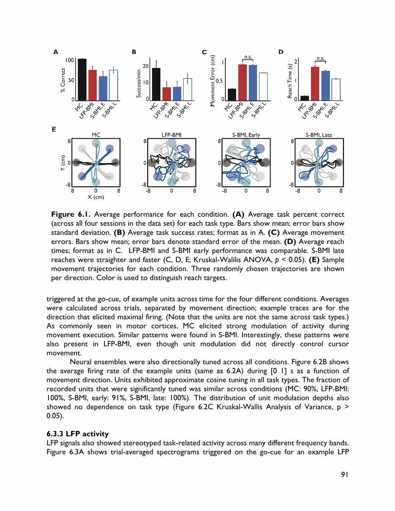
91  

Figure 6.1. Average performance for each condition. (A) Average task percent correct (across all four sessions in the data set) for each task type. Bars show mean; error bars show standard deviation. (B) Average task success rates; format as in A. (C) Average movement errors. Bars show mean; error bars denote standard error of the mean. (D) Average reach times; format as in C. LFP-BMI and S-BMI early performance was comparable. S-BMI late reaches were straighter and faster (C, D, E; Kruskal-Walilis ANOVA, p < 0.05). (E) Sample movement trajectories for each condition. Three randomly chosen trajectories are shown per direction. Color is used to distinguish reach targets.

triggered at the go-cue, of example units across time for the four different conditions. Averages were calculated across trials, separated by movement direction; example traces are for the direction that elicited maximal firing. (Note that the units are not the same across task types.) As commonly seen in motor cortices, MC elicited strong modulation of activity during movement execution. Similar patterns were found in S-BMI. Interestingly, these patterns were also present in LFP-BMI, even though unit modulation did not directly control cursor movement.

Neural ensembles were also directionally tuned across all conditions. Figure 6.2B shows the average firing rate of the example units (same as 6.2A) during [0 1] s as a function of movement direction. Units exhibited approximate cosine tuning in all task types. The fraction of recorded units that were significantly tuned was similar across conditions (MC: 90%, LFP-BMI: 100%, S-BMI, early: 91%, S-BMI, late: 100%). The distribution of unit modulation depths also showed no dependence on task type (Figure 6.2C Kruskal-Wallis Analysis of Variance, p > 0.05).   6.3.3 LFP activity LFP signals also showed stereotyped task-related activity across many different frequency bands. Figure 6.3A shows trial-averaged spectrograms triggered on the go-cue for an example LFP

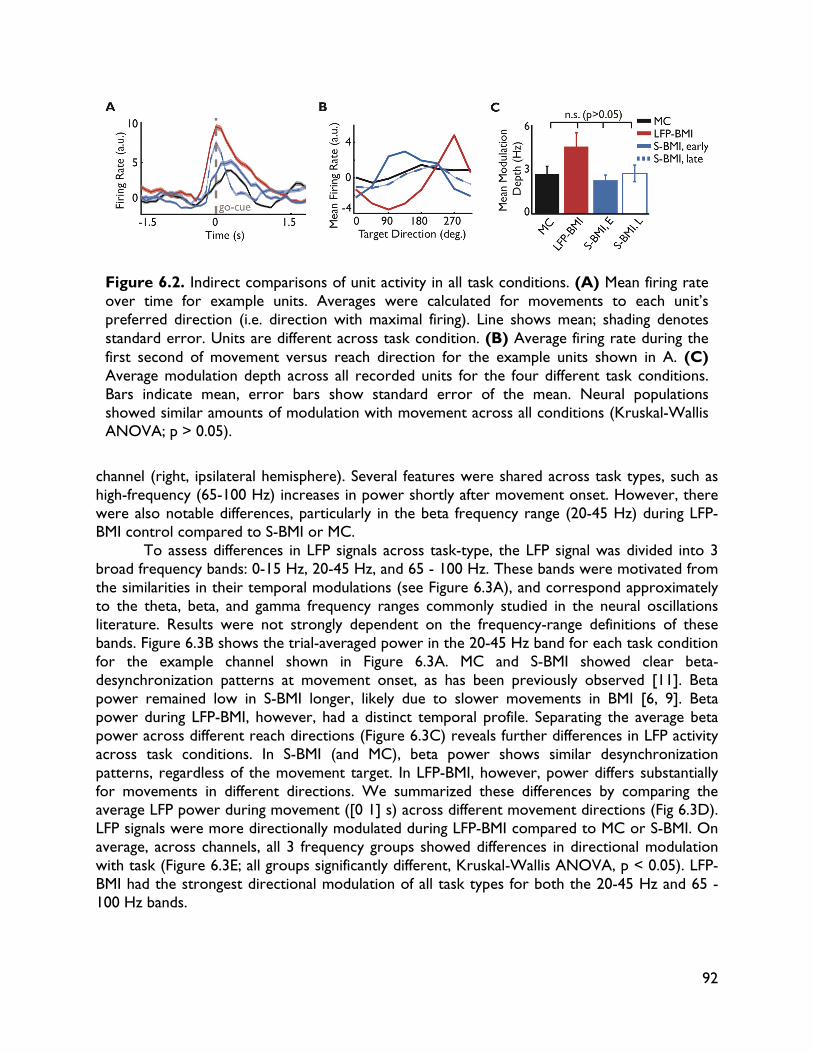
92  

Figure 6.2. Indirect comparisons of unit activity in all task conditions. (A) Mean firing rate over time for example units. Averages were calculated for movements to each unit’s preferred direction (i.e. direction with maximal firing). Line shows mean; shading denotes standard error. Units are different across task condition. (B) Average firing rate during the first second of movement versus reach direction for the example units shown in A. (C) Average modulation depth across all recorded units for the four different task conditions. Bars indicate mean, error bars show standard error of the mean. Neural populations showed similar amounts of modulation with movement across all conditions (Kruskal-Wallis ANOVA; p > 0.05).

channel (right, ipsilateral hemisphere). Several features were shared across task types, such as high-frequency (65-100 Hz) increases in power shortly after movement onset. However, there were also notable differences, particularly in the beta frequency range (20-45 Hz) during LFP-BMI control compared to S-BMI or MC.

To assess differences in LFP signals across task-type, the LFP signal was divided into 3 broad frequency bands: 0-15 Hz, 20-45 Hz, and 65 - 100 Hz. These bands were motivated from the similarities in their temporal modulations (see Figure 6.3A), and correspond approximately to the theta, beta, and gamma frequency ranges commonly studied in the neural oscillations literature. Results were not strongly dependent on the frequency-range definitions of these bands. Figure 6.3B shows the trial-averaged power in the 20-45 Hz band for each task condition for the example channel shown in Figure 6.3A. MC and S-BMI showed clear beta-desynchronization patterns at movement onset, as has been previously observed [11]. Beta power remained low in S-BMI longer, likely due to slower movements in BMI [6, 9]. Beta power during LFP-BMI, however, had a distinct temporal profile. Separating the average beta power across different reach directions (Figure 6.3C) reveals further differences in LFP activity across task conditions. In S-BMI (and MC), beta power shows similar desynchronization patterns, regardless of the movement target. In LFP-BMI, however, power differs substantially for movements in different directions. We summarized these differences by comparing the average LFP power during movement ([0 1] s) across different movement directions (Fig 6.3D). LFP signals were more directionally modulated during LFP-BMI compared to MC or S-BMI. On average, across channels, all 3 frequency groups showed differences in directional modulation with task (Figure 6.3E; all groups significantly different, Kruskal-Wallis ANOVA, p < 0.05). LFP-BMI had the strongest directional modulation of all task types for both the 20-45 Hz and 65 - 100 Hz bands.

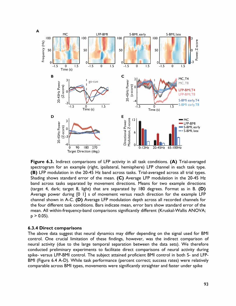
93  

Figure 6.3. Indirect comparisons of LFP activity in all task conditions. (A) Trial-averaged spectrogram for an example (right, ipsilateral, hemisphere) LFP channel in each task type. (B) LFP modulation in the 20-45 Hz band across tasks. Trial-averaged across all trial types. Shading shows standard error of the mean. (C) Average LFP modulation in the 20-45 Hz band across tasks separated by movement directions. Means for two example directions (target 4, dark; target 8, light) that are separated by 180 degrees. Format as in B. (D) Average power during [0 1] s of movement versus reach direction for the example LFP channel shown in A-C. (D) Average LFP modulation depth across all recorded channels for the four different task conditions. Bars indicate mean, error bars show standard error of the mean. All within-frequency-band comparisons significantly different (Kruskal-Wallis ANOVA; p > 0.05).

6.3.4 Direct comparisons The above data suggest that neural dynamics may differ depending on the signal used for BMI control. One crucial limitation of these findings, however, was the indirect comparison of neural activity (due to the large temporal separation between the data sets). We therefore conducted preliminary experiments to facilitate direct comparisons of neural activity during spike- versus LFP-BMI control. The subject attained proficient BMI control in both S- and LFP-BMI (Figure 6.4 A-D). While task performance (percent correct; success rates) were relatively comparable across BMI types, movements were significantly straighter and faster under spike

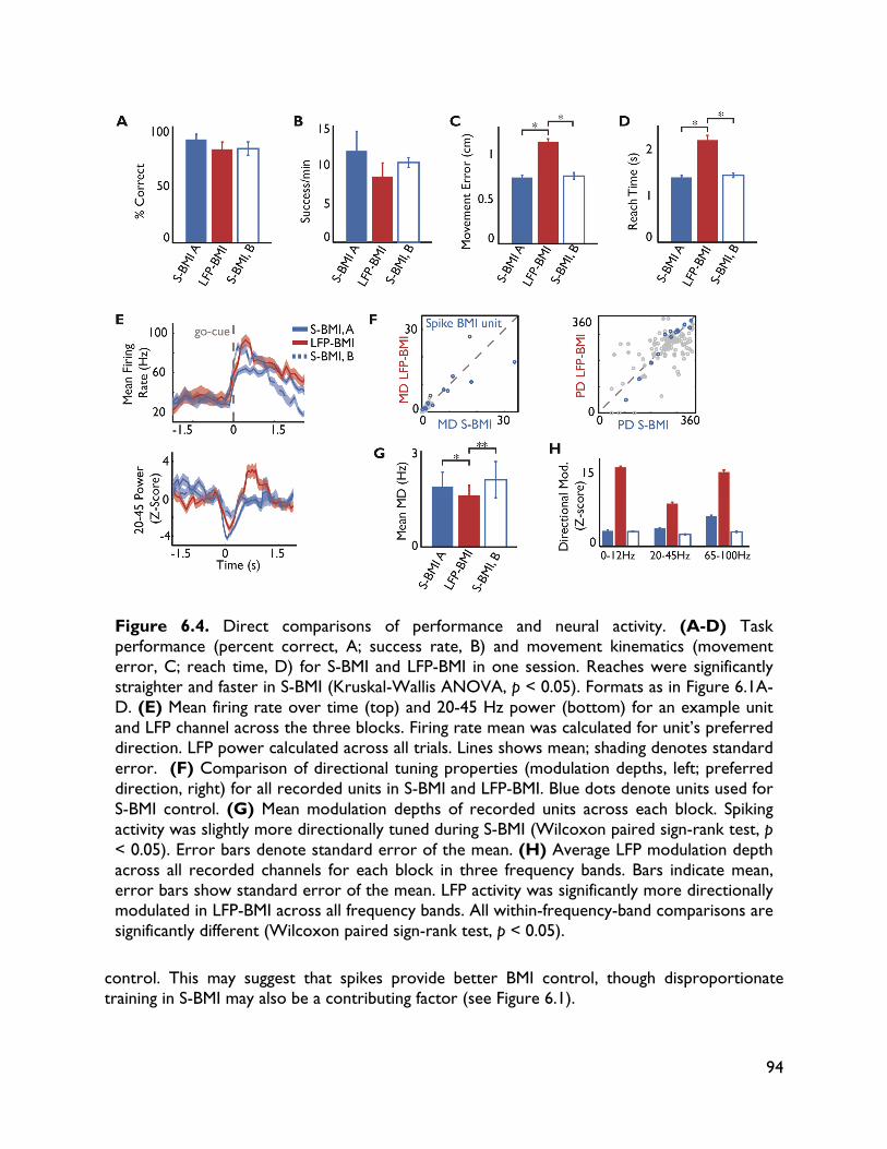
94  

Figure 6.4. Direct comparisons of performance and neural activity. (A-D) Task performance (percent correct, A; success rate, B) and movement kinematics (movement error, C; reach time, D) for S-BMI and LFP-BMI in one session. Reaches were significantly straighter and faster in S-BMI (Kruskal-Wallis ANOVA, p < 0.05). Formats as in Figure 6.1A-D. (E) Mean firing rate over time (top) and 20-45 Hz power (bottom) for an example unit and LFP channel across the three blocks. Firing rate mean was calculated for unit’s preferred direction. LFP power calculated across all trials. Lines shows mean; shading denotes standard error. (F) Comparison of directional tuning properties (modulation depths, left; preferred direction, right) for all recorded units in S-BMI and LFP-BMI. Blue dots denote units used for S-BMI control. (G) Mean modulation depths of recorded units across each block. Spiking activity was slightly more directionally tuned during S-BMI (Wilcoxon paired sign-rank test, p < 0.05). Error bars denote standard error of the mean. (H) Average LFP modulation depth across all recorded channels for each block in three frequency bands. Bars indicate mean, error bars show standard error of the mean. LFP activity was significantly more directionally modulated in LFP-BMI across all frequency bands. All within-frequency-band comparisons are significantly different (Wilcoxon paired sign-rank test, p < 0.05).

control. This may suggest that spikes provide better BMI control, though disproportionate training in S-BMI may also be a contributing factor (see Figure 6.1).

95  

Direct comparisons of spiking and LFP activity reveal similar trends to those found in our indirect analyses. Spiking activity was remarkably similar across S- and LFP-BMI (Figure 6.4 E-G). Individual units had similar directional tuning properties in both conditions (Figure 6.4 E-F). At the population level, units were slightly more directionally modulated in S-BMI (Figure 6.4 G; Wilcoxon paired sign-rank test, p < 0.05). Yet, LFP activity showed notable differences across BMI control types (Figure 6.5 E, H). Across all frequency bands and channels, LFP was significantly more directionally modulated when BMI control was driven by LFP (Figure 6.5 H). Interestingly, the subject readily switched between these strategies with block changes even without overt cues as to the control signal type. 6.4 Discussion Comparison of spiking and LFP activity during BMI paradigms controlled with either signal revealed clear task-modulations in both signal types in all tasks. That is, LFP and spiking signals were strongly modulated in BMI, even when they were not being directly used as a control signal. However, there were differences in the patterns of task-relevant activity based on the control signal used for BMI. The subject modulated LFP signals in a more direction-specific way during LFP-BMI compared to S-BMI or MC. In contrast, LFP signals during spike-based BMI were less directionally modulated, and showed clear temporal similarities to that of natural arm movements (Figures 6.3 and 6.4). Interestingly, unit activity during LFP-BMI showed similar amounts of directional tuning as in spike-based BMI. Direct comparisons also suggest that spiking activity was remarkably similar between different task conditions despite differences in LFP power modulations (Figure 6.4).

The task-relevant modulations in both LFP and spiking activity across both types of BMI also suggest a link between these signals. Previous research showed changes in neural synchrony with operant conditioning of LFP activity (Engelhard et al., 2013). We similarly find clear task-modulation of unit firing during LFP-based BMI control and vice-versa. Co-modulation of spike and LFP activity could suggest promising applications for BMIs that utilize multiple neural signals (Hwang and Andersen, 2009; Ranade et al., 2009). Our results also show that that the control signal used in a BMI may significantly influence neural dynamics. These findings are particularly interesting, given that these data were generated using a decoder adaptation paradigm. CLDA could obviate the need for subject modifications of behavior or strategy, since the decoder adapts to the subject. Yet we still found clear differences in LFP modulations across BMI tasks. These differences are even present when the subject switches between S- and LFP-BMI control within a day and is not cued as to the control signal type (Figure 6.4).

Further analyses and experiments are needed to better understand how these dynamics are influenced by the decoder properties and learning. For instance, we found significant directional modulation of LFP signals in the 0 – 12 Hz and 20-45 Hz ranges, though these bands were not used as decoder inputs. We also saw decreased LFP directional modulation in S-BMI after significant training (Figure 6.3, S-BMI early vs. late). BMI performance also improved significantly between the early and late BMI data sets (Figure 6.1). Changes in LFP modulation might reflect learning and increased selective modulation of spiking, though additional studies are needed to rule out other possible explanations (e.g. decoder differences, recording shifts). Similarly, it will be important to explore spike modulation with prolonged LFP-BMI training. If

96  

and how neural dynamics depend on the BMI decoded signal and training may also shed light on the mechanisms by which subjects modulate neural signals.

Future work and analyses are needed to explore how subjects might produce differential LFP activity with similar spiking (Figure 6.4). LFP is thought to primarily reflect dendritic activity near the recording electrode, and therefore best captures inputs to a cortical area (Pesaran, 2009; Buzáki et al., 2012). The different patterns of LFP across BMI conditions, then, may involve changes in upstream areas during LFP control. That is, rather than directly modulating activity in the primary motor cortices being recorded, subjects might control LFP-BMIs by modulating connecting areas (e.g. pre-motor and/or pre-frontal cortices). However, this hypothesis does not necessarily explain the similarity in spiking activity between LFP-BMI and S-BMI. Changes in inputs to the control area would likely produce differential patterns of outputs (i.e. spikes). An alternate possibility is that subjects control the LFP by changing patterns of neural synchrony within the control area (Buzáki et al., 2012). Recording from upstream areas during BMI, and analyzing within- and across-area correlations will be critical for understanding neural dynamics underlying BMI control.

This study highlights the complexity of neural dynamics in closed-loop BMI. Neuron action-potentials and local field potentials are both modulated during BMI, regardless of the signal being used for control. Their specific dynamics, however, may depend on the control signal. This suggests that multiple neural signals may be useful for neural prostheses, and that neural dynamics may be shaped by real-time feedback and learning in closed-loop settings. Further study of neural dynamics will help elucidate their dependence on control signal type, and the mechanisms underlying their volitional control.

97  

Chapter 7:

Exploring alternative control signals: local field potentials vary with movement dynamics BMIs to date have focused primarily on kinematic control. Indeed, the BMI work presented in this thesis (Chapters 2-6) focused on BMIs that control the position and velocity of a virtual cursor. Pure motion control, however, is unlikely to be sufficient for real-world neuroprostheses that will operate in dynamic environments and interact with objects. Forces and torques play a critical role in these interactions. Dynamic properties of the BMI system have also been shown to influence performance (Carmena et al., 2003; Taylor et al., 2003), even in virtual cursors (Gowda et al., 2012; see Section 1.3.3). Providing control of movement dynamics, then, may be essential as BMIs transition from virtual to physical. Little is known about how the central nervous system (CNS) controls movement dynamics. The natural motor system is highly distributed, with control shared across the spinal cord, the cerebellum, and a host of cortical and sub-cortical areas (Riehle and Vaadia, 2004). As reviewed below, limb dynamics have been closely linked to spinal-level control mediated through reflexes. However, psychophysical evidence suggests that humans can volitionally control limb dynamic properties based on the environmental dynamics. This suggests that cortical areas, typically thought to be involved in higher-level processing of movement goals, might also contribute to the control of movement dynamics. This has yet to be explored at the neurophysiological level. In this chapter, we explore how neural activity in the primary and pre-motor cortices varies with natural limb movements in different dynamic environments. One key goal of this study is to assess whether cortical areas are involved in the direct control of limb dynamics. This will be important for understanding how to incorporate dynamics control into BMIs. While we advocate for a “non-biomimetic,” closed-loop approach to BMIs (see Chapter 1), insights into the natural CNS function may still be highly informative for the design of BMIs. For instance, suppose that movement dynamics like limb stiffness are controlled entirely at the spinal level, and cortical areas have little involvement. Subjects might be able to learn to operate a cortically-driven BMI that uses stiffness as a control signal with practice via biofeedback. But learning might be faster and easier in a BMI that better mimicked the distributed control of the natural CNS (e.g. that used cortical activity to control kinematics, and has “spine-like” mechanism for dynamics control within the decoder or plant). As BMIs scale-up in control complexity (degrees of freedom, kinematic and dynamic control), deeper understanding of the natural motor system will inform the design of BMI system architectures to be explored in closed-loop. This work was done in collaboration with Jose M. Carmena. 7.1 Introduction Our central nervous system (CNS) overcomes feedback delays and unpredictability in the external environment to dexterously maneuver our limbs. Our movements are controlled at

98  

many levels, from the limb biomechanics, to the spinal cord, and a host of cortical areas. Understanding each level’s role and how they combine to produce goal-directed movements is a fundamental question of motor control research. Insight into these control principles is also essential to restoring natural movements to patients with neurological motor deficits.

Research suggests that control of the mechanical impedance (inertia, damping, stiffness) of the upper-limb plays an important role in executing skilled movements. Limb impedance, which describes the limb’s behavior when interacting with the environment, involves the interplay of all levels of the motor system. Impedance is, by definition, a mechanical property of the limb and dependents on posture and muscle biomechanics (Hogan, 1985; Mussa-Ivaldi et al., 1985; Milner 2002; Damm and McIntyre, 2008). Limb stiffness, in particular, can also be modulated by the CNS through co-activation of agonist-antagonist muscle pairs (Hogan, 1985). Because it involves co-contraction, stiffness can be changed without influencing movement kinematics. You can drink your morning coffee with a relaxed or stiff arm. How you bring the cup to your mouth will be the same; the difference is that if someone bumps into you, you either spill coffee on yourself or stay dry. These properties make stiffness both a likely control variable for the CNS and an interesting property for motor control research.

Psychophysical studies show that limb stiffness is, indeed, modulated by the CNS in a task-specific manner using a combination of biomechanical and neural substrates. Humans increase their upper-limb stiffness for tasks requiring increased accuracy (Gribble et al., 2003; Selen et al., 2006; Lametti et al., 2007; Wong et al., 2009), movements in unstable (Burdet et al., 2001; Franklin et al., 2007) and stable (Darainy and Ostry, 2008) novel environments, and while first learning new dynamic environments (Osu et al., 2002; Franklin et al., 2003). What’s more, stiffness is optimized to task requirements (Burdet et al., 2001; Franklin et al., 2007; Lametti et al., 2007; Wong et al., 2009). These stiffness modulations are accompanied by changes in spinal reflex loop gains (Lacquaniti et al., 1991; Liaw et al., 2007; Damm and McIntyre et al., 2008; Krutky et al., 2008; Perreault et al., 2008) and co-contraction (Mussa-Ivaldi et al., 1985; McIntyre et al., 1996; Gribble and Ostry, 1999; Osu et al., 2002; Franklin et al., 2003; Gribble et al., 2003). Given the many observations of task-specific stiffness modulation, we hypothesize that it is a task-relevant variable controlled by the CNS to achieve stable and accurate movements.

While clear mechanisms for stiffness modulation have been identified and well classified, the question of how they combine to achieve control remains unaddressed. In particular, the role of cortical areas, such as primary motor cortex (M1) and dorsal premotor cortex (PMd) is a key question that has received little attention in motor neurophysiology. Representations of movement in motor cortices are a topic of significant debate (Shenoy et al., 2013). Cortical involvement in stiffness control could take several different forms. Spiking activity in M1 and PMd activity shows strong correlation to both muscle activation (including individual muscle activity (Fetz and Cheney, 1980; Bennett and Lemon, 1994; Morrow and Miller, 2003), muscle synergies (Holdefer and Miller, 2002) and co-contraction of antagonist muscle pairs (Humphrey and Reed, 1983)), and abstract movement variables like hand position (Georgopoulos et al., 1986) and velocity (Schwartz et al., 1994; Moran and Schwartz, 1999). Hence, if limb stiffness is represented in motor cortex, these representations might take muscle recruitment-based or more abstract movement-independent forms. In this study, we explore local field potential activity in M1 and PMd during movements in an unstable force-field shown to evoke changes in limb stiffness in humans (Burdet et al., 2001). The relationship between LFP activity and behavior are poorly understood. Neurons in

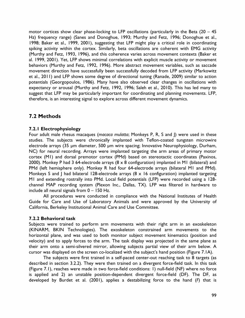
99  

motor cortices show clear phase-locking to LFP oscillations (particularly in the Beta (20 – 45 Hz) frequency range) (Sanes and Donoghue, 1993; Murthy and Fetz, 1996; Donoghue et al., 1998; Baker et al., 1999, 2001), suggesting that LFP might play a critical role in coordinating spiking activity within the cortex. Similarly, beta oscillations are coherent with EMG activity (Murthy and Fetz, 1993, 1996), and this coherence varies across movement contexts (Baker et al. 1999, 2001). Yet, LFP shows minimal correlations with explicit muscle activity or movement behaviors (Murthy and Fetz, 1992, 1996). More abstract movement variables, such as saccade movement direction have successfully been successfully decoded from LFP activity (Markowitz et al., 2011) and LFP shows some degree of directional tuning (Ranade, 2009) similar to action potentials (Georgopoulos, 1986). Many have also observed clear changes in oscillations with expectancy or arousal (Murthy and Fetz, 1992, 1996; Saleh et al., 2010). This has led many to suggest that LFP may be particularly important for coordinating and planning movements. LFP, therefore, is an interesting signal to explore across different movement dynamics. 7.2 Methods 7.2.1 Electrophysiology Four adult male rhesus macaques (macaca mulatta; Monkeys P, R, S and J) were used in these studies. The subjects were chronically implanted with Teflon-coated tungsten microwire electrode arrays (35 μm diameter, 500 μm wire spacing; Innovative Neurophysiology, Durham, NC) for neural recording. Arrays were implanted targeting the arm areas of primary motor cortex (M1) and dorsal premotor cortex (PMd) based on stereotactic coordinates (Paxinos, 2000). Monkey P had 3 64-electrode arrays (8 x 8 configuration) implanted in M1 (bilateral) and PMd (left hemisphere only). Monkey R had four 64-electrode arrays (bilateral M1 and PMd). Monkeys S and J had bilateral 128-electrode arrays (8 x 16 configuration) implanted targeting M1 and extending rostrally into PMd. Local field potentials (LFP) were recorded using a 128-channel MAP recording system (Plexon Inc., Dallas, TX). LFP was filtered in hardware to include all neural signals from 0 – 150 Hz.

All procedures were conducted in compliance with the National Institutes of Health Guide for Care and Use of Laboratory Animals and were approved by the University of California, Berkeley Institutional Animal Care and Use Committee. 7.2.2 Behavioral task Subjects were trained to perform arm movements with their right arm in an exoskeleton (KINARM, BKIN Technologies). The exoskeleton constrained arm movements to the horizontal plane, and was used to both monitor subject movement kinematics (position and velocity) and to apply forces to the arm. The task display was projected in the same plane as their arm onto a semi-silvered mirror, allowing subjects partial view of their arm below. A cursor was displayed on the screen co-localized with the subject’s hand position (Figure 7.1A). The subjects were first trained in a self-paced center-out reaching task to 8 targets (as described in section 3.2.2). They were then trained on a divergent force-field task. In this task (Figure 7.1), reaches were made in two force-field conditions: 1) null-field (NF) where no force is applied and 2) an unstable position-dependent divergent force-field (DF). The DF, as developed by Burdet et al. (2001), applies a destabilizing force to the hand (F) that is

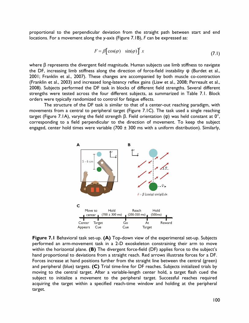
100  

proportional to the perpendicular deviation from the straight path between start and end locations. For a movement along the y-axis (Figure 7.1B), F can be expressed as:

F cos( ) sin() T x (7.1) where β represents the divergent field magnitude. Human subjects use limb stiffness to navigate the DF, increasing limb stiffness along the direction of force-field instability φ (Burdet et al., 2001; Franklin et al., 2007). These changes are accompanied by both muscle co-contraction (Franklin et al., 2003) and increased long-latency reflex gains (Liaw et al., 2008; Perreault et al., 2008). Subjects performed the DF task in blocks of different field strengths. Several different strengths were tested across the four different subjects, as summarized in Table 7.1. Block orders were typically randomized to control for fatigue effects. The structure of the DF task is similar to that of a center-out reaching paradigm, with movements from a central to peripheral target (Figure 7.1C). The task used a single reaching target (Figure 7.1A), varying the field strength β. Field orientation (φ) was held constant at 0°, corresponding to a field perpendicular to the direction of movement. To keep the subject engaged, center hold times were variable (700 ± 300 ms with a uniform distribution). Similarly,

  

Figure 7.1 Behavioral task set-up. (A) Top-down view of the experimental set-up. Subjects performed an arm-movement task in a 2-D exoskeleton constraining their arm to move within the horizontal plane. (B) The divergent force-field (DF) applies force to the subject’s hand proportional to deviations from a straight reach. Red arrows illustrate forces for a DF. Forces increase at hand positions further from the straight line between the central (green) and peripheral (blue) targets. (C) Trial time-line for DF reaches. Subjects initialized trials by moving to the central target. After a variable-length center hold, a target flash cued the subject to initialize a movement to the peripheral target. Successful reaches required acquiring the target within a specified reach-time window and holding at the peripheral target.

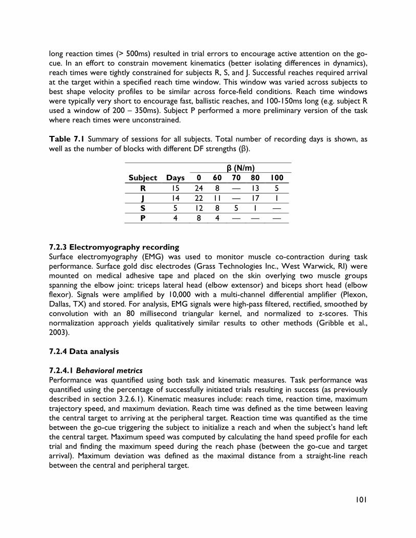
101  

long reaction times (> 500ms) resulted in trial errors to encourage active attention on the go-cue. In an effort to constrain movement kinematics (better isolating differences in dynamics), reach times were tightly constrained for subjects R, S, and J. Successful reaches required arrival at the target within a specified reach time window. This window was varied across subjects to best shape velocity profiles to be similar across force-field conditions. Reach time windows were typically very short to encourage fast, ballistic reaches, and 100-150ms long (e.g. subject R used a window of 200 – 350ms). Subject P performed a more preliminary version of the task where reach times were unconstrained. Table 7.1 Summary of sessions for all subjects. Total number of recording days is shown, as well as the number of blocks with different DF strengths (β).

Subject Days β (N/m)

0 60 70 80 100R 15 24 8 — 13 5 J 14 22 11 — 17 1 S 5 12 8 5 1 — P 4 8 4 — — —

7.2.3 Electromyography recording Surface electromyography (EMG) was used to monitor muscle co-contraction during task performance. Surface gold disc electrodes (Grass Technologies Inc., West Warwick, RI) were mounted on medical adhesive tape and placed on the skin overlying two muscle groups spanning the elbow joint: triceps lateral head (elbow extensor) and biceps short head (elbow flexor). Signals were amplified by 10,000 with a multi-channel differential amplifier (Plexon, Dallas, TX) and stored. For analysis, EMG signals were high-pass filtered, rectified, smoothed by convolution with an 80 millisecond triangular kernel, and normalized to z-scores. This normalization approach yields qualitatively similar results to other methods (Gribble et al., 2003). 7.2.4 Data analysis 7.2.4.1 Behavioral metrics Performance was quantified using both task and kinematic measures. Task performance was quantified using the percentage of successfully initiated trials resulting in success (as previously described in section 3.2.6.1). Kinematic measures include: reach time, reaction time, maximum trajectory speed, and maximum deviation. Reach time was defined as the time between leaving the central target to arriving at the peripheral target. Reaction time was quantified as the time between the go-cue triggering the subject to initialize a reach and when the subject’s hand left the central target. Maximum speed was computed by calculating the hand speed profile for each trial and finding the maximum speed during the reach phase (between the go-cue and target arrival). Maximum deviation was defined as the maximal distance from a straight-line reach between the central and peripheral target.

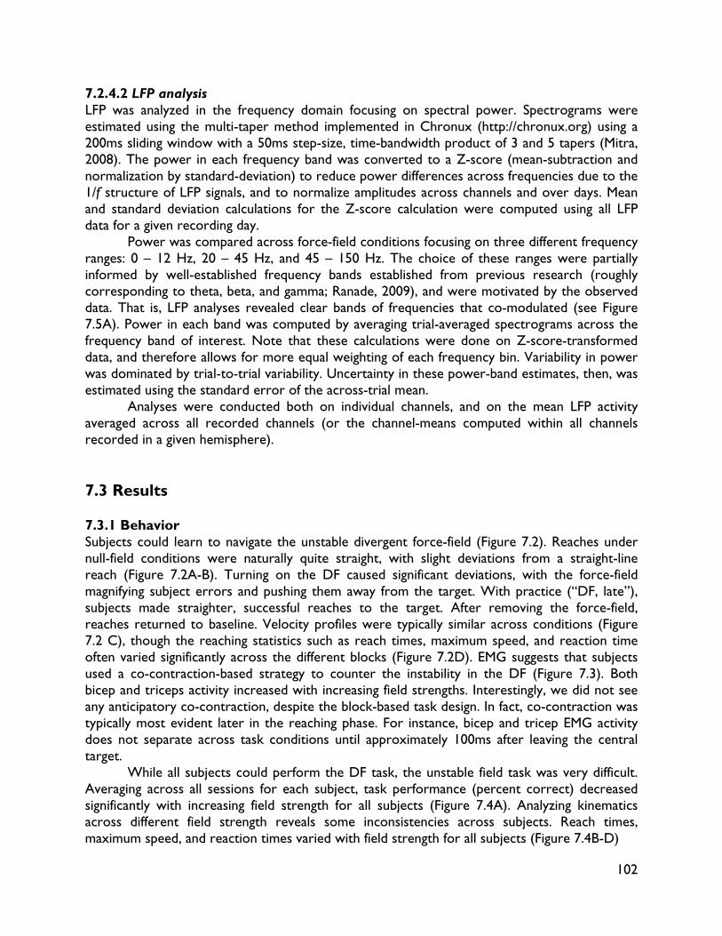
102  

7.2.4.2 LFP analysis LFP was analyzed in the frequency domain focusing on spectral power. Spectrograms were estimated using the multi-taper method implemented in Chronux (http://chronux.org) using a 200ms sliding window with a 50ms step-size, time-bandwidth product of 3 and 5 tapers (Mitra, 2008). The power in each frequency band was converted to a Z-score (mean-subtraction and normalization by standard-deviation) to reduce power differences across frequencies due to the 1/f structure of LFP signals, and to normalize amplitudes across channels and over days. Mean and standard deviation calculations for the Z-score calculation were computed using all LFP data for a given recording day. Power was compared across force-field conditions focusing on three different frequency ranges: 0 – 12 Hz, 20 – 45 Hz, and 45 – 150 Hz. The choice of these ranges were partially informed by well-established frequency bands established from previous research (roughly corresponding to theta, beta, and gamma; Ranade, 2009), and were motivated by the observed data. That is, LFP analyses revealed clear bands of frequencies that co-modulated (see Figure 7.5A). Power in each band was computed by averaging trial-averaged spectrograms across the frequency band of interest. Note that these calculations were done on Z-score-transformed data, and therefore allows for more equal weighting of each frequency bin. Variability in power was dominated by trial-to-trial variability. Uncertainty in these power-band estimates, then, was estimated using the standard error of the across-trial mean. Analyses were conducted both on individual channels, and on the mean LFP activity averaged across all recorded channels (or the channel-means computed within all channels recorded in a given hemisphere). 7.3 Results 7.3.1 Behavior Subjects could learn to navigate the unstable divergent force-field (Figure 7.2). Reaches under null-field conditions were naturally quite straight, with slight deviations from a straight-line reach (Figure 7.2A-B). Turning on the DF caused significant deviations, with the force-field magnifying subject errors and pushing them away from the target. With practice (“DF, late”), subjects made straighter, successful reaches to the target. After removing the force-field, reaches returned to baseline. Velocity profiles were typically similar across conditions (Figure 7.2 C), though the reaching statistics such as reach times, maximum speed, and reaction time often varied significantly across the different blocks (Figure 7.2D). EMG suggests that subjects used a co-contraction-based strategy to counter the instability in the DF (Figure 7.3). Both bicep and triceps activity increased with increasing field strengths. Interestingly, we did not see any anticipatory co-contraction, despite the block-based task design. In fact, co-contraction was typically most evident later in the reaching phase. For instance, bicep and tricep EMG activity does not separate across task conditions until approximately 100ms after leaving the central target. While all subjects could perform the DF task, the unstable field task was very difficult. Averaging across all sessions for each subject, task performance (percent correct) decreased significantly with increasing field strength for all subjects (Figure 7.4A). Analyzing kinematics across different field strength reveals some inconsistencies across subjects. Reach times, maximum speed, and reaction times varied with field strength for all subjects (Figure 7.4B-D)

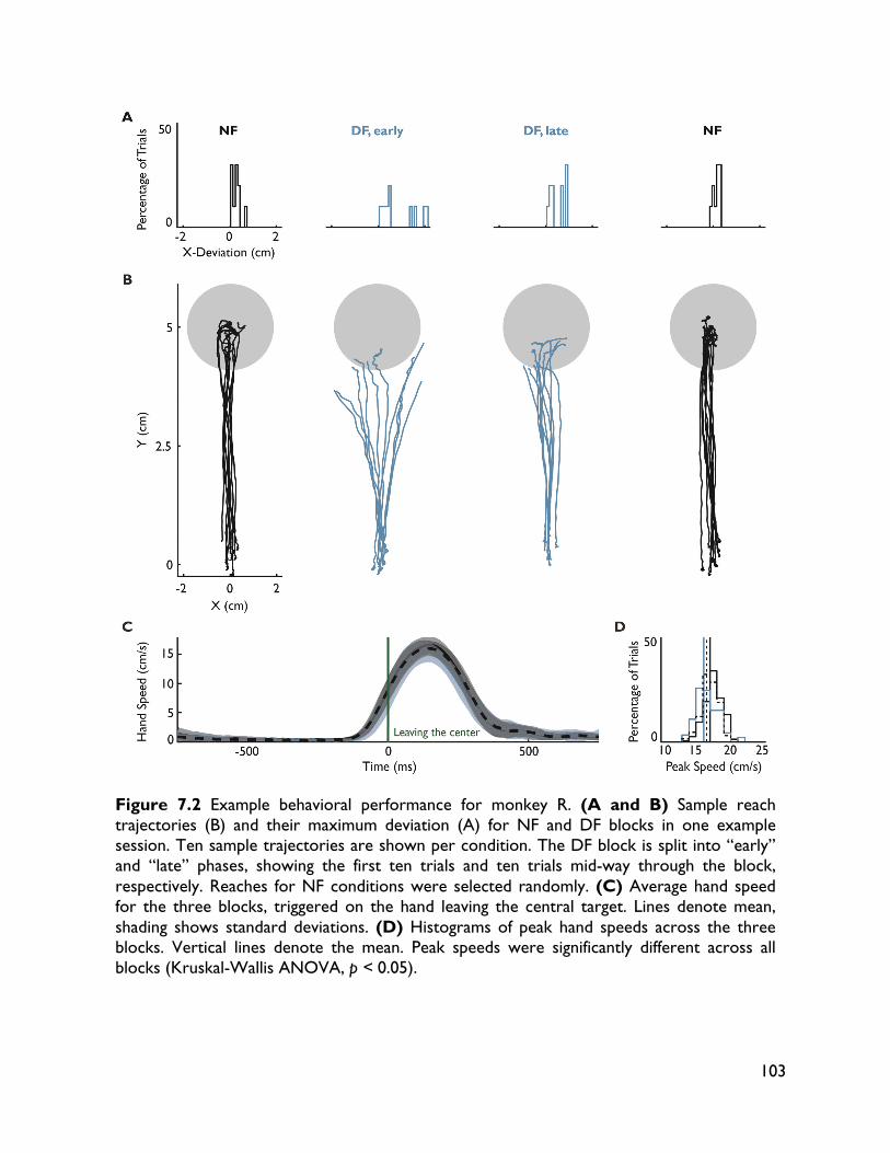
103  

  

Figure 7.2 Example behavioral performance for monkey R. (A and B) Sample reach trajectories (B) and their maximum deviation (A) for NF and DF blocks in one example session. Ten sample trajectories are shown per condition. The DF block is split into “early” and “late” phases, showing the first ten trials and ten trials mid-way through the block, respectively. Reaches for NF conditions were selected randomly. (C) Average hand speed for the three blocks, triggered on the hand leaving the central target. Lines denote mean, shading shows standard deviations. (D) Histograms of peak hand speeds across the three blocks. Vertical lines denote the mean. Peak speeds were significantly different across all blocks (Kruskal-Wallis ANOVA, p < 0.05).

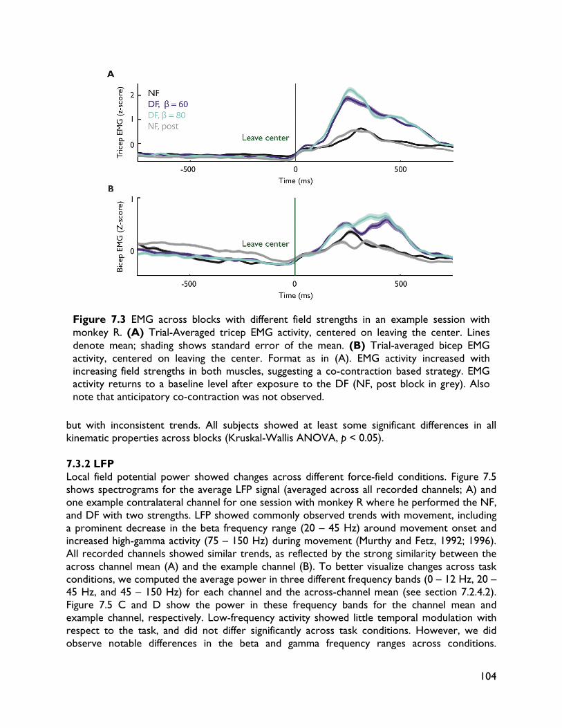
104  

but with inconsistent trends. All subjects showed at least some significant differences in all kinematic properties across blocks (Kruskal-Wallis ANOVA, p < 0.05). 7.3.2 LFP Local field potential power showed changes across different force-field conditions. Figure 7.5 shows spectrograms for the average LFP signal (averaged across all recorded channels; A) and one example contralateral channel for one session with monkey R where he performed the NF, and DF with two strengths. LFP showed commonly observed trends with movement, including a prominent decrease in the beta frequency range (20 – 45 Hz) around movement onset and increased high-gamma activity (75 – 150 Hz) during movement (Murthy and Fetz, 1992; 1996). All recorded channels showed similar trends, as reflected by the strong similarity between the across channel mean (A) and the example channel (B). To better visualize changes across task conditions, we computed the average power in three different frequency bands (0 – 12 Hz, 20 – 45 Hz, and 45 – 150 Hz) for each channel and the across-channel mean (see section 7.2.4.2). Figure 7.5 C and D show the power in these frequency bands for the channel mean and example channel, respectively. Low-frequency activity showed little temporal modulation with respect to the task, and did not differ significantly across task conditions. However, we did observe notable differences in the beta and gamma frequency ranges across conditions.

  

Figure 7.3 EMG across blocks with different field strengths in an example session with monkey R. (A) Trial-Averaged tricep EMG activity, centered on leaving the center. Lines denote mean; shading shows standard error of the mean. (B) Trial-averaged bicep EMG activity, centered on leaving the center. Format as in (A). EMG activity increased with increasing field strengths in both muscles, suggesting a co-contraction based strategy. EMG activity returns to a baseline level after exposure to the DF (NF, post block in grey). Also note that anticipatory co-contraction was not observed.

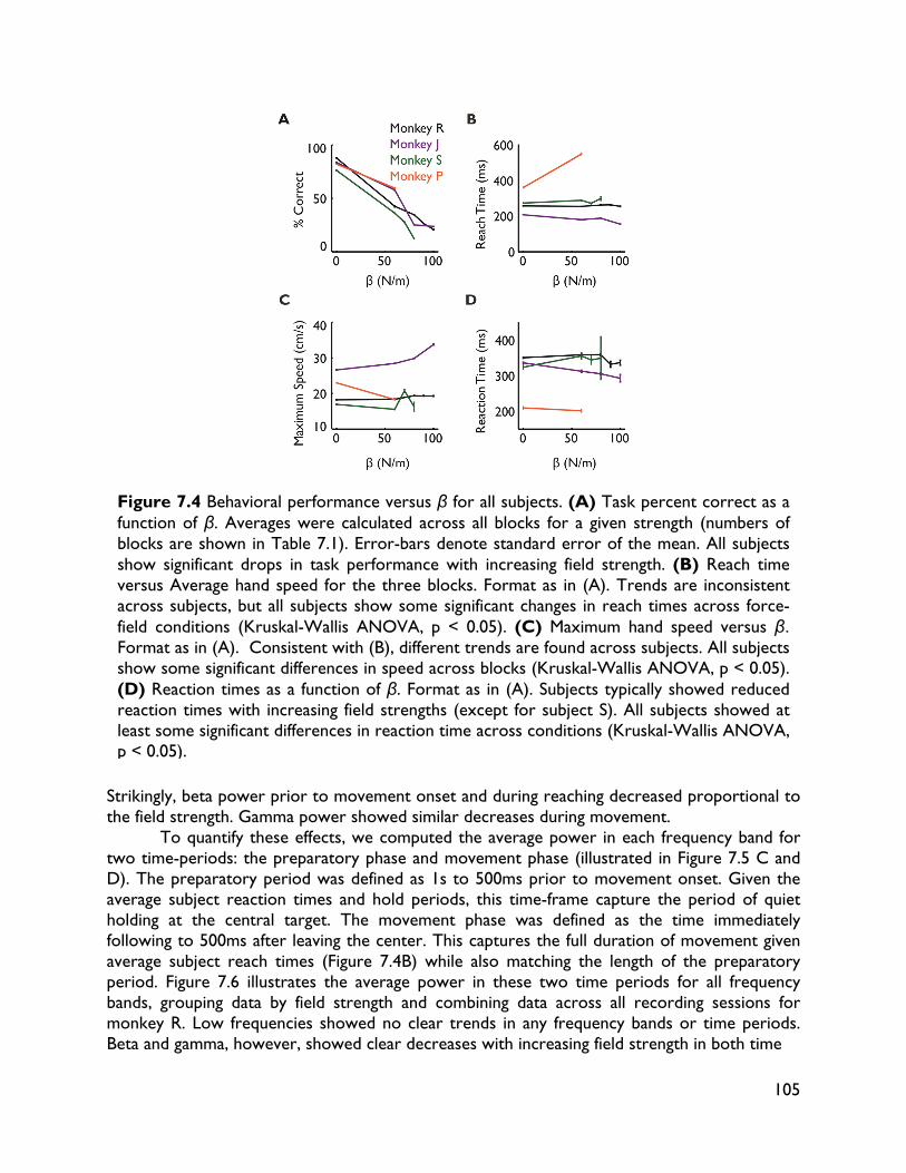
105  

Strikingly, beta power prior to movement onset and during reaching decreased proportional to the field strength. Gamma power showed similar decreases during movement. To quantify these effects, we computed the average power in each frequency band for two time-periods: the preparatory phase and movement phase (illustrated in Figure 7.5 C and D). The preparatory period was defined as 1s to 500ms prior to movement onset. Given the average subject reaction times and hold periods, this time-frame capture the period of quiet holding at the central target. The movement phase was defined as the time immediately following to 500ms after leaving the center. This captures the full duration of movement given average subject reach times (Figure 7.4B) while also matching the length of the preparatory period. Figure 7.6 illustrates the average power in these two time periods for all frequency bands, grouping data by field strength and combining data across all recording sessions for monkey R. Low frequencies showed no clear trends in any frequency bands or time periods. Beta and gamma, however, showed clear decreases with increasing field strength in both time

  

Figure 7.4 Behavioral performance versus β for all subjects. (A) Task percent correct as a function of β. Averages were calculated across all blocks for a given strength (numbers of blocks are shown in Table 7.1). Error-bars denote standard error of the mean. All subjects show significant drops in task performance with increasing field strength. (B) Reach time versus Average hand speed for the three blocks. Format as in (A). Trends are inconsistent across subjects, but all subjects show some significant changes in reach times across force-field conditions (Kruskal-Wallis ANOVA, p < 0.05). (C) Maximum hand speed versus β. Format as in (A). Consistent with (B), different trends are found across subjects. All subjects show some significant differences in speed across blocks (Kruskal-Wallis ANOVA, p < 0.05). (D) Reaction times as a function of β. Format as in (A). Subjects typically showed reduced reaction times with increasing field strengths (except for subject S). All subjects showed at least some significant differences in reaction time across conditions (Kruskal-Wallis ANOVA, p < 0.05).

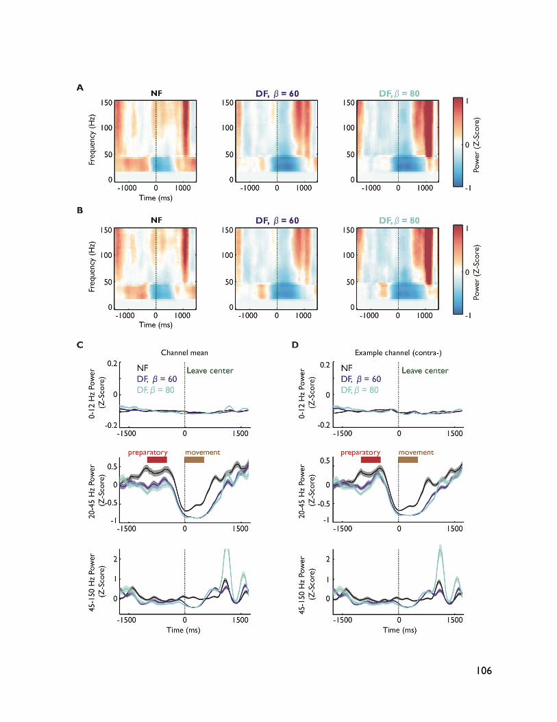
106  

 

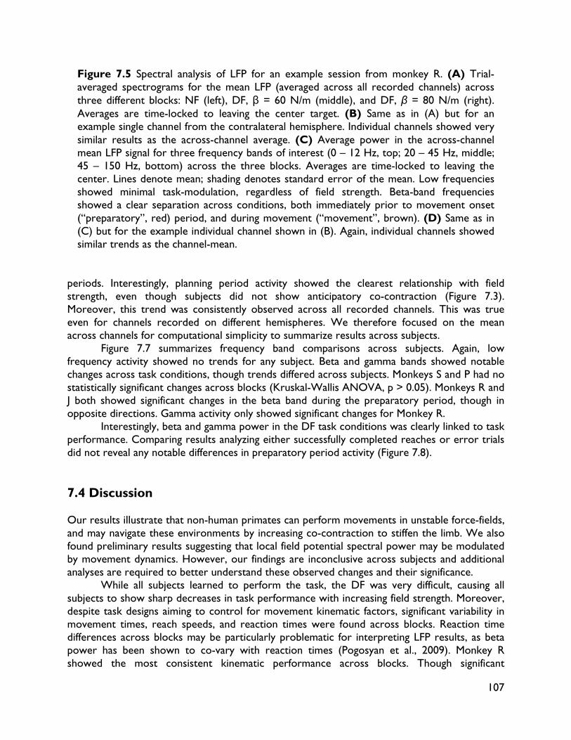
107  

Figure 7.5 Spectral analysis of LFP for an example session from monkey R. (A) Trial-averaged spectrograms for the mean LFP (averaged across all recorded channels) across three different blocks: NF (left), DF, β = 60 N/m (middle), and DF, β = 80 N/m (right). Averages are time-locked to leaving the center target. (B) Same as in (A) but for an example single channel from the contralateral hemisphere. Individual channels showed very similar results as the across-channel average. (C) Average power in the across-channel mean LFP signal for three frequency bands of interest (0 – 12 Hz, top; 20 – 45 Hz, middle; 45 – 150 Hz, bottom) across the three blocks. Averages are time-locked to leaving the center. Lines denote mean; shading denotes standard error of the mean. Low frequencies showed minimal task-modulation, regardless of field strength. Beta-band frequencies showed a clear separation across conditions, both immediately prior to movement onset (“preparatory”, red) period, and during movement (“movement”, brown). (D) Same as in (C) but for the example individual channel shown in (B). Again, individual channels showed similar trends as the channel-mean.

periods. Interestingly, planning period activity showed the clearest relationship with field strength, even though subjects did not show anticipatory co-contraction (Figure 7.3). Moreover, this trend was consistently observed across all recorded channels. This was true even for channels recorded on different hemispheres. We therefore focused on the mean across channels for computational simplicity to summarize results across subjects. Figure 7.7 summarizes frequency band comparisons across subjects. Again, low frequency activity showed no trends for any subject. Beta and gamma bands showed notable changes across task conditions, though trends differed across subjects. Monkeys S and P had no statistically significant changes across blocks (Kruskal-Wallis ANOVA, p > 0.05). Monkeys R and J both showed significant changes in the beta band during the preparatory period, though in opposite directions. Gamma activity only showed significant changes for Monkey R. Interestingly, beta and gamma power in the DF task conditions was clearly linked to task performance. Comparing results analyzing either successfully completed reaches or error trials did not reveal any notable differences in preparatory period activity (Figure 7.8). 7.4 Discussion Our results illustrate that non-human primates can perform movements in unstable force-fields, and may navigate these environments by increasing co-contraction to stiffen the limb. We also found preliminary results suggesting that local field potential spectral power may be modulated by movement dynamics. However, our findings are inconclusive across subjects and additional analyses are required to better understand these observed changes and their significance. While all subjects learned to perform the task, the DF was very difficult, causing all subjects to show sharp decreases in task performance with increasing field strength. Moreover, despite task designs aiming to control for movement kinematic factors, significant variability in movement times, reach speeds, and reaction times were found across blocks. Reaction time differences across blocks may be particularly problematic for interpreting LFP results, as beta power has been shown to co-vary with reaction times (Pogosyan et al., 2009). Monkey R showed the most consistent kinematic performance across blocks. Though significant

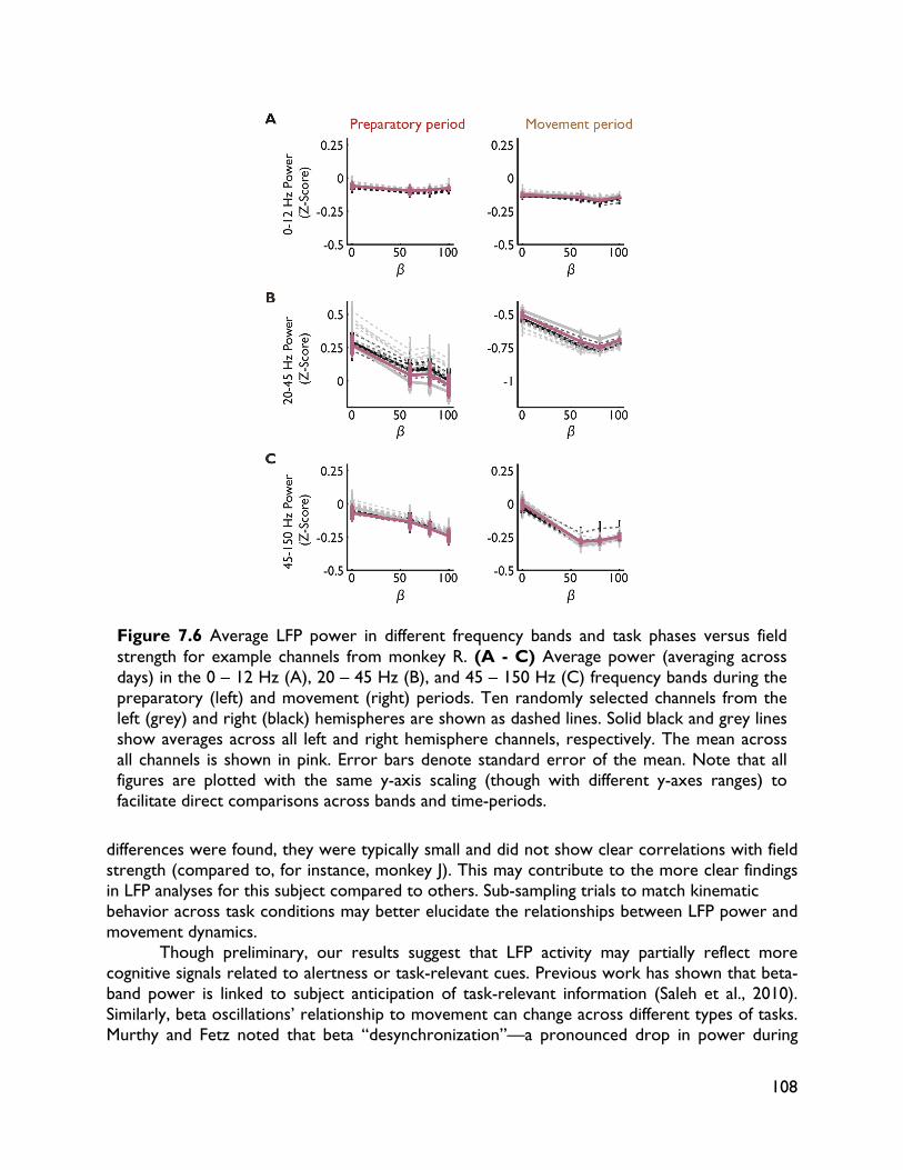
108  

differences were found, they were typically small and did not show clear correlations with field strength (compared to, for instance, monkey J). This may contribute to the more clear findings in LFP analyses for this subject compared to others. Sub-sampling trials to match kinematic behavior across task conditions may better elucidate the relationships between LFP power and movement dynamics. Though preliminary, our results suggest that LFP activity may partially reflect more cognitive signals related to alertness or task-relevant cues. Previous work has shown that beta-band power is linked to subject anticipation of task-relevant information (Saleh et al., 2010). Similarly, beta oscillations’ relationship to movement can change across different types of tasks. Murthy and Fetz noted that beta “desynchronization”—a pronounced drop in power during

  

Figure 7.6 Average LFP power in different frequency bands and task phases versus field strength for example channels from monkey R. (A - C) Average power (averaging across days) in the 0 – 12 Hz (A), 20 – 45 Hz (B), and 45 – 150 Hz (C) frequency bands during the preparatory (left) and movement (right) periods. Ten randomly selected channels from the left (grey) and right (black) hemispheres are shown as dashed lines. Solid black and grey lines show averages across all left and right hemisphere channels, respectively. The mean across all channels is shown in pink. Error bars denote standard error of the mean. Note that all figures are plotted with the same y-axis scaling (though with different y-axes ranges) to facilitate direct comparisons across bands and time-periods.

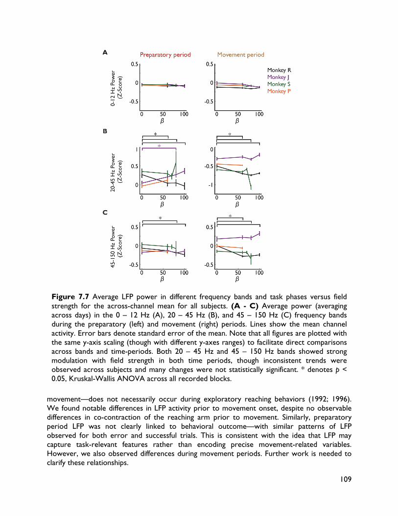
109  

movement—does not necessarily occur during exploratory reaching behaviors (1992; 1996). We found notable differences in LFP activity prior to movement onset, despite no observable differences in co-contraction of the reaching arm prior to movement. Similarly, preparatory period LFP was not clearly linked to behavioral outcome—with similar patterns of LFP observed for both error and successful trials. This is consistent with the idea that LFP may capture task-relevant features rather than encoding precise movement-related variables. However, we also observed differences during movement periods. Further work is needed to clarify these relationships.

  

Figure 7.7 Average LFP power in different frequency bands and task phases versus field strength for the across-channel mean for all subjects. (A - C) Average power (averaging across days) in the 0 – 12 Hz (A), 20 – 45 Hz (B), and 45 – 150 Hz (C) frequency bands during the preparatory (left) and movement (right) periods. Lines show the mean channel activity. Error bars denote standard error of the mean. Note that all figures are plotted with the same y-axis scaling (though with different y-axes ranges) to facilitate direct comparisons across bands and time-periods. Both 20 – 45 Hz and 45 – 150 Hz bands showed strong modulation with field strength in both time periods, though inconsistent trends were observed across subjects and many changes were not statistically significant. * denotes p < 0.05, Kruskal-Wallis ANOVA across all recorded blocks.

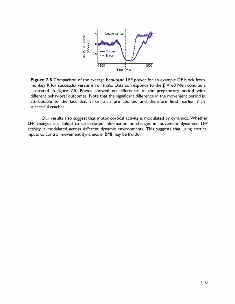
110  

Our results also suggest that motor cortical activity is modulated by dynamics. Whether LFP changes are linked to task-related information or changes in movement dynamics, LFP activity is modulated across different dynamic environments. This suggests that using cortical inputs to control movement dynamics in BMI may be fruitful.

  

Figure 7.8 Comparison of the average beta-band LFP power for an example DF block from monkey R for successful versus error trials. Data corresponds to the β = 60 N/m condition illustrated in figure 7.5. Power showed no differences in the preparatory period with different behavioral outcomes. Note that the significant difference in the movement period is attributable to the fact that error trials are aborted and therefore finish earlier than successful reaches.

111  

Chapter 8:

Conclusions and open questions Movement is fundamental to our daily lives. Whether communicating ideas or interacting with loved ones, we affect change on the world via movements. Unfortunately, millions of Americans have had their ability to move limited by injuries like stroke or spinal cord injury. Brain-machine interfaces (BMIs) have great potential to restore function to these people. Yet many challenges remain before BMIs can become realistic clinical therapies. This thesis focused on one key bottleneck in developing clinically viable neuroprostheses—improving the quality and reliability of the provided control.

The underlying theme of this thesis is the importance of designing BMI systems in “closed-loop.” BMIs create novel, adaptive closed-loop feedback systems that are distinct from the natural motor system. Deeper understanding of these BMI systems will be essential to improving their performance. This thesis explored many key components of closed-loop BMIs, including adaptation of the decoder and it’s interaction with neural adaptation, and how system design (e.g. selection of neural or control signals) might shape BMI performance. Together, this work shows the potential promise and importance of designing BMIs using strategies informed by a closed-loop perspective. However, many open questions and new directions in this nascent field remain. Below, we summarize key findings of this thesis. We then discuss open questions in our understanding of the basic neuroscience of BMIs, and new directions for engineering developments for improving neuroprostheses. Work in both directions will be critical for making the next generation of neuroprostheses capable of restoring robust, natural motor function. 8.1 Summary of contributions In closed-loop, performance is determined by both the decoder and the brain, each of which are dynamic and adaptive. Closed-loop design, then, must take into account system adaptation. One of the main thrusts of this thesis was in exploring system adaptation as a means to improve BMI performance. Closed-loop decoder adaptation (CLDA) is one particularly powerful tool for improving BMI performance. CLDA modifies the decoder parameters based as the subject uses a BMI in closed-loop, and has proven useful for training decoders to improve BMI performance (Taylor et al., 2002; Jarosiewicz et al., 2008; 2013; Shpigelman et al., 2008; Velliste et al., 2008; Gilja et al., 2010; 2012; Collinger et al., 2012; Hochberg et al., 2012; Orsborn et al., 2012) and maintaining BMI performance with non-stationary neural activity (Héliot et al., 2010b; Li et al., 2011). Given the subject-decoder interactions inherent in closed-loop BMIs, the details of CLDA algorithms will significantly influence their utility for different applications. For instance, the timescale of decoder adaptation may be of particular importance when starting from limited initial performance.

In Chapter 3, we developed and tested a CLDA algorithm designed to rapidly improve performance, independent of a subject's initial performance. Such algorithms may be crucial for clinical applications where patients have limited movement and sensory abilities due to motor deficits. We presented SmoothBatch, a CLDA algorithm which uses an exponentially weighted

112  

sliding average to update the decoder parameters on a 1-2 minute time-scale. We experimentally tested SmoothBatch with one non-human primate performing a center-out BMI task, where the algorithm was seeded four different ways with varying offline decoding power. We showed that SmoothBatch could rapidly and reliably improve performance regardless of seeding. After decoder adaptation was stopped, the subject maintained high performance throughout the rest of the session. Moreover, performance improvements were paralleled by SmoothBatch convergence, suggesting that CLDA involves a co-adaptation process between the subject and the decoder.

Designing the SmoothBatch CLDA algorithm in Chapter 3 required multiple important decisions, including: choosing the time-scale of adaptation, selecting which decoder parameters to adapt, crafting the corresponding update rules, and designing CLDA parameters. These design choices, combined with the specific settings of CLDA parameters, will impact the algorithm's ability to make decoder parameters converge to values that optimize performance. In Chapter 4, we presented a general framework for the design and analysis of CLDA algorithms, and support our results with experimental data of two monkeys performing a BMI task. First, we analyzed and compared existing CLDA algorithms to highlight the importance of four critical design elements: the adaptation time-scale, selective parameter adaptation, smooth decoder updates, and intuitive CLDA parameters. Second, we introduced mathematical convergence analysis, using measures such as mean-squared error and KL divergence, as a useful paradigm for evaluating the convergence properties of a prototype CLDA algorithm before experimental testing. By applying these measures to an existing CLDA algorithm, we demonstrated that our convergence analysis is an effective analytical tool that can ultimately inform and improve the design of CLDA algorithms.

Having explored decoder adaptation’s potential for improving BMI performance, in Chapter 5 we asked how to leverage the potential of both CLDA and neural adaptation together. Previous work suggests that neuroplasticity may play a critical role in developing robust, naturally controlled neuroprostheses. This learning, however, is sensitive to system changes, such as the neural activity used for control. The ultimate utility of neuroplasticity in real-world neuroprostheses is thus unclear. CLDA, meanwhile, holds promise for improving neuroprosthetic performance in non-stationary systems. In Chapter 5, we explored using decoder adaptation to shape neuroplasticity in two scenarios relevant for real-world neuroprostheses: non-stationary recordings of neural activity, and changes in control context. Non-human primates learned to control a cursor to perform a reaching task using semi-stationary neural activity, in two contexts: with and without simultaneous arm movements. Decoder adaptation was used to improve initial performance and compensate for changes in neural recordings. We showed that beneficial neuroplasticity can occur alongside decoder adaptation, yielding performance improvements, skill retention, and resistance to interference from native motor networks. These results highlight the importance of neuroplasticity for real-world neuroprostheses.

We next shifted to explore how the BMI system itself—the neural signals, decoder architecture, and actuator dynamics—might shape control. Understanding how different aspects of the BMI system influence performance and neural strategies will be critical for optimizing BMIs. In Chapter 6, we asked how the neural signals used for BMI influence control. BMIs have been developed using a variety of neural signals, including neuron action-potentials and local field-potentials (LFPs). However, little is known about the neural dynamics underlying closed-loop BMI control in these systems, and whether they might be shaped by the signal being used

113  

for control. Better understanding the relationship between neural signals in closed-loop BMI could inform the design of future systems and shed light on the neural mechanisms underlying closed-loop control. We analyzed spiking and LFP activity in pre- and primary-motor cortices as one non-human primate performed closed-loop BMI driven by either spiking or LFP signals. We showed that both LFP and spiking activity were significantly modulated in both types of BMI control. However, the neural dynamics showed significant dependence on the control signal type. LFP signals, in particular, showed more directional modulation when BMI was controlled with LFPs. These results show that the selection of neural signals will significantly influence neural strategies for BMI control, and raise interesting questions about the underlying mechanisms of volitional control of neural activity (see below). It also suggests that neuroplasticity and adaptation may also be shaped strongly by the BMI system itself.

Finally, in Chapter 7 we took steps towards BMIs that could use dynamic control signals, rather than pure kinematic control. Control of dynamics may be particularly important for neuroprostheses operating in the real-world and interacting with objects. Similarly, the control signals used within a BMI will strongly shape performance and user strategies. In this study, we explored how motor cortical activity varies in different movement dynamic conditions using a divergent force-field task. The task creates an inherently unstable environment, which humans can overcome by changing limb dynamic (Burdet et al., 2001; Franklin et al., 2007). We showed that non-human primates likely use similar strategies to navigate this task, and that local field potential activity showed significant modulations with movement dynamic conditions. LFP changes, particularly in the beta (20 – 45 Hz) did not show clear links to evoked muscle activity, but rather showed more global changes linked to the dynamic movement conditions of the behavioral block. Additional work is needed to understand whether these changes are reflective of kinematic changes across conditions, or if they are linked to the task differences. However, these findings do provide evidence that the primary motor cortices may directly contribute to dynamics control. BMI dynamics control driven by motor cortical activity may be particularly fruitful for future generations of real-world BMIs.

8.2 Open questions and future directions Emerging closed-loop BMI approaches show great promise to improve performance. These insights are essential for addressing the challenge of developing sufficient control for clinical viability. The key challenges for BMI control include 1) scaling up the control complexity, 2) improving the robustness and reliability of control, 3) increasing accuracy, and 4) making control as natural as possible. To achieve naturalistic reaching and grasping movements, the number of controlled degrees of freedom must increase significantly. Moreover, incorporating control of dynamic properties may be essential for BMIs that can navigate real-world environments and interact with objects. These increasingly complex BMIs must also be reliable and accurate, giving users high-performance devices with stable long-term performance. Most importantly, these devices must be natural and intuitive to use. Given the strong success of closed-loop design approaches in existing BMI systems, these tools will likely only become more important as the field strives to meet these fundamental challenges. Below, we review future directions for closed-loop design and their potential utility.

114  

8.2.1 Adaptation and learning in BMIs As shown in Chapters 3-5, adaptation may play a critical role in providing high-performance neuroprostheses. Chapter 5 also highlights the promise of explicitly leveraging the two learners (both the brain and decoder) within a BMI. Many questions remain as to how to best combine neural and decoder adaptation. What degree of stability (in the decoder parameters and/or neural inputs) is necessary to trigger beneficial neuroplasticity? The approach presented in Chapter 5 used infrequent CLDA mixed with longer periods of stable decoders, and relatively small changes to neural ensembles over time, to promote learning. Would more frequent CLDA, for instance daily adjustment of parameters, or more frequent changes in the neural ensemble disrupt learning? Results from daily decoder retraining (Chapter 5; Ganguly and Carmena, 2009) show that some degree of stability is essential to facilitating learning, but the limitations are unclear. The answers to these questions will be critical for developing real-world neuroprostheses that can capitalize on two learners. Our results in Chapter 5 and a growing body of literature suggest that neuroplasticity may be essential for creating more robust, naturally controlled neuroprostheses. BMIs should therefore be designed to both incorporate and encourage neuroplasticity (e.g. using two-learner-based approaches like in Chapter 5). Moreover, BMIs should be designed to facilitate and optimize learning, making it easy and quick for subjects to learn to control their neuroprosthesis. Little is known about how this might be accomplished. Co-adaptation may be important for this by gradually shaping subject learning (Chapter 5). The BMI system design itself may also significantly shape learnability, as discussed below. Developing engineering techniques to optimize BMI learning will require a deeper understanding of the basic neuroscience of closed-loop BMI control. Studying learning in BMI systems is a nascent field with many open questions (Orsborn and Carmena, 2013). One key question is how learning in BMI relates to natural motor learning. While BMIs can be controlled without overt movements, their relationship to movement and the natural system is unclear. Are BMIs controlled by repurposing existing motor repertoires, or via direct operant conditioning of neural activity to create new neural networks—or some combination? Emerging work has provided mixed evidence. Some studies suggest that BMI control is strongly linked to natural motor strategies (Hwang et al., 2013), and others show strong evidence for the formation of neural networks specialized for BMI control (Jarosiewicz et al., 2008; Ganguly and Carmena, 2009; Ganguly et al., 2011; Chase et al., 2012; Koralek et al., 2012; 2013; Wander et al., 2013). Understanding BMI's relationship to the natural motor system will be critical for teasing apart the underlying mechanisms involved in BMI learning and relating them to the better-understood mechanisms of natural motor learning, Further work is also needed to explore the potential limitations of neuroplasticity in BMI. The brain can learn arbitrary decoders, as evidenced by many demonstrations of non-biomimetic interface learning (Fetz, 1969, 2007; Ganguly and Carmena, 2009; O’Doherty et al., 2011). The limits of such learning, however, are unclear. The majority of neurons in motor cortices can be modulated via biofeedback (Moritz and Fetz, 2011), but it is unknown if there are constraints on coordinated network activity that might limit learning. Exploring the relationship between BMI decoders and neural changes during learning (as in Chapter 5) may shed light on these questions. Does neural activity reach an "optimal" solution to a decoder, or do network dynamics limit adaptation? Such questions will be essential for developing engineering strategies to maximize learning.

115  

Finally, little is known about the underlying neurophysiology of learning in BMI. What are the physiological mechanisms of BMI learning or lack thereof? Exploring the physiological differences—for instance, synaptic modifications—in networks between learned and novel BMI decoders may help identify the mechanisms of stable neural map formation (Chapter 5; Ganguly and Carmena, 2009). Finding causal interventions that can perturb skill learning will also be essential. It may also be possible to use neural stimulation to modify and shape neural network structure (Jackson et al., 2006; Nishimura et al., 2013) and study the resulting effects on skill learning. Insight into the physiology that underpins BMI learning is a necessity for developing engineering approaches to enhance learning for neuroprostheses. 8.2.2 Optimizing BMI systems Every aspect of the closed-loop BMI interface must be carefully designed to maximize control and robustness. Much as the underlying dynamics of the decoder and actuator may contribute to controllability (see section 1.3.3), the neural input used and the structure of the neural mapping may also significantly influence performance. Indeed, as seen in Chapter 6, neural signal selection can have a strong influence on the neural dynamics underlying BMI control. Traditional open-loop approaches only focus on maximizing decoded information, with little consideration for the final structure of the resulting mapping or the ease of controlling the neural inputs in closed-loop. The structure of the neural input mapping, and how it relates to the dynamics of the decoder or actuator, may strongly influence controllability. For instance, in linear filters, using units with biased distributions of relations to movement (i.e. preferred directions) may be highly undesirable (Chase et al., 2009). The mapping structure may be particularly important for the long-term robustness of BMIs. Decoders designed to incorporate redundancy, for instance, might allow for more reliable performance in the face of unstable or gradually degrading neural activity. These considerations should not only be incorporated into decoder development, but may also influence other closed-loop approaches like CLDA. Current CLDA approaches typically optimize closed-loop performance without consideration of the resulting decoder structure. Ultimately, these learned decoders are reliant on the user's selected strategy for BMI control and could produce highly biased or sub-optimal decoders. Incorporating insights from decoder design strategies into CLDA could facilitate performance improvements while also incorporating considerations for long-term controllability. Decoders and BMI systems not only need to be readily controllable in closed-loop, they must also be structured to facilitate neural skill-consolidation. Little is known about if and how different transform structures influence the ease of learning (see above). Learning may also be significantly influenced by the number of neural inputs used (e.g. number of single units) or type of signal (cortical potentials versus single-unit activity). Actuator dynamics and the control signals will also likely influence learning. Further study in these areas may provide key design constraints for decoder development and BMI system development. 8.3 Conclusion Directly connecting brains to machines opens exciting new avenues for neural engineering. From the cochlear implant to motor neuroprostheses, BMI technology has tremendous potential to restore functions of the central nervous system. In motor BMIs, decades of research show great promise. But it also reveals many challenges inherent in interfacing with

116  

the dynamic, complex central nervous system. Several bottlenecks remain before motor neuroprostheses will be clinically viable, including improving neural implant technologies, incorporating sensory feedback, and providing robust dexterous control. This thesis made significant contributions towards improving BMI performance, with insights into how system adaptation and system design can be used to shape control. Further work exploring the potential of closed-loop design is necessary, with many open questions remaining. Expanding these approaches to more complex systems (e.g. higher degrees of freedom, dynamic actuators), and to clinical settings will be critical before motor BMIs are a realistic therapeutic option. Closed-loop design strategies provide many promising new paths of exploration for the development of neuroprostheses.

117  

Bibliography Baker, S. N., Kilner, J. M., Pinches, E. M., and Lemon, R. N. (1999). The role of synchrony and

oscillations in the motor output. Experimental Brain Research, 128(1-2), 109 – 117.

Baker, S. N., Spinks, R., Jackson, A., and Lemon, R. N. (2001). Synchronization in monkey motor cortex during a precision grip task. 1. Task-dependent modulation in single-unit synchrony. Journal of Neurophysiology, 85(2), 869 – 885.

Bennett, K. M. and Lemon, R. N. (1994). The influence of single monkey cortico-motoneuronal cells at different levels of activity in target muscles. Journal of Physiology, 477(2), 291-307.

Berg, J. A., Dammann, J. F., Tenore, F. V., Tabot, G. A., Boback, J. L., Manfredi, L. R., Peterson, M. L., Katyal, K. D., Johannes, M. S., Makhlin, A., et al. (2013). Behavioral Demonstration of a Somatosensory Neuroprosthesis. IEEE Transactions on Neural and Systems Rehabilitation Engineering 21, 500–507.

Blankertz, B., Sannelli, C., Halder, S., Hammer, E.M., Kübler, A., Müller, K.-R., Curio, G., and Dickhaus, T. (2010). Neurophysiological predictor of SMR-based BCI performance. NeuroImage 51, 1303–1309.

Burdet, E., Osu, R., Franklin, D. W., Milner, T. E., and Kawato, M. (2001). The central nervous system stabilizes unstable dynamics by learning optimal impedance. Nature, 414(6862), 446 – 449.

Carmena, J. M. (2013). Advances in Neuroprosthetic Learning and Control. PLoS Biol. 11, e1001561.

Carmena, J. M., Lebedev, M. A., Crist, R. E., O’Doherty, J. E., Santucci, D. M., Dimitrov, D. F., Patil, P. G., Henriquez, C. S., and Nicolelis, M. A. L. (2003). Learning to Control a Brain–Machine Interface for Reaching and Grasping by Primates. PLoS Biology 1, e42.

Cerf, M., Thiruvengadam, N., Mormann, F., Kraskov, A., Quiroga, R. Q., Koch, C., and Fried, I. (2010). On-line, voluntary control of human temporal lobe neurons. Nature 467, 1104 –1108.

Chapin, J. K., Moxon, K. A., Markowitz, R. S., and Nicolelis, M. A. (1999). Real-time control of a robot arm using simultaneously recorded neurons in the motor cortex. Nature Neuroscience 2, 664 – 670.

Chase, S. M., Schwartz, A. B., and Kass, R. E. (2009). Bias, optimal linear estimation, and the difference between open-loop simulation and closed-loop spiking-based brain-computer interface algorithms. Neural Networks, 22(9), 1203 – 1213.

Chase, S. M., Kass, R. E., and Schwartz, A. B. (2012). Behavioral and neural correlates of visuomotor adaptation observed through a brain-computer interface in primary motor cortex. Journal of Neurophysiology 108, 624 – 644.

Cheng, S. and Sabes, P. N. (2006). Modeling sensorimotor learning with linear dynamical systems. Neural Computation, 18(4), 760 – 793.

118  

Chestek, C. A., Gilja, V., Nuyujukian, P., Foster, J. D., Fan, J. M., Kaufman, M. T., Churchland, M. M., Rivera-Alvidrez, Z., Cunningham, J. P., Ryu, S. I., et al. (2011). Long-term stability of neural prosthetic control signals from silicon cortical arrays in rhesus macaque motor cortex. Journal of Neural Engineering 8, 045005.

Collinger, J. L., Wodlinger, B., Downey, J. E., Wang, W., Tyler-Kabara, E. C., Weber, D. J., McMorland, A. J., Velliste, M., Boninger, M. L., and Schwartz, A. B. (2012). High-performance neuroprosthetic control by an individual with tetraplegia. Lancet. 381(9866), 557 – 564.

Cunningham, J. P., Nuyujukian, P., Gilja, V., Chestek, C. A., Ryu, S. I., and Shenoy, K. V. (2011). A closed-loop human simulator for investigating the role of feedback control in brain-machine interfaces. Journal of Neurophysiology 105, 1932 – 1949.

Damm, L. and McIntyre, J. (2008). Physiological basis of limb-impedance modulation during free and constrained movements. Journal of Neurophysiology, 100(5), 2577 – 2588.

Dangi, S. Gowda, R. Heliot and J.M. Carmena, (2011). Adaptive kalman filtering for closed-loop brain-machine interface systems. In Proceedings of the 5th International conference of the IEEE EMBS on Neural Engineering (NER). pp. 609-612.

Dangi, S., Orsborn, A. L., Moorman, H. G., and Carmena, J. M. (2013a). Design and analysis of closed-loop decoder adaptation algorithms for brain-machine interfaces. Neural Computation 25, 1693–1731

Dangi, S., So, K., Orsborn, A.L., Gastpar, M.C., and Carmena, J.M. (2013b). Brain-machine interface control using broadband spectral power from local field potentials. In Proceedings of the 35th Annual International Conference of the IEEE EMBS, pp. 285–288.

Danziger, Z., Fishbach, A., and Mussa-Ivaldi, F. A. (2009). Learning Algorithms for Human-Machine Interfaces. IEEE Transactions on Biomedical Engineering 56, 1502–1511.

Darainy, M. and Ostry, D. (2008). Muscle cocontraction following dynamics learning. Experimental Brain Research, 190(2), 153 – 163.

Donoghue, J. P., Sanes, J. N., Hatsopoulos, N. G., and Gaál, G. (1998). Neural discharge and local field potential oscillations in primate motor cortex during voluntary movements. Journal of Neurophysiology, 79(1), 159 – 173.

Engelhard, B., Ozeri, N., Israel, Z., Bergman, H., and Vaadia, E. (2013). Inducing Gamma Oscillations and Precise Spike Synchrony by Operant Conditioning via Brain-Machine Interface. Neuron 77, 361–375.

Ethier, C., Oby, E. R., Bauman, M. J., and Miller, L. E. (2012). Restoration of grasp following paralysis through brain-controlled stimulation of muscles. Nature 485, 368–371.

Fetz, E. E. (1969). Operant conditioning of cortical unit activity. Science 163, 955–958.

Fetz, E. E. (2007). Volitional control of neural activity: implications for brain-computer interfaces. Journal of Physiology 579, 571–579.

Fetz, E. E. and Cheney, P. D. (1980). Postspike facilitation of forelimb muscle activity by primate corticomotoneuronal cells. Journal of Neurophysiology, 44(4), 751 – 772.

119  

Fetz, E. E., and Finocchio, D. V. (1975). Correlations between activity of motor cortex cells and arm muscles during operantly conditioned response patterns. Experimental Brain Research 23, 217–240.

Fetz, E. E., and Finocchio, D. V. (1971). Operant conditioning of specific patterns of neural and muscular activity. Science 174, 431–435.

Flint, R. D., Wright, Z. A., Scheid, M. R., and Slutzky, M. W. (2013). Long term, stable brain machine interface performance using local field potentials and multiunit spikes. Journal of Neural Engineering 10, 056005.

Franklin, D. W., Osu, R., Burdet, E., Kawato, M., and Milner, T. E. (2003). Adaptation to stable and unstable dynamics achieved by combined impedance control and inverse dynamics model. Journal of Neurophysiology, 90(5), 3270 – 3282.

Franklin, D. W., Liaw, G., Milner, T. E., Osu, R., Burdet. E., and Kawato, M. (2007). Endpoint stiffness of the arm is directionally tuned to instability in the environment. Journal of Neuroscience 27(29), 7705 – 7716.

Gage, G. J., Ludwig, K. A., Otto, K. J., Ionides, E. L., and Kipke, D. R. (2005). Naïve coadaptive cortical control. Journal of Neural Engineering 2, 52–63.

Ganguly, K., and Carmena, J. M. (2009). Emergence of a stable cortical map for neuroprosthetic control. PLoS Biology 7, e1000153.

Ganguly, K., and Carmena, J. M. (2010). Neural correlates of skill acquisition with a cortical brain-machine interface. Journal of Motor Behavior 42, 355–360.

Ganguly, K., Secundo, L., Ranade, G., Orsborn, A., Chang, E.F., Dimitrov, D.F., Wallis, J.D., Barbaro, N.M., Knight, R.T., and Carmena, J.M. (2009). Cortical Representation of Ipsilateral Arm Movements in Monkey and Man. Journal of Neuroscience 29, 12948–12956.

Ganguly, K., Dimitrov, D. F., Wallis, J. D., and Carmena, J. M. (2011). Reversible large-scale modification of cortical networks during neuroprosthetic control. Nature Neuroscience 14, 662–667.

Georgopoulos, A.P., Schwartz, A.B., and Kettner, R.E. (1986). Neuronal population coding of movement direction. Science 233, 1416–1419

Gilja, V., Nuyujukian, P., Chestek, C., Cunningham, J., Yu, B., Ryu, S., and Shenoy, K. (2010). High-performance continuous neural cursor control enabled by feedback control perspective. In Frontiers in Neuroscience: Computational and Systems Neuroscience conference (COSYNE), doi: 10.3389/conf.fnins.2010.03.00249.

Gilja, V., Chestek, C.A., Diester, I., Henderson, J.M., Deisseroth, K., and Shenoy, K.V. (2011). Challenges and Opportunities for Next-Generation Intracortically Based Neural Prostheses. IEEE Transactions on Biomedical Engineering 58, 1891–1899.

Gilja, V., Nuyujukian, P., Chestek, C. A., Cunningham, J. P., Yu, B. M., Fan, J. M., Churchland, M. M., Kaufman, M. T., Kao, J. C., Ryu, S. I., et al. (2012). A high-performance neural prosthesis enabled by control algorithm design. Nature Neuroscience 15, 1752–1757.

120  

Golub, M. D., Yu, B. M., and Chase, S. M. (2012). Internal models engaged by brain-computer interface control. In the Proceedings of the 34th Annual International Conference of the IEEE EMBS, pp. 1327–1330.

Gowda, S., Orsborn, A. L., and Carmena, J. M. (2012). Parameter estimation for maximizing controllability in brain-machine interfaces. In the Proceedings of the 34th Annual International Conference of the IEEE EMBS, pp. 1314-1317.

Green, A. M., and Kalaska, J. F. (2011). Learning to move machines with the mind. Trends in Neuroscience 34, 61–75.

Gribble, P. L. and Ostry, D. J. (1999). Compensation for interaction torques during single- and multijoint limb movement. Journal of Neurophysiology, 82(5), 2310 – 2326.

Gribble, P. L., Mullin, L. I., Cothros, N., and Mattar, A. (2003). Role of cocontraction in arm movement accuracy. Journal of Neurophysiology, 89(5), 2396 – 2405.

Gürel, T. and Mehring, C. (2012). Unsupervised adaptation of brain-machine interface decoders. Frontiers in Neuroscience 6(164), doi: 10.3389/fnins.2012.00164.

Haykin, S.S. (2002). Adaptive filter theory (Upper Saddle River, N.J: Prentice Hall).

Hayes, M.H. (1996). Statistical digital signal processing and modeling (New York: John Wiley & Sons).

Héliot, R., Ganguly, K., Jimenez, J., and Carmena, J. M. (2010a). Learning in closed-loop brain-machine interfaces: modeling and experimental validation. IEEE Transactions on Systems, Man, and Cybernetics. Part B, Cybernetics 40(5), 1387–1397.

Héliot, R., Venkatraman, S., and Carmena, J. M. (2010b). Decoder remapping to counteract neuron loss in brain-machine interfaces. In Proceedings of the 32nd Annual International Conference of the IEEE EMBS, pp. 1670–1673.

Hochberg, L. R., Serruya, M. D., Friehs, G. M., Mukand, J. A., Saleh, M., Caplan, A. H., Branner, A., Chen, D., Penn, R. D., and Donoghue, J. P. (2006). Neuronal ensemble control of prosthetic devices by a human with tetraplegia. Nature 442, 164–171.

Hochberg, L. R., Bacher, D., Jarosiewicz, B., Masse, N. Y., Simeral, J. D., Vogel, J., Haddadin, S., Liu, J., Cash, S. S., Van der Smagt, P., et al. (2012). Reach and grasp by people with tetraplegia using a neurally controlled robotic arm. Nature 485, 372–375.

Hogan, N. (1985). The mechanics of multi-joint posture and movement control. Biological Cybernetics, 52(5), 315 – 331.

Holdefer, R. and Miller, L. E. (2002). Primary motor cortical neurons encode functional muscle synergies. Experimental Brain Research, 146(2), 233 – 243.

Humphrey, D. and Reed, D. (1983). Separate cortical systems for control of joint movement and joint stiffness: reciprocal activation and coactivation of antagonist muscles. In Motor Control Mechanisms in Health and Disease, Advances in Neurology 39, (New York: Raven Press), pp. 347 – 372.

Hwang, E.J., and Andersen, R.A. (2009). Brain Control of Movement Execution Onset Using Local Field Potentials in Posterior Parietal Cortex. Journal of Neuroscience 29, 14363–14370.

121  

Hwang, E. J., Bailey, P. M., and Andersen, R. A. (2013). Volitional Control of Neural Activity Relies on the Natural Motor Repertoire. Current Biology 23, 353–361.

Jackson, A., Mavoori, J., and Fetz, E. E. (2006). Long-term motor cortex plasticity induced by an electronic neural implant. Nature 444, 56 – 60.

Jackson, A., and Fetz, E. E. (2011). Interfacing With the Computational Brain. IEEE Transactions on Neural and Systems Rehabilitation Engineering 19, 534–541.

Jarosiewicz, B., Chase, S. M., Fraser, G. W., Velliste, M., Kass, R. E., and Schwartz, A. B. (2008). Functional network reorganization during learning in a brain-computer interface paradigm. Proceedings of the National Academy of Sciences U.S.A. 105, 19486–19491.

Jarosiewicz, B., Masse, N. Y., Bacher, D., Cash, S. S., Eskandar, E., Friehs, G., Donoghue, J. P., and Hochberg, L. R. (2013). Advantages of closed-loop calibration in intracortical brain–computer interfaces for people with tetraplegia. Journal of Neural Engineering 10, 046012.

Kim, S.-P., Simeral, J. D., Hochberg, L. R., Donoghue, J. P., and Black, M. J. (2008). Neural control of computer cursor velocity by decoding motor cortical spiking activity in humans with tetraplegia. Journal of Neural Engineering 5, 455–476.

Koralek, A. C., Jin, X., Long II, J. D., Costa, R. M., and Carmena, J. M. (2012). Corticostriatal plasticity is necessary for learning intentional neuroprosthetic skills. Nature 483, 331–335.

Koralek, A. C., Costa, R. M., and Carmena, J. M. (2013). Temporally Precise Cell-Specific Coherence Develops in Corticostriatal Networks during Learning. Neuron 79, 865–872.

Koyama, S., Chase, S. M., Whitford, A. S., Velliste, M., Schwartz, A. B., and Kass, R. E. (2010). Comparison of brain–computer interface decoding algorithms in open-loop and closed-loop control. Journal of Computational Neuroscience 29, 73–87.

Krutky, M. A., Ravichandran, V. J., Trumbower, R. D., and Perreault, E. J. (2008). Reflex modulation is linked to the orientation of arm mechanics relative to the environment. In the Proceedings of the 30th Annual International Conference of the IEEE EMBS, pp. 5350 – 5353.

Lacquaniti, F., Borghese, N. A., and Carrozzo, M. (1991). Transient reversal of the stretch reflex in human arm muscles. Journal of Neurophysiology, 66(3), 939 – 954.

Lametti, D. R., Houle, G., and Ostry, D. J. (2007). Control of movement variability and the regulation of limb impedance. Journal of Neurophysiology, 98(6), 3516 – 3524.

Leuthardt, E. C., Schalk, G., Wolpaw, J. R., Ojemann, J. G., and Moran, D. W. (2004). A brain-computer interface using electrocorticographic signals in humans. Journal of Neural Engineering 1, 63–71.

Li, Z., O’Doherty, J. E., Hanson, T. L., Lebedev, M. A., Henriquez, C. S., and Nicolelis, M. A. L. (2009). Unscented kalman filter for brain-machine interfaces. PLoS ONE, 4(7), e6243.

122  

Li, Z., O’Doherty, J. E., Lebedev, M. A., and Nicolelis, M. A. L. (2011). Adaptive decoding for brain-machine interfaces through bayesian parameter updates. Neural Computation, 23(12), 3162–3204.

Liaw, G., Franklin, D. W., Burdet, E., Kadiallah, A., and Kawato, M. (2007). Reflex contributions to the directional tuning of arm stiffness. In Proceedings of the ICONIP 14th International Conference on Neural Information Processing, pp. 913 – 922.

London, B. M., Jordan, L. R., Jackson, C. R., and Miller, L. E. (2008). Electrical stimulation of the proprioceptive cortex (area 3a) used to instruct a behaving monkey. IEEE Transactions on Neural and Systems Rehabilitation Engineering 16, 32–36.

MacKenzie, I.S., Kauppinen, T., and Silfverberg, M. (2001). Accuracy measures for evaluating computer pointing devices. In Proceedings of the ACM Conference on Human Factors in Computing Systems (New York: ACM Press), pp. 9–16.

Mahmoudi, B. and Sanchez, J. C. (2011). A symbiotic brain-machine interface through value-based decision making. PLoS ONE, 6(3), e14760.

Marathe, A.R. and Taylor, D.M. (2011). Decoding position, velocity, or goal: does it matter for brain-machine interfaces? Journal of Neural Engineering, 8(2), 025016, doi: 10.1088/1741-2560/8/2/025016.

Markowitz, D.A., Wong, Y.T., Gray, C.M., and Pesaran, B. (2011). Optimizing the Decoding of Movement Goals from Local Field Potentials in Macaque Cortex. Journal of Neuroscience 31, 18412–18422

McFarland, D. J., and Wolpaw, J. R. (2011). Brain-Computer Interfaces for Communication and Control. Communications of the ACM 54, 60–66.

McIntyre, J., Mussa-Ivaldi, F. A., and Bizzi, E. (1996). The control of stable postures in the multijoint arm. Experimental Brain Research, 110(2), 248 – 264.

Millán, J. d. R., and Mouriño, J. (2003). Asynchronous BCI and local neural classifiers: an overview of the Adaptive Brain Interface project. IEEE Transactions on Neural and Systems Rehabilitation Engineering 11, 159–161.

Millán, J. d. R., Renkens, F., Mourino, J., and Gerstner, W. (2004). Noninvasive Brain-Actuated Control of a Mobile Robot by Human EEG. IEEE Transactions on Biomedical Engineering 51, 1026–1033.

Millán, J. d. R., Galan, F., Vanhooydonck, D., Lew, E., Philips, J., and Nuttin, M. (2009). Asynchronous non-invasive brain-actuated control of an intelligent wheelchair. In Proceedings of the 31st Annual International Conference of the IEEE EMBS, pp. 3361–3364.

Millán, J. d. R., and Carmena, J.M. (2010). Invasive or Noninvasive: Understanding Brain-Machine Interface Technology. IEEE BME Magazine 29, 16–22

Milner. T. E. (2002). Contribution of geometry and joint stiffness to mechanical stability of the human arm. Experimental Brain Research, 143(4), 515 – 519.

Mitra, P. (2008). Observed brain dynamics (New York: Oxford University Press).

123  

Moran, D. W. and Schwartz, A. B. (1999). Motor cortical representation of speed and direction during reaching. Journal of Neurophysiology, 82(5), 2676 – 2692.

Moritz, C. T., and Fetz, E. E. (2011). Volitional control of single cortical neurons in a brain–machine interface. Journal of Neural Engineering 8, 025017.

Moritz, C. T., Perlmutter, S. I., and Fetz, E. E. (2008). Direct control of paralysed muscles by cortical neurons. Nature 456, 639–642.

Morrow, M. M. and Miller, L. E. (2003). Prediction of muscle activity by populations of sequentially recorded primary motor cortex neurons. Journal of Neurophysiology, 89(4), 2279 – 2288.

Murthy, V. N. and Fetz, E. E. (1992) Coherent 25- to 35-Hz oscillations in the sensorimotor cortex of awake behaving monkeys. Proceedings of the National Academy of Sciences U.S.A., 89, 5670 – 5674.

Murthy, V. N. and Fetz, E. E. (1996) Oscillatory activity in sensorimotor cortex of awake monkeys: synchronization of local field potentials and relation to behavior. Journal of Neurophysiology, 76, 3949 – 3967.

Mussa-Ivaldi, F. A., Hogan, N., and Bizzi, E. (1985). Neural, mechanical, and geometric factors subserving arm posture in humans. Journal of Neuroscience, 5(10), 2732 – 2743.

Musallam, S., Corneil, B. D., Greger, B., Scherberger, H., and Andersen, R. A. (2004). Cognitive control signals for neural prosthetics. Science, 305(5681), 258 –262.

Nishimura, Y., Perlmutter, S. I., Eaton, R. W., and Fetz, E. E. (2013). Spike-timing-dependent plasticity in primate corticospinal connections induced during free behavior. Neuron, 80, 1301 – 1309.

Nunez, P. L. (2012). Electric and magnetic fields produced by the brain. In Brain–Computer Interfaces: Principles and Practice, J.R. Wolpaw & E.W. Wolpaw, eds. (New York: Oxford), pp. 45-64.

Nuyujukian, P., Fan, J.M., Gilja, V., Kalanithi, P.S., Chestek, C.A., and Shenoy, K.V. (2011). Monkey models for brain-machine interfaces: The need for maintaining diversity. In Proceedings of the 33rd Annual International Conference of the IEEE EMBS, pp. 1301–1305.

O’Doherty, J. E., Lebedev, M. A., Hanson, T. L., Fitzsimmons, N. A., and Nicolelis, M. A. L. (2009). A brain-machine interface instructed by direct intracortical microstimulation. Frontiers in Integrative Neuroscience, 3(20), doi: 10.3389/neuro.07.020.2009.

O’Doherty, J. E., Lebedev, M. A., Ifft, P. J., Zhuang, K. Z., Shokur, S., Bleuler, H., and Nicolelis, M. A. L. (2011). Active tactile exploration using a brain–machine–brain interface. Nature 479, 228–231.

Orsborn, A.L., and Carmena, J.M. (2013). Creating new functional circuits for action via brain-machine interfaces. Frontiers in Computational Neuroscience, 7, doi: 10.3389/fncom.2013.00157.

Orsborn, A. L., So, K., Dangi, S., and Carmena, J. M. (2013) Comparison of neural activity during closed-loop control of spike- or LFP-based brain-machine interfaces. In the

124  

Proceedings of the 6th Annual International Conference of the IEEE EMBS on Neural Engineering.

Orsborn, A. L., Dangi, S., Moorman, H. G., and Carmena, J. M. (2011). Exploring timescales of closed-loop decoder adaptation in brain-machine interfaces. In Proceedings of the 33rd Annual International Conference of the IEEE EMBS, pp. 5436–5439.

Orsborn, A.L., Dangi, S., Moorman, H.G., and Carmena, J.M. (2012). Closed-Loop Decoder Adaptation on Intermediate Time-Scales Facilitates Rapid BMI Performance Improvements Independent of Decoder Initialization Conditions. IEEE Transactions on Neural and Systems Rehabilitation Engineering, 20, 468–477.

Osu, R., Franklin, D. W., Kato, H., Gomi, H., Domen, K., Yoshioka, T., and Kawato, M. (2002). Short- and long-term changes in joint co-contraction associated with motor learning as revealed from surface EMG. Journal of Neurophysiology, 88(2), 991 – 1004.

Perreault, E. J., Chen, K., Trumbower, R. D., and Lewis, G. (2008). Interactions with compliant loads alter stretch reflex gains but not intermuscular coordination. Journal of Neurophysiology, 99(5), 2101 – 2113.

Pesaran, B. (2009). Uncovering the Mysterious Origins of Local Field Potentials. Neuron 61, 1–2.

Paxinos, G. (2000). The rhesus monkey brain in stereotaxic coordinates (San Diego, CA: Academic Press).

Pogosyan, A., Gaynor, L. D., Eusebio, A., and Brown, P. (2009). Boosting cortical activity at beta-band frequencies slows movement in humans. Current Biology, 19(19), 1637 – 1641.

Ranade, G. V. (2009) Information in the local field potential: implications for brain machine interfaces. (Master’s thesis, Department of Electrical Engineering and Computer Sciences, University of California, Berkeley).

Ranade, G. V., Ganguly, K., and Carmena, J. (2009). LFP beta power predicts cursor stationarity in BMI task. In Proceedings of the 4th Annual International Conference of the IEEE EMBS on Neural Engineering (NER), pp. 482–485.

Riehle, A. and Vaadia, E., Eds. (2004). Motor cortex in voluntary movements: a distributed system for distributed functions. (Boca Raton, Florida: CRC Press).

Romo, R., Hernández, A., Zainos, A., Brody, C. D., and Lemus, L. (2000). Sensing without touching: psychophysical performance based on cortical microstimulation. Neuron 26, 273–278.

Rouse, A. G., Williams, J. J., Wheeler, J. J., and Moran, D. W. (2013). Cortical Adaptation to a Chronic Micro-Electrocorticographic Brain Computer Interface. Journal of Neuroscience 33, 1326–1330.

Saleh, M., Reimer, J., Penn, R., Ojakangas, C. L., Hatsopoulos, N.G. (2010). Fast and slow oscillations in human primary motor cortex predict oncoming behaviorally relevant cues. Neuron, 65(4), 461 – 471.

125  

Sanes, J. N. and Donoghue, J. P. (1993). Oscillations in local field potentials of the primate motor cortex during voluntary movement. Proceedings of the National Academy of Sciences U.S.A, 90(10), 4470 – 4474.

Santhanam, G., Ryu, S.I., Yu, B.M., Afshar, A., and Shenoy, K.V. (2006). A high-performance brain–computer interface. Nature 442, 195–198.

Schalk, G., Miller, K. J., Anderson, N. R., Wilson, J. A., Smyth, M. D., Ojemann, J. G., Moran, D. W., Wolpaw, J. R., and Leuthardt, E. C. (2008). Two-dimensional movement control using electrocorticographic signals in humans. Journal of Neural Engineering 5, 75–84.

Serruya, M. D., Hatsopoulos, N. G., Paninski, L., Fellows, M. R., and Donoghue, J. P. (2002). Instant neural control of a movement signal. Nature 416, 141–142.

Shpigelman, L., Lalazar, H., and Vaadia, E. (2008). Kernel-ARMA for Hand Tracking and Brain-Machine interfacing During 3D Motor Control. In D. Köller, D. Schuurmans, Y. Bengio, and L. Bottou, (eds.), Advances in Neural Information Processing Systems, 21 (Cambridge, MA: MIT Press).

Schwartz, A. B. (1994). Direct cortical representation of drawing. Science, 265(5171), 540 – 542.

Schwartz, A.B, Cui, X., Weber, D., and Moran, D. (2006). Brain-Controlled Interfaces: Movement Restoration with Neural Prosthetics. Neuron 52, 205–220.

Selen, L., Beek, P., & van Dieën, J. (2006). Impedance is modulated to meet accuracy demands during goal-directed arm movements. Experimental Brain Research, 172(1), 129 – 138.

Shenoy, K.V., Sahani, M. A., and Churchland, M. M. (2013). Cortical Control of Arm Movements: a dynamical systems perspective. Annual Review of Neuroscience, 36, 337–359.

Suminski, A.J., Tkach, D.C., and Hatsopoulos, N.G. (2009). Exploiting multiple sensory modalities in brain-machine interfaces. Neural Networks 22, 1224–1234.

Suminski, A. J., Tkach, D. C., Fagg, A. H., and Hatsopoulos, N. G. (2010). Incorporating Feedback from Multiple Sensory Modalities Enhances Brain-Machine Interface Control. Journal of Neuroscience 30, 16777–16787.

Taylor, D. M., Helms-Tillery, S. I., and Schwartz, A. B. (2002). Direct Cortical Control of 3D Neuroprosthetic Devices. Science 296, 1829–1832.

Taylor, D. M., Tillery, S. I. H., and Schwartz, A. B. (2003). Information conveyed through brain-control: cursor versus robot. IEEE Trans. Neural Syst. Rehabil. Eng. 11, 195–199.

Tehovnik, E. J., Slocum, W. M., Smirnakis, S. M., and Tolias, A. S. (2009). Microstimulation of visual cortex to restore vision. Progress in Brain Research 175, 347–375.

Tkach, D., Reimer, J., and Hatsopoulos, N.G. (2007). Congruent Activity during Action and Action Observation in Motor Cortex. Journal of Neuroscience 27, 13241–13250.

Truccolo, W., Friehs, G.M., Donoghue, J.P., and Hochberg, L.R. (2008). Primary Motor Cortex Tuning to Intended Movement Kinematics in Humans with Tetraplegia. Journal of Neuroscience 28, 1163–1178.

126  

Velliste, M., Perel, S., Spalding, M. C., Whitford, A. S., and Schwartz, A. B. (2008). Cortical control of a prosthetic arm for self-feeding. Nature 453, 1098–1101.

Venkatraman, S., and Carmena, J. M. (2011). Active Sensing of Target Location Encoded by Cortical Microstimulation. IEEE Transactions on Neural and Systems Rehabilitation Engineering 19, 317–324.

Wahnoun, R., He, J., and Helms Tillery, S. I. (2006). Selection and parameterization of cortical neurons for neuroprosthetic control. Journal of Neural Engineering, 3(2), 162–171.

Wander, J. D., Blakely, T., Miller, K. J., Weaver, K. E., Johnson, L. A., Olson, J. D., Fetz, E. E., Rao, R. P. N., and Ojemann, J. G. (2013). Distributed cortical adaptation during learning of a brain-computer interface task. Proceedings of the National Academy of Sciences U.S.A. 110(26), 10818–10823.

Weiland, J. D., and Humayun, M. S. (2008). Visual Prosthesis. Proceedings of the IEEE 96(7), 1076–1084.

Wilson, B. S., Finley, C. C., Lawson, D. T., Wolford, R. D., Eddington, D. K., and Rabinowitz, W. M. (1991). Better speech recognition with cochlear implants. Nature 352, 236–238.

Wolpaw, J. R., Birbaumer, N., McFarland, D. J., Pfurtscheller, G., and Vaughan, T. M. (2002). Brain-computer interfaces for communication and control. Clinical Neurophysiology 113, 767–791.

Wolpaw, J. R., and McFarland, D. J. (2004). Control of a two-dimensional movement signal by a noninvasive brain-computer interface in humans. Proceedings of the National Academy of Sciences U.S.A. 101, 17849–17854.

Wong, J., Wilson, E. T., Malfait, N., and Gribble, P. L. (2009). Limb stiffness is modulated with spatial accuracy requirements during movement in the absence of destabilizing forces. Journal of Neurophysiology, 101(3), 1542 – 1549.

Wu, W., Black, M.J., Gao, Y., Bienenstock, E., Serruya, M., Shaikhouni, A., and Donoghue, J.P. (2003). Neural Decoding of Cursor Motion Using a Kalman Filter. In S. Becker, S. Thrün, & K. Obermayer (Eds.), Advances in neural information processing systems, 15. Cambridge, MA: MIT Press).

Wu, W. and Hatsopoulos, N.G. (2008). Real-time decoding of nonstationary neural activity in motor cortex. IEEE Transactions on Neural and Systems Rehabilitation Engineering 16(3), 213-222.