Time-resolved fluorescence: Novel technical solutions

Springer Ser Fluoresc (2008) 5: 259–275DOI 10.1007/4243_2008_048© Springer-Verlag Berlin HeidelbergPublished online: 27 March 2008

Time-Resolved Fluorescence: Novel Technical Solutions

Uwe Ortmann (�) · Michael Wahl · Peter Kapusta

PicoQuant GmbH, Rudower Chaussee 29, 12489 Berlin, [email protected]

1 Introduction . . . . . . . . . . . . . . . . . . . . . . . . . . . . . . . . . . . 259

2 Excitation Sources . . . . . . . . . . . . . . . . . . . . . . . . . . . . . . . . 2602.1 Picosecond Diode Lasers . . . . . . . . . . . . . . . . . . . . . . . . . . . . 2602.2 Fibre Laser . . . . . . . . . . . . . . . . . . . . . . . . . . . . . . . . . . . . 2622.3 Turn-key Ti:Sapphire Laser Systems . . . . . . . . . . . . . . . . . . . . . . 2622.4 Light-Emitting Diodes . . . . . . . . . . . . . . . . . . . . . . . . . . . . . . 2632.5 Example of the Use of LEDs in Spectroscopy . . . . . . . . . . . . . . . . . 263

3 Detectors . . . . . . . . . . . . . . . . . . . . . . . . . . . . . . . . . . . . . 264

4 TCSPC Electronics and “High Information Content” Data Formats . . . . 2664.1 Fluorescence Lifetime Correlation Spectroscopy . . . . . . . . . . . . . . . 270

5 Conclusion . . . . . . . . . . . . . . . . . . . . . . . . . . . . . . . . . . . . 274

References . . . . . . . . . . . . . . . . . . . . . . . . . . . . . . . . . . . . . . . 274

Abstract Time-resolved techniques are more and more accepted as versatile and powerfultools for the investigation, analysis and online process control of chemical and biologicalprocesses. In the past, the common understanding was that the technique was compli-cated and complex. However, this has changed dramatically and technical advantages inthe field of time-resolved studies are manifold. New laser materials and types have beendeveloped that now ensure a turn-key operation; the measurement electronics have beenimproved and simplified and the detectors have also evolved into more sensitive, yeteasier to handle, devices. Especially, simplifications and reduction of system cost haveboosted the acceptance of time-resolved fluorescence techniques in routine laboratorywork. In this contribution we would like to focus only on areas where large improve-ments have been made in the past. We will mainly focus on small and low-cost excitationsources, novel detector types and the use of modern data acquisition electronics that pre-serve the full photon information. Examples will briefly give some reference to the use ofthese novel techniques in the field of time-resolved spectroscopy.

Keywords FLCS, fluorescence lifetime correlation spectroscopy · Gain switching ·Pulsed diode lasers · SPAD · Time-resolved fluorescence · Time tagging · TTTR

1Introduction

Time-resolved fluorescence techniques are more and more accepted as ver-satile and powerful tools for the investigation, analysis and online process

260 U. Ortmann et al.

control of chemical and biological processes. In the past, the common un-derstanding was that the technique was complicated and complex, requiringinstrumentation that could be handled only by well-trained scientists witha strong background in physics.

However, this has changed dramatically and technical advantages in thefield of time-resolved studies are manifold. New laser materials and typeshave been developed that now ensure a turn-key operation. The measure-ment electronics have been improved and simplified and the detectors havealso evolved into more sensitive, yet easier to handle, devices. Especially,simplifications and reduction of system cost have boosted the acceptance oftime-resolved fluorescence techniques in routine laboratory work.

In the following we will focus only on areas where large improvementshave been made in the past 10 years. This can be only a small fraction andshould not give a full description of what has been done. A full survey of tech-nical features will breach the size of this chapter. We will only concentrateon the currently most frequently used technique for time-resolved meas-urements, which is based on the time domain approach. Frequency domaintechniques are not discussed here, but some of the discussed topics do alsoapply to them, especially in the area of new laser materials.

2Excitation Sources

A key component in time-resolved techniques is the pulsed light source. Gen-erally, they can be separated into coherent sources like lasers and “lamps”like light-emitting diodes (LEDs) or flashlamps. In the following we will givea short review of useful novel light sources for time-resolved spectroscopy. Wetherefore pick from our perspective the best-suited new light sources, whileother new or improved laser sources, such as MicroChip lasers, Nd:YAG lasersor disc lasers, will not be discussed.

2.1Picosecond Diode Lasers

Diode lasers cannot exactly be regarded as “novel” light sources as they havebeen in use since 1996 [1] in the field of time-resolved spectroscopy. However,they are still one of the most frequently used sources because they involvea low cost factor and are reliable, easy to use, and no maintenance or align-ment is needed during operation. Consequently, these features make themone of the best tools suited for untrained users in the area of time-resolvedspectroscopy.

The commonly used technique to generate the light pulses is “gain switch-ing”, where a short electrical pulse is applied to a laser diode. This allows one

Time-Resolved Fluorescence: Novel Technical Solutions 261

to generate laser pulses with a repetition rate up to 80 MHz and a pulse widthdown to 50 ps. Besides this short pulse width, one often overlooked but veryimportant feature of pulsed diode lasers is the ability to tune the repetitionrate freely without large frame optics, such as pulse pickers or Pockel’s cells.The adaptation of the experimental setup to the corresponding sample condi-tions, e.g. to permit lifetime measurements of long-lived samples, is thereforestraightforward.

Unfortunately, the first diode laser systems were only available in the redto infrared spectral region, which limited the usage of these otherwise verynice laser systems. This situation finally changed in 1998 with the introduc-tion of the first GaN laser diode [2]. Today, pulsed diode lasers are available atmany different wavelengths, covering the spectral range from 375 to 1550 nm.However, despite all efforts, there are still no laser diodes available in thegreen/yellow spectral range between 470 and 630 nm, although this region isof high importance due to the large number of available fluorophores.

One possibility to overcome these limitations is to use frequency conver-sion techniques. This requires that the output power of pulsed diode lasershas to be amplified first to allow an efficient conversion. The developed so-lution therefore consists of a gain switched picosecond diode laser as theseed laser along with a tapered amplifier in a master oscillator power ampli-fier (MOPA) arrangement (PicoTA [3]; see Fig. 2). This configuration yields

Fig. 1 Excitation wavelength ranges of available diode lasers, LEDs and frequency-doubled diode lasers


Fig. 2 Scheme of the PicoTA setup

a boost in power by a factor of typically 50 and the output power of the am-plified diode laser pulse is then high enough to be efficiently doubled to either490 or 532 nm, yielding average power levels of more than 4 mW. In analogyto the pulsed diode laser, this amplified system allows any repetition rate upto 80 MHz. Of course, the system can also work without frequency doublingto yield powerful pulses in the red/infrared.

Today, the development of new laser material has come to a practicalstandstill. The current development focuses mainly on the improvement oflaser power, beam quality and laser durability. This development is mostlydriven by the use of these laser diodes in non-spectroscopy applications, e.g.in data storage.

2.2Fibre Laser

Another emerging new laser system is the fibre laser. It consists mainly ofa diode pump laser and a doped fibre of a fixed length. Such a laser systemis quite reliable and does not need any maintenance. The laser delivers sev-eral hundred femtosecond- to picosecond-long laser pulses in the range from1060 to 1600 nm with a fixed repetition rate of typically several tens of mega-hertz to more than 100 MHz. The power of the laser system is sufficient forfrequency conversion to generate laser pulses in the visible spectral range aswell as for two-photon spectroscopy. However, the design making it such a ro-bust source also makes it quite limited in its use. The optical setup is mostlyfixed and no changes are possible after the laser has been supplied. If there isany need for an alteration, e.g. of the quite crucial laser parameter repetitionrate, it can not be fulfilled.

2.3Turn-key Ti:Sapphire Laser Systems

One of the most often used laser sources in the field of time-resolved spec-troscopy is clearly the Ti:sapphire (Ti:Sa) laser. In the past, such a lasersystem consisted of a large pump laser and a Ti:Sa oscillator. This combi-nation was very bulky and expensive and needed very high maintenance


during daily operation. Consequently, such a laser system could mainly beused only by well-trained staff. During the past few years, almost all largeTi:Sa laser manufacturing companies have developed simpler to use turn-keyTi:Sa lasers. These excitation sources have the pump laser incorporated in theframe and feature self-alignment and computer-controlled tuning. Such sys-tems have the same optical properties as the “old” Ti:Sa systems, e.g. 700 to980 nm tuning range and typically 20 to 200 fs pulse width. Therefore, theyare ideal but costly tools for near-infrared and two-photon spectroscopy. Thespectral range can also be further extended in the visible by using frequencyconversion as well as optical parametric oscillators (OPOs). The repetitionrate of these laser systems is typically fixed at 78 to 92 MHz, which is ac-ceptable in applications where the decay time of the sample does not exceed3 to 5 ns. Again, to measure decays of long-lived samples, an adjustment ofthe excitation rate by means of a pulse picker is needed. Compared to diodelasers, the high price tag is still one of the largest drawbacks of such lasersystems.

2.4Light-Emitting Diodes

During the last few years, LEDs have become progressively important intime-resolved spectroscopy. Their robustness and very low cost make thema welcome tool and they are able to fill in the gaps in the spectra covered bydiode lasers (Fig. 1). As a current development, the spectral range of LEDsis more and more pushed towards the deep-UV range [4] and LEDs withwavelengths down to 260 nm are available today. They have been commer-cialized mainly for use in water purification [5], but many applications inspectroscopy also benefit from these novel materials.

With special driving electronics, these new UV LEDs can be pulsed upto 10 MHz, yielding average powers around 1 µW at pulse widths down to500 ps. This is still broad compared to laser sources with pulses down tofemtoseconds, but much smaller than the decay times of most fluorophores,which are typically on the order of several nanoseconds.

2.5Example of the Use of LEDs in Spectroscopy

One of the most striking examples of the use of these new light sources intime-resolved spectroscopy is the investigations done in the area of the intrin-sic fluorescence of proteins due to tryptophan, tyrosine and their derivatives,which absorb far below 375 nm. Until now the necessary UV excitation couldonly be achieved either with slow and bulky lamp systems (e.g. gas-filled flash-lamps) or complex large-scale laser systems such as tripled Ti:Sa lasers. Thenew generation of UV LEDs has solved this problem for many applications.


Fig. 3 Time-resolved fluorescence decay of a 10 µM non-degassed aqueous solution ofNATA (N-acetyl-l-tryptophanamide) at 24 ◦C. The fluorescence decay is fitted with a sin-gle exponential decay function. The estimated fluorescence lifetime is 2.88 ns

As an example of the use of pulsed UV LEDs, the investigation of a 10 µMaqueous solution of NATA (N-acetyl-l-tryptophanamide) at 24 ◦C is shownin Fig. 3. The sample was excited with a pulsed LED at 280 nm, driven ata 2.5 MHz repetition rate using a time domain fluorescence lifetime spec-trometer. Within 60 s 1.3 million counts were collected by a photomultipliertube (PMT), corresponding to an average detection rate of 21.7 kHz, i.e. lessthan 1% of the excitation rate, thereby avoiding pulse pile-up effects. Themeasured instrument response function (IRF) has a FWHM of 700 ps. TheIRF, the decay and the fitted single exponential curve are shown. The esti-mated lifetime is 2.88 ns and the reduced chi-square equals 1.065. The qualityof the fit can also be judged by the residual distribution plotted in the bottompanel.

3Detectors

Solid-state photon counting devices, mostly known under the name single-photon avalanche diodes (SPADs), have been extensively used in time-


resolved fluorescence spectroscopy in the past. For a long time the only com-mercially available detector type was the SPCM-AQR module from Perkin–Elmer (formerly EG&G). Those SPCM-AQR modules feature a very highquantum efficiency in the red spectral range of up to 65%, but only a mod-erate time resolution of typically 350 to 500 ps IRF width (FWHM). Furtherlimitations of these detectors are signal intensity dependent IRF broaden-ing, limited signal rate and general reliability problems. Nonetheless, theyhave been widely used in application areas where high quantum efficiency isneeded, such as fluorescence correlation spectroscopy (FCS) and other relatedsingle-molecule spectroscopy (SMS) techniques. Recently, however, a newtype of SPAD has become available which shows in many areas a much bet-ter performance than the SPCM-AQR modules. These new SPADs are basedon a shallow-junction Geiger mode design in comparison to the SPCM-AQR“reach-through” structure. They are characterized by a very small depletionarea, which allows faster timing down to 50 ps, lower operation voltage andhigher count rate up to 15 Mcps. The achievable maximum quantum effi-ciency does not reach the 65% maximum value of the SPCM-AQR design,but is still much higher than that of conventional PMTs. A comparison of thetypical quantum efficiencies is shown in Fig. 4.

The biggest advantages of this new type of SPAD are the very fast tim-ing and the superior pulse stability and reliability. Even exposure to roomlight when powered on will not destroy these detector types. The timing re-sponse of these SPADs is comparable to the currently fastest single photoncounting detectors available, the micro-channel plate photomultiplier tubes(MCP-PMTs) (Fig. 5).

Fig. 4 Comparison of the typical spectral quantum efficiencies of a new CMOS SPAD ofthe manufacturer Micro Photon Devices, Bolzano, Italy (PDM module), the SPCM-AQRof Perkin–Elmer and a standard H5783 Hamamatsu PMT


Fig. 5 Comparison of the IRF of a PDM SPAD and an MCP-PMT R3809 from Hamamatsu

The potential of this new detector type does not lie only in its better per-formance, but can be further boosted by the fact that its production usesstandard complementary metal–oxide–semiconductor (CMOS) procedures.These procedures have been optimized over the years; devices can be pro-duced in monolithic arrays and with fully integrated control and read-outcircuitry. It is predictable that the manufacturing cost can be reduced stronglywith volume, and therefore the usage of such detectors will not be limited totime-resolved spectroscopy.

4TCSPC Electronics and “High Information Content” Data Formats

Originally, time-correlated single photon counting (TCSPC) evolved asa method of measuring fluorescence decays upon pulsed excitation. TCSPCdata were collected usually with just one number in mind: the fluorescencelifetime. Obtaining fluorescence decays by TCSPC required only histogram-ming time differences between excitation and photon emission. Histogram-ming was implemented in hardware, so that it would meet the counting ratedemands required for reasonably speedy data acquisition. This approach wassensible and efficient when instrumentation resources were limited in termsof electronics and data processing power. However, histogramming in thiscontext is a form of early data reduction. When the TCSPC technique re-ceived a fresh boost from its applications in SMS in the 1990s, it was realized


that there is valuable information beyond the fluorescence lifetime which, inprinciple, could be obtained from the raw photon timing data if they wereprocessed more flexibly. While the fluorescence lifetime very elegantly pro-vided the required discrimination of a fluorescence decay against scatteredlight, the lack of information on the photon intensity dynamics in classicTCSPC, due to histogramming, was a problem. The intensity dynamics ona millisecond scale were important in identifying single molecules in a liquidflow, which show distinct bursts of fluorescence photons. First approaches ofovercoming these limitations were therefore aimed at combining existing in-strumentation, so that one was able to record the time differences betweenexcitation and photon emission, as well as the inter-photon times [6]. De-spite the elegant approach, those early instruments were lacking throughput,due to excessive dead-times upon processing a photon event. The method wasgreatly improved over time, notably in terms of data analysis algorithms, butstill involved combinations of independent instruments with accompanyingthroughput shortcomings [7].

At the same time, new families of integrated TCSPC instruments had beenevolving that allowed much faster processing, although still with conventionalhistogramming. Another approach to the problem of intensity dynamics wastherefore the modification of such fast TCSPC hardware, so that it would allowcollection of histograms repeatedly, in a fast sequence, without any gaps [8].This concept of continuous histogramming is still used today for some appli-cations, notably because of its direct way of delivering lifetime data. However,it has the severe shortcoming of massive redundancy in the data. Notably withsparsely filled histograms, the amount of data versus true information contentcan be enormous. It was therefore another logical consequence that modernintegrated TCSPC electronics evolved, which had the capability of recordingindividual photon events with a dual time-tagging: one timing figure for thedifference between excitation and photon emission and another for the pho-ton arrival on an overall experiment timescale [9]. This concept is referredto as the time-tagged time-resolved (TTTR) mode. Figure 6 shows a timingdiagram for this “classic” TTTR mode.

Fig. 6 Scheme of the “classic” TTTR mode


Collecting the photon arrival time with respect to the start of the experi-ment as opposed to inter-photon times is a small modification of the originalidea for mere convenience in the data processing. The more powerful add-itions to the concept were the introduction of detector coding in the eventrecords and the introduction of special event markers. The latter can be usedto synchronize the photon data with experimental signals, such as pixelsand lines in an image scan. The TTTR mode in this recent form has provenextremely powerful. Today it is the method of choice if time-resolved fluo-rescence is to be used in the most flexible way. It has become the foundationfor data collection in a whole new class of time-resolved fluorescence mi-croscopes for applications not only in SMS but also in general fluorescencelifetime microscopy [10, 11] (also see Chap. 7, in this volume). Furthermore, itis the basis for powerful extensions of laser scanning microscopes (LSMs) fortime-resolved fluorescence imaging [12]. Nevertheless, TTTR-based TCSPCinstrumentation has evolved even further. The separation of TTTR data intoseparate time tags on two different timescales is not strictly necessary. In fact,it originated from the evolution of the instruments, where a second, coarsertiming was added for access to the intensity dynamics in SMS. Similarly, itis due only to the conventional technology of time-to-amplitude converters(TACs) that the instruments must work with pairs of signals (start and stop).

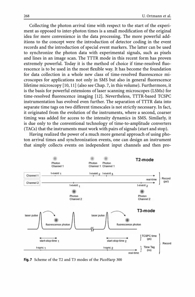
Having realized the power of a much more general approach of using pho-ton arrival times and synchronization events, one can design an instrumentthat simply collects events on independent input channels and then pro-

Fig. 7 Scheme of the T2 and T3 modes of the PicoHarp 300


cesses them according to the nature of the experiment. This allows one to,for example, connect either detectors or laser sync signals, just as required.Start–stop differences are then obtained by a simple subtraction. Coincidencecorrelations can then be calculated not only between successive events butalso across any sequence of events. The first instrument of this kind is thePicoHarp 300 [13]. It uses two independent time digitizers based on fast dig-ital counters with picosecond interpolators. Both time digitizers are lockedto the same crystal clock, so that their readings are always synchronous forsynchronous events. All processing of relative times is done arithmetically ina field programmable gate array (FPGA) or by the host computer. This pro-vides ultimate flexibility in data analysis. For instance, one can use the twoinputs for two detectors and obtain a cross-correlation between them, whichcovers the lag time range from picoseconds to infinity. This mode of collect-ing single number time tags (picosecond-resolved signal arrival times) onindependent and functionally identical inputs is called T2 mode.

Although the two time digitizers used in the PicoHarp design have theshortest dead time of any comparable instrument today, there is a limita-tion when using very fast sync sources (e.g. lasers with excitation rates over10 MHz). This problem is solved by a sync divider at one input. When thisdedicated sync input is used, the instrument is operated in so-called T3 mode,which is conceptually more similar to the original TTTR concept. Each pho-ton event is recorded with two figures: a time difference between excitationand photon emission and the number of the excitation cycle. Knowing the ex-citation period, the latter directly translates to the coarse scale arrival timeof the classic TTTR mode. This is an important improvement, because theclassic TTTR mode would not easily allow one to know the excitation perioda given photon belonged to.

Fig. 8 Analysis possibilities based on a single TTTR file


While the instrument internally always processes data as independent T2mode events, the conventional histogramming as well as T3 mode are imple-mented on top of this layer. By choosing between any of the three modes, theuser can solve almost any problem in time-resolved florescence measurementwith one instrument.

In summary, new developments in electronic design have resulted in veryversatile TCSPC instruments, which gain their power from a very generic ap-proach to photon data collection. This time tagged data collection allows veryinnovative concepts of fluorescence photon processing. The range of methodsof data analysis based on TTTR raw data is virtually unlimited. It ranges fromplain fluorescence lifetime measurements, over FLIM to FRET and FCS. Fig-ure 8 summarizes the most common analysis possibilities based on TTTRdata. While these classical methods are well documented in the literature, oneespecially ingenious and powerful new method will be shown in more detailin the next section.

4.1Fluorescence Lifetime Correlation Spectroscopy

An elegant example is the fusion of time-correlated single photon counting(TCSPC) and fluorescence correlation spectroscopy (FCS), called fluorescencelifetime correlation spectroscopy (FLCS). FLCS is a method that uses picosec-ond time-resolved photon detection for separating different FCS contribu-tions [14, 15].

Conventional FCS is based on recording and subsequent correlation analy-sis of intensity fluctuations caused by molecular movement (e.g. diffusion)and/or photophysical processes (such as association–dissociation, isomeriza-tion, etc.). Essentially, photon bursts with typical durations on the microsecondtimescale are observed. Although individual photon arrival times can be re-solved down to nanoseconds, FCS is in principle still a steady-state methodbecause the fluorescence decay kinetics is not taken into account. The stan-dard light source in FCS is a cw laser and typically photon-to-photon delaysare measured and recorded. The global photon arrival time is sufficient for au-tocorrelation calculation, but it is important to realize that there is no way toguess the origin of the photon. The main problem in FCS is that the detectedphoton signal always contains various unwanted contributions. For example, atvery low sample concentration (which is typical for FCS) a considerable portionof the detected intensity is generated by Rayleigh and Raman scattered exci-tation light and by dark counts (thermal noise). Detector after-pulsing is alsoa serious issue. All these contributions affect the shape of the resulting autocor-relation function (ACF). The subsequent mathematical analysis (fitting) is thencomplicated and/or can lead to misleading results due to parameter correlation.

FLCS provides a solution to many inherent problems of FCS. The mainfeature of FLCS is the statistical separation of a selected signal component


matching a certain TCSPC decay behaviour. This is done before the autocorre-lation analysis, hence the result is a separated, component ACF instead of thelinear combination as usual in FCS. The selected signal component can be, forexample, the fluorescence emitted by one of the species present in the sam-ple, provided its decay curve is known. Alternatively, the method can be usedmerely to suppress various parasitic components (again, with known TCSPChistograms), without any further assumptions on the rest of the signal.

The key to this is the high information content of the TTTR data file.Namely, the photon delay time measured relative to the onset of the excitationpulse is now available in addition to the previously mentioned global pho-ton arrival time. It is evident that sub-nanosecond pulsed excitation should beused instead of cw radiation.

The principle of FLCS is illustrated in the example below. The experi-mental data were acquired with the MicroTime 200 confocal time-resolvedfluorescence microscope [11] equipped with a pulsed diode laser. The tim-ing electronics of this system are based on the TimeHarp 200 or PicoHarp 300TCSPC modules operated in the above described TTTR mode [16].

In a typical FCS-like experiment, the fluorescence from diffusing moleculescomes in bursts of photons. Such photon bursts are often presented as a so-called multi-channel scaling (MCS) trace (Fig. 9). It is the bare number ofphotons plotted against the global arrival time, which shows the intensity evo-

Fig. 9 A 2-s period of intensity fluctuations caused by diffusing fluorescent molecules.Sample: a drop of 50 pM aqueous solution of Atto655 on a glass cover slip at roomtemperature, excited at 635 nm with a 20-MHz pulsed laser diode (LDH-635B)


lution (i.e. fluctuations). In the standard FCS approach, this intensity trace isautocorrelated to give an ACF. During this calculation, only the global arrivaltime of the photon is relevant and each photon contributes equally as a unitintensity carrier.

However, the previously disregarded TCSPC timing information can beused to obtain the conventional decay histogram of the same photons. An im-portant feature of such a TCSPC histogram (Fig. 10) is that it is possible todecompose it (e.g. by reconvolution fitting) into well-defined signal contribu-tions. A quick view on the TCSPC histogram reveals that a large portion ofthe detected intensity originates from scattered light (Rayleigh and Raman,see the sharp spike at the beginning). The fraction of detector dark countsand after-pulsing (on this timescale appearing as an offset) can also be de-termined. Only the remaining photons can be attributed to the fluorescenceoriginating from molecules.

Using the fitted component histograms and the overall decay curve, fil-ter functions can be calculated [12] for each intensity contribution (Fig. 11).In the FLCS approach, these filter functions are used as photon weightingschemes during the autocorrelation calculation (Fig. 9). Contrary to the stan-dard FCS, the TCSPC timing is now taken into account. The software looksup the weight (i.e. the sign and the magnitude) of the photon contribution,which then enters the calculation of the selected component ACF. Note thatthe weight is generally a real number. Dependent on which ACF component

Fig. 10 TCSPC histogram of all photons collected in the FCS experiment (see Fig. 9) andthe result of its decomposition


Fig. 11 Calculated filter functions for the various signal contributions

Fig. 12 Comparison of FCS and FLCS results

is calculated, the same photon contributes with different weights. However,the sum of all weights corresponding to a single photon (characterized by itsTCSPC delay time) is exactly 1, since it carries a unit intensity.


Continuing with the above example, it is interesting to see the effect of theuse of the filter function for pure fluorescence on the resulting ACF. Figure 12compares the ACF calculated by a standard FCS approach with that separated(“filtered”) by FLCS. The increase of the ACF amplitude at the shortest lagtimes is due to filtering out the effect of scattered light and dark noise. Thisis very important because the initial ACF amplitude is interpreted as a recip-rocal value of the average number of molecules inside the detection volume,and is thus related to the absolute concentration. Another effect visible inFig. 12 is the change of the ACF shape. An initial fast decay is completely ab-sent in the FLCS result, proving that the FCS result is affected by detectorafter-pulsing and not, for example, by triplet dynamics. In a nutshell, FLCSprovides correct results in cases where FCS fails.

5Conclusion

The development of novel turn-key instrumentation based on integratedsemiconductor devices, along with tremendous improvements in data pro-cessing and analysis, will continue to boost the power of time-resolved flu-orescence methods. For instance, the concept of collecting single numbertime tags on independent and functionally identical inputs (T2 mode) is ex-tremely powerful, due to the absence of dead times across channels. Work isin progress to extend this concept to more than two inputs. This will allowparallelization of high-throughput applications, as well as novel approachesto general photon coincidence correlation in general quantum physics andquantum information processing research. At the same time, data analysissoftware is evolving rapidly towards a generalized approach based on timetagged single-photon records. This development will lead to more powerfulsolutions in key applications, such as sensitive fluorescence detection, fluores-cence assays and functional studies of biomolecules.

References

1. Legendre BL Jr, Williams DC, Soper SA, Erdmann R, Ortmann U, Enderlein J (1996)Rev Sci Instrum 67:3984

2. Nakamura S, Senoh M, Nagahama S, Iwasa N, Yamada T, Matsushita T, Kiyoku H,Sugimoto Y (1996) Jpn J Appl Phys 35:L74

3. Erdmann R, Langkopf M, Lauritsen K, Bülter A, Wahl M, Wabnitz H, Liebert A,Möller M, Schmitt T (2005) Proc SPIE 5693:43

4. Khan A (2000) Appl Phys Lett 76:2735. SET Inc (2003) Comp Semicond 9:246. Wilkerson CW Jr, Goodwin PM, Ambrose WP, Martin JC, Keller RA (1993) Appl Phys

Lett 62:2030


7. Brand L, Eggeling C, Zander C, Drexhage KH, Seidel CAM (1997) J Phys Chem A101:4313

8. Erdmann E, Ortmann U, Enderlein J, Becker W, Wahl M, Klose EO (1966) Proc SPIE2680:176

9. Wahl M, Erdmann R, Lauritsen K, Rahn HJ (1998) Proc SPIE 3259:17310. Böhmer M, Pampaloni F, Wahl M, Rahn HJ, Erdmann R, Enderlein J (2001) Rev Sci

Instrum 72:414511. Wahl M, Koberling F, Patting M, Rahn HJ, Erdmann R (2004) Curr Pharm Biotechnol

05:29912. Ortmann U, Dertinger T, Wahl M, Patting M, Erdmann R (2004) Proc SPIE 5325:17913. Wahl M (2005) PicoHarp 300 user manual. PicoQuant GmbH, Berlin14. Böhmer M, Wahl M, Rahn HJ, Erdmann R, Enderlein J (2002) Chem Phys Lett 353:43915. Kapusta P, Wahl M, Benda A, Enderlein J (2007) J Fluoresc 17:043–04816. Böhmer M, Enderlein J (2003) ChemPhysChem 04:792

Documents

Time-resolved fluorescence: Novel technical solutions