1

Ref. No: TRN/CP/NL/Y0001

The Title:

Integrated Data Analysis in Time-Resolved Fluorescence and Fluorescence Correlation Spectroscopy

The Running Title:

Data Analysis in Fluorescence Spectroscopy The Titles and Names of Authors:

Dr. Mikalai M. Yatskou1, Mr. Anatoli V. Digris1, Dr. Eugene G. Novikov2, Mr. Victor V. Skakun1, Prof. Vladimir V. Apanasovich1

Affiliations:

1 Department of Systems Analysis, Belarusian State University, Minsk, Belarus 2 Service Bioinformatique, Institut CURIE, Paris, France

Corresponding Author:

Dr. Mikalai M. Yatskou Department of Systems Analysis Belarusian State University 4, Skaryna Ave. Minsk 220050 Belarus Tel./fax: + 375 172 789345 E-mail: yatskou@bsu.by

2

ABSTRACT An enormous number of data analysis methods and calculation techniques featuring well-defined optical experiments has been designed over the past century. However, only a small number of these tools has been systematized into a single analysis scheme. The extant methods of data analysis typically have separately been applied for particular fluorescence spectroscopy areas. This suggests creating a single integrated type of data analysis based on a variety of system objects (data sources, mathematical models, fitting methods, etc) to principally be used for all spectroscopy measurements of any molecular systems. We demonstrate the principles and structure of such integrated object–oriented conception of data analysis. Several fitting software packages, based on the presented data analysis approach, were constructed and applied to process time domain fluorescence, frequency domain fluorescence, and fluorescence correlation spectroscopy data.

INTRODUCTION The method of fluorescence spectroscopy is a trustworthy high-precision tool in the area of physical chemistry for studying chemical and physical processes [1]. A promising trend in the development of fluorescence spectroscopy methods involves the working–out of new data analysis techniques, which could significantly improve a degree of competence for the interpretation of parameters and characteristics of photophysical processes in complex molecular systems. The most commonly used methods of data analysis are: nonlinear least squares, deconvolution methods, target analysis, global analysis, maximum entropy method [2,3,4,5,6]. These methods often require wide range of specific conditions for a particular area of application as well as well–known analytical expressions to describe physical processes. Although these methods and corresponding analytical models frequently offer a considerable level of the physical interpretation, yielding rather high quality approximations for experimental data, they are often less effective during analysis of a complex molecular systems. Nowadays, new complex molecular materials must be investigated in more general and universal way using a superposition of data analysis techniques, applying whole range of known methods and models. More general integrated data analysis technique for fluorescence spectroscopy measurements is therefore required to satisfy all needs arising while researching new complex molecular materials.

In this paper we summarize the existing data analysis techniques and fitting models into a single integrated approach to be applied for a wide range of various experimental fluorescence spectroscopy measurements. This integrated approach combines a set of interacting software objects, incorporating all types of physical and mathematical models, fitting methods, error estimation methods, which can be transported or embedded into the analysis of various chemistry materials. The professional highly-optimized Windows-platform software, designed on a core of the integrated data analysis approach, have been developed to process time domain fluorescence, frequency domain fluorescence, and fluorescence correlation spectroscopy data. Their applications are demonstrated to study the photophysical properties of thin films of porphyrin layers and of photonic dye-zeolite antenna materials.

INTEGRATED APPROACH FOR DATA ANALYSIS

The fluorescence spectroscopy data may originate from different types of experiments, for example, time-correlated single photon counting, fluorescence correlation spectroscopy, time resolved frequency domain measurements, etc. Normally experimental data are represented by one or several statistical characteristics, e.g. – fluorescence intensity, autocorrelation function, distribution of number of counts, etc.

The core of the integrated data analysis concept is ability to process complex fluorescence data of any spectroscopic measurements in a unique and coherent way, whichever experimental design is used. It combines various experimental output characteristics to simultaneously analyze them by a unique model with a global set of parameters. Integrity of this approach is based on so-called object-oriented open-architecture principle: allowing to easily incorporate into the experimental data analysis new experimental designs, methods, physical and mathematical models in form of special software objects. The scheme of the integrated data analysis concept is shown in Figure 1 and represented as a coherent system of the interacting software objects. Each object performs a separate task with a well-defined interface to the other objects from the scheme.

3

Figure1. Integrated approach for data analysis.

Fit parameters

Theoretical statistical characteristics

Measured photon flows

Directly measured characteristics

Directly simulated characteristics

Calculated characteristics

Target fit criterion

Data set 1

K

Analysis data sets Model 1

Model 2

Model N

M

Models

Fit parameters

linking

Fitting method

Criterion 1

Criterion 2

Criterion M

M

Fit quality criteria

Generation of initial guesses

Source statistical characteristics

Measured data Simulated data

Simulated photon flows

Source characteristic 1

Theoretical characteristic 1

Data set N

Source characteristic N

Theoretical characteristic N

4

The objects of the integrated approach are different experimental and calculated data sets, analytical and stochastic models, fit quality and target criteria, fit parameter linking, fitting methods, and methods for generation of initial guesses. In such scheme the data analysis can be represented as a sequence of interactions between different objects executed according to a predefined algorithm.

The block Measured data represents an experimental fluorescence set–up and provides directly measured characteristics, or calculated characteristics, derived from photon flows (the blocks Measured photon flows and Calculated characteristics). Alternatively, for the reasons of testing data analysis algorithms and models as well as the effects of experimental factors, corresponding direct and indirect characteristics can numerically be generated in the blocks Simulated data and Simulated photon flows using computer simulation methods [7,8]. Experimental or simulated direct and calculated characteristics form the source statistical characteristics for the further analysis. Each source statistical characteristic is associated with a model, the blocks Model 1, Model 2, …, Model N, having corresponding number of parameters. The models generate the theoretical data – the theoretical statistical characteristics, which complete forming the analysis data sets. The block Fit parameters linking provides the linkage of common parameters for different models and supplies the procedure of global analysis [9,10]. The analysis procedure adjusts the parameters of the model(s) in such way that to ensure an optimal value of the target fit criterion. Adjustment of the parameters is performed by a fitting method in the block Fitting method. The speed and quality of the integrated analysis are significantly depended on the initial values of the parameters for the iterative adjustment, which are calculated in the block Generation of initial guesses. Ideally these values should be as close as possible to actual values of physical parameters. As soon as the iterative adjustment has been finished one should make a decision about the appropriateness of estimated parameters. For this reason the final target fit criterion is accompanied by additional criteria (Fit quality criteria blocks): the plot of the weighted residuals, the plot of the autocorrelation function of weighted residuals, the runs test [3,11].

We note that this scheme is operable for the experimental data of any nature and mathematical models of any kind. Moreover, we are able within a single data analysis session to combine experimental data of different nature, provided that the correspondent models are available. Moreover, if such models (theoretical characteristics) possess a subset of the equivalent parameters, these parameters can be forced to be equal during the fit.

Now we describe the objects used within the integrated approach for data analysis.

MODELS

Analytical Models The experimental techniques of measuring the time-resolved fluorescence can be divided into two groups: for i) time domain and for ii) frequency domain.

Time domain. In time domain techniques, the sample is excited with a pulse of light. The width of the pulse is made as short as possible and is preferably much shorter than the lifetime of the fluorophore. The time-dependent fluorescence intensity is measured following the excitation pulse, and the lifetime is calculated from the slope of a plot of logarithm of the fluorescence intensity. There are a number of time domain methods for time-resolved measurements [1,12]. One of the most favorite techniques is time-correlated single photon counting (TCSPC) [3,13]. The finite width of an excitation pulse and the delays in a detector make an actual decay, i.e. the impulse response of a fluorescent probe, convoluted with the instrumental function. The instrumental response function, measured via a scatter, is detected at the excitation wavelength instead of the emission wavelength of a sample [14,15,16]. Direct analysis of the fluorescence decay using that instrumental function may cause serious distortions due to discrepancy in the detection wavelength. Several techniques were proposed in order to eliminate the influence of the misshapen instrumental function [17]. Among them, one of the most common and rigorous is the reference reconvolution or δ-function convolution method [14,15]. This method suggests measuring fluorescence decay of the reference compound with the same absorption and emission wavelengths as those used for the sample. The fluorescence decay analysis is related then to that reference decay.

Frequency domain. In time-resolved frequency domain fluorescence measurements [1,18,19], the impulse function of the excitation beam as well as the response signal of the sample are intensity-modulated light. The response signal,

5

that is, the fluorescence decay of the sample, is phase-shifted with respect to the impulse function and demodulated. If a set of impulse functions of the same amplitude but with different modulation frequencies is used, the response signal is the Fourier transform of the impulse response function, which characterizes the transfer system. If this impulse response function can be expressed as a sum of exponentials, it is not necessary to measure and analyze all quantities of the response signal. Instead, the phase shifts alone allow the parameters of the multiexponential function to be determined. This is because of the special analytical form of the Fourier transform of a sum of exponentials [20,21].

In many applications the fluorescence decay obtained either via time domain or frequency domain methods can be adequately approximated by a sum of exponentials [1,3]. Numerous investigations [22,23] have shown that adequate models for electronic energy relaxation in macromolecules cannot be defined by the sum of exponentials, when a mechanism of dipole-dipole energy transfer is taken into account. In recent years most attention has been given to the stretched-exponential Förster decay law [23,24], representing the first-order approximation of dipole-dipole electronic energy transfer. When the concentration of donor molecules is sufficiently low, so that the probability of multistage energy migration processes is negligible and energy is directly transferred to the random distribution of acceptors, the donor fluorescence decay can be represented by a stretched exponential decay model [23].

Other analytical models for the fluorescence decays have been developed with the aim to reproduce the fluorescence response of the systems exhibiting different types of electronic excitation energy transfer [25,26,27], the compartmental systems [5,28], systems with the reactions in the exited state [29,30], diffusion-controlled reactions [31,32], excimer formations [33,34].

Fluorescence Correlation Spectroscopy (FCS) deals with relatively small-scale fluctuations of collected fluorescence from a very small volume by the tightly focused laser beam up to the nanosecond time range. To get the information about the sample under study the normalized fluorescence fluctuation autocorrelation function is calculated and analyzed [35,36].

The earliest publications in the FCS field were devoted to the study of molecular diffusion processes and reaction kinetics, where a diffusion model for the autocorrelation function was introduced [37]. Further theoretical and experimental investigations demonstrated that molecular diffusion might be accompanied by additional processes, e.g. aggregation, concentration, chemical rate constants, and rotational dynamics, that also influence the fluorescence intensity [38]. To describe the molecular diffusion and other processes together, the diffusion model was modified and few new models for the autocorrelation function were developed for studying: FCS flows [39,40], conformational dynamics [41], triplet-state effects [38], external and internal protonation processes [42], chemical reactions [43]. Stochastic models

Stochastic models based on Monte Carlo simulation algorithms appear to be well-suited for description of many physical processes in complex molecular systems [44,45,46,47,48]. Although a Monte Carlo model has been used extensively to test the validity of the approximations made in analytical theories, [49,50,51,52] its possibilities stretch much further. The simulation model is frequently served when the handling of analytical models remain unsatisfactory or can be mathematically very difficult. Modeling processes in molecular assemblies using Monte Carlo simulations has at least two advantages: it operates by the elementary processes, which are easy to understand and to program, and it gives direct insight to the relevant kinetic processes from the experimental complex data.

Different Monte Carlo models have been developed to simulate the fluorescence decay for: dye systems [8,27], the systems exhibiting various types of excitation electronic energy transfer [53,54,55,56], diffusion-controlled reactions and translational diffusion [57,58,59], singlet-singlet annihilation [60], recombination kinetics [61].

An improved Monte Carlo algorithm to investigate physical processes in molecular systems, based on the parameter fitting via Monte Carlo simulations, which does not require an analytical description to be known beforehand, has been reported [62,63]. There are at least four steps to be taken in this approach: (i) create a physical model (which includes the geometry, dynamics, etc.) of the investigated molecular system, (ii) develop and program a simulation model based on the physical model, with the model parameters corresponding to the various kinetic characteristics of the molecular system, (iii) find through parametric fitting an optimum set of parameters of the simulation model

6

corresponding to the experimental data, (iv) calculate the reduced χ2 value for a quantitative determination of the accuracy of the simulated decay curve.

PARAMETRIC ESTIMATION A variety of approaches for fluorescence data fitting has been exercised with the different level of success [64,65]. Among them two groups are clearly prominent: iterative non-linear approach, directly optimizing some fit quality criterion (see the next section) by an optimization method, and non-iterative approach, based on the transformation of the detected decay to a linear algebraic set of equations with respect to unknown parameters.

The approach of non-linear iterative minimization [66] is the most universal for fluorescence data analysis. However, the efficiency of this approach is often suffered from the badly chosen initial guesses. When the initial guesses are far from the true values of parameters, the convergence may be rather slow and, hence, time consuming. That is why general strategy in fluorescence data analysis may be composed of a non-iterative routine, generating initial guesses, and iterative procedure, starting search with those initials.

The main components of the iterative fitting are target fit criterion (TFC) and fitting method. The aim of the fitting or optimization method is to find a set of parameters { }maaaa K

r21,= generated by theoretical models, which ensure

the optimal value of the TFC.

Target fit criterion

The TFC is usually derived from the Likelihood function :

),,...,,()( 21 axxxPaL krr

= , (1)

where xi, i=1,…,k are the experimental data values and ),,...,,( 21 axxxP kr

is the multivariate probability of the experimental values xi, i=1,…,k. If all xi, i=1,…,k are independent, equation (1) can be rewritten as:

∏=

=k

ii axPaL

1),()( rr

. (2)

The maximum likelihood method requires values of the parameters a1, …, am to be chosen so that the above likelihood function is maximized. Further practical treatment is dependent on the experimental statistics, typically Gaussian, Poissonian or Multinomial statistics [67,68], which affects the shape of the functions ),( axP i

r. For the

Gaussian statistics the equation (1) is

( )

πσ

σ

2

2)(exp

),(2

2

i

i

thii

i

aFx

axP

−−

=

r

r

(3)

where )(aF thi

r is value of the theoretical characteristic in the thi − point of arguments space and iσ is a standard

deviation of the experimental value xi. For the Gaussian statistics of the equation (3) the maximization of ( )aL r is

equivalent to minimization of the following χ2 :

( )∑=

−=

k

i i

thii

GaFxa

1 2

22

2)(2)(

σχ

rr

, (4)

In practice the normalized quantity ( )12 −− mkGχ is used, which, for the good fits, should be close to 1.

7

Besides the final value of target fit criterion the additional fit quality criteria can be considered for judging the quality of the fit. Therefore all of them are devoted to the analyzing the results of comparison of source and theoretical data. Often the most useful fit quality criteria are: the plot of weighted residuals, the plot of the autocorrelation function of weightd residuals, normal deviation of 2χ ( 2χ

Z ), Durbin-Watson parameter, Runs test, Heteroscedasticity of

weighted residuals, Normal probability function of weighted residuals [1,3,11,13].

Fitting methods

Fitting or optimization methods are employed for finding an optimum set of fit parameters that maximizes the conformity between source and theoretical characteristics in the fitting [69,70,71]. Each fitting algorithm uses a unique mathematical technique for changing the fit parameters. Commonly used optimization methods might be divided into two large groups: non-derivative methods, which do not require derivatives of the target fit criterion, and gradient methods, requiring derivatives of the target fit criterion. Among the non-derivative methods several classes are widely sited in the literature: Search methods [62,66,72,73] perform one-dimensional search with respect to each fit parameter (grid method, Hooke-Jeeves method, Powell method, Rosenbrock’s method). Simplex methods [73,74,75] construct a polygon (simplex) in the space of fit parameters and move the center of this polygon to the parameters point where target fit criterion value is best. Stochastic methods [76,77,78 ] use a search procedure based on the random determination of the search direction (random walk, Monte Carlo methods, method of “simulated annealing”). Application of the gradient optimization methods in comparison with non-derivative methods ensures faster convergence to the optimum value but requires calculation of first or second derivative of target fit criterion. The most frequently referenced gradient methods are steepest descent method, Gauss-Newton method, and Levenberg-Marquardt method [79,80,81].

Parametric fitting via Monte-Carlo simulations

The Monte Carlo fitting method does not require the analytical equation to be known beforehand, and it includes the analysis of statistical noise to judge the quality of the fit. Once the experimental time domain luminescence decay is collected, it can be analyzed by means of a Monte Carlo decay simulation, yielding the set of physical parameters of the system. The best fit is defined by a criterion (or set of criteria) that shows how far the simulated data deviate from the experimental data. Generally, such a criterion is represented by a function of the experimental and simulated data, and strongly depends on the particular application area, the particular simulation method, and the experimental conditions. According to this criterion the best approximation, corresponding to the set of parameters, is that which yields a minimum for the criterion. An example of application of the statistical χ2 criterion for fluorescence decay fitting using Monte Carlo simulations was reported in [63].

An important point is that the Monte Carlo analysis may result in a local minimum. In general, an adequate determination of the parameters requires a check of their confidence intervals by the exhaustive search method [82]. It is impractical, however, to apply this, since it would result in a dramatic increase of processing time. The less time-consuming, but also less accurate, asymptotic standard errors therefore recommended [83]. Another approach to considerably reduce the risk of landing in local minima is the application of the Monte Carlo confidence interval evaluation method, which is more time-consuming, but still not extensive [84].

Initial Guesses

Whereas iterative fit methods are common and can be applied to virtually any model, the methods for generating initial guesses are essentially model-specific and must be developed for each particular model. We briefly outline here only the references to the generation of initial guesses for a stretched exponential model and a multi-exponential model as most commonly used. The algorithms of initial guesses generation for the stretched exponential models are considered in [85]. Different approaches to generate initial guesses for a multi-exponential model are considered in [86,87,88,89,90].

8

TIME RESOLVED FLUORESCENCE AND FLUORESCENCE CORRELATION FITTING SOFTWARE The integrated object-oriented approach presented in previous sections was taken as a core to develop software products. These software packages are designed for data analysis in area of time-resolved fluorescence and anisotropy measurements, time-resolved frequency domain measurements, and fluorescence correlation spectroscopy measurements.

All software packages provide simultaneous data analysis of more than one source characteristic. The data analysis procedure is developed on the base of on the 2χ target fit criterion. The Levenberg-Marquardt [91] minimization algorithm is used as an optimization method. The software packages provide fixing, linkage and setting minimum and maximum constraints for the fit parameters. The software packages include basic features for judging the quality of the fit. Besides the final value of 2χ criterion, the weighted residuals, and the autocorrelation function are plotted, the confidential intervals for fit parameters are calculated by the exhaustive search or asymptotic standard errors methods [82,83].

Each software package consists of three applications: i) Measurements database, ii) Analysis database and iii) Main application. Measurements database is responsible for importing and storing measured data and preparing them for further analysis. Analysis database is designed for storing and viewing results of previous fits. Main application performs analysis of measured data and provides the possibility to save analysis results and analysis configurations to the analysis database. Main application has a multi document interface and allows comparing the results of different fits. Advanced operations with fit parameters including sorting, quick linkage and easy navigation significantly simplify management of large fit parameter sets. Two- and tree- dimensional charts provide convenient view of measured data and analysis results.

Time Resolved Fluorescence and Anisotropy Data Processor (TRFADP)

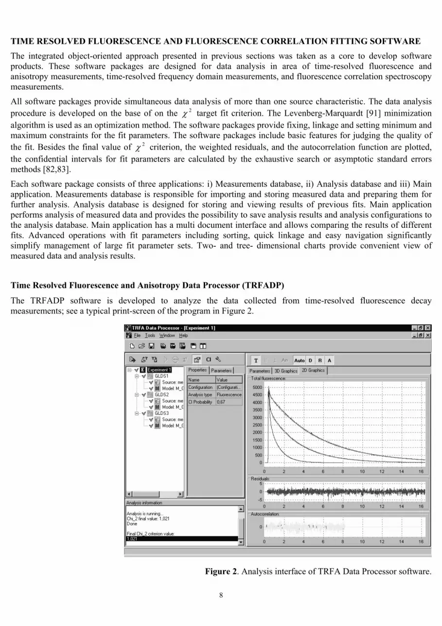
The TRFADP software is developed to analyze the data collected from time-resolved fluorescence decay measurements; see a typical print-screen of the program in Figure 2.

Figure 2. Analysis interface of TRFA Data Processor software.

9

The TRFADP software provides fluorescence and anisotropy decay analysis [92] of fluorescence decays, taken either from measurements with one-exponential reference compound or from measurements with a scatter. Anisotropy analysis is implemented as simultaneous analysis of parallel and perpendicular fluorescence decays. Associative and non-associative anisotropy analysis is supported. While performing parameters estimation, the software takes into account several possible instrumental distortions that can exist in measured data (time shift, background, anisotropy G-factor). The core of software package contains two widely used models: a sum of exponentials and a dipole-dipole energy transfer model. After analysis is done, the values of estimated parameters, final value of chi-square criterion and tree- and two-dimensional graphical dependencies of residuals and autocorrelation functions of residuals are available for judging the quality of the fit.

Time Resolved Frequency Domain Fitting Software (TRFDFS)

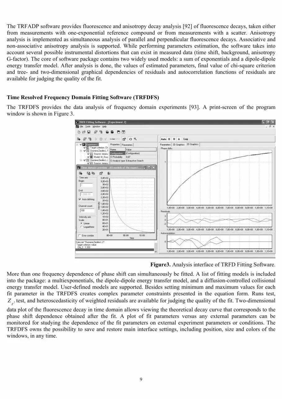
The TRFDFS provides the data analysis of frequency domain experiments [93]. A print-screen of the program window is shown in Figure 3.

Figure3. Analysis interface of TRFD Fitting Software.

More than one frequency dependence of phase shift can simultaneously be fitted. A list of fitting models is included into the package: a multiexponentials, the dipole-dipole energy transfer model, and a diffusion-controlled collisional energy transfer model. User-defined models are supported. Besides setting minimum and maximum values for each fit parameter in the TRFDFS creates complex parameter constraints presented in the equation form. Runs test,

2χZ test, and heteroscedasticity of weighted residuals are available for judging the quality of the fit. Two-dimensional data plot of the fluorescence decay in time domain allows viewing the theoretical decay curve that corresponds to the phase shift dependence obtained after the fit. A plot of fit parameters versus any external parameters can be monitored for studying the dependence of the fit parameters on external experiment parameters or conditions. The TRFDFS owns the possibility to save and restore main interface settings, including position, size and colors of the windows, in any time.

10

Fluorescence Correlation Spectroscopy Data Processor (FCSDP)

The FCSDP software is developed to process the fluorescence correlation function. The software is fully compatible with ConfoCor and ConfoCor2 (Carl Zeiss Jena GmbH). A print-screen of the program window is represented in Figure 4.

Figure 4. Analysis interface of FCS Data Processor software.

The FCSDP can import both raw data traces and directly measured correlation functions. Software generates autocorrelation and crosscorrelation functions, photon counting distribution, first and single event distributions, inter-event time distribution from imported raw data. More than one correlation function can simultaneously be analyzed. Base software package contains a set of most popular models for correlation functions: pure-diffusion model, triplet-state model, conformational model, protonation model, and diffusion flow model. Quick and easy creation and saving of user-defined models is supported. Besides standard graphs displaying the analysis produce a graphical dependence of fit parameters on any variable of source characteristics.

All software packages can dynamically be upgrated with new models and more powerful optimization methods by including additional dll libraries. This can be done without any necessity to update any other parts of application. These futures are possible due to the modular architecture of the software.

Due to the same object-oriented analysis scheme that underlies all software packages the interface of corresponding applications from different packages is quite similar. The similarity, simplicity and usability of the interface of developed software make easier the investigation of samples measured by different experimental methods.

The software packages are available for Windows 95/98/Me/Nt 4.0/2000/XP operating systems.

APPLICATIONS The integrated data analysis approach has been applied to analyze the photophysical properties of thin films of porphyrin layers and photonic dye-zeolite antenna materials. These applications summarize the complex data analysis for three fluorescence spectroscopy areas: i) time domain fluorescence spectroscopy, ii) frequency domain fluorescence spectroscopy, and iii) fluorescence correlation spectroscopy.

11

Time domain fluorescence spectroscopy Porphyrin molecules are interesting building blocks for the construction of very thin films as artificial antenna’s systems, for organic solar cells [94,95]. As compared to inorganic films, organic films have received less attention, but their interest has been rapidly growing during the past decades. With the application to light-harvesting antennas in solar cells in mind the energy transfer and excited state decay properties of artificial antenna’s have been investigated by the time-resolved fluorescence and fluorescence anisotropy measurements [96,97]. Steady state fluorescence spectra and the fluorescence polarization decay of porphyrin oligomers in solution as well as of thin solid films has been measured via streak camera time-correlated single photon counting methods and were analyzed by the integrated object-oriented approach, incorporating the global analysis, a multi-exponential model, a Förster point dipole-dipole model and Monte Carlo simulation models.

This application is focused on the structure and photophysics of

• zinc mono-(4-pyridyl)-triphenylporphyrin (Zn(4-Py)TrPP) self-organizing into a tetramer [Zn(4-Py)TrPP]4

• self-organizing zinc tetra(-octylphenyl)-porphyrin (ZnTOPP) layers on an inert substrate.

Films of Zn(4-Py)TrPP and ZnTOPP were made by spincoating from toluene. The global analysis of steady-state and time resolved fluorescence spectroscopy data has shown that ZnM(4-Py)TrPP in solution polymerizes to a tetramer through internal zinc-pyridyl ligation (Figure 5). The results of the object-oriented analysis and Monte Carlo simulations of ZnM(4-Py)TrPP films agree with this tetramer model, yielding a fluorescence lifetime and nearest neighbor energy transfer rate constant of ~ 1.5 ns and ~ 40 ns-1, respectively.

Figure 5. Molecular structure of [Zn(4-Py)TrPP]4 (left)and fragment of ZnTOPP layer on a quartz substrate (right).

Applying our integrated approach to the experimental fluorescence- and fluorescence anisotropy decay of ZnTOPP films results in a multi-domain model of parallel porphyrin stacks. In each stack the porphyrin planes are perpendicular to the substrate and form an angle of 45˚ with the long stack axis (Figure 5). The calculations yield the rate constants for intra-stack and inter-stack energy transfer as ~ 1 ps-1 and ~ 80 ns-1, whereas the fluorescence lifetime is ~ 1.8 ns.

Frequency domain spectroscopy Excitation energy migration within assemblies of dyes embedded in hexagonal crystals of cylinder morphology is an attractive phenomenon for the construction of a photonic antenna [98,99]. Detailed knowledge of the zeolite structure, guest-dye spectroscopic properties, the nature and strength of the host-guest interactions is required to optimize energy migration throughout a cylinder crystal [100]. Whether a dye-zeolite antenna efficiently transports excitation energy is mainly determined by the mechanism and rate of energy transfer between the dyes embedded in

12

the zeolite channels. The integrated approach and the Monte Carlo simulation-fitting method have been used to investigate the energy migration and excited-state properties of a photonic dye-zeolite antenna [101]. Using this computational technique the complex time-resolved frequency domain fluorescence decay of the guest-dye in the zeolite crystals has been analyzed.

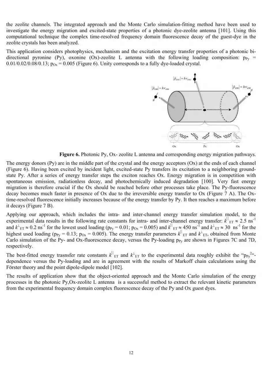
This application considers photophysics, mechanism and the excitation energy transfer properties of a photonic bi-directional pyronine (Py), oxonine (Ox)-zeolite L antenna with the following loading composition: pPy = 0.01/0.02/0.08/0.13; pOx = 0.005 (Figure 6). Unity corresponds to a fully dye-loaded crystal.

excexc hp ν=r

emem hp ν=r

emem hp ν=r

Ox OxPx Figure 6. Photonic Py, Ox- zeolite L antenna and corresponding energy migration pathways.

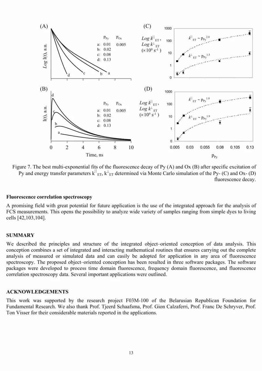
The energy donors (Py) are in the middle part of the crystal and the energy acceptors (Ox) at the ends of each channel (Figure 6). Having been excited by incident light, excited-state Py transfers its excitation to a neighboring ground-state Py. After a series of energy transfer steps the exciton reaches Ox. Energy migration is in competition with spontaneous emission, radiationless decay, and photochemically induced degradation [100]. Very fast energy migration is therefore crucial if the Ox should be reached before other processes take place. The Py-fluorescence decay becomes much faster in presence of Ox due to the irreversible energy transfer to Ox (Figure 7 A). The Ox- time-resolved fluorescence initially increases because of the energy transfer by Py. It then reaches a maximum before it decays (Figure 7 B).

Applying our approach, which includes the intra- and inter-channel energy transfer simulation model, to the experimental data results in the following rate constants for intra- and inter-channel energy transfer: kET ≈ 2.5 ns-1 and k⊥ET ≈ 0.2 ns-1 for the lowest used loading (pPy = 0.01; pOx = 0.005) and kET ≈ 450 ns-1 and k⊥ET ≈ 30 ns-1 for the highest used loading (pPy = 0.13; pOx = 0.005). The energy transfer parameters kET and k⊥ET, obtained from Monte Carlo simulation of the Py- and Ox-fluorescence decay, versus the Py-loading pPy are shown in Figures 7C and 7D, respectively.

The best-fitted energy trasnsfer rate constants kET and k⊥ET to the experimental data roughly exhibit the “pPy2“-

dependence versus the Py-loading and are in agreement with the results of Markoff chain calculations using the Förster theory and the point dipole-dipole model [102].

The results of application show that the object-oriented approach and the Monte Carlo simulation of the energy processes in the photonic Py,Ox-zeolite L antenna is a successful method to extract the relevant kinetic parameters from the experimental frequency domain complex fluorescence decay of the Py and Ox guest dyes.

13

0

1

10

100

1000

0.005 0.03 0.055 0.08 0.105 0.13

0

1

10

100

1000

0.005 0.03 0.055 0.08 0.105 0.13

0 2 4 6 8 10Time, ns

I(t),

a.u

.Lo

gI(

t), a

.u.

abcd

a

b

c

d

(A)

(B)

(C)

(D)

Log kET ,Log k⊥ ET(×109 s-1 )

Log kET ,Log k⊥ ET(×109 s-1 )

pPy

kET ∼ pPy1.9

k⊥ ET ∼ pPy1.9

kET ∼ pPy2.0

k⊥ ET ∼ pPy1.5

a: 0.01b: 0.02c: 0.08d: 0.13

pPy pOx

0.005

a: 0.01b: 0.02c: 0.08d: 0.13

pPy pOx

0.005

Figure 7. The best multi-exponential fits of the fluorescence decay of Py (A) and Ox (B) after specific excitation of

Py and energy transfer parameters kET, k⊥ET determined via Monte Carlo simulation of the Py- (C) and Ox- (D) fluorescence decay.

Fluorescence correlation spectroscopy A promising field with great potential for future application is the use of the integrated approach for the analysis of FCS measurements. This opens the possibility to analyze wide variety of samples ranging from simple dyes to living cells [42,103,104].

SUMMARY

We described the principles and structure of the integrated object–oriented conception of data analysis. This conception combines a set of integrated and interacting mathematical routines that ensures carrying out the complete analysis of measured or simulated data and can easily be adopted for application in any area of fluorescence spectroscopy. The proposed object–oriented conception has been resulted in three software packages. The software packages were developed to process time domain fluorescence, frequency domain fluorescence, and fluorescence correlation spectroscopy data. Several important applications were outlined.

ACKNOWLEDGEMENTS This work was supported by the research project F03M-100 of the Belarusian Republican Foundation for Fundamental Research. We also thank Prof. Tjeerd Schaafsma, Prof. Gion Calzaferri, Prof. Franc De Schryver, Prof. Ton Visser for their considerable materials reported in the applications.

14

REFERENCES

1. Lakowicz, J.R. 1999, Principles of Fluorescence Spectroscopy, 2nd ed. Kluwer Academic/Plenum Publishers, New York.

2. Straume, M., Frasier-Cadoret, S.G., and Johanson, M.L. 1991, Topics in Fluorescence Spectroscopy, Volume 2, J.R. Lakowicz (Ed.), Plenum Press, New York, 177.

3. Demas, J.N. 1983, Excited State Lifetime Measurements, Academic Press, New York.

4. Beechem, J.M., Ameloot, M., and Brand, L. 1985, Anal. Instrum., 14, 379.

5. Beechem, J.M., Ameloot, M., and Brand, L. 1985, Chem. Phys. Letts., 120, 466.

6. Levesey, A.K., and Brochon, J.C. 1987, Biophys. J., 52, 693.

7. Rubinstein, R., and Shapiro, A. 1998, Modern Simulation and Modelling, John Willey & Sons Inc., New York.

8. Chowdhury, F.N., Kolber, Z.S., and Barkley, M.D. 1991, Rev. Sci. Instrum., 62, 47.

9. Knutson, J.R., Beechem, J.M., and Brand, L. 1983, Chem. Phys. Lett., 102, 501.

10. Beechem, J.M., Gratton, E., Ameloot, M., Knutson, J.R., and Brand, L. 1991, Topics in Fluorescence Spectroscopy, Volume 2., J.R. Lakowicz (Ed.), Plenum Press, New York, 241.

11. Knuth, D.E. 1997-2001, The Art of Computer Programming, Reading Addison-Wesley, Massachusetts.

12. Holzwarth, A.R. 1995, Methods Enzymol., 246, 334.

13. O’Connor, D.V., and Phillips, D. 1984, Time-Correlated Single Photon Counting, Academic Press, London.

14. Zuker, M., Szabo, A.G., Bramall L., and Krajcarski, D.T. 1985, Rev. Sci. Instrum., 52, 14.

15. Boens, N., Ameloot, M., Yamazaki, I., and Schryver, F.C. 1988, Chem. Phys. 121, 73.

16. Vecer, J., Kowalczyk, A.A., Davenport, L. and Dale, R.E. 1993, Rev. Sci. Instrum., 64, 3413.

17. Zegel, M. van den, Boens, N., Daems, D., and Schryver, F.C. de 1986, Chem. Phys., 101, 311.

18. Gratton, E., and Limkeman, M. 1983, Biophys. J., 44, 315.

19. Lakowicz, J.R., and Maliwal, B.P. 1985, Biophys. Chem., 21, 61.

20. Lakowicz, J.R., Laczko, G., Cherek, H., Gratton, E., and Limkeman, M. 1984, Biophys. J., 46, 463.

21. Gratton, E., Limkeman, M., Lakowicz, J.R., Mailwal, B., Cherek, H., and Laczko, G. 1984, Biophys. J., 46, 479.

22. Fredrickson, G.H., and Frank, C.W. 1983, Macromolecules, 16, 1198.

23. Ghiggino, K.P., and Smith, T.A. 1993, Prog. Reaction Kinetics., 18, 375.

24. Förster, T. 1949, Z. Naturforsch, 4a, 321.

25. Kaschke, M., and Vogler, K. 1988, Laser Chem., 8, 19.

26. Grabowska, J., and Sienicki, K. 1995, Chem. Phys., 192, 89.

27. Andrews, L., and Demidov, A. 1999, Resonance Energy Transfer, John Wiley & Sons Ltd Inc, New York.

28. Ameloot, M, Boens, N., Andriessen, R., Berg, V. Van den, and Dchryver, F.C. de 1991, 95, 2041.

29. Loken, M.R., Hayes, J.W., Gohlke, J.R., and Brand, L. 1972, Biochemistry, 11, 4779.

30. Lows, W.R., and Brand, L. 1979, J. Phys. Chem., 83, 795.

31. Smoluchowski, M., 1917, Z. Phys. Chem., 92, 129.

32. Noyes, R.M. 1961, Prog. React. Kinetics, 1, 129.

15

33. Itagaki, H., Horie, K, and Mita, I. 1983, Macromolecules, 16, 1395.

34. Hirayama, S, Sakai, Y., Ghiggino, K.P., and Smith, T.A. 1990, J. Photochem. Photobiol. A. (Chem.), 52, 27.

35. Visser, A.J.W.G., and Hink, M.A. 1999, J. Fluoresc., 9, 81.

36. Elson, E., and Rigler, R. (Eds.) 2001, Fluorescence Correlation Spectroscopy. Theory and Applications., Springer-Verlag, Berlin.

37. Magde, D., Elson, E.L., and Webb, W.W. 1974, Biopolymers, 13, 29.

38. Widengren, J., and Rigler, R. 1998, Bioimaging, 4, 149

39. Gosch, M., Blom, H., Holm, J., Heino, T., and Rigler, R. 2000, Anal. Chem., 72, 3260.

40. Brinkmeier, M., Dörre, K., Stephan, J., and Eigen, M. 1999, Anal. Chem., 71, 609.

41. Bonnet, G., Krichevsky, O., and Libchaber, A. 1998, Proc. Natl. Acad. Sci. USA, 95, 8602.

42. Haupts, U., Maiti, S., Schwille, P., and Webb, W.W. 1998, Proc. Natl. Acad. Sci. USA, 95, 573.

43. Hess, S.T., Huang, S., Heikal, A.A., and Webb, W.W. 2002, Biochemistry, 41, 697.

44. Rubinstein, R., and Shapiro, A. 1998, Modern Simulation and Modeling, John Wiley & Sons Ltd., Inc., New York.

45. Binder, K., and Heerman, D. V. 1992, Monte Carlo Simulation in Statistical Physics, Springer-Verlag, Berlin.

46. Moon, S.-D., and Miyano, Y. 1997, Bull. Korean Chem. Soc., 18, 291.

47. Lachet, V., Boutin, A., Tavitian, B., and Fuchs, A. H. 1999, Langmuir, 15, 8678.

48. Frenkel, D., and Smit, B. 2002, Understanding Molecular Simulations, (Eds.: D. Frenkel, M. Klein, M. Parrinello, B. Smit), Academic Press: Bodmin, Greate Britan, A Division of Harcourt, Inc.Elseivere.

49. Harvey, S. C., and Cheung, H. C. 1972, Proc. Natl. Acad. Sci. U.S.A., 69, 3670.

50. Berberan-Santos, M. N.; Valeur, B. 1991, J. Chem. Phys., 95, 8049.

51. Johansson, L. B. Е., Engström, S., and Lindberg, M. 1992, J. Phys. Chem., 96, 3845.

52. Hussey, D. M., Matzinger, S., and Fayer, M. D. 1998, J. Chem. Phys., 109, 8708.

53. Markovitsi, D., Germain, A., Millieґ, P., Leґcuyer, P., Gallos, L. K., Argyrakis, P., Bengs, H., and Ringsdorf, H. 1995, J. Phys. Chem., 99, 1005.

54. Berberan-Santos, M. N., Choppinet, P., Fedorov, A., Jullien, L., and Valeur, B. 1999, J. Am. Chem. Soc., 121, 2526.

55. Arx, M.E. von , Langford, V.S., Oetliker, U., and Hauser, A. 2002, J. Phys. Chem. A., 106, 7099.

56. Berneу, C., and Danuser, G. 2003, Biophys. J., 84, 3992.

57. Gütürk, K.S., Giz, A.T., and Pecan, Ö. 1998, Polymer, 39, 1983.

58. Martins, J., Naqvi, R.K., and Melo, E. 2000, J. Phys. Chem., 104, 4986.

59. Krishna, M.M., Das, R., Periasamy, N., and Nityananda, R. 2000, J.Chem. Phys., 112, 8502.

60. Demidov, A.A. 1989, J. Appl. Spectr., 50, 87.

61. Abramavicius, D, Gulbinas, V., Ruseckas, A., Undzenas, A., and Valkunas, L. 1999, J. Chem. Phys., 111, 5611.

62. Apanasovich, V. V., Novikov, E.G., Yatskov, N. N. 1997, Proc. SPIE, 2980, 495.

63. Yatskou, M.M., Donker, H., Novikov, E., Koehorst, R.B.M., Hoek, A. van, Apanasovich, V.V., and Schaafsma, T. J. 2001, J. Phys. Chem. A., 105, 9498.

16

64. O’Connor, D.V., Ware, W.R., and Andre, J.C. 1979, J. Phys. Chem., 3, 1333.

65. Apanasovich, V.V., and Novikov, E.G. 1992, J. Appl. Spectrosc., 56, 538.

66. Bevington, P.R. 1969, Data Reduction and Error Analysis for the Physical Sciences, McGraw-Hill, New York.

67. Baker, S., and Cousins, R.D., 1984, Nucl. Instrum. Meth., 221, 437.

68. Hall, P., and Selinger, B. 1981, J. Phys. Chem. 85, 2941.

69. Nemhauser, G.L., Rinnooy Kan, A.H.G., and Todd, M.J. 1989, Optimization, North -Holland, Amsterdam.

70. Bertsekas, D.P. 1996, Constrained Optimization and Lagrange Multiplier Methods, Athena Scientific, Belmont.

71. Dennis, J.E., Schnabel, R.B. 1996, Numerical Methods for Unconstrained Optimization and Nonlinear Equations, SIAM, Philadelphia.

72. Schwefcl, H.P. 1996, Evaluation and Optimum Seeking, John Willey & Sons Inc., New York.

73. Himmelblau, D.M. 1970, Process Analysis by Statistical Methods, John Willey & Sons Inc., New York.

74. Spendley, W., Hext, G.R., and Himsworth, F.R. 1962, Technometrics, 4, 441.

75. Nelder, J.A., and Mead, R. 1965, Comput. J., 8, 308.

76. Ermoliev, Y., Wets, R.J.B. 1992, Numerical Techniques for Stochastic Optimization, Springer-Verlag, Berlin.

77. Shew, S.L., and Olsen, C.L. 1992, Anal. Chem., 64, 1546.

78. Bohachevsky, I.O., Johnson, M.E., and Stein, M.L. 1982, Technometrics, 28, 209.

79. Flecher, R. 1987, Practical Methods of Optimization, John Willey & Sons Inc., New York.

80. Bates, D.M., and Watts, D.G. 1988, Nonlinear Regression Analysis and Its Applications, John Wiley & Sons Inc., New York.

81. Gill, P.E., Murray, W., Saunders, M.A., and Wright, M.H. 1989, Practical Optimizationm Academic Press, New York.

82. Beechem, J. M. 1992, Methods Enzymol., 210, 37.

83. Johanson, M. J., and Faunt, L. M. 1992, Methods Enzymol., 210, 1.

84. Straume, M., Johanson, M.J., and Frasier, S.G. 1992, Methods Enzymol., 210, 117.

85. Novikov, E.G., Hoek, A. van, Visser, A.J.W.G., and Hofstraat, J.W. 1999, Opt. Commun., 166, 189.

86. Apanasovich, V.V., and Novikov E.G. 1990, Opt. Commun., 78, 279.

87. Novikov, E.G. 1998, Opt. Commun., 151, 313.

88. Apanasovich V.V., and Novikov, E.G. 1996 Rev. Sci. Instrum., 67, 48.

89. Apanasovich V.V., and Novikov E.G. 1992, J. Appl. Spectr., 62, 1069.

90. Novikov E.G. 1998, Rev. Scie. Instrum., 69, 2603.

91. Marquardt, D. W. 1963, J. Soc.Industr. Appl. Math., 11, 431.

92. Digris, A.V., Skakun, V.V., Novikov, E.G., van Hoek, A., Claiborne, A., and Visser, A.J.W.G. 1999, Eur. Biophys J., 28, 526.

93. Meyer, M., Yatskou, M.M., Pfenniger, M., Huber, S., Calzaferri, G., Digris, A., Skakun, V., Barsukov, E., and Apanasovich, V.V. 2003, J. Comp. Meth. Sci. Eng., 3, 201-208.

94. Kerp, H. R., Donker, H., Koehorst, R.B.M., Schaafsma, T.J., and Faassen, E. E. Van 1998, Chem. Phys. Lett., 298, 302.

17

95. Yatskou, M.M., Donker, H., Koehorst, R.B.M., Hoek, A. Van, and Schaafsma, T.J.2001, Chem. Phys. Lett., 345, 141.

96. Yatskou, M.M., Koehorst, R.B.M., Donker, H., and Schaafsma, T.J. 2001, J. Phys. Chem. A, 105, 11425.

97. Yatskou, M.M., Koehorst, R.B.M., Donker, H., van Hoek, A., Schaafsma, T.J., Gobets, S., van Stokkum, I., and van Grondelle, R. 2001, J. Phys. Chem. A, 105, 11432.

98. Megelski, S., Lieb, A., Pauchard, M., Drechsler, A., Glaus, S., Debus, C., Meixner, A. J., and Calzaferri, G. 2001, J. Phys. Chem. B, 105, 23.

99. Megelski, S., and Calzaferri, G. 2001, Adv. Function. Mater., 11, 277.

100. Calzaferri, G., Maas, H., Pauchard, M., Pfenniger, M., Migelski, S., and A. Devaux 2002, Advances in Photochemisry, Volume 27,: D.C. Neckers, T. Wolff, W.S. Jenks (Eds.), Wiley-VCH, pp. 1.

101. Yatskou, M.M., Meyer, M., Huber, S., Pfenniger, M., and Calzaferri, G. 2003, Chem. Phys. Chem., 4, 567.

102. Gfeller, N., and Calzaferri, G. 1997, J. Phys. Chem. B, 101, 1396.

103. Schwille, P. 2001, Cell Bioch. Bioph., 34, 383.

104. Walter, N.S., Schwille, P., and Eigen, M. 1996, Proc. Nat. Acad. Sci. USA, 93, 12805.