Light and fluorescence microscopy

Jacinta ConradCHEE 6327Spring 2016

Reference: www.olympusmicro.com for online tutorial

Outline for lecture

• Introduction to optics and brightfield microscopy

• Contrast-enhancing techniques

- Darkfield, phase contrast, DIC, polarized

• Fluorescence and confocal microscopy

• Digital imaging

• Image processing

- Histograms

- Convolution

- Fourier transforms and Fourier shift theorem

- Particle tracking

Introduction

• Microscopes are designed to produce magnified images of small objects

- Visual images: to eye

- Photographic images: to camera

• Tasks in a typical microscopy experiment:

- Produce a magnified image of the specimen

- Separate out the details in the image

- Render details visible to human eye or camera

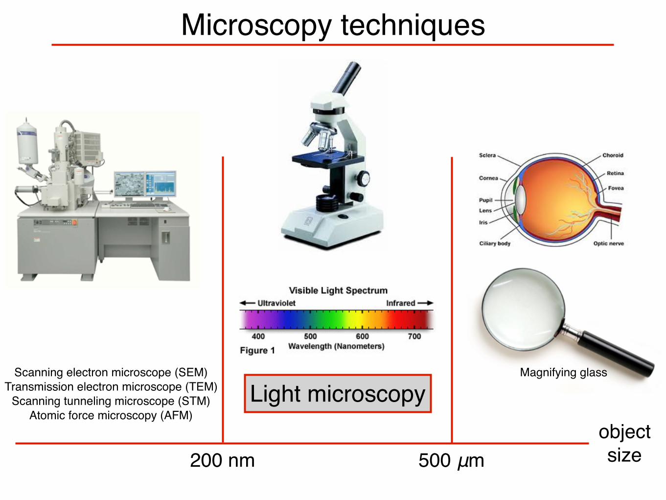
Microscopy techniques

objectsize200 nm 500 μm

Scanning electron microscope (SEM)Transmission electron microscope (TEM)

Scanning tunneling microscope (STM)Atomic force microscopy (AFM)

Light microscopyMagnifying glass

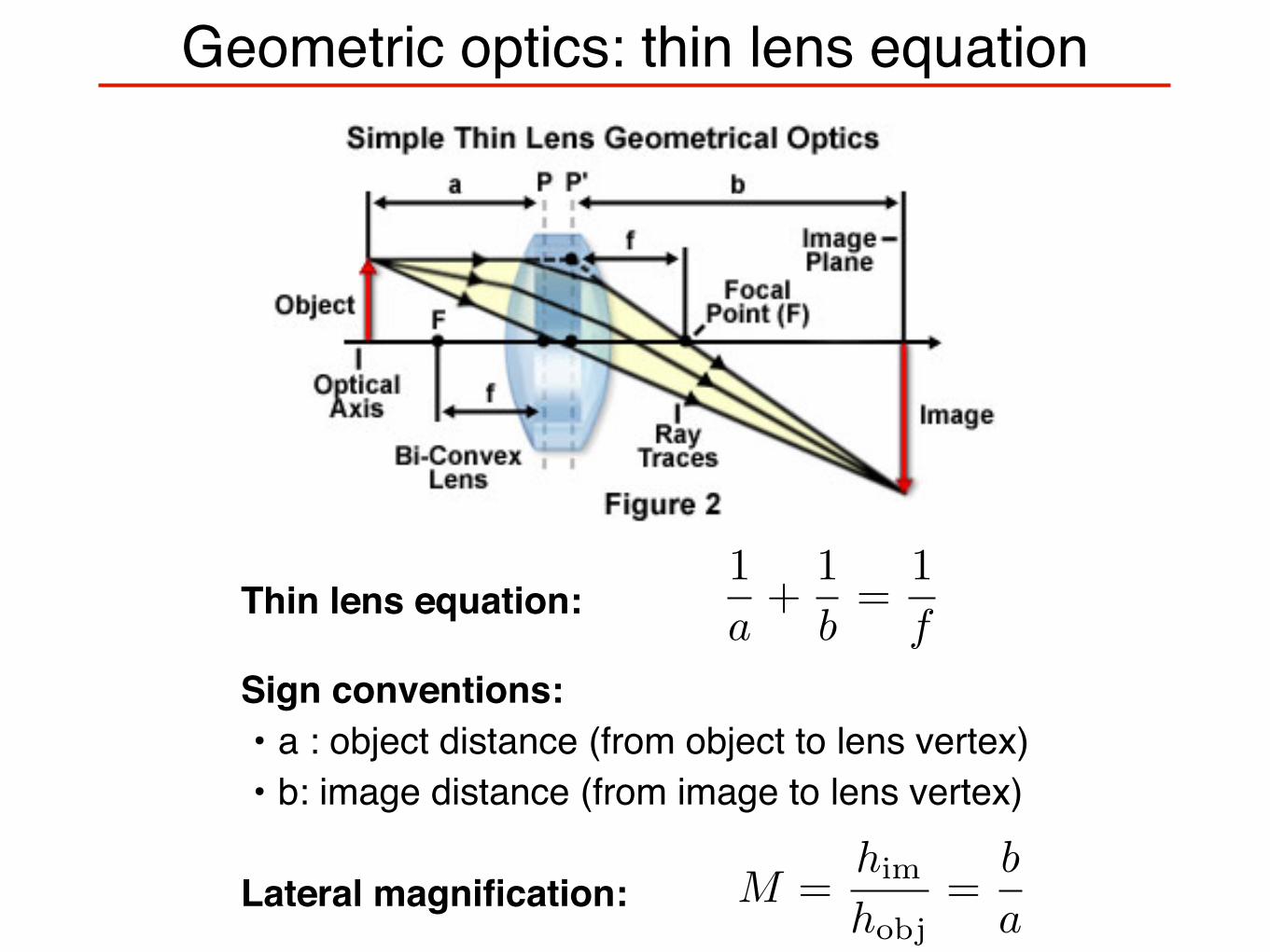
M =

him

hobj

=

b

a

Geometric optics: thin lens equation

1

a+

1

b=

1

fThin lens equation:

Sign conventions:• a : object distance (from object to lens vertex)• b: image distance (from image to lens vertex)

Lateral magnification:

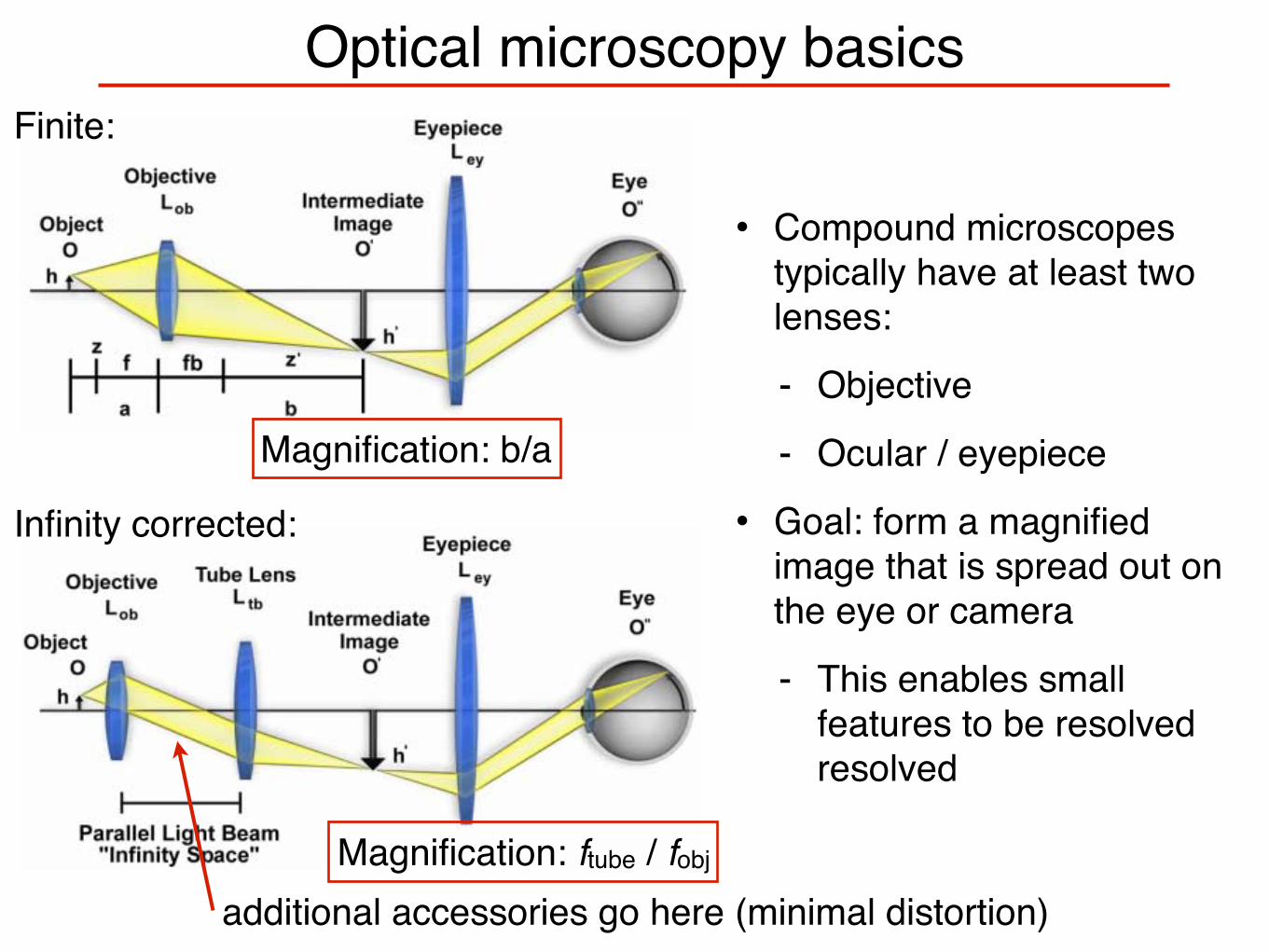
Optical microscopy basics

• Compound microscopes typically have at least two lenses:

- Objective

- Ocular / eyepiece

• Goal: form a magnified image that is spread out on the eye or camera

- This enables small features to be resolved resolved

OPTICAL MICROSCOPY Davidson and Abramowitz

2

of a conventional finite tube length microscope (17). Anobject (O) of height h is being imaged on the retina ofthe eye at O”. The objective lens (Lob) projects a realand inverted image of O magnified to the size O’ into theintermediate image plane of the microscope. This occursat the eyepiece diaphragm, at the fixed distance fb + z’behind the objective. In this diagram, fb represents theback focal length of the objective and z’ is the optical tubelength of the microscope. The aerial intermediate imageat O’ is further magnified by the microscope eyepiece(Ley) and produces an erect image of the object at O” onthe retina, which appears inverted to the microscopist.The magnification factor of the object is calculated byconsidering the distance (a) between the object (O) andthe objective (Lob) , and the front focal length of theobjective lens (f). The object is placed a short distance(z) outside of the objective’s front focal length (f), suchthat z + f = a. The intermediate image of the object, O’, islocated at distance b, which equals the back focal lengthof the objective (fb) plus (z’), the optical tube length ofthe microscope. Magnification of the object at theintermediate image plane equals h’. The image height atthis position is derived by multiplying the microscopetube length (b) by the object height (h), and dividing thisby the distance of the object from the objective: h’ = (h xb)/a. From this argument, we can conclude that the lateralor transverse magnification of the objective is equal to afactor of b/a (also equal to f/z and z’/fb), the back focallength of the objective divided by the distance of the objectfrom the objective. The image at the intermediate plane(h’) is further magnified by a factor of 25 centimeters(called the near distance to the eye) divided by the focallength of the eyepiece. Thus, the total magnification ofthe microscope is equal to the magnification by theobjective times that of the eyepiece. The visual image(virtual) appears to the observer as if it were 10 inchesaway from the eye.

Most objectives are corrected to work within a narrowrange of image distances, and many are designed to workonly in specifically corrected optical systems withmatching eyepieces. The magnification inscribed on theobjective barrel is defined for the tube length of themicroscope for which the objective was designed.

The lower portion of Figure 1 illustrates the opticaltrain using ray traces of an infinity-corrected microscopesystem. The components of this system are labeled in asimilar manner to the finite-tube length system for easycomparison. Here, the magnification of the objective isthe ratio h’/h, which is determined by the tube lens (Ltb).Note the infinity space that is defined by parallel lightbeams in every azimuth between the objective and the tubelens. This is the space used by microscope manufacturersto add accessories such as vertical illuminators, DIC

prisms, polarizers, retardation plates, etc., with muchsimpler designs and with little distortion of the image(18). The magnification of the objective in the infinity-corrected system equals the focal length of the tube lensdivided by the focal length of the objective.

Fundamentals of Image FormationIn the optical microscope, when light from the

microscope lamp passes through the condenser and thenthrough the specimen (assuming the specimen is a lightabsorbing specimen), some of the light passes both aroundand through the specimen undisturbed in its path. Suchlight is called direct light or undeviated light. Thebackground light (often called the surround) passingaround the specimen is also undeviated light.

Some of the light passing through the specimen isdeviated when it encounters parts of the specimen. Suchdeviated light (as you will subsequently learn, calleddiffracted light) is rendered one-half wavelength or 180

Figure 1. Optical trains of finite-tube and infinity-correctedmicroscope systems. (Upper) Ray traces of the optical trainrepresenting a theoretical finite-tube length microscope. The object(O) is a distance (a) from the objective (Lob) and projects anintermediate image (O’) at the finite tube length (b), which is furthermagnified by the eyepiece (Ley) and then projected onto the retinaat O’’. (Lower) Ray traces of the optical train representing atheoretical infinity-corrected microscope system.

OPTICAL MICROSCOPY Davidson and Abramowitz

2

of a conventional finite tube length microscope (17). Anobject (O) of height h is being imaged on the retina ofthe eye at O”. The objective lens (Lob) projects a realand inverted image of O magnified to the size O’ into theintermediate image plane of the microscope. This occursat the eyepiece diaphragm, at the fixed distance fb + z’behind the objective. In this diagram, fb represents theback focal length of the objective and z’ is the optical tubelength of the microscope. The aerial intermediate imageat O’ is further magnified by the microscope eyepiece(Ley) and produces an erect image of the object at O” onthe retina, which appears inverted to the microscopist.The magnification factor of the object is calculated byconsidering the distance (a) between the object (O) andthe objective (Lob) , and the front focal length of theobjective lens (f). The object is placed a short distance(z) outside of the objective’s front focal length (f), suchthat z + f = a. The intermediate image of the object, O’, islocated at distance b, which equals the back focal lengthof the objective (fb) plus (z’), the optical tube length ofthe microscope. Magnification of the object at theintermediate image plane equals h’. The image height atthis position is derived by multiplying the microscopetube length (b) by the object height (h), and dividing thisby the distance of the object from the objective: h’ = (h xb)/a. From this argument, we can conclude that the lateralor transverse magnification of the objective is equal to afactor of b/a (also equal to f/z and z’/fb), the back focallength of the objective divided by the distance of the objectfrom the objective. The image at the intermediate plane(h’) is further magnified by a factor of 25 centimeters(called the near distance to the eye) divided by the focallength of the eyepiece. Thus, the total magnification ofthe microscope is equal to the magnification by theobjective times that of the eyepiece. The visual image(virtual) appears to the observer as if it were 10 inchesaway from the eye.

Most objectives are corrected to work within a narrowrange of image distances, and many are designed to workonly in specifically corrected optical systems withmatching eyepieces. The magnification inscribed on theobjective barrel is defined for the tube length of themicroscope for which the objective was designed.

The lower portion of Figure 1 illustrates the opticaltrain using ray traces of an infinity-corrected microscopesystem. The components of this system are labeled in asimilar manner to the finite-tube length system for easycomparison. Here, the magnification of the objective isthe ratio h’/h, which is determined by the tube lens (Ltb).Note the infinity space that is defined by parallel lightbeams in every azimuth between the objective and the tubelens. This is the space used by microscope manufacturersto add accessories such as vertical illuminators, DIC

prisms, polarizers, retardation plates, etc., with muchsimpler designs and with little distortion of the image(18). The magnification of the objective in the infinity-corrected system equals the focal length of the tube lensdivided by the focal length of the objective.

Fundamentals of Image FormationIn the optical microscope, when light from the

microscope lamp passes through the condenser and thenthrough the specimen (assuming the specimen is a lightabsorbing specimen), some of the light passes both aroundand through the specimen undisturbed in its path. Suchlight is called direct light or undeviated light. Thebackground light (often called the surround) passingaround the specimen is also undeviated light.

Some of the light passing through the specimen isdeviated when it encounters parts of the specimen. Suchdeviated light (as you will subsequently learn, calleddiffracted light) is rendered one-half wavelength or 180

Figure 1. Optical trains of finite-tube and infinity-correctedmicroscope systems. (Upper) Ray traces of the optical trainrepresenting a theoretical finite-tube length microscope. The object(O) is a distance (a) from the objective (Lob) and projects anintermediate image (O’) at the finite tube length (b), which is furthermagnified by the eyepiece (Ley) and then projected onto the retinaat O’’. (Lower) Ray traces of the optical train representing atheoretical infinity-corrected microscope system.

additional accessories go here (minimal distortion)

Finite:

Infinity corrected:

Magnification: b/a

Magnification: ftube / fobj

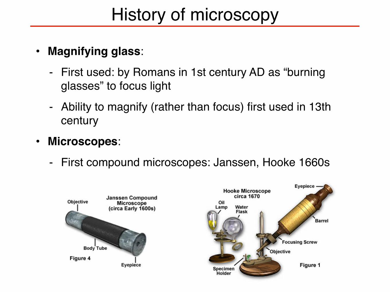
History of microscopy

• Magnifying glass:

- First used: by Romans in 1st century AD as “burning glasses” to focus light

- Ability to magnify (rather than focus) first used in 13th century

• Microscopes:

- First compound microscopes: Janssen, Hooke 1660s

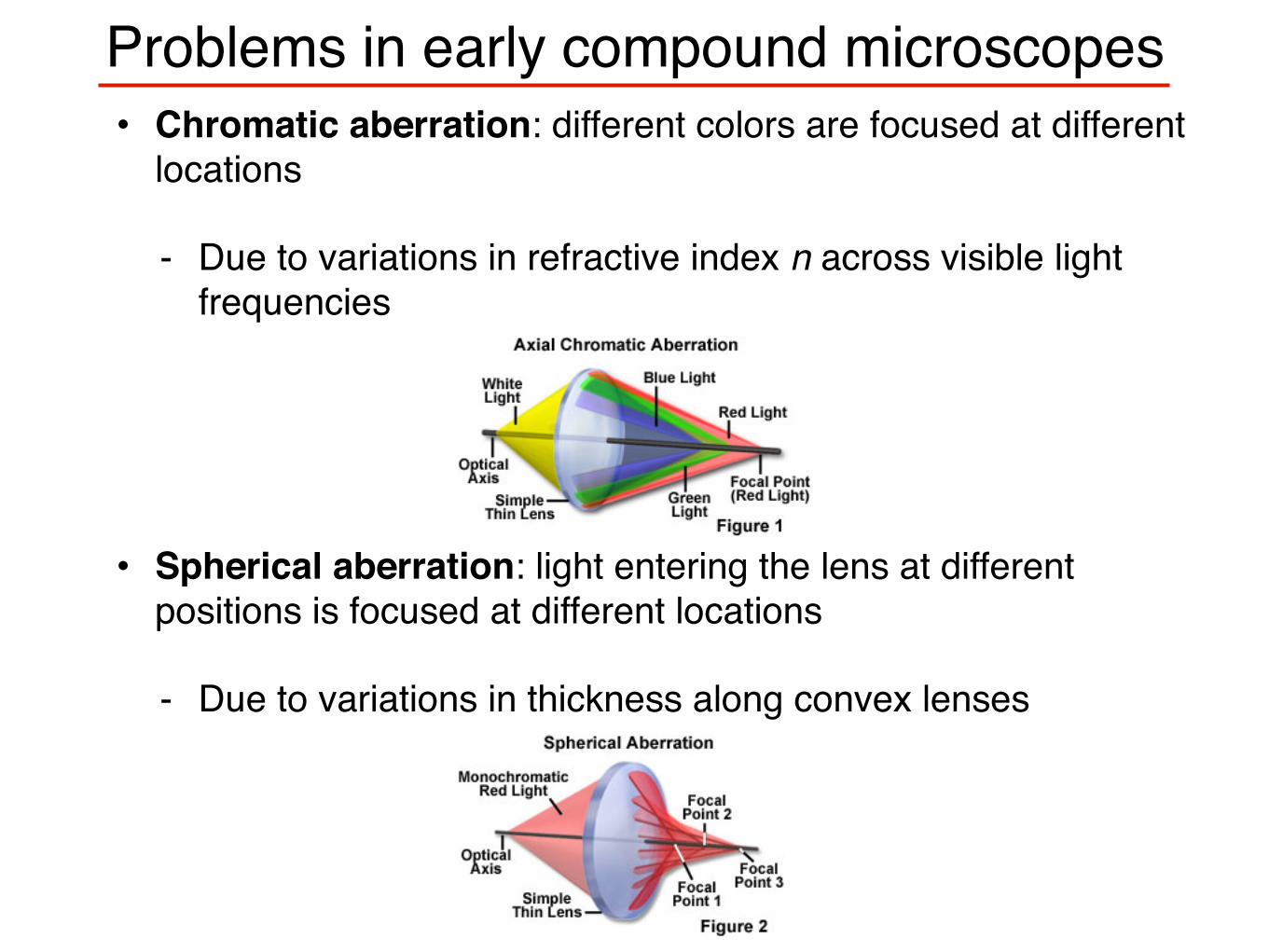
Problems in early compound microscopes• Chromatic aberration: different colors are focused at different

locations

- Due to variations in refractive index n across visible light frequencies

• Spherical aberration: light entering the lens at different positions is focused at different locations

- Due to variations in thickness along convex lenses

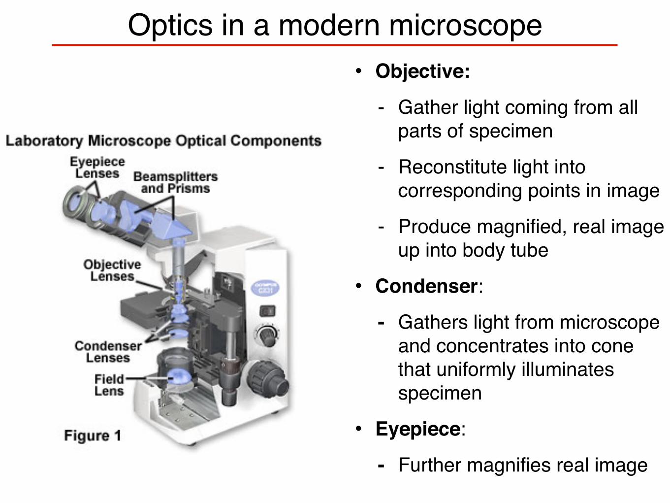
Optics in a modern microscope• Objective:

- Gather light coming from all parts of specimen

- Reconstitute light into corresponding points in image

- Produce magnified, real image up into body tube

• Condenser:

- Gathers light from microscope and concentrates into cone that uniformly illuminates specimen

• Eyepiece:

- Further magnifies real image

Objective lensesOPTICAL MICROSCOPY Davidson and Abramowitz

10

objectives yield their best results with light passed througha green filter (often an interference filter) and using blackand white film when these objectives are employed forphotomicrography. The lack of correction for flatnessof field (or field curvature) further hampers achromatobjectives. In the past few years, most manufacturers havebegun providing flat field corrections for achromatobjectives and have given these corrected objectives thename of plan achromats.

The next higher level of correction and cost is foundin objectives called fluorites or semi-apochromatsillustrated by the center objective in Figure 8. This figuredepicts three major classes of objectives: The achromatswith the least amount of correction, as discussed above;the fluorites (or semi-apochromats) that have additionalspherical corrections; and, the apochromats that are themost highly corrected objectives available. Fluoriteobjectives are produced from advanced glass formulationsthat contain materials such as fluorspar or newer syntheticsubstitutes (5). These new formulations allow for greatlyimproved correction of optical aberration. Similar to theachromats, the fluorite objectives are also correctedchromatically for red and blue light. In addition, thefluorites are also corrected spherically for two colors.The superior correction of fluorite objectives comparedto achromats enables these objectives to be made with ahigher numerical aperture, resulting in brighter images.Fluorite objectives also have better resolving power thanachromats and provide a higher degree of contrast, makingthem better suited than achromats for colorphotomicrography in white light.

The highest level of correction (and expense) is foundin apochromatic objectives, which are correctedchromatically for three colors (red, green, and blue),

almost eliminating chromatic aberration, and are correctedspherically for two colors. Apochromatic objectives arethe best choice for color photomicrography in white light.Because of their high level of correction, apochromatobjectives usually have, for a given magnification, highernumerical apertures than do achromats or fluorites. Manyof the newer high-end fluorite and apochromat objectivesare corrected for four colors chromatically and fourcolors spherically.

All three types of objectives suffer from pronouncedfield curvature and project images that are curved ratherthan flat. To overcome this inherent condition, lensdesigners have produced flat-field corrected objectivesthat yield flat images. Such lenses are called planachromats, plan fluorites, or plan apochromats, andalthough this degree of correction is expensive, theseobjectives are now in routine use due to their value inphotomicrography.

Uncorrected field curvature is the most severeaberration in higher power fluorite and apochromatobjectives, and it was tolerated as an unavoidable artifactfor many years. During routine use, the viewfield wouldhave to be continuously refocused between the center andthe edges to capture all specimen details. The introductionof flat-field (plan) correction to objectives perfected theiruse for photomicrography and video microscopy, andtoday these corrections are standard in both general useand high-performance objectives. Correction for field

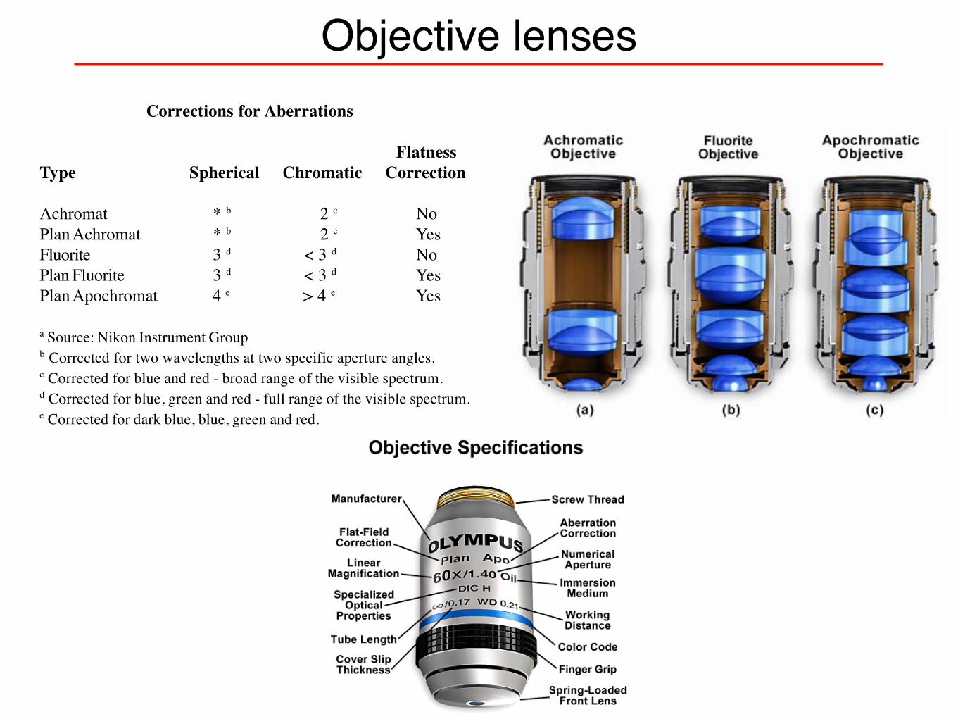
Table 2 Objective Lens Types and Corrections a

Corrections for Aberrations

FlatnessType Spherical Chromatic Correction

Achromat * b 2 c NoPlan Achromat * b 2 c YesFluorite 3 d < 3 d NoPlan Fluorite 3 d < 3 d YesPlan Apochromat 4 e > 4 e Yes

a Source: Nikon Instrument Groupb Corrected for two wavelengths at two specific aperture angles.c Corrected for blue and red - broad range of the visible spectrum.d Corrected for blue, green and red - full range of the visible spectrum.e Corrected for dark blue, blue, green and red.

Figure 8. Levels of optical correction for aberration in commercialobjectives. (a) Achromatic objectives, the lowest level of correction,contain two doublets and a single front lens; (b) Fluorites or semi-apochromatic objectives, a medium level of correction, containthree doublets, a meniscus lens, and a single front lens; and (c)Apochromatic objectives, the highest level of correction, contain atriplet, two doublets, a meniscus lens, and a single hemisphericalfront lens.

OPTICAL MICROSCOPY Davidson and Abramowitz

10

objectives yield their best results with light passed througha green filter (often an interference filter) and using blackand white film when these objectives are employed forphotomicrography. The lack of correction for flatnessof field (or field curvature) further hampers achromatobjectives. In the past few years, most manufacturers havebegun providing flat field corrections for achromatobjectives and have given these corrected objectives thename of plan achromats.

The next higher level of correction and cost is foundin objectives called fluorites or semi-apochromatsillustrated by the center objective in Figure 8. This figuredepicts three major classes of objectives: The achromatswith the least amount of correction, as discussed above;the fluorites (or semi-apochromats) that have additionalspherical corrections; and, the apochromats that are themost highly corrected objectives available. Fluoriteobjectives are produced from advanced glass formulationsthat contain materials such as fluorspar or newer syntheticsubstitutes (5). These new formulations allow for greatlyimproved correction of optical aberration. Similar to theachromats, the fluorite objectives are also correctedchromatically for red and blue light. In addition, thefluorites are also corrected spherically for two colors.The superior correction of fluorite objectives comparedto achromats enables these objectives to be made with ahigher numerical aperture, resulting in brighter images.Fluorite objectives also have better resolving power thanachromats and provide a higher degree of contrast, makingthem better suited than achromats for colorphotomicrography in white light.

The highest level of correction (and expense) is foundin apochromatic objectives, which are correctedchromatically for three colors (red, green, and blue),

almost eliminating chromatic aberration, and are correctedspherically for two colors. Apochromatic objectives arethe best choice for color photomicrography in white light.Because of their high level of correction, apochromatobjectives usually have, for a given magnification, highernumerical apertures than do achromats or fluorites. Manyof the newer high-end fluorite and apochromat objectivesare corrected for four colors chromatically and fourcolors spherically.

All three types of objectives suffer from pronouncedfield curvature and project images that are curved ratherthan flat. To overcome this inherent condition, lensdesigners have produced flat-field corrected objectivesthat yield flat images. Such lenses are called planachromats, plan fluorites, or plan apochromats, andalthough this degree of correction is expensive, theseobjectives are now in routine use due to their value inphotomicrography.

Uncorrected field curvature is the most severeaberration in higher power fluorite and apochromatobjectives, and it was tolerated as an unavoidable artifactfor many years. During routine use, the viewfield wouldhave to be continuously refocused between the center andthe edges to capture all specimen details. The introductionof flat-field (plan) correction to objectives perfected theiruse for photomicrography and video microscopy, andtoday these corrections are standard in both general useand high-performance objectives. Correction for field

Table 2 Objective Lens Types and Corrections a

Corrections for Aberrations

FlatnessType Spherical Chromatic Correction

Achromat * b 2 c NoPlan Achromat * b 2 c YesFluorite 3 d < 3 d NoPlan Fluorite 3 d < 3 d YesPlan Apochromat 4 e > 4 e Yes

a Source: Nikon Instrument Groupb Corrected for two wavelengths at two specific aperture angles.c Corrected for blue and red - broad range of the visible spectrum.d Corrected for blue, green and red - full range of the visible spectrum.e Corrected for dark blue, blue, green and red.

Figure 8. Levels of optical correction for aberration in commercialobjectives. (a) Achromatic objectives, the lowest level of correction,contain two doublets and a single front lens; (b) Fluorites or semi-apochromatic objectives, a medium level of correction, containthree doublets, a meniscus lens, and a single front lens; and (c)Apochromatic objectives, the highest level of correction, contain atriplet, two doublets, a meniscus lens, and a single hemisphericalfront lens.

OPTICAL MICROSCOPY Davidson and Abramowitz

11

curvature adds a considerable number of lens elementsto the objective, in many cases as many as four additionallenses. This significant increase in the number of lenselements for plan correction also occurs in alreadyovercrowded fluorite and apochromat objectives,frequently resulting in a tight fit of lens elements withinthe objective barrel (4, 5, 18).

Before the transition to infinity-corrected optics, mostobjectives were specifically designed to be used with aset of oculars termed compensating eyepieces. Anexample is the former use of compensating eyepieces withhighly corrected high numerical aperture objectives tohelp eliminate lateral chromatic aberration.

There is a wealth of information inscribed on thebarrel of each objective, which can be broken down intoseveral categories (illustrated in Figure 9). These includethe linear magnification, numerical aperture value, opticalcorrections, microscope body tube length, the type ofmedium the objective is designed for, and other criticalfactors in deciding if the objective will perform as needed.Additional information is outlined below (17):

· Optical Corrections: These are usually abbreviatedas Achro (achromat), Apo (apochromat), and Fl, Fluar,Fluor, Neofluar, or Fluotar (fluorite) for betterspherical and chromatic corrections, and as Plan, Pl, EF,Acroplan, Plan Apo or Plano for field curvaturecorrections. Other common abbreviations are: ICS(infinity corrected system) and UIS (universal infinitysystem), N and NPL (normal field of view plan),

Ultrafluar (fluorite objective with glass that istransparent down to 250 nanometers), and CF and CFI(chrome-free; chrome-free infinity).

· Numerical Aperture: This is a critical value thatindicates the light acceptance angle, which in turndetermines the light gathering power, the resolving power,and depth of field of the objective. Some objectivesspecifically designed for transmitted light fluorescenceand darkfield imaging are equipped with an internal irisdiaphragm that allows for adjustment of the effectivenumerical aperture. Designation abbreviations for theseobjectives include I, Iris, W/Iris.

· Mechanical Tube Length: This is the length of themicroscope body tube between the nosepiece opening,where the objective is mounted, and the top edge of theobservation tubes where the oculars (eyepieces) areinserted. Tube length is usually inscribed on the objectiveas the size in number of millimeters (160, 170, 210, etc.)for fixed lengths, or the infinity symbol ( ) for infinity-corrected tube lengths.

· Cover Glass Thickness: Most transmitted lightobjectives are designed to image specimens that arecovered by a cover glass (or cover slip). The thicknessof these small glass plates is now standardized at 0.17mm for most applications, although there is some variationin thickness within a batch of cover slips. For this reason,some of the high numerical aperture dry objectives havea correction collar adjustment of the internal lenselements to compensate for this variation (Figure 10).Abbreviations for the correction collar adjustment includeCorr, w/Corr, and CR, although the presence of amovable, knurled collar and graduated scale is also an

Figure 9. Specifications engraved on the barrel of a typicalmicroscope objective. These include the manufacturer, correctionlevels, magnification, numerical aperture, immersion requirements,tube length, working distance, and specialized optical properties.

Figure 10. Objective with three lens groups and correction collarfor varying cover glass thicknesses. (a) Lens group 2 rotated tothe forward position within the objective. This position is used forthe thinnest cover slips. (b) Lens group 2 rotated to the rearwardposition within the objective. This position is used for the thickestcoverslips.

∞∞∞∞∞

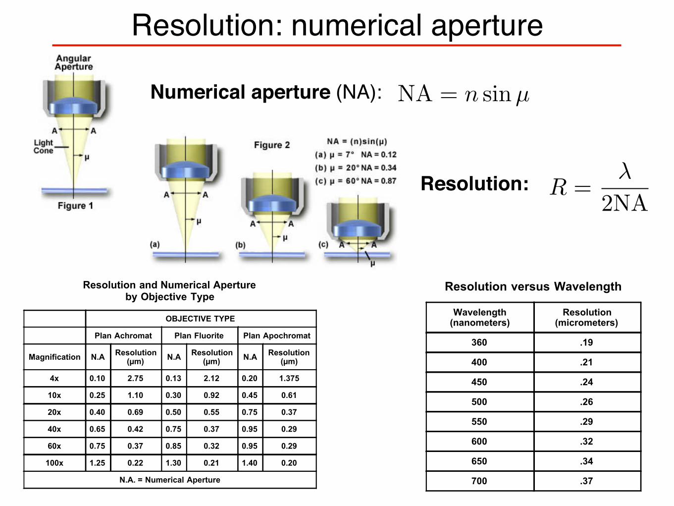
NA = n sinµ

R =λ

2NA

Resolution: numerical aperture

Numerical aperture (NA):

capable of resolving details to a greater degree than are the longer wavelengths. There are severalequations that have been derived to express the relationship between numerical aperture, wavelength, andresolution:

R = � / 2NA (1)

R = 0.61� / NA (2)

R = 1.22� / (NA(obj) + NA(cond)) (3)

Where R is resolution (the smallest resolvable distance between two objects), NA equals numericalaperture, � equals wavelength, NA(obj) equals the objective numerical aperture, and NA(Cond) is thecondenser numerical aperture. Notice that equation (1) and (2) differ by the multiplication factor, which is0.5 for equation (1) and 0.61 for equation (2). These equations are based upon a number of factors(including a variety of theoretical calculations made by optical physicists) to account for the behavior ofobjectives and condensers, and should not be considered an absolute value of any one general physicallaw. In some instances, such as confocal and fluorescence microscopy, the resolution may actuallyexceed the limits placed by any one of these three equations. Other factors, such as low specimencontrast and improper illumination may serve to lower resolution and, more often than not, the real-worldmaximum value of R (about 0.25 �m using a mid-spectrum wavelength of 550 nanometers) and anumerical aperture of 1.35 to 1.40 are not realized in practice. Table 2 provides a list resolution (R) andnumerical aperture (NA) by objective magnification and correction.

Resolution and Numerical Apertureby Objective Type

OBJECTIVE TYPE

Plan Achromat Plan Fluorite Plan Apochromat

Magnification N.A Resolution(�m) N.A Resolution

(�m) N.A Resolution(�m)

4x 0.10 2.75 0.13 2.12 0.20 1.375

10x 0.25 1.10 0.30 0.92 0.45 0.61

20x 0.40 0.69 0.50 0.55 0.75 0.37

40x 0.65 0.42 0.75 0.37 0.95 0.29

60x 0.75 0.37 0.85 0.32 0.95 0.29

100x 1.25 0.22 1.30 0.21 1.40 0.20

N.A. = Numerical Aperture

Table 2

When the microscope is in perfect alignment and has the objectives appropriately matched with thesubstage condenser, then we can substitute the numerical aperture of the objective into equations (1) and(2), with the added result that equation (3) reduces to equation (2). An important fact to note is thatmagnification does not appear as a factor in any of these equations, because only numerical aperture andwavelength of the illuminating light determine specimen resolution. As we have mentioned (and can beseen in the equations) the wavelength of light is an important factor in the resolution of a microscope.Shorter wavelengths yield higher resolution (lower values for R) and visa versa. The greatest resolvingpower in optical microscopy is realized with near-ultraviolet light, the shortest effective imagingwavelength. Near-ultraviolet light is followed by blue, then green, and finally red light in the ability toresolve specimen detail. Under most circumstances, microscopists use white light generated by atungsten-halogen bulb to illuminate the specimen. The visible light spectrum is centered at about 550nanometers, the dominant wavelength for green light (our eyes are most sensitive to green light). It is thiswavelength that was used to calculate resolution values in Table 2. The numerical aperture value is alsoimportant in these equations and higher numerical apertures will also produce higher resolution, as isevident in Table 2. The effect of the wavelength of light on resolution, at a fixed numerical aperture (0.95),is listed in Table 3.

Resolution versus Wavelength

Wavelength(nanometers)

Resolution(micrometers)

360 .19

400 .21

450 .24

500 .26

550 .29

600 .32

650 .34

700 .37

Table 3

When light from the various points of a specimen passes through the objective and is reconstituted as animage, the various points of the specimen appear in the image as small patterns (not points) known asAiry patterns. This phenomenon is caused by diffraction or scattering of the light as it passes through theminute parts and spaces in the specimen and the circular back aperture of the objective. The centralmaximum of the Airy patterns is often referred to as an Airy disk, which is defined as the region enclosedby the first minimum of the Airy pattern and contains 84 percent of the luminous energy. These Airy disksconsist of small concentric light and dark circles as illustrated in Figure 3. This figure shows Airy disks andtheir intensity distributions as a function of separation distance.

Figure 3(a) illustrates a hypothetical Airy disk that essentially consists of a diffraction pattern containing acentral maximum (typically termed a zeroth order maximum) surrounded by concentric 1st, 2nd, 3rd, etc.,order maxima of sequentially decreasing brightness that make up the intensity distribution. Two Airy disksand their intensity distributions at the limit of optical resolution are illustrated in Figure 3(b). In this part ofthe figure, the separation between the two disks exceeds their radii, and they are resolvable. The limit atwhich two Airy disks can be resolved into separate entities is often called the Rayleigh criterion. Figure3(c) shows two Airy disks and their intensity distributions in a situation where the center-to-center distancebetween the zeroth order maxima is less than the width of these maxima, and the two disks are notindividually resolvable by the Rayleigh criterion.

Airy Disk Size and Resolution

Explore how wavelength and numerical aperture control Airy disksize and resolution.

Start Tutorial »

The smaller the Airy disks projected by an objective in forming the image, the more detail of the specimenthat becomes discernible. Objectives of higher correction (fluorites and apochromats) produce smaller Airydisks than do objectives of lower correction. In a similar manner, objectives that have a higher numericalaperture are also capable of producing smaller Airy disks. This is the primary reason that objectives ofhigh numerical aperture and total correction for optical aberration can distinguish finer detail in thespecimen.

Figure 4 illustrates the effect of numerical aperture on the size of Airy disks imaged with a series ofhypothetical objectives of the same focal length, but differing numerical apertures. With small numericalapertures, the Airy disk size is large, as shown in Figure 4(a). As the numerical aperture and light coneangle of an objective increases however, the size of the Airy disk decreases as illustrated in Figure 4(b)and Figure 4(c). The resulting image at the eyepiece diaphragm level is actually a mosaic of Airy diskswhich we perceive as light and dark. Where two disks are too close together so that their central spots

capable of resolving details to a greater degree than are the longer wavelengths. There are severalequations that have been derived to express the relationship between numerical aperture, wavelength, andresolution:

R = � / 2NA (1)

R = 0.61� / NA (2)

R = 1.22� / (NA(obj) + NA(cond)) (3)

Where R is resolution (the smallest resolvable distance between two objects), NA equals numericalaperture, � equals wavelength, NA(obj) equals the objective numerical aperture, and NA(Cond) is thecondenser numerical aperture. Notice that equation (1) and (2) differ by the multiplication factor, which is0.5 for equation (1) and 0.61 for equation (2). These equations are based upon a number of factors(including a variety of theoretical calculations made by optical physicists) to account for the behavior ofobjectives and condensers, and should not be considered an absolute value of any one general physicallaw. In some instances, such as confocal and fluorescence microscopy, the resolution may actuallyexceed the limits placed by any one of these three equations. Other factors, such as low specimencontrast and improper illumination may serve to lower resolution and, more often than not, the real-worldmaximum value of R (about 0.25 �m using a mid-spectrum wavelength of 550 nanometers) and anumerical aperture of 1.35 to 1.40 are not realized in practice. Table 2 provides a list resolution (R) andnumerical aperture (NA) by objective magnification and correction.

Resolution and Numerical Apertureby Objective Type

OBJECTIVE TYPE

Plan Achromat Plan Fluorite Plan Apochromat

Magnification N.A Resolution(�m) N.A Resolution

(�m) N.A Resolution(�m)

4x 0.10 2.75 0.13 2.12 0.20 1.375

10x 0.25 1.10 0.30 0.92 0.45 0.61

20x 0.40 0.69 0.50 0.55 0.75 0.37

40x 0.65 0.42 0.75 0.37 0.95 0.29

60x 0.75 0.37 0.85 0.32 0.95 0.29

100x 1.25 0.22 1.30 0.21 1.40 0.20

N.A. = Numerical Aperture

Table 2

When the microscope is in perfect alignment and has the objectives appropriately matched with thesubstage condenser, then we can substitute the numerical aperture of the objective into equations (1) and(2), with the added result that equation (3) reduces to equation (2). An important fact to note is thatmagnification does not appear as a factor in any of these equations, because only numerical aperture andwavelength of the illuminating light determine specimen resolution. As we have mentioned (and can beseen in the equations) the wavelength of light is an important factor in the resolution of a microscope.Shorter wavelengths yield higher resolution (lower values for R) and visa versa. The greatest resolvingpower in optical microscopy is realized with near-ultraviolet light, the shortest effective imagingwavelength. Near-ultraviolet light is followed by blue, then green, and finally red light in the ability toresolve specimen detail. Under most circumstances, microscopists use white light generated by atungsten-halogen bulb to illuminate the specimen. The visible light spectrum is centered at about 550nanometers, the dominant wavelength for green light (our eyes are most sensitive to green light). It is thiswavelength that was used to calculate resolution values in Table 2. The numerical aperture value is alsoimportant in these equations and higher numerical apertures will also produce higher resolution, as isevident in Table 2. The effect of the wavelength of light on resolution, at a fixed numerical aperture (0.95),is listed in Table 3.

Resolution versus Wavelength

Wavelength(nanometers)

Resolution(micrometers)

360 .19

400 .21

450 .24

500 .26

550 .29

600 .32

650 .34

700 .37

Table 3

When light from the various points of a specimen passes through the objective and is reconstituted as animage, the various points of the specimen appear in the image as small patterns (not points) known asAiry patterns. This phenomenon is caused by diffraction or scattering of the light as it passes through theminute parts and spaces in the specimen and the circular back aperture of the objective. The centralmaximum of the Airy patterns is often referred to as an Airy disk, which is defined as the region enclosedby the first minimum of the Airy pattern and contains 84 percent of the luminous energy. These Airy disksconsist of small concentric light and dark circles as illustrated in Figure 3. This figure shows Airy disks andtheir intensity distributions as a function of separation distance.

Figure 3(a) illustrates a hypothetical Airy disk that essentially consists of a diffraction pattern containing acentral maximum (typically termed a zeroth order maximum) surrounded by concentric 1st, 2nd, 3rd, etc.,order maxima of sequentially decreasing brightness that make up the intensity distribution. Two Airy disksand their intensity distributions at the limit of optical resolution are illustrated in Figure 3(b). In this part ofthe figure, the separation between the two disks exceeds their radii, and they are resolvable. The limit atwhich two Airy disks can be resolved into separate entities is often called the Rayleigh criterion. Figure3(c) shows two Airy disks and their intensity distributions in a situation where the center-to-center distancebetween the zeroth order maxima is less than the width of these maxima, and the two disks are notindividually resolvable by the Rayleigh criterion.

Airy Disk Size and Resolution

Explore how wavelength and numerical aperture control Airy disksize and resolution.

Start Tutorial »

The smaller the Airy disks projected by an objective in forming the image, the more detail of the specimenthat becomes discernible. Objectives of higher correction (fluorites and apochromats) produce smaller Airydisks than do objectives of lower correction. In a similar manner, objectives that have a higher numericalaperture are also capable of producing smaller Airy disks. This is the primary reason that objectives ofhigh numerical aperture and total correction for optical aberration can distinguish finer detail in thespecimen.

Figure 4 illustrates the effect of numerical aperture on the size of Airy disks imaged with a series ofhypothetical objectives of the same focal length, but differing numerical apertures. With small numericalapertures, the Airy disk size is large, as shown in Figure 4(a). As the numerical aperture and light coneangle of an objective increases however, the size of the Airy disk decreases as illustrated in Figure 4(b)and Figure 4(c). The resulting image at the eyepiece diaphragm level is actually a mosaic of Airy diskswhich we perceive as light and dark. Where two disks are too close together so that their central spots

Resolution:

Improving resolution with immersion lenses

Basic idea: adding a higher-n medium between coverslip and lens reduces light deviation due to refraction

Two major types of immersion lenses:• oil: best for imaging samples with index of refraction close to glass• water: best for imaging biological samples in aqueous media

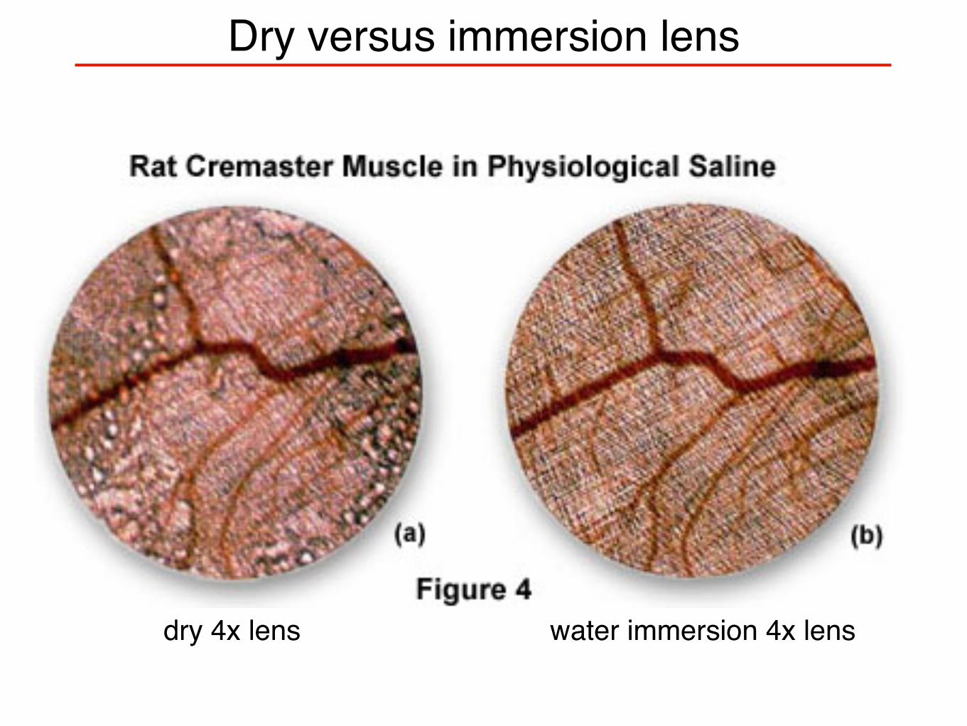
Dry versus immersion lens

dry 4x lens water immersion 4x lens

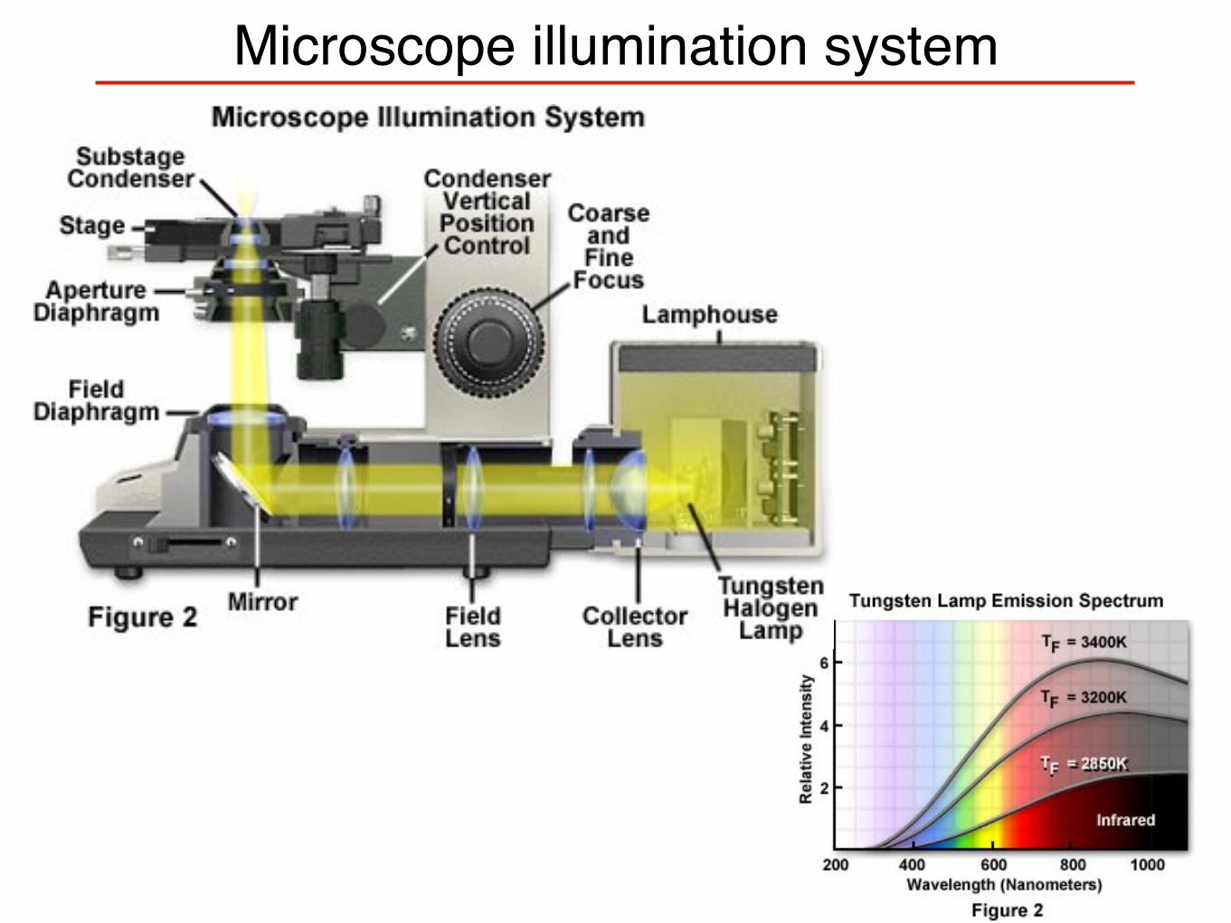
Microscope illumination system

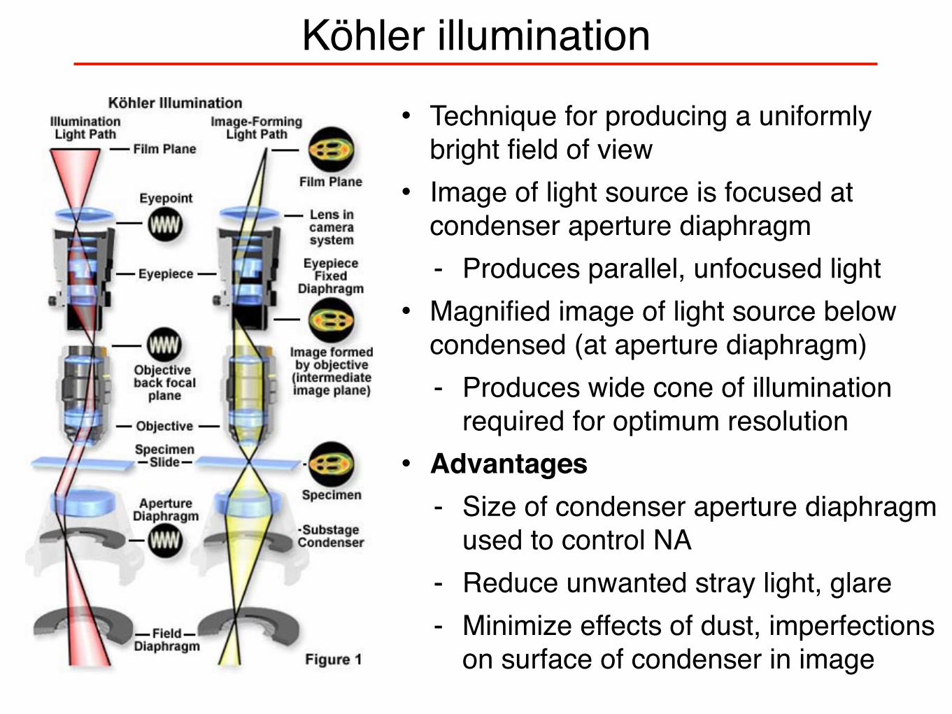
Köhler illumination• Technique for producing a uniformly

bright field of view• Image of light source is focused at

condenser aperture diaphragm - Produces parallel, unfocused light

• Magnified image of light source below condensed (at aperture diaphragm) - Produces wide cone of illumination

required for optimum resolution• Advantages

- Size of condenser aperture diaphragm used to control NA

- Reduce unwanted stray light, glare- Minimize effects of dust, imperfections

on surface of condenser in image

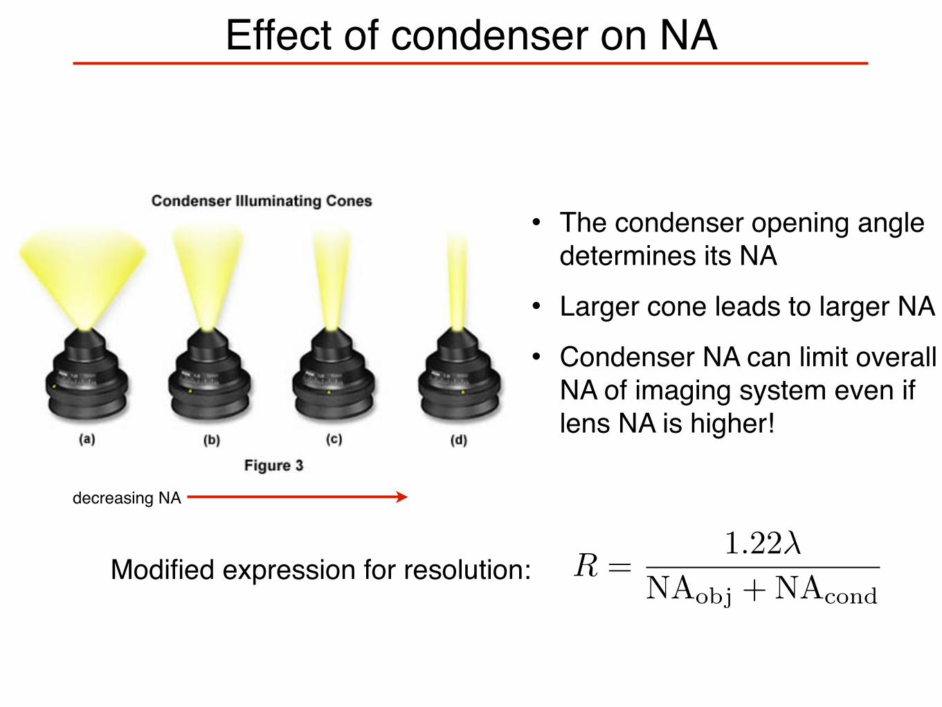
R =1.22λ

NAobj + NAcond

Effect of condenser on NA

decreasing NA

• The condenser opening angle determines its NA

• Larger cone leads to larger NA

• Condenser NA can limit overall NA of imaging system even if lens NA is higher!

Modified expression for resolution:

Choice of microscope geometryUpright Inverted

Especially useful for:• metallurgy• tissue and cell culture• microfluidics / PDMS• large samples

Most commonly found

Choice of light: transmitted vs. reflected

• Transmitted (diascopic):

- Light passes through the sample

- Used for thin, almost transparent samples (biology, porous media)

• Reflected (episcopic):

- Light is reflected from the sample

- Used for opaque objects like integrated circuits (materials science) and metals

Techniques for improving contrast

• Darkfield microscopy

• Phase contrast microscopy

• Differential interference contrast (DIC) microscopy

• Polarized light microscopy

• Fluorescence microscopy

• Confocal microscopy

• Hoffman modulation contrast microscopy

• Rheinberg illumination

Percent contrast:(BI − SI)

BI

× 100

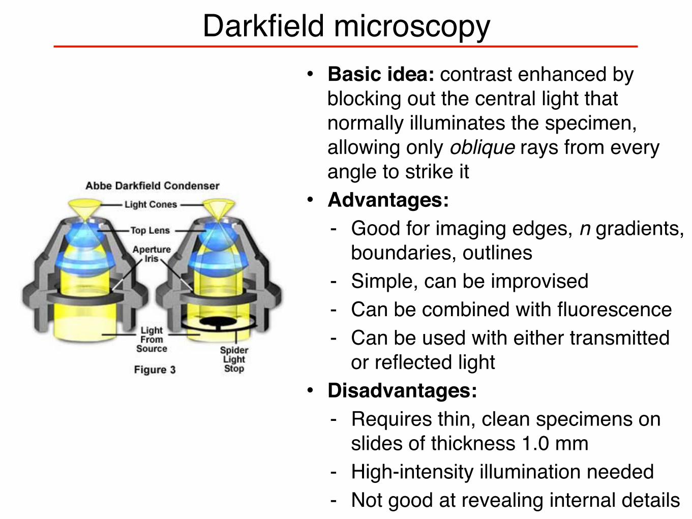
Darkfield microscopy• Basic idea: contrast enhanced by

blocking out the central light that normally illuminates the specimen, allowing only oblique rays from every angle to strike it• Advantages:

- Good for imaging edges, n gradients, boundaries, outlines

- Simple, can be improvised - Can be combined with fluorescence- Can be used with either transmitted

or reflected light• Disadvantages:

- Requires thin, clean specimens on slides of thickness 1.0 mm

- High-intensity illumination needed- Not good at revealing internal details

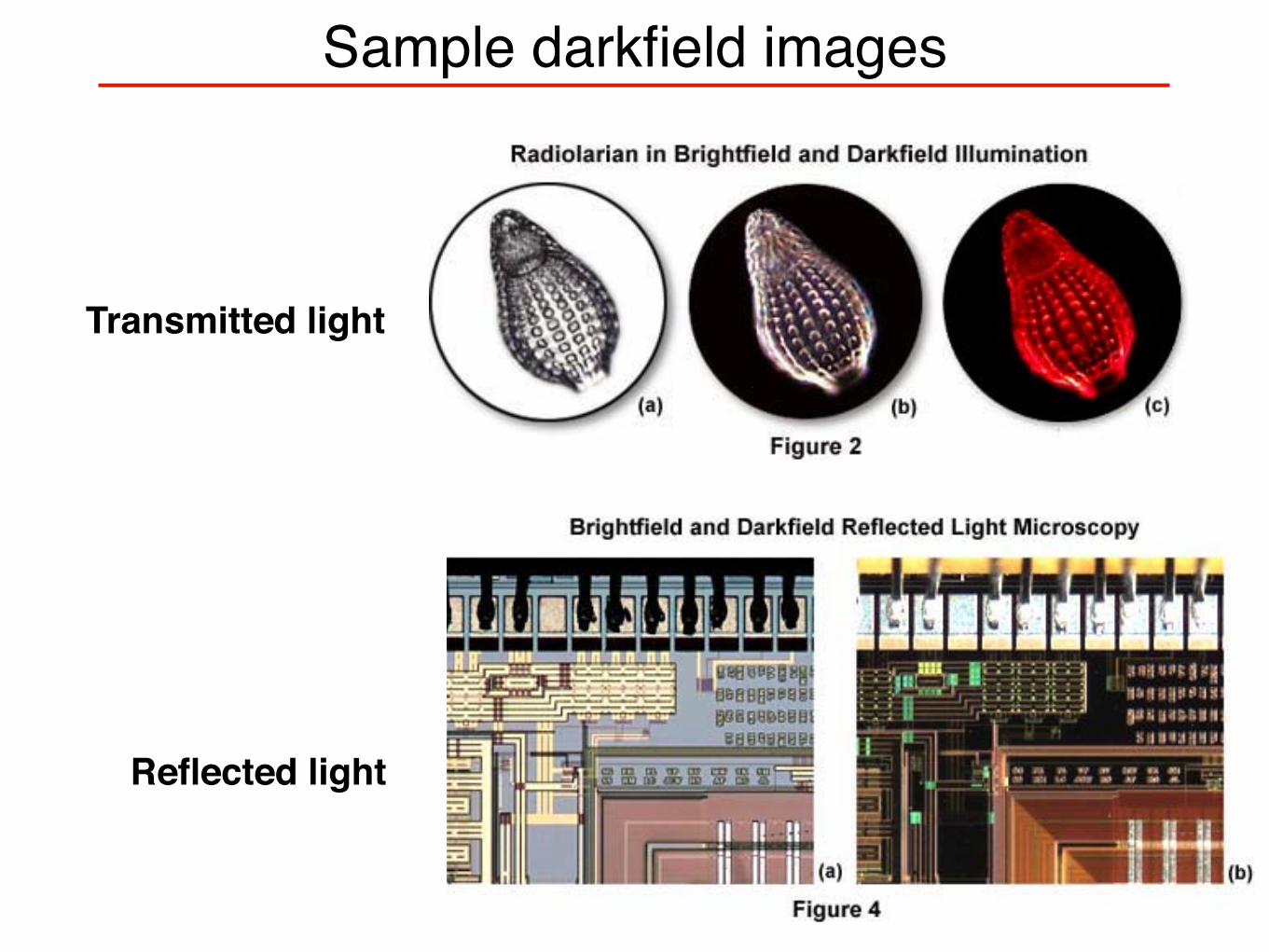
Sample darkfield images

Transmitted light

Reflected light

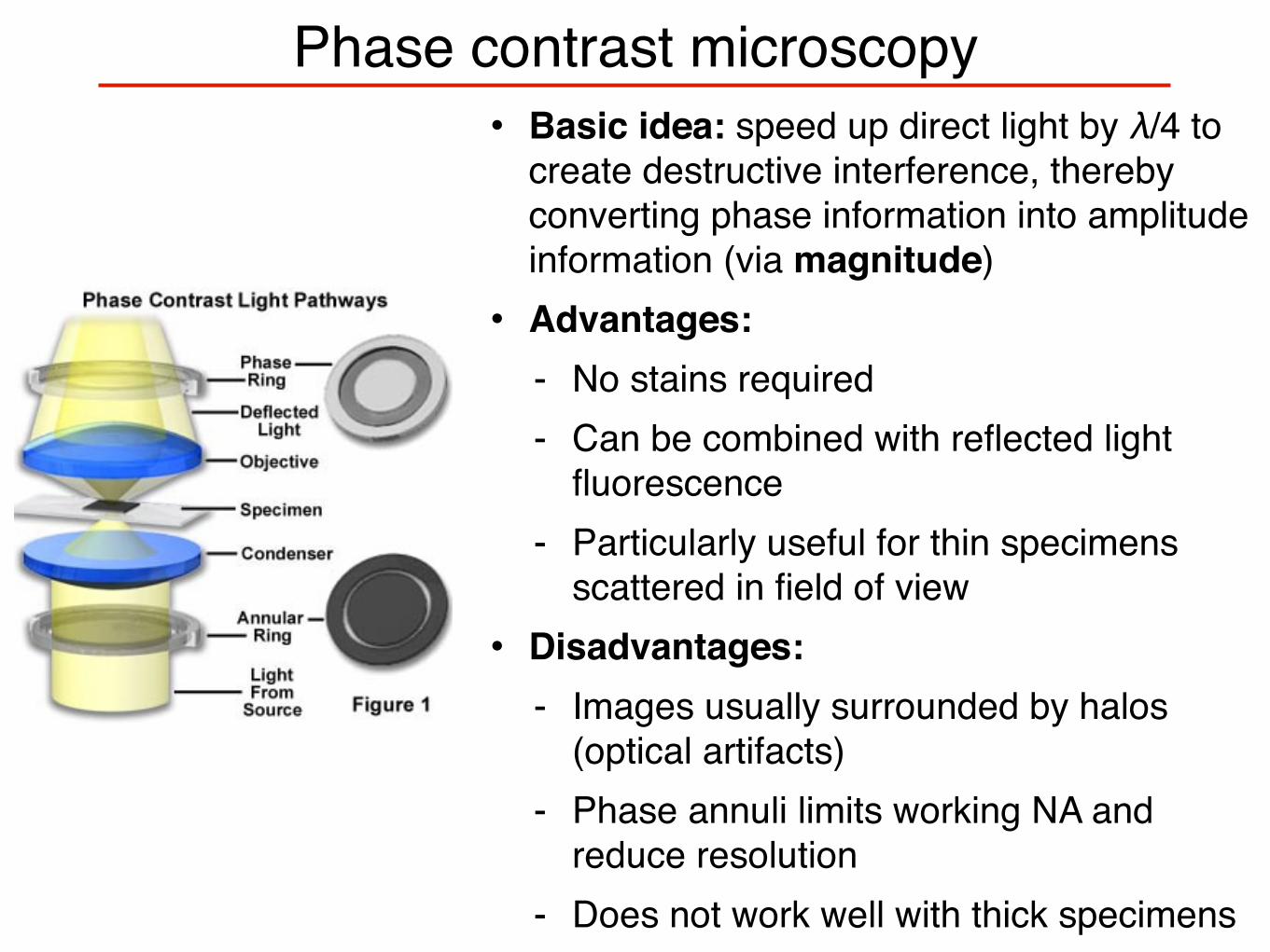
Phase contrast microscopy• Basic idea: speed up direct light by λ/4 to

create destructive interference, thereby converting phase information into amplitude information (via magnitude)• Advantages:

- No stains required- Can be combined with reflected light

fluorescence- Particularly useful for thin specimens

scattered in field of view• Disadvantages:

- Images usually surrounded by halos (optical artifacts)

- Phase annuli limits working NA and reduce resolution

- Does not work well with thick specimens

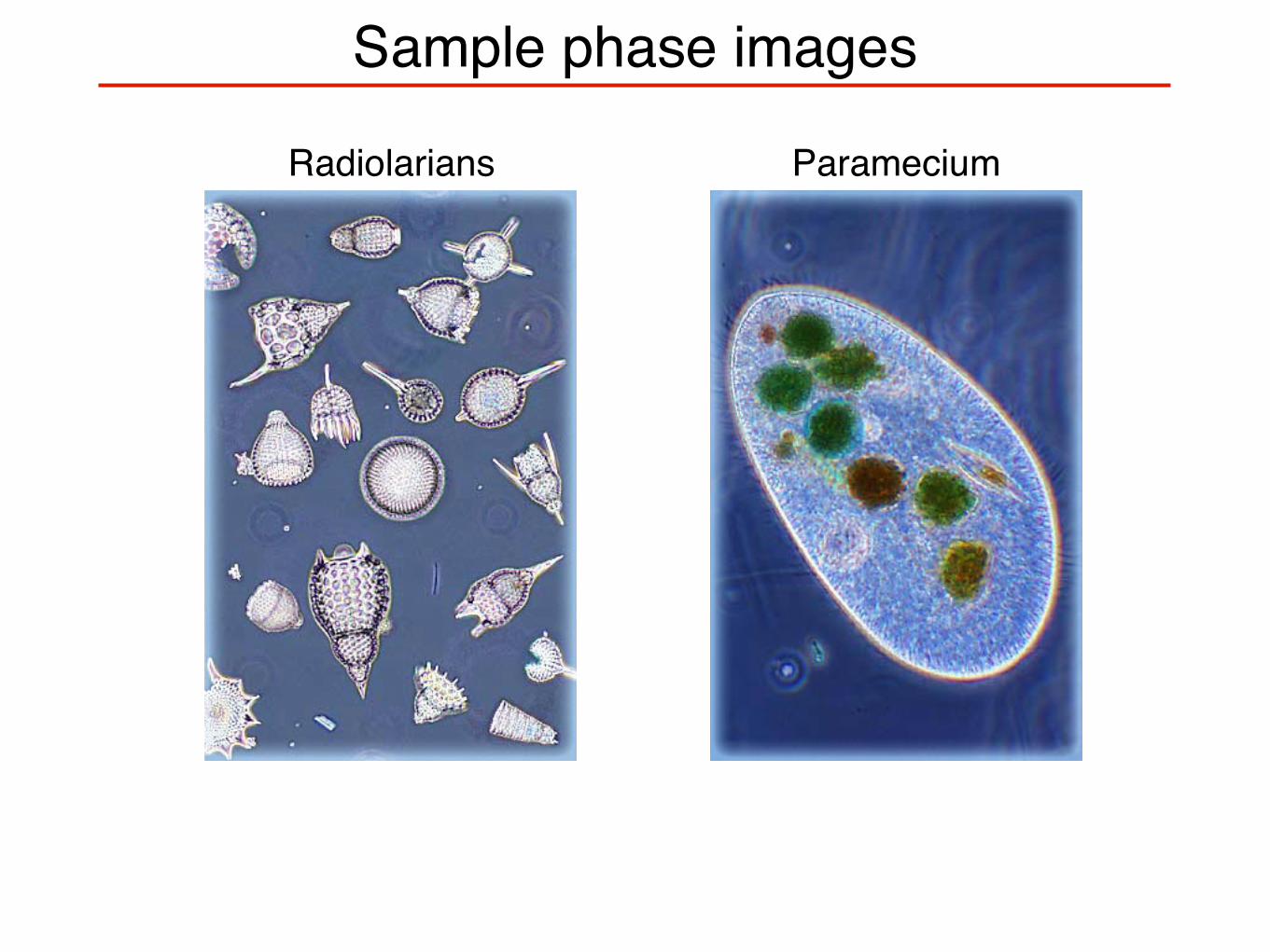
Sample phase images

Radiolarians Paramecium

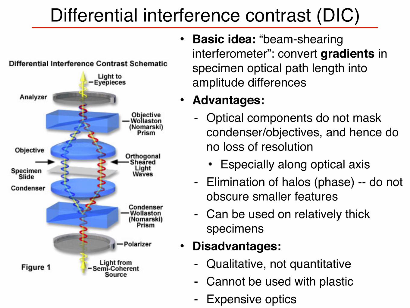
Differential interference contrast (DIC)• Basic idea: “beam-shearing

interferometer”: convert gradients in specimen optical path length into amplitude differences• Advantages:

- Optical components do not mask condenser/objectives, and hence do no loss of resolution• Especially along optical axis

- Elimination of halos (phase) -- do not obscure smaller features

- Can be used on relatively thick specimens

• Disadvantages:- Qualitative, not quantitative- Cannot be used with plastic- Expensive optics

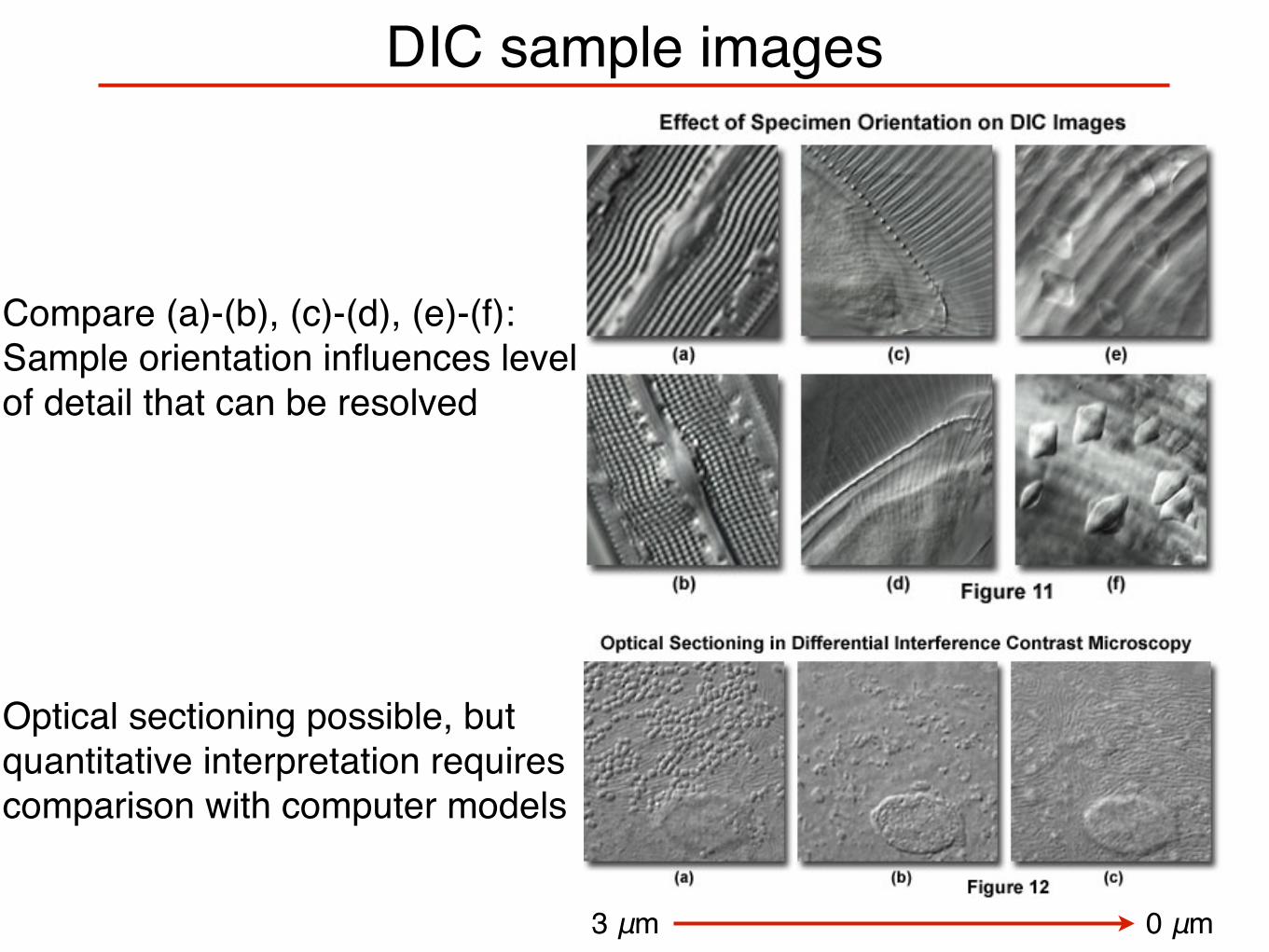
DIC sample images

Compare (a)-(b), (c)-(d), (e)-(f): Sample orientation influences level of detail that can be resolved

Optical sectioning possible, but quantitative interpretation requires comparison with computer models

3 μm 0 μm

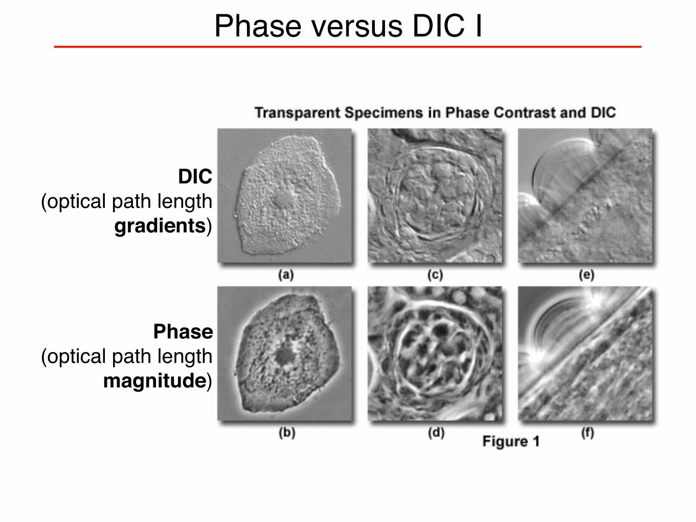
Phase versus DIC I

DIC(optical path length

gradients)

Phase(optical path length

magnitude)

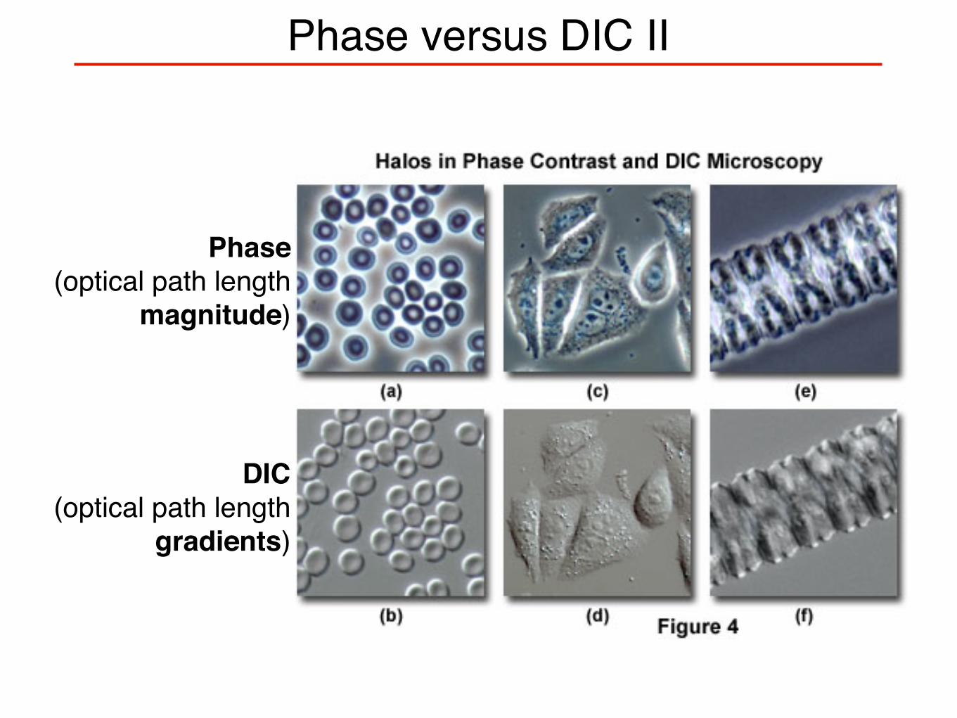
Phase versus DIC II

DIC(optical path length

gradients)

Phase(optical path length

magnitude)

Polarized light microscopy• Basic idea: image contrast is

created by the interaction of plane-polarized light with a birefringent specimen

• Advantages:

- Colors yield quantitative information on path differences

• Disadvantages:

- Only works for birefringent samples

- Requires strain-free objectives

• Useful for: liquid crystals, crystals, oriented polymers

B = |nmax − nmin|

Γ = tB = t|nmax − nmin|

Birefringence:

Retardation:

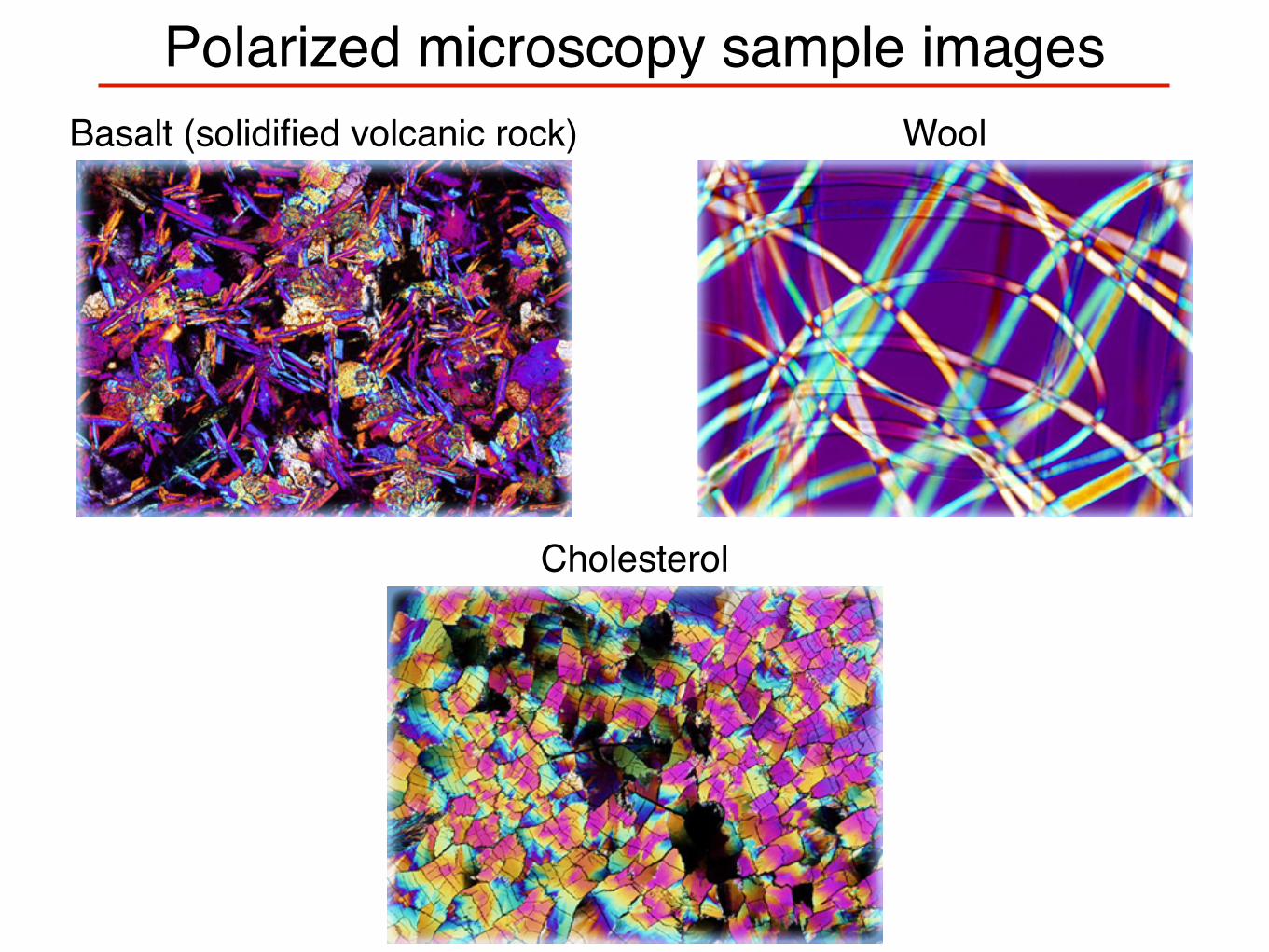
Polarized microscopy sample imagesWoolBasalt (solidified volcanic rock)

Cholesterol

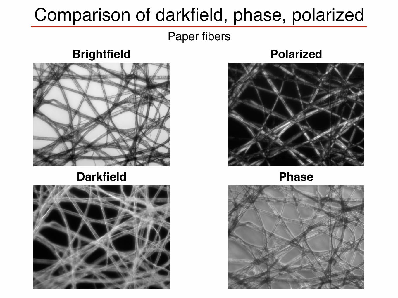
Comparison of darkfield, phase, polarizedPaper fibers

Brightfield Polarized

Darkfield Phase

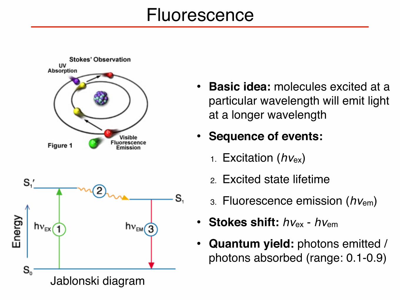
Fluorescence

• Basic idea: molecules excited at a particular wavelength will emit light at a longer wavelength

• Sequence of events:

1. Excitation (hνex)

2. Excited state lifetime

3. Fluorescence emission (hνem)

• Stokes shift: hνex - hνem

• Quantum yield: photons emitted / photons absorbed (range: 0.1-0.9)

Fluorescence� Stage.1:.Excitation� Stage.2:.Excited6State.Lifetime.(conformational.changes,.collisional quenching,.FRET)

� Stage.3:.Fluorescence.Emission� Stokes.Shift:.h�EX � h�EM� Quantum.Yield:.photon.emitted./.photon.absorbed.(0.0561)

� Molar.Extinction.Coef..for.Absorption:.5000.to.200,000.cm61M61

Jablonski Diagram

Jablonski diagram

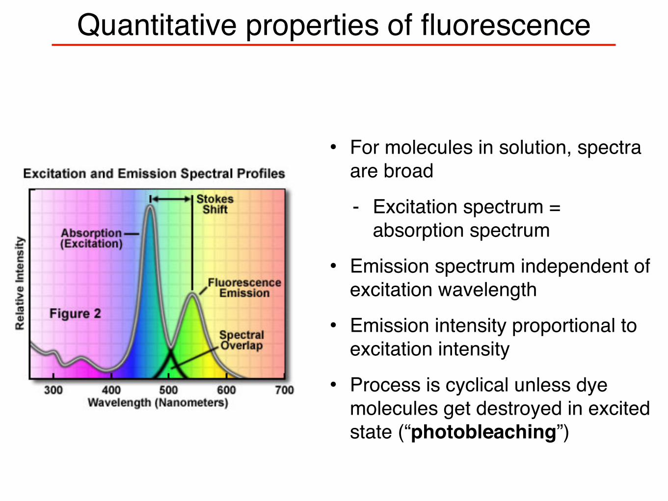
Quantitative properties of fluorescence

• For molecules in solution, spectra are broad

- Excitation spectrum = absorption spectrum

• Emission spectrum independent of excitation wavelength

• Emission intensity proportional to excitation intensity

• Process is cyclical unless dye molecules get destroyed in excited state (“photobleaching”)

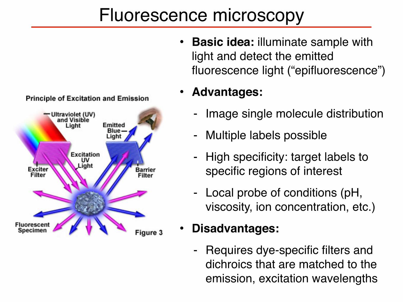
Fluorescence microscopy• Basic idea: illuminate sample with

light and detect the emitted fluorescence light (“epifluorescence”)

• Advantages:

- Image single molecule distribution

- Multiple labels possible

- High specificity: target labels to specific regions of interest

- Local probe of conditions (pH, viscosity, ion concentration, etc.)

• Disadvantages:

- Requires dye-specific filters and dichroics that are matched to the emission, excitation wavelengths

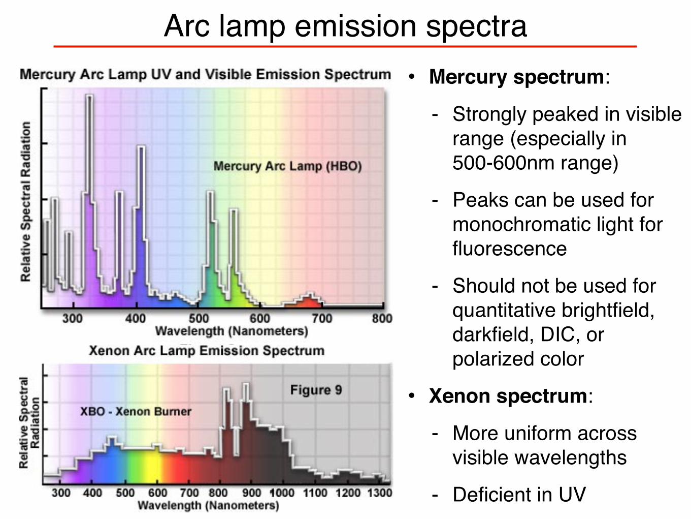
Arc lamp emission spectra• Mercury spectrum:

- Strongly peaked in visible range (especially in 500-600nm range)

- Peaks can be used for monochromatic light for fluorescence

- Should not be used for quantitative brightfield, darkfield, DIC, or polarized color

• Xenon spectrum:

- More uniform across visible wavelengths

- Deficient in UV

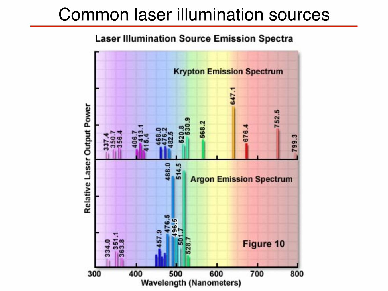
Common laser illumination sources

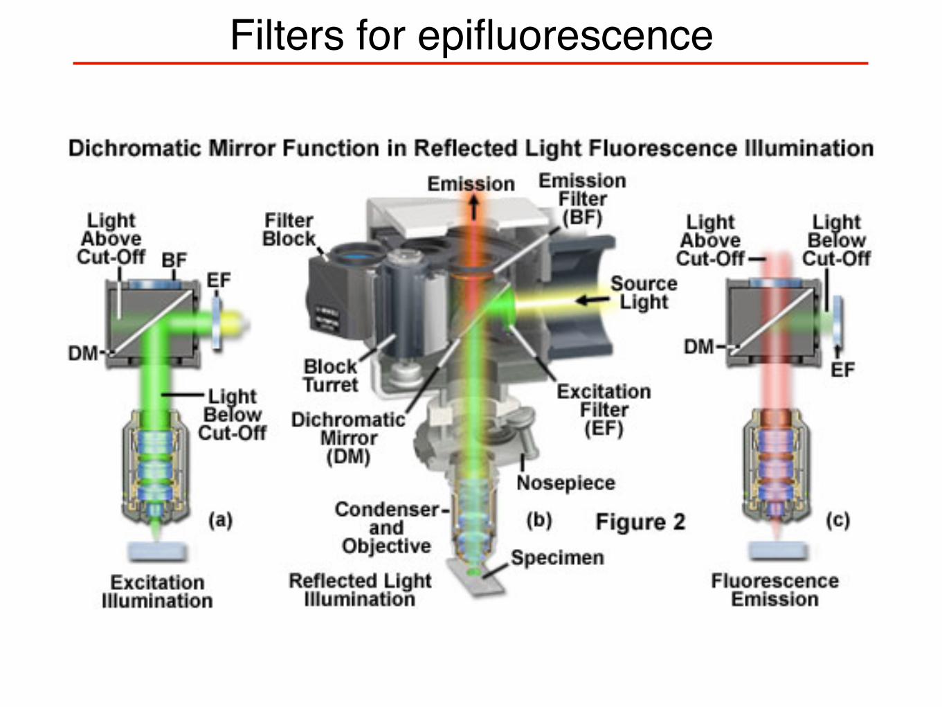
Filters for epifluorescence

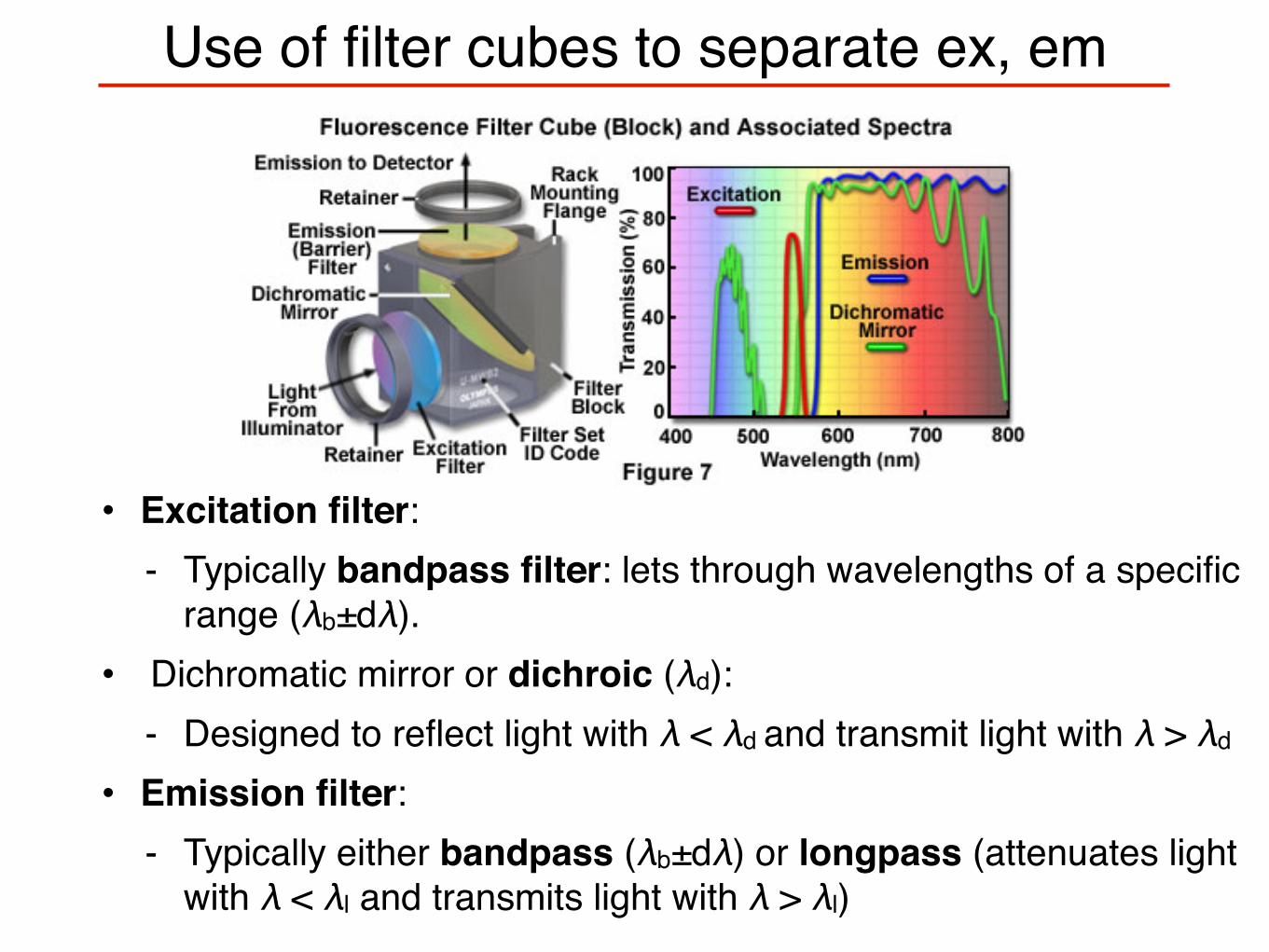
Use of filter cubes to separate ex, em

• Excitation filter: - Typically bandpass filter: lets through wavelengths of a specific

range (λb±dλ).• Dichromatic mirror or dichroic (λd):

- Designed to reflect light with λ < λd and transmit light with λ > λd

• Emission filter: - Typically either bandpass (λb±dλ) or longpass (attenuates light

with λ < λl and transmits light with λ > λl)

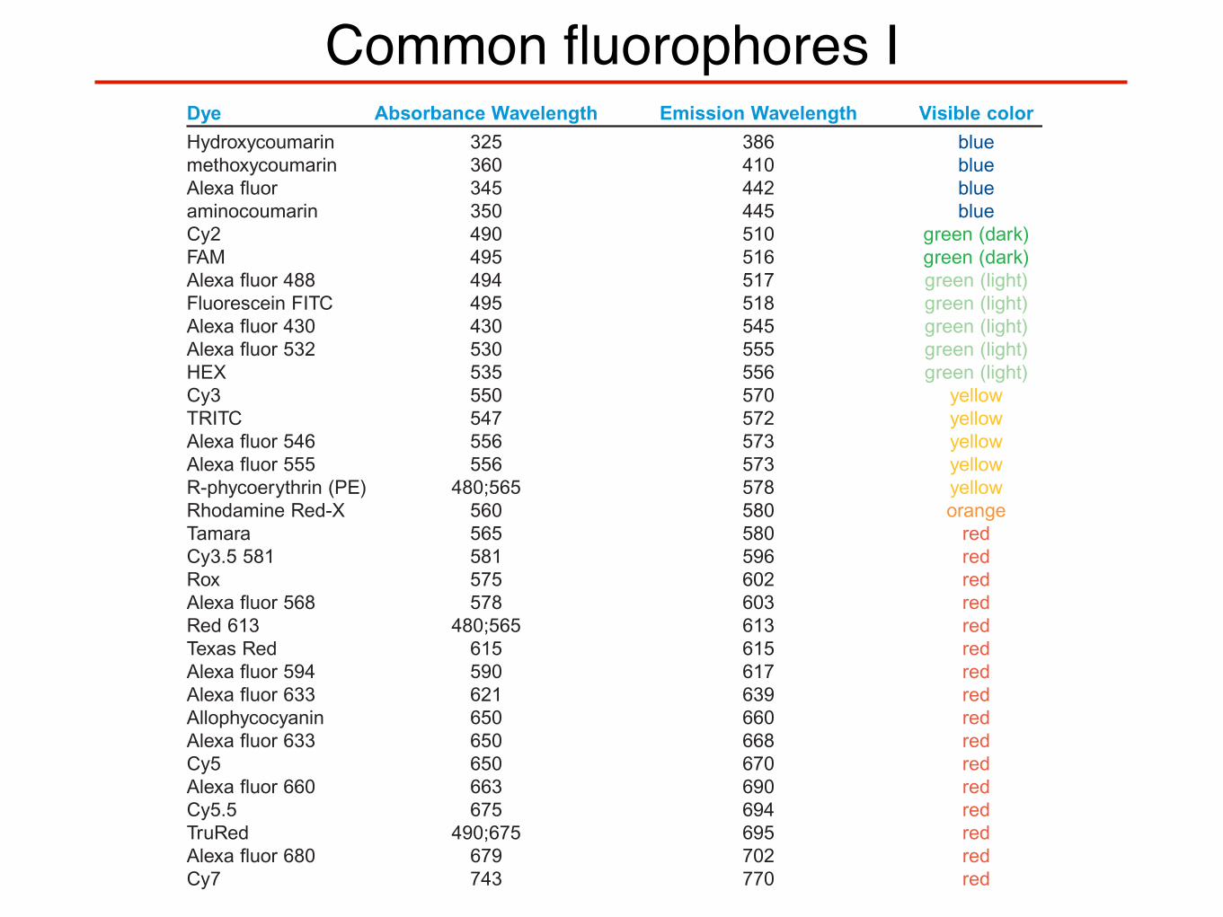
Common fluorophores IFLUOROPHORE TABLEDye Absorbance Wavelength Emission Wavelength Visible colorHydroxycoumarin 325 386 bluemethoxycoumarin 360 410 blueAlexa fluor 345 442 blueaminocoumarin 350 445 blueCy2 490 510 green (dark)FAM 495 516 green (dark)Alexa fluor 488 494 517 green (light)Fluorescein FITC 495 518 green (light)Alexa fluor 430 430 545 green (light)Alexa fluor 532 530 555 green (light)HEX 535 556 green (light)Cy3 550 570 yellowTRITC 547 572 yellowAlexa fluor 546 556 573 yellowAlexa fluor 555 556 573 yellowR-phycoerythrin (PE) 480;565 578 yellowRhodamine Red-X 560 580 orangeTamara 565 580 redCy3.5 581 581 596 redRox 575 602 redAlexa fluor 568 578 603 redRed 613 480;565 613 redTexas Red 615 615 redAlexa fluor 594 590 617 redAlexa fluor 633 621 639 redAllophycocyanin 650 660 redAlexa fluor 633 650 668 redCy5 650 670 redAlexa fluor 660 663 690 redCy5.5 675 694 redTruRed 490;675 695 redAlexa fluor 680 679 702 redCy7 743 770 red

Nucleic acid probes:

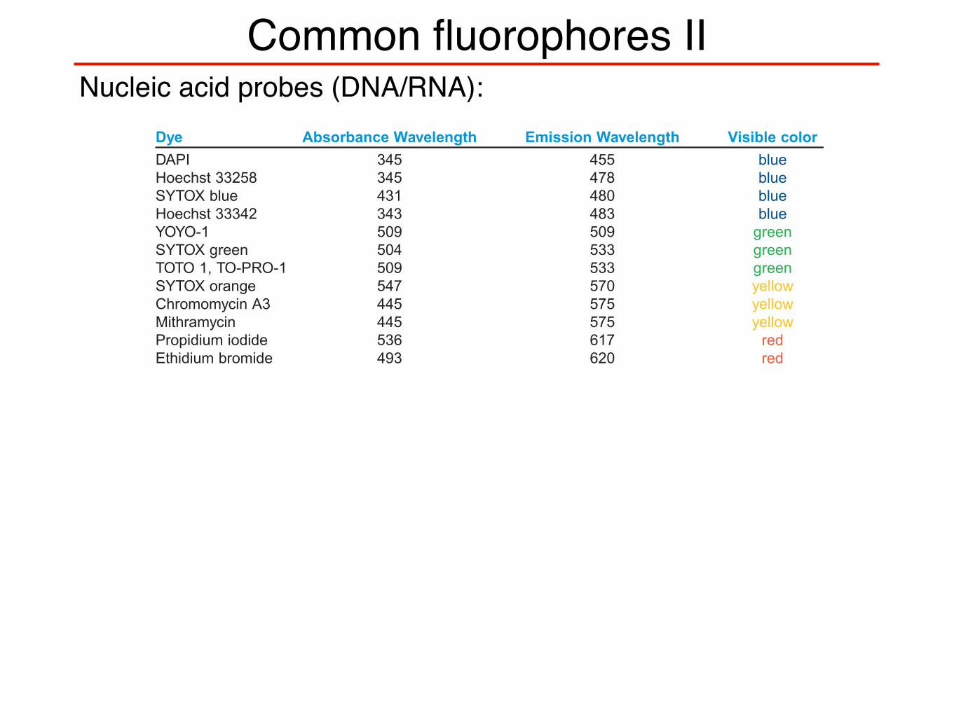
Dye Absorbance Wavelength Emission Wavelength Visible colorDAPI 345 455 blueHoechst 33258 345 478 blueSYTOX blue 431 480 blueHoechst 33342 343 483 blueYOYO-1 509 509 greenSYTOX green 504 533 greenTOTO 1, TO-PRO-1 509 533 greenSYTOX orange 547 570 yellowChromomycin A3 445 575 yellowMithramycin 445 575 yellowPropidium iodide 536 617 redEthidium bromide 493 620 red

www.abcam.com/technical 1

Common fluorophores II

FLUOROPHORE TABLEDye Absorbance Wavelength Emission Wavelength Visible colorHydroxycoumarin 325 386 bluemethoxycoumarin 360 410 blueAlexa fluor 345 442 blueaminocoumarin 350 445 blueCy2 490 510 green (dark)FAM 495 516 green (dark)Alexa fluor 488 494 517 green (light)Fluorescein FITC 495 518 green (light)Alexa fluor 430 430 545 green (light)Alexa fluor 532 530 555 green (light)HEX 535 556 green (light)Cy3 550 570 yellowTRITC 547 572 yellowAlexa fluor 546 556 573 yellowAlexa fluor 555 556 573 yellowR-phycoerythrin (PE) 480;565 578 yellowRhodamine Red-X 560 580 orangeTamara 565 580 redCy3.5 581 581 596 redRox 575 602 redAlexa fluor 568 578 603 redRed 613 480;565 613 redTexas Red 615 615 redAlexa fluor 594 590 617 redAlexa fluor 633 621 639 redAllophycocyanin 650 660 redAlexa fluor 633 650 668 redCy5 650 670 redAlexa fluor 660 663 690 redCy5.5 675 694 redTruRed 490;675 695 redAlexa fluor 680 679 702 redCy7 743 770 red

Nucleic acid probes:

Dye Absorbance Wavelength Emission Wavelength Visible colorDAPI 345 455 blueHoechst 33258 345 478 blueSYTOX blue 431 480 blueHoechst 33342 343 483 blueYOYO-1 509 509 greenSYTOX green 504 533 greenTOTO 1, TO-PRO-1 509 533 greenSYTOX orange 547 570 yellowChromomycin A3 445 575 yellowMithramycin 445 575 yellowPropidium iodide 536 617 redEthidium bromide 493 620 red

www.abcam.com/technical 1

Nucleic acid probes (DNA/RNA):

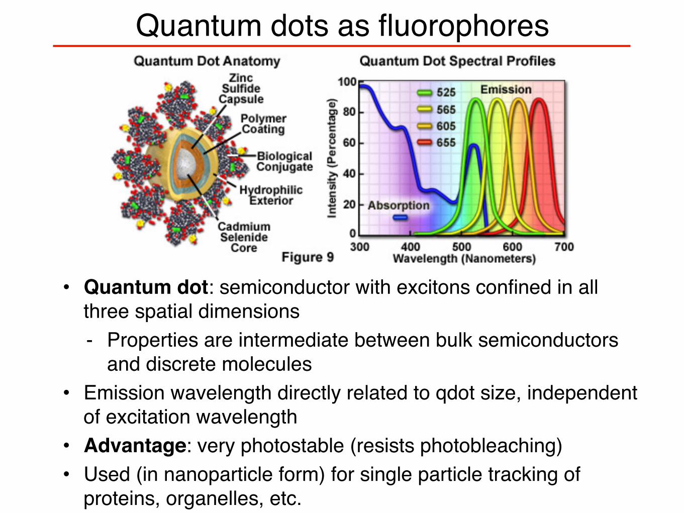
Quantum dots as fluorophores

• Quantum dot: semiconductor with excitons confined in all three spatial dimensions- Properties are intermediate between bulk semiconductors

and discrete molecules• Emission wavelength directly related to qdot size, independent

of excitation wavelength• Advantage: very photostable (resists photobleaching)• Used (in nanoparticle form) for single particle tracking of

proteins, organelles, etc.

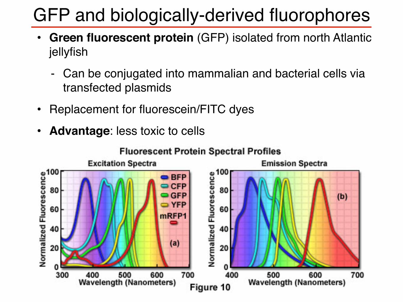
GFP and biologically-derived fluorophores• Green fluorescent protein (GFP) isolated from north Atlantic

jellyfish

- Can be conjugated into mammalian and bacterial cells via transfected plasmids

• Replacement for fluorescein/FITC dyes

• Advantage: less toxic to cells

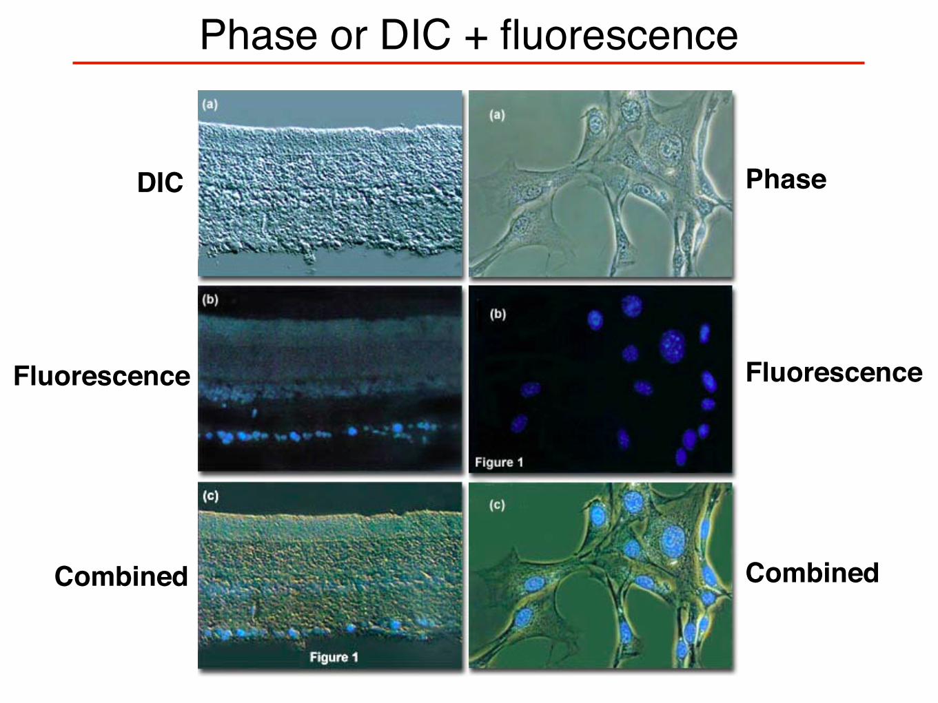
Phase or DIC + fluorescence

DIC

Fluorescence

Combined

Phase

Fluorescence

Combined

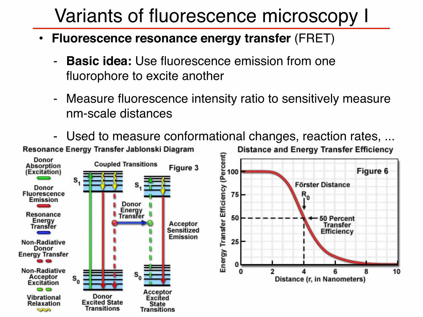
Variants of fluorescence microscopy I• Fluorescence resonance energy transfer (FRET)

- Basic idea: Use fluorescence emission from one fluorophore to excite another

- Measure fluorescence intensity ratio to sensitively measure nm-scale distances

- Used to measure conformational changes, reaction rates, ...

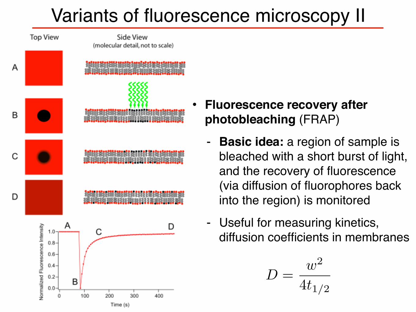
Variants of fluorescence microscopy II

• Fluorescence recovery after photobleaching (FRAP)

- Basic idea: a region of sample is bleached with a short burst of light, and the recovery of fluorescence (via diffusion of fluorophores back into the region) is monitored

- Useful for measuring kinetics, diffusion coefficients in membranes

D =w2

4t1/2

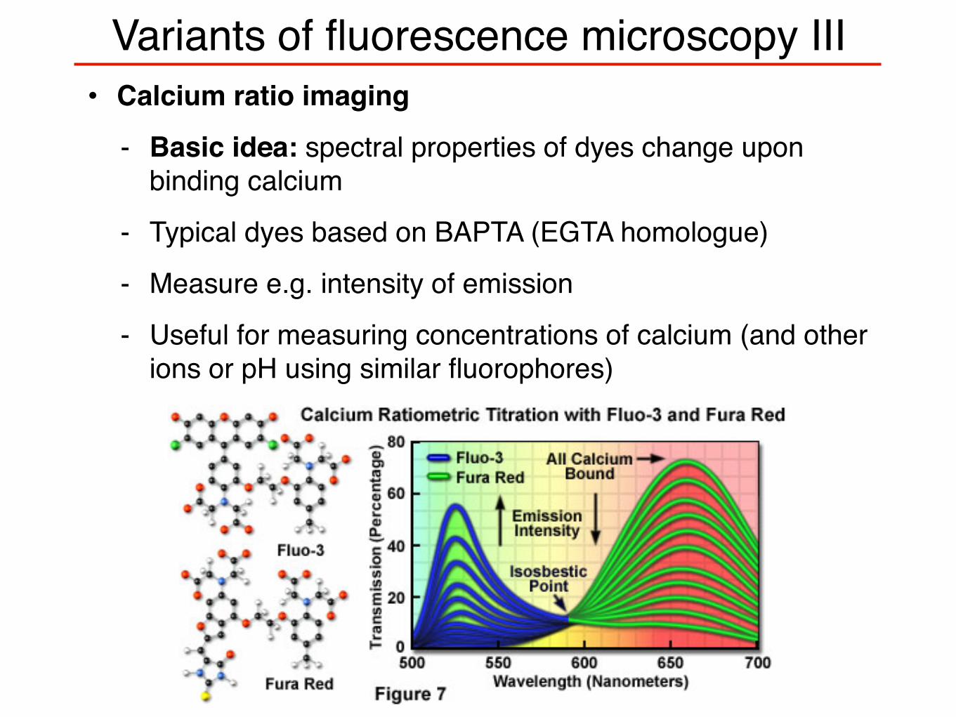
Variants of fluorescence microscopy III• Calcium ratio imaging

- Basic idea: spectral properties of dyes change upon binding calcium

- Typical dyes based on BAPTA (EGTA homologue)

- Measure e.g. intensity of emission

- Useful for measuring concentrations of calcium (and other ions or pH using similar fluorophores)

Variants of fluorescence microscopy IV

• Spectrofluorometry and microplate readers

- Basic idea: Measure average properties of bulk samples (micro- to milliliter) over continuous range of wavelengths

• Fluorescence scanners and microarray readers

- Basic idea: Use 2-D fluorescence to characterize macroscopic objects such as electrophoresis gels, blots, chromatograms, microfluidic devices, DNA sequences

• Flow cytometry

- Basic idea: Quantify subpopulations within a large sample by measuring fluorescence per cell in a flowing stream

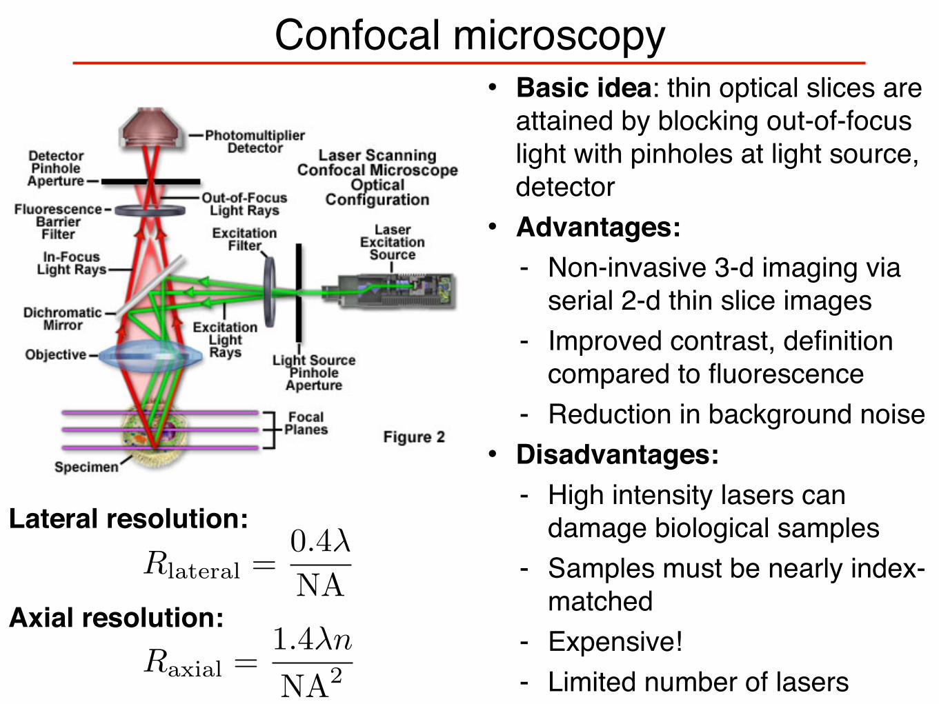
Confocal microscopy• Basic idea: thin optical slices are

attained by blocking out-of-focus light with pinholes at light source, detector• Advantages:

- Non-invasive 3-d imaging via serial 2-d thin slice images

- Improved contrast, definition compared to fluorescence

- Reduction in background noise• Disadvantages:

- High intensity lasers can damage biological samples

- Samples must be nearly index-matched

- Expensive!- Limited number of lasers

Lateral resolution:

Axial resolution:

Rlateral =0.4λ

NA

Raxial =1.4λn

NA2

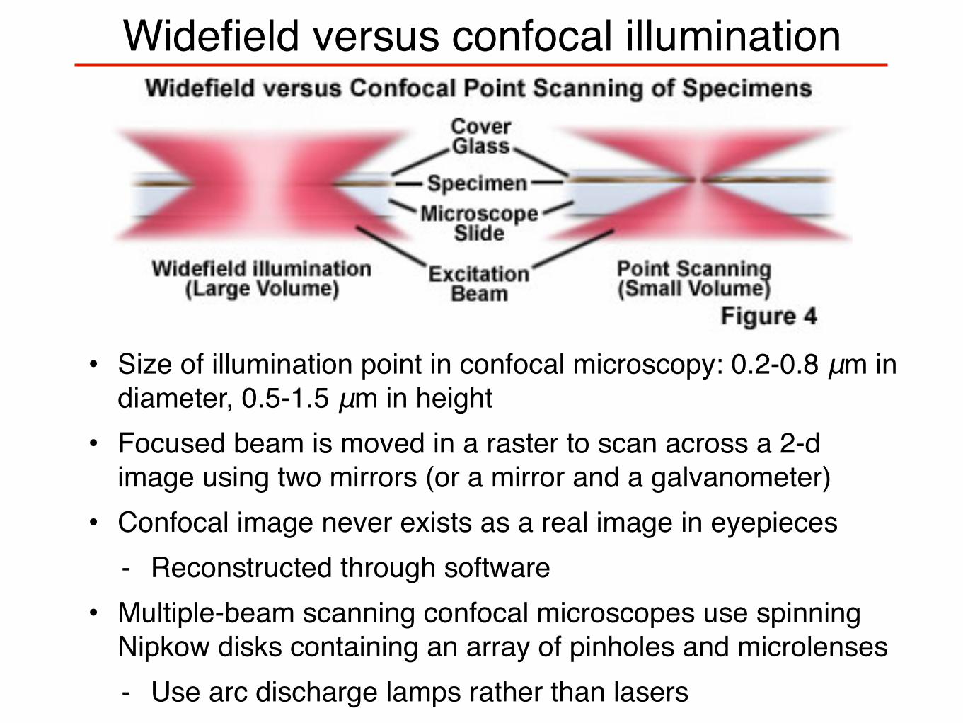
Widefield versus confocal illumination

• Size of illumination point in confocal microscopy: 0.2-0.8 μm in diameter, 0.5-1.5 μm in height

• Focused beam is moved in a raster to scan across a 2-d image using two mirrors (or a mirror and a galvanometer)

• Confocal image never exists as a real image in eyepieces- Reconstructed through software

• Multiple-beam scanning confocal microscopes use spinning Nipkow disks containing an array of pinholes and microlenses- Use arc discharge lamps rather than lasers

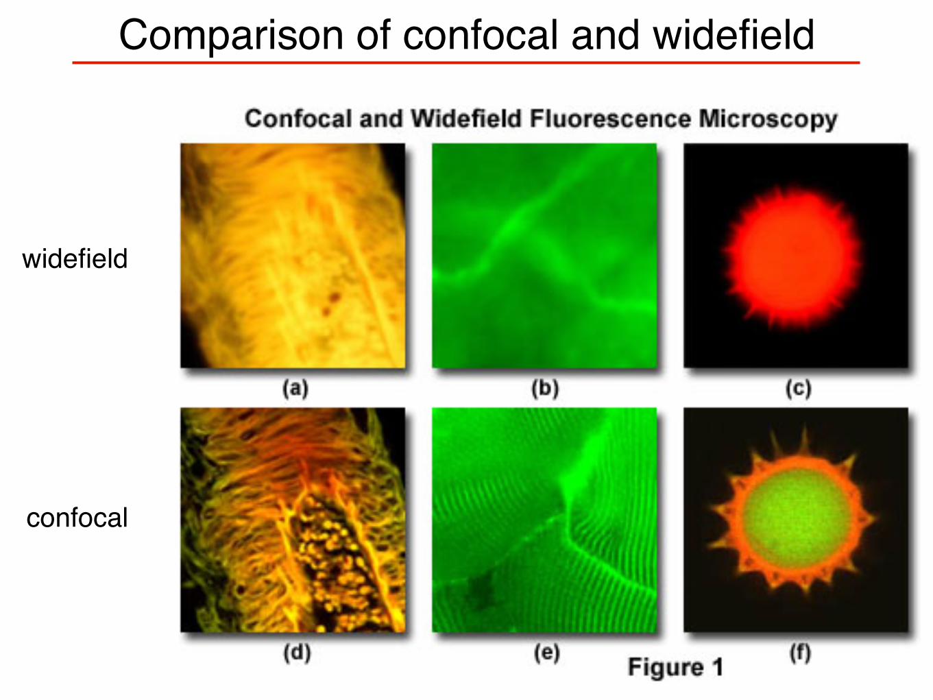
Comparison of confocal and widefield

widefield

confocal

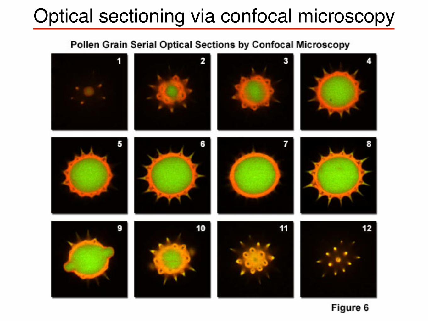
Optical sectioning via confocal microscopy

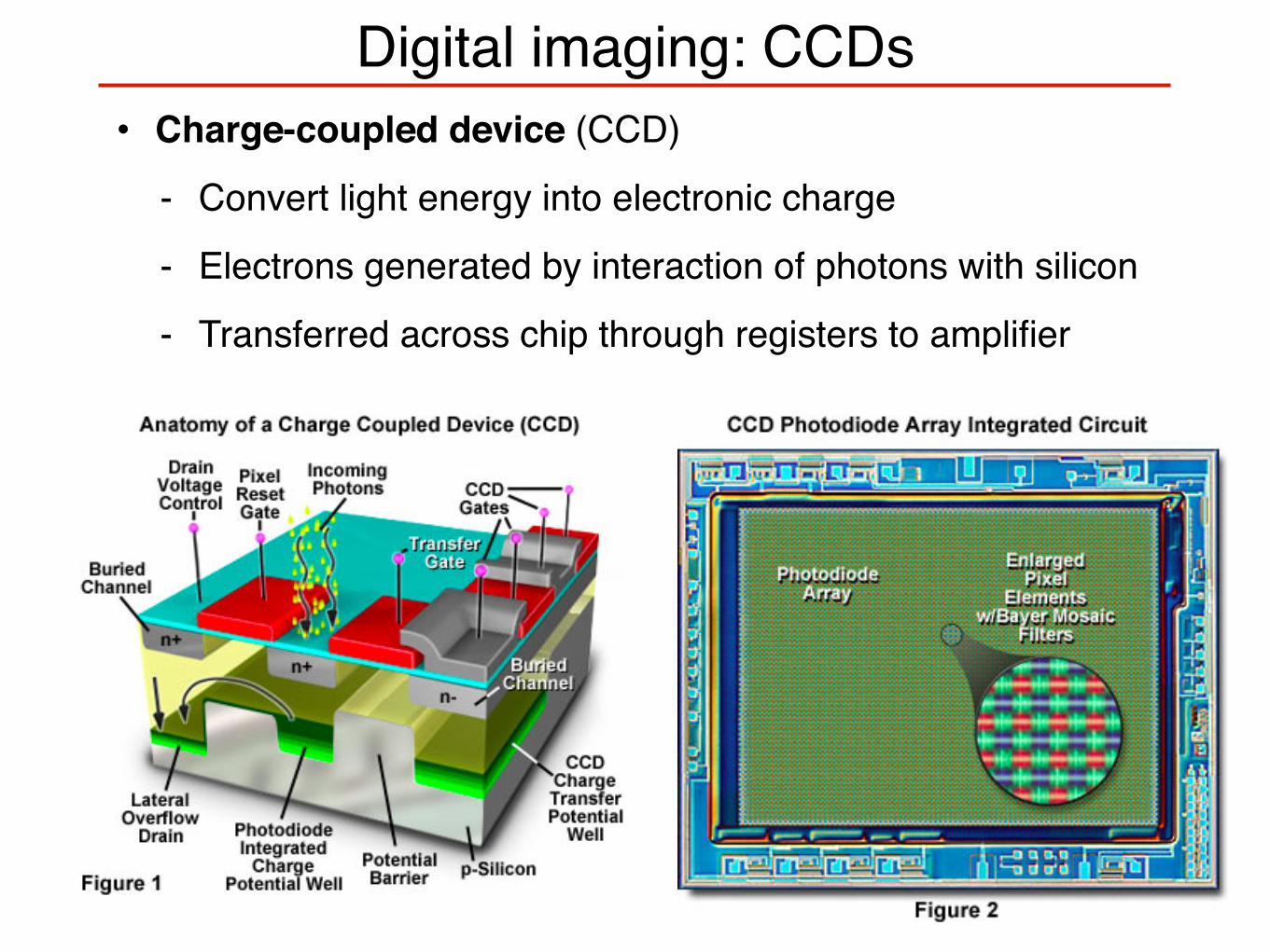
Digital imaging: CCDs• Charge-coupled device (CCD)

- Convert light energy into electronic charge

- Electrons generated by interaction of photons with silicon

- Transferred across chip through registers to amplifier

Digital imaging: camera types

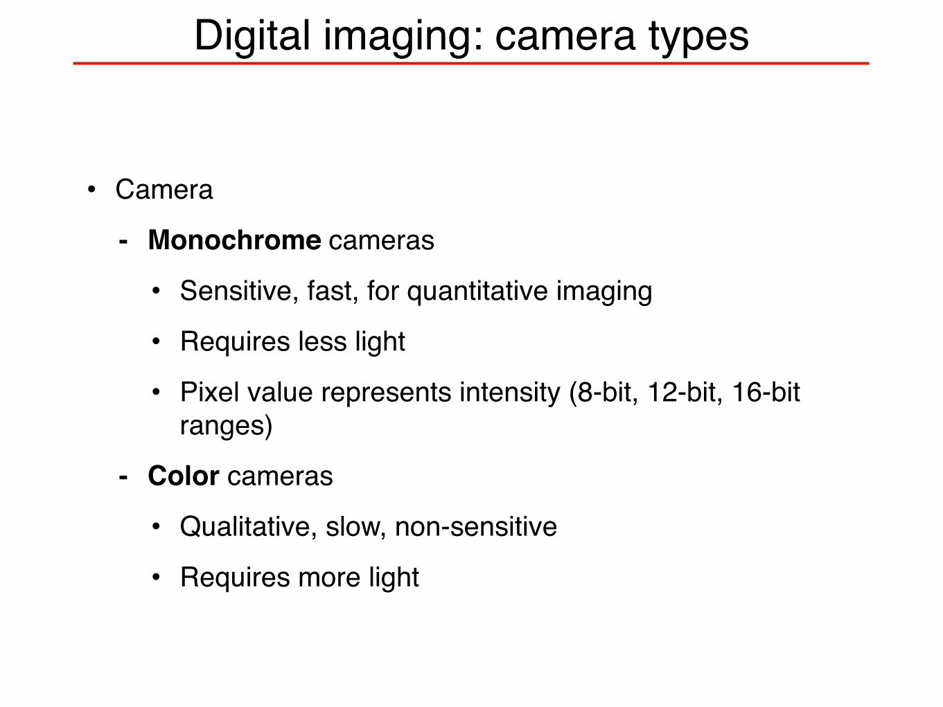
• Camera

- Monochrome cameras

• Sensitive, fast, for quantitative imaging

• Requires less light

• Pixel value represents intensity (8-bit, 12-bit, 16-bit ranges)

- Color cameras

• Qualitative, slow, non-sensitive

• Requires more light

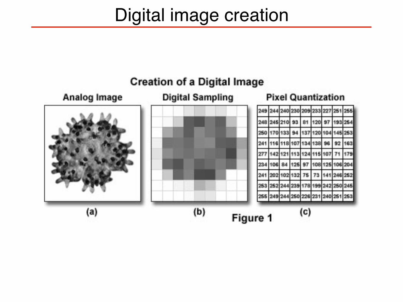
Digital image creation

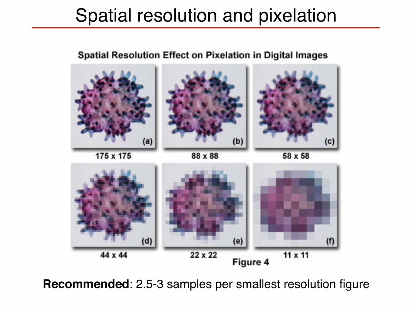
Spatial resolution and pixelation

Recommended: 2.5-3 samples per smallest resolution figure

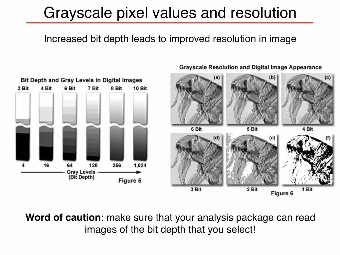
Grayscale pixel values and resolutionIncreased bit depth leads to improved resolution in image

Word of caution: make sure that your analysis package can read images of the bit depth that you select!

Software packages for image processing• Microscope acquisition packages (Leica, Zeiss, Olympus, Nikon)

• ImageJ

- (http://rsbweb.nih.gov/ij/)

- Free, lots of plug-ins available

• Matlab

- Image processing toolbox, avialable through CCoE

• Adobe Photoshop

• Image Pro Plus

• NI Vision

• Many others

• NOTE: for publications all parts of an image must be processed equally!

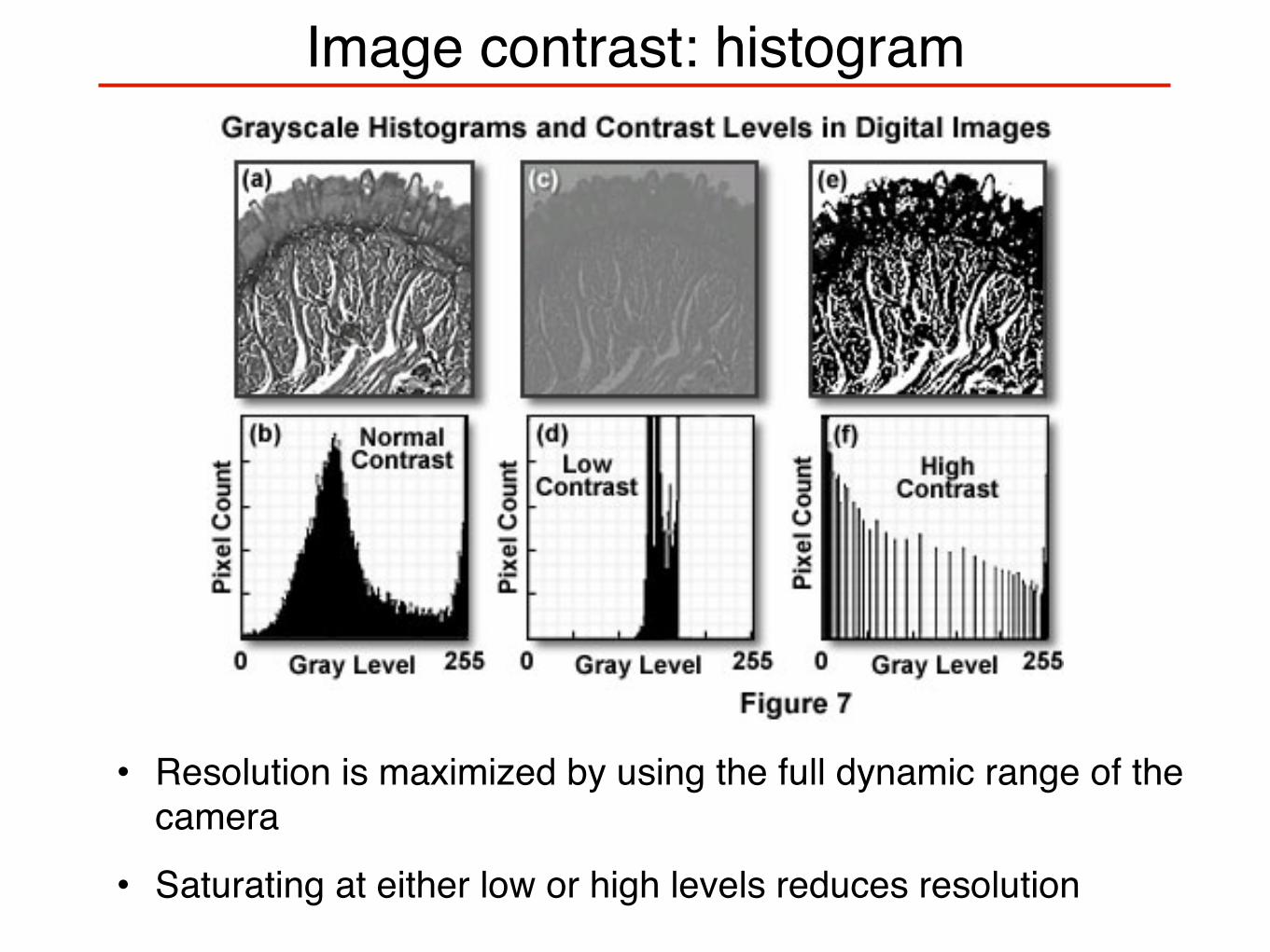
Image contrast: histogram

• Resolution is maximized by using the full dynamic range of the camera

• Saturating at either low or high levels reduces resolution

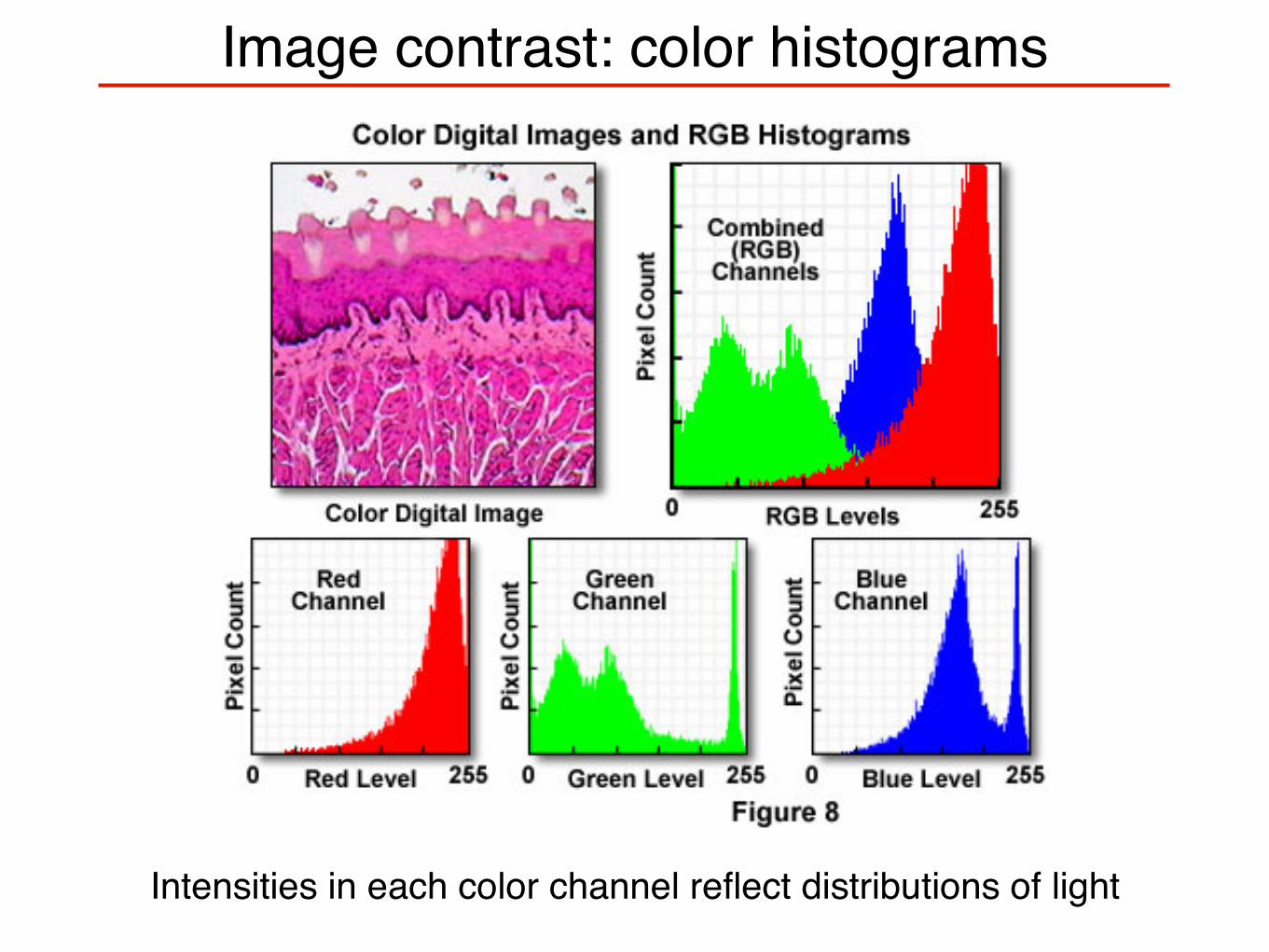
Image contrast: color histograms

Intensities in each color channel reflect distributions of light

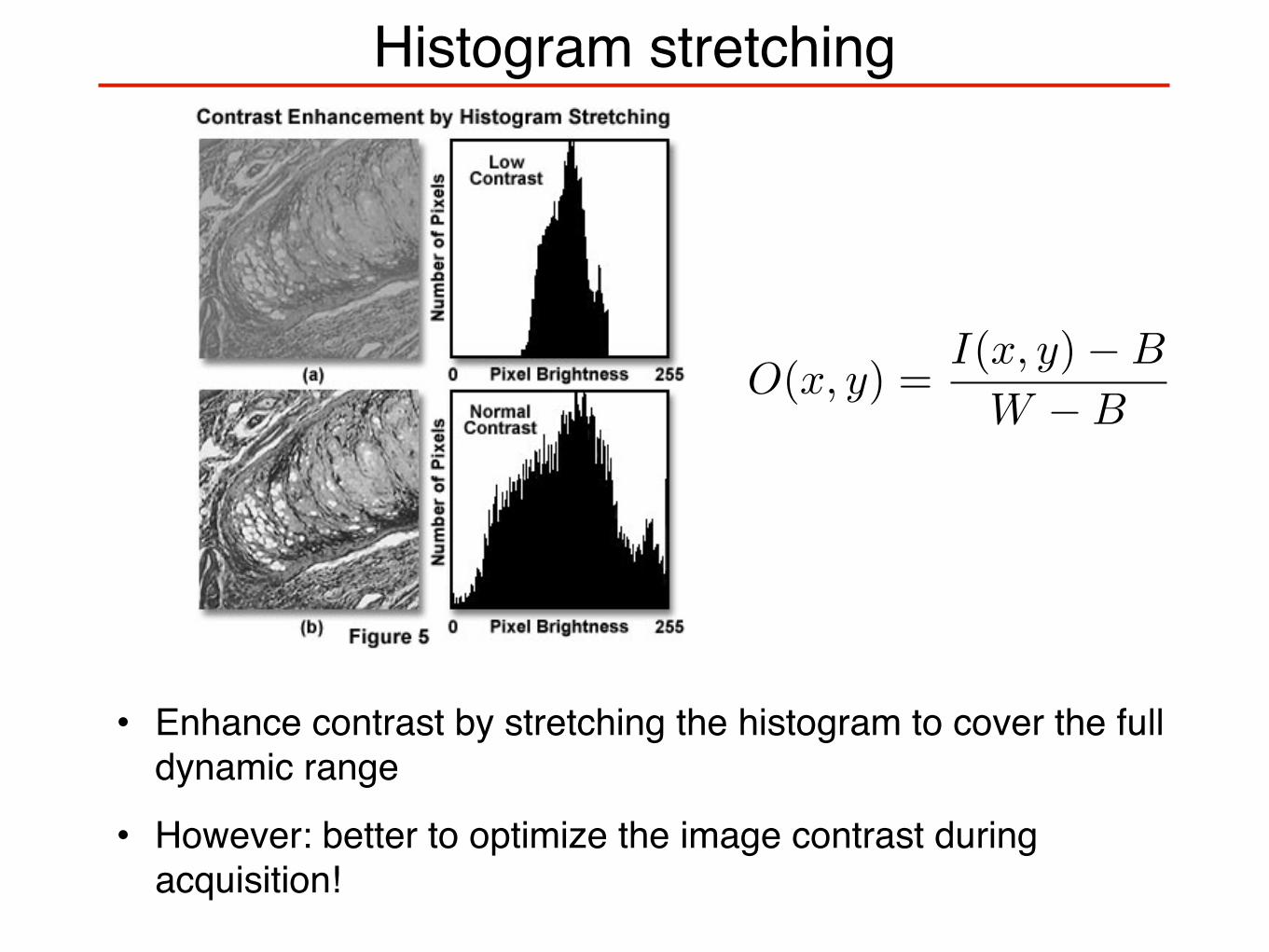
Histogram stretching

• Enhance contrast by stretching the histogram to cover the full dynamic range

• However: better to optimize the image contrast during acquisition!

O(x, y) =I(x, y) − B

W − B

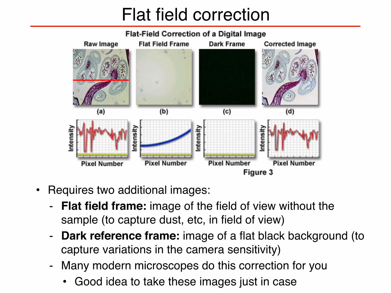
Flat field correction

• Requires two additional images:- Flat field frame: image of the field of view without the

sample (to capture dust, etc, in field of view)- Dark reference frame: image of a flat black background (to

capture variations in the camera sensitivity)- Many modern microscopes do this correction for you• Good idea to take these images just in case

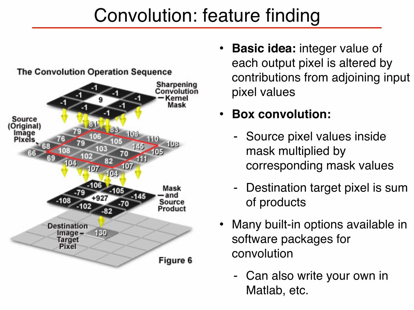
Convolution: feature finding• Basic idea: integer value of

each output pixel is altered by contributions from adjoining input pixel values

• Box convolution:

- Source pixel values inside mask multiplied by corresponding mask values

- Destination target pixel is sum of products

• Many built-in options available in software packages for convolution

- Can also write your own in Matlab, etc.

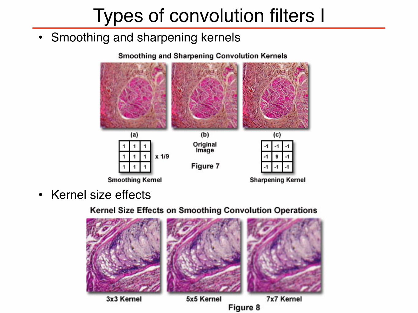
Types of convolution filters I• Smoothing and sharpening kernels

• Kernel size effects

Types of convolution filters II• Median convolution filters

- Effective at eliminating “faulty” pixels (unusually high or low brightness) and image noise

- Source pixel value replaced by median of pixel values in the convolution kernel - Good for images with high contrast (preserves edges)

• Derivative filters - e.g. Sobel filter: produces a derivative in any of eight direction depending on

matrix choice- Used for edge enhancement

• Laplacian filters (operators)- Used to calculate second derivative of intensity as a function of position- Generates sharp peaks at the edges- Enhances brightness slopes

• Unsharp masks - Subtraction of blurred image from original image, followed by adjustment of

gray values- Preserves high-frequency detail while allowing shading correction, background

suppression- User-adjustable but also increases noise -- use with caution

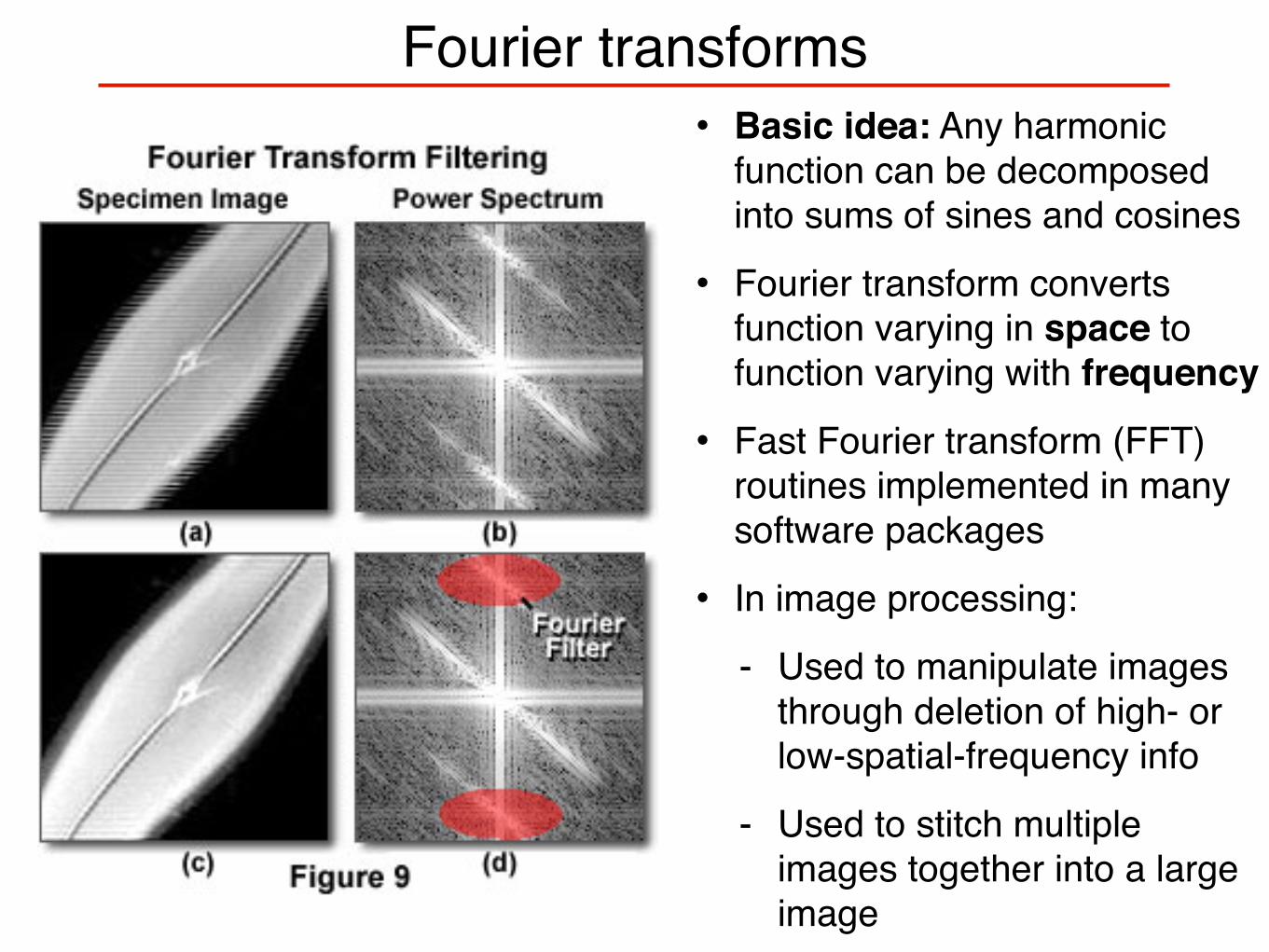
Fourier transforms• Basic idea: Any harmonic

function can be decomposed into sums of sines and cosines

• Fourier transform converts function varying in space to function varying with frequency

• Fast Fourier transform (FFT) routines implemented in many software packages

• In image processing:

- Used to manipulate images through deletion of high- or low-spatial-frequency info

- Used to stitch multiple images together into a large image

h(x) = (f ∗ g)(x) =

!∞

−∞

f(y)g(x − y)dy

h(ξ) = f(ξ) · g(ξ)

f(ξ) ≡

!∞

−∞

f(x)e−2πixξdx

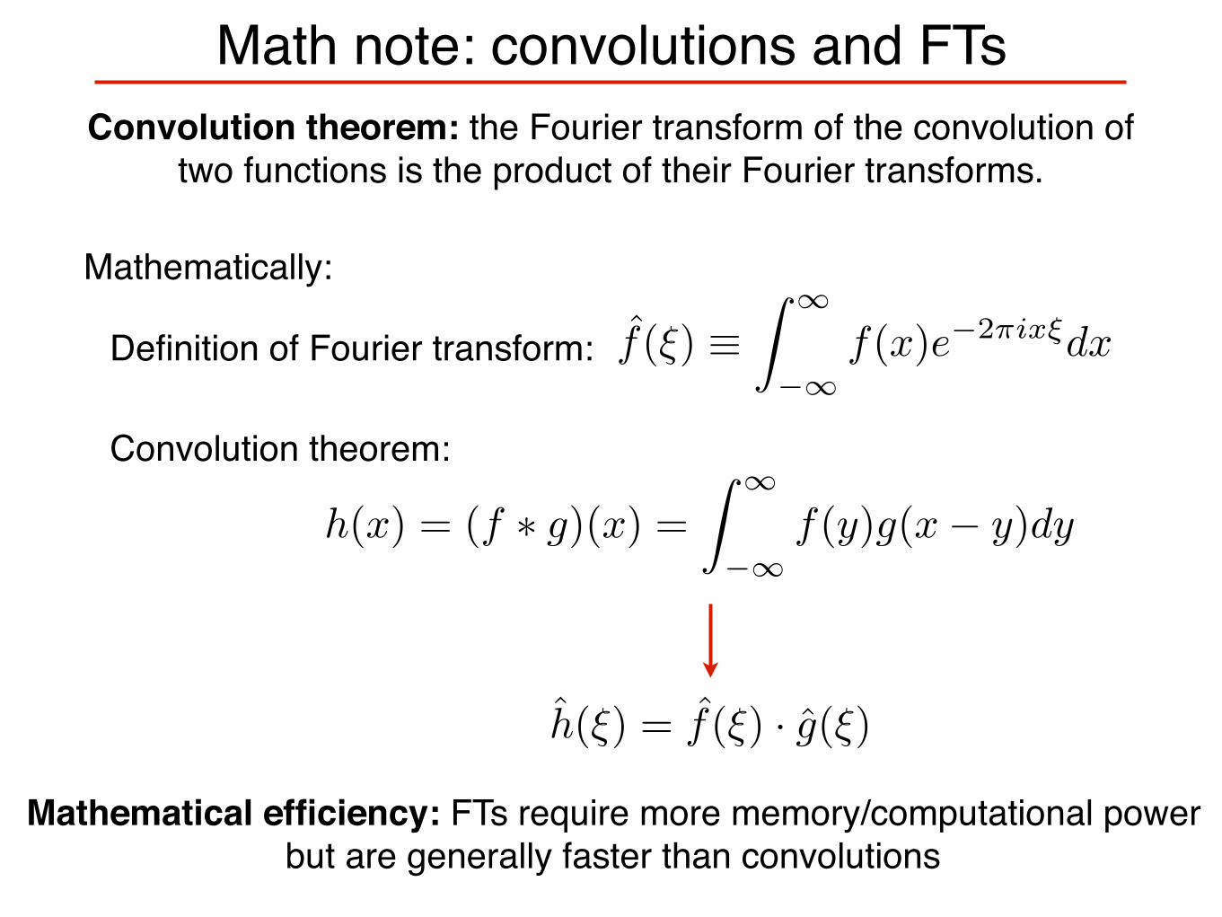
Math note: convolutions and FTsConvolution theorem: the Fourier transform of the convolution of

two functions is the product of their Fourier transforms.

Mathematically:

Convolution theorem:

Definition of Fourier transform:

Mathematical efficiency: FTs require more memory/computational power but are generally faster than convolutions

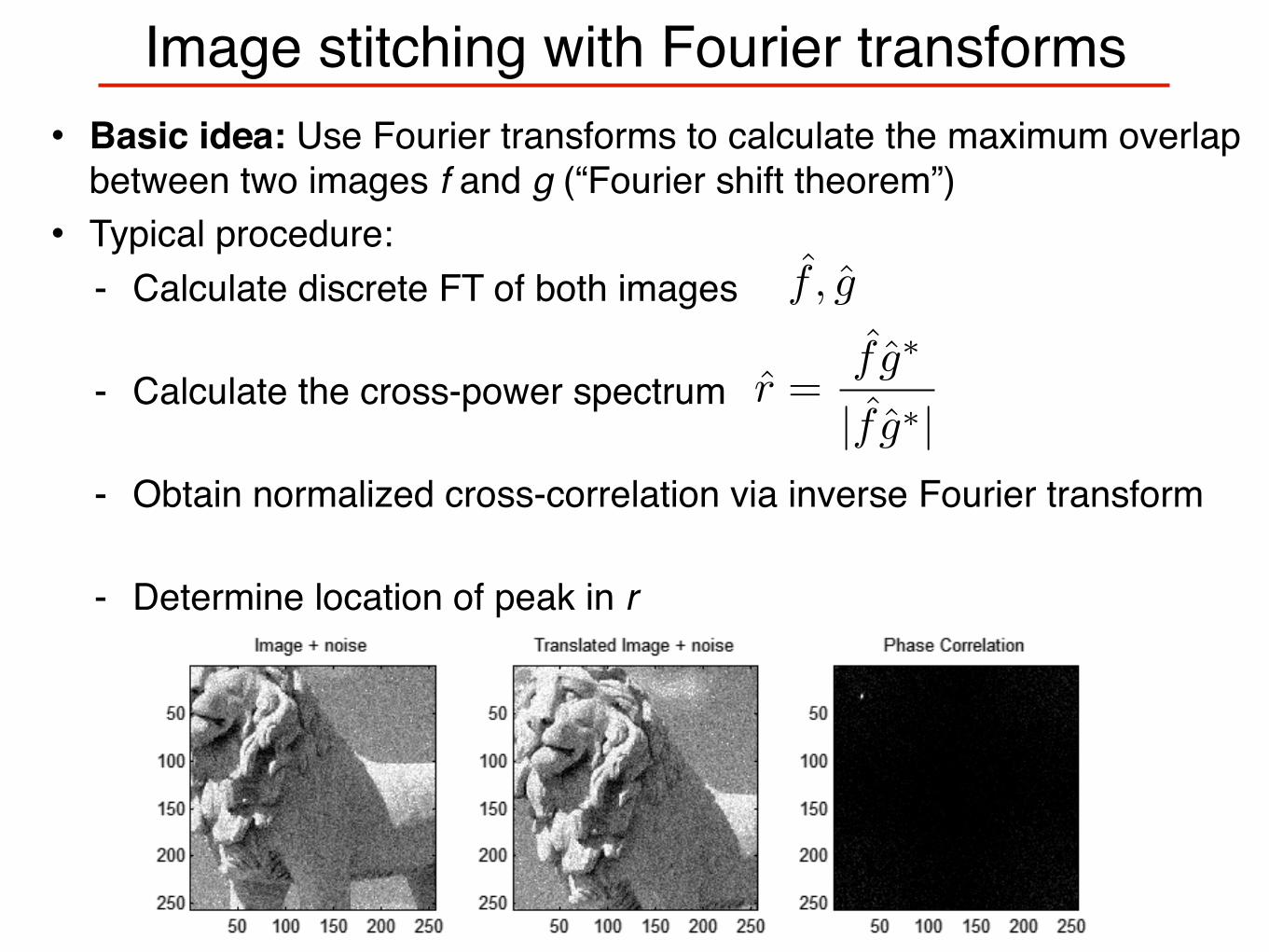
Image stitching with Fourier transforms• Basic idea: Use Fourier transforms to calculate the maximum overlap

between two images f and g (“Fourier shift theorem”)• Typical procedure:

- Calculate discrete FT of both images

- Calculate the cross-power spectrum

- Obtain normalized cross-correlation via inverse Fourier transform

- Determine location of peak in r

f , g

r =f g∗

|f g∗|

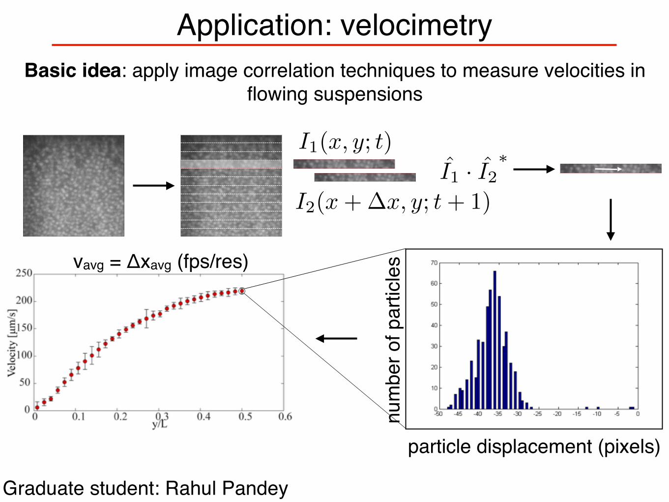
Application: velocimetry

num

ber o

f par

ticle

s

particle displacement (pixels)

vavg = Δxavg (fps/res)

I1 · I2⇤

I1(x, y; t)

I2(x+�x, y; t+ 1)

Basic idea: apply image correlation techniques to measure velocities in flowing suspensions

Graduate student: Rahul Pandey

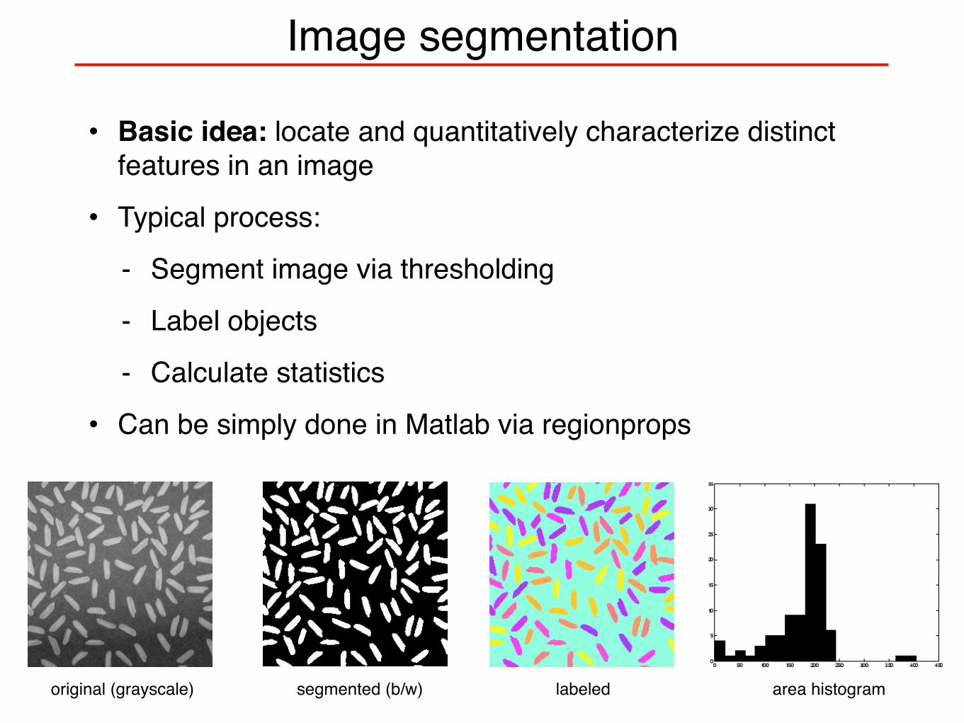
Image segmentation

• Basic idea: locate and quantitatively characterize distinct features in an image

• Typical process:

- Segment image via thresholding

- Label objects

- Calculate statistics

• Can be simply done in Matlab via regionprops

Image&Processing

Original&Image(Grayscale)

Segmented&Image(Black&and&White)

Labeling(Identifying&objects)

Statistics&and&Analysis

original (grayscale) segmented (b/w) labeled area histogram

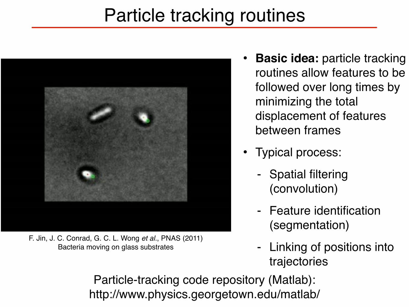
Particle tracking routines

• Basic idea: particle tracking routines allow features to be followed over long times by minimizing the total displacement of features between frames

• Typical process:

- Spatial filtering (convolution)

- Feature identification (segmentation)

- Linking of positions into trajectories

F. Jin, J. C. Conrad, G. C. L. Wong et al., PNAS (2011)Bacteria moving on glass substrates

Particle-tracking code repository (Matlab): http://www.physics.georgetown.edu/matlab/

20 µm

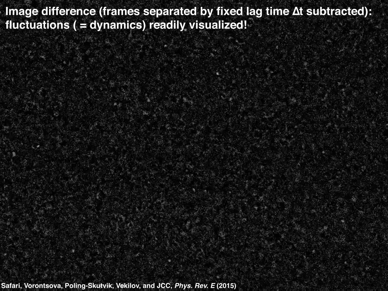
Brightfield movie: diffusing objects invisibleImage difference (frames separated by fixed lag time ∆t subtracted):fluctuations ( = dynamics) readily visualized!

Safari, Vorontsova, Poling-Skutvik, Vekilov, and JCC, Phys. Rev. E (2015)

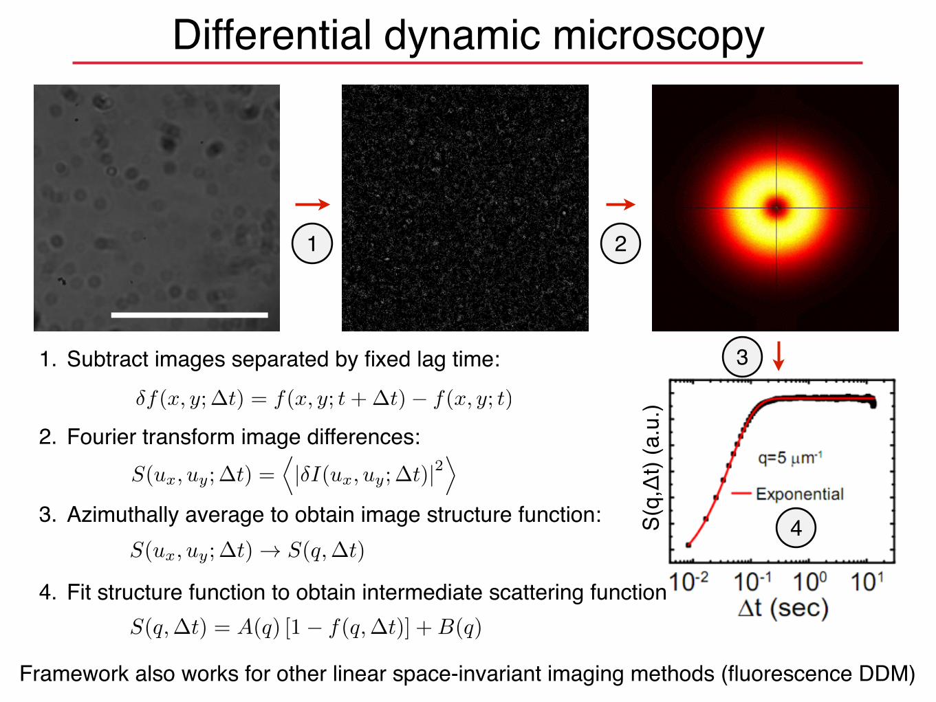
S(q,�t) = A(q) [1� f(q,�t)] +B(q)

�f(x, y;�t) = f(x, y; t+�t)� f(x, y; t)

1. Subtract images separated by fixed lag time:

2. Fourier transform image differences:

3. Azimuthally average to obtain image structure function:

4. Fit structure function to obtain intermediate scattering function:

Differential dynamic microscopy

2

3

S(ux

, uy

;�t) ! S(q,�t)

S(q,Δ

t) (a

.u.)

4

1

S(ux

, uy

;�t) =D|�I(u

x

, uy

;�t)|2E

Framework also works for other linear space-invariant imaging methods (fluorescence DDM)

Summary for microscopy lecture

• Introduction to optics and brightfield microscopy

• Contrast-enhancing techniques

- Darkfield, phase contrast, DIC, polarized

• Fluorescence and confocal microscopy

• Digital imaging

• Image processing

- Histograms

- Convolution

- Fourier transforms and Fourier shift theorem

- Particle tracking

- Fluctuation analysis (differential dynamic microscopy)