Fluorescence Optical Diffusion Tomography

Fluorescence optical diffusion tomography

Adam B. Milstein, Seungseok Oh, Kevin J. Webb, Charles A. Bouman, Quan Zhang,David A. Boas, and R. P. Millane

A nonlinear, Bayesian optimization scheme is presented for reconstructing fluorescent yield and lifetime,the absorption coefficient, and the diffusion coefficient in turbid media, such as biological tissue. Themethod utilizes measurements at both the excitation and the emission wavelengths to reconstruct allunknown parameters. The effectiveness of the reconstruction algorithm is demonstrated by simulationand by application to experimental data from a tissue phantom containing the fluorescent agent Indo-cyanine Green. © 2003 Optical Society of America

OCIS codes: 170.6280, 290.7050, 100.3190, 100.6950, 170.3010, 290.3200.

1. Introduction

Optical diffusion tomography �ODT� is emerging as apowerful tissue imaging modality.1,2 In ODT, im-ages are comprised of the spatially dependent absorp-tion and scattering properties of the tissue.Boundary measurements from several sources anddetectors are used to recover the unknown parame-ters from a scattering model described by a partialdifferential equation. Contrast between the proper-ties of diseased and healthy tissue might then be usedin clinical diagnosis. In principle, sinusoidally mod-ulated, continuous-wave �cw�, or pulsed excitationlight is launched into the biological tissue, where itundergoes multiple scattering and absorption beforeexiting. One can use the measured intensity andphase �or delay� information to reconstruct three-dimensional �3-D� maps of the absorption and scat-tering properties by optimizing a fit to diffusionmodel computations. As a result of the nonlineardependence of the diffusion equation photon flux onthe unknown parameters and the inherently 3-D na-ture of photon scattering, this inverse problem is

A. B. Milstein, S. Oh, K. J. Webb �[email protected]�, andC. A. Bouman are with the School of Electrical and ComputerEngineering, Purdue University, West Lafayette, Indiana 47907-1285. Q. Zhang and D. A. Boas are with the Nuclear MagneticResonance Center, Massachusetts General Hospital, HarvardMedical School, Charlestown, Massachusetts 02129. R. P. Mill-ane is with the Department of Electrical and Computer Engineer-ing, University of Canterbury, Christchurch, New Zealand.

Received 31 August 2002; revised manuscript received 19 De-cember 2002.

0003-6935�03�163081-14$15.00�0© 2003 Optical Society of America

computationally intensive and must be solved itera-tively.

A relatively modest intrinsic contrast between theoptical parameters of diseased and healthy breasttissue has been reported in some studies.3,4 Use ofexogenous fluorescent agents has the potential to im-prove the contrast and thus to facilitate early diag-nosis. In recent years, use of fluorescent indicatorsas exogenous contrast agents for in vivo imaging oftumors with near-infrared or visible light has showngreat promise, attracting considerable inter-est.5–14 In experimental studies with animal sub-jects,5–7,9,10,13,14 fluorescence has been successfullyused to visualize cancerous tissue in vivo near theskin surface. In addition, Ntziachristos et al.12 haveused ODT after Indocyanine Green �ICG� injection toimage the absorption of a malignant breast tumor ina human subject. The injected fluorophore maypreferentially accumulate in diseased tissue becauseof increased blood flow from tumor neovasculariza-tion.9 Alternatively, the agent may have differentdecay properties in diseased tissue, which could beuseful to localize tumors independently of fluoro-phore concentration.7 In addition, contrast betweentumors and surrounding tissue may be substantiallyimproved by use of diagnostic agents that selectivelytarget receptors specific to cancer cells.8,10,13,14

In frequency-domain fluorescence ODT, sinusoi-dally modulated light at the fluorophore’s excitationwavelength is launched into the tissue. The excitedfluorophore, when it decays to the ground state, emitslight at a longer �emission� wavelength, and thisemission is measured by an array of detection de-vices. These emission data are then used to performa volumetric reconstruction of the yield �a measure ofthe fluorescence efficiency� and the lifetime �the flu-

1 June 2003 � Vol. 42, No. 16 � APPLIED OPTICS 3081

orescent decay parameter�. However, the multiplescattering in tissue complicates the reconstruc-tion.15,16 The emission intensity of the fluorophoreis proportional to the optical intensity at the excita-tion wavelength at that position, which depends inturn on the optical parameters of the scattering do-main at the excitation wavelength. Therefore a rig-orous reconstruction of fluorescence property mapsshould also include reconstructions of absorption andscattering parameters at the excitation and emissionwavelengths. In addition, reconstruction of the un-known absorption and scattering coefficients by useof ODT can function as an adjunct image to the flu-orescence image in screening for tumors.

Fluorescence imaging simulations with 3-D �Ref.17� and two-dimensional18–20 geometries have recon-structed fluorescence yield and lifetime parameters.These simulations have generally assumed that theabsorption and scattering parameters are known inadvance, except for Roy and Sevick-Muraca17 whoalso reconstructed the excitation wavelength absorp-tion. In an early experimental result, Chang et al.21

used a transport theory model to reconstruct fluores-cent yield in a heterogeneous tissue phantom con-taining Rhodamine 6G. Their study used cw datarecorded in a two-dimensional plane geometry. Re-cently, Ntziachristos and Weissleder22 used a nor-malized Born approximation to reconstruct 3-Dfluorescent heterogeneities containing the near-infrared cyanine dye Cy5.5 embedded in a tissuephantom. Under the assumption of known back-ground optical properties and absorbers limited to aperturbative regime, their technique can circumventthe need for recording background measurements be-fore contrast agent administration.

The development of nonlinear inversion methodsfor ODT is necessary because of the fundamentallylimited accuracy of methods that linearize the for-ward model.23 Previously, we have presented a non-linear Bayesian approach24–26 and shown that itproduces high-quality images compared with previ-ous methods such as the distorted Born iterativemethod.27 The method formulates the inversion asthe optimization of an objective function that incor-porates a model of the detection system and a prioriknowledge about the image properties. We foundthat a neighborhood regularization scheme used in aBayesian framework reduces artifacts characteristicof previous approaches that impose a penalty on thenorm of the image updates.24 The inversion can bemade more computationally efficient by multigridtechniques.25

Here we extend our previous approach to includefluorescence yield and lifetime in the inverse prob-lem. We present a new inversion algorithm and ameasurement scheme for reconstructing all the un-known fluorescence, absorption, and diffusion param-eters. Numerical simulations validate the schemeand demonstrate its computational efficacy. We usethe method to image a spherical heterogeneity in a

tissue phantom by use of transmission data collectedby a cw imaging device. The heterogeneity containsICG, a fluorescent diagnostic agent approved by theU.S. Food and Drug Administration for use in thenear-infrared range, where biomedical imaging withlight is most practical.

2. Fluorescence Diffusion Tomography Problem

The transport of modulated light �at modulation an-gular frequency �, i.e., exp� j�t� variation� in a fluo-rescent, highly scattering medium with an externalsource at the excitation wavelength is modeled by useof the coupled diffusion equations15,16,28:

� � �Dx�r��x�r, �� ax�r� � j��c��x�r, ��

� �r � rsk�, (1)

� � �Dm�r��m�r, �� am�r� � j��c��m�r, ��

� �x�r, ��af�r�

1 � j��r�

1 � ��r��2 , (2)

where the subscripts x and m, respectively, denoteexcitation and emission wavelengths x and m;��r, �� is the complex modulation envelope of thephoton flux; �r� is the Dirac function; and rsk

is thelocation of the excitation point source. We also as-sume single exponential decay in this model. Theoptical parameters are the diffusion coefficients D�r�and the absorption coefficients �a�r�. The fluores-cence parameters are the lifetime ��r� and the fluo-rescent yield ��af

�r�. The fluorescent yieldincorporates the fluorophore’s quantum efficiency ��which depends on the type of fluorophore and thechemical environment� and its absorption coefficient�af

�which depends on the fluorophore concentration�.Note the right-hand side of Eq. �2�, where the lightabsorbed by fluorophores and subsequently emittedat the emission wavelength is incorporated into aneffective source term. In the case of an externalpoint source at the emission wavelength, the flux isgoverned by

� � �Dm�r��m�r, �� am�r� � j��c��m�r, ��

� �r � rsk�. (3)

In the most general case, the unknown parametersin Eqs. �1� and �2� are �ax

, �am, Dx, Dm, �, and ��af

.Reconstructions of the Dx and �ax

images can be ob-tained by use of data from sources and detectors atthe excitation wavelength x. Similarly, Dm and �am

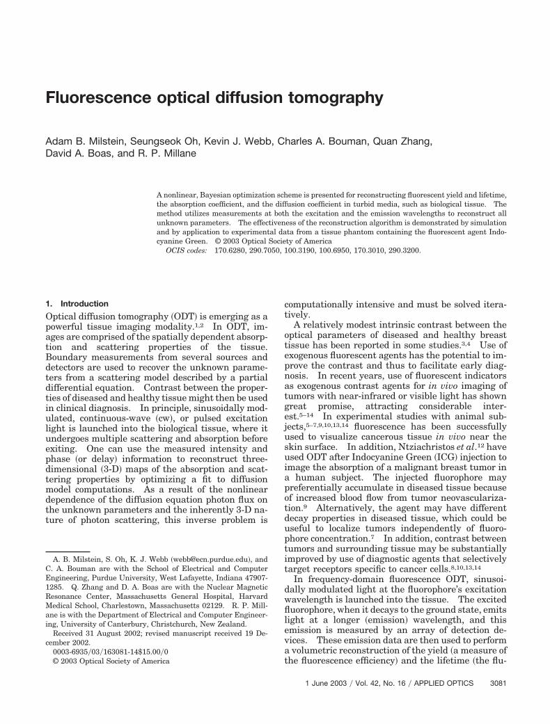
can be obtained by use of data from sources and de-tectors at the emission wavelength m. Finally, hav-ing found these parameters, use of sources at x anddetectors filtered at m will yield the fluorescenceparameters. Figure 1 depicts this measurement ap-proach schematically.

After discretizing the domain into N voxels of equalsize, one can regard the unknown parameters as

3082 APPLIED OPTICS � Vol. 42, No. 16 � 1 June 2003

three image vectors, each corresponding to a mea-surement set. Let ri denote the position of the ithvoxel centroid, i.e., the location of a node in a Carte-sian finite-difference representation of Eqs. �1�–�3�.We define the image vectors as

xx � �xxa

xxb� � ��ax

�r1�· · ·�ax�rN�, Dx�r1�· · ·Dx�rN��T,

xm � �xma

xmb� � ��am

�r1�· · ·�am�rN�, Dm�r1�· · ·Dm�rN��T,

xf � �xfa

xf b� � ��r1�· · ·��rN�, ��r1�· · ·��rN��T, (4)

where the subscript f denotes the fluorescence imageand the superscript T denotes the transpose opera-tion. Note that the three image vectors are each ofsize 2N, consisting of two unknown parameter vec-tors of size N. In addition, we reparameterize thefluorescence unknowns ��af

, �� to ��, �� using

��r, �� af�r�

11 � ��r��2 , (5)

which, when substituted into Eq. �2�, yields

� � �Dm�r��m�r, �� am�r� � j��c��m�r, ��

� �x�r, ��r, ��1 � j��r��. (6)

As explained in Appendix A, this new parameteriza-tion is useful because, in a sequential optimizationscheme, it takes advantage of the inherent linearityof the fluorescence inverse problem while allowingregularization to be applied to � directly. The sets offlux measurements corresponding to the above imagevectors are defined, respectively, as yx, ym, and yf.

3. Inversion

The estimation of each of the unknown images �xx,xm, xf � from the corresponding observations �yx, ym,yf � is an ill-posed, typically underdetermined, inverseproblem. As in previous studies,24–26,29 we addressthis by formulating the inverse problem in a Bayes-ian framework. This framework allows the incorpo-ration of a priori information, and it encapsulates allavailable information about the problem model intoan objective function to be optimized. Let x denoteone of the images of Eqs. �4� and let y denote itscorresponding observations. We use Bayes’ rule to

compute the maximum a posteriori �MAP� estimate,given by

xMAP � arg maxx�0

� p�y�x� � p�x��, (7)

where p�y�x� is the data likelihood and p�x� is theprior density for the image. The data likelihood canbe formed from a Gaussian model when we consider,for example, the physical properties of a photocurrentshot-noise-limited measurement system.24 Thisgives

p�y�x� �1

��P��1 exp��y � f�x��

2

� � , (8)

where P is the number of measurements; f is theappropriate forward operator; � is a scalar parameterthat scales the noise variance; and, for an arbitraryvector w, �w��

2 � wH�w �where H denotes Hermitiantranspose� and ��2��1 is the covariance matrix.In a small signal shot-noise model, the measure-ments are independent and normally distributedwith a mean equal to the exact �noiseless� measure-ment and a variance proportional to the exact mea-surement at a modulation frequency of zero �dc�.Following Ye et al.,24 we approximate the dc flux forthe ith datum as �yi�. The resulting covariance ma-trix is given by

�

2�1 �

�

2diag�� y1�, � y2�, . . . � yP��. (9)

For the prior density p�x�, we use the generalizedGaussian Markov random field �GGMRF� model,which enforces smoothness in the solution whilepreserving sharp edge transitions.24,30 For eachnode �representing a voxel� inside the image, weform a 3-D neighborhood from the 26 adjacent nodes.Let xT � �xa

T, xbT�, as in Eqs. �4�. Assuming inde-

pendence of xa and xb, the density function is givenby

p�x� � p�xa� � p�xb� (10)

� � 1�a

Nz� pa�exp�

1pa�a

pa

� ��i, j��a

bij�xi � xj �pa�� 1

�bNz� pb�

exp�1

pb�bpb

� ��i, j��b

bij�xi � xj �pb�� , (11)

where the subscripts a and b have the same meaningas in Eqs. �4�, xi denotes the ith node of x, the set �consists of all pairs of neighboring nodes, and bij isthe weighting coefficient corresponding to the ith andjth nodes. The coefficients bij are assigned to beinversely proportional to the node separation in a

Fig. 1. Proposed measurement scheme.


cube-shaped node layout, with the requirement thatthat ¥j bij � 1. The constants p and � control the

shape and scale of the distribution, and the factorz�p� is a normalization term.

As in previous research,25 we incorporate � into theinverse problem as an unknown for each image. Wefound that this tends to improve the robustness andspeed of convergence. As a result, we perform a jointmaximum a posteriori estimation of both x and � foreach image:

xx � arg maxxx�0,�x

� p�xx�yx, �x��, (12)

xm � arg maxxm�0,�m

� p�xm�ym, �m��, (13)

xf � arg maxxf�0,�f

� p�xf �yf, �f, xx, xm��. (14)

The estimations of xx and xm are performed indepen-dently of each other, with Eqs. �1� and �3� used as therespective forward models. Subsequently, these es-timates are incorporated into the coupled diffusionequations �Eqs. �1� and �2�� to estimate xf.

Let x and � correspond to one of the images in Eqs.�12�–�14�. Ye et al.25 showed that the above recon-structions are equivalent to one maximizing the logposterior probability l�x�, which can be derived withEqs. �7�, �8�, and �11�:

l�x� � P ln �y � f�x��2 �

1pa�a

pa ��i, j��a

bij

� �xi � xj �pa �1

pb�bpb �

�i, j��b

bij�xi � xj �pb. (15)

Optimizing l�x� can be implemented by alternatingclosed-form updates of � with updates of x25:

� �1P

�y � f�x��2 , (16)

x � arg maxx�0

�ln p�y�x, �� ln p�x��, (17)

where � implies an update iteration rather than afull optimization. The x updates represent morecomputationally expensive steps toward optimizing

Eq. �7� than the � updates. For each image, we forman objective function from Eqs. �8� and �11�:

The variables have the same meaning as in Eqs. �8�and �11�, and their subscripts have the same meaningas in Eqs. �4�. Note that forward operator ff is afunction of xf and the estimates xx and xm. In prin-ciple, one could jointly optimize Eqs. �18�–�20� overxx, xm, and xf, but for computational simplicity, wefirst optimize Eqs. �18� and �19� and subsequentlyincorporate the estimates into Eq. �20�. With theobjective functions defined by Eqs. �18�–�20� estab-lished, an optimization algorithm to minimize thesecosts is needed, which is described in Section 4.

4. Iterative Coordinate Descent Optimization

The optimizations of Eqs. �18�–�20� are performed byuse of the iterative coordinate descent �ICD� algo-rithm,24,26,31 a sequential single-site update schemesimilar to the Gauss–Seidel method used in otherproblems. One ICD scan consists of the formation ofa local quadratic approximation to the cost function,followed by an update of each image element individ-ually to minimize the approximate objective function.On each subsequent scan, the Frechet derivative ofthe nonlinear forward operator is recomputed, and anew quadratic approximation is made.

Once again, let x denote one of the three images tobe optimized. During the scan, the individual voxelsof x are sequentially updated in random order. Atthe beginning of the scan, f�x� is first expressed byuse of a Taylor expansion as

�y � f�x��2 � �y � f�x� � F��x��x��

2 , (21)

where �x � x x, and F��x� represents the Frechetderivative of f�x� with respect to x at x � x. UsingEq. �21�, we formulate the approximate cost function:

c�x, �� 1�

�z � F��x�x��2 �

1pa�a

pa ��i, j��a

bij

� �xi � xj �pa �1

pb�bpb �

�i, j��b

bij�xi � xj �pb,

(22)

c�xx, �x� �1�x

�yx � fx�xx��x

2 �1

pxa�xapxa �

�i, j��xa

bij�xxai� xxaj

�pxa �1

pxb�xbpxb �

�i, j��xb

bij�xxbi� xxbj

�pxb, (18)

c�xm, �m� �1

�m�ym � fm�xm��m

2 �1

pma�mapma �

�i, j��ma

bij�xmai� xmaj

�pma �1

pmb�mbpmb �

�i, j��mb

bij�xmbi� xmbj

�pmb,

(19)

c�xf, xx, xm, �f� �1�f

�yf � ff�xf, xx, xm��f

2 �1

pfa�fapfa �

�i, j��fa

bij�xfai xfaj

�pfa�1

pf b�f bpf b �

�i, j��f b

bij�xf bi xf bj

�pf b.

(20)


where

z � y � f�x� � F��x�x. (23)

With the other image elements fixed, the ICD updatefor xi is given by

xi � arg minxi �0

1�

�y � f�x� � �F��x��*�i�� xi � xi��2

�1

p�p �j��i

bij�xi � xj �p , (24)

where �F��x��*�i� is the ith column of the Frechet de-rivative matrix and �i is the set of nodes neighboringnode i, and p and � are chosen appropriately from �pa,pb� and ��a, �b�. This one-dimensional minimizationis solved by use of a simple half-interval search.24

The Frechet derivative matrices used for each imageare given in Appendix A. In Appendix B we sum-marize the ICD optimization algorithm inpseudocode form.

Previously, we found that multiresolution tech-niques can reduce the computational burden and im-prove robustness of convergence for the ODTproblem.25 Hence, for large computational domains,it may be beneficial to perform several ICD scans ata reduced resolution followed by interpolation as aninitialization step for the full-resolution problem.

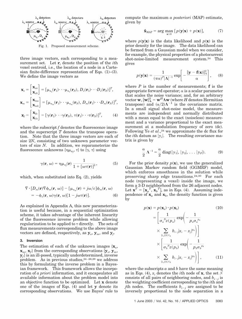
5. Simulations

Figure 2 shows cross-sectional images of a 17.3 cm �17.3 cm � 6 cm tissue phantom having backgroundvalues �ax,m

� 0.01 cm1, Dx,m � 0.047 cm, � � 0 ns,and ��af

� 0 cm1. A slightly off-center sphericalheterogeneity with a diameter of roughly 3 cm ispresent, with �ax

� 0.05 cm1, �am� 0.01 cm1, Dx

and Dm � 0.30 cm, � � 0.55 ns, and ��af� 0.02 cm1.

Figure 2�g� shows the location and size of the fluoro-phore as the ��af

� 0.01-cm1 isosurface. As shownin Fig. 3, the bottom face of the domain contains 16sources �modulated at 70 MHz� arranged in a 4 � 4grid pattern. On the top face, 16 detectors areplaced in an identical grid. Using multigrid finitedifferences32 to solve the diffusion equations, we gen-erated synthetic measurements. Additive noise wasintroduced by use of the approximate shot-noisemodel of Eqs. �8� and �9�, giving an average signal-to-noise ratio of 34 dB and a maximum signal-to-noise ratio of 41 dB. In the forward solution, anextrapolated zero-flux boundary condition33 was usedto model the free-space absorbing boundaries.

For each of the xx, xm, and xf inversions, 20 ICDiterations at a resolution of 17 � 17 � 9 nodes, fol-lowed by 20 ICD iterations at a resolution of 33 �33 � 17 nodes, were performed. For the nonlinearxx and xm problems, multigrid finite differences wereused to solve the forward model prior to each ICDimage update. During the inversions, the log poste-rior probability was evaluated as the convergencecriterion. For each image, convergence �with subse-quent iterations changing the images very little� wasobtained in approximately 10 min of computation on

an AMD Athlon 1333-MHz workstation. Althoughautomatic estimation of the GGMRF hyperparam-eters p and � is in principle possible with amaximum-likelihood estimation technique,34 we fol-low Ye et al.24 and use parameter values that empir-ically give good results. For each reconstruction, the

Fig. 2. True phantom, with cross sections of the widest part of theheterogeneity: �a� �ax

is in cm1, �b� Dx is in cm, �c� �amis in cm1,

�d� Dm is in cm, �e� � is in ns, �f � ��afis in cm1, �g� ��af

� 0.01 cm1

isosurface.

Fig. 3. Grid used for both sources and detectors in the simulation,with the relative location of the sphere depicted.


estimates were initialized with homogeneous imagesequal to the correct background values, as the ICDmethod’s convergence is slow for low-spatial-frequency image components.31 We have shownpreviously that multigrid inversion methods in con-junction with ICD updates alleviate this difficul-ty,25,35,36 but, again, we do not address them in thisinvestigation.

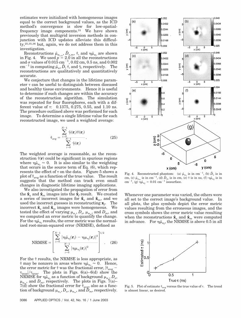
Reconstructions �ax,m, Dx,m, �, and ��af

are shownin Fig. 4. We used p � 2.0 in all the reconstructionsand � values of 0.015 cm1, 0.02 cm, 0.5 ns, and 0.002cm1 in computing �a, D, �, and �, respectively. Thereconstructions are qualitatively and quantitativelyaccurate.

We conjecture that changes in the lifetime param-eter � can be useful to distinguish between diseasedand healthy tissue environments. Hence it is usefulto determine if such changes are within the accuracyof the reconstruction algorithm. The simulationwas repeated for four fluorophores, each with a dif-ferent value of �: 0.1375, 0.275, 0.55, and 1.10 ns.The procedure outlined above was performed for eachimage. To determine a single lifetime value for eachreconstructed image, we used a weighted average:

�avg ��i�0

N1

��ri��ri�

�i�0

N1

��ri�

. (25)

The weighted average is reasonable, as the recon-struction ��r� could be significant in spurious regionswhere ��af

� 0. It is also similar to the weightingthat occurs in the source term of Eq. �6�, which rep-resents the effect of � on the data. Figure 5 shows aplot of �avg as a function of the true value. The resultsuggests that the method can track even smallchanges in diagnostic lifetime imaging applications.

We also investigated the propagation of error fromthe xx and xm images into the xf result. We createda series of incorrect images for xx and xm, and weused the incorrect guesses in reconstructing xf. Theincorrect xx and xm images were homogeneous. Wetested the effect of varying �ax

, Dx, �am, and Dm, and

we computed an error metric to quantify the change.For the ��af

results, the error metric was the normal-ized root-mean-squared error �NRMSE�, defined as

NRMSE � ��i�0

N1

��af�ri� � ��af

�ri��2

�i�0

N1

��af�ri��2 �

1�2

. (26)

For the � results, the NRMSE is less appropriate, as� may be nonzero in areas where ��af

� 0. Hence,the error metric for � was the fractional error, ��avg �true��true. The plots in Figs. 6�a�–6�d� show theNRMSE for ��af

as a function of background �ax, Dx,

�am, and Dm, respectively. The plots in Figs. 7�a�–

7�d� show the fractional error for �avg, also as a func-tion of background �ax

, Dx, �am, and Dm, respectively.

Whenever one parameter was varied, the others wereall set to the correct image’s background value. Inall plots, the plus symbols depict the error metricvalues resulting from the erroneous images, and thecross symbols shows the error metric value resultingwhen the reconstructions xx and xm were computedin advance. For ��af

, the NRMSE is above 0.5 in all

Fig. 4. Reconstructed phantom: �a� �axis in cm1, �b� Dx is in

cm, �c� �amis in cm1, �d� Dm is in cm, �e� � is in ns, �f � ��af

is incm1, �g� ��af

� 0.01 cm1 isosurface.

Fig. 5. Plot of estimate �avg versus the true value of �. The trendis almost linear, as desired.


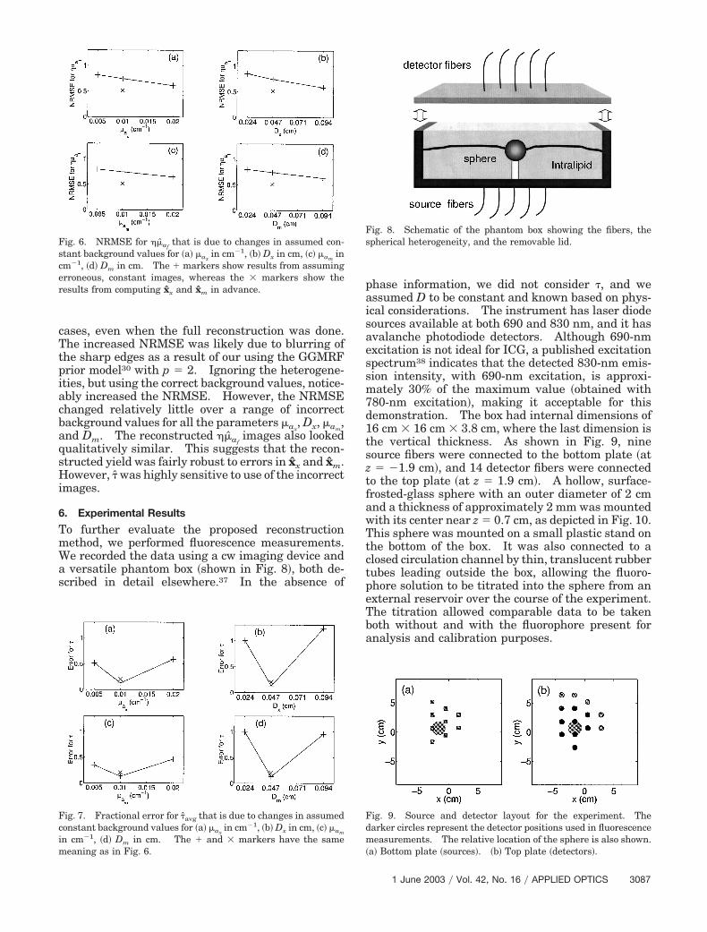
cases, even when the full reconstruction was done.The increased NRMSE was likely due to blurring ofthe sharp edges as a result of our using the GGMRFprior model30 with p � 2. Ignoring the heterogene-ities, but using the correct background values, notice-ably increased the NRMSE. However, the NRMSEchanged relatively little over a range of incorrectbackground values for all the parameters �ax

, Dx, �am,

and Dm. The reconstructed ��afimages also looked

qualitatively similar. This suggests that the recon-structed yield was fairly robust to errors in xx and xm.However, � was highly sensitive to use of the incorrectimages.

6. Experimental Results

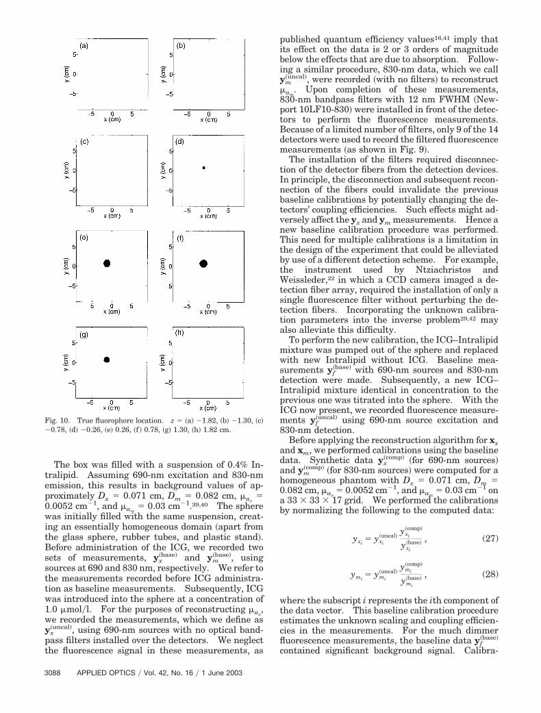
To further evaluate the proposed reconstructionmethod, we performed fluorescence measurements.We recorded the data using a cw imaging device anda versatile phantom box �shown in Fig. 8�, both de-scribed in detail elsewhere.37 In the absence of

phase information, we did not consider �, and weassumed D to be constant and known based on phys-ical considerations. The instrument has laser diodesources available at both 690 and 830 nm, and it hasavalanche photodiode detectors. Although 690-nmexcitation is not ideal for ICG, a published excitationspectrum38 indicates that the detected 830-nm emis-sion intensity, with 690-nm excitation, is approxi-mately 30% of the maximum value �obtained with780-nm excitation�, making it acceptable for thisdemonstration. The box had internal dimensions of16 cm � 16 cm � 3.8 cm, where the last dimension isthe vertical thickness. As shown in Fig. 9, ninesource fibers were connected to the bottom plate �atz � 1.9 cm�, and 14 detector fibers were connectedto the top plate �at z � 1.9 cm�. A hollow, surface-frosted-glass sphere with an outer diameter of 2 cmand a thickness of approximately 2 mm was mountedwith its center near z � 0.7 cm, as depicted in Fig. 10.This sphere was mounted on a small plastic stand onthe bottom of the box. It was also connected to aclosed circulation channel by thin, translucent rubbertubes leading outside the box, allowing the fluoro-phore solution to be titrated into the sphere from anexternal reservoir over the course of the experiment.The titration allowed comparable data to be takenboth without and with the fluorophore present foranalysis and calibration purposes.

Fig. 6. NRMSE for ��afthat is due to changes in assumed con-

stant background values for �a� �axin cm1, �b� Dx in cm, �c� �am

incm1, �d� Dm in cm. The � markers show results from assumingerroneous, constant images, whereas the � markers show theresults from computing xx and xm in advance.

Fig. 7. Fractional error for �avg that is due to changes in assumedconstant background values for �a� �ax

in cm1, �b� Dx in cm, �c� �am

in cm1, �d� Dm in cm. The � and � markers have the samemeaning as in Fig. 6.

Fig. 8. Schematic of the phantom box showing the fibers, thespherical heterogeneity, and the removable lid.

Fig. 9. Source and detector layout for the experiment. Thedarker circles represent the detector positions used in fluorescencemeasurements. The relative location of the sphere is also shown.�a� Bottom plate �sources�. �b� Top plate �detectors�.


The box was filled with a suspension of 0.4% In-tralipid. Assuming 690-nm excitation and 830-nmemission, this results in background values of ap-proximately Dx � 0.071 cm, Dm � 0.082 cm, �ax

�0.0052 cm1, and �am

� 0.03 cm1.39,40 The spherewas initially filled with the same suspension, creat-ing an essentially homogeneous domain �apart fromthe glass sphere, rubber tubes, and plastic stand�.Before administration of the ICG, we recorded twosets of measurements, yx

�base� and ym�base�, using

sources at 690 and 830 nm, respectively. We refer tothe measurements recorded before ICG administra-tion as baseline measurements. Subsequently, ICGwas introduced into the sphere at a concentration of1.0 �mol�l. For the purposes of reconstructing �ax

,we recorded the measurements, which we define asyx

�uncal�, using 690-nm sources with no optical band-pass filters installed over the detectors. We neglectthe fluorescence signal in these measurements, as

published quantum efficiency values16,41 imply thatits effect on the data is 2 or 3 orders of magnitudebelow the effects that are due to absorption. Follow-ing a similar procedure, 830-nm data, which we callym

�uncal�, were recorded �with no filters� to reconstruct�am

. Upon completion of these measurements,830-nm bandpass filters with 12 nm FWHM �New-port 10LF10-830� were installed in front of the detec-tors to perform the fluorescence measurements.Because of a limited number of filters, only 9 of the 14detectors were used to record the filtered fluorescencemeasurements �as shown in Fig. 9�.

The installation of the filters required disconnec-tion of the detector fibers from the detection devices.In principle, the disconnection and subsequent recon-nection of the fibers could invalidate the previousbaseline calibrations by potentially changing the de-tectors’ coupling efficiencies. Such effects might ad-versely affect the yx and ym measurements. Hence anew baseline calibration procedure was performed.This need for multiple calibrations is a limitation inthe design of the experiment that could be alleviatedby use of a different detection scheme. For example,the instrument used by Ntziachristos andWeissleder,22 in which a CCD camera imaged a de-tection fiber array, required the installation of only asingle fluorescence filter without perturbing the de-tection fibers. Incorporating the unknown calibra-tion parameters into the inverse problem29,42 mayalso alleviate this difficulty.

To perform the new calibration, the ICG–Intralipidmixture was pumped out of the sphere and replacedwith new Intralipid without ICG. Baseline mea-surements yf

�base� with 690-nm sources and 830-nmdetection were made. Subsequently, a new ICG–Intralipid mixture identical in concentration to theprevious one was titrated into the sphere. With theICG now present, we recorded fluorescence measure-ments yf

�uncal� using 690-nm source excitation and830-nm detection.

Before applying the reconstruction algorithm for xxand xm, we performed calibrations using the baselinedata. Synthetic data yx

�comp� �for 690-nm sources�and ym

�comp� �for 830-nm sources� were computed for ahomogeneous phantom with Dx � 0.071 cm, Dm �0.082 cm, �ax

� 0.0052 cm1, and �am� 0.03 cm1 on

a 33 � 33 � 17 grid. We performed the calibrationsby normalizing the following to the computed data:

yxi� yxi

�uncal�yxi

�comp�

yxi

�base� , (27)

ymi� ymi

�uncal�ymi

�comp�

ymi

�base� , (28)

where the subscript i represents the ith component ofthe data vector. This baseline calibration procedureestimates the unknown scaling and coupling efficien-cies in the measurements. For the much dimmerfluorescence measurements, the baseline data yf

�base�

contained significant background signal. Calibra-

Fig. 10. True fluorophore location. z � �a� 1.82, �b� 1.30, �c�0.78, �d� 0.26, �e� 0.26, �f � 0.78, �g� 1.30, �h� 1.82 cm.


tions were performed to account for the unknowncoupling efficiencies and to remove these backgroundcomponents from the fluorescence data:

yfi � � yfi�uncal� � yfi

�base��yxi

�comp�

yxi

�base� , (29)

where we used the 690-nm calibration factors. Theresulting fluorescence data contain an unknown scalefactor that is due to the filter attenuation of the830-nm fluorescence light.

The reconstructions �axand �am

are shown in Figs.11 and 12, respectively. For each inversion, a vol-ume representing the whole box was discretized into33 � 33 � 17 voxels. The �ax

computation used � �0.015 cm1 and p � 2, and the �am

computation used� � 0.03 cm1 and p � 2. For both images, the ICDalgorithm was run for 20 iterations on a 927-MHzPentium III workstation, taking approximately 10min. The resulting �ax

and �amimages show a het-

erogeneity with accurate shape, although with arti-facts present in the region close to the top plate. In

both images, the sphere’s vertical positions are sim-ilar, but below the true location by approximately 4 or5 mm. The similarity of the two reconstructions,despite the fact that they are based on independentdata sets, suggests that this error is due to a system-atic effect in the reconstruction method. This maybe a result of calibration errors, as the assumption ofa diffuse, homogeneous medium in the baseline cali-brations neglected the presence of the low-scatteringglass sphere, the plastic stand used to hold thesphere, and the thin rubber tubes used to pump in theICG solution. Small errors in the assumed Dx andDm values might also contribute to artifacts in thereconstructions. In addition, placing the sphereclose to the detectors may have resulted in modelingerrors under the diffusion approximation. In �ax

,the reconstructed ICG absorption is slightly smallerthan the predicted value of 0.039 cm1, which onewould expect from the results of Sevick-Muraca etal.,16 after correcting for use of 690-nm, rather than780-nm, excitation with the above-mentioned 30%factor.38 The �am

image has higher contrast than

Fig. 11. Reconstructions of �axin cm1. Values of z for �a�–�h�

are the same as in Fig. 10.Fig. 12. Reconstructions of �am

in cm1. Values of z for �a�–�h�are the same as in Fig. 10.


the �aximage, in contrast to a published absorption

spectrum for ICG of 6.5 �mol�l, which shows higherabsorption at 690 nm than at 830 nm. It is possiblethat ICG’s instability in aqueous solution causessome variability in its optical spectrum; Landsman etal.43 observed a shift in the absorption peak towardlonger wavelengths with decreasing concentration.In addition, the effect of an Intralipid suspension onICG’s absorption spectrum has not been investigatedin detail, to our knowledge.

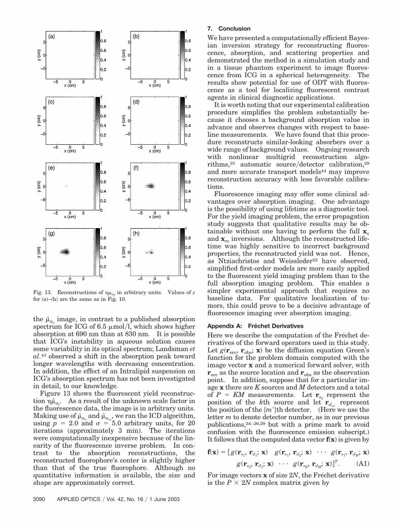
Figure 13 shows the fluorescent yield reconstruc-tion ��af

. As a result of the unknown scale factor inthe fluorescence data, the image is in arbitrary units.Making use of �ax

and �am, we ran the ICD algorithm,

using p � 2.0 and � � 5.0 arbitrary units, for 20iterations �approximately 3 min�. The iterationswere computationally inexpensive because of the lin-earity of the fluorescence inverse problem. In con-trast to the absorption reconstructions, thereconstructed fluorophore’s center is slightly higherthan that of the true fluorophore. Although noquantitative information is available, the size andshape are approximately correct.

7. Conclusion

We have presented a computationally efficient Bayes-ian inversion strategy for reconstructing fluores-cence, absorption, and scattering properties anddemonstrated the method in a simulation study andin a tissue phantom experiment to image fluores-cence from ICG in a spherical heterogeneity. Theresults show potential for use of ODT with fluores-cence as a tool for localizing fluorescent contrastagents in clinical diagnostic applications.

It is worth noting that our experimental calibrationprocedure simplifies the problem substantially be-cause it chooses a background absorption value inadvance and observes changes with respect to base-line measurements. We have found that this proce-dure reconstructs similar-looking absorbers over awide range of background values. Ongoing researchwith nonlinear multigrid reconstruction algo-rithms,25 automatic source�detector calibration,29

and more accurate transport models44 may improvereconstruction accuracy with less favorable calibra-tions.

Fluorescence imaging may offer some clinical ad-vantages over absorption imaging. One advantageis the possibility of using lifetime as a diagnostic tool.For the yield imaging problem, the error propagationstudy suggests that qualitative results may be ob-tainable without one having to perform the full xxand xm inversions. Although the reconstructed life-time was highly sensitive to incorrect backgroundproperties, the reconstructed yield was not. Hence,as Ntziachristos and Weissleder22 have observed,simplified first-order models are more easily appliedto the fluorescent yield imaging problem than to thefull absorption imaging problem. This enables asimpler experimental approach that requires nobaseline data. For qualitative localization of tu-mors, this could prove to be a decisive advantage offluorescence imaging over absorption imaging.

Appendix A: Frechet Derivatives

Here we describe the computation of the Frechet de-rivatives of the forward operators used in this study.Let g�rsrc, robs; x� be the diffusion equation Green’sfunction for the problem domain computed with theimage vector x and a numerical forward solver, withrsrc as the source location and robs as the observationpoint. In addition, suppose that for a particular im-age x there are K sources and M detectors and a totalof P � KM measurements. Let rsk

represent theposition of the kth source and let rdm�

representthe position of the �m��th detector. �Here we use theletter m to denote detector number, as in our previouspublications,24–26,29 but with a prime mark to avoidconfusion with the fluorescence emission subscript.�It follows that the computed data vector f�x� is given by

f�x� � � g�rs1, rd1

; x� g�rs1, rd2

; x� · · · g�rs1, rdM

; x�

g�rs2, rd1

; x� · · · g�rsK, rdM

; x��T. (A1)

For image vectors x of size 2N, the Frechet derivativeis the P � 2N complex matrix given by

Fig. 13. Reconstructions of ��afin arbitrary units. Values of z

for �a�–�h� are the same as in Fig. 10.


For the absorption and scattering coefficients, thediscrete representations of the Frechet derivativematrix elements have been derived and reported pre-viously27,45 as

�g�rsk, rdm�

; x�

��a�ri�� g�rdm�

, ri; x� g�rsk, ri; x�V, (A3)

�g�rsk, rdm�

; x�

�D�ri�� g�rdm�

, ri; x� � �g�rsk, ri; x�V,

(A4)

where � is used because of domain discretizationerrors, V is the voxel volume, ri is the position of theith voxel, and reciprocity46 �which allows replace-ment of g�rsrc, robs; x� with g�robs, rsrc; x�� was used toreduce the computation. Here, � is the spatial gra-dient operator, which, in our computations, is evalu-ated numerically as a symmetric first difference.The separability of relations �A3� and �A4� with re-spect to source index and detector index enables ad-ditional savings in computation and in storage.29

Rather than creating the entire KM � 2N matrix, itsuffices to initially compute and store two Green’sfunction matrices of sizes K � N and M � N, respec-tively:

G�s� � �g�rs1, r1; x� · · · g�rs1

, rN; x�···

· · ····

g�rsK, r1; x� · · · g�rsK

, rN; x�� , (A5)

G�d� � � g�rd1, r1; x� · · · g�rd1

, rN; x�···

· · ····

g�rdM, r1; x� · · · g�rdM

, rN; x�� . (A6)

During the ICD scan, when the ith voxel of x is to bemodified, the ith column of F��x� can be formed fromEqs. �A5� and �A6�.

For the fluorescence problem, more specific nota-tion is needed. Let gx�rsrc, robs; xx� denote the xGreen’s function obtained when we solve Eq. �1� andlet gm�rsrc, robs; xm� denote the m Green’s function

obtained when we solve Eq. �3�. We denote theGreen’s function matrices accordingly:

Gx�s� � �gx�rs1

, r1; xx� · · · gx�rs1, rN; xx�

···· · ·

···gx�rsK

, r1; xx� · · · gx�rsK, rN; xx�

� , (A7)

Gx�d� � � gx�rd1

, r1; xx� · · · gx�rd1, rN; xx�

···· · ·

···gx�rdM

, r1; xx� · · · gx�rdM, rN; xx�

� , (A8)

Gm�s� � �gm�rs1

, r1; xm� · · · gm�rs1, rN; xm�

···· · ·

···gm�rsK

, r1; xm� · · · gm�rsK, rN; xm�

� , (A9)

Gm�d� � � gm�rd1

, r1; xm� · · · gm�rd1, rN; xm�

···· · ·

···gm�rdM

, r1; xm� · · · gm�rdM, rN; xm�

� .

(A10)

Consider one reparameterization on the right-handside of Eq. �2�:

��af�r�

1 � j��r�

1 � ��r��2 � �R�r� � j�I�r�. (A11)

It follows immediately that the inverse problem for�R and �I is linear. Let gf �rsrc, robs; xx, xm� denotethe fluorescence observed at robs emitted in responseto excitation at rsrc. The Frechet derivatives for �Iand �R are given by

�gf �rsk, rdm�

; xx, xm�

��R�ri�� gm�rdm�

, ri; xm�

� gx�rsk, ri; xx�V, (A12)


; xx, xm�

��I�ri�� jgm�rdm�

, ri; xm�

� gx�rsk, ri; xx�V. (A13)

F��x� � ��g�rs1

, rd1; x�

� x1

�g�rs1, rd1

; x�

� x2

· · ·�g�rs1

, rd1; x�

� x2N1

�g�rs1, rd1

; x�

� x2N

�g�rs1, rd2

; x�

� x1

�g�rs1, rd2

; x�

� x2

· · ·�g�rs1

, rd2; x�

� x2N1

�g�rs1, rd2

; x�

� x2N···

···· · ·

······

�g�rs1, rdM

; x�

� x1

�g�rs1, rdM

; x�

� x2

· · ·�g�rs1

, rdM; x�

� x2N1

�g�rs1, rdM

; x�

� x2N

�g�rs2, rd1

; x�

� x1

�g�rs2, rd1

; x�

� x2

· · ·�g�rs2

, rd1; x�

� x2N1

�g�rs2, rd1

; x�

� x2N···

···· · ·

······

�g�rsK, rdM

; x�

� x1

�g�rsK, rdM

; x�

� x2

· · ·�g�rsK

, rdM; x�

� x2N1

�g�rsK, rdM

; x�

� x2N

� . (A2)


It is possible to solve the fluorescence inverse problemwith this parameterization and then convert the re-sult into the physical parameters ��af

and �. How-ever, the computation of � requires a division of �I by�R, an operation that could result in large noise ar-tifacts in regions where �R is small. To circumventthis problem, we use the � and � parameterization ofEq. �6�, permitting us to apply regularization directlyto �. In our sequential update scheme, � is assumedconstant while updates of � are performed, and viceversa. As a result, we use the following Frechet de-rivative expressions:


; xx, xm�

��ri�� gm�rdm�

, ri; xm� gx�rsk, ri; xx�

� �1 � j��ri��V, (A14)


; xx, xm�

��ri�� j��ri� gm�rdm�

, ri; xm�

� gx�rsk, ri; xx�V. (A15)

After the reconstructions of xx and xm are obtained,Gx�rs, r; xx� and Gm�rd, r; xm� have already beenstored, and the Green’s functions of relations �A14�and �A15� need not be recomputed. As the estimates� and � are updated, they are incorporated into thederivative expressions.

Appendix B: Pseudocode for the Inversion Algorithm

main �1. Initialize xx, xm, and xf with background es-

timates.2. Repeat until converged: �

�a� �x 4 �1�Px� �yx fx�xx��x

2

�b� For k � 1:K �Compute gx�rsk

, r; xx� by solving Eq. �1� withsource at rsk

��c� For m� � 1:M �

Compute gx�rdm�, r; xx� by solving Eq. �1�

with source at rdm�

��d� Form Gx

�s� and Gx�d� with Eqs. �A7� and �A8�

�e� xx 4 ICD_update�xx, �x, Gx�s�, Gx

�d��

3. Repeat until converged: ��a� �m 4 1�Pm �ym fm�xm��m

2

�b� For k � 1:K �Compute gm�rsk

, r; xm� by solving Eq. �3�with source at rsk

��c� For m� � 1:M �

Compute gm�rdm�, r; xm� by solving Eq. �3�

with source at rdm�

��d� Form Gm

�s� and Gm�d� with Eqs. �A9� and �A10�

�e� xm 4 ICD_update�xm, �m, Gm�s�, Gm

�d��

4. Repeat until converged: ��a� �f 4 �1�Pf� �yf ff �xf, xx, xm��f

2

�b� xf 4 ICD_update�xf, �f, Gx�s�, Gm

�d��

�

x 4 ICD_update�x, �, G�s�, G�d�; x� �1. For i � 1, . . . , N �in random order�, �

�a� Compute �F��x��*�i�, as described in Ap-pendix A

�b� Update xi, as described by Ye et al.24:

xi 4 arg minxi �0

1�

�y � f�x� � �F��x��*�i�� xi � xi��2

�1

pa�apa �

j��i

bij�xi � xi �pa�

2. For i � N � 1, . . . , 2N �in random order�, �

�a� Compute �F��x��*�i�, as described inAppendix A

�b� Update xi, as described by Ye et al.24:

xi 4 arg minxi �0

1�

�y � f�x� � �F��x��*�i�� xi � xi��2

�1

pb�bpb �

j��i

bij�xi � xi �pb�

3. Return x.�

This research was funded by the National ScienceFoundation under contract CCR-0073357. QuanZhang and David A. Boas acknowledge support fromAdvanced Research Technologies Inc. In addition,we thank Tina Chaves for her assistance with thelaboratory equipment.

References1. S. R. Arridge, “Optical tomography in medical imaging,” In-

verse Probl. 15, R41–R93 �1999�.2. D. A. Boas, D. H. Brooks, E. L. Miller, C. A. DiMarzio, M.

Kilmer, R. J. Gaudette, and Q. Zhang, “Imaging the body withdiffuse optical tomography,” IEEE Signal Process. Mag. 18,57–75 �2001�.

3. V. G. Peters, D. R. Wyman, M. S. Patterson, and G. L. Frank,“Optical properties of normal and diseased human breast tis-sues in the visible and near infrared,” Phys. Med. Biol. 35,1317–1334 �1990�.

4. T. L. Troy, D. L. Page, and E. M. Sevick-Muraca, “Opticalproperties of normal and diseased breast tissue: prognosisfor optical mammography,” J. Biomed. Opt. 1, 342–355�1996�.

5. A. Pelegrin, S. Folli, F. Buchegger, J. Mach, G. Wagnieres, andH. van den Bergh, “Antibody-fluorescein conjugates for photo-immunodiagnosis of human colon carcinoma in nude mice,”Cancer 67, 2529–2537 �1991�.

6. B. Ballou, G. W. Fisher, T. R. Hakala, and D. L. Farkas,“Tumor detection and visualization using cyaninefluorochrome-labeled antibodies,” Biotechnol. Prog. 13, 649–658 �1997�.


7. R. Cubeddu, G. Canti, A. Pifferi, P. Taroni, and G. Valentini,“Fluorescence lifetime imaging of experimental tumors in he-matoporphyrin derivative-sensitized mice,” Photochem. Pho-tobiol. 66, 229–236 �1997�.

8. J. A. Reddy and P. S. Low, “Folate-mediated targeting of ther-apeutic and imaging agents to cancers,” Crit. Rev. Ther. DrugCarrier Syst. 15, 587–627 �1998�.

9. J. S. Reynolds, T. L. Troy, R. H. Mayer, A. B. Thompson, D. J.Waters, K. K. Cornell, P. W. Snyder, and E. M. Sevick-Muraca,“Imaging of spontaneous canine mammary tumors using flu-orescent contrast agents,” Photochem. Photobiol. 70, 87–94�1999�.

10. U. Mahmood, C. Tung, J. A. Bogdanov, and R. Weissleder,“Near-infrared optical imaging of protease activity for tumordetection,” Radiology 213, 866–870 �1999�.

11. K. Licha, B. Riefke, V. Ntziachristos, A. Becker, B. Chance,and W. Semmler, “Hydrophilic cyanine dyes as contrast agentsfor near-infrared tumor imaging: synthesis, photophysicalproperties and spectroscopic in vivo characterization,” Photo-chem. Photobiol. 72, 392–398 �2000�.

12. V. Ntziachristos, A. G. Yodh, M. Schnall, and B. Chance, “Con-current MRI and diffuse optical tomography of breast afterindocyanine green enhancement,” Proc. Natl. Acad. Sci. USA97, 2767–2772 �2000�.

13. A. Becker, C. Hessenius, K. Licha, B. Ebert, U. Sukowski, W.Semmler, B. Wiedenmann, and C. Grotzinger, “Receptor-targeted optical imaging of tumors with near-infrared fluores-cent ligands,” Nat. Biotechnol. 19, 327–331 �2001�.

14. J. E. Bugaj, S. Achilefu, R. B. Dorshow, and R. Rajagopalan,“Novel fluorescent contrast agents for optical imaging of in vivotumors based on a receptor-targeted dye-peptide conjugateplatform,” J. Biomed. Opt. 6, 122–133 �2001�.

15. M. S. Patterson and B. W. Pogue, “Mathematical model fortime-resolved and frequency-domain fluorescence spectros-copy in biological tissues,” Appl. Opt. 33, 1963–1974 �1994�.

16. E. M. Sevick-Muraca, G. Lopez, J. S. Reynolds, T. L. Troy,and C. L. Hutchinson, “Fluorescence and absorption contrastmechanisms for biomedical optical imaging using frequency-domain techniques,” Photochem. Photobiol. 66, 55–64�1997�.

17. R. Roy and E. M. Sevick-Muraca, “Three-dimensional uncon-strained and constrained image-reconstruction techniques ap-plied to fluorescence, frequency-domain photon migration,”Appl. Opt. 40, 2206–2215 �2001�.

18. M. A. O’Leary, D. A. Boas, X. D. Li, B. Chance, and A. G. Yodh,“Fluorescence lifetime imaging in turbid media,” Opt. Lett. 21,158–160 �1996�.

19. D. Paithankar, A. Chen, B. Pogue, M. Patterson, and E.Sevick-Muraca, “Imaging of fluorescent yield and lifetime frommultiply scattered light reemitted from random media,” Appl.Opt. 36, 2260–2272 �1997�.

20. H. Jiang, “Frequency-domain fluorescent diffusion tomogra-phy: a finite-element-based algorithm and simulations,”Appl. Opt. 37, 5337–5343 �1998�.

21. J. Chang, H. L. Graber, and R. L. Barbour, “Luminescenceoptical tomography of dense scattering media,” J. Opt. Soc.Am. A 14, 288–299 �1997�.

22. V. Ntziachristos and R. Weissleder, “Experimental three-dimensional fluorescence reconstruction of diffuse media byuse of a normalized Born approximation,” Opt. Lett. 26, 893–895 �2001�.

23. D. A. Boas, “A fundamental limitation of linearized algorithmsfor diffuse optical tomography,” Opt. Express 1, 404–413�1997�; http:��www.opticsexpress.org.

24. J. C. Ye, K. J. Webb, C. A. Bouman, and R. P. Millane, “Opticaldiffusion tomography by iterative-coordinate-descent optimi-zation in a Bayesian framework,” J. Opt. Soc. Am. A 16, 2400–2412 �1999�.

25. J. C. Ye, C. A. Bouman, K. J. Webb, and R. P. Millane,“Nonlinear multigrid algorithms for Bayesian optical diffu-sion tomography,” IEEE Trans. Image Process. 10, 909–922�2001�.

26. A. B. Milstein, S. Oh, J. S. Reynolds, K. J. Webb, C. A. Bouman,and R. P. Millane, “Three-dimensional Bayesian optical diffu-sion tomography with experimental data,” Opt. Lett. 27, 95–97�2002�.

27. J. C. Ye, K. J. Webb, R. P. Millane, and T. J. Downar, “Modifieddistorted Born iterative method with an approximate Frechetderivative for optical diffusion tomography,” J. Opt. Soc. Am. A16, 1814–1826 �1999�.

28. J. S. Reynolds, C. A. Thompson, K. J. Webb, F. P. LaPlant,and D. Ben-Amotz, “Frequency domain modeling of reradia-tion in highly scattering media,” Appl. Opt. 36, 2252–2259�1997�.

29. S. Oh, A. B. Milstein, R. P. Millane, C. A. Bouman, and K. J.Webb, “Source–detector calibration in three-dimensionalBayesian optical diffusion tomography,” J. Opt. Soc. Am. A 19,1983–1993 �2002�.

30. C. A. Bouman and K. Sauer, “A generalized Gaussian imagemodel for edge-preserving MAP estimation,” IEEE Trans. Im-age Process. 2, 296–310 �1993�.

31. K. Sauer and C. A. Bouman, “A local update strategy for iter-ative reconstruction from projections,” IEEE Trans. SignalProcess. 41, 534–548 �1993�.

32. J. C. Adams, “MUDPACK: multigrid portable FORTRANsoftware for the efficient solution of linear elliptic partial dif-ferential equations,” Appl. Math. Comput. 34, 113–146 �1989�.

33. J. J. Duderstadt and L. J. Hamilton, Nuclear Reactor Analysis�Wiley, New York, 1976�.

34. S. S. Saquib, C. A. Bouman, and K. Sauer, “ML parameterestimation for Markov random fields with applications toBayesian tomography,” IEEE Trans. Image Process. 7, 1029–1044 �1998�.

35. S. Oh, A. B. Milstein, C. A. Bouman, and K. J. Webb, “Multi-grid inversion algorithms with applications to optical diffusiontomography,” in Proceedings of the 36th Asilomar Conferenceon Signals, Systems, and Computers �Institute of Electricaland Electronics Engineers, New York, 2002�, pp. 901–905.

36. K. Sauer and C. Bouman, “Bayesian estimation of transmis-sion tomograms using segmentation based optimization,”IEEE Trans. Nucl. Sci. 39, 1144–1152 �1992�.

37. Q. Zhang, T. J. Brukilacchio, T. Gaudett, L. Wang, A. Li, andD. A. Boas, “Experimental comparison of using continuous-wave and frequency-domain diffuse optical imaging systems todetect heterogeneities,” in Optical Tomography and Spectros-copy of Tissue IV, B. Chance, R. R. Alfano, B. J. Tromberg, M.Tamura, and E. M. Sevick-Muraca, eds., Proc. SPIE 4250,219–238 �2001�.

38. R. H. Mayer, J. S. Reynolds, and E. M. Sevick-Muraca, “Mea-surement of the fluorescence lifetime in scattering media byfrequency-domain photon migration,” Appl. Opt. 38, 4930–4938 �1999�.

39. H. J. van Staveren, C. J. M. Moes, J. van Marie, S. A. Prahl,and M. J. C. van Gemert, “Light scattering in Intralipid-10% inthe wavelength range of 400–1100 nm,” Appl. Opt. 30, 4507–4514 �1991�.

40. G. M. Hale and M. R. Querry, “Optical constants of water inthe 200-nm to 200-�m wavelength region,” Appl. Opt. 12, 555–563 �1973�.

41. R. C. Benson and H. A. Kues, “Fluorescence properties of in-docyanine green as related to angiography,” Phys. Med. Biol.23, 159–163 �1978�.

42. D. Boas, T. Gaudette, and S. Arridge, “Simultaneous imagingand optode calibration with diffuse optical tomography,” Opt.Exp. 8, 263–270 �2001�; http:��opticsexpress.org.

43. M. L. J. Landsman, G. Kwant, G. A. Mook, and W. G. Zijlstra,


“Light-absorbing properties, stability, and spectral stabiliza-tion of indocyanine green,” J. Appl. Physiol. 40, 575–583�1976�.

44. A. D. Klose and A. H. Hielscher, “A transport-theory-basedreconstruction algorithm for optical tomography,” in OpticalTomography and Spectroscopy of Tissue III, B. Chance, R. R.

Alfano, and B. J. Tromberg, eds., Proc. SPIE 3597, 26–35�1999�.

45. S. R. Arridge, “Photon-measurement density functions. Part1: Analytical forms,” Appl. Opt. 34, 7395–7409 �1995�.

46. W. C. Chew, Waves and Fields in Inhomogeneous Media �VanNostrand Reinhold, New York, 1990�.


Documents

Fluorescence Optical Diffusion Tomography