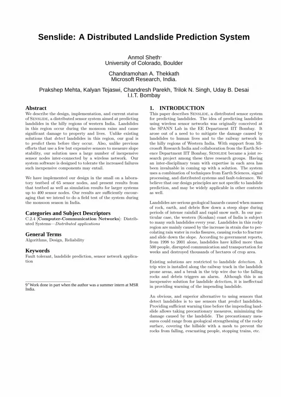
Senslide: A Distributed Landslide Prediction System

Anmol Sheth∗

University of Colorado, Boulder

Chandramohan A. ThekkathMicrosoft Research, India.

Prakshep Mehta, Kalyan Tejaswi, Chandresh Parekh, Trilok N. Singh, Uday B. DesaiI.I.T. Bombay

AbstractWe describe the design, implementation, and current statusof Senslide, a distributed sensor system aimed at predictinglandslides in the hilly regions of western India. Landslidesin this region occur during the monsoon rains and causesignificant damage to property and lives. Unlike existingsolutions that detect landslides in this region, our goal isto predict them before they occur. Also, unlike previousefforts that use a few but expensive sensors to measure slopestability, our solution uses a large number of inexpensivesensor nodes inter-connected by a wireless network. Oursystem software is designed to tolerate the increased failuressuch inexpensive components may entail.

We have implemented our design in the small on a labora-tory testbed of 65 sensor nodes, and present results fromthat testbed as well as simulation results for larger systemsup to 400 sensor nodes. Our results are sufficiently encour-aging that we intend to do a field test of the system duringthe monsoon season in India.

Categories and Subject DescriptorsC.2.4 [Computer-Communication Networks]: Distrib-uted Systems—Distributed applications

General TermsAlgorithms, Design, Reliability

KeywordsFault tolerant, landslide prediction, sensor network applica-tion

9∗Work done in part when the author was a summer intern at MSRIndia.

1. INTRODUCTIONThis paper describes Senslide, a distributed sensor systemfor predicting landslides. The idea of predicting landslidesusing wireless sensor networks was originally conceived atthe SPANN Lab in the EE Department IIT Bombay. Itarose out of a need to to mitigate the damage caused bylandslides to human lives and to the railway network inthe hilly regions of Western India. With support from Mi-crosoft Research India and collaboration from the Earth Sci-ence Department IIT Bombay, Senslide became a joint re-search project among these three research groups. Havingan inter-disciplinary team with expertise in each area hasbeen invaluable in coming up with a solution. The systemuses a combination of techniques from Earth Sciences, signalprocessing, and distributed systems and fault-tolerance. Webelieve that our design principles are not specific to landslideprediction, and may be widely applicable in other contextsas well.

Landslides are serious geological hazards caused when massesof rock, earth, and debris flow down a steep slope duringperiods of intense rainfall and rapid snow melt. In our par-ticular case, the western (Konkan) coast of India is subjectto many such landslides every year. Landslides in this rockyregion are mainly caused by the increase in strain due to per-colating rain water in rocks fissures, causing rocks to fractureand slide down the slope. According to government reports,from 1998 to 2001 alone, landslides have killed more than500 people, disrupted communication and transportation forweeks and destroyed thousands of hectares of crop area.

Existing solutions are restricted to landslide detection. Atrip wire is installed along the railway track in the landslideprone areas, and a break in the trip wire due to the fallingrocks and debris triggers an alarm. Although this is aninexpensive solution for landslide detection, it is ineffectualin providing warning of the impending landslide.

An obvious, and superior alternative to using sensors thatdetect landslides is to use sensors that predict landslides.Providing sufficient warning time before the impending land-slide allows taking precautionary measures, minimizing thedamage caused by the landslide. The precautionary mea-sures could range from geological strengthening of the rockysurface, covering the hillside with a mesh to prevent therocks from falling, evacuating people, stopping trains, etc.

Various such prediction sensors have been proposed in theliterature [6]. Typical sensors used for monitoring slope sta-bility are multi-point bore hole extensometers, tilt sensors,displacement sensors, and volumetric soil water content sen-sors. These require drilling 20-30 meter holes into the sur-face, making the installation very expensive (about $50 permeter) and requiring skilled labor. Furthermore, these areexpensive sensors, making wide scale deployment infeasible.Installing a single sensor for monitoring an entire hill sideis not sufficient as the properties of the rocks change every100-200 meters. Wiring each sensor to a central data loggeris also not feasible in the rocky terrain because it requireshigh maintenance, and is subject to a single point of failure.

In contrast to existing fixed single-point approaches, a fun-damentally new approach to measure slope stability is bycombining observations from a large number of distributedinexpensive sensors. Senslide uses an array of inexpensivesingle-axis strain gauges connected to cheap nodes (specif-ically, TelosB motes [3]), each with a CPU, battery, and awireless transmitter. Our sensors make point measurementsat various parts of a rock, but make no attempt at measur-ing the relative motion between rocks. Our strategy is basedon the simple observation that rock slides occur because ofincreased strain in the rocks. Thus, by measuring the causeof the landslide, we can predict landslides as easily as if wewere measuring the incipient relative movement of rocks.

Geologists familiar with our terrain estimate that sensorscan be separated by 30–40 meters. This would imply thatwe need about 600–900 sensors for each square kilometer ofhillside surrounding the railway track. We call this collectionof sensors a sensor patch, which is our basic unit of scale.The sensor patch contains only a modest number of sensorsthat we can reasonably expect our solutions to work at thisscale. Yet, the patch is large enough that we can duplicateit conveniently to cover the stretches of the railway trackthat are most prone to landslides. In our current design,each patch is independent of other patches; for all practicalpurposes this appears to be a reasonable assumption.

The point measurements made by individual sensors arepropagated to a set of “base stations” that have GPRSand/or 802.11 connectivity to each other. In addition totheir improved network connectivity, base stations are lo-cated in places with access to ground power, and have morecomputation and storage resources than the sensor nodes.Each sensor patch has 3–6 base stations, both for increasedfault-tolerance as well for limiting hop count between sensornodes and base stations.

There are some advantages to using simple strain sensors.The strain sensors can operate at low depths (25–30 cms);the orders of magnitude lower depth of operation make straingauge deployment much cheaper and more convenient with-out specialized equipment or a sophisticated labor force.The small size, low cost, and wireless connectivity allowdenser coverage over a larger area without significantly in-creasing the difficulty or the cost of deployment.

1.1 Key ContributionsWe believe our design is novel compared to previous sensornetwork systems because of the unique challenges we face in

our environment. A potential issue with using small, cheapsensors is that failures are more likely to occur and systemsoftware has to compensate to keep the system functional.Similarly, the larger number of sensors implies that the sys-tem software must be scalable.

We also believe that as sensor networks become more widelydeployed in harsh environments where failure is common,and power and network connectivity is unreliable, our designtechniques will become increasingly more applicable. Toour knowledge, though there have been sensor network sys-tems deployed in hostile environments (e.g., volcanic mon-itoring [25]), typically these systems have not focused onfault-tolerance or scalability. As a result, they can sufferfrom network outages and low data yield due to the failureof system components.

In trying to design a system to solve the needs of our appli-cation, we encountered several challenges, which we brieflyenumerate below. We use distributed systems algorithmsas well as techniques from machine learning to provide solu-tions to these challenges. The combination of these solutionsmakes our design unique, which ensures fault tolerance atevery level of the system and maximizes the lifetime of thesystem.

1. Noisy sensor data: Triggering an alarm based onlocally sampled raw sensor data would lead to a largenumber of false positives and negatives. The sensorsignal must therefore be smoothed before further process-ing.

2. Fault Tolerance: The system should not contain sin-gle points of failure, and should automatically adapt tocommunication links, nodes and base station failures.

3. Spatial summary of sensor data: Even thoughdata from individual sensors is smoothed, single sen-sor observations are insufficient to predict a landslide;data from several spatially distributed sensors must beincorporated to detect anomalies indicative of a land-slide. Without due care, such incorporation of datacould lead to excessive communication.

4. Unequal energy depletion in the network: Theprotocol used for routing packets from the individualsensor nodes to the base station should avoid the for-mation of hotspots in the network. Hot spots leadto unequal energy drain at some nodes due to the in-creased energy requirements for transmitting and re-ceiving packets. Nodes that are energy depleted cancause a network partition.

5. Balance between rare event detection and peri-odic data collection: Landslides are relatively rareevents. Thus, we could potentially conserve power andnever transmit data until a landslide is incipient. Thisconserves battery life in the network, but it could leadto a large number of false alarms and also defeats thepurpose of timely gathering of seismic data [8].

We address the first issue through straightforward signalsmoothing techniques.

We deal with failures of the base station by synchronouslyreplicating data on multiple base stations. We deal with thenode and link failures by using skeptics [20] and a modifiedversion of the Beacon Vector Routing algorithm [9] to builda resilient data forwarding protocol in the sensor network.

We deal with the last three issues using the same mechanism:hierarchical decomposition. A subset of the sensor nodes aredesignated as aggregators that collect smoothed local data,and create spatial summaries. These aggregator nodes com-municate with the base station providing summary data atadaptively adjusted frequencies. The location of the aggre-gators are chosen to spread the energy depletion uniformlyin the network. We tolerate failures of the aggregators byperiodic re-election of these nodes. The presence of aggrega-tors in the network reduces the average hop-count and thusthe number of radio transmissions required. It also increasesthe data yield of the network by avoiding congestion causedby transmitting all the sensor data to a centralized base sta-tion. The improved yield and uniform energy depletion ofthe network significantly improves the detection accuracyand lifetime of the network.

Although Senslide uses inexpensive sensor nodes connectedby a wireless network, our focus is quite different from previ-ous sensor network projects we are familiar with. A majorityof these projects [18, 24] focus on innovative data collectiontechniques, where recovery from failures is not the principalconcern. In contrast, our primary objective is to provide adistributed sensor system that is robust in the face of fail-ures.

The data collection strategy of Senslide is also differentfrom prior work. In fact, our work falls between two ex-tremes: rare event detection schemes [11, 22] and periodicsampling networks where data is collected at a central basestation for offline analysis. In our system, data must be sam-pled periodically to help earth scientists gather much neededhistorical trend information [8], while ensuring that the life-time of the network is not adversely affected by frequentsampling. Existing data collection based applications use atree-based routing algorithm to route all the data to a cen-tralized base station. This naive mechanism does not scalewith network size and leads to higher energy depletion of thenodes near the base station. Section 3 describes Senslide’shierarchical decomposition technique. Although the tech-nique is similar in principle to LEACH [13], it overcomessome of the limitations of LEACH which make it unsuitablefor our application.

We are aware of one other landslide detection research beingdone at John Hopkins [23], although we are not aware ofany implementation of that design. Our design differs fromtheirs in two aspects: (a) they process data only at thecentral base station, and (b) they do not explicitly deal withthe failures of components.

We have tested the efficacy of our techniques by deployingthe above described system in an indoor 65-node labora-tory testbed. We have also tested the scaling behavior ofour system on larger configurations (up to 400 nodes) usingthe ns-2 network simulator [2]. Encouraged by our results

from the prototype, we plan to do our field tests during themonsoons in India.

Section 2 describes the characteristics of our rocks, the lab-oratory set up we use to measure the behavior of the rocksunder strain, and the details of our detection algorithm. Sec-tion 3 describes our design in greater detail and Section 4illustrates the performance of our system on our testbed andin simulation. Section 5 provides a complete treatment ofrelated research, and Section 6 concludes our current projectstatus and future plans.

2. DETECTING LANDSLIDESIn this section, we describe the characteristics of the rocksthat are prevalent on the Konkan hillsides and our methodfor detecting an impending landslide.

2.1 Gathering Rock InformationThe primary rock characteristic we care about is the stress-strain behavior. The kind of rocks that are found in theKonkan region of India are classified as volcanic igneous,which are a type of “brittle” rock. The stress-strain curves ofigneous rocks exhibit linear behavior until there is a fracture.This near ideal behavior makes the terrain particularly well-suited to our technique.

Unfortunately, not all igneous rocks of the same type havethe same stress-strain behavior. Individual variations inthe crystalline structure as well as macroscopic variationin chemical composition and physical characteristics lead toobservable differences in their behavior to stress.

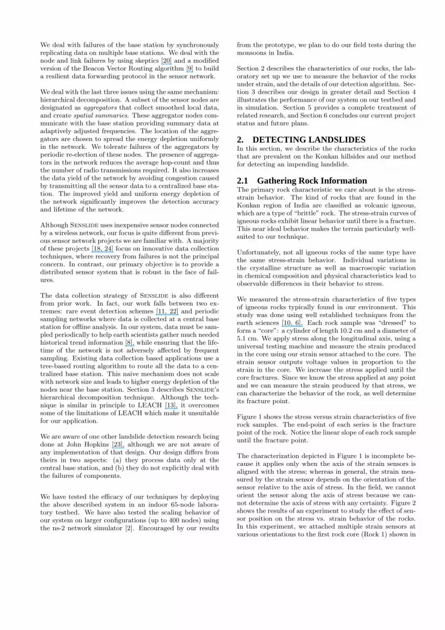
We measured the stress-strain characteristics of five typesof igneous rocks typically found in our environment. Thisstudy was done using well established techniques from theearth sciences [10, 6]. Each rock sample was “dressed” toform a “core”: a cylinder of length 10.2 cm and a diameter of5.1 cm. We apply stress along the longitudinal axis, using auniversal testing machine and measure the strain producedin the core using our strain sensor attached to the core. Thestrain sensor outputs voltage values in proportion to thestrain in the core. We increase the stress applied until thecore fractures. Since we know the stress applied at any pointand we can measure the strain produced by that stress, wecan characterize the behavior of the rock, as well determineits fracture point.

Figure 1 shows the stress versus strain characteristics of fiverock samples. The end-point of each series is the fracturepoint of the rock. Notice the linear slope of each rock sampleuntil the fracture point.

The characterization depicted in Figure 1 is incomplete be-cause it applies only when the axis of the strain sensors isaligned with the stress; whereas in general, the strain mea-sured by the strain sensor depends on the orientation of thesensor relative to the axis of stress. In the field, we cannotorient the sensor along the axis of stress because we can-not determine the axis of stress with any certainty. Figure 2shows the results of an experiment to study the effect of sen-sor position on the stress vs. strain behavior of the rocks.In this experiment, we attached multiple strain sensors atvarious orientations to the first rock core (Rock 1) shown in

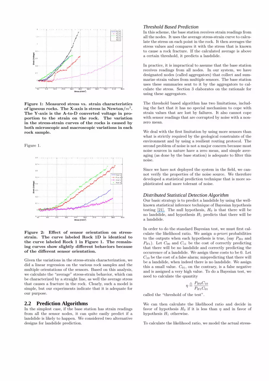
Figure 1: Measured stress vs. strain characteristicsof igneous rocks. The X-axis is stress in Newton/m2.The Y-axis is the A-to-D converted voltage in pro-portion to the strain on the rock. The variationin the stress-strain curves of the rocks is caused byboth microscopic and macroscopic variations in eachrock sample.

Figure 1.

Figure 2: Effect of sensor orientation on stress-strain. The curve labeled Rock 1D is identical tothe curve labeled Rock 1 in Figure 1. The remain-ing curves show slightly different behaviors becauseof the different sensor orientation.

Given the variations in the stress-strain characterization, wedid a linear regression on the various rock samples and themultiple orientations of the sensors. Based on this analysis,we calculate the “average” stress-strain behavior, which canbe characterized by a straight line, as well the average stressthat causes a fracture in the rock. Clearly, such a model issimple, but our experiments indicate that it is adequate forour purpose.

2.2 Prediction AlgorithmsIn the simplest case, if the base station has strain readingsfrom all the sensor nodes, it can quite easily predict if alandslide is likely to happen. We considered two alternativedesigns for landslide prediction.

Threshold Based PredictionIn this scheme, the base station receives strain readings fromall the nodes. It uses the average stress-strain curve to calcu-late the stress on each point in the rock. It then averages thestress values and compares it with the stress that is knownto cause a rock fracture. If the calculated average is abovea certain threshold, it predicts a landslide.

In practice, it is impractical to assume that the base stationreceives readings from all nodes. In our system, we havedesignated nodes (called aggregators) that collect and sum-marize strain values from multiple sensors. The base stationuses these summaries sent to it by the aggregators to cal-culate the stress. Section 3 elaborates on the rationale forusing these aggregators.

The threshold based algorithm has two limitations, includ-ing the fact that it has no special mechanism to cope withstrain values that are lost by failures. It also cannot copewith sensor readings that are corrupted by noise with a non-zero mean.

We deal with the first limitation by using more sensors thanwhat is strictly required by the geological constraints of theenvironment and by using a resilient routing protocol. Thesecond problem of noise is not a major concern because mostnoise sources in nature have a zero mean, and simple aver-aging (as done by the base station) is adequate to filter thisnoise.

Since we have not deployed the system in the field, we can-not verify the properties of the noise source. We thereforedeveloped a statistical prediction technique that is more so-phisticated and more tolerant of noise.

Distributed Statistical Detection AlgorithmOur basic strategy is to predict a landslide by using the well-known statistical inference technique of Bayesian hypothesistesting [21]. The null hypothesis, H0 is that there will beno landslide, and hypothesis H1 predicts that there will bea landslide.

In order to do the standard Bayesian test, we must first cal-culate the likelihood ratio. We assign a-priori probabilitiesto the outputs when each hypothesis is true, (say PH0 andPH1). Let C00 and C11 be the cost of correctly predictingthat there will be no landslide and correctly predicting theoccurrence of a landslide. We assign these costs to be 0. LetC10 be the cost of a false alarm; mispredicting that there willbe a landslide, when indeed there is no landslide. We assignthis a small value. C01, on the contrary, is a false negativeand is assigned a very high value. To do a Bayesian test, weneed to calculate the quantity

η4=

PH0C10

PH1C01

called the “threshold of the test”.

We can then calculate the likelihood ratio and decide infavor of hypothesis H0 if it is less than η and in favor ofhypothesis H1 otherwise.

To calculate the likelihood ratio, we model the actual stress-

Figure 3: Typical stress-strain curve. A typicalstress versus strain curve in the presence of noise.

strain strain curves seen in the field using multi-modal Gaussianrandom variables. Figure 3 shows a typical curve we seebased on our experiments. We divide the curve into tworegions— SNLS , corresponding to no landslide, and SLS ,corresponding to landslides— based on a cut-off value of thestress. We then model the data in each region as a multi-modal Gaussian distribution. In our particular example, wehave used 6 Gaussians in the SNLS region, with mean andvariance µ0i and σ0i, i = 1..6. Similarly we use 3 Gaus-sians in the SLS region, with mean and variance µ1i andσ1i, i = 1..3.

Now, given k observations of the strain represented by thek dimensional vector α, the base station can calculate thelikelihood ratio as:

L(α) =

P6j=1 nj

1√(2π)k|R1j |

e

�− 1

2 (α−µ1j)T (R1j)−1(α−µ1j)�

P3i=1 di

1√(2π)k|R0i|

e

�− 1

2 (α−µ0i)T (R0i)−1(α−µ0i)�

µij is a k dimensional mean vector, Rij is a k x k covariancematrix for the jth Gaussian distribution and hypothesis Hi,i ∈ {0, 1}. α is a k dimensional vector formed by data sam-ples from k nodes. nj and di are the weight vectors assignedto the Gaussians in the numerator and denominator.

Notice that we are taking a weighted-average of the Gaus-sians here, but for the moment, in the absence of field data,we use equal weights: 1/6 for each Gaussian in the numera-tor, and 1/3 for each Gaussian in the denominator. In prac-tice, we expect that rock characteristics in different regionsmay require different weights.

Notice also that to compute the likelihood ratio, we musthave efficient floating point calculations. Thus, this algo-rithm is computationally feasible at the base stations. Ad-ditionally, we also plan to implement a fixed-point versionof the algorithm that could be executed on the sensor nodes.

Figure 4: Non-uniform energy drain due toconverge-casting traffic at base station The X-axisand Y-axis form a 160 × 160 meter grid. The Z-axis is the number of packets transmitted by thenode. Nodes closer to the base station have to for-ward a higher volume of data, and hence exhausttheir battery power at a higher rate. The circle at(0,100) represents the location of a single base sta-tion. Our experiments with multiple base stationsconfirm that a similar effect occurs in that case aswell.

3. SYSTEM DESIGNOur fundamental design goal is to arrange for the sensordata gathered at the sensor nodes to be delivered to a set ofbase stations so that we can run the prediction algorithm.Unfortunately this goal is complicated by two factors: thefinite energy resources in the network, and the failures ofsensors nodes and base stations.

Energy in the network is an important factor because ourapplication needs periodic data. In most existing sensor net-work applications, sensor nodes periodically forward theirdata over multiple hops to a centralized base station. Thisdata routing mechanism is ill-suited for long lived applica-tions and leads to non-uniform energy drain in the network.As shown in Figure 4, nodes closer to the base station draintheir battery power at a much faster rate and eventually leadto disconnection of the entire network. We solve the energydepletion problem by using a two-level hierarchy. A subsetof the nodes are designated as aggregators that collect thelocally smoothed sensor data and create summaries, whichare then communicated to the base station that is closestto the aggregator node. Base stations are located along therailway tracks with access to ground power, in addition toGPRS and WiFi connectivity.

Although our use of aggregator nodes is similar to LEACH [13],our design does not have some of its limitations, as elabo-rated in Section 5. Our algorithms for energy conservationand fault-tolerance are facilitated by dividing time into fixedinterval or “epochs”, which are currently 15 minutes long inour implementation.

In the next section we describe the details of our strategyto have uniform energy depletion. The subsequent sectiondescribes the details of our fault-tolerance strategy.

3.1 Energy DepletionDuty Cycling the NodesEach sensor node implements a low duty cycle sleep-wakeupschedule to conserve battery power. Having the micro-controllerand radio idle when no data is being sensed or forwarded re-duces the lifetime of the network to a few days. Each sensornode wakes up once per epoch and stays awake for a quar-ter of the epoch before going back to low power sleep. Thisinterval (about 4 minutes) is sufficient for each node to sam-ple the ADC, to transmit beacons for the routing protocol,and forward data to the closest aggregator node as describedbelow.

Duty cycling the sensor nodes requires loose time synchro-nization of the sensor nodes with the base stations. Onceevery hour, the base station broadcasts a time synchroniza-tion packet containing a sequence number and a timestamp.On receiving this packet, sensor nodes synchronize their lo-cal clocks with the time stamp embedded therein and broad-cast the packet downstream. Broadcasts are limited by em-bedding a Time-To-Live (TTL) counter. The local clock isnot updated if a time update with a higher sequence num-ber is already received. Also, time synchronization packetsare given higher priority in the radio transmission queue toreduce queuing delays.

Clearly, our time synchronization protocol is not very ac-curate. When deployed on an indoor testbed of 50 nodeswith a network diameter of 4 hops, it resulted in an errorof 1-2 seconds. However, this magnitude of error is muchsmaller than the time scales required by a seismic applica-tion such as Senslide. If this proves to be a problem in thefield deployments, we plan on implementing a low overheadaccurate time synchronization protocol in the future.

Routing and AggregationIn addition to duty cycling nodes, it is important to payattention to routing in order to achieve uniform energy de-pletion in the network. To avoid the non-uniform energy de-pletion shown in Figure 4, Senslide uses aggregator nodesto compute summaries of the strain data received from thesensor nodes, and forwards only the summary data to thebase stations. (We use multiple base stations to deal withfailures.) This significantly reduces the volume of data for-warded by nodes close to the base stations, and also reducesthe number of hops over which the data packets are for-warded.

Existing in-network aggregation schemes like TAG [17] use atree-based aggregation scheme, where a parent node aggre-gates data from its child nodes before forwarding the dataupstream to the central base station. The three main limita-tions of TAG that make it unsuitable for our deployment are:(a) Complex distributed statistical detection algorithms of-ten require access to the raw strain data from the distributedsensors, (b) TAG supports only simple aggregation functionslike MIN/MAX, AVERAGE etc., and (c) TAG aggregates

data only along a tree based topology rooted at a centralbase station.

Implementing Senslide’s hierarchical structure requires in-network point-to-point routing rather than a traditional treebased routing. We use Beacon Vector Routing (BVR), agreedy link-state point-to-point routing protocol [9], becauseit is robust under failures, and outperforms other point-to-point protocols with which we are familiar.

We modify the BVR algorithm such that the base stationsin the network are permanently assigned as the beaconingnodes. Each base station sends out beacons once an epoch.These periodic beacons are used by every sensor node tocalculate an n-dimensional coordinate vector, where the ith

element of the coordinate vector is its hop count to the ith

base station. Thus every sensor node is located within the“n-dimensional” virtual coordinate system based on radioconnectivity. BVR routes data from the sensor nodes to theaggregator nodes based on their coordinates.

At the end of every three epochs, each sensor sends statusinformation to its nearest base station. The status messagecontains the node’s BVR coordinates, energy level, and thelist of its neighboring nodes. The status messages receivedat the base stations are collected at a designated leader basestation, where an aggregator selection algorithm is executed.

It is important to emphasize that the BVR coordinates donot necessarily reflect geographical coordinates. That is,two nodes that are close to each other physically may beout of radio range from each other and may have very dif-ferent BVR coordinates based on their hop counts to thebeacon sources. This difference has to be factored in whenaggregation points are selected as described below.

Our aggregator selection algorithm satisfies the followingconstraints.

1. An aggregator node must be located at a suitable BVRcoordinate so that several nodes require only a few hopcounts to reach it, and it, in turn can reach the basestations in a few hops.

2. Aggregator nodes should not be geographically co-located.This ensures that a localized failure in the terrain doesnot cause all aggregator nodes to stop functioning.

3. An aggregator node should have sufficient residual bat-tery power to process the data collected from the neigh-boring nodes

4. An aggregator node must be well-connected to the restof the network so as to avoid formation of hot links.

The first constraint is satisfied by using k-means clustering—a well-known unsupervised learning algorithm [16]— to se-lect k aggregator nodes in the network. The radio coordi-nate vectors of the nodes are used to select the k aggregatornodes, such that the distance in terms of radio hops is min-imized to route data to the closest aggregator node. Thiseffectively reduces the energy consumption of the network.

The second constraint can be readily satisfied because thebase station has complete information of the physical lo-cation of the nodes. Thus, given multiple sets of aggre-gator nodes, the set of aggregator nodes whose pair-wisegeographic distance is the largest is selected.

The third and fourth constraints are satisfied by the infor-mation present in the status messages. The number of neigh-bor nodes and energy level of the aggregator nodes are usedto satisfy the two constraints.

It is not always possible to satisfy some of these constraintssimultaneously. At each stage of the aggregator selectionalgorithm, sets of aggregator nodes that do not satisfy theconstraint are eliminated. If at any point in the aggregatorselection algorithm the set of aggregator nodes is empty, werelax the constraint and select the aggregator nodes fromthe non-empty set.

3.2 Fault ToleranceThe critical nature of Senslide requires the system not haveany single points of failure. Senslide achieves fault tol-erance by introducing redundancy at various levels of thesystem.

Intermittent radio link failuresPrior research [26, 27] has shown that dense wireless net-works consisting of the low power radios [1] exhibit hightemporal and spatial variation of link quality. Achievingpacket delivery guarantees in the presence of varying andintermittent link failures requires a careful selection of linksover which data is routed. To deal with intermittent linkfailures, Senslide uses a skeptic [20] to reduce the failurerate of an intermittent link and weed out the low qualitylinks. Link qualities are updated every epoch and only linksabove a preset threshold of 65% are used to route data.The three main properties of a skeptic [20] that are used bySenslide are as follows:

• Links with good histories must be allowed to fail andrecover without significant penalty. Senslide achievesthis by maintaining a weighted moving average of thelink quality and marking the link as “live” only if it isabove the threshold.

• A link’s average failure rate must not be allowed toexceed a threshold. Senslide achieves this by count-ing the number of time the quality of a link falls belowthe threshold. If the count exceeds a threshold overthree epochs, the link is permanently marked “dead”and not used.

• A link that stops being bad should eventually be for-given. Senslide achieves this by raising the link qual-ity threshold to 80% for links recovering from inter-mittent failures.

Existing link quality estimation techniques only maintain aweighted mean of the link quality [26]. Thus, even thoughthe link quality estimate tracks the actual link quality closely,it would not be able to limit the failure rate of the link.A node having many such intermittently failing neighbor

nodes could have a different coordinate vector each epoch.The second property of the skeptic listed above limits thefailure rate of such intermittently failing nodes, and henceavoids such neighbors when estimating a nodes coordinatevector. Thus, the skeptic prevents unnecessary aggregatorre-selections caused due to changing coordinate vectors ofthe nodes.

Sensor node failuresOur design tolerates the failure of sensor nodes by the use ofperiodic beacons and skeptics. Periodic beacons transmittedby the base stations automatically update the coordinatevector of a node in presence of node failures. Also, sinceBVR makes a locally greedy decision at each hop to routedata, failed nodes are bypassed.

To deal with errors due to malformed packets that bypassthe CRC error checks and other memory corruption errors,we enable the hardware watchdog timer on the TelosB moteto reset the node once every 12 epochs. Before a node isreset, it writes a small amount of state information to non-volatile memory, and reads it back after reset. The stateinformation stored in the flash includes the node’s uniqueID and its sequence number. After every reboot a nodereconstructs its state information (route table and coordi-nate vector). This ensures that a sensor node is always leftin a known state after a reboot and can recover from thetransient errors.

Aggregator node failuresAggregator failure is detected by monitoring the loss rate atbase stations since aggregators transmit periodic summarydata to the closest base station. Base stations keep trackof aggregator liveness by monitoring sequence numbers inthe data packets received from the aggregator. An aggrega-tor failure triggers the aggregator node selection algorithm.Changes in aggregator nodes and other control messages arebroadcast by the leader base station to the entire network.

Base station failureBase stations are PCs that have wired power and networkconnectivity. We can therefore deal with failures of the sta-tions using any well established technique such as replicatedstate machines [15]. We have not implemented anythingso elaborate currently because of time constraints, but wehave implemented a simple solution that provides reasonablefault-tolerance.

Base stations use ping messages to monitor the liveness ofeach other. The base station with the largest IP addresselects itself the leader for the purpose of executing the ag-gregator selection and detection algorithms. We do not han-dle network partitions. Data received at the base station issynchronously replicated to the others. This includes sum-maries from aggregators and status messages from nodes.The replicated status messages from nodes allow us to redothe aggregator selection algorithm if a base station dies. Thereplicated summary data allows to reconstruct the strainover the entire patch in the presence of base station failure.

Since BVR is a distance vector based routing protocol, fail-ure of a base station causes the sensor nodes to start count-ing to infinity. The count-to-infinity problem is solved by

judiciously selecting the maximum diameter of the network.Hence, if the coordinate of the failed base station increasesabove the preset maximum diameter, the node sets the co-ordinate to infinity. In our testbed sensor nodes detect basestation failures within two epochs.

4. SYSTEM EVALUATIONWe have not deployed our system in the field yet, but wehave evaluated its behavior in our laboratory testbed as wellas done simulation studies.

4.1 Laboratory Testbed SetupWe have set up 65 Mica TelosB motes interconnected by awireless network and three base stations in our lab at theUniversity of Colorado. These emulate a single patch, albeitat a scale that is an order of magnitude smaller than actual.Our testbed has a maximum diameter of 6 hops.

Each TelosB mote consists of a 8 MHz microcontroller with10 KB RAM and 1 MB of external flash memory and runsthe MANTIS operating system [4]. The radio is a 2.4 GHzIEEE 802.15.4 compliant with a maximum data rate of 250Kbps. The mote also has a 8 channel 12-bit ADC converter.Each base station in the testbed is a regular Linux desktop.The base stations are networked together using a 100 Mbpswired network.

In addition to the wireless network, the TelosB motes arealso connected to a wired USB backbone network, which isused to download software, induce faults, collect debug andstatus information, and for other controlled experimentalsteps.

We have collected strain data from rock specimens in ourlaboratory at IIT Bombay (as described in Section 2). Weload a set of these strain measurements, after the addition ofsuitable noise, into the external flash memory of each TelosBmote in our testbed in Colorado. The additive noise comesfrom a zero-mean Gaussian noise source, and constitutes asignificant fraction— up to about 40%— of the raw strainvalue. The raw strain values (before the noise is added tothem) increase in magnitude at a rate that would be typicalduring an impending landslide in the field. Each time theADC in the TelosB is sampled, we read a new strain samplefrom the flash memory.

4.2 Testbed ResultsWe did two sets of experiments to evaluate the energy draincharacteristics of our patch, and the effect of using aggrega-tors in the design.

In the first set of experiments, we used in-network aggrega-tors, but varied their number so that data from 13, 26, or52 TelosB motes are routed to each aggregator. Base sta-tions were used in these experiments, but not as aggregators,only for generating BVR beacons. In this arrangement, eachmote forwards data only to its aggregator (as chosen by thek-means clustering algorithm), so they make fewer networkhops than if they went to a base station. Furthermore, thepresence of aggregators in the interior of the network leadsto less congestion near the base station.

In the second set of runs, we did not use aggregators, instead

all aggregation was done at one or more of the base stations.Again, we varied the number of aggregation points, so thatdata from 13, 26, or 52 TelosB motes were sent to eachaggregation point.

We are interested in two characteristics with respect to en-ergy drain. First, energy drain should be uniform, so thathotspots don’t develop in the network causing disconnec-tion. Second, the average drain must be small, so that wecan stretch our meager energy resources to the fullest ex-tent. In-network aggregators can have a significant effecton both of these metrics, because their presence alters thenumber of packets each node has to transmit, which in turnhas a measurable impact on energy drain.

Figure 5 plots the Jain’s fairness index [14] for the two ap-proaches. Jain’s index is a commonly used metric for fairnessand is similar to using standard deviation. It is bounded inthe interval [0,1], with 1 indicating that each node transmitsthe same number of packets, and hence has the same energydrain.

Figure 5: Uniform energy depletion in the presenceof aggregators The X-axis is a measure of the num-ber of aggregators in the system. The Y-axis is ameasure of the variance in the energy depletion lev-els in the motes.

Our motes wake up every 15 minutes, and process data andthen go back to sleep. During the sleep phase, they drawa current of a few micro amperes, which we ignore for thiscalculation. During normal processing, each packet trans-mission draws 18 mA, while an idle radio consumes 15 mA.In addition, we also account for the current drawn by thereal strain sensor (12 mA). The battery is rated at 1800mA-h. Figure 6 plots the lifetime of the motes. Again, withaggregation, it appears likely that our system can last amonsoon season in the Konkan region without running outof energy.

The results from Figures 5 and 6 are encouraging and sup-port our decision to use aggregators for effective energy us-age.

The next experiment evaluates the accuracy of our system.We measure accuracy as the number of landslides that arecorrectly predicted. Mispredictions can occur with our sys-tem due to three reasons:

Figure 6: Battery lifetime in the presence of aggre-gators. The X-axis is a measure of the number ofaggregators in the system. The Y-axis shows thatour system can, quite comfortably, outlast a mon-soon season, which typically lasts 3-4 months.

• Noise in the strain values.

• Dropped packets. When there is increased congestionin the network, especially near the base station, pack-ets get lost or corrupted.

• Node failure.

We have not studied the effect of node failures in the ourtestbed, but we study its effect in simulation and report onit in the next section. Here we describe our experiments tostudy the effects of the other two factors on accuracy.

Our prediction scheme is based on using a threshold, i.e., afraction of the critical stress value that will cause a landslide.A landslide is predicted if we measure stress beyond thisthreshold. The value of the threshold and the rate at whichstress builds up will determine how long before the actualevent we will be able to make a prediction, assuming idealnoise-free and fault-free conditions. We refer to this timeinterval as the “lead time”, denoted by ∆.

In real-life, we would pick a value for ∆ based on how long wewould need to take precautionary actions against a landslide.Fixing ∆ and knowing the historical behavior of the stressbuild in rocks during landslides, we would select a suitablethreshold. Based on the best estimates of geologists familiarwith the terrain we use a value of 24 hours for ∆ and picka threshold of 65%.

Due to noise and other inaccuracies, a system may not beable to predict a landslide within this lead time. This re-sults in false negatives, a condition we would like to avoidin practice.

The series of raw (noise-free) strain values gathered from thelab in IIT Bombay that is loaded in each sensor node alwaysresults in a landslide after some time. Call this time T. Wesay that a landslide prediction during the interval T-∆ andT, is a true positive. A prediction after time T, is a falsenegative, which can have dire consequences in real-life. Withour current set of data samples, it is impossible in principle

to have a false positive. However, for our purposes, we treata landslide predicted before T-∆ as a false positive. Thismodels our expectation that if noisy sensor data temporarilyleads to a high value of stress in the rocks, our system shouldnot predict a landslide.

Figure 7 shows the accuracy of our predictions in the pres-ence of noise and dropped packets. We have also shownthe beneficial effects of aggregators, which mitigate the con-gestion and leads to fewer corrupt packets. The absolutepercentage values are a function of the specific values of thethreshold and ∆ we have chosen. However, the trend linesare more widely applicable and show that with aggregatorswe can reliably achieve a given level of prediction accuracy.

Figure 7: Accuracy in the presence of noise and net-work congestion. The X-axis is a measure of thenumber of aggregators. Aggregators lessen the illeffects of network congestion. False negatives aremispredicted landslides which can cause major lossto life and property.

In addition to the above, in practice we have a number ofother effects that we would like understand. In particular,we would like to understand how lost packets, node, aggre-gator, and base station failures, and scale affect the energyprofile of the system (and hence its longevity) and the overallaccuracy of landslide predictions. We study these propertiesof our system using simulation.

4.3 Simulation ResultsWe implemented Senslide in the ns-2 simulator [2], a dis-crete event network simulator. We modified the defaultparameters of the ns-2 radio model to match those of theCC2420 [1] radio in the TelosB motes. The 802.15.4 MACprotocol was used with link layer acknowledgments turnedoff. In addition, based on extensive measurements on thetestbed, we build a simple radio link loss model for the sim-ulator that resembles the link losses observed on the actualtestbed. As part of the link loss model, we attach a prob-ability of 0.87 to successfully forward a packet to the nexthop and a probability of 0.13 to drop a packet.

In the simulations, we vary the size of the sensor patch fromfrom 100m × 100m to 500m × 500m, but keep the densityof motes in the patch fixed. This results in the smallestpatch having about 20 motes to the largest patch having400 motes. Also a patch of 200m × 200m contains 64 motes,

which is similar to the size of our laboratory testbed. Wevalidated the simulator results from this patch with the realtestbed.

Each simulation uses three base stations and a varying num-ber of aggregators, proportional to the square-root of thenumber of sensor nodes in the patch. The sensor nodes wererandomly selected within the patch, and for each patch weaverage results from 15 different random topologies.

The first metric we wished to quantify was “yield”. Yield ismeasured as the percentage of motes from which data hasbeen received at an aggregation point. A low value of yieldleads to incomplete information about the spatial distrib-ution of strain on the rock, and could lead to inaccuratedetection.

Figure 8: Variation of yield with scale. The yieldis measured as an average over many epochs. Ag-gregator nodes selected by the k-means clusteringalgorithm provides higher yield and also scales withthe patch size.

Yield is affected by scale. As the scale increases, more nodessend their data to the base station. As a result, more pack-ets are dropped closer to the base station due to increasedcontention and packet collisions. However by selecting in-termediate aggregator nodes that are optimally located, thesharp drop in yield is avoided. Figure 8 shows the effect ofscale on yield. Yield is averaged over many epochs. (Re-call from Section 3 that every epoch, sensor nodes wake up,sample the strain sensor and forward the data to the closestaggregation point.) The figure shows the beneficial effectsof in-network aggregation. A random aggregator selectionleads to a noticeable loss and variability in the yield.

Yield is also obviously affected by node failures, and wewould like our system to be resilient in the presence offailures. We anticipate that the inexpensive hardware andharsh environmental conditions in which the system is de-ployed will lead to the failure of sensor nodes. To test thebehavior of the system in presence of failures, we performedsimulations for a fixed patch size of 400m × 400m and in-creased the number of sensor nodes that are failed. Sensornodes were randomly selected to model random independentfailures. We have not investigated the effects of correlatednode failures.

Figure 9 shows the yield as the number of failed nodes are

Figure 9: Variation of yield with node failures. Ex-pected yield is what we would theoretically predictwhen a certain fraction of the nodes have failed.Measured yield is the yield that is observed in prac-tice. The patch size is 400m × 400m.

increased. From the graph we observe that the difference be-tween the measured yield and the expected yield remains al-most constant as the percentage of failed nodes is increased.This fixed penalty can be attributed to packet loss due tolossy links and congestion, and roughly about 8% for thisspecific patch size. For smaller patches, the penalty wouldbe slightly lower.

Having analyzed the variations in yield, we describe how theaccuracy of the prediction is affected by this phenomenondue to scale and by node failures.

Figure 10 demonstrates the accuracy of the prediction al-gorithm as the network is scaled. The specific percentagevalues of the curve are dependent on the specific threshold(65%) and lead time (24 hours) values we chose. However,the variation in the accuracy as scale changes is of greaterconcern. We observe from the graph that some form of in-network aggregation appears necessary, both for sufficientabsolute values and for lowered variance.

Figure 10: Accuracy of detection remains high asthe network is scaled.

Figure 11 shows the detection accuracy when we introducenode failures into a patch of 400m × 400m. Normally, wewould expect overall accuracy to be significantly affectedby yield, and recall from Figure 9, that the yield falls from

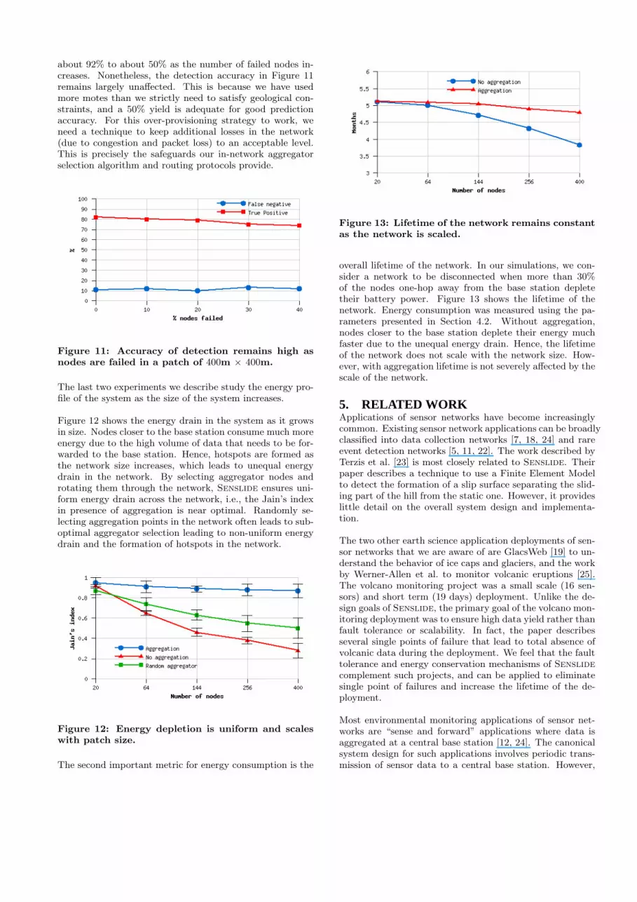
about 92% to about 50% as the number of failed nodes in-creases. Nonetheless, the detection accuracy in Figure 11remains largely unaffected. This is because we have usedmore motes than we strictly need to satisfy geological con-straints, and a 50% yield is adequate for good predictionaccuracy. For this over-provisioning strategy to work, weneed a technique to keep additional losses in the network(due to congestion and packet loss) to an acceptable level.This is precisely the safeguards our in-network aggregatorselection algorithm and routing protocols provide.

Figure 11: Accuracy of detection remains high asnodes are failed in a patch of 400m × 400m.

The last two experiments we describe study the energy pro-file of the system as the size of the system increases.

Figure 12 shows the energy drain in the system as it growsin size. Nodes closer to the base station consume much moreenergy due to the high volume of data that needs to be for-warded to the base station. Hence, hotspots are formed asthe network size increases, which leads to unequal energydrain in the network. By selecting aggregator nodes androtating them through the network, Senslide ensures uni-form energy drain across the network, i.e., the Jain’s indexin presence of aggregation is near optimal. Randomly se-lecting aggregation points in the network often leads to sub-optimal aggregator selection leading to non-uniform energydrain and the formation of hotspots in the network.

Figure 12: Energy depletion is uniform and scaleswith patch size.

The second important metric for energy consumption is the

Figure 13: Lifetime of the network remains constantas the network is scaled.

overall lifetime of the network. In our simulations, we con-sider a network to be disconnected when more than 30%of the nodes one-hop away from the base station depletetheir battery power. Figure 13 shows the lifetime of thenetwork. Energy consumption was measured using the pa-rameters presented in Section 4.2. Without aggregation,nodes closer to the base station deplete their energy muchfaster due to the unequal energy drain. Hence, the lifetimeof the network does not scale with the network size. How-ever, with aggregation lifetime is not severely affected by thescale of the network.

5. RELATED WORKApplications of sensor networks have become increasinglycommon. Existing sensor network applications can be broadlyclassified into data collection networks [7, 18, 24] and rareevent detection networks [5, 11, 22]. The work described byTerzis et al. [23] is most closely related to Senslide. Theirpaper describes a technique to use a Finite Element Modelto detect the formation of a slip surface separating the slid-ing part of the hill from the static one. However, it provideslittle detail on the overall system design and implementa-tion.

The two other earth science application deployments of sen-sor networks that we are aware of are GlacsWeb [19] to un-derstand the behavior of ice caps and glaciers, and the workby Werner-Allen et al. to monitor volcanic eruptions [25].The volcano monitoring project was a small scale (16 sen-sors) and short term (19 days) deployment. Unlike the de-sign goals of Senslide, the primary goal of the volcano mon-itoring deployment was to ensure high data yield rather thanfault tolerance or scalability. In fact, the paper describesseveral single points of failure that lead to total absence ofvolcanic data during the deployment. We feel that the faulttolerance and energy conservation mechanisms of Senslidecomplement such projects, and can be applied to eliminatesingle point of failures and increase the lifetime of the de-ployment.

Most environmental monitoring applications of sensor net-works are “sense and forward” applications where data isaggregated at a central base station [12, 24]. The canonicalsystem design for such applications involves periodic trans-mission of sensor data to a central base station. However,

these systems lack fault tolerance and have several singlepoints of failure. Existing system designs for rare event de-tection like sniper localization [22], intrusion detection sys-tems [5, 11] only communicate with the base station whenthe target is detected. However, the application goals ofSenslide require a fine balance to be maintained betweenrare event detection and periodic data collection.

In-network aggregation, as exemplified by TAG [17], is acommonly used data reduction mechanism in sensor net-works. Our technique for aggregation differs significantlyfrom TAG as already detailed in Section 3.

Senslide’s hierarchical decomposition of the sensor nodesinto a two level hierarchy is similar to LEACH [13]. How-ever, LEACH assumes that each sensor node is a single hopaway from the aggregator node, requires each cluster head tobe non-interfering with the others and requires 3 rounds ofcommunication to setup a TDMA schedule. These featuresof LEACH make it ill-suited for a large class of applications,including Senslide.

There have been a large number of studies that demonstratethe high variability of link qualities observed in dense de-ployments of sensor networks [26, 27]. In addition to theabove, recent deployments of sensor networks have also re-ported low yields [12, 24]. Senslide deals with low datayields due to the varying intermittent links by using skep-tics [20]. A skeptic limits the failure rate of a link by de-laying the recovery of a “bad” link, blacklisting links with ahigh failure rate and allowing “good” links to recover quicklyfrom a failure.

To compensate for the low yield due to the varying link qual-ities of the sensor radios and noisy sensor data due to thelow cost uncalibrated sensors, applications are required toincorporate signal processing algorithms in the system de-sign. Due to the limited resources on the sensor nodes, mostapplications [22, 24] perform the complex signal processingat a centralized powerful server. In contrast, there are appli-cations which perform the signal processing in-network [5,11] and communicate with a central server only when ananomaly is detected. Senslide adopts a hybrid approach,where the aggregator nodes perform the spatial summary ofdata and the base aggregates these spatial summaries fromdistributed aggregator nodes to trigger the warning.

6. CONCLUSION AND FUTURE WORKIn this paper we described the design, implementation, andevaluation of Senslide, a distributed landslide predictionsystem. In contrast to existing sensor network applications,our primary objective is to build a distributed sensor systemthat is robust in the face of failures.

A unique feature of our design is that we combine severaldistributed systems techniques to deal with the complexitiesof a distributed sensor network environment where connec-tivity is poor and power budgets are very constrained, whilesatisfying real-world requirements of safety. We also believethat this combination of techniques will be more importantin the future when sensor networks are widely deployed inenvironments where failures and intermittent connectivity

have to be tolerated without compromising the correct func-tioning of the system.

Although Senslide is not yet deployed in the field, we havebuilt a 65-node indoor sensor network and also tested itin simulation. Based on laboratory experiments we havecharacterized rocks that are typically found in the landslideprone areas, and used this real data to drive the experimentsin the testbed and simulations.

Senslide hierarchically structures the network into sensornodes and aggregator nodes. This hierarchical structuringof the network improves the data yield and ensures uniformenergy depletion across the network. The improved yieldand uniform energy depletion of the network significantlyimproves the detection accuracy and lifetime of the network.Our simulation results also show the robustness of the sys-tem design. By incorporating sufficient redundancy into thesystem and low overhead health monitoring, Senslide cantolerate failures of sensor nodes, aggregator nodes, and basestations.

As part of future work, we plan to build improved models ofthe stress versus strain characteristics of the rocks. We alsointend to field test the system during the monsoon seasonin India.

7. REFERENCES[1] Chipcon cc2420 radio data sheet.

http://www.chipcon.com.

[2] The network simulator - ns2.http://www.isi.edu/nsnam/ns.

[3] Telosb mote platform. http://www.moteiv.com/.

[4] Abrach, H., Bhatti, S., Carlson, J., Dai, H.,Rose, J., Sheth, A., Shucker, B., Deng, J., andHan, R. Mantis: system support for multimodalnetworks of in-situ sensors. In WSNA ’03: Proceedingsof the 2nd ACM international conference on Wirelesssensor networks and applications (New York, NY,USA, 2003), ACM Press, pp. 50–59.

[5] Arora, A., Dutta, P., Bapat, S., Kulathumani,V., Zhang, H., Naik, V., Mittal, V., Cao, H.,Demirbas, M., Gouda, M., Choi, Y.-R., Herman,T., Kulkarni, S. S., Arumugam, U., Nesterenko,M., Vora, A., and Miyashita, M. A line in thesand: A wireless sensor network for target detection,classification, and tracking. Computer Networks(2004), 605–634.

[6] Brown, E. T. Rock characterisation, testing andmonitoring. ISRM suggested methods. Internationalof Journal of Rock Mechanics and Mining Science andGoemechanics Abstracts 18 (December 1981),109–110.

[7] Cerpa, A., Elson, J., Estrin, D., Girod, L.,Hamilton, M., and Zhao, J. Habitat monitoring:application driver for wireless communicationstechnology. SIGCOMM Comput. Commun. Rev. 31, 2supplement (2001), 20–41.

[8] Eberhardt, E., Stead, D., Stimpson, B., andRead, R. S. Identifying crack initiation andpropagation thesholds in brittle rock. CanadianGeotechnical Journal 35, 2 (1998), 222–233.

[9] Fonseca, R., Ratnasamy, S., Culler, D.,Shenker, S., and Stoica, I. Beacon vector routing:Scalable point-to-point in wireless sensornets. In NSDI’05: Proceedings of the 2nd Symposium on NetworkedSystems Design and Implementation (Boston, MA,United States, 2005).

[10] Goodman, R. E. Introduction to Rock Mechanics.Wiley, New York, 1980.

[11] Gu, L., Jia, D., Vicaire, P., Yan, T., Luo, L.,Tirumala, A., Cao, Q., He, T., Stankovic, J. A.,Abdelzaher, T., and Krogh, B. H. Lightweightdetection and classification for wireless sensornetworks in realistic environments. In SenSys ’05:Proceedings of the 3rd international conference onEmbedded networked sensor systems (New York, NY,USA, 2005), ACM Press, pp. 205–217.

[12] Hartung, C., Seielstad, C., Holbrook, S., andHan, R. Firewxnet a multi-tiered portable wirelesssystem for monitoring weather conditions in wildlandfire environments. In MobiSys ’06: Proceedings of the4th International Conference on Mobile Systems,Applications, and Services (Uppsala, Sweden, June2006).

[13] Heinzelman, W., Chandrakasan, A., andBalakrishnan, H. An application-specific protocolarchitecture for. In IEEE Transactions on WirelessCommunications (2002), vol. 1.

[14] Jain, R., Chiu, D., and Hawe, B. A quantitativemeasure of fairness and discrimination for resourceallocation in shared computer systems. DEC ResearchReport TR-301 (1984).

[15] Lamport, L. The part-time parliament. In ACMTransactions on Computer Systems (May 1998),vol. 16, pp. 133–169.

[16] MacQueen, J. B. Some methods for classificationand analysis of multivariate observations. InProceedings of 5th Berkeley Symposium onMathematical Statistics and Probability (Berkeley,California, USA, 1967), University of California Press,pp. 281–297.

[17] Madden, S., Franklin, M. J., Hellerstein, J. M.,and Hong, W. Tag: a tiny aggregation service forad-hoc sensor networks. In OSDI ’02: Proceedings ofthe 5th symposium on Operating systems design andimplementation (New York, NY, USA, 2002), ACMPress, pp. 131–146.

[18] Mainwaring, A., Culler, D., Polastre, J.,Szewczyk, R., and Anderson, J. Wireless sensornetworks for habitat monitoring. In WSNA ’02:Proceedings of the 1st ACM international workshop onWireless sensor networks and applications (New York,NY, USA, 2002), ACM Press, pp. 88–97.

[19] Martinez, K., Hart, J. K., and Ong., R.Environmental sensor networks. In IEEE Computer(2004), vol. 37, IEEE, pp. 50–56.

[20] Rodeheffer, T. L., and Schroeder, M. D.Automatic reconfiguration in autonet. In SOSP ’91:Proceedings of the thirteenth ACM symposium onOperating systems principles (New York, NY, USA,1991), ACM Press, pp. 183–197.

[21] Savas, O., Alanyali, M., Venkatesh, S., andAeron, S. Distributed Bayesian hypothesis testing in

sensor networks. In Proceeding of the 2004 AmericanControl Conference (June 2004), pp. 5369–5374.

[22] Simon, G., Maroti, M., Ledeczi, A., Balogh, G.,Kusy, B., Nadas, A., Pap, G., Sallai, J., andFrampton, K. Sensor network-based countersnipersystem. In SenSys ’04: Proceedings of the 2ndinternational conference on Embedded networkedsensor systems (New York, NY, USA, 2004), ACMPress, pp. 1–12.

[23] Terzis, A., Moore, K., Anandarajah, R., andWang, I. Slip surface localization in wireless sensornetworks for landslide prediction. In IPSN ’06:Proceedings of the 5th International Symposium onInformation Processing in Sensor Networks(Nashville, TN, USA, April 2006).

[24] Tolle, G., Polastre, J., Szewczyk, R., Culler,D., Turner, N., Tu, K., Burgess, S., Dawson, T.,Buonadonna, P., Gay, D., and Hong, W. Amacroscope in the redwoods. In SenSys ’05:Proceedings of the 3rd international conference onEmbedded networked sensor systems (New York, NY,USA, 2005), ACM Press, pp. 51–63.

[25] Werner-Allen, G., Lorincz, K., Johnson, J.,Lees, J., and Welsh, M. Fidelity and yield in avolcano monitoring sensor network. In OSDI ’06:Proceedings of the 7th USENIX Symposium onOperating Systems Design and Implementation(Seattle, WA, USA, 2006).

[26] Woo, A., Tong, T., and Culler, D. Taming theunderlying challenges of reliable multihop routing insensor networks. In SenSys ’03: Proceedings of the 1stinternational conference on Embedded networkedsensor systems (New York, NY, USA, 2003), ACMPress, pp. 14–27.

[27] Zhao, J., and Govindan, R. Understanding packetdelivery performance in dense wireless sensornetworks. In SenSys ’03: Proceedings of the 1stinternational conference on Embedded networkedsensor systems (New York, NY, USA, 2003), ACMPress, pp. 1–13.