Embed Size (px)
Citation preview
applied sciences
Article
Landslide Susceptibility Mapping CombiningInformation Gain Ratio and Support VectorMachines: A Case Study from Wushan Segmentin the Three Gorges Reservoir Area, China
Lanbing Yu 1,2, Ying Cao 1, Chao Zhou 3,*, Yang Wang 1 and Zhitao Huo 2,4
1 Faculty of Engineering, China University of Geosciences, Wuhan 430074, China;[email protected] (L.Y.); [email protected] (Y.C.); [email protected] (Y.W.)
2 Central South China Centre for Geoscience Innovation, Wuhan 430205, China; [email protected] School of Geography and Information Engineering, China University of Geosciences, Wuhan 430078, China4 Wuhan Centre of China Geological Survey, Wuhan 430205, China* Correspondence: [email protected]
Received: 11 October 2019; Accepted: 4 November 2019; Published: 7 November 2019�����������������
Abstract: Landslides are destructive geological hazards that occur all over the world. Due to theperiodic regulation of reservoir water level, a large number of landslides occur in the Three GorgesReservoir area (TGRA). The main objective of this study was to explore the preference of machinelearning models for landslide susceptibility mapping in the TGRA. The Wushan segment of TGRA wasselected as a case study. At first, 165 landslides were identified and a total of 14 landslide causal factorswere constructed from different data sources. Multicollinearity analysis and information gain ratio(IGR) model were applied to select landslide causal factors. Subsequently, the landslide susceptibilitymapping using the calculated results of four models, namely, support vector machines (SVM),artificial neural networks (ANN), classification and regression tree (CART), and logistic regression(LR). The accuracy of these four maps were evaluated using the receive operating characteristic(ROC) and the accuracy statistic. Results revealed that eliminating the inconsequential factors canperhaps improve the accuracy of landslide susceptibility modelling, and the SVM model had the bestperformance in this study, providing strong technical support for landslide susceptibility modellingin TGRA.
Keywords: landslides; susceptibility mapping; support vector machines; Three Gorges Reservoirarea (TGRA)
1. Introduction
Landslides are destructive geological hazards that may result in serious economic damage andhuman losses all over the world [1]. Thousands of landslides occurred in January 2011 in Rio de Janeirocausing more than 1500 people to die [2]. China has suffered much from natural hazards in the pastdecade. On 24 June 2017, a rocky landslide occurred in Maoxian County, Sichuan Province, China,causing the whole village to be buried and the death of 83 people [3]. On 7 August 2010, catastrophicdebris flows occurred in Zhouqu, China, leading to 1765 deaths [4]; among these geohazards, landslidesoccurred most widely and accounted for the highest proportion. In 2018, 1613 landslides occurred,accounting for 55% of the total geological disasters [5], and the economic loss exceeded 2 billion CNY.
Three Gorges Project, the largest hydropower station in the world, has formed a 660 km longbackwater area after impoundment. The highest water level in the Three Gorges Reservoir area (TGRA)has risen to 175 m since 2009, with an annual variation of 30 m. The frequent changes of water level
Appl. Sci. 2019, 9, 4756; doi:10.3390/app9224756 www.mdpi.com/journal/applsci
Appl. Sci. 2019, 9, 4756 2 of 19
have significantly changed the geological environment of the TGRA. This has led to the reactivation ofcertain old landslides and the occurrence of new landslides. These landslides seriously threaten thesafety of local residents and their property. For instance, Qianjiangping landslide and its associated30 m impulse wave occurred shortly after the initial impoundment of TGRA in July 2003, causing24 deaths, destroying 346 houses, and capsizing many ships [6]. Shanshucao landslide occurred inSeptember 2014, which was triggered by both the rising water level of the TGRA at high speed andrainfall, causing the Daling Power Station and part of the G348 national highway (about 200 meterslong) to slide into the river [7]. Hence, considering the number of disasters and the damage theycaused, it is crucial and urgent to monitor the TGRA.
Landslide susceptibility modelling can be considered as the initial step towards a landslidehazard and risk assessment, and can notably improve land-use planning [8]. At present, the landslidesusceptibility models can be divided into qualitative models and quantitative models. Qualitativemodels include inventory-based models and knowledge-driven models, whereas quantitative modelsmainly include data-driven models and physically based methods [9]. Qualitative models are basedon simple expert knowledge, which is easier to obtain but greatly affected by subjective factors.Physically based models can simulate the failure process of landslides, but it is not practical forlarge-scale areas in terms of its necessary of plenty of parameters [10]. At present, data-driven modelshave been widely used, the accuracy of which have been greatly improved because of the high dataquality. The data-driven models include information value model [11], weight-of-evidence [12], logisticregression (LR) [13], artificial neural network (ANN) [14–16], support vector machine (SVM) [17–19],decision tree [20], and classified and regression tree (CART) [21], among others. Among those models,machine learning methods have become popular in landslide susceptibility modelling because of theirgood non-linear prediction ability. The performance of machine learning models may vary in differentcases. In the TGRA or other landslide-prone areas, there is no universal agreement for the selection oflandslide susceptibility models until now. Therefore, it is necessary to analyze and compare landslidesusceptibility models.
Landslide development is jointly influenced by many factors, and different causal factors havedifferent ways of influence [10]. Some inconsequential factors may contribute less to improving theaccuracy of susceptibility modelling than the errors caused by noise, thus reducing the accuracy ofmodelling. The important causal factors should be selected and the less important causal factors shouldbe eliminated to improve the modelling accuracy of landslide susceptibility [22,23]. The informationgain ratio (IGR) is an effective method used to calculate the factor contribution for model accuracy.It provides a powerful technique to quantitatively identify and select significant causal factors forlandslide susceptibility modelling.
In this paper, the Wushan segment of TGRA was selected as a study area. Multicollinearityanalysis and IGR were applied to select landslide causal factors. Then, three machine learning models(SVM, ANN, CART) and a multivariate statistical model (LR) were utilized to conduct landslidesusceptibility modelling. Finally, the accuracy of the four models was evaluated and compared usingthe receiver operating characteristic (ROC) and the accuracy statistic methods. The authors hopedthat it would find the model that can generate a landslide susceptibility map with higher accuracy inthe TGRA.
2. Materials and Methods
2.1. Description of the Study Area
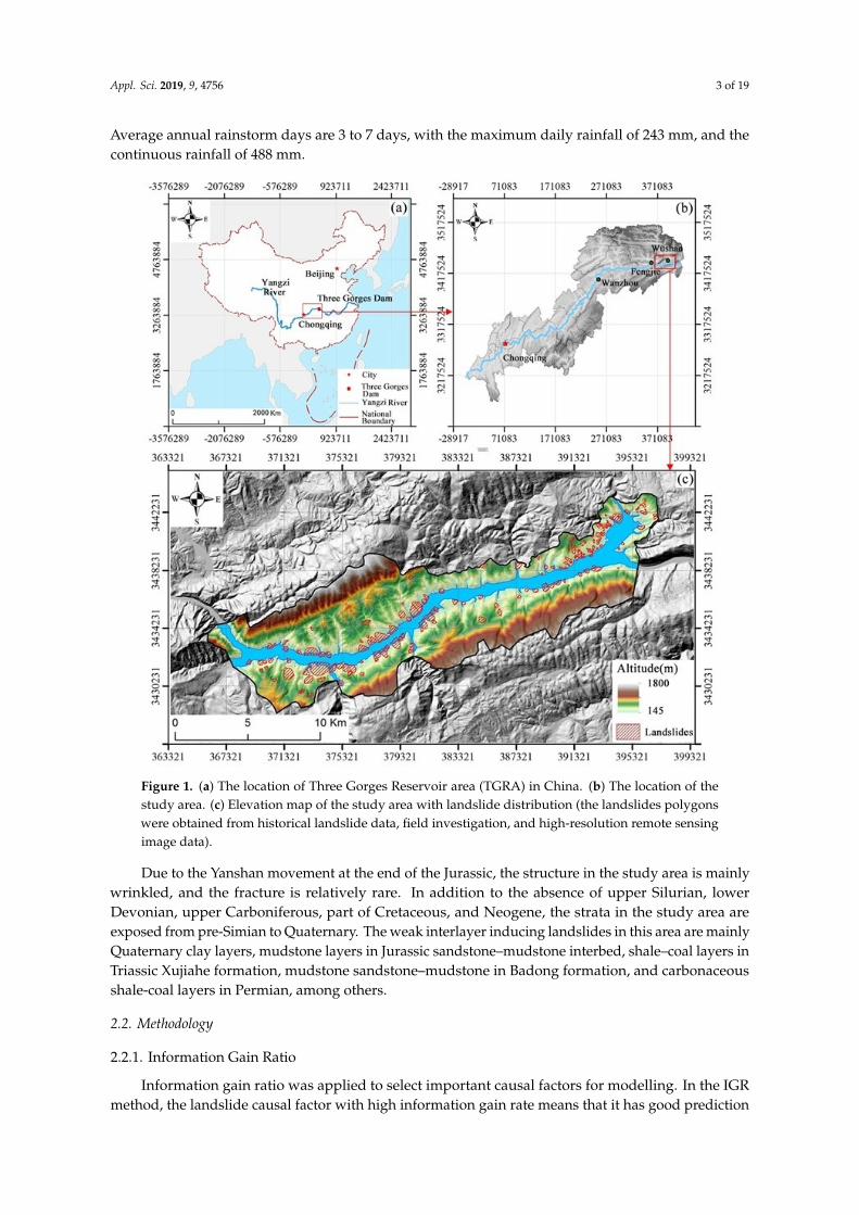
The study area is located in the southwest of China, a mountainous region in southwest Chongqing.It is in the middle reaches of the TGRA, with a longitude of 109◦36′57”E~110◦55′4”E and latitude of30◦58′12”N~31◦6′36”N (Figure 1). The regional altitude range is from 145 to 1800 m. The study areabelongs to the subtropical monsoon region with high air humidity and high average temperature.Rainfall mainly occurs from May to September, which accounts for 69% of the total annual rainfall.
Appl. Sci. 2019, 9, 4756 3 of 19
Average annual rainstorm days are 3 to 7 days, with the maximum daily rainfall of 243 mm, and thecontinuous rainfall of 488 mm.
Appl. Sci. 2019, 9, x FOR PEER REVIEW 3 of 20
temperature. Rainfall mainly occurs from May to September, which accounts for 69% of the total annual rainfall. Average annual rainstorm days are 3 to 7 days, with the maximum daily rainfall of 243 mm, and the continuous rainfall of 488 mm.
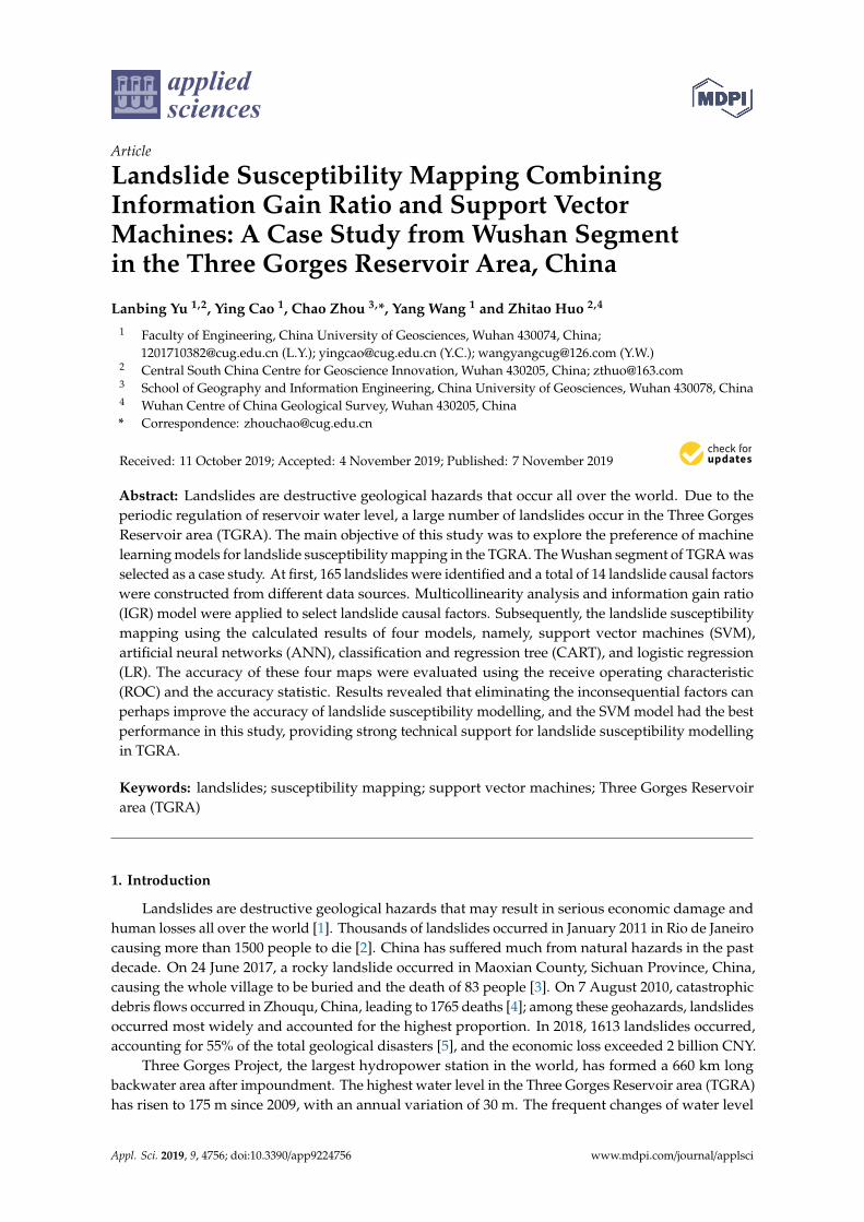
Figure 1. (a) The location of Three Gorges Reservoir area (TGRA) in China. (b) The location of the study area. (c) Elevation map of the study area with landslide distribution (the landslides polygons were obtained from historical landslide data, field investigation, and high-resolution remote sensing image data).
Due to the Yanshan movement at the end of the Jurassic, the structure in the study area is mainly wrinkled, and the fracture is relatively rare. In addition to the absence of upper Silurian, lower Devonian, upper Carboniferous, part of Cretaceous, and Neogene, the strata in the study area are exposed from pre-Simian to Quaternary. The weak interlayer inducing landslides in this area are mainly Quaternary clay layers, mudstone layers in Jurassic sandstone–mudstone interbed, shale–coal layers in Triassic Xujiahe formation, mudstone sandstone–mudstone in Badong formation, and carbonaceous shale-coal layers in Permian, among others.
2.2. Methodology
2.2.1. Information Gain Ratio
Figure 1. (a) The location of Three Gorges Reservoir area (TGRA) in China. (b) The location of thestudy area. (c) Elevation map of the study area with landslide distribution (the landslides polygonswere obtained from historical landslide data, field investigation, and high-resolution remote sensingimage data).
Due to the Yanshan movement at the end of the Jurassic, the structure in the study area is mainlywrinkled, and the fracture is relatively rare. In addition to the absence of upper Silurian, lowerDevonian, upper Carboniferous, part of Cretaceous, and Neogene, the strata in the study area areexposed from pre-Simian to Quaternary. The weak interlayer inducing landslides in this area are mainlyQuaternary clay layers, mudstone layers in Jurassic sandstone–mudstone interbed, shale–coal layers inTriassic Xujiahe formation, mudstone sandstone–mudstone in Badong formation, and carbonaceousshale-coal layers in Permian, among others.
2.2. Methodology
2.2.1. Information Gain Ratio
Information gain ratio was applied to select important causal factors for modelling. In the IGRmethod, the landslide causal factor with high information gain rate means that it has good prediction
Appl. Sci. 2019, 9, 4756 4 of 19
ability in modelling. Assuming that the training data T contains n samples, Ci (landslide, non-landslide)is a classification set of sample data, and the following formula can obtain the information entropy ofthe factors:
In f o(T) = −2∑
i=1
n(Ci, T)|T|
log2n(Ci, T)|T|
(1)
the amount of information (T1, T2, . . . , Tm) split from T regarding the causal factor F is estimated as:
In f o(T, F) = −m∑
j=1
T j
|T|log2 In f o(T) (2)
then, the IGR of the landslide causal factor F can be written as follows:
IGR(T, F) =In f o(T) − In f o(T, F)
SplitIn f o(T, F)(3)
where SplitInfo represents the potential information generated by dividing the training data T into msubsets. The formula of SplitInfo is shown as follows:
SplitIn f o(T, F) = −m∑
j=1
∣∣∣T j∣∣∣|T|
log2
∣∣∣T j∣∣∣|T|
(4)
2.2.2. Support Vector Machines
Support vector machine is a recently developed nonlinear classification method, which is basedon statistical learning theory. It transforms original input space into a higher-dimensional feature spaceto find optimal separating hyperplane. The hyperplane has the largest distance to the nearest trainingdata point of any class [24].
Assuming samples (xi, xj) = 1, 2 . . . , n, the following function can solve the optimalseparating hyperplane:
Min(
12‖⇀w‖
2+ C
n∑i=1
ξi
)yi(⇀w ·
⇀xi + b
)− 1 + ξi ≥ 0
ξi ≥ 0, i = 1, 2 · · · , n
(5)
where w is the weight vector that determines the orientation of the hyperplane, b is the bias, ξi is thepositive slack variables for the data points that allow for penalized constraint violation, and C is thepenalty parameter that controls the trade-off between the complexity of the decision function and thenumber of training examples misclassified. The function can be converted into an equivalent dualproblem based on the Wolf duality theory:
Max
∑iαi −
12∑i jαiα jyiy j
(⇀xi ·
⇀x j
)∑iαiyi = 0, 0 ≤ αi ≤ C
(6)
where αi are Lagrange multipliers and C is the penalty. Then, the decision function, which will be usedfor the classification of new data, can be written:
f (x) = sgn
n∑i=1
yiαiK(xi, x j
)+ b
(7)
where K(xi, xj) is the kernel function. The radial basis kernel was adopted as kernel function for theSVM model in this study.
Appl. Sci. 2019, 9, 4756 5 of 19
2.2.3. Artificial Neural Networks
Artificial neural networks have been widely used in many fields, including landslide research [25,26].ANNs are a series of statistical learning models inspired by biological neural networks and are usedto estimate or approximate unknown function depending on a large number of inputs. So far, manykinds of neural network algorithms have been proposed all over the world, and back propagationneural network (BPNN) is one of the most widely used artificial neural network models in landslidesusceptibility modelling, one that was adopted in this study.
The learning process of BPNN includes two phases: forward propagation and backwardpropagation. In forward propagation, the input values act on the output values through the hiddenlayer, and the state of neurons in each layer only affect the state of neurons in the next layer. Ifthe actual output value is not expected, the output error will be transferred back to the input layer,which is the backpropagation. After many times of “learning” by adjusting the weights between theneurons, the neural network provides a model that should be able to predict a target value from agiven input value.
The learning rate is an essential parameter of ANN model, which may affect its performance.In this study, the learning rate will be automatically calculated using the following formula:
η(n) = η(n− 1) ∗ exp(log(ηmin/ηmax)/d) (8)
where η(n) is the learning rate in the nth times training, ηmin is the minimum value of the learning rate,ηmax is the maximum value of the learning rate, and d is the delay rate. In this study, the initial rate,the maximum and minimum learning rate, and the delay rate are 0.3, 0.1, 0.01, and 30, respectively.
2.2.4. Classification and Regression Tree
Classification and regression tree is a non-parametric and non-linear classification regressionmethod proposed by Breiman [21], and its main idea is to recursively partition the data space togenerate a decision tree and prune the tree by the validation data. The CART model does not need topresuppose the relationship between dependent variables and independent variables, but on the basisof dependent variables it uses recursive partitioning method to divide the space defined by independentvariables into categories as homogeneous as possible. CART is composed of a classification tree anda regression tree; the former is used to predict discrete data, whereas the latter is used to predictcontinuous data.
Assuming F is an attribute of data set Xm,p, we sorted all samples by these attributes, and theaverage value of two adjacent values was taken as the separating points, which was called ηs(s = 1, 2. . . , m−1). The data set Xm,pwas divided into two subsets according to the value taken on attribute F,the subset X1 larger than ηs and the subset X2 smaller than or equal to ηs. The GINI coefficients of thisclassification method can be expressed as:
GηsF (X) =
|X1|
pI(X1) +
|X2|
pI(X2) (9)
where p is the number of all samples, |X1| is number of samples of subset X1, |X2| is number of samplesof subset X2, and I(X) can be calculated using the following formula:
I(X) = 1−2∑
i=1
(|Ci|∣∣∣X j
∣∣∣ )2( j = 1, 2) (10)
where |Xj| is the number of samples in dataset Xj, and |Cj| is the number of samples belonging to Cj indata set Xj.
Appl. Sci. 2019, 9, 4756 6 of 19
If the dataset Xm,p contained m data and p attributes, each attribute corresponded to m-1 partitionpoints, and the GINI coefficient of each partition point was Gηs
F (X), then the point, which had minimumGINI coefficient, was selected to partition the dataset Xm,p.
According to this method, the sub-nodes of the tree were constructed, and this process wasrepeated until all the samples of the sub-nodes belonged to the same class of splitting attractors.
2.2.5. Logistic Regression
Logistic regression is a common model in landslide susceptibility assessment [27], which is amultivariate data analysis model similar to multiple linear regression analysis. The dependent variablesof LR can be bi-categorized or multi-categorized. In this study, the occurrences of landslides weretaken as dependent variables of the model, which could be expressed as 0 for non-landslide and 1 forlandslide. The factors of landslide susceptibility, such as altitude, slope, and aspect, were selected asindependent variables of the model. The application of LR model in landslide susceptibility assessmentwas to find the optimal fitting function, which can quantitatively describe the relationship between theoccurrence of landslide and causal factors. The advantage of the LR model is that the independentvariables can be either continuous, discrete, or any combination of both types. They do not necessarilyhave normal distributions. The formula can be expressed as:
y =1
1 + e−(α+β1x1+β2x2+···+βnxn)(11)
where α is a constant, n is the number of independent variables, xi(i = 1, 2 . . . , n) is the predictorvariables, and βi(i = 1, 2 . . . , n) is the coefficient of the LR model.
2.3. Data Preparation and Analysis
2.3.1. Landslide Inventory Map
The most crucial step in the landslide susceptibility mapping is to identify landslide locations anddetermine when the landslide occurs. Therefore, a detailed and reliable landslide inventory map is thepremise of an accurate assessment of landslide susceptibility. This study constructed the landslideinventory map from high-resolution remote sensing image data, field investigation, and historicallandslide data, and a total of 165 landslides were identified in the study area (Figure 1). The totaldisaster area of the study area was 12.65 km2, and the area of single landslide ranged from 1664 m2
to 1.06 km2. Most of the landslides in this study area occurred on the bank of the Yangtze River andthe gully.
2.3.2. Landslide Causal Factors
The occurrence of a landslide is caused by the combination of the basic geological conditionsof the slope and the external environmental factors. The former are factors that play a controllingrole in the occurrence of a landslide, including topography and geological structures, among otherfactors. The latter are triggering factors for the occurrence of a landslide, such as hydrogeologicalenvironment, earthquake, and human engineering activities, among others [28]. According to the fieldsurvey and preliminary research results in TGRA [29–31], 14 causal factors were initially selected asthe factors for landslide susceptibility modelling, including altitude, slope, aspect, curvature, plancurvature, profile curvature, stream power index (SPI), topographic wetness index (TWI), terrainroughness index (TRI), lithology, bedding structure, distance to faults, distance to rivers, and distanceto gully. The factors were prepared using a digital elevation model (DEM) with a spatial resolution of25 m, and geological and geomorphology maps, which were collected from the Chongqing NaturalResources Bureau. In this study, ArcGIS 10.2 (http://www.esrichina.com.cn/) was applied to processgeodata, and slope and aspect was obtained by Three Dimensions spatial analysis function; SPI andTWI were calculated by hydrological analysis function and the Raster calculator, respectively. TRI was
Appl. Sci. 2019, 9, 4756 7 of 19
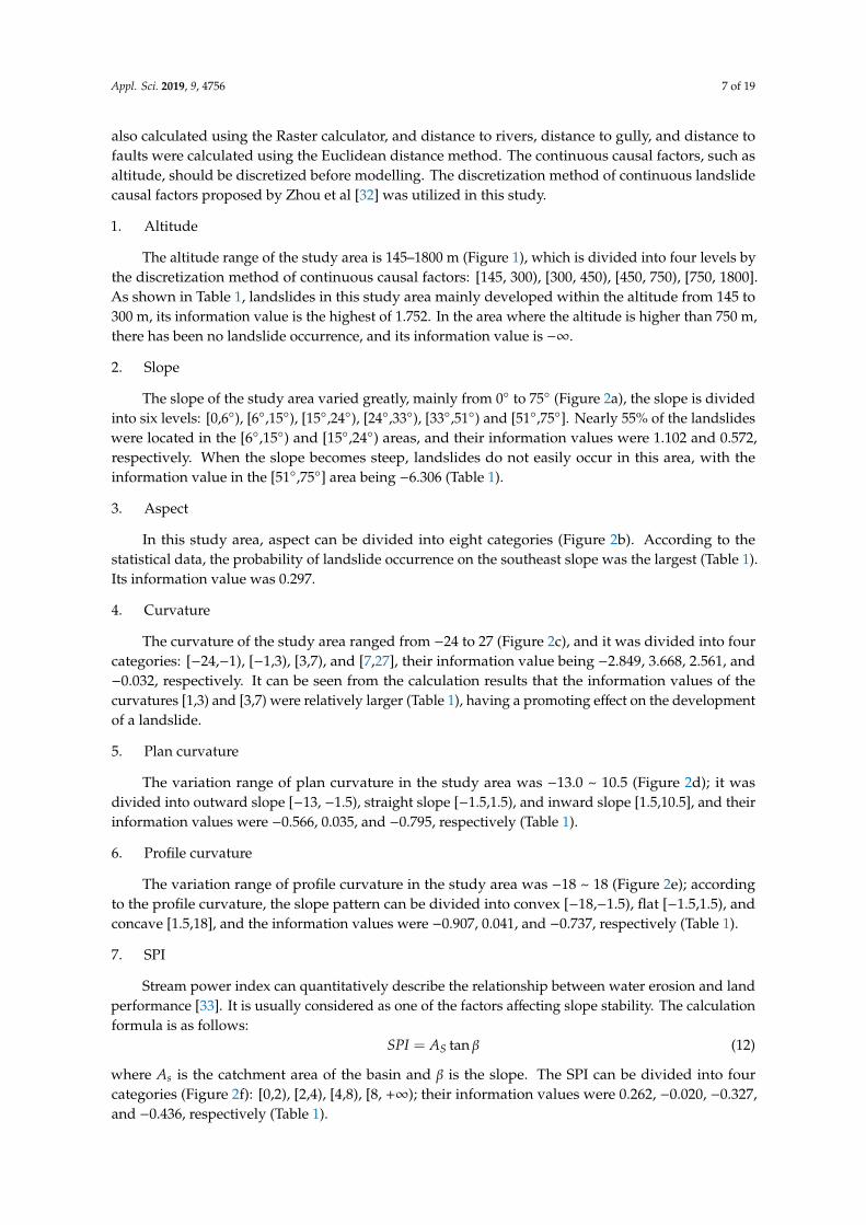
also calculated using the Raster calculator, and distance to rivers, distance to gully, and distance tofaults were calculated using the Euclidean distance method. The continuous causal factors, such asaltitude, should be discretized before modelling. The discretization method of continuous landslidecausal factors proposed by Zhou et al [32] was utilized in this study.
1. Altitude
The altitude range of the study area is 145–1800 m (Figure 1), which is divided into four levels bythe discretization method of continuous causal factors: [145, 300), [300, 450), [450, 750), [750, 1800].As shown in Table 1, landslides in this study area mainly developed within the altitude from 145 to300 m, its information value is the highest of 1.752. In the area where the altitude is higher than 750 m,there has been no landslide occurrence, and its information value is −∞.
2. Slope
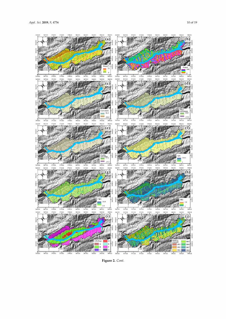
The slope of the study area varied greatly, mainly from 0◦ to 75◦ (Figure 2a), the slope is dividedinto six levels: [0,6◦), [6◦,15◦), [15◦,24◦), [24◦,33◦), [33◦,51◦) and [51◦,75◦]. Nearly 55% of the landslideswere located in the [6◦,15◦) and [15◦,24◦) areas, and their information values were 1.102 and 0.572,respectively. When the slope becomes steep, landslides do not easily occur in this area, with theinformation value in the [51◦,75◦] area being −6.306 (Table 1).
3. Aspect
In this study area, aspect can be divided into eight categories (Figure 2b). According to thestatistical data, the probability of landslide occurrence on the southeast slope was the largest (Table 1).Its information value was 0.297.
4. Curvature
The curvature of the study area ranged from −24 to 27 (Figure 2c), and it was divided into fourcategories: [−24,−1), [−1,3), [3,7), and [7,27], their information value being −2.849, 3.668, 2.561, and−0.032, respectively. It can be seen from the calculation results that the information values of thecurvatures [1,3) and [3,7) were relatively larger (Table 1), having a promoting effect on the developmentof a landslide.
5. Plan curvature
The variation range of plan curvature in the study area was −13.0 ~ 10.5 (Figure 2d); it wasdivided into outward slope [−13, −1.5), straight slope [−1.5,1.5), and inward slope [1.5,10.5], and theirinformation values were −0.566, 0.035, and −0.795, respectively (Table 1).
6. Profile curvature
The variation range of profile curvature in the study area was −18 ~ 18 (Figure 2e); accordingto the profile curvature, the slope pattern can be divided into convex [−18,−1.5), flat [−1.5,1.5), andconcave [1.5,18], and the information values were −0.907, 0.041, and −0.737, respectively (Table 1).
7. SPI
Stream power index can quantitatively describe the relationship between water erosion and landperformance [33]. It is usually considered as one of the factors affecting slope stability. The calculationformula is as follows:
SPI = AS tan β (12)
where As is the catchment area of the basin and β is the slope. The SPI can be divided into fourcategories (Figure 2f): [0,2), [2,4), [4,8), [8, +∞); their information values were 0.262, −0.020, −0.327,and −0.436, respectively (Table 1).
Appl. Sci. 2019, 9, 4756 8 of 19
8. TWI
Topographic wetness index can quantitatively simulate the dry and wet conditions of topographyand soil moisture in the watershed [33]. The calculation formula is as follows:
TWI = In(α
tanβ
)(13)
where α is the upstream convergence area and β is the slope. The TWI can be divided into fourcategories (Figure 2g): [0,4.5), [4.5,6.5), [6.5,8), and [8, +∞); their information values were 0.047, −0.158,0.069, and −0.292, respectively (Table 1).
9. TRI
Terrain roughness index (TRI) is an index reflecting the change of surface fluctuation. TRI rangesfrom 1 to 3.9, and the main range is 1 to 1.2, which accounts for about 70% of the total area of thestudy area. The continuous factors classified method was applied to classify TRI into four categories(Figure 2h): [1,1.2), [1.2,1.4), [1.4,1.6), and [1.6,3.9]; their information values were 0.338, −1.167, −2.291,and −6.780, respectively (Table 1).
10. Lithology
Lithology is the material basis for the development of a landslide. According to the lithologicalcharacteristics of outcropping strata in the study area, they can be divided into seven categories(Table 2), and their spatial distribution is shown in Figure 2i. Nearly 60% of the landslides in the studyarea developed in category B, and its information value was 0.849 (Table 1).
11. Bedding structure
According to “Technical Requirements for Investigation and Evaluation of Collapse, Landslide,Debris Flow” from the China Geological Survey [34], slope structure can be classified into eightcategories (Figure 2j; Table 3), and the statistical results of the information value of each slope structuretype are shown in Table 1.
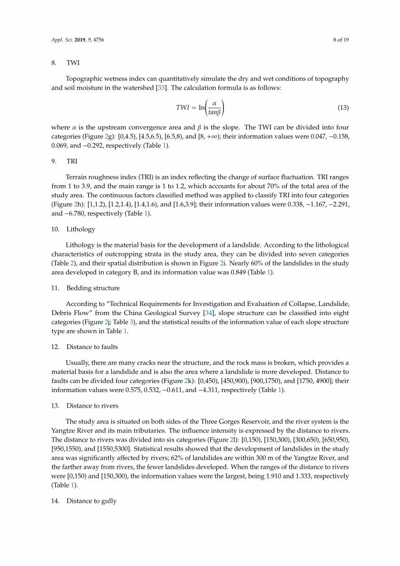
12. Distance to faults
Usually, there are many cracks near the structure, and the rock mass is broken, which provides amaterial basis for a landslide and is also the area where a landslide is more developed. Distance tofaults can be divided four categories (Figure 2k): [0,450), [450,900), [900,1750), and [1750, 4900]; theirinformation values were 0.575, 0.532, −0.611, and −4.311, respectively (Table 1).
13. Distance to rivers
The study area is situated on both sides of the Three Gorges Reservoir, and the river system is theYangtze River and its main tributaries. The influence intensity is expressed by the distance to rivers.The distance to rivers was divided into six categories (Figure 2l): [0,150), [150,300), [300,650), [650,950),[950,1550), and [1550,5300]. Statistical results showed that the development of landslides in the studyarea was significantly affected by rivers; 62% of landslides are within 300 m of the Yangtze River, andthe farther away from rivers, the fewer landslides developed. When the ranges of the distance to riverswere [0,150) and [150,300), the information values were the largest, being 1.910 and 1.333, respectively(Table 1).
14. Distance to gully
Appl. Sci. 2019, 9, 4756 9 of 19
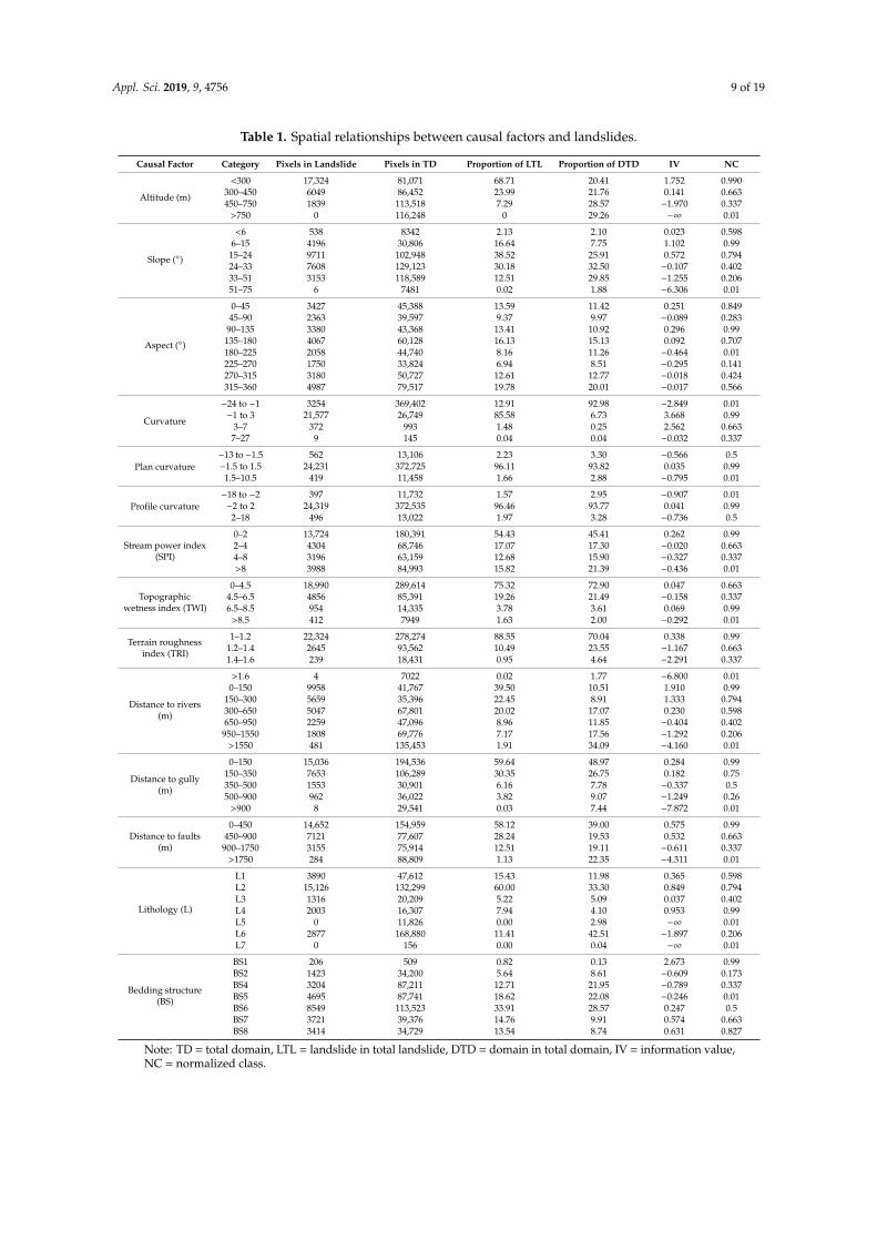
Table 1. Spatial relationships between causal factors and landslides.
Causal Factor Category Pixels in Landslide Pixels in TD Proportion of LTL Proportion of DTD IV NC
Altitude (m)
<300 17,324 81,071 68.71 20.41 1.752 0.990300–450 6049 86,452 23.99 21.76 0.141 0.663450–750 1839 113,518 7.29 28.57 −1.970 0.337
>750 0 116,248 0 29.26 −∞ 0.01
Slope (◦)
<6 538 8342 2.13 2.10 0.023 0.5986–15 4196 30,806 16.64 7.75 1.102 0.99
15–24 9711 102,948 38.52 25.91 0.572 0.79424–33 7608 129,123 30.18 32.50 −0.107 0.40233–51 3153 118,589 12.51 29.85 −1.255 0.20651–75 6 7481 0.02 1.88 −6.306 0.01
Aspect (◦)
0–45 3427 45,388 13.59 11.42 0.251 0.84945–90 2363 39,597 9.37 9.97 −0.089 0.28390–135 3380 43,368 13.41 10.92 0.296 0.99
135–180 4067 60,128 16.13 15.13 0.092 0.707180–225 2058 44,740 8.16 11.26 −0.464 0.01225–270 1750 33,824 6.94 8.51 −0.295 0.141270–315 3180 50,727 12.61 12.77 −0.018 0.424315–360 4987 79,517 19.78 20.01 −0.017 0.566
Curvature
−24 to −1 3254 369,402 12.91 92.98 −2.849 0.01−1 to 3 21,577 26,749 85.58 6.73 3.668 0.99
3–7 372 993 1.48 0.25 2.562 0.6637–27 9 145 0.04 0.04 −0.032 0.337
Plan curvature−13 to −1.5 562 13,106 2.23 3.30 −0.566 0.5−1.5 to 1.5 24,231 372,725 96.11 93.82 0.035 0.99
1.5–10.5 419 11,458 1.66 2.88 −0.795 0.01
Profile curvature−18 to −2 397 11,732 1.57 2.95 −0.907 0.01−2 to 2 24,319 372,535 96.46 93.77 0.041 0.99
2–18 496 13,022 1.97 3.28 −0.736 0.5
Stream power index(SPI)
0–2 13,724 180,391 54.43 45.41 0.262 0.992–4 4304 68,746 17.07 17.30 −0.020 0.6634–8 3196 63,159 12.68 15.90 −0.327 0.337>8 3988 84,993 15.82 21.39 −0.436 0.01
Topographicwetness index (TWI)
0–4.5 18,990 289,614 75.32 72.90 0.047 0.6634.5–6.5 4856 85,391 19.26 21.49 −0.158 0.3376.5–8.5 954 14,335 3.78 3.61 0.069 0.99>8.5 412 7949 1.63 2.00 −0.292 0.01
Terrain roughnessindex (TRI)
1–1.2 22,324 278,274 88.55 70.04 0.338 0.991.2–1.4 2645 93,562 10.49 23.55 −1.167 0.6631.4–1.6 239 18,431 0.95 4.64 −2.291 0.337
Distance to rivers(m)
>1.6 4 7022 0.02 1.77 −6.800 0.010–150 9958 41,767 39.50 10.51 1.910 0.99
150–300 5659 35,396 22.45 8.91 1.333 0.794300–650 5047 67,801 20.02 17.07 0.230 0.598650–950 2259 47,096 8.96 11.85 −0.404 0.402950–1550 1808 69,776 7.17 17.56 −1.292 0.206
>1550 481 135,453 1.91 34.09 −4.160 0.01
Distance to gully(m)
0–150 15,036 194,536 59.64 48.97 0.284 0.99150–350 7653 106,289 30.35 26.75 0.182 0.75350–500 1553 30,901 6.16 7.78 −0.337 0.5500–900 962 36,022 3.82 9.07 −1.249 0.26
>900 8 29,541 0.03 7.44 −7.872 0.01
Distance to faults(m)
0–450 14,652 154,959 58.12 39.00 0.575 0.99450–900 7121 77,607 28.24 19.53 0.532 0.663900–1750 3155 75,914 12.51 19.11 −0.611 0.337
>1750 284 88,809 1.13 22.35 −4.311 0.01
Lithology (L)
L1 3890 47,612 15.43 11.98 0.365 0.598L2 15,126 132,299 60.00 33.30 0.849 0.794L3 1316 20,209 5.22 5.09 0.037 0.402L4 2003 16,307 7.94 4.10 0.953 0.99L5 0 11,826 0.00 2.98 −∞ 0.01L6 2877 168,880 11.41 42.51 −1.897 0.206L7 0 156 0.00 0.04 −∞ 0.01
Bedding structure(BS)
BS1 206 509 0.82 0.13 2.673 0.99BS2 1423 34,200 5.64 8.61 −0.609 0.173BS4 3204 87,211 12.71 21.95 −0.789 0.337BS5 4695 87,741 18.62 22.08 −0.246 0.01BS6 8549 113,523 33.91 28.57 0.247 0.5BS7 3721 39,376 14.76 9.91 0.574 0.663BS8 3414 34,729 13.54 8.74 0.631 0.827
Note: TD = total domain, LTL = landslide in total landslide, DTD = domain in total domain, IV = information value,NC = normalized class.
Appl. Sci. 2019, 9, 4756 10 of 19
Appl. Sci. 2019, 9, x FOR PEER REVIEW 11 of 20
ranges of the distance to the gully were [0,150) and [150,350), the information values were 0.285 and 0.182, respectively (Table 1).
Figure 2. Cont.
Appl. Sci. 2019, 9, 4756 11 of 19
Appl. Sci. 2019, 9, x FOR PEER REVIEW 12 of 20
Figure 2. Cont.
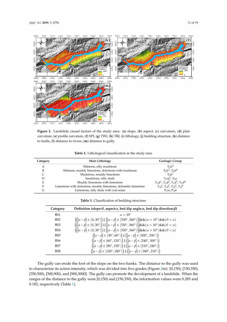
Figure 2. Landslide causal factors of the study area: (a) slope, (b) aspect, (c) curvature, (d) plan curvature, (e) profile curvature, (f) SPI, (g) TWI, (h) TRI, (i) lithology, (j) bedding structure, (k) distance to faults, (l) distance to rivers, (m) distance to gully.
2.4. Landslide Causal Factors Selection
2.4.1. Multicollinearity Analysis
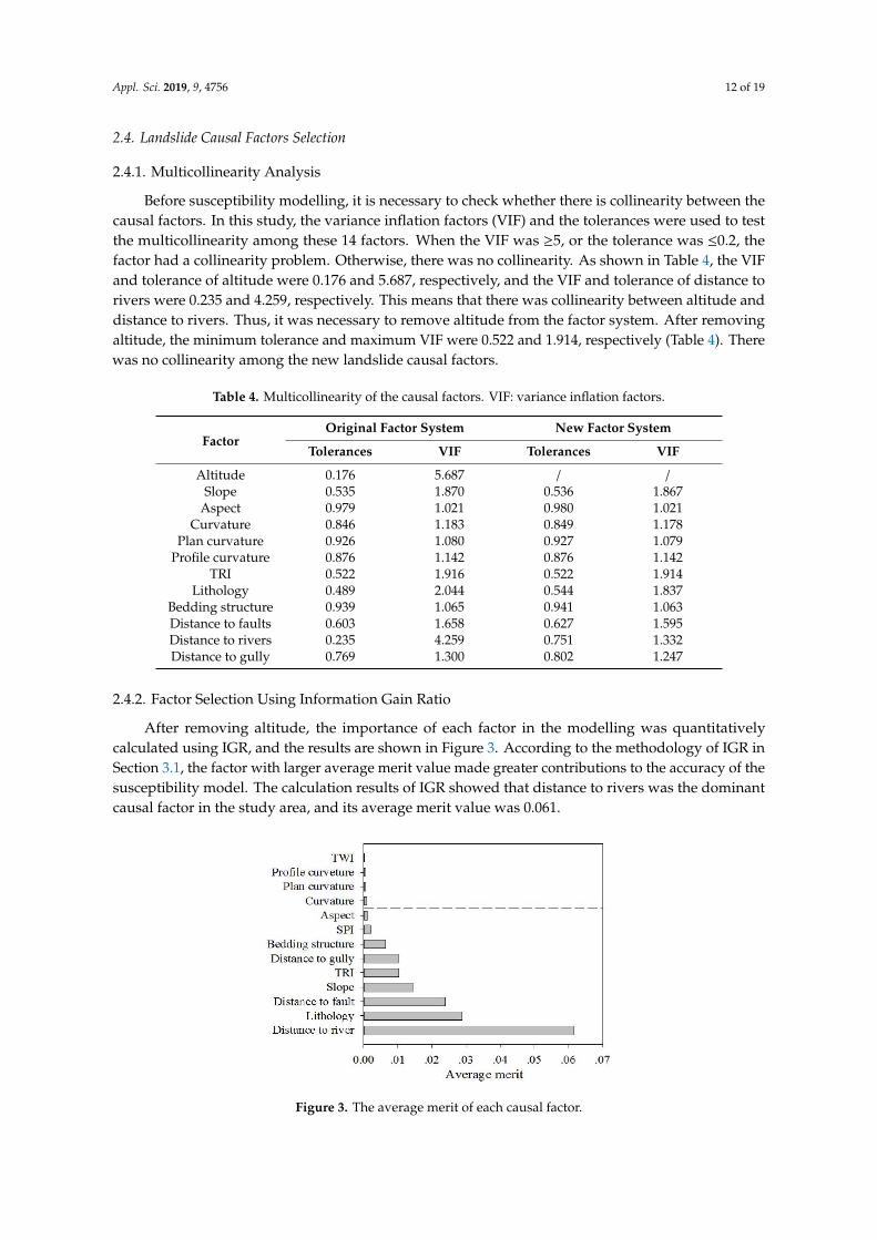
Before susceptibility modelling, it is necessary to check whether there is collinearity between the causal factors. In this study, the variance inflation factors (VIF) and the tolerances were used to test the multicollinearity among these 14 factors. When the VIF was ≥5, or the tolerance was ≤0.2, the factor had a collinearity problem. Otherwise, there was no collinearity. As shown in Table 4, the VIF and tolerance of altitude were 0.176 and 5.687, respectively, and the VIF and tolerance of distance to rivers were 0.235 and 4.259, respectively. This means that there was collinearity between altitude and distance to rivers. Thus, it was necessary to remove altitude from the factor system. After removing altitude, the minimum tolerance and maximum VIF were 0.522 and 1.914, respectively (Table 4). There was no collinearity among the new landslide causal factors.
Table 4. Multicollinearity of the causal factors. VIF: variance inflation factors.
Factor Original Factor System New Factor System
Tolerances VIF Tolerances VIF Altitude 0.176 5.687 / /
Slope 0.535 1.870 0.536 1.867 Aspect 0.979 1.021 0.980 1.021
Curvature 0.846 1.183 0.849 1.178 Plan curvature 0.926 1.080 0.927 1.079
Profile curvature 0.876 1.142 0.876 1.142 TRI 0.522 1.916 0.522 1.914
Lithology 0.489 2.044 0.544 1.837 Bedding structure 0.939 1.065 0.941 1.063 Distance to faults 0.603 1.658 0.627 1.595
Figure 2. Landslide causal factors of the study area: (a) slope, (b) aspect, (c) curvature, (d) plancurvature, (e) profile curvature, (f) SPI, (g) TWI, (h) TRI, (i) lithology, (j) bedding structure, (k) distanceto faults, (l) distance to rivers, (m) distance to gully.
Table 2. Lithological classification in the study area.
Category Main Lithology Geologic Group
A Siltstone, silty mudstone T2b2
B Siltstone, muddy limestone, dolostone with mudstone T2b3, T2b4
C Mudstone, muddy limestone T2b1
D Sandstone, silty shale T3xj1, T3eE Muddy limestone with limestone T1d1, T1d2, T1d3, T1d4
F Limestone with dolostone, muddy limestone, dolomitic limestone T1j1, T1j2, T1j3, T1j4
G Limestone, silty shale with coal seam P3w, P3d
Table 3. Classification of bedding structure.
Category Definition (slope:θ, aspect:σ, bed dip angle:α, bed dip direction:β)
BS1 α < 10◦
BS2((∣∣∣α− β∣∣∣ ∈ (0, 30◦]
)‖
(∣∣∣α− β∣∣∣ ∈ [330◦, 360◦)))
&&(α > 10◦)&&(θ > α)
BS3((∣∣∣α− β∣∣∣ ∈ (0, 30◦]
)‖
(∣∣∣α− β∣∣∣ ∈ [330◦, 360◦)))
&&(α > 10◦)&&(θ = α)
BS4((∣∣∣α− β∣∣∣ ∈ (0, 30◦]
)‖
(∣∣∣α− β∣∣∣ ∈ [330◦, 360◦)))
&&(α > 10◦)&&(θ < α)
BS5(∣∣∣α− β∣∣∣ ∈ [30◦, 60◦)
)‖
(∣∣∣α− β∣∣∣ ∈ [300◦, 330◦))
BS6(∣∣∣α− β∣∣∣ ∈ [60◦, 120◦)
)‖
(∣∣∣α− β∣∣∣ ∈ [240◦, 300◦))
BS7(∣∣∣α− β∣∣∣ ∈ [90◦, 150◦)
)‖
(∣∣∣α− β∣∣∣ ∈ [210◦, 240◦))
BS8(∣∣∣α− β∣∣∣ ∈ [120◦, 180◦)
)‖
(∣∣∣α− β∣∣∣ ∈ [180◦, 210◦))
The gully can erode the foot of the slope on the two banks. The distance to the gully was usedto characterize its action intensity, which was divided into five grades (Figure 2m): [0,150), [150,350),[350,500), [500,900), and [900,3000]. The gully can promote the development of a landslide. When theranges of the distance to the gully were [0,150) and [150,350), the information values were 0.285 and0.182, respectively (Table 1).
Appl. Sci. 2019, 9, 4756 12 of 19
2.4. Landslide Causal Factors Selection
2.4.1. Multicollinearity Analysis
Before susceptibility modelling, it is necessary to check whether there is collinearity between thecausal factors. In this study, the variance inflation factors (VIF) and the tolerances were used to testthe multicollinearity among these 14 factors. When the VIF was ≥5, or the tolerance was ≤0.2, thefactor had a collinearity problem. Otherwise, there was no collinearity. As shown in Table 4, the VIFand tolerance of altitude were 0.176 and 5.687, respectively, and the VIF and tolerance of distance torivers were 0.235 and 4.259, respectively. This means that there was collinearity between altitude anddistance to rivers. Thus, it was necessary to remove altitude from the factor system. After removingaltitude, the minimum tolerance and maximum VIF were 0.522 and 1.914, respectively (Table 4). Therewas no collinearity among the new landslide causal factors.
Table 4. Multicollinearity of the causal factors. VIF: variance inflation factors.
FactorOriginal Factor System New Factor System
Tolerances VIF Tolerances VIF
Altitude 0.176 5.687 / /Slope 0.535 1.870 0.536 1.867
Aspect 0.979 1.021 0.980 1.021Curvature 0.846 1.183 0.849 1.178
Plan curvature 0.926 1.080 0.927 1.079Profile curvature 0.876 1.142 0.876 1.142
TRI 0.522 1.916 0.522 1.914Lithology 0.489 2.044 0.544 1.837
Bedding structure 0.939 1.065 0.941 1.063Distance to faults 0.603 1.658 0.627 1.595Distance to rivers 0.235 4.259 0.751 1.332Distance to gully 0.769 1.300 0.802 1.247
2.4.2. Factor Selection Using Information Gain Ratio
After removing altitude, the importance of each factor in the modelling was quantitativelycalculated using IGR, and the results are shown in Figure 3. According to the methodology of IGR inSection 3.1, the factor with larger average merit value made greater contributions to the accuracy of thesusceptibility model. The calculation results of IGR showed that distance to rivers was the dominantcausal factor in the study area, and its average merit value was 0.061.
Appl. Sci. 2019, 9, x FOR PEER REVIEW 13 of 20
Distance to rivers 0.235 4.259 0.751 1.332 Distance to gully 0.769 1.300 0.802 1.247
2.4.2. Factor Selection Using Information Gain Ratio
After removing altitude, the importance of each factor in the modelling was quantitatively calculated using IGR, and the results are shown in Figure 3. According to the methodology of IGR in Section 3.1, the factor with larger average merit value made greater contributions to the accuracy of the susceptibility model. The calculation results of IGR showed that distance to rivers was the dominant causal factor in the study area, and its average merit value was 0.061.
Figure 3. The average merit of each causal factor.
Support vector machine has many advantages, such as a stable result and fast operation speed; thus, it was used to test the prediction accuracy of different factor combinations, and the accuracy was calculated using receiver operating characteristic [35]. As shown in Table 5, when eliminating TWI, curvature, plan curvature, and profile curvature, the accuracy of susceptibility modelling was the highest of 0.922. However, when the aspect was excluded, the accuracy of susceptibility modelling was significantly reduced to 0.908. The elimination of inconsequential factors can improve the accuracy of susceptibility modelling. Finally, nine important causal factors were selected for susceptibility modelling.
Table 5. The prediction accuracy with elimination of the less important factors.
Model Eliminating Less Important Factors Accuracy Model 1 Without eliminating any factor 0.918 Model 2 TWI 0.918 Model 3 TWI, profile curvature 0.920 Model 4 TWI, profile curvature, plan curvature 0.919 Model 5 TWI, profile curvature, plan curvature, curvature 0.922 Model 6 TWI, profile curvature, plan curvature, curvature, aspect 0.908
3. Results and Accuracy Analysis
3.1. Landslide Susceptibility Modelling
In the susceptibility mapping, landslide susceptibility index was considered for the probability of landslide occurrence (landslide: 1, non-landslide: 0). Before landslide susceptibility modelling, the data of landslide causal factors should be normalized. In this study, we normalized the factors into the range of [0.01, 0.99] on the basis of their information values. The normalized value was used as input data, whereas the susceptibility index was used as output data.
Figure 3. The average merit of each causal factor.
Appl. Sci. 2019, 9, 4756 13 of 19
Support vector machine has many advantages, such as a stable result and fast operation speed;thus, it was used to test the prediction accuracy of different factor combinations, and the accuracywas calculated using receiver operating characteristic [35]. As shown in Table 5, when eliminatingTWI, curvature, plan curvature, and profile curvature, the accuracy of susceptibility modellingwas the highest of 0.922. However, when the aspect was excluded, the accuracy of susceptibilitymodelling was significantly reduced to 0.908. The elimination of inconsequential factors can improvethe accuracy of susceptibility modelling. Finally, nine important causal factors were selected forsusceptibility modelling.
Table 5. The prediction accuracy with elimination of the less important factors.
Model Eliminating Less Important Factors Accuracy
Model 1 Without eliminating any factor 0.918Model 2 TWI 0.918Model 3 TWI, profile curvature 0.920Model 4 TWI, profile curvature, plan curvature 0.919Model 5 TWI, profile curvature, plan curvature, curvature 0.922Model 6 TWI, profile curvature, plan curvature, curvature, aspect 0.908
3. Results and Accuracy Analysis
3.1. Landslide Susceptibility Modelling
In the susceptibility mapping, landslide susceptibility index was considered for the probabilityof landslide occurrence (landslide: 1, non-landslide: 0). Before landslide susceptibility modelling,the data of landslide causal factors should be normalized. In this study, we normalized the factors intothe range of [0.01, 0.99] on the basis of their information values. The normalized value was used asinput data, whereas the susceptibility index was used as output data.
In order to test the performance of the used methods, the landslide locations were randomlydivided into two parts. A total of 50% of the landslide locations were utilized for the training model,and the remaining 50% were applied to verify the model performance. In the training process ofthe models, too much or too little training data of any kind would lead to the imbalance of modeltraining. Therefore, the same number of data was randomly selected from the non-landslide area asthe training samples. Three machine learning models (SVM, ANN, and CART) and the multivariatestatistical model (LR) were used for landslide susceptibility modelling with nine important causalfactors. The modelling process of the four models was completed in Clementine 12.
Furthermore, the parameters of SVM and ANN were obtained by error and trial algorithm(Table 6). The CART model did not need any parameter in modelling. In the LR model, the formula ofLR model for calculating the landslide susceptibility index (LSI) was as follows:
LSI = (−6.651) + (SPI ∗ (−0.055)) + (TRI ∗ 1.826) + (Lithology ∗ 1.417)+(Slope ∗ 1.458) + (Gully ∗ 0.806) + (Aspect ∗ 0.384)+(River ∗ 3.792) + (Faults ∗ 0.174)
(14)
Table 6. The parameters of support vector machine (SVM) and artificial neural network (ANN) models.
Models Parameters Notes
SVM c = 20, γ = 1.3 c is the penalty factor, γ is the parameter of the kernel functionANN n = 5, α = 0.9 n is the neurons number, α is the momentum
The landslide susceptibility index was calculated by SVM, ANN, CART, and LR model, and thenwas divided into four levels: high (20%), moderate (20%), low (20%) and very low (40%), respectively.The results are shown in Figure 4.
Appl. Sci. 2019, 9, 4756 14 of 19
Appl. Sci. 2019, 9, x FOR PEER REVIEW 14 of 20
In order to test the performance of the used methods, the landslide locations were randomly divided into two parts. A total of 50% of the landslide locations were utilized for the training model, and the remaining 50% were applied to verify the model performance. In the training process of the models, too much or too little training data of any kind would lead to the imbalance of model training. Therefore, the same number of data was randomly selected from the non-landslide area as the training samples. Three machine learning models (SVM, ANN, and CART) and the multivariate statistical model (LR) were used for landslide susceptibility modelling with nine important causal factors. The modelling process of the four models was completed in Clementine 12.
Furthermore, the parameters of SVM and ANN were obtained by error and trial algorithm (Table 6). The CART model did not need any parameter in modelling. In the LR model, the formula of LR model for calculating the landslide susceptibility index (LSI) was as follows:
( . ) ( ( . )) ( . ) ( . )
( . ) ( . ) ( . )
( . ) ( . )
LSI = − + ∗ − + ∗ + ∗
+ ∗ + ∗ + ∗
+ ∗ + ∗
SPI TRI Lithology
Slope Gully Aspect
River Faults
6 651 0 055 1 826 1 417
1 458 0 806 0 384
3 792 0 174
(14)
Table 6. The parameters of support vector machine (SVM) and artificial neural network (ANN) models.
Models Parameters Notes SVM c = 20, γ = 1.3 c is the penalty factor, γ is the parameter of the kernel function ANN n = 5, α = 0.9 n is the neurons number, α is the momentum
The landslide susceptibility index was calculated by SVM, ANN, CART, and LR model, and then was divided into four levels: high (20%), moderate (20%), low (20%) and very low (40%), respectively. The results are shown in Figure 4.
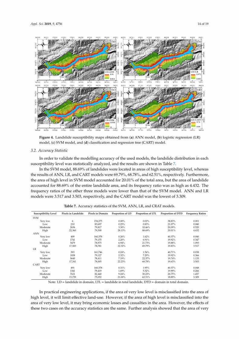
Figure 4. Landslide susceptibility maps obtained from (a) ANN model, (b) logistic regression (LR) model, (c) SVM model, and (d) classification and regression tree (CART) model.
3.2. Accuracy Statistic
In order to validate the modelling accuracy of the used models, the landslide distribution in each susceptibility level was statistically analyzed, and the results are shown in Table 7.
Table 7. Accuracy statistics of the SVM, ANN, LR, and CRAT models.
Figure 4. Landslide susceptibility maps obtained from (a) ANN model, (b) logistic regression (LR)model, (c) SVM model, and (d) classification and regression tree (CART) model.
3.2. Accuracy Statistic
In order to validate the modelling accuracy of the used models, the landslide distribution in eachsusceptibility level was statistically analyzed, and the results are shown in Table 7.
In the SVM model, 88.69% of landslides were located in areas of high susceptibility level, whereasthe results of ANN, LR, and CART models were 69.79%, 68.78%, and 62.51%, respectively. Furthermore,the area of high level in SVM model accounted for 20.01% of the total area, but the area of landslideaccounted for 88.69% of the entire landslide area, and its frequency ratio was as high as 4.432. Thefrequency ratios of the other three models were lower than that of the SVM model. ANN and LRmodels were 3.517 and 3.503, respectively, and the CART model was the lowest of 3.309.
Table 7. Accuracy statistics of the SVM, ANN, LR, and CRAT models.
Susceptibility Level Pixels in Landslide Pixels in Domain Proportion of LD Proportion of LTL Proportion of DTD Frequency Ratios
SVMVery low 6 154,275 0.00% 0.02% 38.83% 0.001
Low 210 83,697 0.25% 0.83% 21.07% 0.040Moderate 2636 79,817 3.30% 10.46% 20.09% 0.520
High 22,360 79,500 28.13% 88.69% 20.01% 4.432ANN
Very low 409 160,378 0.26% 1.62% 40.37% 0.040Low 1741 79,155 2.20% 6.91% 19.92% 0.347
Moderate 5479 78,975 6.94% 21.73% 19.88% 1.093High 17,583 78,781 22.32% 69.79% 19.83% 3.517
LRVery low 393 161,746 0.24% 1.56% 40.71% 0.038
Low 1838 79,127 2.32% 7.29% 19.92% 0.366Moderate 5640 78,411 7.19% 22.37% 19.74% 1.133
High 17,341 78,005 22.23% 68.78% 19.63% 3.503CART
Very low 491 160,378 0.31% 1.95% 40.37% 0.048Low 1341 79,419 1.69% 5.32% 19.99% 0.266
Moderate 7621 82,440 9.24% 30.23% 20.75% 1.457High 15,759 75,052 21.00% 62.51% 18.89% 3.309
Note: LD = landslide in domain, LTL = landslide in total landslide, DTD = domain in total domain.
In practical engineering applications, if the area of very low level is misclassified into the area ofhigh level, it will limit effective land-use. However, if the area of high level is misclassified into thearea of very low level, it may bring economic losses and casualties in the area. However, the effects ofthese two cases on the accuracy statistics are the same. Further analysis showed that the area of very
Appl. Sci. 2019, 9, 4756 15 of 19
low level of SVM model accounted for 40% of the total study area, but its landslide only accounted for0.02% of the entire landslide area. Its frequency ratio was the lowest of 0.001, which was much lowerthan those of ANN, LR, and CART models, with those being 0.040, 0.038, and 0.048, respectively.
By comparing the accuracy statistics of the four models, we can see that the SVM model had thehighest classification accuracy in the area of high level and the lowest misclassification in the area ofvery low level, showing better prediction performance.
3.3. Using ROC Curve
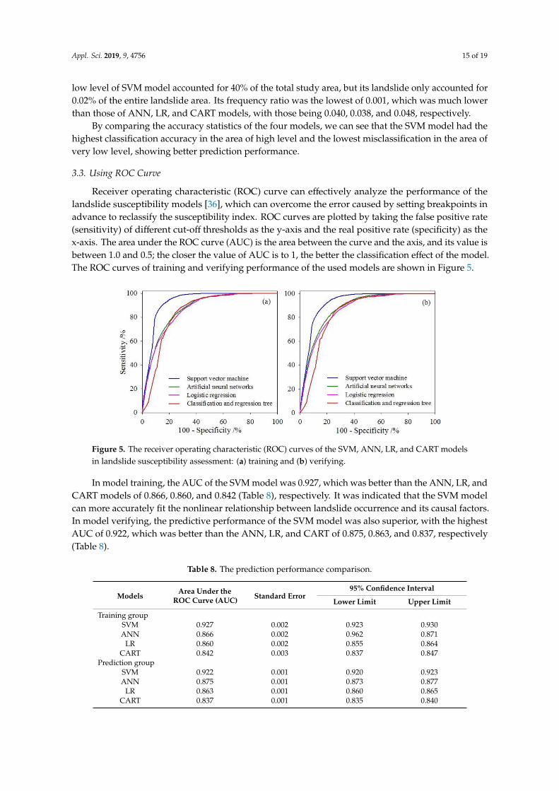
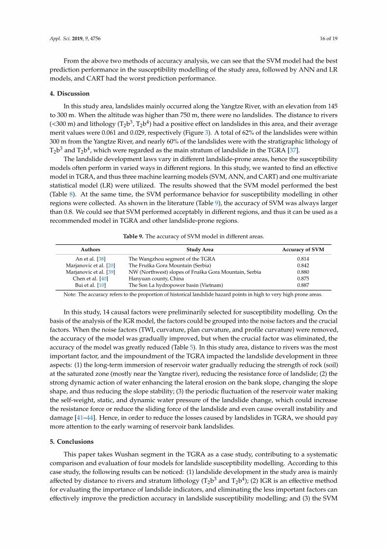
Receiver operating characteristic (ROC) curve can effectively analyze the performance of thelandslide susceptibility models [36], which can overcome the error caused by setting breakpoints inadvance to reclassify the susceptibility index. ROC curves are plotted by taking the false positive rate(sensitivity) of different cut-off thresholds as the y-axis and the real positive rate (specificity) as thex-axis. The area under the ROC curve (AUC) is the area between the curve and the axis, and its value isbetween 1.0 and 0.5; the closer the value of AUC is to 1, the better the classification effect of the model.The ROC curves of training and verifying performance of the used models are shown in Figure 5.
Appl. Sci. 2019, 9, x FOR PEER REVIEW 16 of 20
Figure 5. The receiver operating characteristic (ROC) curves of the SVM, ANN, LR, and CART models in landslide susceptibility assessment: (a) training and (b) verifying. In model training, the AUC of the SVM model was 0.927, which was better than the ANN, LR,
and CART models of 0.866, 0.860, and 0.842 (Table 8), respectively. It was indicated that the SVM model can more accurately fit the nonlinear relationship between landslide occurrence and its causal factors. In model verifying, the predictive performance of the SVM model was also superior, with the highest AUC of 0.922, which was better than the ANN, LR, and CART of 0.875, 0.863, and 0.837, respectively (Table 8).
Table 8. The prediction performance comparison.
Models Area Under
the ROC Curve (AUC)
Standard Error
95% Confidence Interval
Lower Limit Upper Limit
Training group SVM 0.927 0.002 0.923 0.930 ANN 0.866 0.002 0.962 0.871
LR 0.860 0.002 0.855 0.864 CART 0.842 0.003 0.837 0.847
Prediction group SVM 0.922 0.001 0.920 0.923 ANN 0.875 0.001 0.873 0.877
LR 0.863 0.001 0.860 0.865 CART 0.837 0.001 0.835 0.840
From the above two methods of accuracy analysis, we can see that the SVM model had the best prediction performance in the susceptibility modelling of the study area, followed by ANN and LR models, and CART had the worst prediction performance.
4. Discussion
In this study area, landslides mainly occurred along the Yangtze River, with an elevation from 145 to 300 m. When the altitude was higher than 750 m, there were no landslides. The distance to rivers (<300 m) and lithology (T2b3, T2b4) had a positive effect on landslides in this area, and their average merit values were 0.061 and 0.029, respectively (Figure 3). A total of 62% of the landslides were within 300 m from the Yangtze River, and nearly 60% of the landslides were with the stratigraphic lithology of T2b3 and T2b4, which were regarded as the main stratum of landslide in the TGRA [37].
Figure 5. The receiver operating characteristic (ROC) curves of the SVM, ANN, LR, and CART modelsin landslide susceptibility assessment: (a) training and (b) verifying.
In model training, the AUC of the SVM model was 0.927, which was better than the ANN, LR, andCART models of 0.866, 0.860, and 0.842 (Table 8), respectively. It was indicated that the SVM modelcan more accurately fit the nonlinear relationship between landslide occurrence and its causal factors.In model verifying, the predictive performance of the SVM model was also superior, with the highestAUC of 0.922, which was better than the ANN, LR, and CART of 0.875, 0.863, and 0.837, respectively(Table 8).
Table 8. The prediction performance comparison.
ModelsArea Under the
ROC Curve (AUC) Standard Error95% Confidence Interval
Lower Limit Upper Limit
Training groupSVM 0.927 0.002 0.923 0.930ANN 0.866 0.002 0.962 0.871
LR 0.860 0.002 0.855 0.864CART 0.842 0.003 0.837 0.847
Prediction groupSVM 0.922 0.001 0.920 0.923ANN 0.875 0.001 0.873 0.877
LR 0.863 0.001 0.860 0.865CART 0.837 0.001 0.835 0.840
Appl. Sci. 2019, 9, 4756 16 of 19
From the above two methods of accuracy analysis, we can see that the SVM model had the bestprediction performance in the susceptibility modelling of the study area, followed by ANN and LRmodels, and CART had the worst prediction performance.
4. Discussion
In this study area, landslides mainly occurred along the Yangtze River, with an elevation from 145to 300 m. When the altitude was higher than 750 m, there were no landslides. The distance to rivers(<300 m) and lithology (T2b3, T2b4) had a positive effect on landslides in this area, and their averagemerit values were 0.061 and 0.029, respectively (Figure 3). A total of 62% of the landslides were within300 m from the Yangtze River, and nearly 60% of the landslides were with the stratigraphic lithology ofT2b3 and T2b4, which were regarded as the main stratum of landslide in the TGRA [37].
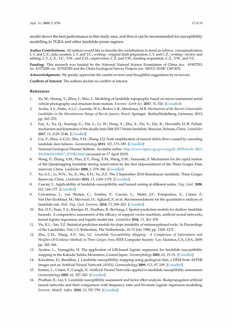
The landslide development laws vary in different landslide-prone areas, hence the susceptibilitymodels often perform in varied ways in different regions. In this study, we wanted to find an effectivemodel in TGRA, and thus three machine learning models (SVM, ANN, and CART) and one multivariatestatistical model (LR) were utilized. The results showed that the SVM model performed the best(Table 8). At the same time, the SVM performance behavior for susceptibility modelling in otherregions were collected. As shown in the literature (Table 9), the accuracy of SVM was always largerthan 0.8. We could see that SVM performed acceptably in different regions, and thus it can be used as arecommended model in TGRA and other landslide-prone regions.
Table 9. The accuracy of SVM model in different areas.
Authors Study Area Accuracy of SVM
An et al. [38] The Wangzhou segment of the TGRA 0.814Marjanovic et al. [20] The Fruška Gora Mountain (Serbia) 0.842Marjanovic et al. [39] NW (Northwest) slopes of Fruška Gora Mountain, Serbia 0.880
Chen et al. [40] Hanyuan county, China 0.875Bui et al. [10] The Son La hydropower basin (Vietnam) 0.887
Note: The accuracy refers to the proportion of historical landslide hazard points in high to very high prone areas.
In this study, 14 causal factors were preliminarily selected for susceptibility modelling. On thebasis of the analysis of the IGR model, the factors could be grouped into the noise factors and the crucialfactors. When the noise factors (TWI, curvature, plan curvature, and profile curvature) were removed,the accuracy of the model was gradually improved, but when the crucial factor was eliminated, theaccuracy of the model was greatly reduced (Table 5). In this study area, distance to rivers was the mostimportant factor, and the impoundment of the TGRA impacted the landslide development in threeaspects: (1) the long-term immersion of reservoir water gradually reducing the strength of rock (soil)at the saturated zone (mostly near the Yangtze river), reducing the resistance force of landslide; (2) thestrong dynamic action of water enhancing the lateral erosion on the bank slope, changing the slopeshape, and thus reducing the slope stability; (3) the periodic fluctuation of the reservoir water makingthe self-weight, static, and dynamic water pressure of the landslide change, which could increasethe resistance force or reduce the sliding force of the landslide and even cause overall instability anddamage [41–44]. Hence, in order to reduce the losses caused by landslides in TGRA, we should paymore attention to the early warning of reservoir bank landslides.
5. Conclusions
This paper takes Wushan segment in the TGRA as a case study, contributing to a systematiccomparison and evaluation of four models for landslide susceptibility modelling. According to thiscase study, the following results can be noticed: (1) landslide development in the study area is mainlyaffected by distance to rivers and stratum lithology (T2b3 and T2b4); (2) IGR is an effective methodfor evaluating the importance of landslide indicators, and eliminating the less important factors caneffectively improve the prediction accuracy in landslide susceptibility modelling; and (3) the SVM
Appl. Sci. 2019, 9, 4756 17 of 19
model shows the best performance in this study area, and thus it can be recommended for susceptibilitymodelling in TGRA and other landslide-prone regions.
Author Contributions: All authors would like to describe the contributions in detail as follows: conceptualization,L.Y. and C.Z.; data curation, L.Y. and Y.C.; writing—original draft preparation, L.Y. and C.Z.; writing—review andediting, L.Y., C.Z., Y.C., Y.W., and Z.H.; supervision, C.Z. and Y.W.; funding acquisition, C.Z., Y.W., and Y.C.
Funding: This research was funded by the National Natural Science Foundation of China (no. 41907253,no. 41572289, no. 41702330) and the China Geological Survey Projects (no. 000121 2018C C60 003).
Acknowledgments: We greatly appreciate the careful reviews and thoughtful suggestions by reviewers.
Conflicts of Interest: The authors declare no conflict of interest.
References
1. Yu, M.; Huang, Y.; Zhou, J.; Mao, L. Modeling of landslide topography based on micro-unmanned aerialvehicle photography and structure-from-motion. Environ. Earth Sci. 2017, 76, 520. [CrossRef]
2. Avelar, A.S.; Netto, A.L.C.; Lacerda, W.A.; Becker, L.B.; Mendonça, M.B. Mechanisms of the Recent CatastrophicLandslides in the Mountainous Range of Rio de Janeiro, Brazil; Springer: Berlin/Heidelberg, Germany, 2013;pp. 265–270.
3. Fan, X.; Xu, Q.; Scaringi, G.; Dai, L.; Li, W.; Dong, X.; Zhu, X.; Pei, X.; Dai, K.; Havenith, H.-B. Failuremechanism and kinematics of the deadly June 24th 2017 Xinmo landslide, Maoxian, Sichuan, China. Landslides2017, 14, 2129–2146. [CrossRef]
4. Cui, P.; Zhou, G.G.D.; Zhu, X.H.; Zhang, J.Q. Scale amplification of natural debris flows caused by cascadinglandslide dam failures. Geomorphology 2013, 182, 173–189. [CrossRef]
5. National Geological Disaster Bulletin. Available online: http://www.cigem.cgs.gov.cn/gzdt_4839/dwdt_4861/
201904/t20190417_479382.html (accessed on 17 April 2019).6. Wang, F.; Zhang, Y.M.; Huo, Z.T.; Peng, X.M.; Wang, S.M.; Yamasaki, S. Mechanism for the rapid motion
of the Qianjiangping landslide during reactivation by the first impoundment of the Three Gorges Damreservoir, China. Landslides 2008, 5, 379–386. [CrossRef]
7. Xu, G.L.; Li, W.N.; Yu, Z.; Ma, X.H.; Yu, Z.Z. The 2 September 2014 Shanshucao landslide, Three GorgesReservoir, China. Landslides 2015, 12, 1169–1178. [CrossRef]
8. Cascini, L. Applicability of landslide susceptibility and hazard zoning at different scales. Eng. Geol. 2008,102, 164–177. [CrossRef]
9. Corominas, J.; van Westen, C.; Frattini, P.; Cascini, L.; Malet, J.P.; Fotopoulou, S.; Catani, F.;Van Den Eeckhaut, M.; Mavrouli, O.; Agliardi, F.; et al. Recommendations for the quantitative analysis oflandslide risk. Bull. Eng. Geol. Environ. 2014, 73, 209–263. [CrossRef]
10. Bui, D.T.; Tuan, T.A.; Klempe, H.; Pradhan, B.; Revhaug, I. Spatial prediction models for shallow landslidehazards: A comparative assessment of the efficacy of support vector machines, artificial neural networks,kernel logistic regression, and logistic model tree. Landslides 2016, 13, 361–378.
11. Yin, K.L.; Yan, T.Z. Statistical prediction models for slope instability of metamorphosed rocks. In Proceedingsof the Landslides, Vols 1-3, Rotterdam, The Netherlands, 10–15 July 1988; pp. 1269–1272.
12. Zhu, C.H.; Wang, X.P.; Soc, I.C. Landslide Susceptibility Mapping: A Comparison of Information andWeights-Of-Evidence Methods in Three Gorges Area; IEEE Computer Society: Los Alamitos, CA, USA, 2009;pp. 342–346.
13. Ayalew, L.; Yamagishi, H. The application of GIS-based logistic regression for landslide susceptibilitymapping in the Kakuda-Yahiko Mountains, Central Japan. Geomorphology 2005, 65, 15–31. [CrossRef]
14. Kawabata, D.; Bandibas, J. Landslide susceptibility mapping using geological data, a DEM from ASTERimages and an Artificial Neural Network (ANN). Geomorphology 2009, 113, 97–109. [CrossRef]
15. Ermini, L.; Catani, F.; Casagli, N. Artificial Neural Networks applied to landslide susceptibility assessment.Geomorphology 2005, 66, 327–343. [CrossRef]
16. Pradhan, B.; Lee, S. Landslide susceptibility assessment and factor effect analysis: Backpropagation artificialneural networks and their comparison with frequency ratio and bivariate logistic regression modelling.Environ. Modell. Softw. 2010, 25, 747–759. [CrossRef]
Appl. Sci. 2019, 9, 4756 18 of 19
17. Xu, C.; Dai, F.C.; Xu, X.W.; Lee, Y.H. GIS-based support vector machine modeling of earthquake-triggeredlandslide susceptibility in the Jianjiang River watershed, China. Geomorphology 2012, 145, 70–80. [CrossRef]
18. Peng, L.; Niu, R.Q.; Huang, B.; Wu, X.L.; Zhao, Y.N.; Ye, R.Q. Landslide susceptibility mapping based onrough set theory and support vector machines: A case of the Three Gorges area, China. Geomorphology 2014,204, 287–301. [CrossRef]
19. Yao, X.; Tham, L.G.; Dai, F.C. Landslide susceptibility mapping based on Support Vector Machine: A casestudy on natural slopes of Hong Kong, China. Geomorphology 2008, 101, 572–582. [CrossRef]
20. Marjanovic, M.; Kovacevic, M.; Bajat, B.; Vozenilek, V. Landslide susceptibility assessment using SVMmachine learning algorithm. Eng. Geol. 2011, 123, 225–234. [CrossRef]
21. Everitt, B.S. Classification and Regression Trees. In Encyclopedia of Statistics in Behavioral Science; John Wiley& Sons, Ltd.: Hoboken, NJ, USA, 2005. [CrossRef]
22. Pradhan, B.; Lee, S. Regional landslide susceptibility analysis using back-propagation neural network modelat Cameron Highland, Malaysia. Landslides 2010, 7, 13–30. [CrossRef]
23. Pham, B.T.; Bui, D.T.; Dholakia, M.B.; Prakash, I.; Pham, H.V.; Mehmood, K.; Le, H.Q. A novel ensembleclassifier of rotation forest and Naive Bayer for landslide susceptibility assessment at the Luc Yen district,Yen Bai Province (Viet Nam) using GIS. Geomat. Nat. Hazards Risk 2017, 8, 649–671. [CrossRef]
24. Shigeo, A. Support Vector Machines for Pattern Classification. In Proceedings of the International JointConference on Neural Networks, Washington, DC, USA, 15–19 July 2001; Volume 36, pp. 7535–7543.
25. Tian, Y.Y.; Xu, C.; Hong, H.Y.; Zhou, Q.; Wang, D. Mapping earthquake-triggered landslide susceptibilityby use of artificial neural network (ANN) models: An example of the 2013 Minxian (China) Mw 5.9 event.Geomat. Nat. Hazards Risk 2019, 10, 1–25. [CrossRef]
26. Kalantar, B.; Pradhan, B.; Naghibi, S.A.; Motevalli, A.; Mansor, S. Assessment of the effects of training dataselection on the landslide susceptibility mapping: A comparison between support vector machine (SVM),logistic regression (LR) and artificial neural networks (ANN). Geomat. Nat. Hazards Risk 2018, 9, 49–69.[CrossRef]
27. Budimir, M.E.A.; Atkinson, P.M.; Lewis, H.G. A systematic review of landslide probability mapping usinglogistic regression. Landslides 2015, 12, 419–436. [CrossRef]
28. Sestras, P.; Bilasco, S.; Rosca, S.; Nas, S.; Bondrea, M.V.; Galgau, R.; Veres, I.; Salagean, T.; Spalevic, V.;Cimpeanu, S.M. Landslides Susceptibility Assessment Based on GIS Statistical Bivariate Analysis in the HillsSurrounding a Metropolitan Area. Sustainability 2019, 11, 23. [CrossRef]
29. Bai, S.B.; Wang, J.; Lu, G.N.; Zhou, P.G.; Hou, S.S.; Xu, S.N. GIS-based logistic regression for landslidesusceptibility mapping of the Zhongxian segment in the Three Gorges area, China. Geomorphology 2010, 115,23–31. [CrossRef]
30. Chen, W.T.; Li, X.J.; Wang, Y.X.; Liu, S.W. Landslide susceptibility mapping using LiDAR and DMC data:A case study in the Three Gorges area, China. Environ. Earth Sci. 2013, 70, 673–685. [CrossRef]
31. Wu, X.L.; Niu, R.Q.; Ren, F.; Peng, L. Landslide susceptibility mapping using rough sets and back-propagationneural networks in the Three Gorges, China. Environ. Earth Sci. 2013, 70, 1307–1318. [CrossRef]
32. Zhou, C.; Yin, K.L.; Cao, Y.; Ahmed, B.; Li, Y.Y.; Catani, F.; Pourghasemi, H.R. Landslide susceptibilitymodeling applying machine learning methods: A case study from Longju in the Three Gorges Reservoirarea, China. Comput. Geosci. 2018, 112, 23–37. [CrossRef]
33. Moore, I.D.; Grayson, R.B.; Ladson, A.R. Digital terrain modelling: A review of hydrological,geomorphological, and biological applications. Hydrol. Process. 1991, 5, 3–30. [CrossRef]
34. Technical Requirements for Investigation and Evaluation of Collapse, Landslide, Debris Flow.Available online: http://www.mnr.gov.cn/gk/bzgf/201004/t20100406_1971713.html (accessed on 6 April2010).
35. Bui, D.T.; Lofman, O.; Revhaug, I.; Dick, O. Landslide susceptibility analysis in the Hoa Binh province ofVietnam using statistical index and logistic regression. Natural Hazards 2011, 59, 1413–1444. [CrossRef]
36. Hanley, J.A.; McNeil, B.J. A method of comparing the areas under receiver operating characteristic curvesderived from the same cases. Radiology 1983, 148, 839–843. [CrossRef]
37. Miao, H.; Wang, G.; Yin, K.; Kamai, T.; Li, Y. Mechanism of the slow-moving landslides in Jurassic red-stratain the Three Gorges Reservoir, China. Eng. Geol. 2014, 171, 59–69. [CrossRef]
38. An, K.; Niu, R. Landslide Susceptibility Assessment Using Support Vector Machine Based onWeighted-information Model. J. Yangtze River Sci. Res. Inst. 2016, 33, 47–51.
Appl. Sci. 2019, 9, 4756 19 of 19
39. Marjanovic, M.; Bajat, B.; Kovacevic, M. Landslide Susceptibility Assessment with Machine Learning Algorithms;IEEE: New York, NY, USA, 2009; pp. 273–278.
40. Chen, W.; Pourghasemi, H.R.; Panahi, M.; Kornejady, A.; Wang, J.L.; Xie, X.S.; Cao, S.B. Spatial prediction oflandslide susceptibility using an adaptive neuro-fuzzy inference system combined with frequency ratio,generalized additive model, and support vector machine techniques. Geomorphology 2017, 297, 69–85.[CrossRef]
41. Bilasco, S.; Horvath, C.; Cocean, P.; Sorocovschi, V.; Oncu, M. Implementation of the usle model using gistechniques. case study the somesean plateau. Carpath. J. Earth Environ. Sci. 2009, 4, 123–132.
42. Zhou, C.; Yin, K.; Cao, Y.; Ahmed, B. Application of time series analysis and PSO–SVM model in predictingthe Bazimen landslide in the Three Gorges Reservoir, China. Eng. Geol. 2016, 204, 108–120. [CrossRef]
43. Zhou, C.; Yin, K.; Cao, Y.; Intrieri, E.; Ahmed, B.; Catani, F. Displacement prediction of step-like landslide byapplying a novel kernel extreme learning machine method. Landslides 2018, 15, 2211–2225. [CrossRef]
44. Tang, H.; Wasowski, J.; Juang, C.H. Geohazards in the three Gorges Reservoir Area, China–Lessons learnedfrom decades of research. Eng. Geol. 2019, 261, 105267. [CrossRef]
© 2019 by the authors. Licensee MDPI, Basel, Switzerland. This article is an open accessarticle distributed under the terms and conditions of the Creative Commons Attribution(CC BY) license (http://creativecommons.org/licenses/by/4.0/).