Chapter 7 Combining messy phenological time series

Jörg Schaber1, Franz Badeck2, Daniel Doktor3, Werner von Bloh2

1Max Planck Institute for Molecular Genetics, Computational Systems Biology,

Berlin, Germany.

2Potsdam Institute of Climate Impact Research, Potsdam, Germany

3 Imperial College, Department of Biology, London, UK

corresponding author: schaber@biologie.hu-berlin.de

1

Abstract

We describe a method for combining phenological time series and outlier detection

based on linear models as presented in Schaber and Badeck (2002). We extend the

outlier detection method based on Gaussian Mixture Models as proposed by Doktor et

al. (2005) in order to take into account year-location interactions. We quantify the

effect of the extension of the outlier detection algorithm using Gaussian Mixture

Models. The proposed methods are adequate for the analysis of messy time series

with heterogeneous distribution in time and space as well as frequent gaps in the time

series. We illustrate the use of combined time series for the generation of

geographical maps of phenological phases using station effects. The algorithms

discussed in the current paper are publicly available in the updated R - package

‘pheno’ (Schaber, 2007).

Key words: linear models, Gaussian mixtures, outliers, station effects, robust

estimation

2

7.1 Introduction

Phenology, the science of 'the timing of recurrent biological events, the causes of their

timing with regard to biotic and abiotic forces, and the interrelation among phases of

the same or different species’ (Lieth 1974) has a long tradition embedded in biological

sciences. Réaumur (1735) already proposed a temperature sum model as explanation

for the variation in the onset of phenological phases, such as leaf bud break or

initiation of flowering in the spring in temperate ecosystems. Linné described the

purpose and methods of phenological observations as early as 1751. Phenological

studies played a prominent role in the discovery of mechanisms with which organisms

synchronise their development and behaviour with the environmental conditions.

Spectacular changes in nature that are associated with the advancement of the seasons

(greening of the vegetation, colourful flowering, indian summer or seasonal migration

of animals) as well as their usefulness for the timing of human activities are at the

origin of observational time series that date back as far as several centuries (see

several chapters in Schwartz 2003 on the history of phenology in different countries).

In recent years these data have been discovered and explored for studies in the context

of climate change research. Since 1991, publications on phenology as one of the

easily detectable biotic responses to climate change have experienced a rapid growth

(for review see Parmesan 2006, Rosenzweig et al. 2007 and papers cited therein). The

growth rate of papers was higher than in other rapidly growing research domains

against a background of a slowly growing number of publications on phenology in

general.

Phenological data have specific limitations that have to be considered, when

inferences are to be made from their analysis. It must be realized that phenological

data origin from observations rather than from exact measurements. To obtain the data

phenological observers use instructions that leave room for interpretation.

Additionally, the exact location of the observation and therefore the environmental

conditions as well as the genotype of plant individuals are usually unknown. These

various sources of uncertainty introduce an intrinsic variability to phenological

observations that is difficult to quantify (Schaber 2002). Moreover, phenological time

3

series are often incomplete and reveal large data gaps, further complicating their

analysis. The problem of the uncertainty of individual time series and gaps is often

reduced by averaging a set of phenological time series over a geographical area of

interest or a time period of interest (e.g. Estrella and Menzel 2006, Menzel et al. 2006,

Menzel et al. 2007). This way the resulting time series has less gaps and noise of

individual time series is reduced at the cost of local information.

The principal problem associated with the use of average time series is often

neglected, but can be demonstrated by a very simple consideration (Fig. 7.1): assume

we have two phenological stations s1 and s2, and s1 has observations in years y1 and y2,

whereas s2 has observations in years y2 and y3. Further assume that observations at s1

are equal, say, c1 and at s2 we observe c2 in both years and c1 > c2. Obviously, by

averaging we obtain a monotonically decreasing time series {c1, (c1+c2)/2, c2}.

Subsequent trend analysis, which is especially popular for phenological time series

(see Schaber 2002 and references therein), would show a negative trend. However,

neither station actually shows a trend and thus, the resulting combined time series

should also not exhibit a trend. In this simple example the resulting trend is clearly

due to the fact that the stations have different observation years and that one station

happens to be earlier than the other.

In general terms, phenological time series are unequally distributed in time and space

and simple averaging in order to obtain less noisy and longer time series can lead to

artifacts as demonstrated in Schaber (2002) for trends of time series of the

International Phenological Gardens as published in Chmielewski and Roetzer (2001).

In the above example, a solution is simple; first, we take a general mean a,

a=(c1+c2)/2 and correct the time series’ observations according to their deviations

from the general mean (i.e. c1-(c1-a) and c2-(c2-a)), and then take the average.

Obviously, the resulting time series is now {a,a,a}, which shows no trend, as we

expect from inspection of the single time series (Fig. 7.1).

4

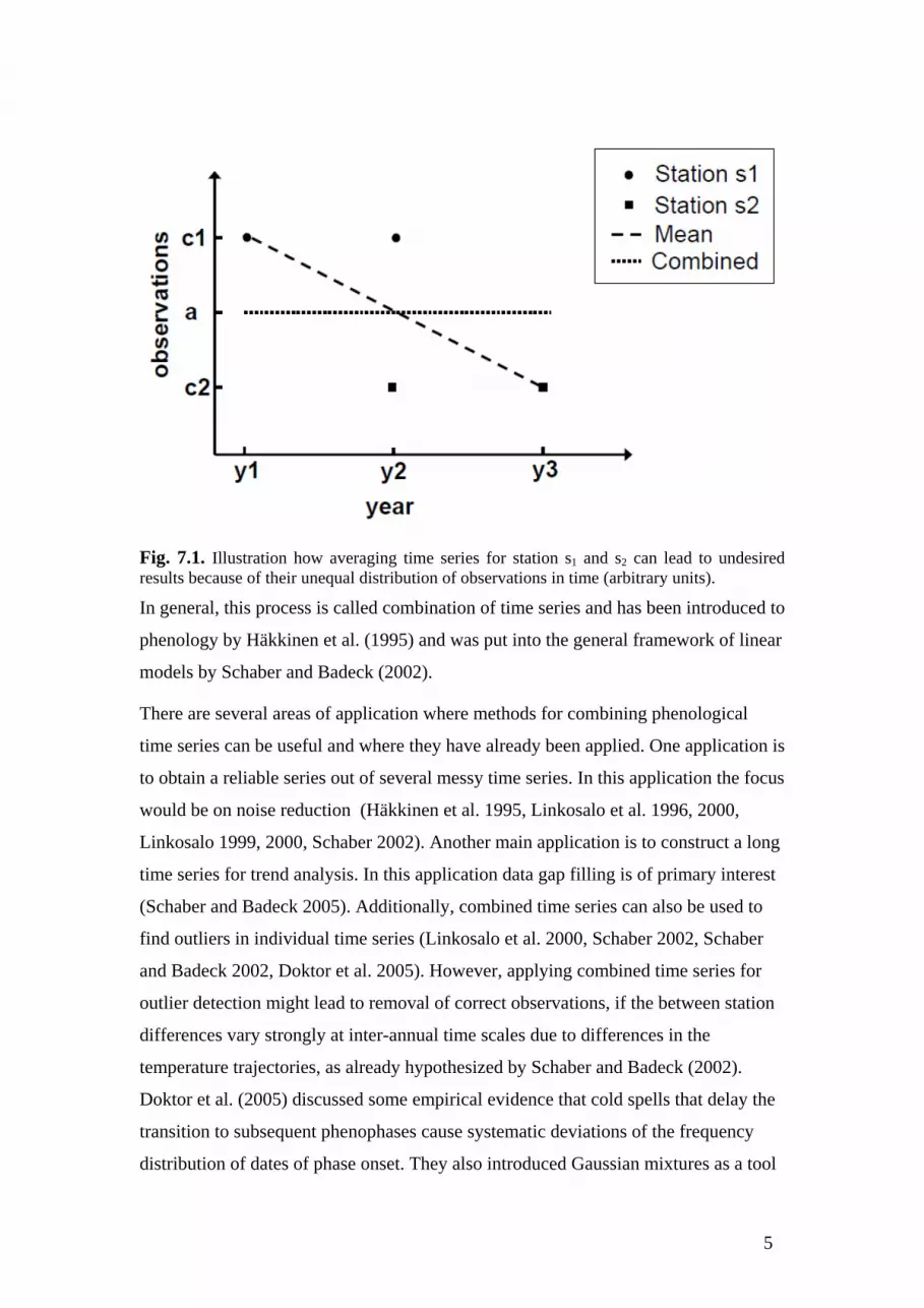
Fig. 7.1. Illustration how averaging time series for station s1 and s2 can lead to undesired results because of their unequal distribution of observations in time (arbitrary units).

In general, this process is called combination of time series and has been introduced to

phenology by Häkkinen et al. (1995) and was put into the general framework of linear

models by Schaber and Badeck (2002).

There are several areas of application where methods for combining phenological

time series can be useful and where they have already been applied. One application is

to obtain a reliable series out of several messy time series. In this application the focus

would be on noise reduction (Häkkinen et al. 1995, Linkosalo et al. 1996, 2000,

Linkosalo 1999, 2000, Schaber 2002). Another main application is to construct a long

time series for trend analysis. In this application data gap filling is of primary interest

(Schaber and Badeck 2005). Additionally, combined time series can also be used to

find outliers in individual time series (Linkosalo et al. 2000, Schaber 2002, Schaber

and Badeck 2002, Doktor et al. 2005). However, applying combined time series for

outlier detection might lead to removal of correct observations, if the between station

differences vary strongly at inter-annual time scales due to differences in the

temperature trajectories, as already hypothesized by Schaber and Badeck (2002).

Doktor et al. (2005) discussed some empirical evidence that cold spells that delay the

transition to subsequent phenophases cause systematic deviations of the frequency

distribution of dates of phase onset. They also introduced Gaussian mixtures as a tool

5

for the quantification of the inter-annual variation in between station differences. This

approach can potentially be integrated into the use of combined time series for outlier

detection in order to avoid assignment of false outliers.

In the following, we will shortly introduce the method of combination of phenological

times series by different types of linear models and discuss some practical issues.

Moreover, we will discuss outlier analyses and show applications. We present the

algorithms for integration of Gaussian normals (Fig. 7.2) into the outlier detection

with combined time series and illustrate the effect of this model improvement (Fig.

7.3).

One useful result of the construction of combined time series is the extraction of

station effects, (i.e. the characteristic deviation of the date of phase onset at a given

observational station relative to the population of all stations). This result is less

sensitive to gaps in the data series and different length of observation periods than the

deviation from average values. It can be applied to producing maps of average

geographical variation in the onset of a phenological phase. We illustrate this

application for the bud break of beech in Germany (Figs. 7.4 – 7.6).

7.2 Linear Models of phenological time series

7.2.1 Linear Models

It is reasonable to assume that over a climatologically sufficiently homogeneous

region, (e.g. middle Europe or Central North America), the phenological development

of certain phases is consistent concerning years and stations. This means that a year,

which is particularly late, should be late for all stations, and a station that is

particularly late, because for example, it is situated on a top of a mountain, should be

late in all years. Putting this in mathematical terms, we say that the effect of year yi,

i=1,…, n and the effect of station sj, j=1,…, m are independent and additive, such that

ijjiij syao , mjni ,...,1 and ,...,1 . (7.1)

6

where oij is the observation in year i at station j and a is the general mean. ij is an

error term that is usually assumed to be homoscedastically normally distributed

around zero with some variance 2, i.e.

),0( 2 Nij (7.2)

In statistics, (Eq. 7.1) is called a linear two-way crossed classification model. Usually,

additional conditions are imposed that assure that a unique solution exists, such as

setting

ii yay ~ and

m

j js1

0 . (7.3)

We call iy~ , i = 1,…, n the combined time series.

Given observations oij, that may have missing data, (7.1) and the conditions (7.3) it is

essentially straightforward to estimate the iy~ and sj using least-square optimisation

(i.e. minimizing the sum of squared residuals SSR),

ji

ijSSR,

2 . (7.4)

7.2.2 Fixed and mixed effects models

Depending on the type of analysis we are interested in, we can treat the year and

station effects differently, which has consequences for the type of estimation

procedure we apply. For instance, when we are mainly interested in the combined

time series iy~ , we can refrain from estimating the specific station effects but rather

consider the stations to be randomly distributed. Thus, we treat the sj as a random

variable

),0( 2sj Ns (7.5)

and estimate the variance component2s , rather than station effects sj. This is called

the mixed model, because we have one fixed and one random effect. For this type of

analysis special estimation and analysis procedures exist (Searle 1987, Milliken and

Johnson 1992, Pinheiro & Bates 2000). Examples of the application of mixed models

7

to obtain reliable phenological time series can be found in Schaber and Badeck (2002,

2005).

On other occasions, we might be interested in the year effects as well as in the specific

station effects in order to identify stations that are particularly late, for instance. In

this case, we would treat both effects as fixed. In section 7.3.2 we will give an

example. For details on linear models and the large theoretical body that comes with

it, please refer to Rencher (2000), Searle (1971, 1987) and Milliken and Johnson

(1992) and the literature cited therein.

7.2.3 Practical issues and the R pheno-package

As already indicated, linear models constitute an entire field in statistics and

calculations are far from being as easy as just calculating an average. The large

theoretical body that comes with the theory of linear models can even be an obstacle

rather than being helpful for phenological applications. Therefore, the authors wrote

the software package ‘pheno: auxiliary functions for phenological data analysis’

(Schaber 2007) that was designed to make calculations of combined phenological

time series and station effects as easy as possible. This software is freely available as

a package for the free statistical computing environment R (R Development Core

Team 2007). The user has just to provide a table with three columns (observation,

year, station) to a function corresponding to the analysis of interest, without having to

worry about the calculations. All subsequent examples were calculated using the

pheno-package.

One especially useful feature of the pheno-package is that it automatically handles

large data sets. To illustrate the problem, we refer to the example in the following

section (Sect. 7.2.4). In order to calculate the average time series of beech and the

station effects for Germany over the years 1951-2004, we considered 74,996 single

data points from 2,318 stations. For calculation of the fixed year and station effects,

this involves the inversion of a 74,996 x (2,319+53+1) matrix. With the usual 8-byte

number coding the matrix itself occupies around 1.4 GB. With the extra storage

needed for matrix inversion, even nowadays most personal computers would exceed

their working storage capacity with this operation. Fortunately, the matrices involved

8

mainly consist of zero-entries, such that the application of sparse matrix algorithms

saves a great deal of computational and storage resources. Sparse matrix algorithms

are provided in other R-packages such as SparseM and quantreg (Koenker and Ng,

Koenker 2006) and are already integrated in the R-pheno package. This way,

combined time series for whole Germany can be computed on a regular personal

computer.

Another prerequisite for the application of linear models is that the time series be

connected or overlapping. For many stations this is usually not a problem, but for few

data (stations or years) it is recommendable to check (Schaber 2002). There are

procedures within the R pheno-package that test for connectivity and automatically

extract connected sets of time series.

7.2.4 Outlier detection

As already mentioned in the introduction, obtaining phenological data is often an

error-prone process (Schaber 2002, Schaber and Badeck 2002). Therefore, a proper

outlier detection method is indispensable. One of the few types of errors that can be

detected is the so-called month mistake. Schaber and Badeck (2002) developed a

method to detect month mistakes with combined time series. The usual least-square

estimation of combined time series is sensitive to outliers. Therefore, Schaber and

Badeck (2002) recommended applying a robust estimation procedure that minimizes

least absolute deviations (LAD) (7.6),

ji

ijLAD,

, (7.6)

before applying the classical least-square estimation. Residuals ij , (i.e. the difference

between observed and predicted values), that are estimated to be larger than 30 days

are considered as month mistakes and are removed. The details of the procedure are

described in Schaber and Badeck (2002) and are also implemented in the R pheno-

package.

9

7.2.5 Gaussian normals

The assumption that year effects and station effects are independent may not always

hold true. This is the case when the inter-station differences vary due to the annual

weather trajectories. Years with retarded phase onset in a subset of phenological

observation stations due to a cold spell as compared to years without intermittent cold

spells are an example of this class of interactions. As an extension to the outlier

detection with LAD estimation, frequency distributions of observed budburst dates

can be characterised and modelled using Gaussian Mixtures Models (GMM) (Fig.

7.2). In many years, observations of a single species can be approximated by a

probability density function (pdf), which consists of one, two or more underlying

distributions. These can be mainly attributed to changing weather situations within

spring, which alter the phenological pace. GMM quantify the number and type of the

underlying distributions and thereby allow distinguishing years with different

temporal evolution of budburst dates in a quantitative manner. The models can

describe distributions with unknown underlying patterns and have the property of

being able to represent any distribution of natural observations (Gilardi et al. 2002). A

mixture distribution with continuous components has a density of the form (Poland

and Shachter 1994):

)(...)()( 11 xfpxfpxf nn (7.7)

Where x is the probability to have an observation at a certain day, npp ,...,1 are

positive numbers summing up to one and )(),...,(1 xfxf n are the component densities

(7.7). To determine potential outliers one has firstly to analyse the uni- or multi-modal

frequency distribution to identify the main underlying components (mixtures) and

their describing parameters mean, standard deviation and weight ( kkk p,, ).

For each year i, all observations oij are related to a component’s mean k . The

component ka an observation oij is most related to is determined based on the

frequencies fijk of component k at the observation day oij :

2

2

2

)(

2k

kijo

k

kijk e

npf

, (7.8)

where n is the total number of observations of the analysed year i. Then,

10

. (7.9) ijkk

a fk maxarg

An observation is declared to be an outlier if

30akijo . (7.10)

An optimisation algorithm is applied on the minimisation of several (here maximum

four) Gaussian Mixture functions. Due to the authors' experience from phenological

data analysis it is very unlikely that changes in temperature regimes with a sustained

impact on the phenological evolution happen more than three times within the period

the plant population is experiencing budburst, at least in Central Europe. Akaike's

Information criterion (Akaike 1974) is applied to choose the most appropriate model,

balancing between model complexity (number of components) and model fit. The

parameterised mixture components are used for outlier detection in order to reduce the

number of falsely detected outliers in years showing bi- or multi-modal distributions

(i.e. in years with a high variability of observed phenological events).

Obviously, this method is more conservative as the one based on LAD estimates.

LAD estimation assumes that observations are distributed around one general mean

per year (i.e. the station effect) whereas applying Gaussian mixtures we assume that

there might be several means. We detect only outliers at the margins of the whole

Gaussian mixture and consequently less than before (Fig. 7.3).

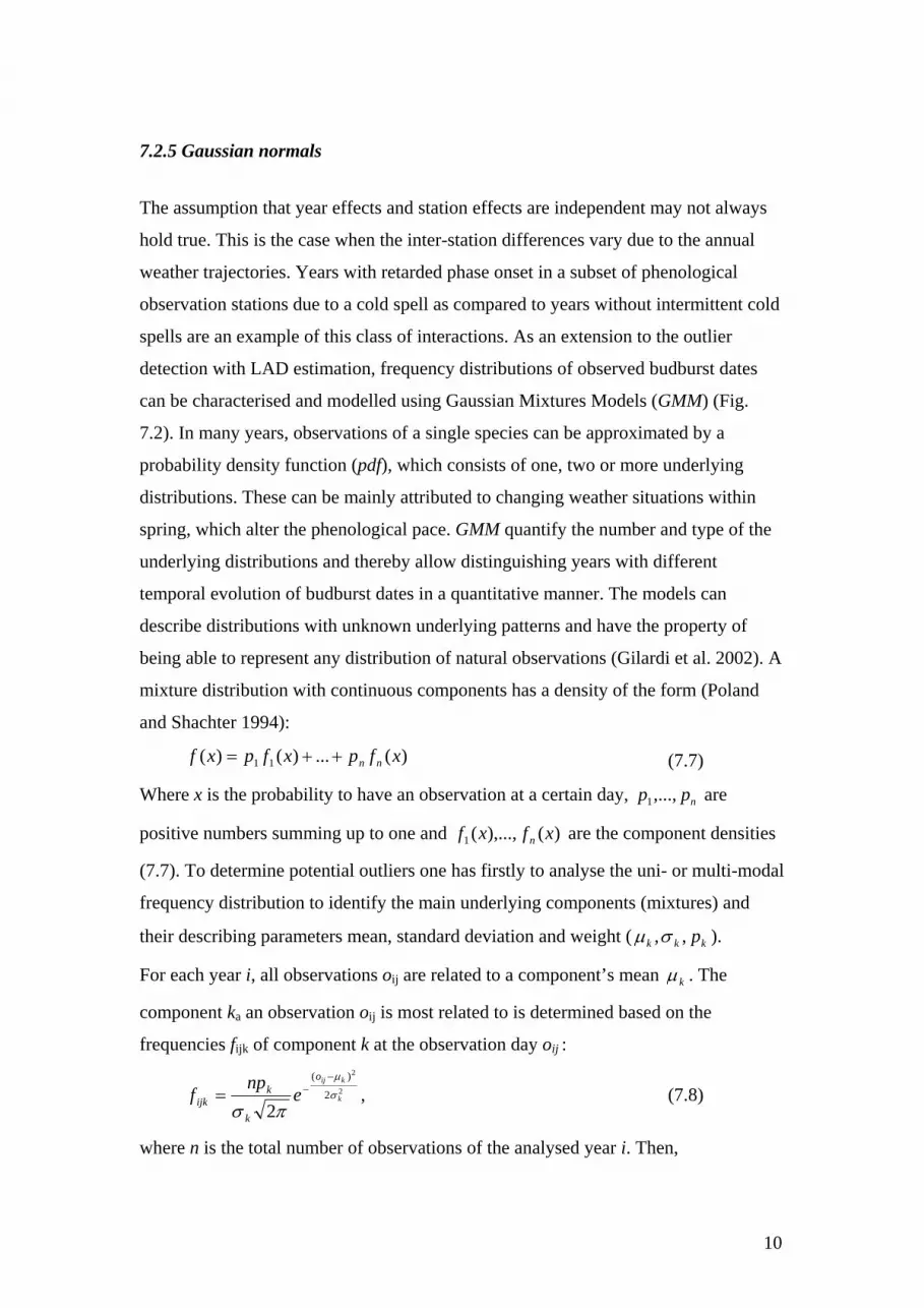
Interestingly, even a unimodal distribution could be more accurately defined by a

Gaussian mixture (Fig. 7.2). In fact, there was not year between 1951 and 2004 where

the distribution of observations could be described by a normal distribution (P < 0.01,

Shapiro-Wilk test).

11

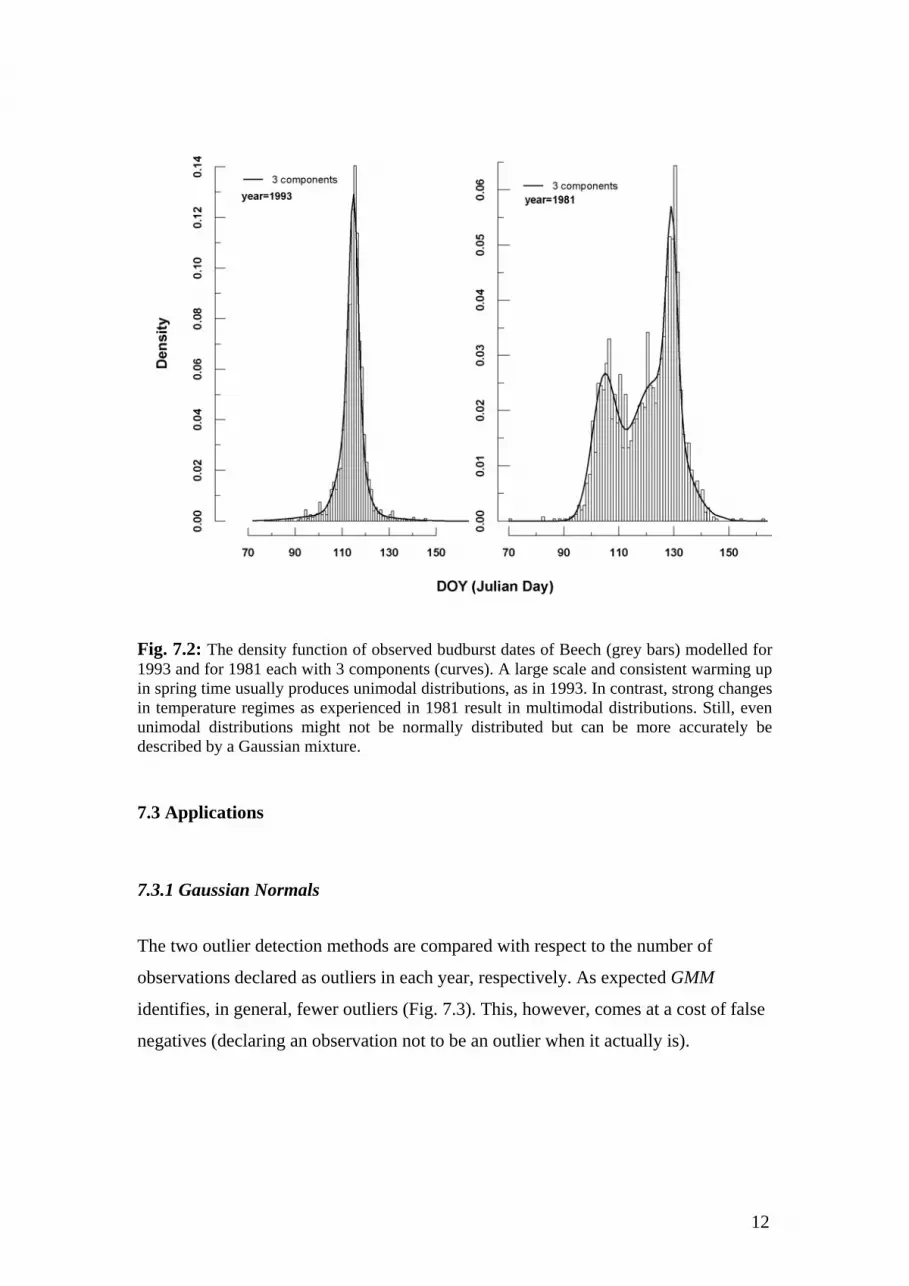
Fig. 7.2: The density function of observed budburst dates of Beech (grey bars) modelled for 1993 and for 1981 each with 3 components (curves). A large scale and consistent warming up in spring time usually produces unimodal distributions, as in 1993. In contrast, strong changes in temperature regimes as experienced in 1981 result in multimodal distributions. Still, even unimodal distributions might not be normally distributed but can be more accurately be described by a Gaussian mixture.

7.3 Applications

7.3.1 Gaussian Normals

The two outlier detection methods are compared with respect to the number of

observations declared as outliers in each year, respectively. As expected GMM

identifies, in general, fewer outliers (Fig. 7.3). This, however, comes at a cost of false

negatives (declaring an observation not to be an outlier when it actually is).

12

Fig. 7.3. Number of detected outliers per year for Beech using the outlier detection algorithm of Schaber and Badeck (2002) (LAD) and using Gaussian Mixture Models (GMM). The mixture components are determined and parameterised by an optimisation algorithm.

7.3.2 Station effects

We calculated the fixed effect model (1) with constraints (2) for whole Germany for

the years 1951–2004 for beech budburst without month-mistakes. We considered

only stations that had at least 20 observations. After the removal of 433 outliers

according to the robust estimation method based we considered 74562 observations

from 2318 stations. In Fig. 7.4 we present a map of the calculated station effects plus

the general mean m=120 (30th of April in non-leap years) in day of the year (DOY).

To our knowledge, this is the first time that a consistent map for the characteristic

timing of a specific phenological phase for such a large region is presented. Note that

for this application the underlying trends (see Schaber and Badeck, 2005) have not

been removed.

13

Fig. 7.4. Computed station effects + the general mean (day of year) based on observed budburst dates of Beech from 1951-2004 over Germany. A Digital Elevation Model (DEM) (1*1 km in meters) represents the topography, which considerably influences the timing of phenological phases in spring time. Observation stations are indicated as coloured points.

The underlying assumption that the observations within the relatively large

geographic space of Germany (357,092 km2) are elements of a unimodal population is

illustrated with Fig. 7.2 (curve for year 1993). In many cases a station net well

distributed over a geographical space with continuous gradients of environmental

conditions will result in such a distribution. However, the distribution may be

different from unimodal, if a geographical domain is made up by two sub-domains

with very different environmental conditions (Fig. 7.2, year 1981).

The maps of the station effects (Fig 7.4) and the interpolated station effects by

external drift krigging (EDK) (Fig. 7.5) illustrate phenological responses to

14

a) climatological differences between regions at similar elevation (e.g. 50 to 100 [m]

asl): the northern lowlands of Saxony are phenologically later than the Muensteraner

Becken and the Northern Upper Rhine valley. The average March and April

temperatures (1951-2003) are 3.94 and 8.27 °C, respectively in Saxony at 15 stations

at 12.4 to 13.9 longitude and 51.4 to 51.9 latitude. They are 5.19 and 8.62 °C,

respectively in the vicinity of Muenster at 11 stations at 7.0 to 7.9 longitude and 51.7

to 52.2 latitude. They are 6.26 and 9.91 °C, respectively in the Northern Upper Rhine

valley at 7 stations at 8.3 to 8.45 longitude and 49.3 to 49.9 latitude,

b) the lapse rate across elevational gradients (the higher, the later),

c) the combined influence of the inverse lapse rate of early spring (see Table 1 and

Fig. 2 in Doktor et al. (2005)) and general climatological gradients between east and

west Germany (northern lowlands: the closer to the sea the later at similar elevation).

15

Fig. 7.5. Computed station effects + general mean (day of year) based on observed budburst dates of Beech interpolated using External Drift Kriging (EDK). The DEM of Germany (1*1 km) provides the external variable. Coordinates are based on the Gauss-Krueger system (4th stripe).

16

Fig. 7.6. Difference of the interpolated maps: the computed station effects - observed mean budburst dates of the respective stations. The difference map (Fig. 7.6) between station effects and station averages shows a

slight general bias towards later combined station effects especially in the eastern part

of Germany. These differences might be due to gaps in the time series, which are

particularly common in this part of Germany. An indication that this is indeed the

case is the fact there is a slight negative tendency between difference and number of

observations per station (P<0.07).

17

7.4 Summary

Phenological data are messy data. Their analysis calls for appropriate methods that

can deal with their inherent uncertainties as well as correct for effects due to their

heterogeneous distribution in time and space. Simple averaging as a method to

accommodate noise and gaps is likely to lead to erroneous results especially when the

ratio of gaps to total number of observations is high or when a low number of

observation series is averaged. The application of linear models to obtain combined

time series constitutes an adequate method to handle gaps and noise in individual time

series.

The application of Bayes statistics is an alternative way of analysing messy

phenological datasets (see e.g. Dose and Menzel 2004). Future work should compare

Bayes statistics to the methods discussed in the current paper and address the

respective sensitivity to assumptions about priors and underlying distributions as well

as to the types of errors and data gaps.

The approach of Gaussian mixtures to consider station x year effects can be further

developed by assigning stations to tentative mixture components before checking for

outliers or including mixed terms in the linear model (1).

With ongoing efforts to expand the databases of phenological observations by data

mining it is very likely that more data sets with sparse data and data gaps will become

available in the near future. For example, see the instructive account of the spatial and

temporal coverage of the Japanese cherry flowering time series and the step-wise

expansion of the data base (Aono and Kazui 2007). The methods described with the

current paper are available as an R-package. The routines within this R pheno-

package allow for the construction of combined time series that can serve for time

series analyses. They can be applied for outlier detection. The calculation of station

and year effects facilitates geo-statistical analyses of geographic patterns in the onset

of phenological phases as well as their relation to weather pattern in specific years.

18

7.5 Acknowledgements

We want to express our thank to Roger Koenker, one of the authors of the R packages

quantreg and SparseM that implement procedures to calculate quantile regression for

robust estimates and sparse matrix algorithms, who was a tremendous help in

incorporating these packages into the pheno-package. We also thank Achim Glauer

for his continuous support in maintenance of the phenological database and the DWD

for making the data available to us.

7.6 References

Akaike, H. (1974). New look at statistical-model identification. IEEE Transactions on Automatic Control, AC19, 716-723.

Aono Y. & Kazui K. (2007) Phenological data series of cherry tree flowering in Kyoto, Japan, and its application to reconstruction of springtime temperatures since the 9th century. International Journal of Climatology, DOI: 10.1002/joc.1594

Chmielewski, F.-M. & Rötzer, T. (2001) Response of tree phenology to climate change across Europe, Agricultural and Forest Meteorology. 108, 101-112.

Doktor D., Badeck F.-W., Hattermann F., Schaber J. & McAllister M. (2005) Analysis and modelling of spatially and temporally varying phenological phases. In: Geostatistics for Environmental Applications. Proceedings of the Fifth European Conference on Geostatistics for Environmental Applications (eds P. Renard, H. Demougeot-Renard, & R. Froidevaux), pp. 137-148. Springer.

Dose V. & Menzel A. (2004) Bayesian analysis of climate change impacts in phenology. Global Change Biology, 10, 259-272.

Estrella N. & Menzel A. (2006) Responses of leaf colouring in four deciduous tree species to climate and weather in Germany. Climate Research, 32, 253-267.

Gilardi, N., Bengio, S. & Kanevski, M. (2002). Conditional gaussian mixture models for environmental risk mapping. IEEE International Workshop on Neural Networks for Signal Processing (NNSP).

Häkkinen R, Linkosalo T, Hari P (1995) Methods for combining phenological time series: application to budburst in birch (B. pendula) in Central Finland for the period 1896–1955. Tree Physiology 15:721–726

Koenker (2006) quantreg: Quantile Regression. R package version 4.01, http://www.r-project.org.

Koenker, Ng. SparseM: Sparse Linear Algebra. R package version 0.71. http://www.econ.uiuc.edu/~roger/research/sparse/sparse.html.

Lieth H., ed. (1974) Phenology and seasonality modelling. Springer, Berlin.

19

Linkosalo T. (1999) Regularities and patterns in the spring phenology of some boreal trees. Silva Fennica, 33, 237-245.

Linkosalo T., Häkkinen R. & Hari P. (1996) Improving the reliability of a combined phenological time series by analyzing observation quality. Tree Physiology, 16, 661-664.

Linkosalo, T. 2000. Analyses of the spring phenology of boreal trees and its response to climate change. Ph.D. Thesis, Univ. Helsinki, Dept. For. Ecol. Publications, No. 22.

Linkosalo, T., T.R. Carter, R. Häkkinen and P. Hari. 2000. Predicting spring phenology and frost damage risk of Betula spp. under climatic warming: a comparison of two models. Tree Physiol. 20:1175–1182.

Menzel A., Estrella N., Heitland W., Susnik A., Schleip C., Dose V. (2007) Bayesian analysis of the species-specific lengthening of the growing season in two European countries and the influence of an insect pest International Journal of Biometeorology, DOI 10.1007/s00484-007-0113-8

Menzel A., Sparks T.H., Estrella N. & Roy D.B. (2006) Altered geographic and temporal variability in phenology in response to climate change. Global Ecology and Biogeography, 15, 498-504.

Milliken, G.A. and D.E. Johnson.(1992). Analysis of messy data. Volume I: Designed experiments. Chapman and Hall, New York, 365 p.

Parmesan C. (2006) Ecological and evolutionary responses to recent climate change. Annual Review of Ecology Evolution and Systematics, 37, 637-669.

Pinheiro, J.C. & Bates, D.M. (2000). Mixed-Effects Models in S and S-Plus. Statistics and Computing, Springer, New York. Poland, W.B. & Shachter, R.D. (1994). Three approaches to probability model selection. In Uncertainty in Artificial Intelligence.

R Development Core Team (2007). R: A language and environment for statistical computing. R Foundation for Statistical Computing, Vienna, Austria. ISBN 3-900051-07-0, http://www.R-project.org

Reaumur R.A. (1735) Observations du thermomètre faites à Paris pendant l'année 5 comparées avec celles qui ont été faites sous la ligne, à l'Isle de France, à Alger et en quelques-unes de nos îles de l'Amérique. Mémoires de l'academie royale des sciences Paris, 737-754.

Rencher, A.C. 2000. Linear Models in Statistics. John Wiley, New York

Rosenzweig C., Casassa G., Karoly D.J., Imeson A., Liu C., Menzel A., Rawlins S., Root T.L., Seguin B. & Tryjanowski P. (2007) Assessment of observed changes and responses in natural and managed systems. Climate Change 2007: Impacts, Adaptation and Vulnerability. Contribution of Working Group II to the Fourth Assessment Report of the Intergovernmental Panel on Climate Change. (eds M.L. Parry, O.F. Canziani, J.P. Palutikof, P.J.v.d. Linden, & C.E. Hanson), pp. 79-131. Cambridge University Press, Cambridge.

20

21

Schaber (2007) pheno: Auxiliary functions for phenological data analysis. R package version 1.3. http://www.r-project.org

Schaber J. (2002) Phenology in Germany in the 20th century: methods, analyses and models (PIK-Report No. 78). PIK, Potsdam, downloadable at: http://www.pik-potsdam.de/research/publications/pikreports

Schaber J. & Badeck F.W. (2002) Evaluation of methods for the combination of phenological time series and outlier detection. Tree Physiology, 22, 973-982.

Schaber J. & Badeck F.W. (2005) Plant phenology in Germany over the 20th century. Regional Environmental Change, 5, 37-46.

Schwartz M.D., ed. (2003) Phenology: an integative environmental science (Vol. 39). Kluwer, Dordrecht, 564 p.

Searle, S.R. 1971. Linear models. John Wiley, New York

Searle, S.R. 1987. Linear models for unbalanced data. John Wiley, New York.