Combining Software and Hardware Verification Techniques

Formal Methods in System Design, 21, 251–280, 2002c© 2002 Kluwer Academic Publishers. Manufactured in The Netherlands.

Combining Software and HardwareVerification Techniques

ROBERT P. KURSHAN [email protected] LEVIN [email protected] Technologies, Bell Laboratories, Murray Hill, NJ 07974, USA

MARIUS MINEA [email protected] of Computer Science, Carnegie Mellon University, Pittsburgh, PA 15213, USA

DORON PELED [email protected] YENIGUN [email protected] Technologies, Bell Laboratories, Murray Hill, NJ 07974, USA

Received June 6, 2000; Accepted December 3, 2001

Abstract. Combining verification methods developed separately for software and hardware is motivated by theindustry’s need for a technology that would make formal verification of realistic software/hardware co-designspractical. We focus on techniques that have proved successful in each of the two domains: BDD-based symbolicmodel checking for hardware verification and partial order reduction for the verification of concurrent softwareprograms. In this paper, we first suggest a modification of partial order reduction, allowing its combination with anyBDD-based verification tool, and then describe a co-verification methodology developed using these techniquesjointly. Our experimental results demonstrate the efficiency of this combined verification technique, and suggestthat for moderate–size systems the method is ready for industrial application.

Keywords: formal verification, model checking, hardware/software co-design, partial order reduction

1. Introduction

Software and hardware verification, although having a lot in common, have developedalong different paths. Even in the specific context of model checking, in which the systemis represented as a graph or an automaton, several differences become apparent. Softwaresystems typically use an asynchronous model of execution, in which concurrent actionsof component modules are interleaved. In verification, the asynchrony is exploited usingpartial order reduction [8, 21, 26], which explores during verification only a subset of theavailable actions from each state. The remaining actions are delayed to a subsequent step,as long as this does not result in any change visible to the specification being checked.

On the other hand, hardware is typically designed for synchronous execution. All com-ponent modules perform an action at each execution step. Hardware verification usuallyexploits the regularity of digital circuits, often built from many identical units, by represent-ing the state space using binary decision diagrams (BDDs) [20]. Another technique which

252 KURSHAN ET AL.

makes hardware verification manageable is localization reduction [14] which abstracts awaythe hardware design parts which are irrelevant to the verified property.

Thus, traditionally, formal verification of hardware and software is done through differ-ent techniques, using tools which are based on different algorithms, representations andprinciples.

However, there are important and growing classes of mixed (combined) hardware-software systems, co-designs, in which hardware and software are tightly coupled. Thetight coupling precludes testing the hardware and software separately. On the other hand,there may be 100 hardware steps for one software step. The difference renders conven-tional simulation test exceedingly inefficient, and results in co-design systems that cannotbe effectively tested by conventional means. New testing methods and commercial tools tosupport them have emerged to address this problem. For example, we refer the reader towebsites of major EDA vendors,1 where co-verification (as a matter of fact, co-simulation)tools are more and more heavely promoted: there are too many of them to mention here.They generally involve ad hoc abstraction of the hardware (such as removing clock depen-dencies), in order to speed up the simulation of the hardware relative to the software. Thesemethods may result both in missed design errors, and false error indications that reflecterrors in the abstraction, not the design. Nonetheless, the design community is forced intothese new methods as the only available alternative.

Yet, there is another alternative, based on model checking. Formal verification in thiscontext has all the well-known advantages over simulation test: better coverage, and itmay be applied sooner in the design cycle. It also is able to deal in a sound fashionwith the interface between hardware and software, in particular, with different speedrates on the two sides. This motivates our efforts to introduce formal verification intothe area of co-design systems. For this, an efficient verification technique is needed thatis able to address co-design systems containing both kinds of components, hardware andsoftware.

In this paper, we attempt to combine the benefits of both methodologies: we suggesta verification technique that combines partial order reduction with a BDD representationand, in general, hardware verification techniques. The partial order reduction principle ofselecting a subset of the enabled actions from each state poses no problem when combiningit with BDDs or localization reduction. It only means that the transition relation needs tobe restricted so that it takes advantage of the potential commutativity between concurrentactions. The idea that this can be done statically, at compile time, was suggested by [12], buttheir implementation required some changes in the depth-first search algorithm (in order tocontrol the backtracking mechanism) of the Spin model checker [11].

The subtle point that has so far made explicit state enumeration seem more appropriatethan BDD-based symbolic exploration for implementing the partial order reduction algo-rithm is the cycle closing problem. Since partial order reduction may defer an action infavor of another one that can be executed concurrently, one needs to ensure that no actionis ignored indefinitely along a cycle in the state space. One solution to this problem wasproposed by [3] and elaborated by [1] in the first attempt at combining partial order reduc-tion with BDDs. Their solution is based on a conservative approximation of when a cyclemay be closed during a breadth-first search. Essentially, when an edge connects a node to

COMBINING SOFTWARE AND HARDWARE VERIFICATION TECHNIQUES 253

another node that is at the same or a lower level in the breadth-first search, it is assumed(conservatively) to close a cycle.

We propose an alternative solution [15] that computes at compile time the conditionswhich guarantee that no action is ignored. The method is based on the observation that anycycle in the global state space projects to a local cycle in each participating process. Theselocal cycles can be detected at compile time. An action from each cycle is selected, suchthat at run time, the execution of each selected action forces a complete exploration of allactions that have been deferred so far in favor of other actions. The number of these specialactions (the more of which there are, the less the achieved reduction) can be minimized byanalyzing the effects of transitions.

Our implementation of the algorithm has the unique feature that all the informationneeded for performing the partial order reduction is obtained during a compilation of thesoftware system model. There is no change at all in the verification tool, in this case themodel checker COSPAN [9, 10]. Thus, with the new algorithm, partial order reduction isimplemented as a compilation or preprocessing phase for model checking, rather than asa modified model checking algorithm. It is precisely this feature that allows a combina-tion of the partial order reduction with BDD-based algorithms and, in general, with anyoptimization technique applied by the model checker.

Can we gain by combining software- and hardware-oriented verification techniques,partial order reduction and BDDs? We answer this question affirmatively: the combinationof partial order reduction and hardware-oriented verification techniques makes possiblehardware/software co-verification, i.e., the integral verification of a hardware/software co-design. In particular, there are examples in this area for which the use of a single method(be it BDDs or partial order reduction) terminates in lack of memory due to state spaceexplosion, whereas the combination of the two methods makes verification possible (seeSection 5).

The remainder of the paper is organized as follows. The next section explains the modifi-cation of partial order reduction aimed at its combination with any existing model checker,in particular, with one based on BDDs. Section 3 presents a co-verification methodology thatmakes use of the combination of partial order reduction with hardware-oriented verificationtechniques. Section 4 describes our current implementation of this co-verification tech-nique with an emphasis on modifying the transition relation according to the partial orderreduction constraints. Section 5 presents experimental results and Section 6 the conclusion.

2. Partial order reduction

In Sections 2.1 and 2.2, we present the basics of the temporal logic LTL [7] and of thepartial order reduction technique. Sections 2.3 and 2.4 describe the modification to partialorder reduction required to fit our needs.

2.1. Preliminaries

The system to be analyzed is viewed as a state graph. If S is the set of states, a transition isa relation α ⊆ S × S. A state graph is defined as a tuple M = (S, S0, T, L), where S0 ⊆ S

254 KURSHAN ET AL.

is the set of initial states and T is the set of transitions. The labeling function L : S → 2AP

associates each state of M with a set of atomic propositions that hold at s.A transition α ∈ T is enabled at state s ∈ S if there exists a state s ′ ∈ S such that (s, s ′) ∈ α.

Otherwise α is said to be disabled at s. For a state s, enabled(s) is the set of all transitions α

such that α is enabled at s. A transition α is called deterministic if for any state s ∈ S in whichα is enabled there is a unique s ′ such that (s, s ′) ∈ α. In this case α can be viewed as a partialfunction on S, and the notation s ′ = α(s) can be used instead of (s, s ′) ∈ α. In this paper, werestrict ourselves to state graphs with only deterministic transitions. Yet, nondeterminismmay appear as a nondeterministic selection among several enabled transitions.

In order to simplify the picture, we avoid states from which no transition is possible,and therefore, for such (i.e. deadlocked) states, force T to have the self-looping transitionδ = {(s, s) | s has no successors except s}.

An execution sequence σ of a state graph M is an infinite alternating sequence of statessi and transitions αi : σ = s0

α0→ s1α1→ · · · such that si+1 = αi (si ) for all i . If s0 ∈ S0 then σ

is referred to as a full execution sequence. We denote by σi the suffix of σ that starts fromits i th element-state, i.e., σi = si

αi→ si+1αi+1→ si+2

αi+2→ · · · .For assertions about the behavior of a program, we use the temporal logic LTL. Given a

set AP of atomic propositions, LTL formulas are defined as follows:

– for all p ∈ AP , p is a formula– if φ and ϕ are formulas, then so are ¬φ, φ ∧ ϕ, ©φ, and φ Uϕ.

An execution sequence σ = s0α0→ s1

α1→ · · · is said to satisfy an LTL formula φ (denotedby σ |= φ) under the following conditions:

– if φ = p for some p ∈ AP, and p ∈ L(s0)– if φ = ¬ϕ, and not σ |= ϕ

– if φ = ϕ ∧ ψ , and (σ |= ϕ) ∧ (σ |= ψ).– if φ = ©ϕ, and σ1 |= ϕ

– if φ = ϕ Uψ , and there exists an i ≥ 0 such that for all 0 ≤ j < i , σ j |= ϕ and σi |= ψ .

We also use the following abbreviations: false = φ ∧ ¬φ, true = ¬false, φ ∨ ϕ =¬((¬φ) ∧ (¬ϕ)), �φ = true Uφ, and φ = ¬�¬φ.

A state graph M satisfies an LTL formula φ (denoted by M |= φ), iff for each fullexecution sequence σ in M , σ |= φ.

In this paper, the verification problem is considered to be “given a state graph M and aspecification expressed by an LTL formula φ, check if M |= φ”. Thus, from now on we con-sider the specification formula φ to be fixed. In order to simplify the following definitionswe assume that the entire set of atomic propositions AP is in fact formed only by the atomicpropositions used in φ. In other words, φ makes use of all the atomic propositions in AP. Thiscondition immediately affects the following definitions of stuttering equivalence and visibil-ity, as well as partial order reduction based on those notions (see Section 2.2), making themrelative to the specification φ. It also reflects the implementation (see Sections 2.4 and 4).

One of the main notions underlying the partial order reduction technique is the stut-tering equivalence relation between execution sequences. In an execution sequence, some


consecutive states may have the same labeling, and specifications that refer to the atomicpropositions without counting the succession of states at which they are true cannot distin-guish between such states. The execution sequence can then be divided into segments, eachconsisting of consecutive identically labeled states. Two execution sequences σ = s0

α0→s1

α1→ · · · and ρ = r0β0→ r1

β1→ · · · , are called stuttering equivalent (denoted by σ ∼st ρ) ifthere exist two infinite sequences of indices 0 = i0 < i1 < · · · and 0 = j0 < j1 < · · · suchthat ∀k ≥ 0, L(sik ) = L(sik+1) = · · · = L(sik+1−1) = L(r jk ) = L(r jk+1) = · · · = L(r jk+1−1).Intuitively, two execution sequences are stuttering equivalent if they have identical statelabelings after in each of them, any finite sequence of identically labeled states is collapsedinto a single state. Two state graphs M and M ′ are said to be stuttering equivalent, denotedby M ∼st M ′, if for each full execution sequence σ of M , there exists a full executionsequence ρ of M ′ such that σ ∼st ρ, and vice versa (for each full execution sequence ρ ofM ′, there exists a full execution sequence σ of M such that ρ ∼st σ ).

The importance of stuttering equivalence is the following. We call an LTL formula φ

stuttering invariant if for any two execution sequences σ and ρ such that σ ∼st ρ, it holdsthat σ |= φ iff ρ |= φ. This definition together with the definition of stuttering equivalencebetween state graphs easily implies that if φ is stuttering invariant and M ∼st M ′, thenM |= φ iff M ′ |= φ. This is the basic idea behind partial order reduction: generate a modelM ′ with a smaller number of states than M and use M ′ to model check a stuttering invariantproperty φ. Lamport [17] showed that any LTL property that does not use the next-timeoperator is stuttering invariant. Conversely, in [22], it is shown that any stuttering invariantLTL formula can be written without the use of the next-time operator ©. From now on, werestrict ourselves only to stuttering invariant LTL formulas.

We conclude this section by introducing two basic concepts used in partial order reduction.A transition α is said to be visible (with respect to φ) if there exist two states s and s ′ suchthat s ′ = α(s) and L(s) �= L(s ′).

The other key concept is the independence relation between the transitions. Two transi-tions α, β ∈ T are said to be independent if for all states s ∈ S, if α, β ∈ enabled(s), then:(i) α ∈ enabled(β(s)); and (ii) β ∈ enabled(α(s)); and (iii) α(β(s)) = β(α(s)). Intuitively,if both transitions are enabled at a state, then the execution of one of them must not disablethe other (i and ii), and executing these transitions in either order must lead to the samestate (iii). If two transitions are not independent, then they are called dependent transitions.

2.2. Basic partial order reduction

As explained in Section 2.1, the purpose of partial order reduction is to generate a reducedstate graph M ′ with a smaller number of states than the original state graph M and with theproperty that M ′ ∼st M , and then perform the model checking of a stuttering invariant LTLformula φ on M ′ rather than on M .

No matter what search technique is used (depth-first, breadth-first, explicit or symbolic),with a traditional model checker one has to generate the successors of a state s for theenabled transitions α ∈ enabled(s). However, a partial order search technique attempts toexplore the successors of a state only for a subset of the enabled transitions of s. Let’scall such a set of transitions ample(s) ⊆ enabled(s). Following [21], we define below this

256 KURSHAN ET AL.

subset of transitions by the conditions C0 through C3 that it must satisfy. Exploring onlythe ample transitions results in the reduced state graph M ′.

C0 (Emptiness). ample(s) = ∅ iff enabled(s) = ∅.

Since we are trying to generate for each execution of M a corresponding, stuttering equiv-alent execution sequence in M ′, we must explore at least one successor of s in M ′, if thereare any successors of s in M . In our case, we have assumed for convenience that state s hasat least one transition enabled in M , cf. Section 2.1. Therefore, C0 implies that ample(s) �= ∅.

C1 (Faithful decomposition). Along every execution sequence of transitions in M thatstarts at s, a transition that is dependent on any transition in ample(s) cannot be executedwithout a transition from ample(s) occurring first.

This constraint is introduced to ensure that any execution sequence of the full stategraph M may be represented by a stuttering equivalent execution sequence in the reducedgraph M ′. For this purpose, the transitions of the original execution sequence may haveto be re-ordered. Condition C1 ensures that all transitions before the first ample transitionα in the original execution sequence are independent of α and, hence, can be commutedwith α.

In order to implement condition C1, we can use further information about the semanticsof the modeled system. For example, given a collection of concurrent processes, with theprogram counter of one process allowing the execution of only one local transition, choos-ing this transition as a singleton ample set will not violate condition C1. On the other hand,consider the case where the program counter of the process is at a point where there isa selection between two input messages, of which one is enabled at the current state andthe other is not (until another process progresses to send such a message). In this case,selecting the enabled input transition α as a singleton ample set may violate C1, since sometransitions independent of α may execute in the other process enabling the alternative inputtransition, which is interdependent with α. Implementing condition C1 typically involvesidentifying such cases, see, for example, [12]. Each such case needs to be checked againstthe definition of condition C1.

C2 (Visibility). If there exists a visible transition α ∈ ample(s), then ample(s) =enabled(s).

In other words, if ample(s) ⊂ enabled(s) then no transition in ample(s) is visible. Inpractice, one tries to avoid including visible transitions in the ample set at state s, sinceotherwise the entire set of enabled transitions enabled(s) has to be explored. Indeed, let twoindependent transitions, α and β, be enabled at state si in graph M and let M allow thesetwo executions:

σ = s0α0→ s1

α1→ · · · siα→ s1

i+1β→ si+2 · · ·

ρ = s0α0→ s1

α1→ · · · siβ→ s2

i+1α→ si+2 · · ·


Condition C1 by itself suggests that we do not necessarily need both executions σ and ρ

in the reduced graph M ′. That is: if only C1 is applied then σ may not be generated inM ′ assuming that ρ will represent it in M ′ (or vice versa). Now, consider the case that thepropositional labeling is different at states s1

i+1 and s2i+1 where the two executions σ and ρ

differ from each other, i.e. L(s1i+1) �= L(s2

i+1). If both transitions α and β are visible then itcannot be guaranteed that executions σ and ρ are stuttering equivalent: they are not if, forinstance, L(si ) �= L(s1

i+1) and L(si ) �= L(s2i+1). Therefore, ample(s) = enabled(s) = {α, β}

must hold in this case to force exploration of both transitions α and β. However, if one of thetwo transitions, let, α, is invisible, then σ ∼st ρ is guaranteed. This is because in this caseL(si ) = L(s1

i+1) and L(s2i+1) = L(si+2). Then, we don’t have to generate both execution

orders in M ′ and may select ample(s) = {α} to factor out the execution sequence ρ.

C3 (Cycle closing). Given an execution sequence σ = s0α0→ s1

α1→ · · · of M , if sk = s0

for some k > 0, then there exists 0 ≤ i < k such that ample(si ) = enabled(si ).

In other words, any cycle in the full state graph of M must have at least one state s onthe cycle such that ample(s) = enabled(s). The intuitive reason for this condition is toavoid postponing an enabled transition indefinitely while generating the reduced graph M ′.A good reduction algorithm will aim at selecting ample sets that satisfy C1 and C2 yetcontain few transitions, thus postponing the execution of visible and dependent transitionsas long as possible. Conditions C1 and C2 guarantee that any postponed transition remainsenabled. However, if the search on the reduced graph M ′ closes a cycle and terminates,the postponed transitions will not be executed at all. This may cause a relevant executionsequence of M to be lost, not being represented by a stuttering equivalent execution of M ′.Condition C3 prevents this.

These four conditions complete the definition of the partial order reduction. It has beenshown [21] that if a search generates M ′ instead of M while satisfying C0 through C3, thenM ′ ∼st M .

2.3. Static partial order reduction

One of the goals for our modification to the basic form of partial order reduction is to separatethis technique from the model checking algorithm. We achieve this by a supplementarycompilation phase which statically analyzes and preprocesses the model, as explained below.

In general, the system to be analyzed is not given directly as a state graph M (cf.Section 2.1), but rather as a set of component processes {P1, P2, . . . , Pn} and a set of vari-ables {V1, V2, . . . , Vm}. The states of M are then tuples (vectors) of the form (c1, . . . , cn,

v1, . . . , vm), where ci is the control point (state) of process Pi and v j is the value of thevariable Vj . Thus, the state vector is composed of a control part and a data part.

The component processes can perform local actions and communicate with each othervia certain mechanisms such as shared variables or message passing (blocking or non-blocking). The transitions of the underlying state graph M are then the local transitions of asingle process, accompanied perhaps by assignments to variables, and the shared transitionsof two or more processes (e.g., a communication transition).

258 KURSHAN ET AL.

Given a state graph M , we define the control flow graph of a component process Pi byprojecting the state vectors of M onto the i th component. More exactly, if s[i] is the i thfield of the state vector s ∈ S, where S is the set of states of M , the set of control points ofprocess Pi is defined as CPi = {s[i] | s ∈ S}.

A transition α ∈ T of the state graph M is actually performed by one or more componentprocesses (in the case of local and shared transitions, respectively). With each transition α

we associate therefore a set of processes act(α) ⊆ {P1, P2, . . . , Pn} that are active for thetransition α. A process is active if it updates its control point and, possibly, some variables,while executing transition α. For example, in a system with rendezvous synchronization,act(α) would include all the processes that participate in the synchronization on α. However,in a message passing system, the active set of a send transition only includes the sendingprocess. The receiving process does not actually participate in this transition, since the sendtransition only updates an input buffer, which is a variable in the system.

The control flow graph G Pi of a process Pi is defined as a labeled directed graph withthe set of vertices CPi . For two control points c1, c2 ∈ CPi , there is an edge from c1 to c2

in G Pi , iff there exist two states s1, s2 ∈ S and a transition α ∈ T such that s1[i] = c1,s2[i] = c2, Pi ∈ act(α), and s2 = α(s1). Thus, transition α is projected onto edges in thecontrol flow graphs of the component processes in act(α). Edge (c1, c2) in G Pi is labeledby (the set of) all the transitions {α1, . . . , αk} ⊆ T which are projected onto this edge. Ifany of those transitions is executed, we say that edge (c1, c2) is executed. Note that the setof transitions labeling an edge is never empty. One may also observe that a system M mayoften be formalized in such a way that each edge in a control flow graph will be labeledwith exactly one global transition.

In the following, the terms local transition and local state are used to refer to an edge anda vertex in a control flow graph G Pi , whereas the terms global transition and global state areused as synonyms for a transition and a state of the underlying state graph M , respectively.The local transition γ of G Pi that corresponds to a global transition α is referred to as thelocal image of α in G Pi .

The generic approach to partial order reduction described in Section 2.2 operates bydefining a reduced state transition graph M ′ which is equivalent to M . Past approaches haveincorporated this technique directly into model checkers, by modifying their algorithms toexplore at each state s the transitions in ample(s) rather than all the transitions in enabled(s).Our key idea is different. Suppose that the component processes of the model can be modifiedto make a transition α enabled at s precisely if α ∈ ample(s) in the original model. Then theoriginal model checking algorithm can be applied without modifications, resulting in theverification of the reduced model M ′. Besides simplicity, this method allows partial orderreduction to be combined with all features of the existing model checker. Essentially, ver-ification of a system is split into two phases: a syntactical transformation of the system toa reduced system that generates the partial order reduction in the course of the state spacesearch of model checking, followed by the actual application of model checking.

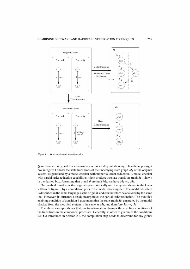
To illustrate the basic idea by an example, suppose that we are given the two-processsystem depicted in the upper left box of figure 1. Each process has only one transition, α andβ respectively, both with enabling condition true. Thus, α is always enabled when processP is at state s1, and β is always enabled when process Q is at state r1. Suppose that P and


s1,r1

β

β

α

s2,r1 s1,r2

s2,r2

α

2

s2,r1

s1,r1

β

α

s2,r2

Model Checking

Basic

Model Checking

Reductionwith Partial Order

βα

βα

M

r2

r1

StaticTransformation

Process QProcess P

Modified System

true

s1

state s2if P is at

s2

M

true

r2

r1

Original System

Process QProcess P

1M

3

s2

s1

true

Figure 1. An example static transformation.

Q run concurrently, and that concurrency is modeled by interleaving. Then the upper rightbox in figure 1 shows the state transitions of the underlying state graph M1 of the originalsystem, as generated by a model checker without partial order reduction. A model checkerwith partial order reduction capabilities might produce the state transition graph M2, shownin the dashed box. Assuming that α and β are invisible, we have M1 ∼st M2.

Our method transforms the original system statically into the system shown in the lowerleft box of figure 1, by a compilation prior to the model checking step. The modified systemis described in the same language as the original, and can therefore be analyzed by the sametool. However, its structure already incorporates the partial order reduction. The modifiedenabling condition of transition β guarantees that the state graph M3 generated by the modelchecker from the modified system is the same as M2, and therefore M3 ∼st M1.

The above example shows that our transformation changes the enabling conditions ofthe transitions in the component processes. Generally, in order to guarantee the conditionsC0–C3 introduced in Section 2.2, the compilation step needs to determine for any global

260 KURSHAN ET AL.

state which transitions can form an ample set, and change the enabling conditions of thetransitions accordingly. This may include introducing conditions on the current state ofother processes. Computing these changes is quite easy for conditions C0–C2, and Section 4explains how to check C0 and C1. However, condition C3 refers to the state transition graphM ′, which is only unfolded in the verification stage. Thus, it seems difficult to determinestatically, at compilation time, the transition cycles that will appear in M ′. Condition C3can be checked naturally during a depth-first search, as implemented in most previouspartial order model checkers, which use explicit state enumeration. However, that is theopposite of our goal, since we aim for BDD-based symbolic verification, which operates ina breadth-first fashion.

To make it easier to implement condition C3 through a syntactic transformation of thesystem, below we conservatively modify this condition and combine it with C2, observingthat both C2 and C3 give conditions under which ample(s) = enabled(s) must hold, i.e. allenabled transitions are to be explored.

A subset of transitions T ⊆ T is called a set of sticky transitions if it satisfies these twoconditions:

– T includes all visible transitions.– Given an execution sequence σ = s0

α0→ s1α1→ · · · of M , if sk = s0 for some k > 0,

then there exists i , 0 ≤ i < k such that αi ∈ T . In other words, any cycle in the full stategraph M includes at least one sticky transition.

Now, we state the combined condition C2′ as follows:

C2′ (Visibility and cycle closing). There exists a set of sticky transitions T such that forany state s, if ample(s) contains a transition from T then ample(s) = enabled(s).

Thus, even when being ample, transitions in T “stick” to all other transitions enabled atstate s and force their exploration. From the definition of T , it follows that any cycle inthe reduced graph M ′ will execute at least one sticky transition. Since M ′ is only exploredthrough ample transitions, C3 is implied. C2 is also implied, since T also includes all visibletransitions. Thus, the partial order reduction can be performed under the three conditionsC0, C1 and C2′.

A set of sticky transitions T may be calculated at compile time. One efficient method ofdoing this is described in the next section.

2.4. Calculating sticky transitions

Recall that a transition is visible iff it changes the value of an atomic proposition used in aspecification φ. We have seen that the set T must contain all visible transitions. In practice, aconcurrent system consists of communicating processes, and atomic propositions appear asboolean predicates over the (data) variables and control points of the processes. We illustratethis using an example. Consider the concurrent system in figure 2, which is composed oftwo processes P and Q, and three variables x , y and z. Process P is a loop that repeatedly


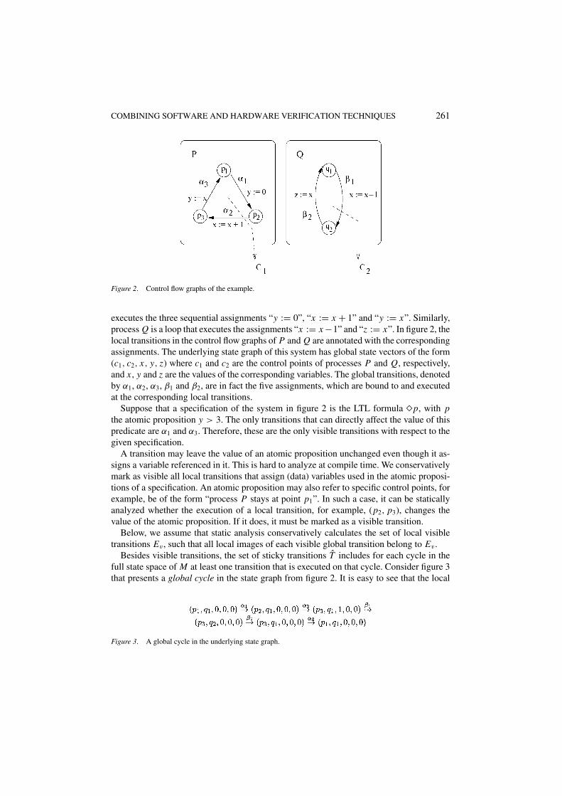
Figure 2. Control flow graphs of the example.

executes the three sequential assignments “y := 0”, “x := x + 1” and “y := x”. Similarly,process Q is a loop that executes the assignments “x := x −1” and “z := x”. In figure 2, thelocal transitions in the control flow graphs of P and Q are annotated with the correspondingassignments. The underlying state graph of this system has global state vectors of the form(c1, c2, x, y, z) where c1 and c2 are the control points of processes P and Q, respectively,and x , y and z are the values of the corresponding variables. The global transitions, denotedby α1, α2, α3, β1 and β2, are in fact the five assignments, which are bound to and executedat the corresponding local transitions.

Suppose that a specification of the system in figure 2 is the LTL formula �p, with pthe atomic proposition y > 3. The only transitions that can directly affect the value of thispredicate are α1 and α3. Therefore, these are the only visible transitions with respect to thegiven specification.

A transition may leave the value of an atomic proposition unchanged even though it as-signs a variable referenced in it. This is hard to analyze at compile time. We conservativelymark as visible all local transitions that assign (data) variables used in the atomic proposi-tions of a specification. An atomic proposition may also refer to specific control points, forexample, be of the form “process P stays at point p1”. In such a case, it can be staticallyanalyzed whether the execution of a local transition, for example, (p2, p3), changes thevalue of the atomic proposition. If it does, it must be marked as a visible transition.

Below, we assume that static analysis conservatively calculates the set of local visibletransitions Ev , such that all local images of each visible global transition belong to Ev .

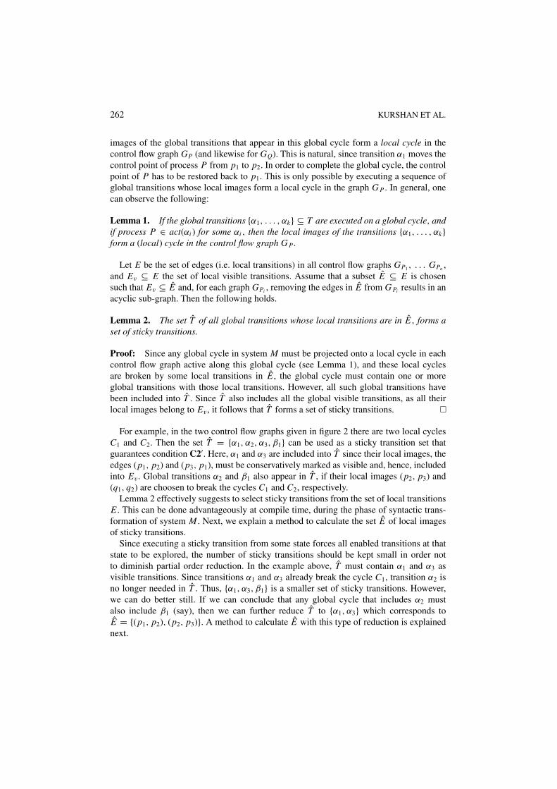
Besides visible transitions, the set of sticky transitions T includes for each cycle in thefull state space of M at least one transition that is executed on that cycle. Consider figure 3that presents a global cycle in the state graph from figure 2. It is easy to see that the local

Figure 3. A global cycle in the underlying state graph.

262 KURSHAN ET AL.

images of the global transitions that appear in this global cycle form a local cycle in thecontrol flow graph GP (and likewise for GQ). This is natural, since transition α1 moves thecontrol point of process P from p1 to p2. In order to complete the global cycle, the controlpoint of P has to be restored back to p1. This is only possible by executing a sequence ofglobal transitions whose local images form a local cycle in the graph G P . In general, onecan observe the following:

Lemma 1. If the global transitions {α1, . . . , αk} ⊆ T are executed on a global cycle, andif process P ∈ act(αi ) for some αi , then the local images of the transitions {α1, . . . , αk}form a (local) cycle in the control flow graph G P .

Let E be the set of edges (i.e. local transitions) in all control flow graphs GP1 , . . . GPn ,and Ev ⊆ E the set of local visible transitions. Assume that a subset E ⊆ E is chosensuch that Ev ⊆ E and, for each graph GPi , removing the edges in E from G Pi results in anacyclic sub-graph. Then the following holds.

Lemma 2. The set T of all global transitions whose local transitions are in E, forms aset of sticky transitions.

Proof: Since any global cycle in system M must be projected onto a local cycle in eachcontrol flow graph active along this global cycle (see Lemma 1), and these local cyclesare broken by some local transitions in E , the global cycle must contain one or moreglobal transitions with those local transitions. However, all such global transitions havebeen included into T . Since T also includes all the global visible transitions, as all theirlocal images belong to Ev , it follows that T forms a set of sticky transitions.

For example, in the two control flow graphs given in figure 2 there are two local cyclesC1 and C2. Then the set T = {α1, α2, α3, β1} can be used as a sticky transition set thatguarantees condition C2′. Here, α1 and α3 are included into T since their local images, theedges (p1, p2) and (p3, p1), must be conservatively marked as visible and, hence, includedinto Ev . Global transitions α2 and β1 also appear in T , if their local images (p2, p3) and(q1, q2) are choosen to break the cycles C1 and C2, respectively.

Lemma 2 effectively suggests to select sticky transitions from the set of local transitionsE . This can be done advantageously at compile time, during the phase of syntactic trans-formation of system M . Next, we explain a method to calculate the set E of local imagesof sticky transitions.

Since executing a sticky transition from some state forces all enabled transitions at thatstate to be explored, the number of sticky transitions should be kept small in order notto diminish partial order reduction. In the example above, T must contain α1 and α3 asvisible transitions. Since transitions α1 and α3 already break the cycle C1, transition α2 isno longer needed in T . Thus, {α1, α3, β1} is a smaller set of sticky transitions. However,we can do better still. If we can conclude that any global cycle that includes α2 mustalso include β1 (say), then we can further reduce T to {α1, α3} which corresponds toE = {(p1, p2), (p2, p3)}. A method to calculate E with this type of reduction is explainednext.


Finding a minimal set of edges breaking the cycles in a graph is known as the feedbackarc set problem, which is shown to be NP-hard in [13]. Our algorithm uses known heuristicmethods to compute such sets, as well as a static analysis of the data effects of transitions,as explained below.

In order to calculate the set of local sticky transitions E , we start by including in it all thelocal visible transitions Ev , and then remove those transitions from the local control flowgraphs G P1 , G P2 , . . . , G Pn . Then, we analyze the resulting local graphs G ′

P1, G ′

P2, . . . , G ′

Pn

to find local transitions that break the remaining local cycles: the found transitions are alsoincluded into E . For this we can use heuristics, such as in [2, 6], to minimize the numberof transitions we select. Alternatively, we can simply perform a depth-first search on theremaining transitions in the local graphs G ′

P1, G ′

P2, . . . , G ′

Pn, and select the backward edges

(edges that go back to a node that is in the DFS stack) found in the course of DFS. Thismay not produce an optimal result, but is linear in the number of edges in the local graph,and performs well in practice. This algorithm can be improved as explained next.

The computation of E as described above conservatively considers only the effect oftransitions on the control part of the state vector. However, a sequence of global transitionsonly closes a global cycle if the data variables also revert to the same value. A smaller set oflocal sticky transitions may be obtained by taking into account the effect of transitions on thedata variables. To preserve the static character of our method, we restrict ourselves to effectsthat can be analyzed at compilation time. To illustrate this, observe that in the global cyclegiven in figure 3, transition α2 changes the value of x to 1, whereas transition β1 restores itto 0. Examining the assignment syntax of the local transitions in figure 2, we deduce thatany global cycle that includes the global transition α2 must also include the execution of theopposite transition β1 (and vice versa), since it is not possible to have a global cycle alongwhich x is only incremented or only decremented. We have already seen that if α2 appearsin a global cycle, then α1 and α3 must also be executed along the same cycle. Thus, we canfurther reduce the set of sticky transitions for this system to T = {α1, α3}.

In general, assume that we are given a subset of variables V ⊆ {V1, . . . , Vm}, heuristicallyviewed as important for partial order reduction, such that for each variable x ∈ V , a partialorder ≺ is defined on the possible values of x . This order also induces an equivalence relation�: namely, x1 � x2 iff x1 �≺ x2 ∧ x2 �≺ x1. We will commonly use the terms “greater”,“less” and “equivalent” when referring to ≺ and �.

For example, in a system M based on message passing, a good choice for a variablex ∈ V is an input buffer queue of a process, and an order ≺ is introduced by the function#(x) that counts the number of messages currently in the queue. For two values x1 and x2

of the queue variable x , we have x1 ≺ x2 iff #(x1) < #(x2).The effect of a local transition γ on variable x ∈ V with respect to order ≺ is said to be

– incrementing (decrementing), if after γ is executed, any new value of x is always greater(less) than the previous value of x , with respect to ≺,

– null (no effect), if γ never changes equivalence class of value of x , with respect to ≺,– complex, otherwise.

A local transition is conservatively classified as having complex effect on a variable xif its effect on x is impossible or difficult to determine statically. This only means that

264 KURSHAN ET AL.

our static analysis extracts no information for reduction in this case, but does not affectour subsequent reasoning. For example, in figure 2, the local transitions that correspond toassignments β1, α2 and β2 have, respectively, decrementing effect, incrementing effect andno effect on x with respect to the natural total order on integers, <. The local transition(that corresponds to) α3 has complex effect on y with respect to < since α3 assigns to thevariable y but no more information about its effect can be immediately deduced.

We assume that static analysis can generate a mapping � that captures effects of localtransitions E on variables in V :

� : E × V → {“incrementing”, “decrementing”, “null”, “complex”}

The mapping �, the set of visible local transitions Ev and the local control flow graphsG ′

P1, . . . , G ′

Pn(with visible transitions removed) together constitute the input to the algo-

rithm ComputeStickySet explained below.A local transition is called a monotonic transition if it has incrementing or decrementing

effect on at least one variable in V .Two local transitions are called opposite to each other iff there exists a variable x ∈ V such

that one transition has incrementing or complex effect on x , and the other has decrementingor complex effect on x . A non-monotonic transition with complex effect on at least onevariable in V is considered opposite to itself.

When selecting sticky transitions that will break all cycles in the global state space, onecan observe that a transition α in the global state graph M that changes the value of somevariable x can only be in a global cycle with a transition that compensates the effect of α

on x . From this follows that every global cycle that executes a monotonic local transition γ

must also execute a local transition opposite to γ , in order to return to the same global state.Hence, some monotonic transitions may be removed and yet enough local transitions mayremain to break all global cycles in M . This observation is problematic to use, since thenumber of cycles in a graph can be exponentially bigger than the size of the graph. Instead,in our algorithm ComputeStickySet we perform a depth-first search in which backwardedges are selected to break the local cycles that remain after removing some monotonictransitions. The following lemma supports this idea:

Lemma 3. For any reachable cycle C in a directed graph G, one of the edges of C willappear as a backward edge in the course of the depth-first search in G, for any order inwhich the successors of a vertex are searched.

Since visible transitions are sticky, cycles that contain a visible transition are automaticallyhandled. Therefore, all visible transitions Ev can be eliminated from the local control flowgraphs as a first step.

Let E ′ be the set of all edges in the resulting control flow graphs G ′P1

, . . . , G ′Pn

, i.e.E ′ = E \ Ev . Define the function

opptr : E ′ → 2E ′

such that opptr(γ ) is the set of all local transitions opposite to γ in E ′; γ is also includedinto this set if it is opposite to itself.


Let � ⊆ E ′ and G a sub-graph of G Pi . We denote by

– edges(G) the set of edges in G,– monotonic(�) the set of monotonic transitions in �,– rem(G, �) the sub-graph remaining after removing the edges � from graph G,– backedges(G) the set of backward edges found in G in the course of DFS (we assume

that the vertices of G are arbitrarily indexed to direct the DFS).

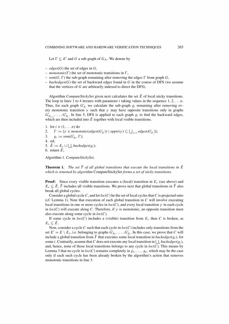
Algorithm ComputeStickySet given next calculates the set E of local sticky transitions.The loop in lines 1 to 4 iterates with parameter i taking values in the sequence 1, 2, . . . n.Thus, for each graph G ′

Piwe calculate the sub-graph gi remaining after removing ev-

ery monotonic transition γ such that γ may have opposite transitions only in graphsG ′

Pi+1, . . . , G ′

Pn. In line 5, DFS is applied to each graph gi to find the backward edges,

which are then included into E together with local visible transitions.

1. for i ∈ (1, . . . n) do2. � := {γ ∈ monotonic(edges(G ′

Pi)) | opptr(γ ) ⊆ ⋃

j>i edges(G ′Pj

)};3. gi := rem(G ′

Pi, �);

4. od;5. E := Ev ∪ ⋃

i backedges(gi );6. return E ;

Algorithm 1. ComputeStickySet.

Theorem 1. The set T of all global transitions that execute the local transitions in Ewhich is returned by algorithm ComputeStickySet forms a set of sticky transitions.

Proof: Since every visible transition executes a (local) transition in Ev (see above) andEv ⊆ E , T includes all visible transitions. We prove next that global transitions in T alsobreak all global cycles.

Consider a global cycle C , and let loc(C) be the set of local cycles that C is projected onto(cf. Lemma 1). Note that execution of each global transition in C will involve executinglocal transitions in one or more cycles in loc(C), and every local transition γ in each cyclein loc(C) will execute along C . Therefore, if γ is monotonic, an opposite transition mustalso execute along some cycle in loc(C).

If some cycle in loc(C) includes a (visible) transition from Ev then C is broken, asEv ⊆ E .

Now, consider a cycle C such that each cycle in loc(C) includes only transitions from theset E ′ = E \ Ev , i.e. belonging to graphs G ′

P1, . . . , G ′

Pn. In this case, we prove that C will

include a global transition from T that executes some local transition in backedges(gi ), forsome i . Contrarily, assume that C does not execute any local transition in

⋃i backedges(gi ),

and, hence, none of those local transitions belongs to any cycle in loc(C). This means byLemma 3 that no cycle in loc(C) remains completely in g1, . . . , gn , which may be the caseonly if each such cycle has been already broken by the algorithm’s action that removesmonotonic transitions in line 3.

266 KURSHAN ET AL.

Consider then a local cycle in loc(C) such that it belongs to graph G ′Pk

with the largestprocess index k, and a monotonic transition γ removed from this cycle by the action in line 3and, hence, included into set � in line 2. Now note that for transition γ to be included into set�, all transitions opposite to γ (if any) must belong to graphs G ′

Pk+1, . . . , G ′

Pn. On the other

hand, as explained above in the proof, γ must have an opposite transition γ in (at least) one ofthe cycles loc(C), hence, in G ′

Pj, where j ≤ k. The contradiction finalizes the proof.

Note that the contents and size of set E returned by algorithm ComputeStickySet maydepend, first, on the order in which control flow graphs G ′

P1, . . . , G ′

Pnare processed by

the loop in lines 1 through 4 (i.e. on the order in which system’s processes are indexed)and, second, on the order in which the vertices of the remaining sub-graph gi are indexedfor DFS. Thus, heuristics for both process ordering and vertex indexing may be useful tooptimize the algorithm. This issue is left open for now.

3. Hardware/software co-verification methodology

In this section we present a co-verification methodology and a tool that combine staticpartial order reduction with hardware-oriented verification techniques.

We have developed a co-verification tool based on existing programming environmentsfor VHDL [28], Verilog [27], and SDL [23], and an existing model checking engine,COSPAN [9, 10]. However, the methodology described below is not strongly tied to aparticular representation of hardware or software, except with respect to synchrony as-sumptions about the design. For hardware, it is assumed that the design is clock cycledependent and thus we use a synchronous model of coordination. In contrast, softwareis presumed to operate under synchronization conditions guaranteed by its host, and thuscoordination among software design components is considered to be asynchronous, andmodeled using interleaving. Since different abstraction levels can be used for hardware andsoftware, we do not make an assumption about their relative speeds.

The choice of a hardware description language is strongly influenced by the computerindustry, where VHDL and Verilog are in widest use and have been standardized by theIEEE. Our platform supports both, by translating them into S/R, the native language ofCOSPAN, using FormalCheckTM2 translators. For the software part, we use SDL, a standardlanguage of the International Telecommunications Union (ITU-T), an overview of which ispresented in the next section. Here, two of the co-authors have developed a model checkingtool SDLCheck [19] that implements static partial order reduction, generates a (reduced)S/R model of the original SDL system and then, on the verification phase, makes useof COSPAN. To support co-verification, SDLCheck also implements interface constructsintroduced in [18] as an extension to SDL to allow describing an interface between softwareand hardware components.

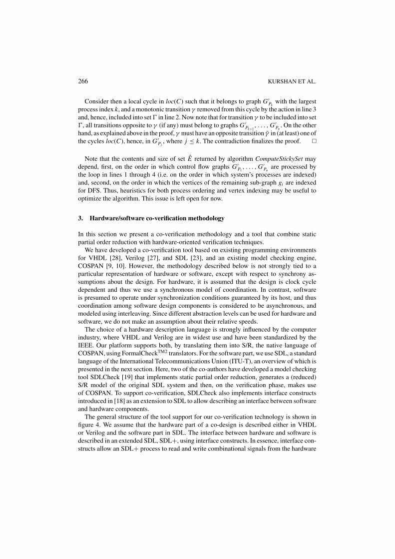
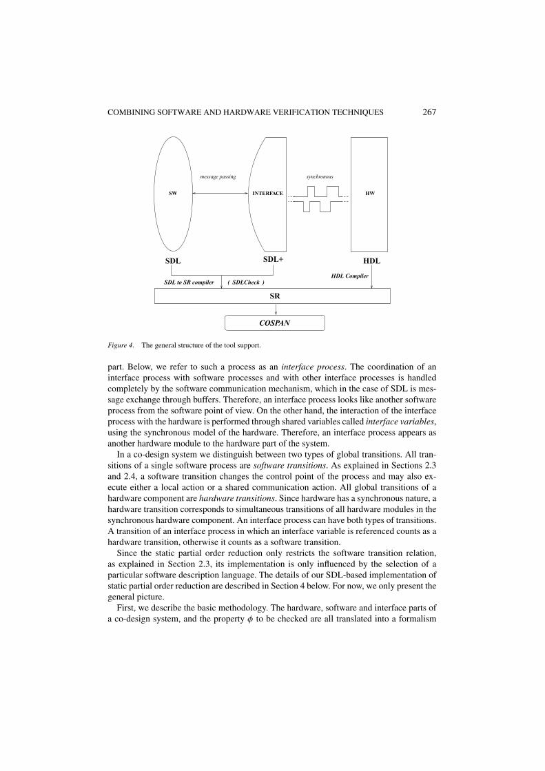
The general structure of the tool support for our co-verification technology is shown infigure 4. We assume that the hardware part of a co-design is described either in VHDLor Verilog and the software part in SDL. The interface between hardware and software isdescribed in an extended SDL, SDL+, using interface constructs. In essence, interface con-structs allow an SDL+ process to read and write combinational signals from the hardware


( SDLCheck )

HW

SDL SDL+

INTERFACESW

synchronousmessage passing

HDL

SDL to SR compilerHDL Compiler

COSPAN

SR

Figure 4. The general structure of the tool support.

part. Below, we refer to such a process as an interface process. The coordination of aninterface process with software processes and with other interface processes is handledcompletely by the software communication mechanism, which in the case of SDL is mes-sage exchange through buffers. Therefore, an interface process looks like another softwareprocess from the software point of view. On the other hand, the interaction of the interfaceprocess with the hardware is performed through shared variables called interface variables,using the synchronous model of the hardware. Therefore, an interface process appears asanother hardware module to the hardware part of the system.

In a co-design system we distinguish between two types of global transitions. All tran-sitions of a single software process are software transitions. As explained in Sections 2.3and 2.4, a software transition changes the control point of the process and may also ex-ecute either a local action or a shared communication action. All global transitions of ahardware component are hardware transitions. Since hardware has a synchronous nature, ahardware transition corresponds to simultaneous transitions of all hardware modules in thesynchronous hardware component. An interface process can have both types of transitions.A transition of an interface process in which an interface variable is referenced counts as ahardware transition, otherwise it counts as a software transition.

Since the static partial order reduction only restricts the software transition relation,as explained in Section 2.3, its implementation is only influenced by the selection of aparticular software description language. The details of our SDL-based implementation ofstatic partial order reduction are described in Section 4 below. For now, we only present thegeneral picture.

First, we describe the basic methodology. The hardware, software and interface parts ofa co-design system, and the property φ to be checked are all translated into a formalism

268 KURSHAN ET AL.

based on synchronous automata, used as an input interface by a model checker (in ourcurrent implementation, the model checker COSPAN and the S/R language). This enablesus to treat the entire co-design system, with parts of different nature, as a single, formallysynchronous model, that is to be verified with regard to an automaton expressing propertyφ. Software asynchrony is modeled by self-looping, using nondeterminism as proposed in[16]. The synchronous model generated for the software and interface processes is aug-mented with an additional constraint automaton, which implements static partial orderreduction by restricting the software transition relation. This model is then composed withthe synchronous hardware model, finalizing the compilation stage of co-verification. Next,the model checking stage starts out by applying localization reduction [14] to the overallcombined synchronous model, reducing it relative to the checked property φ. For example,in software-centric verification (figure 5, discussed below), which is aimed at propertiesensured mainly through control structures in the software part, one may expect much of thehardware to be abstracted by localization reduction. Finally, the remaining reduced modelis analyzed using a BDD-based search.

A more advanced methodology can be applied, if a co-design system is so complicatedthat the simple combination of three reduction techniques, described above, is not sufficient,i.e. may result in state space explosion. In this case, first, the entire co-design system istranslated into a synchronous model in a conventional way, i.e. without static partial orderreduction, and then localization reduction is applied alone to reduce this synchronous modelrelative to the checked property φ: it conservatively removes variables. As a by-product, theset of removed variables is reported. Using it, the localization reduction is automaticallyprojected onto the original co-design system, which is correspondingly simplified by remov-ing those variables. Localization reduction also reduces the range of values of a survivingvariable, by compressing it to the subset really used in the reduced model, and this effect is

sw

sw

sw

sw

sw

sw

swhwhw hw hw

hw

hw

Figure 5. Software-centric view.


also projected onto the original co-design system. At last, the basic methodology is applied,as described above, to this reduced co-design system. Since the system is now smaller, i.e.more abstract, the number of sticky transitions generated by the static partial order reductionwill, in some cases, be smaller too, thus reducing the following model checking search.

Combining partial order reduction with BDDs, or, in general, with hardware-orientedreductions has been motivated by the necessity to deal with the complexity problem knownas state space explosion. However, this is not the only problem faced when verifying a realsystem with a model checker. A non-trivial task also arises from the technological side,namely constraining the system to be verified. In practice, a system is always designedunder certain assumptions with respect to the behavior of the system environment. Theenvironment provides inputs to the system and, in general, interacts with it, ensuring theexternal conditions for correct functionality.

Current model checking technology typically suggests capturing the designer’s envi-ronmental assumptions by constraints expressed in temporal logic [14, 20]. Although thisapproach works when adequate abstractions are obvious enough, there are many other casesin which it fails. In particular, using temporal logic constraints appears difficult for a sub-system of a larger system. A subsystem is not intended to be delivered to a customer as aproduct, and the external conditions necessary for its correct operation are therefore oftennot documented by the designer. Moreover, those conditions typically reflect the internalbehavior of the remainder of the system, and are thus often complicated and difficult toexpress in temporal logic.

Yet, since checking an entire system is often prohibitively complex, such subsystemsmake up a large fraction of the target domain for model checking. We argue that our co-verification methodology can be used to solve this problem by making it feasible to useas an environment the surrounding subsystems themselves, after replacing some of themeither by abstractions in the same design language or by appropriate constraints. Thisenvironment is then translated, together with the central subsystem subject to verification,into a combined synchronous model and subject to model checking. This approach canbe successful under two conditions: first, the description of the central subsystem and thesurrounding subsystems should be easy to extract and modify, and second, the combinedmodel should not lead to irreducible state space overhead. For mixed hardware/softwaredesigns described in high-level languages such as VHDL/Verilog and SDL, respectively, wecan identify two extremal co-verification cases which generally satisfy the first condition,while our approach seems promising in ensuring the second.

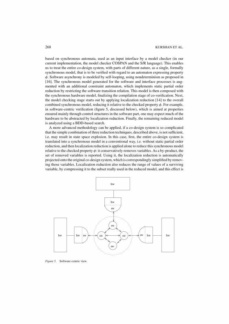
The extremal co-verification cases mentioned above are software-centric and hardware-centric co-verifications, in which the properties to be verified refer entirely or mainly eitherto the software part or to the hardware part, respectively. The two cases are illustratedin figures 5 and 6, which represent software and hardware components by circles andrectangles, respectively, and interface processes by hybrid shapes (half circle, half rectan-gle). In the software-centric view, the central subsystem comprises several software pro-cesses which communicate directly to each other and/or indirectly, via interface processes, tohardware components. The hardware components are generally also connected to each other.In a software-centric view, they are encapsulated by the layer of interface processes and formtogether with this layer the environment of the central software subsystem. Symmetrically,

270 KURSHAN ET AL.

sw hw swhw

sw

sw

hw

sw sw

hw

hw

hw hw

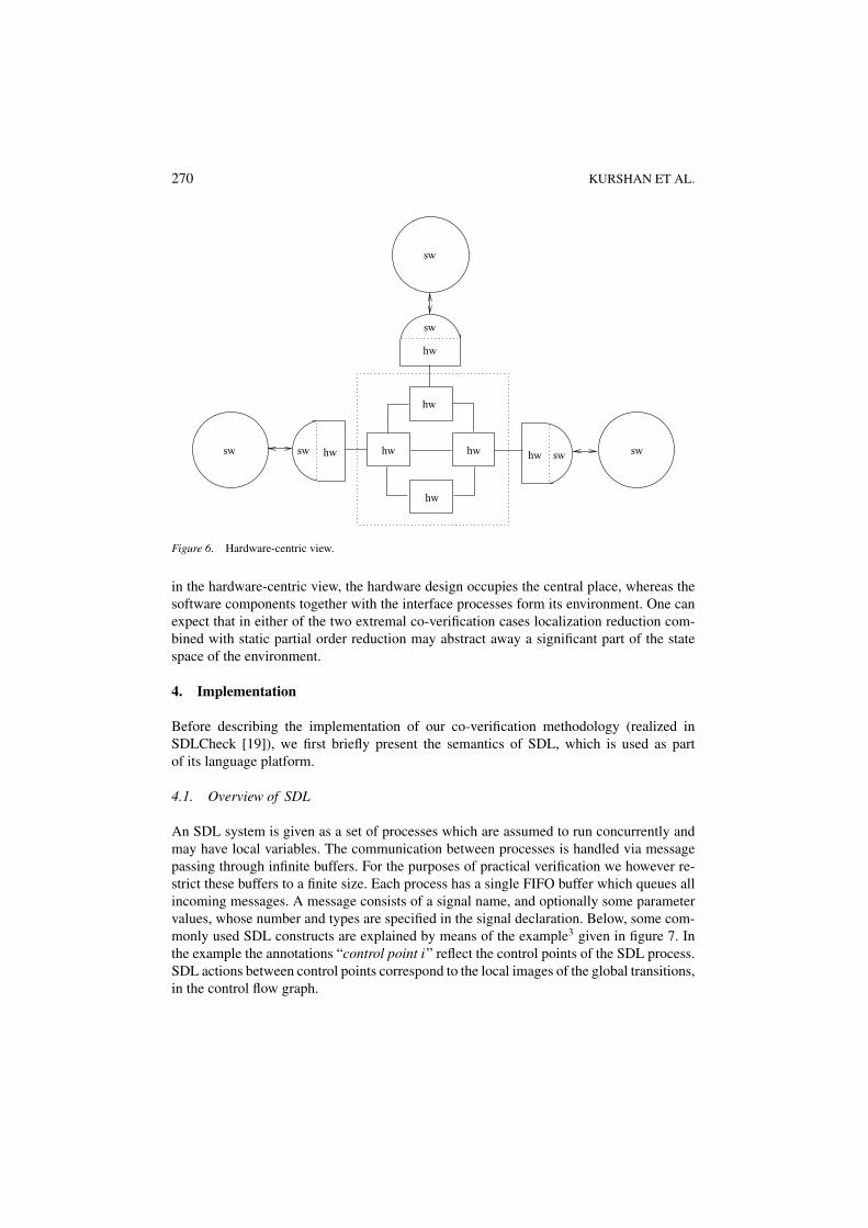
Figure 6. Hardware-centric view.

in the hardware-centric view, the hardware design occupies the central place, whereas thesoftware components together with the interface processes form its environment. One canexpect that in either of the two extremal co-verification cases localization reduction com-bined with static partial order reduction may abstract away a significant part of the statespace of the environment.

4. Implementation

Before describing the implementation of our co-verification methodology (realized inSDLCheck [19]), we first briefly present the semantics of SDL, which is used as partof its language platform.

4.1. Overview of SDL

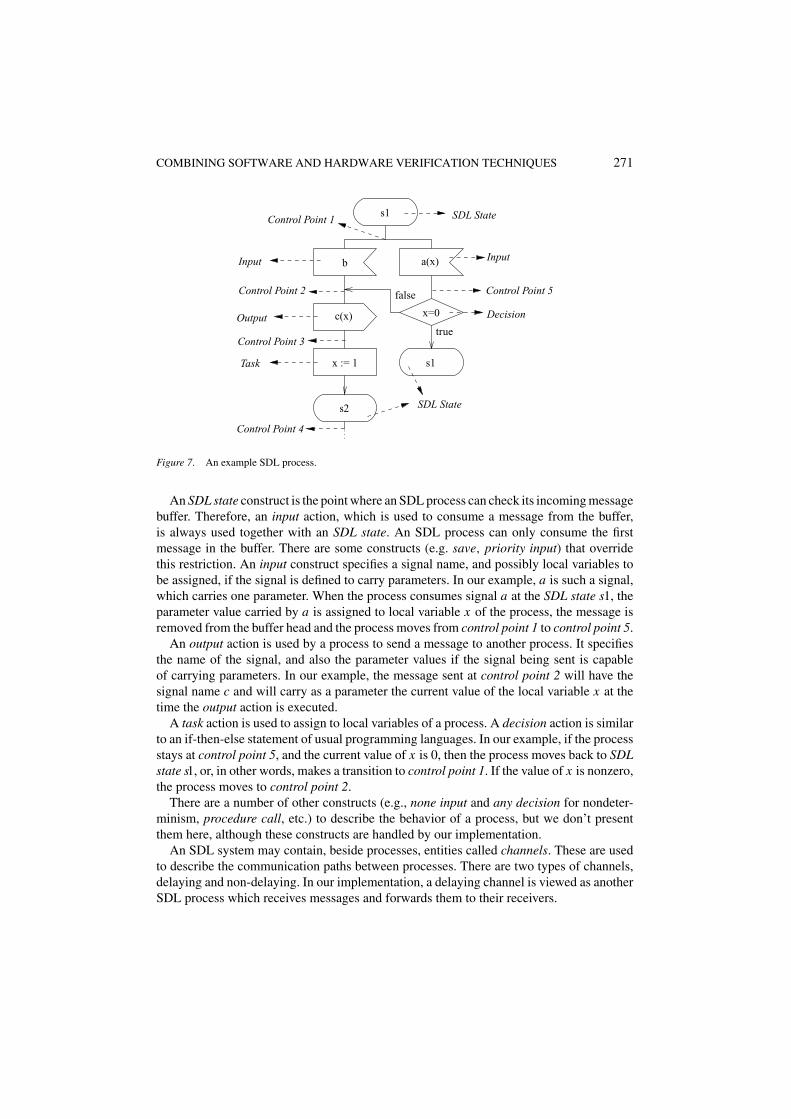
An SDL system is given as a set of processes which are assumed to run concurrently andmay have local variables. The communication between processes is handled via messagepassing through infinite buffers. For the purposes of practical verification we however re-strict these buffers to a finite size. Each process has a single FIFO buffer which queues allincoming messages. A message consists of a signal name, and optionally some parametervalues, whose number and types are specified in the signal declaration. Below, some com-monly used SDL constructs are explained by means of the example3 given in figure 7. Inthe example the annotations “control point i” reflect the control points of the SDL process.SDL actions between control points correspond to the local images of the global transitions,in the control flow graph.


s1

b a(x)

c(x) x=0

x := 1

Control Point 1

Control Point 2

Control Point 3

Control Point 4

SDL State

true

false

s2

s1

Decision

Control Point 5

Input

Output

Task

Input

SDL State

Figure 7. An example SDL process.

An SDL state construct is the point where an SDL process can check its incoming messagebuffer. Therefore, an input action, which is used to consume a message from the buffer,is always used together with an SDL state. An SDL process can only consume the firstmessage in the buffer. There are some constructs (e.g. save, priority input) that overridethis restriction. An input construct specifies a signal name, and possibly local variables tobe assigned, if the signal is defined to carry parameters. In our example, a is such a signal,which carries one parameter. When the process consumes signal a at the SDL state s1, theparameter value carried by a is assigned to local variable x of the process, the message isremoved from the buffer head and the process moves from control point 1 to control point 5.

An output action is used by a process to send a message to another process. It specifiesthe name of the signal, and also the parameter values if the signal being sent is capableof carrying parameters. In our example, the message sent at control point 2 will have thesignal name c and will carry as a parameter the current value of the local variable x at thetime the output action is executed.

A task action is used to assign to local variables of a process. A decision action is similarto an if-then-else statement of usual programming languages. In our example, if the processstays at control point 5, and the current value of x is 0, then the process moves back to SDLstate s1, or, in other words, makes a transition to control point 1. If the value of x is nonzero,the process moves to control point 2.

There are a number of other constructs (e.g., none input and any decision for nondeter-minism, procedure call, etc.) to describe the behavior of a process, but we don’t presentthem here, although these constructs are handled by our implementation.

An SDL system may contain, beside processes, entities called channels. These are usedto describe the communication paths between processes. There are two types of channels,delaying and non-delaying. In our implementation, a delaying channel is viewed as anotherSDL process which receives messages and forwards them to their receivers.

272 KURSHAN ET AL.

4.2. Static partial order reduction in the SDL to S/R compiler

In this section we explain how we implement our method of changing the enabling conditionsof transitions so that the generated code has the partial order reduction incorporated.

As explained in Section 4.1, a transition of an SDL process is always defined to occurbetween two control points of the process. The ample sets that we define will always containall enabled transitions of a single process. Therefore, we say that an SDL process P is ampleat a state if its current enabled transitions form an ample set. Hence, we need to identifythe local states of P for which the current enabled transitions satisfy the conditions C0, C1and C2′.

We start with condition C1 and examine the types of transitions introduced in Section 4.1.We will check if a transition is independent of all transitions of other processes in the entiresystem and if this is the case, tag it as GoodForC1. An input transition is always independentof all transitions of any other process. Note that an input transition may change the localvariables of that process if the consumed signals carries parameters. However, this does notcause a problem since no other process can read4 or write to a local variable of P . Anothereffect of an input transition is the removal of the message at the head of the buffer. Thebuffer of P is also accessed by any process P ′ that can send a message to P , therefore itmay seem that the execution order of these two transitions is important. However, an outputtransition places the message at the tail of the buffer, whereas an input transition removesthe message from the head of the buffer. Therefore, in both execution orders, the resultingbuffer content will be the same. There is no other action of another process that can bedependent on an input transition of P . Hence, an input transition can indeed be tagged asGoodForC1.

The task and decision transitions of process P can only access local variables of P . Atask updates its local variables, and a decision changes the current control point of P . Sinceno other process can directly access the local variables nor the control point of process P , itstask and decision transitions are independent of all other transitions. So, we can tag all suchtransitions as GoodForC1 provided that they appear in a software SDL process. However,in an interface SDL process, which may have interface variables shared by the hardwarepart, any transition that accesses (reads or assigns to) an interface variable is never taggedas GoodForC1, see Section 3.

An output transition of P which sends a message to a process P0, is dependent on anoutput transition of any process P ′ that also sends a message to P0. The reason is thatdifferent execution orders of these transitions will result in a different contents for the inputbuffer of P0, since the messages are queued in their arrival order. We therefore tag an outputtransition from P to P0 as GoodForC1 only if there is no other process P ′ that outputs tothe same process P0.

Note that in some of these cases a transition can enable another transition. For example, anoutput transition can enable an input transition, by providing a message in a buffer that waspreviously empty. This doesn’t affect the reduction technique we use in our implementation,in contrast to some other approaches, because the underlying definition of the independencerelation given in Section 2.1 is relaxed: it specifies that transitions may not disable another,but does not prohibit enabling.


The next step is to find the visible transitions. We assume that the atomic propositionsof the LTL formula φ to be checked are expressed in terms of the control points and localvariables of processes (e.g., “Process P is at control point 1” or “Local variable x of processP has value 5”). Hence, we tag a transition as Visible if it moves the control point ofa process to or from a control point mentioned in an atomic proposition, or it assigns to avariable that is mentioned in an atomic proposition. Note that since visible transitions aredetermined at compile time, and different properties contain different atomic propositions,each LTL formula requires a different compilation run.

After completing the tagging with GoodForC1 and Visible, we perform a similartagging for condition C2′. This time we tag transitions with Sticky such that the set Tof transitions with this tag guarantees C2′. We analyze the types of transition data effectsto reduce this set as explained in Section 2.4. With this regard, we only consider input andoutput transitions as having opposite effects on process input buffer queue, with respect toa given signal A: output of signal A to process P is treated as having incrementing effect,whereas input of signal A in P as having decrementing effect.

This completes the tagging steps. We call a control point of a process an ample controlpoint, if all local transitions from this control point are tagged as GoodForC1 and not taggedas Sticky.

Let the system be composed of processes {P1, P2, . . . , PN }. We define for each processPi a new boolean variable amplei . Pi assigns true to amplei iff its current local state isat an ample control point. All other processes can read the current value of amplei . Wealso impose an artificial priority ordering on the set of processes, for example, as in thelist P1, P2, . . . , PN . Finally, we define the new enabling condition of a local transition ina process Pi as follows: if the original enabling condition of the transition is a booleanpredicate p, it is changed to p ∧ (pC1C2′ ∨ pC0), where

pC1C2′ = ¬ample1 ∧ ¬ample2 ∧ · · · ∧ ¬amplei−1 ∧ ampleipC0 = ¬ample1 ∧ ¬ample2 ∧ · · · ∧ ¬ampleN

As the name implies, pC1C2′ is used to guarantee conditions C1 and C2′. At a givenglobal state, there may be more than one ample process. Since the enabled transitions ofeach ample process form an ample set at that state, we need to execute only one of them: itis selected as the first ample process in the list of processes (P1, P2, . . . , PN ) given in the(artificial) priority order. If no process is ample at the current state, all enabled transitionsare executed. This is guaranteed by pC0, which is true in this case.

Our compiler generates the code in S/R. To implement the amplei variables we use theselection variables of S/R. These are combinational variables which are not part of the stateand thus don’t take up space in the state vector during the search. Hence, the introductionof amplei flags does not introduce any memory overhead.

5. Experimental results

We have evaluated our method with several examples specified in SDL and translated intoS/R using the static partial order reduction method described in this paper. Several case

274 KURSHAN ET AL.

studies have been also conducted by our colleagues at Bell Laboratories and partners at theUniversity of Texas at Austin. Below, four of our examples are described and verificationresults of two other case studies are summarized.

All examples presented below were run on a VA Linux machine with Intel R© Pentium IIIprocessor at 800 MHz and 2300 MB of memory available for a process.

The first example is a concurrent sorting algorithm, SortN. There is a communicationchain comprising N + 1 processes that sort N randomly generated numbers. One processsimply generates N random numbers and sends them to the next process in the chain. Eachprocess that receives a new number compares it with the current number it has and sendsthe greater one to the next process. The last process receives only one number which is thelargest one generated by the first process.

The second example is a leader election protocol, LeaderN, given in [5]. It contains Nprocesses, each with an index number, that form a ring structure. Each process can onlysend a signal to the process on its right and can receive a signal from the process on itsleft. The aim of the protocol is to find the largest index number in the ring. The protocol isverified with respect to all possible initial states, i.e. each process initially selects an indexnumber nondeterministically.

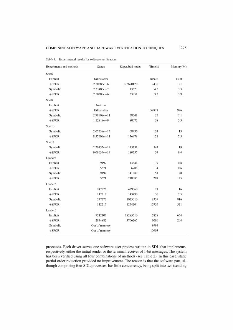
Each of these two examples is naturally scalable through the number of processes N . Wehave attempted to verify each example for various indices N using both explicit search andsymbolic search, with and without static partial order reduction. We have omitted checksfor N if the same combination of methods did not work for N − 1: i.e. ran out of memory ortime. Table 1 presents the results of those experiments. The results for the sorting algorithmsuggest an evidence that in some cases, verification conducted by symbolic search combinedwith static partial order reduction may outperform verification conducted by symbolic searchalone as well as verification conducted by explicit search combined with static partial orderreduction. However, this is not always the case, as suggested by the results for the leaderelection protocol.

On these two examples, SortN and LeaderN, static partial order reduction implementedin SDLCheck gives a reduction in the number of states that is as good as explicit search withdynamic partial order reduction as implemented in Spin [11]. This is due to the fact thatin these two examples the majority of local loops in the component processes are brokenby visible actions and the remaining loops appear inter-dependent through output andinput actions in neighboring processes, cf. Section 4.2. Therefore, in these particular cases,dynamic breaking the global state transition cycles (cf. condition C3 in Section 2.2) doesnot give rise to a decisive advantage over breaking few local cycles by the sticky transitionanalysis (cf. Algorithm 1 in Section 2.4). However, a general comparison between dynamicand static partial order reduction has not been done here, and it is not known how the relativeperformance of these two techniques would compare over a broad set of models.

Our next two examples are combined hardware/software systems. The verification resultsfor them are given by Table 2.

The third example is the alternating bit protocol, HW-ABP. The system was architec-tured hardware-centric in [18]. Its core transmission part is given by a register transfer levelgatelist that may be expressed in Verilog or VHDL. Both sending and receiving end of thehardware transmitter are controlled by their own drivers implemented in SDL+ as interface


Table 1. Experimental results for software verification.

Experiments and methods States Edges/bdd nodes Time(s) Memory(M)

Sort6

Explicit Killed after 84922 1300

+SPOR 2.50388e+6 122690120 2436 121

Symbolic 7.33483e+7 13623 4.2 3.3

+SPOR 2.50388e+6 33851 3.2 3.9

Sort8

Explicit Not run

+SPOR Killed after 59871 976

Symbolic 2.98508e+11 38641 23 7.1

+SPOR 1.12819e+9 80072 38 5.3

Sort10

Symbolic 2.07538e+15 68436 124 13

+SPOR 8.57609e+11 136978 21 7.5

Sort12

Symbolic 2.20155e+19 115731 547 19

+SPOR 9.08039e+14 180557 54 9.4

Leader4

Explicit 9197 13844 1.9 0.8

+SPOR 5571 6708 1.4 0.6

Symbolic 9197 141889 51 20

+SPOR 5571 218087 207 25

Leader5

Explicit 247276 429360 71 16

+SPOR 112217 143490 30 7.5

Symbolic 247276 1025010 8359 816

+SPOR 112217 1234204 15935 521

Leader6

Explicit 9212107 18285510 5828 664

+SPOR 2834882 3766265 1080 204

Symbolic Out of memory 8994

+SPOR Out of memory 10903

processes. Each driver serves one software user process written in SDL that implements,respectively, either the initial sender or the terminal receiver of 1-bit messages. The systemhas been verified using all four combinations of methods (see Table 2). In this case, staticpartial order reduction provided no improvement. The reason is that the software part, al-though comprising four SDL processes, has little concurrency, being split into two (sending

276 KURSHAN ET AL.

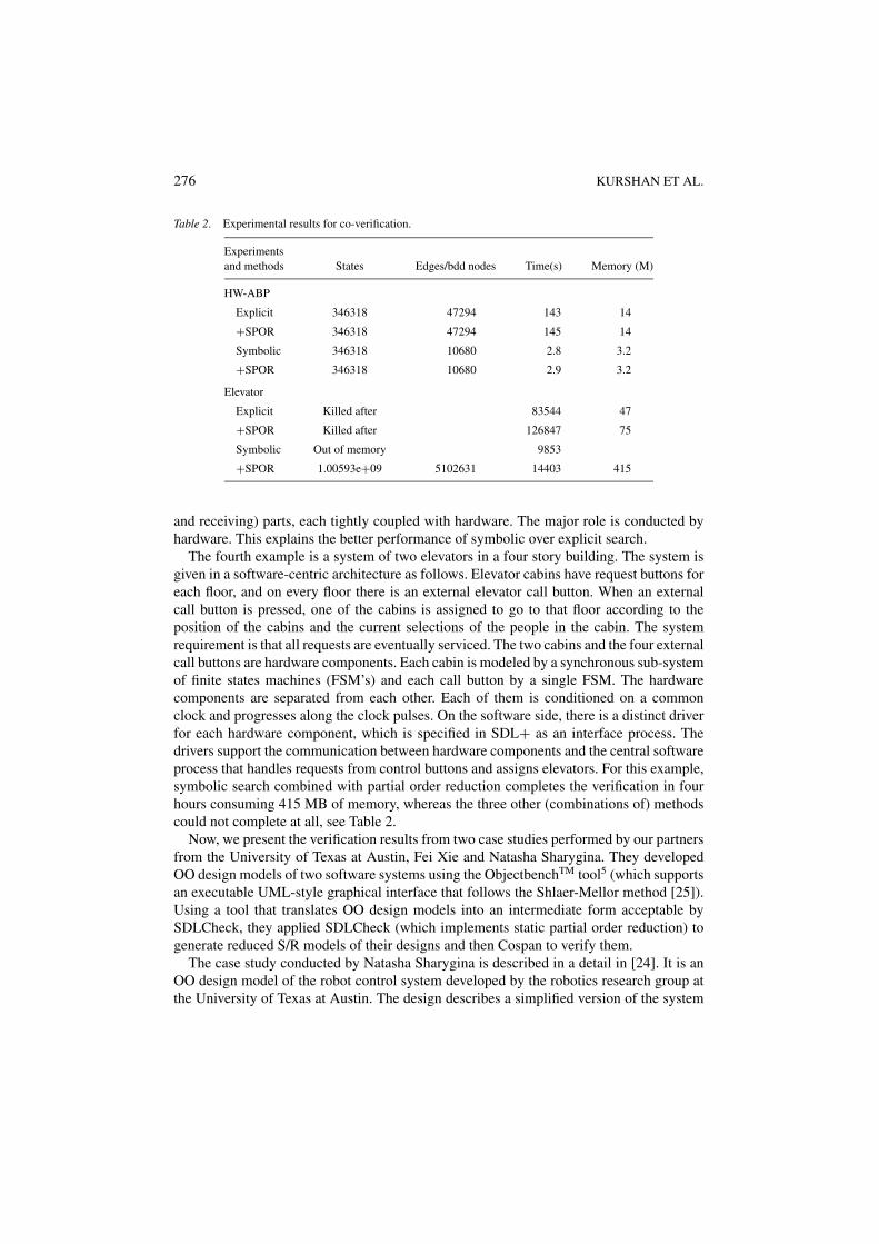
Table 2. Experimental results for co-verification.

Experimentsand methods States Edges/bdd nodes Time(s) Memory (M)

HW-ABP

Explicit 346318 47294 143 14

+SPOR 346318 47294 145 14

Symbolic 346318 10680 2.8 3.2

+SPOR 346318 10680 2.9 3.2

Elevator

Explicit Killed after 83544 47

+SPOR Killed after 126847 75

Symbolic Out of memory 9853

+SPOR 1.00593e+09 5102631 14403 415

and receiving) parts, each tightly coupled with hardware. The major role is conducted byhardware. This explains the better performance of symbolic over explicit search.

The fourth example is a system of two elevators in a four story building. The system isgiven in a software-centric architecture as follows. Elevator cabins have request buttons foreach floor, and on every floor there is an external elevator call button. When an externalcall button is pressed, one of the cabins is assigned to go to that floor according to theposition of the cabins and the current selections of the people in the cabin. The systemrequirement is that all requests are eventually serviced. The two cabins and the four externalcall buttons are hardware components. Each cabin is modeled by a synchronous sub-systemof finite states machines (FSM’s) and each call button by a single FSM. The hardwarecomponents are separated from each other. Each of them is conditioned on a commonclock and progresses along the clock pulses. On the software side, there is a distinct driverfor each hardware component, which is specified in SDL+ as an interface process. Thedrivers support the communication between hardware components and the central softwareprocess that handles requests from control buttons and assigns elevators. For this example,symbolic search combined with partial order reduction completes the verification in fourhours consuming 415 MB of memory, whereas the three other (combinations of) methodscould not complete at all, see Table 2.

Now, we present the verification results from two case studies performed by our partnersfrom the University of Texas at Austin, Fei Xie and Natasha Sharygina. They developedOO design models of two software systems using the ObjectbenchTM tool5 (which supportsan executable UML-style graphical interface that follows the Shlaer-Mellor method [25]).Using a tool that translates OO design models into an intermediate form acceptable bySDLCheck, they applied SDLCheck (which implements static partial order reduction) togenerate reduced S/R models of their designs and then Cospan to verify them.

The case study conducted by Natasha Sharygina is described in a detail in [24]. It is anOO design model of the robot control system developed by the robotics research group atthe University of Texas at Austin. The design describes a simplified version of the system


that controls a robot with one arm. The arm consists of two joints and an end effector thatmoves around and performs designated functions such as grabbing. Two major roboticsalgorithms are captured in the design: arm control and fault recovery. In total, the designmodel includes seven process components (called active objects). The active objects interactby sending to each other messages of 31 different types. A typical active object consistsof 7 object states, at which messages sent to the object may be read. Fourteen differentproperties that express functions of the system have been successfully verified. In all thecases, the best performance has been shown by explicit search combined with static partialorder reduction. Depending on a property, verification times range from 336 seconds toalmost 70 hours, and memory consumption from 0.2 MB to 198 MB.

The case study conducted by Fei Xie is an on-line ticket sale system. The system designincludes four classes of active objects: a single dispatcher and ticket server, and multipleagents and customers. When the dispatcher receives a purchase request from a customer,it assigns an agent to serve the customer. The agent guides the customer through a ticketpurchase transaction with the ticket server. Agents are also responsible for keeping misbe-having customers from corrupting the system. A simplified version of the system (with onlyone agent and one customer) has been successfully verified with regard to five propertiesunder a general fairness assumption that guarantees that none of the active objects enabledto execute is ignored. An example of the verified properties is: if the agent receives infinitelymany purchase requests then it provides infinitely many transaction services. In this case,symbolic search combined with static partial order reduction performs in 1765 secondsconsuming 77 MB of memory, whereas explicit search also combined with static partialorder reduction spends 6682 seconds and 17 MB. Neither of the two methods, symbolic orexplicit, could finish the verification when applied alone, without partial order reduction.

6. Conclusion

We have presented a formal verification methodology that supports the combination ofhardware- and software-oriented model checking techniques. An important consequenceis to be able to run together symbolic BDD-based verification and partial order reduction.Both techniques address the same problem of exponential computational complexity ofstate space exploration, but use search algorithms that are intrinsically different, operatingin breadth-first and, respectively, depth-first manner. To merge these two quite differenttechniques into one methodology, we apply them successively, in two different stages ofthe verification process. Partial order reduction is handled completely in the compilationphase, which generates a reduced model with the transition relation constrained by theample set conditions C0–C2′. Subsequently, the model checking phase can employ BDD-based algorithms as well as any other reduction techniques with no change to the existingverification engine.

We suggest the use of this method primarily for models with large state spaces thatcannot be handled by either reduction technique alone: symbolic evaluation without partialorder reduction or partial order reduction with explicit state enumeration. For such models,combining symbolic evaluation with partial order reduction may make verification feasible.Our experiments and case studies show that such models exist, for which the proposed

278 KURSHAN ET AL.

combined method may succeed, whereas either of its two component techniques appliedalone fails (runs out of memory or time) or performs too slowly. However, the experimentsalso show that this combined method is not always the best. Characterization of the modelsfor which it suits better than other methods is an open problem.

One natural niche for the proposed verification methodology are software/hardware co-design systems. Indeed, partial order reduction reflects (and reduces!) interleaving, com-monly used to model software concurrency, and symbolic evaluation is important for hard-ware verification, where partial order reduction has little or no effect. Our fourth examplein the previous section demonstrates not only the efficiency of the joint approach to reduc-tion, but also the fact that even a simple co-design model may fall out of the scope of astand-alone verification technique. However, we expect that the application area is wider. Itmay also include some software systems whose key issue is interprocess communication,and complicated hardware designs with major communication components represented byinterleaving abstractions.

We have also presented a toolkit that supports the proposed verification methodologyin the area of software/hardware co-design. The toolkit comprises Verilog and VHDLcompilers for translation of hardware components, a tool that translates software parts andgenerates a model incorporating partial order reduction, and finally a model checking enginewith support for both symbolic evaluation and explicit search. Although the implementationis necessarily language specific, the basic ideas explained above are general enough to allowre-implementations for different languages and/or BDD-based model checkers. In fact, are-implementation using ObjectbenchTM prior to the SDL interface has already been doneat Bell Laboratories in collaboration with Professor James C. Browne and his students atthe University of Texas at Austin.

Acknowledgments

We thank James Browne, Fei Xie and Natasha Sharygina for their valuable contributionsthat assisted our method to mature, and the reviewers for their useful comments.

Notes

1. www.cadence.com, www.mentor.com, www.synopsys.com, etc.2. The FormalCheckTM verification system is licensed by Lucent Technologies to Cadence Design Systems, Inc.3. The example is given in the graphical syntax recommended by [23], but italic labels and dashed arrows are just

annotations.4. SDL has two constructs, view and import, that enable a process to see a variable owned by another process. The

import construct is a shorthand of message passing that requests the owner process to send the current value ofthe variable. The view construct, which provides direct read access, is an outdated feature of the first version ofSDL, not recommended (though allowed) by the standard [23]. Currently, we ignore these constructs, althoughboth can be handled by the method of Section 2.3.

5. ObjectbenchTM is owned by Scientific and Engineering Software, Inc.

References

1. R. Alur, R.K. Brayton, T.A. Henzinger, S. Qadeer, and S.K. Rajamani, “Partial-order reduction in symbolicstate space exploration,” in O. Grumberg (ed.), Computer Aided Verification, 9th International Conference,


(CAV ’97) Proceedings, Vol. 1254 of Lecture Notes in Computer Science, Springer-Verlag, Berlin, 1997, pp.340–351.

2. B. Berger and P.W. Shor, “Approximation algorithms for the maximum acyclic subgraph problem,” in FirstACM-SIAM Symp. on Discrete Algorithms. Proceedings, 1990, pp. 236–243.

3. C.-T. Chou and D. Peled, “Formal verification of a partial-order reduction technique for model checking,”in T. Margaria and B. Steffen (Eds.), Tools and Algorithms for the Construction and Analysis of Systems,Second International Workshop (TACAS ’96) Proceedings, Vol. 1055 of Lecture Notes in Computer Science,Springer-Verlag, Berlin, 1996, pp. 241–257.

4. D.L. Dill. Trace Theory for Automatic Hierarchical Verification of Speed-Independent Circuits. MIT Press,Cambridge, MA, 1989.

5. D. Dolev, M. Klawe, and M. Rodeh, “An O(n log n) unidirectional distributed algorithm for extrema findingin a circle,” Journal of Algorithms, Vol. 3, No. 3, pp. 245–260, 1982.

6. P. Eades, X. Lin, and W.M. Smyth, “A fast and effective heuristic for the feedback arc set problem,” InformationProcessing Letters, Vol. 47, No. 6, pp. 319–323, 1993.

7. D. Gabbay, A. Pnueli, S. Shelah, and J. Stavi, “On the temporal analysis of fairness,” in Conference Recordof the Seventh ACM Symposium on Principles of Programming Languages, 1980, pp. 163–173.

8. P. Godefroid and D. Pirottin, “Refining dependencies improves partial-order verification methods,” inC. Courcoubetis (Ed.), Computer Aided Verification, 5th International Conference (CAV ’93) Proceedings,Vol. 697 of Lecture Notes in Computer Science, Springer-Verlag, Berlin, 1993, pp. 438–449.

9. R.H. Hardin, Z. Har’El, and R.P. Kurshan, “COSPAN,” in R. Alur and T.A. Henzinger (Eds.), Computer AidedVerification, 8th International Conference (CAV ’96) Proceedings, Vol. 1102 of Lecture Notes in ComputerScience, Springer-Verlag, Berlin, 1996, pp. 423–427.

10. Z. Har’El and R.P. Kurshan, “Software for analytical development of communication protocols,” AT&TTechnical Journal, Vol. 69, No. 1, pp. 45–59, 1990.

11. G.J. Holzmann, “The model checker Spin,” IEEE Trans. on Software Engineering, Vol. 23, No. 5, pp. 279–295,1997.

12. G.J. Holzmann and D. Peled, “An improvement in formal verification,” in D. Hogrefe and S. Leue (Eds.),Formal Description Techniques VII, Proceedings of the 7th IFIP WG 6.1 International Conference Bern,Switzerland, 1994, pp. 197–211.

13. R.M. Karp, “Reducibility among combinatorial problems,” in Complexity of Computer Computations, PlenumPress, New York, 1972, pp. 85–103.

14. R.P. Kurshan, Computer-Aided Verification of Coordinating Processes: The Automata-Theoretic Approach,Princeton University Press, Princeton, NJ, 1994.

15. R. Kurshan, V. Levin, M. Minea, D. Peled, and H. Yenigun, “Static partial order reduction,” in B. Steffen (Ed.),Tools and Algorithms for the Construction and Analysis of Systems, 4th International Conference (TACAS’98)Proceedings, Vol. 1384 of Lecture Notes in Computer Science, Springer-Verlag, Berlin, 1998, pp. 345–357.

16. R.P. Kurshan, M. Merritt, A. Orda, and S. Sachs, “Modeling asynchrony with a synchronous model,” in P.Wolper (Ed.), Computer Aided Verification, 7th International Conference (CAV’95) Proceedings, Vol. 939 ofLecture Notes in Computer Science, Springer-Verlag, Berlin, 1995, pp. 339–352.

17. L. Lamport, “What good is temporal logic,” in R.E.A. Mason (Ed.), Proceedings of IFIP Congress, NorthHolland, 1983, pp. 657–668.

18. V. Levin, E. Bounimova, O. Basbugoglu, and K. Inan, “A verifiable software/hardware co-design using SDLand COSPAN,” in Proceedings of the COST 247 International Workshop on Applied Formal Methods inSystem Design, Maribor, Slovenia, 1996, pp. 6–16.

19. V. Levin and H. Yenigun, “SDLCheck: A model checking tool,” in G. Berry, H. Comon, and A. Finkel (Eds.),Computer Aided Verification, 13th International Conference (CAV 2001) Proceedings, Vol. 2102 of LectureNotes in Computer Science, Springer-Verlag, Berlin, 2001, pp. 378–381.

20. K.L. McMillan, Symbolic Model Checking. Kluwer Academic Publishers, Boston, MA, 1993.21. D. Peled, “Combining partial order reductions with on-the-fly model-checking,” Formal Methods in System

Design, Vol. 8, pp. 39–64, 1996.22. D. Peled and T. Wilke, “Stutter–invariant temporal properties are expressible without the next-time operator,”

Information Processing Letters, Vol. 63, No. 5, pp. 243–246, 1997.

280 KURSHAN ET AL.

23. SDL92, “Functional specification and description language (SDL), ITU-T Recommendation Z.100,” 1993,Geneva.

24. N. Sharygina, R.P. Kurshan, and J.C. Browne, “A formal object-oriented analysis for software reliability:Design for verification,” in Heinrich Husmann (Ed.), Fundamental Approaches to Software Engineering,4th International Conference (FASE 2001) Proceedings, Vol. 2029 of Lecture Notes in Computer Science,Springer-Verlag, Berlin, 2001, pp. 318–332.

25. S. Shlaer and S.J. Mellor, Object Lifecycles Modeling the World in States, Prentice-Hall, Englewood Cliffs,NJ, 1992.

26. A. Valmari, “A stubborn attack on state explosion,” in E.M. Clarke and R.P. Kurshan (Eds.), Computer-AidedVerification, 2nd International Conference (CAV ’90) Proceedings, Vol. 531 of Lecture Notes in ComputerScience, Springer-Verlag, Berlin, 1990, pp. 156–165.

27. Verilog95, “IEEE standard hardware description language based on the VerilogTM hardware descriptionlanguage, “IEEE Std 1364-1995,” 1996, New York.

28. VHDL93, “IEEE Standard VHDL Language Reference Manual, IEEE Std 1076-1993,” 1994, New York.

Documents

Combining Software and Hardware Verification Techniques