Embed Size (px)
Citation preview
LANDSLIDE HAZARD AND RISK ASSESSMENT

LANDSLIDE HAZARD AND RISK ASSESSMENT
DISSERTATION
zur
ERLANGUNG DES DOKTORGRADS (DR. RER. NAT.)
der
MATHEMATICH-NATURWISSENSCHAFTLICHEN FAKULTÄT
der
RHEINISCHEN FRIEDRICH-WILHELMS-UNIVESTITÄT BONN
vorgelegt von
Fausto Guzzetti
aus
Perugia, Italy
Bonn, November 2005

Angefertigt mit Genehmigung der Mathematich-Naturwissenschaftlichen Fakultät der Rheinischen Friedrich-Wilhelms-Univestität Bonn
1. Referent: Professor Dr. Richard Dikau
2. Referent: Priv. –Doz. Dr. Thomas Glade
Tag del Promotion:

LANDSLIDE HAZARD AND RISK ASSESSMENT
CONCEPTS, METHODS AND TOOLS FOR THE DETECTION AND MAPPING OF LANDSLIDES, FOR LANDSLIDE SUSCEPTIBILITY ZONATION AND HAZARD ASSESSMENT, AND FOR LANDSLIDE
RISK EVALUATION
Se la montagna viene verso di te,
e tu non sei Maometto, corri, perché è una frana.

i
TABLE OF CONTENTS
TABLE OF CONTENTS i SUMMARY vii 1 INTRODUCTION 11.1 Significance of the problem 21.2 Ambition of the work 41.3 Outline of the work 71.4 Specific personal contributions 9 2 STUDY AREAS 132.1 Italy 142.2 Umbria Region, central Italy 182.3 Upper Tiber River basin, central Italy 222.4 Collazzone area, Umbria Region 252.5 Nera River and Corno River valleys, Umbria Region 272.6 Staffora River basin, Lombardy Region, northern Italy 29 3 LANDSLIDE MAPPING 333.1 Theoretical framework 333.2 Landslide recognition 343.3 Landslide inventories 393.3.1 Archive inventories 393.3.1.1 The AVI archive inventory and the SICI information system 403.3.2 Geomorphological inventories 463.3.2.1 Reconnaissance geomorphological inventory map for the Umbria Region 473.3.2.2 Detailed geomorphological inventory map for the Umbria Region 493.3.2.3 Comparison of the two geomorphological inventory maps in Umbria 523.3.3 Event inventories 533.3.3.1 Landslides triggered by prolonged rainfall in the period from 1937 to 1941 543.3.3.2 Landslides triggered by rapid snowmelt in January 1997 543.3.3.3 Landslides triggered by earthquakes in September-October 1997 553.3.3.4 Comparison of the three event inventories in Umbria 553.3.4 Multi-temporal inventories 573.3.4.1 Multi-temporal inventory for the Collazzone area 583.4 Factors affecting the quality of landslide inventories 613.4.1 Quality of landslide inventory maps in the Collazzone area 62
Table of contents
ii
3.5 Summary of achieved results 65 4 ANALYSIS OF THE INVENTORIES 674.1 Landslide abundance 674.1.1 Statistical landslide density maps 684.1.2 Geomorphological landslide density maps 694.2 Comparison of landslide inventories 704.2.1 Comparison of archive and geomorphological inventory maps 714.2.2 Comparison of two geomorphological landslide inventory maps 724.2.2.1 Further comparison of the landslide maps in the Collazzone area 764.3 Completeness of landslide inventories 804.3.1 Completeness of archive inventories 814.3.2 Completeness of geomorphological, event, and multi-temporal maps 834.4 Landslide persistence 854.5 Temporal frequency of slope failures 864.5.1 Exceedance probability of landslide occurrence 864.5.1.1 Temporal probability of historical landslide events in Umbria 884.6 Summary of achieved results 89 5 STATISTICS OF LANDSLIDE SIZE 915.1 Background 915.2 Methods 965.2.1 Statistics of landslide area 965.2.2 Statistics of landslide volume 1025.3 Applications in the Umbria Region inventories 1035.3.1 Completeness of the landslide inventory maps in the Collazzone area 1035.3.2 Statistics of landslide areas in Umbria 1065.4 Discussion 1095.5 Summary of achieved results 111 6 LANDSLIDE SUSCEPTIBILITY ZONING 1136.1 Background 1146.2 Landslide susceptibility methods 1156.2.1 Assumptions 1156.2.2 Mapping units 1166.2.3 Methods 1196.2.3.1 Geomorphological mapping 1206.2.3.2 Analysis of inventories 1206.2.3.3 Heuristic zoning 1206.2.3.4 Statistical methods 1216.2.3.5 Process based models 1276.2.4 Susceptibility methods and mapping units 1286.3 Probabilistic model for landslide susceptibility 1296.3.1 Discussion 1316.4 Landslide susceptibility in the Upper Tiber River basin 1326.4.1 Discussion 1376.5 Verification of a landslide susceptibility forecast 1386.5.1 An example of the verification of a landslide susceptibility model 1406.5.1.1 Susceptibility model for shallow landslides in the Collazzone area 140
Table of contents
iii
6.5.1.2 Degree of model fitting 1426.5.1.3 Ensemble of landslide susceptibility models 1456.5.1.4 Role of independent thematic variables 1456.5.1.5 Model sensitivity 1476.5.1.6 Uncertainty in the susceptibility estimate of individual slope units 1476.5.1.7 Analysis of the model prediction skill 1516.5.2 A framework for the validation of landslide susceptibility models 1546.6 Summary of achieved results 158 7 LANDSLIDE HAZARD ASSESSMENT 1597.1 Background and definitions 1597.2 Probabilistic model for landslide hazard assessment 1627.3 Landslide hazard model for the Staffora River basin 1647.3.1 Probability of landslide size 1667.3.2 Probability of temporal landslide occurrence 1677.3.3 Spatial probability of landslides 1677.3.4 Hazard assessment 1727.3.5 Discussion 1737.4 Assessment of landslide hazard at the national scale 1767.4.1 Spatial probability of landslide events 1767.4.2 Probability of event occurrence 1767.4.3 Probability of the consequences 1777.4.4 Hazard assessment and discussion 1787.5 Rock fall hazard assessment along the Nera and Corno valleys 1807.5.1 The computer program STONE 1807.5.2 Application of the rock fall simulation model 1817.5.3 Rock fall hazard assessment 1847.5.4 Discussion 1877.6 Summary of achieved results 189 8 LANDSLIDE RISK EVALUATION 1918.1 Literature review 1928.2 Concepts and definitions 1948.2.1 Vulnerability and consequence 1958.2.2 Risk analysis 1978.2.3 Discussion 1988.3 Evaluation of landslide risk to individuals and the population 1998.3.1 Landslide risk to the population in Italy 2008.3.1.1 Individual landslide risk 2018.3.1.2 Societal landslide risk 2058.3.2 Comparison of risk posed by different natural hazards in Italy 2088.3.3 Geographical distribution of landslide risk to the population in Italy 2108.3.3.1 Discussion 2158.3.4 Landslide risk to vehicles and pedestrians along roads 2158.3.4.1 Landslide risk to vehicles along the Nera River and Corno River valleys 2168.4 Geomorphological landslide risk evaluation 2178.4.1 Definition of the study area 2188.4.2 Multi-temporal landslide map 218
Table of contents
iv
8.4.3 Landslide frequency 2198.4.4 Landslide intensity 2208.4.5 Landslide Hazard Zones 2208.4.6 Landslide hazard assessment 2218.4.7 Vulnerability of elements at risk 2228.4.8 Specific landslide risk 2238.4.9 Total landslide risk 2258.4.10 Geomorphological landslide risk evaluation in Umbria 2268.4.10.1 Collevalenza village 2268.4.10.2 Terria village 2308.4.11 Discussion 2338.5 Assessing landslide damage and forecasting landslide impact 2358.5.1 Landslide damage in Umbria 2358.5.1.1 Damage to the transportation network and the built-up areas 2368.5.1.2 Damage to the population 2388.5.2 Landslide impact 2388.5.2.1 Expected impact to the transportation network and the built-up areas 2398.5.2.2 Expected impact to the population in the Perugia Municipality 2418.5.2.3 Expected impact to the agriculture 2428.5.3 Discussion 2428.6 Summary of achieved results 243 9 USE OF LANDSLIDE MAPS AND MODELS 2459.1 Landslide inventory maps 2459.2 Landslide density maps 2479.3 Landslide susceptibility zoning 2489.4 Landslide hazard assessments 2509.5 Landslide risk evaluations 2529.6 Establishing a landslide protocol 2539.7 Summary of achieved results 257 10 CONCLUSIONS AND FINAL RECOMMENDATIONS 25910.1 Landslide mapping 25910.2 Landslide susceptibility zoning 26310.3 Landslide hazard assessment 26510.4 Landslide risk evaluation 26710.5 Concluding remarks 26910.6 Prospective thoughts 271 11 ACKNOWLEDGEMENTS 275 12 GLOSSARY 277 13 LIST OF REFERENCES 285
Appendix A1 – Variables used in the text 349Appendix A2 – List of Figures and Tables 353 List of Figures 353 List of Tables 359

Table of contents
v
Appendix A3 – Acronyms 363Appendix A4 – Study areas and landslide products 367Appendix A5 – Curriculum vitae et studiorium 369Appendix A6 – Accompanying publications 371

vii
SUMMARY
Dear friend, I am sorry I don’t have the time
to write you a shorter letter.
Landslides play an important role in the evolution of landforms and represent a serious hazard in many areas of the World. In places, fatalities and economic damage caused by landslides are larger than those caused by other natural hazards, including earthquakes, volcanic eruptions and floods. Due to the extraordinary breadth of the spectrum of landslide phenomena, no single method exists to identify and map landslides, to ascertain landslide hazards, and to evaluate the associated risk. This work contributes to reduce this shortcoming by providing the scientific rationale, a common language, and a set of validated tools for the preparation and the optimal use of landslide maps, landside prediction models, and landslide forecasts.
I begin the work by critically analysing landslide inventories, including archive, geomorphological, event and multi-temporal maps. I then present methods to analyse the information shown in the inventories, including the assessment of landslide density and spatial persistence, the completeness of the landslide maps, and the estimation of the recurrence of landslide events, the latter based on historical information obtained from archive or multi-temporal inventories. I then use statistical methods to obtain the frequency-size statistics of landslides, important information for hazard and risk studies. Next, I discuss landslide the susceptibility zoning and hazard assessment. I examine statistical and physically-based methods to ascertain landslide susceptibility, and I introduce a scheme for evaluating and ranking the quality of susceptibility assessments. I then introduce a probabilistic model to determine landslide hazard, and I test the model at different spatial scales. Next I show how to determine landslide risk at different scales using a variety of approaches, including probabilistic methods and heuristic geomorphological investigations. Risk evaluation is the ultimate goal of landslide studies aimed at reducing the negative effects of landslide hazards. Lastly, I compare the information content of different landslide cartographic products, including maps, models and forecasts, and I introduce the idea of a landslide protocol, a set of regulations established to link terrain domains shown on the different landslide maps to proper land use rules.
I conclude the work by proposing recommendations for the production and optimal use of various landslide cartographic products. The recommendations and most of the results shown in this work are the results of landslide hazard research conducted in central and northern Italy. However, the lessons learned in these areas are general and applicable to other areas in Italy and elsewhere.

1
1. INTRODUCTION
No matter where you are going, the road is uphill and against the wind.
A “landslide” is the movement of a mass of rock, debris, or earth down a slope, under the influence of gravity (Nemčok et al., 1972; Varnes, 1978; Hutchinson, 1988; WP/WLI, 1990; Cruden, 1991; Cruden and Varnes, 1996). Different phenomena cause landslides, including intense or prolonged rainfall, earthquakes, rapid snow melting, and a variety of human activities. Landslides can involve flowing, sliding, toppling or falling movements, and many landslides exhibit a combination of two or more types of movements (Varnes, 1978; Crozier, 1986; Hutchinson, 1988; Cruden and Varnes, 1996; Dikau et al., 1996).
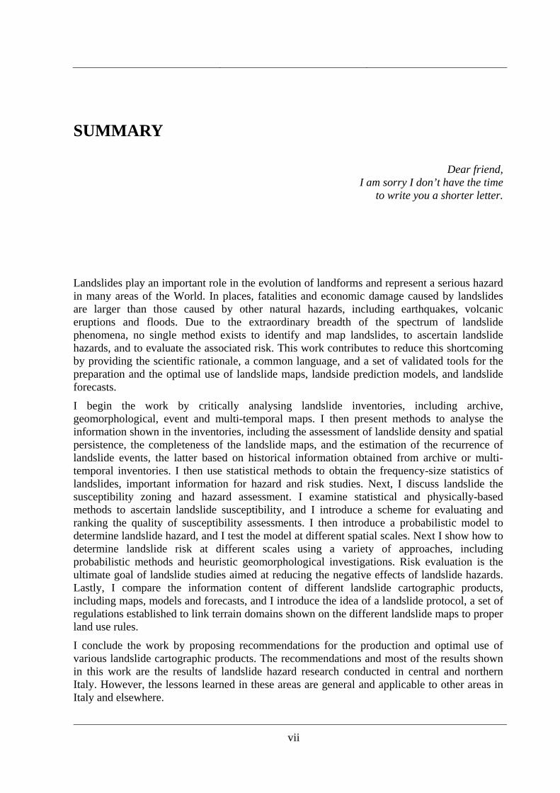
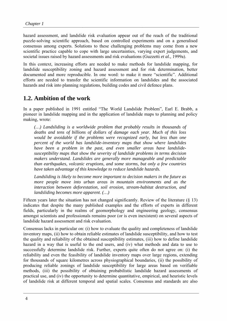
The range of landslide phenomena is extremely large, making mass movements one of the most diversified and complex natural hazard (Figure 1.1). Landslides have been recognized in all continents, in the seas and in the oceans. On Earth, the area of a landslide spans nine orders of magnitude, from a small soil slide involving a few square meters to large submarine landslides covering several hundreds of square kilometres of land and sea floor. The volume of mass movements spans sixteen orders of magnitude, from a single cobble falling from a rock cliff to gigantic submarine slides. Landslide velocity extends at least over fourteen orders of magnitude, from creeping failures moving at millimetres per year (or even less) to rock avalanches travelling at hundreds of kilometres per hour. Mass movements can occur singularly or in groups of up to several thousands. Multiple landslides occur almost simultaneously when slopes are shaken by an earthquake or over a period of hours or days when failures are triggered by intense or prolonged rainfall. Rapid snow melting can trigger slope failures several days after the onset of the triggering meteorological event. An individual landslide-triggering event (e.g., intense or prolonged rainfall, earthquake, snow melting) can involve a single slope or a group of slopes extending for a few hectares, or can affect thousands of square kilometres spanning major physiographic and climatic regions. Total landslide area produced by an individual triggering event ranges from a few tens of square meters to hundreds of square kilometres. The lifetime of a single mass movement ranges from a few seconds in the case of individual rock falls, to several hundreds and possibly thousands of years in the case of large dormant landslides.
The extraordinary breadth of the spectrum of landslide phenomena makes it difficult – if not impossible – to define a single methodology to identify and map landslides, to ascertain landslide hazards, and to evaluate the associated risk. The experience gained in experiments and surveys carried out by geomorphologists and engineering geologists in many areas of the world has shown that different strategies and a combination of different methods and
Chapter 1
2
techniques have to be applied, depending on the type and number of the landslides, the extent and complexity of the study area, and the available resources. This makes landslide mapping, landslide susceptibility and hazard assessment, and landslide risk evaluation a unique challenge for scientists, planners and decision makers.
Figure 1.1 – The large spectrum of landslide phenomena. x-axes show order of magnitude (logarithmic
scale). Landslide length, in metre, landslide area, in square metre, and landslide volume, in cubic metre, refer to a single slope failure. Landslide velocity is in metre per second. Total number is the
number of landslides triggered by an event. Affected area is the territory affected by the trigging event, in square metre. Total landslide area is the cumulative landslide area produced by a triggering event, in
square metre. Triggering time is the period of a landslide triggering event, in second. Lifetime is the lifetime of a landslide, in seconds. Figures in the graph are approximate and for descriptive purposes.
1.1. Significance of the problem
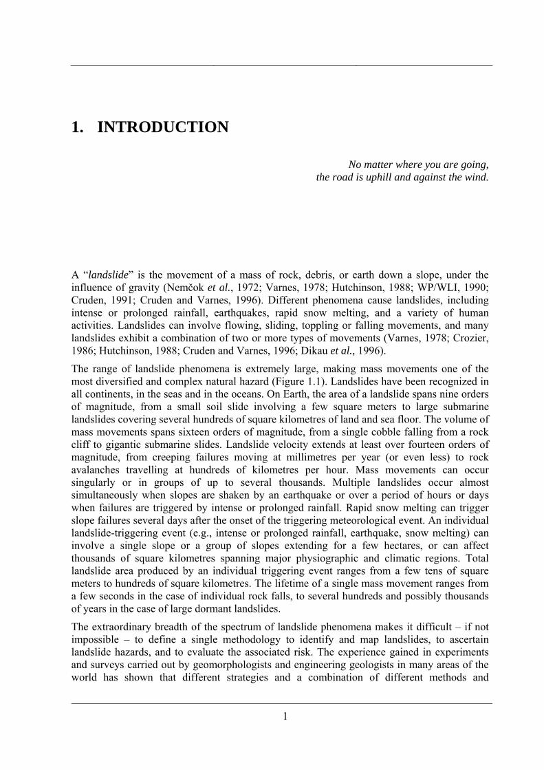
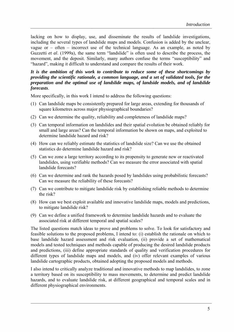
The population of Europe has grown from about 120 millions in 1700 to more than 750 millions in 2000. In the same period, the population of Italy has grown from 13 millions (in 1700), to 57 millions (in 2004) (Figure 1.2). The increase in the population is almost invariably associated with an intensive – and locally excessive – exploitation of the land, including development of new settlements, and construction of roads, railways, and other infrastructures. As an example, from 1950 to 1990 more than 100,000 kilometres of roads were built in Italy, the same as the total length of roads available in 1865. In the same period, the number and the extent of the built-up areas have grown substantially. In many areas of Italy, due to the local physiographical setting, expansion of new settlements and infrastructure occurred in dangerous or potentially hazardous areas. The growing population and the expansion of settlements and life-lines over hazardous areas have increased the impact of landslides in Italy, as in many other industrialized and developing countries.
Introduction
3
Figure 1.2 – Historical variation of the population in Europe (left) and in Italy (right).
Despite the physical (natural) phenomena being the same, the approaches to cope with landslides and their associated hazards and risk vary substantially in industrialized and developing countries. In industrialized countries, the extent and complexity of the problem and a generalized shortage of economic resources hampers systematic, long term investments in structural measures to substantially reduce the risk posed by natural hazards (Plattner, 2005). For landslides the problem is especially difficult (Brabb and Harrod, 1989; Brabb, 1991). Individual remedial measures can be very expensive, and most commonly mitigate the risk only in limited areas, often a single slope or a portion of a slope, making it economically impossible to lessen the hazards over large areas (i.e., an entire region) using structural (engineering) approaches. In developing countries societal and economic problems are often so large and serious that little attention is posed to the negative effects of natural hazards in general, and of landslides in particular. In these countries, the limited available resources are – ate best – invested primarily to improve health and education or to promote the economy, and little remains available to mitigate the catastrophic effects of natural hazards, including slope failures.
In many places the new issue seems to be the implementation of warning systems, and the adoption of new regulations for land utilisation aimed at minimising the loss of lives and property without investing in long-term, costly projects of ground stabilisation. In this framework, landslide hazard assessment and risk evaluation are particularly relevant, and pose a difficult challenge for scientists, civil defence managers, planners, land developers, policy and decision makers, and concerned citizens. Design and implementation of efficient and sustainable planning and land-use policies pose increasingly complex problems. These problems are different from the traditional problems of both pure and applied science. As regards to landslide hazard assessment and risk evaluation, on one side geomorphology is unable to provide a well-founded theory, and on the other side environmental issues and policy decisions challenge geomorphologists with very difficult questions.
Due to the large spectrum of landslide phenomena (Figure 1.1), to uncertainties in data acquisition and handling and in model selection and calibration, and to the complexity and vulnerability of modern societies, landslide mapping, landslide susceptibility zoning, landslide
Chapter 1
4
hazard assessment, and landslide risk evaluation appear out of the reach of the traditional puzzle-solving scientific approach, based on controlled experiments and on a generalised consensus among experts. Solutions to these challenging problems may come from a new scientific practice capable to cope with large uncertainties, varying expert judgements, and societal issues raised by hazard assessments and risk evaluations (Guzzetti et al., 1999a).
In this context, increasing efforts are needed to make methods for landslide mapping, for landslide susceptibility zoning and hazard assessment and for risk determination, better documented and more reproducible. In one word: to make it more “scientific”. Additional efforts are needed to transfer the scientific information on landslides and the associated hazards and risk into planning regulations, building codes and civil defence plans.
1.2. Ambition of the work
In a paper published in 1991 entitled “The World Landslide Problem”, Earl E. Brabb, a pioneer in landslide mapping and in the application of landslide maps to planning and policy making, wrote:
(…) Landsliding is a worldwide problem that probably results in thousands of deaths and tens of billions of dollars of damage each year. Much of this loss would be avoidable if the problems were recognized early, but less than one percent of the world has landslide-inventory maps that show where landslides have been a problem in the past, and even smaller areas have landslide-susceptibility maps that show the severity of landslide problems in terms decision makers understand. Landslides are generally more manageable and predictable than earthquakes, volcanic eruptions, and some storms, but only a few countries have taken advantage of this knowledge to reduce landslide hazards.
Landsliding is likely to become more important to decision makers in the future as more people move into urban areas in mountain environments and as the interaction between deforestation, soil erosion, stream-habitat destruction, and landsliding becomes more apparent. (…)
Fifteen years later the situation has not changed significantly. Review of the literature (§ 13) indicates that despite the many published examples and the efforts of experts in different fields, particularly in the realms of geomorphology and engineering geology, consensus amongst scientists and professionals remains poor (or is even inexistent) on several aspects of landslide hazard assessment and risk evaluation.
Consensus lacks in particular on: (i) how to evaluate the quality and completeness of landslide inventory maps, (ii) how to obtain reliable estimates of landslide susceptibility, and how to test the quality and reliability of the obtained susceptibility estimates, (iii) how to define landslide hazard in a way that is useful to the end users, and (iv) what methods and data to use to successfully determine landslide risk. Further, experts quite often do not agree on: (i) the reliability and even the feasibility of landslide inventory maps over large regions, extending for thousands of square kilometres across physiographical boundaries, (ii) the possibility of producing reliable zonings of landslide susceptibility for large areas based on verifiable methods, (iii) the possibility of obtaining probabilistic landslide hazard assessments of practical use, and (iv) the opportunity to determine quantitative, empirical, and heuristic levels of landslide risk at different temporal and spatial scales. Consensus and standards are also
Introduction
5
lacking on how to display, use, and disseminate the results of landslide investigations, including the several types of landslide maps and models. Confusion is added by the unclear, vague or – often – incorrect use of the technical language. As an example, as noted by Guzzetti et al. (1999a), the same term “landslide” is often used to describe the process, the movement, and the deposit. Similarly, many authors confuse the terms “susceptibility” and “hazard”, making it difficult to understand and compare the results of their work.
It is the ambition of this work to contribute to reduce some of these shortcomings by providing the scientific rationale, a common language, and a set of validated tools, for the preparation and the optimal use of landslide maps, of landside models, and of landslide forecasts.
More specifically, in this work I intend to address the following questions:
(1) Can landslide maps be consistently prepared for large areas, extending for thousands of square kilometres across major physiographical boundaries?
(2) Can we determine the quality, reliability and completeness of landslide maps?
(3) Can temporal information on landslides and their spatial evolution be obtained reliably for small and large areas? Can the temporal information be shown on maps, and exploited to determine landslide hazard and risk?
(4) How can we reliably estimate the statistics of landslide size? Can we use the obtained statistics do determine landslide hazard and risk?
(5) Can we zone a large territory according to its propensity to generate new or reactivated landslides, using verifiable methods? Can we measure the error associated with spatial landslide forecasts?
(6) Can we determine and rank the hazards posed by landslides using probabilistic forecasts? Can we measure the reliability of these forecasts?
(7) Can we contribute to mitigate landslide risk by establishing reliable methods to determine the risk?
(8) How can we best exploit available and innovative landslide maps, models and predictions, to mitigate landslide risk?
(9) Can we define a unified framework to determine landslide hazards and to evaluate the associated risk at different temporal and spatial scales?
The listed questions match ideas to prove and problems to solve. To look for satisfactory and feasible solutions to the proposed problems, I intend to: (i) establish the rationale on which to base landslide hazard assessment and risk evaluation, (ii) provide a set of mathematical models and tested techniques and methods capable of producing the desired landslide products and predictions, (iii) define appropriate standards of quality and verification procedures for different types of landslide maps and models, and (iv) offer relevant examples of various landslide cartographic products, obtained adopting the proposed models and methods.
I also intend to critically analyze traditional and innovative methods to map landslides, to zone a territory based on its susceptibility to mass movements, to determine and predict landslide hazards, and to evaluate landslide risk, at different geographical and temporal scales and in different physiographical environments.
Chapter 1
6
As it will become clear later, the conception and the production of maps is a fundamental part of this work. This is not surprising, as maps are the tools that earth scientists prefer in order to portray geological information and convey it to other scientists, decision-makers, and the public. In the realm of natural hazards, maps are prepared to show where catastrophes have happened or where they are expected to occur, and can be used to divide up land areas into zones of different hazard and to show risk levels. Cartography is a crucial aspect of landslide hazard assessment and risk evaluation, and landslides are no exception.
In this context, landslide cartography must not be intended only as a set of drafting methods and computer tools available to portray landslide-related information on a map or on the screen of a computer. Landslide Cartography is an ensemble of theories, paradigms, models, methods, and techniques to obtain, analyze and generate relevant information on landslides, and to convey it to the end user, i.e., another scientist, a decision or policy maker, or the interested citizens. An ambition of this work is to contribute to base landslide cartography on a well established rationale. This will not prevent using empirical or heuristic approaches. To the opposite, I will show that the combination of various sources of information analyzed with a variety of methods and techniques provides the most advanced and – hopefully – the most useful response to many landslide hazard and risk problems. I also intend to show how to best exploit geomorphological reasoning, including geomorphological information, theories, methods and techniques, to better map landslides, to determine their hazards, and to evaluate the associated risk.
Ideally, a single (“unified”) method for investigating landslides and for the production of relevant landslide cartographic products is desirable. A single method would guarantee consistency and would help comparing products and results obtained in different areas, by different investigators, and at different times. Unfortunately, due to the extraordinary breadth of the spectrum of landslide phenomena (Figure 1.1), such a unified method is difficult to obtain. Instead, I propose that a common set of tools, which I call a “toolbox for landslide cartography”, can be used to map landslides, to determine the spatial persistence and the temporal recurrence of landslides in an area, to zone a territory on the expected susceptibility to mass movements, to determine and predict landslide hazards, and to evaluate the risk posed by slope failures at different spatial and temporal scales. Like in other scientific disciplines where science coexists with its day-to-day application (e.g., in the medical science and practice), a single tool (model, technique or method) cannot solve all problems, always and everywhere. Instead, a large and efficient set of tools proves more effective. In the framework of this work, the toolbox consists of an ensemble of scientific knowledge, case studies, reliable statistics, tested models, proven techniques, and verified procedures.
In the following chapters, I will show examples of landslide maps and models at scales ranging from the local (i.e., large scale) to the regional (i.e., small scale). In general, the models and methods that I will propose and discuss, and the resulting landslide products, are more suited to solve landslide problems at the basin scale, i.e., for areas ranging from a few tens to a several hundreds of square kilometres. However, I will make examples of landslide inventory maps, of hazard assessments, and of risk evaluations completed at the national (synoptic) scale, and at the local (large) scale. In this work, I will not enter the vast realm of the investigations at the site scale, i.e., for individual slopes; a problem more suited to engineering geologists and geotechnical engineers interested in monitoring single slope failures, and in devising the appropriate site specific remedial measurements. Still, I will show that some of the proposed methods (e.g., multi-temporal landslide mapping, § 3.3.4, or geomorphological landslide risk assessment, § 8.4) can be successfully applied at the site
Introduction
7
scale. In combination with other site-specific approaches and investigations, these methods can help understanding the local instability conditions and the evolution of an individual slope, or of a group of slopes.
At the end of the work, I will propose recommendations for the production and optimal use of landslide cartographic products. Much of what I present and discuss, including many of the examples and the final recommendations, are based on the results of landslide studies carried out in the central and the northern Apennines of Italy, and mostly in the Umbria Region. However, I believe that the selected examples are general, and that the lessons learned in the chosen test areas are applicable to other areas, in Italy and elsewhere.
1.3. Outline of the work
Different strategies and various layouts can be adopted for writing a thesis. I have decided not to adopt a traditional layout where the explanation of the methods follows the description of the available data, and it is followed by the analysis of the data, and the latter by the discussion of the results obtained. Given the complexity of the problem, and the lack of a unified framework to address landslide hazard and risk problems, I have decided for a different, hopefully equally interesting, structure based on the sequential discussion of landslide cartographic problems of increasing complexity, from landslide inventory making to landslide risk evaluation. This is justified by the following considerations. Although it is common understanding that risk evaluation is the ultimate goal a landslide investigation – at least in the context of this work – not all landside investigations are aimed at determining landslide risk. Landslide inventory maps can be used to determine susceptibility, hazard, and risk, but exist as independent (standalone) products, with several useful applications. Also, inspection of the literature (§ 13) reveals that researchers involved in the preparation of landslide maps and catalogues may not be equally interested in landslide hazard assessments or risk evaluations. Conversely, investigators of landslide risk problems are not inevitably interested in the methods and techniques used to prepare, compile, or verify a landslide inventory or susceptibility map. Thus, although a clear and logical chain links landslide inventories to landslide susceptibility maps and hazard models, and to landslide risk evaluations, the different landslide products pose different problems and – to some extent – are aimed at difference audiences.
Based on these considerations, I have found convenient to organize the discussion based on four broad categories of landslide products, namely: (i) inventory maps and their analysis, (ii) susceptibility zonings and their verifications, (iii) hazard assessments, and (iv) risk evaluations. Whithin this framework, the thesis is organized in thirteen chapters and six appendixes. Each chapter addresses a specific topic, or a group of related arguments. In each of the main chapters, I first set the scene by introducing the problem and by reviewing the relevant literature. Next, I define the appropriate concepts and the associated language, and I discuss the geomorphological framework and – where applicable – I introduce an appropriate mathematical formulation. To substantiate the discussion, I then present several examples of the different types of discussed landslide products. The latter is done to show that such products can really be prepared and are not only intellectual constructs. Where applicable, at the end of a chapter I list the main results obtained that contribute to answering the question listed in § 1.2.
Chapter 1
8
Following this Introduction (§ 1), in Chapter 2, I describe the study areas where the research discussed in the next chapters was conducted. For each study area, I provide general information on the type and abundance of landslides and on the local setting, including geography, morphology, lithology, structure, climate, and other physiographic characteristics. For some of the areas, I provide information on the type and extent of the damage caused by the landslides, and a description of the topographic, environmental and thematic data used to perform landslide susceptibility zonings, landslide hazard assessments, and landslide risk evaluations.
In Chapter 3, I address Question # 1, by examining various types of landslide inventories, including archive, geomorphological, event and multi-temporal landslide maps. In this chapter, I present the rationale for the production of a landslide inventory map, I briefly outline the criteria used to recognize and map landslides from stereoscopic aerial photographs, and I discuss some of the key limitations of the different types of landslide inventories, including the complex issue of determining the quality of a landslide inventory map (Question # 2). I substantiate the discussion with examples of different types of landslide inventories at various scales, from the local to the national.
In Chapter 4, I discuss some of the most direct applications and preliminary analyses of landslide inventories, including the comparison of inventory maps prepared with different techniques, the assessment of the abundance and the (spatial) persistence of slope failures, and the estimate of the (temporal) frequency of occurrence of landslide events (Question # 3).
In Chapter 5, I show how to obtain frequency-area and frequency-volume statistics of landslides from empirical data obtained from landslide inventories (Question # 4). I then discuss possible applications of the obtained statistics of landslide size, with examples from the Umbria region.
In Chapter 6, I discuss landslide susceptibility zoning (Question # 5). I start by reviewing the principal methods proposed in the literature, including an analysis of the types of mapping units most commonly adopted, and of the relationships between the selected mapping units and the adopted susceptibility methods. I then introduce a probabilistic model for the assessment of landslide susceptibility. To discuss problems in the application of the proposed model and limitations of the obtained results, I present a landslide susceptibility assessment prepared for the Upper Tiber River basin, which extends for more than 4000 square kilometres in central Italy. Next, I examine the problem of the verification of the performance and prediction skills of a landslide susceptibility zoning. To substantiate the discussion, I illustrate the results of a comprehensive verification of a landslide susceptibility model prepared for a test area in Umbria.
In Chapter 7, I discuss the assessment of landslide hazard (Question # 6). I first examine a widely accepted definition of landslide hazard which I contributed to propose. I then introduce a probabilistic model for landslide hazard assessment that fulfils the examined definition, and I discuss problems with its application. Next, I show three examples of application of the proposed probability model for different types of landslides and at different scales, from the basin to the national scale. In the first example, I illustrate an attempt to determine landslide hazard in the Staffora River basin, a catchment in the northern Italian Apennines. For the purpose, I exploit a multi-temporal landslide inventory and thematic data on geo-environmental factors associated with landslides. In the second example, I describe an attempt to determine landslide hazard in Italy, based on synoptic information on geology, soil types and morphology, and an archive inventory of historical landslide events. In the last example, I
Introduction
9
examine the application of a physically-based computer model to simulate rock falls to determine rock fall hazard in a mountain area in Umbria.
In Chapter 8, I discuss landslide risk (Question # 7). After a brief review of the relevant literature, I present concepts and definitions useful for landslide risk assessment, including a discussion of the differences between probabilistic (quantitative) and heuristic (qualitative) approaches. I then make examples of risk evaluations, including: (i) the determination of societal and individual levels of landslide risk in Italy; (ii) the assessment of the geographical distribution of landslide risk to the population in Italy; (iii) the determination of rock fall risk to vehicles and pedestrians along mountain roads in Umbria; (iv) the geomorphological determination of landslide risk levels at selected sites in Umbria; (v) the assessment of the type and extent of landslide damage in Umbria based on the analysis of a catalogue of landslides and their consequences; and (vi) an effort to establish the location and extent of sites of possible landslide impact on the population, the agriculture, the built-up environment, and the transportation network in Umbria.
In Chapter 9, based on the assumption that the value of a map refers to its information content, which depends on the type of data shown, their quality and the extent to which the information is new and essential, I compare the information content of different landslide maps, including various types of inventory maps, density maps, susceptibility maps, hazard maps, and landslide risk evaluations. Next, considering that the goal of landslide maps and models is helping planners and decision makers to better manage landslide problems and to mitigate landslide risk, I introduce and discuss the concept of a “landslide protocol”, i.e., a set of regulations established to link terrain domains shown on the different landslide maps to proper land use rules (Question # 8).
In Chapter 10, I draw the conclusions and I propose general recommendations for the preparation and use of landslide inventory maps, of landslide susceptibility and hazard assessments, and of landslide risk evaluations. I draw the conclusions on what I have presented and discussed in the other chapters, and I propose the recommendations based mostly on the experience gained in landslide studies carried out in the central and the northern Apennines of Italy.
Chapter 11 is dedicated to the acknowledgments. Chapter 12 includes a glossary of the principal terms used in this work. Chapter 13 contains an extensive list of references on landslide cartography and the related topics. Lastly, four appendixes list: (i) the variables, mathematical symbols, and equations used in the text, (ii) the figure and table captions, (iii) the acronyms used in the text, (iv) the main characteristics of the six study areas selected to perform the experiments, (v) a short curriculum vitae et studiorium, and (vi) a list of the accompanying publications.
1.4. Specific personal contributions
This thesis is – at least partially – a synthesis of the results of 20 years of work in landslide cartography (i.e., landslide mapping, landslide map analysis, landslide susceptibility zoning, landslide hazard assessment, and landslide risk evaluation). Most of the work discussed in the thesis was conducted at the Research Institute for Geo-Hydrological Protection (Instituto di Ricerca per la Protezione Idrogeologica, IRPI) of the Italian National Research Council (Consiglio Nazionale delle Ricerche, CNR), in the framework of National, European and U.S. funded projects.
Chapter 1
10
In the period, I have been involved in a number of projects aimed at mapping landslides and at determining landslide hazards and risk, at different scales, from the local to the national, and in different physiographical environments. Inevitably, the work conducted during such a long period and on several different topics and areas, is to some extent the result of team work. However, specific contributions can be singled out. In the following, I list what I consider my main contributions to the fields of research of interest to the thesis. For each heading, I provide the most relevant references.
(a) I prepared a small scale (1:100,000) landslide inventory map for New Mexico, which extends for more than 310,000 square kilometres in the south-western United States (Guzzetti and Brabb, 19887; Cardinali et al., 1990). Based on this unique product, published by the U.S. Geological Survey at 1:500,000 scale, Brabb (1993) proposed a small-scale world-wide landslide inventory, as a contribution to the International Decade for Natural Disasters Reduction (IDNDR).
(b) I prepared regional landslide maps, published at 1:100,000 scale, for the Umbria and Marche Regions of Central Italy, for a total area of 18,000 square kilometres (Guzzetti and Cardinali, 1989; 1990; Antonini et al., 1993). Based on the collected information and on targeted field work, I demonstrated the influence of structural setting and lithology on landslide type and patterns in the Umbria-Marche Apennines (Guzzetti et al., 1996). I have further produced detailed landslide inventory maps for selected areas in the Umbria and Marche Regions of Central Italy (Carrara et al., 1991, 1995; Barchi et al., 1993; Cardinali et al., 1994; 2005) and in the Lombardy Region of Northern Italy (Guzzetti et al., 1992; Antonini et al., 2000; Guzzetti et al., 2005a). I was first to recognize and map debris flow deposits in the Umbria-Marche Apennines (Guzzetti and Cardinali, 1991, 1992), and to map “sakungen” (i.e., large deep-seated gravitational slope deformations) in Umbria (Barchi et al., 1993). I used the obtained map to investigate the spatial distribution of landslides in different morphological and geological environments. I investigated methods to compare different landslide inventory maps and to establish the factors that affect the quality of the landslide maps (Carrara et al., 1992; Ardizzone et al., 2002; Galli et al., 2005).
(c) I produced event inventory maps showing the location, abundance and type of landslides triggered by various events, including: intense rainfall in the Imperia Province (Guzzetti et al., 2004a), intense rainfall in the Orvieto area (Cardinali et al., 2005), rapid snow-melting in central Umbria (Cardinali et al., 2000), and earthquake shaking in the Umbria-Marche Apennines (Antonini et al., 2002b).
(d) I have conducted experiment on the application of methods, techniques and tools (including GIS, DBMS and statistical packages) for the assessment of landslide susceptibility. I was first to show that modern GIS technology coupled with multivariate statistical analysis could be successfully applied to zone a territory on landslide susceptibility, given a set of thematic environmental data and an accurate landslide inventory map (Carrara et al., 1991). I further expanded the research to test the methodology using different landslide mapping methods, different terrain subdivisions, and different combinations of thematic explanatory variables (Carrara et al., 1991, 1995; Guzzetti et al., 1999, 2005a,d). In this framework, I have lead a long term research project aimed at collecting landslide information and thematic environmental data in the Upper Tiber River Basin, a catchment that extends for more than 4000 square kilometres in Central Italy (Cardinali et al., 2001). The project resulted in a landslide susceptibility
Introduction
11
model and map for the entire basin, a unique result given the size and complexity of the area, and the amount of information treated (Cardinali et al., 2002b). I proposed methods, a ranking scheme, and acceptance thresholds for determining and ranking the quality of landslide susceptibility models and maps (Guzzetti et al., 2005d).
(e) I was first to propose a probabilistic model for the determination of landslide hazard at the basin scale that fulfils a widely accepted definition of landslide hazard, which I contributed to establish (Guzzetti et al., 1999a). I tested the proposed model (Guzzetti et al., 2005a,d), showing that all the information needed to complete a probabilistic landslide hazard assessment can be obtained from the systematic analysis of multiple sets of aerial photographs of different dates.
(f) I have studied the frequency-size statistics of landslides in different parts of the world. I was first to prove that for data sets obtained from high quality landslide event inventories, the “rollover” shown in the density distribution for small landslide areas is real and not an artefact due to insufficient mapping (Guzzetti et al., 2002). This observation is relevant for hazard assessments and erosion studies. I proposed a landslide magnitude scale for landslide-triggering events (Malamud et al., 2004a), and I have studied the relationships between landslides, earthquakes, and erosion (Malamud et al., 2004b)
(g) I have developed a physically-based, three-dimensional rock fall simulation computer program capable of producing outputs for small and large areas (up to thousands of square kilometres) relevant to the determination of rock fall hazard and risk (Guzzetti et al., 2002a). I have used the computer code to ascertain landslide risk in Umbria (Guzzetti et al., 2004c) and to define landslide hazard in the Yosemite Valley, California (Guzzetti et al., 2003b).
(h) I have been involved in various research efforts aimed at determining landslide risk. I devised a system to assign heuristic levels of landslide risk to elements at risk based on information obtained from topographical maps and the interpretation of multiple sets of aerial photographs. The system was successfully tested in 79 towns in Umbria (Cardinali et al., 2002; Guzzetti, 2004; Reichenbach et al., 2005). I investigated the type and extent of damage produced by mass movements in Umbria, and I identified the locations of possible future landslide impact on the population, the built-up areas, and the infrastructure (Guzzetti et al., 2003). I have used catalogues of landslide and flood events with human consequences in Italy – which I compiled – to determine the levels of individual and societal landslide and flood risk to the population of Italy (Guzzetti, 2000; Guzzetti et al., 2005b,c).
(i) I lead a nation-wide project aimed at collecting, organizing, and analysing historical information on landslide and flood events in Italy. The project resulted in the largest digital database of information on landslides in Italy (Guzzetti et al., 1994, Guzzetti and Tonelli, 2004). I have used the information stored in this database to ascertain landslide hazards and risk at the national scale and, in combination with historical river discharge records, to establish hydrological thresholds for the occurrence of mass movements in Central Italy (Reichenbach et al., 1998a).
(j) I have critically analysed and compared the information content of different landslide cartographic products, including inventory, density and susceptibility maps. Based on the different type of information shown on the maps, I have proposed the concept of a “landslide protocol” to link terrain domains to land use regulations (Guzzetti et al., 2000).

13
2. STUDY AREAS
Ground truth is important. It shows that your model is wrong.
Select data that
fit your model well.
In this chapter, I describe the study areas where the research illustrated and discussed in the following chapters was conducted. For each area, I provide general information on the type and abundance of landslides and on the local setting, including morphology, lithology, structure, climate, and other physiographic characteristics. For some of the areas, I give information on the type and extent of damage caused by the slope failures. Where appropriate, I provide a brief description of the topographic, environmental and thematic data used to perform landslide susceptibility zonings, landslide hazard assessments, and landslide risk evaluations.
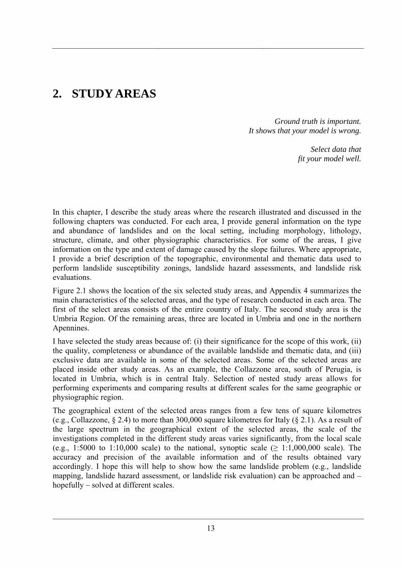
Figure 2.1 shows the location of the six selected study areas, and Appendix 4 summarizes the main characteristics of the selected areas, and the type of research conducted in each area. The first of the select areas consists of the entire country of Italy. The second study area is the Umbria Region. Of the remaining areas, three are located in Umbria and one in the northern Apennines.
I have selected the study areas because of: (i) their significance for the scope of this work, (ii) the quality, completeness or abundance of the available landslide and thematic data, and (iii) exclusive data are available in some of the selected areas. Some of the selected areas are placed inside other study areas. As an example, the Collazzone area, south of Perugia, is located in Umbria, which is in central Italy. Selection of nested study areas allows for performing experiments and comparing results at different scales for the same geographic or physiographic region.
The geographical extent of the selected areas ranges from a few tens of square kilometres (e.g., Collazzone, § 2.4) to more than 300,000 square kilometres for Italy (§ 2.1). As a result of the large spectrum in the geographical extent of the selected areas, the scale of the investigations completed in the different study areas varies significantly, from the local scale (e.g., 1:5000 to 1:10,000 scale) to the national, synoptic scale (≥ 1:1,000,000 scale). The accuracy and precision of the available information and of the results obtained vary accordingly. I hope this will help to show how the same landslide problem (e.g., landslide mapping, landslide hazard assessment, or landslide risk evaluation) can be approached and – hopefully – solved at different scales.
Chapter 2
14
Figure 2.1 – Location of the study areas in Italy.
2.1. Italy
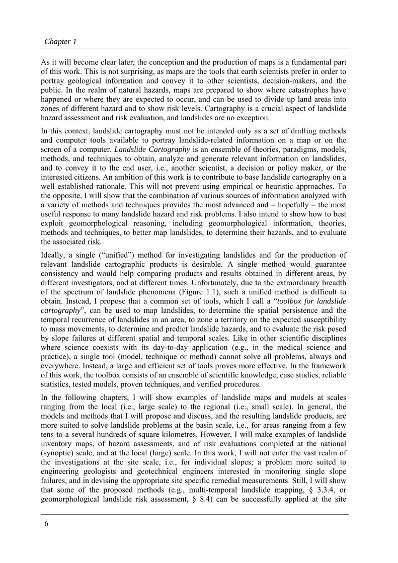
Landslides are abundant and frequent in Italy. Historical information describing landslides in Italy dates back to the Roman Age. Pliny the Elder reported landslides triggered by a large earthquake occurred during the Battle of Trasimeno, in the second Punic War in 264 BC. The societal and economic impact of landslides is high in Italy (Figure 2.2, § 8.3). In the 20th century, a period for which the information is available, the toll amounts to at least 7494 casualties, including 5190 deaths, 88 missing persons and 2216 injured people, and more than 160,000 homeless and evacuated people (Guzzetti et al., 2005c).
Study areas
15
A CB
H
GI
DE
F
A CB
H
GI
DE
F
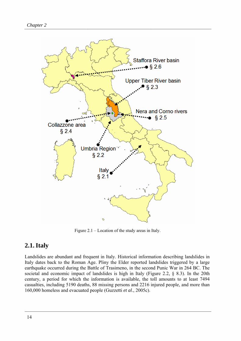
Figure 2.2 – Examples of landslides and landslide damage in Italy. (A) The inundation produced by the Vajont rock slide of 9 Ocotber 1963 on the village of Longarone (source: ANSA, Italy). (B) The
village of Longarone before the inundation. (C) The village of Longarone after the catastrophic inundation. (D) Landslide at Valderchia, Umbria, triggered by heavy rainfall on 6 January 1997. The landslide destroyed 2 houses. (E) and (F) Soil slides and debris flows triggered by intense rainfall in
November 1994 in Piedoment, Northern Italy (source: Casale and Margottini, 1996). (G) The Val Pola rock avalanche, in the Sondrio Province, triggered by heavy rainfall on 28 July 1985 (source: Crosta et
al., 2004). (H) and (I) Rainfall induced landslides and typical landslide damage in Umbria.
Chapter 2
16
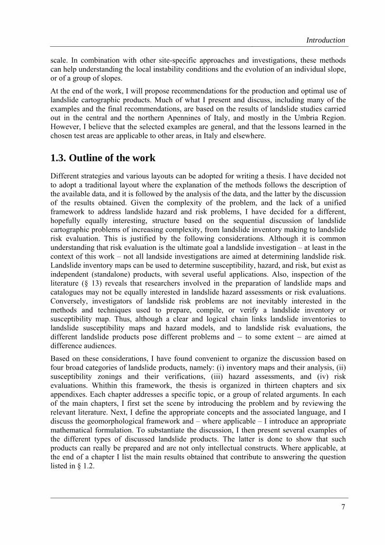
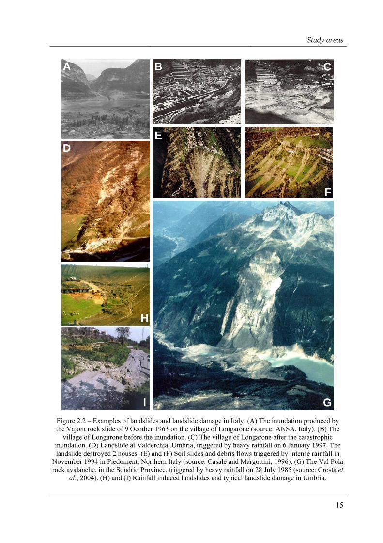
In Italy, regional landslide events can be extremely destructive. The July 1987 catastrophic rainfall in the Southern Alps caused 61 fatalities and produced damage estimated at € 1.2 billion (Guzzetti et al., 1992; 2005c). Single landslides were also extremely costly. The Vajont slide of 9 October 1963 claimed 1917 lives and cost more than € 85 million; the Ancona landslide of 13 December 1982 caused damage estimated at € 1.3 billion; and the damage caused by the Val Pola rock avalanche of 28 July 1987 (§ 2.2.G) was estimated at € 800 million (Catenacci 1992, Alexander 1989). Figure 2.3 summarises the economic damage produced by individual and multiple landslides and flooding events in Italy in the period from 1910 to 2000 (Guzzetti and Tonelli, 2004). Guzzetti et al. (2005c) list 50 major landslide disasters that occurred in Italy from AD 1419 to 2002, and which resulted in 50 or more deaths or missing persons.
Figure 2.3 – Economic damage produced by individual landslides and flooding events in Italy in the
period from 1910 to 2000. Green bars are single landslide events. Blue bars are multiple landslides and flooding events. Modified after Guzzetti and Tonelli (2004).
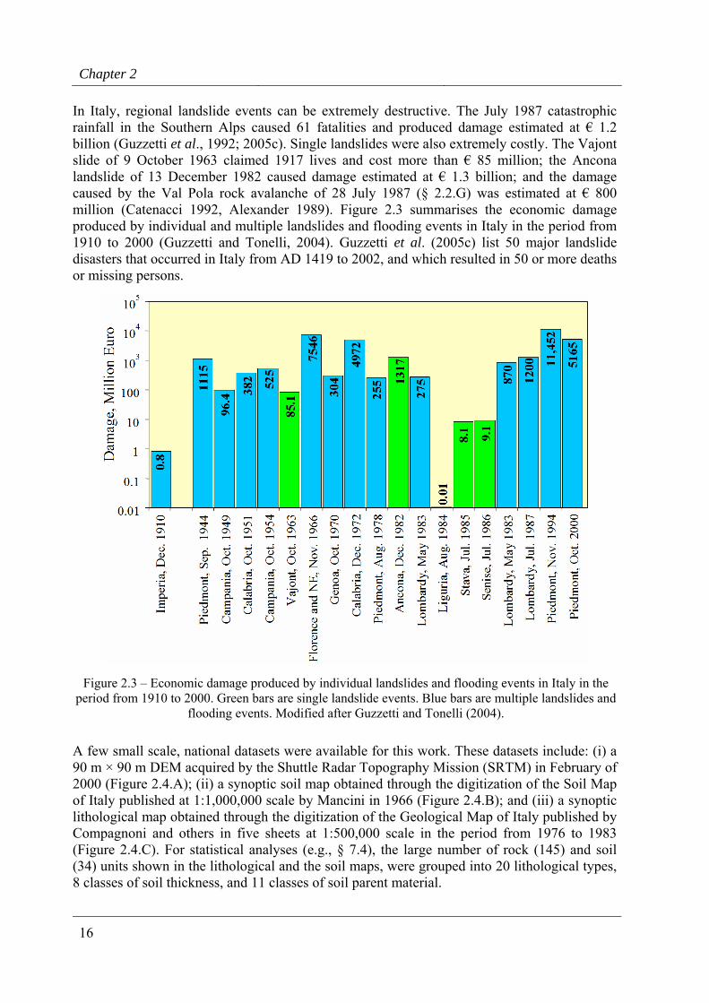
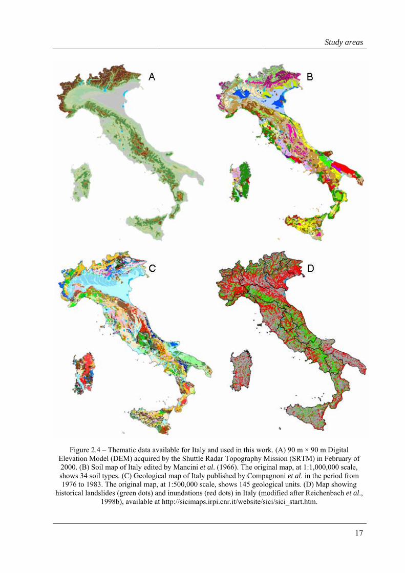
A few small scale, national datasets were available for this work. These datasets include: (i) a 90 m × 90 m DEM acquired by the Shuttle Radar Topography Mission (SRTM) in February of 2000 (Figure 2.4.A); (ii) a synoptic soil map obtained through the digitization of the Soil Map of Italy published at 1:1,000,000 scale by Mancini in 1966 (Figure 2.4.B); and (iii) a synoptic lithological map obtained through the digitization of the Geological Map of Italy published by Compagnoni and others in five sheets at 1:500,000 scale in the period from 1976 to 1983 (Figure 2.4.C). For statistical analyses (e.g., § 7.4), the large number of rock (145) and soil (34) units shown in the lithological and the soil maps, were grouped into 20 lithological types, 8 classes of soil thickness, and 11 classes of soil parent material.
Study areas
17
Figure 2.4 – Thematic data available for Italy and used in this work. (A) 90 m × 90 m Digital Elevation Model (DEM) acquired by the Shuttle Radar Topography Mission (SRTM) in February of 2000. (B) Soil map of Italy edited by Mancini et al. (1966). The original map, at 1:1,000,000 scale, shows 34 soil types. (C) Geological map of Italy published by Compagnoni et al. in the period from 1976 to 1983. The original map, at 1:500,000 scale, shows 145 geological units. (D) Map showing
historical landslides (green dots) and inundations (red dots) in Italy (modified after Reichenbach et al., 1998b), available at http://sicimaps.irpi.cnr.it/website/sici/sici_start.htm.
Chapter 2
18
For Italy, an inventory of historical information on landslides (and floods) was compiled by the National Group of Geo-Hydrological Protection (GNDCI), of the Italian National Research Council (CNR). Guzzetti et al. (1994) described the inventory and showed preliminary applications of the historical information. Guzzetti et al. (1996a) and Reichenbach et al. (1998b) published synoptic maps, at 1:1,200,000 scale, showing the location and abundance of the inventoried historical landslide and flood events in Italy (Figure 2.4.D). Reichenbach et al. (1998a) used the historical information and discharge records at several gauging stations along the Tiber River, to determine regional hydrological thresholds for the occurrence of landslides and inundation events in the Tiber River basin, in central Italy. More recently, Guzzetti and Tonelli (2004) presented a collection of databases containing historical, geographical, damage, hydrological, legislation and bibliographical information on landslides and floods in Italy.
In this work, the archive of historical landslide events in Italy is taken as the prototype of an archive landslide inventory (§ 3.3.1). The archive of historical landslides, in combination with morphological, hydrological, lithological and soil data available at the national scale (Figure 2.4) will be used to determine landslide hazard in Italy (§ 7.4).
For Italy, information exists on the human consequences of various natural hazards, including landslides. Guzzetti (2000) compiled the first catalogue of landslides with human consequences in Italy. Salvati et al. (2003) revised the landslide catalogue and compiled a new catalogue of floods with human consequences in Italy. Guzzetti et al. (2005b) updated the two catalogues prepared by Salvati et al. (2003) to cover the period from 91 BC to 2004, and the period from 1195 to 2004, respectively, and compiled a new catalogue of earthquakes with human consequences in Italy, and a list of volcanic events that resulted in casualties in Italy. Details on the sources of information and on the problems encountered in compiling the catalogues are given in Guzzetti (2000) and Guzzetti et al. (2005b,c).
In this work, the catalogue of landslides with human consequences in Italy will be used to test methods to evaluate the completeness of archive inventories (§ 4.3.1), and to determine levels of societal and individual landslide risk in Italy (§ 8.3.1).
2.2. Umbria Region, central Italy
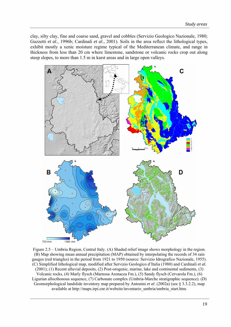
The Umbria Region lays along the Apennines Mountain chain in central Italy, and covers an area of 8456 square kilometres (Figure 2.5.A). In the Region, the territory is hilly and mountainous, with large open valleys striking mostly NW-SE, and deep canyons striking NE-SW. Elevation of the hills and the mountains in the area ranges from 50 m (along the Tiber River valley) to 2436 m (at Monte Vettore, in the Monti Sibillini range). The area is drained by the Tiber River, which flows into the Tyrrhenian Sea. The climate is Mediterranean, with distinct wet and dry seasons. Rainfall occurs mainly from October to December and from March to May, with cumulative annual values ranging from 700 to more than 1300 mm (Figure 2.5.B). Snowfall occurs every year in the mountains and about every five years at lower elevations.
Sedimentary and subordinately volcanic rocks crop out in Umbria. The different rocks and sediments cropping out in the area can be grouped into four major groups, or lithological complexes (Guzzetti et al., 1996b) (Figure 2.5.C) namely: (i) carbonate rocks, comprising layered and massive limestone, cherty limestone and marl, (ii) flysch deposits, comprising layered sandstone, marl, shale and clay, (iii) volcanic rocks, encompassing lava flows, ignimbrites and pyroclasitc deposits, and (iv) marine and continetal sediments made up of
Study areas
19
clay, silty clay, fine and coarse sand, gravel and cobbles (Servizio Geologico Nazionale, 1980; Guzzetti et al., 1996b; Cardinali et al., 2001). Soils in the area reflect the lithological types, exhibit mostly a xenic moisture regime typical of the Mediterranean climate, and range in thickness from less than 20 cm where limestone, sandstone or volcanic rocks crop out along steep slopes, to more than 1.5 m in karst areas and in large open valleys.
Figure 2.5 – Umbria Region, Central Italy. (A) Shaded relief image shows morphology in the region. (B) Map showing mean annual precipitation (MAP) obtained by interpolating the records of 34 rain
gauges (red triangles) in the period from 1921 to 1950 (source: Servizio Idrografico Nazionale, 1955). (C) Simplified lithological map, modified after Servizio Geologico d’Italia (1980) and Cardinali et al.
(2001); (1) Recent alluvial deposits, (2) Post-orogenic, marine, lake and continental sediments, (3) Volcanic rocks, (4) Marly flysch (Marnosa Arenacea Fm.), (5) Sandy flysch (Cervarola Fm.), (6)
Ligurian allocthonous sequence, (7) Carbonate complex (Umbria-Marche stratigraphic sequence). (D) Geomorphological landslide inventory map prepared by Antonini et al. (2002a) (see § 3.3.2.2), map
available at http://maps.irpi.cnr.it/website/inventario_umbria/umbria_start.htm.
Chapter 2
20
Each lithological complex cropping out in Umbria comprises different rock types varying in strength from hard to weak and soft rocks (ISRM, 1978; Deer and Miller, 1966; Cancelli and Casagli, 1995). Hard rocks are layered and massive limestone, cherty limestone, sandstone, pyroclastic deposits, travertine and conglomerate. Weak rocks are marl, rock-shale (Morgenstern and Eigenbrod, 1974), sand, silty clay and stiff over-consolidated clay. Soft rocks are marine and continental clay, silty clay and shale. Rocks are mostly layered and subordinately structurally complex (Esu, 1977). The latter are made up by a regular superposition or a chaotic mixture of two or more lithological components (Morgenstern and Cruden, 1977; D'Elia, 1977; Esu, 1977).
The Umbria region has a complex structural setting resulting from the superposition of two tectonic phases associated to the formation of the Apennines mountain chain. A compressive phase of Miocene to early Pliocene age produced large, east-verging thrusts with associated anticlines, synclines and transcurrent faults, and was followed by an extensional tectonic phase of Pliocene to Holocene age, which produced chiefly sets of normal faults. The region is seismically active and has a long history of earthquakes (Boschi et al., 1998). Based on the available historical record (Boschi et al., 1997), the maximum earthquake intensity in Umbria ranges from 6 to 11 MCS, and the maximum earthquake local magnitude ranges between 4.7 and 6.7. Some of the historical earthquakes are known to have triggered landslides. The oldest reported seismically induced landslide in the area is probably a rockslide at Serravalle del Chienti (in the Marche Region, but close to the Umbria border), triggered by the 30 April 1279 earthquake (Boschi et al., 1998; Antonini et al., 2002b). The most recent seismically induced landslides occurred in the period from September 1997 to April 1998 as a result of the Umbria-Marche earthquake sequence (Antonini et al., 2002b; Bozzano et al., 1998; Esposito et al., 2000).
Due to the lithological, morphological, seismic and climatic setting, landslides are abundant in Umbria (Felicioni et al., 1994; Guzzetti et al., 1996b, 2003a). Landslide abundance and pattern vary largely within each lithological complex that is characterised by a prevalent geomorphological setting and by typical geotechnical and hydrogeological properties (Guzzetti et al., 1996b). Mass movements occur almost every year in the region in response to prolonged or intense rainfall (Guzzetti et al., 2003; Cardinali et al., 2005), rapid snow melting (Cardinali et al., 2005), and earthquake shaking (Antonini et al., 2002b; Bozzano et al., 1998; Esposito et al., 2000). Landslides in Umbria can be very destructive, and have caused damage at several sites (Figure 2.6). In the 20th century a total of 29 people died or were missing and 31 people were injured by slope movements in Umbria in a total of 13 harmful events (Guzzetti et al., 2003; Reichenbach et al., 2005).
Research on slope movements is abundant in Umbria. Landslide inventory maps were compiled by Guzzetti and Cardinali (1989, 1990) (§ 3.3.2.1), Antonini et al. (1993), Cardinali et al. (2001) (§ 2.3), and Antonini et al. (2002a) (§ 3.3.2.2). Such studies revealed that landslides cover about 8% of the territory. Locally, landslide density is much higher, exceeding 20% (Antonini et al., 2002b; Barchi et al., 1993; Carrara et al., 1991, 1995; Cardinali et al., 1994; Galli et al., 2005). Geomorphological relationships between landslide types and pattern, and the morphological, lithological and structural settings were investigated among others by Guzzetti and Cardinali (1992), Barchi et al. (1993), and Cardinali et al. (1994), and were summarized by Guzzetti et al. (1996b). Site-specific, geotechnical investigations on single landslides or landslide sites were conducted at several localities, mostly in urbanised areas (e.g., Crescenti, 1973; Tonnetti, 1978; Diamanti and Soccodato, 1981; Calabresi and Scarpelli, 1984; Lembo-Fazio et al., 1984; Canuti et al., 1986; Cecere and
Study areas
21
Lembo-Fazio, 1986; Righi et al., 1986; Tommasi et al., 1986; Ribacchi et al., 1988; Capocecere et al., 1993; Felicioni et al., 1994). Landslide susceptibility assessments have been completed in test areas and for different landslide types by Carrara et al. (1991, 1995) and by Guzzetti et al. (1999b, 2003b, 2005d). Historical information on the frequency and recurrence of failures in Umbria was compiled by the nation-wide project that archived data on landslides and floods in Italy (Guzzetti et al., 1994; Guzzetti and Tonelli, 2004) (§ 3.3.1.1). This information was recently summarized by Guzzetti et al. (2003a). A reconnaissance estimate of the impact of landslides on the population, the transportation network, and the built-up areas in Umbria was attempted by Guzzetti et al. (2003a). Landslide risk assessments were performed at selected sites by Cardinali et al. (2002b) and by Reichenbach et al. (2005) (§ 8.4).
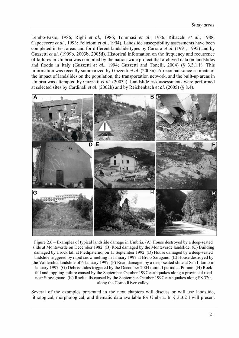
Figure 2.6 – Examples of typical landslide damage in Umbria. (A) House destroyed by a deep-seated slide at Monteverde on December 1982. (B) Road damaged by the Monteverde landslide. (C) Building damaged by a rock fall at Piedipaterno, on 15 September 1992. (D) House damaged by a deep-seated landslide triggered by rapid snow melting in January 1997 at Bivio Saragano. (E) House destroyed by the Valderchia landslide of 6 January 1997. (F) Road damaged by a deep-seated slide at San Litardo in January 1997. (G) Debris slides triggered by the December 2004 rainfall period at Porano. (H) Rock fall and toppling failure caused by the September-October 1997 earthquakes along a provincial road near Stravignano. (K) Rock falls caused by the September-October 1997 earthquakes along SS 320,
along the Corno River valley.
Several of the examples presented in the next chapters will discuss or will use landslide, lithological, morphological, and thematic data available for Umbria. In § 3.3.2 I will present
Chapter 2
22
the geomorphological landslide inventory maps prepared by Guzzetti and Cardinali (1989, 1990) and by Antonini et al. (2002a). In § 3.4.1, the two geomorphological inventories will be compared with a detailed multi-temporal inventory map prepared for the Collazzone area. In § 3.3.3 I will present three recent landslide event inventory maps showing respectively: (i) slope failures triggered by rainfall in the period from the 1937 to 1941 in central Umbria, (ii) landslides triggered by rapid snow melting in January 1997 in Umbria, and (iii) rock falls triggered by the September-October 1997 earthquake sequence in the Umbria-Marche Apennines. In § 8.4 I will illustrate a geomorphological methodology to ascertain landslide risk devised and tested at selected sites in Umbria. Lastly, in § 8.5 I will discuss landslide damage in Umbria, including an attempt to identify areas of potential landslide impact to the built-up areas, the transportation network, and the agriculture.
2.3. Upper Tiber River basin, central Italy
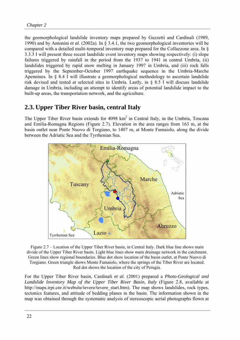
The Upper Tiber River basin extends for 4098 km2 in Central Italy, in the Umbria, Toscana and Emilia-Romagna Regions (Figure 2.7). Elevation in the area ranges from 163 m, at the basin outlet near Ponte Nuovo di Torgiano, to 1407 m, at Monte Fumaiolo, along the divide between the Adriatic Sea and the Tyrrhenian Sea.
Tuscany
Umbria
Emilia-Romagna
Marche
AbruzzoLazioTyrrhenian Sea
AdriaticSea
Tuscany
Umbria
Emilia-Romagna
Marche
AbruzzoLazioTyrrhenian Sea
AdriaticSea
Figure 2.7 – Location of the Upper Tiber River basin, in Central Italy. Dark blue line shows main divide of the Upper Tiber River basin. Light blue lines show main drainage network in the catchment. Green lines show regional boundaries. Blue dot show location of the basin outlet, at Ponte Nuovo di Torgiano. Green triangle shows Monte Fumaiolo, where the springs of the Tiber River are located.
Red dot shows the location of the city of Perugia.
For the Upper Tiber River basin, Cardinali et al. (2001) prepared a Photo-Geological and Landslide Inventory Map of the Upper Tiber River Basin, Italy (Figure 2.8, available at http://maps.irpi.cnr.it/website/tevere/tevere_start.htm). The map shows landslides, rock types, tectonics features, and attitude of bedding planes in the basin. The information shown in the map was obtained through the systematic analysis of stereoscopic aerial photographs flown at
Study areas
23
1:33,000 scale and, limited to the outcrop of lake sediments and recent alluvial deposits, at 1:13,000 scale. Interpretation of the aerial photographs was aided by field surveys at the 1:10,000 scale, and by review of bibliographical data. In the photo-geological map, the rocks that crop out in the catchment are subdivided into 37 lithological units based upon the percentage of hard vs. soft rocks, as ascertained from photo-geological interpretation, field surveys, existing geological maps and other bibliographical data. Bedding plane domains were defined on the basis of photo-geological criteria as areas where the bedding plane attitude appeared to be constant. Within each bedding domain, the attitude of bedding planes was ascertained by comparing the bedding setting with the attitude of the local slope. Bedding dip, in eight classes, was estimated by comparing the local slope of terrain with bedding attitude in areas where bedding planes dipped towards the free face of the slope (Cardinali et al., 2001).
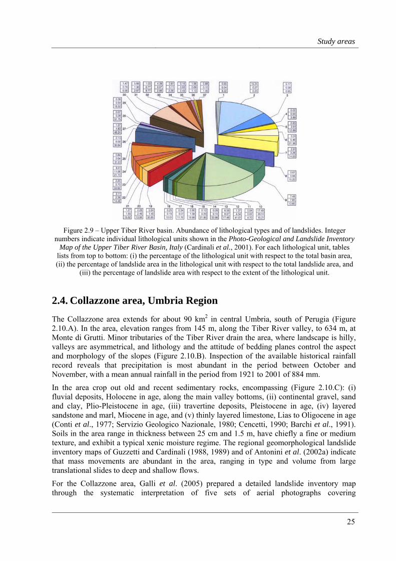
The landslide inventory map for the Upper Tiber River basin shows more than 17,000 landslides, mostly deep seated and shallow slides and debris flows (Cardinali et al., 2001). Deep seated landslides are chiefly translational and more rarely rotational slide, flow, slide earth-flow, complex and compound movements. The area of the deep seated landslides ranges from less than one hectare to more than one square kilometre. Landslides in this class mainly develop along sedimentary or tectonic discontinuities and are mostly dormant, but reactivations are present. Shallow landslides are slumps, earth flows and rotational or translational slides, locally exhibiting a flow component at the toe. Shallow failures mainly involve the colluvial cover and are mostly dormant, but recent, active and seasonal movements are locally present. Shallow landslides are particularly abundant on deep seated landslide deposits, where they occur as minor reactivations. Large debris flow deposits, consisting chiefly of granular materials, are deposited mostly along mountain streams and are most abundant where carbonate rocks crop out. Figure 2.9 shows the abundance of landslides in the 37 lithological units cropping out in the Upper Tiber River basin.
Next, Cardinali et al. (2002b) prepared a Landslide Hazard Map of the Upper Tiber River Basin, Italy (also available at http://maps.irpi.cnr.it/website/tevere/tevere_start.htm), showing landslide susceptibility in the catchment. I will discuss the statistical model constructed to obtain the susceptibility map in § 6.4, as an example of a landslide susceptibility zoning for a large area. The statistical model prepared to ascertain landslide susceptibility in the Upper Tiber River basin will be based upon a considerably large set of geo-environmental factors, including morphology, hydrology, lithology, structure, bedding attitude, and land use. Information on landslides, lithology, structure and attitude of bedding plane was obtained from the photo-geological and landslide inventory map of Cardinali et al. (2001). Morphometric and hydrological information was obtained from a DEM with a ground resolution of 25 m × 25 m. The digital terrain model was obtained from elevation information shown on topographic base maps published by the Italian Military Geographic Institute at 1:25,000 scale. Land use information was obtained through compilation in a GIS of land use maps published at 1:10,000 and 1:25,000 scale for the Umbria, Toscana and Emilia-Romagna Regions. Since the original land use maps had different legends, listing from 12 to more than 30 classes, merging of the land use classes was necessary. When merging the classes, care was taken in retaining information known or considered to be useful for explaining the presence or absence of landslides, their spatial distribution and abundance. Hence, forested areas were kept separated from re-forested terrain, and cultivated land was kept distinct from abandoned terrains. However, land use parcels showing woods with different tree species were merged, as were land parcels showing different types of specialized cultivations (e.g., vineyards, olive grows, fruit grows, etc.).
Chapter 2
24
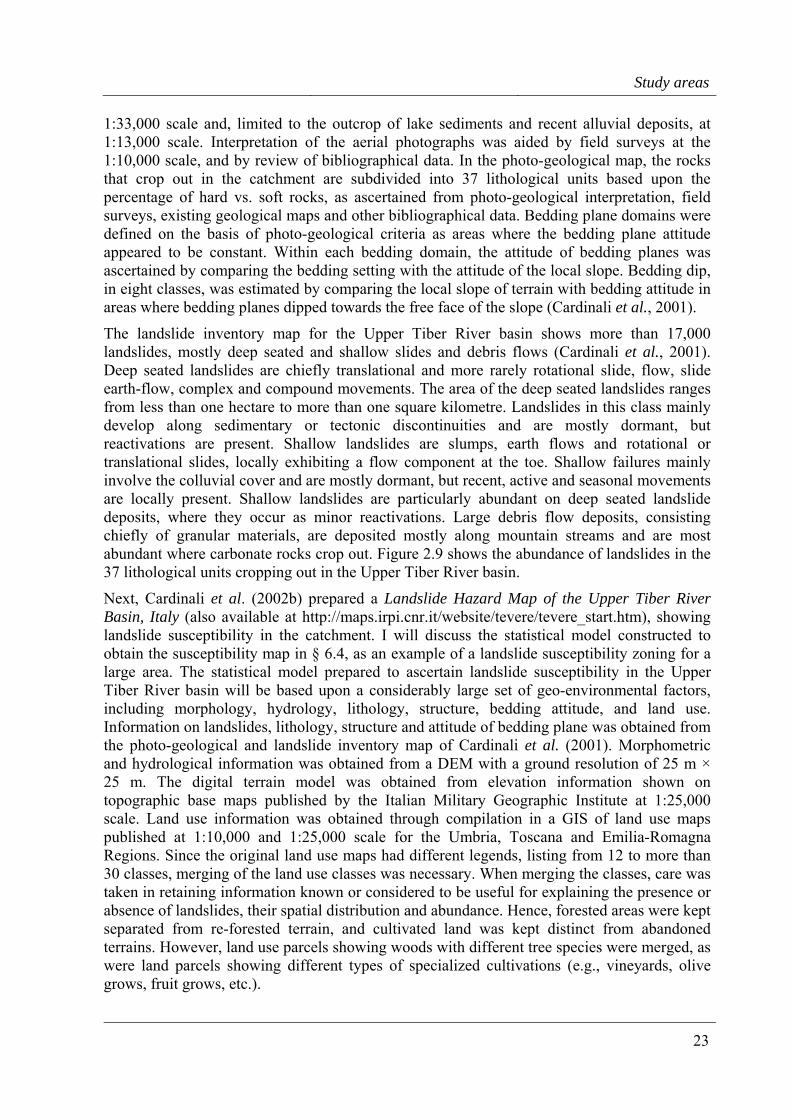
Figure 2.8 – Upper Tiber River basin. Upper map shows the Photo-Geological and Landslide Inventory Map of the Upper Tiber River Basin, Italy of Cardinali et al. (2001), available at
http://maps.irpi.cnr.it/website/tevere/tevere_start.htm. Red line shows location of lower map. Blue line shows Figure 2.9. Lower map is an enlargement of a portion of the upper map showing cartographic
detail. Colours show different rock types. Deep seated landslides are shown in pink. Shallow landslides are shown in violet.
Study areas
25
Figure 2.9 – Upper Tiber River basin. Abundance of lithological types and of landslides. Integer numbers indicate individual lithological units shown in the Photo-Geological and Landslide Inventory
Map of the Upper Tiber River Basin, Italy (Cardinali et al., 2001). For each lithological unit, tables lists from top to bottom: (i) the percentage of the lithological unit with respect to the total basin area, (ii) the percentage of landslide area in the lithological unit with respect to the total landslide area, and
(iii) the percentage of landslide area with respect to the extent of the lithological unit.
2.4. Collazzone area, Umbria Region
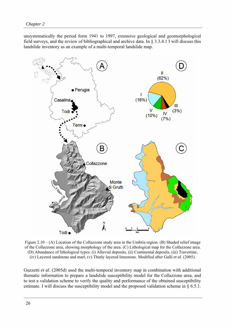
The Collazzone area extends for about 90 km2 in central Umbria, south of Perugia (Figure 2.10.A). In the area, elevation ranges from 145 m, along the Tiber River valley, to 634 m, at Monte di Grutti. Minor tributaries of the Tiber River drain the area, where landscape is hilly, valleys are asymmetrical, and lithology and the attitude of bedding planes control the aspect and morphology of the slopes (Figure 2.10.B). Inspection of the available historical rainfall record reveals that precipitation is most abundant in the period between October and November, with a mean annual rainfall in the period from 1921 to 2001 of 884 mm.
In the area crop out old and recent sedimentary rocks, encompassing (Figure 2.10.C): (i) fluvial deposits, Holocene in age, along the main valley bottoms, (ii) continental gravel, sand and clay, Plio-Pleistocene in age, (iii) travertine deposits, Pleistocene in age, (iv) layered sandstone and marl, Miocene in age, and (v) thinly layered limestone, Lias to Oligocene in age (Conti et al., 1977; Servizio Geologico Nazionale, 1980; Cencetti, 1990; Barchi et al., 1991). Soils in the area range in thickness between 25 cm and 1.5 m, have chiefly a fine or medium texture, and exhibit a typical xenic moisture regime. The regional geomorphological landslide inventory maps of Guzzetti and Cardinali (1988, 1989) and of Antonini et al. (2002a) indicate that mass movements are abundant in the area, ranging in type and volume from large translational slides to deep and shallow flows.
For the Collazzone area, Galli et al. (2005) prepared a detailed landslide inventory map through the systematic interpretation of five sets of aerial photographs covering
Chapter 2
26
unsystematically the period form 1941 to 1997, extensive geological and geomorphological field surveys, and the review of bibliographical and archive data. In § 3.3.4.1 I will discuss this landslide inventory as an example of a multi-temporal landslide map.
Figure 2.10 – (A) Location of the Collazzone study area in the Umbria region. (B) Shaded relief image of the Collazzone area, showing morphology of the area. (C) Lithological map for the Collazzone area.
(D) Abundance of lithological types: (i) Alluvial deposits, (ii) Continental deposits, (iii) Travertine, (iv) Layered sandstone and marl, (v) Thinly layered limestone. Modified after Galli et al. (2005).
Guzzetti et al. (2005d) used the multi-temporal inventory map in combination with additional thematic information to prepare a landslide susceptibility model for the Collazzone area, and to test a validation scheme to verify the quality and performance of the obtained susceptibility estimate. I will discuss the susceptibility model and the proposed validation scheme in § 6.5.1.
Study areas
27
The thematic information used to ascertain landslide susceptibility in the Collazzone area includes morphological, hydrological, lithological, structural, bedding attitude, and land use data. Morphological and hydrological information was obtained from a 10 m × 10 m DEM, prepared by interpolating 10 and 5 meter interval contour lines obtained from 1:10,000 scale topographic maps. Lithological and structural maps, at 1:10,000 scale, were prepared by Galli et al. (2005) through detailed field surveys aided by the interpretation of aerial photographs at various scales. Bedding plane domains were defined on the basis of the same photo-geological criteria adopted to prepare the Photo-Geological and Landslide Inventory Map of the Upper Tiber River Basin, Italy (Cardinali et al., 2001). Information on land use was obtained from a land use map compiled in 1977 by the Umbria Regional Government, and was locally revised by Guzzetti et al. (2005d) who interpreted recent aerial photographs, flown in April 1997 at 1:20,000 scale.
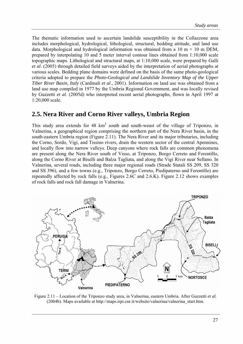
2.5. Nera River and Corno River valleys, Umbria Region
This study area extends for 48 km2 south and south-weast of the village of Triponzo, in Valnerina, a geographical region comprising the northern part of the Nera River basin, in the south-eastern Umbria region (Figure 2.11). The Nera River and its major tributaries, including the Corno, Sordo, Vigi, and Tissino rivers, drain the western sector of the central Apennines, and locally flow into narrow valleys. Deep canyons where rock falls are common phenomena are present along the Nera River south of Visso, at Triponzo, Borgo Cerreto and Ferentillo, along the Corno River at Biselli and Balza Tagliata, and along the Vigi River near Sellano. In Valnerina, several roads, including three major regional roads (Strade Statali SS 209, SS 320 and SS 396), and a few towns (e.g., Triponzo, Borgo Cerreto, Piedipaterno and Ferentillo) are repeatedly affected by rock falls (e.g., Figures 2.6C and 2.6.K). Figure 2.12 shows examples of rock falls and rock fall damage in Valnerina.
Figure 2.11 – Location of the Triponzo study area, in Valnerina, eastern Umbria. After Guzzetti et al. (2004b). Maps available at http://maps.irpi.cnr.it/website/valnerina/valnerina_start.htm.
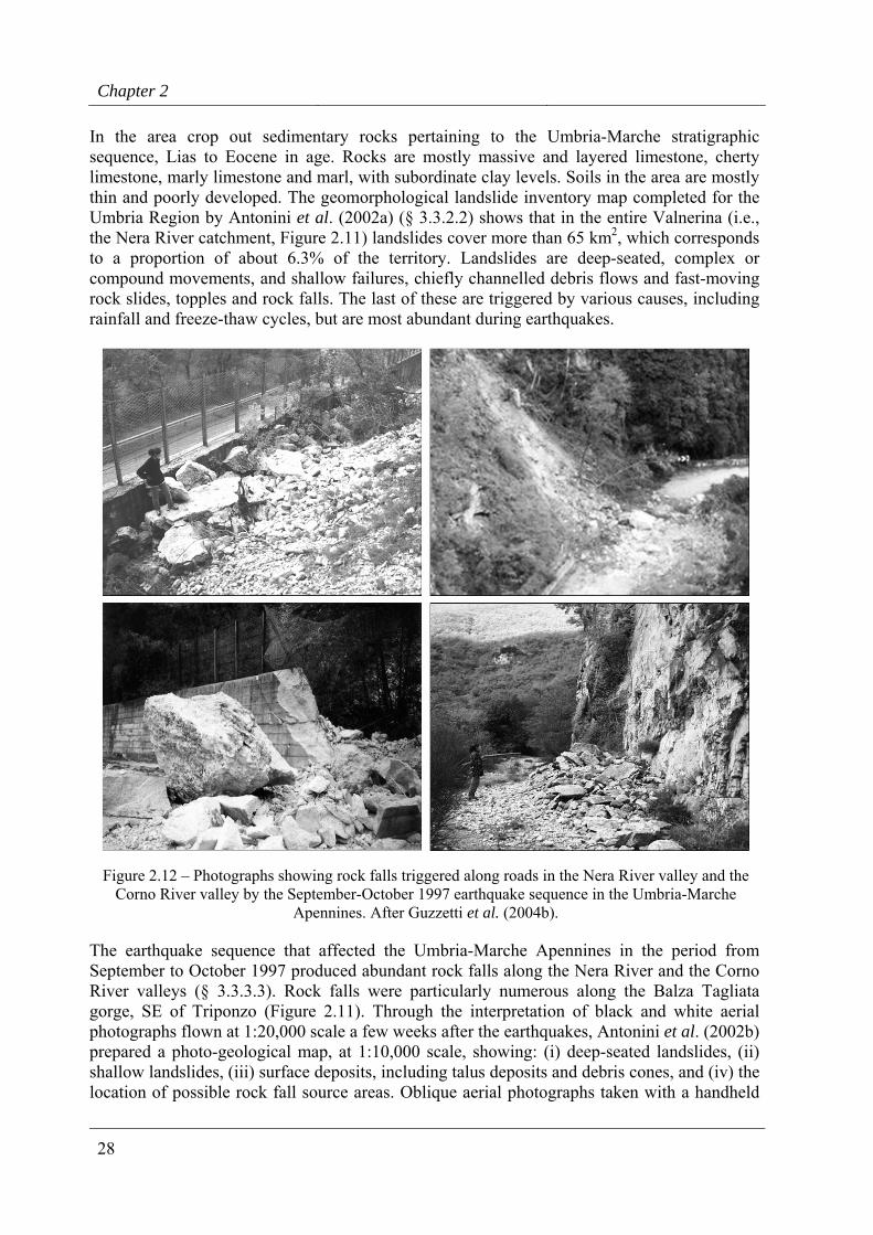
Chapter 2
28
In the area crop out sedimentary rocks pertaining to the Umbria-Marche stratigraphic sequence, Lias to Eocene in age. Rocks are mostly massive and layered limestone, cherty limestone, marly limestone and marl, with subordinate clay levels. Soils in the area are mostly thin and poorly developed. The geomorphological landslide inventory map completed for the Umbria Region by Antonini et al. (2002a) (§ 3.3.2.2) shows that in the entire Valnerina (i.e., the Nera River catchment, Figure 2.11) landslides cover more than 65 km2, which corresponds to a proportion of about 6.3% of the territory. Landslides are deep-seated, complex or compound movements, and shallow failures, chiefly channelled debris flows and fast-moving rock slides, topples and rock falls. The last of these are triggered by various causes, including rainfall and freeze-thaw cycles, but are most abundant during earthquakes.
Figure 2.12 – Photographs showing rock falls triggered along roads in the Nera River valley and the
Corno River valley by the September-October 1997 earthquake sequence in the Umbria-Marche Apennines. After Guzzetti et al. (2004b).
The earthquake sequence that affected the Umbria-Marche Apennines in the period from September to October 1997 produced abundant rock falls along the Nera River and the Corno River valleys (§ 3.3.3.3). Rock falls were particularly numerous along the Balza Tagliata gorge, SE of Triponzo (Figure 2.11). Through the interpretation of black and white aerial photographs flown at 1:20,000 scale a few weeks after the earthquakes, Antonini et al. (2002b) prepared a photo-geological map, at 1:10,000 scale, showing: (i) deep-seated landslides, (ii) shallow landslides, (iii) surface deposits, including talus deposits and debris cones, and (iv) the location of possible rock fall source areas. Oblique aerial photographs taken with a handheld
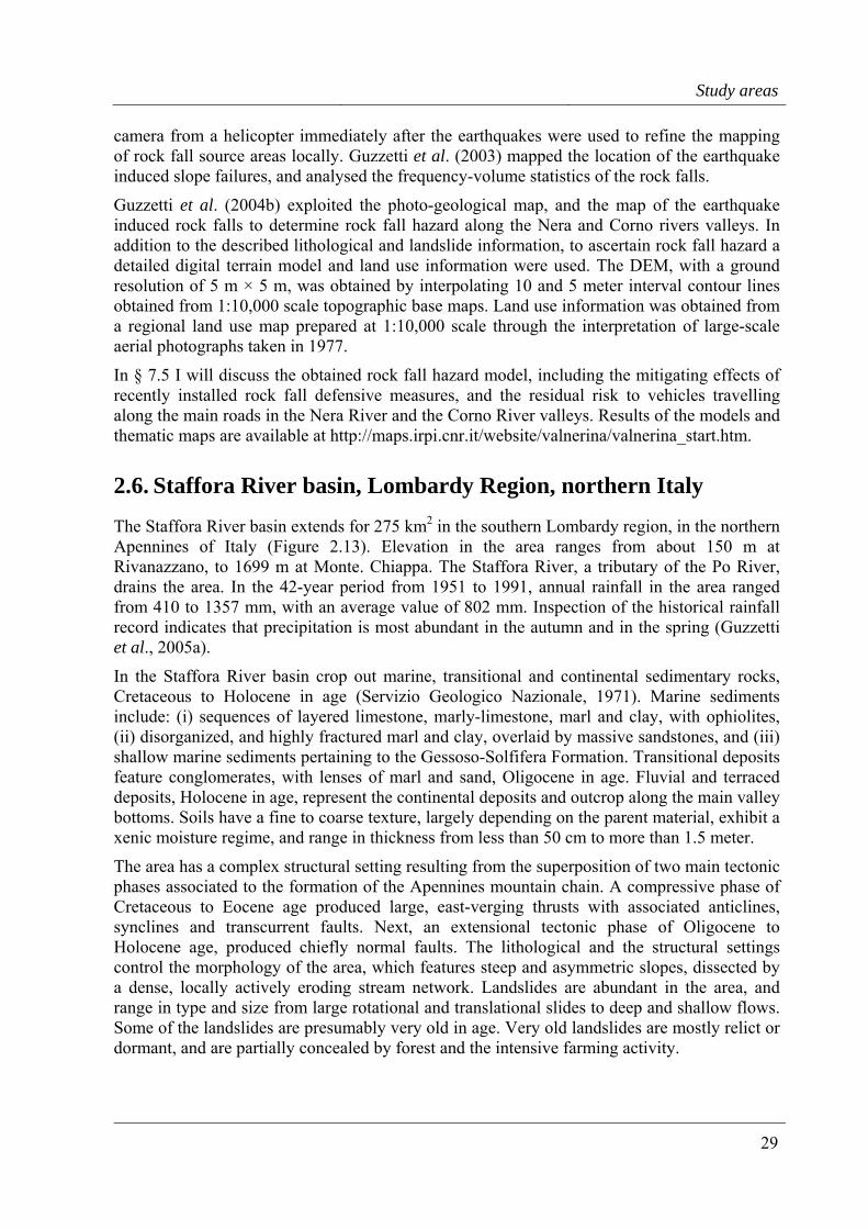
Study areas
29
camera from a helicopter immediately after the earthquakes were used to refine the mapping of rock fall source areas locally. Guzzetti et al. (2003) mapped the location of the earthquake induced slope failures, and analysed the frequency-volume statistics of the rock falls.
Guzzetti et al. (2004b) exploited the photo-geological map, and the map of the earthquake induced rock falls to determine rock fall hazard along the Nera and Corno rivers valleys. In addition to the described lithological and landslide information, to ascertain rock fall hazard a detailed digital terrain model and land use information were used. The DEM, with a ground resolution of 5 m × 5 m, was obtained by interpolating 10 and 5 meter interval contour lines obtained from 1:10,000 scale topographic base maps. Land use information was obtained from a regional land use map prepared at 1:10,000 scale through the interpretation of large-scale aerial photographs taken in 1977.
In § 7.5 I will discuss the obtained rock fall hazard model, including the mitigating effects of recently installed rock fall defensive measures, and the residual risk to vehicles travelling along the main roads in the Nera River and the Corno River valleys. Results of the models and thematic maps are available at http://maps.irpi.cnr.it/website/valnerina/valnerina_start.htm.
2.6. Staffora River basin, Lombardy Region, northern Italy
The Staffora River basin extends for 275 km2 in the southern Lombardy region, in the northern Apennines of Italy (Figure 2.13). Elevation in the area ranges from about 150 m at Rivanazzano, to 1699 m at Monte. Chiappa. The Staffora River, a tributary of the Po River, drains the area. In the 42-year period from 1951 to 1991, annual rainfall in the area ranged from 410 to 1357 mm, with an average value of 802 mm. Inspection of the historical rainfall record indicates that precipitation is most abundant in the autumn and in the spring (Guzzetti et al., 2005a).
In the Staffora River basin crop out marine, transitional and continental sedimentary rocks, Cretaceous to Holocene in age (Servizio Geologico Nazionale, 1971). Marine sediments include: (i) sequences of layered limestone, marly-limestone, marl and clay, with ophiolites, (ii) disorganized, and highly fractured marl and clay, overlaid by massive sandstones, and (iii) shallow marine sediments pertaining to the Gessoso-Solfifera Formation. Transitional deposits feature conglomerates, with lenses of marl and sand, Oligocene in age. Fluvial and terraced deposits, Holocene in age, represent the continental deposits and outcrop along the main valley bottoms. Soils have a fine to coarse texture, largely depending on the parent material, exhibit a xenic moisture regime, and range in thickness from less than 50 cm to more than 1.5 meter.
The area has a complex structural setting resulting from the superposition of two main tectonic phases associated to the formation of the Apennines mountain chain. A compressive phase of Cretaceous to Eocene age produced large, east-verging thrusts with associated anticlines, synclines and transcurrent faults. Next, an extensional tectonic phase of Oligocene to Holocene age, produced chiefly normal faults. The lithological and the structural settings control the morphology of the area, which features steep and asymmetric slopes, dissected by a dense, locally actively eroding stream network. Landslides are abundant in the area, and range in type and size from large rotational and translational slides to deep and shallow flows. Some of the landslides are presumably very old in age. Very old landslides are mostly relict or dormant, and are partially concealed by forest and the intensive farming activity.
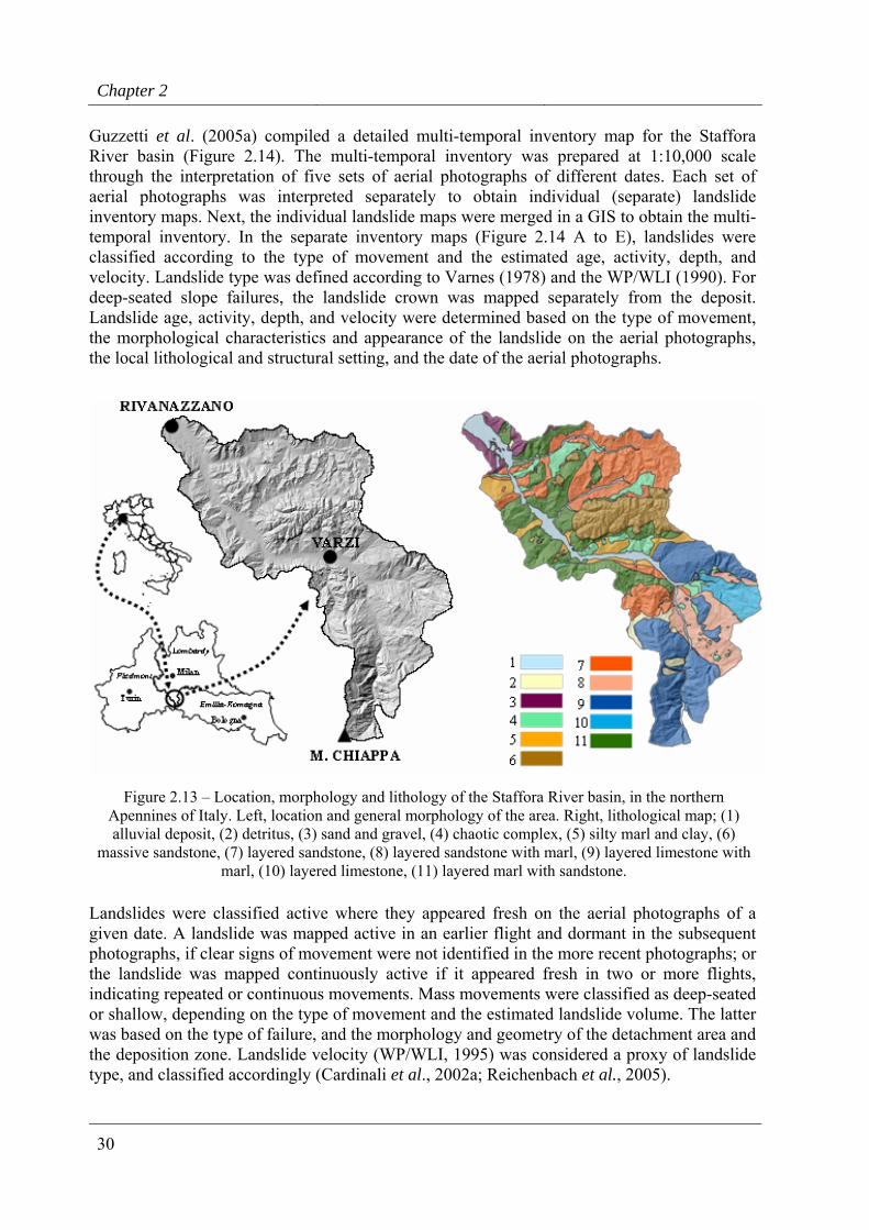
Chapter 2
30
Guzzetti et al. (2005a) compiled a detailed multi-temporal inventory map for the Staffora River basin (Figure 2.14). The multi-temporal inventory was prepared at 1:10,000 scale through the interpretation of five sets of aerial photographs of different dates. Each set of aerial photographs was interpreted separately to obtain individual (separate) landslide inventory maps. Next, the individual landslide maps were merged in a GIS to obtain the multi-temporal inventory. In the separate inventory maps (Figure 2.14 A to E), landslides were classified according to the type of movement and the estimated age, activity, depth, and velocity. Landslide type was defined according to Varnes (1978) and the WP/WLI (1990). For deep-seated slope failures, the landslide crown was mapped separately from the deposit. Landslide age, activity, depth, and velocity were determined based on the type of movement, the morphological characteristics and appearance of the landslide on the aerial photographs, the local lithological and structural setting, and the date of the aerial photographs.
Figure 2.13 – Location, morphology and lithology of the Staffora River basin, in the northern Apennines of Italy. Left, location and general morphology of the area. Right, lithological map; (1) alluvial deposit, (2) detritus, (3) sand and gravel, (4) chaotic complex, (5) silty marl and clay, (6)
massive sandstone, (7) layered sandstone, (8) layered sandstone with marl, (9) layered limestone with marl, (10) layered limestone, (11) layered marl with sandstone.
Landslides were classified active where they appeared fresh on the aerial photographs of a given date. A landslide was mapped active in an earlier flight and dormant in the subsequent photographs, if clear signs of movement were not identified in the more recent photographs; or the landslide was mapped continuously active if it appeared fresh in two or more flights, indicating repeated or continuous movements. Mass movements were classified as deep-seated or shallow, depending on the type of movement and the estimated landslide volume. The latter was based on the type of failure, and the morphology and geometry of the detachment area and the deposition zone. Landslide velocity (WP/WLI, 1995) was considered a proxy of landslide type, and classified accordingly (Cardinali et al., 2002a; Reichenbach et al., 2005).
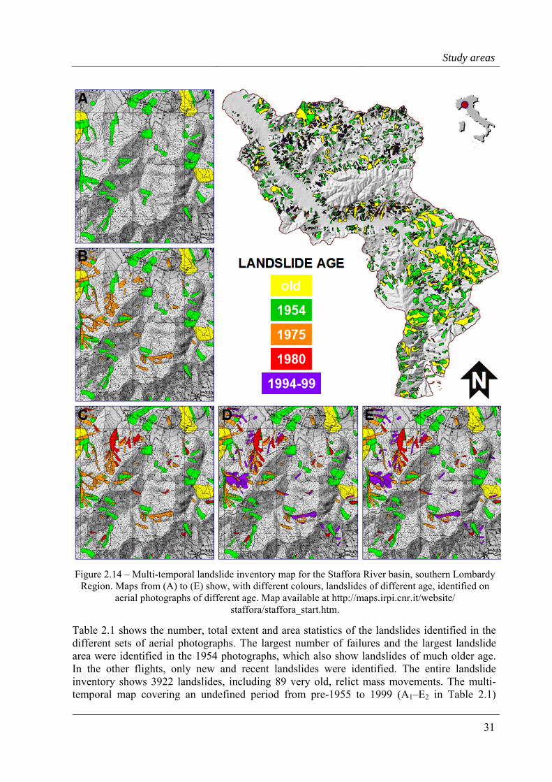
Study areas
31
Figure 2.14 – Multi-temporal landslide inventory map for the Staffora River basin, southern Lombardy Region. Maps from (A) to (E) show, with different colours, landslides of different age, identified on
aerial photographs of different age. Map available at http://maps.irpi.cnr.it/website/ staffora/staffora_start.htm.
Table 2.1 shows the number, total extent and area statistics of the landslides identified in the different sets of aerial photographs. The largest number of failures and the largest landslide area were identified in the 1954 photographs, which also show landslides of much older age. In the other flights, only new and recent landslides were identified. The entire landslide inventory shows 3922 landslides, including 89 very old, relict mass movements. The multi-temporal map covering an undefined period from pre-1955 to 1999 (A1–E2 in Table 2.1)
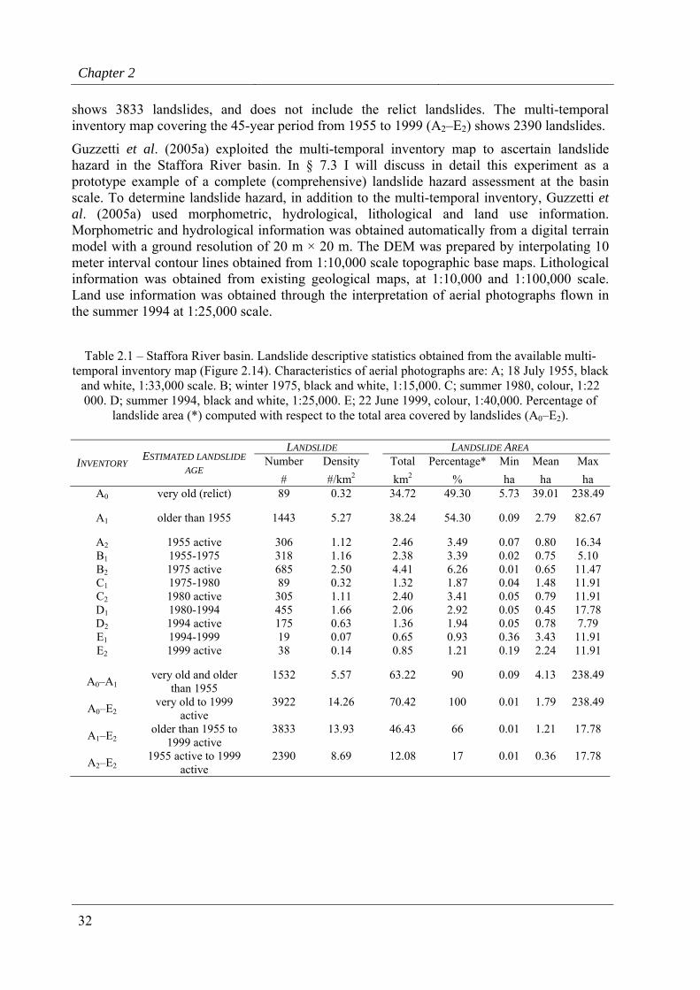
Chapter 2
32
shows 3833 landslides, and does not include the relict landslides. The multi-temporal inventory map covering the 45-year period from 1955 to 1999 (A2–E2) shows 2390 landslides.
Guzzetti et al. (2005a) exploited the multi-temporal inventory map to ascertain landslide hazard in the Staffora River basin. In § 7.3 I will discuss in detail this experiment as a prototype example of a complete (comprehensive) landslide hazard assessment at the basin scale. To determine landslide hazard, in addition to the multi-temporal inventory, Guzzetti et al. (2005a) used morphometric, hydrological, lithological and land use information. Morphometric and hydrological information was obtained automatically from a digital terrain model with a ground resolution of 20 m × 20 m. The DEM was prepared by interpolating 10 meter interval contour lines obtained from 1:10,000 scale topographic base maps. Lithological information was obtained from existing geological maps, at 1:10,000 and 1:100,000 scale. Land use information was obtained through the interpretation of aerial photographs flown in the summer 1994 at 1:25,000 scale.
Table 2.1 – Staffora River basin. Landslide descriptive statistics obtained from the available multi-temporal inventory map (Figure 2.14). Characteristics of aerial photographs are: A; 18 July 1955, black
and white, 1:33,000 scale. B; winter 1975, black and white, 1:15,000. C; summer 1980, colour, 1:22 000. D; summer 1994, black and white, 1:25,000. E; 22 June 1999, colour, 1:40,000. Percentage of
landslide area (*) computed with respect to the total area covered by landslides (A0–E2).
LANDSLIDE LANDSLIDE AREA Number Density Total Percentage* Min Mean Max INVENTORY ESTIMATED LANDSLIDE
AGE # #/km2 km2 % ha ha ha
A0 very old (relict) 89 0.32 34.72 49.30 5.73 39.01 238.49
A1 older than 1955 1443 5.27 38.24 54.30 0.09 2.79 82.67
A2 1955 active 306 1.12 2.46 3.49 0.07 0.80 16.34 B1 1955-1975 318 1.16 2.38 3.39 0.02 0.75 5.10 B2 1975 active 685 2.50 4.41 6.26 0.01 0.65 11.47 C1 1975-1980 89 0.32 1.32 1.87 0.04 1.48 11.91 C2 1980 active 305 1.11 2.40 3.41 0.05 0.79 11.91 D1 1980-1994 455 1.66 2.06 2.92 0.05 0.45 17.78 D2 1994 active 175 0.63 1.36 1.94 0.05 0.78 7.79 E1 1994-1999 19 0.07 0.65 0.93 0.36 3.43 11.91 E2 1999 active 38 0.14 0.85 1.21 0.19 2.24 11.91
A0–A1 very old and older
than 1955 1532 5.57 63.22 90 0.09 4.13 238.49
A0–E2 very old to 1999
active 3922 14.26 70.42 100 0.01 1.79 238.49
A1–E2 older than 1955 to
1999 active 3833 13.93 46.43 66 0.01 1.21 17.78
A2–E2 1955 active to 1999
active 2390 8.69 12.08 17 0.01 0.36 17.78
33
3. LANDSLIDE MAPPING
When you don’t know what you are doing, do it with great precision.
If your data are imprecise,
draw a thick line.
Any serious attempt at ascertaining landslide hazard or at evaluating landslide risk must begin with the collection of information on where landslides are located. This is the goal of landslide mapping. The simplest form of landslide mapping is a landslide inventory, which records the location and, where known, the date of occurrence and types of landslides that have left discernable traces in an area (Hansen, 1984; McCalpin, 1984; Wieczorek, 1984). Inventory maps can be prepared by different techniques, depending on their scope, the extent of the study area, the scales of base maps and aerial photographs, the quality and detail of the accessible information, and the resources available to carry out the work (Guzzetti et al., 2000).
In this chapter, I first critically discuss the various types of landslide inventories and the methods and techniques used to prepare them. Then, I present landslide inventories of different types and scales prepared for Italy, the Umbria Region, and for selected areas in the Umbria Region, including the Collazzone area.
3.1. Theoretical framework
Before discussing the various types of landslide inventories, it is useful to attempt to establish the rationale for a landslide inventory. A landslide inventory depends on the following widely accepted assumptions (Radbruch-Hall and Varnes, 1976; Varnes et al., 1984; Carrara et al., 1991; Hutchinson and Chandler, 1991; Hutchinson, 1995; Dikau et al., 1996; Turner and Schuster, 1996; Guzzetti et al., 1999a):
(a) Landslides leave discernible signs, most of which can be recognized, classified and mapped in the field or from stereoscopic aerial photographs (Rib and Liang, 1978; Varnes, 1978; Hansen, 1984; Hutchinson, 1988; Turner and Schuster, 1996). Most of the signs left by a landslide are morphological, i.e., they refer to changes in the form, position or appearance of the topographic surface. Other signs induced by a slope failure may reflect lithological, geological, land use, or other types of surface or sub-surface changes. If a landslide does not produce identifiable (i.e., observable, measurable) changes the mass movement cannot be recognized and mapped, in the field or by using remotely obtained images.
Chapter 3
34
(b) The morphological signature of a landslide (Pike, 1988) depends on the type (i.e., fall, flow, slide, complex, compound) and the rate of movement of the slope failure (Pašek, 1975; Varnes, 1978; Hansen, 1984; Hutchinson, 1988; Cruden and Varnes, 1996; Dikau et al., 1996). In general, the same type of landslide will result in a similar signature. The morphological signature left by a landslide can be interpreted to determine the extent of the slope failure and to infer the type of movement. From the appearance of a landslide, an expert can also infer qualitative information on the degree of activity, age, and depth of the slope failure. Since morphological converge is possible and the same morphological signs may result from different processes, care must be taken when inferring landslide information from, e.g., aerial photographs.
(c) Landslides do not occur randomly or by chance. Slope failures are the result of the interplay of physical processes, and landsliding is controlled by mechanical laws that can be determined empirically, statistically or in deterministic fashion (Hutchinson, 1988; Crozier, 1986; Dietrich et al., 1995). It follows that knowledge on landslides can be generalized (Aleotti and Chowdhury, 1999; Guzzetti et al., 1999a).
(d) For landslides we can adopt the well known principle, which follows from uniformitarianism (Lyell, 1833), that the past and present are keys to the future (Varnes et al., 1984; Carrara et al., 1991; Hutchinson, 1995; Aleotti and Chowdhury, 1999; Guzzetti et al., 1999). The principle implies that slope failures in the future will be more likely to occur under the conditions which led to past and present instability. Mapping recent slope failures is important to understand the geographical distribution and arrangement of past landslides, and landslide inventory maps are fundamental information to help forecast the future occurrence of landslides.
Ideally, identification and mapping of landslides should derive from all of these assumptions. Failure to comply with them limits the applicability of inventory maps and their derivative products (i.e., susceptibility, hazard or risk assessments) regardless of the methodology used or the goal of the investigation. Unfortunately, satisfactory application of all of these principles proves difficult, both operationally and conceptually (Guzzetti et al., 1999a).
3.2. Landslide recognition
Landslides can be identified and mapped using a variety of techniques and tools, including: (i) geomorphological field mapping (Brunsden, 1985; 1993), (ii) interpretation of vertical or oblique stereoscopic aerial photographs (air photo interpretation, API) (Rib and Liang, 1978; Turner and Schuster, 1996), (iii) surface and sub-surface monitoring (Petley, 1984; Franklin, 1984), and (iv) innovative remote sensing technologies (Mantovani et al., 1996; IGOS Geohazards, 2003; Singhroy, 2005), such as the interpretation of synthetic aperture radar (SAR) images (e.g., Czuchlewski et al., 2003; Hilley et al., 2004; Catani et al., 2005; CENR/IWGEO, 2005; Singhroy, 2005), the interpretation of high resolution multispectral images (Zinck et al., 2001; Cheng et al., 2004), or the analysis of high quality DEMs obtained from space or airborne sensors (Kääb, 2002; McKean and Roering, 2003; Catani et al., 2005). Historical analysis of archives, chronicles, and newspapers has also been used to identify landslide events, to compile landslide catalogues, and to prepare landslide maps (e.g., Reichenbach et al., 1998; Salvati et al., 2003).
Traditionally, visual interpretation of stereoscopic aerial photographs has been the most widely adopted method to identify and map landslides (Rib and Liang, 1978; Turner and
Landslide mapping
35
Schuster, 1996). Interpretation of aerial photographs proves particularly convenient to map landslides because:
(a) A trained investigator can readily recognize and map a landslide on the aerial photographs, aided by the vertical exaggeration introduced by the stereoscopic vision. The vertical exaggeration amplifies the morphological appearance of the terrain, reveals subtle morphological (topographical) changes, and facilitates the recognition and the interpretation of the topographic signature typical of a landslide (Rib and Liang, 1978; Pike, 1988).
(b) National and local governments, geological surveys, environmental and protection agencies, research organizations and private companies have long obtained stereoscopic aerial photographs for a variety of purposes. In most places these aerial photographs are available and can be used for geomorphological studies including the compilation of landslide inventory maps. The availability of multiple sets of aerial photographs for the same area (e.g., Figure 3.1) allows investigating the temporal and the geographical evolution of slope failures (Guzzetti et al., 2005a,d).
(c) For a trained geomorphologist, interpretation of the aerial photographs is an intuitive process that does not require sophisticated technological skills. The technology and tools needed to interpret aerial photographs are simple (e.g., a stereoscope) and inexpensive, if compared to other monitoring or landslide detection methods. Information obtained from the aerial photographs can be readily transferred to paper maps or stored in computer systems.
(d) The size (on average 21 cm × 21 cm) and scale (from 1:5000 to 1:70,000) of the aerial photographs allows for the coverage of large territories with a reasonable number of photographs. Most important, the typical size of a landslide (i.e., from a few tens to several hundred meter in length or width) fits well inside a single pair of stereoscopic aerial photographs, allowing the interpreter to work conveniently. The side and lateral overlaps typical of stereoscopic aerial photographs allow the interpreter to find (most of the time) a suitable combination of photographs to best identify and map the landslides.
(e) The resolution of the available optical aerial photographs remains unmatched by satellite imagery, including the very high resolution images (Emap International, 2002). The highest resolution panchromatic satellite images currently commercially available have a ground resolution of about 60-70 cm, which is similar or coarser than the resolution of medium to high altitude aerial photographs flown at 1:33,000 scale or smaller. In addition, the very high resolution satellite imagery most commonly lacks stereoscopy (particularly for the past), is more expensive, and requires specialized software to be treated. Also, for practical purposes the quality of the aerial photographs printed from large format negatives remains unmatched by images shown on computer screens.
Recognition of any geomorphological feature, including landslides, from stereoscopic aerial photographs is a complex, largely empirical technique that requires experience, training, a systematic methodology, and well-defined interpretation criteria (Speight, 1977; Rib and Liang, 1978; van Zuidan, 1985). The photo-interpreter classifies geological objects and morphological forms based on his or her experience, and on the analysis of a set of characteristics (a “signature”) which can be identified on photographic images. These include shape, size, photographic colour, tone, mottling, texture, pattern of objects, site topography and setting (Ray, 1960; Miller, 1961; Allum, 1966; Rib and Liang, 1978; van Zuidan, 1985).
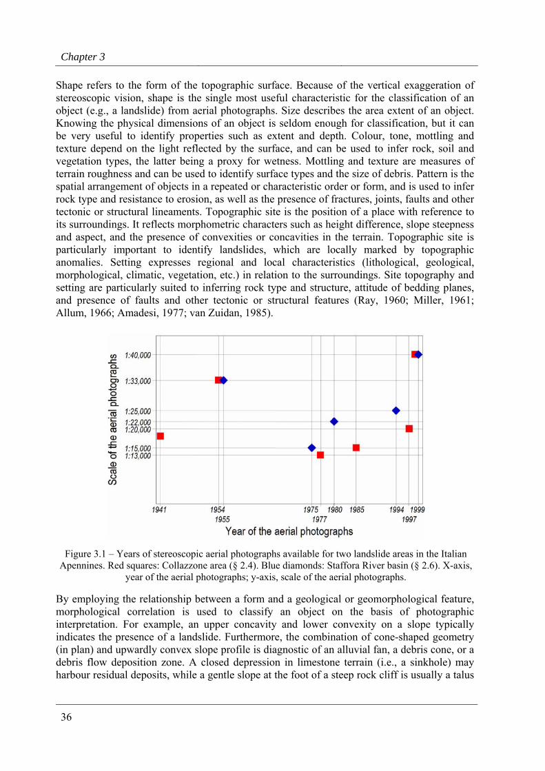
Chapter 3
36
Shape refers to the form of the topographic surface. Because of the vertical exaggeration of stereoscopic vision, shape is the single most useful characteristic for the classification of an object (e.g., a landslide) from aerial photographs. Size describes the area extent of an object. Knowing the physical dimensions of an object is seldom enough for classification, but it can be very useful to identify properties such as extent and depth. Colour, tone, mottling and texture depend on the light reflected by the surface, and can be used to infer rock, soil and vegetation types, the latter being a proxy for wetness. Mottling and texture are measures of terrain roughness and can be used to identify surface types and the size of debris. Pattern is the spatial arrangement of objects in a repeated or characteristic order or form, and is used to infer rock type and resistance to erosion, as well as the presence of fractures, joints, faults and other tectonic or structural lineaments. Topographic site is the position of a place with reference to its surroundings. It reflects morphometric characters such as height difference, slope steepness and aspect, and the presence of convexities or concavities in the terrain. Topographic site is particularly important to identify landslides, which are locally marked by topographic anomalies. Setting expresses regional and local characteristics (lithological, geological, morphological, climatic, vegetation, etc.) in relation to the surroundings. Site topography and setting are particularly suited to inferring rock type and structure, attitude of bedding planes, and presence of faults and other tectonic or structural features (Ray, 1960; Miller, 1961; Allum, 1966; Amadesi, 1977; van Zuidan, 1985).
Figure 3.1 – Years of stereoscopic aerial photographs available for two landslide areas in the Italian Apennines. Red squares: Collazzone area (§ 2.4). Blue diamonds: Staffora River basin (§ 2.6). X-axis,
year of the aerial photographs; y-axis, scale of the aerial photographs.
By employing the relationship between a form and a geological or geomorphological feature, morphological correlation is used to classify an object on the basis of photographic interpretation. For example, an upper concavity and lower convexity on a slope typically indicates the presence of a landslide. Furthermore, the combination of cone-shaped geometry (in plan) and upwardly convex slope profile is diagnostic of an alluvial fan, a debris cone, or a debris flow deposition zone. A closed depression in limestone terrain (i.e., a sinkhole) may harbour residual deposits, while a gentle slope at the foot of a steep rock cliff is usually a talus
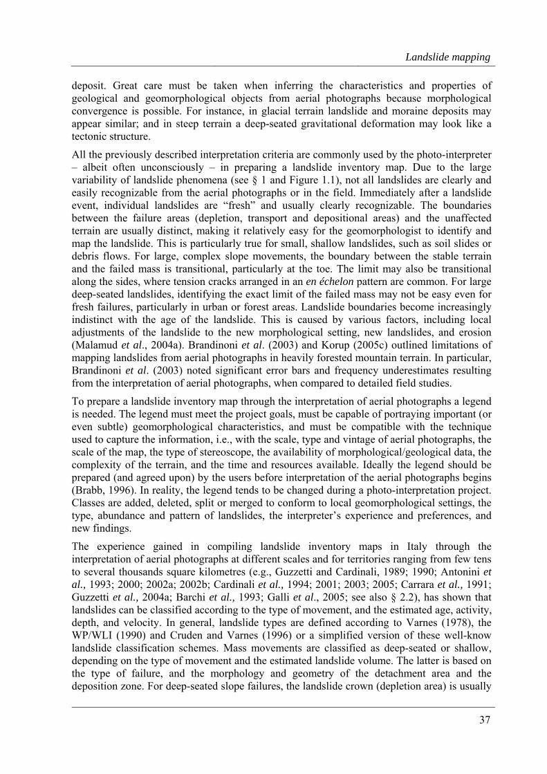
Landslide mapping
37
deposit. Great care must be taken when inferring the characteristics and properties of geological and geomorphological objects from aerial photographs because morphological convergence is possible. For instance, in glacial terrain landslide and moraine deposits may appear similar; and in steep terrain a deep-seated gravitational deformation may look like a tectonic structure.
All the previously described interpretation criteria are commonly used by the photo-interpreter – albeit often unconsciously – in preparing a landslide inventory map. Due to the large variability of landslide phenomena (see § 1 and Figure 1.1), not all landslides are clearly and easily recognizable from the aerial photographs or in the field. Immediately after a landslide event, individual landslides are “fresh” and usually clearly recognizable. The boundaries between the failure areas (depletion, transport and depositional areas) and the unaffected terrain are usually distinct, making it relatively easy for the geomorphologist to identify and map the landslide. This is particularly true for small, shallow landslides, such as soil slides or debris flows. For large, complex slope movements, the boundary between the stable terrain and the failed mass is transitional, particularly at the toe. The limit may also be transitional along the sides, where tension cracks arranged in an en échelon pattern are common. For large deep-seated landslides, identifying the exact limit of the failed mass may not be easy even for fresh failures, particularly in urban or forest areas. Landslide boundaries become increasingly indistinct with the age of the landslide. This is caused by various factors, including local adjustments of the landslide to the new morphological setting, new landslides, and erosion (Malamud et al., 2004a). Brandinoni et al. (2003) and Korup (2005c) outlined limitations of mapping landslides from aerial photographs in heavily forested mountain terrain. In particular, Brandinoni et al. (2003) noted significant error bars and frequency underestimates resulting from the interpretation of aerial photographs, when compared to detailed field studies.
To prepare a landslide inventory map through the interpretation of aerial photographs a legend is needed. The legend must meet the project goals, must be capable of portraying important (or even subtle) geomorphological characteristics, and must be compatible with the technique used to capture the information, i.e., with the scale, type and vintage of aerial photographs, the scale of the map, the type of stereoscope, the availability of morphological/geological data, the complexity of the terrain, and the time and resources available. Ideally the legend should be prepared (and agreed upon) by the users before interpretation of the aerial photographs begins (Brabb, 1996). In reality, the legend tends to be changed during a photo-interpretation project. Classes are added, deleted, split or merged to conform to local geomorphological settings, the type, abundance and pattern of landslides, the interpreter’s experience and preferences, and new findings.
The experience gained in compiling landslide inventory maps in Italy through the interpretation of aerial photographs at different scales and for territories ranging from few tens to several thousands square kilometres (e.g., Guzzetti and Cardinali, 1989; 1990; Antonini et al., 1993; 2000; 2002a; 2002b; Cardinali et al., 1994; 2001; 2003; 2005; Carrara et al., 1991; Guzzetti et al., 2004a; Barchi et al., 1993; Galli et al., 2005; see also § 2.2), has shown that landslides can be classified according to the type of movement, and the estimated age, activity, depth, and velocity. In general, landslide types are defined according to Varnes (1978), the WP/WLI (1990) and Cruden and Varnes (1996) or a simplified version of these well-know landslide classification schemes. Mass movements are classified as deep-seated or shallow, depending on the type of movement and the estimated landslide volume. The latter is based on the type of failure, and the morphology and geometry of the detachment area and the deposition zone. For deep-seated slope failures, the landslide crown (depletion area) is usually
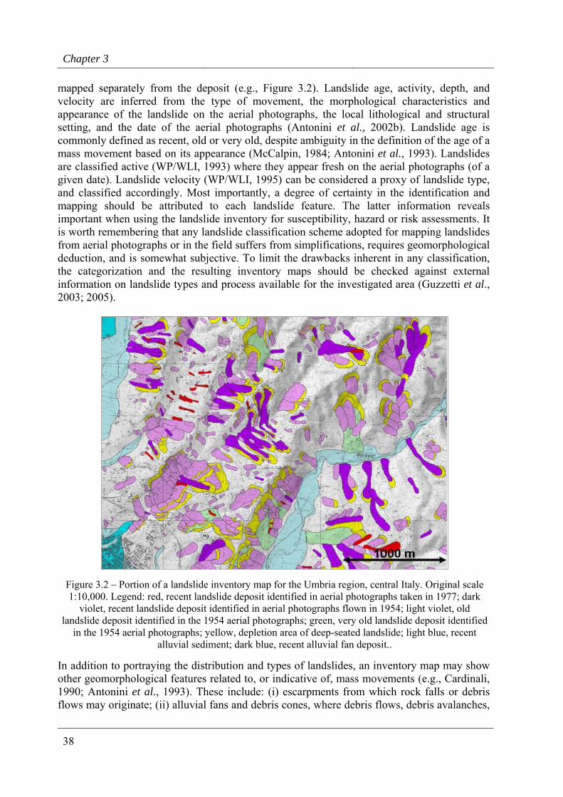
Chapter 3
38
mapped separately from the deposit (e.g., Figure 3.2). Landslide age, activity, depth, and velocity are inferred from the type of movement, the morphological characteristics and appearance of the landslide on the aerial photographs, the local lithological and structural setting, and the date of the aerial photographs (Antonini et al., 2002b). Landslide age is commonly defined as recent, old or very old, despite ambiguity in the definition of the age of a mass movement based on its appearance (McCalpin, 1984; Antonini et al., 1993). Landslides are classified active (WP/WLI, 1993) where they appear fresh on the aerial photographs (of a given date). Landslide velocity (WP/WLI, 1995) can be considered a proxy of landslide type, and classified accordingly. Most importantly, a degree of certainty in the identification and mapping should be attributed to each landslide feature. The latter information reveals important when using the landslide inventory for susceptibility, hazard or risk assessments. It is worth remembering that any landslide classification scheme adopted for mapping landslides from aerial photographs or in the field suffers from simplifications, requires geomorphological deduction, and is somewhat subjective. To limit the drawbacks inherent in any classification, the categorization and the resulting inventory maps should be checked against external information on landslide types and process available for the investigated area (Guzzetti et al., 2003; 2005).
Figure 3.2 – Portion of a landslide inventory map for the Umbria region, central Italy. Original scale 1:10,000. Legend: red, recent landslide deposit identified in aerial photographs taken in 1977; dark
violet, recent landslide deposit identified in aerial photographs flown in 1954; light violet, old landslide deposit identified in the 1954 aerial photographs; green, very old landslide deposit identified
in the 1954 aerial photographs; yellow, depletion area of deep-seated landslide; light blue, recent alluvial sediment; dark blue, recent alluvial fan deposit..
In addition to portraying the distribution and types of landslides, an inventory map may show other geomorphological features related to, or indicative of, mass movements (e.g., Cardinali, 1990; Antonini et al., 1993). These include: (i) escarpments from which rock falls or debris flows may originate; (ii) alluvial fans and debris cones, where debris flows, debris avalanches,
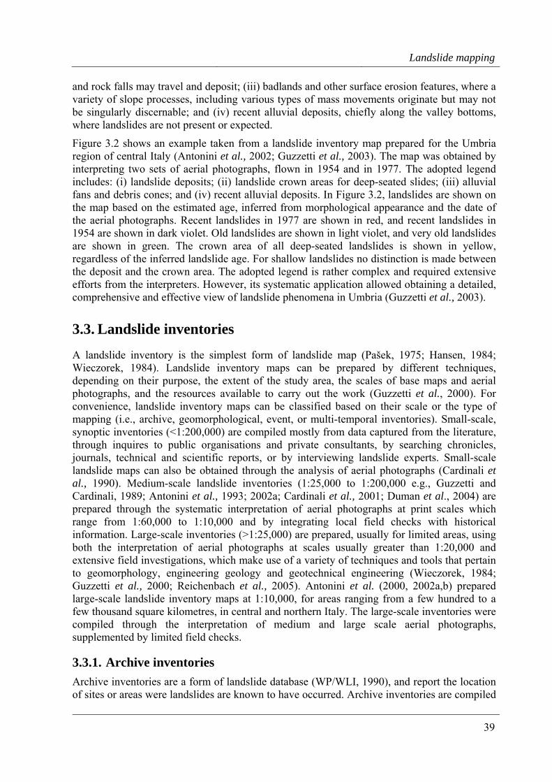
Landslide mapping
39
and rock falls may travel and deposit; (iii) badlands and other surface erosion features, where a variety of slope processes, including various types of mass movements originate but may not be singularly discernable; and (iv) recent alluvial deposits, chiefly along the valley bottoms, where landslides are not present or expected.
Figure 3.2 shows an example taken from a landslide inventory map prepared for the Umbria region of central Italy (Antonini et al., 2002; Guzzetti et al., 2003). The map was obtained by interpreting two sets of aerial photographs, flown in 1954 and in 1977. The adopted legend includes: (i) landslide deposits; (ii) landslide crown areas for deep-seated slides; (iii) alluvial fans and debris cones; and (iv) recent alluvial deposits. In Figure 3.2, landslides are shown on the map based on the estimated age, inferred from morphological appearance and the date of the aerial photographs. Recent landslides in 1977 are shown in red, and recent landslides in 1954 are shown in dark violet. Old landslides are shown in light violet, and very old landslides are shown in green. The crown area of all deep-seated landslides is shown in yellow, regardless of the inferred landslide age. For shallow landslides no distinction is made between the deposit and the crown area. The adopted legend is rather complex and required extensive efforts from the interpreters. However, its systematic application allowed obtaining a detailed, comprehensive and effective view of landslide phenomena in Umbria (Guzzetti et al., 2003).
3.3. Landslide inventories
A landslide inventory is the simplest form of landslide map (Pašek, 1975; Hansen, 1984; Wieczorek, 1984). Landslide inventory maps can be prepared by different techniques, depending on their purpose, the extent of the study area, the scales of base maps and aerial photographs, and the resources available to carry out the work (Guzzetti et al., 2000). For convenience, landslide inventory maps can be classified based on their scale or the type of mapping (i.e., archive, geomorphological, event, or multi-temporal inventories). Small-scale, synoptic inventories (<1:200,000) are compiled mostly from data captured from the literature, through inquires to public organisations and private consultants, by searching chronicles, journals, technical and scientific reports, or by interviewing landslide experts. Small-scale landslide maps can also be obtained through the analysis of aerial photographs (Cardinali et al., 1990). Medium-scale landslide inventories (1:25,000 to 1:200,000 e.g., Guzzetti and Cardinali, 1989; Antonini et al., 1993; 2002a; Cardinali et al., 2001; Duman et al., 2004) are prepared through the systematic interpretation of aerial photographs at print scales which range from 1:60,000 to 1:10,000 and by integrating local field checks with historical information. Large-scale inventories (>1:25,000) are prepared, usually for limited areas, using both the interpretation of aerial photographs at scales usually greater than 1:20,000 and extensive field investigations, which make use of a variety of techniques and tools that pertain to geomorphology, engineering geology and geotechnical engineering (Wieczorek, 1984; Guzzetti et al., 2000; Reichenbach et al., 2005). Antonini et al. (2000, 2002a,b) prepared large-scale landslide inventory maps at 1:10,000, for areas ranging from a few hundred to a few thousand square kilometres, in central and northern Italy. The large-scale inventories were compiled through the interpretation of medium and large scale aerial photographs, supplemented by limited field checks.
3.3.1. Archive inventories Archive inventories are a form of landslide database (WP/WLI, 1990), and report the location of sites or areas were landslides are known to have occurred. Archive inventories are compiled
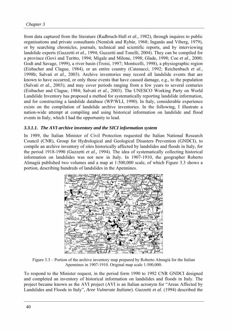
Chapter 3
40
from data captured from the literature (Radbruch-Hall et al., 1982), through inquires to public organisations and private consultants (Nemčok and Rybàr, 1968; Inganäs and Viberg, 1979), or by searching chronicles, journals, technical and scientific reports, and by interviewing landslide experts (Guzzetti et al., 1994; Guzzetti and Tonelli, 2004). They can be compiled for a province (Govi and Turitto, 1994; Migale and Milone, 1998; Glade, 1998; Coe et al., 2000; Godt and Savage, 1999), a river basin (Troisi, 1997; Monticelli, 1998), a physiographic region (Eisbacher and Clague, 1984), or an entire country (Catenacci, 1992; Reichenbach et al., 1998b; Salvati et al., 2003). Archive inventories may record all landslide events that are known to have occurred, or only those events that have caused damage, e.g., to the population (Salvati et al., 2003); and may cover periods ranging from a few years to several centuries (Eisbacher and Clague, 1984; Salvati et al., 2003). The UNESCO Working Party on World Landslide Inventory has proposed a method for systematically reporting landslide information, and for constructing a landslide database (WP/WLI, 1990). In Italy, considerable experience exists on the compilation of landslide archive inventories. In the following, I illustrate a nation-wide attempt at compiling and using historical information on landslide and flood events in Italy, which I had the opportunity to lead.
3.3.1.1. The AVI archive inventory and the SICI information system In 1989, the Italian Minister of Civil Protection requested the Italian National Research Council (CNR), Group for Hydrological and Geological Disasters Prevention (GNDCI), to compile an archive inventory of sites historically affected by landslides and floods in Italy, for the period 1918-1990 (Guzzetti et al., 1994). The idea of systematically collecting historical information on landslides was not new in Italy. In 1907-1910, the geographer Roberto Almagià published two volumes and a map at 1:500,000 scale, of which Figure 3.3 shows a portion, describing hundreds of landslides in the Apennines.
Figure 3.3 – Portion of the archive inventory map prepared by Roberto Almagià for the Italian Apennines in 1907-1910. Original map scale 1:500,000.
To respond to the Minister request, in the period form 1990 to 1992 CNR GNDCI designed and completed an inventory of historical information on landslides and floods in Italy. The project became known as the AVI project (AVI is an Italian acronym for “Areas Affected by Landslides and Floods in Italy”, Aree Vulnerate Italiane). Guzzetti et al. (1994) described the
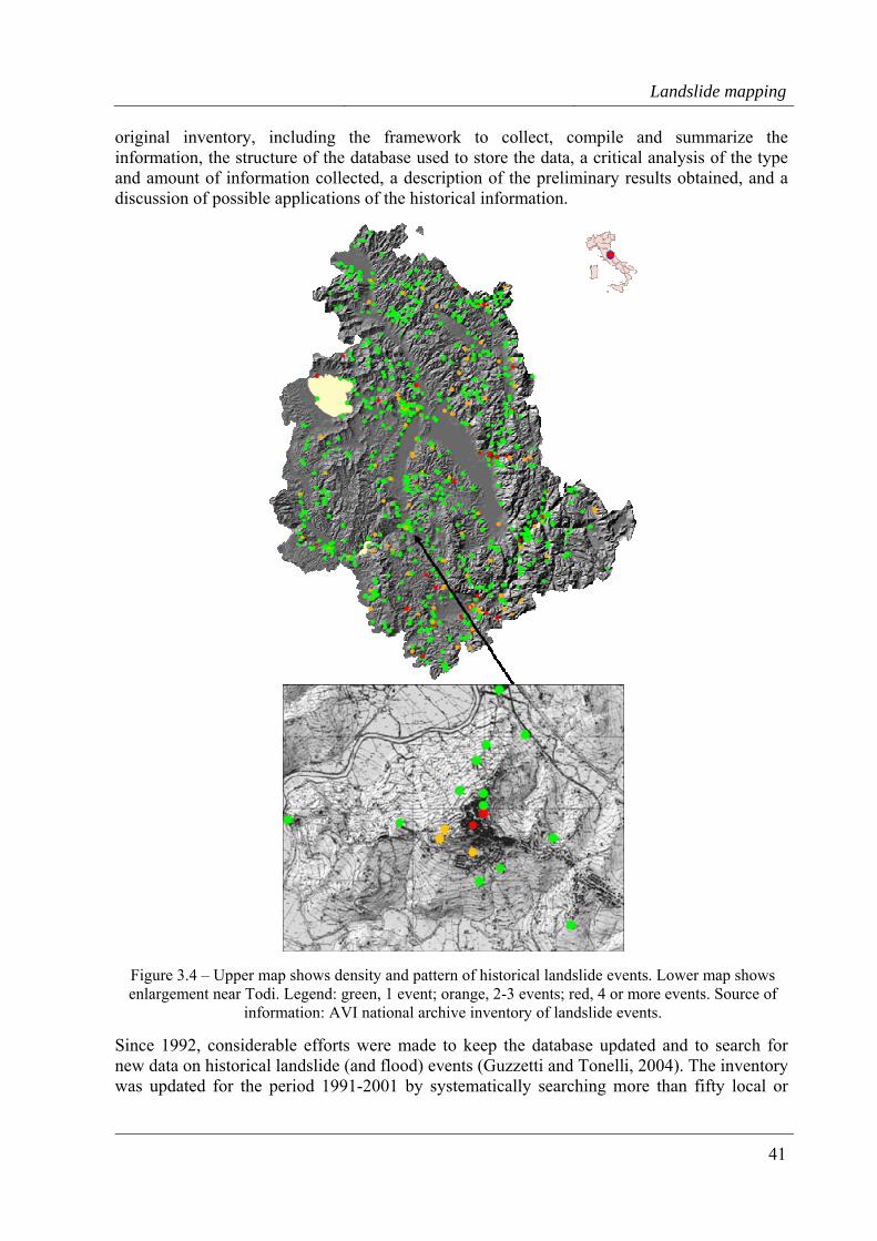
Landslide mapping
41
original inventory, including the framework to collect, compile and summarize the information, the structure of the database used to store the data, a critical analysis of the type and amount of information collected, a description of the preliminary results obtained, and a discussion of possible applications of the historical information.
Figure 3.4 – Upper map shows density and pattern of historical landslide events. Lower map shows enlargement near Todi. Legend: green, 1 event; orange, 2-3 events; red, 4 or more events. Source of
information: AVI national archive inventory of landslide events.
Since 1992, considerable efforts were made to keep the database updated and to search for new data on historical landslide (and flood) events (Guzzetti and Tonelli, 2004). The inventory was updated for the period 1991-2001 by systematically searching more than fifty local or
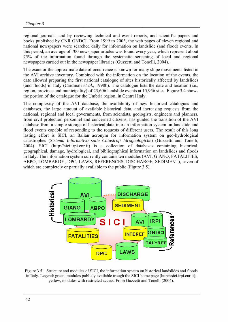
Chapter 3
42
regional journals, and by reviewing technical and event reports, and scientific papers and books published by CNR GNDCI. From 1999 to 2003, the web pages of eleven regional and national newspapers were searched daily for information on landslide (and flood) events. In this period, an average of 700 newspaper articles was found every year, which represent about 75% of the information found through the systematic screening of local and regional newspapers carried out in the newspaper libraries (Guzzetti and Tonelli, 2004).
The exact or the approximate date of occurrence is known for many slope movements listed in the AVI archive inventory. Combined with the information on the location of the events, the date allowed preparing the first national catalogue of sites historically affected by landslides (and floods) in Italy (Cardinali et al., 1998b). The catalogue lists the date and location (i.e., region, province and municipality) of 23,606 landslide events at 15,956 sites. Figure 3.4 shows the portion of the catalogue for the Umbria region, in Central Italy.
The complexity of the AVI database, the availability of new historical catalogues and databases, the large amount of available historical data, and increasing requests from the national, regional and local governments, from scientists, geologists, engineers and planners, from civil protection personnel and concerned citizens, has guided the transition of the AVI database from a simple storage of historical data into an information system on landslide and flood events capable of responding to the requests of different users. The result of this long lasting effort is SICI, an Italian acronym for information system on geo-hydrological catastrophes (Sistema Informativo sulle Catastrofi Idrogeologiche) (Guzzetti and Tonelli, 2004). SICI (http://sici.irpi.cnr.it) is a collection of databases containing historical, geographical, damage, hydrological, and bibliographical information on landslides and floods in Italy. The information system currently contains ten modules (AVI, GIANO, FATALITIES, ABPO, LOMBARDY, DPC, LAWS, REFERENCES, DISCHARGE, SEDIMENT), seven of which are completely or partially available to the public (Figure 3.5).
Figure 3.5 – Structure and modules of SICI, the information system on historical landslides and floods in Italy. Legend: green, modules publicly available trough the SICI home page (http://sici.irpi.cnr.it);
yellow, modules with restricted access. From Guzzetti and Tonelli (2004).
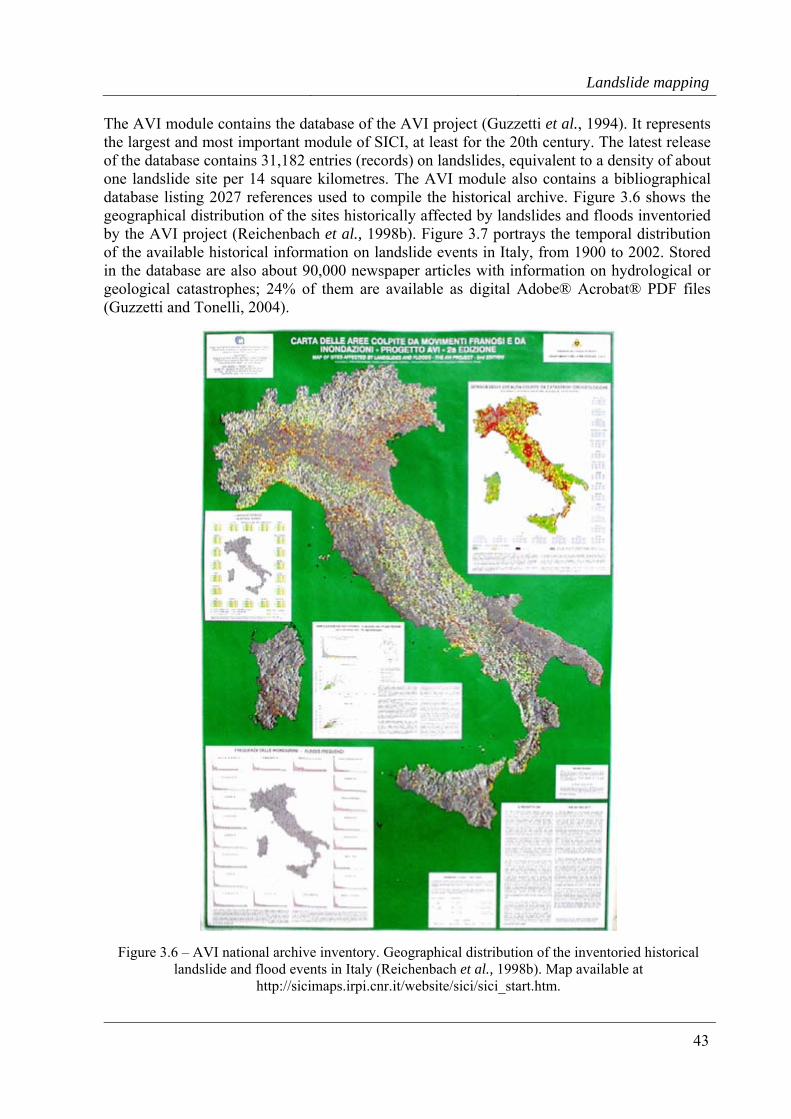
Landslide mapping
43
The AVI module contains the database of the AVI project (Guzzetti et al., 1994). It represents the largest and most important module of SICI, at least for the 20th century. The latest release of the database contains 31,182 entries (records) on landslides, equivalent to a density of about one landslide site per 14 square kilometres. The AVI module also contains a bibliographical database listing 2027 references used to compile the historical archive. Figure 3.6 shows the geographical distribution of the sites historically affected by landslides and floods inventoried by the AVI project (Reichenbach et al., 1998b). Figure 3.7 portrays the temporal distribution of the available historical information on landslide events in Italy, from 1900 to 2002. Stored in the database are also about 90,000 newspaper articles with information on hydrological or geological catastrophes; 24% of them are available as digital Adobe® Acrobat® PDF files (Guzzetti and Tonelli, 2004).
Figure 3.6 – AVI national archive inventory. Geographical distribution of the inventoried historical landslide and flood events in Italy (Reichenbach et al., 1998b). Map available at
http://sicimaps.irpi.cnr.it/website/sici/sici_start.htm.
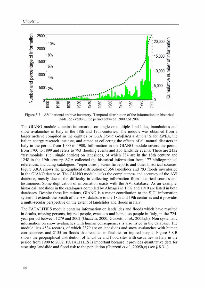
Chapter 3
44
Figure 3.7 – AVI national archive inventory. Temporal distribution of the information on historical landslide events in the period between 1900 and 2002.
The GIANO module contains information on single or multiple landslides, inundations and snow avalanches in Italy in the 18th and 19th centuries. The module was obtained from a larger archive compiled in the eighties by SGA Storia Geofisica e Ambiente for ENEA, the Italian energy research institute, and aimed at collecting the effects of all natural disasters in Italy in the period from 1000 to 1900. Information in the GIANO module covers the period from 1700 to 1899 and refers to 793 flooding events and 356 landslide events. There are 2132 “testimonials” (i.e., single entries) on landslides, of which 884 are in the 18th century and 1248 in the 19th century. SGA collected the historical information from 177 bibliographical references, including catalogues, “repertoires”, scientific reports and other historical sources. Figure 3.8.A shows the geographical distribution of 356 landslides and 793 floods inventoried in the GIANO database. The GIANO module lacks the completeness and accuracy of the AVI database, mostly due to the difficulty in collecting information from historical sources and testimonies. Some duplication of information exists with the AVI database. As an example, historical landslides in the catalogues compiled by Almagià in 1907 and 1910 are listed in both databases. Despite these limitations, GIANO is a major contribution to the SICI information system. It extends the breath of the AVI database to the 18th and 19th centuries and it provides a multi-secular perspective on the extent of landslides and floods in Italy.
The FATALITIES module contains information on landslides and floods which have resulted in deaths, missing persons, injured people, evacuees and homeless people in Italy, in the 724-year period between 1279 and 2002 (Guzzetti, 2000; Guzzetti et al., 2005a,b). Non systematic information on snow avalanches with human consequences is also listed in the database. The module lists 4534 records, of which 2379 are on landslides and snow avalanches with human consequences and 2155 on floods that resulted in fatalities or injured people. Figure 3.8.B shows the geographical distribution of landslide and flood sites with casualties in Italy in the period from 1900 to 2002. FATALITIES is important because it provides quantitative data for assessing landslide and flood risk to the population (Guzzetti et al., 2005b,c) (see § 8.3.1).
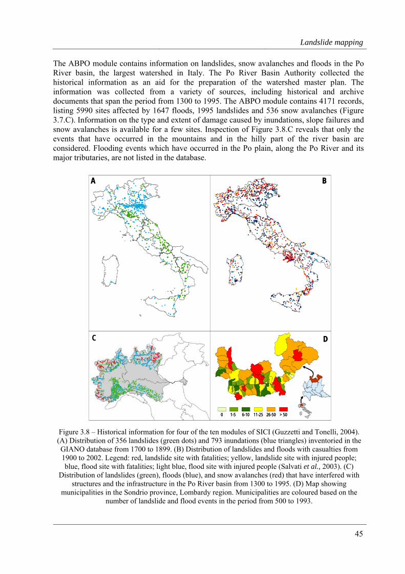
Landslide mapping
45
The ABPO module contains information on landslides, snow avalanches and floods in the Po River basin, the largest watershed in Italy. The Po River Basin Authority collected the historical information as an aid for the preparation of the watershed master plan. The information was collected from a variety of sources, including historical and archive documents that span the period from 1300 to 1995. The ABPO module contains 4171 records, listing 5990 sites affected by 1647 floods, 1995 landslides and 536 snow avalanches (Figure 3.7.C). Information on the type and extent of damage caused by inundations, slope failures and snow avalanches is available for a few sites. Inspection of Figure 3.8.C reveals that only the events that have occurred in the mountains and in the hilly part of the river basin are considered. Flooding events which have occurred in the Po plain, along the Po River and its major tributaries, are not listed in the database.
0 1-5 6-10 11-25 26-50 > 50
A B
DC
0 1-5 6-10 11-25 26-50 > 50
A B
DC
Figure 3.8 – Historical information for four of the ten modules of SICI (Guzzetti and Tonelli, 2004). (A) Distribution of 356 landslides (green dots) and 793 inundations (blue triangles) inventoried in the GIANO database from 1700 to 1899. (B) Distribution of landslides and floods with casualties from 1900 to 2002. Legend: red, landslide site with fatalities; yellow, landslide site with injured people; blue, flood site with fatalities; light blue, flood site with injured people (Salvati et al., 2003). (C)
Distribution of landslides (green), floods (blue), and snow avalanches (red) that have interfered with structures and the infrastructure in the Po River basin from 1300 to 1995. (D) Map showing
municipalities in the Sondrio province, Lombardy region. Municipalities are coloured based on the number of landslide and flood events in the period from 500 to 1993.
Chapter 3
46
The LOMBARDY module contains information on 3765 landslides, debris flows and flooding events in Valtellina and Val Chiavenna, two Alpine valleys in the Sondrio province (Lombardy, northern Italy), in the period from 500 to 1993 (Figure 3.8.D). The historical database contains 2948 records, listing information obtained by systematically searching 590 bibliographical references and historical documents, which were found in local archives by Govi and Turitto (1994). LOMBARDY is a particularly valuable addition to the SICI information system because it provides a measure of the quantity and quality of information that can be expected from a systematic search of historical information in the Italian Alps.
The DPC module contains information on 1389 local surveys and technical activities performed by CNR GNDCI experts and scientists in the period between 1990 and 2000. The investigations were requested by the Mayor of a municipality or the Prefect of a province, and were conducted on behalf of the National Department of Civil Protection (DPC) to investigate landslides and floods that posed an imminent threat to the population. The LAWS module contains information and documents on Italian laws, decrees, and ministry orders on hydrological and geological hazards (Fastelli, 2003a). The database covers the period from 1970 to 2002, and lists 1255 legislative acts. The REFERENCES module is a collection of bibliographical and reference catalogues, for a total of more than 8000 national and international references. Lastly, the DISCHARGE and SEDIMENT modules contain data on daily water discharge and on daily sediment yield. Measurements of mean daily water discharge are available for 111 gauging stations in central Italy, in the period from 1929 to 1996. Data on sediment yield are available for 117 stations and cover (non systematically) the 68-year period from 1929 to 1996.
3.3.2. Geomorphological inventories A geomorphological inventory map shows the sum of many landslide events over a period of some, tens, hundreds or even many thousands of years. Geomorphological inventories are typically prepared thought the systematic interpretation of one or two sets of aerial photographs, at print scales ranging from 1:10,000 to 1:70,000, aided by field checks. Geomorphological inventory maps cover areas ranging from few tens to few thousands square kilometres, at mapping scales ranging from 1:10,000 to 1:100,000 (which usually corresponds to publication scales raging from 1:50,000 to 1:500,000) depending on the extent of the study area, the availability, scale and number of the aerial photographs, the complexity of the study area, and the time and resources available to complete the project.
Typically, a single map is used to portray all different types of landslides. Alternatively, a set of maps can be prepared, each map showing a different type of failure, i.e. deep-seated slides, shallow failures, debris flows, rock falls, etc. (Cardinali et al., 1990). In recent years, availability of GIS technology has facilitated the production of geomorphological landslide databases, which store different information on landslides, and allow for the display and the publication of multiple, complex inventory maps. Besides showing landslides, geomorphological inventory maps may also portray other features related to mass movements, including escarpments, alluvial fans and debris cones, badlands and other surface erosion features, and recent alluvial deposits. In the production of geomorphological inventories, attempts at classifying landslide age and degree of activity based on the morphological appearance of the slope failure are hampered by the inherent difficulty of discriminating landslide age (i.e., the time elapsed since the first failure) from landslide activity (i.e., the state of motion of a landslide (WP/WLI, 1993)) based solely on the visual interpretation of the morphology of a landslide (McCalpin, 1984; Antonini et al., 1993).
Landslide mapping
47
In Italy, geomorphological inventory maps are available for several areas. However, the scale, resolution and completeness of these inventories vary largely. Inventories prepared in the late seventies and in the eighties of the 20th century were typically compiled at 1:25,000 scale, chiefly through the interpretation of medium-scale aerial photographs, with limited field checks. Publication of these inventories was usually at 1:100,000 scale (e.g., IRPI and Regione Piemonte for Piedmont, Guzzetti and Cardinali (1989, 1990) for Umbria, and Antonini et al. (1993) for Marche). More recent inventories were compiled at 1:10,000 scale through the systematic interpretation of one or two sets of medium to large-scale aerial photograph, and field checks (e.g., Fossati et al., (2002) for Lombardy, Antonini et al. (2002a) for Umbria). As part of a large geological mapping project, the Geological Survey of the Emilia-Romagna Region produced a geomorphological landslide inventory map at 1:10,000 scale. The inventory was obtained through systematic field mapping aided by the interpretation of medium-scale aerial photographs. A synoptic map showing the inventory was published at 1:250,000 scale (Bertolini et al., 2002). In 1999, the Italian Geological Survey lunched a project to compile a geomorphological landslide inventory map, with associated database, for the entire country. In this project the inventory map is produced at 1:25,000 scale, by assimilating information obtained through the interpretation of aerial photographs with information on landslides obtained from various historical and contemporary sources (Amanti, 2000; Amanti et al., 2001).
In the next three sub-sections, I illustrate two examples of geomorphological landslide inventories prepared for the Umbria region, and I compare the two inventories, including a discussion of the resources required to prepare the landslide maps.
3.3.2.1. Reconnaissance geomorphological landslide inventory map for the Umbria Region Two landslide inventory maps have been made for the Umbria region. The first map is a reconnaissance inventory prepared by Guzzetti and Cardinali (1989, 1990) as a reconnaissance mapping effort aimed at obtaining general information on the distribution, abundance and type of mass movements in Umbria (Figure 3.9). The reconnaissance inventory of Guzzetti and Cardinali (1989, 1990) was partially revised by Antonini et al. (1993) for the Apennines mountain chain. In 1999, the Regional Government of Umbria adopted the map as part of the Regional Environmental and Urban Plan (Piano Urbanistico e Territoriale della Regione dell’Umbria) (Guzzetti et al., 1999b).
The reconnaissance inventory was prepared by interpreting landslides observed on 1085 black and white, vertical aerial photographs flown in the period from 1954 to 1956, at 1:33,000 scale. Interpretation of the aerial photographs was locally aided by field checks, and was carried out by a team of two geomorphologists who worked simultaneously on adjacent strips. Inasmuch as side-lap between the photographs was 20-30%, a considerable part of the territory was analysed by both photo-interpreters. The landslide information, originally plotted on transparent plastic sheets placed over the aerial photographs, was transferred to 35 topographic maps, at 1:25,000 scale. Transfer of the landslide information to the base maps was accomplished by using a combined optical and manual technique, aided by a large-format photographic projector. The 35 quadrangles were then photographically reduced, assembled, and redrawn for final publication at 1:100,000 scale. Due to the scale of the published map, individual landslides with an area less than about one hectare were shown as points in the final inventory map (Guzzetti and Cardinali, 1990).
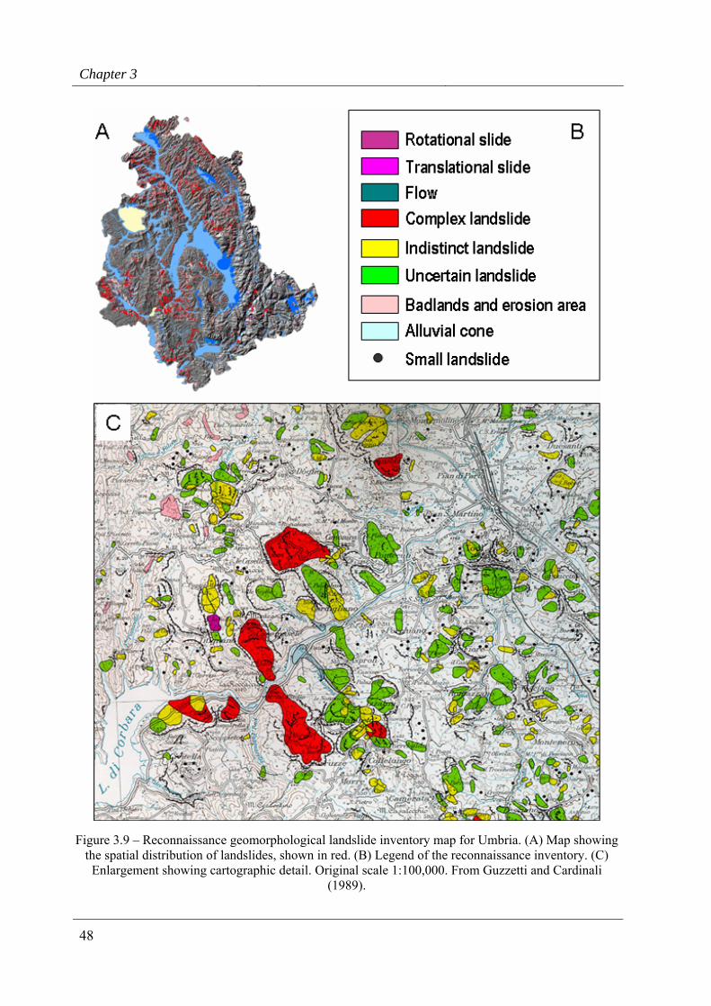
Chapter 3
48
Figure 3.9 – Reconnaissance geomorphological landslide inventory map for Umbria. (A) Map showing the spatial distribution of landslides, shown in red. (B) Legend of the reconnaissance inventory. (C)
Enlargement showing cartographic detail. Original scale 1:100,000. From Guzzetti and Cardinali (1989).
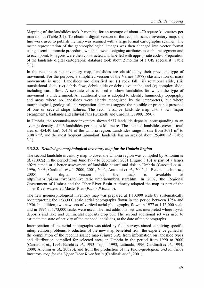
Landslide mapping
49
Mapping of the landslides took 9 months, for an average of about 470 square kilometres per man-month (Table 3.1). To obtain a digital version of the reconnaissance inventory map, the line work used to publish the map was scanned with a large format cartographic scanner. The raster representation of the geomorphological images was then changed into vector format using a semi-automatic procedure, which allowed assigning attributes to each line segment and to each point. Polygons were then constructed and labelled with appropriate codes. Preparation of the landslide digital cartographic database took about 2 months of a GIS specialist (Table 3.1).
In the reconnaissance inventory map, landslides are classified by their prevalent type of movement. For the purpose, a simplified version of the Varnes (1978) classification of mass movements is used. Landslides are classified as: (i) rock fall, (ii) rotational slide, (iii) translational slide, (iv) debris flow, debris slide or debris avalanche, and (v) complex slide, including earth flow. A separate class is used to show landslides for which the type of movement is undetermined. An additional class is adopted to identify hummocky topography and areas where no landslides were clearly recognized by the interpreters, but where morphological, geological and vegetation elements suggest the possible or probable presence of one or several slope failures. The reconnaissance landslide map also shows major escarpments, badlands and alluvial fans (Guzzetti and Cardinali, 1989, 1990).
In Umbria, the reconnaissance inventory shows 5277 landslide deposits, corresponding to an average density of 0.6 landslides per square kilometre. The mapped landslides cover a total area of 454.40 km2, 5.41% of the Umbria region. Landslides range in size from 3071 m2 to 3.08 km2, and the most frequent (abundant) landslide has an area of about 25,400 m2 (Table 3.1).
3.3.2.2. Detailed geomorphological inventory map for the Umbria Region The second landslide inventory map to cover the Umbria region was compiled by Antonini et al. (2002a) in the period from June 1999 to September 2001 (Figure 3.10) as part of a larger effort aimed at a better assessment of landslide hazard and risk in Umbria (Guzzetti et al., 1996, 2003; Cardinali et al., 2000, 2001, 2002; Antonini et al., 2002a,b; Reichenbach et al., 2005). A digital version of the map is available at http://maps.irpi.cnr.it/website/inventario_umbria/umbria_start.htm. In 2002, the Regional Government of Umbria and the Tiber River Basin Authority adopted the map as part of the Tiber River watershed Master Plan (Piano di Bacino).
The new geomorphological inventory map was prepared at 1:10,000 scale by systematically re-interpreting the 1:33,000 scale aerial photographs flown in the period between 1954 and 1956. In addition, two new sets of vertical aerial photographs, flown in 1977 at 1:13,000 scale and in 1994 at 1:73,000 scale, were used. The first additional set was interpreted where flysch deposits and lake and continental deposits crop out. The second additional set was used to estimate the state of activity of the mapped landslides, at the date of the photographs.
Interpretation of the aerial photographs was aided by field surveys aimed at solving specific interpretation problems. Production of the new map benefited from the experience gained in the compilation of the reconnaissance map (Figure 3.9), from information on landslide types and distribution compiled for selected areas in Umbria in the period from 1990 to 2000 (Carrara et al., 1991; Barchi et al., 1993; Toppi, 1993, Lattuada, 1996; Cardinali et al., 1994, 2000; Anonini et al., 2002b), and from the production of the Photo-geological and landslide inventory map for the Upper Tiber River basin (Cardinali et al., 2001).
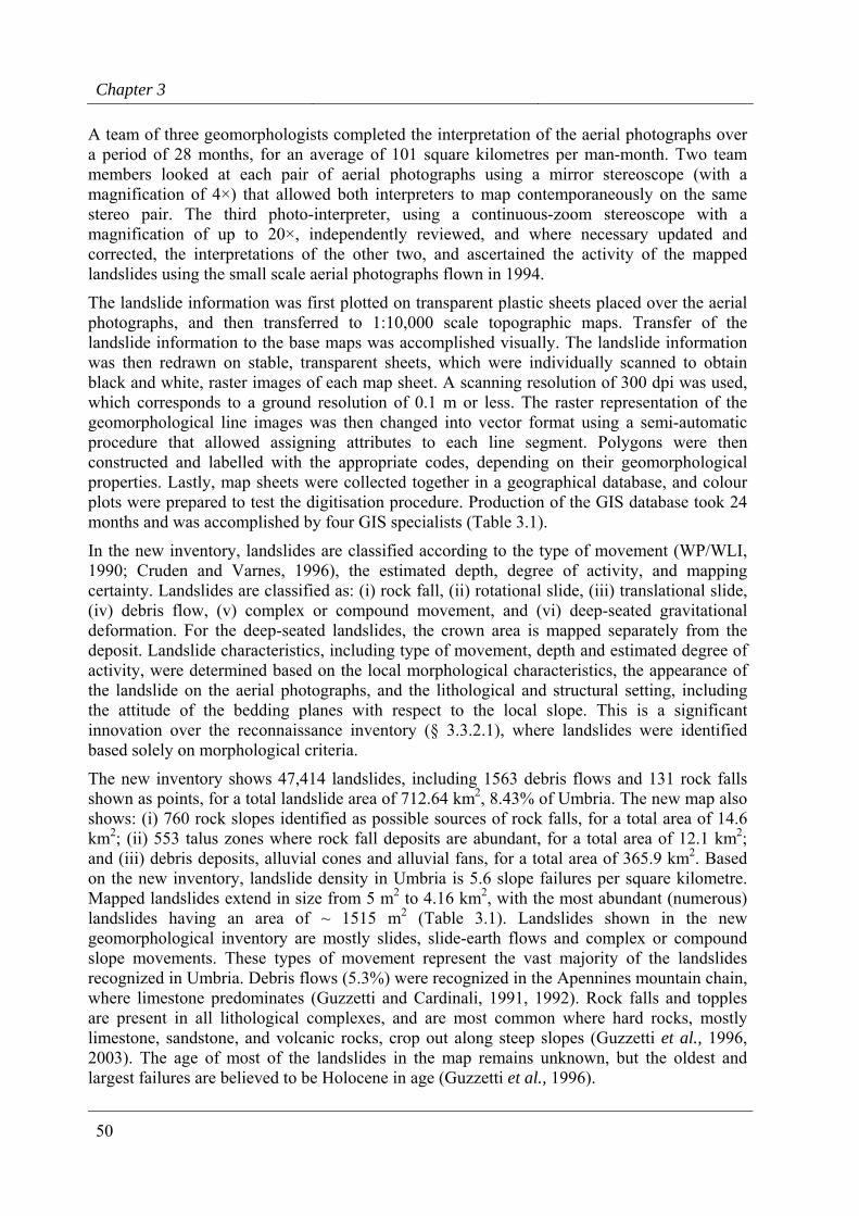
Chapter 3
50
A team of three geomorphologists completed the interpretation of the aerial photographs over a period of 28 months, for an average of 101 square kilometres per man-month. Two team members looked at each pair of aerial photographs using a mirror stereoscope (with a magnification of 4×) that allowed both interpreters to map contemporaneously on the same stereo pair. The third photo-interpreter, using a continuous-zoom stereoscope with a magnification of up to 20×, independently reviewed, and where necessary updated and corrected, the interpretations of the other two, and ascertained the activity of the mapped landslides using the small scale aerial photographs flown in 1994.
The landslide information was first plotted on transparent plastic sheets placed over the aerial photographs, and then transferred to 1:10,000 scale topographic maps. Transfer of the landslide information to the base maps was accomplished visually. The landslide information was then redrawn on stable, transparent sheets, which were individually scanned to obtain black and white, raster images of each map sheet. A scanning resolution of 300 dpi was used, which corresponds to a ground resolution of 0.1 m or less. The raster representation of the geomorphological line images was then changed into vector format using a semi-automatic procedure that allowed assigning attributes to each line segment. Polygons were then constructed and labelled with the appropriate codes, depending on their geomorphological properties. Lastly, map sheets were collected together in a geographical database, and colour plots were prepared to test the digitisation procedure. Production of the GIS database took 24 months and was accomplished by four GIS specialists (Table 3.1).
In the new inventory, landslides are classified according to the type of movement (WP/WLI, 1990; Cruden and Varnes, 1996), the estimated depth, degree of activity, and mapping certainty. Landslides are classified as: (i) rock fall, (ii) rotational slide, (iii) translational slide, (iv) debris flow, (v) complex or compound movement, and (vi) deep-seated gravitational deformation. For the deep-seated landslides, the crown area is mapped separately from the deposit. Landslide characteristics, including type of movement, depth and estimated degree of activity, were determined based on the local morphological characteristics, the appearance of the landslide on the aerial photographs, and the lithological and structural setting, including the attitude of the bedding planes with respect to the local slope. This is a significant innovation over the reconnaissance inventory (§ 3.3.2.1), where landslides were identified based solely on morphological criteria.
The new inventory shows 47,414 landslides, including 1563 debris flows and 131 rock falls shown as points, for a total landslide area of 712.64 km2, 8.43% of Umbria. The new map also shows: (i) 760 rock slopes identified as possible sources of rock falls, for a total area of 14.6 km2; (ii) 553 talus zones where rock fall deposits are abundant, for a total area of 12.1 km2; and (iii) debris deposits, alluvial cones and alluvial fans, for a total area of 365.9 km2. Based on the new inventory, landslide density in Umbria is 5.6 slope failures per square kilometre. Mapped landslides extend in size from 5 m2 to 4.16 km2, with the most abundant (numerous) landslides having an area of ~ 1515 m2 (Table 3.1). Landslides shown in the new geomorphological inventory are mostly slides, slide-earth flows and complex or compound slope movements. These types of movement represent the vast majority of the landslides recognized in Umbria. Debris flows (5.3%) were recognized in the Apennines mountain chain, where limestone predominates (Guzzetti and Cardinali, 1991, 1992). Rock falls and topples are present in all lithological complexes, and are most common where hard rocks, mostly limestone, sandstone, and volcanic rocks, crop out along steep slopes (Guzzetti et al., 1996, 2003). The age of most of the landslides in the map remains unknown, but the oldest and largest failures are believed to be Holocene in age (Guzzetti et al., 1996).
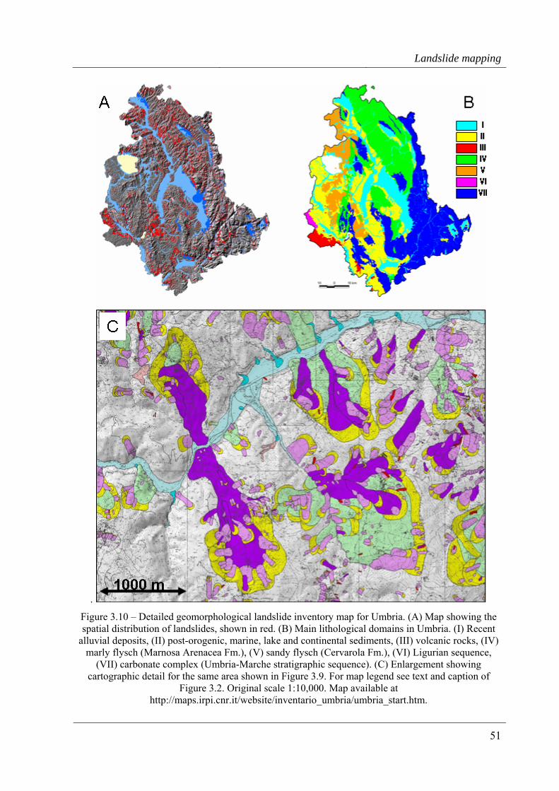
Landslide mapping
51
.
Figure 3.10 – Detailed geomorphological landslide inventory map for Umbria. (A) Map showing the spatial distribution of landslides, shown in red. (B) Main lithological domains in Umbria. (I) Recent
alluvial deposits, (II) post-orogenic, marine, lake and continental sediments, (III) volcanic rocks, (IV) marly flysch (Marnosa Arenacea Fm.), (V) sandy flysch (Cervarola Fm.), (VI) Ligurian sequence,
(VII) carbonate complex (Umbria-Marche stratigraphic sequence). (C) Enlargement showing cartographic detail for the same area shown in Figure 3.9. For map legend see text and caption of
Figure 3.2. Original scale 1:10,000. Map available at http://maps.irpi.cnr.it/website/inventario_umbria/umbria_start.htm.
Chapter 3
52
Figure 3.11 – Landslide abundance in the main lithological types in Umbria. (II) post-orogenic, marine, lake and continental sediments, (III) volcanic rocks, (IV) marly flysch (Marnosa Arenacea
Fm.), (V) sandy flysch (Cervarola Fm.), (VI) Ligurian sequence, (VII) carbonate complex (Umbria-Marche stratigraphic sequence). Recent alluvial deposits (I, Figure 3.10.B) don’t have landslides.
Inspection of Figure 3.10 reveals that landslides are not distributed evenly in the Umbria region (Figure 3.11). Failures are most abundant in the flysch complex, where 50.7% of all landslides were identified. Within this rock complex, the area where marly flysch crops out exhibits the largest number of landslides (32.7%). In the post-orogenic sediments complex and the carbonate complex landslide abundance is similar, 27.8% and 20.7%, respectively. Landslides are less abundant in the volcanic complex (0.8%). In this lithological domain, slope failures initiate moslty in the underlying marine clays and affect only the edge of the volcanic hard cap (Guzzetti et al., 1996)
3.3.2.3. Comparison of the two geomorphological inventory maps in Umbria A general comparison of the two regional geomorphological inventories is possible. As it is a detailed update of a previous reconnaissance mapping (Figure 3.9), the new geomorphological inventory (Figure 3.10) has improved the quality and spatial resolution of the landslide information. In the new – and more detailed – inventory, landslides are mapped more accurately, landslide boundaries follow more precisely the actual landslide geometry, better fitting morphological and lithological constrains (i.e., drainage lines, lithological boundaries, faults, bedding attitude, etc.).
The new geomorphological mapping resulted in an increase of 570% in the number of mapped landslides, and of 151% in the total extent of landslide area, with respect to the previous reconnaissance mapping. These figures quantify the improvement obtained with the new geomorphological inventory map. Visual comparison of the reconnaissance (Figure 3.9) and the detailed (Figure 3.10) geomorphological inventories confirms the better quality of the new mapping. Limited to the outcrop of lake and continental deposits, where large-scale (1:13,000 scale) aerial photographs were used in addition to the medium-scale photographs, the marked increase in the number and of the total area of mapped landslides is due to the larger scale of the photographs, that allowed for the recognition of smaller slope failures. Where flysch deposits crop out, interpretation of large-scale (1:13,000 scale) aerial photographs added limited new information, but allowed for an improved mapping of the landslide boundaries, and a better definition of the internal subdivisions of large landslide deposits.
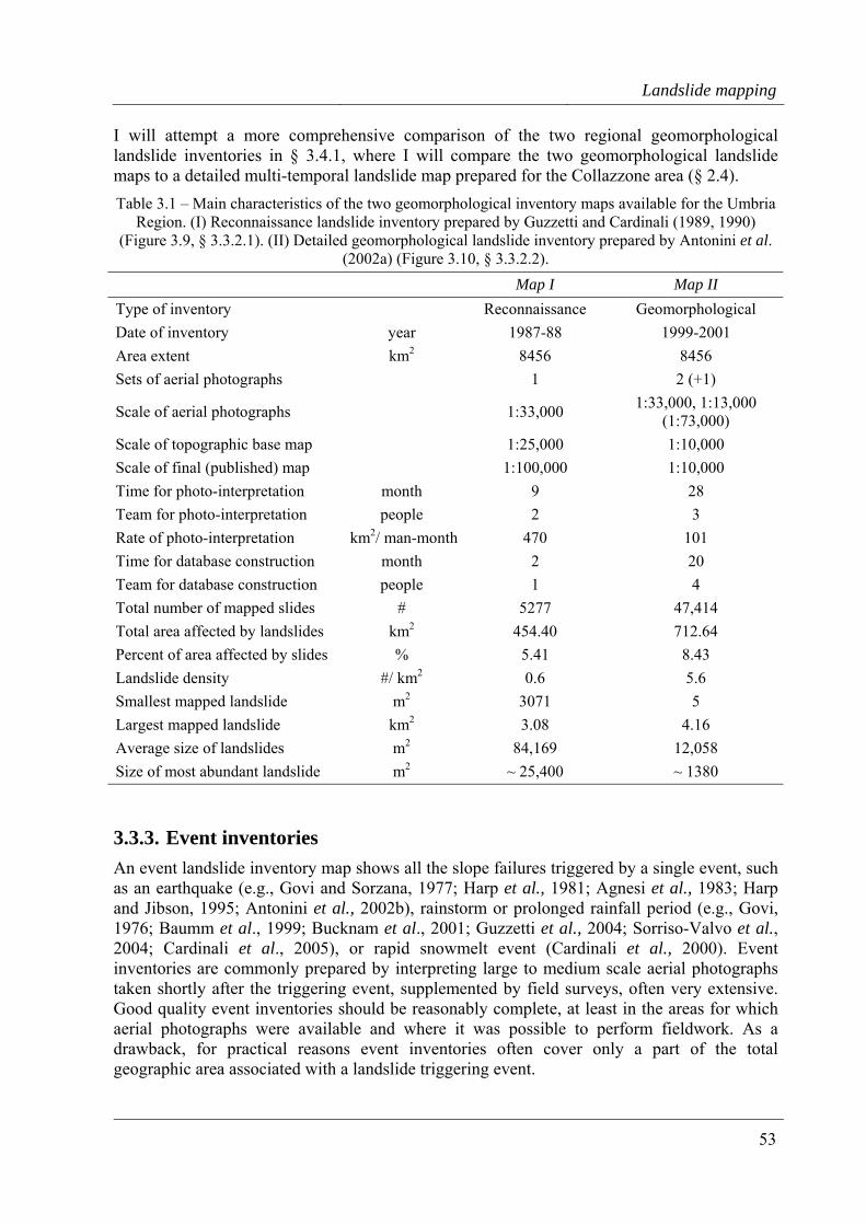
Landslide mapping
53
I will attempt a more comprehensive comparison of the two regional geomorphological landslide inventories in § 3.4.1, where I will compare the two geomorphological landslide maps to a detailed multi-temporal landslide map prepared for the Collazzone area (§ 2.4). Table 3.1 – Main characteristics of the two geomorphological inventory maps available for the Umbria
Region. (I) Reconnaissance landslide inventory prepared by Guzzetti and Cardinali (1989, 1990) (Figure 3.9, § 3.3.2.1). (II) Detailed geomorphological landslide inventory prepared by Antonini et al.
(2002a) (Figure 3.10, § 3.3.2.2). Map I Map II
Type of inventory Reconnaissance Geomorphological Date of inventory year 1987-88 1999-2001 Area extent km2 8456 8456 Sets of aerial photographs 1 2 (+1)
Scale of aerial photographs 1:33,000 1:33,000, 1:13,000 (1:73,000)
Scale of topographic base map 1:25,000 1:10,000 Scale of final (published) map 1:100,000 1:10,000 Time for photo-interpretation month 9 28 Team for photo-interpretation people 2 3 Rate of photo-interpretation km2/ man-month 470 101 Time for database construction month 2 20 Team for database construction people 1 4 Total number of mapped slides # 5277 47,414 Total area affected by landslides km2 454.40 712.64 Percent of area affected by slides % 5.41 8.43 Landslide density #/ km2 0.6 5.6 Smallest mapped landslide m2 3071 5 Largest mapped landslide km2 3.08 4.16 Average size of landslides m2 84,169 12,058 Size of most abundant landslide m2 ~ 25,400 ~ 1380
3.3.3. Event inventories An event landslide inventory map shows all the slope failures triggered by a single event, such as an earthquake (e.g., Govi and Sorzana, 1977; Harp et al., 1981; Agnesi et al., 1983; Harp and Jibson, 1995; Antonini et al., 2002b), rainstorm or prolonged rainfall period (e.g., Govi, 1976; Baumm et al., 1999; Bucknam et al., 2001; Guzzetti et al., 2004; Sorriso-Valvo et al., 2004; Cardinali et al., 2005), or rapid snowmelt event (Cardinali et al., 2000). Event inventories are commonly prepared by interpreting large to medium scale aerial photographs taken shortly after the triggering event, supplemented by field surveys, often very extensive. Good quality event inventories should be reasonably complete, at least in the areas for which aerial photographs were available and where it was possible to perform fieldwork. As a drawback, for practical reasons event inventories often cover only a part of the total geographic area associated with a landslide triggering event.
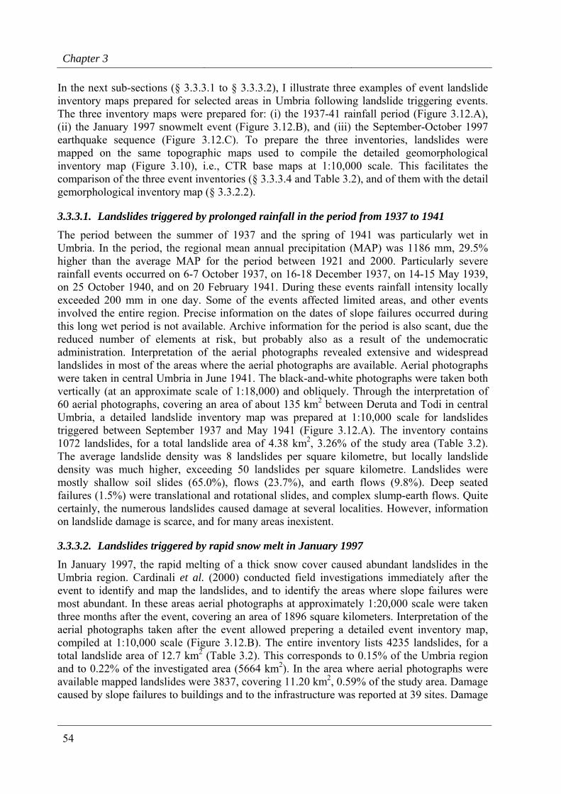
Chapter 3
54
In the next sub-sections (§ 3.3.3.1 to § 3.3.3.2), I illustrate three examples of event landslide inventory maps prepared for selected areas in Umbria following landslide triggering events. The three inventory maps were prepared for: (i) the 1937-41 rainfall period (Figure 3.12.A), (ii) the January 1997 snowmelt event (Figure 3.12.B), and (iii) the September-October 1997 earthquake sequence (Figure 3.12.C). To prepare the three inventories, landslides were mapped on the same topographic maps used to compile the detailed geomorphological inventory map (Figure 3.10), i.e., CTR base maps at 1:10,000 scale. This facilitates the comparison of the three event inventories (§ 3.3.3.4 and Table 3.2), and of them with the detail gemorphological inventory map (§ 3.3.2.2).
3.3.3.1. Landslides triggered by prolonged rainfall in the period from 1937 to 1941 The period between the summer of 1937 and the spring of 1941 was particularly wet in Umbria. In the period, the regional mean annual precipitation (MAP) was 1186 mm, 29.5% higher than the average MAP for the period between 1921 and 2000. Particularly severe rainfall events occurred on 6-7 October 1937, on 16-18 December 1937, on 14-15 May 1939, on 25 October 1940, and on 20 February 1941. During these events rainfall intensity locally exceeded 200 mm in one day. Some of the events affected limited areas, and other events involved the entire region. Precise information on the dates of slope failures occurred during this long wet period is not available. Archive information for the period is also scant, due the reduced number of elements at risk, but probably also as a result of the undemocratic administration. Interpretation of the aerial photographs revealed extensive and widespread landslides in most of the areas where the aerial photographs are available. Aerial photographs were taken in central Umbria in June 1941. The black-and-white photographs were taken both vertically (at an approximate scale of 1:18,000) and obliquely. Through the interpretation of 60 aerial photographs, covering an area of about 135 km2 between Deruta and Todi in central Umbria, a detailed landslide inventory map was prepared at 1:10,000 scale for landslides triggered between September 1937 and May 1941 (Figure 3.12.A). The inventory contains 1072 landslides, for a total landslide area of 4.38 km2, 3.26% of the study area (Table 3.2). The average landslide density was 8 landslides per square kilometre, but locally landslide density was much higher, exceeding 50 landslides per square kilometre. Landslides were mostly shallow soil slides (65.0%), flows (23.7%), and earth flows (9.8%). Deep seated failures (1.5%) were translational and rotational slides, and complex slump-earth flows. Quite certainly, the numerous landslides caused damage at several localities. However, information on landslide damage is scarce, and for many areas inexistent.
3.3.3.2. Landslides triggered by rapid snow melt in January 1997
In January 1997, the rapid melting of a thick snow cover caused abundant landslides in the Umbria region. Cardinali et al. (2000) conducted field investigations immediately after the event to identify and map the landslides, and to identify the areas where slope failures were most abundant. In these areas aerial photographs at approximately 1:20,000 scale were taken three months after the event, covering an area of 1896 square kilometers. Interpretation of the aerial photographs taken after the event allowed prepering a detailed event inventory map, compiled at 1:10,000 scale (Figure 3.12.B). The entire inventory lists 4235 landslides, for a total landslide area of 12.7 km2 (Table 3.2). This corresponds to 0.15% of the Umbria region and to 0.22% of the investigated area (5664 km2). In the area where aerial photographs were available mapped landslides were 3837, covering 11.20 km2, 0.59% of the study area. Damage caused by slope failures to buildings and to the infrastructure was reported at 39 sites. Damage
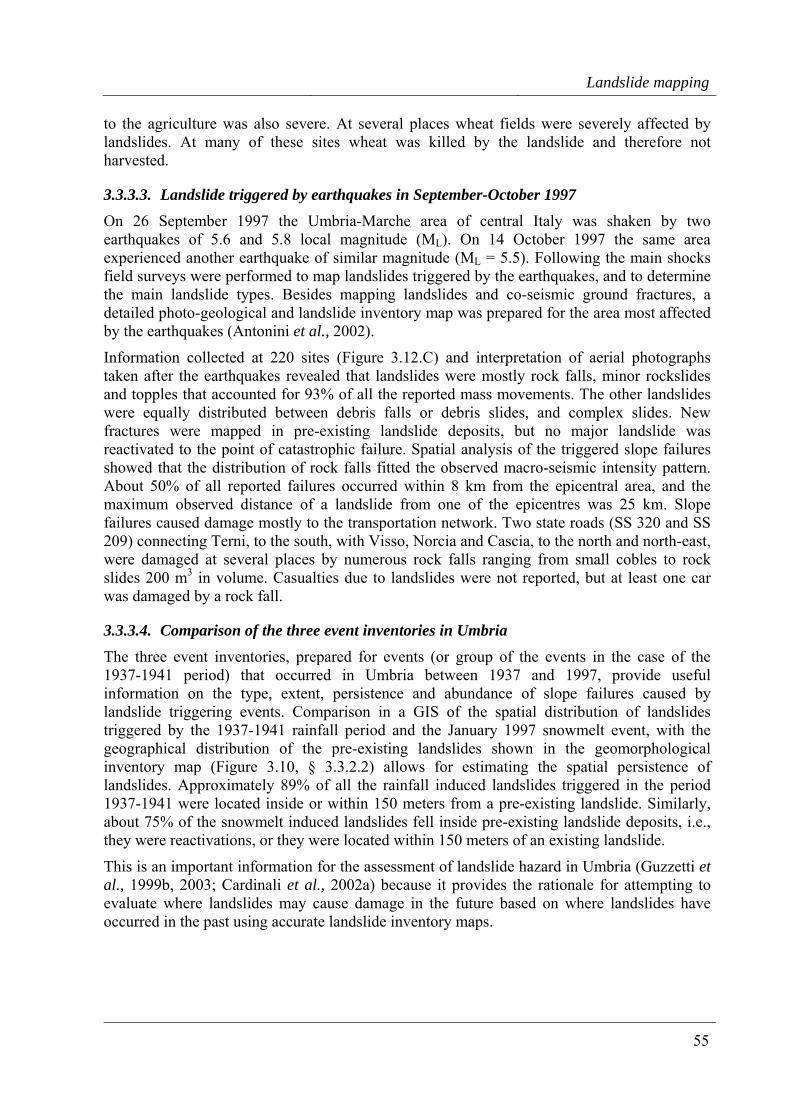
Landslide mapping
55
to the agriculture was also severe. At several places wheat fields were severely affected by landslides. At many of these sites wheat was killed by the landslide and therefore not harvested.
3.3.3.3. Landslide triggered by earthquakes in September-October 1997 On 26 September 1997 the Umbria-Marche area of central Italy was shaken by two earthquakes of 5.6 and 5.8 local magnitude (ML). On 14 October 1997 the same area experienced another earthquake of similar magnitude (ML = 5.5). Following the main shocks field surveys were performed to map landslides triggered by the earthquakes, and to determine the main landslide types. Besides mapping landslides and co-seismic ground fractures, a detailed photo-geological and landslide inventory map was prepared for the area most affected by the earthquakes (Antonini et al., 2002).
Information collected at 220 sites (Figure 3.12.C) and interpretation of aerial photographs taken after the earthquakes revealed that landslides were mostly rock falls, minor rockslides and topples that accounted for 93% of all the reported mass movements. The other landslides were equally distributed between debris falls or debris slides, and complex slides. New fractures were mapped in pre-existing landslide deposits, but no major landslide was reactivated to the point of catastrophic failure. Spatial analysis of the triggered slope failures showed that the distribution of rock falls fitted the observed macro-seismic intensity pattern. About 50% of all reported failures occurred within 8 km from the epicentral area, and the maximum observed distance of a landslide from one of the epicentres was 25 km. Slope failures caused damage mostly to the transportation network. Two state roads (SS 320 and SS 209) connecting Terni, to the south, with Visso, Norcia and Cascia, to the north and north-east, were damaged at several places by numerous rock falls ranging from small cobles to rock slides 200 m3 in volume. Casualties due to landslides were not reported, but at least one car was damaged by a rock fall.
3.3.3.4. Comparison of the three event inventories in Umbria The three event inventories, prepared for events (or group of the events in the case of the 1937-1941 period) that occurred in Umbria between 1937 and 1997, provide useful information on the type, extent, persistence and abundance of slope failures caused by landslide triggering events. Comparison in a GIS of the spatial distribution of landslides triggered by the 1937-1941 rainfall period and the January 1997 snowmelt event, with the geographical distribution of the pre-existing landslides shown in the geomorphological inventory map (Figure 3.10, § 3.3.2.2) allows for estimating the spatial persistence of landslides. Approximately 89% of all the rainfall induced landslides triggered in the period 1937-1941 were located inside or within 150 meters from a pre-existing landslide. Similarly, about 75% of the snowmelt induced landslides fell inside pre-existing landslide deposits, i.e., they were reactivations, or they were located within 150 meters of an existing landslide.
This is an important information for the assessment of landslide hazard in Umbria (Guzzetti et al., 1999b, 2003; Cardinali et al., 2002a) because it provides the rationale for attempting to evaluate where landslides may cause damage in the future based on where landslides have occurred in the past using accurate landslide inventory maps.
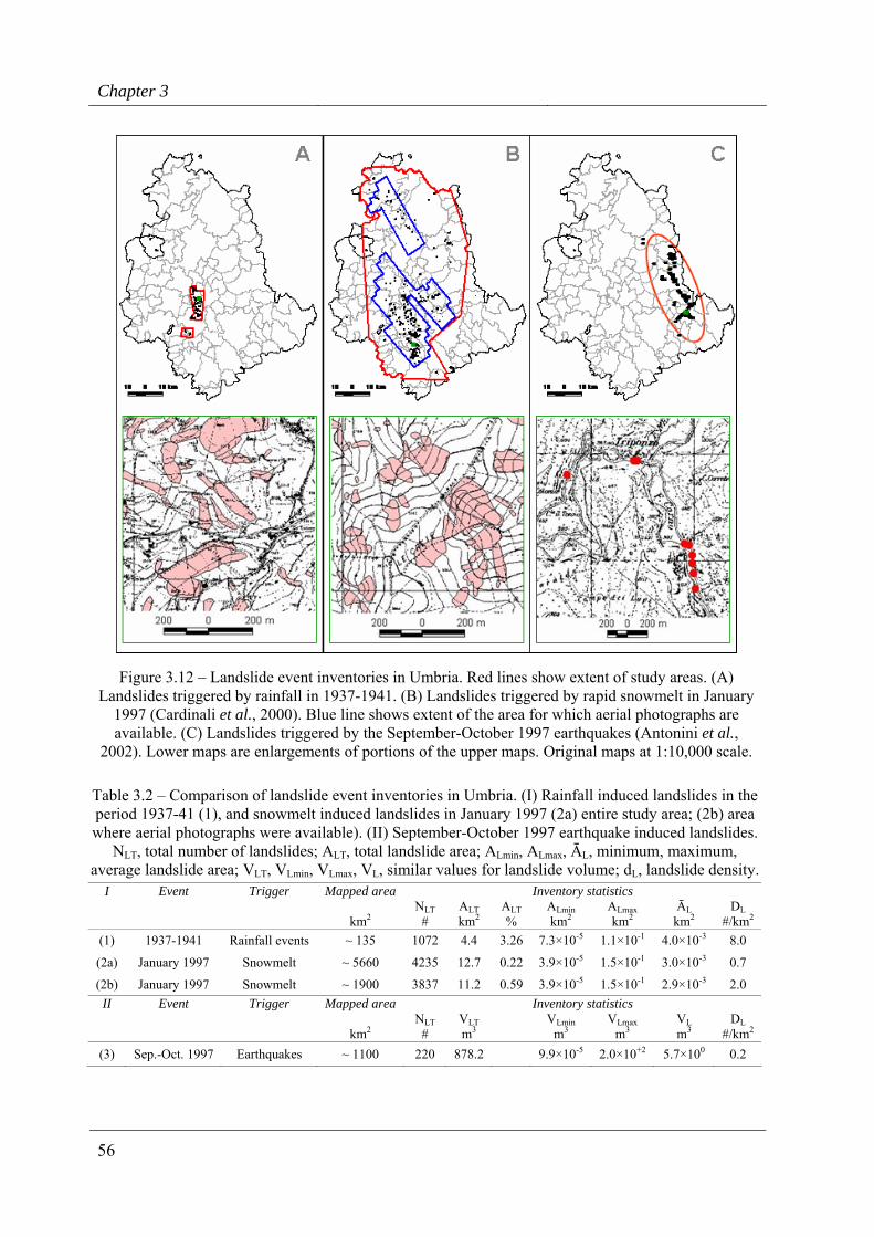
Chapter 3
56
Figure 3.12 – Landslide event inventories in Umbria. Red lines show extent of study areas. (A) Landslides triggered by rainfall in 1937-1941. (B) Landslides triggered by rapid snowmelt in January
1997 (Cardinali et al., 2000). Blue line shows extent of the area for which aerial photographs are available. (C) Landslides triggered by the September-October 1997 earthquakes (Antonini et al.,
2002). Lower maps are enlargements of portions of the upper maps. Original maps at 1:10,000 scale.
Table 3.2 – Comparison of landslide event inventories in Umbria. (I) Rainfall induced landslides in the period 1937-41 (1), and snowmelt induced landslides in January 1997 (2a) entire study area; (2b) area where aerial photographs were available). (II) September-October 1997 earthquake induced landslides.
NLT, total number of landslides; ALT, total landslide area; ALmin, ALmax, ĀL, minimum, maximum, average landslide area; VLT, VLmin, VLmax, VL, similar values for landslide volume; dL, landslide density.
I Event Trigger Mapped area Inventory statistics NLT ALT ALT ALmin ALmax ĀL DL km2 # km2 % km2 km2 km2 #/km2
(1) 1937-1941 Rainfall events ~ 135 1072 4.4 3.26 7.3×10⁻⁵ 1.1×10⁻¹ 4.0×10⁻³ 8.0
(2a) January 1997 Snowmelt ~ 5660 4235 12.7 0.22 3.9×10⁻⁵ 1.5×10⁻¹ 3.0×10⁻³ 0.7
(2b) January 1997 Snowmelt ~ 1900 3837 11.2 0.59 3.9×10⁻⁵ 1.5×10⁻¹ 2.9×10⁻³ 2.0 II Event Trigger Mapped area Inventory statistics NLT VLT VLmin VLmax VL DL km2 # m3 m3 m3 m3 #/km2
(3) Sep.-Oct. 1997 Earthquakes ~ 1100 220 878.2 9.9×10⁻⁵ 2.0×10+2 5.7×100 0.2
Landslide mapping
57
Guzzetti et al. (2003) attempted a comparison of the effects of the three landslide events on the transportation network. The analysis revealed that the largest number of sites with damage was reported as a result of earthquake induced landslides, mostly because of their proximity to the transportation network in the area affected by the earthquakes. Rock falls can be abundant even in areas of limited extent, and they can be very dangerous to people and destructive to structures even for small volumes (less than one cubic meter). In the mountain area where seismic shaking was most severe in 1997, roads most affected by the rock falls were located at or near the valley bottom. Landslides triggered by the rapid snowmelt in 1997 and by rainfall events in the period 1937-1941 were similar, and comprised shallow soil slides, slumps and slump-earth flows, and deep-seated slides, slide earth-flows and complex movements. These landslide types move slowly and with generally limited displacements. These types of movement explains why roads were damaged at several places, but were totally interrupted at only a few sites. It may also explain why landslides did not cause casualties. Despite the fact that the abundance of landslides and the average landslide density for the two events were different, the percentage of landslides that interfered with the transportation network was similar, 2.7% for the 1937-1941 rainfall events and 2.5% for the January 1997 snowmelt event. This may be important information for landslide risk assessment in Umbria.
3.3.4. Multi-temporal inventories A multi-temporal landslide map is the most advanced form of landslide inventory. It shows the location and types of failures in an area, and portrays their recent evolution in space and time. Preparing a multi-temporal inventory is a difficult and time consuming operation that involves the assimilation of multiple information, including: (i) information obtained by systematically interpreting all the aerial photographs available for a study area, irrespective of age, scale and type of the photographs; (ii) data gathered through field surveys, conducted primarily after landslide triggering events; (iii) information on the occurrence of historical landslide events, obtained by searching multiple archive and bibliographical sources; and where available, (iv) information on ground movements obtained through field instrumentations, topographic surveys, and remote sensing technologies (e.g., SAR, Lidar, etc.). Because of the difficulty and complexity in preparing a multi-temporal inventory, these maps are rare, and where they are available they cover areas of limited extent, ranging from few tens to few hundreds of square kilometres (e.g., Hovius et al., 1996; Larsen and Torres-Sánchez, 1996, 1998; Cardinali et al., 2004; Galli et al., 2005; Guzzetti et al., 2005).
Difficulties in preparing a multi-temporal inventory map include: (i) the availability of multiple sets of aerial photographs for the same area, that locally limits the possibility of producing the multi-temporal inventory; (ii) the ability to recognize, interpret, and map subtle morphological changes as slope movements; (iii) the difficulty of inferring consistently the age of the landslides based on their morphological appearance, particularly when the time between two successive flights is long (e.g., a decade or even larger); (iv) the possibility of mapping landslides of different age (obtained from different flights) on the same topographic maps, which may not portray the topography present on the aerial photographs (every time a landslide occurs it changes topography, locally significantly, but this is not shown in the base map); and (v) the difficulty of being precise and consistent when transferring the information on landslides from the aerial photographs to the base maps and in a GIS without loosing information or introducing errors (where morphological changes are subtle it may be difficult to map and digitize the changes). To overcome these limitations, multi-temporal inventory
Chapter 3
58
maps must be prepared by teams of well-trained, experienced and motivated geomorphologists.
3.3.4.1. Multi-temporal landslide inventory for the Collazzone area For the Collazzone area, in central Umbria (§ 2.4), a multi-temporal landslide inventory map was prepared at 1:10,000 scale (Figure 3.13). The map was prepared through the interpretation of multiple sets of aerial photographs and detailed geological and geomorphological field mapping conducted in the period from January to March 1997, in the summer and autumn 2002, and in the period from September 2003 to April 2004. The six sets of aerial photographs used to prepare the multi-temporal map were taken: (i) in the summer of 1941 at 1:18,000 scale, (ii) on 30 August 1954 at 1:33,000 scale, (iii) on 13 June 1977 at 1:13,000 scale, (iv) on 1 July 1985 at 1:15,000 scale, (v) on April 1997 at 1:20,000 scale, and (vi) in the summer 1999 at 1:40,000 scale.
A team of two geomorphologists carried out the interpretation of the aerial photographs in the 5-month period from July to November 2002, for an average of 8 square kilometres per man-month. The two interpreters looked at each pair of aerial photographs using a mirror stereoscope (4× magnification) and a continue-zoom stereoscope (3× to 20× magnification). Both stereoscopes allowed the interpreters to map contemporaneously on the same stereo pair. The interpreters used all morphological, geological and landside information available from published maps, previous work carried out in the same area (including the two described regional inventories, shown in Figures 3.9 and 3.10), and discussion with other geologists and geomorphologists. Care was taken in identifying areas where morphology had changed in response to mass movements, and to avoid interpretation errors due to land use modifications or to the different views provided by aerial photographs taken at different dates.
The landslide information was drawn on transparent plastic sheets placed over the aerial photographs. Depending on the local abundance and complexity of the landslides, a single sheet or multiple sheets were used to map landslides of different ages (i.e., identified on aerial photographs of different dates). To transfer the landslide information from the aerial photographs to the base maps, at 1:10,000 scale, and to construct the GIS database, the procedure used to prepare the detailed geomorphological inventory (§ 3.3.2.2, Figure 3.10) was adapted to cope with larger and more complex landslide information. In the GIS database, landslides attributed to a single date (e.g., a rainfall event) or period were stored separately. Following this procedure, new and active landslides recognized, e.g., in the 1977 aerial photographs were stored in a separate layer than the landslides mapped as inactive in the same photographs. The procedure required intensive and time-consuming GIS work to correct topological and geographical errors. The obtained GIS database stores information on landslides attributed to twelve different dates or periods. The combination of the different layers represents the multi-temporal landslide inventory map.
In the multi-temporal inventory map, landslides are classified according to the type of movement, and the estimated age, activity, depth, and velocity. Landslide type is defined according to Cruden and Varnes (1996). Adopting the same procedure used to compile the detailed geomorphological inventory for Umbria (§ 3.3.2.2, Figure 3.10), for deep-seated slope failures, the landslide crown is mapped separately from the deposit. The distinction is not made for shallow landslides. Landslide age, activity, depth, and velocity were determined based on the type of movement, the morphological characteristics and appearance of the landslides on the aerial photographs, the local lithological and structural setting, and the date
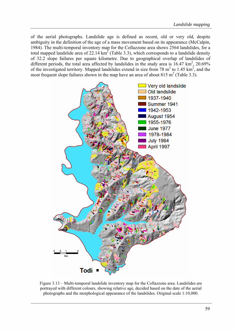
Landslide mapping
59
of the aerial photographs. Landslide age is defined as recent, old or very old, despite ambiguity in the definition of the age of a mass movement based on its appearance (McCalpin, 1984). The multi-temporal inventory map for the Collazzone area shows 2564 landslides, for a total mapped landslide area of 22.14 km2 (Table 3.3), which corresponds to a landslide density of 32.2 slope failures per square kilometre. Due to geographical overlap of landslides of different periods, the total area affected by landslides in the study area is 16.47 km2, 20.69% of the investigated territory. Mapped landslides extend in size from 78 m2 to 1.45 km2, and the most frequent slope failures shown in the map have an area of about 815 m2 (Table 3.3).
Figure 3.13 – Multi-temporal landslide inventory map for the Collazzone area. Landslides are portrayed with different colours, showing relative age, decided based on the date of the aerial
photographs and the morphological appearance of the landslides. Original scale 1:10,000.
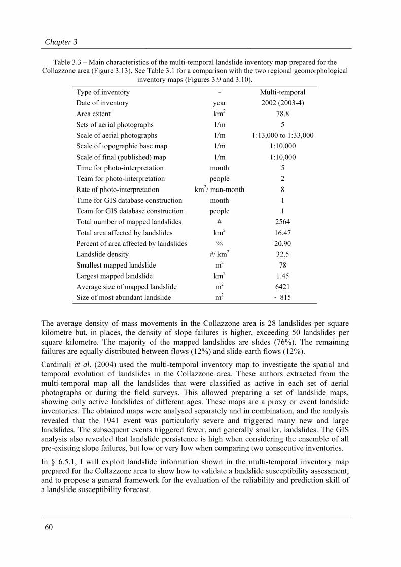
Chapter 3
60
Table 3.3 – Main characteristics of the multi-temporal landslide inventory map prepared for the Collazzone area (Figure 3.13). See Table 3.1 for a comparison with the two regional geomorphological
inventory maps (Figures 3.9 and 3.10).
Type of inventory - Multi-temporal Date of inventory year 2002 (2003-4) Area extent km2 78.8 Sets of aerial photographs 1/m 5 Scale of aerial photographs 1/m 1:13,000 to 1:33,000 Scale of topographic base map 1/m 1:10,000 Scale of final (published) map 1/m 1:10,000 Time for photo-interpretation month 5 Team for photo-interpretation people 2 Rate of photo-interpretation km2/ man-month 8 Time for GIS database construction month 1 Team for GIS database construction people 1 Total number of mapped landslides # 2564 Total area affected by landslides km2 16.47 Percent of area affected by landslides % 20.90 Landslide density #/ km2 32.5 Smallest mapped landslide m2 78 Largest mapped landslide km2 1.45 Average size of mapped landslide m2 6421 Size of most abundant landslide m2 ~ 815
The average density of mass movements in the Collazzone area is 28 landslides per square kilometre but, in places, the density of slope failures is higher, exceeding 50 landslides per square kilometre. The majority of the mapped landslides are slides (76%). The remaining failures are equally distributed between flows (12%) and slide-earth flows (12%).
Cardinali et al. (2004) used the multi-temporal inventory map to investigate the spatial and temporal evolution of landslides in the Collazzone area. These authors extracted from the multi-temporal map all the landslides that were classified as active in each set of aerial photographs or during the field surveys. This allowed preparing a set of landslide maps, showing only active landslides of different ages. These maps are a proxy or event landslide inventories. The obtained maps were analysed separately and in combination, and the analysis revealed that the 1941 event was particularly severe and triggered many new and large landslides. The subsequent events triggered fewer, and generally smaller, landslides. The GIS analysis also revealed that landslide persistence is high when considering the ensemble of all pre-existing slope failures, but low or very low when comparing two consecutive inventories.
In § 6.5.1, I will exploit landslide information shown in the multi-temporal inventory map prepared for the Collazzone area to show how to validate a landslide susceptibility assessment, and to propose a general framework for the evaluation of the reliability and prediction skill of a landslide susceptibility forecast.
Landslide mapping
61
3.4. Factors affecting the quality of landslide inventories
A recognized limitation of landslide inventory maps refers to their intrinsic subjectivity, and to the difficulty of measuring their reliability and completeness (Guzzetti et al., 2000; Malamud et al., 2004a). Reliability, completeness and resolution are issues to consider when preparing and using an inventory map. An incomplete or unreliable inventory may result in erroneous susceptibility, hazard, and risk assessments.
The reliability of archive inventories depends largely on the quality and abundance of the information sources (Guzzetti et al., 1994; Ibsen and Brunsden, 1996; Glade, 1998; Cruden, 1997; Glade, 2001). For inventory maps compiled through the interpretation of aerial photographs, the experience gained from surveys carried out in different parts of the world has shown that trained investigators can reliably detect landslides by standard photo-interpretation techniques coupled with systematic checks in the field (Soeters and van Westen, 1996; Rib and Liang, 1978). However, the reliability of these inventories (geomorphological, event or multi-temporal) depends on many factors, including: (i) landslide freshness and age, (ii) the persistence of landslide morphology within the landscape, (iii) the type, quality and scale of aerial photographs and base maps, including the scale of the final map, (iv) the morphological and geological complexity of the study area, (v) land use types and alterations, (vi) the quality of the stereoscopes used to analyse the aerial photographs, and (vii) the degree of experience of the interpreter who completes the inventory (Hansen, 1984; Fookes et al., 1991; Carrara et al., 1992; Ardizzone et al., 2002).
Once a landslide is recognized in the field or from the aerial photographs it must be mapped, i.e. information about the landslide’s location and characteristics is obtained and transferred onto paper. This operation is not trivial and is prone to errors. Since absolute coordinates of the boundaries of a landslide are seldom available, the geomorphologist uses available base maps and the topographical and morphological features shown on the maps to locate the landslide. Where the topographic map is accurate and shows the actual morphology, and where landslides have a distinct morphological signature, locating and mapping the landslide is straightforward and subject to little uncertainty. Where the topographic map does not represent faithfully the morphology or the landslide is not very distinct, significant location and mapping errors are possible. In placing the landslide on the topographic map, the geomorphologist uses all of the information on the map, including the position and shape of divides and drainage lines, the pattern of vegetation and land use, and the presence of vulnerable elements (e.g. roads, buildings, etc.). If these are not shown correctly or are incomplete, the mapping can be affected by errors and uncertainties. Consequently, the reliability of a landslide inventory map varies spatially, depending on morphology, hydrography, land-use pattern, presence of forest, and abundance and location of vulnerable elements. In addition, for large-scale landslide inventory maps (>1:20,000) the landslide and the topographic information are strictly coupled. Thus, landslides should be shown only with the topographic maps used to prepare the inventory.
Once the landslide has been mapped on paper, the information is digitized for further analysis and display. This last step in the production of a landslide inventory is also error-prone, and can introduce a variety of cartographic errors, some severe. An error in the location of a landslide boundary of only 1-2 mm on the topographic map (i.e. 10-20 m on the ground at 1:10 000 scale) may result in >5 per cent difference in landslide area for small (<1 ha) slope failures. After landslides are transferred to a GIS, computations of landslide areas are possible.
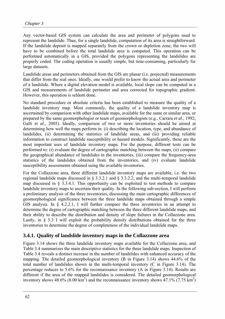
Chapter 3
62
Any vector-based GIS system can calculate the area and perimeter of polygons used to represent the landslide. Thus, for a single landslide, computation of its area is straightforward. If the landslide deposit is mapped separately from the crown or depletion zone, the two will have to be combined before the total landslide area is computed. This operation can be performed automatically in a GIS, provided the polygons representing the landslides are properly coded. The coding operation is usually simple, but time-consuming, particularly for large datasets.
Landslide areas and perimeters obtained from the GIS are planar (i.e. projected) measurements that differ from the real ones. Ideally, one would prefer to know the actual area and perimeter of a landslide. Where a digital elevation model is available, local slope can be computed in a GIS and measurements of landslide perimeter and area corrected for topographic gradient. However, this operation is seldom done.
No standard procedure or absolute criteria has been established to measure the quality of a landslide inventory map. Most commonly, the quality of a landslide inventory map is ascertained by comparison with other landslide maps, available for the same or similar area, or prepared by the same geomorphologist or team of geomorphologists (e.g., Carrara et al., 1992; Galli et al., 2005). Ideally, comparison of two or more inventories should be aimed at determining how well the maps perform in: (i) describing the location, type, and abundance of landslides, (ii) determining the statistics of landslide areas, and (iii) providing reliable information to construct landslide susceptibility or hazard models. Significantly, these are the most important uses of landslide inventory maps. For the purpose, different tests can be performed to: (i) evaluate the degree of cartographic matching between the maps, (ii) compare the geographical abundance of landslides in the inventories, (iii) compare the frequency-area statistics of the landslides obtained from the inventories, and (iv) evaluate landslide susceptibility assessments obtained using the available inventories.
For the Collazzone area, three different landslide inventory maps are available, i.e. the two regional landslide maps discussed in § 3.3.2.1 and § 3.3.2.2, and the multi-temporal landslide map discussed in § 3.3.4.1. This opportunity can be exploited to test methods to compare landslide inventory maps to ascertain their quality. In the following sub-section, I will perform a preliminary analysis of the three inventories, discussing the main cartographic differences of geomorphological significance between the three landslide maps obtained through a simple GIS analysis. In § 4.2.2.1, I will further compare the three inventories in an attempt to determine the degree of cartographic matching between the three different landslide maps, and their ability to describe the distribution and density of slope failures in the Collazzone area. Lastly, in § 5.3 I will exploit the probability density distributions obtained for the three inventories to determine the degree of completeness of the individual landslide maps.
3.4.1. Quality of landslide inventory maps in the Collazzone area Figure 3.14 shows the three landslide inventory maps available for the Collazzone area, and Table 3.4 summarizes the main descriptive statistics for the three landslide maps. Inspection of Table 3.4 reveals a distinct increase in the number of landslides with enhanced accuracy of the mapping. The detailed geomorphological inventory (B in Figure 3.14) shows 44.6% of the total number of landslides shown in the multi-temporal inventory (C in Figure 3.14). The percentage reduces to 5.6% for the reconnaissance inventory (A in Figure 3.14). Results are different if the area of the mapped landslides is considered. The detailed geomorphological inventory shows 48.6% (8.00 km2) and the reconnaissance inventory shows 47.1% (7.75 km2)
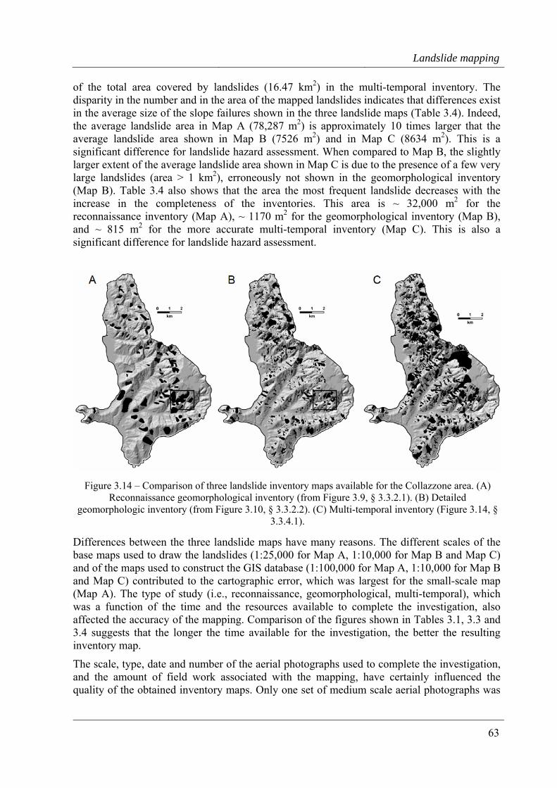
Landslide mapping
63
of the total area covered by landslides (16.47 km2) in the multi-temporal inventory. The disparity in the number and in the area of the mapped landslides indicates that differences exist in the average size of the slope failures shown in the three landslide maps (Table 3.4). Indeed, the average landslide area in Map A (78,287 m2) is approximately 10 times larger that the average landslide area shown in Map B (7526 m2) and in Map C (8634 m2). This is a significant difference for landslide hazard assessment. When compared to Map B, the slightly larger extent of the average landslide area shown in Map C is due to the presence of a few very large landslides (area > 1 km2), erroneously not shown in the geomorphological inventory (Map B). Table 3.4 also shows that the area the most frequent landslide decreases with the increase in the completeness of the inventories. This area is ~ 32,000 m2 for the reconnaissance inventory (Map A), ~ 1170 m2 for the geomorphological inventory (Map B), and ~ 815 m2 for the more accurate multi-temporal inventory (Map C). This is also a significant difference for landslide hazard assessment.
Figure 3.14 – Comparison of three landslide inventory maps available for the Collazzone area. (A) Reconnaissance geomorphological inventory (from Figure 3.9, § 3.3.2.1). (B) Detailed
geomorphologic inventory (from Figure 3.10, § 3.3.2.2). (C) Multi-temporal inventory (Figure 3.14, § 3.3.4.1).
Differences between the three landslide maps have many reasons. The different scales of the base maps used to draw the landslides (1:25,000 for Map A, 1:10,000 for Map B and Map C) and of the maps used to construct the GIS database (1:100,000 for Map A, 1:10,000 for Map B and Map C) contributed to the cartographic error, which was largest for the small-scale map (Map A). The type of study (i.e., reconnaissance, geomorphological, multi-temporal), which was a function of the time and the resources available to complete the investigation, also affected the accuracy of the mapping. Comparison of the figures shown in Tables 3.1, 3.3 and 3.4 suggests that the longer the time available for the investigation, the better the resulting inventory map.
The scale, type, date and number of the aerial photographs used to complete the investigation, and the amount of field work associated with the mapping, have certainly influenced the quality of the obtained inventory maps. Only one set of medium scale aerial photographs was
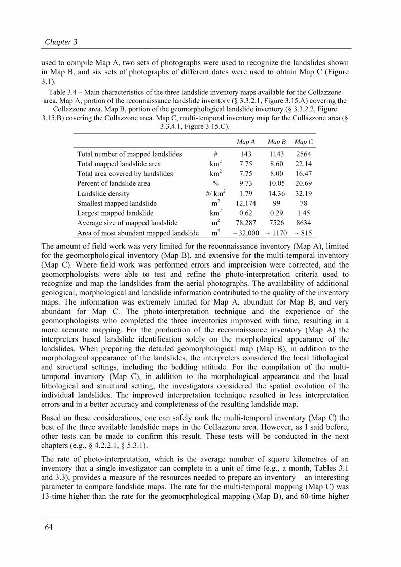
Chapter 3
64
used to compile Map A, two sets of photographs were used to recognize the landslides shown in Map B, and six sets of photographs of different dates were used to obtain Map C (Figure 3.1).
Table 3.4 – Main characteristics of the three landslide inventory maps available for the Collazzone area. Map A, portion of the reconnaissance landslide inventory (§ 3.3.2.1, Figure 3.15.A) covering the
Collazzone area. Map B, portion of the geomorphological landslide inventory (§ 3.3.2.2, Figure 3.15.B) covering the Collazzone area. Map C, multi-temporal inventory map for the Collazzone area (§
3.3.4.1, Figure 3.15.C).
Map A Map B Map C
Total number of mapped landslides # 143 1143 2564 Total mapped landslide area km2 7.75 8.60 22.14 Total area covered by landslides km2 7.75 8.00 16.47 Percent of landslide area % 9.73 10.05 20.69 Landslide density #/ km2 1.79 14.36 32.19 Smallest mapped landslide m2 12,174 99 78 Largest mapped landslide km2 0.62 0.29 1.45 Average size of mapped landslide m2 78,287 7526 8634 Area of most abundant mapped landslide m2 ~ 32,000 ~ 1170 ~ 815
The amount of field work was very limited for the reconnaissance inventory (Map A), limited for the geomorphological inventory (Map B), and extensive for the multi-temporal inventory (Map C). Where field work was performed errors and imprecision were corrected, and the geomorphologists were able to test and refine the photo-interpretation criteria used to recognize and map the landslides from the aerial photographs. The availability of additional geological, morphological and landslide information contributed to the quality of the inventory maps. The information was extremely limited for Map A, abundant for Map B, and very abundant for Map C. The photo-interpretation technique and the experience of the geomorphologists who completed the three inventories improved with time, resulting in a more accurate mapping. For the production of the reconnaissance inventory (Map A) the interpreters based landslide identification solely on the morphological appearance of the landslides. When preparing the detailed geomorphological map (Map B), in addition to the morphological appearance of the landslides, the interpreters considered the local lithological and structural settings, including the bedding attitude. For the compilation of the multi-temporal inventory (Map C), in addition to the morphological appearance and the local lithological and structural setting, the investigators considered the spatial evolution of the individual landslides. The improved interpretation technique resulted in less interpretation errors and in a better accuracy and completeness of the resulting landslide map.
Based on these considerations, one can safely rank the multi-temporal inventory (Map C) the best of the three available landslide maps in the Collazzone area. However, as I said before, other tests can be made to confirm this result. These tests will be conducted in the next chapters (e.g., § 4.2.2.1, § 5.3.1).
The rate of photo-interpretation, which is the average number of square kilometres of an inventory that a single investigator can complete in a unit of time (e.g., a month, Tables 3.1 and 3.3), provides a measure of the resources needed to prepare an inventory – an interesting parameter to compare landslide maps. The rate for the multi-temporal mapping (Map C) was 13-time higher than the rate for the geomorphological mapping (Map B), and 60-time higher
Landslide mapping
65
than the rate for the reconnaissance mapping (Map A). This implies that the team of two geomorphologists that completed the multi-temporal inventory map for the Collazzone area in 5 months would need 45 years to cover the entire Umbria Region (8456 km2), assuming the team uses the same technique and the same sets of aerial photographs. The figure compares with the 28 months needed by a team of three geomorphologists to complete the geomorphological map, and with the 9 months required by a team of two interpreters to compile the reconnaissance inventory (Table 3.1).
Based on these figures, I conclude that it is probably not feasible to prepare an accurate multi-temporal inventory map for the entire Umbria Region – or an area of similar extent and morphological complexity – with the proposed methodology. More generally, I conclude that at the regional scale, i.e., for areas extending for thousands of square kilometres, only geomorphological or event inventories can be obtained by teams of experienced geomorphologists. This somewhat limits the possibility of preparing reliable landslide hazard maps for large territories (§ 7).
3.5. Summary of achieved results
In this chapter, I have:
(a) Demonstrated the feasibility of landslide inventory maps that reliably cover areas extending for thousands of square kilometres. However, such maps need to be prepared by experienced geomorphologists.
(b) Demonstrated the feasibility and importance of landslide event inventory maps. From such inventories, unique information is obtained which is of primary importance to determine landslide hazard and to evaluate the associated risk.
(c) Shown that multi-temporal inventory maps prepared through the assimilation of multiple information are a superior type of landslide map. However due to their complexity, such maps can be prepared only for areas of limited extent.
(d) Established the basis for measuring the quality of landslide inventory maps, which allows for a comparison of different maps prepared for the same area.
This largely responds to Questions # 1 and # 2 posed in the Introduction (§ 1.2).

67
4. ANALYSIS OF THE INVENTORIES
Super competence is worst than incompetence.
The cost of an expertise is proportional to the number of words you understand.
The information shown on landslide inventories can be used for a variety of analyses, including: (i) investigating landslide spatial abundance, through the production of landslide density maps; (ii) comparing inventory maps obtained from different sources (e.g., archive and geomorphological) for the same area; (iii) evaluating the completeness of the inventories; (iv) ascertaining landslide geographical persistence, by comparing event and geomorphological inventories; (v) estimating the frequency of slope failure occurrence, by analysing historical catalogues of landslide events or multi-temporal inventory maps; (vi) obtaining the statistics of landslide size; (vii) ascertaining landslide susceptibility and hazards, including the validation of the obtained susceptibility and hazard forecasts; (viii) determining the possible impact of landslides on built-up areas or the infrastructure; and (ix) contributing to establish levels of landslide risk. The quality and reliability of the different analyses obtained from a landslide inventory depend largely (often entirely) on the quality and completeness of the original landslide map. For this reason, one should always: (i) aim at compiling accurate and precise inventories, (ii) document the sources of information used to obtain the inventories, (iii) accurately describe the techniques, methods and tools used to prepare or compile the inventories, and (iv) try to assess the completeness of the obtained inventories. Limitations of landslide inventories should always be known (i.e., explicit and clear) to the users of the maps or the archives.
In this chapter, I discuss some of the possible applications of landslide inventories. I first demonstrate the construction and use of landslide density maps. I then show methods to compare geomorphological and historical inventories. I discuss an index to quantify the degree of matching between inventories, and I show an application for the comparison of the three landslide maps available for the Collazzone study area. I further discuss the issue of the completeness of the landslide inventories, and I use two event inventories available for Umbria to investigate geographical landslide persistence. Finally, I show how to ascertain the temporal frequency of slope failures from archive inventories.
4.1. Landslide abundance
To quantify the geographical (spatial) abundance of landslides, landslide density maps can be prepared. Landslide density (or frequency) maps measure the spatial distribution of slope
Chapter 4
68
failures (Campbell, 1973; Wright et al., 1974; DeGraff, 1985; DeGraff and Canuti, 1988). Landslide density is the proportion (i.e., frequency, percentage) of landslide area, and is commonly computed as:
M
LL A
AD = , 0 ≤ DL ≤ 1 (4.1)
where, AM is the area of the mapping unit used to compute the density (e.g., grid cell, slope unit, unique condition unit, etc., see § 6.2.2), and AL is the total landslide area in the mapping unit. In each mapping unit landslide density varies from 0, for landslide free units, to 1, where the entire unit is occupied by landslides.
Density maps have different applications. They have been used to: (i) show a synoptic view of landslide distribution for large regions or entire nations (Radbruch-Hall et al., 1982; Reichenbach et al., 1998a; Guzzetti et al., 2003), (ii) portray a first-order overview of landslide abundance (Campbell, 1973; Wright et al., 1974; Wright and Nilsen, 1974; Pomeroy, 1978; Moreiras, 2004), (iii) show the magnitude of slope failures triggered by severe storms (Campbell, 1975; Ellen and Wieczorek, 1988), (iv) evaluate landslide abundance or landslide activity in relation to forest management, agricultural practise, and land use changes (DeGraff, 1985; DeGraff and Canuti, 1988), (v) show the spatial distribution of the historical frequency of rock fall events (Chau et al., 2003), and (vi) as a week proxy of landslide susceptibility (Bulut et al., 2000; Guzzetti et al., 2005d).
Landslide density maps are filler of space. This is different from inventory maps, which provide information only where landslides were recognized and mapped (§ 9.1). Density maps provide insight on the expected (or inferred) occurrence of landslides in any part of the investigated area without leaving unclassified areas. A density map does not show were landslides are located, but this loss in resolution is compensated for by improved map readability and reduced cartographic errors (Carrara et al., 1992; Ardizzone et al., 2002). Additionally, landslide density is independent of the extent of the study area, which makes comparison between different regions straightforward. Such characteristics make density maps appealing to decision-makers and land developers (§ 9.2).
Depending on the type of mapping unit used to compute and portray the density, landslide density maps can be based on statistical or geomorphological criteria (Guzzetti et al., 2000).
4.1.1. Statistical landslide density maps In statistically-based density maps, the mapping unit is usually an ensemble of grid cells (i.e., pixels), square or nearly circular in shape, with a size generally 10 to 100 times larger than the size of the individual grid cell (Guzzetti et al., 2000). Density is determined by counting the percentage of landslide area within the mapping unit (in this case an artificial “kernel”), which is moved systematically across the territory. This is equivalent to a moving average filtering technique. Additional filtering or weighting techniques can be applied to improve map consistency and readability. By interpolating equal quantity (isopleth) lines, a statistically-based density map can be portrayed as a contour map (Wright et al., 1974). The latter was the favoured method for showing landslide density (Campbell, 1973, 1975; Wright and Nielsen, 1974; DeGraff, 1985) before GIS technology and raster colour display were largely available.
Statistically-based landslide density maps rely on the assumption that landslide occurrence is a continuous variable that can be spatially interpolated (Schmid and MacCanell, 1955; Wright et
Analysis of inventories
69
al., 1974; Guzzetti et al., 1999a). Hence, they perform best in homogeneous terrain – where lithology and morphology do not change abruptly. This assumption is strong (geomorphologically) and holds true only as a general approximation – at small scale – and in homogeneous physiographic environments (Guzzetti et al., 2000). At larger scales, the assumption of spatial continuity does not take into account the existing relations between slope failures and the local morphological, geological or land use settings. As an example, where layered rocks crop out, slope forms and processes are influenced by the attitude of bedding planes. In susceptible geologic environments, landslides are often larger and more abundant where bedding dips toward the slope free face. Conversely, where bedding dips into the slope (reverse slope) terrain is steep and landslides are less abundant (e.g., Guzzetti et al., 1996b). In such conditions, an isopleth map prepared without considering the presence of streams or divides will be misleading, particularly on reverse slopes. This limitation is partly overcome by selecting a mapping unit that bears a physical relation to the geomorphology of landsliding (Carrara et al., 1995; Guzzetti et al., 1999a).
4.1.2. Geomorphological landslide density maps For geomorphological density maps, slope units (as defined in Carrara et al., 1991, see § 6.2.2) appear to be particularly suited to the determination of landslide spatial frequency. This subdivision of the terrain partitions the territory into domains bounded by drainage divides and stream lines. To delineate the divide and stream networks, manual techniques or automatic selection criteria can be adopted. The latter is based on the analysis of a digital terrain matrix (DTM) that acts as a computerised representation of topography (Carrara, 1988; Carrara et al., 1991). Slope units, therefore, correspond to the actual slopes on which landslides take place. The percentage of landslide area within each slope unit, as counted, is equivalent to the percentage of failed area on each slope (see equation 4.1 and Figure 4.1). The landslide density in this case, is the proportion or percentage of the slope unit that is occupied by the landslides.
As they are delimited by morphological boundaries, slope units avoid the pitfall of forecasting high landslide densities in areas that are mapped as essentially landslide free but are close to known failures (for example, across the divide of an asymmetric ridge which is controlled by the attitude of bedding planes). In addition, slope units mitigate the effects of possible identification and mapping errors. As landslide density is computed for the entire mapped area, possible mapping or drafting errors made within each slope unit are averaged.
The advantage of morphologically soundness and the limitation of mapping errors are counterbalanced by the loss of resolution (Figure 4.1). The resolution of slope-unit based density maps is lower than that of grid based or contour based maps, unless the grid or contour spacing is particularly large for the amplitude of the terrain under study. As a result of interpolation procedures, landslide density is a derivative of the spatial distribution of landslides (i.e., the inventory). Interpolation inevitably causes information to be lost. Indeed, even if landslides were mapped in great detail, nothing could be said about the exact location of any single landslide within a slope unit. However, if the size of slope units is chosen in relation to the size of landslides to be studied, the loss of resolution is only apparent and does not correspond to a loss in the applicability and utility of the map (Carrara et al., 1992, 1995, 1999; Guzzetti et al., 1999a, 2000).
Errors and inconsistencies associated with the definition of slope units from DTMs, to the geometrical consistency between slope units and landslide boundaries, to the size of slope
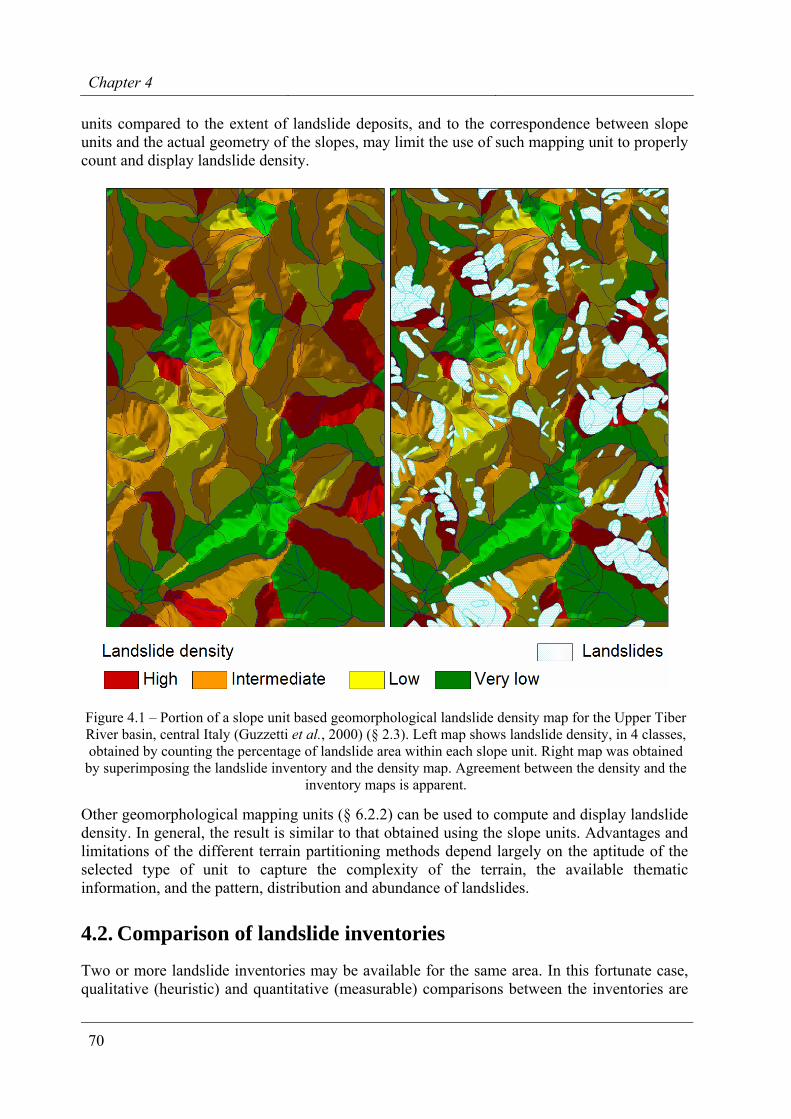
Chapter 4
70
units compared to the extent of landslide deposits, and to the correspondence between slope units and the actual geometry of the slopes, may limit the use of such mapping unit to properly count and display landslide density.
Figure 4.1 – Portion of a slope unit based geomorphological landslide density map for the Upper Tiber River basin, central Italy (Guzzetti et al., 2000) (§ 2.3). Left map shows landslide density, in 4 classes, obtained by counting the percentage of landslide area within each slope unit. Right map was obtained
by superimposing the landslide inventory and the density map. Agreement between the density and the inventory maps is apparent.
Other geomorphological mapping units (§ 6.2.2) can be used to compute and display landslide density. In general, the result is similar to that obtained using the slope units. Advantages and limitations of the different terrain partitioning methods depend largely on the aptitude of the selected type of unit to capture the complexity of the terrain, the available thematic information, and the pattern, distribution and abundance of landslides.
4.2. Comparison of landslide inventories
Two or more landslide inventories may be available for the same area. In this fortunate case, qualitative (heuristic) and quantitative (measurable) comparisons between the inventories are
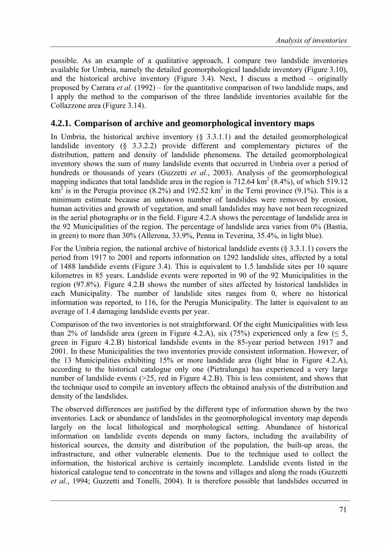
Analysis of inventories
71
possible. As an example of a qualitative approach, I compare two landslide inventories available for Umbria, namely the detailed geomorphological landslide inventory (Figure 3.10), and the historical archive inventory (Figure 3.4). Next, I discuss a method – originally proposed by Carrara et al. (1992) – for the quantitative comparison of two landslide maps, and I apply the method to the comparison of the three landslide inventories available for the Collazzone area (Figure 3.14).
4.2.1. Comparison of archive and geomorphological inventory maps In Umbria, the historical archive inventory (§ 3.3.1.1) and the detailed geomorphological landslide inventory (§ 3.3.2.2) provide different and complementary pictures of the distribution, pattern and density of landslide phenomena. The detailed geomorphological inventory shows the sum of many landslide events that occurred in Umbria over a period of hundreds or thousands of years (Guzzetti et al., 2003). Analysis of the geomorphological mapping indicates that total landslide area in the region is 712.64 km2 (8.4%), of which 519.12 km2 is in the Perugia province (8.2%) and 192.52 km2 in the Terni province (9.1%). This is a minimum estimate because an unknown number of landslides were removed by erosion, human activities and growth of vegetation, and small landslides may have not been recognized in the aerial photographs or in the field. Figure 4.2.A shows the percentage of landslide area in the 92 Municipalities of the region. The percentage of landslide area varies from 0% (Bastia, in green) to more than 30% (Allerona, 33.9%, Penna in Teverina, 35.4%, in light blue).
For the Umbria region, the national archive of historical landslide events (§ 3.3.1.1) covers the period from 1917 to 2001 and reports information on 1292 landslide sites, affected by a total of 1488 landslide events (Figure 3.4). This is equivalent to 1.5 landslide sites per 10 square kilometres in 85 years. Landslide events were reported in 90 of the 92 Municipalities in the region (97.8%). Figure 4.2.B shows the number of sites affected by historical landslides in each Municipality. The number of landslide sites ranges from 0, where no historical information was reported, to 116, for the Perugia Municipality. The latter is equivalent to an average of 1.4 damaging landslide events per year.
Comparison of the two inventories is not straightforward. Of the eight Municipalities with less than 2% of landslide area (green in Figure 4.2.A), six (75%) experienced only a few (≤ 5, green in Figure 4.2.B) historical landslide events in the 85-year period between 1917 and 2001. In these Municipalities the two inventories provide consistent information. However, of the 13 Municipalities exhibiting 15% or more landslide area (light blue in Figure 4.2.A), according to the historical catalogue only one (Pietralunga) has experienced a very large number of landslide events (>25, red in Figure 4.2.B). This is less consistent, and shows that the technique used to compile an inventory affects the obtained analysis of the distribution and density of the landslides.
The observed differences are justified by the different type of information shown by the two inventories. Lack or abundance of landslides in the geomorphological inventory map depends largely on the local lithological and morphological setting. Abundance of historical information on landslide events depends on many factors, including the availability of historical sources, the density and distribution of the population, the built-up areas, the infrastructure, and other vulnerable elements. Due to the technique used to collect the information, the historical archive is certainly incomplete. Landslide events listed in the historical catalogue tend to concentrate in the towns and villages and along the roads (Guzzetti et al., 1994; Guzzetti and Tonelli, 2004). It is therefore possible that landslides occurred in
Chapter 4
72
places and were not reported. Slope failures occurred in remote or distant areas may have not been noticed by the population. Alternatively, they may have been observed but quickly removed, or they may have not been reported because they did not cause significant damage.
Figure 4.2 – Umbria Region. Comparison of geomorphological and historical inventory maps. (A) Percentage of landslide areas in the 92 Municipality obtained from the detailed geomorphological
landslide inventory (see § 3.3.2.2). Histogram shows number of Municipalities in five classes of the percentage of landslide area. (B) Number of historical landslide sites in each Municipality obtained
from the archive inventory (see § 3.3.1.1). Histogram shows abundance of Municipalities in four classes of number of historical landslide sites.
4.2.2. Comparison of two geomorphological landslide inventory maps Only a few authors have attempted to quantitatively compare geomorphological landslide inventory maps (Roth, 1983; Carrara et al., 1992; Ardizone et al., 2000; Galli et al., 2005). Carrara et al. (1992) proposed a quantitative and reproducible method for comparing two landslide inventory maps. For the purpose, these authors introduced an index to measure the degree of mismatch between two inventory maps. The mismatch (or error) index, E, is given by:
Analysis of inventories
73
)AA()AA()AA(E ''
LT'LT
''LT
'LT
''LT
'LT
∪∩−∪
= , 0 ≤ E ≤ 1 (4.2)
Where, 'LTA and ''
LTA are the total landslide area in the first and in the second inventory, respectively, and ∪ and ∩ are the geographical union and intersection of the two inventories, easily obtained in a GIS.
From equation 4.2, the degree of matching, M, between two inventory maps can be obtained as:
EM −= 1 , 0 ≤ M ≤ 1 (4.3)
If two landslide inventory maps portray exactly the same landslides (a rather improbable situation), E = 0 and M = 1, i.e., matching is perfect and mismatch is nil. If the two inventory maps disagree completely, E = 1 and M = 0, i.e., cartographic matching is nil and mismatch is maximum.
Figure 4.3 shows a comparison of two geomorphological inventory maps prepared for the La Honda area, in the San Francisco Bay region, used by Carrara et al. (1992) to investigate uncertainties associated with landslide inventory making. In this experiment, GIS technology was used to determine and quantitatively compare the effect of mapping errors produced by different causes in the compilation of inventory maps from the interpretation of aerial photographs.
Three tests were performed. The first test consisted in comparing two geomorphological landslide inventory maps produced independently by two equally experienced interpreters, which mapped landslides in the La Honda area using black-and-white, 1:18,000 scale aerial photographs and 1:24,000 scale base maps (Figure 4.3, left map). Before starting the operation, one of the two investigators had the opportunity to visit the area. Visual inspection of the maps produced by the two separate investigators indicates that the overall spatial distribution of landslides in the two maps is fairly similar. The percentages of landslide area were 13.5% and 16.8%, for the first and the second investigator, respectively. GIS analysis revealed that 9.9% of the total landslide area was common to both maps (geometrical intersection), and that 20.3% of the area was classified as bearing landslides by either the first or the second interpreter (geometrical union). The mismatch error computed with equation 4.2 was 51.5%, corresponding to a cartographic matching (eq. 4.3) of (only) 48.5%.
An attempt was made to separate the errors caused by differences in investigators’ interpretation and judgement from other sources of errors, including inaccuracies in topographic data location, and data restitution, drafting, digitization and construction of the GIS database. For the purpose, a buffer was traced around each mapped landslide in both inventories. The operation was repeated four times, using buffers of 25, 50, 100 and 200 m width. Results (Figure 4.3, right graph) indicated that first the error decreased at a slow rate, and then it declined more rapidly, and (almost) linearly. Because of the scale of the base maps (1:24,000) and of the aerial photographs (1:18,000) used for the investigation, and the standard inaccuracy in data digitizing and storing landslide information in the GIS database, the total error associated with such operations was accounted by a buffer of approximately 50 m in width. This leaded to an error of approximately 5% (Figure 4.3, right graph). The remaining error (approximately 46%) represented the actual mismatch due to the different geomorphological interpretations performed by the two investigators.
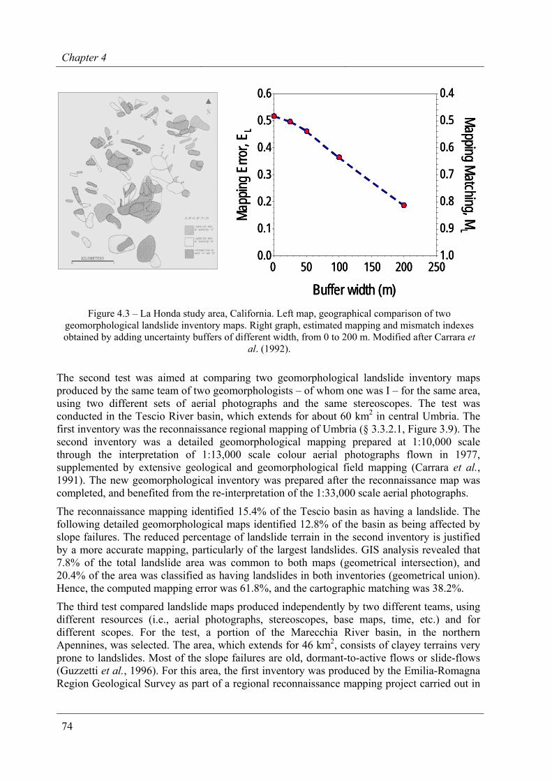
Chapter 4
74
0.0
0.1
0.2
0.3
0.4
0.5
0.6
0 50 100 150 200 250
Buffer width (m)
Mapp
ing E
rror,
E L1.0
0.9
0.8
0.7
0.6
0.5
0.4Mapping Matching, M
L
0.0
0.1
0.2
0.3
0.4
0.5
0.6
0 50 100 150 200 250
Buffer width (m)
Mapp
ing E
rror,
E L1.0
0.9
0.8
0.7
0.6
0.5
0.4Mapping Matching, M
L
0.0
0.1
0.2
0.3
0.4
0.5
0.6
0 50 100 150 200 250
Buffer width (m)
Mapp
ing E
rror,
E L1.0
0.9
0.8
0.7
0.6
0.5
0.4Mapping Matching, M
L
Figure 4.3 – La Honda study area, California. Left map, geographical comparison of two geomorphological landslide inventory maps. Right graph, estimated mapping and mismatch indexes obtained by adding uncertainty buffers of different width, from 0 to 200 m. Modified after Carrara et
al. (1992).
The second test was aimed at comparing two geomorphological landslide inventory maps produced by the same team of two geomorphologists – of whom one was I – for the same area, using two different sets of aerial photographs and the same stereoscopes. The test was conducted in the Tescio River basin, which extends for about 60 km2 in central Umbria. The first inventory was the reconnaissance regional mapping of Umbria (§ 3.3.2.1, Figure 3.9). The second inventory was a detailed geomorphological mapping prepared at 1:10,000 scale through the interpretation of 1:13,000 scale colour aerial photographs flown in 1977, supplemented by extensive geological and geomorphological field mapping (Carrara et al., 1991). The new geomorphological inventory was prepared after the reconnaissance map was completed, and benefited from the re-interpretation of the 1:33,000 scale aerial photographs.
The reconnaissance mapping identified 15.4% of the Tescio basin as having a landslide. The following detailed geomorphological maps identified 12.8% of the basin as being affected by slope failures. The reduced percentage of landslide terrain in the second inventory is justified by a more accurate mapping, particularly of the largest landslides. GIS analysis revealed that 7.8% of the total landslide area was common to both maps (geometrical intersection), and 20.4% of the area was classified as having landslides in both inventories (geometrical union). Hence, the computed mapping error was 61.8%, and the cartographic matching was 38.2%.
The third test compared landslide maps produced independently by two different teams, using different resources (i.e., aerial photographs, stereoscopes, base maps, time, etc.) and for different scopes. For the test, a portion of the Marecchia River basin, in the northern Apennines, was selected. The area, which extends for 46 km2, consists of clayey terrains very prone to landslides. Most of the slope failures are old, dormant-to-active flows or slide-flows (Guzzetti et al., 1996). For this area, the first inventory was produced by the Emilia-Romagna Region Geological Survey as part of a regional reconnaissance mapping project carried out in
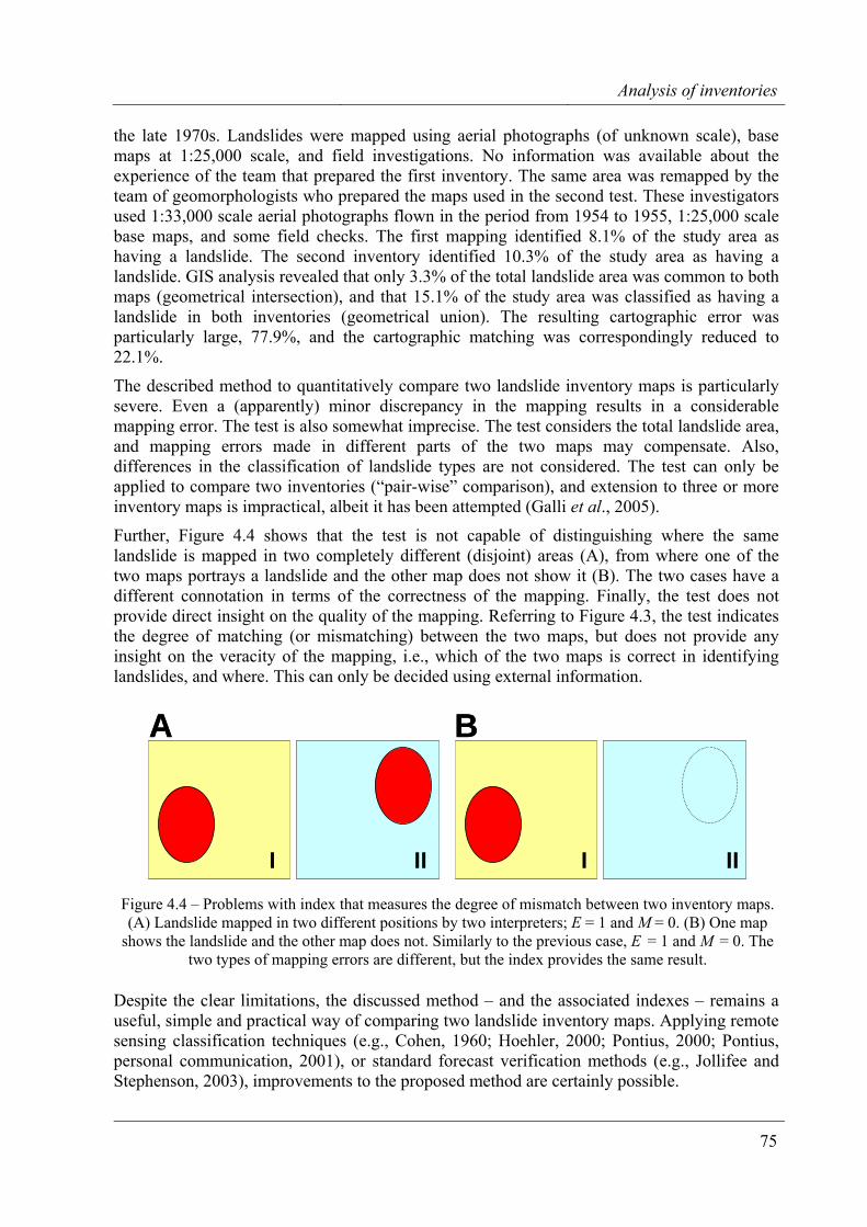
Analysis of inventories
75
the late 1970s. Landslides were mapped using aerial photographs (of unknown scale), base maps at 1:25,000 scale, and field investigations. No information was available about the experience of the team that prepared the first inventory. The same area was remapped by the team of geomorphologists who prepared the maps used in the second test. These investigators used 1:33,000 scale aerial photographs flown in the period from 1954 to 1955, 1:25,000 scale base maps, and some field checks. The first mapping identified 8.1% of the study area as having a landslide. The second inventory identified 10.3% of the study area as having a landslide. GIS analysis revealed that only 3.3% of the total landslide area was common to both maps (geometrical intersection), and that 15.1% of the study area was classified as having a landslide in both inventories (geometrical union). The resulting cartographic error was particularly large, 77.9%, and the cartographic matching was correspondingly reduced to 22.1%.
The described method to quantitatively compare two landslide inventory maps is particularly severe. Even a (apparently) minor discrepancy in the mapping results in a considerable mapping error. The test is also somewhat imprecise. The test considers the total landslide area, and mapping errors made in different parts of the two maps may compensate. Also, differences in the classification of landslide types are not considered. The test can only be applied to compare two inventories (“pair-wise” comparison), and extension to three or more inventory maps is impractical, albeit it has been attempted (Galli et al., 2005).
Further, Figure 4.4 shows that the test is not capable of distinguishing where the same landslide is mapped in two completely different (disjoint) areas (A), from where one of the two maps portrays a landslide and the other map does not show it (B). The two cases have a different connotation in terms of the correctness of the mapping. Finally, the test does not provide direct insight on the quality of the mapping. Referring to Figure 4.3, the test indicates the degree of matching (or mismatching) between the two maps, but does not provide any insight on the veracity of the mapping, i.e., which of the two maps is correct in identifying landslides, and where. This can only be decided using external information.
A B
I III II
A B
I III II
Figure 4.4 – Problems with index that measures the degree of mismatch between two inventory maps. (A) Landslide mapped in two different positions by two interpreters; E = 1 and M = 0. (B) One map
shows the landslide and the other map does not. Similarly to the previous case, E = 1 and M = 0. The two types of mapping errors are different, but the index provides the same result.
Despite the clear limitations, the discussed method – and the associated indexes – remains a useful, simple and practical way of comparing two landslide inventory maps. Applying remote sensing classification techniques (e.g., Cohen, 1960; Hoehler, 2000; Pontius, 2000; Pontius, personal communication, 2001), or standard forecast verification methods (e.g., Jollifee and Stephenson, 2003), improvements to the proposed method are certainly possible.
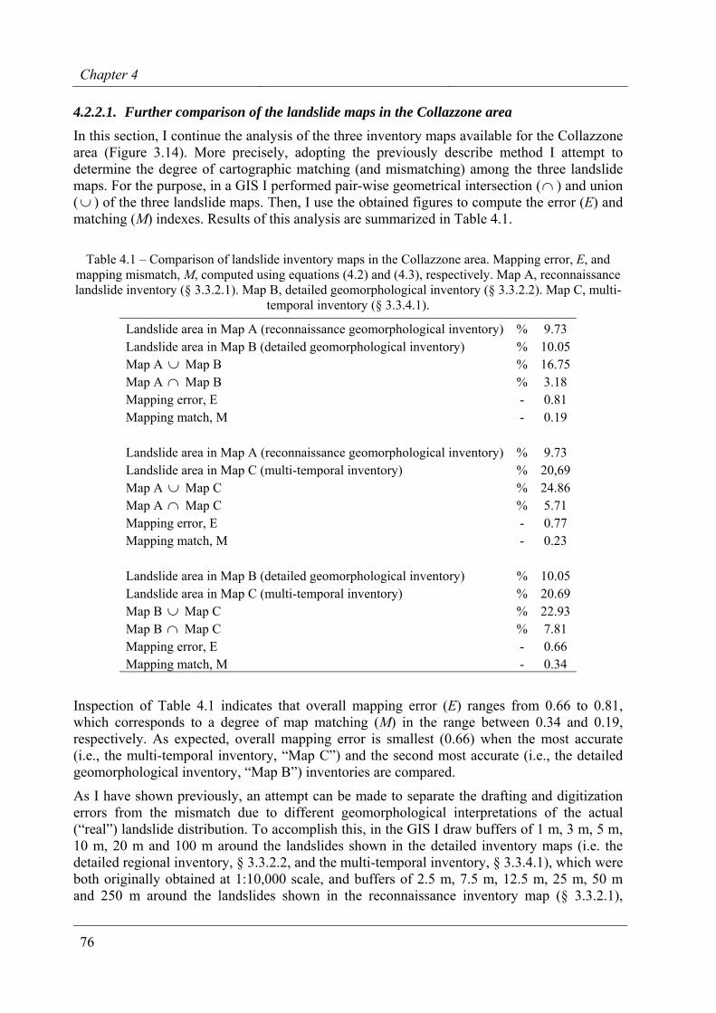
Chapter 4
76
4.2.2.1. Further comparison of the landslide maps in the Collazzone area In this section, I continue the analysis of the three inventory maps available for the Collazzone area (Figure 3.14). More precisely, adopting the previously describe method I attempt to determine the degree of cartographic matching (and mismatching) among the three landslide maps. For the purpose, in a GIS I performed pair-wise geometrical intersection (∩ ) and union (∪ ) of the three landslide maps. Then, I use the obtained figures to compute the error (E) and matching (M) indexes. Results of this analysis are summarized in Table 4.1.
Table 4.1 – Comparison of landslide inventory maps in the Collazzone area. Mapping error, E, and
mapping mismatch, M, computed using equations (4.2) and (4.3), respectively. Map A, reconnaissance landslide inventory (§ 3.3.2.1). Map B, detailed geomorphological inventory (§ 3.3.2.2). Map C, multi-
temporal inventory (§ 3.3.4.1).
Landslide area in Map A (reconnaissance geomorphological inventory) % 9.73 Landslide area in Map B (detailed geomorphological inventory) % 10.05 Map A ∪ Map B % 16.75 Map A ∩ Map B % 3.18 Mapping error, E - 0.81 Mapping match, M - 0.19
Landslide area in Map A (reconnaissance geomorphological inventory) % 9.73 Landslide area in Map C (multi-temporal inventory) % 20,69 Map A ∪ Map C % 24.86 Map A ∩ Map C % 5.71 Mapping error, E - 0.77 Mapping match, M - 0.23
Landslide area in Map B (detailed geomorphological inventory) % 10.05 Landslide area in Map C (multi-temporal inventory) % 20.69 Map B ∪ Map C % 22.93 Map B ∩ Map C % 7.81 Mapping error, E - 0.66 Mapping match, M - 0.34
Inspection of Table 4.1 indicates that overall mapping error (E) ranges from 0.66 to 0.81, which corresponds to a degree of map matching (M) in the range between 0.34 and 0.19, respectively. As expected, overall mapping error is smallest (0.66) when the most accurate (i.e., the multi-temporal inventory, “Map C”) and the second most accurate (i.e., the detailed geomorphological inventory, “Map B”) inventories are compared.
As I have shown previously, an attempt can be made to separate the drafting and digitization errors from the mismatch due to different geomorphological interpretations of the actual (“real”) landslide distribution. To accomplish this, in the GIS I draw buffers of 1 m, 3 m, 5 m, 10 m, 20 m and 100 m around the landslides shown in the detailed inventory maps (i.e. the detailed regional inventory, § 3.3.2.2, and the multi-temporal inventory, § 3.3.4.1), which were both originally obtained at 1:10,000 scale, and buffers of 2.5 m, 7.5 m, 12.5 m, 25 m, 50 m and 250 m around the landslides shown in the reconnaissance inventory map (§ 3.3.2.1),
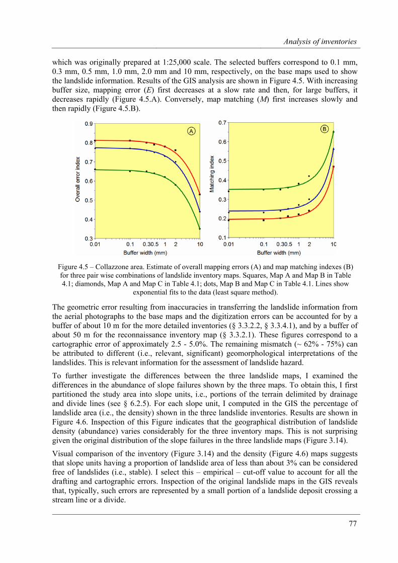
Analysis of inventories
77
which was originally prepared at 1:25,000 scale. The selected buffers correspond to 0.1 mm, 0.3 mm, 0.5 mm, 1.0 mm, 2.0 mm and 10 mm, respectively, on the base maps used to show the landslide information. Results of the GIS analysis are shown in Figure 4.5. With increasing buffer size, mapping error (E) first decreases at a slow rate and then, for large buffers, it decreases rapidly (Figure 4.5.A). Conversely, map matching (M) first increases slowly and then rapidly (Figure 4.5.B).
Figure 4.5 – Collazzone area. Estimate of overall mapping errors (A) and map matching indexes (B) for three pair wise combinations of landslide inventory maps. Squares, Map A and Map B in Table 4.1; diamonds, Map A and Map C in Table 4.1; dots, Map B and Map C in Table 4.1. Lines show
exponential fits to the data (least square method).
The geometric error resulting from inaccuracies in transferring the landslide information from the aerial photographs to the base maps and the digitization errors can be accounted for by a buffer of about 10 m for the more detailed inventories (§ 3.3.2.2, § 3.3.4.1), and by a buffer of about 50 m for the reconnaissance inventory map (§ 3.3.2.1). These figures correspond to a cartographic error of approximately 2.5 - 5.0%. The remaining mismatch (~ 62% - 75%) can be attributed to different (i.e., relevant, significant) geomorphological interpretations of the landslides. This is relevant information for the assessment of landslide hazard.
To further investigate the differences between the three landslide maps, I examined the differences in the abundance of slope failures shown by the three maps. To obtain this, I first partitioned the study area into slope units, i.e., portions of the terrain delimited by drainage and divide lines (see § 6.2.5). For each slope unit, I computed in the GIS the percentage of landslide area (i.e., the density) shown in the three landslide inventories. Results are shown in Figure 4.6. Inspection of this Figure indicates that the geographical distribution of landslide density (abundance) varies considerably for the three inventory maps. This is not surprising given the original distribution of the slope failures in the three landslide maps (Figure 3.14).
Visual comparison of the inventory (Figure 3.14) and the density (Figure 4.6) maps suggests that slope units having a proportion of landslide area of less than about 3% can be considered free of landslides (i.e., stable). I select this – empirical – cut-off value to account for all the drafting and cartographic errors. Inspection of the original landslide maps in the GIS reveals that, typically, such errors are represented by a small portion of a landslide deposit crossing a stream line or a divide.
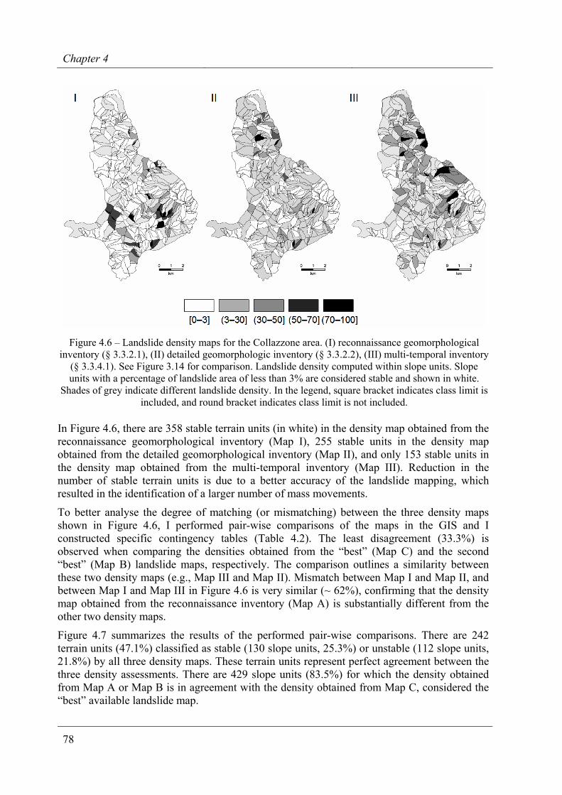
Chapter 4
78
Figure 4.6 – Landslide density maps for the Collazzone area. (I) reconnaissance geomorphological inventory (§ 3.3.2.1), (II) detailed geomorphologic inventory (§ 3.3.2.2), (III) multi-temporal inventory
(§ 3.3.4.1). See Figure 3.14 for comparison. Landslide density computed within slope units. Slope units with a percentage of landslide area of less than 3% are considered stable and shown in white.
Shades of grey indicate different landslide density. In the legend, square bracket indicates class limit is included, and round bracket indicates class limit is not included.
In Figure 4.6, there are 358 stable terrain units (in white) in the density map obtained from the reconnaissance geomorphological inventory (Map I), 255 stable units in the density map obtained from the detailed geomorphological inventory (Map II), and only 153 stable units in the density map obtained from the multi-temporal inventory (Map III). Reduction in the number of stable terrain units is due to a better accuracy of the landslide mapping, which resulted in the identification of a larger number of mass movements.
To better analyse the degree of matching (or mismatching) between the three density maps shown in Figure 4.6, I performed pair-wise comparisons of the maps in the GIS and I constructed specific contingency tables (Table 4.2). The least disagreement (33.3%) is observed when comparing the densities obtained from the “best” (Map C) and the second “best” (Map B) landslide maps, respectively. The comparison outlines a similarity between these two density maps (e.g., Map III and Map II). Mismatch between Map I and Map II, and between Map I and Map III in Figure 4.6 is very similar (~ 62%), confirming that the density map obtained from the reconnaissance inventory (Map A) is substantially different from the other two density maps.
Figure 4.7 summarizes the results of the performed pair-wise comparisons. There are 242 terrain units (47.1%) classified as stable (130 slope units, 25.3%) or unstable (112 slope units, 21.8%) by all three density maps. These terrain units represent perfect agreement between the three density assessments. There are 429 slope units (83.5%) for which the density obtained from Map A or Map B is in agreement with the density obtained from Map C, considered the “best” available landslide map.
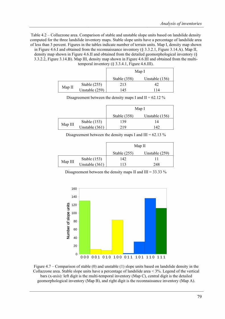
Analysis of inventories
79
Table 4.2 – Collazzone area. Comparison of stable and unstable slope units based on landslide density computed for the three landslide inventory maps. Stable slope units have a percentage of landslide area of less than 3 percent. Figures in the tables indicate number of terrain units. Map I, density map shown
in Figure 4.6.I and obtained from the reconnaissance inventory (§ 3.3.2.1, Figure 3.14.A). Map II, density map shown in Figure 4.6.II and obtained from the detailed geomorphological inventory (§ 3.3.2.2, Figure 3.14.B). Map III, density map shown in Figure 4.6.III and obtained from the multi-
temporal inventory (§ 3.3.4.1, Figure 4.6.III).
Map I
Stable (358) Unstable (156) Stable (255) 213 42 Map II
Unstable (259) 145 114
Disagreement between the density maps I and II = 62.12 %
Map I
Stable (358) Unstable (156) Stable (153) 139 14 Map III
Unstable (361) 219 142
Disagreement between the density maps I and III = 62.13 %
Map II
Stable (255) Unstable (259) Stable (153) 142 11 Map III
Unstable (361) 113 248
Disagreement between the density maps II and III = 33.33 %
0 0 0 0 0 1 0 1 0 0 1 11 0 0 1 0 1 1 1 0 1 1 1
160
120
80
140
100
60
20
0
40Num
ber o
f slo
pe u
nits
0 0 0 0 0 1 0 1 0 0 1 11 0 0 1 0 1 1 1 0 1 1 1
160
120
80
140
100
60
20
0
40Num
ber o
f slo
pe u
nits
Figure 4.7 – Comparison of stable (0) and unstable (1) slope units based on landslide density in the Collazzone area. Stable slope units have a percentage of landslide area < 3%. Legend of the vertical
bars (x-axis): left digit is the multi-temporal inventory (Map C), central digit is the detailed geomorphological inventory (Map B), and right digit is the reconnaissance inventory (Map A).
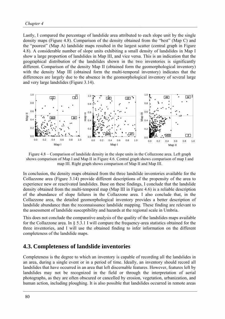
Chapter 4
80
Lastly, I compared the percentage of landslide area attributed to each slope unit by the single density maps (Figure 4.8). Comparison of the density obtained from the “best” (Map C) and the “poorest” (Map A) landslide maps resulted in the largest scatter (central graph in Figure 4.8). A considerable number of slope units exhibiting a small density of landslides in Map I show a large proportion of landslides in Map III, and vice versa. This is an indication that the geographical distribution of the landslides shown in the two inventories is significantly different. Comparison of the density Map II (obtained form the geomorphological inventory) with the density Map III (obtained form the multi-temporal inventory) indicates that the differences are largely due to the absence in the geomorphological inventory of several large and very large landslides (Figure 3.14).
0.0
0.2
0.4
0.6
0.8
1.0
0.0 0.2 0.4 0.6 0.8 1.0map A
4545 1313
2727429429
Map I
Map
III
0.0
0.2
0.4
0.6
0.8
1.0
0.0 0.2 0.4 0.6 0.8 1.0Map A
463463 3434
661111
Map I
Map
II
0.0
0.2
0.4
0.6
0.8
1.0
0.0 0.2 0.4 0.6 0.8 1.0map B
453453 33
14144444
Map IIM
ap II
I
0.0
0.2
0.4
0.6
0.8
1.0
0.0 0.2 0.4 0.6 0.8 1.0map A
4545 1313
2727429429
Map I
Map
III
0.0
0.2
0.4
0.6
0.8
1.0
0.0 0.2 0.4 0.6 0.8 1.0map A
45454545 13131313
27272727429429429429
Map I
Map
III
0.0
0.2
0.4
0.6
0.8
1.0
0.0 0.2 0.4 0.6 0.8 1.0Map A
463463463463 34343434
666611111111
Map I
Map
II
0.0
0.2
0.4
0.6
0.8
1.0
0.0 0.2 0.4 0.6 0.8 1.0map B
453453 33
14144444
Map IIM
ap II
I0.0
0.2
0.4
0.6
0.8
1.0
0.0 0.2 0.4 0.6 0.8 1.0map B
453453453453 3333
1414141444444444
Map IIM
ap II
I
Figure 4.8 – Comparison of landslide density in the slope units in the Collazzone area. Left graph shows comparison of Map I and Map II in Figure 4.6. Central graph shows comparison of map I and
map III. Right graph shows comparison of Map II and Map III.
In conclusion, the density maps obtained from the three landslide inventories available for the Collazzone area (Figure 3.14) provide different descriptions of the propensity of the area to experience new or reactivated landslides. Base on these findings, I conclude that the landslide density obtained from the multi-temporal map (Map III in Figure 4.6) is a reliable description of the abundance of slope failures in the Collazzone area. I also conclude that, in the Collazzone area, the detailed geomorphological inventory provides a better description of landslide abundance than the reconnaissance landslide mapping. These finding are relevant to the assessment of landslide susceptibility and hazards at the regional scale in Umbria.
This does not conclude the comparative analysis of the quality of the landslides maps available for the Collazzone area. In § 5.3.1 I will compare the frequency-area statistics obtained for the three inventories, and I will use the obtained finding to infer information on the different completeness of the landslide maps.
4.3. Completeness of landslide inventories
Completeness is the degree to which an inventory is capable of recording all the landslides in an area, during a single event or in a period of time. Ideally, an inventory should record all landslides that have occurred in an area that left discernable features. However, features left by landslides may not be recognized in the field or through the interpretation of aerial photographs, as they are often obscured or cancelled by erosion, vegetation, urbanization, and human action, including ploughing. It is also possible that landslides occurred in remote areas
Analysis of inventories
81
but were not reported because they did not cause damage. For these reasons, landslide inventories are generally incomplete.
Estimating the completeness of a landslide inventory is a difficult task, and considerations differ for archive, geomorphological, event and multi-temporal inventories. A formal definition of completeness requires that a landslide inventory includes all landslides associated with a landslide event (a single trigger) or multiple landslide events over time (geomorphological or multi-temporal). This definition assumes that all landslides are visible and recognizable, or that they were accurately reported, and that the entire study area affected, even marginally, by the trigger(s) is fully and thoroughly investigated. For practical reasons, these criteria are never met.
A functional definition of completeness requires that the landslide inventory includes a substantial fraction of all landslides at all scales. The tools and techniques available to compile the inventory must be able to meet this requirement within the study area. An important attribute of this definition is that a substantially complete inventory must include a substantial fraction of the smallest landslides. It is important to understand that the definition is applicable to landslide event inventories, but not to geomorphological inventories, because many smaller and intermediate-size landslides in geomorphological inventories have been erased by erosion and human action. Thus, a geomorphological inventory is always incomplete. This should be considered when determining landslide hazard and risk.
4.3.1. Completeness of archive inventories Archive inventories are non-instrumental records of past events. Analysis of the information content of archive inventories of natural events is difficult and rarely pursued (Guzzetti et al., 1994, 2005b,c; Ibsen and Brunsden, 1996; Glade, 1988; Guzzetti, 2000; Glade et al., 2001; Guzzetti and Tonelli, 2004). An approach to evaluate the completeness of an archive inventory consists in the analysis of the cumulative number of historical landslide events. For a catalogue of historical events, the cumulative number of events is easily obtained by adding progressively the number of events recorded in each time interval (e.g., a day or a year).
Figure 4.9.A shows the temporal distribution of fatal landslide events in Italy, from 1500 to 2004. In this figure, the y-axis (logarithmic scale) shows the number of the consequences, i.e., fatalities (deaths and missing persons) and injured people. Also shown are events for which casualties occurred in unknown number. Inspection of the graph indicates that the distribution of the inventoried events varies substantially with time.
In an attempt to evaluate the completeness of this catalogue, in Figure 4.9.B I show the cumulative curves of fatal landslides events, in the period from 1410 to 2004. Inspection of Figure 4.9.B reveals that, as it might be expected, the cumulative number of landslide fatalities has increased largely since the beginning of the record, but also that the rates at which fatal events have occurred has increased. This may be a result of variations in the completeness of the historical catalogue. The more remote the period considered, the larger the number of events that probably remained unrecorded. This is especially evident for events that caused fewer than three fatalities. In the historical catalogue, such events rarely appear before 1800 (only 29 events). After 1800 they represent 30.5% of the total number of landslide events. The percentage increases to 73.4% after 1900. Even considering the increase in population that has occurred in Italy (Figure 1.2), there is no reason for the distribution of less catastrophic events to be so skewed, except for the incompleteness of the catalogue.
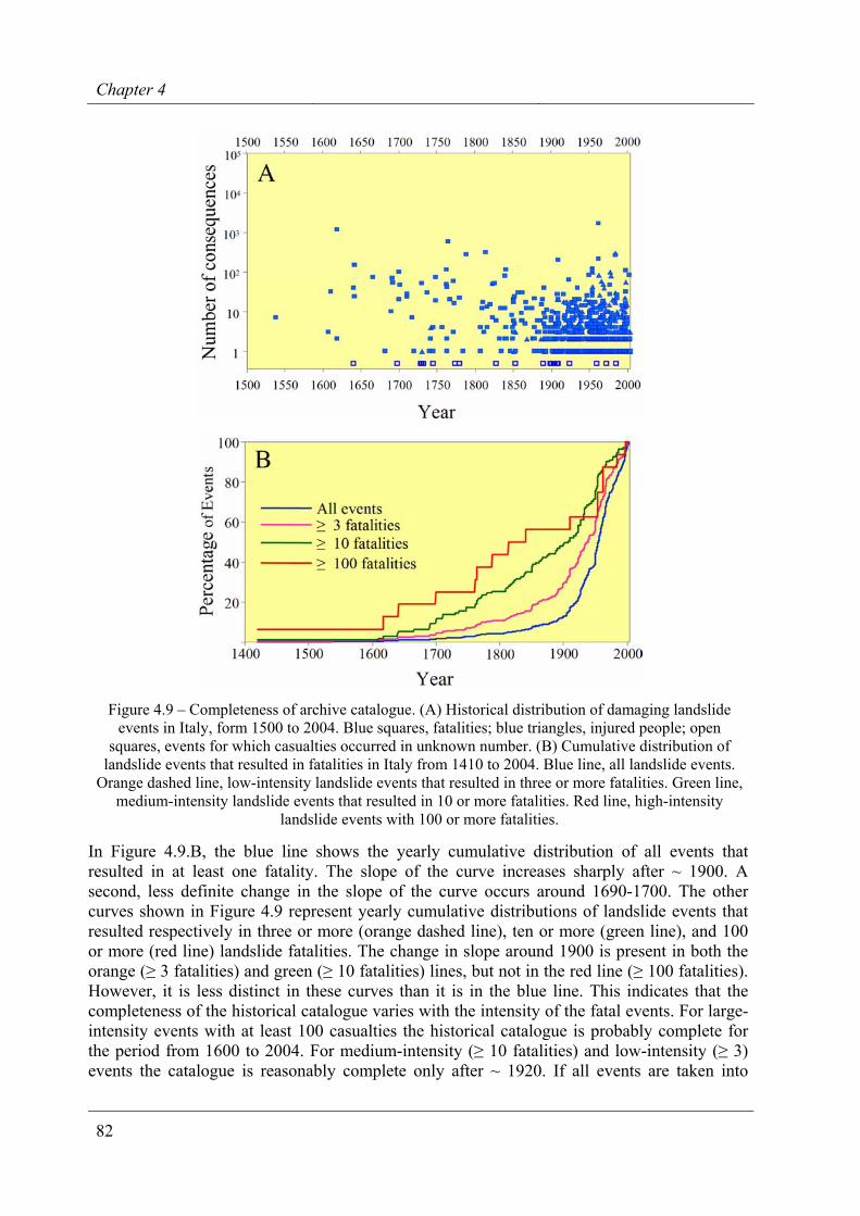
Chapter 4
82
Figure 4.9 – Completeness of archive catalogue. (A) Historical distribution of damaging landslide events in Italy, form 1500 to 2004. Blue squares, fatalities; blue triangles, injured people; open
squares, events for which casualties occurred in unknown number. (B) Cumulative distribution of landslide events that resulted in fatalities in Italy from 1410 to 2004. Blue line, all landslide events.
Orange dashed line, low-intensity landslide events that resulted in three or more fatalities. Green line, medium-intensity landslide events that resulted in 10 or more fatalities. Red line, high-intensity
landslide events with 100 or more fatalities.
In Figure 4.9.B, the blue line shows the yearly cumulative distribution of all events that resulted in at least one fatality. The slope of the curve increases sharply after ~ 1900. A second, less definite change in the slope of the curve occurs around 1690-1700. The other curves shown in Figure 4.9 represent yearly cumulative distributions of landslide events that resulted respectively in three or more (orange dashed line), ten or more (green line), and 100 or more (red line) landslide fatalities. The change in slope around 1900 is present in both the orange (≥ 3 fatalities) and green (≥ 10 fatalities) lines, but not in the red line (≥ 100 fatalities). However, it is less distinct in these curves than it is in the blue line. This indicates that the completeness of the historical catalogue varies with the intensity of the fatal events. For large-intensity events with at least 100 casualties the historical catalogue is probably complete for the period from 1600 to 2004. For medium-intensity (≥ 10 fatalities) and low-intensity (≥ 3) events the catalogue is reasonably complete only after ~ 1920. If all events are taken into
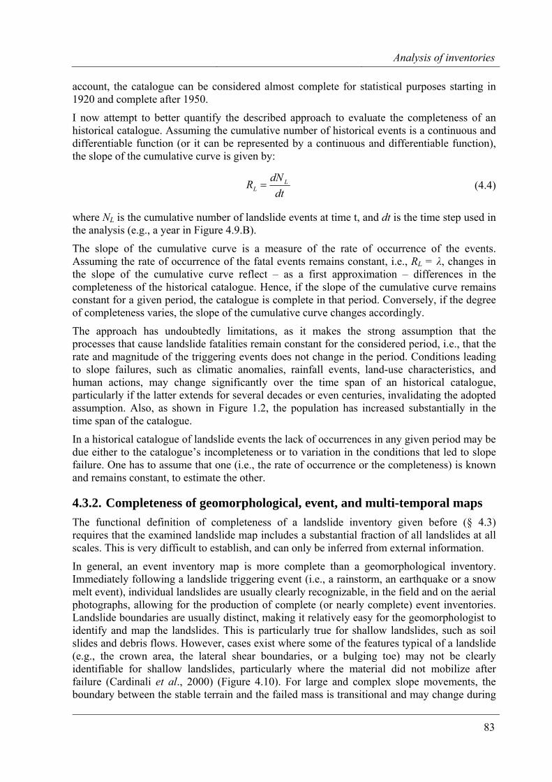
Analysis of inventories
83
account, the catalogue can be considered almost complete for statistical purposes starting in 1920 and complete after 1950.
I now attempt to better quantify the described approach to evaluate the completeness of an historical catalogue. Assuming the cumulative number of historical events is a continuous and differentiable function (or it can be represented by a continuous and differentiable function), the slope of the cumulative curve is given by:
dtdNR L
L = (4.4)
where NL is the cumulative number of landslide events at time t, and dt is the time step used in the analysis (e.g., a year in Figure 4.9.B).
The slope of the cumulative curve is a measure of the rate of occurrence of the events. Assuming the rate of occurrence of the fatal events remains constant, i.e., RL = λ, changes in the slope of the cumulative curve reflect – as a first approximation – differences in the completeness of the historical catalogue. Hence, if the slope of the cumulative curve remains constant for a given period, the catalogue is complete in that period. Conversely, if the degree of completeness varies, the slope of the cumulative curve changes accordingly.
The approach has undoubtedly limitations, as it makes the strong assumption that the processes that cause landslide fatalities remain constant for the considered period, i.e., that the rate and magnitude of the triggering events does not change in the period. Conditions leading to slope failures, such as climatic anomalies, rainfall events, land-use characteristics, and human actions, may change significantly over the time span of an historical catalogue, particularly if the latter extends for several decades or even centuries, invalidating the adopted assumption. Also, as shown in Figure 1.2, the population has increased substantially in the time span of the catalogue.
In a historical catalogue of landslide events the lack of occurrences in any given period may be due either to the catalogue’s incompleteness or to variation in the conditions that led to slope failure. One has to assume that one (i.e., the rate of occurrence or the completeness) is known and remains constant, to estimate the other.
4.3.2. Completeness of geomorphological, event, and multi-temporal maps The functional definition of completeness of a landslide inventory given before (§ 4.3) requires that the examined landslide map includes a substantial fraction of all landslides at all scales. This is very difficult to establish, and can only be inferred from external information.
In general, an event inventory map is more complete than a geomorphological inventory. Immediately following a landslide triggering event (i.e., a rainstorm, an earthquake or a snow melt event), individual landslides are usually clearly recognizable, in the field and on the aerial photographs, allowing for the production of complete (or nearly complete) event inventories. Landslide boundaries are usually distinct, making it relatively easy for the geomorphologist to identify and map the landslides. This is particularly true for shallow landslides, such as soil slides and debris flows. However, cases exist where some of the features typical of a landslide (e.g., the crown area, the lateral shear boundaries, or a bulging toe) may not be clearly identifiable for shallow landslides, particularly where the material did not mobilize after failure (Cardinali et al., 2000) (Figure 4.10). For large and complex slope movements, the boundary between the stable terrain and the failed mass is transitional and may change during
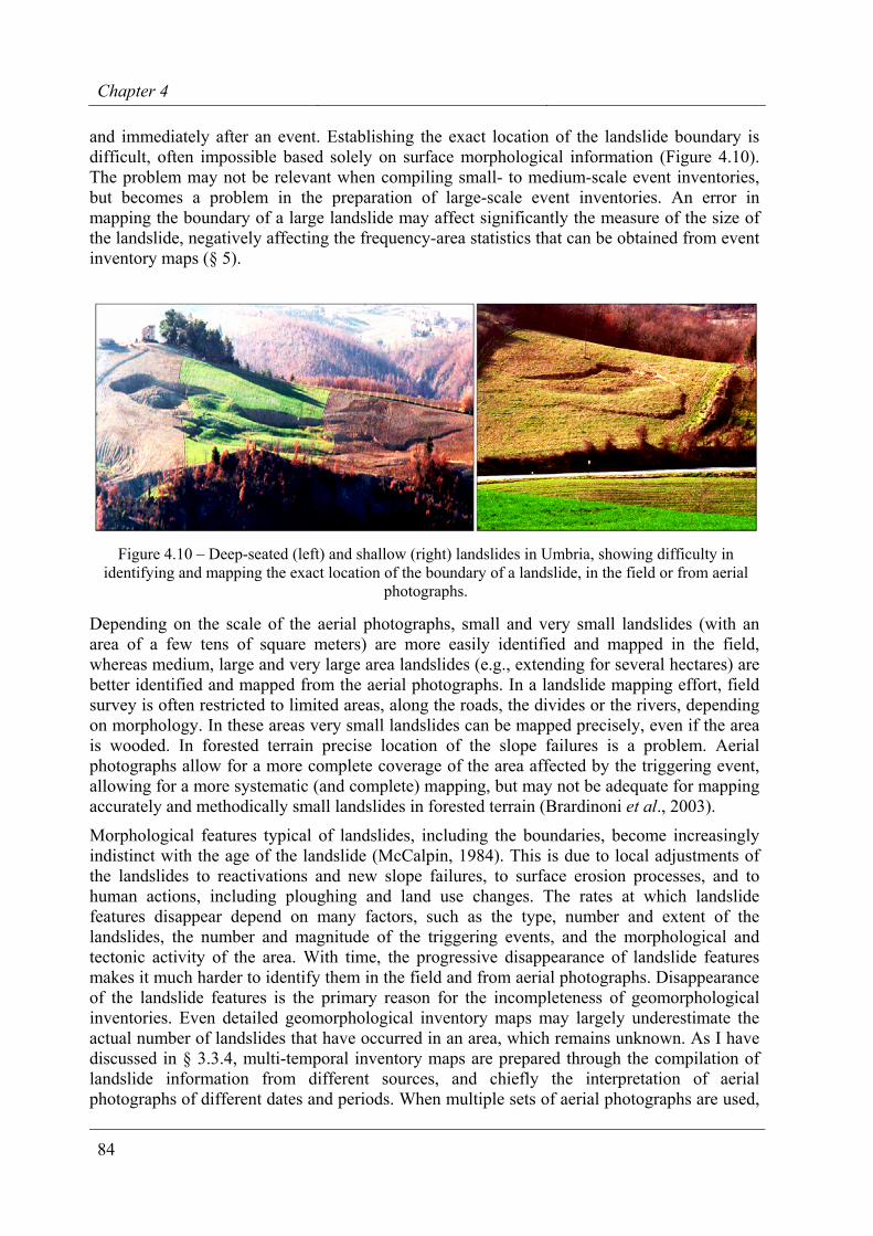
Chapter 4
84
and immediately after an event. Establishing the exact location of the landslide boundary is difficult, often impossible based solely on surface morphological information (Figure 4.10). The problem may not be relevant when compiling small- to medium-scale event inventories, but becomes a problem in the preparation of large-scale event inventories. An error in mapping the boundary of a large landslide may affect significantly the measure of the size of the landslide, negatively affecting the frequency-area statistics that can be obtained from event inventory maps (§ 5).
Figure 4.10 – Deep-seated (left) and shallow (right) landslides in Umbria, showing difficulty in identifying and mapping the exact location of the boundary of a landslide, in the field or from aerial
photographs.
Depending on the scale of the aerial photographs, small and very small landslides (with an area of a few tens of square meters) are more easily identified and mapped in the field, whereas medium, large and very large area landslides (e.g., extending for several hectares) are better identified and mapped from the aerial photographs. In a landslide mapping effort, field survey is often restricted to limited areas, along the roads, the divides or the rivers, depending on morphology. In these areas very small landslides can be mapped precisely, even if the area is wooded. In forested terrain precise location of the slope failures is a problem. Aerial photographs allow for a more complete coverage of the area affected by the triggering event, allowing for a more systematic (and complete) mapping, but may not be adequate for mapping accurately and methodically small landslides in forested terrain (Brardinoni et al., 2003).
Morphological features typical of landslides, including the boundaries, become increasingly indistinct with the age of the landslide (McCalpin, 1984). This is due to local adjustments of the landslides to reactivations and new slope failures, to surface erosion processes, and to human actions, including ploughing and land use changes. The rates at which landslide features disappear depend on many factors, such as the type, number and extent of the landslides, the number and magnitude of the triggering events, and the morphological and tectonic activity of the area. With time, the progressive disappearance of landslide features makes it much harder to identify them in the field and from aerial photographs. Disappearance of the landslide features is the primary reason for the incompleteness of geomorphological inventories. Even detailed geomorphological inventory maps may largely underestimate the actual number of landslides that have occurred in an area, which remains unknown. As I have discussed in § 3.3.4, multi-temporal inventory maps are prepared through the compilation of landslide information from different sources, and chiefly the interpretation of aerial photographs of different dates and periods. When multiple sets of aerial photographs are used,
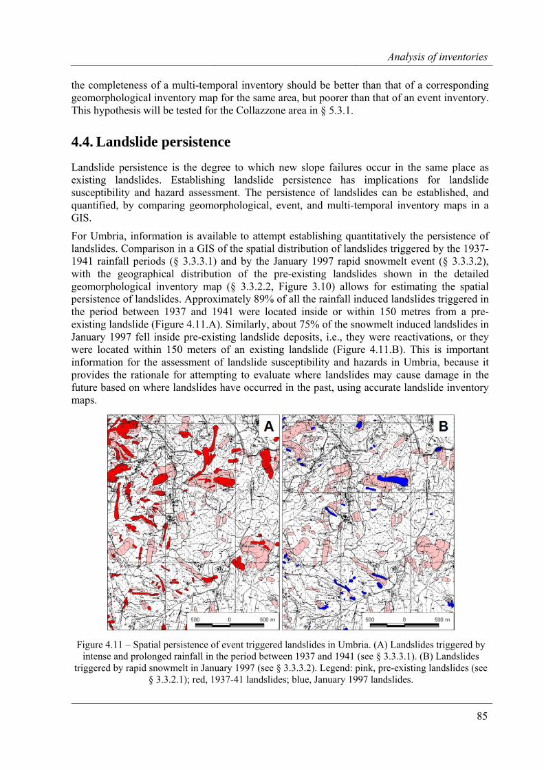
Analysis of inventories
85
the completeness of a multi-temporal inventory should be better than that of a corresponding geomorphological inventory map for the same area, but poorer than that of an event inventory. This hypothesis will be tested for the Collazzone area in § 5.3.1.
4.4. Landslide persistence
Landslide persistence is the degree to which new slope failures occur in the same place as existing landslides. Establishing landslide persistence has implications for landslide susceptibility and hazard assessment. The persistence of landslides can be established, and quantified, by comparing geomorphological, event, and multi-temporal inventory maps in a GIS.
For Umbria, information is available to attempt establishing quantitatively the persistence of landslides. Comparison in a GIS of the spatial distribution of landslides triggered by the 1937-1941 rainfall periods (§ 3.3.3.1) and by the January 1997 rapid snowmelt event (§ 3.3.3.2), with the geographical distribution of the pre-existing landslides shown in the detailed geomorphological inventory map (§ 3.3.2.2, Figure 3.10) allows for estimating the spatial persistence of landslides. Approximately 89% of all the rainfall induced landslides triggered in the period between 1937 and 1941 were located inside or within 150 metres from a pre-existing landslide (Figure 4.11.A). Similarly, about 75% of the snowmelt induced landslides in January 1997 fell inside pre-existing landslide deposits, i.e., they were reactivations, or they were located within 150 meters of an existing landslide (Figure 4.11.B). This is important information for the assessment of landslide susceptibility and hazards in Umbria, because it provides the rationale for attempting to evaluate where landslides may cause damage in the future based on where landslides have occurred in the past, using accurate landslide inventory maps.
Figure 4.11 – Spatial persistence of event triggered landslides in Umbria. (A) Landslides triggered by intense and prolonged rainfall in the period between 1937 and 1941 (see § 3.3.3.1). (B) Landslides
triggered by rapid snowmelt in January 1997 (see § 3.3.3.2). Legend: pink, pre-existing landslides (see § 3.3.2.1); red, 1937-41 landslides; blue, January 1997 landslides.
Chapter 4
86
It should be noted that new landslides do not necessarily occur inside or in the vicinity of pre-existing landslide deposits. For the Staffora River basin, in the northern Apennines (§ 2.6), Guzzetti et al. (2005a) found low values of landslide persistence. By analysing a multi-temporal inventory map compiled through the systematic analysis of five sets of aerial photographs covering the period between 1955 and 1999, these authors found that in the Staffora basin 40% of all the landslides identified in the period from 1955 to 1999 occurred inside pre-existing landslides mapped on the 1955 aerial photographs. Considering only the landslides occurred in the 45-year period from 1955 to 1999, only 12% of the slope failures occurred in the same area of other landslides occurred in the same period. This is lower landslide persistence than the one observed in Umbria.
4.5. Temporal frequency of slope failures
The temporal frequency (or the recurrence) of landslide events can be established from archive inventories (Coe et al., 2000; Guzzetti et al., 2003a) and from multi-temporal landslide maps (Guzzetti et al., 2005a). In § 7, I will show how to obtain information on the temporal probability of landslide events from a multi-temporal inventory map, and how to exploit this information to determine landslide hazard.
4.5.1. Exceedance probability of landslide occurrence Before showing how to obtain the probability of landslide occurrence from archive inventories, it is convenient to establish an appropriate mathematical framework. As a first approximation, landslides can be considered as independent random point-events in time (Crovelli, 2000). In this framework, the exceedance probability of occurrence of landslide events during time t is:
[ ]1≥= )t(NP)N(P LL (4.5)
where NL(t) is the number of landslides that occur during time t in the investigated area.
Two probability models are commonly used to investigate the occurrence of naturally occurring random point-events in time: (i) the Poisson model and (ii) the binomial model1 (Crovelli, 2000; Önöz and Bayazit, 2001). The Poisson model is a continuous-time model consisting of random-point events that occur independently in ordinary time, which is considered naturally continuous. The Poisson model has been used to investigate the temporal occurrence of floods (Yevjevich, 1972; Önöz and Bayazit, 2001), volcanic eruptions (Klein, 1982; Connor and Hill, 1995; Nathenson, 2001) and landslides (Crovelli, 2000; Coe et al., 2000; Roberds, 2005). Adopting a Poisson model for the temporal occurrence of landslides, the probability of experiencing n landslides during time t is given by
!n)t(e]n)t(N[P
n)t(
Lλ
== λ− n = 0, 1, 2, … (4.6)
1 Other probability distributions used to model naturally occurring random point-events in time include the
Weibull distribution (Bebbington and Lai, 1996) and the mixed exponential distribution (Cox and Lewis, 1966; Nathenson, 2001).
Analysis of inventories
87
where λ is the estimated average rate of occurrence of landslides, which corresponds to 1/µ, with µ the estimated mean recurrence interval between successive failure events. The model parameters λ and µ can be obtained from a historical catalogue of landslide events or from a multi-temporal landslide inventory map.
From equation 4.6, the probability of experiencing one or more landslides during time t (i.e., the exceedance probability) is
µ−λ− −=−==−=≥ /ttLL ee])t(N[P])t(N[P 11011 (4.7)
Discussing equation 4.7, Crovelli (2000) noted that for a given period of time t, if µ→∞, then ])t(N[P L 1≥ → 0, i.e., if the estimated mean recurrence interval between successive events
is very large, chances are that no failures will be experienced in the considered period. Also, if the estimated mean recurrence µ is fixed, and the time interval is very long (t→∞), then
])t(N[P L 1≥ → 1 and one is certain to observe a landslide event.
The Poisson model allows for determining the probability of future landslides for different times t (i.e., for a different number of years) based on the statistics of past landslide events, under the following assumptions (Crovelli, 2000): (i) the number of landslide events which occur in disjoint time intervals are independent, (ii) the probability of an event occurring in a very short time is proportional to the length of the time interval, (iii) the probability of more than one event in a short time interval is negligible, (iv) the probability distribution of the number of events is the same for all time intervals of fixed length, and (v) the mean recurrence of events will remain the same in the future as it was observed in the past. These assumptions, which may not always hold for landslide events, should be considered when interpreting (and using) the results of the Poisson probability model.
As an alternative to the Poisson model, a binomial model can be adopted. The binomial probability model is a discrete-time model consisting of the occurrence or random-point events in time. In this model time is divided into discrete increments of equal length, and within each time increment a single point-event may or may not occur. The binomial model was adopted by Costa and Baker (1981) to investigate the occurrence of floods, and by Keaton et al. (1988), Lips and Wieczorek (1990), Coe et al. (2000), Raetso et al. (2002), and Vandine et al. (2004) to study the temporal occurrence of landslides and debris flows.
Following Crovelli (2000), and adopting the binomial probability model, the exceedance probability of experiencing one or more landslides during time t is
ttLL )/()p(])t(N[P])t(N[P µ−−=−−==−=≥ 11111011 (4.8)
where, p is the estimated probability of a landslide event in time t, and µ = 1/p is the estimated mean recurrence interval between successive slope failures. As for the Poisson model, µ can be obtained from a historical catalogue of landslide events or from a multi-temporal landslide inventory map. The binomial model holds under the same or similar assumptions listed for the Poisson model.
Crovelli (2000) compared the Poisson and the binomial probability models, and showed that the two models differ for short mean recurrence intervals (i.e., when µ is small) and for short periods of time (i.e., when t is small), with the binomial model over estimating the exceedance probability of future landslide events. For large periods of times and large mean recurrence intervals, the two models provide very similar or identical estimates of the probability of
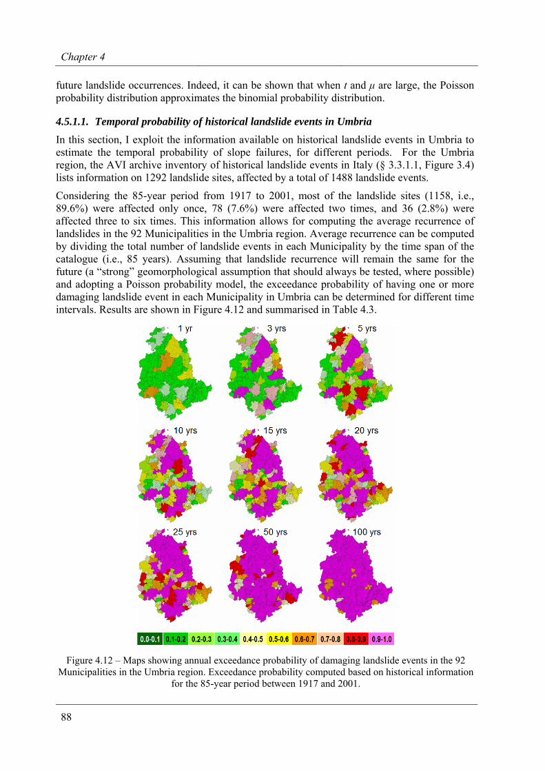
Chapter 4
88
future landslide occurrences. Indeed, it can be shown that when t and µ are large, the Poisson probability distribution approximates the binomial probability distribution.
4.5.1.1. Temporal probability of historical landslide events in Umbria
In this section, I exploit the information available on historical landslide events in Umbria to estimate the temporal probability of slope failures, for different periods. For the Umbria region, the AVI archive inventory of historical landslide events in Italy (§ 3.3.1.1, Figure 3.4) lists information on 1292 landslide sites, affected by a total of 1488 landslide events.
Considering the 85-year period from 1917 to 2001, most of the landslide sites (1158, i.e., 89.6%) were affected only once, 78 (7.6%) were affected two times, and 36 (2.8%) were affected three to six times. This information allows for computing the average recurrence of landslides in the 92 Municipalities in the Umbria region. Average recurrence can be computed by dividing the total number of landslide events in each Municipality by the time span of the catalogue (i.e., 85 years). Assuming that landslide recurrence will remain the same for the future (a “strong” geomorphological assumption that should always be tested, where possible) and adopting a Poisson probability model, the exceedance probability of having one or more damaging landslide event in each Municipality in Umbria can be determined for different time intervals. Results are shown in Figure 4.12 and summarised in Table 4.3.
Figure 4.12 – Maps showing annual exceedance probability of damaging landslide events in the 92 Municipalities in the Umbria region. Exceedance probability computed based on historical information
for the 85-year period between 1917 and 2001.
Analysis of inventories
89
Inspection of Table 4.3 reveals that for a 5-year period only five Municipalities in Umbria (5.4%) have a 0.90 or larger probability of experiencing at least one damaging landslide, and 17 Municipalities (18.5%) have a 0.50 or larger probability of experiencing at least one damaging slope failure. These figures increase to 11 (12.0%) and 40 (43.5%) Municipalities for a 10-year period, and to 25 (27.2%) and 68 (73.9%) Municipalities for a 25-year period, respectively. After 100 years, all the Municipalities in Umbria have a 50% or larger probability of experiencing a landslide, and 76 Municipalities (82.6%) have a 90% or larger probability of having at least one slope failure (Figure 4.12). Table 4.3 – Number and percentage (in parenthesis) of municipalities in Umbria that exceed the given probability of experiencing one or more damaging landslide. Values for different time intervals, from 5
to 50 years. Based on a historical record spanning the 85-year period between 1917 and 2001.
EXCEEDANCE PROBABILITY 5 YRS 10 YRS 20 YRS 25 YRS 50 YRS > 0.99 2 (2.2%) 5 (5.4%) 11 (12.0%) 14 (15.2%) 25 (27.2%) > 0.95 5 (5.4%) 10 (10.9%) 16 (17.4%) 18 (19.6%) 40 (43.5%) > 0.90 5 (5.4%) 11 (12.0%) 19 (20.7%) 25 (27.2%) 58 (63.0%) > 0.80 9 (9.8%) 16 (17.4%) 30 (32.6%) 40 (43.5%) 68 (73.9%) > 0.50 17 (18.5) 40 (43.5%) 68 (73.9%) 68 (73.9%) 76 (82.6%)
4.6. Summary of achieved results
In this chapter, I have:
(a) Further demonstrated how to compare landslide maps, and to measure the quality and completeness of different landslide inventory maps.
(b) Proposed methods for the construction of landslide density maps, a weak proxy for susceptibility zonings where these are not available.
(c) Proposed methods for the analysis of the spatial persistence of slope failures, important information for landslide hazard and risk assessments.
(d) Shown how to obtain temporal information on landslides from archive inventories, including a measure of the completeness of the historical archives, essential information for probabilistic landslide hazard assessments.
This contributes to responds to Questions # 2 and # 3 posed in the Introduction (§ 1.2).

91
5. STATISTICS OF LANDSLIDE SIZE
Somehow you need years to recognize something obvious.
Not all what can be counted counts, and
not all what counts can be counted.
The size (e.g. length, area, volume) of individual landslides varies largely. As shown in Figure 1.1, the length of landslides varies from less than a meter to several hundreds or even thousands of kilometres for submarine slides. Landslide area spans the range from less than a few square meters, for shallow soil slides, to thousands of square kilometres, for large submarine failures. The volume of single mass movements ranges from less than a cubic decimetre, for rock fragments falling off a cliff, to several hundreds of cubic kilometres, for gigantic submarine slides (Locat and Mienert, 2003), or for slope failures identified on the Moon (Hsu, 1975), Mars (McEwen, 1989) and Venus (Malin, 1992).
The frequency-size distribution of landslides is important information to determine landslide hazards (Guzzetti et al., 2005a) (see § 7.3), and to estimate the contribution of landslides to erosion and sediment yield (e.g., Hovius et al., 1997, 2000; Martin et al., 2002; Guthrie and Evans, 2004b; Lavé and Burbank, 2004). For these reasons, it is essential that the distributions are quantified precisely, using accurate and reliable methods.
In this chapter, after a review of the limited literature, I show how to obtain frequency-area and frequency-volume statistics of landslides from empirical data obtained from landslide inventories. I then discuss applications of the obtained frequency statistics of landslides, with examples from the Umbria region, including an application to investigate the completeness of the three landslide inventory maps available for the Collazzone area.
5.1. Background
Review of the literature (§ 13) reveals that only a few authors have investigated the frequency-area, or the frequency-volume statistics of landslides. Fujii (1969) was probably the first to investigate the problem. Studying an inventory of 800 landslides caused by heavy rainfall in Japan, he obtained a cumulative number-area distribution that correlated well with a power law relation of the type α−∝ LCL AN , where NCL is the cumulative number of landslides, AL is the landslide area, and α = 0.96. This author also obtained a similar cumulative number-volume distribution that correlated with a power law α−∝ LCL VN , with VL the landslide volume and α = 0.85. Other investigators have studied the frequency-size distribution of landslides in Japan. Ohmori and Hirano (1988) examined 3511 landslides occurred in the 8-year period
Statistics of landslide size
92
between 1975 and 1983, and provided cumulative number-area distributions that correlated with power laws with exponents α in the range between 1.34 and 1.62, depending on the type of the mapped landslides. Sugai et al. (1994) and Ohmori and Sugai (1995) examined 3424 landslides in the Akaishi Ranges, in central Japan, and found power law correlations for landslides in different rock types and elevation zones with values of α in the range from 1.27 to 2.49. Sasaki et al. (1991) investigated the width of landslides triggered by heavy rainfall in the Misumi and Masuda areas, in south western Japan, and found a relationship between the cumulative number of landslides and the maximum width of the slope failures that was approximated by a power law with an exponent α ~ 3.3.
Pelletier et al. (1997) have given cumulative frequency-area distributions of rainfall induced landslides in Japan and in Bolivia, and of earthquake induced landslides in California. The data set for Japan was the same compiled by Sugai et al. (1994) for the Akaishi Ranges described before. For this data set, Pelletier et al. (1997) found a power law relation between the area of the landslides and the cumulative number of slope failures with an exponent α = 2.0, for slope failures larger than about 1×10⁵ m2. The data set for Bolivia was compiled by Blodgett (1998), who mapped 1130 rainfall induced landslides in the Challana Valley, in the Eastern Cordillera. For this data set, Pelletier et al. (1997) found power law relationships with exponents ranging between α = 1.6 and α = 2.0, for landslides larger than about 5×10⁴ m2. The data set for California consisted in about 11,000 landslides triggered by the 17 January 1994 Northridge earthquake and mapped by Harp and Jibson (1995, 1996). For this data set, the cumulative distribution of landslide areas was approximated by a power law taking the slope α = 1.6, for landslides larger than about 3×10³ m2. Malamud and Turcotte (1999) analysed the same data sets used by Pelletier et al. (1997), and another data set listing 709 landslides mapped by Nielsen et al. (1975) for the Eden Canyon area in Alameda County, California. The obtained non-cumulative frequency-area distributions exhibited a “rollover” for landslides areas smaller than about 2×10³ ~ 1×10⁴ m2, depending on the resolution of the mapping, and were all reasonably well approximated by power laws with exponents, α+1, in the range between 2.3 and 3.3.
Hovius et al. (1997) have given a cumulative number-area distribution for 4984 landslides mapped in a mountain area east of the Alpine fault in New Zealand. Their logarithmically binned data correlated with a power law relation with α = 0.7, over the range AL = 7×10² m2 to AL = 1×10⁶ m2. Hovius et al. (2000) have given a number-area distribution of 1040 fresh landslides in the Ma-An and Wan-Li catchments on the eastern side of the Central Range in Taiwan. The logarithmically binned data correlated with a power law relation with exponent α = 1.15 over the range AL = 1×10³ m2 to AL = 5×10⁴ m2. Stark and Hovius (2001) revised the given number-area distributions obtained for southern New Zealand and central Taiwan. The revised estimates were obtained by fitting non-cumulative distributions of the available data to cover the mapped landslide areas, a significant improvement over pre-existing published work. For the purpose, the authors introduced a five parameters double-Pareto distribution (§ 5.2.1, equation 5.3), and obtained estimates for the slope of the power law tail of the distribution of α+1 = 2.11 for the Taiwan inventory, and α+1 = 2.46±0.2 for the New Zealand inventory.
Various authors have examined the frequency-area distributions of landslides in British Columbia, Canada. Martin et al. (2002) studied 615 landslides in the Queen Charlotte Islands, which ranged in area from 200 to 52,000 m2, and spanned the volume from 217 m3 to 16,100 m3. The non-cumulative probability-density distributions for landslide areas were approximated by power laws with exponents α+1 = 1.80, for primary landslides, and α+1 = 3.20 for gully sidewall events. Guthrie and Evans (2004b) analyzed three inventories showing
Chapter 5
93
landslides occurred on the west coast of British Columbia. The first inventory listed 201 debris slides and debris flows, 136 of which occurred in the 47-year period from 1950 to 1996, in a 286 km2 study area in the Brooks Peninsula. The second inventory listed 92 landslides in the Loughborough Inlet. The third inventory showed 1109 landslides inventoried by the British Columbia Ministry of Forest in the Clayoquot study area. The mapped landslides ranged in size from 500 m2 to 400,000 m2, and their non-cumulative frequency-area distributions obeyed power law relationships with exponents α+1 ranging between 2.51 and 2.77, for landslide areas ranging from AL = 1×10⁴ m2 to AL = 4×10⁵ m2. In another paper, Guthrie and Evans (2004a) have given the frequency-area statistics for 101 rainfall-induced landslides occurred on 18 November 2001 in the Loughborough Inlet, a slightly different data set than then one used in the previous paper. These landslides ranged in size from 1124 m2 to 409,000 m2, and their frequency-area distribution was described by a power law with a slope α+1 = 2.24, for landslides larger than ~1×10⁴ m2. Guthrie and Evans (2004a,b) argued that the rollover shown in their non-cumulative distributions was real, and not an artefact due to under-sampling of the landslides. Brardinoni and Church (2004), working in the Capilano coastal watershed in British Columbia, have determined that in this area the rollover occurs for landslides greater than about 4000 m3.
Guzzetti et al. (2002) have given non-cumulative frequency-area distributions for two landslide data sets in central Italy. The first data set consisted of 16,809 landslides in the Umbria and Marche area. These landslides were originally mapped by Guzzetti and Cardinali (1989) (§ 3.3.2.1) and by Antonini et al. (1993) through the interpretation of medium-scale aerial photographs and limited field checks. The second data set consisted in 4233 landslides triggered by rapid snow melting in Umbria on 1 January 1997 (§ 3.3.3.2). The two data sets exhibited distinct rollovers for the smallest mapped landslides, and were found to correlate well with a power law relation with exponent α+1 = 2.5 for the largest landslides, albeit for different (but overlapping) ranges: i.e., AL = 3×10⁴ m2 to AL = 4×10⁶ m2 for the reconnaissance geomorphological mapping, and AL = 1×10³ m2 to AL = 1×10⁵ m2 for the event inventory. Guzzetti et al. (2002) argued that the rollover for small landslide areas shown in the non-cumulative distributions had different explanations. The rollover shown in the reconnaissance inventory was attributed to incompleteness of the landslide record due to erosion and to limitations in the reconnaissance mapping technique used to compile the inventory, whereas the rollover in the event inventory was considered real, and possibly associated with the surface morphology or the landslide process itself. Guzzetti et al. (2004a) examined an inventory of 1204 landslides triggered by intense rainfall on 23 November 2000 in the Imperia Province, northern Italy. In this inventory, landslides ranged in size from 50 m2 to 7×10⁴ m2, for a total landslide area of 1.6 km2. The obtained non-cumulative probability density of landslide areas exhibited two features typical of landslide-area distributions, namely, (i) the distribution had a distinct power law tail with an exponent α+1 = 2.5, and (ii) the distribution exhibited a distinct rollover for the smaller landslide areas, showing that a characteristic size existed for which landslides were most abundant in the study area.
Guzzetti et al. (2005a) have estimated the non-cumulative probability density distribution for 2390 landslides occurred in the 45-year period from 1955 to 1999 in the Staffora River basin, in the northern Apennines of Italy. The landslide information used to determine the probability density of landslide areas was obtained from the multi-temporal inventory described in § 2.6. The obtained probability density of landslide areas obeys a power law relation for landslide areas in the range from 5×10³ m2 to 2×10⁵ m2, and exhibits a distinct rollover for landslides smaller than 1.5×10³ m2. To obtain the probability density, Guzzetti et al. (2005a) used the
Statistics of landslide size
94
double-Pareto distribution of Stark and Hovius (2001) (equation 5.3) and the truncated inverse Gamma distribution of Malamud et al. (2004a) (equation 5.4). The obtained values for the exponent of the power law tail of the distribution were α+1 = 2.77 for inverse Gamma (std. dev. = 0.08) and α+1 = 2.50 for double Pareto (std. dev. = 0.05).
Malamud et al. (2004a), in a paper describing methods for the determination of the statistical properties of landslide inventories, have given frequency-area distributions for several landslide data sets. These authors have used the inventory of 11,111 landslides triggered by the 17 January 1994 Northridge earthquake (Harp and Jibson, 1995, 1996), the inventory of 4233 landslides triggered by rapid snow melting in Umbria on 1 January 1997 (Cardinali et al., 2000) (§ 3.3.3.2), and a previously not considered inventory listing 9594 landslides triggered by heavy rainfall from Hurricane Mitch in Guatemala in late October and early November 1998 (Bucknam, 2001) to estimate a general probability density distribution for landslide areas. For the purpose, they introduced a three parameters inverse Gamma distribution that fits well the empirical event landslide data (§ 5.2.1, equation 5.4). Based on the proposed probability distribution, the scaling exponent of the power law tail of the distribution that fits the three data sets has a slope, α+1 = 2.4. In the same paper, Malamud et al. (2004a) showed non-cumulative frequency-density distributions for: (i) landslides in the Challana Valley collected by Blodgett (1998) and analysed by Pelletier et al. (1997) and Malamud and Turcotte (1999), (ii) landslides in the Ma-An and Wan-Li catchments in the Central Range of Taiwan analysed by Hovius et al. (2000), (iii) the reconnaissance geomorphological landslide inventory available for Umbria (§ 3.3.2.1), and (iv) the detailed geomorphological landslide inventory for Umbria (§ 3.3.2.2). Again, all the obtained non-cumulative distributions showed that: (i) landslides were most abundant for a particular landslide size, and (ii) obeyed a power law scaling for landslides larger than a minimum size. The authors attributed the rollover found in the reconnaissance inventories to incompleteness of the landslide record due to erosion and to limitations in the adopted mapping technique, and the rollover in the event inventories to a real characteristic of the data sets possibly associated with the surface morphology or the landslide process.
Rouau and Jaaidi (2003) analysed 759 landslides in the central Rif Mountains of Morocco and, using cumulative statistics, obtained a scaling exponent α = 1.58. More recently, Korup (2005) examined the size distribution of a regional medium-scale inventory of 778 landslides in the mountainous southwest of New Zealand. Using non-cumulative statistics, the author obtained a power law exponent α+1 = 1.55 for landslide areas in the range from 2×10⁴ to 2×10⁷ m2.
Following the work of Fujii (1969), other investigators have collected information on the volume of individual landslides. Whalley et al. (1983) examined data (originally collected by Jónsson, 1976) for 224 large rockslides ranging in size from less than 1×10⁶ to 4×10⁷ m3 in Iceland. Whitehouse and Griffiths (1983) examined 42 rock avalanche deposits ranging in size from 1×10⁶ to 5×10⁸ m3 in the central Southern Alps of New Zealand. The cited authors did not provide frequency-volume statistics for the inventoried landslides. However, inspection of the published data reveals that the volume of large landslides obeys some kind of power law scaling. Gardner (1970, 1980, 1983) investigated more than one thousand rock falls and rock slides in Alberta, Canada, and provided a preliminary relationship between the volume and the frequency of occurrence (i.e., number of events per year per 100 km2) of the failed materials. The tentative exponential relationship spanned the range from 10-4 to 107 m3. Hungr et al. (1999) have given cumulative frequency-volume distribution for 1937 rock falls and rock slides along the main transportation corridors of south-western British Columbia. The data correlate reasonably well with a power law relation taking the slope to be α = 0.5 ± 0.2. Dai
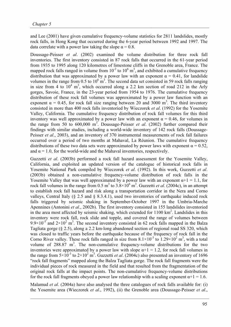
Chapter 5
95
and Lee (2001) have given cumulative frequency-volume statistics for 2811 landslides, mostly rock falls, in Hong Kong that occurred during the 6-year period between 1992 and 1997. The data correlate with a power law taking the slope α = 0.8.
Doussage-Peisser et al. (2002) examined the volume distribution for three rock fall inventories. The first inventory consisted in 87 rock falls that occurred in the 61-year period from 1935 to 1995 along 120 kilometres of limestone cliffs in the Grenoble area, France. The mapped rock falls ranged in volume from 10-2 to 106 m3, and exhibited a cumulative frequency distribution that was approximated by a power law with an exponent α = 0.41, for landslide volumes in the range from 0.5 to 106 m3. The second data set consisted in 59 rock falls ranging in size from 4 to 104 m3, which occurred along a 2.2 km section of road 212 in the Arly gorges, Savoie, France, in the 23-year period from 1954 to 1976. The cumulative frequency distribution of these rock fall volumes was approximated by a power law function with an exponent α = 0.45, for rock fall size ranging between 20 and 3000 m3. The third inventory consisted in more than 400 rock falls inventoried by Wieczorek et al. (1992) for the Yosemite Valley, California. The cumulative frequency distribution of rock fall volumes for this third inventory was well approximated by a power law with an exponent α = 0.46, for volumes in the range from 50 to 600,000 m3. Doussage-Peisser et al. (2002) further compared their findings with similar studies, including a world-wide inventory of 142 rock falls (Doussage-Peisser et al., 2003), and an inventory of 370 instrumental measurements of rock fall failures occurred over a period of two months at Mahaval, La Réunion. The cumulative frequency distributions of these two data sets were approximated by power laws with exponent α = 0.52, and α = 1.0, for the world-wide and the Mahaval inventories, respectively.
Guzzetti et al. (2003b) performed a rock fall hazard assessment for the Yosemite Valley, California, and exploited an updated version of the catalogue of historical rock falls in Yosemite National Park compiled by Wieczorek et al. (1992). In this work, Guzzetti et al. (2003b) obtained a non-cumulative frequency-volume distribution of rock falls in the Yosemite Valley that was well approximated by a power law with an exponent α+1 = 1.1, for rock fall volumes in the range from 0.5 m3 to 3.8×10⁶ m3. Guzzetti et al. (2004c), in an attempt to establish rock fall hazard and risk along a transportation corridor in the Nera and Corno valleys, Central Italy (§ 2.5 and § 8.3.4.1), used two inventories of earthquake induced rock falls triggered by seismic shaking in September-October 1997 in the Umbria-Marche Apennines (Antonini et al., 2002b). The first inventory consisted in 155 landslides inventoried in the area most affected by seismic shaking, which extended for 1100 km2. Landslides in this inventory were rock fall, rock slide and topple, and covered the range of volumes between 9.9×10⁻⁵ and 2×10² m3. The second inventory consisted in 62 rock falls mapped in the Balza Tagliata gorge (§ 2.5), along a 2.2 km-long abandoned section of regional road SS 320, which was closed to traffic years before the earthquake because of the frequency of rock fall in the Corno River valley. These rock falls ranged in size from 8.1×10⁻³ to 1.29×10² m3, with a total volume of 288.87 m3. The non-cumulative frequency-volume distributions for the two inventories were approximated by a power law with slope α+1 = 1.2, for rock fall volumes in the range from 5×10⁻³ to 2×10² m3. Guzzetti et al. (2004c) also presented an inventory of 1696 “rock fall fragments” mapped along the Balza Tagliata gorge. The rock fall fragments were the individual pieces of rock measured in the field and that resulted from the fragmentation of the original rock falls at the impact points. The non-cumulative frequency-volume distributions for the rock fall fragments obeyed a power law relationship with a scaling exponent α+1 = 1.6.
Malamud et al. (2004a) have also analysed the three catalogues of rock falls available for: (i) the Yosemite area (Wieczorek et al., 1992), (ii) the Grenoble area (Doussage-Peisser et al.,

Statistics of landslide size
96
2002), and (iii) the Umbria region (Antonini et al., 2002b). These authors have given non-cumulative frequency density distributions that were well approximated by a power law with a slope, α+1 = 1.07. Martin et al. (2002), using the described data set for Queen Charlotte Islands gave non-cumulative distributions for landslide volumes that were approximated by power laws with exponent α+1 = 1.87, for primary failures, and α+1 = 2.94 for gully sidewall failures. Brandinoni and Church (2004), working in the Capilano coastal watershed in British Columbia, measured the volume of debris mobilized by individual landslides and gave a non-cumulative frequency-volume relationship that obeyed a power law relation with exponents ranging between α+1 = 2.7 and α+1 = 3.6. Issler et al. (2005) performed a statistical study of submarine debris flows in the Storega landslide area, off the western coast of Norway. These authors found that the cumulative frequency distribution of landslide volume for the Storega lobes was well approximated by the logarithmic relationship LLC Vlog..N 214629 −= , with the volume of the landslide in km3, for submarine landslide volumes in the range from 1×10⁴ to 3×10⁸ m3.
Inspection of the literature has revealed variability in the scaling exponents of the power law tails of the distributions of landslide areas and of landslide volumes. Part of this variability is natural, i.e., due to morphological and lithological characteristics. However, a considerable part of the variability is due to the methods used by the different authors to obtain their frequency distributions. The latter is unfortunate and should be avoided.
5.2. Methods
Inspection of a landslide inventory map or field survey in an area recently affected by slope failures reveal that the abundance of landslides varies with the size of the slope failures. As a first approximation, the number of landslides reduces with the increase of the size (i.e., area or volume) of the triggered mass movements. As an example, Figure 5.1 shows the distribution of the areas of 4246 single landslides triggered by rapid snow melt in Umbria in January 1997 (§ 3.3.3.2). Inspection of Figure 5.1 indicates that rapid snow melt in Umbria resulted in a large number of small landslides and in a very small number of large slope failures. Indeed, the inventory lists 1789 landslides (42.13%) smaller than 1000 square meters and only 3 landslides (0.07%) larger than 80,000 square meters. Similar results are found for other inventories, in Umbria and elsewhere. Given that the distribution of the size of the landslides is not simply distributed (e.g., normally, log-normally, etc.), the problem consists in how to properly estimate the size distribution of the landslides. In the next sub-section (§ 5.2.1), I discuss methods to determine the distribution of landslide areas. In sub-section § 5.2.2, I will examine the problem of the determination of the distribution of landslide volumes.
5.2.1. Statistics of landslide area The first step in the determination of the distribution of landslide areas consists in obtaining reliable information on the area of the individual landslides. This is a crucial, often neglected step in the analysis. Problems related with the compilation and the quality of landslide inventory maps were discussed in § 3.4, § 4.2 and § 4.3. Here, I assume the inventory is the “best” possible inventory given the type of mapping (e.g., event, geomorphological, multi-temporal), the scale of the maps and of the aerial photographs used to prepare the inventory, the time available to complete the investigation, and the other factors that affect the quality and completeness of an inventory.
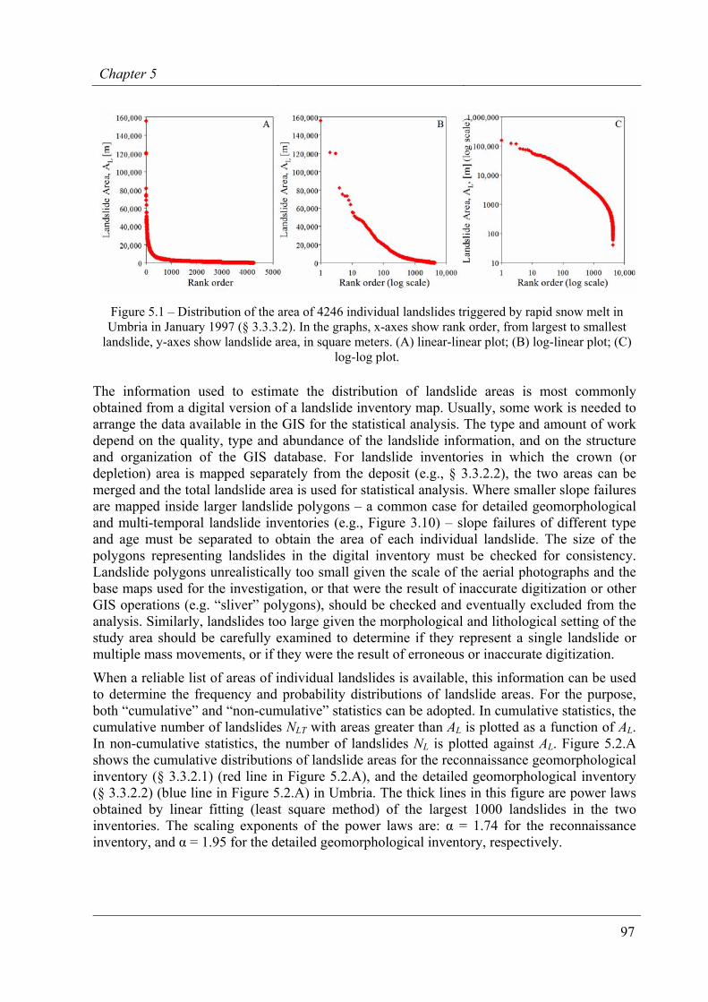
Chapter 5
97
Figure 5.1 – Distribution of the area of 4246 individual landslides triggered by rapid snow melt in Umbria in January 1997 (§ 3.3.3.2). In the graphs, x-axes show rank order, from largest to smallest
landslide, y-axes show landslide area, in square meters. (A) linear-linear plot; (B) log-linear plot; (C) log-log plot.
The information used to estimate the distribution of landslide areas is most commonly obtained from a digital version of a landslide inventory map. Usually, some work is needed to arrange the data available in the GIS for the statistical analysis. The type and amount of work depend on the quality, type and abundance of the landslide information, and on the structure and organization of the GIS database. For landslide inventories in which the crown (or depletion) area is mapped separately from the deposit (e.g., § 3.3.2.2), the two areas can be merged and the total landslide area is used for statistical analysis. Where smaller slope failures are mapped inside larger landslide polygons – a common case for detailed geomorphological and multi-temporal landslide inventories (e.g., Figure 3.10) – slope failures of different type and age must be separated to obtain the area of each individual landslide. The size of the polygons representing landslides in the digital inventory must be checked for consistency. Landslide polygons unrealistically too small given the scale of the aerial photographs and the base maps used for the investigation, or that were the result of inaccurate digitization or other GIS operations (e.g. “sliver” polygons), should be checked and eventually excluded from the analysis. Similarly, landslides too large given the morphological and lithological setting of the study area should be carefully examined to determine if they represent a single landslide or multiple mass movements, or if they were the result of erroneous or inaccurate digitization.
When a reliable list of areas of individual landslides is available, this information can be used to determine the frequency and probability distributions of landslide areas. For the purpose, both “cumulative” and “non-cumulative” statistics can be adopted. In cumulative statistics, the cumulative number of landslides NLT with areas greater than AL is plotted as a function of AL. In non-cumulative statistics, the number of landslides NL is plotted against AL. Figure 5.2.A shows the cumulative distributions of landslide areas for the reconnaissance geomorphological inventory (§ 3.3.2.1) (red line in Figure 5.2.A), and the detailed geomorphological inventory (§ 3.3.2.2) (blue line in Figure 5.2.A) in Umbria. The thick lines in this figure are power laws obtained by linear fitting (least square method) of the largest 1000 landslides in the two inventories. The scaling exponents of the power laws are: α = 1.74 for the reconnaissance inventory, and α = 1.95 for the detailed geomorphological inventory, respectively.
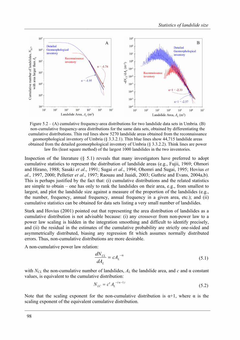
Statistics of landslide size
98
Figure 5.2 – (A) cumulative frequency-area distributions for two landslide data sets in Umbria. (B) non-cumulative frequency-area distributions for the same data sets, obtained by differentiating the
cumulative distributions. Thin red lines show 5270 landslide areas obtained from the reconnaissance geomorphological inventory of Umbria (§ 3.3.2.1). Thin blue lines show 44,715 landslide areas
obtained from the detailed geomorphological inventory of Umbria (§ 3.3.2.2). Think lines are power law fits (least square method) of the largest 1000 landslides in the two inventories.
Inspection of the literature (§ 5.1) reveals that many investigators have preferred to adopt cumulative statistics to represent the distribution of landslide areas (e.g., Fujii, 1969; Ohmori and Hirano, 1988; Sasaki et al., 1991; Sugai et al., 1994; Ohomri and Sugai, 1995; Hovius et al., 1997, 2000; Pelletier et al., 1997; Raouau and Jaaidi, 2003; Guthrie and Evans, 2004a,b). This is perhaps justified by the fact that: (i) cumulative distributions and the related statistics are simple to obtain – one has only to rank the landslides on their area, e.g., from smallest to largest, and plot the landslide size against a measure of the proportion of the landslides (e.g., the number, frequency, annual frequency, annual frequency in a given area, etc.); and (ii) cumulative statistics can be obtained for data sets listing a very small number of landslides.
Stark and Hovius (2001) pointed out that representing the area distribution of landslides as a cumulative distribution is not advisable because: (i) any crossover from non-power law to a power law scaling is hidden in the integration smoothing and difficult to identify precisely, and (ii) the residual in the estimates of the cumulative probability are strictly one-sided and asymmetrically distributed, biasing any regression fit which assumes normally distributed errors. Thus, non-cumulative distributions are more desirable.
A non-cumulative power law relation: α−= L
L
CL cAdA
dN (5.1)
with NCL the non-cumulative number of landslides, AL the landslide area, and c and α constant values, is equivalent to the cumulative distribution:
)(LLC A'cN 1−α−= (5.2)
Note that the scaling exponent for the non-cumulative distribution is α+1, where α is the scaling exponent of the equivalent cumulative distribution.
Chapter 5
99
Guzzetti et al. (2002) exploited this characteristic to obtain the non-cumulative distribution by differentiating the equivalent cumulative distribution. The method requires the landslide areas are arranged from largest to smallest, and that a cumulative distribution is obtained from the ranked areas, which is then converted to a non-cumulative distribution. The non-cumulative distribution is defined as the negative of the derivative of the cumulative distribution,
LCLL dA/dN)A(n −= , and it is calculated by approximation as the slope of the best-fit line to a specified number (usually five) of adjacent cumulative data points. The result is then normalized to the total mapped landslide area, ALT, and a linear fit (in log-log space) is performed to establish the characteristics (i.e., scaling exponent and intercept) of the power law tail of the obtained non-cumulative distribution. An example is given in Figure 5.2.B for the regional geomorphological inventories available for Umbria (§ 3.3.2.1 and § 3.3.2.2).
A more appropriate way of representing non-cumulative distributions consists in constructing a histogram from the available catalogue of landslide areas. To construct a histogram, we divide the interval covered by the data values into equal sub-intervals, known as “bins”. When we construct a histogram, we need to consider two main points: the size of the bins (the “bin width”) and the end points of the bins. Different strategies are possible, which involve using linear or logarithmic bins to obtain the histogram, and linear or logarithmic coordinates to display the obtained distribution. Figure 5.3 shows examples for the inventory of snowmelt induced landslides in Umbria (§ 3.3.3.2).
In Figure 5.3, histograms on the left side were obtained using linear bins, i.e. bins of equal size in linear coordinates (in this case 50 m2) covering the entire range of landslide sizes (i.e., from AL = 30 m2 to AL = 180,000 m2), whereas histograms on the right side of the Figure were obtained using logarithmic bins, i.e. bins of increasing width in linear coordinates but of constant width in logarithmic coordinates. In this figure, histograms on the same raw display the non-cumulative distribution of landslide areas for the snow melt event in Umbria using, from top to bottom, linear-linear coordinates, log-linear coordinates, and log-log coordinates. Inspection of Figure 5.3 indicates that best results are obtained using logarithmic bins and adopting logarithmic coordinates to display the results.
When constructing a histogram in log-log space, care must be taken to correctly normalize the bins, considering if the bins are in linear or logarithmic coordinates. This is done in Figure 5.3, which shows the frequency density and the probability density of landslide areas. The frequency density was computed by normalizing the number of landslides in each logarithmic bin by the width of the bin. The probability density was obtained by further normalizing the frequency density found in each logarithmic bin by the total number of landslides in the inventory.
Construction of a histogram may result in problems, particularly in the bins where the data are scarce, most commonly on the tail of the distribution. This is because histograms are not smooth, and they depend on the selection of the end points of the bins and on the width of the bins. These problems can be alleviated using kernel density estimation. In kernel density estimation, we centre a “kernel” of given width at each data point, and we estimate the density within the kernel. The kernel is then moved across the entire range of data, providing a smooth estimation of the density. Kernel of different types can be used, including uniform, triangular and Gaussian (normal). Figure 5.3 shows a comparison between the probability density obtained by construction of the histogram and by using kernel density estimation.
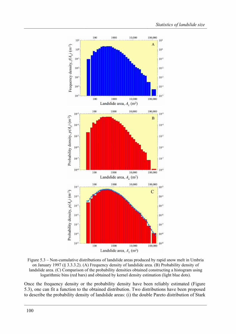
Statistics of landslide size
100
Figure 5.3 – Non-cumulative distributions of landslide areas produced by rapid snow melt in Umbria
on January 1997 (§ 3.3.3.2). (A) Frequency density of landslide area. (B) Probability density of landslide area. (C) Comparison of the probability densities obtained constructing a histogram using
logarithmic bins (red bars) and obtained by kernel density estimation (light blue dots).
Once the frequency density or the probability density have been reliably estimated (Figure 5.3), one can fit a function to the obtained distribution. Two distributions have been proposed to describe the probability density of landslide areas: (i) the double Pareto distribution of Stark
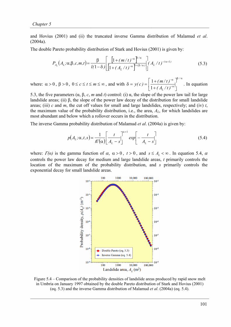
Chapter 5
101
and Hovius (2001) and (ii) the truncated inverse Gamma distribution of Malamud et al. (2004a).
The double Pareto probability distribution of Stark and Hovius (2001) is given by:
( ) [ ][ ]
)(L)/(
L
/
LA )t/A()t/A()t/m(
)(lt,m,c,,;AP
L
111
11
+α−αβ+α−
αβα−
⎥⎥⎦
⎤
⎢⎢⎣
⎡
+
+δ−
β=βα (5.3)
where: 0>α , 0>β , ∞≤≤≤≤ mtc0 , and with αβ
α−
α−
⎥⎦
⎤⎢⎣
⎡++
==δ/
L )t/A()t/m()c(y
11 . In equation
5.3, the five parameters (α, β, c, m and t) control: (i) α, the slope of the power law tail for large landslide areas; (ii) β, the slope of the power law decay of the distribution for small landslide areas; (iii) c and m, the cut off values for small and large landslides, respectively; and (iv) t, the maximum value of the probability distribution, i.e., the area, AL, for which landslides are most abundant and below which a rollover occurs in the distribution.
The inverse Gamma probability distribution of Malamud et al. (2004a) is given by:
( ) ( ) ⎥⎦
⎤⎢⎣
⎡−
−⎥⎦
⎤⎢⎣
⎡−αΓ
=α+α
sAtexp
sAt
ts,t,;Ap
LLL
11 (5.4)
where: Γ(α) is the gamma function of α, 0>α , 0>t , and ∞<≤ LAs . In equation 5.4, α controls the power law decay for medium and large landslide areas, t primarily controls the location of the maximum of the probability distribution, and s primarily controls the exponential decay for small landslide areas.
Figure 5.4 – Comparison of the probability densities of landslide areas produced by rapid snow melt in Umbria on January 1997 obtained by the double Pareto distribution of Stark and Hovius (2001)
(eq. 5.3) and the inverse Gamma distribution of Malamud et al. (2004a) (eq. 5.4).
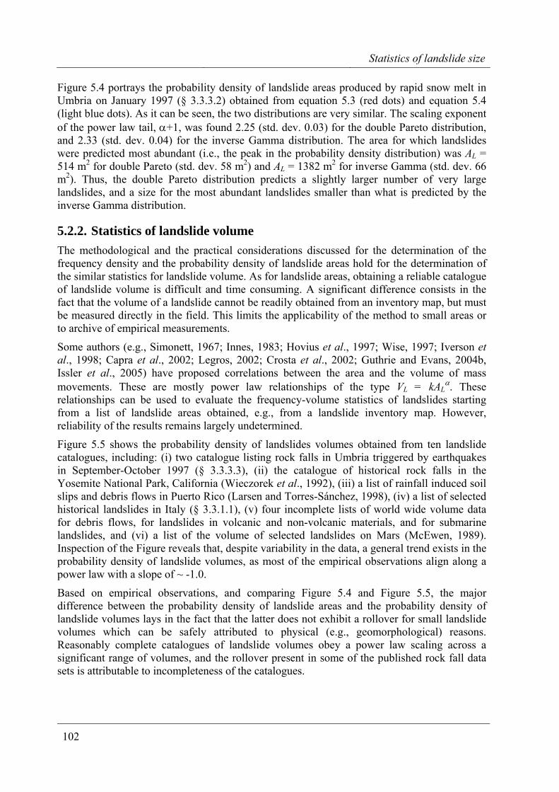
Statistics of landslide size
102
Figure 5.4 portrays the probability density of landslide areas produced by rapid snow melt in Umbria on January 1997 (§ 3.3.3.2) obtained from equation 5.3 (red dots) and equation 5.4 (light blue dots). As it can be seen, the two distributions are very similar. The scaling exponent of the power law tail, α+1, was found 2.25 (std. dev. 0.03) for the double Pareto distribution, and 2.33 (std. dev. 0.04) for the inverse Gamma distribution. The area for which landslides were predicted most abundant (i.e., the peak in the probability density distribution) was AL = 514 m2 for double Pareto (std. dev. 58 m2) and AL = 1382 m2 for inverse Gamma (std. dev. 66 m2). Thus, the double Pareto distribution predicts a slightly larger number of very large landslides, and a size for the most abundant landslides smaller than what is predicted by the inverse Gamma distribution.
5.2.2. Statistics of landslide volume The methodological and the practical considerations discussed for the determination of the frequency density and the probability density of landslide areas hold for the determination of the similar statistics for landslide volume. As for landslide areas, obtaining a reliable catalogue of landslide volume is difficult and time consuming. A significant difference consists in the fact that the volume of a landslide cannot be readily obtained from an inventory map, but must be measured directly in the field. This limits the applicability of the method to small areas or to archive of empirical measurements.
Some authors (e.g., Simonett, 1967; Innes, 1983; Hovius et al., 1997; Wise, 1997; Iverson et al., 1998; Capra et al., 2002; Legros, 2002; Crosta et al., 2002; Guthrie and Evans, 2004b, Issler et al., 2005) have proposed correlations between the area and the volume of mass movements. These are mostly power law relationships of the type VL = kAL
α. These relationships can be used to evaluate the frequency-volume statistics of landslides starting from a list of landslide areas obtained, e.g., from a landslide inventory map. However, reliability of the results remains largely undetermined.
Figure 5.5 shows the probability density of landslides volumes obtained from ten landslide catalogues, including: (i) two catalogue listing rock falls in Umbria triggered by earthquakes in September-October 1997 (§ 3.3.3.3), (ii) the catalogue of historical rock falls in the Yosemite National Park, California (Wieczorek et al., 1992), (iii) a list of rainfall induced soil slips and debris flows in Puerto Rico (Larsen and Torres-Sánchez, 1998), (iv) a list of selected historical landslides in Italy (§ 3.3.1.1), (v) four incomplete lists of world wide volume data for debris flows, for landslides in volcanic and non-volcanic materials, and for submarine landslides, and (vi) a list of the volume of selected landslides on Mars (McEwen, 1989). Inspection of the Figure reveals that, despite variability in the data, a general trend exists in the probability density of landslide volumes, as most of the empirical observations align along a power law with a slope of ~ -1.0.
Based on empirical observations, and comparing Figure 5.4 and Figure 5.5, the major difference between the probability density of landslide areas and the probability density of landslide volumes lays in the fact that the latter does not exhibit a rollover for small landslide volumes which can be safely attributed to physical (e.g., geomorphological) reasons. Reasonably complete catalogues of landslide volumes obey a power law scaling across a significant range of volumes, and the rollover present in some of the published rock fall data sets is attributable to incompleteness of the catalogues.
Chapter 5
103
Figure 5.5 – Probability density of landslide volumes for different landslide catalogues. (A) Rock falls triggered by the Umbria – Marche earthquakes in September-October 1997 (Antonini et al.,
2002b) (§ 3.3.3.3). (B) Rock falls triggered along the Balza Tagliata canyon by the Umbria – Marche earthquakes in September-October 1997. (C) Rock falls in the Yosemite National Park (Wieczorek et
al., 1992). (D) Rainfall induced soil slips and debris flows in Puerto Rico (Larsen and Torres-Sánchez, 1998). (E) Historical landslides in Italy (the AVI project, § 3.3.1.1). (F) World wide debris
flow data, various sources. (G) World wide data for landslides in non-volcanic materials, various sources. (H) World wide data for landslides in volcanic materials, various sources. (I) World wide data on submarine landslides, various sources. (J) Martian landslides (McEwen, 1989). Grey line is
power law with exponent -1.0.
5.3. Applications to the Umbria Region inventories
I this section, I use the methods presented before to obtain and study the statistics of landslide area for multiple data sets available in Umbria. First, I further exploit the opportunity of having three different landslide inventory maps for the Collazzone area to attempt a measurable assessment of the degree of completeness of the three landslide maps (Figure 3.14). Next, I compare statistics of landslide area in Umbria obtained from geomorphological, event, and multi-temporal inventory maps.
5.3.1. Completeness of the landslide inventory maps in the Collazzone area Figure 5.6.A shows the dependence of the landslide probability density on landslide area for the three inventory maps available for the Collazzone area (Figure 3.14). Figure 5.6.B shows the relationship between landslide frequency and landslide area for the same three inventories. In a previous example (Figure 5.4) I have shown that equations 5.3 and 5.4 provide very similar results in Umbria. Hence, here I show only statistics obtained from equation 5.4, i.e.
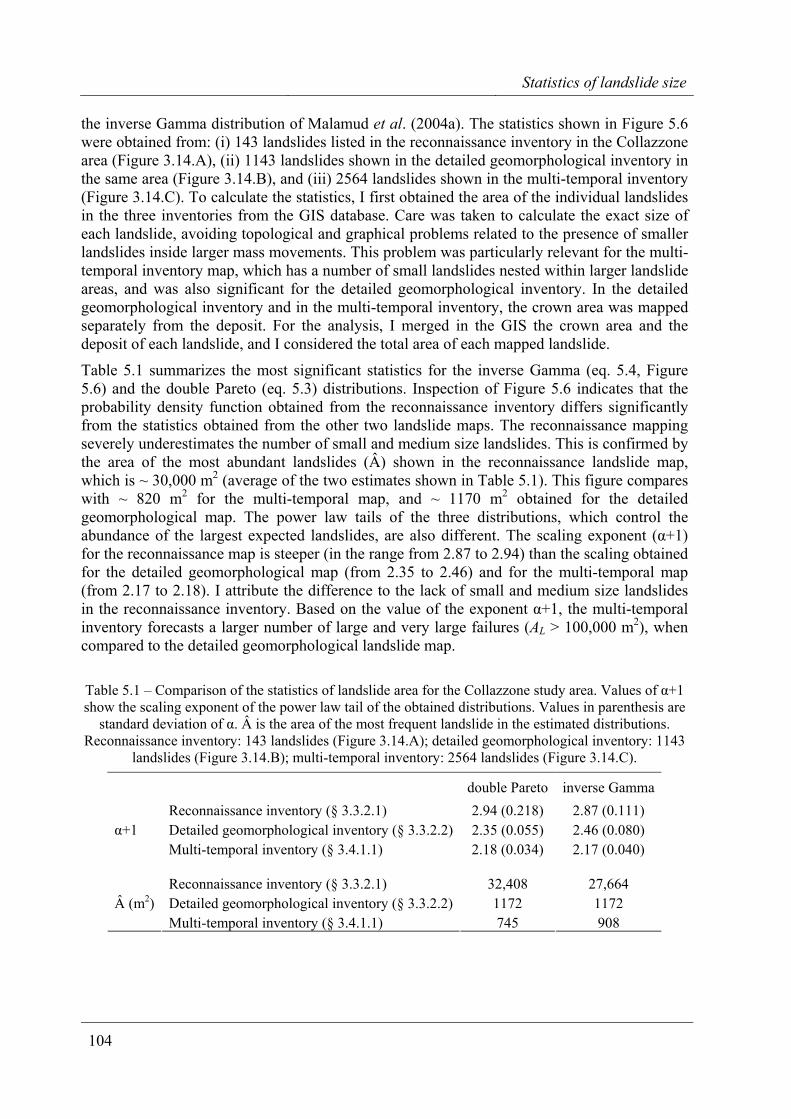
Statistics of landslide size
104
the inverse Gamma distribution of Malamud et al. (2004a). The statistics shown in Figure 5.6 were obtained from: (i) 143 landslides listed in the reconnaissance inventory in the Collazzone area (Figure 3.14.A), (ii) 1143 landslides shown in the detailed geomorphological inventory in the same area (Figure 3.14.B), and (iii) 2564 landslides shown in the multi-temporal inventory (Figure 3.14.C). To calculate the statistics, I first obtained the area of the individual landslides in the three inventories from the GIS database. Care was taken to calculate the exact size of each landslide, avoiding topological and graphical problems related to the presence of smaller landslides inside larger mass movements. This problem was particularly relevant for the multi-temporal inventory map, which has a number of small landslides nested within larger landslide areas, and was also significant for the detailed geomorphological inventory. In the detailed geomorphological inventory and in the multi-temporal inventory, the crown area was mapped separately from the deposit. For the analysis, I merged in the GIS the crown area and the deposit of each landslide, and I considered the total area of each mapped landslide.
Table 5.1 summarizes the most significant statistics for the inverse Gamma (eq. 5.4, Figure 5.6) and the double Pareto (eq. 5.3) distributions. Inspection of Figure 5.6 indicates that the probability density function obtained from the reconnaissance inventory differs significantly from the statistics obtained from the other two landslide maps. The reconnaissance mapping severely underestimates the number of small and medium size landslides. This is confirmed by the area of the most abundant landslides (Â) shown in the reconnaissance landslide map, which is ~ 30,000 m2 (average of the two estimates shown in Table 5.1). This figure compares with ~ 820 m2 for the multi-temporal map, and ~ 1170 m2 obtained for the detailed geomorphological map. The power law tails of the three distributions, which control the abundance of the largest expected landslides, are also different. The scaling exponent (α+1) for the reconnaissance map is steeper (in the range from 2.87 to 2.94) than the scaling obtained for the detailed geomorphological map (from 2.35 to 2.46) and for the multi-temporal map (from 2.17 to 2.18). I attribute the difference to the lack of small and medium size landslides in the reconnaissance inventory. Based on the value of the exponent α+1, the multi-temporal inventory forecasts a larger number of large and very large failures (AL > 100,000 m2), when compared to the detailed geomorphological landslide map.
Table 5.1 – Comparison of the statistics of landslide area for the Collazzone study area. Values of α+1 show the scaling exponent of the power law tail of the obtained distributions. Values in parenthesis are
standard deviation of α. Â is the area of the most frequent landslide in the estimated distributions. Reconnaissance inventory: 143 landslides (Figure 3.14.A); detailed geomorphological inventory: 1143
landslides (Figure 3.14.B); multi-temporal inventory: 2564 landslides (Figure 3.14.C).
double Pareto inverse Gamma Reconnaissance inventory (§ 3.3.2.1) 2.94 (0.218) 2.87 (0.111) Detailed geomorphological inventory (§ 3.3.2.2) 2.35 (0.055) 2.46 (0.080) α+1 Multi-temporal inventory (§ 3.4.1.1) 2.18 (0.034) 2.17 (0.040)
Reconnaissance inventory (§ 3.3.2.1) 32,408 27,664 Detailed geomorphological inventory (§ 3.3.2.2) 1172 1172 Â (m2) Multi-temporal inventory (§ 3.4.1.1) 745 908
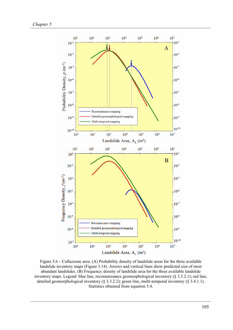
Chapter 5
105
Figure 5.6 – Collazzone area. (A) Probability density of landslide areas for the three available landslide inventory maps (Figure 3.14). Arrows and vertical lines show predicted size of most abundant landslides. (B) Frequency density of landslide area for the three available landslide
inventory maps. Legend: blue line, reconnaissance geomorphological inventory (§ 3.3.2.1); red line, detailed geomorphological inventory (§ 3.3.2.2); green line, multi-temporal inventory (§ 3.4.1.1).
Statistics obtained from equation 5.4.
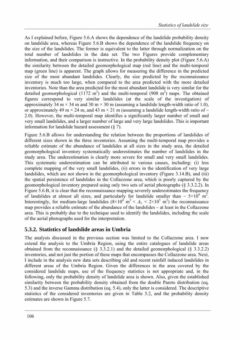
Statistics of landslide size
106
As I explained before, Figure 5.6.A shows the dependence of the landslide probability density on landslide area, whereas Figure 5.6.B shows the dependence of the landslide frequency on the size of the landslides. The former is equivalent to the latter through normalization on the total number of landslides in the data set. The two Figures provide complementary information, and their comparison is instructive. In the probability density plot (Figure 5.6.A) the similarity between the detailed geomorphological map (red line) and the multi-temporal map (green line) is apparent. The graph allows for measuring the difference in the predicted size of the most abundant landslides. Clearly, the size predicted by the reconnaissance inventory is much too large, when compared to the area predicted with the more detailed inventories. Note than the area predicted for the most abundant landslide is very similar for the detailed geomorphological (1172 m2) and the multi-temporal (908 m2) maps. The obtained figures correspond to very similar landslides (at the scale of the investigation) of approximately 34 m × 34 m and 30 m × 30 m (assuming a landslide length-width ratio of 1.0), or approximately 49 m × 24 m, and 43 m × 21 m (assuming a landslide length-width ratio of ~ 2.0). However, the multi-temporal map identifies a significantly larger number of small and very small landslides, and a larger number of large and very large landslides. This is important information for landslide hazard assessment (§ 7).
Figure 5.6.B allows for understanding the relation between the proportions of landslides of different sizes shown in the three inventories. Assuming the multi-temporal map provides a reliable estimate of the abundance of landslides at all sizes in the study area, the detailed geomorphological inventory systematically underestimates the number of landslides in the study area. The underestimation is clearly more severe for small and very small landslides. This systematic underestimation can be attributed to various causes, including: (i) less complete mapping of the very small landslides, (ii) errors in the identification of very large landslides, which are not shown in the geomorphological inventory (Figure 3.14.B), and (iii) the spatial persistence of landslides in the Collazzone area, which is poorly captured by the geomorphological inventory prepared using only two sets of aerial photographs (§ 3.3.2.2). In Figure 5.6.B, it is clear that the reconnaissance mapping severely underestimates the frequency of landslides at almost all sizes, and particularly for landslide smaller than ~ 5×10⁴ m2. Interestingly, for medium-large landslides (8×10⁴ m2 < AL < 2×10⁵ m2) the reconnaissance map provides a reliable estimate of the abundance of the landslides – at least in the Collazzone area. This is probably due to the technique used to identify the landslides, including the scale of the aerial photographs used for the interpretation.
5.3.2. Statistics of landslide areas in Umbria The analysis discussed in the previous section was limited to the Collazzone area. I now extend the analysis to the Umbria Region, using the entire catalogues of landslide areas obtained from the reconnaissance (§ 3.3.2.1) and the detailed geomorphological (§ 3.3.2.2) inventories, and not just the portion of these maps that encompasses the Collazzone area. Next, I include in the analysis new data sets describing old and recent rainfall induced landslides in different areas of the Umbria Region. Given the differences in the area covered by the considered landslide maps, use of the frequency statistics is not appropriate and, in the following, only the probability density of landslide area is shown. Also, given the established similarity between the probability density obtained from the double Pareto distribution (eq. 5.3) and the inverse Gamma distribution (eq. 5.4), only the latter is considered. The descriptive statistics of the considered inventories are given in Table 5.2, and the probability density estimates are shown in Figure 5.7.
Chapter 5
107
Table 5.2 – Comparison of the statistics of landslide area in Umbria. Type refers to the type of inventory: G, geomorphological inventory; E, event inventory; ME, multiple events inventory; MT,
multi-temporal inventory. Values of α+1 show the scaling exponent of the power law tail of the obtained distributions. Values in parenthesis are standard deviation of α.
Dataset § Type Landslide Area (m2) α+1
# mean min max DP IG
Regional reconnaissance 3.3.2.1 G 5270 84,169 220 3.1×10⁶ 2.59
(0.028) 2.91
(0.046)
Detailed geomorphological 3.3.2.2 G 46,379 12,058 40 1.4×10⁶ 2.26
(0.009) 2.26
(0.011) Rainfall induced landslides (1937-41) 3.3.3.1 ME 861 3954 74 1.1×10⁵
2.65 (0.092)
2.84 (0.107)
Snowmelt induced landslides (1997) 3.3.3.2 E 4246 3019 39 1.5×10⁵ 2.25
(0.027) 2.33
(0.038) Rainfall induced landslides (2004) ME 628 2468 15 6.0×10⁴ 2.55
(0.114) 2.47
(0.128) Multi-temporal inventory (Collazzone) 3.3.4.1 MT 2189 4362 78 1.5×10⁶
2.55 (0.055)
2.66 (0.078)
There is much to be learnt from the analysis of Figure 5.7. First, all obtained probability densities exhibit a similar trend. The probability density increases with the area of the landslide up to a maximum value, where slope failures are most abundant, then it decays along a power law. The slope of the power law tail of the distribution ranges from α+1 = 2.26 to α+1 = 2.91.
The size of the most abundant landslide exhibits a much larger variation. To facilitate the investigation of the relationships between the size of the most abundant landslide and the type of the inventory, in Figure 5.7 the different types of inventories (i.e., geomorphological, event, multiple-events, multi-temporal) are shown with different symbols. The reconnaissance map (§ 3.3.2.1) clearly underestimates the abundance of the smallest landslides. The most abundant slope failures in this inventory have an area of ~ 2.5×10⁴ m2, six times larger than the area predicted by the detailed geomorphological inventory (~ 4×10³ m2), and at least eight times larger than the area predicted by the 1997 snowmelt event inventory (~ 3×10³ m2). When compared to the other inventories, the two geomorphological maps show a larger proportion of large and very large landslide areas. For the reconnaissance mapping this is evident for landslides larger than ~ 1×10⁴ m2, and for the detailed geomorphological mapping for landslides larger than ~ 2×10³ m2. This finding has several reasons. The geomorphological maps do not show small landslides, which were not visible in the single set of medium scale aerial photographs used to obtain the landslide information. In places, the geomorphological inventories show a number of coalescent landslides as a single larger landslide (or landslide area), overestimating the size of the larger slope failures. Lastly, the reconnaissance mapping is affected by cartographic inaccuracies, which also lead to overestimation of the size of the large landslides (§ 3.4, Carrara et al., 2002).
Noticeably, the multi-temporal inventory obtained for the Collazzone area is not affected by this bias, indicating the ability of a good quality multi-temporal landslide map to reliably describe the size of the landslides, at least for slope failures having AL ≥ 1.5×10³ m2. This is an important result, as it provides the rationale for using information on landslide size obtained
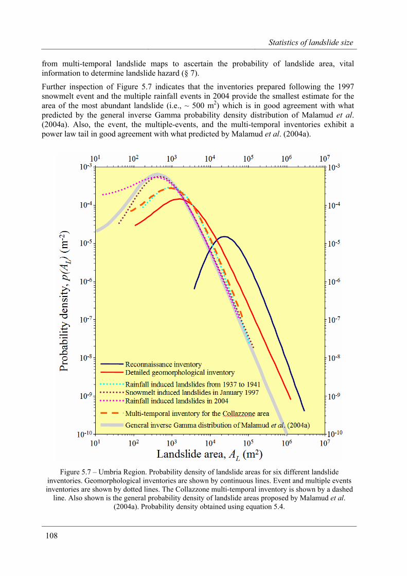
Statistics of landslide size
108
from multi-temporal landslide maps to ascertain the probability of landslide area, vital information to determine landslide hazard (§ 7).
Further inspection of Figure 5.7 indicates that the inventories prepared following the 1997 snowmelt event and the multiple rainfall events in 2004 provide the smallest estimate for the area of the most abundant landslide (i.e., ~ 500 m2) which is in good agreement with what predicted by the general inverse Gamma probability density distribution of Malamud et al. (2004a). Also, the event, the multiple-events, and the multi-temporal inventories exhibit a power law tail in good agreement with what predicted by Malamud et al. (2004a).
Figure 5.7 – Umbria Region. Probability density of landslide areas for six different landslide
inventories. Geomorphological inventories are shown by continuous lines. Event and multiple events inventories are shown by dotted lines. The Collazzone multi-temporal inventory is shown by a dashed
line. Also shown is the general probability density of landslide areas proposed by Malamud et al. (2004a). Probability density obtained using equation 5.4.
Chapter 5
109
5.4. Discussion
Frequency-size statistics of landslides are important for the quantification of erosion processes in mountain areas. Statistics of landslide area and volume have been used to determine sediment fluxes and to the estimate denudation rates (Hovius et al., 1997, 2000; Martin et al., 2002; Lavé and Burbank, 2004; Malamud et al., 2004b). The Frequency-size statistics of landslides are also important for the quantification of landslide hazard (Malamud et al., 2004a; Guzzetti et al., 2005a). A discussion on these topics is not within the scope of this work (§ 1.2). In the following, I will concentrate on two relevant issues, namely: (i) why medium and large landslides consistently satisfy a power law (i.e., fractal) frequency-area statistics, and (ii) why small and very small landslides systematically deviate from the power law correlation. I will also investigate the differences between the frequency-area and the frequency-volume statistics observed in the available empirical data.
There is now clear evidence that medium and large size landslides consistently satisfy power law frequency-area statistics. Reasons for this behaviour remain undetermined. One potential explanation for this power law behaviour is the concept of self-organized criticality (SOC, Back et al., 1987, 1988). This concept was introduced to explain the behaviour of the “sandpile” model. In this model, there is a square grid of boxes, at each time step a particle is dropped into a randomly-selected box. When there are four particles in a box they are redistributed to the four adjacent boxes, or in the case of boxes on the boundaries of the grid, are lost. A single redistribution can lead to an “avalanche” of redistributions. The size of the “avalanche”’ is the area of boxes AB participating in the redistributions. The non-cumulative number of “avalanches” NA with area AB satisfies the power law distribution 01.
BA AN −≈ (Kadanoff et al., 1989).
Noever (1993) has associated the power law frequency-area statistics of large landslides with the “sandpile” model and the concept of self-organized criticality. However, there is a large extrapolation from the “sandpile” model to actual landslides. The available empirical data indicate that, for the medium and large landslides, the power law exponent is α+1 = 2.4 ± 0.4, considerably larger than the value of 1.0 predicted by the “sandpile” model (Malamud et al., 2004a). This is not surprising considering the simplicity of the model and the three-dimensional nature of actual landslides, and could indicate that a revision of the “rules” for the “sandpile” model is needed for a realistic analogue of actual landslides in nature. Pelletier et al. (1997) have combined a slope stability analysis with a soil-moisture analysis and found a power law distribution. The cumulative frequency-area distribution of the modelled landslides found by these authors has a scaling exponent α = 1.6. Hertgarten and Neugebauer (2000) have used a numerical model combining slope stability and mass movement and found an approximation to a power law distribution with an exponent of α+1 ~ 2.1. More recently, these authors have used a cellular-automata model with time-dependent weakening, similar to the “sandpile” model, and found a power law distribution with α+1 ~ 2.0 (Hertgarten and Neugebauer, 2000). Czirók et al. (1997) performed laboratory experiments using a micro-model of a ridge and produced landslides by spraying the ridge with water, thus simulating rainfall. These authors obtained a density distribution for the area of the micro-landslides that correlated with a power law with α+1 ~ 1.0, in good agreement with the “sandpile” model prediction, but different from what is observed in natural landslides. Although it is certainly possible to develop idealized models that reproduce the observed power law dependence of actual landslide data, there is a real question whether these models are realistic in terms of the governing physics (Turcotte et al., 2002).
Statistics of landslide size
110
Despite its clear limitations, the relatively simple “sandpile” model may provide the basis for understanding the power law statistics of large landslides (Malamud et al., 2004a; Turcotte et al., 2002). In the “sandpile” model the region over which an avalanche will spread is well defined prior to the avalanche. Similarly, the area over which a landslide will spread can be defined before the landslide is triggered. In both, there are metastable areas. As particles are added, the metastable avalanche areas grow. As mountains grow, metastable landslide areas also grow. Detailed studies of the “sandpile” model show that this growth is dominated by the coalescence of smaller metastable regions (Turcotte, 1999). Also, the coalescence cross sections lead directly to a power law distribution of metastable areas. It can be expected that a similar coalescence and growth process would be applicable to metastable landslide areas, explaining the observed power law frequency area distribution of large landslides.
There is also good evidence that landslide area obtained from reasonably complete (for statistical purposes) empirical inventories deviate from the power law correlation for small landslides. The reasons for this behaviour are also undetermined. One possibility is that the rollover scale has a geomorphological explanation (Guzzetti et al., 2002). The rollover occurs for linear scales less than about 30 meters, which is the scale on which well defined stream networks form. The incision associated with stream and river networks would be expected to play a significant role in the geometry of landslides, at least for climatically controlled slope failures. For climatically controlled landslides, water and groundwater are important issues and both relate to the size of the slope, which in turn depends on the pattern and density of the drainage network. For seismically induced landslides, the relationship is less clear. These landslides, and particularly rock falls and disrupted rock slides, occur where slopes are steeper, where the seismic shaking concentrates, and where the rock is weaker. An alternative explanation for the rollover of the data is that this scale represents a transition from failures controlled mostly by cohesion through the sliding mass to failures controlled mostly by basal friction. Deviation from the power law scaling for small landslide areas may also reflect geometrical characteristic of the landslides. Very large landslides exhibit – necessarily – a larger area to volume ratio. The same ratio for small landslides will depend on the type of landslides. Shallow soil slides have an area to volume ratio of 0.2 or lower, whereas small rock falls may exhibit a ratio close to 1.0 (i.e., a cube of rock sliding on one of the faces). This may also explain why the statistics of landslide volume do not change for small landslides. Indeed, in the statistics of landslide volume given in Figure 5.5 several different types of landslides are shown, including rock falls.
Frequency-size statistics of landslides have implications for landslide hazard and risk assessment. In § 7.3, I will use the probability density of landslide area obtained from a multi-temporal inventory to measure the magnitude of the expected slope failures; mandatory information to ascertain landslide hazard. There are other ways to use the statistics of landslide size to ascertain landslide hazards. Malamud et al. (2004a) investigated three substantially complete landslide event inventories (including the landslides triggered by rapid snow melting in Umbria in 1997, § 3.3.3.2) and proposed a general probability density distribution for landslide area. This general distribution is based on their inverse Gamma distribution (eq. 5.4), taking α+1 = 2.40, t = 1.28×10³ m2, and s = -1.32×10² m2. Using their general distribution, these authors computed descriptive statistics for landslides, including the average area of a landslide in an inventory (ĀL =3.07×10³ m2). Assuming the applicability of the proposed general distribution, other useful statistics can be computed. Where the total number of landslides in a (complete) inventory is known, the total landslide area (ALT =ĀL×NLT = (3.07×10³ m2) × NLT), and the area of the largest expected landslide (ALmax = (1.10×10³ m2) ×
Chapter 5
111
NLT0.714) can be easily determined. Further, assuming a relationship between landslide volume
and landslide area of the type VL = εAL1.50, the average landslide volume, LV , the total
landslide volume, VLT, and the maximum landslide volume, VLmax, can also be determined (Malamud et al., 2004a,b). This is important information to ascertain landslide hazard and risk (e.g., Cardinali et al., 2002; Reichenbach et al., 2005).
Based on the same general probability density distribution for landslide areas, Malamud et al. (2004a) proposed a magnitude scale, mL, for a landslide event, and defined it as the logarithm to the base 10 of the total number of landslides associated with the event (eq. 5.5). This is similar to what was proposed by Keefer (1984) and later by Rodríguez et al. (1999) who used a scale to quantify the number of landslides in earthquake-triggered landslide events: 100-1000 landslides were classified as a two, 1000-10,000 landslides a three, etc. Knowing the total number of landslides triggered by an event, the landslide magnitude of the event is determined as:
mL =log10 NLT (5.5)
Using this scale, the rapid snowmelt event that resulted in 4246 landslides in January 1997 in Umbria (§ 3.3.3.2) has a landslide magnitude mL = 3.63. This compares with a landslide magnitude mL = 2.80 for the prolonged rainfall periods that triggered 628 landslides in Umbria in 2004.
Malamud et al. (2004a,b) further combined the landslide volume statistics obtained from their general distribution, with an empirical correlation obtained by Keffer (1994) between the total volume of landslides, VLT, triggered by an earthquake and the magnitude ME of the earthquake, and obtained an approximate relation between the earthquake magnitude ME and the magnitude of the landslide event, mL, triggered by the earthquake. This relation is
mL =1.29ME – 5.65 (5.6)
This is important information for the determination of the hazard posed by earthquake induced landslides. Unfortunately, no similar correlations are available for landslides triggered by rainfall or snowmelt, largely because no established measure exists for the magnitude of these meteorological events.
5.5. Summary of achieved results
In this chapter, I have:
(a) Shown how to obtain reliable statistics of landslide area and volume from landslide inventory maps or landslide catalogues.
(b) Demonstrated how statistical information on landslide area can be used to evaluate the completeness of a landslide inventory, contributing to establish the quality of the inventory.
(c) Shown how statistics of landslide area and volume can prove useful to determine landslide hazard and the associated risk.
This responds to Question # 4 and contributes to respond to Question # 2 given in the Introduction (§ 1.2).

113
6. LANDSLIDE SUSCEPTIBLITY ZONING
The process of categorizing … involves an act of invention.
(Bruner, Goodnow and Austin
A Study of Thinking, 1956)
In the literature, confusion exists between the terms landslide “susceptibility” and landslide “hazard”. Often, the terms are used as synonymous despite the two words expressing different concepts. Landslide susceptibility is the likelihood of a landslide occurring in an area on the basis of local terrain conditions (Brabb, 1984). It is the degree to which a terrain can be affected by slope movements, i.e., an estimate of “where” landslides are likely to occur. Susceptibility does not consider the temporal probability of failure (i.e., when or how frequently landslides occur), nor the magnitude of the expected landslide (i.e., how large or destructive the failure will be) (Committee on the Review of the National Landslide Hazards Mitigation Strategy, 2004). In mathematical language, landslide susceptibility is the probability of spatial occurrence of slope failures, given a set of geo-environmental conditions. This is called “landslide analysis” by Vandine et al. (2004). Landslide hazard is the probability that a landslide of a given magnitude will occur in a given period and in a given area. Besides predicting “where” a slope failure will occur, landslide hazard forecasts “when” or “how frequently” it will occur, and “how large” it will be (Guzzetti et al., 2005a). Landslide hazard is more difficult to obtain than landslide susceptibility, as susceptibility is a component (the spatial component) of the hazard. More generally, landslide susceptibility consists in the assessment of what has happened in the past, and landslide hazard evaluation consists in the prediction of what will happen in the future.
In this Chapter, I discuss landslide susceptibility zoning, whereas landslide hazard modelling will be dealt with in § 7. Here, I review the methods proposed to ascertain landslide susceptibility, including an analysis of the types of mapping units most commonly adopted, and of the relationships between the selected mapping units and the adopted susceptibility methods. I then examine a probabilistic model for landslide susceptibility, including problems and difficulties in its application, and I present an example of a landslide susceptibility model for the Upper Tiber River basin, an area that extends for about 4100 km2 in central Italy. Lastly, I discuss the problem of the verification of the performances of a landslide susceptibility model, including examples for the Collazzone area, in central Umbria.
In the following, I will often refer to the literature on landslide hazard, including some of my own work (e.g., Guzzetti et al., 1999a). This is because of two reasons: (i) due to the mentioned confusion between susceptibility and hazard, literature on landslide hazard often discusses methods and techniques to obtain landslide susceptibility (and not landslide hazard);
Chapter 6
114
and (ii) some of the arguments (e.g., selection of the mapping unit of reference, statistical modelling, and validation techniques) are common to both susceptibility and hazard modelling.
6.1. Background
Over the past decades, government, environmental and research organizations worldwide have invested resources in the attempt to assess landslide susceptibility (or hazard), and to produce maps portraying its spatial distribution (landslide susceptibility or hazard zonation). Inspection of the literature reveals that a few reviews of the concepts, principles, techniques and methodologies for landslide susceptibility and hazard evaluation have been proposed (Cotecchia, 1978b; Humam and Radulescu, 1978; Carrara, 1983; Brabb, 1984; Crozier, 1986; Hansen, 1984a; Varnes and IAEG Commission on Landslides and other Mass-Movements, 1984; Crozier, 1986; Einstein, 1988; Hartlen and Viberg, 1988; Mulder, 1991; van Westen, 1993, 1994; Soeters and van Westen, 1996; van Westen et al., 1997; Aleotti and Chowdhury, 1999; Chung and Fabbri, 1999; Guzzetti et al., 1999a; Crozier and Glade, 2005; Glade and Crozier, 2005b; Glade et al., 2005). Comparatively, little work has been done on the systematic comparison of different techniques to determine landslide susceptibility, outlining advantages and limitations of the proposed methods (Carrara et al., 1992, 1995; van Westen, 1993; Pistocchi et al., 2002; Gorsevski et al., 2003; Lee et al., 2004; Süzen and Doyuran, 2004a; Crozier and Glade, 2005; Glade et al., 2005), or to the critical discussion of the basic principles and the underlying assumptions of landslide susceptibility/hazard zonation (Varnes and IAEG Commission on Landslides and other Mass-Movements, 1984; Carrara et al., 1995; Hutchinson, 1995; Soeters and van Westen, 1996; van Westen et al., 1997; Aleotti and Chowdhury, 1999; Guzzetti et al., 1999; Committee on the Review of the National Landslide Hazards Mitigation Strategy, 2004; Crozier and Glade, 2005). Recently, Glade and Crozier (2005b) have published a review of landslide susceptibility (and hazard) models at the catchment, regional and national scale, published in the period from 1977 to 2004.
The majority of papers discuss specific attempts at the evaluation of landslide susceptibility in limited areas. Only a few authors report on long-term projects on the evaluation of slope instability conditions, and the related hazards and risk, over large regions. Notable examples are represented by the work carried out in San Mateo County, California, by the U.S. Geological Survey (Nilsen and Brabb, 1977; Brabb et al., 1978; Mark, 1992; Brabb, 1995); by the proposal made by the French Bureau des Recherché Géologiques et Minières for a geomorphologically based evaluation of landslide hazard (Humbert, 1976, 1977; Antoine, 1977; Landry, 1979; Porcher and Guiloppe, 1979; Delaunay, 1981; Godefroy and Humbert, 1983; Leroi, 1996); and by the work carried out in Hong Kong by the Geotechnical Engineering Office (Brand, 1988; Brand et al., 1982; Burnett et al., 1985; Hansen et al., 1995; Ng et al., 2003) and other investigators (Dai and Lee, 1999, 2001, 2002, 2003; Dai et al., 2002; Zhou et al., 2002; 2003; Chen and Lee, 2003, 2004; Chau et al., 2003, 2004).
Italy has a long tradition of landslide mapping (Almagià, 1907, 1910; Govi, 1976; Bosi, 1978; Carrara, 1978; Cotecchia, 1978b), and efforts to produce a detailed national geomorphological inventory are under way (Amanti, 2000; Amanti et al., 2001). Several regional governments have already produced geomorphological inventory maps at 1:25,000 or 1:10,000 scale. Despite these significant mapping efforts, attempts at producing susceptibility and hazard maps by the application of statistical techniques are mostly limited to academic exercises in pilot areas (Carrara, 1983; Carrara et al., 1991, 1995, 2003; Guzzetti et al., 1999; Ardizzone et
Landslide susceptibility
115
al., 2002; Clerici et al., 2002; Donati and Turrini, 2002; Sorriso-Valvo, 2005; Guzzetti et al., 2005a,d). The same occurs for the application of physically based models for determining the susceptibility of shallow landslides (Borga et al., 1998, 2002a, 2002b; Crosta and Dal Negro, 2003; Crosta and Frattini, 2003) and of rock falls (Guzzetti et al., 2004b). With this respect, the experiment conducted in the Upper Tiber River basin to produce a susceptibility map for a large area (~ 4100 km2) represents an important exception (Cardinali et al., 2001; 2002b). I will discuss the results of this experiment in § 6.4.
6.2. Landslide susceptibility methods
Several different methods and techniques for evaluating landslide susceptibility have been proposed and tested. However, no general agreement exists either on the methods for or on the scope of producing susceptibility maps (Brabb, 1984; Varnes and IAEG Commission on Landslides and other Mass-Movements, 1984; Carrara, 1989; Nieto, 1989; Carrara et al., 1991a, 1997; Soeters and van Westen, 1996; van Westen et al., 1997; Aleotti and Chowdhury, 1999; Guzzetti et al., 1999a, Committee on the Review of the National Landslide Hazards Mitigation Strategy, 2004; Crozier and Glade, 2005; Glade and Crozier, 2005b). Operational and conceptual differences include: (i) the general underlying assumptions; (ii) the type of mapping unit selected for the investigation; and (iii) the techniques and tools favoured for the analysis and the susceptibility assessment.
6.2.1. Assumptions Despite conflicting views among experts, all the proposed methods are based upon a few, widely accepted assumptions (Varnes and IAEG Commission on Landslides and other Mass-Movements, 1984; Carrara et al., 1991a; Hutchinson and Chandler, 1991; Hutchinson, 1995; Turner and Schuster, 1996; Guzzetti et al., 1999a). These are the same assumptions which lay at the base of landslide mapping (see § 2.1), namely:
(a) Slope failures leave discernible features that can be recognized, classified and mapped in the field or through remote sensing, chiefly stereoscopic aerial photographs (Rib and Liang, 1978; Varnes, 1978; Hansen, 1984; Hutchinson, 1988; Cruden and Varnes, 1996; Dikau et al., 1996; Griffiths, 1999).
(b) Landslides are controlled by mechanical laws that can be determined empirically, statistically or in deterministic fashion. Conditions that cause landslides (instability factors), or directly or indirectly linked to slope failures, can be collected and used to build predictive models of landslide occurrence (Crozier, 1986; Hutchinson, 1988; Dietrich et al., 1995).
(c) For landslides, the past and present are keys to the future (Varnes and IAEG Commission on Landslides and other Mass-Movements, 1984; Carrara et al., 1991a; Hutchinson, 1995). The principle implies that future slope failures will be more likely to occur under the conditions which led to past and present instability. Hence, the understanding of past failures is essential in the assessment of landslide hazard (Varnes and IAEG Commission on Landslides and other Mass-Movements, 1984; Carrara et al., 1991a, 1995; Hutchinson, 1995; Guzzetti et al., 1999a).
In addition, the following assumption also applies:
Chapter 6
116
(d) Landslide occurrence, in space or time, can be inferred from heuristic investigations, computed through the analysis of environmental information or inferred from physical models. Therefore, a territory can be zoned into susceptibility (or hazard) classes ranked according to different probabilities (Carrara et al., 1995; Soeters and van Westen, 1996; Aleotti and Chowdhury, 1999; Guzzetti et al., 1999a).
Ideally, evaluation of landslide susceptibility and its mapping should derive from all of these assumptions. Failure to comply with them will limit the applicability of any susceptibility assessment, regardless of the methodology used for the investigation. Unfortunately, as it will become clear later, satisfactory application of these principles proves difficult, both operationally and conceptually (Carrara et al., 1995, 1999; Guzzetti et al., 1999a).
6.2.2. Mapping units Evaluation of the likelihood of a landslide occurring in an area on the basis of local terrain conditions requires the preliminary selection of a suitable terrain mapping unit (TMU). The term refers to a portion of the land surface which contains a set of ground conditions that differ from the adjacent units across definable boundaries (Hansen, 1984; Carrara et al., 1995; van Westen et al., 1997; Luckman et al., 1999). At the scale of the analysis, a mapping unit represents a domain that maximises internal homogeneity and between-units heterogeneity. Soil scientists have challenged the concept of TMU as land subdivisions separated by distinct (“crisp”) boundaries, suggesting that soil and landform variations are more continuous than discrete (Odeh et al., 1992), and calling for a continuous approach to landform classification (Burrough and McDonnell, 1998; Burrough et al., 2001a; Gorsevski et al., 2003). Based on the concept of a distinct, clearly definable TMU, various methods have been proposed to partition the landscape for landslide susceptibility assessment and mapping (Meijerink, 1988; Carrara et al., 1995; Soeters and van Westen, 1996; Guzzetti et al., 1999a). All methods fall into one of the following six groups: (i) grid cells, (ii) terrain units, (iii) unique condition units, (iv) slope units, (v) geo-hydrological units, (vi) topographic units, and (vii) political or administrative units.
Grid cells divide the territory into regular areas (“cells”) of pre-defined size, which become the mapping unit of reference (e.g., Carrara, 1983; Bernknopf et al., 1988; Pike, 1988; Mark, 1992; van Westen, 1993, 1994; Mark and Ellen, 1995; Chung and Fabbri, 1999; Dymond et al., 1999; Clerici et al., 2002; Lee and Min, 2002; Remondo et al., 2003a, 2003b; Chau et al., 2004; Lee, 2004; Lee et al., 2002, 2004; Ayalew and Yamagishi, 2005; Lan et al., 2005; Moreiras, 2005). Grid cells are preferred by raster-based GIS users. For this reason, most commonly cells are squares but rectangular, triangular or hexagonal subdivisions (Di Gregorio et al., 1999a,b) are possible. Each grid cell is assigned a value for each factor (e.g., morphological, geological, of land-use, etc.) taken into consideration. Alternatively, a stack of raster layers, each mapping a single instability factor, is prepared. The main conceptual limitation of grid cells refers to the representation of continuous geological and morphological forms in discrete form, and the representation of linear and area features (such as geological boundaries, landslide deposits, lithological units) using cells of predefined shape and size. Advancements in computer technology (e.g., size of available memory and processing speed) have largely (but not completely) overcome this limitation, allowing for grid cells of very small size that can capture more faithfully the terrain characteristics.
Terrain units are traditionally favoured by field geomorphologists. They are based on the observation that in natural environments the interrelations between materials, forms and
Landslide susceptibility
117
processes result in boundaries which reflect geomorphological and geological differences. Terrain units are the basis for the land-system classification approach which has found application in many land resources investigations (Cooke and Doornkamp, 1974; Speight, 1977; Verstappen, 1983; Burnett et al., 1985; Meijerink, 1988; Hansen et al., 1995, van Westen et al., 1997; Ng et al., 2003; Fannin et al., 2005). The main limit of terrain units lies in their subjectivity. It is difficulty to establish clearly defined rules to unambiguously delineate the boundaries between the different terrain units, and even more difficult to apply them consistently. For susceptibility studies, it is difficult to infer the degree of landslide propensity based solely on geomorphological forms and processes, and to derive from this information an objective subdivision of the territory.
First introduced to investigate mineral resources, unique condition units (UCU) (Bonham-Carter et al., 1989; Bonham-Carter, 1994; Carrara et al., 1995; Chung et al., 1995; van Westen et al., 1997; Chung and Fabbri, 1999) imply the classification of each factor controlling or conditioning slope instability into a few significant classes which are stored into a single map, or layer. By sequentially overlying all the layers, homogeneous domains (unique conditions) are singled out whose number, size and nature depend on the criteria used in classifying the input factors. Unique condition units are particularly suited for vector-based representations of the geographical information (Carrara et al., 1995). However, they are largely adopted also by users of raster-based GIS systems (Bonham-Carter, 1994; Chung et al., 1995), because of their straightforward implementation and ease of use (Carrara et al., 1995; 1999). Conceptual problems with UCU include the fact that, for practical purposes, layers showing continuous thematic information (e.g., elevation, terrain slope, aspect, soil thickness) must be classified using a small number of classes. Selection of the classes is seldom based on local knowledge of the physical processes controlling landslides. Fabbri et al. (2003) investigated the problem, and found selection of the number of classes used to categorize continuous thematic layers not particularly significant for their data sets. Also, the number of classes and the class limits may affect the statistical analysis. In a vector-based GIS system, overlay of several thematic layers, or of layers containing many small polygons, easily results in a very large number (hundreds of thousands) of mapping units, making it difficult (or at least impracticable) to analyze the results (Carrara et al., 1995). Intersections of layers affected by minor digitization errors (e.g., mismatch between a landslide boundary and the river network) may results in a small UCU whose geomorphological significance is difficult to interpret. A small polygon or a single grid cell may reflect unique (exclusive) environmental conditions important to determine landslide susceptibility, or it may be the result of cartographic or mapping errors, irrelevant to landslide susceptibility.
Slope units partition the territory into hydrological regions bounded by drainage and divide lines (Carrara, 1988; Carrara et al., 1991; 1995; Guzzetti et al., 1999a). They can be identified manually from accurate topographic maps. As an alternative, specific software was developed to automatically delineate slope units from high-quality DTMs, eventually aided by simplified versions of the drainage network (e.g., Carrara, 1988; Hutchinson, 1989; Fairfield and Laymarie, 1991). The computerized method is preferred for its speed and efficiency, and because it guarantees an objective, reproducible subdivision of terrain. Hydrological and morphometric parameters (and their statistics) can be computed for each slope unit, and used in susceptibility analyses. Significantly, hydrological and morphometric parameters obtained for individual slope units do not reflect “spot” values (like in grid cells). Instead, they refer to the entire terrain subdivision, providing more reliable and geomorphological meaningful results. Since landslides occur on slopes, and slope units represent slopes, this type of
Chapter 6
118
subdivision is – at least in principle – particularly suited to investigate landslide susceptibility. Depending on the type of instability to be investigated (e.g., deep seated vs. shallow slides or complex slides vs. debris flows), the mapping unit may correspond either to an individual slope unit (a sub-basin) or to the combination of two (or more) slope units representing a small catchment. Limitations of slope units include: (i) the difficulty in their preparation, which requires resources, including specialized software; (ii) the difficulty in tailoring the size of the slope units to the known distribution of landslides; (iii) a certain lack of representativeness of slope units for small shallow landslides; and (iv) the fact that hydrological boundaries (drainage and divide lines) may not correspond to geomorphological or land use subdivisions important for determining landslide susceptibility.
The latter problem is partially solved by adopting a subdivision based on geo-hydrological units. Geo-hydrological units are obtained by further partitioning the slope units based on the main lithological types cropping out in a region and considered important to separate dissimilar susceptibility conditions within the same slope (Ardizzone et al., 2000; Cardinali et al., 2002b). This can be easily obtained in a GIS by intersecting the slope units subdivision with a simplified lithological map. A geo-hydrological subdivision retains all the information typical of a division based solely on drainage and divides lines (i.e., the morphological and hydrological factors), and limits the problem of having in the same slope unit two or more rock types with distinctly different landslide propensity (e.g., stable hard rocks underlined by unstable weak sediments). One can imagine extending the concept of geo-hydrological units by further subdividing them based on main land use types, e.g., forested vs. non forested terrain. This further subdivision may prove useful where landslides are principally controlled by the type of land cover.
Topographic units are vector-based subdivisions obtained by partitioning a catchment, or a single slope, into stream tube elements of irregular size and shape. The upper and lower boundaries of a stream tube are defined by adjacent contours, and the lateral boundaries are delineated by flow lines orthogonal to contours (O’Loughlin, 1986; Moore et al., 1988; Moore and Grayson, 1991). Thus, topographic units are a particular subdivision of slope units. For each stream tube, local morphometric and hydrological variables are computed, including the cumulative drainage area of all up-slope elements. Due to their surface and sub-surface hydrological significance, topographic units are most suited to model the behaviour of shallow landslides, coupling slope instability and infiltration models. Topographic units appear less adapt to model large, deep-seated slides. Limitations of topographic units parallel those of the hydrologically-based units (i.e., slope units and geo-hydrological units), and include: (i) the difficulty in their preparation, which requires specialized software; (ii) the difficulty in tailoring their size to the known distribution of landslides or to local topographic conditions; and (iii) the fact that surface hydrological boundaries may not correspond to sub-surface morphological and hydrological conditions important for the initiation of shallow landslides.
When investigating very large areas, such an entire region or a nation, political, administrative or demographic units can be adopted (e.g., census zones, municipalities, districts, provinces) (Guzzetti et al., 2003a). Most commonly, these geographical units do not reflect morphological, hydrological, or lithological boundaries. This is undoubtedly a limitation for landslide susceptibility studies. However, clear linkage between a geographical mapping unit and political or administrative offices and/or responsibilities makes the subdivision appealing to politicians and decision makers, particularly at the regional and the national scale. Administrative units are suited to analyze and synthesize information stored in archive inventories (Guzzetti and Tonelli, 2004).
Landslide susceptibility
119
Selection of an appropriate mapping unit depends on a number of factors, including: (i) the type of landslide phenomena to be studied, (ii) the scale of the investigation, (iii) the available resources, (iv) the quality, resolution, scale and type of the thematic information required, and (v) the availability of the adequate information management and analysis tools. Each technique for partitioning the territory has advantages and limitations that can be enhanced or reduced choosing the appropriate susceptibility evaluation method (Carrara et al., 1995; Guzzetti et al., 1999a).
6.2.3. Methods Review of the literature (Varnes and IAEG Commission on Landslides and other Mass-Movements, 1984; Carrara et al., 1995; Hutchinson, 1995; Soeters and van Westen, 1996; van Westen et al., 1997; Aleotti and Chowdhury, 1999; Guzzetti et al., 1999a; Gorsevski et al., 2003; Committee on the Review of the National Landslide Hazards Mitigation Strategy, 2004, and reference therein) reveals that methods for ranking slope instability factors and assigning different susceptibility levels can be: (i) qualitative or quantitative, and (ii) direct or indirect. Qualitative methods are subjective, ascertain susceptibility heuristically, and portray susceptibility levels using descriptive (qualitative) terms. Quantitative methods produce numerical estimates, i.e., probabilities of the occurrence of landslide phenomena in any susceptibility zone. Only quantitative methods are suited for the quantitative evaluation of landslide hazard (see § 7).
A direct method consists in the (direct) geomorphological mapping of landslide susceptibility, in the field, from the aerial photographs (Verstappen, 1983) or from satellite images (Nossin, 1989). Most commonly (but not necessarily), it is associated with the production of a landslide inventory map. Indirect methods for landslide susceptibility assessment are essentially stepwise. They require: (i) the recognition and mapping of landslides over a target region or a subset of it (i.e., the training area), which is obtained by preparing a landslide inventory map, (ii) the identification and mapping of the physical factors which are directly or indirectly correlated with slope instability (the instability factors, or independent variables), (iii) an estimate of the relative contribution of the instability factors in generating slope failures, (iv) the classification of the land surface into domains of different levels of susceptibility, and (v) the assessment of the model performance.
The most common approaches proposed in the literature can be grouped into five main categories (Carrara et al., 1992, 1995; van Westen, 1993; Hutchinson, 1995; Soeters and van Westen, 1996; van Westen et al., 1997; Aleotti and Chowdhudry, 1999; Guzzetti et al., 1999a; Committee on the Review of the National Landslide Hazards Mitigation Strategy, 2004), namely: (i) direct geomorphological mapping, (ii) analysis of landslide inventories, (iii) heuristic or index based methods, (iv) statistical methods, including neural networks and expert systems, and (v) process based, conceptual models (Table 6.1). This classification of susceptibility methods is “fuzzy”. Approaches blend one in to the other, and authors are not always clear in describing the method they have used to ascertain landslide susceptibility, including the similarities or the differences with other published methods. Van Westen et al. (1997) provide detailed schemes for the applications of some of the susceptibility methods in a GIS environment.
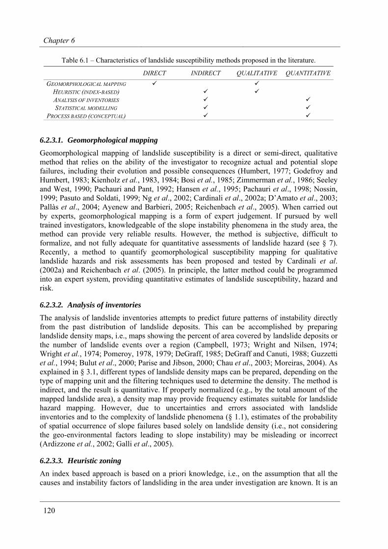
Chapter 6
120
Table 6.1 – Characteristics of landslide susceptibility methods proposed in the literature.
DIRECT INDIRECT QUALITATIVE QUANTITATIVEGEOMORPHOLOGICAL MAPPING
HEURISTIC (INDEX-BASED) ANALYSIS OF INVENTORIES STATISTICAL MODELLING
PROCESS BASED (CONCEPTUAL)
6.2.3.1. Geomorphological mapping Geomorphological mapping of landslide susceptibility is a direct or semi-direct, qualitative method that relies on the ability of the investigator to recognize actual and potential slope failures, including their evolution and possible consequences (Humbert, 1977; Godefroy and Humbert, 1983; Kienholz et al., 1983, 1984; Bosi et al., 1985; Zimmerman et al., 1986; Seeley and West, 1990; Pachauri and Pant, 1992; Hansen et al., 1995; Pachauri et al., 1998; Nossin, 1999; Pasuto and Soldati, 1999; Ng et al., 2002; Cardinali et al., 2002a; D’Amato et al., 2003; Pallàs et al., 2004; Ayenew and Barbieri, 2005; Reichenbach et al., 2005). When carried out by experts, geomorphological mapping is a form of expert judgement. If pursued by well trained investigators, knowledgeable of the slope instability phenomena in the study area, the method can provide very reliable results. However, the method is subjective, difficult to formalize, and not fully adequate for quantitative assessments of landslide hazard (see § 7). Recently, a method to quantify geomorphological susceptibility mapping for qualitative landslide hazards and risk assessments has been proposed and tested by Cardinali et al. (2002a) and Reichenbach et al. (2005). In principle, the latter method could be programmed into an expert system, providing quantitative estimates of landslide susceptibility, hazard and risk.
6.2.3.2. Analysis of inventories The analysis of landslide inventories attempts to predict future patterns of instability directly from the past distribution of landslide deposits. This can be accomplished by preparing landslide density maps, i.e., maps showing the percent of area covered by landslide deposits or the number of landslide events over a region (Campbell, 1973; Wright and Nilsen, 1974; Wright et al., 1974; Pomeroy, 1978, 1979; DeGraff, 1985; DeGraff and Canuti, 1988; Guzzetti et al., 1994; Bulut et al., 2000; Parise and Jibson, 2000; Chau et al., 2003; Moreiras, 2004). As explained in § 3.1, different types of landslide density maps can be prepared, depending on the type of mapping unit and the filtering techniques used to determine the density. The method is indirect, and the result is quantitative. If properly normalized (e.g., by the total amount of the mapped landslide area), a density map may provide frequency estimates suitable for landslide hazard mapping. However, due to uncertainties and errors associated with landslide inventories and to the complexity of landslide phenomena (§ 1.1), estimates of the probability of spatial occurrence of slope failures based solely on landslide density (i.e., not considering the geo-environmental factors leading to slope instability) may be misleading or incorrect (Ardizzone et al., 2002; Galli et al., 2005).
6.2.3.3. Heuristic zoning
An index based approach is based on a priori knowledge, i.e., on the assumption that all the causes and instability factors of landsliding in the area under investigation are known. It is an
Landslide susceptibility
121
indirect (or semi-direct), mostly qualitative method whose reliability depends on how well and how much the investigator understands the geomorphological processes acting upon the terrain. Instability factors are classified, ranked and weighted according to their assumed or expected importance in causing mass movements. Based on this information, heuristic, subjective decision rules are established to define possibly unstable areas and to zone landslide susceptibility accordingly (Nilsen and Brabb, 1977; Amadesi and Vianello, 1978; Hollingsworth and Kovacs, 1981; Neeley and Rice, 1990; Montgomery et al., 1991; Pachauri and Pant, 1992; Mejıa-Navarro et al., 1994; Sarkar et al., 1995; McClelland et al., 1997 Pachauri et al., 1998; Nagarajan et al., 2000; Lee et al., 2002; He et al., 2003; Liu et al., 2004; Moreiras, 2005). Ideally, rules used to rank, weigh and combine the instability factors should be based on detailed knowledge of the physical processes controlling landslides. In practice, this is rarely done, and ranking and weighing procedures are based (solely) on the experience of the investigator, a procedure that introduces subjectivity. van Westen et al. (1997) argued that subjectivity is not necessarily bad, particularly if it is based on the opinion of an expert. Nonetheless, subjectivity adds to the uncertainty of the model. To limit this problem, the expected importance of each instability factor can be obtained “objectively” by investigating the relative abundance of landslides (Pachauri et al., 1998; He et al., 2003) or from regression analysis (Nagarajan et al., 2000). This process has also limitations, the most severe of which consists in not considering the complex interactions between the multiple factors controlling slope instability. As an example, slope and lithology are often considered separately, whereas in Nature it is their complex interaction that controls the position and abundance of landslides. The results of index based models are shown using qualitative levels of landslide susceptibility. For this reason they are also not well suited for quantitative assessments of landslide hazard (see § 6). Since they are based on generally simple rules, index-based approaches are suited to be implemented in computer expert systems (Al-Homoud and Masanat, 1998; Al-Homoud and Al-Masri, 1999; Pistocchi et al., 2002).
6.2.3.4. Statistical methods Statistical models to determine spatial landslide instability are constructed to describe the functional relationships between instability factors and the past and present distribution of slope failures (Carrara, 1983). The approach is indirect and provides quantitative results suitable to the quantitative assessment of landslide hazard. The simplest statistical methods are based on the determination of the relative abundance (proportion, percentage, frequency, incidence) of landslides in the classes in which thematic layers showing the geographical distribution of stability/instability factors are ranked. Different approaches have been proposed, including: a general instability index (Carrara et al., 1978; 1982), a landslide susceptibility/hazard index (Sarkar et al., 1995; van Westen, 1997; Parise and Jibson, 2000; Rautela and Lakhera, 2000; Lee et al., 2002; Carrasco et al., 2003; Lee, 2004; Saha et al., 2005), a frequency index (Parise and Jibson, 2000), and a surface percentage index (Uromeihy and Mahdvifar, 2000). These indexes measure, directly or in a weighted form, the relative or absolute abundance of landslide area or number in different terrain categories. This information is then used by the investigator to establish susceptibility levels.
More advanced methods employ a variety of classification techniques that can be broadly ordered based on the adopted “philosophical” classification approach, including (Michie et al., 1994): (i) classical (frequentist or Fisherian) statistical techniques, (ii) modern (subjectivist or Bayesian) statistical methods, (iii) fuzzy logic systems, (iv) neural networks, and (v) expert systems.
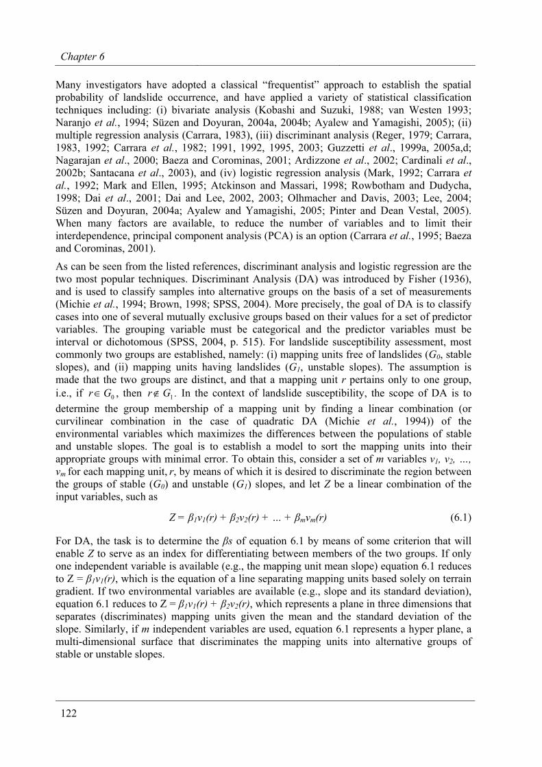
Chapter 6
122
Many investigators have adopted a classical “frequentist” approach to establish the spatial probability of landslide occurrence, and have applied a variety of statistical classification techniques including: (i) bivariate analysis (Kobashi and Suzuki, 1988; van Westen 1993; Naranjo et al., 1994; Süzen and Doyuran, 2004a, 2004b; Ayalew and Yamagishi, 2005); (ii) multiple regression analysis (Carrara, 1983), (iii) discriminant analysis (Reger, 1979; Carrara, 1983, 1992; Carrara et al., 1982; 1991, 1992, 1995, 2003; Guzzetti et al., 1999a, 2005a,d; Nagarajan et al., 2000; Baeza and Corominas, 2001; Ardizzone et al., 2002; Cardinali et al., 2002b; Santacana et al., 2003), and (iv) logistic regression analysis (Mark, 1992; Carrara et al., 1992; Mark and Ellen, 1995; Atckinson and Massari, 1998; Rowbotham and Dudycha, 1998; Dai et al., 2001; Dai and Lee, 2002, 2003; Olhmacher and Davis, 2003; Lee, 2004; Süzen and Doyuran, 2004a; Ayalew and Yamagishi, 2005; Pinter and Dean Vestal, 2005). When many factors are available, to reduce the number of variables and to limit their interdependence, principal component analysis (PCA) is an option (Carrara et al., 1995; Baeza and Corominas, 2001).
As can be seen from the listed references, discriminant analysis and logistic regression are the two most popular techniques. Discriminant Analysis (DA) was introduced by Fisher (1936), and is used to classify samples into alternative groups on the basis of a set of measurements (Michie et al., 1994; Brown, 1998; SPSS, 2004). More precisely, the goal of DA is to classify cases into one of several mutually exclusive groups based on their values for a set of predictor variables. The grouping variable must be categorical and the predictor variables must be interval or dichotomous (SPSS, 2004, p. 515). For landslide susceptibility assessment, most commonly two groups are established, namely: (i) mapping units free of landslides (G0, stable slopes), and (ii) mapping units having landslides (G1, unstable slopes). The assumption is made that the two groups are distinct, and that a mapping unit r pertains only to one group, i.e., if 0Gr∈ , then 1Gr∉ . In the context of landslide susceptibility, the scope of DA is to determine the group membership of a mapping unit by finding a linear combination (or curvilinear combination in the case of quadratic DA (Michie et al., 1994)) of the environmental variables which maximizes the differences between the populations of stable and unstable slopes. The goal is to establish a model to sort the mapping units into their appropriate groups with minimal error. To obtain this, consider a set of m variables v1, v2, …, vm for each mapping unit, r, by means of which it is desired to discriminate the region between the groups of stable (G0) and unstable (G1) slopes, and let Z be a linear combination of the input variables, such as
Z = β1v1(r) + β2v2(r) + … + βmvm(r) (6.1)
For DA, the task is to determine the βs of equation 6.1 by means of some criterion that will enable Z to serve as an index for differentiating between members of the two groups. If only one independent variable is available (e.g., the mapping unit mean slope) equation 6.1 reduces to Z = β1v1(r), which is the equation of a line separating mapping units based solely on terrain gradient. If two environmental variables are available (e.g., slope and its standard deviation), equation 6.1 reduces to Z = β1v1(r) + β2v2(r), which represents a plane in three dimensions that separates (discriminates) mapping units given the mean and the standard deviation of the slope. Similarly, if m independent variables are used, equation 6.1 represents a hyper plane, a multi-dimensional surface that discriminates the mapping units into alternative groups of stable or unstable slopes.
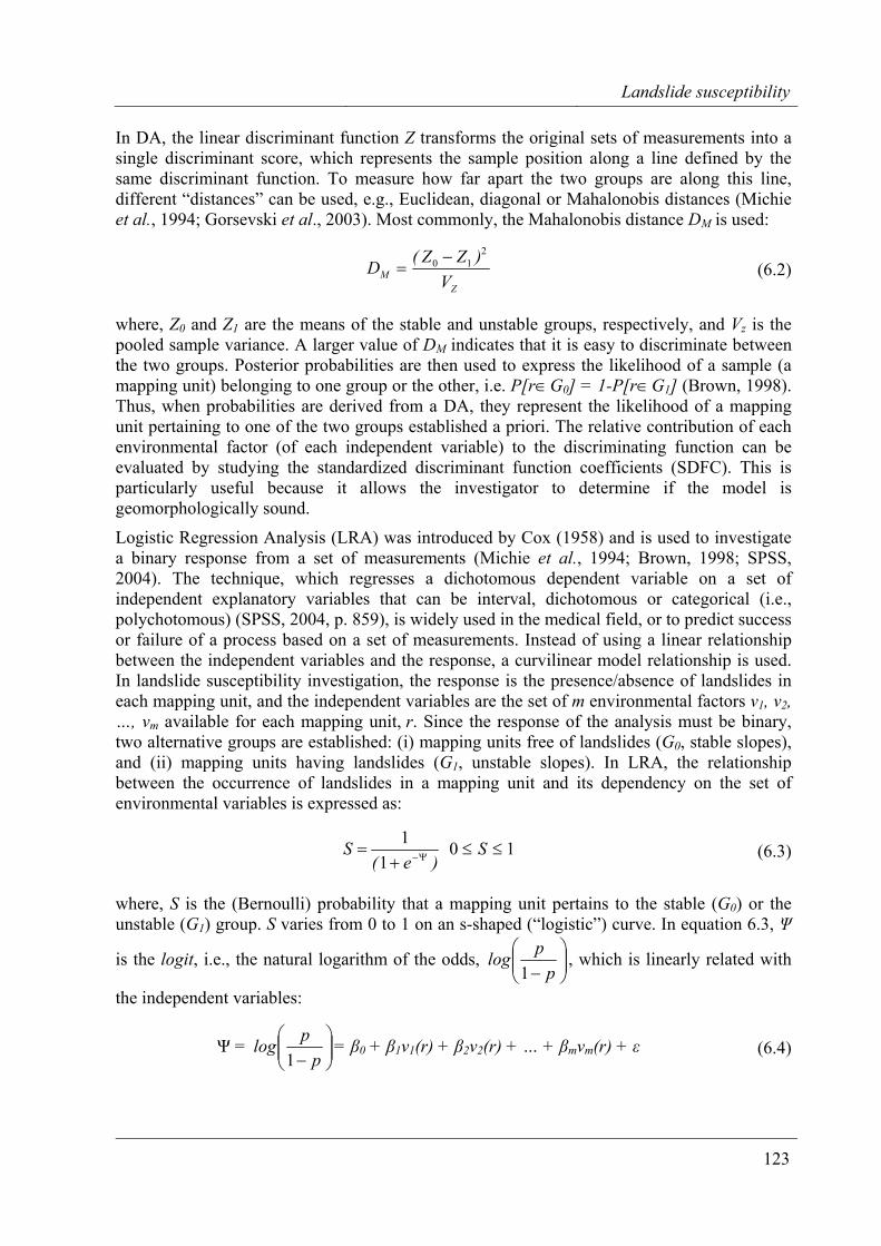
Landslide susceptibility
123
In DA, the linear discriminant function Z transforms the original sets of measurements into a single discriminant score, which represents the sample position along a line defined by the same discriminant function. To measure how far apart the two groups are along this line, different “distances” can be used, e.g., Euclidean, diagonal or Mahalonobis distances (Michie et al., 1994; Gorsevski et al., 2003). Most commonly, the Mahalonobis distance DM is used:
ZM V
)ZZ(D2
10 −= (6.2)
where, Z0 and Z1 are the means of the stable and unstable groups, respectively, and Vz is the pooled sample variance. A larger value of DM indicates that it is easy to discriminate between the two groups. Posterior probabilities are then used to express the likelihood of a sample (a mapping unit) belonging to one group or the other, i.e. P[r∈G0] = 1-P[r∈G1] (Brown, 1998). Thus, when probabilities are derived from a DA, they represent the likelihood of a mapping unit pertaining to one of the two groups established a priori. The relative contribution of each environmental factor (of each independent variable) to the discriminating function can be evaluated by studying the standardized discriminant function coefficients (SDFC). This is particularly useful because it allows the investigator to determine if the model is geomorphologically sound.
Logistic Regression Analysis (LRA) was introduced by Cox (1958) and is used to investigate a binary response from a set of measurements (Michie et al., 1994; Brown, 1998; SPSS, 2004). The technique, which regresses a dichotomous dependent variable on a set of independent explanatory variables that can be interval, dichotomous or categorical (i.e., polychotomous) (SPSS, 2004, p. 859), is widely used in the medical field, or to predict success or failure of a process based on a set of measurements. Instead of using a linear relationship between the independent variables and the response, a curvilinear model relationship is used. In landslide susceptibility investigation, the response is the presence/absence of landslides in each mapping unit, and the independent variables are the set of m environmental factors v1, v2, …, vm available for each mapping unit, r. Since the response of the analysis must be binary, two alternative groups are established: (i) mapping units free of landslides (G0, stable slopes), and (ii) mapping units having landslides (G1, unstable slopes). In LRA, the relationship between the occurrence of landslides in a mapping unit and its dependency on the set of environmental variables is expressed as:
)e(S Ψ−+=
11 10 ≤≤ S (6.3)
where, S is the (Bernoulli) probability that a mapping unit pertains to the stable (G0) or the unstable (G1) group. S varies from 0 to 1 on an s-shaped (“logistic”) curve. In equation 6.3, Ψ
is the logit, i.e., the natural logarithm of the odds, ⎟⎟⎠
⎞⎜⎜⎝
⎛− pplog
1, which is linearly related with
the independent variables:
Ψ = ⎟⎟⎠
⎞⎜⎜⎝
⎛− pplog
1= β0 + β1v1(r) + β2v2(r) + … + βmvm(r) + ε (6.4)
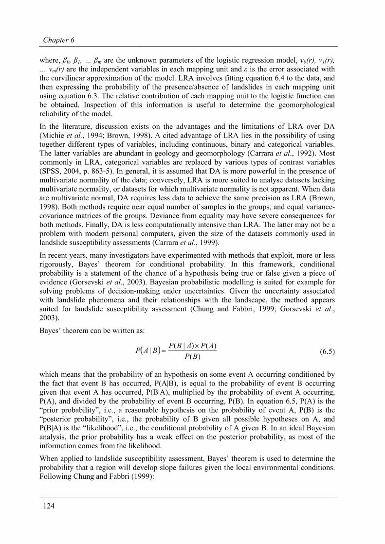
Chapter 6
124
where, β0, β1, … βm are the unknown parameters of the logistic regression model, v0(r), v1(r), … vm(r) are the independent variables in each mapping unit and ε is the error associated with the curvilinear approximation of the model. LRA involves fitting equation 6.4 to the data, and then expressing the probability of the presence/absence of landslides in each mapping unit using equation 6.3. The relative contribution of each mapping unit to the logistic function can be obtained. Inspection of this information is useful to determine the geomorphological reliability of the model.
In the literature, discussion exists on the advantages and the limitations of LRA over DA (Michie et al., 1994; Brown, 1998). A cited advantage of LRA lies in the possibility of using together different types of variables, including continuous, binary and categorical variables. The latter variables are abundant in geology and geomorphology (Carrara et al., 1992). Most commonly in LRA, categorical variables are replaced by various types of contrast variables (SPSS, 2004, p. 863-5). In general, it is assumed that DA is more powerful in the presence of multivariate normality of the data; conversely, LRA is more suited to analyse datasets lacking multivariate normality, or datasets for which multivariate normality is not apparent. When data are multivariate normal, DA requires less data to achieve the same precision as LRA (Brown, 1998). Both methods require near equal number of samples in the groups, and equal variance-covariance matrices of the groups. Deviance from equality may have severe consequences for both methods. Finally, DA is less computationally intensive than LRA. The latter may not be a problem with modern personal computers, given the size of the datasets commonly used in landslide susceptibility assessments (Carrara et al., 1999).
In recent years, many investigators have experimented with methods that exploit, more or less rigorously, Bayes’ theorem for conditional probability. In this framework, conditional probability is a statement of the chance of a hypothesis being true or false given a piece of evidence (Gorsevski et al., 2003). Bayesian probabilistic modelling is suited for example for solving problems of decision-making under uncertainties. Given the uncertainty associated with landslide phenomena and their relationships with the landscape, the method appears suited for landslide susceptibility assessment (Chung and Fabbri, 1999; Gorsevski et al., 2003).
Bayes’ theorem can be written as:
( ))(
)()|(|BP
APABPBAP ×= (6.5)
which means that the probability of an hypothesis on some event A occurring conditioned by the fact that event B has occurred, P(A|B), is equal to the probability of event B occurring given that event A has occurred, P(B|A), multiplied by the probability of event A occurring, P(A), and divided by the probability of event B occurring, P(B). In equation 6.5, P(A) is the “prior probability”, i.e., a reasonable hypothesis on the probability of event A, P(B) is the “posterior probability”, i.e., the probability of B given all possible hypotheses on A, and P(B|A) is the “likelihood”, i.e., the conditional probability of A given B. In an ideal Bayesian analysis, the prior probability has a weak effect on the posterior probability, as most of the information comes from the likelihood.
When applied to landslide susceptibility assessment, Bayes’ theorem is used to determine the probability that a region will develop slope failures given the local environmental conditions. Following Chung and Fabbri (1999):
Landslide susceptibility
125
{ }( ) { }( ) ⎥
⎦
⎤⎢⎣
⎡…
×…=…
)( v, (r), v(r),v)()|)( v, (r), v(r),v()( v, (r), v(r),v|
m10
m10m10 rP
APArPrAP LLL (6.6)
where, AL denotes that a landslide of area A will occur in a mapping unit r for which v0(r), v1(r), … vm(r) independent environmental conditions are known. It is further assumed that the combination of environmental conditions is unique to the mapping unit r.
Equation 6.6 indicates that the probability that a mapping unit r in the study area will be affected by a landslide is equal to the probability of a landslide in the study area, P(AL), multiplied by the probability of a specific (unique) combination of environmental factors given the presence of a landslide, divided by the probability of the same combination of environmental factors in the entire study area. A straightforward assumption is to obtain the three probabilities in the right hand side of equation 6.6 in a GIS from the corresponding spatial densities. This can be obtained as follows: (i) for P(AL), by dividing the total landslide area (AL) in the study area by the area of the mapping unit, (ii) for ( ))( v, (r), v(r),v m10 rP … , by dividing the total area of the unique condition unit by the extent of the study area, and (iii) for
{ } )|)( v, (r), v(r),v( m10 LArP … , by computing the percentage of landslide area in the study area characterized by the total area of the considered unique environmental setting.
Similar approaches have been proposed by several investigators, including: weight of evidence methods (Bonham-Carter, 1991; Lee et al., 2002a, 2002b; Wu et al., 2004), weighting factors (Çevik and Topal, 2003), weighted linear combination of instability factors (Ayalew et al., 2004), landside nominal risk factor (Gupta and Joshi, 1990; Saha et al., 2005), likelihood ratio (Chung and Fabbri, 2003, 2005; Fabbri et al., 2003; Lee, 2004), certainty factors (Binaghi et al., 1998), information value (van Westen, 1997; Lin and Tung, 2004; Saha et al., 2005), and modified Bayesian estimation (Chung and Fabbri, 1999). Understanding the differences between the proposed approaches is not always simple, the main differences being the rigor of the approach (e.g., Chung and Fabbri, 1999) and the method used to estimate the prior probability of landslide occurrence. An advantage of Bayesian probabilistic modelling is the possibility of incorporating uncertainty into the susceptibility model, and to explicitly consider expert knowledge, which often exists for the investigated area (Chung and Fabbri, 1999). Use of expert knowledge is more difficult (but not impossible) when adopting classical statistical classification methods.
A few landslide investigators have attempted to apply fuzzy sets to landslide susceptibility zonation (Juang, 1992; Binaghi et al., 1998; Uromeihy and Mahdavifar, 2000; Ercanoglu and Gokceoglu, 2002; 2004; Pistocchi et al., 2002; Gorsevski et al., 2003; Saboya et al., 2005). Fuzzy set theory was introduced by Zadeh (1975, 1978) as an extension of ordinary set theory. In ordinary set theory an element belongs (or does not belong) to a set, i.e., it allows only 0 or 1 values as possible membership degrees. In fuzzy set theory, membership degree can take any value from 0 and 1, i.e., a fuzzy set contains elements that have varying degrees of membership. When applied to landslide susceptibility, for each class of an environmental variable (e.g., for each slope category) a membership degree is established between the presence/absence of landslides and the parameter class (e.g., the presence of landslides in the 10-20 degree slope category). Various methods can be used to establish this relationship, whose “strength” is the degree of membership. A fuzzy set is then constructed for each environmental variable, which expresses the landslide susceptibility for each of the considered classes (e.g., landslide susceptibility in each slope category). Fuzzy sets for different
Chapter 6
126
environmental factors are then combined using rules of various complexities (Ercanoglu and Gokceoglu, 2002) to obtain an estimate of landslide susceptibility.
Expert knowledge approaches applied to landslide susceptibility assessment include artificial neural networks and expert systems. Artificial neural networks are computational frameworks capable of simulating – albeit in a crude fashion – the behaviour of the human brain in solving a complex problem (Michie et al., 1994). Conceptually, the advantage of neural networks over other classification methods consists in the fact that they are independent of the distribution of the data, although artificial neural networks are calibrated to the data and the calibration defines the functionality of the network. Also, neural networks require less data for training than other statistical methods (Lee et al., 2004). Most commonly, back propagation learning algorithms are adopted. These are made by multiple layers of “neurons” (i.e., individual processing nodes), including an input and an output layer and one or more hidden layers. A neural network takes the input information and “learns” how to predict the output by establishing and adjusting weights between neurons on the same or on different layers, in response to errors between predicted and known output values. At each neuron, adjustment occurs through weighting summations and non linear functions. At the end of the training phase, the neural network should be able to predict the output values (e.g., landslide susceptibility) given a set of inputs (e.g., the environmental factors). The main limitation of artificial neural networks lays in the fact that is very difficult – if not impossible – to know why they work for any given set of data and for any given calibration set. This restrains the possibility of using findings obtained with a neural network prepared for an area to a neighbouring area. Also, the role, functionality and significance of the weights and of the non-linear calibration functions are difficult to interpret. Artificial neural networks have been applied to landslide susceptibility mapping by, e.g., Arora et al. (2004), Lee et al. (2003a, 2003b, 2004), Ermini et al. (2005), Ferentinou and Sakellariou, (2005), Gómez et al. (2005) and Wang et al. (2005).
Expert systems are computer programs capable of exploiting complex information to make decisions based on a set of rules. Decisions taken by expert systems include categorization, i.e., selection between alternatives (Michie et al., 1994). Rules used in expert systems can be established a priori, or defined by the same system that “learns” from errors. In principle, index based landslide susceptibility methods (for which “slope instability rules” are known) are suited for the implementation in an expert system framework (Guzzetti et al., 1999a). Particularly interesting is the possibility of establishing rules to cope with “special cases”, or individual instability conditions that cannot be captured by, e.g., statistical or physically based models. Inspection of the literature indicates that only a few authors have attempted to implement rule-based expert systems for landslide susceptibility zonation (Al-Homoud and Masanat, 1998; Al-Homoud and Al-Masri, 1999; Pistocchi et al., 2001). This is probably because the effort is not justified by the result obtained. An expert system is mostly suited when decisions (e.g. categorization) have to be taken repeatedly. This is usually not the case for landslide susceptibility assessments. When a susceptibility model is prepared and validated, it can be used for years without the need for any further processing.
Following the widespread availability of GIS technology and of user friendly statistical packages, statistical models have become the method favoured by many investigators to determine landslide susceptibility. However, review of the most recent literature – which is abundant (Uromeihy and Mahdavifar, 2000; Dai et al., 2001; Dai and Lee, 2003; Olhmacher and Davis, 2003; Ercanoglu and Gokceoglu, 2002; 2004; Çevik and Topal, 2003; Gorsevski et al., 2003; Lee, 2004; Lee et al. 2003a; 2003b; 2004; Santacana et al., 2003; Wu et al., 2004;
Landslide susceptibility
127
Ayalew et al., 2004) – reveals that many investigators are interested chiefly in applying different statistical methods, and much less concerned in: (i) collecting detailed, high quality information related to slope failures, (ii) identifying new environmental parameters useful to the assessment of landslide susceptibility, (iii) validating quantitatively the model results, (iv) explaining the geomorphological aspects of terrain zoning for landslide susceptibility assessment, or (v) in the examination of the socio-economical implications of the susceptibility models. This is rather unfortunate because it leads investigators to focus on the tool (a classification technique) rather than on the target (an optimal landslide susceptibility assessment). Also disappointing is the fact that in the copious literature on landslide susceptibility assessment very few attempts to quantitatively compare susceptibility models prepared by different methods, critically evaluating their advantages and limitations, are available (Carrara et al., 1992; 1995; Chung and Fabbri, 1999; Pistocchi et al., 2002; Lee, 2004; Süzen and Doyuran, 2004a).
6.2.3.5. Process based models Process based (deterministic or physically based) models for the assessment of landslide susceptibility rely upon the understanding of the physical laws controlling slope instability. In general, due to lack of information or poor understanding of the physical laws controlling landslide initiation and development, only simplified, “conceptual” models are considered. These models are indirect and provide quantitative results, which may or may not be suited for quantitative landslide hazard assessment depending on the types of output. Review of the literature reveals that process based models are developed mostly to study a particular type of landslide (e.g., shallow soil slips, debris flows, or rock falls), or to investigate the effect of a specific trigger, i.e., an intense rainfall period or an earthquake.
When applied to the prediction of shallow rainfall-induced landslides, process based models attempt to extend spatially the simplified stability models widely adopted in geotechnical engineering. These models calculate the stability of a slope using parameters such as normal stress, angle of internal friction, cohesion, pore water pressure, seismic acceleration, external weights, etc. Most commonly, computation results in a factor of safety, i.e., an index expressing the ratio between the local stabilizing and driving forces. Values of the index greater than 1.0 indicate stability of the slope, and values less than 1.0 identify unstable conditions. A safety factor of exactly 1.0 indicates the meta-stable condition produced by equivalence of the stabilizing and driving forces. When applied over large areas, local stability conditions are generally evaluated by means of a static stability model, such as the well known ‘‘infinite slope model’’, where the local equilibrium along a potential slip surface is considered. For simplicity, the slip surface is assumed planar, at a fixed depth, and most commonly parallel to the topographic surface, and some assumed value of pore fluid pressure is selected. More advanced models include seepage from neighbouring areas. Other models couple the infinite slope stability model with more or less complex rainfall infiltration models (Ward et al., 1981, 1982; Okimura and Kawatani, 1987; Benda and Zhang, 1990; Dunne, 1991; Hammond et al., 1992; van Ash et al., 1999; Montgomery and Dietrich, 1994; Dietrich et al., 1995; Terlien et al., 1995, Dymond et al., 1999; Gritzner et al., 2001; Borga et al., 2002a; Crosta and Frattini, 2003; Crosta and Dal Negro, 2003; D’Odorico and Fagherazzi, 2003; Lan et al., 2005). Most commonly, distributed models for the stability of slopes are based on a raster representation of the landscape and exploit GIS-raster technology, including map algebra, to implement the models, which generally relay heavily on a digital representation of the terrain (i.e., a DTM). Alternative approaches are based on topographic
Chapter 6
128
units and stream tube elements, which are hydrological, vector based representations of the terrain. Some of the most advanced distributed models for the stability of slopes and the forecast of shallow landslides take as input the surface and sub-surface information on lithological, hydrological and geo-mechanical conditions, including the depth of the shear surface and of the water table at the beginning of the simulation, and a measured or inferred rainfall pattern (in space and time). These models run in incremental time steps and estimate the location and the time of the expected slope failures. With this respect, the results of such models are superior to a simple susceptibility assessment.
Specific, physically based models were developed for predicting the effects of seismic shaking on the stability of slopes over large areas, or to explain the known distribution of seismically induced landslides (Jibson et al., 1998; Miles and Ho, 1999; Luzi, 2000; Luzi and Pergalani, 2000; Jibson and Jibson, 2001; Lin and Tung, 2004; Paléz et al., 2005). Some of the most reliable approaches extend the Newmark method designed for estimating the stability of dams or embankments subject to seismic shaking to the stability of individual slopes (Newmark, 1965; Wieczorek et al., 1985; Wilson, 1993). When applied to large regions, these models are based on a grid partitioning of the terrain. Potential landslides are considered as rigid bodies subject to seismic acceleration, ascertained from measured or synthetic accelerographs. For each grid cell, the cumulative displacement of the rigid block subject to seismic acceleration is computed. If an established threshold is exceeded, a grid cell becomes unstable and a landslide occurs. Displacement thresholds depend on the type of landslide, and are decided largely based on the experience of the investigators. Rock falls require a smaller displacement to fail than large, deep-seated slides. Groundwater conditions can also be considered.
Physically based models to simulate rock fall processes were developed by van Dijke and van Westen (1990) and by Guzzetti et al. (2002a). The latter model uses a DTM and spatially distributed information on the location of the source areas of rock falls, and of the energy lost at impact points and where boulders are rolling, to simulate in three dimensions rock fall phenomena for areas ranging from a few thousands of square meters to several hundreds of square kilometres (Guzzetti et al., 2002a, 2003b). Results of the model include: (i) the extent and location of the areas potentially subject to rock falls, and (ii) estimates of the maximum velocity and of the maximum distance to the ground of the falling rocks. This information can be combined to obtain quantitative estimates of landslide hazards (Crosta and Agliardi, 2004; Guzzetti et al., 2004b).
6.2.4. Susceptibility methods and mapping units Susceptibility methods and mapping units are conceptually and operationally interrelated (Carrara et al., 1995). Table 6.2 summarizes the main correlations. In direct susceptibility mapping, the geomorphological unit of reference is implicitly defined by the interpreter who maps the portions of the territory that are subject to different geomorphological hazards (Hansen, 1984). In all other cases (i.e., grid-based modelling, unique condition units, slope-units, geo-hydrological units, topographic units), the mapping unit is explicitly defined by the operator before the investigation begins. In general, grid cells are preferred for heuristic (Pike, 1988; Mejıa-Navarro et al., 1994), statistical (Carrara, 1983; van Westen, 1994; Chung and Fabbri, 1999; Lee and Min, 2002; Remondo et al., 2003; Pinter and Dean Vestal, 2005) and process based or simulation (Mark, 1992; Terlien et al., 1995, Di Gregorio et al., 1999a, 1999b; Dymond et al., 1999; Guzzetti et al., 2002a; Crosta and Frattini, 2003) modelling.
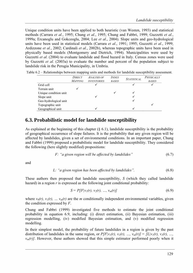
Landslide susceptibility
129
Unique condition units have been applied to both heuristic (van Westen, 1993) and statistical methods (Carrara et al., 1995; Chung et al., 1995; Chung and Fabbri, 1999; Guzzetti et al., 1999a; Ercanoglu and Gokceoglu, 2004; Lee et al., 2004). Slope units and geo-hydrological units have been used in statistical models (Carrara et al., 1991; 1995; Guzzetti et al., 1999; Ardizzone et al., 2002; Cardinali et al., 2002b), whereas topographic units have been used in physically based models (Montgomery and Dietrich, 1994). Municipalities were used by Guzzetti et al. (2004) to evaluate landslide and flood hazard in Italy. Census zones were used by Guzzetti et al. (2003a) to evaluate the number and percent of the population subject to landslide risk in the Perugia Municipality, in Umbria. Table 6.2 – Relationships between mapping units and methods for landslide susceptibility assessment.
DIRECT MAPPING
ANALYSIS OF INVENTORIES
INDEX BASED STATISTICAL PHYSICALLY
BASED Grid cell Terrain unit Unique condition unit Slope unit Geo-hydrological unit Topographic unit Geographical unit
6.3. Probabilistic model for landslide susceptibility
As explained at the beginning of this chapter (§ 6.1), landslide susceptibility is the probability of geographical occurrence of slope failures. It is the probability that any given region will be affected by landslides, given a set of environmental conditions. In an important paper, Chung and Fabbri (1999) proposed a probabilistic model for landslide susceptibility. They considered the following (here slightly modified) propositions:
F: “a given region will be affected by landslides” (6.7)
and
L: “a given region has been affected by landslides”. (6.8)
These authors then proposed that landslide susceptibility, S (which they called landslide hazard) in a region r is expressed as the following joint conditional probability:
S = P[F|v1(r), v2(r), …, vm(r)] (6.9)
where v0(r), v1(r), … vm(r) are the m conditionally independent environmental variables, given the condition expressed by F.
Chung and Fabbri (1999) investigated five methods to estimate the joint conditional probability in equation 6.9, including: (i) direct estimation, (ii) Bayesian estimation, (iii) regression modelling, (iv) modified Bayesian estimation, and (v) modified regression modelling.
In their simplest model, the probability of future landslides in a region is given by the past distribution of landslides in the same region, or P[F|v1(r), v2(r), …, vm(r)] = [L|v1(r), v2(r), …, vm(r)]. However, these authors showed that this simple estimator performed poorly when it
Chapter 6
130
comes to estimating future landslides in their study area. In their second model, Bayesian estimation (equations 6.5 and 6.6) was used to determine S based on the prior probability of landslide occurrence, and on bivariate conditional probability functions, which were obtained from the known distribution of past landslides (i.e., using proposition L, equation 6.8). In their third model the probability of future landslides was obtained through multivariate regression. The conditional joint probability that a region r will be affected by a landslide was regressed against the bivariate conditional probabilities that a landslide will occur given a thematic environmental variable. Again, not knowing beforehand the distribution of future landslides, the bivariate conditional probabilities between landsliding and each of the available environmental factors were obtained from the known distribution of (past) landslides. In their fourth and fifth models, Chung and Fabbri (1999) proposed to modify the estimates obtained through Bayesian reasoning and multivariate regression modelling based on some kind of expert knowledge, which was available to them. This was obtained by using modified bivariate conditional probability functions obtained from experts instead of the bivariate conditional probability functions obtained in a GIS from the past distribution of landslides. Experts may or may not have used (or known) the past distribution of landslides to establish their estimates.
A similar probabilistic model to ascertain landslide susceptibility is now proposed. Adopting proposition F, “a given region will be affected by landslides” (6.7), and knowing m environmental factors v1, v2, …, vm which are related to slope instability in the region, landslide susceptibility is
S = P [F is true, given { morphology, lithology, structure, land use, etc. }] (6.10)
The statement is a rephrase of equation 6.9, where S is the conditional probability that a region r will be affected by future landslides given a set of m independent environmental variables v1, v2, …, vm in the same region. As before, the problem with this proposition is that the future distribution of landslides is unknown to the investigator. At the beginning of a landslide susceptibility assessment, only past landslides in a region are known (e.g., through landslide mapping). Hence, terrain classification can be made only on the basis of the known distribution of past slope failures. Adopting proposition L, one can write the counterpart of equation 6.10 for the past distribution of landslides. This becomes
D = P [L is true, given { morphology, lithology, structure, land use, etc. }] (6.11)
or
D = P[L|v1(r), v2(r), …, vm(r)] (6.12)
where D is now the conditional probability that the region r was affected by landslides given the same set of known independent environmental variables, v1, v2, …, vm.
In § 6.2.3 it was shown that the spatial probability of known (past) landslides can be estimated using a variety of classical statistical techniques. Using DA or LRA, the probability assigned to any given region (i.e., to each terrain mapping unit) is the probability that the region pertains to one of two mutually exclusive groups, namely: (i) the group of mapping units having landslides, G1, or (ii) the group of mapping units free of landslides, G0, given the set of independent environmental variables used in the analysis. A straightforward deduction is to assume S = D, and S= P[r∈G0] = 1-P[r∈G1], or
Landslide susceptibility
131
P [F | v1(p), v2(p), …, vm(p)] = P [L | v1(p), v2(p), …, vm(p)] (6.13)
In other words, if a region pertains to the group of terrain units having known (i.e., past) landslides because of the local environmental setting, it is likely that the same region will experience slope failures again in the future (even if we don’t know when). Equally, if a region pertains to the group of terrain units free of (known) past landslides, it is unlikely that the same region will experience mass movements in the future.
6.3.1. Discussion The proposed probabilistic models for landslide susceptibility can predict the spatial occurrence of future landslides under the general assumption that in any given area slope failures will occur in the future under the same circumstances and because of the same conditions that caused them in the past. This is a geomorphological rephrase of the well-known postulate “the past is the key to the future” (§ 6.2.1). However, it is not certain that the postulate applies to landslides. New, first-time failures occur under conditions of peak resistance (friction and cohesion), whereas reactivations occur under intermediate or residual conditions. It is well know that terrain gradient is an important factor for the occurrence of landslides. An obvious effect of a slope failure is to change the morphology of the terrain where the failure occurs. In addition, when a landslide moves it may change the hydrological conditions of the slope. It is also well known that landslides can change their type of movement and velocity with time. Lastly, landslide occurrence and abundance are a function of environmental conditions that vary with time at different rates. Some of the environmental variables are affected by human actions (e.g., land use, deforestation, irrigation, etc.), which are also highly changeable. As a consequence of these complications, each landslide occurs in a distinct environmental context, which may have been different from the past and that might be different in the future (Guzzetti et al., 1999a).
Despite these limitations, it is reasonable to assume that the postulate holds “statistically”, i.e., that in the investigated area future landslides will occur in general under the same circumstances and because of the same conditions that triggered them in the past. This means accepting the equality expressed by equation 6.13. When a landslide susceptibility assessment is attempted in any given area, this equality has to be shown correct. Alternatively, limits for the equality have to be identified. This can be done explicitly or implicitly. An explicit demonstration of the equality may come from the analysis of multi-temporal inventory maps or from archive inventories. If the type and abundance of landslides does not change significantly in the study area with time, then the assumption can be made that the equality holds, and that the spatial probability of future slope failures (S) can be obtained from the spatial probability of past landslides (D).
An implicit demonstration may come from geomorphological inference. If in an area only rainfall induced landslides are expected, and the distribution of past rainfall induced landslides is known in detail, the latter can be used to predict the former. However, the distribution of past rainfall induced landslides may not predict accurately landslides triggered by earthquakes or snowmelt in the same region. It should be understood that in many areas the past distribution of known landslides is the result of different triggers, including intense or prolonged rainfall periods, earthquakes and snowmelt events, and that most commonly, a geomorphological inventory does not distinguish the triggers of the landslides. This limits our ability to test the equality in equation 6.13. In order to apply the probabilistic models one has
Chapter 6
132
to further assume that our knowledge of the distribution of past failures is reasonably accurate and complete, i.e., that the landslide inventory is reliable (§ 6.2.1). All these simplifications are needed to make the problem tractable, and should always be considered when interpreting and using the results of a susceptibility model.
6.4. Landslide susceptibility in the Upper Tiber River basin
In this section, I present and discuss the results of a landslide susceptibility model prepared for the Upper Tiber River basin. The model exploits all the available geographical information on landslides and on the thematic environmental factors presented in § 2.3, and relies on the probability model of landslide susceptibility discussed in § 6.3.
To obtain landslide susceptibility the basin – which extends for 4098 km2 – was first subdivided into ~ 16,000 slope units (§ 6.2.2). For each slope unit, a set of morphometric and hydrological parameters useful to explain the spatial distribution of landslides were then obtained from the available DTM (e.g., Carrara et al., 1991, 1995). Tests were made to calibrate the size of the slope units with the dimension of the landslides. Due to the large extent of the basin, calibration was not straightforward and required several iterations. To limit the unrealistic condition of landslides falling in two or more slope units, slope units corresponding to first order channels were selected relatively large (i.e., ~ 20 hectares). Next, the slope units were further subdivided based upon the main rock types cropping out in the basin (§ 2.3). This allowed splitting the slope units characterized by two (or more) rock types, corresponding to different morphological settings and landslide types and abundances, in distinct mapping units. In the end, the procedure subdivided the Upper Tiber River basin into more than 28,600 geo-hydrological units (§ 6.2.2), which became the mapping unit of reference for the statistical assessment of the landslide susceptibility.
Using GIS technology, a large set of geo-environmental variables (139 variables) derived from the available thematic maps was assigned to each mapping unit. The data set contained: (i) two variables showing the percentage of deep seated and shallow landslide area, (ii) 17 morphometric variables, describing the slope unit and its drainage line (e.g., area, slope, aspect, stream order, contributing area, etc.), obtained from the DTM, (iii) 21 litho-technical variables, obtained by grouping, based upon the relative abundance of hard vs. weak rocks, the 35 lithological types cropping out in the basin, (iv) five geological structure variables describing dip of bedding, obtained from the information on the bedding attitude, (v) six variables describing the interaction between the bedding attitude and slope aspect, and (vi) ten variables describing land use. To these primary variables, obtained directly from existing thematic maps, were added 45 variables obtained through the combination of primary variables or geographical operations. Of the added variables, 8 refer to the morphology of the slope, 31 to the interaction between lithology and bedding attitude, and 6 to the interaction between bedding attitude and land use.
Since in the Upper Tiber River basin most of the shallow landslides are spatially associated with deep-seated failures (i.e., landslide persistence is high, § 4.4), only one model that included both type of movements was prepared. Using as dependent variable the presence/absence of landslide deposits in each mapping unit, a linear discriminant function weighted on the mapping unit area was developed. Of the 139 independent input variables (i.e., not considering the variables describing the percentage of landslide area), 41 entered into the discriminant model (Table 6.3). Of these variables, 12 refer to lithology, 9 to bedding
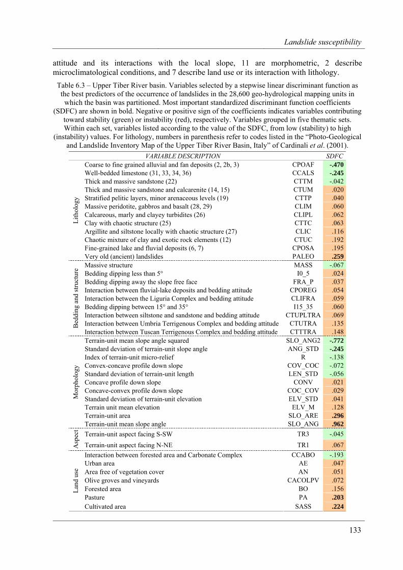
Landslide susceptibility
133
attitude and its interactions with the local slope, 11 are morphometric, 2 describe microclimatological conditions, and 7 describe land use or its interaction with lithology.
Table 6.3 – Upper Tiber River basin. Variables selected by a stepwise linear discriminant function as the best predictors of the occurrence of landslides in the 28,600 geo-hydrological mapping units in
which the basin was partitioned. Most important standardized discriminant function coefficients (SDFC) are shown in bold. Negative or positive sign of the coefficients indicates variables contributing
toward stability (green) or instability (red), respectively. Variables grouped in five thematic sets. Within each set, variables listed according to the value of the SDFC, from low (stability) to high
(instability) values. For lithology, numbers in parenthesis refer to codes listed in the “Photo-Geological and Landslide Inventory Map of the Upper Tiber River Basin, Italy” of Cardinali et al. (2001).
VARIABLE DESCRIPTION SDFCCoarse to fine grained alluvial and fan deposits (2, 2b, 3) CPOAF -.470Well-bedded limestone (31, 33, 34, 36) CCALS -.245Thick and massive sandstone (22) CTTM -.042Thick and massive sandstone and calcarenite (14, 15) CTUM .020Stratified pelitic layers, minor arenaceous levels (19) CTTP .040Massive peridotite, gabbros and basalt (28, 29) CLIM .060Calcareous, marly and clayey turbidites (26) CLIPL .062Clay with chaotic structure (25) CTTC .063Argillite and siltstone locally with chaotic structure (27) CLIC .116Chaotic mixture of clay and exotic rock elements (12) CTUC .192Fine-grained lake and fluvial deposits (6, 7) CPOSA .195
Lith
olog
y
Very old (ancient) landslides PALEO .259Massive structure MASS -.067Bedding dipping less than 5° I0_5 .024Bedding dipping away the slope free face FRA_P .037Interaction between fluvial-lake deposits and bedding attitude CPOREG .054Interaction between the Liguria Complex and bedding attitude CLIFRA .059Bedding dipping between 15° and 35° I15_35 .060Interaction between siltstone and sandstone and bedding attitude CTUPLTRA .069Interaction between Umbria Terrigenous Complex and bedding attitude CTUTRA .135B
eddi
ng a
nd st
ruct
ure
Interaction between Tuscan Terrigenous Complex and bedding attitude CTTTRA .148Terrain-unit mean slope angle squared SLO_ANG2 -.772Standard deviation of terrain-unit slope angle ANG_STD -.245Index of terrain-unit micro-relief R -.138Convex-concave profile down slope COV_COC -.072Standard deviation of terrain-unit length LEN_STD -.056Concave profile down slope CONV .021Concave-convex profile down slope COC_COV .029Standard deviation of terrain-unit elevation ELV_STD .041Terrain unit mean elevation ELV_M .128Terrain-unit area SLO_ARE .296
Mor
phol
ogy
Terrain-unit mean slope angle SLO_ANG .962Terrain-unit aspect facing S-SW TR3 -.045
Asp
ect
Terrain-unit aspect facing N-NE TR1 .067Interaction between forested area and Carbonate Complex CCABO -.193Urban area AE .047Area free of vegetation cover AN .051Olive groves and vineyards CACOLPV .072Forested area BO .156Pasture PA .203
Land
use
Cultivated area SASS .224
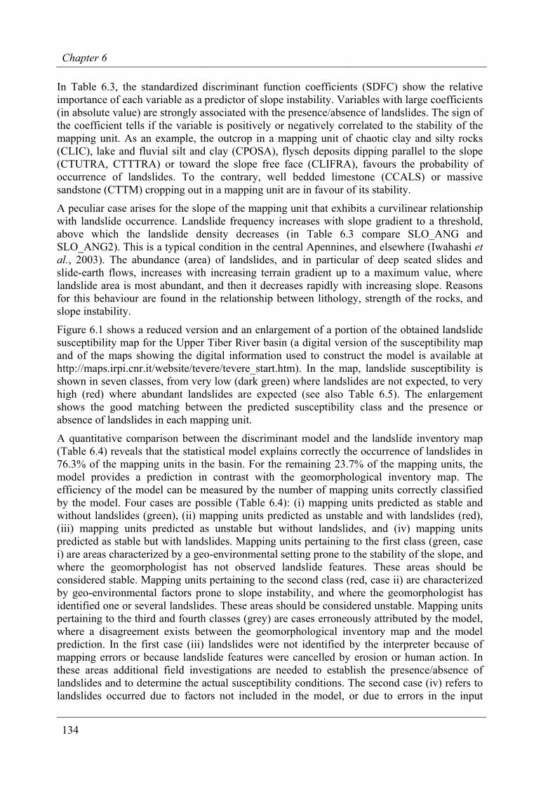
Chapter 6
134
In Table 6.3, the standardized discriminant function coefficients (SDFC) show the relative importance of each variable as a predictor of slope instability. Variables with large coefficients (in absolute value) are strongly associated with the presence/absence of landslides. The sign of the coefficient tells if the variable is positively or negatively correlated to the stability of the mapping unit. As an example, the outcrop in a mapping unit of chaotic clay and silty rocks (CLIC), lake and fluvial silt and clay (CPOSA), flysch deposits dipping parallel to the slope (CTUTRA, CTTTRA) or toward the slope free face (CLIFRA), favours the probability of occurrence of landslides. To the contrary, well bedded limestone (CCALS) or massive sandstone (CTTM) cropping out in a mapping unit are in favour of its stability.
A peculiar case arises for the slope of the mapping unit that exhibits a curvilinear relationship with landslide occurrence. Landslide frequency increases with slope gradient to a threshold, above which the landslide density decreases (in Table 6.3 compare SLO_ANG and SLO_ANG2). This is a typical condition in the central Apennines, and elsewhere (Iwahashi et al., 2003). The abundance (area) of landslides, and in particular of deep seated slides and slide-earth flows, increases with increasing terrain gradient up to a maximum value, where landslide area is most abundant, and then it decreases rapidly with increasing slope. Reasons for this behaviour are found in the relationship between lithology, strength of the rocks, and slope instability.
Figure 6.1 shows a reduced version and an enlargement of a portion of the obtained landslide susceptibility map for the Upper Tiber River basin (a digital version of the susceptibility map and of the maps showing the digital information used to construct the model is available at http://maps.irpi.cnr.it/website/tevere/tevere_start.htm). In the map, landslide susceptibility is shown in seven classes, from very low (dark green) where landslides are not expected, to very high (red) where abundant landslides are expected (see also Table 6.5). The enlargement shows the good matching between the predicted susceptibility class and the presence or absence of landslides in each mapping unit.
A quantitative comparison between the discriminant model and the landslide inventory map (Table 6.4) reveals that the statistical model explains correctly the occurrence of landslides in 76.3% of the mapping units in the basin. For the remaining 23.7% of the mapping units, the model provides a prediction in contrast with the geomorphological inventory map. The efficiency of the model can be measured by the number of mapping units correctly classified by the model. Four cases are possible (Table 6.4): (i) mapping units predicted as stable and without landslides (green), (ii) mapping units predicted as unstable and with landslides (red), (iii) mapping units predicted as unstable but without landslides, and (iv) mapping units predicted as stable but with landslides. Mapping units pertaining to the first class (green, case i) are areas characterized by a geo-environmental setting prone to the stability of the slope, and where the geomorphologist has not observed landslide features. These areas should be considered stable. Mapping units pertaining to the second class (red, case ii) are characterized by geo-environmental factors prone to slope instability, and where the geomorphologist has identified one or several landslides. These areas should be considered unstable. Mapping units pertaining to the third and fourth classes (grey) are cases erroneously attributed by the model, where a disagreement exists between the geomorphological inventory map and the model prediction. In the first case (iii) landslides were not identified by the interpreter because of mapping errors or because landslide features were cancelled by erosion or human action. In these areas additional field investigations are needed to establish the presence/absence of landslides and to determine the actual susceptibility conditions. The second case (iv) refers to landslides occurred due to factors not included in the model, or due to errors in the input
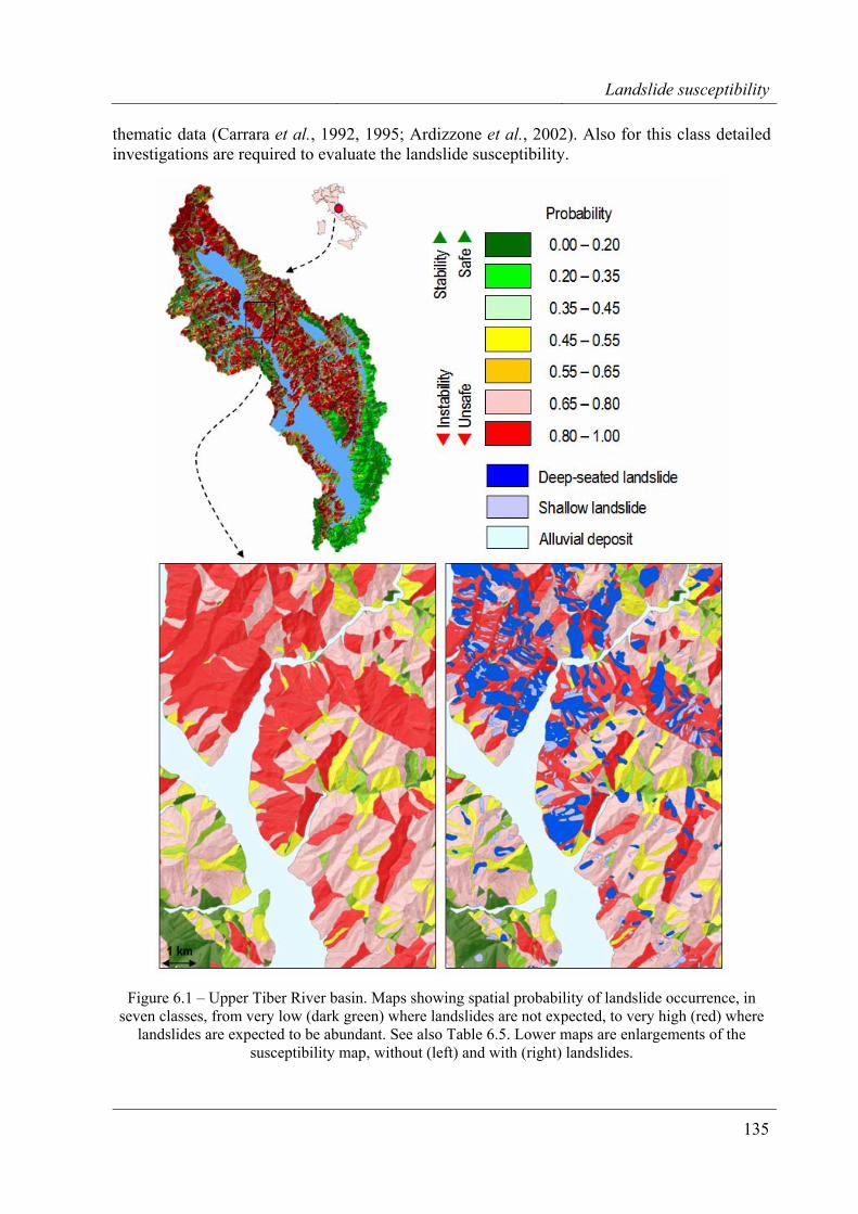
Landslide susceptibility
135
thematic data (Carrara et al., 1992, 1995; Ardizzone et al., 2002). Also for this class detailed investigations are required to evaluate the landslide susceptibility.
Figure 6.1 – Upper Tiber River basin. Maps showing spatial probability of landslide occurrence, in seven classes, from very low (dark green) where landslides are not expected, to very high (red) where
landslides are expected to be abundant. See also Table 6.5. Lower maps are enlargements of the susceptibility map, without (left) and with (right) landslides.
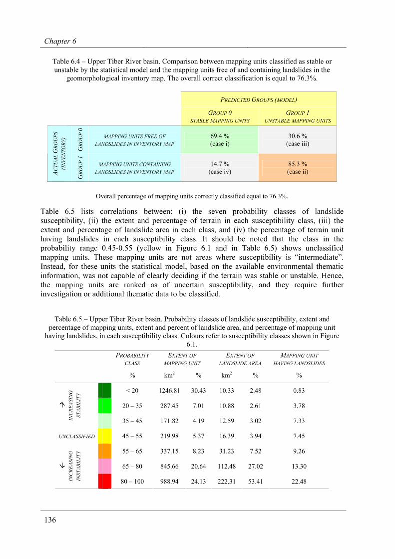
Chapter 6
136
Table 6.4 – Upper Tiber River basin. Comparison between mapping units classified as stable or unstable by the statistical model and the mapping units free of and containing landslides in the
geomorphological inventory map. The overall correct classification is equal to 76.3%.
PREDICTED GROUPS (MODEL)
GROUP 0 STABLE MAPPING UNITS
GROUP 1 UNSTABLE MAPPING UNITS
GRO
UP
0
MAPPING UNITS FREE OF LANDSLIDES IN INVENTORY MAP
69.4 % (case i)
30.6 % (case iii)
ACTU
AL G
ROU
PS
(INVE
NTO
RY)
GRO
UP
1
MAPPING UNITS CONTAINING LANDSLIDES IN INVENTORY MAP
14.7 % (case iv)
85.3 % (case ii)
Overall percentage of mapping units correctly classified equal to 76.3%.
Table 6.5 lists correlations between: (i) the seven probability classes of landslide susceptibility, (ii) the extent and percentage of terrain in each susceptibility class, (iii) the extent and percentage of landslide area in each class, and (iv) the percentage of terrain unit having landslides in each susceptibility class. It should be noted that the class in the probability range 0.45-0.55 (yellow in Figure 6.1 and in Table 6.5) shows unclassified mapping units. These mapping units are not areas where susceptibility is “intermediate”. Instead, for these units the statistical model, based on the available environmental thematic information, was not capable of clearly deciding if the terrain was stable or unstable. Hence, the mapping units are ranked as of uncertain susceptibility, and they require further investigation or additional thematic data to be classified.
Table 6.5 – Upper Tiber River basin. Probability classes of landslide susceptibility, extent and percentage of mapping units, extent and percent of landslide area, and percentage of mapping unit
having landslides, in each susceptibility class. Colours refer to susceptibility classes shown in Figure 6.1.
PROBABILITY CLASS
EXTENT OF MAPPING UNIT
EXTENT OF LANDSLIDE AREA
MAPPING UNIT HAVING LANDSLIDES
% km2 % km2 % %
< 20 1246.81 30.43 10.33 2.48 0.83
20 – 35 287.45 7.01 10.88 2.61 3.78
IN
CRE
ASIN
G
STAB
ILIT
Y
35 – 45 171.82 4.19 12.59 3.02 7.33
UNCLASSIFIED 45 – 55 219.98 5.37 16.39 3.94 7.45
55 – 65 337.15 8.23 31.23 7.52 9.26
65 – 80 845.66 20.64 112.48 27.02 13.30
IN
CRE
ASIN
G
INST
ABIL
ITY
80 – 100 988.94 24.13 222.31 53.41 22.48
Landslide susceptibility
137
6.4.1. Discussion I now discuss the problems encountered in the production of the susceptibility model for the Upper Tiber River basin, and I examine the validity of the assumptions under which the susceptibility model holds, which largely condition its applicability. The discussion is based upon the results of the Upper Tiber River basin susceptibility mapping experiment, but some of the conclusions are general and applicable to other areas, in Italy and elsewhere.
The two principal assumptions of the proposed landslide susceptibility model are: (i) that landslides will occur in the future under the same circumstances and because of the same factors that produced them in the past (§ 6.2.1), and (ii) that landslide abundance is controlled by – and can be inferred from – the local known geo-environmental conditions.
The first assumption requires that the landslide predisposing factors (the geological and environmental conditions) “remain the same in the future” in order to cause similar slope failures. But, for how long in the future must conditions not change? The statistical model does not indicate a temporal validity for thee susceptibility forecast. This is common for susceptibility maps. Landslide susceptibility assessments do not incorporate the time component of a landslide hazard assessment (which is why they are called susceptibility models), and quite often do not even provide a temporal framework for the validity of the prediction, limiting their applicability (§ 9.3), and reducing the possibility of establishing if (or two what extent) the main assumptions hold in the investigated area. A solution is to establish the validity of the susceptibility model based on: (i) external information on landslides (e.g., an archive inventory of slope failures, or quantitative information on landslide age, etc.), (ii) the expected validity of the susceptibility map for any practical application (e.g., the time frame of a building code or land use regulation to which the susceptibility map is expected to contribute), or (iii) the engineering lifetime of structures and infrastructure that can be affected by landslides (e.g., from tens to few hundreds of years).
When the expected temporal validity of the susceptibility model is established, the problem becomes that of investigating the possibility that the predisposing factors will change in the considered period, affecting landslide susceptibility. Assuming a validity of the model between 50 and 100 years (which is reasonable for the Upper Tiber River basin), it is safe to imagine that geological factors (including lithology, structure and seismicity) will not change significantly in such a short geological time. In the established period, morphological changes can occur due to stream erosion, landslides and human actions, but extensive modifications are not reasonably probable. Inspection of Table 6.3, which lists the variables entered into the statistical model, shows that the majority (34 out of 41) of thematic variables are not expected to change significantly in the considered period. Accordingly, landslide susceptibility is not expected to change in the period. However, if significant geological and morphological changes should occur, the model should be abandoned, or at least revaluated.
Further inspection of Table 6.3 reveals the presence of seven variables describing land use types that entered into the susceptibility model, some with high SDFC. These variables may change significantly in the considered period. Changes in land use, including logging, are known to affect landslide frequency and abundance (Guthrie, 2002; Glade, 2003). Qualitative estimates of land use change in Umbria indicate a reduction of about 20-25% of the forest coverage since 1950, in favour of cultivated and abandoned land. In the same period, agricultural practices have changed, largely aided by powerful mechanical equipments. Cardinali et al. (2000), investigating recent snowmelt induced landslides in Central Umbria (§ 3.3.3.2), suggested that areas recently deforested for agricultural purposes are more prone to
Chapter 6
138
landslides. If land use changes significantly in the basin, landslide susceptibility will change accordingly. Important is the fact that the obtained susceptibility model does not incorporate variables describing land use changes (e.g., variable showing areas previously covered by forest that were cleared, and as a result suffered landslides). New variables showing areas of land use change should be introduced in the model to describe the possible initiation of landslides.
In the Upper Tiber River basin, landslides are mostly rainfall induced and snowmelt induced. Rainfall is correlated with elevation, and the mean elevation of the mapping unit is considered in the model. Snowmelt is controlled by elevation and slope exposure, two variables also included in the model. Despite, meteorological factors are not explicitly included into the susceptibility model (as in any other model of this type). Changes in the frequency or intensity of the driving mechanisms will not affect (at least not in the considered period) susceptibility, but it may affect the rate of occurrence of landslide events.
Lastly, the susceptibility model aims at describing the known distribution of landslides, i.e., the available landslide inventory map. If the landslide inventory is erroneous or incomplete, the susceptibility model will be negatively affected. Determining the degree to which lack of information in the landslide inventory affects the susceptibility model is no trivial task. Minor, non-systematic errors in the inventory will not affect the model significantly. To the opposite, if the statistical model is robust it will compensate for the lack of landslide information in the inventory. Systematic inconsistencies in mapping the landslides will affect severely the susceptibility model. The model was constructed to forecast the probability of spatial distribution of shallow and deep-seated slides and slide earth flows (the most common type of mass movements in the Upper Tiber River basin). Other types of landslides, including debris flows shown in the “Photo-Geological and Landslide Inventory Map of the Upper Tiber River Basin, Italy” (Cardinali et al., 2001), are not considered by the model.
6.5. Verification of a landslide susceptibility forecast
A forecast should always be verified (Jollifee and Stephenson, 2004). Models for landslide susceptibility are forecasts of the spatial occurrence of landslides, and their performance should be tested. Unfortunately, this is rarely done. Inspection of the literature reveals that only recently have authors started to publish susceptibility models together with their quantitative verifications (Chung and Fabbri, 1999; Zinck et al., 2001; Lee et al., 2002, 2003; Chung and Fabbri, 2003; Remondo et al., 2003a; Santacana et al., 2003; Lee, 2004; Chung and Fabbri, 2005; Guzzetti et al., 2005a,d; Moreiras, 2005). In recent papers, Chung and Fabbri (2003, 2005) and Fabbri et al. (2003) have defined the problems (and the misunderstandings) associated with the verification/validation of statistical models for the assessment of multivariate landslide susceptibility. Their indications are applicable to susceptibility assessments prepared using all types of methods.
In general, a susceptibility assessment (i.e., a prediction of landslide spatial occurrence) should be tested: (i) against the information used to prepare the forecast, and (ii) against the future, when it finally happens. The former is a way of investigating the “goodness of fit” of the susceptibility model. The second aims at testing the ability of the model to actually predict future landslides. In general it is easier to obtain higher levels of model fit than to achieve similar levels of prediction performance. However, the latter is more important for practical purposes. A decision maker willing to include landslide susceptibility in a land use or building
Landslide susceptibility
139
code is more interested in the performance of the susceptibility model with time (i.e., the aptitude of the model to predict future landslides) and less in how well the same model fits the known distribution of past slope failures. A susceptibility model can also be tested outside the area where it was prepared. This involves testing the exportability of the model to neighbouring areas.
The goodness of fit of index based models can be ascertained by counting and comparing the percentage of landslide area in each susceptibility classes. A higher susceptibility class is expected to contain a larger percentage of landslide (unstable) area than a lower susceptibility class. For statistical models, measures of goodness of fit are obtained by preparing contingency tables showing the number of cases correctly classified and by comparing them against the cases that were misclassified by the model. Since two different types of errors can occur (i.e., mapping units free of landslides classified as unstable (error type 1); and mapping units having landslides which are classified as stable (error type 2), models can be calibrated to reduce one type of error (usually error type 2), depending on the user requirements (Carrara et al., 1995; 1999). Alternatively, a graph showing the model success rates can be prepared (Chung and Fabbri, 1999; 2005; Guzzetti et al., 2005a,d). The graph shows the percentage of the study area (in the x-axis) against the cumulative distribution function of landslide area in each predicted susceptibility class (y-axis). A straight diagonal line starting from the origin of the graph represents a model with a very low degree of success. Rapid deviation of the success rate curve from the diagonal line indicates a model with a higher performance. These graphs can also be used to test heuristic models and process based susceptibility models. For the latter, an a priori decision has to be made whether a given stability condition is considered representing a landslide or not. As an example, if a distributed model of shallow slope stability computes the factor of safety at each grid cells, all the cells with a value of the factor of safety equal or less than 1.0 can be considered as having a landslide, and tested against the inventory of past landslides.
Testing a model prediction against the future is more tricky task, as (in theory) it involves waiting for the future to happen. For many practical applications, including landslide susceptibility assessments, one has not the luxury to wait for the future to materialize and the prediction to self validate. To the opposite, one needs to have a measure of the model ability to predict the future before the model is used. To reach this goal several strategies can be adopted, all of which involve exploiting some sort of temporal information on landslide occurrence (Chung and Fabbri, 1999; 2003; Guzzetti et al., 2005a,d). Where an event landslide inventory map is available, the map can be easily compared in a GIS with a susceptibility model prepared with any of the discussed methods. Contingency tables and prediction rate curves can be prepared to evaluate the model performance. Prediction rate curves are similar to success rate curves, the difference being that the former are prepared using the new landslides, i.e., the landslides which have occurred after the model was prepared (Chung and Fabbri, 1999). Statistical models are more flexible. Where landslides for at least two periods are available (e.g., from the interpretation of aerial photographs of different dates), one can establish susceptibility levels using only slope failures which occurred before a selected date, i.e., the “past” landslides, and then test the result against the distribution of the landslides occurred after that date, i.e., the “future” landslides (Chung and Fabbri, 1999). Where a multi-temporal inventory map is available, the process can be repeated several times, studying the temporal variation of the model capability to predict future landslides (Guzzetti et al., 2005a).
Chapter 6
140
Testing the exportability of a susceptibility model is also a difficult task. In principle, a sound susceptibility model developed for a representative area (the training area) should be capable of predicting landslide susceptibility in other areas, provided the environmental conditions which lead to slope instability don’t change significantly. In practice, the usefulness of the approach is very limited for most, if not all, the proposed susceptibility methods. For the geomorphological approach, application to neighbouring or distant area is meaningless. Being a direct method, landslide susceptibility has to be assessed independently for each new area. The only advantage being that the experience made in one area may help the investigator in compiling the susceptibility assessment in the new area. All indirect methods are based on the collection and use of a (often large) set of environmental factors related to slope instability, including the distribution of past and present slope failures (i.e., the landslide inventory). When this information is available, it is more convenient to exploit it to prepare a more general model, rather than to attempt to apply a model constructed using a geographical sub-set of the thematic information. However, the geographical operation can be useful to test the spatial robustness of a model. This can be achieved in different ways. One technique consists in first preparing a susceptibility model for the entire study area, i.e., using the total number of mapping units, and then to prepare a number of different susceptibility models using randomly selected sub-sets of mapping units (Carrara et al., 1991b). Comparison of the model performances provides indication on the robustness of the original model, and may help identifying problems with specific areas and/or peculiar environmental conditions. A slightly different approach consists in splitting the total number of mapping units in two sub-sets, a training set and a target set. A susceptibility model is prepared using the information of the training set, and it is then applied against the mapping units that represent the validation set (Chung and Fabbri, 2003). A still different approach consists in subdividing the study area beforehand into two sub-areas. A susceptibility model is constructed using the information available for one of the two areas, and then an attempt is made to apply (or test) the result in the neighbouring area. The method, which in principle appears appealing, quite easily results in practical problems that limit its application. If a new rock type or land use class are present in the target area but were not present in the training area, if the abundance of landslides differs in the two areas, or if the combination of the environmental factors changes in the new area, the exportability of the constructed model may become impossible, or geomorphologically meaningless.
6.5.1. An example of the verification of a landslide susceptibility model For the Collazzone area (§ 2.4), the availability of a multi-temporal landslide inventory map, of information on recent landslide events, and on detailed thematic data, allows for a good opportunity to prepare a landslide susceptibility model and to verify it, using different techniques.
6.5.1.1. Susceptibility model for shallow landslides in the Collazzone area A susceptibility model for shallow landslides in the Collazzone area was prepared adopting the same statistical classification method (i.e., discriminant analysis), a similar terrain subdivision (i.e., slope units), and a similar set of environmental thematic data used to obtain the landslide susceptibility model for the Upper Tiber River Basin (§ 6.4). To ascertain landslide susceptibility, the study area was first partitioned into 894 slope units, starting from a 10 m × 10 m DTM. As the dependent variable for the statistical analysis, the presence or absence of shallow landslides in the 894 slope units was used. The distribution of landslides was obtained
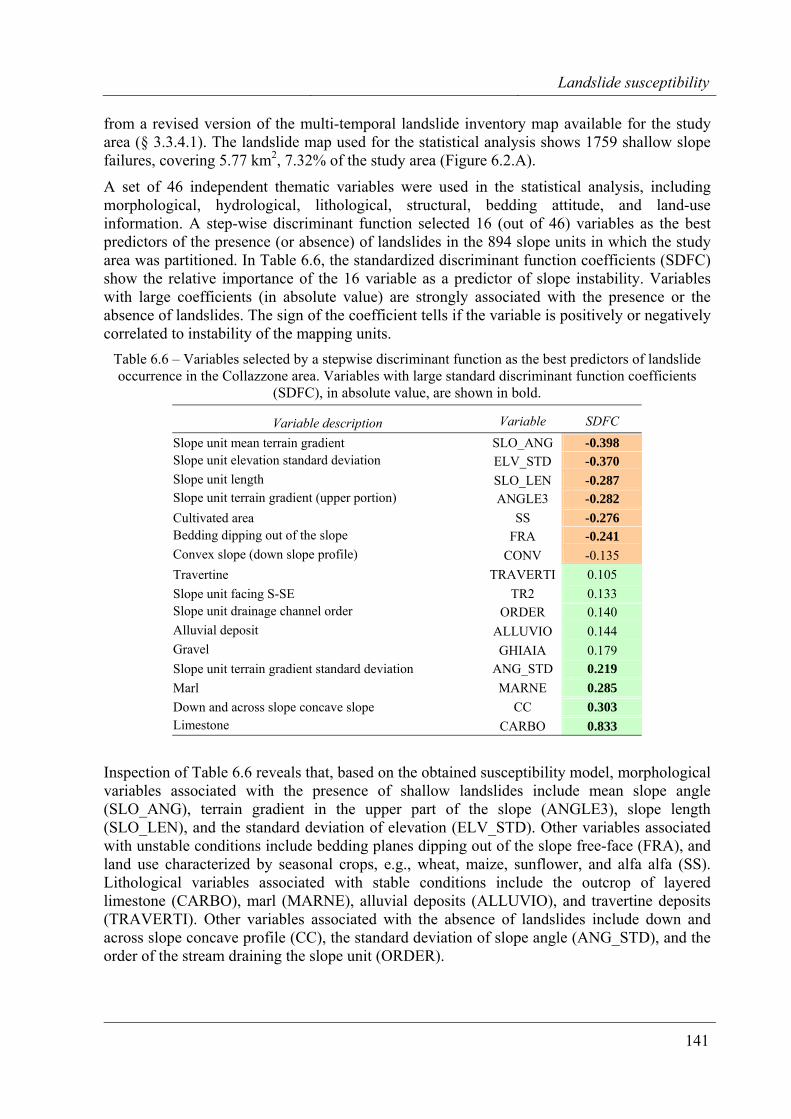
Landslide susceptibility
141
from a revised version of the multi-temporal landslide inventory map available for the study area (§ 3.3.4.1). The landslide map used for the statistical analysis shows 1759 shallow slope failures, covering 5.77 km2, 7.32% of the study area (Figure 6.2.A).
A set of 46 independent thematic variables were used in the statistical analysis, including morphological, hydrological, lithological, structural, bedding attitude, and land-use information. A step-wise discriminant function selected 16 (out of 46) variables as the best predictors of the presence (or absence) of landslides in the 894 slope units in which the study area was partitioned. In Table 6.6, the standardized discriminant function coefficients (SDFC) show the relative importance of the 16 variable as a predictor of slope instability. Variables with large coefficients (in absolute value) are strongly associated with the presence or the absence of landslides. The sign of the coefficient tells if the variable is positively or negatively correlated to instability of the mapping units.
Table 6.6 – Variables selected by a stepwise discriminant function as the best predictors of landslide occurrence in the Collazzone area. Variables with large standard discriminant function coefficients
(SDFC), in absolute value, are shown in bold.
Variable description Variable SDFC Slope unit mean terrain gradient SLO_ANG -0.398 Slope unit elevation standard deviation ELV_STD -0.370 Slope unit length SLO_LEN -0.287 Slope unit terrain gradient (upper portion) ANGLE3 -0.282 Cultivated area SS -0.276 Bedding dipping out of the slope FRA -0.241 Convex slope (down slope profile) CONV -0.135 Travertine TRAVERTI 0.105 Slope unit facing S-SE TR2 0.133 Slope unit drainage channel order ORDER 0.140 Alluvial deposit ALLUVIO 0.144 Gravel GHIAIA 0.179 Slope unit terrain gradient standard deviation ANG_STD 0.219 Marl MARNE 0.285 Down and across slope concave slope CC 0.303 Limestone CARBO 0.833
Inspection of Table 6.6 reveals that, based on the obtained susceptibility model, morphological variables associated with the presence of shallow landslides include mean slope angle (SLO_ANG), terrain gradient in the upper part of the slope (ANGLE3), slope length (SLO_LEN), and the standard deviation of elevation (ELV_STD). Other variables associated with unstable conditions include bedding planes dipping out of the slope free-face (FRA), and land use characterized by seasonal crops, e.g., wheat, maize, sunflower, and alfa alfa (SS). Lithological variables associated with stable conditions include the outcrop of layered limestone (CARBO), marl (MARNE), alluvial deposits (ALLUVIO), and travertine deposits (TRAVERTI). Other variables associated with the absence of landslides include down and across slope concave profile (CC), the standard deviation of slope angle (ANG_STD), and the order of the stream draining the slope unit (ORDER).
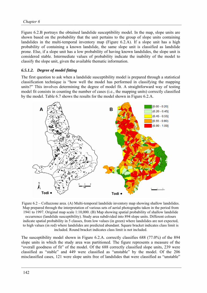
Chapter 6
142
Figure 6.2.B portrays the obtained landslide susceptibility model. In the map, slope units are shown based on the probability that the unit pertains to the group of slope units containing landslides in the multi-temporal inventory map (Figure 6.2.A). If a slope unit has a high probability of containing a known landslide, the same slope unit is classified as landslide prone. Else, if a slope unit has a low probability of having known landslides, the slope unit is considered stable. Intermediate values of probability indicate the inability of the model to classify the slope unit, given the available thematic information.
6.5.1.2. Degree of model fitting The first question to ask when a landslide susceptibility model is prepared through a statistical classification technique is “how well the model has performed in classifying the mapping units?” This involves determining the degree of model fit. A straightforward way of testing model fit consists in counting the number of cases (i.e., the mapping units) correctly classified by the model. Table 6.7 shows the results for the model shown in Figure 6.2.A.
Figure 6.2 – Collazzone area. (A) Multi-temporal landslide inventory map showing shallow landslides. Map prepared through the interpretation of various sets of aerial photographs taken in the period from 1941 to 1997. Original map scale 1:10,000. (B) Map showing spatial probability of shallow landslide
occurrence (landslide susceptibility). Study area subdivided into 894 slope units. Different colours indicate spatial probability in 5 classes, from low values (in green) where landslides are not expected, to high values (in red) where landslides are predicted abundant. Square bracket indicates class limit is
included. Round bracket indicates class limit is not included.
The susceptibility model shown in Figure 6.2.A. correctly classifies 688 (77.0%) of the 894 slope units in which the study area was partitioned. The figure represents a measure of the “overall goodness of fit” of the model. Of the 688 correctly classified slope units, 239 were classified as “stable” and 449 were classified as “unstable” by the model. Of the 206 misclassified cases, 121 were slope units free of landslides that were classified as “unstable”
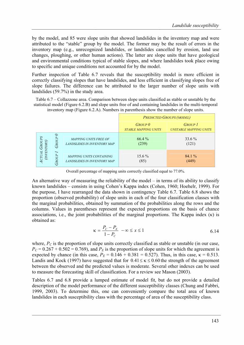
Landslide susceptibility
143
by the model, and 85 were slope units that showed landslides in the inventory map and were attributed to the “stable” group by the model. The former may be the result of errors in the inventory map (e.g., unrecognized landslides, or landslides cancelled by erosion, land use changes, ploughing, or other human actions). The latter are slope units that have geological and environmental conditions typical of stable slopes, and where landslides took place owing to specific and unique conditions not accounted for by the model.
Further inspection of Table 6.7 reveals that the susceptibility model is more efficient in correctly classifying slopes that have landslides, and less efficient in classifying slopes free of slope failures. The difference can be attributed to the larger number of slope units with landslides (59.7%) in the study area.
Table 6.7 – Collazzone area. Comparison between slope units classified as stable or unstable by the statistical model (Figure 6.2.B) and slope units free of and containing landslides in the multi-temporal
inventory map (Figure 6.2.A). Numbers in parenthesis show the number of slope units. PREDICTED GROUPS (MODEL) GROUP 0
STABLE MAPPING UNITS GROUP 1
UNSTABLE MAPPING UNITS
GRO
UP
0
MAPPING UNITS FREE OF LANDSLIDES IN INVENTORY MAP
66.4 % (239)
33.6 % (121)
ACTU
AL G
ROU
PS
(INVE
NTO
RY)
GRO
UP
1
MAPPING UNITS CONTAINING LANDSLIDES IN INVENTORY MAP
15.6 % (85)
84.1 % (449)
Overall percentage of mapping units correctly classified equal to 77.0%.
An alternative way of measuring the reliability of the model – in terms of its ability to classify known landslides – consists in using Cohen’s Kappa index (Cohen, 1960; Hoehelr, 1999). For the purpose, I have rearranged the data shown in contingency Table 6.7. Table 6.8 shows the proportion (observed probability) of slope units in each of the four classification classes with the marginal probabilities, obtained by summation of the probabilities along the rows and the columns. Values in parentheses represent the expected proportions on the basis of chance associations, i.e., the joint probabilities of the marginal proportions. The Kappa index (κ) is obtained as:
C
EC
PPP
−−
=κ1
1≤≤∞− x 6.14
where, PC is the proportion of slope units correctly classified as stable or unstable (in our case, PC = 0.267 + 0.502 = 0.769), and PE is the proportion of slope units for which the agreement is expected by chance (in this case, PE = 0.146 + 0.381 = 0.527). Thus, in this case, κ = 0.513. Landis and Kock (1997) have suggested that for 600410 .. ≤κ≤ the strength of the agreement between the observed and the predicted values is moderate. Several other indexes can be used to measure the forecasting skill of classification. For a review see Mason (2003).
Tables 6.7 and 6.8 provide a lumped estimate of model fit, but do not provide a detailed description of the model performance of the different susceptibility classes (Chung and Fabbri, 1999, 2003). To determine this, one can conveniently compare the total area of known landslides in each susceptibility class with the percentage of area of the susceptibility class.
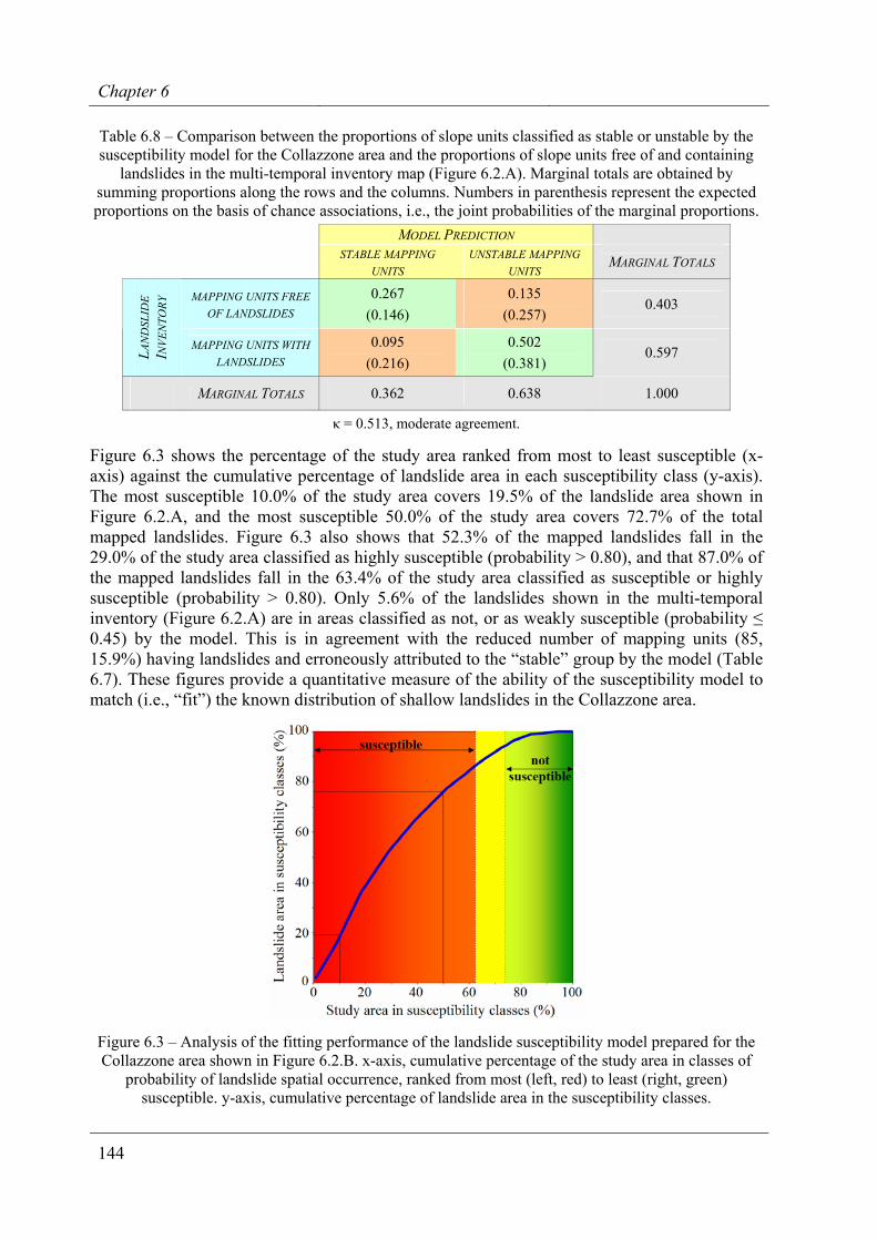
Chapter 6
144
Table 6.8 – Comparison between the proportions of slope units classified as stable or unstable by the susceptibility model for the Collazzone area and the proportions of slope units free of and containing
landslides in the multi-temporal inventory map (Figure 6.2.A). Marginal totals are obtained by summing proportions along the rows and the columns. Numbers in parenthesis represent the expected proportions on the basis of chance associations, i.e., the joint probabilities of the marginal proportions.
MODEL PREDICTION
STABLE MAPPING
UNITS UNSTABLE MAPPING
UNITS MARGINAL TOTALS
MAPPING UNITS FREE OF LANDSLIDES
0.267 (0.146)
0.135 (0.257)
0.403
LAN
DSL
IDE
INVE
NTO
RY
MAPPING UNITS WITH LANDSLIDES
0.095 (0.216)
0.502 (0.381)
0.597
MARGINAL TOTALS 0.362 0.638 1.000
κ = 0.513, moderate agreement.
Figure 6.3 shows the percentage of the study area ranked from most to least susceptible (x-axis) against the cumulative percentage of landslide area in each susceptibility class (y-axis). The most susceptible 10.0% of the study area covers 19.5% of the landslide area shown in Figure 6.2.A, and the most susceptible 50.0% of the study area covers 72.7% of the total mapped landslides. Figure 6.3 also shows that 52.3% of the mapped landslides fall in the 29.0% of the study area classified as highly susceptible (probability > 0.80), and that 87.0% of the mapped landslides fall in the 63.4% of the study area classified as susceptible or highly susceptible (probability > 0.80). Only 5.6% of the landslides shown in the multi-temporal inventory (Figure 6.2.A) are in areas classified as not, or as weakly susceptible (probability ≤ 0.45) by the model. This is in agreement with the reduced number of mapping units (85, 15.9%) having landslides and erroneously attributed to the “stable” group by the model (Table 6.7). These figures provide a quantitative measure of the ability of the susceptibility model to match (i.e., “fit”) the known distribution of shallow landslides in the Collazzone area.
Figure 6.3 – Analysis of the fitting performance of the landslide susceptibility model prepared for the Collazzone area shown in Figure 6.2.B. x-axis, cumulative percentage of the study area in classes of
probability of landslide spatial occurrence, ranked from most (left, red) to least (right, green) susceptible. y-axis, cumulative percentage of landslide area in the susceptibility classes.
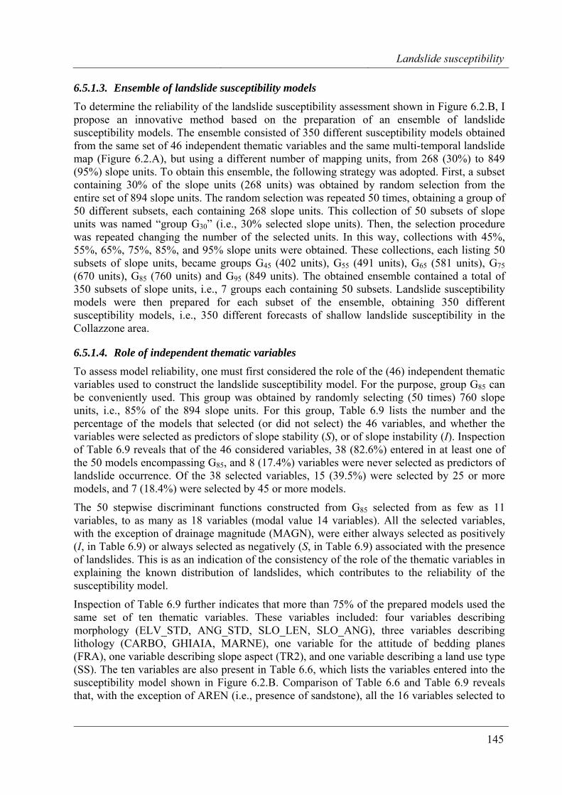
Landslide susceptibility
145
6.5.1.3. Ensemble of landslide susceptibility models To determine the reliability of the landslide susceptibility assessment shown in Figure 6.2.B, I propose an innovative method based on the preparation of an ensemble of landslide susceptibility models. The ensemble consisted of 350 different susceptibility models obtained from the same set of 46 independent thematic variables and the same multi-temporal landslide map (Figure 6.2.A), but using a different number of mapping units, from 268 (30%) to 849 (95%) slope units. To obtain this ensemble, the following strategy was adopted. First, a subset containing 30% of the slope units (268 units) was obtained by random selection from the entire set of 894 slope units. The random selection was repeated 50 times, obtaining a group of 50 different subsets, each containing 268 slope units. This collection of 50 subsets of slope units was named “group G30” (i.e., 30% selected slope units). Then, the selection procedure was repeated changing the number of the selected units. In this way, collections with 45%, 55%, 65%, 75%, 85%, and 95% slope units were obtained. These collections, each listing 50 subsets of slope units, became groups G45 (402 units), G55 (491 units), G65 (581 units), G75 (670 units), G85 (760 units) and G95 (849 units). The obtained ensemble contained a total of 350 subsets of slope units, i.e., 7 groups each containing 50 subsets. Landslide susceptibility models were then prepared for each subset of the ensemble, obtaining 350 different susceptibility models, i.e., 350 different forecasts of shallow landslide susceptibility in the Collazzone area.
6.5.1.4. Role of independent thematic variables To assess model reliability, one must first considered the role of the (46) independent thematic variables used to construct the landslide susceptibility model. For the purpose, group G85 can be conveniently used. This group was obtained by randomly selecting (50 times) 760 slope units, i.e., 85% of the 894 slope units. For this group, Table 6.9 lists the number and the percentage of the models that selected (or did not select) the 46 variables, and whether the variables were selected as predictors of slope stability (S), or of slope instability (I). Inspection of Table 6.9 reveals that of the 46 considered variables, 38 (82.6%) entered in at least one of the 50 models encompassing G85, and 8 (17.4%) variables were never selected as predictors of landslide occurrence. Of the 38 selected variables, 15 (39.5%) were selected by 25 or more models, and 7 (18.4%) were selected by 45 or more models.
The 50 stepwise discriminant functions constructed from G85 selected from as few as 11 variables, to as many as 18 variables (modal value 14 variables). All the selected variables, with the exception of drainage magnitude (MAGN), were either always selected as positively (I, in Table 6.9) or always selected as negatively (S, in Table 6.9) associated with the presence of landslides. This is as an indication of the consistency of the role of the thematic variables in explaining the known distribution of landslides, which contributes to the reliability of the susceptibility model.
Inspection of Table 6.9 further indicates that more than 75% of the prepared models used the same set of ten thematic variables. These variables included: four variables describing morphology (ELV_STD, ANG_STD, SLO_LEN, SLO_ANG), three variables describing lithology (CARBO, GHIAIA, MARNE), one variable for the attitude of bedding planes (FRA), one variable describing slope aspect (TR2), and one variable describing a land use type (SS). The ten variables are also present in Table 6.6, which lists the variables entered into the susceptibility model shown in Figure 6.2.B. Comparison of Table 6.6 and Table 6.9 reveals that, with the exception of AREN (i.e., presence of sandstone), all the 16 variables selected to
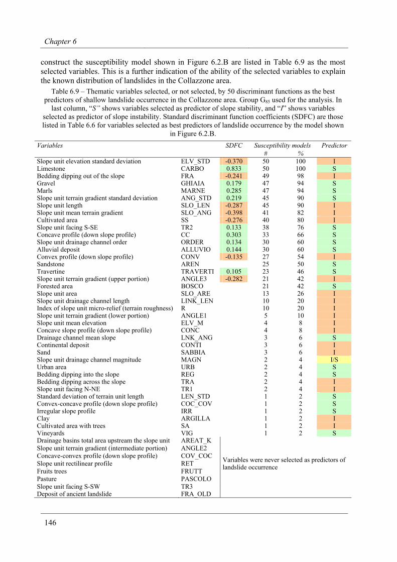
Chapter 6
146
construct the susceptibility model shown in Figure 6.2.B are listed in Table 6.9 as the most selected variables. This is a further indication of the ability of the selected variables to explain the known distribution of landslides in the Collazzone area.
Table 6.9 – Thematic variables selected, or not selected, by 50 discriminant functions as the best predictors of shallow landslide occurrence in the Collazzone area. Group G85 used for the analysis. In
last column, “S” shows variables selected as predictor of slope stability, and “I” shows variables selected as predictor of slope instability. Standard discriminant function coefficients (SDFC) are those listed in Table 6.6 for variables selected as best predictors of landslide occurrence by the model shown
in Figure 6.2.B. Variables SDFC Susceptibility models Predictor
# % Slope unit elevation standard deviation ELV_STD -0.370 50 100 I Limestone CARBO 0.833 50 100 S Bedding dipping out of the slope FRA -0.241 49 98 I Gravel GHIAIA 0.179 47 94 S Marls MARNE 0.285 47 94 S Slope unit terrain gradient standard deviation ANG_STD 0.219 45 90 S Slope unit length SLO_LEN -0.287 45 90 I Slope unit mean terrain gradient SLO_ANG -0.398 41 82 I Cultivated area SS -0.276 40 80 I Slope unit facing S-SE TR2 0.133 38 76 S Concave profile (down slope profile) CC 0.303 33 66 S Slope unit drainage channel order ORDER 0.134 30 60 S Alluvial deposit ALLUVIO 0.144 30 60 S Convex profile (down slope profile) CONV -0.135 27 54 I Sandstone AREN 25 50 S Travertine TRAVERTI 0.105 23 46 S Slope unit terrain gradient (upper portion) ANGLE3 -0.282 21 42 I Forested area BOSCO 21 42 S Slope unit area SLO_ARE 13 26 I Slope unit drainage channel length LINK_LEN 10 20 I Index of slope unit micro-relief (terrain roughness) R 10 20 I Slope unit terrain gradient (lower portion) ANGLE1 5 10 I Slope unit mean elevation ELV_M 4 8 I Concave slope profile (down slope profile) CONC 4 8 I Drainage channel mean slope LNK_ANG 3 6 S Continental deposit CONTI 3 6 I Sand SABBIA 3 6 I Slope unit drainage channel magnitude MAGN 2 4 I/S Urban area URB 2 4 S Bedding dipping into the slope REG 2 4 S Bedding dipping across the slope TRA 2 4 I Slope unit facing N-NE TR1 2 4 I Standard deviation of terrain unit length LEN_STD 1 2 S Convex-concave profile (down slope profile) COC_COV 1 2 S Irregular slope profile IRR 1 2 S Clay ARGILLA 1 2 I Cultivated area with trees SA 1 2 I Vineyards VIG 1 2 S Drainage basins total area upstream the slope unit AREAT_K Slope unit terrain gradient (intermediate portion) ANGLE2 Concave-convex profile (down slope profile) COV_COC Slope unit rectilinear profile RET Fruits trees FRUTT Pasture PASCOLO Slope unit facing S-SW TR3
Variables were never selected as predictors of landslide occurrence
Deposit of ancient landslide FRA_OLD
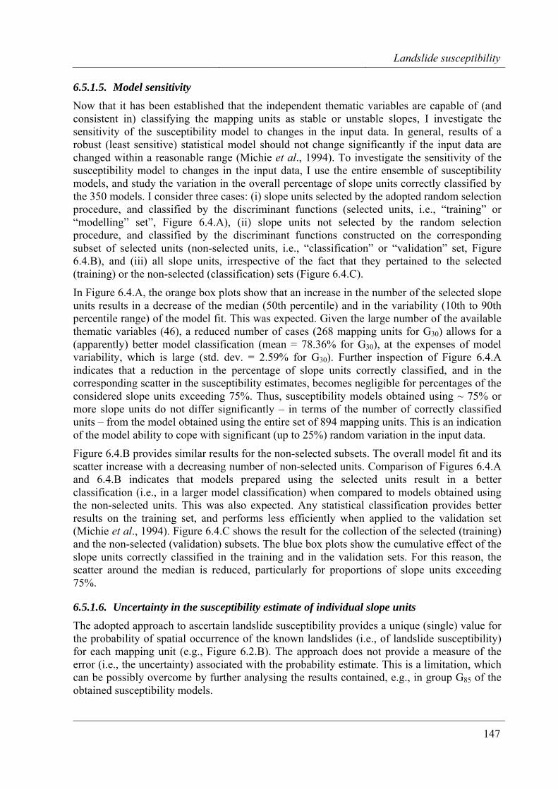
Landslide susceptibility
147
6.5.1.5. Model sensitivity Now that it has been established that the independent thematic variables are capable of (and consistent in) classifying the mapping units as stable or unstable slopes, I investigate the sensitivity of the susceptibility model to changes in the input data. In general, results of a robust (least sensitive) statistical model should not change significantly if the input data are changed within a reasonable range (Michie et al., 1994). To investigate the sensitivity of the susceptibility model to changes in the input data, I use the entire ensemble of susceptibility models, and study the variation in the overall percentage of slope units correctly classified by the 350 models. I consider three cases: (i) slope units selected by the adopted random selection procedure, and classified by the discriminant functions (selected units, i.e., “training” or “modelling” set”, Figure 6.4.A), (ii) slope units not selected by the random selection procedure, and classified by the discriminant functions constructed on the corresponding subset of selected units (non-selected units, i.e., “classification” or “validation” set, Figure 6.4.B), and (iii) all slope units, irrespective of the fact that they pertained to the selected (training) or the non-selected (classification) sets (Figure 6.4.C).
In Figure 6.4.A, the orange box plots show that an increase in the number of the selected slope units results in a decrease of the median (50th percentile) and in the variability (10th to 90th percentile range) of the model fit. This was expected. Given the large number of the available thematic variables (46), a reduced number of cases (268 mapping units for G30) allows for a (apparently) better model classification (mean = 78.36% for G30), at the expenses of model variability, which is large (std. dev. = 2.59% for G30). Further inspection of Figure 6.4.A indicates that a reduction in the percentage of slope units correctly classified, and in the corresponding scatter in the susceptibility estimates, becomes negligible for percentages of the considered slope units exceeding 75%. Thus, susceptibility models obtained using ~ 75% or more slope units do not differ significantly – in terms of the number of correctly classified units – from the model obtained using the entire set of 894 mapping units. This is an indication of the model ability to cope with significant (up to 25%) random variation in the input data.
Figure 6.4.B provides similar results for the non-selected subsets. The overall model fit and its scatter increase with a decreasing number of non-selected units. Comparison of Figures 6.4.A and 6.4.B indicates that models prepared using the selected units result in a better classification (i.e., in a larger model classification) when compared to models obtained using the non-selected units. This was also expected. Any statistical classification provides better results on the training set, and performs less efficiently when applied to the validation set (Michie et al., 1994). Figure 6.4.C shows the result for the collection of the selected (training) and the non-selected (validation) subsets. The blue box plots show the cumulative effect of the slope units correctly classified in the training and in the validation sets. For this reason, the scatter around the median is reduced, particularly for proportions of slope units exceeding 75%.
6.5.1.6. Uncertainty in the susceptibility estimate of individual slope units The adopted approach to ascertain landslide susceptibility provides a unique (single) value for the probability of spatial occurrence of the known landslides (i.e., of landslide susceptibility) for each mapping unit (e.g., Figure 6.2.B). The approach does not provide a measure of the error (i.e., the uncertainty) associated with the probability estimate. This is a limitation, which can be possibly overcome by further analysing the results contained, e.g., in group G85 of the obtained susceptibility models.
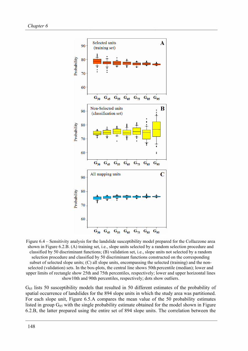
Chapter 6
148
Figure 6.4 – Sensitivity analysis for the landslide susceptibility model prepared for the Collazzone area shown in Figure 6.2.B. (A) training set, i.e., slope units selected by a random selection procedure and classified by 50 discriminant functions; (B) validation set, i.e., slope units not selected by a random selection procedure and classified by 50 discriminant functions constructed on the corresponding
subset of selected slope units; (C) all slope units, encompassing the selected (training) and the non-selected (validation) sets. In the box-plots, the central line shows 50th percentile (median); lower and
upper limits of rectangle show 25th and 75th percentiles, respectively; lower and upper horizontal lines show10th and 90th percentiles, respectively; dots show outliers.
G85 lists 50 susceptibility models that resulted in 50 different estimates of the probability of spatial occurrence of landslides for the 894 slope units in which the study area was partitioned. For each slope unit, Figure 6.5.A compares the mean value of the 50 probability estimates listed in group G85 with the single probability estimate obtained for the model shown in Figure 6.2.B, the latter prepared using the entire set of 894 slope units. The correlation between the
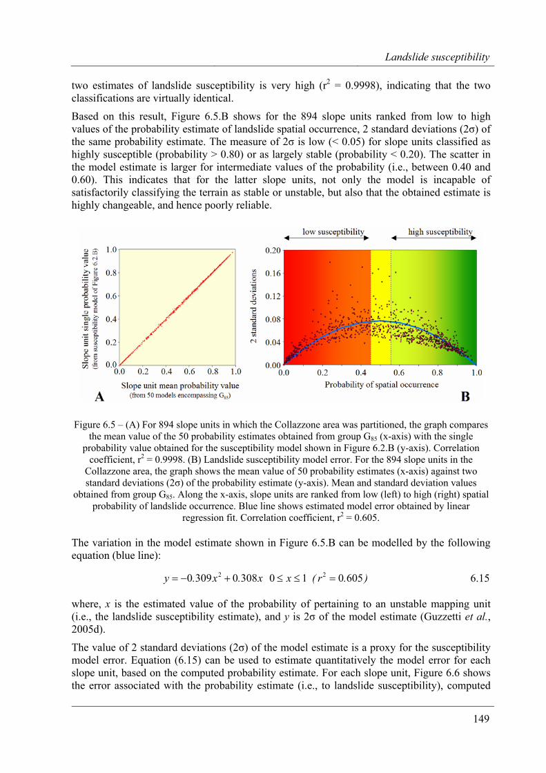
Landslide susceptibility
149
two estimates of landslide susceptibility is very high (r2 = 0.9998), indicating that the two classifications are virtually identical.
Based on this result, Figure 6.5.B shows for the 894 slope units ranked from low to high values of the probability estimate of landslide spatial occurrence, 2 standard deviations (2σ) of the same probability estimate. The measure of 2σ is low (< 0.05) for slope units classified as highly susceptible (probability > 0.80) or as largely stable (probability < 0.20). The scatter in the model estimate is larger for intermediate values of the probability (i.e., between 0.40 and 0.60). This indicates that for the latter slope units, not only the model is incapable of satisfactorily classifying the terrain as stable or unstable, but also that the obtained estimate is highly changeable, and hence poorly reliable.
Figure 6.5 – (A) For 894 slope units in which the Collazzone area was partitioned, the graph compares the mean value of the 50 probability estimates obtained from group G85 (x-axis) with the single
probability value obtained for the susceptibility model shown in Figure 6.2.B (y-axis). Correlation coefficient, r2 = 0.9998. (B) Landslide susceptibility model error. For the 894 slope units in the
Collazzone area, the graph shows the mean value of 50 probability estimates (x-axis) against two standard deviations (2σ) of the probability estimate (y-axis). Mean and standard deviation values
obtained from group G85. Along the x-axis, slope units are ranked from low (left) to high (right) spatial probability of landslide occurrence. Blue line shows estimated model error obtained by linear
regression fit. Correlation coefficient, r2 = 0.605.
The variation in the model estimate shown in Figure 6.5.B can be modelled by the following equation (blue line):
x.x.y 30803090 2 +−= 10 ≤≤ x ).r( 60502 = 6.15
where, x is the estimated value of the probability of pertaining to an unstable mapping unit (i.e., the landslide susceptibility estimate), and y is 2σ of the model estimate (Guzzetti et al., 2005d).
The value of 2 standard deviations (2σ) of the model estimate is a proxy for the susceptibility model error. Equation (6.15) can be used to estimate quantitatively the model error for each slope unit, based on the computed probability estimate. For each slope unit, Figure 6.6 shows the error associated with the probability estimate (i.e., to landslide susceptibility), computed
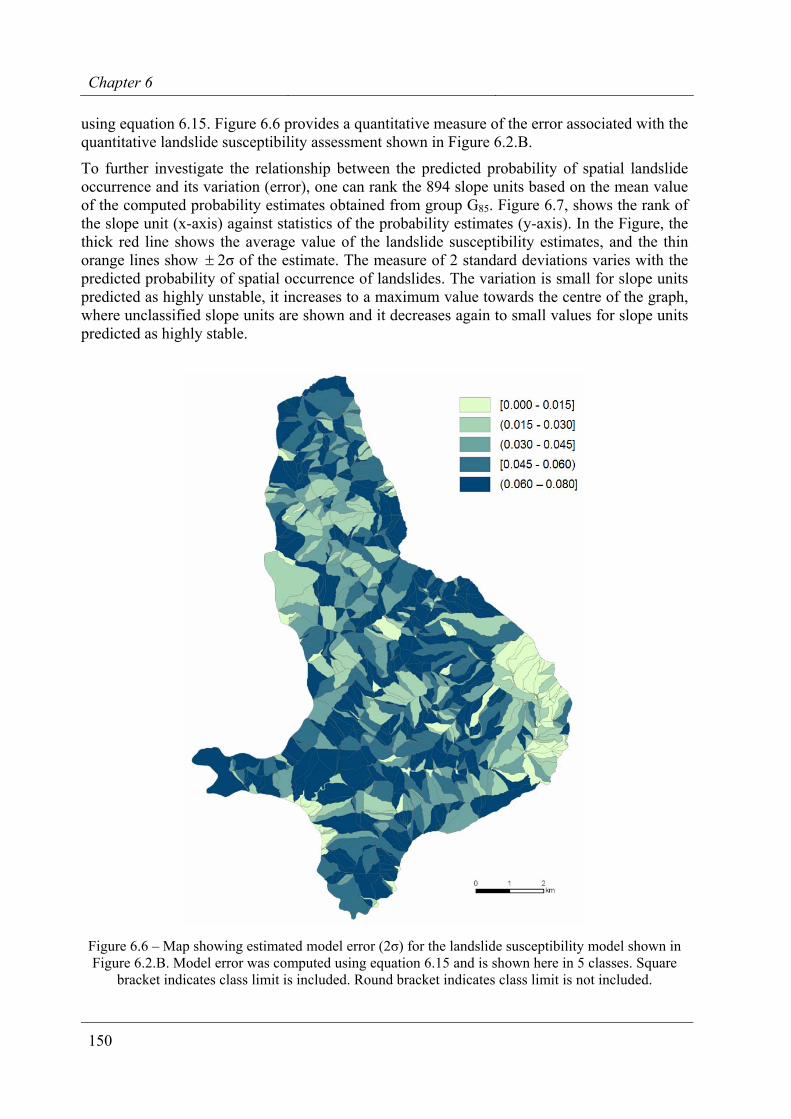
Chapter 6
150
using equation 6.15. Figure 6.6 provides a quantitative measure of the error associated with the quantitative landslide susceptibility assessment shown in Figure 6.2.B.
To further investigate the relationship between the predicted probability of spatial landslide occurrence and its variation (error), one can rank the 894 slope units based on the mean value of the computed probability estimates obtained from group G85. Figure 6.7, shows the rank of the slope unit (x-axis) against statistics of the probability estimates (y-axis). In the Figure, the thick red line shows the average value of the landslide susceptibility estimates, and the thin orange lines show ± 2σ of the estimate. The measure of 2 standard deviations varies with the predicted probability of spatial occurrence of landslides. The variation is small for slope units predicted as highly unstable, it increases to a maximum value towards the centre of the graph, where unclassified slope units are shown and it decreases again to small values for slope units predicted as highly stable.
Figure 6.6 – Map showing estimated model error (2σ) for the landslide susceptibility model shown in Figure 6.2.B. Model error was computed using equation 6.15 and is shown here in 5 classes. Square
bracket indicates class limit is included. Round bracket indicates class limit is not included.
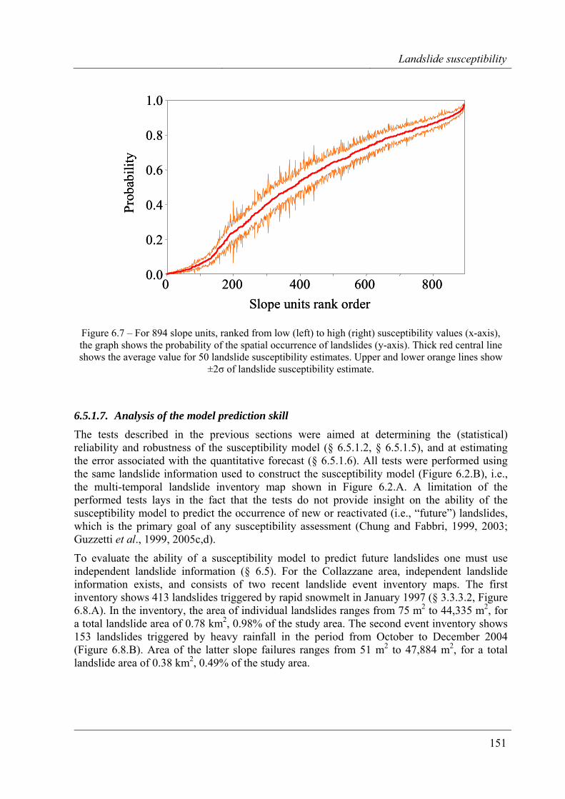
Landslide susceptibility
151
Slope units rank order0 200 400 600 800
0.0
0.2
0.4Prob
abili
ty
0.6
0.8
1.0
Slope units rank order0 200 400 600 800
0.0
0.2
0.4Prob
abili
ty
0.6
0.8
1.0
Figure 6.7 – For 894 slope units, ranked from low (left) to high (right) susceptibility values (x-axis), the graph shows the probability of the spatial occurrence of landslides (y-axis). Thick red central line shows the average value for 50 landslide susceptibility estimates. Upper and lower orange lines show
±2σ of landslide susceptibility estimate.
6.5.1.7. Analysis of the model prediction skill The tests described in the previous sections were aimed at determining the (statistical) reliability and robustness of the susceptibility model (§ 6.5.1.2, § 6.5.1.5), and at estimating the error associated with the quantitative forecast (§ 6.5.1.6). All tests were performed using the same landslide information used to construct the susceptibility model (Figure 6.2.B), i.e., the multi-temporal landslide inventory map shown in Figure 6.2.A. A limitation of the performed tests lays in the fact that the tests do not provide insight on the ability of the susceptibility model to predict the occurrence of new or reactivated (i.e., “future”) landslides, which is the primary goal of any susceptibility assessment (Chung and Fabbri, 1999, 2003; Guzzetti et al., 1999, 2005c,d).
To evaluate the ability of a susceptibility model to predict future landslides one must use independent landslide information (§ 6.5). For the Collazzane area, independent landslide information exists, and consists of two recent landslide event inventory maps. The first inventory shows 413 landslides triggered by rapid snowmelt in January 1997 (§ 3.3.3.2, Figure 6.8.A). In the inventory, the area of individual landslides ranges from 75 m2 to 44,335 m2, for a total landslide area of 0.78 km2, 0.98% of the study area. The second event inventory shows 153 landslides triggered by heavy rainfall in the period from October to December 2004 (Figure 6.8.B). Area of the latter slope failures ranges from 51 m2 to 47,884 m2, for a total landslide area of 0.38 km2, 0.49% of the study area.
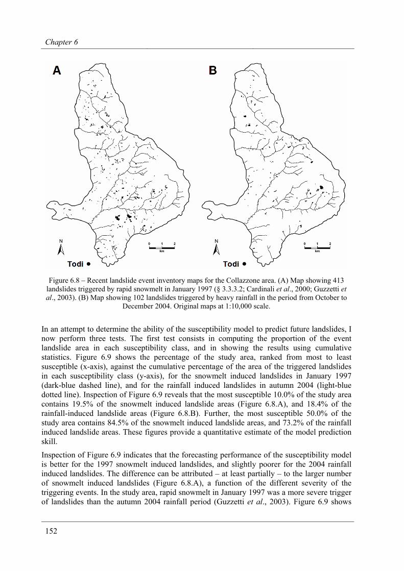
Chapter 6
152
Figure 6.8 – Recent landslide event inventory maps for the Collazzone area. (A) Map showing 413 landslides triggered by rapid snowmelt in January 1997 (§ 3.3.3.2; Cardinali et al., 2000; Guzzetti et al., 2003). (B) Map showing 102 landslides triggered by heavy rainfall in the period from October to
December 2004. Original maps at 1:10,000 scale.
In an attempt to determine the ability of the susceptibility model to predict future landslides, I now perform three tests. The first test consists in computing the proportion of the event landslide area in each susceptibility class, and in showing the results using cumulative statistics. Figure 6.9 shows the percentage of the study area, ranked from most to least susceptible (x-axis), against the cumulative percentage of the area of the triggered landslides in each susceptibility class (y-axis), for the snowmelt induced landslides in January 1997 (dark-blue dashed line), and for the rainfall induced landslides in autumn 2004 (light-blue dotted line). Inspection of Figure 6.9 reveals that the most susceptible 10.0% of the study area contains 19.5% of the snowmelt induced landslide areas (Figure 6.8.A), and 18.4% of the rainfall-induced landslide areas (Figure 6.8.B). Further, the most susceptible 50.0% of the study area contains 84.5% of the snowmelt induced landslide areas, and 73.2% of the rainfall induced landslide areas. These figures provide a quantitative estimate of the model prediction skill.
Inspection of Figure 6.9 indicates that the forecasting performance of the susceptibility model is better for the 1997 snowmelt induced landslides, and slightly poorer for the 2004 rainfall induced landslides. The difference can be attributed – at least partially – to the larger number of snowmelt induced landslides (Figure 6.8.A), a function of the different severity of the triggering events. In the study area, rapid snowmelt in January 1997 was a more severe trigger of landslides than the autumn 2004 rainfall period (Guzzetti et al., 2003). Figure 6.9 shows
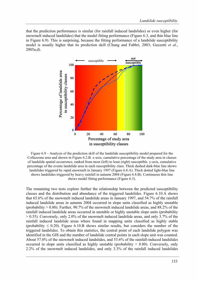
Landslide susceptibility
153
that the prediction performance is similar (for rainfall induced landslides) or even higher (for snowmelt induced landslides) that the model fitting performance (Figure 6.3, and thin blue line in Figure 6.9). This is surprising, because the fitting performance of a landslide susceptibility model is usually higher that its prediction skill (Chung and Fabbri, 2003; Guzzetti et al., 2005a,d).
0 20 40 60 80 1000
20
40
60
80
Perc
enta
ge o
f lan
dslid
e ar
ea
in su
scep
tibili
ty c
lass
es
Percentage of study area in susceptibility classes
100
not susceptiblesusceptible
0 20 40 60 80 1000
20
40
60
80
Perc
enta
ge o
f lan
dslid
e ar
ea
in su
scep
tibili
ty c
lass
es
Percentage of study area in susceptibility classes
100
not susceptiblesusceptible
Figure 6.9 – Analysis of the prediction skill of the landslide susceptibility model prepared for the Collazzone area and shown in Figure 6.2.B. x-axis, cumulative percentage of the study area in classes of landslide spatial occurrence, ranked from most (left) to least (right) susceptible. y-axis, cumulative percentage of the events landslide area in each susceptibility class. Thick dashed dark-blue line shows
landslides triggered by rapid snowmelt in January 1997 (Figure 6.8.A). Thick dotted light-blue line shows landslides triggered by heavy rainfall in autumn 2004 (Figure 6.8.B). Continuous thin line
shows model fitting performance (Figure 6.3).
The remaining two tests explore further the relationship between the predicted susceptibility classes and the distribution and abundance of the triggered landslides. Figure 6.10.A shows that 65.6% of the snowmelt induced landslide areas in January 1997, and 54.7% of the rainfall induced landslide areas in autumn 2004 occurred in slope units classified as highly unstable (probability > 0.80). Further, 90.7% of the snowmelt induced landslide areas, and 88.2% of the rainfall induced landslide areas occurred in unstable or highly unstable slope units (probability > 0.55). Conversely, only 2.0% of the snowmelt induced landslide areas, and only 3.7% of the rainfall induced landslide areas where found in mapping units classified as highly stable (probability ≤ 0.20). Figure 6.10.B shows similar results, but considers the number of the triggered landslides. To obtain this statistics, the central point of each landslide polygon was identified in the GIS and the number of landslide central points in each slope unit was counted. About 57.0% of the snowmelt induced landslides, and 53.6% of the rainfall-induced landslides occurred in slope units classified as highly unstable (probability > 0.80). Conversely, only 2.2% of the snowmelt induced landslides, and only 3.3% of the rainfall induced landslides
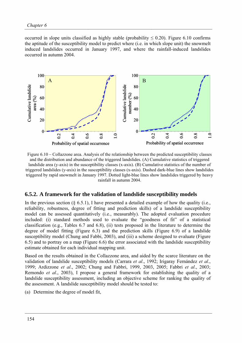
Chapter 6
154
occurred in slope units classified as highly stable (probability ≤ 0.20). Figure 6.10 confirms the aptitude of the susceptibility model to predict where (i.e. in which slope unit) the snowmelt induced landslides occurred in January 1997, and where the rainfall-induced landslides occurred in autumn 2004.
Probability of spatial occurrence
0.2
0.4
0.6
0.8
1.0
Probability of spatial occurrence
0.2
0.4
0.6
0.8
1.00
20
40
Cum
ulat
ive
land
slid
enu
mbe
r (%
)
60
80
100
0
20
40
Cum
ulat
ive
land
slid
ear
ea (%
) 60
80
100A B
Probability of spatial occurrence
0.2
0.4
0.6
0.8
1.0
Probability of spatial occurrence
0.2
0.4
0.6
0.8
1.00
20
40
Cum
ulat
ive
land
slid
enu
mbe
r (%
)
60
80
100
0
20
40
Cum
ulat
ive
land
slid
ear
ea (%
) 60
80
100A B
Figure 6.10 – Collazzone area. Analysis of the relationship between the predicted susceptibility classes and the distribution and abundance of the triggered landslides. (A) Cumulative statistics of triggered
landslide area (y-axis) in the susceptibility classes (x-axis). (B) Cumulative statistics of the number of triggered landslides (y-axis) in the susceptibility classes (x-axis). Dashed dark-blue lines show landslides triggered by rapid snowmelt in January 1997. Dotted light-blue lines show landslides triggered by heavy
rainfall in autumn 2004.
6.5.2. A framework for the validation of landslide susceptibility models In the previous section (§ 6.5.1), I have presented a detailed example of how the quality (i.e., reliability, robustness, degree of fitting and prediction skills) of a landslide susceptibility model can be assessed quantitatively (i.e., measurably). The adopted evaluation procedure included: (i) standard methods used to evaluate the “goodness of fit” of a statistical classification (e.g., Tables 6.7 and 6.8), (ii) tests proposed in the literature to determine the degree of model fitting (Figure 6.3) and the prediction skills (Figure 6.9) of a landslide susceptibility model (Chung and Fabbi, 2003), and (iii) a scheme designed to evaluate (Figure 6.5) and to portray on a map (Figure 6.6) the error associated with the landslide susceptibility estimate obtained for each individual mapping unit.
Based on the results obtained in the Collazzone area, and aided by the scarce literature on the validation of landslide susceptibility models (Carrara et al., 1992; Irigaray Fernández et al., 1999; Ardizzone et al., 2002; Chung and Fabbri, 1999, 2003, 2005; Fabbri et al., 2003; Remondo et al., 2003), I propose a general framework for establishing the quality of a landslide susceptibility assessment, including an objective scheme for ranking the quality of the assessment. A landslide susceptibility model should be tested to:
(a) Determine the degree of model fit,
Landslide susceptibility
155
(b) Establish the aptitude of the thematic information to construct the model, including an assessment of the sensitivity of the model to changes in the landslide and the thematic information used to construct the model,
(c) Determine the error associated with the probabilistic estimate obtained for each mapping unit, and
(d) Test the skill of the model prediction to forecast “future” landslides.
Determining the degree of model fit consists in establishing how well the model describes (i.e., matches) the known distribution of landslides. The task is easily performed in a GIS using the same landslide information used to construct the susceptibility model. For the purpose, contingency tables (e.g., Tables 6.4, 6.7 and 6.8), and cumulative statistics of the abundance of landslides in the susceptibility classes (e.g., Figure 6.3) can be prepared. However, for the test to be significant, the landslide information must be representative, accurate, and complete.
To evaluate the role of the thematic information in the construction of the landslide susceptibility model (e.g., Tables 6.3 and 6.6), and to evaluate the model sensitivity (e.g., Figure 6.4), one can study the list of thematic variables entered (and not entered) in a set of discriminant classification functions constructed on a sub-set of randomly selected mapping units (e.g., group G85, for the Collazzone case study). In the proposed scheme, the random selection procedure accounted for the variability in the input data.
The expected error (i.e., the level of uncertainty) associated with the probabilistic susceptibility estimate obtained for each mapping unit can be determined by investigating the variability of the obtained estimate in the mapping units. For the purpose, I have assumed that two standard deviations (2σ) of the model estimate was a reasonable measure of the model uncertainty, and modelled the expected error consequently (i.e., using equation 6.14). Alternative measures of model uncertainty can be adopted.
Testing the ability of the susceptibility model to forecast new (i.e., “future”) landslides can only be accomplished using landslide information not available to construct the susceptibility model (Chung and Fabbri, 2003, 2005; Guzzetti et al., 2005a,d). In the Collazzone area, I obtained independent landslide information from two recent event inventory maps showing new slope failures triggered by rapid snow melting and by intense rainfall. Chung and Fabbri (2003, 2005) obtained a similar result by splitting a multi-temporal inventory in two temporal subsets, i.e., a training set containing landslide occurred before an established date, and a classification set showing landslides occurred after the established date. I maintain that the scheme adopted here is superior to the scheme used by Chung and Fabbri (2003, 2005). In the first scheme, to construct the susceptibility model the entire set of available information on the past landslides is exploited, and not a temporal (i.e., limited) subset of it. As a potential drawback, the scheme is more “severe”, as a much reduced number of landslides is used to ascertain the model prediction skill.
Table 6.10 lists a set of criteria for ranking and comparing the quality of landslide susceptibility assessments. Based on the listed criteria, when no information is available on the quality of a landslide susceptibility model the obtained product has the lowest possible level of quality (level 0). This level of quality should be considered unacceptable. When estimates of model fit are available, the susceptibility assessment has the least acceptable quality level (level 1). When the error associated with the predicted susceptibility estimate for each mapping unit is established, the susceptibility assessment has a higher level of quality (level
Chapter 6
156
2). Lastly, when the prediction skill of the model is known, the susceptibility assessment has a still higher quality rank (level 4). The proposed scheme allows for summing the individual quality levels. As an example, a susceptibility assessment for which the fitting performance (level 1) and prediction skill (level 4) were determined is quality level 5. When, for the same susceptibility assessment, the error associated with the predicted susceptibility for each mapping unit is established (level 2), the quality level becomes 7. Adopting the proposed scheme, the landslide susceptibility model prepared for the Collazzone area has the highest quality level (i.e., level 7).
Table 6.10. Criteria and levels of quality for landslide susceptibility models and associated maps.
Description Level
No information is available, or no test was performed to determine the quality and the prediction skill of the landslide susceptibility assessment. 0
Estimates of degree of model fit are available. Tests were performed using the same landslide information used to obtain the susceptibility estimate. 1
Estimates of the error associated with the predicted susceptibility value in each terrain unit are available. Tests were performed using the same landslide information used to obtain the susceptibility estimate.
2
Estimates of the model prediction performance are available. Tests were performed using independent landslide information, not used to obtain the susceptibility model. 4
The criteria listed in Table 6.10 do not guarantee as such the quality of a susceptibility estimate. To obtain this, the results of specific tests must be matched against established acceptance thresholds. Defining such thresholds is not an easy task. Based on the experience gained in numerous landslide susceptibility assessments completed in southern (Carrara, 1983), central (Carrara et al., 1991; 1995; 2003; Cardinali et al., 2002) and northern (Ardizzone et al., 2002; Guzzetti et al., 2005c) Italy, I propose a set of acceptance thresholds, and I compare the results of the performed tests to the proposed thresholds.
I consider acceptable a susceptibility model with an overall degree of model fit greater than at least 75%, and I regard a classification as very satisfactory when the overall model fit is greater that 80%. Further, I consider an extremely high value of the overall model fit (e.g., ≥ 90%) as an indication that the model matches too closely the original landslide inventory map (a case of model “over fitting”). When such case arises, the model prediction is virtually indistinct from a prediction made using solely the landslide inventory, making the model useless and unreliable. The case may arise, e.g., where the spatial distribution of landslides is “trivial” (i.e., very easy) to forecast, or where the number of mapping units is very small compared to the number of the explanatory variables (e.g., Campus et al., 1999). An additional indication of the quality of the model consists in a reduced number of mapping units with landslides erroneously classified as “stable” areas by the model. The overall fit obtained for the susceptibility model prepared for the Collazzone area is 77.0% (Table 6.7), and the proportion of mapping units with landslides erroneously classified as stable areas is 9.5% (85 units).
Landslide susceptibility
157
A statistical model obtained using a reduced number of geomorphologically meaningful explanatory variables is “less expensive” and superior to a model which uses a very large number of variables. Further, use of a stable combination of variables provides for a robust model that can cope with (some) uncertainty in the input data. The discriminant function used to construct the susceptibility model for the Collazzone area shown in Figure 6.2.B selected 16 of the 46 available thematic variables (34.8%). Analysis of Table 6.9 reveals that the selected variables are consistent in classifying the slope units as stable or unstable in a large number of models. This is an indication of the robustness of the obtained model.
To appraise the fitting performance and the prediction skill of a landslide susceptibility model, Chung and Fabbri (2003) proposed comparing the proportion of landslide area in each susceptibility class (AL) with the proportion of the susceptibility class (AS) in the study area. For a successful classification, the “effectiveness ratio” AL/AS should be greater than one in the areas predicted as landslide prone by the model, and less than one in the areas predicted as stable by the model. A very effective prediction class has a ratio close to zero or very large, depending if the class predicts stability or instability. Where the effectiveness ratio is near one, the proportion of landslides in the susceptibility class is not different from the average landslide density in the study area, and the performance of the susceptibility class in determining the known (“fitting” performance) or the future (“prediction” skill) location of landslides is weak. Chung and Fabbri (2003) considered “effective” a susceptibility class with a ratio larger than at least 3 (unstable areas) or less than at most 0.2 (stable areas), and “significantly effective” a susceptibility class with a ratio larger than at least 6 or less than at most 0.1. These criteria are hard to match in complex areas where landslides are large and numerous, and where the landscape exhibits considerable geomorphological variability. For such areas, I consider “effective” a susceptibility class with a ratio larger than 1.5 or smaller than 0.5, corresponding to a 50% increase or a 50% decrease from the expected proportion of landslides in the susceptibility class.
It should be clear that all the proposed acceptance thresholds are not absolute, fixed thresholds. The proposed limits were selected heuristically, based on the experience of the investigators. The acceptance criteria need to be tested in other areas and by different investigators. Depending on the geomorphological setting and the complexity of a study area, other investigators may select different thresholds.
Lastly, I like to point out that the proposed framework for the evaluation of the quality of a landslide susceptibility model considers the most relevant sources of errors in a statistically based susceptibility assessment, but other factors resulting in errors that affect a susceptibility assessment exist. These factors include: (i) imprecision and incompleteness in the landslide information used to construct and test the susceptibility model (Carrara et al., 1992; Ardizzone et al., 2002; Galli et al., 2005), (ii) quality, abundance, precision and completeness of the thematic data used to obtain the susceptibility assessment (Carrara et al., 1992; 1999; Soeters and van Westen, 1996), (iii) characteristics and limitations of the statistical technique used to obtain the classification, including the experience of the investigator in applying the selected statistical tools (Carrara et al., 1992; Michie et al., 1994), and (iv) selection of the appropriate mapping unit (e.g., slope units, unique condition units, grid cells, etc., § 6.2.2) (Carrara et al., 1995; Guzzetti et al., 1999a). All these factors require choices from the investigator, which inevitably introduce uncertainty in the susceptibility assessment. The levels of uncertainty introduced by the listed factors should also be established.
Chapter 6
158
6.6. Summary of achieved results
In this chapter, I have:
(a) Demonstrated that a large territory can be subdivided based on its propensity to generate new or reactivated landslides, using reliable and reproducible methods.
(b) Shown how to validate the performances and prediction skills of a landslide susceptibility forecasts.
(c) Proposed objective criteria for ranking and comparing the quality of landslide susceptibility forecasts.
This responds to Question # 5 posed in the Introduction (§ 1.2).
159
7. LANDSLIDE HAZARD ASSESSMENT
Nothing is more dangerous than underestimating a hazard.
There are many good reasons
not to avoid hazards.
A hazard is the likelihood that a danger will materialize. A natural hazard is the hazard posed by a potentially damaging natural event or process, such as an earthquake, flood, volcanic eruption, snow avalanche, hurricane, ground subsidence or mass movement. Landslide hazard refers to the potential for the occurrence of a damaging slope failure within a given area and in a given period. To properly define landslide hazard, the magnitude, size, or dimension of the expected failure must also be quantified, deterministically or in probabilistic terms, because the “magnitude” of the event is linked to its destructive power. Landslide hazard is portrayed on maps. A landslide hazard map partitions a territory based upon different levels of landslide hazard (landslide hazard zoning). As it will become clear later, producing a single landslide hazard map is problematic, as different hazard conditions (or probabilities) must be shown on the same map. An ensemble of maps can be prepared to show landslide hazard, and displayed in a GIS.
In this chapter, I first examine a definition of landslide hazard, I then introduce a probabilistic model for landslide hazard assessment that fulfils the adopted definition, and I discuss known problems with the given definition and limitations of the proposed probability model. Next, I show three examples of the application of the proposed probability model for different types of landslides and at different scales, from the catchment to the national scale. In the first example, I illustrate an attempt to determine landslide hazard in the Staffora River basin (§ 2.6), exploiting a detailed multi-temporal inventory map and thematic information on geo-environmental factors associated with landslides. In the second example, I describe an attempt to determine levels of landslide hazard in Italy, based on synoptic information on geology, soil types and morphology, and an archive inventory of historical landslide events. In the third example, I exploit a physically-based computer model capable to simulating rock falls for the determination of rock fall hazard in south-eastern Umbria (§ 2.5).
7.1. Background and definitions
Physical scientists define a natural hazard either as the probability that a reasonably stable condition may change abruptly (Scheidegger, 1994), or as the probability of occurrence of a potentially damaging phenomenon within a given area and in a given period of time (Varnes and the IAEG Commission on Landslides and other Mass-Movements, 1984). Vandine et al.
Chapter 7
160
(2004) define landslide hazard the estimate of the probability of occurrence of a specific landslide and that the landslide being a threat to an element at risk, without considering the effects or potential consequences.
The definition proposed by Varnes and the IAEG Commission on Landslides and other Mass-Movements, (1984) remains the most widely accepted definition for natural hazard and for maps portraying its distribution over a region (IDNHR, 1987; Starosolszky and Melder, 1989; Horlick-Jones et al., 1995; Murck et al., 1997). The definition incorporates – more or less explicitly – the concepts of: (i) magnitude, (ii) geographical location, and (iii) time recurrence. The first refers to the “size” or “intensity” of the natural phenomenon which conditions its behaviour and destructive power. The second implies the ability to identify the place “where” the phenomenon will occur or may develop. The third refers to the temporal frequency of the event, i.e., the ability to predict “when” or how frequently the expected event will happen (Guzzetti et al., 1999a).
Application of the given definition to the various natural hazards differs, making conceptual and practical comparison and integration of hazard assessments difficult, if not impossible (Guzzetti et al., 1999a; Natural Hazard Working Group, 2005). Without the ambition of completeness, I now examine differences in the assessment of the hazard for some of the most common natural hazards, namely: earthquakes, floods, volcanic eruptions and mass movements. Traditionally, earthquake predictive models attempt to define hazard in terms of magnitude – a quantitative measure of the energy released by a seismic event –, affected area, and time recurrence. Ideally, earthquake hazard assessments largely fulfil the definition of hazard previously mentioned. Unfortunately, scientists are generally unable to predict at the same time and with the required accuracy where and when an earthquake will take place, and how severe it will be. Amongst scientists there is a general consensus that with the present state of knowledge the exact (or even approximate) time of an earthquake cannot be predicted. Probabilistic Seismic Hazard Analysis is based on the statistical analysis of past earthquake events. Despite some criticism, PSHA remains the most widely applied method to define seismic risk (Castaños and Lomnitz, 2002; Bommer, 2003; Wang et al., 2003).
Despite the different meanings of the term “flood” (Baker, 1994), flood hazard evaluation essentially consists in the temporal prediction of an extreme hydrological event of a given magnitude (i.e., peak water flow or volume), whereas geographical location and spatial extent of the potentially inundated areas are determined from other sources of information, such as historical records and ground morphology. Estimates of the temporal occurrence of floods are mainly obtained from probabilistic analysis of the historical records of water levels or discharge measurements. For many gauging stations the record of measurements is short, and extrapolation techniques are used to obtain estimates of flood levels or water discharge for longer periods. Extrapolation inevitably introduces uncertainty in the hazard assessment. Where catchments are small, establishing hazard from water flow measurements may not be adequate (lack of warning time), or measurements may be completely lacking (“ungauged” basins). In these areas, the temporal prediction of an extreme hydrological event is obtained by studying measured, estimated, or forecasted rainfall. This undoubtedly introduces uncertainties in the hazard assessment. The extent and location of the potentially inundated areas are obtained from historical information and through the application of conceptual (simplified), physically based flood models, assuming a detailed description of topography and an input hydrograph. Accuracy of DTM and significance of the selected hydrograph are fundamental for the quality and relevance of flood spatial hazard assessments.
Landslide Hazard Assessment
161
For volcanoes, the area affected by the eruption is implicitly defined in the analysis, i.e., the same volcano, which is usually well known in space. Before or during an eruption, scenarios are prepared to predict where individual or multiple lava flows or pyroclastic flows can travel and at what speed. The areas potentially affected by ash falls can also be determined. Again, these models (mostly physically based) are determined from external sources of information. The temporal occurrence of an eruption is estimated assimilating geological and volcanological knowledge, historical information and – most importantly – monitoring of physical and chemical properties, at depth and on the surface, including topographic deformations. The magnitude and destructiveness of an eruption depend largely on the type of the volcano. It is established mostly heuristically through the analysis of past eruptions and the recent behaviour of the investigated volcano.
For mass movements a conceptual confusion arises from the use of the same term “landslide” to address both the landslide deposit (the failed mass) and the movement of slope material or of an existing landslide mass (Bosi, 1978; Cruden, 1991; Guzzetti et al., 1999a). It is like mistaking an earthquake with its ground effects, an eruption with the area affected by lava flows or ash falls, or a river flood with the inundated area. Landslide predictive models most commonly attempt to identify only “where” landslides may occur over a given region on the basis of a set of relevant environmental characteristics. Such models do not directly incorporate “time” and “magnitude”, i.e., size (Fell, 1994; Cardinali et al., 2002, Reichenbach et al., 2005), speed (Cruden and Varnes, 1996), kinetic energy (Hsu, 1975; Sassa, 1988), destructiveness (Hungr, 1997) or momentum of the failed mass. For this reason, these models cannot be correctly defined as hazard models (§ 6). Predictive models of landslide movement are generally confined to single slopes or individual small catchments (e.g., in the case of debris flows) where detailed geotechnical site investigations attempt to assess when and to what extent the slope-forming material, frequently an existing landslide deposit, will move. Also in this case the term hazard is somewhat incorrect since the location of the phenomenon under study is implicit, or derives from information acquired from other sources.
The wide spectrum of landslide phenomena (Figure 1.1) and the complexity and variability of their interactions with the environment, both natural and human, make the acceptance of a single definition of landslide hazard difficult. For example, very large and fast moving rock avalanches are the most destructive and hazardous mass movements, but are relatively rare events. Slow-moving, deep-seated failures rarely claim lives but can cause large property damage. Fast-moving soil slips and debris flows cause widespread damage and casualties, and are as frequent as their potential triggers (i.e., high intensity rainfall events). Rock falls, despite their often small size, are among the most destructive mass movements, and a primary cause of landslide fatalities in many areas. Each type of slope movement poses different threats and may require a separate assessment, based on distinct definitions of landslide hazard.
Recurrence, the expected time for the repetition of an event, is evaluated studying historical records (§ 3.3.1, § 4.5) or multiple-temporal inventories (§ 3.3.4). Historical data are difficult to obtain for single landslides or landslide prone areas. Despite the lack of consensus on the reliability and usefulness of historic information, where historical information is available it can be used for the temporal evaluation of landslide hazard at various scales (Guzzetti et al., 1994; 2003; Ibsen and Brunsden, 1996; Cruden, 1997; Evans, 1997; Glade, 1998). Historical records may be integrated with temporal data derived from dendrocronology and other dating techniques which have been used by some investigators to date landslide deposits (Stout, 1977; DeGraff and Agard, 1984; Trustrum and De Rose, 1988; Fantucci and Sorriso-Valvo,
Chapter 7
162
1999; Lang et al., 1999; Stefanini, 2004). For first-time failures (Hutchinson, 1988) recurrence is not applicable. First-time landslides occur at or close to peak strength values, whereas reactivations occur between peak and residual conditions. Thus, first-time landslides provide little information on the behaviour of reactivations. Additionally, each time a landslide occurs, the topographic, geological and hydrological settings of the slope change, often dramatically, giving rise to different conditions of instability (§ 6.3.1). These changes allow geomorphologists to identify landslides and understand mechanisms and causes of failures, but limit their ability to forecast new landslides of reactivations.
Finally, quantitative landslide hazard models predict the occurrence of future slope failures under the general assumption that in any given area slope failures will occur in the future under the same circumstances and because of the same conditions that caused them in the past. I examined the problems encountered in adopting the principle that “the past is the key to the future” when I introduced rationale for landslide mapping (§ 3.1) and when I discussed landslide susceptibility assessment (§ 6.2.1, § 6.3.1). The same arguments apply to landslide hazard evaluation.
7.2. Probabilistic model for landslide hazard assessment
In their well-known report, Varnes and the IAEG Commission on Landslides and other Mass-Movements (1984) proposed that the definition adopted by UNDRO for all natural hazards be applied to mass movements. Landslide hazard is therefore “the probability of occurrence within a specified period of time and within a given area of a potentially damaging phenomenon”. Guzzetti et al. (1999a) amended the definition to include the magnitude of the event. Hence, the definition becomes:
Landslide hazard is the probability of occurrence within a specified period and within a given area of a landslide of a given magnitude. (7.1)
For a landslide hazard forecast, the area and period for the prediction are simple to decide (albeit difficult to know). Definition of magnitude is more difficult because, in contrast to other natural hazards (e.g., earthquakes, volcanic eruptions, hurricanes), no unique measure of landslide magnitude is available. For earthquakes, magnitude is a measure of the energy released during an event ranked by the well known Richter scale, developed by Charles Richter and Beno Gutenberg. For volcanic eruptions, the Volcanic Explosivity Index devised by Christopher G. Newhall and Steve Self provides a relative measure (in 8 grades) of the explosiveness of eruptions based on a number of things that can be observed during an eruption. For hurricanes, the Saffir-Simpson scale measures the intensity of a hurricane in 5 grades, based on wind speed and atmospheric pressure, and gives an estimate of the potential property damage and flooding expected from a hurricane landfall. For landslides a measure of the energy released during failure is difficult to obtain. Malamud et al. (2004a) introduced a landslide-event magnitude scale, based on the number of landslides triggered by a meteorological or seismic event. Hungr (1997) proposed destructiveness to be a measure of landslide magnitude. Raetzo et al. (2001) introduced an intensity scale for the magnitude of the damage. Building on the latter definitions, Cardinali et al. (2002), Guzzetti (2004) and Reichenbach et al. (2005) defined landslide destructiveness as a function of the landslide volume and of the expected landslide velocity, the latter obtained from the landslide type. For large regions, landslide volume and velocity are difficult to evaluate systematically, making the approach impracticable. Alternatively, where slope failures are chiefly slow moving slides
Landslide Hazard Assessment
163
and slide earth-flows, destructiveness can be related to the area of the landslide, information which is readily available from landslide inventory maps.
The definition of landslide hazard given in proposition 7.1 incorporates the concepts of location, time and size. To complete a hazard assessment one has to predict “where” a landslide will occur, “when”, or how frequently it will occur, and “how large” the landslide will be. In mathematical terms, this can be written as:
HL=P[AL ≥ aL in a time interval t, given {morphology, lithology, structure, land use,…}] (7.2)
where, AL is the landslide area, measured e.g., in square meters. For any given area, equation 7.2 expresses landslide hazard as the conditional probability of landslide size, P(AL), of landslide occurrence in an established period, P(NL), and of landslide spatial occurrence, S, given the local environmental setting. Assuming independence among the three probabilities, the landslide hazard, i.e., the joint probability is:
S)N(P)A(PH LLL ××= (7.3)
In the previous chapters, I have shown how to obtain the three probabilities in equation 7.3. The probability of landslide size can be estimated from the analysis of the frequency-area distribution of known landslides (§ 5, and equations 5.3 and 5.4). The probability of landslide occurrence in an established period can be estimated from the analysis of archive or multi-temporal inventories, and can be quantified adopting a Poisson or a binomial distribution model for the occurrence of the landslide events (§ 4.5, and equations 4.7 and 4.8). Susceptibility, the spatial probability of landslide occurrence, can be obtained using a variety of methods and techniques (§ 6.2). For probabilistic landslide hazard assessments, susceptibility must be obtained with indirect, quantitative methods that provide numerical (probabilistic) estimates of the spatial probability of landslide occurrence (§ 6.2.3).
The proposed probability model for landslide hazard relays on the same assumptions on which landslide mapping (§ 3.1) and the three considered individual probability models are based (see § 4.5, § 5.2, § 6.2.1). Failures to comply with one or all of the assumptions will affect the reliability of the model and the relevance and applicability of the results. In § 7.3.5 I will investigate the problems posed by each of the assumptions, including examples of how to evaluate their impact on a landslide hazard assessment. In addition, independence between the three probabilities is assumed. From a geomorphological point of view, this assumption is strong and may not hold, always and everywhere. In many areas one may expect slope failures to be more frequent (time component) where landslides are more abundant and landslide area is large (spatial component). However, given the lack of understanding of landslide phenomena, independence is an acceptable first approximation that makes the problem mathematically tractable (Guzzetti et al., 2005a). The assumption of independence is a simplification, and more complex models can be constructed using, e.g., Bayesian reasoning or Copulae. However, these approaches require the investigator to know the marginal probabilities. This is rather difficult, given the general lack of information on the statistics of landslide size and on the temporal statistics of slope failures.
Chapter 7
164
7.3. Landslide hazard model for the Staffora River basin
In this section, I discuss a landslide hazard assessment prepared for the Staffora River basin, in Lombardy Region. The hazard assessment was obtained by exploiting the thematic and landslide information available for the study area and presented in § 2.6, and it relies on the probabilistic landslide hazard model introduced in section § 7.2.
To ascertain landslide hazard, the territory of the Staffora River basin – which extends for 275 km2 – was partitioned into 2243 homogenous mapping units. For the purpose, the same procedure used to partition the Upper Tiber River basin for landslide susceptibility assessment (§ 6.4) was adopted. Starting from a DEM with a ground resolution of 20 m × 20 m, and a geographically coherent simplified representation of the main drainage lines, the territory was first subdivided into slope units (§ 6.2.2). The slope units were then further subdivided according to the main rock types cropping out in the basin. The further partitioning, solved problems of slope units characterized by rock types with different landslide abundance (i.e., different susceptibility). In this way, the study area was subdivided into 2243 geo-hydrological units, which represent the mapping units used for the hazard assessment.
Most of the landslide information needed to ascertain landslide hazard was obtained from the detailed multi-temporal landslide inventory map presented in § 2.6, which shows 3922 landslides, including 89 very old, relict mass movements. Figure 7.1 shows the multi-temporal landslide inventory used for the analysis, and Table 7.1 summarizes statistics of the mapped landslides, for different periods. In the following, I will exploit the temporal information on landslides shown in the multi-temporal inventory to determine the temporal probability of slope failure occurrence, and to verify the performance of the obtained landslide susceptibility model.
Table 7.1 – Staffora River basin. Landslide descriptive statistics obtained from the available multi-temporal inventory map shown in Figure 7.1. Percentage of landslide area (*) computed with respect to
the total area covered by landslides (A0–E2). LANDSLIDES LANDSLIDE AREA
Number Total Percentage* INVENTORY ESTIMATED LANDSLIDE AGE # km2 %
A0 very old (relict) 89 34.72 49.30
A1 older than 1955 1443 38.24 54.30
A2 1955 active 306 2.46 3.49 B1 1955-1975 318 2.38 3.39 B2 1975 active 685 4.41 6.26 C1 1975-1980 89 1.32 1.87 C2 1980 active 305 2.40 3.41 D1 1980-1994 455 2.06 2.92 D2 1994 active 175 1.36 1.94 E1 1994-1999 19 0.65 0.93 E2 1999 active 38 0.85 1.21
A0–A1 very old and older than 1955 1532 63.22 90 A0–E2 very old to 1999 active 3922 70.42 100 A1–E2 older than 1955 to 1999 active 3833 46.43 66 A2–E2 1955 active to 1999 active 2390 12.08 17
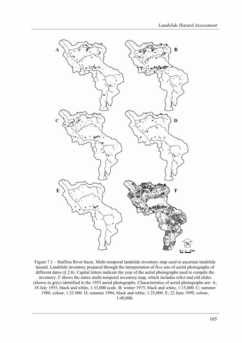
Landslide Hazard Assessment
165
Figure 7.1 – Staffora River basin. Multi-temporal landslide inventory map used to ascertain landslide hazard. Landslide inventory prepared through the interpretation of five sets of aerial photographs of different dates (§ 2.6). Capital letters indicate the year of the aerial photographs used to compile the
inventory. F shows the entire multi-temporal inventory map, which includes relict and old slides (shown in grey) identified in the 1955 aerial photographs. Characteristics of aerial photographs are: A; 18 July 1955, black and white, 1:33,000 scale. B; winter 1975, black and white, 1:15,000. C; summer
1980, colour, 1:22 000. D; summer 1994, black and white, 1:25,000. E; 22 June 1999, colour, 1:40,000.
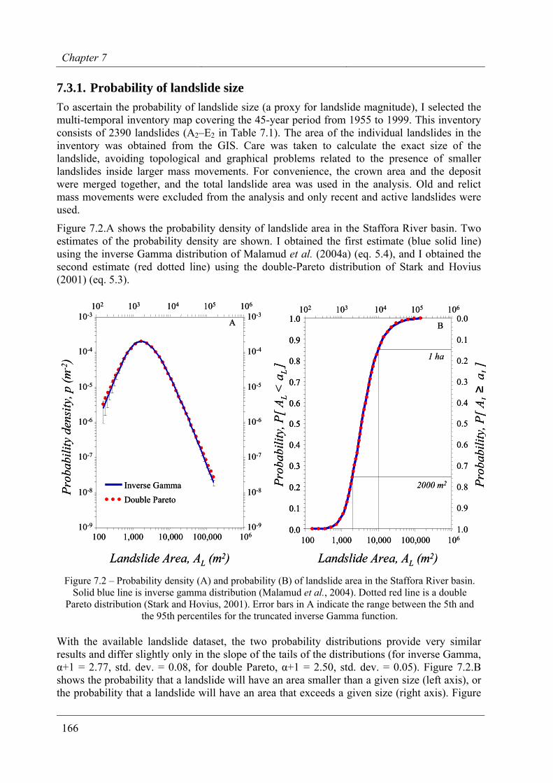
Chapter 7
166
7.3.1. Probability of landslide size To ascertain the probability of landslide size (a proxy for landslide magnitude), I selected the multi-temporal inventory map covering the 45-year period from 1955 to 1999. This inventory consists of 2390 landslides (A2–E2 in Table 7.1). The area of the individual landslides in the inventory was obtained from the GIS. Care was taken to calculate the exact size of the landslide, avoiding topological and graphical problems related to the presence of smaller landslides inside larger mass movements. For convenience, the crown area and the deposit were merged together, and the total landslide area was used in the analysis. Old and relict mass movements were excluded from the analysis and only recent and active landslides were used.
Figure 7.2.A shows the probability density of landslide area in the Staffora River basin. Two estimates of the probability density are shown. I obtained the first estimate (blue solid line) using the inverse Gamma distribution of Malamud et al. (2004a) (eq. 5.4), and I obtained the second estimate (red dotted line) using the double-Pareto distribution of Stark and Hovius (2001) (eq. 5.3).
Landslide Area, AL (m2)
Prob
abili
ty d
ensi
ty, p
(m-2
)
Double ParetoInverse Gamma
10-9
10-8
10-7
10-6
10-5
10-4
10-3
10-9
10-8
10-7
10-6
10-5
10-4
10-3
100 1,000 10,000 100,000 106
102 103 104 105 106
A
Landslide Area, AL (m2)
0.0
0.1
0.2
0.3
0.4
0.5
0.6
0.7
0.8
0.9
1.0
Prob
abili
ty, P
[ AL
< a
L]
102 103 104 105 106
100 1,000 10,000 100,000 1061.0
0.9
0.8
0.7
0.6
0.5
0.4
0.3
0.2
0.1
0.0
Prob
abili
ty, P
[ AL≥
a L]1 ha
2000 m2
B
Landslide Area, AL (m2)
Prob
abili
ty d
ensi
ty, p
(m-2
)
Double ParetoInverse Gamma
10-9
10-8
10-7
10-6
10-5
10-4
10-3
10-9
10-8
10-7
10-6
10-5
10-4
10-3
100 1,000 10,000 100,000 106
102 103 104 105 106
A
Landslide Area, AL (m2)
0.0
0.1
0.2
0.3
0.4
0.5
0.6
0.7
0.8
0.9
1.0
0.0
0.1
0.2
0.3
0.4
0.5
0.6
0.7
0.8
0.9
1.0
Prob
abili
ty, P
[ AL
< a
L]
102 103 104 105 106
100 1,000 10,000 100,000 1061.0
0.9
0.8
0.7
0.6
0.5
0.4
0.3
0.2
0.1
0.0
Prob
abili
ty, P
[ AL≥
a L]1 ha
2000 m2
B
Figure 7.2 – Probability density (A) and probability (B) of landslide area in the Staffora River basin. Solid blue line is inverse gamma distribution (Malamud et al., 2004). Dotted red line is a double
Pareto distribution (Stark and Hovius, 2001). Error bars in A indicate the range between the 5th and the 95th percentiles for the truncated inverse Gamma function.
With the available landslide dataset, the two probability distributions provide very similar results and differ slightly only in the slope of the tails of the distributions (for inverse Gamma, α+1 = 2.77, std. dev. = 0.08, for double Pareto, α+1 = 2.50, std. dev. = 0.05). Figure 7.2.B shows the probability that a landslide will have an area smaller than a given size (left axis), or the probability that a landslide will have an area that exceeds a given size (right axis). Figure
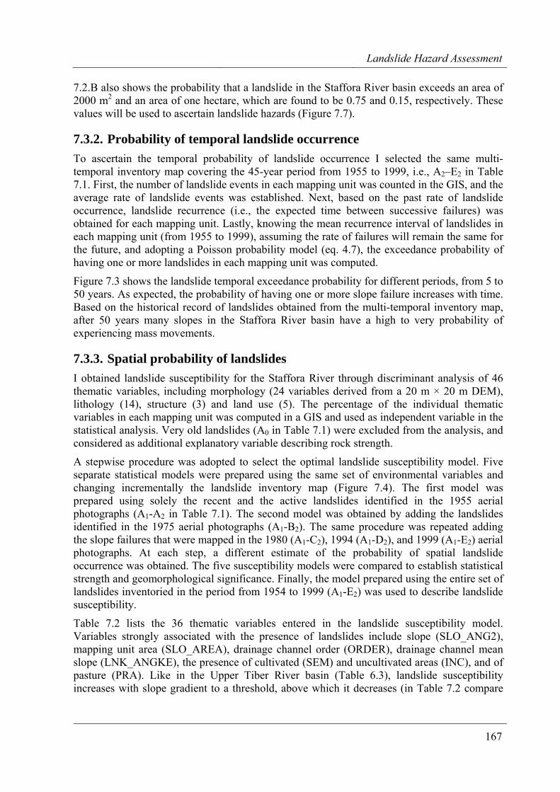
Landslide Hazard Assessment
167
7.2.B also shows the probability that a landslide in the Staffora River basin exceeds an area of 2000 m2 and an area of one hectare, which are found to be 0.75 and 0.15, respectively. These values will be used to ascertain landslide hazards (Figure 7.7).
7.3.2. Probability of temporal landslide occurrence To ascertain the temporal probability of landslide occurrence I selected the same multi-temporal inventory map covering the 45-year period from 1955 to 1999, i.e., A2–E2 in Table 7.1. First, the number of landslide events in each mapping unit was counted in the GIS, and the average rate of landslide events was established. Next, based on the past rate of landslide occurrence, landslide recurrence (i.e., the expected time between successive failures) was obtained for each mapping unit. Lastly, knowing the mean recurrence interval of landslides in each mapping unit (from 1955 to 1999), assuming the rate of failures will remain the same for the future, and adopting a Poisson probability model (eq. 4.7), the exceedance probability of having one or more landslides in each mapping unit was computed.
Figure 7.3 shows the landslide temporal exceedance probability for different periods, from 5 to 50 years. As expected, the probability of having one or more slope failure increases with time. Based on the historical record of landslides obtained from the multi-temporal inventory map, after 50 years many slopes in the Staffora River basin have a high to very probability of experiencing mass movements.
7.3.3. Spatial probability of landslides I obtained landslide susceptibility for the Staffora River through discriminant analysis of 46 thematic variables, including morphology (24 variables derived from a 20 m × 20 m DEM), lithology (14), structure (3) and land use (5). The percentage of the individual thematic variables in each mapping unit was computed in a GIS and used as independent variable in the statistical analysis. Very old landslides (A0 in Table 7.1) were excluded from the analysis, and considered as additional explanatory variable describing rock strength.
A stepwise procedure was adopted to select the optimal landslide susceptibility model. Five separate statistical models were prepared using the same set of environmental variables and changing incrementally the landslide inventory map (Figure 7.4). The first model was prepared using solely the recent and the active landslides identified in the 1955 aerial photographs (A1-A2 in Table 7.1). The second model was obtained by adding the landslides identified in the 1975 aerial photographs (A1-B2). The same procedure was repeated adding the slope failures that were mapped in the 1980 (A1-C2), 1994 (A1-D2), and 1999 (A1-E2) aerial photographs. At each step, a different estimate of the probability of spatial landslide occurrence was obtained. The five susceptibility models were compared to establish statistical strength and geomorphological significance. Finally, the model prepared using the entire set of landslides inventoried in the period from 1954 to 1999 (A1-E2) was used to describe landslide susceptibility.
Table 7.2 lists the 36 thematic variables entered in the landslide susceptibility model. Variables strongly associated with the presence of landslides include slope (SLO_ANG2), mapping unit area (SLO_AREA), drainage channel order (ORDER), drainage channel mean slope (LNK_ANGKE), the presence of cultivated (SEM) and uncultivated areas (INC), and of pasture (PRA). Like in the Upper Tiber River basin (Table 6.3), landslide susceptibility increases with slope gradient to a threshold, above which it decreases (in Table 7.2 compare
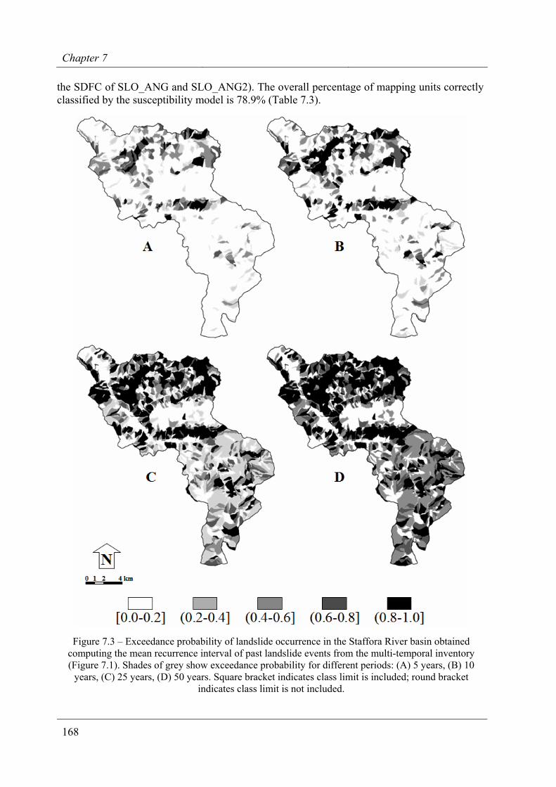
Chapter 7
168
the SDFC of SLO_ANG and SLO_ANG2). The overall percentage of mapping units correctly classified by the susceptibility model is 78.9% (Table 7.3).
Figure 7.3 – Exceedance probability of landslide occurrence in the Staffora River basin obtained computing the mean recurrence interval of past landslide events from the multi-temporal inventory (Figure 7.1). Shades of grey show exceedance probability for different periods: (A) 5 years, (B) 10
years, (C) 25 years, (D) 50 years. Square bracket indicates class limit is included; round bracket indicates class limit is not included.
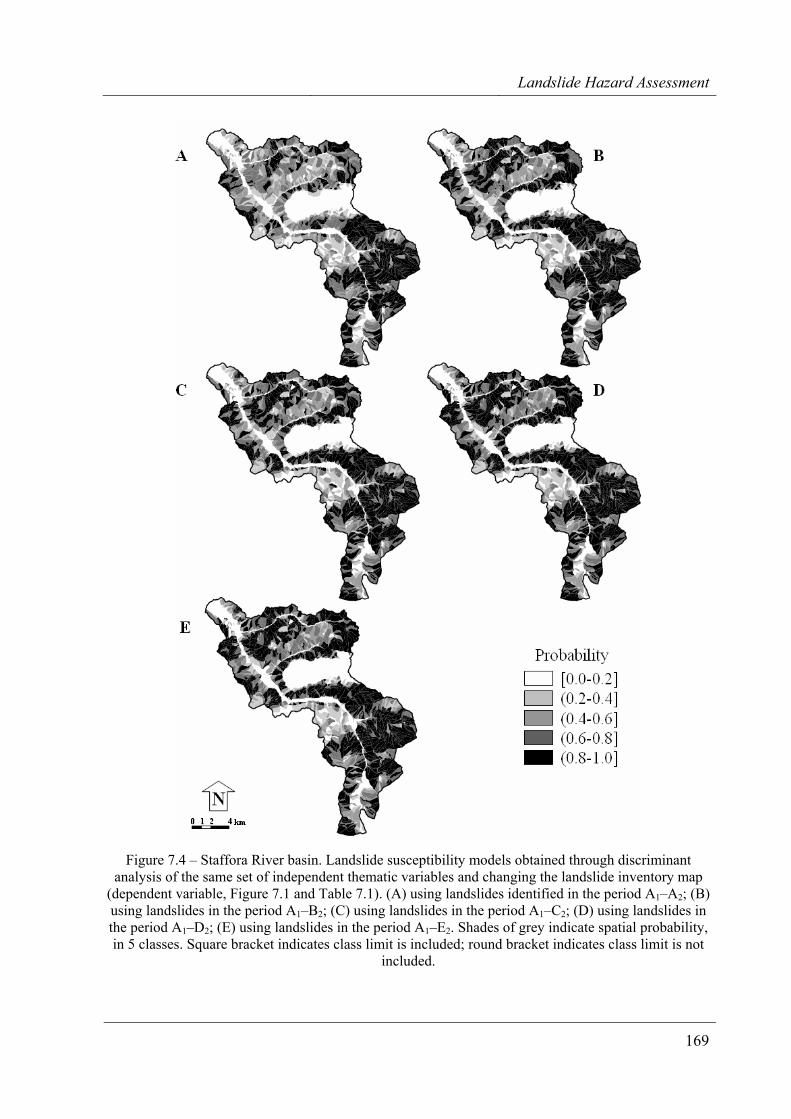
Landslide Hazard Assessment
169
Figure 7.4 – Staffora River basin. Landslide susceptibility models obtained through discriminant analysis of the same set of independent thematic variables and changing the landslide inventory map
(dependent variable, Figure 7.1 and Table 7.1). (A) using landslides identified in the period A1–A2; (B) using landslides in the period A1–B2; (C) using landslides in the period A1–C2; (D) using landslides in the period A1–D2; (E) using landslides in the period A1–E2. Shades of grey indicate spatial probability, in 5 classes. Square bracket indicates class limit is included; round bracket indicates class limit is not
included.
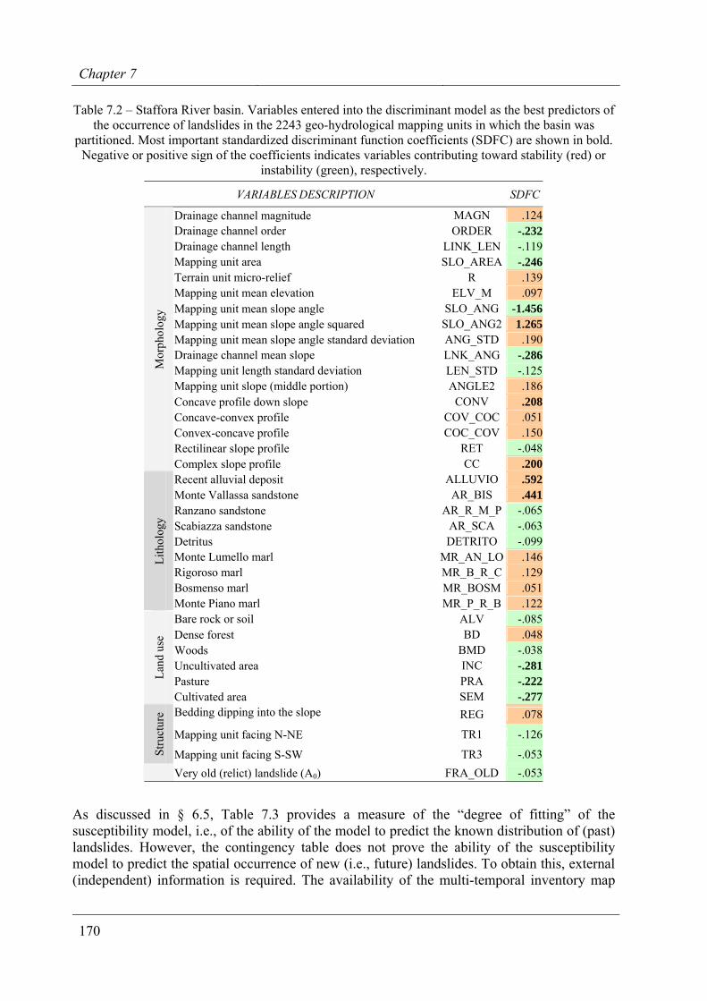
Chapter 7
170
Table 7.2 – Staffora River basin. Variables entered into the discriminant model as the best predictors of the occurrence of landslides in the 2243 geo-hydrological mapping units in which the basin was
partitioned. Most important standardized discriminant function coefficients (SDFC) are shown in bold. Negative or positive sign of the coefficients indicates variables contributing toward stability (red) or
instability (green), respectively.
VARIABLES DESCRIPTION SDFC
Drainage channel magnitude MAGN .124 Drainage channel order ORDER -.232 Drainage channel length LINK_LEN -.119 Mapping unit area SLO_AREA -.246 Terrain unit micro-relief R .139 Mapping unit mean elevation ELV_M .097 Mapping unit mean slope angle SLO_ANG -1.456 Mapping unit mean slope angle squared SLO_ANG2 1.265 Mapping unit mean slope angle standard deviation ANG_STD .190 Drainage channel mean slope LNK_ANG -.286 Mapping unit length standard deviation LEN_STD -.125 Mapping unit slope (middle portion) ANGLE2 .186 Concave profile down slope CONV .208 Concave-convex profile COV_COC .051 Convex-concave profile COC_COV .150 Rectilinear slope profile RET -.048
Mor
phol
ogy
Complex slope profile CC .200 Recent alluvial deposit ALLUVIO .592 Monte Vallassa sandstone AR_BIS .441 Ranzano sandstone AR_R_M_P -.065 Scabiazza sandstone AR_SCA -.063 Detritus DETRITO -.099 Monte Lumello marl MR_AN_LO .146 Rigoroso marl MR_B_R_C .129 Bosmenso marl MR_BOSM .051
Lith
olog
y
Monte Piano marl MR_P_R_B .122 Bare rock or soil ALV -.085 Dense forest BD .048 Woods BMD -.038 Uncultivated area INC -.281 Pasture PRA -.222 La
nd u
se
Cultivated area SEM -.277 Bedding dipping into the slope REG .078
Mapping unit facing N-NE TR1 -.126
Stru
ctur
e
Mapping unit facing S-SW TR3 -.053 Very old (relict) landslide (A0) FRA_OLD -.053
As discussed in § 6.5, Table 7.3 provides a measure of the “degree of fitting” of the susceptibility model, i.e., of the ability of the model to predict the known distribution of (past) landslides. However, the contingency table does not prove the ability of the susceptibility model to predict the spatial occurrence of new (i.e., future) landslides. To obtain this, external (independent) information is required. The availability of the multi-temporal inventory map
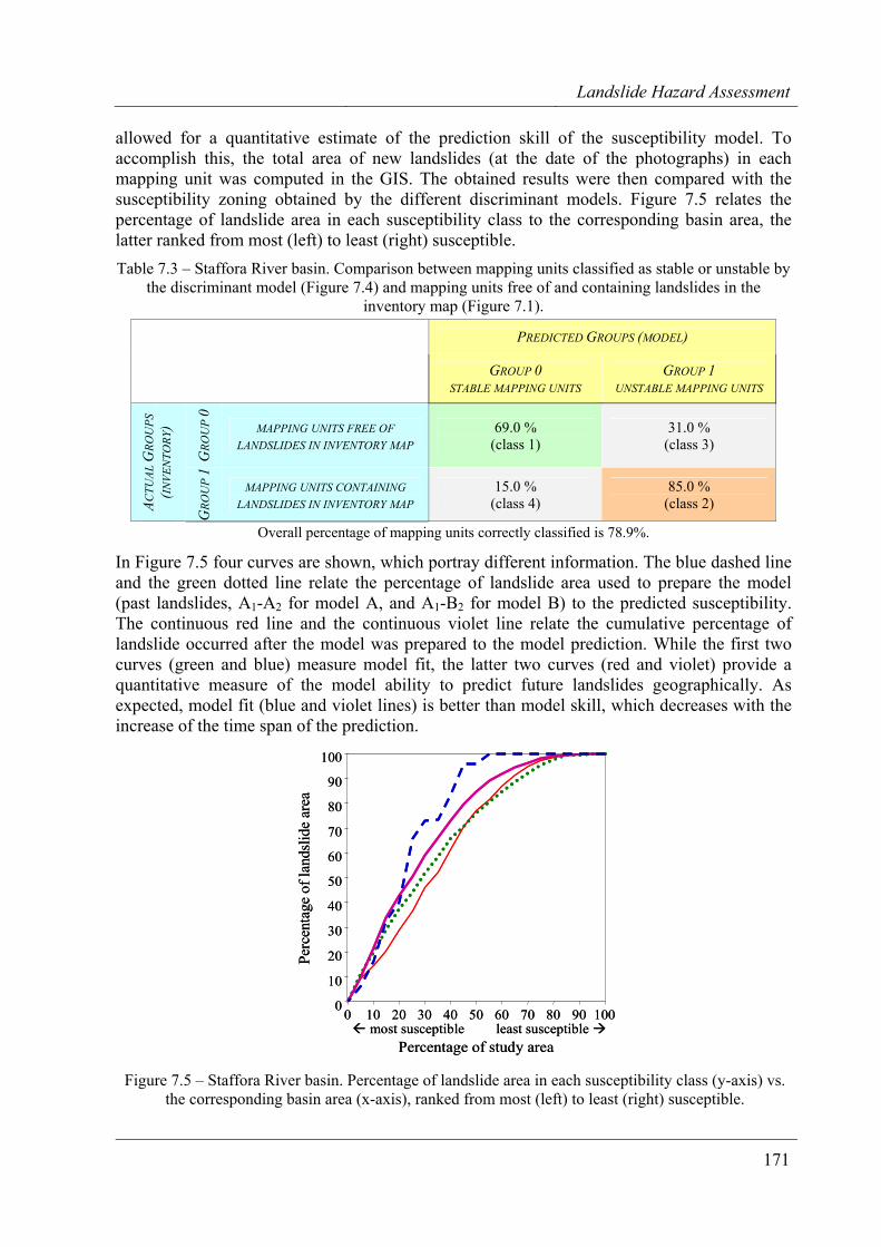
Landslide Hazard Assessment
171
allowed for a quantitative estimate of the prediction skill of the susceptibility model. To accomplish this, the total area of new landslides (at the date of the photographs) in each mapping unit was computed in the GIS. The obtained results were then compared with the susceptibility zoning obtained by the different discriminant models. Figure 7.5 relates the percentage of landslide area in each susceptibility class to the corresponding basin area, the latter ranked from most (left) to least (right) susceptible. Table 7.3 – Staffora River basin. Comparison between mapping units classified as stable or unstable by
the discriminant model (Figure 7.4) and mapping units free of and containing landslides in the inventory map (Figure 7.1).
PREDICTED GROUPS (MODEL)
GROUP 0 STABLE MAPPING UNITS
GROUP 1 UNSTABLE MAPPING UNITS
GRO
UP
0
MAPPING UNITS FREE OF LANDSLIDES IN INVENTORY MAP
69.0 % (class 1)
31.0 % (class 3)
ACTU
AL G
ROU
PS
(INVE
NTO
RY)
GRO
UP
1
MAPPING UNITS CONTAINING LANDSLIDES IN INVENTORY MAP
15.0 % (class 4)
85.0 % (class 2)
Overall percentage of mapping units correctly classified is 78.9%.
In Figure 7.5 four curves are shown, which portray different information. The blue dashed line and the green dotted line relate the percentage of landslide area used to prepare the model (past landslides, A1-A2 for model A, and A1-B2 for model B) to the predicted susceptibility. The continuous red line and the continuous violet line relate the cumulative percentage of landslide occurred after the model was prepared to the model prediction. While the first two curves (green and blue) measure model fit, the latter two curves (red and violet) provide a quantitative measure of the model ability to predict future landslides geographically. As expected, model fit (blue and violet lines) is better than model skill, which decreases with the increase of the time span of the prediction.
0
10
20
30
40
50
60
70
80
90
100
0 10 20 30 40 50 60 70 80 90 100
Percentage of study area
Perc
enta
ge o
f lan
dslid
e ar
ea
most susceptible least susceptible
0
10
20
30
40
50
60
70
80
90
100
0 10 20 30 40 50 60 70 80 90 100
Percentage of study area
Perc
enta
ge o
f lan
dslid
e ar
ea
most susceptible least susceptible
Figure 7.5 – Staffora River basin. Percentage of landslide area in each susceptibility class (y-axis) vs. the corresponding basin area (x-axis), ranked from most (left) to least (right) susceptible.
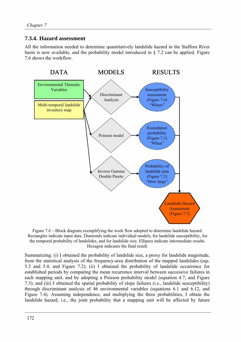
Chapter 7
172
7.3.4. Hazard assessment All the information needed to determine quantitatively landslide hazard in the Staffora River basin is now available, and the probability model introduced in § 7.2 can be applied. Figure 7.6 shows the workflow.
Environmental ThematicVariables
Multi-temporal landslideinventory map
Susceptibilityassessment(Figure 7.4)
“Where”
DiscriminantAnalysis
Exceedanceprobability(Figure 7.3)
“When”
Poisson model
Probability oflandslide area(Figure 7.2)“How large”
Inverse GammaDouble Pareto
DATA MODELS RESULTS
Landslide HazardAssessment(Figure 7.7)
Figure 7.6 – Block diagram exemplifying the work flow adopted to determine landslide hazard. Rectangles indicate input data. Diamonds indicate individual models, for landslide susceptibility, for the temporal probability of landslides, and for landslide size. Ellipses indicate intermediate results.
Hexagon indicates the final result.
Summarizing: (i) I obtained the probability of landslide size, a proxy for landslide magnitude, from the statistical analysis of the frequency-area distribution of the mapped landslides (eqs. 5.3 and 5.4, and Figure 7.2); (ii) I obtained the probability of landslide occurrence for established periods by computing the mean recurrence interval between successive failures in each mapping unit, and by adopting a Poisson probability model (equation 4.7, and Figure 7.3); and (iii) I obtained the spatial probability of slope failures (i.e., landslide susceptibility) through discriminant analysis of 46 environmental variables (equations 6.1 and 6.12, and Figure 7.4). Assuming independence, and multiplying the three probabilities, I obtain the landslide hazard, i.e., the joint probability that a mapping unit will be affected by future
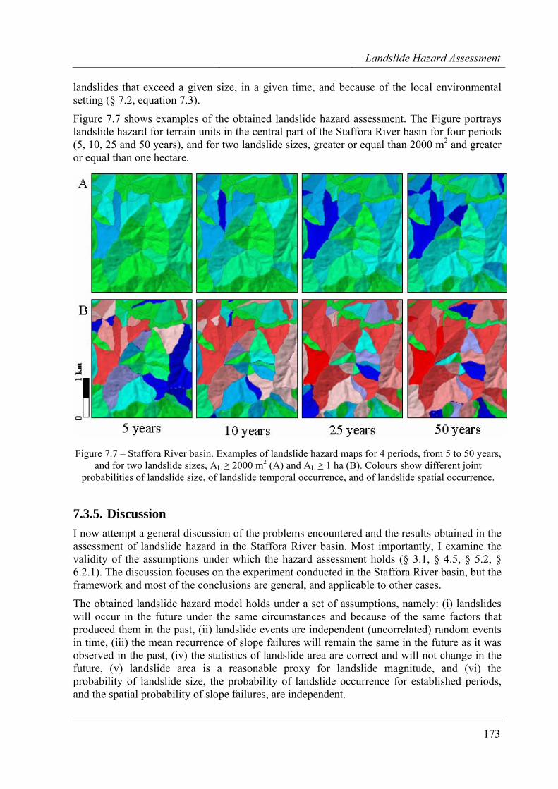
Landslide Hazard Assessment
173
landslides that exceed a given size, in a given time, and because of the local environmental setting (§ 7.2, equation 7.3).
Figure 7.7 shows examples of the obtained landslide hazard assessment. The Figure portrays landslide hazard for terrain units in the central part of the Staffora River basin for four periods (5, 10, 25 and 50 years), and for two landslide sizes, greater or equal than 2000 m2 and greater or equal than one hectare.
Figure 7.7 – Staffora River basin. Examples of landslide hazard maps for 4 periods, from 5 to 50 years, and for two landslide sizes, AL ≥ 2000 m2 (A) and AL ≥ 1 ha (B). Colours show different joint
probabilities of landslide size, of landslide temporal occurrence, and of landslide spatial occurrence.
7.3.5. Discussion I now attempt a general discussion of the problems encountered and the results obtained in the assessment of landslide hazard in the Staffora River basin. Most importantly, I examine the validity of the assumptions under which the hazard assessment holds (§ 3.1, § 4.5, § 5.2, § 6.2.1). The discussion focuses on the experiment conducted in the Staffora River basin, but the framework and most of the conclusions are general, and applicable to other cases.
The obtained landslide hazard model holds under a set of assumptions, namely: (i) landslides will occur in the future under the same circumstances and because of the same factors that produced them in the past, (ii) landslide events are independent (uncorrelated) random events in time, (iii) the mean recurrence of slope failures will remain the same in the future as it was observed in the past, (iv) the statistics of landslide area are correct and will not change in the future, (v) landslide area is a reasonable proxy for landslide magnitude, and (vi) the probability of landslide size, the probability of landslide occurrence for established periods, and the spatial probability of slope failures, are independent.
Chapter 7
174
That slope failures will occur in the future under the same conditions and because of the same factors that triggered them in the past is a recognized postulate for all functional (statistically based) susceptibility assessments (see § 6.2.1 and 6.4.1 for a discussion). As for the Upper Tiber River basin (§ 6.4), the main difficulty with this assumptions is that the environmental conditions (predisposing factors) that caused landslides “must remain the same in the future” in order to cause similar slope failures. It is reasonable to established (assume) a validity of the hazard model for the Staffora River basin of 50 years, approximately equivalent to the length of the period covered by the multi-temporal inventory used to establish landslide recurrence. Hence, the problem is that of investigating the possibility that the predisposing factors will change in the next 50 years, changing landslide susceptibility.
It is safe to assume that geological factors (e.g., lithology, structure, seismicity) will not change (significantly) in such a short geological time. Local morphological modifications can occur in the period due to stream erosion, landslides and human actions, but extensive morphological changes are not reasonably foreseeable. If significant changes should occur, the susceptibility model should be rejected or revaluated. Inspection of Table 7.2 reveals that 30 of the 36 thematic variables entered into the susceptibility model are not expected to change significantly in the considered period. However, variables describing land use types may change, locally significantly, and changes in land use are known to affect landslide frequency and abundance (Guthrie, 2002; Glade, 2003). Quantitative estimates of land use change are not available for the Staffora River basin, although they could be obtained by interpreting and comparing the available sets of aerial photographs. Qualitative estimates indicate a reduction of about 25% of the forest coverage in the period from 1955 to 1999, in favour of cultivated land. In the same period, agricultural practices have changed, largely aided by powerful mechanical equipments. If land use will change considerably in the Staffora River basin, the role of some the environmental variables considered in the susceptibility model will also change, hampering the validity of the model. A new model should be prepared, considering variables showing areas of land use change.
The adopted susceptibility model does not consider the landslide triggering factors, i.e., rainfall, seismic shaking or snow melting. Changes in the frequency or intensity of the driving forces will not affect (at least not in the considered period) the susceptibility model. However, the changes may affect the rate of occurrence of landslide events.
In the Apennines, evidence exists that where abundant clay, marl and sandstone crop out landslides exhibit spatial persistence, i.e., landslides occur more abundantly where they occurred in the past (Cardinali et al., 2000, § 4.4). If this is the case for the Staffora River basin, the assumption that landslide events are uncorrelated random events in time may be violated. Analysis in a GIS of the multi-temporal inventory reveals that 40% of all the landslides identified in the period from 1955 to 1999 (A2–E2 in Table 7.2) occurred inside landslide areas mapped on the 1955 aerial photographs (A0–A1). Considering only the 2390 landslides occurred in the 45-year period from 1955 to 1999 (A2–E2), 12% of the slope failures occurred in the same area of other landslides occurred in the same period. For the Staffora River basin, an archive inventory of historical landslide events covering the period from 1850 to 1998 is available. Analysis of the information listed in this inventory indicates that 389 landslide events occurred at 332 different sites, with only 38 sites affected two or more times. The same landslide site was affected on average 1.2 times, indicating a low rate of recurrence of events at the same site. All this concurs to establish that for the period of the hazard assessment (i.e., 50 years) in the Staffora River basin landslides can be considered uncorrelated random events in time.
Landslide Hazard Assessment
175
Analysis of the archive inventory provides information also on the triggering mechanisms of the slope failures. Of the 248 landslide events listed in the catalogue for which the triggering mechanism is known, 210 (84.7%) were the result of intense rainfall, 16 (6.5%) to a combination of intense rainfall and snow melting, infiltration, irrigation or broken pipes, 14 (5.6%) to erosion at the base of the slope, and eight (3.2%) to other causes. The analysis indicates that most of the landslides in the Staffora River basin are rainfall induced. If the rate of occurrence of the meteorological events that trigger landslides changes, the mean rate of slope failures will also change. If the intensity (amplitude and duration) of the rainfall will change, the rate of slope failures might change, in a way that is not predictable. For the coming decades, south of the Alps models of global climate change forecast the same total amount of yearly rainfall concentrated in a fewer number of high intensity events (Bradley et al., 1987; Brunetti et al., 2000; Easterling et al., 2000; IPCC, 2001). This may result in more abundant shallow landslides and in less frequent deep-seated slope failures (Buma and Dehn, 1998; Dehn and Buma, 1999). Modifications in land use induced by changes in agricultural practices may also locally change the rate of occurrence of landslides.
As I have shown in § 5, determining the statistics of landslide area is no trivial task (Guzzetti et al., 2002b; Malamud et al., 2004a). The (scant) available literature (Stark and Hovius, 2001; Guzzetti et al., 2002b; Guthrie and Evans, 2004a,b; Malamud et al., 2004a,b) seems to indicate that the frequency-area statistics of landslide areas does not change significantly across lithological or physiographical boundaries. Malamud et al. (2004a) showed that three different populations of landslides produced by different triggers (i.e., seismic shaking, intense rainfall, rapid snow melting) in different physiographical regions (southern California, central America, central Italy), exhibit virtually identical probability density functions. Data available for Umbria indicates that the probability density of landslide area does not change significantly with time. It is therefore safe to assume that in the Staffora River basin the frequency-area statistics of landslide area will not change in the period considered for the hazard assessment. It is also justified to use a single probability density function for the entire basin.
Hungr (1997) argued that no unique measure of landslide magnitude is available, and proposed to adopt destructiveness as a measure of landslide magnitude. In the Staffora River basin, landslide area was taken as a proxy for landslide destructiveness and of landslide magnitude. The area of the individual landslides was obtained in a GIS from the multi-temporal inventory. However, it is not established in the Staffora River basin that landslide area is necessarily a good measure of landslide destructiveness. Analysis of the archive inventory reveals that information on the size (area, length and width) of landslides is available for 26 events (6.7%), which range from 600 m2 to 0.6 km2 (mean = 5.8 ha, std. dev. = 13.5 ha). Damage caused by these landslides was mostly to the roads and subordinately to private homes and to the aqueduct. Information on landslide type is available for 28 events (7.2%), of which 15 were slides, 6 flows and 5 falls. Slides and flows caused the most severe damage, and falls produced only minor, temporary interruptions along the roads. Information on landslide velocity is available for five events, and ranges from 10 cm/h to 1 m/day. The ensemble of the historical information on damaging slope failures indicates that damage in the Staffora River basin is caused mostly by slow to rapid moving slides and flows (i.e., the type of failures considered in the hazard assessment), and that large landslides tend to produce larger damage.
The last assumption of the proposed model is that the probabilities of landslide size, of temporal occurrence, and of spatial incidence of mass movements are all independent. The
Chapter 7
176
legitimacy of this assumption is difficult to prove. As previously shown, in the Staffora River basin the probability of landslide area is largely independent from the physiographical setting. Hence, the probability of landslide area is independent from landslide susceptibility. The susceptibility model was constructed without considering the driving forces (meteorological or others) that control the rate of occurrence of slope failures in the basin. Thus, the rate of landslide events is largely independent from landslide susceptibility. Lastly, analysis of the information listed in the archive inventory revealed that slope failures occurred in all sizes, indicating that the rate of failures is independent from landslide size. Finally, the hazard model has produced many hazard maps, one for any of the many possible landslide scenarios (e.g., different landslide sizes, different return periods, etc.). How to combine this large number of maps into a single product useful to decision makers remains an open problem (§ 9.4).
7.4. Assessment of landslide hazard at the national scale
Establishing the level of landslide hazard for an entire nation is a difficult task, and only a few – largely empirical – attempts have been pursued (e.g., Radbruch-Hall et al., 1982; Brabb et al., 1999). The main difficulty of such attempts lies in the scant availability of relevant information for territories extending for hundreds of thousands of square kilometres. In Italy, relevant information is available to attempt a quantitative assessment of landslide hazard using a modified version of the probability model presented in § 7.2. The model requires three probability estimates, namely: (i) of the spatial probability of landslides (i.e., susceptibility), (ii) of the temporal occurrence of landslides, and (iii) of the magnitude (or the destructiveness) of the expected landslide event. Preliminary to the definition of landslide hazard is the selection of an appropriate mapping unit. For this experiment, the municipality (an administrative and political subdivision, § 6.2.2) is selected as the terrain partitioning unit. Italy is divided into 8102 municipalities, ranging in size from 1285 km2 (Rome) to 0.11 km2 (Atrani, Campania) (mean area = 37.3 km2, mode = 26.25 km2, std. dev. = 50.00 km2).
7.4.1. Spatial probability of landslide events Landslide susceptibility in each municipality was ascertained through discriminant analysis of independent thematic variables describing morphometry, hydrology, lithology and soil types (§ 2.1). Morphometric and hydrological variables were obtained in a raster GIS from the 90 m × 90 m DEM acquired by the Shuttle Radar Topography Mission (SRTM) in February of 2000. Lithological information was obtained from a synoptic geological map published by Compagnoni and his collaborators, in the period from 1976 to 1983. For the statistical analysis, the large number of rock units shown in the synoptic geological map (145 units) was grouped into 20 lithological types. Similarly, the 34 soil types shown in the synoptic soil map of Mancini (1966) were grouped into 8 classes of soil thickness and 11 classes of soil parent material. As a dependent variable, the presence/absence of historical landslide events listed in the archive inventory of the AVI project (see § 3.3.1.1) was used. Figure 7.8 shows the result of the susceptibility assessment.
7.4.2. Probability of event occurrence To establish the recurrence of the landslide events, and to estimate the probability of landslide occurrence in an established period, the archive inventory compiled by the AVI project was used (§ 3.3.1.1). This inventory lists 22,547 landslide events in the period between 1900 and 2001. In each municipality, the average recurrence of landslide events was obtained dividing
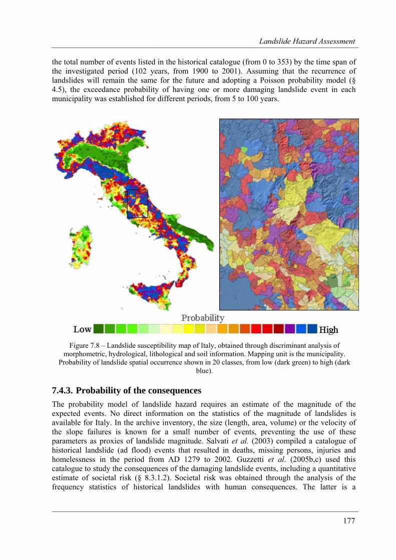
Landslide Hazard Assessment
177
the total number of events listed in the historical catalogue (from 0 to 353) by the time span of the investigated period (102 years, from 1900 to 2001). Assuming that the recurrence of landslides will remain the same for the future and adopting a Poisson probability model (§ 4.5), the exceedance probability of having one or more damaging landslide event in each municipality was established for different periods, from 5 to 100 years.
Figure 7.8 – Landslide susceptibility map of Italy, obtained through discriminant analysis of morphometric, hydrological, lithological and soil information. Mapping unit is the municipality.
Probability of landslide spatial occurrence shown in 20 classes, from low (dark green) to high (dark blue).
7.4.3. Probability of the consequences The probability model of landslide hazard requires an estimate of the magnitude of the expected events. No direct information on the statistics of the magnitude of landslides is available for Italy. In the archive inventory, the size (length, area, volume) or the velocity of the slope failures is known for a small number of events, preventing the use of these parameters as proxies of landslide magnitude. Salvati et al. (2003) compiled a catalogue of historical landslide (ad flood) events that resulted in deaths, missing persons, injuries and homelessness in the period from AD 1279 to 2002. Guzzetti et al. (2005b,c) used this catalogue to study the consequences of the damaging landslide events, including a quantitative estimate of societal risk (§ 8.3.1.2). Societal risk was obtained through the analysis of the frequency statistics of historical landslides with human consequences. The latter is a
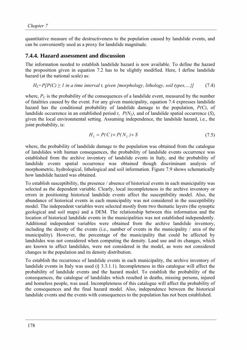
Chapter 7
178
quantitative measure of the destructiveness to the population caused by landslide events, and can be conveniently used as a proxy for landslide magnitude.
7.4.4. Hazard assessment and discussion The information needed to establish landslide hazard is now available. To define the hazard the proposition given in equation 7.2 has to be slightly modified. Here, I define landslide hazard (at the national scale) as:
HL=P[P(C) ≥ 1 in a time interval t, given {morphology, lithology, soil types,…}] (7.4)
where, PC is the probability of the consequences of a landslide event, measured by the number of fatalities caused by the event. For any given municipality, equation 7.4 expresses landslide hazard has the conditional probability of landslide damage to the population, P(C), of landslide occurrence in an established period t, P(NL), and of landslide spatial occurrence (S), given the local environmental setting. Assuming independence, the landslide hazard, i.e., the joint probability, is:
S)N(P)C(PH LL ××= (7.5)
where, the probability of landslide damage to the population was obtained from the catalogue of landslides with human consequences, the probability of landslide events occurrence was established from the archive inventory of landslide events in Italy, and the probability of landslide events spatial occurrence was obtained though discriminant analysis of morphometric, hydrological, lithological and soil information. Figure 7.9 shows schematically how landslide hazard was obtained.
To establish susceptibility, the presence / absence of historical events in each municipality was selected as the dependent variable. Clearly, local incompleteness in the archive inventory or errors in positioning historical landslide events affect the susceptibility model. Also, the abundance of historical events in each municipality was not considered in the susceptibility model. The independent variables were selected mostly from two thematic layers (the synoptic geological and soil maps) and a DEM. The relationship between this information and the location of historical landslide events in the municipalities was not established independently. Additional independent variables were obtained from the archive landslide inventory, including the density of the events (i.e., number of events in the municipality / area of the municipality). However, the percentage of the municipality that could be affected by landslides was not considered when computing the density. Land use and its changes, which are known to affect landslides, were not considered in the model, as were not considered changes in the population and its density distribution.
To establish the recurrence of landslide events in each municipality, the archive inventory of landslide events in Italy was used (§ 3.3.1.1). Incompleteness in this catalogue will affect the probability of landslide events and the hazard model. To establish the probability of the consequences, the catalogue of landslides which resulted in deaths, missing persons, injured and homeless people, was used. Incompleteness of this catalogue will affect the probability of the consequences and the final hazard model. Also, independence between the historical landslide events and the events with consequences to the population has not been established.
Landslide Hazard Assessment
179
Figure 7.9 – Schematic representation of the procedure adopted to evaluate landslide hazard at the national scale, in Italy.
As in the case of the Staffora River basin (§ 7.3), the hazard model has produced (or can produce) many different hazard maps, one for any of the several possible landslide scenarios (e.g., different expected number of fatalities, different return periods, etc.). How to combine the large number of maps into a product useful to decision makers remains an open problem (§ 9.4).
Chapter 7
180
The obtained assessment is the first quantitative and reproducible estimate of landslide hazard available for Italy, at the national (synoptic) scale. The model is functional (i.e., statistical), and its quality depends (almost) entirely on the quality, completeness and relevance of the input data. Most vitally, the validity and limitations of the basic assumptions on which the probabilistic model was developed were not proven for this national hazard assessment. This is not an easy task that requires further investigation.
7.5. Rock fall hazard assessment along the Nera and Corno valleys
Rock fall is a common-place geomorphological process and represents a major hazard in mountain areas worldwide (Whalley, 1984; Flageollet and Weber, 1996). Rock falls range in size from small cobbles to large boulders of hundreds of cubic meters, travel at speeds ranging from few to tens of meters per second, and for long distances from the detachment zone to the deposition area (Cruden and Varnes, 1996). Despite their often relatively small size, rock falls are among the most destructive mass movements (Whalley, 1984; Rochet, 1987, Evans and Hungr, 1993; Evans, 1997), and in Italy they represent a primary cause of landslide fatalities (Guzzetti, 2000; Guzzetti et al., 2005c).
The size and speed of rock falls, and their ability to travel long distances (exceeding one kilometre) makes the previously discussed methods to ascertain landslide hazard largely unsuitable to rock falls. In particular, it is the subdivision of terrain based on slope units or geo-hydrological units that is largely incompatible with this landslide type. A boulder detached from a rock cliff can travel across geo-hydrological or slope unit boundaries. Rock fall susceptibility and hazard are not related only to where rock falls occur (i.e., where they detach), but also to where rock falls travel and deposit. For rock falls, quantitative measures of their magnitude are possible. Knowing the mass of the falling boulder (i.e., the volume × the rock density) and its velocity, kinetic or potential energy can be easily computed, which represent a direct measure of the magnitude of the event, a good proxy for destructiveness. If the size of the boulder is undetermined, velocity can be selected as a reasonable proxy for magnitude.
In the following, I describe a quantitative attempt to determine rock fall hazard along the Nera River and the Corno River valleys, in south eastern Umbria (§ 2.5). The attempt is based on the use of the computer programme STONE (Guzzetti et al., 2002), which I briefly describe below..
7.5.1. The computer program STONE To assess rock fall hazard, knowledge on the spatial (geographical) distribution of the expected rock falls is essential. To obtain this information, I contributed to develop STONE (Guzzetti et al., 2002), a computer program capable of simulating rock fall processes in three-dimensions. STONE uses a lumped-mass approach to simulate rock fall processes. The falling boulder is considered dimensionless and a kinematic simulation is performed. The input data required by STONE include: (i) the location of the detachment areas of rock falls, (ii) the number of boulders launched from each detachment area, (iii) the starting velocity and horizontal angle of the rock fall, (iv) a velocity threshold below which a boulder stops, (v) a DEM describing topography, and (vi) the coefficients of dynamic rolling friction, and of normal and tangential energy restitution used to simulate the loss of energy where the boulder
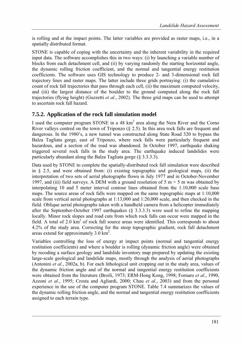
Landslide Hazard Assessment
181
is rolling and at the impact points. The latter variables are provided as raster maps, i.e., in a spatially distributed format.
STONE is capable of coping with the uncertainty and the inherent variability in the required input data. The software accomplishes this in two ways: (i) by launching a variable number of blocks from each detachment cell, and (ii) by varying randomly the starting horizontal angle, the dynamic rolling friction coefficient, and the normal and tangential energy restitution coefficients. The software uses GIS technology to produce 2- and 3-dimensional rock fall trajectory lines and raster maps. The latter include three grids portraying: (i) the cumulative count of rock fall trajectories that pass through each cell, (ii) the maximum computed velocity, and (iii) the largest distance of the boulder to the ground computed along the rock fall trajectories (flying height) (Guzzetti et al., 2002). The three grid maps can be used to attempt to ascertain rock fall hazard.
7.5.2. Application of the rock fall simulation model I used the computer program STONE in a 48 km2 area along the Nera River and the Corno River valleys centred on the town of Triponzo (§ 2.5). In this area rock falls are frequent and dangerous. In the 1980’s, a new tunnel was constructed along State Road 320 to bypass the Balza Tagliata gorge, east of Triponzo, where rock falls were particularly frequent and hazardous, and a section of the road was abandoned. In October 1997, earthquake shaking triggered several rock falls in the study area. The earthquake induced landslides were particularly abundant along the Balza Tagliata gorge (§ 3.3.3.3).
Data used by STONE to complete the spatially-distributed rock fall simulation were described in § 2.5, and were obtained from: (i) existing topographic and geological maps, (ii) the interpretation of two sets of aerial photographs flown in July 1977 and in October-November 1997, and (iii) field surveys. A DEM with a ground resolution of 5 m × 5 m was obtained by interpolating 10 and 5 meter interval contour lines obtained from the 1:10,000 scale base maps. The source areas of rock falls were mapped on the same topographic maps at 1:10,000 scale from vertical aerial photographs at 1:13,000 and 1:20,000 scale, and then checked in the field. Oblique aerial photographs taken with a handheld camera from a helicopter immediately after the September-October 1997 earthquakes (§ 3.3.3.3) were used to refine the mapping locally. Minor rock slopes and road cuts from which rock falls can occur were mapped in the field. A total of 2.0 km2 of rock fall source areas were identified. This corresponds to about 4.2% of the study area. Correcting for the steep topographic gradient, rock fall detachment areas extend for approximately 3.0 km2.
Variables controlling the loss of energy at impact points (normal and tangential energy restitution coefficients) and where a boulder is rolling (dynamic friction angle) were obtained by recoding a surface geology and landslide inventory map prepared by updating the existing large-scale geological and landslide maps, mostly through the analysis of aerial photographs (Antonini et al., 2002a, b). For each lithological unit cropping out in the study area, values of the dynamic friction angle and of the normal and tangential energy restitution coefficients were obtained from the literature (Broili, 1973; ERM-Hong Kong, 1998; Fornaro et al., 1990, Azzoni et al., 1995; Crosta and Agliardi, 2000; Chau et al., 2003) and from the personal experience in the use of the computer program STONE. Table 7.4 summarizes the values of the dynamic rolling friction angle, and the normal and tangential energy restitution coefficients assigned to each terrain type.
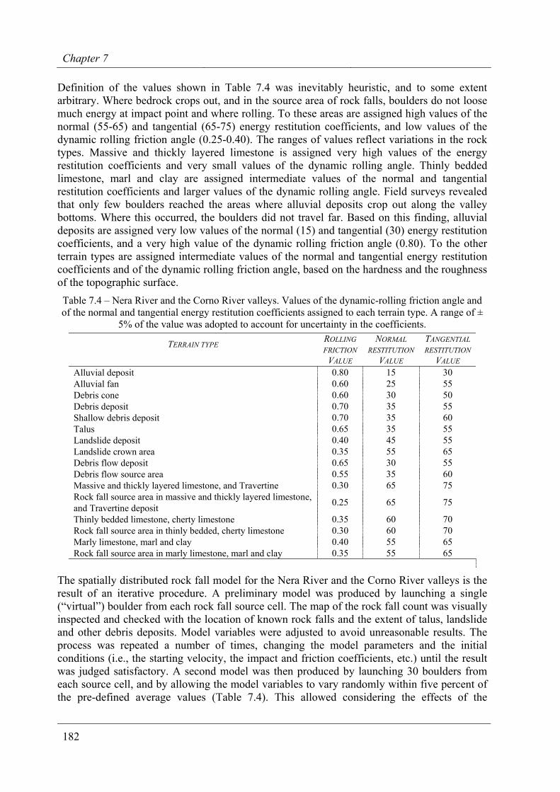
Chapter 7
182
Definition of the values shown in Table 7.4 was inevitably heuristic, and to some extent arbitrary. Where bedrock crops out, and in the source area of rock falls, boulders do not loose much energy at impact point and where rolling. To these areas are assigned high values of the normal (55-65) and tangential (65-75) energy restitution coefficients, and low values of the dynamic rolling friction angle (0.25-0.40). The ranges of values reflect variations in the rock types. Massive and thickly layered limestone is assigned very high values of the energy restitution coefficients and very small values of the dynamic rolling angle. Thinly bedded limestone, marl and clay are assigned intermediate values of the normal and tangential restitution coefficients and larger values of the dynamic rolling angle. Field surveys revealed that only few boulders reached the areas where alluvial deposits crop out along the valley bottoms. Where this occurred, the boulders did not travel far. Based on this finding, alluvial deposits are assigned very low values of the normal (15) and tangential (30) energy restitution coefficients, and a very high value of the dynamic rolling friction angle (0.80). To the other terrain types are assigned intermediate values of the normal and tangential energy restitution coefficients and of the dynamic rolling friction angle, based on the hardness and the roughness of the topographic surface.
Table 7.4 – Nera River and the Corno River valleys. Values of the dynamic-rolling friction angle and of the normal and tangential energy restitution coefficients assigned to each terrain type. A range of ±
5% of the value was adopted to account for uncertainty in the coefficients.
TERRAIN TYPE ROLLING FRICTION
NORMAL RESTITUTION
TANGENTIAL RESTITUTION
VALUE VALUE VALUE Alluvial deposit 0.80 15 30 Alluvial fan 0.60 25 55 Debris cone 0.60 30 50 Debris deposit 0.70 35 55 Shallow debris deposit 0.70 35 60 Talus 0.65 35 55 Landslide deposit 0.40 45 55 Landslide crown area 0.35 55 65 Debris flow deposit 0.65 30 55 Debris flow source area 0.55 35 60 Massive and thickly layered limestone, and Travertine 0.30 65 75 Rock fall source area in massive and thickly layered limestone, and Travertine deposit 0.25 65 75
Thinly bedded limestone, cherty limestone 0.35 60 70 Rock fall source area in thinly bedded, cherty limestone 0.30 60 70 Marly limestone, marl and clay 0.40 55 65 Rock fall source area in marly limestone, marl and clay 0.35 55 65
The spatially distributed rock fall model for the Nera River and the Corno River valleys is the result of an iterative procedure. A preliminary model was produced by launching a single (“virtual”) boulder from each rock fall source cell. The map of the rock fall count was visually inspected and checked with the location of known rock falls and the extent of talus, landslide and other debris deposits. Model variables were adjusted to avoid unreasonable results. The process was repeated a number of times, changing the model parameters and the initial conditions (i.e., the starting velocity, the impact and friction coefficients, etc.) until the result was judged satisfactory. A second model was then produced by launching 30 boulders from each source cell, and by allowing the model variables to vary randomly within five percent of the pre-defined average values (Table 7.4). This allowed considering the effects of the
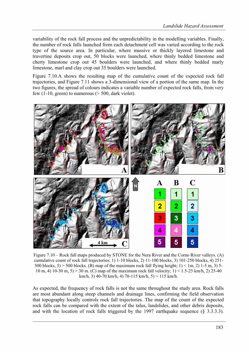
Landslide Hazard Assessment
183
variability of the rock fall process and the unpredictability in the modelling variables. Finally, the number of rock falls launched from each detachment cell was varied according to the rock type of the source area. In particular, where massive or thickly layered limestone and travertine deposits crop out, 50 blocks were launched, where thinly bedded limestone and cherty limestone crop out 45 boulders were launched, and where thinly bedded marly limestone, marl and clay crop out 35 boulders were launched.
Figure 7.10.A shows the resulting map of the cumulative count of the expected rock fall trajectories, and Figure 7.11 shows a 3-dimensional view of a portion of the same map. In the two figures, the spread of colours indicates a variable number of expected rock falls, from very few (1-10, green) to numerous (> 500, dark violet).
Figure 7.10 – Rock fall maps produced by STONE for the Nera River and the Corno River valleys. (A) cumulative count of rock fall trajectories; 1) 1-10 blocks, 2) 11-100 blocks, 3) 101-250 blocks, 4) 251-500 blocks, 5) > 500 blocks. (B) map of the maximum rock fall flying height; 1) < 1m, 2) 1-5 m, 3) 5-10 m, 4) 10-30 m, 5) > 30 m. (C) map of the maximum rock fall velocity; 1) < 1.5-25 km/h, 2) 25-40
km/h, 3) 40-70 km/h, 4) 70-115 km/h, 5) > 115 km/h.
As expected, the frequency of rock falls is not the same throughout the study area. Rock falls are most abundant along steep channels and drainage lines, confirming the field observation that topography locally controls rock fall trajectories. The map of the count of the expected rock falls can be compared with the extent of the talus, landslides, and other debris deposits, and with the location of rock falls triggered by the 1997 earthquake sequence (§ 3.3.3.3).
Chapter 7
184
Comparison with the extent of talus deposits reveals that only at few places the map of the rock fall count exceeds down-slope the extent of the talus deposits. In places this occurs where the lower limit of the talus corresponds to the flat part of the valley bottom. Comparison with the location of the earthquake-induced failures reveals that the extent of the expected rock fall areas and the frequency of rock fall trajectories are in good agreement with the available information on known rock fall events. Of the 109 known rock fall deposits, 98 (89.9%) are located in areas where rock falls are expected, and 11 (10.1%) occur in areas where rock falls are not expected. This is an efficient form of model validation. A final model validation was performed by randomly inspecting the distribution of the vertical distance of the rock fall trajectories (Figure 7.10.B) (flying height, i.e., the distance of the boulder to the ground) and of the rock fall maximum velocity (Figure 7.10.C). Results indicate that the computed rock fall velocity locally exceeds 250 km·h-1 and the computed rock fall flying height ranges from zero, where boulders are rolling, to more that 165 metres above the ground, near high cliffs.
Figure 7.11 – Triponzo area, along the Nera River and the Corno River valleys. Three-dimensional view of a portion of the grid map showing the count of rock fall trajectories (Figure 7.10.A). Colours indicate increasing number of rock fall trajectories, from few (light blue) to very many (dark violet).
7.5.3. Rock fall hazard assessment The three raster maps produced by STONE and discussed before can be used to ascertain rock fall hazard along the Nera River and the Corno River valleys. The map showing the total number of rock fall trajectories (Figure 7.10.A) can be considered a convenient proxy for the expected frequency of rock fall occurrence. For each grid cell the count of rock fall trajectories is a proxy for the probability of being struck by a falling or rolling boulder. The larger the number of computed trajectories, the higher the expected frequency of rock fall occurrence. Maps of the largest distance to the ground (Figure 7.10.B) and of the highest computed velocity (Figure 7.10.C) provide information on the intensity of the expected rock fall, a proxy for the maximum kinetic energy at each grid cell (Guzzetti et al., 2002).
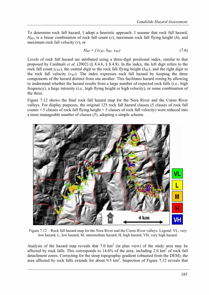
Landslide Hazard Assessment
185
To determine rock fall hazard, I adopt a heuristic approach. I assume that rock fall hazard, HRF, is a linear combination of rock fall count (c), maximum rock fall flying height (h), and maximum rock fall velocity (v), or
HRF = f (cRF, hRF, vRF) (7.6)
Levels of rock fall hazard are attributed using a three-digit positional index, similar to that proposed by Cardinali et al. (2002) (§ 8.4.6, § 8.4.8). In the index, the left digit refers to the rock fall count (cRF), the central digit to the rock fall flying height (hRF), and the right digit to the rock fall velocity (vRF). The index expresses rock fall hazard by keeping the three components of the hazard distinct from one another. This facilitates hazard zoning by allowing to understand whether the hazard results from a large number of expected rock falls (i.e., high frequency), a large intensity (i.e., high flying height or high velocity), or some combination of the three.
Figure 7.12 shows the final rock fall hazard map for the Nera River and the Corno River valleys. For display purposes, the original 125 rock fall hazard classes (5 classes of rock fall counts × 5 classes of rock fall flying height × 5 classes of rock fall velocity) were reduced into a more manageable number of classes (5), adopting a simple scheme.
Figure 7.12 – Rock fall hazard map for the Nera River and the Corno River valleys. Legend: VL, very low hazard, L, low hazard, M, intermediate hazard, H, high hazard, VH, very high hazard.
Analysis of the hazard map reveals that 7.0 km2 (in plan view) of the study area may be affected by rock falls. This corresponds to 14.6% of the area, including 2.0 km2 of rock fall detachment zones. Correcting for the steep topographic gradient (obtained from the DEM), the area affected by rock falls extends for about 9.5 km2. Inspection of Figure 7.12 reveals that
Chapter 7
186
rock fall hazard is not distributed uniformly. About 3.4 km2 of the study area (in plan view) are subject to low (25.5%) or very low (23.0%) hazard, 1.5 km2 (22.2%) are subject to intermediate hazard conditions, and 2.0 km2 are subject to high (15.3%) or very high (14.0%) hazard.
By overlaying the rock fall hazard map with the map of the transportation network in a GIS, the sections of the roads potentially subject to rock falls can be identified. Of the 31.8 km of paved roads in the study area, 9.0 km (28.5%) are found to be potentially affected by rock fall hazard.
Comparison of the hazard map with the location of the earthquake-induced rock fall events in 1997 reveals that 72.5% of the seismically induced rock falls occurred in areas where the hazard is expected to be moderate to high or very high, and 17.4% in areas where rock fall hazard is expected to be low or very low. The remaining 10.1% of the earthquake induced failures occurred in areas where rock falls are not forecasted by the model. The latter, are largely due to minor inconsistencies in the DEM used to perform the simulation.
Immediately after the earthquakes of September-October 1997, the Government of Umbria and the National Road Company (ANAS) invested considerable resources to install defensive measures to mitigate rock fall hazard and risk along the Nera River and the Corno River valleys. Four types of defensive measures were installed: (i) passive revetment nets, (ii) elastic rock fences, (iii) concrete retaining walls, and (iv) artificial tunnels. The remedial measurements were taken without considering the hazard assessment discussed here. Also, the rock fall hazard assessment shown in Figure 7.12 does not consider the presence of the defensive measures. Hence, the model locally overestimates the hazard and the associated risk.
To determine the mitigating effects of existing defensive structures, I now perform a set of three additional simulations. The first simulation (Model 2, Table 7.5) considers the presence of the passive revetment nets. The areas where passive revetment nets were installed were mapped in the field using the same base maps at 1:10,000 scale used to identify the rock fall source areas. A total of 0.3 km2 of revetment nets were mapped, mostly along or in the vicinity of the roads. The revetment nets are assumed fully capable of preventing rock falls, i.e., that no boulder could detach or fall where the revetment nets are present. Based on this assumption, a new rock fall hazard model is prepared that differed from the previous model (shown in Figure 7.12) only in terms of the reduced extent of the rock fall source areas. In this new model the total rock fall source areas extend for 1.7 km2 (Table 7.5). According to the new model, the area potentially affected by rock falls decreases to 6.5 km2 (13.5%) and the length of roads subject to rock fall hazard decreases to 6.5 km (20.5%). The presence of the passive revetment nets reduces by 7.4% the extent of the area potentially subject to rock falls, and by about 27.9% the total length of roads subject to rock fall hazard. The reduction is larger along the roads than in the rest of the hazardous areas.
In the second simulation (Model 3, Table 7.5) the presence of the other defensive structures, namely the elastic rock fences, the concrete barriers, and the artificial tunnels, is considered. For simplicity, the possibility of a boulder that breaks through, or flies over an elastic fences or a concrete barrier is excluded. Rock fences and concrete barriers are linear features in plan view, and for modelling purposes they are transformed into strips of adjacent pixels 5 m × 5 m in size. A new rock fall hazard model is prepared taking into account the presence of the revetment nets (i.e., reducing the extent of the rock fall source area), the location of the elastic rock fall fences and concrete barriers (i.e., the rock fall retaining structures), and the presence of the artificial tunnels. The new model reveals that the extent of the area subject to rock fall
Landslide Hazard Assessment
187
hazard decreases to 6.3 km2 (13.1%). Correspondingly, the total length of road subject to rock fall hazard reduces to 2.9 kilometres, or 9.2% of the considered road network. The analysis indicates that the combined effect of all the existing defensive structures reduced by about 10.4% the extent of the area subject to rock falls, and by about 67.8% the total length of roads subject to rock fall hazard. Again, the reduction is larger along the roads than in other areas, because of the location of the defensive structures, which were installed chiefly along or in the immediate vicinities of the roads.
Table 7.5 – Nera River and the Corno River valleys. Comparison of different rock fall hazard models prepared considering and not considering the presence and efficacy of the rock fall defensive structures
installed in the area.
ROCK FALL SOURCE AREA AFFECTED AREA AFFECTED ROADS
km2 km2 % km %
Model 1 Defensive measures not considered 2.0 7.0 14.6 9.0 28.5
Model 2 Revetment nets considered 1.7 6.5 13.5 6.5 20.5
Model 3 All defensive measures present in the area, considered fully efficient 1.7 6.3 13.1 2.9 9.2
Model 4 All defensive measures present in the area, efficacy is considered 1.7 6.4 8.9 4.1 12.8
The third simulation (Model 4, Table 7.5) consists in the evaluation the efficacy of the rock fall retaining structures. This is accomplished in two steps. First, for each grid cell the maximum height of the computed rock fall trajectories was compared to the height of the retaining structures. The analysis revealed that 20.7% of the retaining structures could be “jumped” by high flying rocks. Then, the possibility that a boulder could have enough kinetic energy to break through an elastic fence or a concrete wall was considered. For the purpose, it was assumed that the retaining structures could absorb up to 2500 kJ, a reasonable value for the structures present in the study area. At each grid cell the maximum computed rock fall velocity was used to calculate the corresponding boulder maximum kinetic energy, assuming a characteristic volume of 2 cubic meters and a unit weight of 2500 kg·m3. The latter spatial analysis reveals that 10.2% of the existing retaining structures can be destroyed or damaged by falling blocks. The analysis also shows that 21.0% of the rock fall elastic fences or concrete walls can be either bypassed by high flying rock falls, or can be damaged or destroyed by fast moving boulders. These defensive structures are at least partly ineffective in protecting from rock falls. The final step in the analysis consists in preparing a last hazard model not considering the presence of the “ineffective” defensive structures. This last model reveals that 4.1 km of roads in the study area (12.8%) are potentially subject to rock fall hazard. The combined effect of all the effective defensive structures reducs by about 8.9% the total extent of the area subject to rock falls, and by about 55.1% the total length of roads subject to rock fall hazard. The model indicates that, despite the considerable reduction in rock falls risk due to the presence of numerous defensive structures, residual risk still exists along roads in the Nera River and the Corno River valleys.
Chapter 7
188
7.5.4. Discussion I now briefly discuss the results obtained in the assessment of rock fall hazard along the Nera River and the Corno River valleys. The discussion focuses on the performed experiment, but conclusions are applicable to other areas and, more generally, I consider them relevant to the application of process-based models for the assessment of landslide susceptibility and hazard (§ 6.2.3.5).
The model of the rock fall process implemented in the computer code STONE is necessarily simplified (Guzzetti et al., 2002; Agliardi and Crosta, 2004). Constraints in the model reflect into the software outputs and in the hazard assessment. In the shown experiment, selection of the input parameters required by STONE was heuristic and to some extent arbitrary. The horizontal starting velocity was kept constant (in scale and direction) throughout the study area, and was not selected considering the ground movements measured at nearby accelerometer stations. Values of the parameters used to simulate the loss of energy where boulders are rolling and at the impact points (Table 7.4) were selected heuristically, without any field experiment (which however is difficult to perform). The version of the software STONE used for the analysis does not consider the volume, shape and mass of the falling boulder (i.e., fully kinematic modelling). The simplification may be relevant where the boulder is flying at high speeds along ballistic trajectories (air friction is neglected), and at impact points, where the shape, volume and mass of the boulder are important to determine the energy lost during impact and the velocity and direction of the flying boulder. The implemented model does not consider sliding of the boulder, which may be important in the early stages of a rock fall (i.e., in the detachment area) and at the impact point. Finally, the model does not consider the possibility that at impact points a boulder may brake and rock fragments fly in different directions at various velocities. This is a condition that exists in nature, and that can result in very hazardous situations.
The quality of the rock fall simulation depends also on other factors, including the complete and accurate identification of rock fall source cells and the quality of the DEM. Over large areas the detachment areas of rock falls are not easy to identify and map precisely. Minor rock slopes and small road cuts may not be shown in the map of the rock fall source cells. As a consequence the model may locally underestimate the spatial extent of the rock fall problem. Where terrain is very steep and bedrock crops out, contour lines were not shown in the base maps. In these areas the DEM does not accurately represent the topography, and the rock fall hazard model may be locally imprecise.
Values of the adopted rock fall hazard index do not provide an absolute ranking of hazard levels. If the extreme values are easy to define, intermediate conditions of rock fall hazard are more difficult to rank. A grid cell where rock fall frequency is very low and the flying height and velocity are very low (HRF = 111) will have a much lower hazard than a grid cell that exhibits very high rock fall frequency, and very large flying height and velocity (HRF = 555). Deciding whether a grid cell with very high frequency and light rock fall intensity (HRF = 511) has a larger hazard than that of a grid cell with very low expected frequency and very high rock fall intensity (HRF = 155) is not straightforward, and may be a matter of opinion or local judgment (e.g., Cardinali et al., 2002; Reichenbach et al., 2005).
The evaluation of the efficacy of the rock fall defensive structures is affected by completeness and resolution of the mapping. Identification of revetment nets, elastic rock fences, and rock walls was straightforward, but accurate mapping was locally difficult due to the size of the structures (locally a few tens of square meters) compared to the scale of the maps (1:10,000).
Landslide Hazard Assessment
189
When estimating the mitigating effects of the revetment nets, the assumption was made that structures were completely efficient in preventing the detachment of rock falls. The assumption may be incorrect where large boulders are expected. The output of the computer model provided information only on the maximum values of the rock fall flying height and travel velocity. Average, or modal values were not considered and the frequency of the extreme values remains unknown. For the identification of the sections of the retaining structures that were unable to catch all the high-flying boulders or that could be destroyed by fast moving blocks, only the maximum computed values were used. As a result, the extent of the potentially ineffective retaining structures may have been overestimated. In addition, the estimate of the efficacy of the retaining structures did not consider the presence of multiple sets of elastic fences along the slopes.
As a result of these considerations, the spatial evaluation of the rock fall hazard along the Nera River valley and the assessment of the possible associated risk along the roads are undoubtedly affected by uncertainties and limitations that must be considered when using the model results for mitigation and planning purposes.
7.6. Summary of achieved results
In this chapter, I have:
(a) Proposed a probabilistic model for the assessment of landslide hazard, which fulfils a standard definition of landslide hazard.
(b) Tested the proposed model at the catchment scale, exploiting geomorphological information on slope failures obtained from a multi-temporal landslide inventory map.
(c) Demonstrated that probabilistic landslide hazard assessment can be conducted at the national scale. However, verification of the validity of the many assumptions on which the model is based was not possible at the synoptic scale.
(d) Demonstrated that the proposed probabilistic framework can also be adopted to determine the hazard posed by rock falls – a different type of mass movement – exploiting results obtained by a 3-dimensional rock fall simulation model.
This responds to Question # 6 posed in the Introduction (§ 1.2).

191
8. LANDSLIDE RISK EVALUATION
A disaster is often a sequence of apparently harmless, little mistakes.
Before I step into a puddle,
I'd like to know how deep it is.
Risk assessment is the final goal of many landslide investigations. It lays at the fuzzy boundary between science, technology, economy and politics, including planning and policy making. Assessing landslide risk is a complex and uncertain operation that requires the combination of different techniques, methods and tools, and the interplay of various expertises pertaining – among the others – to geology and geomorphology, engineering and environmental sciences, meteorology, climatology, mathematics, information technology, economics, social sciences and history. Despite the indisputable importance of landslide risk evaluation for decision making, comparatively little efforts have been made to establish and systematically test methods for landslide risk assessment, and to determine their advantages and limitations.
In this chapter, after a brief review of the relevant literature, I present concepts and definitions useful for landslide risk assessment, including a discussion of the differences between quantitative (probabilistic) and qualitative (heuristic) approaches. I then make various examples of probabilistic, heuristic, and geomorphological landslide risk assessments. The examples include: (i) the determination of societal and individual levels of landslide risk in Italy, and a comparison with risk levels posed by other natural and man-made hazards, and by the principal medical causes of deaths in Italy, (ii) a preliminary attempt to establish the geographical distribution of landslide risk to the population in Italy, (iii) the determination of rock fall risk to vehicles and pedestrians along roads in the Nera River and the Corno River valleys, in eastern Umbria, (iv) the design and application of a geomorphological method for the determination of heuristic levels of landslide risk at selected sites in Umbria, based on information obtained from the interpretation of multiple sets of aerial photographs of different ages, combined with the analysis of historical information on past landslide events, and pre-existing knowledge on landslide type and abundance, (v) an attempt to determine the type and extent of landslide damage in Umbria, based on the analysis of a catalogue of landslides and their consequences, and (vi) an effort to establish the location and extent of sites of possible landslide impact on the population, the agriculture, the built-up environment, and the transportation network in Umbria.
Chapter 8
192
8.1. Literature review
Literature on landslide risk is less ample than the literature on landslide mapping and landslide susceptibility and hazard assessment. This has several reasons, including: (i) the inherent difficulty to ascertain landslide risk – an operation that requires the preliminary assessment of landslide abundance, susceptibility and hazard, (ii) a generalized lack of relevant information to determine landslide risk, heuristically or using probabilistic methods, (iii) the interdisciplinary nature of landslide risk evaluation that requires the cooperative interplay of different expertises – a condition often difficult to obtain, and (iv) the fact that only recently have scientists, practitioners and decision makers demonstrated interest in landslide risk assessment studies.
Literature dealing with the general principles, theory, mathematics, economy, management, and philosophy of risk posed by natural hazards – including landslides – comprises: Starr (1969), IDNHR Advisory Committee, (1987), Slovic 1987), Ale (1991), Canadian Standards Association (1991), UNDRO (1991), The Royal Society (1992), Funtowicz and Ravetz (1995), Horlick-Jones et al. (1995), Olshansky (1990, 1996), Stern and Fineberg (1996), Keller et al. (1997); Quarantelli (1998), National Research Council (1999), Tobin (1999), Woo (1999), Alexander (2000, 2002), Papadopoulos et al. (2000), Batabyal and Beladi (2001), Skidmore (2001), Vecchia (2001) and Sandin (2004). In recent years, a few books and technical reports specifically aimed at reviewing and discussing the principles, concepts and definitions of landslide risk, at examining the theory of landslide risk assessment, and at proposing quantitative and qualitative methods for the evaluation of landslide risk have been published. These references include: Cruden and Fell, eds. (1997), Vecchia, ed. (2001), Wise et al., eds. (2004a), Lee (2004), Glade et al., eds. (2005) and Hungr et al., eds. (2005). Significantly, the majorities of the references is the cooperative result of multi-author efforts, or represent the outcome of conferences or specialized technical workshops.
A systematic and critical evaluation of the literature on landslide risk is beyond the scope of this work. An initial, but sufficiently complete review of the literature reveals that books, scientific papers and technical reports on landslide risk cover a large and diversified spectrum of topics, including:
(i) Nomenclature, concepts and definitions, an important and often overlooked aspect or landslide risk assessment. Recognized nomenclature and clearly stated definitions allow for establishing standards and for comparing the results of risk assessments (Varnes and IAEG Commission on Landslides and other Mass-Movements, 1984; Canadian Standards Association, 1991; ANCOLD, 1994; Fell, 1994, 2000; Canuti and Casagli, 1996; Chowdhury, 1996; Cruden and Fell, 1997; Evans, 1997; International Union of Geological Sciences Committee on Risk Assessment, 1997; Morgenstern, 1997; Geotechnical Engineering Office, 1998; Australian Geomechanics Society, 2000; Raetzo et al., 2002; Guzzetti et al., 2003a; Committee on the Review of the National Landslide Hazards Mitigation Strategy; 2004; Lee, 2004; Technical Committee on Risk Assessment and Management, 2004; Vandine et al., 2004a, 2004b; Wise et al., 2004a; Crozier, 2005; Crozier and Glade, 2005; Fell et al., 2005; Glade et al., 2005; Reichenbach et al., 2005; VanDine et al., 2005);
(ii) Principles, theory, probability methods and modelling approaches, which lay at the foundation of scientific landslide risk assessment (Varnes and IAEG Commission on Landslides and other Mass-Movements, 1984; Einstein, 1988, 1997; Canadian Standards Association, 1991; ANCOLD, 1994; Fell, 1994; Wu et al., 1996; Cruden and Fell, 1997; Fell
Landslide risk
193
and Hartford, 1997; Vecchia, 2001; Wise et al., 2004a; Xie and Xia, 2004; Guzzetti et al., 2005b,c; Plattner, 2005);
(iii) Assessment, application and discussion of case studies. In landslide risk assessment, demonstration, comparison and critical analysis of the results of risk evaluations are the best way of testing theories, methods and models (Stevenson, 1977, 1978; Fukuoka, 1978; Lessing et al., 193; Brand, 1988; Neeley and Rice, 1990; Olshansky, 1990; Carrara et al., 1991b; Morgan et al., 1992; Anderson et al., 1996; Eusebio et al., 1996; Leroi, 1996; Cruden, 1997; Cruden and Fell, eds. 1997; ERM-Hong Kong, 1998; Geotechnical Engineering Office, 1998; Michael-Leiba et al., 1999; Alexander, 2000; Budetta, 2002; Cardinali et al., 2002a; Dai et al., 2002; Guzzetti et al., 2003a, 2003b; Bonnard, et al., 2004; Chatterton, 2004; Guzzetti et al., 2004c; Lee, 2004; Wise et al., 2004a; Crosta et al., 2005; Fell et al., 2005; Glade et al., 2005; Leroi et al., 2005; Malone, 2005; Michael-Leiba et al., 2005; Reichenbach et al., 2005; Roberds, 2005; Sorriso-Valvo, 2005);
(iv) Management and mitigation methods and strategies. Risk assessment as such is of little interest to society. Risk assessment becomes useful when it provides insight on mitigation strategies and management methods (Fleming et al., 1979; Olshansky and Rogers, 1987; Flageollet, 1989; Anderson et al., 1996; Baum and Johnson, 1996; Einstein, 1997; Fell and Hartford, 1997; Roberds et al., 1997; Geotechnical Engineering Office, 1998; Malone, 1998; Swanston and Schuster, 1989; Australian Geomechanics Society, 2000; Fell, 2000; Dai et al., 2002; Chowdhury and Flentje, 2003; Davis et al., 2003; Bonnard, et al., 2004; Committee on the Review of the National Landslide Hazards Mitigation Strategy; 2004; Wise et al., 2004a; Butler and DeChano, 2005; Crozier, 2005; Fannin et al., 2005; Fell et al., 2005; Flentje et al., 2005; Hollenstein, 2005; Pflügner, 2005; Plattner, 2005; Leroi et al., 2005; Plattner, 2005; Michaels, 2005; Wieczorek et al., 2005);
(v) Vulnerability, assessment of the consequences, damage and socioeconomic significance, including cost-benefit analysis and insurance. Establishing the societal and economic consequences of slope failures is of primary interest. It is particularly significant when consequences to the population are ascertained (Hungr, 1981, 1997; Schuster and Fleming, 1986; Taylor and Brabb, 1986; Alexander, 1989, 2000; Brabb and Harrod, 1989; DRM Délégation aux Risques Majeurs, 1990; Olshansky, 1990; Brabb, 1991; Morgan, 1991; Morgan et al., 1992; Barton and Nishenko, 1994; Fell, 1994; Mejía-Navarro et al., 1994, 1996; Leone et al., 1996; Evans, 1997; Cruden and Fell, 1997; Morgenstern, 1997; Wong et al., 1997; ERM-Hong Kong, 1998; Luckman et al., 1999; Alexander, 2000, 2005; Australian Geomechanics Society, 2000; Guzzetti, 2000; Schuster and Highland, 2001; Dai et al., 2002; Kong, 2002; Raetzo et al., 2002; Chau et al., 2003; Davis et al., 2003; Guzzetti et al., 2003a, 2005b,c; Salvati et al., 2003; Glade, 2004; Wise et al., 2004a; Crozier and Glade, 2005; Düzgün and Lacasse, 2005; Glade and Crozier, 2005; Koler, 2005; Leventhal and Walker, 2005; Leroi et al., 2005; Paus, 2005; Petley et al., 2005; Pflügner, 2005; Reichenbach et al., 2005; Roberds, 2005; Wong, 2005; Yin and Wang, 2005);
(vi) Perception, acceptance and acceptable criteria. To some extent, risk is a matter of acceptance, which is related to perception. Establishing individual and collective levels for landslide risk, and comparing it to the risk posed by other natural, technological and societal hazards, is an important field of investigation (Starr, 1969; Whitman, 1984; Slovic, 1987; The Royal Society, 1992; ANCOLD, 1994; Fell, 1994; Sobkowicz, 1996; Finlay and Fell, 1997; Cruden and Fell, 1997; ERM-Hong Kong, 1998; Guzzetti, 2000; Dai et al., 2002; Nicol, 2004;
Chapter 8
194
Butler and DeChano, 2005; Düzgün and Lacasse, 2005; Fell et al., 2005; Harmsworth and Raynor, 2005; Leroi et al., 2005; Plattner, 2005; Wong, 2005);
(vii) Awareness, preparedness, planning and decision making, and public education. The final scope of any risk assessment effort should be the reduction of the consequences. This often needs planning, dissemination of information, and education (Starr, 1969; Slovic, 1987; Ahlberg et al., 1988; Swanston and Schuster, 1989; Olshansky, 1990; Ale, 1991; Cruden and Fell, eds. 1997; Yim et al., 1999; Spiker and Gori, 2000, 2003; Brabb, 2002; Raetzo et al., 2002; U.S. Geological Survey, 2002; Solana and Kilburn, 2003; Bonnard et al., 2004; Committee on the Review of the National Landslide Hazards Mitigation Strategy, 2004; Hollenstein, 2005; Malone, 2005; McInnes, 2005);
(viii) Multiple hazards risk assessment. In many areas mass movements are not the sole natural hazard posing a threat. Investigating the relationships between multiple hazards, and deciding on the associated risk, is a poorly explored subject of increasing interest (IDNHR Advisory Committee, 1987; Barton and Nishenko, 1994; Horlick-Jones et al., 1995; ERM-Hong Kong, 1998; National Research Council, 1999; Vecchia, 2001; Glade and Evlerfeldt, 2005; Guzzetti et al., 2005b,c).
Some of the listed references (and many others not listed here) discuss methods, techniques and procedures to determine the risk associated with single, natural or artificial slopes (e.g., Yong et al., 1977; Whitman, 1984; Brand, 1988; Chowdhury, 1988, 1996; Vedris, 1990; Popa and Fatea, 1996; Ragozin, 1996; Morgenstern, 1997; Malone, 1998; Ho et al., 2000; Kong, 2002; Chowdhury and Flentje, 2003; Sivakumar Babu and Mukesh, 2003; Bonnard, et al., 2004; Sassa et al., 2004; Xie and Xia, 2004; Bromhead, 2005; Jakob and Weatherly, 2005; Nadim et al., 2005; Roberds, 2005; Wong, 2005). To be consistent with the scopes of the work (declared in § 1.2), the risk posed by single slopes or individual landslides will not be considered in this chapter.
Many of the cited references cover two or more of the subjects listed here. This explains why several references are listed under more than one heading.
8.2. Concepts and definitions
The aim of risk evaluation is substantially different from that of landslide susceptibility or hazard assessment. When assessing landslide susceptibility (§ 6) or hazard (§ 7), the interest is on the single slope or the mapping unit where landslides can occur, posing a threat and eventually causing damage. When attempting to establish landslide risk, the focus is on the asset, i.e., the element at risk that may suffer damage from a harmful landslide. This apparently insignificant difference has large consequences. The first, to determine landslide risk information on slope failures and their expected evolution is necessary, but insufficient. Estimation of landslide risk requires information on the type, abundance, distribution, vulnerability and value of the assets in the study area. The second, if it is possible to zone an area for landslide susceptibility or hazards, it is generally unfeasible to zone an area for landslide risk. Risk is an attribute of an element and not of the area where the element is located. In the same area (e.g., in the same slope or mapping unit) many elements may be present, each with a different type or degree of vulnerability. Further, the distribution and abundance of the elements at risk in an area may change with time. As an example, traffic along roads varies during the day, and the number of residents in mountain resorts varies seasonally.
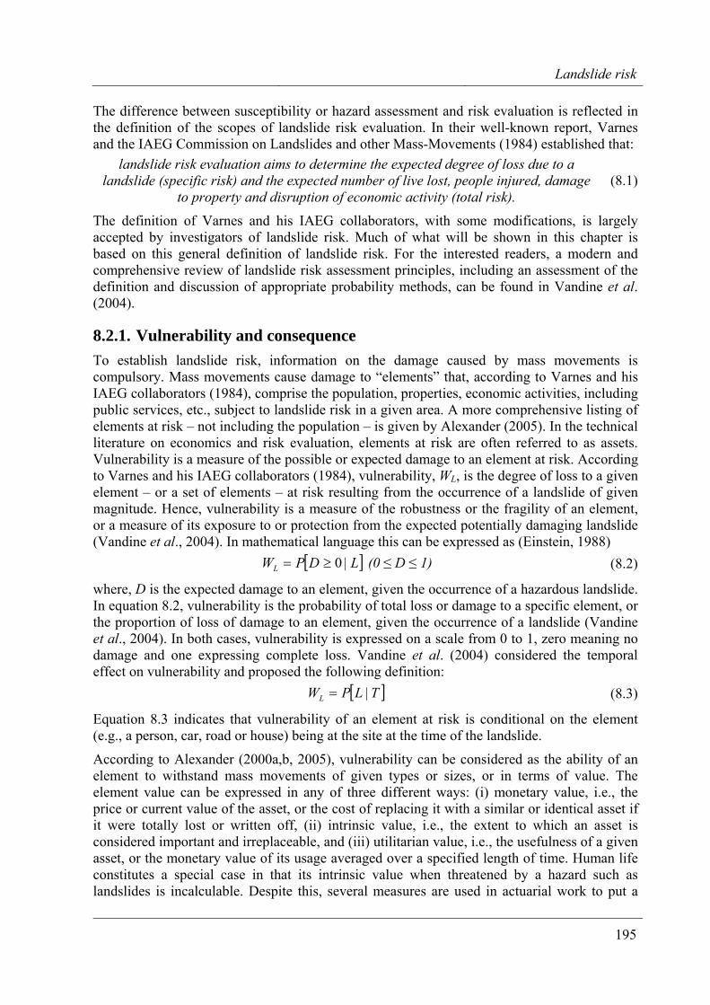
Landslide risk
195
The difference between susceptibility or hazard assessment and risk evaluation is reflected in the definition of the scopes of landslide risk evaluation. In their well-known report, Varnes and the IAEG Commission on Landslides and other Mass-Movements (1984) established that:
landslide risk evaluation aims to determine the expected degree of loss due to a landslide (specific risk) and the expected number of live lost, people injured, damage
to property and disruption of economic activity (total risk). (8.1)
The definition of Varnes and his IAEG collaborators, with some modifications, is largely accepted by investigators of landslide risk. Much of what will be shown in this chapter is based on this general definition of landslide risk. For the interested readers, a modern and comprehensive review of landslide risk assessment principles, including an assessment of the definition and discussion of appropriate probability methods, can be found in Vandine et al. (2004).
8.2.1. Vulnerability and consequence To establish landslide risk, information on the damage caused by mass movements is compulsory. Mass movements cause damage to “elements” that, according to Varnes and his IAEG collaborators (1984), comprise the population, properties, economic activities, including public services, etc., subject to landslide risk in a given area. A more comprehensive listing of elements at risk – not including the population – is given by Alexander (2005). In the technical literature on economics and risk evaluation, elements at risk are often referred to as assets. Vulnerability is a measure of the possible or expected damage to an element at risk. According to Varnes and his IAEG collaborators (1984), vulnerability, WL, is the degree of loss to a given element – or a set of elements – at risk resulting from the occurrence of a landslide of given magnitude. Hence, vulnerability is a measure of the robustness or the fragility of an element, or a measure of its exposure to or protection from the expected potentially damaging landslide (Vandine et al., 2004). In mathematical language this can be expressed as (Einstein, 1988)
[ ]L|DPWL 0≥= (0 ≤ D ≤ 1) (8.2)
where, D is the expected damage to an element, given the occurrence of a hazardous landslide. In equation 8.2, vulnerability is the probability of total loss or damage to a specific element, or the proportion of loss of damage to an element, given the occurrence of a landslide (Vandine et al., 2004). In both cases, vulnerability is expressed on a scale from 0 to 1, zero meaning no damage and one expressing complete loss. Vandine et al. (2004) considered the temporal effect on vulnerability and proposed the following definition:
[ ]T|LPWL = (8.3)
Equation 8.3 indicates that vulnerability of an element at risk is conditional on the element (e.g., a person, car, road or house) being at the site at the time of the landslide.
According to Alexander (2000a,b, 2005), vulnerability can be considered as the ability of an element to withstand mass movements of given types or sizes, or in terms of value. The element value can be expressed in any of three different ways: (i) monetary value, i.e., the price or current value of the asset, or the cost of replacing it with a similar or identical asset if it were totally lost or written off, (ii) intrinsic value, i.e., the extent to which an asset is considered important and irreplaceable, and (iii) utilitarian value, i.e., the usefulness of a given asset, or the monetary value of its usage averaged over a specified length of time. Human life constitutes a special case in that its intrinsic value when threatened by a hazard such as landslides is incalculable. Despite this, several measures are used in actuarial work to put a
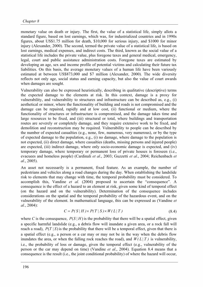
Chapter 8
196
monetary value on death or injury. The first, the value of a statistical life, simply allots a standard figure, based on lost earnings, which was, for industrialized countries and in 1990s figures, about US$1.75 million for death, $10,000 for serious injury, and $1000 for minor injury (Alexander, 2000). The second, termed the private value of a statistical life, is based on lost earnings, medical expenses, and indirect costs. The third, known as the social value of a statistical life includes the private value, plus foregone taxes and general medical, emergency, legal, court and public assistance administration costs. Foregone taxes are estimated by developing an age, sex and income profile of potential victims and calculating their future tax liabilities. On this basis, the average monetary values of a human life have been variously estimated at between US$873,000 and $7 million (Alexander, 2000). The wide diversity reflects not only age, social status and earning capacity, but also the value of court awards when damages are sought.
Vulnerability can also be expressed heuristically, describing in qualitative (descriptive) terms the expected damage to the elements at risk. In this context, damage is a proxy for vulnerability, and vulnerability to structures and infrastructure can be described as, e.g., (i) aesthetical or minor, where the functionality of building and roads is not compromised and the damage can be repaired, rapidly and at low cost, (ii) functional or medium, where the functionality of structures or infrastructure is compromised, and the damage takes time and large resources to be fixed, and (iii) structural or total, where buildings and transportation routes are severely or completely damage, and they require extensive work to be fixed, and demolition and reconstruction may be required. Vulnerability to people can be described by the number of expected casualties (e.g., none, few, numerous, very numerous), or by the type of expected damage to the population, e.g., (i) no damage, where damage to the population is not expected, (ii) direct damage, where casualties (deaths, missing persons and injured people) are expected, (iii) indirect damage, where only socio-economic damage is expected, and (iv) temporary damage, where temporary or permanent loss of private houses is foreseen (i.e., evacuees and homeless people) (Cardinali et al., 2003; Guzzetti et al., 2004; Reichenbach et al., 2005).
An asset not necessarily is a permanent, fixed feature. As an example, the number of pedestrians and vehicles along a road changes during the day. When establishing the landslide risk to elements that may change with time, the temporal probability must be considered. To accomplish this, Vandine et al. (2004) proposed to ascertain the “consequence”. A consequence is the effect of a hazard to an element at risk, given some kind of temporal effect (on the hazard and on the vulnerability). Determination of the consequence includes considerations on the spatial and the temporal probability of the hazardous event, and on the vulnerability of the element. In mathematical language, this can be expressed as (Vandine et al., 2004):
)T|L(W)S|T(P)H|S(PC ××= (8.4)
where C is the consequence, )|( HSP is the probability that there will be a spatial effect, given a specific harmful landslide (e.g., a debris flow will inundate a given area, or a rock fall will reach a road), )|( STP is the probability that there will be a temporal effect, given that there is a spatial effect (e.g., a person or a car may or may not be in the way when the debris flow inundates the area, or when the falling rock reaches the road), and )T|L(W is vulnerability, i.e., the probability of loss or damage, given the temporal effect (e.g., vulnerability of the person or the car may depend on time) (Vandine et al., 2004). Equation 8.4 means that a consequence is the result (i.e., the joint conditional probability) of where the hazard will occur,
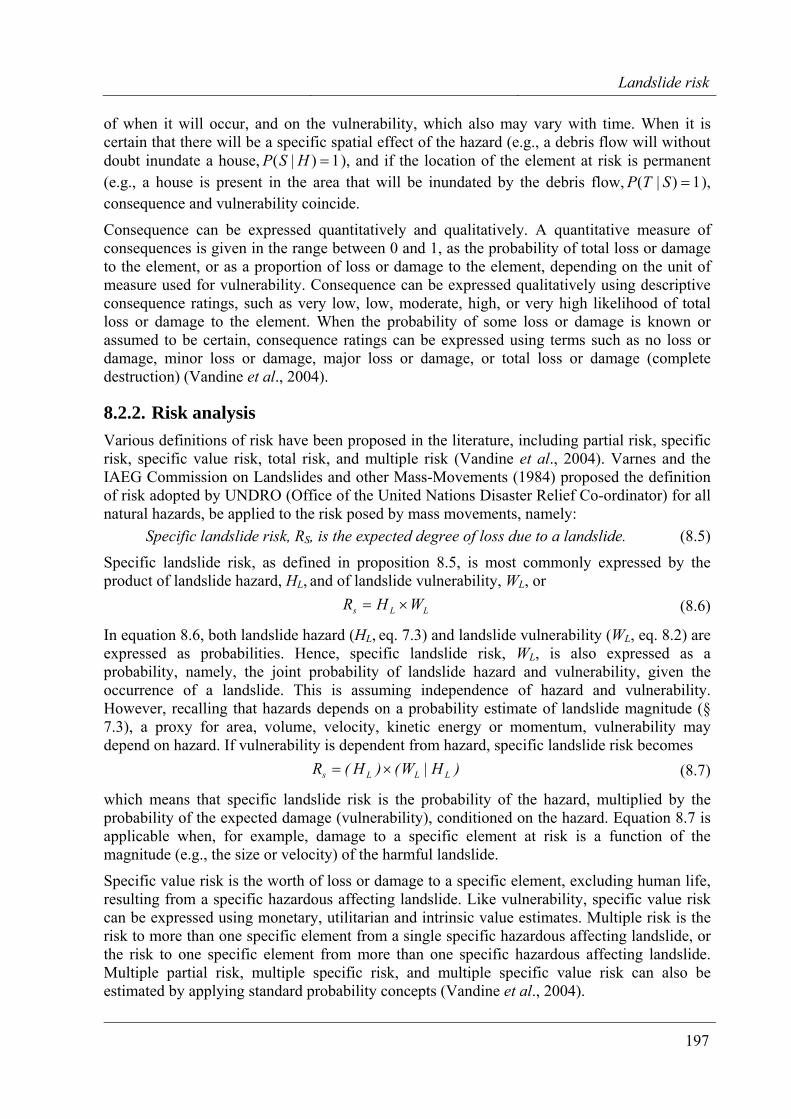
Landslide risk
197
of when it will occur, and on the vulnerability, which also may vary with time. When it is certain that there will be a specific spatial effect of the hazard (e.g., a debris flow will without doubt inundate a house, 1)|( =HSP ), and if the location of the element at risk is permanent (e.g., a house is present in the area that will be inundated by the debris flow, 1)|( =STP ), consequence and vulnerability coincide.
Consequence can be expressed quantitatively and qualitatively. A quantitative measure of consequences is given in the range between 0 and 1, as the probability of total loss or damage to the element, or as a proportion of loss or damage to the element, depending on the unit of measure used for vulnerability. Consequence can be expressed qualitatively using descriptive consequence ratings, such as very low, low, moderate, high, or very high likelihood of total loss or damage to the element. When the probability of some loss or damage is known or assumed to be certain, consequence ratings can be expressed using terms such as no loss or damage, minor loss or damage, major loss or damage, or total loss or damage (complete destruction) (Vandine et al., 2004).
8.2.2. Risk analysis Various definitions of risk have been proposed in the literature, including partial risk, specific risk, specific value risk, total risk, and multiple risk (Vandine et al., 2004). Varnes and the IAEG Commission on Landslides and other Mass-Movements (1984) proposed the definition of risk adopted by UNDRO (Office of the United Nations Disaster Relief Co-ordinator) for all natural hazards, be applied to the risk posed by mass movements, namely:
Specific landslide risk, RS, is the expected degree of loss due to a landslide. (8.5)
Specific landslide risk, as defined in proposition 8.5, is most commonly expressed by the product of landslide hazard, HL, and of landslide vulnerability, WL, or
LLs WHR ×= (8.6)
In equation 8.6, both landslide hazard (HL, eq. 7.3) and landslide vulnerability (WL, eq. 8.2) are expressed as probabilities. Hence, specific landslide risk, WL, is also expressed as a probability, namely, the joint probability of landslide hazard and vulnerability, given the occurrence of a landslide. This is assuming independence of hazard and vulnerability. However, recalling that hazards depends on a probability estimate of landslide magnitude (§ 7.3), a proxy for area, volume, velocity, kinetic energy or momentum, vulnerability may depend on hazard. If vulnerability is dependent from hazard, specific landslide risk becomes
)H|W()H(R LLLs ×= (8.7)
which means that specific landslide risk is the probability of the hazard, multiplied by the probability of the expected damage (vulnerability), conditioned on the hazard. Equation 8.7 is applicable when, for example, damage to a specific element at risk is a function of the magnitude (e.g., the size or velocity) of the harmful landslide.
Specific value risk is the worth of loss or damage to a specific element, excluding human life, resulting from a specific hazardous affecting landslide. Like vulnerability, specific value risk can be expressed using monetary, utilitarian and intrinsic value estimates. Multiple risk is the risk to more than one specific element from a single specific hazardous affecting landslide, or the risk to one specific element from more than one specific hazardous affecting landslide. Multiple partial risk, multiple specific risk, and multiple specific value risk can also be estimated by applying standard probability concepts (Vandine et al., 2004).
Chapter 8
198
Finally, total landslide risk, RT, was defined as the expected number of lives lost, person injured, damage to property, or disruption of
economic activity due to a landslide (8.8)
by Varnes and the IAEG Commission on Landslides and other Mass-Movements (1984), and as
the risk to all specific elements from all specific hazardous affecting landslides (8.9)
by Vandine et al. (2004). In the latter definition total landslide risk is expressed as a probability, and it can be estimated using standard probability concepts and methods.
8.2.3. Discussion In the previous pages, concepts and definitions useful for landslide risk assessment were presented and discussed, together with their mathematical (probabilistic) formulation. From a practical point of view, the given definitions can be used in several of different ways, depending on: (i) the scope of the analysis, (ii) the availability, quality and reliability of the necessary information, (iii) the extent of the study area, (iv) the resources available to complete the analysis, (v) the experience and skill of the investigator, and (vi) the existence of established thresholds for acceptance of risk.
In general, when attempting to establish landslide risk, two main approaches are possible: (i) a quantitative (probabilistic) approach, and (ii) a qualitative (heuristic) approach. Quantitative landslide risk analysis (QLRA) uses numerical values and mathematical methods to estimates objective probabilities, e.g., the probability of loss of life, or the probability of damage to a structure or infrastructure due to mass movements. QLRA investigates the relationships between the frequency of the damaging events and the intensity of their consequences, and seeks to establish quantitative (numerical) acceptable or tolerable thresholds. When applied to establish risk to the population, QLRA can be used to establish probabilistic levels of individual and collective risk. The former is most commonly investigated by computing mortality rates, which are given by, e.g., the number of deaths per 100,000 of any given population over a pre-defined period. The latter is ascertained by constructing f-N or F-N plots, which describe the relationship between the frequency of the damaging events and their intensity, as measured by the number of fatalities (§ 8.3). Another method of QLRA consists in the event tree decomposition (e.g., Budetta, 2002; Nicol, 2004; Vandine et al., 2004). The method is based on: (i) the systematic decomposition of risk into all the individual (single) components, (ii) the quantitative estimation of the probability (or the monetary, intrinsic and utilitarian values) for each single component of the risk, and (iii) an estimate of the risk, for all the possible established outcomes. Event trees can be constructed for specific risk and for specific value risk. In the first case the method provides probability estimates, and in the second case it provides monetary estimates (e.g., actual costs).
QLRA often requires a catalogue of landslides and their consequences, the latter measured quantitatively. Compilation of lists or catalogues of landslides and their consequences is a difficult, time consuming, expensive and uncertain operation, mostly because of the lack of relevant information (Guzzetti et al., 1994; Ibsen and Brunsden, 1996; Glade, 1988; Glade et al., 2001). A few of such lists have been prepared for landslides with human consequences (Evans, 1997; Guzzetti, 2000; Kong, 2002; Salvati et al., 2003; Guzzetti et al., 2005b,c). When this information is available, levels of individual and societal risk can be determined.
Landslide risk
199
However, the completeness, time span and reliability of the landslide catalogue greatly affect the reliability of such quantitative risk assessments.
When attempting to evaluate specific and total landslide risk for a single site or an entire region where slope failures are likely to take various forms or pose various threats, the quantitative approach can prove impracticable, uneconomical or even impossible (Guzzetti et al., 2003). It may not be easy to ascertain the magnitude, frequency and forms of evolution of landslides in an area, and detailed and reasonably complete catalogues of historical events and their consequences may not be readily available. As an alternative to quantitative risk assessment, a qualitative approach can be pursued in such a way as to establish qualitative levels of landslide risk. Qualitative landslide risk analysis (qLRA) uses relative qualitative (descriptive) ratings, and may result in designing landslide scenarios.
A landslide scenario is a description of one or several hypothetical, potentially damaging landslide events, including the consequences on the population, properties, economic activities, and the landscape. As in a theatre play, a scenario should include: (i) the “actors”, i.e., the assets involved in or affected by the event, including the population; and (ii) the “context”, i.e., the temporal arrangement and evolution and the geographical location of the event and the assets, including the social, economical, administrative and legal aspects directly or indirectly related to the event. For a scenario, a probability of occurrence should be established. The probability can be determined quantitatively, e.g., modelling an historical record of landslide events, or it can be established empirically, e.g., by using external information. The probability of a scenario associated with rare events may be difficult (or impossible) to determine quantitatively, and can be decided using geomorphological inference, the personal experience of the investigator, or other information. The design of a landslide scenario for a given area is a complex, largely empirical procedure that involves: (i) identification of the assets and their vulnerability, (ii) identification of the types of slope processes present in the study area, (iii) accurate mapping of the existing landslides, and (iv) assessment of the possible (or probable) evolution of the slope movements. The latter, can be ascertained qualitatively by experts, or it can be determined quantitatively using mathematical or physically-based models which simulate the expected evolution of a landslide. Multiple landslide scenarios can be prepared, one scenario for each landslide or landslide types present in the study area.
With regard to precision accuracy and reliability, quantitative landslide risk estimates are not necessarily better than qualitative estimates. In landslide risk analysis, the precision and reliability of an estimate does not depend on the use of numbers or probabilistic equations. It rather depends on whether all the components of the analysis have been appropriately considered and on the availability, quality, and reliability of the required data (Vandine et al., 2004).
8.3. Evaluation of landslide risk to individuals and the population
Quantitative landslide risk assessment (QLRA) can be used to determine the risk posed by landslides to identified individuals or the population (Cruden and Fell, 1997; Fell and Hartford, 1997; Evans, 1997; Guzzetti, 2000; Wise et al., 2004; Nicol, 2004; Guzzetti et al., 2005b,c). Most commonly, the method requires a catalogue of landslides and their human consequences, i.e., deaths, missing persons, injured people, evacuees and homeless. The completeness and time span of the catalogue affect the reliability of the risk assessments. Only
Chapter 8
200
a few lists of landslides with human consequences have been prepared. Such lists are mostly limited to specific areas or individual countries (Evans, 1997; Guzzetti, 2000; Kong, 2002; Salvati et al., 2003; Nicol, 2004; Guzzetti et al., 2005b,c).
When a sufficiently complete catalogue of landslide events with human consequences is available, levels of individual and societal risk can be determined (Cruden and Fell, 1997; ISSMGE TC32, 2004; Wise et al., 2004). Individual risk is the risk posed by a hazard to any identified individual and it is commonly expressed using mortality (or death) rates, which are usually given by the number of deaths per 100,000 of any given population over a pre-defined period. Societal (or collective) risk is the risk imposed by a landslide on society as a whole, and it is established by investigating the relationship between the frequency of the damaging events and their intensity, as measured by the number of deaths, fatalities or casualties. The relationship between the frequency of the harmful events and their consequences is shown on cumulative (F-N) or non-cumulative (f-N) plots (Cruden and Fell, 1997; Evans, 1997; Guzzetti, 2000). When such plots are prepared in log-log scale, the relationship between the number of events and the number of the consequences in each event exhibits a linear trend. This is important because, in principle, it allows determining the frequency and magnitude of large events (i.e., events with numerous fatalities) by studying the frequency and magnitude of the small events, i.e., those resulting in few fatalities. A linear trend in a log-log plot suggests a power law scaling, and power laws are commonly used to model such probability distributions (Evans, 1997; Guzzetti, 2000; Guzzetti et al., 2005b,c).
Quantitative landslide risk assessment allows determining acceptable risk levels. Acceptable levels of individual and collective landslide risk can be determined by comparison with other natural, technological and societal hazards for which acceptable risk levels have already been established (e.g., Whitman, 1984; Fell and Hartford 1997; Salvati et al., 2003; Nicol, 2004; Guzzetti et al., 2005b). In the following, examples will be given of the use of QLRA techniques to determine landslide risk to the population in Italy.
8.3.1. Landslide risk to the population in Italy In Italy, information exists to determine quantitatively the risk posed by landslides to the population, and to compare it with the risk posed by other natural and man made hazards, and by the leading medical causes of death. Systematic information on landslides with human consequences in Italy was first compiled by Guzzetti (2000), for the period between 1279 and 1999. Guzzetti et al. (2005b) revised this information and compiled an updated catalogue for the 2096-year period from 91 BC to 2004. The new catalogue lists 2444 events with human consequences, of which 1305 events with casualties. In the examined period, landslide casualties were at least 13,250, comprising 10,892 deaths, 85 missing persons, and 2273 injured people. The catalogue also lists 1331 events with homeless or evacuated people, for a total population exceeding 180,000. The new catalogue of Guzzetti et al. (2005b,c) also lists systematic information on floods with human consequences in the period from 1195 to 2004, and systematic information on earthquakes with human consequences in the period from 51 AD to 2004. Figure 8.1 shows the historical distribution of landslide events with casualties in Italy, for the period from 1500 to 2004. In the graph, open squares indicate the number of fatalities in each event, and open triangles the number of the injured people. Grey squares indicate landslide events for which casualties are known to have occurred but for which the exact, or even an approximate number, is unknown. Between 1500 and 2004, the most catastrophic year for landslides was 1963 with 1950 casualties, 1921 of which occurred at Vajont. The second worst year was 1618, when 1200 people were killed by the Piuro
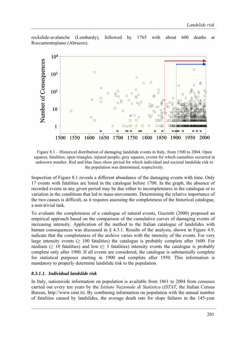
Landslide risk
201
rockslide-avalanche (Lombardy), followed by 1765 with about 600 deaths at Roccamontepiano (Abruzzo).
1950
1
10
102
103
104
1500 1550 1600 1650 1700 1750 1800 1850 1900 2000
Num
ber o
f Con
sequ
ence
s
1950
1
10
102
103
104
1500 1550 1600 1650 1700 1750 1800 1850 1900 2000
Num
ber o
f Con
sequ
ence
s
Figure 8.1 – Historical distribution of damaging landslide events in Italy, from 1500 to 2004. Open squares, fatalities; open triangles, injured people; grey squares, events for which casualties occurred in unknown number. Red and blue lines show period for which individual and societal landslide risk to
the population was determined, respectively.
Inspection of Figure 8.1 reveals a different abundance of the damaging events with time. Only 17 events with fatalities are listed in the catalogue before 1700. In the graph, the absence of recorded events in any given period may be due either to incompleteness in the catalogue or to variation in the conditions that led to mass-movements. Determining the relative importance of the two causes is difficult, as it requires assessing the completeness of the historical catalogue, a non-trivial task.
To evaluate the completeness of a catalogue of natural events, Guzzetti (2000) proposed an empirical approach based on the comparison of the cumulative curves of damaging events of increasing intensity. Application of the method to the Italian catalogue of landslides with human consequences was discussed in § 4.3.1. Results of the analysis, shown in Figure 4.9, indicate that the completeness of the archive varies with the intensity of the events. For very large intensity events (≥ 100 fatalities) the catalogue is probably complete after 1600. For medium (≥ 10 fatalities) and low (≥ 3 fatalities) intensity events the catalogue is probably complete only after 1900. If all events are considered, the catalogue is substantially complete for statistical purposes starting in 1900 and complete after 1950. This information is mandatory to properly determine landslide risk to the population.
8.3.1.1. Individual landslide risk
In Italy, nationwide information on population is available from 1861 to 2004 from censuses carried out every ten years by the Istituto Nazionale di Statistica (ISTAT, the Italian Census Bureau, http://www.istat.it). By combining information on population with the annual number of fatalities caused by landslides, the average death rate for slope failures in the 145-year
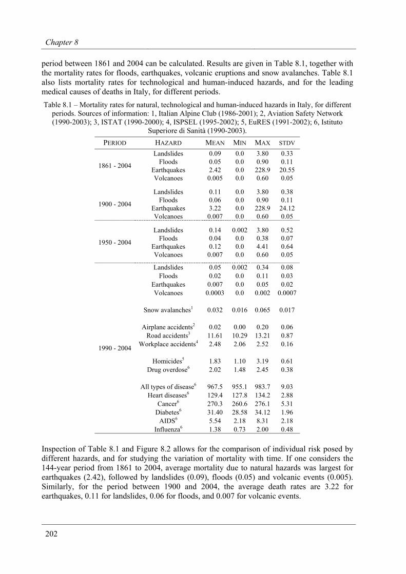
Chapter 8
202
period between 1861 and 2004 can be calculated. Results are given in Table 8.1, together with the mortality rates for floods, earthquakes, volcanic eruptions and snow avalanches. Table 8.1 also lists mortality rates for technological and human-induced hazards, and for the leading medical causes of deaths in Italy, for different periods. Table 8.1 – Mortality rates for natural, technological and human-induced hazards in Italy, for different
periods. Sources of information: 1, Italian Alpine Club (1986-2001); 2, Aviation Safety Network (1990-2003); 3, ISTAT (1990-2000); 4, ISPSEL (1995-2002); 5, EuRES (1991-2002); 6, Istituto
Superiore di Sanità (1990-2003). PERIOD HAZARD MEAN MIN MAX STDV
Landslides 0.09 0.0 3.80 0.33 Floods 0.05 0.0 0.90 0.11
Earthquakes 2.42 0.0 228.9 20.55 1861 - 2004
Volcanoes 0.005 0.0 0.60 0.05
Landslides 0.11 0.0 3.80 0.38 Floods 0.06 0.0 0.90 0.11
Earthquakes 3.22 0.0 228.9 24.12 1900 - 2004
Volcanoes 0.007 0.0 0.60 0.05
Landslides 0.14 0.002 3.80 0.52 Floods 0.04 0.0 0.38 0.07
Earthquakes 0.12 0.0 4.41 0.64 1950 - 2004
Volcanoes 0.007 0.0 0.60 0.05
Landslides 0.05 0.002 0.34 0.08 Floods 0.02 0.0 0.11 0.03
Earthquakes 0.007 0.0 0.05 0.02 Volcanoes 0.0003 0.0 0.002 0.0007
Snow avalanches1 0.032 0.016 0.065 0.017
Airplane accidents2 0.02 0.00 0.20 0.06
Road accidents3 11.61 10.29 13.21 0.87 Workplace accidents4 2.48 2.06 2.52 0.16
Homicides5 1.83 1.10 3.19 0.61
Drug overdose6 2.02 1.48 2.45 0.38
All types of disease6 967.5 955.1 983.7 9.03 Heart diseases6 129.4 127.8 134.2 2.88
Cancer6 270.3 260.6 276.1 5.31 Diabetes6 31.40 28.58 34.12 1.96
AIDS6 5.54 2.18 8.31 2.18
1990 - 2004
Influenza6 1.38 0.73 2.00 0.48
Inspection of Table 8.1 and Figure 8.2 allows for the comparison of individual risk posed by different hazards, and for studying the variation of mortality with time. If one considers the 144-year period from 1861 to 2004, average mortality due to natural hazards was largest for earthquakes (2.42), followed by landslides (0.09), floods (0.05) and volcanic events (0.005). Similarly, for the period between 1900 and 2004, the average death rates are 3.22 for earthquakes, 0.11 for landslides, 0.06 for floods, and 0.007 for volcanic events.
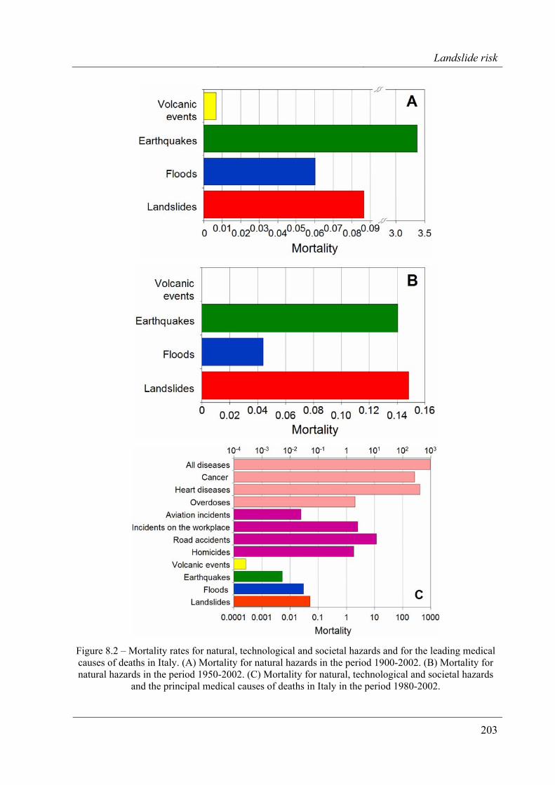
Landslide risk
203
Figure 8.2 – Mortality rates for natural, technological and societal hazards and for the leading medical causes of deaths in Italy. (A) Mortality for natural hazards in the period 1900-2002. (B) Mortality for natural hazards in the period 1950-2002. (C) Mortality for natural, technological and societal hazards
and the principal medical causes of deaths in Italy in the period 1980-2002.
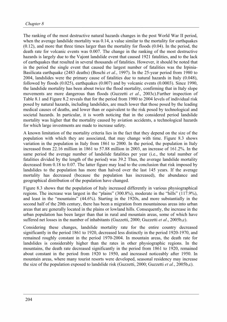
Chapter 8
204
The ranking of the most destructive natural hazards changes in the post World War II period, when the average landslide mortality was 0.14, a value similar to the mortality for earthquakes (0.12), and more that three times larger than the mortality for floods (0.04). In the period, the death rate for volcanic events was 0.007. The change in the ranking of the most destructive hazards is largely due to the Vajont landslide event that caused 1921 fatalities, and to the lack of earthquakes that resulted in several thousands of fatalities. However, it should be noted that in the period the single event that caused the largest number of fatalities was the Irpinia-Basilicata earthquake (2483 deaths) (Boschi et al., 1997). In the 25-year period from 1980 to 2004, landslides were the primary cause of fatalities due to natural hazards in Italy (0.048), followed by floods (0.025), earthquakes (0.007) and by volcanic events (0.0003). Since 1990, the landslide mortality has been about twice the flood mortality, confirming that in Italy slope movements are more dangerous than floods (Guzzetti et al., 2003c).Further inspection of Table 8.1 and Figure 8.2 reveals that for the period from 1980 to 2004 levels of individual risk posed by natural hazards, including landslides, are much lower that those posed by the leading medical causes of deaths, and lower than or equivalent to the risk posed by technological and societal hazards. In particular, it is worth noticing that in the considered period landslide mortality was higher that the mortality caused by aviation accidents, a technological hazards for which large investments are made to increase safety.
A known limitation of the mortality criteria lies in the fact that they depend on the size of the population with which they are associated, that may change with time. Figure 8.3 shows variation in the population in Italy from 1861 to 2000. In the period, the population in Italy increased from 22.16 million in 1861 to 57.88 million in 2003, an increase of 161.2%. In the same period the average number of landslide fatalities per year (i.e., the total number of fatalities divided by the length of the period) was 39.2 Thus, the average landslide mortality decreased from 0.18 to 0.07. The latter figure may lead to the conclusion that risk imposed by landslides to the population has more than halved over the last 145 years. If the average mortality has decreased (because the population has increased), the abundance and geographical distribution of the population have changed.
Figure 8.3 shows that the population of Italy increased differently in various physiographical regions. The increase was largest in the “plains” (300.8%), moderate in the “hills” (117.9%), and least in the “mountains” (44.6%). Starting in the 1920s, and more substantially in the second half of the 20th century, there has been a migration from mountainous areas into urban areas that are generally located in the plains or lowland hills. Consequently, the increase in the urban population has been larger than that in rural and mountain areas, some of which have suffered net losses in the number of inhabitants (Guzzetti, 2000; Guzzetti et al., 2005b,c).
Considering these changes, landslide mortality rate for the entire country decreased significantly in the period 1861 to 1920, decreased less distinctly in the period 1920-1970, and remained roughly constant in the period 1970-2004. In mountain areas, the death rate for landslides is considerably higher than the rates in other physiographic regions. In the mountains, the death rate decreased significantly in the period from 1861 to 1920, remained about constant in the period from 1920 to 1950, and increased noticeably after 1950. In mountain areas, where many tourist resorts were developed, seasonal residency may increase the size of the population exposed to landslide risk (Guzzetti, 2000; Guzzetti et al., 2005b,c).
Landslide risk
205
Figure 8.3 – Population and landslide mortality rates in Italy from 1860 to 2004. Upper graph: distribution of the population in different physiographical regions. Lower graph: lines show landslide
mortality rates for different physiographical regions; histogram shows yearly number of landslide fatalities (log scale). Source of population data: Istituto Nazionale di Statistica.
8.3.1.2. Societal landslide risk Estimates of societal risk are obtained by investigating the relationship between the frequency of the landslide events and their intensity, as measured by the number of fatalities. Figure 8.4.A shows the non-cumulative frequency-consequences plot (f-N plot) for landslides in Italy. The plot shows, for each intensity class as measured by the number of fatalities, the corresponding number of events. To minimize problems of database completeness, only the section of the historical catalogue considered substantially complete was used to construct the graphs, i.e., the subset from 1900 to 2002. In the log-log plot the relationship between the number of the events (NE) and the number of fatalities (NF) in each event exhibits a distinct linear trend, at least in the range between 1 and ~30 fatalities (more than 97% of the events). This suggests a self-similar scaling behaviour of the losses, which is important, because in principle it allows the use of frequent, small intensity events to estimate the rate of occurrence of rare, large events. However, the tail of the raw distributions (which contain less than 3% of the events, in the range from 30 to several hundreds fatalities) is erratic, and not adequate to fit a power law to the data.
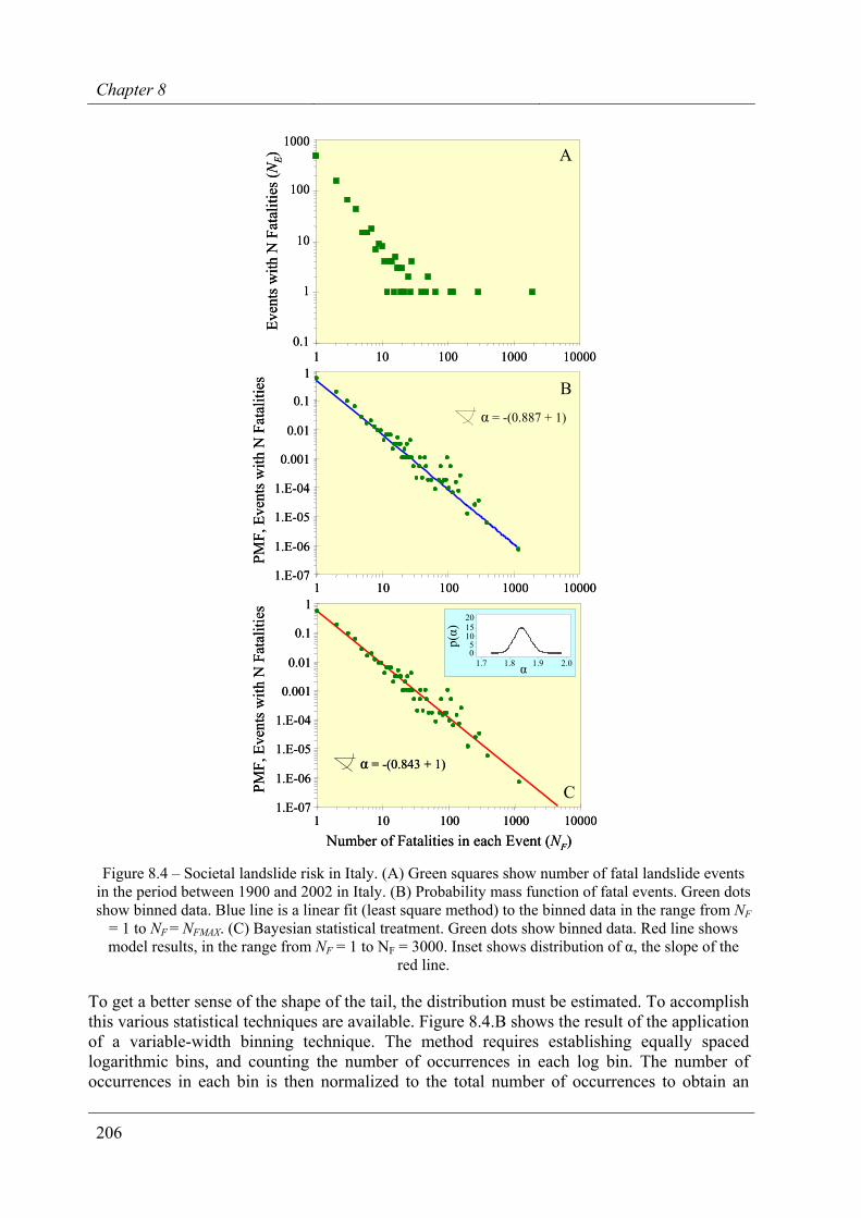
Chapter 8
206
1 10 100 1000 100001.E-07
1.E-06
1.E-05
1.E-04
0.001
0.01
0.1
1
PMF,
Eve
nts w
ith N
Fat
aliti
es Bα = -(0.887 + 1)
1.E-07
1.E-06
1.E-05
1.E-04
0.001
0.01
0.1
1
1 10 100 1000 10000
PMF,
Eve
nts w
ith N
Fat
aliti
es
C
α = -(0.843 + 1)
Number of Fatalities in each Event (NF)
1.7 1.8 1.905
1015
2.0
20
α
p(α)
0.1
1
10
100
1000
1 10 100 1000 10000
Even
ts w
ith N
Fat
aliti
es (N
E) A
1 10 100 1000 100001.E-07
1.E-06
1.E-05
1.E-04
0.001
0.01
0.1
1
PMF,
Eve
nts w
ith N
Fat
aliti
es Bα = -(0.887 + 1)
1.E-07
1.E-06
1.E-05
1.E-04
0.001
0.01
0.1
1
1 10 100 1000 10000
PMF,
Eve
nts w
ith N
Fat
aliti
es
C
α = -(0.843 + 1)α = -(0.843 + 1)
Number of Fatalities in each Event (NF)
1.7 1.8 1.905
1015
2.0
20
α
p(α)
1.7 1.8 1.905
1015
2.0
20
α
p(α)
0.1
1
10
100
1000
1 10 100 1000 10000
Even
ts w
ith N
Fat
aliti
es (N
E) A
Figure 8.4 – Societal landslide risk in Italy. (A) Green squares show number of fatal landslide events in the period between 1900 and 2002 in Italy. (B) Probability mass function of fatal events. Green dots show binned data. Blue line is a linear fit (least square method) to the binned data in the range from NF
= 1 to NF = NFMAX. (C) Bayesian statistical treatment. Green dots show binned data. Red line shows model results, in the range from NF = 1 to NF = 3000. Inset shows distribution of α, the slope of the
red line.
To get a better sense of the shape of the tail, the distribution must be estimated. To accomplish this various statistical techniques are available. Figure 8.4.B shows the result of the application of a variable-width binning technique. The method requires establishing equally spaced logarithmic bins, and counting the number of occurrences in each log bin. The number of occurrences in each bin is then normalized to the total number of occurrences to obtain an
Landslide risk
207
estimate of the probability mass function1 (Guzzetti et al., 2005b,c). In Figure 8.4.B, the number of fatalities (NF) caused by harmful landslide events is shown versus the estimated probability mass function (pmf) of the events with NF fatalities. In the figure, there is a clear (log-log) linear relationship between the event intensity, measured by the number of reported fatalities (NF), and the probability of the event, which permits a straightforward linear regression (“fit”). The estimated distribution can be approximated by a power law. The log-log linear trend of the regression fit extends for three orders of magnitude, indicating a consistent power law scaling behaviour of the landslide fatalities.
The weakness of the described approach is the need to “bin” the data. Although the variable-width binning technique performs this task well, binning can be avoided altogether if the raw data are treated using a full probability model and model parameters are inferred directly from the data through, e.g., Bayesian techniques. When data samples appear to be power law distributed, there are two probability distributions that statisticians use to model them: (i) the Pareto distribution prescribes a power law probability for the size of a random event, given that the size can take any fractional value above a given minimum value; (ii) the zeta distribution also prescribes a power law probability for the size of a random event, which takes an integer value of at least one. Numbers of fatalities are integer values. So, if one wants to treat the frequency distributions of such data as a power law, a zeta distribution model must be assumed, in which the number of fatalities NF has a pmf:
)1()(
)1(
+=
+−
αζ
αF
FNNP (8.10)
where P(NF) is the probability that NF fatalities will occur in a single random event, α is the power law exponent, and ζ is the Riemann zeta function. In this model, there is no upper limit to the number of fatalities that can occur in a single event (Guzzetti et al., 2005b,c).
Each harmful event is treated as an independent and uncorrelated stochastic event, and the number of fatalities NF is modelled as a ζ random variate. The inventory of harmful events is combined into likelihood, which is the relative probability that all the harmful events would cause the observed number of fatalities. It is obtained by multiplying together, for all Ne events, the probability that each harmful event should have caused the reported number of fatalities:
])[(])2[(])1[(}){|( eNNPNPNPNaL FFFF ×××= Κ (8.11)
Since each NF is a zeta variate,
eN
aFFF
FNNNN
NaL)}1({
} ][]2[]1[{}){|(
)1(e
+×××
=+−
αζΚ
(8.12)
One needs to estimate the value of the power law scaling exponent α. Bayes’ theorem allows to infer the probability distribution of α given the data {NF}. This is called the posterior distribution of α:
posterior probability (α | {NF}) ∝ likelihood (α |{NF}) × prior probability (α) (8.13)
1 The probability distribution of a discrete random variable is represented by its probability mass function (pmf).
Chapter 8
208
The difficulty of a Bayesian analysis lies in the concept implicit in this equation: that one has some a priori idea of the likely value of the scaling exponent α, and that this idea is revised when one looks at the data {NF}. The way in which the idea is revised depends on the model understanding of how likely a certain value of α is, given the observations {NF}: hence the term “likelihood”. The likelihood moulds the prior probabilistic description of the scaling exponent α into a posterior probability distribution for α.
Ideally, in a Bayesian analysis the prior distribution has only a very weak effect on the posterior inference, and most of the information comes from the likelihood. Many Bayesian treatments use what are called “non-informative” priors, which are designed to be as vague a statement as possible about the model parameters, so as not to bias the inference unduly. A uniform distribution is a “weakly informative” prior that provides little information about the model parameters. The steepness of the power law α-1 is assumed to be anywhere in the range between -1 and -3. Hence, a weakly informative prior for the zeta scaling exponent takes the form
prior probability (α) = U(0,2) (8.14)
Hence, a priori, we consider any value of α between zero and two as equally likely.
The challenge in Bayesian modelling is to turn the proportionality in equation 8.13 into an equality, i.e. to normalize the right hand side of the equation so that it becomes a true probability. For most Bayesian models, normalization is only possible through numerical integration. A method of numerical integration is Markov chain Monte Carlo (MCMC) sampling, in which (pseudo)random samples are generated in such a way that their distribution obeys (asymptotically) the posterior distribution. Guzzetti et al. (2005b,c) have implemented an MCMC solution of the zeta power law distribution model for fatalities caused by natural hazard using software called WinBUGS (http://www.mrc-bsu.cam.ac.uk/bugs). The results of the Bayesian MCMC analysis are shown in Figure 8.4.C.
Figure 8.4 allows for a comparison of the results of the Bayesian treatment of the raw data (red line in Figure 8.4.C) with those of the linear regression fits to the binned data (blue line in Figure 8.4.B), and with the raw data, in the form of the observed frequency of events (Figure 8.4.A). In the examined period (from 1900 to 2004), the actual frequency of landslide events that resulted in one fatality was 4.69 (483 events in 103 years). This figure compares to the estimate of 4.27 obtained from the linear fit of the data, and to the estimate of 4.98 obtained by the Bayesian model. Hence, for landslide events that resulted in one fatality, the linear regression fit slightly underestimates the landslide frequency, and the Bayesian model slightly overestimates the landslide frequency.
8.3.2. Comparison of risk posed by different natural hazards in Italy For Italy, information exists to compare the societal risk posed by different natural hazards. Figure 8.5 shows estimates of societal risk for landslides, floods, earthquakes and volcanic events. The estimates were obtained applying the Bayesian method described in § 8.3.1.2. Data used to obtain the estimates of societal risk span the period from 1900 to 2004 and were collected by Guzzetti et al. (2005b,c).
The steepness of the curves in the log-log plots of Figure 8.5 indicates the relative frequency of the small, less intense events versus the large, more destructive events. For a given number of fatalities, a steeper curve assesses a lower (predicted) frequency of events than a gently dipping curve, which predicts a higher frequency of harmful events. Assuming that the more
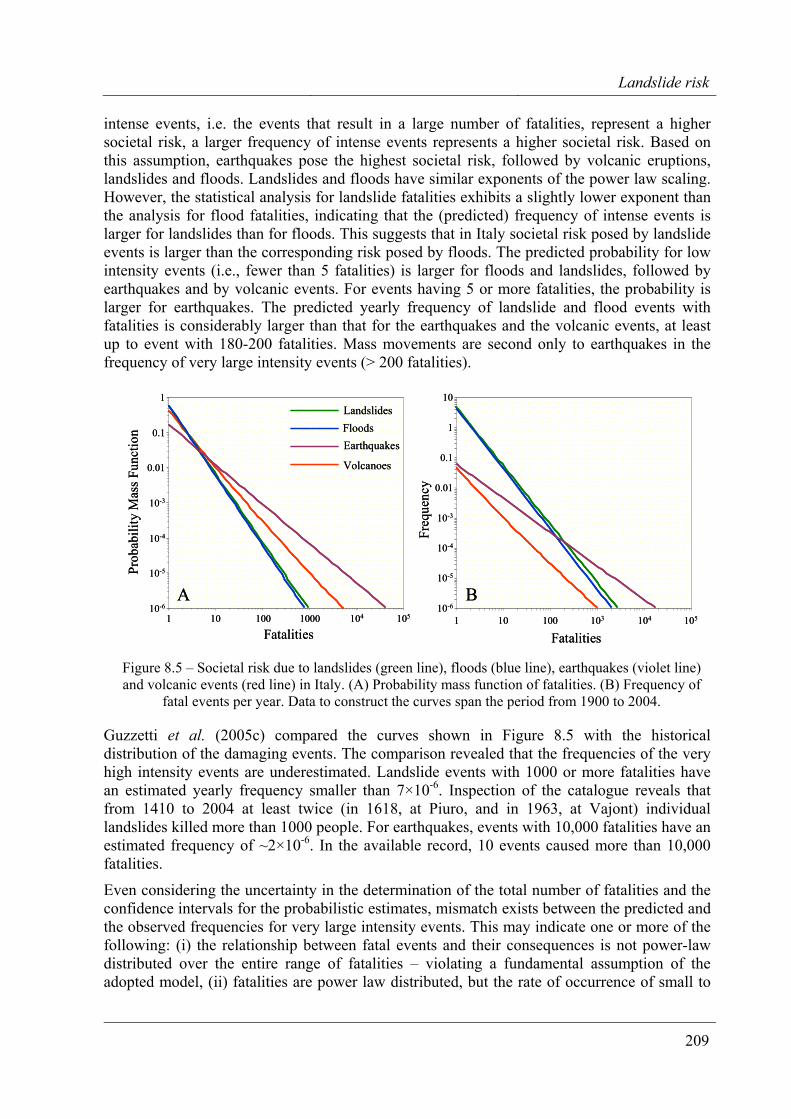
Landslide risk
209
intense events, i.e. the events that result in a large number of fatalities, represent a higher societal risk, a larger frequency of intense events represents a higher societal risk. Based on this assumption, earthquakes pose the highest societal risk, followed by volcanic eruptions, landslides and floods. Landslides and floods have similar exponents of the power law scaling. However, the statistical analysis for landslide fatalities exhibits a slightly lower exponent than the analysis for flood fatalities, indicating that the (predicted) frequency of intense events is larger for landslides than for floods. This suggests that in Italy societal risk posed by landslide events is larger than the corresponding risk posed by floods. The predicted probability for low intensity events (i.e., fewer than 5 fatalities) is larger for floods and landslides, followed by earthquakes and by volcanic events. For events having 5 or more fatalities, the probability is larger for earthquakes. The predicted yearly frequency of landslide and flood events with fatalities is considerably larger than that for the earthquakes and the volcanic events, at least up to event with 180-200 fatalities. Mass movements are second only to earthquakes in the frequency of very large intensity events (> 200 fatalities).
10-6
10-5
10-4
10-3
0.01
0.1
1
1 10 100 1000 105
Fatalities
Prob
abili
ty M
ass F
unct
ion
Volcanoes
LandslidesFloodsEarthquakes
10410-6
10-5
10-4
10-3
0.01
0.1
1
10
1 10 100 103 104 105
Fatalities
Freq
uenc
y
BA10-6
10-5
10-4
10-3
0.01
0.1
1
1 10 100 1000 105
Fatalities
Prob
abili
ty M
ass F
unct
ion
Volcanoes
LandslidesFloodsEarthquakes
10410-6
10-5
10-4
10-3
0.01
0.1
1
10
1 10 100 103 104 105
Fatalities
Freq
uenc
y
BA
Figure 8.5 – Societal risk due to landslides (green line), floods (blue line), earthquakes (violet line) and volcanic events (red line) in Italy. (A) Probability mass function of fatalities. (B) Frequency of
fatal events per year. Data to construct the curves span the period from 1900 to 2004.
Guzzetti et al. (2005c) compared the curves shown in Figure 8.5 with the historical distribution of the damaging events. The comparison revealed that the frequencies of the very high intensity events are underestimated. Landslide events with 1000 or more fatalities have an estimated yearly frequency smaller than 7×10⁻⁶. Inspection of the catalogue reveals that from 1410 to 2004 at least twice (in 1618, at Piuro, and in 1963, at Vajont) individual landslides killed more than 1000 people. For earthquakes, events with 10,000 fatalities have an estimated frequency of ~2×10⁻⁶. In the available record, 10 events caused more than 10,000 fatalities.
Even considering the uncertainty in the determination of the total number of fatalities and the confidence intervals for the probabilistic estimates, mismatch exists between the predicted and the observed frequencies for very large intensity events. This may indicate one or more of the following: (i) the relationship between fatal events and their consequences is not power-law distributed over the entire range of fatalities – violating a fundamental assumption of the adopted model, (ii) fatalities are power law distributed, but the rate of occurrence of small to
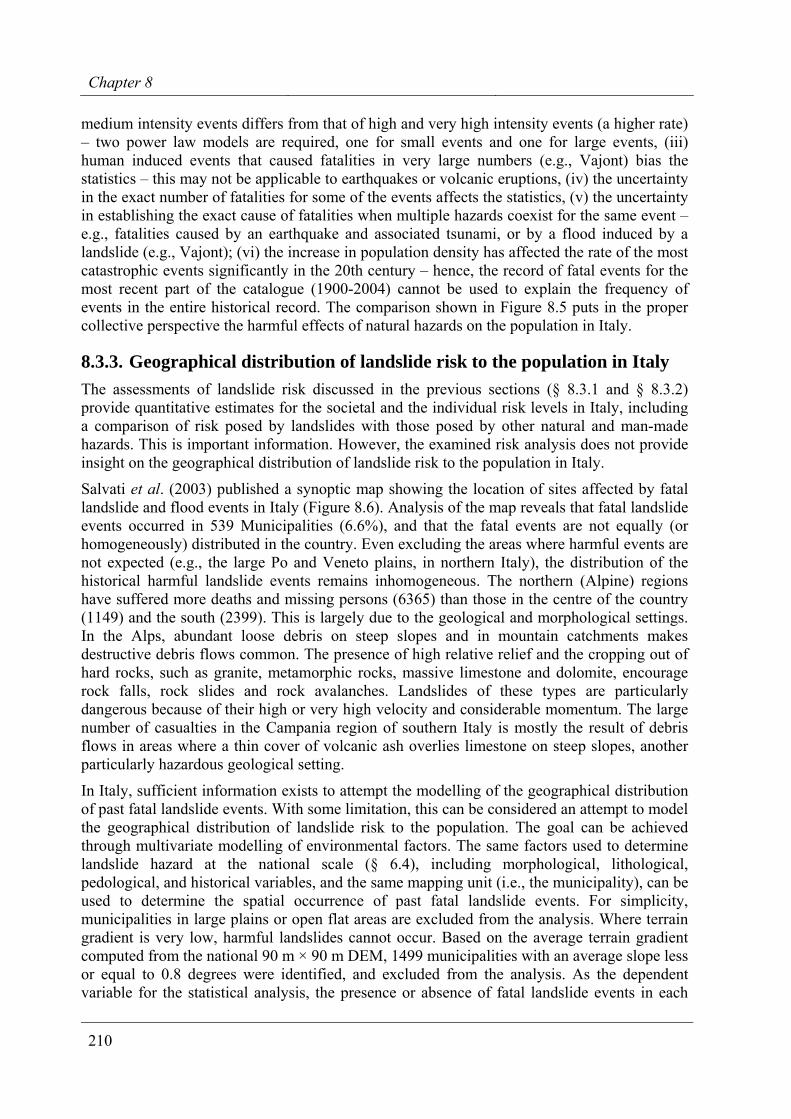
Chapter 8
210
medium intensity events differs from that of high and very high intensity events (a higher rate) – two power law models are required, one for small events and one for large events, (iii) human induced events that caused fatalities in very large numbers (e.g., Vajont) bias the statistics – this may not be applicable to earthquakes or volcanic eruptions, (iv) the uncertainty in the exact number of fatalities for some of the events affects the statistics, (v) the uncertainty in establishing the exact cause of fatalities when multiple hazards coexist for the same event – e.g., fatalities caused by an earthquake and associated tsunami, or by a flood induced by a landslide (e.g., Vajont); (vi) the increase in population density has affected the rate of the most catastrophic events significantly in the 20th century – hence, the record of fatal events for the most recent part of the catalogue (1900-2004) cannot be used to explain the frequency of events in the entire historical record. The comparison shown in Figure 8.5 puts in the proper collective perspective the harmful effects of natural hazards on the population in Italy.
8.3.3. Geographical distribution of landslide risk to the population in Italy The assessments of landslide risk discussed in the previous sections (§ 8.3.1 and § 8.3.2) provide quantitative estimates for the societal and the individual risk levels in Italy, including a comparison of risk posed by landslides with those posed by other natural and man-made hazards. This is important information. However, the examined risk analysis does not provide insight on the geographical distribution of landslide risk to the population in Italy.
Salvati et al. (2003) published a synoptic map showing the location of sites affected by fatal landslide and flood events in Italy (Figure 8.6). Analysis of the map reveals that fatal landslide events occurred in 539 Municipalities (6.6%), and that the fatal events are not equally (or homogeneously) distributed in the country. Even excluding the areas where harmful events are not expected (e.g., the large Po and Veneto plains, in northern Italy), the distribution of the historical harmful landslide events remains inhomogeneous. The northern (Alpine) regions have suffered more deaths and missing persons (6365) than those in the centre of the country (1149) and the south (2399). This is largely due to the geological and morphological settings. In the Alps, abundant loose debris on steep slopes and in mountain catchments makes destructive debris flows common. The presence of high relative relief and the cropping out of hard rocks, such as granite, metamorphic rocks, massive limestone and dolomite, encourage rock falls, rock slides and rock avalanches. Landslides of these types are particularly dangerous because of their high or very high velocity and considerable momentum. The large number of casualties in the Campania region of southern Italy is mostly the result of debris flows in areas where a thin cover of volcanic ash overlies limestone on steep slopes, another particularly hazardous geological setting.
In Italy, sufficient information exists to attempt the modelling of the geographical distribution of past fatal landslide events. With some limitation, this can be considered an attempt to model the geographical distribution of landslide risk to the population. The goal can be achieved through multivariate modelling of environmental factors. The same factors used to determine landslide hazard at the national scale (§ 6.4), including morphological, lithological, pedological, and historical variables, and the same mapping unit (i.e., the municipality), can be used to determine the spatial occurrence of past fatal landslide events. For simplicity, municipalities in large plains or open flat areas are excluded from the analysis. Where terrain gradient is very low, harmful landslides cannot occur. Based on the average terrain gradient computed from the national 90 m × 90 m DEM, 1499 municipalities with an average slope less or equal to 0.8 degrees were identified, and excluded from the analysis. As the dependent variable for the statistical analysis, the presence or absence of fatal landslide events in each
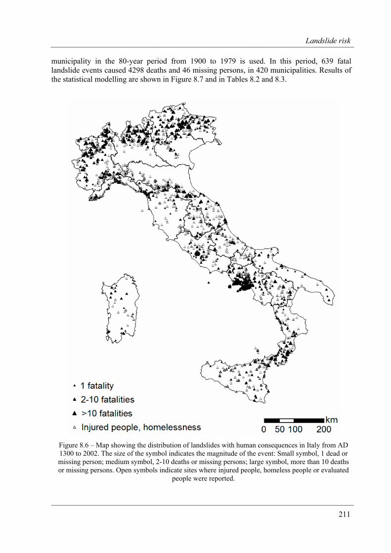
Landslide risk
211
municipality in the 80-year period from 1900 to 1979 is used. In this period, 639 fatal landslide events caused 4298 deaths and 46 missing persons, in 420 municipalities. Results of the statistical modelling are shown in Figure 8.7 and in Tables 8.2 and 8.3.
Figure 8.6 – Map showing the distribution of landslides with human consequences in Italy from AD 1300 to 2002. The size of the symbol indicates the magnitude of the event: Small symbol, 1 dead or missing person; medium symbol, 2-10 deaths or missing persons; large symbol, more than 10 deaths or missing persons. Open symbols indicate sites where injured people, homeless people or evaluated
people were reported.
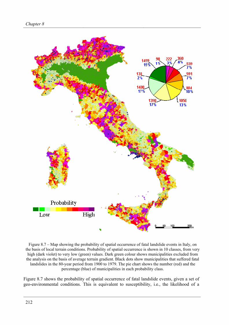
Chapter 8
212
Figure 8.7 – Map showing the probability of spatial occurrence of fatal landslide events in Italy, on the basis of local terrain conditions. Probability of spatial occurrence is shown in 10 classes, from very high (dark violet) to very low (green) values. Dark green colour shows municipalities excluded from
the analysis on the basis of average terrain gradient. Black dots show municipalities that suffered fatal landslides in the 80-year period from 1900 to 1979. The pie chart shows the number (red) and the
percentage (blue) of municipalities in each probability class.
Figure 8.7 shows the probability of spatial occurrence of fatal landslide events, given a set of geo-environmental conditions. This is equivalent to susceptibility, i.e., the likelihood of a
Landslide risk
213
landslide event with fatalities occurring in a municipality on the basis of the local terrain setting (§ 7.) For display purposes, in Figure 8.7 the probability of spatial occurrence of fatal landslide events is shown in 10 classes, from very high (dark violet) to very low (green) values. In the map, municipalities excluded from the analysis on the basis of the very low mean terrain gradient are shown in dark green. The pie chart shows the number (in red) and the percentage (in blue) of municipalities in each probability class.
Table 8.2 lists the 13 variables selected by a stepwise discriminant function as the best predictors of the occurrence of fatal landslide events in the municipalities. The standardized discriminant function coefficients (SDFC) show the relative importance of each variable as a predictor of landslide risk to the population in Italy. Variables with large coefficients (in absolute value) are strongly associated with the presence or the absence of fatal landslide events in the municipalities. The sign of the coefficient tells if the variable is positively or negatively correlated to the occurrence of fatal events. Inspection of Table 8.2 reveals that the range in slope angle (0.792), the presence of regosols (0.629), lithosols (0.356) and of volcanic soils (0.308) are the conditions most correlated to the occurrence of fatal landslide events.
Table 8.2 – Variables entered into the discriminant model as the best predictors of the presence of fatal landslide events in the 6604 municipalities exhibiting average terrain gradient greater than 0.8 degrees. Most important standardized discriminant function coefficients (SDFC) are shown in bold. Negative or
positive sign of the coefficients indicates variables contributing toward risk (green) or safety (red). VARIABLES DESCRIPTION SDFC
Mean terrain elevation -.275 Podzolic soil -.115 Sandstone -.090 Low grade metamorphic rocks .111 Plain area .177 Podsols .204 Maximum mean annual rainfall .211 Historical events in neighbouring municipalities .255 Drainage network area .285 Volcanic soil .308 Lithosols .356 Regosols .629 Range in terrain slope .792
Table 8.3 shows a comparison between the municipalities classified as “safe” or “at risk” by the model (columns), and the municipalities that did not or did suffer fatal landslides in the period from 1900 to 1979 (rows). The table also shows the overall model correct classification, which is 74.4%. The latter figure indicates that about ¾ of the municipalities defined “at risk” or “safe” by the model, did or did not experience fatal landslides in the considered period, respectively. Inspection of Table 8.3 indicates that, among the municipalities that were correctly classified by the discriminant model, those that did not suffer fatalities were classified more efficiently (i.e., in larger number, 75.1%) that those that experienced fatal landslide events (only 64.8%). We attribute the difference in the model ability to classify municipalities “at risk” or “safe”, to the much larger number of municipalities that did not suffered fatal landslide events (6184, 93%) in the catalogue, and the correspondingly much lower number of municipalities with landslide fatalities (420, 7%).
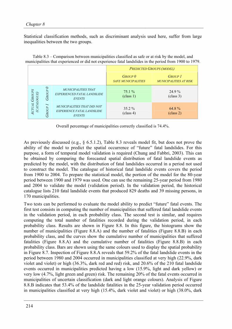
Chapter 8
214
Statistical classification methods, such as discriminant analysis used here, suffer from large inequalities between the two groups.
Table 8.3 – Comparison between municipalities classified as safe or at risk by the model, and municipalities that experienced or did not experience fatal landslides in the period from 1900 to 1979.
PREDICTED GROUPS (MODEL) GROUP 0
SAFE MUNICIPALITIES GROUP 1
MUNICIPALITIES AT RISK
GRO
UP
0
MUNICIPALITIES THAT EXPERIENCED FATAL LANDSLIDE
EVENTS
75.1 % (class 1)
24.9 % (class 3)
ACTU
AL G
ROU
PS
(CAT
ALO
GU
E)
GRO
UP
1 MUNICIPALITIES THAT DID NOT EXPERIENCE FATAL LANDSLIDE
EVENTS
35.2 % (class 4)
64.8 % (class 2)
Overall percentage of municipalities correctly classified is 74.4%.
As previously discussed (e.g., § 6.5.1.2), Table 8.3 reveals model fit, but does not prove the ability of the model to predict the spatial occurrence of “future” fatal landslides. For this purpose, a form of temporal model validation is required (Chung and Fabbri, 2003). This can be obtained by comparing the forecasted spatial distribution of fatal landslide events as predicted by the model, with the distribution of fatal landslides occurred in a period not used to construct the model. The catalogue of historical fatal landslide events covers the period from 1900 to 2004. To prepare the statistical model, the portion of the model for the 80-year period between 1900 and 1979 was used. One can use the remaining 25-year period from 1980 and 2004 to validate the model (validation period). In the validation period, the historical catalogue lists 210 fatal landslide events that produced 829 deaths and 39 missing persons, in 170 municipalities.
Two tests can be performed to evaluate the model ability to predict “future” fatal events. The first test consists in computing the number of municipalities that suffered fatal landslide events in the validation period, in each probability class. The second test is similar, and requires computing the total number of fatalities recorded during the validation period, in each probability class. Results are shown in Figure 8.8. In this figure, the histograms show the number of municipalities (Figure 8.8.A) and the number of fatalities (Figure 8.8.B) in each probability class, and the curves show the cumulative number of municipalities that suffered fatalities (Figure 8.8.A) and the cumulative number of fatalities (Figure 8.8.B) in each probability class. Bars are shown using the same colours used to display the spatial probability in Figure 8.7. Inspection of Figure 8.8.A reveals that 59.2% of the fatal landslide events in the period between 1980 and 2004 occurred in municipalities classified at very high (22.9%, dark violet and violet) or high (36.3%, dark red and red) risk, and 20.6% of the 210 fatal landslide events occurred in municipalities predicted having a low (15.9%, light and dark yellow) or very low (4.7%, light green and green) risk. The remaining 20% of the fatal events occurred in municipalities of uncertain classification (dark and light orange colours). Analysis of Figure 8.8.B indicates that 53.4% of the landslide fatalities in the 25-year validation period occurred in municipalities classified at very high (15.4%, dark violet and violet) or high (38.0%, dark
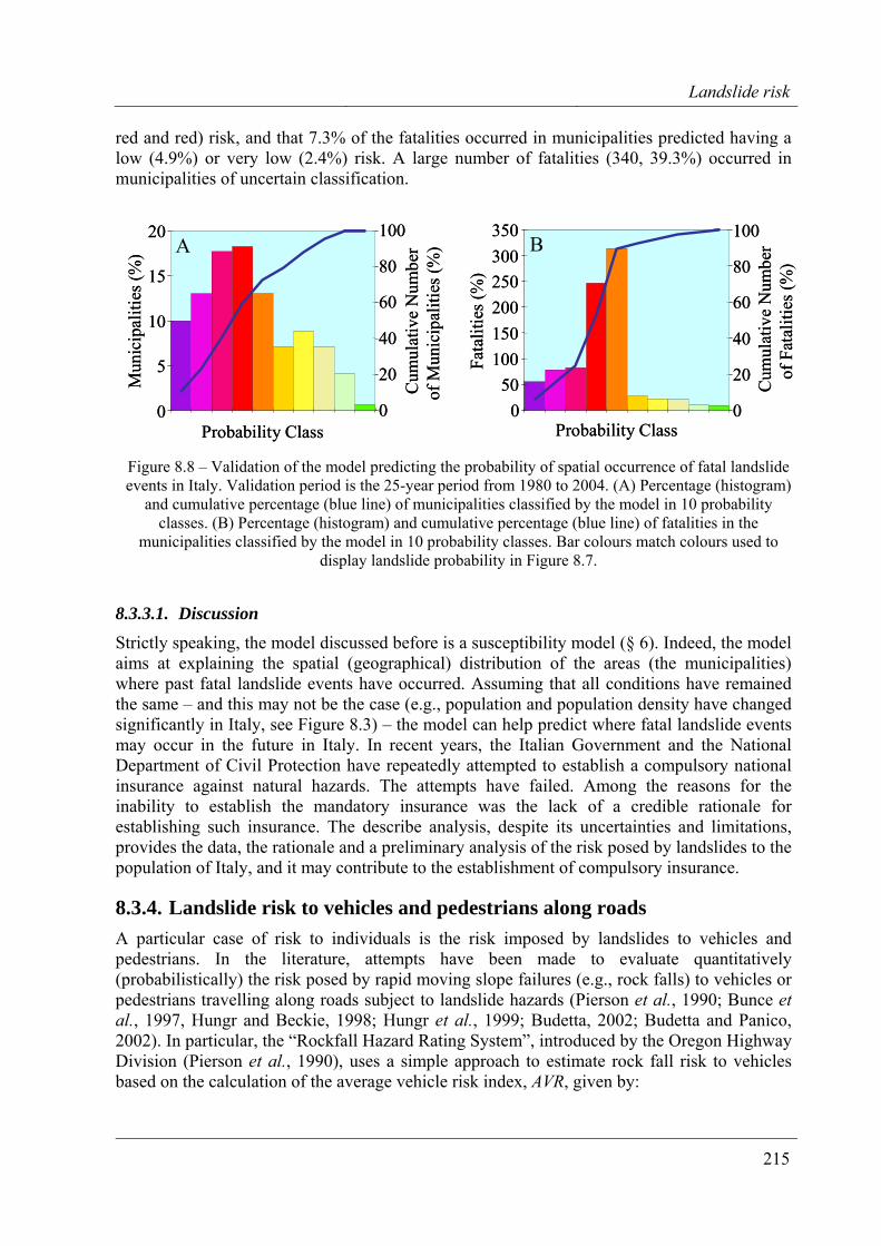
Landslide risk
215
red and red) risk, and that 7.3% of the fatalities occurred in municipalities predicted having a low (4.9%) or very low (2.4%) risk. A large number of fatalities (340, 39.3%) occurred in municipalities of uncertain classification.
0
5
10
15
20
Probability Class
Mun
icip
aliti
es (%
)
0
20
40
60
80
100
Cum
ulat
ive
Num
ber
of M
unic
ipal
ities
(%) A
050
100150200250300350
Fata
litie
s (%
)
Probability Class
B
Cum
ulat
ive
Num
ber
of F
atal
ities
(%)
0
20
40
60
80
100
0
5
10
15
20
Probability Class
Mun
icip
aliti
es (%
)
0
20
40
60
80
100
Cum
ulat
ive
Num
ber
of M
unic
ipal
ities
(%) A
050
100150200250300350
Fata
litie
s (%
)
Probability Class
B
Cum
ulat
ive
Num
ber
of F
atal
ities
(%)
0
20
40
60
80
100
Figure 8.8 – Validation of the model predicting the probability of spatial occurrence of fatal landslide events in Italy. Validation period is the 25-year period from 1980 to 2004. (A) Percentage (histogram)
and cumulative percentage (blue line) of municipalities classified by the model in 10 probability classes. (B) Percentage (histogram) and cumulative percentage (blue line) of fatalities in the
municipalities classified by the model in 10 probability classes. Bar colours match colours used to display landslide probability in Figure 8.7.
8.3.3.1. Discussion
Strictly speaking, the model discussed before is a susceptibility model (§ 6). Indeed, the model aims at explaining the spatial (geographical) distribution of the areas (the municipalities) where past fatal landslide events have occurred. Assuming that all conditions have remained the same – and this may not be the case (e.g., population and population density have changed significantly in Italy, see Figure 8.3) – the model can help predict where fatal landslide events may occur in the future in Italy. In recent years, the Italian Government and the National Department of Civil Protection have repeatedly attempted to establish a compulsory national insurance against natural hazards. The attempts have failed. Among the reasons for the inability to establish the mandatory insurance was the lack of a credible rationale for establishing such insurance. The describe analysis, despite its uncertainties and limitations, provides the data, the rationale and a preliminary analysis of the risk posed by landslides to the population of Italy, and it may contribute to the establishment of compulsory insurance.
8.3.4. Landslide risk to vehicles and pedestrians along roads A particular case of risk to individuals is the risk imposed by landslides to vehicles and pedestrians. In the literature, attempts have been made to evaluate quantitatively (probabilistically) the risk posed by rapid moving slope failures (e.g., rock falls) to vehicles or pedestrians travelling along roads subject to landslide hazards (Pierson et al., 1990; Bunce et al., 1997, Hungr and Beckie, 1998; Hungr et al., 1999; Budetta, 2002; Budetta and Panico, 2002). In particular, the “Rockfall Hazard Rating System”, introduced by the Oregon Highway Division (Pierson et al., 1990), uses a simple approach to estimate rock fall risk to vehicles based on the calculation of the average vehicle risk index, AVR, given by:
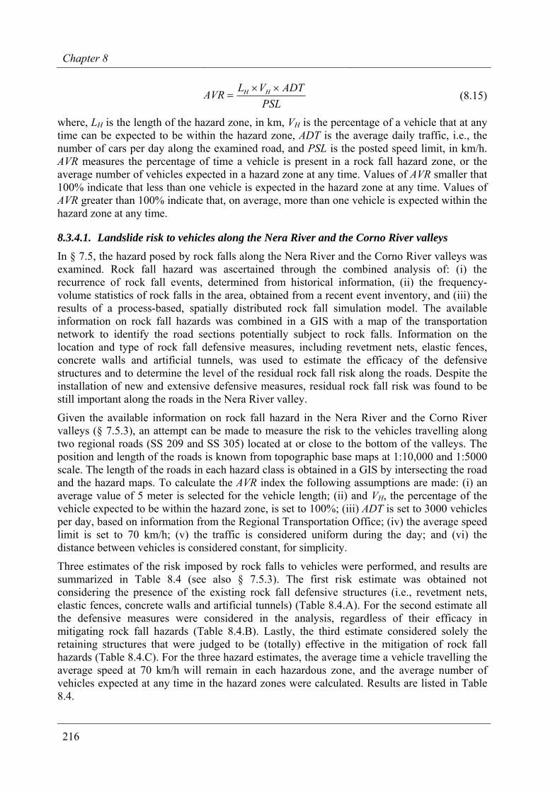
Chapter 8
216
PSLADTVLAVR HH ××
= (8.15)
where, LH is the length of the hazard zone, in km, VH is the percentage of a vehicle that at any time can be expected to be within the hazard zone, ADT is the average daily traffic, i.e., the number of cars per day along the examined road, and PSL is the posted speed limit, in km/h. AVR measures the percentage of time a vehicle is present in a rock fall hazard zone, or the average number of vehicles expected in a hazard zone at any time. Values of AVR smaller that 100% indicate that less than one vehicle is expected in the hazard zone at any time. Values of AVR greater than 100% indicate that, on average, more than one vehicle is expected within the hazard zone at any time.
8.3.4.1. Landslide risk to vehicles along the Nera River and the Corno River valleys In § 7.5, the hazard posed by rock falls along the Nera River and the Corno River valleys was examined. Rock fall hazard was ascertained through the combined analysis of: (i) the recurrence of rock fall events, determined from historical information, (ii) the frequency-volume statistics of rock falls in the area, obtained from a recent event inventory, and (iii) the results of a process-based, spatially distributed rock fall simulation model. The available information on rock fall hazards was combined in a GIS with a map of the transportation network to identify the road sections potentially subject to rock falls. Information on the location and type of rock fall defensive measures, including revetment nets, elastic fences, concrete walls and artificial tunnels, was used to estimate the efficacy of the defensive structures and to determine the level of the residual rock fall risk along the roads. Despite the installation of new and extensive defensive measures, residual rock fall risk was found to be still important along the roads in the Nera River valley.
Given the available information on rock fall hazard in the Nera River and the Corno River valleys (§ 7.5.3), an attempt can be made to measure the risk to the vehicles travelling along two regional roads (SS 209 and SS 305) located at or close to the bottom of the valleys. The position and length of the roads is known from topographic base maps at 1:10,000 and 1:5000 scale. The length of the roads in each hazard class is obtained in a GIS by intersecting the road and the hazard maps. To calculate the AVR index the following assumptions are made: (i) an average value of 5 meter is selected for the vehicle length; (ii) and VH, the percentage of the vehicle expected to be within the hazard zone, is set to 100%; (iii) ADT is set to 3000 vehicles per day, based on information from the Regional Transportation Office; (iv) the average speed limit is set to 70 km/h; (v) the traffic is considered uniform during the day; and (vi) the distance between vehicles is considered constant, for simplicity.
Three estimates of the risk imposed by rock falls to vehicles were performed, and results are summarized in Table 8.4 (see also § 7.5.3). The first risk estimate was obtained not considering the presence of the existing rock fall defensive structures (i.e., revetment nets, elastic fences, concrete walls and artificial tunnels) (Table 8.4.A). For the second estimate all the defensive measures were considered in the analysis, regardless of their efficacy in mitigating rock fall hazards (Table 8.4.B). Lastly, the third estimate considered solely the retaining structures that were judged to be (totally) effective in the mitigation of rock fall hazards (Table 8.4.C). For the three hazard estimates, the average time a vehicle travelling the average speed at 70 km/h will remain in each hazardous zone, and the average number of vehicles expected at any time in the hazard zones were calculated. Results are listed in Table 8.4.
Landslide risk
217
Table 8.4 – Rock fall risk to vehicles travelling along two regional roads in the Nera River and the Corno River valleys. See § 7.5 for explanation of hazard classes and rock fall hazard modelling. (A)
Risk to vehicles not considering the existing rock fall defensive structures. (B) Risk to vehicles considering all existing rock fall defensive structures. (C) Risk to vehicles considering only rock fall
defensive structures that are effective in mitigating rock fall hazard. AVR shows the number of vehicles per day in each hazard class. Travel time, time and percent of time a vehicle travelling at 70 km/h will remain in each hazard class. Cars, is the expected number of vehicles at any time in each hazard class.
ROCK FALL HAZARD CLASS
ROAD LENGTH AVR TRAVEL TIME CARS
km % minutes #
A Very low (VL) 2.36 10,114 26.05 2.02 4.21 Low (L) 1.83 7843 20.20 1.57 3.27 Intermediate (M) 1.84 7886 20.31 1.58 3.29 High (H) 2.13 9129 23.51 1.83 3.80 Very High (VH) 0.90 3857 9.93 0.77 1.61 Total 9.06 38,829 7.77 16.18
B Very low (VL) 1.08 4629 37.11 0.93 1.93 Low (L) 0.82 3514 28.18 0.70 1.46 Intermediate (M) 0.54 2314 18.56 0.46 0.96 High (H) 0.44 1886 15.12 0.38 0.79 Very High (VH) 0.03 129 1.03 0.03 0.05 Total 2.91 12,471 2.49 5.20
C Very low (VL) 1.26 5400 30.96 1.08 2.25 Low (L) 0.89 3814 21.87 0.76 1.59 Intermediate (M) 0.80 3429 19.66 0.69 1.43 High (H) 0.94 4029 23.10 0.81 1.68 Very High (VH) 0.18 771 4.42 0.15 0.32 Total 4.07 17,443 3.49 7.27
Analysis of the results indicates that the existing rock fall defensive measures greatly reduce the AVR, but confirms that a level of residual risk still exists along the considered regional roads in the Nera River and the Corno River valleys. Reduction of the AVR, of the average time a vehicle will remain in a dangerous zone, and of the total number of vehicles in hazardous areas, is higher where rock fall risk is estimated to be very high (VH). This confirms that rock fall defensive structures were installed where the hazard was most severe. The analysis also suggests that even where the hazard is not particularly severe, rock fall risk to the vehicles is not negligible, particularly where the expected frequency of rock falls is high.
8.4. Geomorphological landslide risk evaluation
Cardinali et al. (2002b), Guzzetti et al. (2004) and Reichenbach et al. (2005) described an attempt to determine qualitative landslide risk levels in Umbria. The method is based on the geomorphological interpretation of multiple sets of aerial photographs of different ages (a process of multi-temporal landslide mapping), aided by the analysis of historical information on past landslide events. The method involves the definition of the study area and the careful scrutiny of the “state of nature”, i.e., of all the existing and past landslides that can be identified in the study area. The possible short term evolution of the slopes, the probable type
Chapter 8
218
of failures and their expected frequency of occurrence, are inferred from the observed changes in the distribution and pattern of landslides. The information is used to estimate the landslide hazard, and to evaluate specific and total levels of landslide risk. More precisely, the method involves: (i) the preliminary definition of the extent of the study area, (ii) the compilation of a multi-temporal landslide inventory map, including landslide classification, (iii) the definition of landslide hazard zones, (iv) the assessment of landslide hazard, using a two-digit positional index, (v) the identification and mapping of the elements at risk, including an assessment of their vulnerability to different landslide types, (vi) the evaluation of specific landslide risk, using a three-digit positional index, and (vii) the determination of total landslide risk levels. The proposed method is a form of Structured Expert Judgment.
8.4.1. Definition of the study area Preliminary to the landslide hazards and risk assessment is the definition of the area to be investigated. This apparently trivial problem is essential to the analysis and the application of the results. For the purpose of the investigation, a “site” was defined as an area bounded by drainage and divide lines around the place selected for the landslide risk assessment. Thus, a site is an ensemble of one or more adjacent “elementary slopes” or watersheds. In general, major divides and drainage lines are used to outline a site. Where this is not possible, minor divides or drainage lines are used. In Umbria, mapping of elementary slopes or watersheds was accomplished at 1:10,000 scale, using large-scale topographic base maps, locally aided by the analysis of recent, large and medium scale aerial photographs. At each site, the number and the extent of the elementary slopes depended on the local geological and morphological setting, and on the type, number and extent of landslides.
8.4.2. Multi-temporal landslide map For each site, the spatial distribution of landslides is ascertained through the interpretation of multiple sets of vertical, stereoscopic aerial photographs, and detailed field surveys. In Umbria, for a period of about 60 years (from 1941 to 2001), seven sets of aerial photographs taken in different years are available. The oldest photographs were taken in 1941, and the youngest in 1997. Nominal scale of the aerial photographs ranged from 1:13,000 to 1:73,000. Only three sets of photographs cover the entire territory, whereas the other flights were limited to specific areas. Field surveys used to complete the inventory and to test the methodology were carried out mostly in the years 2000 and 2001 (Antonini et al., 2002a).
To prepare the multi-temporal landslide inventory map, landslides were first identified on aerial photographs taken in 1954-55. This set was selected because it was the oldest flight covering the entire Region, because the aerial images were taken in a period when intense cultivation of the land by mechanical equipments had not started, and the forms of old and recent landslides were clearly visible on the photographs (Guzzetti and Cardinali, 1989, 1990). The other sets of aerial photographs were analysed separately and in conjunction with the 1954-55 photographs and with the other flights. In this way separate landslide inventory maps were prepared, one for each set of aerial photographs and for the field surveys. Landslide information collected through the interpretation of aerial photographs or mapped in the field was transferred to 1:10,000 scale topographic base maps. The different landslide maps were overlaid and merged to obtain a single, multi-temporal landslide inventory map (§ 3.3.4). The process required adjustments to eliminate positional and drafting errors. The multi-temporal landslide inventory map was then digitised and stored into a GIS database.
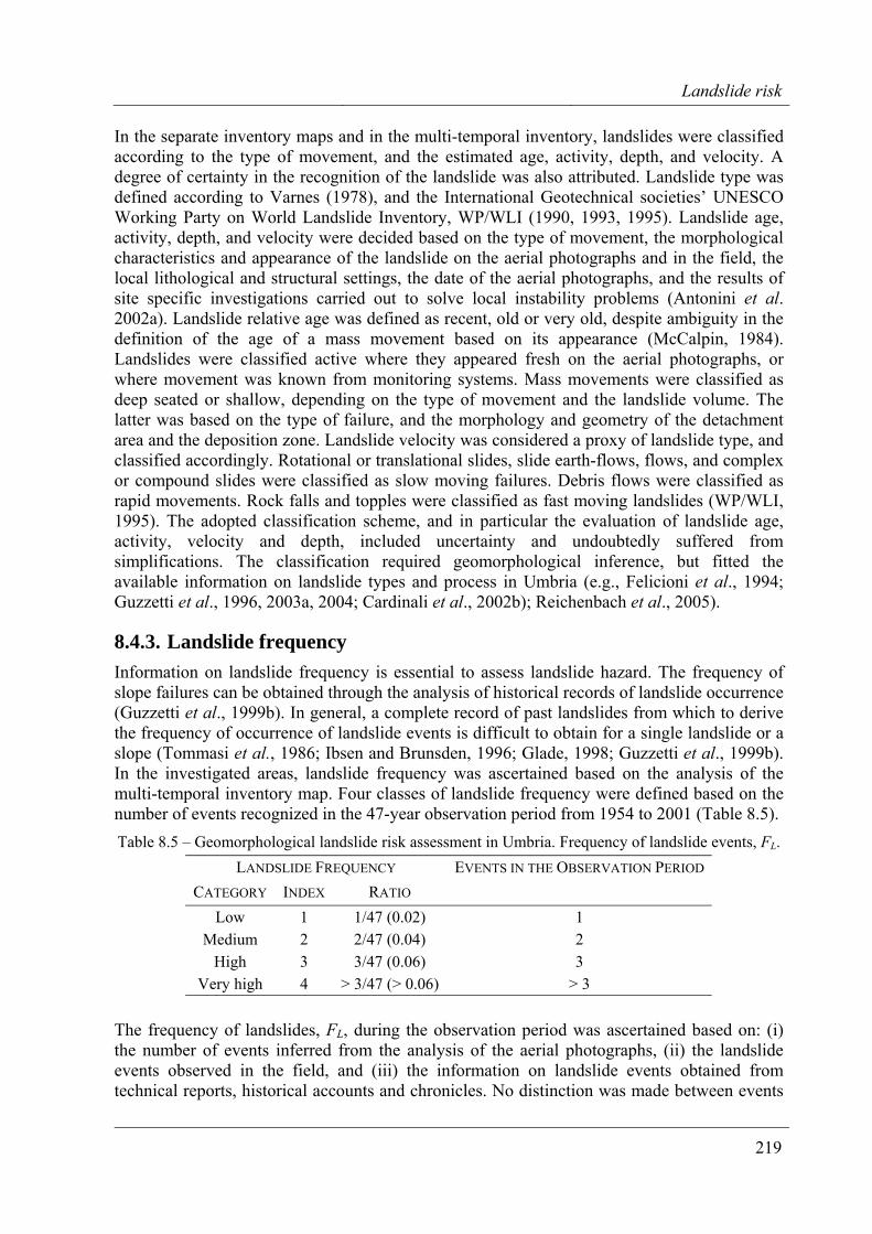
Landslide risk
219
In the separate inventory maps and in the multi-temporal inventory, landslides were classified according to the type of movement, and the estimated age, activity, depth, and velocity. A degree of certainty in the recognition of the landslide was also attributed. Landslide type was defined according to Varnes (1978), and the International Geotechnical societies’ UNESCO Working Party on World Landslide Inventory, WP/WLI (1990, 1993, 1995). Landslide age, activity, depth, and velocity were decided based on the type of movement, the morphological characteristics and appearance of the landslide on the aerial photographs and in the field, the local lithological and structural settings, the date of the aerial photographs, and the results of site specific investigations carried out to solve local instability problems (Antonini et al. 2002a). Landslide relative age was defined as recent, old or very old, despite ambiguity in the definition of the age of a mass movement based on its appearance (McCalpin, 1984). Landslides were classified active where they appeared fresh on the aerial photographs, or where movement was known from monitoring systems. Mass movements were classified as deep seated or shallow, depending on the type of movement and the landslide volume. The latter was based on the type of failure, and the morphology and geometry of the detachment area and the deposition zone. Landslide velocity was considered a proxy of landslide type, and classified accordingly. Rotational or translational slides, slide earth-flows, flows, and complex or compound slides were classified as slow moving failures. Debris flows were classified as rapid movements. Rock falls and topples were classified as fast moving landslides (WP/WLI, 1995). The adopted classification scheme, and in particular the evaluation of landslide age, activity, velocity and depth, included uncertainty and undoubtedly suffered from simplifications. The classification required geomorphological inference, but fitted the available information on landslide types and process in Umbria (e.g., Felicioni et al., 1994; Guzzetti et al., 1996, 2003a, 2004; Cardinali et al., 2002b); Reichenbach et al., 2005).
8.4.3. Landslide frequency Information on landslide frequency is essential to assess landslide hazard. The frequency of slope failures can be obtained through the analysis of historical records of landslide occurrence (Guzzetti et al., 1999b). In general, a complete record of past landslides from which to derive the frequency of occurrence of landslide events is difficult to obtain for a single landslide or a slope (Tommasi et al., 1986; Ibsen and Brunsden, 1996; Glade, 1998; Guzzetti et al., 1999b). In the investigated areas, landslide frequency was ascertained based on the analysis of the multi-temporal inventory map. Four classes of landslide frequency were defined based on the number of events recognized in the 47-year observation period from 1954 to 2001 (Table 8.5). Table 8.5 – Geomorphological landslide risk assessment in Umbria. Frequency of landslide events, FL.
LANDSLIDE FREQUENCY EVENTS IN THE OBSERVATION PERIOD CATEGORY INDEX RATIO
Low 1 1/47 (0.02) 1 Medium 2 2/47 (0.04) 2
High 3 3/47 (0.06) 3 Very high 4 > 3/47 (> 0.06) > 3
The frequency of landslides, FL, during the observation period was ascertained based on: (i) the number of events inferred from the analysis of the aerial photographs, (ii) the landslide events observed in the field, and (iii) the information on landslide events obtained from technical reports, historical accounts and chronicles. No distinction was made between events
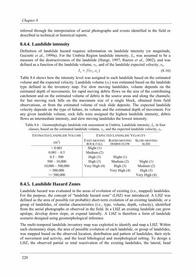
Chapter 8
220
inferred through the interpretation of aerial photographs and events identified in the field or described in technical or historical reports.
8.4.4. Landslide intensity Definition of landslide hazard requires information on landslide intensity (or magnitude, Guzzetti et al., 1999a). For the Umbria Region landslide intensity, IL, was assumed to be a measure of the destructiveness of the landslide (Hungr, 1997; Raetzo et al., 2002), and was defined as a function of the landslide volume, vL, and of the landslide expected velocity, sL,
),( LLL svfI = (8.16)
Table 8.6 shows how the intensity level was assigned to each landslide based on the estimated volume and the expected velocity. Landslide volume (vL) was estimated based on the landslide type defined in the inventory map. For slow moving landslides, volume depends on the estimated depth of movements; for rapid moving debris flows on the size of the contributing catchment and on the estimated volume of debris in the source areas and along the channels; for fast moving rock falls on the maximum size of a single block, obtained from field observations, or from the estimated volume of rock slide deposits. The expected landslide velocity depends on the type of failure, its volume and the estimated depth of movement. For any given landslide volume, rock falls were assigned the highest landslide intensity, debris flows an intermediate intensity, and slow moving landslides the lowest intensity.
Table 8.6 – Geomorphologic landslide risk assessment in Umbria. Landslide intensity, IL, in four classes, based on the estimated landslide volume, vL, and the expected landslide velocity, sL.
ESTIMATED LANDSLIDE VOLUME EXPECTED LANDSLIDE VELOCITY
(m3) FAST-MOVING ROCK FALL
RAPID-MOVING DEBRIS FLOW
SLOW-MOVING SLIDE
< 0.001 Slight (1) 0.001 – 0.5 Medium (2) 0.5 – 500 High (3) Slight (1)
500 – 10,000 High (3) Medium (2) Slight (1) 10,000 – 500,000 Very High (4) High (3) Medium (2)
> 500,000 Very High (4) High (3) >> 500,000 Very High (4)
8.4.5. Landslide Hazard Zones Landslide hazard was evaluated in the areas of evolution of existing (i.e., mapped) landslides. For the purpose, the concept of “landslide hazard zone” (LHZ) was introduced. A LHZ was defined as the area of possible (or probable) short-term evolution of an existing landslide, or a group of landslides, of similar characteristics (i.e., type, volume, depth, velocity), identified from the aerial photographs or observed in the field. In a LHZ an existing landslide can grow upslope, develop down slope, or expand laterally. A LHZ is therefore a form of landslide scenario designed using geomorphological inference.
The multi-temporal landslide inventory map was exploited to identify and map a LHZ. Within each elementary slope, the area of possible evolution of each landslide, or group of landslides, was mapped based on the observed location, distribution and pattern of landslides, their style of movement and activity, and the local lithological and morphological setting. To design a LHZ, the observed partial or total reactivation of the existing landslides, the lateral, head
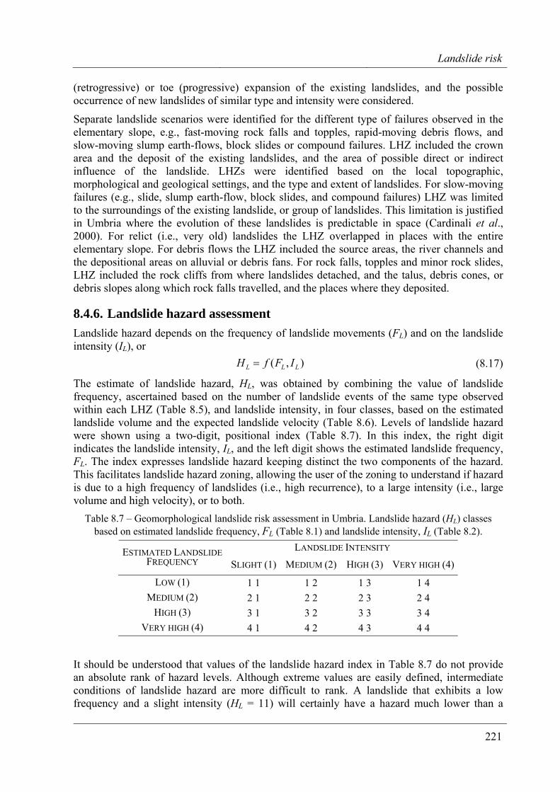
Landslide risk
221
(retrogressive) or toe (progressive) expansion of the existing landslides, and the possible occurrence of new landslides of similar type and intensity were considered.
Separate landslide scenarios were identified for the different type of failures observed in the elementary slope, e.g., fast-moving rock falls and topples, rapid-moving debris flows, and slow-moving slump earth-flows, block slides or compound failures. LHZ included the crown area and the deposit of the existing landslides, and the area of possible direct or indirect influence of the landslide. LHZs were identified based on the local topographic, morphological and geological settings, and the type and extent of landslides. For slow-moving failures (e.g., slide, slump earth-flow, block slides, and compound failures) LHZ was limited to the surroundings of the existing landslide, or group of landslides. This limitation is justified in Umbria where the evolution of these landslides is predictable in space (Cardinali et al., 2000). For relict (i.e., very old) landslides the LHZ overlapped in places with the entire elementary slope. For debris flows the LHZ included the source areas, the river channels and the depositional areas on alluvial or debris fans. For rock falls, topples and minor rock slides, LHZ included the rock cliffs from where landslides detached, and the talus, debris cones, or debris slopes along which rock falls travelled, and the places where they deposited.
8.4.6. Landslide hazard assessment Landslide hazard depends on the frequency of landslide movements (FL) and on the landslide intensity (IL), or
),( LLL IFfH = (8.17)
The estimate of landslide hazard, HL, was obtained by combining the value of landslide frequency, ascertained based on the number of landslide events of the same type observed within each LHZ (Table 8.5), and landslide intensity, in four classes, based on the estimated landslide volume and the expected landslide velocity (Table 8.6). Levels of landslide hazard were shown using a two-digit, positional index (Table 8.7). In this index, the right digit indicates the landslide intensity, IL, and the left digit shows the estimated landslide frequency, FL. The index expresses landslide hazard keeping distinct the two components of the hazard. This facilitates landslide hazard zoning, allowing the user of the zoning to understand if hazard is due to a high frequency of landslides (i.e., high recurrence), to a large intensity (i.e., large volume and high velocity), or to both.
Table 8.7 – Geomorphological landslide risk assessment in Umbria. Landslide hazard (HL) classes based on estimated landslide frequency, FL (Table 8.1) and landslide intensity, IL (Table 8.2).
LANDSLIDE INTENSITY ESTIMATED LANDSLIDE FREQUENCY SLIGHT (1) MEDIUM (2) HIGH (3) VERY HIGH (4)
LOW (1) 1 1 1 2 1 3 1 4 MEDIUM (2) 2 1 2 2 2 3 2 4
HIGH (3) 3 1 3 2 3 3 3 4 VERY HIGH (4) 4 1 4 2 4 3 4 4
It should be understood that values of the landslide hazard index in Table 8.7 do not provide an absolute rank of hazard levels. Although extreme values are easily defined, intermediate conditions of landslide hazard are more difficult to rank. A landslide that exhibits a low frequency and a slight intensity (HL = 11) will certainly have a hazard much lower than a
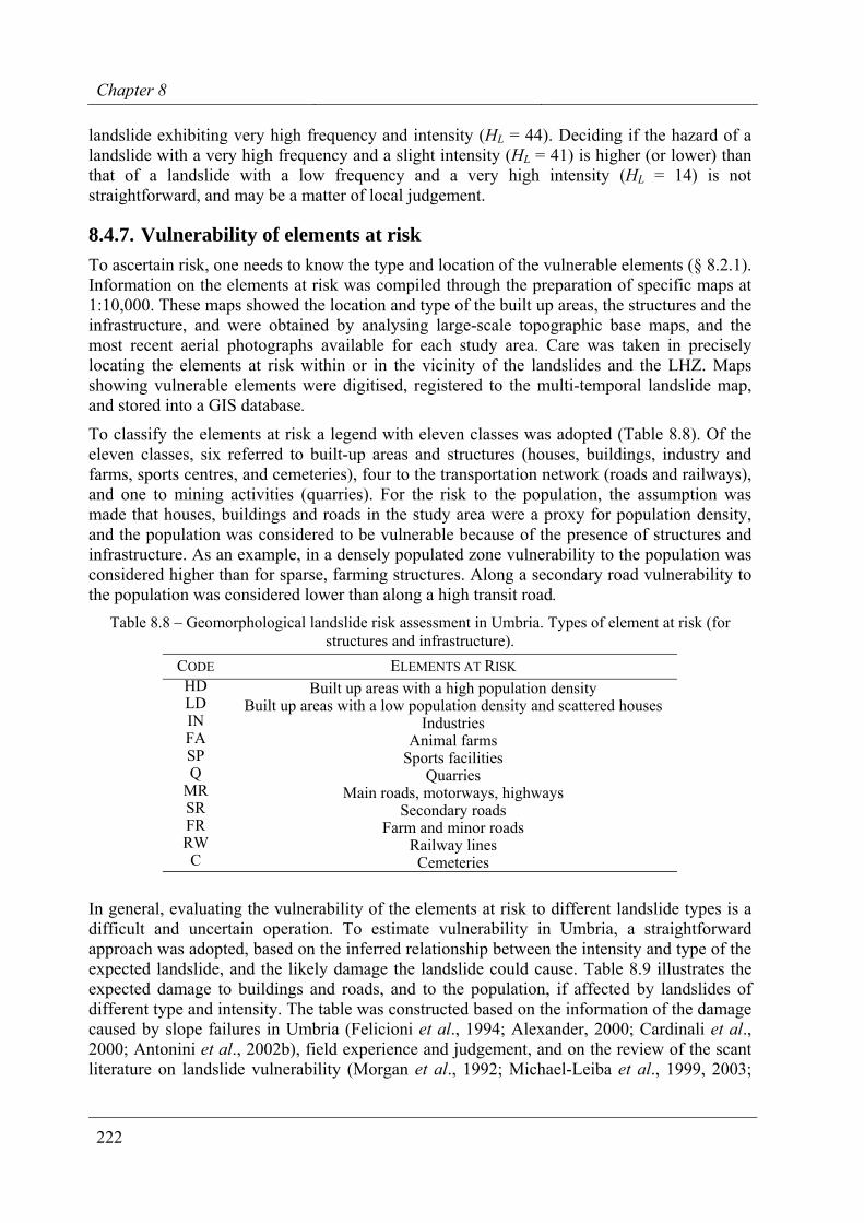
Chapter 8
222
landslide exhibiting very high frequency and intensity (HL = 44). Deciding if the hazard of a landslide with a very high frequency and a slight intensity (HL = 41) is higher (or lower) than that of a landslide with a low frequency and a very high intensity (HL = 14) is not straightforward, and may be a matter of local judgement.
8.4.7. Vulnerability of elements at risk To ascertain risk, one needs to know the type and location of the vulnerable elements (§ 8.2.1). Information on the elements at risk was compiled through the preparation of specific maps at 1:10,000. These maps showed the location and type of the built up areas, the structures and the infrastructure, and were obtained by analysing large-scale topographic base maps, and the most recent aerial photographs available for each study area. Care was taken in precisely locating the elements at risk within or in the vicinity of the landslides and the LHZ. Maps showing vulnerable elements were digitised, registered to the multi-temporal landslide map, and stored into a GIS database.
To classify the elements at risk a legend with eleven classes was adopted (Table 8.8). Of the eleven classes, six referred to built-up areas and structures (houses, buildings, industry and farms, sports centres, and cemeteries), four to the transportation network (roads and railways), and one to mining activities (quarries). For the risk to the population, the assumption was made that houses, buildings and roads in the study area were a proxy for population density, and the population was considered to be vulnerable because of the presence of structures and infrastructure. As an example, in a densely populated zone vulnerability to the population was considered higher than for sparse, farming structures. Along a secondary road vulnerability to the population was considered lower than along a high transit road.
Table 8.8 – Geomorphological landslide risk assessment in Umbria. Types of element at risk (for structures and infrastructure).
CODE ELEMENTS AT RISK HD Built up areas with a high population density LD Built up areas with a low population density and scattered houses IN Industries FA Animal farms SP Sports facilities Q Quarries
MR Main roads, motorways, highways SR Secondary roads FR Farm and minor roads RW Railway lines C Cemeteries
In general, evaluating the vulnerability of the elements at risk to different landslide types is a difficult and uncertain operation. To estimate vulnerability in Umbria, a straightforward approach was adopted, based on the inferred relationship between the intensity and type of the expected landslide, and the likely damage the landslide could cause. Table 8.9 illustrates the expected damage to buildings and roads, and to the population, if affected by landslides of different type and intensity. The table was constructed based on the information of the damage caused by slope failures in Umbria (Felicioni et al., 1994; Alexander, 2000; Cardinali et al., 2000; Antonini et al., 2002b), field experience and judgement, and on the review of the scant literature on landslide vulnerability (Morgan et al., 1992; Michael-Leiba et al., 1999, 2003;
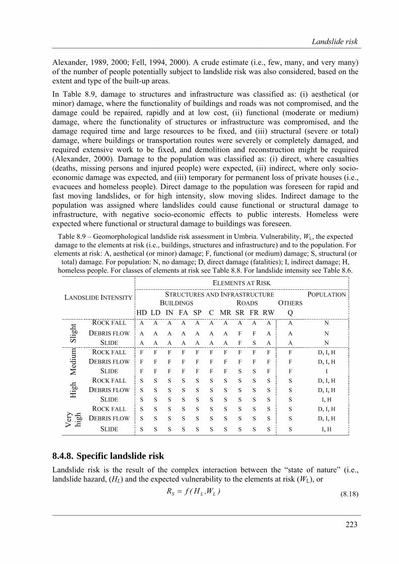
Landslide risk
223
Alexander, 1989, 2000; Fell, 1994, 2000). A crude estimate (i.e., few, many, and very many) of the number of people potentially subject to landslide risk was also considered, based on the extent and type of the built-up areas.
In Table 8.9, damage to structures and infrastructure was classified as: (i) aesthetical (or minor) damage, where the functionality of buildings and roads was not compromised, and the damage could be repaired, rapidly and at low cost, (ii) functional (moderate or medium) damage, where the functionality of structures or infrastructure was compromised, and the damage required time and large resources to be fixed, and (iii) structural (severe or total) damage, where buildings or transportation routes were severely or completely damaged, and required extensive work to be fixed, and demolition and reconstruction might be required (Alexander, 2000). Damage to the population was classified as: (i) direct, where casualties (deaths, missing persons and injured people) were expected, (ii) indirect, where only socio-economic damage was expected, and (iii) temporary for permanent loss of private houses (i.e., evacuees and homeless people). Direct damage to the population was foreseen for rapid and fast moving landslides, or for high intensity, slow moving slides. Indirect damage to the population was assigned where landslides could cause functional or structural damage to infrastructure, with negative socio-economic effects to public interests. Homeless were expected where functional or structural damage to buildings was foreseen.
Table 8.9 – Geomorphological landslide risk assessment in Umbria. Vulnerability, WL, the expected damage to the elements at risk (i.e., buildings, structures and infrastructure) and to the population. For elements at risk: A, aesthetical (or minor) damage; F, functional (or medium) damage; S, structural (or
total) damage. For population: N, no damage; D, direct damage (fatalities); I, indirect damage; H, homeless people. For classes of elements at risk see Table 8.8. For landslide intensity see Table 8.6.
ELEMENTS AT RISK STRUCTURES AND INFRASTRUCTURE POPULATION
BUILDINGS ROADS OTHERS LANDSLIDE INTENSITY
HD LD IN FA SP C MR SR FR RW Q ROCK FALL A A A A A A A A A A A N
DEBRIS FLOW A A A A A A A F F A A N
Slig
ht
SLIDE A A A A A A A F S A A N ROCK FALL F F F F F F F F F F F D, I, H
DEBRIS FLOW F F F F F F F F F F F D, I, H
Med
ium
SLIDE F F F F F F F S S F F I ROCK FALL S S S S S S S S S S S D, I, H
DEBRIS FLOW S S S S S S S S S S S D, I, H
Hig
h
SLIDE S S S S S S S S S S S I, H ROCK FALL S S S S S S S S S S S D, I, H
DEBRIS FLOW S S S S S S S S S S S D, I, H
Ver
y hi
gh
SLIDE S S S S S S S S S S S I, H
8.4.8. Specific landslide risk Landslide risk is the result of the complex interaction between the “state of nature” (i.e., landslide hazard, (HL) and the expected vulnerability to the elements at risk (WL), or
)W,H(fR LLS = (8.18)
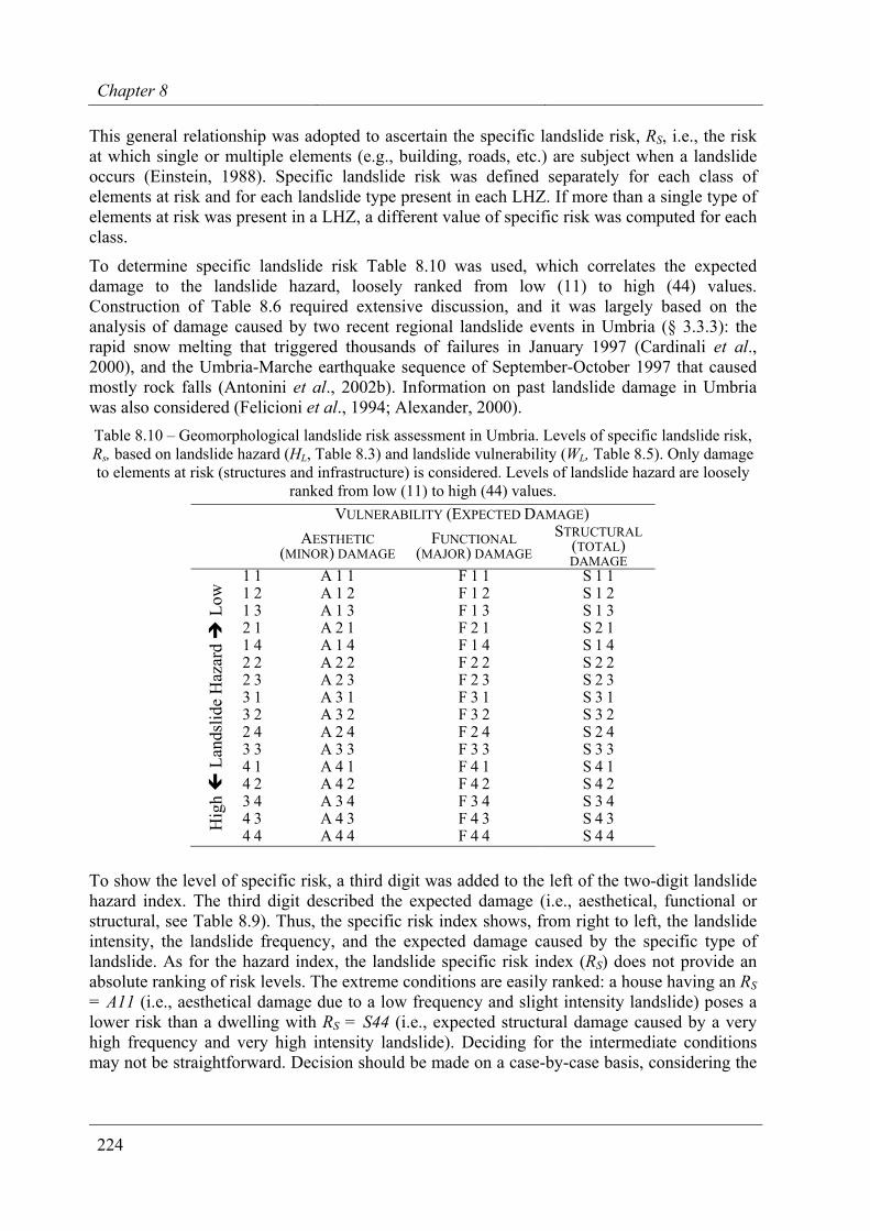
Chapter 8
224
This general relationship was adopted to ascertain the specific landslide risk, RS, i.e., the risk at which single or multiple elements (e.g., building, roads, etc.) are subject when a landslide occurs (Einstein, 1988). Specific landslide risk was defined separately for each class of elements at risk and for each landslide type present in each LHZ. If more than a single type of elements at risk was present in a LHZ, a different value of specific risk was computed for each class.
To determine specific landslide risk Table 8.10 was used, which correlates the expected damage to the landslide hazard, loosely ranked from low (11) to high (44) values. Construction of Table 8.6 required extensive discussion, and it was largely based on the analysis of damage caused by two recent regional landslide events in Umbria (§ 3.3.3): the rapid snow melting that triggered thousands of failures in January 1997 (Cardinali et al., 2000), and the Umbria-Marche earthquake sequence of September-October 1997 that caused mostly rock falls (Antonini et al., 2002b). Information on past landslide damage in Umbria was also considered (Felicioni et al., 1994; Alexander, 2000). Table 8.10 – Geomorphological landslide risk assessment in Umbria. Levels of specific landslide risk, Rs, based on landslide hazard (HL, Table 8.3) and landslide vulnerability (WL, Table 8.5). Only damage to elements at risk (structures and infrastructure) is considered. Levels of landslide hazard are loosely
ranked from low (11) to high (44) values. VULNERABILITY (EXPECTED DAMAGE)
AESTHETIC (MINOR) DAMAGE
FUNCTIONAL (MAJOR) DAMAGE
STRUCTURAL (TOTAL) DAMAGE
1 1 A 1 1 F 1 1 S 1 1 1 2 A 1 2 F 1 2 S 1 2 1 3 A 1 3 F 1 3 S 1 3 2 1 A 2 1 F 2 1 S 2 1 1 4 A 1 4 F 1 4 S 1 4 2 2 A 2 2 F 2 2 S 2 2 2 3 A 2 3 F 2 3 S 2 3 3 1 A 3 1 F 3 1 S 3 1 3 2 A 3 2 F 3 2 S 3 2 2 4 A 2 4 F 2 4 S 2 4 3 3 A 3 3 F 3 3 S 3 3 4 1 A 4 1 F 4 1 S 4 1 4 2 A 4 2 F 4 2 S 4 2 3 4 A 3 4 F 3 4 S 3 4 4 3 A 4 3 F 4 3 S 4 3 H
igh
Lan
dslid
e H
azar
d L
ow
4 4 A 4 4 F 4 4 S 4 4
To show the level of specific risk, a third digit was added to the left of the two-digit landslide hazard index. The third digit described the expected damage (i.e., aesthetical, functional or structural, see Table 8.9). Thus, the specific risk index shows, from right to left, the landslide intensity, the landslide frequency, and the expected damage caused by the specific type of landslide. As for the hazard index, the landslide specific risk index (RS) does not provide an absolute ranking of risk levels. The extreme conditions are easily ranked: a house having an RS = A11 (i.e., aesthetical damage due to a low frequency and slight intensity landslide) poses a lower risk than a dwelling with RS = S44 (i.e., expected structural damage caused by a very high frequency and very high intensity landslide). Deciding for the intermediate conditions may not be straightforward. Decision should be made on a case-by-case basis, considering the
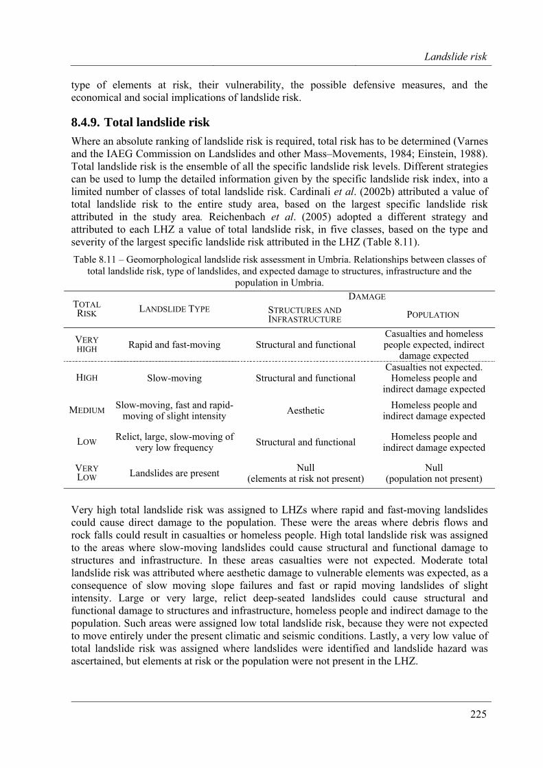
Landslide risk
225
type of elements at risk, their vulnerability, the possible defensive measures, and the economical and social implications of landslide risk.
8.4.9. Total landslide risk Where an absolute ranking of landslide risk is required, total risk has to be determined (Varnes and the IAEG Commission on Landslides and other Mass–Movements, 1984; Einstein, 1988). Total landslide risk is the ensemble of all the specific landslide risk levels. Different strategies can be used to lump the detailed information given by the specific landslide risk index, into a limited number of classes of total landslide risk. Cardinali et al. (2002b) attributed a value of total landslide risk to the entire study area, based on the largest specific landslide risk attributed in the study area. Reichenbach et al. (2005) adopted a different strategy and attributed to each LHZ a value of total landslide risk, in five classes, based on the type and severity of the largest specific landslide risk attributed in the LHZ (Table 8.11). Table 8.11 – Geomorphological landslide risk assessment in Umbria. Relationships between classes of
total landslide risk, type of landslides, and expected damage to structures, infrastructure and the population in Umbria.
DAMAGE TOTAL RISK LANDSLIDE TYPE STRUCTURES AND
INFRASTRUCTURE POPULATION
VERY HIGH Rapid and fast-moving Structural and functional
Casualties and homeless people expected, indirect
damage expected
HIGH Slow-moving Structural and functional Casualties not expected.
Homeless people and indirect damage expected
MEDIUM Slow-moving, fast and rapid-moving of slight intensity Aesthetic Homeless people and
indirect damage expected
LOW Relict, large, slow-moving of very low frequency Structural and functional Homeless people and
indirect damage expected
VERY LOW Landslides are present Null
(elements at risk not present) Null
(population not present)
Very high total landslide risk was assigned to LHZs where rapid and fast-moving landslides could cause direct damage to the population. These were the areas where debris flows and rock falls could result in casualties or homeless people. High total landslide risk was assigned to the areas where slow-moving landslides could cause structural and functional damage to structures and infrastructure. In these areas casualties were not expected. Moderate total landslide risk was attributed where aesthetic damage to vulnerable elements was expected, as a consequence of slow moving slope failures and fast or rapid moving landslides of slight intensity. Large or very large, relict deep-seated landslides could cause structural and functional damage to structures and infrastructure, homeless people and indirect damage to the population. Such areas were assigned low total landslide risk, because they were not expected to move entirely under the present climatic and seismic conditions. Lastly, a very low value of total landslide risk was assigned where landslides were identified and landslide hazard was ascertained, but elements at risk or the population were not present in the LHZ.
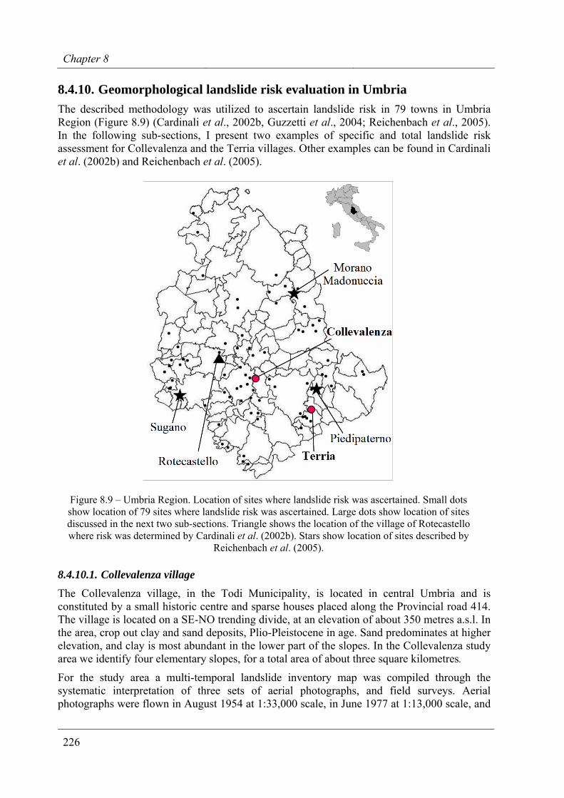
Chapter 8
226
8.4.10. Geomorphological landslide risk evaluation in Umbria The described methodology was utilized to ascertain landslide risk in 79 towns in Umbria Region (Figure 8.9) (Cardinali et al., 2002b, Guzzetti et al., 2004; Reichenbach et al., 2005). In the following sub-sections, I present two examples of specific and total landslide risk assessment for Collevalenza and the Terria villages. Other examples can be found in Cardinali et al. (2002b) and Reichenbach et al. (2005).
Figure 8.9 – Umbria Region. Location of sites where landslide risk was ascertained. Small dots show location of 79 sites where landslide risk was ascertained. Large dots show location of sites discussed in the next two sub-sections. Triangle shows the location of the village of Rotecastello where risk was determined by Cardinali et al. (2002b). Stars show location of sites described by
Reichenbach et al. (2005).
8.4.10.1. Collevalenza village The Collevalenza village, in the Todi Municipality, is located in central Umbria and is constituted by a small historic centre and sparse houses placed along the Provincial road 414. The village is located on a SE-NO trending divide, at an elevation of about 350 metres a.s.l. In the area, crop out clay and sand deposits, Plio-Pleistocene in age. Sand predominates at higher elevation, and clay is most abundant in the lower part of the slopes. In the Collevalenza study area we identify four elementary slopes, for a total area of about three square kilometres.
For the study area a multi-temporal landslide inventory map was compiled through the systematic interpretation of three sets of aerial photographs, and field surveys. Aerial photographs were flown in August 1954 at 1:33,000 scale, in June 1977 at 1:13,000 scale, and
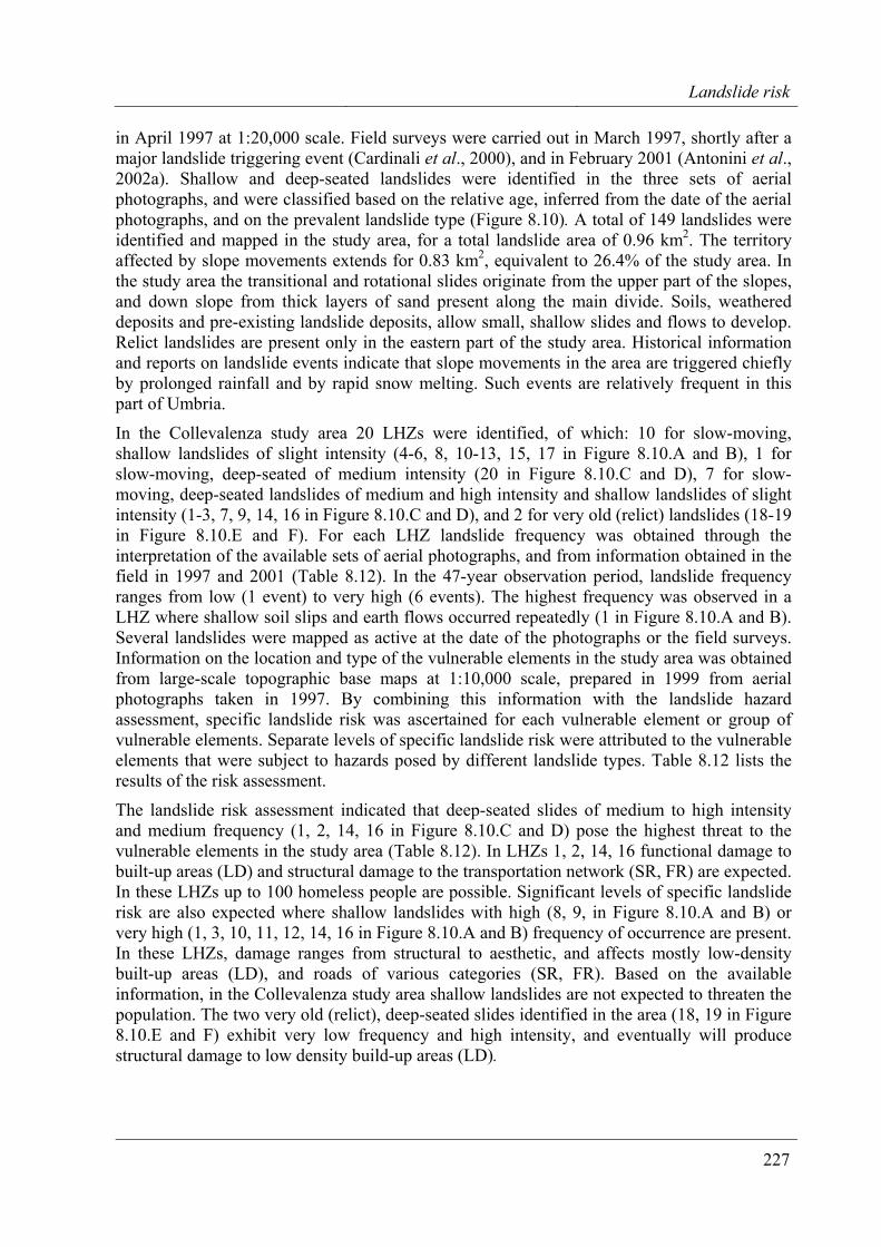
Landslide risk
227
in April 1997 at 1:20,000 scale. Field surveys were carried out in March 1997, shortly after a major landslide triggering event (Cardinali et al., 2000), and in February 2001 (Antonini et al., 2002a). Shallow and deep-seated landslides were identified in the three sets of aerial photographs, and were classified based on the relative age, inferred from the date of the aerial photographs, and on the prevalent landslide type (Figure 8.10). A total of 149 landslides were identified and mapped in the study area, for a total landslide area of 0.96 km2. The territory affected by slope movements extends for 0.83 km2, equivalent to 26.4% of the study area. In the study area the transitional and rotational slides originate from the upper part of the slopes, and down slope from thick layers of sand present along the main divide. Soils, weathered deposits and pre-existing landslide deposits, allow small, shallow slides and flows to develop. Relict landslides are present only in the eastern part of the study area. Historical information and reports on landslide events indicate that slope movements in the area are triggered chiefly by prolonged rainfall and by rapid snow melting. Such events are relatively frequent in this part of Umbria.
In the Collevalenza study area 20 LHZs were identified, of which: 10 for slow-moving, shallow landslides of slight intensity (4-6, 8, 10-13, 15, 17 in Figure 8.10.A and B), 1 for slow-moving, deep-seated of medium intensity (20 in Figure 8.10.C and D), 7 for slow-moving, deep-seated landslides of medium and high intensity and shallow landslides of slight intensity (1-3, 7, 9, 14, 16 in Figure 8.10.C and D), and 2 for very old (relict) landslides (18-19 in Figure 8.10.E and F). For each LHZ landslide frequency was obtained through the interpretation of the available sets of aerial photographs, and from information obtained in the field in 1997 and 2001 (Table 8.12). In the 47-year observation period, landslide frequency ranges from low (1 event) to very high (6 events). The highest frequency was observed in a LHZ where shallow soil slips and earth flows occurred repeatedly (1 in Figure 8.10.A and B). Several landslides were mapped as active at the date of the photographs or the field surveys. Information on the location and type of the vulnerable elements in the study area was obtained from large-scale topographic base maps at 1:10,000 scale, prepared in 1999 from aerial photographs taken in 1997. By combining this information with the landslide hazard assessment, specific landslide risk was ascertained for each vulnerable element or group of vulnerable elements. Separate levels of specific landslide risk were attributed to the vulnerable elements that were subject to hazards posed by different landslide types. Table 8.12 lists the results of the risk assessment.
The landslide risk assessment indicated that deep-seated slides of medium to high intensity and medium frequency (1, 2, 14, 16 in Figure 8.10.C and D) pose the highest threat to the vulnerable elements in the study area (Table 8.12). In LHZs 1, 2, 14, 16 functional damage to built-up areas (LD) and structural damage to the transportation network (SR, FR) are expected. In these LHZs up to 100 homeless people are possible. Significant levels of specific landslide risk are also expected where shallow landslides with high (8, 9, in Figure 8.10.A and B) or very high (1, 3, 10, 11, 12, 14, 16 in Figure 8.10.A and B) frequency of occurrence are present. In these LHZs, damage ranges from structural to aesthetic, and affects mostly low-density built-up areas (LD), and roads of various categories (SR, FR). Based on the available information, in the Collevalenza study area shallow landslides are not expected to threaten the population. The two very old (relict), deep-seated slides identified in the area (18, 19 in Figure 8.10.E and F) exhibit very low frequency and high intensity, and eventually will produce structural damage to low density build-up areas (LD).
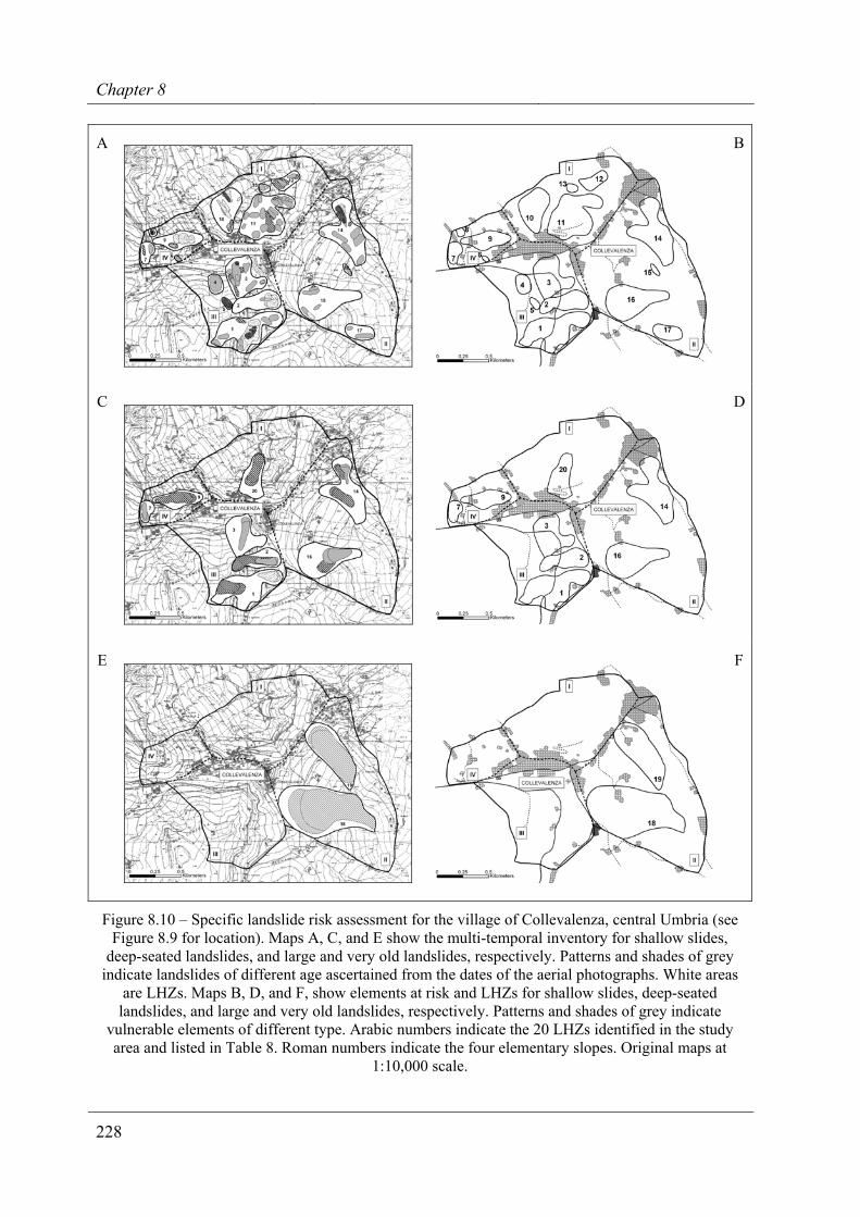
Chapter 8
228
A
B
C
D
E
F
Figure 8.10 – Specific landslide risk assessment for the village of Collevalenza, central Umbria (see Figure 8.9 for location). Maps A, C, and E show the multi-temporal inventory for shallow slides,
deep-seated landslides, and large and very old landslides, respectively. Patterns and shades of grey indicate landslides of different age ascertained from the dates of the aerial photographs. White areas
are LHZs. Maps B, D, and F, show elements at risk and LHZs for shallow slides, deep-seated landslides, and large and very old landslides, respectively. Patterns and shades of grey indicate
vulnerable elements of different type. Arabic numbers indicate the 20 LHZs identified in the study area and listed in Table 8. Roman numbers indicate the four elementary slopes. Original maps at
1:10,000 scale.
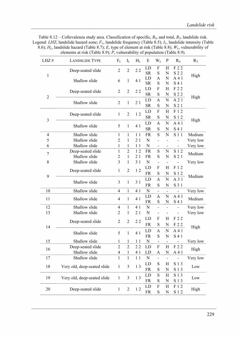
Landslide risk
229
Table 8.12 – Collevalenza study area. Classification of specific, RS, and total, RT, landslide risk. Legend: LHZ, landslide hazard zone; FL, landslide frequency (Table 8.5); IL, landslide intensity (Table
8.6); HL, landslide hazard (Table 8.7); E, type of element at risk (Table 8.8); WL, vulnerability of elements at risk (Table 8.9); P, vulnerability of population (Table 8.9).
LHZ # LANDSLIDE TYPE FL IL HL E WL P RS RT
LD F H F 2 2 Deep-seated slide 2 2 2 2 SR S N S 2 2 LD A N A 4 1 1
Shallow slide 6 1 4 1 SR S N S 4 1
High
LD F H F 2 2 Deep-seated slide 2 2 2 2 SR S N S 2 2 LD A N A 2 1
2 Shallow slide 2 1 2 1 SR S N S 2 1
High
LD F H F 1 2 Deep-seated slide 1 2 1 2SR S N S 1 2 LD A N A 4 1
3 Shallow slide 5 1 4 1
SR S N S 4 1
High
4 Shallow slide 1 1 1 1 FR S N S 1 1 Medium 5 Shallow slide 2 1 2 1 N - - - Very low6 Shallow slide 1 1 1 1 N - - - Very low
Deep-seated slide 1 2 1 2 FR S N S 1 2 7 Shallow slide 2 1 2 1 FR S N S 2 1 Medium
8 Shallow slide 3 1 3 1 N - - - Very lowLD F H F 1 2 Deep-seated slide 1 2 1 2 FR S N S 1 2 LD A N A 3 1
9 Shallow slide 3 1 3 1
FR S N S 3 1
Medium
10 Shallow slide 4 1 4 1 N - - - Very lowLD A N A 4 1 11 Shallow slide 4 1 4 1 FR S N S 4 1 Medium
12 Shallow slide 4 1 4 1 N - - - Very low13 Shallow slide 2 1 2 1 N - - - Very low
LD F H F 2 2 Deep-seated slide 2 2 2 2FR S N F 2 2 LD A N A 4 1
14 Shallow slide 5 1 4 1
FR S N S 4 1
High
15 Shallow slide 1 1 1 1 N - - - Very lowDeep-seated slide 2 2 2 2 LD F H F 2 2 16
Shallow slide 4 1 4 1 LD A N A 4 1 High
17 Shallow slide 1 1 1 1 N - - - Very lowLD S H S 1 3 18 Very old, deep-seated slide 1 3 1 3 FR S N S 1 3 Low
LD S H S 1 3 19 Very old, deep-seated slide 1 3 1 3 FR S N S 1 3 Low
LD F H F 1 2 20 Deep-seated slide 1 2 1 2 FR S N S 1 2 High
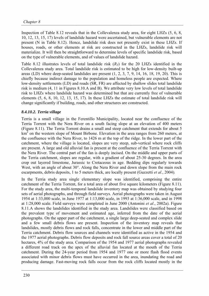
Chapter 8
230
Inspection of Table 8.12 reveals that in the Collevalenza study area, for eight LHZs (5, 6, 8, 10, 12, 13, 15, 17) levels of landslide hazard were ascertained, but vulnerable elements are not present (N in Table 8.12). Hence, landslide risk does not presently exist in these LHZs. If houses, roads, or other elements at risk are constructed in the LHZs, landslide risk will materialize. It will then be straightforward to determine levels of specific landslide risk, based on the type of vulnerable elements, and of values of landslide hazard.
Table 8.12 illustrates levels of total landslide risk (RT) for the 20 LHZs identified in the Collevalenza study area. Total landslide risk is estimated to be high for low-density built-up areas (LD) where deep-seated landslides are present (1, 2, 3, 7, 9, 14, 16, 18, 19, 20). This is chiefly because indirect damage to the population and homeless people are expected. Where low-density settlements (LD) and roads (SR, FR) are affected by shallow slides total landslide risk is medium (4, 11 in Figures 8.10.A and B). We attribute very low levels of total landslide risk to LHZs where landslide hazard was determined but that are currently free of vulnerable elements (5, 6, 8, 10, 12, 13, 15, 17). In these LHZs the estimate of total landslide risk will change significantly if building, roads, and other structures are constructed.
8.4.10.2. Terria village Terria is a small village in the Ferentillo Municipality, located near the confluence of the Terria Torrent with the Nera River on a south facing slope at an elevation of 400 meters (Figure 8.11). The Terria Torrent drains a small and steep catchment that extends for about 5 km2 on the western slope of Mount Birbone. Elevation in the area ranges from 260 meters, at the confluence with the Nera River, to 1426 m at the top of the ridge. In the lower part of the catchment, where the village is located, slopes are very steep, sub-vertical where rock cliffs are present. A large and old alluvial fan is present at the confluence of the Terria Torrent with the Nera River. The central part of the fan is deeply incised. On the middle and upper parts of the Terria catchment, slopes are regular, with a gradient of about 25-30 degrees. In the area crop out layered limestone, Jurassic to Cretaceous in age. Bedding dips regularly towards West, with an angle of about 30°. Along the Nera River and down slope from the main rock escarpments, debris deposits, 1 to 5 meters thick, are locally present (Guzzetti et al., 2004).
In the Terria study area single elementary slope was identified, comprising the entire catchment of the Terria Torrent, for a total area of about five square kilometers (Figure 8.11). For the study area, the multi-temporal landslide inventory map was obtained by studying four sets of aerial photographs, and through field surveys. Aerial photographs were taken in August 1954 at 1:33,000 scale, in June 1977 at 1:13,000 scale, in 1993 at 1:36,000 scale, and in 1998 at 1:28,000 scale. Field surveys were completed in June 2000 (Antonini et al., 2002a). Figure 8.11.A shows the landslides identified in the study area. Landslides were classified based on the prevalent type of movement and estimated age, inferred from the date of the aerial photographs. On the upper part of the catchment, a single large deep-seated and complex slide and a few small debris flows are present. Inspection of the inventory map reveals that landslides, mostly debris flows and rock falls, concentrate in the lower and middle part of the Terria catchment. Debris flow sources and channels were identified as active in the 1954 and the 1977 aerial photographs. Debris flow deposits and rock fall source areas cover a total of 20 hectares, 4% of the study area. Comparison of the 1954 and 1977 aerial photographs revealed a different road track on the apex of the alluvial fan located at the mouth of the Terria catchment. During the 24-year period from 1954 and 1977 one or more flash flood events associated with minor debris flows must have occurred in the area, inundating the road and producing damage. Fast-moving rock falls occur from the rock cliffs located mostly in the
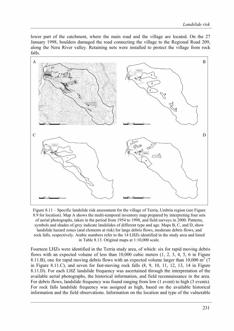
Landslide risk
231
lower part of the catchment, where the main road and the village are located. On the 27 January 1998, boulders damaged the road connecting the village to the Regional Road 209, along the Nera River valley. Retaining nets were installed to protect the village from rock falls.
A
B
C
D
Figure 8.11 – Specific landslide risk assessment for the village of Terria, Umbria region (see Figure 8.9 for location). Map A shows the multi-temporal inventory map prepared by interpreting four sets
of aerial photographs, taken in the period from 1954 to 1998, and field surveys in 2000. Patterns, symbols and shades of grey indicate landslides of different type and age. Maps B, C, and D, show
landslide hazard zones (and elements at risk) for large debris flows, moderate debris flows, and rock falls, respectively. Arabic numbers refer to the 14 LHZs identified in the study area and listed
in Table 8.13. Original maps at 1:10,000 scale.
Fourteen LHZs were identified in the Terria study area, of which: six for rapid moving debris flows with an expected volume of less than 10,000 cubic meters (1, 2, 3, 4, 5, 6 in Figure 8.11.B), one for rapid moving debris flows with an expected volume larger than 10,000 m3 (7 in Figure 8.11.C), and seven for fast-moving rock falls (8, 9, 10, 11, 12, 13, 14 in Figure 8.11.D). For each LHZ landslide frequency was ascertained through the interpretation of the available aerial photographs, the historical information, and field reconnaissance in the area. For debris flows, landslide frequency was found ranging from low (1 event) to high (3 events). For rock falls landslide frequency was assigned as high, based on the available historical information and the field observations. Information on the location and type of the vulnerable
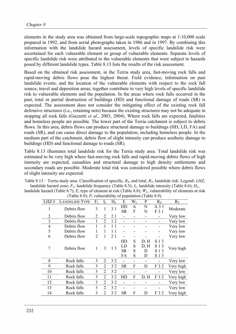
Chapter 8
232
elements in the study area was obtained from large-scale topographic maps at 1:10,000 scale prepared in 1992, and from aerial photographs taken in 1986 and in 1997. By combining this information with the landslide hazard assessment, levels of specific landslide risk were ascertained for each vulnerable element or group of vulnerable elements. Separate levels of specific landslide risk were attributed to the vulnerable elements that were subject to hazards posed by different landslide types. Table 8.13 lists the results of the risk assessment.
Based on the obtained risk assessment, in the Terria study area, fast-moving rock falls and rapid-moving debris flows pose the highest threat. Field evidence, information on past landslide events, and the location of the vulnerable elements with respect to the rock fall source, travel and deposition areas, together contribute to very high levels of specific landslide risk to vulnerable elements and the population. In the areas where rock falls occurred in the past, total or partial destruction of buildings (HD) and functional damage of roads (SR) is expected. The assessment does not consider the mitigating effect of the existing rock fall defensive structures (i.e., retaining nets) because the existing structures may not be adequate in stopping all rock falls (Guzzetti et al., 2003, 2004). Where rock falls are expected, fatalities and homeless people are possible. The lower part of the Terria catchment is subject to debris flows. In this area, debris flows can produce structural damage to buildings (HD, LD, FA) and roads (SR), and can cause direct damage to the population, including homeless people. In the medium part of the catchment, debris flow of slight intensity can produce aesthetic damage to buildings (HD) and functional damage to roads (SR).
Table 8.13 illustrates total landslide risk for the Terria study area. Total landslide risk was estimated to be very high where fast-moving rock falls and rapid-moving debris flows of high intensity are expected, casualties and structural damage to high density settlements and secondary roads are possible. Moderate total risk was considered possible where debris flows of slight intensity are expected. Table 8.13 – Terria study area. Classification of specific, RS, and total, RT, landslide risk. Legend: LHZ,
landslide hazard zone; FL, landslide frequency (Table 8.5); IL, landslide intensity (Table 8.6); HL, landslide hazard (Table 8.7); E, type of element at risk (Table 8.8); WL, vulnerability of elements at risk
(Table 8.9); P, vulnerability of population (Table 8.9). LHZ # LANDSLIDE TYPE FL IL HL E WL P RS RT
HD A N A 3 1 1 Debris flow 3 1 3 1 SR F N F 3 1 Moderate
2 Debris flow 2 2 2 1 - - - - Very low 3 Debris flow 1 2 1 2 - - - - Very low 4 Debris flow 1 1 1 1 - - - - Very low 5 Debris flow 1 1 1 1 - - - - Very low 6 Debris flow 2 1 2 1 - - - - Very low
HD S D, H S 1 3 LD S D, H S 1 3 SR S D S 1 3 7 Debris flow 1 3 1 3
FA S D S 1 3
Very high
8 Rock falls 3 2 3 2 - - - - Very low 9 Rock falls 3 2 3 2 SR F D F 3 2 Very high
10 Rock falls 3 2 3 2 - - - - Very low 11 Rock falls 3 2 3 2 HD F D, H F 3 2 Very high 12 Rock falls 3 2 3 2 - - - - Very low 13 Rock falls 3 2 3 2 - - - - Very low 14 Rock falls 3 2 3 2 SR F D F 3 2 Very high
Landslide risk
233
8.4.11. Discussion The described method to determine landslide hazards and to evaluate specific and total landslide risk complies with the existing definitions of landslide hazard (see § 6, § 7, Varnes and IAEG Commission on Landslides and other Mass-Movements, 1984; Guzzetti et al. 1999a, 1999b) and of landslide risk (see § 8.2, Varnes and IAEG Commission on Landslides and other Mass-Movements, 1984; Einstein, 1988; Cruden and Fell, 1997; Guzzetti, 2002). The method is empirical and subject to various levels of uncertainty, but has proved to be consistent, allowing for detailed and comparable assessments of landslide hazard and specific and total landslide risk levels in urban and rural areas in Umbria. The method allows the comparison of landslide hazard and risk in distinct and distant areas, and where different landslide types are present.
The method was applied in 210 landslide hazard zones located around or in the vicinity of 79 towns and villages in Umbria (Antonini et al., 2002a; Cardinali et al., 2002b; Guzzetti et al., 2004; Reichenbach et al., 2005). In these areas landslide hazard was determined, vulnerable elements were identified, and specific and total risk levels were evaluated. The time and human resources required for completing the risk assessment procedure at each site varied, depending on the extent of the study area, the number, type and scale of the aerial photographs, the available thematic and historical information, the extent and type of landslides present in the study area, and the local geological and morphological setting. On average, completion of the risk assessment procedure at each site required five days for a team of 3-4 geomorphologists, including bibliographical investigation, interpretation of the aerial photographs, field surveys, storage of landslide and other thematic information in the GIS database, and the production of the final hazard, vulnerability and risk maps.
The proposed method requires extensive geomorphological judgment. For this reason it should only be used by skilled geomorphologists. If the extent, type, distribution and pattern of past and present landslides are not correctly and fully identified, errors can occur, affecting the estimate of landslide hazards and risk. With this in mind, the definition of the temporal frequency of landslides from the analysis of the multi-temporal inventory map is particularly important. In the Umbria Region, the multi-temporal landslide maps cover a period of about 47 years, which is long enough to evaluate the short-term behaviour of slopes in the areas investigated. Should information on landslide frequency be available only for a shorter period of time (e.g., 10-15 years or less), the reliability of the hazard forecast will be reduced. If a landslide event fails to be recognized, the frequency of occurrence is underestimated, and hazard and risk estimates are negatively affected. It should be noted that the method estimates the expected landslide frequency based on what has happened (and was observed) in the recent past. If low frequency, high magnitude events did not occur or were not recognised in a LHZ, the hazard assessment in the area may be biased, and the actual landslide risk is underestimated. This is a limitation of the method.
The method allows for detailed and articulated hazard and risk assessments. Landslide hazard is determined separately for all the different landslide types that may be present in the study area. Specific landslide risk is determined independently for each type of vulnerable element in the study area. Thus, vulnerable elements may be subject to multiple levels of specific landslide risk, and landslide hazard may be ascertained where vulnerable elements are not present. The proposed method assesses landslide hazard in the areas of probable evolution of the existing landslides (i.e., in a landslide hazard zone). The method says nothing about the hazard outside a LHZ, even within the same elementary slope. In these areas minor landslides,
Chapter 8
234
mostly superficial failures can occur with a low frequency. For a regional, spatially distributed landslide hazard and risk assessment, other methods should be used (see § 6 and 7).
Uncertainty varies with the different steps of the method. The production of the separate landslide inventory maps and of the multi-temporal landslide map is less uncertain than the identification of the landslide hazard zones, or the possible spatial evolution of the existing landslides, which is obtained mostly through geomorphological inference. Landslides mapped through the interpretation of aerial photographs were carefully checked in the field, whereas the identification and mapping of LHZs was based on the observation of other landslides and on the inferred geomorphological behaviour of slopes. Evaluation of landslide frequency, which determines landslide hazards, is conditioned by the availability of aerial photographs and historical information, and by the investigator ability to recognize past and present landslide events. Estimates of landslide volume and velocity, which are essential for the evaluation of landslide intensity, also exhibit uncertainty.
Uncertainty arises also because a difference exists between geomorphological and historical information on landslides. Geomorphological information obtained through field mapping and the analysis of aerial photographs provides the basis for determining the prevalent landslide types and location, but provides poor constrain on the date (or the age) of the slope failures. Historical and archived information provides precisely the date and, more rarely, the time of occurrence of some of the landslide events, and the type and extent of damage caused by mass movements, but provide little information on the type of failures and the precise location and extent of the landslides. Combination of geomorphological and historical information on mass movements is not straightforward, and may be locally a matter of interpretation and local judgement.
The proposed method relies on a set of correlation tables, which are used to define landslide frequency (Table 8.1) and intensity (Table 8.2), to ascertain landslide hazard (Table 8.3), to evaluate the expected damage to the vulnerable elements (Table 8.5), and to attribute levels of specific (Table 8.6) and total (Table 8.7) landslide risk. The tables were based on empirical observations and on the investigators experience, but are also the result of a heuristic approach. Whenever possible, several possibilities should be evaluated and the differences compared after each attempt. The adopted tables fit the present understanding of landslide processes and match landslide damage in Umbria satisfactorily (Felicioni et al., 1994; Alexander, 2000; Cardinali et al., 2000; Antonini et al., 2002b; Guzzetti et al., 2003). However, the tables are not definitive, and should not be used unconditionally in all settings. If applied to other sites, or in other study areas, the tables should be carefully checked with the local information on landslide types and damage. If one, or more, of the tables is changed significantly, the hazard and risk assessment will vary, and may not be comparable to the one we have prepared. This is particularly important for Table 8.5 (vulnerability) and Table 8.6 (specific risk).
Landslide hazard and specific risk are expressed using a multiple-digit, “positional” index that shows, in a compact and convenient format, all the variables used to ascertain landslide hazard and risk (i.e., intensity, frequency, and vulnerability). The index allows for the ranking of risk conditions at the end of the risk assessment process, when all the necessary information is available, and not “a priori”, based on pre-defined (often ill formalized) categories. This a major advantage of the method, giving risk managers and decision makers great flexibility in deciding which area exhibits the highest risk, and providing geologists and engineers with a clue about why any given vulnerable element is at risk. In addition, the use of a simple index
Landslide risk
235
to express levels of specific landslide risk makes it possible to adopt different schemes to determine levels of total landslide risk, depending on the priorities or the specific interests of the investigators or the end-users.
Lastly, the proposed method is not simple or straightforward. A dependable and consistent prediction requires multiple sets of aerial photographs and a team of experienced geomorphologists to interpret them. This cannot be considered a limitation: landslide hazard and risk assessments are difficult tasks, and require proper expertise and skills.
8.5. Assessing landslide damage and forecasting landslide impact
An alternative way of establishing semi-quantitative levels of landslide risk consists in investigating the damage caused by slope failures in the past, and in attempting to forecast the impact that landslides will have in the future, in a given area (Brabb, 1991). The former consists in studying archive or event inventories, the latter involves designing landslide scenarios (§ 8.2.3). Where a detailed historical catalogue of landslides and their consequences exists, and where inventory maps documenting individual landslide events have been prepared, the vulnerability of the elements at risk can be ascertained, and the sites repeatedly affected by catastrophic events can be determined. More precisely, historical and event information can be exploited to: (i) evaluate the most common type of landslide damage, (ii) determine the extent and spatial distribution of the damage, and (iii) obtain quantitative estimates of the cost of single or multiple landslides (e.g., Taylor and Brabb, 1972; Godt and Savage, 1999; Guzzetti et al., 2003b). Where a sufficiently detailed landslide inventory map and maps showing the population, structures, infrastructure, and land use types are available, simple geographical operations in a GIS allow determining where landslides may interfere with the elements at risk, providing estimates of the impact that landslides may have in the future in a given area (e.g., Garberi et al., 1999; Brabb et al., 2000; Antonini et al., 2002a; Guzzetti et al., 2003a).
In the following three sub-sections, I attempt to ascertain the type and extent of landslide damage caused past landslide events in Umbria, and to determine the expected impact that slope failures can have on the population, the structures and infrastructure, and the agriculture.
8.5.1. Landslide damage in Umbria Due to the lithological, morphological and climatic setting, landslides are abundant in Umbria (Felicioni et al., 1994; Guzzetti et al., 1996; 2003a; Antonini et al., 2002a). In the region, landslides range from fast moving rock falls and debris flows, most abundant in mountain areas, to slow moving complex failures extending up to several hectares in the hilly part of the region. Mass movements occur almost every year in Umbria in response to prolonged or intense rainfall (Guzzetti et al., 2003a), rapid snow melting (Cardinali et al., 2000), and earthquake shaking (Bozzano et al., 1998; Esposito et al., 2000; Antonini et al., 2002b). Individual slope failures in Umbria can be very destructive and have caused damage at many sites, including the city of Perugia and the towns of Allerona, Assisi, Montone, Orvieto, Spoleto and Todi (for a review, see Felicioni et al., 1994).
Despite landslides occurring every year, the full extent of damage caused by slope failures in Umbria remains largely unknown. No systematic analysis of the archive (Felicioni et al., 1994; Guzzetti et al., 2003a; Guzzetti and Tonelli, 2004), geomorphological (Antonini et al., 2002b; Cardinali et al., 2002b; Reichenbach et al., 2005), and geotechnical (Felicioni et al.,
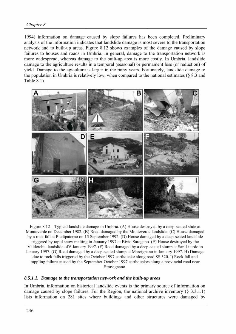
Chapter 8
236
1994) information on damage caused by slope failures has been completed. Preliminary analysis of the information indicates that landslide damage is most severe to the transportation network and to built-up areas. Figure 8.12 shows examples of the damage caused by slope failures to houses and roads in Umbria. In general, damage to the transportation network is more widespread, whereas damage to the built-up area is more costly. In Umbria, landslide damage to the agriculture results in a temporal (seasonal) or permament loss (or reduction) of yield. Damage to the agiculture is larger in the rainy years. Fortunately, landslide damage to the population in Umbria is relatively low, when compared to the national estimates (§ 8.3 and Table 8.1).
Figure 8.12 – Typical landslide damage in Umbria. (A) House destroyed by a deep-seated slide at Monteverde on December 1982. (B) Road damaged by the Monteverde landslide. (C) House damaged by a rock fall at Piedipaterno on 15 September 1992. (D) House damaged by a deep-seated landslide
triggered by rapid snow melting in January 1997 at Bivio Saragano. (E) House destroyed by the Valderchia landslide of 6 January 1997. (F) Road damaged by a deep-seated slump at San Litardo in
January 1997. (G) Road damaged by a deep-seated slump at Marcignano in January 1997. H) Damage due to rock falls triggered by the October 1997 earthquake along road SS 320. I) Rock fall and
toppling failure caused by the September-October 1997 earthquakes along a provincial road near Stravignano.
8.5.1.1. Damage to the transportation network and the built-up areas In Umbria, information on historical landslide events is the primary source of information on damage caused by slope failures. For the Region, the national archive inventory (§ 3.3.1.1) lists information on 281 sites where buildings and other structures were damaged by
Landslide risk
237
landslides, and 661 sites where roads and railways were damaged by slope failures. In the archive, damage is classified as: (i) light, where damage was aesthetic; (ii) severe, where the functionality of the building or the transportation line was compromised; and (iii) total, where a building was destroyed or a road or railway was interrupted. Along the transportation network about 34.2% of the damage was classified as light, 61.6% as severe and 4.2% as total damage. For the built-up areas, 26.5% of the damage was classified as light, 62.7% as severe, and 10.8% as total damage.
Additional information on the impact of slope failures on the built-up areas and the transportation network in Umbria can be obtained analysing three recent landslide event inventories. The prolonged earthquake sequence of September-October 1997 caused the largest impact to the transportation network (§ 3.3.3.3). Rock falls, topples and minor rock slides were mapped at 220 sites along approximately 600 kilometres of roads. These failures correspond to a density of 2.7 damaging landslides every kilometre. Along the Nera River and the Corno River valleys the density of rock falls was locally much higher. Two main regional roads (i.e., SS 320 and SS 209) running at the bottom of the valleys were interrupted at several sites and remained closed for weeks after the earthquakes, while remedial works were completed (Figure 8.12.H) (§ 7.5). The road interruptions caused severe transportation problems for the local population, and made it harder for the earthquake post-event relief efforts. At least € 15 millions (1998) were spent by the National Department of Civil Protection, the Regional Government, and the National Road Company for repairing the damage and for installing new defensive measures, including several hundreds of meters of rock fall elastic barriers and new artificial tunnels (Guzzetti et al., 2003a, 2004c).
Landslides triggered by the January 1997 snowmelt event (§ 3.3.3.2, Cardinali et al., 2000) caused damage mostly to the transportation network and to a few houses, some of which had to be abandoned (Figure 8.12.E). By intersecting in the GIS the map of the transportation network with the event landslide inventory map, 115 sites were identified where landslides triggered by rapid snowmelt intersected (i.e., interfered) with the road and railroad network. Sites damaged by landslides were found one every 56 kilometres of highways, every 32 kilometres of roads, and every 47 kilometres of railroads. An additional 112 sites where landslides were in the immediate vicinity of the transportation network were identified by drawing a buffer zone around each road or railway. Considering the buffer zone, the frequency of slope failures increased to one every 13 km of highways, 16 km of roads and 37 km of railways. In the area where the aerial photographs were available to complete the event inventory, 158 sites were identified where landslides intersected (73) or were close to (85) roads and railways. Damage to the transportation network was generally localized. The section of the roads affected by slope failures extended from a few tens to a few hundred meters. Estimates of the Regional Government suggest that the amount of money spent repairing the damage along the transportation network exceeded € 10 million (1997) (Guzzetti et al., 2003a).
Landslides triggered by rainfall events in the period from 1937 to 1941 (§ 3.3.3.1) probably caused damage to built-up areas, roads and railways (Guzzetti et al., 2003a). Unfortunately, very little information is available in the historical archive that in this period lists only 13 sites where landslide damage is reported. Intersection in a GIS of the map showing the transportation network with the event landslide inventory map (where available, i.e., in a 135 km2 area) revealed that landslides have directly interfered with roads of various categories at 27 sites. This is an average of one damaging landslide every five kilometres of roads. At other 26 sites landslides were identified in the immediate vicinity of the transportation network. If
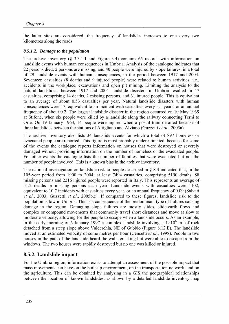
Chapter 8
238
the latter sites are considered, the frequency of landslides increases to one every two kilometres along the roads.
8.5.1.2. Damage to the population
The archive inventory (§ 3.3.1.1 and Figure 3.4) contains 65 records with information on landslide events with human consequences in Umbria. Analysis of the catalogue indicates that 22 persons died, 2 persons are missing, and 40 people were injured by slope failures, in a total of 29 landslide events with human consequences, in the period between 1917 and 2004. Seventeen casualties (8 deaths and 9 injured people) were related to human activities, i.e., accidents in the workplace, excavations and open pit mining. Limiting the analysis to the natural landslides, between 1917 and 2004 landslide disasters in Umbria resulted in 47 casualties, comprising 14 deaths, 2 missing persons, and 31 injured people. This is equivalent to an average of about 0.53 casualties per year. Natural landslide disasters with human consequences were 17, equivalent to an incident with casualties every 5.1 years, or an annual frequency of about 0.2. The largest landslide disaster in the region occurred on 10 May 1939 at Stifone, when six people were killed by a landslide along the railway connecting Terni to Orte. On 19 January 1963, 14 people were injured when a postal train derailed because of three landslides between the stations of Attigliano and Alviano (Guzzetti et al., 2003a).
The archive inventory also lists 34 landslide events for which a total of 897 homeless or evacuated people are reported. This figure is most probably underestimated, because for some of the events the catalogue reports information on houses that were destroyed or severely damaged without providing information on the number of homeless or the evacuated people. For other events the catalogue lists the number of families that were evacuated but not the number of people involved. This is a known bias in the archive inventory.
The national investigation on landslide risk to people described in § 8.3 indicated that, in the 105-year period from 1900 to 2004, at least 7494 casualties, comprising 5190 deaths, 88 missing persons and 2216 injured people were reported in Italy. This represents an average of 51.2 deaths or missing persons each year. Landslide events with casualties were 1102, equivalent to 10.7 incidents with casualties every year, or an annual frequency of 0.09 (Salvati et al., 2003; Guzzetti et al., 2005b,c). If compared to these figures, landslide risk to the population is low in Umbria. This is a consequence of the predominant type of failures causing damage in the region. Damaging slope failures are mostly slides, slide-earth flows and complex or compound movements that commonly travel short distances and move at slow to moderate velocity, allowing for the people to escape when a landslide occurs. As an example, in the early morning of 6 January 1997 a complex landslide involving ~ 1×10⁶ m3 of rock detached from a steep slope above Valderchia, NE of Gubbio (Figure 8.12.E). The landslide moved at an estimated velocity of some metres per hour (Cencetti et al., 1998). People in two houses in the path of the landslide heard the walls cracking but were able to escape from the windows. The two houses were rapidly destroyed but no one was killed or injured.
8.5.2. Landslide impact For the Umbria region, information exists to attempt an assessment of the possible impact that mass movements can have on the built-up environment, on the transportation network, and on the agriculture. This can be obtained by analysing in a GIS the geographical relationships between the location of known landslides, as shown by a detailed landslide inventory map
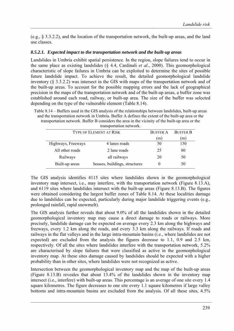
Landslide risk
239
(e.g., § 3.3.2.2), and the location of the transportation network, the built-up areas, and the land use classes.
8.5.2.1. Expected impact to the transportation network and the built-up areas
Landslides in Umbria exhibit spatial persistence. In the region, slope failures tend to occur in the same place as existing landslides (§ 4.4, Cardinali et al., 2000). This geomorphological characteristic of slope failures in Umbria can be exploited to determine the sites of possible future landslide impact. To achieve the result, the detailed geomorphological landslide inventory (§ 3.3.2.2) was intersect in the GIS with maps of the transportation network and of the built-up areas. To account for the possible mapping errors and the lack of geographical precision in the maps of the transportation network and of the built-up areas, a buffer zone was established around each road, railway, or built-up area. The size of the buffer was selected depending on the type of the vulnerable element (Table 8.14).
Table 8.14 – Buffers used in the GIS analysis of the relationships between landslides, built-up areas and the transportation network in Umbria. Buffer A defines the extent of the built-up area or the
transportation network. Buffer B considers the area in the vicinity of the built-up area or the transportation network.
TYPE OF ELEMENT AT RISK BUFFER A BUFFER B (m) (m)
Highways, Freeways 4 lanes roads 50 150 All other roads 2 lane roads 25 80
Railways all railways 20 50 Built-up areas houses, buildings, structures 0 50
The GIS analysis identifies 4115 sites where landslides shown in the geomorphological inventory map intersect, i.e., may interfere, with the transportation network (Figure 8.13.A), and 6119 sites where landslides intersect with the built-up areas (Figure 8.13.B). The figures were obtained considering the largest buffer zones of Table 8.14. At these localities damage due to landslides can be expected, particularly during major landslide triggering events (e.g., prolonged rainfall, rapid snowmelt).
The GIS analysis further reveals that about 9.0% of all the landslides shown in the detailed geomorphological inventory map may cause a direct damage to roads or railways. More precisely, landslide damage can be expected on average every 2.3 km along the highways and freeways, every 1.2 km along the roads, and every 3.3 km along the railways. If roads and railways in the flat valleys and in the large intra-mountain basins (i.e., where landslides are not expected) are excluded from the analysis the figures decrease to 1.1, 0.9 and 2.5 km, respectively. Of all the sites where landslides interfere with the transportation network, 5.2% are characterised by slope failures that were classified as active in the geomorphological inventory map. At these sites damage caused by landslides should be expected with a higher probability than in other sites, where landslides were not recognized as active.
Intersection between the geomorphological inventory map and the map of the built-up areas (Figure 8.13.B) reveales that about 13.4% of the landslides shown in the inventory map intersect (i.e., interfere) with built-up areas. This percentage is an average of one site every 1.4 square kilometres. The figure decreases to one site every 1.1 square kilometres if large valley bottoms and intra-mountain basins are excluded from the analysis. Of all these sites, 4.5%
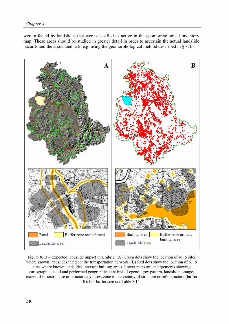
Chapter 8
240
were affected by landslides that were classified as active in the geomorphological inventory map. These areas should be studied in greater detail in order to ascertain the actual landslide hazards and the associated risk, e.g. using the geomorphological method described in § 8.4.
Figure 8.13 – Expected landslide impact in Umbria. (A) Green dots show the location of 4115 sites where known landslides intersect the transportation network. (B) Red dots show the location of 6119
sites where known landslides intersect built-up areas. Lower maps are enlargements showing cartographic detail and performed geographical analysis. Legend: grey pattern, landslide; orange,
extent of infrastructure or structures; yellow, zone in the vicinity of structure or infrastructure (buffer B). For buffer size see Table 8.14.
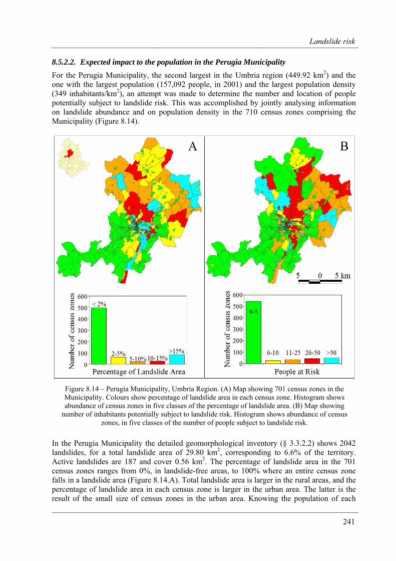
Landslide risk
241
8.5.2.2. Expected impact to the population in the Perugia Municipality For the Perugia Municipality, the second largest in the Umbria region (449.92 km2) and the one with the largest population (157,092 people, in 2001) and the largest population density (349 inhabitants/km2), an attempt was made to determine the number and location of people potentially subject to landslide risk. This was accomplished by jointly analysing information on landslide abundance and on population density in the 710 census zones comprising the Municipality (Figure 8.14).
Figure 8.14 – Perugia Municipality, Umbria Region. (A) Map showing 701 census zones in the Municipality. Colours show percentage of landslide area in each census zone. Histogram shows abundance of census zones in five classes of the percentage of landslide area. (B) Map showing
number of inhabitants potentially subject to landslide risk. Histogram shows abundance of census zones, in five classes of the number of people subject to landslide risk.
In the Perugia Municipality the detailed geomorphological inventory (§ 3.3.2.2) shows 2042 landslides, for a total landslide area of 29.80 km2, corresponding to 6.6% of the territory. Active landslides are 187 and cover 0.56 km2. The percentage of landslide area in the 701 census zones ranges from 0%, in landslide-free areas, to 100% where an entire census zone falls in a landslide area (Figure 8.14.A). Total landslide area is larger in the rural areas, and the percentage of landslide area in each census zone is larger in the urban area. The latter is the result of the small size of census zones in the urban area. Knowing the population of each
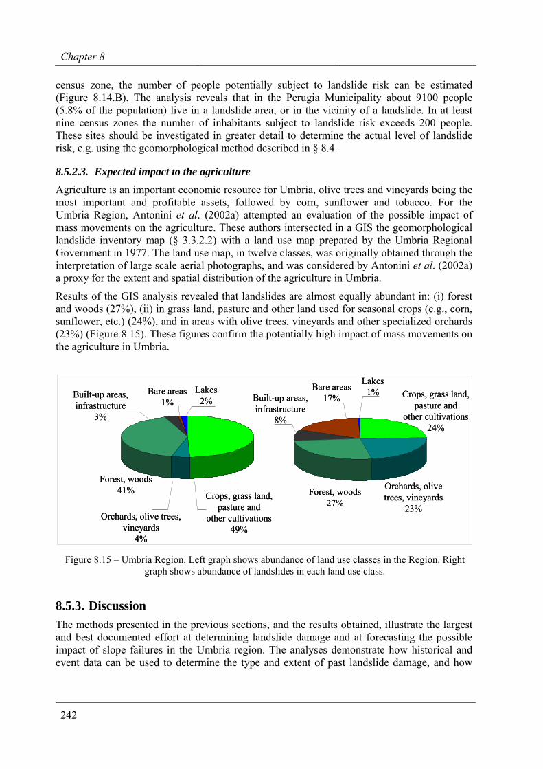
Chapter 8
242
census zone, the number of people potentially subject to landslide risk can be estimated (Figure 8.14.B). The analysis reveals that in the Perugia Municipality about 9100 people (5.8% of the population) live in a landslide area, or in the vicinity of a landslide. In at least nine census zones the number of inhabitants subject to landslide risk exceeds 200 people. These sites should be investigated in greater detail to determine the actual level of landslide risk, e.g. using the geomorphological method described in § 8.4.
8.5.2.3. Expected impact to the agriculture Agriculture is an important economic resource for Umbria, olive trees and vineyards being the most important and profitable assets, followed by corn, sunflower and tobacco. For the Umbria Region, Antonini et al. (2002a) attempted an evaluation of the possible impact of mass movements on the agriculture. These authors intersected in a GIS the geomorphological landslide inventory map (§ 3.3.2.2) with a land use map prepared by the Umbria Regional Government in 1977. The land use map, in twelve classes, was originally obtained through the interpretation of large scale aerial photographs, and was considered by Antonini et al. (2002a) a proxy for the extent and spatial distribution of the agriculture in Umbria.
Results of the GIS analysis revealed that landslides are almost equally abundant in: (i) forest and woods (27%), (ii) in grass land, pasture and other land used for seasonal crops (e.g., corn, sunflower, etc.) (24%), and in areas with olive trees, vineyards and other specialized orchards (23%) (Figure 8.15). These figures confirm the potentially high impact of mass movements on the agriculture in Umbria.
Figure 8.15 – Umbria Region. Left graph shows abundance of land use classes in the Region. Right graph shows abundance of landslides in each land use class.
8.5.3. Discussion The methods presented in the previous sections, and the results obtained, illustrate the largest and best documented effort at determining landslide damage and at forecasting the possible impact of slope failures in the Umbria region. The analyses demonstrate how historical and event data can be used to determine the type and extent of past landslide damage, and how
Crops, grass land, pasture and
other cultivations49%
Orchards, olive trees, vineyards
4%
Forest, woods 41%
Built-up areas, infrastructure
3%
Bare areas 1%
Lakes 2%
Crops, grass land, pasture and
other cultivations24%
Orchards, olive trees, vineyards
23%
Forest, woods 27%
Built-up areas, infrastructure
8%
Bare areas 17%
Lakes 1%
Crops, grass land, pasture and
other cultivations49%
Orchards, olive trees, vineyards
4%
Forest, woods 41%
Built-up areas, infrastructure
3%
Bare areas 1%
Lakes 2%
Crops, grass land, pasture and
other cultivations24%
Orchards, olive trees, vineyards
23%
Forest, woods 27%
Built-up areas, infrastructure
8%
Bare areas 17%
Lakes 1%
Landslide risk
243
GIS technology can be used to help determining the impact of slope failures on the population, the built-up areas, the transportation network and the agriculture.
The described approach is innovative and reliable. However, the described analyses should be considered preliminary, as they suffer from simplifications. For this reason, results may be locally inaccurate. Quality, completeness and resolution of the landslide inventory maps and of the maps showing the elements at risk largely affects the quality of the results. If existing landslides are not shown in the inventory, or if the extent or location of the built-up areas or the roads is not shown precisely in the maps, the GIS analysis is inevitably erroneous. Identification of the areas where known landslides may interfere with the transportation network and the built-up areas did not consider the possibility that a landslide can travel a long distance from the source area. This may affect significantly the impact analysis, particularly in mountain areas where debris flows and rock falls that can travel long distances are common. The GIS analysis may also be biased locally by the presence of tunnels below landslide shear planes, and of bridges or viaducts not affected by shallow landslides. In built-up areas remedial works may have been completed, reducing landslide hazards. However, the mitigating effect of the remedial measures was not considered.
Estimation of landslide risk to the population in Umbria is also affected by uncertainty. The impact of landslides on the population depends on many factors, including: (i) the location, type and frequency of landslides, (ii) the abundance and distribution of the population, and (iii) the number and location on the vulnerable elements related to the presence of the population (e.g., homes, schools, offices, utilities, roads, etc.). If buildings or homes are built in dangerous landslide areas, the risk to the population will increase. Where defensive measures have been installed (e.g., rock fall fences along railways), proper maintenance is required to maintain the existing safety levels. If the performance of the defensive measures is reduced, risk to the population will increase, as the risk to the structures and infrastructure.
The assessment of landslide risk to the population in the Perugia Municipality is a first-order estimate. The analysis does not take into consideration the exact location of the landslides and the population in the census zones. In a census zone, landslides may exist but they may not pose a threat to the population. For simplicity, the analysis was performed considering only the extent of the landslides shown in the geomorphological inventory map. Possible enlargements of a landslide due to its movement or to reactivations were not considered. Debris flows and rock falls were not shown in the considered inventory map. Hence, the risk associated with these types of landslide was also not considered. Changes in the distribution and abundance of population will also affect the risk assessment.
Despite these inherent limitations, the ensemble of the results obtained confirms that mass movements in Umbria represent a societal and economic problem that should not be overlooked.
8.6. Summary of achieved results
In this chapter, I have:
(a) Shown that reliable methods for determining and ranking landslide risk can be established.
(b) Demonstrated that landslide risk can be determined at various geographical scales using probabilistic or heuristic (geomorphological) approaches.
Chapter 8
244
(c) Proposed a geomorphological method for the determination of landslide risk.
(d) Shown that where sufficient information is not available to attempt a probabilistic or heuristic (geomorphological) assessment of landslide risk, the expected impact of slope failures can be established exploiting landslide information and GIS technology.
This responds to Question # 6 and partly to Question # 7 posed in the Introduction (§ 1.2).
245
9. USE OF LANDSLIDE MAPS AND MODELS
It’s good to have a map, if you know how to use it.
A good strategy consists in sticking to the facts and in telling the truth.
The value of a map refers to its information content, which depends on the type of data shown, their quality and the extent to which the information is new and essential. A map is valuable when the data shown are useful to the user, i.e., when the map is both relevant and understood by the user (Guzzetti et al., 2000).
A carefully designed inventory map that shows landslides as recognised by the interpreter, without any modification apart from scale or graphical constrains, is a basic map. A landslide density map obtained by interpolating an inventory map without any additional information is a derivative map. Landslide susceptibility and hazard maps obtained from an inventory are also derivative maps but, since they include additional information on factors such as lithology and morphology that are used to build the susceptibility or hazard models, they have an information content which is superior to that of the input maps, including the inventory. Risk assessments are complex, high level products that exploit basic, derivative and other thematic information and maps (Guzzetti et al., 2000).
In this chapter, I first describe and compare the information content of different landslide cartographic products, including inventory, density, susceptibility and hazard maps, and risk evaluations. Next, I introduce and discuss the concept of a “landslide protocol”, i.e., a set of regulations established to link terrain domains shown on the different landslide maps to proper land use rules.
9.1. Landslide inventory maps
In § 3, I have shown that landslide inventory maps can be prepared using different techniques, depending on their purpose, the extent of the study area, the scales of base maps and aerial photographs, and the resources available to carry out the work. Regardless of the adopted techniques and of the sources of information used to prepare or compile the inventories, landslide inventory maps show the location and, where known, additional characteristics of the slope movements (e.g., type of movement, depth, date, age, degree of activity, etc.) that left discernable features in an area, or that are known to have occurred in an area (Hansen, 1994; Wieczorek, 1984; Guzzetti et al., 2000). In other chapters, I have shown how the information portrayed in a landslide inventory can be exploited to determine the abundance of landslides (§ 4.1), to determine the frequency-area statistics of landslides in an area (§ 5), to ascertaining
Chapter 9
246
landslide susceptibility (§ 6) or hazard (§ 7), and to evaluate landslide risk (§ 8). Hence, the usefulness of landslide inventories should now be clear.
Landslide inventory maps are easy to understand (i.e., straightforward, direct) for experts, such as geomorphologists, and non-experts, such as decision makers, planners and civil defence managers. Inventory maps are easily prepared by well trained geomorphologists and do not require large investments, particularly when compared to other thematic maps showing environmental data, including geological and soil maps. Only limited resources are required for the completion of landslide inventory maps, namely aerial photographs, base maps, and a good quality stereoscope. Experiments conducted in northern and central Apennines of Italy have demonstrated that, with the resources commonly available to complete a landslide mapping project, accurate multi-temporal inventory maps can be successfully prepared for areas extending from a few tens to a few hundreds of square kilometres (e.g., Galli et al., 2005; Guzzetti et al., 2005a), whereas good quality, geomorphological inventory maps can be prepared for larger areas, extending for thousands of square kilometres (e.g., Antonini et al., 1993, 2000, 2002a; Cardinali et al., 2001).
Despite the ease with which they are prepared and their immediateness, landslide inventories are not yet very common. Inventory maps are available for only a few countries and mostly for limited areas (Brabb and Harrod, 1989; Brabb, 1991, 1993, 1995). This is surprising because inventory maps provide fundamental information on location and size of landslides that is necessary in the assessment of slope stability at any scale, and in any physiographical environment. The reasons for this shortcoming are manifold and depend on general and local conditions (Brabb, 1991, 1993; Guzzetti et al., 2000).
There is a certain inability of environmental and planning agencies, and of national and regional geological surveys, to understand the value of regional inventories for planning purposes (Brabb, 1991, 1996). This is often coupled with inability or lack of resolve in preparing landslide inventories for large regions, which has the effect of limiting knowledge of landslide distributions, types and patterns. Indeed, some planning agencies prefer to ignore where landslides are located: lack of knowledge in this case represents a degree of freedom (Guzzetti et al., 2000). The opinion that landslide mapping, and in particular inventory making, is not “scientific” finds advocates even among earth scientists (Sassi et al., 1998). I believe that landslide mapping is an important, scientific operation, but I am conscious of the fact that preparing a landslide inventory, particularly from aerial photographs with or without field surveys, is a subjective operation that requires skills and training. Maps prepared by personnel not sufficiently trained or experienced, or lacking the proper resources may be wrong and unreliable. The subjectivity and the difficulty in assessing quantitatively its reliability, makes landslide inventory maps somewhat unreliable in the eyes of some potential user. The fact that most published inventories are not accompanied by clear documentation on the tools, methods and techniques used to prepare or to compile them, and lack sufficient specifications on the estimated degree of completeness and reliability, add to the difficulty of using landslide inventories. Lastly, in the recent years there has been a general, largely unjustified, preference for “high-tech” remote sensing techniques, which are not yet capable of mapping landslides efficiently over even small areas (Soaters et al., 1991).
Landslide inventory maps are important and useful products but suffer from limitations, which is important to know and expose clearly. Even if it is very accurate and precise, a landslide inventory map cannot portray all slope failures that have occurred in an area. Geomorphological inventories portray only a reduced fraction of the total number or the total
Use of landslide maps and models
247
area of landslides that have occurred in a region over time (Malamud et al., 2004a). A landslide map will show only slope failures that have (presumably) left discernible morphological signs on the date and at the scale of the investigation. If aerial photographs are used to complete the investigation, the inventory map will portray only landslides visible on the aerial photographs. Thus, the quality of a landslide inventory depends: (i) on the persistence of landslide morphology within the landscape, (ii) the skill of the interpreter to capture the morphological features typical of a landslide, and (iii) the ability of the interpreter to properly understand the geomorphic evolution of the slopes. In the areas that are shown as having landslides in an inventory map, interpreters are (usually) confident that landslide scars and or deposits exist, but nothing is said about the reliability of such statement – i.e., the veracity of the map. Additionally, where landslides are not shown, most commonly nothing is said about the potential presence or absence of slope failures. Indeed, authors of inventory maps often state that areas not mapped as landslides cannot be considered free of mass movements, but rather represent domains where the interpreter was not able to identify a slope failure (e.g., Guzzetti and Cardinali, 1989, 1990; Antonini et al., 1993; Cardinali et al., 1990, 2001). For most potential users of landslide inventory maps the difference is significant.
In landslide inventory maps, no effort is made to distinguish areas that are landslide-free (such as large alluvial plains, valley bottoms, flat ridge tops, and recognized stable ground) from areas where landslides could exist but either are not present at the date of the investigation or were not recognised (Guzzetti et al., 2000). The imprecision limits the value of landslide inventory maps, and may jeopardise their usefulness for planning, land development and decision making. Indeed, where landslides are recognised, actions can be taken and proper regulations can be established before planning or land development takes place. Much less clear is what to do where landslides are not recognised, particularly in the vicinity of existing mass movements or in terrain that is prone to slope failures. As an example, on 5 May 1998 rainfall induced shallow failures were triggered on the steep slopes mantled by volcanic deposits of the Pizzo d’Alvano area (Campania Region, Italy) (Guadagno et al., 1999; Guadagno and Periello Zampelli, 2000; Crosta and Dal Negro, 2003). The resulting debris flows killed 137 people in the village of Episcopio (Sarno). Twenty-three additional casualties were reported at Quindici, Siano, Braciliano and San Felice a Cancello (Guzzetti, 2000). Inspection of medium-scale (1:33,000) aerial photographs flown in 1955 showed that prior to the event little could be said about the exact location of the source areas of the individual debris flows. However, on the basis of the overall geological and geomorphological settings, slopes could be interpreted to be highly susceptible to failures. Archive data confirmed that the area suffered similar catastrophic landslides in historical and recent time. Thus, a reconnaissance landslide inventory – which was not available for the area at the time of the catastrophic event – may have failed to predict the exact location of the individual landslides, but a detailed geomorphological inventory map would have quite certainly identified the areas potentially subject to debris flow hazards, e.g., mapping the fans where debris flow deposited.
9.2. Landslide density maps
To improve the accuracy with which future landslides are predicted (in space), the density of slope failures (§ 4.1) can be determined within pre-defined terrain domains, or mapping units (§ 6.2.2). Geomorphological terrain subdivisions, such as slope units, have proven particularly adequate for computing and displaying landslide density, at the local and the regional scales. Density is a clearly definable and easily comprehended quantitative measure of the spatial
Chapter 9
248
distribution of slope failures (§ 4.1). Regardless of the geological or morphological setting, where landslides are abundant, density is high and, conversely, where landslides are sparse, density is low. This is an advantage of density maps over more complicated forms of mapping, such as susceptibility and hazard maps. The advantage may be particularly significant for non-expert users, such as decision and policy makers.
As an improvement to landslide inventories, landslide density maps are fillers of space. Such maps provide insight on the expected (or inferred) occurrence of landslides in any part of the investigated area without leaving unclassified areas. A density map does not show where landslides are located but this (apparent) loss in resolution is compensated for by improved map readability and reduced cartographic errors (Carrara et al., 1992; Guzzetti et al., 2000; Ardizzone et al., 2002; Galli et al., 2005). Additionally, landslide density is independent of the extent of the study area, which makes comparison between different regions straightforward. Such characteristics contribute to making density maps appealing to decision makers and land developers.
Landslide density maps can be conveniently combined with the inventory maps from which they were obtained (Guzzetti et al., 2000). This can be easily achieved in a GIS, by overlying a geomorphological landslide inventory on top of the corresponding density map. This was demonstrated in § 4.1.2 for the Upper Tiber River basin, in central Italy. The resulting map, shown in Figure 4.1, is based on slope units and retains the advantages of a landslide inventory map (i.e., it shows where failures were recognised by the investigator) and fills spaces, thus providing insight into the geographical distribution and abundance of slope failures. The use of an appropriate terrain unit (i.e., the slope unit) guarantees a match with the local morphological setting. The map shown in Figure 4.1 was further improved by clipping out of the frequency count the areas that are known to be landslide free (e.g., large valley bottoms). The combined inventory and density map gains in readability and applicability to decision making and land use planning.
Density maps represent an improvement over landslide inventories, but have limitations. These maps are based on the assumption that landslide density is continuous in space, which may not be the case everywhere (§ 4.1). If the original landslide inventory is incorrect, i.e., if the original landslide map does not show some of the slope failures present in an area, or if it overestimates the extent of the slope failures, the density map will inherit the errors and will be incorrect or imprecise. A level of uncertainty cannot be easily associated to the density estimate, further limiting the applicability of landslide density maps for planning and decision making. Also, despite improvements, landslide density maps do not incorporate any physical relation between slope failures and the landscape. Thus, they cannot be used to establish and investigate the factors that control landslide occurrence. Indeed, density maps can be used to decide where landslides are more abundant but not why this is so. They can be of help in specifying where subsequent studies have to be made, but not to model the effects of remedial works. This is the goal of landslide susceptibility modelling.
9.3. Landslide susceptibility zoning
In § 6, I have shown that good quality landslide susceptibility maps can be obtained from deterministic or statistical models. The latter, usually incorporate several instability factors and use a variety of classification methods (Michie et al., 1994). Reliable susceptibility models are capable of explaining why the known (i.e., past) landslides are abundant or sparse. Under
Use of landslide maps and models
249
assumptions (e.g., § 6.2.1, § 6.4.1), this information can be used to predict where new or reactivated landslides will be abundant or sparse in the future. Given that landslides take many different forms and are the result of the interplay of a variety of causes (§ 1.1, Schuster and Krizek, 1978; Crozier, 1986; Dikau et al., 1996; Turner and Schuster, 1996), different susceptibility models can be prepared that take into account the main instability factors (slope morphology, rock composition, structure, hydrological conditions, land use types, etc.) and the various landslide types (deep-seated slides, shallow failures, debris flows, rock falls, etc.).
The availability of different methods (§ 6.2.3) and the numerous published examples (§ 6.1), indicate that landslide susceptibility maps are relatively simple to prepare. The experience gained in Italy has shown that for the production of reliable landslide susceptibility maps, quality and abundance of the available landslide and thematic information is more important than selection of a “best” statistical classification method (Carrara et al., 1992, 1995, 1999; Guzzetti et al., 1999a). Others authors have expressed a different opinion, supported by field data and statistical analyses (e.g., Chung and Fabbri, 2004), but it is unquestionable that where sufficient information exists landslide susceptibility can be ascertained, and maps showing its spatial distribution can be prepared. Indeed, susceptibility models and maps of different forms and reliability can be obtained for the same area depending on the type and quality of the available information.
By incorporating information on the instability factors that are known or supposed to control landslide spatial occurrence and abundance, susceptibility maps are capable of predicting the location of landslides even in the areas where landslides were not recognized or mapped. As a result, errors in the landslide inventory maps are compensated for by a reliable susceptibility model. This is a marked improvement over inventory and density maps. Susceptibility maps are also filler in space and, if combined with the corresponding landslide inventory (e.g., Cardinali et al., 2002b), they retain the advantages of the inventory, e.g. they show where landslides were recognized and mapped, and they provide a quantitative assessment of the probability of spatial occurrence of future landslides for the entire territory.
Landslide susceptibility models – and the resulting maps – represent a marked improvement over inventories and density maps, but have limitations. In a landslide susceptibility map only the presence (and not the extent or the number) of landslides is predicted. Within each mapping unit (and regardless of the type of the adopted mapping unit) no distinction is made between a small slope failure and a large landslide, or between several small failures and a single large mass movement. The problem is less severe when using grid cells as the mapping unit of reference, and is more severe when adopting one of the other types of terrain subdivisions (§ 6.2.2). Most commonly, the degree of activity of the known landslides is not accounted for by a susceptibility assessment. A further limitation of a landslide susceptibility map lays in the fact that such map does not provide any insight on the temporal frequency of occurrence, or the magnitude (i.e., the size or destructiveness) of the expected slope failures. In a susceptibility map, no distinction is made between mapping units where landslides are expected with a high temporal frequency (e.g., every rainy season), from those where slope failures are expected only every tens, hundreds or even thousands of years. Also, no distinction is made on the size (e.g., length, area, volume) of the expected landslides, which in many cases directly affects their destructive power. In addition, statistically-based susceptibility models are negatively influenced by the extent of the investigated area, which makes it difficult to compare susceptibility classes from different locations (Carrara et al., 1991, 1995; Guzzetti et al., 1999a; 2000). These limitations jeopardize the potential use of landslide susceptibility maps for civil defence, for applications in landslide warning systems,
Chapter 9
250
and to some extent even for land use planning. In a pristine area, where elements at risk are not yet present, a susceptibility map can be applied, and more detailed studies can be made to determine the temporal occurrence of landslides. In an area where elements are risk are already present (e.g., houses, roads, the population, etc.), and decisions have to be made on remedial or relocation measures, it is difficult to establish a policy without knowing when (or at least how frequently) a landslide will occur, and how large or destructive the mass movement is expected to be.
Although they are diagnostically powerful and superior to more simple approaches, such as inventory and density maps, landslide susceptibility models are complex tools that can be difficult to master and exploit. They need to be applied with care to planning and land development, and only by experienced geomorphologists, who will often be the same people who helped build them. This is particularly relevant for areas that were either misclassified by the susceptibility model, or where the model was unable to classify the terrain. In these places, it is essential to understand how a model behaves before it can be put to any practical use. A landslide susceptibility model should always be used in combination with all the information that was used to build it. The operation is simplified if the information is available in digital format in a properly organised GIS database.
Lastly, it should be understood that landslide susceptibility models – and the resulting associated maps – are nothing more than geomorphological spatial predictions. Like any other scientific prediction, they should be accompanied by a quantitative estimate of the error associated with the prediction (Jolliffe and Stephenson, 2003). Susceptibility maps should be further quantitatively tested to evaluate their prediction skills (§ 6.5). To those embarking in the preparation a landslide susceptibility assessment, it should be clear that a policy maker interested in incorporating their landslide susceptibility prediction into a land use regulation or a building code is most probably more concerned in the performance of the susceptibility model with time (i.e., in the aptitude of the model of predicting new landslides) and less interested by how well the same model fits the known distribution of past slope failures. Lack of proper model verification and of relevant information on the error associated with the susceptibility estimate, is a primary reason for the limited application of landslide susceptibility models and maps in building codes, civil defence scenarios, and land development and exploitation plans.
9.4. Landslide hazard assessments
Landslide hazard assessments are the most sophisticated and complex form of landslide cartography currently available (e.g., Guzzetti et al., 2005a). As they are derived from the analysis of many instability/environmental factors, landslide hazard models are capable of explaining why landslides are abundant or sparse (through their landslide spatial probability component), to provide estimates of the frequency of landslide occurrence, and of the magnitude (e.g., size, or destructiveness) of the expected slope failures (§ 7). These are considerable enhancements over susceptibility zonations, which make hazard models and maps particularly appealing to decision makers, land use planners, and civil defence managers.
Like density and susceptibility maps, landslide hazard maps are filler of space. If combined with the corresponding (multi-temporal) inventory maps, they retain the advantages of the inventories, e.g. they can show where landslides were recognized and mapped, including information on the age of the landslides inferred from the date of the aerial photographs or of
Use of landslide maps and models
251
the field surveys. Hazard models incorporate a susceptibility component, i.e., the spatial probability of landslide occurrence. For this reason, many of the advantages and the limitations discussed for susceptibility models and maps also apply to hazard models and maps, including the need for proper model verification and for a quantitative estimate of the error associated with the hazard prediction.
Landslide hazard models are indubitably the most powerful analytical and diagnostic tool currently available to geomorphologists and decision makers to predict the spatial and temporal occurrence of mass movements, and the evolution of landslide hazards in a region. However, models of landslide hazard are more difficult to prepare than susceptibility models or density maps (§ 7). Hazard modelling requires considerable efforts to collect and validate input data that are often not readily available (e.g., multi-temporal landslide inventory maps). Being dependent on information on the temporal occurrence of landslides, which can be currently effectively colleted only for relatively small areas, hazard models are also negatively influenced by the extent of the investigated area. Lastly, hazard models needs interaction between expert geomorphologists and statisticians in order to process the available data in such a way as to avoid statistically sound but geomorphologically unrealistic results.
More than any other landslide cartographic product, hazard models need to be applied with great care to planning and land development, and only by the same team of experienced geomorphologists and statisticians who helped prepare them. The problem is particularly relevant for the areas that were either misclassified by the susceptibility component of the hazard model, or where the susceptibility assessment was unable to classify the terrain. The problem is also significant where the temporal component of the hazard model was unable to provide reliable estimates of landslide occurrence (or recurrence), or where the model component for landslide magnitude was unable to provide reliable estimates of the expected landslide size or destructiveness. In these places, it is essential (mandatory) to understand how a hazard model behaves before it can be put to any practical use.
Like the other previously discussed landslide cartographic products, a landslide hazard model must always be used in combination with all the geomorphological and the thematic information used to construct it. However, there is a significant difference between hazard models and the other cartographic products (i.e., landslide inventory, density and susceptibility maps). The probabilistic model adopted to ascertain landslide hazard at the basin scale (§ 7.3), and its variations used to determine landslide hazard at the national scale (§ 7.4), or to determine rock fall hazard along roads (§ 7.5), all generate a very large number of predictions (i.e., of hazard assessments). Each prediction represents a possible landslide scenario, i.e., a combination of landslide spatial occurrence, of expected landslide size or destructiveness, and of landslide temporal probability for a different period. Individual landslide scenarios can be shown by separate hazard maps, each portraying different levels of landslide hazard. Efficient display of multiple hazard scenarios cannot be obtained using traditional (paper) maps. A large ensemble of landslide hazard maps and of the geomorphological and thematic information used to prepare them can be accomplished efficiently by exploiting GIS technology, provided the information is stored in a properly organized database.
Even an efficient GIS system that operates on a well organized geographical database cannot solve two problems typical of (i.e., inherent to) landslide hazard assessments. The first problem concerns the development and use of methods and techniques to synthesize the large number of predictions produced by a single hazard assessment in a reduced number of maps or charts. This involves establishing criteria and defining thresholds to efficiently cluster hazard
Chapter 9
252
scenarios in a reduced set manageable by decision makers, land developers, civil defence managers, and concerned citizens. The second problem concerns the comprehensive assessment of the level of hazard posed by different threats, e.g., by different landslide types, or by different natural hazards (e.g., landslides, floods, show avalanches, etc.) present in the same area at the same or at different times. This includes investigations on methods and techniques for the appropriate analysis of multiple hazards.
9.5. Landslide risk evaluations
A significant difference exists between the information provided by landslide risk evaluations (as discussed in § 8) and the information supplied by the other landslide cartographic products (§ 9.1 to § 9.4). The goal of a landslide inventory map consists in showing the location of slope failures. The purpose of landslide density, susceptibility and hazard maps is to zone (rank) the territory, based upon the abundance of landslides, the levels of landslide susceptibility, or the levels of landslide hazard. Thus, the focus of landslide inventory, density, susceptibility, and hazard maps is the territory. Conversely, landslide risk assessment aims at determining the loss or the expected damage to a specific element (e.g., a person, house, road, or asset), resulting from a hazardous affecting landslide (§ 8.2, Varnes and IAEG Commission on Landslides and other Mass-Movements, 1984; Vandine et al., 2004). Hence, the focus of a landslide risk assessment is the element at risk (and not the territory). The difference is significant and should be made clear to the potential users of landslide risk evaluations.
Establishing heuristic or probabilistic levels of landslide risk is a complex operation that most commonly involves designing multiple landslide scenarios. From what I have presented in § 8, it should be clear that preparing a single landslide risk assessment does not make much sense. Risk depends on hazard (i.e., on the state of nature, § 7) as much as on the type, distribution, abundance and vulnerability of the elements at risk (§ 8.2.1). The latter varies for the different types of mass movements. As an example, a person travelling along a road may be highly vulnerable to small rock falls, which may cause only minor, aesthetic damage to the road. Conversely, a large but slow moving landslide may not cause direct harm to the people leaving or working on the landslide, whose houses however may be severely damaged or destroyed by the movement of the landslide.
Difficulties in preparing and using risk assessments include: (i) the difficulty in determining all the relevant information needed to establish levels of landslide risk (lack of information), (ii) problems in selecting meaningful and realistic landslide scenarios, (iii) the fact that establishing risk levels is a political and economical as much as a technical, scientific and logical decision (see below), (iv) the difficulty in combining in a meaningful and useful form the results obtained for different scenarios (multiple risk), and the results obtained by different experts (lack of consensus), and (v) the fact that even minor changes, e.g., in the number, position or type of the elements at risk can affect significantly the result of the risk assessment effort (large uncertainty). For these reasons, even more than for the susceptibility and hazard assessments presented before, risk evaluations should always be used in conjunction with all the information used to obtain them. The user of a risk assessment should always be aware of the information, data, assumptions, logics and constrains used or assumed to perform the risk evaluation. If the information changes, the assumptions don’t hold true, or constrains are modified, the risk evaluation should be reconsidered, updated or rejected. Risk evaluations need to be applied with extreme care to planning, land development, civil defence and warning
Use of landslide maps and models
253
systems, and only by experienced scientists in combination with decision and policy makers and qualified risk managers.
Establishing landslide risk levels is a political and economical as much as a technical decision-making process, which depends on the interests and the assets of the person, institution, company, etc. (i.e., of the “stakeholder”) potentially bearing the physical, economical and political consequences of the landslide(s). For the manger of a mountain road network, rock falls endangering a highly trafficked road used daily by local inhabitants and tourists, may represent a severe hazard. For this manager, the road and the people travelling along it may be at high risk, requiring first-priority mitigation efforts. For the manager of a gas duct laid along the same mountain road, rock falls may not represent a significant threat to the pipeline. The second manager may be more concerned about debris flows destroying a bridge and severing the pipeline; a condition of high economical and technological risk for the gas duct. The Maier of a town may have to decide how to invest finite economic resources to mitigate the hazard posed by a large magnitude but low frequency landslide event (a large rock slide), with potential catastrophic consequences to private properties of high economic value to the community (e.g., hotels in a mountain resort), or to reduce the risk posed by frequent, but small rock falls and by recurrent, minor debris flows along the access road to the town. The Maier decision will – quite certainly – be taken not solely on a technical (e.g., geomorphological) background, but will require the analysis of several – probably conflicting – information, interests, constraints and obligations.
9.6. Establishing a landslide protocol
For civil defence purposes, land use planning and policy making, a single landslide map (whether it be an inventory, density, susceptibility or hazard map), or even a combination of two or more types of landslide maps, is seldom considered adequate (Godefroy and Humbert, 1983; Ahlberg et al., 1988; Swanston and Schuster, 1989; Brabb, 1991, 1995, 1996, 2002; Guzzetti et al., 1999, 2000; Raetzo et al., 2002). To exploit the map(s) potential to the full, a “protocol” must be established. A “landslide protocol” consists in a coherent and organized set of regulations that links terrain domains to proper rules for best exploitation of the terrain and maximum acceptable safety to human beings and the assets. This is comparable to a protocol in the medical science and practice, which is followed (adopted) by researchers and doctors to cure a specific illness based on scientific knowledge, verified statistics, available information, and the results of specific laboratory tests.
A landslide protocol should exploit all the available knowledge on landslides in a given area – including maps and predictive models – to allow decision and policy makers to make the best possible choice on the use of the land, given the existing constrains and the available information. A landslide protocol: (i) should fit the local morphological, geological, meteorological, and land use setting, including the different types of mass movements that may be present in an area, and their most common triggers; (ii) it should be tailored to respond to specific and general user needs. More than one protocol may be established on the same area by different users (e.g., the two managers of the mountain road network and of the gas duct discussed in § 9.5 may adopt different landslide protocols); (iii) it should be “scalable”, i.e., it should be able to use additional or new information when it becomes available (e.g., it should be able to exploit the information provided by a new susceptibility map prepared for an area for which an inventory and a density map are already available and used by the protocol); (iv) it should comply with the existing local and national legislation – or it should be able to
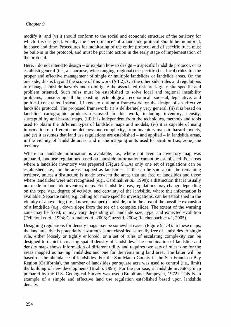
Chapter 9
254
modify it; and (v) it should conform to the social and economic structure of the territory for which it is designed. Finally, the “performance” of a landslide protocol should be monitored, in space and time. Procedures for monitoring of the entire protocol and of specific rules must be built-in in the protocol, and must be put into action in the early stage of implementation of the protocol.
Here, I do not intend to design – or explain how to design – a specific landslide protocol, or to establish general (i.e., all-purpose, wide-ranging, regional) or specific (i.e., local) rules for the proper and effective management of single or multiple landslides or landslide areas. On the one side, this is beyond the scope of this work (§ 1.2). On the other side, rules and regulations to manage landslide hazards and to mitigate the associated risk are largely site specific and problem oriented. Such rules must be established to solve local and regional instability problems, considering all the existing technological, economical, societal, legislative, and political constrains. Instead, I intend to outline a framework for the design of an effective landslide protocol. The proposed framework: (i) is deliberately very general, (ii) it is based on landslide cartographic products discussed in this work, including inventory, density, susceptibility and hazard maps, (iii) it is independent from the techniques, methods and tools used to obtain the different types of landslide maps and models, (iv) it is capable of using information of different completeness and complexity, from inventory maps to hazard models, and (v) it assumes that land use regulations are established – and applied – in landslide areas, in the vicinity of landslide areas, and in the mapping units used to partition (i.e., zone) the territory.
Where no landslide information is available, i.e., where not even an inventory map was prepared, land use regulations based on landslide information cannot be established. For areas where a landslide inventory was prepared (Figure 9.1.A) only one set of regulations can be established, i.e., for the areas mapped as landslides. Little can be said about the remaining territory, unless a distinction is made between the areas that are free of landslides and those where landslides were not recognised (e.g., Cardinali et al., 1990); a distinction that is usually not made in landslide inventory maps. For landslide areas, regulations may change depending on the type, age, degree of activity, and certainty of the landslide, where this information is available. Separate rules, e.g. calling for more specific investigations, can be established in the vicinity of an existing (i.e., known, mapped) landslide, or in the area of the possible expansion of a landslide (e.g., down slope from the toe of a complex slide). The extent of the warning zone may be fixed, or may vary depending on landslide size, type, and expected evolution (Felicioni et al., 1994; Cardinali et al., 2003; Guzzetti, 2004; Reichenbach et al., 2005).
Designing regulations for density maps may be somewhat easier (Figure 9.1.B). In these maps, the land area that is potentially hazardous is not classified as totally free of landslides. A single rule, either loosely or tightly enforced, or a set of rules of escalating complexity can be designed to depict increasing spatial density of landslides. The combination of landslide and density maps shows information of different utility and requires two sets of rules: one for the areas mapped as having landslides and one for the remaining land area. The latter will be based on the abundance of landslides. For the San Mateo County in the San Francisco Bay Region (California), the number of landslides per square acre was used to control (i.e., limit) the building of new developments (Brabb, 1995). For the purpose, a landslide inventory map prepared by the U.S. Geological Survey was used (Brabb and Pampeyan, 1972). This is an example of a simple and effective land use regulation established based upon landslide density.
Use of landslide maps and models
255
Figure 9.1 – Conceptual example for the design of a landslide protocol. Rules are based on the type of landslide map, and the type and abundance of the available landslide information.
Chapter 9
256
It can be difficult to design a protocol for a landslide susceptibility map (Figure 9.1.C). Rules can be made that take model output and reliability into consideration, and deal differently with terrain domains classified as unconditionally stable or unstable, and those for which further investigation is required. A complex set of regulations based on a susceptibility model would cover areas mapped as having landslides, those that the model defines as landslide-prone or stable, those of uncertain definition, and even the areas that were mapped erroneously (i.e., misclassified) by the susceptibility model. Where the quality of the susceptibility model was quantitatively verified, and the error (i.e., a measure of the uncertainty) associated with the probability estimate was determined, the information can be used to modify individual rules, e.g., by calling for more specific investigations in areas where the uncertainty is large. Development of a thorough protocol based on landslide susceptibility may be greatly aided by GIS technology.
Design of a landslide protocol that fully exploits the information provided by a complete landslide hazard assessment (Figure 9.1.D) can be extremely complex, but may also prove very effective (advantageous) for the end user , allowing for the optimal development of a territory, given the physiographical setting and the social, economical and political constrains. Where a landslide hazard assessment exists, rules can be made that: (i) cover areas mapped as having landslides, (ii) consider the spatial probability of landslide occurrence (i.e., susceptibility), (iii) consider the expected recurrence of landslides, for different time periods, and (iv) consider the magnitude (e.g., area, volume, destructiveness) of the expected slope failures. For landslide areas, the same considerations made for landslide inventories apply, i.e., regulations may change depending on the type, age, degree of activity, and certainty of the landslide, where this information is available. Separate rules can be established in the vicinity of an existing landslide, or in the area of the possible or probable expansion of a landslide. For the spatial probability of landslide occurrence the same considerations made for susceptibility maps apply, i.e., rules can be established for areas defined as stable or unstable by the model, for unclassified areas, and for areas misclassified by the model. In addition, specific rules can be established – or the existing rules can be modified – based on the expected magnitude or the expected recurrence of the slope failures. As a complete hazard assessment results in a large set of scenarios, a comprehensive protocol exploiting all the available hazard information would probably be linked to different landslide scenarios. For the purpose, GIS technology becomes essential. Within a GIS environment encompassing all the information used to build the hazard model, rules can be defined that consider information such as topography, morphology, lithology, urban expansion, and land use, which is not readily available from landslide inventory, density or susceptibility maps.
Establishing general land use regulations based on the results of a landslide risk evaluation is problematic, and to some extent controversial. For this reason, I have not considered landslide risk in Figure 9.1. As I have explained before (§ 9.5), the focus of a landslide risk evaluation differs from that of the other types of landslide investigations. The focus of a risk assessment is an individual element at risk (e.g., a single house), a group of elements at risk (e.g., a group of houses, or a village), or a class of elements at risk (e.g., all residential buildings in a village). Thus, focus of a risk assessment are the elements at risk present or anticipated in an area, and not the area per se (i.e., the territory) – unless the area is considered an asset. Since the rules of a landslide protocol apply to terrain domains (i.e., to clearly defined land areas), establishing rules based on risk evaluations is difficult. Further, landslide risk results from the complex interaction between hazards (i.e., the “state of nature”, Cardinali et al., 2003), the presence of the elements at risk, and their individual and cumulative vulnerability to the
Use of landslide maps and models
257
expected hazards (§ 8.2). Thus, regulations should take into account all the three mentioned aspects, including hazards, elements at risk, and vulnerability. Such regulations may be very difficult to establish, and controversial in places. This is not to say that the results of a landslide risk evaluation cannot be used to mitigate the negative effects of landslide hazards. Landslide risk evaluations can be used to determine the levels of risk of single or multiple elements at risk. Based on this information, actions to reduce the risk to the vulnerable elements can be selected and implemented, including structural and non-structural measurements aimed at mitigating the hazards.
It is worth pointing out that the design of a landslide protocol – as such – does not guarantee that landslide hazards are reduced, and that landslide risk is mitigated or avoided. To mitigate the hazards and reduce the associated risk, a protocol must be: (i) adopted, (ii) implemented, (iii) monitored, and (iv) modified and updated, where necessary. Adoption and implementation of a landslide protocol, including possible modifications to the existing legislation, is the task of decision makers and legislators. Geomorphologists can provide technical expertise to encourage the adoption of the landslide protocol, and can help designing the new legislation, where needed. Monitoring of the landslide protocol is essential. This complex operation should be performed by teams of experts, including geomorphologists, covering various expertises. Verifying the performance of a landslide protocol, or of specific rules within the protocol, requires establishing criteria and thresholds. The latter, is a very difficult task that requires various expertises and multiple iterations. When problems or deficiencies are outlined in an adopted protocol, these should be carefully considered and proper solutions should be searched, including specific (local) modifications to the existing rules, the introduction of local rules, and the introduction of new, general rules.
9.7. Summary of achieved results
In this chapter, I have:
(a) Critically evaluated the information content – including advantages and limitations – of different landslide maps and models, in view of their potential use by various end users.
(b) Shown that, despite limitations, all the discussed cartographic products have potential useful applications, but also that landslide cartographic products are specific (i.e., not interchangeable).
(c) Proposed the idea of a “landslide protocol”, i.e. of a coherent and organized ensemble of rules linking terrain domains to land use regulations.
This responds to Question # 8 and contributes to respond to Question # 9 posed in the Introduction (§ 1.2).

259
10. CONCLUSION AND FINAL RECOMMENDATIONS
The player's attention is on the instrument, a composer thinks to the whole opera.
We don’t use good advice.
We just pass it to others.
In this last chapter, I draw the conclusions and I propose general recommendations for the preparation and use of landslide inventory maps, of landslide susceptibility and hazard assessments, and of landslide risk evaluations. I draw my conclusions on what I have presented and discussed in the previous chapters, and I propose the recommendations based on the experience gained in landslide studies carried out mostly in Central Italy in the last twenty years.
10.1. Landslide mapping
Landslide mapping (or “landslide inventory making”) is a mandatory step for any rational and effective landslide investigation aimed at zoning a territory on landslide susceptibility, at ascertaining landslide hazards, or at determining landslide risk. In § 3, I have illustrated the characteristics, advantages and limitations of different types of landslide inventories, including archive inventories, geomorphological maps, event-inventory maps, and multi-temporal landslide maps. The latter represent the most advanced form of landslide inventory. In § 4, I have shown how to analyze the information portrayed in landslide inventories to: (i) ascertain the spatial distribution and abundance of landslides (through the construction of density maps), (ii) ascertain the temporal frequency of slope failures, (iii) compare different inventories quantitatively, and (iv) evaluate the completeness and reliability of the available landslide inventory maps. In the other chapters, I have demonstrated the use of landslide inventory maps to: (i) determine the frequency-size statistics of landslides, important information for erosion analysis, for landscape modelling, and for landslide hazards and risk evaluations (§ 5), (ii) prepare models for the appraisal and zoning of landslide susceptibility (§ 6), (iii) determine landslide hazards (§ 7), and (iv) to evaluate landslide risk (§ 8).
Good quality, reliable geomorphological landslide inventory maps provide knowledge on landslide distribution, abundance, types and patterns in a region. Geomorphological inventory maps: (i) are used to zone the landslide susceptibility in large and complex regions (e.g., § 6.4; Cardinali et al., 2001, 2002b), (ii) supply valuable data to study the relationships between the lithological and structural settings and the landslide types and pattern (Guzzetti et al., 1996), and (iii) can be used to determine the possible impact of landslides on the structures, the infrastructure, or the agriculture (e.g., § 8.5.2; Guzzetti et al., 2003). Despite the fact that
Chapter 10
260
geomorphological inventory maps prove extremely valuable for susceptibility, hazard and risk studies – particularly over large areas – review of the literature shows that such products are rare. The reasons for this shortcoming are manifold, and include inability of environmental and planning agencies to understand the value of regional geomorphological inventories (Brabb, 1996), the difficulty of preparing landslide maps over large areas accurately and consistently (Guzzetti et al., 2000), and the complexity of building reliable geographical databases containing landslides, lithological, and structural information for large regions (Carrara et al., 1999). The experiments conducted in Umbria (§ 3.3.2.2; Antonini et al., 2002a; Guzzetti et al., 2003) and in the Upper Tiber River basin (Cardinali et al., 2001, 2002b) have demonstrated that a team of qualified geomorphologists can prepare reliable geomorphological inventory maps for large regions, at a cost comparable to – or lower than – the cost for the acquisition of other environmental information (e.g., geological, soil or land use mapping). Based on this experience, I recommend that geomorphological landslide inventory maps are prepared for large territories (e.g., a large river basin, a province, a region) and even for entire countries, using proper mapping methods and tools (e.g., photo-interpretation techniques aided by field surveys).
The experience gained in the Umbria Region, where detailed, large-scale (i.e., 10,000 scale) geomorphological landslide inventory maps were prepared for large areas (§ 3.3.2.2), has demonstrated that the landslide and the topographic information are strictly coupled, and that landslides should be shown only with the topographic maps used to prepare the inventory. Where this is not possible, information should be given to the user of the landslide inventory on the type, date and cartographic characteristics of the map used to identify and map the landslides, and of the base map used to portray or publish the landslide information. This cartographic recommendation is valid for all types of inventories, including the event and the multi-temporal maps, and applies particularly to landslide inventories shown or distributed in digital format, e.g. http://maps.irpi.cnr.it.
Event inventory maps prove extremely important for a variety of applications, including: (i) establishing the extent, abundance and types of slope failures triggered by a single event or by multiple events (e.g., § 3.3.3; Antonini et al., 2002b; Cardinali et al., 2000, 2005; Guzzetti et al., 2004), (ii) determine the extent of damage caused by a triggering event on the population, the structures and the infrastructure (e.g., § 3.3.3.4; Guzzetti et al., 2003a; Cardinali et al., 2005), (iii) determine the frequency-size (i.e., area and volume) statistics of landslides in a region (§ 5; Guzzetti et al., 2002b; Malamud et al., 2004a), (iv) contribute to the production of multi-temporal inventory maps (e.g., § 3.3.4, § 7.3), and (v) to the verification of landslide susceptibility, hazard and risk assessments (e.g., 6.5.1.7). For these reasons, I recommend that accurate event inventory maps are prepared after each landslide triggering event (e.g., a rainstorm, a prolonged period of rain, an earthquake, or a rapid snowmelt event).
To prepare an event inventory map, recent (with respect to the event) stereoscopic aerial photographs taken from airplanes (or high-resolution, stereoscopic or pseudo-stereoscopic optical images of comparable resolution taken from satellites) must be available. I further recommend that such remotely-sensed images are systematically taken immediately after a landslide-triggering event. Images taken immediately after an event provide unique information on the type and extent of damage, including landslides, caused by the event, at a cost that is a fraction of any remedial effort. It is equally important that aerial photographs be obtained after large magnitude events, affecting a large territory, and moderate or slight magnitude events, affecting only a limited area.
Conclusion and recommendations
261
Field surveys should also be conducted after an event, to: (i) obtain reliable landslide information (i.e., “ground truth”) to guide the interpretation of the aerial photographs, (ii) obtain information not or poorly visible on the available aerial photographs, (e.g., to map landslides under a thick forest cover or landslides too small to be shown on the aerial photographs, or to determine the thickness of the failed material), (iii) estimate the completeness of an inventory obtained solely from the interpretation of the aerial photographs, and (iv) update an inventory prepared from the interpretation of aerial photographs. The event inventories should cover the entire territory affected by the event, and not only a part (often small) of the affected area. When this is not possible (e.g., for lack of resources), an estimate of the area affected by the landslides should be given, and a clear distinction should be made between areas where landslides were mapped systematically, areas where landslides were mapped un-systematically (e.g., only along the roads), and areas where slope failures were not searched.
Multi-temporal landslide inventory maps represent the most advanced and sophisticated form of a landslide inventory. They show landslides of different types and ages, allowing for the combined investigation of the spatial and temporal evolution of the slope failures in an area. The latter analysis provides very useful information for landslide hazard studies (§ 7.3, Guzzetti et al., 2005a) and for geomorphologically-based landslide risk assessments (§ 8.4; Cardinali et al., 2002a; Guzzetti et al., 2004; Reichenbach et al., 2005). In a good quality multi-temporal inventory map, landslides of different dates or periods are classified according to the type of movement, and the estimated age, activity, depth, and velocity – at the date of the aerial photographs or field investigations (e.g., 3.3.4.1; Galli et al., 2005). For many areas in the world, stereoscopic aerial photographs are available since about the mid 1950’s, and in places earlier than that. Where multiple sets of aerial photographs taken at different dates are available, multi-temporal landslide inventory maps can be completed to estimate the local landslide recurrence, and to investigate the spatial relationships between failures of different ages and types. I recommend that multi-temporal inventory mapping is pursued wherever information on the short-term (e.g., 25-50 years) evolution of slopes is important (or mandatory) to correctly map the landslides, to evaluate the hazards, and to ascertain the associated risk.
The experience gained in the preparation of multi-temporal landslide maps in the Staffora River basin (§ 7.3, Guzzetti et al., 2005a), in the Collazzone area (§ 3.3.4.1, 6.5.1; Galli et al., 2005), and at other sites in Umbria (§ 8.4; Cardinali et al., 2002a; Guzzetti et al., 2004; Reichenbach et al., 2005), has demonstrated that obtaining a reliable multi-temporal inventory is a difficult and time consuming operation. In the production of a multi-temporal inventory, great care must be taken in the location of landslides of different dates or periods, and in identifying areas where local morphology has changed in response to mass movements, avoiding interpretation errors due to land use modifications or to the different views provided by aerial photographs taken at different dates. This is not an easy task (§ 3.3.4.1). For this reason, I recommend that multi-temporal inventories are prepared only where sufficient geomorphological competence and information exist, including the availability of multiple sets of aerial photographs. I further recommend that efforts are made to train personnel capable of preparing, maintaining and using multi-temporal landslide inventory maps.
Multi-temporal inventories are expensive maps, when compared to other types of landslide inventories. In Umbria, an area for which inventory maps of different types are available (§ 3.4.1) the rate of photo-interpretation for a multi-temporal map was found 13-time higher than the rate for a detailed regional geomorphological map, and 60-time higher than the rate for a
Chapter 10
262
regional reconnaissance map. These figures indicate that multi-temporal inventory maps can effectively be prepared only for limited areas, where the added value of the combined analysis of spatial and temporal information is important (e.g., where landslide hazard or risk have to be determined).
Record of historical landslide events provide useful information, e.g. to: (i) determine the temporal frequency (or the recurrence) of landslide events in a region (§ 4.5, Guzzetti et al., 2003a), (ii) ascertain landslide hazard at the national scale (§ 7.4), (iii) determine societal and individual risk levels at the regional or national scale (§ 8.3.1), or (iv) ascertaining the most common type of damage caused by slope failures in a region (§ 8.5). Regional and national Geological Surveys, environmental and planning agencies, civil defence offices, and other concerned organizations should keep records of the landslides and the landslide events that have occurred in historical times in any given area. Maintaining information on landslides and their consequences can be done at different levels of completeness, ranging form the compilation of simple lists showing the date of occurrence of an event and the consequences (e.g., the number of casualties, Guzzetti, 2000; Salvati et al., 2003), to the production of complex landslide databases, recording topographical, morphological, lithological, geotechnical, etc., information on individual and multiple slope failures. An ideal historical landslide record should be “long” and “comprehensive”, i.e., it should span many years and it should contain information on all aspects of the landslide phenomenon. However, due to time, financial and other constrains this is rarely (or never) possible. I recommend that organizations and individuals interested in compiling landslide records tailor their efforts to the available resources and abilities, aiming at constructing longer catalogues rather than complex but less extended databases (Guzzetti et al., 2000).
Landslide inventory maps are very effective products that can – and should – be prepared for small and large areas (i.e., entire river basins, provinces or regions), and even for entire countries, for the benefit of many. To prepare landslide inventories, consistent and reproducible methods should be adopted, as the reliability and quality of the adopted methods influence the quality of the final product. Completeness, resolution and reliability of the landslide inventory maps (of all types) and of the landslide historical records, should always be ascertained. I recommend that, when preparing a landslide inventory map, the techniques, methods and tools used to complete the inventory, including type of stereoscope, type and scale of aerial photographs and base maps, level of experience of the investigators, time required, and extent of field checking, are clearly specified. Without this information an inventory map may be used by others for scopes for which the map was not originally prepared. Knowing the characteristics of a landslide catalogue, including completeness, sources and methods used to compile the information, is important when using the landslide record to estimate landslide susceptibility, hazard or risk.
A recognized limitation of landslide inventory maps refers to their intrinsic subjectivity, and to the difficulty of measuring their quality (Guzzetti et al., 2000; Malamud et al., 2004a). Absolute criteria to establish the quality of landslide inventory maps have not been established, and the quality of a landslide inventory is ascertained in relative terms, i.e., by comparison with other inventories (§ 3.4). In general, comparisons should be aimed at establishing how well the different inventories: (i) describe the location, type, and abundance of the landslides in the investigated region (§ 4.2, § 4.3), (ii) can be used to determine the statistics of landslide areas (§ 5), and (iii) provide reliable information to construct landslide susceptibility models (§ 6). Where two (or more) landslide inventory maps are available, I recommend that the maps are compared to assess: (i) the extent of the cartographic
Conclusion and recommendations
263
matching between the maps, (ii) the differences in the abundance and distribution of the mapped landslides, (iii) the frequency-size (i.e., area, volume) statistics of the mapped landslides, and (iv) the performance of the inventory maps as predictors of landslide susceptibility or landslide hazard. To reach these goals, specific tests are available. Pair-wise analysis of the mapped landslides in a GIS allows for testing the degree of cartographic agreement (or disagreement) between two maps (§ 4.2.2). To quantify the geographical correspondence, specific mapping error and map matching indexes can be computed. Drawing confidence belts of different sizes around the mapped landslides helps determining the proportion of the mismatch due to drafting and other cartographic errors, from map differences due to diverse geomorphological interpretations (§ 4.2.2). Simple geographical operations in a GIS allow for quantifying the differences in the abundance of the mapped landslides. For the purpose, a geomorphologically meaningful subdivision of the terrain is required. Slope units proved to be particularly suited for the scope, but other terrain subdivisions can be adopted. To summarize the differences, contingency tables and specific plots can be prepared. The frequency-area statistics of landslides can be obtained from digital catalogues of landslide areas (§ 5). In preparing the catalogues, care must be taken in defining the area of the individual landslides (Malamud et al., 2004a). Estimating the probability density or the frequency density of landslide area from an empirical distribution is not a trivial exercise. Care must be taken in the application of the obtained statistics, considering the errors (i.e., the levels of uncertainty) associated with the statistics (Guzzetti et al., 2002; Malamud et al., 2004a). Lastly, the significance of a landslide map as a source of information to assess landslide susceptibility can be established by comparing a susceptibility model prepared using the map to be tested against a second susceptibility model prepared using the same set of thematic data and different (more reliable) landslide information (Galli et al., 2005). Again, to summarize the differences between different susceptibility models, contingency tables and plots can be prepared.
10.2. Landslide susceptibility zoning
Landslide susceptibility is the likelihood of a landslide occurring in an area on the basis of the local terrain conditions (Brabb, 1984). It is the degree to which a terrain can be affected by slope movements, i.e., an estimate of “where” landslides are likely to occur in the future. In § 6, I have discussed the – numerous – methods proposed in the literature to ascertain landslide susceptibility, including a description of the applicable terrain subdivisions (i.e., the “mapping units”). I have then introduced a probabilistic model for landslide susceptibility, discussing problems and difficulties in its application, and presenting an example for the Upper Tiber River basin (§ 6.4). Lastly, I have discussed the problem of the verification of the performances and the prediction skills of a landslide susceptibility model. To illustrate the concepts and the proposed solutions, I have shown an example of a complete verification of a landslide susceptibility model prepared for the Collazzone area (§ 6.5.1).
The literature on landslide susceptibility assessment is vast (§ 6.1 and § 6.2), indicating a considerable interest for the topic worldwide. In Italy, several examples exist of landslide susceptibility assessments at various scales and in different physiographic regions. The Italian examples range from the pioneering work of Carrara (1983), who was essentially the first to introduce sound, classical statistical methods to determine landslide susceptibility, to modern examples exploiting GIS technology and large thematic databases, some of which cover areas extending for thousands of square kilometres (Cardinali et al., 2002b). The experience gained
Chapter 10
264
in preparing landslide susceptibility models and maps in Italy (e.g., Carrara, 1983; Carrara et al., 1991, 1995, 1999, 2003; Guzzetti et al., 1999a, 2000; Ardizzone et al., 2002; Clerici et al., 2002; Donati and Turrini, 2002; Cardinali et al., 2002b; Sorriso-Valvo, 2005; Guzzetti et al., 2005a,d) has shown that the quality and reliability of a landslide susceptibility assessment depend more on the quality, resolution, completeness and reliability of the thematic information used to ascertain the susceptibility, than on the classification method used to complete the susceptibility assessment. In order words, quality of the landslide and thematic information is more important than the type of modelling approach. Based on this result, I recommend that resources are invested in the acquisition of high-quality information that is relevant to the distribution and characteristics of landslides in a study area. This is not a trivial or inexpensive task. In places, establishing what type of thematic information to collect to successfully ascertain landslide susceptibility is not obvious. The search for relevant parameters should be tailored to the complexity of the study area and the type of landslides to be investigated. Unreliable, badly formulated, low-quality data should not be used to ascertain landslide susceptibility, and investigators should refrain from using “whatever information is available” to construct a landslide susceptibility model. Unfortunately, review of the literature suggests that this is often the case. Many authors seem to be more interested in experimenting classification methods, often not even new, to estimate landslide susceptibility, rather than spending time and resources to obtain reliable landslide inventory maps and high quality thematic information. In addition, authors appear even less interested in obtaining data necessary for the verification of the obtained susceptibility models. If this practice can be tolerated (but certainly not applauded) in an academic environment, where results do not necessarily have a direct and immediate impact on society, it cannot be accepted for regional and national Geological Surveys or for planning agencies, whose task is to provide reliable information to the planners and decision makers, with the aim of establishing policies that may directly effect the life of individuals or the economy of a region. For these Institutions and Organizations the quality and reliability of the results of a landslide susceptibility zoning are (at least) as important as the methods used to obtain the zoning.
The work carried out in the central and northern Apennines has also shown that landslide susceptibility models and maps can be prepared at scales suitable for land planning and for areas extending from several tens to few thousands of square kilometres, using detailed geomorphological and thematic information at scales ranging from 1:10,000 to 1:25,000 (e.g., Cardinali et al., 2001; 2002a). Based on this experience, I recommend that landslide susceptibility models and maps are prepared for large areas (i.e., entire provinces or regions) using consistent, scientifically-based, and reproducible methods. Selection of the modelling techniques should be aided by the type of landslides to be investigated and the availability of relevant thematic information, and not by the GIS, statistical or modelling software at hand. Statistical (i.e., functional) and deterministic (i.e., physically-based) methods should be preferred. Experiences obtained by different teams in different physiographical environments in Italy and elsewhere have proved that these methods provide the most reliable, quantitative results.
Models for landslide susceptibility zoning are forecasts of the spatial occurrence of landslides that, like any other forecast, should always be verified. Inspection of the literature reveals that only recently a handful of authors have began considering the problem of the verification / validation of landslide susceptibility assessments, and have started publishing susceptibility models together with their quantitative verifications (§ 6.5). Lack of proper quantitative model validation may explain why planners, land developers and decision makers are reluctant to
Conclusion and recommendations
265
adopt landslide susceptibility zoning. I recommend that the quality, reliability and sensitivity of landslide susceptibility model and map are always carefully verified and tested. This should be accomplished by checking the model results against good quality inventory maps. I further recommend that a landslide susceptibility model is tested to: (i) determine the degree of model fit, (ii) establish the aptitude of the thematic information to construct the model, including an assessment of the sensitivity of the model to changes in the landslide and the thematic information used to construct the model, (iii) determine the error associated with the probabilistic estimate obtained for each mapping unit, and (iv) verify the skill of the model prediction to forecast “future” landslides. The latter, can only be accomplished using landslide information not available to construct the susceptibility model.
In § 6.5.2, I have discussed criteria for comparing and ranking the quality of landslide susceptibility assessments. I recommend that such criteria are adopted for evaluating the quality of all susceptibility models. Based on the proposed criteria, when no information is available on the quality of a landslide susceptibility model (when no verification test is conducted) the obtained susceptibility product has the lowest possible level of quality (level 0). This level of quality should be considered unacceptable. When estimates of model fit – i.e., the ability of the model to replicate the known distribution of (past) landslides – are available, the susceptibility assessment has the least acceptable quality level (level 1). When a quantitative estimate of the error associated with the predicted susceptibility value for each mapping unit is available, the susceptibility assessment has a higher level of quality (level 2). Lastly, when the prediction skill of the model is known – i.e., the ability of the model to predict the location of new (future) landslides –, the susceptibility assessment has a still higher quality rank (level 4). The proposed scheme allows summing the individual quality levels, making available a flexible and comprehensive system for ranking the quality of landslide susceptibility predictions, provided acceptance thresholds are established. Defining acceptance thresholds for all the proposed verification tests which are valid for different study areas is not a trivial task. Much work needs to be done in this area.
I provide a last recommendation for landslide susceptibility assessments. Where landslide, geomorphological and environmental information is not available, or is not of adequate quality to prepare a reliable susceptibility model, or where the susceptibility model cannot be verified quantitatively, it is perhaps better to base land planning on a simpler form of landslide cartography (e.g., a landslide density map, or a simple landslide inventory) rather than using ill-formalized, unreliable, or unverified susceptibility models.
10.3. Landslide hazard assessment
The largely accepted definition of landslide hazard given by Varnes and the IAEG Commission on Landslides and other Mass-Movements (1984) is now more than 20 years old. Amendments and modifications to this definition have been proposed by various researchers, including Guzzetti et al. (1999a) and Vandine et al. (2004), based on field and laboratory experiences. Despite the time and the extensive list of published papers – most of which, in spite of the title or the intention of the authors, deal with landslide susceptibility and not with landslide hazard (§ 6.1, 6.2, 7.1) – to the best of my knowledge only one example exists of a comprehensive (i.e., “complete”) landslide hazard assessment at the basin scale (e.g., Guzzetti et al., 2005a; § 7.3). This is largely due to difficulties associated with the quantitative determination of landslide hazard.
Chapter 10
266
In § 7.2 I have reviewed the relevant literature on landslide hazard assessment, and I have proposed a probabilistic model for the quantitative definition of landslide hazard. Following Varnes and his IAEG collaborators (1984) and Guzzetti et al. (1999a), the model defines landslide hazard as the probability of occurrence within a specified period and within a given area of a landslide of a given magnitude. Hence, for a complete landslide hazard assessment one must determine not only “where” landslide can occur, with a certain probability but also with what frequency (“when”), and “how large”, destructive or intensive the landslides will be. Based on the proposed model, to determine landslide hazard one has to establish the probability of landslide spatial occurrence (i.e., susceptibility, § 6), the probability of temporal landslide occurrence (§ 4.5), and the probability of landslide area (§ 5), the latter is considered a proxy for landslide magnitude. When the three probabilities are known, and assuming independence, the investigator can successfully determine landslide hazard by multiplying the three individual probabilities.
As explained in § 7.2, the proposed probabilistic model is conceptually simple. The operational difficulty lays in the complexity of obtaining the required information. Despite the difficulty in data acquisition, Guzzetti et al. (2005a) successfully completed a landslide hazard assessment for the Staffora River basin, an area that extends for 275 square kilometres (§ 7.3). Based on the results obtained in the Staffora River basin, I recommend that landslide hazard is determined at the basin scale, using the proposed probabilistic model, or adopting a different model. In the latter case, I recommend that the adopted model is well founded, mathematically and geomorphologically.
Models for landslide hazard assessment are forecasts of the probability of the spatial and of the temporal occurrence of slope failures, and of the probability of landslide magnitude (e.g., area, volume, destructiveness, etc.). Like any other forecast, hazard assessments should be carefully verified. To verify a landslide hazard model, one has to verify the individual model components (i.e., the probabilities of spatial occurrence, of temporal occurrence, an of landslide size), and their ensemble (i.e., the joint probability). The latter involves establishing the validity for the condition of independence between the three individual probabilities, which may not be easy to prove. To verify the probability of spatial occurrence of landslides, I recommend that the same procedure and the same tests devised to verify a landslide susceptibility zoning are used (§ 6.5). The temporal aspect of landslide hazard (i.e., when or how frequently a landslide will occur in any given area) remains a crucial, poorly formalized problem. The difficulties encountered in the preparation of multi-temporal landslide inventory maps (§ 3.3.4, § 3.4.1), which are fundamental sources of information to establish landslide hazard (§ 7.3), may limit our ability to prepare landslide hazard assessments to areas of limited extent (e.g., from some tens to a few hundred square kilometres). I recommend that multi-temporal landslide inventory maps are prepared to obtain information on the temporal occurrence of landslides. I also recommend that efforts are made to better incorporate time into spatially distributed (statistical or deterministic) landslide hazard models (Guzzetti et al., 2005a,d), and to establish quantitative tests to validate the landslide temporal predictions. Where this is not possible (e.g., due to lack of relevant data), I suggest that an estimated time-frame for the validity of a hazard model (and the associated maps) is provided using external information (e.g., the age of the oldest landslides in a region, the known or inferred return period of the main landslide triggering events). I further recommend that tests are designed to verify and validate the estimates of the probability of landslide size used in the hazard models, and that the hypothesis that landslide size (e.g., area, volume) or landslide destructiveness are reasonable proxies for landslide magnitude is carefully tested.
Conclusion and recommendations
267
The latter can be established analysing historical records of landslides and their consequences, and by exploiting geomorphological reasoning.
A comprehensive set of criteria for ranking the quality of landslide hazard assessments is not available yet. I recommend that such criteria to evaluate the quality of hazard assessments are developed as an extension to the criteria used to rank the quality of landslide susceptibility zonings. This will involve establishing appropriate acceptance thresholds for the proposed verification tests.
I conclude these remarks on landslide hazard modelling reminding that the proposed probabilistic method used to ascertain landslide hazard at the basin scale (e.g., in the Staffora River basin, Guzzetti et al., 2005a; § 7.3), and its variations adopted to assess landslide hazard to the population of Italy (at the national scale, § 7.4), or to determine rock fall hazard (e.g., along the Nera River and the Corno River valleys, Guzzetti et al., 2004b; § 7.5), all produced a considerable number of maps, i.e., a – potentially very large – number of predictions, one for each of several possible landslide scenarios. How to fully exploit this large amount of information needs further investigation. I recommend that studies are made to investigate methods and tools to make better products useful to the end users (e.g., civil defence managers, planners, decision makers, land developers, etc.). This includes investigations on how to treat multiple hazards, and how to properly transfer scientific information to key users and the public.
10.4. Landslide risk evaluation
The evaluation of the risk posed by individual slope failures or by multiple landslides on different assets, including the population, is the ultimate goal of all the investigations aimed at mitigating the consequences of the slope failures. In § 8, I have presented concepts and definitions useful for landslide risk assessment, including a discussion of the differences between quantitative (i.e., probabilistic) and qualitative (i.e., heuristic) approaches. In the same chapter, I have shown examples of probabilistic and heuristic (geomorphologically based) landslide risk assessments performed at several different scales, from the local scale (§ 8.4) to the national scale (§ 8.3.1). Based on the results obtained, I recommend that specific and total landslide risk evaluations be performed, quantitatively and qualitatively, at local, regional and national scales.
The literature on landslide risk evaluation is expanding rapidly (e.g., Wise et al., eds. (2004a); Glade et al., eds. (2005); Hungr et al., eds. (2005)). Inspection of the recent literature reveals that not enough good quality examples are available to allow for a critical evaluation of the techniques and methods currently used to ascertain landslide risk, particularly where different types of slope failures pose multiple risks (Wise et al., 2004b). Both qualitative and quantitative risk assessments may prove useful, depending on the type, quality and abundance of the available data. I argue than more information should be collected, and renewed efforts should be made to critically compare the outcomes of different risk assessment procedures.
Where a detailed and sufficiently complete catalogue of landslides and their human consequences is available, individual and societal risk levels can be established (§ 8.3.1; Guzzetti, 2000; Salvati et al., 2003; Guzzetti et al., 2005b,c). Such analyses should be encouraged, and the results should be compared with quantitative estimates available (or obtainable) for other natural (e.g., earthquakes, floods, volcanic eruption, snow avalanches,
Chapter 10
268
etc.), societal (e.g., homicides, workplace accidents, overdoses), and technological (e.g., car and airplane accidents) hazards, and for the leading medical causes of deaths (Salvati et al., 2003; Guzzetti et al., 2005b,c). This may also help defining acceptable risk criteria. I recommend the application of mathematically sound methods to define individual and societal risk levels.
Where information to complete probabilistic risk assessments is not available, or is not sufficiently detailed or reliable, heuristic (e.g., geomorphological) assessments can be attempted. Based on the results obtained in Umbria, I recommend the experimentation of heuristic approaches that exploit geomorphological information and inference (§ 8.4). Such methods proved efficient, reliable and cost effective in Umbria (Cardinali et al., 2002b; Guzzetti et al., 2004; Reichenbach et al., 2005). Where information is not available even to attempt a heuristic analysis of landslide risk, I recommend that the possible impact of landslides on different assets is determined (§ 8.5.2). An estimate of the expected impact on slope failures on different types of elements at risk can be easily obtained by jointly analysing in a GIS the know distribution of landslides (i.e., a landslide inventory map) and the distribution of the elements at risk, including the population (8.5.2.2), the structures and infrastructure (8.5.2.1), and the agriculture (8.5.2.3) (Guzzetti et al., 2003a). I encourage efforts aimed at ascertaining the possible (or expected) impact of slope failures on the population, the built-up environment, the transportation network and the other lifelines, at all scales, from the local to the national scale. When performing such exercises, I recommend that great care is taken in assessing the quality, reliability and consistency of the thematic data used for the analysis, including those showing the location and types of the vulnerable elements. Apparently minor errors in the various thematic layers of a GIS database, and small cartographic mismatches between the different layers, may result in large errors in the obtained estimates of the expected landslide impact.
Serious attempts to ascertain landslide risk relay on the availability of reliable information on the frequency of landslide phenomena, and on the type and severity of the damage (i.e., the consequence) caused by the expected landslides (i.e., the vulnerability). Systematic records of historical landslide events and their consequences are rare, difficult to construct and expensive (§ 3.3.1). However, such catalogues provide fundamental (mandatory) information to determine landslide risk. I recommend that more resources are allocated to the construction of historical catalogues of landslide events and their consequences. The catalogues should contain information on all types of landslide consequence (including damage to the population), important information for determining the vulnerability of the various elements at risk to slope failures.
Lastly, I like to stress that establishing landslide risk levels is a political as much as a technical decision-making process. Landslide experts should spend more time working in cooperation with economists, decision makers, land developers, civil defence managers, and concerned citizens in order to perform landslide risk analyses. This is most important when attempting to determine total risk, a process that includes the comparison and integration of landslide risk assessments with assessments for other natural and man-made hazards. Involvement of concerned or directly interested people (i.e., people whose life, assets or interests are potentially or directly at risk) is of paramount importance, and should be pursued – where possible – from the early stages of a landslide risk assessment effort. Informed people take sound, dependable decisions.
Conclusion and recommendations
269
10.5. Concluding remarks
In the Introduction I gave myself nine major questions to answer (§ 1.2). These questions corresponded to ideas to verify and problems to solve. I can now say that I have answered all the questions, but I have not solved all the problems.
For most of the problems I was able to find a positive and satisfactory solution. I was able to demonstrate that landslide maps can be prepared consistently and reliably even for very large areas spanning across major physiographical boundaries, and that the quality, reliability and completeness of landslide maps can be determined and measured. I showed how the temporal information on slope failures can be obtained from archive and multi-temporal landslide inventories, and how this information can be exploited to determine landslide hazard and risk. I presented methods to obtain reliable statistics of landslide area and volume, and I have shown how to use the obtained statistics for probabilistic landslide hazard modelling. I have demonstrated that landslide susceptibility can be ascertained over large areas, allowing for large territories to be zoned based on their propensity to generate mass movements, and that the quality of the susceptibility forecasts can be measured and ranked. I have demonstrated that landslide hazard can be determined using simple probabilistic methods that exploit geomorphological information available from the interpretation of aerial photographs, and I have shown how landslide risk can be determined at different geographical scales. Lastly, I have proposed a method to best exploit the available landslide maps, models and forecasts to contribute to mitigate the risk posed by mass movements.
As I said, open problems remain. As an example, it is unclear how to obtain reliable multi-temporal landslide information with a spatial resolution suitable for probabilistic landslide hazard assessments over large areas. Also, it remains unclear to what extent probabilistic and heuristic (geomorphological) risk evaluations can be reconciled, and at what scale. Finally, I was not able to identify a single, unified framework for landslide cartography, i.e., for the science and art of mapping landslides, of determining landslide hazards, and of evaluating the associated risk. It is worth spending a few more words on this last open problem.
Landslides are the result of different geophysical (i.e., earthquakes, volcanic eruptions) and meteorological (i.e., intense rainfall, prolonged rain periods, rapid show melt) triggers, and of a variety of human actions, including topographical, morphological, hydrological and land use changes (Crozier, 1986; Turner and Schuster, 1996). The diversity of the triggers, and the large variety of morphological, geological, and climatic environments where landslides can develop, contribute to make slope failures extremely diversified phenomena that cover broad ranges in space (length, width, area, thickness and volume), time, velocity, energy, magnitude and destructiveness. Due to extraordinary breadth of the spectrum of landslide phenomena (§ 1.1), a single (unique) method to identify and map the landslides, to ascertain their hazards, and to evaluate the associated risk, is out of our reach at the present state of knowledge and technology. It remains unclear if such a “unified” method will be possible in the future, with improved knowledge and new technologies. This does not mean that similar approaches and comparable methods and techniques cannot be adopted. To the opposite, in this work I have demonstrated that a common set of tools (i.e., a “toolbox”) can be used to map landslides, to zone their susceptibility, to ascertain the hazard levels, and to evaluate the risk posed by slope failures at different spatial and temporal scales.
The “toolbox” consists of an ensemble of scientific knowledge, case studies, reliable statistics, tested models, proven techniques, and verified procedures. With this respect, a similarity
Chapter 10
270
exists between a doctor (or a team of medical specialists) attempting to diagnose a complex illness and a geomorphologist (or a team of Earth scientists) investigating a landslide, or a population of landslides, and attempting to define the associated hazard and risk levels. In both cases, no single “tool” (i.e., procedure, method, technique, model, etc.) is available to solve the problem for all the people or for all the landslides, at all the times. Instead, both experts use a variety of tools, depending on the specific case and on the problem at hand. The type, number, precision and reliability of the available tools change with time, depending on the availability of new knowledge, additional or improved information, the available resources, and on technological advancements. What is also common to both experts is that availability of a large and efficient “toolbox” is meaningful only if the tools are used by well-trained and experienced professionals. Sophisticated tools in the hands of incompetent professionals are useless, or even dangerous.
Despite efforts, landslide phenomena are still poorly understood, particularly at the regional scale. Additionally, their interactions with the economic and human sphere remain a largely novel problem to geomorphologists and even more to social scientists. Geomorphology has only recently provided well-founded models (§ 6.3) and reliable and verified examples for landslide susceptibility assessment (§ 6.5). A model for landslide hazard assessment exists (§ 7.2), but applications remain limited, in extent and number. For landslide risk evaluation, models exist (§ 8.2) but no general agreement on their use has been reached among experts, and only a few reliable applications are available.
In this context, industrialised societies and developing countries face increasingly complex problems of civil defence, land use planning and environmental policy making (Plattner, 2005). These are different from the traditional problems of both pure and applied science (Funtowicz and Ravetz, 1995; Murck et al., 1997). Environmental issues and policy decisions challenge geomorphologists with very difficult issues. Due to the uncertainties in data acquisition and handling, and in model selection and calibration, landslide hazard assessment, and risk evaluation are out of the reach of the traditional “puzzle-solving” scientific approach, based on controlled experiments. In general, predictive models of landslide hazard and risk cannot be readily tested by traditional scientific methods. Indeed, the only way a landslide prediction can be verified is through time (Hutchinson, 1995). Solutions to these challenging problems may come from a new scientific practice enabling to cope with large uncertainties, varying expert judgements, and societal issues raised by new hazard and risk evaluations. Within this framework, geomorphology may play a renewed role, particularly if geomorphologists will be able to better formalise and extend their knowledge on slope processes at different scales and in different physiographic environments. I hope this work has contributed to this ambitious goal.
Landslides are multivariate, multi-temporal, highly non linear phenomena with complex feedbacks varying in scale from the local to the regional. The geomorphological and economic impact of mass movements ranges from the very short to the very long term. Indeed, landslides represent a “complex” problem, and to a large extent a nightmare for modelling and forecasting. If the problem is “complex”, why there should be an easy solution? This work has demonstrated that there is no such easy solution. Landslide identification and mapping, landslide susceptibility zoning, landslide hazard assessment, and landslide risk evaluation, all require extensive work, and the collaborative efforts of skilful, well trained experts in several different fields.
Conclusion and recommendations
271
10.6. Prospective thoughts
Problems remain to be solved in the realm of landslide cartography. It is perhaps useful to conclude this work with a look into the future, in an attempt to foresee (or to envision) strategies to solve the remaining problems and new problems that may arise.
Landslide inventory maps covering systematically entire nations, or even an entire continent, are not available, but methods to prepare such maps are available and have been successfully tested. It is not difficult to envision a landslide inventory map covering the whole of Europe, at a scale and with a resolution suitable for local decision making and land use planning. Such map will not only prove useful to obtain a continent-wide estimate of landslide susceptibility, it will also allow for, e.g., investigating the types, pattern and abundance of landslides in relation to agriculture, and in particular to changes induced to the landscape by agricultural policies of the European Union. This issue is relevant to many areas in Europe, and may become even more relevant in the near future. A detailed landslide inventory map of Europe will also contribute significantly to investigate the slope processes that shape the landscape of the continent, including soil erosion.
The assessment of landslide susceptibility is, in my opinion, a largely solved problem, at least for areas covering from a few tens to a few thousands of square kilometres. The challenge in this particular field is the preparation of landslide susceptibility zonings for very large territories, covering a large region, an entire country, or a whole continent. In this context the difficulty lays in the availability of the relevant information, and on the complexity and amount of the information. I envision the possibility of obtaining multiple landslide susceptibility zonings for entire nations, based on sound statistical modelling of detailed geo-environmental data, of the same or of higher quality and resolution than the information used to obtain, e.g., the landslide susceptibility map for the Upper Tiber River basin in Central Italy. I further envision the possibility to prepare susceptibility models at different spatial scales, nested one into the other like Russian dolls. Each model will exploit all the available thematic and landslide information at a given scale, will provide information relevant to different users, and will be linked to the other models obtained at smaller and larger scales.
In landslide susceptibility, the main issue today seems to be that of the validation of the obtained forecasts. On this topic, much can be learned from disciplines (e.g., meteorology and weather forecast) for which forecast verification has a long tradition and has become a daily practice. Schemes for susceptibility model validation are emerging, and criteria for acceptance or rejection of a susceptibility forecast have been proposed. I imagine the development and wide spread use of accepted, standardized criteria for the validation of the performances and the ranking of the quality of landslide susceptibility forecasts. This will provide much needed credibility to the landslide cartographic products.
To validate landslide susceptibility forecasts, information on new or reactivated landslides is compulsory. This type of information is not currently collected in a systematic fashion, using accepted, certified methods. I envision a system – a network of institutions, organizations, research groups, and individual investigators – capable of routinely and systematically collecting accurate and detailed information on slope failures, and particularly after each landslide triggering event. This system will exploit established mapping techniques (e.g., field surveys and the interpretation of aerial photographs) and innovative technologies, including very high resolution images obtained from satellite or high altitude airplanes. However, the remotely sensed images will have to allow for stereoscopic vision. Detailed spatial monitoring
Chapter 10
272
of landslides will also exploit innovative technologies capable of monitor subtle ground deformations, including networks of continuous GPS measuring stations, and the differential interferometric analysis of SAR images. The latter will require overcoming some of the limitations inherent in the existing satellites (e.g., short wavelength and consequent widespread loss of coherence, insufficient revisit time, etc.).
Probabilistic landslide hazard assessment is currently feasible only for relatively limited areas, extending at most for a few hundreds of square kilometres. However the proposed methods are – in principle – applicable to much larger areas. I envision the possibility of preparing multi-temporal landslide inventory maps (i.e., the basic building block for probabilistic landslide hazard assessment) for large and very large areas, extending for several thousands of square kilometres. This will require teams of well trained and motivated geomorphologists, and the wide spread utilization of new mapping techniques, including the exploitation of remote sensing technology and ground-based monitoring methods. To obtain landslide hazard, the frequency-size statistics of landslides must be determined as accurately as possible. Methods for obtaining reliable estimates of the probability distribution of landslide size from empirical data are available. However, only a handful of inventories – and only event inventories – are sufficiently complete to allow for a reliable estimate of the statistics of landslide size. I imagine the possibility of exploiting detailed nation-wide or continent-wide inventory maps, and of complete event inventories prepared after landslide triggering events of different magnitude and in different physiographical environments, to determine unequivocally the probability distribution of landslide area and volume.
For many applications, including the probabilistic definition of landslide hazard and the design of reliable and credible landslide risk scenarios, information on past slope failures is vital. For other natural hazards, and most prominently for earthquakes, large efforts have been made – and considerable resources have been invested – to collect historical information on past events and their consequences. Similar information is generally lacking for landslides. Where available, the historical information typically covers a comparatively short period of time (e.g., one or two centuries) or a small area (a single town, a valley or a group of valleys). Lack of historical data on the occurrence of landslides and their triggers hampers the definition of landslide hazard. I envision the systematic collection and analysis of historical information on landslides, and related natural hazards. This information will greatly contribute to the understanding of the landslide phenomena and to the design of better forecasting models and risk mitigation strategies. The historical information may also contribute to better determining the vulnerability to the different types of mass movements, which remains largely unknown.
To determine landslide susceptibility or landslide hazard, physically based methods are currently not applicable over very large areas, mostly due to the lack of relevant information and the simplifications required to make the models feasible (i.e., solvable). Availability of new thematic information (e.g., digital terrain models with sub-metric resolution prepared routinely, i.e., every year, every few months, or on demand, for entire nations, or information on soil thickness and water content obtained exploiting remote sensing technology) can foster the application of physically based methods for determining landslide hazard. I imagine the possibility of coupling physically-based and statistically-based methods for the better definition of landslide hazard at the national scale.
Methods and strategies to evaluate landslide risk are available. Better and more sophisticated methods can certainly be designed and implemented. However, in risk assessment the main issue seems to be the availability of relevant and reliable data to apply the available methods
Conclusion and recommendations
273
and models. Another issue is the possibility to – and again the availability of information for – the validation of the risk evaluations. In this context, multiple-risk analysis appears to be the next challenge. I foresee the possibility of completing complex risk analyses encompassing all hazards in area, including natural hazards and in particular landslide hazard.
Finally, I like to imagine a system – or a set of systems linked to form a network – that routinely (e.g. every day, or even every hour) ascertain the level of landslide hazard over very large areas or an entire nation, exploiting existing and new data and modelling facilities, real and near-real time measurements obtained from surface and sub-surface probes, networks of continuous GPS stations, and products obtained from remotely sensed observations. Coupled with reliable, quantitative weather forecasts, and detailed information on the type and location of the elements at risk, including information on the vulnerability of the different elements at risk, such system will contribute to mitigate landslide risk substantially, and chiefly by reducing the human consequences of potentially damaging landslide events. A measure of the success of such an idealized system will be the reduced number of lives lost due to mass movements.

275
11. ACKNOWLEDGEMENTS
Team work is essential. It allows you to blame your co-authors and collaborators.
I decided to enrol in a Ph.D. programme at the University of Bonn, in Germany, when I was well into my working carrier as a research geomorphologist in Italy. Embarking in such a venture required support from many, and particularly from my family and my closest colleagues.
During this endeavour, I received constant encouragement and support from Emanuela and Martina. Their unconditioned and relentless assistance and appreciation was indispensable.
I am indebted to many colleagues, and above all to my friends at the Istituto di Ricerca per la Protezione Idrogeologica (IRPI) in Perugia. During the last twenty years, I was fortuned to work with Mauro Cardinali, whose ability to obtain valuable geological and geomorphological information from aerial photographs is extraordinary, with Paola Reichenbach, that always surprises me for her curiosity and an amazing ability to solve all sorts of GIS problems, and with Francesca Ardizzone, whose endurance in building complex GIS databases was fundamental for much of the work.
At IRPI, I was lucky to interact with Mirco Galli, a student and a friend with remarkable endurance and competence in the interpretation of aerial photographs. I had the pleasure to collaborate with Guendalina Antonini, and I am indebted to Paola Salvati and Cinzia Bianchi for their persistence and expertise in searching historical sources seeking for information on landslides with human consequences, mandatory information for quantitative risk assessment. During the years I have also enjoyed the collaboration of Gabriele Tonelli. We started working together on a database of historical information on landslides and floods, and we ended up going on vacation together with our families.
I had various teachers, a few of them very important to this work. Gianpaolo Pialli thought me geology. Earl Brabb introduced me to landslide cartography, showed me how to approach a scientific problem, and thought me how to write a scientific paper. Our initial collaboration on landslide mapping in New Mexico evolved into a good and long-lasting friendship. Earl reviewed large parts of this thesis. Alberto Carrara introduced me to multivariate statistics and its application to quantitative landslide susceptibility assessment. He showed me the importance of spending days collecting good quality data.
During the years, I had the opportunity to work with other excellent scientists. I am indebted to Donald L. Turcotte and Bruce D. Malamud, for introducing me to the statistics of landslide size and their many interesting applications. Don is a top scientist and a patient teacher. Bruce is a sharp scientist with the rare ability to make difficult problems look easy. He is a good friend. I was fortunate to meet and work with Colin P. Stark. I am always surprised by his

Chapter 11 Acknowledgements
276
remarkable mathematical skills and his uncommon ability to see the physics beneath geomorphological phenomena. He is also a good friend. I was lucky to collaborate with David E. Alexander, Giovanni B. Crosta and Gerald F. Wieczorek. I learned from them. I benefited from discussions with Franco Siccardi, who introduced me to the European Geophysical Society, now the European Geosciences Union.
Richard Dikau and Thomas Glade are my thesis advisories. I am grateful to both of them. I first encountered Richard in 1987 during an unforgettable field trip in New Mexico. Together with Mauro Cardinali and Earl Brabb, we mapped landslides, we slept in a tent, and we cooked good food. I met Thomas at an EGS general assembly years ago. We never had a chance to work together, but we have time.
I dedicate this work to my much loved parents, Rita and Emilio.
277
12. GLOSSARY
There is no need for precision, if you don’t know what you are talking about.
Rocks are lighter than words.
Nomenclature is important. Despite the efforts, in landslide recognition and mapping (Varnes, 1978; Cruden, 1991; Cruden and Varnes, 1996; WP/WLI, 1990, 1993, 1995), susceptibility and hazard assessment (Varnes and IAEG Commission on landslides and other mass movements, 1984; Aleotti and Chowdhury, 1999; Guzzetti et al., 1999; Partnership for Reducing Landslide Risk, 2004) and risk evaluation (Varnes and IAEG Commission on landslides and other mass movements, 1984; Einstein, 1988; 1997; Cruden and Fell, 1997; ISSMGE TC32, 2004; Partnership for Reducing Landslide Risk, 2004; Vandine et al., 2004; Wise et al., 2004; Glade et al., 2005), confusion exists on the use and application of many terms. This often results in difficulty in comparing the results of different investigators. The simplified glossary presented in this chapter does not have the ambition of solving the problem. In the following, some of the most important terms or expressions used in this work are listed. For each term a short explanation is provided and, where appropriate, reference is made to the relevant literature. Meaning of some of the language used in this work may not be the same as that found in the literature.
A
ACCEPTABLE RISK: A risk for which, for the purposes of life or work, stakeholders are prepared to accept “as is,” and for which no risk control is needed (Wise et al., 2004).
ARCHIVE INVENTORY: A form of landslide database, reports the location of sites or areas were landslides are known to have occurred from bibliographical, literature and archive inquires (WP/WLI, 1990).
ARTIFICIAL NEURAL NETWORKS: Computational frameworks capable of simulating in a crude fashion the behaviour of the human brain in solving a complex problem (Michie et al., 1994).
ASSESSMENT: a description of what has happened and what is there, how much of it, and possibly why it got there and how (Fabbri et al., 2003).
ASSETS: A synonym of Elements at risk.
Chapter 12
278
C CASUALTIES: Sum of fatalities (deaths and missing persons) and injured people caused by a
damaging event.
CATASTROPHISM: In geology, the doctrine that at intervals in the earth’s history all living things have been destroyed by cataclysms (e.g., floods or earthquakes) and replaced by an entirely different population.
COMPLETENESS (OF AN INVENTORY): The degree to which the landslide inventory records all the slope failures occurred in an area, during a single event or in a period of time (Malamud et al., 2004a).
CONSEQUENCE: The effect on human well-being, property, the environment, or other things of value, or a combination of these (Wise et al., 2004).
D DAMAGE (EXPECTED DAMAGE): Expected loss, monetary or else, to an element at risk given the
occurrence of a hazardous landslide.
DANGER: A (natural) phenomenon that can lead to damage, described in terms of its geometry, mechanical and other characteristics. Danger can be existing or potential. Threat is a synonym of danger.
DEATH RATE: A synonym of mortality rate.
DENSITY MAP: A map showing landslide density, measures the spatial distribution of slope failures (DeGraff, 1985).
DESTRUCTIVENESS: The power of a landslide to cause damage. A proxy for the magnitude of the landslide.
DISASTER: A serious disruption of the functioning of a community or a society causing widespread human, material, economic or environmental losses which exceed the ability of the affected community or society to cope using its own resources (ISSMGE TC32, 2004).
DISCRIMINANT ANALYSIS: A classical multivariate statistical technique used to classify samples into alternative groups on the basis of a set of measurements.
E
ELEMENTS AT RISK: The population, properties, economic activities, including public services, etc., at risk in a given area (Varnes and IAEG Commission on Landslides and other Mass-Movements, 1984).
EVACUEES: People forced to abandon their homes temporarily.
EVENT INVENTORY: A form of landslide inventory shows all the landslides triggered by a single event, such as an earthquake, rainstorm or prolonged rainfall period, or snowmelt event. It is typically prepared thought the systematic interpretation of aerial photographs taken shortly after an event, supplemented by field surveys.
EXCEEDANCE PROBABILITY: For any threshold, x, the probability that during a period t, (e.g., a year) a random variable, X, will exceed some x; or P[X>x].
Glossary
279
EXPERT: An individual with specialized knowledge or skill in a field, gained normally through a combination of training and experience.
EXPERT SYSTEMS: Computer programs capable of exploiting complex information to make decisions, usually based on a set of rules.
F FATAL EVENT: Event that resulted in fatalities.
FATALITIES: Sum of the deaths and missing persons caused by a damaging event.
G GEO-HYDROLOGICAL UNIT: A type of mapping unit obtained by subdividing slope units based
on the main lithological types cropping out in a region (Cardinali et al., 2002b).
GEOMORPHOLOGICAL INVENTORY: A form of landslide inventory shows the sum of many landslide events over a period of tens, hundreds or even many thousands of years. It is typically prepared thought the systematic interpretation of aerial photographs.
GRID CELL: Divide the territory into regular squares of pre-defined size. Used in raster-based GIS systems.
H HAZARD: A source of potential harm. The probability or likelihood that a danger (or threat)
will materialize.
HOMELESS: People who lost their homes.
HUMAN CONSEQUENCES: Casualties, homeless people and the evacuees.
I INDIVIDUAL RISK: Risk imposed by a hazard (e.g., a landslide) to any unidentified individual
(Cruden and Fell, 1997; ISSMGE TC32, 2004).
INVOLUNTARY RISK: Risk imposed on an individual or society. Examples include building structural failure, dam failure, and lightning strikes (Wise et al., 2004).
ISOPLETH LINES: Lines showing equal quantity. Used to show, e.g., landslide density (Wright et al., 1974).
J JUDGMENT: An estimate or conclusion drawn on the basis of all the information available,
including data, models, literature, and experience.
L LANDSLIDE CARTOGRAPHY: The science and art of preparing landslide maps and models. An
ensemble of theories, paradigms, models, methods, and techniques to obtain, analyze and generate relevant information on landslides, and to convey it to the end users.
Chapter 12
280
LANDSLIDE DENSITY: The frequency or percentage of landslide area in any given region (DeGraff, 1985).
LANDSLIDE HAZARD MODEL: Model (and associated maps) showing landslide hazard.
LANDSLIDE HAZARD ZONE: Area of possible or probable evolution of an existing landslide or a group of landslides of similar characteristics (Cardinali et al., 2002b).
LANDSLIDE HAZARD: The probability of occurrence within a specified period and within a given area of a landslide of given magnitude (Guzzetti et al., 1999).
LANDSLIDE INTENSITY: A measure of the destructiveness of a landslide (Hungr 1997). A synonym of, or a proxy for, landslide magnitude. In geomorphological risk assessment, it is defined as a function of the landslide volume and of the landslide velocity.
LANDSLIDE INVENTORY: The simplest for of landslide map. It shows the location and, where known, the type of landslides that left discernable features in an area (Hansen, 1984).
LANDSLIDE MAGNITUDE: A synonym of landslide intensity. Measured by the size (area or volume), speed, momentum or destructiveness of the landslide.
LANDSLIDE PROTOCOL: A set of regulations that links terrain domains on inventory, density, susceptibility and hazard maps, to proper land use or planning rules.
LANDSLIDE SUSCEPTIBILITY/HAZARD ZONATION: Division of the land into homogeneous areas or domains and ranking of the areas according to their degree of actual o potential landslide susceptibility or hazard (Guzzetti et al., 1999a).
LANDSLIDE: The movement of a mass of rock, debris, or earth down a slope (Cruden and Varnes, 1996).
LIKELIHOOD: In Bayesian statistics, the conditional probability of an outcome given a set of data, assumptions and information. Also used as a qualitative description of probability and frequency.
LOGISTIC REGRESSION ANALYSIS: A classical multivariate statistical technique used to investigate a binary response from a set of independent measurements.
M
MAPPING UNIT: Portion of land containing a set of ground conditions that differ from the adjacent units across definable boundaries (Hansen, 1984).
MORTALITY RATE: The number of deaths per 100,000 of any given population over a pre-defined period.
MULTIPLE RISK: Risk to more than one specific element from a single specific hazardous affecting landslide or the risk to one specific element from more than one specific hazardous affecting landslide (Vandine et al., 2004).
MULTI-TEMPORAL INVENTORY: The most advanced form of landslide inventory. It shows the location and types of failures in an area, and portrays their evolution in space and in time. Typically prepared thought the systematic interpretation of aerial photographs of different periods available in an area, field surveys, and
Glossary
281
information on the occurrence of historical landslide events, obtained by searching archives and bibliographical sources.
N NATURAL HAZARD: The hazard posed by a potentially damaging natural event or process, such
as an earthquake, flood, volcanic eruption, snow avalanche, hurricane, ground subsidence or landslide.
P PARTIAL RISK: The product of the probability of occurrence of a specific hazardous landslide
and the probability of that landslide reaching or otherwise affecting the site occupied by a specific element. Also referred to as the probability of a specific hazardous affecting landslide (ISSMGE TC32, 2004).
PERSISTENCE: The degree to which new a slope failure occurs in the same place as an existing landslide.
PREDICTION: A description of what will happen in the future, where it will happen, and when (Fabbri et al., 2003).
PROBABILITY DENSITY FUNCTION: The probability distribution of a continuous random variable.
PROBABILITY MASS FUNCTION: The probability distribution of a discrete random variable. Often depicted graphically by a probability histogram.
PROBABILITY OF LANDSLIDE SIZE: The probability that a landslide will have an area greater or equal than an established landslide area, AL. It can be estimated from the analysis of the frequency-area distribution of known landslides, obtained from landslide inventory maps.
R
RESIDUAL RISK: The risk remaining after all risk control strategies have been applied (Wise et al. 1997).
RESIDUAL RISK: The risk remaining after all risk control strategies have been applied (Wise et al. 1997).
RISK: Mathematically expressed as the product of the probability of the occurrence and the probability of the consequence.
S SCENARIO: A description of a hypothetical, potentially damaging event and its consequences,
including includes a description of the “actors” and the “context”.
SLOPE UNIT: A type of mapping unit that partitions the territory into hydrological regions between drainage and divide lines (Carrara et al., 1991).
SOCIETAL RISK: Risk imposed by a hazard (e.g., a landslide) on society as a whole (Cruden and Fell, 1997; ISSMGE TC32, 2004).
Chapter 12
282
SPECIFIC RISK: The expected degree of loss due to a particular natural phenomenon. It may be expressed as the product of hazard and vulnerability (Varnes and IAEG Commission on Landslides and other Mass-Movements, 1984). The risk of loss or damage to a specific element, resulting from a specific hazardous affecting landslide (Vandine et al., 2004).
SPECIFIC VALUE OF RISK: The worth of loss or damage to a specific element, excluding human life, resulting from a specific hazardous affecting landslide (Vandine et al., 2004).
STAKEHOLDERS: Any individual, group, or organization able to affect, be affected by, or believe they might be affected by, a decision or activity. Decision-makers are stakeholders (Wise et al., 2004).
STRUCTURED EXPERT JUDGMENT: A systematic set of steps and analytic methods for accurately representing the range of expert estimates or conclusions about an uncertain variable or outcome.
SUSCEPTIBILITY MAP: Map showing where landslides may form. Ranks slope stability of an area into categories from stable to unstable.
SUSCEPTIBILITY: The likelihood of a landslide occurring in an area on the basis of local terrain conditions (Brabb, 1984).
T TERRAIN MAPPING UNIT: A type of subdivision of the terrain based on the observation that in
natural environments the interrelations between materials, forms and processes result in boundaries which frequently reflect geomorphological and geological differences.
THREAT: A synonym of danger.
TOOLBOX (FOR LANDSLIDE CARTOGRAPHY): An ensemble of scientific knowledge, case studies, reliable statistics, tested models, proven techniques, and verified procedures to prepared landslide cartographic products.
TOPOGRAPHIC UNIT: Vector-based subdivision of the terrain obtained by partitioning a catchment or a single slope into stream tube elements of irregular size and shape (O’Loughlin, 1986).
TOLERABLE RISK: Risk that stakeholders are willing to live with so as to secure certain net benefits, knowing that the risk is being properly controlled, kept under review, and further reduced as and when possible (Wise et al., 2004).
TOTAL RISK: The expected number of lives lost, persons injured, damage to property, or disruption of economic activity due to a landslide (Varnes and IAEG Commission on Landslides and other Mass-Movements, 1984). Risk to all specific elements from all specific hazardous affecting landslides (Vandine et al., 2004).
U UNCERTAINTY: Describes any situation without certainty, whether or not it is describe by a
probability distribution. Caused by natural variation and/or incomplete knowledge (ISSMGE TC32)
Glossary
283
UNIFORMITARIANISM: A theory that rejects the idea that catastrophic forces were responsible for the current conditions on the Earth. The theory suggests that continuing uniformity of existing processes are responsible for the present and past conditions of this planet. In geology, doctrine holding that changes in the earth’s surface that occurred in past geologic time are referable to the same causes as changes now being produced upon the earth’s surface.
UNIQUE CONDITION UNIT: A type of mapping unit that implies the classification of each instability factor into a few significant classes which are stored into a single map, or layer (Chung et al., 1995).
V VOLUNTARY RISK: Risk that an individual or society usually takes willingly. Examples include
rock climbing, skiing, and motorcycle riding (Wise et al., 2004).
VULNERABILITY: The degree of loss to a given element or set of elements at risk resulting from the occurrence of a landslide (Varnes and IAEG Commission on Landslides and other Mass-Movements, 1984).
Z ZONATION (ZONING): Division of the land surface into areas of actual or potential landslide
susceptibility, hazard or risk.

285
13. LIST OF REFERENCES
Two months in the lab may save you a couple of hours in the library.
When everything else fails,
read the manual.
I have a passion for reading. I spent time in public, sheared and personal libraries, searching the literature and the Internet, exchanging papers, reports, maps and information with colleagues and friends, photocopying, printing, reading and digesting information on landslide recognition, mapping, susceptibility and hazard assessment, risk evaluation and mitigation, planning and policy making, and related topics. The following list of references is the result of this work.
A star (“ ”) shown at the end of a reference indicates that I am the author or a co-author of the listed paper, report or map.
A [1] Adams, W.M., Bockington, D., Dyson, J. and Vira, B. (2003) Managing tragedies:
understanding conflict over common pool resources. Science, 302: 1915-1916. [2] Agnesi, V., Carrara, A., Macaluso, T., Monteleone, S., Pipitone, G. and Sorriso-Valvo, M.
(1983) Elementi tipologici e morfologici dei fenomeni di instabilità dei versanti indotti dal sisma del 1980 (alta valle del Sele). Geologia Applicata e Idrogeologia, 18:1 309-341 (in Italian).
[3] Agostoni, S., Laffi, R. and Sciesa, E. (1997a) Centri abitati instabili della Provincia di Sondrio. Regione Lombaria and CNR Gruppo Nazionale per la Difesa dalle Catastrofi Idrogeologiche Publication n. 1580, Milano, maps at 1:10,000 scale, 59 p. (in Italian).
[4] Agostoni, S., Laffi, R. and Rossetti, R. (1997b) Centri abitati instabili della Provincia di Pavia. Regione Lombaria and CNR Gruppo Nazionale per la Difesa dalle Catastrofi Idrogeologiche Publication n. 1780, Milano, maps at 1:10,000 scale, 59 p. (in Italian).
[5] Agterberg, F.P., Bonham–Carter, G.F. and Wright, D.F. (1990) Statistical Pattern Integration for Mineral Exploration. In: Gaal, G. and Merriam, D.F. (eds.) Computer Applications in Resource Estimation: Prediction and Assessment for Metals and Petroleum, Pergamon, Oxford, 1-21.
[6] Ahlberg, P., Stigler, B. and Viberg, L. (1988) Experiences of landslide risk considerations in land use planning in Sweden. Proceedings 5th International Symposium on Landslides, Lausanne, 2: 1091-1096.
[7] Alcantara-Ayala, I. (2004) Hazard assessment of rainfall-induced landsliding in Mexico. Geomorphology, 61:1-2 19-40.
Chapter 13
286
[8] Ale, B.J.M. (1991) Risk analysis and risk policy in the Netherlands and the EEC. Journal of Loss Prevention in the Process Industries, 4: 58-64.
[9] Aleotti, P. (2004) A warning system for rainfall-induced shallow failures. Engineering Geology, 73:3-4 247-265.
[10] Aleotti, P. and Chowdhury, R. (1999) Landslide hazard assessment: summary review and new perspectives, Bulletin of Engineering Geology and the Environment, 58: 21-44.
[11] Aleotti, P. and Polloni, G. (2000) Fractal structure of spatial distribution of landslides triggered by November 1994 heavy rain in the Piedimont region (North West Italy). In: Internationales Symposion Interpraevent 2000 - Villach, 1: 183-189.
[12] Alexander, E.D. (1989) Urban landslides. Progress in Physical Geography, 13: 157-191. [13] Alexander, E.D. (1995) A survey of the field of natural hazards and disaster studies. In:
Carrara, A. and Guzzetti, F. (eds.) Geographical Information Systems in Assessing Natural Hazards, Kluwer Academic Publisher, Dordrecht, The Netherlands, 1-19.
[14] Alexander, E.D. (2000a) Confronting Catasrophe. Terra Publishing, Harpenden, 282 p. [15] Alexander, E.D. (2000b) Landslide risk estimation in Umbria Region. Unpublished technical
report for CNR IRPI, Perugia, 110 p. [16] Alexander, E.D. (2002) Principles of emergency planning and management. Terra Publishing,
Harpenden, 340 p. [17] Alexander, E.D. (2005) Vulnerability to landslides. In: Glade, T., Anderson, M.G. and Crozier,
M.J. (eds.) Landslide risk assessment. John Wiley, 175-198. [18] Alger, C.S. and Brabb, E.E. (1986) Bibliography of United States landslide maps and reports.
U.S. Geological Survey Open-File Report 85-585, 119 p. [19] Al-Homoud, A.S. and Al-Masri, G.A. (1999) CSEES: an expert system for analysis and design
of cut slopes and embankments. Environmental Geology, 39:1, 75-89. [20] Al-Homoud, A.S. and Masanat, Y. (1998) A classification system for the assessment of slope
stability of terrains along highway routes in Jordan. Enviromental Geology, 34:1 59-69. [21] Allison, C., Sidle, R.C. and Tait, D. (2003) Application of Decision Analysis to Forest Road
Deactivation in Unstable Terrain. Environmental Management, 33:2 173-185. [22] Allum, J.A.E. (1966) Photogeology and regional mapping. Institute of Geological Sciences,
Photogeological Unit, Pergamon Press, Oxford, 107 p. [23] Almagià, R. (1907) Studi Geografici sopra le frane in Italia. Volume I, Parte generale -
L’Appennino Settentrionale e il Preappennino Tosco-Romagnolo. Società Geografica Italiana, Roma, 13: 343 p. (in Italian).
[24] Almagià, R. (1910) Studi Geografici sopra le frane in Italia. Volume II, L’Appennino centrale e meridionale - Conclusioni generali. Società Geografica Italiana, Roma, 14: 435 p. (in Italian).
[25] Altimir, J., Altimir, R., Altimir, J.M., Altimir, J. and Amigó, J. (2003) Integrated Landslide Susceptibility Analysis and Hazard Assessment in the Principality of Andorra. Natural Hazards, 30:3 421-435.
[26] Amadesi, E. (1977) Manuale di fotointerpretazione con elementi di fotogrammetria. Pitagora Editrice, Bologna, 182 p. (in Italian).
[27] Amadesi, E. and Vianello, G. (1978) Nuova guida alla realizzazione di una carta di stabilità dei versanti. Memorie Società Geologica Italiana, 19: 53-60 (in Italian).
[28] Amanti, M. (2000) The IFFI Project - Italian Landslides Inventory Project. Proccedings 10th Congresso Ordine Nazionale dei Geologi, “Il territorio fragile”, 7-10 december 2000, Roma.
References
287
[29] Amanti, M., Bertolini, G. and Damasco, M. (2001) The Italian Landslides Inventory - IFFI Project. In: Proceedings of III Simposio Panamericano De Deslizamientos, July 29 - August 2, 2001, Cartagena de Indias, Colombia, Sociedad Colombiana de Geotecnica, 1-2.
[30] Annovi, A. and Simoni, G. (1993) Atlante dei centri abitati instabili dell’Emilia-Romagna. CNR Gruppo Nazionale per la Difesa dalle Catastrofi Idrogeologiche Publication n. 1430, 6 volumes (in Italian).
[31] Anbalgan, R. (1992) Landslide hazard evaluation and zonation mapping in mountainous terrain. Engineering Geology, 32: 269-277.
[32] Anbalagan, R. and Singh, B. (1996) Landslide hazard and risk assessment mapping of mountainous terrains–a case study from Kumaun Himalaya, India. Engineering Geology, 43: 237-246.
[33] ANCOLD (1994) Guidelines on risk assessment. Australian National Committee on Large Dams, Sydney, 116 p.
[34] ANCOLD (1997) Guidelines for the Design of Dams for Earthquake. Australian National Committee on Large Dams, Sidney, 98 p.
[35] Anderson, L.R., Bowles, D.S., Pack, R.T. and Keaton, J.R. (1996) A risk-based method for landslide mitigation. In: Senneset, K. (ed.) Landslides. Proceedings of the 7th International Symposium on Landslides, Trondheim, 17-21 June 1996, 1: 135-140.
[36] Antoine, P. (1977) Rèflextions sur la cartographie ZERMOS et bilan des esperiences en cours. Bulletin Bureau des Recherches Géologiques et Minières, 3:2 9-20 (in French).
[37] Antoine, P. (1978) Glissements de terrains et aménagement de la montagne. Bulletin de la Société Vaudoise de Sciences Naturelle, 74/1, Estr. 353, 14 (in French).
[38] Antonello, G., Casagli, N., Farina, P., Leva, D., Nico, G., Sieber, A.J. and Tarchi, D. (2004) Ground-based SAR interferometry for monitoring mass movements. Landslides, 1:1 21-28.
[39] Antonini, G., Ardizzone, F., Cacciano, M., Cardinali, M., Castellani, M., Galli, M., Guzzetti, F., Reichenbach, P. and Salvati, P. (2002a) Rapporto Conclusivo Protocollo d’Intesa fra la Regione dell'Umbria, Direzione Politiche Territoriali Ambiente e Infrastrutture, ed il CNR-IRPI di Perugia per l'acquisizione di nuove informazioni sui fenomeni franosi nella regione dell'Umbria, la realizzazione di una nuova carta inventario dei movimenti franosi e dei siti colpiti da dissesto, l'individuazione e la perimetrazione delle aree a rischio da frana di particolare rilevanza, e l'aggiornamento delle stime sull’incidenza dei fenomeni di dissesto sul tessuto insediativo, infrastrutturale e produttivo regionale. Unpublished report, May 2002, 140 p. (in Italian).
[40] Antonini, G., Ardizzone, F., Cardinali, M., Carrara, A., Detti, R., Galli, M., Guzzetti, F., Reichenbach, P., Sotera, M. and Tonelli, G. (2000) Rapporto Finale Convenzione fra il CNR, IRPI di Perugia e CSITE di Bologna, e la Regione Lombardia, Direzione Generale al Territorio ed Edilizia Residenziale, per lo sviluppo di tecniche e metodologie idonee alla produzione di carte della pericolosità e del rischio da frana in aree campione rappresentative del territorio della Regione Lombardia. Unpublished report, November 2000, 120 p. (in Italian).
[41] Antonini, G., Ardizzone, F., Cardinali, M., Galli, M., Guzzetti, F. and Reichenbach, P. (2002b) Surface deposits and landslide inventory map of the area affected by the 1997 Umbria-Marche earthquakes. Bollettino Società Geologica Italiana, 121:2 843-853.
[42] Antonini, G., Cardinali, M., Guzzetti, F., Reichenbach, P. and Sorrentino, A. (1993) Carta Inventario dei Fenomeni Franosi della Regione Marche ed aree limitrofe. CNR Gruppo Nazionale per la Difesa dalle Catastrofi Idrogeologiche Publication n. 580, 2 sheets, scale 1:100,000 (in Italian).
Chapter 13
288
[43] Ardizzone, F., Cardinali, M., Carrara, A., Guzzetti, F. and Reichenbach, P. (2002) Uncertainty and errors in landslide mapping and landslide hazard assessment. Natural Hazards and Earth System Sciences, 2:1-2 3-14.
[44] Arora, M.K., Das Gupta, A.S. and Gupta, R.P. (2004) An artificial neural network approach for landslide hazard zonation in the Bhagirathi (Ganga) Valley, Himalayas. International Journal of Remote Sensing, 25: 559-572.
[45] Asté, J.P. and Girault, F. (1995) GIS, SPOT, DEM and morphology of major land movements. In: Bell, D.H. (ed.) Landslides. Proceedings of the 6th International Symposium, Christchurch, 10-14 February 1991, 1539-1545.
[46] Atkinson, P.M. and Massari, R. (1998) Generalised linear modelling of susceptibility lo landsliding in the Central Apennines, Italy. Computers & Geosciences, 24:4 373-385.
[47] Aulitzky, H. (1980) Preliminary two-fold classification of torrents. Proceedings International Symposium INTERPRAEVENT 1980, Bad-Ischl, 4: 285-309.
[48] Australian Geomechanics Society (2000) Landslide risk management concepts and guidelines. Sub-committee on landslide risk management, Australian Geomechanics, March 2000, 49-92.
[49] Ayalew, L. (1999) The effect of seasonal rainfall on landslides in the highlands of Ethiopia. Bulletin of Engineering Geology and the Environment, 58:1 9-19.
[50] Ayalew, L. and Yamagishi, H. (2005) The application of GIS-based logistic regression for landslide susceptibility mapping in the Kakuda-Yahiko Mountains, Central Japan. Geomorphology, 65:1-2 15-31.
[51] Ayalew, L., Yamagishi, H. and Ugawa, N. (2004) Landslide susceptibility mapping using GIS-based weigthed linear combination, the case in Tsugawa area of Agano River, Niigata Prefecture, Japan. Landslides, 1:1 73-81.
[52] Ayenew, T. and Barbieri, G. (2005) Inventory of landslides and susceptibility mapping in the Dessie area, northern Ethiopia. Engineering Geology, 77:1-2 1-15.
[53] Azzoni, A., La Barbera, G. and Mazzà, G. (1991) Studio con modello matematico e con sperimentazione in sito del problema di caduta massi. Bollettino Associazione Mineraria Subalpina, Torino, 28:4 547-573 (in Italian).
[54] Azzoni, A. and de Freitas, M.H. (1995) Experimentally gained parameters, decisive for rockfall analysis. Rock Mechanics and Rock Engineering, 28:2 111-124.
[55] Azzoni, A., La Barbera, G. and Zaninetti, A. (1995) Analysis and prediction of rockfalls using a mathematical model. International Journal Rock Mechanics Mineral Sciences & Geochemistry Abstract, 32:7 709-724.
B [56] Baeza, C. and Corominas, J. (2001) Assessment of shallow landslide susceptibility by means of
multivariate statistical techniques. Earth Surface Processes and Landforms, 26:12 1251-1263.
[57] Bak, P., Tang, C. and Wiensefeld, K. (1987) Self-organized criticality: An explanation of 1/f noise. Physical Review Letters, 59: 381-384.
[58] Bak, P., Tang, C. and Wiensefeld, K. (1988) Self-organized criticality. Physical Review, A38: 364-374.
[59] Barchi, M., Brozzetti, F. and Lavecchia, G. (1991) Analisi strutturale e geometrica dei bacini della media valle del Tevere e della valle umbra. Bollettino Società Geologica Italiana, 110: 65-76 (in Italian)
References
289
[60] Barchi, M., Cardinali, M., Guzzetti, F. and Lemmi, M. (1993) Relazioni fra movimenti di versante e fenomeni tettonici nell'area del M. Coscerno - M. di Civitella, Val Nerina (Umbria). Bollettino Società Geologica Italiana, 112: 83-111 (in Italian).
[61] Barret, R.K. and Pfeiffer, T. (1989) Rockfall modeling and attenuator testing. U.S. Department of Transportation, Federal Highway Administration, Final Report, 107 p.
[62] Baker, V.R. (1994) Geomorphological understanding of floods. Geomorphology, 10: 139-156. [63] Barnard, P.L., Owen, L.A., Sharma, M.C. and Finkel, R.C. (2001) Natural and human-induced
landsliding in the Garhwal Himalaya of northern India. Geomorphology, 40:1-2 21-35. [64] Barton, C. and Nishenko, S. (1994) Natural disasters - Forecasting economic and life losses.
Selected Issues in the U.S. Geological Survey Marine and Coastal Geology Program, 4 p. [65] Bassato, G., Cocco, S. and Silvano, S. (1985) Programma di simulazione per lo
scoscendimento di blocchi rocciosi. Dendronatura, 6:2 34-36 (in Italian). [66] Batabyal, A.A. and Beladi, H. (2001) Aspects of theory of financial risk management for
natural disasters. Applied Mathematics Letters, 14: 875-880. [67] Baum, R.L., Crone, A.J., Escobar, D., Harp, E.L., Major, J.J., Martinez, M., Pullinger, C. and
Smith, M.E. (2001) Assessment of landslide hazards resulting from the February 13, 2001, El Salvador earthquake; a report to the government of El Salvador and the U. S. Agency for International Development. U.S. Geological Survey Open-File Report, 2001-119, 21 p.
[68] Baum, R.L., Chleborad, A.F. and Schuster, R. L. (1998) Landslides triggered by the winter 1996-97 storms in the Puget Lowland, Washington. U.S. Geological Survey Open-File Report, 98-239, 19 p.
[69] Baum, R.L., Harp, E.L. and Hultman, W.A. (2000) Map showing recent and historic landslide activity on coastal bluffs of Puget Sound between Shilshole Bay and Everett, Washington. U.S. Geological Survey Miscellaneous Field Studies Map, MF-2346, scale 1:24,000.
[70] Baum, R.L. and Johnson, A.M. (1996) Overview of landslide problems, research, and mitigation, Cincinnati, Ohio, area. U.S. Geological Survey Bullettin, A1-A33.
[71] Baum, R.L., Schuster, R.L. and Godt, J.W. (1999) Map showing locations of damaging landslides in Santa Cruz County, California, resulting from 1997-98 El Nino rainstorms. U.S. Geological Survey Miscellaneous Field Studies Map, MF-2325-D, scale 1:125,000.
[72] Bebbington, M.S. and Lai, C.D. (1996) On nonhomogeneous models for volcanic eruptions. Mathematical Geology, 28: 585-600.
[73] Begueria, S. and Lorente, A. (1999) Landslide hazard mapping by multivariate statistics; comparison of methods and case study in the Spanish Pyrenees. The Damocles project work, contract No EVG1-CT 1999- 00007, technical report, 20 p.
[74] Benda, L. and Zhang, W. (1990) Accounting for the stocastic occurrences of landslides when predicting sediment yields. Proceedings Fiji Symposium, IAHS-AISH Pubblication 192, 115-127.
[75] Benedetti, A.I., Casagli, N., Dapporto, S., Calmieri, M. and Linoni, F. (2005) Modello statistico per la previsione operativa dei fenomeni franosi nella regione Emilia-Romagna. Bollettino Società Geologica Italiana, 124: 333-344 (in Italian).
[76] Berardino, P., Costantini, M., Franceschetti, G., Iodice, A., Pietranera, L. and Rizzo, V. (2003) Use of differential SAR interferometry in monitoring and modelling large slope instability at Maratea (Basilicata, Italy). Engineering Geology, 68:1-2 31-51.
[77] Bernknopf, R.L., Campbell, R.H., Brookshire, D.S. and Shapiro, C.D. (1988) A probabilistic approach to landslide hazard mapping in Cincinnati, Ohio, with applications for economic evaluation. Bulletin American Association of Engineering Geologists, 25:1 39-56.
Chapter 13
290
[78] Bertolini, G., Canuti, P., Cassagli, N., De Nardo M.T., Egifi, D., Galliani, G., Genevois, r., Mainetti, M., Pignone, R., Pizzaiolo, M., Pomi, L. and Zinoni, F. (eds.) (2002) Carta della pericolosità relativa da frana ai fini di protezione civile. Regione Emilia Romagna, Direzione Generale Ambiente e Difes del Suolo e della Costa, map at 1:250,000 (in Italian)
[79] Bhasin, R., Grimstad, E., Larsen, J.O., Dhawan, A.K., Singh, R. and Verma, S.K. and Venkatachalam, K. (2002) Landslide hazards and mitigation measures at Gangtok, Sikkim Himalaya. Engineering Geology, 64:4 351-368.
[80] Biarez, J., Boucek, B. and Pardo-Parga, D. (1988) Risque de glissement rapide d'un terrain argileux instable. In: Bonnard, Ch. (ed.) Landslides. Proceedings of the 5th International Symposium on Landslides, Lausanne, 10-15 July 1988, 2: 1107-111 (in French).
[81] Binaghi, E., Luzi, L., Madella, P., Pergalani, F. and Rampini, A. (1998) Slope instability zonation: a comparison between certainty factor and Fuzzy Dempster–Shafer approaches. Natural Hazards, 17: 77-97.
[82] Blackweel, B. (1989) United Nations Environment Programme. Environmental Data Report, Part 9, Natural Disasters. GEMS Monotoring and Assessment Research Centre, London, 479-504.
[83] Blijmberg, H. (1998) Triggering and frequency of hillslope debris flows in the Bachelard valley, Southern French Alps. International Institute for Aerospace Survey and Earth Sciences, Enschede, 223 p.
[84] Blodgett, T.A. (1998) Erosion rates on the NE escarpment of the Eastern Cordillera, Bolivia derived from aerial photographs and Thematic Mapper images. Unplublished Ph.D. Thesis, Cornell University, Ithaca, 139 p.
[85] Blong, R.J. and Eyes, G.O. (1989) Landslides – Extent and economic significance in Australia, New Zealand and Papua New Guinea. In: Brabb, E.E. and Harrod, B.L. (eds.) Landslides: Extent and economic significance. A.A. Balkema Publisher, Rotterdam, 343-355.
[86] Bolle, A. (1988) Estimation des risques entrainés par une grande excavation au pied d'un versant. In: Bonnard, Ch. (ed.) Landslides. Proceedings of the 5. International Symposium on Landslides, Lausanne, 10-15 July 1988, 2: 1111-1117.
[87] Bommer, J.J. (2003) Uncertainty about uncertainty in seismic hazard analysis. Engineering Geology, 70 165-168.
[88] Bommer, J.J. and Rodríguez, C.E. (2002) Earthquake-induced landslides in Central America. Engineering Geology, 63: 189-220.
[89] Bonham-Carter, G.F. (1991) Integration of geosceintic data using GIS. In: Goodchild, M.F., Rhind, D.W. and Maguire, D.J. (eds.) Geographic Information Systems: Principle and Applications. Longdom, London, 171-184.
[90] Bonham-Carter, G.F. (1994) Geographic Information Systems for Geoscientists: Modelling with GIS. Pergamon Press, Ottawa, 398 p.
[91] Bonham-Carter, G.F., Agterberg, F.P. and Wright, D.F. (1989) Weights of evidence modeling: a new approach to mapping mineral potential. In: Agterberg, F.P. and Bonham-Carter, G.F. (eds.) Statistical applications in the Earth Science, Geological Survey of Canada Paper 89-9, Ottawa, Canada, 171-183.
[92] Bonnard, Ch., Coraglia B., Durville J.L. and Forlati, F. (2004) Suggestions, guidelines and perspectives of development. In: Bonnard et al. (eds.) Identification and mitigation of large landslide risks in Europe. A.A. Balkema Publishers, 289-306.
[93] Bonnard, Ch., Forlati, F. and Scavia, C. (eds.) (2004) Identification and mitigation of large landslide risks in Europe. A.A. Balkema Publishers, 317 p.
References
291
[94] Bonnard, Ch. and Glastonbury, J. (2005) Risk assessment for very large natural rock slopes. In: Hungr, O., Fell, R., Couture, R. and Eberhardt, E. (eds.) Landslide Risk Management. A.A. Balkema Publishers, 335-349.
[95] Borga, M., Dalla Fontana, G. and Cazorzi, F. (2002a) Analysis of topographic and climatic control on rainfall-triggered shallow landsliding using a quasi-dynamic wetness index. Journal of Hydrology, 268: 56-71.
[96] Borga, M., Dalla Fontana, G. and De Ros, D. (1998) Shallow landslide hazard assessment using a physically based model and digital elevation data. Environmental Geology, 35: 81–88.
[97] Borga, M., Dalla Fontana, G., De Ros, D. and Marchi, L. (2002b) Assessment of shallow landsliding by using a physically based model of hillslope stability. Hydrological Processes, 17:2 505-508.
[98] Boschi, E., Favali, P., Frugoni, F., Scalera, G., Smaziglio, G. (1995) Maximum felt intensity in Italy. Istituto Nazionale di Geofisica, map at 1:1,500,000 scale (in Italian).
[99] Boschi, E., Guidoboni, E., Ferrari, G., Valensise, G. and Gasperini, P. (1997) Catalogo dei forti terremoti in Italia dal 461 a.C. al 1990, Istituto Nazionale di Geofisica, Bologna (in Italian).
[100] Boschi, E., Guidoboni, E., Ferrari, G. and Valensise, G. (1998) I Terremoti dell’Appennino Umbro-Marchigiano. Area sud orientale dal 99 a.C. al 1984. Istituto Nazionale di Geofisica and SGA-Storia Geofisica Ambiente, Tipografia Compositori Publisher, Bologna, 267 pp. (in Italian).
[101] Bosi, C. (1978) Considerazioni e proposte metodologiche sulla elaborazione di carte della stabilità. Geologia Applicata ed Idrogeologia, 13: 246-281 (in Italian).
[102] Bosi, C., Dramis, F. and Gentili, B. (1985) Carte geomorfologiche di dettaglio and indirizzo applicativo e carte di stabilità a base geomorfologica. Geologia Applicata ed Idrogeologia, 20:2 53-62 (in Italian).
[103] Bozzano, F., Gambino, P., Prestininzi, A., Scarascia Mugnozza, G. and Valentini, G. (1998) Ground effects induced by Umbria-Marche earthquakes of September-October 1997, Central Italy. In: Moore, D. and Hungr, O. (eds.) Proceedings of 8th International Congress of International Association for Engineering Geology and the Environment (IAEG), Vancouver, 21-25 September 1998, 825-830.
[104] Bozzolo, D. and Pamini, R. (1986) Modello matematico per lo studio della caduta dei massi. Laboratorio di Fisica Terrestre ICTS, Dipartimento Pubblica Educazione, Lugano-Trevano, 89 p. (in Italian).
[105] Brabb, E.E. (1981) Preparation and use of a landslide susceptibility map for a County near San Francisco, California, USA In: Sheco, A. (ed.) Landslides and Mudflows. Reports of Alma-Ata International Seminar, October 1981, 407-419.
[106] Brabb, E.E. (1984) Innovative approaches to landslide hazard mapping. Proceedings 4th International Symposium on Landslides, Toronto, 1: 307-324.
[107] Brabb, E.E. (1984) Minimum landslide damage in the United States, 1973-1983. U.S. Geological Survey Open-File Report, 84-486, 5 p.
[108] Brabb, E.E. (1987) Analyzing and portraying geologic and cartographic information for landuse planning, emergency response and decision making in San Mateo County, California. In: Proceedings, GIS’87. American Society of Photogrammetry and Remote Sensing, Falls Church, VA, 362-374.
[109] Barbb, E.E. (1989) Landslides – Extent and economic significance in the United Satates. In: Brabb, E.E. and Harrod, B.L. (eds.) Landslides: Extent and economic significance. A.A. Balkema Publisher, Rotterdam, 25-50.
Chapter 13
292
[110] Brabb, E.E. (1991) The World Landslide Problem. Episodes, 14:1 52-61. [111] Brabb, E.E. (1993) Proposal for world-wide landslide hazard maps. In: Novosad, S. and
Wagner, P. (eds.) Proceedings 7th International Conference and Field Workshop on Landslides. A.A. Balkema Publisher, Rotterdam, 15-27.
[112] Brabb, E.E. (1995) The San Mateo County California GIS project for predicting the consequences of hazardous geologic processes. In: Carrara, A. and Guzzetti, F. (eds.) Geographical Information Systems in Assessing Natural Hazards, Kluwer Academic Publisher, Dordrecht, The Netherlands, 299-234.
[113] Brabb, E.E. (1996) Hazard maps are not enough. In: Chacon, J. and Irigary, C. (eds.) Natural Hazards, Land-Use Planning and Environment, Proceedings 6th Spanish Congress and International Conference on Environmental Geology and Land-Use Planning, 1: 331-335.
[114] Brabb, E.E. (2002) Which governments provide the best laws and actions in dealing with landslides? In: Ciesielczuk, J. and Ostaficzuk, S. (eds.) Landslide Hazard, Protective Measures Mitigation, Engineering Problems Triggering Mechanisms, Proceedings 10th International Conference and Fieldtrip on Landslides, Warszawa-Krakow, Gdansk, 6-16 September 2002, 84-86.
[115] Brabb, E.E., Colgan, J.P. and Best, T.C. (2000) Map showing inventory and regional susceptibility for Holocane debris flows and related fast-mmoving landslides in the conterminous United States: U.S. Geological Survey Miscellaneous Field Studies Map, MF-2329, online version available at http://geopubs.wr.usgs.gov/map-mf/mf2329/.
[116] Brabb, E.E., Guzzetti, F., Mark, R. and Simpson, R.W. (1989) The Extent of Landsliding in Northern New Mexico and Similar Semi-Arid Regions. In: Sadler, D.M. and Morton, P.M. (eds.) Landslides in a Semi-arid Environment. Publications of the Inland Geological Society, 2, 163-173.
[117] Brabb, E.E. and Harrod, B.L. (eds.) (1989) Landslides: Extent and economic significance. A.A. Balkema Publisher, Rotterdam, 385 p.
[118] Brabb, E.E., Howell, D.G. and Cotton, W.R. (2002) A thumbnail sketch of what governments around the world are doing to reduce the consequence of landslides In: Ciesielczuk, J. and Ostaficzuk, S. (eds.) Landslide Hazard, Protective Measures Mitigation, Engineering Problems Triggering Mechanisms, Proceedings 10th International Conference and Fieldtrip on Landslides, Warszawa-Krakow, Gdansk, 6-16 September 2002, 15-33.
[119] Brabb, E.E. and Pampeyan, E.H. (1972) Preliminary map of landslide deposits in San Mateo County, California. U.S. Geological Survey Miscellaneous Field Studies Map, MF-344.
[120] Brabb, E.E., Pampeyan, E.H. and Bonilla, M.G. (1978) Landslide susceptibility in San Mateo County, California. U.S. Geological Survey Miscellaneous Field Studies Map, MF-360, scale 1:62,500.
[121] Brabb, E.E., Roberts, S., Cotton, W.R., Kropp, A.L., Wright, R.H. and Zinn, E.N. (2000) Possible costs associated with investigating and mitigating geologic hazards in rural areas of western San Mateo County, California with a section on using the USGS website to determine the cost of developing property for residences in rural parts of San Mateo County, California. U.S. Geological Survey Open File Report 00-127, 20 p.
[122] Brabb, E.E., Wieczorek, G.F. and Harp, E.L. (1989) Map showing 1983 landslides in Utah. U.S. Geological Survey Miscellaneous Field Studies Map MF-1867.
[123] Bradley, R.S., Diaz, H.F., Eischeid, J.K., Jones, P., Kelly, P. and Goodess, C. (1987) Precipitation fluctuations over Northern Hemisphere land areas since the mid-19th Century. Science, 237: 171-175.
[124] Brand, E.W. (1985) Landslides in Hong Kong. Proceedings 8th South-East Asian Geotechnical Conference, Kuala Lampur, 2: 107-122.
References
293
[125] Brand, E.W. (1988) Special lecture: Landslide risk assessment in Hong Kong. Proceedings 5th International Symposium on Landslides, Lausanne, 2: 1059-1074.
[126] Brand, E.W. (1989) Occurrence and significance of landslides in Southeast Asia. In: Brabb, E.E. and Harrod, B.L. (eds.) Landslides: Extent and economic significance. A.A. Balkema Publisher, Rotterdam, 303-324.
[127] Brand, E.W., Styles, K.A. and Burnett, A.D. (1982) Geotechnical land use maps for planning in Honk Kong. Proceedings 4th Congress International Association Engineering Geologists, New Delhi, 1: 145-153.
[128] Brardinoni, F. and Church, M. (2004) Representing the landslide magnitude-frequency relation: Capilano River basin, British Columbia. Earth Surface Processes and Landforms, 29:1 115-124.
[129] Brardinoni, F., Slaymaker, O. and Hassan, M.A. (2003) Landslide inventory in a rugged forested watershed: a comparison between air-photo and field survey data. Geomorphology, 54:3-4 179-196.
[130] Broili, L. (1973) In situ tests for the study of rockfall. Geologia Applicata e Idrogeologia, 8:1 105-111 (in Italian).
[131] Bromhead, E.N. (2005) Geotechnical structures for landslide risk reduction. In: Glade, T., Anderson, M.G. and Crozier, M.J. (eds.) Landslide risk assessment. John Wiley, 549-594.
[132] Bromhead, E.N. and Ibsen M.-L. (2004) Bedding-controlled coastal landslides in Southeast Britain between Axmouth and the Thames Estuary. Landslides, 1:2 131-141.
[133] Brown, C.E. (1998) Applied Multiple Statistics in Geohydrology and Related Sciences. Springer-Verlag, 248 p.
[134] Brunetti, M., Buffoni, L., Maugeri, M. and Nanni, T. (2000) Precipitation intensity trends in Northern Italy. International Journal of Climatology, 20: 1017-1032.
[135] Brunsden, D. (1985) Landslide types, mechanisms, recognition, identification. In: C.S. Morgan (ed.) Landslides in the South Wales coalfield, Proceedings Symposium Poly. of Wales, 19-28.
[136] Brunsden, D. (1993) Mass movements; the research frontier and beyond: a geomorphological approach. Geomorphology, 7: 85-128.
[137] Brunsden, D. (1999) Some geomorphological considerations for the future development of landslide models. Geomorphology, 30:1-2 13-24.
[138] Brunsden, D., Doornkamp, P.G., Fookes, D.K.C. and Kelly, J.M.H. (1975) Large scale geomorphology mapping and highway engineering design. Quarterly Journal of Engineering Geology, 8: 227-253.
[139] Brunsden, D. and Prior, D.B. (eds.) (1984) Slope Instability. John Wiley and Sons, 620 p. [140] Bucknam, R.C., Coe, J.A., Chavarria, M.M., Godt, J.W., Tarr, A.C., Bradley, L.-A., Rafferty,
S., Hancock, D., Dart, R.L. and Johnson, M.L. (2001) Landslides Triggered by Hurricane Mitch in Guatemala - Inventory and Discussion. U.S. Geological Survey Open File Report 01-443, 38 p.
[141] Budetta, P. (2002) Risk assessment from debris flows in pyroclastic deposits along a motorway, Italy. Bulletin Engineering Geology and Environment, 61:4 293-301.
[142] Budetta, P. and Panico, M. (2002) Il metodo “Rockfall Hazard Rating System” modificato per la valutazione del rischio da caduta massi sulle vie di comunicazione. Geologia Tecnica & Ambientale 2/2002, 2-13 (in Italian).
[143] Bulut, F., Boynukalin, S., Tarhan, S. and Ataoglu, E. (2000) Reliability of landslide isopleth maps. Bulletin of Engineering Geology and the Environment, 58:2 95-98.
Chapter 13
294
[144] Buma, J. and Dehn, M. (1998) A method for predicting the impact of climate change on slope stability. Environmental Geology, 35:2-3 190-196.
[145] Bunce, C.M., Cruden, D.M. and Morgenstern, N.R. (1997) Assessment of the hazard from rock fall on a highway. Canadian Geotechnical Journal, 34: 344-356.
[146] Burrough, P.A. and McDonnell, R.A. (1998) Principles of Geographical Information Systems. Oxford University press, Oxford, 333 p.
[147] Burrough, P.A., van Gaans P.F.M. and MacMillan, R.A. (2001a) High resolution landform classification using fuzzy k-means. Fuzzy Sets and Systems, 113: 37-52.
[148] Burrough, P.A., Wilson, J.P., van Gaans P.F.M. and Hansen, A.J. (2001b) Fuzzy k-means classification of topo-climatic data as an aid to forest mapping in the Greater Yellowstone Area, USA. Landscape Ecology, 16: 523-546.
[149] Burke, T.J., Sattler, D.N. and Terich, T. (2002) The socioeconomic effects of a landslide in Western Washington Global Environmental Change Part B. Environmental Hazards, 4:4 129-136.
[150] Burnett, A.D., Brand, E.W. and Styles, K.A. (1985) Terrain classification mapping for a landslide inventory in Honk Kong. Proceedings 4th International Conference and Field Workshop on Landslides, Tokyo, 63-68.
[151] Burton, A. and Bathurst, J.C. (1998) Physically based modelling of shallow landslide sediment yield at a catchment scale. Environmental Geology, 35:2.3 89-99.
[152] Burton, A., Arkell, T.J. and Bathurst, J.C. (1998) Filed variability of landslie model parameters. Environmental Geology, 35:2-3 100-114.
[153] Burton, I., Kates, R.W. and White, G.F. (1993) The enviroment as hazard, 2nd edition. Guilford Press, New York, 290 p.
[154] Butler, D.R. and DeChano, L.M. (2005) Landslide risk perception, knowledge and associated risk management: case studies and general lessons from Glaciaer National Park, Montana, USA. In: Glade, T., Anderson, M.G. and Crozier, M.J. (eds.) Landslide risk assessment. John Wiley, 201-218.
[155] Butler, D.R., Oelfke, J.G. and Oelfke, L.A. (1987) Historic rockfall avalanches, Northewestern Glacier National Park, Montana, USA. Mountain Research and Development, 6:3 261-271.
C [156] Calabresi, G. and Scarpelli, G. (1984) A typical earthflow in a weathered clay ad Todi.
Proceedings IV International Symposium on Landslides, Toronto, 2: 175-180. [157] Calcaterra, D., Parise, M. and Palma, B. (2003) Combinino historical and geological data for
the assessment of the landslide hazard: a case study from Campania, Italy. Natural Hazards and Earth System Sciences, 3:1-2 3-16.
[158] Calcaterra, D. and Santo, A. (2004) The January 10, 1997 Pozzano landslide, Sorrento Peninsula, Italy. Engineering Geology, 75:2 181-200.
[159] Campbell, R.H. (1973) Isopleth map of landslide deposits, Point Dume Quadrangle, Los Angeles County, California; an experiment in generalizing and quantifying areal distribution of landslides. U.S. Geological Survey Miscellaneous Field Studies Map MF–535, scale 1:24,000.
[160] Campbell, R.H. (1975) Soil slips, debris flows and rainstorms in the Santa Monica Mountains and vicinity, Southern California. U.S. Geological Survey Professional Paper 851, Denver, Colorado, 51 p.
References
295
[161] Campbell, R.H. (1985) Methods and costs for delineation of susceptibility to mudflows and other landslides. In: Campbell, R.H. (ed.) Feasibility of a nation wide problem for the identification and delineation of hazards from mudflows and other landslides. U.S. Geological Survey Open File Report 85/276 C1-C4.
[162] Campus, S., Forlati, F. and Pegoraro, C. (1999) Studio propedeutico alla valutazione della pericolosità geologica inerente l’instabilità dei versanti mediante tecniche GIS ed approccio statistico multivariato. In: Regione Piemonte (ed.) Eventi alluvionali in Piemonte, Regione Piemonte, Torino, 288-295 (in Italian).
[163] Canadian Standards Association (1991) Risk analysis requirements and guidelines. Toronto, Ontario, CAN/CSA-634-91.
[164] Canceill, M. (1983) Risques naturels et théorie mathématique du risque. Hydrogéologie - Géologie de l'Ingénieur, 2: 137-146 (in French).
[165] Cancelli, A. (1977) Residual shear strength and stability analysis of a landslide in fissured oveconsolidated clays. Bullettin IAEG, 16: 193-197.
[166] Cancelli, A. and Casagli, N. (1995) Classificazione e modellazione di fenomeni di instabilità in ammassi rocciosi sovrapposti ad argilliti o argille sovraconsolidate. Memorie Società Geologica Italiana, 50: 83-100 (in Italian).
[167] Cancelli, A., Chinaglia, N. and Mazzoccola, D. (1991) Fenomeni di espandimento laterale nell'Appennino Settentrionale. Proceedings workshop “Movimenti franosi e metodi di stabilizzazione”, Potenza, 16-17 January 1992, 43-68 (in Italian).
[168] Cancelli, A. and Crosta, G. (1993) Hazard and risk assessment in rockfall prone areas. In: Skipp, B.O. (ed.) Risk and Reliability in Ground Engineering, Institute of Civil Engineering, Thomas Telford, 177-190.
[169] Cancelli, A. and Pellegrini, M. (1987) Deep-seated gravitational deformations in the Northern Apennines, Italy. Proceedings 5th International Conference and Field Workshop on Landslides, Japan, 171-178.
[170] Cancelli, A., Pellegrini, M. and Tonnetti, G. (1984) Geological features of landslides along the Adriatic coast, Central Italy. Proceedings 4th International Symposium on Landslides, Toronto, 2: 7-12.
[171] Cancelli, A., Pellegrini, M., Tosatti., M. and Bertolini, G. (1987) Alcuni esempi di deformazioni gravitative profonde di versante nell'Appennino settentrionale. Memorie Società Geologica Italiana, 39: 447-466 (in Italian).
[172] Canuti, P. (1982) Ambienti geologici investigati nell’ambito del Sottoprogetto Fenomeni Franosi, Convegno Conclusivo del Progetto Finalizzato Conservazione del Suolo, Relazione Generale, Sottoprogetto Fenomeni Franosi, 9-10 June 1982, Roma, 227-234 (in Italian).
[173] Canuti, P. (1997) Cartografia della pericolosità da frana ai fini di protezione civile. Relazione Finale. Regione Emilia Romagna, Servizio di Protezione Civile, Bologna, 35 p. (in italian).
[174] Canuti, P. and Casagli, N. (1996) Considerazioni sulla valutazione del rischio di frana. Atti del Convegno Fenomeni Franosi e Centri Abitati, Bologna, 27 May 1994, CNR Gruppo Nazionale per la Difesa dalle Catastrofi Idrogeologiche Publication n. 846, 57 p. (in Italian).
[175] Canuti, P., Casagli, N. and Ermini, L. (2004) Landslide activity as a geoindicator in Italy: significance and new perspectives from remote sensing. Environmental Geology, 45:7 907-919.
[176] Canuti, P., Marcucci, E., Trastulli, S., Ventura, P. and Vincenti, G. (1986) Studi per la stabilizzazione della frana di Assisi. Proceedings XVI Convegno Nazionale Geotecnica, Bologna, 14¬16 May 1986, 1, 165-174 (in Italian).
Chapter 13
296
[177] Capocecere, P., Martini, E. and Peronacci, M. (1993) Sistemi di monitoraggio del colle di Todi. Studio Monitoraggio e Bonifica dei Centri Abitati Instabili, ENEA, Roma, 67-71 (in Italian).
[178] Capolongo, D., Refice, A. and mankelow, J. (2002) Evaluation earthquake-triggered landslide hazard at the basin scale through GIS in the Upper Sele River valley. Surveys in Geophysics, 23: 595-625.
[179] Capecchi, F. and Focardi, P. (1988) Rainfall and landslides: research into a critical precipitation coefficient in an area of Italy. Proceedings 5th International Symposium on Landslides, Lausanne.
[180] Capra, L., Macias, J.L., Scott, K.M., Abrams, M. and Garduno-Monroy, V.H. (2002) Debris avalanches and debris flows transformed from collapses in the Trans-Mexican Volcanic Belt, Mexico – Behavior, and implication for hazard assessment. Journal of Volcanology and Geothermal Research, 113: 81-110.
[181] Cardinali, M., Antonini, G., Reichenbach, P. and Guzzetti, F. (2001) Photo-geological and landslide inventory map for the Upper Tiber River basin. CNR Gruppo Nazionale per la Difesa dalle Catastrofi Idrogeologiche Publication n. 2154, scale 1:100,000.
[182] Cardinali, M., Ardizzone, F., Galli, M., Guzzetti, F. and Reichenbach P. (2000) Landslides triggered by rapid snow melting: the December 1996-January 1997 event in Central Italy. In: Claps, P. and Siccardi, F. (eds.) Proceedings 1st Plinius Conference, Maratea, Bios Publisher, Cosenza, 439-448.
[183] Cardinali, M., Carrara, A., Donzellini, G., Giovetti, S., Guzzetti, F., Menegatti, P., Reichenbach, P. and Tonelli, G. (1998a) MAPPAVI. Software per la visualizzazione del Catalogo delle informazioni storiche sulle località colpite da frane ed inondazioni censite dal progetto AVI, release 1.2, CNR Gruppo Nazionale per la Difesa dalle Catastrofi Idrogeologiche Publication n. 1800 (in Italian).
[184] Cardinali, M., Carrara, A., Guzzetti, F. and Reichenbach, P. (2002b) Landslide hazard map for the Upper Tiber River basin. CNR Gruppo Nazionale per la Difesa dalle Catastrofi Idrogeologiche Publication n. 2116, scale 1:100,000.
[185] Cardinali, M., Cipolla, F., Guzzetti, F., Lolli, O., Pagliacci, S., Reichenbach, P., Sebastiani, C. and Tonelli, G. (1998b) Catalogo delle informazioni sulle località italiane colpite da frane e da inondazioni. CNR Gruppo Nazionale per la Difesa dalle Catastrofi Idrogeologiche Pubblicazione n. 1799, 2 volumes (in Italian).
[186] Cardinali, M., Galli, M., Ardizzone, F., Reichenbach P. and Guzzetti, F. (2004) Analysis of landslide occurrence in the Collazzone Area, central Umbria, Italy. Geophysical Research Abstracts, 6: 02792, SRef-ID: 1607-7962/gra/EGU04-A-02792.
[187] Cardinali, M., Galli, M., Guzzetti, F., Ardizzone, F., Reichenbach, P. and Bartoccini, P. (2005, submitted) Rainfall induced landslies in December 2004 in South-Western Umbria, Central Italy. Natural Hazards and Earth System Science.
[188] Cardinali, M., Galli, M., Guzzetti F., Reichenbach, P. and Borri, G. (1994) Relazioni fra movimenti di versante e fenomeni tettonici nel bacino del Torrente Carpina (Umbria settentrionale). Geografia Fisica e Dinamica Quaternaria, 17: 3-17 (in Italian).
[189] Cardinali, M., Guzzetti, F. and Brabb, E.E. (1990) Preliminary map showing landslide deposits and related features in New Mexico. U.S. Geological Survey Open File Report 90/293, 4 sheets, scale 1:500,000.
[190] Cardinali, M., Reichenbach, P., Guzzetti, F., Ardizzone, F., Antonini, G., Galli, M., Cacciano, M., Castellani, M. and Salvati, P. (2002a) A geomorphological approach to estimate landslide hazard and risk in urban and rural areas in Umbria, central Italy. Natural Hazards and Earth System Science, 2:1-2 57-72.
References
297
[191] Carrara, A. (1978) Considerazioni sulla cartografia applicata alla stabilità dei versanti. Seminario Sottoprogetto Fenomeni Franosi, March 1978, Bari, 11 p. (in Italian).
[192] Carrara, A. (1982) Cartografia tematica, stoccaggio ed elaborazione dati. Convegno Conclusivo Progetto Finalizzato Conservazione del Suolo, Relazione Generale, Sottoprogetto Fenomeni Franosi, 9-10 June 1982, Roma, 265-281 (in Italian).
[193] Carrara, A. (1983) A multivariate model for landslide hazard evaluation. Mathematical Geology, 15: 403-426.
[194] Carrara, A. (1988) Drainage and divide networks derived from high–fidelity digital terrain models. In: Chung, C.-J. F., et al. (eds.) Quantitative analysis of mineral and energy resources. NATO–ASI Series, D. Reidel Publishing Co., Dordrecht, 581-597.
[195] Carrara, A. (1989) Landslide hazard mapping by statistical methods: a “black–box” model approach. In: Siccardi, F. and Bras, R. (eds.) International Workshop on Natural Disasters in European–Mediterranean Countries, Perugia, 27 June-1 July 1989, CNR–US NFS, 427-445.
[196] Carrara, A. (1992) Landslide hazard assessment. Proceeding 1st Symposio Internationale Sensores Remotos y Sistema de Informativo Geografico para el Studio de Resorces Naturales, 10-12 March, Bogotá, 329-355.
[197] Carrara, A., Agnesi, V., Macaluso, T., Monteleone, S., Pipitone, G., Reali, C. and Sorriso-Valvo, M. (1985) Modelli geomatematici per la valutazione della pericolosità connessa ai fenomeni di instabilità dei versanti. Geologia Applicata e Idrogeologia, 20:2 63-91 (in Italian).
[198] Carrara, A., Bitelli, G. and Carlà, R. (1997) Comparison of techniques for generating digital terrain models from contour lines. International Journal Geographical Information System 11: 451-473.
[199] Carrara, A., Cardinali, M., Detti, R., Guzzetti, F., Pasqui, V. and Reichenbach, P. (1991a) GIS Techniques and statistical models in evaluating landslide hazard. Earth Surface Processes and Landform 16:5 427-445.
[200] Carrara, A., Cardinali, M., Detti, R., Guzzetti, F., Pasqui, V. and Reichenbach, P. (1991b) Geographical information systems and mutivariate models in landslide hazard evaluation. Proceedings ALPS 90 6th International Conference and Field Workshop on Landslides, Milan, 12 September 1990, 17-28.
[201] Carrara, A., Cardinali, M. and Guzzetti, F. (1992) Uncertainty in assessing landslide hazard and risk”. ITC Journal, 2: 172-183.
[202] Carrara, A., Cardinali, M., Guzzetti, F. and Reichenbach, P. (1995) GIS technology in mapping landslide hazard. In: Carrara, A. and Guzzetti, F. (eds.) Geographycal Information Systems in Assessing Natural Hazards. Kluwer Academic Publisher, Dordrecht, The Netherlands, 135-175.
[203] Carrara, A., Carton, A., Dramis, F., Panizza, M. and Prestininzi, A. (1987) Cartografia della pericolosità connessa ai fenomeni di instabilità dei versanti. Bollettino Società Geologica Italiana, 106: 199-221 (in Italian).
[204] Carrara, A., Catalano, E., Sorriso-Valvo, M., Reali, C. and Orso, I. (1978) Digital terrain analysis for land evaluation. Geologia Applicata ed Idrogeologia, 13: 69-117.
[205] Carrara, A., Crosta, G.B. and Frattini, P. (2003) Geomorphological and historical data in assessing landslide hazard. Earth Surface Processes and Landforms, 28:10 1125-1142.
[206] Carrara, A., D’Elia, B. and Semenza, E. (1983) Classificazione e nomenclatura dei fenomeni franosi. Geologia Applicata e Idrogeologia, 18:3 201-221 (in Italian).
Chapter 13
298
[207] Carrara, A. and Guzzetti, F. (eds.) (1995) Geographical Information Systems in Assessing Natural Hazards. Kluwer Academic Publisher, Dordrecht, The Netherlands, 353 p.
[208] Carrara, A., Guzzetti, F., Cardinali, M. and Reichenbach, P. (1998) Current limitations in modeling landslide hazard. In: Buccianti, A., Nardi, G. and Potenza, R. (eds.) Proceedings of International Association for Mathematical Geology 1998 Annual Meeting (IAMG’98), Ischia, Italy, October 1998, 195-203.
[209] Carrara, A., Guzzetti, F., Cardinali, M. and Reichenbach, P. (1999) Use of GIS Technology in the Prediction and Monitoring of Landslide Hazard. Natural Hazards, 20:2-3 117-135.
[210] Carrara, A. and Merenda, L. (1974) Metodologia per un censimento degli eventi franosi in Calabria. Geologia Applicata e Idrogeologia, 9: 237-355 (in Italian).
[211] Carrara, A., Pugliese-Carratelli, E. and Merenda, L. (1977) Computer based data bank and statistichal analysis of slope instability phenomena. Zeiscrift für Geomorphologie N.F., 21:2 187-222.
[212] Carrara, A., Sorriso-Valvo, M. and Reali, C. (1982) Analysis of landslide form and incidence by statistical technique, Southern Italy. Catena, 9: 35-62.
[213] Carrara, P.E. and Dethier, D.P. (1999) Preliminary map of landslide deposits in the Los Alamos 30’ x 60’ quadrangle, New Mexico. U.S. Geological Survey Miscellaneous Field Studies Map, MF-2328, scale 1:100,000.
[214] Carrasco, R.M., Pedraza, J., Martin-Duque, J.F., Mattera, M., Sanz, M.A. and Bodoque, J.M. (2003) Hazard Zoning for Landslides Connected to Torrential Floods in the Jerte Valley (Spain) by using GIS Techniques. Natural Hazards, 30:3 361-381.
[215] Carrillo-Gil, A. and Carrillo-Delgado, E. (1988) Landslides risk in the Peruvian Andes. In: Bonnard, Ch. (ed.) Landslides. Proceedings of the 5th International Symposium on Landslides, Lausanne, 10-15 July 1988, 2: 1137-1142.
[216] Carvalho Vieira, B. and Ferreira Fernandes, N. (2004) Landslides in Rio de Janeiro: The role played by variations in soil hydraulic conductivity. Hydrological Processes, 18:4 791-805.
[217] Casale and Margottini (eds.) (1996) Meteorological Events and Natural Disasters. An appraisal of the Piedmont (North Italy) case history of 4-6 November 1994 by CEC field mission. Arti Grafiche Tilligraf S.p.A., Roma, 96 p.
[218] Casadei, M., Dietrich, W.E. and Miller, N.L.(2003) Testing a model for predicting the timing and location of shallow landslide initiation in soil-mantled landscapes. Earth Surface Processes and Landforms, 28:9 925-950.
[219] Cascini, L., Bonnard, Ch., Corominas, J., Jibson, R. and Montero-Olarte, J. (2005) Landslide hazard and risk zoning for urban planning and development. In: Hungr, O., Fell, R., Couture, R. and Eberhardt, E. (eds.) Landslide Risk Management. A.A. Balkema Publishers, Rotterdam, 199-235.
[220] Castaños, H. and Lomnitz, C. (2002) PSHA: is it science? Engineering Geology, 66: 315-317. [221] Catani, F., Farina, P., Moretti, S., Nico, G and Strozzi, T. (2005) On the application of SAR
interferometry to geomorphological studies: estimation of landform attributes and mass movements. Geomorphology, 66:1-4 119-131.
[222] Catenacci, V. (1992) Il dissesto geologico e geoambientale in Italia dal dopoguerra al 1990. Memorie Descrittive della Carta Geologica d'Italia, Servizio Geologico Nazionale, 47: 301 p. (in Italian).
[223] Cazzaniga, C. and Sciesa, E. (eds.) (2001) Valutazione della pericolosità e de rischio da frana in Lombardia. Regione Lombardia, Territorio ed Urbanistica, 2 volumes and 4 maps at 1:10,000 scale (in Italian).
References
299
[224] Cecere, V. and Lembo-Fazio, A. (1996) Condizioni di sollecitazioni indotte dalla presenza di una placca lapidea su un substrato deformabile. Proceedings XVI Convegno Nazionale Geotecnica, Bologna, 14-16 May 1986, 1: 191-202 (in Italian).
[225] CENR/IWGEO (2005) Strategic Plan for the U.S. Integrated Earth Observation System. National Science and Technology Council Commitee on Environment and Natural Resourcs, Washington, D.C., available at http://iwgeo.ssc.nasa.gov.
[226] Cencetti, C. (1990) Il Villafranchiano della “riva umbra” del F. Tevere: elementi di geomorfologia e di neotettonica. Bollettino Società Geologica Italiana, 109:2, 337-350 (in Italian).
[227] Cencetti, C., Conversini, P., Ribaldi, C. and Tacconi, P. (1998) The landslide in Valderchia near Gubbio, Umbria, Central Italy. Proceedings 8th International Congress International Association for Engineering Geology and the Environment. Moore, D. and Hungr, O. (eds.) A.A. Balkema Publishers, Rotterdam, 1469-1476.
[228] Çevik, E. and Topal, T. (2003) GIS-based landslide susceptibility mapping for a problematic segment of the natural gas pipeline, Hendek (Turkey). Environmental Geology, 44:8 949-962.
[229] Çevik, E. and Topal, T. (2004) Topal Relocation of a Problematic Segment of a Natural Gas Pipeline Using GIS-Based Landslide Susceptibility Mapping, Hendek (Turkey). Lecture Notes in Earth Sciences, 104: 265-274.
[230] Chandler, J.H. (1999) Effective application of automated digital photogrammetry for geomorphological research. Earth Surface Processes and Landforms, 24:1 51-63.
[231] Chandler, J.H. and Brunsden, D. (1995) Steady state behaviour of the Black Ven mudslide: the application of archival analytical photogrammetry to studies of landflorm change. Earth Surface Processes and Landforms, 20:3 255-275.
[232] Chandler, J.H. and Cooper, M.A.R. (1989) The extraction of positional data from historical photographs and their application to geomoprhology. Photogrammetric Record, 13:73 69-78.
[233] Chang, J.-C. and Slaymaker, O. (2002) Frequency and spatial distribution of landslides in a mountainous drainage basin: Western Foothills, Taiwan. Catena, 46:4 285-307.
[234] Chatterton, A. (2004) Qualitative analysis of partial risk and specific value of risk from roads, landslides and gullies: San Juan River watershed, Vancouver Island, British Columbia. In: Wise et al. (eds.) Landslide Risk Case Studies in Forest Development Planning and Operations. B.C., Ministry of Forests, Forest Science Program, Abstract of Land Management Handbook 56, 27-36.
[235] Chau, K.T., Sze, Y.L., Fung, M.K., Wong, W.Y., Fong, E.L. and Chan, L.C.P. (2004) Landslide hazard analysis for Hong Kong using landslide inventory and GIS. Computers and Geosciences, 30:4 429-443.
[236] Chau, K.T., Wong, R.H.C., Liu, J. and Lee, C.F. (2003) Rockfall Hazard Analysis for Hong Kong Based on Rockfall Inventory. Rock Mechanics and Rock Engineering, 36:5 383-408.
[237] Chau, K.T., Wong, R.H.C. and Wu, J.J. (2002) Coefficient of restitution and rotational motions of rockfall impacts. International Journal of Rock Mechanics & Mining Sciences, 39: 69-77.
[238] Chen, H. and Lee, C.F. (2003) A dynamic model for rainfall-induced landslides on natural slopes. Geomorphology, 51:4, 269-288.
[239] Chen, H. and Lee, C.F. (2004) Geohazards of slope mass movement and its prevention in Hong Kong. Engineering Geology, 76:1-2, 3-25.
Chapter 13
300
[240] Cheng, K.S., Wei, C. and Chang, S.C. (2004) Locating landslides using multi-temporal satellite images. Advances in Space Research, 33:3 96-301.
[241] Chigira, M., Duan, F., Yagi, H. and Furuya, T. (2004) Using airborne laser scanner for the identification of shallow landslides and susceptibility assessment in an area of ignimbrite overlain by permeable pyroclastics. Landslides, 1:3 203-209.
[242] Chleborad, A.F. and Powers, P.S. (1996) Slope map and locations of irrigation-induced landslides and seepage areas, Hagerman Fossil Beds National Monument, Idaho. U.S. Geological Survey Open-File Report, 96-258.
[243] Chowdhury, R.N. (1980) Probabilistic evaluation of natural slope failure. Proceedings International Conference on Protection from Natural Disaster, A.I.T., Bangkok, 605-615.
[244] Chowdhury, R.N. (1988) Analysis methods for assessing landslide risk - recent development. Proceedings 5th International Symposium on Landslides, Lausanne, 1: 515-525.
[245] Chowdhury, R.N. (1996) Aspects of risk assessment for landslides. In: Senneset, K. (ed.) Landslides. Proceedings of the 7th International Symposium on Landslides, Trondheim, 17-21 June 1996, 1: 183-188.
[246] Chowdhury, R.N. and Flentje, P. (2002) Uncertainties in rainfall-induced landslide hazard. Engineering Geology and Hydrogeology, 35:1, 61-70.
[247] Chowdhury, R.N. and Flentje, P. (2003) Role of slope reliability analysis in landslide risk management. Bulletin of Engineering Geology and the Environment, 62:1 47-56.
[248] Christian, J.T., Ladd, C.C. and Gregory, B.B. (1994) Reliability applied to slope stability analysis. Journal of Geotechnical Engineering, ASCE, 120/4 2180-2207.
[249] Chung C.-J. F. and Fabbri, A.G., (1993) The representation of geoscience information for data integration. Nonrenewable Resources, 2:2 122-139.
[250] Chung C.-J. F. and Fabbri, A.G. (1998) Three Bayesian prediction models for landslide hazard, In: Buccianti, A., Nardi, G. and Potenza, R. (eds.) Proceedings of International Association for Mathematical Geology 1998 Annual Meeting (IAMG’98), Ischia, Italy, October 1998, 204-211.
[251] Chung C.-J. F. and Fabbri, A.G. (1999) Probabilistic prediction models for landslide hazard mapping. Photogrammetric Engineering & Remote Sensing, 65:12 1389-1399.
[252] Chung C.-J. F. and Fabbri, A.G. (2001) Prediction models for landslide hazard using a fuzzy set approach. In, Marchetti M. and Rivas, V. (eds.,) Geomorphology and Environmental Impact Assessment, A.A. Balkema, Rotterdam, 31-47.
[253] Chung C.-J. F. and Fabbri, A.G. (2002) Modeling the conditional probability of the occurrences of future landslides in a study area characterized by spatial data. Proceedings ISPRS 2002, Ottawa, Canada, July 8-12, 2002, CD.
[254] Chung C.-J. and Fabbri, A.G. (2003) Validation of Spatial Prediction Models for Landslide Hazard Mapping. Natural Hazards, 30:3 451-472.
[255] Chung C.-J. F. and Fabbri, A.G. (2005a) Spatial prediction of the occurrences of future landslides and their validations. In: Hungr, O., Fell, R., Couture, R. and Eberhardt, E. (eds.) Landslide Risk Management. A.A. Balkema Publishers, Cd-Rom, 10 p.
[256] Chung C.-J. F. and Fabbri, A.G. (2005b) Systematic procedures of landslide hazard mapping for risk assessment using spatial prediction models. In: Glade, T., Anderson, M.G. and Crozier, M.J. (eds.) Landslide risk assessment. John Wiley, 139-174.
[257] Chung C.-J. F., Fabbri, A.G. and van Westen, C.J. (1995) Multivariate regression analysis for landslide hazard zonation. In: Carrara, A. and Guzzetti, F. (eds.) Geographical Information Systems in Assessing Natural Hazards, Kluwer Academic Publisher, Dordrecht, The Netherlands, 107-142.
References
301
[258] Chung, C.-J, Kojima, H. and Fabbri, A.G. (2002) Stability analysis of prediction models for landslide hazard mapping. In: Allison, R.J. (ed.) Applied Geomorphology: Theory and Practice. New York, John Wiley and Sons, 3-19.
[259] Clerici, A., Perego, S., Tellini, C. and Vescovi, P. (2002) A procedure for landslide susceptibility zonation by the conditional analysis method. Geomorphology, 48: 349-364.
[260] Cocco, S. (1993) Frane di crollo: definizione dei coefficienti di dissipazione dell’energia. Acta Geologica, Trento, 68: 3-30 (in Italian).
[261] Coe, J.A., Godt, J.W., Brian, D. and Houdre, N. (1999) Map showing locations of damaging landslides in Alameda County, California, resulting from 1997-98 El Nino rainstorms. U.S. Geological Survey Miscellaneous Field Studies Map, MF-2325-B, scale 1:125,000.
[262] Coe, J.A., Godt, J.W. and Tachker, P. (2004) Map showing recent (1997-98 El Nino) and historical landslides, Crow Creek and vicinity, Alameda and Contra Costa Counties, California. U.S. Geological Survey Scientific Investigations Map, SIM-2859, 16 p., scale 1:18,000.
[263] Coe, J.A., Michael, J.A., Crovelli, R.A. and Savage, W.Z. (2000) Preliminary map showing landslide densities, mean recurrence intervals, and exceedance probabilities as determined from historic records, Seattle, Washington. U.S. Geological Survey Open-File Report, 00-303.
[264] Cohen, J. (1960). A coefficient of agreement for nominal scales. Educational and Psychological Measurement, 20: 37-46.
[265] Committee on the Review of the National Landslide Hazards Mitigation Strategy (2004) Partnerships for Reducing Landslide Risk. Assessment of the National Landslide Hazards Mitigation Strategy. Board on Earth Sciences and Resources, Division on Earth and Life Studies, The National Academic Press, Washington, D.C., 143 p.
[266] Compagnoni, B., Damiani, A.V., Valletta, M., Finetti, I., Cirese, E., Pannuti, S., Sorrentino, F. and Rigano, C. (eds.) (1976-1983) Carta Geologica d'Italia. Servizio Geologico d'Italia, Stabilimento Salomone, Roma, scale 1:500,000, 5 sheets.
[267] Compass Resource Management (unknown date) Eliciting Expert Judgment. A SDM Training Workshop. Compass Resource Management, 1260 Hemilton St., Vancouver, British Columbia, V6B 2S8, 88 p.
[268] Connor, C.B. and Hill, B.E. (1995) Three nonhomogeneous Poisson models for the probabilità of basaltic volcanism: Application to the Yucca Mountain region, Nevada. Journal of Geophysical Research, 100: 10107-10125.
[269] Conti, M.A. and Girotti, O. (1977) Il Villafranchiano nel “Lago Tiberino”, ramo sud-occidentale: schema stratigrafico e tettonico. Geologia Romana, 16: 67-80 (in Italian).
[270] Cooke, R.U. and Doornkamp, J.C. (1974) Geomorphology in environmental management. Claridon Press, Oxford, 413 p.
[271] Corominas, J. and Moya, J. (1999) Reconstructing recent landslide activity in relation to rainfall in the Llobregat River basin, Eastern Pyrenees, Spain. Geomorphology, 30:1-2, 79-93.
[272] Cotecchia, V. (1978a) Evoluzione dei versanti, fenomeni franosi e loro controllo (Progetto Finalizzato del CNR “Conservazione del Suolo”: Sottoprogetto “Fenomeni Franosi”). Memorie Società Geologica Italiana, 19: 29-51 (in Italian).
[273] Cotecchia, V. (1978b) Systematic reconnaissance mapping and registration of slope movements. Bulletin International Association Engineering Geology, 17: 5-37.
[274] Cox, D.R. (1958) The Regression Analysis of Binary Sequences. Journal of the Royal Statistical Society. Series B (Methodological), 20: 215-242.
Chapter 13
302
[275] Crosta, G.B, Cucchiaro, S. and Frattini, P. (2002) Determination of the inundation area for debris flows through semiempirical equations. Proceedings of the 4th EGS Plinius Conference on Mediterranean Storms held at Mallorca, Spain, October 2002.
[276] Crovelli, R. (2000) Probability models for estimation of number and costs of landslides. U.S. Geological Survey Open File Report 00-249, 23 p.
[277] Cox, D.R. and Lewis, P.A.W. (1966) The statistical analysis of time series of events. Matheuen, London, 285 p.
[278] Crescenti, U. (1973) Studi di conservazione territoriale. I movimenti franosi in Comune di Montone, Perugia. Geologia Applicata & Idrogeologia. 12: 11 p. (in Italian).
[279] Crosta, G.B. (1998) Rainfall threshold regionalization: an aid for landslide susceptibility zonation. Environmental Geology, 35:2/3 131-145.
[280] Crosta, G.B. and Agliardi F. (2004) Parametric evaluation of 3D dispersion of rockfall trajectories. Natural Hazards and Earth System Sciences, 4: 583–598.
[281] Crosta, G.B., Chen, H. and Lee, C.F. (2004) Replay of the 1987 Val Pola Landslide, Italian Alps. Geomorphology, 60: 127-146.
[282] Crosta, G.B. and Dal Negro, P. (2003) Observations and modelling of soil slip-debris flow initiation processes in pyroclastic deposits: the Sarno 1988 event. Natural Hazards and Earth System Sciences, 3:1-2 53-69.
[283] Crosta, G.B. and Frattini, P. (2003) Distributed modelling of shallow landslides triggered by intense rainfall. Natural Hazards and Earth System Sciences, 3:1-2 81-93.
[284] Crosta, G.B., Frattini, P., Fugazza, F. and Caluzzi, L. (2005) Cost-benefit analysis for debris avalanche risk management. In: Hungr, O., Fell, R., Couture, R. and Eberhardt, E. (eds.) Landslide Risk Management. A.A. Balkema Publishers, 517-524.
[285] Crosta, G., Guzzetti, F., Marchetti, M. and Reichenbach, P. (1990) Morphological classification of debris-flow processes in South-Central Alps (Italy). Proceedings 6th International Congress IAEG, Amsterdam, The Netherlands, 6-10 August 1990, 1565-1572.
[286] Crosta, G.B. and Locatelli, C. (1999) Approccio alla valutazione del rischio da frane per crollo.
In: Atti Studi Geografici e Geologici in onore di Severino Belloni. Glauco Brigatti Publisher, Genova, 259-286 (in Italian).
[287] Crovelli, R.A. (2000) Probability models for estimation of number and costs of landslides. U.S. Geological Survey Open-File Report, 2000-249, 17 p.
[288] Crozier, M.J. (1973) Techniques for the morphometric analysis of landslips. Zeiscrift für Geomorphologie, N.F. 17: 78-101.
[289] Crozier, M.J. (1984) Field assessment of slope instability. In: Brunsden, D. and Prior, D.B. (eds.) Slope Instability, John Wiley & Sons Ltd., Chichester, Chapter 4, 103-142.
[290] Crozier, M.J. (1986) Landslides: causes, consequences & environment. Croom Helm Pub., London.
[291] Crozier, M.J. (2005) Management frameworks for landslie hazard and risk: issues and options. In: Glade, T., Anderson, M.G. and Crozier, M.J. (eds.) Landslide risk assessment. John Wiley, 331-350.
[292] Crozier, M.J. and Glade, T.; (1999) Frequency and magnitude of landsliding: fundamental research issues. Zeitschrift für Geomorphologie. Supplementband, 115: 141-155.
[293] Crozier, M.J. and Glade, T. (2005) Landslide hazard and risk: issues, concepts and approach. In: Glade, T., Anderson, M.G. and Crozier, M.J. (eds.) Landslide risk assessment. John Wiley, 1-40.
References
303
[294] Cruden, D.M. (1991) A simple definition of a landslide. Bulletin International Association of Engineering Geology, 43: 27-29.
[295] Cruden, D.M. (1997) Estimating the risk from landslide historical data. In: Cruden, D.M. and Fell, R. (Eds.) Landslide Risk Assessment, A.A. Balkema Publisher, Rotterdam, 177-184.
[296] Cruden, D.M. and Fell, R. (eds.) (1997) Landslide Risk Assessment. Proceedings International Workshop on Landslide Risk Assessment, Honolulu, 19-21 February 1997, A.A. Balkema Publisher, Rotterdam, 371 p.
[297] Cruden, D.M. and Varnes, D.J. (1996) Landslide types and processes. In: Turner, A.K. and Schuster, R.L. (eds.) Landslides, Investigation and Mitigation, Transportation Research Board Special Report 247, Washington D.C., 36-75.
[298] Cubito, A., Ferrara, V. and Pappalardo, G. (2005) Landslide hazard in the Nebrodi Mountains (Northeastern Sicily). Geomorphology, 66:1-4 359-372.
[299] Czuchlewski, K.R., Weissel, J.K. and Kim, Y. (2003) Polarimetric synthetic aperture radar study of the Tsaoling landslide generated by the 1999 Chi-Chi earthquake, Taiwan. Journal of Geophysical Research, 108: F1, 7/1-10, 6006, doi:10.1029/2003JF000037.
[300] Czirók, A., Somfai, E. and Vicsek, T. (1997) Fractal scaling and power-law landslide distribution in a micromodel of geomorphological evolution. Geologische Rundschau, 86:3 525-530.
D [301] D’Amato Avanzi, G., Marchetti, D., Pochini, A. and Puccinelli, A. (2003) Determination of the
stability conditions of a rock slope using ab integrated geological, geomorphological and lithotechnical approach: the example of Bolognana (Lucca, Italy). In: Atti 1 Congresso Nazonale AIGA, Chieti, 19-20 Febbraio 2003, 277-291.
[302] D’Ambrosio, D., Di Gregorio, S., Iovine, G. Lupiano, V., Rongo, R. and Spataro, W. (2002) Modelling Surface Flows for Macroscopic Phenomena by Cellular Automata: An Application to Debris Flows. In: Bandini, S., Chopard, B. and Tomassini, M. (eds.) Proceedings 5th International Conference on Cellular Automata for Research and Industry, Lecture Notes in Computer Science, 2493/2002, 304-314.
[303] D’Agostino, V., Cerato, M. and Coali, R. (1996) Extreme events of sediment transport in the eastern Trentino torrents. Proceedings International Symposium INTERPRAEVENT 1996 - Garmisch Partenkirchen, 1: 377-386.
[304] D’Ambrosio, D., Di Gregorio, S., Iovine, G., Lupiano, V., Merenda, L., Rongo, R. and Spataro, W. (2002) Simulating the Curti-Sarno debris flow through cellular automata: the model SCIDDICA (release S2). Physics and Chemistry of the Earth, 27:36 1577-1585.
[305] D’Ambrosio, D., Di Gregorio, S., Iovine, G., Lupiano, V., Rongo, R. (2003) First simulations of the Sarno debris flows through Cellular Automata modelling. Geomorphology, 54:1-2 91-117.
[306] D’Odorico, P. and Fagherazzi, S. (2003) a probabilistic model of rainfall-triggered shallow landslides in hollows: a long-term analysis. Water Resources Research, 39:9 doi- 10.1029/2002WR001595.
[307] D’Odorico, P., Fagherazzi, S. and Rigon, R. (2005) Potentil for landsliding: dependance on hyetograph characteristics. Journal of Geophysical Research, 1110:F01007 1-10.
[308] Dhakal, A.S. and Sidle, R.C. (2004) Distributed simulations of landslides for different rainfall conditions. Hydrological Processes, 18:4 757-776.
[309] Dai, F.C. and Lee, C.F. (1999) Analysis of rainstorm-induced slide-debris flows on natural terrain of Lantau Island, Hong Kong. Engineering Geology, 51:4 279-290.
Chapter 13
304
[310] Dai, F.C. and Lee, C.F. (2001) Frequency-volume relation and prediction of rainfall-induced landslides. Engineering Geology, 59: 253–266.
[311] Dai, F.C. and Lee, C.F. (2002) Landslide characteristics and slope instability modelling using GIS, Lantau Island, Hong Kong. Geomorphology, 42: 213-228.
[312] Dai, F.C. and Lee, C.F. (2003) A spatiotemporal probabilistic modelling of storm-induced shallow landsliding using aerial photographs and logistic regression. Earth Surface Processes and Landforms, 28:5 527-545.
[313] Dai, F.C., Lee, C.F. and Ngai, Y.Y. (2002) Landslide risk assessment and management: an overview. Engineering Geology, 64:1 65-87.
[314] Dai, F.C, Lee, C.F., Than, L.G., Ng, K.C. and Shum, W.L. (2004) Logistic regression modelling of storm-induced shallow landsliding in time and space on a natural terrain of Lantau Island, Hong Kong. Bulletin of Engineering Geology and the Environment, 63:4 315-327.
[315] Dai, F.C., Lee, C.F. and Xu, Z.W. (2001) Assessment of landslide susceptibility on the natural terrain of Lantau Island, Hong Kong. Environmental Geology, 40:3 381-391.
[316] Dai, F.C. and Li, J. (2000) Application of geographical information systems in landslide studies. Geological Science and Technology Information, 19:1 91-96.
[317] Dapples, F., van Leeuwen, A.F., van Leeuwen, J.F.N., van der Knaap, W.O., van Leeuwen, J.F.N., and Fankhauser, A. (2002) Paleolimnological evidence for increased landslide activity due to forest clearing and land-use since 3600 cal BP in the western Swiss Alps. Journal of Paleolimnology, 27:2 239-248.
[318] Dattilo, G. and Spezzano, G. (2003) Simulation of a cellular landslide model with CAMELOT on high performance computers. Parallel Computing, 29:10 1403-1418.
[319] Desmet, P.J. and Govers, G. (1996) Comparison of routing algorithms for digital elevation models and their application for predicting ephemeral gullies. International Journal of Geographical Information Systems, 10: 311-331.
[320] Davis, J.F., Berg, T., Schuster, R., Highland, L., Bobrowsky, P. and Gori, P. (2003) Consensus Strategies to Acquire Accurate Landslide Damage Cost Data and Apply Insights to Mitigation. Geological Society of America, Annual Meeting, Abstract 2003.
[321] Deere, D.U. and Miller, R.P. (1966) Engineering classification and index properties for intact rock: Technical Report AFNL-TR-65-116, Air Force Weapons Laboratory, New Mexico, USA.
[322] DeGraff, J.V. (1985) Using isopleth maps of landslides deposits as a tool in timber sale planning. Bulletin American Association of Engineering Geologists, 22: 445-453.
[323] DeGraff, J.V. and Agard, S.S. (1984) Defining geologic hazards for natural resources management using tree-ring analysis. Environmental Geology and Water Sciences, 6:3 147-155.
[324] DeGraff, J.V. and Canuti, P. (1988) Using isopleth mapping to evaluate landslide activity in relation to agricultural practices. International Association Engineering Geology Bulletin, 36: 61-71.
[325] De La Ville, N., Ramirez, A. and Ramirez, D. (2002) Remote Sensing and GIS Technologies as Tools to Support Sustainable Management of Areas Devastated by Landslides. Environment, Development and Sustainability, 4:2 221-229.
[326] De Ploey, J.; Kirkby, M.J. and Ahnert, F. (1991) Hillslope erosion by rainstorms - A magnitude-frequency analysis. Earth Surface Processes and Landforms, 16: 399-409.
References
305
[327] De Vita, P. and Reichenbach, P., with contributions by Bathurst, J.C., Borga, M., Crosta, G., Crozier, M., Glade, T., Guzzetti, F., Hansen, A. and Wasowski, J. (1998) Rainfall-triggered landslides: a reference list. Environmental Geology, 35:2-3 219-233.
[328] Dehn, M. and Buma, J. (1999) Modelling future landslide activity based on general circulation models. Geomorphology, 30:1-2 175-187.
[329] Del Gaudio, V. and Wasowski, J. (2004) Time probabilistic evaluation of seismically induced landslide hazard in Irpinia (Southern Italy). Soil Dynamics and Earthquake Engineering, 24:12 915-928.
[330] Del Prete, M., Giaccari, E. and Trisorio-Liuzzi, G. (1992) Rischio da frane intermittenti a cinematica lenta nelle aree montuose e collinari urbanizzate della Basilicata. CNR Gruppo Nazionale per la Difesa dalle Catastrofi Idrogeologiche Publication n. 841 (in Italian).
[331] Del Prete, M., Guadagno, F.M. and Scarascia Mugnozza, G. (1998) Earthquake induced damage in an historic area: the September-October 1997 seismic sequence which affected Assisi, Central Italy. Bulletin of Engineering Geology and the Environment, 57: 101-109.
[332] Del Prete, M., Guadagno, F.M. and Hawkins, A.B. (1998) Preliminary report on the landslides of 5 May 1998, Campania, southern Italy. Bulletin of Engineering Geology and the Environment, 57:2 113-129.
[333] Delaunay, J. (1981) Carte de France des zones vulnèrables a des glissements, écroulements, affaissements et effrondrements de terrain. Bureau de Recherches Géologiques et Minières, 81 SGN 567 GEG, 23 p. (in French).
[334] D'Elia, B. (1977) Geotechnical complexity of some italian variegated clay shales. Proceedings International Symposium on the Geotechnics of Structurally Complex Formations, Capri, 2: 215-221.
[335] Di Gregorio, S. and Serra, R. (1999) An empirical method for modelling and simulating some complex macroscopic phenomena by cellular automata. Future Generation Computer Systems, 16:2-3 259-271.
[336] Di Gregorio, S., Rongo, R., Siciliano, C., Sorriso-Valvo, M. and Spataro, W. (1999) Mount Ontake landslide simulation by the cellular automata model SCIDDICA-3. Physics and Chemistry of the Earth, A-24:2 97-100.
[337] Diamanti, L. and C. Soccodato (1981) Consolidation of the historical cities of San Leo and Orvieto. Proceedings X International Conference on Soil Mechanics and Foundation Engineering, Stockolm, June 1981, 3, 75-82.
[338] Dietrich, E.W., Reiss, R., Hsu, M-L. and Montgomery, D.R. (1995) A process–based model for colluvial soil depth and shallow landsliding using digital elevation data. Hydrological Process, 9: 383-400.
[339] Dikau, R., Brunsden, D., Schrott, L. and Ibsen, M.-L. (eds.) (1996) Landslide recognition. Identification, movements and causes. John Wiley & Sons Ltd, Chichester, England, 251 p.
[340] Dikau, R. and Schrott, L. (1999) The temporal stability and activity of landslides in Europe with respect to climatic change (TESLEC): main objectives and results. Geomorphology, 30:1-2 1-12.
[341] Domínguez Cuesta, M.J, Jiménez Sánchez, M. and Rodríguez García, A. (1999) Press archives as temporal records of landslides in the North of Spain: relationships between rainfall and instability slope events. Geomorphology, 30:1-2 125-132.
[342] Donati, L. and Turrini, M.C. (2002) An objective method to rank the importance of the factors predisposing to landslides with the GIS methodology: application to an area of the Apennines (Valnerina; Perugia, Italy). Engineering Geology, 63:3-4 277-289.
Chapter 13
306
[343] Dussage-Peisser, C., Grasso and Helmstetter, A. (2003) Statistical analysis of rockfall volume distributions: implications for rockfall dynamics. Journal of Geophysical Research, 108(B6) 2286 [DOI:10.1029/2001JB000650].
[344] Dussage-Peisser, C., Helmstetter, A., Grasso, J.R., Hantz, D., Desvarreaux, P., Jeannin, M. and Giraud, A. (2002) Probabilistic approach to rock fall hazard assessment: potential of historical data analysis. Natural Hazards and Earth System Sciences, 2:1-2 15-26.
[345] DRM Délégation aux Risques Majeurs (1985a) Catalogue de mesures de prévention, Mouvements de Terrains. Plan d’Exposition aux Risques. Rapport Administratif et Technique provisoire. Premier Ministre, 443 p. (in French).
[346] DRM Délégation aux Risques Majeurs (1985b) Mise en oeuvre de Plans d’Exposition aux Risques naturels prévisibles. Plan d’Exposition aux Risques. Rapport Administratif et Technique provisoire. Premier Ministre. (in French).
[347] DRM Délégation aux Risques Majeurs (1987a) Cluses réglenentaires – Fiches informatives. Mouvements de terrain. Plan d’Exposition aux Risques. Rapport Administratif et Technique provisoire. Premier Ministre, 119 p. (in French).
[348] DRM Délégation aux Risques Majeurs (1987b) Mesures de prévention. Mouvements de terrain. Plan d’Exposition aux Risques. Rapport Administratif et Technique provisoire. Premier Ministre, 529 p. (in French).
[349] DRM Délégation aux Risques Majeurs (1988) Evaluation de la vulnérabilité. Plan d’Exposition aux Risques. Ministère de l’Environnement. Direction de l’Eau et de la Prévention des Pollutions et des Risques. La Documentation Françoise, 112 p. (in French).
[350] DRM Délégation aux Risques Majeurs (1990) Les études préliminaires à la cartographie réglementaire des risques naturels majeurs. Secrétariat d’Etat auprès du premier Ministre chargé de l’Environnement et de la Prévention des Risques technologiques et naturels majeurs. La Documentation Françoise, 143 p. (in French).
[351] Duman, T.Y., Çan, T., Emre, Ö., Keçer, M., Doğan, A., Şerafettin, A. and Serap, D. (2005) Landslide inventory of northwestern Anatolia, Turkey. Engineering Geology, 77:1-2 99-114.
[352] Dunne, T. (1991) Stochastic aspects of the relations between climate, hydrology and landform evolution. Transaction Japanese Geomorphological Union, 12: 1-24.
[353] Dussauge-Peisser, C., Helmstetter, A., Grasso, J.R., Hantz, D., Desvarreux, P., Jeannin, M. and Giraud, A. (2002) Probabilisitic approach to rock fall hazard assessment: potential of historical data analysis. Natural Hazards Earth System Sciences, 2: 1-3 (in French).
[354] DUTI Détection et Utilisation des Terrains Instables (1985) Rapport final. Ecole Polytechnique Fédérale de Lausanne, 229 p. (in French).
[355] Düzgün, H.S.B. and Lacasse, S. (2005) Vulnerability and acceptable risk in integrated risk assessment framework. In: Hungr, O., Fell, R., Couture, R. and Eberhardt, E. (eds.) Landslide Risk Management. A.A. Balkema Publishers, 505-515.
[356] Dykes, A.P. (2002) Weathering-limited rainfall-triggered shallow mass movements in undisturbed steepland tropical rainforest. Geomorphology, 46:1-2 73-93.
[357] Dymond, J.R., Jessen, M.R. and Lovell, L.R. (1999) Computer simulation of shallow landsliding in New Zealand hill country. International Journal of Applied Earth Observation and Geoinformation, 1:2, 122-131.
E [358] Easterling, D.R., Meehl, G.M., Parmesan, C., Changnon, S.A., Karl, T.R. and Mearns, L.O.
(2000) Climate Extremes: Observations, Modeling, and Impacts. Science, 289: 2068-2074.
References
307
[359] Einstein, H.H. (1988) Landslide risk assessment procedure. Proceeding 5th International Symposium on Landslides, Lausanne, 2: 1075-1090.
[360] Einstein, H.H. (1997) Landslide Risk - Systematic approaches to assessment and management. In: Cruden, D.M. and Fell, R. (eds.) Landslide Risk Assessment, A.A. Balkema Publisher, Rotterdam, 25-50.
[361] Eisbacher, G.H. and Clague, J.J. (1984) Destructive Mass Movements in High Mountains: Hazard and Management. Geological Survey of Canada, Paper 84-16, 230 p.
[362] Elias, P.B. and Bandis, S.C. (2000) Neurofuzzy systems in landslide hazard assessment. In: Proceedings 4th International Symposium on Spatial Accurracy Assessment in Natural Resources and Environmenatl Sciences, 199-202.
[363] Ellen, S.D. and Wieczorek, G.F. (eds.) (1988) Landslides, floods and marine effects of the storm of January 3-5, 1982 in the San Francisco Bay Region, California. U.S. Geological Survey Professional Paper 1434, 310 p.
[364] Ellen, S.D., Mark, R.K., Cannon, S.H. and Knifong, D.K. (1993) Map of Debris Flow Hazard in the Honolulu District of Oahu, Hawaii. U.S. Geological Survey Open-File Report 93-213.
[365] Ellen, S.D., Mark, R.K., Wieczorek, G.F., Wentworth, C.M., Ramsey, D.W. and May, T.E. (1997) Map Showing Principal Debris-Flow Source Areas in the San Francisco Bay Region, California. U.S. Geological Survey Open-File Report 97-745E, map scales 1:275,000 and 1:125,000.
[366] Emap International (2002) QuickBird aerial product comparison prepared by Emap international for Digitalglobe. 39 p.
[367] Ercanoglu, M. and Gokceoglu, C. (2002) Assessment of landslide susceptibility for a landslide-prone area (north of Yenice, NW Turkey) by fuzzy approach. Environmental Geology, 41:6 720-730.
[368] Ercanoglu, M. and Gokceoglu, C. (2004) Use of fuzzy relations to produce landslide susceptibility map of a landslide prone area (West Black Sea Region, Turkey). Engineering Geology, 75:3-4 229-250.
[369] Ercanoglu. M., Gokceoglu. C. and Van Asch, Th.W.J. (2004) Landslide susceptibility zoning north of Yenice (NW Turkey) by multivariate statistical techniques. Natural Hazards, 32: 1-23.
[370] ERM-Hong Kong, Ltd. (1998). Landslides and boulder falls from natural terrain: Interim Risk Guidelines. Geotechnical Engineering Office, Geo Report No. 75, 182 p.
[371] Ermini, L., Catani, F. and Casagli, N. (2005) Artificial Neural Networks applied to landslide susceptibility assessment. Geomorphology, 66:1-4 327-343.
[372] Esu, F. (1977) Behavior of slopes in structurally complex formations. International Symposium on the Geotechnics of Structurally Complex Formations, Capri, 2: 292-304.
[373] Ercanoglu, M. and Gokceoglu, C. (2004) Use of fuzzy relations to produce landslide susceptibility map of a landslide prone area (West Black Sea Region, Turkey). Engineering Geology, 75:3-4 229-250.
[374] Esposito, E., Porfido, S., Simonelli, A.L., Mastrolorenzo, G. and Iaccarino, G. (2000) Landslides and other surface induced by the 1997 Umbria-Marche seismic sequence. Engineering Geology, 58: 353-376.
[375] Esu, F. (1976) Problemi di stabilità dei pendii naturali in argille sovraconsolidate e fessurate italiane. Istituto di Scienza delle Costruzioni, Torino, 75 p. (in Italian).
[376] Esu, F. (1977) Behaviour of slopes in structurally comlex formations: International Symposium on the Geotechnics of Structurally Complex Formations, Capri, 2: 292-304.
Chapter 13
308
[377] Esu, F. and Martinetti, S. (1965) Considerazioni sulle caratteristiche delle argille Plio-Pleistoceniche della fascia costiera adriatica fra Rimini e Vasto. Geotecnica, 12:4 164-185 (in Italian).
[378] Eusebio, A., Grasso, P., Mahtab, A. and Morino, A. (1996) Assessment of risk and prevention of landslides in urban areas of the Italian Alps. In: Senneset, K. (ed.) Landslides. Proceedings of the 7th International Symposium on Landslides, Trondheim, 17-21 June 1996, 1: 189-194.
[379] Evans, M., Hastings, N. and Peacock, J.B. (2000) Statistical Distributions, 3rd ed., John Wiley, New York.
[380] Evans, S.G. (1997) Fatal landslides and landslide risk in Canada. In: Cruden, D.M. and Fell, R. (eds.) Landslide risk assessment, A.A. Balkema Publisher, Rotterdam, 185-196.
[381] Evans, S.G. (1989) The 1946 Mount Colonel Foster rock avalanche and associated displacement wave, Vancouver Island, British Columbia. Canadian Geotechnical Journal, 26: 447-452
[382] Evans, S.G. and Hungr, O. (1993) The assessment of rockfall hazard at the base of talus slopes. Canadian Geotechnical Journal, 30: 620-636.
F [383] Fabbri, A.G. (1990) Quantification and geology: methods of pattern detection and of
integrating multidisciplinary knowledge. ITC Journal, 2: 145-151. [384] Fabbri, A.G. and Chung, C. F. (1993) Predictive spatial data analysis in the geosciences.In:
Fisher, M., Scholten, H.J. and Unwin, D. (eds.) Spatial Analytical Prerspective on GIS. The GISDATA Specialist Meeting on GIS & Spatial Analysis, Amsterdam, December 1-5.
[385] Fabbri, A.G., Chang, J.C. and Cendrero, A. (2001) Misconceptions about spatial factors for landslide susceptibility mapping. Proceedings UNESCO/IGCP 425 Meeting, January 2001, Japan.
[386] Fabbri, A.G., Chung C.-J. F., Cendrero, C. and Remondo, J. (2003) Is Prediction of Future Landslides Possible with a GIS? Natural Hazards, 30:3 487-503.
[387] Fairfield, J. and Laymarie, P. (1991) Drainage networks from grid Digital Elevation Models. Water Resources Research, 27:5 709-717.
[388] Falcetta, J.L. (1985) Un nouveau modèle de calcul de trajectoires de blocs rocheux. Revue Francaise de Geotechnique, 30: 11-17 (in French).
[389] Fannin, R.J., Moore, G.D., Schwab, J.W. and VanDine, D.F. (2005) Landslide risk management in forest practices. In: Hungr, O., Fell, R., Couture, R. and Eberhardt, E. (eds.) Landslide Risk Management. A.A. Balkema Publishers, 299-320.
[390] Fantucci, R. and Sorriso-Valvo, M. (1999) Dendrogeomorphological analysis of a slope near Lago, Calabria (Italy). Geomorphology, 30:1-2 165-174.
[391] Farquhard, O.C. (1978) Landslides in Puerto Rico. Bulletin of the International Association of Engineering Geology, 17: 44.
[392] Fastelli, C. (ed.) (2003a) Sintesi 1985-2001. Attività e Legislazione. Volume I, CNR Gruppo Nazionale per la Difesa dalle Catastrofi Idrogeologiche, Perugia, 238 p. (in Italian).
[393] Fastelli, C. (ed.) (2003b) Sintesi 1985-2001. Catalogo delle Pubblicazioni. Volume II, CNR Gruppo Nazionale per la Difesa dalle Catastrofi Idrogeologiche, Perugia, 412 p. (in Italian).
[394] Felicioni, G., Martini, E. and Ribaldi, G. (1994) Studio dei centri abitati instabili in Umbria. Atlante Regionale. CNR Gruppo Nazionale per la Difesa dalle Catastrofi Idrogeologiche Publication n. 979, 418 p. (in Italian).
References
309
[395] Fell, R. (1994) Landslide risk assessment and acceptable risk. Canadian Geotechnical Journal, 31:2 261-272.
[396] Fell, R. (2000) Landslide risk management concepts and guidelines. Australian Geomechanics Society, Sub-committee on landslide risk management, 69 p.
[397] Fell, R. and Hartford, D. (1997) Landslide risk management. In: Cruden, D.M. and Fell, R. (eds.) Landslide Risk Assessment, A.A. Balkema Publisher, Rotterdam, 51-109.
[398] Fell, R., Ho, K.K.S., Lacasse, S. and Leroi, E. (2005) A framework for landslide risk assessment and management. In: Hungr, O., Fell, R., Couture, R. and Eberhardt, E. (eds.) Landslide Risk Management. A.A. Balkema Publishers, 3-25.
[399] Ferentinou, M.D. and Sakellariou, M.G. (2005) Assessing landslide hazard on medium and large scales, using self-organizing maps. In: Hungr, O., Fell, R., Couture, R. and Eberhardt, E. (eds.) Landslide Risk Management. A.A. Balkema Publishers, 639-648.
[400] Fernández, T., Irigaray Fernández, C., El Hamdouni, R. and Chacón Montero, J. (2003) Methodology for Landslide Susceptibility Mapping by Means of a GIS. Application to the Contraviesa Area (Granada, Spain). Natural Hazards, 30:3 297-308.
[401] Fernández Merodo, J.A., Pastor, M., Mira, P., Tonni, L., Herreros, M.I., Gonzalez, E. and Tamagnini, R. (2004) Modelling of diffuse failure mechanisms of catastrophic landslides. Computer Methods in Applied Mechanics and Engineering, 193:27-29 2911-2939.
[402] Ferrara, V. and Pappalardo, G. (2005) Kinematic analysis of rock falls in an urban area: the case of Castelmola hill near Taormina (Sicily, Italy). Geomorphology, 66: 373-383.
[403] Finlay, P.J. and Fell, R. (1997) Landslides: risk perception and acceptance. Canadian Geotechnical Journal, 34: 169-188.
[404] Fisher, R.A. (1936) The use of multiple measurements in taxonomic problems. Annales Eugenics, 7: 179-188.
[405] Flageollet, J.C. (1989) Landslides in France – a risk reduced by recent legal provisions. In: Brabb, E.E. and Harrod, B.L. (eds.) Landslides: Extent and economic significance. A.A. Balkema Publisher, Rotterdam, 157-167.
[406] Flageollet, J.C. and Weber, D. (1996) Fall. In: Dikau, R., Brunsden, D., Schrott, L. and Ibsen, M.-L. (eds.) Landslide recognition, identification, movement and causes. John Wiley and Sons, New York, 13-28.
[407] Fleming, R.A. and Taylor, F.A. (1980) Estimating the Costs of Landslide Damages in the United States, U.S. Geological Survey Circular 832, 21 p.
[408] Fleming, R.A. and Varnes, D.J. and Schuster, R.L. (1979) Landslide hazards and their reduction. American Planning Association Journal, 45:4 428-439.
[409] Flentje, P.N., Chowdhury, R.N., Tobin, P. and Brizga, V. (2005) Towards real-time landslide risk management in an urban area. In: Hungr, O., Fell, R., Couture, R. and Eberhardt, E. (eds.) Landslide Risk Management. A.A. Balkema Publishers, 741-751.
[410] Floris, M. and Veneri, F. (2004) Landslide Risk Assessment in Italy: A Case Study in the Umbria-Marche Apennines. Lecture Notes in Earth Sciences, 104: 738-744.
[411] Fredlund, D.C. (1987) Slope stability analysis incorporating the effect of soil suction. In: Anderson, M.G. and Richards, K.S. (eds.) Slope Stability, John Wiley & sons, 113-144.
[412] Fookes, P.G., Dale, S.G. and Land, J.M. (1991) Some observations on a comparative aerial photography interpretation of a landslipped area. Quarterly Journal of Engineering Geology, 24: 249-265.
[413] Fornaro, M., Peila, D. and Nebbia, M. (1990) Block falls on rock slopes - Application of a numerical simulation program to some real cases. Proceedings 6th International Association of Engineering Geology Congress, A.A. Balkema, Rotterdam, 2173-2180.
Chapter 13
310
[414] Fossati, D., Cagnoni, A., Cantone, G., Carelli, M., Cazzaniga, C., Ceriani, M., Mazzoccola, D., Pozza, F., Ratti, R. and Sciesa, E. (2002) Inventario delle frane e dei dissesti idrogeologici della regione Lombardia. Note Illustrative. Bollettino Ufficiale della Regione Lombardia n. 31, Edizione Speciale del 31 luglio 2002, 23:184 bis 47 p. and 2 CD-Roms (in Italian).
[415] Franklin, A.J. (1984) Slope instrumentation and monitoring. In: Brunsden, D. and Prior, D.B. (eds.) Slope Instability. John Wiley and Sons, 1-25.
[416] Funtowicz, S.O. and Ravetz, J.R. (1995) Planning and decision-making in an uncertain world: the challenge of post-normal science. In: Horlick–Jones, et al. (eds.) Natural risk and civil protection. Commission of the European Communities, E & FN Spon, London, 415-423.
[417] Fujii, Y. (1969) Frequency distribution of landslides caused by heavy rainfall. Journal Seismological Society Japan, 22: 244-247.
[418] Fukuoka, M. (1978) Estimation of risk due to landslides. Bulletin of the International Association of Engineering Geology, 17: 44.
G [419] Gabet, E.J., Burbank, D.W., Putkonen, J.K., Pratt-Sitaula, B.A., Ojha, T. (2004) Rainfall
thresholds for landsliding in the Himalayas of Nepal. Geomorphology, 63:3-4 131-143. [420] Galli, M., Ardizzone, F., Cardinali, M., Guzzetti, F. and Reichenbach, P. (2005, submitted)
Comparison of landslide inventory maps. Geomorphology. [421] Garberi, M.L., Palumbo, A. and Pizzaiolo, M. (1999) I numeri sulle frane. Regione Emilia-
Romagna, Servizio Cartografico e Geologico, 94 p. (in Italian). [422] Gardner, J.S. (1970) Rockfall: a geomorphic process in high mountain terrain. Albertan
Geographer, 16: 15-20. [423] Gardner, J.S. (1980) Frequency, magnitude, and spatial distribution of mountain rockfalls and
rockslides in the Highwood Pass area, Alberta, Canada. In: Coates, D.R. and Vitek, J.D. (eds.) Thresholds in Geomorphology, Allen and Unwin, New York, 267-295.
[424] Gardner, J.S. (1983) Rockfall frequency and distribution in the Highwood Pass area, Canadian Rocky Mountain. Zeitschrift für Geomorphologie, 27:3 311-324.
[425] Gazzetta Ufficiale della Repubblica Italiana. Misure urgenti per la prevenzione del rischio idrogeologico ed a favore delle zone colpite da disastri franosi nella regione Campania. Serie Generale, Anno 139, n. 208, 7 September 1998, 53-74 (in Italian).
[426] Geotechnical Engineering Office (1998) Landslides and boulder falls from natural terrain: interim risk guidelines. GEO Report no. 75, 184 p.
[427] Glade, T. (1998) Establishing the frequency and magnitude of landslide-triggering rainstorm events in New Zealand. Environmental Geology, 35:2-3 160-174.
[428] Glade, T. (2000) Modelling landslide triggering rainfall thresholds at a range of complexities. In: Bromhead, E., Dixon, N. and Ibsen, M.-L. (eds.) Landslides in research, theory and practice. Cardiff, Thomas Telford, 633-40.
[429] Glade, T. (2001) Landslide hazard assessment and historical landslide data - an inseparable couple? In: Glade, T., Frances, F. and Albini, P. (eds.) The use of historical data in natural hazard assessments, Dordrecht, Kluwer Academic Publishers, 7:153-68.
[430] Glade, T. (2003) Landslide occurrence as a response to land use change: a review of evidence from New Zealand. Catena, 51:3-4 297-314.
[431] Glade, T. (2004) Vulnerability assessement in landslide risk analysis. Die Erde, 134: 123-146. [432] Glade, T., Albini, P. and Frances, F. (eds.) (2001) The use of historical data in natural hazard
assessments. Kluwer academic Publisher, Dordrecht, 220 p.
References
311
[433] Glade, T., Anderson, M.G. and Crozier, M.J. (eds.) (2005) Landslide risk assessment. John Wiley, 832 p.
[434] Glade, T. and Crozier, M.J. (2005a) The nature of landslide hazard impact. In: Glade, T., Anderson, M.G. and Crozier, M.J. (eds.) Landslide risk assessment. John Wiley, 43-74.
[435] Glade, T. and Crozier, M.J. (2005b) A review of scale dependency in landslide hazard and risk analysis. In: Glade, T., Anderson, M.G. and Crozier, M.J. (eds.) Landslide risk assessment. John Wiley, 75-138.
[436] Glade, T. and Elverfeldt, K.V. (2005) MultiRISK: An innovative concept to model natual risks. In: Hungr, O., Fell, R., Couture, R. and Eberhardt, E. (eds.) Landslide Risk Management. A.A. Balkema Publishers, 551-555.
[437] Godefroy, P. and Humbert, M. (1983) La cartographie des risques naturels liés aux mouvements de terrain et aux séismes. Hydrogéologie et Géologie de l'Ingénieur, 2: 69-90 (in French).
[438] Godt, J.W. and Savage, W.Z. (1999) El Niño 1997-98: direct costs of damaging landslides in the San Francisco Bay Region. In: Griffiths, S. and Stokes, M.R. (eds.) Proceedings 9th International Conference and Field Workshop on Landslides, Bristol, 47-55.
[439] Godt, J.W., Savage, W.Z. and Wilson, R.C. (1999) Map showing locations of damaging landslides in Napa County, California, resulting from 1997-98 El Nino rainstorms. U.S. Geological Survey Miscellaneous Field Studies Map, MF-2325-A, scale 1:125,000.
[440] Gokceoglu, C, and Aksoy, H. (1996) Landslide susceptibility mapping of the slopes in the residual soils of the Mengen region (Turkey) by deterministic stability analyses and image processing techniques. Engineering Geology, 44: 147-161
[441] Gokceoglu, C., Sonmez. H. and Ercanoglu, M. (2000) Discontinuity controlled probabilistic slope failure risk maps of Altındağ (settlement) region (Turkey). Engineering Geology, 55: 277-296.
[442] Gómez, H. and Kavzoglu, T. (2005) Assessment of shallow landslide susceptibility using artificial neural networks in Jabonosa River Basin, Venezuela. Engineering Geology, 78:1-2 11-27.
[443] González-Díez, A, Remondo, J., Díaz de Terán, J.R. and Alberto Gonzalez-Dıez de Teran and Cendrero, A. (1999) A methodological approach for the analysis of the temporal occurrence and triggering factors of landslides. Geomorphology, 30:1-2, 95-113.
[444] Gorsevski, P.V., Gessler, P.E. and Foltz, R.B. (2000) Spatial prediction of landslide hazard using logistic regression and GIS. In: Proceedings 4th Interneational Conference on Integrating GIS and Environmental Modelling, Alberta, Canada, 9 p.
[445] Gorsevski, P.V., Gessler, P.E. and Jankowski, P. (2003) Integrating a fuzzy k-means classification and a Bayesian approach for spatial prediction of landslide hazard. Journal of Geographical Systems, 5:3 223-251.
[446] Govi, M. (1976) L’evento alluvionale del 7-8 ottobre 1970 in Liguria, i dissesti sui versanti a nord di Voltri (Genova). CNR IRPI, Torino (in Italian).
[447] Govi, M. (1989) The 1987 landslide on Mount Zandila in the Valtellina, Northern Italy. Landslide News, 3: 1-3.
[448] Govi, M. and Sorzana, P.F. (1977) Effetti del terremoto: le frane. Rivista Italiana di Paleontologia e Stratigrafia, 83:2 329-368 (in Italian).
[449] Govi, M. and Turitto, O. (1994) Ricerche bibliografiche per un catalogo sulle inondazioni, piene torrentizie e frane in Valtellina e Valchiavenna. Associazione Mineraria Subalpina, Quaderni di Studi e Documentazione, Quaderno 16, 249 p. (in Italian).
Chapter 13
312
[450] Griffiths, J.S. (1999) Proving the occurrence and cause of a landslide in a legal context. Bulletin of Engineering Geology and the Environment, 58: 75-85.
[451] Griffiths, J.S., Mather, A.E. and Hart, A.B. (2002) Landslide susceptibility in the Rio Aguas catchment, SE Spain. Engineering Geology and Hydrogeology, 35:1, 9-17.
[452] Gritzner, M.L., Marcus, W.A., Aspinall, R. and Custer, S.G. (2001). Assessing landslide potential using GIS, soil wetness modelling and topographic attributes, Payette River, Idaho. Geomoprhology, 37: 149-165.
[453] Guadagno, F.M., Forte, R., Revellino, P., Fiorillo, F. and Focareta, M. (2005) Some aspects of the initiation of debris avalanches in the Campania Region: the role of morphological slope discontinuities and the development of failure. Geomorphology, 66:1-4 237-254.
[454] Guadagno, F.M. and Periello Zampelli, S. (2000) Triggering mechanisms of the landslides that inundated Sarno, Quindici, Siano, and Bracigliano (S. Italy) on May 5-6, 1998. In: Bromhead, E., Dixon, N. and Ibsen. M.-L. (eds.) Landslides in Research, Theory and Practice, Proceedings of the 8th International Symposium on Landslides, Cardiff, 26-30 June 2000, 2: 671-676.
[455] Guadagno, F.M., Martino, S. and Scarascia Mugnozza, G. (2002) Influence of man-made cuts on the stability of pyroclastic covers (Campania, southern Italy): a numerical modelling approach. Environmental Geology, 43:4 371-384.
[456] Guadagno, F.M., Celico, P.B., Esposito, L., Perriello Zampelli, S., Piscopo, V. and Scarascia-Mugnozza, G. (1999) The debris flow of 5-6 May 1998 in Campania, Southern Italy. Landslide News, 12: 5-7.
[457] Gupta, R.P. and Joshi, B.C. (1990) Landslide hazard zoning using the GIS approach-A case study from the Ramganga catchment, Himalayas. Engineering Geology, 28: 119-131.
[458] Gupta, R.P., Saha, A.K., Arora, M.K. and Kumar, A. (1999) Landslide hazard zonaion in a part of the Bhagirati Valley, Garwal Himalayas, using integrated remote sensing-GIS. Hymalayan Geology, 20: 71-85.
[459] Guthrie, R.H. (2002) The effects of logging on frequency and distribution of landslides in three watersheds on Vancouver Island, British Columbia. Geomorphology, 43:3-4 273-292.
[460] Guthrie, R.H. and Evans, S.G. (2004a) Magnitude and frequency of landslides triggered by a storm event, Loughborough Inlet, British Columbia. Natural Hazards and Earth System Science, 4: 475-483.
[461] Guthrie, R.H. and Evans, S.G. (2004b) Analysis of landslide frequencies and characteristics in a natural system, coastal British Columbia. Earth Surface Processes and Landforms, 29:11 1321-1339.
[462] Guthrie, R.H. and Evans, S.G. (2005) The role of magnitude-frequency relations in regional landslide risk analysis. In: Hungr, O., Fell, R., Couture, R. and Eberhardt, E. (eds.) Landslide Risk Management. A.A. Balkema Publishers, 375-380.
[463] Guzzetti, F. (ed.) (1998) Preface. Hydrological Triggers of Diffused Landsliding, Environmental Geology, 35:2-3 79-80.
[464] Guzzetti, F. (2000) Landslide fatalities and evaluation of landslide risk in Italy. Engineering Geology, 58: 89-107.
[465] Guzzetti, F. (2002) Landslide hazard assessment and risk evaluation: overview, limits and prospective. Proceedings 3rd MITCH Workshop Floods, Droughts and Landslides – Who plans, who pays, 24-26 November 2002, Potsdam, available at http://www.mitch-ec.net/workshop3/Papers/paper_guzzetti.pdf.
References
313
[466] Guzzetti, F. (2004) Landslide Mapping, Hazard Assessment and Risk Evaluation: Limits and Potential. Proceedings International Symposium on Landslide and Debris Flow Hazard Assessment, National Center for Research on Earthquake Engineering, Taipei, 7-8 October 2004, C1-C17.
[467] Guzzetti, F. and Brabb, E.E. (1987) Map showing landslide deposits in north western New Mexico. U.S. Geological Survey Open File Report 87/70, 2 sheets, scale 1:500;000.
[468] Guzzetti, F. and Cardinali, M. (1989) Carta Inventario dei Fenomeni Franosi della Regione dell'Umbria ed aree limitrofe. CNR Gruppo Nazionale per la Difesa dalle Catastrofi Idrogeologiche Publication n. 204, 2 sheets, scale 1:100,000 (in Italian).
[469] Guzzetti, F. and Cardinali, M. (1990) Landslide inventory map of the Umbria region, Central Italy. In: Cancelli, A. (ed.) Proceedings ALPS 90 6th International Conference and Field Workshop on Landslides, Milan, 12 September 1990, 273-284.
[470] Guzzetti, F. and Cardinali, M. (1991) Debris-flow phenomena in the Central Apennines of Italy. Terra Nova, 3: 619-627.
[471] Guzzetti, F. and Cardinali, M. (1992) Debris-flow phenomena in the Umbria-Marche Apennines (Central Italy). Proceedings Interpraevent 1992, Bern, 2: 181-192.
[472] Guzzetti, F., Cardinali, M. and Reichenbach, P. (1994) The AVI Project: a bibliographical and archive inventory of landslides and floods in Italy. Environmental Management, 18:4 623- 633.
[473] Guzzetti, F., Cardinali, M. and Reichenbach, P. (1996a) Map of sites historically affected by landslides and floods in Italy. CNR Gruppo Nazionale per la Difesa dalle Catastrofi Idrogeologiche Publication n. 1356, scale 1:1,200,000.
[474] Guzzetti, F., Cardinali, M. and Reichenbach, P. (1996b) The influence of structural setting and lithology on landslide type and pattern. Environmental and Engineering Geoscience, 2:4 531-555.
[475] Guzzetti, F., Cardinali, M., Reichenbach, P. and Ardizzone, F. (1999b) Risultati della ricerca finalizzata alla realizzazione di una base di dati sulle conoscenze relative ai movimenti franosi e stima della loro incidenza sull'uso del suolo e sul tessuto insediativo ed infrastrutturale, a supporto della pianificazione territoriale ed urbanistica. Bollettino Ufficiale della Regione dell'Umbria, Supplemento ordinario n. 2, Serie Generale, n. 16 del 17 marzo 1999, Parte prima, Sezione 2, 134 p. (in Italian).
[476] Guzzetti, F., Cardinali, M., Reichenbach, P. and Carrara, A. (2000) Comparing landslide maps: A case study in the upper Tiber River Basin, central Italy. Environmental Management, 25:3, 247-363.
[477] Guzzetti, F., Cardinali, M., Reichenbach, P., Cipolla, F., Sebastiani, C., Galli, M. and Salvati, P. (2004a) Landslides triggered by the 23 November 2000 rainfall event in the Imperia Province, Western Liguria, Italy. Engineering Geology, 73:2 229-245.
[478] Guzzetti, F., Cardinali, M., Reichenbach, P., Galli, M., Ardizzone, F. and Salvati, P. (2004b) Geomorphological mapping to assess landslide risk: examples from the Umbria Region, Central Italy. Proceedings 2004 International Conference on Slopeland Disaster Mitigation, Taipei, 5-6 October 2004, 61-79.
[479] Guzzetti, F., Carrara, A., Cardinali, M. and Reichenbach, P. (1999a) Landslide hazard evaluation: an aid to a sustainable development. Geomorphology, 31: 181-216.
[480] Guzzetti, F., Crosta, G.B., Detti, R. and Agliardi, F. (2002a) STONE: a computer program for the three-dimensional simulation of rock-falls. Computers & Geosciences, 28:9 1079-1093.
Chapter 13
314
[481] Guzzetti, F., Crosta, G., Marchetti, M. and Reichenbach, P. (1992) Debris flows triggered by the July, 17-19, 1987 storm in the Valtellina area (Northern Italy). Proceedings Interpraevent 1992, Bern, 2: 193-204.
[482] Guzzetti, F., Malamud, B.D., Turcotte, D.L. and Reichenbach, P. (2002b) Power-law correlations of landslide areas in Central Italy. Earth and Planetary Science Letters, 195: 169-183.
[483] Guzzetti, F. and Reichenbach, P. (1994) Toward the definition of topographic divisions of Italy. Geomorphology, 11: 57-74.
[484] Guzzetti, F., Reichenbach, P., Ardizzone F., Cardinali, M. and Galli, M. (2005d, submitted) Estimating the quality of landslide susceptibility models. Geomorphology.
[485] Guzzetti, F., Reichenbach, P., Cardinali, M., Ardizzone, F. and Galli, M. (2003a) Impact of landslides in the Umbria Region, Central Italy. Natural Hazards and Earth System Sciences, 3:5, 469-486.
[486] Guzzetti, F., Reichenbach, P., Cardinali, M., Galli, M. and Ardizzone, F. (2005a) Landslide hazard assessment in the Staffora basin, northern Italian Apennines. Geomorphology.
[487] Guzzetti, F., Reichenbach, P. and Ghigi, S. (2004c) Rockfall hazard and risk assessment in the Nera River Valley, Umbria Region, central Italy. Environmental Management, 34:2 191-208, DOI: 10.1007/s00267-003-0257-1.
[488] Guzzetti, F., Reichenbach, P. and Wieczorek, G.F. (2003b) Rockfall hazard and risk assessment in the Yosemite Valley, California, USA. Natural Hazards and Earth System Sciences, 3:6, 491-503.
[489] Guzzetti, F., Salvati, P. and Stark, C.P. (2005b) Evaluation of risk to the population posed by natural hazards in Italy. In: Hungr, O., Fell, R., Couture, R. and Eberhardt, E. (eds.) Landslide Risk Management. A.A. Balkema Publishers, 381-389.
[490] Guzzetti, F., Stark, C.P. and Salvati, P. (2005c) Evaluation of flood and landslide risk to the population of Italy. Environmental Management, 36:1 5-36.
[491] Guzzetti, F. and Tonelli, G. (2004) SICI: an information system on historical landslides and floods in Italy. Natural Hazards and Earth System Sciences, 4:2 213-232.
H [492] Habib, P. (1977) Note sur le rebondissement des blocs rocheux. In: Proceedings Meeting on
Rockfall Dynamics and Protective Works Effectiveness. Bergamo, Italy. ISMES Publication n. 90, Bergamo, 25-38 (in French).
[493] Hammond, C.J., Prellwitz, R.W. and Miller, S.M. (1992) Landslide hazard assessment using Monte Carlo Simulation. In: Bell, D.H. (ed.) Proceedings 6th International Symposium on Landslides, Christchurch, New Zealand, A.A. Balkema publisher, 959-964.
[494] Hansen, A. (1984a) Landslide hazard analysis. In: Brunsden, D. and Prior, D.B. (eds.) Slope instability, Wiley & Sons, New York, 523-602.
[495] Hansen, A. (1984b) Engineering geomorphology: the application of an evolutionary model of Hong Kong’s terrain. Zeiscrift für Geomorphologie, Supplementband 51: 39-50.
[496] Hansen, A., Franks, C.A.M., Kirk, P.A., Brimicombe, A.J. and Tung, F. (1995) Application of GIS to hazard assessment, with particular reference to landslides in Hong Kong. In: Carrara, A. and Guzzetti, F. (eds.) Geographical Information Systems in Assessing Natural Hazards, Kluwer Academic Publisher, Dordrecht, The Netherlands, 135-175.
[497] Hansen, M.J. (1984) Strategies for classification of landslides. Brunsden, D. and Prior, D.B. (eds.) Slope Instability. John Wiley and Sons, 1-25.
References
315
[498] Harmsworth, G. and Raynor, B. (2005) Cultural consideration in landslide risk perception. In: Glade, T., Anderson, M.G. and Crozier, M.J. (eds.) Landslide risk assessment. John Wiley, 219-249.
[499] Harp, E.L. (2002) Landslide susceptibility map of Tegucigalpa, Honduras. U.S. Geological Survey Open File Report, 2002/219, 2 sheets, scale 1:15;000.
[500] Harp, E.L. Reid, M.E. and Michael, J.A. (2004) Hazard analysis of landslides triggered by Typhoon Chata'an on July 2, 2002, in Chuuk State, Federated States of Micronesia. U.S. Geological Survey Open File Report, 2004/1348, 2 plates, 24 p.
[501] Harp, E.L. and Jibson, R.L. (1995) Inventory of landslides triggered by the 1994 Northridge, California earthquake. U.S. Geological Survey Open File Report 95–213.
[502] Harp, E.L. and Jibson, R.L. (1996) Landslides triggered by the 1994 Northridge, California earthquake. Seismological Society of America Bulletin, 86: S319–S332.
[503] Harp, E.L., Jibson, R.L., Savage, W.Z., Highland, L.M., Larson, R.A. and Tan, S.S. (1999) Landslides triggered by January and March 1995 storms in southern California. In: Sassa, K. (ed.) Landslides of the World, Kyoto University Press, 268-273.
[504] Harp, E.L., Wilson, R.C. and Wieczorek, G.F. (1981) Landslides from the February 4, 1976 Guatemala Earthquake. U.S. Geological Survey Professional Paper 1204-A, 35 p.
[505] Hartlén, J. and Viberg, L. (1988) Evaluation of landslide hazard. Proceedings 5th International Symposium on Landslides, Lausanne, 2: 1037-1058.
[506] He, Y.P. Xie, H., Cui, P., Wei, F.Q., Zhong, D.L. and Gardner, J.S. (2003) GIS-based hazard mapping and zonation of debris flows in Xiaojiang Basin, southwestern China. Environmental Geology, 45: 286-293.
[507] Hemilton, R., with the contribution for landslides of Wieczorek, G.F., Evans, S., Guzzetti, F., Highland, L. and Sassa, K. (1997) Report on Early Warning Capabilities for Geological Hazards. IDNDR Early Warning Programme, IDNDR Secretariat, Geneva, 35 p.
[508] Hennrich, K. and Crozier, M.J. (2004) A hillslope hydrology approach for catchment-scale slope stability analysis. Earth Surface Processes and Landforms, 29:5 599-610.
[509] Hergarten, S. (2002) Self-Organized Criticality in Earth Systems. Springer, Berlin, 272 p. [510] Hergarten, S. (2003) Is the Earth’s surface Critical? The role of fluvial erosion and landsldies.
Lectues Notes in the Earth Sciences, 97: 271-290. [511] Hergarten, S. and Neugebauer, H.J. (1998) Self-organized criticality in a landslide model.
Geophysical Research Letters, 25: 801-804. [512] Hergarten, S. and Neugebauer, H.J. (eds.) (1999) Process Modelling and Landform Evolution.
Lecture Notes in Earth Sciences, Springer, Berlin, 305 p. [513] Hergarten, S. and Neugebauer, H.J. (2000) Self-organized criticality in two-variable models.
Physical Review, E61: 2382-2385. [514] Hervás, J. Barredo, J.I., Rosin, P.L., Pasuto, A., Mantovani, F. and Silvano, S. (2003)
Monitoring landslides from optical remotely sensed imagery: the case history of Tessina landslide, Italy. Geomorphology, 54: 63-75.
[515] Higaki, D.; Ueno, T. and Yoshimatsu, H. (1993) Progress kevels and fractal evolution of landslide slopes. In: Novosad, S. and Wagner, P. (eds). Proceedings 7th. International Conference and Fields Workshop on Landslides in Czech and Slovac Republics, 28 August-15 September 1993, Balkema, 83-88.
[516] Hilley, G.E., Bürgmann, R., Ferretti, A., Novali, F. and Rocca, F. (2004) Dynamics of Slow-Moving Landslides from Permanent Scatterer Analysis. Science, 304: 1952-1955.
Chapter 13
316
[517] Hirano, M. and Ohmori, H. (1989) Magnitude-frequency distribution of rapid mass movements and its geomoprhological implication. Transactions Japanese Geomoprhological Union, 10: 95-111.
[518] Hiura, H. and Fukuoka, H. (1993) Fractal structure of spatial distribution of landslides in Hokkaido island, Japan. In: Novosad, S. and Wagner, P. (eds). Proceedings of the 7th International Conference and Fields Workshop on Landslides in Czech and Slovac Republics, 28 August-15 September 1993, Balkema, 29-34.
[519] Ho, K.K.S., Leroi, E. and Roberds, W.J. (2000) Quantitative risk assessment-applications, myths and future direction. Proceedings GeoEng 2000, International Conference on Geotechnical and Geological Engineering, Melbourne, 269-312.
[520] Hoek, E. (2000) Analysis of rock fall hazards. Chapter 9. Pages 115-136 in Rock Engineering. http://www.rocscience.com/roc/Hoek/Hoeknotes2000.htm.
[521] Hoehler, F.K. (2000) Bias and prevalence effects on kappa viewed in terms of sensitivity and specificity. Journal of Clinical Epidemiology, 53:5 499-503.
[522] Hollenstein, K. (2005) The role of adminsitrative bodies in landslide risk assessment. In: Glade, T., Anderson, M.G. and Crozier, M.J. (eds.) Landslide risk assessment. John Wiley, 285-310.
[523] Hollingsworth, R. and Kovacs, G.S. (1981) Soil slumps and debris flows: prediction and protection. Bulletin American Association of Engineering Geologists, 18:1 17-28.
[524] Hong Kong Civil Service (2004) Using IT to enhance slope safety. Civil Service Bureau, 4 p. [525] Horlick-Jones, T., Amendola, A. and Casale, R. (eds.) (1995) Natural risk and civil protection.
Commission of the European Communities, E & FN Spon, London, 554 p. [526] Hovius, N., Stark, C.P. and Allen, P.A. (1997) Sediment flux from a mountain belt derived by
landslide mapping. Geology, 25: 231–234. [527] Hovius, N., Stark, C.P., Hao-Tsu, C. and Jinn-Chuan, L. (2000) Supply and removal of
sediment in a landslide-dominated mountain belt: Central Range, Taiwan. Journal of Geology, 108: 73-89.
[528] Howard, A.D. (1994) A detachment-limited model of drainage basin evolution. Water Resources Research, 30:7 2261-2285.
[529] Howell, D.G., Brabb, E.E. and Ramsey, A.W. (1999) How useful is landslide hazard information? Lesson learned in the San Francisco Bay region. International Geology Review, 41: 368-381.
[530] Hsu, K. (1975) Catastrophic debris stream (Sturzstorm) generated by rockfalls. Geological Society of America Bulletin, 86: 129-140.
[531] Humam Io. and Radulescu, D. (1978) Automatic production of thematic maps of slope stability. International Association Engineering Geology Bulletin, 17: 95-99.
[532] Humbert, M. (1976) Le cartographie en France des Zones Exposées à des Risques liés aux Mouvements du Sol. Cartes ZERMOS. International Association Engineering Geology Bulletin, 16: 80-82 (in French).
[533] Humbert, M. (1977) La Cartographie ZERMOS. Modalités d’établissement des cartes des zones exposées. (in French).
[534] Humbert, M. and Vogt, J. (1983) Le ficheur d’ informations sur le mouvements de terrain en France et ses applications. Hidrogéolgie and Géologie de l’Ingenieur, 2: 91-101 (in French).
[535] Hungr, O. (1981) Dynamics of rock avalanches and other types of mass movements. Ph.D. Thesis, University of Alberta, British Columbia, Canada.
References
317
[536] Hungr, O. (1997) Some methods of landslide hazard intensity mapping. In: Cruden, D.M. and Fell, R. (eds.) Landslide risk assessment, A.A. Balkema Publisher, Rotterdam, 215-226.
[537] Hungr, O. and Beckie, R.D. (1998) Assessment of the hazard from rockfall on highway: discussion. Canadian Geotechnical Journal, 35: 409.
[538] Hungr, O. and Evans, S.G. (1988) Engineering evaluation of fragmental rockfall hazards. Proceedings 5th International Symposium on Landslides. Lausanne, Switzerland, 1: 685-690.
[539] Hungr, O., Evans, S.G. and Hazzard, J. (1999) Magnitude and frequency of rock falls and rock slides along the main transportation corridors of southwestern British Columbia. Canadian Geotechnical Journal, 36:2 224-238.
[540] Hungr, O., Evans, S.G., Bovis, M.J. and Hutchnison, N.J. (2001) A review of the classification of landslides of the flow type. Environmental and Engineering Geoscience, 7:3 221-238.
[541] Hungr, O., Fell, R., Couture, R. and Eberhardt, E. (2005) Landslide Risk Management. Proceedings of the International conference on Landslide Risk Management. Vancouver, Canada, 31 May – June 3 2005, A.A. Balkema Publishers, 764 p. and CD-ROM.
[542] Hungr, O. and Rawlings, G. (1995) Assessment of terrain hazards for planning purposes: Cheekye Fan, British Columbia In: Proceedings of 48. Canadian Geotechnical Conference, Vancouver, 25-27 September 1995, 1: 509-517.
[543] Hungr, O., Sobkowicz, J. and Morgan, G. (1993) How to economize on natural hazards. Geotechnical News, 7/1 54-57.
[544] Hutchinson, J.N. (1988) General report: Morphological and geotechnical parameters of landslides in relation to geology and hydrology. Proceedings 5th International Symposium on Landslides, Lausanne, 1: 3-35.
[545] Hutchinson, J.N. (1995) Keynote paper: Landslide hazard assessment. In: Bell (ed.) Landslides, A.A. Balkema, Rotterdam, 1805-1841.
[546] Hutchinson, J.N. and Chandler, M.P. (1991) A preliminary landslide hazard zonation of the Undercliff of the Isle of Wight. Slope Stability Engineering, Thomas Telford, London, 197-205.
[547] Hutchinson, M.F. (1989) A new procedure for gridding elevation and stream line data with automatic removal of spurious pits. Journal of Hydrology, 106: 211-232.
I [548] Ibsen, M.-L. and Brunsden, D. (1996) The nature, use and problems of historical archives for
the temporal occurrence of landslides, with specific reference to the south coast of Britain, Ventnor, Isle of Wight. Geomorphology, 15: 241-258.
[549] Ibsen, M.-L. and Casagli, N. (2004) Rainfall patterns and related landslide incidence on the Porretta-Vergato region, Italy. Landslides, 1:2 143-150.
[550] Iida, T. (1999) A stochastic hydro-geomorphological model for shallow landsliding due to rainstorm. Catena, 34:3-4 293-313.
[551] IDNHR Advisory Committee (1987) Confronting Natural Disasters. An International Decade for Natural Hazard Reduction. National Academy Press, Washington, 60 p.
[552] IGOS Geohazards (2003) IGOS Geohazards Theme Report. April 2003, European Space Agency, Data User Programme, http://dup.esrin.esa.it/igos-geohazards, 50 p.
[553] Iiritano, G., Versace, P. and Sirangelo, B. (1998) Real-time estimation of hazard for landslies triggered by rainfall. Environmental Geology, 35:2-3 275-183.
[554] Ikeya, H. (1981) A method for designation for areas in danger of debris flows. Erosion and Sediment Transport in the Pacific Rim Steeplands, IAHS Special Publication 132, 576-588.
Chapter 13
318
[555] Inganäs, V. and Viberg, L. (1979) Inventory of clay landslides in Sweden. Proceedings of Nordiska Geoteknikermotet, Helsingfars, 549-556 (in Swedish). Cited in: Viberg, L. 1989. Extent and economic significance of landslides in Sweden. In: Brabb, E.E. and Harrod, B. (eds.) Landslides: extent and economic significance. A.A. Balkema Publisher, Rotterdam, 141-147.
[556] Innes, J.L. (1983) Lichenometric dating of debris-flow deposits in the Scottish Higlands. Earth Surface Processes and Landforms, 8: 579-588.
[557] Intergovernmental Panel on Climate Change (2001) Third Assessment Report, Working Group I. Summary for policymakers. Available at: www.ipcc.ch.
[558] International Association Engineering Geology, Commission on Engineering Geological Maps (1976) Enginnering Geological Maps. A guide to their preparation. Unesco, Paris, 79 p.
[559] International Union of Geological Sciences, Working Group on Landslides, Committee on Risk Assessment (1997) Quantitative risk assessment for slopes and landslides – The state of the art. In: Cruden, D. and Fell, R. (eds.) Proceedings of the International Workshop on Landslide Risk Assessment, A.A. Balkema, Rotterdam, Netherlands, 3-12.
[560] Ioana, I. and Malcolm, G.A. (2003) A new approach to soil characterisation for hydrology–stability analysis models. Geomorphology, 49:3-4 269-279.
[561] Irigaray Fernández, C., Fernández del Castillo, T., El Hamdouni, R. and Chacón Montero, J. (1999) Verification of landslide susceptibility mapping: a case study. Earth Surfaces Processes and Landforms, 24: 537-544.
[562] Issler, D., De Blasio, F.V., Elverhøi, A., Bryn, P. and Lien, R. (2005) Scaling behaviour of clay-rich submarine debris flows. Marine and Petroleum Geology, 22: 1-2 187-194.
[563] ISRM - International Society of Rock Mechanics, Commission on Standardization of Laboratory and Field Tests (1978) Suggested methods for the quantitative description of discontinuities in rock masses: International Journal of Rock Mechanics, 15:6, 319-368
[564] Iverson, R.M. (2000) Landslide triggering by rain infiltration. Water Resources Research, 36: 1897-1910.
[565] Iverson, R.M., Schilling, S.P. and Vallance, J.W. (1998) Objective delineation of lahar-inundation hazard zones. Geolocial Society of America Bullettin, 110: 972-984.
[566] Iwahashi, J., Watanabe, S. and Furuya, T. (2001) Landform analysis of slope movements using DEM in Higashikubiki area, Japan. Computers and Geosciences, 27:7 851-865.
[567] Iwahashi, J., Watanabe, S. and Furuya, T. (2003) Mean slope-angle frequency distribution and size frequency distribution of landslide masses in Higashikubiki area, Japan. Geomorphology, 50:4 349-364.
J [568] Jacobacci, A., Centamore, E., Chiocchino, M., Malferrari, N., Martelli, G. and Micarelli, A.
(1974) Note esplicative alla Carta Geologica d’Italia, Foglio 290, Cagli, alla scala 1:50,000. Servizio Geologico Nazionale, 41 p., with geologic map and slope-stabiloty map (in Italian).
[569] Jade, S. and Sarkar, S. (1993) Statistical model for slope instability classification. Enginnering Geology, 36: 91-98.
[570] Jakob, M. and Weatherly, H. (2003) A hydroclimatic threshold for landslide initiation on the North Shore Mountains of Vancouver, British Columbia. Geomorphology, 54:3-4 137-156.
[571] Jakob, M. and Weatherly, H. (2005) Debris flow hazard and risk assessment, Jones Creek, Washington. In: Hungr, O., Fell, R., Couture, R. and Eberhardt, E. (eds.) Landslide Risk Management. A.A. Balkema Publishers, 533-541.
References
319
[572] Jibson, R.W. (2005) Landslide hazards at La Conchita, California. U.S. Geological Survey Open-File Report 2005-1067, 12 p.
[573] Jibson, R.W. and Crone, A.J. (2001) Observations and recommendations regarding landslide hazards related to the January 13, 2001 M-7.6 El Salvador earthquake. U.S. Geological Survey Open-File Report 2001-141, 19 p.
[574] Jibson, R.W., Harp, E.L. and Michael, J.A. (1998) A method for producing digital probabilistic seismic landslide hazard maps: an example from the Los Angeles, California, area. U.S. Geological Survey Open-File Report 98-113.
[575] Jibson, R.W. and Jibson, M.W. (2001) Programs to using Newmark's method to model slope performance during earthquakes. U.S. Geological Survey Open File Report 01-116.
[576] Jibson, R.W. (2002) A Public Health Issue Related To Collateral Seismic Hazards: The Valley Fever Outbreak Triggered By The 1994 Northridge, California Earthquake. Surveys in Geophysics, 23: 511-528.
[577] Jiménez, S.M., Farias, P., Rodríguez, A. and Menéndez Duarte, R.A. (1999) Landslide development in a coastal valley in Northern Spain: conditioning factors and temporal occurrence. Geomorphology, 30:1-2 115-123.
[578] Jin, X.M. and Liu, J.T. (1999) Hazard condition evaluation of landslide in Wanxian city. Journal of Engineering Geology, 7:1 25-29.
[579] Johnson, N.L. and Kotz., S. (1970) Continuous Univariate Distribution, Chapter 17. Houghton Mifflin: Boston.
[580] Jollifee, I.T. and Stephenson, D.B. (eds.) (2003) Forecast Verification. A Practitioner’s Guide in Atmospheric Science. John Wiley, 240 p.
[581] Jones, C.L., Higgins, J.D., Andrew, R.D. (2000) Colorado Rockfall Simulation Program Version 4.0. Colorado Department of Transportation, Colorado Geological Survey, March 2000, 127 p.
[582] Jónsson, O. (1976) Berghlaup, Raektunar felag Norourlands, Akureyri, Iceland, 623 p. (in Islandic).
[583] Juang C.H., Lee D.H. and Sheu, C (1992) Mapping slope failure potential using fuzzy sets. Journal of Geotechnical Enginnering, 188:3 475-493.
K [584] Kääb, A. (2002) Monitoring high-mountain terrain deformation from repeated air- and
spaceborne optical data: examples using digital aerial imagery and ASTER data ISPRS. Journal of Photogrammetry and Remote Sensing, 57:1-2 39-52.
[585] Kadanoff, L.P., Nagel, S.R., Wu, L, and Zhou, S.M. (1989) Scaling and universality in avalanches. Physical Review, A39: 6524-6533.
[586] Keaton, J.R., Anderson, L.R. and Mathewson, C.C. (1988) Assessing debris flow hazards on alluvial fans in Davis County, Utah. In: Fragaszy, R.J. (ed.) Proceedings 24th Annual Symposium on Engineering Geology and Soil Engineering, Pullman, Washington State University, 89-108.
[587] Keefer, D.K. (1984) Landslides caused by earthquakes. Geological Society of America Bulletin, 95: 406-421.
[588] Keefer, D.K. (1994) The importance of earthquake-induced landslides to long-term slope erosion and slope-failure hazards in seismically active regions. Geomorphology, 10: 265-284.
Chapter 13
320
[589] Keefer, D.K. (1998) The Loma Prieta, California, earthquake of October 17, 1989; landslides. U.S. Geological Survey Professional Paper, 1551-C, C1-C185.
[590] Keefer, D.K. (2002) Investigating Landslides Caused by Earthquakes – A Historical Review. Surveys in Geophysics, 23: 473-510.
[591] Keefer, D.K., Wilson, R.C., Mark, R.K., Brabb, E.E., Brown, W.M.-III, Ellen, S.D., Harp, E.L., Wieczorek, G.F., Alger, C.S. and Zatkin, R.S. (1987) Real-time landslide warning during heavy rainfall. Science, 238: 921-925.
[592] Keller, A.Z., Meniconi, M., Al-Shammari, I. and Cassidy, K. (1997) Analysis of fatalità, injury, evacuation and cost data using the Bradford Disaster Scale. Disaster Prevention and Management, 6:1 33-42.
[593] Kienholz, H. (1978) Maps of geomorphology and natural hazard of Grindelwald, Switzerland: scale 1:10.000. Arctic and Alpine Research, 10:2 169-184.
[594] Kienholz, H., Hafner, H., Schneider, G. and Tamrakar, R. (1983) Mountain hazards mapping in Nepal's Middle Mountains. Maps of land use and geomorphic damages (Kathmandu-Kakani area). Mountain Research and Development, 3:3 195-220.
[595] Kienholz, H., Schneider, G., Bichsel, M., Grunder, M. and Mool, P. (1984) Mapping of mountain hazards and slope stability. Mountain Research and Development, 4:3 247-266.
[596] Kirsten, H.A.D. and Moss, A.S.E. (1985) Probability applied to slope design - case histories. Rock Masses: Modeling of Underground openings. Probability of failure. Fracture of intact rock, ASCE, New York.
[597] Klein, F.W. (1982) Patters of historical eruptions at Hawaiian volcanoes. Journal of Volcanology and Geothermal Research, 12: 1-35.
[598] Ko Ko, C., Flentje, P. and Chowdhury, R. (2004) Landslides qualitative hazard and risk assessment method and its reliability. Bulletin of Engineering Geology and the Environment, 63:2 149-165.
[599] Ko Ko, C., Flentje, P. and Chowdhury, R. (2004) Interpretation of probability of landsliding triggered by rainfall. Landslides, 1:4 263-275.
[600] Kobashi, S. and Suzuki, M. (1988) Hazard index for the judjement of slope stability in the Rokko Mountain region. In: Proceedings INTERPRAEVENT, Graz, Asutria, 1: 223-233.
[601] Kobayashi, Y., Harp, E.L., Kagawa, T. (1990) Simulation of rockfalls triggered by earthquakes. Rock Mechanics and Rock Engineering, 23: 1-20.
[602] Kockelman, W.J. (1975) Use of USGS Earth Science Products by City Planning Agencies in the San Francisco Bay Region, California. U.S. Geological Survey Open File Report 75-276, 110 p.
[603] Kockelman, W.J. (1986) Some techniques for reducing landslide hazards. Bulletin American Association Engineering Geologists, 23:1 29-52.
[604] Koirala, A., Jäger, S., Kerntke, M., Busch, K., Shrestha, O.M. and Hanisch, J. (1999) A geo-environmental map for the sustainable development of the Kathmandu Valley, Nepal. GeoJournal, 49:2 165-172.
[605] Koler, T.E. (2005) Business decision-making and utility ecenomics of large landslides within national forest system lands in the United States. In: Hungr, O., Fell, R., Couture, R. and Eberhardt, E. (eds.) Landslide Risk Management. A.A. Balkema Publishers, 391-399.
[606] Kong, W.K. (2002) Risk assessment of slopes. Quarterly Journal Engineering Geology and Hydrogeology, 35: 213-222.
[607] Korup, O. (2005a) Geomorphic imprint of landslides on alpine river systems, southwest New Zealand. Earth Surface Processes and Landforms, 30: 783-800.
References
321
[608] Korup, O. (2005b) Geomorphic hazard assessment of landslide dams in South Westland, New Zealand: fundamental problems and approaches. Geomorphology, 66: 1-4 167-188.
[609] Korup, O. (2005c) Distribution of landslides in southwest New Zealand. Landslides, 2:1, 43-51.
[610] Krejcí, O., Baron, I., Bíl, M., Hubatka, F., Jurová, Z. and Kirchner, K. (2002) Slope movements in the Flysch Carpathians of Eastern Czech Republic triggered by extreme rainfalls in 1997: a case study. Physics and Chemistry of the Earth, 27:36 1567-1576.
[611] Kubota, T. (1996) A study on the fractal dimension and geological condition of landslide. In: Chacon, J.; Irigaray, C. and Fernandez, T. (eds.) Landslides, Proceedings 8th International Conference and Field Trip on Landslides, Granada, 27-28 September 1996, 385-392.
[612] Kwong, A.K.L., Wang, M., Lee, C.F. and Law, K.T. (2004) A review of landslide problems and mitigation measures in Chongqing and Hong Kong: similarities and differences. Engineering Geology, 76:1-2 27-39.
L [613] Lan, H.X., Lee, C.F., Zhou, C.H. and Martin, C.D. (2005) Dynamic characteristics analysis of
shallow landslies in response to rainfall event using GIS. Environmental Geology, 47: 254-267.
[614] Lan, H.X., Zhou, C.H., Wang, L.J., Zhang, H.Y. and Li, R.H. (2004) Landslide hazard spatial analysis and prediction using GIS in the Xiaojiang watershed, Yunnan, China. Engineering Geology, 76:1-2 109-128.
[615] Landis, J.R. and Kock, G.G. (1977) The measurement of observer agreement for categorial data. Biometrics, 33: 159-174.
[616] Landry, J. (1979) Carte ZERMOS. Zones exposées à des risques liés aux mouvements du sol et du sous-sol. Région de Lons-le-Saunier s Poligny (Jura). Orlèans, Bureau de Recherche Géologique et Minière, 14 p., map at 1:25,000 scale (in French).
[617] Lang, A., Moya, J., Corominas, J., Schrott, L. and Dikau, R. (1999) Classic and new dating methods for assessing the temporal occurrence of mass movements. Geomorphology, 30:1-2 33-52.
[618] Lapenna, V., Lorenzo, P., Perrone, A., Piscitelli, S., Sdao, F. and Rizzo, E. (2003) High-resolution geoelectrical tomographies in the study of Giarossa landslide (southern Italy). Bulletin of Engineering Geology and the Environment, 62:3 259-268.
[619] Larsen, M.C. and Parks, J. E. (1998) Map showing landslide susceptibility in the Comerio Municipality, Puerto Rico. U.S. Geological Survey Open File Report 98-556, scale 1:20;000.
[620] Laresen, M.C. and Simon, A. (1993) Rainfall-treshold conditions for landslides in humid-tropical system, Puerto Rico. Geographical Annales, 75A:1-2 13-23.
[621] Larsen, M.C. and Torres-Sánchez, A.J. (1992) Landslides triggered by Hurricane Hugo in eastern Puerto Rico, September 1989. Caribbian Journal of Sciences, 28:3-4 113-125.
[622] Larsen, M.C. and Torres-Sánchez, A.J. (1996) Geographic relations of landslide distribution and assessment of landslide hazards in the Blanco, cibuco and Coamo river basins, Puerto Rico. U.S. Geological Survey Water Resources Investigation Report 95-4029, 56 p.
[623] Larsen, M.C. and Torres-Sánchez, A.J. (1998) The frequency and distribution of recent landslies in three montane tropical regions of Puerto Rico. Geomorphology, 24: 309-331.
Chapter 13
322
[624] Lavé, J. and Burbank, D. (2004) Denudation processes and rates in the Transverse Ranges, southern California: Erosional response of a transitional landscape to external and anthropogenic forcing. Journal of Geophysical Research, 109: F01006-1-31, Doi:10.1029/2003jf000023.
[625] Lee, C.F., Ye, H., Yeung, M.R., Shan, X. and Chen,G. (2001) AIGIS based methodology for natural terrain landslide susceptibility mapping in Hong Kong. Episodes, 24:3 150-159.
[626] Lee, E.M. (2004) Landslide Risk Assessment. Thomas Telford Ltd, 256 p. [627] Lee, E.M., Meadowcroft, I.C., Hall, J.W. and Walkden, M. (2002) Coastal landslide activity: a
probabilistic simulation model. Bulletin of Engineering Geology and the Environment, 61:4 347-355.
[628] Lee, S. (2004) Application of Likelihood Ratio and Logistic Regression Models to Landslide Susceptibility Mapping Using GIS. Environmental Management, 34:2 223-232.
[629] Lee, S. (2005) Application of logistic regression model and its validation for landslide susceptibility mapping using GIS and remote sensing data journals. International Journal of Remote Sensing, 26:7 1477-1491.
[630] Lee, S., Choi, J. and Min, K. (2002a) Landslide susceptibility analysis and verification using the Bayesian probability model. Environmental Geology, 43:1-2 120-131.
[631] Lee, S., Chwae, U. and Min, K. (2002b) Landslide susceptibility mapping by correlation between topography and geological structure: the Janghung area, Korea. Geomorphology, 46:3-4 149-162.
[632] Lee, S. and Min, K. (2001) Statistical analysis of landslide susceptibility at Yongin, Korea. Environmental Geology, 40: 1095-1113.
[633] Lee, S. and Min, K. (2002) Landslide susceptibility analysis and verification using a Bayesian probability model. Environmental Geology, 43: 120-131.
[634] Lee, S., Ryu, J.-H., Won, J.-S. and Park, H.-J. (2004) Determination and application of the weights for landslide susceptibility mapping using an artificial neural network. Engineering Geology, 71:3-4 289-302.
[635] Lee, S., Ryu, J.-H., Min, K. and Won J.-N. (2003) Use of an artificial neural network for analysis of the susceptibility to landslides at Bou, Korea. Environmental Geology, 44:7 820-833.
[636] Lee, S., Ryu, J.-H., Min, K. and Won J.-N. (2004) Landslide susceptibility analysis using GIS and artificial neural network. Earth Surface Processes and Landforms, 28:12 1361-1376.
[637] Lee, S. and Talib, J.A. (2005) Probabilistic landslide susceptibility and factor effect analysis. Environmental Geology, 47:7 982-990.
[638] Legros, F. (2002) The mobility of long-runout landslides. Engineering Geology, 63: 301-331 [639] Leonard, T. and Hsu, S.J. (1999) Bayesian methods. Cambridge Series in Statistical and
Probabilistic Mathematics, Cambridge University Press, Cambridge, 333 p. [640] Leone, F., Asté, J.P. and Leroi, E. (1996) Vulnerability assessment of elements exposed to
mass-movement: working toward a better risk perception. In: Senneset (ed.) Landslides, A.A. Balkema Publisher, Rotterdam, 263-269.
[641] Lembo-Fazio, A., Manfredini, G., Ribacchi, R. and Sciotti, M. (1984) Slope failure and cliff instability in the Orvieto tuff. Proceedings IV International Symposium on Landslides, Toronto, 2: 115-120.
[642] Lessing, P., Messina, C.P. and Fonner, R.F. (1983) Landslide risk assessment. Environmental Geology, 5:2 93-99.
References
323
[643] Leroi, E. (1996) Landslide hazard-risk maps at different scales: Objectives, tools and developments. In: Senneset (ed.) Landslides, A.A. Balkema Publisher, Rotterdam, 35-51.
[644] Leroi, E., Bonnard, Ch., Fell, R. and McInnes, R. (2005) Risk assessment and management. In: Hungr, O., Fell, R., Couture, R. and Eberhardt, E. (eds.) Landslide Risk Management. A.A. Balkema Publishers, 159-198.
[645] Leventhal, A.R. and Walker, B.F. (2005) Risky business – Development and implementation of a national landslide risl management system. In: Hungr, O., Fell, R., Couture, R. and Eberhardt, E. (eds.) Landslide Risk Management. A.A. Balkema Publishers, 401-409.
[646] Lin, M.-L. and Tung, C.-C. (2004) A GIS-based potential analysis of the landslides induced by the Chi-Chi earthquake. Engineering Geology, 71:1-2 63-77.
[647] Lineback Gritzner, M., Marcus, W.A., Aspinall, R. and Custer, S. (2001) Assessing landslide potential using GIS, soil wetness modeling and topographic attributes, Payette River, Idaho. Geomorphology, 37:1-2 149-165.
[648] Lips, E.W. and Wieczorek, G.F. (1990) Recurrence of debris flows on an alluvial fan in central Utah. In: French, R.H. (ed.) Hydraulic/Hydrology of Arid Lands, Proceedings of the International Symposium, American Society of Civil Engineers, 555-560.
[649] Liu, J.G., Mason, P.J., Clerici, N., Chen, S., Davis, A., Miao, F., Deng, H. and Liang, L. (2004) Landslide hazard assessment in the Three Gorges area of the Yangtze river using ASTER imagery: Zigui–Badong. Geomorphology, 61:1-2 171-187.
[650] Locat, J. and Mienert, J. (eds.) (2003) Submarine Mass Movements and Their Consequences. Advances in Natural and Technological Hazards Research, 19: Kluwer Academic Publisher, 552 p.
[651] Lu, P. and Rosembaum, M.S. (2003) Artificial Neural Networks and Grey Systems for the prediction of slope stability. Natural Hazards, 30: 383-398.
[652] Lucini, D. (1969) Un metodo grafico per la valutazione della franosità. Memorie Note Istituto Geolologia Applicata, Napoli, 2: 1-14 (in Italian).
[653] Luino, F., Ramasco, M. and Susella, G. (1993) Atlante dei centri abitati instabili del Piemonte. CNR Gruppo Nazionale per la Difesa dalle Catastrofi Idrogeologiche Publication n. 964, 245 p. (in Italian).
[654] Luckman, P.G., Gibson, R.D. and Derose, R.C. (1999) Landslide erosion risk to New Zealand pastoral steeplands productivity. Land Degradation & Development, 10:1 49-65.
[655] Luoto, M. and Hjort, J. (2005) Evaluation of current statistical approaches for predictive geomorphological mapping. Geomorphology, 67:3-4 299-315.
[656] Luino, F. (1999) The Flood and Landslide Event of November 4-6 1994 in Piedmont Region (Northwestern Italy): Causes and Related Effects in Tanaro Valley. Physics and Chemistry of the Earth, 24:2 123-129.
[657] Luzi, L. and Pergalani, F. (1996) Applications of statistical and GIS techniques to slope instability zonation (1:50.000 Fabriano geological map sheet). Soil Dynamics and Earthquake Engineering, 15: 83-94.
[658] Luzi, L. and Pergalani, F. (2000) A correlation between slope failures and accelerometric parameters: the 26 September 1997 earthquake (Umbria-Marche, Italy). Soil Dynamics and Earthquake Engineering, 20: 301-313.
[659] Luzi, L., Pergalani, F. and Terlien, M.T.J. (2000) Slope vulnerability to earthquakes at subregional scale, using probabilistic techniques and Geographic Information Systems. Engineering Geology, 58: 313-336.
[660] Lyell, C. (1830-1833) Principles of Geology, 3 volumes.
Chapter 13
324
M [661] MacMillan, R.A., Pettapiece, W.W., Nolan, S.C. and Goddard, T.W. (2000) A generic
procedure for authomatically segmenting landforms into landform elements using DEMs, heuristic rules and fuzzy logic. Fuzzy Sets and Systems, 113: 81-109.
[662] Maharaj, R. (1993) Landslide processes and landslide susceptibility analysis from an upland watershed: A case study from St. Andrew, Jamaica, West Indies. Engineering Geology, 34: 53-79.
[663] Malafronte, R., Catapano, F., Cossolino, P., Magliano, L. and Maj, M. (2002) Psychosocial consequences of the 1998 landslide in Sarno, Italy.
[664] Malamud, B.D. and Turcotte, D.L. (1999) Self-Organized Criticality Applied to Natural Hazards. Natural Hazards, 20:2 93-116.
[665] Malamud, B.D. and Turcotte, D.L. (2000) Cellular-automata models applied to natural hazards. IEEE Computing Sceince and Engineering, 2: 42-51.
[666] Malamud, B.D., Turcotte, D.L., Guzzetti, F. and Reichenbach, P. (2004a) Landslide inventories and their statistical properties. Earth Surface Processes and Landforms, 29:6 687-711.
[667] Malamud, B.D., Turcotte, D.L., Guzzetti, F. and Reichenbach, P. (2004b) Landslides, earthquakes and erosion. Earth and Planetary Science Letters, 229: 45-59.
[668] Malet, J.-P., Maquaire, O. and Calais, E. (2002) The use of Global Positioning System techniques for the continuous monitoring of landslides: application to the Super-Sauze earthflow (Alpes-de-Haute-Provence, France). Geomorphology, 43:1-2 33-54.
[669] Malet, J.-P., Maquaire, O., Locat, J. and Renaitre, A. (2002) Assessing debris flow hazards associated with slow moving landslides: methodology and numerical analyses. Landslides, 1:1 83-90.
[670] Malet, J.-P., van Asch, TH.W.J, van Beek, R. and Maquaire, O. (2005) Forecasting the behaviours of complex landslides with a spatially distributed hydrological model. Natural Hazards and Earth System Sciences, 5:1 71-85.
[671] Malin, M.C. (1992) Mass Movements on Venus: Preliminary Results from Magellan Cycle I Observations. Journal of Geophysical Research, 97: E10, 16337-16352.
[672] Malin Space Science Systems, P. O. Box 910148, San Diego, CA 92191-0148 [673] Malone, A.W. (1998) Risk management and slope safety in Hong Kong. In: Li, K.S., Kay, J.N.
and Ho, K.K.S. (eds.) Slope Engineering in Hong Kong, Rotterdam, A.A. Balkema, 3-17. [674] Malone, A.W. (2005) The story of quantified risk and its place in slope safety policy in Hong
Kong. In: Glade, T., Anderson, M.G. and Crozier, M.J. (eds.) Landslide risk assessment. John Wiley, 643-674.
[675] Mancini, L. (ed.) (1966) Soil map of Italy. Società Geografica, A.GA.F-A. & R. Senatori, scale 1:1,000,000.
[676] Mantovani, F., Soeters, R. and van Westen, C.J. (1996) Remote sensing techniques for landslide studies and hazard zonation in Europe. Geomorphology, 15: 213-225.
[677] Mark, R.K. (1992) Map of debris flow probability, San Mateo County, California, scale 1:62,500. U.S. Geological Survey Miscellaneous Investigation Map I–1257–M.
[678] Mark, R.K. and Ellen, S.D. (1995) Statistical and simulation models for mapping debris-flow hazard. In: Carrara, A. and Guzzetti, F. (eds.) Geographical Information Systems in assessing Natural Hazards, Kluwer Publishing co., Dordrecht, The Netherlands, 93-106.
References
325
[679] Marques, F.M.S.F. (2003) Landslide activity in Upper Palaeozoic shale sea cliffs: a case study along the western coast of the Algarve (Portugal). Bulletin of Engineering Geology and the Environment, 62:4 299-313.
[680] Martin, Y., Rood, K., Schwab, J.W., and Church, M. (2002) Sediment transfer by shallow landsliding in the Queen Charlotte Islands, British Columbia. Canadian Journal of Earth Sciences, 39:2 189-205.
[681] Mason, I.B. (2003) Binary events. Chapter 3. In: Jollifee, I.T. and Stephenson, D.B. (eds.) Forecast Verification. A Practitioner’s Guide in Atmospheric Science. John Wiley, 37-76.
[682] Mason, P.J. and Rosenbaum, M.S. (2002) Predicting future landslides in a residential area on the basis of geohazard mapping: the Langhe Hills in Piemonte, NW Italy. Quarterly Journal of Engineering Geology and Hydrology, 35: 317-326.
[683] May, C.L. and Gresswell, R.E. (2004) Spatial and temporal patterns of debris-flow deposition in the Oregon Coast Range, USA. Geomorphology, 57:3-4 135-149.
[684] McCalpin, J. (1984) Preliminary age classification of landslides for inventoty mapping. Proceedings 21st annual Enginnering Geology and Soils Engineering Symposium, Moscow, Idaho, 99-111
[685] McClelland, D.E., Foltz, R.B., Wilson, W.D., Cundy, T.W., Heinemann, R. Saurbier, J.A. and Schuster, R.L. (1997) Assessment of the 1995 & 1996 floods and landslides on the Clearwater National Forest, Part I: landslide assessment. Report to the regional Forester Northern Region U.S. Forest Service.
[686] McEwen, A.S. (1989) Mobility of Large Rock Avalanches: Evidence from Valles Marineris, Mars. Geology, 17: 1111-1114.
[687] McKean, J. and Roering, J. (2003) Objective landslide detection and surface morphology mapping using high-resolution airborne laser altimetry. Geomorphology, 57:3-4 331-351.
[688] McInnes, R. (2005) Instability management form policy to practice. In: Glade, T., Anderson, M.G. and Crozier, M.J. (eds.) Landslide risk assessment. John Wiley, 401-428.
[689] McMichael, A.J., Butler, C.D. and Folke, C. (2003) New visions for addressing sustainability. Science, 302: 1919-1920.
[690] Meijerink, A.M.J. (1988) Data acquisition and data capture through terrain mapping units. ITC Journal, 1988:1 23-44.
[691] Mejìa-Navarro, M. and Garcia, L.A. (1996) Natural Hazard and Risk Assessment using decision support systems, application: Glenwood Springs, Colorado. Environmental & Engineering Geosciences, 2:3 299-324.
[692] Mejìa -Navarro M., Wohl, E.E. and Oaks, S.D. (1994) Geological hazards, vulnerability and risk assessment using GIS: model for Glenwood Springs, Colorado. Geomorphology, 10: 331-354.
[693] Menard, S. (2002) Applied Logistic Regression Analysis, Second Editino, SAGE University Paper, 111 p.
[694] Menéndez-Duarte, R., Marquínez, J. and Devoli G. (2003) Slope instability in Nicaragua triggered by Hurricane Mitch: distribution of shallow mass movements. Environmental Geology, 44:3 290-300.
[695] Michael-Leiba, M., Baynes, F. and Scott, G. (1999) Quantitative landslides of Cains. Australian Geological Survey Organisation, Department of Industry, Science & Resources, AGSO Records 1999/36, 40 p.
[696] Michael-Leiba, M., Baynes, F., Scott, G. and Granger, K. (2003) Regional landslide risk to the Cairns community. Natural Hazards, 30:2 233-249.
Chapter 13
326
[697] Michael-Leiba, M., Baynes, F., Scott, G. and Granger, K. (2005) Quantitative landslide risk assessment of Cairns, Australia. In: Glade, T., Anderson, M.G. and Crozier, M.J. (eds.) Landslide risk assessment. John Wiley, 621-642.
[698] Michaels, S. (2005) Addressing landslide hazards: Towards a knowlwdge management perspective. In: Glade, T., Anderson, M.G. and Crozier, M.J. (eds.) Landslide risk assessment. John Wiley, 311-328.
[699] Michie, D., Spiegelhalter, D.J. and Taylor, C.C. (eds.) (1994) Machine Learning, Neural and Statistical Classification. Internet version (http://www.amsta.leeds.ac.uk/~charles/statlog/).
[700] Migale, L.S. and Milone, A. (1998) Ricerca Storica sulle colate di fango in terreni piroclastici della Campagna. CNR Gruppo Nazionale per la Difesa dalle Catastrofi Idrogeologiche, U.O. 2.38. Unpublished Final Report, 60 p. (in Italian).
[701] Miles, S.B. and Ho, C.L. (1999) Rigorous landslide hazard zonation using Newmark's method and stochastic ground motion simulation. Soil Dynamics and Earthquake Engineering, 18:4 305-323.
[702] Miller, V.C. (1961). Photogeology. Mc Graw Hill Book Company, New York, 248 p. [703] Monticelli, P. (1998) Ricostruzione storica degli eventi alluvionali nelle Valli di Lanzo tra il
1400 ed il 1900. Regione Piemonte, Direzione Servizi Tecnici di Prevenzione, Quaderno 12, 92 p. (in Italian).
[704] Montgomery, D.R. and Dietrich, W.E. (1994) A physically based model for the topographic control of shallow landsliding. Water Resources Research, 30:4 1153-1171.
[705] Montgomery, D.R., Wright, R.H. and Booth, T. (1991) Debris flow hazard mitigation for colluvium–filled swales. Bulletin Association of Engineering Geologists, 28:3 303-323.
[706] Monroe, W.H. (1979) Map showing landslides and areas of susceptibility to landsliding in Puerto Rico. U. S. Geological Survey Map I-1148, scale 1:240,000, 1 sheet.
[707] Moon, A.T., Wilson, R.A. and Flentje, P.N. (2005) Developing and using landslide size frequency models. In: Hungr, O., Fell, R., Couture, R. and Eberhardt, E. (eds.) Landslide Risk Management. A.A. Balkema Publishers, 681-690.
[708] Moore, I.D., Gessler, P.E., Nielsen, G.A. and Peterson, G.A. (1993) Soil attribute prediction using terrain analysis. Soil Science Society of America Journal, 57: 443-452.
[709] Moore, I.D. and Grayson, R.B. (1991) Terrain-based catchment partitioning and runoff prediction using vector elevation data. Water Resources Research, 27:6 1171-1191.
[710] Moore, I.D., O’Loughlin, E.M. and Burch, G.J. (1988). A computer based topographic model and its hydrologic and ecological applications. Earth Surface Processes and Landforms, 13: 305-320.
[711] Mora, P., Baldi, P., Casula, G., Fabris, M., Ghirotti, M., Mazzini, E. and Pesci, A. (2003) Global Positioning Systems and digital photogrammetry for the monitoring of mass movements: application to the Ca' di Malta landslide (northern Apennines, Italy). Engineering Geology, 68:1-2 103-121.
[712] Moreiras, S.M. (2004) Landslie incidence zonation in the Rio Mendoza valley, Mendoza Province, Argentina. Earth Surface Processes and Landforms, 29: 255-266.
[713] Moreiras, S.M. (2005) Landslide susceptibility zonation in the Rio Mendoza valley, Argentina. Geomorphology, 66:1-4 345-357.
[714] Morgan, G.C. (1991) Quantification of risks from slope hazards. Geological Survey of Canada Open File Report, 1992-15.
[715] Morgan, G.C., Rawlings, G.E. and Sobkowicz, J.C. (1992) Evaluating total risk to communities from large debris flows. In: Proceedings Geotechnique and Natural Hazards Symposium Canadian Geotechnical Society, Bi-Tech Publishers, Vancouver, B.C., 225-236.
References
327
[716] Morgenstern, N.R. (1997) Toward landslide risk assessment in practice. In: Cruden, D.M. and Fell, R. (eds.) Landslide risk assessment, A.A. Balkema Publisher, Rotterdam, 15-23.
[717] Morgenstern, N.R. and Cruden, D.M. (1977) Description and classification of geotechnical complexities. International Symposium on the Geotechnics of Structurally Complex Formations. Capri, Italy, 2: 195-204.
[718] Morgenstern, N.R. and Eigenbrod, K.D. (1974) Classification of argilaceous soils and rocks. ASCE, Journal Geotechnical Engineering Division, 100: 1137-1156.
[719] Morrissey, M.M., Wieczorek, G.F. and Morgan, B.A. (2001) A comparative analysis of hazard models for predicting debris flows in Madison County, Virginia. U.S. Geological Survey Open File Report 01-67, 16 p.
[720] Mulder, H.F.H.M. (1991) Assessment of landslide hazard. Profschrift ter Verkrijging van Graad van Doctor an de Rijkuniversiteit te Utrecht, University of Utrecht, 150 p.
[721] Murck, B.W., Skinner, B.J. and Porter, S.C. (1997) Dangerous Earth. An Introduction to Geological Hazards. John Wiley, New York, 300 p.
N [722] Nadim, F., Einstein, H. and Roberds, W. (2005) Probabilisitc stability for individual slopes in
soil and rock. In: Hungr, O., Fell, R., Couture, R. and Eberhardt, E. (eds.) Landslide Risk Management. A.A. Balkema Publishers, 63-98.
[723] Nagarajan, R., Mukherjee, A., Roy, A. and Khire, M.V. (1998) Temporal reote sensing data and GIS application in landslide hazard zonation of part of Western Ghat, India. International Journal of Remote Sensing, 19: 573-585.
[724] Nagarajan, R., Roy, A., Vinod Kumar, R., Mukhetjess, A. and Khire, M.V. (2000) Landslide hazard susceptibility mapping based on terrain and climatic factors for tropical monsoon regions. Bulletin of Engineering Geology and the Environment, 58:4 275-287.
[725] Naranjo, J.L., van Westen, C.J. and Soeters, R. (1994) Evaluating the use of training areas in bivariate statistical landslide hazard analysis: a case study in Colombia. ITC Journal, 3: 292-300.
[726] Nathenson, M. (2001) Probabilities of volcanic eruptions and application to the recent history of Medicine Lake Volcano. In: Vecchia, A.V. (ed.) U.S. Geological Survey Open-file Report 2001-324, 71-74.
[727] National Research Council (1999) The Impacts of Natural Disasters, A Framework for Loss Estimation. Washington, D.C., National Academy Press, 80 p.
[728] Natural Hazard Working Group (2005) The Role of Science in Physical Natural Hazard Assessment. Report to the United Kingdom Government. Department of Trade and Industry, DTI/Pubblicaton 7874/1k/06/05/NP.URN 05/1260, 42 p.
[729] Nawari, O., Hartmann, R. and Lackner R. (1997) Stability analysis of rock slopes with the direct sliding blocks method. International Journal of Rock Mechanics and Mineral Science, 34:3/4 516-525.
[730] Neeley, M.K. and Rice, R.M. (1990) Estimating risk of debris slides after timber harvest in northwestern California. Bulletin American Association of Engineering Geologists, 27:3 281-289.
[731] Nemčok, A. and Rybàř, J. (1968) Synoptic map of Czechoslovak landslide areas. Geol. Ustar Ceskoslovachia Akademia, Praha.
[732] Nemčok, A., Pašek, J. and Rybář, J. (1972) Classification of landslides and other mass movements. Rock Mechanics, 4: 71-78.
[733] Neuland, H. (1976) A prediction model of landslips. CATENA, 3: 215-230.
Chapter 13
328
[734] Newman, E.B., Paradis, A.R. and Brabb, E.E. (1978) Feasibility and Cost of Using a Computer to Prepare Landslide Susceptibility Maps of the San Francisco Bay Region, California. U.S. Geological Survey Bulletin, 1443.
[735] Newmark, N.M. (1965) Effects of earthquakes on dams and embankments. Géotechnique, 15: 139-160.
[736] Ng, K.C., Parry, S., King, J.P., Franks, C.A.M. and Shaw, R. (2003) Guidelines for natural terrain hazard studies. Geotechnical Engineering Office, Geo Report No. 138, 138 p.
[737] Ngecu, W.M. and Ichang'I, D.W. (1999) The environmental impact of landslides on the population living on the eastern footslopes of the Aberdare ranges in Kenya: a case study of Maringa Village landslide. Environmental Geology, 38:3 259-264.
[738] Ngecu, W.M., Nyamai, C.M. and erima, G. (2004) The extent and significance of mass-movements in Eastern Africa: case studies of some major landslides in Uganda and Kenya. Environmental Geology, 46:8 1123-1133.
[739] Nicol, D. (2004) Qualitative and Quantitative Analysis of Specific Value of Risk from a Road Repair Option: Nakusp, British Columbia. In: Wise et al. (eds.) Landslide Risk Case Studies in Forest Development Planning and Operations. B.C. Ministry of Forests, Forest Science Program, Abstract of Land Management Handbook, 56: 91-100 p.
[740] Nieto, A.S. (1989) Mechanical models and geological observations: closing the prediction gap. In: Siccardi, F. and Bras, R. (eds.) International Workshop on Natural Disasters in European-Mediterranean Countries, Perugia, 27 June - 1 July 1989, CNR – US NFS, 145-164.
[741] Nilsen, T.H., Bartow, J.A., Frizzell Jr., V.A., and Sims, J.D. (1975) Preliminary photointerpretation maps of landslide and other surficial deposits of 56 7 1/2-minute quadrangles in the southeastern San Francisco Bay region, Alameda, Contra Costa, and Santa Clara counties, California, U.S. Geological Survey Open-File Report, 75-0277.
[742] Nilsen T.H. and Brabb, E.E. (1971) Preliminary photointerpretation and damage maps of landslide and other surficial deposits in northeastern San Jose, Santa Clara County, California. U.S. Geological Survey Open-File Report, 71-0217.
[743] Nilsen T.H. and Brabb, E.E. (1972) Preliminary photointerpretation and damage maps of landslide and other surficial deposits in northeastern San Jose, Santa Clara County, California. U.S. Geological Survey Miscellaneous Field Studies Map, MF-361.
[744] Nilsen T.H. and Brabb, E.E. (1973) Current slope-stability studies in the San Francisco Bay region, California. Journal of Research of the US Geological Survey, 1:4 431-327.
[745] Nilsen, T.H. and Brabb, E.E. (1977) Slope stability studies in the San Francisco Bay region, California. Geological Society of America, Reviews in Engineering Geology, 3: 235-243.
[746] Nilsen, T.H., Taylor, F.A. and Brabb, E.E. (1976) Recent landslides in Alameda County, California (1940-71); an estimate of economic losses and correlations with slope, rainfall, and ancient landslide deposits. U.S. Geoloigcal Survey Bulleetin, 1398, 21 p.
[747] Nilsen, T.H. and Turner, B.L. (1975) Influence of Rainfall and Ancient Landslide Deposits on Recent Landslides (1950-71) in Urban Areas of Contra Costa County, California. U.S. Geological Survey Bulletin, 1388: 18 p.
[748] Nilsen, T.H., Wright, R.H., Vlasic, C. and Spangle, W.E. (1979) Relative slope stability and land–use planning in the San Francisco Bay region, California. U.S. Geological Survey Professional Paper 944, 104 p.
[749] Noever, D.A. (1993) Himalayan sandpiles. Physical Review, E47: 724-725. [750] Nossin, J.J. (1975) Multidisciplinary surveys and integration necessary to their fulfillment in
development planning. ITC Journal, 4: 429-443.
References
329
[751] Nossin, J.J. (1989) Aerospace survey of natural hazards. ITC Journal, 3-4: 183-188. [752] Nossin, J.J. (1999) Monitoring of hazards and urban growth in Villavicencio, Colombia, using
scanned air photos and satellite imagery. GeoJournal, 49:2 151-158.
O [753] O’Loughlin, E.M. (1986) Prediction of surface saturation zones in natural catchments by
topographic analysis. Water Resources Research, 22:5 794-804. [754] Odeh, I.O.A., McBratney, A.B. and Chittleborough, D.J. (1992) Soil pattern recognition with
fuzzy c-means: Application to classification and soil-landform interrelationship. Soil Science Society of America Journal, 56: 505-516.
[755] Ohlmacher, G.C. and Davis, J.C. (2003) Using multiple logistic regression and GIS technology to predict landslide hazard in northeast Kansas, USA. Engineering Geology, 69:3-4 331-343.
[756] Ohmori, H. (1992) Morphological characteristics of the scar created by large-scale rapid mass movements. Transactions Japanese Geomoprhological Union, 13: 185-202.
[757] Ohmori, H. and Hirano, M. (1985) Mathematical explanation of some characteristics of altiude dstributions of landforms in an equilibrium state. Transactions Japanese Geomoprhological Union, 5: 293-310.
[758] Ohmori, H. and Hirano, M. (1988) Magnitude, frequency and geomorphological significance of rocky mud flows, landcreep and the collapse of steep slopes. Zeiscrift für Geomorphologie, Supplementband 67: 55-65.
[759] Ohmori, H. and Sugai, T. (1995) Toward geomorphometric models for estimating landslide dynamics and forecasting landslide occurrence in Japanese mountains. Zeiscrift für Geomorphologie, Supplementband 101: 149-164.
[760] Okimura, T. and Kawatani, T. (1987) Mapping of the potential surface-failure sites on granite slopes. In: Gardiner, E. (ed.) International Geomorphology 1986, Part I, John Wiley, Chichester, 121-138.
[761] Oliver, P. and Renet, J.P. (1976) Essai de cartographie des risques liés à des mouvments de terrain dans la région de Saint-Martin-Belleville. Bulletin Liaison Laboratoires Ponts et Chaussé, Paris, 2: 40-55 (in French).
[762] Ollier, C.D. (1977) Terrain classification: methods, applications and principles. In: Hails, J.R. (ed.) Applied Geomorphology, Elsevier Scientific Publishing Co., Amsterdam, 277-316.
[763] Olshansky, R.B. (1990) Landslide hazard in the United States. Case studies in planning and policy development. Garland Publishing, New York, 178 p.
[764] Olshansky, R.B. (1996) Financing Landslide Hazard Mitigation in the United States. Journal of Environmental Planning and Management, 39:3, 371-385.
[765] Olshansky, R.B. and Rogers, J.D. (1987) Unstable ground – landslide policy in the United States. Ecology Law Quarterly, 13:4 939-1006.
[766] Onofri, R. and Candian, C. (1979) Indagine sui limiti di massima invasione dei blocchi franati durante il sisma del Friuli del 1976. Considerazioni sulle opere di difesa. Regione Autonoma Friuli-Venzia Giulia and Università degli Studi di Trieste. Cluet Publisher, Trieste, 41 p. (in Italian).
[767] Önöz, B. and Bayazit, M. (2001) Effect of the occurrence process of the peaks over threshold on the flood estimates. Journal of Hydrology, 244: 86-96.
[768] Ottens, H.F.L. (1992) GIS in Europe. Proceedings II European Conference on GIS, Brussels, 2-5 April 1991, 1: 1-9.
Chapter 13
330
P [769] Pachauri, A.K., Gupta, P.V. and Chander, R. (1998) Landslide zoning in a part of the Garhwal
Himalayas. Environmental Geology, 36:3-4 325-334. [770] Pachauri, A.K. and Pant, M. (1992) Landslide hazard mapping based on geological attributes.
Engineering Geology, 32: 81-100. [771] Pack, R.T., Tarboton, D.G. and Goodwin, C.N. (1998) The Sinmap Approach to Terrain
Stability Mapping. Proceedings 8th Congress of the International Association of Engineering Geology, Vancouver, British Columbia.
[772] Pair, D.L. and Kappel, W.M. (2002) Geomorphic studies of landslides in the Tully Valley, New York: implications for public policy and planning. Geomorphology, 47:2-4 125-135.
[773] Pallàs, R., Vilaplana, J.M., Guinau, M., Falgàs, E., Alemany, X., Muňoz, A. (2004) A pragmatic approach to debris flow hazard mapping in areas affected by Hurricane Mitch: example from NW Nicaragua. Engineering Geology, 72:1-2 57-72.
[774] Papadopoulos, G.A., Murty, T., Venkatesh, S. and Blong, R. (2000) Natural Hazards. State-of-the-Art at the end of the second millennium. Kluwer Academic Publishers, Dordrecht, 398 p.
[775] Parise, M. (2001) Landslide mapping techniques and their use in the assessment of the landslide hazard. Physics and Chemistry of the Earth, Part C, 26:9 697-703.
[776] Parise, M. and Jibson, R.W. (2000) A seismic landslide susceptibility rating of geologic units based on analysis of characteristics of landslides triggered by the 17 January, 1994 Northridge, California earthquake, Engineering Geology, 58: 251-270.
[777] Parise, M. and Wasowski, J. (1999) Landslide activity maps for landslide hazard evaluation: Three case studies from southern Italy. Natural Hazards, 20: 159-183.
[778] Paronuzzi, P. (1987) Modelli di calcolo per l’analisi della propagazione di blocchi rocciosi in frana. Rivista Italiana di Geotecnica, 21:4 145-165 (in Italian).
[779] Paronuzzi, P. and Artini, E. (1999) Un nuovo programma in ambiente Windows per la modellazione della caduta massi. Geologia Tecnica e Ambientale, 1/99, 13-24 (in Italian).
[780] Pašek, J. (1975) Landslide inventory. International Association Engineering Geologist Bulletin, 12: 73-74.
[781] Pasuto, A. and Silvano. S. (1998) Rainfall as a trigger of shallow mass movements. A case study in the Dolomites, Italy. Environmental Geology, 35:2-3 184-189.
[782] Pasuto, A. and Soldati, M. (1999) The use of landslide units in geomorphological mapping: an example in the Italian Dolomites. Geomorphology, 30:1-2 53-64.
[783] Paus, H.-P. (2005) Reply of insurance industry to landslide risk. In: Glade, T., Anderson, M.G. and Crozier, M.J. (eds.) Landslide risk assessment. John Wiley, 251-283.
[784] Peláez, J., Delgado, J. and López Casado, Ca. (2005) A preliminary probabilistic seismic hazard assessment in terms of Arias intensity in southeastern Spain. Engineering Geology, 77: 1-2 139-151.
[785] Pelletier, J.D., Malamud, B.D., Blodgett, T. and Turcotte, D.L. (1997) Scale-invariance of soil moisture variability and its implications for the frequency-size distribution of landslides. Engineering Geology, 48: 255-268.
[786] Perotto-Baldiviezo, H.L., Thurow, T.L., Smith, C.T., Fisher, R.F. and Wu, X.B. (2004) GIS-based spatial analysis and modeling for landslide hazard assessment in steeplands, southern Honduras. Agriculture, Ecosystems & Environment, 103:1 165-176.
[787] Perrot, A. (1988) Cartographie des risques de glissements en Lorraine. Proceeding 5th International Symposium on Landslides, Lausanne, 2: 1217-1222 (in French).
References
331
[788] Petak, W.J. and Atkisson, A.A. (1978) Natural hazard risk assessment and public policy. Springer-Verlag, New York, 489 p.
[789] Petley, D.N., Dunning, S.A. and Rosser, N.J. (2005) The analysis of a global landslide risk through the creation of a database of worldwide landslide fatalities. In: Hungr, O., Fell, R., Couture, R. and Eberhardt, E. (eds.) Landslide Risk Management. A.A. Balkema Publishers, 367-373.
[790] Petley, D.N., Mantovani, F., Bulmer, M.H. and Zannoni, A. (2005) The use of surface monitoring data for the interpretation of landslide movement patterns. Geomorphology, 66:1-4 133-147.
[791] Petrucci, O. and Polemio, M. (2003) The use of historical data for the characterization of multiple damaging hydrogeological events. Natural Hazards and Earth System Sciences, 3:1-2 17-30.
[792] Pfeiffer, T.J. and Bowen, T. (1989) Computer simulation of rockfalls. Bulletin of the Association of Engineering Geologists, 26:1 135-146.
[793] Pfeiffer T.J., Higgins, J.D., Schultz, R. and Andrew, R.D. (1991) Colorado Rockfall Simulation Program Users Manual for Version 2.1. Colorado Department of Transformation, Denver, 127 p.
[794] Pflügner, W. (2005) Basic data and decision support for landslide management: a conceptual framework. In: Glade, T., Anderson, M.G. and Crozier, M.J. (eds.) Landslide risk assessment. John Wiley, 377-400.
[795] Picarelli, L., Oboni, F., Evans, S.G., Mostyn, G. and Fell, R. (2005) Hazard characterization and quantification. In: Hungr, O., Fell, R., Couture, R. and Eberhardt, E. (eds.) Landslide Risk Management. A.A. Balkema Publishers, 27-61.
[796] Pierson, L.A. (1991) The Rockfall Hazard Rating System. Proceeding National Symposium on Highway and Railroad Slope Maintenance, Association Engineering Geologists, Chicago, 1-22.
[797] Pierson, L.A., Davis, S.A. and van Vickle, R. (1990) The Rockfall Hazard Rating System implementation manual. Oregon State Highway Division, Report FHWA-OR-EG-90-01, Washington, USA, 80 p.
[798] Pike, R.J. (1988) The geometric signature: quantifying landslide-terrain types from digital elevation models. Mathematical Geology, 20:5 491-511.
[799] Pike, R.J. (1997) Index to Detailed Maps of Landslides in the San Francisco Bay Region, California. U.S. Geological Survey Open-File Report 97-745 D, map scale 1:275,000.
[800] Pinter, N. and Dean Vestal, W. (2005) El Niño-driven landsliding and postgraziong vegetative recovery, Santa Cruz Island, California. Journal of Geophysical Research, 110: F02003, doi: 10.1029/2004JF00203.
[801] Pistocchi, A., Luzi, L. and Napolitano, P. (2002) The use of predictive modeling techniques for optimal exploitation of spatial databases: a case study in landslide hazard mapping with expert system-like methods. Environmental Geology, 41:7 765-775.
[802] Piteau, D.R. and Clayton, R. (1976) Computer Rockfall Model. Proceedings Meeting on Rockfall Dynamics and Protective Works Effectiveness, ISMES Publication n. 90, Bergamo, 123-125.
[803] Plattner, Th. (2005) Modelling public risk evaluation of natural hazards: a conceptual approach. Natural Hazards and Earth System Science, 5: 357-366.
[804] Polemio, M and Sdao, F. (1999) The role of rainfall in the landslide hazard: the case of the Avigliano urban area (Southern Apennines, Italy). Engineering Geology, 53:3-4 297-309.
Chapter 13
332
[805] Pomeroy, J.S. (1978) Isopleth maps of landslide deposits, Washington county, Pennsylvenia – a guide to comparative slope stability. U.S. Geological Survey Miscellaneous Field Investigation Map, MF-1010.
[806] Pomeroy, J.S. (1978) Map showing landslides and area susceptible to sliding in Beaver County, Pennsylvania. U.S. Geological Survey Miscellaneous Field Investigation Map, MF-1160, scale 1:50,000.
[807] Pontius, R.G. (2000) Quantification error versus location error in comparison of categorical maps. Photogrammetric Engineering & Remote Sensing, 66:8 1011-1016.
[808] Popa, A. and Fatea, L. (1996) Risk factor monitoring for landslides. In: Senneset, K. (ed) Landslides. Proceedings of the 7th International Symposium on Landslides, Trondheim, 17-21 June 1996, 1: 337-338.
[809] Popper, K.R. (1959) The Logic of Scientific Discovery. Basic Books, New York, 480 p. [810] Porcher, M. and Guiloppe, P. (1979) Cartographie des risques ZERMOS appliqué à des plans
d’occupation des sols en Normandie. Bulletin de Liaison des Laboratoires des Ponts et Chaussées, 99 : 43-54 (in French).
[811] Postpischl, D. (ed.) (1985) Catalogo dei terremoti italiani dall’anno 1000 al 1980. CNR Progetto Finalizzato Geodinamica, Quaderni de “La Ricerca Scientifica”, 114:2B, Roma (in Italian).
[812] Prandini, L., Giudicini, G., Bottura, J.A., Poncano, W.L. and Santos, A.R. (1977) Behavior of the vegetation in slope stability: a critical review. International Association Engineering Geologist Bulletin, 16: 51-55.
[813] Priest, S.D. and Brown, E.T. (1983) Probabilistic analysis of rock slopes. Transaction Institute Mineralogy and Metallurgy, A92(1) A1-A12.
Q [814] Quarantelli, E.L. (ed.) (1998) What is a Disaster? Perspective on the Question. Routledge,
London, 321 p. [815] Qin, S., Jiao, J.J. and Wang, S. (2000) The predictable time scale of landslides. Bulletin of
Engineering Geology and the Environment, 59:4 307-312. [816] Qin, S., Jiao, J.J. and Wang, S. (2002) A nonlinear dynamical model of landslide evolution.
Geomorphology, 43:1-2 77-85. [817] Quinn, P.F., Beven, K.J., Chevallier, P. and Planchon, O. (1991) The prediction of hillslope
flow paths for distributed hydrological modelling using digital terrain models. Hydrological Processes, 9: 161-182.
R [818] Radbruch-Hall, D.H., Colton, R.B., Davies, W.E., Lucchitta, I., Skipp, B.A. and Varnes, D.J.
(1982) Landslide overview map of the conterminous United States. U.S. Geological Survey Professional Paper 1183, 25 p.
[819] Radbruch-Hall, D.H. and Varnes, D.J. (1976) Landslides: causes and effect. International Association Engineering Geologist Bulletin, 14: 205-216.
[820] Radbruch-Hall, D.H. and Wentworth, C. (1971) Estimated Relative Abundance of Landslides in the San Francisco Bay Region, California, U.S. Geological Survey Open-File Map, 1:500,000 scale.
[821] Raetzo, H., Lateltin, O., Bollinger, D. and Tripet, J.P. (2002) Hazard assessment in Switzerland - Codes of Practice for mass movements. Bulletin of Engineering Geology and the Environment, 61:3 263-268.
References
333
[822] Ragozin, A.L. (1996) Modern problems and quantitative methods of landslide risk assessment. In: Senneset, K. (ed.) Landslides. Proceedings of the 7th International Symposium on Landslides, Trondheim, 17-21 June 1996, 1: 339-344.
[823] Ray, R.G. (1960) Aerial photograph in geologic interpretation and mapping. U.S. Geological Survey Professional Paper 373, Washington, 230 p.
[824] Rahardjo, H., Li, X.W., Toll, D.G. and Leong, E.C. (2001) The effect of antecedent rainfall on slope stability. Geotechnical and Geological Engineering, 19:3 371-399.
[825] Rautela, P. and Lakhera, R.C. (2000) Landslide risk analysis between Giri and Tons rivers in Himachal Himalaya (India). International Journal Applied Earth Observation GeoInfo, 2: 153-160.
[826] Reid, L.M. (1998) Calculation of average landslides frequency using climatic records. Water Resources Research, 34:4 869-877.
[827] Reid, L.M. and Page, M.J. (2002) Magnitudo and frequency of landsliding in a large New Zealand catchment. Geomoprhology, 49: 71-88.
[828] Refice, A. and Capolongo, D. (2002) Probabilistic modeling of uncertainties in earthquake-induced landslide hazard assessment. Computers and Geosciences, 28:6 735-749.
[829] Reger, J.P. (1979) Discriminant analysis as a possible tool in landslide investigations. Earth Surface Processes and Landforms, 4: 267-273.
[830] Reichenbach, P., Cardinali M., De Vita, L. and Guzzetti, F. (1998a) Regional hydrological thresholds for landslides and floods in the Tiber River basin (Central Italy). Environmental Geology, 35:2-3 146-159.
[831] Reichenbach, P., Galli, M., Cardinali, M., Guzzetti, F. and Ardizzone, F. (2005) Geomorphologic mapping to assess landslide risk: concepts, methods and applications in the Umbria Region of central Italy. In: Glade, T., Anderson, M.G. and Crozier, M.J. (eds.) Landslide risk assessment. John Wiley, 429-468.
[832] Reichenbach, P., Guzzetti, F. and Cardinali, M. (1998b) Map of sites historically affected by landslides and floods in Italy, 2nd edition. CNR Gruppo Nazionale per la Difesa dalle Catastrofi Idrogeologiche Publication n. 1786, scale 1:1,200,000.
[833] Reichenbach, P., Guzzetti, F. and Carrara, A. (eds.) (2002) Assessing and mapping landslide hazard and risk. Natural Hazards and Earth System Science, 2:1-2 82 p.
[834] Reid, L.M. and Page, M.J. (2003) Magnitude and frequency of landsliding in a large New Zealand catchment. Geomorphology, 49:1-2 71-88.
[835] Remondo, J., González-Díez, A., De Terán, J.R.D., Cendrero, A., Fabbri, A. and Chung C.-J. F. (2003a) Validation of Landslide Susceptibility Maps; Examples and Applications from a Case Study in Northern Spain. Natural Hazards, 30: 437-449.
[836] Remondo, J., González-Díez, A., Diaz De Terán, J.R. and Cendrero, A. (2003b) Landslide Susceptibility Models Utilising Spatial Data Analysis Techniques. A Case Study from the Lower Deba Valley, Guipúzcoa (Spain). Natural Hazards, 30:3 267-279.
[837] Remondo, J., Soto, J., González-Díez, A., Diaz De Terán, J.R. and Cendrero, A. (2005) Human impact on geomorphic processes and hazards in mountain areas in northern Spain. Geomorphology, 66:1-4 69-84.
[838] Revellino, P. Hungr, O., Guadagno, F.M. and Evans, S.G. (2004) Velocity and runout simulation of destructive debris flows and debris avalanches in pyroclastic deposits, Campania region, Italy. Environmental Geology, 45:3 295-311.
[839] Rheams, K.F., Brabb, E.E. and Taylor, F.A. (1987) Preliminary map showing landslides in Alabama. U.S. Geological Survey Miscellaneous Field Studies Map, MF-1954.
Chapter 13
334
[840] Ribacchi, R., Sciotti, M. and Tommasi, P. (1988) Stability problems of some towns in Central Italy: geotechnical situations and remedial measurements. Proceedings International Symposium IAEG on Engineering Geology of Ancient Works, Monuments and Historical Sites, Athens, 1: 27-36.
[841] Rib, H.T. and Liang, T. (1978) Recognition and identification. In: Schuster, R.L. and Krizek, R.J. (eds.) Landslide Analysis and Control, National Academy of Sciences, Transportation Research Board Special Report 176, Washington, 34-80.
[842] Rickenmann, D. and Zimmermann, M. (1993) The 1987 debris flows in Switzerland: documentation and analysis. Geomorphology, 8: 175-189.
[843] Riemer, W., Ruppert, F.R., Locher, T.C. and Nunez, I. (1988) Regional assessment of slide hazard. In: Bonnard, Ch. (ed.) Landslides. Proceedings of the 5th International Symposium on Landslides, Lausanne, 10-15 July 1988, 2: 1223-1226.
[844] Righi, P.V., Marchi, G. and Dondi, G. (1986) Stabilizzazione mediante pozzi drenanti di un movimento franoso nella città di Perugia. Proceedings XVI Convegno Nazionale Geotecnica, Bologna, 14-16 May 1986, 2: 167-179 (in Italian).
[845] Ritchie, A.M. (1963) Evaluation of rockfall and its control. Highway Research Board, Highway Research Record, National Academy of Sciences-National Research Council. Washington, DC, 17: 13-28.
[846] Roberds, W. (2005) Estimating temporal and spatial variability and vulnerability. In: Hungr, O., Fell, R., Couture, R. and Eberhardt, E. (eds.) Landslide Risk Management. A.A. Balkema Publishers, 129-157.
[847] Roberds, W.J., Ho, K. and Leung, K.W. (1997) An integrated methodology for risk management for development below potential natural terrain landslides. In: Cruden, D.M. and Fell, R. (eds.) Landslide risk assessment, A.A. Balkema Publisher, Rotterdam, 333-346.
[848] Roberts, B., Ward, B. and Rollerson, T. (2004) A comparison of landslide rates following helicopter and conventional cable-based clear-cut logging operations in the Southwest Coast Mountains of British Columbia. Geomorphology, 61:3-4 337-346.
[849] Rodolfi, G. (1988) Geomorphological mapping applied to land evaluation and soil conservation in agricultural planning. Some examples from Tuscany (Italy). Zeiscrift für Geomorphologie, Supplementband 68: 155-174.
[850] Rodríguez, C.E., Bommer, J.J. and Chandler, R.J. (1999) Earthquake-induced landslides: 1980-1997. Soil Dynamics and Earthquake Engineering, 18:5 325-346.
[851] Roessner, S. Wetzel, H.U., Kaufmann, H. and Sarnagoev, A. (2005) Potential of satellite remote sensing and GIS for landslide hazard assessment in southern kyrgyzstan (Central Asia). Natural Hazards, 35:3 395-416.
[852] Romeo, R. (2002) Seismically induced landslide displacements: a predictive model. Engineering Geology, 58: 337-351.
[853] Rosenfeld, C.L. (1994) The geomorphological dimensions of natural disasters. Geomorphology, 10: 27-36.
[854] Rosenfeld, C.L. (1999) Forest engineering implication of storm-induced mass wasting in the Oregon Coast Range, USA. Geomorphology, 31:1-4 217-228.
[855] Rosendahl, J.; Vekić, M. and Kelley, J. (1993) Persistent self-organization of sandpiles. Physical review E, 47:5 1401-1404.
[856] Rossetti, R. (1997) Centri abitati instabili della Provincia di Pavia. CNR Gruppo Nazionale per la Difesa dalle Catastrofi Idrogeologiche Publication n. 1780 (in Italian).
[857] Roth, R.A. (1983) Factors affecting landslide susceptibility in San Mateo County, California. Association Engineering Geologists Bulletin, 20:4 353-372.
References
335
[858] Rouai, M. and Jaaidi, E.B. (2003) Scaling properties of landslides in the Rif mountains of Morocco. Engineering Geology, 68:3-4 353-359.
[859] Rowbotham, D. and Dudycha, D.N. (1998) GIS modelling of slope stability in Phewa Tal watershed, Nepal. Geomorphology, 26: 151-170.
S [860] Saboya, F., Pinto, W.D. and Gatts, C.E.N. (2005) Assessment of slope failure susceptibility
using Fuzzy Logic. In: Hungr, O., Fell, R., Couture, R. and Eberhardt, E. (eds.) Landslide Risk Management. A.A. Balkema Publishers, 649-655.
[861] Sabto, M. (1991) Probabilistic modelling applied to landslides in central Colombia using GIS procedures. Unpublished Msc. Thesis, ITC, Enschede, Netherlands, 26 p.
[862] Saha, A.K., Gupta, R.P. and Arora, K.M., (2002) GIS-based landslide hazard zonation in the Bhagirathi (Ganga) Valley, Himalayas. International Journal of Remote Sensing, 23: 357-369.
[863] Saha, A.K., Gupta, R.P., Sarkar, I., Arora, K.M., Csaplovics, E. (2005) An approach for GIS-based statistical landslide susceptibility zonation – with a case study in the hymalayas. Landslides, 2:1 61-69.
[864] Salvaneschi, P. and Lazzari, M. (1999) Embedding a Geographic Information System in a Decision Support System for Landslide Hazard Monitoring. Natural Hazards, 20:2 185-195.
[865] Salvati, P., Guzzetti, F., Reichenbach, P., Cardinali, M. and Stark, C.P. (2003) Map of landslides and floods with human consequences in Italy. CNR Gruppo Nazionale per la Difesa dalle Catastrofi Idrogeologiche Publication n. 2822, scale 1:1,200,000.
[866] Sandin, P. (2004) Better safe than sorry. Applying philosophical methods to the debate on risk and the precautionary principle. Ph.D. Thisis. Theses in Philosophy from the Royal Institute of Technology, Stockholm, 5: 90 p.
[867] Santacana, N., Baeza, B, Corominas, J., De Paz, A. and Marturiá, J. (2003) A GIS-Based Multivariate Statistical Analysis for Shallow Landslide Susceptibility Mapping in La Pobla de Lillet Area (Eastern Pyrenees, Spain). Natural Hazards, 30:3 281-295.
[868] Sarkar, S. and Kanungo, D.P. (2004) An integrated approach for landslie susceptibility mapping using remote sensing and GIS. Photogrammetric Engineering and Remote Sensing, 70: 617-625.
[869] Sarkar, S., Kanungo, D.P. and Mehrotra, G.S. (1995) Landslide hazard zoning: a case study in Garhwal Himalaya, India. Mountain Resaerch and Development, 15:4 301-309.
[870] Sasaki, Y., Abe, M. and Hirano, I. (1991) Fractal of slope failure size-number distribution. Journal of the Japan Society of Engineering Geology, 32:3 1-11 (abstract, text in Japanese).
[871] Sassa, K. (1988) Special Lecture: Geotechnical model for the motion of landslides. Proceedings 5th International Symposium on Landslides, Lausanne, 1: 37-55.
[872] Sassa, K., Wang, G., Fukuoka, H., Wang, F., Ochiai, T., Sugiyama, M. and Sekiguchi, T. (2004) Landslide risk evaluation and hazard zoning for rapid and long-travel landslides in urban development areas. Landslides, 1:3 221-235.
[873] Sassi, F.P., Boriani, A., Cocco, M., Simone, L., Sorriso Valvo, M., Sprovieri, R. and Vai, G.B. (1998) Criteri di valutazione riguardanti l’attività scientifica nelle Scienze della Terra. Geoitalia, 2: 19-22 (in Italian).
[874] Scheidegger, A.E. (1994) Hazards: singularities in geomorphic systems. Geomorphology, 10: 19-5.
Chapter 13
336
[875] Schmid, C.F. and MacCannell, E.H. (1955) Techniques and theory of isopleth mapping. Journal of the American Statistical Association, 50:269 221-239.
[876] Schmidt, J. and Dikau, R. (2004) Modeling historical climate variability and slope stability. Geomorphology, 60:3-4 433-447.
[877] Schuster, R.L. (1995a) Keynote paper: Recent advances in slope stabilization. In: Bell (ed.) Landslides, A.A. Balkema, Rotterdam, 1715-1745.
[878] Schuster, R.L. (2001) Landslides: Effects on the Natural Environment. Proceedings Symposium on Engineering Geology and the Environment, International Association of Engineering Geologists, 5: 3371-3387.
[879] Schuster, R.L. (1996) Socioeconomic significance of landslides. In: Turner, A.K., Schuster, R.L. (eds.) Landslides, Investigation and Mitigation. Transportation Research Board Special Report 247. National Academy Press, WA, 12-35.
[880] Schuster, R.L. and Fleming, R.W. (1986) Economic losses and fatalities due to landslides. Bulletin American Association Engineering Geologists, 23:1 11-28.
[881] Schuster, R.L. and Highland, L.M. (2001) Socioeconomic and Environmental Impacts of Landslides in the Western Hemisphere. U.S. Geological Survey Open-File Report 01-0276, 47 p.
[882] Schuster, R.L. and Krizek, R.J. (1978) Landslides analysis and control. National Academy of Sciences, Transportation Research Board Special Report 176, Washington, 234 p.
[883] Scioldo, G. (1991) La statistica Robust nella simulazione del rotolamento massi. Proceedings Meeting “La meccanica delle rocce a piccola profondità”, Torino, 319-323 (in Italian).
[884] Scott, G.R. (1972) Map Showing Landslides and Areas Susceptible to Landslides in the Morrison Quadrangle, Jefferson County, Colorado. U.S. Geological Survey Miscellaneous Geologic Investigations Map I-790-B, scale 1:24,000.
[885] Scott, K.M., Vallance, J.W., Kerle, N., Macías, J.L., Strauch, W. and Devoli G. (2005) Catastrophic precipitation-triggered lahar at Casita volcano, Nicaragua: occurrence, bulking and transformation. Earth Surface Processes and Landforms, 30:1 59-79.
[886] Seeley, M.W. and West, D.O. (1990) Approach to geologic hazard zoning for regional planning, Inyo National Forest, California and Nevada. Bulletin American Association of Engineering Geologists, 27:1 23-35.
[887] Sekiguchi, T. and Sato, H.P. (2004) Mapping of micro topography using airborne laser scanning. Landslides, 1:3 195-202.
[888] Servizio Geologico d’Italia (1928) Carta Geologica d’Italia, Foglio 102 – San Remo, map at 1:100,000 scale (in Italian).
[889] Servizio Geologico d’Italia (1941) Carta Geologica d'Italia, Foglio 132 – Norcia, map at 1:100,000 scale (in Italian).
[890] Servizio Geologico d’Italia (1952) Carta Geologica d'Italia, Foglio 116 – Gubbio, map at 1:100,000 scale (in Italian).
[891] Servizio Geologico d’Italia (1968) Carta Geologica d'Italia, Foglio 123 – Assisi, map at 1:100,000 scale (in Italian).
[892] Servizio Geologico d’Italia (1968) Carta Geologica d'Italia, Foglio 131 – Foligno, map at 1:100,000 scale (in Italian).
[893] Servizio Geologico d’Italia (1969) Carta Geologica d'Italia, Foglio 108 – Mercato Saraceno, map at 1:100,000 scale (in Italian).
[894] Servizio Geologico d’Italia (1969) Carta Geologica d'Italia, Foglio 115 – Città di Castello, map at 1:100,000 scale (in Italian).
References
337
[895] Servizio Geologico d’Italia (1971) Carta Geologica d’Italia, Foglio 71 – Voghera, map at 1:100,000 scale (in Italian).
[896] Servizio Geologico Nazioanle (1972) Carta Geologica d'Italia, Foglio 290 – Cagli, map at 1:50,000 scale (in Italian).
[897] Servizio Geologico Nazioanle (1973) Carta della Stabilità, Foglio 290 – Cagli, map at 1:50,000 scale (in Italian).
[898] Servizio Geologico Nazioanle (1975) Carta Geologica d'Italia, Foglio 301 – Fabriano, map at 1:50,000 scale (in Italian).
[899] Servizio Geologico Nazionale (1980) Carta Geologica dell’Umbria. Map at 1:250,000 scale, (legend in Italian).
[900] Servizio Idrografico Nazionale (1955) Precipitazioni massime con durata da uno a cinque giorni consecutivi. Bacini con foce al litorale tirrenico dal Fiora al Lago di Fondi. Ministero dei Lavori Pubblici. Pubblication No. 25:1, Rome, 1955, pp. 208. (in Italian).
[901] Sharpe, C.F.S. (1938) Landslides and related phenomena: A study of mass movements of soil and rock. Columbia University Press, New York, 137 p.
[902] Siddle, H.J., Jones, D.B. and Payne, H.R. (1991) Development of a methodology for landslip potential mapping in the Rhonda Valley. In: Chandler R.J. (ed.) Slope Stability Engineering, T. Teldford Publisher, London, 137-142.
[903] Sidle, R.C., Pearce, A.J. and O’Loughlin, C.L. (1984) Hillslope Stability and Land Use. Water Resources Monograph Series 11, Washington D.C., American Geophysical Union, 140 p.
[904] Sidle, R.C., Taylor, D., Lu, X.X., Adger, W.N., Lowe, D.J., de Lange, W.P., Newnham, R.M. and Dodson, J.R. (2004) Interactions of natural hazards and society in Austral-Asia: evidence in past and recent records. Quaternary International, 118-119: 181-203.
[905] Simonett, D.S. (1967) Landslide distribution and earthquakes in the Bewani and Torricelli Mountains, New Guinea. In: Jennings, J.N. and Mabbutt, J.A. (eds.) Landform Studies from Australia and New Guinea, Cambridge University Press, Cambridge, 64-84.
[906] Singhroy, V. (2005) Remote sensing of landslides. In: Glade, T., Anderson, M.G. and Crozier, M.J. (eds.) Landslide risk assessment. John Wiley, 469-492.
[907] Singhroy, V. and Molch, K. (2004) Characterizing and monitoring rockslides from SAR techniques. Advances in Space Research, 33:3 290-295.
[908] Sirangelo, B. and Braca, G. (2004) Identification of hazard conditions for mudflow occurrence by hydrological model: Application of FLaIR model to Sarno warning system. Engineering Geology, 73:3-4 267-276.
[909] Sivakumar Babu, G.L. and Mukesh, M.D. (2003) Risk analysis of landslides – A case study. Geotechnical and Geological Engineering, 21:2 113-127.
[910] Skidmore, M. (2001) Risk, natural disasters, and household savings in a life cycle model. Japan and the World Economy, 13:1 15-34.
[911] Slovic, P. (1987) Perception of risk. Science, 236, pp. 280-285 [912] Smith, M.J. and Clark, C.D. (2005) methods for the visualization of digital elevation models
for landform mapping. Earth Surface Processes and Landforms, 30: 885-900. [913] Sobkowicz, J. (1996) Natural hazards, risk to groups and acceptable land use. Proceedings
Symposium on Risk Assessment in Geotechnical and Geo-Environmental Engineering, The Geotechnical Society of Edmond, 2 April 1987.
Chapter 13
338
[914] Soeters, R., Rengers, N. and van Westen, C.J. (1991) Remote sensing and geographical information systems as applied to mountain hazard analysis and environmental monitoring. 8th Thematic Conference Geology Remote Sensing (ERIM), 29 April - 2 May 1991, Denver, 2: 1389-1402.
[915] Soeters, R. and van Westen, C.J. (1996) Slope instability recognition, analysis and zonation. In: Turner, A.K. and Schuster, R.L. (eds.) Landslide investigation and mitigation, National Research Council, Transportation Research Board Special Report 247, 129-177.
[916] Solana, C.M. and Kilburn, C.R.J. (2003) Public awareness of landslide hazards: the Barranco de Tirajana, Gran Canaria, Spain. Geomorphology, 54:1-2 9-48.
[917] Soldati, M., Corsini, A. and Pasuto, A. (2004) Landslides and climate change in the Italian Dolomites since the Late glacial. Catena, 55:2 141-161.
[918] Solid Earth Science Working Group (2002) Living on a Restless Planet. National Aeronautics and Space Administration and Jet Propulsion Laboratory, California Institute of Technology, 63 p.
[919] Sornette, D., Helmstetter, A., Andersen, J.V., Gluzman, S., Grasso, J.-R., Pisarenko, V. (2004) Towards landslide predictions: two case studies. Physica A, 338:3-4 605-632.
[920] Sorriso-Valvo, M. (2005) Landslide risk assessment in Italy. In: Glade, T., Anderson, M.G. and Crozier, M.J. (eds.) Landslide risk assessment. John Wiley, 699-732.
[921] Sorriso-Valvo, M., Antronico, L., Gaudio, R., Gullà, G., Iovine, G., Merenda, L., Minervino, I., Nicoletti, P.G., Petrucci, O. and Terranova, O. (2004) Map of mass movement, erosion and flooding coused in south Calabria by the 8-10 september 2000 storms. CNR Gruppo Nazionale per la Difesa dalle Catastrofi Idrogeologiche Publication n. 2859, Rubettino Industrie Grafiche ed Editoriali, map at 1:50,000 scale (in Italian and English).
[922] Sowers, G.F. and Royster, D.L. (1978). Field investigation. In: Schuster, R.L. and Krizek, R.J. (eds.) Landslide analysis and control, National Academy of Sciences, Transportation Research Board Special Report 176, Washington, 81-111.
[923] Speight, J.G. (1977) Landform pattern description from aerial photographs. Photogrammetry, 32: 161-182.
[924] Spiker, E.C. and Gori, P.L. (2000) National Landslide Hazards Mitigation Strategy - A Framework for Loss Reduction, U.S. Geological Survey Open-File Report 00-450, 49 p.
[925] Spiker, E.C. and Gori, P.L. (2003) National Landslide Hazards Mitigation Strategy - A Framework for Loss Reduction, U.S. Geological Survey Circular 1244, 56 p.
[926] SPSS (2004) SPSS 13.0 Command Sintax Reference. SPSS inc. Chicago, 1994 p. [927] Squarzoni, C., Delacourt, C. and Allemand, P. (2003) Nine years of spatial and temporal
evolution of the La Valette landslide observed by SAR interferometry. Engineering Geology, 68:1-2 53-66.
[928] Starosolszky, O. and Melder, O.M. (1989) Hydrology of disasters. World Meteorological Organization Technical Conference, Geneva, November 1988, James and James, London, 319 p.
[929] Stark, C.P. and Hovius, N. (2001) The characterization of landslide size distributions. Geophysics Research Letters, 28: 1091–1094.
[930] Starr, C. (1969) Social benefit versus technological risk: What is our society willing to pay for safety? Science, 165: 1232-1238.
[931] Stefanini, M.C. (2004) Spatio-temporal analysis of a complex landslide in the Northern Apennines (Italy) by means of dendrochronology. Geomorphology, 63:3-4 191-202.
References
339
[932] Stern, P.C. and Fineberg, H.V. (eds.) (1996) Understanding Risk, Informing Decisions in a Democratic Society. National Research Council, Washington, D.C., National Academy Press, 249 p.
[933] Stevens, W. (1998) RocFall: a tool for probabilistic analysis, design of remedial measures and prediction of rockfalls. M.A.Sc. Thesis. Department of Civil Engineering, University of Toronto. Ontario, Canada, 105 p.
[934] Stevenson, P.C. (1977) An Empirical Method for the Evaluation of Relative Landslide Risk. Bulletin International Association of Engineering Geology, 16: 69-72.
[935] Stevenson, P.C. (1978) The evolution of risk-zoning system for landslide area. Tasmania Geological Survey, Australia, 10 p.
[936] Sugai, T., Ohmori, H. and Hirano, M. (1994) Rock control on magnitude-frequency distributions of landslides. Transactions Japan Geomorphology Union, 15: 233-251.
[937] Süzen, M.L. and Doyuran, V. (2004a) A comparison of the GIS based landslide susceptibility assessment methods: multivariate versus bivariate. Environmental Geology, 45:5 665-679.
[938] Süzen, M.L. and Doyuran, V. (2004b) Data driven bivariate landslide susceptibility assessment using geographical information systems: a method and application to Asarsuyu catchment, Turkey. Engineering Geology, 71:3-4 303-321.
[939] Swanston, D.N. and Schuster, R.L. (1989) Long-term landslide hazard mitigation programs: Structure and experience from other Countries. Bulletin American Association of Engineering Geologists, 26:1 109-113.
[940] Swanston, D.N. and Swanson, F.J. (1976) Timber harvesting, mass erosion, and steepland forest geomorphology in the Pacific Northwest. In Coates, D.R. (ed.) Geomorphology and Engineering. Stroudsburg, Dowden, Hutchinson & Ross, 199-221.
T [941] Takahashi, T., Aschida, K. and Sawai, K. (1981) Delineation of debris flow hazard areas.
Erosion and Sediment Transport in the Pacific Rim Steeplands, IAHS Special Publication 132, 589-603.
[942] Tarchi, D., Casagli, N., Fanti, R., Leva, D.D., Luzi, G., Pasuto, A., Pieraccini, M. and Silvano, S. (2003) Landslide monitoring by using ground-based SAR interferometry: an example of application to the Tessina landslide in Italy. Enginnering Geology, 68: 15-30.
[943] Taylor, F.A. and Brabb, E.E. (1972) Maps Showing Distribution and Cost by Counties of Structurally Damaging Landslides in the San Francisco Bay Region, California, Winter of 1968-69. U.S. Geological Survey Miscellaneous Field Studies Map MF-327, scales 1:500,000, 1:1,000,000.
[944] Taylor, F. and Brabb, E.E. (1986) Map showing landslides in California that have caused fatalities or at least $1,000,000 in damages from 1906 to 1984. U.S. Geological Survey Miscellaneous Field Studies Map, MF-1867.
[945] Taylor, F. and Brabb, E.E. (1986) Map showing the status of landslide inventory and susceptibility mapping in California. U.S. Geological Survey Open File Report 86-100, 39 p.
[946] Technical Committee on Risk Assessment and Management (2004) Glossary of Risk Assessment Terms. Version 1, International Society of Soil Mechanics and Geotechnical Engineering TC32, 7 p., http://www.engmath.dal.ca/tc32/2004Glossary_Draft1.pdf.
[947] Temesgen, B., Mohammed, M.U. and Korme, T. (2001) Natural hazard assessment using GIS and remote sensing methods, with particular reference to the landslides in the Wondogenet Area, Ethiopia. Physics and Chemistry of the Earth, 26:9 665-675.
Chapter 13
340
[948] Terlien, M.T.J. (1997) The determination of statistical and deterministic hydrological landslide-triggering thresholds. Environmental Geology, 35:2-3 124-130.
[949] Terlien, M.T.J., van Westen, C.J. and van Asch, Th.W.J. (1995) Deterministic modelling in GIS-based landslide hazard assessment. In: Carrara, A. and Guzzetti, F. (eds.) Geographical Information Systems in Assessing Natural Hazards, Kluwer Academic Publisher, Dordrecht, The Netherlands, 57-77.
[950] The Royal Society (1992) Risk: analysis, perception and management. The Royal Society, Report of a Royal Society Study Group, London. U.K.
[951] Thierry, P. and Vinet, L. (2003) Mapping an urban area prone to slope instability: Greater Lyons. Bulletin of Engineering Geology and the Environment, 62:2 135-143.
[952] Toblin, G.A. (1999) Sustainability and community resilience: the holy grail of hazards planning? Environmental Hazards, 1: 23-25.
[953] Tommasi, P., Ribacchi, R. and Sciotti, M. (1986) Analisi storica dei dissesti e degli interventi sulla Rupe di Orvieto. Geologia Applicata & Idrogeologia, 21: 99-153 (in Italian).
[954] Tonnetti, G. (1978) Osservazioni geomorfologiche sulla frana del Fosso delle Lucrezie presso Todi, Perugia. Memorie Società Geologica Italiana, 19: 205-213 (in Italian).
[955] Toppe, R. (1987) Terrain models as a tool for natural hazard mapping. In: Salm, B. and Gubler, H. (eds.) Avalanche formation, movement and effects. International association of Hydrological Sciences, Wallingford, U.K., Publication n° 162, 629-638.
[956] Toppi, A. (1993) Studio geologico–tecnico sullo stato di dissesto del bacino idrografico del F.sso Bianco-T. Caldaro in Provincia di Terni. Unpublished Thesis, Dipartimento di Scienze della Terra, University of Perugia, Perugia, 103 p. (in Italian).
[957] Troisi, C. (1997) Esame di alcuni dati storici relativi ad eventi alluvionali e fenomeni di instabilità naturale nelle valli dei torrenti Orco e Soana, Alto Canavese, Provincia di Torino. Regione Piemonte, Settore per la Prevenzione del Rischio Geologico, Meteorologico e Sismico, Torino, 90 p. (in Italian).
[958] Trustrum, N.A. and De Rose, R.C. (1988) Soil depth–age relationship of landslides on deforested hillslopes, Taranaki, New Zealand. Geomorphology, 1: 143-160.
[959] Turcotte, D.L. (1997) Fractals and Chaos in Geology and Geophysics, 2nd ed. Cambridge University Press: Cambridge, 398 p.
[960] Turcotte, D.L. (1999) Self-organized criticality. Reports on Progress in Physics, 62: 1377-1429.
[961] Turcotte, D.L., Malamud, B.D., Guzzetti, F. and Reichenbach, P. (2002) Self-organization, the cascade model and natural hazards. Proceedings National Academy of Sciences, USA, February 2002, 99, Supp. 1, 2530-2537.
[962] Turcotte, D.L., Malamud, BD., Guzzetti, F. and Reichenbach, P. (2005) A general landslide distribution: Further examination. In: Hungr, O., Fell, R., Couture, R. and Eberhardt, E. (eds.) Landslide Risk Management. A.A. Balkema Publishers, 675-680.
[963] Turcotte, D.L., Malamud, BD., Morein, G. and Newman, W.I. (1999) An inverse-cascade model for self-organized critical behaviour. Physica A, 268: 629-643.
[964] Turner, A.K. and Schuster, R.L. (eds.) (1996) Landslides: Investigation and Mitigation. Washington, D.C., National Research Council, Transportation Research Board Special Report 247, 673 p.
[965] Turrini, M.C. and Visintainer, P. (1998) Proposal of a method to define areas of landslide hazard and application to an area of the Dolomites, Italy. Engineering Geology, 50: 255-265.
References
341
U [966] Uchida, T., Kosugi, K. and Mizuyama, T. (2001) Effects of pipeflow on hydrological process
and its relation to landslide: a review of pipeflow studies in forested headwater catchments. Hydrological Processes, 15:11 2151-2174.
[967] UNDRO (1991) Mitigating Natural Disasters. Phenomena, Effects and Options. United Nations, New York, 164 p.
[968] Unità di Crisi per la Liguria Occidentale (2001) Ordinanza del Ministro dell’Interno delegato per il coordinamento della Protezione Civile. CIMA, University of Genova, Unpublished report, 352 pp. (in Italian).
[969] Uromeihy, A. and Mahdavifar, M.R. (2000) Landslide hazard zonation of the Khorshrostam area, Iran. Bulletin of Engineering Geology and the Environment, 58:3 207-213.
[970] U.S. Committee on Ground Failure Hazards (1985) Reducing losses from landsliding in the United States. Washington, D.C., U.S. National Research Council, 41 p.
[971] U.S. Geological Survey (1982) Goals and tasks of the landslide part of a ground failure hazard reduction program. U.S. Geological Survey Circular 880, 44 p.
[972] U.S. Geological Survey (2002) National Landslide Hazards Mitigation Strategy - A Framework for Loss Reduction. U.S. Geological Survey Circular 1244, 64 p.
V [973] van Asch, Th.W.J., Buma, J. and van Beek, L.P.H. (1999) A view on some hydrological
triggering systems in landslides. Geomorphology, 30:1-2 25-32. [974] van Asch, Th.W.J., Kuipers, B. and van der Zanden (1993) An information system for large-
scale quantitative hazard analysis on landslides. Zeiscrift für Geomorphologie N.F., Supp.-Bd., 87: 133-140.
[975] van Dijke, J.J. and van Westen, C.J. (1990) Rockfall hazard: a geomorphologic application of neighborhood analysis with ILWIS. ITC Journal 1990:1 40-44.
[976] van Driel, N. (1991) Geographic information systems for earth science applications. Proceedings 4th International Conference on Seismic Zonation, Stanford, 1: 469–485.
[977] van Steijn, H. (1996) Debris-flow magnitude-frequency relationships for mountainous regions of Central and Northwest Europe. Geomorphology, 15: 259-273.
[978] van Westen, C.J. (1993) Application of Geographical Information System to landslide hazard zonation. ITC Publication n. 15, ITC, Enschede, 245 p.
[979] van Westen, C.J. (1994) GIS in landslide hazard zonation: a review with examples from the Colombian Andes. In: Price, M.F. and Heywood, D.I. (eds.) Taylor and Francis, London, 135-165.
[980] van Westen, van Duren, I., Kruse, H.M.G. and Terlien, M.T.J. (1993) GISSIZ: training package for geographic information systems in slope instability zonation. ITC Publication number 15, 2 volumes, ITC, Enschede, The Netherlands.
[981] van Westen, C.J. and Lulie Getahun, F. (2003) Analyzing the evolution of the Tessina landslide using aerial photographs and digital elevation models. Geomorphology, 54:1-2 77-89.
[982] van Westen, C.J., Rengers, N. and Soeters, R. (2003) Use of geomorphological information in indirect landslide susceptibility assessment. Natural Hazards, 30: 399-419.
[983] van Westen, C.J., Rengers, N., Terlien, M.T.J. and Soeters, R. (1997) Prediction of the occurrence of slope instability phenomenal through GIS-based hazard zonation. Geologische Rundschau, 86: 404-414.
Chapter 13
342
[984] van Westen, C.J, Seijmonsbergen, A.C. and Mantovani, F. (1999) Comparing landslide hazard maps. Natural Hazards, 20:2-3 137-158.
[985] van Westen, C.J. and Terlien, M.T.J. (1996) An approach towards deterministic landslide hazard analysis in GIS. A case study from Manizales (Colombia). Earth Surface Processes and Landforms, 21: 853-868.
[986] van Zuidan, R.A. (1985) Aerial Photo-Interpretation in Terrain Analysis and Geomorphologic Mapping. International Institute for Aerospace Survey and Earth Sciences (ITC), Smits Publishers, The Hague, 442 p.
[987] van Den Eeckhaut, M., Poesen, J., Verstraeten, G., Vanacker, V., Moeyersons, J., Nyssen, J. and Van Beek, L.P.H. (2005) The effectiveness of hillshade maps and expert knowledge in mapping old deep-seated landslides. Geomorphology, 67: 351-363.
[988] Vandine, D.F., Moore, G. and Wise, M. (2005) A comparison of landslide risk terminology. In: Hungr, O., Fell, R., Couture, R. and Eberhardt, E. (eds.) Landslide Risk Management. A.A. Balkema Publishers, 557-562.
[989] Vandine, D.F., Moore, G., Wise, M., Vanbuskirk, C. and Gerath, R. (2004) Chapter 3 - Technical Terms and Methods. In: Wise et al. (eds.) Landslide Risk Case Studies in Forest Development Planning and Operations. B.C., Ministry of Forests, Forest Science Program, Abstract of Land Management Handbook 56, 13-26.
[990] Vanossi, M. (ed.) (1991) Alpi Liguri. Guide Geologiche Regionali. Volume 2, Società Geologica Italiana, BE-MA publisher, Roma, 295 pp. (in Italian).
[991] Varnes, D.J. (1974) The logic of geological maps, with reference to their interpretation and use for engineering purposes. U.S. Geological Survey Professional Paper 837, 48 p.
[992] Varnes, D.J. (1978) Slope movements: types and processes. In: Schuster, R.L. and Krizek, R.J. (eds.) Landslide analysis and control, National Academy of Sciences, Transportation Research Board Special Report 176, Washington, 11-33.
[993] Varnes, D.J. and IAEG Commission on Landslides and other Mass-Movements (1984) Landslide hazard zonation: a review of principles and practice. The UNESCO Press, Paris, 63 p.
[994] Vaunat, J. and Leroueil, S. (2002) Analysis of Post-Failure Slope Movements within the Framework of Hazard and Risk Analysis. Natural Hazards, 26:1 81-107.
[995] Vecchia, A.V. (ed.) (2001) A unified approach to probabilistic risk assessments for earthquakes, floods, landslides, and volcanoes: Proceedings of a multidisciplinary workshop held in Golden, Colorado, November 16-17, 1999. U.S. Geological Survey Open-file Report, 2001-324 77 p.
[996] Vedris, E. jr. (1990) Special lecture: evaluation of risks associated with slope instability. In: Bonnard, Ch. (ed.) Landslides. Proceedings of the 5th International Symposium on Landslides, Lausanne, 10-15 July 1988, 3: 1491-1496.
[997] Verstappen, H.T. (1977) Remote sensing in geomorphology. Elsevier Scientific Publishing Co., Amsterdam.
[998] Verstappen, H.T. (1983) Applied geomorphology: Geomorphological survey for environmental development. Elsevier Scientific Publishing Co., Amsterdam.
[999] Viberg, L. (1989) Extent and economic significance of landslides in Sweden. In: Brabb, E.E. and Harrod, B.L. (eds.) Landslides: Extent and economic significance. A.A. Balkema Publisher, Rotterdam, 141-147.
References
343
W [1000] Wadge, G. (1988) The potential of GIS modeling of gravity flows and slope instabilities.
International Journal of Geographical Information Systems, 2: 143-152. [1001] Walsh, J.S., Lightfoot, D.R. and Butler, D.R. (1987) Recognition and assessment of error in
Geographic Information Systems. Photogrammetric Engineering and Remote Sensing, 53:10 1423-1430.
[1002] Wang, H.B. and Sassa, K. (2005) Comparative evaluation of landslide susceptibility in Minamata area, Japan. Environmental Geology, 47:7 956-966.
[1003] Wang, H.B., Sassa, K., Fukuoka, K. and Wang, G.H. (2005) Hazard assessment of landslides triggered by heavy rainfall using Artificial Neural Network and GIS. In: Hungr, O., Fell, R., Couture, R. and Eberhardt, E. (eds.) Landslide Risk Management. A.A. Balkema Publishers, 669-674.
[1004] Wang, S.Q. and Unwin, D.J. (1992) Modelling landslide distribution oh loess sols in China: an investigation. International Journal of Geographical Information Systems, 6:5 391-405.
[1005] Wang, Z., Woolery, E., Shi, B. and Kiefer, J.D. (2003) Communicating with uncertainty: a critical issue with probabilistic seismic hazard analysis. EOS, 84:46 501, 506, 508.
[1006] Ward, T.J., Li, R.M. and Simons, D.B. (1981) Use of a mathematical model for estimating potential landslide sites in steep forested drainage basins. IAHS Pubblication 132: 21-41.
[1007] Ward, T.J., Li, R.M. and Simons, D.B. (1982) Mapping landslides in forested watersheds. ASCE Journal Geotechnical Enginnering Division, 8: 319-324.
[1008] Wasowski, J. (1997) Understanding rainfall-landslide relationships in man-modified environments: a case-history from Caramanico Terme, Italy. Environmental Geology, 35:2-3 197-209.
[1009] Wasowski, J., Del Gaudio, V., Pierri, P. and Capolongo, D. (2002) Factors Controlling Seismic Susceptibility of the Sele Valley Slopes: The Case of the 1980 Irpinia Earthquake Re-Examined. Surveys in Geophysics, 23:6 563-593.
[1010] Wen, B.P. and Aydin, A. (2005) Mechanism of a rainfall-induced slide-debris flow: constraints from microstructure of its slip zone. Engineering Geology, 78: 1-2 69-88.
[1011] Wen, B.P., Han, Z.Y., Wang, S.J., Wang, E.Z. and Zhang, J.M. (2005) Recent landslide disasters in China and lessons learned for landslide risk management. In: Hungr, O., Fell, R., Couture, R. and Eberhardt, E. (eds.) Landslide Risk Management. A.A. Balkema Publishers, 427-434.
[1012] Wentworth, C.M., Graham, S.E., Pike, R.J., Beukelman, G.S., Ramsey, D.W. and Barron, A.D. (1997) Summary Distribution of Slides and Earth Flows in the San Francisco Bay Region, California. U.S. Geological Survey Open-File Report 97-745 C, map scales 1:275,000 and 1:125,000.
[1013] Whalley, W.B. (1984) Rockfalls. In: Brunsden, D. and Prior, D.B. (eds.) Slope Stability, Chapter 7, John Wiley & Sons, New York, 217-256.
[1014] Whalley, W.B., Douglas, G.R. and Jonsonn, A. (1983) The magnitude and frequency of large rockslides in Iceland in the postglacial. Geografiska Annaler, 65 A:1-2 99-110.
[1015] Whitehouse, I.E. and Griffiths, G.A. (1983) Frequency and hazard of large rock avalanches in the central Southern Alps, New Zealand. Geology, 11: 331-334.
[1016] Whitman, R.V. (1984) Evaluating calculated risk in geotechnical enginnering. Journal of Geotechnical Engineering, ASCE, 110:2 145-188.
[1017] Wieczorek, G.F. (1982) Map Showing Recently Active and Dormant Landslides near La Honda, Central Santa Cruz Mountains, California. U.S. Geological Survey Miscellaneous Field Studies Map MF-1422.
Chapter 13
344
[1018] Wieczorek, G.F. (1984) Preparing a detailed landslide-inventory map for hazard evaluation and reduction. Bulletin Association Engineering Geologists, 21:3 337-342.
[1019] Wieczorek, G.F. (1996) Landslide triggering mechanisms. In: Turner, A.K. and Schuster, R.L. (eds.) Landslides: Investigation and Mitigation. Washington, D.C., National Research Council, Transportation Research Board Special Report 247, 76-90.
[1020] Wieczorek, G.F., Coe, J.A. and Godt, J.W. (2003) Remote sensing of rainfall for debris-flow hazard analysis. In: Rickenmann, D. and Chen, C.-L. (eds.) Debris-Flow Hazards Mitigation: Mechanics, Prediction, and Assessment. Proceedings of the Third International Conference on Debris-Flow Hazards Mitigation, Davos, Switzerland, September 10-12. Rotterdam, Millpress.
[1021] Wieczorek, G.F., Gori, P.L., Campbell, R.H. and Morgan, B.A. (1995) Landslide and debris-flow hazards caused by the June 27, 1995, storm in Madison County, Virginia: includes discussion of mitigation options. U.S. Geological Survey Open-File Report, 95-822, 33 p.
[1022] Wieczorek, G.F., Gori, P.L. and Highland, L.M. (2005) Reducing landslide hazards and risk in the United States: the role of the U.S. Geological Survey. In: Glade, T., Anderson, M.G. and Crozier, M.J. (eds.) Landslide risk assessment. John Wiley, 351-375.
[1023] Wieczorek, G.F., Gori, P.L., Jager, S., Kappel, W.M. and Negussey, D. (1996) Assessment and Management of Landslide Hazards near Tully Valley Landslide, Syracuse, New York, USA. In: Proceedings 7th International Symposium on Landslides, Trondheim. A.A. Balkema Publishers, Rotterdam, 411- 416.
[1024] Wieczorek, G.F., McWreath, H.C. and Davenport, C. (2002) Remote sensing for landslide Hazard Analysis. Proceedings 3rd EGS Plinius Conference on Mediterranean Storms, Baja Sardinia, Italy, 1-3 October, 409-412.
[1025] Wieczorek, G.F., Morgan, B.A. and Campbell, R.H. (2000) Debris-Flow Hazards in the Blue Ridge of Central Virginia. Environmental and Engineering Geosciences, 6:1 3-23.
[1026] Wieczorek, G.F., Morrisey, M.M., Iovine, G. and Godt, J. (1992) Rock fall hazards in Yosemite Valley. U.S. Geological Survey Open-File Report, 92-387.
[1027] Wieczorek, G.F., Mossa, G.S. and Morgan, B.A. (2004) Regional debris-flow distribution and preliminary risk assessment from severe storm events in the Appalachian Blue Ridge Province, USA. Landslides, 1:1 53-59.
[1028] Wieczorek, G.F. and Snyder, J.B. (2003) Historical Rock Falls in Yosemite National Park, California. U.S. Geological Survey Open-File Report, 03-491, 10 p.
[1029] Wieczorek, G.F., Snyder, J.B., Alger, C.S., and Isaacson, K.A. (1992) Rock falls in Yosemite Valley, California. U.S. Geological Survey Open-File Report, 92-0387, 38 p.
[1030] Wieczorek, G.F., Wilson, R.J. and Harp, E.L. (1985) Map showing slope stability during earthquakes in San Mateo County, California. U.S. Geological Survey Miscellaneous Investigation, Map I-1257-E.
[1031] Wilford, D.J., Sakals, M.E., Innes, J.L., Sidle, R.C. and Bergerud, W.A. (2004) Recognition of debris flow, debris flood and flood hazard through watershed morphometrics. Landslides, 1:1 61-66.
[1032] Wilson, R.A., Moon, A.T., Hendrickx, M. and Stewart, I.E. (2005) Application of quantitative risk assessment to the Lawrene Hargrave Drive Project, New South Wales, Australia. In: Hungr, O., Fell, R., Couture, R. and Eberhardt, E. (eds.) Landslide Risk Management. A.A. Balkema Publishers, 589-598.
[1033] Wilson, R.C. (1993) Predicting earthquake-induced landslide displacements using Newmark's sliding block analysis. Transportation Research Record, 1411: 9-17.
References
345
[1034] Wilson, R.C., Wieczorek, G.F., Keefer, D.K., Harp, E.L. and Tannaci, N.E. (1985) Map showing ground failures from the Greenville/Mount Diablo earthquake sequence of January 1980, Northern California. U.S. Geological Survey Miscellaneous Field Studies Map 1711.
[1035] Wise, M.P. (1997) Probabilisitc modelling of debris flow travel distance using empirical volumetric relationships. MSc Thesis, University of British Columbia, Vancouver, B.C.
[1036] Wise, M., Moore, G. and Vandine, D. (eds.) (2004a) Landslide Risk Case Studies in Forest Development Planning and Operations. B.C. Ministry of Forests, Forest Science Program, Abstract of Land Management Handbook 56, 130 p.
[1037] Wise, M., Moore, G. and Vandine, D. (2004b) Chapter 2: Definitions of terms and framework for landslide risk management. Wise et al. (eds.) Landslide Risk Case Studies in Forest Development Planning and Operations. B.C. Ministry of Forests, Forest Science Program, Abstract of Land Management Handbook 56, 5-11.
[1038] Wold, R.L. Jr. and Jochim, C.L. (1989) Landslide loss reduction – a guide to state and local government planning. United States Federal Emergency Management Agency, Earthquake Hazards Reduction Series, 52: 50 p.
[1039] Wong, H.N. (2005) Landslide risk assessment for individual facilities. In: Hungr, O., Fell, R., Couture, R. and Eberhardt, E. (eds.) Landslide Risk Management. A.A. Balkema Publishers, 237-296.
[1040] Wong, H.N., Ho, K.K.S. and Chan, Y.C. (1997) Assessment of consequences of landslides. In: Cruden, D.M. and Fell, R. (Eds.) Landslide Risk Assessment, A.A. Balkema Publisher, Rotterdam, 111-149.
[1041] Woo, G. (1999) The mathematics of natural catastrophes. Imperial College Press, London, 292 p.
[1042] WP/WLI - International Geotechnical societies’ UNESCO Working Party on World Landslide Inventory (1990) A suggested method for reporting a landslide. International Association Engineering Geology Bulletin, 41: 5-12.
[1043] WP/WLI - International Geotechnical societies’ UNESCO Working Party on World Landslide Inventory (1993) A suggested method for describing the activity of a landslide. International Association Engineering Geology Bulletin, 47: 53-57.
[1044] WP/WLI - International Geotechnical societies’ UNESCO Working Party on World Landslide Inventory (1995) A suggested method for describing the rate of movement of a landslide. International Association Engineering Geology Bulletin, 52: 75-78.
[1045] WP/WLI - International Geotechnical societies’ UNESCO Working Party on World Landslide Inventory (2001) A suggested method for reporting landslide remedial measures. Bulletin Engineering Geology and the Environment, 60: 69-74.
[1046] Wright, R.H. and Nilsen, T.H. (1974) Isopleth map of landslide deposits, southern San Francisco Bay Region, California. U.S. Geological Survey Miscellaneous Field Studies Map MF-550, scale 1:250,000.
[1047] Wright, R.H., Campbell, R.H. and Nilsen, T.H. (1974) Preparation and use of isopleth maps of landslide deposits. Geology, 2: 483-485.
[1048] Wu, W. and Sidle, R.C. (1995) A distributed slope stability model for steep forested basins. Water Resources Research, 31: 2097- 2110.
[1049] Wu, S., Jin, Y., Zhang, Y., Shi, J., Dong, C., Lei, W., Shi, L., Tan, C. and Hu, D. (2004) Investigations and assessment of the landslide hazards of Fengdu county in the reservoir region of the Three Gorges project on the Yangtze River. Environmental Geology, 45:4 560-566.
Chapter 13
346
[1050] Wu, S., Shi, L., Wang, R., Tan, C., Hu, D., Mei, Y. and Xu, R. (2001) Zonation of the landslide hazard in the fore reservoir region of the Three Gorges Project on the Yangtze River. Engineering Geology, 59: 51-58.
[1051] Wu, T.H. and Swanston, D.N. (1980) Risk of landslides in shallow soils and its relation to clearcutting in Southeastern Alaska. Forest Science, 26:3 495-510.
[1052] Wu, T.H., Tang, W.H. and Einstein, H.H. (1996) Chapter 6: Landslide Hazard and Risk Assessment. In: Turner, A.K. and Schuster, R.L. (eds.) Landslides: Investigation and Mitigation, Special Report 247, Transportation Research Board, National Research Council, Washington, D.C., National Academy Press, 106-118.
X [1053] Xie, Q.M. and Xia, Y.Y (2004) Systems Theory for Risk Evaluation of Landslide Hazard.
International Journal of Rock Mechanics and Mining Sciences, 41:3 460-465. [1054] Xie, M., Esaki, T., Zhou, G. and Mitani, Y. (2003) Three-dimensional stability evaluation of
landslides and a sliding process simulation using a new geographic information systems component. Environmental Geology, 43: 503-512.
[1055] Xie, M., Esaki, T. and Cai, M. (2004) A time-space based approach for mapping rainfall-induced shallow landslide hazard. Environmental Geology, 46:6-7 840-850.
Y [1056] Yesilnacar, E. and Topal, T. (2005) Landslide susceptibility mapping: A comparison of logistic
regression and neural networks methods in a medium scale study, Hendek region (Turkey). Engineering Geology, 79:3-4 251-266.
[1057] Yevjevich, V. (1972) Probability and statistics in hydrology. Water Resources Publications, Fort Collins, Colorado, 302 p.
[1058] Yim, K.P., Lau, S.T. and Massey, J.B. (1999) Community Preparedness and Response in Landslide Risk Reduction. Proceedings of the Seminar on Geotechnical Risk Management in Hong Kong Institution of Engineers: 145-155.
[1059] Yin, Y. and Wang, S. (2005) Landslide hazard reduction strategy and action in China. In: Hungr, O., Fell, R., Couture, R. and Eberhardt, E. (eds.) Landslide Risk Management. A.A. Balkema Publishers, 423-426.
[1060] Yin, K.L., Yan, T.Z. (1988) Statistical prediction model for slope instability of metamorphosed rocks. Proceedings 5th International Symposium on Landslides, Lausanne, Switzerland, 2: 1269-1272.
[1061] Yokoi, Y., Carr, J.R. and Watters, R.J. (1995) Fractal character of landslide. Environmental & Engineering Geoscience, 1:1 75-81.
[1062] Yong, R.N., Alonso, E., Tabba, M.M. and Fransham, P.N. (1977) Application of Risk Analysis to the prediction of slope instability. Canadian Geotechnical Journal, 14:4 540-553.
[1063] Yu, Y.F. (2002) Correlations between rainfall, landslide frequency and slope information for registered man-made slopes. Geotechnical Engineering Office, GEO Report no 144, 109 p.
Z [1064] Zadeh, L.A. (1975) The concept of a linguistic varabile and its application to approximate
reasoning. Information Science, 8: 199-249. [1065] Zadeh, L.A. (1978) Fuzzy sets as a basis for a theory of possibilty. Fuzzy Sets and Systems, 1:
3-28.
References
347
[1066] Zadeh, L.A. (1983) The role of fuzzy logic in the management of uncertainty in expert systems. Fuzzy Sets and Systems, 11: 199-227.
[1067] Zadeh, L.A. (1984) Fuzzy probabilities. Information Processing and Management, 19: 148-153.
[1068] Záruba, Q. and Mencl, V. (1969) Landslides and their control. New York, Elsevier, 205 p. [1069] Zêzere, J.L. (2002) Landslide susceptibility assessment considering landslide typology. A case
study in the area north of Lisbon (Portugal). Natural Hazards and Earth System Sciences, 2: 73-82.
[1070] Zêzere, J.L., de Brum Ferreira, A. and Rodrigues, M.L. (1999) The role of conditioning and triggering factors in the occurrence of landslides: a case study in the area north of Lisbon (Portugal). Geomorphology, 30:1-2 133-146.
[1071] Zêzere, J.L., de Brum Ferreira, A. and Rodrigues, M.L. (1999) Landslides in the North of Lisbon Region (Portugal): Conditioning and Triggering Factors. Physics and Chemistry of the Earth, 24:10 925-934.
[1072] Zhou, C.H., Lee, C.F., Li, J. and Xu, Z.W. (2002) On the spatial relationship between landslides and causative factors on Lantau Island, Hong Kong. Geomorphology, 43:3-4 197-207.
[1073] Zhou, G., Esaki, T., Mitani, Y., Xie, M. and Mori, J. (2003) Spatial probabilistic modeling of slope failure using an integrated GIS Monte Carlo simulation approach. Engineering Geology, 68:3-4 373-386.
[1074] Zimbelman, D., Watters, R.J., Bowman, S. and Firth, I. (2003) Quantifying hazard and risk assessment at active volcanoes. Eos, 84:23 213, 216-217.
[1075] Zimmerman, M., Bichsel, M. and Kienholz, H. (1986) Mountain hazards mapping in the Khumbu Himal, Nepal, with prototype map, scale 1:50,000. Mountain Research and Development, 6:1 29-40.
[1076] Zinck, J.A., López, J., Metternicht, G.I., Shrestha, D.P. and Vázquez-Selem, L. (2001) Mapping and modelling mass movements and gullies in mountainous areas using remote sensing and GIS techniques. International Journal of Applied Earth Observation and Geoinformation, 3:1 43-53.
[1077] Zischinsky, U. (1969) Uber sackungen. Rock Mechanics, 1: 30-52.

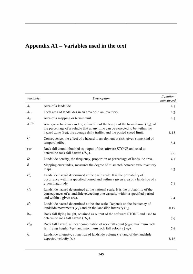
349
Appendix A1 – Variables used in the text
Variable Description Equation introduced
AL Area of a landslide. 4.1ALT Total area of landslides in an area or in an inventory. 4.2AM Area of a mapping or terrain unit. 4.1AVR Average vehicle risk index, a function of the length of the hazard zone (LH), of
the percentage of a vehicle that at any time can be expected to be within the hazard zone (VH), the average daily traffic, and the posted speed limit. 8.15
C Consequence, the effect of a hazard to an element at risk, given some kind of temporal effect. 8.4
cRF Rock fall count, obtained as output of the software STONE and used to determine rock fall hazard (HRF). 7.6
DL Landslide density, the frequency, proportion or percentage of landslide area. 4.1E Mapping error index, measures the degree of mismatch between two inventory
maps. 4.2HL Landslide hazard determined at the basin scale. It is the probability of
occurrence within a specified period and within a given area of a landslide of a given magnitude. 7.1
HL Landslide hazard determined at the national scale. It is the probability of the consequences of a landslide exceeding one casualty within a specified period and within a given area. 7.4
HL Landslide hazard determined at the site scale. Depends on the frequency of landslide movements (FL) and on the landslide intensity (IL). 8.17
hRF Rock fall flying height, obtained as output of the software STONE and used to determine rock fall hazard (HRF). 7.6
HRF Rock fall hazard, a linear combination of rock fall count (cRF), maximum rock fall flying height (hRF), and maximum rock fall velocity (vRF). 7.6
IL Landslide intensity, a function of landslide volume (vL) and of the landslide expected velocity (sL) 8.16
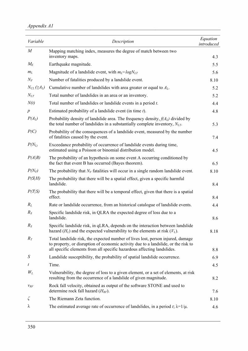
Appendix A1
350
Variable Description Equation introduced
M Mapping matching index, measures the degree of match between two inventory maps. 4.3
ME Earthquake magnitude. 5.5mL Magnitude of a landslide event, with mL=logNLT 5.6NF Number of fatalities produced by a landslide event. 8.10NCL (≥AL) Cumulative number of landslides with area greater or equal to AL. 5.2NLT Total number of landslides in an area or an inventory. 5.2N(t) Total number of landslides or landslide events in a period t. 4.4p Estimated probability of a landslide event (in time t). 4.8P(AL) Probability density of landslide area. The frequency density, f(AL) divided by
the total number of landslides in a substantially complete inventory, NLT. 5.3P(C) Probability of the consequences of a landslide event, measured by the number
of fatalities caused by the event. 7.4P(NL) Exceedance probability of occurrence of landslide events during time,
estimated using a Poisson or binomial distribution model. 4.5P(A|B) The probability of an hypothesis on some event A occurring conditioned by
the fact that event B has occurred (Bayes theorem). 6.5P(NF) The probability that NF fatalities will occur in a single random landslide event. 8.10P(S|H) The probability that there will be a spatial effect, given a specific harmful
landslide. 8.4P(T|S) The probability that there will be a temporal effect, given that there is a spatial
effect. 8.4RL Rate or landslide occurrence, from an historical catalogue of landslide events. 4.4RS Specific landslide risk, in QLRA the expected degree of loss due to a
landslide. 8.6RS Specific landslide risk, in qLRA, depends on the interaction between landslide
hazard (HL) and the expected vulnerability to the elements at risk (VL). 8.18RT Total landslide risk, the expected number of lives lost, person injured, damage
to property, or disruption of economic activity due to a landslide, or the risk to all specific elements from all specific hazardous affecting landslides. 8.8
S Landslide susceptibility, the probability of spatial landslide occurrence. 6.9t Time. 4.5WL Vulnerability, the degree of loss to a given element, or a set of elements, at risk
resulting from the occurrence of a landslide of given magnitude. 8.2vRF Rock fall velocity, obtained as output of the software STONE and used to
determine rock fall hazard (HRF). 7.6ζ The Riemann Zeta function. 8.10λ The estimated average rate of occurrence of landslides, in a period t; λ=1/µ. 4.6
Variables
351
Variable Description Equation introduced
µ Estimated mean recurrence interval between successive landslide events, in a period t; µ=1/ λ and µ=1/p. 4.6
Γ(ξ) Gamma function, ∫∞
−ξ >ξ−=ξΓ0
1 0,dy)yexp(y)( 5.4

353
Appendix A2 – List of Figures and Tables
List of Figures
Figure Caption Page
.1 The spectrum of landslide phenomena. 2
1.2 Historical variation of the population in Europe and in Italy. 3
2.1 Location of the study areas in Italy. 14
2.2 Examples of landslides and landslide damage in Italy. 15
2.3 Economic damage produced by individual landslides and flooding events in Italy in the period from 1910 to 2000. 16
2.4 Thematic data available for Italy and used in this work. (A) Digital Elevation Model. (B) Soil map of Italy. (C) Geological map of Italy. (D) Map showing historical landslides and inundations in Italy. 17
2.5 Umbria Region. (A) Shaded relief image showing morphology. (B) Map showing mean annual precipitation. (C) Simplified lithological map. (D) Landslide inventory map. 19
2.6 Examples of typical landslide damage in Umbria. 21
2.7 Location of the Upper Tiber River basin, in Central Italy. 22
2.8 Photo-Geological and Landslide Inventory Map of the Upper Tiber River Basin, Italy. 24
2.9 Abundance of lithological types and landslides in the Upper Tiber River basin, Central Italy. 25
2.10 Collazzone study area. (A) Location of the study area. (B) Shaded relief image showing morphology of the area. (C) Lithological map. (D) Abundance of lithological types. 26
Appendix A2
354
Figure Caption Page
2.11 Location of the Triponzo study area, in Valnerina, eastern Umbria. 27
2.12 Photographs showing rock falls triggered along roads in the Nera River valley and the Corno River valley by the September-October 1997 earthquakes in the Umbria-Marche Apennines. 28
2.13 Location, morphology and lithology of the Staffora River basin, Lombardy Region. 30
2.14 Multi-temporal landslide inventory map for the Staffora River basin. 31
3.1 Years of stereoscopic aerial photographs available for two landslide areas in the Italian Apennines. 36
3.2 Portion of a landslide inventory map for the Umbria region, central Italy. 38
3.3 Portion of the archive inventory map prepared by Roberto Almagià for the Italian Apennines in 1907-1910. 40
3.4 Map showing historical landslide events in Umbria. 41
3.5 Structure and modules of SICI, the information system on historical landslides and floods in Italy. 42
3.6 Map showing distribution of historical landslide and flood events in Italy. 43
3.7 Temporal distribution of the information on landslide events in Italy in the period between 1900 and 2002. 44
3.8 Historical information for four of the ten modules of SICI. 45
3.9 Reconnaissance geomorphological landslide inventory map for Umbria. 48
3.10 Detailed geomorphological landslide inventory map for Umbria. 61
3.11 Landslide abundance in the main lithological types in Umbria. 52
3.12 Landslide event inventories in Umbria. 56
3.13 Multi-temporal landslide inventory map for the Collazzone area. 59
3.14 Comparison of three landslide inventory maps available for the Collazzone area. 63
4.1 Portion of a slope-unit based geomorphological landslide density map for the Upper Tiber River basin, central Italy. 70
4.2 Comparison of geomorphological and historical inventory maps in the Umbria Region. 72
4.3 Comparison of two landslide inventory maps prepared for the La Honda area, California 74
List of figures and tables
355
Figure Caption Page
4.4 Problems with index that measures the degree of mismatch between two inventory maps. 75
4.5 Collazzone area. Estimate of overall mapping errors and map matching indexes for three pair wise combinations of landslide inventory maps. 77
4.6 Landslide density maps for the Collazzone area. 78
4.7 Comparison of stable and unstable slope units based on landslide density in the Collazzone area. 79
4.8 Comparison of landslide density in the slope units in the Collazzone area. 80
4.9 Completeness of historical catalogue of landslide events that resulted in fatalities in Italy from 1410 to 2004. 82
4.10 Deep-seated and shallow landslides in Umbria, showing difficulty in identifying and mapping the exact location of the boundary of a landslide, in the field or from aerial photographs. 84
4.11 Spatial persistence of event triggered landslides in Umbria. 85
4.12 Maps showing annual exceedance probability of damaging landslide events in the 92 Municipalities in Umbria. 88
5.1 Distribution of the area of 4246 individual landslides triggered by rapid snow melt in Umbria in January 1997. 97
5.2 Cumulative and non-cumulative frequency-area distributions for two landslide inventories in Umbria. 98
5.3 Non-cumulative frequency-area distributions of landslides triggered by rapid snow melt in Umbria on January 1997. 100
5.4 Comparison of the probability density of landslide areas produced by rapid snow melt in Umbria on January 1997 obtained by the double Pareto distribution of Stark and Hovius (2001) and the inverse Gamma distribution of Malamud et al. (2004a). 101
5.5 Probability density of landslide volumes obtained from different catalogues. 103
5.6 Probability density and frequency density of landslide areas for the three landslide inventory maps available for the Collazzone area. 105
5.7 Probability density of landslide areas obtained from six different landslide inventories. 108
6.1 Upper Tiber River basin. Maps showing spatial probability of landslide occurrence, in seven classes, from very low, where landslides are not expected, to very high, where landslides are expected to be abundant. 135
Appendix A2
356
Figure Caption Page
6.2 Collazzone area. (A) Multi-temporal landslide inventory map showing shallow landslides. (B) Map showing spatial probability of landslide occurrence. 142
6.3 Analysis of the fitting performance of the landslide susceptibility model prepared for the Collazzone area shown in Figure 6.2.B. 144
6.4 Sensitivity analysis for the landslide susceptibility model prepared for the Collazzone area shown in Figure 6.2.B. 148
6.5 Landslide susceptibility model error. 149
6.6 Collazzone area. Map showing estimated model error (2σ) for the landslide susceptibility model shown in Figure 6.2.B. 150
6.7 Collazzone area. Probability of spatial occurrence of landslides for 894 slope units, ranked from low to high susceptibility values. 151
6.8 Recent landslide event inventory maps for the Collazzone area. 152
6.9 Analysis of the prediction skill of the landslide susceptibility model prepared for the Collazzone area and shown in Figure 6.2.B. 153
6.10 Collazzone area. Relationship between the predicted susceptibility classes and the distribution and abundance of the triggered landslides. 154
7.1 Staffora River basin. Multi-temporal landslide inventory map used to ascertain landslide hazard. 165
7.2 Staffora River basin. Probability density and cumulative probability of landslide area. 166
7.3 Staffora River basin. Exceedance probability of landslide occurrence obtained computing the mean recurrence interval of past landslide events from the multi-temporal inventory. 168
7.4 Staffora River basin. Landslide susceptibility models obtained through discriminant analysis of the same set of independent thematic variables and changing the landslide inventory map. 169
7.5 Staffora River basin. Percentage of landslide area in each susceptibility class vs. the corresponding basin area, ranked from most to least susceptible 171
7.6 Block diagram exemplifying the work flow adopted to determine landslide hazard. 172
7.7 Staffora River basin. Landslide hazard maps for four periods, from 5 to 50 years, and for two landslide sizes, AL ≥ 2000 m2 and AL ≥ 1 ha. 173
List of figures and tables
357
Figure Caption Page
7.8 Landslide susceptibility map of Italy, obtained through discriminant analysis of morphometric, hydrological, lithological and soil information. 177
7.9 Schematic representation of the procedure adopted to evaluate landslide hazard at the national scale, in Italy. 179
7.10 Rock fall maps produced by STONE for the Nera River and the Corno River valleys. 183
7.11 Triponzo area, along the Nera River and the Corno River valleys. Three-dimensional view of a portion of the grid map showing the count of rock fall trajectories. 184
7.12 Rock fall hazard map for the Nera River and the Corno River valleys. 185
8.1 Historical distribution of damaging landslide events in Italy from 1500 to 2004. 201
8.2 Mortality rates for natural, technological and societal hazards and for the leading medical causes of deaths in Italy. 203
8.3 Population and landslide mortality rates in Italy from 1860 to 2004. 205
8.4 Societal landslide risk in Italy. 206
8.5 Societal risk due to landslides, floods, earthquakes, and volcanic events in Italy. 209
8.6 Map showing the distribution of landslides with human consequences in Italy from AD 1300 to 2002. 211
8.7 Map showing the probability of spatial occurrence of fatal landslide events in Italy, on the basis of local terrain conditions. 212
8.8 Validation of the model predicting the probability of spatial occurrence of fatal landslide events in Italy. 215
8.9 Umbria Region. Location of sites where landslide risk was ascertained. 226
8.10 Specific landslide risk assessment for the village of Collevalenza. 228
8.11 Specific landslide risk assessment for the village of Terria. 231
8.12 Examples of typical landslide damage in Umbria region. 236
8.13 Expected landslide impact on the built-up areas and the transportation network in Umbria. 240
8.14 Perugia Municipality, Umbria Region. Map showing 701 census zones in the Municipality. Map showing number of inhabitants potentially subject to landslide risk. 241

Appendix A2
358
Figure Caption Page
8.15 Umbria Region. Left graph shows abundance of land use classes in the Region. Right graph shows abundance of landslides in each land use class. 242
9.1 Conceptual examples for a possible landslide protocol. Rules are based on the type of landslide map, and the type and abundance of the available information. 255
List of figures and tables
359
List of Tables
Table Caption Page
2.1 Descriptive statistics of landslides in the Staffora River basin obtained from the multi-temporal inventory map. 32
3.1 Main characteristics of the two geomorphological inventory maps available for the Umbria Region. 53
3.2 Comparison of landslide event inventories in Umbria. 56
3.3 Main characteristics of the multi-temporal landslide inventory map prepared for the Collazzone area. 60
3.4 Main characteristics of the three landslide inventory maps available for the Collazzone area. 64
4.1 Comparison of landslide inventory maps in the Collazzone area. 76
4.2 Comparison of stable and unstable slope units based on landslide density in the Collazzone area. 79
4.3 Number and percentage of municipalities in Umbria that exceed a given probability of experiencing one or more damaging landslide. 89
5.1 Comparison of the statistics of landslide area for the Collazzone study area obtained from three landslide inventories and adopting two different probability distributions. 104
5.2 Comparison of the statistics of landslide area in Umbria obtained from different inventories. 107
6.1 Characteristics of landslide susceptibility methods proposed in the literature. 120
6.2 Relationships between mapping units and methods for landslide susceptibility assessment. 129
6.3 Upper Tiber River basin. Variables selected by a stepwise linear discriminant function as the best predictors of the occurrence of landslides in the 28,600 geo-hydrological mapping units in which the basin was partitioned. 133
6.4 Upper Tiber River basin. Comparison between mapping units classified as stable or unstable by the statistical model and mapping units free of and containing landslides in the geomorphological inventory map. 136
Appendix A2
360
Table Caption Page
6.5 Upper Tiber River basin. Probability classes of landslide susceptibility, extent and percentage of mapping units, extent and percent of landslide area, and percentage of mapping unit having landslides, in each susceptibility class. 136
6.6 Variables selected by a stepwise discriminant function as the best predictors of landslide occurrence in the Collazzone area. 141
6.7 Collazzone area. Comparison between slope units classified as stable or unstable by the statistical model and slope units free of and containing landslides in the multi-temporal inventory map. 143
6.8 Collazzone area. Comparison between the proportions of slope units classified as stable or unstable by the susceptibility model, and the proportions of slope units free of and containing landslides in the multi-temporal inventory map. 144
6.9 Independent thematic variables selected, or not selected, by 50 discriminant functions as the best predictors of shallow landslide occurrence in the Collazzone area. 146
6.10 Criteria and levels of quality for landslide susceptibility models and associated maps. 156
7.1 Staffora River basin. Statistics of landslide size, abundance, and total landslide area for different periods. 164
7.2 Staffora River basin. Variables entered into the discriminant model as the best predictors of the occurrence of landslides in the 2243 geo-hydrological mapping units in which the basin was partitioned. 170
7.3 Staffora River basin. Comparison between mapping units classified as stable or unstable by the discriminant model and mapping units free of and containing landslides in the inventory map. 171
7.4 Nera River and the Corno River valleys. Values of the dynamic-rolling friction angle and of the normal and tangential energy restitution coefficients assigned to each terrain type. 182
7.5 Nera River and the Corno River valleys. Comparison of different rock fall hazard models prepared considering and not considering the presence and efficacy of the rock fall defensive structures installed in the area. 187
8.1 Mortality rates for natural, technological and human-induced hazards in Italy, for different periods. 202
8.2 Variables entered into the discriminant model as the best predictors of the presence of fatal landslide events in the 6604 municipalities exhibiting average terrain gradient greater than 0.8 degrees. 213
List of figures and tables
361
Table Caption Page
8.3 Comparison between municipalities classified as safe or at risk by the model, and municipalities that experienced or did not experience fatal landslides in the period from 1900 to 1979. 214
8.4 Rock fall risk to vehicles travelling along two regional roads in the Nera River and the Corno River valleys. 217
8.5 Geomorphological landslide risk assessment in Umbria. Frequency of landslide events. 219
8.6 Geomorphologic landslide risk assessment in Umbria. Landslide intensity, IL, in four classes, based on the estimated landslide volume, vL, and the expected landslide velocity, sL. 220
8.7 Geomorphological landslide risk assessment in Umbria. Landslide hazard (HL) classes based on estimated landslide frequency, FL (Table 8.1) and landslide intensity, IL (Table 8.2). 221
8.8 Geomorphological landslide risk assessment in Umbria. Types of element at risk (for structures and infrastructure). 222
8.9 Geomorphological landslide risk assessment in Umbria. Vulnerability, VL, the expected damage to the elements at risk (i.e., buildings, structures and infrastructure) and to the population. 223
8.10 Geomorphological landslide risk assessment in Umbria. Levels of specific landslide risk, Rs, based on landslide hazard (HL, Table 8.3) and landslide vulnerability (VL, Table 8.5). 224
8.11 Geomorphological landslide risk assessment in Umbria. Relationships between classes of total landslide risk, type of landslides, and expected damage to structures, infrastructure and the population in Umbria. 225
8.12 Collevalenza study area. Classification of specific, RS, and total, RT, landslide risk. 229
8.13 Terria study area. Classification of specific, RS, and total, RT, landslide risk. 232
8.14 Buffers used in the GIS analysis of the relationships between landslides, built-up areas and the transportation network in Umbria. 239

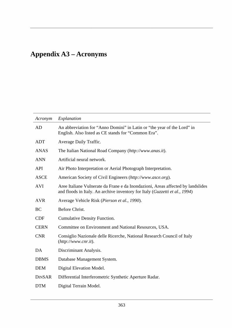
363
Appendix A3 – Acronyms
Acronym Explanation
AD An abbreviation for “Anno Domini” in Latin or “the year of the Lord” in English. Also listed as CE stands for “Common Era”.
ADT Average Daily Traffic.
ANAS The Italian National Road Company (http://www.anas.it).
ANN Artificial neural network.
API Air Photo Interpretation or Aerial Photograph Interpretation.
ASCE American Society of Civil Engineers (http://www.asce.org).
AVI Aree Italiane Vulnerate da Frane e da Inondazioni, Areas affected by landslides and floods in Italy. An archive inventory for Italy (Guzzetti et al., 1994)
AVR Average Vehicle Risk (Pierson et al., 1990).
BC Before Christ.
CDF Cumulative Density Function.
CERN Committee on Environment and National Resources, USA.
CNR Consiglio Nazionale delle Ricerche, National Research Council of Italy (http://www.cnr.it).
DA Discriminant Analysis.
DBMS Database Management System.
DEM Digital Elevation Model.
DINSAR Differential Interferometric Synthetic Aperture Radar.
DTM Digital Terrain Model.
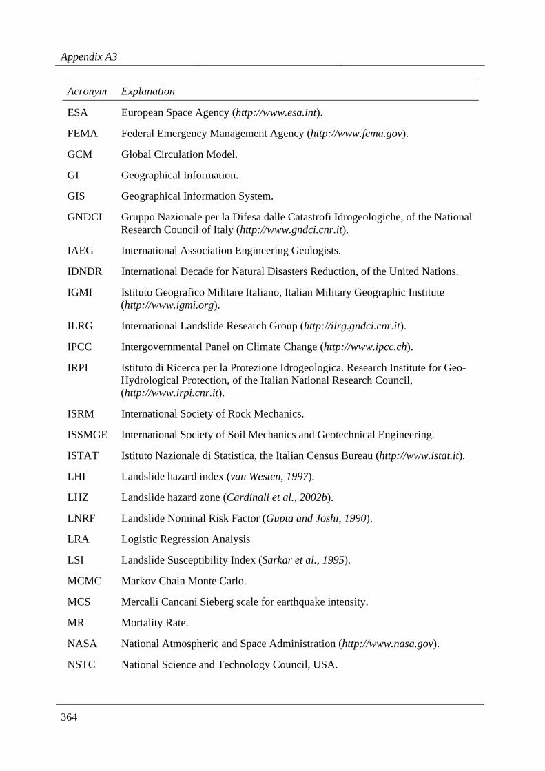
Appendix A3
364
Acronym Explanation
ESA European Space Agency (http://www.esa.int).
FEMA Federal Emergency Management Agency (http://www.fema.gov).
GCM Global Circulation Model.
GI Geographical Information.
GIS Geographical Information System.
GNDCI Gruppo Nazionale per la Difesa dalle Catastrofi Idrogeologiche, of the National Research Council of Italy (http://www.gndci.cnr.it).
IAEG International Association Engineering Geologists.
IDNDR International Decade for Natural Disasters Reduction, of the United Nations.
IGMI Istituto Geografico Militare Italiano, Italian Military Geographic Institute (http://www.igmi.org).
ILRG International Landslide Research Group (http://ilrg.gndci.cnr.it).
IPCC Intergovernmental Panel on Climate Change (http://www.ipcc.ch).
IRPI Istituto di Ricerca per la Protezione Idrogeologica. Research Institute for Geo-Hydrological Protection, of the Italian National Research Council, (http://www.irpi.cnr.it).
ISRM International Society of Rock Mechanics.
ISSMGE International Society of Soil Mechanics and Geotechnical Engineering.
ISTAT Istituto Nazionale di Statistica, the Italian Census Bureau (http://www.istat.it).
LHI Landslide hazard index (van Westen, 1997).
LHZ Landslide hazard zone (Cardinali et al., 2002b).
LNRF Landslide Nominal Risk Factor (Gupta and Joshi, 1990).
LRA Logistic Regression Analysis
LSI Landslide Susceptibility Index (Sarkar et al., 1995).
MCMC Markov Chain Monte Carlo.
MCS Mercalli Cancani Sieberg scale for earthquake intensity.
MR Mortality Rate.
NASA National Atmospheric and Space Administration (http://www.nasa.gov).
NSTC National Science and Technology Council, USA.
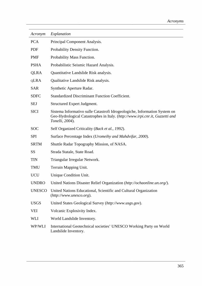
Acronyms
365
Acronym Explanation
PCA Principal Component Analysis.
PDF Probability Density Function.
PMF Probability Mass Function.
PSHA Probabilistic Seismic Hazard Analysis.
QLRA Quantitative Landslide Risk analysis.
QLRA Qualitative Landslide Risk analysis.
SAR Synthetic Aperture Radar.
SDFC Standardized Discriminant Function Coefficient.
SEJ Structured Expert Judgment.
SICI Sistema Informativo sulle Catastrofi Idrogeologiche, Information System on Geo-Hydrological Catastrophes in Italy. (http://www.irpi.cnr.it, Guzzetti and Tonelli, 2004).
SOC Self Organized Criticality (Back et al., 1992).
SPI Surface Percentage Index (Uromeihy and Mahdvifar, 2000).
SRTM Shuttle Radar Topography Mission, of NASA.
SS Strada Statale, State Road.
TIN Triangular Irregular Network.
TMU Terrain Mapping Unit.
UCU Unique Condition Unit.
UNDRO United Nations Disaster Relief Organization (http://ochaonline.un.org/).
UNESCO United Nations Educational, Scientific and Cultural Organization (http://www.unesco.org).
USGS United States Geological Survey (http://www.usgs.gov).
VEI Volcanic Explosivity Index.
WLI World Landslide Inventory.
WP/WLI International Geotechnical societies’ UNESCO Working Party on World Landslide Inventory.

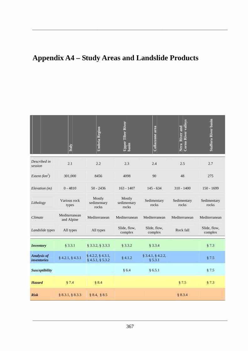
367
Appendix A4 – Study Areas and Landslide Products
Ital
y
Um
bria
Reg
ion
Upp
er T
iber
Riv
er
basi
n
Col
lazz
one
area
Ner
a R
iver
and
C
orno
Riv
er v
alle
ys
Staf
fora
Riv
er b
asin
Described in session 2.1 2.2 2.3 2.4 2.5 2.7
Extent (km2) 301,000 8456 4098 90 48 275
Elevation (m) 0 - 4810 50 - 2436 163 - 1407 145 - 634 310 - 1400 150 - 1699
Lithology Various rock types
Mostly sedimentary
rocks
Mostly sedimentary
rocks
Sedimentary rocks
Sedimentary rocks
Sedimentary rocks
Climate Mediterranean and Alpine Mediterranean Mediterranean Mediterranean Mediterranean Mediterranean
Landslide types All types All types Slide, flow, complex
Slide, flow, complex Rock fall Slide, flow,
complex
Inventory § 3.3.1 § 3.3.2, § 3.3.3 § 3.3.2 § 3.3.4 § 7.3
Analysis of inventories § 4.2.1, § 4.3.1 § 4.2.2, § 4.3.1,
§ 4.5.1, § 5.3.2 § 4.1.2 § 3.4.1, § 4.2.2, § 5.3.1 § 7.5
Susceptibility § 6.4 § 6.5.1 § 7.5
Hazard § 7.4 § 8.4 § 7.5 § 7.3
Risk § 8.3.1, § 8.3.3 § 8.4, § 8.5 § 8.3.4

369
Appendix A5 – Corriculum vitae et studiorium
Current rank From 1996 Senior Scientist (Primo Ricercatore), Research Institute for Geo-Hydrological Protection (Istituto di Ricerca per la Protezione Idrogeologica, IRPI), of the Italian National Research Council (Consiglio Nazionale delle Ricerche), Perugia, Italy.
Appointments • President Natural Hazards Division, European Geosciences Union (2002 -) • Secretary IWG on Natural Hazards, European Geophysical Society (2001-2002) • Head of the Applied Geology and Geomorphology Team, CNR - IRPI (1991 -) • CNR Researcher, at CNR - IRPI (1985-1996) • Visiting scientist, U.S. Geological Survey, Menlo Park, California (1985-1986) • Consultant, Field Geologist (1983-1984)
Education
• 1983, Laurea in Scienze Geologiche (110/110 cum laudae) – Dipartimento di Scienze della Terra, Università degli Studi di Perugia, Perugia, Italy
• 1984, National Examination for Registered Geologist. Università “La Sapienza”, Rome.
• 1978, Scientific School Final Examination (Maturità Scientifica) - Liceo Scientifico Statale A. Avogadro, Biella, Italy
National and International memberships and professional affiliations • Italian Geological Society (1985 -); Registered Professional Geologist, Italy (1985 -);
American Geophysical Union (1989 -); Italian Group for Physical Geography and Geomorphology (1993 -); Centre Européen Recherche Géomorphologique (1995 -); European Geophysical Society (1996 - 2002); European Geosciences Union, founding member (2002 -); IAEG, International Association of Engineering Geology.
Appendix A5 Curriculum vitae et studiorium
370
Referee / Advisor for • Advances in Geosciences, ASCE, Bollettino Società Geologica Italiana, Cambridge
University Press, Computers & Geosciences, Disasters, Earth Surface Processes and Landforms, Encyclopaedias of Earth Sciences Series, Engineering Geology, Environmental Management, Forest Ecology and Management, Geological Society, Geological Society of America, Geomorphology, Journal Environmental Management, Journal Asian of Earth Science, Journal of Cultural Heritage, Landslides, Natural Hazards, Natural Hazards and Earth System Sciences, Surveys in Geophysics, Water Resources Research.
• Science Foundation of Ireland (2004-2005), National Science Foundation, USA (2005), National Environmental Research Council, U.K. (2002), Italian Space Agency (2000-2001), National Minister for University and Scientific Research (1999-2001).
Editorial activities • Associated editor for Natural Hazards and Earth System Sciences (2001 -) • Associated editor for Landslides (2004 -) [1] Couture, R. and Guzzetti, F., editors (2004) Geo-Databases for Natural Hazards and Risk
Assessment. Natural Hazards and Earth Systems Sciences, vol. 4:3, 183 - 242. [2] Reichenbach, P. and Guzzetti, F., editors (2003) Landslide Risk Assessment and Mapping.
Natural Hazards and Earth Systems Sciences, vol. 3:5, 403 - 486. [3] Reichenbach, P., Carrara, A. and Guzzetti, F., editors (2002) Assessing and Mapping
Landslide Hazards and Risk. Natural Hazards and Earth Systems Sciences, vol. 2:1-2, 82 p.
[4] Mugnai, A., Guzzetti, F. and Roth, G., editors (2001) Proceedings 2nd Plinius Conference on Mediterranean Storms, Siena, CNR GNDCI Publication n. 2547, 529 p.
[5] Carrara, A. and Guzzetti, F., editors (1999) Techniques and tools for Mapping Natural Hazards and Risk Impact on the Developed Environment. Natural Hazards, vol. 20:2-3, November 1999, 93-324.
[6] Guzzetti, F., editor (1998) Hydrological triggers of diffused landsliding. Environmental Geology, vol. 35:2-3, 240 p.
[7] Carrara, A. and Guzzetti, F., editors (1995) Geographical Information Systems in Assessing Natural Hazards. Kluwer Academic Publisher, Dordrecht, The Netherlands, June 1995, 342 p.
Publications Author and co-author of 28 papers in peer-reviewed international journals, 5 chapters in multi-authored books, 9 maps, 30 papers in the proceedings of international conferences, more than 25 papers published in Italian journals or conference proceedings, more than 30 technical reports, and more than 100 abstracts submitted to national and international conferences.
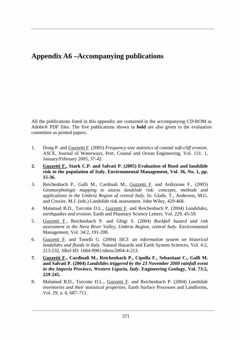
371
Appendix A6 –Accompanying publications
All the publications listed in this appendix are contained in the accompanying CD-ROM as Adobe® PDF files. The five publications shown in bold are also given to the evaluation committee as printed papers.
1. Dong P. and Guzzetti F. (2005) Frequency-size statistics of coastal soft-cliff erosion.
ASCE, Journal of Waterways, Port, Coastal and Ocean Engineering, Vol. 131: 1, January/February 2005, 37-42.
2. Guzzetti F., Stark C.P. and Salvati P. (2005) Evaluation of flood and landslide risk to the population of Italy. Environmental Management, Vol. 36, No. 1, pp. 15-36.
3. Reichenbach P., Galli M., Cardinali M., Guzzetti F. and Ardizzone F., (2005) Geomorphologic mapping to assess landslide risk: concepts, methods and applications in the Umbria Region of central Italy. In: Glade, T., Anderson, M.G. and Crozier, M.J. (eds.) Landslide risk assessment. John Wiley, 429-468.
4. Malamud B.D., Turcotte D.L., Guzzetti F. and Reichenbach P. (2004) Landslides, earthquakes and erosion. Earth and Planetary Science Letters. Vol. 229, 45-59.
5. Guzzetti F., Reichenbach P. and Ghigi S. (2004) Rockfall hazard and risk assessment in the Nera River Valley, Umbria Region, central Italy. Environmental Management, Vol. 34:2, 191-208.
6. Guzzetti F. and Tonelli G. (2004) SICI: an information system on historical landslides and floods in Italy. Natural Hazards and Earth System Sciences, Vol. 4:2, 213-232, SRef-ID: 1684-9981/nhess/2004-4-213.
7. Guzzetti F., Cardinali M., Reichenbach P., Cipolla F., Sebastiani C., Galli M. and Salvati P. (2004) Landslides triggered by the 23 November 2000 rainfall event in the Imperia Province, Western Liguria, Italy. Engineering Geology, Vol. 73:2, 229-245.
8. Malamud B.D., Turcotte D.L., Guzzetti F. and Reichenbach P. (2004) Landslide inventories and their statistical properties. Earth Surface Processes and Landforms, Vol. 29, n. 6, 687–711.
Appendix 6
372
9. Guzzetti F., Reichenbach P. and Wieczorek G.F. (2003) Rockfall hazard and risk assessment in the Yosemite Valley, California, USA. Natural Hazards and Earth System Sciences, Vol. 3, n. 6, 491-503.
10. Guzzetti F., Reichenbach P., Cardinali M., Ardizzone F. and Galli M. (2003) Impact of landslides in the Umbria Region, Central Italy. Natural Hazards and Earth System Sciences. Vol. 3, n. 5, 469 - 486.
11. Guzzetti F., Crosta G., Detti R. and Agliardi F. (2002) STONE: a computer program for the three-dimensional simulation of rock-falls. Computers and Geosciences, Vol. 28: 9, 1079-1093.
12. Turcotte D.L., Malamud B.D., Guzzetti F. and Reichenbach P. (2002) Self-organization, the cascade model and natural hazards. Proceedings National Academy of Sciences, USA, February 2002, Vol. 99, Supp. 1, 2530-2537.
13. Cardinali M., Reichenbach P., Guzzetti F., Ardizzone F., Antonini G., Galli M., Cacciano M., Castellani M. and Salvati P. (2002) A geomorphological approach to estimate landslide hazard and risk in urban and rural areas in Umbria, central Italy. Natural Hazards and Earth System Sciences, Vol. 2:1-2, 57-72.
14. Ardizzone F., Cardinali M., Carrara A., Guzzetti F. and Reichenbach P. (2002) Impact of mapping errors on the reliability of landslide hazard maps. Natural Hazards and Earth System Sciences, Vol. 2:1-2, 3-14.
15. Guzzetti F., Malamud B.D., Turcotte D.L. and Reichenbach P. (2002) Power-law correlations of landslide areas in Central Italy. Earth and Planetary Science Letters, Vol. 195: 169-183.
16. Guzzetti F. (2000) Landslide fatalities and evaluation of landslide risk in Italy. Engineering Geology, Vol. 58: 89-107.
17. Guzzetti F., Cardinali M., Reichenbach P. and Carrara A. (2000) Comparing landslide maps: A case study in the upper Tiber River Basin, central Italy. Environmental Management, Vol. 25: 3, 247-363.
18. Carrara A., Guzzetti F., Cardinali M. and Reichenbach P. (1999) Use of GIS Technology in the Prediction and Monitoring of Landslide Hazard. Natural Hazards, Vol. 20: 2-3, 117-135.
19. Guzzetti F., Carrara A., Cardinali M. and Reichenbach P. (1999) Landslide hazard evaluation: an aid to a sustainable development. Geomorphology, Vol. 31, 181-216.
20. Guzzetti F., Cardinali M. and Reichenbach P. (1996) The influence of structural setting and lithology on landslide type and pattern. Environmental and Engineering Geosciences, Vol. 2: 4, Winter 1996, 531-555.
21. Carrara A., Cardinali M., Guzzetti F. and Reichenbach P. (1995) GIS technology in mapping landslide hazard. In: Carrara A. and Guzzetti F. (eds.), Geographical Information Systems in Assessing Natural Hazards. Kluwer Academic Publisher, Dordrecht, The Netherlands, 135-175.
22. Guzzetti F., Cardinali M. and Reichenbach P. (1994) The AVI Project: A bibliographical and archive inventory of landslides and floods in Italy. Environmental Management, Vol. 18, 623-633.

Accompanying publications
373
23. Carrara A., Cardinali M. and Guzzetti F. (1992) Uncertainty in assessing landslide hazard and risk. ITC Journal, The Netherlands, Vol. 2, 172-183.
24. Guzzetti F. and Cardinali M. (1991) Debris-flow phenomena in the Central Apennines of Italy. TerraNova, Vol. 3, 619-627.
25. Carrara A., Cardinali M., Detti R., Guzzetti F., Pasqui V. and Reichenbach P. (1991) GIS Techniques and statistical models in evaluating landslide hazard. Earth Surface Processes and Landform. Vol. 16: 5, 427-445.