Embed Size (px)
Citation preview

arX
iv:1
011.
3049
v1 [
cs.D
C]
12 N
ov 2
010
Distributed Verification and Hardness of Distributed Approximation
Atish Das Sarma∗ Stephan Holzer† Liah Kor ‡ Amos Korman§
Danupon Nanongkai¶ Gopal Pandurangan‖ David Peleg‡ Roger Wattenhofer†
Abstract
We study theverificationproblem in distributed networks, stated as follows. LetH be a subgraph ofa networkG where each vertex ofG knows which edges incident on it are inH . We would like to verifywhetherH has some properties, e.g., if it is a tree or if it is connected. We would like to perform thisverification in a decentralized fashion via a distributed algorithm. The time complexity of verification ismeasured as the number of rounds of distributed communication.
In this paper we initiate a systematic study of distributed verification, and give almost tight lowerbounds on the running time of distributed verification algorithms for many fundamental problems such asconnectivity, spanning connected subgraph, ands− t cut verification. We then show applications of theseresults in deriving strong unconditional time lower boundson thehardness of distributed approximationfor many classical optimization problems including minimum spanning tree, shortest paths, and minimumcut. Many of these results are the first non-trivial lower bounds for both exact and approximate distributedcomputation and they resolve previous open questions. Moreover, our unconditional lower bound ofapproximating minimum spanning tree (MST) subsumes and improves upon the previous hardness ofapproximation bound of Elkin [STOC 2004] as well as the lowerbound for (exact) MST computation ofPeleg and Rubinovich [FOCS 1999]. Our result implies that there can be no distributed approximationalgorithm for MST that is significantly faster than the current exact algorithm, forany approximationfactor.
Our lower bound proofs show an interesting connection between communication complexity anddistributed computing which turns out to be useful in establishing the time complexity of exact and ap-proximate distributed computation of many problems.
∗Google Research, Google Inc., Mountain View, USA. E-mail:[email protected]. Part of the work done while atGeorgia Institute of Technology.
†Computer Engineering and Networks Laboratory (TIK), ETH Zurich, CH-8092 Zurich, Switzerland. E-mail:stholzer,[email protected].
‡Department of Computer Science and Applied Mathematics, The Weizmann Institute of Science, Rehovot, 76100 Israel. E-mail: liah.kor,[email protected]. Supported by a grant from the United States-Israel Binational ScienceFoundation (BSF).
§CNRS and LIAFA, Univ. Paris 7, Paris, France. E-mail:[email protected].¶College of Computing, Georgia Institute of Technology, Atlanta, GA 30332, USA. E-mail:[email protected]‖Division of Mathematical Sciences, Nanyang TechnologicalUniversity, Singapore 637371 and Department of Computer Sci-
ence, Brown University, Providence, RI 02912, USA. E-mail:[email protected]. Supported in part by NSFgrant CCF-1023166 and by a grant from the United States-Israel Binational Science Foundation (BSF).

1 Introduction
Large and complex networks, such as the human society, the Internet, or the brain, are being studied intenselyby different branches of science. Each individual node in such a network can directly communicate only withits neighboring nodes. Despite being restricted to suchlocal communication, the network itself should worktowards aglobal goal, i.e., it should organize itself, or deliver a service.
In this work we investigate the possibilities and limitations of distributed/decentralized computation, i.e.,to what degree local information is sufficient to solve global tasks. Many tasks can be solved entirely vialocal communication, for instance, how many friends of friends one has. Research in the last 30 years hasshown that some classic combinatorial optimization problems such as matching, coloring, dominating set, orapproximations thereof can be solved using small (i.e., polylogarithmic) local communication. For example,a maximal independent set can be computed in timeO(log n) [18], but not in timeΩ(
√
log n/ log log n)[13] (n is the network size). This lower bound even holds if message sizes are unbounded.
However “many” important optimization problems are “global” problems from the distributed compu-tation point of view. To count the total number of nodes, to determining the diameter of the system, or tocompute a spanning tree, information necessarily must travel to the farthest nodes in a system. If exchanginga message over a single edge costs one time unit, one needsΩ(D) time units to compute the result, whereD is the network diameter. If message size was unbounded, one can simply collect all the information inO(D) time, and then compute the result. Hence, in order to arrive at a realistic problem, we need to introducecommunication limits, i.e., each node can exchange messages with each of its neighbors in each step of asynchronous system, but each message can have at mostB bits (typicallyB is small, sayO(log n)). How-ever, to compute a spanning tree, even single-bit messages are enough, as one can simply breadth-first-searchthe graph in timeO(D) and this is optimal [20].
But, can weverify whether an existing spanning tree indeed is a correct spanning tree?! In this paperwe show that this is not generally possible inO(D) time – instead one needsΩ(
√n + D) time. (Thus, in
contrast to traditional non-distributed complexity, verification is harder than computation in the distributedworld!). Our paper is more general, as we show interesting lower and upper bounds (these are almost tight)for a whole selection of verification problems. Furthermore, we show a key application of studying such ver-ification problems to proving strong unconditional time lower bounds on exact and approximate distributedcomputation for many classical problems.
1.1 Technical Background and Previous Work
Distributed Computing. Consider a synchronous network of processors with unbounded computationalpower. The network is modeled by an undirectedn-vertex graph, where vertices model the processors andedges model the links between the processors. The processors (henceforth, vertices) communicate by ex-changing messages via the links (henceforth, edges). The vertices have limited global knowledge, in particu-lar, each of them has its own local perspective of the network(a.k.a graph), which is confined to its immediateneighborhood. The vertices may have to compute (cooperatively) some global function of the graph, such asa spanning tree (ST) or a minimum spanning tree (MST), via communicating with each other and running adistributed algorithm designed for the task at hand. There are several measures to analyze the performanceof such algorithms, a fundamental one being the running time, defined as the worst-case number ofroundsof distributed communication. This measure naturally gives rise to a complexity measure of problems, calledthe time complexity. On each round at mostB bits can be sent through each edge in each direction, whereB is the bandwidth parameter of the network. The design of efficient algorithms for this model (henceforth,theB model), as well as establishing lower bounds on the time complexity of various fundamental graphproblems, has been the subject of an active area of research called (locality-sensitive)distributed computing(see [20] and references therein.)
Distributed Algorithms, Approximation, and Hardness. Much of the initial research focus in the area ofdistributed computing was on designing algorithms for solving problems exactly, e.g., distributed algorithms
1

for ST, MST, and shortest paths are well-known [20, 19]. Overthe last few years, there has been interestin designing distributed algorithms that provide approximate solutions to problems. This area is known asdistributed approximation. One motivation for designing such algorithms is that they can run faster or havebetter communication complexity albeit at the cost of providing suboptimal solution. This can be especiallyappealing for resource-constrained and dynamic networks (such as sensor or peer-to-peer networks). Forexample, there is not much point in having an optimal algorithm in a dynamic network if it takes too muchtime, since the topology could have changed by that time. Forthis reason, in the distributed context, suchalgorithms are well-motivated even for network optimization problems that are not NP-hard, e.g., minimumspanning tree, shortest paths etc. There is a large body of work on distributed approximation algorithms forvarious classical graph optimization problems (e.g., see the surveys by Elkin [4] and Dubhashi et al. [3], andthe work of [10] and the references therein).
While a lot of progress has been made in the design of distributed approximation algorithms, the samehas not been the case with the theory of lower bounds on the approximability of distributed problems, i.e.,hardnessof distributed approximation. There are some inapproximability results that are based on lowerbounds on the time complexity of the exact solution of certain problems and on integrality of the objectivefunctions of these problems. For example, a fundamental result due to Linial [16] says that 3-coloring ann-vertex ring requiresΩ(log∗ n) time. In particular, it implies that any 3/2-approximationprotocol for thevertex-coloring problem requiresΩ(log∗ n) time. On the other hand, one can state inapproximability resultsassuming that vertices are computationally limited; underthis assumption, any NP-hardness inapproxima-bility result immediately implies an analogous result in the distributed model. However, the above resultsare not interesting in the distributed setting, as they provide no new insights on the roles of locality andcommunication [7].
There are but a few significant results currently known on thehardness of distributed approximation.Perhaps the first important result was presented for the MST problem by Elkin in [7]. Specifically, he showedstrongunconditionallower bounds (i.e., ones that do not depend on complexity-theoretic assumptions) fordistributed approximate MST (more on this result below). Later, Kuhn, Moscibroda, and Wattenhofer [13]showed lower bounds on time approximation trade-offs for several problems.
1.2 Distributed Verification
The above discussion summarized two major research aspectsin distributed computing, namely studyingdistributed algorithms and lower bounds for (1) exact and (2) approximate solutions to various problems. Thethird aspect — that turns out to have remarkable applications to the first two — calleddistributed verification,is the main subject of the current paper. In distributed verification, we want to efficiently check whether agiven subgraph of a network has a specified property via a distributed algorithm1. Formally, given a graphG = (V,E), a subgraphH = (V,E′) with E′ ⊆ E, and a predicateΠ, it is required to decide whetherH satisfiesΠ. The predicateΠ may specify statements such as “H is connected” or “H is a spanningtree” or “H contains a cycle”. (Each vertex inG knows which of its incident edges (if any) belong toH.)The goal is to study bounds on the time complexity of distributed verification. The time complexity of theverification algorithm is measured with respect to parameters ofG (in particular, its sizen and diameter2 D),independently fromH.
We note that verification is different from construction problems, which have been the traditional focusin distributed computing. Indeed, distributed algorithmsfor constructing spanning trees, shortest paths, andother problems have been well studied ([20, 19]). However, the corresponding verification problems havereceived much less attention. To the best of our knowledge, the only distributed verification problem that hasreceived some attention is the MST (i.e., verifying ifH is a MST); the recent work of Kor et al. [11] gives aΩ(
√n/B+D) deterministic lower bound on distributed verification of MST, whereD is the diameter of the
1Such problems have been studied in the sequential setting, e.g., Tarjan[22] studied verification of MST.2The length of a pathp in G is the number of edges it contains. Thedistancebetween two vertices is the length of the shortest
path connecting them. ThediameterD of G is the maximum distance between any two vertices ofG.
2

networkG. That paper also gives a matching upper bound (see also [12]). Note that distributedconstructionof MST has rather similar lower and upper bounds [21, 8]. Thusin the case of the MST problem, verificationand construction have the same time complexity. We later show that the above result of Kor et al. is subsumedby the results of this paper, as we show that verifyinganyspanning tree takes so much time.
Motivations. The study of distributed verification has two main motivations. The first is understanding thecomplexity of verification versus construction. This is obviously a central question in the traditional RAMmodel, but here we want to focus on the same question in the distributed model. Unlike in the centralized set-ting, it turns out that verification isnot in general easier than construction in the distributed setting! In fact, aswas indicated earlier, distributively verifying a spanning tree turns out to be harder than constructing it in theworst case. Thus understanding the complexity of verification in the distributed model is also important. Sec-ond, from an algorithmic point of view, for some problems, understanding the verification problem can helpin solving the construction problem or showing the inherentlimitations in obtaining an efficient algorithm.In addition to these, there is yet another motivation that emerges from this work: We show that distributedverification leads to showingstrong unconditional lower bounds on distributed computation (both exact andapproximate)for a variety of problems, many hitherto unknown. For example, we show that establishing alower bound on the spanning connected subgraph verificationproblem leads to establishing lower bounds forthe minimum spanning tree, shortest path tree, minimum cut etc. Hence, studying verification problems maylead to proving hardness of approximation as well as lower bounds for exact computation for new problems.
1.3 Our Contributions
In this paper, our main contributions are two fold. First, weinitiate a systematic study ofdistributed verifi-cation, and give almost tight uniform lower bounds on the running time of distributed verification algorithmsfor many fundamental problems. Second, we make progress in establishing strong hardness results on thedistributed approximation of many classical optimizationproblems. Our lower bounds also apply seamlesslyto exact algorithms. We next state our main results (the precise theorem statements are in the respectivesections as mentioned below).1. Distributed Verification. We show a lower bound ofΩ(
√
n/(B log n) + D) for many verificationproblems in theB model, includingspanning connected subgraph, s-t connectivity, cycle-containment, bi-partiteness, cut, least-element list, ands−t cut(cf. Section 4). These bounds apply torandomizedalgorithmsas well, and clearly hold also for asynchronous networks. Moreover, it is important to note that our lowerbounds apply even to graphs of small diameter (D = O(log n)). (Indeed, the problems studied in this pa-per are “global” problems, i.e., the network diameter ofG imposes an inherent lower bound on the timecomplexity.)
Additionally, we show that another fundamental problem, namely, the spanning tree verification problem(i.e., verifying whetherH is a spanning tree) has the same lower bound ofΩ(
√
n/(B log n)+D) (cf. Section6). However, this bound applies to only deterministic algorithms. This result strengthens the lower boundresult of MST verification by Kor et al. [11]. Moreover, we note the interesting fact that although finding aspanning tree (e.g., a breadth-first tree) can be done inO(D) rounds [20], verifying if a given subgraph is aspanning tree requiresΩ(
√n +D) rounds! Thus the verification problem for spanning trees is harder than
its construction in the distributed setting. This is in contrast to this well-studied problem in the centralizedsetting. Apart from the spanning tree problem, we also show deterministic lower bounds for other verificationproblems, includingHamiltonian cycleandsimple path.
Our lower bounds are almost tight as we show that there exist algorithms that run inO(√n log∗ n+D)
rounds (assumingB = O(log n)) for all the verification problems addressed here (cf. Appendix C).
2. Bounds on Hardness of Distributed Approximation. An important consequence of our verificationlower bound is that it leads to lower bounds for exact and approximate distributed computation. We show theunconditional time lower bound ofΩ(
√
n/(B log n) +D) for approximating many optimization problems,including MST, shortests − t path, shortest path tree, and minimum cut (Section 5). The important point
3

Previous lower bound for MST New lower bound for MST,DiameterD and shortest-path tree [7] shortest-path tree and
(for exact algorithms, useα = 1) all problems in Fig. 2.
nδ , 0 < δ < 1/2 Ω(√
nαB
) Ω(√
nB)
Θ(log n) Ω(√
nαB log n
) Ω(√
nB log n
)
Constant≥ 3 Ω(( nαB
)1
2− 1
2D−2 ) Ω(( nB)1
2− 1
2D−2 )
4 Ω(( nαB
)1/3) Ω(( nB)1/3)
3 Ω(( nαB
)1/4) Ω(( nB)1/4)
Figure 1: Lower bounds of randomizedα-approximation algorithms on graphs of various diameters.Bounds in the first columnare for the MST and shortest path tree problems [7] while those in the second column are for these problems and many problemslisted in Fig. 2. We note that these bounds almost match theO(
√n log∗ n+D) upper bound for the MST problem [8, 15] and are
independent of the approximation-factorα.
to note is that the above lower bound applies forany approximation ratioα ≥ 1. Thus the same boundholds for exact algorithms also (α = 1). All these hardness bounds hold for randomized algorithms. Asin our verification lower bounds, these bounds apply even to graphs of small (O(log n)) diameter. Figure 1summarizes our lower bounds for various diameters.
Our results improve over previous ones (e.g., Elkin’s lowerbound for approximate MST and shortestpath tree [7]) and subsumes some well-established exact bounds (e.g., Peleg and Rubinovich lower boundfor MST [21]) as well as shows new strong bounds (both for exact and approximate computation) for manyother problems (e.g., minimum cut), thus answering some questions that were open earlier (see the survey byElkin [4]).
The new lower bound for approximating MST simplifies and improves upon the previousΩ(√
n/(αB log n)+D) lower bound by Elkin [7], whereα is the approximation factor. [7] showed atradeoff between therunning time and the approximation ratio of MST. Our result shows that approximating MST requiresΩ(
√
n/(B log n) + D) rounds, regardless ofα. Thus our result shows that there is actually no trade-off,since there can be no distributed approximation algorithm for MST that is significantly faster than the currentexact algorithm [15, 6], for any approximation factorα > 1.
2 Overview of Technical Approach
We prove our lower bounds by establishing an interesting connection between communication complexityand distributed computing. Our lower bound proofs considerthe family of graphs evolved through a seriesof papers in the literature [7, 17, 21]. However, while previous results [7, 21] rely on counting the numberof states to analyze themailing problem(along with some sophisticated techniques for the variant,calledcorrupted mail problem, in the case of approximation algorithm lower bounds) and use Yao’s method [26](with appropriate input distributions) to get lower boundsfor randomized algorithms, our results are achievedusing the following three steps of simple reductions, as follows.
(Section 3) First, we reduce the lower bounds of problems in the standard communication complexitymodel [14] to the lower bounds of the equivalent problems in the “distributed version” of communicationcomplexity. Specifically, we relate thecommunicationlower bound from the standard communication com-plexity model [14] to compute some appropriately chosen function f , to the distributedtime complexitylower bound for computing the same function in a specially chosen graphG. In the standard model, Aliceand Bob can communicate directly (via a bidirectional edge of bandwidth one). In the distributed model, weassume that Alice and Bob are some vertices ofG and they together wish to compute the functionf using thecommunication graphG. The choice of graphG is critical. We use a graph calledG(Γ, d, p) (parameterizedby Γ, d andp) that was first used in [7]. We show a reduction from the standard model to the distributedmodel, the proof of which relies on certain observations similar to those used in previous results (e.g., [21]).
(Section 4) The connection established in the first step allows us to bypass the state counting argumentand Yao’s method, and reduces our task in proving lower bounds of verification problems to merely pickingthe right functionf to reduce from. The functionf that is useful in showing our randomized lower bounds is
4

set disjointness
connected spanning subgraph s-t connectivity cycle e-cycle bipartiteness
connectivity k-component cut s-t cut least-element list edge on all paths
MST s-source distance shortest path tree min s-t cut shortests-t path
shallow-light tree min routing cost tree min cut generalized Steiner forest
equality
Hamiltonian cycle
spanning tree simple path
VerificationA
pproximationRandomized Deterministic
Section 4 Appendix A.1 Appendix A.2 Appendix A.3Section 5 Appendix D Appendix B.2 Appendix B.3
Figure 2: Problems and reductions between them to obtain randomized and deterministic lower bounds. For all problems, weobtain lower bounds as in Fig. 1
theset disjointness function, which is the quintessential problem in the world of communication complexitywith applications to diverse areas and has been studied for decades (see a recent survey in [1]). Following theresult well known in communication complexity [14], we showthat the distributed version of this problemhas anΩ(
√
n/(B log n)) lower bound on graphs of small diameter. We then reduce this problem to theverification problems using simple reductions similar to those used in data streams [9]. The set disjointnessfunction yields randomized lower bounds and works for many problems (see Fig. 2), but it does not reduceto certain other problems such as spanning tree. To show lower bounds for these and a few other problems,we use a different functionf calledequality. However, this reduction yields only deterministic lower boundsfor the corresponding verification problems.
(Section 5) Finally, we reduce the verification problem to hardness of distributed approximation for avariety of problems to show that the same lower bounds hold for approximation algorithms as well. For this,we use a reduction whose idea is similar to one used to prove hardness of approximating TSP (TravelingSalesman Problem) on general graphs (see, e.g., [24]): We convert a verification problem to an optimizationproblem by introducing edge weight in such a way that there isa large gap between the optimal values forthe cases whereH satisfies, or does not satisfy a certain property. This technique is surprisingly simple, yetyields strong unconditional hardness bounds — many hitherto unknown, left open (e.g., minimum cut) [4]and some that improve over known ones (e.g., MST and shortestpath tree) [7]. As mentioned earlier, ourapproach shows that approximating MST byany factor needsΩ(
√n) time, while the previous result due to
Elkin gave a bound that depends onα (the approximation factor), i.e.Ω(√
n/α), using more sophisticatedtechniques.
Fig. 2 summarizes these reductions that will be proved in this paper. Due to the space constraint, wefocus on the proofs towards the lower bound of approximatingminimum spanning tree in the main paper.Other results can be found in the Appendix.
3 Connection between Communication Complexity and Distributed Computing
Consider the following problem. There are two parties that have unbounded computational power. Each partyreceives ab-bit string, for some integerb ≥ 1, denoted byx and y in 0, 1b. They both want to togethercomputef(x, y) for some boolean functionf : 0, 1b × 0, 1b → 0, 1. We consider two models ofcommunication.
• Direct communication:This is the standard model in communication complexity. Twoparties can com-municate via a bidirectional edge of bandwidth one. We call the party receivingx Alice, and the otherpartyBob. At the end of the process, Bob will outputf(x, y).
• Communication through networkG(Γ, d, p): Two parties are distinct vertices in aB model distributednetwork, calledG(Γ, d, p), for some parametersΓ, d, andp; the network hasΘ(Γdp) vertices and adiameter ofΘ(2p+2). (This network was first defined in [7] and described below.) We denote the vertex
5

P1
Pℓ
PΓ
v10 v11 v12 v1dp−1
vℓ0 vℓ1 vℓ2 vℓdp−1
vΓ0 vΓ1 vΓ2 vΓdp−1
s = up0
updp−1 = ru
p1 u
p2
u00
up−10 u
p−11
R2
R1R0
(a)
P1
PΓ−1
PΓ
v10 v11 v12 v1dp−1
vℓ0 vℓ1 vℓ2 vℓdp−1
vΓ0 vΓ1 vΓ2 vΓdp−1
s = up0
updp−1 = ru
p1 u
p2
u00
up−10 u
p−11
(b)
Figure 3: (a) The GraphG(Γ, d, p) (here,d = 2). (b) Example ofH for the spanning connected subgraph problem (marked withthick red edges) whenx = 0...10 andy = 1...00.
receivingx by s and the vertex receivingy by r. At the end of the process,r will output f(x, y).
We consider time lower bounds forpublic coin randomized algorithmsunder both models. In particular,we assume that all parties (Alice and Bob in the first model andall vertices inG(Γ, d, p) in the second model)share a random bit string of infinite length. For anyǫ ≥ 0, we say that a randomized algorithmA is ǫ-errorif for any input, it outputs the correct answer with probability at least1− ǫ, where the probability is over allpossible random bit strings. The running time ofA, denoted byTA, is the number of rounds in the worst case(over all inputs and random strings). LetRcc−pub
ǫ (f) andRG(Γ,d,p),s,rǫ (f) denote the best time complexity
of ǫ-error algorithms in the models of direct communication andcommunication through graphG(Γ, d, p),respectively. We are particularly interested in the case where we pickb to beΓ (for any choice ofΓ). The restof this section is devoted to showing that if there is a fastǫ-error algorithm for computingf onG(Γ, d, p),then there is a fastǫ-error algorithm for Alice and Bob to computef .
Theorem 3.1. For anyΓ, d, p, B, ǫ ≥ 0, and functionf : 0, 1Γ × 0, 1Γ → 0, 1, if RG(Γ,d,p),s,rǫ (f) <
dp−12 thenRcc−pub
ǫ (f) ≤ 2dpBRG(Γ,d,p),s,rǫ (f).
We first describe the graphG(Γ, d, p) with parametersΓ, d andp and distinct verticess andr.
The graph G(Γ, d, p) [7]: The two basic units in the construction arepathsand atree. There areΓ paths,denoted byP1,P2, . . . ,PΓ, each havingdp vertices, i.e., forℓ = 1, 2, . . . Γ, V (Pℓ) = vℓ0, . . . , vℓdp−1 andE(Pℓ) = (vℓi , vℓi+1) | 0 ≤ i < dp − 1. There is a tree, denoted byT having depthp where each non-leafvertex hasd children (thus, there aredp leaf vertices). We denote the vertices ofT at levelℓ from left to rightby uℓ0, . . . , u
ℓdℓ−1
(so,u00 is the root ofT andup0, . . . , updp−1 are the leaves ofT ). For anyℓ andj, the leaf
vertexupj is connected to the corresponding path vertexvℓj by aspokeedge(upj , vℓj). Finally, we set the two
special vertices (which will receive input stringsx and y) ass = up0 andr = updp−1. Fig. 3(a) depicts thisgraph. The number of vertices inG(Γ, d, p) its diameter are analyzed in [7], as follows.
Lemma 3.2. [7] The number of vertices inG(Γ, d, p) is n = Θ(Γm) and its diameter is2p+ 2.
Terminologies: For 1 ≤ i ≤ ⌊(dp − 1)/2⌋, define thei-left and thei-right of the pathPℓ asLi(Pℓ) =vℓj | j ≤ dp − 1 − i andRi(Pℓ) = vℓj | j ≥ i, respectively. Define thei-left of the treeT , denoted byLi(T ), as the union of setS = upj | j ≤ dp−1− i and all ancestors of all vertices inS in T . Similarly, thei-right Ri(T ) of the treeT is the union of setS = upj | j ≥ i and all ancestors of all vertices inS. Now,
the i-left andi-right sets ofG(Γ, d, p) are the union of those left and right sets,Li =⋃
ℓ Li(Pℓ) ∪ Li(T )
6

andRi =⋃
ℓRi(Pℓ) ∪ Ri(T ). For i = 0, the definition is slightly different; we setL0 = V \ r andR0 = V \ s . See Fig. 3(a).
LetA be anydeterministicdistributed algorithm run on graphG(Γ, d, p) for computing a functionf . Fixany input stringsx andy given tos andr respectively. LetϕA(x, y) denote the execution ofA on x andy.Denote thestateof the vertexv at the end of roundt during the executionϕA(x, y) by σA(v, t, x, y). In twodifferent executionsϕA(x, y) andϕA(x
′, y′), a vertex reaches the same state at timet (i.e.,σA(v, t, x, y) =σA(v, t, x
′, y′)) if and only if it receives the same sequence of messages on each of its incoming links.For a given set of verticesU = v1, . . . , vℓ ⊆ V , aconfigurationCA(U, t, x, y) = < σA(v1, t, x, y), . . .,
σA(vℓ, t, x, y) > is a vector of the states of the vertices ofU at the end of roundt of the executionϕA(x, y).We note the following crucial observation used in [21] and many later results.
Observation 3.3.For any setU ⊆ U ′ ⊆ V ,CA(U, t, x, y) can be uniquely determined byCA(U′, t−1, x, y)
and all messages sent toU fromV \ U ′ at timet.
Proof. Recall that the state of each vertexv in U can be uniquely determined by its stateσA(v, t − 1, x, y)at timet− 1 and the messages sent to it at timet. Moreover, the messages sent tov from vertices insideU ′
can be determined byCA(U′, t, x, y). Thus if the messages sent from vertices inV \ U ′ are given then we
can determine all messages sent toU at timet and thus we can determineCA(U, t, x, y).
From now on, to simplify notation, whenA, x andy are clear from the context, we useCLt andCRt todenoteCA(Lt, t, x, y) andCA(Rt, t, x, y), respectively. The lemma below states thatCLt (CRt , respectively)can be determined byCLt−1 (CRt−1 , respectively) anddp messages generated by some vertices inRt−1 (Lt−1
respectively) at timet. It essentially follows from Observation 3.3 and an observation that there are at mostdp edges linking between vertices inV \Rt−1 (V \ Lt−1 respectively) and vertices inRt (Lt respectively).
Lemma 3.4. Fix any deterministic algorithmA and input stringsx and y. For any0 < t < (dp − 1)/2,there exist functionsgL andgR, B-bit messagesMLt−1
1 , . . . ,MLt−1
dp sent by some vertices inLt−1 at timet,
andB-bit messagesMRt−1
1 , . . . ,MRt−1
dp sent by some vertices inRt−1 at timet such that
CLt = gL(CLt−1 ,MRt−1
1 , . . . ,MRt−1
dp ) (1) CRt = gR(CRt−1 ,MLt−1
1 , . . . ,MLt−1
dp ) (2)
Proof. We prove Eq. (2) only. (Eq. (1) is proved in exactly the same way.) Observe that all neighbors ofall path vertices inRt are inRt−1. Similarly, all neighbors of all leaf vertices inV (T ) ∩ Rt are inRt−1.Moreover, for any non-leave tree vertexuℓi (for someℓ and i), if uℓi is in Rt then its parent and verticesuℓi+1, u
ℓi+2, . . . , u
ℓdℓ−1
are inRt−1. For anyℓ < p andt, let uℓ(Rt) denote the leftmost vertex that is at level
ℓ of T and inRt, i.e.,uℓ(Rt) = uℓi wherei is such thatuℓi ∈ Rt anduℓi−1 /∈ Rt. (For example, in Fig. 3(a),
up−1(R1) = up−10 andup−1(R2) = up−1
1 .) Finally, observe that for anyi andℓ, if uℓi−1 is in Rt then allchildren ofuℓi are inRt (otherwise, all children ofuℓi−1 are not inRt and so isuℓi−1, a contradiction). Thus,all edges linking between vertices inRt andV \Rt−1 are in the following form:(uℓ(Rt), u
′) for someℓ andchild u′ of uℓ(Rt).
SettingU ′ = Rt−1 andU = Rt in Observation 3.3, we have thatCRt can be uniquely determined byCRt−1 and messages sent touℓ(Rt) from its children inV \Rt−1. Note that each of these messages containsat mostB bits since they correspond to a message sent on an edge in one round.
Observe further that, for anyt < (dp − 1)/2, V \ Rt−1 ⊆ Lt−1 sinceLt−1 andRt−1 share some pathvertices. Moreover, eachuℓ(Rt) hasd children. Therefore, if we letMLt−1
1 , . . . ,MLt−1
dp be the messagessent from children ofu0(Rt), u
1(Rt), . . . , up−1(Rt) in V \ Rt−1 to their parents (note that if there are less
thandp such messages then we add some empty messages) then we can uniquely determineCRt by CRt−1
andMLt−1
1 , . . . ,MLt−1
dp . Eq. (2) thus follows.
Using the above lemma, we can now prove Theorem 3.1.
7

Proof of Theorem 3.1.Let f be the function in the theorem statement. LetAǫ be anyǫ-error distributedalgorithm for computingf on graphG(Γ, d, p). Fix a random stringr used byAǫ (shared by all vertices inG(Γ, d, p)) and consider thedeterministicalgorithmA run on the input ofAǫ and the fixed random stringr.Let TA be the worst case running time of algorithmA (over all inputs). We only considerTA < (dp − 1)/2,as assumed in the theorem statement. We show that Alice and Bob, when givenr as the public random string,can simulateA using2dpTA communication bits, as follows.
Alice and Bob makeTA iterations of communications. Initially, Alice computesCL0 which dependsonly on x. Bob also computesCR0 which depends only ony. In each iterationt > 0, we assume that Aliceand Bob knowCLt−1 andCRt−1 , respectively, before the iteration starts. Then, Alice and Bob will exchangeat most2dpB bits so that Alice and Bob knowCLt andCRt , respectively, at the end of the iteration.
To do this, Alice sends to Bob the messagesMLt−1
1 , . . . ,MLt−1
dp as in Lemma 3.4. Alice can generatethese messages since she knowsCLt−1 (by assumption). Then, Bob can computeCRt using Eq. (2) inLemma 3.4. Similarly, Bob sendsdp messages to Alice and Alice can computeCLt . They exchange at most2dpB bits in total in each iteration since there are2dp messages, each ofB bits, exchanged.
After TA-th iterations, Bob knowsC(RTA, TA, x, y). In particular, he knows the output ofA (output by
r) since he knows the state ofr afterA terminates. He thus outputs the output ofr.SinceAǫ is ǫ-error, the probability (over all possible shared random strings) thatA outputs the correct
value off(x, y) is at least1 − ǫ. Therefore, the communication protocol run by Alice and Bobis ǫ-error aswell. Moreover, Alice and Bob communicates at most2dpBTA bits. The theorem follows.
4 Randomized Lower Bounds for Distributed Verification
In this section, we present randomized lower bounds for manyverification problems for graph of variousdiameters, as shown in Fig. 1.
The general theorem is below. For brevity, in the main section of the paper, we prove the theorem onlyfor the spanning connected subgraph verification problem. This will be useful later in proving many hardnessof approximation results. In this problem, we want to verifywhetherH is connected and spans all nodes ofG, i.e., every node inG is incident to some edge inH. Definitions of other problems and proofs of theirlower bounds are in Appendix A.
Theorem 4.1. For anyp ≥ 1, B ≥ 1, andn ∈ 22p+1pB, 32p+1pB, . . ., there exists a constantǫ > 0 such
that anyǫ-error distributed algorithm for any of the following problems requiresΩ((n/(pB))12− 1
2(2p+1) ) timeon someΘ(n)-vertex graph of diameter2p+2 in theB model: Spanning connected subgraph, connectivity,s-t connectivity,k-components, bipartiteness, cycle containment,e-cycle containment, cut,s-t cut, least-element list [2, 10], and edge on all paths.
In particular, for graphs with diameterD = 4, we getΩ((n/B)1/3) lower bound and for graphs withdiameterD = log n we getΩ(
√
n/(B log n)). Similar analysis also leads to aΩ(√
n/B) lower bound forgraphs of diameternδ for anyδ > 0, andΩ((n/B)1/4) lower bound for graphs of diameter 3 using the sameanalysis as in [7]. We note that the lower bound holds even in the public coin model where every vertex sharesa random string. To prove the theorem, we need the lower boundfor computingset disjointness function.
Definition 4.2 (Set Disjointness function). Given two b-bit strings x and y, the set disjointness function,denoted bydisj(x, y), is defined to be1 if the inner product< x, y > is 0 (i.e.,xi = 0 or yi = 0 for every1 ≤ i ≤ b) and0 otherwise. We refer to the problem of computingdisj function onG(Γ, d, p) on Γ-bitinput strings given tos andr by DISJ(G(Γ, d, p), s, r,Γ).
The following lemma is a consequence of Theorem 3.1 and the communication complexity lower boundof computingdisj.
Lemma 4.3. For anyΓ, d, p, there exists a constantǫ > 0 such that anyǫ-error algorithm solvingDISJ(G(Γ, d, p), s, r,Γ) requiresΩ(min(dp, Γ
dpB )) time.
8

Proof. If RG(Γ,d,p),s,rǫ (disj) ≥ (dp − 1)/2 thenRG(Γ,d,p),s,r
ǫ (disj) = Ω(dp) and we are done. Other-
wise, Theorem 3.1 implies thatRcc−pubǫ (disj) ≤ 2dpB · RG(Γ,d,p),s,r
ǫ (disj). Now we use the fact thatRcc−pub
ǫ (disj) = Ω(Γ) for the functiondisj onΓ-bit inputs, for someǫ > 0 (see, e.g., [14, Example 3.22]
and references therein). It follows thatRG(Γ,d,p),s,rǫ (disj) = Ω(Γ/(dpB)).
The lower bound of spanning connected subgraph verificationessentially follows from the followinglemma.
Lemma 4.4. For anyΓ, d ≥ 2 andp, there exists a constantǫ > 0 such that anyǫ-error distributed algorithmfor spanning connected subgraph verification on graphG(Γ, d, p) can be used to solve theDISJ(G(Γ, d, p), s, t,Γ) problem onG(Γ, d, p) with the same time complexity.
Proof. Consider anǫ-error algorithmA for the spanning connected subgraph verification problem, and sup-pose that we are given an instance of theDISJ(G(Γ, d, p), s, t,Γ) problem with input stringsx and y. WeuseA to solve this instance of set disjointness problem as follows.
First, we mark all path edges and tree edges as participatingin H. All spoke edges are marked as notparticipating in subgraphH, except those incident tos andr for which we do the following: For each bitxi,1 ≤ i ≤ Γ, vertexs indicates that the spoke edge(s, vi0) participates inH if and only if xi = 0. Similarly,for each bityi, 1 ≤ i ≤ Γ, vertexr indicates that the spoke edge(r, vidp−1) participates inH if and only ifyi = 0. (See Fig. 3(b).)
Note that the participation of all edges decide independently of the particular input to participate inH,except those incident tos andr. Moreover, one round is sufficient fors andr to inform their neighbors theparticipation of edges incident to them. Hence, one round isenough to constructH. Then, algorithmA isstarted.
Once algorithmA terminates, vertexr determines its output for the set disjointness problem by statingthat both input strings are disjoint if and only if spanning connected subgraph verification algorithm verifiedthat the given subgraphH is indeed a spanning connected subgraph.
Observe thatH is a spanning connected subgraph if and only if for all1 ≤ i ≤ Γ at least one of theedges(s, vi0) and(r, vidp−1) is in H; thus, by the construction ofH, H is a spanning connected subgraph ifand only if the input stringsx, y are disjoint, i.e., for everyi eitherxi = 0 or yi = 0. Hence the resultingalgorithm has correctly solved the given instance of the setdisjointness problem.
Using Lemma 4.3, we obtain the following result.
Corollary 4.5. For anyΓ, d, p, there exists a constantǫ > 0 such that anyǫ-error algorithm for spanningconnected subgraph verification problem requiresΩ(min(dp, Γ
dpB )) time on someΘ(Γdp)-vertex graph ofdiameter2p+ 2.
In particular, if we considerΓ = dp+1pB thenΩ(min(dp,Γ/(dpB))) = Ω(dp). Moreover, by Lemma 3.2,
G(dp+1pB, d, p) hasn = Θ(d2p+1pB) vertices and thus the lower boundΩ(dp) becomesΩ((n/(pB))12− 1
2(2p+1) ).Theorem 4.1 (for the case of spanning connected subgraph) follows.
5 Hardness of Distributed Approximation
In this section we show a time lower bound ofΩ(√
n/(B log n)) for approximation algorithms of manyproblems. For distributed approximation problems such as MST, we assume that a weight functionω : E →R+ associated with the graph assigns a nonnegative real weightω(e) to each edgee = (u, v) ∈ E. Initially,
the weightω(e) is known only to the adjacent vertices,u andv. We assume that the edge weights are boundedby a polynomial inn (the number of vertices). It is assumed thatB is large enough to allow the transmissionof any edge weight in a single message.
We show the hardness of distributed approximation for many problems, as in the theorem below. Forbrevity, we only prove the theorem for the minimum spanning tree problem here. Definitions and proofs ofother problems can be found in Appendix D.
9

Theorem 5.1. For any polynomial functionα(n), numbersp, B ≥ 1, andn ∈ 22p+1pB, 32p+1pB, . . .,there exists a constantǫ > 0 such that anyα(n)-approximationǫ-error distributed algorithm for any of
the following problems requiresΩ(( npB )
12− 1
2(2p+1) ) time on someΘ(n)-vertex graph of diameter2p + 2 intheB model: minimum spanning tree [7, 21], shortests-t path, s-source distance [5],s-source shortestpath tree [7], minimum cut [4], minimums-t cut, maximum cut, minimum routing cost spanning tree [25],shallow-light tree [20], and generalized Steiner forest [10].
Recall that in the minimum spanning tree problem, we are given a connected graphG and we want tocompute the minimum spanning tree (i.e., the spanning tree of minimum weight). At the end of the processeach vertex knows which edges incident to it are in the outputtree.
Recall the following standard notions of anapproximation algorithm. We say that a randomized algo-rithmA isα-approximationǫ-error if, for any input instanceI, algorithmA outputs a solution that is at mostα times the optimal solution ofI with probability at least1 − ǫ. Therefore, in the minimum spanning tree,anα-approximationǫ-error algorithm should output a number that is at mostα times the total weight of theminimum spanning tree, with probability at least1− ǫ.
Proof of Theorem 5.1 for the case of minimum spanning tree.Let Aǫ be anα(n)-approximationǫ-error al-gorithm for the minimum spanning tree problem. We show thatAǫ can be used to solve the spanning con-nected subgraph verification problem using the same runningtime.
To do this, construct a weight function on edges inG, denoted byω, by assigning weight1 to all edgesin H andnα(n) to all other edges. Note that constructingω does not need any communication since eachvertex knows which edges incident to it are inH. Now we find the weightW of the minimum spanning treeusingAǫ and announce thatH is a spanning connected subgraph if and only ifW is less thannα(n).
Now we show that the weighted graph(G,ω) has a spanning tree of weight less thannα(n) if andonly if H is a spanning connected subgraph ofG and thus the algorithm above is correct: Suppose thatHis a spanning connected subgraph. Then, there is a spanning tree that is a subgraph ofH and has weightn − 1 < nα(n). Thus the minimum spanning tree has weight less thannα(n). Conversely, suppose thatHis not a spanning connected subgraph. Then, any spanning tree must contain an edge not inH. Therefore,any spanning tree has weight at leastnα(n) as claimed.
6 Deterministic Lower Bounds
We show the following lower bound of deterministic algorithms for problems listed in the theorem below.We note that our lower bound of spanning tree verification simplifies and generalizes the lower bound ofminimumspanning tree verification shown in [11]. Due to space constraints, problem definitions and proofsare placed in Appendix B.
Theorem 6.1.For anyp, B ≥ 1, andn ∈ 22p+1pB, 32p+1pB, . . ., any deterministic distributed algorithm
for any of the following problems requiresΩ(( npB )
12− 1
2(2p+1) ) time on someΘ(n)-vertex graph of diameterO(2p + 2) in theB model: Hamiltonian cycle, spanning tree, and simple path verification.
7 Conclusion
We initiate the systematic study of verification problems inthe context of distributed network algorithms andpresent a uniform lower bound for several problems. We also show how these verification bounds can beused to obtain lower bounds on exact and approximation algorithms for many problems.
Several problems remain open. A general direction for extending all of this work is to study similarverification problems in special classes of graphs, e.g., a complete graph. A few specific open questionsinclude proving better lower or upper bounds for the problems of shortests-t path, single-source distancecomputation, shortest path tree,s-t cut, minimum cut. (Some of these problems were also asked in [4].)Also, showing randomized bounds for Hamiltonian path, spanning tree, and simple path verification remainsopen.
10

References
[1] Arkadev Chattopadhyay and Toniann Pitassi. The Story ofSet Disjointness.SIGACT News, 41(3):59–85, 2010.
[2] Edith Cohen. Size-Estimation Framework with Applications to Transitive Closure and Reachability.J.Comput. Syst. Sci., 55(3):441–453, 1997. Also in FOCS’94.
[3] Devdatt P. Dubhashi, Fabrizio Grandioni, and Alessandro Panconesi. Distributed Algorithms via LPDuality and Randomization. InHandbook of Approximation Algorithms and Metaheuristics. Chapmanand Hall/CRC, 2007.
[4] Michael Elkin. Distributed approximation: a survey.SIGACT News, 35(4):40–57, 2004.
[5] Michael Elkin. Computing almost shortest paths.ACM Transactions on Algorithms, 1(2):283–323,2005.
[6] Michael Elkin. A faster distributed protocol for constructing a minimum spanning tree.J. Comput.Syst. Sci., 72(8):1282–1308, 2006. Also in SODA’04.
[7] Michael Elkin. An Unconditional Lower Bound on the Time-Approximation Trade-off for the Dis-tributed Minimum Spanning Tree Problem.SIAM J. Comput., 36(2):433–456, 2006. Also in STOC’04.
[8] Juan A. Garay, Shay Kutten, and David Peleg. A Sublinear Time Distributed Algorithm for Minimum-Weight Spanning Trees.SIAM J. Comput., 27(1):302–316, 1998. Also in FOCS ’93.
[9] Monika R. Henzinger, Prabhakar Raghavan, and Sridhar Rajagopalan. Computing on data streams.In James M. Abello and Jeffrey Scott Vitter, editors,External memory algorithms, pages 107–118.American Mathematical Society, Boston, MA, USA, 1999.
[10] Maleq Khan, Fabian Kuhn, Dahlia Malkhi, Gopal Pandurangan, and Kunal Talwar. Efficient distributedapproximation algorithms via probabilistic tree embeddings. InPODC, pages 263–272, 2008.
[11] Liah Kor, Amos Korman, and David Peleg. Tight bounds fordistributed MST verification.In prepara-tion, 2010.
[12] Amos Korman and Shay Kutten. Distributed verification of minimum spanning trees.DistributedComputing, 20(4):253–266, 2007.
[13] Fabian Kuhn, Thomas Moscibroda, and Roger Wattenhofer. What cannot be computed locally! InPODC, pages 300–309, 2004.
[14] Eyal Kushilevitz and Noam Nisan.Communication complexity. Cambridge University Press, NewYork, NY, USA, 1997.
[15] Shay Kutten and David Peleg. Fast Distributed Construction of Smallk-Dominating Sets and Applica-tions. J. Algorithms, 28(1):40–66, 1998.
[16] Nathan Linial. Locality in distributed graph algorithms. SIAM J. Comput., 21(1):193–201, 1992.
[17] Zvi Lotker, Boaz Patt-Shamir, and David Peleg. Distributed MST for constant diameter graphs.Dis-tributed Computing, 18(6):453–460, 2006.
[18] Michael Luby. A simple parallel algorithm for the maximal independent set problem.SIAM J. Comput.,15(4):1036–1053, 1986. Also in STOC’85.
11

[19] Nancy Lynch.Distributed Algorithms. Morgan Kaufmann, 1996.
[20] David Peleg.Distributed computing: a locality-sensitive approach. Society for Industrial and AppliedMathematics, Philadelphia, PA, USA, 2000.
[21] David Peleg and Vitaly Rubinovich. A Near-Tight Lower Bound on the Time Complexity of DistributedMinimum-Weight Spanning Tree Construction.SIAM J. Comput., 30(5):1427–1442, 2000. Also inFOCS’99.
[22] Robert Endre Tarjan. Applications of path compressionon balanced trees.J. ACM, 26(4):690–715,1979.
[23] Ramakrishna Thurimella. Sub-Linear Distributed Algorithms for Sparse Certificates and BiconnectedComponents.J. Algorithms, 23(1):160–179, 1997.
[24] Vijay V. Vazirani. Approximation Algorithms. Springer, July 2001.
[25] Bang Ye Wu, Giuseppe Lancia, Vineet Bafna, Kun-Mao Chao, R. Ravi, and Chuan Yi Tang. Apolynomial-time approximation scheme for minimum routingcost spanning trees.SIAM J. Comput.,29(3):761–778, 1999. Also in SODA’98.
[26] Andrew Chi-Chih Yao. Probabilistic Computations: Toward a Unified Measure of Complexity. InFOCS, pages 222–227, 1977.
12

Appendix
A Randomized lower bounds
In this section, we show the randomized lower bounds as claimed in Theorem 4.1 for the following problems(listed in Fig. 2).
Definition A.1 (Problems with randomized lower bounds). We define:
• s-t connectivity verification problem: In addition toG andH, we are given two verticess andt (sandt are known by every vertex). We would like to verify whethers andt are in the same connectedcomponent ofH. (Section A.1.)
• cycle containment verification problem: We want to verify ifH contains a cycle. (Section A.2.)
• e-cycle containment verification problem: Given an edgee in H (known to vertices adjacent to it),we want to verify ifH contains a cycle containinge. (Section A.2.)
• bipartiteness verification problem: We want to verify whetherH is bipartite. (Section A.2.)
• connectivity verification problem: We want to verify whetherH is connected. We also considerthek-component verification problemwhere we want to verify whetherH has at mostk connectedcomponents. (Note thatk is not part of the input so2-component and3-component problems aredifferent problems.) The connectivity verification problem is the special case wherek = 1. (SectionA.3)
• cut verification problem: We want to verify whetherH is a cut ofG, i.e.,G is not connected whenwe remove edges inH. (Section A.3)
• s-t cut verification problem: We want to verify whetherH is ans-t cut, i.e., when we remove alledgesEH of H from G, we want to know whethers andt are in the same connected component ornot. (Section A.3)
• least-element list verification problem [2, 10]:Given a distinct rank (integer)r(v) to each nodev inthe weighted graphG, for any nodesu andv, we say thatv is theleast elementof u if v has the lowestrank among vertices of distance at mostd(u, v) from u. Here,d(u, v) denotes the weighted distancebetweenu andv. TheLeast-Element List(LE-list) of a nodeu is the set< v, d(u, v) > | v is theleast element ofu . (Section A.3)
In the least-element list verification problem, each vertexknows its rank as an input, and some vertexu is given a setS = < v1, d(u, v1) >,< v2, d(u, v2) >, . . . as an input. We want to verify whetherS is the least-element list ofu. (Section A.3)
• edge on all paths verification problem:Given nodesu, v and edgee. We want to verify whetherelies on all paths betweenu, v in H. (Section A.3)
Lower bounds of the above problems are stated in Theorem 4.1 and the reductions are summarized inFig. 2.
A.1 Randomized lower bound ofs-t connectivity verification
Similar to the lower bound of the spanning connected subgraph verification problem, the lower bounds ofs-tconnectivity follow from the following lemma.
Lemma A.2. For anyΓ, d ≥ 2 andp, there exists a constantǫ > 0 such that anyǫ-error distributed algorithmfor s-t connectivity verification problem on graphG(Γ, d, p) can be used to solve theDISJ(G(Γ, d, p), s, r,Γ)problem onG(Γ, d, p) with the same time complexity.
13

P1
PΓ−1
PΓ
v10 v11 v12 v1dp−1
vℓ0 vℓ1 vℓ2 vℓdp−1
vΓ0 vΓ1 vΓ2 vΓdp−1
s = up0
updp−1 = ru
p1 u
p2
u00
up−10 u
p−11
Figure 4: Example ofH for s-t connectivity problem (marked with thick red edges) whenx = 0...10 andy = 1...00.
Proof. We use the same argument as in the proof of Lemma 4.4 except that we construct the subgraphH asfollows.
s-t verification: First, all path edges are marked as participating in subgraph H. All tree edges aremarked as not participating inH. All spoke edges, except those incident tos andr, are also marked as notparticipating. For each bitxi, 1 ≤ i ≤ Γ, vertexs indicates that the spoke edge(s, vi0) participates inH ifand only ifxi = 1. Similarly, for each bityi, 1 ≤ i ≤ Γ, vertexr indicates that the spoke edge(r, vidp−1)participates inH if and only if yi = 1. (See Fig. 4.)
Once algorithmAst terminates, vertexr determines its output for the set disjointness problem by statingthat both input strings are disjoint if and only ifs-r connectivity verification algorithm verified thats andrarenot connected in the given subgraph.
For the correctness of this algorithm, observe thats andr are connected inH if and only if there exists1 ≤ i ≤ Γ such that both edges(vi0, s), (v
idp−1, r) are inH; thus, by the construction of thes-r connected
subgraph candidateH, H is s-r connected if and only if the input stringsx andy arenot disjoint, i.e., thereexistsi such thatxi = 1 andyi = 1. Hence the resulting algorithm has correctly solved the given instance ofthe set disjointness problem.
A.2 A randomized lower bound for cycle containment,e-cycle containment, and bipartiteness verifi-cation problem
Lemma A.3. There exists a constantǫ > 0 such that anyǫ-error distributed algorithm for cycle containment,e-cycle containment, or bipartiteness verification problemon graphG(Γ, d, p) can be used to solve theDISJ(G(Γ, d, p), s, r,Γ) problem onG(Γ, d, p) with the same time complexity.
Proof. cycle verification problem:We constructH in the same way as in the proof of Lemma A.2exceptthat the tree edges are participating inH (see Fig. 5).
In the case that the input strings are disjoint,H will consist of the tree connectings andr as well as 1)paths connected tos but not tor and 2) paths connected tor but not tos and 3) paths connected neither tornor s. Thus there is no cycle inH. In the case that the input strings are not disjoint, we leti be an index thatmakes them not disjoint, that isxi = yi = 1. This causes a cycle inH consisting of some tree edges and pathP i that are connected by edges(s, vi0) and(vidp−1, r) at their endpoints. Thus we have the following claim.
Claim A.4. H contains a cycle if and only if the input strings are not disjoint.
14

P1
PΓ−1
PΓ
v10 v11 v12 v1dp−1
vℓ0 vℓ1 vℓ2 vℓdp−1
vΓ0 vΓ1 vΓ2 vΓdp−1
s = up0
updp−1 = ru
p1 u
p2
u00
up−10 u
p−11
Figure 5: Example ofH for the cycle ande-cycle containment and bipartiteness verification problemwhen x = 0...10 andy = 1...00.
e-cycle containment verification problem:We use the previous construction forH and lete be the treeedge adjacent tos (i.e., e connectss to its parent). Observe that, in this construction,H contains a cycle ifand only ifH contains a cycle containinge. Therefore, we have the following claim.
Claim A.5. e is contained in a cycle inH if and only if the input strings are not disjoint.
bipartiteness verification problem:Finally, we can verify if such an edgee is contained in a cycle byverifying the bipartiteness. First, we replacee = (s, up−1
0 ) by a path(s, v′, up−10 ), wherev′ is an addi-
tional/virtual vertex. This can be done without changing the input graphG by having vertexs simulatedalgorithms on boths andv′. The communication betweens andv′ can be done internally. The communi-cation betweenv′ andup−1
0 can be done bys. We constructH ′ the same way asH with both (s, v′) and(v′, up−1
0 ) marked as participating. The lower bound of bipartite follows from this claim.Like in the previous proofs, we observe that if the input strings are not disjoint, then eitherH or H ′ are
not bipartite. We consider two cases: whendp is even and odd. Whendp is even and the input strings are notdisjoint, there existsi such that there is a cycle inH consisting of some tree edges (includinge) and pathPi
that are connected by edges(s, vi0) and(vidp−1, r) at their endpoints. This cycle is of length2p+(dp−1)+2– an odd number causingH to be not bipartite. Ifdp is odd, then by the same argument there is an odd cycleof length(2p+ 1) + (dp − 1) + 2 in H ′ (this cycle includes the edges(s, v′) and(v′, up−1
0 ) that replacese);thusH ′ is not bipartite.
Now we consider the converse: If the input strings are disjoint, thenH does not contain a cycle by theargument of the proof of the cycle containment problem (which uses the same graph). In follows thatH ′
does not contain a cycle as well. Therefore, we have the following claim.
Claim A.6. H andH ′ are both bipartite if and only if the input strings are disjoint.
A.3 Randomized lower bounds of connectivity,k-component, cut,s-t cut, least-element list, and edgeon all paths verification
connectivity verification problem:We reduce from the spanning connected subgraph verificationproblem.Let A(G,H) be an algorithm that verifies ifH is connected inO(τ(n)) time on anyn-vertex graphG and
15

subgraphH, we show that there is an algorithmA′(G′,H ′) that verifies whetherH ′ is a spanning connectedsubgraph inO(τ(n′)+D′) time, wheren′ andD′ is the number of vertices inG′ and its diameter, respectively.Thus, the lower bounds (which are larger thanD) of the spanning connected subgraph problem apply to theconnectivity verification problem as well.
To do this, recall that, by definition,H ′ is a spanning connected subgraph if and only if every node isincident to at least one edge inH ′ andH ′ is connected. Verifying that every node is incident to at least oneedge inH ′ can be done inO(D) rounds and checking ifH ′ is connected can be done inO(τ(n′)) rounds bycallingA(G,H) with H = H ′ andG = G′. The total running time ofA′ is thusO(τ(n′) +D).
k-component verification problem:The above argument can be extended to show the lower bound ofk-component problem, as follows. Suppose again that we want tocheck ifH is a spanning connected subgraph.Now we addk − 1 virtual nodes adjacent to some nodes in G. These nodes are added toH (denote theresulting subgraph byH ′) but will not be incident to any edges inH ′ and are simulated bys. Observe thatthe new graph, sayG′, has diameterD′ = D + 1 and the number of nodes isn′ = n + k ≤ 2n. Moreover,H is a spanning tree ofG if and only if H ′ hask connected component inG′ (the spanning subgraphH ofG plusk− 1 single nodes). Therefore, if we can check ifH has at mostk (k constant) connected componentin G′ in O(τ(n′)) time then we can also check ifH is a spanning connected subgraph inG.
cut verification problem:We again reduce from the spanning connected subgraph problem. Recall the def-inition of the cut thatH is a cut if and only ifG is not connected when we remove edges inH. In otherwords,H is a cut if and only ifH is not a spanning connected subgraph ofG whereH is the graph resultingfrom removing edges inH.
Thus, given a subgraphH ′, we verify if H ′ is a spanning connected subgraph as follows. LetH ′′ bethe graph obtained by removing edgesE(H ′) of H ′ from G. Recall again thatH ′ is a spanning connectedsubgraph if and only ifH ′′ is not a cut. Thus, we verify ifH ′′ is a cut. We announce thatH ′ is a spanningconnected subgraph if and only ifH ′′ is verified not to be a cut.
s-t cut verification problem:The lower bound ofs-t cut is proved similarly:H ′ is s-t connected if andonly if H ′′ obtained by removing edges inH ′ from G is not ans-t cut.
Least-element list verification problem:We reduce froms-t connectivity. We set the rank ofs to 0 andthe rank of other nodes to any distinct positive integers. Assign weight0 to all edges inH and1 to otheredges. Give a setS = < s, 0 > to vertext. Then we verify ifS is the least-element list oft. Observe thatif s andt are connected byH then the distance between them must be0 and thusS is the least-element listof t. On the other hand, ifs andt are not connected then the distance between them will be at least1 andSwill not be the least-element list oft.
Edge on all paths verification problem:We reduce from thee-cycle containment problem using the fol-lowing observation:H does not contain a cycle containinge if and only if e lies on all paths betweenu andv in H wheree = uv.
B Deterministic Lower Bounds
In this section, we show the randomized lower bounds as claimed in Theorem 6.1 for the following problems(also listed in Fig. 2).
Definition B.1 (Problems with deterministic lower bounds). We define:
• Hamiltonian cycle: Given a graphG and subgraphH of G, we would like to verify whetherH is aHamiltonian cycle ofG, i.e.,H is a simple cycle of lengthn.
• Spanning tree (ST) verification: We would like to verify whetherH is a spanning tree ofG.
16

• Simple path verification Given a graphG, subgraphH of G verify thatH is a simple path.
We first prove the lower bound of the first problem and later extend to other problems. To do this, weneed a deterministic lower bound of computing theequality function, as follows.
B.1 A deterministic lower bound of computing equality function
Definition B.2 (Equality function). Given two b-bit strings x and y, the equality function, denoted byeq(x, y), is defined to be one ifx = y and zero otherwise. We refer to the problem of computingeqfunction onG(Γ, d, p) onΓ-bit input strings given tos andr asEQ(G(Γ, d, p), s, r,Γ).
The following lemma follows from Theorem 3.1 and the communication complexity lower bound ofcomputingeq.
Lemma B.3. For anyΓ, d, p, any deterministic algorithm solvingEQ(G(Γ, d, p), s, r,Γ) requiresΩ(min(dp,Γ/dpB)) time.
Proof. We use the fact thatRcc−pub0 (eq) = Ω(Γ) for the functioneq onΓ-bit inputs (see, e.g., [14, Example
1.21] and references therein). Thus by Theorem 3.1,RG(Γ,d,p),s,r0 (f) = Ω(min dp,Γ/dpB) implying the
lemma.
Corollary B.4. For anyΓ, d, p and b = Θ(Γ), any deterministic algorithm solvingEQ(G(Γ, d, p), s, r, b)requiresΩ(min(dp,Γ/dpB)) time.
B.2 A deterministic lower bound for Hamiltonian cycle verification
Lemma B.5. Any distributed algorithm for Hamiltonian cycle verification on a graphG(Γ, 2, p)′ (as definedin the proof) can be used to solve theEQ(G(Γ, 2, p), r, s, b), problem onG(Γ, 2, p), whereΓ = 2+12b, withthe same time complexity.
Proof. We constructG(Γ, 2, p)′ from G(Γ, 2, p) by adding edges and vertices toG(Γ, 2, p). Sinced = 2thusT will be a binary tree. Letm = dp − 1. First we edges in such a way that the subgraph induced by theverticesv10 , . . . , vΓ0 is a clique and the subgraph induced by the verticesv1m, . . . , vΓm is a clique as well.So far we only modified left/right parts of the graphs that arefar away from the middle – this modificationdoes not change the argument in the proof causing the lower bound for the equality problem. Now we addedges(upi , u
pi+1) for all 0 ≤ i ≤ m − 1. Thus we shorten the distance between each pair of nodesupi and
upi+1 from ≤ 3 to 1 (red edges in Figure 6). This will affect the lower bound by at most a constant factor.Now for each nodeuli we add a path of lengthp− l+1 containingp− l new nodes connectinguli to up
i·dp−l+1(green paths/nodes in Figure 6). This will affect the lower bound by at most a constant factor as well sinceit will increase the amount of messages that can be sent through the graph within a certain time by at most3times. Furthermore we add the edges(vΓ−2
m−1, up0), (v
Γ−3m , up0) and(vΓm, u00). This will affect the lower bound
only by a constant as well. Thus the lower bound for the equality problem remains valid onG(Γ, 2, p)′.To simplify and shorten the proof, we do some preparation. First, we consider stringsx andy of length
b and defineΓ to be2 + 12b – this changes the bound only by a constant factor. Now, fromx and y, weconstruct strings of lengthm (we assumem to be even)
x′ := 1x101x101x201x201 . . . 01xb01xb01x101x101 . . . 01xb01xb010,
y′ := 1y101y101y201y201 . . . 01yb01yb01y101y101 . . . 01yb01yb010
wherexi andyi denote negations ofxi andyi.Now we constructH in five stages: in the first stage we create some short paths that we call lines. In the
next two stages we construct from these lines two pathsS1 andS2 by connecting the lines in special wayswith each other (the connections depend on the input strings). In the fourth stage we construct a pathS3 that
17

u40 u4
15
u00
u30
u37
Figure 6: Example of the modification of the tree-part ofG in the casep = 4. In red: the new edges(upi , u
pi+1
), ingreen, the new paths/nodes connectingul
i to up
i·dp−l+1.
will connect the left over lines with each other. These threepaths will cover all nodes. The final stage is toconnect all three paths with each other. If the input stringsare equal the resulting graphH is an Hamiltoniancycle. If the input strings are not equal, things are gettingmessed up and we can show that the result is not aHamiltonian cycle. Observe that in the case the strings are equal all three paths will look like disjoint snakeswhen using the graph layout of Figure 3(a). The formal description of the five stages will be accompaniedby a small example in Figures 7 and 9.x = 01 = y.
First stage: we create the lines by marking most path edges (to be more precise, all edges(vij , vij+1) for
all i ∈ [1,Γ] andj ∈ 2, . . . ,m− 2 for j ∈ 1, . . . ,m− 1 as participating in subgraphH. In addition weadd the edges(v1m−1, v
1m) and(v10 , v
11) to H. These basic elements are called lines now (see Figure 7).
Second stage:define pathS1 – all spoke edges incident toH1 are marked asnot participating inH, ex-cept those incident tos and r: for each bitx′i, 1 ≤ i ≤ Γ, vertex s indicates that the edge(vi0, v
i+10 )
participates inH if and only if x′i = 1. Similarly, for each bity′i, 1 ≤ i ≤ mK , vertexr indicates that thespoke edge(vim, vi+1
m ) participates inH if and only if y′i = 0. Furthermore for2 ≤ i ≤ m each edge(vi0, vi1)
participates inH if and only if x′i−1 6= x′i. Similarly for 2 ≤ i ≤ mK each edge(vim−1, vim) participates in
H if and only if y′i−1 6= y′i. In addition we let edges(v10 , v11) and(v1m−1, v
1m) participate inH. We denote the
path that results from connecting the lines according to therules above byS1. An example is given in Figure7.
Third stage: defineS2 – we connect the other lines (but not the highways) and those nodes that are notcovered by any path/line yet. On thes-side of the graph, for0 ≤ i ≤ 2b, whenever
• x′2+6i = 0 (and thusx′5+6i = 0 due to the definition ofx′), then edges(v3+6i1 , v3+6i
0 ), (v3+6i0 , v6+6i
0 )
and(v6+6i0 , v6+6i
1 ) are indicated to participate inH.
• x′2+6i = 1 (and thusx′5+6i = 1 due to the definition ofx′), edges(v3+6im , v3+6i
m−1), (v3+6i1 , v6+6i
1 ) and(v6+6i
m−1, v6+6im ) will participate inH.
On ther-side of the graph, for0 ≤ i ≤ 2b we indicate the following edges to participate inH:
• (v5+6im , v
2+6(i+1)m ) if y′5+6i = 0 andy′2+6(i+1) = 0.
• (v5+6im , v
3+6(i+1)m−1 ) if y′5+6i = 0 andy′2+6(i+1) = 1.
• (v6+6im−1, v
2+6(i+1)m ) if y′5+6i = 1 andy′2+6(i+1) = 0.
• (v6+6im−1, v
3+6(i+1)m−1 ) if y′5+6i = 1 andy′2+6(i+1) = 1.
18

Stage 1 Stage 2v10
v20
v30
v40
v50
v60
v70
v80
v90
v100
v110
v120
v130
v140
v150
v160
v170
v180
v190
v200
v210
v220
v230
v240
v250
v260
v115
v215
v315
v415
v515
v615
v715
v815
v915
v1015
v1115
v1215
v1315
v1415
v1515
v1615
v1715
v1815
v1915
v2015
v2115
v2215
v2315
v2415
v2515
v2615
x01 = 1
x1 = x0
2 = 0
x03 = 0
x04 = 1
x1 = x0
5 = 0
x06 = 0
x07 = 1
x2 = x0
8 = 1
x09 = 0
x010 = 1
x2 = x0
11 = 1
x012 = 0
x013 = 1
x1 = x0
14 = 1
x015 = 0
x016 = 1
x1 = x0
17 = 1
x018 = 0
x019 = 1
x2 = x0
20 = 0
x021 = 0
x022 = 1
x2 = x0
23 = 0
x024 = 0
x025 = 1
x026 = 0
1 = y01
0 = y02 = y1
0 = y03
1 = y04
0 = y05 = y1
0 = y06
1 = y07
1 = y08 = y2
0 = y09
1 = y010
1 = y011 = y2
0 = y012
1 = y013
1 = y014 = y1
0 = y015
1 = y016
1 = y017 = y1
0 = y018
1 = y019
0 = y020 = y2
0 = y021
1 = y022
0 = y023 = y2
0 = y024
1 = y025
0 = y026v261 v2614
Figure 7: Example of the reduction using input stringsx = 01 = y, thusΓ is 12 · 2 + 2 = 26 and we used = 2 andp = 4. In stage one, we add lines toH , that are displayed in blue. In stage two we createS1, the red-colored path thatlooks like a snake.
We denote the path that results from connecting lines according to the rules above byS2. An example isgiven in Figure 9.
Fourth stage: We include edges of the modified tree in a canonical way toH such that the pathS3 lookslike a snake – for all oddi in 0 ≤ i ≤ m− 1 we include the edge(upi , u
pi+1) in H. For all0 ≤ l ≤ p− 1 and
all 0 ≤ i ≤ dl we include the edges(uli, ul+1i·d+1) in H – if i is odd, we also include the path connectinguli to
ui·dp−l+1 in H. An example is given in Figure 8.
u40 u4
15
u00
u30
u37
Stage 4
Figure 8: The modified tree forp = 4 andd = 2. In red/bold: pathS3.
Fith stage: connect the endpoints!Lets investigate the six endpoints of the three paths:
• one endpoint of the snakeS3 is u00, another endpoint isup0.
• snakeS2 has both endpoints on ther-side. Lets denote these endpoints bye1 ande2. Depending onthe input strings, endpointe1 is eitherv3m−1 or v2m, the other endpointe2 is eithervΓ−2
m−1 or vΓ−3m−1.
19
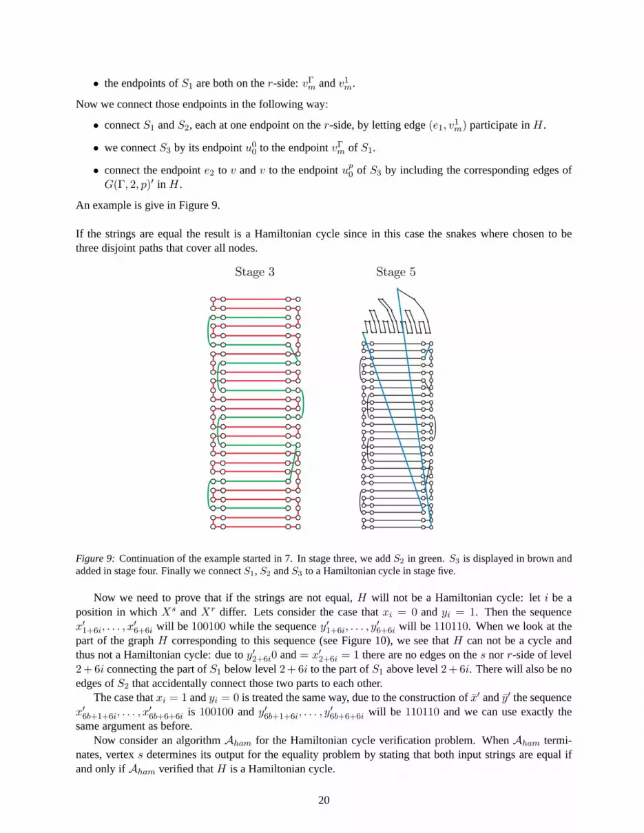
• the endpoints ofS1 are both on ther-side:vΓm andv1m.
Now we connect those endpoints in the following way:
• connectS1 andS2, each at one endpoint on ther-side, by letting edge(e1, v1m) participate inH.
• we connectS3 by its endpointu00 to the endpointvΓm of S1.
• connect the endpointe2 to v andv to the endpointup0 of S3 by including the corresponding edges ofG(Γ, 2, p)′ in H.
An example is give in Figure 9.
If the strings are equal the result is a Hamiltonian cycle since in this case the snakes where chosen to bethree disjoint paths that cover all nodes.
Stage 3 Stage 5
Figure 9: Continuation of the example started in 7. In stage three, we addS2 in green.S3 is displayed in brown andadded in stage four. Finally we connectS1, S2 andS3 to a Hamiltonian cycle in stage five.
Now we need to prove that if the strings are not equal,H will not be a Hamiltonian cycle: leti be aposition in whichXs andXr differ. Lets consider the case thatxi = 0 andyi = 1. Then the sequencex′1+6i, . . . , x
′6+6i will be 100100 while the sequencey′1+6i, . . . , y
′6+6i will be 110110. When we look at the
part of the graphH corresponding to this sequence (see Figure 10), we see thatH can not be a cycle andthus not a Hamiltonian cycle: due toy′2+6i0 and= x′2+6i = 1 there are no edges on thes nor r-side of level2+ 6i connecting the part ofS1 below level2+ 6i to the part ofS1 above level2+ 6i. There will also be noedges ofS2 that accidentally connect those two parts to each other.
The case thatxi = 1 andyi = 0 is treated the same way, due to the construction ofx′ andy′ the sequencex′6b+1+6i, . . . , x
′6b+6+6i is 100100 andy′6b+1+6i, . . . , y
′6b+6+6i will be 110110 and we can use exactly the
same argument as before.Now consider an algorithmAham for the Hamiltonian cycle verification problem. WhenAham termi-
nates, vertexs determines its output for the equality problem by stating that both input strings are equal ifand only ifAham verified thatH is a Hamiltonian cycle.
20

x01+6i = 1
xi = x0
2+6i = 0
x0
3+6i = 0
x0
4+6i = 1
xi = x0
5+6i = 0
x06+6i = 0
1 = y01+6i
1 = y02+6i = yi
0 = y0
3+6i
1 = y0
4+6i
1 = y0
5+6i = yi
0 = y06+6i
Figure 10:Example of the case thatxi = 0 andyi = 1.
Hence an fast algorithm for the Hamiltonian cycle problem onG(Γ, 2, p)′ can be used to correctly solvethe given instance of the equality problem onG(Γ, 2, p)′ and thus onG(Γ, 2, p) faster. A contradiction to thelower bound for the equality problem, which holds for alld (we usedd = 2).
Combined with Corollary B.4, we now have
Theorem B.6. For everyΓ and correspondingp, any distributed algorithm for solving Hamiltonian cycleproblem on the graph(Γ, 2, p)′ in theB model forB ≥ 3 requiresΩ(min(dp,Γ/dpB)) time.
Using the same analysis as in Section 4, we obtain:
Corollary B.7. For anyp ≥ 1, B ≥ 3, andn ∈ 22p+1pB, 32p+1pB, . . ., any distributed algorithm for the
Hamiltonian cycle problem in theB model forB ≥ 3 requiresΩ( npB
12− 1
2(2p+1) ) time on somen-vertex graphof diameter2p + 2.
B.3 A deterministic lower bound for spanning tree and path verification problems
Lemma B.8. For any p ≥ 1, B ≥ 3, andn ∈ 22p+1pB, 32p+1pB, . . ., anyB ≥ 3, any deterministic
algorithm for spanning tree verification requiresΩ( npB
12− 1
2(2p+1) ) time in some family ofn-vertex graph ofdiameter2p+ 2.
Proof. We reduce Hamiltonian cycle verification to spanning tree verification usingO(D) rounds using thefollowing observation:H is a Hamiltonian cycle if and only if every vertex has degree exactly two andH \e,for any edgee in H, is a spanning tree.
Therefore, to verify thatH is a Hamiltonian cycle, we first check whether every vertex has degree exactlytwo inH. If this is not true thenH is not a Hamiltonian cycle. This part needsO(D) rounds. Next, we checkif H \ e, for any edgee in H, is a spanning tree. We announce thatH is a Hamiltonian cycle if and onlyif H \ e is a spanning tree.
Lemma B.9. For any p ≥ 1, B ≥ 3, andn ∈ 22p+1pB, 32p+1pB, . . ., anyB ≥ 3, any deterministic
algorithm for path verification requiresΩ(( npB
12− 1
2(2p+1) )) time in some family ofn-vertex graph of diameter2p+ 2.
Proof. Similar to the above proof, we reduce Hamiltonian cycle verification to path verification usingO(D)rounds using the following observation:H is a Hamiltonian cycle if and only if every vertex has degreeexactly two andH \ e is a path (without cycles).
C Tightness of lower bounds
We note that all lower bounds of verification problems statedso far are almost tight. To show this we willpresent deterministicO(
√n log∗ n+D)-time algorithms for thes-t connectivity,k-component, connectivity,
cut, s-t-cut, bipartiteness, edge on all path, and simple path verification problems. Algorithms for all otherproblems stated in this paper can be found using the reductions given in Figure 2.
In particular, one can use the MST algorithm by Kutten and Peleg [15] and the connected componentalgorithm by Thurimella [23][Algorithm 5] to verify these properties.
21

Deterministic algorithms almost matching the deterministic lower bounds: We need to give upperbounds for thek-spanning tree and path verification problems.
Path verification problem:compute a breath first search-treeT onG \H in timeO(D) connect the treeT toH by a single edge ofG. The resulting subgraph ofG is a spanning tree ofG if and only ifH is a path.
k-spanning tree verification problem:We construct a weighted graphG′ by assigning weight zero toall edges inHk := H and one to other edges. We then find a minimum spanningT k tree ofH using theO(
√n log∗ n + D)-time algorithm in [15]. Now we createHk−1 := Hk \ T k. Hk−1 is ak − 1-spanning
tree if and only ifHk is ak-spanning tree. If allT j were spanning trees, afterk iterations we are left withH0 which contains no nodes and no edges if and only ifHk was ak-spanning tree.
Deterministic algorithms almost matching the randomized lower bounds: We need to give upperbounds for thes-t connectivity, cycle, connectivity,k-components, cut,s-t cut, bipartiteness and edge onpath-verification problems.
s-t connectivity verification problem: To do this, we run the connected component algorithm byThurimella [23][Algorithm 5] where, given a subgraphH of G, the algorithm outputs a labelℓ(v) for eachnodev such that for any two nodesu and v, ℓ(u) = ℓ(v) if and only if u and v are in the same con-nected component. [23][Theorem 6] states that the distributed time complexity of [23][Algorithm 5] isO(D + f(n) + g(n) +
√n) wheref(n) andg(n) are the distributed time complexities of finding an MST
and a√n -dominating set, respectively. Due to [15] we have thatf(n) = g(n) = O(F +
√n log∗ n). We
can now verify whethers andt are in the same connected component by verifying whetherℓ(s) = ℓ(t).cycle verification problem: Assign weight0 to all edges ofH and weight1 to all edges ofG \ H.
Compute a minimum spanning tree ofG using [15].H contains no cycle if and only if all edgesEH of Hare in the minimum spanning tree, i.e.,W = n− 1− |E(H)| where|E(H)| is the number of edges inH.
edge on all path verification problem:If and only if u andv are disconnected inH \ e, thene is onall paths betweenu andv. We can use thes-t connectivity verification algorithm from above to check that.
cut verification problem:To verify if H is a cut, we simply verify ifG after removing the edgesEH ofH is connected.
s-t cut verification problem: To verify if H is ans-t cut, we simply verifys-t connectivity ofG afterremoving the edgesEH of H.
e-cycle verification problem:To verify if e is in some cycle ofH, we simply verifys-t connectivity ofH ′ = H \ e wheres andt are the end nodes ofe. It is thus left to verifys-t connectivity.
k-components verification problem:We simply put weight1 on edges inH and2 on other edges andfind the MST using an algorithm in [15]. Observe thatH has at mostk connected component if and only ifthere are at mostk − 1 edges of weight2 in the MST, i.e., the MST has weight at mostn− 1 + (k − 1).
connectivity verification problem:Same as above fork = 1.spanning connected subgraph verification problem:One can use the above described algorithm to verify
thatH is connected. Verifying that the verticesVG of G are the same as the verticesVH of H completes thealgorithm.
bipartiteness verification problem:Compute a minimum spanning treeTH of H in timeO(√n log∗ n+
D) using [15]. Now2-color this tree. Now all nodes check if their neighbors havea different color thenthemselves. They will have a different color if and only ifH is bipartite.
D Details of hardness of approximation
In this section, we show the randomized lower bounds as claimed in Theorem 5.1 for the following problems(listed in Fig. 2).
Problems: Given a connected graphG with a weight functionω on edges (where, for each edgee, ω(e) isknown to nodes incident toe), we consider the following problems.
• In the minimum spanning tree problem [7, 21], we want to compute the weight of the minimum
22

spanning tree (i.e., the spanning tree of minimum weight). In the end of the process a node outputs thisweight.
• Given two nodess andt, theshortests-t path problem is to find the shortest path betweens andt. Inthe end of the process a node outputs the length of the shortest path.
• Given a nodes, thes-source distanceproblem [5] is to find the distance froms to every node. In theend of the process, every node knows its distance froms. Thes-source shortest path treeproblem [7]is to find the shortest path spanning tree rooted ats, i.e., the shortest path froms to any nodet has thesame weight as the unique path froms to t in such a tree.
• A set of edgesE′ is acut if G is not connected when we deleteE′. Theminimum cut problem [4]is to find a cut of minimum weight. A set of edgesE′ is as-t cut if s andt are not connected whenwe deleteE′. Theminimum s-t cut problem is to find ans-t cut of minimum weight. In the end ofthe process, a node outputs the weight of the minimum cut and minimum s-t cut. Themaximum cutproblem is to find a cut of maximum weight.
• Theminimum routing cost spanning treeproblem [25] is defined as follows. We think of the weighton an edge as the cost of routing messages through this edge. The routing cost for a pair of vertices ina given spanning tree is the sum of the weights of the edges in the unique tree path between them. Therouting cost of the tree itself is the sum over all pairs of vertices of the routing cost for the pair in thetree. Our goal is to find a spanning tree with minimum routing cost.
• The generalized Steiner forestproblem [10] is defined as follows. We are givenk disjoint subsetsof verticesV1, ..., Vk. The goal is to find a minimum weight subgraph in which each pair of verticesbelonging to the same subsets are connected.
• Given a network with two cost functions associated to edges:weight and length. Given a root noderand the desired radiusℓ, ashallow-light tree [20] is the spanning tree whose radius (defined by length)is at mostℓ and the total weight is minimized (among trees of the desiredradius).
We recall the following standard notion of an approximationalgorithm which we defined earlier in Sec-tion 5. For any minimization problemX , we say that an algorithmA is anα-approximation if, for any inputinstanceI, algorithmA outputs a solution that is at mostα times the optimal solution ofI.
Therefore, in the minimum spanning tree, minimum cut, minimums-t cut, and shortests-t path problemsstated above, anα-approximation algorithm should find a solution that has total weight at mostα times theweight of the optimal solution. For thes-source distance problem, anα-approximation algorithm should findan approximate distanced(v) of every vertexv such thatdistance(s, v) ≤ d(v) ≤ α · distance(s, v) wheredistance(s, v) is the distance ofs from v. Similarly, anα-approximation algorithm fors-source shortestpath tree should find a spanning treeT such that, for any nodev, the lengthℓ of a unique path froms to v inT satisfiesℓ ≤ α · distance(s, v).
Additionally, we say that a randomized algorithmA is α-approximationǫ-error if, for any input instanceI, algorithmA outputs a solution that is at mostα times the optimal solution ofI with probability at least1− ǫ.
Proof of Theorem 5.1.The proof idea for these problems is similar to the proof thatthe general case Travel-ing Salesman Problem cannot be approximated withinα(n) for any polynomial computable functionα(n)(see, e.g., [24]): We will define a weighted graphG′ in such a way that if the subgraphH satisfies the desiredproperty then the approximation algorithm must return somevalue that is at mostf(n), for some functionf . Conversely, ifH does not satisfy the property, the approximation algorithmwill outputs some value that
23

is strictly more thanf(n). Thus, we can distinguish between the two cases. We have already used thistechnique to proof the lower bound of the MST problem in Section 5. We now show lower bounds of otherproblems using the same technique.
The lower bound for shallow-light tree follows immediatelywhen we set the length of every edge to beone and radius requirement to ben. In this case, the spanning tree satisfies the radius requirement and so theminimum-weight shallow-light tree becomes the minimum spanning tree.
The lower bound ofs-source distance and shortest path spanning tree follow in asimilar way: H is aspanning connected subgraph if and only if the distance froms to every node is at mostn − 1 (i.e.,A haveapproximate distance at most(n − 1)α(n)) if and only if the shortest path spanning tree contain only edgesof weight one (i.e., the total weight of the shortest path spanning tree is at most(n− 1)α(n)).
For the lower bound of the shortests-t path, observe thats andt are connected inH if and only if thedistance froms to t in G′ is at mostn− 1, i.e.,A outputs a value of at most(n− 1)α(n). The lower boundfollows from the lower bound ofs-t connectivity verification problem.
For the lower bound of the minimum cut, first observe thatH is a spanning connected component if andonly if H, obtained by deleting all edgesE(H) of H from G, is not a cut. (Recall thatG is assumed to beconnected in the problem definition.) Therefore, verifyingif H is a cut also has the same lower bound. Now,we defineG′ by assigning weight one to all edges inH andnα(n) to all other edges and use the fact thatHis a cut if and only ifG′ has minimum cut of weight at mostn− 1, i.e.,A outputs value at most(n− 1)α(n).The same argument applies tos-t cut: s andt arenot connected inH if and only if H is ans-t cut if andonly if G′ has minimums− t cut of weightn− 1.
For the minimum routing cost spanning tree problem, we assign weight 1 to edges inH andn3α(n) toother edges. Observe that ifH is a spanning connected subgraph, the routing cost between any pair will be atmostn− 1 and thus the cost of theα(n)-approximation minimum routing cost spanning tree will be at most(n− 1)
(n2
)
α(n) < n3α(n). Conversely, ifH is not a spanning connected subgraph, some pair of nodes willhave routing cost at leastn3α(n) and thus the minimum routing cost spanning tree will cost at leastn3α(n).
For the generalized Steiner forest problem, we will reduce from the lower bound ofs-r connectivity. Wewill have only one setV1 = s, r. We assign weight1 to edges inH andnα(n) to other edges. Observethat the minimum generalized Steiner forest will have weight at mostn− 1 if H is s-t connected and at leastnα(n) otherwise. (Recall thatG is assumed to be connected in the problem definition.)
Our MST lower bound here matches the lower bound of exact MST algorithms and improves the lowerbound ofΩ(
√
nαB ) by Elkin [7]. Our lower bound fors-source distance complements the results in [5].
24

a b c d
e f g h
i j k l
s m n r
o
A
B
C L

a b c d
e f g h
i j k l
m n o p
A
B
C L
s r
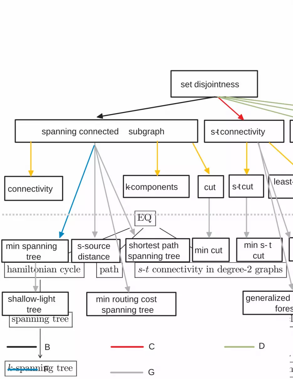
DISJ
spanning connected subgraph s-t connectivity cycle e-cycle
connectivity k-components cut s-t cut bipartiteness edge on
EQ
hamiltonian cycle path s-t connectivity in degree-2 graphs
spanning tree
k-spanning tree
min spanning tree
min s- t cut
min cut s-source distance
min routing cost spanning tree
generalized Sforest
least-
shallow-light tree
shortest path spanning tree
set disjointness
spanning connected subgraph
connectivity k -components cut
s- t connectivity
s- t cut
c
B C D
F G

min spanning tree
min s- t cut
min cut s-source distance
min routing cost spanning tree
generalized Sforest
least-
shallow-light tree
shortest path spanning tree
set disjointness
spanning connected subgraph
connectivity k -components cut
s- t connectivity
s- t cut
c
B C D

min spanning tree
min s- t cut
min cut s-source distance
min routing cost spanning tree
generalized Sforest
least-
shallow-light tree
shortest path spanning tree
set disjointness
spanning connected subgraph
connectivity k -components cut
s- t connectivity
s- t cut
c
B C
F G
Randomized

T X W U
2 3 1
W
4
6
K L M
7
N
A B
E F
randomized


