Embed Size (px)
Citation preview

Simulation Modelling Practice and Theory 47 (2014) 276–303
Contents lists available at ScienceDirect
Simulation Modelling Practice and Theory
journal homepage: www.elsevier .com/locate /s impat
On-line distributed prediction of traffic flow in a large-scale road
networkhttp://dx.doi.org/10.1016/j.simpat.2014.06.0111569-190X/� 2014 Elsevier B.V. All rights reserved.
⇑ Corresponding author. Tel.: +31 152781566.E-mail addresses: [email protected] (Y. Wang), [email protected] (J.H. van Schuppen), [email protected] (J. Vrancken
Yubin Wang a,⇑, Jan H. van Schuppen b, Jos Vrancken a
a Faculty of Technology, Policy and Management, The Netherlandsb Department of Mathematics, Delft University of Technology, 2600 GA Delft, The Netherlands
a r t i c l e i n f o a b s t r a c t
Article history:Received 5 December 2013Received in revised form 13 June 2014Accepted 23 June 2014
Keywords:Traffic simulationParallel simulationDistributed simulation
For on-line traffic control at traffic control centers there is a need for fast computations ofpredictions of traffic flow over a short prediction horizon, say 30 min, to evaluate theimpact of different scenarios for the purpose of on-line scenario selection. A novelapproach is presented to predict the traffic flow in a large-scale traffic network in anasynchronous, parallel, and distributed way at two or more subnetworks combined witha consistency check at the network level within a reasonable-small computation time.
� 2014 Elsevier B.V. All rights reserved.
1. Introduction
Road traffic is the most important but also the most expensive and the most problematic means of transport in mostcountries. Among the downside of road traffic we find frequent congestion, high environmental pollution and rather highaccident rates. Traffic management is a well established means to improve traffic efficiency and to counter the negativeeffects of road traffic. Road Traffic Control (RTC) is one of the main activities within road traffic management, next to demandmanagement, incident handling and pricing. RTC is about influencing traffic streams in order to improve traffic flow. RTCmeasures implement a scenario, such as rerouting, and are themselves implemented using the proper actuators.
The current status of traffic control in most industrialized countries is that there is a variety of different types ofmeasures, among which the traffic signal is still the most important one, that a large number of these measures have beendeployed, but that the majority of these measures has only a local effect and works largely reactive. Coordinating a numberof local measures is still not common, neither is it that measures can look into the future and respond proactively toupcoming adverse traffic conditions. This project aims especially at these two aspects. All traffic control measures underconsideration in this project display visual signals, shown locally to drivers. This means that controlling a network cannotbe more than coordinating local measures. For this reason, we use the term network control for the coordination of localmeasures. A traffic prediction/simulation model is needed for the purpose of network control.
The usual approach of traffic prediction is a network-based model that simulates the traffic based on spatial information,temporal information and traffic flow dynamics. There are many different types of network-based models in the literaturesuch as microscopic, mesoscopic, and macroscopic traffic models. The network-based prediction model can be used as adecision support system to evaluate the impact of different control scenarios for the purpose of both offline scenarioplanning and on-line scenario selection.
).

Y. Wang et al. / Simulation Modelling Practice and Theory 47 (2014) 276–303 277
However, centralized prediction of traffic flow is not suitable for simulation and for scenario evaluation of large networkssuch as all motorways in the Netherlands since long computation times and other drawbacks make it unsuitable forreal-time use. Thus, an algorithm is needed for distributed/parallel prediction of traffic flow.
The main goal of distributed/parallel prediction is to develop a fast, accurate and scalable distributed/parallel predictionwhich can be used to predict the traffic flow, on-line and in real-time, in a large-scale motorway network for implementationat a traffic control center.
The purpose of this paper is to present an algorithm for the distributed/parallel prediction of a large-scale motorwaynetwork including rings and to describe the performance of the algorithm for a motorway network near Amsterdam.
The contents of the paper is as follows. The next section contains the problem statement. The existing approaches as wellas the proposed approach are described in detail in Section 3. The framework of the proposed approach is described inSection 4. The performance evaluation criteria of the proposed algorithm is discussed in Section 5. A case study is presentedto illustrate the performance of the proposed approach in Section 6. Concluding remarks can be found in Section 7. Theappendices provide information about technical details of the algorithm.
2. Problem statement
In the Netherlands there are five traffic control centers for on-line monitoring and control of motorway networks. Toassist the operators with their control tasks, predictions of traffic flow have to be generated for a prediction horizon. Thepredictions are to be used for control of motorway traffic, in particular to evaluate the current state of the control measuresand to evaluate the performance of one or more control scenarios.
The Traffic Control Center of North-Holland monitors and stores the traffic flow data on the motorways and on severalprovincial roads on an hourly, daily, weekly, and yearly basis. Control measures like on-ramp metering, dynamic speedcontrol, routing advice, and other measures are taken partly automatically and partly by the road operators.
The problem treated in this chapter is to predict the traffic flow in a large-scale motorway network for the next 30 minwithin a time frame of sec. To solve the problem, one has to exploit the computational power of multiple cores or multiple PCin order to meet the performance objective of a short computation time.
Based on the description above, the traffic prediction in a large network can be formulated as a parallel prediction/simulation problem while the computations are executed on multiple cores or multiple PCs.
3. Parallel prediction/simulation approaches
Simulation and prediction are quite similar and most of the techniques can be applied to both, but there are somedifferences. Simulation is the imitation of some real thing, state of affairs, or process. The act of simulating somethinggenerally entails representing certain key characteristics or behaviors of a selected physical or abstract system. Predictionis the process of making statements about events in the future whose actual outcomes (typically) have not yet beenobserved. Thus, prediction deals with algorithms which have to run on-line. This imposes more stringent requirementson the performance, the accuracy, and the reliability of the algorithm.
A wide range of distributed parallel simulation/prediction approaches has been applied to a large-scale traffic simulation/prediction. The most common approach of a distributed parallel simulation/prediction is a synchronized approach whichmeans each subnetwork synchronizes each prediction cycle with other subnetworks to which it is connected. The synchro-nized approach is classified into four categories: Conservative, Optimistic, Relaxed synchronization and Mixed-mode.
Conservative In general, this approach always ensures safe timestamp-ordered processing of simulationevents within each Local Processor (LP). In other words, an LP does not execute an event untilit can guarantee that no event with a smaller time stamp will later be received by that LP. Threetechniques in literature are used to improve the conservative parallel simulation: Lookaheadapproach [1], Bounded lag algorithm [2] and Critical Channel [3].
Optimistic In general, this approach avoids blocked waiting by optimistically processing the events beyondthe lookahead window. When several events are later detected to have been processed in anincorrect order, the system invokes compensation code such as state restoration or reversecomputation. The following techniques described in the literature are used to improve theconservative parallel simulation: Time Warp [4], Local adaptive protocol [5], Adaptive time warp[6–8], Filtered rollback algorithm [9], Efficient state saving [1] and Reverse computation [1].
Relaxed synchronization This approach relaxes the constraint that events be strictly processed in time stamp order [1].For example, it might be deemed acceptable to process two events out of order if their timestamps are close enough. This approach offers the potential of providing a simplified approachto synchronization, but without the lookahead constraints that plague conservative execution.
Mixed-mode This approach combines elements of the previous three [1]. For example, sometimes it mighthelp to have some parts of the application execute optimistically ahead, while other partsexecute conservatively.

278 Y. Wang et al. / Simulation Modelling Practice and Theory 47 (2014) 276–303
The above techniques are applied to distributed microscopic traffic simulation packages like ParamGrid [10], AIMSUN[11], Paramics [12], and TRANSIMS [13,14]. There are many other publications about distributed microscopic trafficsimulation [10,15–18]. However, the main limitation of distributed microscopic traffic simulation is that the computationis much more complex and very slow for a large scale traffic networks. Thus, distributed microscopic traffic simulation isnot suitable for the on-line purpose. Therefore, distributed macroscopic traffic simulation is used in this paper. In [19], 1-stepand 2-step algorithms are presented to solve the macroscopic traffic simulation equations with fewer inter-processorcommunication. In [20], a PC-based distributed macroscopic traffic simulation methodology that can be applicable forreal-time estimation of time-variant parameters in freeway traffic flow is presented.
However, for the conservative approaches, the lookahead time window or the ‘no risk’ time interval is very hard to extractin complex applications, as it tends to be implicitly defined in the source code interdependencies. The optimistic approachesmight cause a lot of rollback overhead which can degrade the performance of parallel simulation. Sometimes the overheadmakes the performance of optimistic approaches even worse than the performance of conservative approaches. In general,the synchronized simulation approaches are processed in the sequence of their time stamps. Therefore, these approacheshave a strong limitation on simulation concurrence which makes the simulation be determined by the slowest LP. In theworst case, the simulation cannot continue anymore if one of LP is stuck or crashed. Another limitation is that the fullsimulation has to be done again if only a small part of the simulation is changed or modified.
In order to solve the problem mentioned above, asynchronous iterative approaches are introduced. One of the approachcalled state matching is described in [21] for time-parallel simulation. In this approach, simulation in each time interval canbe performed concurrently, if the simulation of a time interval starts from an initial state that is inconsistent with the finalstate of the previous interval, correcting these afterward by the use of fix-up computations. Instead of an exact solution tothe problem, approximate state matching [22,23] is a heuristic approach that accepts deviations in final and initial states ofadjacent intervals while guaranteeing the quality of the simulation. In this approach, a number of iterations are needed inorder to have consistent states at two adjacent intervals. However, convergence analysis is not addressed in these papers.Therefore, convergence is not guaranteed. In addition, the iterations might lead to a lot of overhead which can degradethe performance of parallel simulation.
Another asynchronous iterative approach, called a gluing algorithm, is proposed in [24,25] to solve the convergenceproblems for distributed simulation of physical systems and power grid systems. At each time step, each subsystem simulatein parallel by guessing the initial states on the boundary points. Then a Newton–Raphson method is used to fix-up the mis-match of the initial states. By using this approach, the convergence is guaranteed. However, a large number of iterationsmight be needed if the guessed initial states are far away from the actual states. In [26], a parallel Newton method isproposed to reduce 75% of iterations. The method can be interpreted as a Newton–Raphson method applied to a systemin a entire simulation horizon instead of each time step. In other words, the parallel Newton method solves the convergenceproblem for the entire simulation horizon of a system simultaneously. As a result, the number of iterations can besignificantly reduced.
However, the parallel Newton method needs a centralized coordinator to compute a matrix inverse which is also costexpensive. In [27], an asynchronous iterative approach has been developed to predict the conditions in the network forthe purpose of real-time scenario evaluation. However, the paper only gives a conclusion (without more detailed explanationor proof) that a few iterations (less than 10) are needed to achieve the convergence. In this paper, the asynchronous iterativeapproach combined with adaptive predictions at boundary points is explained in more detail and demonstrated in a casestudy of both a linear model and a nonlinear model. More precisely, using as the initial guess for the inputs of the subnet-works predictions from a previous time step or of adaptive predictions. Then, the drawbacks of synchronized approaches canbe prevented. The advantages of the proposed approach are:
� Computation speed: The proposed parallel simulation does not depend on the computation speed of the slowest agent inthe sense that it can already have computation results before finishing the computation of the slowest agent, althoughone iteration might need to refine the simulation/prediction results later. However, the computation speed of the tradi-tional parallel simulation depends on the simulation speed of the slowest agent (task).� Loss of communication: The proposed parallel simulation can still advance the simulation based on the initial guess
(whether from adaptive filter or from historic data on the boundary points). Although the simulation might not be accu-rate, the initial guess on the boundary points can still give the best possible inputs to advance the simulation. Therefore,the simulation can be performed even in case one agent is not performing or stuck in its simulation. However, the tradi-tional parallel simulation is not able to advance the simulation any more in case of loss of communication betweenagents.� Control measures evaluation: The proposed parallel simulation only need to simulate the part of agents which are
affected by the control measures again. However, the full simulation of all agents have to be performed again for the tra-ditional parallel simulation.� Scalability: When the network is extended further to the Netherlands road network or the European road network, the
proposed parallel simulation is scalable. The total simulation speed does not change too much when the size of the net-work increases. However, the simulation speed decreases dramatically with the size of the network for a centralizedsimulation.
Y. Wang et al. / Simulation Modelling Practice and Theory 47 (2014) 276–303 279
4. The framework for distributed prediction
The proposed approach of the distributed or parallel prediction/simulation consists of the following steps:
1. Partition the full network into two or more subnetworks each of which has only a one-directional traffic flow.2. Predict the traffic flow of each subnetwork based on an initialization of the predicted inflow of the subnetwork.3. Take care of the consistency of the predictions produced for the subnetworks; thus if the outflow of one subnetwork is to
be equal to the inflow of another network then take care that these traffic flows are approximately equal. The consistencyrequires an algorithm with iterations.
The detailed description of each of the above steps follows in the next subsections.In Section 6 the example of the ring network of Amsterdam is used. A realistic system will be formulated and distributed
prediction will be proposed. To illustrate the theoretical framework of the paper a simple ring road network will be used.
Example 4.1. Consider a road network consisting of a ring. The reader may think of the motorway ring around the city ofAmsterdam, though many cities have such rings. The ring road has traffic inflows from motorways and traffic inflows fromon-ramps. The example is continued later on in this section.
4.1. Partitioning of the network
Any road network will be partitioned into two or more subnetworks. The main objective for such a partitioning of a roadnetwork is to reduce computation time by the synchronous parallel computations of the subnetworks. However, there is anoverhead due to the coordination of the subnetwork computations at the network level. The selection of the number of sub-networks and the size of subnetworks is a complexity problem which requires a separate paper. It is briefly discussed in thesubsection.
Consider then the problem of partitioning or decomposing a road network into two or more subnetworks. The criterionfor such a partition is to allow distributed and parallel computation and to achieve an approximately equal load for thecomputations of the subnetworks. In general, decomposition approaches include functional decomposition, temporaldecomposition and spatial decomposition. Spatial decomposition is the most common approach in the field of roadtraffic simulation. The existing spatial decomposition approaches are equally-sized method [10], minimization ofNeighbors [14], Macroscopic-Simulation-Based Division (MaSBD) and Microscopic-Simulation-Based Division (MiSBD)methods [28].
Below a road network is related to a graph. The nodes of the graph correspond to particular locations of the road network,often an intersection or a crossing. An edge of a graph corresponds in the road network to a road from one location to anadjacent location. If one distinguishes the driving directions of each road then every edge is associated with that directionand the graph is then called a directed graph. A path in a directed graph is a sequence of directed edges. A tree in the graph isdefined as a node from where exists a directed path to all other nodes. This concept is used below.
Consider then a network of motorways possibly with several rings. The problem is to partition the considered motorwaynetwork into two or more subnetworks such that the following requirements are met.
Definition 4.2. Define the partitioning requirements as:
1. No subnetwork has a ring of roads.2. The traffic flow in any subnetwork is unidirectional.3. Any network bottleneck should not be on the boundary of the subnetworks.4. The length of a subnetwork is in the range of 9–16 km; the upper bound is a somewhat arbitrary choice motivated by the
duration of the computation time of the full prediction recursion.5. Load balancing. The computation times of the subnetworks should be approximately equal.6. The number of interconnections between subnetworks should be minimal.
Problem 4.3. Partition a motorway network into several subnetworks such that each subnetwork meets the partitioningrequirements of Definition 4.2.
The preliminary procedure to partition a large motorway network into two or more subnetworks is stated below.
Procedure 4.4. Consider a motorway network.
1. If the network or if a subnetwork contains a ring then cut the ring into two or more subnetworks such that eachsubnetwork consists of a stretch of motorway and no stretch contains a motorway intersection in the interior of thesubnetwork. Thus the ring is first cut at the points where there are motorway intersections.

280 Y. Wang et al. / Simulation Modelling Practice and Theory 47 (2014) 276–303
2. If the remaining collection of subnetworks contains a subnetwork which is longer than the maximum stretch length set inthe partitioning criteria then cut the subnetwork into pieces of almost the same length such that each new subnetworkmeets the partitioning criteria.
The argument to cut the ring network at the junction with the motorways is a choice which is motivated by experiencewith larger networks. It allows a simple partitioning in case of networks with two or more rings. Experience has to be gainedwith this choice of partitioning. The approach is illustrated in the case study in Section 6. For the road network of theprovince of North-Holland in The Netherlands, there will be approximately 100 subnetworks.
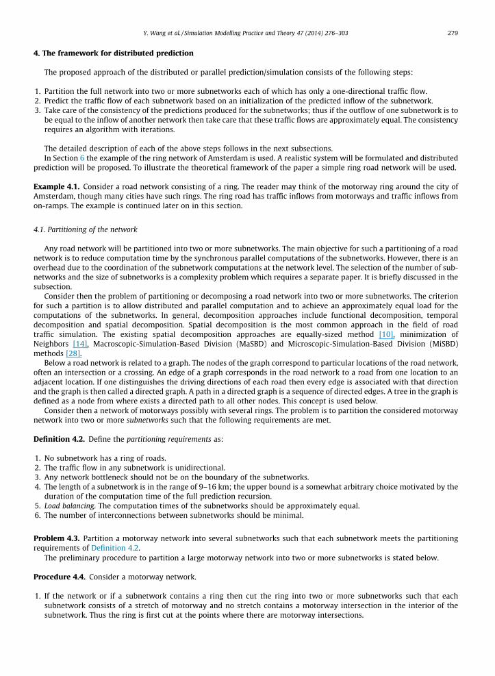
Example 4.5. Consider the simple ring network of Example 4.1. The ring is partitioned in two parts labelled Subnetwork 1and 2. See Fig. 1 for the illustration of the partition.
4.2. Prediction of the traffic flow in a subnetwork
Consider then a subnetwork as obtained by the partitioning approach of Section 4.1. The subnetwork is assumed to satisfythe partitioning conditions of Definition 4.2.
Problem 4.6 (Prediction of the traffic flow in a subnetwork). Predict the traffic flow for the considered prediction horizon ineach of the cells of the subnetwork and of the outflows of the network. It is assumed that there are available predictions of allthe inflows of the subnetwork, i.e. those from other motorways and from on-ramps.
It is assumed that there is available a system describing the traffic flow in the subnetwork. The prediction of the trafficflow in a deterministic system is based on simulation of the system of the traffic flow in the subnetwork. There are varioustypes of models for the dynamics of traffic flow such as microscopic, mesoscopic and macroscopic traffic models [29–33]. Inthis paper, a macroscopic traffic model is used to demonstrate the proposed parallel simulation approach. A macroscopictraffic model computes per cell, based on predictions of all traffic inflows into the subnetwork, the predictions of the densityand of the speed of the traffic flow in the subnetwork and of all traffic outflows to other subnetworks.
Each subnetwork must have boundary points. At these boundary points there are traffic inflows and outflows. The trafficinflows include: (1) inflows of one or more motorways into the subnetwork and (2) the inflows from all on-ramps. If theorigin of a subnetwork is a traffic merge then there will be traffic inflows from two motorways. If the origin of the subnet-work is at a motorway intersection there could be three traffic inflows from as many motorways entering a subnetwork. Thetraffic outflows include: (1) the motorway traffic outflows of the subnetwork to other subnetworks; (2) the traffic outflows ofoff-ramps. Note that at a traffic intersection there could be two or three motorway outflows. For the remainder of the paper itis necessary to distinguish between the motorway inflows and the other traffic inflows. The prediction model must have theinformation of all inflows at these boundary points for the prediction horizon.
The authors have published an adaptive prediction algorithm for the traffic inflows of a subnetwork at boundary points ofthe network, both for motorways and for on-ramps, see [34,35]. The purpose of the adaptive prediction algorithm is to pro-vide predictions of traffic flow at the boundary points of the road network. The effectiveness of these adaptive predictionswas illustrated in those references for data of traffic flow on the Amsterdam ring network.
Below a system is defined which describes the traffic flow in a subnetwork. Such models are standard in the literature ofdynamic traffic management and the authors have used such models in the past. A macroscopic model is used to describe thetraffic flow. The road network of a subnetwork is partitioned into several sections, typically of 500 m. length. Each sectionhas two state variables, the density of the traffic in vehicles per km per lane and the speed of the traffic in the section inkm per hour. The dynamics of the system is not detailed in this paper, it is denoted by the function f in Definition 4.7.The reader may find the METANET model in [30] and other models in [36,37]. In Section 6 for the actual simulations shown,use was made of a linearized system and of the Fast Lane model, see [32].
Definition 4.7. Define the system for the traffic flow in a subnetwork denoted by the equations,
Fig. 1. The simple ring network. From left to right: the Simple Ring Network, Subnetwork 1, and Subnetwork 2.

Y. Wang et al. / Simulation Modelling Practice and Theory 47 (2014) 276–303 281
xðt þ 1Þ ¼ f ðxðtÞ;umðtÞ;uinðtÞÞ; xðt0Þ ¼ x0;
zmðtÞ ¼ hmðxðtÞÞ;T ¼ ft0; t0 þ 1; . . . ; g � Z; the time index set;x : T ! Rn; um : T ! Rmm ; uin : T ! Rmin ; zm : T ! Rpz :
In these equations, the vector xðtÞ represents the state with a density and a speed for each section of the subnetwork, theinput um represents the traffic inflow(s) of motorways, and the input uin represents the traffic inflows of on-ramps. Thevariable zm represents the traffic outflow of the subnetwork to motorways, which is the product of the density and the speedof the last section of the subnetwork. The off-ramp traffic flow is not explicitly indicated, since we assume that it is a certainpercentage of traffic flow on motorways.
For control of motorway networks the above system can be generalized to a control system with inputs for the trafficcontrol measures.
The prediction system produces on-line predictions of the traffic flow in the subnetwork. This is done sequentially, for anytime the system produces predictions for the prediction horizon. For example, at 10:00 h it produces predictions for thehorizon 10:00–10:30 h, and at 10:10 h for the horizon 10:10–10:40 h, etc.
Definition 4.8. Define the horizon-prediction system of a subnetwork in terms of its inflows by the following equations. Fixa time moment t 2 T . Of the motorway input denoted by um denote the prediction of the value at time t þ 1 made at timet 2 T by umðt þ 1jtÞ, for subsequent times by umðt þ sjtÞ for s 2 Zþ, and similarly for the other variables.
The predictions of the traffic outflow are computed by simulation of the system, see the equations,
xðt þ sþ 1jtÞ ¼ f ðxðt þ sjtÞ; umðt þ sjtÞ; uinðt þ sjtÞÞ; xðtjtÞ ¼ xðtÞ; ð1Þzmðt þ sjtÞ ¼ hmðxðt þ sÞÞ; s ¼ 1;2; . . . ; tp; ð2Þxðt þ sjtÞ 2 Rn; umðt þ sjtÞ 2 Rmm ; uinðt þ sjtÞ 2 Rmin : ð3Þ
The initial state of the predictor, xðtÞ, is the one-step prediction produced by a state estimator. This estimate is produced bywhat is called the filter system. The filter system estimates the state of the traffic system for all sections and for all statevariables. A state estimator was formulated in the publications of S.A. Smulders, see [38–40]. It is assumed that a stateestimator is available in the traffic control center of the subnetwork.
The variable xðt þ sjtÞ denotes the prediction of the state xðt þ sÞ based on observations available at time t. Similarly, thevariable zmðt þ sjtÞ denotes the prediction of the traffic outflow of the subnetwork to motorways at time t þ s based onobservations available at time t. These outflows may be inflows of another subnetwork or they may leave the consideredroad network.
Denote the predictions of several variables on a prediction horizon by,
t 2 T; a time moment of the time index set;TpðtÞ ¼ ft þ 1; t þ 2; . . . ; t þ tpg;
the prediction horizon at time t of length tp 2 Zþ;
umðt þ 1 : t þ tpjtÞ ¼ umðt þ 1jtÞ; umðt þ 2jtÞ; . . . ; umðt þ tpjtÞ� �T 2 Rtpmm ;
the predicted inflows of motoways on the prediction horizon;
uinðt þ 1 : t þ tpjtÞ ¼ uinðt þ 1jtÞ; uinðt þ 2jtÞ; . . . ; uinðt þ tpjtÞ� �T 2 Rtpmin ;
the predicted inflows of on-ramps;
zmðt þ 1 : t þ tpjtÞ ¼ zmðt þ 1jtÞ; zmðt þ 2jtÞ; . . . ; zmðt þ tpjtÞ� �T 2 Rtppz ;
the predicted outflows to motorways on the prediction horizon:
The map defined above by the algorithm which produces from an estimate xðtÞ of the state of the system at time t 2 T , fromthe predicted traffic inflows of motorways umðt þ 1 : t þ tpjtÞ and of on-ramps uinðt þ 1 : t þ tpjtÞ on the prediction horizon,the predicted outflows of the subnetwork over the prediction horizon zmðt þ 1 : t þ tpjtÞ is denoted by,
zmðt þ 1 : t þ tpjtÞ ¼ fhðxðtÞ; umðt þ 1 : t þ tpjtÞ; uinðt þ 1 : t þ tpjtÞÞ; f h : Rn � Rtpmm � Rtpmin ! Rtppz : ð4Þ
Several of the components of the predicted outflows of a subnetwork are equal to the predicted inflows of a downstreamsubnetwork as will be described below.
Typically, the time step of the discrete-time system is 10 s. while the prediction horizon is 30 min, and the dimension ofthe motorway input is 1 (one), hence there are 30� 6 ¼ 180 time steps of the prediction horizon. With these numbers, thedimensions of the vectors umðt þ 1 : t þ tpjtÞ and zmðt þ 1 : t þ tpjtÞ are then 180.
4.3. Predictions of subnetworks made consistent at the network level
How to obtain predictions computed by the subnetworks which are consistent at the network level?

282 Y. Wang et al. / Simulation Modelling Practice and Theory 47 (2014) 276–303
The framework for prediction of traffic flow in a network consists of a two level system. At the subnetwork level there aretwo or more subnetworks. The subnetworks have been obtained by partitioning the network into several parts. As describedin the previous subsection, each subnetwork is able to compute from predicted inflows of the subnetwork over the predic-tion horizon the predicted outflows of the subnetwork over the same prediction horizon. Those computations can be carriedout in parallel reducing complexity. But the output of a subnetwork may have to be equal to the input of another subnetworkand this may hold for a large number of subnetworks.
At the network level therefore the predictions of the subnetworks have to be made consistent. The task of the predictionsystem at the network level is to produce predictions of the subnetworks of which the traffic outflows of a subnetwork areequal or approximately equal to the traffic inflows of a downstream subnetwork if the subnetworks are so related. Theapproximation criterion for the corresponding traffic outflows and traffic inflows will be specified below.
Problem 4.9 (Problem of consistent predictions at the network level). Consider a motorway network and a prediction systemwith two levels, the lowest level for the predictions of the subnetworks and the highest level for the prediction of thenetwork. Formulate a procedure for obtaining predictions of the traffic flow in the network on the prediction horizon suchthat the motorway traffic outflows of a subnetwork are equal to or approximately equal to the motorway traffic inflows ofthe corresponding downstream subnetwork if there exists such a downstream network.
The procedure to achieve consistency is to be based on an approximation criterion. The approximation criterion compares(1) the traffic inflows into a subnetwork with (2) the predictions of traffic outflows of the corresponding upstreamsubnetwork for the same prediction horizon and for the same locations and that for all locations of the network wheretwo subnetworks are connected. If inflows and outflows are not consistent, a minimal demand supply scheme [32] has tobe used to determine inflows and outflows.
Definition 4.10. Define the horizon-prediction system of a network by the following objects and functions.Denote the index set of all subnetworks of the considered network by the set J ¼ f1;2; . . . ; jsng. For all j 2 J define the
index subsets of subnetworks,
JinðjÞ ¼ fi 2 Jj9 motorway outflow of Subnetwork i to Subnetwork j; ð5Þ
JoutðjÞ ¼ fi 2 Jj9 motorway outflow of Subnetwork j to Subnetwork i: ð6Þ
The indices of the system of Subnetwork j 2 J are now denoted by, nnet;j the state-space dimension, mnet;j;m the dimension ofthe motorway input, mnet;j;in the dimension of the external inflows, and pnet;j;z the dimension of the motorway outflow.
Recall that for any subnetwork j 2 J the horizon-prediction system of Subnetwork j at time t 2 T based on a prediction ofthe traffic inflow over the prediction horizon from outside the network denoted by the input vector uj;mðt þ 1 : t þ tpjtÞproduces the traffic outflows over the prediction horizon as the vector zj;mðt þ 1 : t þ tpjtÞ. Denote then,
mmp ¼ tp
Xjsn
j¼1
mnet;j; minp ¼ tp
Xjsn
j¼1
mnet;j;in; pzp ¼ tp
Xjsn
j¼1
pnet;j;z; ð7Þ
unet;mðt þ 1 : t þ tpÞ ¼
unet;1;mðt þ 1 : t þ tpjtÞ...
unet;js ;mðt þ 1 : t þ tpjtÞ
0BB@
1CCA 2 Rmmp ;
correspondingly; unet;inðt þ 1 : t þ tpjtÞ 2 Rminp ; znet;mðt þ 1 : t þ tpjtÞ 2 Rpzp :
ð8Þ
The graph of the network and its partition into subnetworks defines the relation between outflows of a subnetwork toinflows of the corresponding downstream subnetwork. Thus, the outflow of traffic of a subnetwork j may equal the inflowof traffic of another subnetwork, say i. However, there are subnetworks whose inflow is only the traffic flow from outside thenetwork. For the k-th iteration of the computation the relation between the traffic flows can then be described by theequation,
uðkþ1Þnet;i;mðt þ 1 : t þ tpjtÞ ¼
zðkÞnet;jðt1 : t þ tpjtÞ; if i 2 JoutðjÞ;unet;i;mðt þ 1 : t þ tpjtÞ; if i 2 J n JoutðjÞ:
(ð9Þ
This relation is formalized in the linear map,
Fnet;z 2 f0;1gmmp�pzp ; Fnet;m 2 f0;1gmmp�mmp ; ð10Þ
Fnet;z;i;j ¼Itp ; if i 2 JoutðjÞ; or; uiðt þ 1 : t þ tpjtÞ ¼ zjðt1 : t þ tpjtÞ;0 else;
�ð11Þ
Fnet;in;i;j ¼Itp ; if i 2 J n JoutðjÞ; or; uiðt þ 1 : t þ tpjtÞ ¼ ui;inðt þ 1 : t þ tpjtÞ;0 else;
�ð12Þ

Y. Wang et al. / Simulation Modelling Practice and Theory 47 (2014) 276–303 283
uð1Þnet;mðt þ 1 : t þ tpjtÞ ¼Fnet;zznetðt þ 1 : t þ tpjtÞ þ Fnet;inunet;inðt þ 1 : t þ tpjtÞ;¼Fnet;zfnetðxðtÞ; uð0Þnet;mðt þ 1 : t þ tpjtÞ; unet;int þ 1 : t þ tpjtÞÞþ Fnet;inunet;inðt þ 1 : t þ tpjtÞ; ð13Þwhere the index ð0Þ denotes the initial value andð1Þ denotes the first iteration:
The matrices Fnet;z and Fnet;in consists of zeros and ones only and are based only on the graph of the network. In case the
outflow of a subnetwork is not an input to another subnetwork, then the vector uð1Þnetðt þ 1 : t þ tpjtÞ equals for that componentthe predicted traffic inflow produced by the adaptive filter and denoted by unet;mðt þ 1 : t þ tpjtÞ.
Example 4.11. Consider the simple ring network, see Examples 4.1 and 4.5. For this ring network with only twosubnetworks and without external inflows from motorways the matrices of the interconnection map are� �
Fnet;z ¼0 I
I 0; Fnet;in ¼ 0:
Next the consistency of the input predictions and of the computed outputs can be defined mathematically.
Definition 4.12. Define the fixpoint equation of consistency of traffic flows at the network level as stated below. Considerthe horizon-prediction system at the network level of Definition 4.10. Consider a prediction time t 2 T. In reference to thissystem define the fixpoint equation of consistency as
uð0Þnet;mðt þ 1 : t þ tpjtÞ ¼ uð1Þnet;mðt þ 1 : t þ tpjtÞ;¼ Fnet;zðfnetðxðtÞ; uð0Þnet;mðt þ 1 : t þ tpjtÞ; unet;int þ 1 : t þ tpjtÞÞþ Fnet;inunet;inðt þ 1 : t þ tpjtÞ ð14Þ¼ ffpðt; uð0Þnet;mðt þ 1 : t þ tpjtÞÞ; hence; ð15Þ
v ¼ ffpðt;vÞ; is the fixpoint equation and then ð16Þv ¼ uð0Þnet;mðt þ 1 : t þ tpjtÞ 2 Rmmp : ð17Þ
In the fixpoint equation, the state at time t 2 T; xðtÞ, and the inflows of on-ramps, unet;inðt þ 1 : t þ tpjtÞ, are fixed to the valuesprovided. The symbol ffp denotes the function of the fixpoint equation.
In Appendix B, two methods are proposed to solve the fixpoint equation: a successive approximation method and a recur-sive method. After a comparison of the two methods, the distributed successive approximation algorithm is chosen for thispaper. We prove that the distributed successive approximation algorithm for the approximation of the solution of the fix-point equation is quite effective and converges sufficiently fast for the application considered.
In Appendix C, the fixpoint method is analysed for the simple ring network with a linear system. We prove that the con-ditions for the existence of a unique fixpoint of Eq. (C.14) are satisfied. The convergence speed is determined by the eigen-values of the system.
In Appendix A, the complete prediction algorithm is stated.In realistic models of traffic flow the dynamics of the system is nonlinear. Then the questions of existence of a solution to
the fixpoint equation, the uniqueness of the solution, and the convergence rate are not so easy to answer.Based on the structure of the system, one can argue that the system should be contractive, meaning that there exists a
solution of the fixpoint equation. The reason for this is that the dynamic system is dissipative as understood in control the-ory. The traffic flow passing at any point in the subnetwork leaves the network at all off-ramps hence if one considers a ringthen after one loop no cars who have entered at this point will exit the network at this point.
The domain of attraction of the unique solution is expected to be the full state set. The convergence rate is not clearbecause of the nonlinearities of the system. The high dimensions of the system will make it difficult to carry out a mathe-matical analysis of the convergence.
In case of congested traffic the convergence rate could be much slower than in noncongested traffic.
5. Performance
In this paper, the performance of the proposed algorithm will be evaluated in terms of computational complexity andcommunication complexity.
5.1. Communication complexity
For the communication protocol for sending a prediction of traffic outflow, say znet;jðt þ 1 : t þ tpjtÞ, from subnetwork j 2 Jto a downstream subnetwork i 2 J there are two options:

284 Y. Wang et al. / Simulation Modelling Practice and Theory 47 (2014) 276–303
1. Communication protocol 1. There exists a dedicated communication line from the controller of Subnetwork j 2 J to thecontrollers of its downstream Subnetworks iJoutðjÞ and that for all j 2 J, which can be used without any interference withcommunications between other subnetworks.
2. Communication protocol 2. There exists only communication lines between any subnetwork and the network communi-cation center of the full network. In this case a subnetwork whose prediction vector of traffic outflows is needed byanother subnetwork communicates its prediction vector to the network communication center which in turn forwardsthis prediction vector to the downstream subnetworks needing that prediction vector.
The authors favor Communication Protocol 1 because of its much lower communication complexity. The communicationcomplexity differs by the communication protocol used. The complexity formula is derived in Section 5.2. It is clear that thefirst communication protocol has a much lower communication time complexity than the second communication protocol.Therefore, the road operator has an incentive to install dedicated communication lines between adjacent subnetworks. Thisinvolves economic costs which are not treated in this paper.
Next the second aspect of distributed computation of the vector of inflow traffic predictions is discussed. There are twoways to handle the computations for the approximation criterion:
1. The approximation criterion is computed at the network level.2. The approximation criterion is computed at each of the subnetworks and only whether the criterion is met or not is
communicated to the network level.
The approximation criterion of the recursive computation of the solution of the fixpoint equation is often a vector norm.At iteration ðkþ 1Þ 2 Zþ the approximation criterion decomposes over the subnetworks as displayed in the next equation forthe L2 vector norm,
kuðkþ1Þnet;mðt þ 1 : t þ tpjtÞ � uðkÞnet;mðt þ 1 : t þ tpjtÞk2
2 ¼Xnnet
j¼1
ð�ðkþ1Þnet;j cjÞ
2,Xnnet
j¼1
cj; cj ¼ dim�net;j: ð18Þ
For the l1 norm of a vector in Rn the sum operation is replaced by a maximization operation. It is of interest for the efficientcomputation that an approximation criterion is selected which allows a distributed computation of the criterion.
The conclusion is thus that the computation of the approximation criterion for the network can be distributed to compu-tation of the approximation criterion for each subnetwork combined with communication of the local norms to the networkcommunication center. This is a gain in communication complexity because each subnetwork only sends one real number,the value of its local approximation criterion. The communication protocol is then that each subnetwork (1) computes thevalue of the local approximation criterion, say
�ðkþ1Þnet;i ¼ ku
ðkþ1Þnet;i;mðt þ 1 : t þ tpjtÞ � uðkÞnet;i;mðt þ 1 : t þ tpjtÞk2; ð19Þ
and communicates this real number to the communication center of the network. At the network level the value of theapproximation criterion of the network is computed. (2) the network communication center communicates the outcomeof the network approximation criterion to all subnetworks.
The second method for computation of the approximation criterion is that the computations are done entirely at thesubnetwork level. Thus, the subnetworks could compute the value of the subnetwork approximation criterion and comparethis to the threshold �net;i;m ¼ �net;m=nnet where �net;m denotes the tolerance level at the network. The threshold then isuniformly distributed over all subnetworks. The fact that at a subnetwork the approximation criterion is met is thencommunicated from each subnetwork to the network. Once the network prediction system has received a reaction fromall subnetworks that the prediction approximation criteria are met, it informs all subnetworks that the approximation forthe full network has been achieved.
Which of these methods is better than the other, is not yet clear. The decision is based on the computational and the com-munication complexity.
5.2. Computational complexity
The time complexity of the computation is of interest because of the distributed character.Consider the distributed computation of an approximation of the solution of the fixpoint equation. This complexity is to
be compared with a centralized computation. Below the formula for the time complexity follows. Because only timecomplexity is considered and space complexity is not discussed, the expression complexity denotes from now on the timecomplexity.
Proposition 5.1. Consider the algorithm for the distributed computation of an approximation solution of the fixpoint equation.
(a) The complexity of the distributed computation (acronym comp) and that of the communication (acronym comm) withCommunication Protocol 1 is polynomial and equals,

Y. Wang et al. / Simulation Modelling Practice and Theory 47 (2014) 276–303 285
Ocompððn� þ p�zÞtpkmaxÞ; Ocommðm�mptpkmaxÞ: ð20Þ
(b) The complexity of the distributed computation and of the communication with Communication Protocol 2 is polynomial andequals,
Ocompððn� þ p�zÞtpkmaxÞ; Ocommðjsnm�mptpkmaxÞ: ð21Þ
(c) The complexity of the computation by a centralized algorithm is polynomial and equals,
Ocompððn� þ p�zÞtpjsn þm�mptpjsnÞ; Ocomm ¼ 0: ð22Þ
Distributed computation has thus a lower complexity than centralized computation if kmax < jsn, thus if the maximal number ofiterations required for the approximation is smaller than the number of subnetworks. The symbols denote,
tp the length in steps of the prediction horizon;kmax the maximal number of iterations of the fixpoint approximation;
n� the maximum of the state-space dimensions of all subnetworks;n� ¼ max
j2Jnnet;j;
m�mp the maximum of the dimensions of the motorway inflows;
m�mp ¼ maxj2J
mnet;j;m;
p�z the maximum of the output dimensions of all subnetworks;p�z ¼ max
j2Jpnet;j;z;
jsn the number of subnetworks of the road network:
Proof
(a) Consider first the computation of the predictions by a subnetwork. For each step of the prediction a state ofdimension n and an output of dimension pz have to be computed, hence the term ðnþ pzÞ. This has to be donefor tp time steps of the prediction horizon, hence ðnþ pzÞtp. Because the computations are done in parallel for allsubnetworks, the expression ðn� þ p�zÞtp follows. According to Communication Protocol 1, there is the communi-cation time for the communication of the vector umðt1 : t þ tpjtÞ from a subnetwork to a downstream network.The time complexity of this communication is thus m�mptp because the communications are carried out inparallel.
(b) The difference with part (a) is that the communications are now carried out in a centralized way hence in series for allsubnetworks. Hence the communication complexity is jsnm�mtp, and that two times which factor 2 is not listed.
(c) The formula follows analogously as in (a) and (b) but with differences. The system has now a state space dimensionwhich is the sum of all state-space dimensions of the subnetworks, which is upperbounded by jsnn�. The second termin the complexity formula is because the end result has to be communicated to the subnetwork in by a centralizedprotocol. h
In an example, typical values for the parameters of the complexity formulas are tp ¼ 180, n ¼ 1, m�mp ¼ 1, pz ¼ 1, jsn ¼ 10.Distributed computation has then a lower time complexity if the maximal number of iterations is lower than jsn ¼ 10.
6. Case study: Distributed prediction in AgentScape
The performance of the proposed prediction procedure is best evaluated based on actual on-line traffic data. At the timethis paper is written, the authors do no longer have access to on-line traffic data. The hope that in the near future a companywith access to on-line traffic data is willing to test the proposed prediction algorithm with actual data.
The reader finds below an evaluation of the prediction procedure for a medium-scale road network, about 144 km. inlength. Simulations of the prediction of the traffic flow over a horizon of 30 min are provided. In addition, the computationaltime complexity is summarized.
6.1. Introduction: AgentScape
AgentScape is a middleware layer that supports large-scale agent systems. It has been implemented in Java by the Facultyof Technology, Policy and Management of the Delft University of Technology (TUD). The rationale behind the designdecisions are

286 Y. Wang et al. / Simulation Modelling Practice and Theory 47 (2014) 276–303
1. To provide a platform for large-scale agent systems.2. Support multiple code bases and operating systems.3. Interoperability with other agent platforms.
The main motivation of using AgentScape in the case study is that it provides a platform to simulate agents in multi-coresor multi-PCs. It has the functionality of assigning the resources of CPUs according to the demanding simulation/predictiontasks of different agents automatically. It also has the functionality to handle the communications between two agents. Suchthat researchers or developers only need to focus on implementing the simulation/prediction algorithm without thinkingabout the software architecture or the low-level communication software.
In the case study, both a linear model and a nonlinear model will be implemented in AgentScape to demonstrate theproposed algorithm. The case study is performed under Dell Core i7 Windows 7.
6.2. Distributed prediction of a linear model
In this paper, a simple ring network with subnetwork 1 and 2 as shown in Fig. 1. The subnetwork 1 consists of foursections or cells with one on-ramp and one off-ramp. The subnetwork 2 consists of five cells with one on-ramp and twooff-ramps. In this case study, a linear model is considered for this simple ring network.
6.2.1. Linear modelThe flow of cells in Subnetwork 1 is modeled as:
x1ðt þ 1Þ ¼ a11x1ðtÞ þ b1u11ðtÞ ð23Þ
x2ðt þ 1Þ ¼ a21x1ðtÞ þ a22x2ðtÞ � h2x2ðtÞ ð24Þ
x3ðt þ 1Þ ¼ a32x2ðtÞ þ a33x3ðtÞ þm3a31ðtÞ ð25Þ
x4ðt þ 1Þ ¼ a43x3ðtÞ þ a44x4ðtÞ � h4x4ðtÞ ð26Þ
y1ðt þ 1Þ ¼ h4x4ðtÞ ð27Þ
The equations are then collected in the following system for all sections.
xðt þ 1Þ ¼ A1xðtÞ þ B1uðtÞ; ð28Þ
y1ðt þ 1Þ ¼ C1xðtÞ; ð29Þ
xðtÞ ¼
x1ðtÞ
x2ðtÞ
x3ðtÞ
x4ðtÞ
0BBBBB@
1CCCCCA; uðtÞ ¼
u11ðtÞ
a31ðtÞ
!; ð30Þ
A1 ¼
a11 0 0 0
a21 a22 � h2 0 0
0 a32 a33 0
0 0 a43 a44 � h4
0BBBBB@
1CCCCCA; B1 ¼
b1 0
0 0
0 m3
0 0
0BBBBBB@
1CCCCCCA; ð31Þ
C1 ¼ 0 0 0 h4ð Þ: ð32Þ
The traffic flow in Subnetwork 2 is modeled next. Again the state is denoted by the symbol x and the reader is warned not toidentify this vector with that of Subnetwork 1.
x1ðt þ 1Þ ¼ A11x1ðtÞ þ B1u12ðtÞ ð33Þx2ðt þ 1Þ ¼ A21x1ðtÞ þ A22x2ðtÞ � H2x2ðtÞ ð34Þx3ðt þ 1Þ ¼ A32x2ðtÞ þ A33x3ðtÞ þM3a32ðtÞ ð35Þx4ðt þ 1Þ ¼ A43x3ðtÞ þ A44x4ðtÞ � H4x4ðtÞ ð36Þx5ðt þ 1Þ ¼ A54x4ðtÞ þ A55x5ðtÞ � H5x5ðtÞ ð37Þy2ðt þ 1Þ ¼ H5x5ðtÞ ð38Þ
The equations are then collected in the following system for all sections.

Table 1Six itera
1st i
SubnSubn
4th i
SubnSubn
Y. Wang et al. / Simulation Modelling Practice and Theory 47 (2014) 276–303 287
xðt þ 1Þ ¼ A2xðtÞ þ B2uðtÞ; ð39Þyðt þ 1Þ ¼ C2xðtÞ; ð40Þ
xðtÞ ¼
x1ðtÞx2ðtÞx3ðtÞx4ðtÞx5ðtÞ
0BBBBBB@
1CCCCCCA; uðtÞ ¼ u12ðtÞ a32ðtÞð Þ; ð41Þ
A2 ¼
A11 0 0 0 0A21 A22 � H2 0 0 00 A32 A33 0 00 0 A43 A44 � H4 00 0 0 A54 A55 � H5
0BBBBBB@
1CCCCCCA; B2 ¼
B1 00 00 M3
0 00 0
0BBBBBB@
1CCCCCCA; ð42Þ
C1 ¼ 0 0 0 0 H5ð Þ: ð43Þ
The interconnection of the two subnetworks is then described by the relations,
u1ðtÞ ¼ y1ðtÞ; u2ðtÞ ¼ y2ðtÞ: ð44Þ
The parameter values of the two subnetworks were selected to be,
0:5 ¼ a11 ¼ a21 ¼ a22 ¼ a32 ¼ a33 ¼ a43 ¼ a44;
0:5 ¼ A11 ¼ A21 ¼ A22 ¼ A32 ¼ A33 ¼ A43 ¼ A44 ¼ A54 ¼ A55;
0:1 ¼ h2 ¼ h4 ¼ H2 ¼ H4 ¼ H5 ¼ m3 ¼ M3;
1 ¼ b1 ¼ B1 ¼ 1:
The traffic inflow from the two on-ramps were selected to be constant with the values a3ðtÞ ¼ A3ðtÞ ¼ 1000.
6.2.2. Random inflow initial guessIf the current traffic state is unknown, initial values of inflow in the subnetwork 1 (u11ðtÞ) and the subnetwork 2 (u12ðtÞ)
are randomly selected. In this paper, the constant inflow u11ðtÞ ¼ 1000 and u12ðtÞ ¼ 1000 are selected. Six iterations areneeded to have a consistent simulation. The results of the six iterations can be read in Table 1.
We can conclude that iterations are needed if the initial guess of the inflow is far away from the convergence value.
6.2.3. Adaptive prediction as inflow initial guessIn case of on-line traffic prediction, we assume that the current traffic state is known. Based on the current traffic state, an
adaptive filtering algorithm [34,35] gives an accurate prediction of traffic demand on the boundary of a network. Using thisas the initial input, the predicted inflow provides a rather close initial guess to the convergence value. In this case study, weassume that the result from adaptive filtering gives about 5% difference from the convergence value. Therefore, a constantinflow u11ðtÞ ¼ 76 and u12ðtÞ ¼ 86 are selected. Then, the results are almost the same as the 6th iteration in Table 1. Thepredicted outputs of the two network parts achieve consistency in one iteration.
We can conclude that only one iteration is needed if the initial guess, by using adaptive filtering algorithm, is close to theconvergence value.
6.2.4. PerformancePerformance in terms of communication, computation and accuracy can be described as follows.For one subnetwork, only one iteration is needed for the linear model. If the inflow on the boundary point is accurately
predicted by the adaptive filter, iteration is not needed any more. The computation time and communication time have beenmeasured and are shown in Table 2. Each communication between two agents take 0.0001 s. The traditional parallel
tions of two subnetworks.
teration Input Output 2nd iteration Input Output 3rd iteration Input Output
etwork 1 1000 500 Subnetwork 1 400 230 Subnetwork 1 220 150etwork 2 1000 400 Subnetwork 2 500 220 Subnetwork 2 230 125
teration Input Output 5th iteration Input Output 6th iteration Input Output
etwork 1 125 110 Subnetwork 1 90 90 Subnetwork 1 80 90etwork 2 150 90 Subnetwork 2 110 80 Subnetwork 2 90 80

Table 2Comparison of computation time and communication time.
Method Computation (s) Communication (s)
Traditional parallel simulation 0.002 0.0360Centralized simulation 0.004 0Proposed parallel simulation Adaptive prediction initial guess 0.004 0.0002
Random initial guess 0.012 0.0005
288 Y. Wang et al. / Simulation Modelling Practice and Theory 47 (2014) 276–303
simulation synchronizes the inflow and the outflow at boundary points at each time step. If we are trying to simulate for ahalf hour and 5 s for each time step, agents have to communicate 360 times at the boundary points. This means thecommunication time is 0.036 s. The computation time of a centralized simulation is also measured and shown in Table 2.
For the traditional parallel prediction approach, the computation of the fastest agent and the slowest agent take 0.0015 sand 0.002 s respectively. For the proposed parallel prediction approach, the computation time is two times that of thetraditional parallel prediction approach in case of using adaptive prediction as initial guess; the computation time is sixtimes that of the traditional parallel prediction approach in case of a random initial guess.
In general, the traditional parallel simulation takes 0.038 s, since it depends on the simulation time of the slowest agent(0.002 s) and the communication time (0.036 s). However, the proposed parallel simulation takes 0.0042 s in case of adaptiveprediction and 0.0125 s in the worst case (random initial guess). On average, the proposed parallel simulation is much fasterthan the traditional parallel simulation. However, for the small toy network, the proposed parallel simulation does not showany advantages in terms of the total time spent comparing with a centralized simulation. The advantage of the proposedapproach will be demonstrated in a larger road network case study later in this paper.
Considering accuracy of the parallel simulation, we can observe the following. By using the iterative approach, we canguarantee that the inflow of the downstream subnetwork exactly equals the outflow of the upstream subnetwork. So theaccuracy of the proposed parallel simulation is exactly the same as the other two approaches.
6.3. Distributed prediction of a nonlinear model
In this case study, the road network in the Amsterdam area (see Fig. 2) including A10, A4, A1, A8 and A2 is considered.
Fig. 2. Amsterdam Ringnetwork A.10. (Photocredit Google maps).

1.1 1.15 1.2 1.25 1.3 1.35 1.4x 10
5
4.75
4.8
4.85
4.9
4.95
5x 10
5
x cooridinate (m)
y co
orid
inat
e (m
)
Amsterdam network
Fig. 3. Amsterdam network.
Y. Wang et al. / Simulation Modelling Practice and Theory 47 (2014) 276–303 289
6.3.1. Network subdivisionThe subdivision procedure formulated above is now illustrated for the Amsterdam network.
Example 6.1. Consider the Motorway Ring of Amsterdam consisting of only the ring and its nodes with the four motorwaysending on it, the A1, A2, A4, and A8, and the on-ramps and off-ramps of this ring. One can distinguish in a ring the clock-wiseand the counter clock-wise traffic flows.
Partition the ring into four subnetworks each of which starts at a junction with one of the four motorways and ends at thenext intersection or junction. The subnetworks are then labelled by the tuple of start and end points in terms of themotorways connected to those points. Due to the considered clock-wise traffic flow, the subnetworks are labelled as (A1,A2),(A2,A4), (A4,A8), and (A8,A1). The stretch (A8,A1) is long and may be partitioned into two consecutive pieces if this isregarded as appropriate.
See Fig. 2 for the map of the Amsterdam Ring.The Network is decomposed into 16 subnetworks (one directional road) and further to cells from a shape file automat-
ically. Fig. 3 shows the subnetworks by using different colors.1 The basic steps are as follows:
1. Create major junctions in a semi-automatic way [41,42].2. A subnetwork can be generated automatically in the following way: Find all the links from a split point of a junction to a
merge point of the neighboring junction by using the shortest path algorithm.3. Links are further subdivided into cells: the maximal length of a cell is 500 m.
The number of cells for the subnetworks are between 13 and 33. One of the example the subnetwork model is shown inTable 3. The first row is the cells with length in meters; the second row is the on-ramp (1) and the off-ramp (�1).
6.3.2. Nonlinear modelThe FastLane model has been implemented in Matlab since 2008 by the Department of Civil Engineering of the Delft Uni-
versity of Technology (TUD). Fastlane is a multi-class first-order traffic flow model [32]. The Fastlane model considers modelequations for different user classes such as passenger cars and trucks. For each user class, the discrete conservation Eq. (45)holds.
1 For
qu;iðt þ DtÞ ¼ qu;iðtÞ þDtDxðqu;iþ1=2ðtÞ � qu;i�1=2ðtÞÞ ð45Þ
where Dt denotes the discrete time step which satisfies Dt 6 Dxtmax
Each user class has its own fundamental diagram Eq. (46),
qu ¼ Q uðqÞ: ð46ÞFor each user class, the relation of the traffic flow (47) holds.
qu ¼ qutu ð47Þ
where qu denotes the class specific density; qu denotes the class specific flow; vu denotes the class specific velocity.
interpretation of color in Fig. 3, the reader is referred to the web version of this article.

Table 3Subnetwork mode.
444 193 500 309 500 364 356 500 500 500 439 438 500
�1 +1 0 0 0 �1 +1 0 0 0 �1 +1 0
0 5 10 15 20 25 30 35400
500
600
700
800
900
1000
1100
1200
Time (minutes)
Flo
w (
Veh
s/h)
Inflow of subnetwork 1
1st iteration2nd iteration3rd iteration4th iteration5th iteration
(a) Subnetwork1
0 5 10 15 20 25 30 35400
500
600
700
800
900
1000
1100
Time (minutes)F
low
(V
ehs/
h)
Inflow of subnetwork 2
1st iteration2nd iteration3rd iteration4th iteration5th iteration
0 5 10 15 20 25 30 35400
500
600
700
800
900
1000
1100
Time (minutes)
Flo
w (
Veh
s/h)
Inflow of subnetwork 3
1st iteration2nd iteration3rd iteration4th iteration5th iteration
0 5 10 15 20 25 30 35400
500
600
700
800
900
1000
1100
Time (minutes)
Flo
w (
Veh
s/h)
Inflow of subnetwork 4
1st iteration2nd iteration3rd iteration4th iteration5th iteration
(b) Subnetwork2
(c) Subnetwork3 (d) Subnetwork4
Fig. 4. Inflow of each subnetwork.
290 Y. Wang et al. / Simulation Modelling Practice and Theory 47 (2014) 276–303
Based on the Eqs. (45)–(47), one is able to calculate qu; qu and vu. The Eq. (48) is the total density which equals a weightedsummation over all class specific densities.
q ¼X
u
guqu ð48Þ
where gu denotes the weight of specific user class.In this case study, a single class FastLane model has been implemented on top of AgentScape for the A10 ring network
(see Fig. 2).Subdivision is described in the previous subsection. For each subnetwork, one agent is created in the AgentScape. The
subnetwork mode is read into the traffic model to perform a simulation of the subnetwork. 16 subnetworks are simulatedin parallel.

0 5 10 15 20 25 30 35600
650
700
750
800
850
900
950
1000
1050
Time (minutes)
Flo
w (
Veh
s/h)
Outflow of subnetwork 1
1st iteration2nd iteration3rd iteration4th iteration5th iteration
0 5 10 15 20 25 30 35650
700
750
800
850
900
950
1000
1050
1100
Time (minutes)
Flo
w (
Veh
s/h)
Outflow of subnetwork 2
1st iteration2nd iteration3rd iteration4th iteration5th iteration
0 5 10 15 20 25 30 35700
750
800
850
900
950
1000
1050
1100
Time (minutes)
Flo
w (
Veh
s/h)
Outflow of subnetwork 3
1st iteration2nd iteration3rd iteration4th iteration5th iteration
0 5 10 15 20 25 30 35800
850
900
950
1000
1050
1100
1150
Time (minutes)
Flo
w (
Veh
s/h)
Outflow of subnetwork 4
1st iteration2nd iteration3rd iteration4th iteration5th iteration
(a) Subnetwork1 (b) Subnetwork2
(c) Subnetwork3 (d) Subnetwork4
Fig. 5. Outflow of each subnetwork.
Table 41st iteration of four inner ring subnetworks.
1st iteration Input Output
Subnetwork 1 500 635Subnetwork 2 500 250Subnetwork 3 500 737Subnetwork 4 500 823
Y. Wang et al. / Simulation Modelling Practice and Theory 47 (2014) 276–303 291
6.3.3. Random inflow initial guessIf the current traffic state is unknown, initial values of inflow in the 16 subnetworks are randomly selected. In this paper,
the initial inflow of 500 veh/h from motorways, the constant inflow of 100 veh/h from on-ramps and the constant turn frac-tion 0.1 are selected for each subnetwork. In case of free flow, it can be treated as a linear model which described above. Fiveiterations are needed to achieve consistency of predictions in the 16 subnetworks. The subnetworks on A1, A2, A4, and A8only need one iteration. The subnetworks on the ring road need a few more iterations. The results of the first iteration for thefour inner ring subnetworks can be read in Table 4. Subnetwork 1, 2, 3 and 4 are the four subnetworks of the A10 inner ring.
Inflow and outflow of each subnetwork can be seen from Figs. 4 and 5 respectively. We can see from the figures thatinflow and outflow are updated at each iteration. On the other hand, the results prove the recursive method.
In case of congested traffic, the fixpoint method will be used. We assume that subnetwork 2 is congested such that it has afixed outflow (250 veh/h). Five iterations are needed to achieve consistency at the boundaries.

0 5 10 15 20 25 30 35400
500
600
700
800
900
1000
Time (minutes)
Flo
w (
Veh
s/h)
Inflow of subnetwork 1
1st iteration2nd iteration3rd iteration4th iteration
0 5 10 15 20 25 30 35500
550
600
650
700
750
800
Time (minutes)
Flo
w (
Veh
s/h)
Inflow of subnetwork 3
1st iteration2nd iteration
0 5 10 15 20 25 30 35500
550
600
650
700
750
800
850
900
950
Time (minutes)
Flo
w (
Veh
s/h)
Inflow of subnetwork 4
1st iteration2nd iteration3rd iteration
(a) Subnetwork1 (b) Subnetwork3
(c) Subnetwork4
Fig. 6. Inflow of each subnetwork.
292 Y. Wang et al. / Simulation Modelling Practice and Theory 47 (2014) 276–303
Inflow and outflow of each subnetwork can be seen from Figs. 6 and 7 respectively. We can see from the figures thatinflow and outflow are corrected at each iteration. Although four iterations are needed in total, not all subnetworks haveto iterate four times. The subnetworks on A1, A2, A4, and A8 only need one iteration and some subnetworks need 2 or 3iterations.
6.3.4. Adaptive prediction as inflow initial guessIn case of on-line traffic prediction, we assume that the current traffic state is known. Based on the current traffic state, an
adaptive filtering algorithm [34,35] gives an accurate prediction of traffic demand on the boundary of a network. Using thisas the initial input, the predicted inflow provides a rather close initial guess to the convergence value. After the network issimulated to a steady state, we assume that the inflows on the boundary of A8 increase 10 percent. We can see the simu-lation result from Fig. 8. The conclusion is the same as in the linear model, that only one iteration is needed if the initial guessis close to the convergence value.
6.3.5. PerformancePerformance in terms of communication, computation and accuracy is discussed in this subsection.The computation time and the communication time are discussed and measured for the nonlinear model for both free
flow and congested traffic. If the inflow on the boundary point is accurately predicted by the adaptive filter, only oneiteration is needed. The computation time and communication time are measured and shown below. Each instance ofcommunication between two agents takes 0.0001 s. The traditional parallel simulation synchronizes the inflow and the

0 5 10 15 20 25 30 35600
650
700
750
800
850
900
950
1000
1050
Time (minutes)
Flo
w (
Veh
s/h)
Outflow of subnetwork 1
1st iteration2nd iteration3rd iteration4th iteration
(a) Subnetwork1
0 5 10 15 20 25 30 35700
750
800
850
900
950
Time (minutes)
Flo
w (
Veh
s/h)
Outflow of subnetwork 3
1st iteration2nd iteration
(b) Subnetwork3
0 5 10 15 20 25 30 35820
840
860
880
900
920
940
960
980
Time (minutes)
Flo
w (
Veh
s/h)
Outflow of subnetwork 4
1st iteration2nd iteration3rd iteration
(c) Subnetwork4
Fig. 7. Outflow of each subnetwork.
0 5 10 15 20 25 301000
1020
1040
1060
1080
1100
1120
1140
1160
1180
1200
Time (minutes)
Flo
w (
Veh
s/h)
Inflow of subnetwork 1
1st iteration2nd iteration
Fig. 8. Inflow of subnetwork 1.
Y. Wang et al. / Simulation Modelling Practice and Theory 47 (2014) 276–303 293

Table 5Comparison of computation time and communication time.
Method Computation (s) Communication (s)
Traditional parallel simulation 0.015 0.0360Centralized simulation 0.078 0Proposed parallel simulation Adaptive prediction initial guess 0.030 0.0002
Random initial guess 0.075 0.0005
294 Y. Wang et al. / Simulation Modelling Practice and Theory 47 (2014) 276–303
outflow at boundary points at each time step. If we are trying to simulate for a half hour, using 5 s for each time step, agentshave to communicate 360 times at the boundary points. This means the communication time is 0.036 s. The computationtime of a centralized simulation is also measured and shown in Table 5.
For the traditional parallel prediction approach, the computation of the fastest agent (For the subnetwork with 13 cells)and the slowest agent (for the subnetwork with 33 cells) take 0.002 s and 0.015 s respectively. For the proposed parallelprediction approach, the computation time is the same as the traditional parallel prediction approach in case of the adaptivefiltering algorithm as initial guess; the computation time is five times the traditional parallel prediction approach in case of arandom initial guess (since five iterations are needed).
In general, the traditional parallel simulation takes 0.051 s, since it depends on the simulation time of the slowest agent(0.015 s) and the communication time (0.036 s). However, the proposed parallel simulation takes 0.0151 s in the best caseand 0.0751 s in the best case. Comparison with a centralized simulation shows that it is lower than the proposedparallel simulation. In addition, the centralized simulation is not scalable. If the size of the network further increases, theproposed approach will have increasing advantages in terms of speed. The proposed parallel simulation does not showany benefits compared with the traditional parallel simulation in terms of total speed, using a random initial guess, butthe proposed parallel simulation with an adaptive filtering algorithm for the initial guess is faster than the traditionalparallel simulation.
Accuracy of the proposed parallel simulation compared with both traditional parallel simulation and centralized simula-tion is analysed. Due to the congested subnetwork, the outflow of the subnetwork can be considered as a fixed outflow suchthat we can guarantee that the inflow of the downstream subnetwork exactly equals the outflow of the upstream subnet-work. The accuracy of the proposed parallel simulation is exactly the same as for the other two approaches.
7. Conclusions
This paper presents a scalable algorithm for the prediction of traffic flow in a large-scale motorway network. Botha linear and a nonlinear traffic model are demonstrated for the proposed algorithm. It is illustrated by applying thealgorithm to a simple toy network and the Amsterdam ring network. In case of both the linear and nonlinear model,the fixpoint method with adaptive filtering algorithm as an initial guess, is applied to predict a large-scale motorwaynetwork with two iterations. We can conclude that the total computation time of the proposed algorithm is muchshorter than that of the traditional parallel prediction algorithm and the centralized prediction algorithm. The mostimportant feature of the proposed algorithm for both linear and nonlinear cases is that it benefits from the asynchro-nous iterative approach. This is a scalable approach for large-scale motorway networks, even in case of loss of com-munication. The computer program is considered for implementation into the software of traffic control centers in TheNetherlands.
Appendix A. Algorithm for the prediction of traffic flow in a road network
The overall algorithm is summarized. The algorithm includes statements for the computation of the fixpoint equationwhich have been discussed in Appendix B.
Algorithm A.1. Algorithm of prediction of traffic flow in a road network by coordinated-distributed computations. Consider theprediction systems defined above.
Data. The systems of the subnetworks. The initial time t0 2 N, the duration of one discrete-time step ts 2 Rþ, thetime step between the successive predictions tr 2 Zþ, the prediction horizon tp 2 Zþ, and the terminal time t1 2 Zþ.(Example, t0 ¼ 0; ts ¼ 10 s, tr ¼ 60, tp ¼ 180 (corresponds to 30 min), and t1 ¼ 1080 (corresponds to 3 h).) Themaximum number of iterations of the convergence kmax. The acceptable value of the approximation criterion, thetolerance, �tol 2 ð0;1Þ � R.
Initialization. Set the prediction of the motorway inputs unet;jðt0 þ 1 : t0 þ tpjt0Þ at time t0 2 Zþ equal to the values of thesame vector measured last week for the prediction horizon.
Carry out the computations:
1. For t ¼ t0; t0 þ tr ; t0 þ 2tr; . . . ; t1, do,

Y. Wang et al. / Simulation Modelling Practice and Theory 47 (2014) 276–303 295
(a) At all subnetworks j 2 J compute asynchronously in parallel:i. Read the estimate of the current state of the filter systems xnet;jðtÞ. The filter system is not part of this algorithm.
ii. Read the subnetwork traffic inflows which are not coming from motorways thus are coming from on-ramps,uinðt þ 1 : t þ tpjtÞ. These predictions are produced by another part of the prediction system and may be based onthe method described in [43].
(b) For k ¼ 1;2; . . . ; kmax if �ðkÞnet > �tol compute:i. At all subnetworks j 2 J compute asynchronously in parallel,
A. Compute by simulation,
s ¼ 1; . . . ; tp;
xðkþ1Þnet;j ðt þ sþ 1jtÞ ¼ f ðxkþ1Þ
net;j ðt þ sjtÞ; uðkÞnet;j;mðt þ sjtÞ; unet;j;inðt þ sjtÞÞ; ðA:1Þ
xðkþ1Þnet;j ðtjtÞ ¼ xnet;jðtÞ; ðA:2Þ
zðkþ1Þnet;j ðt þ sjtÞ ¼ hnet;jðxðkþ1Þðt þ sÞÞ; ðA:3Þ
zðkþ1Þnet;j ðt þ 1 : t þ tpjtÞ ¼
zðkþ1Þnet;j ðt þ 1jtÞ
zðkþ1Þnet;j ðt þ 2jtÞ
..
.
zðkþ1Þnet;j ðt þ tpjtÞ
0BBBBBB@
1CCCCCCA2 Rtppnet;j;z : ðA:4Þ
B. Send from Subnetwork j to each of its downstream subnetworks indexed by JoutðjÞ � J, the predicted outflow of motor-way traffic of Subnetwork j, zðkþ1Þ
net;j ðt þ 1 : t þ tpjtÞ.C. If appropriate, receive from one of the upstream subnetworks indexed by JinðjÞ � J their prediction of motorway out-
flows which are inflows of Subnetwork j.D. Compute the new motorway inflow of Subnetwork j 2 J based on the successive approximation method, see Appendix
B, by insertion of the newly computed values at the appropriate places. The algorithm applies a supply–demand stepdeveloped in the reference []. This step allows for the propagation of a traffic congestion from a subnetwork to anupstream or a downstream network.
uðkþ1Þnet;j;m;iðt þ 1jtÞ ¼ zðkþ1Þ
net;i ðt þ 1jtÞ; if i 2 JinðjÞ;unet;j;m;iðt þ 1jtÞ; else;
(ðA:5Þ
uðkþ1Þnet;j;m;iðt þ 2jtÞ; . . . ; uðkþ1Þ
net;j;m;iðt þ tpjtÞ; correspondingly; ðA:6Þ
hence obtain; uðkþ1Þnet;j;mðt þ 1 : t þ tpjtÞ: ðA:7Þ
E. Compute the local value of the approximation criterion of Subnetwork j.
�ðkþ1Þnet;j ¼ ku
ðkþ1Þnet;j;mðt þ 1 : t þ tpjtÞ � uðkÞnet;j;mðt þ 1 : t þ tpjtÞk2: ðA:8Þ
F. Send from Subnetwork j to the network prediction system the current value of the approximation error �ðkþ1Þnet;j .
ii. At the network prediction system compute the new value of the approximation error and check the obtained valueagainst the tolerance, according to,
ð�ðkþ1Þnet Þ
2¼Xnnet
j¼1
ð�ðkþ1Þnet;j cjÞ
2,Xnnet
j¼1
cj; cj ¼ dim�net;j: ðA:9Þ
�ðkþ1Þnet 6�tol: ðA:10Þ
The iteration has converged or not depending on whether �ðkþ1Þnet 6 �tol or the converse holds respectively.
iii. The prediction system at the network level does, depending on the case:A. if �ðkþ1Þ
net > �tol and if k < kmax then the iteration continues;B. if �ðkþ1Þ
net > �tol and if k P kmax then the network prediction system sends to all subnetworks a message with the infor-mation that convergence was not reached in kmax steps after which the algorithm stops;
C. if �ðkþ1Þnet 6 �tol then the prediction system sends to the prediction systems of all subnetworks a message with the infor-
mation that convergence was reached in k 2 Zþ steps and then the algorithm leaves the iteration step of thealgorithm;
iv. Each subnetwork prediction system asynchronously and in parallel does:A. Receives from the network prediction system the information about the convergence or the nonconvergence of the
iteration; continue the algorithm in case of convergence; stop the algorithm in case of nonconvergence;

296 Y. Wang et al. / Simulation Modelling Practice and Theory 47 (2014) 276–303
B. Communicates to its local station: the predicted traffic flows of the state xnet;jðt1 : t þ tpjtÞ, of the off-ramp flows, and ofthe motorway outflows at the boundary points of the network znet;jðt þ 1 : t þ tpjtÞ and znet;j;outðt þ 1 : t þ tpjtÞ;
v. The subnetwork computes the initial prediction of the motorway inflows for the next time step of the prediction,
uð0Þnet;j;mðEXPjt þ trÞ ¼uðkþ1Þ
net;j;mðEXPjtÞ; if EXP ¼ t þ tr þ 1 : t þ tp;
unet;j;mðEXPÞ; if EXP ¼ t þ tp þ 1 : t þ tp þ tr:
(ðA:11Þ
where unet;j;mð:Þ denotes the traffic flow data of last week or an application of the adaptive predictor to the past predictions.
Appendix B. Solutions of the fixpoint equation
In Section 4, a fixpoint equation was derived for the traffic inflows into a subnetwork. In this section it is show how tocompute a solution to such a fixpoint equation.
Problem B.1. Consider the fixpoint equation for the vector of predicted inflows. Determine the vector of inflows which is asolution of the fixpoint Eq. (16).
The computation of the solution of a fixpoint equation is a known topic of mathematics, see for example the book [44].The following methods can be used for the fixpoint equation of the prediction of traffic flow: (1) a successive approximationmethod; and (2) a recursive method for a short horizon. These methods are described in the following subsections.
The successive approximation methods require the selection of an approximation criterion. The approximation criterion
will be taken to be the L2-norm of a vector v 2 Rk as kvk2 ¼ ½Pk
i¼1v2i �
1=2. Other norms could be used.
In case that after one iteration the approximation criterion of a subnetwork is already zero then there is no need forthat subnetwork to recompute from the predicted motorway inflows the corresponding predicted motorway outflows.This then applies also for subnetworks downstream from that with the zero error. Note that in the case that a subnetworkhas only motorway traffic inflows from outside the network the error will be zero after one iteration. The zero approxi-mation error of a subnetwork can be used to further reduce the computational complexity but this is not discussedfurther.
Of interest to the problem of this paper is the distributed character of the computation for the approximation of the solu-tion of the fixpoint equation. Distinguish the following aspects of the fixpoint computation:
1. The recursive computation of successive approximations of the fixpoint equation;2. The computation of the value of the approximation criterion.
These items are discussed below.Consider first the recursive computation of the successive approximations of the fixpoint equation. The computations are
in principle carried out at the subnetwork level where the subsystem is available. Any subnetwork needs to have availablethe predictions of the inflows into the subnetwork. These predictions for the prediction horizon of traffic inflows consists of(1) the prediction of the outflow of upstream subnetworks, say znet;jðt þ 1 : t þ tpjtÞ; and (2) the prediction of traffic inflow atthe boundary of the network, say unet;j;inðt þ 1 : t þ tpjtÞ. The latter predictions do not change during the computations for aparticular time moment. The first predictions have to be communicated by the upstream subnetwork to a downstream net-work. Thus, the recursive computation requires only the communication of computed predictions of traffic flow of a subnet-work to a downstream subnetwork. In this section an algorithm is provided for the solution of the fixpoint equation definedin the previous section.
B.1. Successive approximation method
Problem B.2. Consider the fixpoint equation, repeated from Eq. (16),
v ¼ f fpðt; vÞ; for the vector v ¼ unet;mðt þ 1 : t þ tpjtÞ 2 Rmnet;m : ðB:1Þ
Formulate an algorithm to compute an approximation of the solution of this equation which allows a coordinated-distrib-uted computation.
The coordinated-distributed computation is defined to consists of synchronous parallel computations by the subnetworksand a check at the network level after each step of the iteration or after a few steps.
Below are successively discussed the centralized computation and the distributed computation of the solution of the fix-point equation.
Consider then first the centralized computation in which the solution of the fixpoint equation is computed at the networklocation. The main algorithms used to compute an approximation of the fixpoint equation are:
Y. Wang et al. / Simulation Modelling Practice and Theory 47 (2014) 276–303 297
� The successive approximation method which consists of the formulas
vðkþ 1Þ ¼ f fpðt;vðkÞÞ;vð0Þ ¼ v0 2 Rnv ;nv ¼ mnet;m; fvðkÞ; k 2 Ng: ðB:2Þ
In practice one stops the sequence of iterations, fvðkÞ; k 2 Ng, after a finite number of steps when a convergence criterion hasdropped below a tolerance level.� The Newton method for a fixpoint equation, see [45, Sec. 10.3].� The steepest descent method, see [45, Sec. 10.4].
The Newton method is also stated in [46, Section 9.5].For any algorithm to compute the solution of the fixpoint equation, the following questions have to be investigated:
1. Does there exist a solution uðt þ 1 : t þ tpjtÞ 2 Rnv of the Eq. (16)?2. If there exists a solution, is the solution unique?3. Does the considered algorithm produce an approximation sequence which converges to a solution of the equation?4. Can the convergence rate of the recursion be made fast by an appropriate choice of the recursion?
There exists a unique solution of the fixpoint equation if the function f fpðt; :Þ satisfies the condition of a contraction map or ifdiagonal dominance holds, see [45, Sec. 10.3]. The convergence of the successive approximation methods is not the fastestpossible. The Newton method results in general in a faster convergence than the successive approximation method at theexpense of more computations per iteration.
A centralized computation for the predictions of the motorway inputs converges for many examples as simulation indi-cates. There is a structural property that supports this experience, the fixpoint equation possesses a dissipation property, themotorway inputs have an effect on the outputs of the same subnetwork only after the number of steps required for the fast-est car to reach from the entry point the exit point of the subnetwork.
Consider next the distributed computation of the solution of a fixpoint equation. The reader should think of a road net-work with two or more subnetworks. The distributed computation requires a specification of the algorithm in regard to thelevels of the network and an analysis of the computational complexity.
The distributed computation of the successive approximation method is proposed in this paper. Algorithm A.1 specifiesthe distributed computations for the network and the subnetwork levels. At any subnetwork the computations can be car-ried out for that subnetwork. Next it is required that each subnetwork communicates its temporal local solution to down-stream subnetworks if any. After receipt of temporal local solutions of upstream networks, the subnetwork can compute thevalue of the local approximation criterion. At the network level then only the value of the approximation criterion of the fullnetwork has to be computed. The computational complexity and the communication complexity are stated in Proposition5.1.
In Appendix C a mathematical analysis and a numerical example is provided for the computation of the solution of thefixpoint equation when the fixpoint function is an affine map. In that case the answers to the above questions of existenceand of uniqueness of a solution and the convergence rates follow directly from the eigenvalues of the matrix of the linearfunction. The eigenvalues belong all to the interior of the stability domain of the spectrum hence convergence is established.
In examples of network prediction problems the convergence seems always to occur. The number of iterations requiredfor a tolerance of 10�k with k ¼ 2 is about 1 or 2 iterations.
The algorithm of the distributed Newton method has a higher computational complexity. An approximation of the inverseof the first derivative of the fixpoint function has to be computed in a distributive way. The authors have neither carried outcomputations nor a mathematical analysis for a distributed Newton algorithm also because the experiences with the distrib-uted successive approximation algorithm are quite positive.
The conclusion of this subsection is that the distributed successive approximation algorithm for the approximation of thesolution of the fixpoint equation is quite effective and converges sufficiently fast for the application considered.
B.2. Recursive method
The authors have after an investigation decided not to implement this method. Therefore it is shortly summarized. In thissubsection the recursive method is presented to achieve coordination of the traffic predictions of subnetworks at the net-work level. The formalization is preceded by an example.
Example B.3. Consider the ring network consisting of two subnetworks. Note that the effect of a prediction for themotorway input at the point where a particular subnetwork starts will have an effect on the predictions of the motorwayoutflow at the same location only if there was sufficient time for traffic to drive around the full ring. Thus, if the ring has alength of 9 km as in this example and if the travel speed is at most 120 km/h, than the travel time of the traffic flow to travelaround the full loop is 9� 60=120 ¼ 4;5 min ¼ 270 s. In 240 s ¼ 4 min or 24 steps of 10 s each, then there is no effect of themotorway input on the motorway output at the same location.

298 Y. Wang et al. / Simulation Modelling Practice and Theory 47 (2014) 276–303
Therefore a recursion can be set up to recursively compute the predictions over the horizon. Denote by td for delay time,the minimal number of time steps of 10 s each for the traffic to travel around the ring. Take the value of the recursion steptr 2 Zþ to be such that tr < td. In the above example, td ¼ 270 s. while tr ¼ 240 s. The computations are then,
unet;m;hðt þ 1 : t þ tr jtÞ;assumed available from the initializationor from the previous time step;znet;m;hðt þ 1 : t þ tr jtÞ ¼ f net;m;hðxnetðtÞ; unet;m;hðt þ 1 : t þ tr jtÞÞ;unet;m;hðt þ tr þ 1 : t þ 2tr jtÞ ¼ znet;m;hðt þ tr þ 1 : t þ 2trjtÞ;znet;m;hðt þ k� tr þ 1 : t þ ðkþ 1Þ � tr jtÞ ¼ f net;m;hðxnetðtÞ; unet;m;hðt þ k� tr þ 1 : t þ ðkþ 1Þ � tr jtÞÞ;etc:
The number of recursion steps depends on the length of the prediction horizon and the length of the duration tr chosen.By the above recursive method one can compute the output flows of the motorway network over the prediction
horizon.The principle of the recursive method to achieve coordination of the predictions of the subnetworks is thus to determine
the duration of the recursion and then to carry out the predictions in a recursive manner. The computation of the recursionduration depends on the network considered. If the network has one or more rings, the recursion duration is strictly less thanthe shortest travel time around the ring. If the network has no rings then choose the recursion duration about half the lengthof the prediction horizon to take care of the fact that at time t there are no prediction for the last 10 min of the 30 minhorizon in the example.
The notation and the recursions follow.
Algorithm B.4. The recursive coordination of predictions of traffic flow in a road network.Data. t0 2 N the initial time, t1 2 Zþ the terminal time, ts 2 Rþ the duration of a time step in sec, tq 2 Zþ the time step at
which predictions are to be computed, tp 2 Zþ the duration of the prediction horizon in steps, td 2 R the minimal timeneeded to drive around the shortest ring network. (Example. t0 ¼ 0; t1 ¼ 1080 s, ts ¼ 10 s, tq ¼ 60, tp ¼ 180, td ¼ 900 s.).
1. Compute tr 2 Zþ as the maximal number such that ðtr þ 2Þ � ts < td where the two extra steps in ts þ 2 are a precaution-ary measure, tr ¼minftr ; tpg to guarantee that the number or recursion steps is smaller than the prediction horizon.Define kmax ¼ dtp=tre 2 Zþ.
2. For t ¼ 0; ts;2ts; . . . ; t1 do,(a) For k ¼ 0;1; . . . ; kmax � 1 do,
i.
ð1Þ
unet;mðt þ ktr þ 1 : t þ ktr þ tr jtÞselect arbitrary; for example equal to last weeks traffic inflow; ðB:3Þzð1Þnet;mðt þ ktr þ 1 : t þ ktr þ tr jtÞ¼ f net;jðxðt þ ktr jtÞ; uð1Þnet;mðt þ ktr þ 1 : t þ ktr þ trjtÞ; uin;jðt þ ktr þ 1 : t þ ktr þ tr jtÞÞ; ðB:4Þ
uð2Þnet;mðt þ ktr þ 1 : t þ ktr þ tr jtÞ¼ zð1Þnet;mðt þ ktr þ 1 : t þ ktr þ tr jtÞ; ðB:5Þ
zð2Þnet;mðt þ ktr þ 1 : t þ ktr þ tr jtÞ¼ f net;jðxðt þ ktr jtÞ; uð2Þnet;mðt þ ktr þ 1 : t þ ktr þ trjtÞuin;jðt þ ktr þ 1 : t þ ktr þ trjtÞÞ; ðB:6Þ
xðt þ tr jtÞcomputed along with zð2Þnet;mðt þ ktr þ 1 : t þ ktr þ tr jtÞ: ðB:7Þ
In Algorithm B.4 the step of Eq. (B.6) is not explicitly needed, it is a by product of Eq. (B.7) for the computation of thepredicted state xðt þ tr jtÞ. The advantage of the recursive method is that the computations are carried out in a recursivemethod and that no iterations of the predictions over the full horizon are required. This is in contrast with the fixpointmethod where iterations of the predictions over the full horizon are required.
Above the recursive method is described for the case of a centralized computation. The reader can now easily formulatethe algorithm in case the computations are carried out at all subnetworks and coordinated at the network level.

Y. Wang et al. / Simulation Modelling Practice and Theory 47 (2014) 276–303 299
The authors do not favor the recursive method for the fixpoint equation. The successive approximation methodcompares the current prediction with that of the previous step and then improves by another iteration if the toleranceis not met.
Appendix C. Fixpoint method – Linear case
In this section the fixpoint method is analysed for the simple ring network with a linear system. This subsection is acontinuation of Examples 4.1, 4.5, and 4.11.
C.1. The system
The focus of the fixpoint method is in this subsection restricted to a ring network with two parts, labelled Subnetwork 1and Subnetwork 2. The dynamics of the system and of the output equation are affine maps. Within this scope one can provethat the fixpoint equation has a unique solution if a condition on a matrix is met. In Section 6 computations will be shown forthe case of a ring network with two parts and linear equations.
Definition C.1. Define of Subnetwork 1 the linear system by the equations,
x1ðt þ 1Þ ¼ A1x1ðtÞ þ B1;mu1;mðtÞ þ B1;inu1;inðtÞ; x1ðt0Þ ¼ x1;0;
z1;mðtÞ ¼ C1x1ðtÞ:
For simplicity it is assumed that there is no inflow into the last section before the point at which Part 1 of the networkends.
The solution of the state and of the output is then,
x1ðtÞ ¼ At�t01 x1ðt0Þ þ
Xt�1
s¼t0
At�s�11 B1;mu1;mðsÞ þ
Xt�1
s¼t0
At�s�11 B1;inu1;inðsÞ; ðC:1Þ
z1;mðtÞ ¼ C1At�t01 x1ðt0Þ þ
Xt�1
s¼t0
C1At�s�11 B1;mu1;mðsÞ þ
Xt�1
s¼t0
C1At�s�11 B1;inu1;inðsÞ: ðC:2Þ
Definition C.2. Define the horizon-prediction system of the Part 1 Subnetwork. Define the variables, (1) the state (x1;0ðtjtÞ) attime t 2 T; (2) the predicted inflow on the prediction horizon from the main motorway (u1;mðt þ 1 : t þ tpjtÞ), and (3) thepredicted inflow on the prediction horizon from on-ramps (u1;inðt þ 1 : t þ tpjtÞ). The representation follows.
z1;mðt0 : t1 � 1jtÞ ¼
z1;mðt þ 1jtÞz1;mðt þ 2jtÞ...
z1;mðt þ tpjtÞ
0BBBB@
1CCCCA; u1;mðt þ 1 : t þ tpjtÞ; u1;inðt þ 1 : t þ tpjtÞ; ðC:3Þ
HðA1;B1;m;C1Þ ¼
0 0 0 . . . 0C1B1;m 0 0 . . . 0C1A1B1;m C1B1;m 0 . . . 0
..
. . .. . .
. . ..
0C1At1�1
1 B1;m C1At1�21 B1;m . . . C1B1;m 0
0BBBBBBB@
1CCCCCCCA; ðC:4Þ
obsmatðA1;C1Þt1¼
C1
C1A1
C1A21
..
.
C1At1�11
0BBBBBBB@
1CCCCCCCA; ðC:5Þ
z1;mðt þ 1 : t þ tpjtÞ ¼ obsmatðA1; C1Þx1ðtjtÞ þ HðA1;B1;m;C1Þu1;mðt þ 1 : t þ tpjtÞþ HðA1;B1;in;C1Þu1;inðt þ 1 : t þ tpjtÞ: ðC:6Þ
C.2. The ring network
Consider next the simple ring network consisting of two parts referred to as Part 1 and Part 2. The corresponding relationsfor the trajectories of these parts and their interconnections are then described by the equations,

300 Y. Wang et al. / Simulation Modelling Practice and Theory 47 (2014) 276–303
z1;mðt þ 1 : t þ tpjtÞ ¼obsmatðA1;C1Þx1ðtÞ þ HðA1;B1;m;C1Þu1;mðt þ 1 : t þ tpjtÞþ ðC:7Þþ HðA1;B1;in;C1Þu1;inðt þ 1 : t þ tpjtÞ; ðC:8Þ
z2;mðt þ 1 : t þ tpjtÞ ¼HðA2; B2;m;C2Þu2;mðt þ 1 : t þ tpjtÞ þ obsmatðA2;C2Þx2ðtÞþ ðC:9Þþ HðA2;B2;in;C2Þu2;inðt þ 1 : t þ tpjtÞ; ðC:10Þ
u1;mðt þ 1 : t þ tpjtÞ ¼z2;mðt þ 1 : t þ tpjtÞ; ðC:11Þu2;mðt þ 1 : t þ tpjtÞ ¼z1;mðt þ 1 : t þ tpjtÞ;8t 2 T: ðC:12Þ
Definition C.3. Define the fixpoint equation for the input vectors of the motorway traffic inflows in case of a ring networkwith two parts and with linear dynamics by the following equation and definitions,
u1;m
u2;m
� �¼ þ
0 HðA2; B2;m;C2ÞHðA1;B1;m; C1Þ 0
� �u1;m
u2;m
� �
þ0 obsmatðA2; C2ÞobsmatðA1;C1Þ 0
� �x1ðtÞx2ðtÞ
� �
þ0 HðA2;B2;in; C2ÞHðA1; B1;in;C1Þ 0
� �u1;in
u2;in
� �ðC:13Þ
um ¼ Amum þ bm; or; ðC:14Þbm ¼ Fmum; where; ðC:15Þ
Am ¼0 HðA2;B2;m; C2ÞHðA1;B1;m;C1Þ 0
� �; ðC:16Þ
Fm ¼ I � Am; ðC:17Þ
bm ¼0 obsmatðA2;C2ÞobsmatðA1; C1Þ 0
� �x1ðtÞx2ðtÞ
� �
þ0 HðA2;B2;in;C2ÞHðA1;B1;in; C1Þ 0
� �u1;inðt þ 1 : t þ tpjtÞu2;inðt þ 1 : t þ tpjtÞ
� �ðC:18Þ
um ¼u1;mðt þ 1 : t þ tpjtÞu2;mðt þ 1 : t þ tpjtÞ
� �: ðC:19Þ
The definition above leads to the conclusion that one must analyse the fixpoint Eq. (C.14).
Proposition C.4. Consider the fixpoint Eq. (C.14).
(a) If rankðFmÞ ¼ rankðFmbmÞ and this number equals the number of elements of the vector um (the number of unknowns) thenthere exists a unique solution of the fixpoint equation. Denote then the solution by u�m 2 Rm
mp hence Fmu�m ¼ bm.(b) If there exists a unique solution and if the eigenvalues of the matrix Am are in the interior of the unit circle in the set of the
complex numbers, C, then the sequence fuðkÞm 2 Rmmp; k 2 Zþg produced by the successive approximation
uðkþ1Þm ¼ AmuðkÞm þ bm; ðC:20Þ
converges to the solution, limk!1uðkÞm ¼ u�m. The convergence speed is determined by the eigenvalues of the matrix Am.
Proof.
(a) This is a standard result of linear algebra, see for example [47, Th. 3.6.b].(b) The recursion is well defined and may be interpreted as the simulation of the system modeling the road network.
Denote the difference between the sequence produced by the recursion and the solution by,
DuðkÞ ¼ uðkÞm � u�m; ðC:21ÞDuðkþ1Þ ¼ AmuðkÞm þ bm � Amu�m � bm ¼ AmDuðkÞ: ðC:22Þ
It is then a standard result of linear algebra or of linear difference equations that the eigenvalues of Am in the interior of the
unit circle in the complex numbers implies that the sequence converges to the zero vector, hence limk!1uðkÞm ¼ u�m. It is clearfrom the above displayed formula that the convergence speed of DuðkÞ is determined by the eigenvalues of the matrix Am. h

Y. Wang et al. / Simulation Modelling Practice and Theory 47 (2014) 276–303 301
Proposition C.5. Consider the matrices,
Am ¼0 HðA2;B2;m; C2Þ
HðA1;B1;m;C1Þ 0
� �; ðC:23Þ
H1 ¼ HðA1;B1;m;C1Þ; H2 ¼ HðA2;B2;m;C2Þ: ðC:24Þ
Any eigenvalue kðAmÞ of the matrix Am equals either the positive or the negative square root of an eigenvalue of the matrix H1H2.The eigenvalues and the eigenvectors of the matrix Am can be computed by the steps,
solve for the eigenvalues kðH1H2Þ of the matrix H1H2;
solve the following equation for the vector v2 2 Ck;
H1H2v2 ¼ kðH1H2Þv2; and set; ðC:25Þv1 ¼ þ=� kðH1H2Þ�1H2v2; kðAmÞ ¼ þ=� kðH1H2Þ1=2
; ðC:26Þ
v ¼v1
v2
� �; then; ðC:27Þ
Amv ¼ kðAmÞv: ðC:28Þ
Proof. Note the calculations,
kðAmÞv ¼ Amv ¼0 H2
H1 0
� �v ; ðC:29Þ
() H2v2 ¼ kðAmÞv1; H1v1 ¼ kðAmÞv2; ) H1H2v2 ¼ kðAMÞH1v1 ¼ kðAmÞ2v2; ðC:30Þfrom which kðAmÞ and v2 follow;
kðAmÞv1 ¼ H2v2; ) v1 ¼ kðAmÞ�1H2v2: � ðC:31Þ
C.3. Linear case – Numerical example
There follows a numerical example of the simple ring network of the previous subsection with linear dynamics and out-put equation.
Consider the simple ring network, see Example 4.1 and 4.5. The ring is partitioned into two parts labelled Subnetwork 1and the Subnetwork 2 as shown in Fig. 1 respectively as the left-half and as the right-half of the ring. Subnetwork 1 consistsof four sections or cells with one on-ramp and one off-ramp. Subnetwork 2 consists of five cells with one on-ramp and twooff-ramps.
Denote the indices of the road network by,
SubNet ¼ f1;2g; ðC:32ÞSecsð1Þ ¼ f1;2;3;4g; Secsð2Þ ¼ f1;2;3;4;5g; ðC:33ÞSubNetmð1Þ ¼ f1g; SubNetonð1Þ ¼ f3g; SubNetof ð1Þ ¼ f2;4g; ðC:34ÞSubNetmð2Þ ¼ f1g; SubNetonð2Þ ¼ f3g; SubNetof ð2Þ ¼ f2;4;5g: ðC:35Þ
The dynamics of the traffic flow is as defined in the linear system of Definition C.1. The values of the parameters of this sys-tem of the two subnetworks are,
A1 ¼
0:5 0 0 00:5 0:4 0 00 0:5 0:5 00 0 0:5 0:4
0BBB@
1CCCA;B1;m ¼
1000
0BBB@
1CCCA;B1;on ¼
0010
0BBB@
1CCCA;
C1 ¼ 0 0 0 0:4ð Þ;
A2 ¼
0:5 0 0 0 00:5 0:4 0 0 00 0:5 0:5 0 00 0 0:5 0:4 00 0 0 0:5 0:4
0BBBBBB@
1CCCCCCA; B2;m ¼
10000
0BBBBBB@
1CCCCCCA;B2;on ¼
00100
0BBBBBB@
1CCCCCCA;
C2 ¼ 0 0 0 0 0:4ð Þ:

302 Y. Wang et al. / Simulation Modelling Practice and Theory 47 (2014) 276–303
Of interest are the eigenvalues of the matrices A1 and A2. These are specðA1Þ ¼ f0:4;0:4;0:5;0:5g and specðA2Þ ¼f0:4; 0:4;0:4;0:5; 0:5g. The eigenvalues can be read off from the diagonal of the matrices because the structure of thematrices consists of a diagonal and the first subdiagonal. A computation shows that the matrix Am has eigenvalues strictlyinside the unit circle of the complex numbers hence that the conditions for the existence of a unique fixpoint of Eq. (C.14) aresatisfied.
References
[1] K. Perumalla, Parallel and distributed simulation: traditional techniques and recent advances, in: Proceedings of the Winter Simulation Conference,2006, WSC 06, 2006, pp. 84–95. http://dx.doi.org/10.1109/WSC.2006.323041.
[2] B. Lubachevsky, B. Unger, D. Jefferson, Bounded lag distributed discrete event simulation, in: Distributed Simulation, 1988, pp. 182–192.[3] Z. Xiao, B. Unger, R. Simmonds, J. Cleary, Scheduling critical channels in conservative parallel discrete event simulation, in: Proceedings of the
Thirteenth Workshop on Parallel and Distributed Simulation, PADS ’99, IEEE Computer Society, Washington, DC, USA, 1999, pp. 20–28. <http://dl.acm.org/citation.cfm?id=301429.301452>.
[4] D.R. Jefferson, Virtual time, ACM Trans. Program. Lang. Syst. 7 (3) (1985) 404–425, http://dx.doi.org/10.1145/3916.3988.[5] D.O. Hamnes, A. Tripathi, Investigations in adaptive distributed simulation, in: Proceedings of the Eighth Workshop on Parallel and Distributed
Simulation, PADS ’94, ACM, New York, NY, USA, 1994, pp. 20–23, http://dx.doi.org/10.1145/182478.182481.[6] K.H. Shum, Adaptive distributed simulation for computationally intensive modelling, in: Proc. of the 11th U.K. Performance Eng. Workshop for
Computer and Telecomm. Systems, Springer-Verlag, 1995.[7] K. Panesar, R. Fujimoto, Adaptive flow control in time warp, in: Proceedings. 11th Workshop on Parallel and Distributed Simulation, 1997, pp. 108–115.
http://dx.doi.org/10.1109/PADS.1997.594593.[8] A. Ferscha, J. Lthi, Estimating rollback overhead for optimism control in time warp, in: Proceedings of the 28th Annual Simulation Symposium, 1995,
pp. 2–12.[9] B. Lubachevsky, A. Shwartz, A. Weiss, Rollback sometimes works. . . if filtered, in: Simulation Conference Proceedings, 1989, Winter, 1989, pp. 630–639.
http://dx.doi.org/10.1109/WSC.1989.718736.[10] R. Klefstad, Y. Zhang, M. Lai, R. Jayakrishnan, R. Lavanya, A distributed, scalable, and synchronized framework for large-scale microscopic traffic
simulation, in: Proceedings Intelligent Transportation Systems, 2005, IEEE, 2005, pp. 813–818. http://dx.doi.org/10.1109/ITSC.2005.1520154.[11] J. Barcelo, J.L. Ferrer, F. Garcia, D., E.L.M., Saux, Parallelization of microscopic traffic simulation for ATT systems analysis, in: Equilibrium and Advanced
Transportation Modelling, 1998.[12] D.G. Cameron, Paramics–parallel microscopic simulation of road traffic, J. Supercomput. 10 (1996) 25–53.[13] M. Rickert, K. Nagel, Dynamic traffic assignment on parallel computers in TRANSIMS, Future Gener. Comput. Syst. 17 (5) (2001) 637–648, http://
dx.doi.org/10.1016/S0167-739X(00)00032-7.[14] K. Nagel, M. Rickert, Parallel implementation of the TRANSIMS micro-simulation, Parallel Comput. 27 (12) (2001) 1611–1639, http://dx.doi.org/
10.1016/S0167-8191(01)00106-5. <http://www.sciencedirect.com/science/article/pii/S0167819101001065> (applications of parallel computing intransportation).
[15] U. Klein, T. Schulze, S. Strassburger, Traffic simulation based on the high level architecture, 1998.[16] W. Dai, J. Zhang, D. Zhang, Parallel simulation of large-scale microscopic traffic networks, in: 2nd International Conference on Advanced Computer
Control (ICACC), 2010, vol. 3, 2010, pp. 22–28. http://dx.doi.org/10.1109/ICACC.2010.5486730.[17] T. Potuzak, Distributed traffic simulation and the reduction of inter-process communication using traffic flow characteristics transfer, in: Proceedings
of the Tenth International Conference on Computer Modeling and Simulation, UKSIM ’08, IEEE Computer Society, Washington, DC, USA, 2008, pp. 525–530, http://dx.doi.org/10.1109/UKSIM.2008.35.
[18] D.-H. Lee, P. Chandrasekar, A framework for parallel traffic simulation using multiple instancing of a simulation program, J. Intell. Transport. Syst. 7 (3–4) (2002) 279–294, http://dx.doi.org/10.1080/713643721. <arXiv: http://www.tandfonline.com/doi/pdf/10.1080/713643721, http://www.tandfonline.com/doi/abs/10.1080/713643721>.
[19] C.M. Johnston, A.T. Chronopoulos, The parallelization of a highway traffic flow simulation, in: Proceedings of the 7th Symposium on the Frontiers ofMassively Parallel Computation, FRONTIERS ’99, IEEE Computer Society, Washington, DC, USA, 1999, p. 192. <http://dl.acm.org/citation.cfm?id=795668.796740>.
[20] E. Kwon, B. Choi, H. Park, Distributed simulation of freeway traffic flow using personal computers, Comput.-Aided Civ. Infrastruct. Eng. 15 (3) (2000)167–175, http://dx.doi.org/10.1111/0885-9507.00181.
[21] R.M. Fujimoto, Parallel and Distributed Simulation Systems, John Wiley & Sons, 2000.[22] T. Kiesling, S. Pohl, Time-parallel simulation with approximative state matching, in: Proceedings of the Eighteenth Workshop on Parallel and
Distributed Simulation, PADS ’04, ACM, New York, NY, USA, 2004, pp. 195–202, http://dx.doi.org/10.1145/1013329.1013361.[23] T. Kiesling, J. Luthi, Towards time-parallel road traffic simulation, in: Proceedings of the 19th Workshop on Principles of Advanced and Distributed
Simulation, PADS ’05, IEEE Computer Society, Washington, DC, USA, 2005, pp. 7–15, http://dx.doi.org/10.1109/PADS.2005.33.[24] J. Wang, Z. dong Ma, G.M. Hulbert, B. Ci, A gluing algorithm for distributed simulation of multibody systems, Nonlinear Dynam. 34 (1–2) (2003) 159–
188.[25] M. Nakhla, R. Achar, D. Paul, N. Nakhla, Parallel simulation of general electrical and mixed-domain circuits, Data processing: structural design,
modeling, simulation, and emulation modeling by mathematical expression.[26] B.A. Robbins, V.M. Zavala, Convergence analysis of a parallel newton scheme for dynamic power grid simulations, in: Proceedings of the First
International Workshop on High Performance Computing, Networking and Analytics for the Power Grid, HiPCNA-PG ’11, ACM, New York, NY, USA,2011, pp. 3–10, http://dx.doi.org/10.1145/2096123.2096127.
[27] S. Hoogendoorn, B.D. Schutter, H. Schuurman, Decision support in dynamic traffic management. Real-time scenario evaluation, Eur. J. TransportInfrastruct. Res. 3 (1) (2003) 21–38.
[28] T. Potuzak, Comparison of road traffic network division based on microscopic and macroscopic simulation, in: Proceedings of the 2011 UKSim 13thInternational Conference on Modelling and Simulation, UKSIM ’11, IEEE Computer Society, Washington, DC, USA, 2011, pp. 409–414, http://dx.doi.org/10.1109/UKSIM.2011.84.
[29] S. Smulders, Modelling and Simulation of Freeway Traffic Flow, Report OS-R8615, Centre for Mathematics and Computer Science, Amsterdam.[30] A. Messmer, M. Papageorgiou, A macroscopic simulation program for motorway networks, Traffic Eng. Control 31 (1990) 466–470.[31] M. Lighthill, G. Whitham, On kinematic waves: a theory of traffic flow on long crowded roads, Proc. Roy. Soc. Ser. A 229 (1955) 317–345.[32] J. van Lint, S.P. Hoogendoorn, M. Schreuder, Fastlane – A New Multi-Class First Order Traffic Flow Model, Transportation Research Record. ISSN 0361-
1981 CODEN TRREDM.[33] Y. Wang, J.L.M. Vrancken, M.S. Soares, A distributed simulator for road network control, in: Proceedings of IEEE International Conference on
Networking, Sensing and Control, 2010, pp. 20–25. http://dx.doi.org/10.1109/ICNSC.2010.5461557.[34] Y. Wang, J.H. van Schuppen, J.L.M. Vrancken, Adaptive prediction of traffic flow into a motorway network, in: Proceedings of the ITS World Congress,
2011, pp. 1–8.[35] Y. Wang, J. van Schuppen, J. Vrancken, Prediction of traffic flow at the boundary of a motorway network, IEEE Trans. Intell. Transport. Syst. 15 (1)
(2014) 214–227, http://dx.doi.org/10.1109/TITS.2013.2278192.

Y. Wang et al. / Simulation Modelling Practice and Theory 47 (2014) 276–303 303
[36] S. Smulders, Modelling and filtering of freeway traffic flow, Proceedings of the 10th International Symposium on Transportation and Traffic Theory(1987) 139–158.
[37] J. van Schuppen, A. Steenbeek, P. de Waal, Simulation of a Routing Control Algorithm for Motorway Networks, Annex J DACCORD Deliverable D06.3.[38] S. Smulders, Modelling and Filtering of Freeway Traffic Flow, Report os-r8706, Centre for Mathematics and Computer Science, Amsterdam, 1987.[39] S. Smulders, Filtering of Freeway Traffic Flow, Report OS-R8806, Centrum voor Wiskunde en Informatica, Amsterdam, 1988.[40] S. Smulders, Control of freeway traffic flow by variable speed signs, Transpn. Res. B 24B (1990) 111–132.[41] Y. Wang, J. Vrancken, M.S. Soares, Road network representation using Dijkstra’s shortest path algorithm, in: iTS conference in Sweden 2009, November
2009.[42] Y. Wang, J.L.M. Vrancken, M.S. Soares, Road network representation software generator, in: 12th IFAC Symposium on Control in Transportation
Systems, 2009, pp. 190–195.[43] Y. Wang, J.H. van Schuppen, J. Vrancken, Prediction of Traffic Demand at the Boundary of a Motorway Network, Report, Faculty TBM, Delft University of
Technology, Delft, 2013.[44] J. Ortega, W. Rheinboldt, Iterative Solutions of Nonlinear Equations in Several Variables, Academic Press, New York, 1970.[45] D. Luenberger, Optimization by Vector Space Methods, John Wiley & Sons, New York, 1969.[46] S. Boyd, L. Vandenberghe, Convex Optimization, (with corrections) Edition, Cambridge University Press, Cambride, UK, 2007.[47] B. Noble, Applied Linear Algebra, Prentice-Hall, Englewood Cliffs, NJ, 1969.


