POP-TRAFFIC: A Novel Fuzzy Neural Approach to Road Traffic Analysis and Prediction

IEEE TRANSACTIONS ON INTELLIGENT TRANSPORTATION SYSTEMS, VOL. 7, NO. 2, JUNE 2006 133

POP-TRAFFIC: A Novel Fuzzy Neural Approach toRoad Traffic Analysis and Prediction

Chai Quek, Michel Pasquier, and Bernard Boon Seng Lim

Abstract—Although much research has been done over thedecades on the formulation of statistical regression models forroad traffic relationships, they have been largely unsuitable dueto the complexity of traffic characteristics. Traffic engineers haveresorted to alternative methods such as neural networks, butdespite some promising results, the difficulties in their design andimplementation remain unresolved. In addition, the opaqueness oftrained networks prevents understanding the underlying models.Fuzzy neural networks, which combine the complementary capa-bilities of both neural networks and fuzzy logic, thus constitutea more promising technique for modeling traffic flow. This paperdescribes the application of a specific class of fuzzy neural networkknown as the pseudo outer-product fuzzy neural network us-ing the truth-value-restriction method (POPFNN-TVR) for short-term traffic flow prediction. The obtained results highlight thecapability of POPFNN-TVR in fuzzy knowledge extraction andgeneralization from input data as well its high degree of pre-diction capability as compared to traditional feedforward neuralnetworks using backpropagation learning.

Index Terms—Density and volume prediction, fuzzy neuralnetwork, noise tolerance, pseudo outer-product-based fuzzy neu-ral network (POPFNN), traffic analysis, traffic prediction andmodeling, truth-value-restriction fuzzy inference.

I. INTRODUCTION

THE FIELD of transportation studies has in recent yearsseen an increased interest in neural network applications

due to the inability of traditional methods to address the com-plexity of road traffic characteristics and relationships. Resultsthat are comparable or better than that obtained using mathe-matical models—typically statistical regression models—havethus been achieved using neural networks in areas such asdriver behavior prediction, road pavement maintenance, vehi-cle detection and classification, congestion detection, trafficcontrol analysis, and intelligent transmission control [1]–[13].Although some results are promising, the difficulties in thedesign and implementation of neural networks remain unre-solved and the opaqueness of the trained networks preventsunderstanding the underlying models. A possible solution isto adopt instead a knowledge-based approach that consists ofautomatically generating a set of expert rules to model theproblem and subsequently using the rules independently. In thecase of traffic flow and driver behavior modeling, such rules

Manuscript received November 6, 2004; revised July 13, 2005 and October7, 2005. The Associate Editor for this paper was H. Dia.

C. Quek and M. Pasquier are with the Centre for Computational Intelligence(formerly Intelligent Systems Laboratory), Nanyang Technological University,Singapore 639798 (e-mail: [email protected]; [email protected]).

B. B. S. Lim is with Ernst & Young Laboratories, Singapore 049315, andalso with the Institute of Systems Sciences, Singapore 119615.

Digital Object Identifier 10.1109/TITS.2006.874712

can represent those characteristics that are invaluable to trafficengineers. The model thus obtained becomes useful in devel-oping highway and transportation plans, performing economicsanalysis, establishing geometric design criteria, selecting andimplementing traffic control measures, as well as evaluating theservice quality of transport facilities. In addition, this modelprovides traffic engineers with the basis for a platform fortransportation planning and simulation. Most notably are recentefforts in the application of fuzzy neural techniques to modeltraffic patterns [7], [11].

Fuzzy neural networks, which combine the capabilities ofboth neural networks and fuzzy logic, are seen as a verypromising technique for automatically deriving from exper-imental data an approximate rule-based model. This paperdescribes a novel approach to the analysis and prediction oftraffic flow using a specific class of fuzzy neural networksknown as the pseudo outer-product fuzzy neural network usingthe truth-value-restriction method (POPFNN-TVR), which wasdeveloped at the Centre for Computational Intelligence, for-merly Intelligent Systems Laboratory, Nanyang TechnologicalUniversity, Singapore [14]. As the original POPFNN-TVRimplements a fixed-label architecture that is not suitable fortraffic modeling, it was modified into a generic fuzzy neuralsystem that can accommodate multiple labels. The system wasthen trained and employed specifically for short-term trafficflow prediction and interlane traffic modeling. The formeris elaborated in the following sections, whereas the latter isdescribed in a forthcoming paper. The results obtained highlightthe capability of POPFNN-TVR to extract a working fuzzyknowledge rule base as well as generalize from the inputdata. Experimental results also demonstrate that POPFNN-TVR possesses a higher degree of prediction capability aswell as better noise tolerance than feedforward neural networksusing conventional backpropagation learning (FFBP) [15].

II. TRAFFIC FLOW ANALYSIS

This section briefly describes fundamental traffic flow char-acteristics and associated analytical techniques, knowledge ofwhich is essential in the planning, design, and operation oftransportation systems.

A. Macroscopic and Microscopic Analysis

A transportation system can be viewed as consisting of manymoving particles that interact with one another as well as withthe environment. Traffic flow analysis can be performed usingeither microscopic parameters, which relate to the behavior ofindividual vehicles in the traffic stream with respect to each

1524-9050/$20.00 © 2006 IEEE

134 IEEE TRANSACTIONS ON INTELLIGENT TRANSPORTATION SYSTEMS, VOL. 7, NO. 2, JUNE 2006

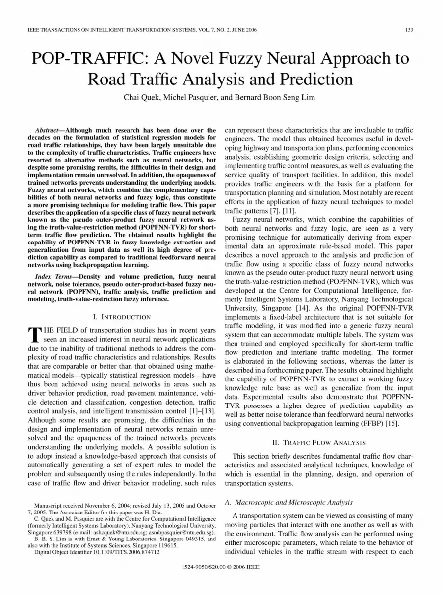
Fig. 1. Photograph of the Pan-Island Expressway site 29 in the directiontoward Changi.

other, or macroscopic parameters, which describe the trafficstream as a whole. Microscopic parameters include character-istics such as spacing and headway, which refer to the distancebetween the front bumpers of successive vehicles in a trafficstream and the time delay between successive vehicles as theypass a particular road location, respectively. Both the spacingand headway of individual vehicles vary over a range of valuesthat is generally based on the speed of the traffic stream.Therefore, in aggregate, microscopic parameters are related tothe macroscopic flow parameters: speed, volume, and density.

On one hand, microscopic analysis may be selected formoderate-size systems, where the number of vehicles is rela-tively small, and there is a need to study their individual behav-ior. On the other hand, macroscopic analysis may be selectedfor higher density larger scale systems, for which a study ofthe global behavior of groups of vehicles is sufficient. Becausethe main objective of this project is to model a highway sectionas a whole, macroscopic analysis is a more appropriate choice.This work differs from [11] as it employs raw data as inputas opposed to a transformed space (wavelet). Furthermore, thelogical inference system in [14] is based on theoretical truth-value-restriction fuzzy inference paradigm [33].

B. Field Data Collection

The set of data employed in this project is described here-after. Both vehicle classification counts and speed data werecollected from a five-lane section along the Pan Island Express-way, Singapore, in both the eastward and westward directionstoward Changi and Jurong, respectively. Site 30 is the upstreamstation located between the Toa Payoh South Fly-over andThomson road, whereas site 29, which is shown in Fig. 1,is located further down the stream near Kim Keat Avenue.Data samples were collected from inductive and piezoelectricloop detectors installed beneath the road surface by the LandTransport Authority of Singapore in 1996 to facilitate trafficdata collection, as depicted in Fig. 2. Detectors are connected toa traffic counter, which, in this case, is a microprocessor-basedMarksman 660 traffic counter classifier.

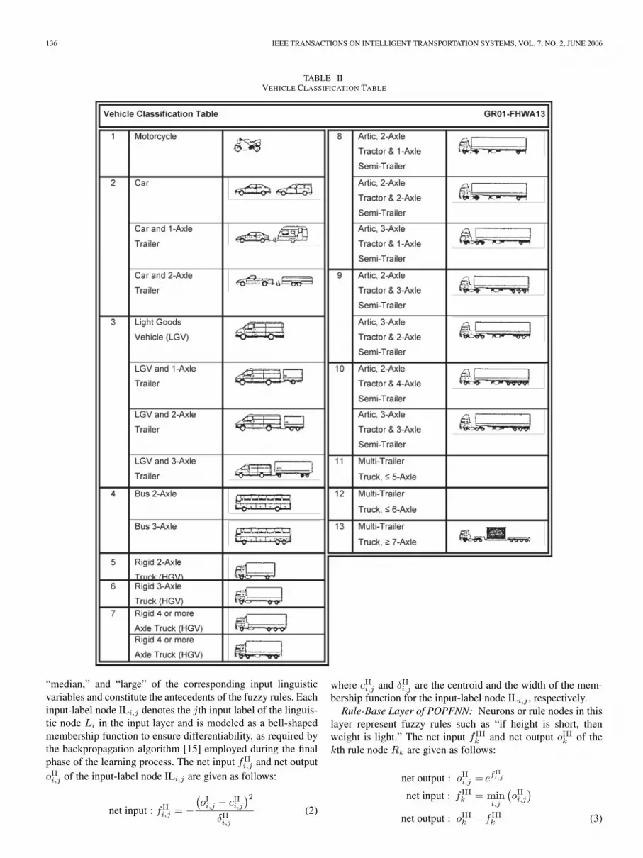
The loop detectors are capable of recording vehicle count,vehicle speed, and vehicle classification of up to 13 categories.They are not perfect, however, and errors such as vehiclemisclassification and undercounting are unavoidable. Videorecordings were thus taken from overhead bridges next to therespective counting stations to monitor the actual traffic flowconditions during data collection. The data used in this projectwere collected at 5-min intervals over a period of 6 days, withthe Marksman 660 configured to classify speed data and vehiclecounts into nine speed and 13 vehicle categories, as shown inTables I and II, respectively.

III. FUZZY NEURAL NETWORKS

Fuzzy neural networks are hybrid intelligent systems thatpossess the advantages of both neural networks and fuzzysystems—in the former, the learning and optimization abilities,as well as the connectionist structure; and in the latter, thehuman-like reasoning capacity and the ease of incorporatingexpert knowledge [16]. In addition, such hybrid intelligentsystems alleviate the shortcomings of the respective techniques.These include common problems encountered in the design offuzzy rule-based systems; for example, the determination of themembership functions, the identification of the fuzzy rules, aswell as the fuzzy inference process. Such problems in fuzzyrule-based systems can be resolved in fuzzy neural networksusing neural net techniques. One well-acknowledged drawbackof neural networks is their opaqueness. The integration offuzzy concepts in fuzzy neural systems greatly improves thetransparency for a better understanding of their inner workings.Each membership function and fuzzy rule used in fuzzy neuralnetworks have clear semantic meanings, hence, the neural-network-like structure of fuzzy neural networks becomes in-creasingly transparent once they are trained. In addition, thechoice of the initial values for the parameters is made simplerin fuzzy neural networks.

An important aspect in the design of fuzzy neural networksis the identification of the fuzzy rules. However, there is nosystematic design procedure at present. The recent researchdirection in the identification of the fuzzy rules in fuzzy neuralnetworks is to learn and modify the rules from past experience.Currently, much research work that uses linguistic as well asnumerical information to generate and adapt fuzzy rules hasbeen reported [7], [14], [17]–[23], [29]–[31]. They can becategorized into the following approaches:

Approach 1: This approach uses linguistic information toidentify fuzzy rules in the fuzzy neural networks priorto the application of neural network techniques to adjustthe rules [18], [24]–[27]. The incorporation of linguisticinformation prevents the random choice of the initialfuzzy rules employed in the system. Consequently, thesystem converges faster during training and performsbetter. However, the approach is rather subjective be-cause linguistic information from experts may vary fromperson to person, and from time to time.

Approach 2: This approach uses unsupervised learning al-gorithms to identify fuzzy rules in the fuzzy neural

QUEK et al.: POP-TRAFFIC: FUZZY NEURAL APPROACH TO ROAD TRAFFIC ANALYSIS AND PREDICTION 135

Fig. 2. Five-lane and three-lane road sections at sites 29 and 30 of the Pan-Island Expressway.

TABLE ISUMMARY OF SPEED BIN

networks prior to the application of neural networktechniques to adjust the rules [17], [19], [28]–[31]. Be-cause the training data set is the only source of informa-tion employed in the second approach, it must thereforebe representative. Otherwise, the derived fuzzy rules willbe ill defined and the resultant fuzzy neural networkwill not model the behavior inadequately. Moreover, theunsupervised learning algorithms that are used in therule identification process must be carefully selected inthe absence of experts’ opinions.

Approach 3: This approach uses supervised learning algo-rithm (particularly the backpropagation technique) toidentify the fuzzy rules in the fuzzy neural networks[7], [20], [21]. These fuzzy neural networks are essen-tially multilayered with the inputs and outputs as fuzzymembership values that satisfy certain constraints. Thebackpropagation learning algorithm [32] is often utilizedin such fuzzy neural networks to produce the mappingfrom inputs to outputs. However, the fuzzy neural net-work appears as a “black box” at the end of the trainingprocess. The actual model acquired through trainingand the semantics of the structure remain opaque. Theopaqueness contradicts the original intention for theintegration of fuzzy concepts in neural networks.

IV. POPFNN-TVR FUZZY NEURAL NETWORK

This section describes the fuzzy neural network used in thisproject for traffic flow analysis and prediction.

A. Characteristics of Pseudo Outer-Product-Based FuzzyNeural Network (POPFNN)

The POPFNN is a hybrid system that possesses the advan-tages of both neural networks and fuzzy systems. It belongs toa class of fuzzy systems that are constructed using numericaldata with their parameters adjusted using neural network tech-niques. In our case, the initial set of parameters and the systemstructure are not derived from linguistic information providedby experts but constructed from a set of training data usingan unsupervised learning algorithm and fine tuned on the basisof the numerical information [19]. The functions performed byeach layer of the POPFNN correspond to the inference steps ofthe truth-value-restriction method [33].

One of the most important aspects of fuzzy neural networksis the identification of fuzzy rules, using unsupervised learningalgorithms such as the self-organizing algorithm [34] and com-petitive learning algorithm [35]. The rule identification methodused in POPFNN is the one-pass lazy pseudo outer-product(LazyPOP) learning algorithm [22], which is closely related toHebbian’s learning law. The use of POPFNN as the fuzzy neuralnetwork for traffic flow prediction has the advantages to beefficient, convenient, highly intuitive, and easier to understandthan other rule identification algorithms.

B. Structure of POPFNN

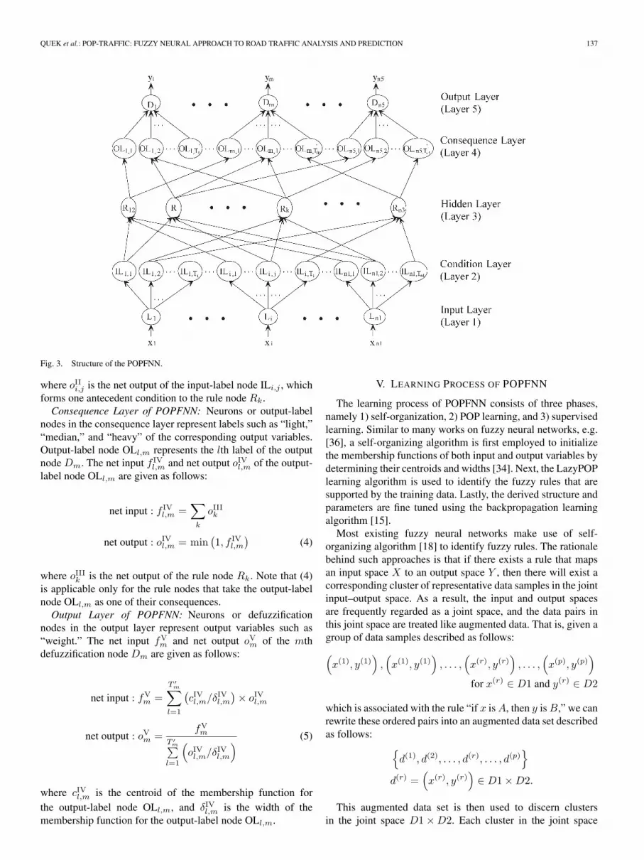
The POPFNN [14] has a five-layer structure, as depicted inFig. 3, where each layer is characterized by the fuzzy operationthat it performs, namely input (fuzzification), condition, rulecombination, consequence, and output (defuzzification). Theseoperations are elaborated in the following subsections.Input Layer of POPFNN: Neurons or linguistic nodes in the

input layer represent input linguistic variables such as “height”and “width” and directly transmit nonfuzzy input values to thesecond layer. The net input f I

i and net output oIi of the ith

linguistic node Li are given as follows:

f Ii = xi oI

i = f Ii (1)

where xi is the ith element of the input vector X.Condition Layer of POPFNN: Neurons or input-label

nodes in the condition layer represent labels such as “small,”


TABLE IIVEHICLE CLASSIFICATION TABLE

“median,” and “large” of the corresponding input linguisticvariables and constitute the antecedents of the fuzzy rules. Eachinput-label node ILi,j denotes the jth input label of the linguis-tic node Li in the input layer and is modeled as a bell-shapedmembership function to ensure differentiability, as required bythe backpropagation algorithm [15] employed during the finalphase of the learning process. The net input f II

i,j and net outputoII

i,j of the input-label node ILi,j are given as follows:

net input : f IIi,j = −

(oI

i,j − cIIi,j)2

δIIi,j(2)

where cIIi,j and δIIi,j are the centroid and the width of the mem-bership function for the input-label node ILi,j , respectively.Rule-Base Layer of POPFNN: Neurons or rule nodes in this

layer represent fuzzy rules such as “if height is short, thenweight is light.” The net input f III

k and net output oIIIk of the

kth rule node Rk are given as follows:

net output : oIIi,j = ef II

i,j

net input : f IIIk = min

i,j

(oII

i,j

)

net output : oIIIk = f III

k (3)


Fig. 3. Structure of the POPFNN.

where oIIi,j is the net output of the input-label node ILi,j , which

forms one antecedent condition to the rule node Rk.Consequence Layer of POPFNN: Neurons or output-label

nodes in the consequence layer represent labels such as “light,”“median,” and “heavy” of the corresponding output variables.Output-label node OLl,m represents the lth label of the outputnode Dm. The net input f IV

l,m and net output oIVl,m of the output-

label node OLl,m are given as follows:

net input : f IVl,m =

∑k

oIIIk

net output : oIVl,m = min

(1, f IV

l,m

)(4)

where oIIIk is the net output of the rule node Rk. Note that (4)

is applicable only for the rule nodes that take the output-labelnode OLl,m as one of their consequences.Output Layer of POPFNN: Neurons or defuzzification

nodes in the output layer represent output variables such as“weight.” The net input fV

m and net output oVm of the mth

defuzzification node Dm are given as follows:

net input : fVm =

T ′m∑

l=1

(cIVl,m/δ

IVl,m

) × oIVl,m

net output : oVm =

fVm

T ′m∑

l=1

(oIV

l,m/δIVl,m

) (5)

where cIVl,m is the centroid of the membership function forthe output-label node OLl,m, and δIVl,m is the width of themembership function for the output-label node OLl,m.

V. LEARNING PROCESS OF POPFNN

The learning process of POPFNN consists of three phases,namely 1) self-organization, 2) POP learning, and 3) supervisedlearning. Similar to many works on fuzzy neural networks, e.g.[36], a self-organizing algorithm is first employed to initializethe membership functions of both input and output variables bydetermining their centroids and widths [34]. Next, the LazyPOPlearning algorithm is used to identify the fuzzy rules that aresupported by the training data. Lastly, the derived structure andparameters are fine tuned using the backpropagation learningalgorithm [15].

Most existing fuzzy neural networks make use of self-organizing algorithm [18] to identify fuzzy rules. The rationalebehind such approaches is that if there exists a rule that mapsan input space X to an output space Y , then there will exist acorresponding cluster of representative data samples in the jointinput–output space. As a result, the input and output spacesare frequently regarded as a joint space, and the data pairs inthis joint space are treated like augmented data. That is, given agroup of data samples described as follows:

(x(1), y(1)

),(x(1), y(1)

), . . . ,

(x(r), y(r)

), . . . ,

(x(p), y(p)

)

for x(r) ∈ D1 and y(r) ∈ D2

which is associated with the rule “if x is A, then y is B,” we canrewrite these ordered pairs into an augmented data set describedas follows:

{d(1), d(2), . . . , d(r), . . . , d(p)

}

d(r) =(x(r), y(r)

)∈ D1 ×D2.

This augmented data set is then used to discern clustersin the joint space D1 ×D2. Each cluster in the joint space


Fig. 4. Clusters in input–output as rules.

Fig. 5. Clusters in input–output space and their projections.

D1 ×D2 corresponds to a rule that maps the input space D1to the output space D2 as shown in Fig. 4. The checkeredarea in Fig. 4 represents the fuzzy boundary between clusters.This clustering process is often accomplished by using a self-organizing algorithm [18].

However, in most integrated fuzzy neural networks, wherethe membership functions are determined prior to the identifica-tion of the fuzzy rules, self-organizing or competitive learningbecomes redundant. In such cases, the boundary of the clustersin the input and output spaces have already been predefined.Thus, it is unnecessary to use self-organizing algorithms todetermine the fuzzy partitions of the input–output space.

Clusters or subsets of data samples in the input and outputspaces map onto clusters in the joint space (see Fig. 5). Asa result, once the clusters in the input and output spaces areknown, the clusters in their joint space are therefore apparent tosome degree. Some efforts have been attempted to make useof the known membership functions to find the fuzzy rules.An example is Lin and Lee’s work [17], where competitivelearning is employed to identify the fuzzy rules. In his work,all the possible fuzzy rules must be listed before the initiationof competitive learning. These fuzzy rules are then repeatedlytested against the training data to find their most likely conse-quence. After the competitive learning, the link with the largestweight is selected, and the consequence that it connects to issubsequently held as the real consequence of the rule. AlthoughLin and Lee’s method does integrate information of clusters inthe input and output spaces to some degree, it involves iterativetraining before the system comes to a stable state. To moreeffectively utilize the information derived from the identifiedmembership functions, we proposed a new rule-identificationalgorithm in this paper, called the pseudo outer-product (POP)learning algorithm. The proposed POP learning algorithm is aone-pass learning algorithm, and in this sense, it is superior

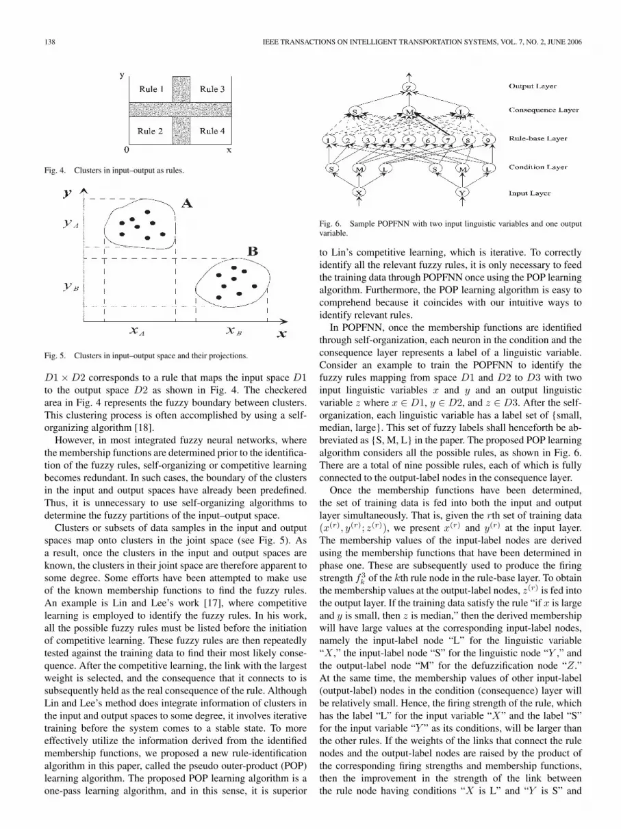
Fig. 6. Sample POPFNN with two input linguistic variables and one outputvariable.

to Lin’s competitive learning, which is iterative. To correctlyidentify all the relevant fuzzy rules, it is only necessary to feedthe training data through POPFNN once using the POP learningalgorithm. Furthermore, the POP learning algorithm is easy tocomprehend because it coincides with our intuitive ways toidentify relevant rules.

In POPFNN, once the membership functions are identifiedthrough self-organization, each neuron in the condition and theconsequence layer represents a label of a linguistic variable.Consider an example to train the POPFNN to identify thefuzzy rules mapping from space D1 and D2 to D3 with twoinput linguistic variables x and y and an output linguisticvariable z where x ∈ D1, y ∈ D2, and z ∈ D3. After the self-organization, each linguistic variable has a label set of {small,median, large}. This set of fuzzy labels shall henceforth be ab-breviated as {S, M, L} in the paper. The proposed POP learningalgorithm considers all the possible rules, as shown in Fig. 6.There are a total of nine possible rules, each of which is fullyconnected to the output-label nodes in the consequence layer.

Once the membership functions have been determined,the set of training data is fed into both the input and outputlayer simultaneously. That is, given the rth set of training data(x(r), y(r); z(r)), we present x(r) and y(r) at the input layer.The membership values of the input-label nodes are derivedusing the membership functions that have been determined inphase one. These are subsequently used to produce the firingstrength f3

k of the kth rule node in the rule-base layer. To obtainthe membership values at the output-label nodes, z(r) is fed intothe output layer. If the training data satisfy the rule “if x is largeand y is small, then z is median,” then the derived membershipwill have large values at the corresponding input-label nodes,namely the input-label node “L” for the linguistic variable“X ,” the input-label node “S” for the linguistic node “Y ,” andthe output-label node “M” for the defuzzification node “Z.”At the same time, the membership values of other input-label(output-label) nodes in the condition (consequence) layer willbe relatively small. Hence, the firing strength of the rule, whichhas the label “L” for the input variable “X” and the label “S”for the input variable “Y ” as its conditions, will be larger thanthe other rules. If the weights of the links that connect the rulenodes and the output-label nodes are raised by the product ofthe corresponding firing strengths and membership functions,then the improvement in the strength of the link betweenthe rule node having conditions “X is L” and “Y is S” and


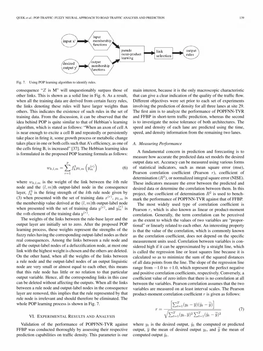
Fig. 7. Using POP learning algorithm to identify rules.

consequence “Z is M” will unquestionably surpass those ofother links. This is shown as a solid line in Fig. 6. As a result,when all the training data are derived from certain fuzzy rules,the links denoting these rules will have larger weights thanothers. This indicates the existence of such rules in the set oftraining data. From the discussion, it can be observed that theidea behind POP is quite similar to that of Hebbian’s learningalgorithm, which is stated as follows: “When an axon of cell Ais near enough to excite a cell B and repeatedly or persistentlytake place in firing it, some growth process or metabolic changetakes place in one or both cells such that A’s efficiency, as one ofthe cells firing B, is increased” [37]. The Hebbian learning ideais formulated in the proposed POP learning formula as follows:

wk,l,m =p∑

r=1

f3kµl,m

(y(r)

m

)(6)

where wk,l,m is the weight of the link between the kth rulenode and the (l,m)th output-label node in the consequencelayer, f3

k is the firing strength of the kth rule node given by(3) when presented with the set of training data x(r), µl,m isthe membership value derived at the (l,m)th output-label nodewhen presented with the set of training data y(r), and y

(r)m is

the mth element of the training data y(r).The weights of the links between the rule-base layer and the

output layer are initially set to zero. After the proposed POPlearning process, these weights represent the strengths of thefuzzy rules having the corresponding output-label nodes as theirreal consequences. Among the links between a rule node andall the output-label nodes of a defuzzification node, at most onelink with the highest weight is chosen and the others are deleted.On the other hand, when all the weights of the links betweena rule node and the output-label nodes of an output linguisticnode are very small or almost equal to each other, this meansthat this rule node has little or no relation to that particularoutput variable. Hence, all the corresponding links in this casecan be deleted without affecting the outputs. When all the linksbetween a rule node and output-label nodes in the consequencelayer are removed, this implies that the rule represented by thatrule node is irrelevant and should therefore be eliminated. Thewhole POP learning process is shown in Fig. 7.

VI. EXPERIMENTAL RESULTS AND ANALYSIS

Validation of the performance of POPFNN-TVR againstFFBP was conducted thoroughly by assessing their respectiveprediction capabilities on traffic density. This parameter is our

main interest, because it is the only macroscopic characteristicthat can give a clear indication of the quality of the traffic flow.Different objectives were set prior to each set of experimentsinvolving the prediction of density for all three lanes at site 29.The first aim is to analyze the performance of POPFNN-TVRand FFBP in short-term traffic prediction, whereas the secondis to investigate the noise tolerance of both architectures. Thespeed and density of each lane are predicted using the time,speed, and density information from the remaining two lanes.

A. Measuring Performance

A fundamental concern in prediction and forecasting is tomeasure how accurate the predicted data set models the desiredoutput data set. Accuracy can be measured using various formsof statistical indicators, such as mean square error (mse),Pearson correlation coefficient (Pearson r), coefficient ofdetermination (R2), or normalized integral square error (NISE).These indicators measure the error between the predicted anddesired data or determine the correlation between them. In thisproject, the coefficient of determination R2 is used to bench-mark the performance of POPFNN-TVR against that of FFBP.

The most widely used type of correlation coefficient isPearson r, which is also known as linear or product-momentcorrelation. Generally, the term correlation can be perceivedas the extent to which the values of two variables are “propor-tional” or linearly related to each other. An interesting propertyis that the value of the correlation, which is commonly knownas the correlation coefficient, does not depend on the specificmeasurement units used. Correlation between variables is con-sidered high if it can be approximated by a straight line, whichis called the regression line or least squares line because it iscalculated so as to minimize the sum of the squared distancesof all data points from the line. The slope of the regression linerange from −1.0 to +1.0, which represent the perfect negativeand positive correlation coefficients, respectively. Conversely, acoefficient value of zero infers that there is no correlation at allbetween the variables. Pearson correlation assumes that the twovariables are measured on at least interval scales. The Pearsonproduct-moment correlation coefficient r is given as follows:

r =

[∑Tt=1(yt − y)(yt − y)

]√∑T

t=1(yt−y)2∑T

t=1(yt − y)2(7)

where yt is the desired output, yt the computed or predictedoutput, y the mean of desired output yt, and y the mean ofcomputed output yt.


The coefficient of determination R2 can be thought of as ameasure of linear association between yt and yt and thereforeas a measure of the goodness of fit, with 0 ≤ R2 ≤ 1. When R2

equals zero, the predicted and desired outputs are totally uncor-related. In contrast, whenR2 equals 1, the predicted and desiredoutputs are exactly the same. For the purpose of this project, thealternative formulation of R2 given as follows was employed:

R2 =

[∑Tt=1(yt − y)(yt − y)

]2

∑Tt=1(yt−y)2

∑Tt=1(yt − y)2

. (8)

B. Short-Term Traffic Forecasting

The experiments to assess the forecasting ability ofPOPFNN-TVR and FFBP are organized into two parts. We firstassessed the ability of both systems in short-term traffic densityprediction from 5 min ahead (t+ 5) in time to 1 h ahead(t+ 60) and then their ability to tolerate white noise of 10%and 30% induced into the testing data. In all the experimentsperformed with FFBP, a three-layer feedforward network with100 neurons in the hidden layer was employed, with a standardsigmoid as for the activation function. This configurationwas derived from similar experiments and was by no meansthe optimal configuration arising from this project. As forPOPFNN-TVR, an initial assumption was made that all inputdata to the network are classifiable into at least three clusters(e.g., low, medium, and high). This assumption is required bythe data clustering process that automatically derives the fuzzysets used for logical inference.

C. Traffic Density Prediction

The aim of this set of experiments is to compare the short-term prediction ability of POPFNN-TVR against that of FFBP.The R2 index was used to gauge the performance of bothnetworks. Note that different performance criteria may be used,depending on the application. In the forecasting of foreignexchange rate, for instance, the neural network’s ability tocapture the market trend is far more important than achievingan accurate prediction that would miss most of the upward anddownward trends. Experiments were conducted for each of thethree lanes at site 29, where time, speed, volume, and densitywere used as inputs to predict the traffic density for the next 5 to60 min. Theoretically, there should be a significant correlationbetween the current density of traffic flow and the density5 min ahead under normal flow condition, baring, of course,unforeseen events such as accidents. As the time interval getslarger, the correlation should decrease, and thus, the modelingability of both POPFNN-TVR and FFBP should also decrease.Because POPFNN-TVR has the ability to extract rules from thetraining set, it will be able to formalize the relations betweentime and the other input variables, effectively reducing the fluc-tuation of the predicted output as the forecasting time intervalis increased. If these points can be verified from the obtainedresults, then it can be concluded that POPFNN-TVR possessesgreater prediction ability than a conventional FFBP.Experimental Setup: Two series comprising an identical

number of experiments were designed for the FFBP and

Fig. 8. Prediction using time delay windows of one and three, respectively.

POPFNN-TVR networks. The problem at hand must first bemapped onto a representative form of the analysis technique,which involves the choice of a suitable neural network archi-tecture. Past research has shown that a multilayer feedforwardnetwork, when coupled with a suitable learning algorithm suchas the backpropagation algorithm, can be trained to computeany arbitrary nonlinear function [38].FFBP: To gauge the performance of FFBP, time, volume,

speed, and density of all three lanes are used as inputs to predictthe traffic density of lane 1, lane 2, and lane 3. The inputdata at time t is used to predict density at (t+X), where Xdenotes the time interval ranging from 5 to 60 min. In thissetup, the length of the time window is 1, as depicted by thetop diagram in Fig. 8. As such, the network does not rely ona sequence of past information for its prediction. The bottomdiagram in Fig. 8 shows another experimental setup wherethree consecutive time-dependent variables xt (t = t, t− 5, andt− 10) are used to predict the value of the variable at a futuretime t+ 25, hence, the length of the time delay window is 3.The latter technique is normally employed when the onlyfeature vector available is a historical time series of the datato be modeled, as, for instance, in the prediction of the stockmarket using historical data of shares.

The neural network consists therefore of ten input neurons,which are the time vector and macroscopic parameters (speed,volume, and density) for each of the three lanes, and one outputneuron for the density vector to be predicted at (t+X). Forthe hidden layer, a total of 100 neurons were chosen. Lastly,the sigmoid function was used as the activation function of thenetwork. Instead of the standard backpropagation algorithm, analternative variant known as backpropagation with momentumterm and flat spot elimination was used in these experiments,as this algorithm is known to converge faster and is provideddirectly by the Stuttgart neural network simulator (SNNS)platform used for implementing FFBP [39]. Four learning pa-rameters are defined as follows: 1) η is the learning parameter,which is used to specify the step width of the gradient descentalgorithm; 2) µ is the momentum term, which is used to specifythe amount of the old weight change that is added to the currentchange; 3) c is the constant flat spot elimination value, which isto be added to the derivative of the activation function to enablethe network to pass flat spots in the error surface; 4) dmax is themaximum difference dj = tj − oj between a teaching value tjand an output oj of an output unit that is propagation back.

After a series of trial experimentation, we found that thenetwork could converge after a reasonable period of time whenusing the following settings: η = 0.2, µ = 0.5, c = 0.1, and


TABLE IIIMAXIMUM, MINIMUM, AND AVERAGE VALUE OF DATA SET FOR SITE 29

dmax = 0.0. No change was made to the network in subsequentexperiments other than adjusting the learning rate because nosingle value is optimal for all dimensions. Having identified thenetwork architecture and learning algorithm, the last stage ofthe experimental setup involved preprocessing of the input data,the type which is largely dependent on the chosen activationfunction of the neural network.

The transfer function of a unit is typically chosen so that itcan accept input in any range and produce output in a strictlylimited range. Although the input can be of any value, theunit is only sensitive to input values within a fairly limitedinterval. A sigmoid function is used in the experiments, withthe steepness factor β set to 1. In this case, the output is inthe range [0,1], and the input is sensitive in a range not muchlarger than [−1,+1]. The data samples used for training andtesting the neural network were normalized using the min–maxnormalization technique given as follows:

Xn =(X −Xmin)

(Xmax −Xmin)(9)

where Xn is the normalized value, and X , Xmin and Xmax arean instance of the minimum and the maximum values of thevector to be normalized. This reduces the possibility of reachingthe saturation regions of the sigmoid transfer function duringtraining.

Table III summarizes the statistical indicators for the macro-scopic parameters at site 29, including the max, min, mean,standard deviation, and coefficient of variance. Using these val-ues, the normalization of data samples is performed by simplysubstituting the necessary parameters into (9). The normalizeddata samples are then divided such that 40% will be used fortraining the neural network, and the other 60% will be usedfor testing the trained network. It is necessary to ensure thatthe network is trained using sufficient data to cover the entireproblem domain, including maximum and minimum values foreach variable as well as a good distribution of values within thisrange. Selecting a smaller portion of the training data preventsovertraining of the network and ensures that it will generalizewell when presented with new data. This criterion for data parti-tioning is applicable to both FFBP and POPFNN-TVR systems.POPFNN-TVR: For the case of POPFNN-TVR, the predic-

tion problem is mapped onto a five-layer POPFNN networkwith the following configuration. The time input is discretizedinto four labels (early morning, morning, afternoon, night). Thenormalized traffic volume inputs of the three lanes, which aredenoted by V 1, V 2, and V 3, respectively, are represented bythree labels (low, medium, high) and, similarly, for the speed

and density of the traffic flow, which are denoted by denotedU1,U2, andU3 andD1,D2, andD3. Lastly, the output densityof lane l at (t+X) minutes is denoted by Dl −X discretizedinto three labels (low, medium, and high).

The optimal number of rule nodes to be used is automaticallydetermined by the LazyPOP algorithm during the unsupervisedlearning phase. Experimentation with the POPFNN-TVR net-work employed another form of normalization technique dueto the characteristics of the fuzzy neural network. Specifically,because the self-organization phase of POPFNN attempts tolearn the structure of the data through clustering, the use ofthe min–max normalization technique might cause a spuriousdispersion of the clusters in the original data, greatly affectingthe precision of the data. Thus, the data for POPFNN arenormalized in the following manner: Time is normalized to2400 h, Ui are normalized to 80 km/h, whereas Vi and Di arenormalized to the average volume and density of the ith lane,respectively. This method allows the normalized speed to beinterpreted more easily as compared to the min–max technique.Results and Analysis: In this phase, seven experiments had

to be carried out for the first lane of site 29 and five experimentsfor the two remaining lanes. Therefore, a total of 17 ex-periments were conducted using FFBP and, similarly, usingPOPFNN-TVR. Due to the large number of experiments andthe long training time required, the training of the FFBP net-work was executed in batch mode using SNNS. Batch processeswere programmed to terminate when the SSE expressed in (10)reached 0.8 or less:

SSE =T∑

i=1

(yi − yi)2. (10)

The results of FFBP predictions for all the three lanes wererecorded for increasing values of the time interval ranging fromt+ 5 to t+ 60 min. The time samples spanned over 2400 minfor a period of approximately 3 days from September 7 to 10,1996. The computed output of the network was plotted againstthe desired output to give an indication of FFBP’s ability tofollow the general trend of the traffic data, and the R2 valueswere calculated accordingly. Similarly, experimental data werecollected using POPFNN-TVR for each of the three lanes, itsoutputs monitored, and the R2 values calculated accordingly.In general, traffic flow follows a repetitive pattern, even thoughits amplitude is stochastic in nature, and so two near-periodiccycles were observed. Specifically, the traffic density was low atthe beginning of the day and showed significant increase on twooccasions, namely 1) the morning peak hours P1 when large


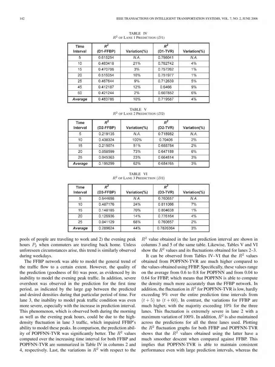
TABLE IVR2 OF LANE 1 PREDICTION (D1)

TABLE VR2 OF LANE 2 PREDICTION (D2)

TABLE VIR2 OF LANE 3 PREDICTION (D3)

pools of people are traveling to work and 2) the evening peakhours P2 when commuters are traveling back home. Unlessunforeseen circumstances arise, this trend is similarly observedduring weekdays.

The FFBP network was able to model the general trend ofthe traffic flow to a certain extent. However, the quality ofthe prediction (goodness of fit) was poor, as evidenced by itsinability to model the evening peak traffic. In addition, severeovershoot was observed in the prediction for the first timeperiod, as indicated by the large gap between the predictedand desired densities during that particular period of time. Forlane 3, the inability to model peak traffic condition was evenmore severe, especially with the increase in prediction interval.This phenomenon, which is observed both during the morningas well as the evening peak hours, could be due to the high-density fluctuation in lane 3 traffic, which impaired FFBP’sability to model these peaks. In comparison, the prediction abil-ity of POPFNN-TVR was significantly better. The R2 valuescomputed over the increasing time interval for both FFBP andPOPFNN-TVR are summarized in Table IV in columns 2 and4, respectively. Last, the variations in R2 with respect to the

R2 value obtained in the last prediction interval are shown incolumns 3 and 5 of the same table. Likewise, Tables V and VIshow the R2 values and its fluctuations obtained for lanes 2–3.

It can be observed from Tables IV–VI that the R2 valuesobtained from POPFNN-TVR are much higher compared tothe values obtained using FFBP. Specifically, these values rangeon the average from 0.6 to 0.8 for POPFNN and from 0.04 to0.64 for FFBP, which means that POPFNN is able to computethe density much more accurately than the FFBP network. Inaddition, the fluctuation in R2 for POPFNN-TVR is low, hardlyexceeding 9% over the entire prediction time intervals from(t+ 5) to (t+ 60). In contrast, the variations for FFBP aremuch higher, with the majority exceeding 10% for the threelanes. This fluctuation is extremely severe in lane 2 with amaximum variation of 100%. In addition, R2 is also maintainedacross the predictions for all the three lanes used. Plottingthe R2 fluctuation graphs for both FFBP and POPFNN-TVRshows that the R2 values obtained using the latter have amuch smoother descent when compared against FFBP. Thisimplies that POPFNN-TVR is able to maintain consistentperformance even with large prediction intervals, whereas the


performance of FFBP drops drastically as prediction intervalsincrease.

Further experiments show that a higher percentage of pre-dicted density falls within the qualifying bands described inearlier paragraphs. On the average, the ratio of predictions thatare within range for POPFNN-TVR over FFBP is greater than1.5. This observation further substantiates our initial hypothesisthat POPFNN-TVR provides a better prediction model com-pared to FFBP. Overall, two conclusions can be made fromthe results obtained. First, the comparison of the R2 values inTables IV–VI proves that the short-term prediction ability ofPOPFNN-TVR is superior to that of FFBP. Second, the lowfluctuation in R2 evidenced in the same tables also suggeststhat POPFNN-TVR is a more suitable model for prediction overlonger period of time.

D. Noise Tolerance Ability

The next set of experiments serves to study and contrast thenetworks’ noise tolerance ability, with the objective to provethat POPFNN-TVR is more tolerant to noisy input data thanFFBP. To verify this hypothesis, POPFNN-TVR must be ableto maintain its prediction capability under the influence ofnoisy input data. The performance of POPFNN-TVR is againgauged using theR2 indicator. The test data used in the previoussection have to be preprocessed prior to the experiments, withwhite noise of 10% and 30% injected into the volume Vi,speed Ui, and density Di components of the original test set,whereas the time and desired output density are left unchangedfor comparison purposes. In the experiments described here,POPFNN-TVR only operated in the test mode, which meansthat the network performs pure forward propagation of theinput data without modification. The preprocessed noisy dataare fed into POPFNN-TVR, and the corresponding outputs areobtained at the output layer, which are then compared againstthe desired outputs to generate the performance indexes. Asimilar set of experiments is performed using FFBP and thefinal computed R2 values are compared against that obtainedfor POPFNN-TVR.Experimental Setup: The setup for this series of experiments

is similar to that conducted previously. The network structureand the weights of all synaptic links for both FFBP andPOPFNN-TVR networks as trained in the previous experimentswere saved to facilitate further experimentation. The structuresof the two networks are given as follows. The FFBP consistsof three layers, namely 1) the input layer with ten neurons(time, V 1, V 2, V 3, U1, U2, U3, D1, D2, and D3), 2) thehidden layer with 100 neurons, and 3) the output layer withone neuron (Dl −X , which is the lane l density at t+X).POPFNN-TVR, on the other hand, is configured with fourinput variables, with the time discretized into four labels (earlymorning, morning, afternoon, and night) and V , U , D eachdiscretized into three labels (low, medium, and high), and oneoutput variable Dl −X , which is again discretized into threelabels (slow, medium, and high).

The new test sets are generated by introducing white noiseof 10% and 30% into the original test data used in the previoussection. At each noise level, seven test sets are generated for

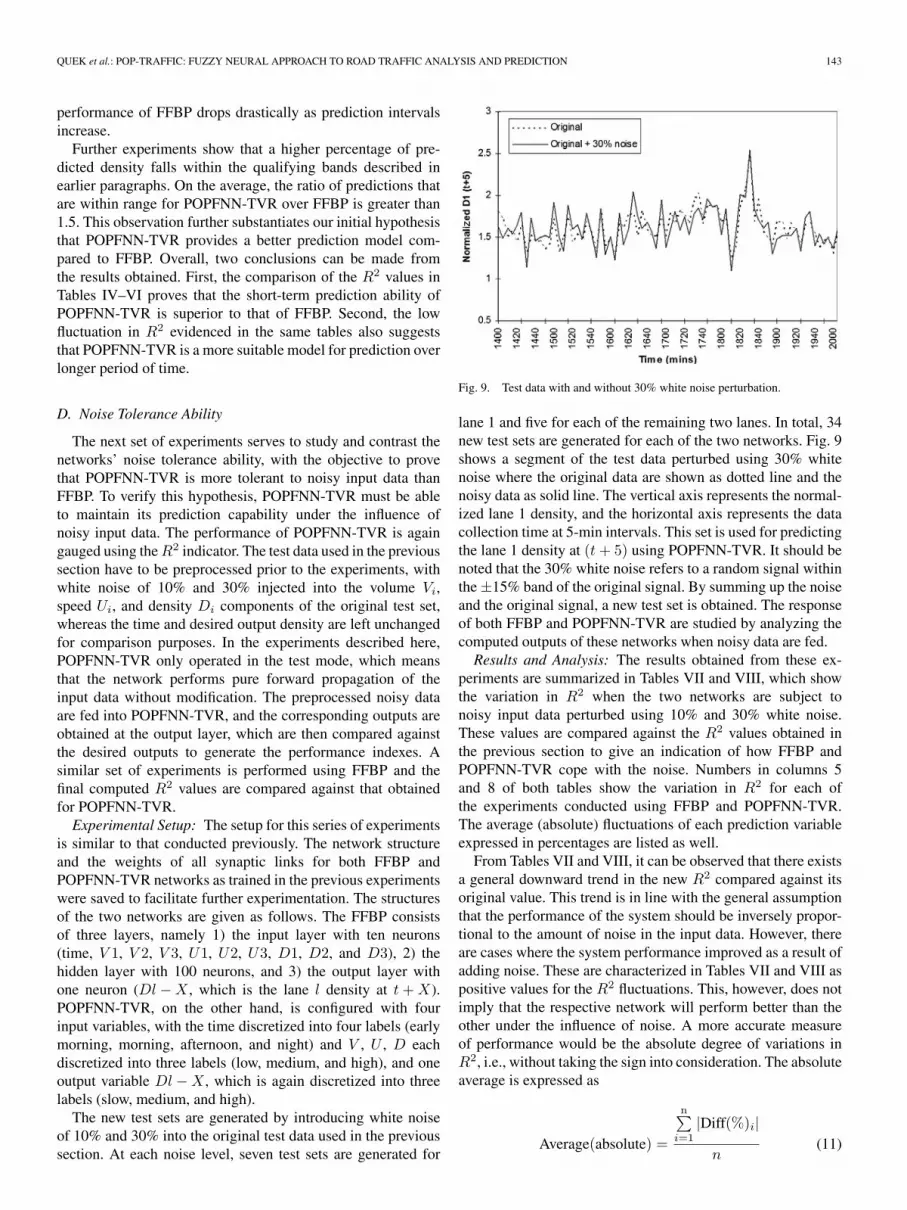
Fig. 9. Test data with and without 30% white noise perturbation.

lane 1 and five for each of the remaining two lanes. In total, 34new test sets are generated for each of the two networks. Fig. 9shows a segment of the test data perturbed using 30% whitenoise where the original data are shown as dotted line and thenoisy data as solid line. The vertical axis represents the normal-ized lane 1 density, and the horizontal axis represents the datacollection time at 5-min intervals. This set is used for predictingthe lane 1 density at (t+ 5) using POPFNN-TVR. It should benoted that the 30% white noise refers to a random signal withinthe ±15% band of the original signal. By summing up the noiseand the original signal, a new test set is obtained. The responseof both FFBP and POPFNN-TVR are studied by analyzing thecomputed outputs of these networks when noisy data are fed.Results and Analysis: The results obtained from these ex-

periments are summarized in Tables VII and VIII, which showthe variation in R2 when the two networks are subject tonoisy input data perturbed using 10% and 30% white noise.These values are compared against the R2 values obtained inthe previous section to give an indication of how FFBP andPOPFNN-TVR cope with the noise. Numbers in columns 5and 8 of both tables show the variation in R2 for each ofthe experiments conducted using FFBP and POPFNN-TVR.The average (absolute) fluctuations of each prediction variableexpressed in percentages are listed as well.

From Tables VII and VIII, it can be observed that there existsa general downward trend in the new R2 compared against itsoriginal value. This trend is in line with the general assumptionthat the performance of the system should be inversely propor-tional to the amount of noise in the input data. However, thereare cases where the system performance improved as a result ofadding noise. These are characterized in Tables VII and VIII aspositive values for the R2 fluctuations. This, however, does notimply that the respective network will perform better than theother under the influence of noise. A more accurate measureof performance would be the absolute degree of variations inR2, i.e., without taking the sign into consideration. The absoluteaverage is expressed as

Average(absolute) =

n∑i=1

|Diff(%)i|n

(11)


TABLE VIIR2 FLUCTUATION WITH 10% WHITE NOISE

TABLE VIIIR2 FLUCTUATION WITH 30% WHITE NOISE

where Diff(%) are the values listed in columns 5 and 8 ofTables VII and VIII, and n is the total number of experimentsfor each prediction variable.

The values thus calculated for this measure are denoted as theabsolute average in Tables VII and VIII. A lower fluctuation inR2 signifies that the network is able to prune spurious noisewhile maintaining its original characteristic. In contrast, a high

value indicates a large deviation in the newR2 from the originalR2. In Table VIII, it can be observed that R2 fluctuation forPOPFNN-TVR is generally much lower than FFBP across allthree lanes. The fluctuation in the prediction of the lane 2density is particularly serious for the FFBP network, asR2 vari-ation can reach a high of over 400% in certain cases. However,it is observed that the absolute average of the lane 3 prediction


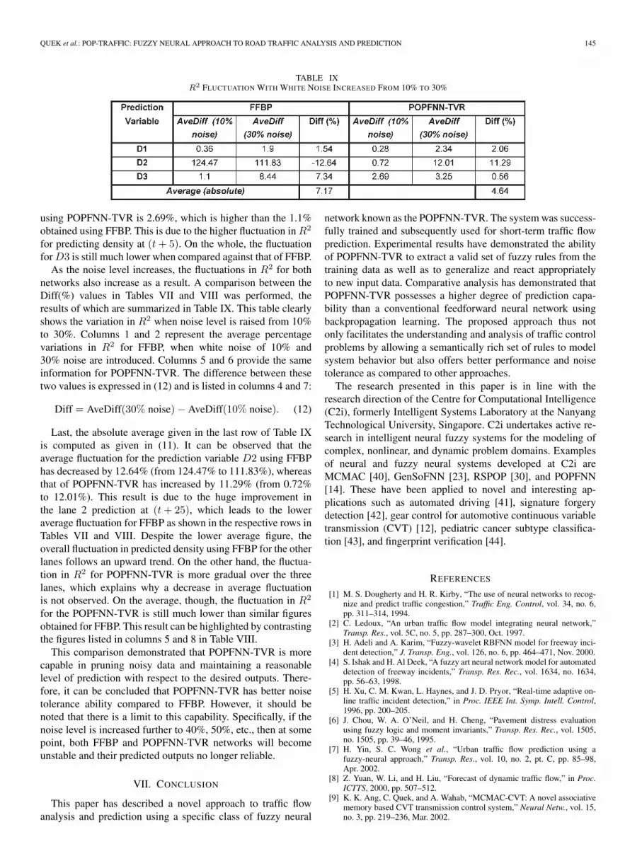
TABLE IXR2 FLUCTUATION WITH WHITE NOISE INCREASED FROM 10% TO 30%

using POPFNN-TVR is 2.69%, which is higher than the 1.1%obtained using FFBP. This is due to the higher fluctuation in R2

for predicting density at (t+ 5). On the whole, the fluctuationforD3 is still much lower when compared against that of FFBP.

As the noise level increases, the fluctuations in R2 for bothnetworks also increase as a result. A comparison between theDiff(%) values in Tables VII and VIII was performed, theresults of which are summarized in Table IX. This table clearlyshows the variation in R2 when noise level is raised from 10%to 30%. Columns 1 and 2 represent the average percentagevariations in R2 for FFBP, when white noise of 10% and30% noise are introduced. Columns 5 and 6 provide the sameinformation for POPFNN-TVR. The difference between thesetwo values is expressed in (12) and is listed in columns 4 and 7:

Diff = AveDiff(30% noise) − AveDiff(10% noise). (12)

Last, the absolute average given in the last row of Table IXis computed as given in (11). It can be observed that theaverage fluctuation for the prediction variable D2 using FFBPhas decreased by 12.64% (from 124.47% to 111.83%), whereasthat of POPFNN-TVR has increased by 11.29% (from 0.72%to 12.01%). This result is due to the huge improvement inthe lane 2 prediction at (t+ 25), which leads to the loweraverage fluctuation for FFBP as shown in the respective rows inTables VII and VIII. Despite the lower average figure, theoverall fluctuation in predicted density using FFBP for the otherlanes follows an upward trend. On the other hand, the fluctua-tion in R2 for POPFNN-TVR is more gradual over the threelanes, which explains why a decrease in average fluctuationis not observed. On the average, though, the fluctuation in R2

for the POPFNN-TVR is still much lower than similar figuresobtained for FFBP. This result can be highlighted by contrastingthe figures listed in columns 5 and 8 in Table VIII.

This comparison demonstrated that POPFNN-TVR is morecapable in pruning noisy data and maintaining a reasonablelevel of prediction with respect to the desired outputs. There-fore, it can be concluded that POPFNN-TVR has better noisetolerance ability compared to FFBP. However, it should benoted that there is a limit to this capability. Specifically, if thenoise level is increased further to 40%, 50%, etc., then at somepoint, both FFBP and POPFNN-TVR networks will becomeunstable and their predicted outputs no longer reliable.

VII. CONCLUSION

This paper has described a novel approach to traffic flowanalysis and prediction using a specific class of fuzzy neural

network known as the POPFNN-TVR. The system was success-fully trained and subsequently used for short-term traffic flowprediction. Experimental results have demonstrated the abilityof POPFNN-TVR to extract a valid set of fuzzy rules from thetraining data as well as to generalize and react appropriatelyto new input data. Comparative analysis has demonstrated thatPOPFNN-TVR possesses a higher degree of prediction capa-bility than a conventional feedforward neural network usingbackpropagation learning. The proposed approach thus notonly facilitates the understanding and analysis of traffic controlproblems by allowing a semantically rich set of rules to modelsystem behavior but also offers better performance and noisetolerance as compared to other approaches.

The research presented in this paper is in line with theresearch direction of the Centre for Computational Intelligence(C2i), formerly Intelligent Systems Laboratory at the NanyangTechnological University, Singapore. C2i undertakes active re-search in intelligent neural fuzzy systems for the modeling ofcomplex, nonlinear, and dynamic problem domains. Examplesof neural and fuzzy neural systems developed at C2i areMCMAC [40], GenSoFNN [23], RSPOP [30], and POPFNN[14]. These have been applied to novel and interesting ap-plications such as automated driving [41], signature forgerydetection [42], gear control for automotive continuous variabletransmission (CVT) [12], pediatric cancer subtype classifica-tion [43], and fingerprint verification [44].

REFERENCES

[1] M. S. Dougherty and H. R. Kirby, “The use of neural networks to recog-nize and predict traffic congestion,” Traffic Eng. Control, vol. 34, no. 6,pp. 311–314, 1994.

[2] C. Ledoux, “An urban traffic flow model integrating neural network,”Transp. Res., vol. 5C, no. 5, pp. 287–300, Oct. 1997.

[3] H. Adeli and A. Karim, “Fuzzy-wavelet RBFNN model for freeway inci-dent detection,” J. Transp. Eng., vol. 126, no. 6, pp. 464–471, Nov. 2000.

[4] S. Ishak and H. Al Deek, “A fuzzy art neural network model for automateddetection of freeway incidents,” Transp. Res. Rec., vol. 1634, no. 1634,pp. 56–63, 1998.

[5] H. Xu, C. M. Kwan, L. Haynes, and J. D. Pryor, “Real-time adaptive on-line traffic incident detection,” in Proc. IEEE Int. Symp. Intell. Control,1996, pp. 200–205.

[6] J. Chou, W. A. O’Neil, and H. Cheng, “Pavement distress evaluationusing fuzzy logic and moment invariants,” Transp. Res. Rec., vol. 1505,no. 1505, pp. 39–46, 1995.

[7] H. Yin, S. C. Wong et al., “Urban traffic flow prediction using afuzzy-neural approach,” Transp. Res., vol. 10, no. 2, pt. C, pp. 85–98,Apr. 2002.

[8] Z. Yuan, W. Li, and H. Liu, “Forecast of dynamic traffic flow,” in Proc.ICTTS, 2000, pp. 507–512.

[9] K. K. Ang, C. Quek, and A. Wahab, “MCMAC-CVT: A novel associativememory based CVT transmission control system,” Neural Netw., vol. 15,no. 3, pp. 219–236, Mar. 2002.


[10] K. Hayashi, Y. Shimizu, Y. Dote, A. Takayama, and A. Hirako, “Neurofuzzy transmission control for automobile with variable loads,” IEEETrans. Control Syst. Technol., vol. 3, no. 1, pp. 49–52, Mar. 1995.

[11] H. Xiao, H. Sun, and B. Ran, “The fuzzy-neural network traffic predic-tion framework with wavelet decomposition,” Transp. Res. Rec., to bepublished.

[12] A. Kotsialos, M. Papageorgiou, C. Diakaki, Y. Pavis, andF. Middelham, “Traffic flow modeling of large-scale motorway usingthe macroscopic modeling tool METANET,” IEEE Trans. Intell. Transp.Syst., vol. 3, no. 4, pp. 282–292, Dec. 2002.

[13] C. H. Wu, J. M. Ho, and D. T. Lee, “Travel-time prediction withsupport vector regression,” IEEE Trans. Intell. Transp. Syst., vol. 5, no. 4,pp. 276–281, Dec. 2004.

[14] R. W. Zhou and C. Quek, “POPFNN: A pseudo outer-product based fuzzyneural network,” Neural Netw., vol. 9, no. 9, pp. 1569–1581, Dec. 1996.

[15] D. E. Rumelhart, G. E. Hinton, and R. J. Williams, “Learning internalrepresentations by error propagation,” in Parallel Distributed Processing:Explorations in the Microstructure of Cognition, vol. 1. Cambridge,MA: MIT Press, 1986.

[16] C. T. Lin, Neural Fuzzy Control System With Structure and ParameterLearning. Singapore: World Scientific, 1994.

[17] C. T. Lin and C. S. Lee, “Neural-network-based fuzzy logic control anddecision system,” IEEE Trans. Comput., vol. 40, no. 12, pp. 1320–1336,Dec. 1991.

[18] R. R. Yager, “Modeling and formulating fuzzy knowledge bases usingneural network,” Neural Netw., vol. 7, no. 8, pp. 1273–1283, 1994.

[19] I. Hayashi, H. Nomura, H. Yamasaki, and N. Wakami, “Construction offuzzy inference rules by NDF and NDFL,” Int. J. Approx. Reason., vol. 6,no. 2, pp. 241–266, Feb. 1992.

[20] M. Lee, S. Y. Lee, and C. H. Park, “A new neuro-fuzzy identificationmodel of nonlinear dynamic systems,” Int. J. Approx. Reason., vol. 10,no. 1, pp. 30–44, Jan. 1994.

[21] H. Ishibuchi, H. Tanaka, and H. Okada, “Interpolation of fuzzy if-then rules by neural networks,” Int. J. Approx. Reason., vol. 10, no. 1,pp. 3–27, Jan. 1994.

[22] C. Quek and R. W. Zhou, “The POP learning algorithms: Reducing workin identifying fuzzy rules,” Neural Netw., vol. 14, no. 10, pp. 1431–1445,Dec. 2001.

[23] W. L. Tung and C. Quek, “GenSoFNN: A generic self-organising fuzzyneural network,” IEEE Trans. Neural Netw., vol. 13, no. 5, pp. 1075–1086,Sep. 2002.

[24] J. M. Keller, R. R. Yager, and H. Tahani, “Neural network implementationof fuzzy logic,” Fuzzy Sets Syst., vol. 45, no. 1, pp. 1–12, Jan. 1992.

[25] B. Krause, C. von Altrock, K. Limper, and W. Schafers, “A neuro-fuzzyadaptive control strategy for refuse incineration plants,” Fuzzy Sets Syst.,vol. 63, no. 3, pp. 329–338, May 1994.

[26] S. Horikawa, H. Furuhashi, and Y. Uchikawa, “On fuzzy modeling usingfuzzy neural networks with the back-propagation algorithm,” IEEE Trans.Neural Netw., vol. 3, no. 5, pp. 801–806, Sep. 1992.

[27] S. R. Jang, “ANFIS: Adaptive-network-based fuzzy inference sys-tems,” IEEE Trans. Syst., Man, Cybern., vol. 5, no. 23, pp. 665–685,May/Jun. 1993.

[28] S. K. Halgamuge and M. Glesner, “Neural networks in designing fuzzysystems for real world applications,” Int. J. Fuzzy Sets Syst., vol. 65, no. 1,pp. 1–12, Jul. 1994.

[29] C. Quek and W. L. Tung, “Falcon: Fuzzy neural control and decisionsystems using FKP and PFKP clustering algorithms,” IEEE Trans. Syst.,Man, Cybern., vol. 34, no. 1, pp. 686–694, Feb. 2004.

[30] K. K. Ang and C. Quek, “RSPOP: Rough set-based pseudo-outer-productfuzzy rule identification algorithm,” Neural Comput., vol. 17, no. 1,pp. 205–243, Jan. 2005.

[31] C. Quek and R. W. Zhou, “POPFNN-AARS: A pseudo outer-productbased fuzzy neural network,” IEEE Trans. Syst., Man, Cybern., vol. 29,no. 6, pp. 859–870, Dec. 1999.

[32] P. J. Werbos, “Backpropagation: Past and future,” in Proc. 2nd Int. Conf.Neural Netw., 1988, pp. 343–353.

[33] R. L. Mantaras, Approximate Reasoning Models. London, U.K.: EllisHorwood Limited, 1990.

[34] T. Kohonen, Self-Organisation and Associative Memory. Berlin,Germany: Springer-Verlag, 1988.

[35] B. Kosko, “Unsupervised learning in noise,” IEEE Trans. Neural Netw.,vol. 1, no. 1, pp. 44–57, Mar. 1990.

[36] P. J. Werbos, “Neuro-control and fuzzy logic: Connections and designs,”Int. J. Approx. Reason., vol. 6, no. 2, pp. 185–219, Feb. 1992.

[37] D. O. Hebb, The Organisation of Behaviour. New York: Wiley, 1949.[38] D. W. Patterson, Artificial Neural Networks, Theory and Applications.

Englewood Cliffs, NJ: Prentice-Hall, 1995.

[39] A. Zell et al., “SNNS: Stuttgart neural network simulator user manual,”Institute for Parallel and Distributed High Performance Systems (IPVR),Univ. Stuttgart, Stuttgart, Germany, Tech. Rep. 6, 1995.

[40] K. K. Ang and C. Quek, “Improved MCMAC with momentum neighbor-hood and averaged trapezoidal output,” IEEE Trans. Syst., Man, Cybern.B, Cybern., vol. 30, no. 3, pp. 491–500, Jun. 2000.

[41] M. Pasquier, C. Quek, and M. Toh, “Fuzzylot: A self-organising fuzzy-neural rule-based pilot system for automated vehicles,” Neural Netw.,vol. 14, no. 8, pp. 1099–1112, 2001.

[42] C. Quek and R. W. Zhou, “Antiforgery: A novel pseudo-outer productbased fuzzy neural network driven signature verification system,” PatternRecognit. Lett., vol. 23, no. 14, pp. 1795–1816, Dec. 2002.

[43] W. L. Tung and C. Quek, “GenSo-FDSS: A neural-fuzzy decisionsupport system for pediatric ALL cancer subtype identification usinggene expression data,” Artif. Intell. Med., vol. 33, no. 1, pp. 61–88,Jan. 2005.

[44] C. Quek, K. B. Tan, and V. K. Sagar, “Pseudo-outer product based fuzzyneural network fingerprint verification system,” Neural Netw., vol. 14,no. 3, pp. 305–323, Apr. 2001.

Chai Quek received the B.Sc. degree in electricaland electronics engineering and the Ph.D. degreein intelligent control from Heriot Watt University,Edinburgh, U.K., in 1986 and 1990, respectively.

He is an Associate Professor and a Memberof the Centre for Computational Intelligence (for-merly the Intelligent Systems Laboratory), School ofComputer Engineering, Nanyang Technological Uni-versity, Singapore. His research interests include in-telligent control, intelligent architectures, artificialintelligence in education, neural networks, fuzzy sys-

tems, fuzzy rule-based systems, genetic algorithms, neurocognitive computa-tional architectures, and semantic learning memory systems.

Michel Pasquier received the B.S. degree in elec-trical engineering and the Ph.D. degree in com-puter science from the National Polytechnic Instituteof Grenoble, Grenoble, France, in 1985 and 1988,respectively,

In 1989, he left the LIFIA laboratory (nowGRAVIR-INRIA) for the Science City of Tsukuba,Japan, where he worked as a Visiting Researcher atthe ElectroTechnical Laboratory until 1992. He thenjoined the Sanyo Electric’s Intelligent Systems Lab-oratory. In 1994, he joined the School of Computer

Engineering, Nanyang Technological University, Singapore, where he currentlyteaches artificial intelligence and other computer science courses. He is alsoa Co-Founder and the Director of the Centre for Computational Intelligence,Nanyang Technological University. He has led funded projects and servedas a Consultant in various application areas, including intelligent roboticsand automation, transportation and automotive systems, online learning ande-business, and financial engineering. His research interests include cognitivearchitectures and systems, adaptation and learning processes, and nature-inspired systems, as well as methods for approximate reasoning, optimization,and planning.

Bernard Boon Seng Lim received the B.Eng. degreein computer engineering from the School of AppliedScience, Nanyang Technological University, Singa-pore, in 1997.

He is currently a Manager at Ernst & Young Lab-oratories for Internet and Security within the TSRSpractice of Ernst & Young, Singapore. Prior to join-ing Ernst & Young, he was with the DSO NationalLaboratories Singapore, specializing in system andnetworking intrusion research and penetration testingfor many government ministries and statutory boardsin Singapore.

Documents

POP-TRAFFIC: A Novel Fuzzy Neural Approach to Road Traffic Analysis and Prediction