Embed Size (px)
Citation preview

L E A R N I N G G O A L S
506
LEVERAGE ANDCAPITAL STRUCTURE
C H A P T E R
Across the Disciplines W H Y T H I S C H A P T E R M AT T E R S TO YO U
Accounting: You need to understand how to calculate andanalyze operating and financial leverage and to be familiar withthe tax effects of various capital structures.
Information systems: You need to understand the types of cap-ital and what capital structure is, because you will providemuch of the information needed in management’s determina-tion of the best capital structure for the firm.
Management: You need to understand leverage so that youcan magnify returns for the firm’s owners and to understand
capital structure theory so that you can make decisions aboutthe firm’s optimal capital structure.
Marketing: You need to understand breakeven analysis, whichyou will use in pricing and product feasibility decisions.
Operations: You need to understand the impact of fixed andvariable operating costs on the firm’s breakeven point and itsoperating leverage, because these costs will have a majorimpact on the firm’s risk and return.
Explain the optimal capital structure using agraphical view of the firm’s cost-of-capital func-tions and a zero-growth valuation model.
Discuss the EBIT–EPS approach to capitalstructure.
Review the return and risk of alternative capitalstructures, their linkage to market value, andother important considerations related to capitalstructure.
LG6
LG5
LG4Discuss the role of breakeven analysis, the oper-ating breakeven point, and the effect of changingcosts on it.
Understand operating, financial, and total lever-age and the relationships among them.
Describe the types of capital, external assess-ment of capital structure, the capital structure of non-U.S. firms, and capital structure theory.
LG3
LG2
LG1
12
507
In April 2000, Krispy Kreme Doughnutswent public at $21 a share. Investors
gobbled up the shares as fast as con-sumers did its hot-from-the-oven glazeddoughnuts. In 2001 the stock split, andthe company did a secondary offeringthat doubled the number of shares in the market. By the end of its fiscal year in January 2002, thecompany’s market capitalization was over $2 billion.
Krispy Kreme used the proceeds from its equity issues to fund an aggressive expansioncampaign to build stores in new U.S. and international markets. Its timing was particularly good:Investors were looking for an alternative to dot-com high fliers, and the company’s popular brandand product appealed to many different types of consumers. Krispy Kreme’s financial conditionwas also strong. Sales growth—24 percent for the period 1998–2001 and a projected 5-year rateof over 26 percent—was well above its peers in the retail restaurant industry. Net income andEPS were beginning to climb as the company brought new stores online. Its capital structure (themix of debt and equity used to fund the company) at October 31, 2001, consisted of $9.7 million inlong-term debt and $175.8 million in stockholders’ equity. With a debt-to-equity ratio of just 5.2percent (extremely low compared to the industry average of 92 percent) and a times interestearned ratio of 122, Krispy Kreme has plenty of flexibility in its capital structure.
Is a capital structure consisting mostly of equity better than one with a higher percentageof debt? Not necessarily. Capital structure varies among companies in the same industry andacross industry groups. Within the restaurant sector, for example, you’ll find California PizzaKitchen and Cheesecake Factory with no debt; debt-to-equity ratios of 20–30 percent at Wendy’sand Applebee’s; Papa John’s and Dave & Buster’s at around 60 percent; Chart House andMcDonald’s with close to equal amounts of debt and equity; and Atomic Burrito with more thantwice as much debt as equity.
A company’s choice of debt versus equity depends on many factors. Conditions in the equitymarkets may be unfavorable when a company needs to raise funds. When interest rates are low,the debt markets become attractive. Before issuing debt, however, a company must be sure thatit can generate cash flows adequate to repaying its debt obligations.
Each type of long-term capital has its advantages. As we learned in Chapter 11, debt costsless than equity. Adding debt, with its fixed rate, to the capital structure creates financial lever-age, the use of fixed financial costs to magnify returns. Leverage also increases risk. This chapterwill show that financial leverage and capital structure are closely related concepts that can mini-mize the cost of capital and maximize owners’ wealth.
KRISPY KREMEINVESTORS EAT UPKRISPY KREME STOCK
508 PART 4 Long-Term Financial Decisions
capital structureThe mix of long-term debt andequity maintained by the firm.
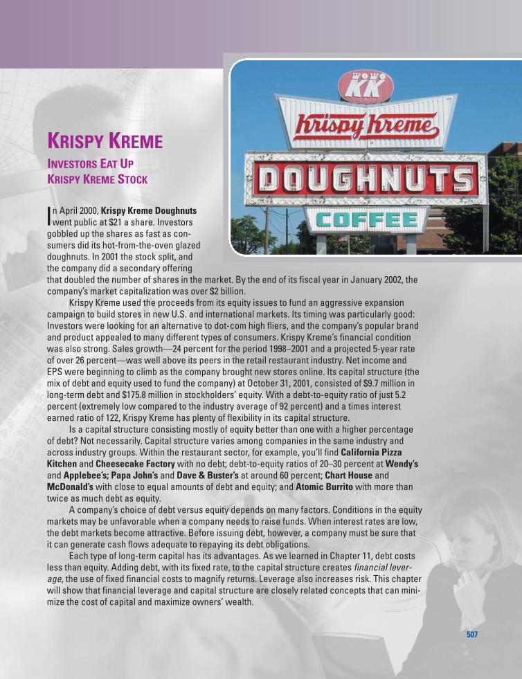
T A B L E 1 2 . 1 General Income Statement Format and Types of Leverage
Sales revenue
L�
e�s�s�:��C�
o�s�t��
o�f��
g�o�o�d�
s��
s�o�l�d�
Operating leverage Gross profits
L�
e�s�s�:��O�
p�e�r�a�t�i�n�g��
e�x�p�e�n�s�e�s���������������
Earnings before interest and taxes (EBIT)
L�
e�s�s�:��I�n�t�e�r�e�s�t�����������
Total leverageNet profits before taxes
L�
e�s�s�:��T�
a�x�e�s����������
Financial leverageNet profits after taxes
L�
e�s�s�:��P�r�e�f�e�r�r�e�d��
s�t�o�c�k��
d�i�v�i�d�e�n�d�s�������������
Earnings available for common stockholders
Earnings per share (EPS)
LG1 LG2
leverageResults from the use of fixed-costassets or funds to magnifyreturns to the firm’s owners.
12.1 LeverageLeverage results from the use of fixed-cost assets or funds to magnify returns tothe firm’s owners. Generally, increases in leverage result in increased return andrisk, whereas decreases in leverage result in decreased return and risk. Theamount of leverage in the firm’s capital structure—the mix of long-term debt andequity maintained by the firm—can significantly affect its value by affectingreturn and risk. Unlike some causes of risk, management has almost completecontrol over the risk introduced through the use of leverage. Because of its effecton value, the financial manager must understand how to measure and evaluateleverage, particularly when making capital structure decisions.
The three basic types of leverage can best be defined with reference to thefirm’s income statement, as shown in the general income statement format inTable 12.1.
• Operating leverage is concerned with the relationship between the firm’ssales revenue and its earnings before interest and taxes, or EBIT. (EBIT is adescriptive label for operating profits.)
• Financial leverage is concerned with the relationship between the firm’s EBITand its common stock earnings per share (EPS).
• Total leverage is concerned with the relationship between the firm’s sales rev-enue and EPS.
We will examine the three types of leverage concepts in detail in sections thatfollow. First, though, we will look at breakeven analysis, which lays the founda-tion for leverage concepts by demonstrating the effects of fixed costs on the firm’soperations.
breakeven analysisIndicates the level of operationsnecessary to cover all operatingcosts and the profitability associ-ated with various levels of sales.
operating breakeven pointThe level of sales necessary tocover all operating costs; thepoint at which EBIT � $0.
CHAPTER 12 Leverage and Capital Structure 509
1. Quite often, the breakeven point is calculated so that it represents the point at which all operating and financialcosts are covered. Our concern in this chapter is not with this overall breakeven point.2. Some costs, commonly called semifixed or semivariable, are partly fixed and partly variable. An example is salescommissions that are fixed for a certain volume of sales and then increase to higher levels for higher volumes. Forconvenience and clarity, we assume that all costs can be classified as either fixed or variable.
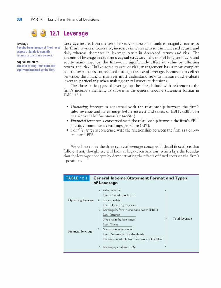
T A B L E 1 2 . 2 Operating Leverage, Costs, andBreakeven Analysis
AlgebraicItem representation
Sales revenue (P�Q)
Operating leverageLess: Fixed operating costs � FC
L�
e�s�s�:��V�
a�r�i�a�b�l�e��
o�p�e�r�a�t�i�n�g��
c�o�s�t�s�����
��
(�V�
C��
���
Q�
)�
Earnings before interest and taxes EBIT
Breakeven AnalysisBreakeven analysis, sometimes called cost-volume-profit analysis, is used by thefirm (1) to determine the level of operations necessary to cover all operating costsand (2) to evaluate the profitability associated with various levels of sales. Thefirm’s operating breakeven point is the level of sales necessary to cover all operat-ing costs. At that point, earnings before interest and taxes equals $0.1
The first step in finding the operating breakeven point is to divide the cost ofgoods sold and operating expenses into fixed and variable operating costs. Fixedcosts are a function of time, not sales volume, and are typically contractual; rent,for example, is a fixed cost. Variable costs vary directly with sales and are a func-tion of volume, not time; shipping costs, for example, are a variable cost.2
The Algebraic Approach
Using the following variables, we can recast the operating portion of the firm’sincome statement given in Table 12.1 into the algebraic representation shown inTable 12.2.
P� sale price per unitQ� sales quantity in units
FC� fixed operating cost per periodVC�variable operating cost per unit
Rewriting the algebraic calculations in Table 12.2 as a formula for earningsbefore interest and taxes yields Equation 12.1:
EBIT� (P�Q)�FC� (VC�Q) (12.1)
Simplifying Equation 12.1 yields
EBIT�Q� (P�VC)�FC (12.2)
510 PART 4 Long-Term Financial Decisions
3. Because the firm is assumed to be a single-product firm, its operating breakeven point is found in terms of unitsales, Q. For multiproduct firms, the operating breakeven point is generally found in terms of dollar sales, S. This isdone by substituting the contribution margin, which is 100% minus total variable operating costs as a percentage oftotal sales, denoted VC%, into the denominator of Equation 12.3. The result is Equation 12.3a:
S� (12.3a)
This multiproduct-firm breakeven point assumes that the firm’s product mix remains the same at all levels of sales.
FC��1�VC%
As noted above, the operating breakeven point is the level of sales at which allfixed and variable operating costs are covered—the level at which EBIT equals$0. Setting EBIT equal to $0 and solving Equation 12.2 for Q yield
Q� (12.3)
Q is the firm’s operating breakeven point.3
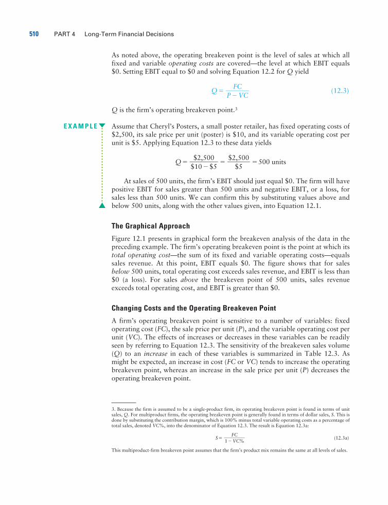
E X A M P L E Assume that Cheryl’s Posters, a small poster retailer, has fixed operating costs of$2,500, its sale price per unit (poster) is $10, and its variable operating cost perunit is $5. Applying Equation 12.3 to these data yields
Q� � �500 units
At sales of 500 units, the firm’s EBIT should just equal $0. The firm will havepositive EBIT for sales greater than 500 units and negative EBIT, or a loss, forsales less than 500 units. We can confirm this by substituting values above andbelow 500 units, along with the other values given, into Equation 12.1.
The Graphical Approach
Figure 12.1 presents in graphical form the breakeven analysis of the data in thepreceding example. The firm’s operating breakeven point is the point at which itstotal operating cost—the sum of its fixed and variable operating costs—equalssales revenue. At this point, EBIT equals $0. The figure shows that for salesbelow 500 units, total operating cost exceeds sales revenue, and EBIT is less than$0 (a loss). For sales above the breakeven point of 500 units, sales revenueexceeds total operating cost, and EBIT is greater than $0.
Changing Costs and the Operating Breakeven Point
A firm’s operating breakeven point is sensitive to a number of variables: fixedoperating cost (FC), the sale price per unit (P), and the variable operating cost perunit (VC). The effects of increases or decreases in these variables can be readilyseen by referring to Equation 12.3. The sensitivity of the breakeven sales volume(Q) to an increase in each of these variables is summarized in Table 12.3. Asmight be expected, an increase in cost (FC or VC) tends to increase the operatingbreakeven point, whereas an increase in the sale price per unit (P) decreases theoperating breakeven point.
$2,500�
$5$2,500
��$10�$5
FC�P�VC
CHAPTER 12 Leverage and Capital Structure 511
Sales Revenue
TotalOperatingCost
Operating Breakeven Point
EBIT
FixedOperatingCost
5000 1,000 1,500 2,000 2,500 3,000
Loss
12,000
10,000
8,000
6,000
4,000
2,000
Cost
s/Rev
enues
($)
Sales (units)
FIGURE 12 .1
Breakeven Analysis
Graphical operatingbreakeven analysis
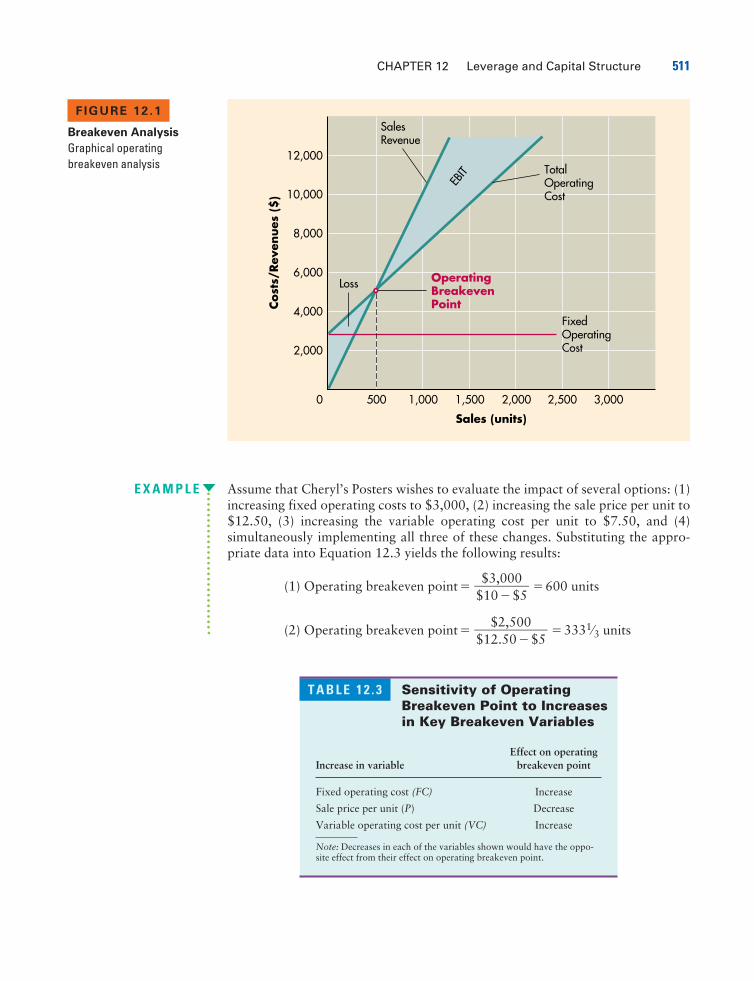
T A B L E 1 2 . 3 Sensitivity of OperatingBreakeven Point to Increasesin Key Breakeven Variables
Effect on operatingIncrease in variable breakeven point
Fixed operating cost (FC) Increase
Sale price per unit (P) Decrease
Variable operating cost per unit (VC) Increase
Note: Decreases in each of the variables shown would have the oppo-site effect from their effect on operating breakeven point.
E X A M P L E Assume that Cheryl’s Posters wishes to evaluate the impact of several options: (1)increasing fixed operating costs to $3,000, (2) increasing the sale price per unit to$12.50, (3) increasing the variable operating cost per unit to $7.50, and (4)simultaneously implementing all three of these changes. Substituting the appro-priate data into Equation 12.3 yields the following results:
(1) Operating breakeven point� �600 units
(2) Operating breakeven point� �3331⁄3 units$2,500
��$12.50�$5
$3,000��$10�$5
512 PART 4 Long-Term Financial Decisions
2,000
4,000
6,000
8,000
10,000
12,000
14,000
16,000
5000 1,000 1,500 2,000 2,500 3,000Q1 Q2
Sales (units)
Cost
s/Rev
enues
($)
EBIT1($2,500)
EBIT2($5,000)
Loss
EBIT
FixedOperatingCost
TotalOperatingCost
Sales Revenue
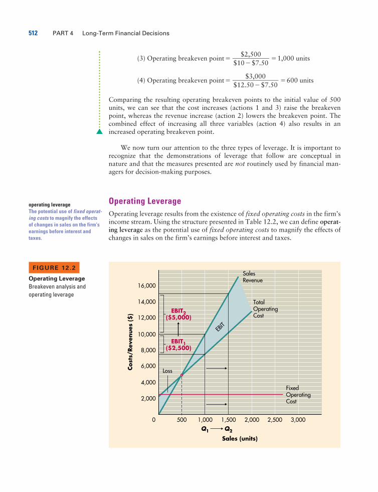
FIGURE 12 .2
Operating Leverage
Breakeven analysis andoperating leverage
operating leverageThe potential use of fixed operat-ing costs to magnify the effectsof changes in sales on the firm’searnings before interest andtaxes.
(3) Operating breakeven point� �1,000 units
(4) Operating breakeven point� �600 units
Comparing the resulting operating breakeven points to the initial value of 500units, we can see that the cost increases (actions 1 and 3) raise the breakevenpoint, whereas the revenue increase (action 2) lowers the breakeven point. Thecombined effect of increasing all three variables (action 4) also results in anincreased operating breakeven point.
We now turn our attention to the three types of leverage. It is important torecognize that the demonstrations of leverage that follow are conceptual innature and that the measures presented are not routinely used by financial man-agers for decision-making purposes.
Operating LeverageOperating leverage results from the existence of fixed operating costs in the firm’sincome stream. Using the structure presented in Table 12.2, we can define operat-ing leverage as the potential use of fixed operating costs to magnify the effects ofchanges in sales on the firm’s earnings before interest and taxes.
$3,000��$12.50�$7.50
$2,500��$10�$7.50
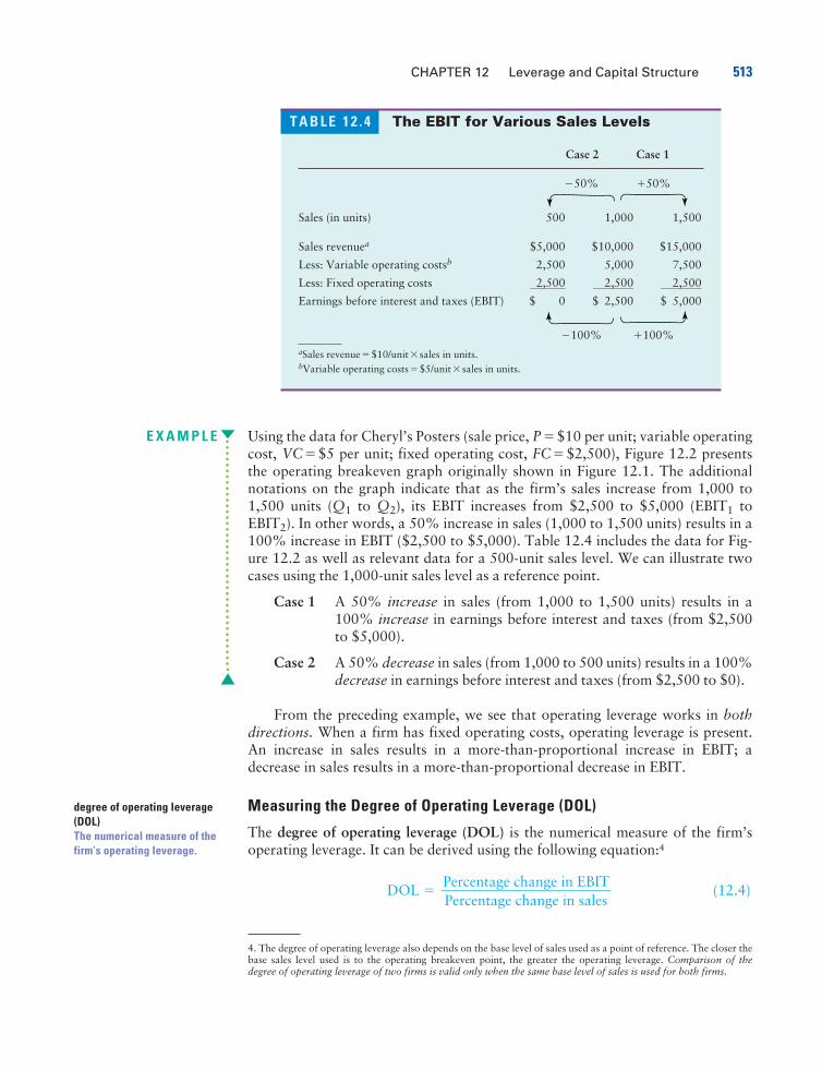
E X A M P L E Using the data for Cheryl’s Posters (sale price, P�$10 per unit; variable operatingcost, VC�$5 per unit; fixed operating cost, FC�$2,500), Figure 12.2 presentsthe operating breakeven graph originally shown in Figure 12.1. The additionalnotations on the graph indicate that as the firm’s sales increase from 1,000 to1,500 units (Q1 to Q2), its EBIT increases from $2,500 to $5,000 (EBIT1 toEBIT2). In other words, a 50% increase in sales (1,000 to 1,500 units) results in a100% increase in EBIT ($2,500 to $5,000). Table 12.4 includes the data for Fig-ure 12.2 as well as relevant data for a 500-unit sales level. We can illustrate twocases using the 1,000-unit sales level as a reference point.
Case 1 A 50% increase in sales (from 1,000 to 1,500 units) results in a100% increase in earnings before interest and taxes (from $2,500to $5,000).
Case 2 A 50% decrease in sales (from 1,000 to 500 units) results in a 100%decrease in earnings before interest and taxes (from $2,500 to $0).
From the preceding example, we see that operating leverage works in bothdirections. When a firm has fixed operating costs, operating leverage is present.An increase in sales results in a more-than-proportional increase in EBIT; adecrease in sales results in a more-than-proportional decrease in EBIT.
Measuring the Degree of Operating Leverage (DOL)
The degree of operating leverage (DOL) is the numerical measure of the firm’soperating leverage. It can be derived using the following equation:4
DOL � (12.4)Percentage change in EBIT���Percentage change in sales
CHAPTER 12 Leverage and Capital Structure 513
degree of operating leverage(DOL)The numerical measure of thefirm’s operating leverage.
T A B L E 1 2 . 4 The EBIT for Various Sales Levels
Case 2 Case 1
�50% �50%
Sales (in units) 500 1,000 1,500
Sales revenuea $5,000 $10,000 $15,000
Less: Variable operating costsb 2,500 5,000 7,500
Less: Fixed operating costs�2�,�5�0�0� ��
2�
,�5�0�0� ��
2�,�5�0�0�
Earnings before interest and taxes (EBIT) $ 0 $ 2,500 $ 5,000
�100% �100%aSales revenue�$10/unit� sales in units.bVariable operating costs�$5/unit� sales in units.
4. The degree of operating leverage also depends on the base level of sales used as a point of reference. The closer thebase sales level used is to the operating breakeven point, the greater the operating leverage. Comparison of thedegree of operating leverage of two firms is valid only when the same base level of sales is used for both firms.
514 PART 4 Long-Term Financial Decisions
5. Because the concept of leverage is linear, positive and negative changes of equal magnitude will always result inequal degrees of leverage when the same base sales level is used as a point of reference. This relationship holds for alltypes of leverage discussed in this chapter.6. Technically, the formula for DOL given in Equation 12.5 should include absolute value signs because it is possibleto get a negative DOL when the EBIT for the base sales level is negative. Because we assume that the EBIT for thebase level of sales is positive, we do not use the absolute value signs.7. When total sales in dollars—instead of unit sales—are available, the following equation, in which TR�dollarlevel of base sales and TVC� total variable operating costs in dollars, can be used.
DOL at base dollar sales TR�
This formula is especially useful for finding the DOL for multiproduct firms. It should be clear that because in thecase of a single-product firm, TR�P�Q and TVC�VC�Q, substitution of these values into Equation 12.5results in the equation given here.
TR�TVC��TR�TVC�FC
Whenever the percentage change in EBIT resulting from a given percentage changein sales is greater than the percentage change in sales, operating leverage exists.This means that as long as DOL is greater than 1, there is operating leverage.
E X A M P L E Applying Equation 12.4 to cases 1 and 2 in Table 12.4 yields the following results:5
Case 1: �2.0
Case 2: �2.0
Because the result is greater than 1, operating leverage exists. For a given baselevel of sales, the higher the value resulting from applying Equation 12.4, thegreater the degree of operating leverage.
A more direct formula for calculating the degree of operating leverage at abase sales level, Q, is shown in Equation 12.5.6
DOL at base sales level Q� (12.5)
E X A M P L E Substituting Q�1,000, P�$10, VC�$5, and FC�$2,500 into Equation 12.5yields the following result:
DOL at 1,000 units� � �2.0
The use of the formula results in the same value for DOL (2.0) as that found byusing Table 12.4 and Equation 12.4.7
Fixed Costs and Operating Leverage
Changes in fixed operating costs affect operating leverage significantly. Firmssometimes can incur fixed operating costs rather than variable operating costsand at other times may be able to substitute one type of cost for the other. Forexample, a firm could make fixed-dollar lease payments rather than paymentsequal to a specified percentage of sales. Or it could compensate sales representa-tives with a fixed salary and bonus rather than on a pure percent-of-sales com-
$5,000�$2,500
1,000� ($10�$5)����1,000� ($10�$5)�$2,500
Q� (P�VC)���Q� (P�VC)�FC
�100%��50%
�100%��50%
CHAPTER 12 Leverage and Capital Structure 515
In Practice
Adobe Systems, the secondlargest PC software company inthe United States, dominates thegraphic design, imaging, dynamicmedia, and authoring-tool soft-ware markets. Web site designersprefer its Photoshop and Illustratorsoftware applications, andAdobe’s Acrobat software hasbecome a standard for sharingdocuments online.
Despite a sales slowdown in2001, the company continued tomeet its earnings targets. Its abil-ity to manage discretionaryexpenses helped to keep its bot-tom line strong. As a softwarecompany, it has an additionaladvantage: operating leverage, theuse of fixed operating costs tomagnify the effect of changes insales on earnings before interestand taxes (EBIT).
Adobe and its peers in thesoftware industry incur the bulk oftheir costs early in a product’s lifecycle, in the research and devel-opment and initial marketingstages. The up-front developmentcosts are fixed, regardless of how
many copies of a program thecompany sells, and subsequentproduction costs are practicallyzero. The economies of scale arehuge; once a company sellsenough copies to cover its fixedcosts, incremental revenue dollarsgo primarily to profit.
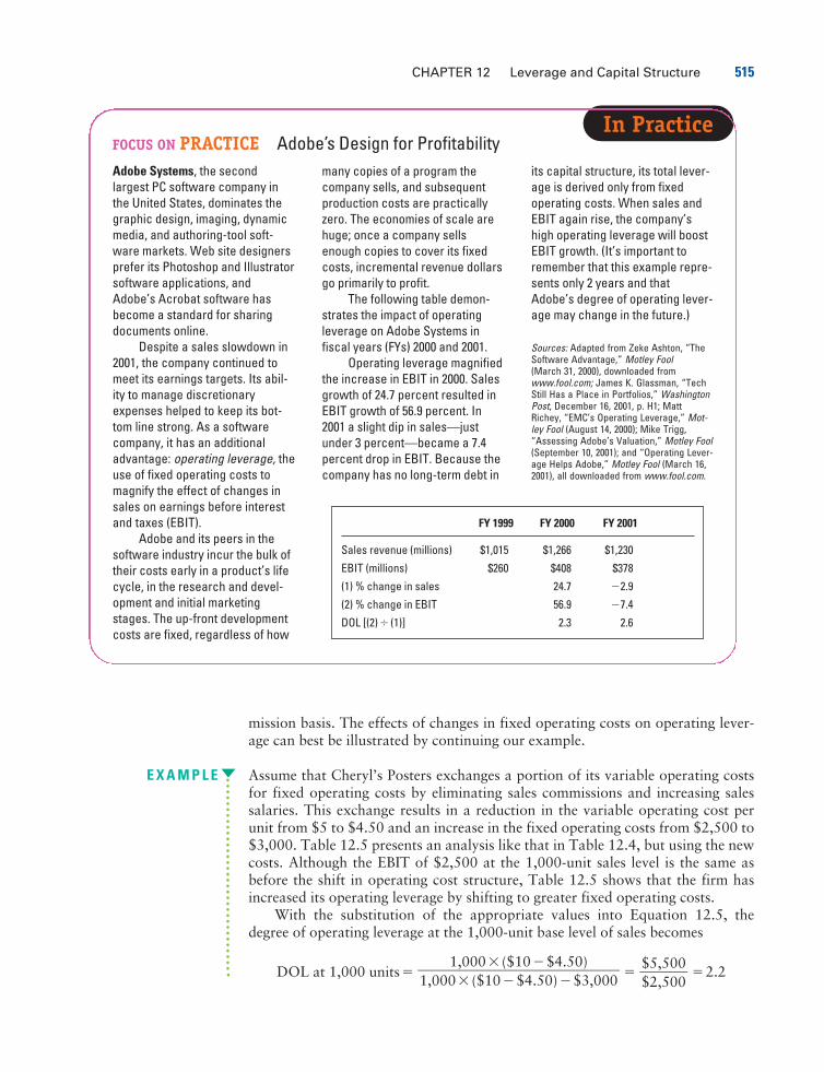
The following table demon-strates the impact of operatingleverage on Adobe Systems infiscal years (FYs) 2000 and 2001.
Operating leverage magnifiedthe increase in EBIT in 2000. Salesgrowth of 24.7 percent resulted inEBIT growth of 56.9 percent. In2001 a slight dip in sales—justunder 3 percent—became a 7.4percent drop in EBIT. Because thecompany has no long-term debt in
its capital structure, its total lever-age is derived only from fixedoperating costs. When sales andEBIT again rise, the company’shigh operating leverage will boostEBIT growth. (It’s important toremember that this example repre-sents only 2 years and thatAdobe’s degree of operating lever-age may change in the future.)
Sources: Adapted from Zeke Ashton, “TheSoftware Advantage,” Motley Fool(March 31, 2000), downloaded fromwww.fool.com; James K. Glassman, “TechStill Has a Place in Portfolios,” WashingtonPost, December 16, 2001, p. H1; MattRichey, “EMC’s Operating Leverage,” Mot-ley Fool (August 14, 2000); Mike Trigg,“Assessing Adobe’s Valuation,” Motley Fool(September 10, 2001); and “Operating Lever-age Helps Adobe,” Motley Fool (March 16,2001), all downloaded from www.fool.com.
FOCUS ON PRACTICE Adobe’s Design for Profitability
FY 1999 FY 2000 FY 2001
Sales revenue (millions) $1,015 $1,266 $1,230
EBIT (millions) $260 $408 $378
(1) % change in sales 24.7 �2.9
(2) % change in EBIT 56.9 �7.4
DOL [(2) � (1)] 2.3 2.6
mission basis. The effects of changes in fixed operating costs on operating lever-age can best be illustrated by continuing our example.
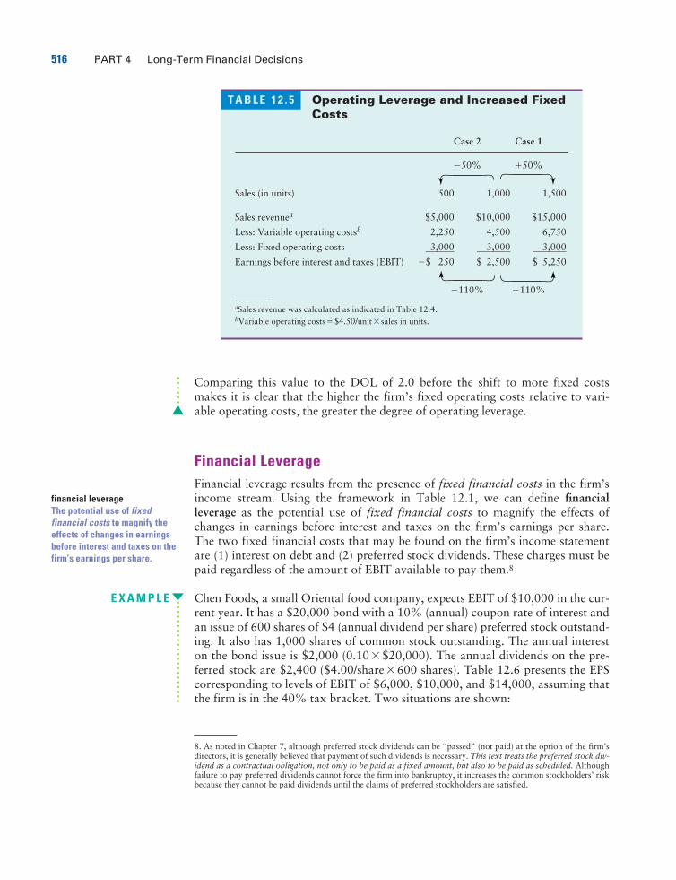
E X A M P L E Assume that Cheryl’s Posters exchanges a portion of its variable operating costsfor fixed operating costs by eliminating sales commissions and increasing salessalaries. This exchange results in a reduction in the variable operating cost perunit from $5 to $4.50 and an increase in the fixed operating costs from $2,500 to$3,000. Table 12.5 presents an analysis like that in Table 12.4, but using the newcosts. Although the EBIT of $2,500 at the 1,000-unit sales level is the same asbefore the shift in operating cost structure, Table 12.5 shows that the firm hasincreased its operating leverage by shifting to greater fixed operating costs.
With the substitution of the appropriate values into Equation 12.5, thedegree of operating leverage at the 1,000-unit base level of sales becomes
DOL at 1,000 units� � �2.2$5,500�$2,500
1,000� ($10�$4.50)����1,000� ($10�$4.50)�$3,000
516 PART 4 Long-Term Financial Decisions
8. As noted in Chapter 7, although preferred stock dividends can be “passed” (not paid) at the option of the firm’sdirectors, it is generally believed that payment of such dividends is necessary. This text treats the preferred stock div-idend as a contractual obligation, not only to be paid as a fixed amount, but also to be paid as scheduled. Althoughfailure to pay preferred dividends cannot force the firm into bankruptcy, it increases the common stockholders’ riskbecause they cannot be paid dividends until the claims of preferred stockholders are satisfied.
T A B L E 1 2 . 5 Operating Leverage and Increased FixedCosts
Case 2 Case 1
�50% �50%
Sales (in units) 500 1,000 1,500
Sales revenuea $5,000 $10,000 $15,000
Less: Variable operating costsb 2,250 4,500 6,750
Less: Fixed operating costs�3�,�0�0�0� ��
3�,�0�0�0� ��
3�,�0�0�0�
Earnings before interest and taxes (EBIT) �$ 250 $ 2,500 $ 5,250
�110% �110%
aSales revenue was calculated as indicated in Table 12.4.bVariable operating costs�$4.50/unit� sales in units.
financial leverageThe potential use of fixedfinancial costs to magnify theeffects of changes in earningsbefore interest and taxes on thefirm’s earnings per share.
Comparing this value to the DOL of 2.0 before the shift to more fixed costsmakes it is clear that the higher the firm’s fixed operating costs relative to vari-able operating costs, the greater the degree of operating leverage.
Financial LeverageFinancial leverage results from the presence of fixed financial costs in the firm’sincome stream. Using the framework in Table 12.1, we can define financialleverage as the potential use of fixed financial costs to magnify the effects ofchanges in earnings before interest and taxes on the firm’s earnings per share.The two fixed financial costs that may be found on the firm’s income statementare (1) interest on debt and (2) preferred stock dividends. These charges must bepaid regardless of the amount of EBIT available to pay them.8
E X A M P L E Chen Foods, a small Oriental food company, expects EBIT of $10,000 in the cur-rent year. It has a $20,000 bond with a 10% (annual) coupon rate of interest andan issue of 600 shares of $4 (annual dividend per share) preferred stock outstand-ing. It also has 1,000 shares of common stock outstanding. The annual intereston the bond issue is $2,000 (0.10�$20,000). The annual dividends on the pre-ferred stock are $2,400 ($4.00/share�600 shares). Table 12.6 presents the EPScorresponding to levels of EBIT of $6,000, $10,000, and $14,000, assuming thatthe firm is in the 40% tax bracket. Two situations are shown:
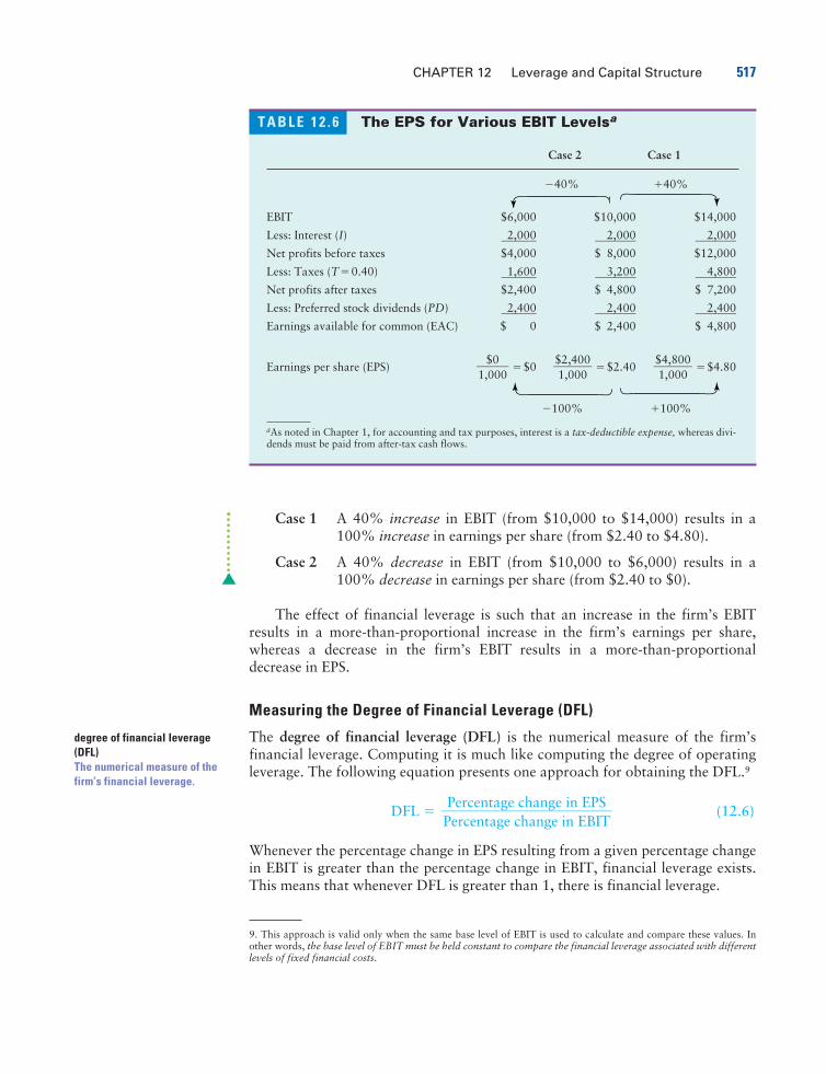
Case 1 A 40% increase in EBIT (from $10,000 to $14,000) results in a100% increase in earnings per share (from $2.40 to $4.80).
Case 2 A 40% decrease in EBIT (from $10,000 to $6,000) results in a100% decrease in earnings per share (from $2.40 to $0).
The effect of financial leverage is such that an increase in the firm’s EBITresults in a more-than-proportional increase in the firm’s earnings per share,whereas a decrease in the firm’s EBIT results in a more-than-proportionaldecrease in EPS.
Measuring the Degree of Financial Leverage (DFL)
The degree of financial leverage (DFL) is the numerical measure of the firm’sfinancial leverage. Computing it is much like computing the degree of operatingleverage. The following equation presents one approach for obtaining the DFL.9
DFL � (12.6)
Whenever the percentage change in EPS resulting from a given percentage changein EBIT is greater than the percentage change in EBIT, financial leverage exists.This means that whenever DFL is greater than 1, there is financial leverage.
Percentage change in EPS���Percentage change in EBIT
CHAPTER 12 Leverage and Capital Structure 517
degree of financial leverage(DFL)The numerical measure of thefirm’s financial leverage.
T A B L E 1 2 . 6 The EPS for Various EBIT Levelsa
Case 2 Case 1
�40% �40%
EBIT $6,000 $10,000 $14,000
Less: Interest (I)�2�,�0�0�0� ��
2�,�0�0�0� ��
2�,�0�0�0�
Net profits before taxes $4,000 $ 8,000 $12,000
Less: Taxes (T�0.40)�1�,�6�0�0� ��
3�,�2�0�0� ��
4�,�8�0�0�
Net profits after taxes $2,400 $ 4,800 $ 7,200
Less: Preferred stock dividends (PD)�2�,�4�0�0� ��
2�,�4�0�0� ��
2�,�4�0�0�
Earnings available for common (EAC) $ 0 $ 2,400 $ 4,800
Earnings per share (EPS) �$0 �$2.40 �$4.80
�100% �100%
aAs noted in Chapter 1, for accounting and tax purposes, interest is a tax-deductible expense, whereas divi-dends must be paid from after-tax cash flows.
$4,800�1,000
$2,400�1,000
$0�1,000
9. This approach is valid only when the same base level of EBIT is used to calculate and compare these values. Inother words, the base level of EBIT must be held constant to compare the financial leverage associated with differentlevels of fixed financial costs.
518 PART 4 Long-Term Financial Decisions
10. By using the formula for DFL in Equation 12.7, it is possible to get a negative value for the DFL if the EPS for thebase level of EBIT is negative. Rather than show absolute value signs in the equation, we instead assume that thebase-level EPS is positive.
total leverageThe potential use of fixed costs,both operating and financial, tomagnify the effect of changes insales on the firm’s earnings pershare.
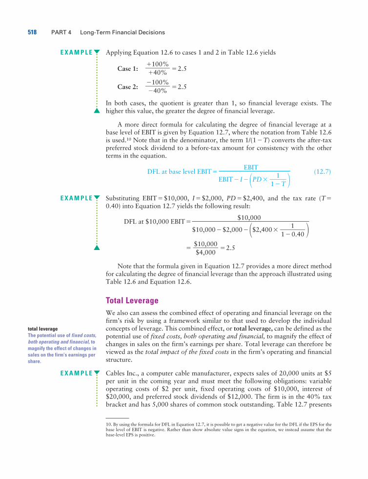
E X A M P L E Applying Equation 12.6 to cases 1 and 2 in Table 12.6 yields
Case 1: �2.5
Case 2: �2.5
In both cases, the quotient is greater than 1, so financial leverage exists. Thehigher this value, the greater the degree of financial leverage.
A more direct formula for calculating the degree of financial leverage at abase level of EBIT is given by Equation 12.7, where the notation from Table 12.6is used.10 Note that in the denominator, the term 1/(1�T) converts the after-taxpreferred stock dividend to a before-tax amount for consistency with the otherterms in the equation.
EBIT(12.7)DFL at base level EBIT�
EBIT� I��PD� �E X A M P L E Substituting EBIT�$10,000, I�$2,000, PD�$2,400, and the tax rate (T�
0.40) into Equation 12.7 yields the following result:
$10,000DFL at $10,000 EBIT�
$10,000�$2,000��$2,400� �� �2.5
Note that the formula given in Equation 12.7 provides a more direct methodfor calculating the degree of financial leverage than the approach illustrated usingTable 12.6 and Equation 12.6.
Total LeverageWe also can assess the combined effect of operating and financial leverage on thefirm’s risk by using a framework similar to that used to develop the individualconcepts of leverage. This combined effect, or total leverage, can be defined as thepotential use of fixed costs, both operating and financial, to magnify the effect ofchanges in sales on the firm’s earnings per share. Total leverage can therefore beviewed as the total impact of the fixed costs in the firm’s operating and financialstructure.
E X A M P L E Cables Inc., a computer cable manufacturer, expects sales of 20,000 units at $5per unit in the coming year and must meet the following obligations: variableoperating costs of $2 per unit, fixed operating costs of $10,000, interest of$20,000, and preferred stock dividends of $12,000. The firm is in the 40% taxbracket and has 5,000 shares of common stock outstanding. Table 12.7 presents
$10,000�$4,000
1�1�0.40
1�1�T
�100%��40%
�100%��40%
CHAPTER 12 Leverage and Capital Structure 519
degree of total leverage (DTL)The numerical measure of thefirm’s total leverage.
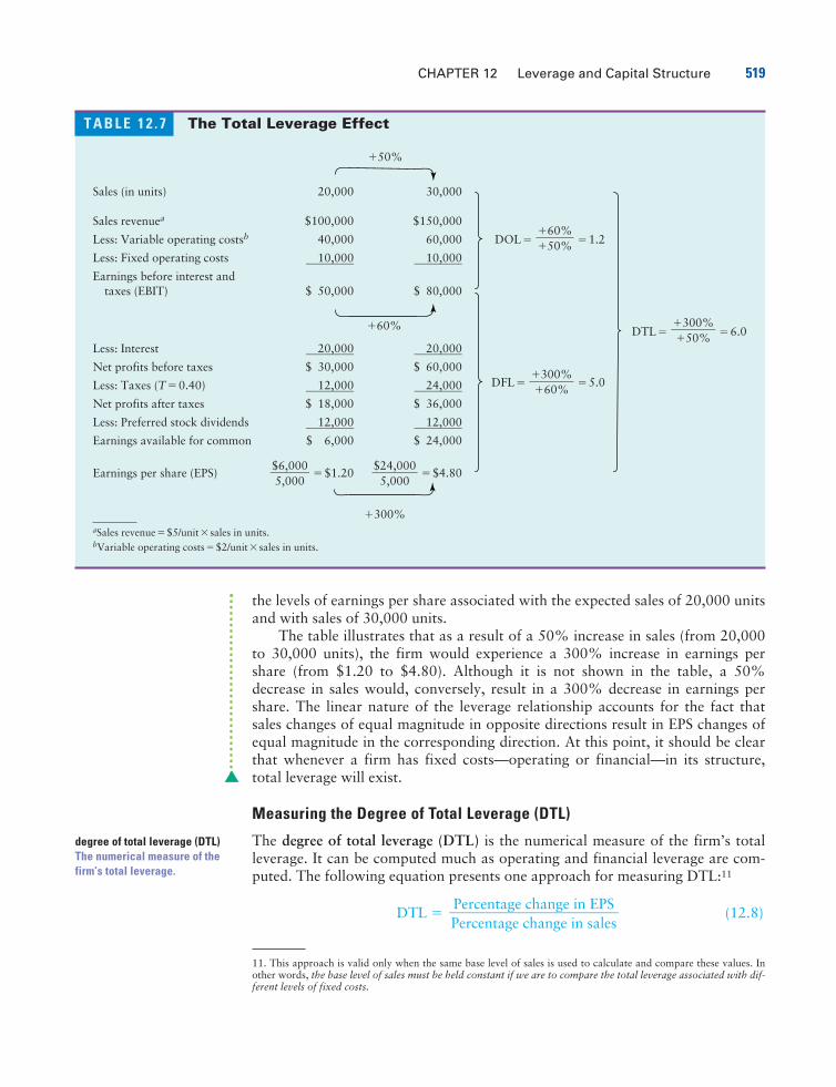
T A B L E 1 2 . 7 The Total Leverage Effect
�50%
Sales (in units) 20,000 30,000
Sales revenuea $100,000 $150,000
Less: Variable operating costsb 40,000 60,000 DOL� �1.2
Less: Fixed operating costs��
1�0�,�0�0�0� ��
1�0�,�0�0�0�
Earnings before interest andtaxes (EBIT) $ 50,000 $ 80,000
�60% DTL� �6.0Less: Interest
��2�0�,�0�0�0� ��
2�0�,�0�0�0�
Net profits before taxes $ 30,000 $ 60,000
Less: Taxes (T�0.40)��
1�2�,�0�0�0� ��
2�4�,�0�0�0�
DFL� �5.0
Net profits after taxes $ 18,000 $ 36,000
Less: Preferred stock dividends��
1�2�,�0�0�0� ��
1�2�,�0�0�0�
Earnings available for common $ 6,000 $ 24,000
Earnings per share (EPS) �$1.20 �$4.80
�300%aSales revenue�$5/unit� sales in units.bVariable operating costs�$2/unit� sales in units.
$24,000�
5,000$6,000�5,000
�300%��60%
�300%��50%
�60%��50%
11. This approach is valid only when the same base level of sales is used to calculate and compare these values. Inother words, the base level of sales must be held constant if we are to compare the total leverage associated with dif-ferent levels of fixed costs.
the levels of earnings per share associated with the expected sales of 20,000 unitsand with sales of 30,000 units.
The table illustrates that as a result of a 50% increase in sales (from 20,000to 30,000 units), the firm would experience a 300% increase in earnings pershare (from $1.20 to $4.80). Although it is not shown in the table, a 50%decrease in sales would, conversely, result in a 300% decrease in earnings pershare. The linear nature of the leverage relationship accounts for the fact thatsales changes of equal magnitude in opposite directions result in EPS changes ofequal magnitude in the corresponding direction. At this point, it should be clearthat whenever a firm has fixed costs—operating or financial—in its structure,total leverage will exist.
Measuring the Degree of Total Leverage (DTL)
The degree of total leverage (DTL) is the numerical measure of the firm’s totalleverage. It can be computed much as operating and financial leverage are com-puted. The following equation presents one approach for measuring DTL:11
DTL � (12.8)Percentage change in EPS���Percentage change in sales
520 PART 4 Long-Term Financial Decisions
12. By using the formula for DTL in Equation 12.9, it is possible to get a negative value for the DTL if the EPS forthe base level of sales is negative. For our purposes, rather than show absolute value signs in the equation, weinstead assume that the base-level EPS is positive.
Whenever the percentage change in EPS resulting from a given percentage changein sales is greater than the percentage change in sales, total leverage exists. Thismeans that as long as the DTL is greater than 1, there is total leverage.
E X A M P L E Applying Equation 12.8 to the data in Table 12.7 yields
DTL� �6.0
Because this result is greater than 1, total leverage exists. The higher the value,the greater the degree of total leverage.
A more direct formula for calculating the degree of total leverage at a givenbase level of sales, Q, is given by Equation 12.9,12 which uses the same notationthat was presented earlier:
Q� (P�VC)(12.9)DTL at base sales level Q�
Q� (P�VC)�FC� I��PD� �E X A M P L E Substituting Q�20,000, P�$5, VC�$2, FC�$10,000, I�$20,000, PD�
$12,000, and the tax rate (T�0.40) into Equation 12.9 yields
DTL at 20,000 units20,000� ($5�$2)
�
20,000� ($5�$2)�$10,000�$20,000��$12,000� �� �6.0
Clearly, the formula used in Equation 12.9 provides a more direct method forcalculating the degree of total leverage than the approach illustrated using Table12.7 and Equation 12.8.
The Relationship of Operating, Financial, and Total Leverage
Total leverage reflects the combined impact of operating and financial leverageon the firm. High operating leverage and high financial leverage will cause totalleverage to be high. The opposite will also be true. The relationship between oper-ating leverage and financial leverage is multiplicative rather than additive. Therelationship between the degree of total leverage (DTL) and the degrees of operat-ing leverage (DOL) and financial leverage (DFL) is given by Equation 12.10.
DTL�DOL�DFL (12.10)
$60,000�$10,000
1�1�0.40
1�1�T
�300%��50%
CHAPTER 12 Leverage and Capital Structure 521
13. Of course, although capital structure is financially important, it, like many business decisions, is generally not soimportant as the firm’s products or services. In a practical sense, a firm can probably more readily increase its valueby improving quality and reducing costs than by fine-tuning its capital structure.
LG3 LG4
E X A M P L E Substituting the values calculated for DOL and DFL, shown on the right-handside of Table 12.7, into Equation 12.10 yields
DTL�1.2�5.0�6.0
The resulting degree of total leverage is the same value that we calculated directlyin the preceding examples.
R e v i e w Q u e s t i o n s
12–1 What is meant by the term leverage? How are operating leverage, financialleverage, and total leverage related to the income statement?
12–2 What is the operating breakeven point? How do changes in fixed operat-ing costs, the sale price per unit, and the variable operating cost per unitaffect it?
12–3 What is operating leverage? What causes it? How is the degree of operat-ing leverage (DOL) measured?
12–4 What is financial leverage? What causes it? How is the degree of financialleverage (DFL) measured?
12–5 What is the general relationship among operating leverage, financial lever-age, and the total leverage of the firm? Do these types of leverage comple-ment each other? Why or why not?
12.2 The Firm’s Capital StructureCapital structure is one of the most complex areas of financial decision makingbecause of its interrelationship with other financial decision variables.13 Poorcapital structure decisions can result in a high cost of capital, thereby loweringthe NPVs of projects and making more of them unacceptable. Effective capitalstructure decisions can lower the cost of capital, resulting in higher NPVs andmore acceptable projects—and thereby increasing the value of the firm. This sec-tion links together many of the concepts presented in Chapters 4, 5, 6, 7, and 11and the discussion of leverage in this chapter.
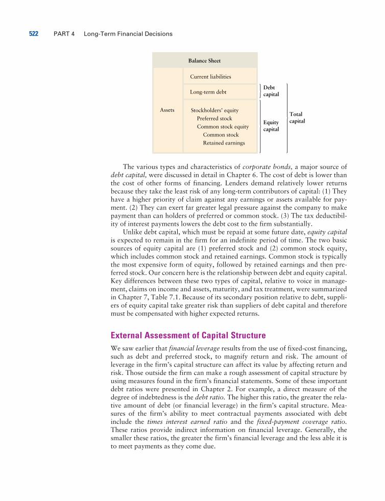
Types of CapitalAll of the items on the right-hand side of the firm’s balance sheet, excluding cur-rent liabilities, are sources of capital. The following simplified balance sheet illus-trates the basic breakdown of total capital into its two components, debt capitaland equity capital.
522 PART 4 Long-Term Financial Decisions
The various types and characteristics of corporate bonds, a major source ofdebt capital, were discussed in detail in Chapter 6. The cost of debt is lower thanthe cost of other forms of financing. Lenders demand relatively lower returnsbecause they take the least risk of any long-term contributors of capital: (1) Theyhave a higher priority of claim against any earnings or assets available for pay-ment. (2) They can exert far greater legal pressure against the company to makepayment than can holders of preferred or common stock. (3) The tax deductibil-ity of interest payments lowers the debt cost to the firm substantially.
Unlike debt capital, which must be repaid at some future date, equity capitalis expected to remain in the firm for an indefinite period of time. The two basicsources of equity capital are (1) preferred stock and (2) common stock equity,which includes common stock and retained earnings. Common stock is typicallythe most expensive form of equity, followed by retained earnings and then pre-ferred stock. Our concern here is the relationship between debt and equity capital.Key differences between these two types of capital, relative to voice in manage-ment, claims on income and assets, maturity, and tax treatment, were summarizedin Chapter 7, Table 7.1. Because of its secondary position relative to debt, suppli-ers of equity capital take greater risk than suppliers of debt capital and thereforemust be compensated with higher expected returns.
External Assessment of Capital StructureWe saw earlier that financial leverage results from the use of fixed-cost financing,such as debt and preferred stock, to magnify return and risk. The amount ofleverage in the firm’s capital structure can affect its value by affecting return andrisk. Those outside the firm can make a rough assessment of capital structure byusing measures found in the firm’s financial statements. Some of these importantdebt ratios were presented in Chapter 2. For example, a direct measure of thedegree of indebtedness is the debt ratio. The higher this ratio, the greater the rela-tive amount of debt (or financial leverage) in the firm’s capital structure. Mea-sures of the firm’s ability to meet contractual payments associated with debtinclude the times interest earned ratio and the fixed-payment coverage ratio.These ratios provide indirect information on financial leverage. Generally, thesmaller these ratios, the greater the firm’s financial leverage and the less able it isto meet payments as they come due.
Balance Sheet
Long-term debt
Assets Stockholders’ equity
Preferred stock
Common stock equity
Common stock
Retained earnings
Current liabilities
Equitycapital
Debtcapital
Totalcapital
CHAPTER 12 Leverage and Capital Structure 523
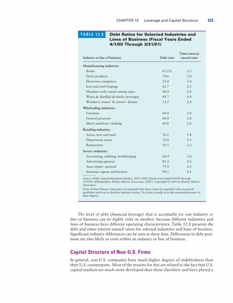
T A B L E 1 2 . 8 Debt Ratios for Selected Industries andLines of Business (Fiscal Years Ended4/1/00 Through 3/31/01)
Times interest Industry or line of business Debt ratio earned ratio
Manufacturing industries
Books 65.2% 3.3
Dairy products 74.6 3.0
Electronic computers 55.4 3.4
Iron and steel forgings 62.7 2.3
Machine tools, metal cutting types 60.4 2.4
Wines & distilled alcoholic beverages 69.7 4.4
Women’s, misses’ & juniors’ dresses 53.5 2.4
Wholesaling industries
Furniture 69.4 3.0
General groceries 66.8 2.8
Men’s and boys’ clothing 60.8 2.6
Retailing industries
Autos, new and used 76.1 1.4
Department stores 52.8 2.3
Restaurants 92.5 2.3
Service industries
Accounting, auditing, bookkeeping 68.4 5.6
Advertising agencies 81.3 4.2
Auto repair—general 75.9 2.5
Insurance agents and brokers 94.1 4.1
Source: RMA Annual Statement Studies, 2001–2002 (fiscal years ended 4/1/00 through3/31/01) (Philadelphia: Robert Morris Associates, 2001). Copyright © 2001 by Robert MorrisAssociates.Note: Robert Morris Associates recommends that these ratios be regarded only as generalguidelines and not as absolute industry norms. No claim is made as to the representativeness ofthese figures.
The level of debt (financial leverage) that is acceptable for one industry orline of business can be highly risky in another, because different industries andlines of business have different operating characteristics. Table 12.8 presents thedebt and times interest earned ratios for selected industries and lines of business.Significant industry differences can be seen in these data. Differences in debt posi-tions are also likely to exist within an industry or line of business.
Capital Structure of Non-U.S. FirmsIn general, non-U.S. companies have much higher degrees of indebtedness thantheir U.S. counterparts. Most of the reasons for this are related to the fact that U.S.capital markets are much more developed than those elsewhere and have played a
524 PART 4 Long-Term Financial Decisions
In Practice
Enron Corp.’s December 31, 2000,balance sheet showed long-termdebt of $10. 2 billion and $300 mil-lion in other financial obligations.These figures gave the company a41 percent ratio of total obliga-tions to total capitalization. Thatdidn’t seem out of line for a com-pany in the capital-intensiveenergy industry.
Yet as the company’s finan-cial condition fell apart in the fall of2001, investors and lenders discov-ered that Enron’s true debt loadwas far beyond what its balancesheet indicated. By selling assetsto perfectly legal special-purposeentities (SPEs), Enron had movedbillions of dollars of debt off its bal-ance sheet into subsidiaries,trusts, partnerships, and other cre-ative financing arrangements. For-mer CFO Andrew Fastow claimedthat these complex arrangementswere disclosed in footnotes and
that Enron was not liable for repay-ment of the debts of these SPEs.
Enron’s required filing of Form10-Q with the SEC, on November19, 2001, told a different story: If itsdebt were to fall below investmentgrade, Enron would have to repaythose off-balance-sheet partner-ship obligations. Ironically, its dis-closure of about $4 billion in off-balance-sheet liabilities triggeredthe downgrade of its debt to “junk”status and accelerated debtrepayment. Enron’s secrecy aboutits off-balance-sheet ventures ledto its loss of credibility in theinvestment community. Its stockand bond prices slid downward; itsmarket value plunged $35 billion inabout a month; and on Decem-ber 2, 2001, Enron became thelargest U.S. company ever to havefiled for bankruptcy.
Enron is not alone in its use ofoff-balance-sheet debt. Most air-
lines have large aircraft leasesstructured through off-balance-sheet vehicles, although analystsand investors are aware that thetrue leverage is higher. Pacific Gas& Electric, Southern CaliforniaEdison, and Xerox have also runinto problems from off-balance-sheet debt obligations. Don’texpect the Enron debacle to elimi-nate special-purpose entities,although the SEC has been callingfor tighter consolidation rules.Companies like the flexibility thatoff-balance-sheet financingsources provide, not to mentionthat such financing makes debtratios and returns look better.
Sources: Peter Behr, “Cause of Death: Mis-trust,” Washington Post (December 13, 2001),p. E1; Ronald Fink, “What Andrew FastowKnew,” CFO (January 1, 2002); and DavidHenry, “Who Else Is Hiding Debt?” BusinessWeek (January 28, 2002).
FOCUS ON PRACTICE Enron Plays Hide and Seek with Debt
greater role in corporate financing than has been the case in other countries. Inmost European countries and especially in Japan and other Pacific Rim nations,large commercial banks are more actively involved in the financing of corporateactivity than has been true in the United States. Furthermore, in many of thesecountries, banks are allowed to make large equity investments in nonfinancial cor-porations—a practice that is prohibited for U.S. banks. Finally, share ownershiptends to be more tightly controlled among founding-family, institutional, and evenpublic investors in Europe and Asia than it is for most large U.S. corporations.Tight ownership enables owners to understand the firm’s financial condition bet-ter, resulting in their willingness to tolerate a higher degree of indebtedness.
On the other hand, similarities do exist between U.S. corporations and cor-porations in other countries. First, the same industry patterns of capital structuretend to be found all around the world. For example, in nearly all countries, phar-maceutical and other high-growth industrial firms tend to have lower debt ratiosthan do steel companies, airlines, and electric utility companies. Second, the capi-tal structures of the largest U.S.-based multinational companies, which haveaccess to many different capital markets around the world, typically resemble thecapital structures of multinational companies from other countries more thanthey resemble those of smaller U.S. companies. Finally, the worldwide trend is
CHAPTER 12 Leverage and Capital Structure 525
14. Franco Modigliani and Merton H. Miller, “The Cost of Capital, Corporation Finance, and the Theory of Invest-ment,” American Economic Review (June 1958), pp. 261–297.15. Perfect-market assumptions include (1) no taxes, (2) no brokerage or flotation costs for securities, (3) symmetri-cal information—investors and managers have the same information about the firm’s investment prospects, and (4)investor ability to borrow at the same rate as corporations.
away from reliance on banks for corporate financing and toward greater relianceon security issuance. Over time, the differences in the capital structures of U.S.and non-U.S. firms will probably lessen.
Capital Structure TheoryScholarly research suggests that there is an optimal capital structure range. It isnot yet possible to provide financial managers with a specified methodology foruse in determining a firm’s optimal capital structure. Nevertheless, financial the-ory does offer help in understanding how a firm’s chosen financing mix affectsthe firm’s value.
In 1958, Franco Modigliani and Merton H. Miller14 (commonly known as“M and M”) demonstrated algebraically that, assuming perfect markets,15 thecapital structure that a firm chooses does not affect its value. Many researchers,including M and M, have examined the effects of less restrictive assumptions onthe relationship between capital structure and the firm’s value. The result is a the-oretical optimal capital structure based on balancing the benefits and costs ofdebt financing. The major benefit of debt financing is the tax shield, which allowsinterest payments to be deducted in calculating taxable income. The cost of debtfinancing results from (1) the increased probability of bankruptcy caused by debtobligations, (2) the agency costs of the lender’s monitoring the firm’s actions, and(3) the costs associated with managers having more information about the firm’sprospects than do investors.
Tax Benefits
Allowing firms to deduct interest payments on debt when calculating taxableincome reduces the amount of the firm’s earnings paid in taxes, thereby makingmore earnings available for bondholders and stockholders. The deductibility ofinterest means the cost of debt, ki, to the firm is subsidized by the government.Letting kd equal the before-tax cost of debt and letting T equal the tax rate, fromChapter 11 (Equation 11.2), we have ki �kd � (1�T).
Probability of Bankruptcy
The chance that a firm will become bankrupt because of an inability to meet itsobligations as they come due depends largely on its level of both business risk andfinancial risk.
Business Risk In Chapter 11, we defined business risk as the risk to the firmof being unable to cover its operating costs. In general, the greater the firm’s oper-ating leverage—the use of fixed operating costs—the higher its business risk.Although operating leverage is an important factor affecting business risk, two
526 PART 4 Long-Term Financial Decisions
T A B L E 1 2 . 9 Sales and Associated EBITCalculations for Cooke Company ($000)
Probability of sales .25 .50 .25
Sales revenue $400 $600 $800
Less: Fixed operating costs 200 200 200
Less: Variable operating costs (50% of sales)�2�0�0� �
3�0�0� �
4�0�0�
Earnings before interest and taxes (EBIT) $������
0��
$��1��0��0��
$��2��0��0��
Hint The cash flows toinvestors from bonds areless risky than the dividendsfrom preferred stock, whichare less risky than dividendsfrom common stock. Onlywith bonds is the issuercontractually obligated topay the scheduled interest,and the amounts due tobondholders and preferredstockholders are usuallyfixed. Therefore, therequired return for bonds isgenerally lower than thatfor preferred stock, which islower than that for commonstock.
other factors—revenue stability and cost stability—also affect it. Revenue stabil-ity reflects the relative variability of the firm’s sales revenues. Firms with reason-ably stable levels of demand and with products that have stable prices have stablerevenues. The result is low levels of business risk. Firms with highly volatile prod-uct demand and prices have unstable revenues that result in high levels of businessrisk. Cost stability reflects the relative predictability of input prices such as thosefor labor and materials. The more predictable and stable these input prices are,the lower the business risk; the less predictable and stable they are, the higher thebusiness risk.
Business risk varies among firms, regardless of their lines of business, and isnot affected by capital structure decisions. The level of business risk must betaken as a “given.” The higher a firm’s business risk, the more cautious the firmmust be in establishing its capital structure. Firms with high business risk there-fore tend toward less highly leveraged capital structures, and firms with low busi-ness risk tend toward more highly leveraged capital structures. We will holdbusiness risk constant throughout the discussions that follow.
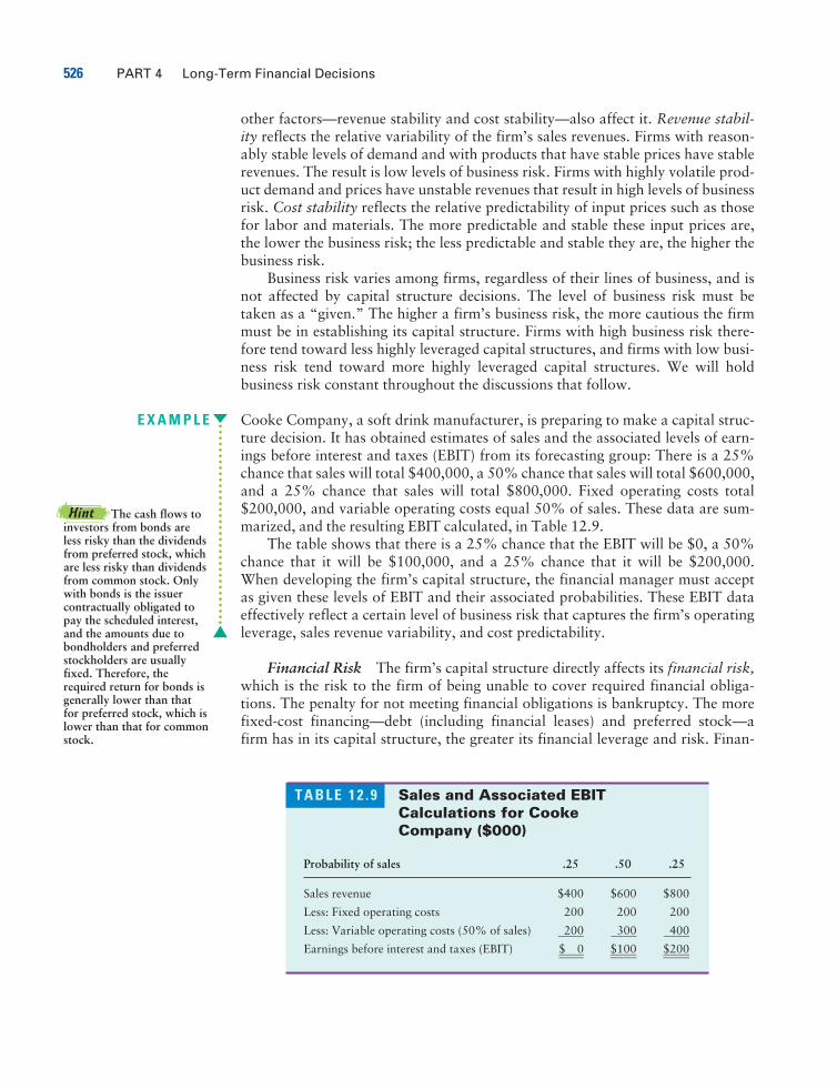
E X A M P L E Cooke Company, a soft drink manufacturer, is preparing to make a capital struc-ture decision. It has obtained estimates of sales and the associated levels of earn-ings before interest and taxes (EBIT) from its forecasting group: There is a 25%chance that sales will total $400,000, a 50% chance that sales will total $600,000,and a 25% chance that sales will total $800,000. Fixed operating costs total$200,000, and variable operating costs equal 50% of sales. These data are sum-marized, and the resulting EBIT calculated, in Table 12.9.
The table shows that there is a 25% chance that the EBIT will be $0, a 50%chance that it will be $100,000, and a 25% chance that it will be $200,000.When developing the firm’s capital structure, the financial manager must acceptas given these levels of EBIT and their associated probabilities. These EBIT dataeffectively reflect a certain level of business risk that captures the firm’s operatingleverage, sales revenue variability, and cost predictability.
Financial Risk The firm’s capital structure directly affects its financial risk,which is the risk to the firm of being unable to cover required financial obliga-tions. The penalty for not meeting financial obligations is bankruptcy. The morefixed-cost financing—debt (including financial leases) and preferred stock—afirm has in its capital structure, the greater its financial leverage and risk. Finan-
CHAPTER 12 Leverage and Capital Structure 527
T A B L E 1 2 . 1 0 Capital Structures Associated withAlternative Debt Ratios for Cooke Company
Capital structure ($000) Shares of commonDebt Equity stock outstanding (000)
Debt ratio Total assetsa [(1)� (2)] [(2)� (3)] [(4)�$20]b
(1) (2) (3) (4) (5)
0% $500 $ 0 $500 25.00
10 500 50 450 22.50
20 500 100 400 20.00
30 500 150 350 17.50
40 500 200 300 15.00
50 500 250 250 12.50
60 500 300 200 10.00
aBecause the firm, for convenience, is assumed to have no current liabilities, its total assets equal itstotal capital of $500,000.bThe $20 value represents the book value per share of common stock equity noted earlier.
16. This assumption is needed so that we can assess alternative capital structures without having to consider thereturns associated with the investment of additional funds raised. Attention here is given only to the mix of capital,not to its investment.
Hint As you learned inChapter 2, the debt ratio isequal to the amount of totaldebt divided by the totalassets. The higher this ratio,the more financial leveragea firm is using.
cial risk depends on the capital structure decision made by the management, andthat decision is affected by the business risk the firm faces.
The total risk of a firm—business and financial risk combined—determinesits probability of bankruptcy. Financial risk, its relationship to business risk, andtheir combined impact can be demonstrated by continuing the Cooke Companyexample.
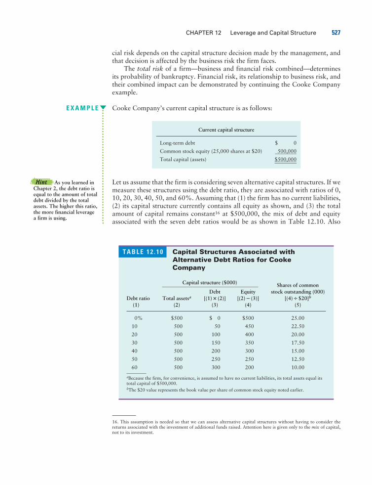
E X A M P L E Cooke Company’s current capital structure is as follows:
Let us assume that the firm is considering seven alternative capital structures. If wemeasure these structures using the debt ratio, they are associated with ratios of 0,10, 20, 30, 40, 50, and 60%. Assuming that (1) the firm has no current liabilities,(2) its capital structure currently contains all equity as shown, and (3) the totalamount of capital remains constant16 at $500,000, the mix of debt and equityassociated with the seven debt ratios would be as shown in Table 12.10. Also
Current capital structure
Long-term debt $ 0
Common stock equity (25,000 shares at $20)�5�0�0�,�0�0�0�
Total capital (assets) $��5��0��0��,��0��0��0��
528 PART 4 Long-Term Financial Decisions
T A B L E 1 2 . 1 1 Level of Debt, Interest Rate, andDollar Amount of Annual InterestAssociated with Cooke Company’sAlternative Capital Structures
Interest rate Interest ($000)Capital structure Debt ($000) on all debt [(1)� (2)]
debt ratio (1) (2) (3)
0% $ 0 0.0% $ 0.00
10 50 9.0 4.50
20 100 9.5 9.50
30 150 10.0 15.00
40 200 11.0 22.00
50 250 13.5 33.75
60 300 16.5 49.50
17. For explanatory convenience, the coefficient of variation of EPS, which measures total (nondiversifiable anddiversifiable) risk, is used throughout this chapter as a proxy for beta, which measures the relevant nondiversifi-able risk.
shown in the table is the number of shares of common stock outstanding undereach alternative.
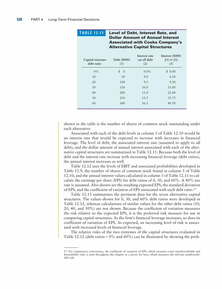
Associated with each of the debt levels in column 3 of Table 12.10 would bean interest rate that would be expected to increase with increases in financialleverage. The level of debt, the associated interest rate (assumed to apply to alldebt), and the dollar amount of annual interest associated with each of the alter-native capital structures are summarized in Table 12.11. Because both the level ofdebt and the interest rate increase with increasing financial leverage (debt ratios),the annual interest increases as well.
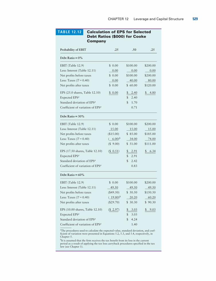
Table 12.12 uses the levels of EBIT and associated probabilities developed inTable 12.9, the number of shares of common stock found in column 5 of Table12.10, and the annual interest values calculated in column 3 of Table 12.11 to cal-culate the earnings per share (EPS) for debt ratios of 0, 30, and 60%. A 40% taxrate is assumed. Also shown are the resulting expected EPS, the standard deviationof EPS, and the coefficient of variation of EPS associated with each debt ratio.17
Table 12.13 summarizes the pertinent data for the seven alternative capitalstructures. The values shown for 0, 30, and 60% debt ratios were developed inTable 12.12, whereas calculations of similar values for the other debt ratios (10,20, 40, and 50%) are not shown. Because the coefficient of variation measuresthe risk relative to the expected EPS, it is the preferred risk measure for use incomparing capital structures. As the firm’s financial leverage increases, so does itscoefficient of variation of EPS. As expected, an increasing level of risk is associ-ated with increased levels of financial leverage.
The relative risks of the two extremes of the capital structures evaluated inTable 12.12 (debt ratios�0% and 60%) can be illustrated by showing the prob-
CHAPTER 12 Leverage and Capital Structure 529
T A B L E 1 2 . 1 2 Calculation of EPS for SelectedDebt Ratios ($000) for CookeCompany
Probability of EBIT .25 .50 .25
Debt Ratio�0%
EBIT (Table 12.9) $ 0.00 $100.00 $200.00
Less: Interest (Table 12.11)��
0�.�0�0� ���
0�.�0�0� ���
0�.�0�0�
Net profits before taxes $ 0.00 $100.00 $200.00
Less: Taxes (T�0.40)��
0�.�0�0� ��
4�0�.�0�0� ��
8�0�.�0�0�
Net profits after taxes $ 0.00 $ 60.00 $120.00
EPS (25.0 shares, Table 12.10) $����
0��.��0��0��
$������
2��.��4��0��
$������
4��.��8��0��
Expected EPSa $ 2.40
Standard deviation of EPSa $ 1.70
Coefficient of variation of EPSa 0.71
Debt Ratio�30%
EBIT (Table 12.9) $ 0.00 $100.00 $200.00
Less: Interest (Table 12.11)�1�5�.�0�0� ��
1�5�.�0�0� ��
1�5�.�0�0�
Net profits before taxes ($15.00) $ 85.00 $185.00
Less: Taxes (T�0.40) (��
6�.�0�0�)b
��3�4�.�0�0� ��
7�4�.�0�0�
Net profits after taxes ($ 9.00) $ 51.00 $111.00
EPS (17.50 shares, Table 12.10) ($����
0��.��5��1��) $
������2��.��9��1��
$������
6��.��3��4��
Expected EPSa $ 2.91
Standard deviation of EPSa $ 2.42
Coefficient of variation of EPSa 0.83
Debt Ratio�60%
EBIT (Table 12.9) $ 0.00 $100.00 $200.00
Less: Interest (Table 12.11)��
4�9�.�5�0� ��
4�9�.�5�0� ��
4�9�.�5�0�
Net profits before taxes ($49.50) $ 50.50 $150.50
Less: Taxes (T�0.40) (�1�9�.�8�0�)b
��2�0�.�2�0� ��
6�0�.�2�0�
Net profits after taxes ($29.70) $ 30.30 $ 90.30
EPS (10.00 shares, Table 12.10) ($����
2��.��9��7��) $
������3��.��0��3��
$������
9��.��0��3��
Expected EPSa $ 3.03
Standard deviation of EPSa $ 4.24
Coefficient of variation of EPSa 1.40
aThe procedures used to calculate the expected value, standard deviation, and coef-ficient of variation were presented in Equations 5.2, 5.3, and 5.4, respectively, inChapter 5.bIt is assumed that the firm receives the tax benefit from its loss in the currentperiod as a result of applying the tax loss carryback procedures specified in the taxlaw (see Chapter 1).
530 PART 4 Long-Term Financial Decisions
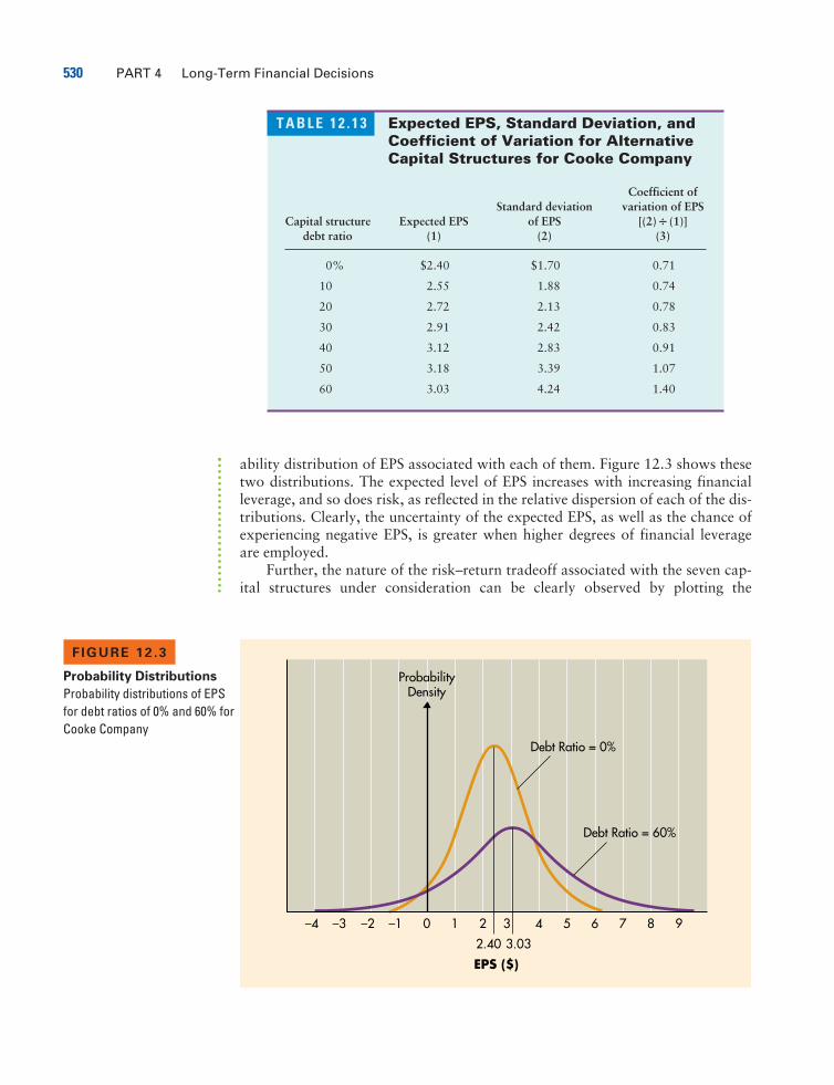
T A B L E 1 2 . 1 3 Expected EPS, Standard Deviation, andCoefficient of Variation for AlternativeCapital Structures for Cooke Company
Coefficient ofStandard deviation variation of EPS
Capital structure Expected EPS of EPS [(2)� (1)]debt ratio (1) (2) (3)
0% $2.40 $1.70 0.71
10 2.55 1.88 0.74
20 2.72 2.13 0.78
30 2.91 2.42 0.83
40 3.12 2.83 0.91
50 3.18 3.39 1.07
60 3.03 4.24 1.40
0–1–2–3–4 1 2 3
3.032.40
4 5 6 7 8 9
EPS ($)
Debt Ratio = 0%
Debt Ratio = 60%
ProbabilityDensity
FIGURE 12 .3
Probability Distributions
Probability distributions of EPSfor debt ratios of 0% and 60% forCooke Company
ability distribution of EPS associated with each of them. Figure 12.3 shows thesetwo distributions. The expected level of EPS increases with increasing financialleverage, and so does risk, as reflected in the relative dispersion of each of the dis-tributions. Clearly, the uncertainty of the expected EPS, as well as the chance ofexperiencing negative EPS, is greater when higher degrees of financial leverageare employed.
Further, the nature of the risk–return tradeoff associated with the seven cap-ital structures under consideration can be clearly observed by plotting the
CHAPTER 12 Leverage and Capital Structure 531
3.50
3.003.18
2.50
2.00 0.50
0.75
1.00
1.25
1.50
Expec
ted E
PS
($)
Coef
fici
ent
of
Vari
ation o
f EP
S
10 20 30 40 50 60 1000 20 30 40 50 60 70 80
Financial Risk
BusinessRisk
Debt Ratio (%)(b)
Debt Ratio (%)(a)
Maximum EPS
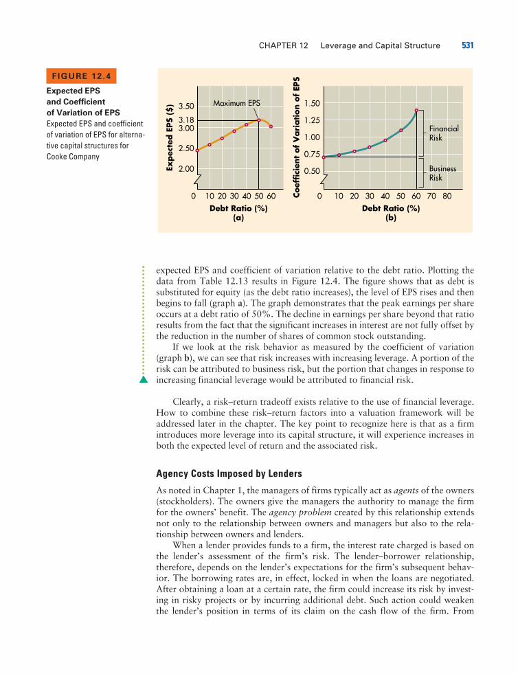
FIGURE 12 .4
Expected EPS
and Coefficient
of Variation of EPS
Expected EPS and coefficientof variation of EPS for alterna-tive capital structures forCooke Company
expected EPS and coefficient of variation relative to the debt ratio. Plotting thedata from Table 12.13 results in Figure 12.4. The figure shows that as debt issubstituted for equity (as the debt ratio increases), the level of EPS rises and thenbegins to fall (graph a). The graph demonstrates that the peak earnings per shareoccurs at a debt ratio of 50%. The decline in earnings per share beyond that ratioresults from the fact that the significant increases in interest are not fully offset bythe reduction in the number of shares of common stock outstanding.
If we look at the risk behavior as measured by the coefficient of variation(graph b), we can see that risk increases with increasing leverage. A portion of therisk can be attributed to business risk, but the portion that changes in response toincreasing financial leverage would be attributed to financial risk.
Clearly, a risk–return tradeoff exists relative to the use of financial leverage.How to combine these risk–return factors into a valuation framework will beaddressed later in the chapter. The key point to recognize here is that as a firmintroduces more leverage into its capital structure, it will experience increases inboth the expected level of return and the associated risk.
Agency Costs Imposed by Lenders
As noted in Chapter 1, the managers of firms typically act as agents of the owners(stockholders). The owners give the managers the authority to manage the firmfor the owners’ benefit. The agency problem created by this relationship extendsnot only to the relationship between owners and managers but also to the rela-tionship between owners and lenders.
When a lender provides funds to a firm, the interest rate charged is based onthe lender’s assessment of the firm’s risk. The lender–borrower relationship,therefore, depends on the lender’s expectations for the firm’s subsequent behav-ior. The borrowing rates are, in effect, locked in when the loans are negotiated.After obtaining a loan at a certain rate, the firm could increase its risk by invest-ing in risky projects or by incurring additional debt. Such action could weakenthe lender’s position in terms of its claim on the cash flow of the firm. From
532 PART 4 Long-Term Financial Decisions
asymmetric informationThe situation in which managersof a firm have more informationabout operations and futureprospects than do investors.
18. The results of the survey of Fortune 500 firms are reported in J. Michael Pinegar and Lisa Wilbricht, “WhatManagers Think of Capital Structure Theory: A Survey,” Financial Management (Winter 1989), pp. 82–91, and theresults of a similar survey of the 500 largest OTC firms are reported in Linda C. Hittle, Kamal Haddad, andLawrence J. Gitman, “Over-the-Counter Firms, Asymmetric Information, and Financing Preferences,” Review ofFinancial Economics (Fall 1992), pp. 81–92.19. Stewart C. Myers, “The Capital Structure Puzzle,” Journal of Finance (July 1984), pp. 575–592.
Hint Typical loanprovisions included incorporate bonds are discussedin Chapter 6.
pecking orderA hierarchy of financing thatbegins with retained earnings,which is followed by debt financ-ing and finally external equityfinancing.
another point of view, if these risky investment strategies paid off, the stockhold-ers would benefit. Because payment obligations to the lender remain unchanged,the excess cash flows generated by a positive outcome from the riskier actionwould enhance the value of the firm to its owners. In other words, if the riskyinvestments pay off, the owners receive all the benefits; but if the risky invest-ments do not pay off, the lenders share in the costs.
Clearly, an incentive exists for the managers acting on behalf of the stock-holders to “take advantage” of lenders. To avoid this situation, lenders imposecertain monitoring techniques on borrowers, who as a result incur agency costs.The most obvious strategy is to deny subsequent loan requests or to increase thecost of future loans to the firm. Because this strategy is an after-the-fact approach,other controls must be included in the loan agreement. Lenders typically protectthemselves by including provisions that limit the firm’s ability to alter signifi-cantly its business and financial risk. These loan provisions tend to center onissues such as the minimum level of liquidity, asset acquisitions, executivesalaries, and dividend payments.
By including appropriate provisions in the loan agreement, the lender cancontrol the firm’s risk and thus protect itself against the adverse consequences ofthis agency problem. Of course, in exchange for incurring agency costs by agree-ing to the operating and financial constraints placed on it by the loan provisions,the firm should benefit by obtaining funds at a lower cost.
Asymmetric Information
Two surveys examined capital structure decisions.18 Financial executives wereasked which of two major criteria determined their financing decisions: (1) main-taining a target capital structure or (2) following a hierarchy of financing. Thishierarchy, called a pecking order, begins with retained earnings, which is fol-lowed by debt financing and finally external equity financing. Respondents from31 percent of Fortune 500 firms and from 11 percent of the (smaller) 500 largestover-the-counter firms answered target capital structure. Respondents from 69percent of the Fortune 500 firms and 89 percent of the 500 largest OTC firmschose the pecking order.
At first glance, on the basis of financial theory, this choice appears to beinconsistent with wealth maximization goals, but Stewart Myers has explainedhow “asymmetric information” could account for the pecking order financingpreferences of financial managers.19 Asymmetric information results when man-agers of a firm have more information about operations and future prospectsthan do investors. Assuming that managers make decisions with the goal of max-imizing the wealth of existing stockholders, then asymmetric information canaffect the capital structure decisions that managers make.
CHAPTER 12 Leverage and Capital Structure 533
signalA financing action by manage-ment that is believed to reflect itsview of the firm’s stock value;generally, debt financing isviewed as a positive signal thatmanagement believes the stockis “undervalued,” and a stockissue is viewed as a negativesignal that management believesthe stock is “overvalued.”
Suppose, for example, that management has found a valuable investmentthat will require additional financing. Management believes that the prospectsfor the firm’s future are very good and that the market, as indicated by the firm’scurrent stock price, does not fully appreciate the firm’s value. In this case, itwould be advantageous to current stockholders if management raised therequired funds using debt rather than issuing new stock. Using debt to raise fundsis frequently viewed as a signal that reflects management’s view of the firm’sstock value. Debt financing is a positive signal suggesting that managementbelieves that the stock is “undervalued” and therefore a bargain. When the firm’spositive future outlook becomes known to the market, the increased value will befully captured by existing owners, rather than having to be shared with newstockholders.
If, however, the outlook for the firm is poor, management may believe thatthe firm’s stock is “overvalued.” In that case, it would be in the best interest ofexisting stockholders for the firm to issue new stock. Therefore, investors ofteninterpret the announcement of a stock issue as a negative signal—bad news con-cerning the firm’s prospects—and the stock price declines. This decrease in stockvalue, along with high underwriting costs for stock issues (compared to debtissues), make new stock financing very expensive. When the negative future out-look becomes known to the market, the decreased value is shared with newstockholders, rather than being fully captured by existing owners.
Because conditions of asymmetric information exist from time to time, firmsshould maintain some reserve borrowing capacity by keeping debt levels low.This reserve allows the firm to take advantage of good investment opportunitieswithout having to sell stock at a low value and thus send signals that undulyinfluence the stock price.
The Optimal Capital StructureWhat, then, is an optimal capital structure, even if it exists (so far) only in theory?To provide some insight into an answer, we will examine some basic financialrelationships. It is generally believed that the value of the firm is maximized whenthe cost of capital is minimized. By using a modification of the simple zero-growth valuation model (see Equation 7.3 in Chapter 7), we can define the valueof the firm, V, by Equation 12.11.
V� (12.11)
where
EBIT�earnings before interest and taxesT � tax rate
EBIT� (1�T)� the after-tax operating earnings available to the debt andequity holders
ka � weighted average cost of capital
Clearly, if we assume that EBIT is constant, the value of the firm, V, is maximizedby minimizing the weighted average cost of capital, ka.
EBIT� (1�T)��
ka
534 PART 4 Long-Term Financial Decisions
Annual C
ost
(%
)V
alu
e
V*
M = Optimal Capital Structure
Debt/Total Assets0
V = EBIT × (1 – T )
ka
ks = cost of equity
ka = WACC
ki = cost of debt
Financial Leverage
(a)
(b)
FIGURE 12 .5
Cost Functions
and Value
Capital costs and the optimalcapital structure
optimal capital structureThe capital structure at whichthe weighted average cost ofcapital is minimized, therebymaximizing the firm’s value.
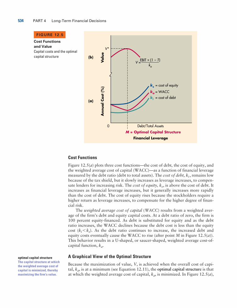
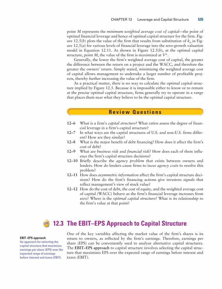
Cost Functions
Figure 12.5(a) plots three cost functions—the cost of debt, the cost of equity, andthe weighted average cost of capital (WACC)—as a function of financial leveragemeasured by the debt ratio (debt to total assets). The cost of debt, ki , remains lowbecause of the tax shield, but it slowly increases as leverage increases, to compen-sate lenders for increasing risk. The cost of equity, ks, is above the cost of debt. Itincreases as financial leverage increases, but it generally increases more rapidlythan the cost of debt. The cost of equity rises because the stockholders require ahigher return as leverage increases, to compensate for the higher degree of finan-cial risk.
The weighted average cost of capital (WACC) results from a weighted aver-age of the firm’s debt and equity capital costs. At a debt ratio of zero, the firm is100 percent equity-financed. As debt is substituted for equity and as the debtratio increases, the WACC declines because the debt cost is less than the equitycost (ki �ks). As the debt ratio continues to increase, the increased debt andequity costs eventually cause the WACC to rise (after point M in Figure 12.5(a)).This behavior results in a U-shaped, or saucer-shaped, weighted average cost-of-capital function, ka.
A Graphical View of the Optimal Structure
Because the maximization of value, V, is achieved when the overall cost of capi-tal, ka, is at a minimum (see Equation 12.11), the optimal capital structure is thatat which the weighted average cost of capital, ka, is minimized. In Figure 12.5(a),
CHAPTER 12 Leverage and Capital Structure 535
EBIT–EPS approachAn approach for selecting thecapital structure that maximizesearnings per share (EPS) over theexpected range of earningsbefore interest and taxes (EBIT).
LG5
point M represents the minimum weighted average cost of capital—the point ofoptimal financial leverage and hence of optimal capital structure for the firm. Fig-ure 12.5(b) plots the value of the firm that results from substitution of ka in Fig-ure 12.5(a) for various levels of financial leverage into the zero-growth valuationmodel in Equation 12.11. As shown in Figure 12.5(b), at the optimal capitalstructure, point M, the value of the firm is maximized at V*.
Generally, the lower the firm’s weighted average cost of capital, the greaterthe difference between the return on a project and the WACC, and therefore thegreater the owners’ return. Simply stated, minimizing the weighted average costof capital allows management to undertake a larger number of profitable proj-ects, thereby further increasing the value of the firm.
As a practical matter, there is no way to calculate the optimal capital struc-ture implied by Figure 12.5. Because it is impossible either to know or to remainat the precise optimal capital structure, firms generally try to operate in a rangethat places them near what they believe to be the optimal capital structure.
R e v i e w Q u e s t i o n s
12–6 What is a firm’s capital structure? What ratios assess the degree of finan-cial leverage in a firm’s capital structure?
12–7 In what ways are the capital structures of U.S. and non-U.S. firms differ-ent? How are they similar?
12–8 What is the major benefit of debt financing? How does it affect the firm’scost of debt?
12–9 What are business risk and financial risk? How does each of them influ-ence the firm’s capital structure decisions?
12–10 Briefly describe the agency problem that exists between owners andlenders. How do lenders cause firms to incur agency costs to resolve thisproblem?
12–11 How does asymmetric information affect the firm’s capital structure deci-sions? How do the firm’s financing actions give investors signals thatreflect management’s view of stock value?
12–12 How do the cost of debt, the cost of equity, and the weighted average costof capital (WACC) behave as the firm’s financial leverage increases fromzero? Where is the optimal capital structure? What is its relationship tothe firm’s value at that point?
12.3 The EBIT–EPS Approach to Capital StructureOne of the key variables affecting the market value of the firm’s shares is itsreturn to owners, as reflected by the firm’s earnings. Therefore, earnings pershare (EPS) can be conveniently used to analyze alternative capital structures.The EBIT–EPS approach to capital structure involves selecting the capital struc-ture that maximizes EPS over the expected range of earnings before interest andtaxes (EBIT).
536 PART 4 Long-Term Financial Decisions
20. The relationship that is expected to exist between EPS and owner wealth is not one of cause and effect. As indi-cated in Chapter 1, the maximization of profits does not necessarily ensure that owners’ wealth is also being maxi-mized. Nevertheless, it is expected that the movement of earnings per share will have some effect on owners’ wealth,because EPS data constitute one of the few pieces of information investors receive, and they often bid the firm’sshare price up or down in response to the level of these earnings.21. A convenient method for finding one EBIT–EPS coordinate is to calculate the financial breakeven point, the levelof EBIT for which the firm’s EPS just equals $0. It is the level of EBIT needed just to cover all fixed financial costs—annual interest (I) and preferred stock dividends (PD). The equation for the financial breakeven point is
Financial breakeven point� I�
where T is the tax rate. It can be seen that when PD�$0, the financial breakeven point is equal to I, the annualinterest payment.
PD�1�T
financial breakeven pointThe level of EBIT necessary tojust cover all fixed financialcosts; the level of EBIT for whichEPS � $0.
Presenting a Financing Plan GraphicallyTo analyze the effects of a firm’s capital structure on the owners’ returns, we con-sider the relationship between earnings before interest and taxes (EBIT) and earn-ings per share (EPS). A constant level of EBIT—constant business risk—isassumed, to isolate the effect on returns of the financing costs associated withalternative capital structures. EPS is used to measure the owners’ returns, whichare expected to be closely related to share price.20
The Data Required
To graph a financing plan, we need to know at least two EBIT–EPS coordinates.The approach for obtaining coordinates can be illustrated by an example.
E X A M P L E EBIT–EPS coordinates can be found by assuming specific EBIT values and calcu-lating the EPS associated with them.21 Such calculations for three capital struc-tures—debt ratios of 0, 30, and 60%—for Cooke Company were presented inTable 12.12. For EBIT values of $100,000 and $200,000, the associated EPS val-ues calculated there are summarized in the table within Figure 12.6.
Plotting the Data
The Cooke Company data can be plotted on a set of EBIT–EPS axes, as shown inFigure 12.6. The figure shows the level of EPS expected for each level of EBIT.For levels of EBIT below the x-axis intercept, a loss (negative EPS) results. Eachof the x-axis intercepts is a financial breakeven point, the level of EBIT necessaryto just cover all fixed financial costs (EPS�$0).
Comparing Alternative Capital StructuresWe can compare alternative capital structures by graphing financing plans asshown in Figure 12.6.
E X A M P L E Cooke Company’s capital structure alternatives were plotted on the EBIT–EPSaxes in Figure 12.6. This figure shows that each capital structure is superior tothe others in terms of maximizing EPS over certain ranges of EBIT. The zero-leverage capital structure (debt ratio�0%) is superior to either of the other capi-
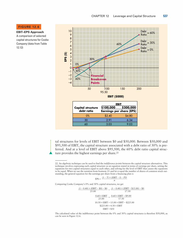
CHAPTER 12 Leverage and Capital Structure 537
Capital structuredebt ratio
EBIT$100,000 $200,000Earnings per share (EPS)
0%
3060
$2.40
2.913.03
$4.80
6.349.03
109876543210
–1 30%
30%
60%
60%
EBIT ($000)
0%
50 10095.50
150 200
–2–3–4
EPS
($)
Debt Ratio
Debt RatioDebt Ratio
= 60%
= 30%
= 0%
FinancialBreakevenPoints
FIGURE 12 .6
EBIT–EPS Approach
A comparison of selectedcapital structures for CookeCompany (data from Table12.12)
22. An algebraic technique can be used to find the indifference points between the capital structure alternatives. Thistechnique involves expressing each capital structure as an equation stated in terms of earnings per share, setting theequations for two capital structures equal to each other, and solving for the level of EBIT that causes the equationsto be equal. When we use the notation from footnote 21 and let n equal the number of shares of common stock out-standing, the general equation for the earnings per share from a financing plan is
EPS�
Comparing Cooke Company’s 0% and 30% capital structures, we get
�
�
10.50�EBIT�15.00�EBIT�$225.00$225.00�4.50�EBIT
EBIT�$50
The calculated value of the indifference point between the 0% and 30% capital structures is therefore $50,000, ascan be seen in Figure 12.6.
0.60�EBIT�$9.00���
17.500.60�EBIT��
25.00
(1�0.40)� (EBIT�$15.00)�$0����
17.50(1�0.40)� (EBIT�$0)�$0����
25.00
(1�T)� (EBIT� I)�PD���
n
tal structures for levels of EBIT between $0 and $50,000. Between $50,000 and$95,500 of EBIT, the capital structure associated with a debt ratio of 30% is pre-ferred. And at a level of EBIT above $95,500, the 60% debt ratio capital struc-ture provides the highest earnings per share.22
538 PART 4 Long-Term Financial Decisions
23. The degree of financial leverage (DFL) is reflected in the slope of the EBIT–EPS function. The steeper the slope,the greater the degree of financial leverage, because the change in EPS (y axis) that results from a given change inEBIT (x axis) increases with increasing slope and decreases with decreasing slope.
Considering Risk in EBIT–EPS AnalysisWhen interpreting EBIT–EPS analysis, it is important to consider the risk of eachcapital structure alternative. Graphically, the risk of each capital structure can beviewed in light of two measures: (1) the financial breakeven point (EBIT-axisintercept) and (2) the degree of financial leverage reflected in the slope of the cap-ital structure line: The higher the financial breakeven point and the steeper theslope of the capital structure line, the greater the financial risk.23
Further assessment of risk can be performed by using ratios. As financialleverage (measured by the debt ratio) increases, we expect a correspondingdecline in the firm’s ability to make scheduled interest payments (measured by thetimes interest earned ratio).
E X A M P L E Reviewing the three capital structures plotted for Cooke Company in Figure12.6, we can see that as the debt ratio increases, so does the financial risk of eachalternative. Both the financial breakeven point and the slope of the capital struc-ture lines increase with increasing debt ratios. If we use the $100,000 EBIT value,for example, the times interest earned ratio (EBIT� interest) for the zero-leveragecapital structure is infinity ($100,000�$0); for the 30% debt case, it is 6.67($100,000�$15,000); and for the 60% debt case, it is 2.02 ($100,000�$49,500). Because lower times interest earned ratios reflect higher risk, theseratios support the conclusion that the risk of the capital structures increases withincreasing financial leverage. The capital structure for a debt ratio of 60% isriskier than that for a debt ratio of 30%, which in turn is riskier than the capitalstructure for a debt ratio of 0%.
The Basic Shortcoming of EBIT–EPS AnalysisThe most important point to recognize when using EBIT–EPS analysis is that thistechnique tends to concentrate on maximizing earnings rather than maximizingowner wealth. The use of an EPS-maximizing approach generally ignores risk. Ifinvestors did not require risk premiums (additional returns) as the firm increasedthe proportion of debt in its capital structure, a strategy involving maximizingEPS would also maximize owner wealth. But because risk premiums increasewith increases in financial leverage, the maximization of EPS does not ensureowner wealth maximization. To select the best capital structure, both return(EPS) and risk (via the required return, ks) must be integrated into a valuationframework consistent with the capital structure theory presented earlier.
R e v i e w Q u e s t i o n
12–13 Explain the EBIT–EPS approach to capital structure. Include in yourexplanation a graph indicating the financial breakeven point; label theaxes. Is this approach consistent with maximization of the owners’ wealth?
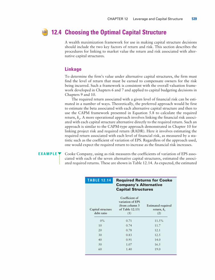
CHAPTER 12 Leverage and Capital Structure 539
T A B L E 1 2 . 1 4 Required Returns for CookeCompany’s AlternativeCapital Structures
Coefficient ofvariation of EPS(from column 3 Estimated required
Capital structure of Table 12.13) return, ksdebt ratio (1) (2)
0% 0.71 11.5%
10 0.74 11.7
20 0.78 12.1
30 0.83 12.5
40 0.91 14.0
50 1.07 16.5
60 1.40 19.0
LG6 12.4 Choosing the Optimal Capital StructureA wealth maximization framework for use in making capital structure decisionsshould include the two key factors of return and risk. This section describes theprocedures for linking to market value the return and risk associated with alter-native capital structures.
LinkageTo determine the firm’s value under alternative capital structures, the firm mustfind the level of return that must be earned to compensate owners for the riskbeing incurred. Such a framework is consistent with the overall valuation frame-work developed in Chapters 6 and 7 and applied to capital budgeting decisions inChapters 9 and 10.
The required return associated with a given level of financial risk can be esti-mated in a number of ways. Theoretically, the preferred approach would be firstto estimate the beta associated with each alternative capital structure and then touse the CAPM framework presented in Equation 5.8 to calculate the requiredreturn, ks. A more operational approach involves linking the financial risk associ-ated with each capital structure alternative directly to the required return. Such anapproach is similar to the CAPM-type approach demonstrated in Chapter 10 forlinking project risk and required return (RADR). Here it involves estimating therequired return associated with each level of financial risk, as measured by a sta-tistic such as the coefficient of variation of EPS. Regardless of the approach used,one would expect the required return to increase as the financial risk increases.
E X A M P L E Cooke Company, using as risk measures the coefficients of variation of EPS asso-ciated with each of the seven alternative capital structures, estimated the associ-ated required returns. These are shown in Table 12.14. As expected, the estimated
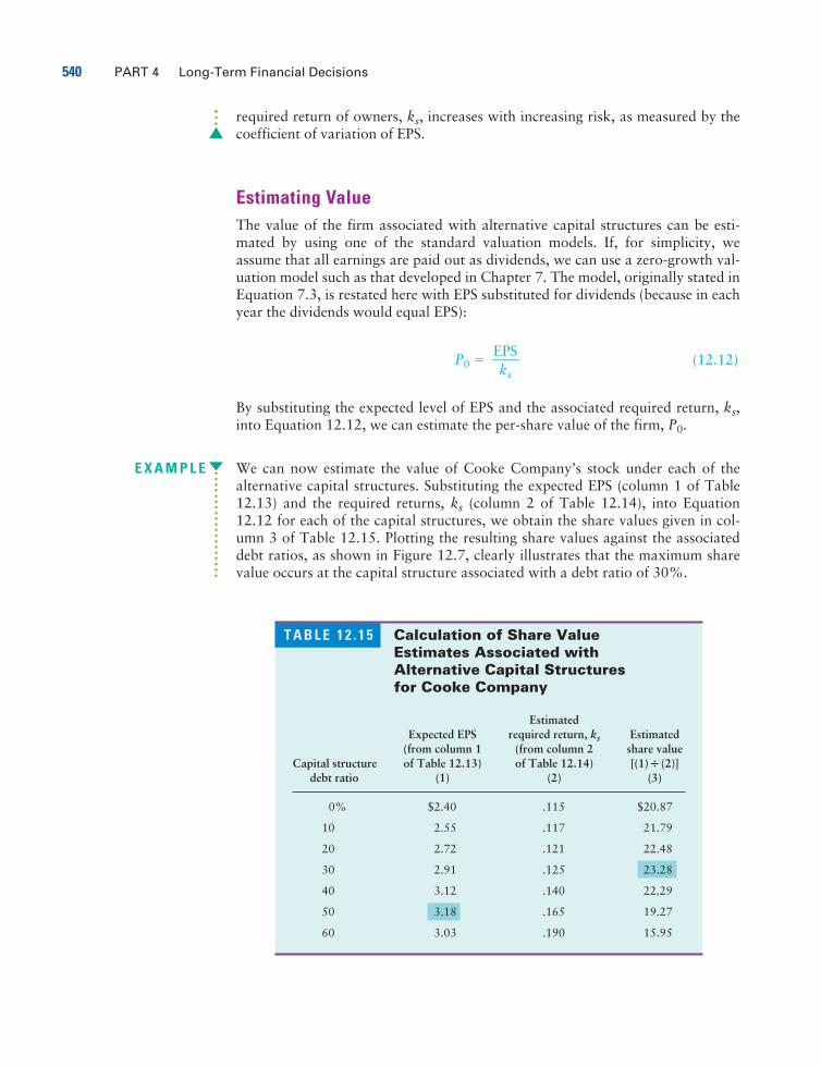
540 PART 4 Long-Term Financial Decisions
T A B L E 1 2 . 1 5 Calculation of Share Value Estimates Associated with Alternative Capital Structures for Cooke Company
EstimatedExpected EPS required return, ks Estimated
(from column 1 (from column 2 share valueCapital structure of Table 12.13) of Table 12.14) [(1)� (2)]
debt ratio (1) (2) (3)
0% $2.40 .115 $20.87
10 2.55 .117 21.79
20 2.72 .121 22.48
30 2.91 .125 23.28
40 3.12 .140 22.29
50 3.18 .165 19.27
60 3.03 .190 15.95
required return of owners, ks, increases with increasing risk, as measured by thecoefficient of variation of EPS.
Estimating ValueThe value of the firm associated with alternative capital structures can be esti-mated by using one of the standard valuation models. If, for simplicity, weassume that all earnings are paid out as dividends, we can use a zero-growth val-uation model such as that developed in Chapter 7. The model, originally stated inEquation 7.3, is restated here with EPS substituted for dividends (because in eachyear the dividends would equal EPS):
P0 � (12.12)
By substituting the expected level of EPS and the associated required return, ks,into Equation 12.12, we can estimate the per-share value of the firm, P0.
E X A M P L E We can now estimate the value of Cooke Company’s stock under each of thealternative capital structures. Substituting the expected EPS (column 1 of Table12.13) and the required returns, ks (column 2 of Table 12.14), into Equation12.12 for each of the capital structures, we obtain the share values given in col-umn 3 of Table 12.15. Plotting the resulting share values against the associateddebt ratios, as shown in Figure 12.7, clearly illustrates that the maximum sharevalue occurs at the capital structure associated with a debt ratio of 30%.
EPS�ks
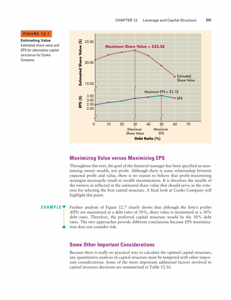
CHAPTER 12 Leverage and Capital Structure 541
2.002.503.003.50
15.00
20.00
25.00
10 20 30 40 50 60 700Maximum
Share ValueMaximum
EPSDebt Ratio (%)
Estim
ate
d S
hare
Valu
e ($
)EP
S ($
)
EPS
Estimated Share Value
Maximum Share Value = $23.28
Maximum EPS = $3.18
FIGURE 12 .7
Estimating Value
Estimated share value andEPS for alternative capitalstructures for CookeCompany
Maximizing Value versus Maximizing EPSThroughout this text, the goal of the financial manager has been specified as max-imizing owner wealth, not profit. Although there is some relationship betweenexpected profit and value, there is no reason to believe that profit-maximizingstrategies necessarily result in wealth maximization. It is therefore the wealth ofthe owners as reflected in the estimated share value that should serve as the crite-rion for selecting the best capital structure. A final look at Cooke Company willhighlight this point.
E X A M P L E Further analysis of Figure 12.7 clearly shows that although the firm’s profits(EPS) are maximized at a debt ratio of 50%, share value is maximized at a 30%debt ratio. Therefore, the preferred capital structure would be the 30% debtratio. The two approaches provide different conclusions because EPS maximiza-tion does not consider risk.
Some Other Important ConsiderationsBecause there is really no practical way to calculate the optimal capital structure,any quantitative analysis of capital structure must be tempered with other impor-tant considerations. Some of the more important additional factors involved incapital structure decisions are summarized in Table 12.16.
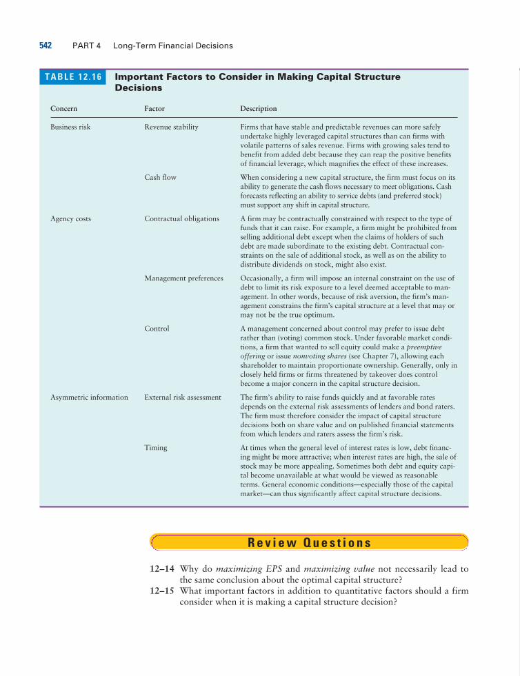
542 PART 4 Long-Term Financial Decisions
T A B L E 1 2 . 1 6 Important Factors to Consider in Making Capital Structure Decisions
Concern Factor Description
Business risk Revenue stability Firms that have stable and predictable revenues can more safelyundertake highly leveraged capital structures than can firms withvolatile patterns of sales revenue. Firms with growing sales tend tobenefit from added debt because they can reap the positive benefitsof financial leverage, which magnifies the effect of these increases.
Cash flow When considering a new capital structure, the firm must focus on itsability to generate the cash flows necessary to meet obligations. Cashforecasts reflecting an ability to service debts (and preferred stock)must support any shift in capital structure.
Agency costs Contractual obligations A firm may be contractually constrained with respect to the type offunds that it can raise. For example, a firm might be prohibited fromselling additional debt except when the claims of holders of suchdebt are made subordinate to the existing debt. Contractual con-straints on the sale of additional stock, as well as on the ability todistribute dividends on stock, might also exist.
Management preferences Occasionally, a firm will impose an internal constraint on the use ofdebt to limit its risk exposure to a level deemed acceptable to man-agement. In other words, because of risk aversion, the firm’s man-agement constrains the firm’s capital structure at a level that may ormay not be the true optimum.
Control A management concerned about control may prefer to issue debtrather than (voting) common stock. Under favorable market condi-tions, a firm that wanted to sell equity could make a preemptiveoffering or issue nonvoting shares (see Chapter 7), allowing eachshareholder to maintain proportionate ownership. Generally, only inclosely held firms or firms threatened by takeover does controlbecome a major concern in the capital structure decision.
Asymmetric information External risk assessment The firm’s ability to raise funds quickly and at favorable ratesdepends on the external risk assessments of lenders and bond raters.The firm must therefore consider the impact of capital structuredecisions both on share value and on published financial statementsfrom which lenders and raters assess the firm’s risk.
Timing At times when the general level of interest rates is low, debt financ-ing might be more attractive; when interest rates are high, the sale ofstock may be more appealing. Sometimes both debt and equity capi-tal become unavailable at what would be viewed as reasonableterms. General economic conditions—especially those of the capitalmarket—can thus significantly affect capital structure decisions.
R e v i e w Q u e s t i o n s
12–14 Why do maximizing EPS and maximizing value not necessarily lead tothe same conclusion about the optimal capital structure?
12–15 What important factors in addition to quantitative factors should a firmconsider when it is making a capital structure decision?
CHAPTER 12 Leverage and Capital Structure 543
S U M M A RYFOCUS ON VALUE
The amount of leverage (fixed-cost assets or funds) employed by a firm directly affects itsrisk, return, and share value. Generally, higher leverage raises, and lower leverage reduces,risk and return. Operating leverage is concerned with the level of fixed operating costs;financial leverage focuses on fixed financial costs, particularly interest on debt and any pre-ferred stock dividends. The firm’s financial leverage is determined by its capital structure—its mix of long-term debt and equity financing. Because of its fixed interest payments, themore debt a firm employs relative to its equity, the greater its financial leverage. The valueof the firm is clearly affected by its degree of operating leverage and by the composition ofits capital structure. The financial manager must therefore carefully consider the types ofoperating and financial costs it incurs, recognizing that with greater fixed costs comeshigher risk. Major decisions with regard to both operating cost structure and capital struc-ture must therefore focus on their impact on the firm’s value. Only those leverage and capi-tal structure decisions that are consistent with the firm’s goal of maximizing its stock priceshould be implemented.
REVIEW OF LEARNING GOALS
Discuss the role of breakeven analysis, the oper-ating breakeven point, and the effect of chang-
ing costs on it. Breakeven analysis measures thelevel of sales necessary to cover total operatingcosts. The operating breakeven point may be calcu-lated algebraically, by dividing fixed operating costsby the difference between the sale price per unit andvariable operating cost per unit, or it may be deter-mined graphically. The operating breakeven pointincreases with increased fixed and variable operat-ing costs and decreases with an increase in saleprice, and vice versa.
Understand operating, financial, and totalleverage and the relationships among them.
Operating leverage is the use of fixed operatingcosts by the firm to magnify the effects of changesin sales on EBIT. The higher the fixed operatingcosts, the greater the operating leverage. Financialleverage is the use of fixed financial costs by thefirm to magnify the effects of changes in EBIT onEPS. The higher the fixed financial costs—typically,interest on debt and preferred stock dividends—the
LG2
LG1 greater the financial leverage. The total leverage ofthe firm is the use of fixed costs—both operatingand financial—to magnify the effects of changes insales on EPS. Total leverage reflects the combinedeffect of operating and financial leverage.
Describe the types of capital, external assess-ment of capital structure, the capital structure
of non-U.S. firms, and capital structure theory. Twobasic types of capital—debt capital and equity capi-tal—make up a firm’s capital structure. They differwith respect to voice in management, claims on in-come and assets, maturity, and tax treatment. Capi-tal structure can be externally assessed by using fi-nancial ratios—debt ratio, times interest earnedratio, and fixed-payment coverage ratio. Non-U.S.companies tend to have much higher degrees of in-debtedness than do their U.S. counterparts, primar-ily because U.S. capital markets are much more de-veloped. Similarities between U.S. corporations andthose of other countries include industry patterns ofcapital structure, large multinational company capi-tal structures, and the trend toward greater reliance
LG3
544 PART 4 Long-Term Financial Decisions
on securities issuance and less reliance on banks forfinancing.
Research suggests that there is an optimal capitalstructure that balances the firm’s benefits and costs ofdebt financing. The major benefit of debt financing isthe tax shield. The costs of debt financing include theprobability of bankruptcy, caused by business andfinancial risk; agency costs imposed by lenders; andasymmetric information, which typically causesfirms to raise funds in a pecking order of retainedearnings, then debt, and finally external equityfinancing, in order to send positive signals to the mar-ket and thereby enhance the wealth of shareholders.
Explain the optimal capital structure using agraphical view of the firm’s cost-of-capital
functions and a zero-growth valuation model. Thezero-growth valuation model can be used to definethe firm’s value as its after-tax EBIT divided by itsweighted average cost of capital. Assuming thatEBIT is constant, the value of the firm is maxi-mized by minimizing its weighted average cost ofcapital (WACC). The optimal capital structure isthe one that minimizes the WACC. Graphically,although both debt and equity costs rise withincreasing financial leverage, the lower cost of debtcauses the WACC to decline and then rise withincreasing financial leverage. As a result, the firm’sWACC exhibits a U-shape, whose minimum valuedefines the optimal capital structure that maximizesowner wealth.
LG4
Discuss the EBIT–EPS approach to capitalstructure. The EBIT–EPS approach evaluates
capital structures in light of the returns they providethe firm’s owners and their degree of financial risk.Under the EBIT–EPS approach, the preferred capitalstructure is the one that is expected to provide max-imum EPS over the firm’s expected range of EBIT.Graphically, this approach reflects risk in terms ofthe financial breakeven point and the slope of thecapital structure line. The major shortcoming ofEBIT–EPS analysis is that it concentrates on maxi-mizing earnings rather than owners’ wealth.
Review the return and risk of alternative capi-tal structures, their linkage to market value,
and other important considerations related to capi-tal structure. The best capital structure can be se-lected by using a valuation model to link returnand risk factors. The preferred capital structure isthe one that results in the highest estimated sharevalue, not the highest EPS. Other important non-quantitative factors, such as revenue stability, cashflow, contractual obligations, management prefer-ences, control, external risk assessment, and timing,must also be considered when making capital struc-ture decisions.
LG6
LG5
LG1 LG2
SELF-TEST PROBLEMS (Solutions in Appendix B)
ST 12–1 Breakeven point and all forms of leverage TOR most recently sold 100,000units at $7.50 each; its variable operating costs are $3.00 per unit, and its fixedoperating costs are $250,000. Annual interest charges total $80,000, and thefirm has 8,000 shares of $5 (annual dividend) preferred stock outstanding. Itcurrently has 20,000 shares of common stock outstanding. Assume that the firmhas a 40% tax rate.a. At what level of sales (in units) would the firm break even on operations (that
is, EBIT�$0)?b. Calculate the firm’s earnings per share (EPS) in tabular form at (1) the cur-
rent level of sales and (2) a 120,000-unit sales level.c. Using the current $750,000 level of sales as a base, calculate the firm’s degree
of operating leverage (DOL).
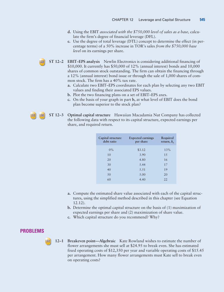
CHAPTER 12 Leverage and Capital Structure 545
LG5
LG3 LG6
LG1
d. Using the EBIT associated with the $750,000 level of sales as a base, calcu-late the firm’s degree of financial leverage (DFL).
e. Use the degree of total leverage (DTL) concept to determine the effect (in per-centage terms) of a 50% increase in TOR’s sales from the $750,000 baselevel on its earnings per share.
ST 12–2 EBIT–EPS analysis Newlin Electronics is considering additional financing of$10,000. It currently has $50,000 of 12% (annual interest) bonds and 10,000shares of common stock outstanding. The firm can obtain the financing througha 12% (annual interest) bond issue or through the sale of 1,000 shares of com-mon stock. The firm has a 40% tax rate.a. Calculate two EBIT–EPS coordinates for each plan by selecting any two EBIT
values and finding their associated EPS values.b. Plot the two financing plans on a set of EBIT–EPS axes.c. On the basis of your graph in part b, at what level of EBIT does the bond
plan become superior to the stock plan?
ST 12–3 Optimal capital structure Hawaiian Macadamia Nut Company has collectedthe following data with respect to its capital structure, expected earnings pershare, and required return.
a. Compute the estimated share value associated with each of the capital struc-tures, using the simplified method described in this chapter (see Equation12.12).
b. Determine the optimal capital structure on the basis of (1) maximization ofexpected earnings per share and (2) maximization of share value.
c. Which capital structure do you recommend? Why?
PROBLEMS
12–1 Breakeven point—Algebraic Kate Rowland wishes to estimate the number offlower arrangements she must sell at $24.95 to break even. She has estimatedfixed operating costs of $12,350 per year and variable operating costs of $15.45per arrangement. How many flower arrangements must Kate sell to break evenon operating costs?
Capital structure Expected earnings Requireddebt ratio per share return, ks
0% $3.12 13%
10 3.90 15
20 4.80 16
30 5.44 17
40 5.51 19
50 5.00 20
60 4.40 22
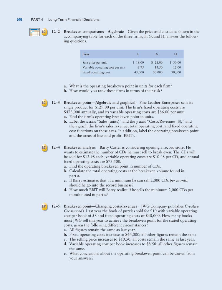
546 PART 4 Long-Term Financial Decisions
LG1
LG1
LG1
LG1
12–2 Breakeven comparisons—Algebraic Given the price and cost data shown in theaccompanying table for each of the three firms, F, G, and H, answer the follow-ing questions.
a. What is the operating breakeven point in units for each firm?b. How would you rank these firms in terms of their risk?
12–3 Breakeven point—Algebraic and graphical Fine Leather Enterprises sells itssingle product for $129.00 per unit. The firm’s fixed operating costs are$473,000 annually, and its variable operating costs are $86.00 per unit.a. Find the firm’s operating breakeven point in units.b. Label the x axis “Sales (units)” and the y axis “Costs/Revenues ($),” and
then graph the firm’s sales revenue, total operating cost, and fixed operatingcost functions on these axes. In addition, label the operating breakeven pointand the areas of loss and profit (EBIT).
12–4 Breakeven analysis Barry Carter is considering opening a record store. Hewants to estimate the number of CDs he must sell to break even. The CDs willbe sold for $13.98 each, variable operating costs are $10.48 per CD, and annualfixed operating costs are $73,500.a. Find the operating breakeven point in number of CDs.b. Calculate the total operating costs at the breakeven volume found in
part a.c. If Barry estimates that at a minimum he can sell 2,000 CDs per month,
should he go into the record business?d. How much EBIT will Barry realize if he sells the minimum 2,000 CDs per
month noted in part c?
12–5 Breakeven point—Changing costs/revenues JWG Company publishes CreativeCrosswords. Last year the book of puzzles sold for $10 with variable operatingcost per book of $8 and fixed operating costs of $40,000. How many booksmust JWG sell this year to achieve the breakeven point for the stated operatingcosts, given the following different circumstances?a. All figures remain the same as last year.b. Fixed operating costs increase to $44,000; all other figures remain the same.c. The selling price increases to $10.50; all costs remain the same as last year.d. Variable operating cost per book increases to $8.50; all other figures remain
the same.e. What conclusions about the operating breakeven point can be drawn from
your answers?
Firm F G H
Sale price per unit $ 18.00 $ 21.00 $ 30.00
Variable operating cost per unit 6.75 13.50 12.00
Fixed operating cost 45,000 30,000 90,000
CHAPTER 12 Leverage and Capital Structure 547
LG1
LG2
LG2
12–6 Breakeven analysis Molly Jasper and her sister, Caitlin Peters, got into the nov-elties business almost by accident. Molly, a talented sculptor, often made littlefigurines as gifts for friends. Occasionally, she and Caitlin would set up a boothat a crafts fair and sell a few of the figurines along with jewelry that Caitlinmade. Little by little, demand for the figurines, now called Mollycaits, grew, andthe sisters began to reproduce some of the favorites in resin, using molds of theoriginals. The day came when a buyer for a major department store offered thema contract to produce 1,500 figurines of various designs for $10,000. Molly andCaitlin realized that it was time to get down to business. To make bookkeepingsimpler, Molly had priced all of the figurines at $8.00. Variable operating costsamounted to an average of $6.00 per unit. In order to produce the order, Mollyand Caitlin would have to rent industrial facilities for a month, which wouldcost them $4,000.a. Calculate Mollycait’s operating breakeven point.b. Calculate Mollycait’s EBIT on the department store order.c. If Molly renegotiates the contract at a price of $10.00, what will the
EBIT be?d. If the store refuses to pay more than $8.00 per unit but is willing to
negotiate quantity, what quantity of figurines will result in an EBIT of$4,000?
e. At this time, Mollycaits come in 15 different varieties. Whereas the averagevariable cost per unit is $6.00, the actual cost varies from unit to unit. What recommendation would you have for Molly and Caitlin with regard to pricing and/or the numbers and types of units that they offerfor sale?
12–7 EBIT sensitivity Stewart Industries sells its finished product for $9 per unit. Its fixed operating costs are $20,000, and the variable operating cost per unitis $5.a. Calculate the firm’s earnings before interest and taxes (EBIT) for sales of
10,000 units.b. Calculate the firm’s EBIT for sales of 8,000 and 12,000 units, respectively.c. Calculate the percentage changes in sales (from the 10,000-unit base level)
and associated percentage changes in EBIT for the shifts in sales indicatedin part b.
d. On the basis of your findings in part c, comment on the sensitivity of changesin EBIT in response to changes in sales.
12–8 Degree of operating leverage Grey Products has fixed operating costs of$380,000, variable operating costs of $16 per unit, and a selling price of $63.50per unit.a. Calculate the operating breakeven point in units.b. Calculate the firm’s EBIT at 9,000, 10,000, and 11,000 units, respectively.c. With 10,000 units as a base, what are the percentage changes in units sold
and EBIT as sales move from the base to the other sales levels used in part b?
d. Use the percentages computed in part c to determine the degree of operatingleverage (DOL).
548 PART 4 Long-Term Financial Decisions
LG2
LG2
LG2
LG2 LG5
LG1 LG2
e. Use the formula for degree of operating leverage to determine the DOL at10,000 units.
12–9 Degree of operating leverage—Graphical Levin Corporation has fixed operat-ing costs of $72,000, variable operating costs of $6.75 per unit, and a sellingprice of $9.75 per unit.a. Calculate the operating breakeven point in units.b. Compute the degree of operating leverage (DOL) for the following unit sales
levels: 25,000, 30,000, 40,000. Use the formula given in the chapter.c. Graph the DOL figures that you computed in part b (on the y axis) against
sales levels (on the x axis).d. Compute the degree of operating leverage at 24,000 units; add this point to
your graph.e. What principle do your graph and figures illustrate?
12–10 EPS calculations Southland Industries has $60,000 of 16% (annual interest)bonds outstanding, 1,500 shares of preferred stock paying an annual dividend of$5 per share, and 4,000 shares of common stock outstanding. Assuming that thefirm has a 40% tax rate, compute earnings per share (EPS) for the following lev-els of EBIT:a. $24,600b. $30,600c. $35,000
12–11 Degree of financial leverage Northwestern Savings and Loan has a current cap-ital structure consisting of $250,000 of 16% (annual interest) debt and 2,000shares of common stock. The firm pays taxes at the rate of 40%.a. Using EBIT values of $80,000 and $120,000, determine the associated earn-
ings per share (EPS).b. Using $80,000 of EBIT as a base, calculate the degree of financial leverage
(DFL).c. Rework parts a and b assuming that the firm has $100,000 of 16% (annual
interest) debt and 3,000 shares of common stock.
12–12 DFL and graphical display of financing plans Wells and Associates has EBIT of$67,500. Interest costs are $22,500, and the firm has 15,000 shares of commonstock outstanding. Assume a 40% tax rate.a. Use the degree of financial leverage (DFL) formula to calculate the DFL for
the firm.b. Using a set of EBIT–EPS axes, plot Wells and Associates’ financing plan.c. If the firm also has 1,000 shares of preferred stock paying a $6.00 annual
dividend per share, what is the DFL?d. Plot the financing plan, including the 1,000 shares of $6.00 preferred stock,
on the axes used in part b.e. Briefly discuss the graph of the two financing plans.
12–13 Integrative—Multiple leverage measures Play-More Toys produces inflatablebeach balls, selling 400,000 balls a year. Each ball produced has a variable oper-
CHAPTER 12 Leverage and Capital Structure 549
LG1 LG2
LG2
LG3
LG3
ating cost of $0.84 and sells for $1.00. Fixed operating costs are $28,000. Thefirm has annual interest charges of $6,000, preferred dividends of $2,000, and a40% tax rate.a. Calculate the operating breakeven point in units.b. Use the degree of operating leverage (DOL) formula to calculate DOL.c. Use the degree of financial leverage (DFL) formula to calculate DFL.d. Use the degree of total leverage (DTL) formula to calculate DTL. Compare
this to the product of DOL and DFL calculated in parts b and c.
12–14 Integrative—Leverage and risk Firm R has sales of 100,000 units at $2.00 perunit, variable operating costs of $1.70 per unit, and fixed operating costs of$6,000. Interest is $10,000 per year. Firm W has sales of 100,000 units at $2.50per unit, variable operating costs of $1.00 per unit, and fixed operating costs of$62,500. Interest is $17,500 per year. Assume that both firms are in the 40%tax bracket.a. Compute the degree of operating, financial, and total leverage for firm R.b. Compute the degree of operating, financial, and total leverage for firm W.c. Compare the relative risks of the two firms.d. Discuss the principles of leverage that your answers illustrate.
12–15 Integrative—Multiple leverage measures and prediction Carolina Fastener,Inc., makes a patented marine bulkhead latch that wholesales for $6.00. Each latch has variable operating costs of $3.50. Fixed operating costs are$50,000 per year. The firm pays $13,000 interest and preferred dividends of$7,000 per year. At this point, the firm is selling 30,000 latches a year and istaxed at 40%.a. Calculate Carolina Fastener’s operating breakeven point.b. On the basis of the firm’s current sales of 30,000 units per year and
its interest and preferred dividend costs, calculate its EBIT and net profits.
c. Calculate the firm’s degree of operating leverage (DOL).d. Calculate the firm’s degree of financial leverage (DFL).e. Calculate the firm’s degree of total leverage (DTL).f. Carolina Fastener has entered into a contract to produce and sell an addi-
tional 15,000 latches in the coming year. Use the DOL, DFL, and DTL topredict and calculate the changes in EBIT and net profit. Check your work bya simple calculation of Carolina Fastener’s EBIT and net profit, using thebasic information given.
12–16 Various capital structures Charter Enterprises currently has $1 million in totalassets and is totally equity-financed. It is contemplating a change in capital struc-ture. Compute the amount of debt and equity that would be outstanding if thefirm were to shift to each of the following debt ratios: 10, 20, 30, 40, 50, 60,and 90%. (Note: The amount of total assets would not change.) Is there a limitto the debt ratio’s value?
12–17 Debt and financial risk Tower Interiors has made the forecast of sales shown inthe following table. Also given is the probability of each level of sales.
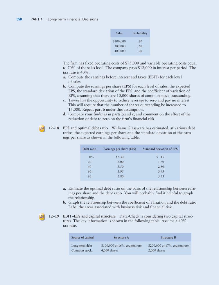
550 PART 4 Long-Term Financial Decisions
LG4
LG5
The firm has fixed operating costs of $75,000 and variable operating costs equalto 70% of the sales level. The company pays $12,000 in interest per period. Thetax rate is 40%.a. Compute the earnings before interest and taxes (EBIT) for each level
of sales.b. Compute the earnings per share (EPS) for each level of sales, the expected
EPS, the standard deviation of the EPS, and the coefficient of variation ofEPS, assuming that there are 10,000 shares of common stock outstanding.
c. Tower has the opportunity to reduce leverage to zero and pay no interest.This will require that the number of shares outstanding be increased to15,000. Repeat part b under this assumption.
d. Compare your findings in parts b and c, and comment on the effect of thereduction of debt to zero on the firm’s financial risk.
12–18 EPS and optimal debt ratio Williams Glassware has estimated, at various debtratios, the expected earnings per share and the standard deviation of the earn-ings per share as shown in the following table.
a. Estimate the optimal debt ratio on the basis of the relationship between earn-ings per share and the debt ratio. You will probably find it helpful to graphthe relationship.
b. Graph the relationship between the coefficient of variation and the debt ratio.Label the areas associated with business risk and financial risk.
12–19 EBIT–EPS and capital structure Data-Check is considering two capital struc-tures. The key information is shown in the following table. Assume a 40%tax rate.
Source of capital Structure A Structure B
Long-term debt $100,000 at 16% coupon rate $200,000 at 17% coupon rate
Common stock 4,000 shares 2,000 shares
Debt ratio Earnings per share (EPS) Standard deviation of EPS
0% $2.30 $1.15
20 3.00 1.80
40 3.50 2.80
60 3.95 3.95
80 3.80 5.53
Sales Probability
$200,000 .20
300,000 .60
400,000 .20
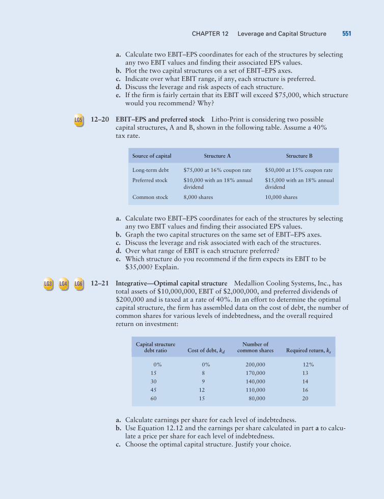
CHAPTER 12 Leverage and Capital Structure 551
LG5
LG3 LG4 LG6
a. Calculate two EBIT–EPS coordinates for each of the structures by selectingany two EBIT values and finding their associated EPS values.
b. Plot the two capital structures on a set of EBIT–EPS axes.c. Indicate over what EBIT range, if any, each structure is preferred.d. Discuss the leverage and risk aspects of each structure.e. If the firm is fairly certain that its EBIT will exceed $75,000, which structure
would you recommend? Why?
12–20 EBIT–EPS and preferred stock Litho-Print is considering two possible capital structures, A and B, shown in the following table. Assume a 40%tax rate.
a. Calculate two EBIT–EPS coordinates for each of the structures by selectingany two EBIT values and finding their associated EPS values.
b. Graph the two capital structures on the same set of EBIT–EPS axes.c. Discuss the leverage and risk associated with each of the structures.d. Over what range of EBIT is each structure preferred?e. Which structure do you recommend if the firm expects its EBIT to be
$35,000? Explain.
12–21 Integrative—Optimal capital structure Medallion Cooling Systems, Inc., hastotal assets of $10,000,000, EBIT of $2,000,000, and preferred dividends of$200,000 and is taxed at a rate of 40%. In an effort to determine the optimalcapital structure, the firm has assembled data on the cost of debt, the number ofcommon shares for various levels of indebtedness, and the overall requiredreturn on investment:
a. Calculate earnings per share for each level of indebtedness.b. Use Equation 12.12 and the earnings per share calculated in part a to calcu-
late a price per share for each level of indebtedness.c. Choose the optimal capital structure. Justify your choice.
Capital structure Number ofdebt ratio Cost of debt, kd common shares Required return, ks
0% 0% 200,000 12%
15 8 170,000 13
30 9 140,000 14
45 12 110,000 16
60 15 80,000 20
Source of capital Structure A Structure B
Long-term debt $75,000 at 16% coupon rate $50,000 at 15% coupon rate
Preferred stock $10,000 with an 18% annual $15,000 with an 18% annual dividend dividend
Common stock 8,000 shares 10,000 shares
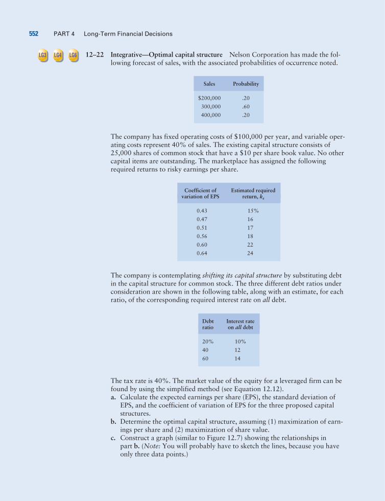
552 PART 4 Long-Term Financial Decisions
LG3 LG4 LG6 12–22 Integrative—Optimal capital structure Nelson Corporation has made the fol-lowing forecast of sales, with the associated probabilities of occurrence noted.
The company has fixed operating costs of $100,000 per year, and variable oper-ating costs represent 40% of sales. The existing capital structure consists of25,000 shares of common stock that have a $10 per share book value. No othercapital items are outstanding. The marketplace has assigned the followingrequired returns to risky earnings per share.
The company is contemplating shifting its capital structure by substituting debtin the capital structure for common stock. The three different debt ratios underconsideration are shown in the following table, along with an estimate, for eachratio, of the corresponding required interest rate on all debt.
The tax rate is 40%. The market value of the equity for a leveraged firm can befound by using the simplified method (see Equation 12.12).a. Calculate the expected earnings per share (EPS), the standard deviation of
EPS, and the coefficient of variation of EPS for the three proposed capitalstructures.
b. Determine the optimal capital structure, assuming (1) maximization of earn-ings per share and (2) maximization of share value.
c. Construct a graph (similar to Figure 12.7) showing the relationships inpart b. (Note: You will probably have to sketch the lines, because you haveonly three data points.)
Debt Interest rateratio on all debt
20% 10%
40 12
60 14
Coefficient of Estimated requiredvariation of EPS return, ks
0.43 15%
0.47 16
0.51 17
0.56 18
0.60 22
0.64 24
Sales Probability
$200,000 .20
300,000 .60
400,000 .20
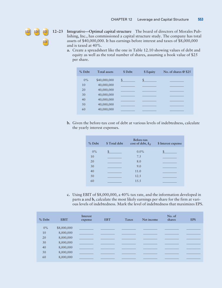
CHAPTER 12 Leverage and Capital Structure 553
LG3 LG4 LG5
LG6
12–23 Integrative—Optimal capital structure The board of directors of Morales Pub-lishing, Inc., has commissioned a capital structure study. The company has totalassets of $40,000,000. It has earnings before interest and taxes of $8,000,000and is taxed at 40%.a. Create a spreadsheet like the one in Table 12.10 showing values of debt and
equity as well as the total number of shares, assuming a book value of $25per share.
b. Given the before-tax cost of debt at various levels of indebtedness, calculatethe yearly interest expenses.
c. Using EBIT of $8,000,000, a 40% tax rate, and the information developed inparts a and b, calculate the most likely earnings per share for the firm at vari-ous levels of indebtedness. Mark the level of indebtedness that maximizes EPS.
Interest No. of% Debt EBIT expense EBT Taxes Net income shares EPS
0% $8,000,000��������� ��������� ��������� ��������� ��������� ���������
10 8,000,000��������� ��������� ��������� ��������� ��������� ���������
20 8,000,000��������� ��������� ��������� ��������� ��������� ���������
30 8,000,000��������� ��������� ��������� ��������� ��������� ���������
40 8,000,000��������� ��������� ��������� ��������� ��������� ���������
50 8,000,000��������� ��������� ��������� ��������� ��������� ���������
60 8,000,000��������� ��������� ��������� ��������� ��������� ���������
Before-tax% Debt $ Total debt cost of debt, kd $ Interest expense
0% $���������
0.0% $���������
10���������
7.5���������
20���������
8.0���������
30���������
9.0���������
40���������
11.0���������
50���������
12.5���������
60���������
15.5���������
% Debt Total assets $ Debt $ Equity No. of shares @ $25
0% $40,000,000 $���������
$��������� ���������
10 40,000,000��������� ��������� ���������
20 40,000,000��������� ��������� ���������
30 40,000,000��������� ��������� ���������
40 40,000,000��������� ��������� ���������
50 40,000,000��������� ��������� ���������
60 40,000,000��������� ��������� ���������
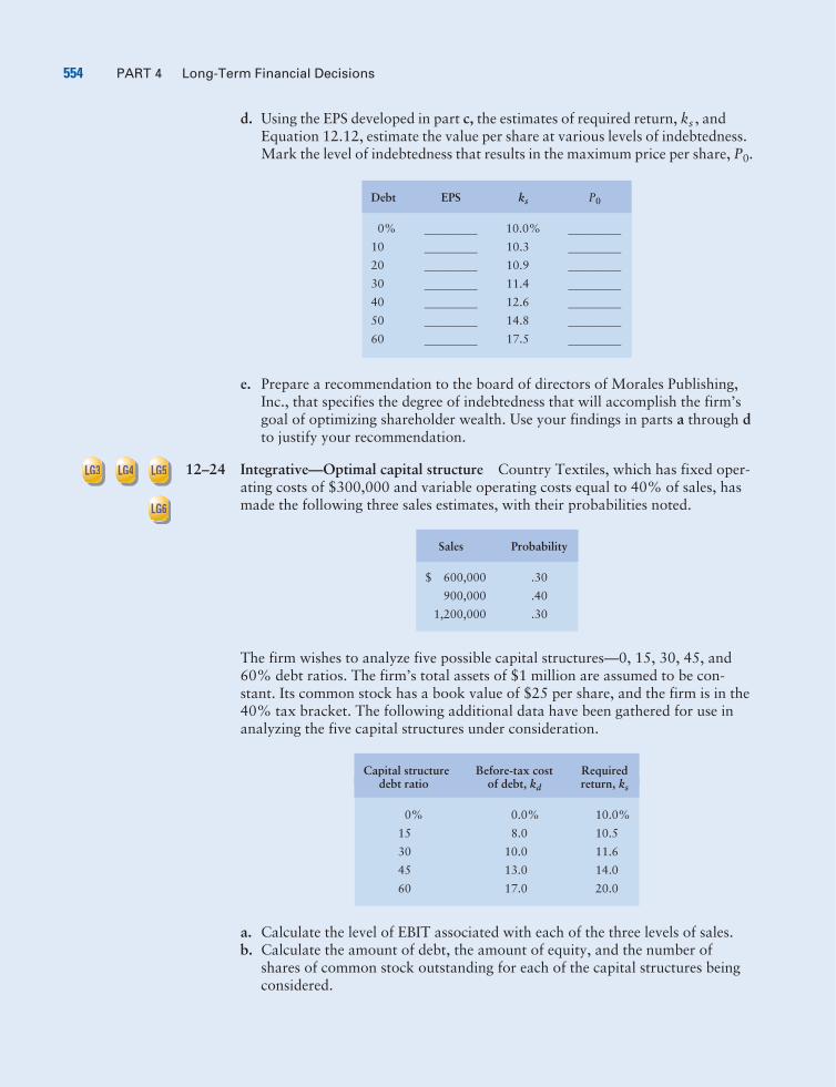
554 PART 4 Long-Term Financial Decisions
LG3 LG4 LG5
LG6
d. Using the EPS developed in part c, the estimates of required return, ks , andEquation 12.12, estimate the value per share at various levels of indebtedness.Mark the level of indebtedness that results in the maximum price per share, P0.
e. Prepare a recommendation to the board of directors of Morales Publishing,Inc., that specifies the degree of indebtedness that will accomplish the firm’sgoal of optimizing shareholder wealth. Use your findings in parts a through dto justify your recommendation.
12–24 Integrative—Optimal capital structure Country Textiles, which has fixed oper-ating costs of $300,000 and variable operating costs equal to 40% of sales, hasmade the following three sales estimates, with their probabilities noted.
The firm wishes to analyze five possible capital structures—0, 15, 30, 45, and60% debt ratios. The firm’s total assets of $1 million are assumed to be con-stant. Its common stock has a book value of $25 per share, and the firm is in the40% tax bracket. The following additional data have been gathered for use inanalyzing the five capital structures under consideration.
a. Calculate the level of EBIT associated with each of the three levels of sales.b. Calculate the amount of debt, the amount of equity, and the number of
shares of common stock outstanding for each of the capital structures beingconsidered.
Capital structure Before-tax cost Requireddebt ratio of debt, kd return, ks
0% 0.0% 10.0%
15 8.0 10.5
30 10.0 11.6
45 13.0 14.0
60 17.0 20.0
Sales Probability
$ 600,000 .30
900,000 .40
1,200,000 .30
Debt EPS ks P0
0%���������
10.0%���������
10���������
10.3���������
20���������
10.9���������
30���������
11.4���������
40���������
12.6���������
50���������
14.8���������
60���������
17.5���������
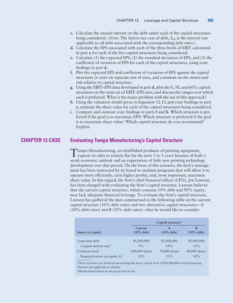
CHAPTER 12 Leverage and Capital Structure 555
c. Calculate the annual interest on the debt under each of the capital structuresbeing considered. (Note: The before-tax cost of debt, kd, is the interest rateapplicable to all debt associated with the corresponding debt ratio.)
d. Calculate the EPS associated with each of the three levels of EBIT calculatedin part a for each of the five capital structures being considered.
e. Calculate (1) the expected EPS, (2) the standard deviation of EPS, and (3) thecoefficient of variation of EPS for each of the capital structures, using yourfindings in part d.
f. Plot the expected EPS and coefficient of variation of EPS against the capitalstructures (x axis) on separate sets of axes, and comment on the return andrisk relative to capital structure.
g. Using the EBIT–EPS data developed in part d, plot the 0, 30, and 60% capitalstructures on the same set of EBIT–EPS axes, and discuss the ranges over whicheach is preferred. What is the major problem with the use of this approach?
h. Using the valuation model given in Equation 12.12 and your findings in parte, estimate the share value for each of the capital structures being considered.
i. Compare and contrast your findings in parts f and h. Which structure is pre-ferred if the goal is to maximize EPS? Which structure is preferred if the goalis to maximize share value? Which capital structure do you recommend?Explain.
CHAPTER 12 CASE Evaluating Tampa Manufacturing’s Capital Structure
Tampa Manufacturing, an established producer of printing equipment,expects its sales to remain flat for the next 3 to 5 years because of both a
weak economic outlook and an expectation of little new printing technologydevelopment over that period. On the basis of this scenario, the firm’s manage-ment has been instructed by its board to institute programs that will allow it tooperate more efficiently, earn higher profits, and, most important, maximizeshare value. In this regard, the firm’s chief financial officer (CFO), Jon Lawson,has been charged with evaluating the firm’s capital structure. Lawson believesthat the current capital structure, which contains 10% debt and 90% equity,may lack adequate financial leverage. To evaluate the firm’s capital structure,Lawson has gathered the data summarized in the following table on the currentcapital structure (10% debt ratio) and two alternative capital structures—A(30% debt ratio) and B (50% debt ratio)—that he would like to consider.
Capital structurea
Current A BSource of capital (10% debt) (30% debt) (50% debt)
Long-term debt $1,000,000 $3,000,000 $5,000,000
Coupon interest rateb 9% 10% 12%
Common stock 100,000 shares 70,000 shares 40,000 shares
Required return on equity, ksc 12% 13% 18%
aThese structures are based on maintaining the firm’s current level of $10,000,000 of total financing.bInterest rate applicable to all debt.cMarket-based return for the given level of risk.
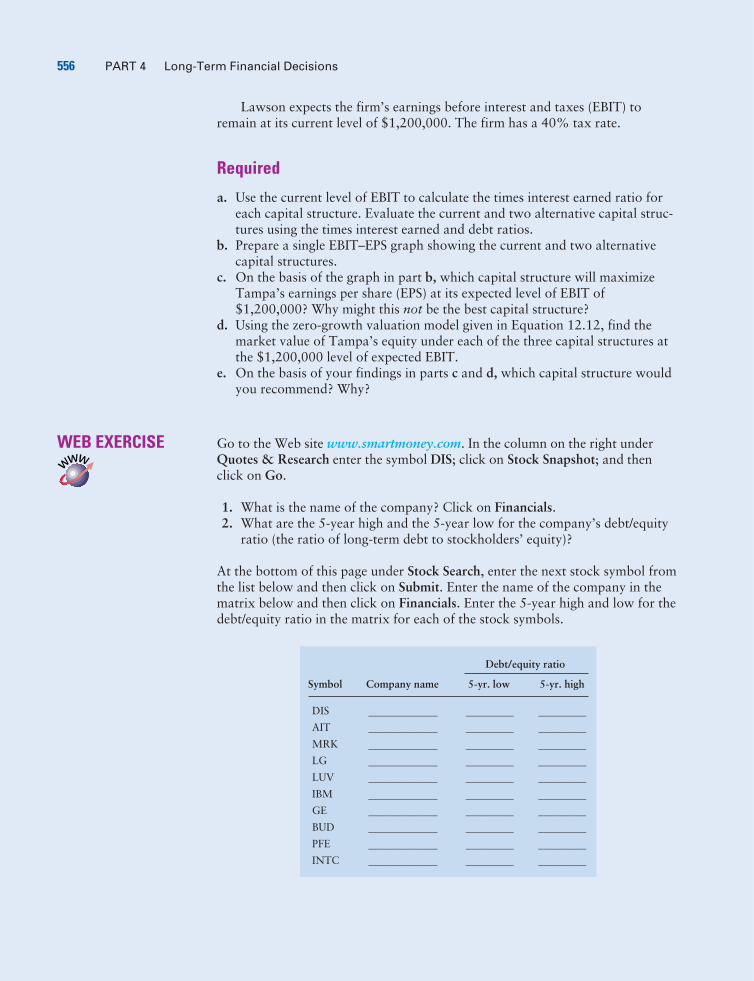
556 PART 4 Long-Term Financial Decisions
WWW
Lawson expects the firm’s earnings before interest and taxes (EBIT) toremain at its current level of $1,200,000. The firm has a 40% tax rate.
Required
a. Use the current level of EBIT to calculate the times interest earned ratio foreach capital structure. Evaluate the current and two alternative capital struc-tures using the times interest earned and debt ratios.
b. Prepare a single EBIT–EPS graph showing the current and two alternativecapital structures.
c. On the basis of the graph in part b, which capital structure will maximizeTampa’s earnings per share (EPS) at its expected level of EBIT of$1,200,000? Why might this not be the best capital structure?
d. Using the zero-growth valuation model given in Equation 12.12, find themarket value of Tampa’s equity under each of the three capital structures atthe $1,200,000 level of expected EBIT.
e. On the basis of your findings in parts c and d, which capital structure wouldyou recommend? Why?
WEB EXERCISE Go to the Web site www.smartmoney.com. In the column on the right underQuotes & Research enter the symbol DIS; click on Stock Snapshot; and thenclick on Go.
1. What is the name of the company? Click on Financials.2. What are the 5-year high and the 5-year low for the company’s debt/equity
ratio (the ratio of long-term debt to stockholders’ equity)?
At the bottom of this page under Stock Search, enter the next stock symbol fromthe list below and then click on Submit. Enter the name of the company in thematrix below and then click on Financials. Enter the 5-year high and low for thedebt/equity ratio in the matrix for each of the stock symbols.
Debt/equity ratio
Symbol Company name 5-yr. low 5-yr. high
DIS������������� ��������� ���������
AIT������������� ��������� ���������
MRK������������� ��������� ���������
LG������������� ��������� ���������
LUV������������� ��������� ���������
IBM������������� ��������� ���������
GE������������� ��������� ���������
BUD������������� ��������� ���������
PFE������������� ��������� ���������
INTC������������� ��������� ���������

CHAPTER 12 Leverage and Capital Structure 557
Remember to check the book’s Web site at
www.aw.com/gitman
for additional resources, including additional Web exercises.
3. Which of the companies have high debt/equity ratios?4. Which of the companies have low debt/equity ratios?5. Why do the companies that have a low debt/equity ratio use more equity
even though it is more expensive than debt?