Disponible en: http://redalyc.uaemex.mx/src/inicio/ArtPdfRed.jsp?iCve=21210701

RedalycSistema de Información Científica

Red de Revistas Científicas de América Latina, el Caribe, España y Portugal

VÉLEZ-PAREJA, IGNACIO; IBRAGIMOV, RAUF; THAM, JOSEPH

CONSTANT LEVERAGE AND CONSTANT COST OF CAPITAL: A COMMON

KNOWLEDGE HALF-TRUTH

Estudios Gerenciales, Vol. 24, Núm. 107, abril-junio, 2008, pp. 13-33

Universidad ICESI

Cali, Colombia

¿Cómo citar? Número completo Más información del artículo Página de la revista

Estudios Gerenciales

ISSN (Versión impresa): 0123-5923

estgerencial@icesi.edu.co

Universidad ICESI

Colombia

www.redalyc.orgProyecto académico sin fines de lucro, desarrollado bajo la iniciativa de acceso abierto

13ESTUDIOSGERENCIALES estud.gerenc., Vol. 24 No. 107 (Abril - Junio, 2008), 13-33.

Fecha de recepción: 21-04-2008 Fecha de aceptación: 29-05-2008Fecha de corrección: 20-05-2008

CONSTANT LEVERAGE AND CONSTANT COST OF CAPITAL:

A COMMON KNOWLEDGE HALF-TRUTHIGNACIO VÉLEZ–PAREJA

Ingeniero Industrial, M. Sc. en Ingeniería Industrial. Profesor Asociado, Universidad Tecnológica de Bolívar, Cartagena, Colombia.

ivelez@unitecnologica.edu.co, nachovelez@gmail.com

RAUF IBRAGIMOVMatemático, Ph.D en Ciencias (Candidato), Maestría en Administración.

Profesor asociado, Graduate School of Finance and Management, Moscow, Russia.ibrauf@rambler.ru

JOSEPH THAM Matemático, EdD, Harvard University.

Profesor asistente visitante, Duke University - Duke Center for International Development, Estados Unidosjoseph.tham@duke.edu

First version: June 29, 2007

This version: July 8, 2008

ABSTRACTA typical approach for valuing finite cash flows is to assume that lever-age is constant (usually as target leverage) and the cost of equity, Ke and the Weighted Average Cost of Capital, WACC are also assumed to be constant. For cash flows in per-petuity, and with the cost of debt, Kd as the discount rate for the tax shield, it is indeed the case that the Ke and WACC applied to the FCF are constant if the leverage is constant. However this does not hold true for finite cash flows.

In this document we show that for finite cash flows, Ke and hence WACC

depend on the discount rate that is used to value the tax shield, TS and as expected, Ke and WACC are not constant with Kd as the discount rate for the tax shield, even if the leverage is constant. We illustrate this situation with a simple example. We analyze five methods: DCF using APV, FCF and traditional and gen-eral formulation for WACC, present value of CFE plus debt and Capital Cash Flow, CCF.

KEY WORDSWACC, constant cost of capital, con-stant leverage, cash flows.

Clasificación JEL: D61, G31, H43

14 ESTUDIOSGERENCIALES Vol. 24 No. 107 • Abril - Junio de 2008

RESUMENUn enfoque típico para valorar flu-jos de caja finitos es suponer que el endeudamiento es constante (gene-ralmente como un endeudamiento objetivo o deseado) y que por tanto, el costo del patrimonio, Ke y el costo promedio ponderado de capital CPPC, también son constantes. Para los flu-jos de caja perpetuos, y con el costo de la deuda, Kd como la tasa de des-cuento para el ahorro en impuestos o escudo fiscal, Ke y el CPPC aplicado al flujo de caja libre FCL son constan-tes si el endeudamiento es constante. Sin embargo esto no es verdad para los flujos de caja finitos.

En este documento mostramos que para flujos de caja finitos, Ke y por lo tanto el CPPC dependen de la tasa de

descuento que se utiliza para valorar el ahorro en impuestos, AI y según lo esperado, Ke y el CPPC no son constantes con Kd como la tasa de descuento para el ahorro en impues-tos, aunque el endeudamiento sea constante. Ilustramos esta situación con un ejemplo simple. Analizamos cinco métodos: el flujo de caja descon-tado, FCD, usando APV, el FCD y la formulación tradicional y general del CPPC, el valor presente del flujo de caja del accionista, FCA más deuda y el flujo de caja de capital, FCC.

PALABRAS CLAVECosto promedio ponderado de capital, CPPC, costo de capital constante, endeudamiento constante, flujos de caja.

15ESTUDIOSGERENCIALESConstant leverage and constant cost of capital: A common knowledge half-truth

INTRODUCTIONIn this document we show that us-ing the findings of Tham and Velez-Pareja (2002), for finite cash flows, Ke (cost of levered equity) and hence WACC (Weighted Average Cost of Capital), depend on the discount rate that is used to value the tax shield (TS), and as expected, Ke and WACC are not constant with Kd (cost of debt) as the discount rate for the tax shield, even if the leverage is constant. We illustrate this situation with a simple example. We analyze five methods: DCF Discounted Cash flows (the Free Cash Flow, FCF) using APV, FCF and traditional and general formula-tion for WACC, present value of Cash Flow to equity (CFE) plus debt and Capital Cash Flow (CCF).

A typical approach for project or firm valuation which could be found in practice (See for example World Bank (2002), Benninga (1997, 2006), Bre-aley and Myers (2000, 2003), Brealey, Myers and Allen (2006), Copeland, Koller and Murrin (1995, 2000) is to discount cash flows expected within the finite time horizon at constant cost of capital, (usually as a target leverage) assuming that target lever-age is maintained throughout the life of the project, and thus its cost of levered equity Ke and the WACC are constant. Though it might be convenient to perform calculations under such assumption, it is not in fact always true that Ke and WACC are constant under the constant leverage financing policy. As could be seen from the findings and example of Inselbag and Kaufold (1997), and as a general expression for Ke and WACC derived by Tham and Velez-Pareja (2002), both the cost of levered equity and

the Weighted Average Cost of Capital depend on the value of the interest tax shield (VTS), and in the case of finite cash flows valuation, they could be changing from period to period if certain choice is made for the rate to discount expected tax shields.

The case of variable leverage has been studied elsewhere by Mian and Velez Pareja (2008), Velez-Pareja (2004, 2005), Velez-Pareja and Burbano (2006), Velez-Pareja and Tham (2001, 2004, 2006a, 2006b), and Tham and Velez Pareja (2002, 2004). In these cases, they find complete consistency between all methods and with differ-ent assumptions about the discount rate for the tax shields.

Practitioners frequently assume that the risk (and corresponding discount rate, ψ) of the interest tax shield is the cost of debt, Kd. This is done explicitly when, for example, the APV method is applied, or im-plicitly, if popular formula Ke= Ku + (Ku−Kd)×(1−T)×D/E (Ku, the cost of unlevered equity; T, corporate tax rate; D and E are market values of debt and equity, respectively) is used to estimate the cost of equity capital. As Taggart (1991) and Tham and Velez-Pareja (2002, 2004) prove, this formulation is valid only for a fixed (in perpetuity) dollar amount of debt, thus under constant leverage assumption it could be applied only to perpetual cash flows. However, this formula is used by Fernandez (2002), Shapiro (2005) and others even within finite planning horizon and when dol-lar amount of debt is changing from period to period. Another example of implicit ψ = Kd assumption is apply-ing Hamada’s formulation to unlever and relever betas. Initially developed

16 ESTUDIOSGERENCIALES Vol. 24 No. 107 • Abril - Junio de 2008

by Hamada (1972) for flat perpetu-ity and risk free debt, his formula is persistently used in conjunction with discounting at constant WACC under constant leverage assump-tion,1 potentially producing signifi-cant valuation errors as can be seen from the comprehensive example analyzed by Mian and Velez-Pareja (2008). Velez-Pareja and Tham (2004, 2006a, 2006b) repeatedly show that, if assumptions and formulae are mismatched, inconsistencies arise when calculating value with different methods. So analysts should be very careful dealing with finite cash flows. To obtain correct and consistent valu-ation results one should specify as-sumption for the risk of the tax shield (ψ) first, and from that assumption choose the proper formulation for Ke and WACC.

Different values one proposes for ψ, the risk or discount rate for the TS might be questioned based on the particular debt policy and underlying expectations for the cash flow profile. However, when selecting the assump-tion or approach for ψ, we have to be consistent in the use of the formula-tion for the cost of capital. If under the constant leverage financing policy the risk ψ of the interest tax shield is assumed2 to be equal to Kd, then Ke and WACC could not be assumed constant. Put it another way, ψ = Kd and constant Ke and WACC are incompatible assumptions within the constant leverage set up.

To illustrate the scenario of non con-stant cost of capital with constant le-verage3 we present a simple example, and analyze five DCF methods:

1. Adjusted present value (APV);

2. Discounting FCF at WACC calculated from the traditional formulation;

3. Discounting FCF at WACC cal-culated from the general formu-lation;4

4. Cash flow to equity (CFE) dis-counted at the cost of levered equity plus the value of debt, and

5. Capital Cash Flow (CCF) dis-counted at the corresponding cost of capital.

The rest of the document is organized as follows: in Section Two, we present the generalized formulation for the cost of capital for the finite cash flow valuation, and in particular formu-lae under the assumption that the discount rate for the tax shield (TS) is Kd. In Section Three we show a simple example. In Section Four we conclude.

1. GENERAL FORMULATION FOR KE AND WACCTaggart (1991) presents a revision of the set of formulations for the cost of levered Ke and WACC for perpetuities and finite cash flows. He introduces the formulation with and

1 Here we can mention very different texts from practitioners and academics: Pratt, Reilly and Schweihs (2000), Abrams (2001), Damodaran (2002),

2 This assumption is by itself debatable3 Which for example could be achieved through debt rebalancing at the end of every period to keep constant

its percentage of the estimated project value)4 See Tham and Velez-Pareja (2002, 2004).

17ESTUDIOSGERENCIALES

without personal taxes and for differ-ent level of risk for discounting the TS, including the Miles and Ezzell (1980). However, Taggart does not include the case of ψ = Kd for finite cash flows. Inselbag and Kaufold (1997) include the formulation of Ke and WACC for the case of Kd, the cost of debt as the level of risk for the TS and finite cash flows, but neither Tag-gart (1991) nor Inselbag and Kaufold (1997) show the formulation for the cost of capital appropriate to discount capital cash flow (CCF) under ψ = Kd and finite cash flows scenario.

Tham and Velez-Pareja (2002) pres-ent a derivation of the general expres-sion for Ke, the cost of levered equity for different levels of ψ corresponding to the risk of the tax shields, and re-sulting formulations for the general WACC, which should be applied to discount the Free Cash Flow (FCF) and Capital Cash Flow (CCF) both for finite time horizon valuation and for perpetuities.

The general formulation for Ke is,

L1-i

TS1-i

iiL1-i

1-iiiii E

V)�� - (Ku -

E

D)Kd - (Ku Ku Ke ��

Where Ku is the unlevered cost of equity, ψ is the risk (discount rate) of the TS, D is market value of debt, E is market value of equity and VTS is the market value of TS; i is the period of analysis.

The general formulation for WACCFCF is,

L1i

TS1i

iiL1-i

ii

FCFi

V

V)�(Ku -

V

TS - KuWACC

�

���

where TS is tax savings, VL is the mar-ket value of the levered firm and the other variables were defined above.

Following the path of the classic WACC derivation, we can easily show that general expression for the classic WACC is

L1-i

iL1-i

1-iL1-i

1-iFCFi V

TS - Kd

VD

KeVE

WACC ��

and we obtain traditional formula

)1(KdD%KeE%WACC 1-i1-iFCFi T������

)1(KdD%KeE%WACC 1-i1-iFCFi T������

when TSi = Kd×Di-1×T.

The general formulation for the WACCCCF is

L1i

TS1i

iiiCCFi

V

V)�[(Ku - KuWACC

�

���

The general formula for the value of TS is

��

� ��

N

ijj

jTS1i �)(1

TS V

When the risk of TS, ψ, is Ku, then Ke simplifies to

E

D)Kd - (Ku Ku Ke

1-i

1-iiiii ��

This formulation is valid for finite cash flows or perpetuities.

The WACC for the FCF simplifies to

V

TS - KuWACC

L1-i

ii

FCFi �

When taxes are paid when accrued and there is enough EBIT to earn the TS, then WACCFCF is

KdD%T - Ku

V

KdDT - KuWACC

1-ii

L1-i

1-ii

FCFi

���

���

And the WACC for the CCF simpli-fies to

KuWACC iCCFt �

Constant leverage and constant cost of capital: A common knowledge half-truth

18 ESTUDIOSGERENCIALES Vol. 24 No. 107 • Abril - Junio de 2008

The value of the TS is

��

� ��

N

iii

iTS1i )uK(1

TS V

When the risk of TS, ψ, is Kd, then Ke simplifies to

� � ���

����

���

1-i1-i

1-iiiii E

- E

DKd - Ku KuKe

TS1iV �

for finite cash flows and

� �� �E

DT-1Kd - Ku KuKe

1-i

1-iiii i ��

for perpetuities.

The WACC for the FCF simplifies to

L1i

TS1i

iiL1-i

ii

FCFi

V

V)Kd[(Ku -

V

TS - KuWACC

�

���

for finite cash flows.

And the WACC for the CCF simpli-fies to

� �L1-i

TS1-i

iiiCCF

V

VdK -Ku - KuWACC �

The value of the TS is

��

� ��

N

1ii

iTS1i )dK(1

TS V

Observe that in the case of ψ = Ku, Ke does not depend on TS and does not depend on the value of TS. Instead, when ψ = Kd, Ke depends on TS and the value of TS. On the other hand, when ψ = Ku, WACC depends on TS and it will be constant when taxes are paid when accrued and there is enough EBIT to earn the TS. Instead, when ψ = Kd, WACC depends on TS and the value of TS.

From these formulations we can conclude that for finite cash flows leverage and cost of capital are con-stant when:

1. There is enough EBIT to fully earn the TS.

2. Taxes are paid when accrued.3. The risk of TS is Ku.4. Tax rate T, is constant.5. Interest rate on debt is equal to

the (market) cost of debt, Kd.

With this set of formulations we can illustrate with a simple numerical example that Ke and WACC are not constant when leverage is main-tained constant if one assumes Kd (or any other value different from Ku) to be the appropriate discount rate for the expected interest tax shields. This can be seen in the formulation for Ke and WACC.

Full consistency in valuation results could be obtained for all five methods we mentioned in the Introduction if proper formulation for the cost of capital is applied to discount corre-sponding cash flow.

2. SIMPLE EXAMPLEA typical approach for valuing finite cash flows is to assume that leverage is constant and hence, Ke and WACC are introduced as constant. In this document, we show that using the findings of Tham and Velez-Pareja (2002), Ke, and hence WACC, de-pends on the value of the tax shield, TS, and as expected, Ke and WACC are not constant when we assume the risk of TS as Kd. We illustrate this situation with a simple example. We analyze five methods:

1. APV;

2. DCF using FCF and traditional formulation for WACC;

3. DCF using FCF and general formulation for WACC;

19ESTUDIOSGERENCIALES

4. Present value of CFE plus debt, and

5. Capital Cash Flow, CCF dis-counted at the WACC for CCF.

In the Appendix, the reader will find the complete information and the financial statements.

Assume a project (or the firm) with the following information:

1. Some input data.

2. Income Statement, Cash Budget and Balance Sheet.

3. Cash flows derived from the financial statements.

Year 1 Year 2 Year 3 Year 4

Real increase in sales 2% 2% 2% 2%

Inflation rate 6% 6% 6% 6%

Tax rate 35% 35% 35% 35%

Cost of debt Kd 11.20% 11.20% 11.20% 11.20%

Unlevered return, Ku 15.10% 15.10% 15.10% 15.10%

Risk of TS, Kd 11.20% 11.20% 11.20% 11.20%

D% 60% 60% 60% 60%

E% 40% 40% 40% 40%

Accounts receivable AR 10% 10% 10% 10%

Accounts payable AP 5% 5% 5% 5%

Gross margin 40% 40% 40% 40%

Table 2. Final debt schedule

Table 1. Input Data

Assume that the input data is as in Table 1.

Sales start with $10 in year 1. The fixed assets cost $4. The expected ending balance for the initial debt is shown in Table 2.

The complete financial statements are shown in the Appendix. From the financial statements we derive the following cash flows:

1. Free Cash Flow, FCF.

2. Cash Flow to Debt, CFD.

3. Cash Flow to Equity, CFE.

4. Tax savings.

Year 0 Year 1 Year 2 Year 3 Year 4

Ending debt balance 3.14 2.78 1.97 1.04

Principal payment 0.36 0.81 0.93 1.04

Interest payment 0.35 0.31 0.22 0.12

Constant leverage and constant cost of capital: A common knowledge half-truth

20 ESTUDIOSGERENCIALES Vol. 24 No. 107 • Abril - Junio de 2008

Table 3a. Working capital

Year 1 2 3 4

Accounts Receivable 1.00 1.08 1.17 1.26

Accounts Payable 0.30 0.32 0.35 0.38

Working Capital, WC 0.70 0.76 0.82 0.88

Change in WC 0.70 0.06 0.06 0.07

With the change in working capital we can construct the FCF using the indirect method.

Table 3b. Calculation of the FCF

Year 1 2 3 4

EBIT(1−T) 1.95 2.00 2.02 2.02

Depreciation 1.00 1.25 1.56 1.95

Change in WC -0.70 -0.06 -0.06 -0.07

Purchase of assets -1.00 -1.25 -1.56 -1.95

FCF 1.25 1.94 1.96 1.95

We show the different cash flows in the next table.

Table 4. Cash flows derived from the Financial Statements with Debt as % of Market Value

Year 1 2 3 4

FCF 1.25 1.94 1.96 1.95

CFD from the CB 0.72 0.72 0.71 0.67

TS from the CB 0.12 0.11 0.08 0.04

CFE from the CB 0.67 0.92 0.89 0.84

CFE = FCF + TS − CFD 0.67 0.92 0.89 0.84

With this information we can perform the valuation of the cash flows. In the next tables we show the valuation for each method after solving the itera-

tion process to solve the circularity between value and discount rate, where necessary.

Now we calculate the working capital for each year.

21ESTUDIOSGERENCIALES

Table 5. Adjusted Present Value, APV

Year 0 1 2 3 4

FCF 1.25 1.94 1.96 1.95

TS 0.12 0.11 0.08 0.04

APV

PV(FCF at Ku) 4.95 4.45 3.18 1.69

PV(TS at Kd) 0.28 0.19 0.10 0.04

APV 5.23 4.64 3.28 1.73

Value of debt, D 3.14 2.78 1.97 1.04

Leverage, D% 60% 60% 60% 60%

Using the APV and assuming that the discount rate for the TS is Kd:

Using the DCF, the traditional WACC, and assuming that the discount rate for the TS is Kd:

Table 6. Traditional WACC

Year 0 1 2 3 4

FCF 1.25 1.94 1.96 1.95

Weight of debt D% 60.00% 60.00% 60.00% 60.00%

After tax cost of debt 7.28% 7.28% 7.28% 7.28%

Contribution of debt to WACC 4.37% 4.37% 4.37% 4.37%

Equity

Relative weight of equity E% 40.00% 40.00% 40.00% 40.00%

Ke = Ku + (Ku-Kd)(D%/E%-VTS/E) 20.43% 20.55% 20.65% 20.75%

Contribution of equity to WACC 8.17% 8.22% 8.26% 8.30%

After tax WACC 12.54% 12.59% 12.63% 12.67%

Value 5.23 4.64 3.28 1.73

Value of debt, D 3.14 2.78 1.97 1.04

Leverage, D% 60% 60% 60% 60%

Observe that Ke and WACC are not constant. This occurs because the Ke is a function of the value of TS.

Using the DCF, the general WACC, and assuming that the discount rate for the TS is Kd:

Constant leverage and constant cost of capital: A common knowledge half-truth

22 ESTUDIOSGERENCIALES Vol. 24 No. 107 • Abril - Junio de 2008

Table 7. General WACC

Year 0 1 2 3 4FCF 1.25 1.94 1.96 1.95After tax WACC (general)

L1i

TS1i

iiL1-i

ii

FCFi

V

V)Kd[(Ku -

V

TS - KuWACC

�

���12.54% 12.59% 12.63% 12.67%

V 5.23 4.64 3.28 1.73Value of debt, D 3.14 2.78 1.97 1.04Leverage, D% 60% 60% 60% 60%

Using the CFE and assuming that the discount rate for the TS is Kd:

Table 8. Value Calculation with CFE

Year 0 1 2 3 4

Ending debt balance 3.14 2.78 1.97 1.04

Tax shield TS 0.09 0.07 0.05 0.02

PV(TS at Kd) 0.28 0.19 0.10 0.04

CFE= FCF + TS – CFD (with market value of debt) 0.67 0.92 0.89 0.84

Relative weight of debt D% 60.0% 60.0% 60.0% 60.0%

Relative weight of equity E% 40.0% 40.0% 40.0% 40.0%

Ke = Ku + (Ku-Kd)(D%/E%-VTS/E) 20.43% 20.55% 20.65% 20.75%

Value of equity 2.09 1.85 1.31 0.69

Value of debt 3.14 2.78 1.97 1.04

Total value 5.23 4.64 3.28 1.73 -

Leverage, D% 60% 60% 60% 60%

And finally, using the CCF with the WACCCCF , and assuming that the dis-count rate for the TS is Kd:

23ESTUDIOSGERENCIALES

Table 9. Capital Cash Flow

Year 0 1 2 3 4

FCF 1.25 1.94 1.96 1.95

TS 0.12 0.11 0.08 0.04

CCF 1.37 2.05 2.04 1.99

WACC for CCF:

� �L1-i

TS1-i

iiiCCF

V

VdK -Ku - KuWACC �

14.89% 14.94% 14.98% 15.02%

Value 5.23 4.64 3.28 1.73 0.00

Value of debt, D 3.14 2.78 1.97 1.04

Leverage, D% 60% 60% 60% 60%

Observe that the WACCCCF is not constant even if we assume that Ku is constant. WACCCCF is constant and equal to Ku (assuming no change in the operating risk for the firm and constant inflation) when we assume that the discount rate for the TS is Ku. The reason is identical to the one that makes Ke and WACCFCF non constant when leverage is constant and we assume the risk of TS equal to Kd: Ke, WACCFCF and WACCCCF depend on the value of TS.

As we have shown, first of all, all methods match5 when we use the proper formulation for the cost of capital (Ke and WACC); second, we have shown that the constant lever-age does not mean that Ke and WACC are constant. Tham and Velez-Pareja (2002, 2005), and Velez-Pareja and Tham (2006a, 2006b) have shown

that when using Ku as the risk for the TS and some conditions regarding the payment of taxes, the existence of enough EBIT to earn the TS and the source of the TS, the cost of capital is constant.6

Observe that the value calculated assuming ψ equal to Kd is higher than the value when we assume that ψ equal to Ku. A question arises here: is it reasonable to think that, changing the financing policy from constant leverage to predetermined debt schedule (non constant lever-age), the firm will increase its value? We leave the answer to this question for another work.

Now we can check the difference be-tween the initial debt schedule and the new debt schedule based on the market value of debt.

5 This is a matching of identical results. We have tested it for more than 10 decimals and the difference is strictly, zero. The interested reader might receive the spreadsheet upon request to the authors.

6 We are assuming that EBIT≥0. When this condition is not met, the traditional expression for WACC is no longer valid. When this happens we should use equation (4) and as can be seen from it, WACC might not be constant (imagine that there is not TS earned during some period). When TS is not earned, WACC for the FCF is just Ku.

Constant leverage and constant cost of capital: A common knowledge half-truth

24 ESTUDIOSGERENCIALES Vol. 24 No. 107 • Abril - Junio de 2008

Table 10. Initial debt schedule

Year 0 1 2 3 4Ending debt balance 3.75 2.45 1.50 0.75 Principal payment 1.30 0.95 0.75 0.75Interest payment 0.42 0.27 0.17 0.08

The new debt schedule is shown in next table.

Table 11. Debt Based on D%×Market Value of firm

Year 0 1 2 3 4Ending debt balance 3,14 2,78 1,97 1,04 Principal payment 0,36 0,81 0,93 1,04Interest payment 0,35 0,31 0,22 0,12

This means that management has to adjust debt from the beginning in order to achieve the target leverage. The difference in debt level is as follows.

Table 12. Difference of Market Value Debt with Initial Debt

Year 0 1 2 3 4Difference with initial debt 0.61 -0.33 -0.47 -0.29 0.00

3. SUMMARY AND CONCLUDING REMARKSWe have shown that a constant lever-age does not grant that the cost of capital is constant when the risk of the TS is Kd. Moreover, in order to achieve a proper valuation of finite cash flows with a constant leverage when the risk of TS is Kd, we have to use some formulations that differ from the traditional used by practi-tioners and textbooks. In other words, assuming constant leverage is not a sufficient condition to have constant cost of capital. We need to make explicit assumptions on the risk for the TS and use formulation for the cost of capital that is consistent with the assumed risk of the tax shield. Using the proper formulation in this scenario, we obtain full consistency in the calculation of value. This means that there are no advantages of one

method over another. All of them give the same value (when properly done) and all of them (even the APV) require iterations when the risk of the TS is Kd.

In short, we can conclude that for finite cash flows leverage and cost of capital are constant when:

1. There is enough EBIT to fully earn the TS.

2. Taxes are paid when accrued.

3. The risk of TS is Ku.

4. Tax rate T, is constant.

5. Interest rate on debt is equal to the (market) cost of debt, Kd.

In addition, we have to be aware that performing cash flow valuation with constant Ke and WACC under constant leverage assumption implies that particular formulations must be

25ESTUDIOSGERENCIALES

used for the estimation of Ke. Since the possibility of constant leverage and constant cost of capital scenario arises only when ψ = Ku, analysts should use formula

E

D)Kd - (Ku Ku Ke

L1-i

1-iiiii ��

to calculate the cost of levered equity directly, and formula

i�u

1-i

1-i

1-i

1-iiiLev

ED

1

ED

�d�

�

��

or

1-i

1-iiiiiLev

ED

)�d�u(�u� ���

for unlevering and levering the beta in case they use the CAPM. Here βu and βLev are the unlevered and levered β’s and Dt-1 and Et-1 are the market values of debt and equity.

Table 13. WACC for different approaches assuming constant leverage (60%)

Year 1 2 3 41. APV = PV(FCF at Ku) + PV(TS at Kd)WACC ND ND ND ND2. Traditional WACCAfter tax WACC Kd×D%×(1-T) + Ke×E% 12.54% 12.59% 12.63% 12.67%3. General WACC

L1i

TS1i

iiL1-i

ii

FCFi

V

V)Kd[(Ku -

V

TS - KuWACC

�

��� 12.54% 12.59% 12.63% 12.67%

4. V = PV(CFE at Ke) + DKe = Ku + (Ku-Kd)(D%/E%-VTS/E) 20.43% 20.55% 20.65% 20.75%5. Capital Cash Flow, CCF:

� �L1-i

TS1-i

iiiCCF

V

VdK -Ku - KuWACC � 14.89% 14.94% 14.98% 15.02%

When we assume that the risk of the TS is Kd, we cannot assume constant WACC or Ke because leverage is constant. The formulations for Ke and WACC (either for the Free Cash Flow, FCF or the Capital Cash Flow, CCF) depend not only on the constant leverage, but on the value of the TS and that refrains the cost of capital from being constant even if leverage is constant.

Summary of results assuming Kd as the risk of the TS, Table 13.

In the case of the risk for the TS equal to Ku, we can observe the equations for Ke, WACC for the FCF and the CCF, as follows:

The general formulation for Ke is,

L1-i

TS1-i

iiL1-i

1-iiiii E

V)� - (Ku -

E

D)Kd - (Ku Ku Ke ��

When the risk of the TS is Ku, the third term of the RHS of the equation

Constant leverage and constant cost of capital: A common knowledge half-truth

26 ESTUDIOSGERENCIALES Vol. 24 No. 107 • Abril - Junio de 2008

vanishes and Ke depends only on Ku, Kd and leverage (constants). Hence, Ke is constant.

The general formulation for WAC-CFCF is,

L1i

TS1i

iiL1-i

ii

FCFi

V

V)�(Ku -

V

TS- KuWACC

�

���

�

When the risk of the TS is Ku, the third term in the previous equa-tion vanishes and the second term is T×Kd×D% and hence WACCFCF depends only on leverage which is constant. Hence, WACC is constant.

L1-i

iL1-i

1-iL1-i

1-iFCFi V

TS- Kd

VD

KeVE

WACC ��

In this case, if Ke is constant then WACCFCF is constant.

The general formulation for the WACCCCF is

L1i

TS1i

iiiCCFi

V

V)�[(Ku - KuWACC

�

���

When the risk of the TS is Ku, the sec-ond term of the RHS of the equation vanishes and WACCCCF = Ku which is a constant.

27ESTUDIOSGERENCIALES

Financial Statements and Cash Flows

Table A1. Input Data

Real increase in sales 2%

Inflation rate 6% D% 60%

Tax rate 35% E% 40%

Cost of debt Kd 11.20% Ke 20.95%

Ku = Unlevered return 15.10%

Year 1 2 3 4

Unlevered return 15.10% 15.10% 15.10% 15.10%

psi = Kd 11.20% 11.20% 11.20% 11.20%

Inflation 6% 6% 6% 6%

Real increase in sales 2% 2% 2% 2%

Accounts Receivable 10% 10% 10% 10%

Accounts Payable 5% 5% 5% 5%

Gross margin 40% 40% 40% 40%

Table A2a. Initial Income Statement

Year 1 2 3 4

Sales revenues 10.00 10.81 11.69 12.64

COGS -6.00 -6.49 -7.01 -7.58

Gross income 4.00 4.32 4.68 5.06

Depreciation -1.00 -1.25 -1.56 -1.95

EBIT 3.00 3.07 3.11 3.10

Interest payments -0.42 -0.27 -0.17 -0.08

EBT 2.58 2.80 2.95 3.02

Taxes -0.90 -0.98 -1.03 -1.06

Net income 1.68 1.82 1.91 1.96

Appendix A

Constant leverage and constant cost of capital: A common knowledge half-truth

28 ESTUDIOSGERENCIALES Vol. 24 No. 107 • Abril - Junio de 2008

Table A2b. Final Income Statement (Debt as % of Market Value)

Year 1 2 3 4

Sales revenues 10.00 10.81 11.69 12.64

COGS -6.00 -6.49 -7.01 -7.58

Gross income 4.00 4.32 4.68 5.06

Depreciation -1.00 -1.25 -1.56 -1.95

EBIT 3.00 3.07 3.11 3.10

Interest payments -0.35 -0.31 -0.22 -0.12

EBT 2.65 2.76 2.89 2.99

Taxes -0.93 -0.97 -1.01 -1.05

Net income 1.72 1.80 1.88 1.94

Table A3a. Initial Balance Sheet

Year 0 1 2 3 4

Accounts Receivable AR 1.00 1.08 1.17 1.26

Fixed assets 4.00 5.00 6.25 7.81 9.77

Cumulated depreciation -1.00 -2.25 -3.81 -5.77

Net fixed assets 4.00 4.00 4.00 4.00 4.00

Total assets 4.00 5.00 5.08 5.17 5.26

Accounts Payable AP 0.30 0.32 0.35 0.38

Debt 3.75 2.45 1.50 0.75

Equity 0.25 0.25 0.25 0.25 0.25

New equity 2.00 1.01 0.81 0.82

Repurchase of equity

Net equity 0.25 2.25 3.26 4.07 4.88

Total liabilities and equity 4.00 5.00 5.08 5.17 5.26

29ESTUDIOSGERENCIALES

Table A3b. Final Balance Sheet (Debt as % of Market Value)

Year 0 1 2 3 4

Accounts Receivable AR 1.00 1.08 1.17 1.26

Fixed assets 4.00 5.00 6.25 7.81 9.77

Cumulated depreciation -1.00 -2.25 -3.81 -5.77

Net fixed assets 4.00 4.00 4.00 4.00 4.00

Total assets 4.00 5.00 5.08 5.17 5.26

Accounts Payable AP 0.30 0.32 0.35 0.38

Debt 3.14 2.78 1.97 1.04

Equity 0.86 0.86 0.86 0.86 0.86

New equity 0.00 1.06 1.93 2.92 4.02

Repurchase of equity

Net equity 0.86 1.92 2.79 3.78 4.88

Total liabilities and equity 4.00 5.00 5.08 5.17 5.26

Table A4a. Initial Cash Budget

Year 0 1 2 3 4

Cash Budget

Accounts Receivable 0.00 1.00 1.08 1.17

Sales revenues no credit 9.00 9.73 10.52 11.38

Suppliers payments -5.70 -6.16 -6.66 -7.20

Accounts payable 0.00 -0.30 -0.32 -0.35

Purchase of assets -4.00 -1.00 -1.25 -1.56 -1.95

Taxes -0.90 -0.98 -1.03 -1.06

Net Cash Balance NCB -4.00 1.40 2.04 2.02 1.98

Loan inflow 3.75

Loan principal payment -1.30 -0.95 -0.75 -0.75

Interest payment -0.42 -0.27 -0.17 -0.08

NCB 3.75 -1.72 -1.22 -0.92 -0.83

Initial equity investment 0.25

New (repurchase of) equity 2.00 1.01 0.81 0.82

Repurchase of equity

Dividends -1.68 -1.82 -1.91 -1.96

NCB 0.25 0.32 -0.81 -1.10 -1.15

Net cumulated balance - - - - -

Constant leverage and constant cost of capital: A common knowledge half-truth

30 ESTUDIOSGERENCIALES Vol. 24 No. 107 • Abril - Junio de 2008

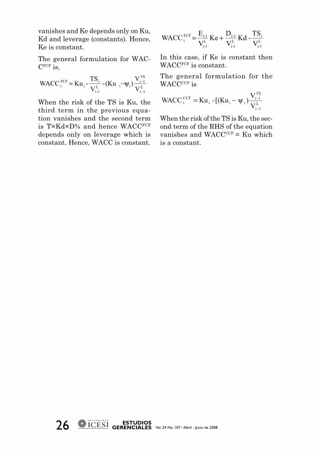
Table A4b. Final Cash Budget (Debt as a % of Market Value)

Year 0 1 2 3 4

Cash Budget 0.00 1.00 1.08 1.17

Accounts Receivable 9.00 9.73 10.52 11.38

Sales revenues no credit -5.70 -6.16 -6.66 -7.20

Suppliers payments 0.00 -0.30 -0.32 -0.35

Accounts payable -4.00 -1.00 -1.25 -1.56 -1.95

Purchase of assets -0.93 -0.97 -1.01 -1.05

Taxes -4.00 1.37 2.05 2.04 1.99

Net Cash Balance NCB 3.14

Loan inflow -0.36 -0.81 -0.93 -1.04

Loan principal payment -0.35 -0.31 -0.22 -0.12

Interest payment 3.14 -0.71 -1.13 -1.15 -1.15

NCB 0.86

Initial equity investment 1.06 0.87 0.99 1.11

New (repurchase of) equity

Repurchase of equity -1.72 -1.80 -1.88 -1.94

Dividends 0.86 -0.67 -0.92 -0.89 -0.84

NCB 0.00 0.00 0.00 0.00 0.00

Net cumulated balance 0.00 1.00 1.08 1.17

Table A5a. Working Capital

Year 0 1 2 3 4

AR 0.00 1.00 1.08 1.17 1.26

AP 0.00 0.30 0.32 0.35 0.38

WC 0.00 0.70 0.76 0.82 0.88

Change in WC 0.70 0.06 0.06 0.07

Table A5b. Cash Flow Calculation

Year 0 1 2 3 4

EBIT(1-T) 1.95 2.00 2.02 2.02

Depreciation 1.00 1.25 1.56 1.95

Change in WC -0.70 -0.06 -0.06 -0.07

Purchase of assets -1.00 -1.25 -1.56 -1.95

FCF 1.25 1.94 1.96 1.95

31ESTUDIOSGERENCIALES

Table A6a. Initial debt schedule

Year 0 1 2 3 4

Ending debt balance 3.75 2.45 1.50 0.75

Principal payment 1.30 0.95 0.75 0.75

Interest payment 0.42 0.27 0.17 0.08

Table A6b. Debt schedule Based on Market Value

Year 0 1 2 3 4

Ending debt balance market value 3.14 2.78 1.97 1.04

Principal payment 0.36 0.81 0.93 1.04

Interest payment 0.35 0.31 0.22 0.12

Table A7. Cash Flow Calculations

Year 0 1 2 3 4

Tax shield 0.12 0.11 0.08 0.04

CFD 0.71 1.13 1.15 1.15

CFE from the CB = Dividends – New Equity 0.67 0.92 0.89 0.84

FCF = CFD+CFE-TS 1.25 1.94 1.96 1.95

CFE = FCF + TS - CFD 0.67 0.92 0.89 0.84

Constant leverage and constant cost of capital: A common knowledge half-truth

32 ESTUDIOSGERENCIALES Vol. 24 No. 107 • Abril - Junio de 2008

BIBLIOGRAPHYAbrams, J.B. (2001). Quantitative Busi-

ness Valuation: A Mathematical Approach for Today’s Professional. New York, NY: McGraw-Hill.

Benninga, S.Z. (2006). Principles of Finance with Excel. New York, NY: Oxford University Press.

Benninga, S.Z., & Oded, H.S. (1997). Corporate Finance. A Valuation Approach. New York, NY: Mc-Graw-Hill.

Brealey, R. & Myers, S.C. (2000). Principles of Corporate Finance (6th ed.). New York, NY: McGraw Hill-Irwin.

Brealey, R. & Myers, S.C. (2003). Principles of Corporate Finance (7th ed.). New York, NY: McGraw Hill-Irwin.

Brealey, R., Myers, S.C., & Allen, F. (2006). Principles of Corporate Finance (8th ed.). New York, NY: McGraw Hill-Irwin.

Copeland, T.E., Koller, T. & Murrin, J. (1995). Valuation: Measuring and Managing the Value of Companies (2nd ed.). New York, NY: John Wiley & Sons.

Copeland, T.E., Koller, T. & Murrin, J. (2000). Valuation: Measuring and Managing the Value of Companies (3rd ed.). New York, NY: John Wiley & Sons.

Damodaran, A. (2002). Investment Valuation: Tools and Techniques for Determining the Value of Any Asset (2nd ed.). New York, NY: John Wiley & Sons.

Fernandez, P. (2002). Valuation Meth-ods and Shareholder Value Cre-ation. San Diego, CA: Academic Press.

Hamada, R.S. (1972). The Effect of the Firm’s Capital Structure on

the Systematic Risk of Common Stock. Journal of Finance, 27(2), 435-452.

Inselbag, I. & Kaufold, H. (1997, Spring). Two DCF Approaches in Valuing Companies under Alter-native Financing Strategies (and How to Choose between Them). Journal of Applied Corporate Fi-nance, 10(1), 114-122.

International Bank for Reconstruction and Development – The World Bank. (2002). Financial Modeling of Regulatory Policy [CD set].

Mian, M.A. & Velez-Pareja, I. (2008). Applicability of the Classic WACC Concept in Practice. Latin Ameri-can Business Review, 2(8). Avai-lable at SSRN: http://ssrn.com/ab-stract=804764

Miles, J. & Ezzell, J.R. (1980). The Weighted Average Cost of Capital, Perfect Capital Markets, and Proj-ect Life: A Clarification. Journal of Financial and Quantitative Analysis, 15, 719-730.

Pratt, S.P., Reilly, R.F. & Schweihs, P. (2000). Valuing A Business: The Analysis and Appraisal of Closely Held Companies (4th ed.) New York, NY: McGraw-Hill.

Shapiro, A.C. (2005). Capital Budget-ing and Investment Analysis. Upper Saddle River, NJ: Pearson Prentice Hall.

Taggart, R.A., Jr. (1991). Consistent Valuation and Cost of Capital Expressions with Corporate and Personal Taxes. Financial Man-agement, 20(3), 8-20.

Tham, J. & Velez–Pareja, I. (2002). An Embarrassment of Riches: Win-ning Ways to Value with the WACC (SSRN Working Paper 352180). Available at: http://papers.ssrn.com/sol3/papers.cfm?abstract_id=352180

33ESTUDIOSGERENCIALESConstant leverage and constant cost of capital: A common knowledge half-truth

Tham, J. & Velez-Pareja, I. (2004). Principles of Cash Flow Valuation. An Integrated Market Approach. London: Academic Press.

Tham, J. & Velez–Pareja, I. (2005). Modeling Cash Flows with Con-stant Leverage: A Note (SSRN Working Paper 754444). Available at: http://papers.ssrn.com/sol3/pa-pers.cfm?abstract_id=754444

Velez-Pareja, I. (2004). Modeling the Financial Impact of Regulatory Policy: Practical Recommendatio-ns and Suggestions. The Case of World Bank (SSRN Working Paper 580042). Available at: http://ssrn.com/abstract=580042

Velez-Pareja, I. (2005). Cash Flow Va-luation in an Inflationary World: The Case of World Bank for Regu-lated Firms. (SSRN Working Paper 643266). Available at: http://ssrn.com/abstract=643266

Velez–Pareja, I. & Burbano, A. (2006). Consistency in Valuation: A Practi-cal Guide (SSRN Working Paper 758664). Available at: http://papers.ssrn.com/sol3/papers.cfm?abstract_id=758664

Velez–Pareja, I. & Tham, J. (2001). A Note on the Weighted Average

Cost of Capital WACC (SSRN Working Paper 254587). Available at: http://papers.ssrn.com/sol3/pa-pers.cfm?abstract_id=254587

Velez-Pareja, I. & Tham, J. (2004). Consistency in Chocolate. A Fresh Look at Copeland’s Hershey Foods & Co Case (SSRN Working Paper 490153). Available at: http://ssrn.com/abstract=490153

Velez–Pareja I. & Tham, J. (2006a). Constant Leverage Modeling: A Re-ply to “A Tutorial on the McKinsey Model for Valuation of Companies (SSRN Working Paper 906786). Available at: http://ssrn.com/abs-tract=906786

Velez-Pareja, I. & Tham, J. (2006b). The Mismatching of APV and the DCF in Brealey, Myers and Allen 8th Edition of Principles of Corpo-rate Finance, 2006 (SSRN Working Paper 931805). Available at: http://ssrn.com/abstract=931805

Velez–Pareja I. & Tham, J. (2006c). Va-luation of Cash Flows with Cons-tant Leverage: Further Insights (SSRN Working Paper 879505). Available at: http://papers.ssrn.com/sol3/papers.cfm?abstract_id=879505