Embed Size (px)
Citation preview

Electronic copy available at: http://ssrn.com/abstract=1762116
The Relative Leverage Premium∗
Filippo Ippolito
Universitat Pompeu Fabra
Roberto Steri
Bocconi University
Claudio Tebaldi
Bocconi University
First version: February 14th, 2011
This version: February 28th, 2012
Abstract
The existing empirical evidence does not yet provide a clear understanding ofhow leverage and expected equity returns are related. While in some studies therelationship between financial leverage and returns is positive, in others returnsare either insensitive or decrease with leverage. We re-examine this evidence byexplicitly accounting for the dynamic nature of a firm’s optimal leverage policy inthe presence of frictions. Specifically, we allow firms to temporarily deviate fromtheir optimal capital structure due to adjustment costs. For each firm we estimatetarget leverage, and compute relative leverage as the difference between observedand target leverage. We find that relative leverage is positively and significantlyrelated to expected equity returns, and has a dominant effect over size and book-to-market. The relative leverage premium shows a remarkable symmetry for over-and under-leveraged firms.
JEL Classification: G12, G32Keywords: leverage, cross section of returns, target leverage, dynamic capitalstructure, financial frictions
∗We would like to thank Micheal Brennan, Mark Flannery, Vidhan Goyal, Christopher Hennessy,Peter Kondor, Arthur Korteweg, Eric Lam, Juhani Linnainmaa, Michael Mueller, Alessio Saretto,Stephen Schaefer, Lukas Schmid, Pietro Veronesi, and Kuan Xu for valuable comments and discussions,and Samad Javadi for research assistance. We also have benefited from comments from seminar parteci-pants at Universitat Pompeu Fabra, at Goethe University of Frankfurt, at the 18th Annual Conferenceof the Multinational Finance Society, at the 7th CSEF-IGIER Symposium on Economics and Institu-tions, at the 2011 Northern Finance Association Conference, at the 2012 American Finance AssociationAnnual Meeting, and at the 2012 Midwest Finance Association Annual Meeting. All remaining errorsare our own. Filippo Ippolito is associated with the Department of Economics and Business, Universi-tat Pompeu Fabra and with the Barcelona Graduate School of Economics, Ramon Trias Fargas 25-27,08005 Barcelona, Spain. Roberto Steri and Claudio Tebaldi are affiliated with the Department of Fi-nance at Bocconi University, Via Roentgen 1, 20136 Milan, Italy. Corresponding author: Roberto Steri,Department of Finance, Bocconi University, Via G. Roentgen n. 1 - 20136 - Milano, Room 2-C3-04.

Electronic copy available at: http://ssrn.com/abstract=1762116
1 Introduction
The role of financial leverage as a determinant of the cross-section of equity returns has
increasingly been investigated since Bhandari (1988). However, as illustrated by Gomes
and Schmid (2010), the existing empirical evidence does not yet provide a clear under-
standing of how leverage and returns are related. While some studies show a positive
relationship between financial leverage and expected stock returns, others conclude that
average returns are either insensitive, or decrease with leverage after controlling for the
effects of size and book-to-market equity.
The trade-off theory of capital structure predicts that firms choose their capital
structure by balancing the costs and benefits of operating at different levels of debt
financing.1 A common feature of trade-off models is that they imply the existence of
a firm-specific target leverage ratio. Firms that exhibit a targeting behavior choose
a target leverage ratio and gradually converge towards it.2 However, the presence of
adjustment costs and other frictions may prevent firms from achieving the optimal capital
structure at any one time (Leary and Roberts (2005), Strebulaev (2007)). Firms can then
temporarily deviate from their optimal capital structure, and be over- or under-leveraged
with respect to target. As discussed by Korteweg (2010), this non-frictionless dynamic
environment can generate heterogeneity in the cross-section of observed leverages. The
equity of firms with the same observed leverage but with different target bears a different
risk exposure, and is then priced differently. Looking only at observed debt ratios does
not allow to make this distinction. One should then remove firm-specific heterogeneity
before trying to establish a cross-sectional relationship between leverage and expected
1The corporate finance literature identifies several types of costs and benefits related to the use ofdebt. For example, Korteweg (2010) mentions tax shields of debt, agency benefits of debt due to alower free cash flow, bankruptcy costs, and indirect costs related to debt overhang, asset substitution,and asset fire-sales.
2For an excellent review of dynamic and static trade-off theories see Frank and Goyal (2008). Morespecifically, for recent dynamic models see Fischer, Heinkel, and Zechner (1989), Leland (1994), Gold-stein, Ju, and Leland (2001).
1

Electronic copy available at: http://ssrn.com/abstract=1762116
stock returns.
Differently from previous approaches, in this paper we explicitly account for firm-
specific heterogeneity in target leverage ratios and for deviations from the target. First,
we estimate firm-specific target leverage employing the partial-adjustment model orig-
inally developed by Flannery and Rangan (2006), and later examined by Lemmon,
Roberts, and Zender (2008), Huang and Ritter (2009), and Faulkender, Flannery, Han-
kins, and Smith (2010). Then, we decompose observed leverage into target leverage and
deviation from target. We define the deviation from target as relative leverage. When
relative leverage is positive a firm is over-leveraged with respect to target, while a firm is
under-leveraged when relative leverage is negative. Next, we examine the cross-sectional
relationship between relative leverage and equity returns. Our main objective is to test
whether positive (negative) deviations from target are associated with higher (lower)
expected returns.
The main finding of the paper is that relative leverage is positively and strongly
related to expected equity returns. The marginal effect of relative leverage is very high
in our entire investigation period (1965-2009) and stable across all the sub-periods 1965-
1979, 1980-1994, and 1995-2009. Our empirical evidence also suggests that this variable
has a much more substantial impact on expected stock returns than both size and book-
to-market.
More precisely, we first sort stocks into quintiles by observed market leverage (market
debt ratio (MDR)) and relative leverage, and illustrate that there is no clear pattern in
average returns as one moves from low to high MDR. On the contrary, average returns
show a strong positive correlation with relative leverage within every quintile of MDR.
This indicates that the positive relationship between relative leverage and average stock
returns is observed for both over-leveraged and under-leveraged firms. Moreover, the
premium (discount) associated with relative leverage is fairly symmetric. On average,
2

a deviation of 10% between observed and target leverage corresponds to a premium
(discount) of about 0.5% per month for over- (under-) leveraged firms. Average returns
of firms on target are around 1.5% per month.
We then follow the Fama and MacBeth (1973) (FMB) regression approach and ex-
amine the time-series averages of the estimated coefficients of monthly cross-sectional
regressions of stock returns on size, book-to-market equity, momentum and relative lever-
age. We find that relative leverage plays a dominant role in the cross-section of expected
equity returns. Relative leverage has an average coefficient of 3.509 in the period 1965-
2009, 20.73 standard errors from zero. The explanatory power of (log) book-to-market
equity is weak if both (log) size and relative leverage are included in the same regression.
The positive relation between average returns and relative leverage is strong in all re-
gressions specifications and in all sub-periods, also after controlling for momentum. For
robustness, in the FMB regressions we employ relative leverage based on out-of-sample
estimates of target leverage. Our results remain strong in the out-of-sample estimation.
Next, we compare the explanatory power of relative leverage with that of observed
market leverage. For robustness, we also compute relative leverage and observed leverage
at book values. Our findings provide support to Gomes and Schmid (2010) and Obreja
(2010), in that neither MDR nor book leverage are important in the cross-section of
expected returns after controlling for size and book-to-market. On the contrary, our
results show that relative leverage at market and book value is strongly significant after
controlling for observed leverage (respectively at market and book value). MDR remains
significant (with a negative sign) after controlling for relative leverage. However, further
investigations show that the significance of MDR is driven by the period 1980-1994,
while it does not appear in other periods. Our findings shed light into the relationship
between financial leverage and expected equity returns. Specifically, they suggest that
relative leverage rather that observed leverage is the most relevant leverage variable in
3

the cross-section of equity returns.
Finally, we examine the implications of our results for factor asset pricing models.
Following the approach of Chan, Karceski, and Lakonishok (1998), itself based on Fama
and French (1993), we define a factor mimicking portfolio based on the relative leverage
premium. We define the OMU (over- minus under-leveraged) factor as the difference
between the average monthly returns of stocks with relative leverage above the 80th
percentile and below the 20th percentile. We first run orthogonalizing regressions to
show that the explanatory power of OMU is not subsumed by the Fama and French’s
(FF) factors, RMRF, SMB, and HML. On the contrary, the explanatory power of the
size factor SMB is subsumed by RMRF, HML, and OMU. Accordingly, we compare
the pricing ability of a multi-factor model including RMRF, HML, and OMU with that
of the FF three-factor model and of the CAPM. To do so, we choose 27 portfolios
independently sorted on size, book-to-market equity, and relative leverage as test assets.
We also consider other sets of test assets to verify that our results are not specific to
the 27 portfolios initially selected. We find that the model including OMU is able to
correctly price more assets than the FF model and CAPM, with lower average pricing
errors. These results suggest that (i) the relative leverage premium is not captured by
the FF model, and (ii) a factor based on relative leverage is useful for pricing expected
returns across assets, and is consistent with a rational relative leverage premium.
Our results have implications for both asset pricing and corporate finance. For asset
pricing, we propose relative leverage as a new variable that matters in the cross-section of
equity returns. This variable is strongly significant and has a clear economic meaning.
The premium associated with relative leverage may be explained as follows: during
recessions, firms tend to become more leveraged, because the value of equity tends to
decrease more than that of debt. The opposite holds for firms that are over-leveraged.
As the value of equity drops, in a recession the leverage of these firms moves further
4

away from the desired level. According to the trade-off theory the costs of an unbalanced
capital structure increase as leverage moves away from target. This suggests that the
payoffs of under-leveraged stocks increase during a recession and are counter-cyclical,
while those of over-leveraged stocks tend to decrease and are cyclical. As a result,
risk-averse investors require a lower expected return for under-leveraged stocks than for
over-leveraged ones.
For corporate finance, our results provide support to the existence of a target leverage
ratio which depends on firm-specific characteristics as well as market conditions. Im-
portantly, however, the interpretation of our findings does not require firms to exhibit
a targeting behavior3. Therefore, our results are not inconsistent with the findings of
Chang and Dasgupta (2009) and Iliev and Welch (2010), according to which firms are
sluggish in their convergence towards the targets.
The remainder of the paper is organized as follows. Section 2 reviews the existing
literature and provides an introduction to our main results. Section 3 discusses the
estimation of target leverage based on the partial-adjustment model of Flannery and
Rangan (2006). Section 4 is dedicated to the construction of our sample. Sections 5
and 6 present the empirical results of our asset pricing tests. Section 7 summarizes and
discusses our findings.
3The existing literature is still divided on the right magnitude of the speed of adjustment towardstarget. Flannery and Hankins (2010) provide evidence that the empirical estimates of the speed ofadjustment can vary dramatically depending on the econometric methodology adopted. The speedimplied by our estimation is 23.8% per year and is in line with other recent estimations of the partialadjustment model (e.g. Lemmon, Roberts, and Zender (2008), Faulkender, Flannery, Hankins, andSmith (2010)). Reassuringly enough, Flannery and Hankins (2010) also show that the estimates oftarget leverage are hardly affected by the methodology that one follows in its estimation.
5

2 Related literature and stylized evidence
The starting point of our analysis is Proposition 2 of Modigliani and Miller (1958),
according to which the expected yield of a share of stock is equal to the appropriate
capitalization rate for a pure equity stream, plus a premium related to the debt-to-
equity ratio of the firm. The proposition suggests that the relationship between equity
returns and leverage is positive. Bhandari (1988) is the first to examine this relationship
and to show that a positive relationship between expected stock returns and market
leverage exists, and that leverage remains significant after controlling for both levered
equity beta and market capitalization. This finding represents an empirical violation of
the Capital Asset Pricing Model (CAPM) of Sharpe (1964), Lintner (1965) and Black
(1972). According to CAPM, the relationship between leverage and average returns
should be entirely captured by the beta.
In their well known study, Fama and French (1992) find that the natural logarithms
of market leverage and of book leverage have significant and approximately opposite
coefficients in a Fama-MacBeth (FMB) regression in which returns are the dependent
variable. They argue that the difference between these two leverage measures, i.e. the
natural logarithm of the book-to-market ratio of equity, should be associated with higher
expected stock returns. However, subsequent work does not provide full support to this
argument. Penman, Richardson, and Tuna (1992) propose an accounting decomposition
of the book-to-market ratio into an operating component and a leverage component.
Their evidence indicates that the leverage component is significantly and negatively
related to stock returns. They show that the negative relation holds for both market
and book leverage. George and Hwang (2010) revise this evidence and show that, after
controlling for book-to-market equity, stocks of firms in the highest quintile of book
leverage earn lower average returns, while the opposite holds for those in the lowest
quintile.
6

Two recent theoretical papers, Gomes and Schmid (2010) and Obreja (2010), explore
the relationship between leverage and expected stock returns using dynamic models in
which capital structure and investment decisions interact, thus violating the assumption
of Modigliani and Miller on the separation between financing and investment decisions.
The model of Obreja (2010) studies the interaction between book-to-market and leverage.
After calibration, the model is able to generate samples that replicate the empirical
evidence provided by Bhandari (1988) and Fama and French (1992). Instead, the model
of Gomes and Schmid (2010) shows that expected returns should be positively related
to leverage after controlling for firm size. Such a positive relation is more pronounced
for market than for book leverage. However, after controlling for book-to-market equity,
the relation becomes very weak.
In sum, several empirical studies have directly or indirectly examined the relationship
between leverage and expected equity returns. However, an agreement has not yet been
reached on two fundamental issues, i.e. whether leverage should be relevant in explaining
the cross-section of equity returns, and if the answer to this question is positive, what
sign should leverage have.
In this paper, we argue that one key element that has been ignored by the above
literature is that firms may have different desired leverage ratios, an idea that is at
the heart of the trade-off theory of capital structure. Introducing heterogeneity in the
cross-section of observed leverage ratios may complicate the identification of the linear
relation between leverage and expected returns. If a target leverage ratio exists, then
returns may be related to the deviations from this benchmark, rather than to observed
leverage. Intuitively, a 0.7 leverage ratio for a large firm in a consolidated industry,
such as steel manufacturing, has a very different meaning than for a small firm in a high
growth sector, such as communication technology. We then suggest that the relationship
between leverage and returns should be re-phrased as the relationship between relative
7

leverage and returns.
A related idea has been examined by Caskey, Hughes, and Liu (2011) in the ac-
counting literature. Following Graham (2000), they empirically estimate firms’ excess
leverage with respect to the level that maximizes the tax benefits of debt. They find
that, using annual data from 1980 to 2006, this excess leverage measure is negatively
related to future stock returns, and explains a great part of the negative relationship
documented by Penman, Richardson, and Tuna (1992). Their tests appear to contra-
dict the risk-based explanation proposed by George and Hwang (2010), and support an
alternative interpretation related to market under-reaction.
Figure 1 provides some preliminary evidence on the relationship between leverage
and returns, and between relative leverage and returns. The figure displays average
returns for firms assigned to 25 portfolios through two-way independent sorts on (market)
leverage and relative leverage. The sorting procedure is the same that we will employ
in Section 5 below. The figure shows that there is not a clear relationship between
average returns and observed leverage. Across quintiles of relative leverage, returns are
neither clearly increasing nor clearly decreasing in leverage. On the contrary, the sort
on relative leverage generates a considerable spread in average returns. Returns are
higher for stocks of over-leveraged firms (positive relative leverage) and lower for stocks
of under-leveraged firms (negative relative leverage). This basic finding suggests that
our attempt to remove heterogeneity from the cross-section of observed leverage can be
helpful in explaining expected equity returns.
(Insert Figure 1 about here)
Building on this evidence, Figure 2 illustrates how relative leverage interacts with
firm size, which we compute as in Fama and French (1992). Along the horizontal axis
we report deciles of relative leverage, while along the vertical axis we have size. Both
8

over-leveraged and under-leveraged firms appear to be smaller. Hennessy and Whited
(2007) find that firm’s size is a well-suited proxy for high costs of external financing.
Kurshev and Strebulaev (2007) also suggest that the existence of fixed costs of adjust-
ment prevents small firms to rebalance their capital structure as frequently as large
firms. Therefore, Figure 2 may be interpreted as evidence that smaller firms tend to be
further away from the desired level of leverage than larger firms due to the presence of
adjustment costs. This evidence suggests that size as employed in the specification of
Fama and French (1992) may be proxying for relative leverage.
(Insert Figure 2 about here)
3 The decomposition of leverage
In this section we implement the leverage decomposition of Flannery and Rangan (2006)
(FR) which allows us to identify the firm-specific components of total leverage that we
will use in the asset pricing tests of Section 5.4 Following FR we measure leverage as
the market debt ratio, defined as
MDRi,t =Di,t
Di,t +MEi,t
(1)
where Di,t denotes the stock of interest-bearing debt of firm i in period t and MEi,t
is the stock market capitalization of firm i in period t. We then consider the partial-
adjustment model of FR, according to which firms (partially) adjust their leverage over
4As we discuss below, the measure of target leverage developed by Flannery and Rangan currentlyencompasses other measures because it explicitly accounts for temporary deviations from the optimum.Other measures of target leverage have been proposed in the literature on capital structure. Therelationship between these leverage measures and returns is not examined in this paper, but it representsan possible line of enquiry for future research.
9

time towards the desired level MDR∗i,t+1 at a speed of adjustment λ:
MDRi,t+1 −MDRi,t = λ(MDR∗i,t+1 −MDRi,t) + ϵi,t+1 (2)
with
MDR∗i,t+1 = βXi,t (3)
MDR∗i,t+1 is modeled as a linear function of a set of firm-specific characteristics Xi,t,
and varies both over time and across firms. Equations (2) and (3) lead to the following
estimable model:
MDRi,t+1 = (λβ)Xi,t + (1− λ)MDRi,t + ϵi,t+1 (4)
FR interpret MDR∗i,t+1 as a proxy of a firm’s target leverage within the framework of the
trade-off theory of capital structure. Accordingly, the variables in Xi,t are firm-specific
characteristics that the literature on the trade-off theory has identified as relevant for
capital structure. The parameter λ can be interpreted as the percentage reduction in
the gap between actual and target leverage occurred over one period.
In comparison to other models previously employed in the literature (e.g. Fama and
French (2002); Korajczyk and Levy (2003)), a remarkable feature of the specification in
FR is that it relies on assumptions consistent with theoretical dynamic models of cap-
ital structure in presence of frictions. In particular, a key missing element in previous
specifications was the exclusion of lagged MDR in the estimation of (4). The exclu-
sion of lagged MDR amounts to assuming that a firm’s target leverage coincides with
its observed leverage.5 The very high and significant loading of MDRi,t in the empir-
5If MDRi,t+1 was expected to equal MDR∗i,t+1, then we should find λ = 1 from the estimation of
Equation (4). This is equivalent to saying that firms immediately adjust their capital structure to thedesired level. In this case, the partial-adjustment model in (2) simplifies to
MDRi,t+1 = MDR∗i,t+1 + ϵi,t+1
10
ical estimate of (4) in FR is consistent with Leary and Roberts (2005) and Strebulaev
(2007), according to which the existence of frictions prevents firms from instantaneously
adjusting towards their desired capital structure. In the absence of frictions firms would
always be on-target. Instead, in the presence of frictions it might be optimal for them
to operate away their optimal target, thus avoiding the adjustment costs required to
achieve the target.
The empirical estimation of (4) leads to a decomposition of MDRi,t into a target-
related component (λβ)Xi,t−1, an autoregressive component (1 − λ)MDRi,t−1, and a
residual component ϵi,t. In Section 3.2 we empirically implement this decomposition
and define the variables that we use in our asset pricing tests.
3.1 Data and variables for the estimation of target leverage
For the leverage decomposition of FR, we use the Compustat Industrial Annual database
over the period 1965-2009 including all companies listed on AMEX, NYSE, and NAS-
DAQ, and excluding foreign firms that are not incorporated in the United States. We
exclude financials (SIC codes 6000-6999) and utilities (SIC codes 4900-4999) because of
their special characteristics.
Our measure of leverage is MDR as defined in (1), and is computed as the book
value of short-term plus long-term interest bearing debt (Compustat items DLTT+DLC)
divided by the market value of assets (DLTT+DLC + PRCC F*CSHO). As in FR, Xi,t
contains the following variables:6 Profitability (EBIT TA): Earnings before interest and
taxes (EBIT) over total assets (AT); Market Value over Assets (MB): Book value of
liabilities plus market value of equity (DLTT+DLC + PRCC F*CSHO) over total assets
that isE[MDRi,t+1] = E[MDR∗
i,t+1]
6Variables that are not expressed as ratios are deflated by the consumer price index in 1983 dollars.
11

[AT]; Depreciation (DEP TA): Depreciation (DP) over total assets (AT); Size (lnTA):
Logarithm of total assets (AT); Tangibility (FA TA): Property, plant, and equipment
(PPENT) over total assets (AT); R&D expenses (R&D TA): R&D expenses (XRD)
over total assets (AT); R&D Dummy (R&D DUM): Dummy equal to one for firms with
missing values for R&D expenses (XRD); Industry MDR (Ind Median): Median industry
MDR calculated for each year for two-digit SIC code industries; a firm fixed effect.
Following standard procedures, all the previous variables (including MDR) are win-
sorized at the 1st and 99th percentiles to mitigate the influence of extreme observations.
All variables are based on fiscal years. When included, year dummies are based on
calendar years. Table 1 provides summary statistics for the variables listed above.
(Insert Table 1 about here)
3.2 Estimation of the partial adjustment model
Table 2 reports different specifications for Equation (4). FR and Lemmon, Roberts,
and Zender (2008) underline the importance of including unobservable firm fixed effects
in Xi,t.7 Columns 2 and 3 include these effects, and accordingly the regressions are
estimated as a dynamic panel data model.
(Insert Table 2 about here)
Flannery and Hankins (2010) find that the technique that generates the most accurate
parameter estimates in Equation (4) is the system GMM of Blundell and Bond (1998).
Therefore, as in Lemmon, Roberts, and Zender (2008), Lockhart (2010), and Faulkender,
7The inclusion of a firm fixed effect in target leverage ratios suits well our research design. In partic-ular, it allows to better identify a firm-specific target leverage ratio by taking into account unobservedheterogeneity.
12

Flannery, Hankins, and Smith (2010), in our “base” specification of column 3 we estimate
the partial-adjustment model (4) using Blundell and Bond system GMM.8
The results of our estimations are provided in Table 2 and are in line with previous
work. In particular, our estimate of the adjustment speed λ in column (3) is 23.8% which
is similar to that obtained by others. As econometric theory predicts, our estimate
of the autoregressive term 1 − λ (0.762) lies in the interval between the pooled OLS
estimate in column 1 (0.845), which is expected to be biased upwards, and the fixed-
effect estimate in column 2 (0.647), which is expected to be biased downwards (Hsiao
(2003)). As these three estimates show, the estimated value of the speed of adjustment λ
depends significantly on the methodology employed. Although recent work (Chang and
Dasgupta (2009), Iliev and Welch (2010)) challenges the existence of targeting behavior,
this critique is not a main concern here, because the estimation of target leverage is
not very sensitive to different estimation techniques. Simulation results provided by
Flannery and Hankins (2010) suggest that the econometric techniques employed in the
recent literature generally exhibit satisfactory finite-sample performance (in terms of
average bias) in estimating firm-specific target debt ratios MDR∗i,t+1. In our analysis
of cross-section returns, we use the regression specification of column 3. However, if
the target is estimated as in Flannery and Rangan (2006) - our column 2 - results are
qualitatively unaffected.
For the purpose of Section 5, it is useful to define the leverage-related variables that
we include in our asset pricing tests. These variables are: 1) our measures of relative
leverage obtained as the difference between observed and target leverage, 2) distance,
which is the absolute value of relative leverage, 3) over-leverage which is the maximum
between relative leverage and zero, and 4) under-leverage which is the negative of the
8In the estimation of Equation (4) with the Blundell and Bond system GMM, we consider all right-hand-side variables as predetermined with a lag length of one year. Only year dummies are regardedas fully exogenous. The inclusion of further lags has no significant influence on results.
13

minimum between relative leverage and zero. Noting that ˆMDR∗i,t denotes the estimated
firm-specific target for firm i in period t, obtained from the regression equation in column
3 of Table 2, we have:
Rel Levi,t ≡ MDRi,t − ˆMDR∗i,t (5)
Distancei,t ≡ ∥MDRi,t − ˆMDR∗i,t∥ (6)
Overlevi,t ≡ max{Rel Levi,t, 0} (7)
Underlevi,t ≡ −min{Rel Levi,t, 0} (8)
4 Data and variables for the analysis of returns
In our asset pricing tests we use monthly stock prices and returns for firms on NYSE,
AMEX, Nasdaq covered by the Center of Research in Security Prices (CRSP) from 1965
to 2009. We exclude financial companies (SIC codes 6000-6999) and utility companies
(SIC codes 4900-4999), and foreign firms not incorporated in the United States. De-
listing returns are included in monthly returns.
We match these monthly data to annual income statement and balance sheet data
from the CRSP/COMPUSTAT merged database, and to the annual series of the vari-
ables that we have defined in Section 3. We follow the matching procedure of Fama and
French (1992), which ensures a minimum gap of six months between fiscal year-ends and
returns. Thus, we match monthly prices and returns from July of calendar year t to
June of calendar year t + 1 with data from each company’s latest fiscal year ending in
calendar year t− 1.
In our tests, we consider the natural logarithm of market capitalization, the natu-
ral logarithm of book-to-market equity, and momentum as control variables. Market
capitalization - defined as the product of a company’s stock price times the number of
14

outstanding shares - is measured at June of calendar year t for the returns between July
of calendar year t and June of calendar year t + 1. We measure book-to-market equity
as the ratio between a firm book equity and its market capitalization at the end of De-
cember of calendar year t − 1. Following Fama and French (1993), we compute book
equity as the sum of shareholders’ equity, balance sheet deferred taxes and investments,
and tax credits if available, minus the book value of preferred stocks. Depending on
data availability, we estimate the book value of preferred stocks using, in this order,
their redemption, liquidation or par value. Since we consider the natural logarithm of
book-to-market equity in our tests, we eliminate firms with negative book equity from
our analysis. Finally, similar to Fama and French (2008), we measure momentum as the
continuously compounded return from month t− 12 to month t− 2.
In Section 5.3 we also consider book-valued debt ratios (BDR), defined as the book
value of short-term plus long-term interest bearing debt (DLTT + DLC) divided by the
book value of assets (DLTT + DLC) + book value of equity (BE). For BDR, we estimate
a relative leverage measure following the same procedure as in Section 3. More precisely,
our relative leverage measure for BDR is obtained by re-estimating Equation (4) with
BDR as dependent variable.9
All annual series are matched to monthly data from CRSP as described before.
Therefore, we match leverage, relative leverage, over-leverage, under-leverage, and dis-
tance measures from fiscal year t− 1 to monthly returns from July of year t to June of
year t + 1. In Section 6 and Appendix A we also employ monthly series of Fama and
French’s factors RMRF, HML, SMB, of the risk-free rate RF, and of the momentum
factor MOM. We obtain these data from Kenneth French’s website.
9Accordingly, MDRInd is replaced by the industry median of BDR.
15
5 Relative leverage and expected returns
Table 3 displays a correlation matrix for the main variables of our analysis. In the first
column, MDR and relative leverage present a high average cross-sectional correlation
(0.425) but are far from identical, as can be seen from column two. In particular, over-
leverage has a higher correlation with MDR than under-leverage, which indicates that
relative leverage differs fromMDRmore for under-leveraged firms than for over-leveraged
ones. Furthermore, a correlation of 0.162 between MDR and distance indicates that firms
with high levels of observed leverage tend to deviate from their target debt ratios by
a greater amount (in absolute value). However, distance is correlated to over-leverage
and under-leverage with coefficients of 0.450 and 0.597 respectively: this suggests that
under-leveraged firms are on average more distant from target than over-leveraged firms.
In addition, the table shows that all our leverage-related variables are correlated
to the variables normally known to affect the cross-section of expected equity returns.
Specifically, the natural logarithm of market capitalization is negatively related to the
absolute deviation from target leverage with a mean correlation of -0.121, while the
natural logarithm of book-to-market equity is positively related to relative leverage - with
a correlation of 0.138. Both these interactions are stronger for over-leverage, while under-
leverage is weakly correlated to log(size) and log(bm). Consistent with previous studies,
observed debt ratios are negatively correlated to log(size) and positively correlated to
log(bm). Our measure of momentum is correlated to relative leverage with a coefficient
of 0.137, and it also presents cross-sectional correlations coefficients of similar magnitude
with over-leverage (0.106) and under-leverage (-0.109).
(Insert Table 3 about here)
The sorts of Table 4 allow to examine separately the effects of observed leverage and
relative leverage on expected stock returns. Portfolios are formed each June by indepen-
16

dently ranking stocks into five groups by market debt ratios and relative leverage. The
panels from top-left to bottom-right respectively report averages of monthly time series
of 1) returns, 2) MDR, 3) BE/ME, 4) number of firms, 5) log(size), and 6) momentum.
Starting from the “Average Return” panel, we observe that no clear pattern exists in
average returns as firms move from low to high MDR (vertical shift). Low MDR stocks
are weakly associated with higher returns than high MDR stocks within the first three
quintiles of relative leverage (first three columns). However, this trend is inverted in the
last two columns. Moreover, these effects do not appear to be monotonic across quintiles
of MDR. This evidence suggests that sorting by MDR produces little variation in average
returns. On the contrary, average returns show a strong positive relation with relative
leverage within every quintile of MDR. Average percent monthly returns of stocks in
the lowest relative leverage quintile range from 0.56 and 0.96, while they are between
2.19 and 2.57 for stocks with the highest values of relative leverage. Moreover, average
returns appear to increase monotonically across relative leverage quintiles. This suggests
that relative leverage is positively related to stock returns for both over-leveraged and
under-leveraged firms. As a consequence, the direction of deviations from target capital
structure seems relevant in explaining expected returns.
The “MDR” panel indicates that MDR is roughly constant across relative leverage
quintiles. Therefore, with reference to the “average return” panel, the positive relation-
ship between returns and relative leverage is not due to higher MDR.
In the “log(size)” panel, we observe a U-shaped relationship between relative lever-
age and size. This pattern is consistent with Kurshev and Strebulaev (2007), according
to which the presence of fixed costs of external financing prevents small firms to rebal-
ance their capital structure frequently. Hence, small firms are expected to deviate from
optimal capital structure more than large firms.
The “BE/ME” panel shows the well-known positive relationship between BE/ME
17

and MDR. However, there is no evident relationship between BE/ME and relative lever-
age within any MDR quintile. Thus, the positive correlation between the book-to-market
ratio and relative leverage in Table 3 is likely the result of the positive correlation be-
tween MDR and relative leverage.
Finally, the “Momentum” panel shows that profits due to momentum are higher
for firms with high relative leverage. This stresses the importance to account for the
interaction of the momentum variable with relative leverage.
(Insert Table 4 about here)
Figure 3 depicts average monthly returns of stocks of firms sorted according to relative
leverage. Panel A refers to the full sample, while Panels B, C and D refer to the
subperiods 1965-1979, 1980-1994, and 1995-2009 respectively. The figure emphasizes
the magnitude of the relative leverage premium and shows a certain symmetry around
the estimated target MDR ratios (vertical line). In all four panels, firms that are over-
leveraged by 7.5% to 12.5% consistently earn average returns of about 2% per month,
while firms that are under-leveraged by 7.5% to 12.5% earn average returns of about 1%
per month. Average returns of firms on target are around 1.5% per month.
(Insert Figure 3 about here)
5.1 The Relative Leverage Premium
Table 5 reports time-series averages of the estimated coefficients of monthly cross-
sectional regressions of stock returns on size, book-to-market equity, momentum and
relative leverage. As in Fama and French (1992) and George and Hwang (2010), we
follow the regression approach in Fama and MacBeth (1973) (FMB). We report FMB
tests with a Newey-West correction with lag-length of 2 to assess which regressors have
18
a coefficient that is significantly different from zero. The FMB regressions in Table 5
take the following form:
Ri,t = β0 + β1log(sizei,t−1) + β2log(bmi,t−1) + β3momi,t−1 + β4Rel Levi,t−1 + ϵi,t (9)
where Ri,t denotes realized returns, sizei,t−1 market capitalization, bmi,t−1 book-to-
market equity, momi,t−1 momentum, and Rel Levi,t−1 relative leverage.
The results of Table 5 highlight the dominant role played by relative leverage in
the cross-section of expected equity returns. In the regression of column 7 of Panel
A, relative leverage has an average slope of 3.509%, with a t-statistic of 20.73. In the
same regression, the natural logarithm of market capitalization has a slope of -0.221%,
while the slope of (log) book-to-market equity is not statistically different from zero.
Comparing across columns 6 and 7, we notice that the explanatory power of (log) book-
to-market drops significantly when both (log) size and relative leverage are included in
the same regression. The coefficient of book-to-market is significant when it is the only
variable in the regression (column 2), and when it interacts separately either with size
(column 4) or relative leverage (column 6). The positive relation between average returns
and relative leverage persists across all regressions specifications, also after including
momentum (column 8). The estimated slopes for relative leverage range from 3.509%
to 4.003%, with Newey-West t-statistics between 18.68 and 23.39.
(Insert Table 5 about here)
In Appendix A, Table 11, we report sub-period evidence on the estimation of the
FMB regressions. The coefficient of relative leverage premium is strong in each of the
three sub-periods 1965-1979, 1980-1994, and 1995-2009. In comparison with relative
leverage, the explanatory power of size and book-to-market appears much less stable in
19

the sub-periods. Size has a strong effect on average returns in the 1995-2009 sub-period,
both in terms of estimated slope and significance, while its effect is weak in the sub-
period 1965-1979. Book-to-market has a strong effect in the years 1980-1994, while its
slope is not statistically different from zero in the years 1965-1979 and 1995-2009.
To eliminate potential biases due to in-sample estimationIn the corporate finance lit-
erature, partial adjustment models and, as a consequence, target leverage, are estimated
in-sample. Therefore, the results of Panel A of Table 5 may be affected by look-ahead
bias., we replicate the results of Panel A of Table 5 using out-of-sample estimation.
Results are reported in Panel B of Table 7. We employ the years 1965-1987 as the
estimation period, and for each year between 1987 and 2009 we estimate Equation 4 on
a rolling basis. As the estimation of target leverage contains firm fixed effects, we must
ensure that the estimation of these effects remains stable when Equation 4 is estimated
on a rolling basis. 10 To ensure stability of fixed effects estimation, we impose conditions
on their convergence and exclude observations that do not satisfy these criteria.11
The regressions in Panel B of Table 7 show that the significance of relative leverage
remains strong in the FMB regressions also for the out-of-sample estimation. In column
1, relative leverage is highly significant after controlling for (log) size and (log) book-
10Lemmon, Roberts, and Zender (2008) highlight the importance of using fixed effects as proxies for inthe estimation of partial adjustment models. The inclusion of firm fixed-effects finds theoretical supportin models where investment and financing interact, such as Hennessy and Whited (2007), and Gomesand Schmid (2010). Specifically, firm-specific unobservable shocks generate heterogeneity in firm-levelinvestment opportunities that, in turn, determines optimal leverage decisions. In Table 14 of AppendixA, we estimate the partial adjustment model including only the firm fixed effect as a determinant oftarget leverage, and show that key results are qualitatively unchanged with this specification. Thisfinding further stresses the importance of allowing for firm-specific unobservable heterogeneity in theestimation of target leverage.
11Firm fixed-effect estimates are likely to be noisier than for other coefficients because they are basedonly on individual time series variations. With a rolling estimation procedure, fixed effects are computedon the basis of one observation for the first year a firm appears in the panel, two observations for thesecond year, three for the third, and so on. Due to the unbalanced nature of the panel, and to theshorter time period required by the out-of-sample estimation, ensuring convergence in the estimationof fixed effects becomes particularly important. For this reason we impose convergence conditions. SeeAppendix B for further details on the estimation procedure described here. Table 17 in Appendix Bprovides evidence that our results are robust to several alternative convergence conditions.
20

to-market, with a positive slope of 2.166, and a t-statistic of 8.779. Following the
interpretation in Fama (1976), this slope can be interpreted as the average monthly
return of a self-financing portfolio with unit relative leverage, that hedges the effects
of size and book-to-market in the period 1990-2009. In the Fama and MacBeth (1973)
approach, the standard error is computed as the standard deviation of monthly returns
on this portfolio, divided by the square root of the number of months in the sample
(234 in this case). Hence, a t-statistic of 8.779 can be approximately translated into an
annualized Sharpe ratio of 1.725, assuming an average monthly risk-free rate of 30 basis
points 12 The regression in column 2 shows that after controlling for momentum, our
results are qualitatively in line with those reported in Panel A.13
To provide a term of comparison between the out and in-sample estimates, in columns
3-6 we provide in-sample estimations based on the same period employed for the out-
of-sample estimates (1990-2009) of columns 1-2. In columns 3-4 we estimate relative
leverage with Blundell and Bond (1998) system GMM, while in columns 5-6 we employ
the LSDV approach. A comparison across columns shows that results are similar for
both out and in-sample estimates. In addition, the coefficients of columns 3-4 are similar
to those in columns 5-6. This suggests that using the LSDV estimator instead of Blundell
and Bond (1998) system GMM has no serious impact on our findings, consistent with
the evidence in Flannery and Hankins (2010).
In-sample estimation is convenient for two reasons: 1) it allows asset pricing tests
over the whole period 1965-2009 and the collection of useful sub-period evidence; 2)
due to the asymptotic properties of fixed-effect estimators, longer time-series help mit-
12We estimate the monthly risk-free rate using data from Kenneth French’s website for the periodfrom July 1990 to December 2009.
13The evaluation of the economic relevance of results from FMB regressions should account for thelength of the sample period. The procedure to compute the implied Sharpe ratio from a FMB regressionis such that the magnitude of the t-statistics depends on the number of periods employed. Therefore,one should expect the t-statistics in Panel B to be lower than in Panel A even if relative leverage isestimated in-sample, as effectively is the case.
21

igate the finite-sample bias in the estimation of firm fixed-effects. The cost of using
in-sample estimation is that Fama-MacBeth coefficients do not correspond to directly
implementable trading strategies. Nonetheless, our out-of-sample test bring out that
there exists a convergence condition such that investors can actually implement these
strategies.
As relative leverage is the result of a previous estimation, our FMB regressions may
suffer from an errors-in-variables bias.14 The errors-in-variables problem may bias the
estimated coefficients towards zero (Greene (2008)). Therefore, insofar as our estimate
of relative leverage contains errors, the FMB regressions of Table 5 generate more con-
servative estimates than in the absence of errors.15 This suggests that there is a relative
leverage premium despite of a potential errors-in-variables bias.16
In sum, the FMB regressions provide support to a relative leverage premium, and
indicate that relative leverage plays an important role in explaining the cross-section
of expected equity returns, also after controlling for size, book-to-market equity, and
momentum.
5.2 Symmetry of the Relative Leverage Premium
The regressions in Table 6 investigate the relative importance that the following four
measures of leverage have in explaining equity returns: relative leverage, distance, over-
leverage, and under-leverage. Panel A covers the entire sample from 1965 to 2009. The
slope of distance is significant when relative leverage is not included (column 3), with a
slope of -0.709 and a t-statistic of -2.278. However, confirming our informal tests, the
14This kind of problem exists also for the CAPM beta in Fama and French (1992), and for the distressmeasures in George and Hwang (2010).
15However, this may not be the case if multiple variables in the regression are measured with error.16On the contrary, the problem of errors-in-variables is more serious in Fama and French (1992)
because they argue that the relationship between average returns and CAPM beta is flat. For a broaderdiscussion of the errors-in-variables bias see Kim (2010) and Carmichael and Coen (2008).
22

regression in column 6 of panel A shows that when distance and relative leverage are
included in the same regression, the slope of distance is not statistically different from
zero, with a t-statistic of 0.07. Columns 4 and 5 of panel A confirm that the relative
leverage premium is not driven separately by either under-leveraged or over-leveraged
firms. Over- and under-leverage are statistically insignificant when they are included in
the same regression with relative leverage. 17.
Columns 1 and 2 of Panel B replicate columns 2 and 6 of Panel A, using out-of-sample
estimation. Both over- and under-leverage matter when target leverage is estimated out-
of-sample. Over- and under-leverage are both statistically significant in the regression
in column 1, with slopes of 2.416 (t-statistic = 4.496) and -1.668 (t-statistic = -3.859)
respectively. When relative leverage and distance are included in the same regression
(column 2), distance is not statistically significant, with an estimated coefficient of 0.374
and a t-statistic of 0.914. As in Table 5, the results of the out-of-sample estimation are
in line with those of the in-sample estimation on the same period, both using Blundell
and Bond (1998) system GMM (columns 3-4) and the LSDV approach (columns 5-6).
Returning to Panel A of Table 6, the regression in column 2 shows that over- and
under-leverage have slopes of similar magnitude (3.496 and -3.450 respectively), but
opposite sign. This suggests that their difference, i.e. relative leverage, is what matters
in explaining returns, which is consistent with the results of columns 4 and 5. We perform
a Wald test of the linear restriction that the slope of over-leverage is equal, in absolute
value, to the slope of under-leverage. The test does not reject the null hypothesis that
the restriction holds with an F-stat of 0.02 and a p-value of 0.897.18
The symmetry of the relative leverage premium may be generated mechanically by
17In Table 12 of Appendix A we provide sub-period evidence, and show that the marginal effect ofrelative leverage dominates both distance, over-leverage and under-leverage in each sub-period
18Sub-period evidence in Table 12 of Appendix A confirms that the over- and under-leverage havestatistically equal slopes (in absolute values). In particular, Wald tests cannot reject this restrictionwith p-values of 0.1664 in the sub-period 1965-1979 (column 2 of panel A), of 0.1914 in the sub-period1980-1994 (column 2 of panel B), and of 0.8018 in the sub-period 1995-2009 (column 2 of panel C).
23

the fact that MDR is a function of returns, because leverage decreases when the market
value of equity increases.19 The relationship between size and relative leverage is not
straightforward as for other variables measured as ratios, like market capitalization and
book-to-market equity. However, firm fixed effects are estimated by setting the sample
mean of residuals equal to zero for each individual’s time series. As a result, ceteris
paribus, for a higher (respectively, lower) stock price the estimated firm fixed effect is
higher (lower), the estimated target leverage is higher (lower), and relative leverage is
lower (higher). Since expected returns are by construction inversely related to stock
prices, a perfectly symmetric relative leverage premium may naturally reflect such a
mechanical effect for both over- and under-leveraged firms.
There are three reasons why we believe that our results are not driven by a mechanical
relationship between MDR and prices. First, MDR is computed using data from fiscal
year end t− 1, and then matched to returns from July of year t to June on year t + 1.
Hence, the stock price component of MDR is unlikely to drive the relationship between
relative leverage and returns, because there is a minimum gap of six months between
the accounting data used to compute MDR and returns. Second, as we show in the next
section, the relationship between relative leverage and returns holds also if leverage is
measured at book values. In that case, the stock price is not included in the calculation
of the value of equity and leverage. Third, as firm fixed effects are the channel via which
stock prices affect relative leverage, a higher degree of symmetry should be observed
when target leverage is estimated using only firm fixed effects. On the contrary, the
absolute values of the coefficients for under- and over-leverage are closer in Panel A of
Table 6 (3.496 and 3.450 in column 2) than in Table 14 (2.835 and 3.304 in column 3).
In sum, our results indicate that there is a linear relationship between expected
stock returns and relative leverage. As Figure 1 suggests, the premium associated with
19The evidence in Berk (1995) hints that the mechanical relationship may affect all size-relatedanomalies.
24

over-leverage is comparable to the discount associated with under-leverage.
(Insert Table 6 about here)
5.3 Relative vs. Observed Leverage
As discussed in Section 2, the empirical evidence about leverage in the cross-section of
expected equity returns is mixed. It is not clear yet whether (observed) leverage is an
important variable in explaining expected equity returns. In this section, we explore
this issue and compare the explanatory power of observed leverage with that of relative
leverage. The aim of this section is to show that relative leverage, rather than observed
leverage, is the relevant variable to account for in the cross-section of average stock
returns. To this end we include observed leverage and relative leverage in the same
regression and test the significance of the two coefficients.
A potential source of disagreement among the studies that examine the role of lever-
age in the cross-section of expected stock returns is whether one should consider market
or book leverage. As discussed in Flannery and Rangan (2006), the corporate finance
literature largely focuses on market debt ratios. However, in the interest of complete-
ness, we run the comparison between relative and observed leverage both in book and
market value terms. We then have two pairs of variables: observed leverage at book
and market values, and relative leverage at book and market values. This requires us
to introduce two new variables: book leverage (BDR) which is computed as the book
value of debt (DLTT+DLC) divided by the sum of itself plus the book value of equity
- measured as in Fama and French (1993). The second variable is Rel Lev(book) which
denotes relative leverage with respect to BDR. In the construction of Rel Lev(book) we
follow the same steps employed for the FR decomposition of relative leverage at market
values, discussed in Section 4.
25

Our results are presented in Table 7.20 The comparison between relative and observed
leverage is carried out in columns 3 and 6, respectively for market and book values.
Notice that observed leverage can be decomposed as the sum of relative leverage plus
target leverage. Therefore, we can equivalently interpret the regressions in columns 3
and 6 as tests on the significance of target leverage for explaining equity returns, after
controlling for relative leverage.
Columns 1 and 2 of panel A respectively estimate the slope of market leverage in
a univariate regression and with size and book-to-market equity as control variables.
Consistent with Gomes and Schmid (2010) and Obreja (2010), expected returns are
positively and significantly related to MDR in a univariate setting (with a slope of 0.987
and a t-statistic of 3.296), but they are insignificant after controlling for size and book-
to-market. The regressions for book leverage in columns 4 and 5 are also in line with the
predictions of Gomes and Schmid (2010) and Obreja (2010). In particular, reading from
column 4, the explanatory power of book leverage is lower than that of market leverage,
with an estimated slope of 0.332, 1.833 standard errors from zero. Also, book leverage
is insignificant at the multivariate level, after controlling for market capitalization and
book-to-market equity.
Regressions in columns 3 and 6 show that when relative and observed leverage are
included in the same regression, relative leverage is clearly more important than observed
leverage for explaining expected stock returns, both in economic and statistical terms.
Regardless of whether market or book leverage is employed, relative leverage is highly
significant with estimated slopes of 3.992% (with t-statistic 21.32) for market values,
and 1.542% (with t-statistic 12.17) for book values.
Observed leverage, both at market and book values, remains significant after ac-
counting for relative leverage. More precisely, in column 3 MDR is still significant, with
20In Table 13 of Appendix A we provide the corresponding sub-periods evidence.
26

a negative slope of -1.000 and a t-statistic of -3.725. The residual explanatory power is
much lower for book-valued variables (column 6): the estimated slope of BDR is -0.386,
with a t-statistic of -1.775. We look at Panels A, B, and C of Table 13 in Appendix A
to examine the evidence for the various sub-periods, and find that the significance of
observed leverage is concentrated only in the 1980-1994 sub-period. On the contrary,
observed leverage is not statistically significant at the 5% level neither in the years 1965-
1979, nor in the years 1995-2009. Furthermore, in the years 1980-1994, the significance
level of observed leverage is much lower than that of relative leverage. Considering the
instability of the significance of observed leverage across different estimation periods,
we conclude that noise is driving the results on observed leverage. Our out-of-sample
findings in Panel B are consistent with this interpretation. As columns 1 and 2 show,
MDR and BDR are no longer statistically significant after controlling for relative lever-
age. In column 1, the slope for MDR is -0.507, with a t-statistic of -0.507. In column 2,
the slope for book leverage is -0.079, with a t-statistic of -0.221. Because we impose a
convergence condition in our out-of-sample analysis, the results in columns 1-2 refer to
firms for which target leverage estimates are less noisy.
(Insert Table 7 about here)
6 Implications for factor pricing models
In this section we investigate the implications of the above results for the pricing of assets.
We want to ascertain if the introduction of a new factor based on relative leverage can
improve the pricing performance of existing factor models. We take the Fama and French
(FF) three factor model as a benchmark. We compare its pricing performance to that
of a multi-factor model that contains a factor-mimicking portfolio based on the relative
leverage premium. If we find that the mimicking portfolio helps in pricing assets, we
27

interpret the result as consistent with a rational relative leverage premium coherent with
no-arbitrage in the stock market, in the spirit of the Arbitrage Pricing Theory (APT)
of Ross (1976).
As the evidence in Fama and French (1996) and Fama and French (2008) suggests,
many anomalies do not require the introduction of new factors, but can be explained by
the three factor model. In addition, even if the three factor model does not succeed in
explaining the relative leverage premium, it is not straightforward whether a new multi-
factor model can explain the spread in average returns associated with relative leverage.
If not, the relative leverage premium represents a pricing anomaly that may be exploited
by investors.
As our tests are not based on a theoretical model, a caveat is needed. Our definition
of a factor-mimicking portfolio based on relative leverage is somehow arbitrary, because
it has no theoretical support. Nevertheless, we believe that the tests presented in this
section represent a useful starting point for future theoretical research. Specifically, they
suggest that there is room for a factor model inspired by relative leverage, which not
only has a strong explanatory power, but also a clear economic interpretation.
6.1 Factor-mimicking portfolios
To define a factor mimicking portfolio for relative leverage, we base our approach on
Chan, Karceski, and Lakonishok (1998), itself inspired by Fama and French (1993).
We rank firms with respect to relative leverage at the end of June of each year t, and
assign them to portfolios from July of year t to June of year t + 1. Stocks are assigned
to portfolios on the basis of the distribution of relative leverages of NYSE firms only.
We define the OMU (over- minus under-leveraged) factor as the difference between the
average monthly return of stocks with relative leverage above the 80th percentile for
NYSE firms, minus the average monthly return of stocks with relative leverage below
28

the 20th percentile for NYSE firms.
In order to test the hypothesis that OMU is useful to price other assets, we choose
27 portfolios independently sorted on size, book-to-market equity, and relative leverage
as test assets. In this way we can test whether the FF model explains average returns
on a set of diversified assets that exhibit dispersion against size, book-to-market, and
relative leverage. Individual stocks are re-assigned to equally-weighted portfolios every
June on the basis of NYSE breakpoints for the three variables. They are grouped in
terciles of size, book-to-market, and relative leverage.
To dispel the possibility that our results are driven by the specific test assets that
we have chosen, we carry out additional tests. We select further sets of 25 portfolios
following two-way independent sorts in quintiles. More precisely, two-way sorts are
based on the following pairs of variables: size and book-to-market; size and relative
leverage; book-to-market and relative leverage; momentum and size; momentum and
book-to-market; momentum and relative leverage. The breakpoints and returns of these
portfolios are determined with the same procedure described above.
6.2 Orthogonalizing regressions and factor model identification
In this section we test whether the FF factors, RMRF, SMB, HML, and OMU provide
the same information for pricing assets. In particular, we want to assess whether OMU
is redundant because it is proxied by the other factors.
The “orthogonalizing” regressions in Table 8 suggest that the explanatory power of
OMU is not subsumed by RMRF, SMB, and HML. The regression of OMU on RMRF,
SMB and HML in column 1 reports a statistically significant intercept which means
that OMU cannot be replaced by a linear combination of the FF factors. This implies
that, ex-ante, RMRF, SMB, and HML do not encompass OMU in the explanation of
29

returns. Column 3 and 4 report similar results for the HML factor and the market factor
RMRF respectively. Neither of these two factors can be regarded as redundant due to a
significant intercept. On the contrary, as shown in column 2, when SMB is regressed on
the other factors, the intercept is not statistically different from zero. This suggests that
the pricing ability of SMB is proxied by the joint effects of RMRF, HML, and OMU21.
(Insert Table 8 about here)
6.3 Horse race
From our discussion in the previous section we can use a parsimonious model that
includes only RMRF, OMU, and HML, and excludes SMB. We then compare the pricing
performance of this model with the FF model. For completeness, we also report the
results for CAPM. Our results are displayed in Table 9.
Using the 27 portfolios sorted on size, book-to-market equity, and relative leverage as
test assets, the table shows that the model including RMRF, HML and OMU dominates
the FF model and CAPM. Panel A provides descriptive statistics for the raw monthly
returns of the 27 portfolios in the 1965-2009 period, showing the spreads in mean returns
associated with size, book-to-market equity, and relative leverage. Panels B, C and D
report the estimated pricing errors ai and t-statistics t(ai) for the hypothesis that ai = 0.
These figures are based on the joint GMM estimation of the time series regressions of
21Consider the FF’s model augmented with the OMU factor, that is:
E[Ri,t − rft ] = ai + biE[RMRFt] + siE[SMBt] + hiE[HMLt] + oiE[OMUt]
If the orthogonalizing regression of SMB on RMRF, HML and OMU yields to an estimated interceptindistinguishable from zero, we have
E[SMBt] = βE[RMRFt] + γE[HMLt] + δ[OMUt]
that isE[Ri,t − rft ] = ai + (bi + β)E[RMRFt] + (hi + γ)E[HMLt] + (oi + δ)E[OMUt]
30

portfolio excess returns respectively on the factors of the FF model, of CAPM and of
the model that contains RMRF, HML and OMU. T-tests are based on Newey-West
standard errors with a lag length of 4. Panels B, C, and D also report, for each model,
the average absolute pricing error, the mean-squared pricing error, the number of pricing
errors out of 27 that are significantly different from zero at the 1% significance level,
and the Gibbons, Ross, and Shanken (1989) (GRS) test statistics.
To account for heteroskedasticity and error autocorrelation in the time-series regres-
sions, we also implement Wald-type tests for the joint distribution of pricing errors in the
GMM estimation. As can be expected, the results of Wald-type tests are qualitatively
similar to those of GRS tests, and they are reported in Table 15 in Appendix A. Finally,
since both GRS and Wald-type tests are known to over-reject the null hypothesis in finite
samples, we estimate each model in stochastic discount factor form by efficient iterated
GMM as in Cochrane (1996). We report Hansen’s J test statistics for a chi-square test
of over-identifying restriction and its p-value. As Cochrane (1996) discusses, the test of
over-identifying restrictions is based on the null hypothesis that the model is not rejected
by the data. Accordingly, low p-values should be interpreted as evidence that the model
fails in pricing the test assets. We provide additional details on the implementation of
our GMM tests in Appendix C.
Panel B shows that the estimated intercepts for the FF model are generally high
and statistically different from zero, with very high t-statistics. The FF model fails in
pricing 17 out of 27 test assets at the 1% significance level, with monthly mean absolute
and squared intercepts of 0.437 and 0.287 respectively. In particular, the FF model does
not capture the spread in returns associated with relative leverage. This can be seen by
the resulting trend in the pricing errors. Panel C shows that CAPM fails in pricing 18
out of 27 portfolios at the 1% significance level, with an average absolute pricing error
0.564% per month. The mean squared pricing error is even higher than that of the FF
31

model. Panel D tests the pricing performance of the model that contains RMRF, HML,
and OMU. This model provides the best description of variation in expected returns
for the 27 portfolios. Only 2 intercepts out of 27 are statistically distinguishable from
zero at the 1% significance level. The pricing error is also lower than that of the FF
model and CAPM. For RMRF, our results offer support to the explanation of Fama
and French (1993) that the market factor helps explain why average stock returns are
higher than the risk-free rate. While (unreported) factor loadings for HML and OMU
vary across the test assets and explain variations in expected returns, estimated factor
loadings for RMRF are close to one for all portfolios. Finally, GRS test statistics and
J test statistics are extremely high for both the FF model and the CAPM. Therefore,
both of them fail to price the test assets. On the contrary, the test of over-identifying
restrictions (J=21.46, p-value=0.55) fails to reject the model with RMRF, HML, and
OMU. In Appendix A, Table 16, we also consider the pricing performance of a four-factor
model including RMRF, SMB, HML and momentum. The results are qualitatively the
same.
(Insert Table 9 about here)
In Table 10 we compare the pricing performance of the three factor models on the
remaining test assets. For convenience, we only report the average absolute pricing
error, the mean squared pricing error, the GRS test statistic, the number of intercepts
that are statistically different from zero at the 1% confidence level, the J test-statistics,
and its p-value. Consistent with the results of Table 9, both the FF model and CAPM
are unable to explain spreads in average returns when portfolios are sorted on relative
leverage. More precisely, FF and CAPM report statistically significant intercepts for
almost all portfolios sorted on relative leverage, market capitalization, book-to-market
and momentum. The pricing errors are also high, with high values of the GRS and J
statistics. On the contrary, the model with RMRF, HML and OMU reports statistically
32

significant pricing errors only for 2 out of 25 portfolios sorted by size and relative leverage.
None of the intercepts is significant for both the book-to-market/relative leverage and
the momentum/relative leverage sorting. Average absolute and squared pricing errors,
as well as GRS statistics and J statistics, are much lower than those of the FF model
and CAPM. In addition, for all three sets of test assets, the test for over-identifying
restrictions fails to reject the model with sizeable p-values. In summary, on these three
sets of assets, the multi-factor model with RMRF, HML, and OMU in the one that
provides the best description of expected returns.
The pricing performance of the model with RMRF, HML, and OMU does not appear
to be limited to the test assets that include relative leverage as a sorting variable. It
performs well also on the 25 portfolios sorted on size and book-to-market, on size and
momentum, and on book-to-market and momentum. Average absolute pricing errors
never exceed 0.3% per month, and the model rarely produces statistically significant
intercepts at the 1% level. The pricing performance of both CAPM and FF improves
only if relative leverage is not used to identify assets. However, even under this condition,
CAPM originates significant pricing errors for individual assets (14 for the size/book-
to-market sorts, 10 for the size/momentum sorts, 20 for the book-to-market/momentum
sorts), and generates high mean absolute and squared pricing errors. The FF model
provides a good description of average returns for portfolios formed on size and book-to-
market, and on size and momentum. On these two sets of assets, its mean absolute and
squared pricing errors are slightly lower than those of the model including RMRF, HML
and OMU. Finally, on the 25 portfolios sorted by book-to-market and momentum, the
FF model reports significant pricing errors in 18 cases, even though the average absolute
and squared pricing errors are not as high as for the sorting based on relative leverage.
In sum, the results of this section indicate that a factor based on relative leverage
helps price expected returns across assets. In the APT framework, our findings are
33

consistent with a rational relative leverage premium, that is with the existence of a
source of systematic risk that should be considered to price assets under no arbitrage in
the stock market.
(Insert Table 10 about here)
7 Discussion and conclusions
Leary and Roberts (2005) and Strebulaev (2007) show that in the presence of financial
frictions firms cannot always reach the desired level of leverage. This implies that firms
may be temporarily over- or under-leveraged, as their leverage is above or below the
desired target. In this paper we start by estimating the difference between target and
observed leverage, individually for each firm, and name it relative leverage. This allows
us to remove part of the heterogeneity in the cross-section of leverage in a way that
accounts for firm specific characteristics. We then employ relative leverage as a variable
that explains expected equity returns.
We find that expected equity returns are strongly increasing in relative leverage.
The relation is significant over all sub-periods after controlling for size, book-to-market,
momentum, and observed leverage. On the contrary, observed leverage does not appear
to play a relevant role in explaining equity returns. Our empirical evidence helps clarify
the relationship between expected returns and financial leverage. The significance of
relative leverage as an explanatory variable for equity returns is robust to out-of-sample
estimates of target leverage.
We envisage three possible explanations for our results. First, our findings may be
sample specific. However, considering the remarkable stability of our results suggested by
our sub-period evidence, we are skeptical about the possibility that the relative leverage
premium is confined to our sample. A second possibility is that our findings are the result
34

of mispricing. However, our tests in Section 6 suggest that the relative leverage premium
is consistent with a linear multi-factor model in the absence of arbitrage (Ross (1976)).
This brings in the third possibility, that the relative leverage premium can be explained
within a framework of rational asset pricing. If we follow the interpretation that over-
leveraged (under-leveraged) firms are riskier (safer) for investors, relative leverage has a
clear meaning that can be immediately be related to expected equity returns.
We propose a possible story for a rational relative leverage premium in the framework
of the trade-off theory of capital structure. According to the trade-off theory, there is
a cost of being away from optimum leverage. Suppose that in a recession firm assets
A decrease because of a systematic negative shock to the economy. As a consequence,
ceteris paribus, a firm’s leverage D/A increases because of the systematic shock that
affects A.22 As a result, in a recession over-leveraged firms tend to move further away
from their desired target leverage. While, under-leveraged firms move towards the target.
This implies that in bad times, payoffs will be higher for stocks of firms that are under-
leveraged, and lower for stocks of over-leveraged firms.
In sum, for a risk-averse investor, stocks of under-leveraged firms are counter-cyclical
in that they deliver a higher payoff in bad times, when consumption is low and marginal
utility of consumption is high. Symmetrically, over-leveraged firms are pro-cyclical be-
cause they allow investors to consume more when consumption is high. Thus, given
a firm’s relative leverage, risk-averse investors value under-leveraged (over-leveraged)
firms more (less), and consequently require a lower (higher) expected return. It is worth
stressing that the above interpretation relies on the assumption that firms have a target
leverage, but it does not require firms to exhibit a targeting behavior. Therefore, it is
22Potentially, also a firm’s leverage targets may vary in a non-obvious way during a recession. Wecannot completely rule out this possibility. However, Lemmon, Roberts, and Zender (2008) find thatestimated target debt ratios tend to vary slowly over time. In addition, the interactions among theexplanatory variables in the regressions of Table 2 indicate that a firm’s target does not tend to movetogether with the state of the economy.
35

not inconsistent with Chang and Dasgupta (2009) and Iliev and Welch (2010).
Alternatively, the relative leverage premium may be rationalized in an investment-
based asset pricing perspective. Specifically, suppose that the costs of issuing debt
depend on leverage, as in Kuehn and Schmid (2012)). There is a trade-off between
returning the firm’s cash flows to investors today and building debt capacity (possibly, by
hoarding precautionary cash) for possible investments tomorrow. Over-leveraged firms
have less flexibility in exploiting future investment opportunities, because they will face
high costs of borrowing when opportunities arise. Symmetrically, under-leveraged firms
will have more investment flexibility in the future because they have not exhausted their
debt capacity yet and face lower borrowing costs. A risk-averse investor values the shares
of under-leveraged firms more than those of over-leveraged firms because their payoff is
less correlated with the stochastic discount factor. As a consequence, in the cross-section
of equity returns, over-leveraged firms are more risky and earn higher expected returns
than under-leveraged firms.
Our findings indicate the need for a theoretical model that explains the relative
leverage premium and its implications for linear factor asset pricing models, both in the
consumption-based and in the investment-based asset pricing framework introduced by
Cochrane (1991) and employed for instance by Cochrane (1996), and Zhang (2005).
Finally, our results suggest a possible avenue of future research on the relationship
between leverage and the term structure of equity returns. It is possible that long-
horizon equity returns are related to target leverage, while short-term returns relate
more to relative leverage. Intuitively, long-run expected returns should reflect business
risk rather than temporary deviations from the target. Furthermore, adjustment costs
should matter less in the long-run, and firms should be closer to their target. As a
consequence, target leverage should reflect asset beta and determine long-run returns,
while relative leverage should be related to short-run returns where adjustment costs
36

prevent firms from reaching the optimum.23
23We thank Arthur Korteweg for suggesting this idea.
37

References
Baltagi, Badi H., 2008, Econometric Analysis of Panel Data (John Wiley and Sons:
West Sussex).
Berk, Jonathan B., 1995, A critique of size-related anomalies, Review of Financial Stud-
ies 8, 275–286.
Bhandari, Laxmi Chand, 1988, Debt/equity ratio and expected common stock returns:
Empirical evidence, The Journal of Finance 43, 507–528.
Black, Fisher, 1972, Capital market equilibrium with restricted borrowing, Journal of
Business 45, 444–455.
Blundell, Richard, and Stephen Bond, 1998, Initial conditions and moment restrictions
in dynamic panel data models, Journal of Econometrics 87, 115–143.
Carhart, Mark M., 1997, On persistence in mutual fund performance, The Journal of
Finance 52, 57–82.
Carmichael, Benot, and Alain Coen, 2008, Asset pricing models with errors-in-variables,
Journal of Empirical Finance 15, 778–788.
Caskey, Judson, John S. Hughes, and Jing Liu, 2011, Leverage, excess leverage and
future returns, Working Paper.
Chan, Louis K. C., Jason Karceski, and Josef Lakonishok, 1998, The risk and return
from factors, Journal of Financial and Quantitative Analysis 33, 160–188.
Chang, Xin, and Sudipto Dasgupta, 2009, Target behavior and financing: How conclu-
sive is the evidence?, The Journal of Finance 64, 1767–1796.
38

Cochrane, John H., 1991, Production-based asset pricing and the link between stock
returns and economic fluctuations, The Journal of Finance 46, 209–237.
, 1996, A cross-sectional test of an investment-based asset pricing model, Journal
of Political Economics 104, 572–621.
, 2001, Asset Pricing (Princeton University Press: Princeton, NJ).
Davidson, Russell, and James G. MacKinnon, 1993, Estimation and inference in econo-
metrics (Oxford University Press: New York).
Fama, Eugene F., 1976, Foundations of Finance (Basic Books: New York).
, and Kenneth R. French, 1992, The cross-section of expected stock returns, The
Journal of Finance 47, 427–465.
, 1993, Common risk factors in the returns on stocks and bonds, Journal of
Financial Economics 33, 3–56.
, 2002, Testing trade-off and pecking order predictions about dividends and debt,
Review of Financial Studies 15, 1–34.
, 2008, Dissecting anomalies, The Journal of Finance 63, 1653–1678.
Fama, Eugene F., and James D. MacBeth, 1973, Risk, return and equilibrium: Empirical
tests, Journal of Political Economics 81, 607–636.
Faulkender, Michael, Mark J. Flannery, Kristine Watson Hankins, and Jason M. Smith,
2010, Cash flows and leverage adjustments, Working Paper.
Ferson, Waine E., and Stephen R. Foerster, 1994, Finite sample properties of the gener-
alized method of moments pricing models, Journal of Financial Economics 36, 29–55.
39

Fischer, Edwin O., Robert Heinkel, and Josef Zechner, 1989, Dynamic capital structure
choice: Theory and tests, The Journal of Finance 44, 19–40.
Flannery, Mark J., and Kristine Watson Hankins, 2010, Estimating dynamic panel mod-
els in corporate finance, Working Paper.
Flannery, Mark J., and Kasturi P. Rangan, 2006, Partial adjustment toward target
capital structures, Journal of Financial Economics 79, 469–506.
Frank, Murray Z., and Vidhan H. Goyal, 2008, Trade-off and pecking order theories of
debt, in Bjrn Espen Eckbo, ed.: Handbook of corporate finance: empirical corporate
finance . pp. 135–202 (North Holland).
George, Thomas J., and Chuan-Yang Hwang, 2010, A resolution of the distress risk and
leverage puzzles in the cross section of stock returns, Journal of Financial Economics
96, 56–79.
Gibbons, Michael R., Stephen A. Ross, and Jay Shanken, 1989, A test of the efficiency
of a given portfolio, Econometrica 57, 1121–1152.
Goldstein, Robert, Nengjiu Ju, and Hayne Leland, 2001, An ebit-based model of dynamic
capital structure, The Journal of Business 74, 483–512.
Gomes, Joao F., and Lukas Schmid, 2010, Levered returns, The Journal of Finance 65,
467–494.
Graham, John R., 2000, How big are the tax benefits of debt?, The Journal of Finance
55, 1901–1941.
Greene, William H., 2008, Econometric Analysis, 6th Edition (Prentice Hall: New Jer-
sey).
40

Hansen, Lars P., 1982, Large sample properties of generalized method of moments esti-
mators, Econometrica 50, 1029–1054.
Hennessy, Christopher A., and Toni M. Whited, 2007, How costly is external financing?
evidence from a structural estimation, The Journal of Finance 62, 1705–1745.
Hsiao, Cheng, 2003, Analysis of Panel Data (Cambridge University Press: Cambridge,
UK).
Huang, Rongbing, and Jay R. Ritter, 2009, Testing theories of capital structure and
estimating the speed of adjustment, Journal of Financial and Quantitative Analysis
44, 237–271.
Iliev, Peter, and Ivo Welch, 2010, Reconciling estimates of the speed of adjustment of
leverage ratios, Working Paper.
Kim, Dongcheol, 2010, Issues related to the errors-in-variables problems in asset pricing
tests, in Cheng-Few Lee, Alice C. Lee, and John Lee, ed.: Handbook of Quantitative
Finance and Risk Management . pp. 1091–1108 (Springer).
Korajczyk, Robert A., and Amnon Levy, 2003, Capital structure choice: Macroeconomic
conditions and financial constraints, Journal of Financial Economics 68, 75–109.
Korteweg, Arthur, 2010, The net benefits to leverage, The Journal of Finance 65, 2137–
2170.
Kuehn, Lars-Alexander, and Lukas Schmid, 2012, Investment-based corporate bond
pricing, Working Paper.
Kurshev, Alexander, and Ilya A. Strebulaev, 2007, Firm size and capital structure, AFA
2008 New Orleans Meetings Paper.
41

Leary, Mark T., and Michael R. Roberts, 2005, Do firms rebalance their capital struc-
tures?, The Journal of Finance 60, 2575–2619.
Leland, Hayne E., 1994, Corporate debt value, bond covenants, and optimal capital
structure, The Journal of Finance 49, 1213–1252.
Lemmon, Michael L., Michael L. Roberts, and Jaime F. Zender, 2008, Back to the be-
ginning: Persistence and the cross-section of corporate capital structure, The Journal
of Finance 63, 1575–1608.
Lintner, John, 1965, The valuation of risk assets and the selection of risky investments
in stock portfolios and capital budgets, Review of Economics and Statistics 47, 13–37.
Lockhart, Brandon G., 2010, Adjusting to target capital structure: the effect of credit
lines, Working Paper.
Modigliani, Franco, and Merton Miller, 1958, The cost of capital, corporation finance
and the theory of investment, American Economic Review 48, 655–669.
Obreja, Iulien, 2010, Book-to-market equity, financial leverage and the cross-section of
stock returns, Working Paper.
Penman, Stephen H., Scott A. Richardson, and Irem Tuna, 1992, The book-to-price
effect in stock returns: Accounting for leverage, Journal of Accounting Research 45,
427–467.
Ross, Stephen A., 1976, The arbitrage theory of capital asset pricing, Journal of Eco-
nomic Theory 13, 341–360.
Sharpe, William F., 1964, Capital asset prices: a theory of market equilibrium under
conditions of risk, The Journal of Finance 19, 425–442.
42

Strebulaev, Ilya A., 2007, Do tests of capital structure theory mean what they say?, The
Journal of Finance 62, 1747–1787.
Zhang, Lu, 2005, The value premium, The Journal of Finance 60, 67–103.
43

Figure 1: Average Return for 25 Portfolios Sorted by Relative Leverage and Observed Leverage
Figure 2: Market Capitalization and Deviations from Target Debt Ratio
44

Figure 3: Average Returns for 9 Portfolios Sorted by Relative Leverage
45

Figure 4: Average Returns for 9 Portfolios Sorted by Out-of-Sample Relative Leverage (1990-2009)
46
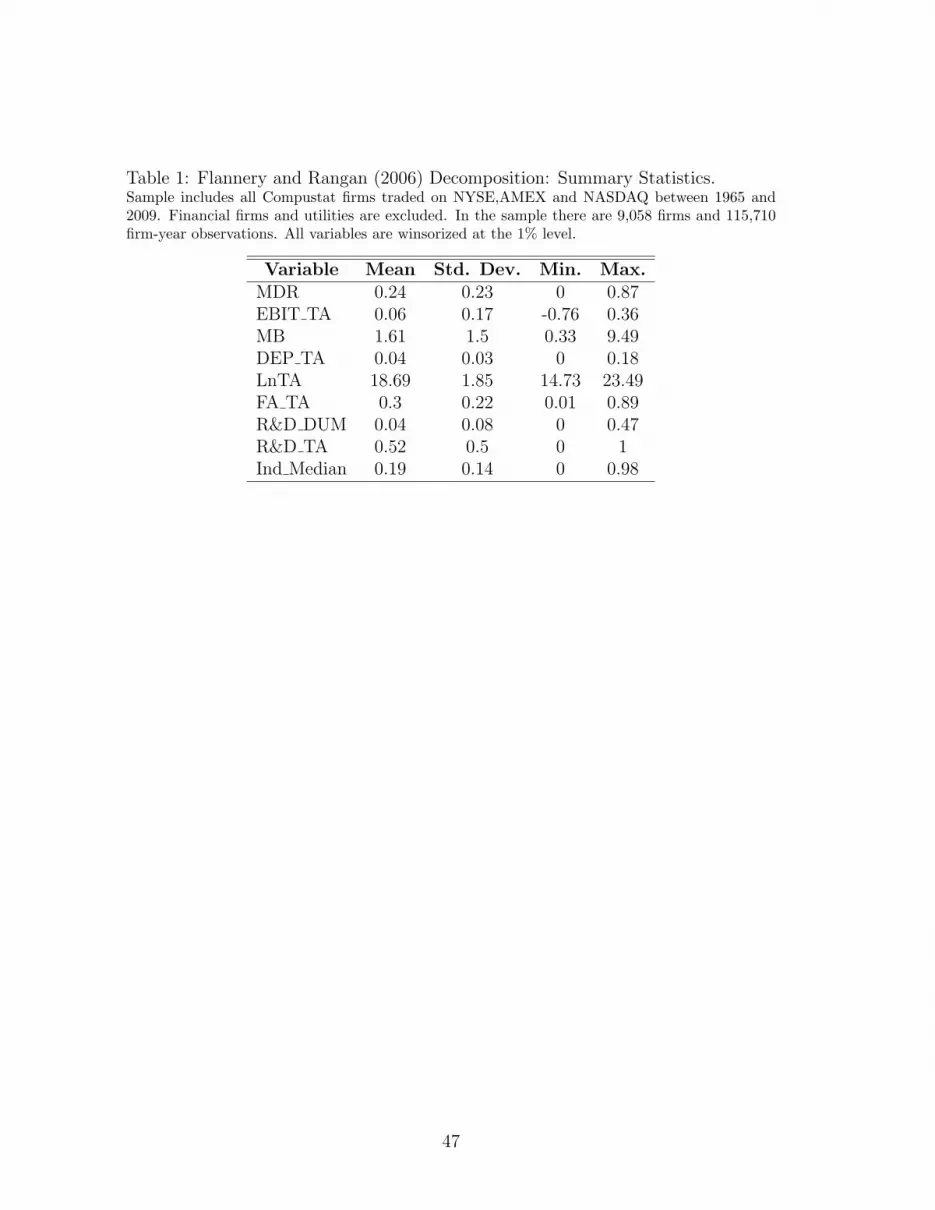
Table 1: Flannery and Rangan (2006) Decomposition: Summary Statistics.Sample includes all Compustat firms traded on NYSE,AMEX and NASDAQ between 1965 and2009. Financial firms and utilities are excluded. In the sample there are 9,058 firms and 115,710firm-year observations. All variables are winsorized at the 1% level.
Variable Mean Std. Dev. Min. Max.MDR 0.24 0.23 0 0.87EBIT TA 0.06 0.17 -0.76 0.36MB 1.61 1.5 0.33 9.49DEP TA 0.04 0.03 0 0.18LnTA 18.69 1.85 14.73 23.49FA TA 0.3 0.22 0.01 0.89R&D DUM 0.04 0.08 0 0.47R&D TA 0.52 0.5 0 1Ind Median 0.19 0.14 0 0.98
47
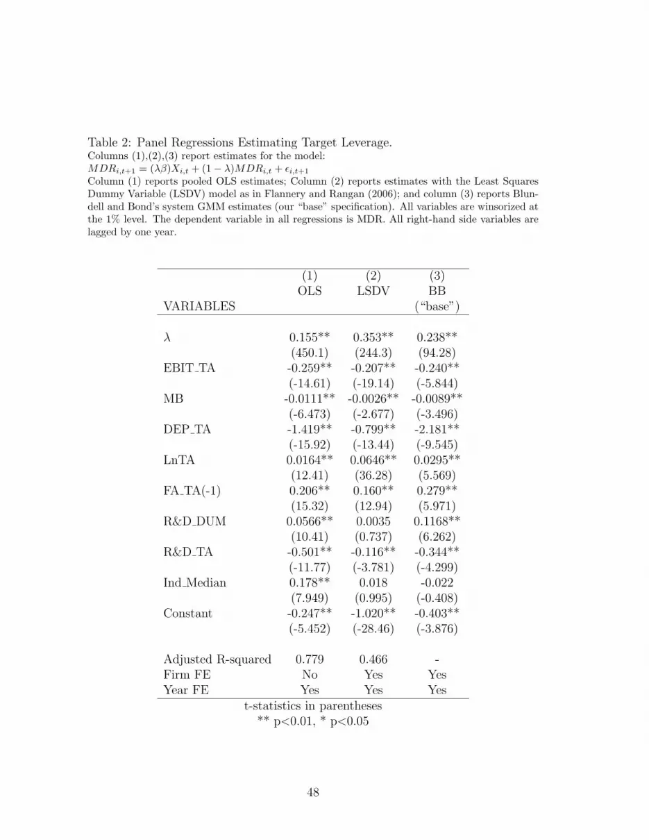
Table 2: Panel Regressions Estimating Target Leverage.Columns (1),(2),(3) report estimates for the model:MDRi,t+1 = (λβ)Xi,t + (1− λ)MDRi,t + ϵi,t+1
Column (1) reports pooled OLS estimates; Column (2) reports estimates with the Least SquaresDummy Variable (LSDV) model as in Flannery and Rangan (2006); and column (3) reports Blun-dell and Bond’s system GMM estimates (our “base” specification). All variables are winsorized atthe 1% level. The dependent variable in all regressions is MDR. All right-hand side variables arelagged by one year.
(1) (2) (3)OLS LSDV BB
VARIABLES (“base”)
λ 0.155** 0.353** 0.238**(450.1) (244.3) (94.28)
EBIT TA -0.259** -0.207** -0.240**(-14.61) (-19.14) (-5.844)
MB -0.0111** -0.0026** -0.0089**(-6.473) (-2.677) (-3.496)
DEP TA -1.419** -0.799** -2.181**(-15.92) (-13.44) (-9.545)
LnTA 0.0164** 0.0646** 0.0295**(12.41) (36.28) (5.569)
FA TA(-1) 0.206** 0.160** 0.279**(15.32) (12.94) (5.971)
R&D DUM 0.0566** 0.0035 0.1168**(10.41) (0.737) (6.262)
R&D TA -0.501** -0.116** -0.344**(-11.77) (-3.781) (-4.299)
Ind Median 0.178** 0.018 -0.022(7.949) (0.995) (-0.408)
Constant -0.247** -1.020** -0.403**(-5.452) (-28.46) (-3.876)
Adjusted R-squared 0.779 0.466 -Firm FE No Yes YesYear FE Yes Yes Yes
t-statistics in parentheses** p<0.01, * p<0.05
48

Table 3: Time-Series Average of Cross-Sectional Correlations.We report time-series averages of monthly cross-sectional correlations using monthly data from July 1965 to December2009. MDR is the market debt ratio. Log(size) is the natural logarithm of market capitalization. Log(bm) is thenatural logarithm of book-to-market equity, Rel Lev is relative leverage, Distance is the distance from target leverage,Overlev is over-leverage, Underlev is under-leverage, and Momentum is the continuously compounded return frommonth t− 12 to month t− 2. All the reported variables are defined and measured as specified in the text.
MDR Rel Lev Distance Overlev Underlev Log(size) Log(bm) MomentumMDR 1.000Rel Lev 0.425 1.000Distance 0.162 -0.130 1.000Overlev 0.467 0.774 0.450 1.000Underlev -0.233 -0.840 0.597 -0.361 1.000Log(size) -0.167 -0.090 -0.121 -0.152 -0.004 1.000Log(bm) 0.435 0.138 0.071 0.163 -0.063 -0.318 1.000Momentum 0.056 0.137 -0.007 0.106 -0.109 -0.011 0.084 1.000
Table 4: Cross-Sectional Patterns: Relative Leverage vs MDR.Using monthly data from July 1965 to December 2009, stocks are sorted independently every June in quintiles basedon their values of MDR and relative leverage. Time-series averages of monthly cross-sectional firm characteristics arereported. Average return is the percent average monthly return, number of firms is the average number of companieseach month in each group, MDR is the market debt ratio, Log(size) is the natural logarithm of market capitalization,BE/ME is book-to-market equity, Momentum is the continuously compounded return from month t − 12 to montht− 2. All the reported variables are defined and measured as specified in the text.
LowRL 2 3 4 HighRL LowRL 2 3 4 HighRLAverage Return Number of firms
LowMDR 0.96 1.27 1.71 1.87 2.19 191.84 182.19 174.78 113.59 34.452 0.72 1.23 1.58 1.90 2.33 104.71 86.73 80.40 67.84 25.743 0.79 1.26 1.57 1.78 2.40 75.82 61.70 66.44 75.57 52.554 0.56 1.22 1.32 1.60 2.38 54.97 45.80 53.52 77.54 101.52HighMDR 0.63 1.17 1.17 1.82 2.57 36.46 33.94 40.66 72.09 208.84
MDR Log(size)LowMDR 0.03 0.03 0.03 0.03 0.03 4.87 5.22 5.11 4.83 4.582 0.13 0.13 0.14 0.14 0.15 5.18 5.56 5.61 5.28 4.513 0.24 0.24 0.24 0.24 0.25 4.96 5.45 5.53 5.35 4.714 0.36 0.36 0.37 0.36 0.37 4.64 5.08 5.09 5.10 4.64HighMDR 0.56 0.57 0.57 0.58 0.62 4.00 4.30 4.42 4.47 4.12
BE/ME MomentumLowMDR 0.64 0.53 0.55 0.52 0.45 -7.07 -4.49 -2.41 -1.09 2.172 0.68 0.63 0.64 0.67 0.67 -8.35 -3.85 -0.58 3.32 3.843 0.80 0.80 0.79 0.79 0.82 -8.58 -2.53 -0.44 1.75 6.944 0.98 0.97 0.94 0.97 0.95 -10.03 -2.87 -1.16 0.76 6.55HighMDR 1.23 1.23 1.24 1.28 1.25 -14.35 -3.90 -2.54 0.79 7.13
49

Tab
le5:
RelativeLeverage,
Size,
Book
-to-Market,Mom
entum.
InPan
elA,each
mon
thbetweenJuly
1965
toDecem
ber
2009
,weestimatecross-sectional
regression
ofstock
returns
onsize,book
-to-market
ratio,
relative
leverage
andmom
entum.In
Pan
elB,in
theregression
sin
columns1-2,
relative
leverage
isestimated
out-of-sam
ple,as
described
inAppen
dix
B.Theregression
sin
columns3-4areestimated
in-
sample
ontheperiod
July
1990
-Decem
ber
2009
usingBlundellan
dBon
d(199
8)system
GMM,as
described
inSection
3.Theregression
sin
columns5-6areestimated
in-sam
ple
ontheperiodJuly
1990
-Decem
ber
2009
usingthe
Least
Squares
DummyVariable
(LSDV)estimator,withthespecification
incolumn2of
table
2.Theindep
endent
variab
lesarematched
tomon
thly
returnsin
linewithFam
aan
dFrench
(199
2),as
specified
inthetext.
Wereport
Fam
a-MacBethcoeffi
cientestimates
andt-statistics
based
onNew
ey-W
eststan
darderrors
withalaglengthof
2.
(1)
(2)
(3)
(4)
(5)
(6)
(7)
(8)
VARIA
BLES
ret
ret
ret
ret
ret
ret
ret
ret
Pan
elA:1965-2009(534
mon
ths)
Log(size)
-0.273
-0.237
-0.243
-0.221
-0.213
(-5.964)
(-4.915)
(-5.384)
(-4.644)
(-4.667)
Log(bm)
0.383
0.173
0.288
0.0960
0.103
(5.080)
(2.157)
(3.947)
(1.228)
(1.335)
Rel
Lev
4.003
3.655
3.706
3.509
3.522
(18.68)
(18.96)
(20.71)
(20.73)
(23.39)
Mom
entum
0.002
(1.010)
Con
stan
t1.047
1.677
1.628
1.171
1.193
1.738
1.270
1.132
(4.045)
(5.695)
(5.244)
(4.837)
(4.528)
(5.797)
(5.141)
(4.854)
t-statistics
inparentheses
50

(1)
(2)
(3)
(4)
(5)
(6)
VARIA
BLES
ret
ret
ret
ret
ret
ret
Pan
elB:1990-2009(234
mon
ths)
Out-of-sam
ple
Est.
BB
Est.
LSDV
Est.
log(size)
-0.238
-0.236
-0.251
-0.248
-0.237
-0.235
(-3.732)
(-3.927)
(-3.916)
(-4.119)
(-3.701)
(-3.886)
log(bm)
0.069
0.068
0.052
0.052
0.039
0.040
(0.616)
(0.681)
(0.459)
(0.519)
(0.351)
(0.400)
Rel
Lev
2.166
2.175
3.486
3.606
3.867
3.966
(8.779)
(8.850)
(12.85)
(13.73)
(12.77)
(13.58)
Mom
entum
-0.003
-0.003
-0.003
(-0.993)
(-1.143)
(-1.185)
Con
stan
t1.321
1.071
1.342
1.088
1.340
1.090
(3.860)
(3.460)
(3.901)
(3.494)
(3.900)
(3.504)
t-statistics
inparentheses
51

Tab
le6:
RelativeLeverage,
Over-Leverage,
Under-Leveragean
dDistance.
InPan
elA,each
mon
thbetweenJuly
1965
toDecem
ber
2009
,weestimatecross-sectional
regression
sof
stock
returnson
size,book
-to-market
ratio,
relative
leverage,distance,over-
leverag
ean
dunder-leverag
e.In
Pan
elB,in
theregression
sin
columns1-3,
relative
leverage,
under-leverag
e,an
dover-leverag
eareestimated
out-of-sam
ple,as
described
inAppen
dix
B.
Intheregression
sin
columns4-6they
areestimated
in-sam
ple
ontheperiod
July
1990
-Decem
ber
2009
usingBlundellan
dBon
d(199
8)system
GMM,as
described
inSection
3.In
theregression
sin
columns7-9,
they
areestimated
in-sam
pleon
theperiodJuly
1990
-Decem
ber
2009
usingtheLeast
Squares
DummyVariable
(LSDV)estimator,withthespecification
incolumn
2of
table
2.Theindep
endentvariab
lesarematched
tomon
thly
returnsin
line
withFam
aan
dFrench
(199
2),as
specified
inthetext.
WereportFam
a-MacBethcoeffi
cient
estimates
andan
dt-statistics
based
onNew
ey-W
eststan
darderrors
withalaglengthof
2.Distance,Overlevan
dUnderlevaredefi
ned
as:
Distance
i,t=
abs{R
elLev
i,t,0}
Overlev i
,t=
max{R
elLev
i,t,0}
Underlev i
,t=
−min{R
elLev
i,t,0}
(1)
(2)
(3)
(4)
(5)
(6)
VARIA
BLES
ret
ret
ret
ret
ret
ret
Pan
elA:1965-2009(534
mon
ths)
Log(size)
-0.221
-0.222
-0.234
-0.222
-0.222
-0.222
(-4.644)
(-4.700)
(-4.905)
(-4.700)
(-4.700)
(-4.700)
Log(bm)
0.0960
0.0962
0.153
0.0962
0.0962
0.0962
(1.228)
(1.230)
(1.915)
(1.230)
(1.230)
(1.230)
Overlev
3.496
0.0457
(7.690)
(0.0716)
Underlev
-3.450
0.0457
(-11.01)
(0.0716)
Rel
Lev
3.509
3.450
3.496
3.473
(20.73)
(11.01)
(7.690)
(15.44)
Distance
-0.709
0.0229
(-2.278)
(0.0716)
Con
stan
t1.270
1.270
1.304
1.270
1.270
1.270
(5.141)
(5.358)
(5.478)
(5.358)
(5.358)
(5.358)
t-statistics
inparentheses
52

(1)
(2)
(3)
(4)
(5)
(6)
VARIA
BLES
ret
ret
ret
ret
ret
ret
Pan
elB:1990-2009(234
mon
ths)
Out-of-sam
ple
Est.
BB
Est.
LSDV
Est.
log(size)
-0.236
-0.236
-0.249
-0.249
-0.236
-0.236
(-3.699)
(-3.699)
(-3.890)
(-3.890)
(-3.674)
(-3.674)
log(bm)
0.0690
0.0690
0.0498
0.0498
0.0396
0.0396
(0.621)
(0.621)
(0.446)
(0.446)
(0.358)
(0.358)
Overlev
2.416
3.492
3.659
(4.496)
(5.045)
(5.257)
Underlev
-1.668
-3.020
-3.654
(-3.859)
(-5.285)
(-5.937)
Rel
Lev
2.042
3.256
3.657
(7.701)
(9.611)
(10.74)
Distance
0.374
0.236
0.002
(0.914)
(0.440)
(0.004)
Con
stan
t1.292
1.292
1.326
1.326
1.347
1.347
(4.011)
(4.011)
(4.147)
(4.147)
(4.241)
(4.241)
t-statistics
inparentheses
53

Tab
le7:
RelativeLeverage,
MarketLeverage,
Book
Leverage.
InPan
elA,each
mon
thbetweenJuly
1965
toDecem
ber
2009
,weestimatecross-sectional
regression
sof
stock
returnson
size,book
-to-market
ratio,
relative
leverage,market
leverag
e,an
dbook
leverag
e.In
Pan
elB,in
theregression
sin
columns1-3,
relative
leverage,under-
leverag
e,an
dover-leverag
eareestimated
out-of-sam
ple,as
described
inAppen
dix
B.In
the
regression
sin
columns4-6they
areestimated
in-sam
ple
ontheperiodJuly
1990
-Decem
ber
2009
usingBlundellan
dBon
d(199
8)system
GMM,as
described
inSection
3.In
theregres-
sion
sin
columns7-9,
they
areestimated
in-sam
ple
ontheperiodJuly
1990
-Decem
ber
2009
usingtheLeast
Squares
DummyVariable
(LSDV)estimator,withthespecification
incolumn
2of
table
2.Theindep
endentvariab
lesarematched
tomon
thly
returnsin
linewithFam
aan
dFrench
(199
2),as
specified
inthetext.
WereportFam
a-MacBethcoeffi
cientestimates
andt-statistics
based
onNew
ey-W
eststan
darderrors
withalaglengthof
2.
(1)
(2)
(3)
(4)
(5)
(6)
VARIA
BLES
ret
ret
ret
ret
ret
ret
Pan
elA:1965-2009(534
mon
ths)
Log(size)
-0.233
-0.223
-0.236
-0.221
(-4.931)
(-4.749)
(-5.025)
(-4.682)
Log(bm)
0.135
0.186
0.163
0.198
(1.798)
(2.488)
(2.082)
(2.501)
MDR
0.987
0.282
-1.000
(3.296)
(1.140)
(-3.725)
Rel
Lev
3.992
(21.32)
BDR
0.332
0.146
-0.386
(1.833)
(0.701)
(-1.775)
Rel
Lev
(book
)1.542
(12.17)
Con
stan
t1.285
1.101
1.573
1.455
1.137
1.385
(4.397)
(4.806)
(6.706)
(5.099)
(4.888)
(6.053)
t-statistics
inparentheses
54

(1)
(2)
(3)
(4)
(5)
(6)
VARIA
BLES
ret
ret
ret
ret
ret
ret
Pan
elB:1990-2009(234
mon
ths)
Out-of-sam
ple
Est.
BB
Est.
LSDV
Est.
log(size)
-0.220
-0.243
-0.229
-0.233
-0.211
-0.236
(-3.666)
(-4.075)
(-3.788)
(-3.887)
(-3.492)
(-3.930)
log(bm)
0.139
0.142
0.166
0.160
0.178
0.159
(1.510)
(1.353)
(1.817)
(1.517)
(1.948)
(1.518)
MDR
-0.507
-1.078
-1.394
(-1.226)
(-2.473)
(-3.137)
Rel
Lev
2.241
4.057
4.805
(7.946)
(11.34)
(12.33)
BDR
-0.0791
-0.361
-0.259
(-0.221)
(-1.023)
(-0.715)
Rel
Lev
(book
)0.757
1.599
1.294
(3.197)
(6.026)
(4.400)
Con
stan
t1.478
1.381
1.675
1.491
1.759
1.461
(4.448)
(4.055)
(4.959)
(4.410)
(5.240)
(4.300)
t-statistics
inparentheses
55

Table 8: Orthogonalizing Regressions.We report orthogonalizing time-series regressions of factors OMU, SMB, HML, and RMRF using monthly data fromJuly 1965 to December 2009. Monthly series of the Fama and French factors are from Kenneth French’s website,while OMU (Over-leveraged Minus Under-leveraged) is defined as the difference between the average monthly returnof stocks with relative leverage above the 80th percentile for NYSE firms, minus the average monthly return of stockswith relative leverage below the 20th percentile for NYSE firms. In order to define OMU, firms are assigned to portfoliosat the end of June of each year. Reported t-statistics are based on standard errors corrected for heteroskedasticity assuggested by Davidson and MacKinnon (1993).
(1) (2) (3) (4)VARIABLES OMU SMB HML RMRF
RMRF -0.0245 0.178*** -0.136***(-0.918) (4.632) (-3.680)
SMB 0.125*** -0.194*** 0.353***(3.810) (-3.239) (3.753)
HML 0.285*** -0.266*** -0.370***(6.708) (-2.811) (-3.582)
OMU 0.352*** 0.585*** -0.136(3.475) (6.657) (-0.942)
Constant 1.532*** -0.285 -0.462** 0.693**(19.61) (-1.465) (-2.583) (2.423)
Observations 534 534 534 534R-squared 0.196 0.153 0.274 0.162
Robust t-statistics in parentheses*** p<0.01, ** p<0.05, * p<0.1
56
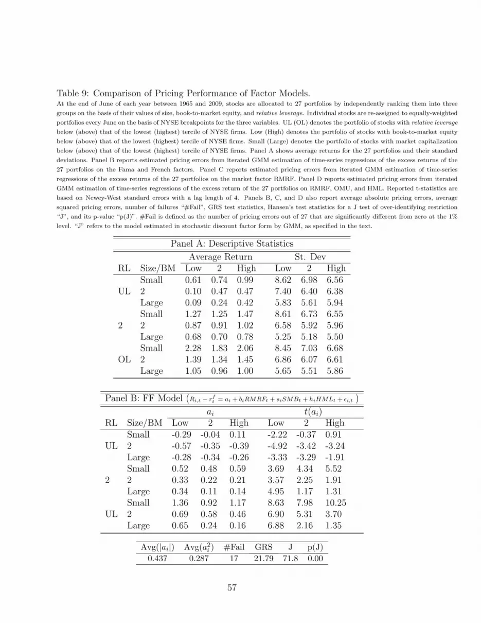
Table 9: Comparison of Pricing Performance of Factor Models.At the end of June of each year between 1965 and 2009, stocks are allocated to 27 portfolios by independently ranking them into three
groups on the basis of their values of size, book-to-market equity, and relative leverage. Individual stocks are re-assigned to equally-weighted
portfolios every June on the basis of NYSE breakpoints for the three variables. UL (OL) denotes the portfolio of stocks with relative leverage
below (above) that of the lowest (highest) tercile of NYSE firms. Low (High) denotes the portfolio of stocks with book-to-market equity
below (above) that of the lowest (highest) tercile of NYSE firms. Small (Large) denotes the portfolio of stocks with market capitalization
below (above) that of the lowest (highest) tercile of NYSE firms. Panel A shows average returns for the 27 portfolios and their standard
deviations. Panel B reports estimated pricing errors from iterated GMM estimation of time-series regressions of the excess returns of the
27 portfolios on the Fama and French factors. Panel C reports estimated pricing errors from iterated GMM estimation of time-series
regressions of the excess returns of the 27 portfolios on the market factor RMRF. Panel D reports estimated pricing errors from iterated
GMM estimation of time-series regressions of the excess return of the 27 portfolios on RMRF, OMU, and HML. Reported t-statistics are
based on Newey-West standard errors with a lag length of 4. Panels B, C, and D also report average absolute pricing errors, average
squared pricing errors, number of failures “#Fail”, GRS test statistics, Hansen’s test statistics for a J test of over-identifying restriction
“J”, and its p-value “p(J)”. #Fail is defined as the number of pricing errors out of 27 that are significantly different from zero at the 1%
level. “J” refers to the model estimated in stochastic discount factor form by GMM, as specified in the text.
Panel A: Descriptive Statistics
Average Return St. DevRL Size/BM Low 2 High Low 2 High
Small 0.61 0.74 0.99 8.62 6.98 6.56UL 2 0.10 0.47 0.47 7.40 6.40 6.38
Large 0.09 0.24 0.42 5.83 5.61 5.94Small 1.27 1.25 1.47 8.61 6.73 6.55
2 2 0.87 0.91 1.02 6.58 5.92 5.96Large 0.68 0.70 0.78 5.25 5.18 5.50Small 2.28 1.83 2.06 8.45 7.03 6.68
OL 2 1.39 1.34 1.45 6.86 6.07 6.61Large 1.05 0.96 1.00 5.65 5.51 5.86
Panel B: FF Model (Ri,t − rft = ai + biRMRFt + siSMBt + hiHMLt + ϵi,t )
ai t(ai)RL Size/BM Low 2 High Low 2 High
Small -0.29 -0.04 0.11 -2.22 -0.37 0.91UL 2 -0.57 -0.35 -0.39 -4.92 -3.42 -3.24
Large -0.28 -0.34 -0.26 -3.33 -3.29 -1.91Small 0.52 0.48 0.59 3.69 4.34 5.52
2 2 0.33 0.22 0.21 3.57 2.25 1.91Large 0.34 0.11 0.14 4.95 1.17 1.31Small 1.36 0.92 1.17 8.63 7.98 10.25
UL 2 0.69 0.58 0.46 6.90 5.31 3.70Large 0.65 0.24 0.16 6.88 2.16 1.35
Avg(|ai|) Avg(a2i ) #Fail GRS J p(J)
0.437 0.287 17 21.79 71.8 0.00
57
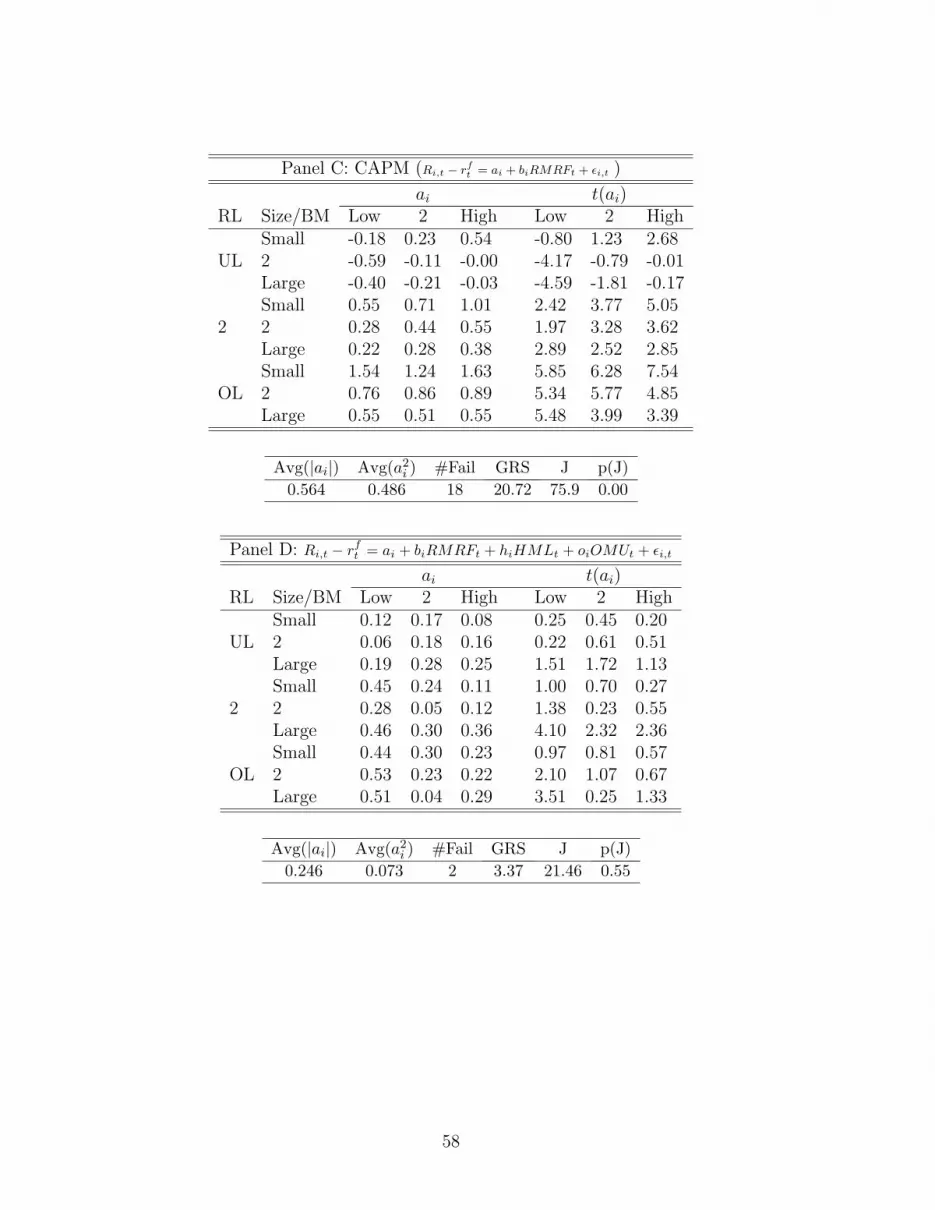
Panel C: CAPM (Ri,t − rft = ai + biRMRFt + ϵi,t )
ai t(ai)RL Size/BM Low 2 High Low 2 High
Small -0.18 0.23 0.54 -0.80 1.23 2.68UL 2 -0.59 -0.11 -0.00 -4.17 -0.79 -0.01
Large -0.40 -0.21 -0.03 -4.59 -1.81 -0.17Small 0.55 0.71 1.01 2.42 3.77 5.05
2 2 0.28 0.44 0.55 1.97 3.28 3.62Large 0.22 0.28 0.38 2.89 2.52 2.85Small 1.54 1.24 1.63 5.85 6.28 7.54
OL 2 0.76 0.86 0.89 5.34 5.77 4.85Large 0.55 0.51 0.55 5.48 3.99 3.39
Avg(|ai|) Avg(a2i ) #Fail GRS J p(J)
0.564 0.486 18 20.72 75.9 0.00
Panel D: Ri,t − rft = ai + biRMRFt + hiHMLt + oiOMUt + ϵi,t
ai t(ai)RL Size/BM Low 2 High Low 2 High
Small 0.12 0.17 0.08 0.25 0.45 0.20UL 2 0.06 0.18 0.16 0.22 0.61 0.51
Large 0.19 0.28 0.25 1.51 1.72 1.13Small 0.45 0.24 0.11 1.00 0.70 0.27
2 2 0.28 0.05 0.12 1.38 0.23 0.55Large 0.46 0.30 0.36 4.10 2.32 2.36Small 0.44 0.30 0.23 0.97 0.81 0.57
OL 2 0.53 0.23 0.22 2.10 1.07 0.67Large 0.51 0.04 0.29 3.51 0.25 1.33
Avg(|ai|) Avg(a2i ) #Fail GRS J p(J)
0.246 0.073 2 3.37 21.46 0.55
58

Tab
le10:Com
parison
ofPricingPerform
ance
ofFactorModels.
Attheendon
Juneof
each
yearbetween19
65an
d20
09,stocksareallocatedto
25portfoliosbyindep
endentlyrankingthem
into
fivegroupson
thebasisof
theirvalues
ofsize
(S),
book
-to-market
equity(B
M),
mom
entum
(M),
andrelative
leverage
(RL).
Individual
stocksarere-assigned
toequally-w
eigh
tedportfolioseveryJuneon
thebasis
ofNYSE
break
points
forthefourvariab
les.
Thetable
show
saverag
eab
solute
pricingerrors,
averag
esquared
pricingerrors,number
offailures“#
Fail”,GRStest
statistics,Han
sen’s
test
statistics
foraJtest
ofover-identifyingrestriction“J”,
anditsp-value“p
(J)”
fortheFam
aan
dFrench
model,theCAPM,an
damodel
includingthemarket
factor
RMRF,HML,an
dOMU.#Failisdefi
ned
asthenumber
ofpricingerrors
outof
25that
aresign
ificantlydifferentfrom
zero
atthe1%
level.Thesetestsarebased
onNew
ey-W
eststandard
errors
withalaglengthof
4.Tim
e-series
regression
sareestimated
byiterated
GMM,as
specified
inthetext.
“J”refers
tothemodel
estimatedin
stochasticdiscountfactor
form
byGMM,as
specified
inthetext.
FF
Model
CAPM
RMRF+HML+OMU
TestAssets
Avg(|ai|)
Avg(a
2 i)
#Fail
GRS
Jp(J)
Avg(|ai|)
Avg(a
2 i)
#Fail
GRS
Jp(J)
Avg(|ai|)
Avg(a
2 i)
#Fail
GRS
Jp(J)
25port.
(5S,5BM)
0.20
00.08
66
3.38
27.9
0.14
0.42
50.28
714
3.77
35.0
0.05
0.27
90.10
33
2.96
26.4
0.19
25port.
(5RL,5BM)
0.51
20.38
019
19.84
84.0
0.00
0.71
90.72
418
18.80
85.2
0.00
0.21
70.05
80
1.83
16.9
0.72
25port.
(5RL,5S)
0.42
80.26
920
19.10
60.8
0.00
0.56
40.48
420
19.29
82.6
0.00
0.23
80.06
72
2.40
18.1
0.64
25port.
(5S,5M)
0.22
60.09
78
2.96
28.5
0.13
0.39
10.25
010
2.87
38.1
0.02
0.24
40.12
72
2.27
15.5
0.80
25port.
(5BM,5M)
0.34
70.16
218
4.67
39.1
0.01
0.61
20.48
420
4.48
51.7
0.00
0.23
90.11
30
2.80
39.0
0.01
25port.
(5RL,5M)
0.50
50.36
820
20.29
67.8
0.00
0.67
20.67
219
20.38
87.6
0.00
0.20
10.08
30
2.75
25.9
0.21
59

Appendix A: Robustness Checks
Table 11: Relative Leverage, Size, Book-to-Market, Momentum: Subperiod Evidence.As in Table 5, We estimate monthly cross-sectional regression of stock returns on size, book-to-market ratio,relative leverage and momentum. Panel A refers to the period between July 1965 and December 1979, Panel Bto the period between January 1980 and December 1994, and Panel C to the period between January 1995 andDecember 2009. The independent variables are matched to monthly returns in line with Fama and French (1992),as specified in the text. We report Fama-MacBeth coefficient estimates and t-statistics based on Newey-Weststandard errors with a lag length of 2.
(1) (2) (3) (4) (5) (6) (7) (8)VARIABLES ret ret ret ret ret ret ret ret
Panel A: 1965-1979 (174 months)Log(size) -0.242 -0.213 -0.189 -0.177 -0.158
(-2.578) (-2.245) (-2.067) (-1.914) (-1.847)Log(bm) 0.383 0.136 0.279 0.0709 0.0743
(2.540) (0.968) (1.930) (0.532) (0.551)Rel Lev 4.252 3.689 3.906 3.410 3.188
(13.02) (15.14) (15.33) (15.95) (15.83)Momentum 0.005
(1.688)Constant 0.690 1.280 1.327 0.795 0.894 1.364 0.963 0.905
(1.707) (2.442) (2.280) (2.206) (2.090) (2.496) (2.498) (2.400)
t-statistics in parentheses
60
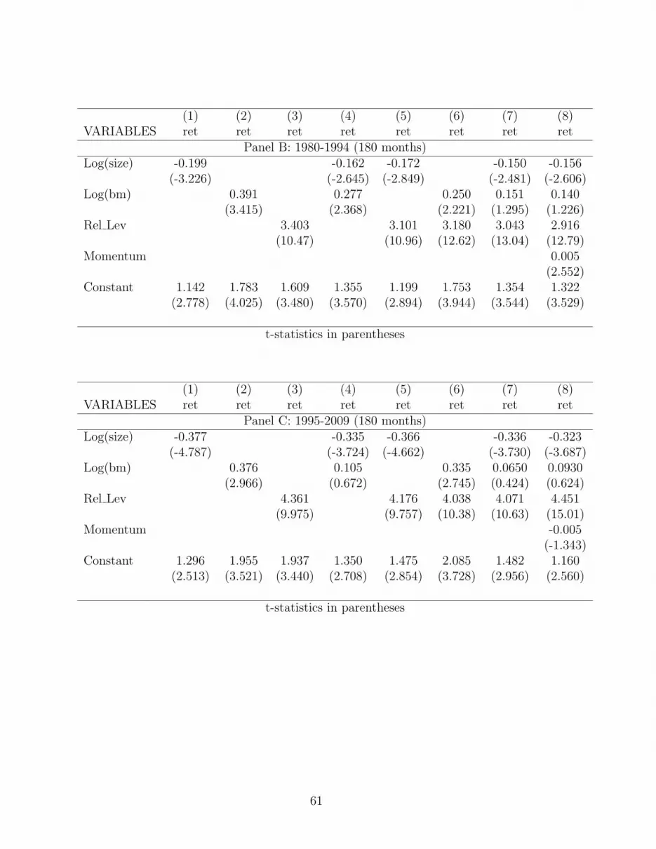
(1) (2) (3) (4) (5) (6) (7) (8)VARIABLES ret ret ret ret ret ret ret ret
Panel B: 1980-1994 (180 months)Log(size) -0.199 -0.162 -0.172 -0.150 -0.156
(-3.226) (-2.645) (-2.849) (-2.481) (-2.606)Log(bm) 0.391 0.277 0.250 0.151 0.140
(3.415) (2.368) (2.221) (1.295) (1.226)Rel Lev 3.403 3.101 3.180 3.043 2.916
(10.47) (10.96) (12.62) (13.04) (12.79)Momentum 0.005
(2.552)Constant 1.142 1.783 1.609 1.355 1.199 1.753 1.354 1.322
(2.778) (4.025) (3.480) (3.570) (2.894) (3.944) (3.544) (3.529)
t-statistics in parentheses
(1) (2) (3) (4) (5) (6) (7) (8)VARIABLES ret ret ret ret ret ret ret ret
Panel C: 1995-2009 (180 months)Log(size) -0.377 -0.335 -0.366 -0.336 -0.323
(-4.787) (-3.724) (-4.662) (-3.730) (-3.687)Log(bm) 0.376 0.105 0.335 0.0650 0.0930
(2.966) (0.672) (2.745) (0.424) (0.624)Rel Lev 4.361 4.176 4.038 4.071 4.451
(9.975) (9.757) (10.38) (10.63) (15.01)Momentum -0.005
(-1.343)Constant 1.296 1.955 1.937 1.350 1.475 2.085 1.482 1.160
(2.513) (3.521) (3.440) (2.708) (2.854) (3.728) (2.956) (2.560)
t-statistics in parentheses
61

Table 12: Relative Leverage, Over-Leverage, Under-Leverage and Distance:Subperiod Evidence.As in Table 6, we estimate monthly cross-sectional regression of stock returns on size, book-to-market ratio, relative leverage, distance, over-leverage and under-leverage. Panel A refersto the period between July 1965 and December 1979, Panel B to the period between January1980 and December 1994, and Panel C to the period between January 1995 and December2009. The independent variables are matched to monthly returns in line with Fama andFrench (1992), as specified in the text. We report Fama-MacBeth coefficient estimates andt-statistics based on Newey-West standard errors with a lag length of 2. Distance, Overlevand Underlev are defined as:Distancei,t = abs{Rel Levi,t, 0}Overlevi,t = max{Rel Levi,t, 0}Underlevi,t = −min{Rel Levi,t, 0}
(1) (2) (3) (4) (5) (6)VARIABLES ret ret ret ret ret ret
Panel A: 1965-1979 (174 months)Log(size) -0.177 -0.173 -0.191 -0.173 -0.173 -0.173
(-1.914) (-1.896) (-2.044) (-1.896) (-1.896) (-1.896)Log(bm) 0.0709 0.0656 0.0815 0.0656 0.0656 0.0656
(0.532) (0.487) (0.585) (0.487) (0.487) (0.487)Overlev 4.377 1.555
(5.203) (1.384)Underlev -2.822 1.555
(-5.636) (1.384)Rel Lev 3.410 2.822 4.377 3.599
(15.95) (5.636) (5.203) (8.905)Distance 0.662 0.778
(1.344) (1.384)Constant 0.963 0.895 0.847 0.895 0.895 0.895
(2.498) (2.332) (2.202) (2.332) (2.332) (2.332)t-statistics in parentheses
62
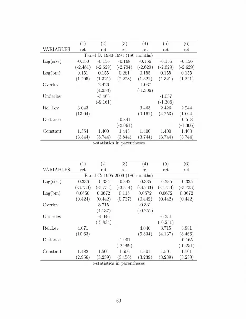
(1) (2) (3) (4) (5) (6)VARIABLES ret ret ret ret ret ret
Panel B: 1980-1994 (180 months)Log(size) -0.150 -0.156 -0.168 -0.156 -0.156 -0.156
(-2.481) (-2.629) (-2.794) (-2.629) (-2.629) (-2.629)Log(bm) 0.151 0.155 0.261 0.155 0.155 0.155
(1.295) (1.321) (2.228) (1.321) (1.321) (1.321)Overlev 2.426 -1.037
(4.253) (-1.306)Underlev -3.463 -1.037
(-9.161) (-1.306)Rel Lev 3.043 3.463 2.426 2.944
(13.04) (9.161) (4.253) (10.64)Distance -0.841 -0.518
(-2.061) (-1.306)Constant 1.354 1.400 1.443 1.400 1.400 1.400
(3.544) (3.744) (3.844) (3.744) (3.744) (3.744)t-statistics in parentheses
(1) (2) (3) (4) (5) (6)VARIABLES ret ret ret ret ret ret
Panel C: 1995-2009 (180 months)Log(size) -0.336 -0.335 -0.342 -0.335 -0.335 -0.335
(-3.730) (-3.733) (-3.814) (-3.733) (-3.733) (-3.733)Log(bm) 0.0650 0.0672 0.115 0.0672 0.0672 0.0672
(0.424) (0.442) (0.737) (0.442) (0.442) (0.442)Overlev 3.715 -0.331
(4.137) (-0.251)Underlev -4.046 -0.331
(-5.834) (-0.251)Rel Lev 4.071 4.046 3.715 3.881
(10.63) (5.834) (4.137) (8.466)Distance -1.901 -0.165
(-2.969) (-0.251)Constant 1.482 1.501 1.606 1.501 1.501 1.501
(2.956) (3.239) (3.456) (3.239) (3.239) (3.239)t-statistics in parentheses
63

Table 13: Relative Leverage, Market Leverage, Book Leverage: Subperiod Evi-dence.As in Table 7, we estimate monthly cross-sectional regression of stock returns on size, book-to-market ratio, relative leverage, market leverage, and book leverage. Panel A refers tothe period between July 1965 and December 1979, Panel B to the period between January1980 and December 1994, and Panel C to the period between January 1995 and December2009. The independent variables are matched to monthly returns in line with Fama andFrench (1992), as specified in the text. We report Fama-MacBeth coefficient estimates andt-statistics based on Newey-West standard errors with a lag length of 2.
(1) (2) (3) (4) (5) (6)VARIABLES ret ret ret ret ret ret
Panel A: 1965-1979 (174 months)Log(size) -0.201 -0.181 -0.209 -0.190
(-2.189) (-1.986) (-2.264) (-2.039)Log(bm) 0.0587 0.150 0.115 0.161
(0.383) (0.987) (0.828) (1.148)MDR 1.378 0.576 -0.847
(2.768) (1.482) (-1.875)Rel Lev 3.791
(12.68)BDR 0.722 0.312 -0.364
(1.808) (0.938) (-0.937)Rel Lev(book) 1.662
(7.448)Constant 0.861 0.660 1.246 1.059 0.723 1.041
(1.812) (2.059) (3.562) (2.322) (2.275) (3.302)t-statistics in parentheses
64
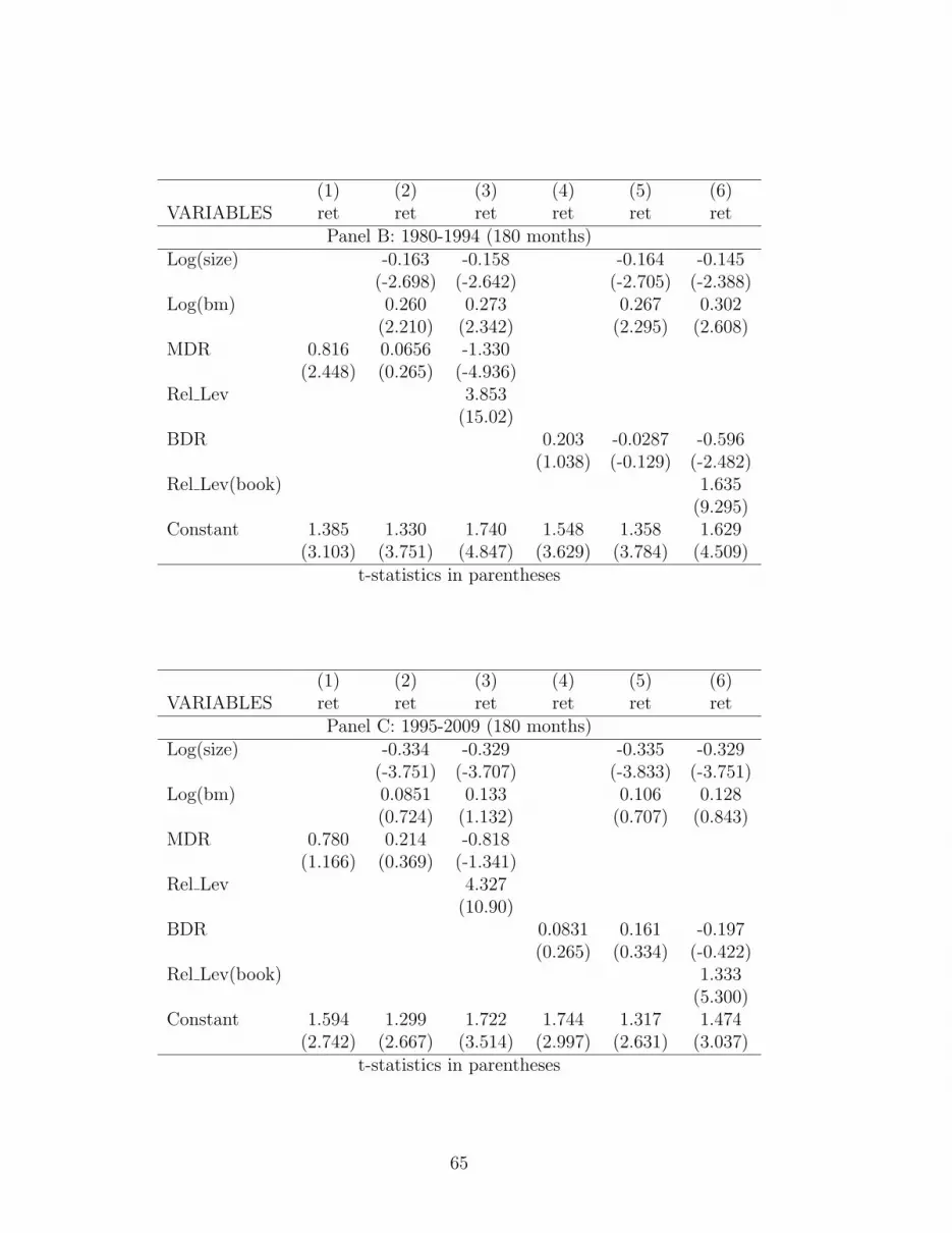
(1) (2) (3) (4) (5) (6)VARIABLES ret ret ret ret ret ret
Panel B: 1980-1994 (180 months)Log(size) -0.163 -0.158 -0.164 -0.145
(-2.698) (-2.642) (-2.705) (-2.388)Log(bm) 0.260 0.273 0.267 0.302
(2.210) (2.342) (2.295) (2.608)MDR 0.816 0.0656 -1.330
(2.448) (0.265) (-4.936)Rel Lev 3.853
(15.02)BDR 0.203 -0.0287 -0.596
(1.038) (-0.129) (-2.482)Rel Lev(book) 1.635
(9.295)Constant 1.385 1.330 1.740 1.548 1.358 1.629
(3.103) (3.751) (4.847) (3.629) (3.784) (4.509)t-statistics in parentheses
(1) (2) (3) (4) (5) (6)VARIABLES ret ret ret ret ret ret
Panel C: 1995-2009 (180 months)Log(size) -0.334 -0.329 -0.335 -0.329
(-3.751) (-3.707) (-3.833) (-3.751)Log(bm) 0.0851 0.133 0.106 0.128
(0.724) (1.132) (0.707) (0.843)MDR 0.780 0.214 -0.818
(1.166) (0.369) (-1.341)Rel Lev 4.327
(10.90)BDR 0.0831 0.161 -0.197
(0.265) (0.334) (-0.422)Rel Lev(book) 1.333
(5.300)Constant 1.594 1.299 1.722 1.744 1.317 1.474
(2.742) (2.667) (3.514) (2.997) (2.631) (3.037)t-statistics in parentheses
65

Table 14: Target Leverage with Only Fixed Effects.Each month between July 1965 to December 2009, we estimate cross-sectional regressions ofstock returns on size, book-to-market ratio, relative leverage, market debt ratio, over-leverageand under-leverage. Relative leverage is estimated using Blundell and Bond (1998) systemGMM, as described in Section 3, where Xi,t contains only a firm fixed-effect. The independentvariables are matched to monthly returns in line with Fama and French (1992), as specifiedin the text. We report Fama-MacBeth coefficient estimates and t-statistics based on Newey-West standard errors with a lag length of 2. Overlev and Underlev are defined as:Overlevi,t = max{Rel Levi,t, 0}Underlevi,t = −min{Rel Levi,t, 0}
(1) (2) (3)VARIABLES ret ret retSample Period: 1965-2009 (534 months)
Log(size) -0.232 -0.234 -0.234(-5.229) (-5.375) (-5.350)
Log(bm) 0.077 0.163 0.081(1.113) (2.468) (1.177)
MDR -0.974(-4.292)
Rel Lev 3.200 3.638(21.15) (21.28)
Overlev 2.835(8.342)
Underlev -3.304(-14.09)
Constant 1.248 1.530 1.269(5.561) (7.078) (5.836)
t-statistics in parentheses
66
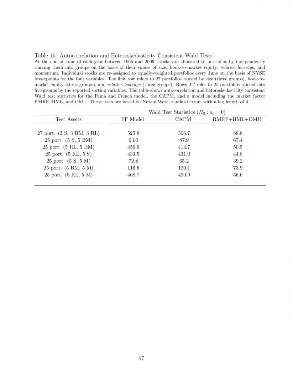
Table 15: Autocorrelation and Heteroskedasticity Consistent Wald Tests.At the end of June of each year between 1965 and 2009, stocks are allocated to portfolios by independentlyranking them into groups on the basis of their values of size, book-to-market equity, relative leverage, andmomentum. Individual stocks are re-assigned to equally-weighted portfolios every June on the basis of NYSEbreakpoints for the four variables. The first row refers to 27 portfolios ranked by size (three groups), book-to-market equity (three groups), and relative leverage (three groups). Rows 2-7 refer to 25 portfolios ranked intofive groups by the reported sorting variables. The table shows autocorrelation and heteroskedasticity consistentWald test statistics for the Fama and French model, the CAPM, and a model including the market factorRMRF, HML, and OMU. These tests are based on Newey-West standard errors with a lag length of 4.
Wald Test Statistics (H0 : ai = 0)
Test Assets FF Model CAPM RMRF+HML+OMU
27 port. (3 S, 3 BM, 3 RL) 525.8 506.7 88.8
25 port. (5 S, 5 BM) 93.6 87.9 67.4
25 port. (5 RL, 5 BM) 456.9 414.7 50.5
25 port. (5 RL, 5 S) 433.5 431.0 44.8
25 port. (5 S, 5 M) 72.8 65.2 39.2
25 port. (5 BM, 5 M) 116.6 120.1 73.9
25 port. (5 RL, 5 M) 468.7 490.9 56.6
67

Table 16: Comparison of Pricing Performance of Factor Models: Carhart Model.At the end of June of each year between 1965 and 2009, stocks are allocated to 27 portfolios by independentlyranking them into three groups on the basis of their values of size, book-to-market equity, and relative leverage.Individual stocks are re-assigned to equally-weighted portfolios every June on the basis of NYSE breakpointsfor the three variables. UL (OL) denotes the portfolio of stocks with relative leverage below (above) that ofthe lowest (highest) tercile of NYSE firms. Low (High) denotes the portfolio of stocks with book-to-marketequity below (above) that of the lowest (highest) tercile of NYSE firms. Small (Large) denotes the portfolio ofstocks with market capitalization below (above) that of the lowest (highest) tercile of NYSE firms. We reportestimated pricing errors from iterated GMM estimation of time-series regressions of the excess returns of the27 portfolios on a four-factor model including the Fama and French factors and the momentum factor, as inCarhart (1997). Reported t-statistics are based on Newey-West standard errors with a lag length of 4. We alsoreport average absolute pricing errors, average squared pricing errors, number of failures “#Fail”, GRS teststatistics, Hansen’s test statistics for a J test of over-identifying restriction “J”, and its p-value “p(J)”. #Fail isdefined as the number of pricing errors out of 27 that are significantly different from zero at the 1% level. “J”refers to the model estimated in stochastic discount factor form by GMM, as specified in the text.
Ri,t − rft = ai + biRMRFt + siSMBt + hiHMLt +miMOMt + ϵi,t
ai t(ai)RL Size/BM Low 2 High Low 2 High
Small 0.01 0.19 0.32 0.04 1.74 2.38UL 2 -0.29 -0.10 -0.16 -2.47 -0.99 -1.23
Large -0.09 -0.19 -0.08 -1.17 -1.88 -0.60Small 0.70 0.65 0.74 4.36 5.69 6.08
2 2 0.41 0.30 0.32 4.54 2.83 2.77Large 0.44 0.20 0.23 5.92 2.36 2.11Small 1.45 1.05 1.29 8.58 8.00 9.89
OL 2 0.76 0.68 0.63 6.79 6.08 4.68Large 0.68 0.33 0.32 6.81 2.97 2.86
Avg(|ai|) Avg(a2i ) #Fail GRS J p(J)
0.467 0.349 16 19.95 37.6 0.02
68

Appendix B: Out-of-Sample Estimation
In this appendix, we provide details and robustness checks on the out-of-sample estima-
tion of relative leverage. First, notice that the properties of the fixed effect estimators
are asymptotic.24 Thus, while consistent, fixed effects estimates may be biased in finite
samples. This may be a problem in our unbalanced panel, because the length of the
time-series for many firms is quite short.
For the out-of-sample analysis, we consider the years 1987-2009 as the period for
which we want to explain equity returns. For each year t between 1987 and 2009 we
estimate Equation 4 on a rolling basis, i.e. using data from 1965 to t. Target leverage
for the i-th stock is estimated in year t only if firm i’s fixed effect estimate is stable
enough. Since fixed effects estimates are consistent, once stability is reached in a given
year, it will also apply in the following years. More specifically, stability of the estimate
for firm i in year t is achieved if and only if there exists a period t∗ between 1989 and t
such that the fixed effect estimate Fi,t∗ can be computed25 and satisfies
Fi,t∗ − Fi,t∗−1 < 0.05
and
Fi,t∗ − Fi,t∗−2 < 0.05.
Once the stability criterion is satisfied for firm i, the fixed effect estimate Fi,t∗ at t∗ is
used to compute target leverage MDR∗i,t for every t ≥ t∗ for which Equation 4 produces
an estimate of target leverage for firm i.26 For computational convenience, in the rolling
24Independently of the estimation method that one employs (LSDV or Blundell and Bond (1998)system GMM), firm fixed effects are determined such that the sample mean of each individual ’s timeseries of residuals equals zero (Baltagi (2008)).
25We require that there are no gaps in the firm i’s time series of Fi,s, for t∗ < s < t.
26Occasionally, due to missing data for one or more regressors in Xi,t−1, it is not possible to estimateMDR∗
i,t for every t ≥ t∗. When this occurs, we do not include the firm in the analysis, and check again
69

estimation, we use the LSDV estimator instead of the Blundell and Bond (1998) system
GMM. Once we have obtained target leverage estimates for the period 1989-2009 and
computed relative leverage as in Equation 5, we match annual series to monthly returns
according to the procedure described in Section 4. This yields monthly time series from
July 1990 to December 2009.
Figure 4 depicts average monthly returns for the period 1990-2009, sorting firms
according to the out-of-sample approach described above. As in Figure 3, a clear relative
leverage premium emerges. Consistent with our previous findings, the premium is fairly
symmetrical around the target.
(Insert Figure 4 about here)
We employ the 0.05 threshold in the out-of-sample estimates of Panels B of Tables
7, 7, and 7. In Table 17 we consider different convergence criteria, with tighter and
looser bounds, and based on estimates for more than two consecutive years. This does
not qualitatively affect our results.
the stability criterion.
70

Tab
le17:Out-of-Sam
ple
Con
vergence
Criteria.
WeestimateRelative
leverage,under-leverag
e,an
dover-leverag
eou
t-of-sam
ple
follow
ingtheprocedure
described
inAppen
dix
B.
Wethen
estimatecross-sectional
regression
sof
stock
returnson
size,book
-to-market
ratio,
relative
leverage,over-leverag
e,under-
leverage,an
dmarket
leverag
e.In
theregression
sin
columns1-3,
thefixed
effectestimateFi,t∗
must
satisfytheconvergen
ceconditionsFi,t∗−Fi,t∗
−1<
0.01
,an
dFi,t∗−Fi,t∗
−2<
0.01
forafirm
tobeincluded
inthean
alysis.
Intheregression
sin
columns
4-6,
thefixed
effectestimateFi,t∗
must
satisfytheconvergen
ceconditionsFi,t∗
−Fi,t∗
−1<
0.10
,an
dFi,t∗
−Fi,t∗
−2<
0.10
fora
firm
tobeincluded
inthean
alysis.
Intheregression
sin
columns7-9,
thefixed
effectestimateFi,t∗
must
satisfytheconvergen
ceconditionsFi,t∗
−Fi,t∗
−1<
0.05
,Fi,t∗
−Fi,t∗
−2<
0.05
,an
dFi,t∗
−Fi,t∗
−3<
0.05
forafirm
tobeincluded
inthean
alysis.
The
indep
endentvariab
lesarematched
tomon
thly
returnsin
linewithFam
aan
dFrench
(199
2),as
specified
inthetext.
Wereport
Fam
a-MacBethcoeffi
cientestimates
andt-statistics
based
onNew
ey-W
eststan
darderrors
withalaglengthof
2.
(1)
(2)
(3)
(4)
(5)
(6)
(7)
(8)
(9)
VARIA
BLES
ret
ret
ret
ret
ret
ret
ret
ret
ret
Sam
ple
Period:1990-2009(234
mon
ths)
TightBou
nds
LooseBou
nds
Three-PeriodBou
nds
Log(size)
-0.227
-0.217
-0.225
-0.239
-0.229
-0.237
-0.219
-0.209
-0.217
(-3.610)
(-3.554)
(-3.570)
(-3.748)
(-3.700)
(-3.709)
(-3.423)
(-3.391)
(-3.385)
Log(bm)
0.041
0.094
0.038
0.069
0.119
0.067
0.071
0.116
0.069
(0.367)
(1.027)
(0.349)
(0.615)
(1.291)
(0.607)
(0.625)
(1.231)
(0.616)
MDR
-0.518
-0.540
-0.478
(-1.247)
(-1.284)
(-1.117)
Rel
Lev
2.093
2.406
2.063
2.359
2.042
2.310
(7.303)
(7.595)
(8.659)
(9.072)
(7.167)
(7.531)
Overlev
2.481
2.382
2.337
(4.249)
(4.341)
(3.872)
Underlev
-1.196
-1.486
-1.432
(-2.316)
(-3.659)
(-2.844)
Con
stan
t1.285
1.433
1.240
1.320
1.469
1.283
1.356
1.492
1.322
(3.792)
(4.435)
(3.915)
(3.861)
(4.423)
(3.976)
(3.897)
(4.507)
(4.086)
t-statistics
inparentheses
71

Appendix C: GMM-based Asset Pricing Tests
In Section 6.3 we test the CAPM, the FF3 model, and a model with RMRF, HML, and
OMU both in their expected return-beta and in their stochastic discount factor repre-
sentation. Both tests are based on Generalized Method of Moments (GMM) estimation.
For an exhaustive treatment of these types of tests, we refer the reader to Hansen (1982),
Cochrane (1996), and Cochrane (2001).
For each set of N test assets we contemplate in Tables 9 and 10, the return-beta
equations for all N assets in vector form can be written as
rt − rft = α + β′ft + ϵt
where ft = [RMRFt]′ for the CAPM, ft = [RMRFt SMBt HMLt]
′ for the FF3 model,
and ft = [RMRFt HMLt OMUt]′ for the model with RMRF, HML, and OMU. The
moment conditions that we consider to map the regression equations above into the
GMM framework are
MT (α, β) ≡
E[ϵt]
E[ϵtft]
The GMM objective is to estimate α and β to minimize the following quadratic form of
the moment conditions
JT (α, β) ≡ MT (α, β)′WMT (α, β)
where W is a weighting matrix. As Ferson and Foerster (1994) suggest, we use iterative
efficient GMM estimation to improve finite-sample performance. Specifically, we initially
set W = W0, and we estimate the model by GMM to get a consistent estimate of the
covariance matrix of moments S. We then impose W = S−1 to obtain efficient next-
stage estimates. We iterate the last step until convergence is achieved. In our analysis,
72

we choose W0 = (ft′ft) ⊗ IN , where ft
′= [1 f ′
t ] and IN is an identity matrix of size N .
At each step, we estimate a heteroskedasticity and autocorrelation consistent matrix S
using a Newey-West kernel with 4 lags.
In this framework, the asymptotic variance matrix of GMM estimates [α β] is
V ar
αβ
=1
TD−1SD−1′
where T is the number of monthly observations in our sample, and D is defined as
D ≡ ∂MT
∂[α′ β′]= −
1 E[ft]
E[ft] E[f 2t ]
⊗ IN
Therefore, a Wald-type test for null hypothesis that the N pricing errors are jointly zero
can be easily implemented. In fact:
α′V ar(α)−1αd−→ χ2
N
Since the GMM system is just identified (the number of parameters to estimate and
the number of moment conditions are both equal to N(K + 1), where K is the number
of factors in each model), the point estimates α and β coincide with OLS estimates of
time-series regressions for the individual assets. However, standard errors differ in that
we do not assume homoscedasticity and independent errors over time in the construction
of the S matrix. Under these two assumptions, the Wald-type test above boils down to
the asymptotic counterpart of the celebrated GRS test.
In order to estimate the three models in stochastic discount factor form, we apply
73

the iterative GMM procedure described above to the following set of moment conditions
MT (b) ≡ E[mt+1(1 + rt)− 1]
The stochastic discount factor mt+1 is parametrized as mt+1 = b0 + b1RMRFt+1 for the
CAPM, mt+1 = b0 + b1RMRFt+1 + b2SMBt+1 + b3HMLt+1 for the FF3 model, and
mt+1 = b0 + b1RMRFt+1 + b2HMLt+1 + b3OMUt+1 for the model with RMRF, HML,
and OMU. Following Cochrane (1996), we now set the initial weighting matrix W0 = IN .
In this setting, we can test whether the pricing errors are jointly zero using the J
test of over-identifying restrictions. In fact
J ≡ TMT (b)′S−1MT (b)
converges to a chi-square distribution with N −K − 1 degrees of freedom. All inverse
matrices are computed as generalized inverses.
74