The price of liquidity in constant leverage strategies

RACSAMRev. R. Acad. Cien. Serie A. Mat.VOL. 103 (2), 2009, pp.373–385Matematica Aplicada / Applied Mathematics

The price of liquidity in constant leverage strategies

Marcos Escobar, Andreas Kiechle, Luis Seco and Rudi Zagst

Abstract. In this paper we develop a formula for the Liquidity Premium of constant leverage strategies(CLS). These financial products are path dependent options where the underlying typically is a hedgefund portfolio. We describe and explain the functionality of CLSs, showing a closed form expression forthe price of a CLS on a hedge fund assuming a Geometric Brownian Motion, discrete rebalancing for thehedge fund investment as well as stochastic interest rates.The risk of default before the next rebalancingdate leads to a liquidity premium for the CLS which increaseswith the volatility of the underlying hedgefund portfolio and the leverage of the strategy. An increasing rebalancing period first leads to a higherliquidity premium, however, as the rebalancing period is extended further the liquidity premium beginsto shrink again.

El precio de liquidez en estrategias con apalancamiento con stante

Resumen. La funcionalidad de las estrategias de apalancamiento constante (CLS) es investigada eneste artıculo. Estos productos financieros son opciones depedendientes del camino, donde los tıpicossubyacentes son Hedge Funds. En particular se encuentra unaformula cerrada para el precio de liquidezde este derivado en el contexto de procesos brownianos geom´etricos con reajuste discreto de la cartera ytasa de interes estocastica. El riesgo de bancarrota antes de un reajuste conlleva a un precio de liquidezpara el CLS, el cual es proporcional a la volatilidad del activo subyacente y al apalancamiento de laestrategia. Un incremento en el periodo entre reajustes implica un incremento inicial en el precio, sinembargo, el precio disminuye para largos periodos de reajuste.

1 Introduction

Constant Leverage Strategies are options where the underlying typically is a hedge fund portfolio. In thiscontext leverage is defined as the ratio of debt to equity. An investment strategy with constant leverageworks as follows. In addition to his own money, which we will refer to as the equity, the investor takes aloan and invests the sum of the equity and the loan in a portfolio. As the portfolio value changes over time,the leverage of the portfolio changes as well. The aim of a constant leverage strategy is to keep the initialleverage constant, which implies that the financing of the portfolio has to be adjusted. In the case that thevalue of the underlying portfolio has increased more than the interest on the loan, the investor has to takean additional loan to uphold the leverage. In the other case,the investor pays back a fraction of the loan.In the end, the investor pays back the cumulative loan (including interest) and his payoff is the value of theportfolio minus the loan and accrued interest. A CLS is a product where the issuer of the option sells aconstant leverage strategy, typically on a hedge fund portfolio, to an investor. The underlying portfolio is

Presentado por / Submitted by Alejandro Balbas.Recibido / Received: February 10, 2009.Aceptado / Accepted: April 1, 2009.Palabras clave / Keywords: CPPI, hedge fund, liquidity premium, constant leverage strategy.Mathematics Subject Classifications: 91B30, 47N30.c© 2009 Real Academia de Ciencias, Espana.

373

M. Escobar, A. Kiechle, L. Seco and R. Zagst

financed by a loan which is provided by the issuer, and by a (large) fraction of the price of the CLS (i.e. theequity) which the issuer charges the investor. The remaining fraction of the price of the CLS is called theliquidity premium and is retained by the issuer.

The properties of continuous-time CLS strategies have beenstudied in the literature as particular casesof Constant proportion portfolio insurance (CPPI)1 strategies. Some clarifying papers on the topic of con-tinuous CPPIs are Bookstaber and Langsam [8, (2000)], Black and Perold [7, (1992)] or Bertrand and Pri-gent [3, (2002)]. The literature on CPPI also deals with the effectsof jump processes, stochastic volatilitymodels and extreme value approaches on the CLS method, c.f. Bertrand and Prigent [4, (2002)], Bertrandand Prigent [5, (2003)]. Nevertheless the issue of discrete-time CLS has been barely covered; in a re-cent working paper Balder-Brandl-Mahayni [2, (2005)] analyze a discrete-time version of a general CPPIstrategy which is used for risk management purposes. Therefore risk measure statistics like shortfall andexpected shortfall given default are all computed under thereal world measure.

One important feature of hedge funds is their illiquidity (see, e.g., Ineichen [10, (2002)]), which meansthat buying or selling shares of a hedge fund is restricted tospecific dates. The period between two consec-utive dates can range from one month to two years. Accordingly, the issuer can only change his investmentin the underlying hedge fund portfolio of the CLS at these specific rebalancing dates. For the investor, thedistinction between carrying out a constant leverage strategy by himself and buying a CLS arises in thecase where the portfolio value falls under the loan between two consecutive rebalancing dates. As for theconstant leverage strategy, this case corresponds to a negative equity which the investor owes to the issuer ofthe loan. Regarding the CLS we will refer to this case as the default of the CLS. The hedge fund portfolio isliquidated and the CLS expires worthless. The payoff for theinvestor is zero and the issuer takes the receiptsto redeem the loan. Thus, the buyer of the CLS is in possessionof a downside protection on his investment.While he could lose more than his original investment by carrying out a constant leverage strategy on hisown, this is not possible if he buys the CLS. Here the option character of the CLS comes into existencefor the investor. The price for this option or downside protection is the liquidity premium. Vice versa, theissuer of the CLS of course bears the risk of losing part of hisloan as he cannot liquidate the hedge fundportfolio immediately when the portfolio value drops belowthe issued loan. Due to this liquidity risk, theissuer will charge more for the CLS than the initial value which he invests into the portfolio. The priceof the CLS is composed by the money invested in the portfolio plus the liquidity premium accounting forthe option the investor buys and which compensates the issuer for bearing the risk of default. In contrastto approaches which determine the liquidity premium for stocks using the expected illiquidity (see, e.g.,Acharya and Lasse [1, (2003)]), the liquidity premium can be calculated in advance and is constant.

The three factors that influence the probability of default of the CLS and thus determine the liquiditypremium are the volatility of the underlying portfolio, thelength of the period between two rebalancingdates, and the leverage of the portfolio. Based on the descriptions above, a CLS can be seen as a stringof call options with a maturity period identical to the timestep between two consecutive rebalancing dates.Obviously, the strike price corresponds to the loan plus accrued interest at a specific rebalancing date. Asthe leverage is reset to a constant level over time, the strike price of the option makes up a particular fractionof the current portfolio value. This means that the relationof portfolio value and strike price is constant ateach rebalancing date, neglecting the case of default. On the other hand, the absolute value of the strikeprice, or the loan respectively, changes with the duration of the CLS. In this paper we focus on a discrete-time CLS, and we price this strategy under the risk neutral measure obtaining a closed form expression forthe liquidity premium.

This paper proceeds as follows. In Section2 we define the CLS mathematically. In Section3 wecalculate the payoff of the CLS at maturity and derive the price of a CLS assuming a Geometric BrownianMotion for the underlying portfolio. To get a better understanding of the sensitivity of the CLS to marketparameters, we elaborate its dynamic behavior in Section4. Finally, we summarize our findings and drawa conclusion.

1A CLS could be seen as a CPPI with zero floor and multiplier equal to a function of the wanted leverage

374


2 Mathematical Definition of the CLS

In this section we define the constant leverage strategy and CLS mathematically and demonstrate its func-tionality by giving a one-step example from one rebalancingdate to the consecutive rebalancing date. Allstochastic processes are defined on a filtered probability space(Ω, F, (Ft)t∈[0,T ], P ) which satisfies thestandard hypotheses. We assume that the underlyingS of the CLS follows a Geometric Brownian Motionin the risk-neutral world where interest rates are stochastic2 and the short rate isrt. Furthermore, we assumethat the market is complete3, i.e. that there exists an equivalent martingale measure (see, e.g., Zagst [11,(2002)]) and that the dynamics of the stock,S is:

dSt = rtSt dt + σSt dWt,

whereWt is the standard Brownian Motion under the risk-neutral measure (see, e.g. Hull [9, (2005)]). Letαt denote the amount ofSt held fromt to t + 1 so that the total money invested in the hedge fund portfolioin t is αtSt. Let Ba

t be the value of the loan int, or respectively the money borrowed from the risklessaccount, after rebalancing int. Ba

t grows toBbt+1 = e

R

t+1t

r(s) dsBat before the rebalancing int + 1 takes

place. The equityVt in t is the difference between the value of the hedge fund portfolio and the loan,Vt = αtSt − Ba

t . Note that the process forVt is self-financing whereas the process forαtSt is not. Thematurity of the CLS and thus the constant leverage strategy is T . Rebalancing occurs inti, i = 1, 2, . . .,N − 1, with N := T/∆t and∆t is the timestep between two rebalancing dates.

To illustrate the functionality of the CLS, we give an one-step example fromti to ti+1. After rebalancingin ti the portfolio value of the underlying hedge fund portfolio is αti

Sti. This amount is financed by the

equity Vtiand the loanBa

tiwhereBa

tiis chosen in such a way that the ratio ofBa

tiandVti

equals thetarget leverage, i.e. the leverage of the portfolio isL = Ba

ti/Vti

. In ti+1 the value of the portfolio beforerebalancing isαti

Sti+1 , the new loan before rebalancing is

Bbti+1

= eR ti+1

tir(s) dsBa

ti

and the equity isVti+1 = αtiSti+1 −Bb

ti+1. Depending on the performance ofS we now have to distinguish

between two cases:

Case 1 αtiSti+1 ≤ Bb

ti+1

In this case the portfolio value has dropped below the loan. As the equityVti+1 is zero or negative inti+1 the CLS defaults and expires worthless. The owner of the option will get back nothing, i.e. hispayoff is zero. The issuer of the option loses the differenceof Bb

ti+1− αti

Sti+1 .

Case 2 αtiSti+1 > Bb

ti+1

In this case it is very likely that the leverage has changed and thus the financing of the portfoliohas to be adjusted. The rebalancing of the portfolio occurs according to two conditions, the constantleverage condition and the self-financing condition forVti+1 . The constant leverage condition impliesthat it must hold

Bati+1

= L · Vti+1 = L(αti+1Sti+1 − Bati+1

). (1)

Solving this forBati+1

leads to

Bati+1

= αti+1Sti+1 ·L

1 + L, i.e. αti+1Sti+1 = (1 + L)Vti+1 . (2)

2The calculations will show that the particular process for the interest rate has no influence in the value of the CLS.3The hedge fund is a derivative in the market not an underlying, and the market itself is arbitrage free and complete. The assets of

the hedge fund, are traded continuously in the market and therebalancing of the hedge fund is discrete.

375


Thus, the amount of money invested in the underlying portfolio is a constant multiple of the equity.Here we can see the similarity to the CPPI strategy (see e.g. Black and Jones [6, (1987)]). Due to theself-financing condition forVt it must also hold that

Vti+1 = αtiSti+1 − Bb

ti+1= αti+1Sti+1 − Ba

ti+1. (3)

By solving (3) for αti+1 we obtain

αti+1 =Vti+1 + Ba

ti+1

Sti+1

=Vti+1 + LVti+1

Sti+1

last equality by (1)

= (1 + L)Vti+1

Sti+1

= (1 + L)(αti

Sti+1 − Bbti+1

)

Sti+1

last equality by (3)

= (1 + L)(αti

Sti+1 − eR ti+1

tir(s) dsBa

ti)

Sti+1

(4)

= (1 + L)αti

(Sti+1 − Sti

L1+L

eR ti+1

tir(s) ds)

Sti+1

by (2)

= αti(1 + L)

(

1 − L

1 + L

Sti

Sti+1

eR ti+1

tir(s) ds

)

= αti+ αti

(

1 − Sti

Sti+1

eR ti+1

tir(s) ds

)

L.

Thus we get

(

1 − Sti

Sti+1

eR ti+1

tir(s) ds

)

< 0 ifSti+1

Sti

< eR ti+1

tir(s) ds, (Case 1)

and(

1 − Sti

Sti+1

eR ti+1

tir(s) ds

)

> 0 ifSti+1

Sti

> eR ti+1

tir(s) ds, (Case 2)

whereSti+1/Stidenotes the performance of the hedge fund portfolio ande

R ti+1ti

r(s) ds is the bond perfor-mance in[ti, ti+1]. Hence,

αti+1 < αtiin Case 1 and

αti+1 > αtiin Case 2.

Using Equation (3) we thus get

Bati+1

= (αti+1 − αti)Sti+1 + Bb

ti+1< Bb

ti+1in Case 1 and

Bati+1

= (αti+1 − αti)Sti+1 + Bb

ti+1> Bb

ti+1in Case 2.

We can draw the following conclusion. In Case 1 we get

αti+1 < αtiand Ba

ti+1< Bb

ti+1,

which means that the loan is decreased to match the initial leverage of the portfolio. For Case 2 we get

αti+1 > αtiand Ba

ti+1> Bb

ti+1,

376


which corresponds to an increase of the loan to match the initial leverage. By substituting the result forαti+1 from Equation (4) into (2), we get forBa

ti+1

Bati+1

= αti(1 + L)

(

1 − L

1 + L

Sti

Sti+1

eR ti+1

tir(s) ds

)

Sti+1

L

1 + L

= αtiL

(

1 − L

1 + L

Sti

Sti+1

eR ti+1

tir(s) ds

)

Sti+1 .

(5)

With this we can now state the new portfolio after rebalancing in ti+1

αti+1Sti+1 = Vti+1 + Bati+1

,

whereαti+1 andBati+1

are given by Equations (4) and (5).Bringing the two cases together, we can now give the value of the equity for the investor in the CLS

after one step fromti to ti+1.

Vti+1 =

αtiSti+1 − Bb

ti+1if αti

Sti+1 > Bbti+1

0 if αtiSti+1 ≤ Bb

ti+1

= maxαtiSti+1 − Bb

ti+1, 0.

The value of the loan for the issuer after one step fromti to ti+1 is

Bbti+1

= mineR ti+1

tir(s) dsBa

ti, αti

Sti+1.

This equation forBbti+1

clearly shows the risk of the bank to lose part of its loan. Above we argued thatdue to this risk the bank will charge a liquidity premium. Hence, the price of the CLS:CO(t0) is

CO(t0) = Vt0 + (Liquidity Premium) . (6)

The liquidity premium arises because of the illiquidity of hedge funds. In the case of continuous returnsand liquidity of the underlying of the CLS, the liquidity premium disappears and the price of the CLS isVt0 .In this case there is no reason for the issuer to charge a premium as the loan doesn’t bear any default riskbecause the hedge fund portfolio can be liquidated as soon asthe portfolio value approaches the value ofthe loan.

As we can see from the previous example, the Constant Leverage strategy is a pro-cyclical strategy.In the case that the underlying portfolio has returned more than the interest on the loan fromt to t + 1,the equity makes up a bigger fraction of the portfolio at the next rebalancingt + 1, or in other words, theleverage of the portfolio has decreased. Therefore, an additional loan has to be taken int + 1 to set up theportfolio with the initial leverage. On the other hand, in the case the underlying portfolio has returned lessthan the interest on the loan (but has not defaulted), the leverage of the portfolio has increased and thussome of the loan will be paid back to restore the initial leverage.

3 Liquidity Premium and the price of CLS.

With the setting from above we can first calculate the price ofa CLS and then the value of the liquiditypremium. This price int0 = 0 is composed by the equityV0 plus the liquidity premium which compensatesthe bank for the risk of losing part of its loan. We first derivethe payoff of the CLS at maturity andafterwards calculate the price of the CLS as the discounted expected value of the payoff at maturity. Inorder to do this, recall that the CLS can be seen as a string of single call options, each with a maturityof ∆t. Thus, we have to check at each rebalancing date if the CLS hasdefaulted or not since the last time

377


we have rebalanced. This means that the payoff at maturity isconditional on the fact that the option hasnot defaulted before. To represent the conditional payoff we use the Indicator Function. This function onlytakes two values,1 for a certain set of events, and0 for the complementary set of events:

1A(x) =

1 if x ∈ A

0 if x /∈ A

Let us now calculate the payoff of the CLS at maturityT . We transform this payoff and express it interms of a normally distributed random variable. This transformation will facilitate the calculation of theexpectated payoff in the following.

Proposition 1 Let Yti:= Wti

− Wti−1 and z :=(

ln L1+L

+ σ2

2 ∆t)

/σ. Then the payoff of a CLS atmaturity timeT = tN is given by

CO(T ) = (1 + L)NVt0eR tN

t0r(s) ds ·

N∏

i=1

(

e−σ2

2 ∆t+σYti − L

1 + L

)

·N∏

i=1

1Yti>z. (7)

PROOF. See AppendixA.

With this result we can now calculate the price of the CLS int0 by calculating the discounted expectationof the payoff derived in the above proposition (see, e.g., Zagst [11, (2002)]).

Proposition 2 The price of the CLS specified by the settings above is

CO(t0) = (1 + L)NVt0 ·(

N(d1) −L

1 + LN(d2)

)N

, (8)

whered1 andd2 are given by

d1 =ln 1+L

L+ σ2

2 ∆t

σ√

∆t, d2 = d1 − σ

√∆t.


Note that in particular the price of the CLS in (8) is independent of the stochastic interest ratert.

Proposition 3 The price of the CLS,CO(t0), can be written as

CO(t0) = Vt0 ·[

1 + (1 + L) · Call

(

L

1 + L, 1, 0, σ, ∆t

)]N

,

whereCall (S, X, r, σ, t) denotes the Black-Scholes call price with underlying priceS, exercise priceX ,riskless returnr, volatility σ, and time to maturityt.


The value of the Liquidity cost is provided next as a result ofEquation (6) and Proposition3.

Corollary 1 The value of the Liquidity Premium,LI(t0), can be written as:

LI(t0) = Vt0 ·(

[

1 + (1 + L) · Call

(

L

1 + L, 1, 0, σ, ∆t

)]N

− 1

)

,

whereCall (S, X, r, σ, t) is as before.

378


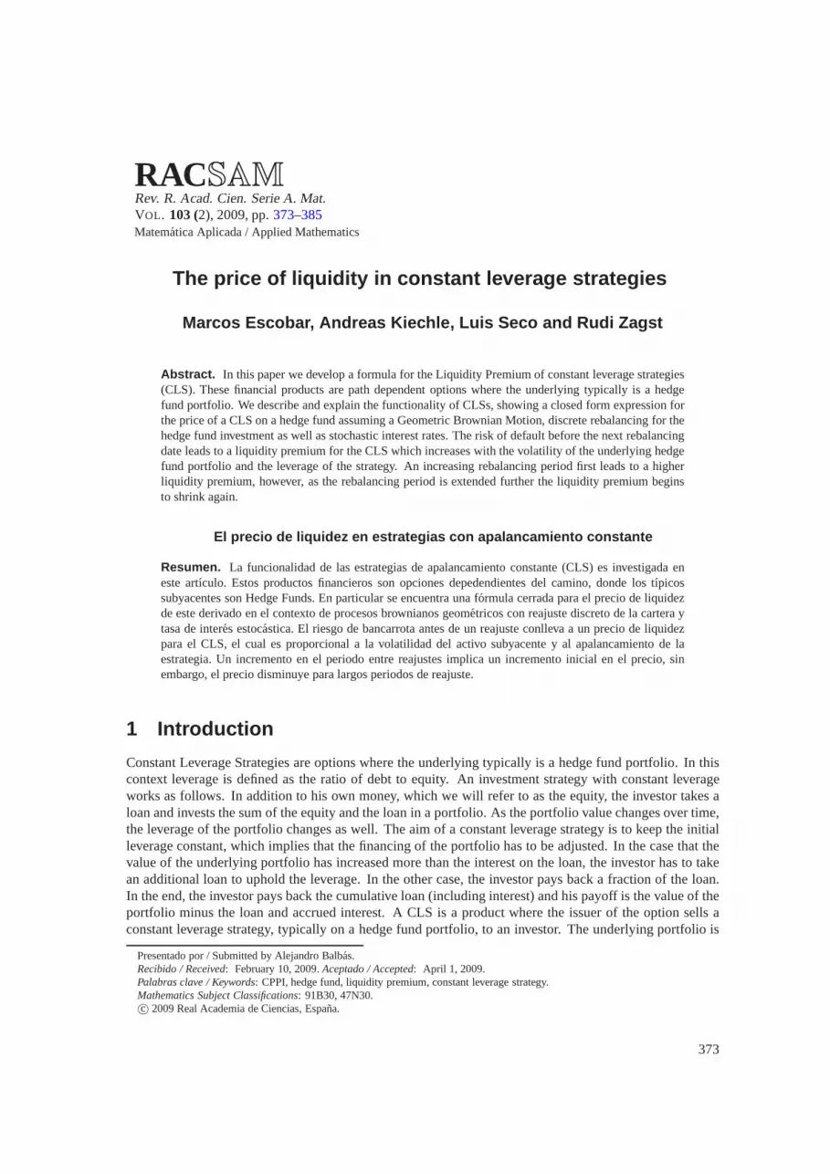
Figure 1. Price of the CPPI Option, T = 10 years, L = 3, Vt0 = 1.0

4 Dynamic Behaviour of Liquidity Premium

For a deeper understanding of the CLS we now show how the priceof the CLS which we have deduced inthe previous section depends on the volatilityσ of the underlying hedge fund portfolio, the period betweentwo consecutive rebalancing dates∆t and the leverageL of the portfolio. First, recall that the price of theCLS is composed by the initial investment of the investor plus the liquidity premium due to the illiquidityof a hedge fund investment. This liquidity premium is strongly related to the probability of default of theCLS. For the investor the option character of the CLS comes into existence in the case of default. The threefactors that influence the probability of default of the CLS and thus determine the liquidity premium areσ,∆t, andL. As we have showed above, the price of the CLS is independent of the stochastic interest ratert.

Figures1 and2 show the price of the CLS int0 with a maturity ofT = 10 years depending onσ and∆t with a leverage ofL = 3 (Figure1) and a leverage ofL = 5 (Figure2). The initial equityVt0 is one.We chose values up to15% for σ and up to2 years for∆t which are typical for a hedge fund portfolio.

As we can see in both figures, the price of the CLS is one, which is the initial investment of the investor,for small values ofσ and∆t. This means that the liquidity premium is close to zero. The reason for thisis that in these cases almost no defaults occur. This becomesclear if we recall that default happens whenthe underlying portfolio loses more than the value of the equity from one rebalancing date to the next one.Thus, default is unlikely if the portfolio exhibits a low standard deviation and is rebalanced frequently.

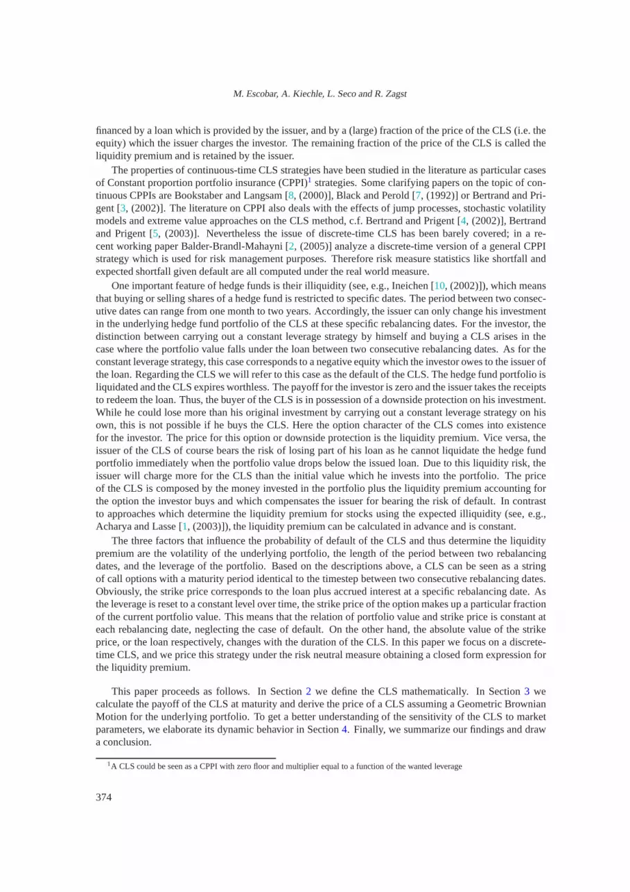
Figures1 and 2 show that the liquidity premium increases with inreasing values forσ and∆t. Asthe volatility of the underlying portfolio increases and the distance between two consecutive rebalancingdates gets bigger the probability of default is rising as well. In the case of default, the buyer of the CLS isbetter off than with a direct investment in the underlying portfolio and therefore has to pay for the liquiditypremium of the CLS. Figure2 shows that the liquidity premium can make up for a large fraction of theprice of the CLS. For a leverageL = 5, σ = 15% and∆t = 2 years for example the liquidity premiumaccounts for0.7 of the price of the option which means that the CLS is almost twice as expensive as a directinvestment. The reason for this high liquidity premium is that in this case the probability of default for theCLS during the maturity is72%. Furthermore, we can see that higher values for the leverageL lead to ahigher liquidity premium. This is obvious as the equity represents a smaller value of a highly leveraged

379



portfolio and thus smaller losses of the underlying portfolio can result in default.In Figures1 and2 the behaviour of the price of the CLS is quite intuitive and easy to understand. To give

a complete picture, we extend the volatility for the underlying portfolio to a maximum of40% in Figure3.At the first glance the fact that the option price is falling again with increasing∆t for greater values ofσmay be surprising and counter-intuitive.

To understand this behaviour of the price, we have to have a closer look at the occurrence of defaults.Figure 4 shows the probability of default for a CLS withT = 10 years andL = 3 depending onσand∆t. It illustrates that the probability of default first increases and then decreases with growing∆t.Recall that with continuous rebalancing there are no defaults. If one waits longer for the next rebalancing,e.g. one or three months, the probability of default increases. With a rebalancing period of one year theprobability for this option to default peaks at about80%. However, the surprising conclusion of this plotis that if the rebalancing period is increased further, the probability of default is decreasing again.Thisbehaviour can be explained as follows. Imagine two (not veryrealistic) CLSs with the same maturityT = 10 years, one rebalancing once after five years (CO 1), the otherone with no rebalancing at all(CO 2). Let the other parameters for this example beσ = 25% andL = 3. The probability of default forCO 1 is higher than for CO 2 simply because there are two possibilities for it to default (int = 5 yearsand in t = 10 years) compared to only one int = 10 years for CO 2. Or in mathematical terms, theprobability of default for CO 1 after five years is41%. The overall probability of default for CO 1 thus is41%+(100%−41%) ·41% = 65%. The probability for a default of CO 2 after ten years is51%. Hence theprobability of default is greater if we conduct a rebalancing after five years compared to the case where wedo not rebalance at all. Knowing that the price of the CLS is closely related to the number of defaults we cannow understand why the price of the CLS begins to decrease again for large values of∆t in Figure3. Thereason for this behaviour of the price is that the probability of default is beginning to decrease for large∆t.

However, these theoretical examinations may not be very relevant in practice. Looking at the maximumof the probability of default in the previous example we can reason that nobody would use a product thathas such high probabilities of default to invest in hedge funds. For a reasonable range of the probability ofdefault (e.g. up to5% or 10%) the price of the CLS increases with increasingσ and∆t as it is shown inFigure1.

380



5 Summary and Conclusion

In this paper we calculated the value of the liquidity premium that appears as a result of discrete rebal-ancing of Constant Leverage Strategies. The main assumptions are a Geometric Brownian Motion for theunderlying hedge fund portfolio and stochastic interest rates. Due to the fact that hedge funds can be tradedonly at specific dates, the CLS can default between two rebalancing dates and thus the price of the CLSmust contain a liquidity premium. The three parameters which influence this premium are the volatilityσof the underlying portfolio, the timestep∆t between two consecutive rebalancing dates and the leverageLwhich determines the financing of the underlying portfolio.We found out that greater values forσ and theL lead to a greater liquidity premium and thus a higher price ofthe CLS. The reason for this is that withincreasingσ andL the probability of default of the CLS also increases. The influence of∆t on the optionprice depends on the specific combination of all three factors σ, ∆t andL. We discovered that for higherbut fixed values ofσ andL the impact of∆t on the probability of default changes with increasing∆t andleads to a hump in the function of the price of the CLS. Finally, it turned out that the price of the CLS doesnot depend on the stocastic interest ratert.

References

[1] ACHARYA , V. AND LASSE, H. P., (2003). Asset Pricing and Liquidity Risk,London Business School, workingpaper.

[2] BALDER, SVEN, BRANDL , M ICHAEL AND MAHAYNI , ANTJE, (2005). Effectiveness of CPPI Strategies underDiscrete-Time Trading, working paper.

[3] BERTRAND, P. AND PRIGENT, J.-L., (2002). Portfolio Insurance Strategies: OBPI versus CPPI, discussionpaper,GREQAMandUniversite Montpellier1.

[4] BERTRAND, P. AND PRIGENT, J.-L., (2002). Portfolio Insurance: The Extreme Value Approach to the CPPI,Finance, 23, 68–86.

381


Figure 4. Probalility of default, T = 10 years, L = 3

[5] BERTRAND, P.AND PRIGENT, J.-L., (2003). Portfolio Insurance Strategies: A Comparison of Standard MethodsWhen the Volatility of the Stoch is Stochastic,International Journal of Business, 8, 15–31.

[6] BLACK , F. AND JONES, R., (1987). Simplifying portfolio insurance,The Journal of Portfolio Management, 14, 1,48–51.

[7] BLACK , F. AND PEROLD, A. R., (1992). Theory of constant proportion portfolio insurance,J. Econ. DynamicsControl, 16, 403–426.

[8] BOOKSTABER, R. AND LANGSAM, J. A., (2000). Portfolio Insurance Trading Rules (Digest Summary),Journalof Futures Markets, 20, 1, 41–57.

[9] HULL , J. C., (2005).Options, Futures and Other Derivatives, Pearson Prentice Hall.

[10] INEICHEN, A. M., (2002).Absolute Returns: The Risk and Opportunities of Hedge Fund Investing, Wiley Fi-nance.

[11] ZAGST, R., (2002).Interest Rate Management, Springer Finance.

A Appendix

PROOF OFPROPOSITION1. For the following calculation of the payoff of the CLS at maturity T we firstneed two results:

1. LetXti:= Sti−1/Sti

, then

N−1∏

s=1

Xts=

St0

StN−1

, i.e. StN−1 =St0

∏tN−1

i=1 Xti

.

382


2. Recall thatSti= S0e

R ti0 r(s) ds− σ2

2 ti+σWti . Then,

Xti=

Sti−1

Sti

= e−

R titi−1

r(s) ds+ σ2

2 ∆t−σYti . (9)

Recall thatWt ∼ N(0, t), which implies thatYti∼ N(0, ∆t). Note that in particularYti

andYtjare

independent fori, j = 1, . . ., N andi 6= j.Now we can give the payoff of the CLS at maturityT = tN . The payoff inT is the excess of the

portfolio value inT over the loanBbT on the condition that there has been no default inti, i = 1, . . ., N .

As theYtiare independent, we can simply multiply the probabilities of default to obtain the conditional

payoff inT . Furthermore, due to the constant leverage property, theseprobabilities of default are the samefor eachti, i = 1, . . ., N .

The payoff of the CLS at maturityT = tN on the condition that no default has occured inti, i = 1, . . .,N − 1 is αtN−1StN

− BbtN

. We now transform this payoff to express it in terms ofYt which is normallydistributed.

CO(T ) =

(

αtN−1StN− e

R tNtN−1

r(s) dsBa

tN−1

)+

·N−1∏

i=1

1(

αti−1Sti

>e

R titi−1

r(s) dsBa

ti−1

)

applying (2)

=

(

αtN−1StN− e

R tNtN−1

r(s) dsαtN−1StN−1 ·

L

1 + L

)

·N∏

i=1

1(

αti−1Sti

>e

R titi−1

r(s) dsBa

ti−1

)

= αtN−1StN−1

(

StN

StN−1

− eR tN

tN−1r(s) ds L

1 + L

)

·N∏

i=1

1(

αti−1Sti

>e

R titi−1

r(s) dsBa

ti−1

)

aplying (4)

= αt0 ·N−1∏

i=1

(

(1 + L)

(

1 − L

1 + Le

R titi−1

r(s) ds Sti−1

Sti

))

StN−1

·(

StN

StN−1

− eR tN

tN−1r(s) ds L

1 + L

)

·N∏

i=1

1(

αti−1Sti

>e

R titi−1

r(s) dsBa

ti−1

)

= αt0(1 + L)N−1StN−1 ·N−1∏

i=1

(

1 − L

1 + Le

R titi−1

r(s) ds Sti−1

Sti

)

·(

StN

StN−1

− eR tN

tN−1r(s) ds L

1 + L

)

·N∏

i=1

1(

StiSti−1

1+LL

>e

R titi−1

r(s) ds

)

applying (9)

= αt0(1 + L)N−1 St0∏N−1

i=1 Xti

·N−1∏

i=1

(

1 − L

1 + Le

R titi−1

r(s) dsXti

)

·(

1

XtN

− eR tN

tN−1r(s) ds L

1 + L

) N∏

i=1

1(

Xti< 1+L

Le−

R titi−1

r(s) ds

)

383


= αt0(1 + L)N−1 St0∏N

i=1 Xti

·N∏

i=1

(

1 − L

1 + Le

R titi−1

r(s) dsXti

)

·N∏

i=1

1(

Xti< 1+L

Le−

R titi−1

r(s) ds

)

applying (9) again

= αt0(1 + L)N−1St0 ·N∏

i=1

(

eR ti

ti−1r(s) ds−σ2

2 ∆t+σYti

)

·N∏

i=1

(

1 − L

1 + Le

R titi−1

r(s) dse−

R titi−1

r(s) ds+ σ2

2 ∆t−σYti

)

·N∏

i=1

1(

Yti>

ln L1+L

+ σ22

∆t

σ=:z

)

= αt0(1 + L)N−1St0 ·N∏

i=1

(

eR ti

ti−1r(s) ds−σ2

2 ∆t+σYti − L

1 + Le

R titi−1

r(s) ds

)

·N∏

i=1

1Yti>z

= αt0(1 + L)N−1St0eR tN

t0r(s) ds ·

N∏

i=1

(

e−σ2

2 ∆t+σYti − L

1 + L

)

·N∏

i=1

1Yti>z

Now we know from Equation (2) thatαti+1Sti+1 = (1 + L)Vti+1 .

PROOF OFPROPOSITION2. Let z :=(

ln L1+L

+ σ2

2 ∆t)

/σ andfytidenote the density function of

Yti, i.e. the normal distributionN(0, ∆t). Then the price of the CLS today is the expected value of the

discounted payoff of the CLS inT .

Et0 [CO(T )] = E[e−

R

T

t0r(s) ds · CO(T )]

applying (7)

= αt0(1 + L)N−1St0

∫ ∞

z

· · ·∫ ∞

z

N∏

i=1

(

e−σ2

2 ∆t+σyi − L

1 + L

)

· f(y1) · · · f(y2) dy1 · · · dyN

= αt0(1 + L)N−1St0

N∏

i=1

∫ ∞

z

(

e−σ2

2 ∆t+σyi − L

1 + L

)

·(

1√2π∆t

e−y2

i2∆t

)

dyi

= αt0(1 + L)N−1St0

·N∏

i=1

(∫ ∞

z

1√2π∆t

e−1

2∆t(y2

i −2σ∆tyi+σ2∆t2) dyi −L

1 + L

∫ ∞

z

1√2π∆t

e−y2

ti2∆t dyti

)

= αt0(1 + L)N−1St0 ·N∏

i=1

(

(

1 − N(z − σ∆t√

∆t

)

)

− L

1 + L

(

1 − N( z√

∆t

)

)

)

= αt0(1 + L)N−1St0 ·(

(

1 − N(z − σ∆t√

∆t

)

)

− L

1 + L

(

1 − N( z√

∆t

)

)

)N

Substitutingz leads to

CO(t0) = αt0(1 + L)N−1St0 ·(

N

(

ln 1+LL

+ σ2

2 ∆t

σ√

∆t

)

− L

1 + LN

(

ln 1+LL

− σ2

2 ∆t

σ√

∆t

))N

.

384


PROOF OFPROPOSITION3. Note that for the priceCO(t0) of the CLS we get, using the put-call parity,

CO1(t0) = (1 + L)NVt0 ·

N

(

− ln( L1+L )−σ2

2 ∆t

σ√

∆t

)

− L1+L

· N(

− ln( L1+L)+σ2

2 ∆t

σ√

∆t

)

N

= (1 + L)NVt0 ·[

Put

(

L

1 + L, 1, 0, σ, ∆t

)]N

= (1 + L)NVt0 ·[

1 − L

1 + L+ Call

(

L

1 + L, 1, 0, σ, ∆t

)]N

= Vt0 ·[

1 + (1 + L) · Call

(

L

1 + L, 1, 0, σ, ∆t

)]N

.

We therefore get a liquidity premium per rebalancing period∆t of

(1 + L) · Call

(

L

1 + L, 1, 0, σ, ∆t

)

.

Marcos Escobar Andreas KiechleDepartment for Mathematics,Ryerson University, Munich University of Technology,[email protected]

Luis Seco Rudi ZagstDirector, Risklab Toronto, Director, HVB-Institute for Mathematical Finance,Sigma Analysis & Management, Munich University of Technology,Toronto Munich,

[email protected]

385

Documents

The price of liquidity in constant leverage strategies