Embed Size (px)
Citation preview

University of Bradford eThesis This thesis is hosted in Bradford Scholars – The University of Bradford Open Access repository. Visit the repository for full metadata or to contact the repository team
© University of Bradford. This work is licenced for reuse under a Creative Commons
Licence.
COMPUTER COLOUR MATCHING WITH FLUORESCENT DYES
The influence of fluorescence on reflectance -
concentration relationships for fluorescent dyes,
singly and in mixtures, and the effects on the
prediction of recipes for use in colour matching.
MAN Tak-ming
f
A thesis submitted for the Degree of Doctor of Philosophy-
of the University of Bradford
Postgraduate School of Studies in
Colour Chemistry and Colour Technology
A
1984
ACKN OWLEDGEMENTS
The auther wishes to express his sincere gratitude for the
patience, advice and encouragement shown upon by Drs. B. Rigg, E. Coates
and Mr. K. K. Chani under whose guidance this work was carried out. The
author also wishes to express his thanks to all in the Institute of
Textiles and Clothing, Hong Kong Polytechnic who have assisted,
especially to Mr. Anthony S. K. Ku. Finallyi but by no means least, the
author would like to record his sincere thanks to Messrs. M. Cheungi
Clement K. M. Lam, Dr. C. Alder and all technical staff in the
Postgrad6ate school of Colour Chemistry and Colour Technology, University
of Bradford.
Thanks are also due to the Staff-development Committee and the
Institute of Textiles and Clothing of the Hong Kong Polytechnic for their
financial support for this research project.
0
C GITENT S
Part I Introduction
Chapter I Colour Matching
1.1 Visual Methods
1.2 Instrumental-aid methods
Chapter II Computer Colour Matching
2.1 Introduction
2.2 General Considerations
2.3 Theoretical Aspects
2.3.1 Colour specification system
2.3.2 Reflectance function
2.3.3 Computation techniques
2.3.4 Colour difference equation
2.4 Basic Operations
2.5 Problems
Page
1
3
4
5
7
8
9
13
14
16
19
Chapter III Computer Colour Matching Involving the Use of
Fluorescent Dyes
3.1 An Introduction to the Measurement of Fluorescent Sample 20
3.1.1 The Fluorescence 20
3.1.2 The Measurement 23
3.2 A Suitable Light Source for Measurement 24
3.3 The Measurement Techniques 27
3.3.1 Direct Measurement of the Total Radiance Factor 27
3.3.2 Measurements with Two Mouochromators 30
3.3.3 One-Monochromator and Abridged Methods 31
a
CCNTENITS Contd
3.4 Matching Involving the Use of Fluorescent Dyes
3.4.1 State of the Art
3.4.2 Ganz's Approach
3.4.3 McKayls Approach
3.4.4 Funk's Approach
Part II Experimental and Results
Chapter IV Introduction and Objectives
Chapter V Review of a Current (1978) Commercial Package in
Computer Colour Matching
5.1 The System -
5.2 A General Study on the Performance of the System
5.2.1 Preparation of Calibration Dyeings
5.2.2 Effect of Sample Size on the Accuracy of
Computer Colour Matching
5.2.3 The Achieved Accuracy
Chpater VI Fluorescent Dyes
6.1 Introduction
6.2 Relationship Between Total Radiance Factors and
Concentration of The Dye
Page
33
33
33
35
39
42
44
45
45
46
47
58
58
0
CONTENTS Contd
Page
6.2.1 Treatment as non-fluorescent Dye - Case 1 64
6.2.2 Treatment as Fluorescent Dye - Cases 2 and 3 69
6.2.3 Development of Computer Program 75
6.3 Mixture Dyeings with a Fluorescent Dye and a 85
non-fluorescent Dye
6.3.1 The non-Fluorescent Dyes 85
6.3.2 Total Radiance Factors - Concentration 90
Relationship in the Mixture Dyeings
6.3.3 Development of Computer Program 93
6.3.4 Amount of Calibration Dyeings Required in 94
Compound Shade
Chapter VII Computer Colour Matching involving the use of
Flourescent Dyes
7.1 Introduction 113
7.2 Computer Colour Matching with Two Dyes in Mixture 114
7.3 Results of Match Prediction 123
Part III Analysis,, D scussion & Conclusions
Chapter VIII Analysis and Discussion
8.1 The Accuracy of Measurements 149
8.2 General Performance of the RFC3 Computer Colour 151
Matching Package
8.3 Computer Colour Matching Involving the Use of 154
Fluorescent Dyes
CONTENTS Contd
Page
8.3.1 Effect of Light Sources on the Measurement 154
of Fluorescent Samples
8.3.2 Development of Equations Relating Fluorescence 159
to Dye Concentrations
8.3.3 The Direct Iteration Technique 163
8.3.4 Matching Involving Fluorescent Dyes 164
Chapter IX Conclusions
Appendix
168
A. A General Study of the Performance of the RFC-3 System 170
A. 1 Calibration Dyeings - Cotton/Reactive Dye 170
System
A. 2 Calibration Dyeings - Polyester/Disperse Dye 177
System
A. 3 Effect of Sample Size on the Accuracy of 179
Computer Colour Matching
A. 4 Location of Target Samples in CIELAB space 180
B. Colorimetric Behaviour of Fluorescent Dyes in Self and 185
Compound Shades with Non-Fluorescent Dyes
B. 1 General Behaviour of Single Dyes 185
B. 2 General Behaviour of Fluorescent Dye Admixed 192
With a non-Fluorescent Dye
B. 3 Total Radiance Factors Curves of Mixture 235
Dyeings - Examples

Appendix Contd
Page
C. Computer Programs and Data
CA Computer Programs: Program I Self colour 245
Program II Mixture 250
Program III Matching 255
C. 2 Data 261
D. An Example of Actual Iteration in the Matching 269
Program - TMS3
E. Total Radiance Factors Curves for'Prediction Trials in 271
the Matching Program TMS3
References 294
4
SUMIARY
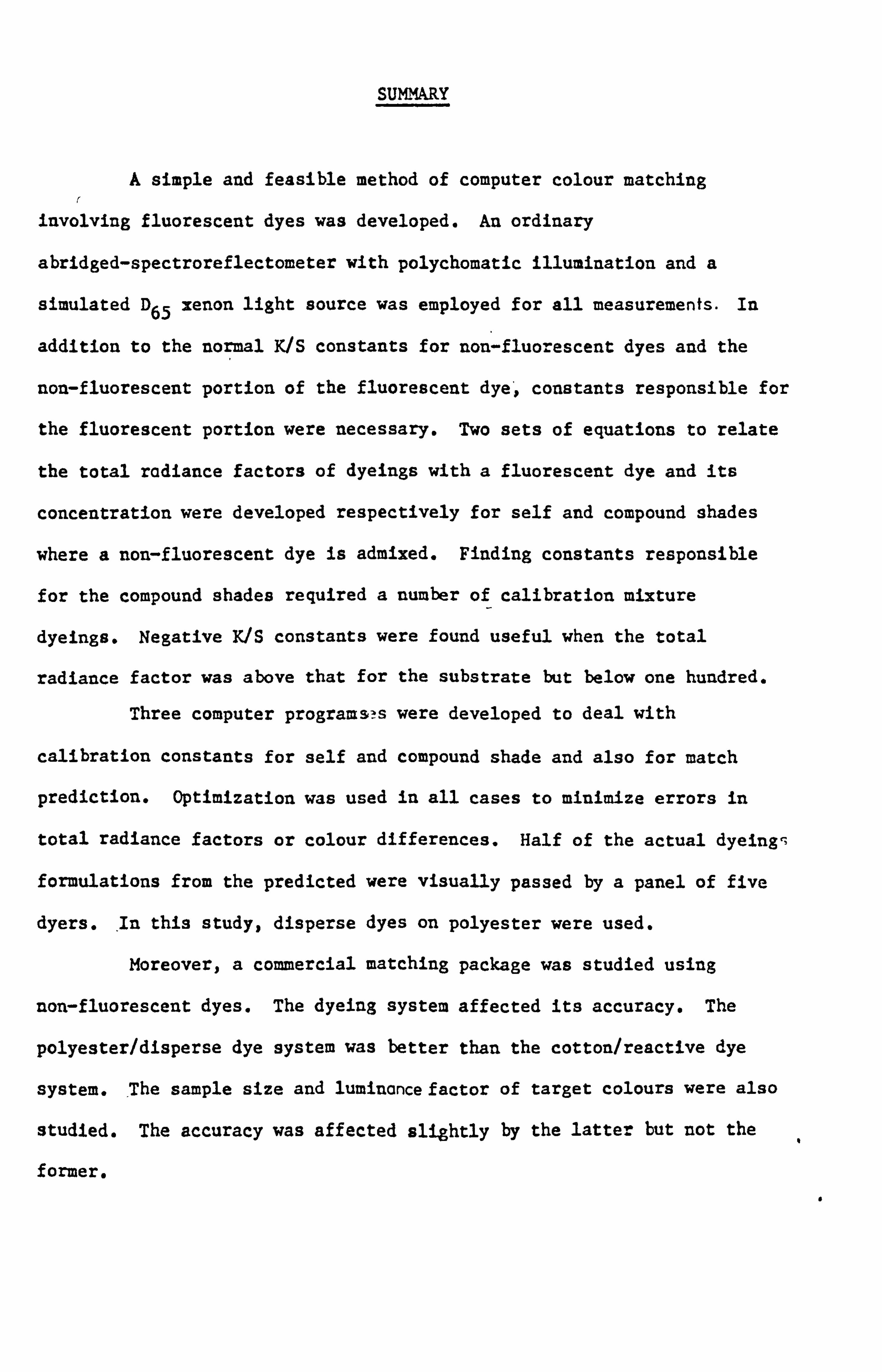
A simple and feasible method of computer colour matching
involving fluorescent dyes was developed. An ordinary
abridged-spectroreflectometer with polychomatic illumination and a
simulated D65 xenon light source was employed for all measurements. In
addition to the normal K/S constants for non-fluorescent dyes and the
non-fluorescent portion of the fluorescent dye'.. constants responsible for
the fluorescent portion were necessary. Two sets of equations to relate
the total radiance factors of dyeings with a fluorescent dye and its
concentration were developed respectively for self and compound shades
where a non-fluorescent dye is admixed. Finding constants responsible
for the compound shades required a number of calibration mixture
dyeings. Negative K/S constants were found useful when the total
radiance factor was above that for the substrate but below one hundred.
Three computer programs? s were developed to deal with
calibration constants for self and compound shade and also for match
prediction. Optimization was used in all cases to minimize errors in
total radiance factors or colour differences. Half of the actual dyeingq
formulations from the predicted were visually passed by a panel of five
dyers. In this study, disperse dyes on polyester were used.
Moreover, a commercial matching package was studied using
non-fluorescent dyes. The dyeing system affected its accuracy. The
polyester/disperse dye system was better than the cotton/reactive dye
system. The sample size and luminancefactor of target colours; were also
studied. The accuracy was affected slightly by the latter but not the
former. S
Part I
Introduction
Chapter I Colour Matching
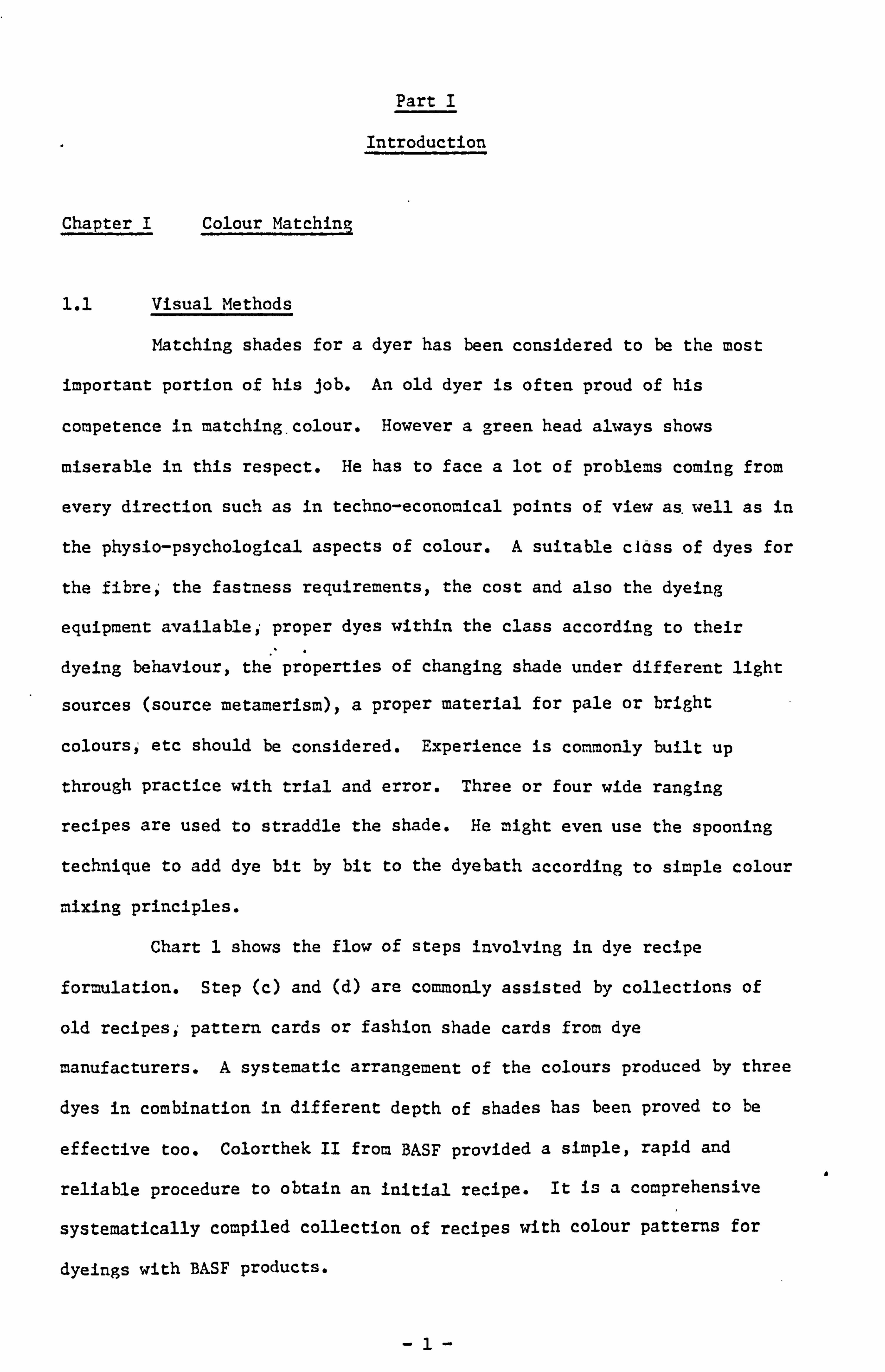
1.1 Visual Methods
Matching shades for a dyer has been considered to be the most
important portion of his job. An old dyer is often proud of his
competence in matching, colour. However a ýcyreen head always shows
miserable in this respect. He has to face a lot of problems coming from
every direction such as in techno-economical points of view as. well as in
the physio-psychological aspects of colour. A suitable cIdss of dyes for
the fibre; the fastness requirements, the cost and also the dyeing
equipment availablei proper dyes within the class according to their
dyeing behaviour, the properties of changing shade under different light
sources (source metamerism), a proper material for pale or bright
coloursý etc should be considered. Experience is commonly built up
through practice with trial and error. Three or four wide ranging
recipes are used to straddle the shade. He might even use the spooning
technique to add dye bit by bit to the dyebath according to simple colour
mixing principles.
Chart 1 shows the flow of steps involving in dye recipe
formulation. Step (c) and (d) are commonly assisted by collections of
old recipes; pattern cards or fashion shade cards from dye
manufacturers. A systematic arrangement of the colours produced by three
dyes in combination in different depth of shades has been proved to be
effective too. Colorthek II from BASF provided a simple, rapid and
reliable procedure to obtain an initial recipe. It is a comprehensive
systematically compiled collection of recipes with colour patterns for
dyeings with BASF products.
a
-1-
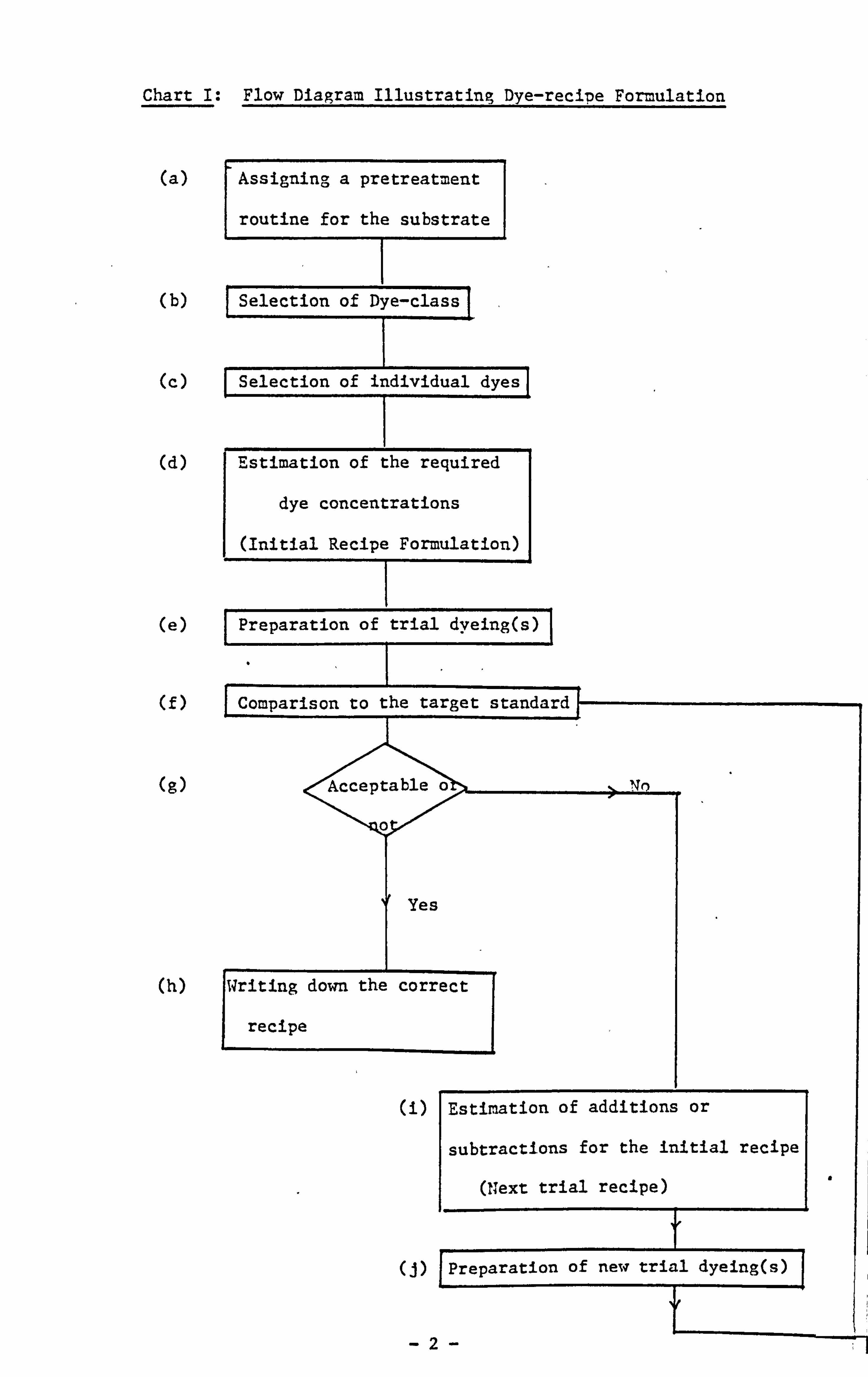
Chart I: Flow Diagram Illustrating Dye-recipe Formulation
(a) Assigning a pretreatment Q
routine for the substrate
Selection of Dye-class
(c) I Selection of individual dyes
Estimation of the required
dye concentrations
(Initial Recipe Formulation)
(e) Preparation of trial dyeing(s)
(f) Comparison to the target standard
(g) e"'Acceptable 6
Yes
I Writing down the correct
recipe
W Estimation Of additions or
subtractions for the initial recipe
(Next trial recipe)
jPreparation of new trial dyeing(s)
-2-
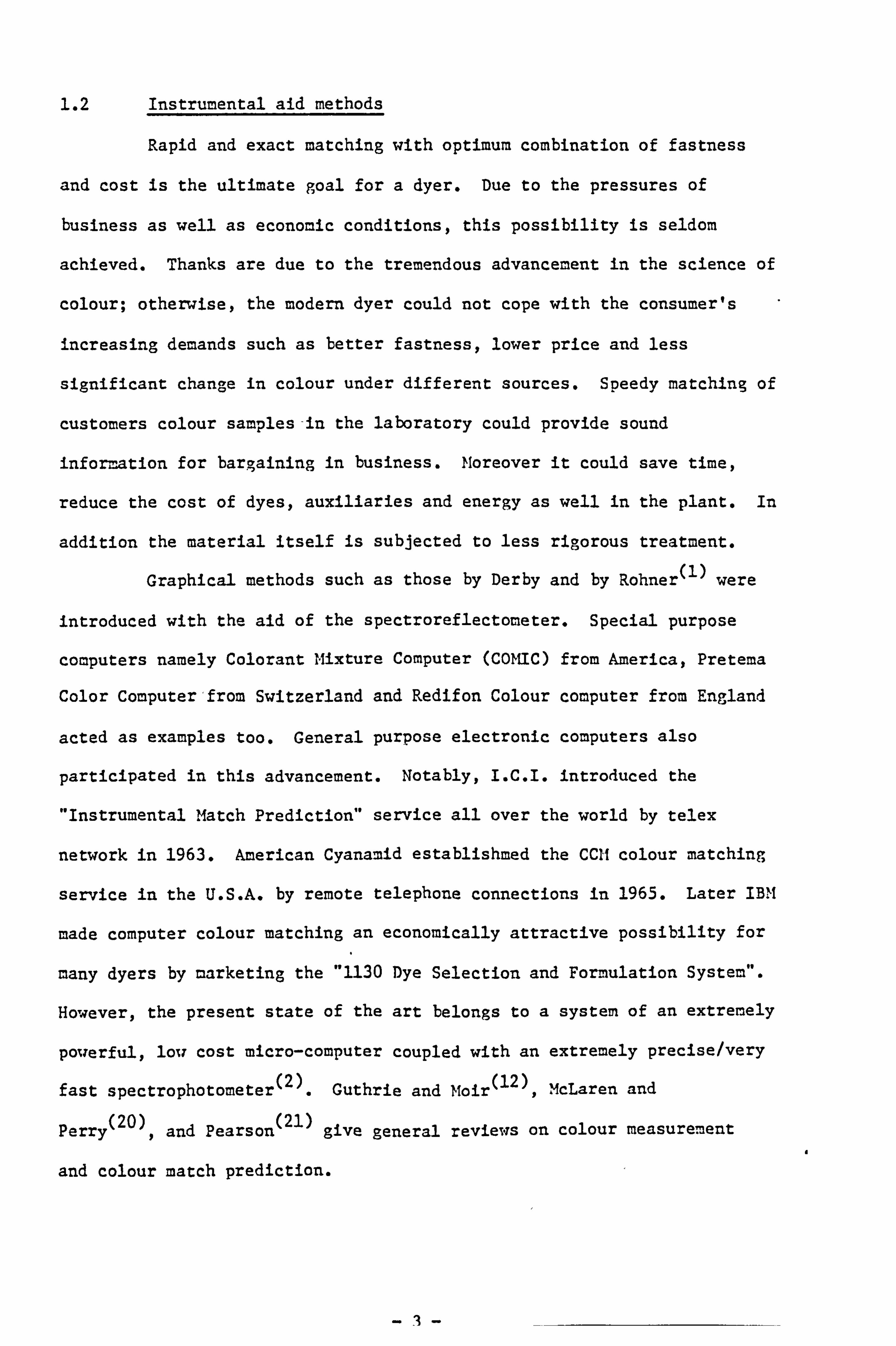
1.2 Instrumental aid methods
Rapid and exact matching with optimum combination of fastness
and cost is the ultimate goal for a dyer. Due to the pressures of
business as well as economic conditions, this possibility is seldom
achieved. Thanks are due to the tremendous advancement in the science of
colour; otherwise, the modern dyer could not cope with the consumer's
increasing demands such as better fastness, lower price and less
significant change in colour under different sources. Speedy matching of
customers colour samples-in the laboratory could provide sound
information for bargaining in business. Moreover it could save time,
reduce the cost of dyes, auxiliaries and energy as well in the plant. In
addition the material itself is subjected to less rigorous treatment. 0
Graphical methods such as those by Derby and by Rohner(') were
introduced with the aid of the spectroreflectometer. Special purpose
computers namely Colorant Mixture Computer (COMIC) from America, Pretema
Color Computer, from Switzerland and Redifon Colour computer from England
acted as examples too. General purpose electronic computers also
participated in this advancement. Notably, I. C. I. introduced the
"Instrumental Match Prediction" service all over the world by telex
network in 1963. American Cyanamid establishmed the CCH colour matching
service in the U. S. A. by remote telephone connections in 1965. Later IB11
made computer colour matching an economically attractive possibility for
many dyers by marketing the "1130 Dye Selection and Formulation System".
However, the present state of the art belongs to a system of an extremely
powerful, low cost micro-computer coupled with an extremely precise/very
fast spectrophotometer (2). Guthrie and Moir(12)., McLaren and
Perry (20) , and Pearson
(21) give general reviews on colour measurement
and colour match prediction.
- -3 -

Chapter II Computer Colour Matching
2.1 Introduction
An impression that computer matching was to be a replacement for
the experienced dyer created a lot of resistance in promoting such an
valuable help to the dyeing industries. Such a fear has gradually
disappeared with time. In the last few years, a small place like Hong
Kong has already been equipped with nine systems. The dyer now realises
the importance of computer colour matching. It is only there in an
advisory capacity and it is up to him to pick up the most workable
formulation from those offered. Anyone else would pick just the cheapest
and could then be in all sorts trouble on the plant. His experience and
knowledge could be used in the preselection of dyes, setting tolerance
limit etc. Furthermore, he could spend his valuable time to deal with
specific problems as well as to carry out product and process
developments instead of wasting time in the labour intensive 0
trial-and-error-approach. Moreover, additional benefits for shade
correction, colour sorting, and quality control can be obtained from the
system.
Fast and accurate formulation provides an immediate benefit for
a dyer. In addition, computer colour matching provides recipes that
exhibit minimum metamerism, low cost, and possibly better performing
formulations in terms of repeatability. In general, the system forces a
review of the-dyes used. It may show up excessive amount of dye in old
recipes, or alternatively that some additional dyes could be used to
reduce costs of medium and heavy shades. Also, when formulations, with a
proven system and good calibration data,, are not too useful, it starts an
investigation into the reason. This can lead to new insights into dye
behaviour and force the development of better dyeing procedures.
0

2.2 General Considerations
Following the flow diagram for colour matching (Chart 1), the 0
computer might be used in the selection of individual dyes from the
chosen class (step c), the estimation of required dye concentrations in
initial recipe (step d), and also estimation of a corrected formulation
(step i). Step c involves a lot of dyer's experience. Dyes within a
usage class may differ in properties such as fastness, flare etc., and
also in dyeing behaviour in self-or compound-shades, and so forth. A
rough preselection of a Sroup of dyes for a dye/fibre processing system
is often a necessity. The computer matching system is only performing I c3
its role according to the individual optical properties of the dyes
stored. Furthermore, the dyer can also contribute his knowledge to
instruct the system as to the number of dyes required per recipe and to
set a tolerance limit of acceptability. These will greatly reduce the
time of computing and also will increase the accuracy'of the sytem (steps
dp go and i).
Ideally it would be desirable to have an accuracy of computer
colour matching well within the tolerance of industrial dyeings, so that
no corrections are needed. Connelly (2 )
reported that five out of seven
predictions were accepted by their plant on first strike. According to
Brockes(3), the first trials of computer colour matching deviate about
2-3 Adams-Nickerson units of colour difference (AN40) from the standard
as an average under good conditions. With less favourable conditions,
errors of 5 or more M140 units can occur. Similar experimental findings
(4) (5) have been published by Hirschler et. al Chong and Siu
The major soruces of error in computer colour matching are the
accuracy of dyeing processes, the change of substrate, the imperfection
of the optical theories and the accuracy of measurement. John(6)
summarized the opportunities where computers can be used to produce the
most benefit, and those instances which produce the least in Tables 1 and
2.
-5-
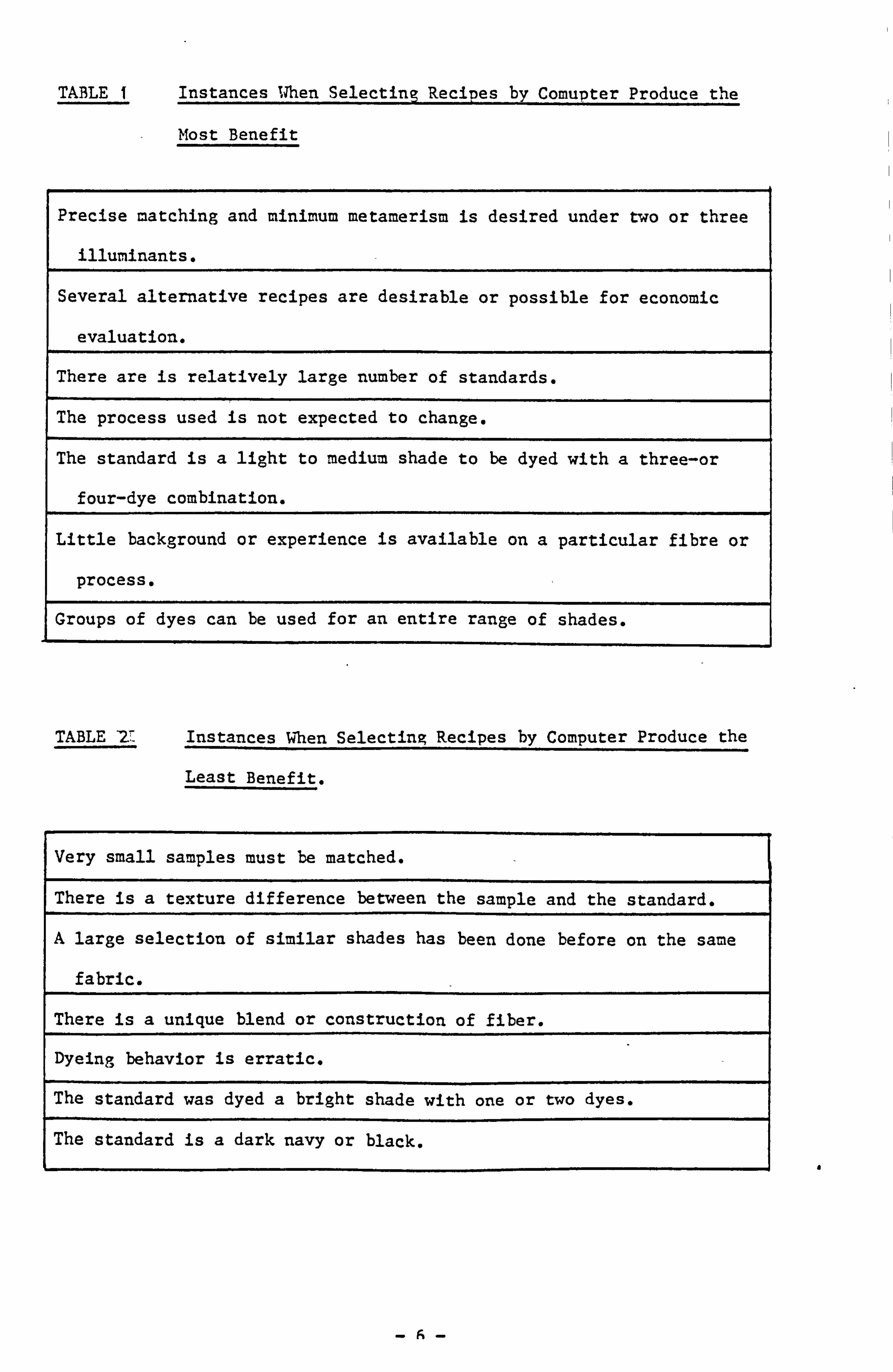
TABLE I Instances When Selecting Recipes_by ComuPter ProduCe the
Most Benefit
Precise matching and minimum metamerism is desired under two or three
illuminants.
Several alternative recipes are desirable or possible for economic
evaluation.
There are is relatively large number of standards.
The process used is not expected to change.
The standard is a light to medium shade to be dyed with a three-or
four-dye combination.
Little background or experience is available on a particular fibre or
process,
Groups of dyes can be used for an entire range of shades.
TABLE Y Instances When Selecting Recipes by Computer Produce the
Least Benefit.
Very small samples must be matched.
There is a texture difference between the sample and the standard.
A large selection of similar shades has been done before on the same
fabric.
There is a unique blend or construction of fiber.
Dyeing behavior is erratic.
The standard was dyed a bright shade with one or two dyes.
The standard is a dark navy or black.
-A-
What is the best instrument or the best program? Saltzman(7)
emphasizes that the answer is and always has been that there is no such
thing. One has to have the best people, one or more people who know what
they are doing - who know-the field of colour and colour matching, as
well as our specific field of technical activity, and can intelligently
put the two together. ' on the other hand, ignorant or stupid people,
using the finest instruments, can botch up a job as fast as the computer
can print out the wrong answers. People are the first and most important
ingredient for success in computer colour matching. Process control is
next. Computer colorant formulation can work only on a process that is
under control. Moreover, sampling techniques have to be stressed.
Proper sampling is commonly ignored. It is because people are fascinated
by the speed with which one can get numbers and "results" out of a
machine. With all these three together and with continuous up-dating of
technology, people can get the most advantages from computer colour
matching.
2.3 Theoretical Aspects
Computer colour matching involves the use of a system to specify
a colour exactly; a mathematical function to correlate the colour and the
concentration of a dyeing and a computation technique to improve the
recipe until a preset tolerance is satisfied. The tolerance is usually
specified in a visually uniform system where the distance calculated
between any two colours can be taken as a measure of the magnitude of
visual difference between them. Moreover, evaluation of metamerism under
different illuminants is also required. It is really an advantage of
computer formulation over an experienced dyer since he has not enough
time to exploit all the possibilities to produce a recipe with minimum
metamerism.
a
2.3.1 Colour Specification System
A system to express colour in terms of numerical values is
necessary in computer operation. Among various colour systems, the one
recommended by the International Commission on Illumination (C. I. E. ) is
the most suitable one, since it follows the visual process for colour
formation. In production of colour visually, a dyeing is illuminated by
a source,, its reflected light leaves the surface and enters into the eye
of an observer, the signals created in the retina pass through nerve
tissues to the brain and are then interpreted as colour sensation based
on previous experience and training. CIE tried to standardize all the
variables which would affect this visual process. Illuminants,
illuminating and viewing geometry, reference white surface and observers
have"been standardised. Therefore colour can be specified in the
following way:
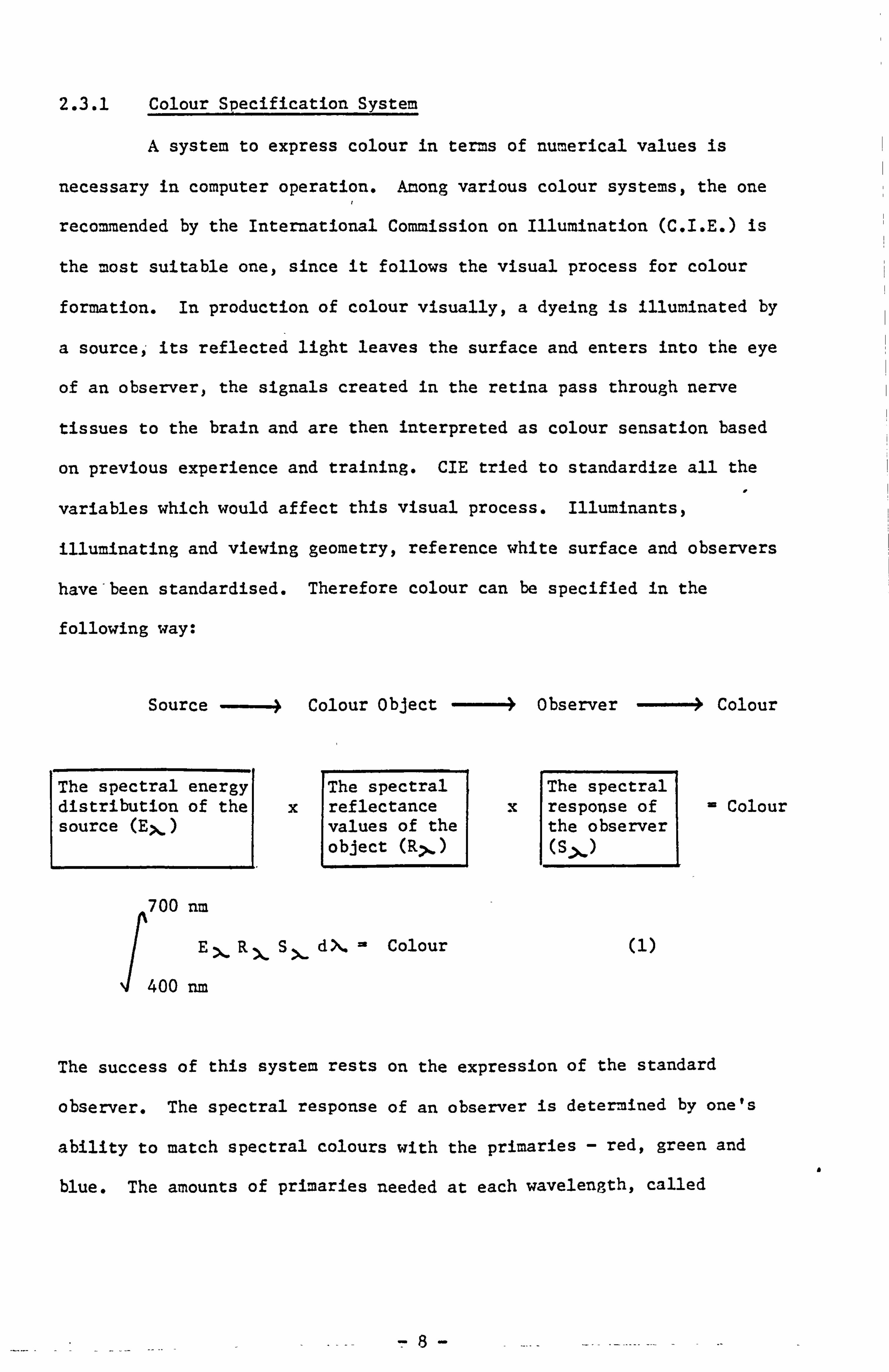
Source Colour object Observer Colour
The spectral energy The spectral The spectral distribution of the x reflectance x response of Colour source values of the the observer
object (R>, ) (S. >-)
700 nm
E>RXS >_ d X. - Colour
1400
nm
The success of this system rests on the expression of the standard
observer. The spectral response of an observer is determined by one's
ability to match spectral colours with the primaries - red, green and
blue. The amounts of primaries needed at each wavelength, called a
8-
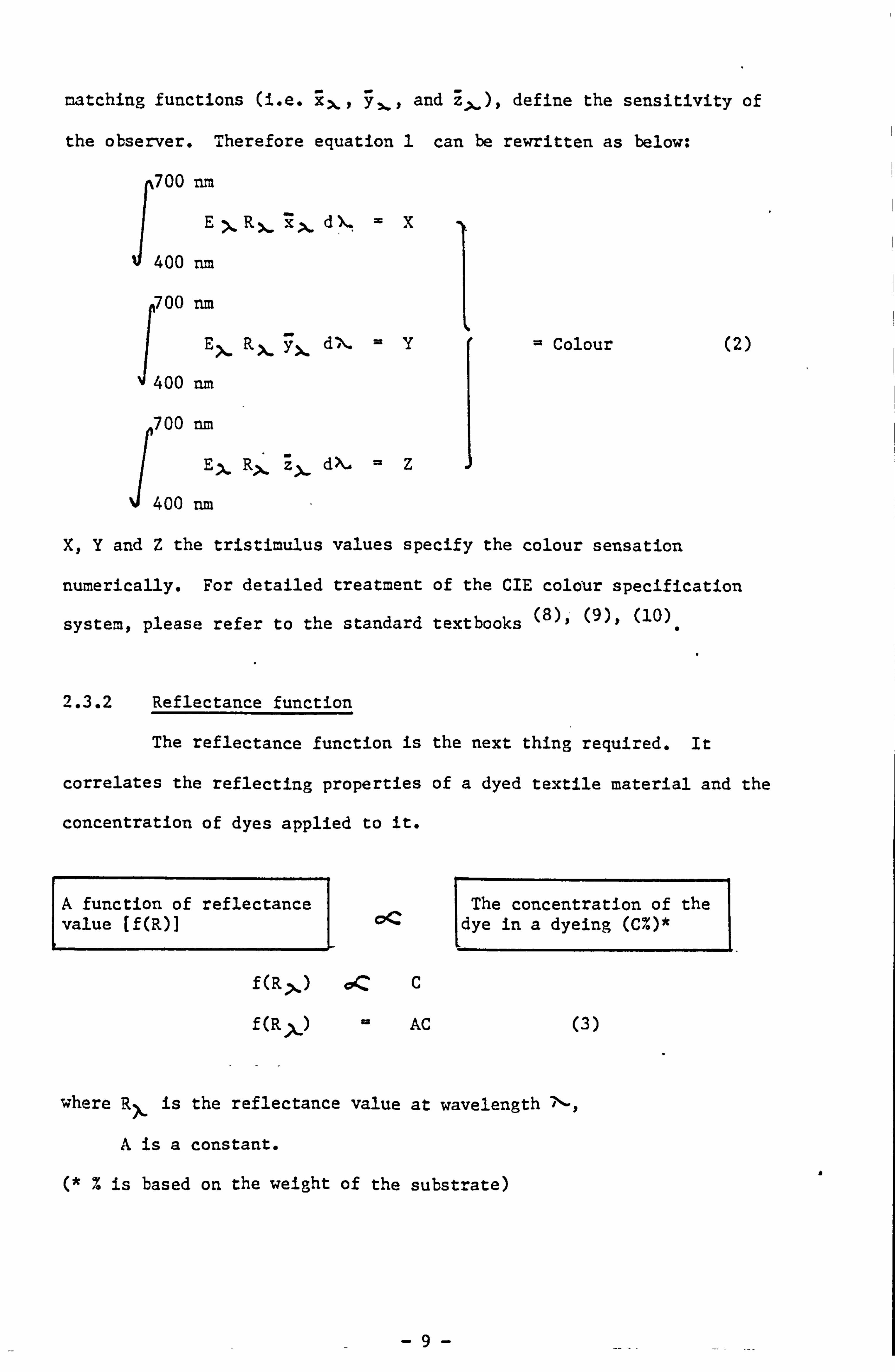
matching functions (i. e* RX and define the sensitivity of
the observer. Therefore equation 1 can be rewritten as below:
700 rLm
E >. R ), _ 7 >. d ý-. =X
f400
rm
700 rm
ER d%, =Y Colour (2)
1400
nm
>- x yx
700 nm
E >_ R> Z), dX. -Z
400 run
X, Y and Z the tristimulus values specify the colour sensation
numerically. For detailed treatment of the CIE colour specification
system, please refer to the standard textbooks (8)9' (9), (10)o
2.3.2 Reflectance function
The reflectance function is the next thing required. It
correlates the reflecting properties of a dyed textile material and the
concentration of dyes applied to it.
A function of reflectance value [f(R)l
f (R>j
f(RX)
The concentration of the dye in a dyeing (C%)*
cc
AC (3)
where Rx is the reflectance value at wavelength
A is a constant.
% is based on the weight of the substrate) a
-9-
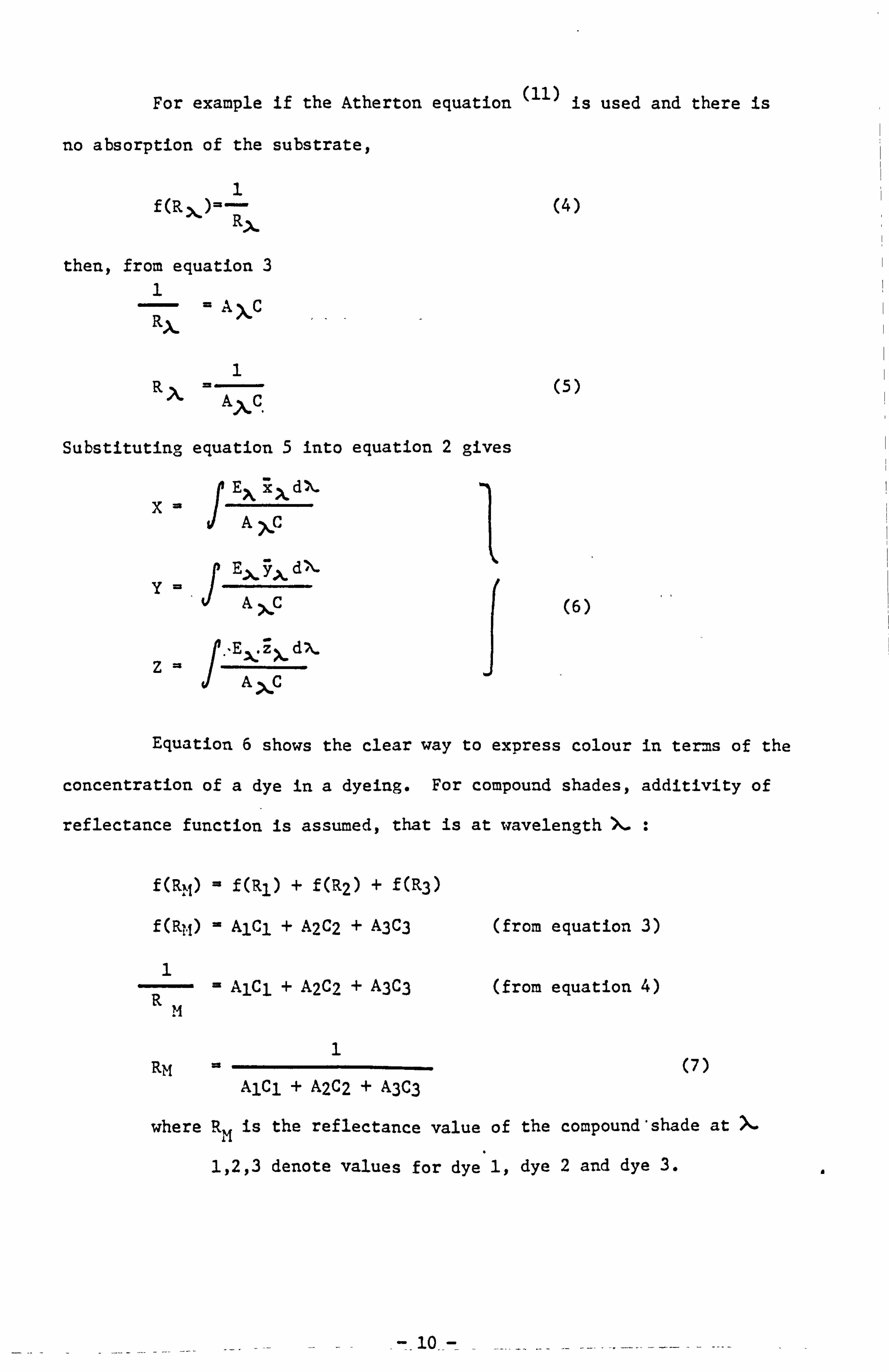
For example if the Atherton equation (11) is used and there is
no absorption of the substrate,
1
then, from equation 3 1
R> A%C
1
AXq
Substituting equation 5 into equation 2 gives
EX d', %- xA
NP
EX d, %- yA
Z Ez> d%
(4)
(5)
(6)
Equation 6 shows the clear way to express colour in terms of the
concentration of a dye in a dyeing. For compound shades, additivity of
reflectance function is assumed, that is at wavelength >ý-
f(Rý?, f(Rl) + f(R2) + f(R3)
f(RI, j) AlCl + A2C2 + A3C3
1 AlCl + A2C2 + A3C3
(from equation 3)
(from equation 4)
RM (7) AlCl + A2C2 + A3C3
where Rm is the reflectance value of the compound'shade at
1,2,3 denote values for dye 1, dye 2 and dye 3.
--

Substituting equation (7) into equation 2
E%d x
AlCl + A2C2 + A3C3
Y E, ),, ? >, d >,
AICJ + A2C2 + A3C3
zE>, _ 'i, \ dk
AlCl + A2C2 + A3C3
Where A,, A2 and A3 depend on wavelength.
(8)
Similarly equation 8 expresses the colour of a compound shade with three
dyes in mixture.
The relationship between reflectance factor and dye
concentration is very complex in its fundamental form. A practical
approximation has been found in the theory of Kubelka and Munk(9). In
this theory, the dyeing is defined by two optical values, K denoting the
coefficient of absorption, and S the coefficient of scattering. In
textiles, it is assumed that K is mainly determined by the dye, while S
only depends upon the fibre. For a thick pad of dyeing, i. e. a
completely opaque sample, its reflectance value (R) can be, expressed in
the simplest way according to the Kubelka and Munk analysis as equation 9.
(IS)2 s
(9)
K Solving for (-)
S
K (1 - R) 2 'H '0 2R (10)
Since S is constant in this case, and K is usually
satisfactorily proportional to the concentration (C) of the dye used in
accordance with Beer and Lambert's law.
AC
- 11 -
(11)
-
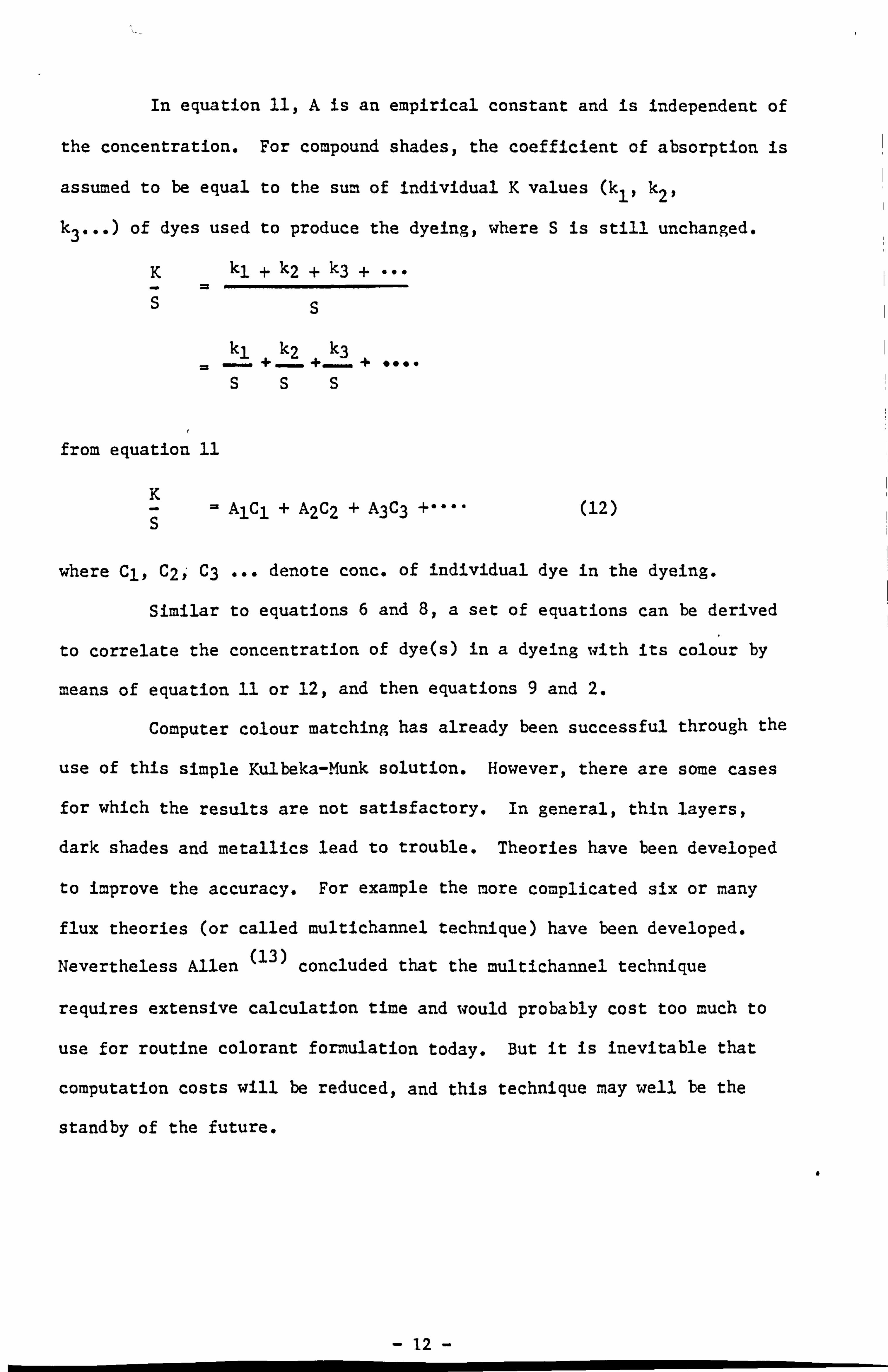
In equation 11, A is an empirical constant and is independent of
the concentration. For compound shades, the coefficient of absorption is
assumed to be equal to the sum of individual K values (kl, k2l
k3,,, ) of dyes used to produce the dyeing, where S is still unchanged.
K kl + k2 + k3 +
ss
kl 2 +L+
k3
sss
I from equation 11
K AlCl + A2C2 + A3C3 (12)
s
where Cl, C21' C3 ... denote conc. of individual dye in the dyeing.
Similar to equations 6 and 8, a set of equations can be derived
to correlate the concentration of dye(s) in a dyeing with its colour by
means of equation 11 or 12, and then equations 9 and 2.
Computer colour matching has already been successful through the
use of this simple Kulbeka-1.1unk solution. However, there are some cases
for which the results are not satisfactory. In general, thin layers,
dark shades and metallics lead to trouble. Theories have been developed
to improve the accuracy. For example the more complicated six or many
flux theories (or called multichannel technique) have been developed.
Nevertheless Allen (13) concluded that the multichannel technique
requires extensive calculation time and would probably cost too much to
use for routine colorant formulation today. But it is inevitable that
computation costs will be reduced, and this technique may well be the
standby of the future.
a
- 12 -
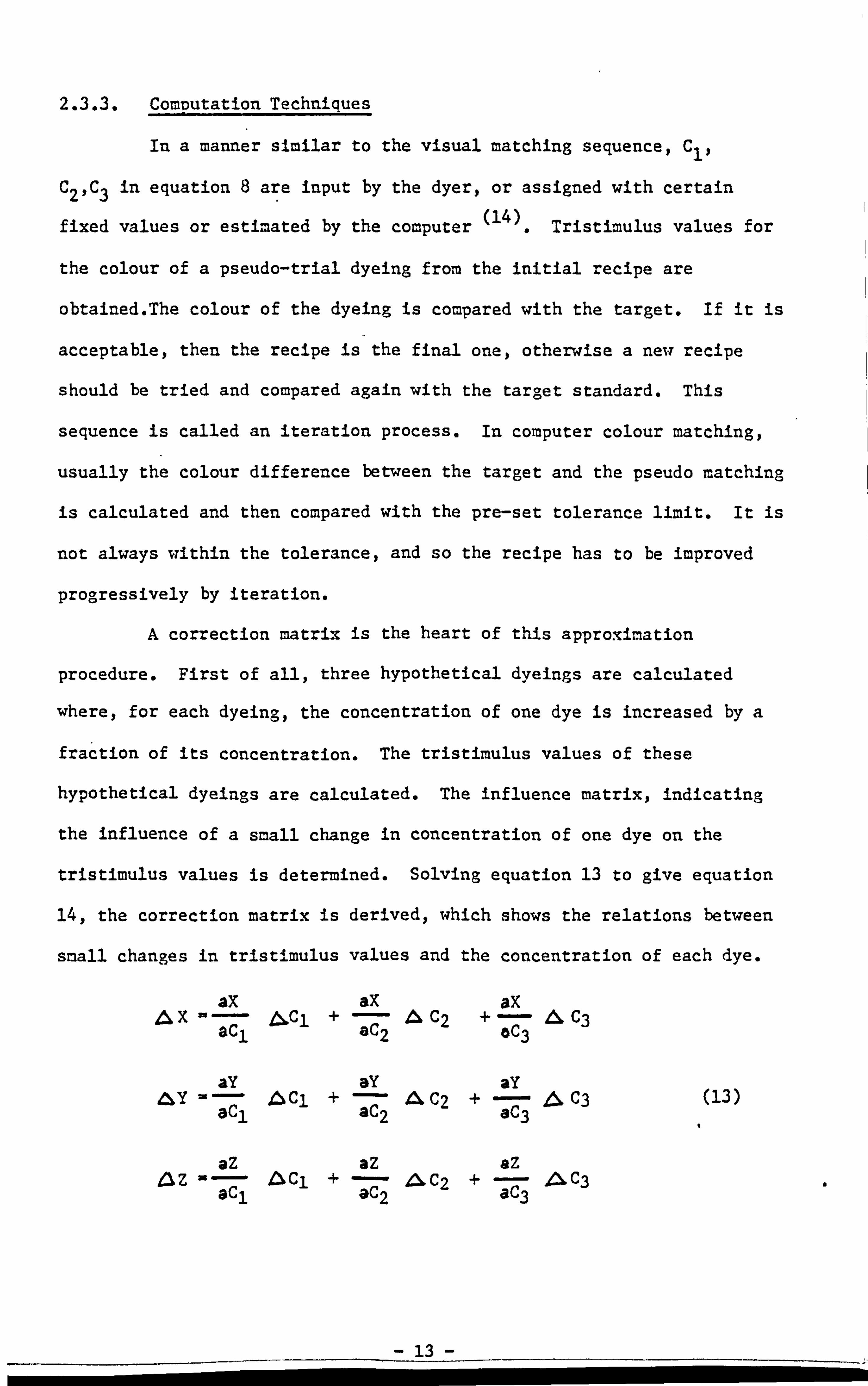
2.3.3. COMDUtation Techniques
In a manner similar to the visual matching sequence, Cl,
C21C3 in equation 8 are input by the dyer, or assigned with certain (14) fixed values or estimated by the computer . Tristimulus values for
the colour of a pseudo-trial dyeing from the initial recipe are
obtained. The colour of the dyeing is compared with the target. If it is
acceptable, then the recipe is the final one, otherwise a new recipe
should be tried and compared again with the target standard. This
sequence is called an iteration process. In computer colour matching,
usually the colour difference between the target and the pseudo matching
is calculated and then compared with the pre-set tolerance limit. It is
not always within the tolerance, and so the recipe has to be improved
progressively by iteration.
A correction matrix is the heart of this approximation
procedure. First of all, three hypothetical dyeings are calculated
where, for each dyeing, the concentration of one dye is increased by a
fraction of its concentration. The tristimulus values of these
hypothetical dyeings are calculated. The influence matrix, indicating
the influence of a small change in concentration of one dye on the
tristimulus values is determined. Solving equation 13 to give equation
14, the correction matrix is derived, which shows the relations between
small changes in tristimulus values and the concentration of each dye.
ax aX ax X"- JI-Cl +- Zý C2 + ý-C C3
acl I 8C2 3
ay ay ay ZhýY '- -t2ý Cl +- 4C2 +- C3 (13)
a, C ac, 3C2 3
az az az az " 7c- acl + '7C- Z-% C2 + --C 2-26 C3 a 23
13
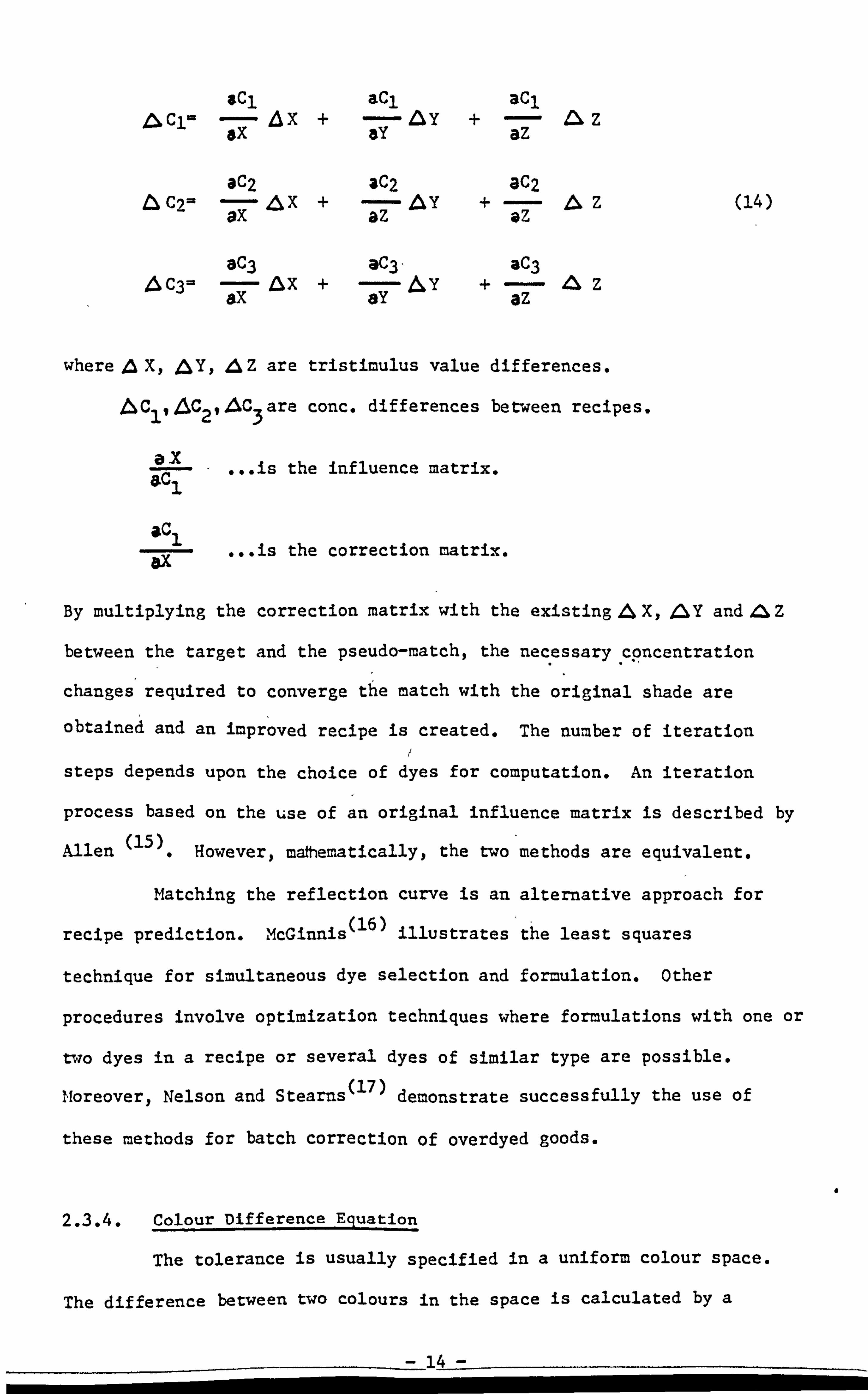
&CJ acl acl - äx + j26 Cl- - - zxy +- A-£ Z ;x x ay aZ
aC2 3C2 aC2 c, )= - j, x+ - -- y +-AZ ;x az az
i3C3 aC3' aC3 4 C3' - ax + '- -Y +- icb Z
ax ;y az
where, a X, Aý6Y, AZ are tristimulus value differences.
,&C1 "ý'C2 "46C3 are conc. differences between recipes.
a1, ois the influence matrix,
aci
ac ... is the correction matrix. ax
(14)
By multiplying the correction matrix with the existing A X, ASY andA: l Z
between the target and the pseudo-match, the necessary c9ncentration
changes required to converge the match with the original shade are
obtained and an improved recipe is created. The number of iteration
steps depends upon the choice of dyes for computation. An iteration
process based on the use of an original influence matrix is described by (15) Allen . However, mathematically, the two methods are equivalent.
Matching the reflection curve is an alternative approach for (16)
recipe prediction. McGinnis illustrates the least squares
technique for simultaneous dye selection and formulation. Other
procedures involve optimization techniques where formulations with one or
two dyes in a recipe or several dyes of similar type are possible.
Moreover, Nelson and Stearns(17) demonstrate successfully the use of
these methods for batch correction of overdyed goods.
a 2.3.4. Colour Difference Equation
The tolerance is usually specified in a uniform colour space.
The difference between two colours in the space is calculated by a
so-called colour difference equation. The difference is taken as a
measure of the magnitude of visual difference between them.
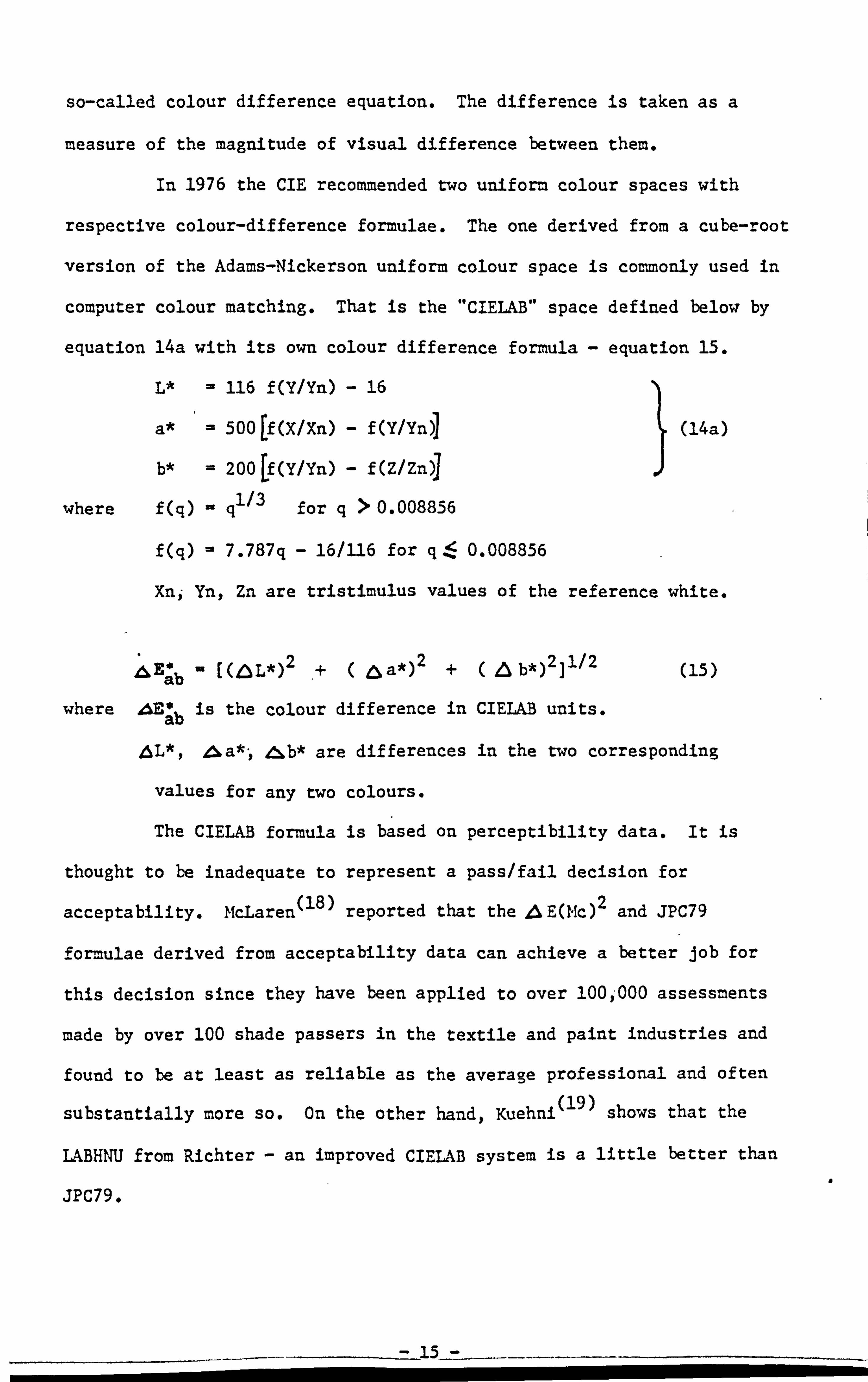
In 1976 the CIE recommended two uniform colour spaces with
respective colour-difference formulae. The one derived from a cube-root
version of the Adams-Nickerson uniform colour space is commonly used in
computer colour matching. That is the "CIELAB" space defined below by
equation 14a with its own co.
L* - 116 f(Y/Yn)
a* = 500[f(X/Xn)
b* = 200[f(Y/Yn)
where f(q) -q 1/3 for q
lour difference formula - equation 15.
- 16
- f(Y/Yn)] (14a)
- f(Z/Zn)]
> 0.008856
f(q) = 7.787q - 16/116 for q40.008856
Xn, - Yn, Zn are tristimulus values of the reference white.
&Ea*b ý E(6L*) 2 6a*)2 +(L b*)211/2 (15)
where AE * is the colour difference in CIELAB units. ab
, 6L*t &b* are differences in the two corresponding
values for any two colours.
The CIELAB formula is based on perceptibility data. It is
thought to be inadequate to represent a pass/fail decision for
acceptability. McLaren (18) reported that the & E(Mc)2 and JPC79
formulae derived from acceptability data can achieve a better job for
this decision since they have been applied to over 100p-000 assessments
made by over 100 shade passers in the textile and paint industries and
found to be at least as reliable as the average professional and often
substantially more so. On the other hand, Kuehni(19) shows that the
LABHNU from Richter - an improved CIELAB system is a little better than
JPC79. a
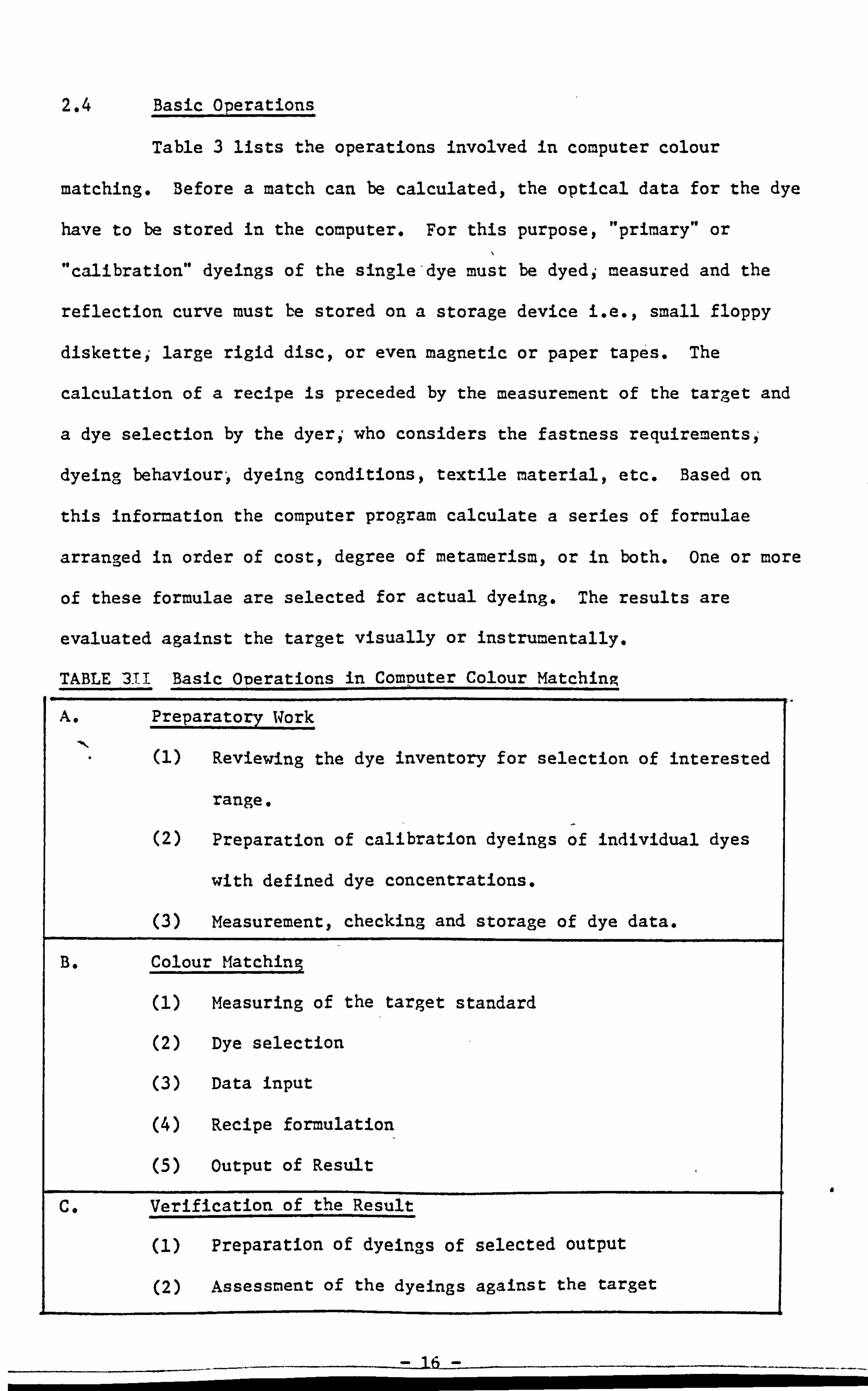
2.4 Basic Operations
Table 3 lists the operations involved in computer colour
matching. Before a match can be calculated, the optical data for the dye
have to be stored in the computer. For this purpose, "primary" or
calibration" dyeings of the single'dye must be dyedi measured and the
reflection curve must be stored on a storage device i. e., small floppy
diskette- large rigid disc, or even magnetic or paper tapes. The
calculation of a recipe is preceded by the measurement of the target and
a dye selection by the dyer; who considers the fastness requirements. -
dyeing behaviour- dyeing conditions, textile material, etc. Based on
this information the computer program calculate a series of formulae
arranged in order of cost, degree of metamerism, or in both. one or more
of these formulae are selected for actual dyeing. The results are
evaluated against the target visually or instrumentally.
TABLE 311 Basic ODerations in COMDUter Colour Matching
A. Preparatory Work
(1) Reviewing the dye inventory for selection of interested
range
(2) Preparation of calibration dyeings of individual dyes
with defined dye concentrations.
Measurement, checking and storage of dye data.
B. Colour Matching
(1) Measuring of the target standard
(2) Dye selection
(3) Data input
(4) Recipe formulation_
(5) Output of Result
C. Verification of the Result
(1) Preparation of dyeings of selected output
a
Assessment of the dyeings against the target
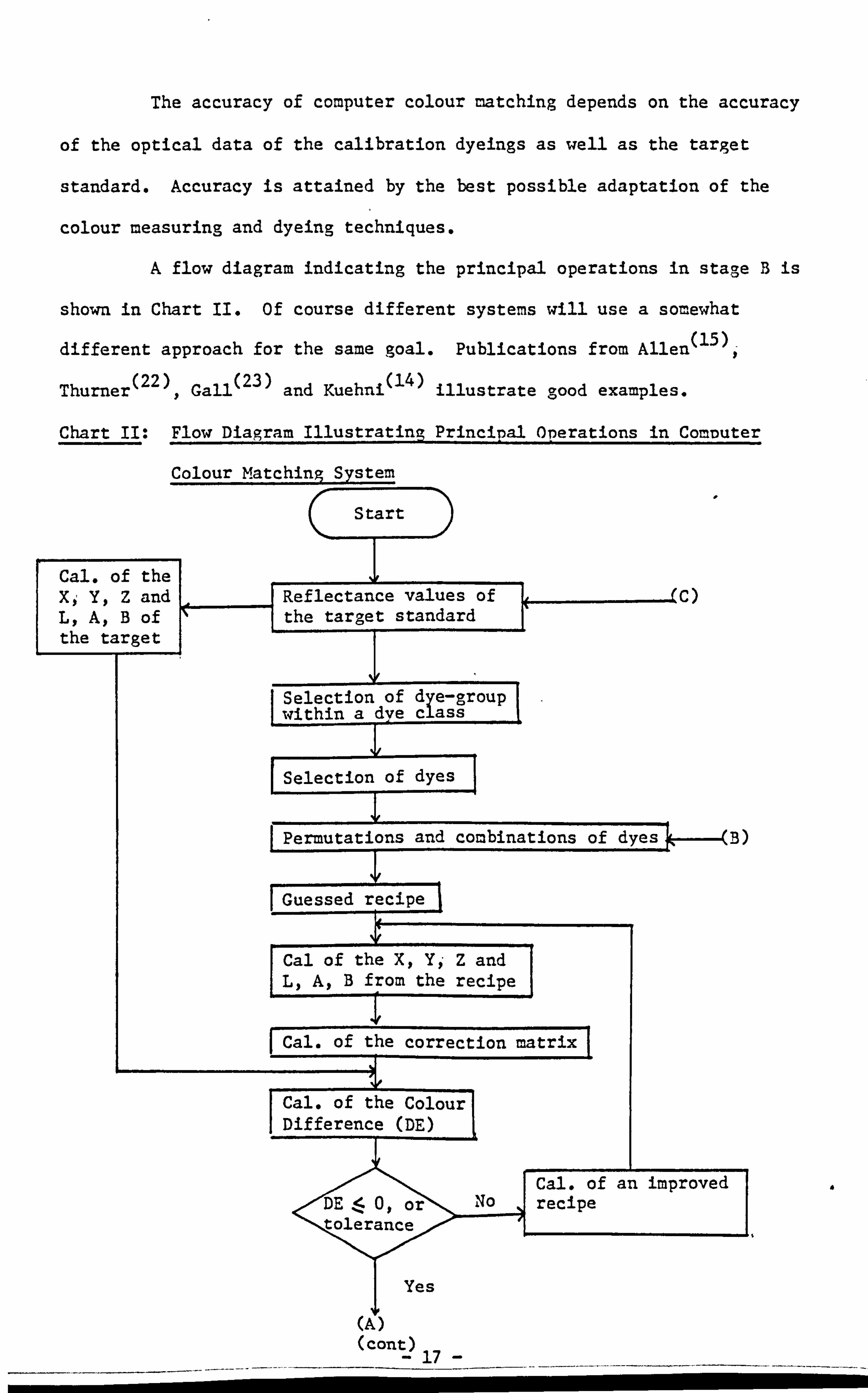
The accuracy of computer colour matching depends on the accuracy
of the optical data of the calibration dyeings as well as the target
standard. Accuracy is attained by the best possible adaptation of the
colour measuring and dyeing techniques.
A flow diagram indicating the principal operations in stage B is 0
shown in Chart II. Of course different systems will use a somewhat
different approach for the same goal. Publications from Allen(15)
(22) (23) and Kuehni (14)
0 Thurner , Gall illustrate aood examples.
Chart II: Flow Diagram Illustrating Principal Operations in COMDUter
Colour Matching System
Start
Cal. of the 1ý Xi Y, Z and Reflectance values 7f
L, A, B of the target standard the target I
Selection of d e-group within a dye class
I
I Selection of dyes I
I Permutations and combinations of dvesi
I Guessed recipe I
Cal of the X, Y)- Z and L, A, B from the recipe
I Cal. of the correction matrix I
Cal. of the Colour Difference (DE)
I
C)
B)
Cal. of an improved 0 No
, or 10 recipe , eranceýý
Yes
(A) (cont)
17

Chart II Conzýtinued
(A)
Cal. of the degree of source metamerism
Output of Recipe degree of metameri; m,
I
correction matrix
I
All --ý>
possible combinatio No
--., exhausted?
Yes
All get stanLdardr> No exhausteý?
Yes
Stop
-I^-

2.5 Problems
Over twenty years, computer colour matching -"a child of
industrial competition" - has reached maturity under increasing rather
than decreasing compe tition(20) . flost success has come in working with
solid colours and single fibres. Blends of fibresi fancy patterns,
unusual surfaced fabrics and a whole host of processing variables create
a lot of problems. Connelly (2) claimed that the biggest problem facing
computer colour formulation is the need to be able to react to radical
changes in conditions with the minimum expenditure of time and money.
For example; a governmental finding that a chemical used in dyeing is
harmful may devastate a dye file painstakingly compiled over a
considerable period of time if replacement of the chemical causes all of
the dyes to perform differently. In the short run, adjustments, can be
made. In the long run should we redye all the primaries? This is not.
always acceptable. Alternativelyi it is desired '- with a minimum of new
data describing the nature of the change; to correct the overall data.
Brockes' method (3)
of "test dyeing" might solve this problem to some
extent. Dyeing of fibre blends is the next serious problem. Moreover.,
fluorescence presents probably the most difficult problem for both theory
and practical application. This will be dealt with in next chapter.
a
Chapter III Computer Colour Matching Involving the Use of Fluorescent
DVes
3.1 An Introduction to the Measurement of Fluorescent Sample
The Fluorescence
Fluorescence is a well known phenomenon. It increases the
whiteness of a bleached fabric and provides a warning signal on
life-guard-clothing. It also attracts the attention of mothers for the
lovely brilliant light colour baby-wears. An over simplified definition
of fluorescence is that a molecule immediately releases its absorbed
radiation in the form of light at an other; longer wavelen, &,, th.
'The fundamental action of all dyes is the absorption of
radiation in some parts of the spectrum. The absorption of radiation is
a quantum effect. A photon from the incident radiation that is absorbed
transfers its energy to the molectile. This energy is used to raise an
electron from the gound state (energy level So in Fig 1) to an excited
state of energy (Sl). Only photons with an energy equal to the energy
difference -between S1 and So Can be used to cause the excitation to
Slo In fact each of the levels Sop' Sloe*,, which are called singlet
states.; is split up into different levels of'vibrational energy. While
the electron transition to an excited state always starts at the lowest
vibrational level of the ground state So; the upper level of the molecule
which is reached depends on the energy of the absorbed photon and
therefore on the wavelength (X) of the absorbed radiation; which is
inversely proportional to the photon energy E.
he
where h is the Planck's constant.
c is the velocity of light.
a
si
tý S..
So
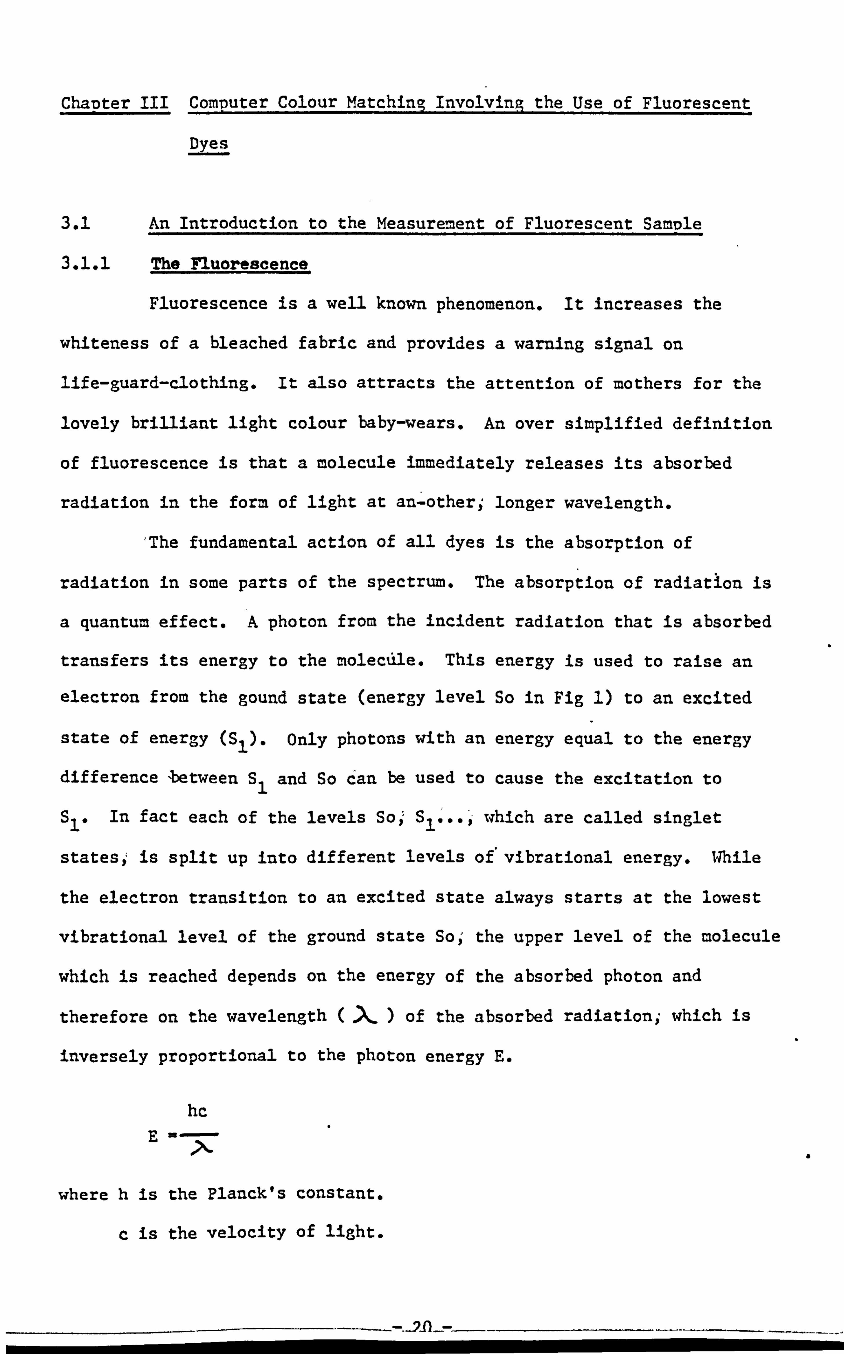
Fig. 1(41 ) Excitation and deactivation processes
Note: So, - Sl, Tl, ' are energy levels of the molecule.
A is absorption.
is fluorescence.
P is phosphorescence.
is thermal deactivation.
I is. interaction.
ril -
The absorption processes is'almost instantaneous and takes about
10-15 sec. The excited moleucle returns to the ground state So by
loosing its additional energy; and there are several possible ways: CD
thermal or chemical deactivation without light emittance, or
fluorescence; or phosphorescence. However deactivation of energy by
collision with other molecules to the lowest vibrational level of the
excited electronic stage occurs before these three concurrent processes.
In most dye molecules; the transition to T, is the'most
probable. Because the life time of the electron in the state T, is in
general quite long; the chance of interactions with neighboring molecules a
_21
in the fibre is high, whereby the excitation energy is lost as thermal
energy or in chemical reactions. In this case, only absorption of light
is observed.
In some moleculesi the electron from T, returns to the ground
state So either directly or via Sl; emitting the energy difference as
phosphorescence. On the other handi if the life time of the sin-let
state S1 is of the order of 10-9 to 10-3 sec. and no transition
occurs from Sl to Tl, the electron returns directly to one of the
vibrational levels of So, while the energy difference is emitted as
flourescence. Since the vibrational energy in So and S, disappears in
thermal collisions., the energy drop is in general smaller than the energy
absorbed; the emitted fluorescence possesses a longer wavelength than the
exciting one. Fluorescence is actually a simpler and quicker way back to
the ground state than the transition to T, and thermal or chemical
deactivation in non-fluorescent system.,
The amount of fluorescence emitted depends on the quantum
efficiency of the dye,: which is the ratio of the number of emitted
fluorescence quanta to the number of absorbed quanta. Since all these
deactivations within the molecule can be disturbed in several ways by
interaction with neighboring molecules of the same or of other chemical
structure, such, as tranfer of energy and reabsorption of fluorescence,
the quenching of flourescence occurs. However the interactions are
specific for a special molecule in a special surrounding.
In the course of this research- the system is confined to P
fluorescent disperse dyes on polyester goods. Fluorescent dyes means
that the dye absorbs and emits visible. light. The, emitted fluorescence
can result from the energy absorbed either in the visible or in the near
ultraviolet region. Fig. IA illustrates the absorption and emission
spectra of a classical fluorescent dye - Rhodamine. The overlapping
region of these two spectra is clearly showni that is the tail of the
22
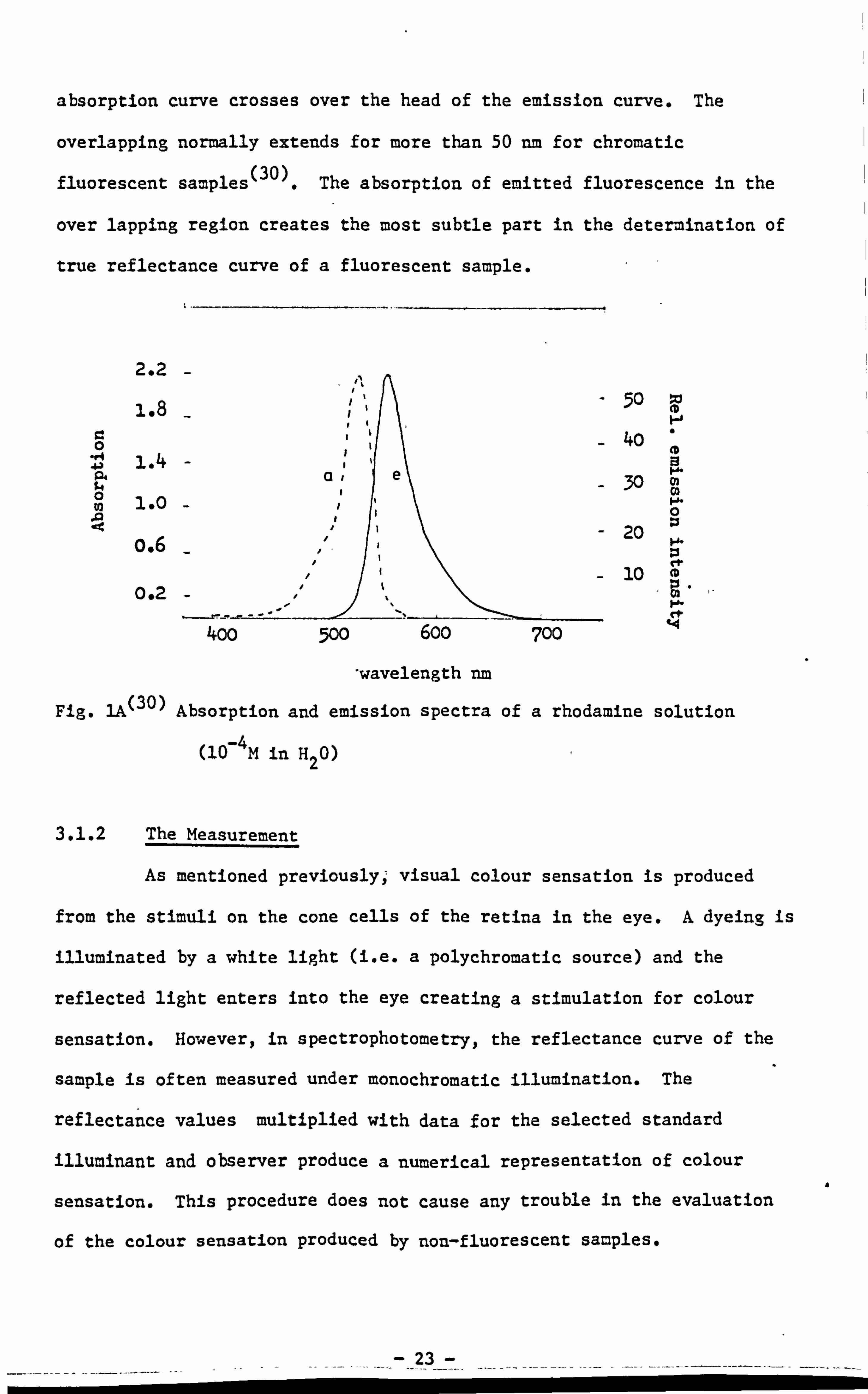
absorption curve crosses over the head of the emission curve. The
overlapping normally extends for more than 50 nm, for chromatic (30) fluorescent samples . The absorption of emitted fluorescence in the
over lapping region creates the most subtle part in the determination of
true reflectance curve of a fluorescent sample.
2.2
1.8
0 -0.4 -0 1.4 - p4 tt 0 1.0 -
o. 6
002
'wavelength rm
50
4o
30 m m
20
10
Fig. I. A(30) Absorption and emission spectra of a rhodamine solution
(10-4 M in H2 0)
3.1.2 The Measurement
As mentioned previously; visual colour sensation is produced
from the stimuli on the cone cells of the retina in the eye. A dyeing is
illuminated by a white light (i. e. a polychromatic source) and the
reflected light enters into the eye creating a stimulation for colour
sensation. However, in spectrophotometry, the reflectance curve of the
sample is often measured under monochromatic illumination. The
reflectance values multiplied with data for the selected standard
illuminant and observer produce a numerical representation of colour
sensation. This procedure does not cause any trouble in the evaluation
of the colour sensation produced by non-fluorescent samples*
a
- 23 -
400 500 600 700

Nevertheless it can produce enormous error for samples with fluorescent
properties. As the sample is illuminated by a monochromatic light in its
excitation region, a portion of the light is absorbed, the other is
reflected. Part of the absorbed energy will be emitted, usually at a
longer wavelength than the incident light. The mixture of the reflected
and emitted light is then measured by the detector as the reflectance
value at the wavelength of the monochromatic light. The reflectance
curve so obtained does not represent the actual values and leads to a
wrong colour sensation (i. e. CIE tristimulus values).
It is believed that the most simple and effective way to measure
fluorescent samplesshould correspond to the original mode of visiual
assessment. That is to illuminate the sample with polychromatic light.
The light emitted and/or reflected from the dyeing is analysed by the
monochromator for recording the reflectance curve. In this way-, the
correct reflectance curve i. e. total radiance factors curve A in Fig 1B)
as well as colour specification can be obtained instrumentally. Since
this arrangement does not produce a different curve for non-fluorescent
samples, it is commonly accepted for building up modern colourimetric
instruments.
3.2 A Suitable Light Source for Measurement
North sky daylight in the Northern Hemisphere and the South for
the Southern one are commonly refered as the standard light-sources for
colour assessment. Because, they are not always availablei standard
illuminants have been recommended by the C. I. E. for general use in colour
evaluation. Standard sources have been manufactured namely A, B and C.
and commonly used for colour investigations. With the wide spread of the
use of fluorescent whitening agents; the ultra-violet content of a
-24-
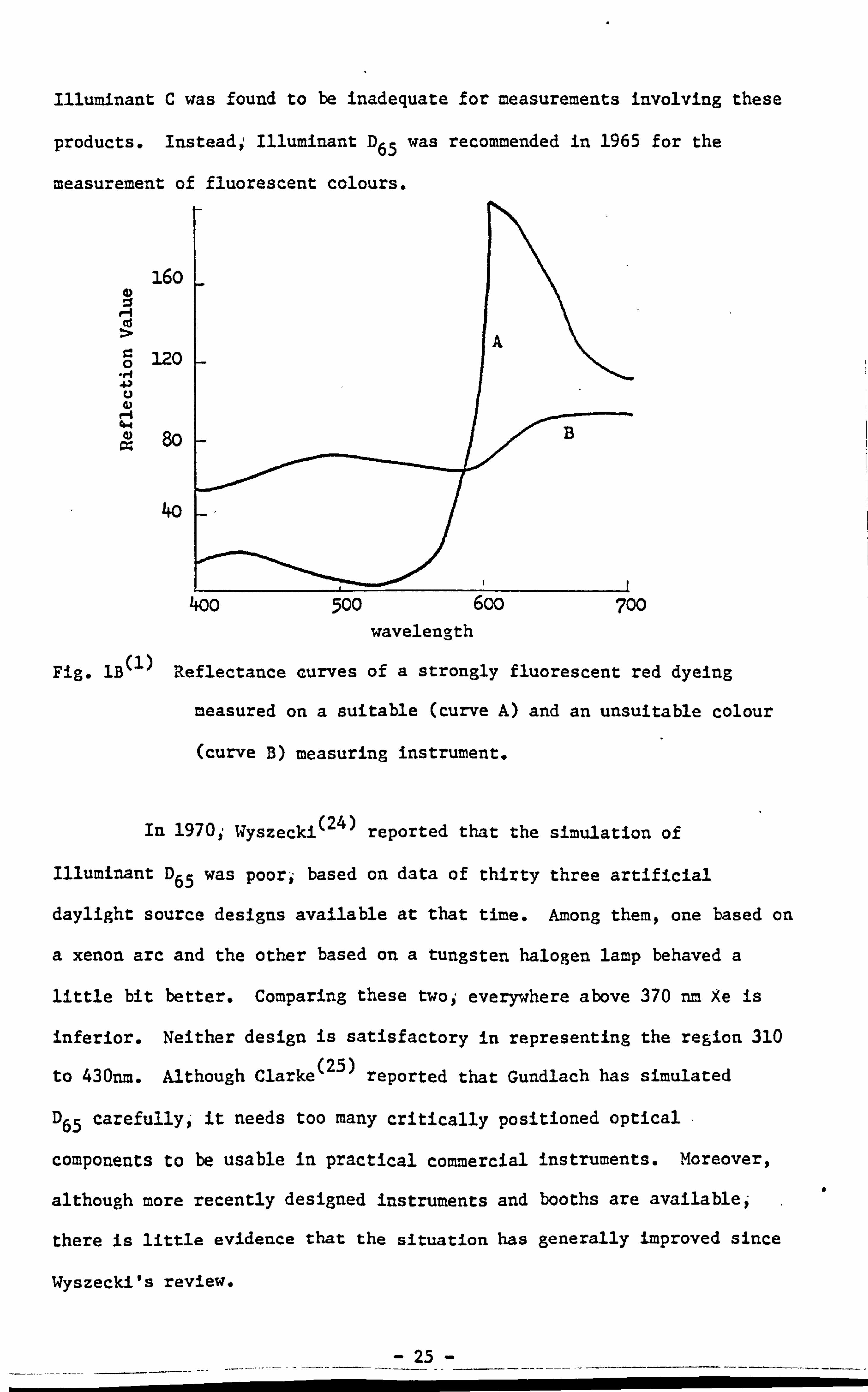
Illuminant C was found to be inadequate for measurements involving these
products. Instead,, Illuminant D65 was recommended in 1965 for the
measurement of fluorescent colours.
160 0
r-I cd
120
80
40
wavelength
Fig. 1B(l) Reflectance curves of a strongly fluorescent red dyeing
measured on a suitable (curve A) and an unsuitable colour
(curve B) measuring instrument.
In 1970; Wyszecki(24) reported that the simulation of
Illuminant D65 was poorý based on data of thirty three artificial
daylight source designs available at that time. Among them, one based on
a xenon arc and the other based on a tungsten halogen lamp behaved a
little bit better. Comparing these twoi everywhere above 370 nm Xe is
inferior. Neither design is satisfactory in representing the region 310
to 430nm. Although Clarke (25)
reported that Gundlach has simulated
D 65 carefully,, it needs too many critically positioned optical ,
components to be usable in practical commercial instruments. Moreover,
although more recently designed instruments and booths are available,
there is little evidence that the situation has generally improved since
Wyszecki's review.
25-7
4oo 500 6oo 700

Since Illuminant D 65 is not available physically; can any one
of the available artificial sources be selected as the standard source
for colour assessment? The answer is no., because real daylight is still
often used for final assessment. Neverthelessi Clarke (25) proposed an
interior daylight ID65 in the 19th session of CIE in Japan. This
illuminant represents an exterior daylight (i. e. D65) attenuated by
average window glass. That is the daylight source which most commonly
occurs in the viewing of critically coloured merchandise, and which can
be practically simulated using a filtered tungsten'halogen source. In
addition, Clarke and McKinnon(26) demonstrate that Illuminant C is a
satisfactory substitute for D65 in the measurement of fluorescent
safety and'signa1colours and so probably is the ID 65*
In'the measurement of fluorescent colours, the emitted radiation
depends on the energy destribution of the incident light in the
excitation region of the colourant. Different laboratories are'using
different D 65 simulations and so give inconsistant colour specification
for the same sample. However, fortunately, a small change in intensity
of a source has little or no effect on the measurement provided that the
variation of intensity does not produce changes in the spectral energy
distribution of the light source and can still supply enough energy to
complete the absorption process. This means an appropriate and well
controlled light source is the most important requirement for making (30)
accurate measurement of fluorescent colours
Finally, i the spread of the three-band daylight'fluorescent
tubes(28) (e. g. TL84 and Ultralume) might create another problem in
metamerism. The new phosphors used absorb long wave ultraviolet
radiation much more strongly than conventional ones. The emitted
radiation contains less ultraviolet in the 320-360 = region which is the 0
excitation region for most whiteners. Therefore the degree of whiteness
is impaired for whitened goods under such a source, and probably the same
will happen for fluorescent dyes due to the lack of availability of
energy at the region of excitation.
3.3 The Measurement Techniques
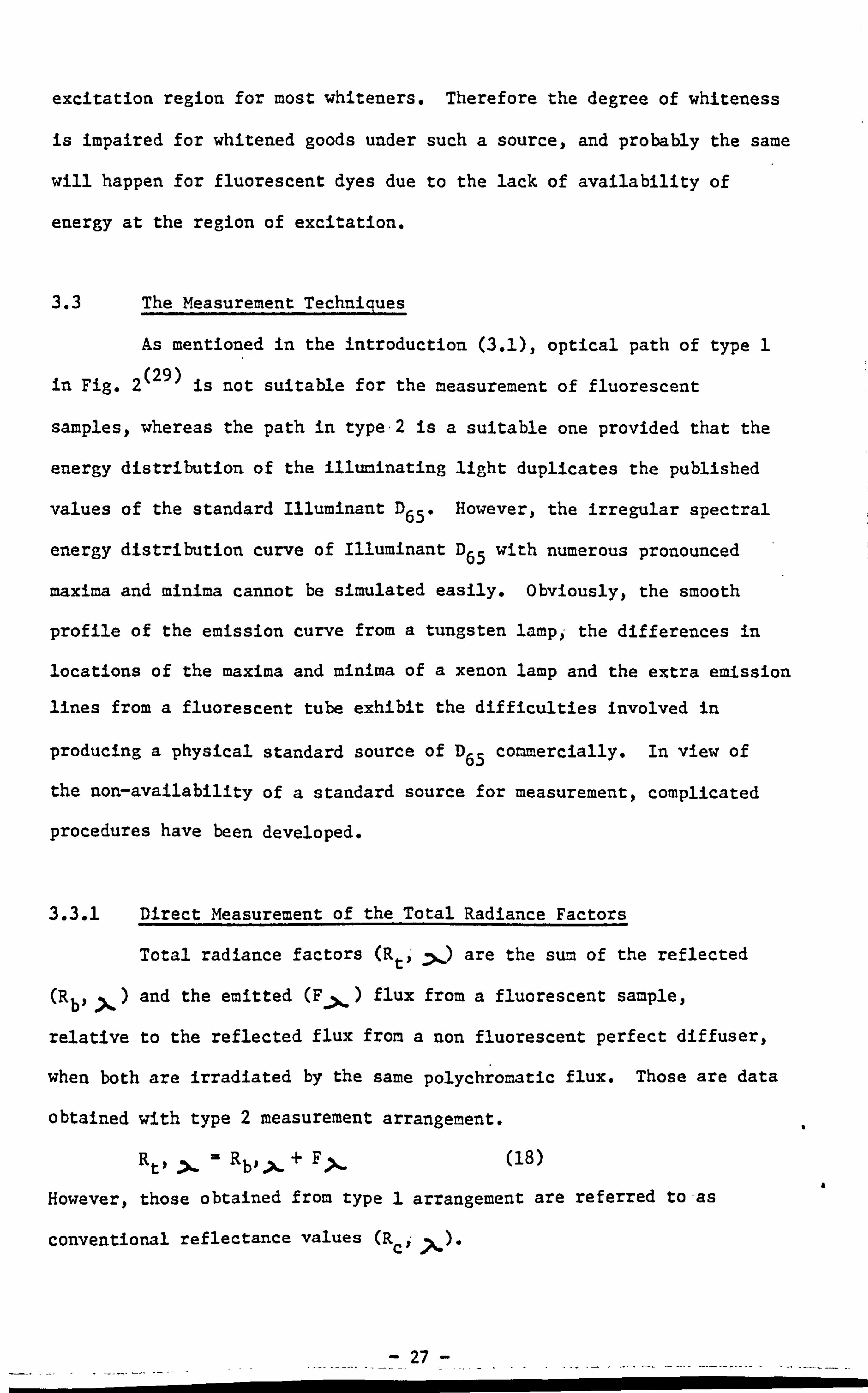
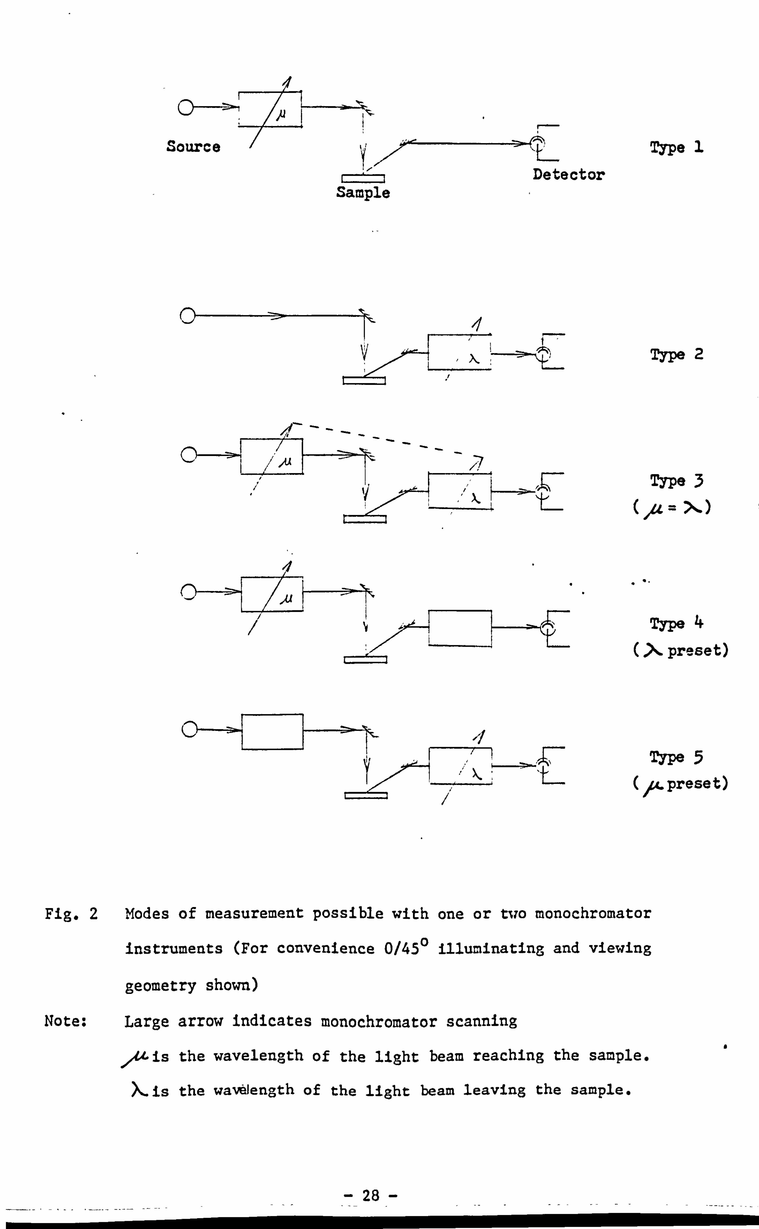
As mentioned in the introduction (3.1), optical path of type 1
in Fig. 2 (29) is not suitable for the measurement of fluorescent
samples, whereas the path in type-2 is a suitable one provided that the
energy distribution of the illuminating light duplicates the published
values of the standard Illuminant D65* However, the irregular spectral
energy distribution curve of Illuminant D 65 with numerous pronounced
maxima and minima cannot be simulated easily. Obviously, the smooth
profile of the emission curve from a tungsten lampi the differences in
locations of the maxima and minima of a xenon lamp and the extra emission
lines from a fluorescent tube exhibit the difficulties involved in
producing a physical standard source of D 65 commercially. In view of
the non-availability of a standard source for measurement, complicated
procedures have been developed.
3.3.1 Direct Measurement of the Total Radiance Factors
Total radiance factors (Rt. ' _->,
) are the sum of the reflected
(R bI X) and the emitted (F> ) flux from a fluorescent sample,
relative to the reflected flux from a non fluorescent perfect diffuser,
when both are irradiated by the same polychromatic flux. Those are data
obtained with type 2 measurement arrangement.
Rty >' RbIX + Fx
However, those obtained from type 1 arrangement are referred to-as
conventional reflectance values (R Ci X).
I
a
27
)U
Source Type 1 Detector
Sample
Type 2
Type 3
Type 4
>-.. preset)
TYPe 5
/A. preset)
Fig. 2 1114odes of measurement possible with one or two monochromator
instruments (For convenience 0/450 illuminating and viewing
geometry shown)
Note: Large arrow indicates monochromator scanning
/4is the wavelength of the light beam reaching the sample.
>, is the wavelength of the light beam leaving the sample.
28

A standardized and well controlled D 65 simulator has to be-
used to shine on the sample directly before passing through the
monochromator. The light leaving the sample surface is analysed by
monochromator-detector units. The result is interpretted as the total
spectral radiance factors, - and is commonly accompanied by Xj Y and Z
tristimulus values; L, A, B and/or other colorimetri. c data.
Alman and Billmeyer (31) recommend using the 450/0 or 0/450
illuminating and viewing geometry for measurement of fluorescent samples.
Howevev; measurement errors resulting from the surface texture of the
sample, and also, possibily the partial polarization of the incident
light generally compensate the merits obtained with such geometry.
Therefore the use of integrating sphere spectroflu6rimeters or
colorimeters is widespread for measurement of non-fluorescent as well as
fluorescent samples. Nevertheless Grum(30) reported that Chong and
Billmeyer showed the average, & E for fluorescent samples measured on four
different instruments with D 65 simulators and integrating spheres is
quite large when compared with those for non-fluorescent samples (i. e.
4.1 to 1.3 CIELAB unit). This variability among instruments can be
attributed to the following factors:
(1) Differences in the simulation of D65*
(2) Lack of control of the source's power supplies.
(3) Differences in the integrating-sphere efficiency.
(4) Differences, - although minor; in instrument illuminating and
viewing geometry.
On the other hand ,, the chromaticity coordinates determined from total
radiance factors and those determined more accurately from a method of
combination of components (Rb'ý'. X. +F>. ) are nearly indentical (32) 0
Fig. 3 furnishes this impression. Direct measurement of the total
radiance factors thus provides a rapid and easy means of generating
29

essential colorimetric information for fluorescent dyes. Nevertheless
the colour specification is limited to the measuring illuminant.
I Green sample
.6
"1 y
Fig.
.2
0- 65 Red sample C3 a
Magenta sample
0-3 o. 4 x 0-5 o. 6
CIE diagram with chromatic samples for D65 Illuminant
0 from total radiance factor measurement Rto
0 from conventional measurement R ce
, 0, f rom Rt+R b*
3.3.2 Measurements with Two Monochromators
Judd. and Wyszecki(9) reported that Donaldson employed a
spectrofluorimeter and carried out a series of scans with the second
monochromator (Fig. 2, Type 5) with the wavelength of the first
monochromator preset at intervals to cover the whole of the-excitation
and visible regions of the spectrum. Actually this method presents a
full picture to illustrate the spectral distribution of-light leaving the
surface and may be considered as the ultimate and most complete way of
analysing a fluorescent sample spectrophotometrically. once the analysis
has been done, the tristimulus values can readily be calculated for any
given source illuminating the sample. Donaldson's approach is sound;
however the procedure is very elaborate and difficult to follow on a
routine basis. a
30
Ways have been investigated to reduce the volume of work
involved in the Donaldson's method. Grum (32i 33) proposes a method to
obtain the total radiance factors by combination of the true reflected
value and the emitted fluorescent value as indicated in equation 18. It
involves the use of several modes of measurement (i. e. type 3 to type 5
in Fig. 2) to obtain the excitation; the emission as well as the
reflectance spectra. Clarke(29) in the National Physical Laboratory
introduced a similar procedure to calculate the tristimnulus values of
fluorescent samples. Minato et. al, (34) determined the fluorescent
emission in the overlapping region by interpolation on the basis of a few
measurements of the fluorescent sample with changing the wavelength
setting in the analysing second monochromator. Neverthless the
complexity and general unavailability of the instru-! ýments used for the
abovementioned methods prevent their use as a standard instrument in
common laboratories. However they are expected to be the reference
methods for checking the simpler one-monochromator and other abridged
methods.
3.3.3 One-monochromator and Abridged Methods
The separation of true reflectance and true fluorescence is
tedious with the two-monochromator method. Grum (30) reported that
Eitle and Ganzi and also Allen introduced the use of filters to eliminate
the neccessity for the second analysing monochromator. On the other hand
Simon (35) demonstrates a simpler two modes method with a one
monochromator instrumentp where the sample is first measured under
monochromatic illumination and then measured under polychromatic light- I
preferably with the same light source and photodectector exchanged from
the forward to the reverse optics arrangement. Furthermore CIE Technical
Committee 2.3 (27,30) establishes a procedure to calculate values of
total spectral radiance factors under standard illuminants from
a
31
measurements made under a slightly dissimilar illuminant. In the other
word, the tristimulus values of a fluorescent sample under CIE standard
Illuminant D65 can be calculated from measurements under a D65
simulator. The recommanded procedure is a modification of the method of
Eitle and Ganz; derived by Alman and Billmeyer. It involves the use of a
one-monochromator instrui-ment equipped with an integrating sphere and
with provision for two modes measurement (i. e. monochromatic and
polychromatic illuminations); and also employs a spectroradiometer to
determine the spectral energy distribution of the illuminating system
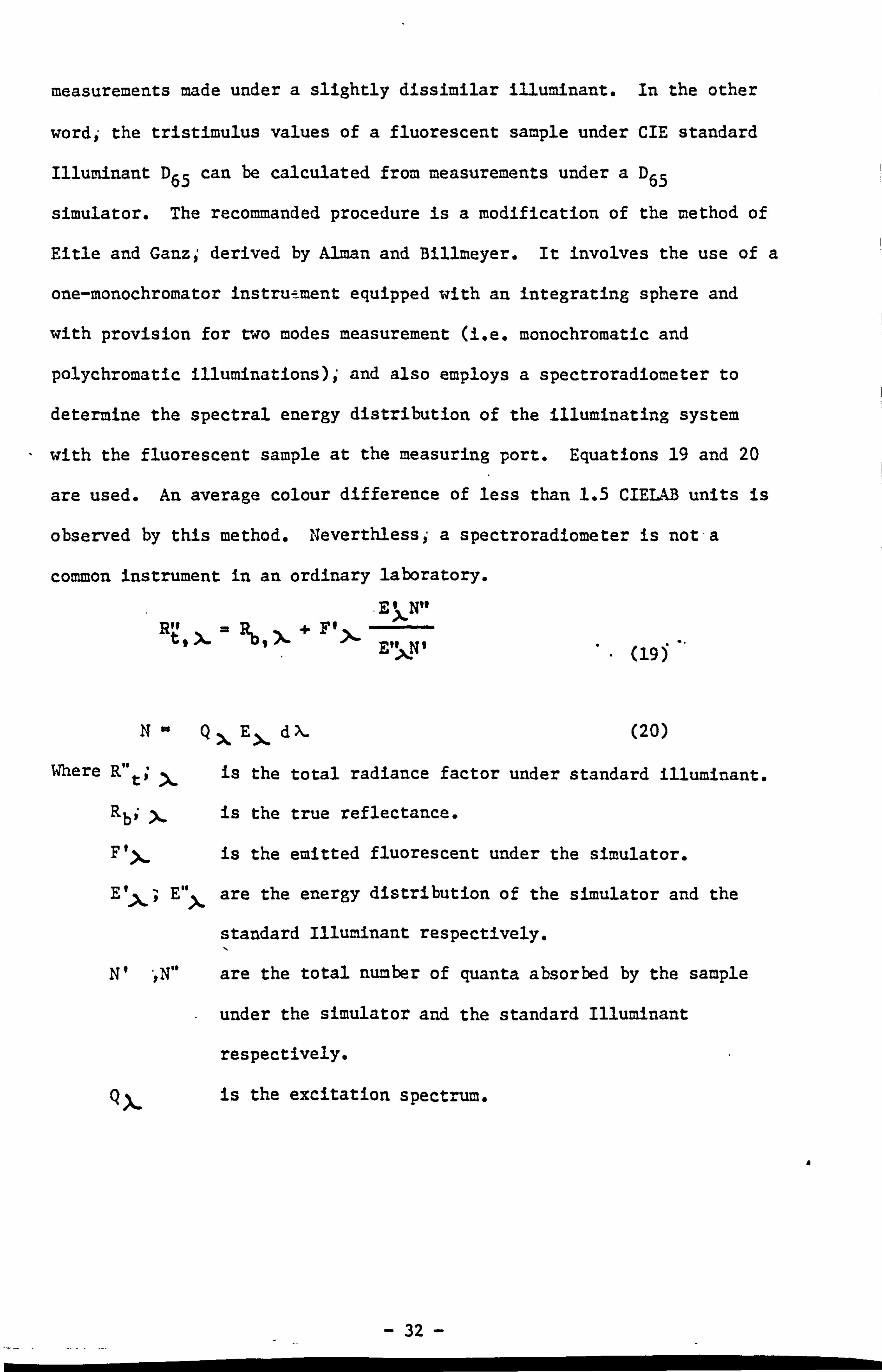
with the fluorescent sample at the measuring port. Equations 19 and 20
are used. An average colour difference of less than 1.5 CIELAB units is
observed by this method. Neverthless; a spectroradiometer is not, a
common instrument in an ordinary laboratory.
R" = Rb , )ý. + Ff tt >. - >- Et! QN1 (10
NQ%E >ý d X. (20)
Where R"t; is the total radiance factor under standard illuminant.
Rb; >- is the true reflectance.
FIN- is the emitted fluorescent under the simulator.
E', X.; E'*. >- are the energy distribution of the simulator and the
standard Illuminant respectively. I
N' YN" are the total number of quanta absorbed by the sample
under the simulator and the standard Illuminant
respectively.
is the excitation spectr=,
a
32
3.4 Matching Involving the Use of Fluorescent Dyes
3.4.1 State of the Art
Fluorescent dyes ýave gained considerable importance because
they extend appreciably the gamut of colours. More recentlyý (2) Connelly reports that an unexpectedly large amount of problem shades
is mainly due to fluorescence in his computer colour matching excerise.
Generally the Kubelka and Munk type calculations are not able to handle
the spectral radiance factors curve. This is because the emitted light
of fluorescent dyes is not linearly related to the dye concentration.
For most of the common available commercial colour formulation packages,
the emitted light is generally neglected. The usually way is to limit
the spectral radiance factors of samples and calibration dyeings to the (36)
corresponding values of the substrate . In this case fluorescence
has been pressed into the frame work of the simple Kubelka-Munk formula.
In the other words-, irrespective of fluorescen(A all matches are based on
the factors of absorption and of scattering only. Matches of fluorescent
samples with the same dyes may be satisfactorily computed by this
method. However, it is possible to get apparently acceptable
formulations with non-fluorescent dyes) but not matching the fluorescent
sample at all. This also applies if the calculation of dye formulations
is based on the true reflectance curve as suggested by Simon (35) in his
two modes method. Following are methods developed to give better
handling of recipe prediction involving the use of fluorescent dyes.
3.4.2 Ganz's Approach
The common computer colour matching program. 2 usually employ the
simple Kubelka and Munk equation for textile industries. If fluorescent
samples are involved, a possible confusion will be obtained for the
values of the reflectance and emission curve over 100%. Table 4
illustrates this problem e. g. values of 120% and 83.33% give the same
(K/S) values.
33
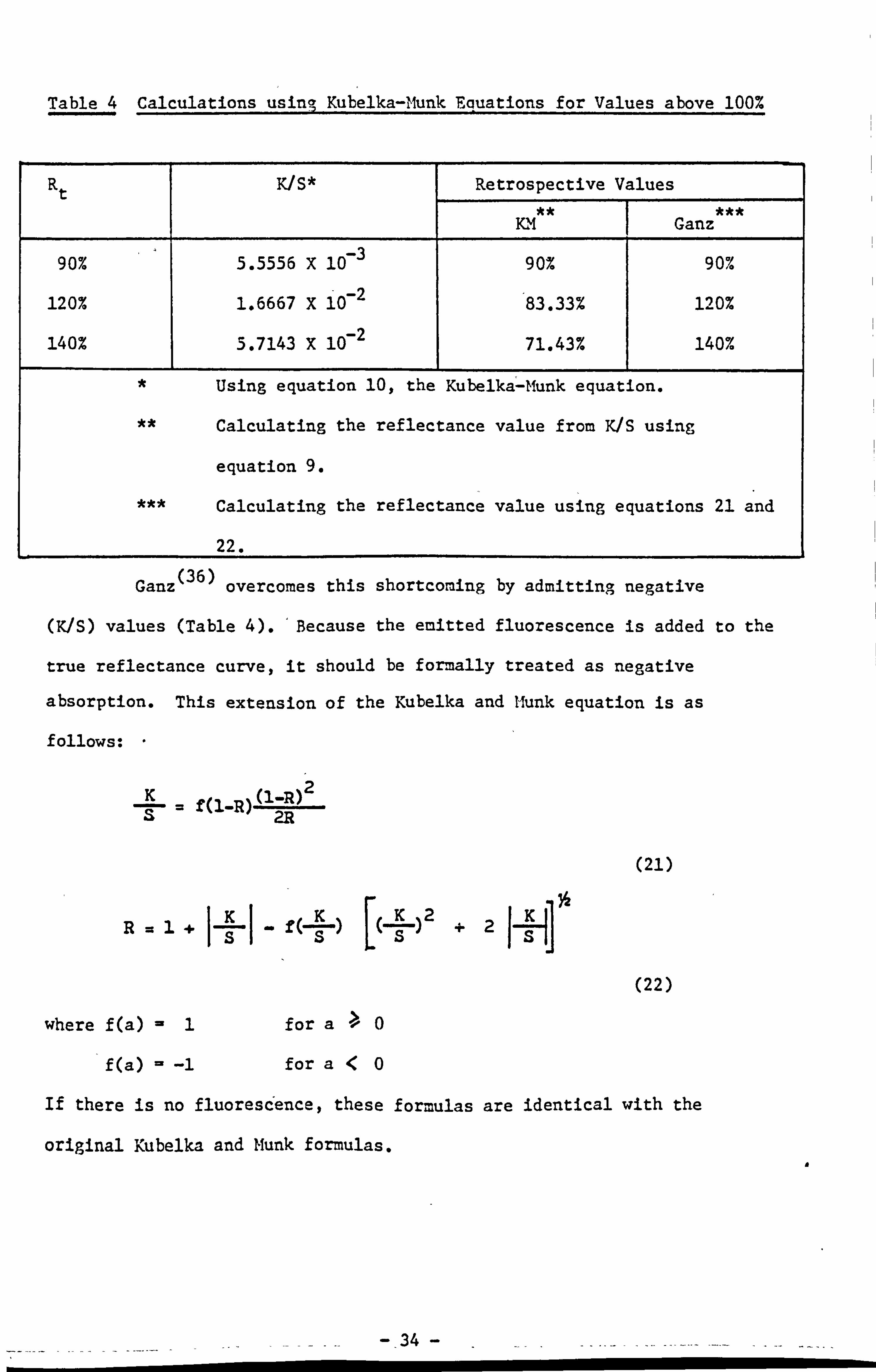
Table 4 Calculations using Kubelka-Munk Equations for Values above 100%
Rt K/S* Retrospective Values
KM. Ganz
90% 5.5556 X 10⁻³ 90% 90%
120% 1.6667 X 10⁻² 83.33% 120%
140% 5.7143 X 10⁻² 71.43% 140%
Using equation 10, the Kubelkaý-Ifunk equation.
Calculating the reflectance value from K/S using
equation 9.
Calculating the reflectance value using equations 21 and
22.
Ganz (36) overcomes this shortcoming by admitting negative
(K/S) values (Table 4). 'Because the emitted fluorescence is added to the
true reflectance curve, it should be formally treated as negative
absorption. This extension of the Kubelka and Munk equation is as
f ollows: -
f(l-R)(1-R) 2R
(21)
J_K 36
_: r(K -. L)2
Sd] R+sss+2s
(22)
where f(a) 1 for a0
f(a) - -1 for a<0
If there is no fluorescence, these formulas are identical with the
original Kubelka and Munk formulas. a
--34
As metioned previously; the total radiance factors under CIE
standard Illuminant can be predicted quite accurately from measurement
under a simulated arbitary light source. With the introduction of the
Ganz's extension (i. e. equations 21 and 22); calculating formulae for
fluorescent samples seams to be feasible. The method can be accurate for
colours produced with one fluoresscent dye alone. Good approximations
are obtained for formulations with a fluorescent dye shaded slightly by
one or more nonfluorescent or fluorescent dyes. With larger admixturesi
too low a concentration of the fluorescent dye is determined. This
happens since no account is taken of the absorption of illuminated energy
by the admixed dyes; which reduces the share of energy available for th;
excitation of fluorescence. The principal advantage of the Ganz's
extension is that fluorescent samples are not matched with nonfluorescent (36) dyes and vice-versa
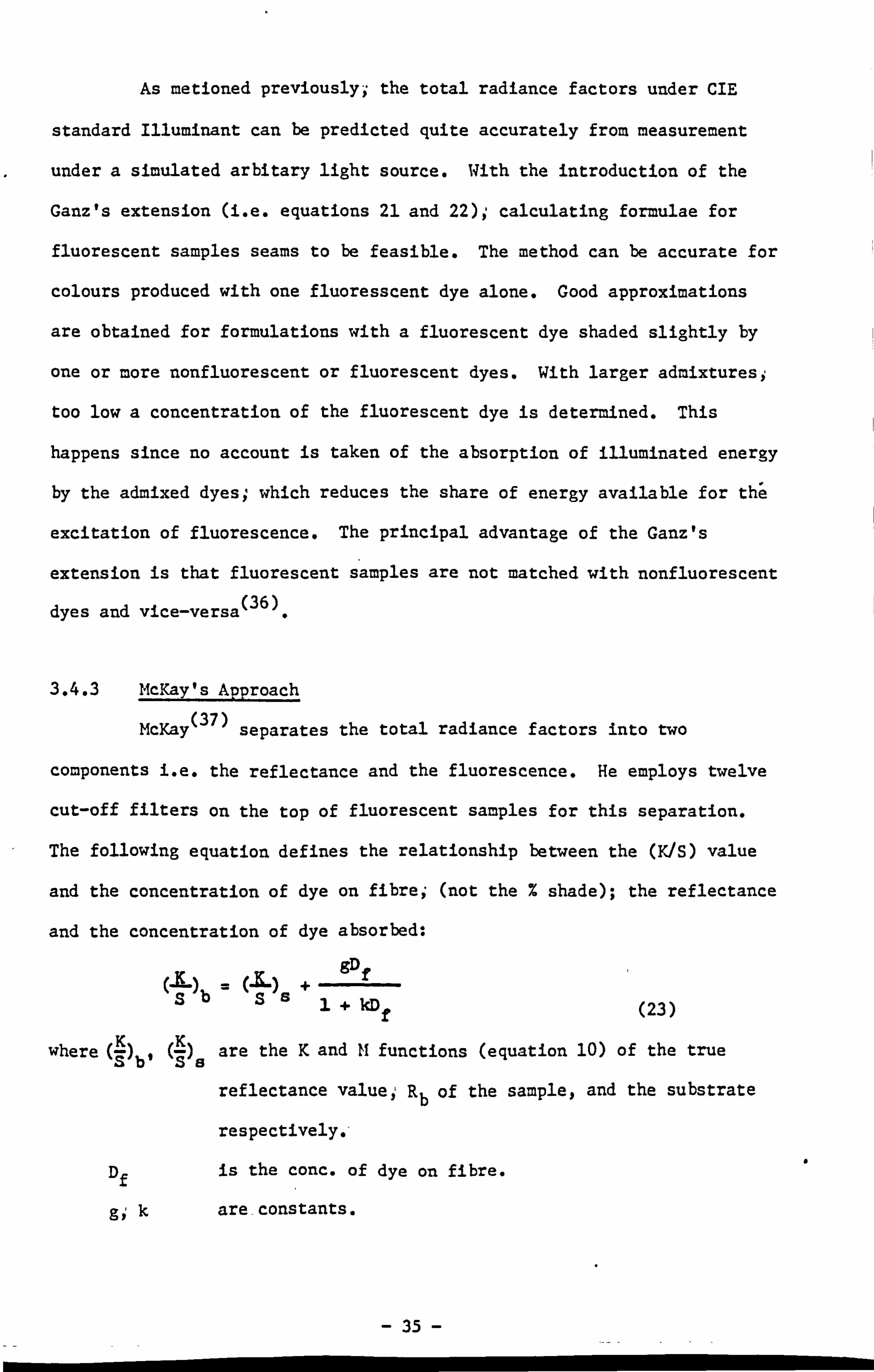
3.4.3 McKay's Approach
McKay (37)
separates the total radiance factors into two
components i. e. the reflectance and the fluorescence. He employs twelve
cut-off filters on the top of fluorescent samples for this separation.
The following equation defines the relationship between the (K/S) value
and the concentration of dye on fibre; (not the % shade); the reflectance
and the concentration of dye absorbed:
(JL) gD f
SbS1+ kD f (23)
where (-K) (. K), 3 are the K and 11 functions (equation 10) of the true S b' S
reflectance value, ' Rb Of the sample, and the substrate
respectively. -
Df is the conc. of dye on fibre.
are-constants.
- 35 -
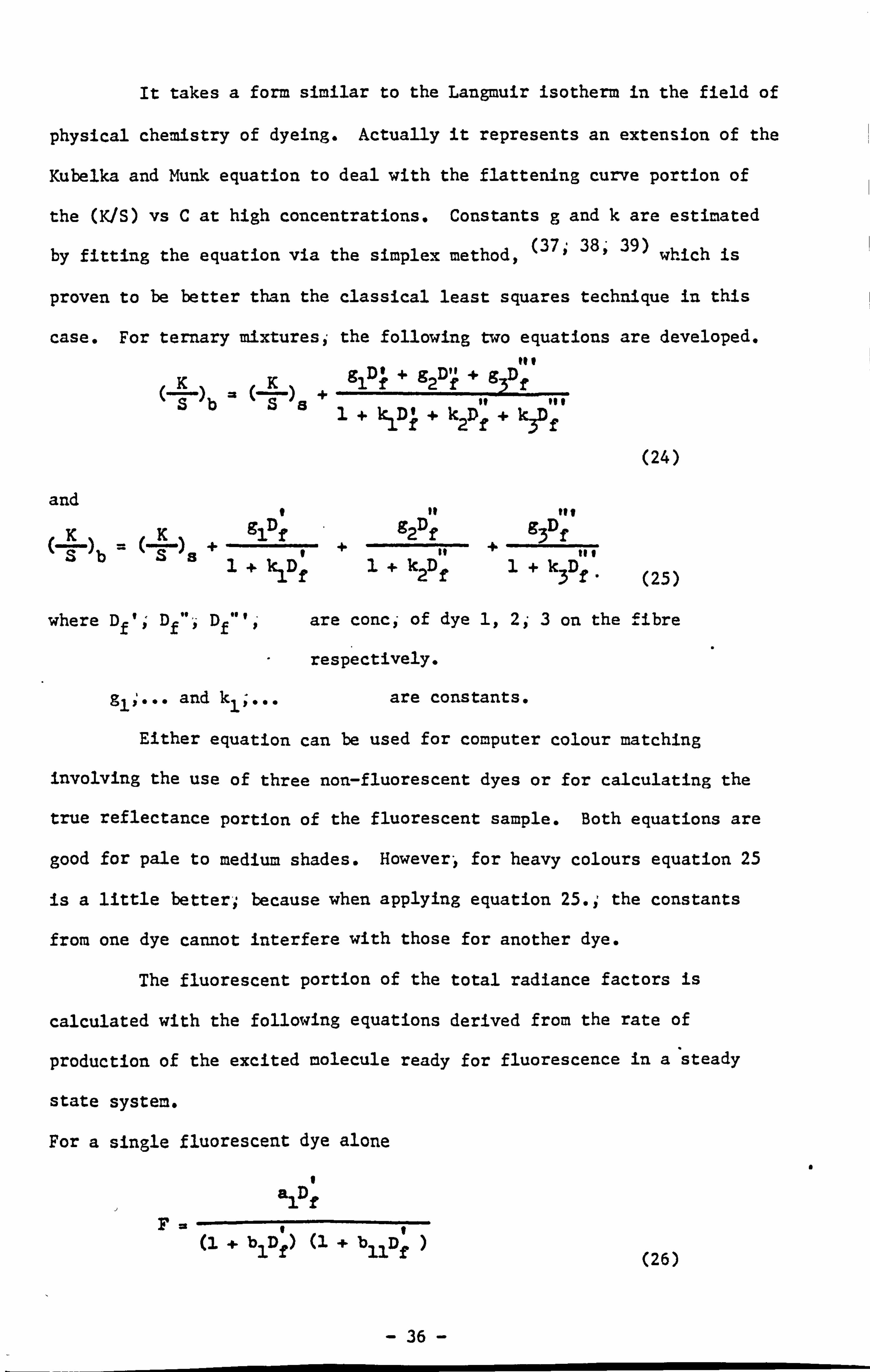
It takes a form similar to the Langmuir isotherm in the field of
physical chemistry of dyeing. Actually it represents an extension of the
Kubelka and Munk equation to deal with the flattening curve portion of
the (K/S) vs C at high concentrations. Constants g and k are estimated
by fitting the equation via the simplex method, (37; 383- 39)
which is
proven to be better than the classical least squares technique in this
case. For ternary mixturesi the following two equations are developed. fit
g D' +9 D" +gD ), ()+
off SbS1+ k1D If +k D" + Ic T' 2f f
(24)
and I it I# I
+ g2 Df
+ 9? f
Sbs8 of III 1+ kDf 1+ kpf 1+ k3Df (25)
where Df'; Df", i Df"vp - are concs of dye 1,2p 3 on the fibre
respectively.
gl;... and kl;,,. are constants,
Either equation can be used for computer colour matching
involving the use of three non-fluorescent dyes or for calculating the
true reflectance portion of the fluorescent sample. Both equations are
good for pale to medium shades. However-y for heavy colours equation 25
is a little better; because when applying equation 25.; the constants
from one dye cannot interfere with those for another dye.
The fluorescent portion of the total radiance factors is
calculated with the following equations derived from the rate of
production of the excited molecule ready for fluorescence in a steady
state system.
For a single fluorescent dye alone
I a1Df
I) (1 + bl, D; (1 b1p f (26)
a
- 36 -
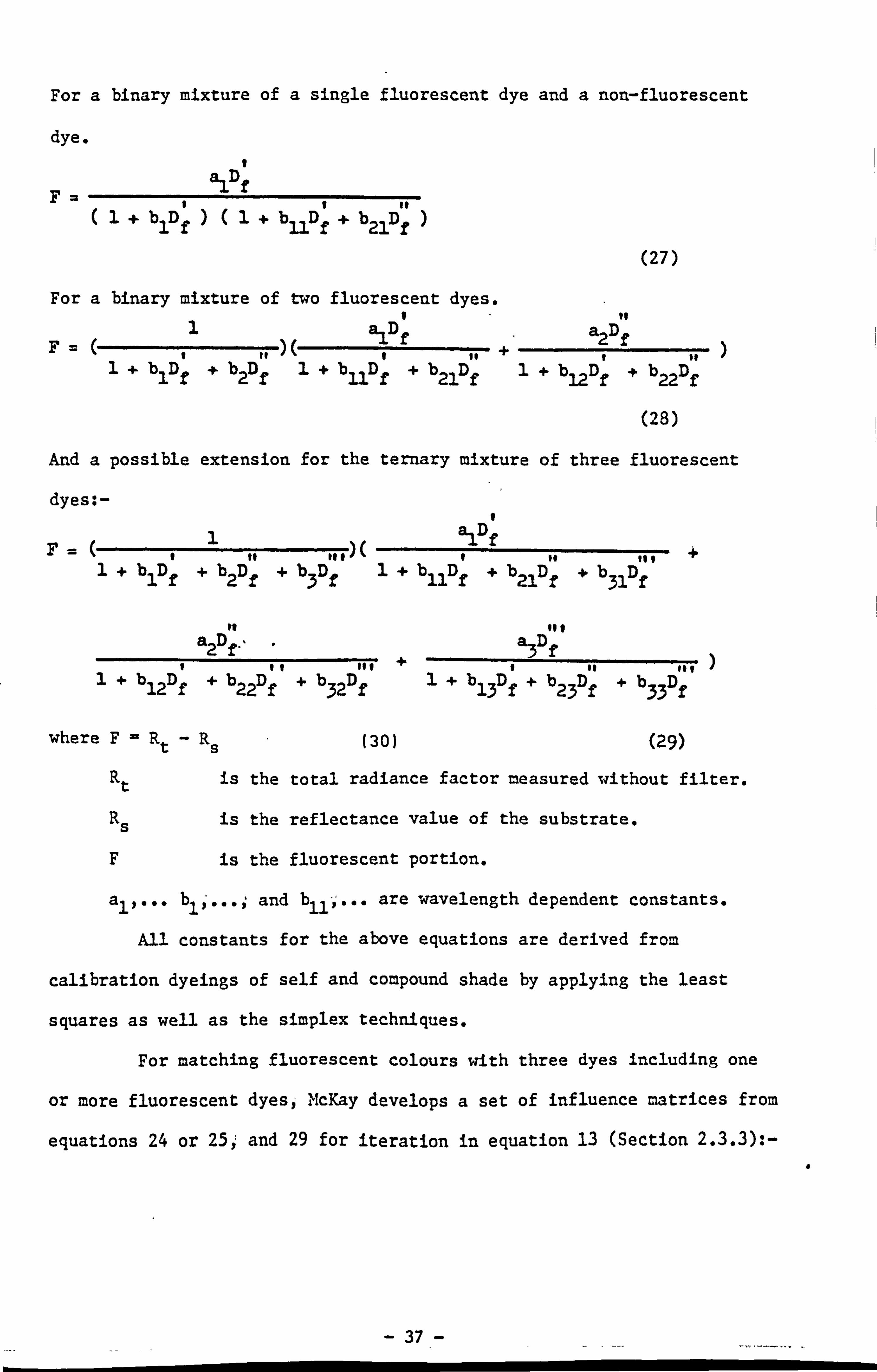
For a binary mixture of a single fluorescent dye and a non-fluorescent
dye.
F ajD f
1+ b1p; 1+ bllpf' +b 2lPf (27)
For a binary mixture of two fluorescent dyes.
n F "i"f
+ a2Df
1+bD+bD1+bDI+b, D1+bDI+b, D 1f2f 11 f 21 f 12 f 22 f
(28)
And a possible extension for the ternary mixture of three fluorescent
dyes: - I
r. (1 ajDf
I ft of t)(I of to I-+ 1+b1Df +b 2Df +b 3Df1+b 11 Df +b Of +b 3, Df
2Df, lot +I
a3D f
1+b 12 Df + b22Df +b 32Df 1+b 13 Df+ b23 Df+b 33 Df
where F-Rt-Rs (30) (29)
Rt is the total radiance factor measured without filter.
Rs is the reflectance value of the substrate.
F is the fluorescent portion.
a,,... bl, ... ; and b 11 ; ... are wavelength dependent constants.
All constants for the above equations are derived from
calibration dyeings of self and compound shade by applying the least
squares as well as the simplex techniques.
For matching fluorescent colours with three dyes including one
or more fluorescent dyes, McKay develops a set of influence matrices from
equations 24 or 25; and 29 for iteration in equation 13 (Section 2.3.3): -
37-
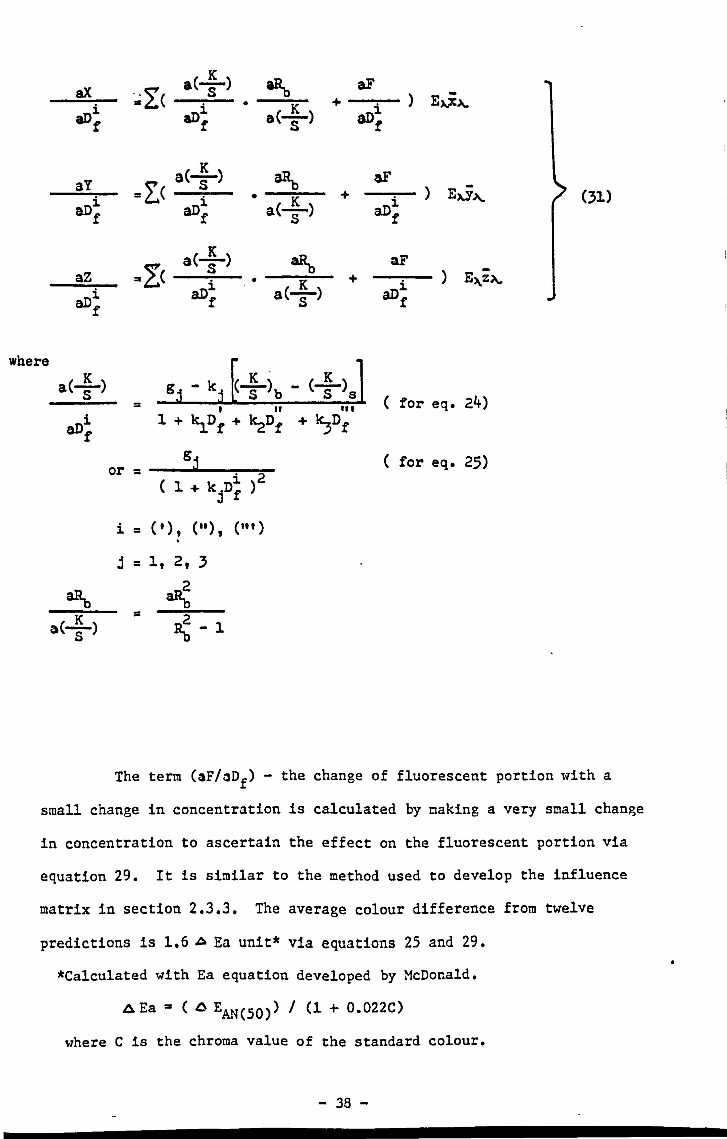
a( 3, ) aF ax s 81% + Exx>,
aD aDl OD I fsf
a( I) aR *F ay. s b- + Exjk &Dl aD
3. a( ') aLDi ffsf
a aR b aF a =Z( Ekz-k z
I aD a(K aD aD ffsf
where KK
b s] for eq. 24)
aD 1+ kDf + k2D f+ k3D f f
or 92 for eq. 25)
1+kiDf)
1 (11) (fit
j 11 2,3
2 aRb
-a% K2
(31)
The term (aF/*D f)- the change of fluorescent portion with a
small change in concentration is calculated by making a very small change
in concentration to ascertain the effect on the fluorescent portion via
equation 29. It is similar to the method used to develop the influence
matrix in section 2.3.3. The average colour difference from twelve
predictions is 1.6, N Ea unit* via equations 25 and 29.
*Calculated with Ea equation developed by McDonald.
&Ea -( 40 EAN(50)) / (1 + 0.022C)
where C is the chroma value of the standard colour.
a
- 38 -
Recipes with one or two fluorescent dyes for a binary shade are
calculated based on the simplex method via equations 24 or 25, and 28.
The true reflectance and the fluorescent portions are estimated
separately; then combined to give the total radiance factors,
Tristimulus values of the predicted recipe are compared with those for
the target sample. The'square root of the sum of square of differences
in tristimulus values is used as the goodness of fit criterion in the
simplex method. The result for twelve predictions is quite good with
average A Ea - 1.4 by using equation 25 and 28.
McKay claims that 80% of first predictions with binary and
ternary mixture of dyes are at least visually good commercial matches.
Since the concentration predicted is dye on fibre-; McKay
develops the following equation to convert them into the dye-applied
concentration (i. e. % shade).
Df c
1- bD f (32)
when C is the-dye applied concentration (% shade).
b is a constant.
Smaller IbI values represent dyes with high exhaustion, while the larger
the value of IbI the lower the exhaustion of a dyeing.
3.4.4 Funk's Approach
(40) Funk employs a two-monochromat6: or system to separate the
true reflectance and the fluorescence portion of the spectral total
radiance factors of a fluorescent sample. The true reflectance portion
of the sample can be calculated using Kubelka and Munk mathematics. The
fluorescent portion is estimated with a set of equations developed, based
on two assumptions, viz.
a
39 -
(1) The distribution of fluorescence emission has a constant shape
at molecular level. That is to say; that if a single dye
molecule of a fluorescent dye is subjected to varying amount and
wavelength-; of excitation energy then the total amount of
fluorescence produced variesi but the shape of the emission
curve remains constant.
(2) The intensity of fluorescence produced is directly proportional
to the quantity of excitation energy absorbed by the fluorescing
molecule.
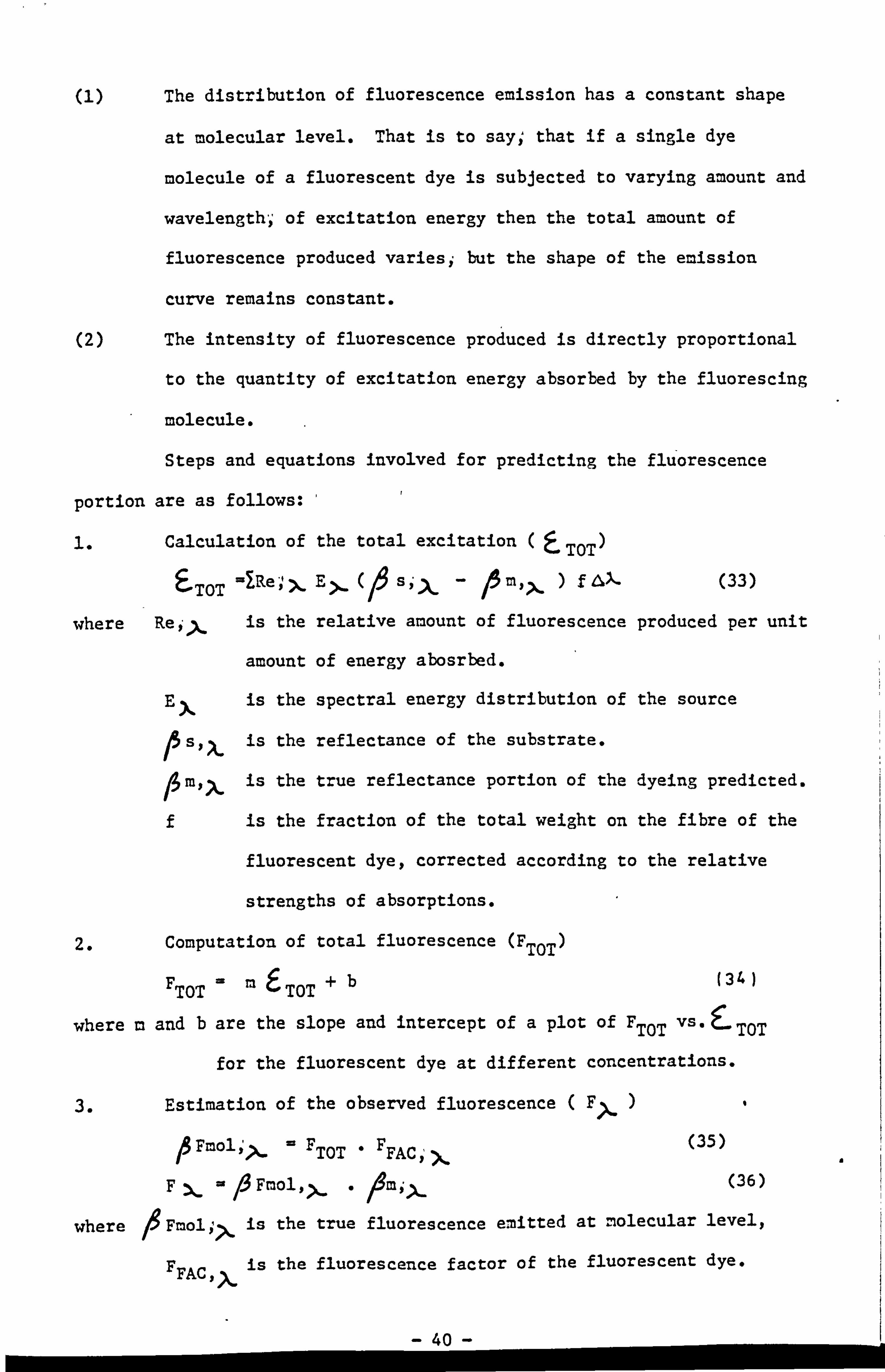
Steps and equations involved for predicting the fluorescence
portion are as follows: 'I
Calculation of the total excitation TOT) ETOT =lRe' ,I >ý E >. ( sp .X-AM, f A; k- (33)
where Re, -, >.. is the relative amount of fluorescence produced per unit
amount of energy abosrbed.
Ex is the spectral energy distribution of the source
S2 x is the reflectance of the substrate.
mx> is the true reflectance portion of the dyeing predicted.
f is the fraction of the total weight on the fibre of the
fluorescent dye, corrected according to the relative
strengths of absorptions.
2. Computation of total fluorescence (F TOT)
F TOT wm6 TOT +b (34)
where m and b are the slope and intercept of a plot of FTOT vs* ý-
TOT
for the fluorescent dye at different concentrations.
3. Estimation of the observed fluorescence ( FX )I
A Fmol; x =F TOT *F FAC (35)
15 Fmol, >
ým; > (36) FZ
where ý Fmol; X is the true fluorescence emitted at molecular level,
FFAC, >
is the fluorescence factor of the fluorescent dye.
a
- 40 -
4. Calculation of the spectral radiance factors curve (pm, x+ F x
It is carried out from the initial concentrations predicted,, and
optimization proceeds from there until the lowest colour difference
possible is obtained. -
The Relex curve (Re; > and , ), the Fluorescence factors (FFAC I
the slope and intercept (m and b) are calculated from primany data (i. e.
the ture reflectance curve and the spectral radiance factors) of
calibration dyeings and the spectral energy distribution of the source
used in the measuring system.
Funk concludes that the results obtained are comparable to those
obtained when formulations using nonfluorescent colorants were first
developed. The major limitations imposed by the methodology established
during the work are that it, requires special apparatus and no
investigation was made to determine the effect of experimental
variability. In total eighteen'shades have been considered with single or
binary mixtures of fluorescent and/or non-fluorescent dyes.
- 41 -

Part II
Experimental & Resutls
ChaDter IV Introduction and Objectives
The general objective as indicated by the title of this thesis is
to develop a way to handle fluorescence in computer colour 6atching, in
order to cope with the widespread use of fluorescent dyes, which extends
the colour gamut of dyeings especially for rich and saturated colours as
well as bright pale and light shades.
As concluded by Ganz (36) i the present practice of cutting off
the fluorescent portion of the spectral radiance factors curve of the
samplej or matching only the true reflectance portion is satisfactory for
identical dyes; that is for a non-metameric match. His method of allowing
the use of negative Kubelka-Munk coefficients is valid only for
applications of a single fluorescent dye, or at most one which may be
shaded slightly by minor additions of other dyes.
Funk (40)
employs a two-monochromator spectroreflectometer which
is not available in themarket in his method. This limits his approach to
the research laboratory. Furthermore, he claims that the results are only
comparable to those obtained when computer colour match was first
developed. McKay (37)
avoids using a special instrument by using a set
of twelve cut-off filters to separate the true reflectance portion of the
dyeing. The time required to produce optical data for calibration dyeings
as well as samples to be matched seems to be longer than the feasible time
available for an ordinary match.
- 42

The present project is trying to establish a simple method using
a popular instrument with polychrornatic illumination via a study of the
influence of fluorescence on relfectance-concentration relationships for
fluorescent dyes, singly and in mixture as indicated in the subtitle.
Moreover, a review of a commercial computer colour matching system is
carried out in order to find an actual firm base for comparsion.
I
- 43
Chapter V Review of a Current (1978) Commercial Package in ComDuter
Colour Matching
5.1 The System
The Carl Zeiss RFC3 automatic spectrophotometer system, which is
one of the well known systems, is used for this study. According to
information supplied by the manufacturer, more than one hundred users are
spread all over the world in more than twenty countries. Sharpe and
Lakowski (42)
reports that it measures colour with high performance,
precision and accuracy. Its capability for colour measurement is at least
as good as that of the other commercially available colour-measuring
instruments that have been tested. In addition; the accuracy of this
instrument is checked regularly four times per year with samples supplied
by the Manufacturers Council on Colour & Appearance of the National Bureau
of Standards of U. S. A. through the Collaborative Reference Program for
colour difference.
The Zeiss RFC3 is an abridged spectroreflectometer equipped with
16 interference filters to cover the whole visible spectrum from 400nm to
700nm. Coloured surfaces are illuminated diffusely with an integrating
sphere and are viewed at 80. Light is provided by a xenon arc lamp
which approximates to Illuminant D 65, Reflectance curves as well as
C. I. E. tristimulus values for Illuminant A and D 65 with 100
supplementary standard observer are obtained. Other jobs, such as colour
differencei dye strength, whiteness; as well as computer colour matching
can also be done through the same computation unit (Hewlett Packard HP 21
mX computer). The HP7900 disc operating system is used for storage of
programs and data. Another advantage of this system is the switchable
measuring aperture. A 30mmy 15mm or 5mm, diameter aperture may be
selected to house both large and small colour surface areas. However the
measuring time of 45 sec. is a little bit too slow for routine work. The
programs and operating system are bought with the instrumente
a
44
5.2 A General Study of the Perfornance of the System
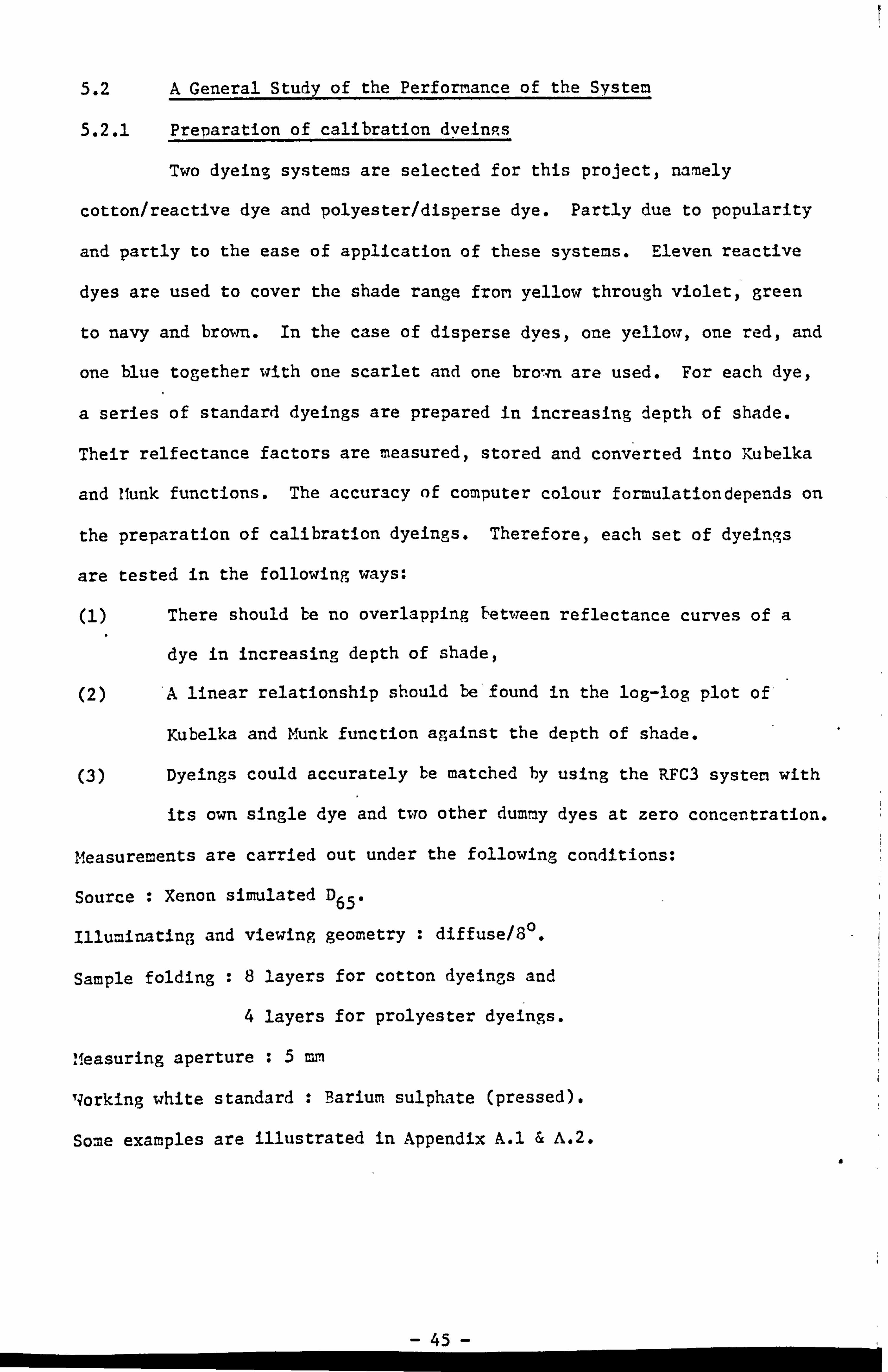
5.2.1 Preparation of calibration dveings
Two dyeing systems are selected for this project, namely
cotton/reactive dye and polyester/disperse dye. Partly due to popularity
and partly to the ease of application of these systems. Eleven reactive
dyes are used to cover the shade range from yellow through violet, green
to navy and brown. In the case of disperse dyes, one yellow, one red, and
one blue together with one scarlet and one brown. are used. For each dye,
a series of standard dyeings are prepared in increasing depth of shade.
Their relfectance factors are measured, stored and converted into Kubelka
and Munk functions. The accuracy of computer colour formulationdepends on
the preparation of calibration dyeings. Therefore, each set of dyeings
are tested in the following ways:
(1) There should be no overlapping between reflectance curves of a
dye in increasing depth of shade,
(2) 'A linear relationship should be'f ound in the log-log plot of'
Kubelka and Munk function against the depth of shade.
(3) Dyeings could accurately be matched by using the RFC3 system with
its own single dye and two other dummy dyes at zero concentration. C2
Measurements are carried out under the following conditions:
Source : Xenon simulated D65.
Illuminating and viewing geometry : diffuse/30.
Sample folding :8 layers for cotton dyeings and
4 layers for prolyester dyeings.
Measuring aperture :5 mm L
Tiorking white standard : Barium sulphate (pressed).
Some examples are illustrated in Appendix A. 1 & A. 2.
a
45 - I-
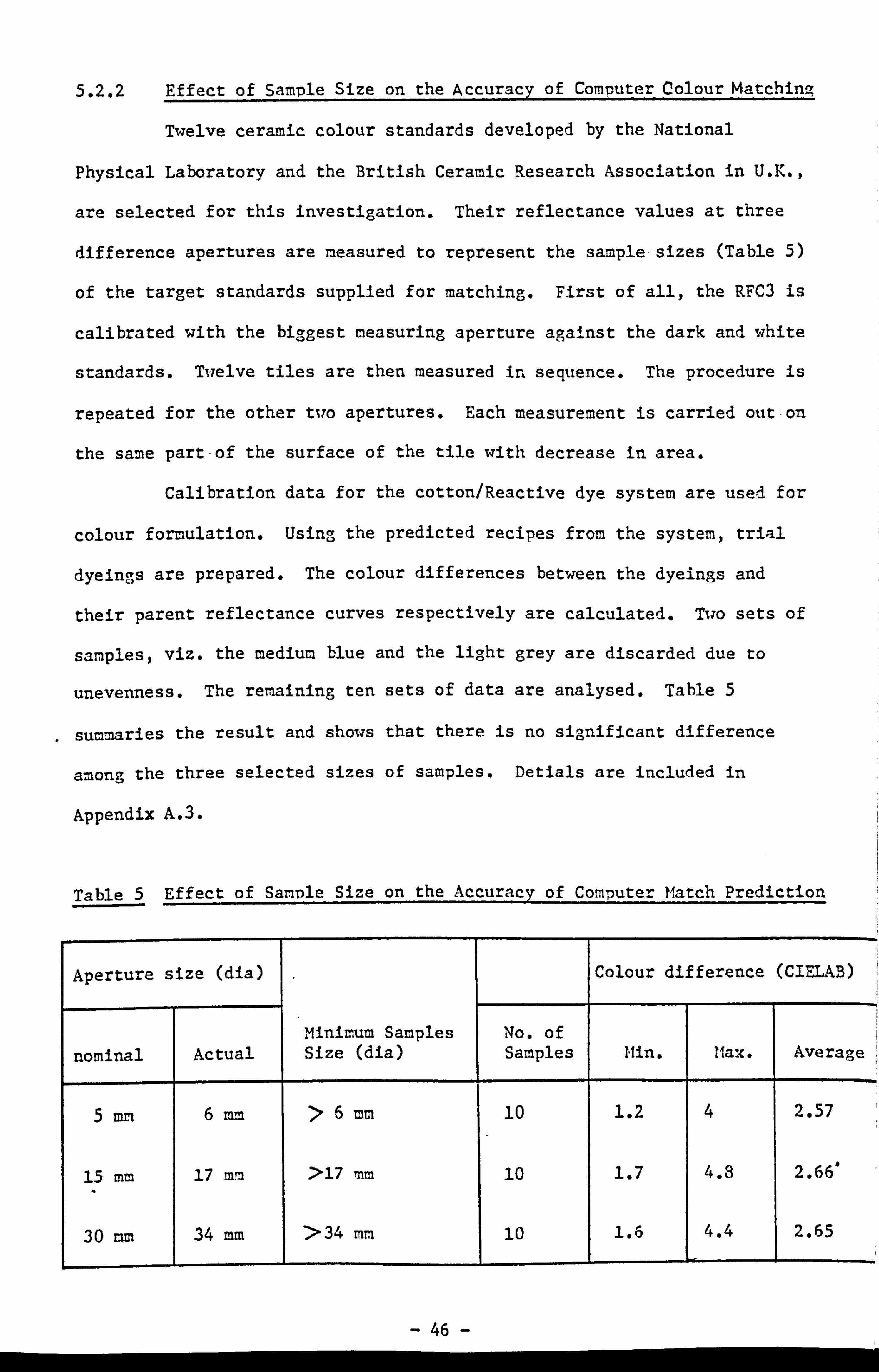
5.2.2 Effect of Sample Size on the Accuracy of Computer Colour Matching
Twelve ceramic colour standards developed by the National
Physical Laboratory and the British Ceramic Research Association in U. K.,
are selected for this investigation. Their reflectance values at three
difference apertures are measured to represent the sample, sizes (Table 5)
of the target standards supplied for matching. First of all, the RFC3 is
calibrated with the biggest measuring aperture against the dark and white
standards. Twelve tiles are then measured in sequence. The procedure is
repeated for the other two apertures. Each measurement is carried out, on
the same part-of the surface of the tile with decrease in area.
Calibration data for the cotton/Reactive dye system are used for
colour formulation. Using the predicted recipes from the system, trial 0
dyeings are prepared. The colour differences between the dyeings and cl
their parent reflectance curves respectively are calculated. Two sets of
samples, viz. the medium blue and the light grey are discarded due to
unevenness. The renaining ten sets of data are analysed. Tahle 5
summaries the result and shows that there is no significant difference 0
among the three selected sizes of samples. Detials are included in
Appendix A. 3.
Table 5 Effect of Sarmle Size on the Accuracy of Computer Match Prediction
Aperture size (dia) Colour difference (CIELAB)
Minimum Samples No. of nominal Actual Size (dia) Samples Ifin. Max. Average
5 mm 6 mm >6 mm 10 1.2 2.57
15 mm. 17 mm >17 m. m 10 1.7 4.8 2.66'
30 mm 34 mm >34 mm 10 1.6 4.4 2.65
46
5.2.3 The Achieved Accuracv
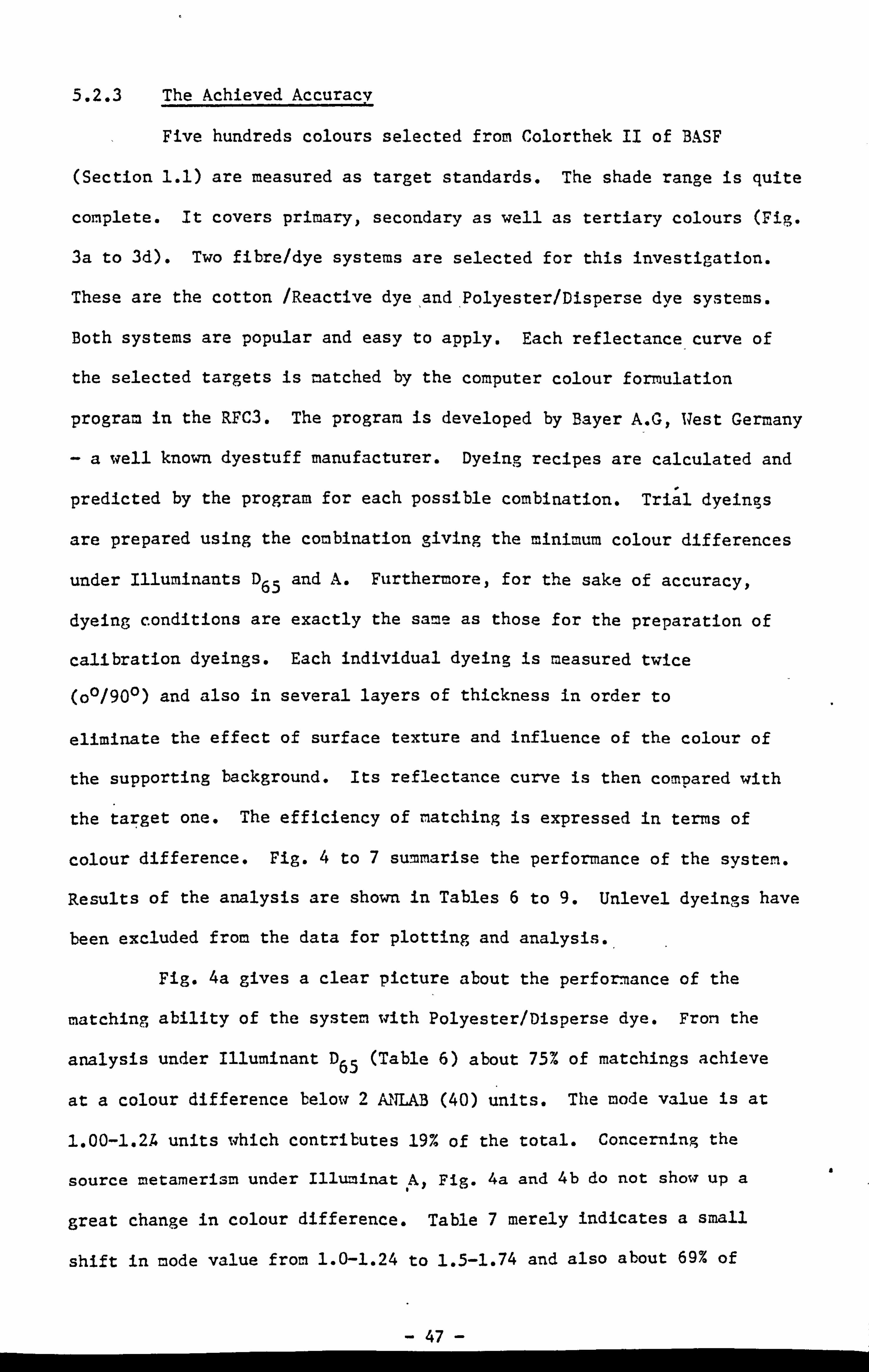
Five hundreds colours selected from Colorthek II of BASF
(Section 1.1) are measured as target standards. The shade range is quite
complete. It covers primary, secondary as well as tertiary colours (Fig.
3a to 3d). Two fibre/dye systems are selected for this investigation.
These are the cotton /Reactive dye, and. Polyester/Disperse dye systems.
Both systems are popular and easy to apply. Each reflectance curve of
the selected targets is matched by the computer colour formulation
program in the RFC3. The program is developed by Bayer A_. G, West Germany
-a well known dyestuff manufacturer. Dyeing recipes are calculated and
predicted by the program for each possible combination. Triýl dyeings
are prepared using the combination giving the minimum colour differences
under Illuminants D65 and A. Furthermore, for the sake of accuracy,
dyeing conditions are exactly the same as those for the preparation of
calibration dyeings. Each individual dyeing is measured twice
(oO/900) and also in several layers of thickness in order to
eliminate the effect of surface texture and influence of the colour of
the supporting background. Its reflectance curve is then compared with
the target one. The efficiency of matching is expressed in terms of
colour difference. Fig. 4 to 7 summarise the performance of the system.
Results of the analysis are shown in Tables 6 to 9. Unlevel dyeings have
been excluded from the data for plotting and analysis.,
Fig. 4a gives a clear picture about the performance of the
matching ability of the system with Polyester/Disperse dye. From the
analysis under Illuminant D 65 (Table 6) about 75% of matchings achieve
at a colour difference below 2 MILAB (40) units. The mode value is at
1.00-1.2L units which contributes 19% of the total. Concerning the
source metamerism under Illuminat, A, Fig. 4a and 4b do not show up a
great change in colour difference. Table 7 merely indicates a small
shift in mode value from 1.0-1.24 to 1.5-1.74 and also about 69% of
47 -

dyeings have a difference below two units. It can be concluded that a
near spectral match was provided by the system in most cases.
Fig. 5 to 6 and Table 8 try to estimate the effect of
tristimulus value Y on the accuracy of computer colour matching. 'Though
some differences were found in the table; the overall picture leads to
the conclusion that the effect is not very significant.
The cotton/Reactive dye system gives a similar distribution
curve (Fig. 7). However, the performance (Table 9) of the system is not
as good as the one with disperse dyes. Only 49.4% of the dyeings give a
colour differenc6 below 2.25 ANLAB (40) units. The mode value is
1.8-2.02 and is nearly one unit worse than for the polyester system.
This significant difference reveals that the accuracy of an instrumental
match prediction can vary among different dyeing systems. It may perform
well in one but not too good for the other system. The result may be due
to the effect of exhaustion on the accuracy of computer colour matching.
The exhaustion of disperse dyes is usually good on polyester., but is not
too good for reactive dyes on cotton. Furthermore the fixation of the
reactive dye on cotton may well contribute another important factor to
this worse result; especially, as an all-in method has been used in this
investigation due to its simplicity.
The actual locations in CIELAB colour space of each target
colours which can be and cannot be matched with the selected reactive
dyes are illustrated in Appendix A. 4.
a
- 48 -
0. p
0.8
0.7-1 1
0., 5
w j44
6L CIL a2 1,37,61,30
ýy 1 r 4
O 15 -, % CI
0.3ý .... ,I-
27 C/6
- ipa 05
0 1 2 1 : '12 ,
ýp j
C. 14
0.1 ý
0,2 C. s C. '3 sx
C'X V. SY
Fig- 3a Location of the Five Hundred Target Colours in CIE Chromaticity Diagram
-49-
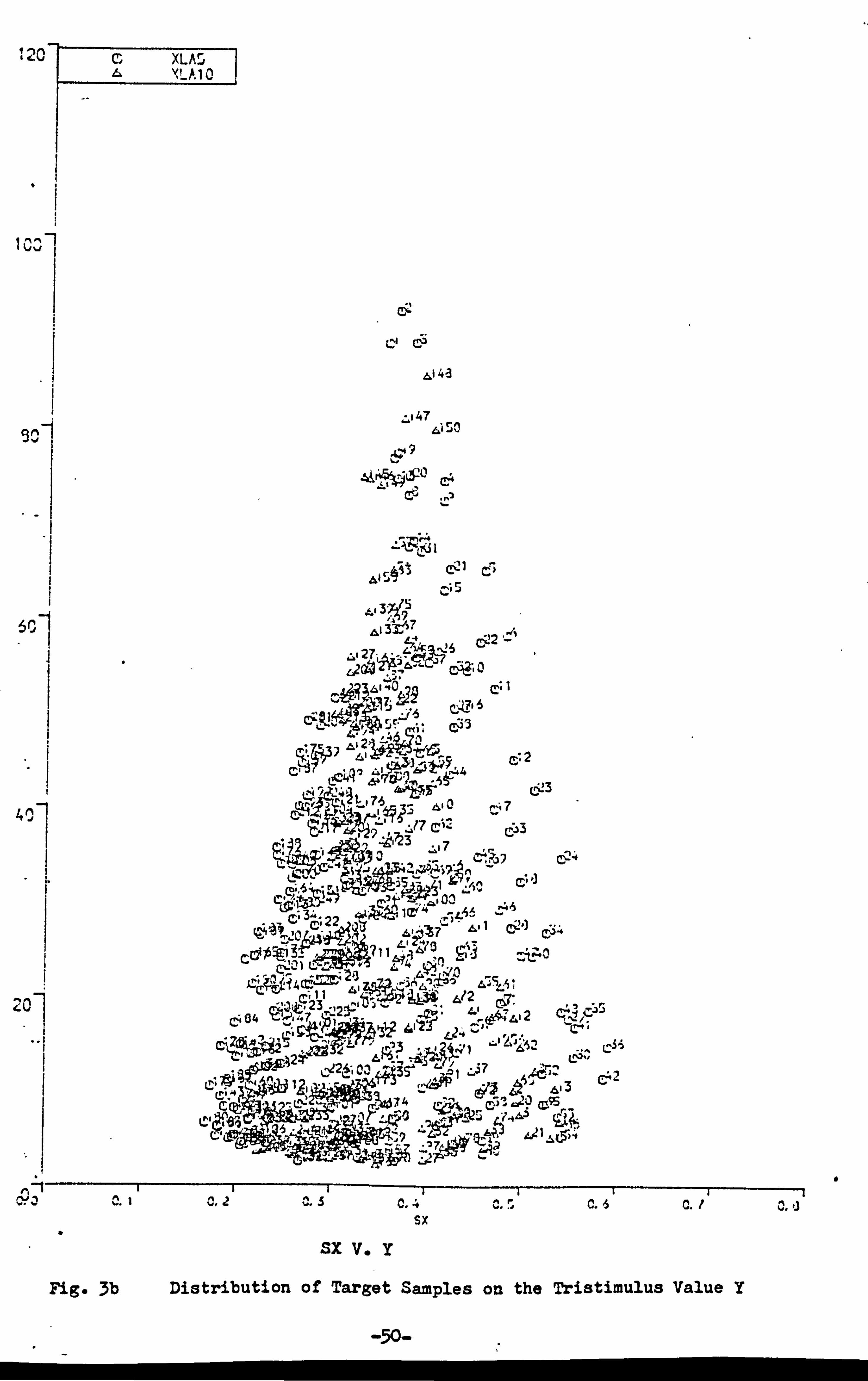
1 20
v
I-
.1
&14-3
I gm-j
. 47
C4
A. 1 rl
-A CP2
C4. ýZj
490
75
J. elk,
46
CLO , 3,3".
P
. ý5644 3 76 7
491723 73 I
e. )"L. v 4-ON"alt
11 i! ý. '
.-C; l
20 Z* ' IM
c
21
r
r4 os JMI 14 4. /)6
7'
41
213
412 07
L24 'WI
4-
1 /I )34 ze,: C*2
Var-ITT ,:, 47 4 COS
A. 2 I
, %J3 012 11.1.5 0.4 0. S C. 's 0.1 O. J sx
Sx V. y
Fig. 3b Distribution of Target Samples on the Tristimulus Value Y
a
-50-
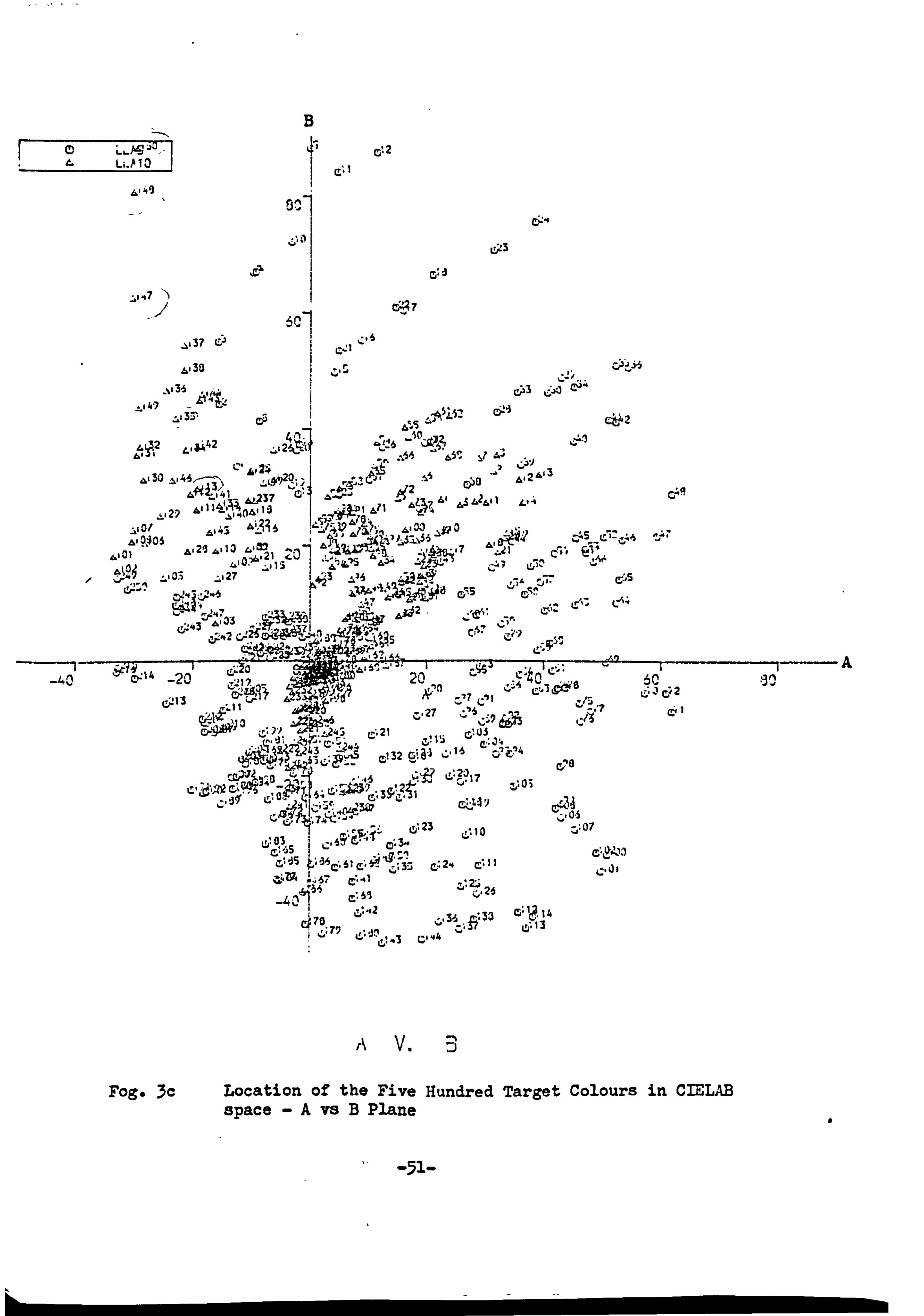
Lýýjll, -
41
B 2
41
03
7
6C]
C; ý. #
-!, 137 64
Cýl
-. %83-6 cw3 6-. 3 bq:, I L'J"
49 - &m
%C 4al 44
24 23 130 4 ' 3 & . 1, El
g2
() 1 &71 A &115 4p 2 , ,1 7 ,
. 1101 zlj:
. &I &IN "04 213 O. 7 I 4 4s 1 F120 N
41 27 az
Aji§2 3
C, %4
C. 17 ýg.? e. I Ak- Paw 66
-40 -20 60 C-il
Lý J 64 2
27 . -IS :; q
7
.. ý, 243 C'. 21
1 '43 Z. 16 4
I- r=. 2 2 -. 03 11 (f.
. 7,4 CIO
&is d ! is cl II
ZýZ& I o. i -57 týi 21
Cý70 Zý, 02
ý. 3,5; V33
I Cs44
A V. ::, )
Fog- 3c Location of the Five Hundred Target Colours in CIELAB space -A vs B Plane
C'.
c4fl
.3n. A
a
-. 51-
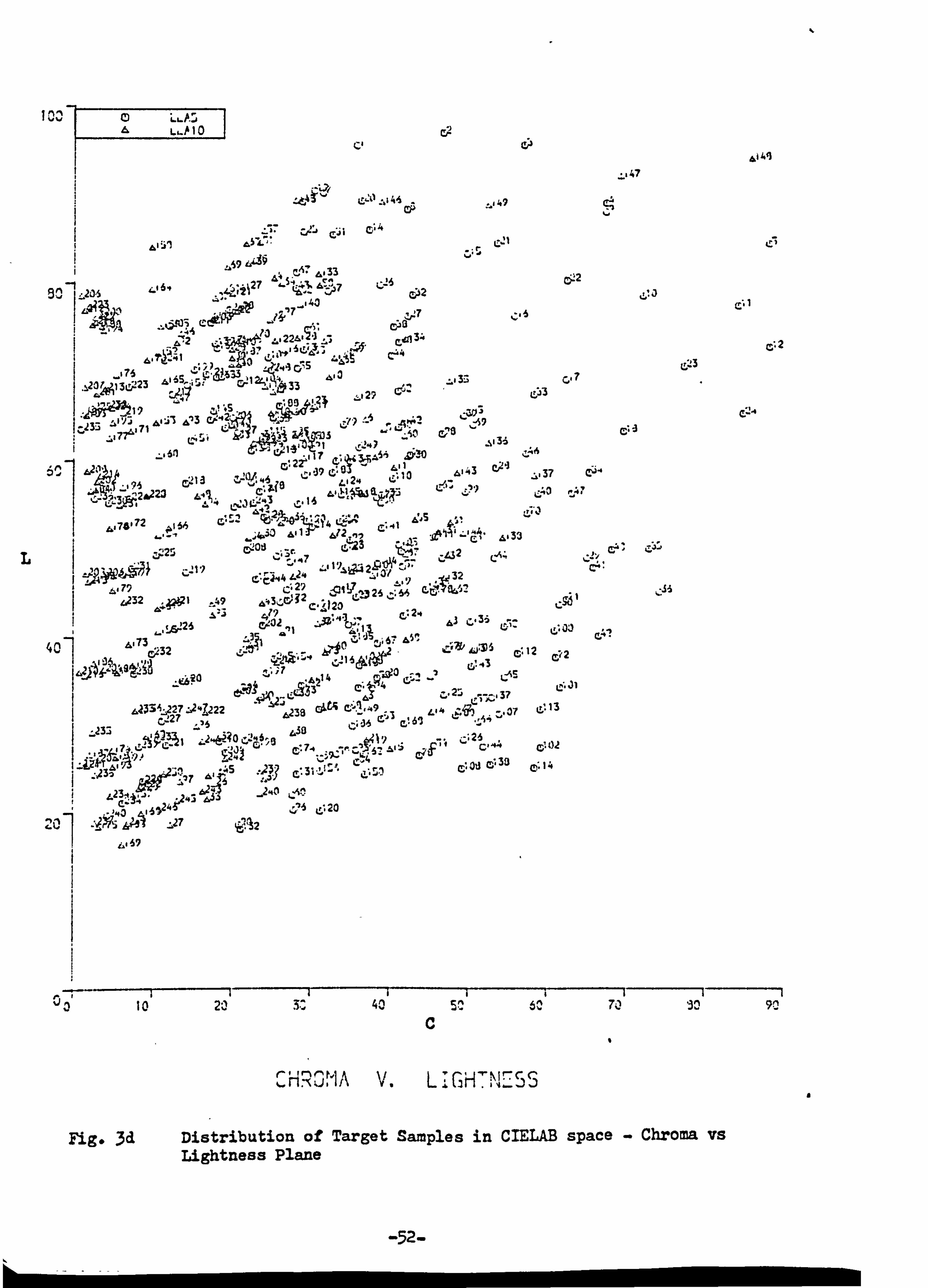
In"N vw
-. 47
: 537 Cý:, Zý i &4
1 '59 'jo
C, 67 &j33 S* C. ;26 Cý2 416-t ' --4", 161ýý7 , 4ý; ii2
L2015 . 4'. 02
'12c C-1
'3 A'2 e4
C, 2 124,33
Z:. 4 1 I'ts "
leg . 31 ý. 127 5
1 :A zc-ft' tý.
AiTS 03 71 ;73L; I :. il C70
WIS
GI 2? 17 ee 5.; Ai
4.11 Oq 37 c 2, # 4.
I
2ao223 &4% C, 43 aý Z. 1
S2 , LaM72 2,156
Y4 L; ýý C. -41
, 7ý "r:. 144 lliý
-, C AM eos
-432 . A4 -7 k-o C- 2!
Cý-EJI#4 42, # al 32 79 :,. 29 6 z, 232 26 6-8 4
'3 79 c- 1123 C7 2-t I A Aj
3,171 . 6-? Ail r4l 73 L! I %;, V. 40ý e32 j'ai
, V"& AA 6 d, 12 2 1 :1 *Z4 lity 16
. do
6,? 0 A4214 !; - 4 25 114, A V---, 37
&433iý; 27 Z-24ý7222 38 0ý" CO, 49 Lr:. 13
C,
C'I C'. 07
L233 . 36
1 ý' ý? -, '5 -e ,
If 2
11 j. 2 ?0C; C; 25,,.
4 7.7-4 c 33 14
7 2140
C. 20
L27
4
2
I I I i i I ---- ------- 201 40 6C 70 .1
c
CHRONA 'GHNESS %- ',, ' a
Fig. 3d Distribution of Target Samples in CIELAB space - Chroma vs Lightness Plane
-52-
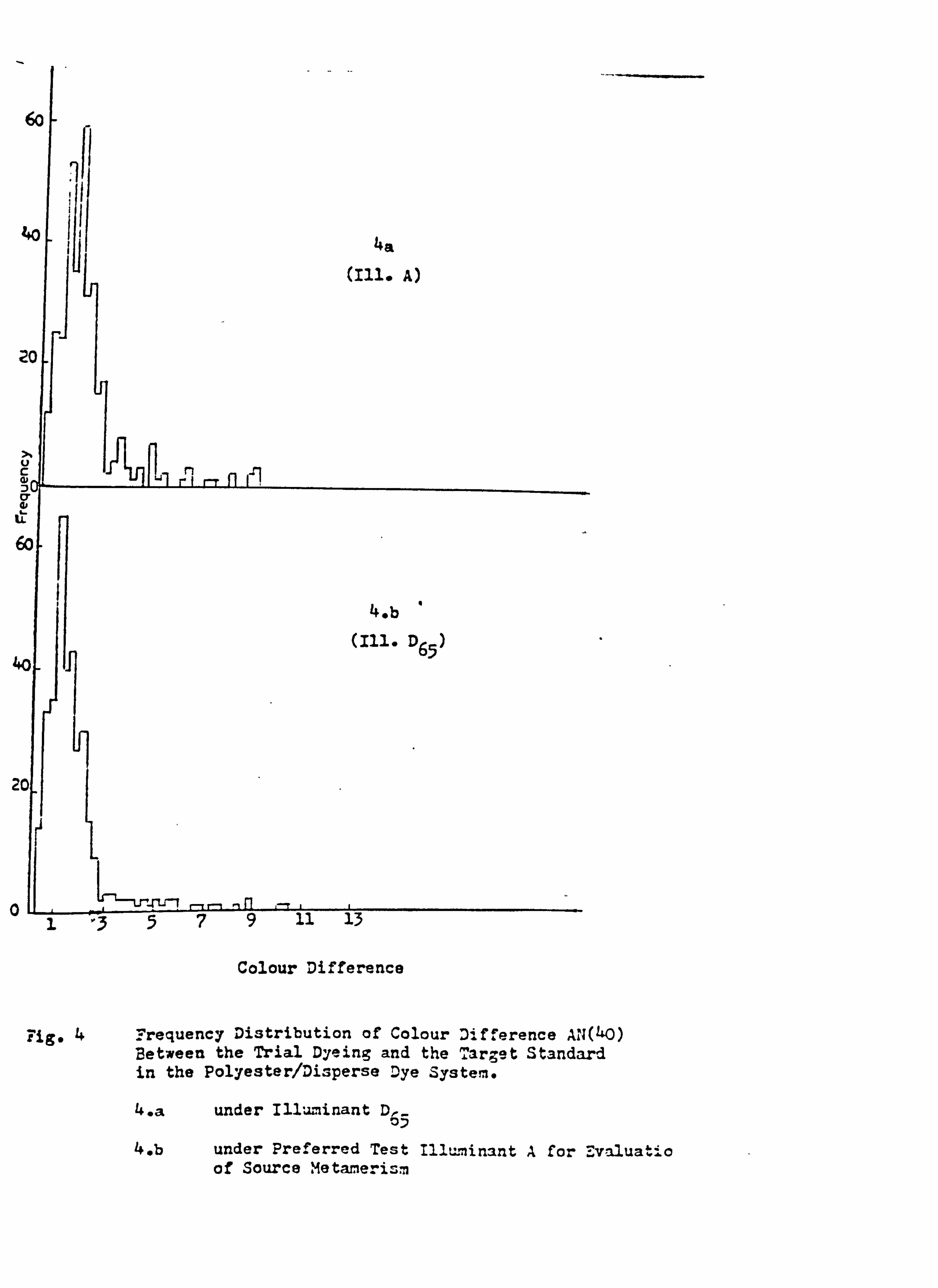
Colour Difference
Fig. 4 Frequency Distribution of Colour Difference AN(40) Between the Trial Dyeing and the 7"arget Standard in the Polyester/Disperse Dye System..
4. a under Illuminant De- 0 -;
4,, b under Preferred Test Ill-w-minant A for Evaluatio of Source Metanerism
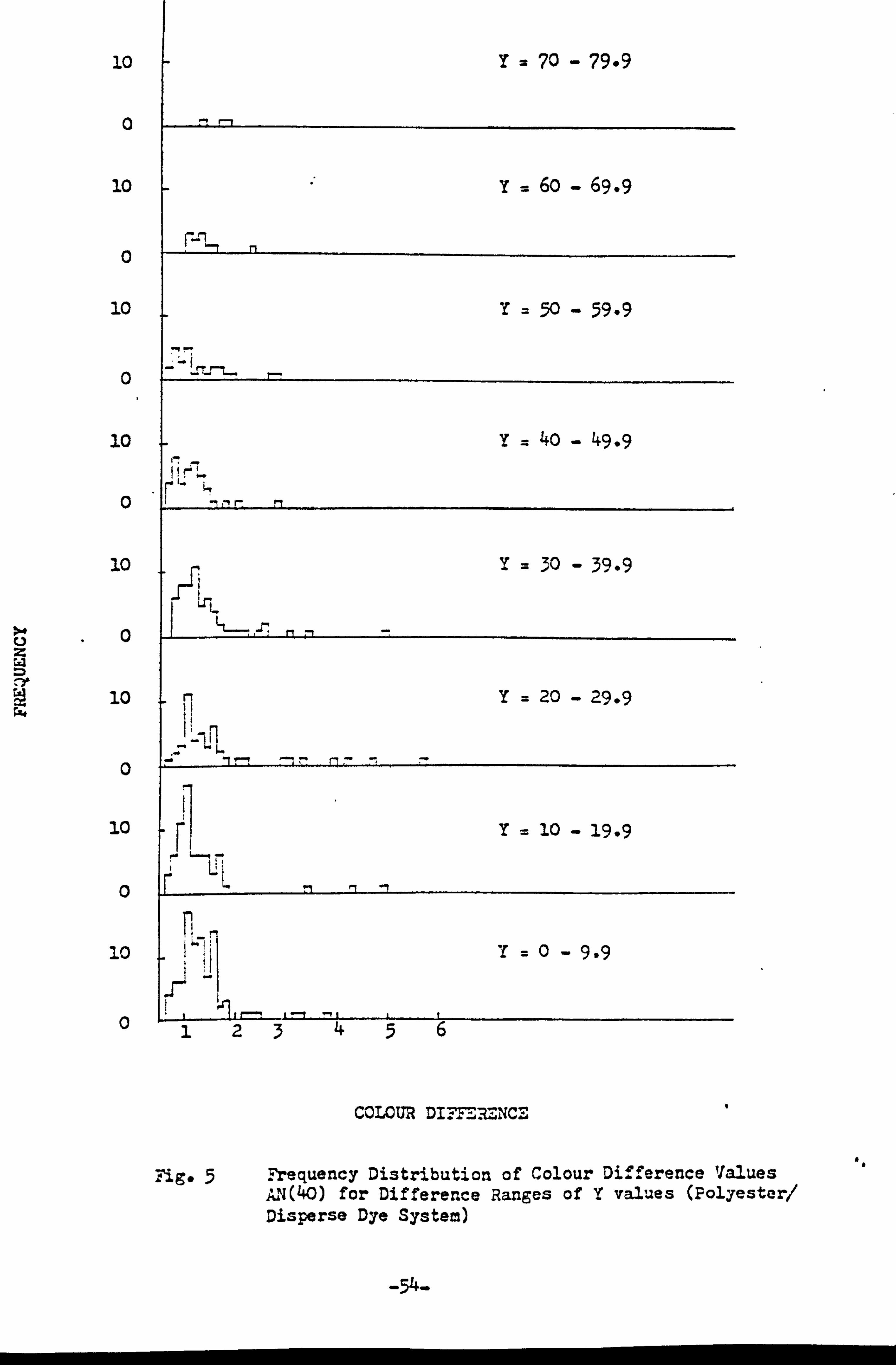
10
0
10
0
10
0
10
0
10
0
10
0
10
0
10
0
Y= 70 - 79-9
Y= 60 - 69.9
y = 50 - 59-9
y. 4o - 49.9
y= 30 - 39.9
Lri- M 71
Y 20 29.9
'-l 71 MI
y 10 19.9
0 - 9.9
I r-_ L 71! 1 1- 124ý?
COLCUR M. FTMENCE I
iF requency Distribution of Colour Difference Values ig* 5 A, 11(40) for Difference Ranges of Y values (Polyester/ Disperse Dye System)
-54-
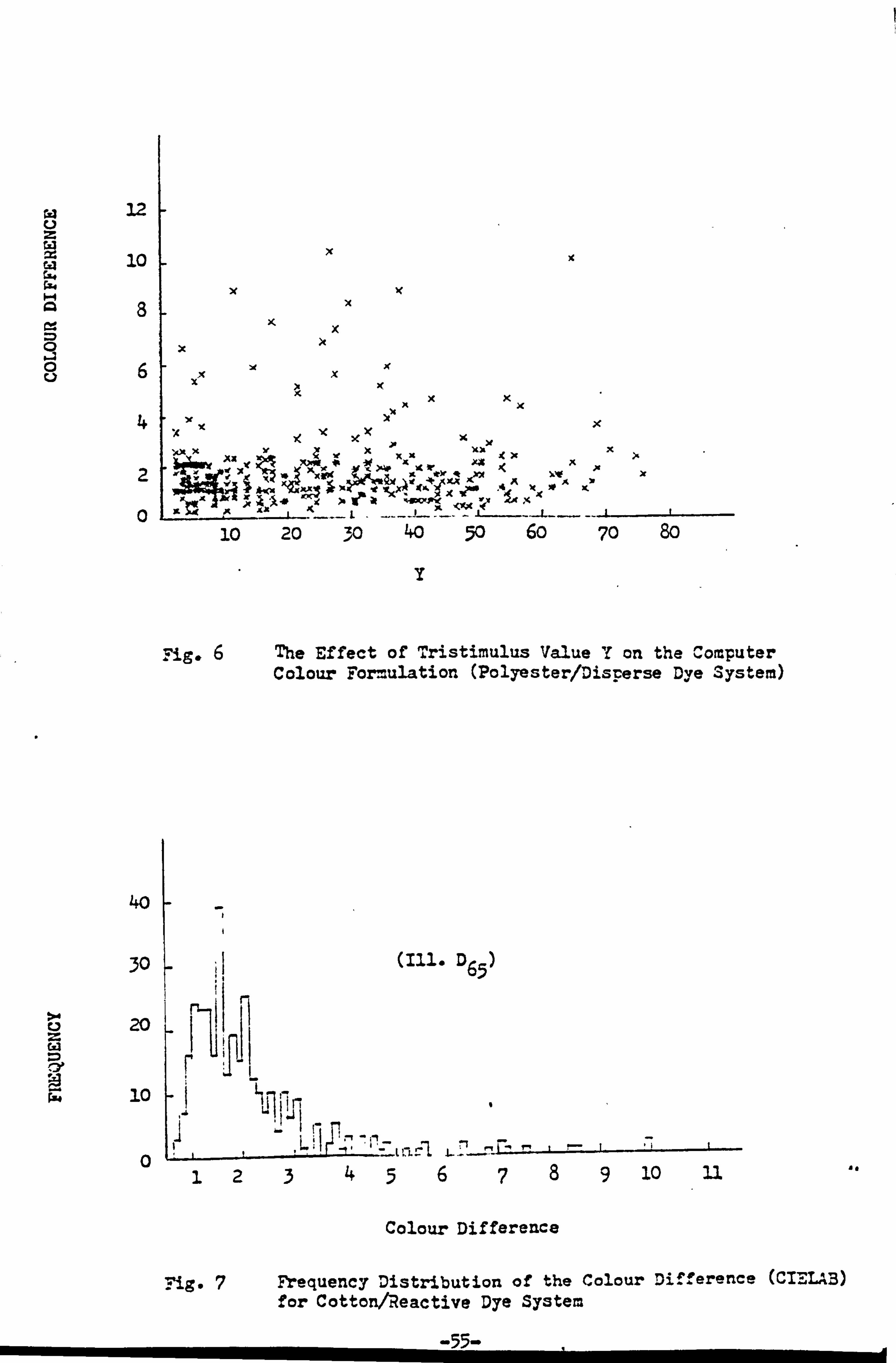
12
22 10
- X
x N. 1 x x
6 xx x )c
x x x 4
X x IL-1. -.
ZwX x
IK ir xa
xx
Ic x
XX jh ?'k ý
x ic 0 xx
%«Ky k>»i z «x 7
10 20 ý, 0 40 50 60 70 80
y
F. ig.
40
30 ý il
The Effect of Tristimulus Value Y on the Computer Colour Formulation (Polyester/Disr. erse Dye System)
20
10
0
(111. D 65 )
I
10
Colour Difference
As
F7 Frequency Distribution of the Colour Difference (CTEIAB) . ig I
for Cotten/Reactive Dye System
-55-
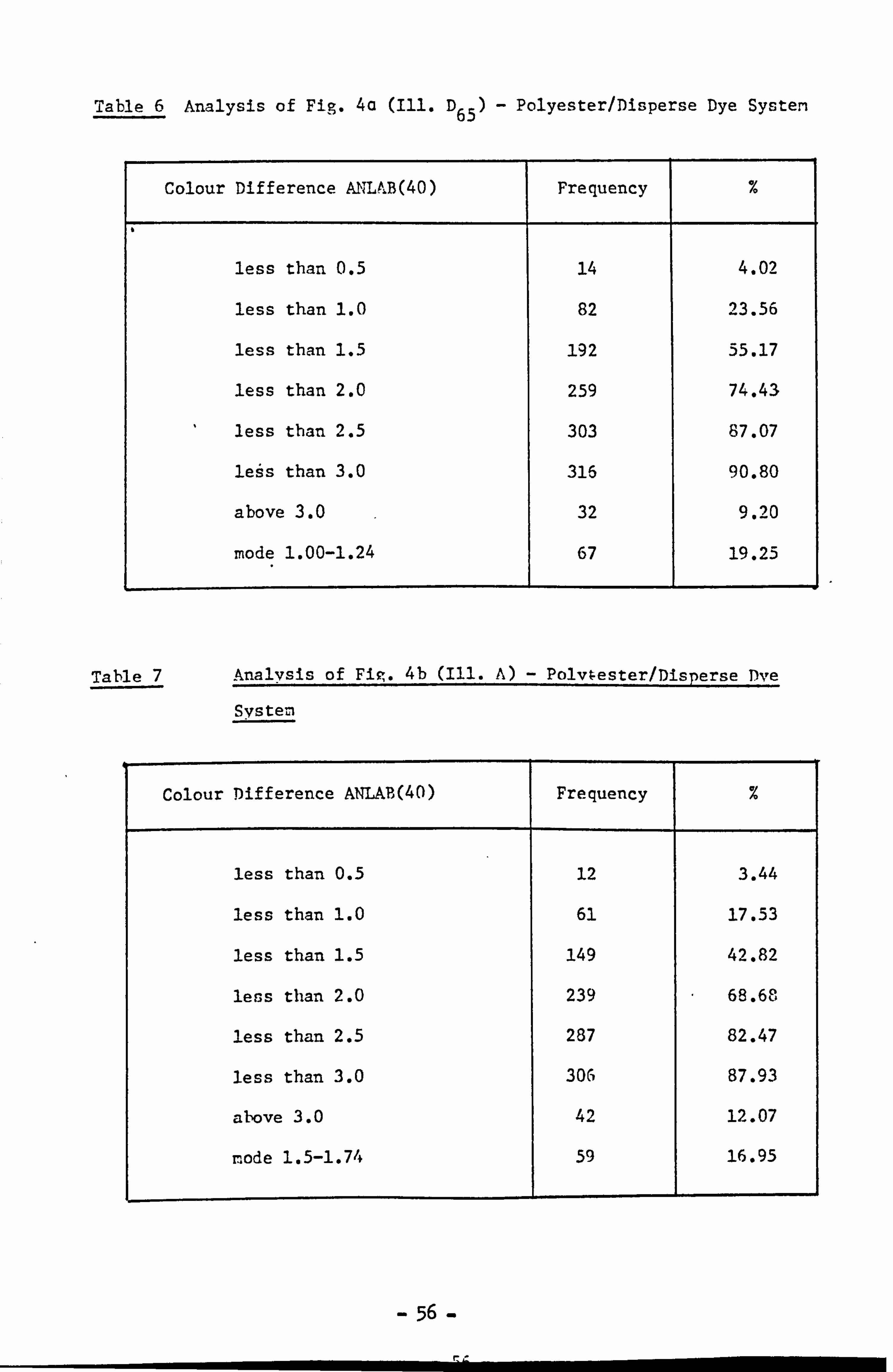
Table 6 Analysis of Fig. 4a (Ill. D 65 )- Polyester/Disperse Dye System
Colour Difference ANUB(40) Frequency %
less than 0.5 14 4.02
less than 1.0 82 23.56
less than 1.5 192 55.17
less than 2.0 259 74.43
less than 2.5 303 87.07
leýs than 3.0 316 90.80
above 3.0 32 9.20
mode 1.00-1.24 67 19.25
Table 7 Analysis of Fie, 4b (Ill. A) - Polvýester/Disperse Dv! l
Svste"m
Colour Difference AMAB(40) Frequency %
less than 0.5 12 3.44
less than 1.0 61 17.53
less than 1.5 149 42.82
less than 2.0 239 68.68'
less than 2.5 287 82.47
less than 3.0 306 87.93
above 3.0 42 12.07
node 1.5-1.74 59 16.95
- 56 -
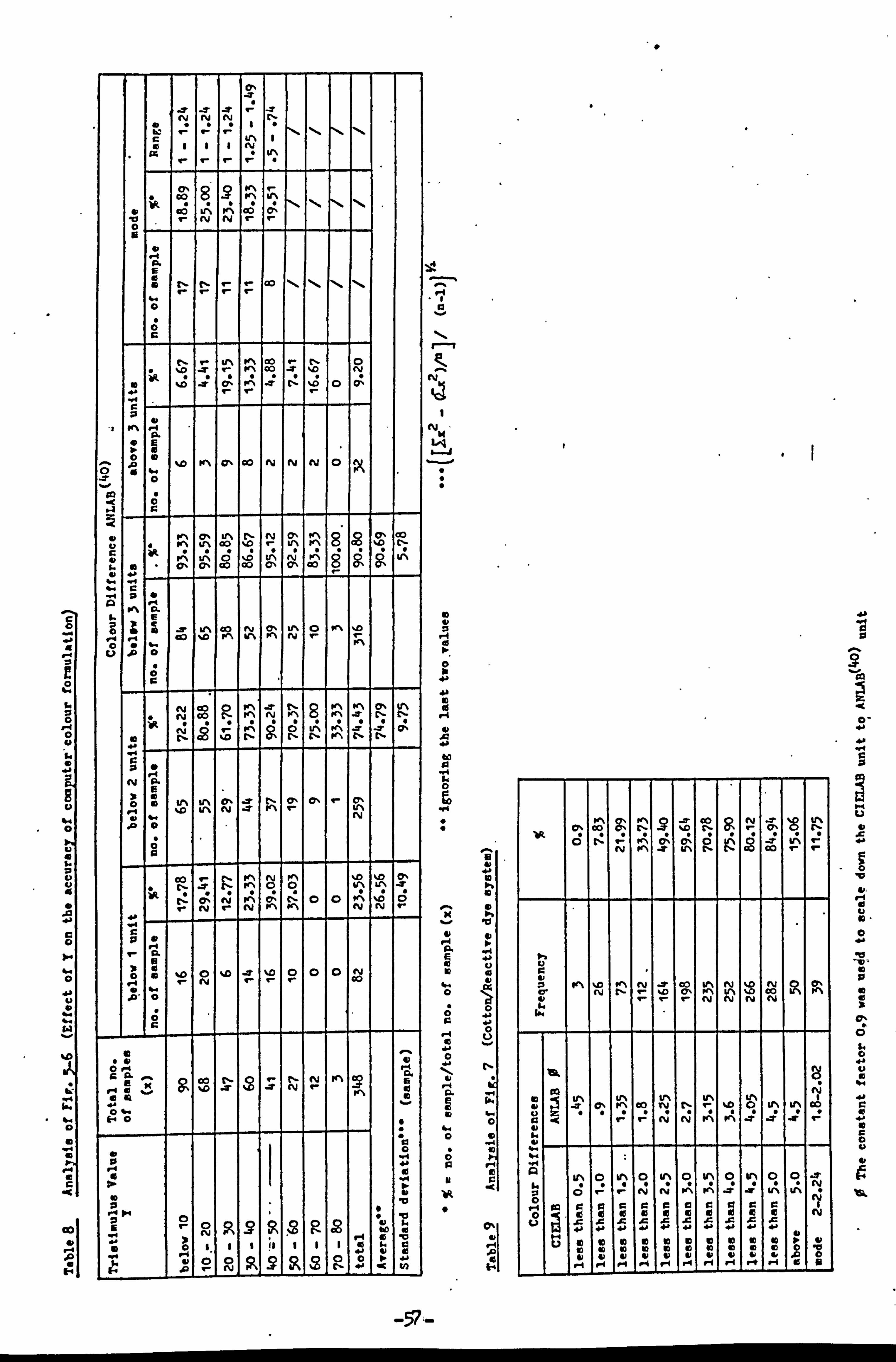
41 A C'01
0%
cli ru cli
10
V- I- q-
tv
lk 430 Lr% n OD 0%
ry ty 0
1: 6
40 Go
4. a
I 0 r.
ld*A co N
10 'D r CA A r rZ %Z 0 0' P
A
- 0 a %D Ir% crý 00 ty N CY 0 X
a %.
0
" ll A
Lr%
N N "' 12 D - r 0
;k 1ý or%
Vý ir, % I %
I Llý
24 % I . ""
0 8
. 9, '
. F,
0
VN I c7% co go 47 0
%.. . 14 4. c
a a V% CO ru (7% 11% 0 ^ 10 .4 .. 0
4: 0 %D ^ kf'% pr% ev Irl ON 0
W ; - 0
co 0 If% lrý ON
cy 00 rý ON 9v I ff'% NI ff% 0 - C; p ý A ; _; at
cu
0 If% LIN 0, 47, C%
, %Q UN
o
ry Ff% -. 0 No
-I k 47, Cý 0 0 fr% %D 0 V\ or\ CY r4
, , %D o %D :r %D 0 0 0 ry Go
0
r
In 01-1 1,0% r IL E Go r- s CY
- or% co
lr .1 ;r CY q _ pe\
0%. fi. 0
0
r C)
0 w
cu . 45
0 C, 1 0
ý9
6
F, cv
(Y bd !: 2j
ID Id
r4
IR
0'
iß .0
0
, 0% Ir', -2' CO r" cý 19 rý %i rý - 0 > , wý, cy, cy, 0 ü g J u-, -
-, r 00 N %D tu w fy g- ý ýD (Y, ýQ %D 00 er% cy Al
90 ic i U. '
l o l - %0 U. 0& .p r, K -% o' I ý C rý r- '
_T J ,
r i-
w% 0 U'N 0 UN 0 V% 0 0 -11' �, Z Z ý A j o 6 * N - r UN U%
1 2 `ý r 1,2 i . mg um r- o . 0 : - 0 . 5 . 5 r
- j C X r x j--
4 4 d j bj Z 43 41 41 k.
o 1 0 1 0 1 0 1 1 ' 0 I n . , . . . . s, ' Z Z
0-
M 1111 IZ
-, v,
-57-
dyeings have a difference below two units. It can be concluded that a
near spectral match was provided by the system in most cases.
Fig. 5 to 6 and Table 8 try to estimate the effect of
tristimulus value Y on the accuracy of computer colour matching. Though
some differences were found in the table, the overall picture leads to
the conclusion that the effect is not very significant.
The cotton/Reactive dye system gives a similar distribution
curve (Fig. 7). However, the performance (Table 9) of the system is not
as good as the one with disperse dyes. Only 49.4% of the dyeings give a
colour difference below 2.25 ANLAB (40) units. The mode value is
1.8-2.02 and is nearly one unit worse than for the polyester system.
This significant difference reveals that the accuracy of an instrumental
match prediction can vary among different dyeing systems. It may perform
well in one but not too good for the other system. The result may be due
to the effect of exhaustion on the accuracy of computer colour matching.
The exhaustion of disperse dyes is usually good on polyester,, but is not
too good for reactive dyes on cotton. Furthermore the fixation of the
reactive dye on cotton may well contribute another important factor to
this worse result, especially, ý as an all-in method has been used in this
investigation due. to its simplicity.
The actual locations in CIEL&B colour space of each target
colours which can be and cannot be matched with the selected reactive
dyes are illustrated in Appendix A. 4.
- 58 -
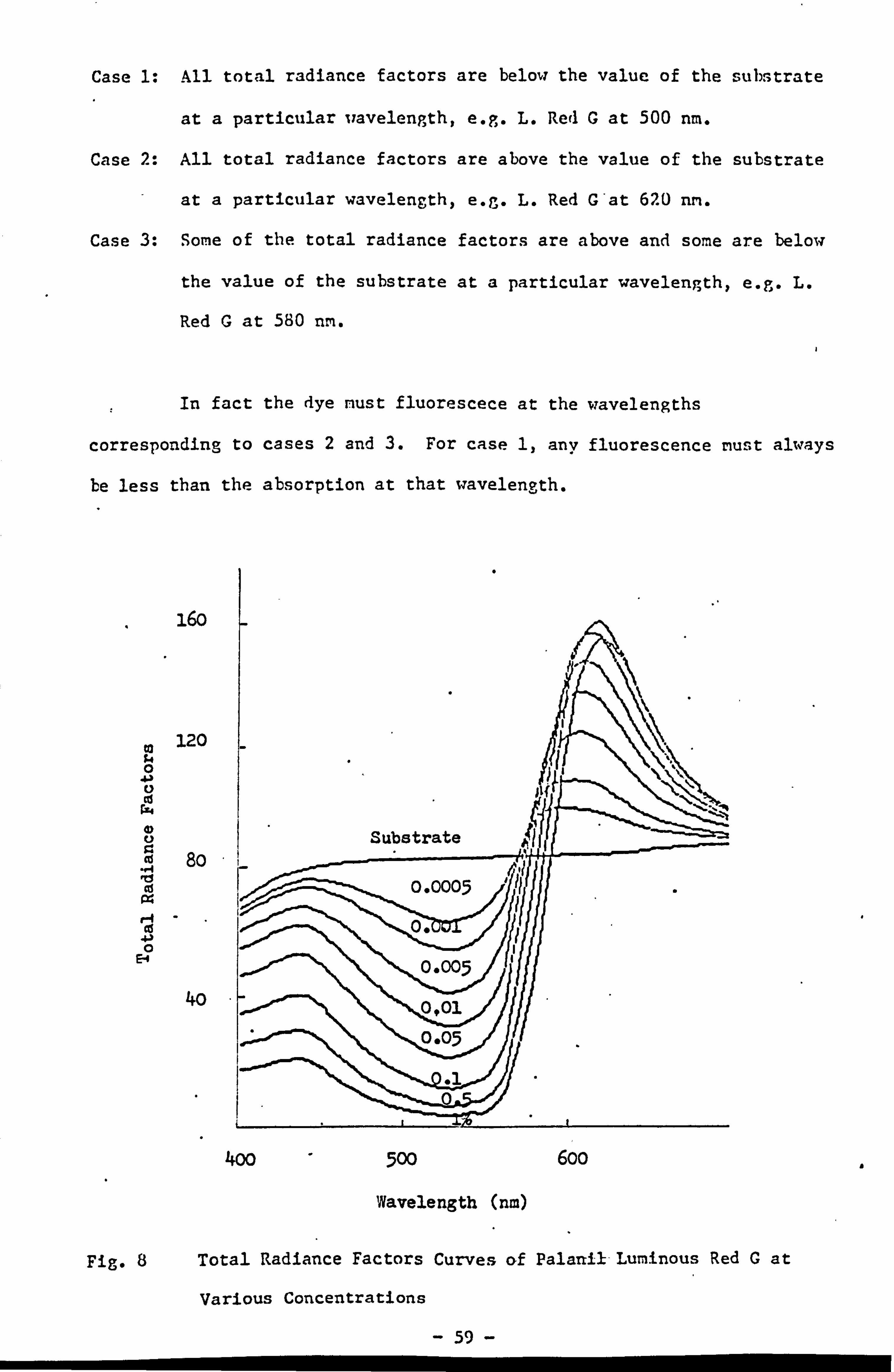
Case 1: All total radiance factors are below the value of the substrate
at a particular wavelength, e. g. L. Red G at 500 nm.
Case 2: All total radiance factors are above the value of the substrate
- at a particular wavelength, e. g. L. Red G'at 620 nn.
Case 3: Some of the total radiance factors are above and some are below
the value of the substrate at a particular wavelength, e. g. L.
Red G at 580 nm. I
In fact the dye nust fluorescece at the wavelengths
corresponding to cases 2 and 3. For case 1, any fluorescence must always
be less than the absorption at that wavelength.
16o
120 0
rz -
Cd 80 Cd
0 E-4
40
400 500 600 a
Wavelength (nm)
Fig. 8 Total Radiance Factors Curves of Palanil-Luminous Red G at
Various Concentrations
- 59 -
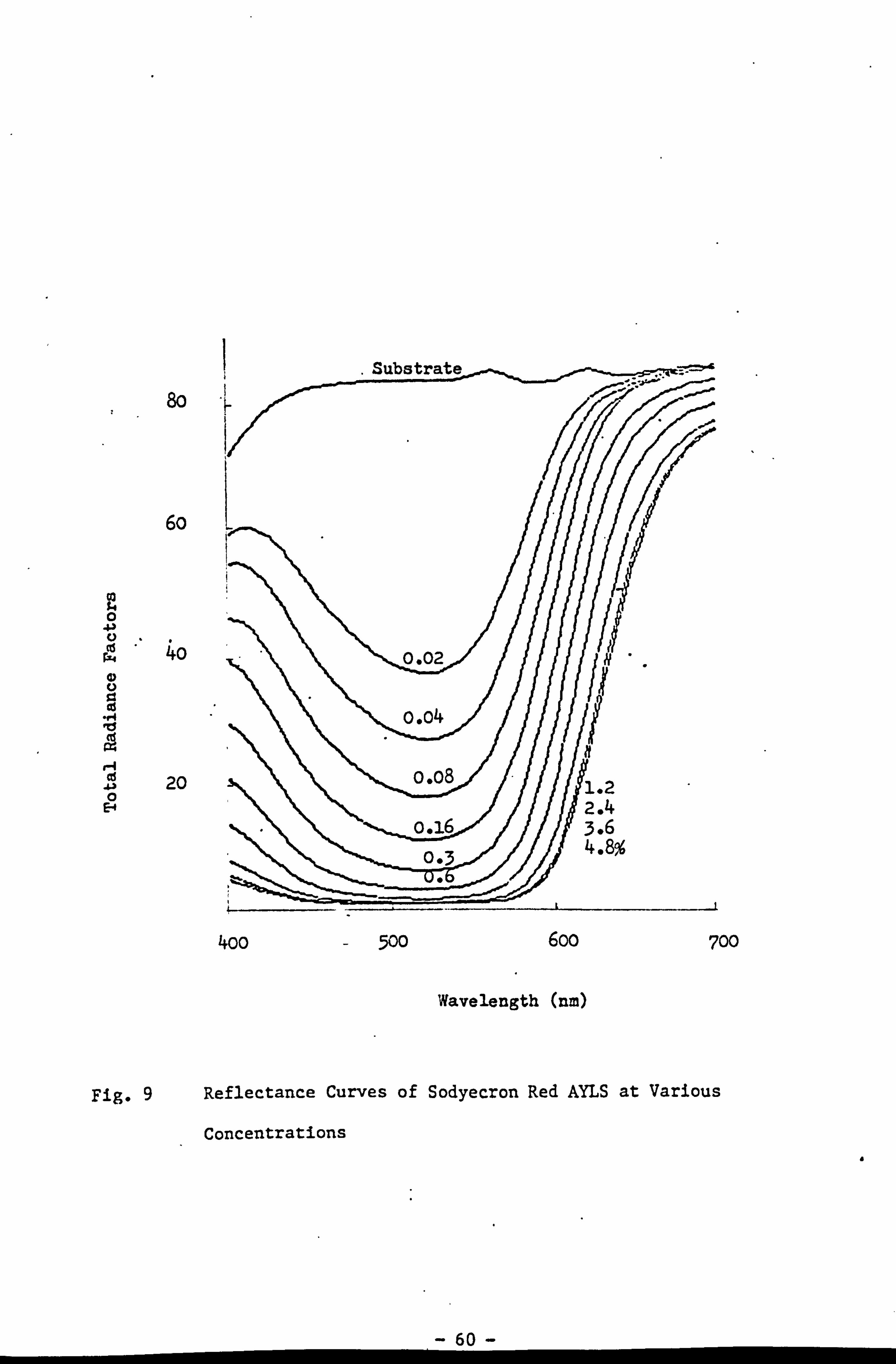
I Substrate
80
60
0
P4 40
Cd -r4 Tf
1-4 Cd
-&j 20 0 E-4
400 500 6oo 700
Wavelength (nm)
Fig. 9 Reflectance Curves of Sodyecron Red AYLS at Various
Concentrations a
60 -
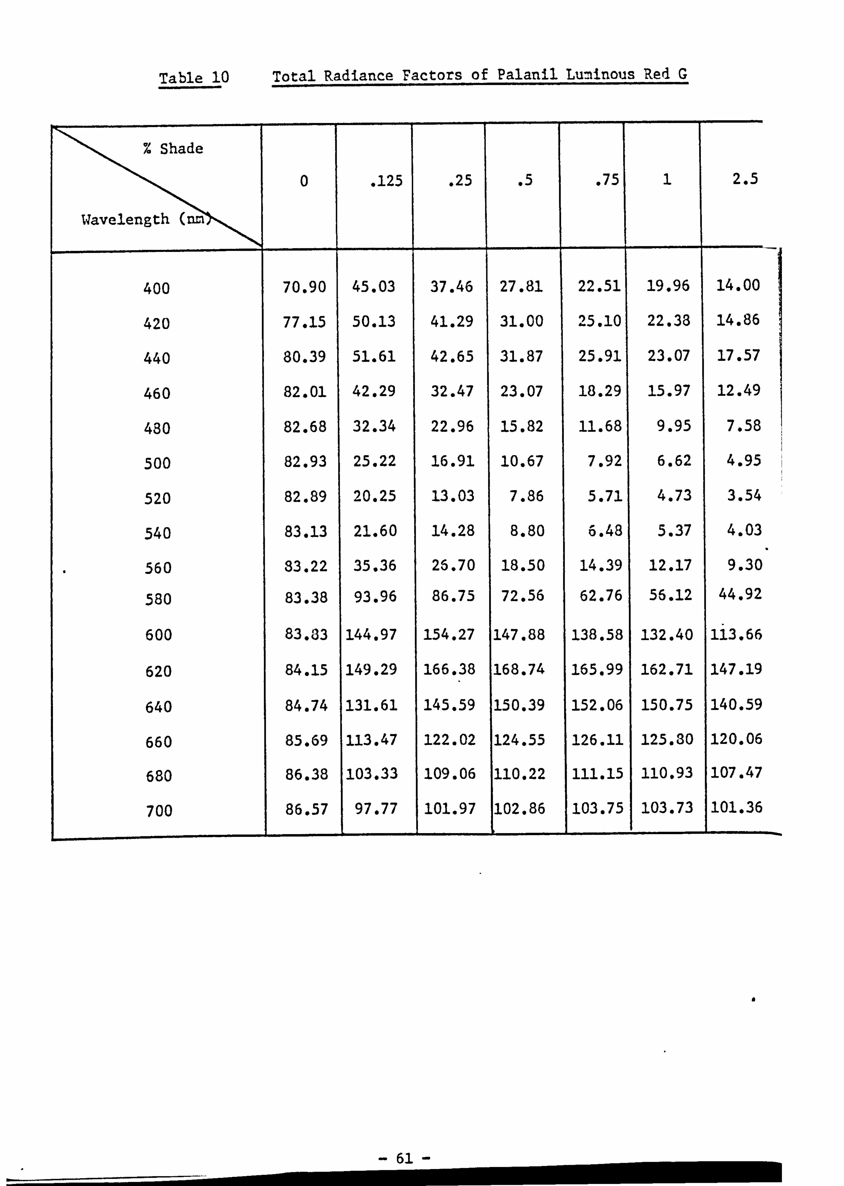
Table 10 Total Radiance Factors of Palanil Luminous Red G
%* Shade
wavelength
0 . 125 . 25 .5 . 75 1 2.5
400 70.90 45.03 37.46 27.81 22.51 19.96 14.00
420 77.15 50.13 41.29 31.00 225.10 22.38 14.86
440 80.39 51.61 42.65 31.87 25.91 23.07 17.57
460 82.01 42.29 32.47 23.07 18.29 15.97 12.49
480 82.68 32.34 22.96 15.82 11.68 9.95 7.58
500 82.93 25.22 16.91 10.67 7.92 6.62 4.95
520 82.89 20.25 13.03 7.86 5.71 4.73 3.54
540 83.13 21.60 14.28 8.80 6.48 5.37 4.03
560 83.22 35.36 25.70 18.50 14.39 12.17 9.30
580 83.38 93.96 86.75 72.56 62.76 56.12 44.92
600 83.33 144.97 154.27 147.88 138.58 132.40 113.66
620 84.15 149.29 166.38 168.74 165.99 162.71 147.19
640 84.74 131.61 145.59 150.39 152.06 150.75 140.59
660 85.69 113.47 122.02 124.55 126.11 125.30 120.06
680 86.38 103.33 109.06 110.22 111.15 110.93 107.47
700 86.57 97.77 101.97 102.86 103.75 103.73 101.36
61

Table 11 Total Radiance Factors of Palanril Luminous Yellow G
% Shade
Wavelength
0 . 125 . 25 .5 . 75 1 2.5
400 70.90 35.26 27.06 18.28 13.64 11.22 7.82
420 77.15 23.61 16.57 10.19 7.30 5.96 4.16
440 80.39 16.72 11.10 6.63 4.75 3.96 2.87
460 82.01 16.14 10.63 6.43 4.57 3.86 2.81
480 82.68 35.55 26.11 17.99 12.73 10.92 7.43
500 82.93 114.05 105.04 93.09 79.48 73.54 58.13
520 82.89 160.34 169.04 172.00 175.09 169.65 157.33
540 83.13 137.90 147.00 156.01 164.31 162.46 160.11
560 83.22 113.80 118.29 124.01 129.05 128.40 126.72
580 83.38 99.67 101.22 104.52 107.21 106-073 104.49
600 83.83 92.73 93.06 94.81 96.51 95.87 93.90
620 84.15 88.72 88.54 89.32 90.38 -89.83 88.31
640 84.74 37.55 87.32 87.70 88.59 88.14 86.85
660 85.69 87.51 87.26 87.27 88.01 87.54 86.13
680 86.38 87.55 87.33 87.09 87.81 87.22 85.69
700 86. 87.41 87.20 86.98 87.61 87.11 85.53
62
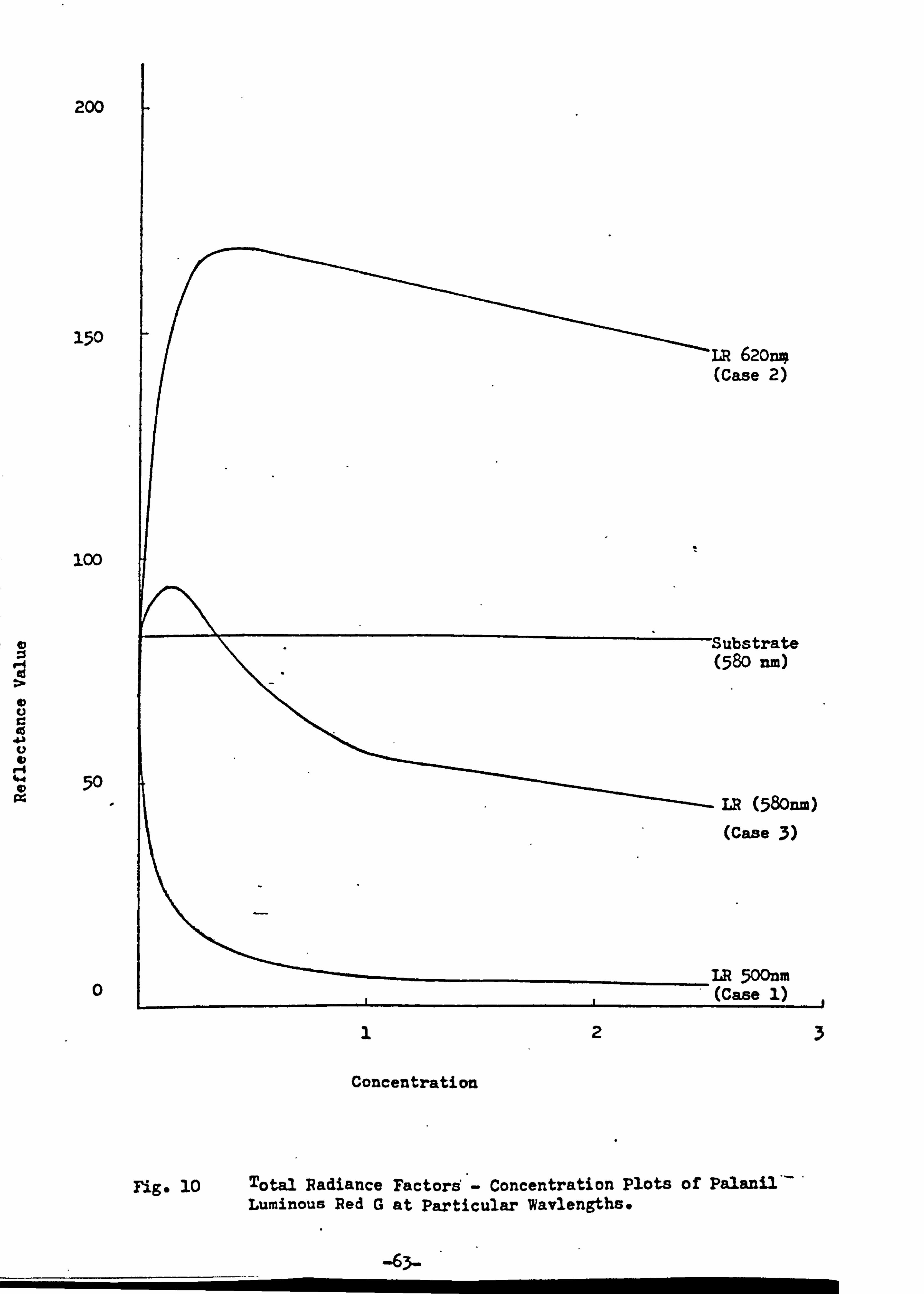
200
150
100
V
r-4 4.4 0 50 pr.
0
Concentration
Fig. 10 Total Radiance Factord - Concentration Plots of Palanil'-' Luminous Red G at Particular Wavlengthse
-63-
1
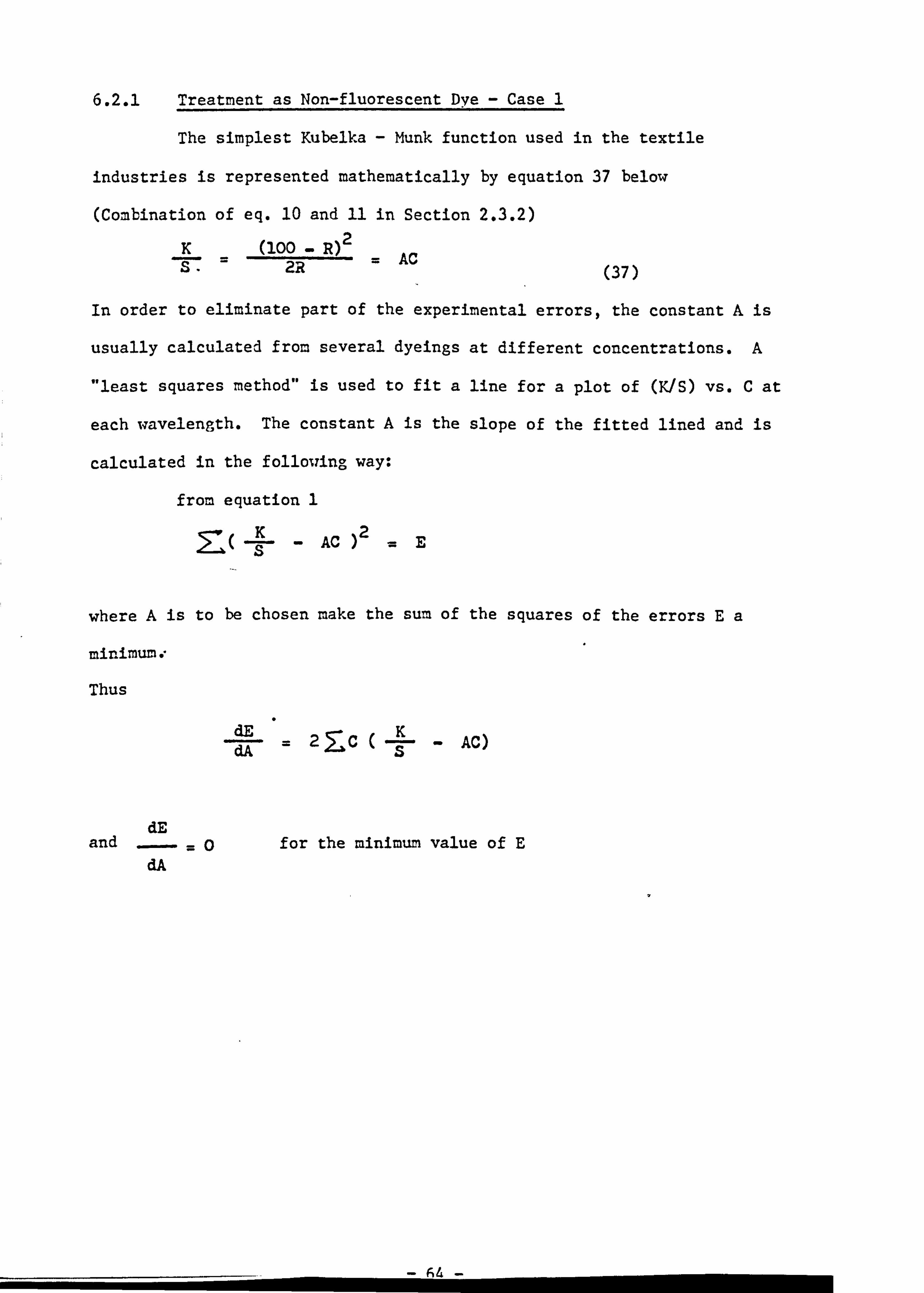
6.2.1 Treatment as Non-fluorescent Dve - Case 1
The simplest Kubelka - Munk function used in the textile
industries is represented mathematically by equation 37 below
(Combination of eq. 10 and 11 in Section 2.3.2)
K (100 - R) 2 AC 2R (37)
In order to eliminate part of the experimental errors, the constant A is
usually calculated from several dyeings at different concentrations. A
"least squares method" is used to fit a line for a plot of (K/S) vs. C at
each wavelength. The constant A is the slope of the fitted lined and is
calculated in the following way:
from equation 1
K- AC )2 =E s
where A is to be chosen make the sum of the squares of the errors Ea
minimum. ý
Thus
dE 2ZC(K- AC) s
dE and -=0 for the minimum value of E
dA
64 -
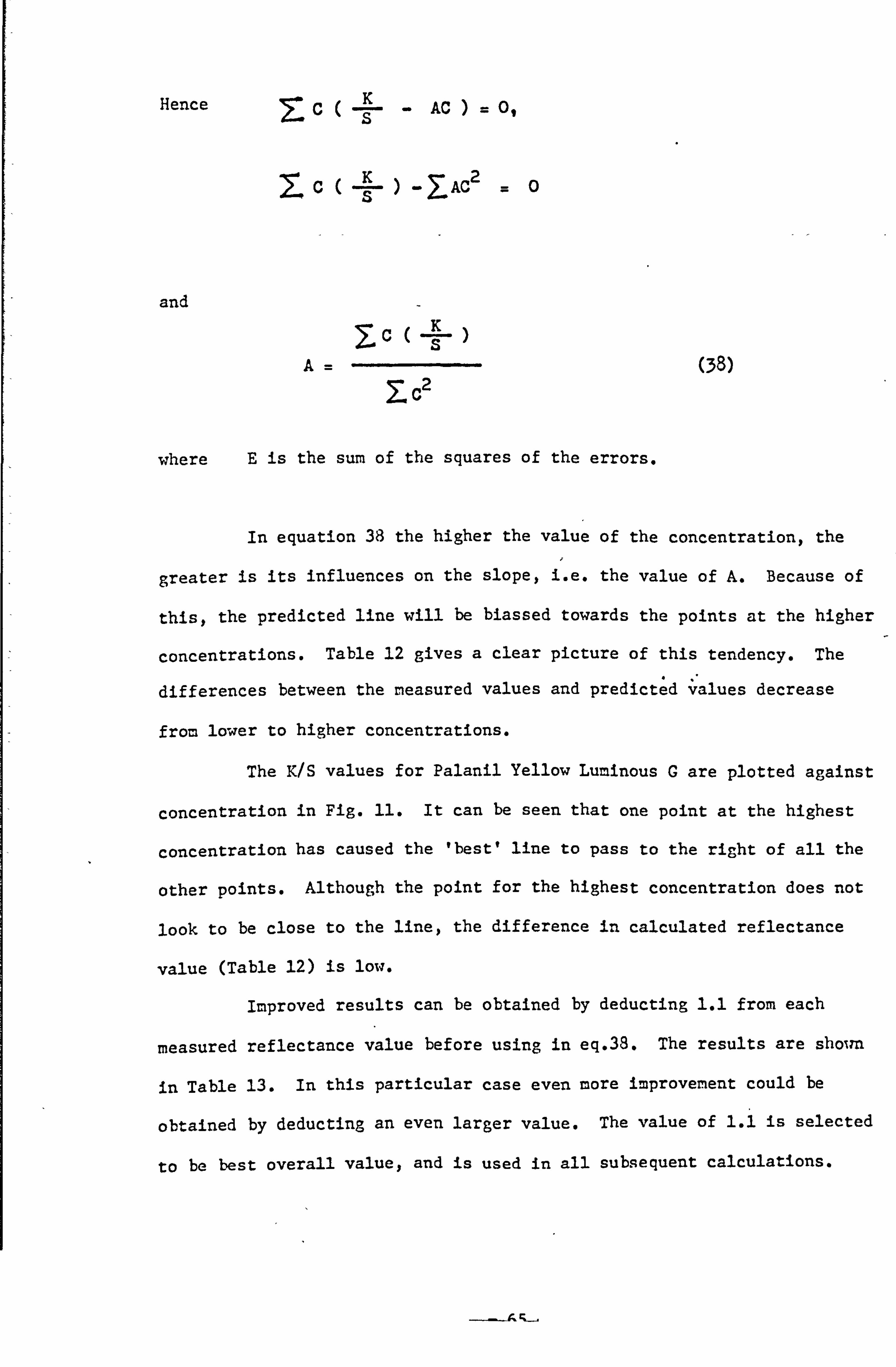
Hence C( --L - AC 0 s
C( _E_ )_2: AC2 =0 s
and
,CK s A= (38)
Zc 2
where E is the sum of the squares of the errors.
In equation 38 the higher the value of the concentration, the
greater is its influences on the slope, i. e. the value of A. Because of
this, the predicted line will be biassed towards the points at the higher
concentrations. Table 12 gives a clear picture of this tendency. The
differences between the measured values and predictýd values decrease
from lower to higher concentrations.
The K/S values for Palanil Yellow Luminous G are plotted against
concentration in Fig. 11. It can be seen that one point at the highest
concentration has caused the 'best' line to pass to the right of all the
other points. Although the point for the highest concentration does not
look to be close to the line, the difference in calculated reflectance
value (Table 12) is low.
Improved results can be obtained by deducting 1.1 from each
measured reflectance value before using in eq. 38. The results are sholm
in Table 13. In this particular case even more improvement could be
obtained by deducting an even larger value. The value of 1.1 is selected
to be best overall values and is used in all subsequent calculations.
----A rl-
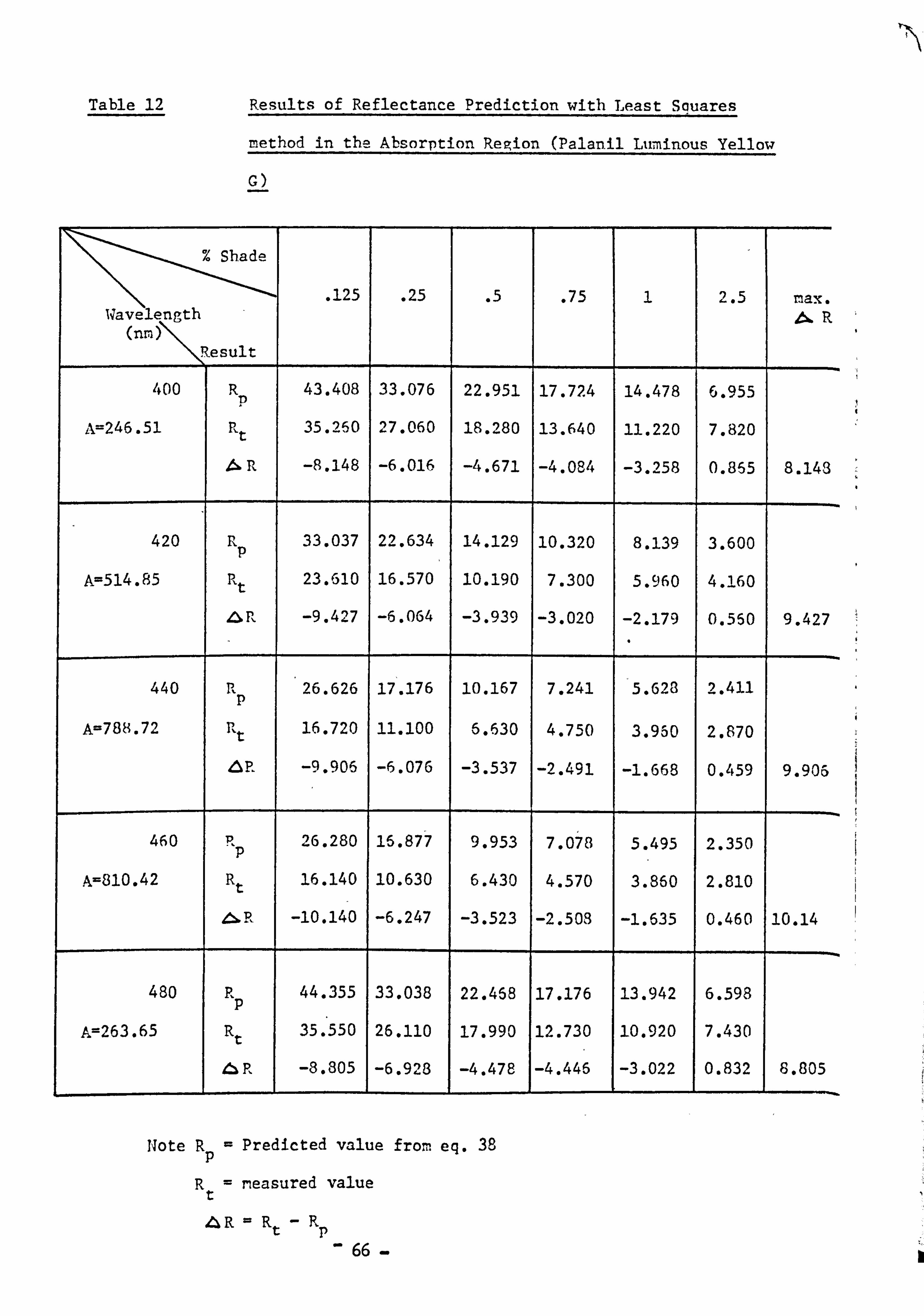
Table 12 Results of Reflectance Prediction with Least Souares
method in the Absorption Region (Palanil Liminous Yellow
G)
% Shadee
. 125 . 25 .5 . 75 1 2.5 max. Wave ength , b. ý R
(nri ýýZesult
400 R 43.408 33.076 22.951 17.724 14.478 6.955 p
A=246.51 Rt 35.260 27.060 18.280 13.640 11.220 7.820
ßýR -8.148 -6.016 -4.671 -4.084 -3.258 0.865 8.143
420 R 33.037 22.634 14.129 10.320 8.139 3.600 p
A--514.85 Rt 23.610 16.570 10.190 7.300 5.960 4.160
-9.427 -6.064 -3.939 -3.020 -2.179 0.550 9.427
440 pl 26.626 17'. 176 10.167 7.241 S. 628 2.411 p
A=788.72 plt 16.720 11.100 6.630 4.750 3.950 2.870
42ýpý -9.906 -6.076 -3.537 -2.491 -1.668 0.459 9.906
460 p 26.280 16.877 9.953 7.078 5.495 2.350 p
A=810.42 Rt 16.14 0 10.630 6.430 4.570 3.860 2.810
, ̂, R 1 -10.140 -6.247 -3.523 -2.503 -1.635 0.460 10.14
480 R 44.355 33.038 22.458 17.176 13.942 6.598 p
A=263.65 Rt 35.550 26.110 17.990 12.730 10.920 7.430
ZiR -8.805 -6.928 -4.478 -4.446 1 -3.022 1 0.832
1 8.805
Note Rp = Predicted value fron, eq. 38
Rt= neasured value
&R ý Rt -Rp- 66
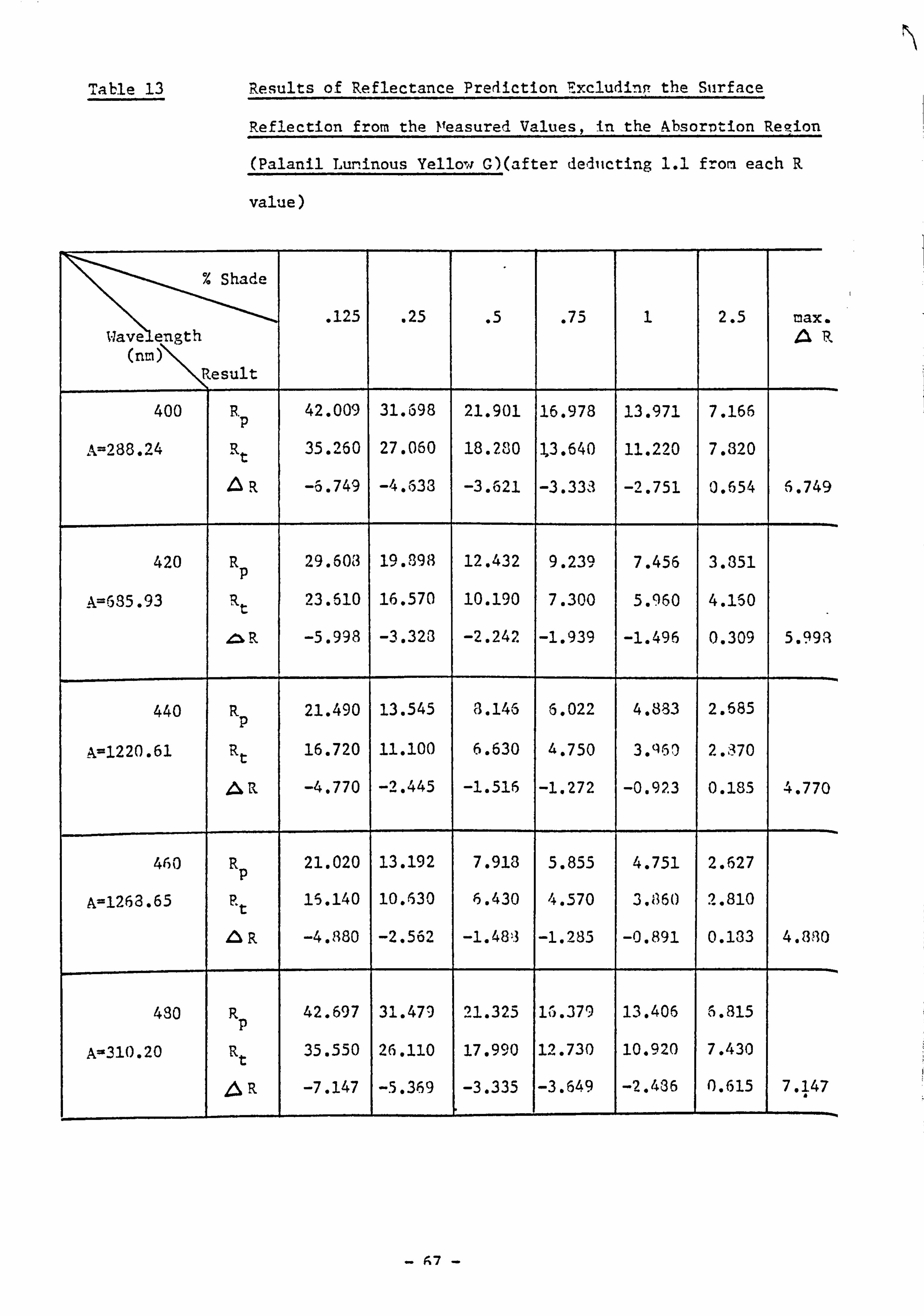
N Table 13 Results of Reflectance Pre4iction ExcludinR the Surface
Reflection from the Measured Values, in the_AbsorT)-%ion Region
(Palanil Luminous Yellow G)(after deditcting 1.1 fron each R
value)
7. Shade Shade
. 125 . 25 .5 . 75 1 2.5 max. I-lave e-ngth 'R,
(nm ' \Result
400 R 42.009 31.698 21.901 16.978
113.971
7.166 p
A=288.24 Rt 35.260 27.060 18.280 13.640 11.220 7.320
LR -6.749 -4.633 -3.621 -3.333 -2.751 0.654 6.749
420 R 29.603 19.898 12.432 9.239 7.456 3.351 p
, k--685.93 Rt 23.610 16.570 10.190 7.300 5.960 4.150
ziR -5.998 -3.323 -2.242 -1.939 -1.496 0.309 5.992
440 R 21.490 13.545 3.146 6.022 4.883 2.685 p
Au'1220.61 Rt 16.720 11.100 6.630 4.750 . qr 3 2.370
AR -4.770 -2.445 -1.516 -1.272 -0.923 0.185 4.770
460 R 21.020 13.192 7.913 5.855 4.751 2.627 p
A=1263.65 P. t 15.140 10.530 6.430 4.570 3.860 2.810
, in6R -4.880 -2.562 -1.48,3 -1.285 -0.891 0.133 4.330
480 R 42.697 31.479 21.325 16.379 13.406 5.815 p
A-310.20 Rt 35.550 26.110 17.990 12.730 10.920 7.430
, j: N R -7.147 -5.369 -3.335 1 -3.649
-- I -2.436 I
0.615 1
7.147 6-
- A7 -
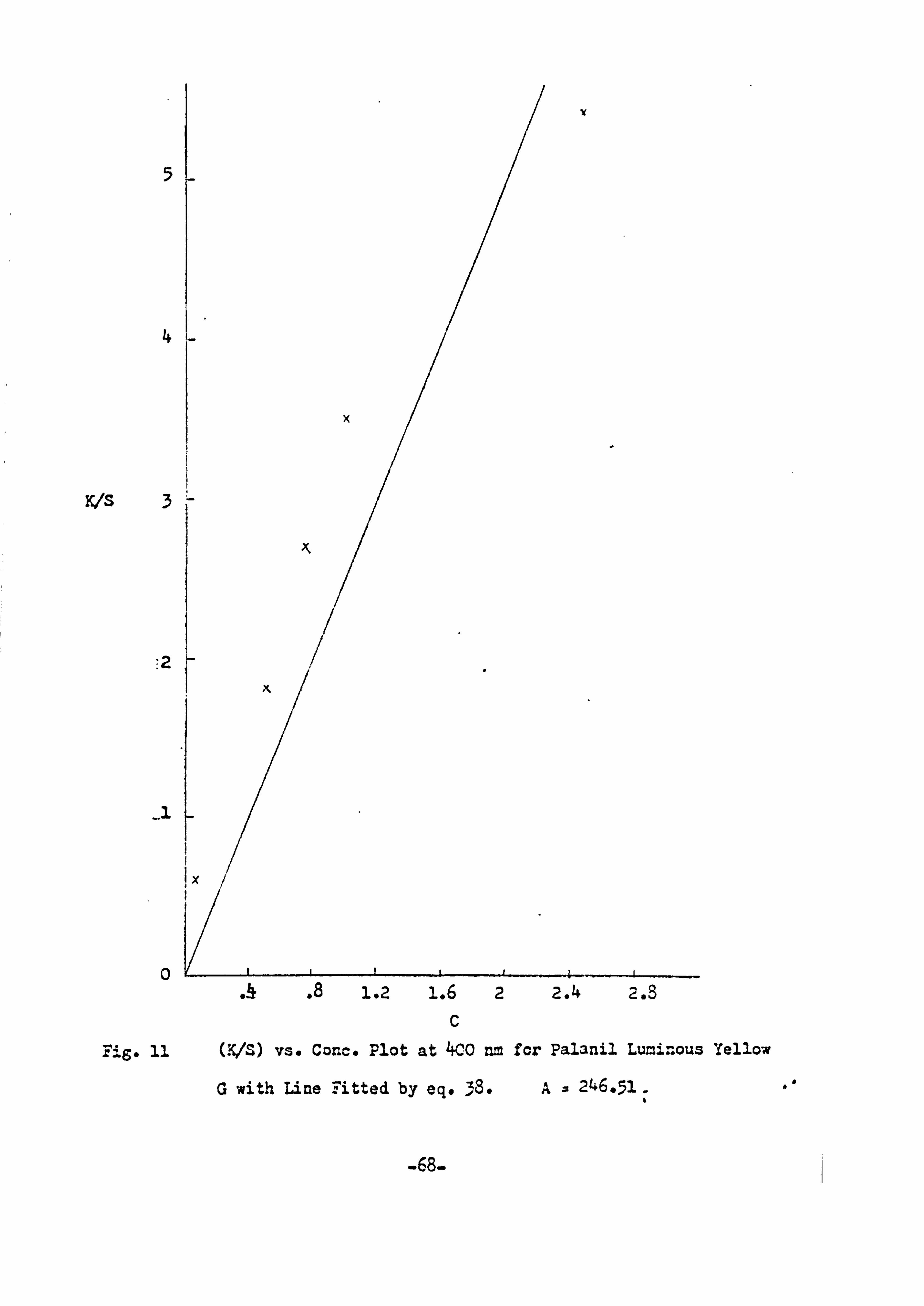
5
KIS
-1
0
c
Fig. 11 OVS) vs. Cane. Plot at 4CO = for Palanil Luminous Yellow
G with Line Fitted by eq. A= 246 -51
-68-
1.2 1.6 2 2.4 2.8
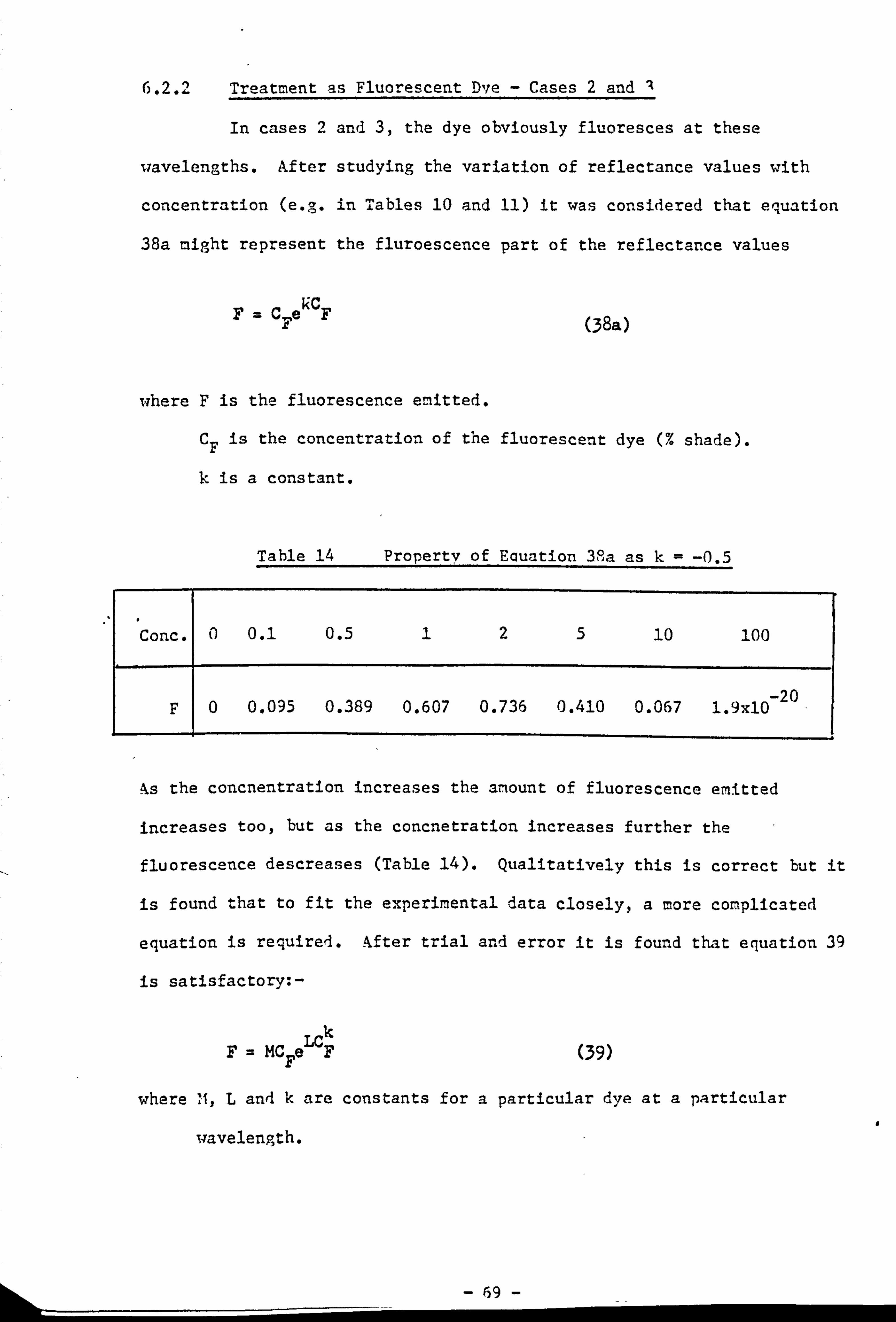
6.2.21 Treatment as Fluorescent Dve - Cases 2 and I
In cases 2 and 3, the dye obviously fluoresces at these
wavelengths. After studying the variation of reflectance values with
-ion (e., concentrat . in Tables 10 and 11) it was considered that equation
38a might represent the fluroescence part of the reflectance values
Ce kc F (38a)
where F is the fluorescence emitted.
CF is the concentration of the fluorescent dye (% shade).
k is a constant.
Table 14 Property of Equation 38a as k= -0.5
Conc. 0 0.1 0.5 125 10 100
F 20 0 0.095 0.389 0.607 0.736 0.410 0.067 1.9xlo-
As the concnentration. increases the amount of fluorescence emitted
increases too, but as the concnetration increases further the
fluorescence descreases (Table 14). Qualitatively this is correct but it
is found that to fit the experimental data closely, a more complicated
equation is required. After trial and error it is found that equation 39
is satisfactory: -
k MCIA F (39)
where 11, L and k are constants for a particular dye at a particular
wavelength. a
- 69 -
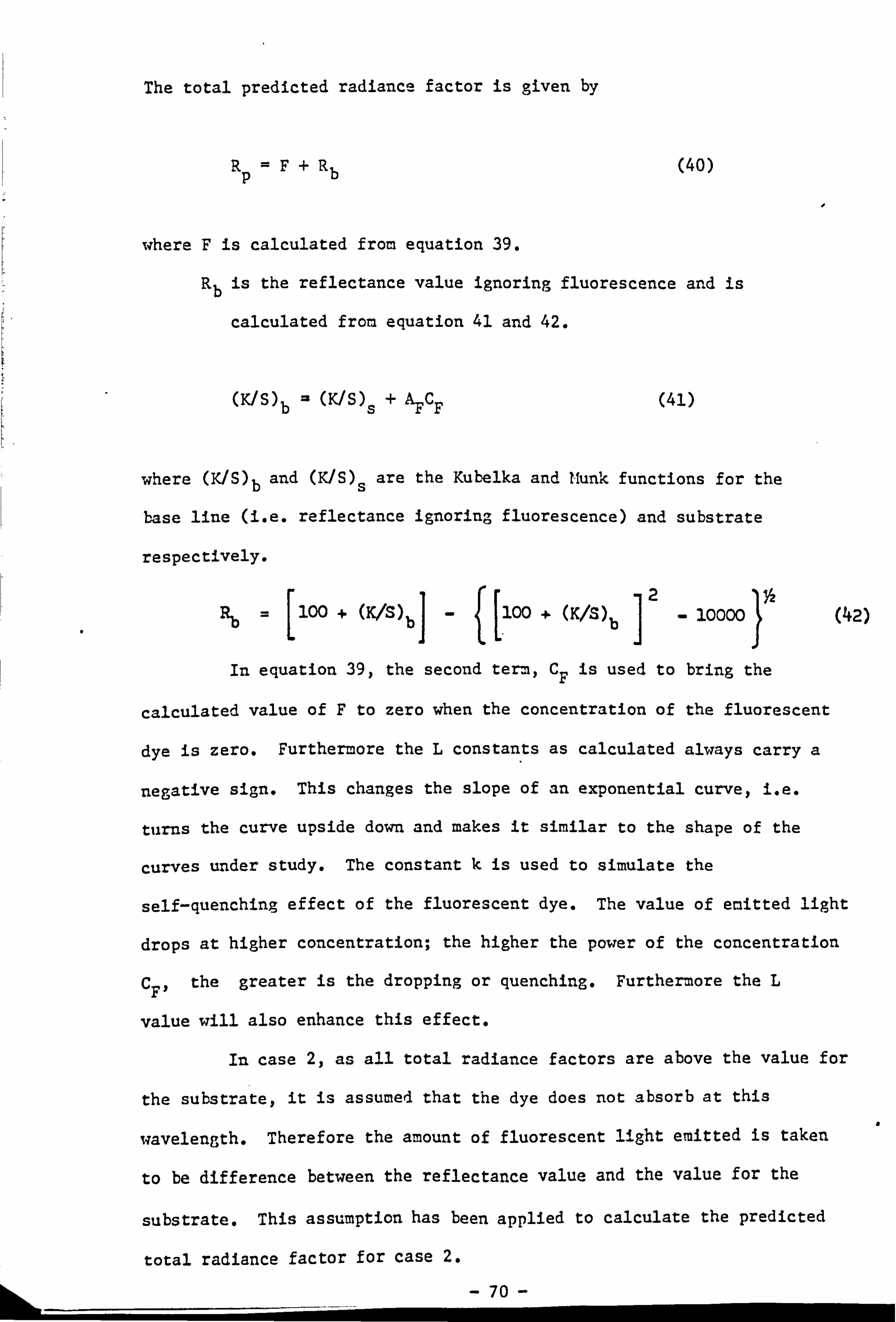
The total predicted radiance factor is given by
Rp =F+Rb (40)
where F is calculated from equation 39.
Rb is the reflectance value ignoring fluorescence and is
calculated from equation 41 and 42.
(K/S) b= (K/S) s+
AFICF
where (YJS)b and (K/S)s are the Kubelka and Munk functions for the
base line (i. e. reflectance ignoring fluorescence) and substrate
respectively.
100 + )bj 2-
10000 1 Y2
(42) Rb '2
[ (K/S
[. 100 + (K/S)b
In equation 39, the second term, CF is used to bring the
calculated value of F to zero when the concentration of the fluorescent
dye is zero. Furthermore the L constan . ts as calculated always carry a
negative sign. This changes the slope of an exponential curve, i. e.
turns the curve upside down and makes it similar to the shape of the
curves under study. The constant k is used to simulate the
self-quenching effect of the fluorescent dye. The value of emitted light
drops at higher concentration; the higher the power of the concentration
CF' the greater is the dropping or quenching. Furthermore the L
value will also enhance this effect.
In case 2, as all total radiance factors are above the value for
the substrate, it is assumed that the dye does not absorb at this
wavelength. Therefore the amount of fluorescent light emitted is taken
to be difference between the reflectance value and the value for the
substrate. This assumption has been applied to calculate the predicted
total radiance factor for case 2.
a
70
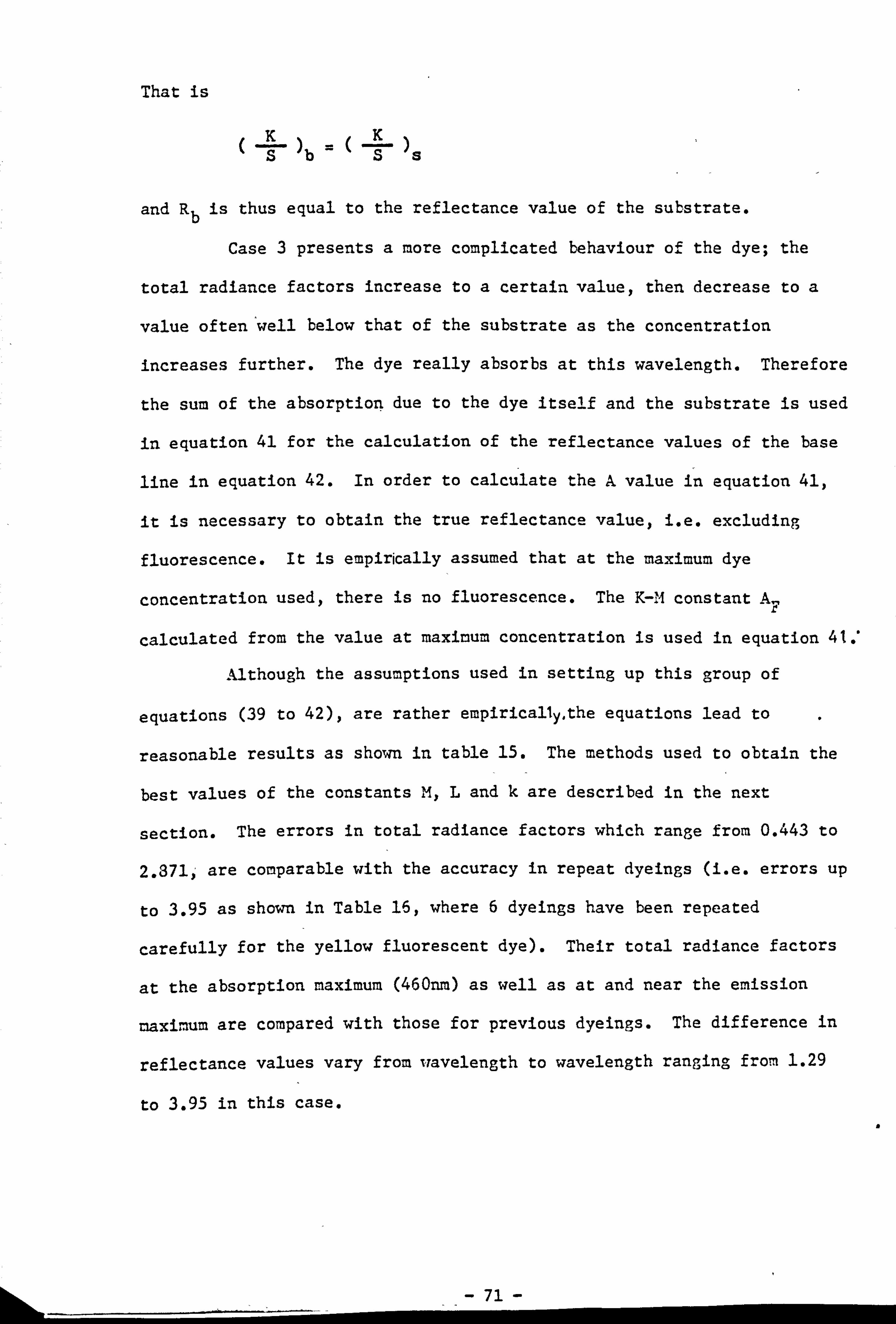
That is
(I) =( I) sb and Rb is thus equal to the reflectance value of the substrate.
' the dye; the Case 3 presents a more complicated behaviour of
total radiance factors increase to a certain value, then decrease to a
value oftenwell below that of the substrate as the concentration
increases further. The dye really absorbs at this wavelength. Therefore
the sum of the absorption due to the dye itself and the substrate is used
in equation 41 for the calculation of the reflectance values of the base
line in equation 42. In order to calculate the A. value in equation 41,
it is necessary to obtain the true reflectance value, i. e. excluding
fluorescence. It is empirically assumed that at the maximum dye
concentration used, there is no fluorescence. The K-M constant AF
calculated from the value at maximum concentration is used in equation 41. '
Although the assumptions used in setting up this group of
equations (39 to 42), are rather empirically, the equations lead to
reasonable results as shown in table 15. The methods used to obtain the
best values of the constants M, L and k are described in the next
section. The errors in total radiance factors which range from 0.443 to
2.371., are comparable with the accuracy in repeat dyeings (i. e. errors up
to 3.95 as shown in Table 16, where 6 dyeings have been repeated
carefully for the yellow fluorescent dye). Their total radiance factors
at the absorption maximum (460nm) as well as at and near the emission
maximum are compared with those for previous dyeings. The difference in
reflectance values vary from wavelength to wavelength ranging from 1.29
to 3.95 in this case.
71 -
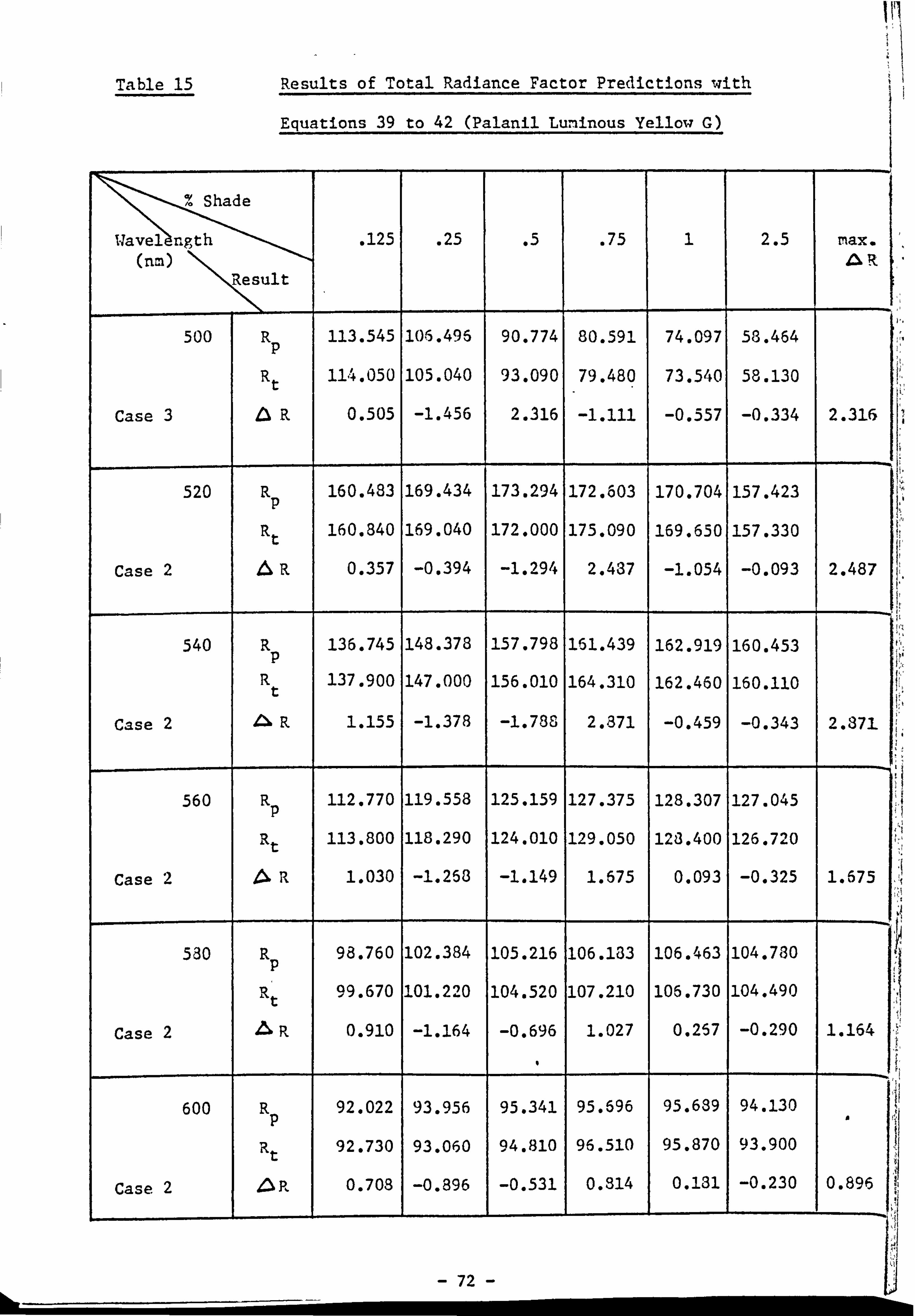
Table 15 Results of Total Radiance Factor Predictions with
Equations 39 to 42 (Palanil Luminous Yellow G)
Shade
Wavel ngth . 125 . 25 .5 . 75 1 2.5 max. (nm)
it
500 R 113.545 105.496 90.774 80.591 74.097 58.464 p
R t 114.050 105.040 93.090 79.480 73.540 58.130
Case 3 ZI R 0.505 -1.456 2.316 -1.111 -0.557 -0.334 2.316
520 R 160.483 169.434 173.294 172.603 170.704 157.423 p
Rt 160.840 169.040 172.000 175.090 169.650 157.330
Case 2 AR 0.357 -0.394 -1.294 2.437 -1.054 -0.093 2.487
540 R 136.745 148.378 157.798 161.439 162.919 160.453 p
R 137.900 147.000 156.010 164.310 162.460 160.110 t
Case 2 06R 1.155 -1.378 -1.788 2.871 -0.459 -0.343 2.371-
560 R 112.770 119.558 125.159 127.375 128.307 127.045 p
Rt 113.800 118.290 124.010 129.050 128.400 126.720
Case 2 R 1.030 -1.253 -1.149 1.675 0.093 -0.325 1.675
530 R 98.760 102.384 105.216 106.133 106.463 104.780 p
Rt 019.670 101.220 104.520 107.210 106.730 104.490
Case 2 P, 0.910 -1.164 -0.696 1.027 0.257 -0.290 1.164
600 R 92.022 93.956 95.341 95.696 95.689 94.130 p
Rt 92.730 93.060 94.810 96.510 95.870 93.900
Case 2 4ýR 0.708 -0.896 -0.531 0.814 0.131 -0.230 0.896
Ii M
72
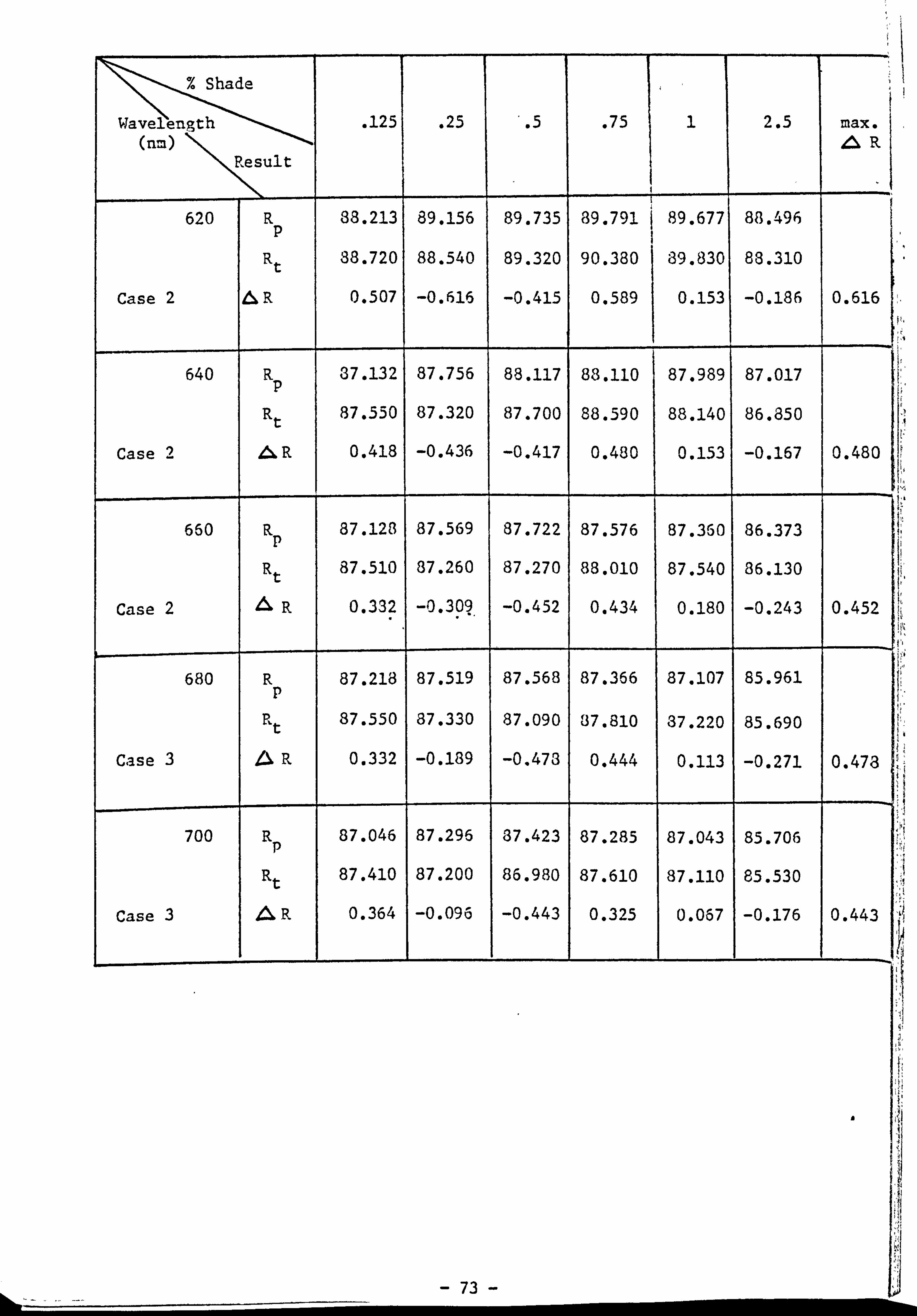
% Shade
Wave en th ýe g . 125 . 25 . .5 . 75 1 2.5 max. nm. NN"' 41 R
ýResult
620 R 38.213 89.156 89.735 89.791 89.677 88.496
Rt 38.720 88.540 89.320 90.380 39.830 83.310
Case 2 AR 0.507 -0.616 -0.415 0.589 0.153 -0.186 0.616
640 R 37.132 87.756 88.117 88.110 87.989 87.017 p
Rt 87.550 87.320 87.700 88.590 88.140 86.850
Case 2 R 0.418 -0.436 -0.417 0.480 0.153 -0.167 0.480
660 R 87.128 87.569 87.722 87.576 87.350 86.373 p
Rt 87.510 87.260 87.270 88.010 87.540 86.130
Case 2 R 0.332 -0.307, -0.452 0.434 0.180 -0.243 0.452
680 R 87.218 87.519 87.568 87.366 87.107 85.961 p
Rt 87.550 87.330 87.090 37.810 37.220 85.690
Case 3 Aa R 0.332 -0.189 -0.473 0.444 0.113 -0.271 0.473
700 Rp 87.046 87.296 37.423 87.285 87.043 85.706
Rt 87.410 87.200 86.980 87.610 87.110 85.530
Case 3 A& R 0.364 -0.096 -0.443 0.325 0.067 -0.176 0.443
73
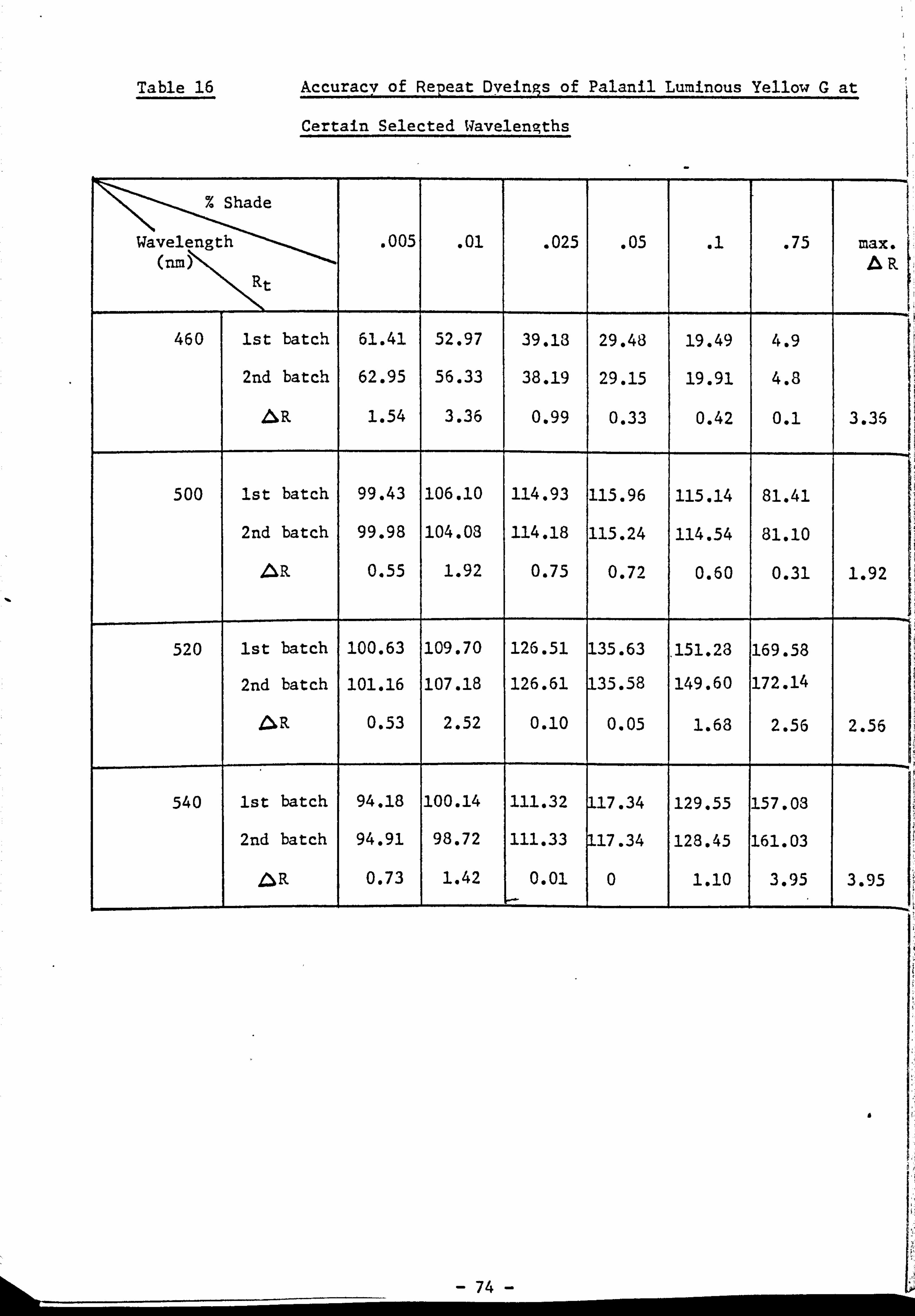
Table 16 Accuracy of Repeat Dyeings of Palanil Luminous Yellow G at
Certain Selected Wavelengths
% Shade
Wavelen; ý-"--,,,
. 005 . 01 . 025 . 05 .1 . 75 max. ,.., (rLm)N R
Rt
460 ist batch 61.41 52.97 39.13 29.48 19.49 4.9
2nd batch 62.95 56.33 38.19 29.15 19.91 4.8
&R 1.54 3.36 0.99 0.33 0.42 0.1 3.36
500 lst batch 99.43 106.10 114.93 115.96 115.14 81.41
2nd batch 99.98 104.03 114.18 115.24 114.54 81.10
, ýNR 0.55 1.92 0.75 0.72 0.60 0.31 1.92
520 ist batch 100.63 109.70 126.51 135.63 . 151.23 169.58
2nd batch 101.16 107.18 126.61 135.58 149.60 172.14
06R 0.53 2.52 0.10 0.05 1.68 2.56 2.56
540 ist batch 94.18 100.14 111.32 117.34 129.55 157.03
2nd batch 94.91 98.72 111.33 117.34 128.45 161.03
, aR 0.73 1.42 0.01 0 1.10 3.95 3.95
- 74 -

6.2.3 Development of Computer Pr gram
Following the ideas developed in Sections 6.2.1 and 6.2.2, flow
chart III is used to develop a computer program for calculating the
constants ky, L, M in equation 39 with data from calibration dyeings of
the fluorescent dyes at various concentrations. (The Actual program is
listed in Appendix C. )
The starting values of k and L are guessed to be 0.25 and -6
respectively (from a series of preliminary calculations at certain
wavelengths), while the constant M is calculated by fitting a line for L-C k
equation 39 (i. e. F vs CFe, F) by the method of least squares.
7 LC k [F (CFe F
m-k (42a) I (CeLCF
The value of F in the equation is calculated as follows:
For case 2
R ri - (43)
For case
( 100 -R X) 2
x 2R x
AKK xsxS sl
/ Cmax (44a)
( -. L )=( --L ) 'A C (44b) sxF
[100 +K]2- 10000 (44c)
bS ')b] [100
+( SK )b
- 75 -
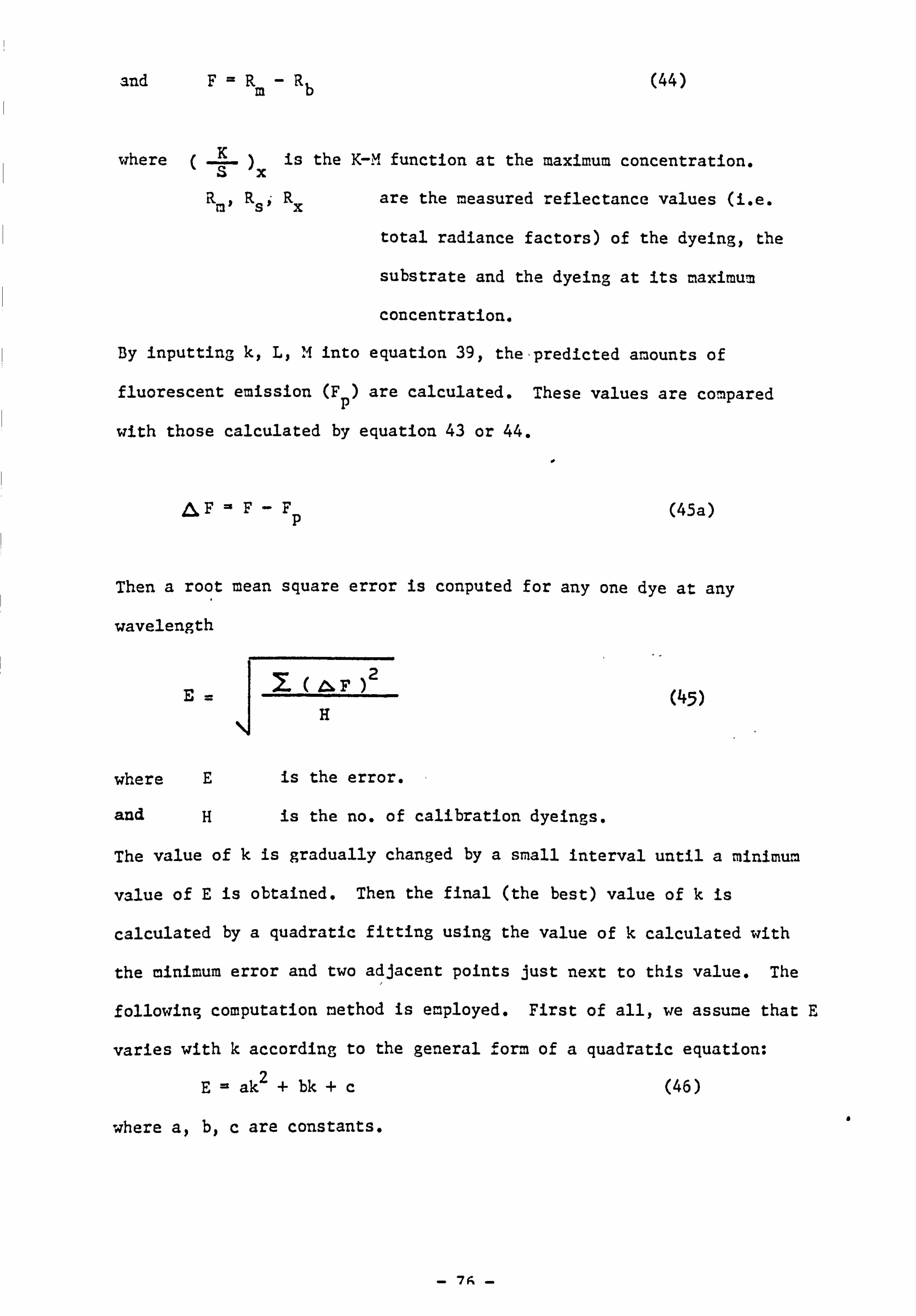
and F=Rm-Rb (44)
where K is the K-M function at the maximum concentration. Sx RsiRx are the measured reflectance values (i. e.
total radiance factors) of the dyeing, the
substrate and the dyeing at its maximum
concentration.
By inputting k, L$ 1.4 into equation 39, the, predicted amounts of
fluorescent emission (F p) are calculated. These values are compared
with those calculated by equation 43 or 44.
,&F=F- (45a)
Then a root mean square error is conputed for any one dye at any
wavelength
J (45)
where E is the error.
and H is the no. of calibration dyeings.
The value of k is gradually changed by a small interval until a miniMum
value of E is obtained. Then the final (the best) value of k is
calculated by a quadratic fitting using the value of k calculated with
the minimum error and two adjacent points just next to this value. The
following computation method is employed. First of all, we assume that E
varies with k according to the general form of a quadratic equation:
E=A2+ bk +c (46)
where a, b, c are constants. a
- 7r% -
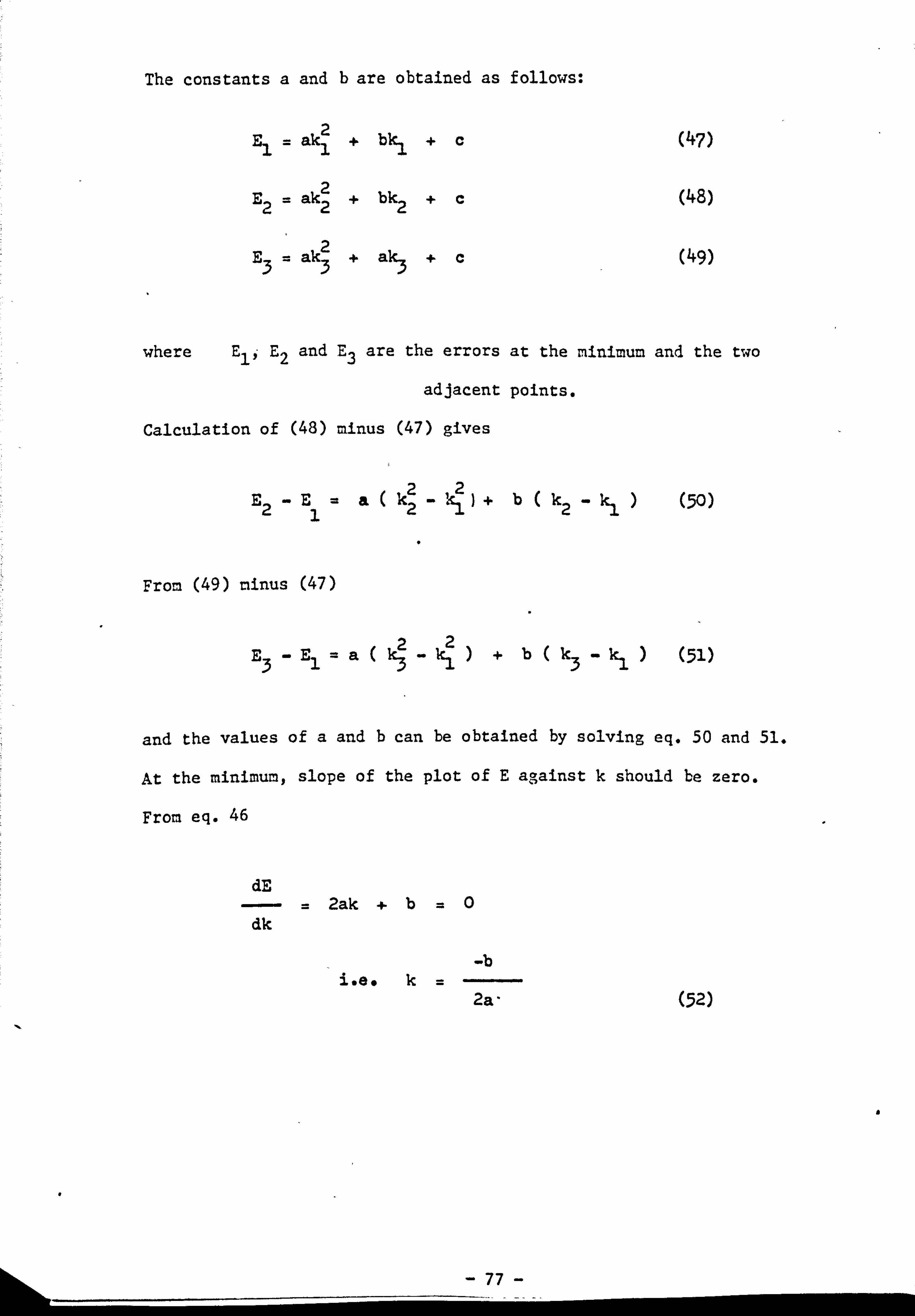
The constants a and b are obtained as follows:
2 E, = aki + bk, +c (47)
E ak 2+ bk +c (48)
222
E ak 2+
ak3 +c (49) 33
where Eli E2 and E3 are the errors at the minimum and the two
adjacent points.
Calculation of (48) minus (47) gives
22 E2-Ea ki Ici) +b(k2- kl (50)
From (49) minus (47)
2 3- El a k, +b( k3 - k,
and the values of a and b can be obtained by solving eq. 50 and 51.
At the minimura, slope of the plot of E a, -,, ainst k should be zero.
From eq. 46
dE 2ak +b=0
dk
-b i. ee
2a- (52)
I
a
- 77
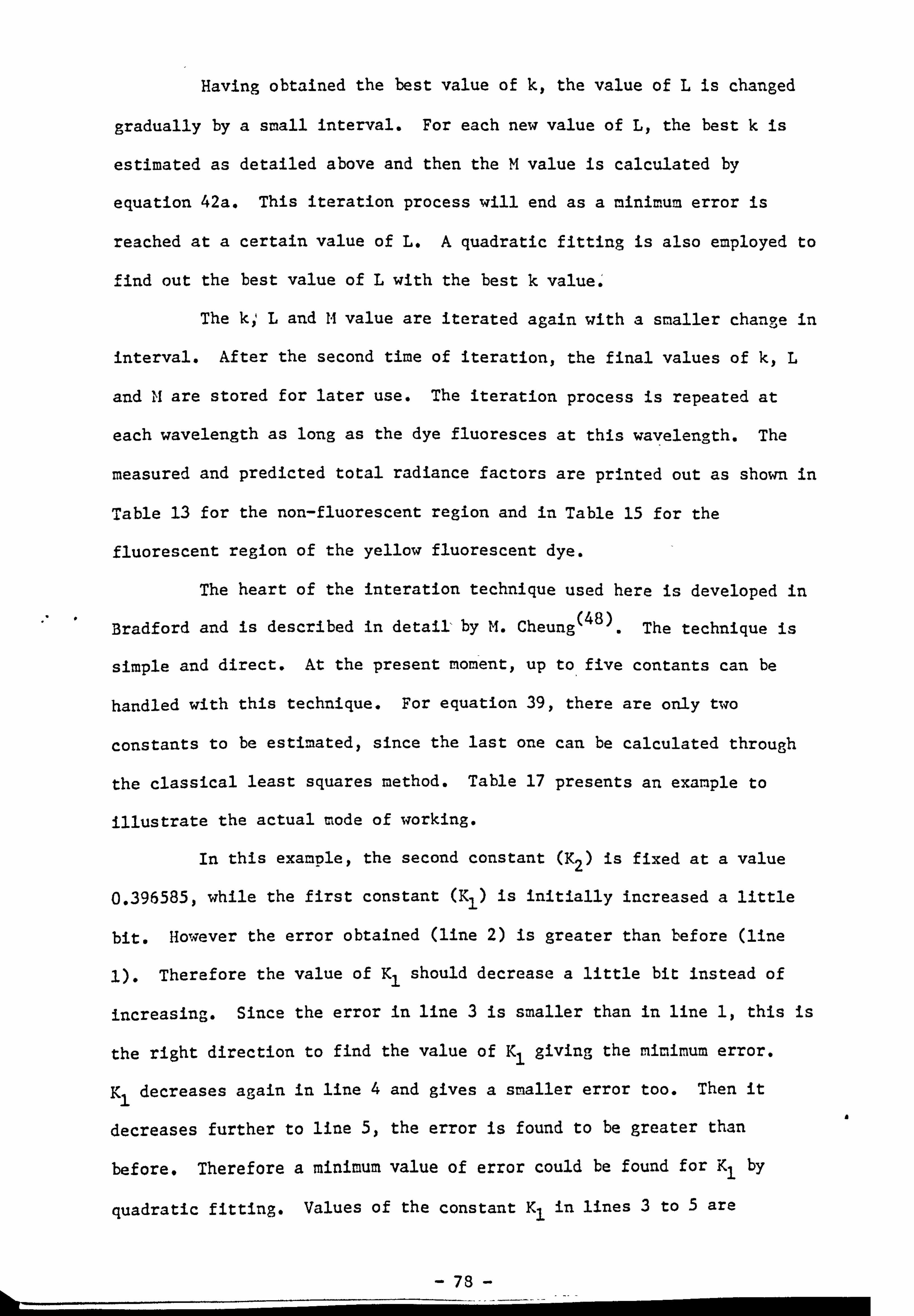
Having obtained the best value of k, the value of L is changed
gradually by a small interval. For each new value of L, the best k is
estimated as detailed above and then the M value is calculated by
equation 42a. This iteration process will end as a minimum error is
reached at a certain value of L. A quadratic fitting is also employed to
find out the best value of L with the best k value. ' .L
The kIL and 14 value are iterated again with a smaller change in
interval. After the second time of iteration, the final values of k, L
and M are stored for later use. The iteration process is repeated at
each wavelength as long as the dye fluoresces at this wavelength. The
measured and predicted total radiance factors are printed out as shown in
Table 13 for the non-fluorescent region and in Table 15 for the
fluorescent region of the yellow fluorescent dye.
The heart of the interation technique used here is developed in (48)
Bradford and is described in detail-by M. Cheung . The technique is
simple and direct. At the present moment, up to five contants can be
handled with this technique. For equation 39, there are only two
constants to be estimated, since the last one can be calculated through
the classical least squares method. Table 17 presents an example to
illustrate the actual mode of working.
In this example, the second constant (K2) is fixed at a value
0.396585, while the first constant (Kl) is initially increased a little
bit. However the error obtained (line 2) is greater than before (line
1). Therefore the value of K, should decrease a little bit instead of
increasing. Since the error in line 3 is smaller than in line 1, this is
the right direction to find the value of K, giving the mimimum error.
K, decreases again in line 4 and gives a smaller error too. Then it
decreases further to line 5, the error is found to be greater than
before. Therefore a minimum value of error could be found for K, by
quadratic fitting. Values of the constant K, in lines 3 to 5 are
a
78

substituted into equations 47 to 49 respectively. The value of K, is
calculated and shown in line 6 with the minimum error (marked with *) at
the fixed value Y'2'
The second step is to change K2 by a bit and then K, is
varied again to obtain the best value with minimum error at this new K2
value (lines 7 to 10). The error at line 10 is compared with one at line
6 for the old value of K2. If it is smaller, the increase in the value
of K2 is the right direction, otherwise its value should be decreased.
Now it is samller, so K2 is further increased to obtain another best
value of 'Kl at this value (lines 11 to 14). The error at line 14 is
smaller than that at line 10, the process is continued till line 22 where
the error is bigger than the one at line 18. Therefore the best value
for K2 is obtained by a quadratic fitting of the K2 values at lines
14,18 and 22. At this new K2, K, is iterated again for the'best
value with minimum error. The final values at line 26 are the chosen
values for K1 and K2. They usually cgive the best fit to the equation
concerned with minimum error. Unfortunately, the value of error at line
26 is a little bit bigger than the one at line 18. This only occurs
sometimes and is an imperfection of the technique. However, it is
thought to be a minor defect and can probably be removed anyway. This
technique is used through out this project and called "Direct Iteration
Technique"i and has proved to be a very useful method.
a
79
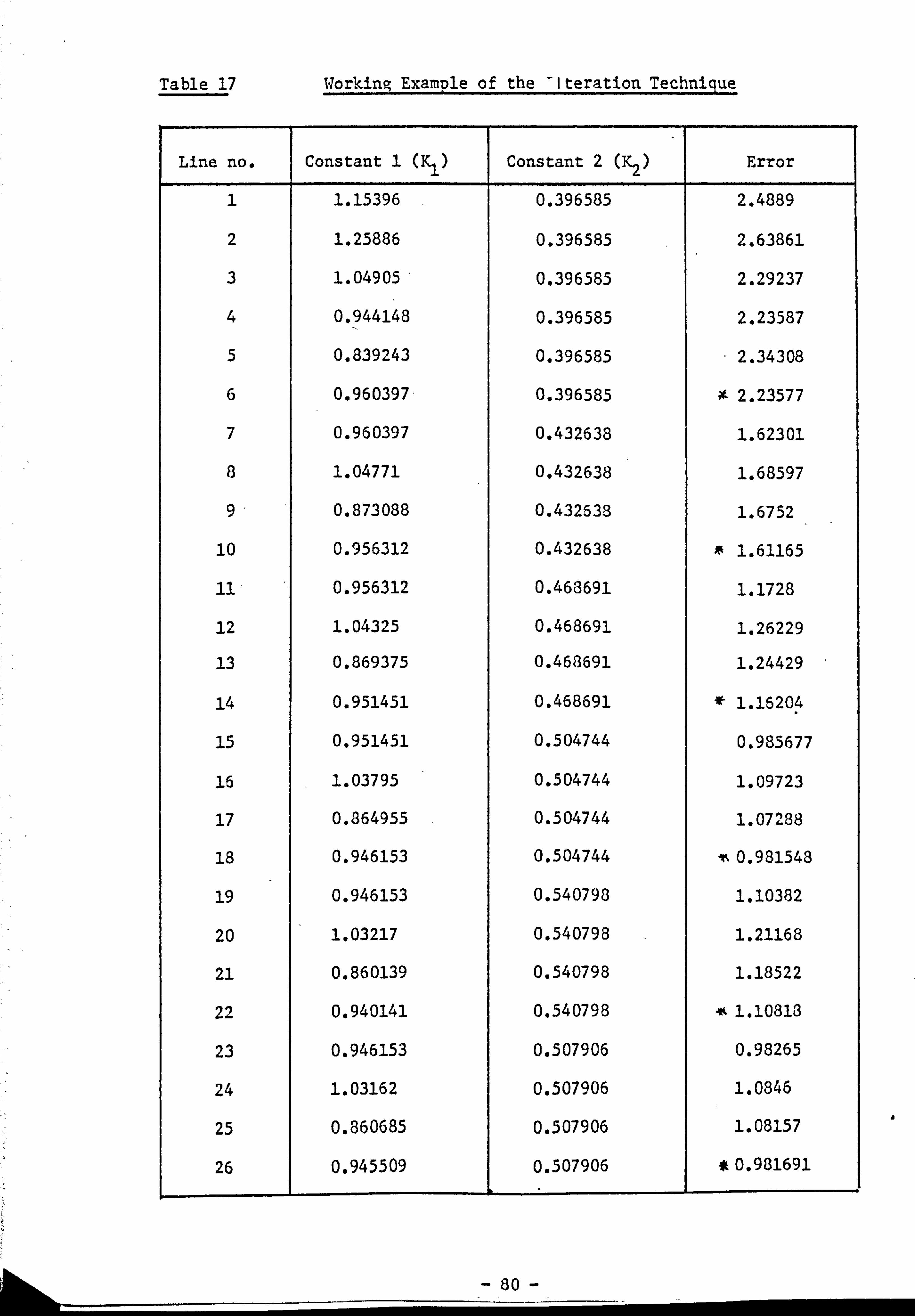
Table 17 Working Example of the 'Iteration Technique
Line no. Constant 1 (K 1 Constant 2( K2) Error
1 1.15396 0.396585 2.4889
2 1.25886 0.396585 2.63861
3 1.04905' 0.396585 2.29237
4 0.944148 0.396585 2.23587
5 0.839243 0.396585 2.34308
6 0.960397, 0.396585 2.23577
7 0.960397 0.432638 1.62301
a 1.04771 0.432638 1.68597
9 0.873088 0.432533 1.6752
10 0.956312 0.432638 1.61165
ill 0.956312 0.463691 1.1728
12 1.04325 0.468691 1.26229
13 0.869375 0.468691 1.24429
14 0.951451 0.468691 1.16204
15 0.951451 0.504744 0.985677
16 1.03795 0.504744 1.09723
17 0.864955 0.504744 1.07d.
18 0.946153 0.504744 -, r, 0.981543
19 0.946153 0.540798 1.10382
20 1.03217 0.540798 1.21168
21 0.860139 0.540798 1.18522
22 0.940141 0.540798 1.10813
23 0.946153 0.507906 0.93265
24 1.03162 0.507906 1.0846
25 0.860685 0.507906 1.08157
26 0.945509 0.507906 L
0.931691
- 80 -
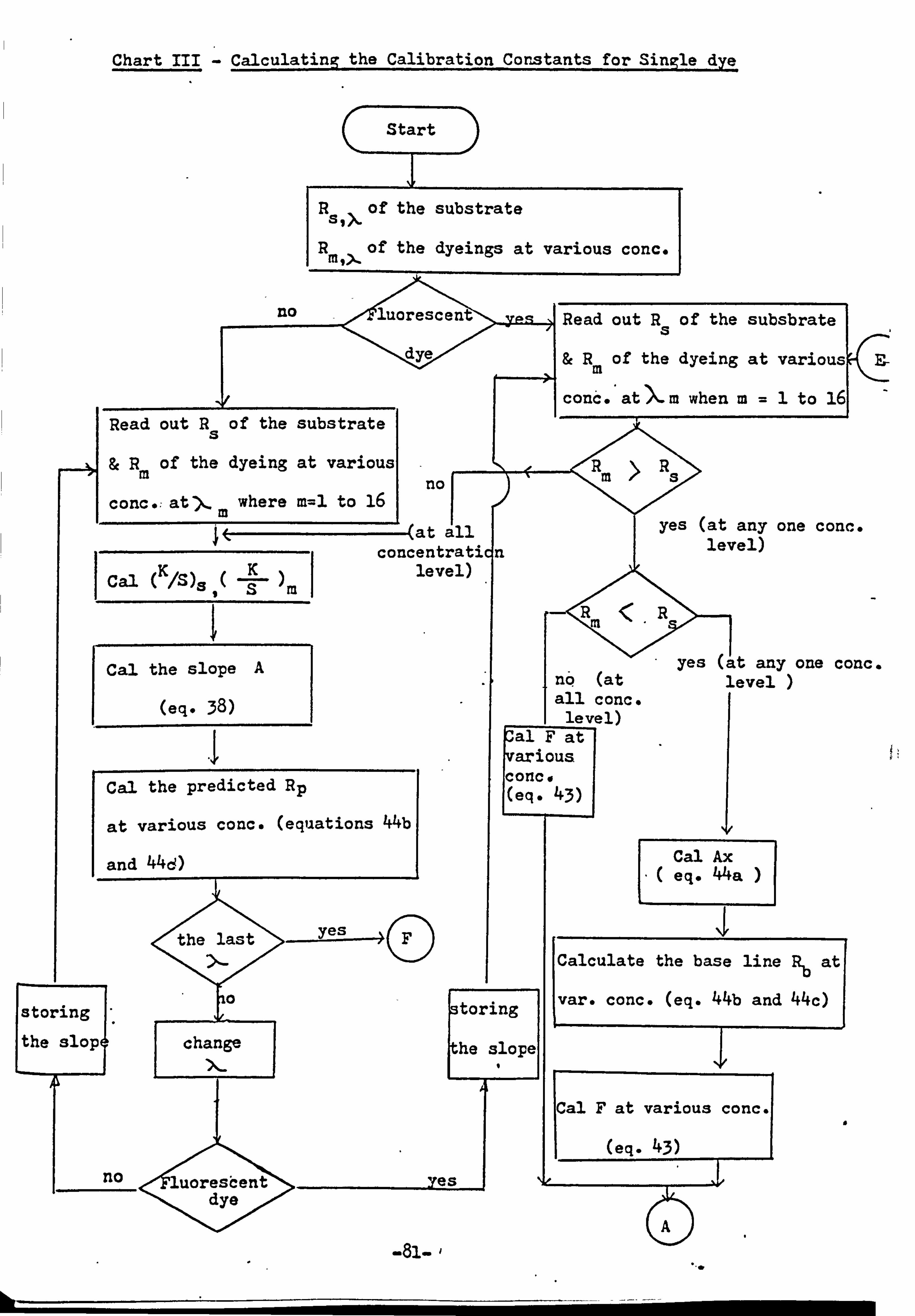
Chart III - Calculating the Calibration Constants for SinSle dye
Start
R SIX of the substrate
R M9>. of the dyeings at various conc.
no lunrescen, Read out R of the subsbrate S de&Rm of the dyeing at various
conc 4, at )ý- m when m=1 to 161 Read out R of the substrate s &Rm of the dyeing at various
no conc.; at-),, where m--1 to 16
concen KK level) Cal ( IS)s
m
Cal the slope A
(eq. 38)
Cal the predicted Rp
at various conc. (equations 44b
and 44d)
the las ---- 4ýf
toring
Ihe slop
yes (. ýt any one conc. level
Cal Ax eq. 44a
I Calculate the base line Rb at
var. conc. (eq. 44b and 44c)
F at various conc.
(eq. 43)
1
no <Zuores6eni dye
_,
>
yes (at any one cone. level)
nq (at all cone.
level) Cal F at various cone e (eq. 43)
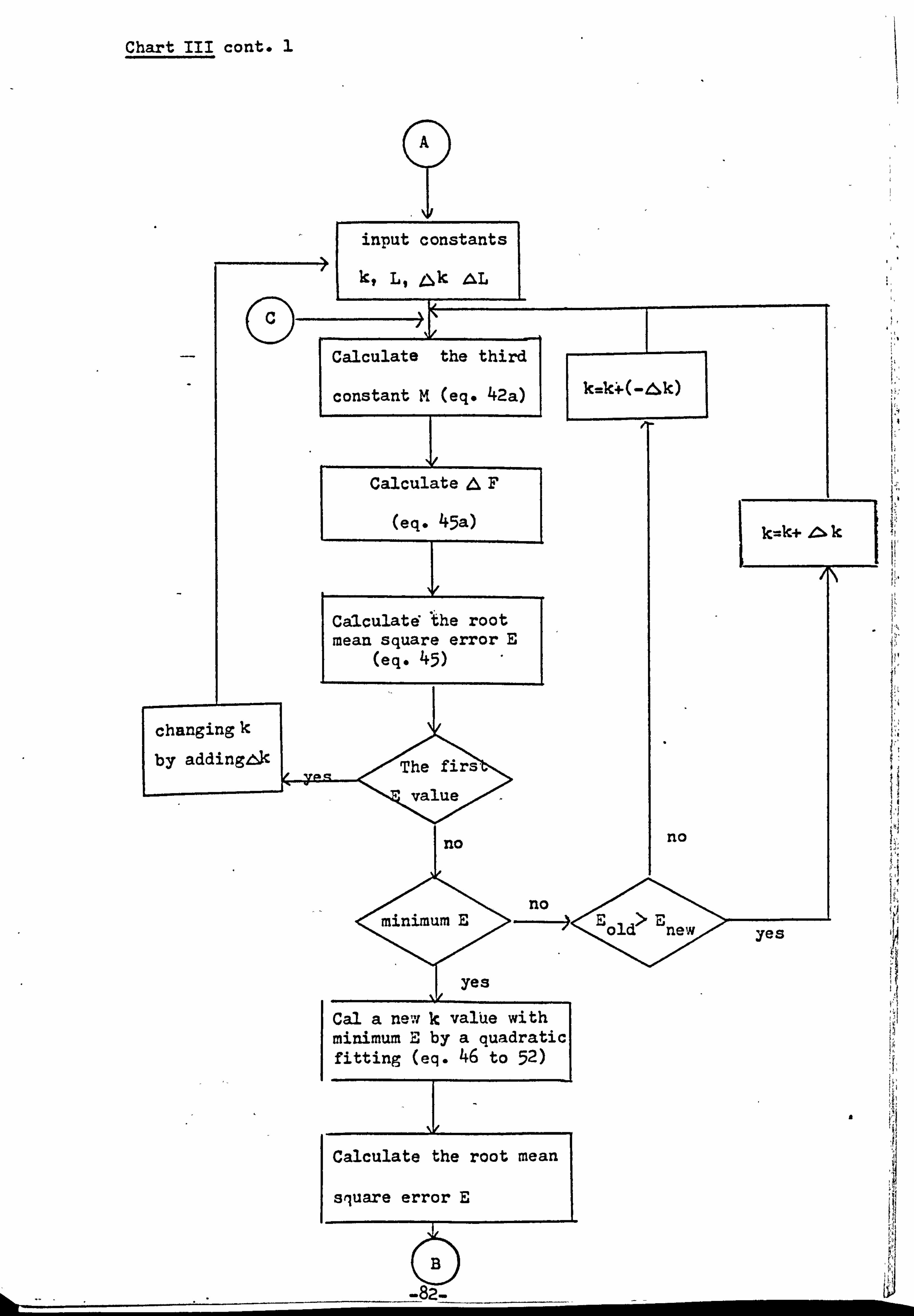
Chart III cont. 1
TA
input constants
L, Llýk AL
ate the third
constant M (eq. 42a)
Calculate AF
(eq. 45a)
k=ký(-Ak)
k=k+ 4ý- k
*the root Cal-culatd mean square error E
(eq. 45)
g
changing k
by adding, 61c The firs-
value
no no
no minimum E>E
od new yes
yes
Cal a new k valUe with minimum E by a quadratic fitting (eq. 46 to 52)
r 10' 1:
1
Calculate the root mean
square error E
B
-82-
Calculatd ihe root mean square error E
(eq. 45)
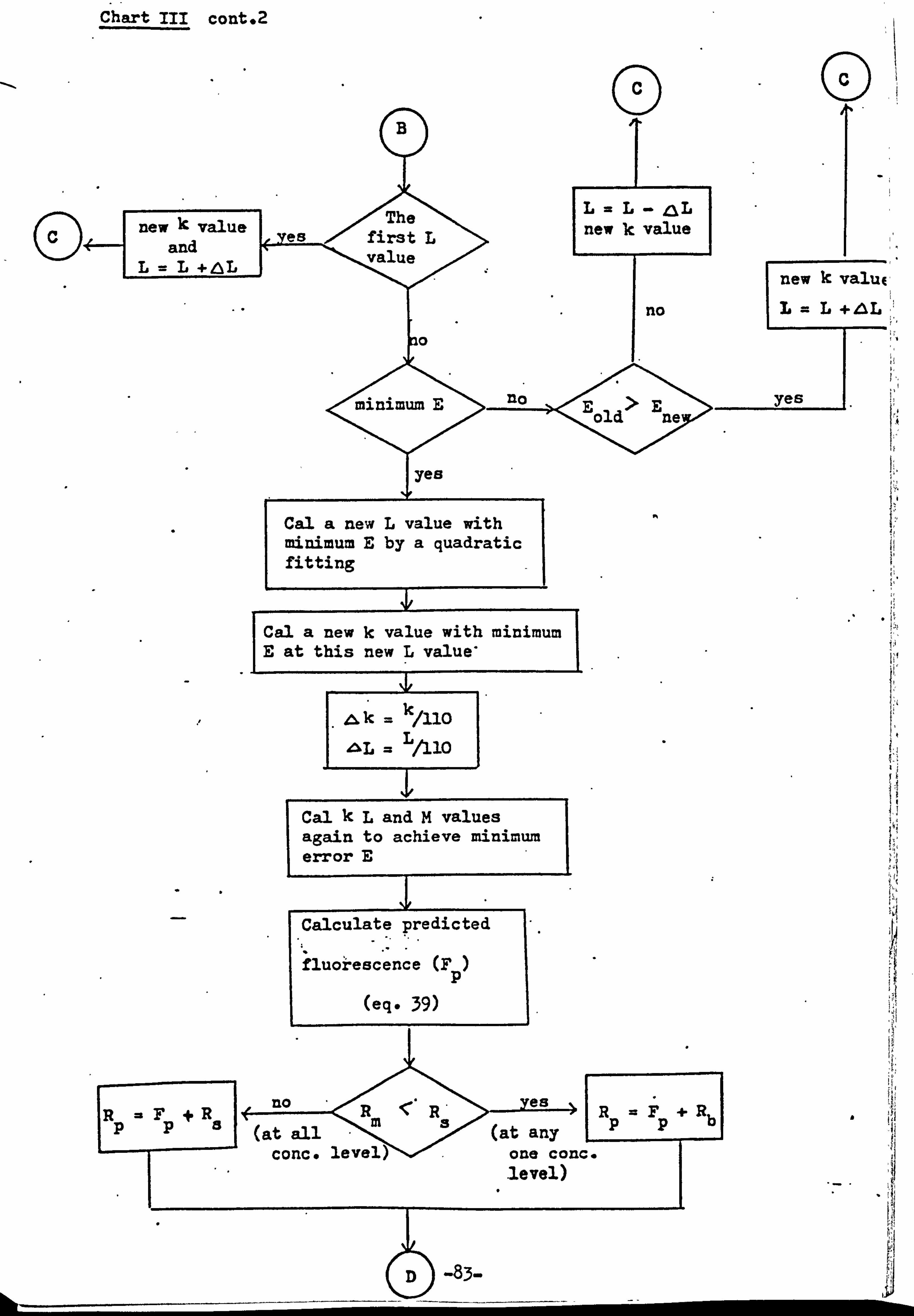
Chart III cont. 2
B
new k value The LL ZIL
Dc es first L new k value and valu lue value LL+, 8L
new k valuc
no L=L+, aL
minimum E yes ld> Ene
yes
Cal a new L value with minimum E by a quadratic fitting
;j
-T- Cal a new k value with minimum E at this new L value'
k= k/110
A'I L= L/l
10
Cal kL and M values again to achieve minimum error E
Calculate predicted
ence (F ) N, iluoiesc* P
(eq. 39)
no es es RaF+R4R R' R+R Ppmb (at all at any PP (at any
conc. level one c O'n one conco level)
D -83-
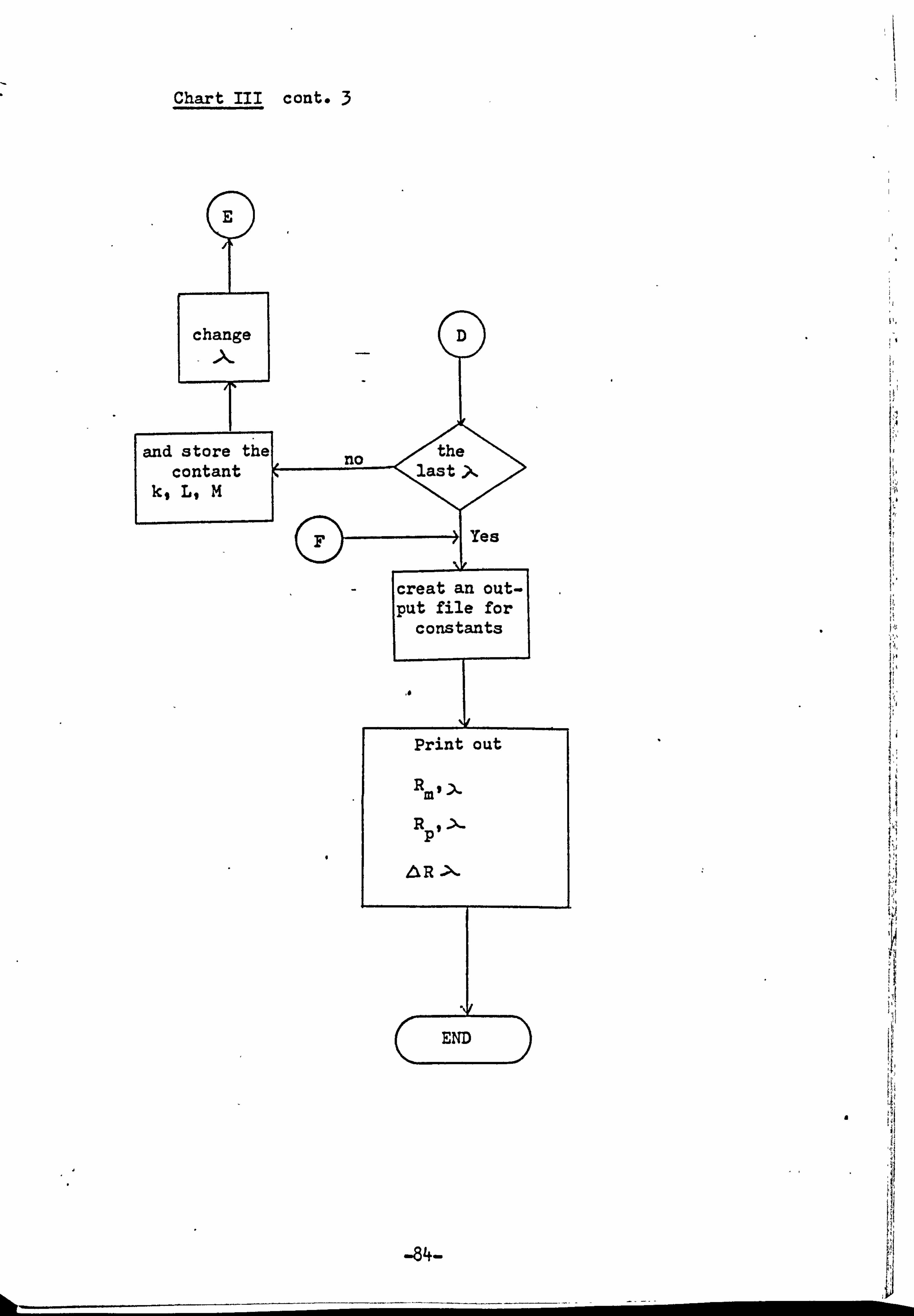
Chart III cont-
-84-
6.3 Mixture Dyeings with a Fluorescent Dve and a Non-fluorescent Dye
6.3.1 The Non-fluorescent Dves
Four dyes are chosen in order to investigate the interaction of 0
them with the fluorescent dyes. They are Palanil Red 5BEL, lalanil Pink
REL, Palanil Yellow 3G and Foron Blue SER. With reference to their
reflectance curves; they might be classified into two groups. The yellow
and blue are said to be true non-fluorescent dyes as their reflectance
values are always below the value of the substrate. The red one shows a
little bit of fluorescence in the red end and the pink one slightly
fluoresces at the same end (Fig. 12 and 13). Therefore they are treated
as pseudo-non-fluorescent dyes. Nevertheless, their behaviour can be
generalized into the following three cases as shown in Fig. 14.
Case 1: Adl reflectance values are below the value of the substrate at a
particular wavelength.
Case 2: All reflectance values are above the value of the substrate, but
below 100% reflectance value at a particular wavelength.
Case 3: Some of the reflectance values are above and some are below the
value of the substrate, and all below 100% reflectance value at
a particular wavelength.
The Kubelka-Munk analysis of equation 37 is directly applied to
case 1 as it is a common practice to calculate out the K-M constants at
each wavelength. The deduction of the surface reflection of value 1.1
from all measured values leads to a better result. For the
pseudo-non-fluorescent dyes as in case 2 and 3, because their reflectance
values are never above 100%, equation 37 can still be used with an
outcome of some negative constants. However, the predicted values agree
well with the measured values as shown in Table 18 for Pink REL. The
errors in the calculated reflectance values are always less than 2.
Table 19 shows that similar results are obtained for the non-fluorescent
, generally- blue dye. Again, the errors arejess than 2, and are comparable with the
errors for repeat dyeings.
a
85

Concentration
a
80
60.2
0.40 r 0» - 1
20
Fig. 13
80
-0 60
40
20 a
4oo . 500 -86-
600 700
Substrate
I-. ---, -- -I Lý00 500 "
roo 700
Reflectance Curves of Palanil Pink REL at Various
rnneentrations
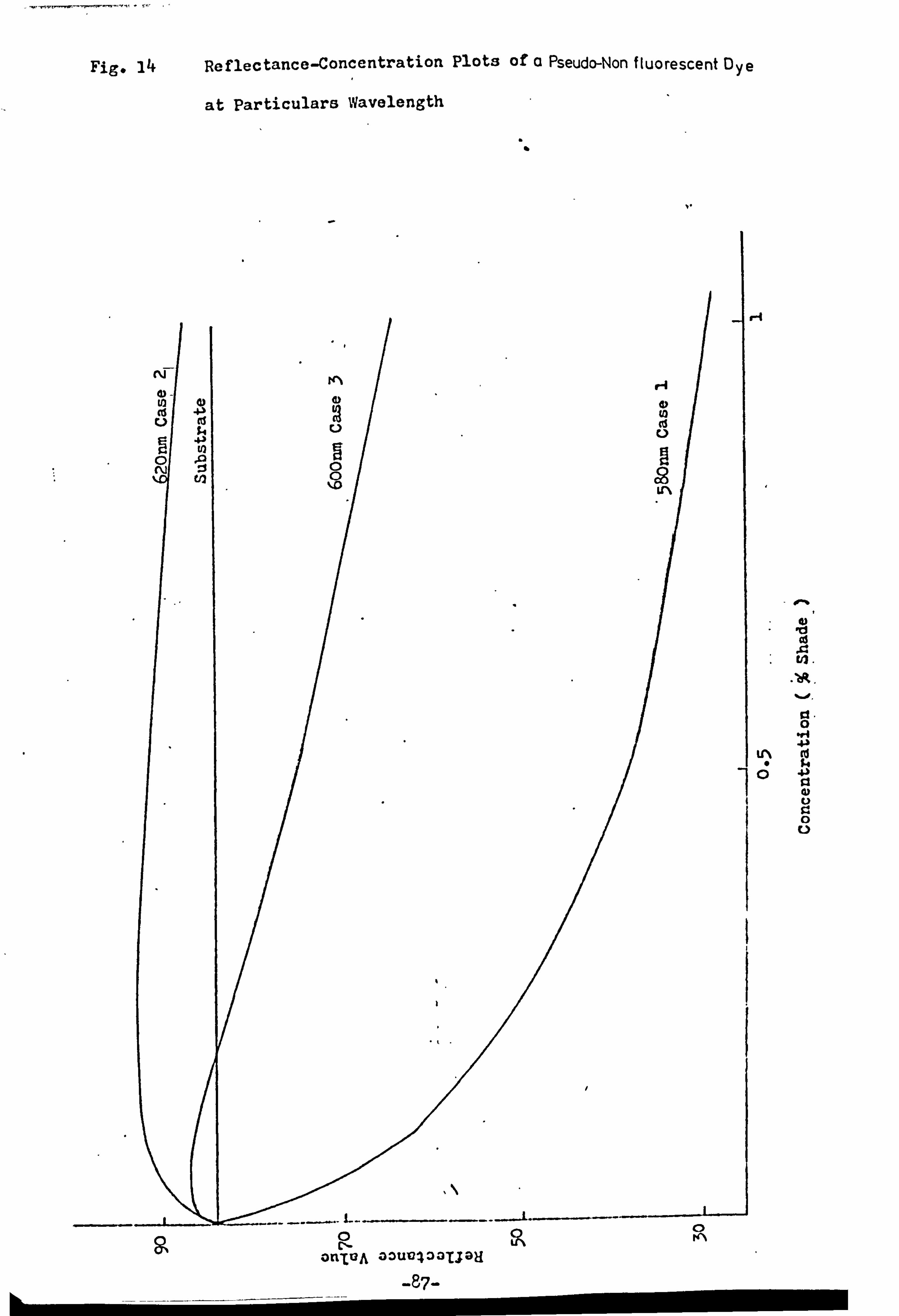
Fig. 14 Reflectance-Concentration Plots of a Pseudo-Non fluorescent Dye
at Particulars Wavelength
9-4
%. 0,
91 - 0
-87-
0 C-
On'EvA 0OU-0433TJOH
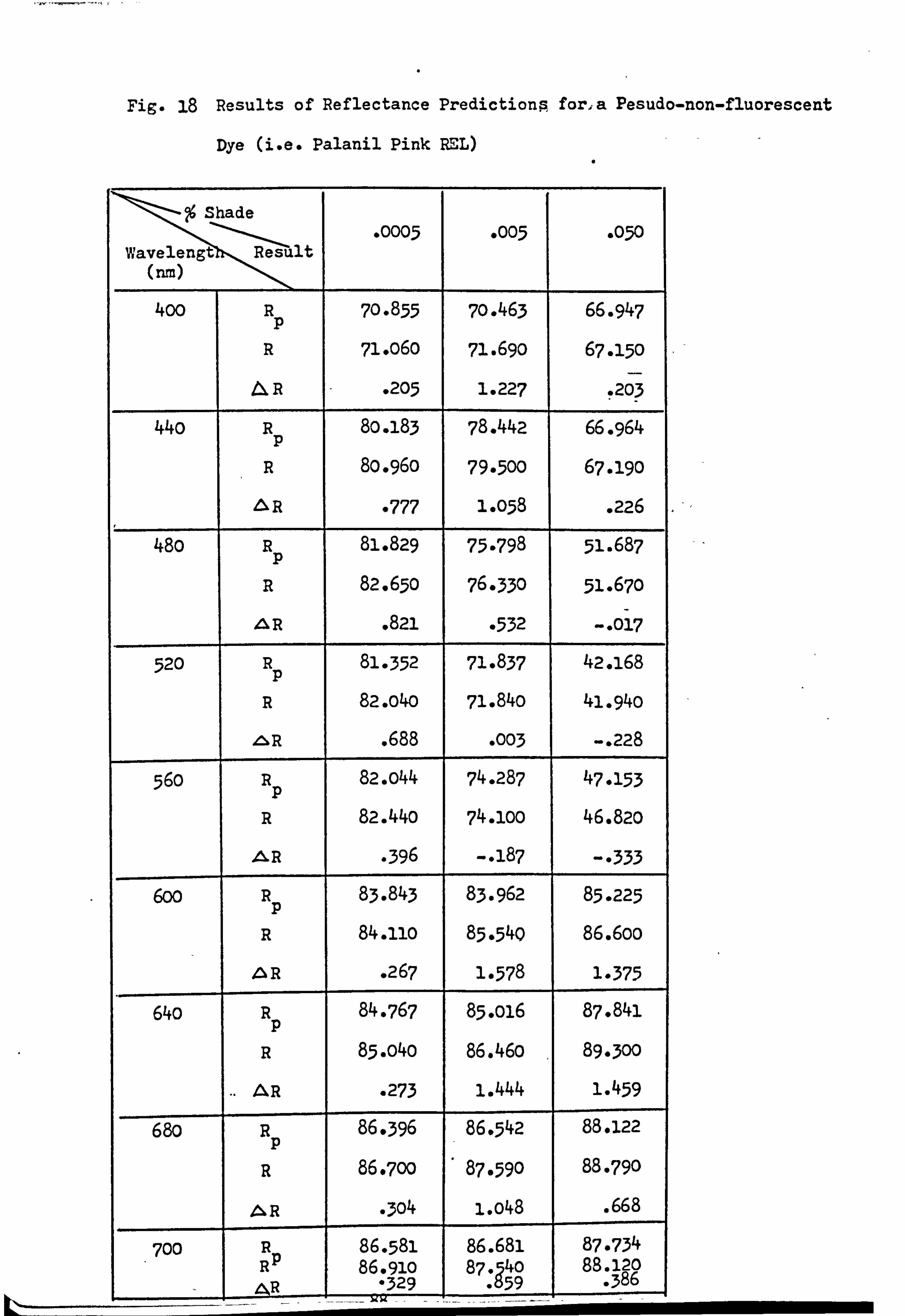
Fig. 18 Results of Reflectance Predictiong for, a Pesudo-non-fluorescent
Dye (i. e. Palanil Pink REL)
Shade
-0005 -005 . 050 Wavelengt Result
(nm)
400 R 70.855 70.463 66.947 p
R 71.060 71.690 67-150
R 205 1.227 . 203
440 R 80.183 78.442 66.964 p
R 8o. 96o 79-500 67-190
&R -777 1-058 . 226
48o R 81.829 75-798 51.687 p R 82.650 76-330 51.670
R . 821 -532 --017
520 R 81-352 71.837 42.168 p
R 82. o4o 71.840 41.94o
, in, R . 688 -003 -. 228
56o R 82.044 74.287 47-153 p
R 82.440 74.100 46.820
AR . 396 -. 187 --333 600 R 83.843 83.962 85.225
p R 84.11o 85-540 86.6oo
ýNR . 267 1-578 1-375
640 R 84-767 85.016 87.841 p
R 85. o4o 86.460 89-300
AR . 273 1.444 1.459
680 R 86-396 86-542 88.122
R 86-700 87-590 88-790
, 4i, R -3o4 i. o48 . 668
700 R 86-581 86.681 87-734 Rp 86.91o 4o 87. 89 120
AR C, 0329 g 59 : 386
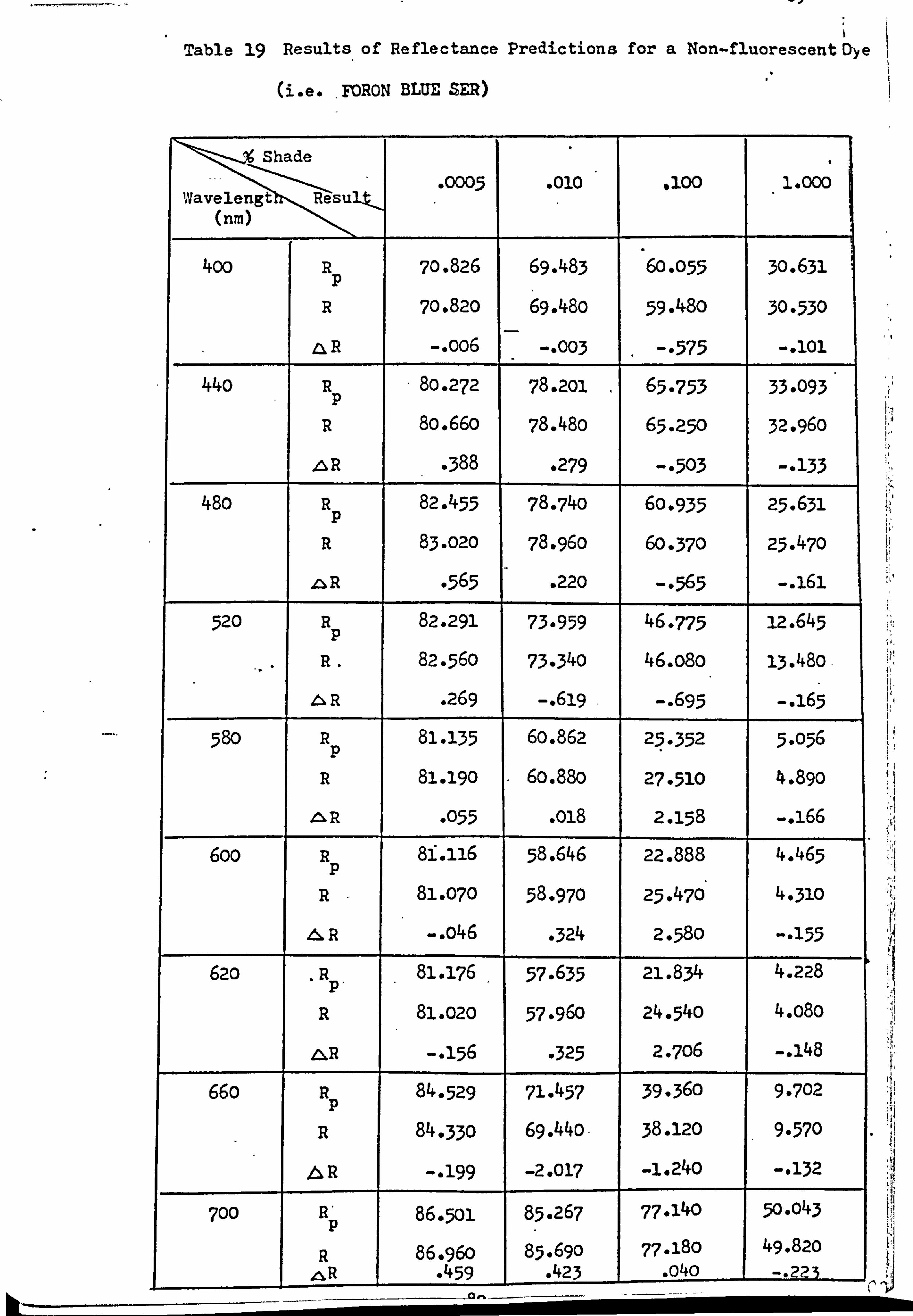
Table 19 Results of Reflectance Predictions for a Non-fluorescent Dye
(i. e. . FORON BLUE SER)
'96 Shade F
-0005 . 010 0100 1.000 lWavelengt Result
(nm)
400 R 70.826 69.483 60-055 30.631 p
R 70.820 69.480 59.48o 30-530
aR -. oo6 --003 . --575 -0101 44o R 8o-272 78*201 65-753 33-093
p R 8o. 66o 78.480 65-250 32.960
, &R -388 279 503 --133 48o R 82.455 78-740 60-935 25.631 p
R 83.020 78.960 60-370 25.470
R -565 . 220 --565 -. 161
520 R 82-291 73-959 46-775 12.645 p R. 82-56o 73-340 46.080 13.48o.
R . 269 -. 619 -. 695 -. 165
580 R 81-135 6o. 862 25-352 5-056 p R 81.1go 6o. 88o 27-510 4.890
&R -055 ol8 2-158 -. 166
600 R 8i. 116 58.646 2? -. 888 4.465 p
R 81-070 58-970 25.47o 4-310
, eS. R -. 046 -324 2-580 --155 620 R 81-176 57.635 21.834 4.228
p R 81.020 57-960 24-540 4.080
&R --156 -325 ? --7o6 -. 148
66o R 84-529 71.457 39-360 9.702 p
R 84-330 69.44o. 38-120 9-570
R -. 199 -2-017 -1,240 --132
700 R* 86.5ol 85.267 77.14o 50.043 p
R 86.960 85.690 77.18o 49.820
, n, R . 459 . 423 __ .
040 -. 223 ____________ ____
C
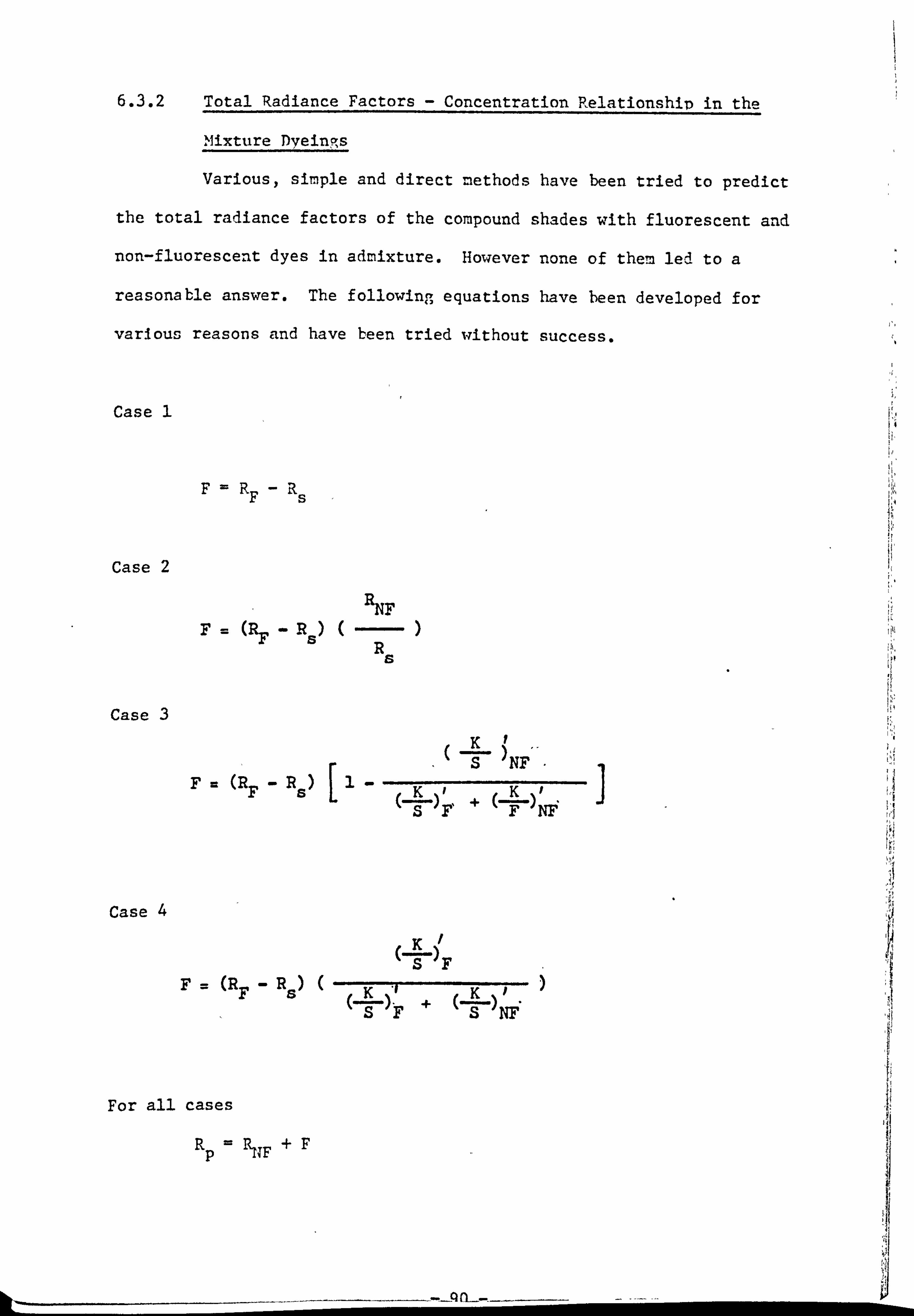
6.3.2 Total Radiance Factors - Concentration Relationship in the
Mixture Dvein, cr, s
Various, simple and direct methods have been tried to predict
the total radiance factors of the compound shades with fluorescent and
non-fluorescent dyes in admixture. However none of them led to a
reasonable answer. The following equations have been developed for
various reasons and have been tried without success.
Case 1
FRF-Rs
Case 2
RNF
F (RF - Rs) -) R
S
Case 3
KI s
)NF" - (R
F-RK+(K )I sF Nlý
Case
K)I sF
(R FR S) K+K
s --r Ni
For all cases
Rp. RITF +F
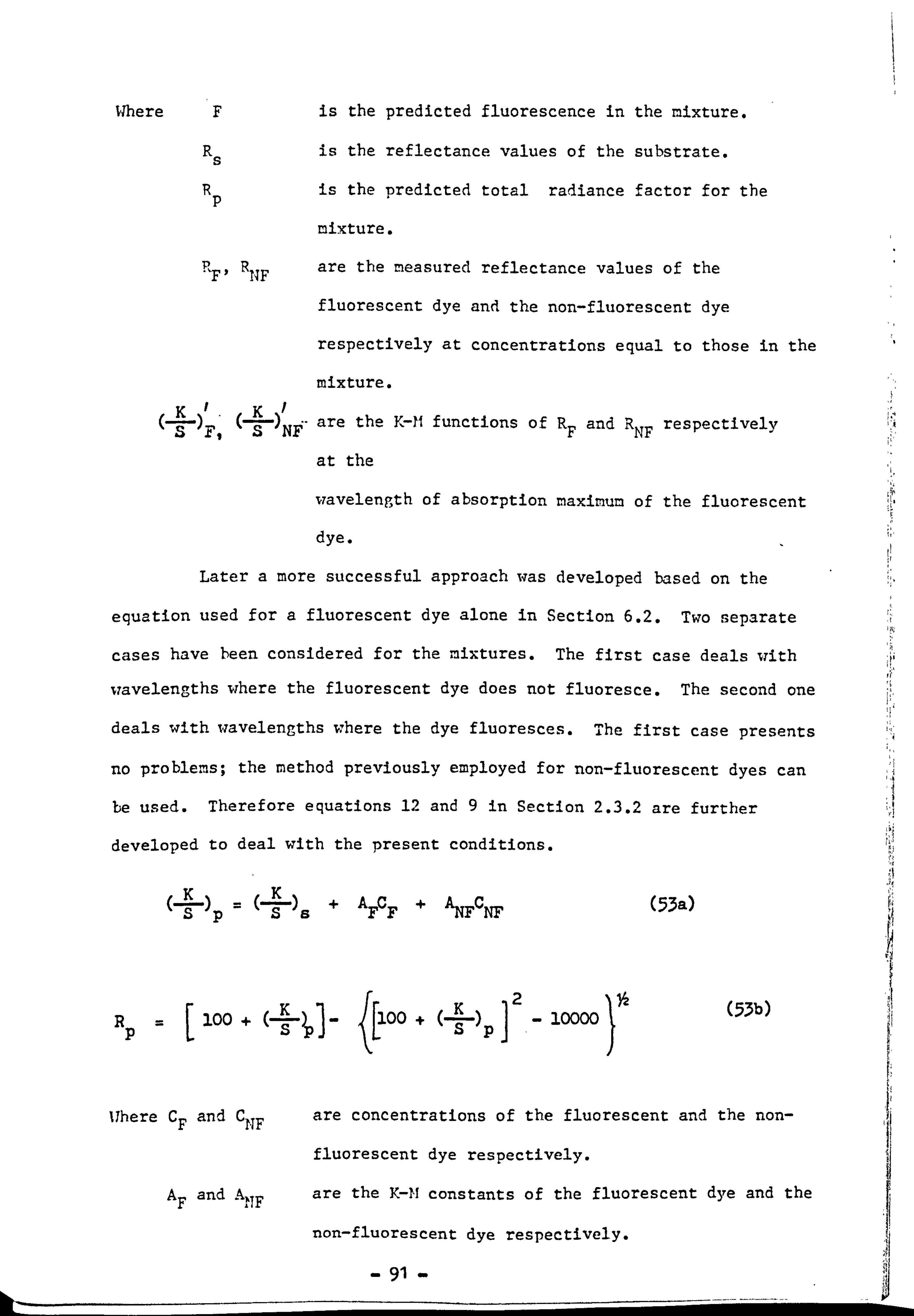
Mere F is the predicted fluorescence in the mixture.
Rs is the reflectance values of the substrate.
Rp is the predicted total radiance factor for the
mixture.
P, R are the measured reflectance values of the "F' 14F
fluorescent dye and the non-fluorescent dye
respectively at concentrations equal to those in the
mixture. II
(--L) ,(K).. are the Y, 711 functions of R and R respectively 3 F, 3 NF F NF
at the
wavelength of absorption maximum of the fluorescent
dye.
Later a more successful approach was developed based on the
equation used for a fluorescent dye alone in Section 6.2. Two separate
cases have been considered for the mixtures. The first case deals with
wavelengths where the fluorescent dye does not fluoresce. The second one
deals with wavelengths where the dye fluoresces. The first case presents
no problems; the method previously employed for non-fluorescent dyes can
be used. Therefore equations 12 and 9 in Section 2.3.2 are further
developed to deal with the present conditions.
(_L_) =(K+ ArCr +A 3pS NIFCNF (53a)
R 100 + 00 . (-E-) 2
10000 1ý (53b)
S PI
Where CF and CNF are concentrations of the fluorescent and the non-
fluorescent dye respectively.
A and A, are the K-11 constants of the fluorescent dye and the F IT
non-fluorescent dye respectively.
91
kk- -M I
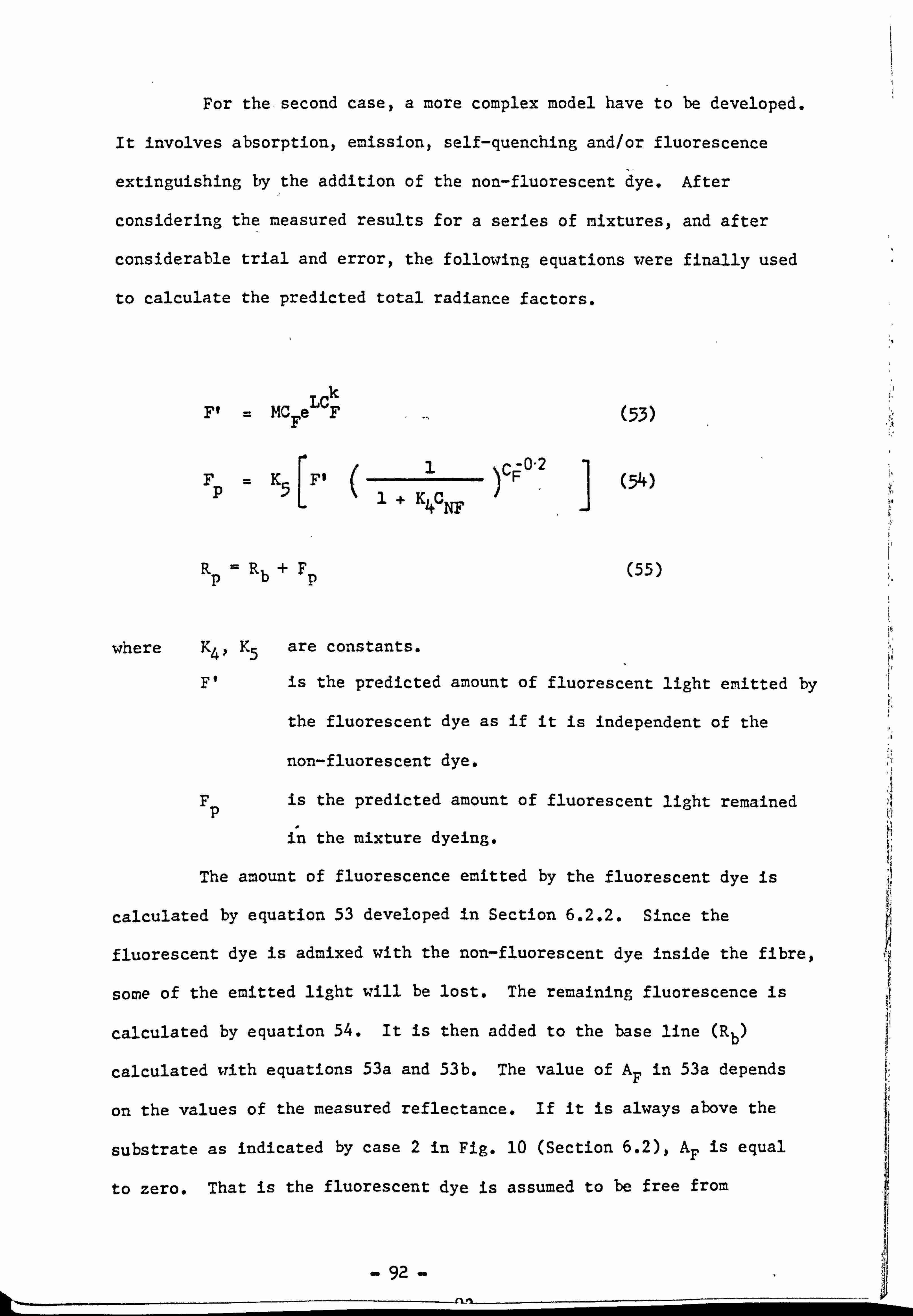
For the. second case, a more complex model have to be developed.
It involves absorption, emission, self-quenching and/or fluorescence
extinguishing by the addition of the non-fluorescent dye. After
considering the measured results for a series of mixtures, and after
considerable trial and error, the following equations were finally used
to calculate the predicted total radiance factors.
Ck F1 MCFe F (53)
F FP=K51 F1 (1+K
4ýNF
)C (54)
Rp = Rb +Fp (55)
vfhere K4, Y, 5 are constants.
F' is the predicted amount of fluoresc ent light emitted by
the fluorescent dye as if it is independent of the
non-fluorescent dye.
Fp is the predicted amount of fluorescent light remained
in the mixture dyeing.
The amount of fluorescence emitted by the fluorescent dye is
calculated by equation 53 developed in Section 6.2.2. Since the
fluorescent dye is admixed with the non-fluorescent dye inside the fibre,
some of the emitted light will be lost. The remaining fluorescence is
calculated by equation 54. It is then added to the base line (Rb)
calculated with equations 53a and 53b. The value of A. in 53a depends
on the values of the measured reflectance. If it is always above the
substrate as indicated by case 2 in Fig. 10 (Section 6.2), AF is equal
to zero. That is the fluorescent dye is assumed to be free from
92 - ýl
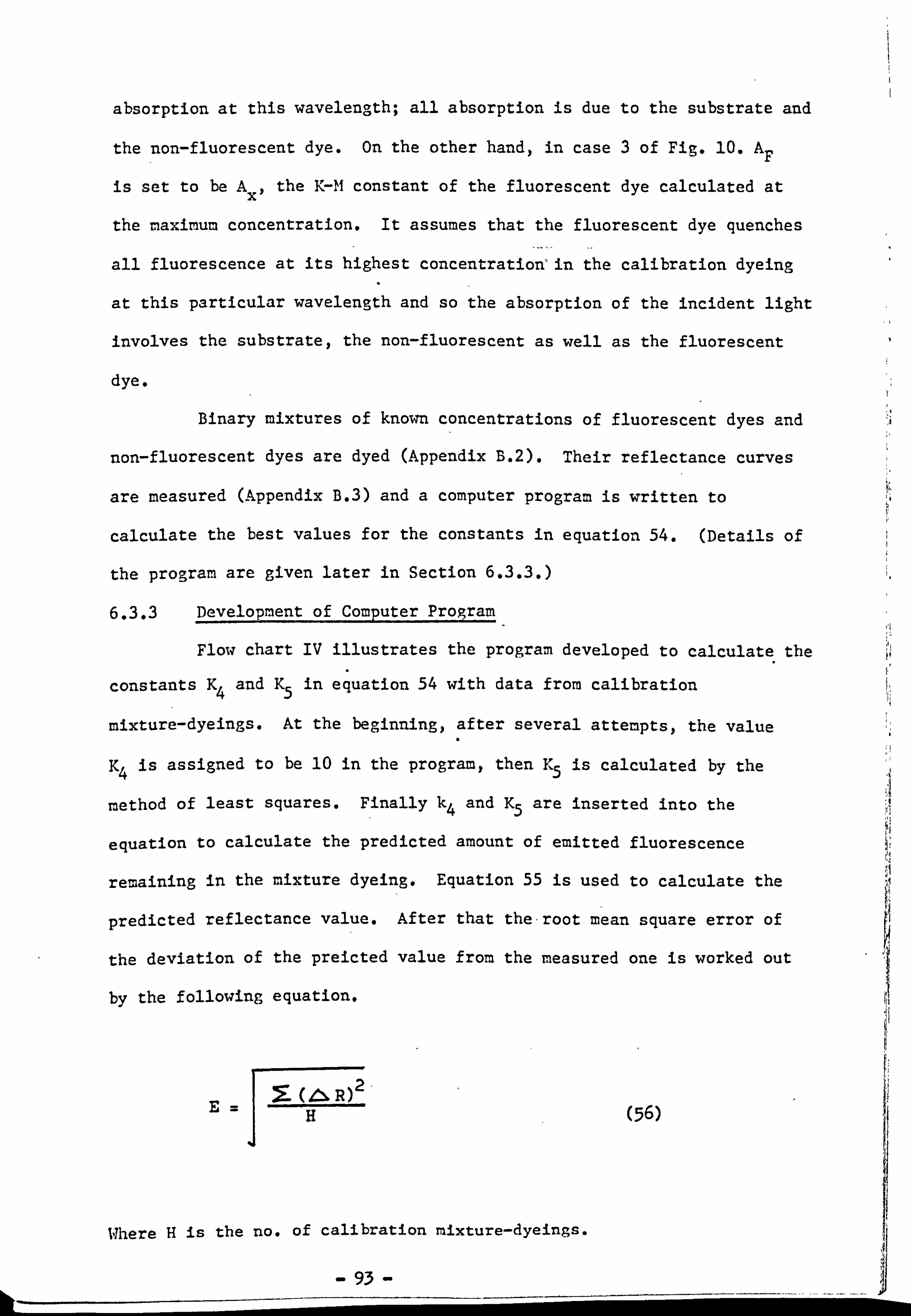
absorption at this wavelength; all absorption is due to the substrate and
the non-fluorescent dye. On the other hand, in case 3 of Fig. 10. AF
is set to be Ax, the K-11 constant of the fluorescent dye calculated at
the maximum concentration. It assumes that the fluorescent dye quenches
all fluorescence at its highest concentration'in the calibration dyeing
at this particular wavelength and so the absorption of the incident light
involves the substrate, the non-fluorescent as well as the fluorescent
dye.
Binary mixtures of known concentrations of fluorescent dyes and
non-fluorescent dyes are dyed (Appendix B. 2). Their reflectance curves
are measured (Appendix B. 3) and a computer program is written to
calculate the best values for the constants in equation 54. (Details of
the program are given later in Section 6.3.3. )
6.3.3 Development of Computer Program
Flow chart IV illustrates the program developed to calculate the
constants K4 and K5 in equation 54 with data from calibration
mixture-dyeings. At the beginning, after several attempts, the value
y, 4 is assigned to be 10 in the program, then Y, 5 is calculated by the
method of least squares. F inally k4 and K5 are inserted into the
equation to calculate the predicted amount of emitted fluorescence
remaining in the mixture dyeing. Equation 55 is used to calculate the
predicted reflectance value. After that the-root mean square error of
the deviation of the preicted value from the measured one is worked out
by the following equation.
(4h. (56)
Where H is the no. of calibration mixture-dyeings.
93
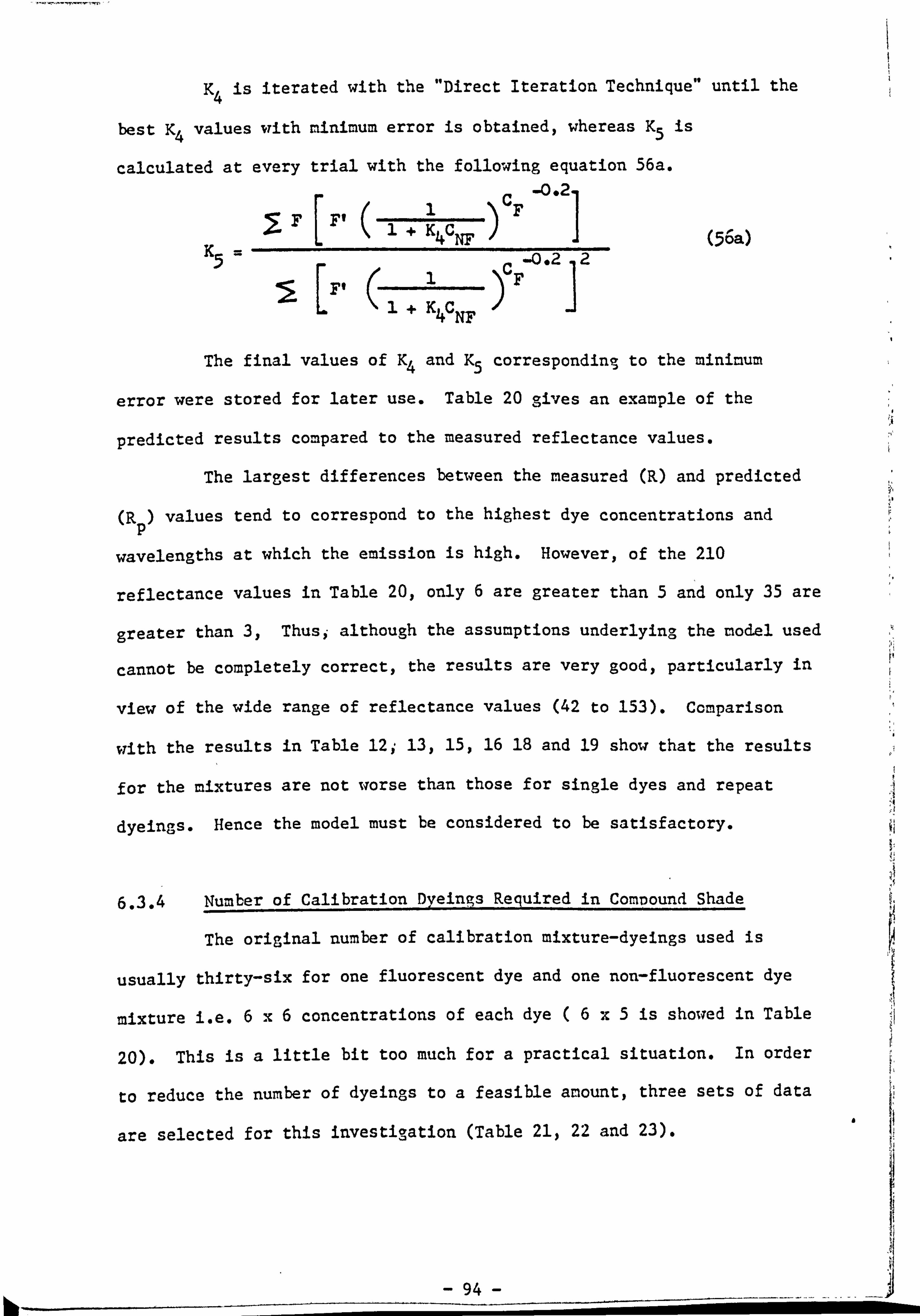
K4 is iterated with the "Direct Iteration Technique" until the
best K4 values with minimum error is obtained, whereas K5 is
calculated at every trial with the following equation 56a.
C -0*2
1+KC6 4 NF (56a K5
ýi Ft (1-CF -0*2 ]2 11+K
4CNF
)
The final values of K4 and K5 corresponding to the minimum
error were stored f or later use. Table 20 gives an example of the
predicted results compared to the measured reflectance values.
The largest differences between the measured (R) and predicted
(R ) values tend to correspond to the highest dye concentrations and P
wavelengths at which the emission is high. However, of the 210
reflectance values in Table 20, only 6 are greater than 5 and only 35 are
greater than 3, Thusi although the assumptions underlying the model used
cannot be completely correct, the results are very good, particularly in
view of the wide range of reflectance values (42 to 153). Comparison
with the results in Table 12; 13,15,16 18 and 19 show that the results
for the mixtures are not worse than those for single dyes and repeat
dyeings. Hence the model must be considered to be satisfactory.
6.3.4 Number of Calibration Dyeings Required in COMDOUnd Shade
The original number of calibration mixture-dyeings used is
usually thirty-six for one fluorescent dye and one norr-fluorescent dye
mixture i. e. 6x6 concentrations of each dye (6x5 is showed in Table
20). This is a little bit too much for a practical situation. In order
to reduce the number of dyein-s to a feasible amount, three sets of data a
are selected for this investigation (Table 21,22 and 23).
94
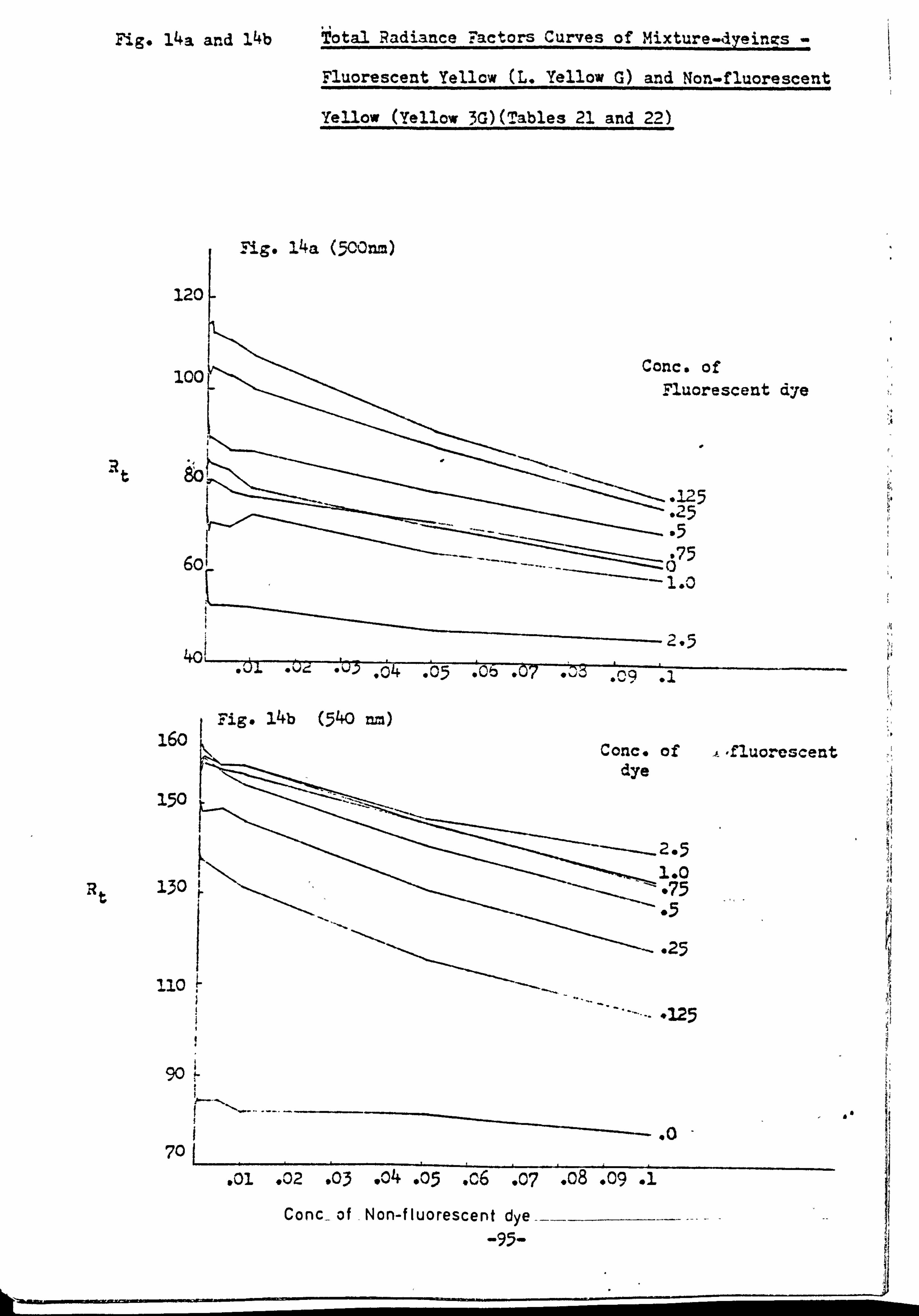
Fig. 14a and l4b Total Radiance Factors Curves of Mixture-dyeinzs
Fluorescent Yellcw (L. Yellow G) and Non-fluorescent
Yellow (Yellow 3G)(Tables 21 and 22)
. 1g. 14a (500=)
120
100
t 8b
6ol
401 . 64
-65
Fig. 14b (540 16o
150
Of -,, fluo. -Cscent
2-5 1.0
130 t 75
. 25
110
, 125
go
701
I, a
, 01 *02 -03 o4 -05 C6 . 07 -08 -09 -1 Conc- of Non-f luorescent dye
-95-
Conc. of luorescent dye
J
. 125 `5
95 75
1.0
2 -5 06 . 67 'cg -ýj
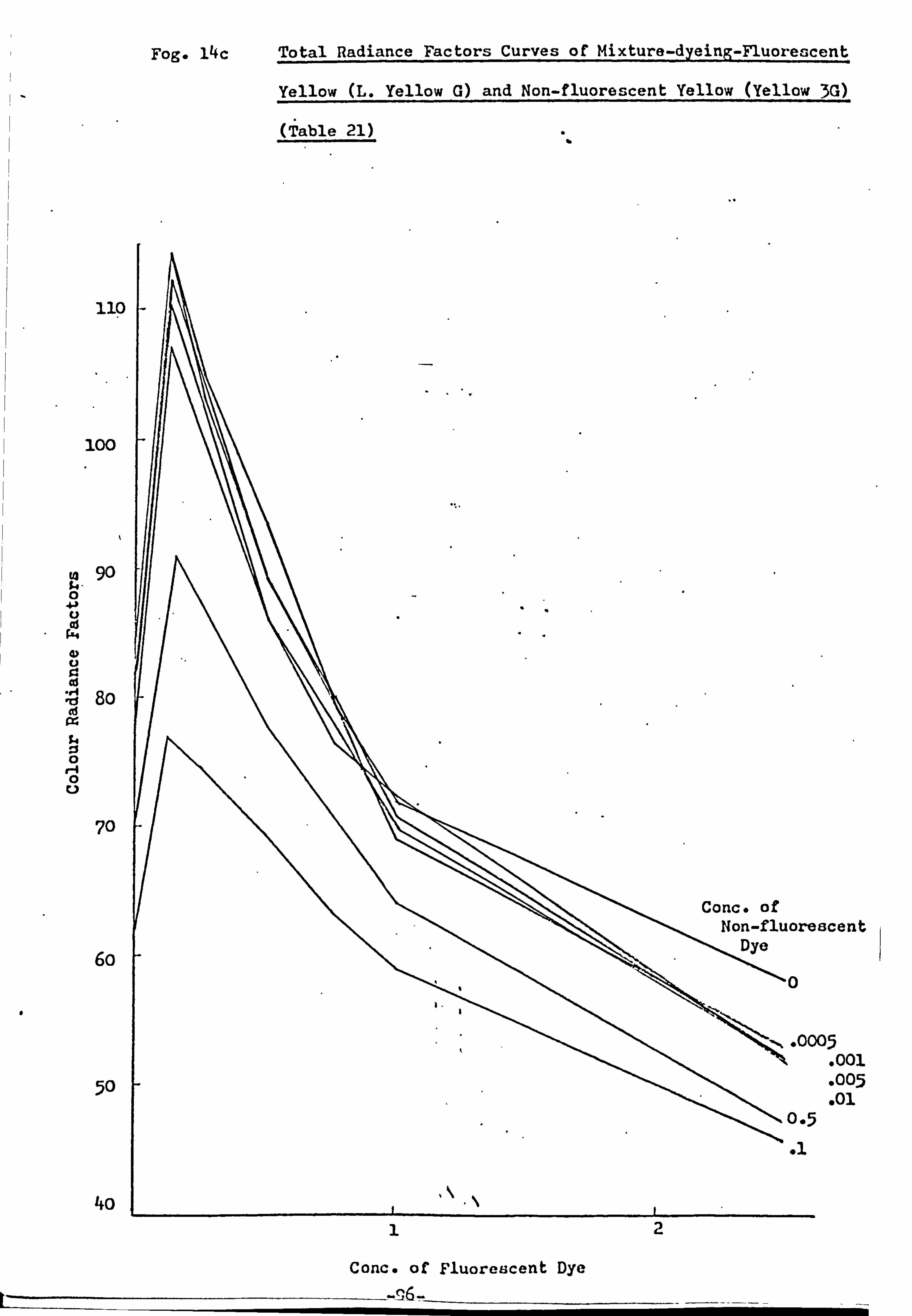
Fog. 14c Total Radiance Factors Curves of Mixture-dyeing-Fluoreacent
Yellow (L. Yellow G) and Non-fluorescent Yellow (Yellow 3G)
(Table 21)
110
100
90
8o
W
70
6o
0
50
40
Escent
05 . 001 -005 . 01
Conc. of Fluorescent Dye -6-
12
- These tables represent various situations which can exist
between a fluorescent and a non-fluorescent dyes. The influence of the
absorption in the excitation region (absorption region) of the
fluorescent dye is studied by a mixture of a fluorescent Yellow with a
non-fluorescent yellow. Table 21 shows data for such a mixture at a
wavelength (500nm) where there is some emission and some absorption while
Table 22 gives data for the same mixture at 540 nm which corresponds to
the emission peak. Table 22 is particularly interesting.
The first row shows that the non-fluorescent dye hardly absorbs
at 540nm. Nevertheless, the effect on the reflectance values is marked.
For most concentrations of the fluorescent dye, addition of 0.1% of the
non-fluorescent dye reduces reflectance by about 30, presumably due to
absorption of the exciting wavelength. The influence of the absorption
in the region of emission peak of the fluorescent dye is illustrated in
Table 23 with mixtures of a fluorescent yellow with a non-fluorescent
pink which absorbs at the emission peak region.
The reflectance values in. Table 20 are based on K4 and K5
values obtained from calibration data for thirty-six mixture dyeings of
the two dyes. It was considered that in practice, the method might be
impractical unless a smaller number of calibration dyeings could be
used. Hence new values of K4 and K5 were calculated using only the
nine mixture marked with an asterisk(*) in Table 21. The calculation was
also repeated using the four values marked with a cross(+) in Table 21.
The results are very encouraging. The resultant root mean square errors
are given in Table 24 and show that four mixtures can produce results
almost as good as those from a much larger number. Presumably care
should be taken in selecting, these concentrations.
a
- 97 -
If a large number of dyesare involved, the numberof possible ,
combinations for, which mixture dyeings might be required is enormous.
However highly fluorescent dyes are only likely to be used for very
bright colours which cannot be matched using non-fluorescent dyes. This
limits the dyes likely to be used to the fluorescent dyes (singly or in
binary mixtures) together with smaller amounts of shading dyes which must
not reduce the purity of the mixture too much. Thus the number of
different mixtures actually used should be quite small. -
4 a
- 98
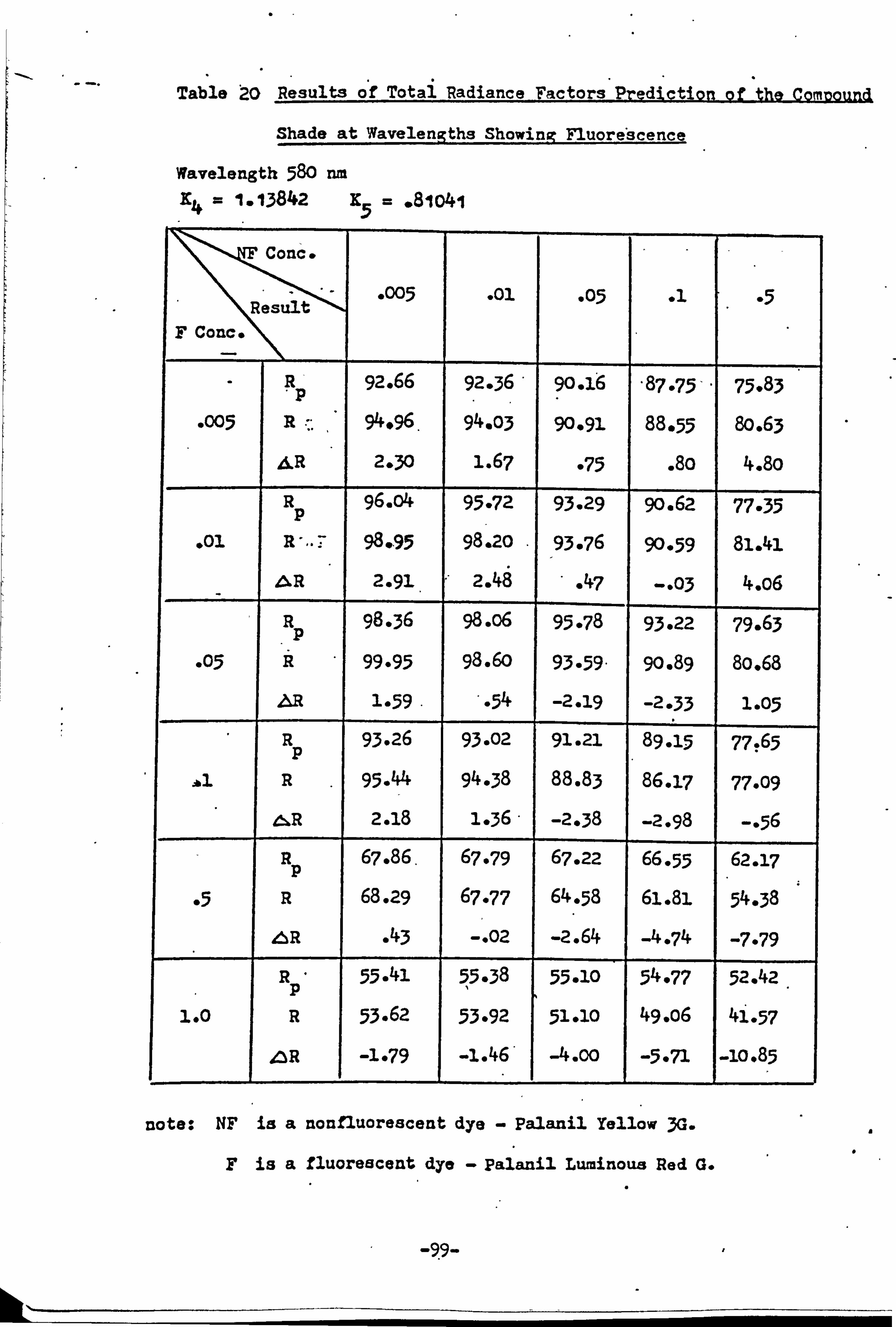
Table ýo Results o. f Totai Radiance Factors Prediction of the Comnound
Shade at Wavelengths Showing Fluore'scence
Wavelength 580 nm X4 = 1.13842 K5- *81041
conc
jt t -005 . 01 -05 .1 *5 Fc Conce
92.66 92-36 90-16 87 -75' 75-83 p
-005 R 94*96. 94 -03 90091 88-55 8o. 63
AR 2*30 1.67 975 . 80 4.8o
Rp 96. o4 95 -72 93-29 90.62 77-35
. 01 R 98-95 98*20 93-76 90-59 81.41 46R 2.91. 2.4A . 47 --03 4. o6
R 98-36 98. o6 95-78 93*22 79.63 12
-05 R 99-95 98.60 93-59- 90-89 8o. 68
AR 1-59. -54 -2.19 -2-33 1-05
R 93.26 93-02 91.21 89.15 77! 65 p
. *l R 95.44 94-38 88-83 86-17 77-09
aý, R 2.18 1-36- -2-38 -2.98 -5 R 67.86, 67-79 67*22 66-55 62-17 p
.5 R 68.29 67-77 64-58 61.81 54-38
, 6R -43 -. 02 -2.64 -4-74 -7-79 R , 55.41 ý5-38 55-10 54-77 52.42 P .
1.0 R 53.62 53*92 51-10 49.06 41-57
4R -1-79 -1.46* -4.00 -5-71 -10.85
note: NF is a nonfluorescent dye - Palanil Yellow 3a.
F is a fluorescent dye - Palanil Luminous Red G.
-99-
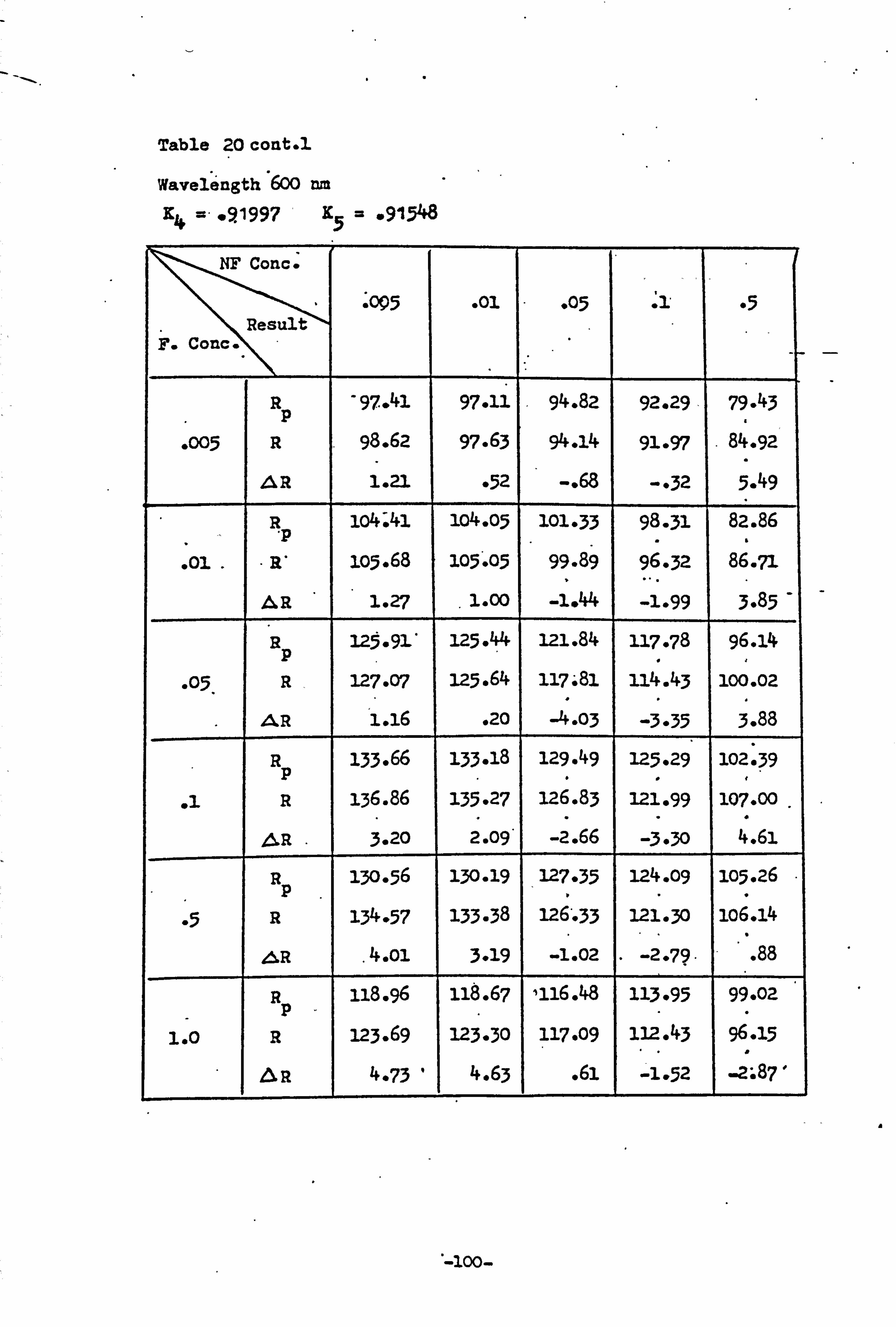
Table 20 cont. l.
Wavelength'600 nm T-4 =. 091997 K . 91548
NF Conc.
XQ5 . 01 -05 1 *5 Result;
F. Conc.
R -97.41 97-11 94.82 92.29- 79.43 p
-005 R 98.62 97-63 94.14 91.97 84.92
AR 1.21 -52 -. 68 --32 5.49
R lo4; 41 io4-05 101-33 98-31 82.86
. 01 R* 105.68 105 . -05 99-89 96-32 86.71
AR 1.27 -1.44 -1.99 3.85
R 125 0 93. 125-ý4 121.84 117-78 96.14 p 1
. 05 R 127-07 125.64 11721 114.43 100.02
AR 1.16 *20 -4-03 -3-35 3.88
R 133.66 133.18 129.49 125*29 102 39 p f, R 136.86 135.27 126.83 121.99 107-00
, 6. R, 3.20 2.09* -2.66 -3-30 4.61
R 130-56 130-19 127-35 124.09 105.26 p
.5 R 134-57 133-38 126'033 121-30 106.14
, 62 . 4.01 3-19 -1.02 - -2-79. . 88
R 118.96 118.67 116.48 113-95 99-02 , p
1.0 R 123.69 123-30 117-09 112.43 96.15
AR 4-73 4.63 . 61 -1-52 1 -2; 87'
. -100-
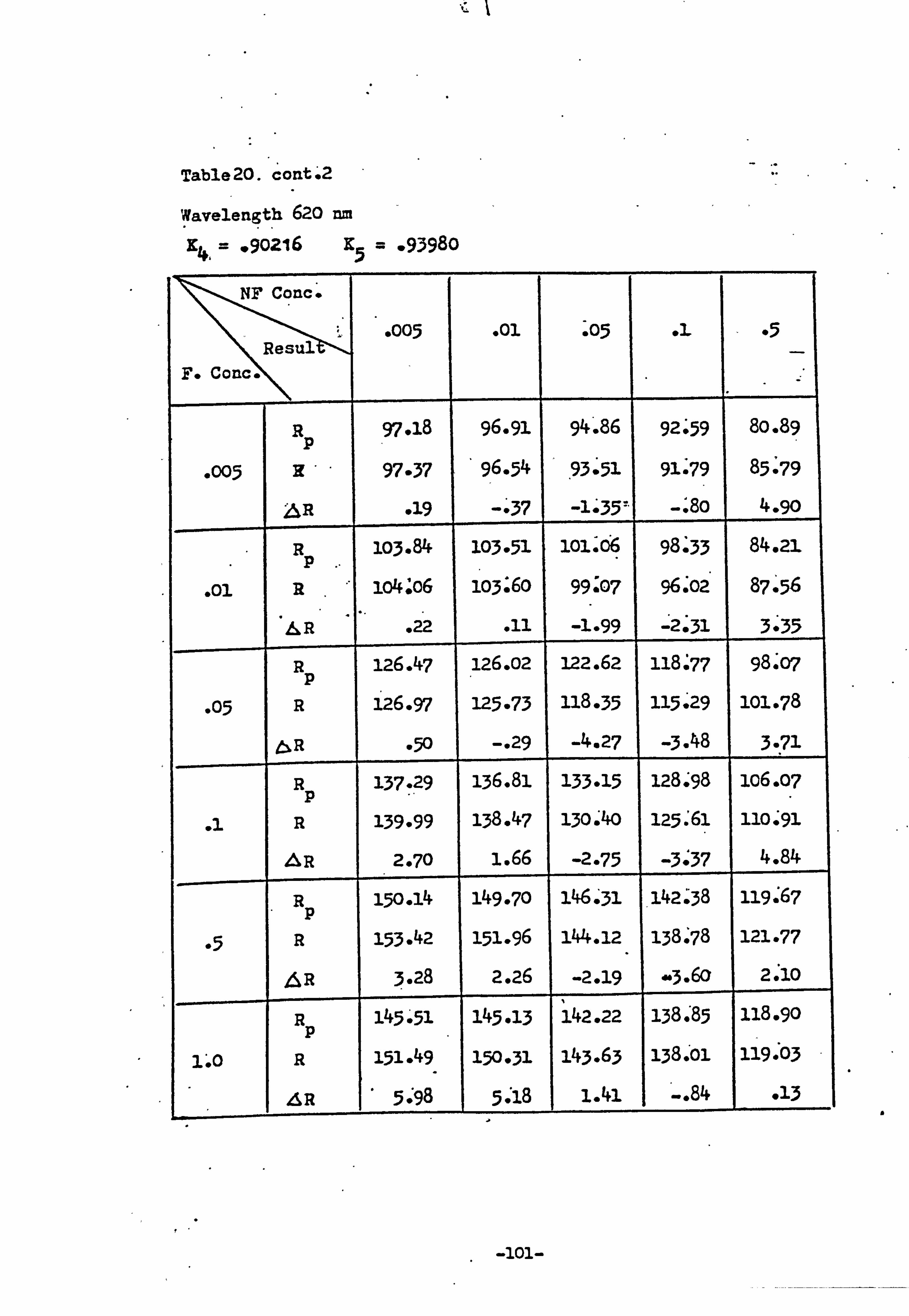
Table20. coat*
Wavelength 620 nm
K 41 = . 90216 K -93980
NF Conco
. 005 . 01 . 05 .: L *5 Resul F* Conc.
R 97-18 96.91 94'. 86 92-59 80.89 p
-005 13 97-37 96.54 . 93951 91.79 85-79
. 19 - _3?
-, 80 4.90
R 103-84 103-51 10140ý 98-33 84.21 p
. 01 R lo4;. 06 103 6o 99 -'07 96.02 87-, 56
AR .22 11 -1.99 2 31 3 35
. ......... ... R 126.47 126.02 122.62 118-77 98.07
p
-05 R 126.97 125-73 118-35 115.29 101.78
950 -. 29 -4.27 -3.48 3-. 71
R 137.29 136.81 133-15 128.98 106-07 p
R 139.99 138.47 130940 1? -5. '61 110.91
AR 2o70 1.66 -2-75 -3-37 4.84
R 150.14 149.70 146931 142o38 119. S7 p
-5 R 153.42 151.96 144.12 ý138-78 121.77
AR 3.28 2o26 -2.19 -3.6o 2.10
R 145951 145-13 142.22 1384D*85 118.90 p
R 151.49 150-31 143.63 138-'01 119.03
äR 5 -*98 5 -*18 1.41 -. 84 -13 a
.
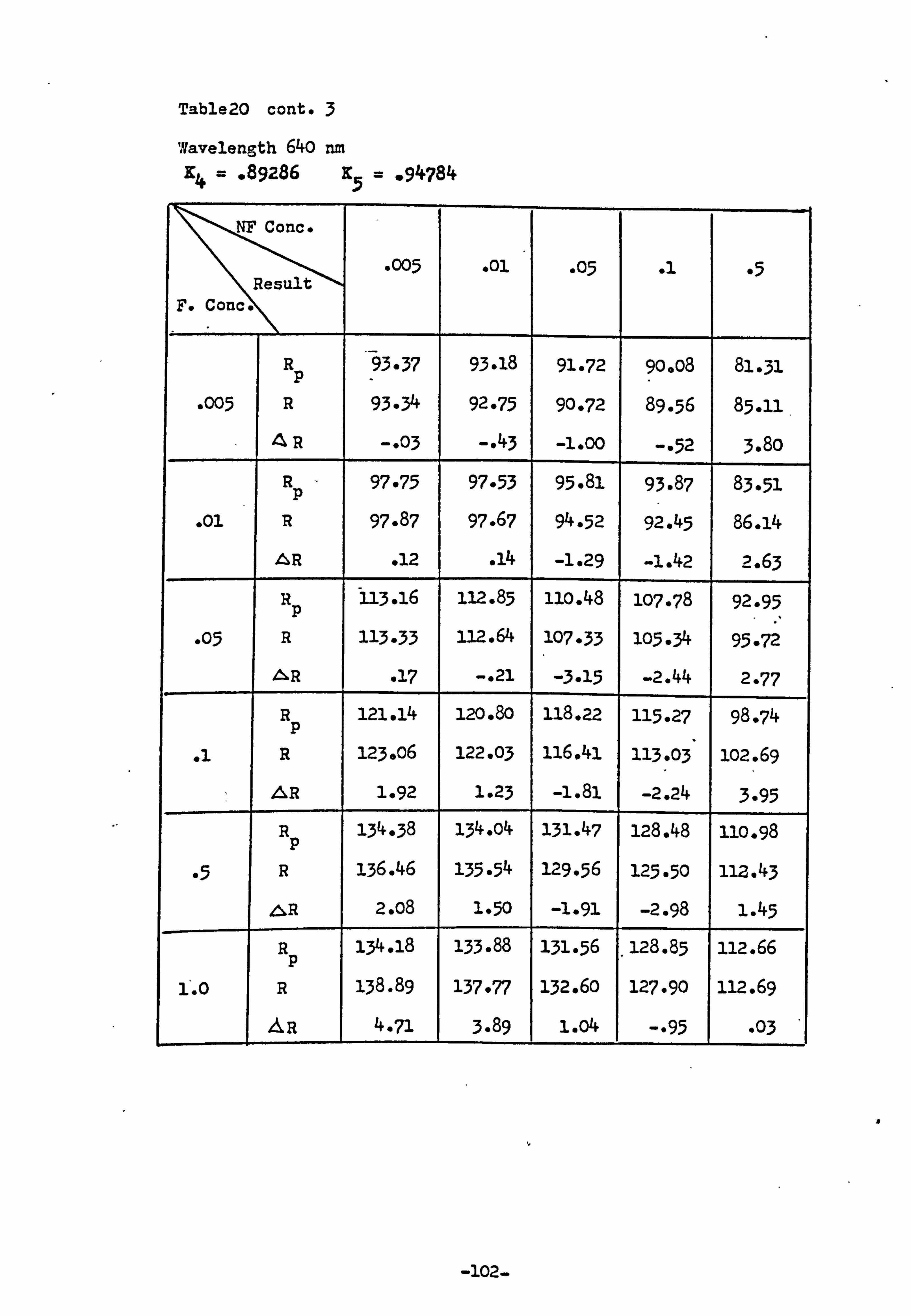
Table20 cont-
Wavelength 640 nm 314 = 89286 115 = -94784
NF Conc.
-005 . 01 -05 .1 *5 R Ilt esult F. Cone.
R 93-37 93.18 91-72 go. o8 81-31 p
-005 R 93-34 92-75 90-72 89-56 85-11,
AR --03 -. 43 -1.00 --52 3.8o
R 97-75 97-53 95.81 93-87 83-51 p
. 01 R 97.87 97-67 94-52 92.45 86.14
44R 012 . 14 -1.29 -1.42 2.63
R 113-16 112-85 110.48 107-78 92-95 p
. 05 R 113-33 112.64 107-33 105-34 95-72
iSR -17 -. 21 -3-15 -2.44 2-77
R 121.14 12o. 8o 118.22 115-27 98-74 p
al R 123. o6 122-03 116.41 113-03 102.69
AR 1.92 1-23 -1.81 -2.24 3-95
R 134-38 134. o4 131.47 128.48 110.98 p
-5 R 136.46 135-54 129-56 125-50 lia. 43
, eS, R 2. o8 1-50 -1.91 -2.98 1.45
R 134.18 133.88 131-56 . 123.85 112.66
p 1'. 0 R 138.89 137-77 132.60 127-90 112.69
AR 4.71 3.89 i. o4 -995 -03
-102-
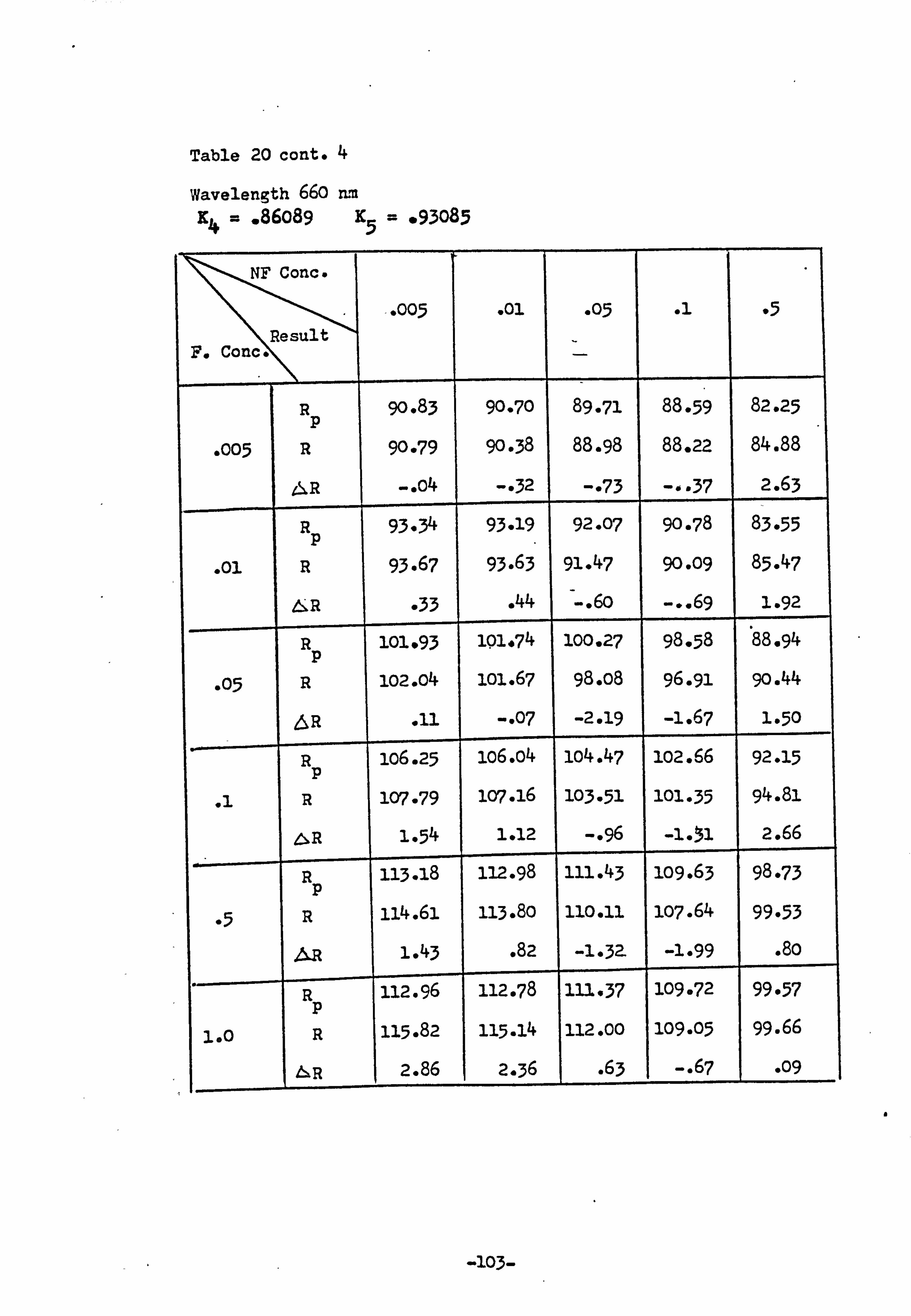
Table 20 cont. 4
Wavelength 660 mm 114 = . 86o8q X5 = *93085
NF Conc.
-%"ý 1305 -01 -05 -5
, ýesult F. c\onN
R 90.83 90-70 89-71 88-59 82-25 p
. 005 R 90-79 90-38 88.98 88,22 84.88
4% R -. o4 --32 -. 73 37 2.63
R 93-34 93-19 92.07 90-78 83-55 p
. 01 R 93.67 93.63 91.47 90-09 85.47
iSR -33 . 44 -. 60 -&. 69 1.92
R 101-93 lQl*74 100*27 98.58 88.94 p
. 05 R 102. o4 lol. 67 98.08 96.91 go. 44
6R . 11 --07 -2.19 -1.67 1-50
R 106.25 106.04 104.47 102.66 92-15 p
R 1CY7 . 79 1CY?. 16 103-51 101-35 94.81
R 1-54 1.12 -. 96 -1.51 2.66
R 113.18 112.98 111.43 log. 63 98-73 p
*5 R : 114.61 113.8o 110.11 107.64 99-53
AR 1.43 . 82 -1-3Z -1.99 . 8o
R 112.96 112-78 13.1-37 109-72 99-57 p
1"o R 115.82 115.14 112.00 109-05 99.66
6, R 2.86 2-36 . 63 -. 67 . 09
a
-103-
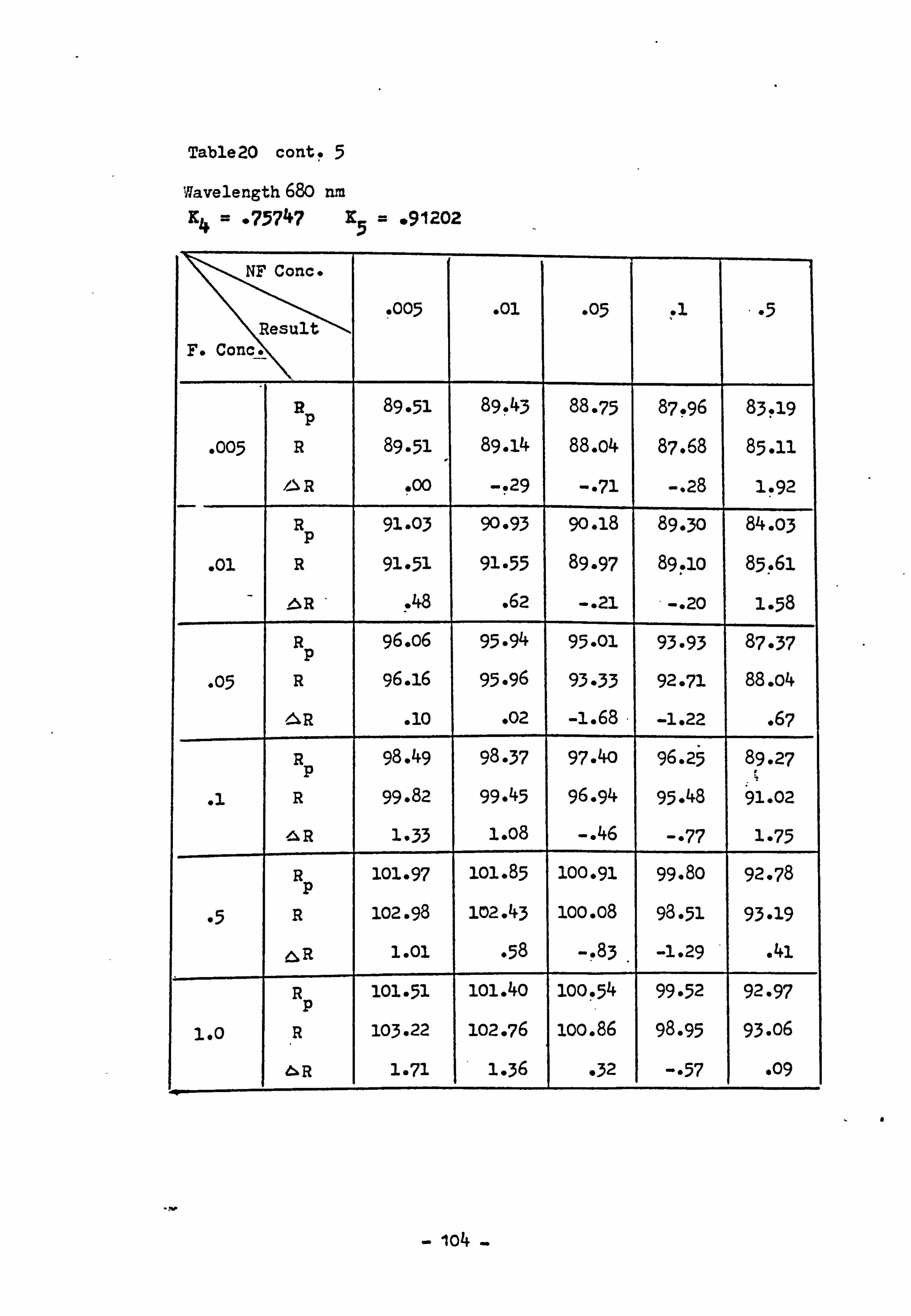
Table2O contý,
Wavelength 680 nm K4 = -75747 15= *91202
NF Conc NF Cc
-005 . 01 -05 --5 Resulýt Re F. Con(ý.
R 89-51 89e43 88-75 87e96 83e19 p
-005 R 89.51 89.14 88. o4 87.68 85.11
/CN R 000 -. 29 -. 71 -. 28 1.92
R 91-03 90-93 90.18 89-30 84-03 p
. 01 R 91-51 91-55 89.97 89.10 85e61
iCbR e48 . 62 -. 21 ý-. 20 1-58
R 96.06 95.94 95-01 93-93 87-37 p
-05 R 96.16 95.96 93-33 92.71 88. o4
. 10 . 02 -1.68 -1.22 . 6,7
R 98.49 98-37 97.40 96.25 8 9.27 p
R 99.82 99.45 96.94 95.48 91.02
-'IR 1-33 1.08 -. 46 --77 1-75
R 101-97 101-85 100-91 99.80 92.78 p
95 R 102.98 102-43 100-08 98-51 93-19
R 1.01 -58 --83 -1.29 . 41
R 101-51 loi. 4o 100-54 99-52 92-97 p
1.0 R 103.22 102.76 100.86 98.95 93.06
dCx R 1.71 1-36 1 -32 1 --57 . 09
- lo4 -
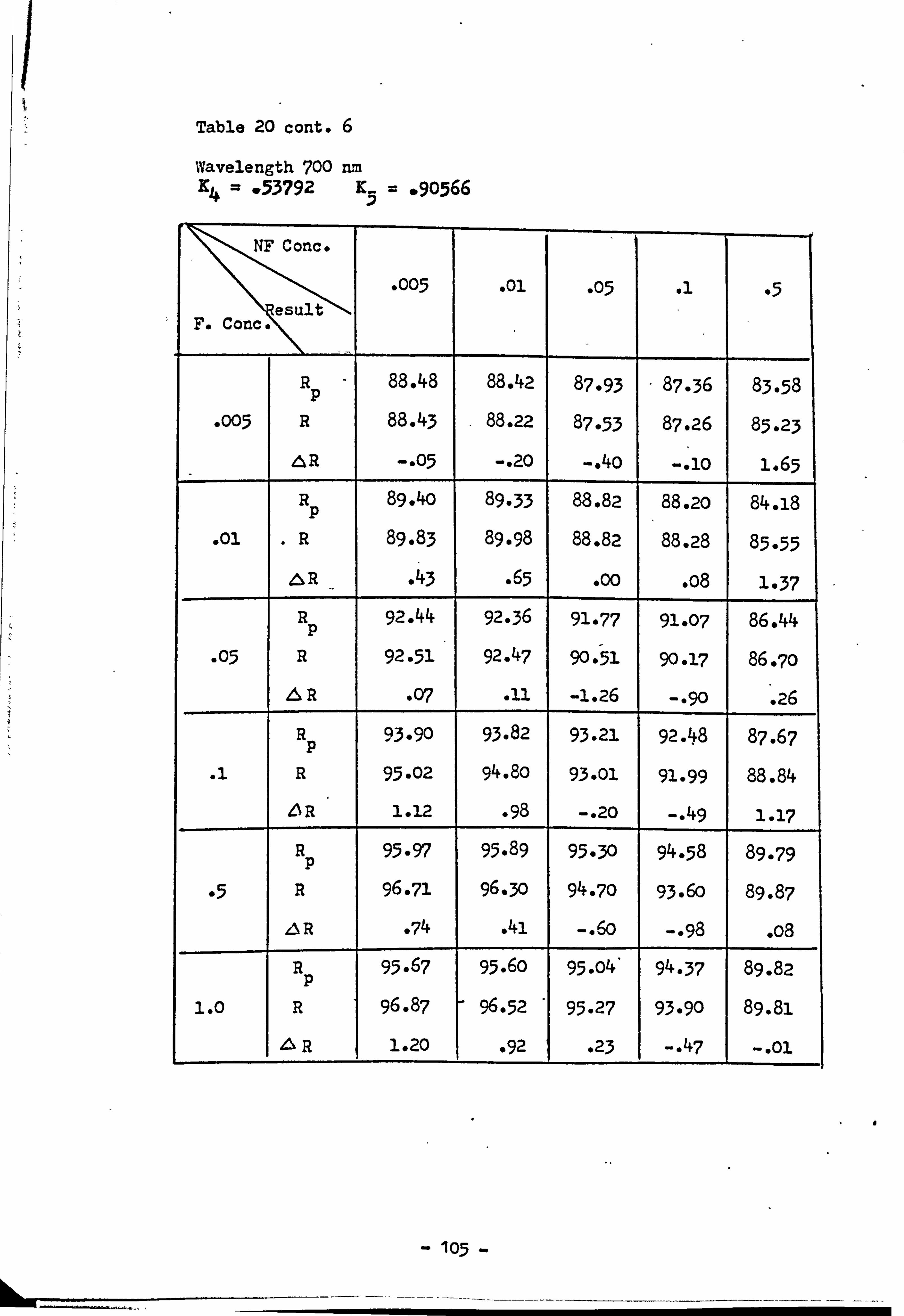
Table 20 cont.
Wavelength 700 rm K= . 53792 K5 = *90566 42
NF Conc. NF C ol
-005 . 01 -05 .1 *5 esult esu Conc F. Conc
R 88.48 88.42 87-93 87-36 83-58 p
-005 R 88.43 88.22 87-53 87.26 85.23
AR --05 -. 20 -. 4o -. 10 1.65
R 89.4o 89-33 88.82 88.20 84.18 p
. 01 R 89.83 89.98 88.82 88.28 85-55
&R . 43 . 65 . 00 o8 1-37
R 92.44 92-36 91-77 91-07 86.44 p
. 05 R 92-51 92.47 90-51 90-17 86-70
.6R -07 . 11 -1.26 -090 . 26
R 93-90 93.82 93.21 92. ý8 87.67 p
.1 R 95.02 94.8o 93-01 91-99 88.84
6R 1.12 . 98 -. 20 -. 49 1.17
R 95-97 95.89 95-30 94-58 89-79 p
io5 R 96-71 96.30 94-70 93.6o 89.87
,6R . 74 . 41 -. 60 -. 98 o8
R 95.67 95.60 95.04* 94-37 89.82 p
1.0 R 96-87 - 96-52 95.27 93-90 89.81
4k R 1*20 '92 *23 -. 47 1 -. 01
- 105 -
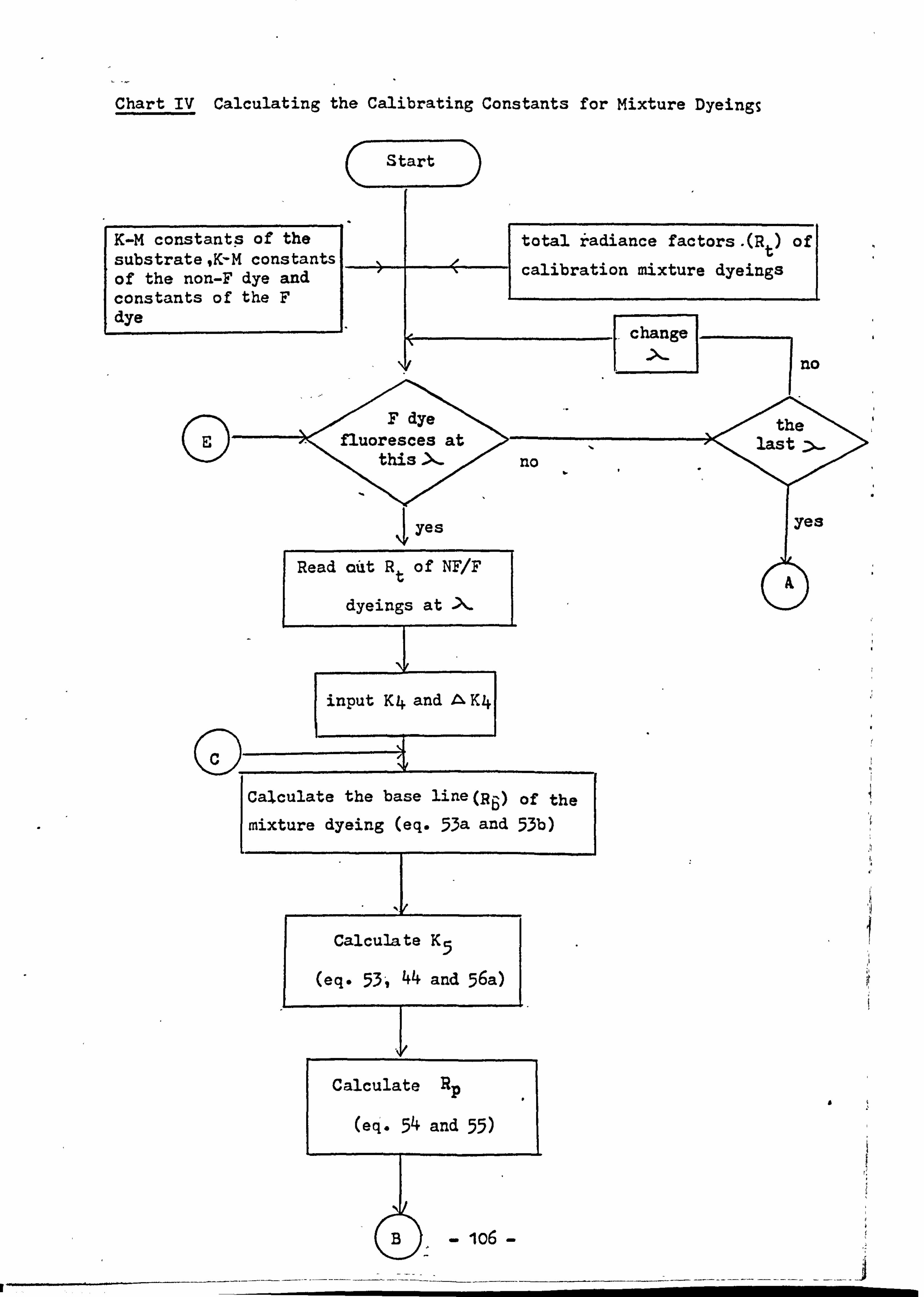
Chart IV Calculating the Calibrating Constants for Mixture DyeingS
r--Start--, ý')
K-M constants of the total radiance factors. (R ) of substrate, K-M constants
t
of the non-F dye and calibration mixture dyeings
constants of the F dye
F chan
no
F dye the fluoresces at last
this >ý-
no yes yes
Read ctitt Rt of NFIF
dyeings at >. -
input K4 and 41, K4
C
Calculate the base line(RB) of the
mixture dyeing (eq. 53a and 53b)
Calculate K 5
(eq- 53-, 44 and 56a)
Calculate Rp
(eq'- 54 and 55)
B lo6

Chart IV cont. 1
YB
Calculate-AR and the root mean
square error (equation 56)
0 jr
K4 ý K4.411ý4'
0 - 107 -
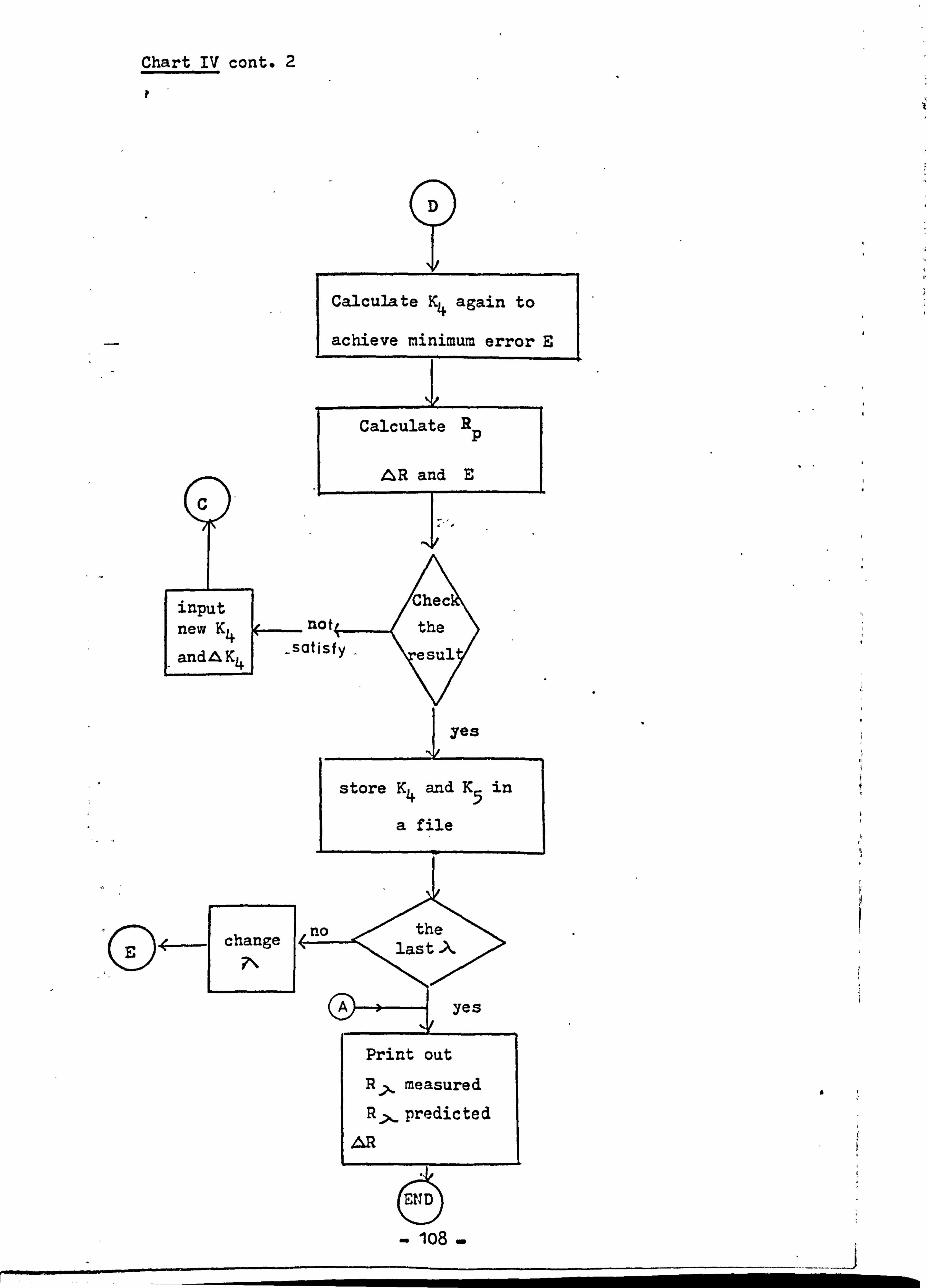
Chart IV cont. 2
D
C
Calculate K4 again to
achieve minimum error
Calculate Rp
, i! ý, R and E
input new K4 notý_
and A K4 -Satisfy -
change 40- the last
yes
Print out R, measured
R -,, _ predicted AR
108
the
asul
I yes
store K4 and K5 in
a file

Table 21 Calibration Data of Mixture-dveinos with the Fluorescent
Yellow (Palanil Luminous Yellow G) and-the non-Fluorescent
Yellow (Palanil Yellow 3G) Dyes at 500 =
"F 0 -0005 . 001 -005 . 01 -05 .1 F
0 82.21 84.16 83-57 82.02 78.11 69-93 61.68'
. 125 114.05 114.28 112-27 110-31 107.20 90.88 76.6o
. 25 105. o4 103.43 104 . 72* 102-73 100.00* 87*35 74-50*
.5 93-09 89.43 89,12 86.3e 86.27 77-55 69.114*
4,75 79.48. 79-37 8o-05* 77-70 76., 220 70.86 63-19*
1.0 73-54 68-77 70-57 69-71 72.21- 63-97 58*89
ý2-5 58-13 53.02 52-17* 52*07 + 51.80* 47-10 45.680+
0 Nine Values used for calculated K4 and K5
+ Four values used for calculated K 4 and K 5
Note: minor irregularities amnng data are shown in Fig. 14a and 14t;.
a
- log -
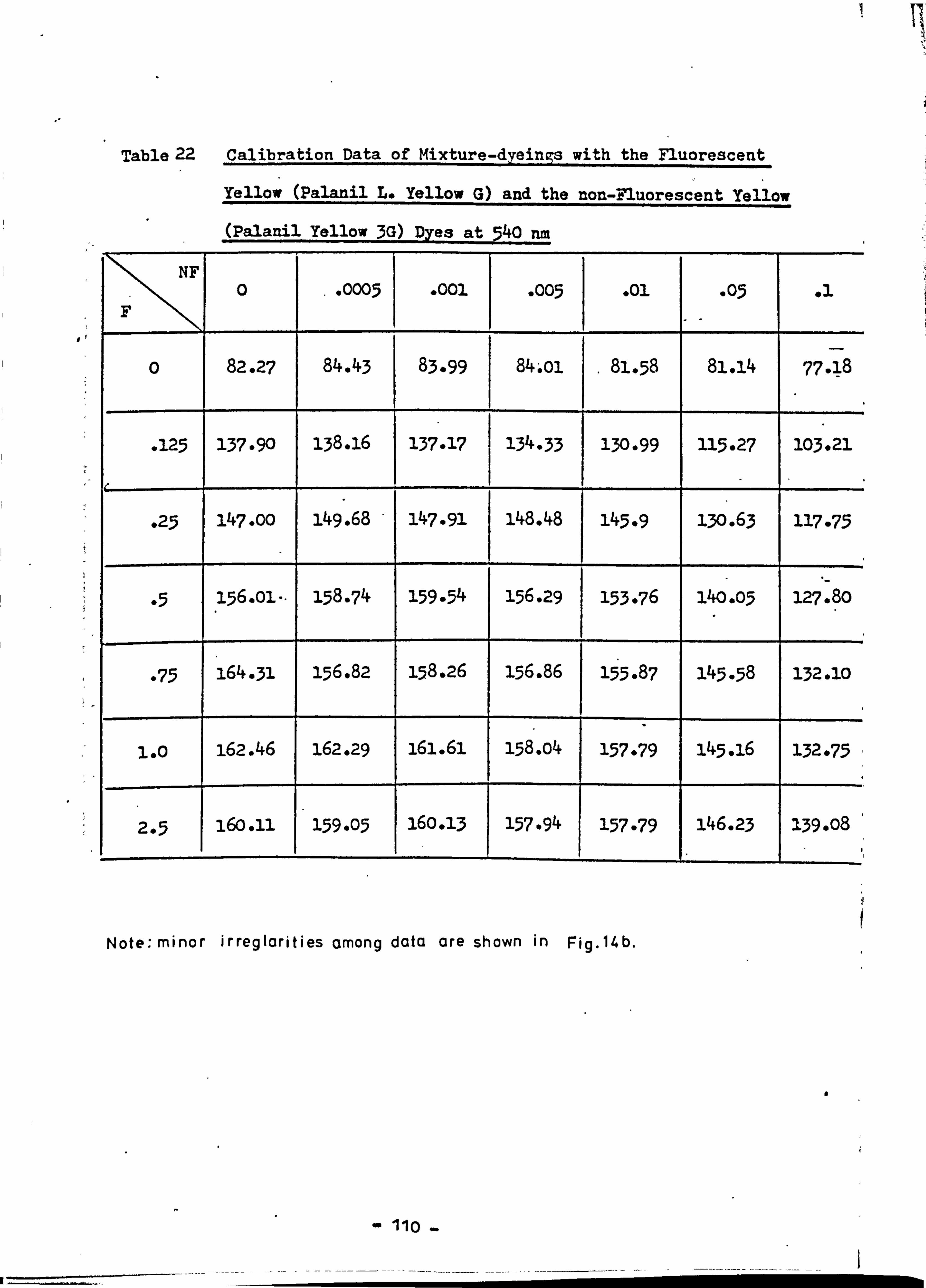
Table 22 Calibration Data of MixtUre-dyeings with the Fluorescent
. Yellow (Palanil L. Yellow G) and the non-Fluorescent, Yellow
(Palanil Yellow 3G) Dyes at 540 nm
NF 0 0005 . 001 -005 . 01 -05 11
0 82.27 84.43 83-99 -ol 840 81-58 81.14 77. ý8
. 125 137-90 138.16 137-17 134-33 130-99 U5.27 103,21
, 25 147-00 149.68 147-91 148.48 145-9 130.63 117-75
.5 156. ol-. 158-74 159-54 156.29 153.76 140-05 127.80
. 75 164-31 156.82 158.26 156.86 155.87 145-58 132.10
1.0 162.46 162*29 161.61 158.04 157-79 145.16 132-75
2.5 160-11 "159-05 16o-13 157.94 157-79 146.23 139.08
Note: minor irreglarities among data are shown in Fig. 14b.
a
- 110 -
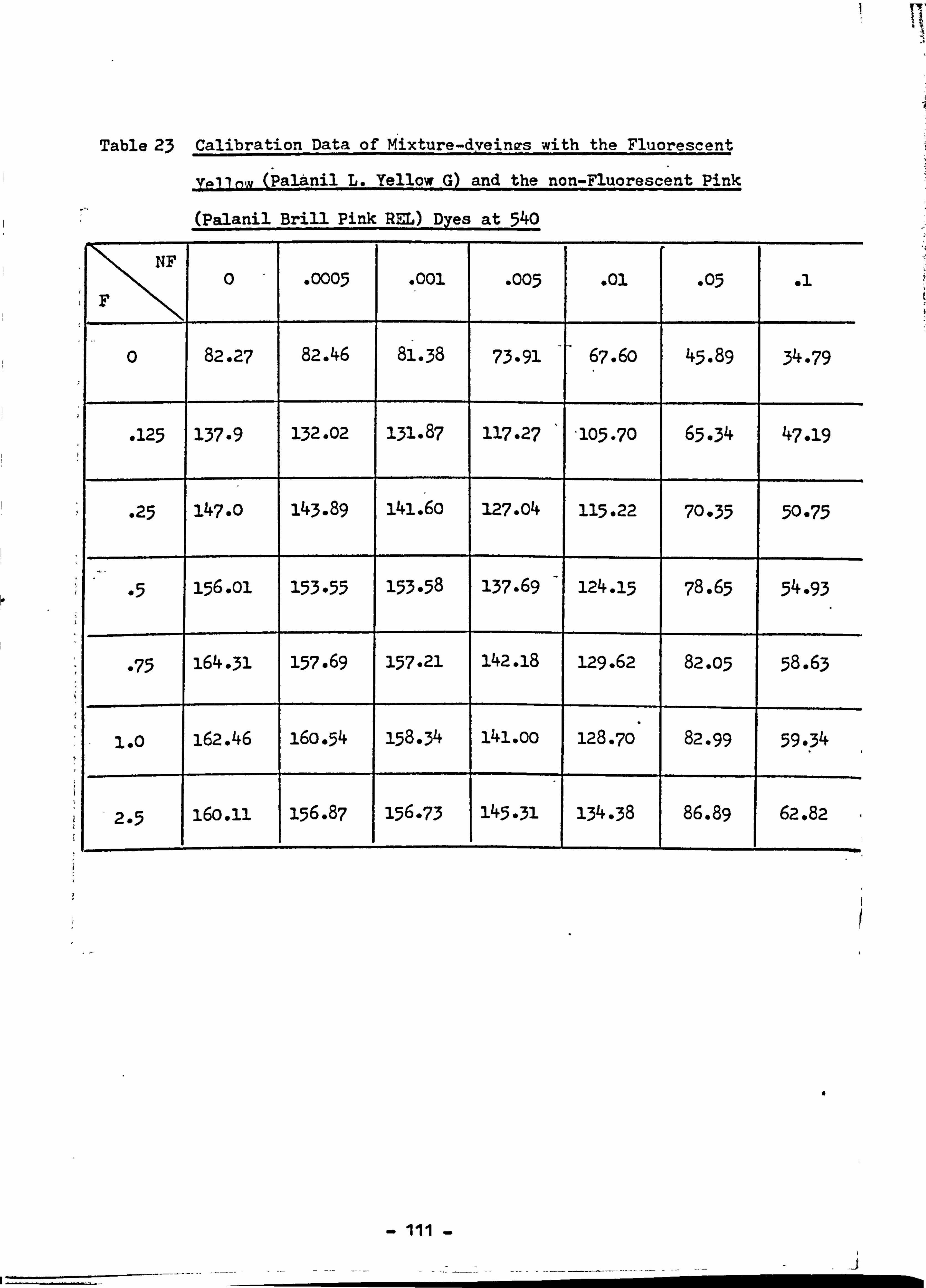
Table 23 Calibration Data of Mixture-dyeiniýs with the Fluorescent
(Pal&nil L. Yellow G) and the non-Fluorescent Pink
(palanil, Brill Pink_REL) Dyes at 540
NF
F 0 -0005 . -Ool -005 . 01 . 05 .1
0 82.27 8? -. 46 81-38 73-91 67-60 45.89 34-79
, 125 137.9 132.02 131.87 117.27 -105-70 65-34 47-19
. 25 147-0 143.89 141.6o 127.04 115.22 70-35 50-75
.5 156. ol 153-55 153-58 137-69 124-15 78.65 54-93
. 75 164-31 157.69 157.21 142.18 129.62 82-05 58.63
1.0 162.46 16o-54 158-34 141. oo 128-70 82.99 59-34
2.5 160.11 156.87 156-73 145-31 134-38 86.89 62.82
0
- ill -
1
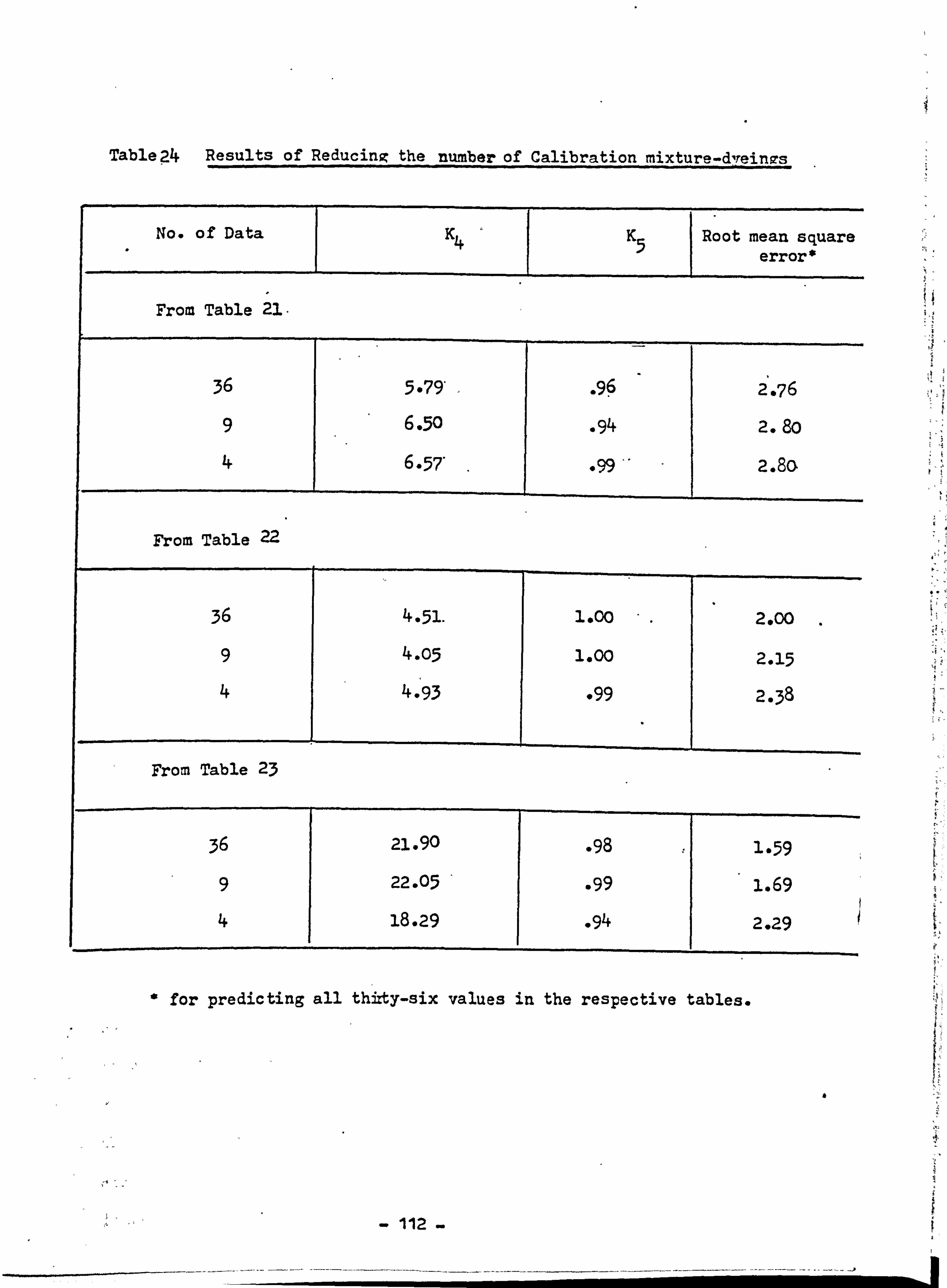
Table ý4 Results of Reducing the number of Calibration mixture -d7! ein%rs
No. of Data K4 K5 Root mean square error*
From Table 21.
36 5-79*, . 9ý 2. -76 9 6.50
. 94 2.80
4 6-57 2.80
From Table
36 4.51. 1000 2.00
9 4-05 1.00 2-15
4 4.93 . 99 2-38
From Table 23
36 21.90 . 98 1-59
9 22-05 . 99 1.69
4 18.29 . 94 2.29
* for predicting all thfity-six values in the respective tables.
a
-112
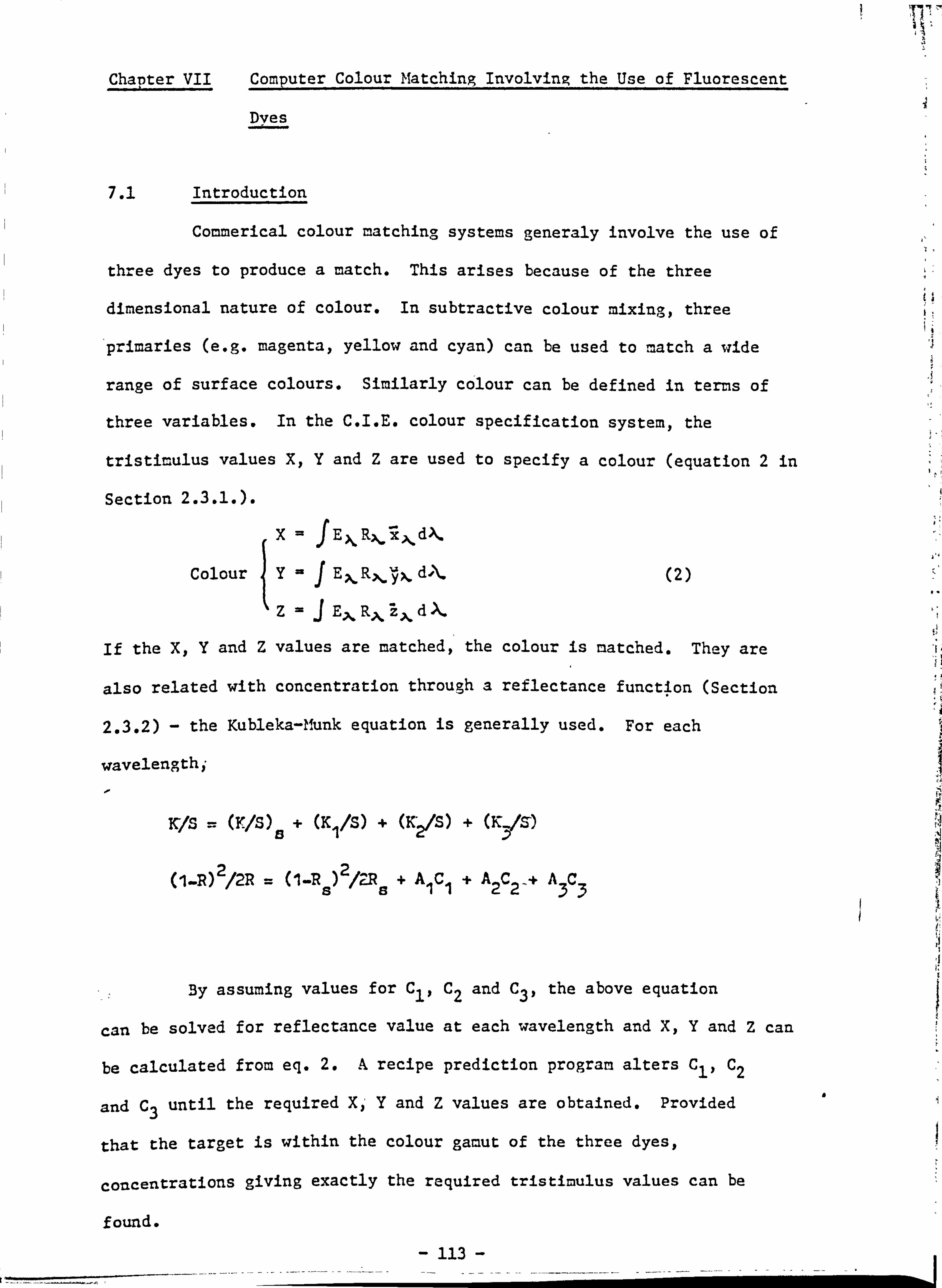
ChaT)ter VII Computer Colour Matching Involving the Use of Fluorescent
Dves
7.1 Introduction
Commerical colour matching systems generaly involve the use of
three dyes to produce a match. This arises because of the three
dimensional nature of colour. In subtractive colour mixing, three
primaries (e. g. magenta, yellow and cyan) can be used to match a wide
range of surface colours. Similarly colour can be defined in terms of
three variables. In the C. I. E. colour specification system, the
tristimulus values X, Y and Z are used to specify a colour (equation 2 in
Section 2.3.1. ).
x E, ), R>, d
Colour yER..,,, yl >,. d A.
z Ex R.,, iA. dk
If the X, Y and Z values are matched, the colour is matched. They are
also related with concentration through a reflectance func4on (Section
2.3.2) - the Kubleka-11(unk equation is generally used. For each
wavelength; I
KIS = (Y/S) 8+
(K I IS) + (K ý'S) + (K3/'S)
(1-R) 2 /2R = (1 -R s) 21a,
s+A1c1+A2c2 -+ A3c3
By assuming values for C 11 C2 and C3, the above equation
can be solved for reflectance value at each wavelength and X, Y and Z can
be calculated from eq. 2. A recipe prediction program alters C 11 C2
and C3 until the required X)' Y and Z values are obtained. Provided
that the target is within the colour gamut of the three dyes,
a
Concentrations giving exactly the required tristimulus values can be
found.
113
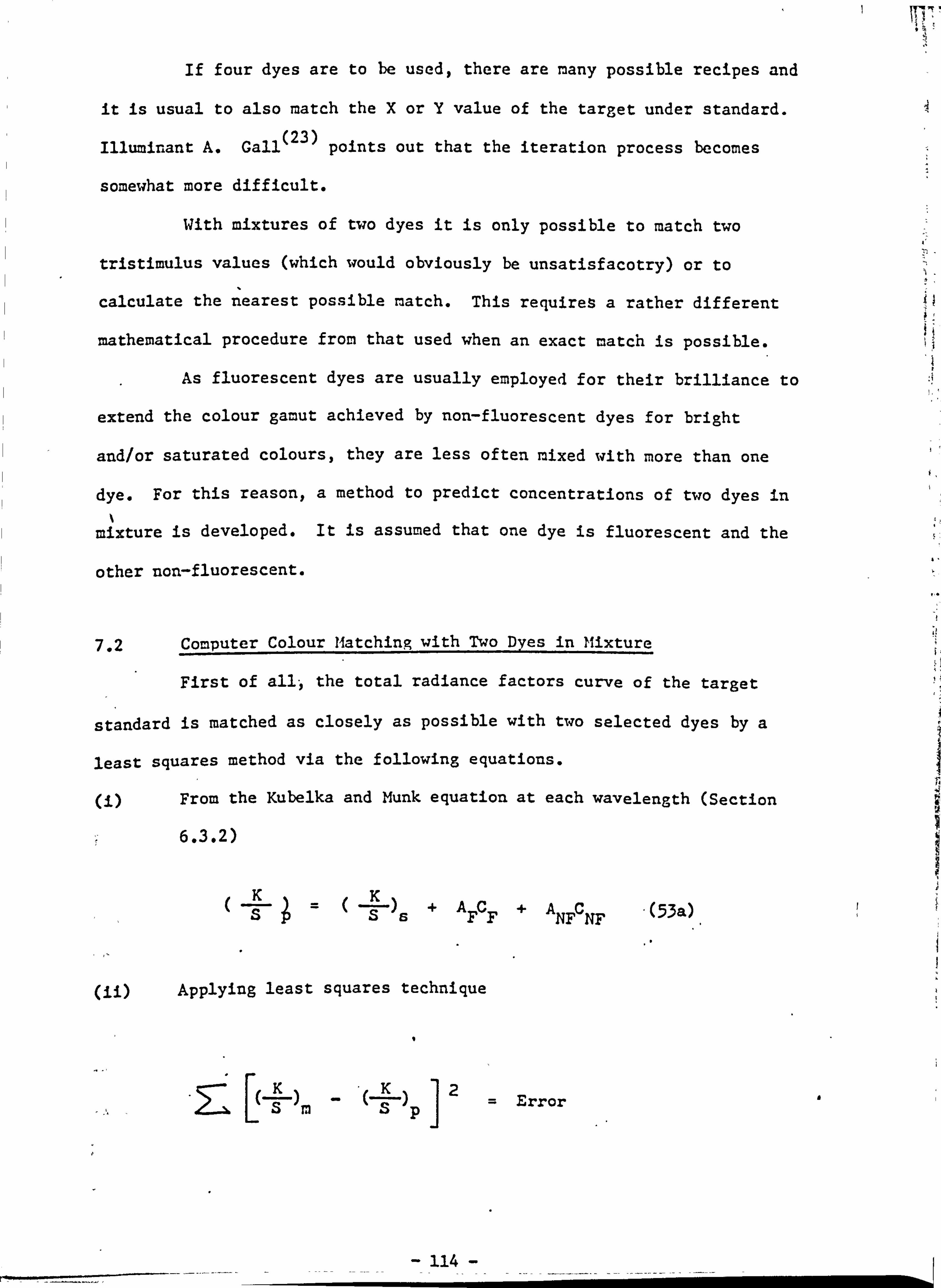
If four dyes are to be used, there are many possible recipes and
it is usual to also match the X or Y value of the target under standard.
Illuminant A. Gall (23) points out that the iteration process becomes
somewhat more difficult.
With mixtures of two dyes it is only possible to match two
tristimulus values (which would obviously be unsatisfacotry) or to
calculate the nearest possible match. This requires a rather different
mathematical procedure from that used when an exact match is possible.
As fluorescent dyes are usually employed for their brilliance to
extend the colour gamut achieved by non-fluorescent dyes for bright
and/or saturated colours, they are less often mixed with more than one
dye. For this reason, a method to predict concentrations of two dyes in
mixture is developed. It is assumed that one dye is fluorescent and the
other non-fluorescent.
7.2 Computer Colour Matching with Two Dyes in Mixture
First of all-, the total radiance factors curve of the target
standard is matched as closely as possible with two selected dyes by a
least squares method via the following equations.
U) From the Kubelka and Munk equation at each wavelength (Section
6.3.2)
SKr+AC+A K
(53a) SFF NFCNF
Applying least squares technique
I
)p 2 Error s n,
- 114 -

or
K )m - AFC F-A NFCNF Error
dError AK) dC FsS
AFCF -A NF c NF
Assuming dError/dC Fý
AK AFCF A F SK )m
s NFCNF 0
K2 AmC -ZA FSsF, F FANFCNF ý-- 0
Similarly
A -IL) - (-" I- ZA AAc0 F NFCF NF NF NF sm >-
I(. I
>ý-
,.
0.1 .
where subscripts
s- substrate, m- measured, p- predicted,
(57)
(58)
F- fluorescent dye; NF - non-fluorescent dye.
During this initial computationt the Kubelka-Munk constants
(AF) at the fluorescent region of the fluorescent dye are taken to be
zero. In the other words no absorption or fluorescence is assumed in
this region. By solving equations 57 and 58 for CF and C NP the -
initial match recipe is obtained. Since fluorescence is ignored the
concnetrations will not be correct, but should be reasonable starting
values for later calculations. Furthermore, the Ganz's extension of the i
y, -ri equation (Section 3.4.2) will be considered during refinement of the
program.
a
-115-
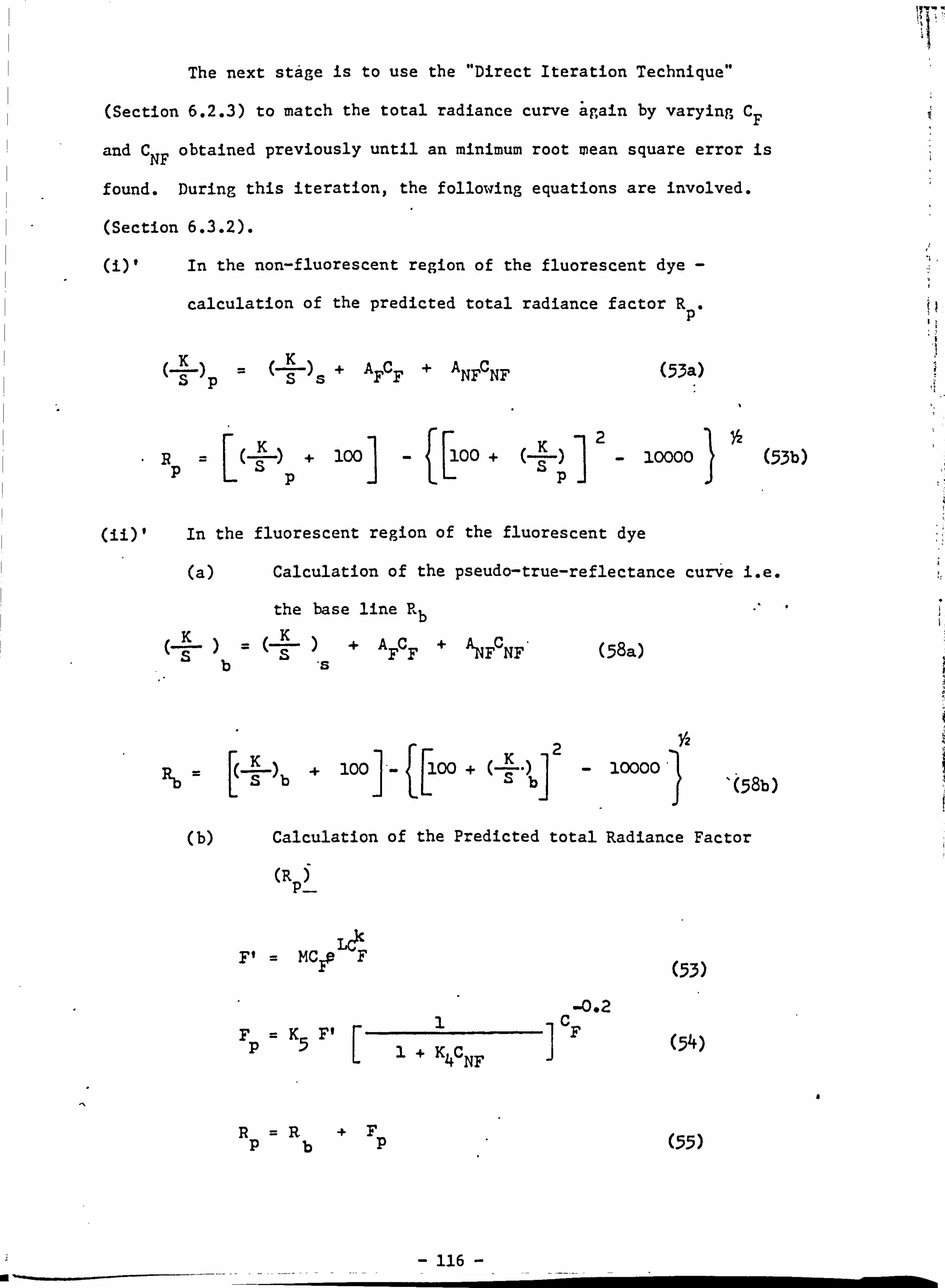
The next stage is to use the "Direct Iteration Technique"
(Section 6.2.3) to match the total radiance curve again by varying CF
and C NF obtained previously until an minimum root mean square error is
found. During this iteration, the following equations are involved.
(Section 6.3.2).
UP In the non-fluorescent region of the fluorescent dye
calculation of the predicted total radiance factor Rp
)p K+A+A ss FCF NFCNF (53a)
K+ loo [loo
+2- 10000 (53b) pspspI
In the fluorescent region of the fluorescent dye
(a) Calculation of the pseudo-true-reflectance curve i. e.
the base line Rb K+A+ PLV C
SSFF NF (58a)
R+ 100 100 + (-E-. ) j2 10000'
YZ
bSb[
13 5bI 08b)
(b) Calculation of the Predicted total Radiance Factor
(R p
Lcý F' = MC? F
(53)
F=K F' p5
1
1+ K4CNF
RFp
-0.2 F (54)
(55)
a
116

(iii), Calculation of the root mean square error
AR - Rm -R (58c)
E &R (58d)
16
The concentrations of the two dyes are varied systematically by the
"Direct Iteration Technique" (described in Section 6.2.3) until the
minimum value for E is obtained.
Having completed the spectral match, the concentrations for the
fluorescent and the non-fluorescent dyes are further iterated by the same
technique to achieve a minimum in colour difference in standard
illuninant D 65 with the supplementary standard 100 observer.
Equation 2 for CIE tristimulus values, 14ofor CIELAB and 15 for colour
difference are used (Section 2.3.1 and 2.3.4).
Flow chart V illustrates the program developed for match
prediction with binary mixture including the use of one flýorescený: dye.
Table 25 illustrates results of an actual prediction at each stage-, while
the actual iteration of this target is in Appendix D. Trial 1 is
obtained with the initial concentrations calculated by the least squares
method and Trial 2 gives a formula with the nearest spectral match. The
final one is resulted from iteration to minimize the colour difference in
CIELAB unit in order to have a close tristimulus. colour match. Fig. 15
shows the total radiance factors curves for data in Table 25.
117 low
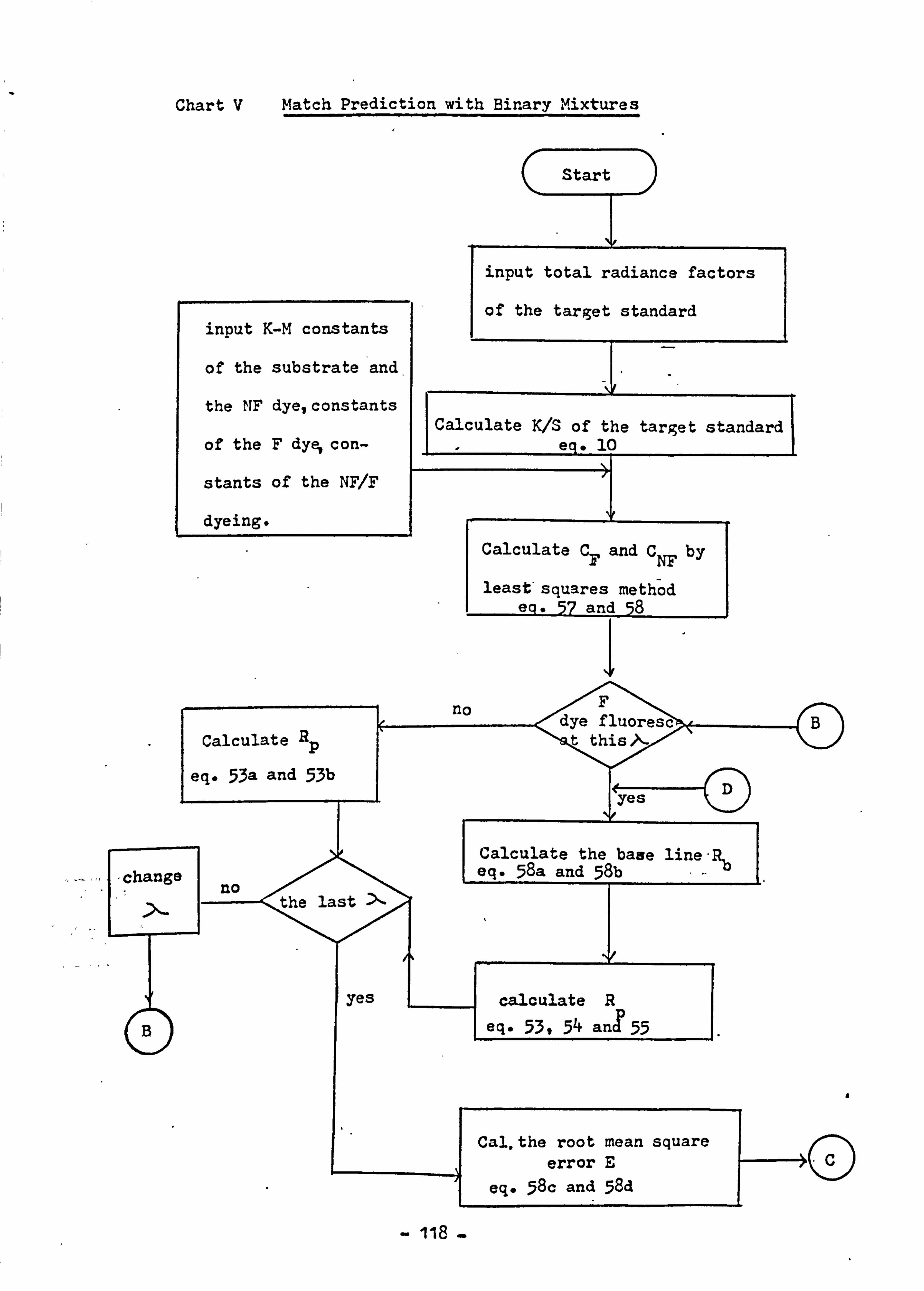
Chart V Match Prediction with Binary Mixtures
I
Start
input total radiance factors
input K-M constants of the target standard
of the substrate and.
the NF dye. constants Calculate K/S of the target standard
of the F dye, con- eq* 10
stants of the NFIF
dyeing.
Calculate CF and C NF by
least'squares method
I Calculate Rp
eq- 53a and 53b
change no the last
B
yes
no F dye fluoresc B
t this
D
Calculate the base line-R eq- 58a and 58b ,_b
calculate R
eq- 53,54 anT 55
a
Cal, the root mean square error E
eq. 58c and 58d
- 118 -
C
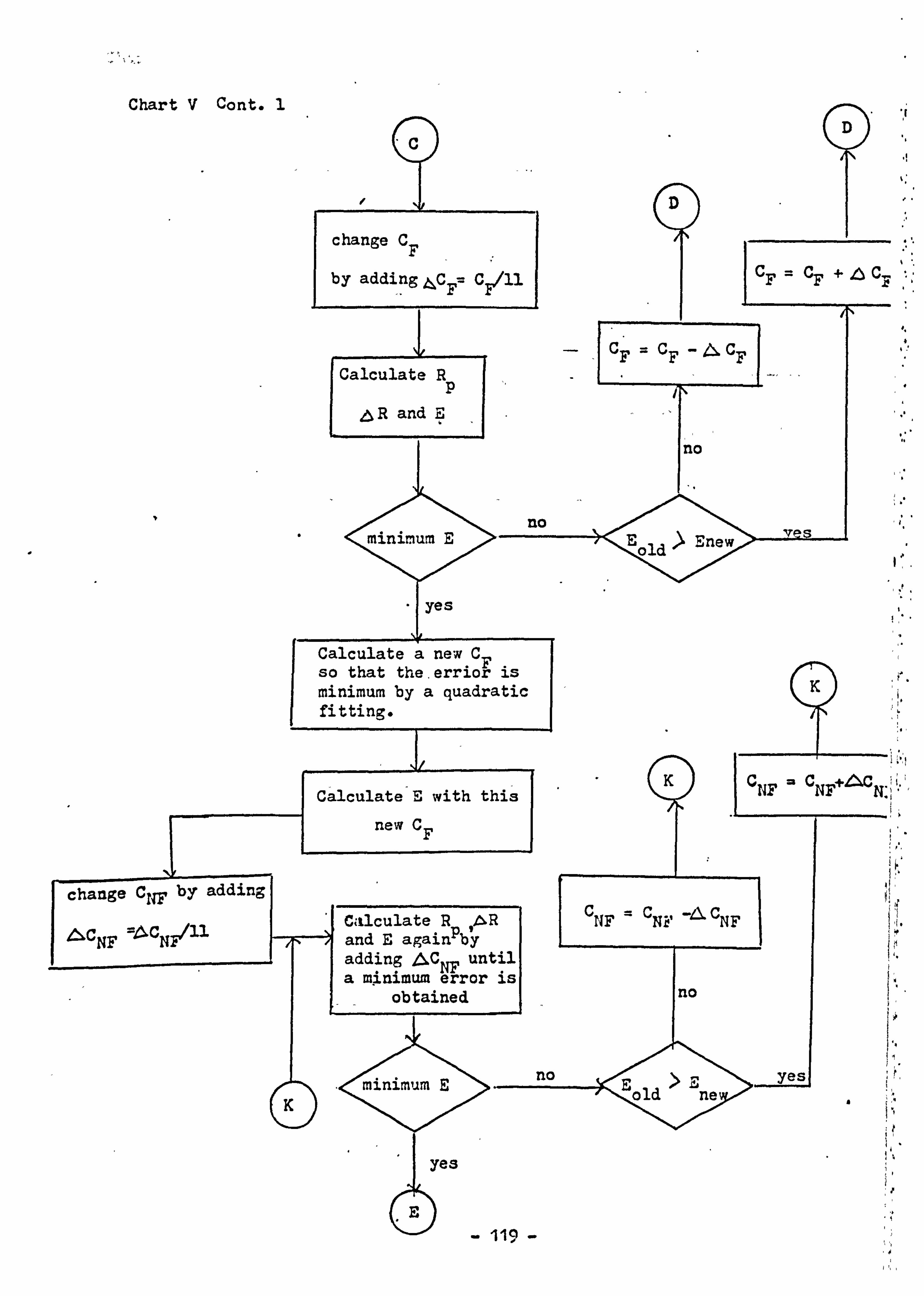
Chart V Cont. I
change CITF by adding
It LISICNF =41CH7111
D C
change CF
by addi I ng 4C F= CI/11 CF CF + CF
CF CF CF Calculate R
,6R and
no
minimum E no
E '-Pnew old
+yes
Calculate a new CF so that the. errior is K minimum by a quadratic fitting.
N. KC NF C N: V+Zý'C Calculate E with this
new C F
CC -16. C calculate R n'ý. R NF N? NF and E againPbý adding AC until NF a mýnimum error is
no obtained 9
no yes minimum E>F, old ne K D
yes
119
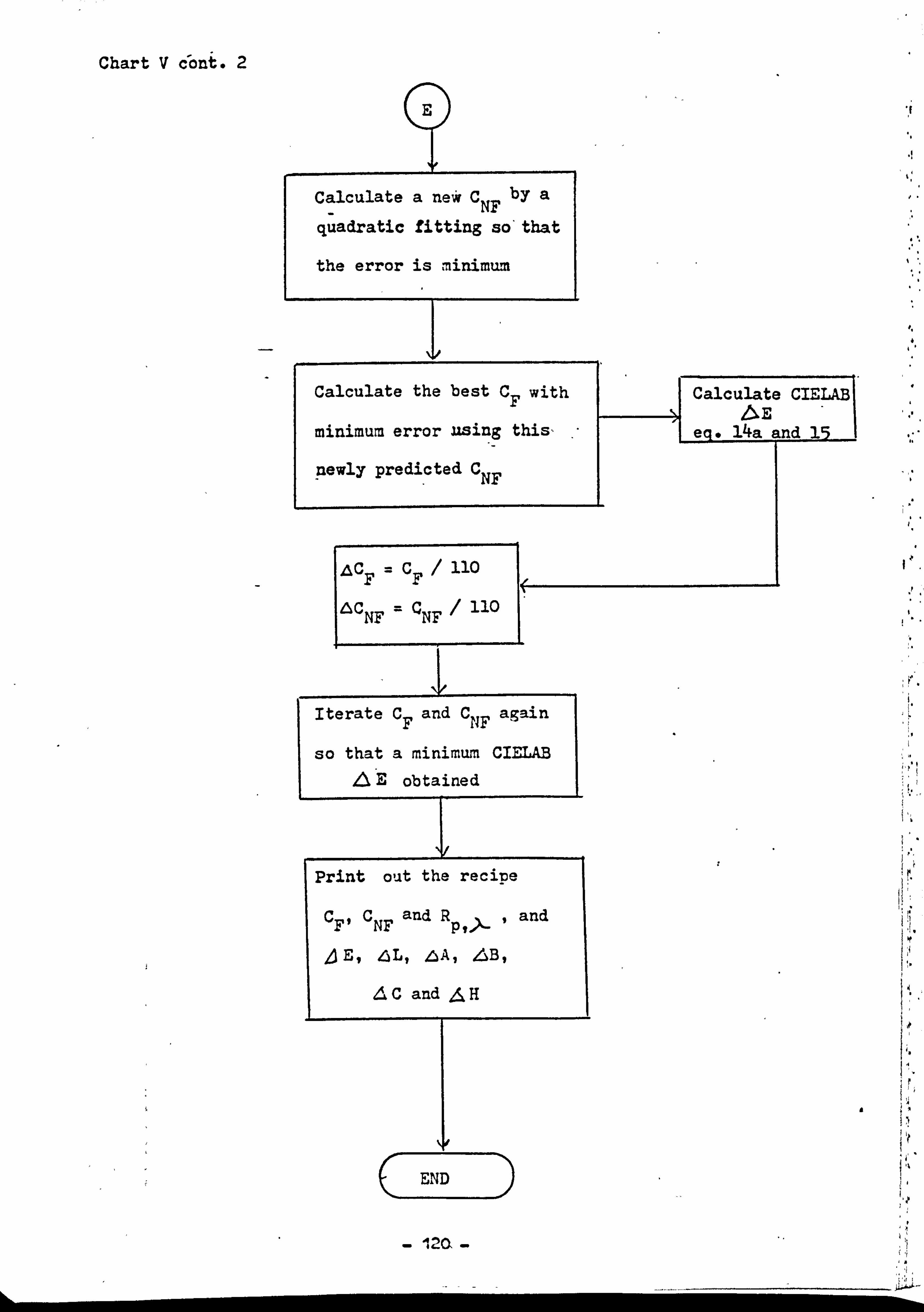
Chart V dont. 2
E
Calculate a ne* C by a NF quadratic fitting so'that
the error is minimum
Calculate the best C with Calculate CIELAB F
minimum error using this, eq. 14a nd 15
pewly predi . cted C NF
'ac F=CF/ 110 1 1.
&C c
110 NF = NF
Iterate C and C again F NF
so that a minimum CIELAB E obtained
Print out the recive
c and R and Fl CNF p
E, 4L, 6A, LB,
AC and H
CýED

Table 25 Print out from the Match - Prediction Programme
Total Radiance Factors
Wavelength (nm) TARGET (J3)
TRIAL 1 TRIAL 2 FINAL
400 42.060 44.624 43.008 44.268
420 45-110 47.459 45.872 47.205
440 44-58o 46-341 44-976 46. ý65
460 35.940 37.824 36-351 37-786
480 27.160 28.408 26.914 28.245
500 21-050 21.289 19.928 21.070
520 17-110 16.497 15.285 16.241
54o 17-520 17-599 16.480 17.489
56o 24.230 25-729 25.118 26.4o5
580 47.14o 44.472 44-978 46.966
600 74.64o 74-556 76.898 78.8o6
620 97-700 95-599 98-367 99.48o
640 98.480 95-380 97.277 97-791
660 94.19o 91-155 92.189 92.485
680 91-590 88.891 89.4ao 89.69o
700 89-580 87.246 87.602 87-74o
DE CIELAB 2-563 1.916 1.476
Luminous Red G . 100 0101 . 121 -Ill
Red 5 BEL . 100 . 099 x96 o88
121
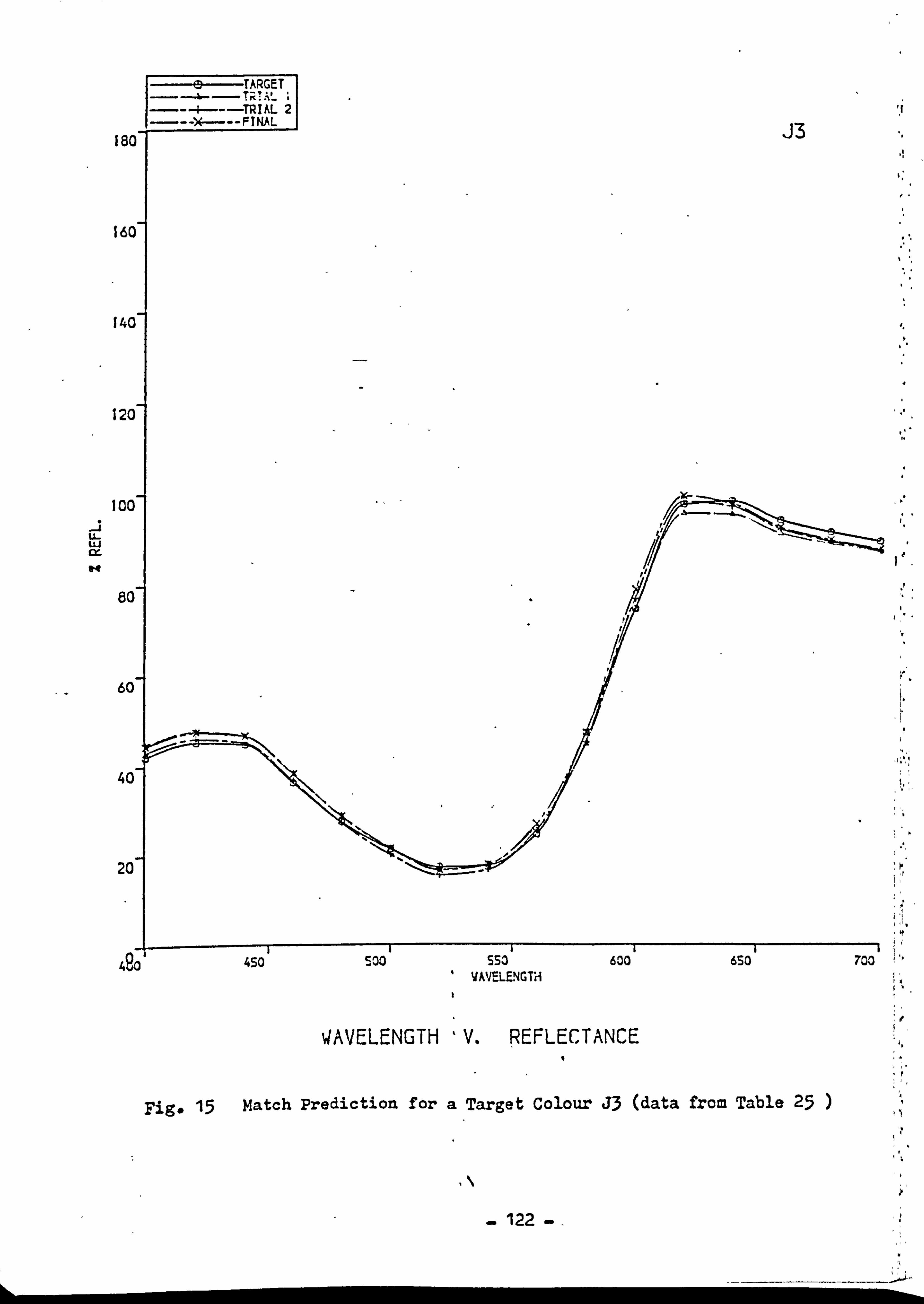
fac
16C
14C
120
100
U- ui cx
80
60
40
20
450 SOO 553 600 6SO 700 490 VAVELENGTH
VAVELENGTH 'V. REFLECTANCE
Fig. 15 Match Prediction for a Target Colour J3 (data from Table 25
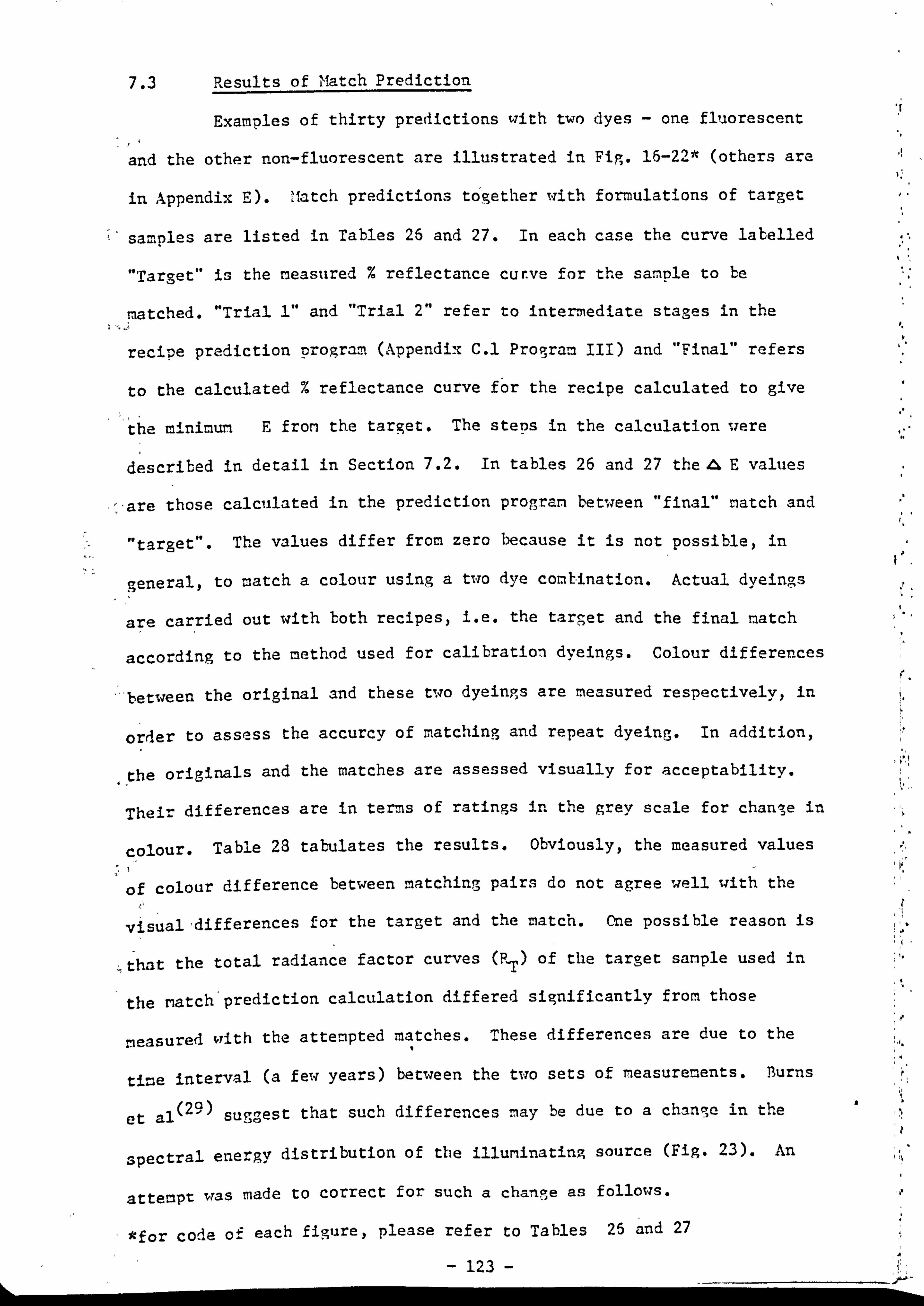
7.3 Results of Match Prediction
Examples of thirty predictions with two dyes - one fluorescent
and the other non-fluorescent are illustrated in Fig. 16-222* (others are
in Appendix E). ', latch predictions together with formulations of target
samples are listed in Tables 26 and 27. In each case the curve labelled
"Target" is the measured % reflectance curve for the sample to be
matched. "Trial 1" and "Trial 2" refer to intermediate stages in the
recipe prediction program (Appendix C. 1 Program III) and "Final" refers
to the calculated % reflectance curve for the recipe calculated to give
the minimum E from the target. The steps in the calculation were
described in detail in Section 7.2. In tables 26 and 27 the AE values
, --are those calculated in the prediction program between "final" match and
"target". The values differ from zero because it is not possible, in
general, to match a colour using a two dYe combination. Actual d. veinc!,, s
are carried out with both recipes, i. e. the target and the final natch 0
according to the method used for calibration dyeings. Colour differences
between the original and these two dyeings are measured respectively, in
order to assess the accurcy of matching and repeat dyeing. In addition,
.; he originals and the matches are assessed visually for acceptability.
Their differences are in terms of ratings in the grey scale for chan-, e in
colour. Table 28 tabulates the results. Obviously, the measured values
of colour difference between matching pairs do not agree well with the
visual, differences for the target and the match. One possible reason is
; that the total radiance factor curves (P ) of the target sample used in IT
the natch'prediction calculation differed significantly from those
measured with the attempted matches. These differences are due to the I
time interval (a few years) between the two sets of measurements. Burns
et al (29) suggest that such differences may be due to a change in the
spectral energy distribution of the illuminating source (Fig. 23). An
attempt Was made to correct for such a cha-iFe as follows.
a
*for cole of each figure, please refer to Tables 25 and 27
123
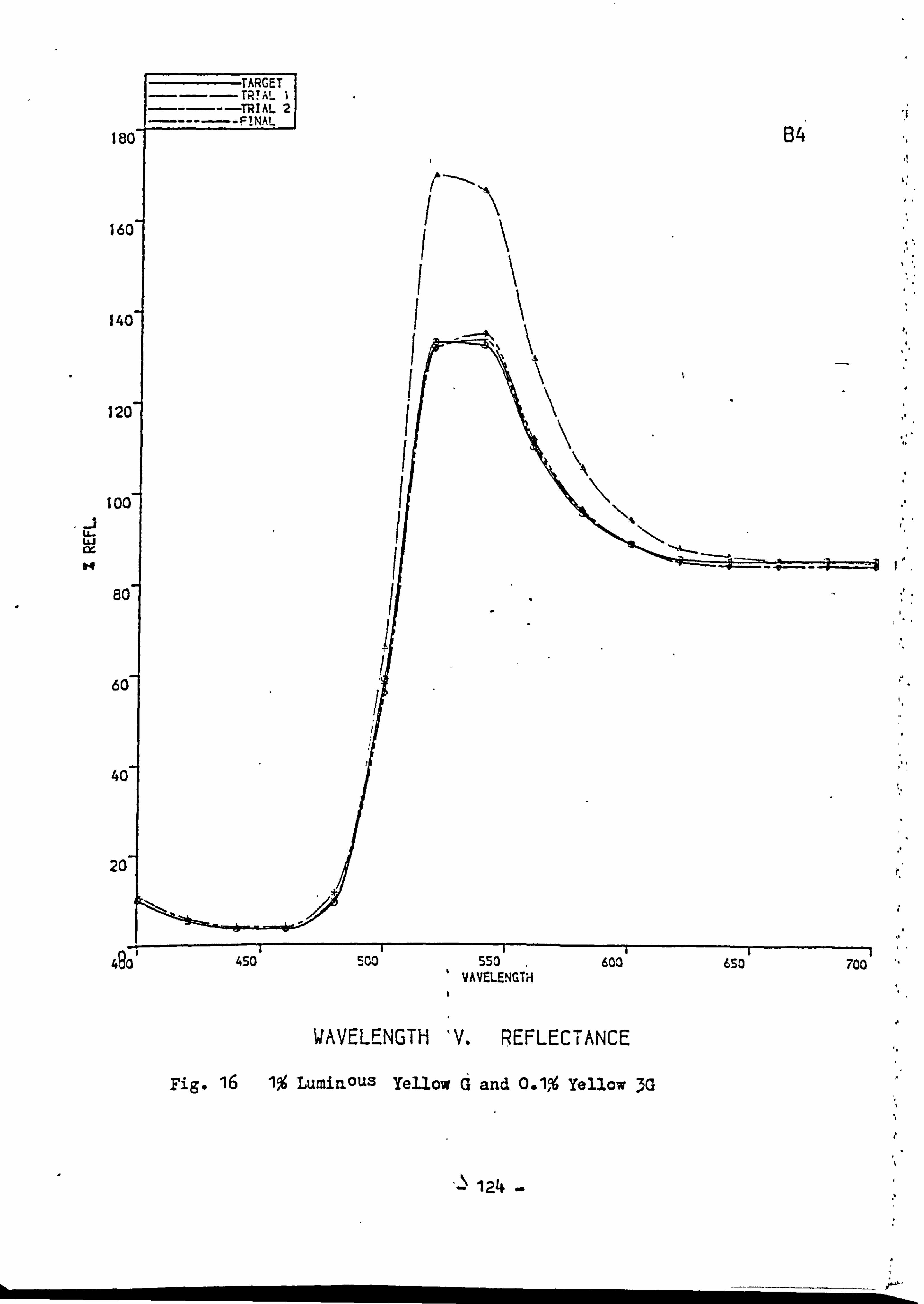
18
161
141
12(
too
80
60
40
20
490 450 500 550 603 VAVELENGTH
VAVELENGTH 'V. REFLECIANCE
Fig. 16 1% Luminous Yellow a and 0.1% Yellow 3G
\ 124 -
650 700

I . ac
160
&40
S20 I
Soo
LL. UJI
80
60
40
20
7
490' 450 Soo 550 600 650 7co 'IAVELENGTH
'dAVELENG-IH V. REFLECTANCE
Fig- 17 . 25% 1- Yellow G and -05% B. Pink REL
-: 6 125
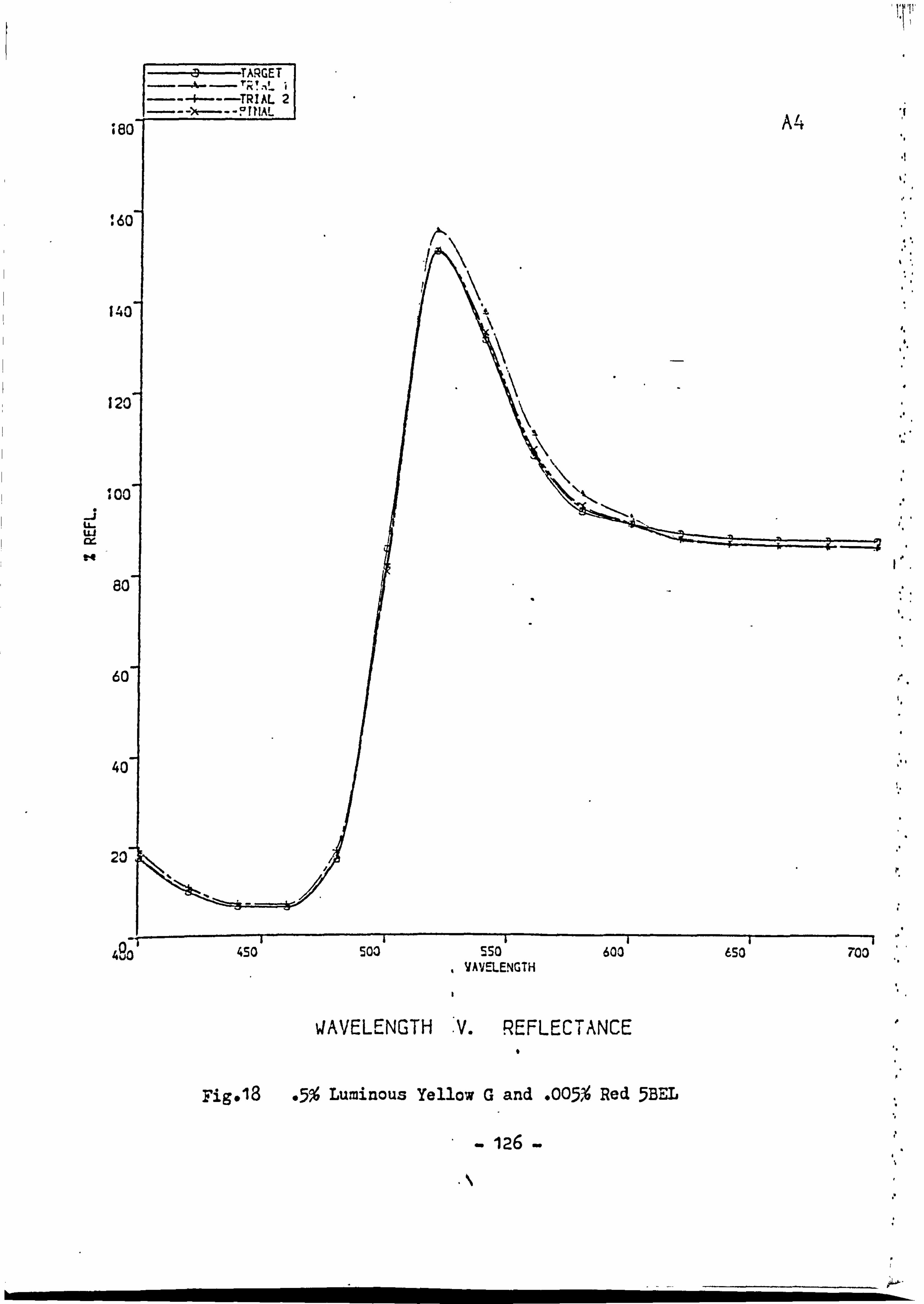
le
1 . 61
I4
12'%
ISO(
-j LL. uj cr-
�4
ac
6C
40
20
70o
Fig. 18 -5% Luminous Yellow G and . 005% Red 5BEL
126
493,450' 503" SSO . 603 . 650 VAVELENGTH
VAVELLENGTH 'V. REFLECIANCE 6
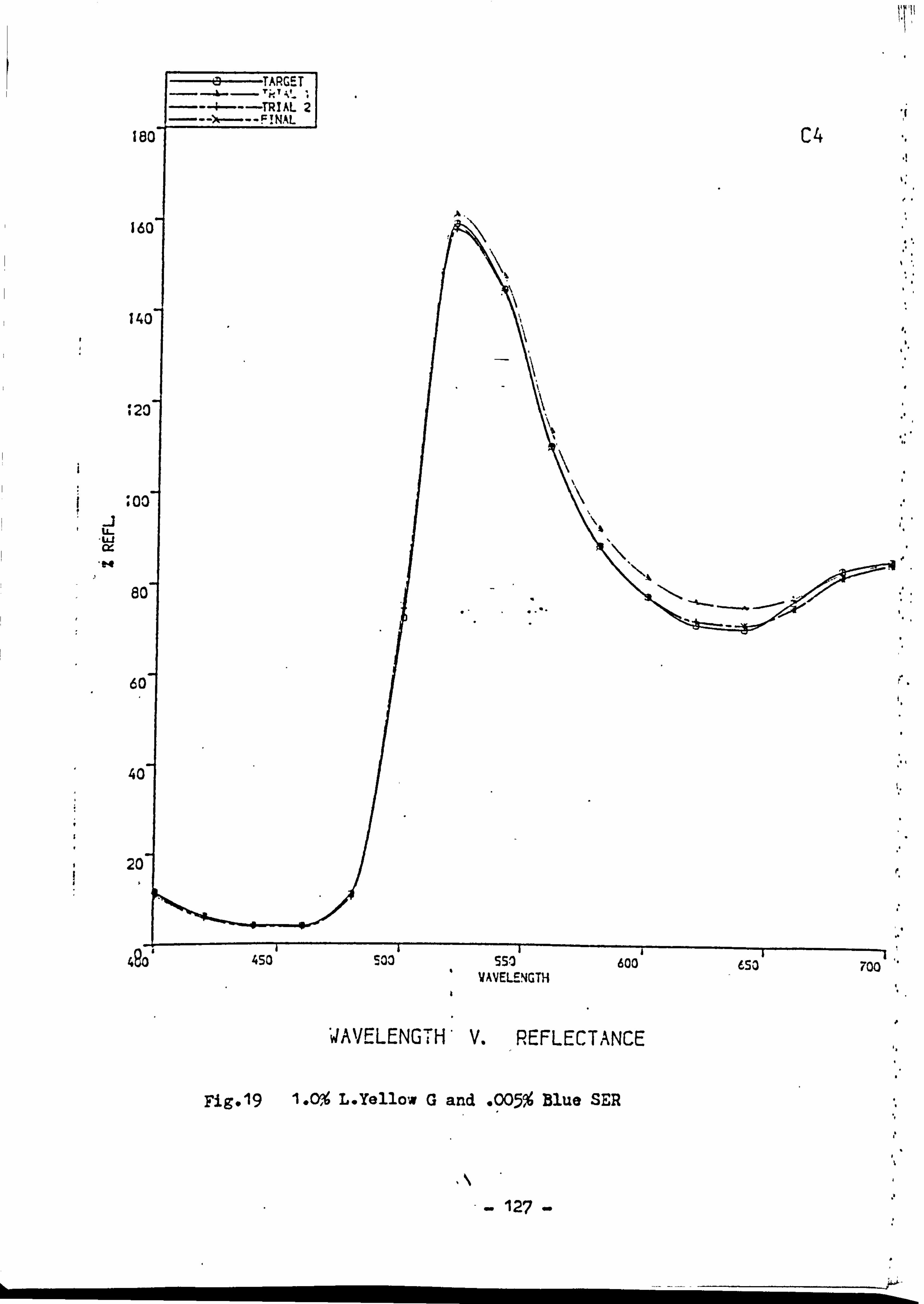
If
ld
14
,2
10i
tAJ cx
6C
40
20
4eO 450 Soo 55.1 600 6so 700 VAVELENGTH
'dAVELENGTH* V.
Fig, 19 1. N, L. Yellow G and -905% Blue SER
127

141
12(
loc
-i 12: p4
ac
6c
40
20
490 450 Soo 553 603 650 700 VAVELENGTH
VAVELENGTH V. REFLECTANCE
Fig. 20 . 025% 1* Red G and *25% Yellow 3G
A 128

0 la
i6
141
M
10(
-i LL- ui ix
ec
60-
40-
20
49ý 450 Soo 550 600 650 700 WAVELENGTH
WAVELENGTH V. REFLECTANCE
Fig*21 95% Lo Red G and -005% Red 5BEL
129
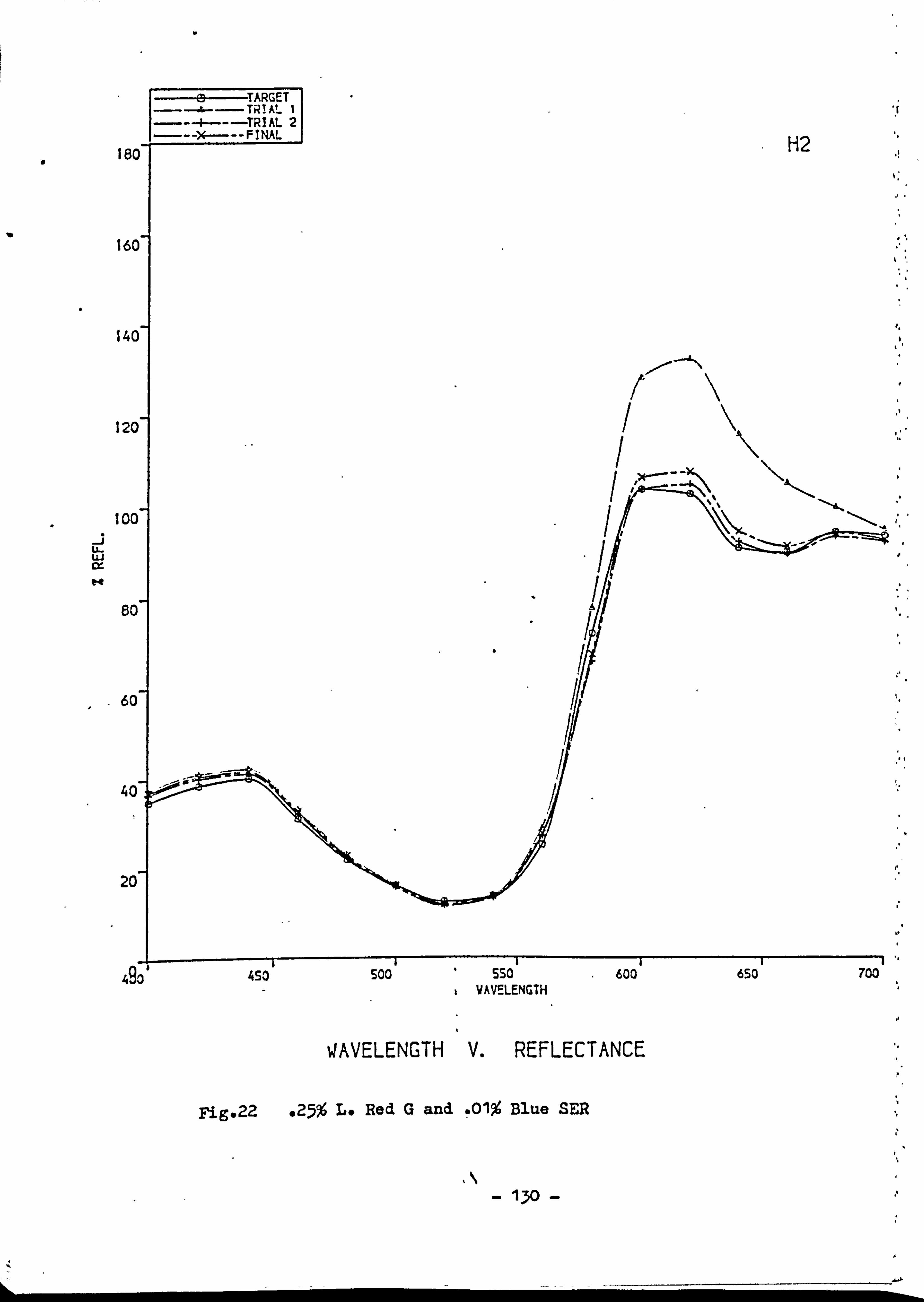
I 8C
16C
14C
120
100
U- LLJ cx
80
- 60
40
1
20
Fig, 22 925% Lo Red G and . 01% Blue SER
130
700 490 450' Soo 550 600 653 VAVELENGTH
OVELENGTH V. REFLECTANCE
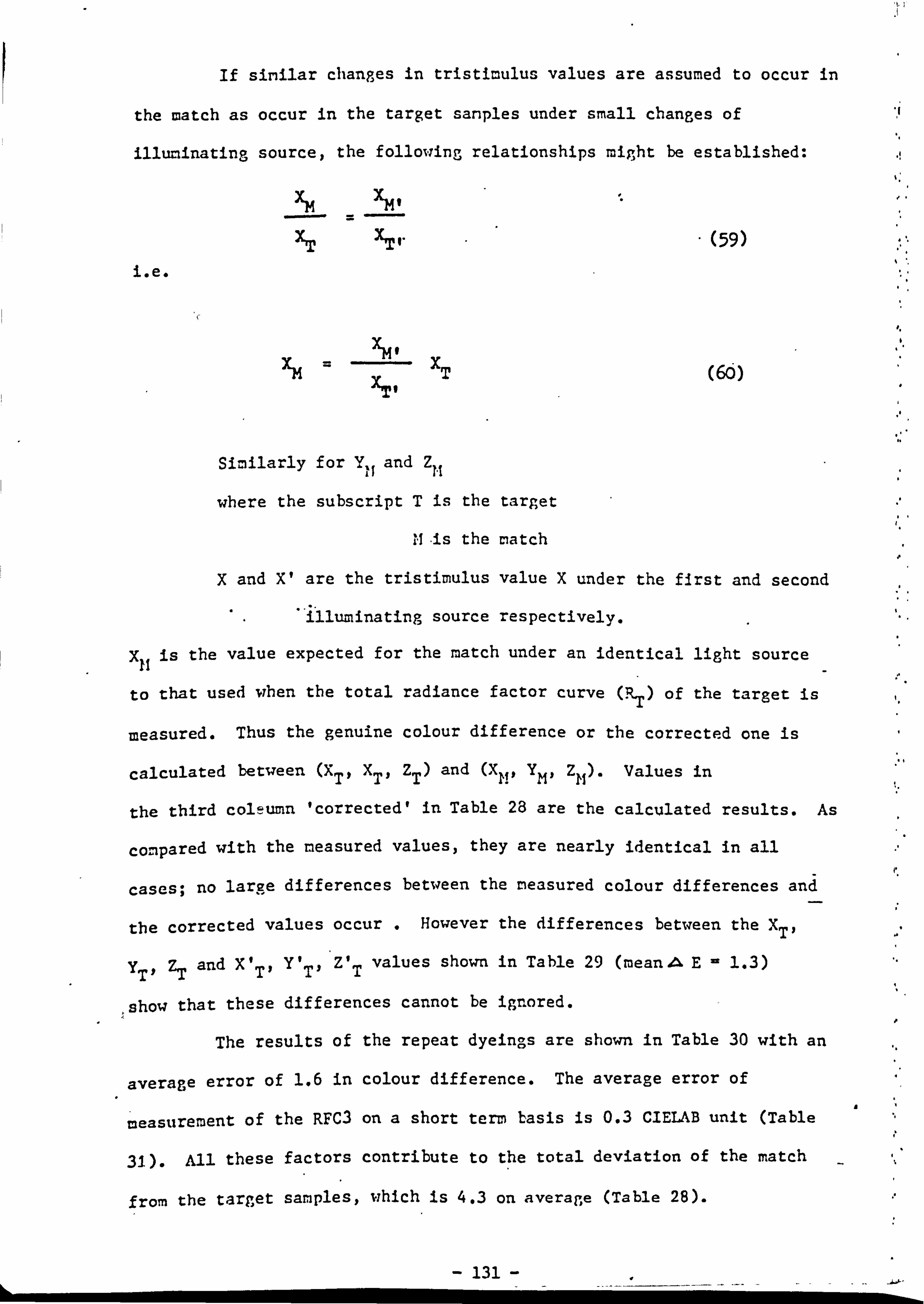
If similar changes in tristimulus values are assumed to occur in
the match as occur in the target sanples under small changes of
illuminating source, the following relationships might be established:
XM XMI
XT XT (59)
i. e.
c
Xý XM IxT
(6b) XTI
Similarly for Y it and Z 1.1
where the subscript T is the target
11 Is the match
X and XI are the tristimulus value X under the first and second
.. "illuminating source respectively.
X if is the value expected for the match under an identical light source
to that used when the total radiance factor curve (RT) of the target is
measured. Thus the genuine colour difference or the corrected one is
calculated between (X TI XTI ZT ) and (XI!, YM, ZM). Values in
the third coleumn 'corrected' in Table 28 are the calculated results. As
compared with the measured values, they are nearly identical in all
cases; no large differences between the measured colour differences and
the corrected values occur . However the differences between the X T'
YTI ZT and V TI Y1 T' ZT values shown in Table 29 (mean AE1.3)
, show that these differences cannot be ignored.
The results of the repeat dyeings are shown in Table 30 with an a
average error of 1.6 in colour difference. The average error of
measurement of the RFC3 on a short term basis is 0.3 CIELAB unit (Table
31). All these factors contribute to the total deviation of the match
from the target samples, which is 4.3 on average (Table 28).
- 131
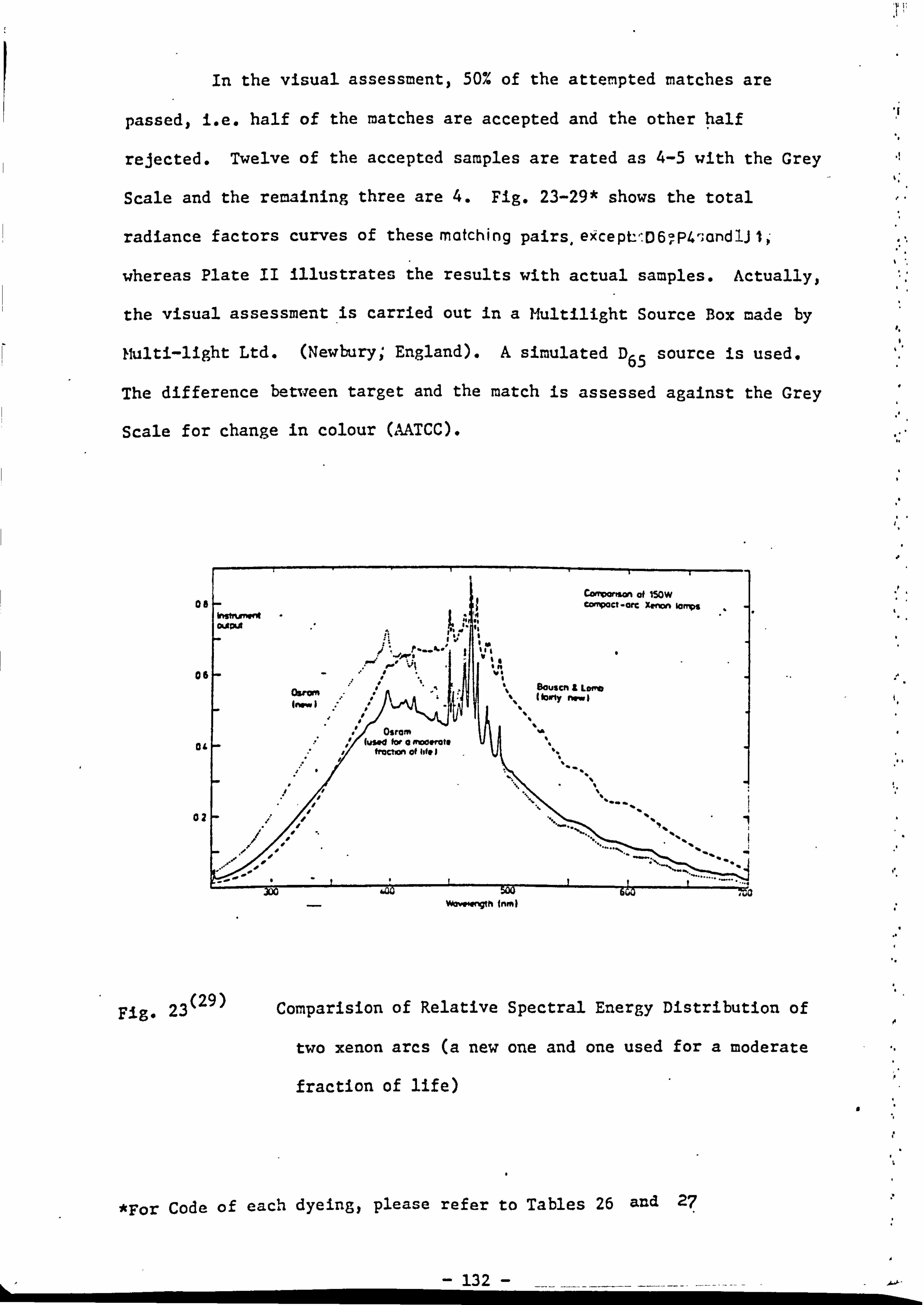
In the visual assessment, 50% of the atteripted matches are
passed, i. e. half of the matches are accepted and the other half
rejected. Twelve of the accepted samples are rated as 4-5 with the Grey__
Scale and the remaining three are 4. Fig. 23-29* shows the total
radiance factors curves of these match in g pairs, eýcept-"D60, P4-, and lj 1),
whereas Plate II illustrates the results with actual samples. Actually,
the visual assessmentis carried out in a Multilight Source Box made by
Ijulti-light Ltd. (Newbury; England). A simulated D 65 source is used.
The difference between target and the match is assessed against the Grey
Scale for change in colour (AATCC).
08
os
0&
02
wilstmiforrit
Inv. I
Osrom (used ftw a mooorate
fractiom of life I
cdyvvwmm of 15aw cm CI-Orc X~ In""
Scuscm A Lore #Orly nm
.......... .
Wavowvth Inmi
Fig. 23 (29) Comparision of Relative Spectral Energy Distribution of
two xenon arcs (a new one and one used for a moderate
fraction of life) a
*For Code of each dyeing, please refer to Tables 26 and 27
132
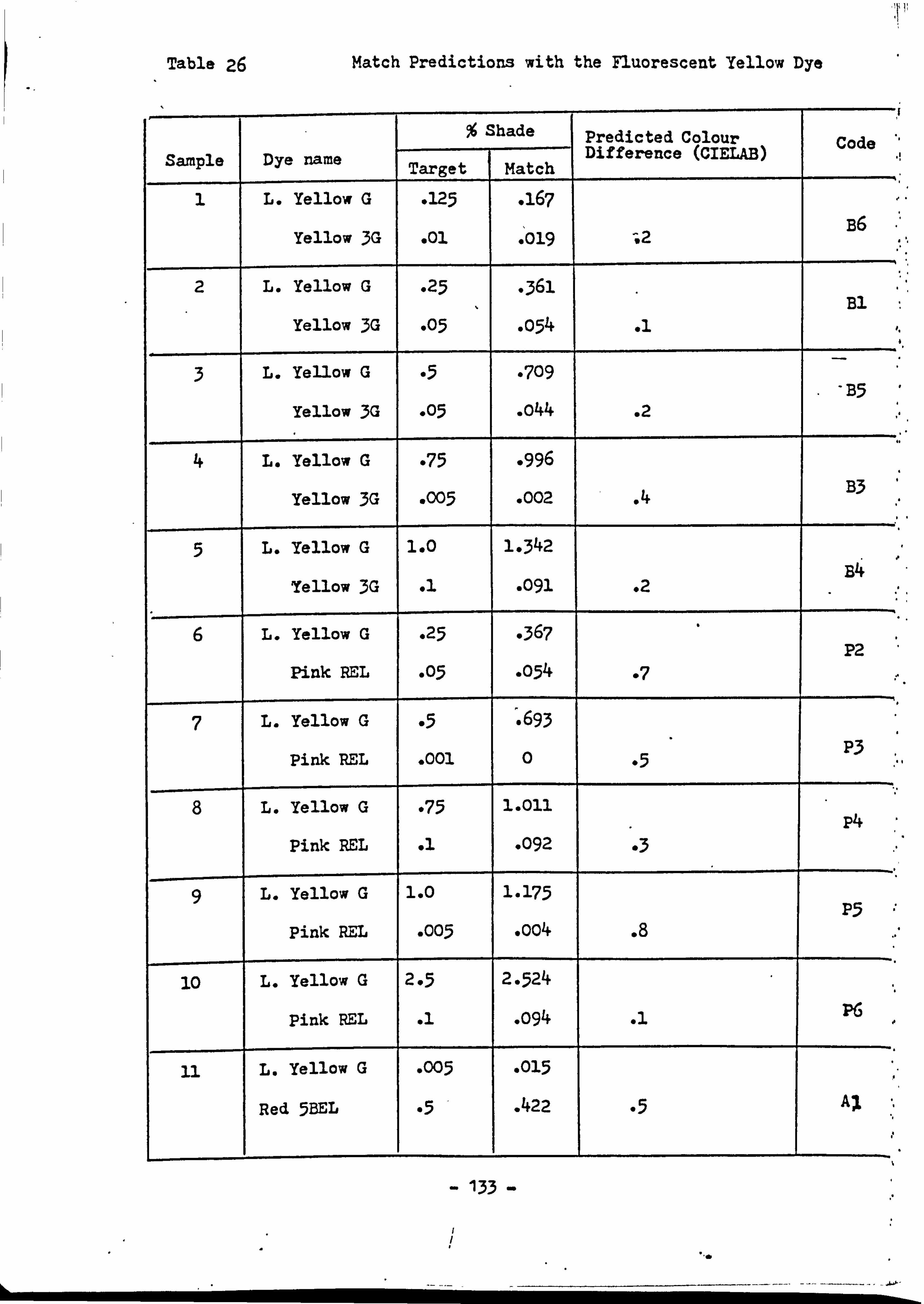
Table 26 Match Predictions with the Fluorescent Yellow Dye
% Shade Predicted Colour Code Sample Dye name Difference (GIELAB)
Target Match
1 L. Yellow G -125 . 167 , B6
Yellow 3G . 01 Olq -, 2
2 L. Yellow G . 25 -361 B1 Yellow 3G -05 -054 .1
3 L. Yellow G *5 *709 -B5
Yellow 3G -05 o44 .2
4 L. Yellow G -75 . 996
Yellow 3G -005 . 002 .4 B3
5 L. Yellow G 1.0 1.342 B4
Yellow 3G .1 . 091 .2
6 L. Yellow G . 25 -367 P2 Pink REL -05 -054 .7
7 L. Yellow G -5 . 693
P3 Pink REL . 001 0 *5
8 L. Yellow G -75 1.011 P4
Pink REL .1 . 092 *3
9 L. Yellow G 1.0 1-175 P5
Pink REL -005 oo4 .8
10 L. Yellow G 2-5 2-524
pink REL .1 x94 .1 P6
L. Yellow G -005 -015
Red 5BEL e5 - . 422 Al
- 133
1.0 000 - -*--------
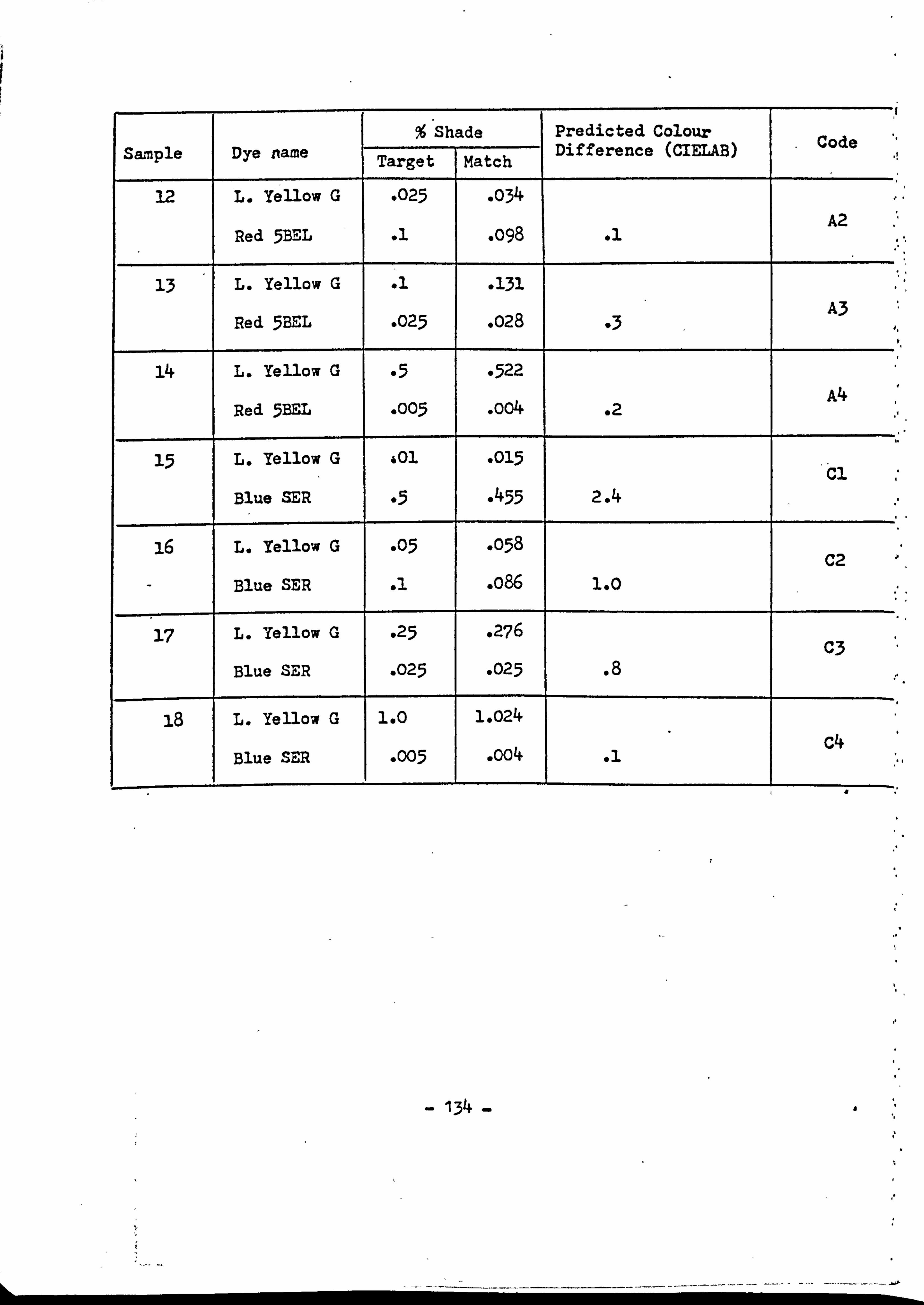
% Shade Predicted Colour Code Sample Dye name Target Match
Difference (CIELAB)
12 L. Yellow G -025 . 034 A2
Red 5BEL .1 . 098 .1
13 L. Yellow G -131 A3
Red 5BEL -025 . 028 -3
14 L. Yellow G 95 *522 A4
Red 5BEL -005 oo4 .2
15 L. Yellow G 1.01 -015 C1 Blue SER *5 . 455 2.4
16 L. Yellow G -05 *058 C2
Blue SER .1 o86 1.0
17 L. 'fellow G 25 . 276 C3
Blue SER . 025 . 025 .8
18 L. Yellow G 1.0 1.024 c4
Blue SER -, 005 . 004
134
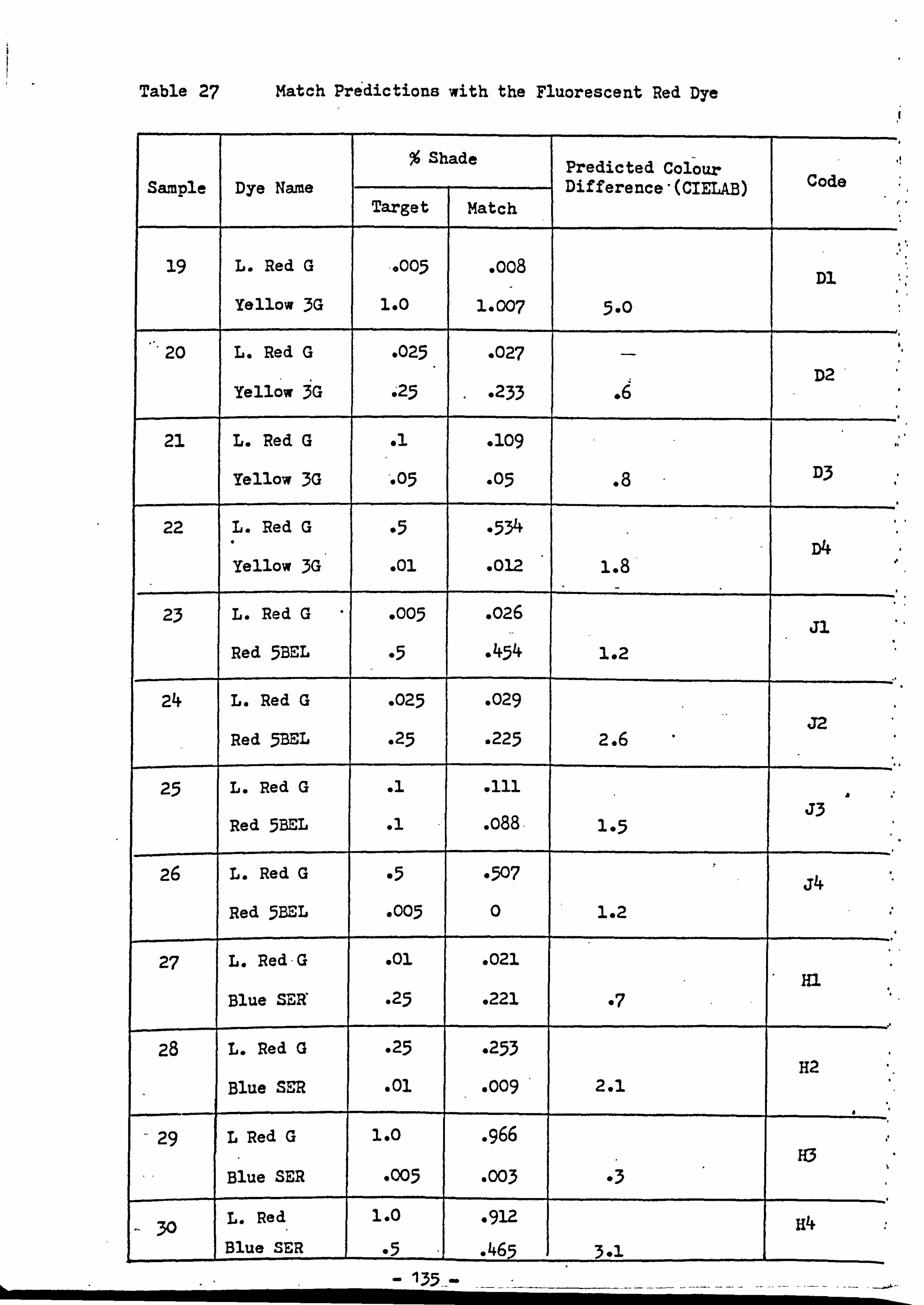
Table 27 Match Predictions with the Fluorescent Red Dye
% Shade Predicted Colour S l N Diff *(C Code amp e Dye ame -- erence IELAB)
Target Match
19 L. Red G -005 oo8 D1
Yellow 3G 100 1-007 5-0
20 L. Red G -025 -027 - D2
Yellow 3G 0,25 *233 .6
21 L. Red G 01 log
Yellow 3G -*05 -05 .8 D3
22 L. Red G *5 -534 D4
Yellow 3G *01 . 012 1.8
23 L. Red G -005 . 026
Red 5BEL e5 . 454 1.2
24 L. Red G . 025 . 029 J2
Red 5BEL . 25 . 225 2.6
25 L. Red G .1 . 111 J3
Red 5BEL .1 x88- 1*5
26 L. Red G e5 *507 j4
Red 5BEL -005 0 1.2
27 L. Red, G . 01 . 021 HI
Blue SEX . 25 . 221 s7
28 L. Red Q . 25 . 253 H2
Blue SER . 01 . 009 2.1
29 L Red G 1.0 . 966 H3
Blue SER -005 . 003 *3
30 L. Red 1.0 . 912 114 Blue SER -5 . 465 3-1
I- 135,
--
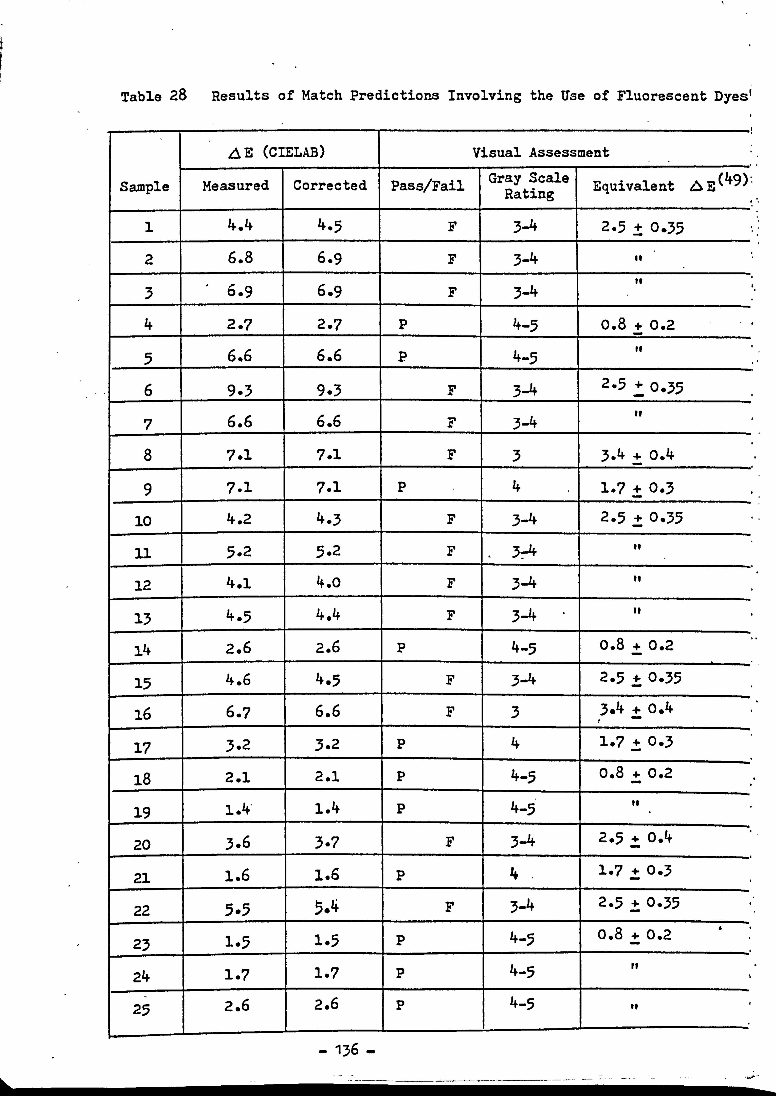
Table 28 Results of Match Predictions Involving the Use of Fluorescent Dyes'
E (CIELAB) Visual Assessment
Sample Measured Corrected Pass/Fail Gray Scale Rating Equivalent N3 (49)
1 4.4 4-5 F 3-4 2-5 + 0-35
2 6.8 6.9 F 3-4
3 6.9 6.9 F 3-4
4 2e7 2-7 P 4-5 0.8 + 0.2
5 6.6 6.6 P 4-5
6 9-3 9-3 F 3-4 2-5 . 10-35
7 6.6 6.6 F 3-4 8 7.1 7-1 F 3 3.4 + o. 4
9 7.1 7.1 P 4 1.7 + 0-3
10 4.2 4-3 F 3-4 2.5 1 0.35
11 5-2 5-2 F 34
12 4.1 4. o F 3-4
13 4-5 4.4 F 3-4
14 2.6 2.6 P 4-5 0.8 + 0.2
15 4.6 4-5 F 3-4 2-5 + 0-35
16 6.7 6.6 F 3 t3.4
+ 0.4
17 3-2 3-2 P 4 1-7 + 0-3
18 2.1 2.1 P 4-5 0.8 + 0.2
19 1.4, 1.4 P 4-5
20 3.6 3-7 F 3-4 2-5 + o. 4
21 1.6 1.6 P 4- 1-7 + 0.3
22 5-5 5.4 F 3-4 2-5 + 0.35
23 1-5 1-5 P 4-5 0.8 + 0.2
24 1.7 1.7 P 4-5
25 2.6 2.6 P 4-5
- 136 -
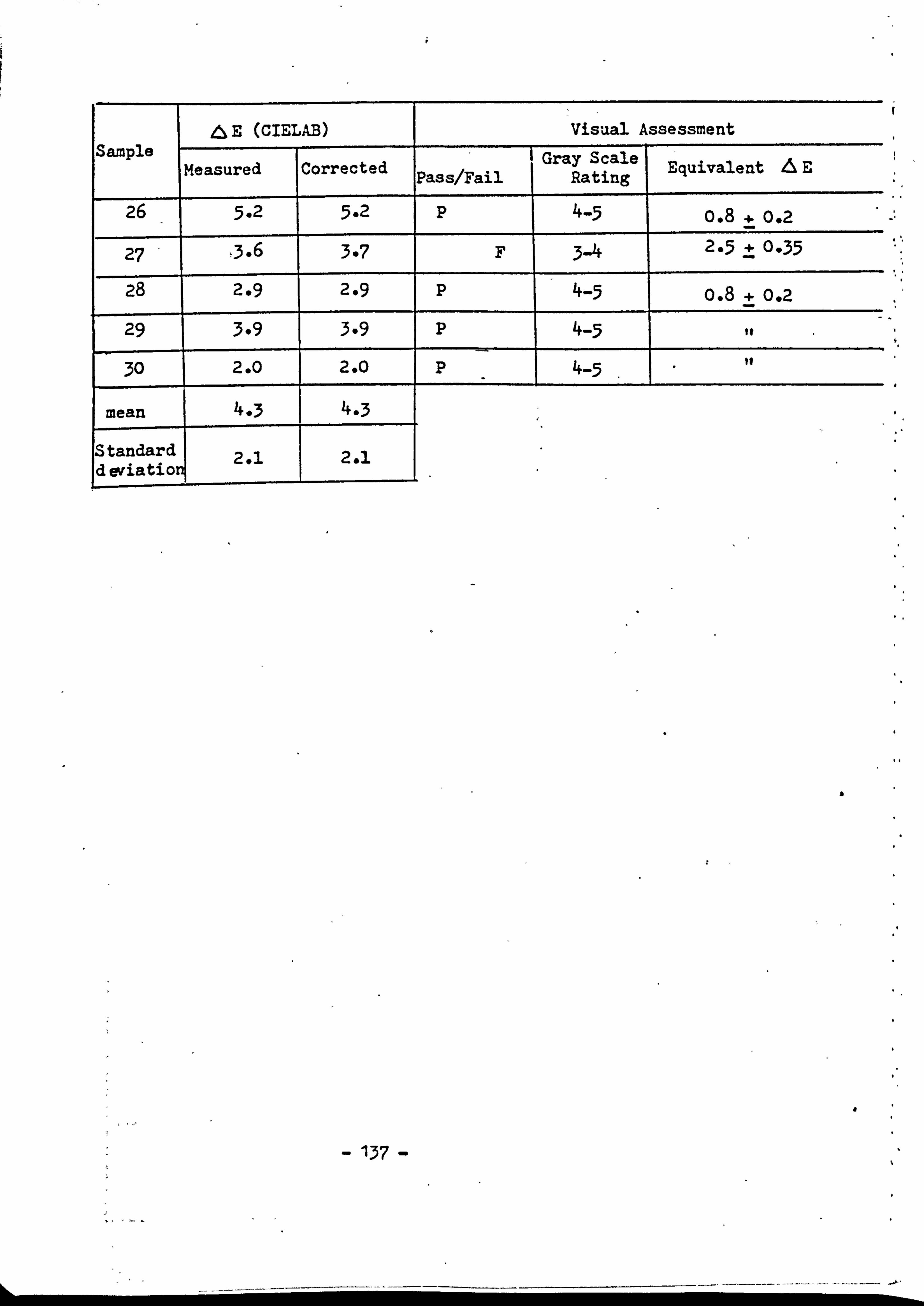
E (CIELAB) Visual Assessment Sample
Measured Corrected Pass/Fail Gray Scale
Rating Equivalent AE
26 5-2 5 -2 P 4-5 0.8 + 092
27 ý3.6 3-7 F 3-4 2-5 :t 0-35
28 2.9 2.9 P 4-5 o. 8 + o. 2
29 3-9 3-9 P 4-5
30 2.0 2.0 P 4-5
mean 4.3 4.3
Standard d eviatiog
2*1 2.1 II .
I
137
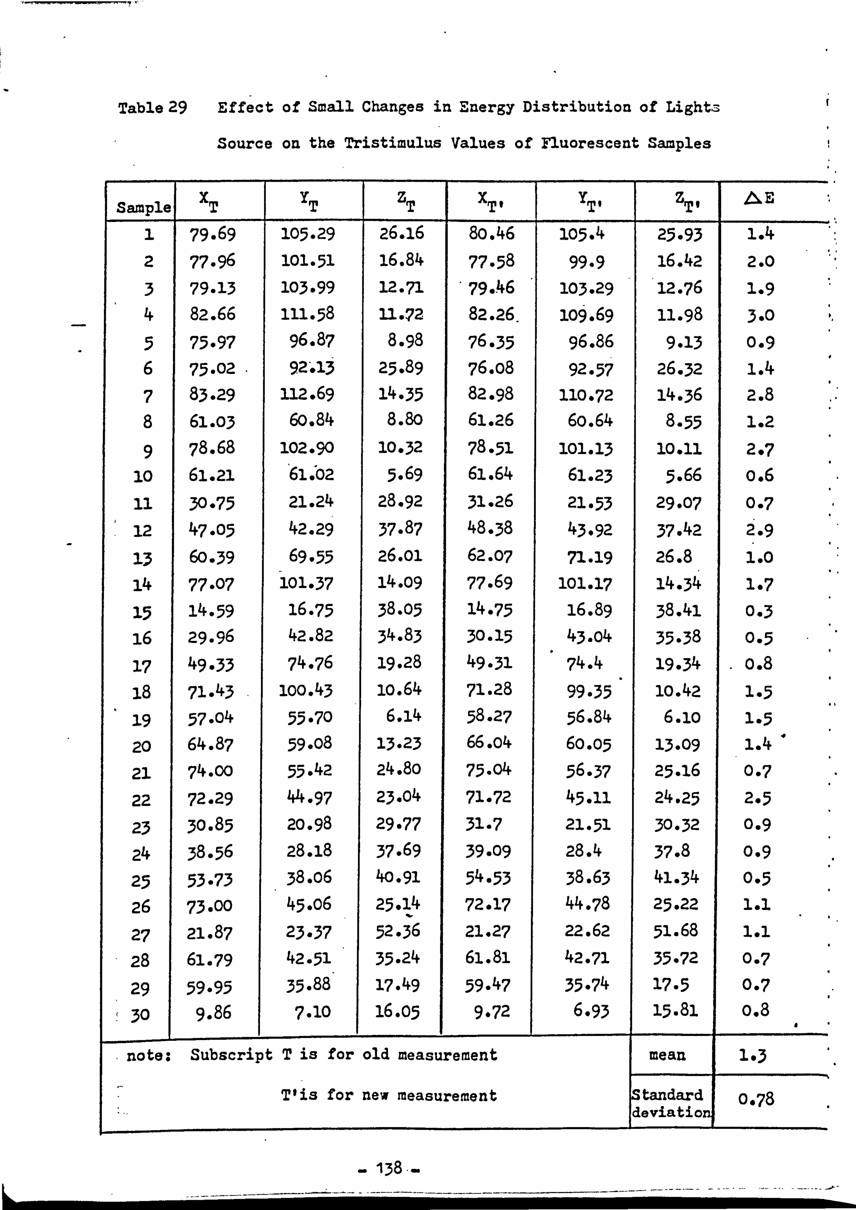
Table 29 Effect of Small Changes in Energy Distribution of Lights
Source on the Tristimulus Values of Fluorescent Samples
Sample xT YT zT x TI YTI ZT t &E
1 79.69 105-29 26.16 80.46 105.4 25-93 1.4 2 77.96 101-51 16.84 77-58 99.9 16.42 2.0 3 79-13 103-99 12-71 79.46 103-29 '12-76 1.9 4 82.66 111-58 11.72 82.26. 109.69 11.98 3-0 5 75-97 96.87 8.98 76-35 96.86 9-13 0.9 6 75.02 92'*13 25.89 76.08 92-57 26-32 1.4 7 83-29 112.69 14-35 82.98 110-72 14-36 2.8 8 61-03 60.84 8.80 61.26 6o. 64 8-55 1.2 9 78.68 102.90 10-32 78-51 101-13 10.11 297
10 61.21 61. '02 5.69 61.64 61.23 5.66 o. 6
11 30-75 21.24 28.92 31-26 21-53 29-07 0-7 12 47-05 42.29 37.87 48-38 43-92 37.42 2.9 13 60-39 69-55 26.01 62-07 71-19 26.8 1.0 14 77-07 101-37 14.09 77.69 101-17 14-34 1*7 15 14-59 16-75 38-05 14-75 16.89 38.41 0-3 16 29.96 42.82 34.83 30-15 43. o4 35-38 0-5 17 49-33 74-76 19.28 49-31 74.4 19-34 0.8 18 71.43 loo. 43 lo. 64 71.28 99-35 10.42 1-5 19 57. o4 55-70 6.14 58.27 56.84 6.1o 1-5 20 64.87 59.08 13.23 66.04 6o-05 13-09 1.4 21 74.00 55.42 24.80 75-04 56-37 25.16 0-7
22 72.29 44-97 23. o4 71-72 45-11 24.25 2-5
23 30.85 20.98 29-77 31-7 21-51 30-32 0.9
24 38-56 28.18 37.69 39-09 28.4 37.8 0.9 25 53-73 38. o6 40.91 54-53 38.63 41-34 0-5
26 73-00 45. o6 25.14 72-17 44-78 25.22 1.1
27 21.87 23-37 52-36 21.27 22.62 51.68 1.1
28 61-79 42-51 35.24 61.81 42-71 35-72 0-7
29 59-95 35.88 17.49 59.47 35-74 17-5 0-7
30 9.86 7-10 16-05 9-72 6-93 15.81 o. 8
note: Subscript T is for old measurement mean 1*3
Vis for new measurement Standard 0-78 deviationj
138--
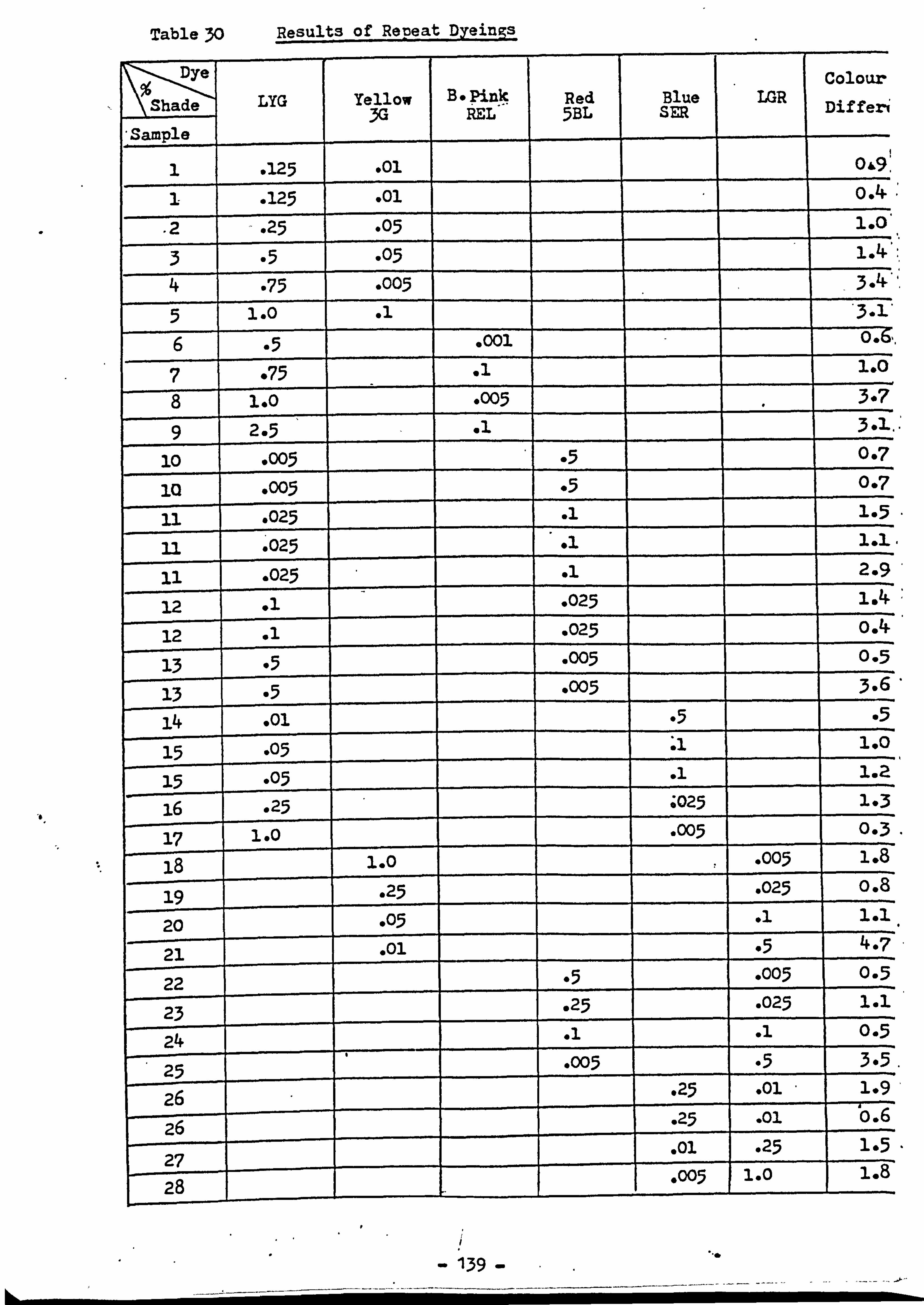
Table 30 Results of Repeat Dyeings
Dye j %S; h: aýýde LYG Yellow
3G B Pink
REL- Red 5BL
Blue SER
LGR Colour
Dif feri
'Sample
1 . 125 001 00,
1 . 125 . 01 0. '+
.2 - . 25 -05 1.0
3 -5 -05 1.4, 4 -75 -005 3
5 1.0 .1 6 -5 . 001 o. 6,,
7 -75 11 1.0
8 1.0 -005 3*7
9 2-5 el 3-1.
10 . 005 o5 0-7
10 . 005 -5 0-7
11 -025 .1 1-5
3.1 . 025 01 1.1.
11 . 025 01 2.9
12 . 025 1.4
12 .1 -025 0.4
13 e5 -005 0-5
13 95 -005 3-6
14 . 01 *5 -5 15 -05
100
15 -05 16 . 25 ; 025 1-3
- 17 __ 1.0 -005 0-3
18 1.0 *005 1.8 - 19 -25 . 025 0.8,
20 -05 .1 1.1
21 . 01 *5 4-7
22 *5 -005 0.5
23 25 . 025 1.1
24 .1 .1 0.5
25 -005 --- *5 3-5
26- -- . 25 . 01
1 1.9
269, - - . 25 *01 0.6
27 2-8-
. 01
. 005 . 25
1.0 1-5 1.8
139
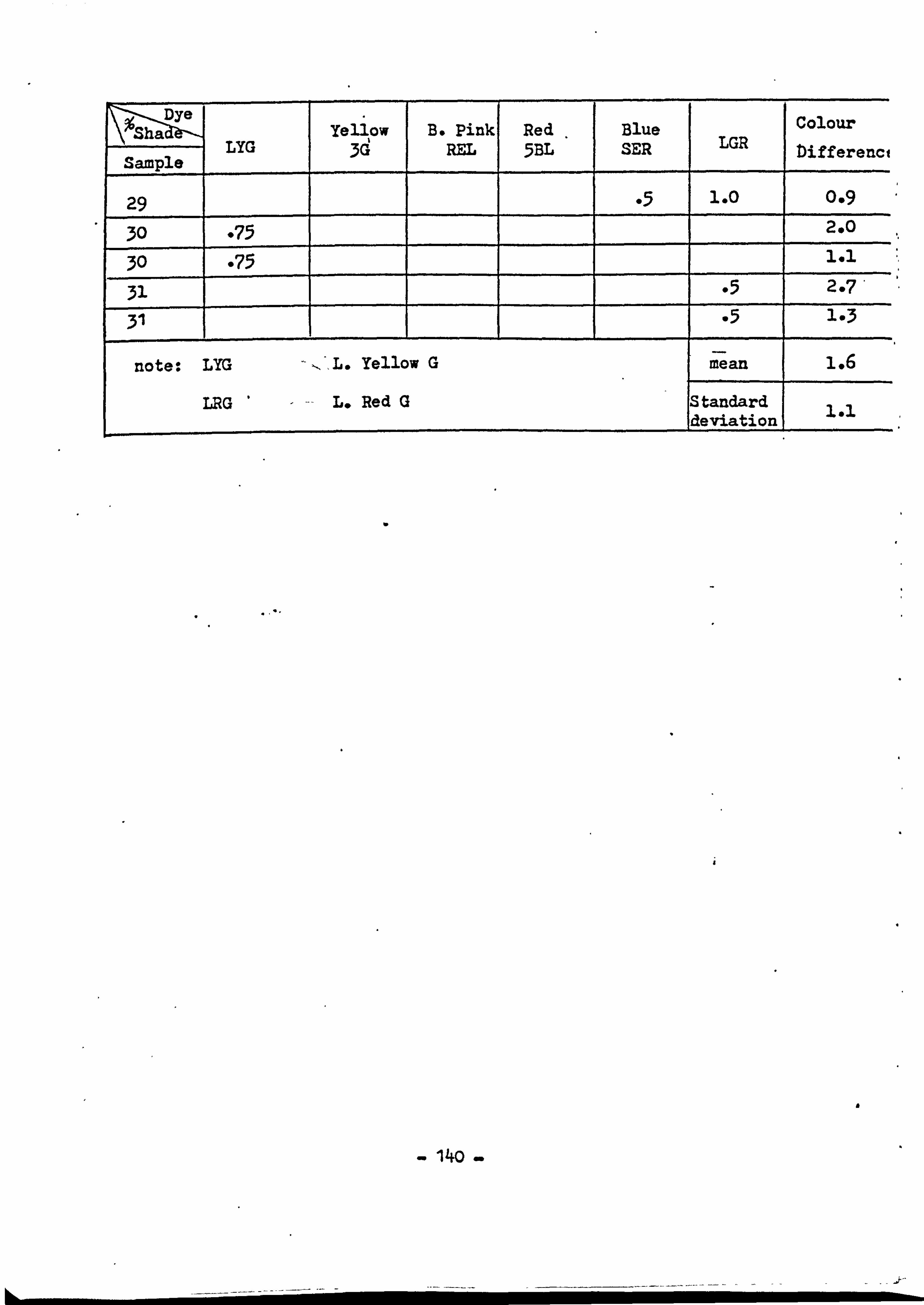
Dye Sha
G yellow
d B. Pink Red Blue
LGR Colour
Sample LY 3 REL 5BL SER Differenci
29 *5 1.0 0.9
30 -75 2*0
30 -75 1.1
31 -5 2.
31 - F- -5 1-3
note: LYG Yellow G mean 1.6
LRG L. Red G Standard deviationj 1.1
- 140 -
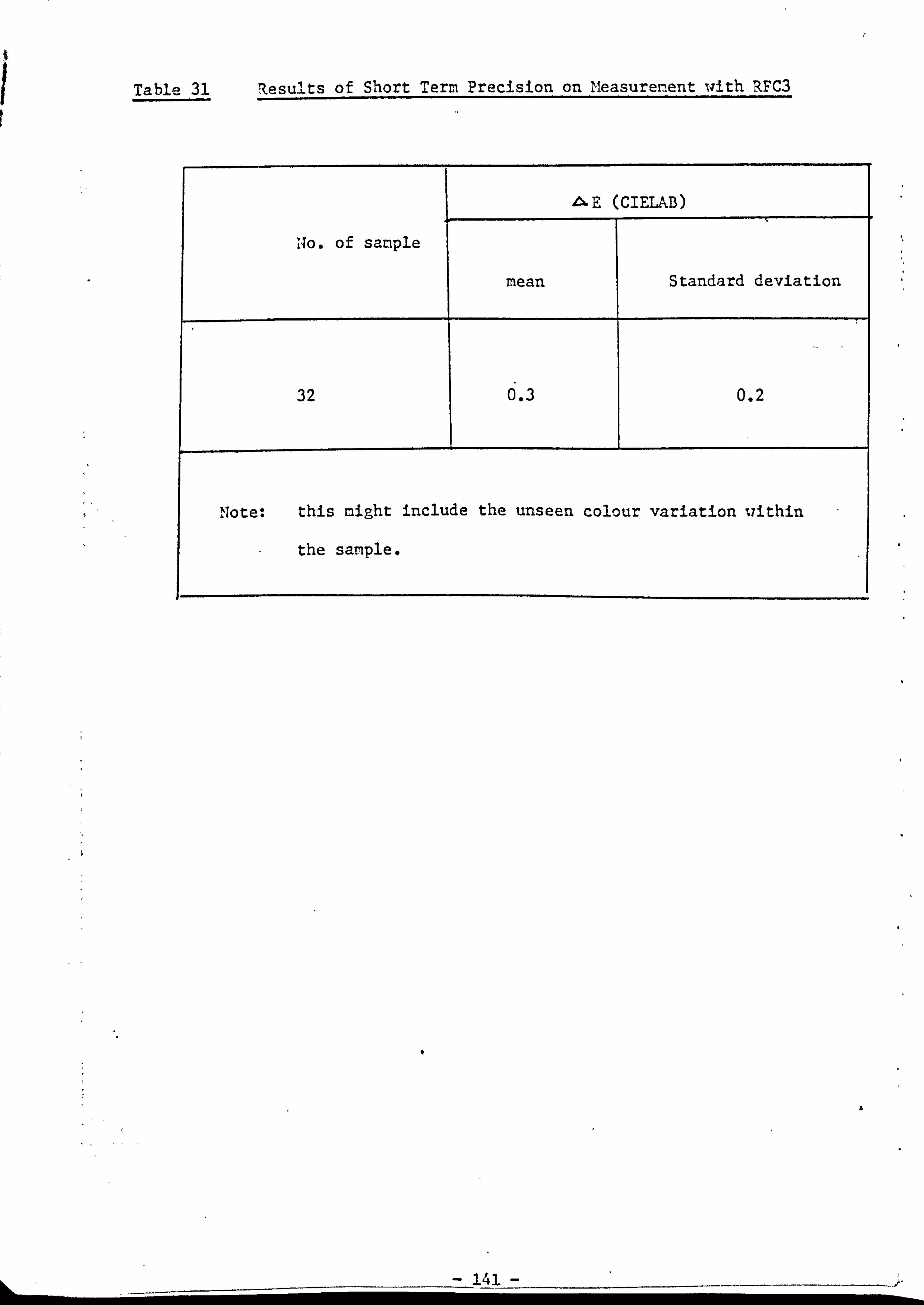
Table 31 Results of Short Term Precision on Measurement with RFC3
AE (CIELAB)
No. of sample
mean Standard deviation
32 0.3 0.2
Note: this might include the unseen colour variation within
the sample.
I
a
141
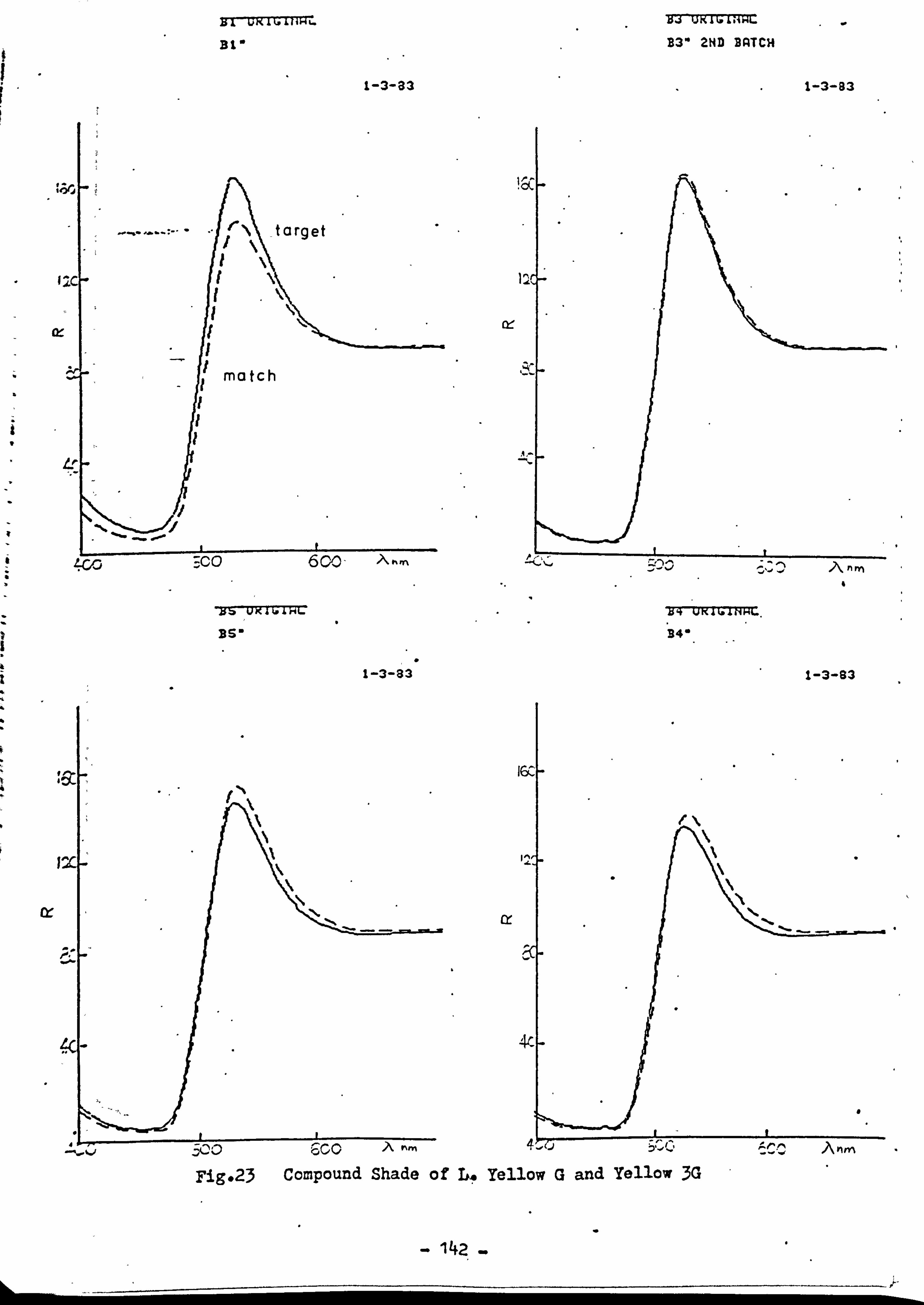
NI UKILsLHW
Bt*
I'
t 9
-Iss WRIGMC DS,
1-3-83
1-3-83
(if
ix
B3* 2ND BATCH
1-3-83
S, ý An rn
UK4k*INHt-.
34'
1-3-83
zk.; ý; ýjk. Aj Z% ýM
Fig#23 Compound Shade of L. yellow G and Yellow 3G
1421
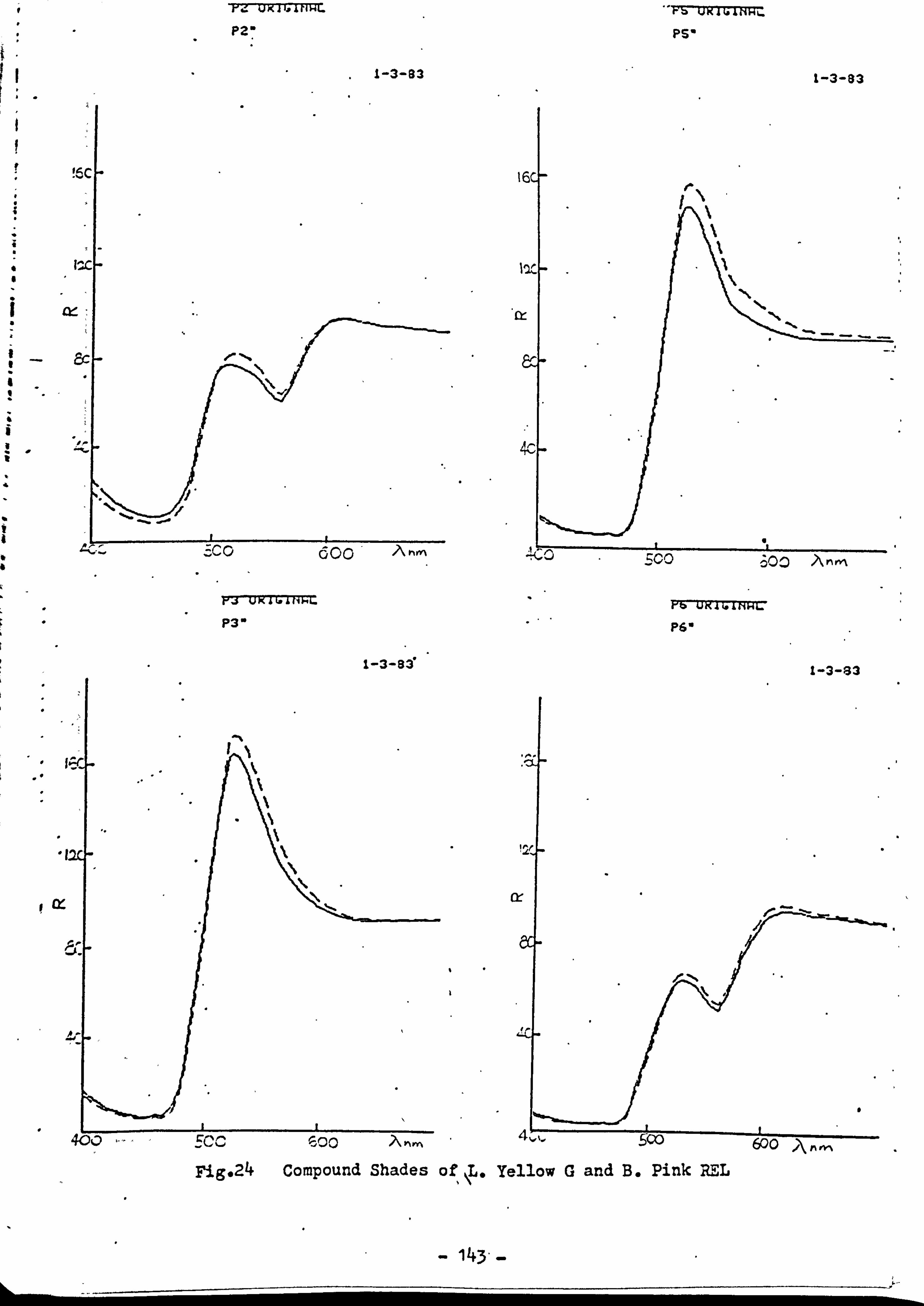
1, zu )c i P2,
1-3-133
"FS
PSI
0-,
1-3-837
Of
1-3-83
P6*
c
1-3-83
rig*24 Compound Shades of L. Yellow G and B. Pink RTL
143'-
P3*
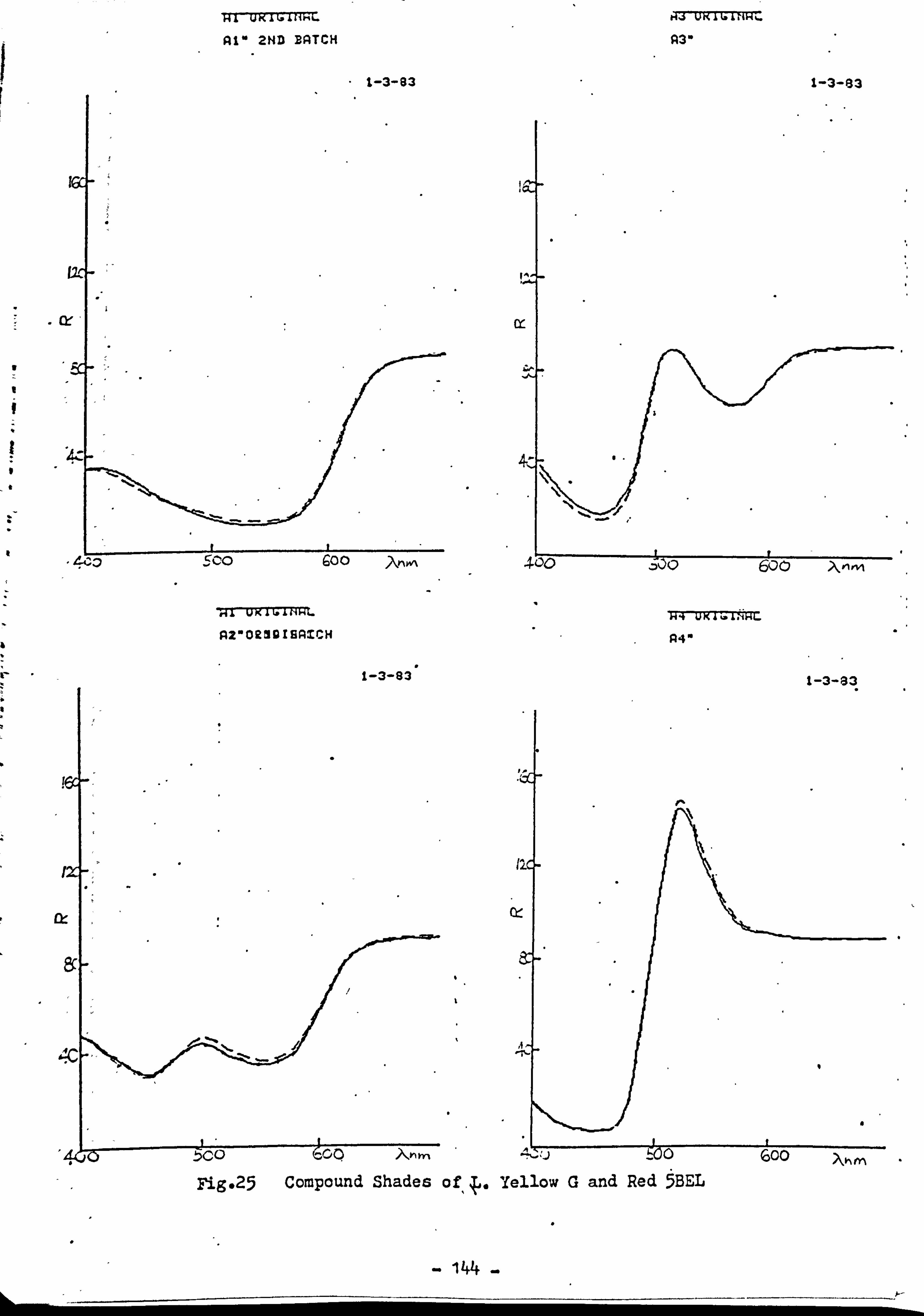
AV
-
t
t
i
W4 UK161. qHC
A4'
c
1-3-83
1-3-83
vy, 600
Fig, 25 Compound Shades of, ý. Yellow G and Red ýBEL
144
HI UKi6iiii4L.
Al* 2ND BATCH
t-3-83
1-3-83

%. I Ui(IULf*4-
CIO
"f6
T4c5
I
1-14-211
600
WKI =qC
C2* 2HD BATCH
1-3-83
C3*
1-3-83
I At
Zuj /N to 6,00
Fig. 26 Compound Shades of L. Yellow G and Blue SER
145
CV

111 TO RI
-Q C
-IU UKiwlf*4C
D3'
MZ UKAIp&(iHL- D4 UK16IN14C
D2" D4'
c 0
1-11-all
1-3-83
fox 0 6oo
Fig. 27 Compound Shades of, ji. Red G and Yellow 3G
146
1-3-33
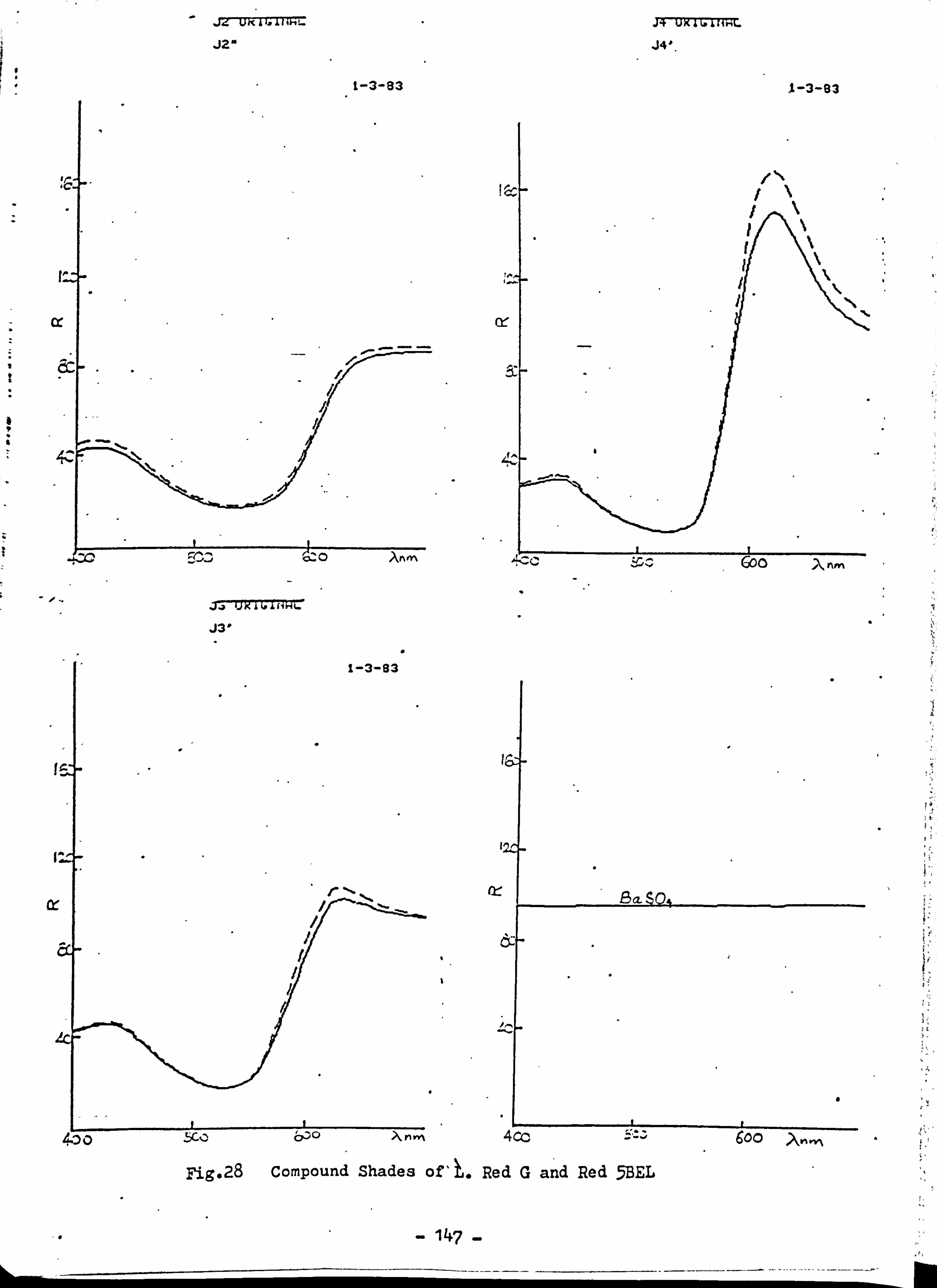
- JZTJè. iti_.
Jz- 1 8,
C
t
JV
1-3-83
C
J2F-uRT7TTT-HL
J4'
1-3-83
Of Of Ba $04
lic-
400 4cc 600 T
rig. 28 Compound Shades of'h* Red G and Red 5BEL
147

HI
Hl'
a
a
1-3-83
rij ORACITTRC
H3"
C
H4*
Q
-to 0 XP%
M . 2c)
rig*29 Compound Shades Of, ý. Red G and Blue SER
1-3-83
148
H2"

Part III
Analysis, Discussion and Conclusions
Chapter 8 Analysis and Discussion
8.1 The Accuracy of Measurements
A Carl Zeiss RFC3 automatic abridged spectrophotometer is used
throughout this project. This is because firstly, it is available in
Hong Kong Polytechnic and secondly it is probably the best systen. among C3
those available in Hong Kong as well as in the University of Bradford.
Besides the RFC3, there are a few IB, 117,341 Textile Colour Analysers
scattered in the Hong Kong dyeing industries. However, the highest value Cý 0
obtained for the most fluorescent sample prepared in this work is less
than 120, whereas the RFC3 provides a reading as high as 175. For the C, C)
sake of accuracy and convenience, the RFC3 is selected.
KCS18 abridged spectrophotometer and the 1-facbeth IIS2000
spectrophotometer are available in the Universitv of Dradford. However
both instruments are limited by their respective control programs. With
the KCS18 the reflectance values run from 0 to 200; a value which should
be 210 appears as 10. This seemed to happen with a few samples. Cn the-
other hand, the IMS2000 tries to round off values to its highest limit of
150 and thus causes error for measuring highly fluorescent samples. TI he
above situation does not occur in our measurements with the RFC3.
Sharpe and Lakowski (42 ) reports the accuracy of measurements
with RFC3 against values obtained with G. F. spectrophotometer. The
accuracy is within a colour difference of 1.2 to 1.4 FMC-2 units. (h the
other hand, results from the collaborative reference program of NBS for
colour and colour difference indicate that the RFC3 used is as accurate
as other instruments participating in the same program throughout the
world. Table 37 reveals that it is always within one standard deviation
of the grand mean.
149
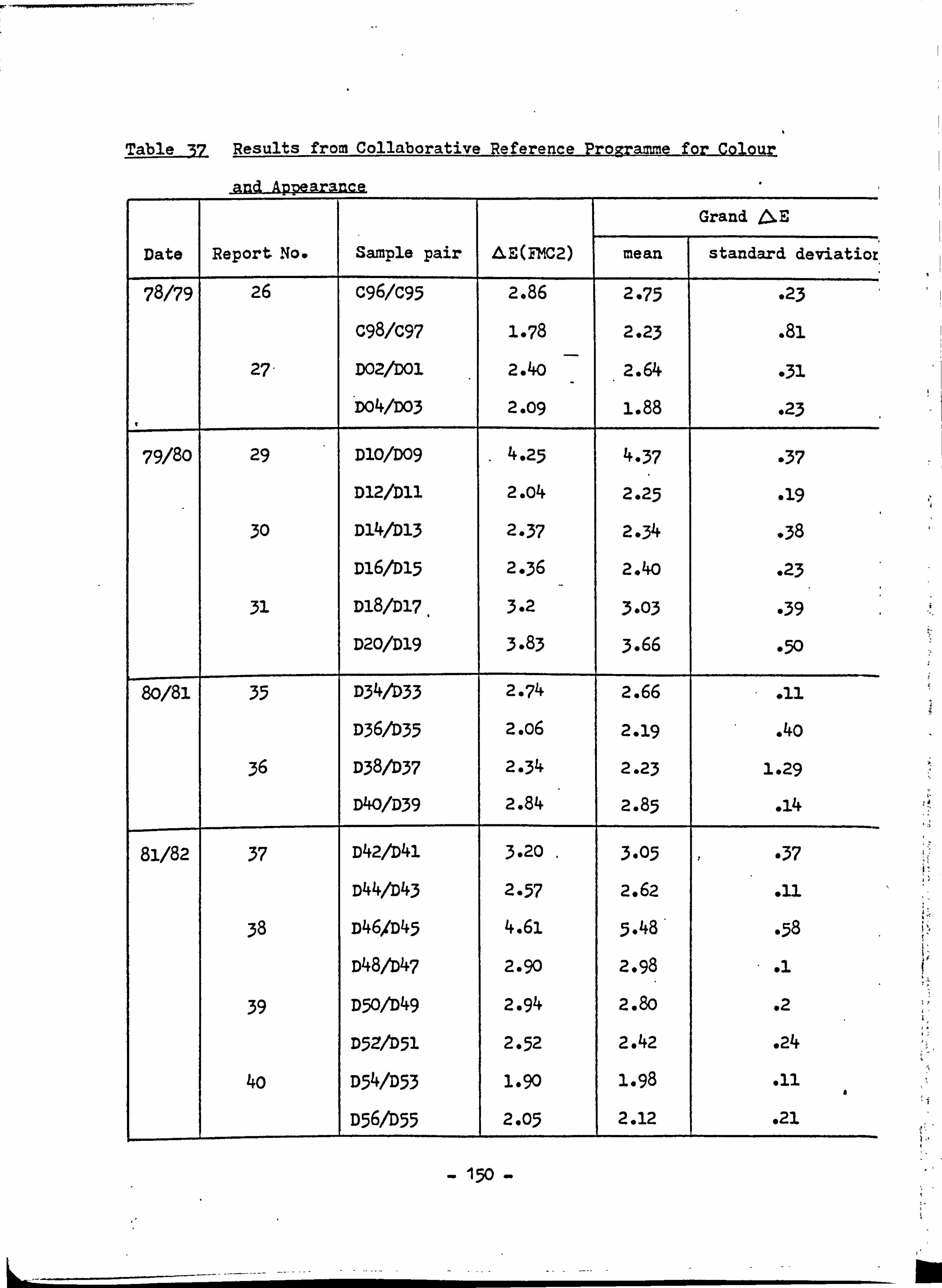
Table 3Z Results from Collaborative Reference Programme for Colour
Grand j! ý, E
Date Report No. Sample pair AE(FMC2) mean standard deviatior
78/79 26 C96/C95 2.86 2-75 -23 c98/c97 1-78 2-23 . 81
27- D02/bOl 2.40 .
2.64 -31 DOVD03 2.09 1.88 -, 23
79/80 29 DlO/DO9 4,25 4-37 -37 D12/bll 2.04 2.25 019
30 DlVD13 2-37 2-34 -38 D16/b15 2-36 2.40 -23
31 D18/D17, 3-2 3-03 -39 D20/D19 3.83 3.66 e5O
80/81 35 D34/D33 2-74 2.66 . 11
D36/D35 2. o6 2.19 . 4o
36 D38/D37 2-34 2-23 1.29
D40/D39 2.84 2.85 . 14
81/82 37 D42/b4l 3.20 3.05 -37 D44/b43 2-57 2.62 . 11
38 D46A45 4.61 5.48' -58 D48/b47 2.90 2.98 .1
39 D50/b4g 2.94 2.80 .2 D52/b5l 2-52 2.42 *24
4o D54/D53 1.90 1.98 . 11
D56/D55 2-05 2.12 . 21
- 150 -
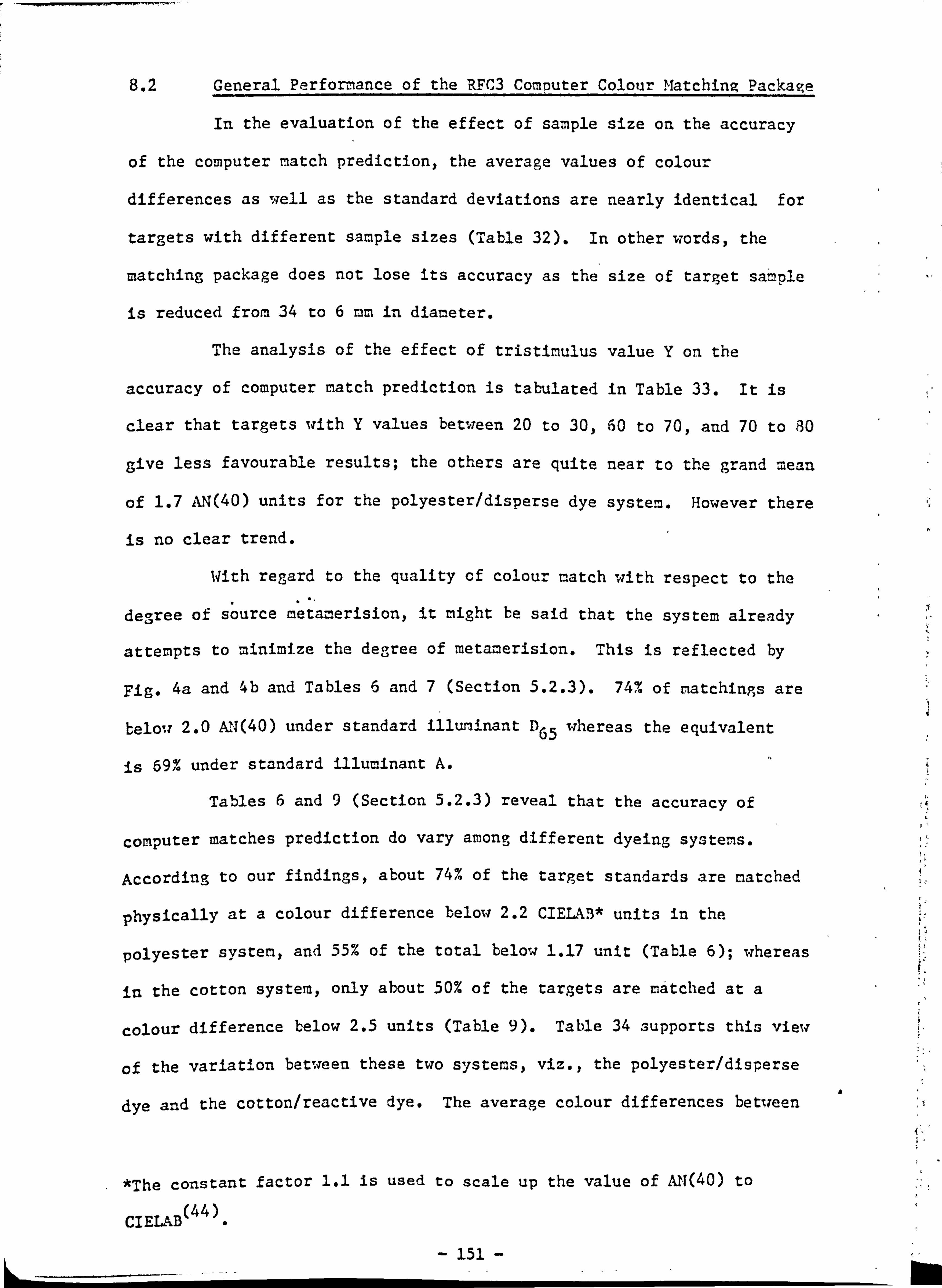
8.2 General Performance of the RFC3 Computer Colour Matching Package
In the evaluation of the effect of sample size on the accuracy
of the computer match prediction, the average values of colour
differences as well as the standard deviations are nearly identical for
targets with different sample sizes (lable 32). In other words, the
matching package does not lose its accuracy as the size of target sample
is reduced from 34 to 6 mm in diameter.
The analysis of the effect of tristimulus value Y on the
accuracy of computer match prediction is tabulated in Table 33. It is
clear that targets with Y values between 20 to 30,60 to 70, a-ad 70 to 80
give less favourable results; the others are quite near to the grand 'nean
of 1.7 m, (40) units for the polyester/disperse dye system. However there
is no clear trend.
With regard to the quality of colou-. match with respect to the
dearee of source metamerision, it might be said that the system already 17
attempts to minimize the degree of metamerision. This is reflected by
Fig. 4a and 4b and Tables 6 and 7 (Section 5.2.3). 74% of matchings are
below 2.0 AN(40) under standard illuninant D 65 whereas the equivalent
is 69%. under standard illuminant A. I
Tables 6 and 9 (Section 5.2.3) reveal that the accuracy of
computer matches prediction do vary among different dyeing systems.
According to our findings, about 74% of the target standards are matched
physically at a colour difference below 2.2 CIET-kB* units in the
polyester system, and 55% of the total below 1.17 unit (Table 6); whereas
in the cotton system, only about 50% of the targets are matched at a
colour difference below 2.5 units (Table 9). Table 34 supports this view
of the variation between these two systems, viz., the polyester/disperse
dye and the cotton/reactive dye. The average colour differences between
*The constant factor 1.1 is used to scale up the value of AN(40) to
(44) CIELAB
151
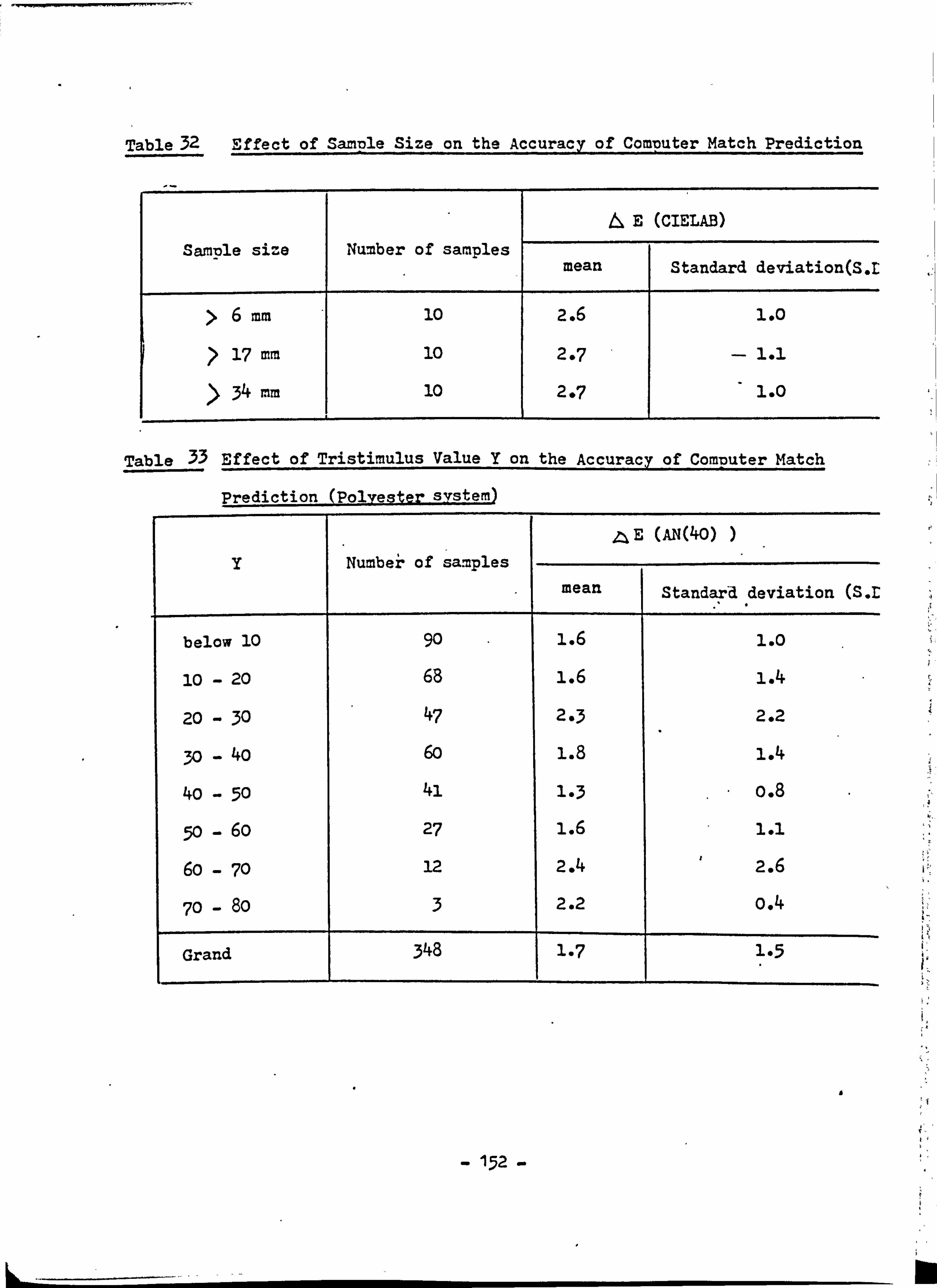
Table 32 Effect of Sample Size on the Accuracy of Computer Match Prediction
E (CIELAB)
Sample size Number of samples mean Standard deviation(S. L
>6 mm 10 2.6 1.0
> 17 mm 10 2.7 1.1
> 34 mm 10 2*7 1.0
Table 33 Effect of Tristimulus Value Y on the Accuracy of Computer Match
Prediction (Polyester system
)4 E (AN (40) )
y les :ý of sam mb N p e u mean Standard deviation (S. r
below 10 go 1.6 1.0
10 - 20 68 1.6 1.4
20 - 30 47 2-3 2.2
3o - 4o 60 1.8 1.4
40 - 50 41 le3 o. 8
5o - 6o 27 1.6 1.1
6o - 70 12 2.4 2.6
70 - 8o 3 2.2 o. 4
Grand 348 1-7 1-5
- 152 -
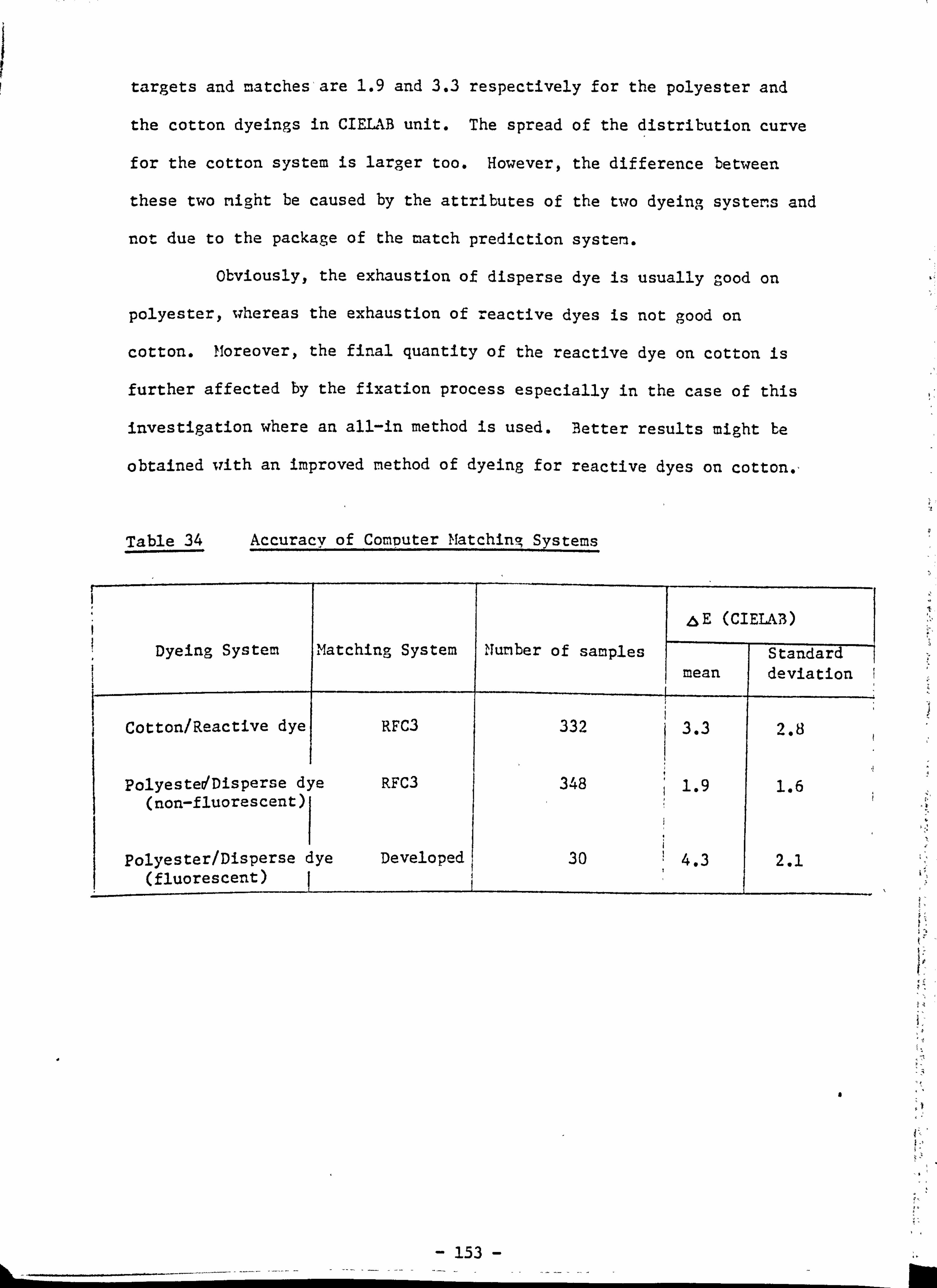
targets and matches'are 1.9 and 3.3 respectively for the polyester and
the cotton dyeings in CIMU unit. The spread of the distribution curve
for the cotton system is larg , er too. However, the difference between
these two night be caused by the attributes of the two dyeina. systems and
not due to the package of the match prediction system.
obviously, the exhaustion of disperse dye is usually good on
polyester, whereas the exhaustion of reactive dyes is not good on
cotton. moreover, the final quantity of the reactive dye on cotton is
further affected by the fixation process especially in the case of this
investigation where an all-in method is used. Better results might be
obtained with an improved method of dyeing for reactive dyes on cotton.,
Table 34 Accuracy of ComDuter Matchina, Systems
E (CIELAB)
Dyeing System Matching System Number of samples Standard mean deviation I
Cotton/Reactive dye RFC3 332 3.3 7
2.8
PolyesteýDisperse dye RFC3 348 1.9 1.6 (non-fluorescent)
Polyester/Disperse dye Developed 30 4.3 2.1 (fluorescent)
a
153
8.3 Computer Colour Matching Involving the Use of Fluorescent Dves
8.3.1 Effect. of Light Sources on the Measurement of Fluorescent Samples
There is no doubt that the energy distriubtion and intensity of
light sources has a definite influence on the emission of fluorescent
radiation. Nevertheless during the course of study in this project, a
small change in energy distirubtion of the xenon source fitted in the
RFc3 only causes aft error of 1.3 CIELAB units (Table 29), which is small
in comparison with the 1.6 units for repeat dyeing of the fluores cent
samples (Table 30).
FiOg. 30 clearly demonstrates the effect of different energy
distribution on two fluorescent dyes, viz. Palanil Lumnious Yellow G and
Palanil Lumnious Red G. Both measuring instruments are fitted with
simulated D illuminants. However, the origins of the sources are 65 1
different, i. e. a tungsten lamp for KCS18 and a xenon lamp for RFC3. The
abnormal peak of the xenon source round 460nm falls exactly on the
excitation region of the fluorescent yellow dye (Fig. 31 and 33). The
measured total radiance factors at the emission region are higher on RFC3
than on KCS18- on the other hand, in the excitation region of the
fluorescent red dye, the energy content of the tungsten lamp is higher
than the xenon lamp (Fig. 32 and 34). Therefore the emitted fluorescence
for the red dye follows the same order. That is, the values from KCS18
are higher than those from RFC3. These difference are of the order of 10
reflectance units and hence much higher than differences between-
reflectance values for non-fluorescent samples.
154

160
140
. -% 120
co C17
- 100
80
6o Pq
40
20
red
0/ .
Inc,
20 40 60 80 100 120 160 180 Total Radiance Factors (RFC3)
Fig-30 Correlation Curve between Measurements for R-FC3 & KCS18
- 155 -
co
XK
; zw ye
.1

14(
12(
loc
P(A I
ec
60
40
20
3
0 0o Zeiss xenon, filtered/ filtri/ gefil tort
1- 065 0
--ZD651 in UVI 0
0 0 0 0 w
0 O 00 000 0 " 0 0 0,
Of
00 400 50 1) 60 0 7n n OýA
Wavelength (nm)
Fig. 31(25) High Quality D Simulator Based on Xenon Lamp, 65
Compared with D 65
IN
loc
sc p 17% 1
60
40
20
300
0000 00
0
r NRC tungsten hologen filtered
10 I
N RC lompe 6 ho loone fI It r6 0 NRC get ilterte Hdogen-GlOhlompe
O GS 106s (In UVI
&UU Duv buu -/Uu ouu Wavelengih Inm)
a
Fig. 32 (25) High Quality D65 Simulator Rased on Tungsten Halogen
Lamp, qompared with D 65
156 -
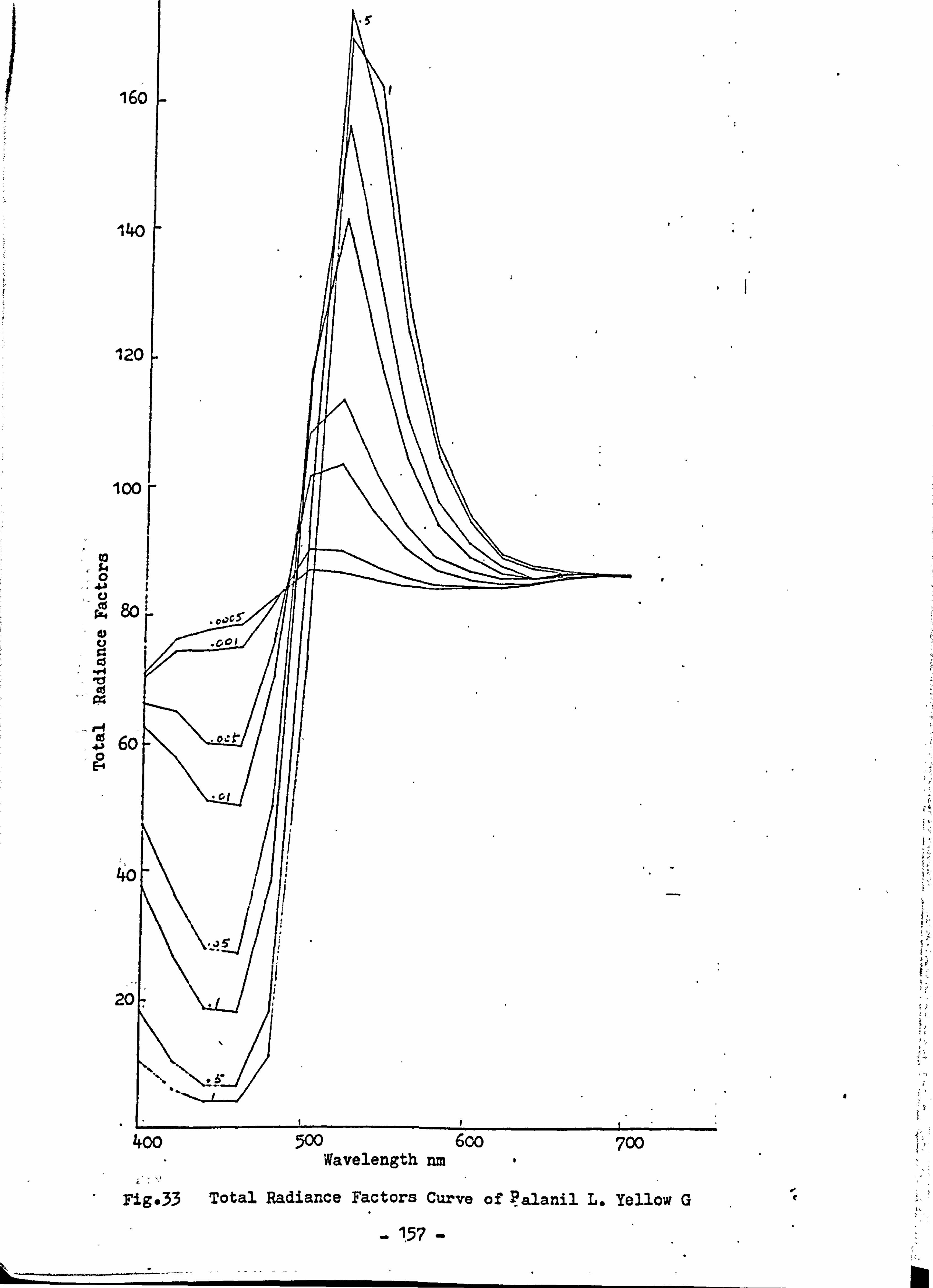
1 16
14
12,
10(
0
V cts
rZ4
cs
-r4
Cd
r-f (d
4., 6c 0 E-4
40
20
k)O I'M 6oo 700 Wavelength nm
Fig-33 Total Radiance Factors Curve of P-alanil L. Yellow G
157
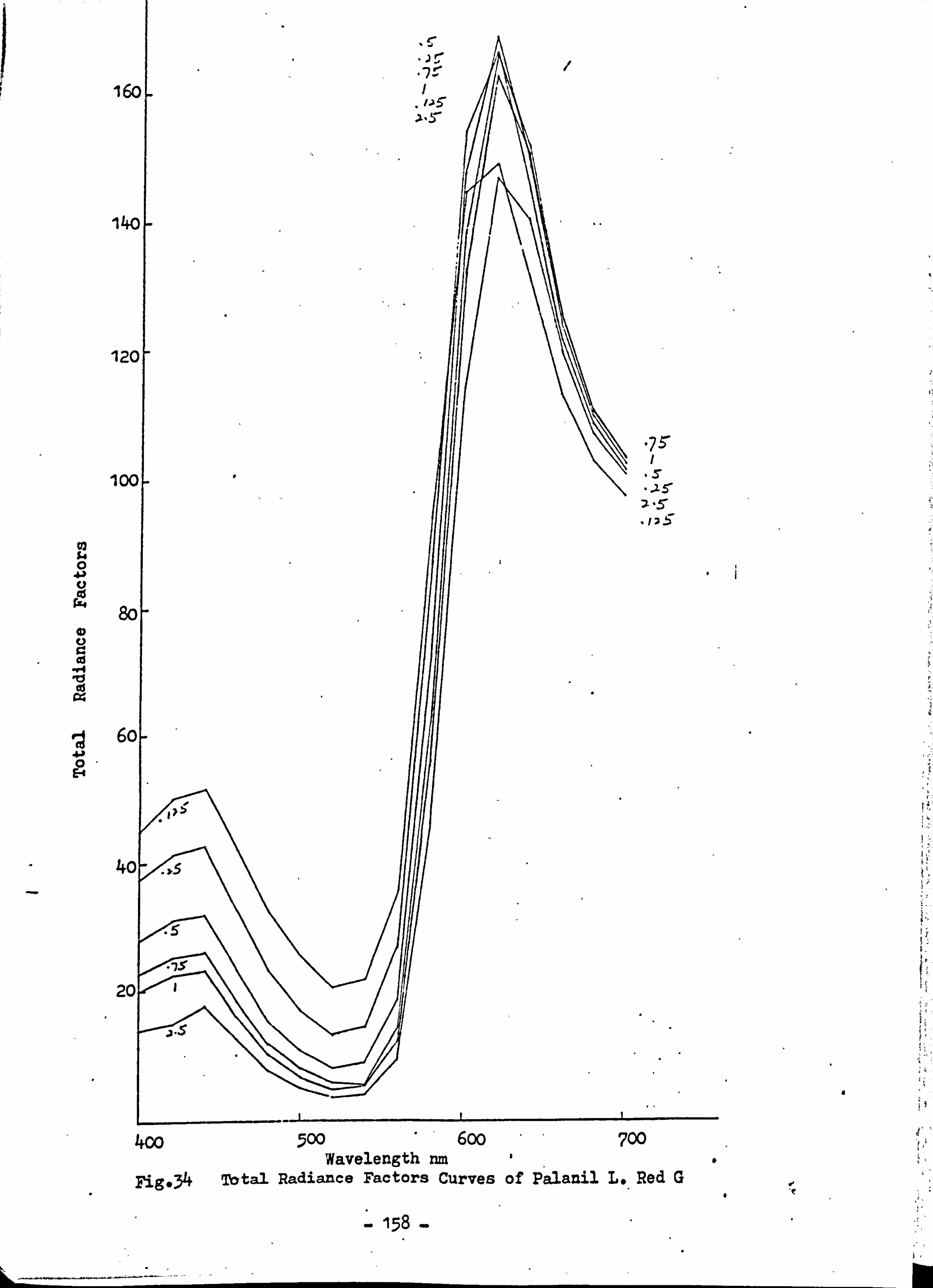
1&
14(
12C
loc
03 54 0
ID
6c 0 E-1
40
20
400 500 600 700 Wavelength nm I a,
Fig-34 Tbtal Radiance Factors Curves of Palanil L,. Red G
158
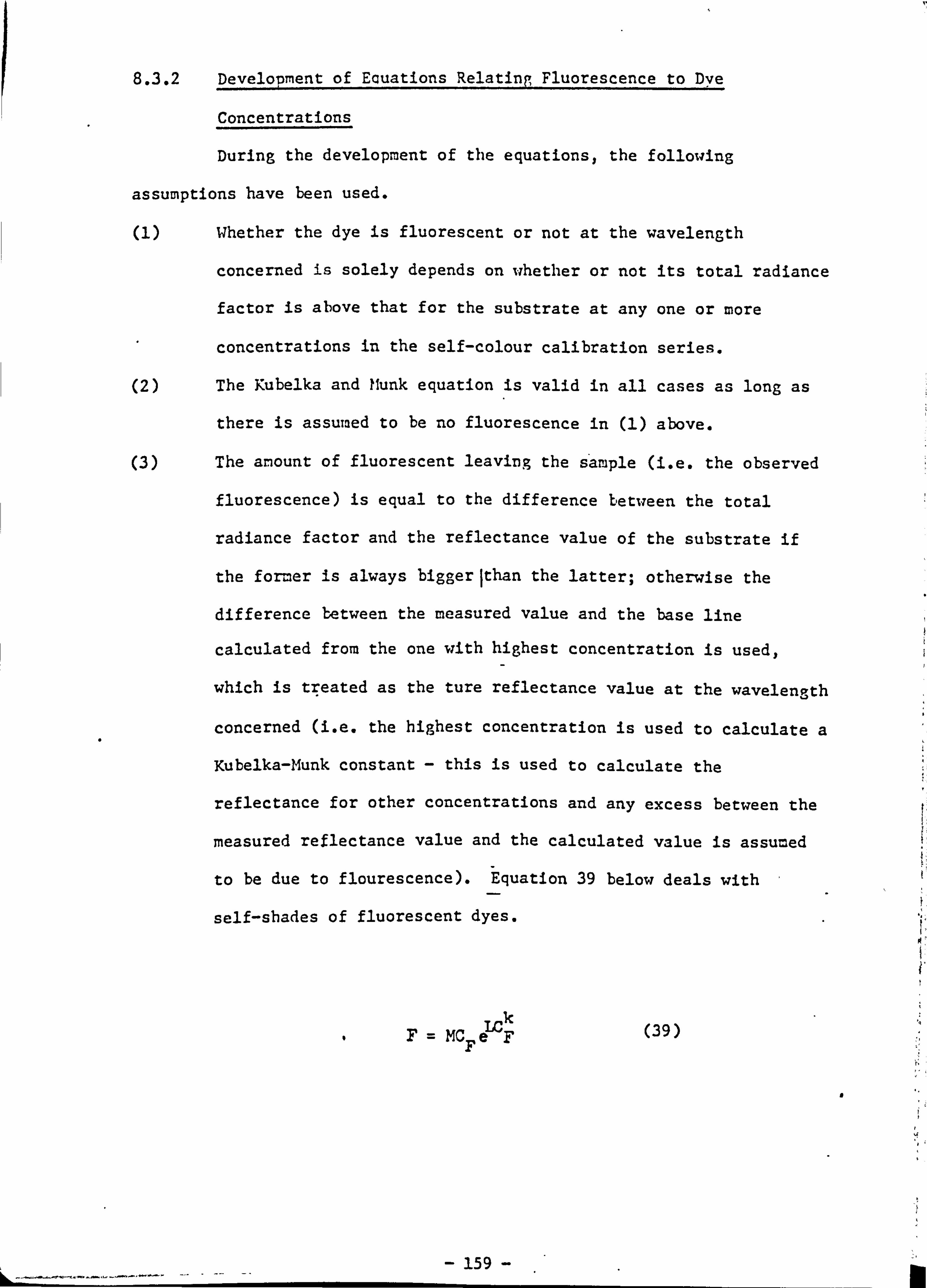
8.3.2 Development of Equations Relating Fluorescence to Dve
Concentrations
During the development of the equations, the following
assumptions have been used.
(1) Whether the dye is fluorescent or not at the wavelength
concerned is solely depends on whether or not its total radiance
factor is above that for the substrate at any one or more
concentrations in the self-colour calibration series.
(2) The Kubelka and Munk equation is valid in all cases as long as
there is assumed to be no fluorescence in (1) above.
The amount of fluorescent leaving the s*ample (i. e. the observed
fluorescence) is equal to the difference between the total
radiance factor and the reflectance value of the substrate if
the former is always biggerithan the latter; otherwise the
difference between the measured value and the base line
calculated from the one with highest concentration is used,
which is nýeated as the ture reflectance value at the wavelength
concerned (i. e. the highest concentration is used to calculate a
Kubelka-Munk constant - this is used to calculate the
reflectance for other concentrations and any excess between the
measured reflectance value and the calculated value is assu=ed
to be due to flourescence). Equation 39 below deals with
self-shades of fluorescent dyes.
k MC FeF
(39)
a
159
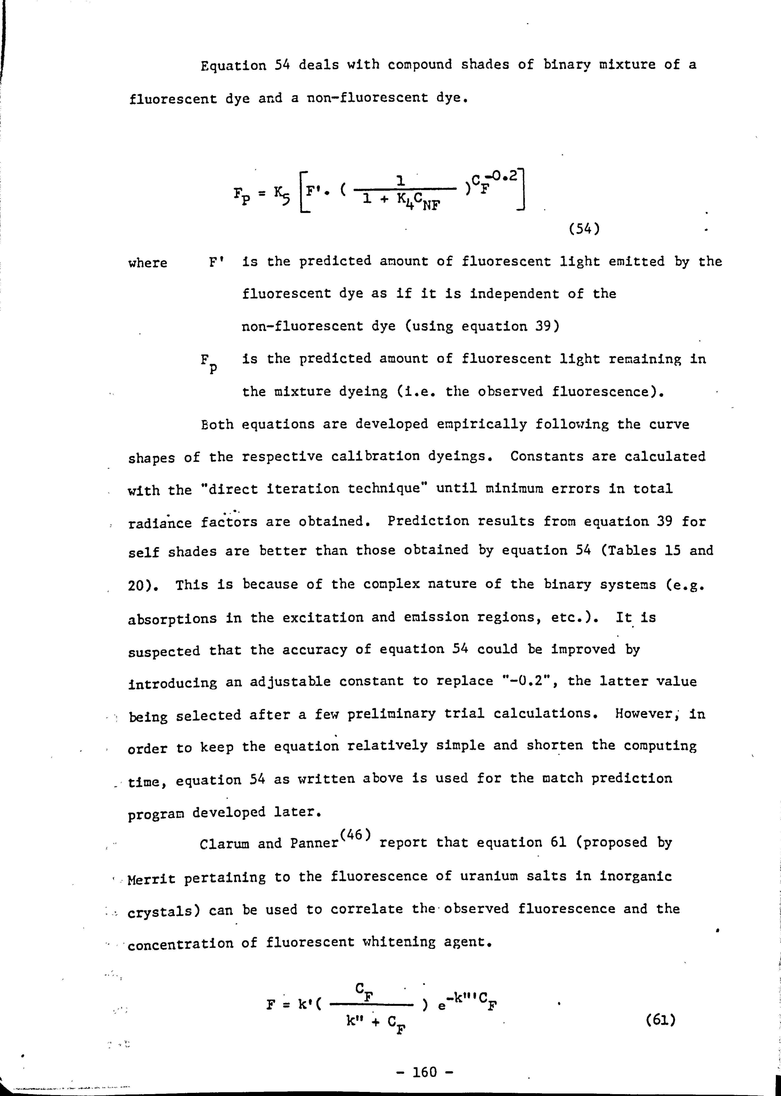
Equation 54 deals with compound shades of binary mixture of a
fluorescent dye and a non-fluorescent dye.
1C -0*2] Fp Y'5
[Ft 1+ K4CNF
)F
(54)
where F' is the predicted amount of fluorescent light emitted by the
fluorescent dye as if it is independent of the
non-fluorescent dye (using equation 39)
FP is the predicted amount of fluorescent light remaining in
the mixture dyeing (i. e. the observed fluorescence).
Both equations are developed empirically following the curve
shapes of the respective calibration dyeings. Constants are calculated
with the "direct iteration technique" until minimum errors in total
radiance factors are obtained. Prediction results from equation 39 for
self shades are better than those obtained by equation 54 (Tables 15 and
20). This is because of the complex nature of the binary systems (e. g.
absorptions in the excitation and emission regions, etc. ). It is
suspected that the accuracy of equation 54 could be improved by
introducing an adjustable constant to replace "-0.2", the latter value
being selected after a few preliminary trial calculations. However$- in
order to keep the equation relatively simple and shorten the computing
., time, equation 54 as written above is used for the match prediction
program developed later. (46)
Clarum and Panner report that equation 61 (proposed by
, --Merrit pertaining to the fluorescence of uranium salts in inorganic
crystals) can be used to correlate the, observed, fluorescence and the
--concentration of fluorescent whitening agent.
kl( Fe -k" CF kll +CF
a
160
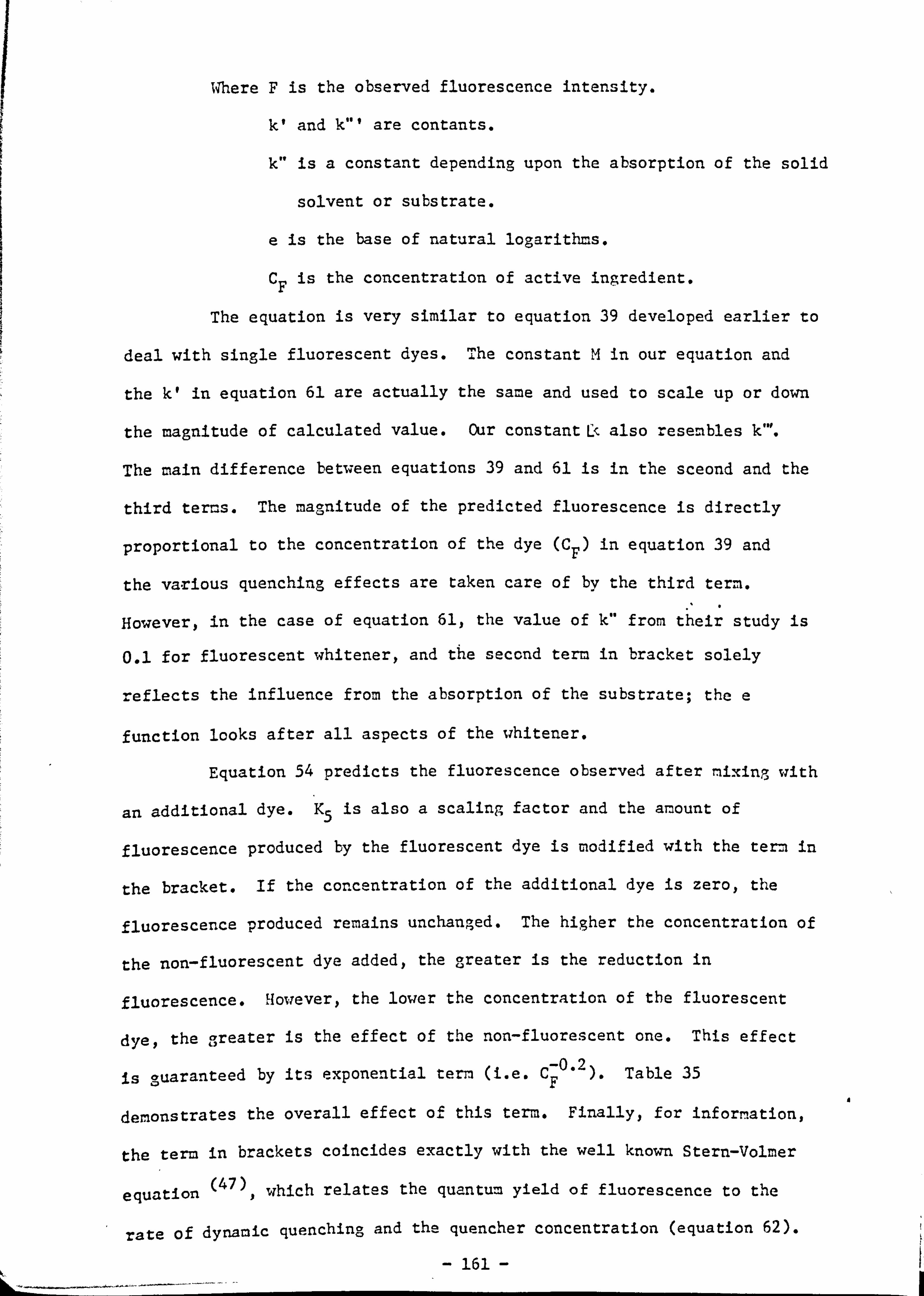
Where F is the observed fluorescence intensity.
k' and k"' are contants.
k" is a constant depending upon the absorption of the solid
solvent or substrate.
e is the base of natural logarithms.
CF is the concentration of active ingredient.
The equation is very similar to equation 39 developed earlier to
deal with single fluorescent dyes. The constant M in our equation and
the k' in equation 61 are actually the same and used to scale up or down
the magnitude of calculated value. Our constant L-, also resembles k"'.
The main difference between equations 39 and 61 is in the sceond and the
third terms. The magnitude of the predicted fluorescence is directly
proportional to the concentration of the dye (C F) in equation 39 and
the various quenching effects are taken care of by the third term.
However, in the case of equation 61, the value of k" from their study is
0.1 for fluorescent whitener, and the second term in bracket solely
reflects the influence from the absorption of the substrate; the e
function looks after all aspects of the whitener.
Equation 54 predicts the fluorescence observed after mixing with
an additional dye. K5 is also a scaling factor and the amount of
fluorescence produced by the fluorescent dye is modified with the term in
the bracket. If the concentration of the additional dye is zero, the
fluorescence produced remains unchanged. The higher the concentration of
the non-fluorescent dye added, the greater is the reduction in
fluorescence. However, the lower the concentration of the fluorescent
dye, the areater is the effect of the non-fluorescent one. This effect 0
is Varanteed by its exponential term, (i. e. C-0.2 ). Table 35 F
demonstrates the overall effect of this term. Finally, for information,
the term in brackets coincides exactly with the well known Stern-Volmer
equation (47)
p which relates the quantum yield of fluorescence to the
rate of dynamic quenching and the quencher concentration (equation 62).
161
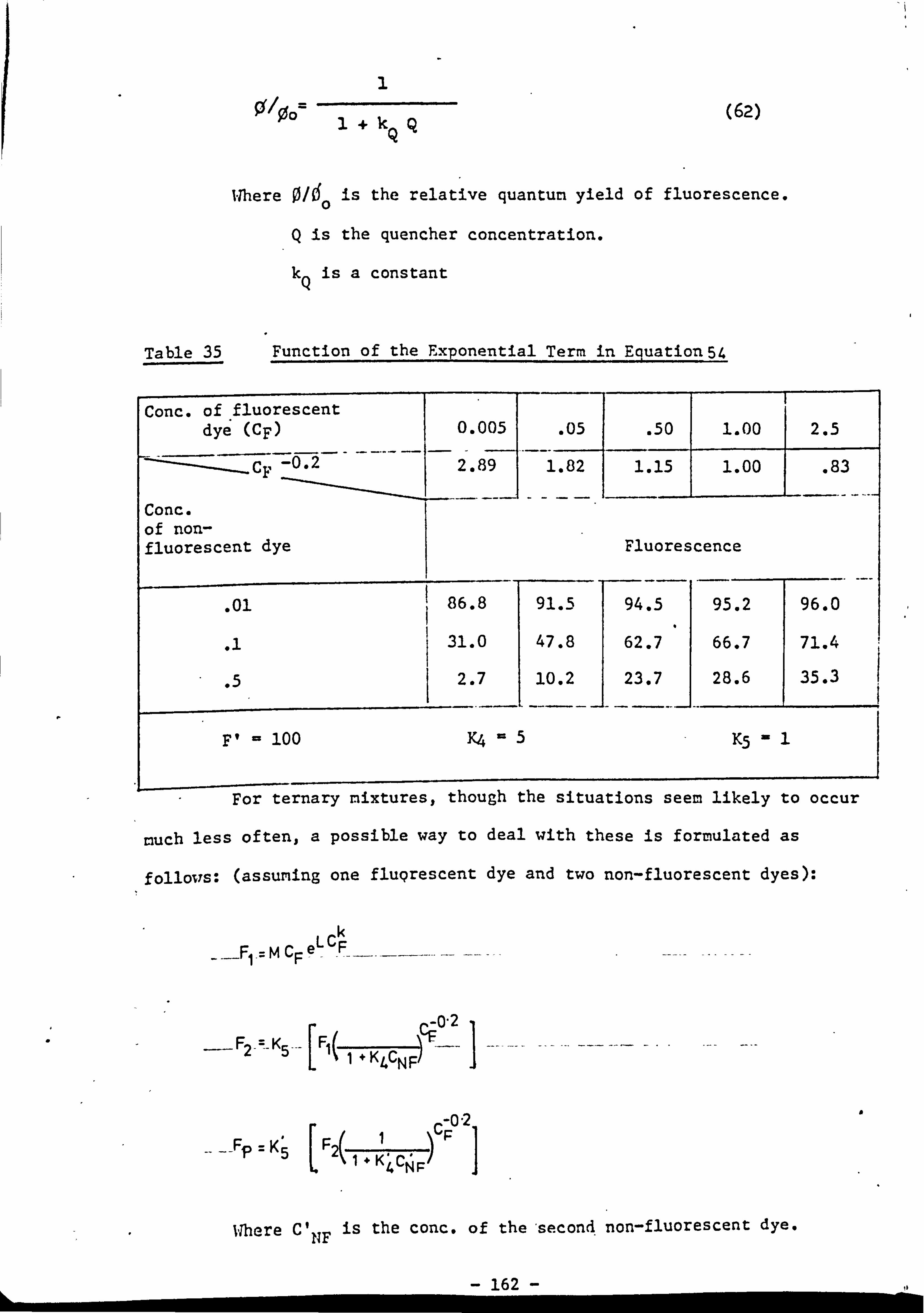
+k (62)
where 0160 is the relative quantum yield of fluorescence.
Q is the quencher concentration.
kQ is a constant
Table 35 Function of the Exponential Term in EquatiorL54
Conc. of fluorescent dye (CF) 0.005 . 05 . 50 1.00 2.5
CF 2.89 1.82 1.15 1.00 . 83
Conc. of non- fluorescent dye Fluorescence
. 01 86.8 91.5 94.5 95.2 96.0
.1 31.0 47.8 62.7 66.7 71.4
.5 2.7 10.2 23.7 28.6 35.3
F' = 100 Y, 4 15 K5 -1
For ternary mixtures, though the situations seem likely to occur
much less often, a possible way to deal with these is formulated as
follows: (assuming one flugrescent dye and two non-fluorescent dyes):
k
--F,. =MC eL -F- F
c -0-2 -F2-=-K5---
F, ( F-1 --- -- ---- --- ---- --- ----
-02
--Fp K' p2 1 1
Where C' NF is the conc. of the'second. non-fluorescent dye.
162 -I
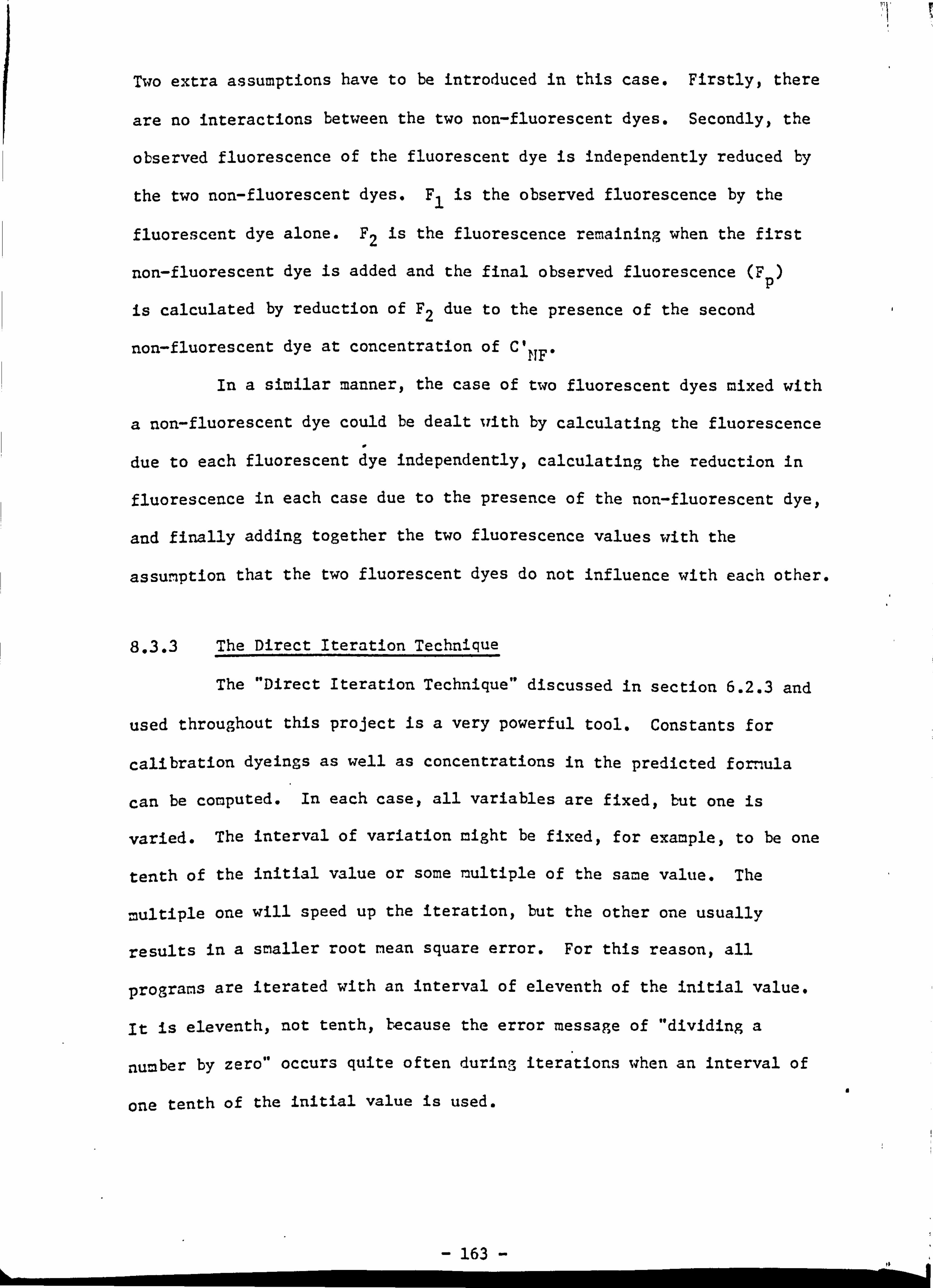
Two extra assumptions have to be introduced in this case. Firstly, there
are no interactions between the two non-fluorescent dyes. Secondly, the
observed fluorescence of the fluorescent dye is independently reduced by
the two non-fluorescent dyes. F, is the observed fluorescence by the
fluorescent dye alone. F2 is the fluorescence remaining when the first
non-fluorescent dye is added and the final observed fluorescence (F P)
is calculated by reduction of F2 due to the presence of the second
non-fluorescent dye at concentration of C' NF*
In a similar manner, the case of two fluorescent dyes mixed with
a non-fluorescent dye could be dealt with by calculating the fluorescence
due to each fluorescent dye independentlyo calculating the reduction in
fluorescence in each case due to the presence of the non-fluorescent dye,
and finally adding together the two fluorescence values with the
assumption that the two fluorescent dyes do not influence with each other.
8.3.3 The Direct Iteration Technique
The "Direct Iteration Technique" discussed in section 6.2.3 and
used throughout this project is a very powerful tool. Constants for
calibration dyeings as well as concentrations in the predicted formula
can be computed. In each case, all variables are fixed, but one is
varied. The interval of variation might be fixed, for example, to be one
tenth of the initial value or some multiple of the same value. The
multiple one will speed up the iteration, but the other one usually
results in a smaller root mean square error. For this reason, all
programs are iterated with an interval of eleventh of the initial value.
it is eleventh, not tenth, lecause the error message of "dividing a
number by zero" occurs quite often during iterations when an interval of
one tenth of the initial value is used. a
163
It is difficult to prove that the minimum error has been found
in every case. However, in the present work it is not necessary to do
so. For example, in calculating the "best" values of -4, L and k in
equation 39, what is really required is a set of values which give
reasonably accurate F values. 11hether a better set of values, or even a
better equation, exists is immaterial. Comparisons of calculated and
measured reflectance values (e. g. Table 15) given earlier show that the
differences are comparable with experimental errors. It is also obvious
that for the reflectance curves from recipe predictions in Fig. 16-22
(Section 7.3) and Appendix E, the technique has produced predicted curves
in close agreement with the measured curves. It is of course possible
that the technique could give unsatisfactory results in some future
calculatlon. However this could be detected by checking the root mean
square error. As long as this is reasonably small the results will be
satisfactory.
8.3.4 Matching Involving Fluorescent Dyes
Table 36 illustrates the analysis of the results of the match
prediction. program developed, which deals with formulations involving the
use of fluorescent dyes. The overall average of 4.3 units (CIELAB) is
quite large when compared with the accuracy achieved with non-fluorescent
dyes.
A
164 -0 .1
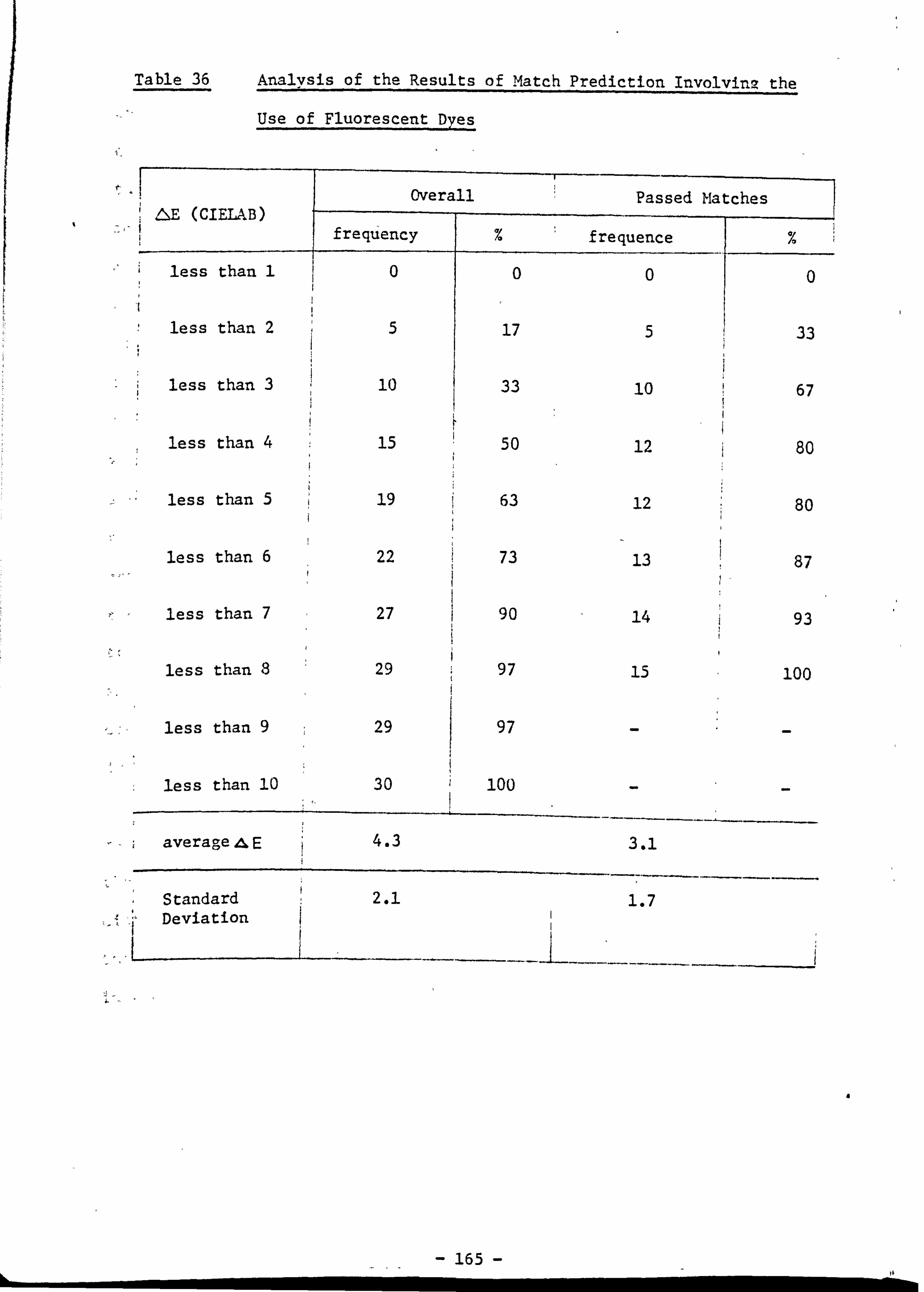
Table 36 Analysis of the Results of Match Prediction Involvin2 the
Use of Fluorescent Dyes
Overall Passed Matches LE (CIEIAB)
frequency % frequence
less than 1 0 0 0
less than 2 5 17 5
less than 3 10 33 10
less than 4 15 50 12
less than 5 i
19 63 12
less than 6 22 73 13
less than 7 27 90 14
less than 8 29 97 15
less than 9 29 97
less than 10 30 100
averacye AE C> 4.3 3.1
Standard 2.1 1.7 Deviation
0
33
67
80
80
87
93
100
a
165
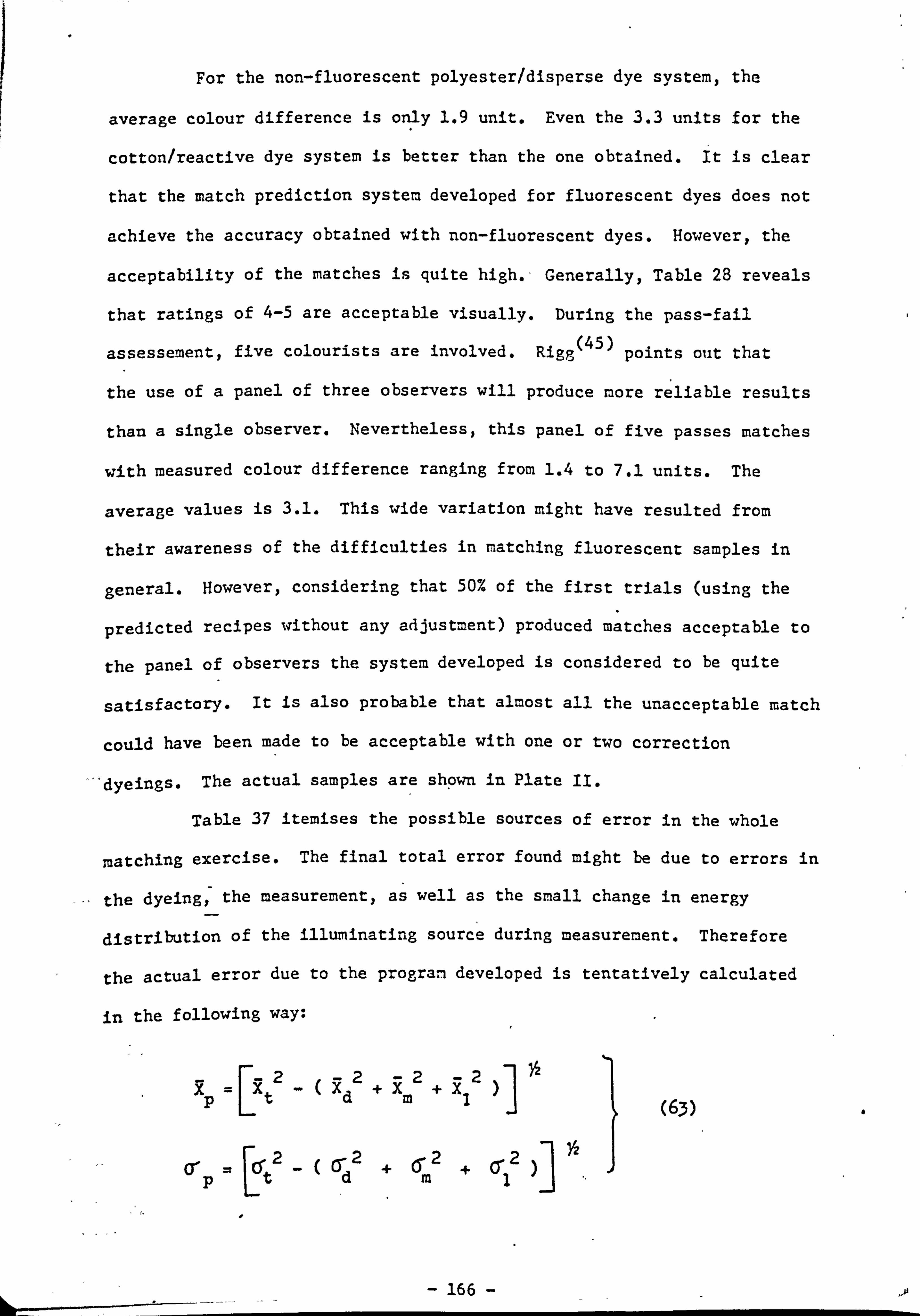
For the non-fluorescent polyester/disperse dye system, the
average colour difference is only 1.9 unit. Even the 3.3 units for the
cotton/reactive dye system is better than the one obtained. It is clear
that the match prediction system developed for fluorescent dyes does not
achieve the accuracy obtained with non-fluorescent dyes. However, the
acceptability of the matches is quite high. ý Generally, Table 28 reveals
that ratings of 4-5 are acceptable visually. During the pass-fail
assessement, five colourists are involved. Rigg (45) points out that
the use of a panel of three observers will produce more reliable results
than a single observer. Nevertheless, this panel of five passes matches
with measured colour difference ranging from 1.4 to 7.1 units. The
average values is 3.1. This wide variation might have resulted from
their awareness of the difficulties in matching fluorescent samples in
general. However, considering that 50% of the first trials (using the
predicted recipes without any adjustment) produced matches acceptable to
the panel of observers the system developed is considered to be quite
satisfactory. It is also probable that almost all the unacceptable match
could have been made to be acceptable with one or two correction
--dyeings. The actual samples are shpwn in Plate II.
Table 37 itemises the possible sources of error in the whole
matching exercise. The final total error found might be due to errors in
the dyeing, the measurement, as well as the small change in energy
distribution of the illuminating source during measurement. Therefore
the actual error due to the program developed is tentatively calculated
in the following way:
p At2 2+ %2 +
22 cr (ir Grý )
(63) a
- 166

Where 9 is the average error.
d is the standard deviation.
Subscripts t is the final total error.
d is the error due to repeat dyeing.
m is the error due to repeat measurement.
1 is, the-error due to small variation in
energy distribution of the source.
p is the error due to the developed program.
The average error-in terms of colour difference for the program
developed is 3.8, and the standard deviation is 1.6. This error is still
large as compared with results for non-fluorescent dyes on polyester.
Nevertheless, it is comparable with that for cotton/reactive dyes by the
-all-in method. That is 3.8 unit of the colour difference with standard
deviation of 1.6 for the developed system, compared with 3.3 unit of
colour difference and a wider spread of values - 2.8 S. D. for the cotton
system investigated.
Table 37 Errors Found in Match Prediction with Fluorescent Dyes
A E(CIELAB) i
Number of Reference Source Standard
samples Mean deivation
Repeat dyeing 41 1.6 1.1 Table 30
32 0.3 0.2 Table 31
Light source variation
overall total error
30 1.3 0.78
30 4.3 2.1
- Program error 3.8
Table 29
Table 28
equation 63
167
ChaDter IX Conclusions
A simple and feasible method to include fluorescent dyes in a
computer colour matching system is developed. According to the results
obtained, it is quite encouraging. 50% of actual dyeings of the first
trials are accepted visually. Others'are visually not far away from
targets too. Therefore a ground work has been established for match
prediction involving the use of fluorescent dyes.
During this course of research, a co=ercially available
abridged spectrophotmeter with polychromatic illumination is used. All
measurements are carried out under a simulated D65 xenon light source.
Some variation of energy distribution of the source due to ageing and 0
changing of a new one is expected in the past four to five years. It
causes an error of 1.3 CIELAB unit in terms of colour difference. It is
assumed that data for calibration dyeings prepared a long time ago
suffers from the same magnitude of error as that for data employed in
match prediction in the later days. However this is not too large when
compared with the error obtained for repeat dyeings of fluorescent dye
samples. This is 1.6 CIEUB unit. In view of this, a two monochromator
spectroreflectometer or a spectrophotometer equipped with a lot of
cut-off filterst employed by other workers seem to be not necessary. A
normal instrument with polychromatic illumination can work for match
prediction including the use of fluorescent dyes. Furthermore, it is not
necessary to use a xenon light source, a strong simulated D651 tungsten
source can also be used (Fig. 30).
Following the engineering principle that "good enougj is best",
an available commercial match prediction package is investigated with
more than three hundred samples covering the whole gamut Of Colours. Two 0.
dyeing systems are studied, namely a polyester/disperse dye and a
cotton/reactive dye systems. It is found that the polyester one is
- 168 -
better than the cotton system. This might be due to the difference in 0
the attributes of these two systems. The final amount of reactive dyes
linked to the fibre depends not only to the percentage of exhaustion but
the percentage of fixation too, whereas the polyester system is simply
depedent on the percentage of exhaustion.
The lightness of samples as represented by the Y tristinulus
value has little'influence on the accuracy of match prediction. In case
of the size of the target samplesi it is found that the accuracy of match
prediction does not fall as the size is reduced from 34 mm to 6 mm in
diameter.
Finally, the developed matching programme also demonstrates the C3
possibility of matching a saturated colour with two yellows or two reds
in a recipey. The pass rate is five out of eight (Table 26-28, sample
1,2,3,4,5,24,25 and 26).
a
- 169
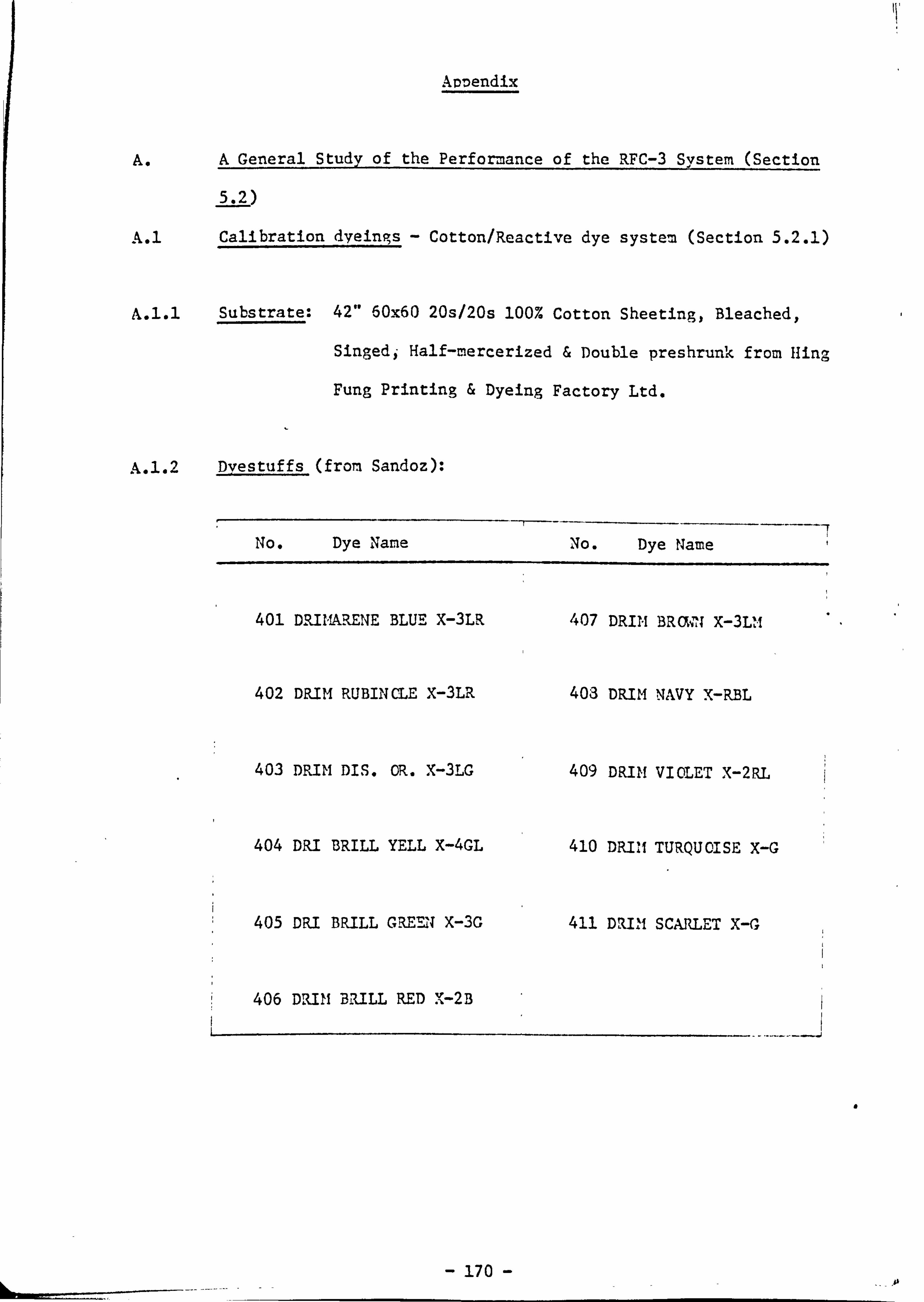
Ainendix
A. A General Study of the Performance of the RFC-3 System (Section
_ý. 2)
A. 1 Calibration dveings - Cotton/Reactive dye system (Section 5.2.1)
A. 1.1 Substrate: 42" 60x6O 20s/20s 100% Cotton Sheeting, Bleached,
Singedi Half-mercerized & Double preshrunk from fling
Fung Printing & Dyeing Factory Ltd.
A. 1.2 Dyestuffs (from Sandoz):
No. Dye Name No. Dye Name
401 D. IUMkU. NE BLUE X-3LR 407 DRIM BRMN X-3LIM
402 DRIM RUBINCLE X-3LR
403 DRIM DIS. OR. X-3LG
404 DRI BRILL YELL X-4GL
405 DR. I BRILL GRE11-711 X-3G
406 MUM BULL RED X 2B
403 DRIM NAVY X-RBL
409 DRIM VIOLET X-2RL
410 DRIM TURQUOISE X-G
411 DRIII SCARLET X-G,
a
- 170
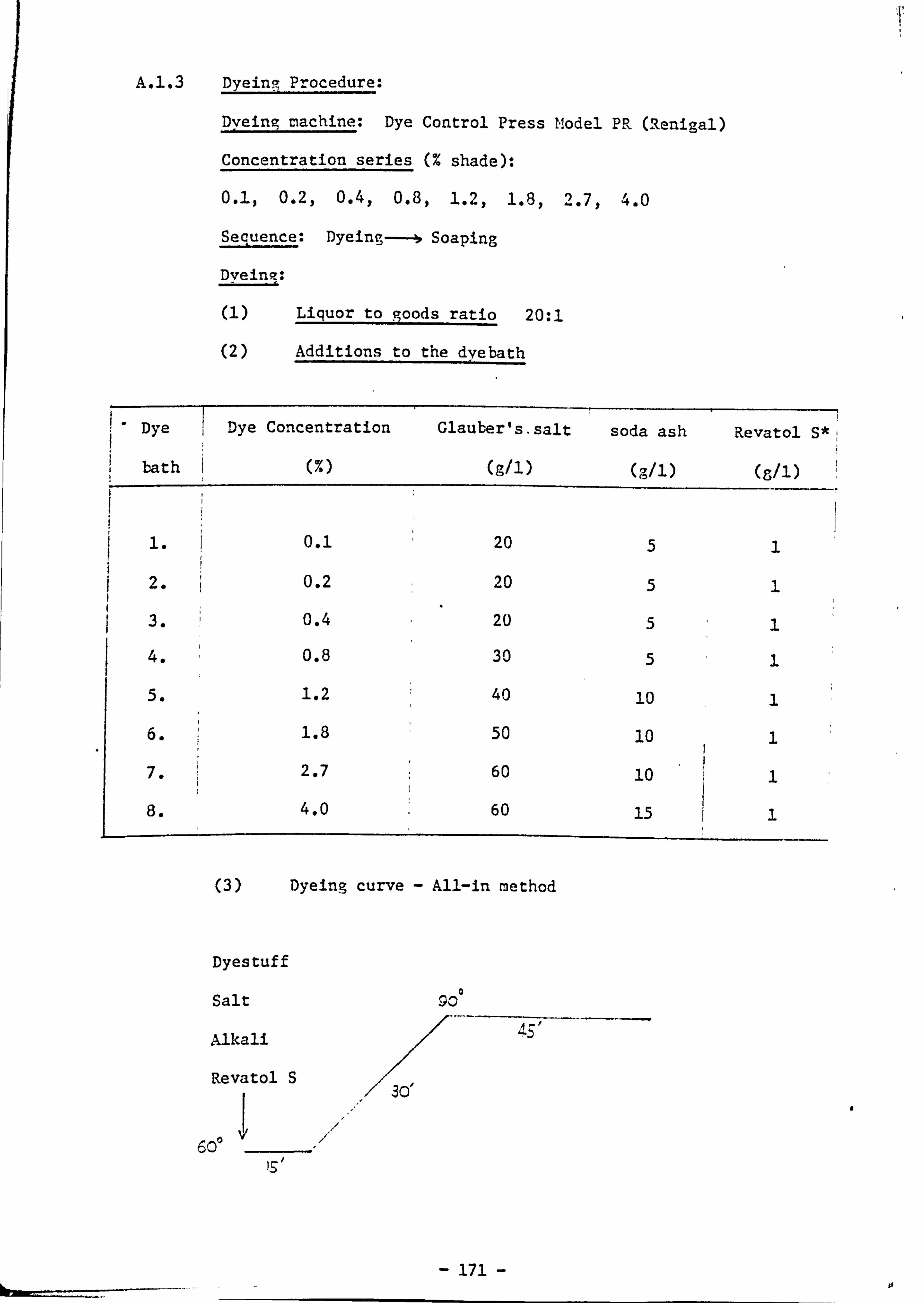
A. 1.3 Dyeing Procedure:
Dyeing machine: Dye Control Press Model PER (Renigal)
Concentration series (% shade):
0.1,0.2,0.4,0.8,1.2,1.8y 2.7, 4.0
Sequence: Dyeing Soaping
Dveine:
(1) Liquor to goods ratio 20: 1
(2) Additions to the dvebath
Dye Dye Concentration Glauber's. salt soda ash Revatol S*ý
bath M (g/1) (-/l)
1. 0.1 20 5
2. 0.2 20 5 1
3. 0.4 20 5
4. 0.8 30 5
5. 1.2 40 10
6. 1.8 50 10
7. 2.7 60 10
8. 4.0 60 15
Dyeing curve - All-in method
Dyestuff
Salt
Alkali
Revatol S
600
171

Soaping**
The goods are well rinsed with hot water, then soaped for 20
minutes of the boil with 0.5 g/l Sandopan DTC* and finally
rinsed with warm and cold water.
*Revatol S- Protective oxidizing agent (Sandoz)
Sandopan DTC - Detergent (Sandoz)
**For dyeing with Drimarene Brillýant Green X-3G (405)
Drimarene Turquoise X-G (410)
an adition of 0.3 g/l soda ash to the soaping bath is required.
a
- 172- - -- - . -- -- - --- --0
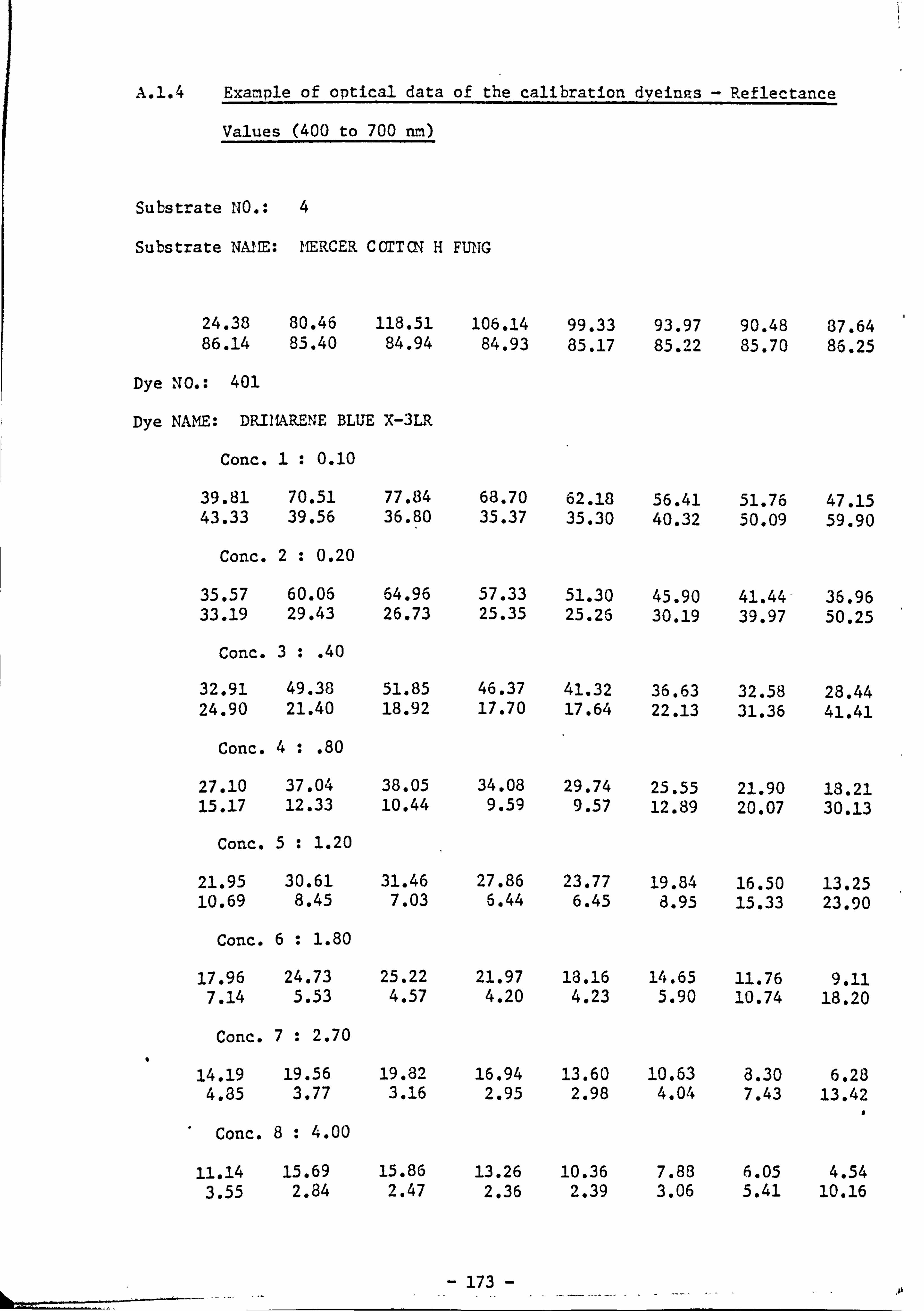
A. 1.4 Example of optical data of the calibration dXeinas - Reflectance
Values (400 to 700 rm)
Substrate NO.: 4
Substrate NAIIE: MERCER CCTTCN H FUNG
24.38 80.46 118.51 106.14 99.33 93.97 90.48 37.64 86.14 85.40 84.94 84.93 85.17 85.22 85.70 86.25
Dye NO.: 401
Dye NAME: DRIMAREENE BLUE X-3LR
Conc. 1: 0.10
39.81 70.51 77.84 68.70 62.18 56.41 51.76 47.15 43.33 39.56 36.80 35.37 35.30 40.32 50.09 59.90
Conc. 2: 0.20
35.57 60.06 64.96 57.33 51.30 45.90 41.44- 36.96 33.19 29.43 26.73 25.35 25.26 30.19 39.97 50.25
Conc. 3: . 40
32.91 49.38 51.85 46.37 41.32 36.63 32.58 28.44 24.90 21.40 18.92 17.70 17.64 22.13 31.36 41.41
Conc. 4: . 80
27.10 37.04 38.05 34.08 29.74 25.55 21.90 13.21 15.17 12.33 10.44 9.59 9.57 12.89 20.07 30.13
Conc. 5: 1.20
21.95 30.61 31.46 27.86 23.77 19.84 16.50 13.25 10.69 8.45 7.03 6.44 6.45 8.95 15.33 23.90
Conc. 6: 1.80
17.96 24.73 25.22 21.97 13.16 14.65 11.76 9.11 7.14 5.53 4.57 4.20 4.23 5.90 10.74 18.20
Conc. 7: 2.70
14.19 19.56 19.82 16.94 13.60 10.63 8.30 6.28 4.85 3.77 3.16 2.95 2.98 4.04 7.43 13.42
Conc. 8: 4.00
11.14 15.69 15.86 13.26 10.36 7.88 6.05 4.54 3.55 2.84 2.47 2.36 2.39 3.06 5.41 10.16
173
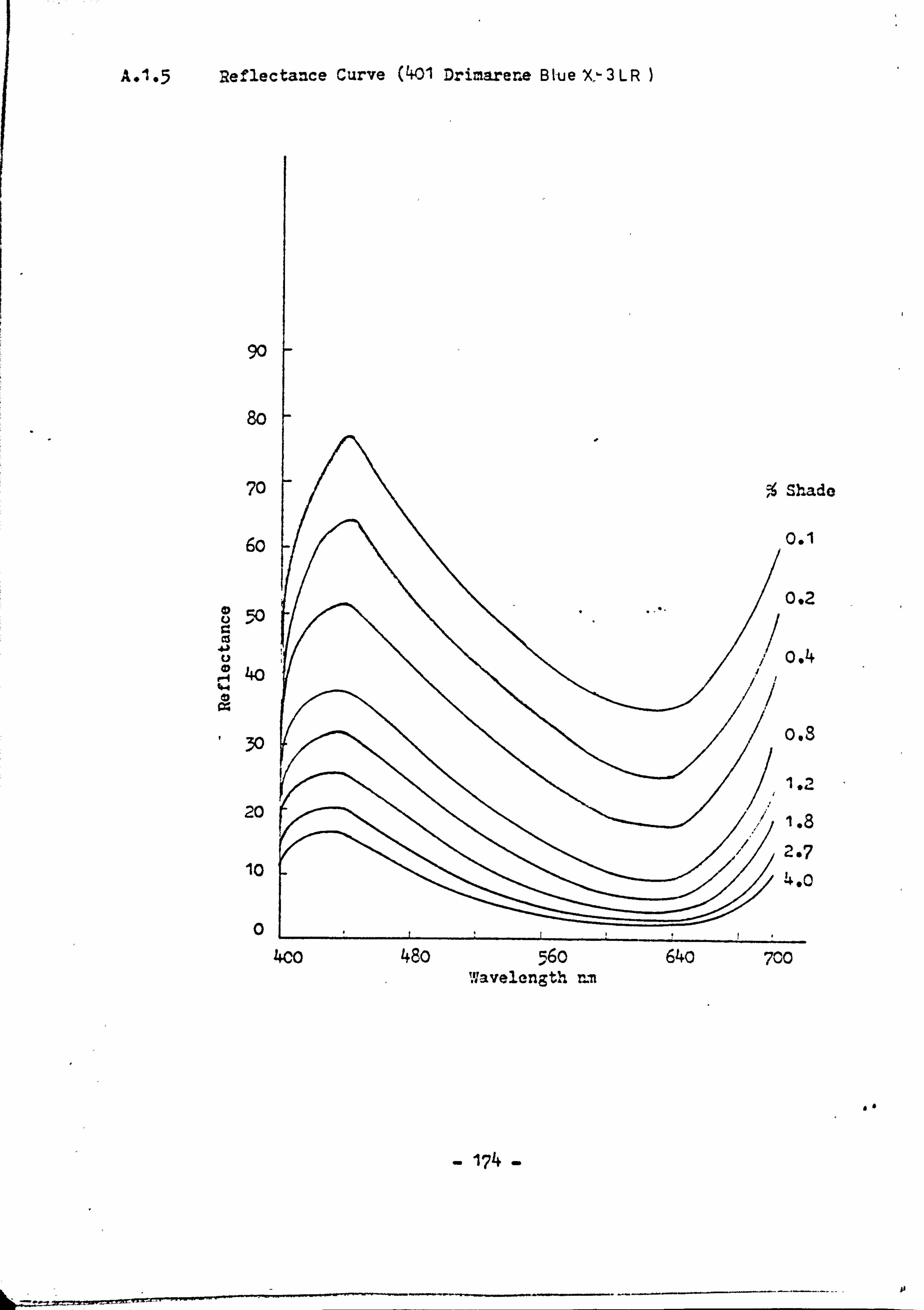
A. 1 *5 Reflectance Curve (401 Drimarene BI-ue %-- 3 LR )
90
80
70
6o
50
4.0
30
20
10
01
400 1.1, lavelength r-n
ado
1
,0
- 174 -
---
C; 480 , Ov 64o 700
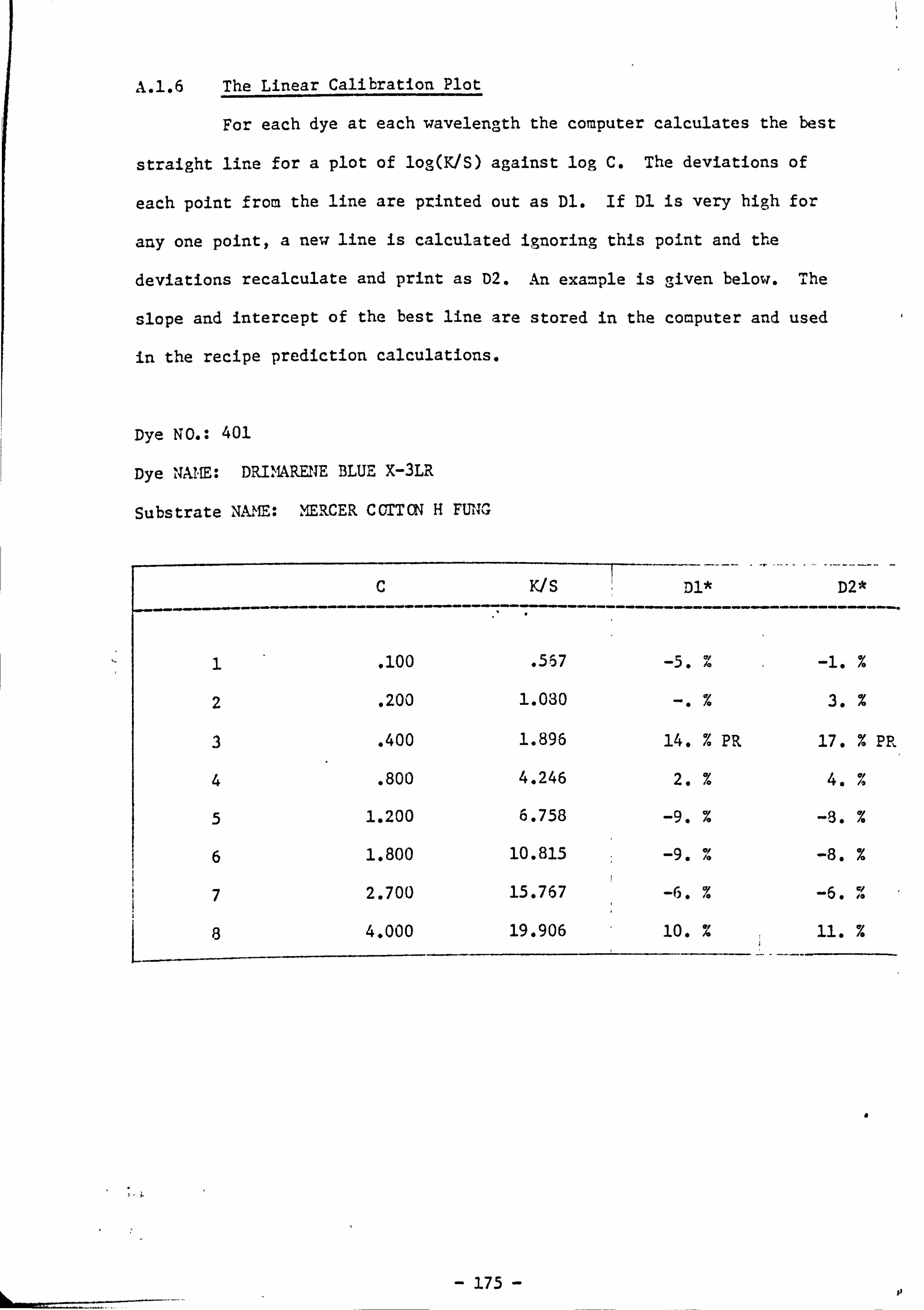
A. 1.6 The Linear Calibration Plot
For each dye at each wavelength the computer calculates the best
straight line for a plot of log(K/S) against log C. The deviations of
each point from the line are printed out as Dl. If D1 is very high for
any one point, a new line is calculated ignoring this point and the
deviations recalculate and print as D2. An example is given below. The
slope and intercept of the best line are stored in the computer and used
in the recipe prediction calculations.
Dye NO.: 401
Dye NAME: DRIMARENE BLUE X-3LR
Substrate NAME: MEIRCER CCTTCN H FUINGY
K/ S Dl* D2*
1 . 100 . 5,57 -5.
2 . 200 1.030 -. %
3 . 400 1.896 14. % PR
4 . 800 4.246 2. %
5 1.200 6.758 -9. %
6 1.800 10.815 -9. 101.1
7 2.700 15.767 -6. %
8 4.000 19.906 10. %
-i. %
3. %
17.7. PR
4. %
%
6 %'
11. %
a
- 175 - 1)
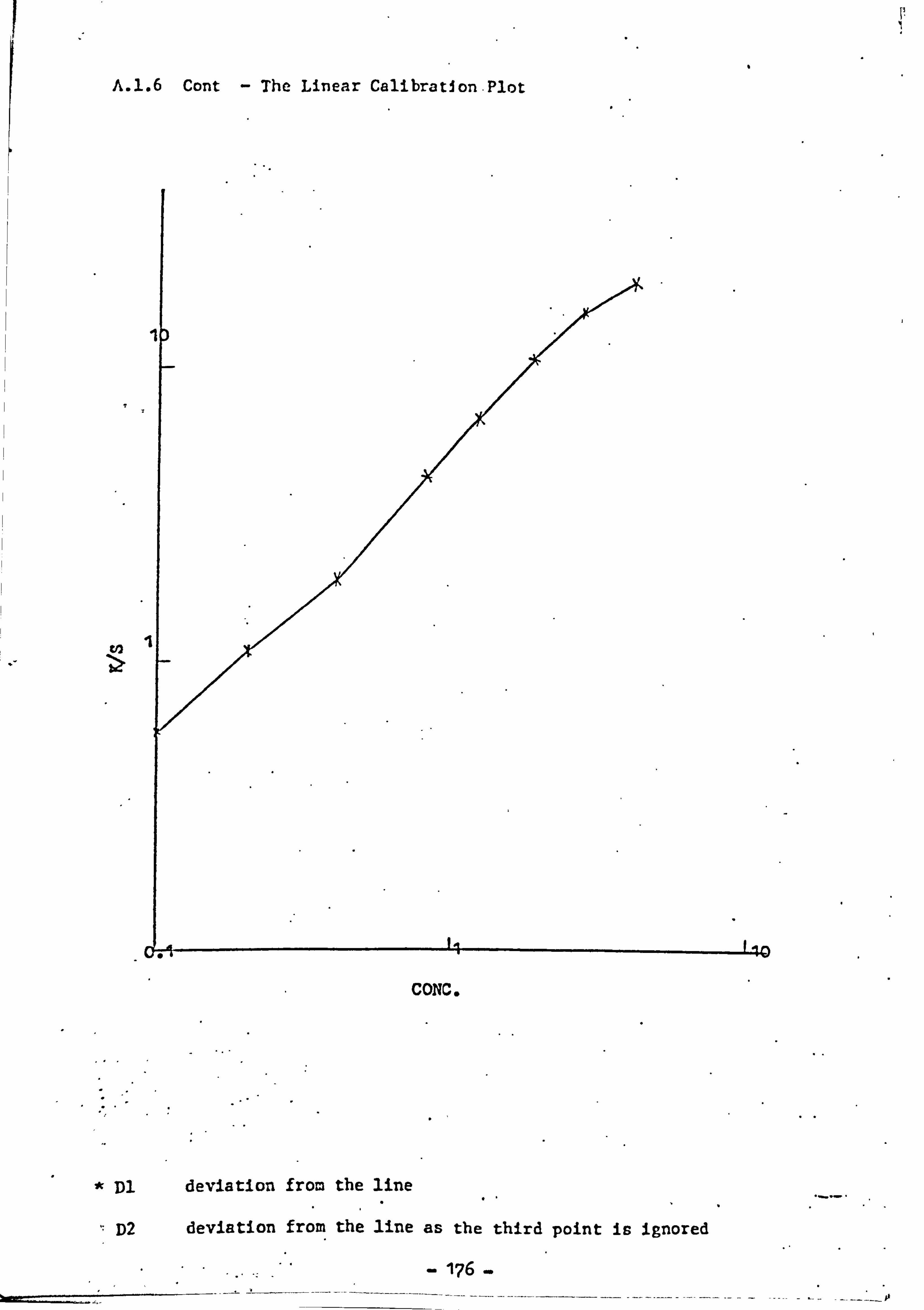
A. 1.6 Cont The Linear Calibration-Plot
V2
CONC.
Dl deviation from the line
D2 deviation from the line as the third point is ignored
176

A. 2 Calibration Dyeings - Polyester/Disperse Dve System (Section 5.2.1)
A. 2.1 Substrate
The Material
100% polyester (1/10OD/24F 22Gx3O") knitted fabric
Texturizing condition
Type of machine Barmag FI(4C
Type of yarn "La coate" Teijen Tetoron Polyester Fibre
Crimp of yarn 20%
Twist level 2911 T/M
over feed % lst 3%
2nd 20%
Crimping temp. 210 0C
Stabilizino, temp. 220 0C
Take-up% 10%
Lubricant 3%
A. 2.2 Dyestuff
1001 Sodyecron Yellow Brown RLS (Sodyeco)
1002 Sodyecron Scarlet 2R (Sodyeco)
1003 Sodyecron Red AYLS (Sodyeco)
1009 Resolin Yellow GGLS (Bayer)
1010 Foron Blue S- RBLT (Sandoz)
A. 2.3 Dyeing procedure
Dyeing machine
Linitest (Original Hanau)
Concentration series (% shade):
. 02, . 04, . 08, . 16, . 31 . 6,1.2,2.4,3.6,4.8
Sequence
Dyeing reduction clear
a
177
..............
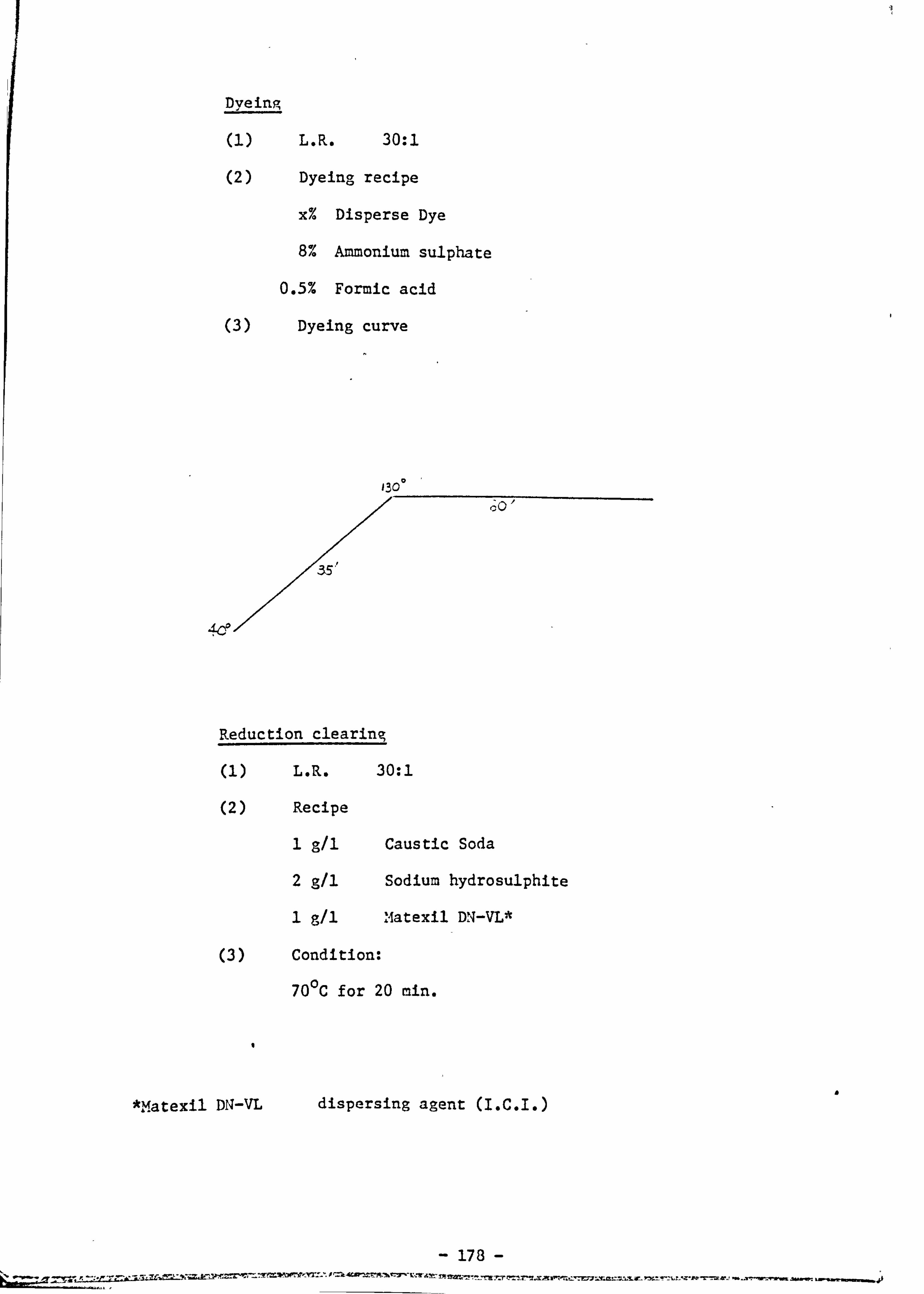
Dyeing
(1) L. R. 30: 1
(2) Dyeing recipe a
x% Disperse Dye
8% Ammonium sulphate
0.5% Formic acid
Dyeing curve
IROO
Co,
35'
4d
Reduction clearing
(1) L. R. 30: 1
(2) Recipe
1 g/l Caustic Soda
2 g/l Sodium hydrosulphite
1 g/l Matexil DN-VL*
(3) Condition:
70 0C for 20 min.
I
*Matexil DN-VL dispersing agent (I. C. I. ) 0
- 178
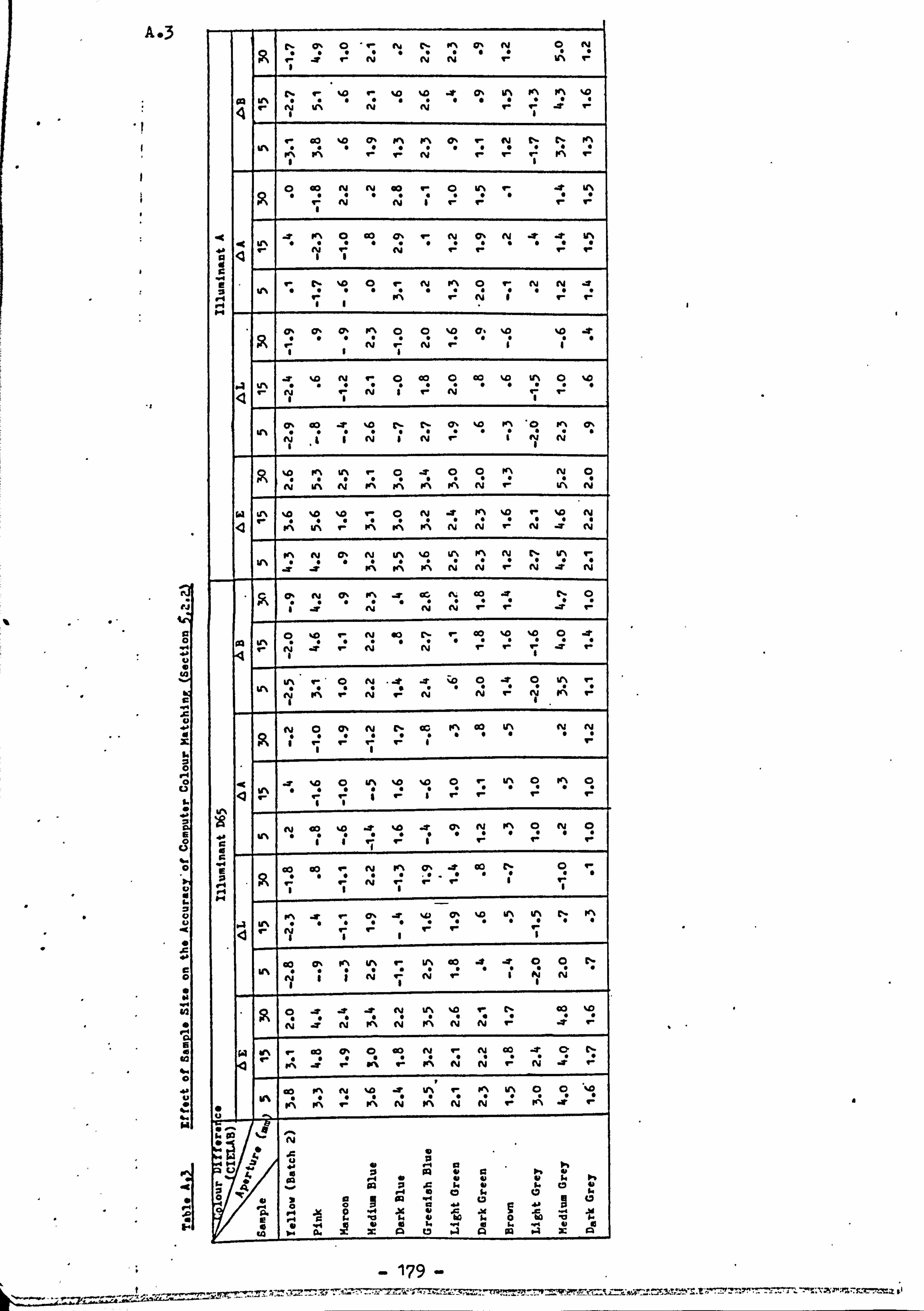
A-3
I..
n 15
:3 a
r4
S I.
C: C! C!
N ult no ry r* q-
IT ; V V- CY I
1 l Oý q Ci 9i 1- 9 Uý I- Uý i Ir- ly ly I I rl V. I
. -C UN ON 0 CO 0% N 0ý N S. .t UN pi cz
V% ON CY I I cl
N fu
11; 'i Oi R Cý %i U) 9 %i ru cy I r. (V t- I-
UN fy ri I CY q- I ey (v
% R 9 llý li 9 I 9%1 WN tv cu I- N
ra UN %* %0 %a V- 0 CY -1 "1% Ni I' Ili li '! A A A s
ar -T WN 191% 191% ru CY q- cu _: r
Cli C!
cy cy cy T- q- -T r.
ai %i %i 'i Ir
CY ty
Ar q-
9 1ý li Cý Ili 1ý ci 1ý li 'i
. -C r %a 9 Uý %i %. i R - Uý 9 1ý R
ýR C%j co %i li -2ý llýl 1% 9 Ci 9
4 C-1 -% ci
N
lfý
q-
C%
1-
-T
1: co
1 N 0 q-
Gi Cý CY C4
12i 'i N
1ý
R 9 N -7 CM If% N n CY CY T-
ci I-i
.4 V% "" A
co j
0% *
0 A
CO *-
tv A
I-
C4 cu
(4 co
': 4 C, ;
C- *
Oi 'A A r.
WN r. WN C) 0 %0
u
z 0
10
A
11
31
14 0 " 1
10"
03 P
m
A
40,
N
1:
0
0
P.. ,
l
"0
a
I
a
179
A. 4 Location of Target SamDles in CIELAB SDace (Section 5.2.3)
Among the five hundred target samples selected 348 targets can Z)
be formulated by the selected desperse dyes and 332 targets by the
selected reactive dyes. An example of cotton/Reactive dye system is
given below. Fig. Aa and A4c illustrate the samples which can be
matched with the selected reactive dyes, whereas Fig. Ab and A4d show up
those which cannot be formulated. Most of the colours in red through
yellow to green and those with lower chroma in the green-blue and the
blue-red quarters (Fig. 4Aa and 4Ab) can be matched. Generally colours
with lower chroma, regardless of hue and lightness can be formulated
(Fig. 4Ac and 4Ad).
a
180
ý k44- - -e� ', ":, -e 2- l=

Fig. Aa Target Samples Which can be Matched in the Cotton/fReactive Dye
System
6
60
)c X 40 x
ý4
e xXx
)(
?c), )?, xAXxxX
)t AxA
X XX
Xx )( 2( XX
It XY "I( AxX
x )( AxX X xx x ý5, x
< :Y Xx X Ac IX lk
xX )K. *< K ,(-, A x
A 6, 2"' IK )C X<].. ý Xx 4" -40 -ac xx . 20
x X ý4
;,
x Xx AA
)c x
xx tol
x

Fig. Ab Target Samples which cannot be Matched in the Cotton/Reactive
Dye System
- 182 -
S
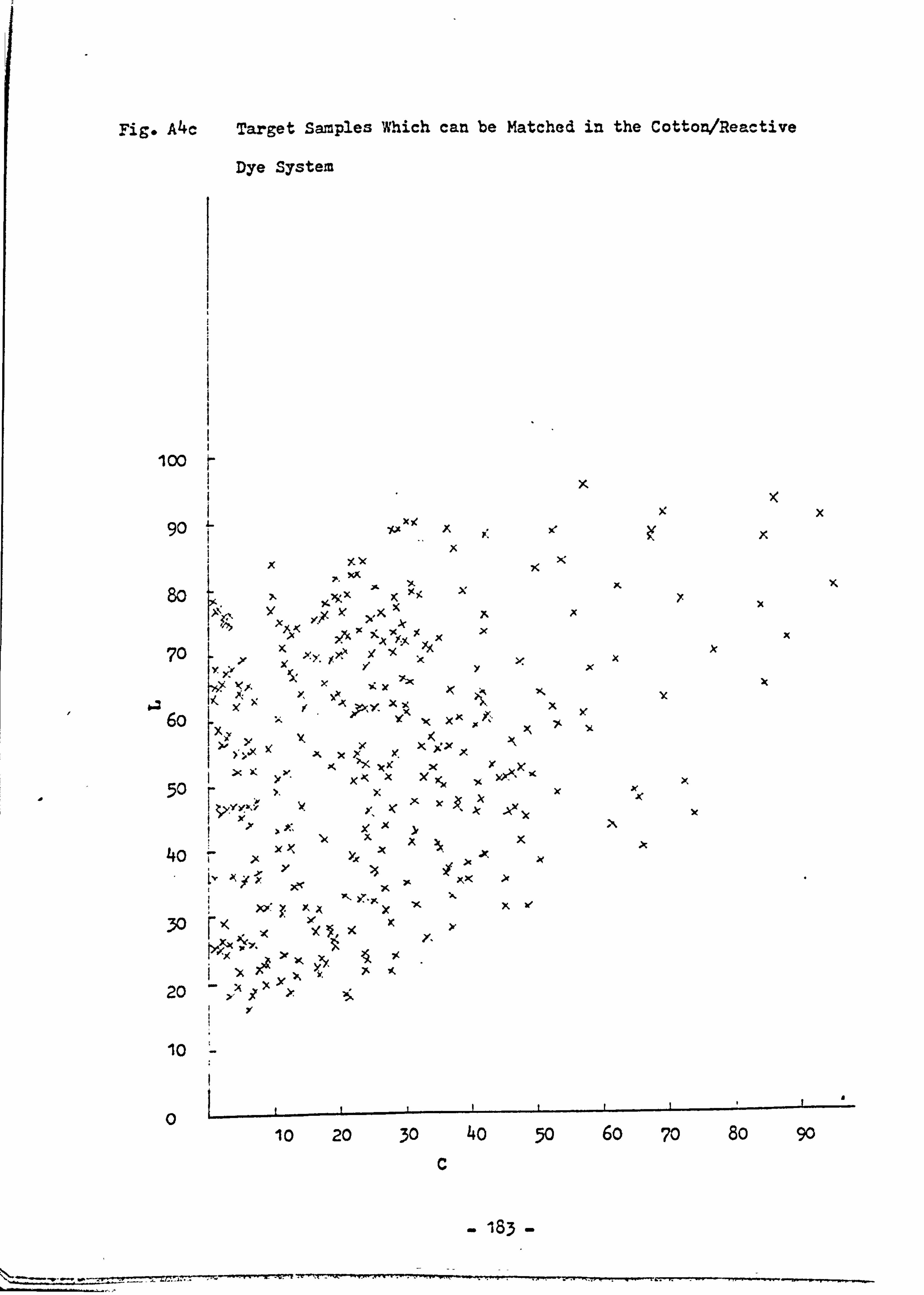
Fig* A4c Target Samples Which cat be Matched in the Cotton/Reactive
Dye System
loo 90 4- -M
X)< A )e
x XK
x 80 X 21
",, K ýkx ý
XII ý( )( x
70 Y. y
ýZý AxX, YX x ýý Xý xf %PY. Xxxy 61 xx oXxX
>ý X 3( wx gx x X, 5ý xKx )c x
X ýý XX(
50 xx A? "
ev
A x
JK X 4o )XI N x ý5 v, iX
9r AX >r
X X. be
30
-4 A lik 'A )e
20 X,
10
0
10 20 30 40 50 60 70 80 90 c
183
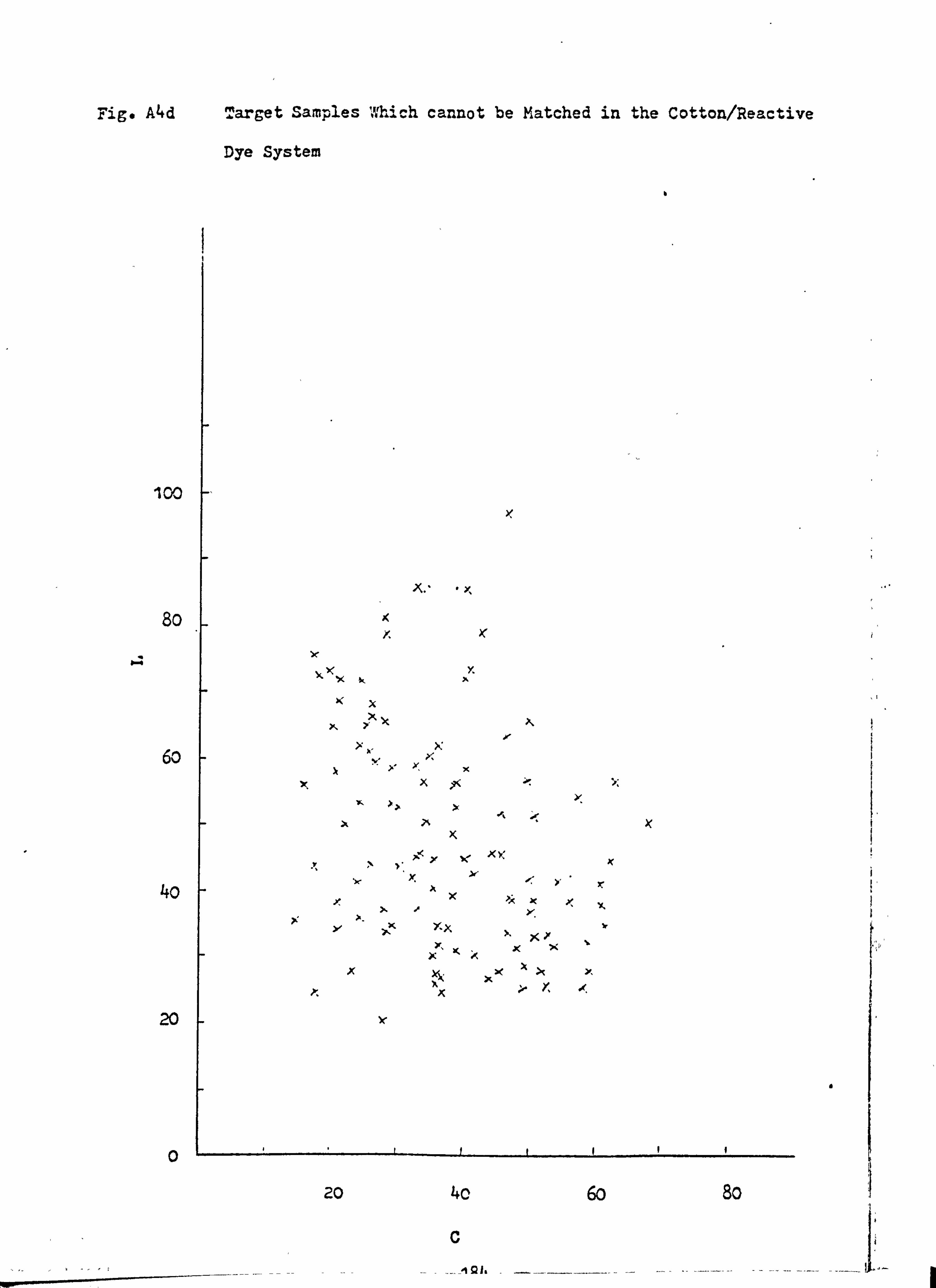
Fig* Ad Target Samples Which cannot be Matched in the Cotton/Reactive
Dye System
b
100
80
4
60
40
20
0
20 4c 60 8o
B. Colorimetric Behaviour of Fluorescent Dyes in Self and in
Compound Shades with Non-fluorescent Dyes.
The behaviour of fluorescent and non-fluorescent dyes are
illustrated in the 1931 CIE colour specification system and in the 1976
CIELAB system ( Ill. D 65 and 100 supplementary standard observer).
Colours in the chromaticity diagram with their respective lightness are
interpretted in two graphs viz., x vs y and x vs Y. In the CIELAB
system, the common A'vs B, L vs C plots are employed. In addition, the
trend of change in hue with respect to lightness is illustrated in the L
vs Ho plot. With this new way of expression, the overall picture of
the colour behaviour of dyeings is enhanced. Furthermore the reflectance
or the total radiance curves complete the illustration.
B. 1 General Behaviour of Single Dyes
In each of the following figures, 1,2 ... 8 refer to
concentrations of 0.0005,0.001 ... 1% shade respectively. The figures
are arranged in the following order:
x vs y, x vs Y, A vs B, C vs L and L vs H0
Code 'I Dye Concentration (% Shade)
LY2 L. Yellow G . 0005 . 001 . 005 . 01 . 05 .1 .5
1603 L. Red G . 005 . 01 . 025 . 05 .1 . 25 .5
Y3G Yellow 3G . 0005 . 001 . 005 . 01 . 05 .1 .5
Pi B. Pink REL . 0005 . 001 . 005 . 01 0.5 .1 .5
1706 Red 5SEL . 005 . 01 . 05 . 075 .1 . 25 0.5
SER1 Blue SEA . 0005 . 005 . 01 . 05 .1 .5 1.0
I
1.0 1.0
1.0 1.0
1.0
a
- 185 -
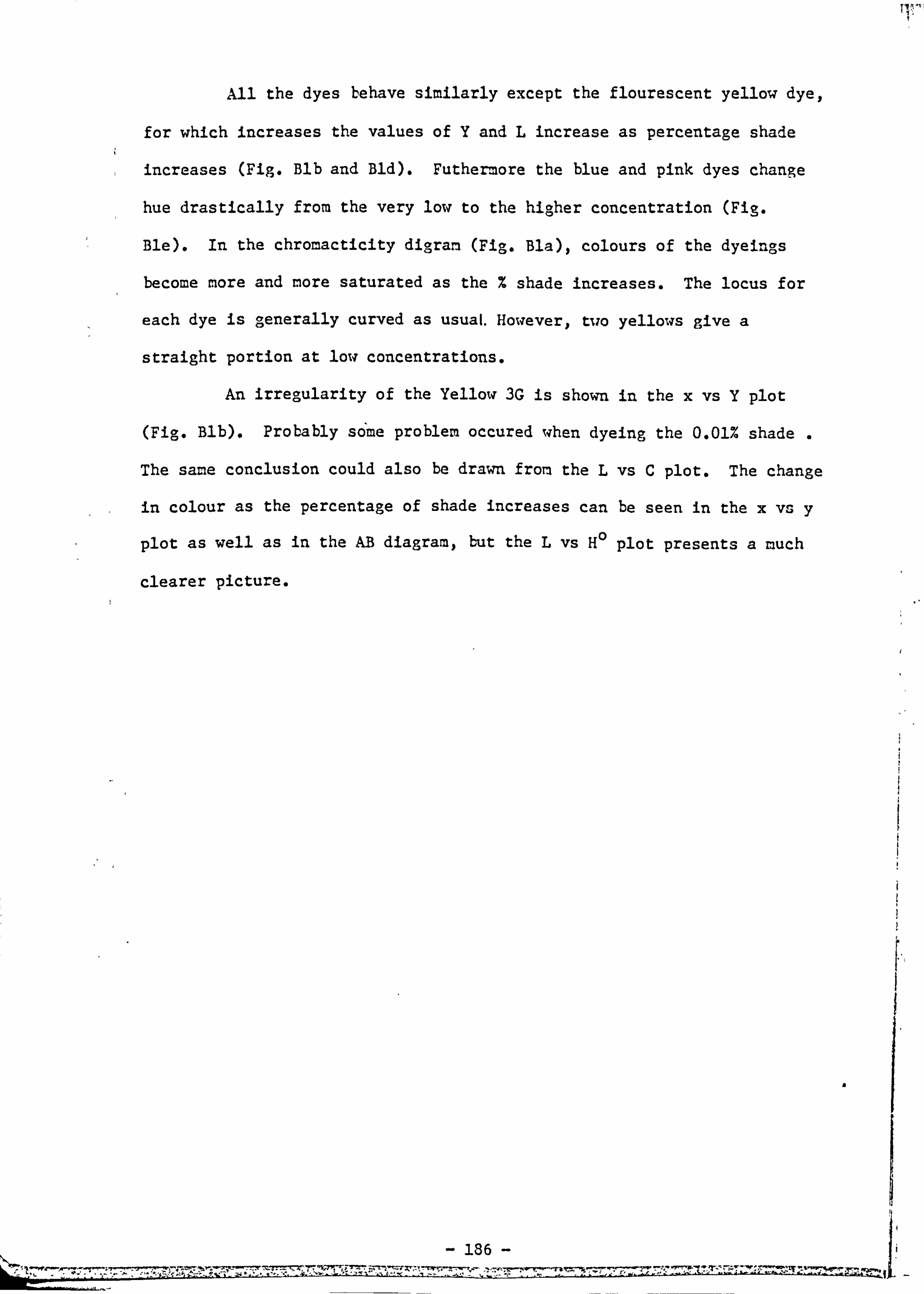
All the dyes behave similarly except the flourescent yellow dye,
for which increases the values of Y and L increase as percentage shade
increases (Fig. Blb and Bld). Futhermore the blue and pink dyes change
hue drastically from the very low to the higher concentration (Fig.
Ble). In the chromacticity digram (Fig. Bla), colours of the dyeings (3 U
become more and more saturated as the % shade increases. The locus for
each dye is generally curved as usual. However, two yellows give a
straight portion at low concentrations.
An irregularity of the Yellow 3G is shown in the x vs Y plot
(Fig. Blb). Probably some problem occured when dyeing the 0.01% shade
The same conclusion could also be drawn from the L vs C plot. The change
in colour as the percentage of shade increases can be seen in the x vs y
plot as well as in the AB diagram, but the L vs H0 plot presents a much
clearer picture.
186 -
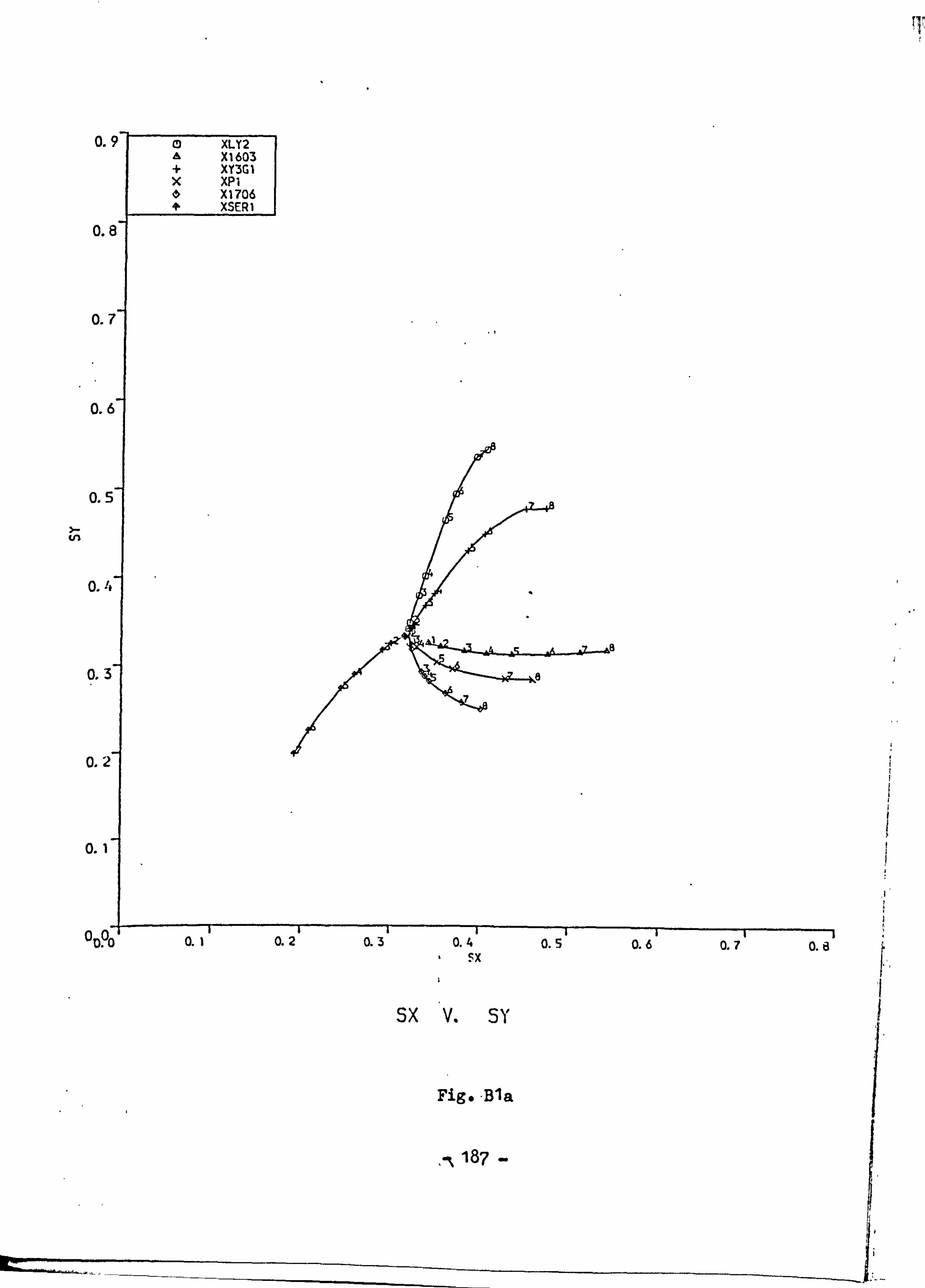
0.
0.
0.
0. (
0.
0.4
0.3
0.2
0.1
ODPO I U. 19 U. a U. 4
.Ix
sx V. SY
Fig. -Bla
, -ý 187 -
0.5 0.6 0.7 0.8
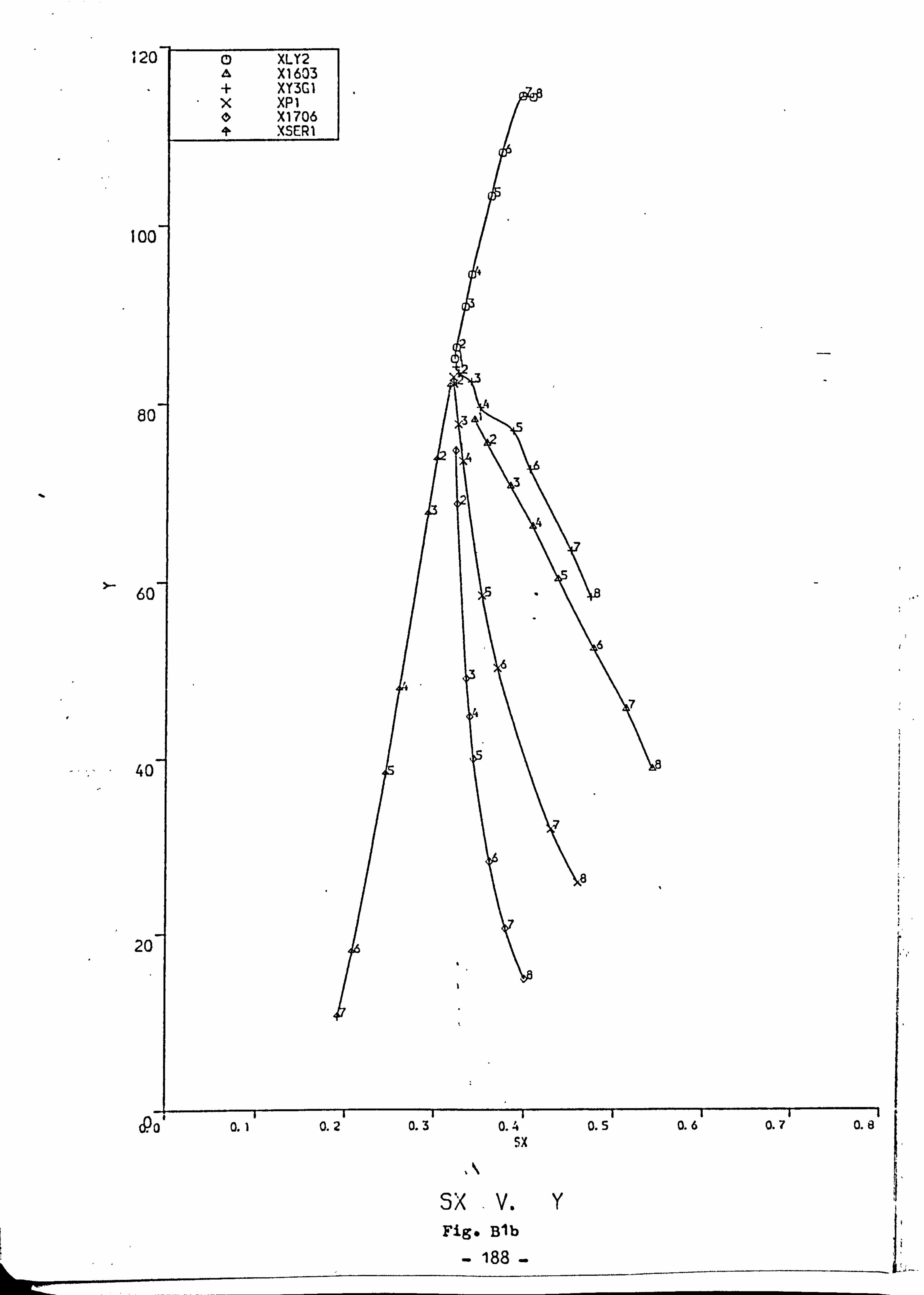
12(
loc
8C
>- 6C
40
20
000,0.1,0.2 0.3 0.4 0.5 0.6 0.7 0.8 ýx
sx V. y Fige Blb
188
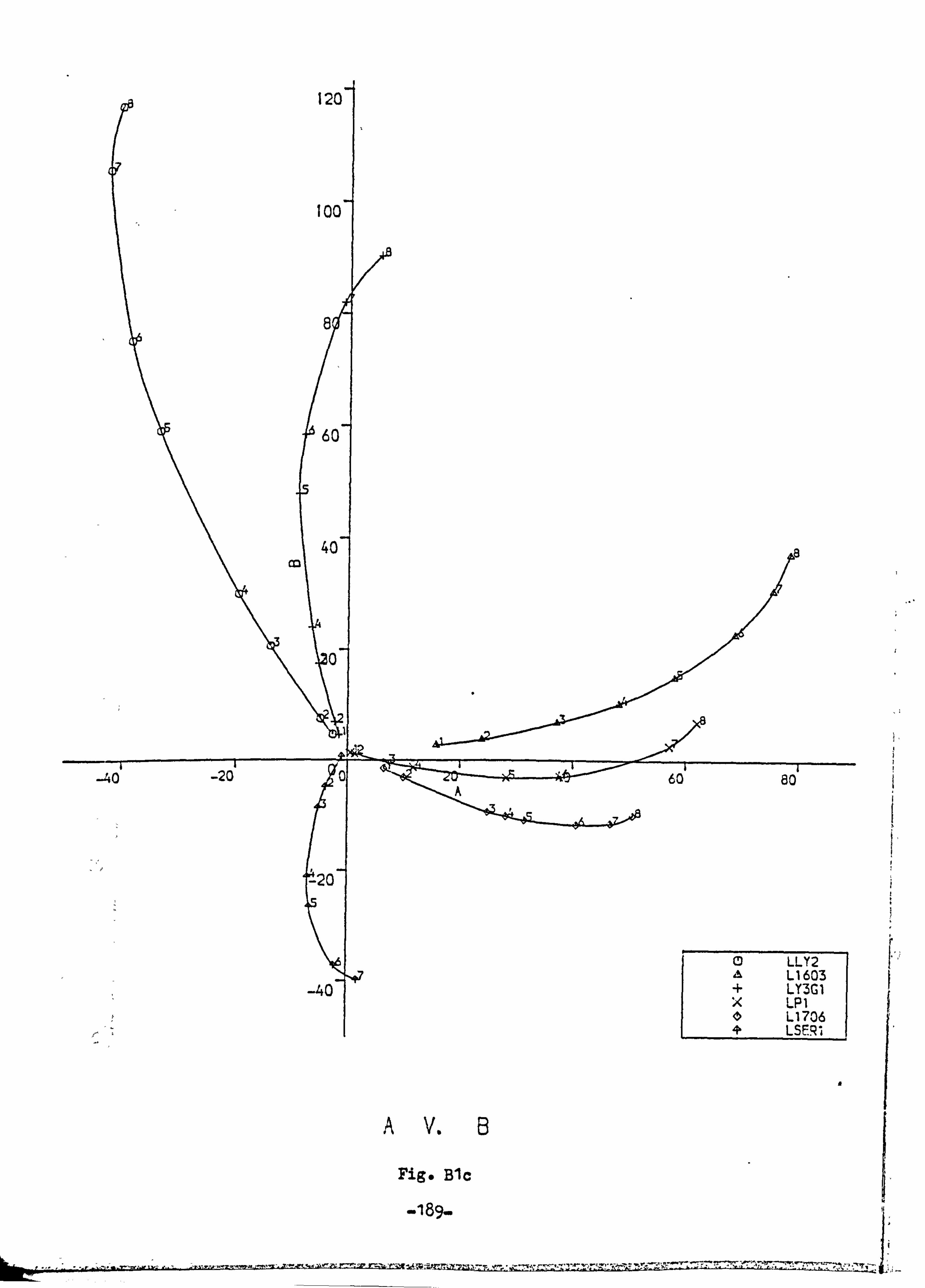
(9 LLY2 A L1603
-40 + LY3G1 x LP1 e L1706
LS ER 1
A V. 6
Fige Blc
-189-
Lý- ,. -, -- -- -- - 't3ai. L%
awoLZ-

-1
loý
6(
6C
4C
20
CHROMA V. LIGHTNESS
58
a
Fig* Bld - 190 -
26' 40- 60* eo* 100' : 20 c
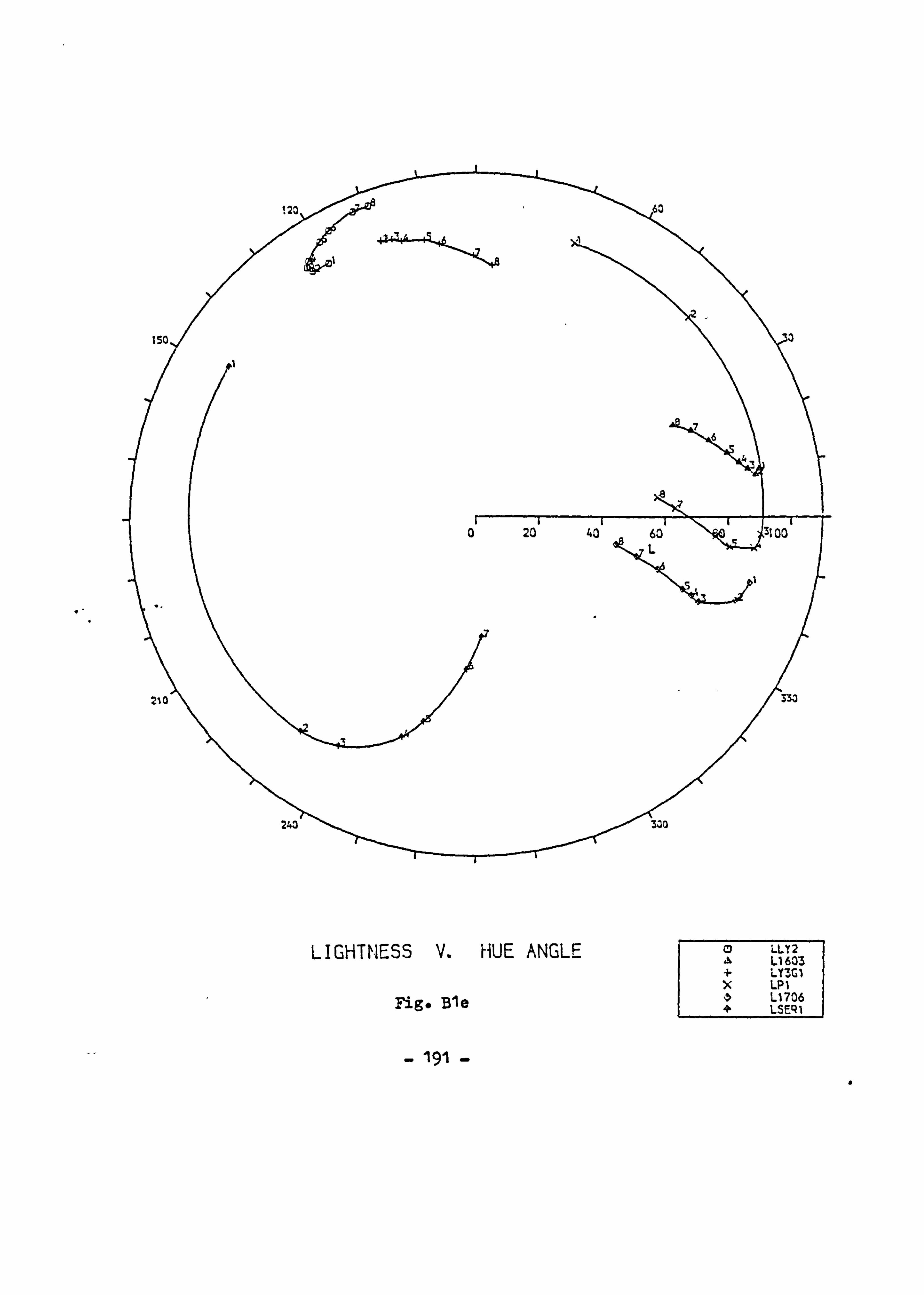
LIGHTNESS A
Fig* Ble
HUE ANGLE LLY2 Ll 603
* LY'. 'Gl * LPI * L1706 * LSFR1
- 191 -

Concentration Shade)
Code L. Yellow G Yellow 3G
LYGl 25 . 0005i . 001, . 005ý . 01, . 05 and .1
LYG2 . 25 . 0005, . 001, . 005, . 01, . 05 and
LYG3 . 50 . 0005, . 001, . 005i . 01, . 05 and
LYG4 . 75 . 0005, . 001, . 005, . 01ý . 05 and
LYG5 1.00 . 0005, . 001, . 005, . 01, . 05 and
LYG6 2.50 . 0005, . 001, . 005, . 01, . 05 and
Some irregularities are found for the low concentrations. The
lines are nearly parallel with each other. Increases in the
concentration of the non-fluorescent yellow cause a great drop in the Y
and L values, but with only a small decreaies in chroma (Fig. 1132.1b and
B2.1d).
- 193 -
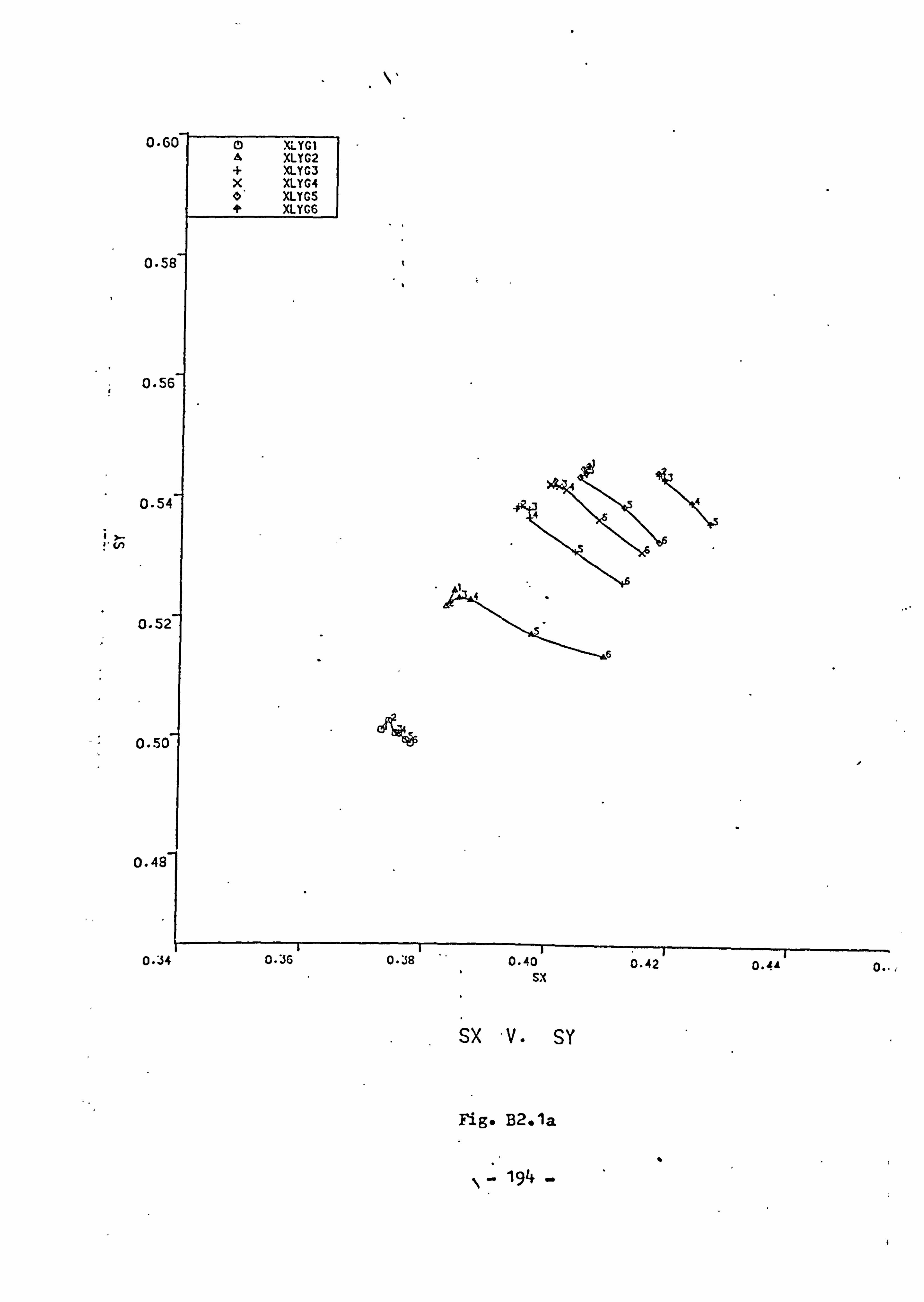
0. (
0.5
0.5
En
0.5,
0.5c
0.48
O-j4 U-4u 0.42 sx
sx N. SY
Fig. B2.1a
194
0.44 0. - ý,
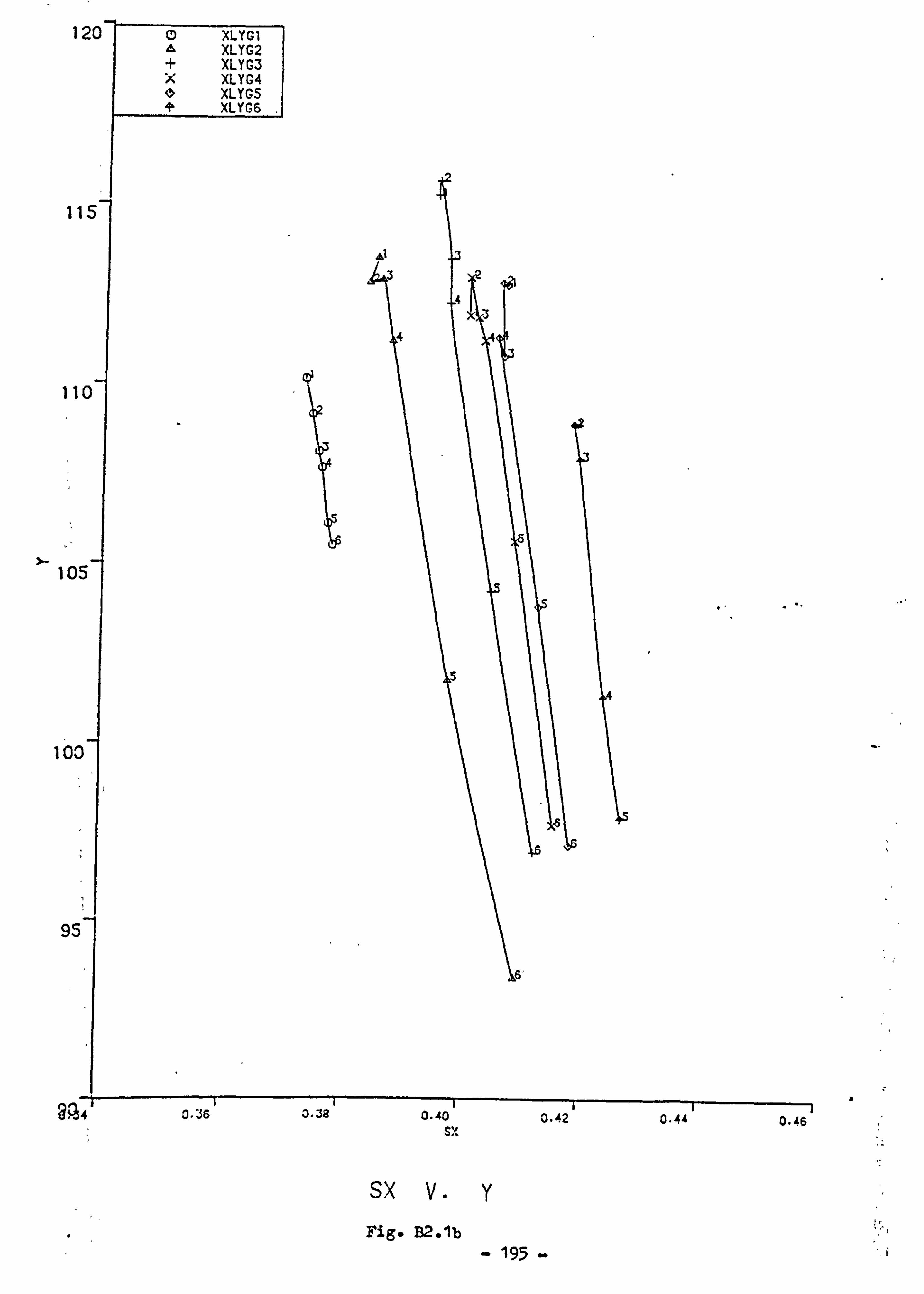
I
I,
II
10
1
9z
? q4
sx V. y Fig. B2. lb
195 -
4u 0-4Z 0-4A 0.46 S"
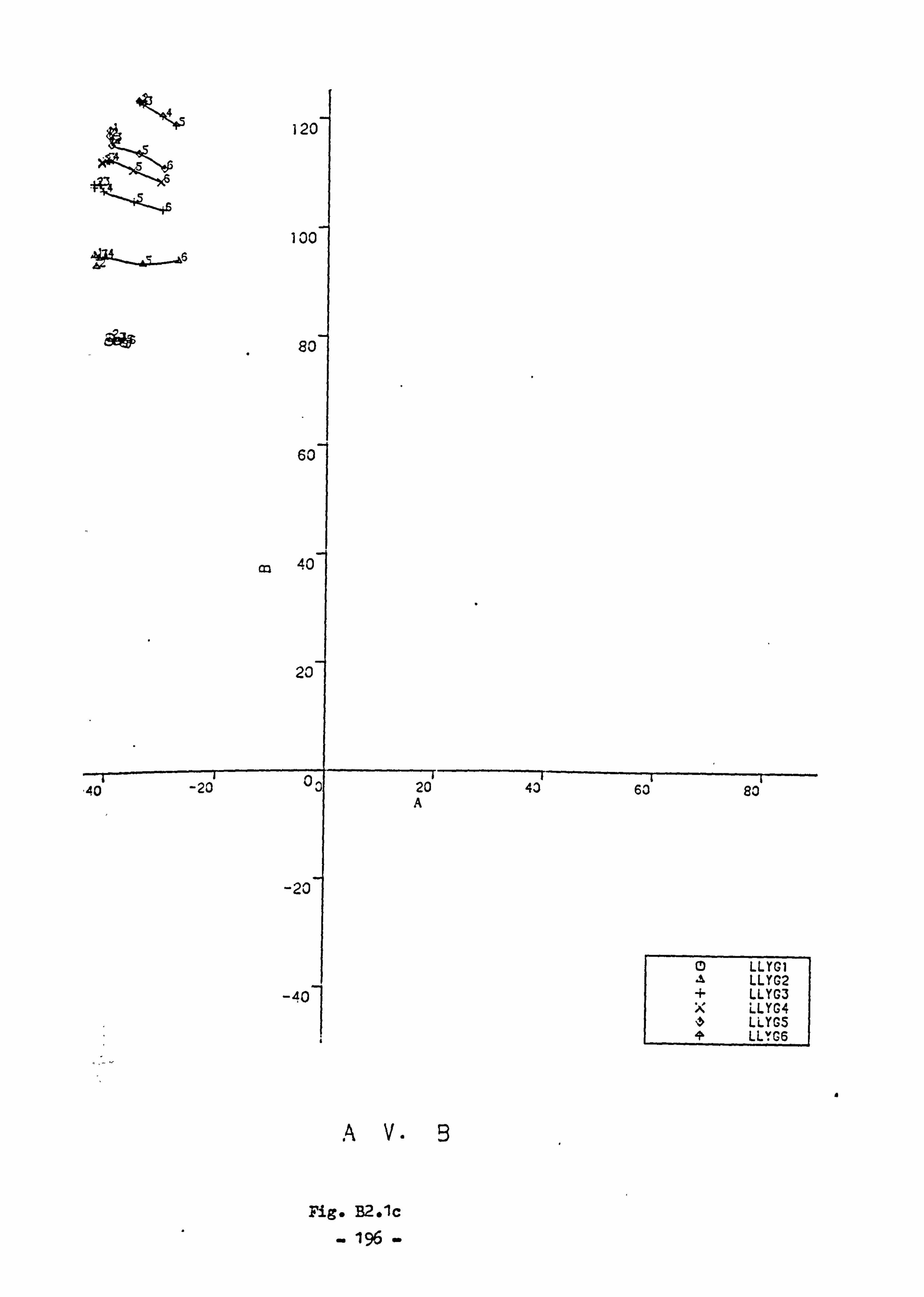
A V. B
Fig. B2*lc
- 196 -
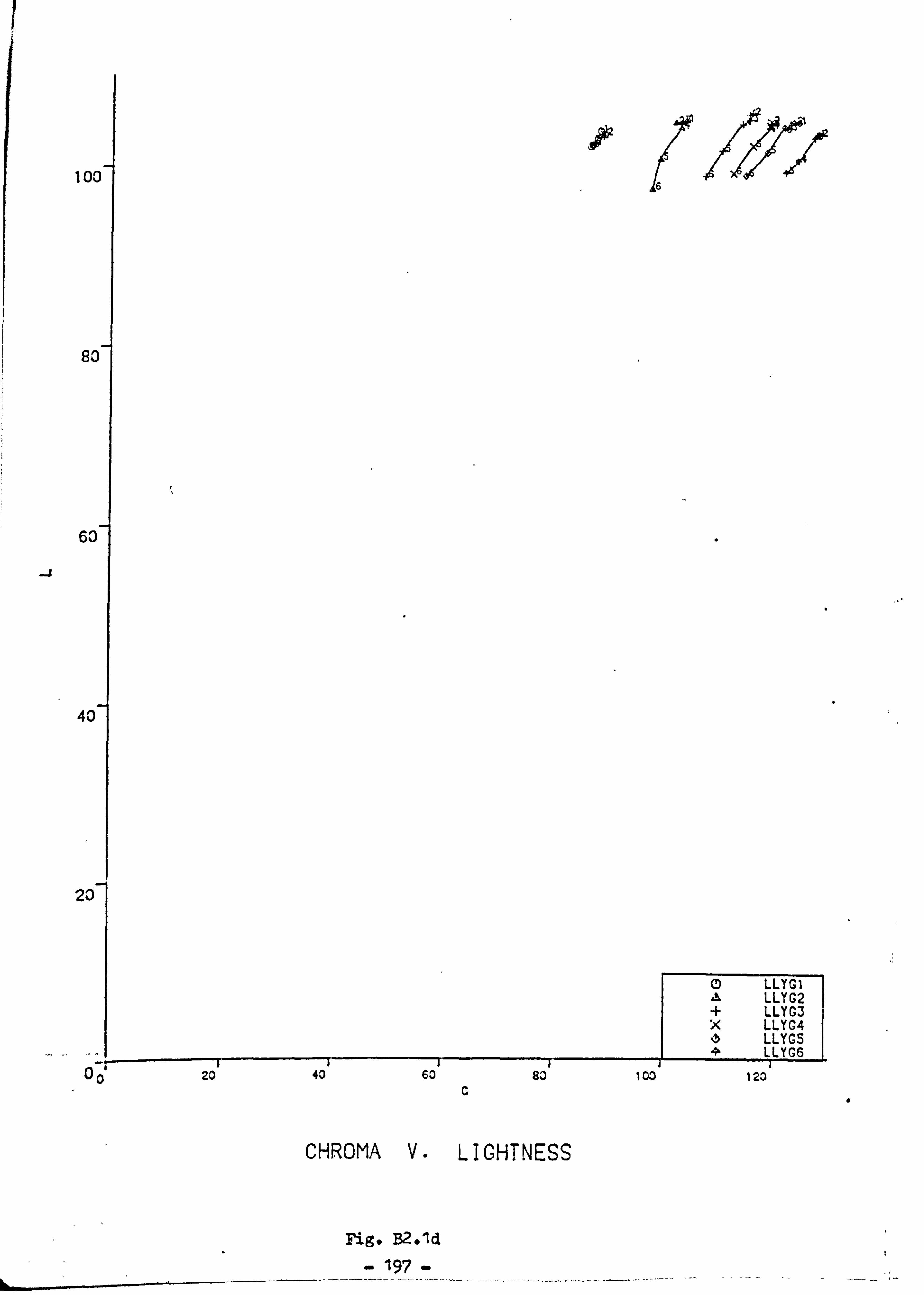
100
80
60
-J
40
20
03 23 40 60 so c
CHROMA V. LIGHTNESS
Fig. B2*ld
CD LLYGI At LLYG2 * LLYG3 * LLYG4 * LOGS 46 LLYG6
100 120
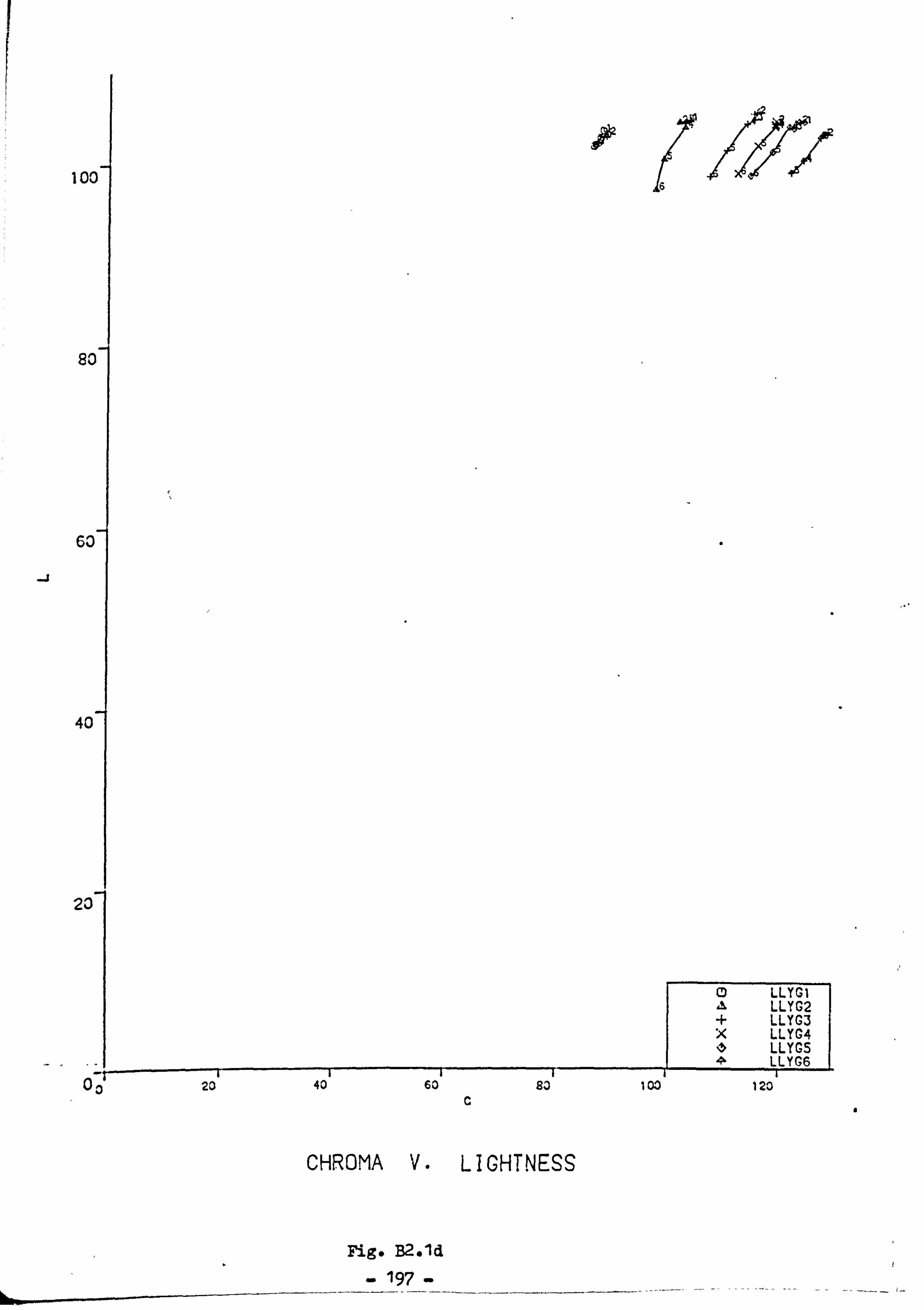
100
80
60
-J
40
20
03 20 40 60 83 c
CHROMA V. LIGHTNESS
Fig* B2old 197
C) LLYGI A LLYG2 * LLYG3 * LLYG4 * LOGS 4, LLYG6
100 120
a
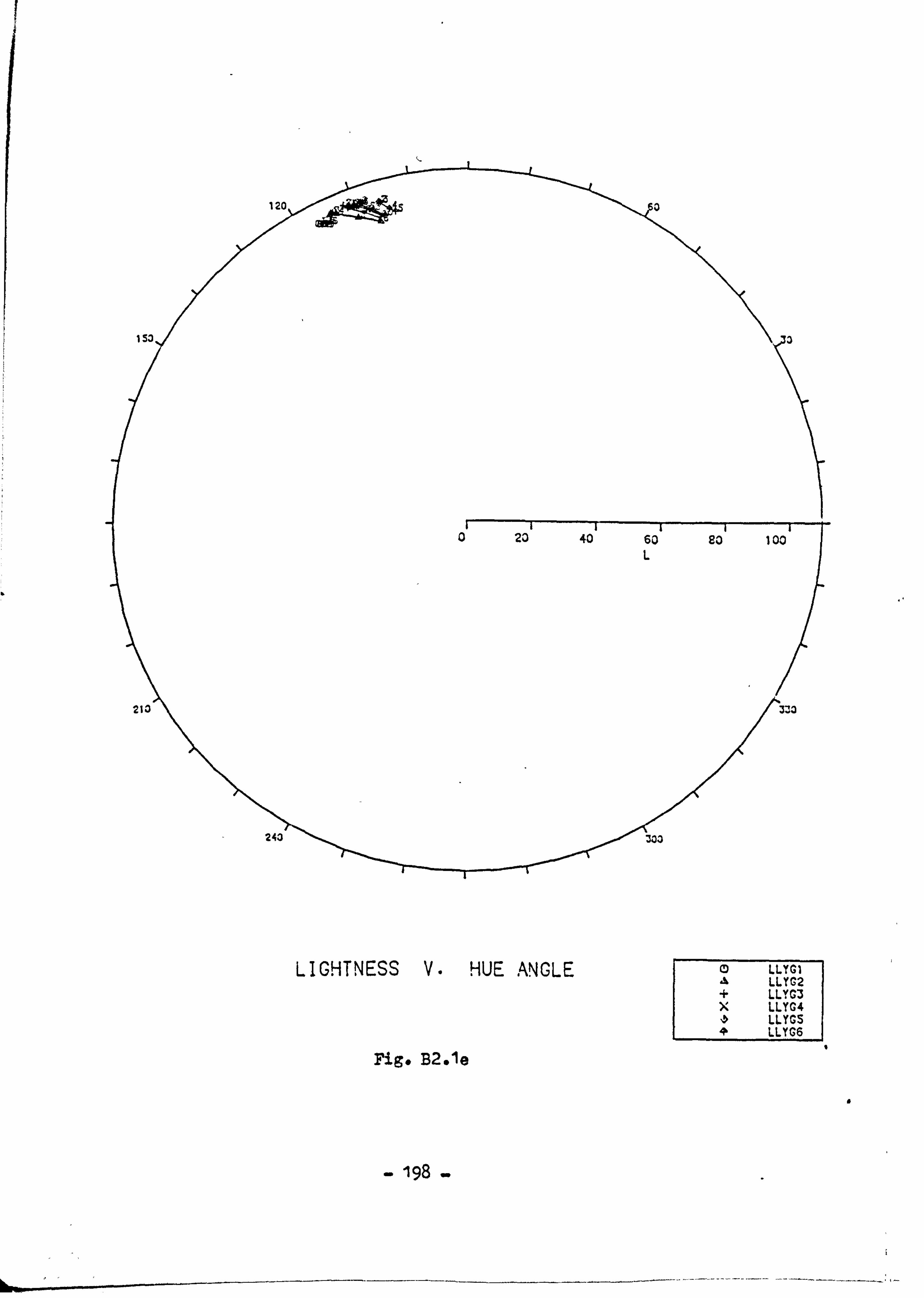
LIGHTNESS V.
Fig. B2. le
HUE ANGLE Q) LLYGI A LLYG2 * LLYG3 * LLYG4
LLYGS LLYG6
- 198 -
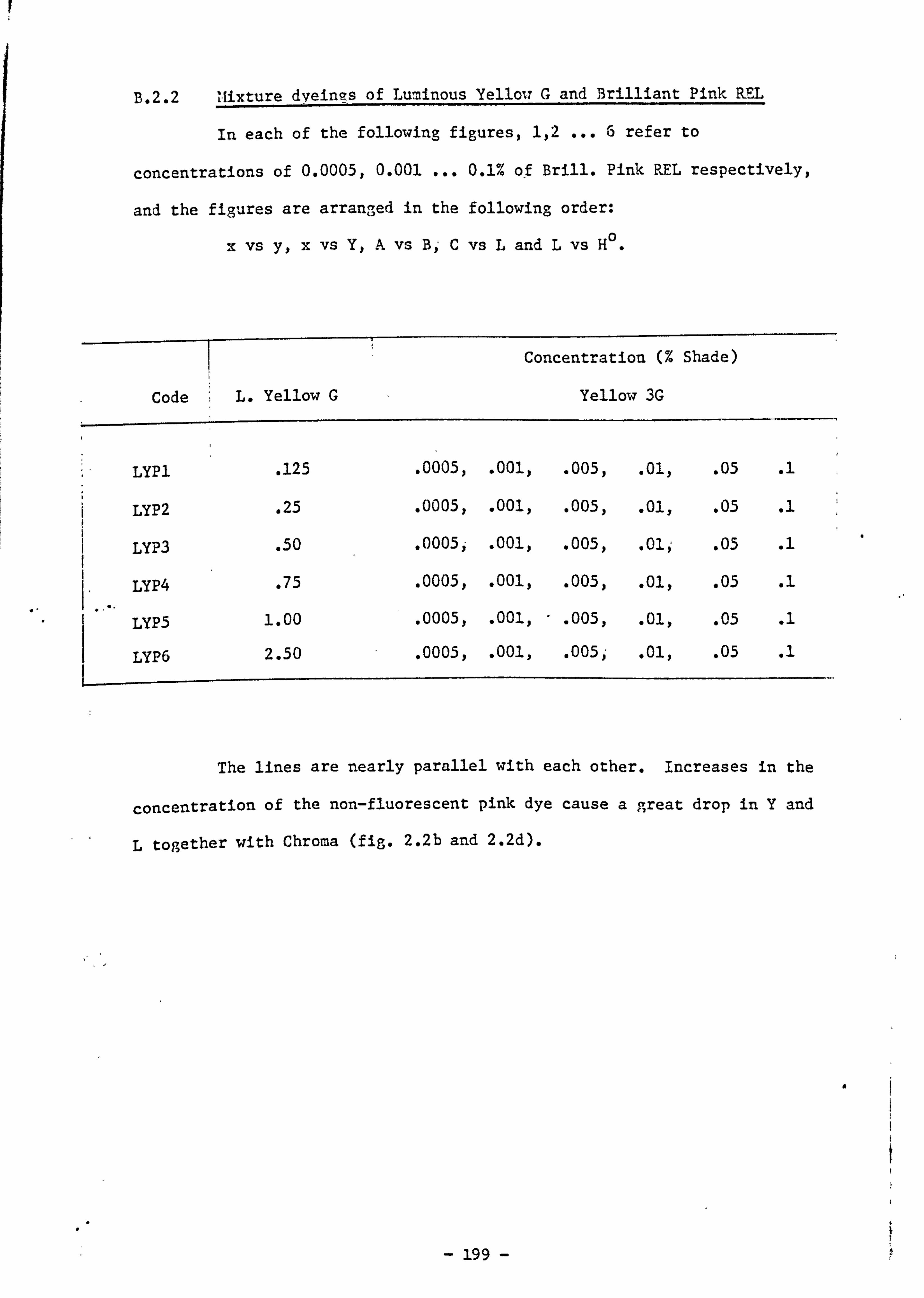
B. 2.2 mixture dveings of Luminous Yellow G and Brilliant Pink R-EL
In each of the following figures, 1,2 ... 6 refer to
concentrations of 0.0005,0.001 ... 0.1% of Brill. Pink REL respectively,
and the figures are arranged in the following order:
0 x vs y, x vs Y, A vs Bý C vs L and L vs H
Concentration (% Shade)
Code L. Yellow G Yellow 3G
LYP1 . 125 . 0005, . 001, . 005, oi, . 05 1
LYP2 . 25 o005e . 001, . 005) oi, . 05
LYP3 . 50 o005i . 001, . 005, olý . 05
LYP4 . 75 . 0005, . 001, . 005, ole . 05
LYP5 1.00 . 0005, . 001, . 005, oi, . 05
LYP6 2.50 . 00051 . 0011 . 005)- 001, . 05
The lines are nearly parallel with each other. Increases in the
concentration of the non-fluorescent pink dye cause a great drop in Y and
L together with Chroma (fig. 2.2b and 2.2d).
- 199 -
a

(I,
0.60
0.55
0.50
0.45
0.40
0,32
SIX
sx V. SY
Fig* B2o2a
- 200 -
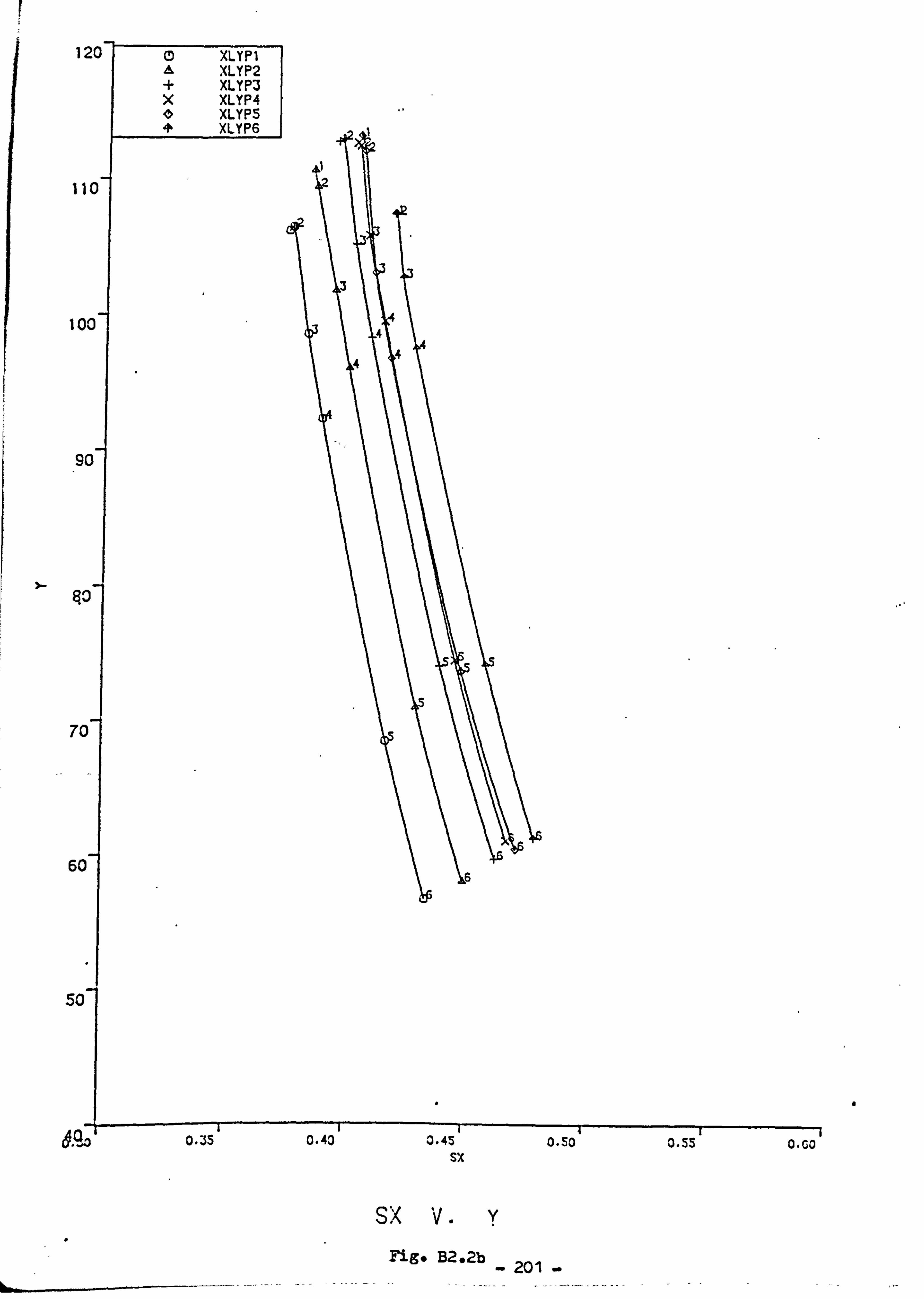
I
Iý
Ic
9
7c
6C
50
a
14011 V. ý U-ja 4u U-45 0.50 O-SS O-CO sx
SX V. y Fig* B2,2b
201 kL-
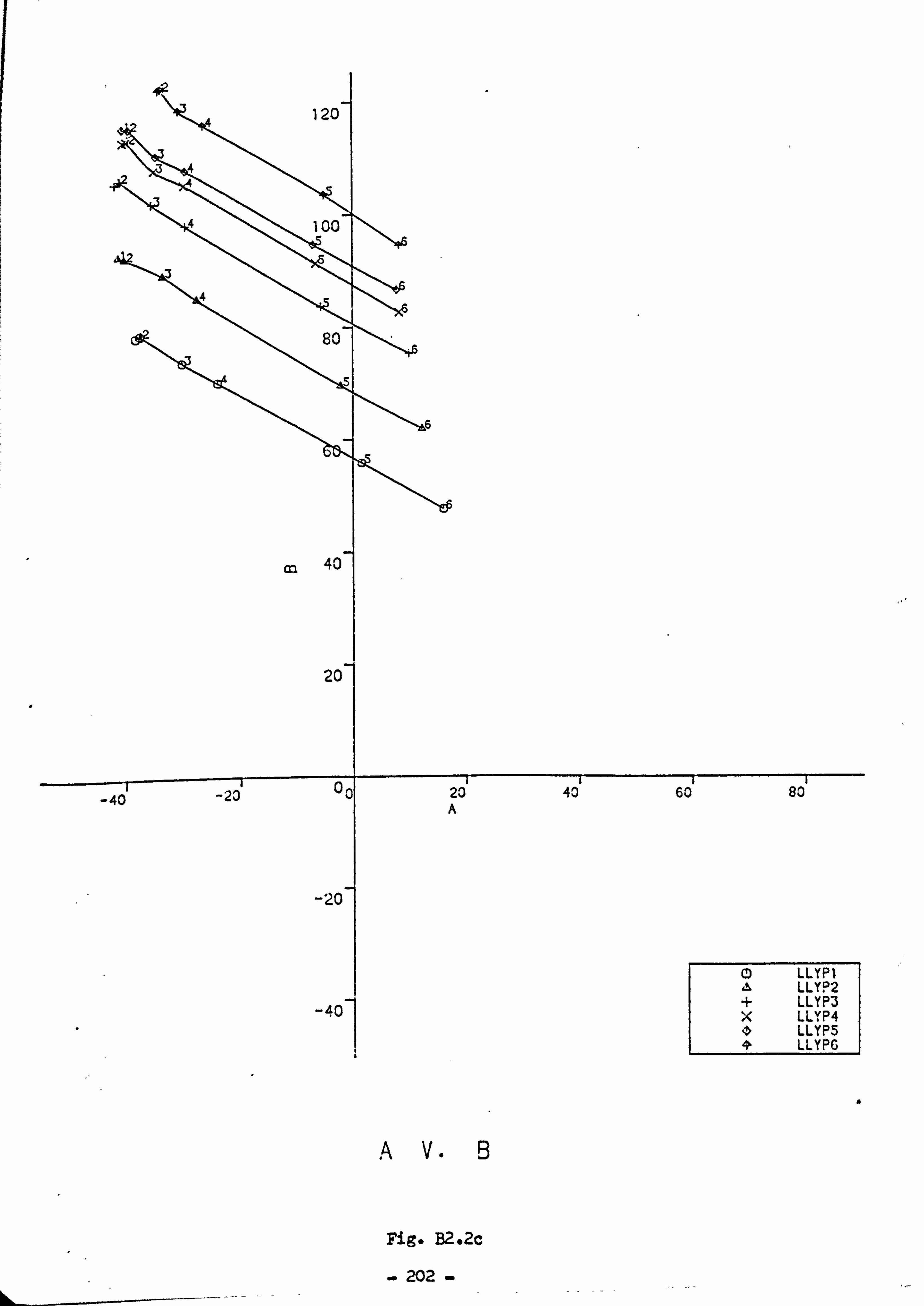
A V. B
Fig. B2*2c
- 202 -
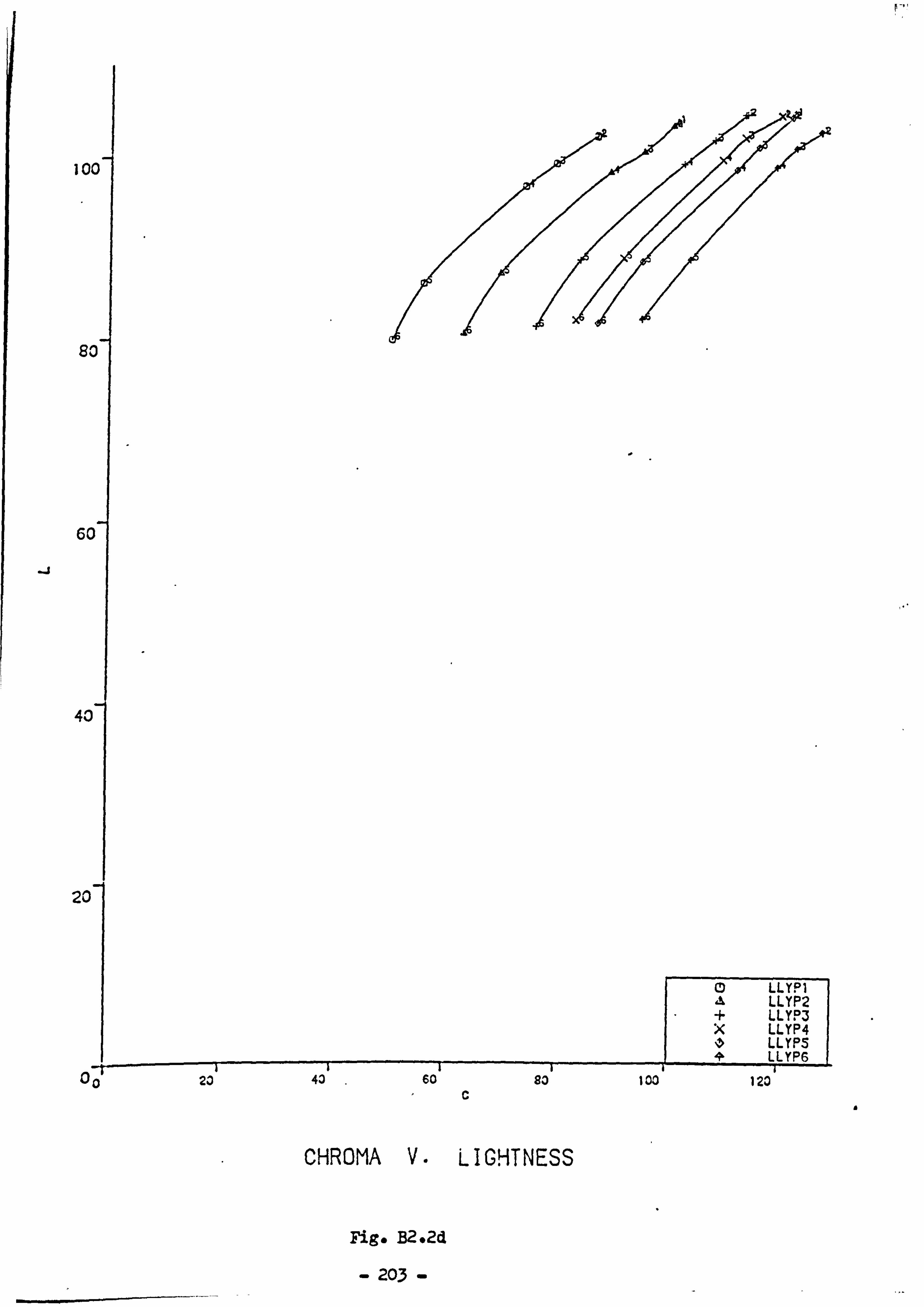
p-
-i
10
S
6C
Al.
20
C
CHROMA V. LIGHTNESS
Fig. B2*2d
- 203 -
00,20- 43 .
60 so 103 120
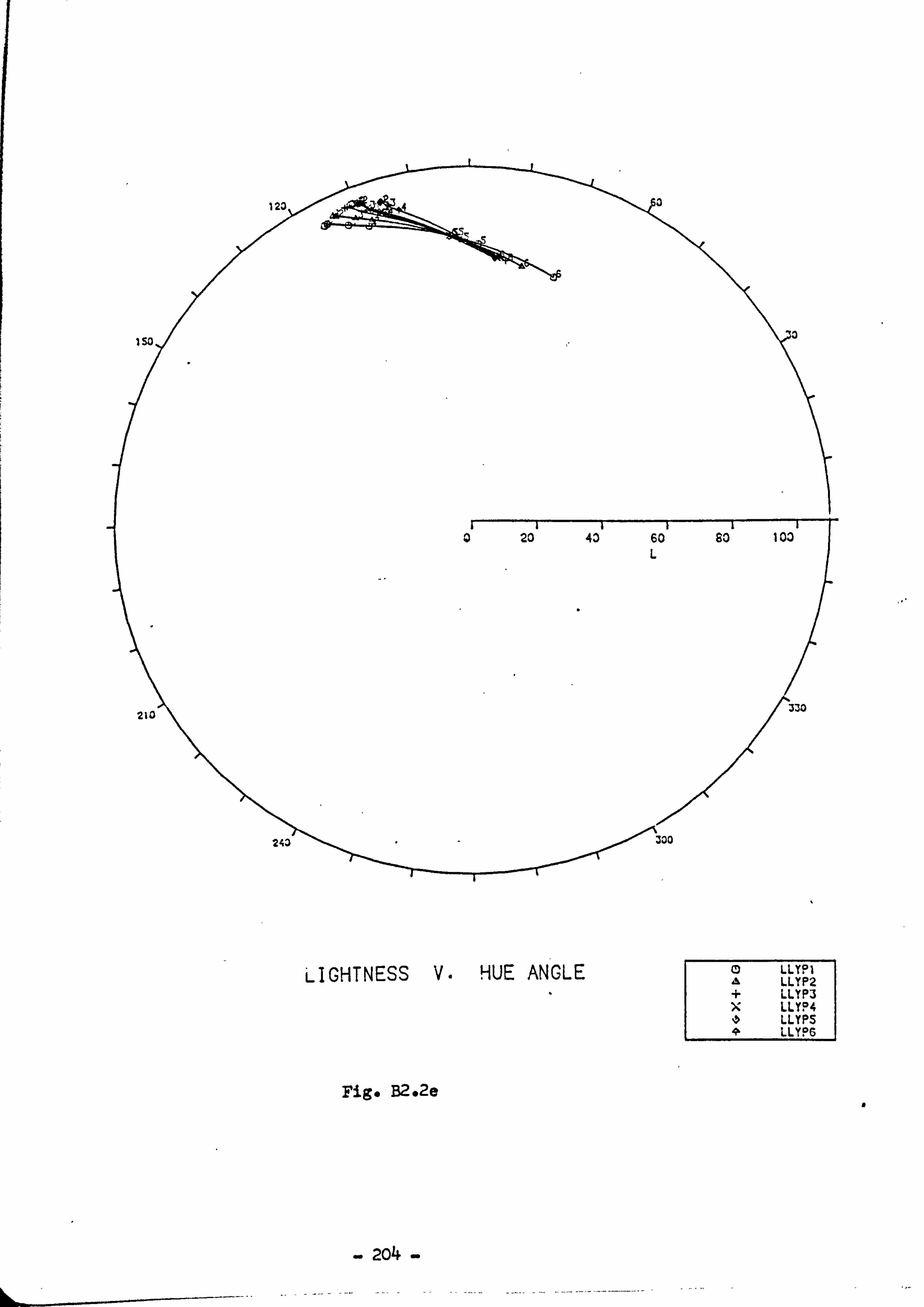
LIGHTNESS V. HUE ANGLE LLYPI LLYP2
+ LLYP3 x LLYP4 0 LLYPS 41 LLYPG
Fig, B2o2e
- 204 -
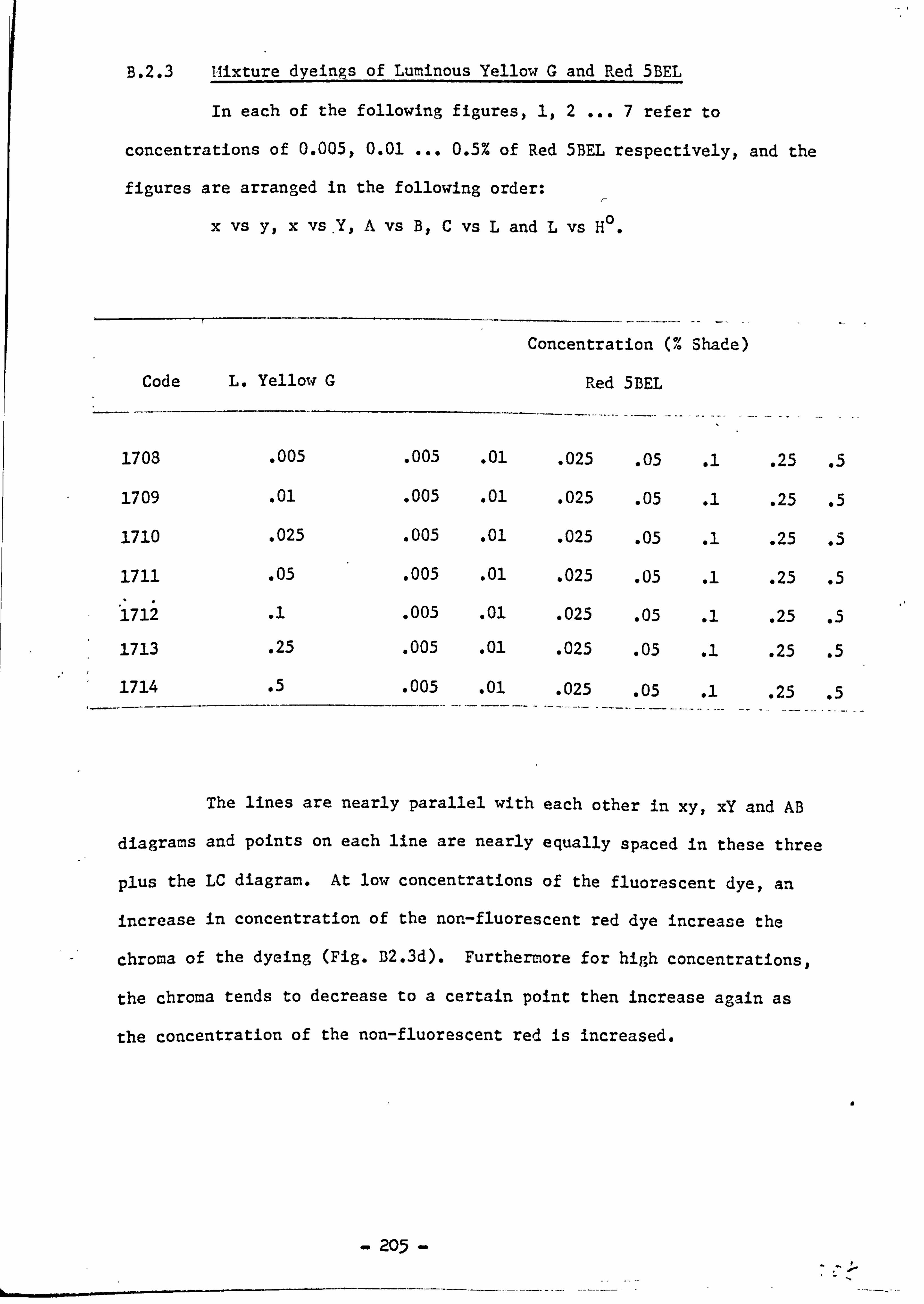
B. 2.3 Mixture dyeings of Luminous Yellow G and Red 5BEL
In each of the following figures, 1,2 ... 7 refer to
concentrations of 0.005,0.01 ... 0.5% of Red 5BEL respectively, and the
figures are arranged in the following order:
0 x vs y, x vs. Y, A vs B, C vs L and L vs H
Code L. Yellow G
1708
1709
1710
1711
1712
1713
1714
. 005
. 01
. 025
. 05
.i
. 25
.5
Concentration Shade)
Red 5BEL
. 005 . 01 . 025 . 05 1 . 25 .5
. 005 . 01 . 025 . 05 1 . 25 .5
. 005 . 01 . 025 . 05 1 . 25 .5
. 005 . 01 . 025 . 05 1 . 25 .5
. 005 . 01 . 025 . 05 1 . 25 .5
. 005 . 01 . 025 . 05 1 . 25 .5
. 005 . 01 . 025 . 05 1 . 25 .5
The lines are nearly parallel with each other in xy, xY and AB
diagrams and points on each line are nearly equally spaced in these three
plus the LC diagram. At low concentrations of the fluorescent dye, an
increase in concentration of the non-fluorescent red dye increase the
chroma of the dyeing (Fig. B2.3d). Furthermore for high concentrations,
the chroma tends to decrease to a certain point then increase again as
the concentration of the non-fluorescent red is increased.
a
- 20.5 - -
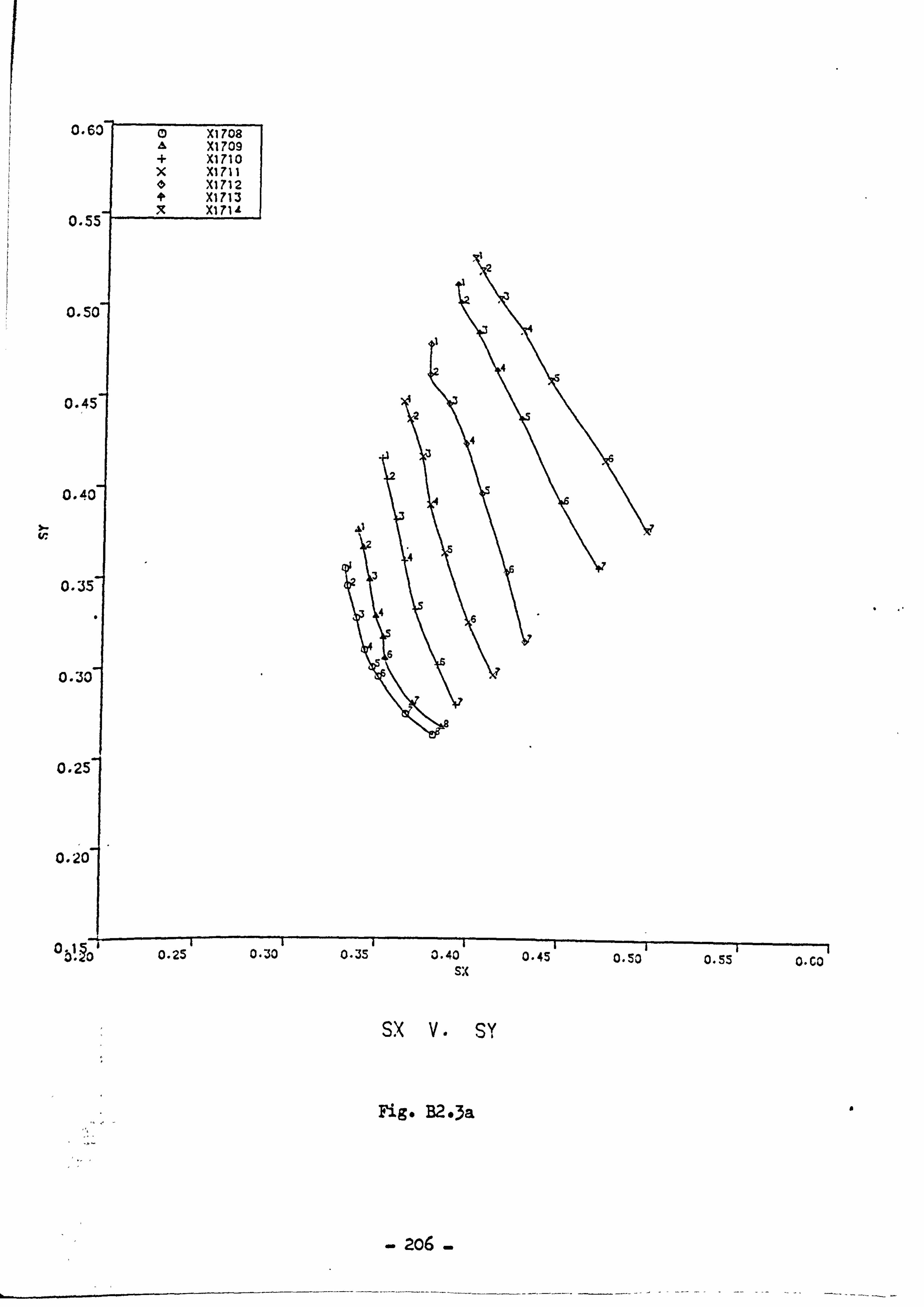
0.
0. ý
0.4
0.4
cr
0.31
0.
0 . 2!
0-2C
0 b! 1.0
Fig- B? --3a a
206
V-ýv U-4.3 0.50 0.55 O-CO SIX
sx V. s Y.
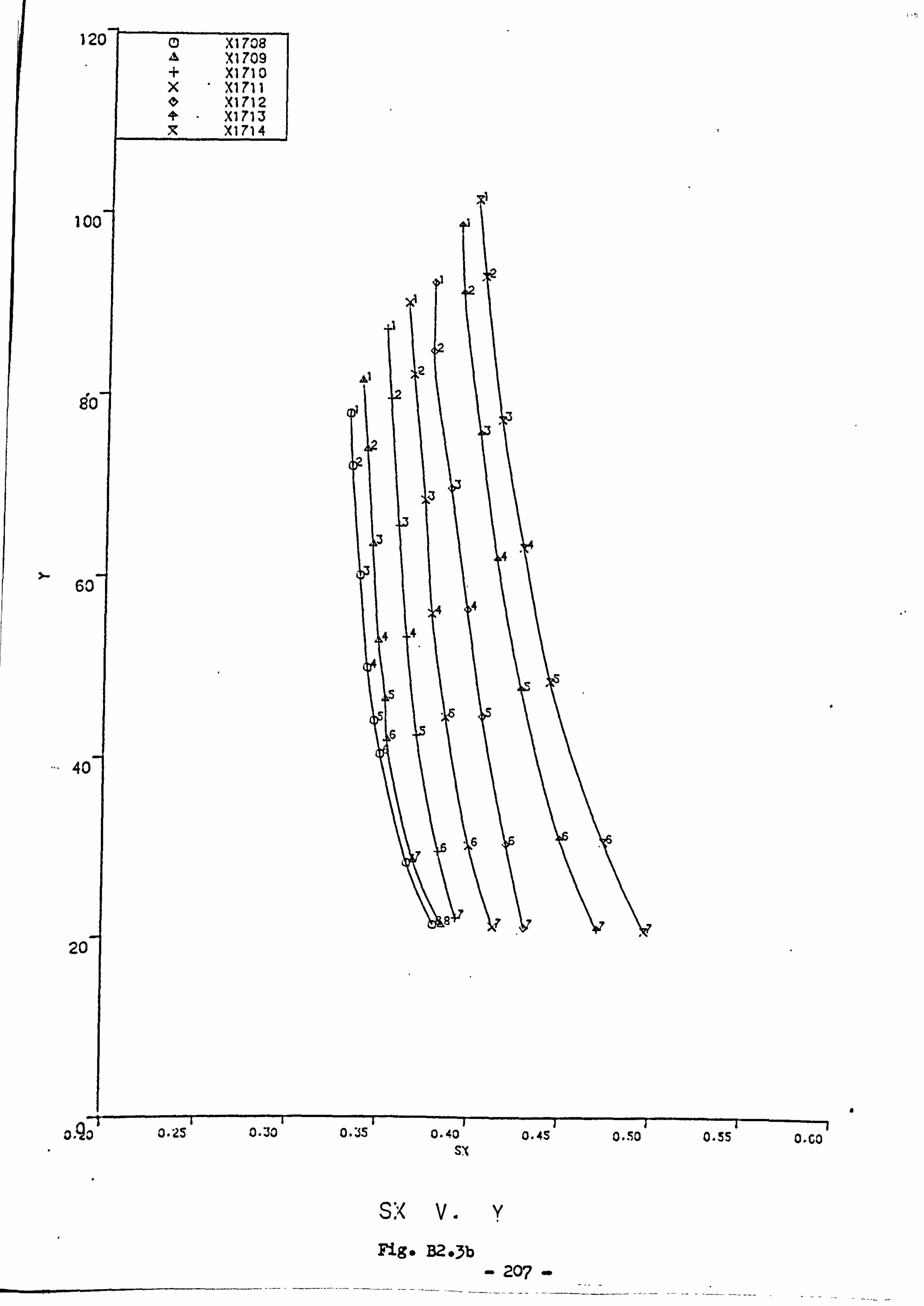
120 (D X1 708 X 1709
+ X1 710 X XI 711 0 X1 712 + XI 713 x XI 714
100
90
60
- 40
20
0.35 0.40 0-4S 0.50 0.55 O-co S, (
SX V. y
Fig- B2-3b 207
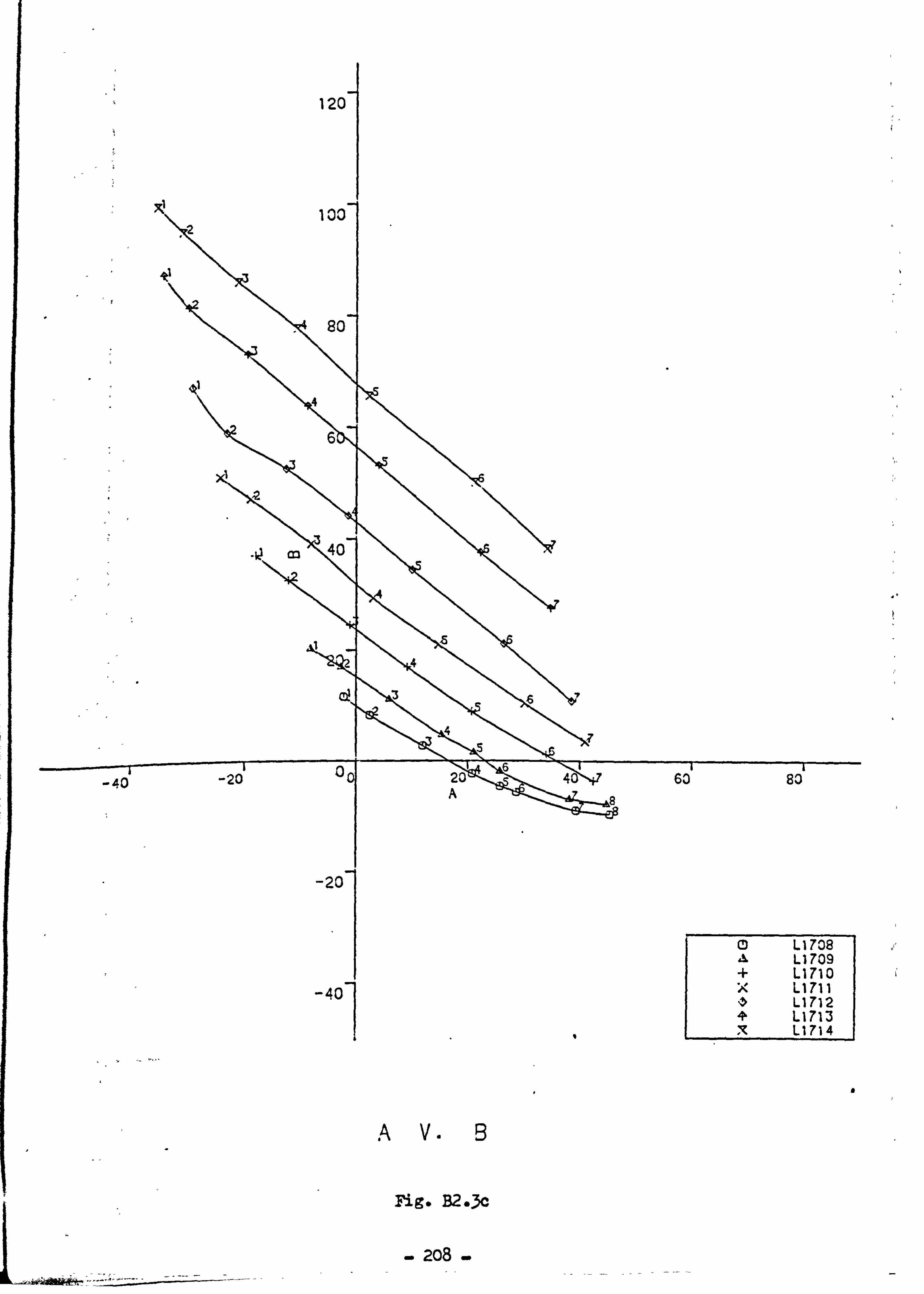
a
A V. B
Fig. B2.3c
208
-40 x L1711 Ll 712 L 1713 Ll 714
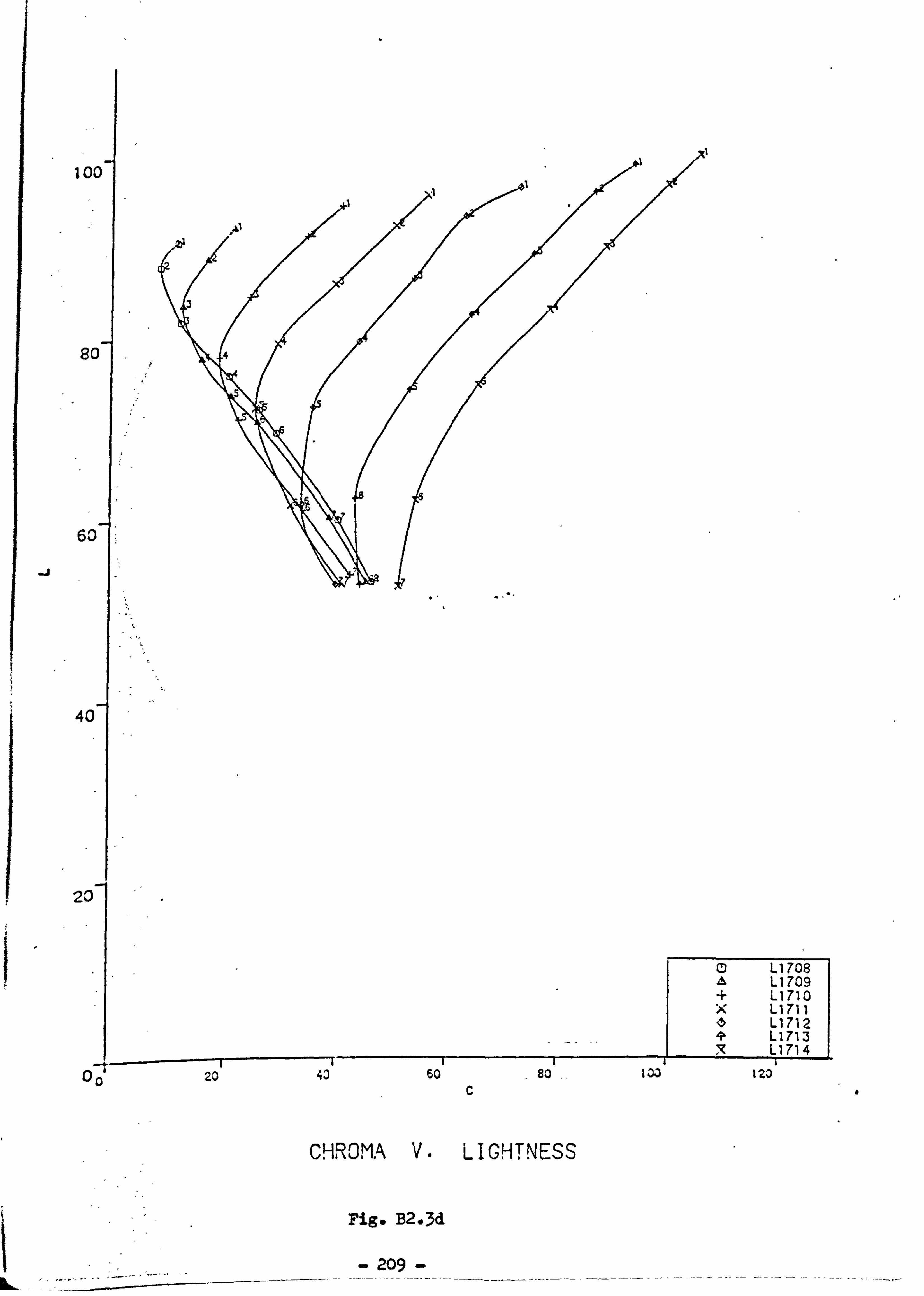
10
81
v.
-j
4C
20
a
CHROMA V. LIGHTNESS
Fig, B2-3d
209
00.20 40 50 - 80 .-I 0i 12D
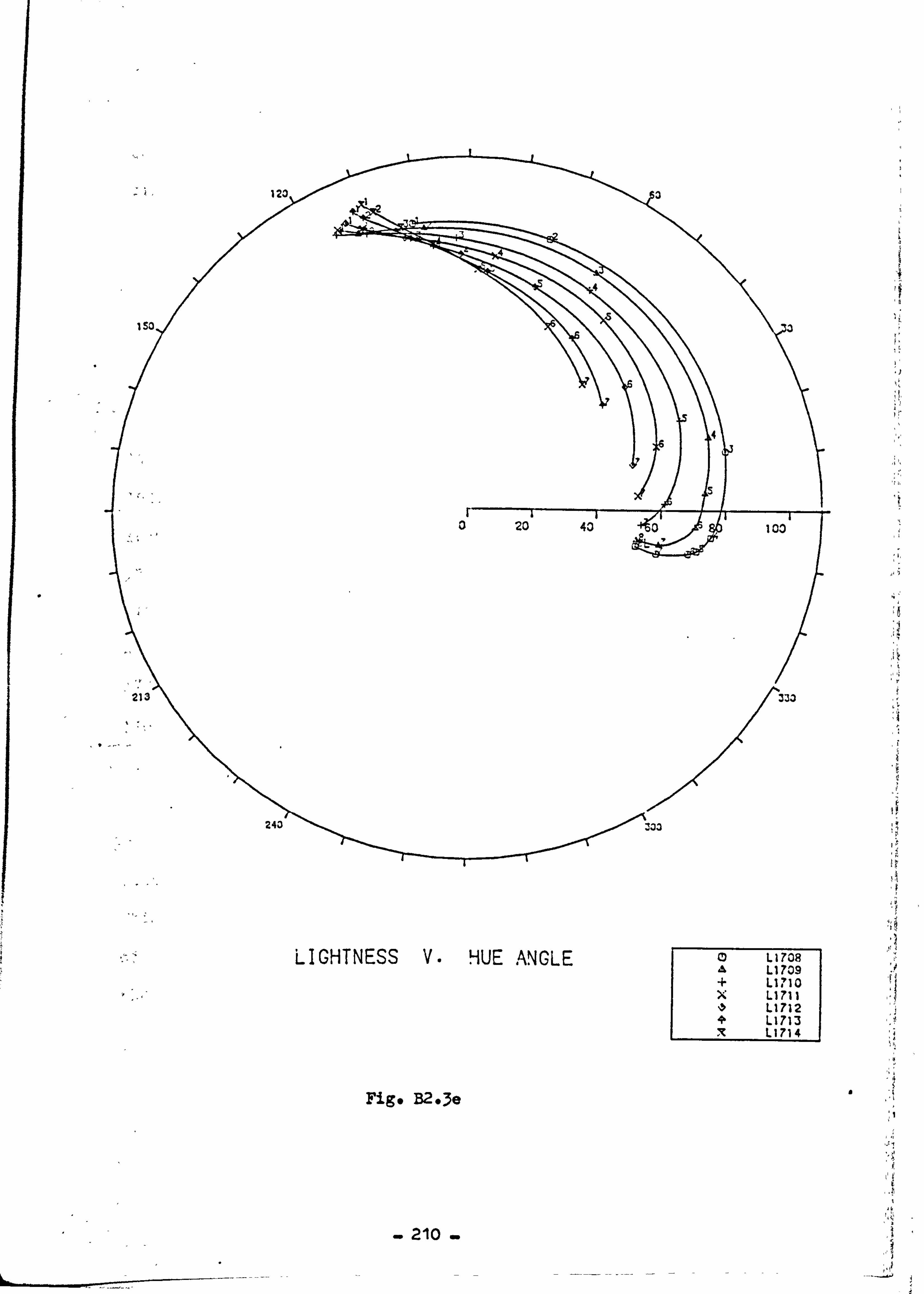
I
213
I
243
LIGHTNESS V. HUE ANGLE
Fig* B20e
: 03
*L 1708 * Ll 709 * L1710 x Ll 711 ,. ýo L1712 + L1713
L 1714
-210
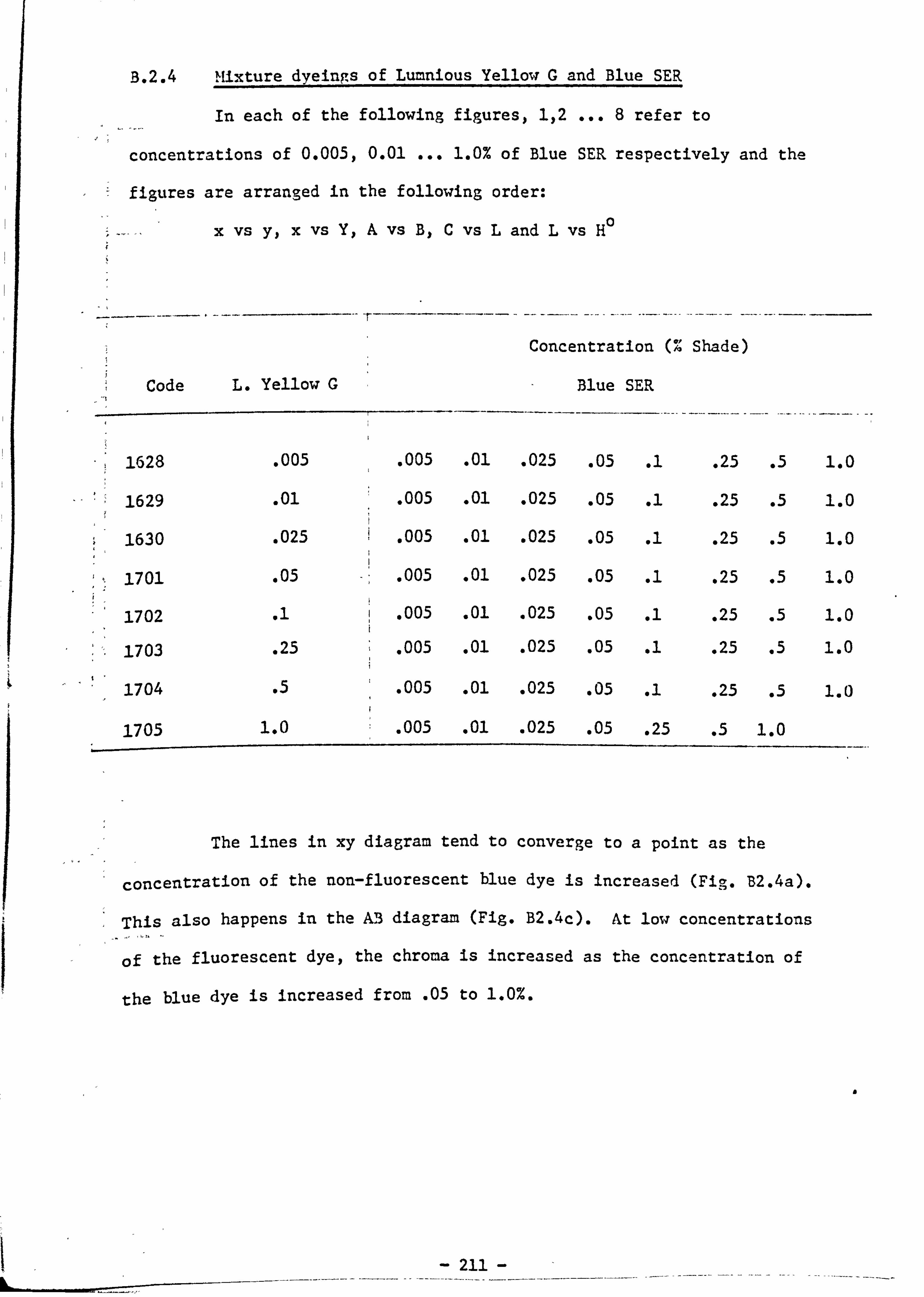
B. 2.4 Mixture dveings of Lumnious Yellow G and Blue SER
In each of the following figures, 1,2 ... 8 refer to
concentrations of 0.005,0.01 ... 1.0% of Blue SER respectively and the
figures are arranged in the following order:
0 x vs y, x vs Y, A vs B, C vs L and L vs H
Concentration C%' Shade)
Code L. Yellow G Blue SER
.ý 1628 . 005 . 005 . 01 . 025 . 05 1 . 25 .5 1.0
1629 . 01 . 005 . 01 . 025 . 05 1 . 25 .5 1.0
1630 . 025 ý . 005 . 01 . 025 . 05 1 . 25 .5 1.0
,t 1701 . 05 ý;, 005 . 01 . 025 . 05 1 . 25 .5 1.0
1702 1 ý . 005 . 01 . 025 . 05 1 . 25 .5 1.0
1703 . 25 . 005 . 01 . 025 . 05 1 . 25 .5 1.0
1704 .5 . 005 . 01 . 025 . 05 1 . 25 .5 1.0
1705 1.0 . 005 . 01 . 025 . 05 . 25 .5 1.0
The lines in xy diagram tend to converge to a point as the
concentration of the non-fluorescent blue dye is increased (Fig. B2.4a).
so happens in the AB diagram (Fig. B2.4c). At low concentrations This al
of the fluorescent dye, the chroma is increased as the concentration of
the blue dye is increased from . 05 to 1.0%.
a
211
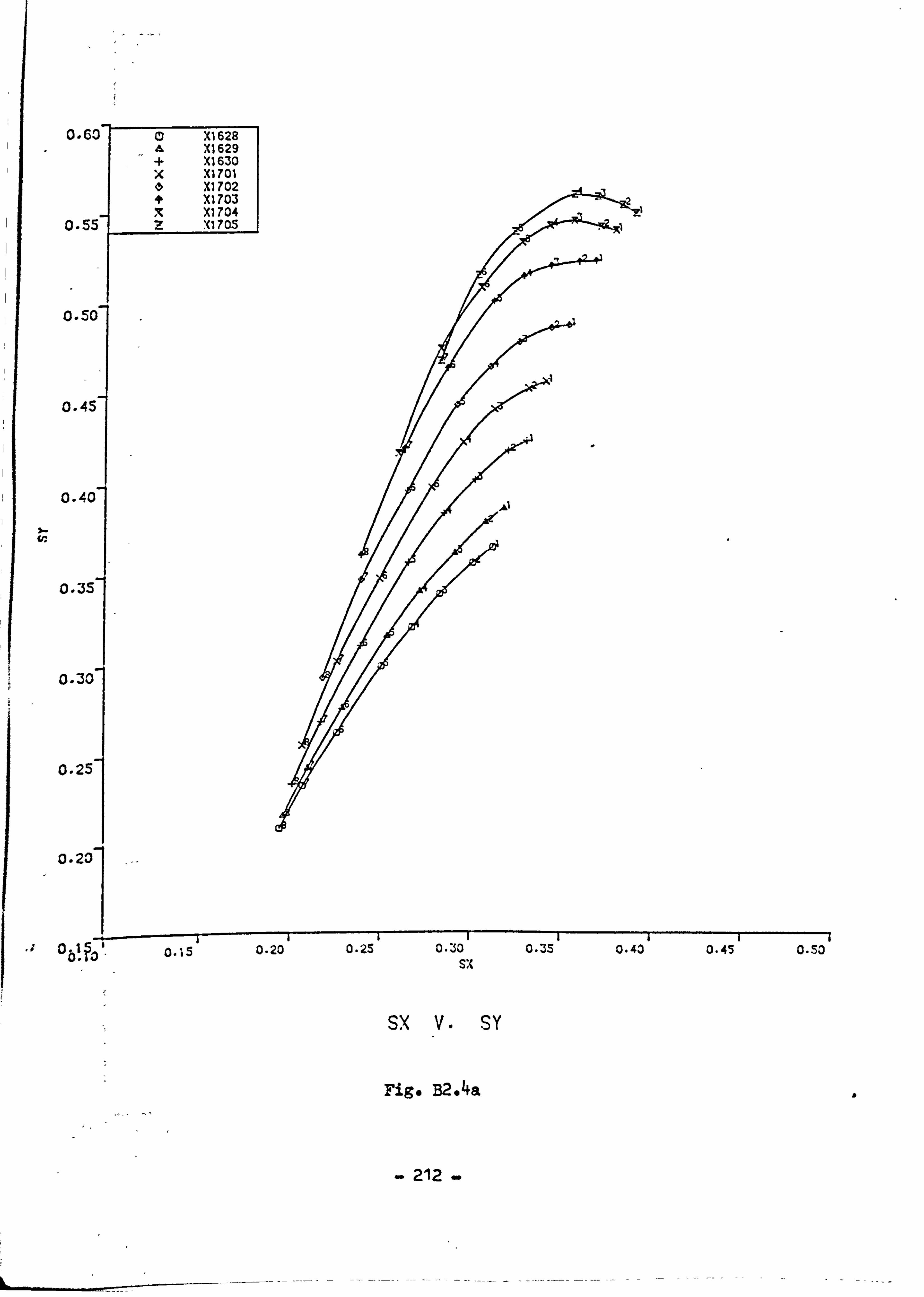
0.60 0 X1 628 A XI 629 + XI 630 x X1 701 * XI 702 * X1 703
XI 704 X 0.55 z XI 705
0.50
0.45
0.40
0-: 35
0.30
0.25
0.20
0 0.20 0.2s 0.30 0.35 0.43 0-4S 0.50
sx V. SY
Fig* B2.4a a
- 212 -
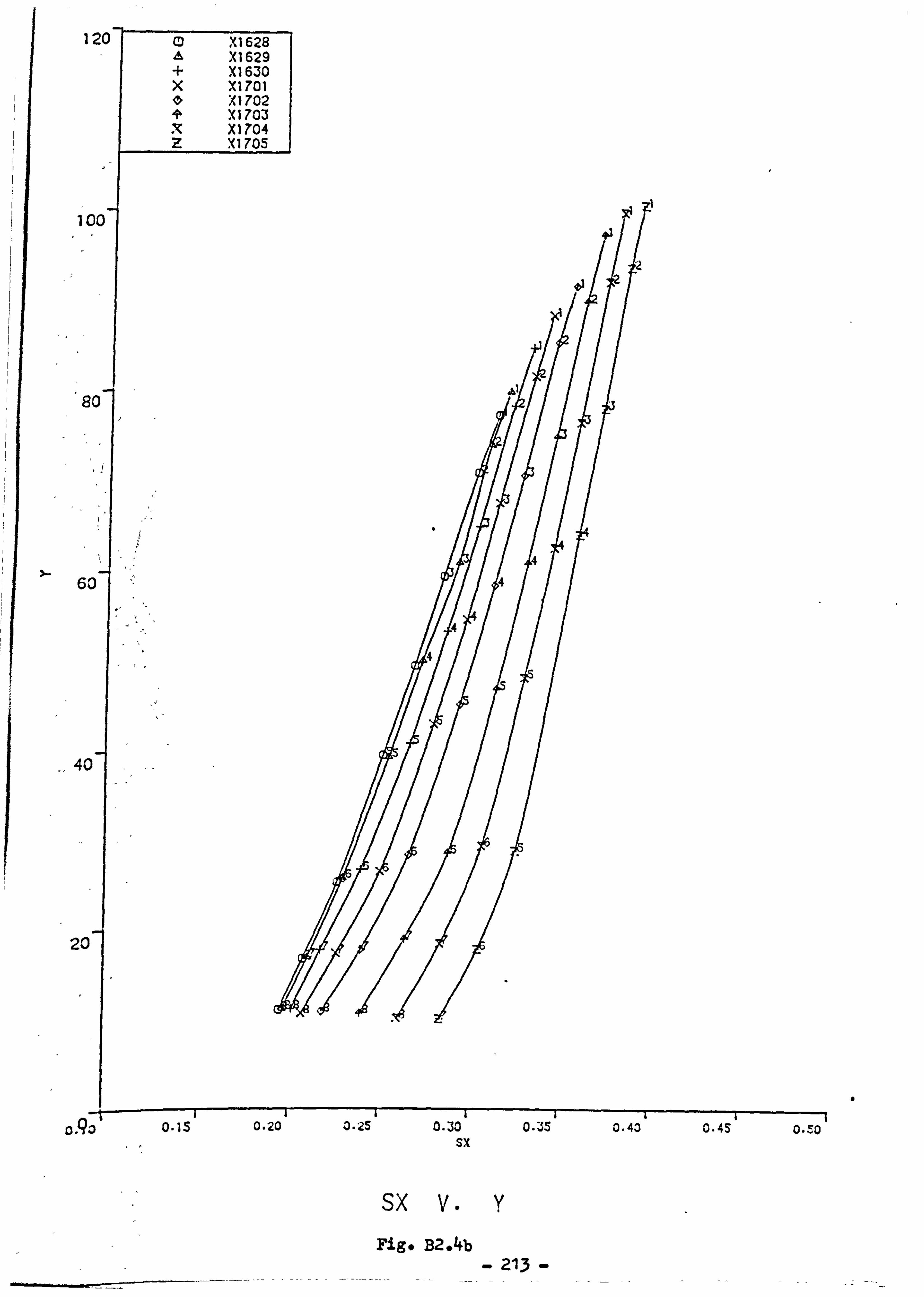
120 CD X1 628 A X1 629 + X1630 x XI 701 0 X1702 + X1703
Xl 704 z XI 705
100
so I
60
40
20
ORO 0.15 0.20 0.25 0.30 0.3s 0.43 0.45 0.50 sx
sx V. y
Figo B2.4b 213
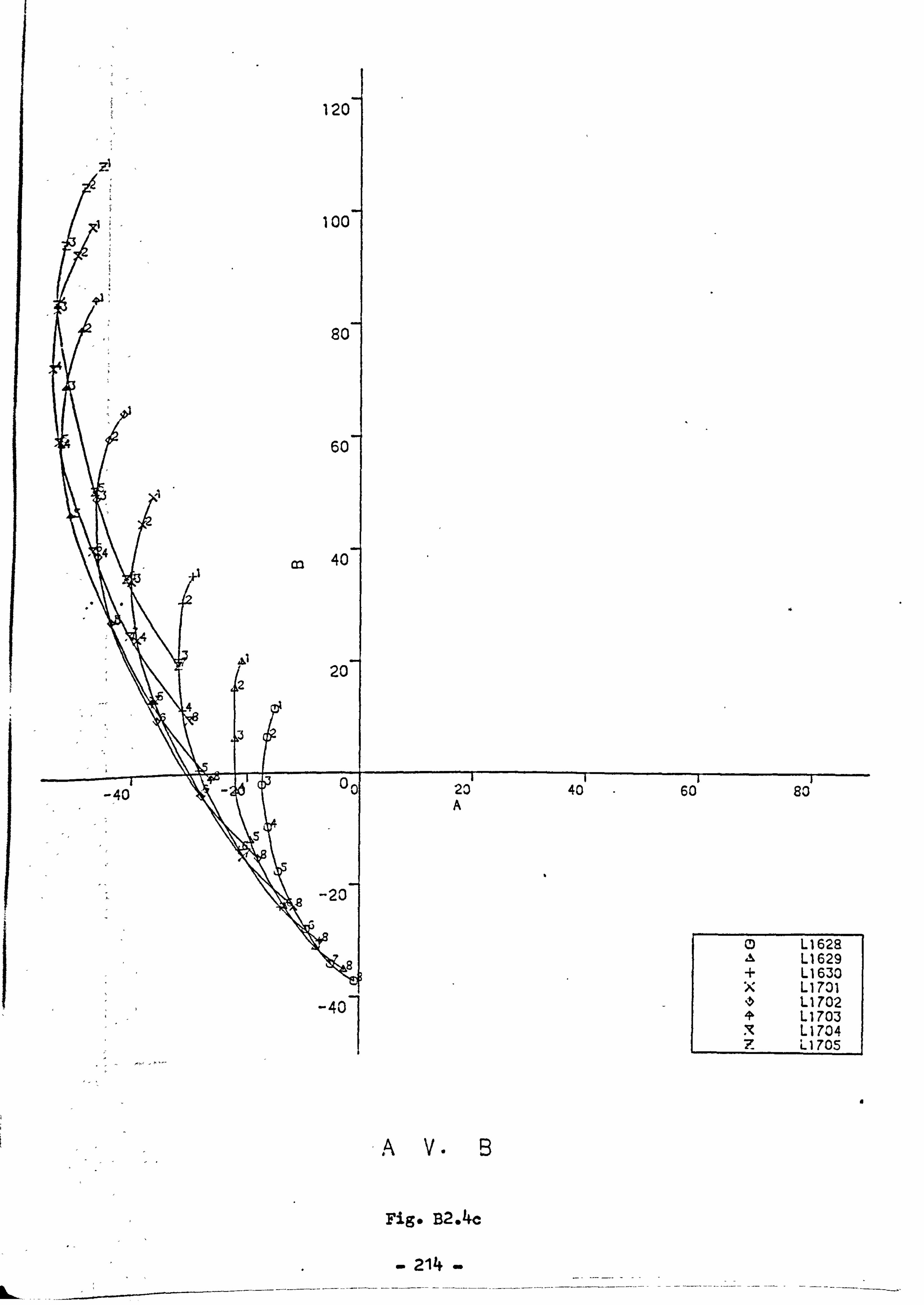
L-
A V. B
Fig* B2.4c
- 214 -
a
-40 1-1702 L1703 L 1704
IzL
1705
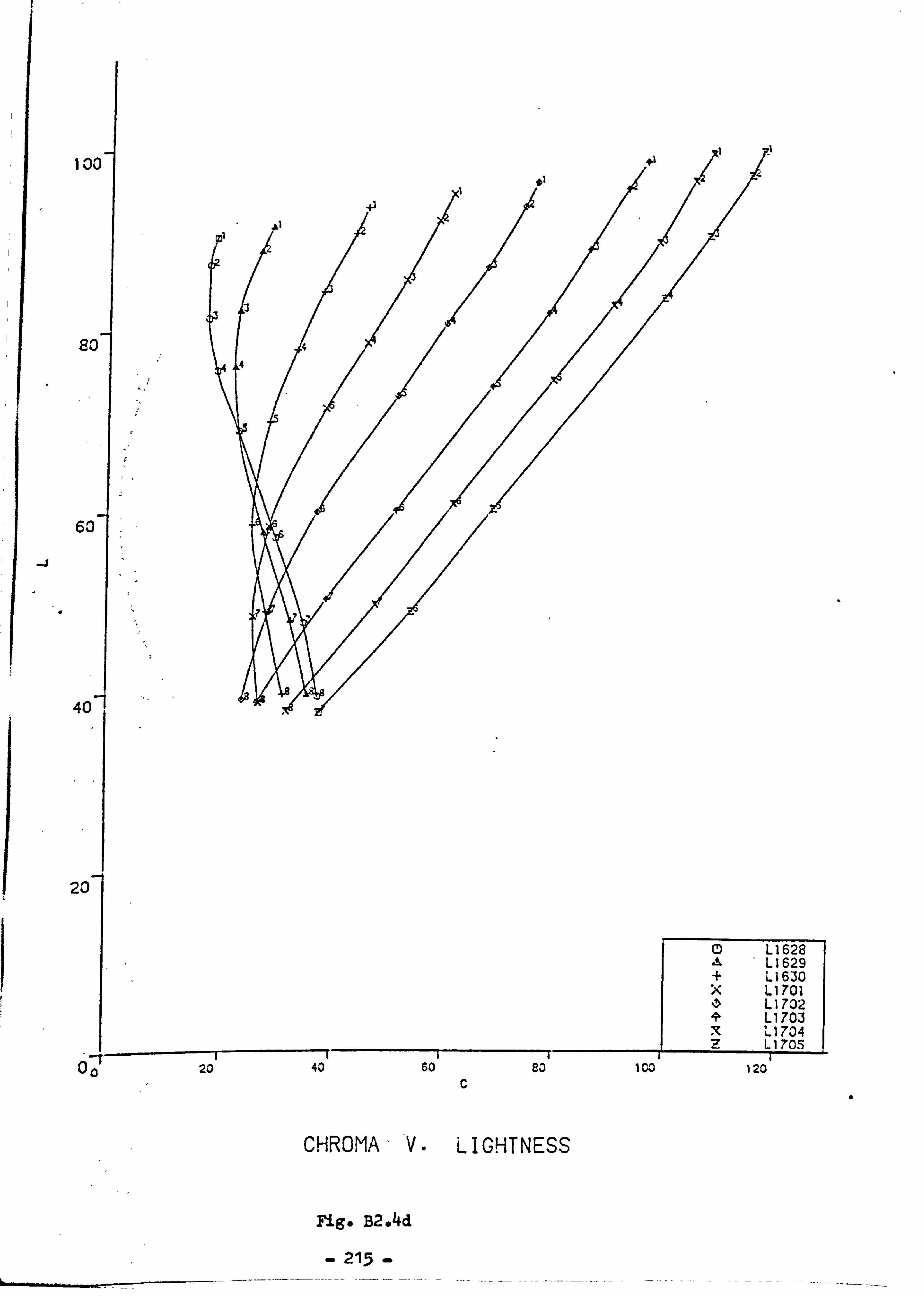
100
-J
so
60
40ý
20
00 20 43 60 83 c
CD L1628 A L1629 + L1630 *L 1701 *L 1702 * L1703
Ll 704 7L 1705
I co 120
a
CHROMAý V. LIGHTNESS
Fig* B2.4d
215
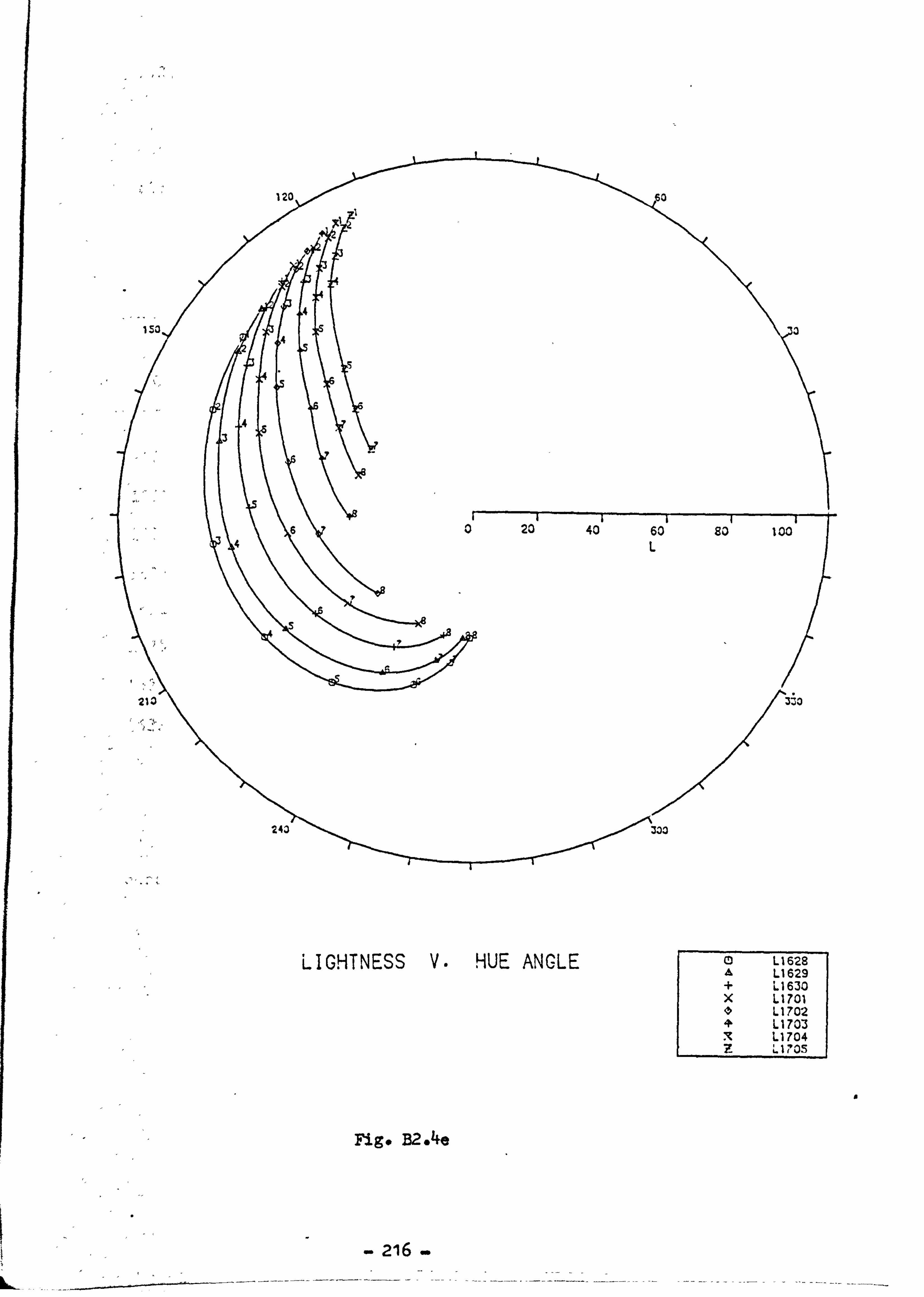
120
153
210
20 40 60 so 100 L
, 3io
243
LIGHTNESS V. HUE ANGLE 0 L1628 A Ll 629 + L 1630 x L 1701 * L 1702 * L 1703 * L1704 7- L 1705
a
Fig* B2, Ae
216 -
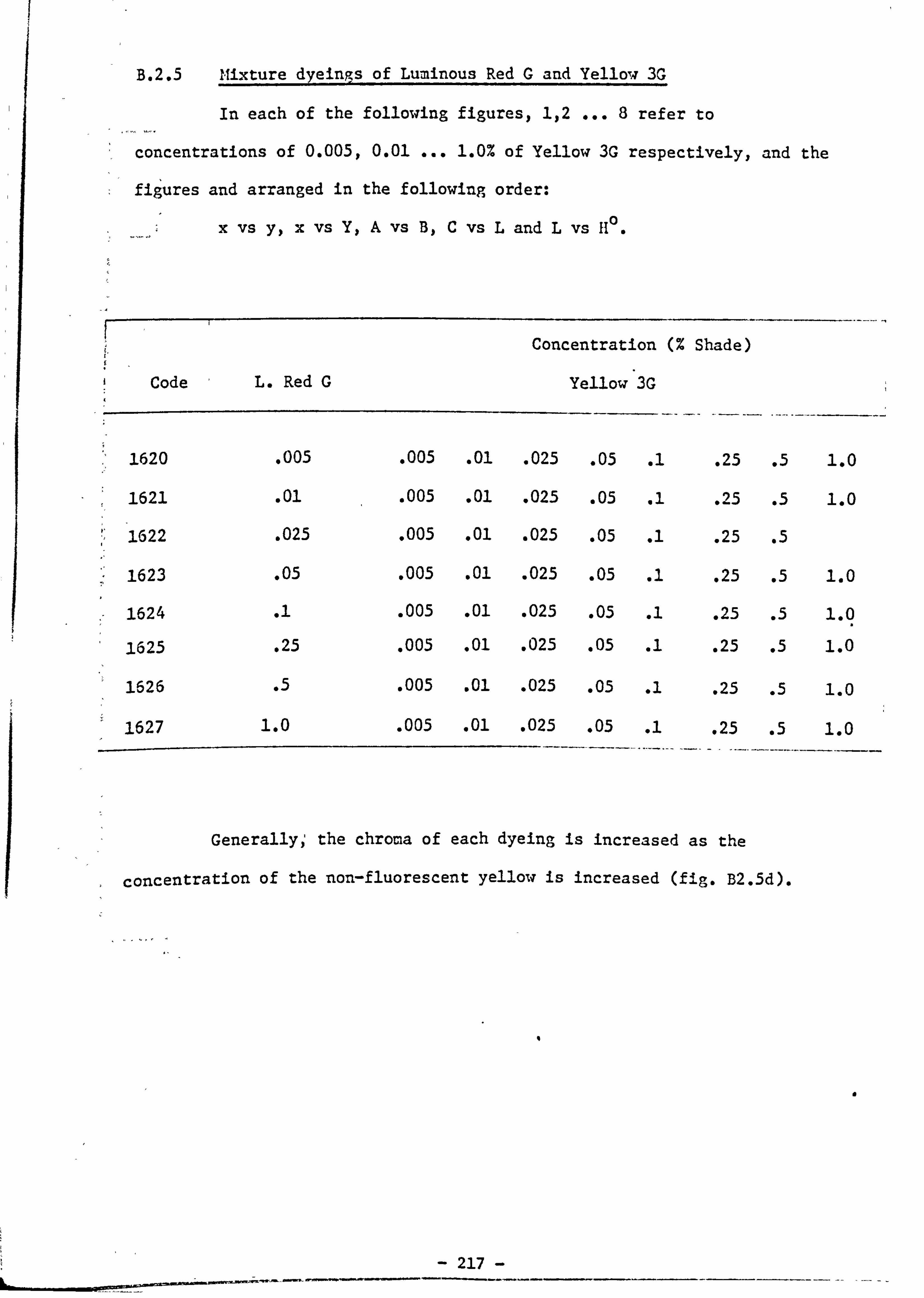
B. 2.5 Mixture dyeings Of Luminous Red G and YelloT,; 3G
In each of the following figures, 1,2 ... 8 refer to
concentrations of 0.005,0.01 ... 1.0% of Yellow 3G respectively, and the
figures and arranged in the following order:
0 x vs y, x vs Y, A vs B, C vs L and L vs 11
Concentration (% Shade)
Code L. Red G Yellow'3G
1620 . 005 . 005 . 01 . 025 . 05 .1 . 25 .5 1.0
1621 . 01 . 005 . 01 . 025 . 05 .1 . 25 .5 1.0
1622 . 025 . 005 . 01 . 025 . 05 .1 . 25 .5
1623 . 05 . 005 . 01 . 025 . 05 .1 . 25 .5 1.0
1624 .1 . 005 . 01 . 025 . 05 .1 . 25 .5 1.0
1625 . 25 . 005 . 01 . 025 . 05 .1 . 25 .5 1.0
1626 .5 . 005 . 01 . 025 . 05 .1 . 25 .5 1.0
1627 1.0 . 005 . 01 . 025 . 05 .1 . 25 .5 1.0
Generally; the chroma of each dyeing is increased as the
concentration of the non-fluorescent yellow is increased (fig. B2.5d).
I
a
217
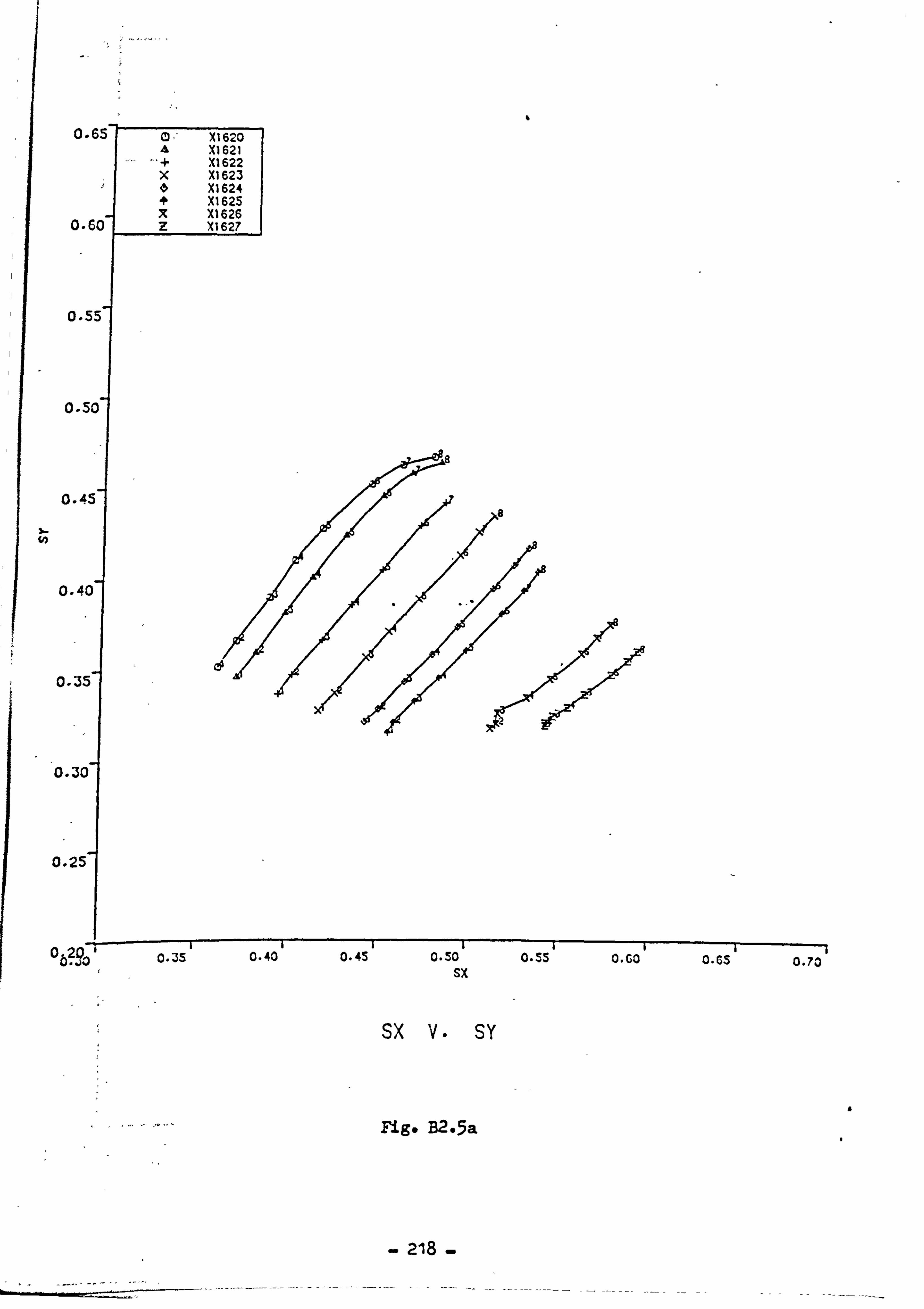
C
U
C',
0
0
0.
0.
o2g3' 0. ib U. 4u u. 43 U--ZU 0--33 0.60 0.65 0.73 sx
sx V. SY
Fig. B2.5a
218
a
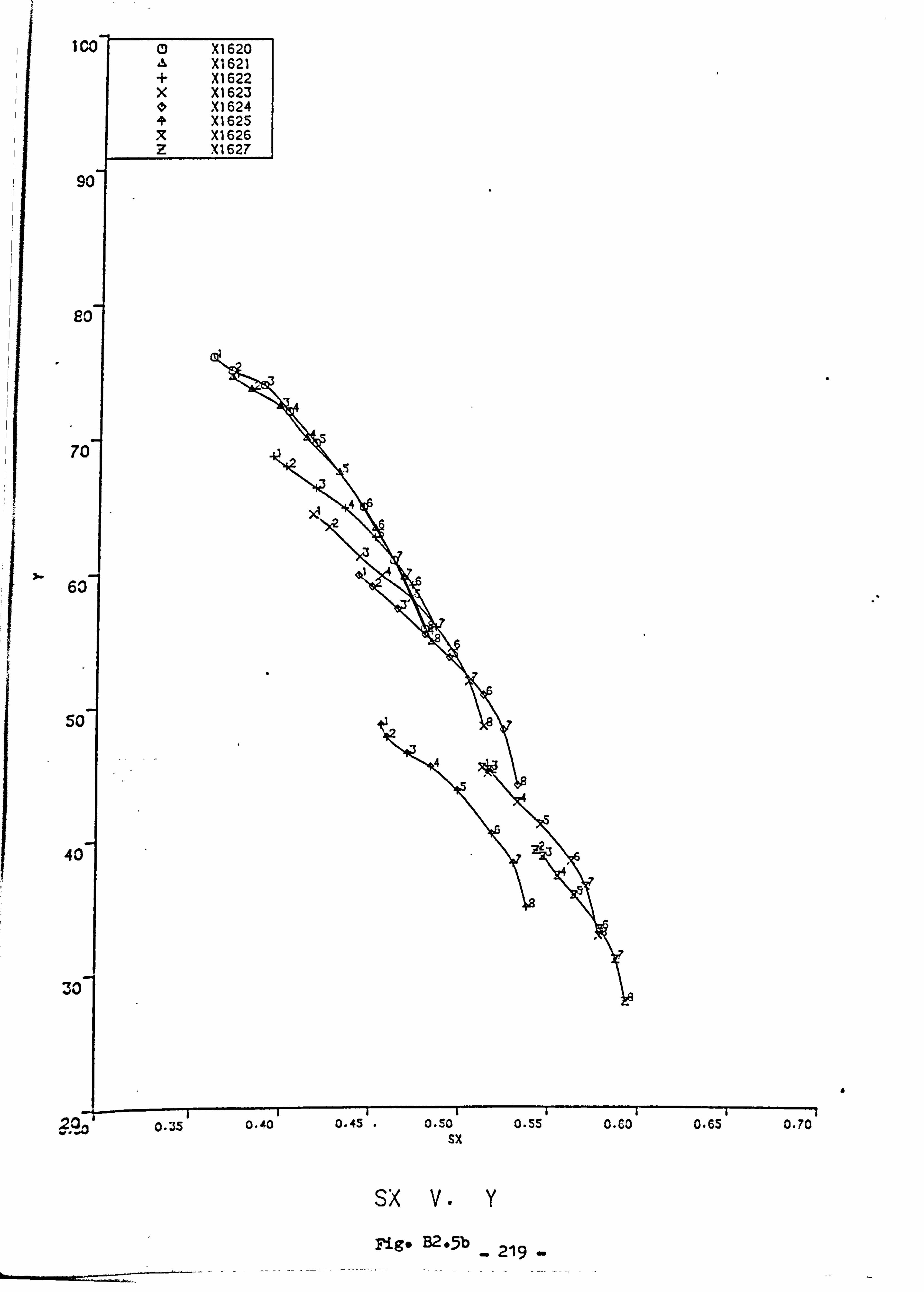
11
C
a
Ti
a-
5c
40
30
a
ago 0.35 0.40 tj., )u U-ZQ U-W U-t). 9 U-fu sx
sx V. y
Fig* B2*5b - 219

A V. B
Fig. B2-5c 220
L1624 -40 L1625
'It L1626 z L1627
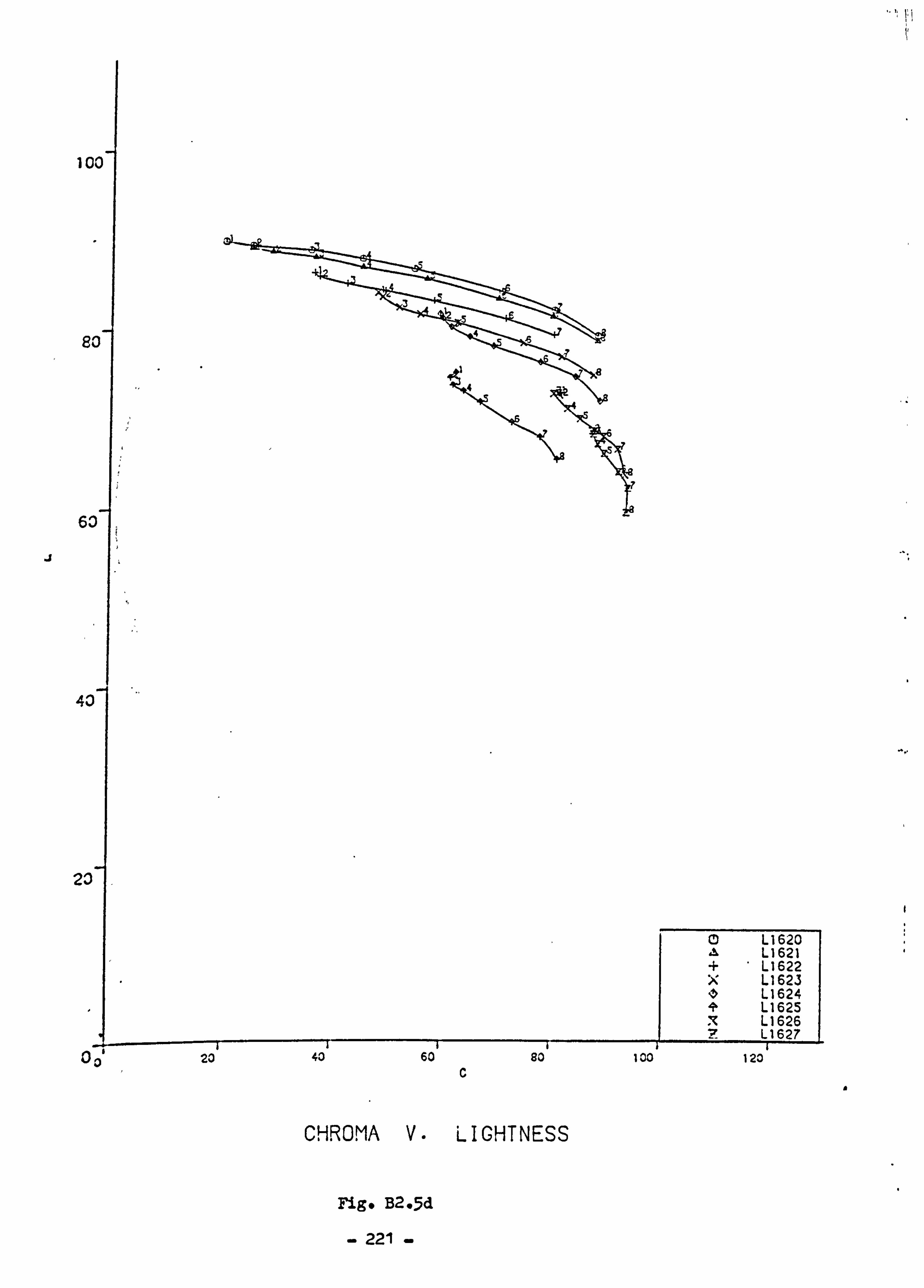
i
I
8
6
4-C.
20
a
CHROMA V. LIGHTNESS
Fig* B2.5d
- 221 -
40 60 so 100 120 c
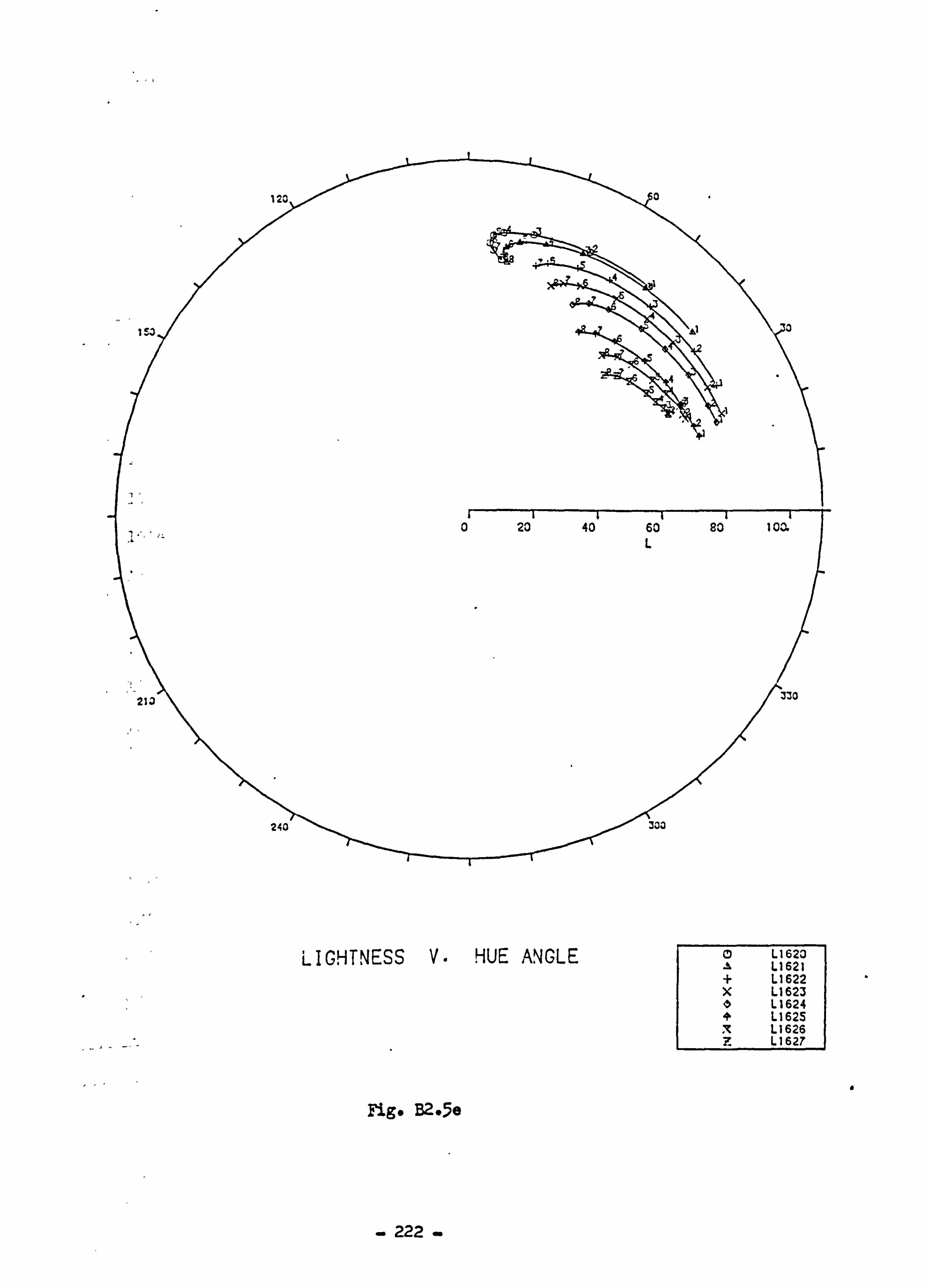
LIGHTNESS V. HUE ANGLE
Fige B2.5a
CD L1620 A L1621 + L1622 x Ll 623 0 L1624 + L162S x L1626 z L1627
- 222 -
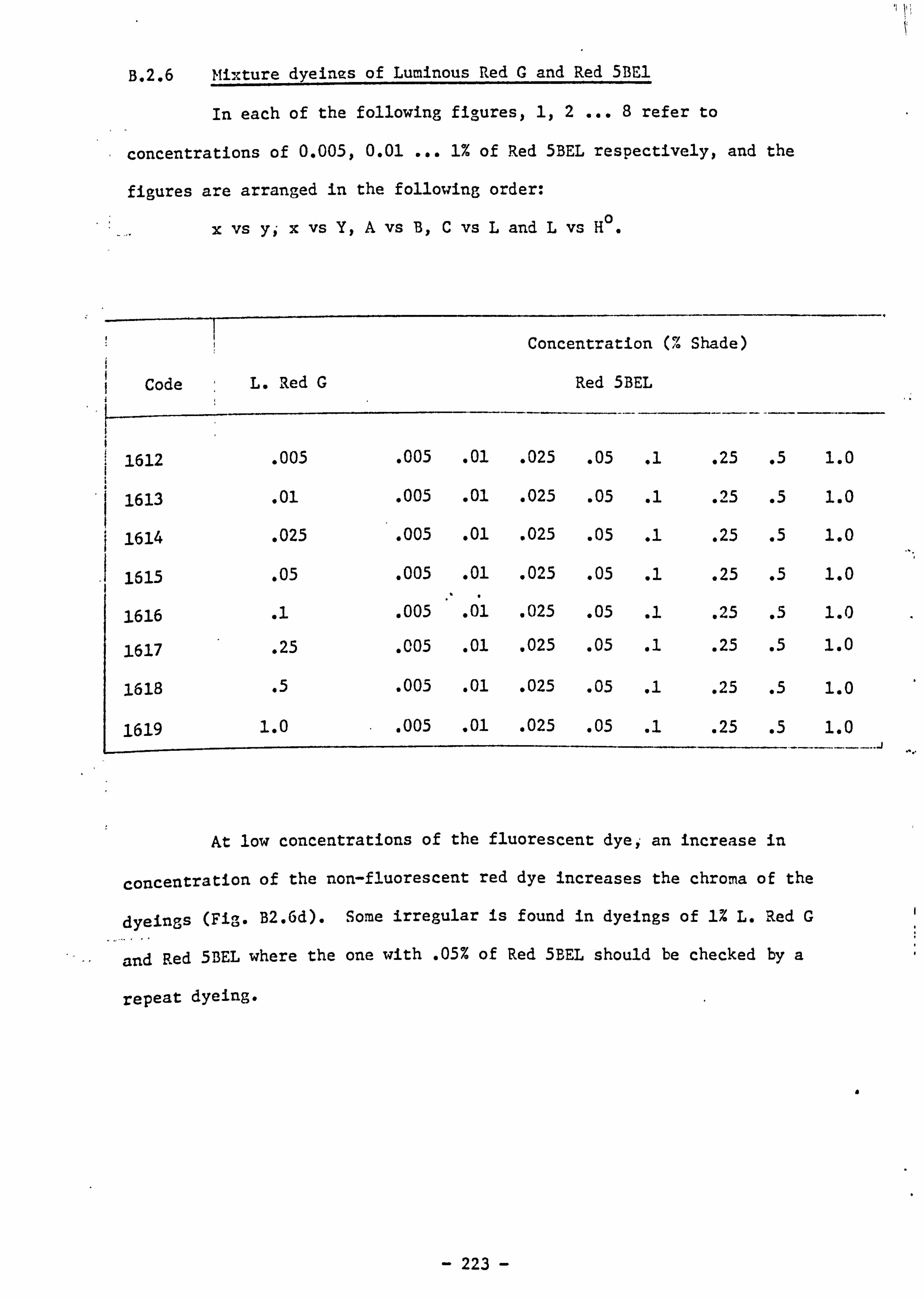
B. 2.6 mixture dyeines of Luminous Red G and Red 5BE1
In each of the following figures, 1,2 ... 8 refer to
concentrations of 0.005,0.01 ... 1% of Red 5BEL respectively, and the
figures are arranged in the following order:
0 x vs y, - x vs Y, A vs B, C vs L and L vs H
Code L. Red G
Concentration 010
Red 5BEL
Shade)
1612 . 005 . 005 . 01 . 025 . 05 .1 . 25 .5 1.0
1 1613 . 01 . 005 . 01 . 025 . 05 .1 . 25 .5 1.0
1 1614 . 025 . 005 . 01 . 025 . 05 .1 . 25 .5 1.0
1615 . 05 . 005 . 01 . 025 . 05 .1 . 25 .5 1.0
1616 .1 . 005 . 01 . 025 . 05 .1 . 25 .5 1.0
1617 . 25 . 005 . 01 . 025 . 05 .1 . 25 .5 1.0
1618 .5 . 005 . 01 . 025 . 05 .1 . 25 .5 1.0
1619 1.0 . 005 . 01 . 025 . 05 .1 . 25 .5 1.0
At low concentrations of the fluorescent dyej an increase in
concentration of the non-fluorescent red dye increases the chroma of the
dyeings (Fig. B2.6d). Some irregular is found in dyeings of 1% L. Red G
and Red SBEL where the one with . 05% of Red 5BEL should be checked by a
repeat dyeing.
a
- 223 -
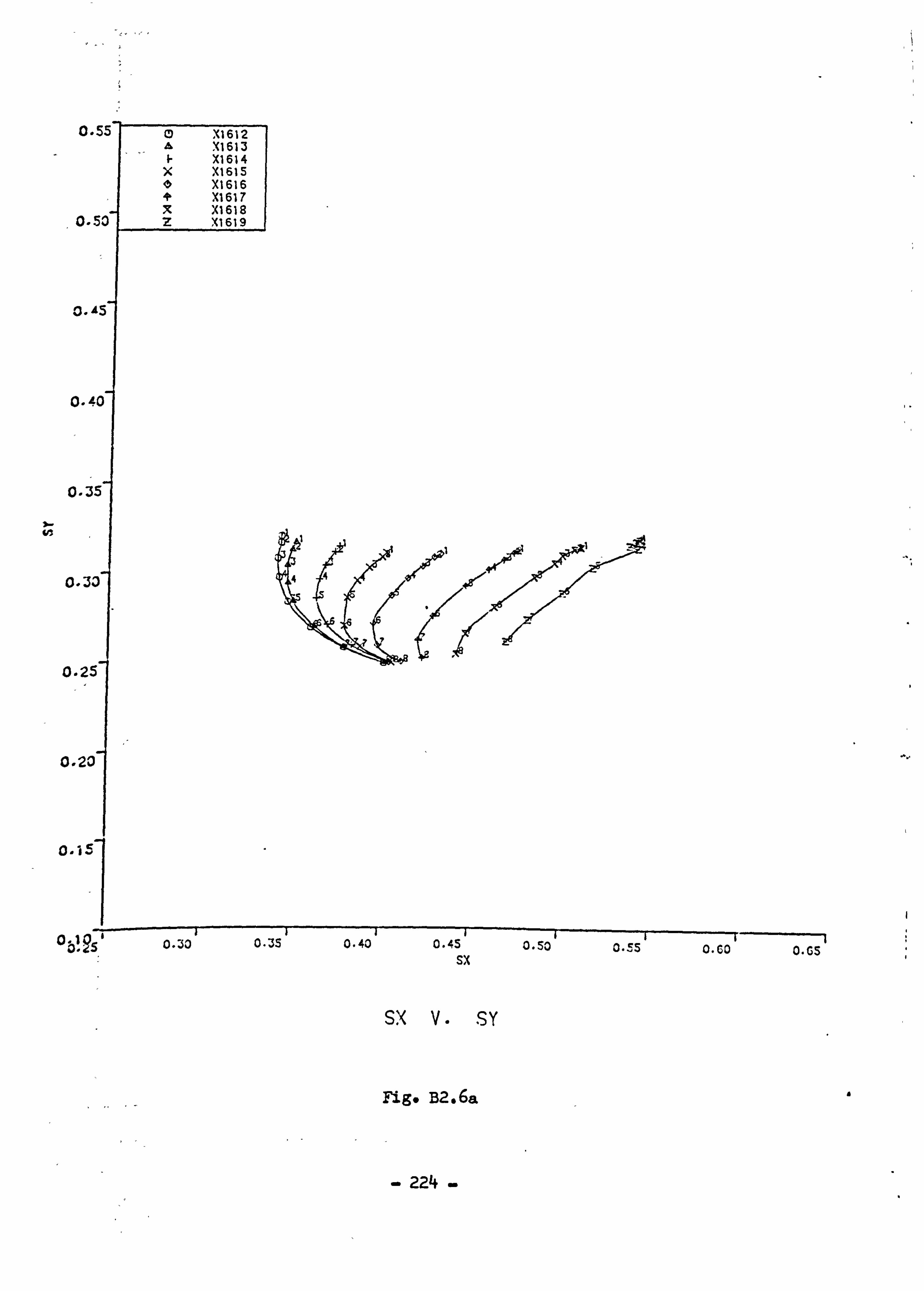
X1 612 XI 613 XI 614
x X1615 0 X1 616 + X1617 7. XI 618 z XI 619
(). AS
0.40
o. 35
0.33
0.2
0.20
0.1
0.3s 0.40 0.4S 0.50 0. co O-Gs sx
sx v SY
Fig* B2.6a
- 224 -

I-
.
0.95 V. Jo V- -tv U- C) U-W
sx
sx V. y Fig* B2.6b
_ 225 -
0.65
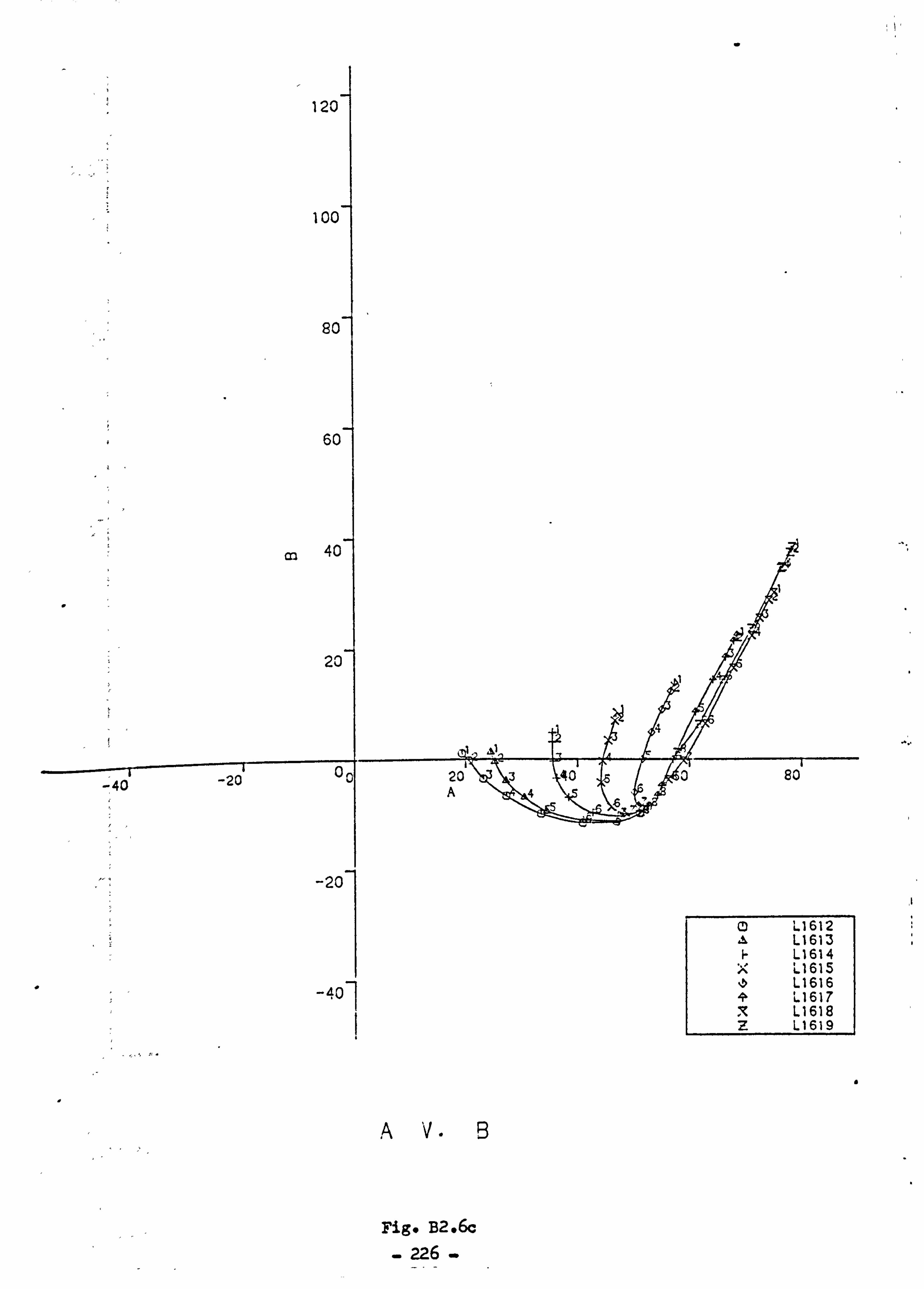
-20
-40
CD Ll 612 L1613 L1614
x L1615 L1616 L1617
X, L 1618 z L1619
a
A V. B
Fige B2*6c 226
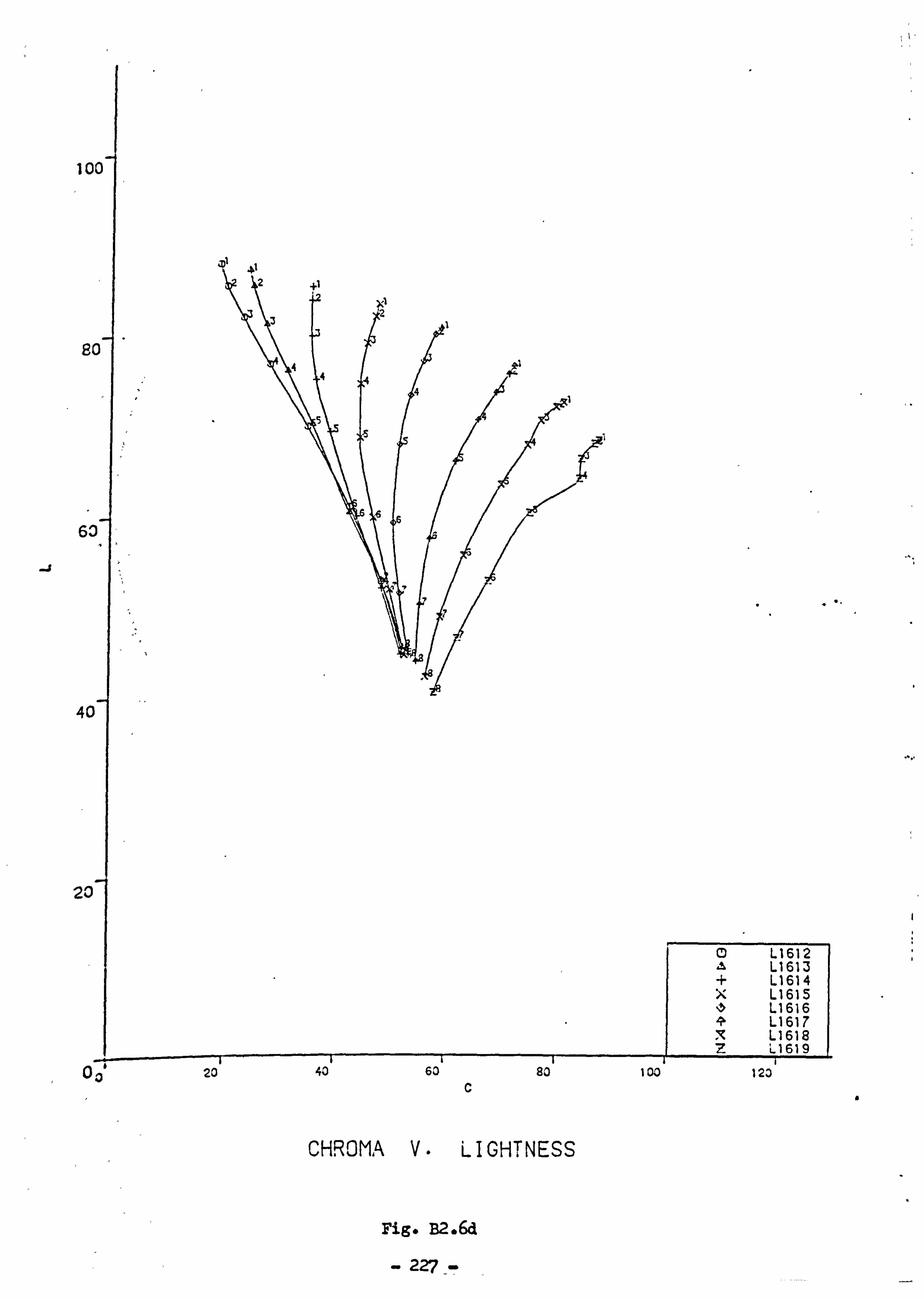
-i
I
8
6
4C
20
a
Fig. B2.6d
- 227 _-
20 40 63 so 100 123 c
CHROMA V. LIGHTNESS
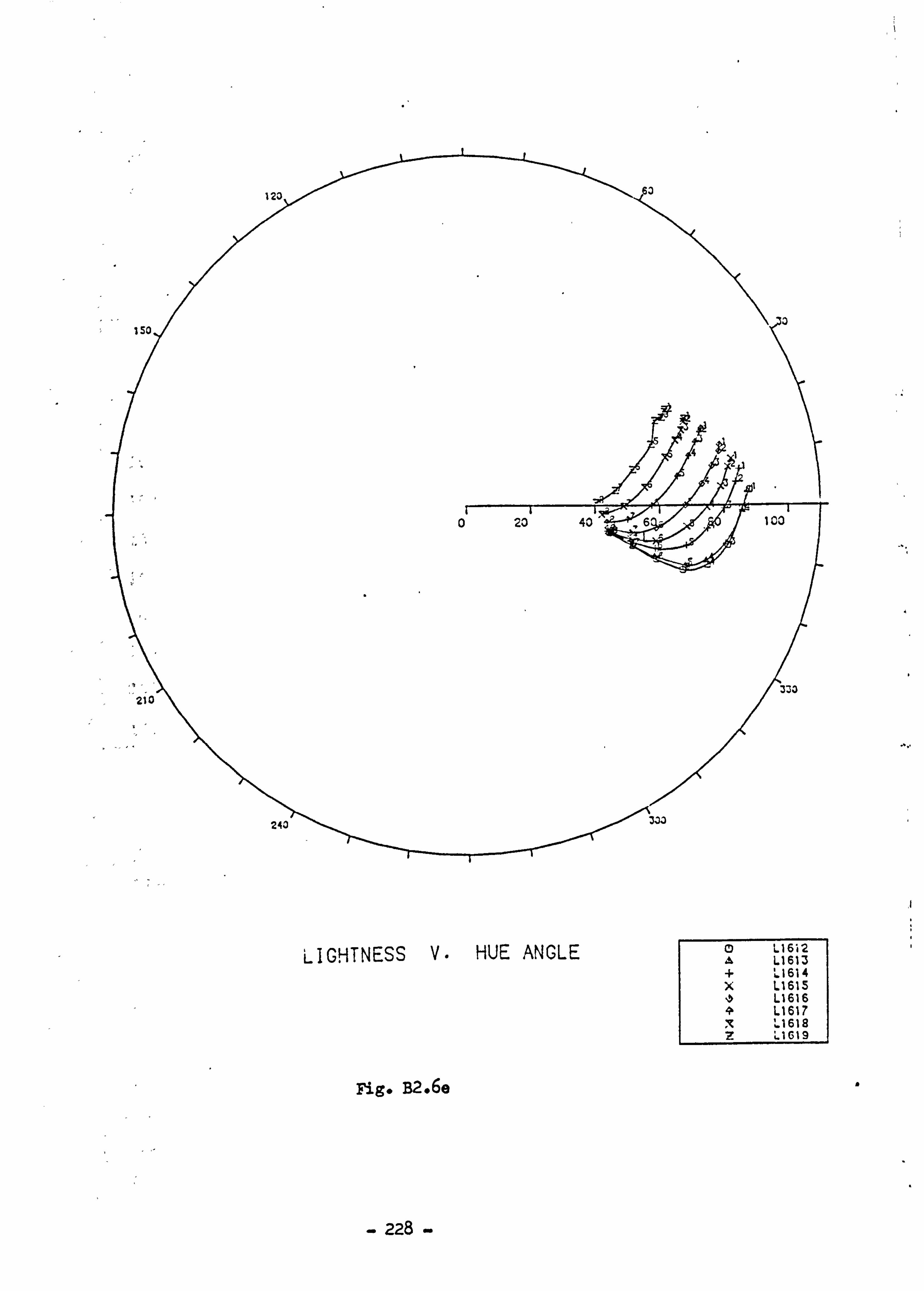
LIGHTNESS V. HUE ANGLE
Fig. B2.6e
L 1612 Ll 613 1.1614 LISIS L1616 Ll 617
a
- 228 -

B. 2.7 Mixture dyeings of Luminous Red G and Blue SER
In each of the following figures, 1,2 ... 8 refer to
concentrations of 0.005,0.01 ... 1.0% of Blue SER respectively, and the
figures are arranged in the following order:
0 x vs y, x vs Y, A vs B, C vs L and L vs H
Concentration (% Shade)
Code L. Red G Blue SER
1604 . 005 . 005 . 01 . 025 . 05
, 1605 . 01 . 005 . 01 . 025 . 05
, 1606 . 025 . 005 . 01 . 025 . 05 1
1607 . 05 . 005 . 01 . 025 . 05
ý 1608 . 005 . 01 . 025 . 05
, 1609 . 25 . 005 . 01 . 025 . 05
.' 1610 .5 . 005 . 01 . 025 . 05 1
1611 1.0 . 005 . 01 . 025 . 05 1
. 25 .5 1.0
. 25 .3 1.0
. 25 .5 1.0
. 25 .5 1.0
. 25 .5 1.0
. 25 .5 1.0
. 25 .5 1.0
. 25 .5 1.0
At low concentrations, the chroma is increased as the
concentration of the non-fluorescent blue dye is increased (fig. B2.7d)
a
- 229 -
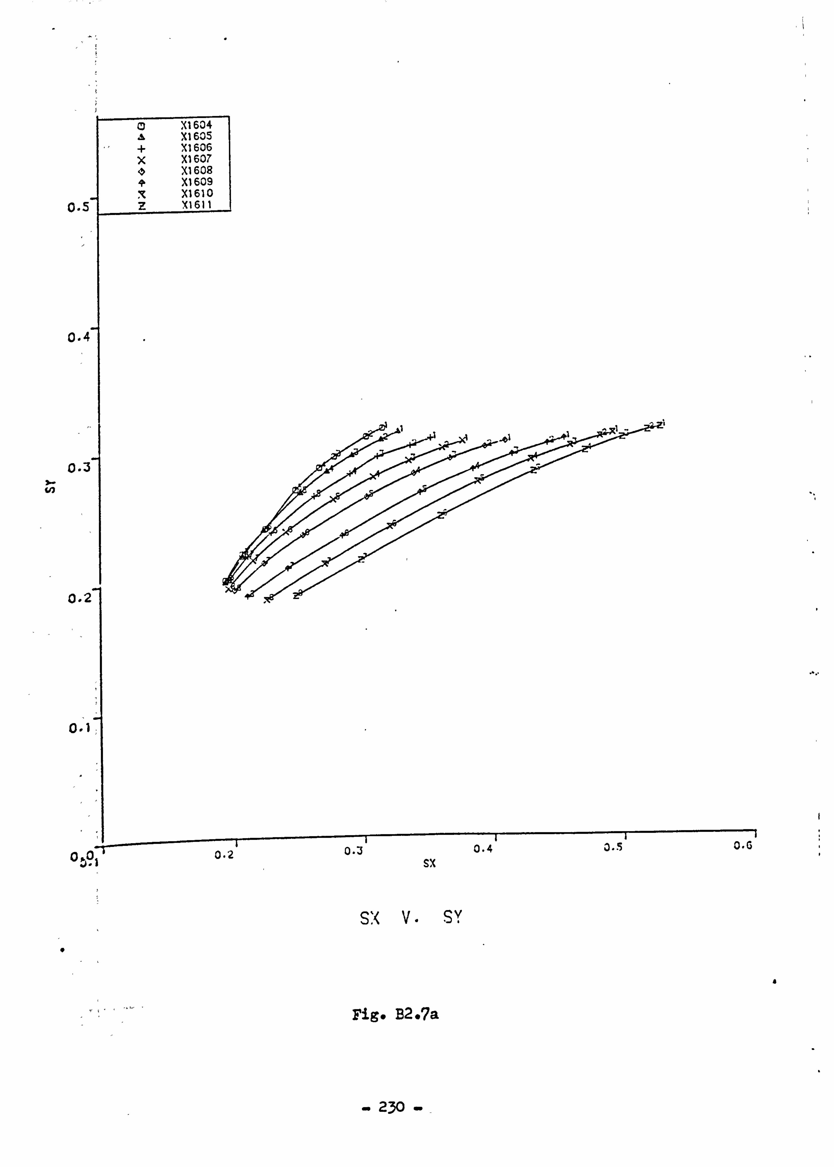
X1 604 X1 60S
+ XI 606 x X1 607 0 X1 608 + XI 609
X1610 0.5 611
0.4
o .3 �I,
0
0
000.3 0.4 0.5 O-G
sx
Sl< v- SY
Fig@ B2*7a
ý 230 -
a
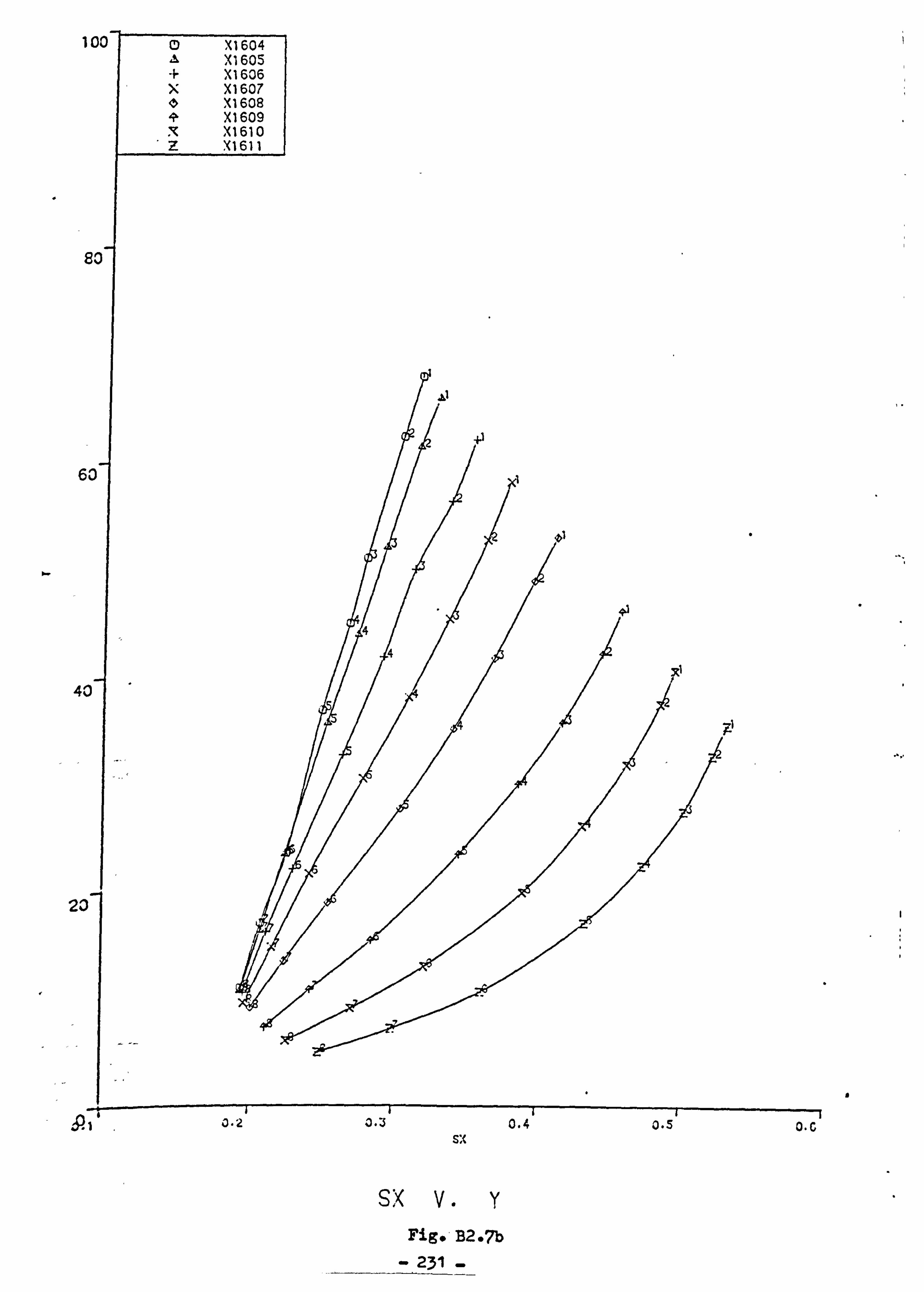
1001 Q) X1 604 Xl 605 X1606 X1607 Xl 608 x1609 XI 610
. x1611
so
63
401
23
/
0.2 0.3 0.4 sx
sx V. y
Fig* B2.7b
- 231 -_
0.5 O-C
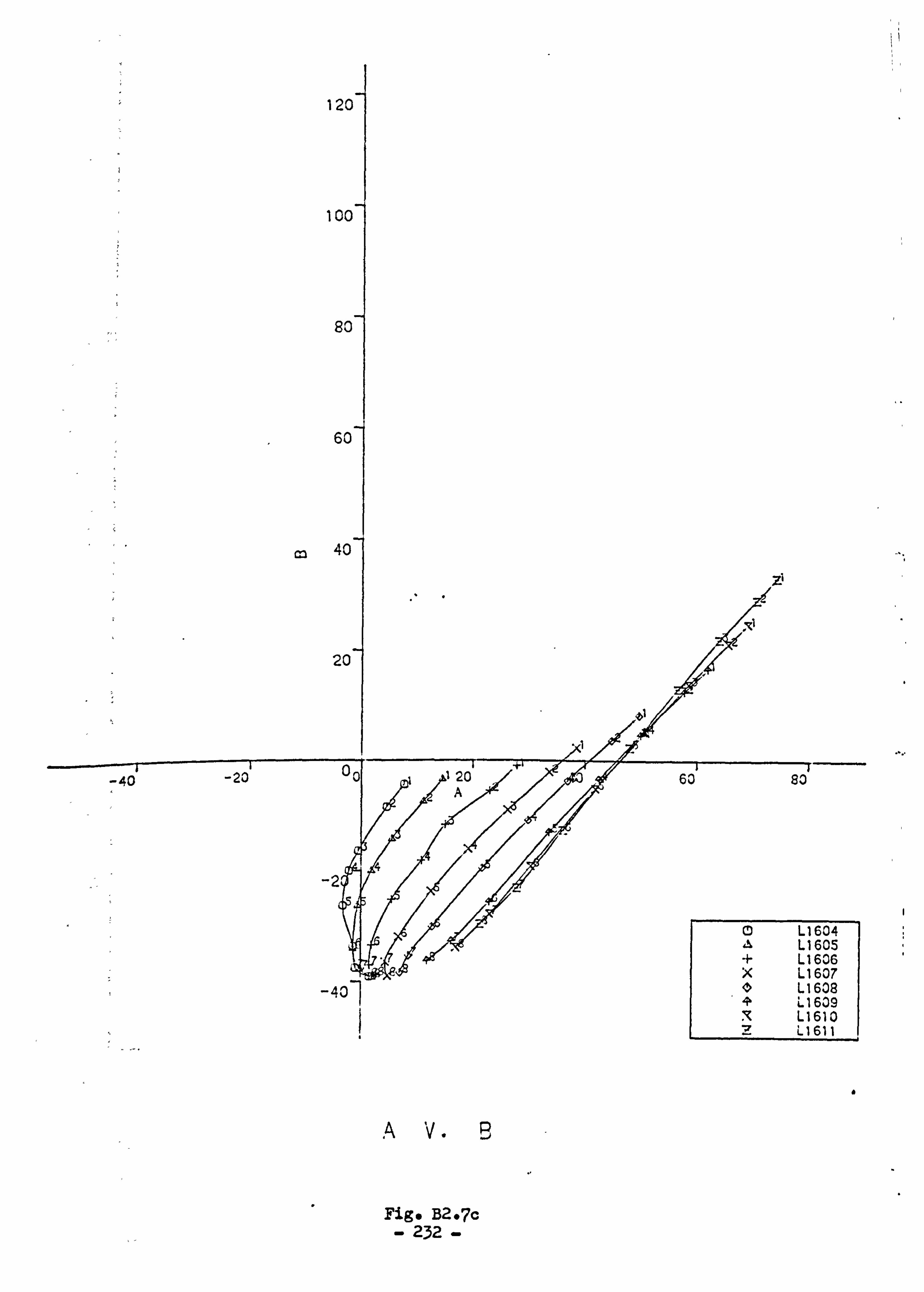
120
100
80
60
-40
PE,
<> L1608 + L1609
Ll 610
1'Z
Ll 611
a
Fig* B2-7c 232 -
40

-j
101
8 ko
6%0
ý IL
4C
20
UO 14U Oj c
; 54 1 uv
CHROMA V. LIGHTNESS
Fig* B2e7d
233
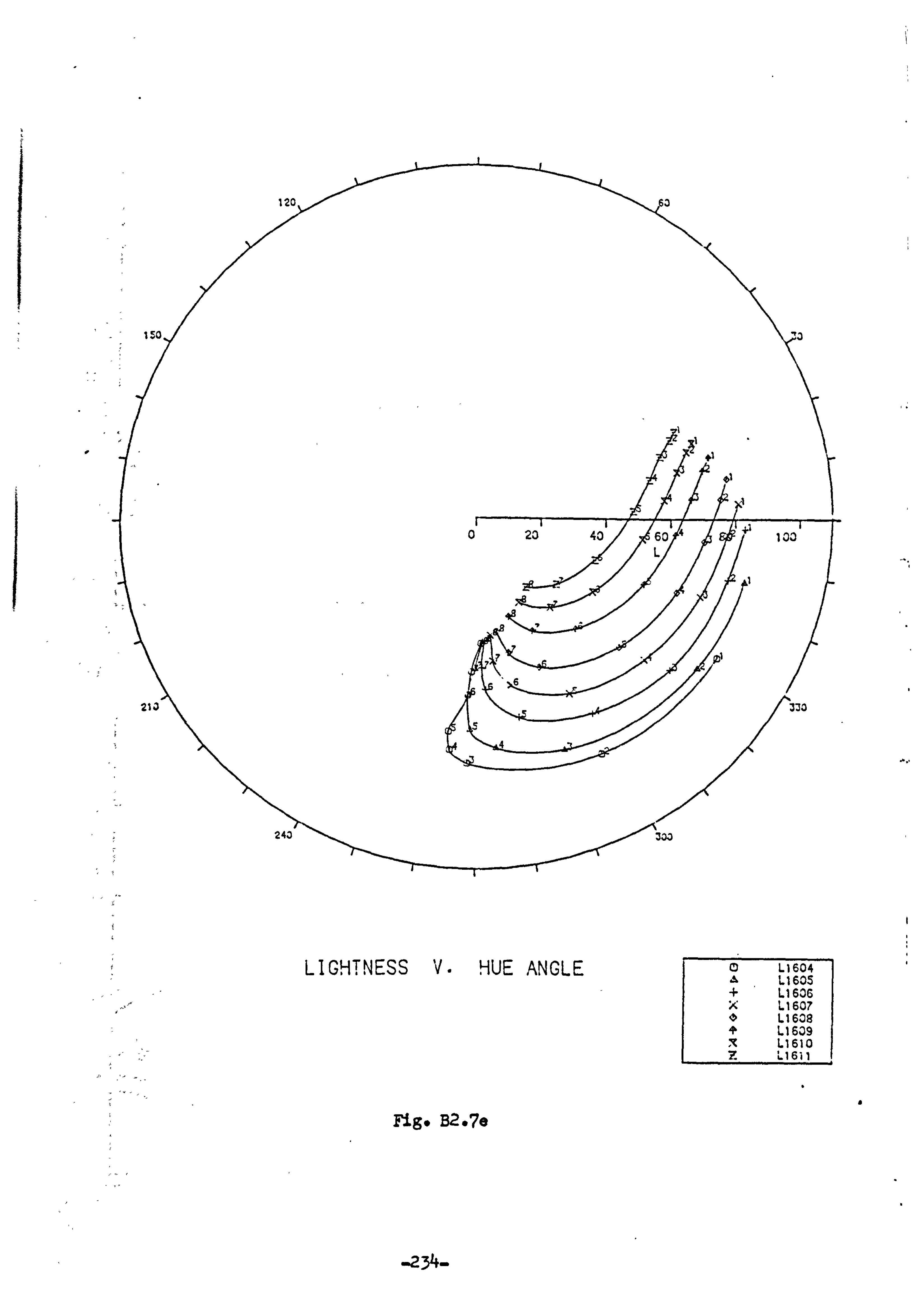
210
I
243
LIGHTNESS V. HUE ANGLE
Fig* B2-7e
303
L1604 L1605
* Ll 636 * L1607 * L1608 * L1609
Ll 610 z LI 6i I
a
-234-
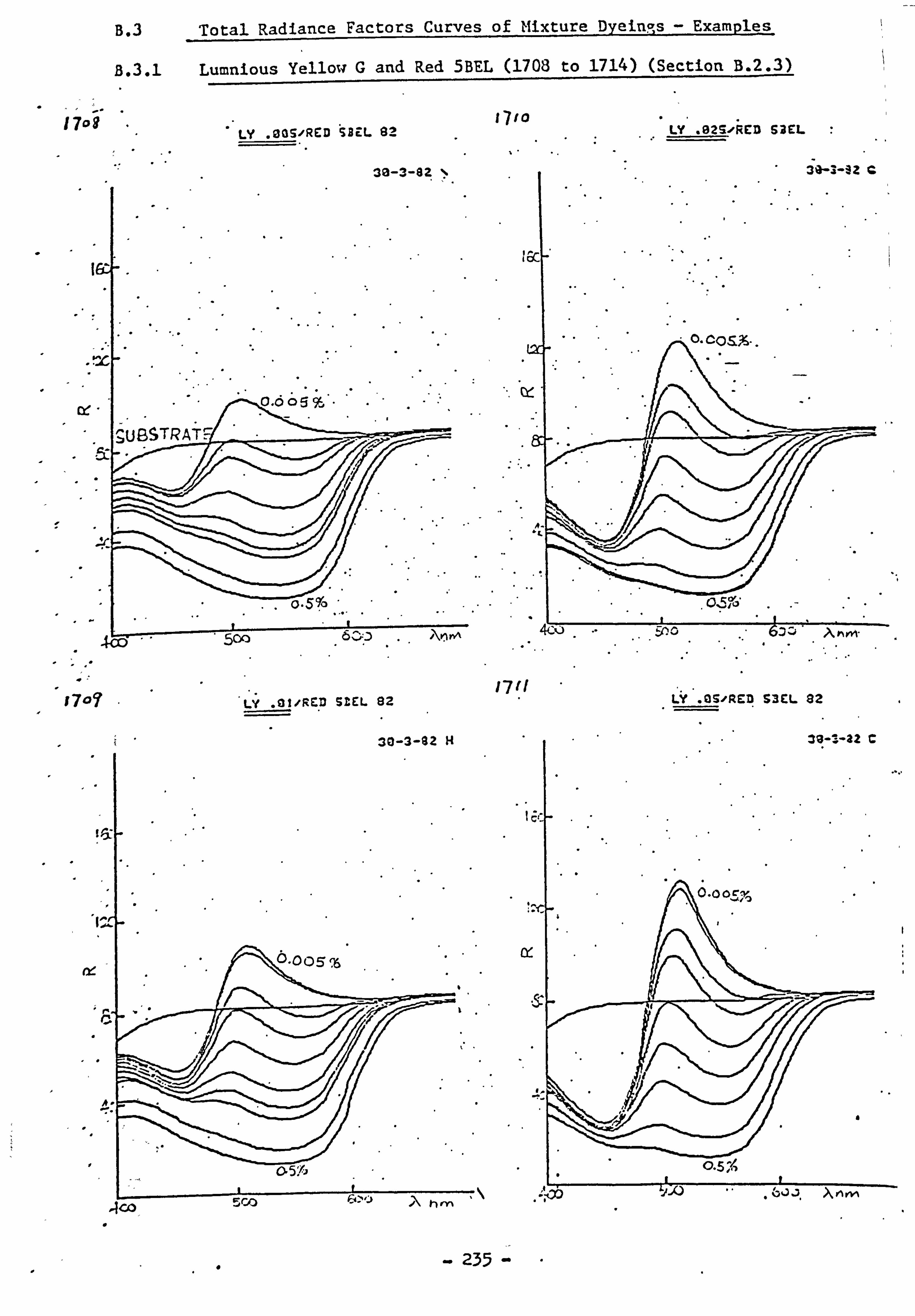
B. 3 Total Radiance Factors Curves of Mixture Dyeings - Examples
B. 3. i Lumnious Yellow G and Red 5BEL (1708 to 1714) (Section B. 2.3)
1700 LY OGS/RED tBEL 82 LY . 029., RED SBEL
0 Ei 9, f
. zo
1707 LY ial/RE: D SZEL 92
a
.
c
235
17ý1 LY as., RED SUL 32

1712 17ý4 LY I/RED SBEL 32 LY S-IRED SUL 32
33-3-92 L
0.00570
0.00 S'n
ac -
ilo .IA ; co 600 -to o 6co
1713 LY' . 25/pED 53EL
f\o
IIN
4CO
236
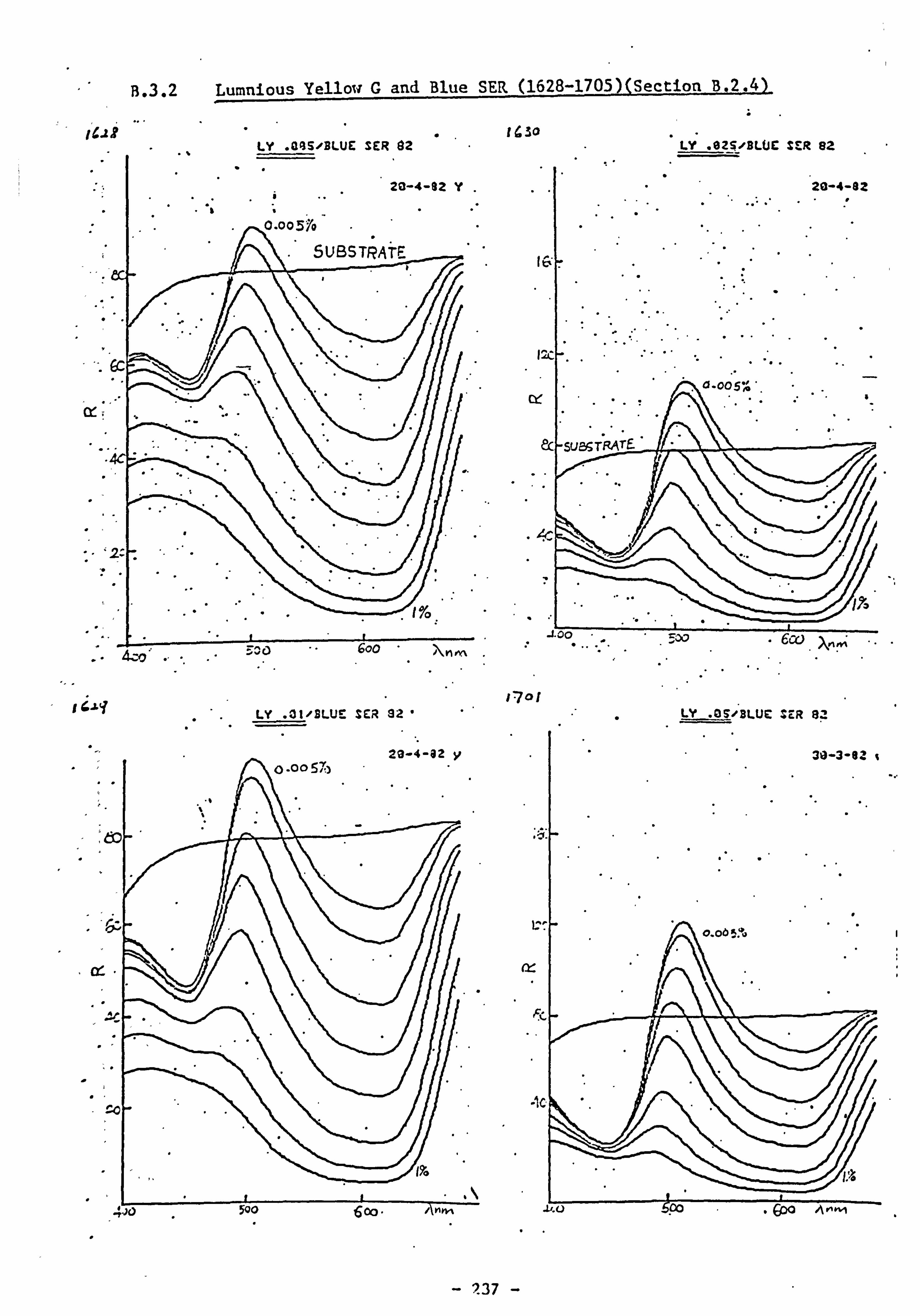
B. 3.2 Lumnious Yellow G and Blue SER (1628-1705) (Section B. 2.4)-
.I LY Q4S. IBLUE SER 92 LY . 025, fBLUE : ER eZ
20-4-92 Y 26-4-
0.0057a
SUBSTRATF,
GC - 0.005.0
ce of
-SU26TRATF- -4C-
fo
6co 600
jýq LY . 01/3LUE SER 32'
v7ol LY : ER 82
20-4-82 v
L
- 937 -

i7o. z LY . 1/2. LUZ: SE. R 132 LY S/lLUC SER oz
0.30-3-az k.. 38-3
cx
t7o3
-C
LY . 2S4P3LUE SER SZ LY 1. OBLUC SCR 22
- 238 .., b
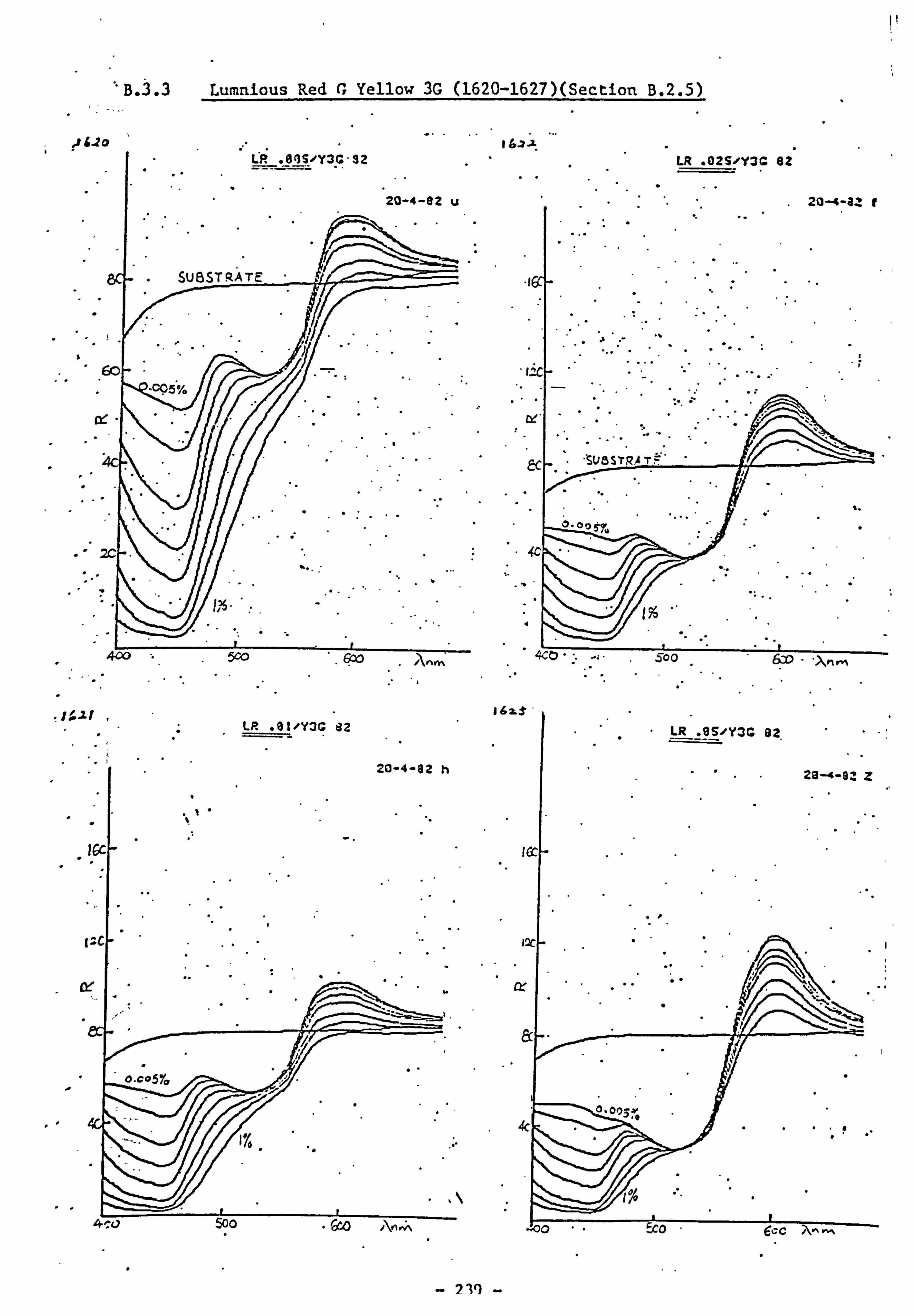
"B. 3.3 Lumnious Red G Yellow 3G (1620-1627)(Section B. 2.5)
LR S'3SIY3G-$2 LR . 02S-IY3C 82
20-4-02 u
8c - SUBSTRATE
-op5% jo
Of -
TIZA T
kx--
ýc - ec
2c
400 5co 4CO 500
LR . 01--ly3o 82 LR . 9slloy3c 92.
20-4-82 h
0
'S
20-4-a2 f
- 219 -
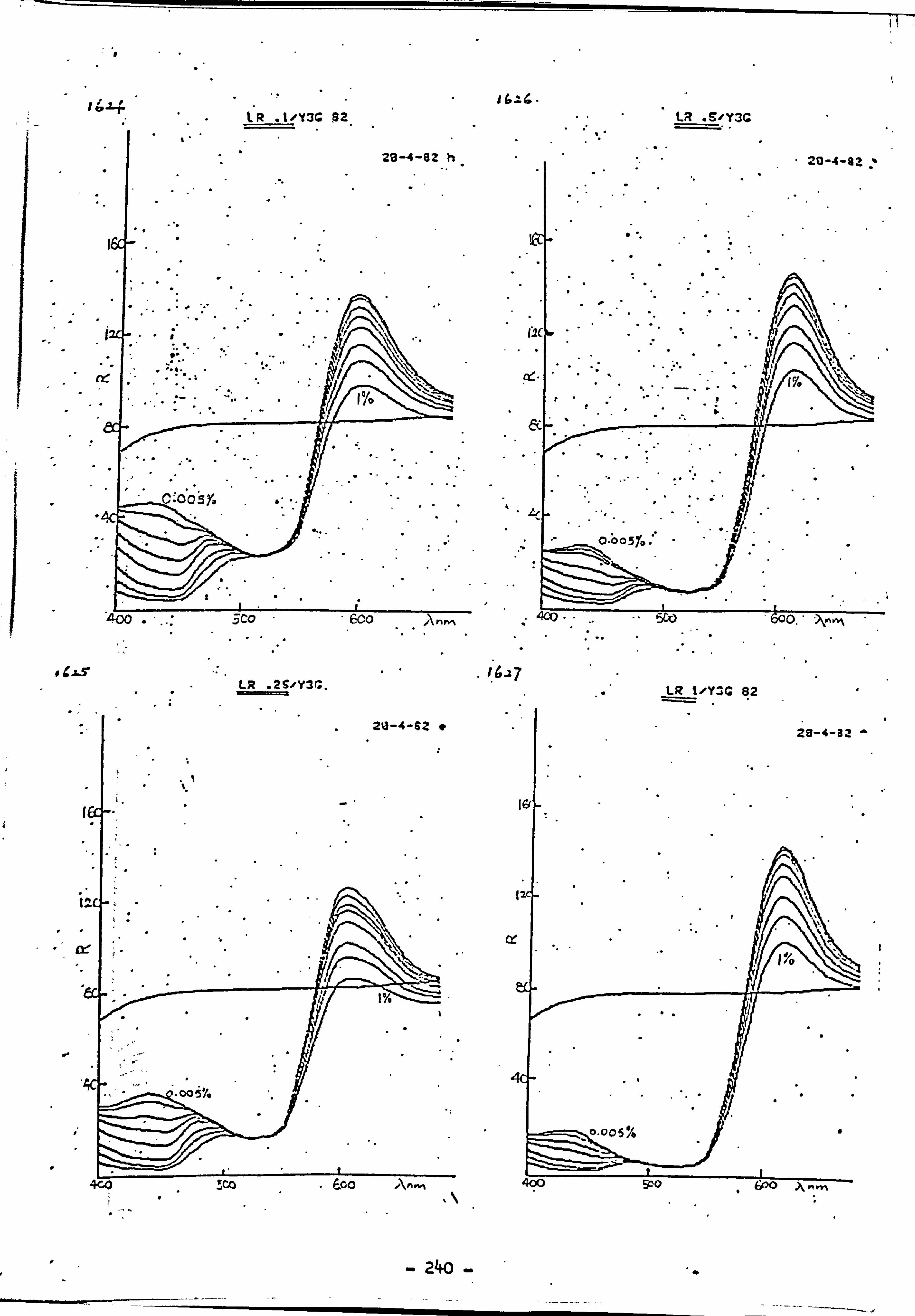
1ey3c 02. LR . 9., Y3G
23-4-82 h
nc ..... alf -, I
0.0051.., '00
'400 .-..: 5. - -5CO 900.
lco 6co Anm
LR . 29/Y3r.. LR t. *Y:; c q2
20-4-92
S.
C
240
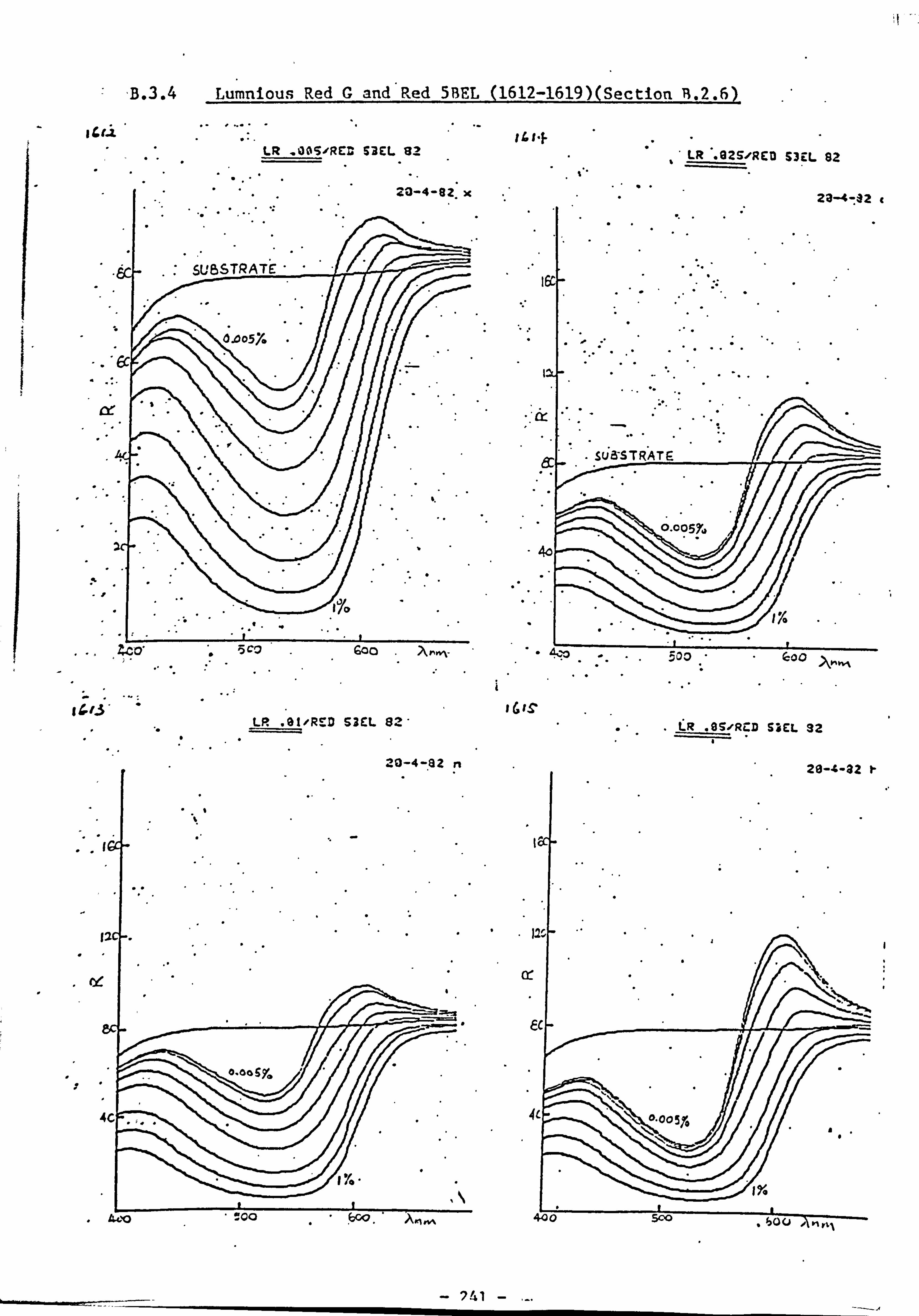
B. 3.4 Lumnioun Red G and Red 5BEL (1612-1619)(Section R. 2.6)
fi If. 1-F LIZ . 00S. "RED S3EL 132 LR . 029/RED SHL 92
20-4-: 32
SLIBSTRATE
cc
5co Goo
il. 3 LR . 91/RED S2EL 82*
20-4-82 n
5-f 40
I
a
LR . 09/RCD S; EL 32
- ? -/&I --

I1
Cc
I
S
"-
I
'4"? -
IC'
I. I
c
24? -
LR VRED S3EL 82
500 Ghoo
LR . 2S/RED SZZL 82
LR . 1-IRED SSEL a2
LR IfREZ SEEL 32

B. 3.5 Lumnious Red G and Blue SER (1604-1611) (Section B,,,? L-U
( tY6 LR. 013S, *SLUC SER LR -OZS/ELUC SER a2
30-3-82 1 33-3-82-Y
"Cl
. 4c -
2. C
ý7, 400 500
t407 L RED Gt/DLUt SEER
a
243
LR AS-03LUr" M 32
30-3-92
� .. '-. �
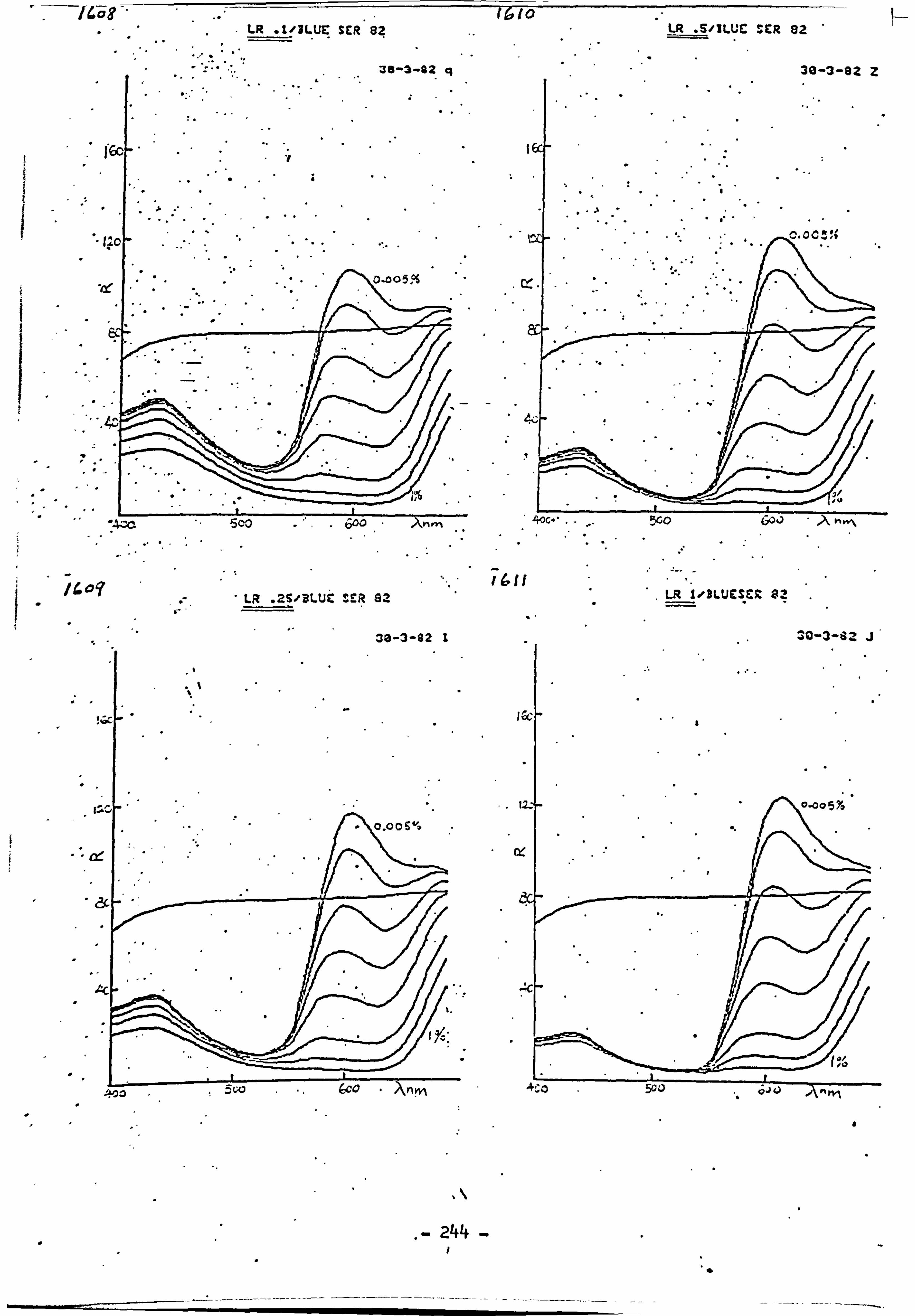
16,10 LR . 1-'ILUE: SER 82 LR S-IILUC SER 82
30-3-92 z
I
, ;,. LR . 29/BLUC SEý az
AC
'00
C
LR 1,01LUESER . 02
30-3-82 1
A
244
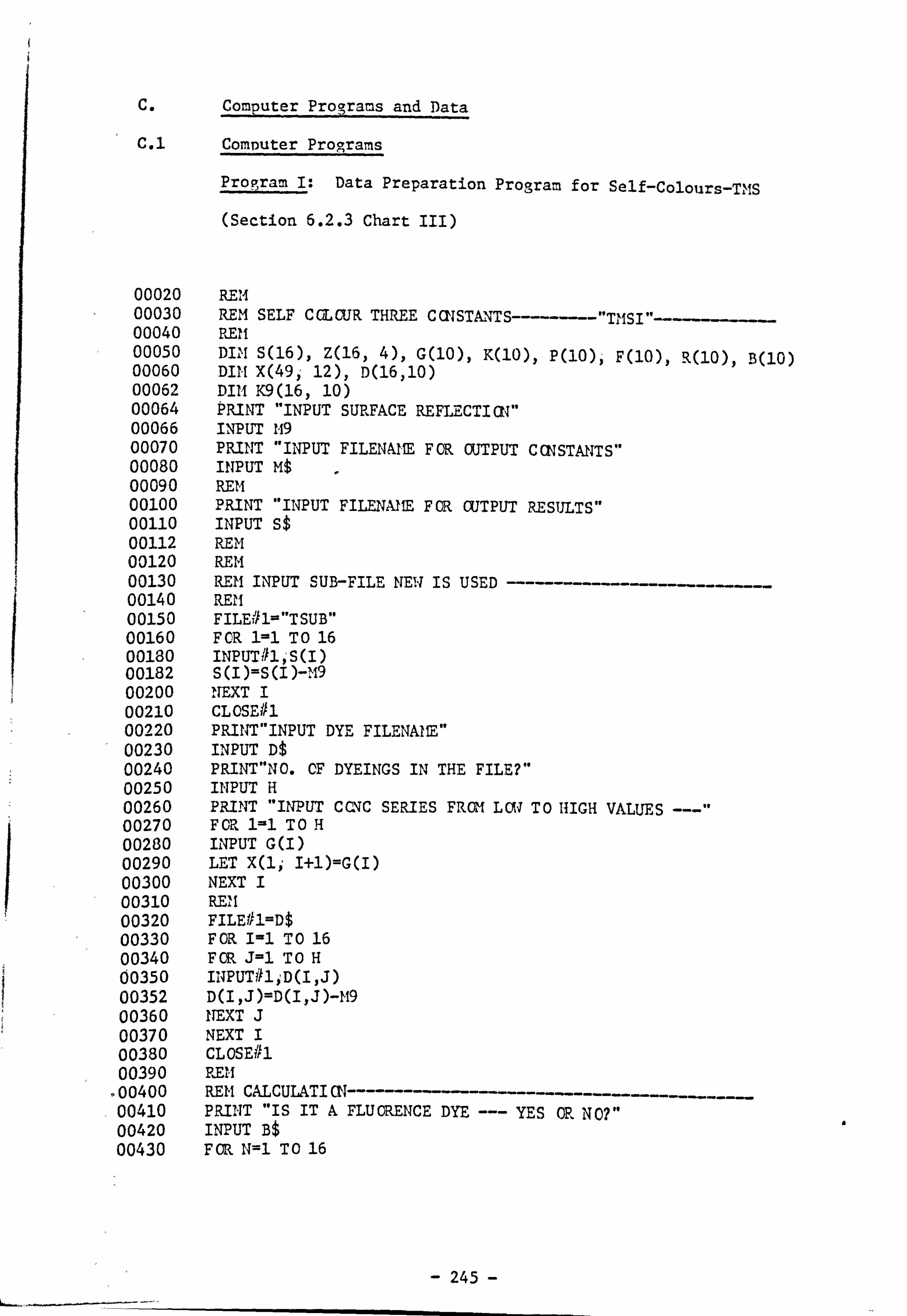
C. Computer Programs and Data
C. 1 ComDuter Programs
Program I: Data Preparation Program for Self-Colours-TIMS
(Section 6.2.3 Chart III)
00020 REM 00030 REM SELF COLCUR THREE CCKSTAl%'TS------"VMSI"--- 00040 REII 00050 DIM S(16), Z(16,4), G(10), K(10), P(10)p F(10), R(10), B(10) 00060 DIN X(49y 12), D(16,10) 00062 DI14 K9(16,10) 00064 PRINT "INPUT SURFACE REFLECTION" 00066 INPUT 1119 00070 PRINT "INPUT FILENAME FOR OUTPUT CCNSTANTS'* 00080 INPUT Mt 00090 REM 00100 PRINT "INPUT FILENAVIE FOR OUTPUT RESULTS" 00110 INPUT St 00112 REM 00120 REM 00130 REM INPUT SSUB-FILE NEW IS USED 00140 REM 00150 FILE7'11-"TSUB" 00160 F CR 1=1 TO 16 00180 INPUT#1'S(I) 00182 S(I)=S(i)-mg 00200 NEXT I 00210 CLOSE#l 00220 PRINVINPUT DYE FILENAME" 00230 INPUT Dt 00240 PRINT"NO. OF DYEINGS IN THE FILE? " 00250 INPUT H 00260 PRINT "INPUT CCNIC SERIES FROM L014 TO HIGH VALUES 00270 F OR 1=1 TO H 00280 INPUT G(I) 00290 LET X(l; I+1)=G(I) 00300 NEXT I 00310 REN 00320 FILE#1=Dt 00330 FOR I-1 TO 16 00340 FOR J=l TO H 00350 INPUT#liD(I, J) 00352 D(I, J)=D(I, J)-M9 00360 NEXT J 00370 NEXT I 00380 CLOSE#l 00390 REM
, 00400 REM CALCULATICN-- 00410 PRINT "IS IT A FLUORENCE DYE --- YES OR NOV' 00420 INPUT B$ 00430 FOR N=l TO 16
0
- 245 -
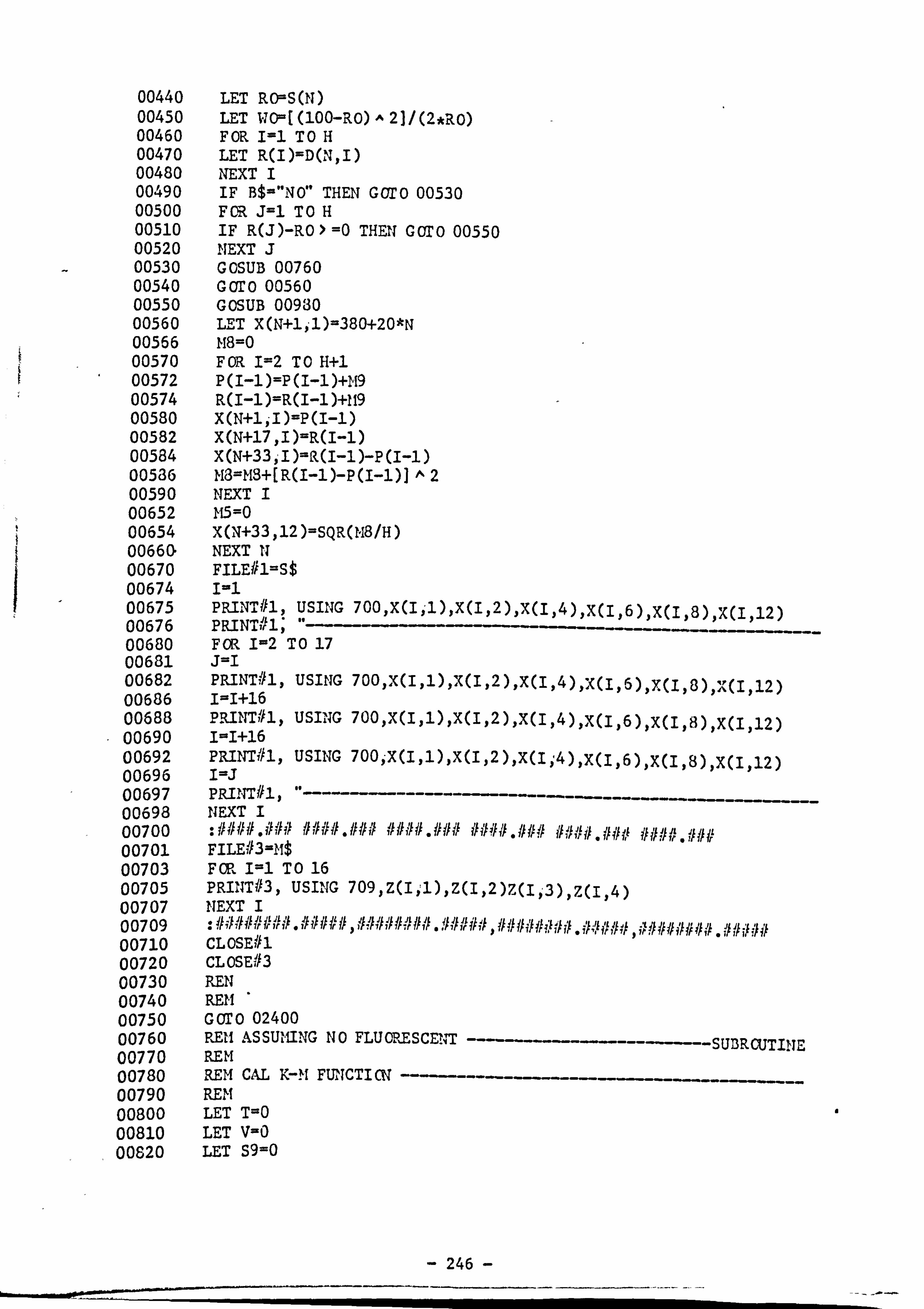
00440 LET RO=S(N) 00450 LET WO= [ (100-RO) A 21/ (2*RO) 00460 FOR I=l TO H 00470 LET R(I)=D(N, I) 00480 NEXT I 00490 IF B$="NO" THEN GOTO 00530 00500 FOR J=l TO H 00510 IF R(J)-RO > =0 THEN GOTO 00550 00520 NEXT J 00530 GOSUB 00760 00540 GOTO 00560 00550 GOSUB 00930 00560 LET X(N+lil)=380+20*N 00566 M8=0 00570 FOR I=2 TO H+l 00572 P(I-1)=P(I-1)+M9 00574 R(I-1)=R(I-1)+119 00580 X(N+lli)=P(1-1) 00582 X(N+17, I)=R(I-1) 00584 X(N+33iI)=R(I-1)-P(I-1) 00536 M3=MS+[R(I-1)-P(I-1)1^ 2 00590 NEXT I 00652 115=0 00654 X(N+33,12)=SQR(1,18/H) 00660 NEXT IT 00670 FILE#1=St 00674 1-1 00675 PRINT#l, USING 700, X(IP-1), X(1,2), X(I, 4), X(I, 6), X(I, 8), X(I, 12) 00676 PRINT? 9ý1; 00680 FOR 1-2 TO 17 00681 J=l 00682 PRINT#l, USING 700, X(I, 1), X(I, 2), X(I, 4), X(I, 6), X(I, 8), 'A(I, 12) 00686 I=I+16 00688 P. RINT#l) USING 700)X(I, 1), X(I, 2), X(I)4), X(I, 6), X(I, S), X(I, 12) 00690 1-1+16 00692 PRINT#l ) USING 700)-X(I, 1), X(I)2), X(I; 4), X(I, 6), X(I, 8), X(I, 12) 00696 I=j 00697 PRINT#lj ----- -- 00698 NEXT I 00700 : ####. ### ####. ### ####. ### ####. ### Ififilmo 00701 FILE#3-M$ 00703 FOR I=l TO 16 00705 PRINT#3, USING 709, Z(I,: l), Z(I, 2)Z(I, -3), Z(I, 4) 00707 NEXT I 00709 00710 CLOSE#l 00720 CLOSE#3 00730 REN 00740 REM 00750 GOTO 02400 00760 REM ASSU11ING NO FLUCRESCE1,41T ------SUBRCUTIITE 00770 REM 00780 IREM CAL K-M FUNCTICN 00790 REM 00800 LET T=O 00810 LET V=O 00820 LET S9=0
- 246 -

00830 FOR 1=1 To H 00840 LET K(I)=([(100-R(I)]A2)/[2*R(I)])-WO 00840 K9(N, I)=K(I) 00850 LET K(I)=K(I)*G(I) 00860 LET V=V+K(I) 00870 LET T=T+G(I) A2 00880 NEXT I 00890 LET S9=V/T 00900 RM STORE THE SLOPE IN Z ARRkY AT EACH WAVELENGTH 00910 LET Z(N, 1)=S9 00920 FOR I=l To H 00930 LET P(I)=S9*G(I)+Wo 00940 LET P(I)=1(100+P(I)I-SQR((100+P(j)] A 2-10000)] 00950 LET P(I)=INT(1000*P(l))/Jooo 00960 NEXT I 00970 RETURN 00980 REM FLUORESCENT AT THIS WAVELEG. NTH -----SUBRCUTINE 00990 FOR I=l TO H 01000 IF R. (I)-R0 -c 0 THEN GOTO 01070 01010 NEXT I 01020 REM SUBSTRATE LINE AS THE BASE LINE 01030 FOR I=l To H 01040 LET B(I)=R(I)-RO 01050 ITEXT I 01060 GOTO 01190 01070 REM ASSUMING NO F AT MAX CCNTC 01080 U=j 01090 R7-R(H) 01100 M5-(((100-R)A 2)/(2*R))7WO 01110 115=M5/G(H) 01120 FOR I=l To H 01130 Rl=Wo+?. 15*G(I) 01140 R2=100+Rl-SQR[ (100+, UL) A 2-10000] 01150 R2(I)=R2 01160 B(I)=R(I)-R2 01170 NEXT I 01180 REM INPUT K, Dl & L, D2 01190 K=. 25 01200 Dl--. 01 01210 L--6 - 01220 D2=. l 01230 GOSUB 01280 01240 Dl=K/110 01250 D2=L/110 01260 GOSUB 01280 01270 GOTO 01620 01230 GOSUB 01850 01290 LET E4=E 01300 LET Ll=K 01310 LET L=L+D2 01320 GOSUB 01850 01330 LET E5=E 01340 IF E5 ) E4 THEN GOTO 01370 01350 LET KI=K 01360 GOTO 01410 - 01370 LET E5=E4 01330 LET E4=E
- 247 -
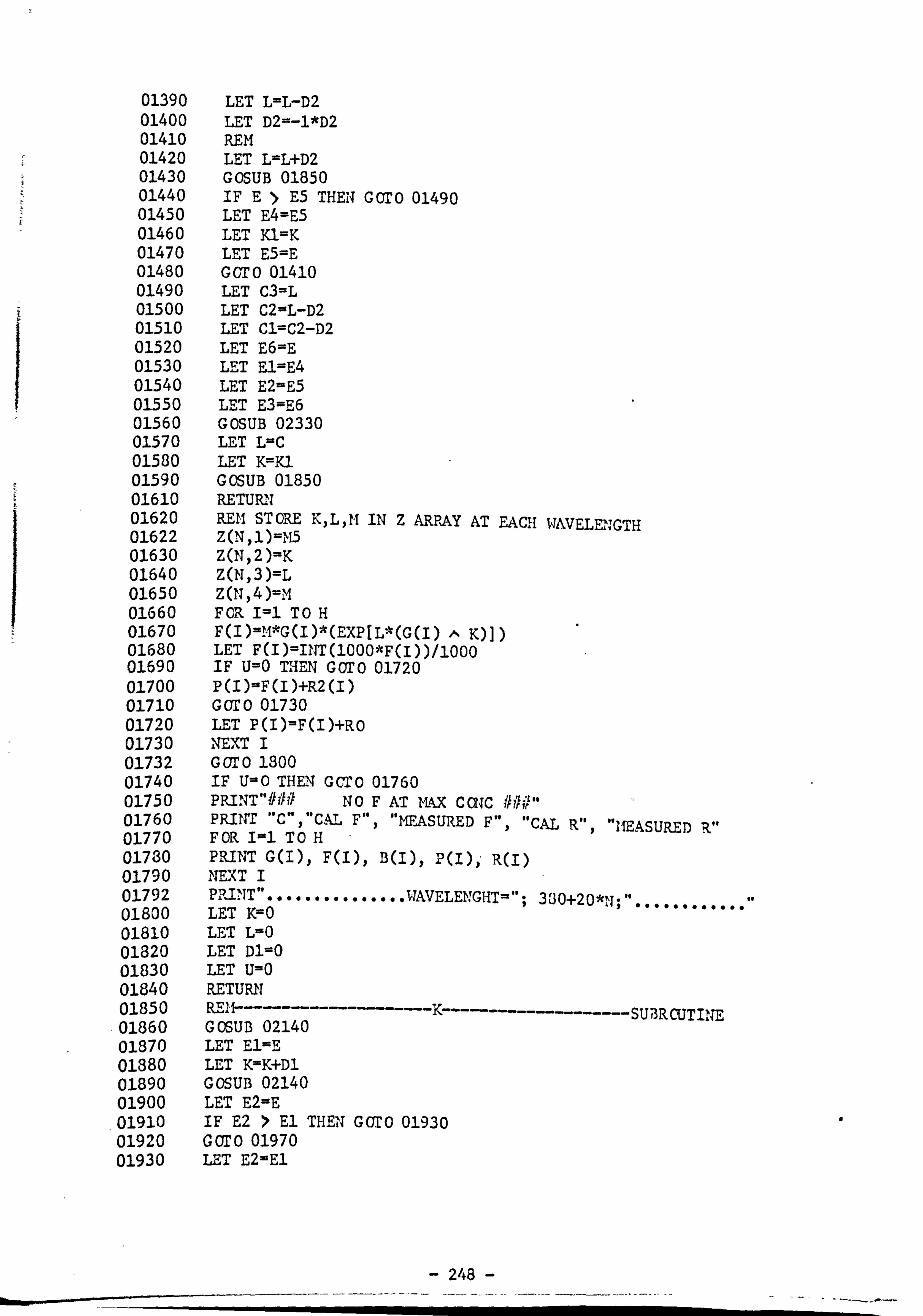
If
01390 01400 01410 01420 01430 01440 01450 01460 01470 01480 01490 01500 01510 01520 01530 01540 01550 01560 01570 01580 01590 01610 01620 01622 01630 01640 01650 01660 01670 01680 01690 01700 01710 01720 01730 01732 01740 01750 01760 01770 01730 01790 01792 01800 01810 01820 01830 01840 01850 01860 01870 01880 01890 01900 01910 01920 01930
LET L=L-D2 LET D2=-l*D2 REM LET L=L+D2 GOSUB 01850 IF E *> E5 THEN GOTO 01490 LET E4=E5 LET Kl=K LET E5=E GCTO 01410 LET C3=L LET C2=L-D2 LET Cl=C2-D2 LET E6=E LET El=E4 LET E2=E5 LET E3=E6 GOSUB 02330 LET L=C LET K-7Kl GOSUB 01850 RETURN REM STORE K, L, M IN Z ARPAy AT EACH WAVELE'NGTH Z(N, 1)=rl5 Z(N22)=K Z(N, 3)=L z(N, 4)=m F OR I=l TO H F(I)=! -I*G(I)*(EXP[L*(G(I) A Ql) LET F(I)=IkTr(1000*F(I))/1000 IF U=O THEN GOTO 01720 P(I)=F(I)+R2(I) GOTO 01730 LET P(I)=F(I)+RO NEXT I GOTO 1800 IF U=O THEN GCTO 01760 PRI!; T"#il# NO F AT lftX CC? jC PRI14T
- "C", "CAL V*2 "MEASURED F", "CAL R", "MEASURED R"
't UK I -. L IV li
PIUNT G(I)p F(I), B(I)y P(I)y, R(J) NEXT I PIEUNT" ............... WAVELaIGHT="; LET K--O LET L=O LET Dl=O LET U=O
330+20*1&, T-, ". ». 000000 tf
RETURN R-171ý--- -----K -- ---------- - ------ SUBROUTINE GOSUB 02140 LET El=EP LET K=K+Dl GOSUB 02140 LET E2=E IF E2 > El THEN GOTO 01930 GOTO 01970 LET E2=El
- 248 -
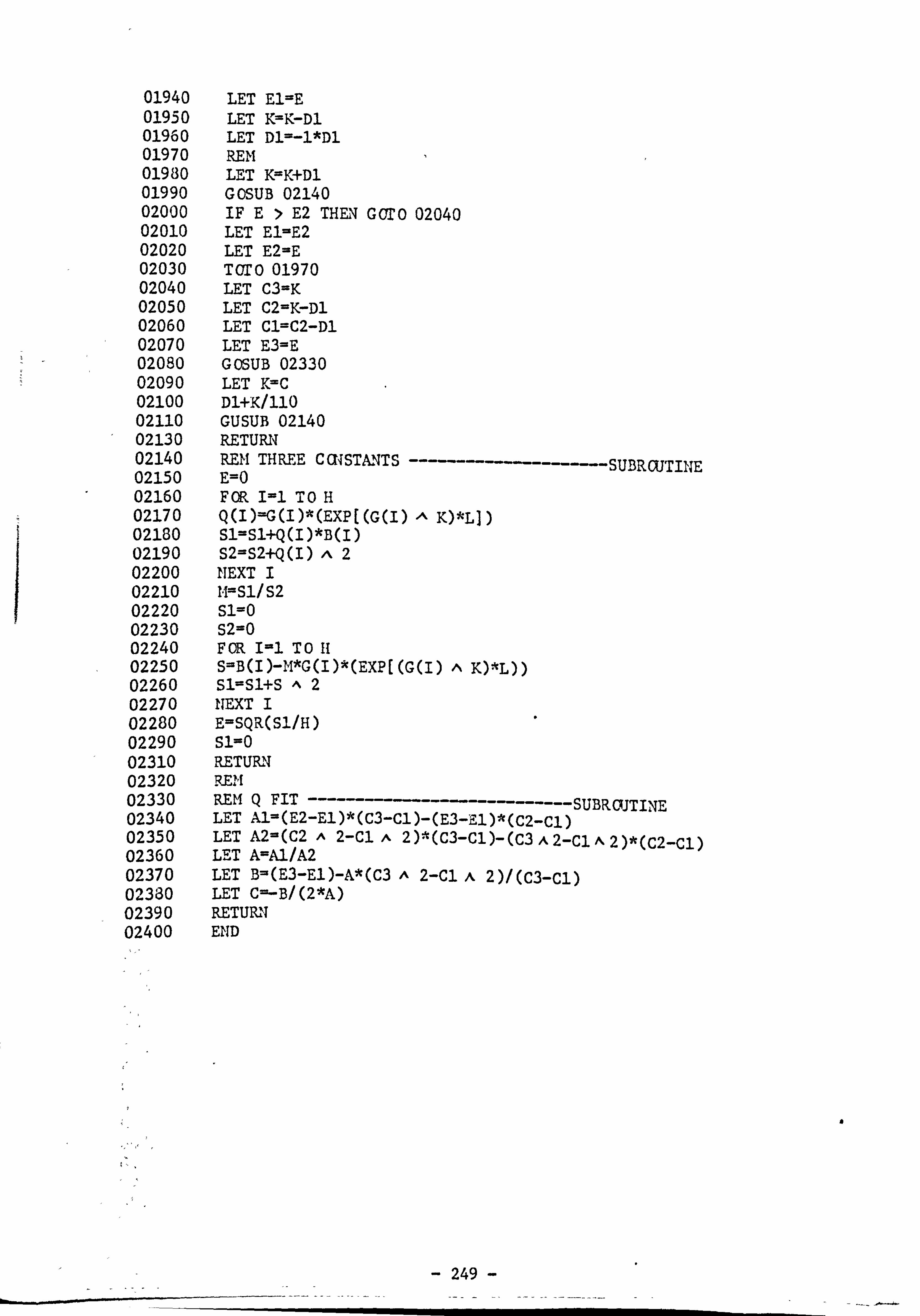
01940 01950 01960 01970 01980 01990 02000 02010 02020 02030 02040 02050 02060 02070 02080 02090 02100 02110 02130 02140 02150 02160 02170 02180 02190 02200 02210 02220 02230 02240 02250 02260 02270 02280 02290 02310 02320 02330 02340 02350 02360 02370 02330 02390 02400
LET El=E LET K--K-Dl LET Dl=-l*Dl REM LET K=K+Dl GOSUB 02140 IF E> E2 THEN GOTO 02040 LET El=E2 LET E2=E TOTO 01970 LET C3=K LET C2=K-Dl LET Cl=C2-Dl LET E3=E GOSUB 02330 LET Y, =C DI+K/110 GUSUB 02140 RETUP14 REM THREE CCNSTANTS --- - --- ---------SUBRCLJTINE E=O FOR I=l TO H Q(I)=G(I)*(EXP[(G(I) A K)*Ll) Sl=Sl+Q(I)*B(I) S2=S2+Q(I) A2 ITEXT I I. I=Sl/S2 sl=o S2=0 F OR I-1 T0 11 S=B(I)-M*G(I)*(EXP[(G(I) A K)*L)) SJ=SJ+S A2 ITEXT I E=SQR(Sl/H) si=o RETURT TRE'll
REM Q FIT ------- -------------- SUBROUTINE LET Al=(E2-El)*(C3-Cl)-(E3-21)*(C2-Cl) LET A2=(C2 A 2-Cl A 2),. "(c3-cl)- (C3 A 2-ClA 2)*(C2-Cl) LET A--Al/A2 LET B=(E3-El)-A*(C3 A 2-Cl A 2)/(C3-Cl) LET C-B/(2*A) RETU%ll END
- 249 -
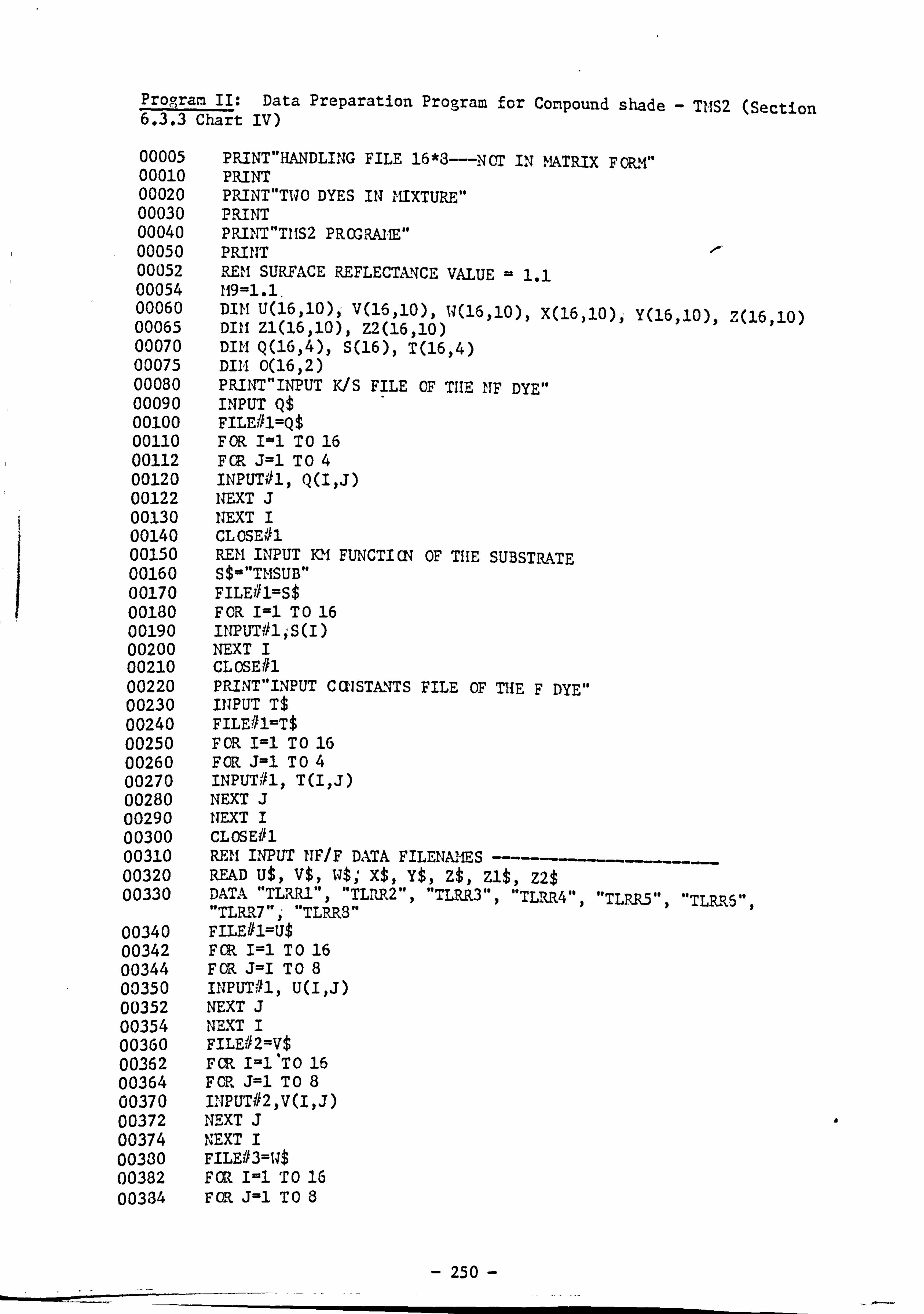
Program II: Data Preparation Program for Compound shade - THS2 (Section 6.3.3 Chart IV)
00005 PRINT"HANDLING FILE 16*3 --- NCT IN MATRIX FORM" 00010 PRINT 00020 PRINT"TWO DYES IN IMIXTURE" 00030 PRINT 00040 PRINT"T11S2 PROGRAIIE" 00050 PRINT 00052 REM SURFACE REFLECTANCE VALUE = 1.1 00054 119=1.1. 00060 DIM U(16,10)i V(16,10), 14(16., 10), X(16,10)j Y(16,10)o Z(16,10) 00065 DIII Zl(16,10), Z2(16,10) 00070 DIM Q(16,4), S(16), T(1604) 00075 DIM 0(16,2) 00080 PRINVINPUT K/S FILE OF THE ITF DYE" 00090 INPUT Q$ 00100 FILE#1=Q$ 00110 FOR I=l TO 16 00112 FGR J=l To 4 00120 INPUT#l, Q(I, J) 00122 NEXT J 00130 NEXT I 00140 CLOSE#l 00150 REM INPUT KM FUNCTICN OF THE SUBSTRATE 00160 S$="TMSUB" 00170 FILE#1=S$ 00130 FOR I=l TO 16 00190 INPUT#ljS(I) 00200 NEXT I 00210 CLOSE#l 00220 PRINVINPUT CCUSTANTS FILE OF THE F DYE" 00230 INPUT T$ 00240 FILE#1-T$ 00250 F OR I=l TO 16 00260 FOR J-1 To 4 00270 INPUT#l$ T(I, J) 00280 NEXT J 00290 NEXT I 00300 CLOSE#l 00310 REM INPUT ITF/F DATA FILENAll-fES 00320 READ U$, V$, W$; X$, Y$, Z$, Zl$, Z2$ 00330 DATA "TLIRRl", "TLPP. 2", "TLRR3") "TLRR4", "TLRR5", "TLILR5",
"TLRR7 ", ' "TLRRS" 00340 FILE#lr-U$ 00342 FOR I=l TO 16 00344 FOR J=I TO 8 00350 INPUT#l, U(I, J) 00352 NEXT J 00354 NEXT I 00360 FILE#2=V$ 00362 F OR I=l 'TO 16 00364 F OR J=l T08 00370 INPUT#2, V(I, J) 00372 NEXT J 00374 NEXT I 00330 FILE#3=li$ 00382 FOR I=l TO 16 00334 FM, J-1 TO 8
- 250 -
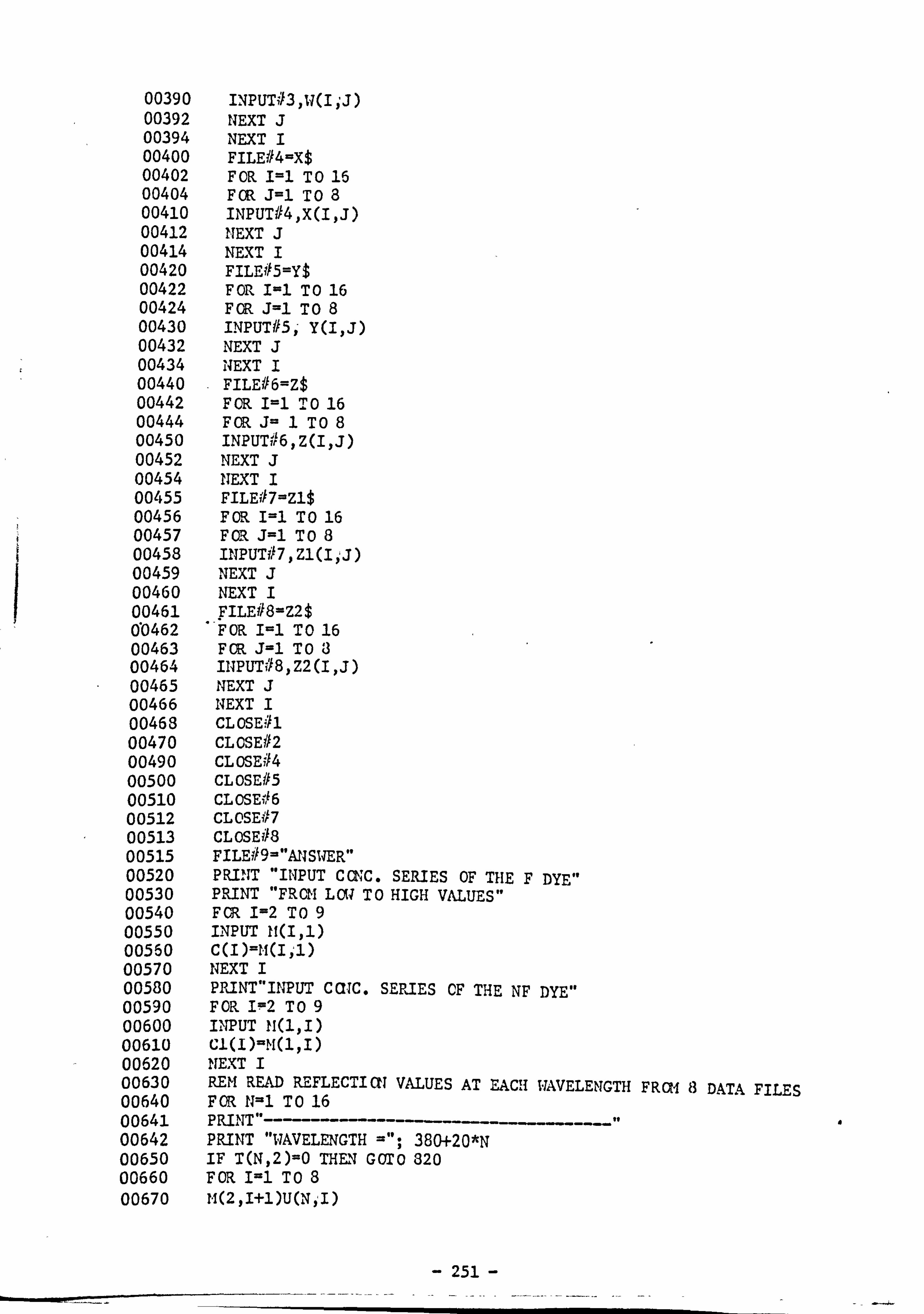
ii
00390 INPUT#3, W(I; J) 00392 NEXT J 00394 NEXT I 00400 FILE#4-X$ 00402 FOR 1=1 TO 16 00404 FOR J2--l TO 8 00410 INPUT#4, X(I, J) 00412 I-TEXT J 00414 NEXT I 00420 FILE#5=Y$ 00422 FOP. 1-1 TO 16 00424 FOR J=l TO 8 00430 INPUT#5,, Y(I, J) 00432 NEXT J 00434 NEXT I 00440 FILE#6=Z$ 00442 FOR 1=1 TO 16 00444 FOR J= 1 TO 8 00450 INPUTijr'6, Z(I, J) 00452 NEXT J 00454 NEXT I 00455 FILE#7=Zl$ 00456 FOR I=l TO 16 00457 FCR J=l To 8 00458 INPUV7, Zl(IýJ) 00459 NEXT J 00460 NEXT I 00461 I? ILE#8=Z2$ 60462 FOR I=l TO 16 00463 FOR J=l TO 3 00464 INPUT#8, Z2(I, J) 00465 NEXT J 00466 NEXT I 00463 CLOSE-11 00470 CLOSE#2 00490 CLOSE#4 00500 CLOSE#5 00510 CLOSEi', 16 00512 CLOSE47 00513 CLOSE#8 00515 FILE# 9 ="All SWER" 00520 PRINT "INPUT WIC. SERIES OF THE F DYE" 00530 PRINT "FROM L014 TO HIGH VALUES" 00540 FCR I=2 TO 9 00550 INPUT lt(I, l) 00550 C(I)=I. I(I; l) 00570 NEXT I 00580 PRINVINPUT CCITC. SERIES CF THE NF DYE" 00590 FOR IF2 TO 9 00600 INPUT ll(lpI) 00610 cl(l)=M(iii) 00620 NEXT I 00630 REM READ REFLECTICtl VALUES AT BACH WAVELENGTH 00640 FOR 11=1 TO 16 00641 PRINV- ------- 00642 PRINT "WAVELENGTH ="; 380+20*N 00650 IF T(N, 2)=O THEN GOTO 320 00660 F OR I=l TO 8 00670 1-1(29I+1)U(NiI)
FROM 13 DATA FILES
- 251 -

II
00680 14(3, I+1)=V(N, I) 00690 M(4, I+1)ý1411, I) 00700 MO)I+1)ýX(N, I) 00710 M(6,1+1)ýY(N, I) 00720 M(7 , I+1)ý-Z(N, I) 00722 M(8, I+I)OZ1(N,, I) 00724 M(9, I+1)=Z2(N, I) 00730 NEXT I 00740 REM INPUT CCUSTANTS ----- - --- -- 00750 Kl=Q(Nýl) 00760 K2ý-T(N, l) 00770 K3=S(N) 00780 K7-T(Ni2) 00790 L=T(14,3) 00800 M--T(N, 4) 00310 GOSUB 00950 00812 GCTO 840 00820 O(N, 1)=O 00330 O(N, 2)=O 00840 NEXT N 00850 PRINT "INPUT A FILENIAME FCR MATCHING CCNSTATNTS F/NF" 00360 INPUT Et 00870 FILE#l=E$ 00880 FOR I=l TO 16 00890 PRINT#lj USING 00910) 0(1)1), 0(1,2) 00900 NEXT I 00910 : ii#lr, ##. #####
), #####. #-####
00920 CLOSE/il 00950 REM MEASURED R IN 1-1 ARRAY 2ND-7TH Rai & 2ND-7T9 CCLUIDI 00960 RE14 00962 PRINT7#9, "WAVELEVGTH="; 380=20*11 00972 K4=10 00974 D1=10 00976 GCTO 1040 01000 PRINT "INPUT A CaISTANT FCR TRIAL--EQ FCIR MIXTURE" 01010 INPUT K4 01020 PRINT "INPUT STEP OF INCREMENT" 01030 INPUT Dl 01040 GOSUB 01080 01050 Dl=K4/11 01060 GOSUB 01080 01070 GOTO 01820 01080 REM GETTING K4 01090 REM 01100 GCSUB 01440 01110 El=E 01120 K4=, K4+Dl 01130 GOSUB 01440
- 01140 E2=E 01150 IF E2 '> El GOTO 01170 01160 GOTO 01210 01170 E2=El 01180 El=E 01190 K4=K4-Dl 01200 Dl=-l*Dl 01220 GOSUB 01440 01230 IF E> E2 GOTO 01270 01240 El=E2 01250 E2=E
a
- 252 -

01260 01270 01280 01290 01300 01310 01320 01330 01340 01350 01360 01370 01380 01390 01400 01410 01420 01430 01440 01450 01460 01470 01480 01490 01500 01502 01504 01506 01510 01520 01530 01540 01550 01560 01570 01580 01590 01600 01610 01620 01630 01640 01650 01660 01670 01630 01682 01684 01636 01690 01700 01710 01720 01730 01740 01750 01760 01770 01780
GOTO 01210 c3=K4 C=K4-Dl Cl=C2-Dl E3=E GOSUB 01370 K4=c GOSUB 01440 RETURN REM QUADUETIC FITTING REM Al=(E2-El)*(C3-Cl)-(E3-El)*(C2-Cl) A2=(C2 A 2-Cl A 2)*(C3-Cl)-(C3A2-CJA'-))*(C2-Cl) A=Al/A2 B-'2((E2-El)-A*(C2A2-ClA2)1/(C2-Cl) C-B/(2*A) RETURN PRINT REM CAL F WITH EXP EQ FOR F DYE REM FOR I=2 TO 9 F=14*C(I)*(EXP[(C(I)AK)*Ll) REN CAL F' WITH EQ FOR THE MIXTURE RETI FCR J=2 TO 9 K7=1+K4*Cl(J) IF K7=0 THEN K7=. 0000000001 IF C(I)< 0 THEN C(I) =. 00001 Fl=F*((l/K7)&[C(I)A(-. 2)1) F2-F2+Fl 2 REM CAL R' FROM K/S CCNSTANTS
EI RM RýK3+Kl*Cl(J)+K2*C(I) R=(100+R)-SQR((100+R)A2-10000) F3=M(I yJ)-R-M9 F4=F4+F3*Fl NEXT J NEXT I Y, 5=F4/F2 F2=0- F4=0 FOR I=2 TO 9 FOR J=2 TO 9 REM CAL THE DIFFERENCE BETWEEN REM F=M*C(I)*(EXPC(C(I)AK)*Ll) K7-1+K4*Cl(J) IF K7=0 THEN K7=. 000000001 IF C(I) 40 THEN C(I)=. 00001 F5-K5*(F*((l/K7)A(C(I)A(-. 2)))) R=K3+KI*Cl(J)+K2*C(I) P, -(100+R)-SQR((100+R)A2-10000) Rl(IIJ)=F5+R+M9 D=M(I, J)-RI(I, J) D4-=D4+D 2 R2(1, J)=D NEXT J NEXT I E-SQR(D4/64)
MEASLIRED R& CALCULATED R
- 253 -
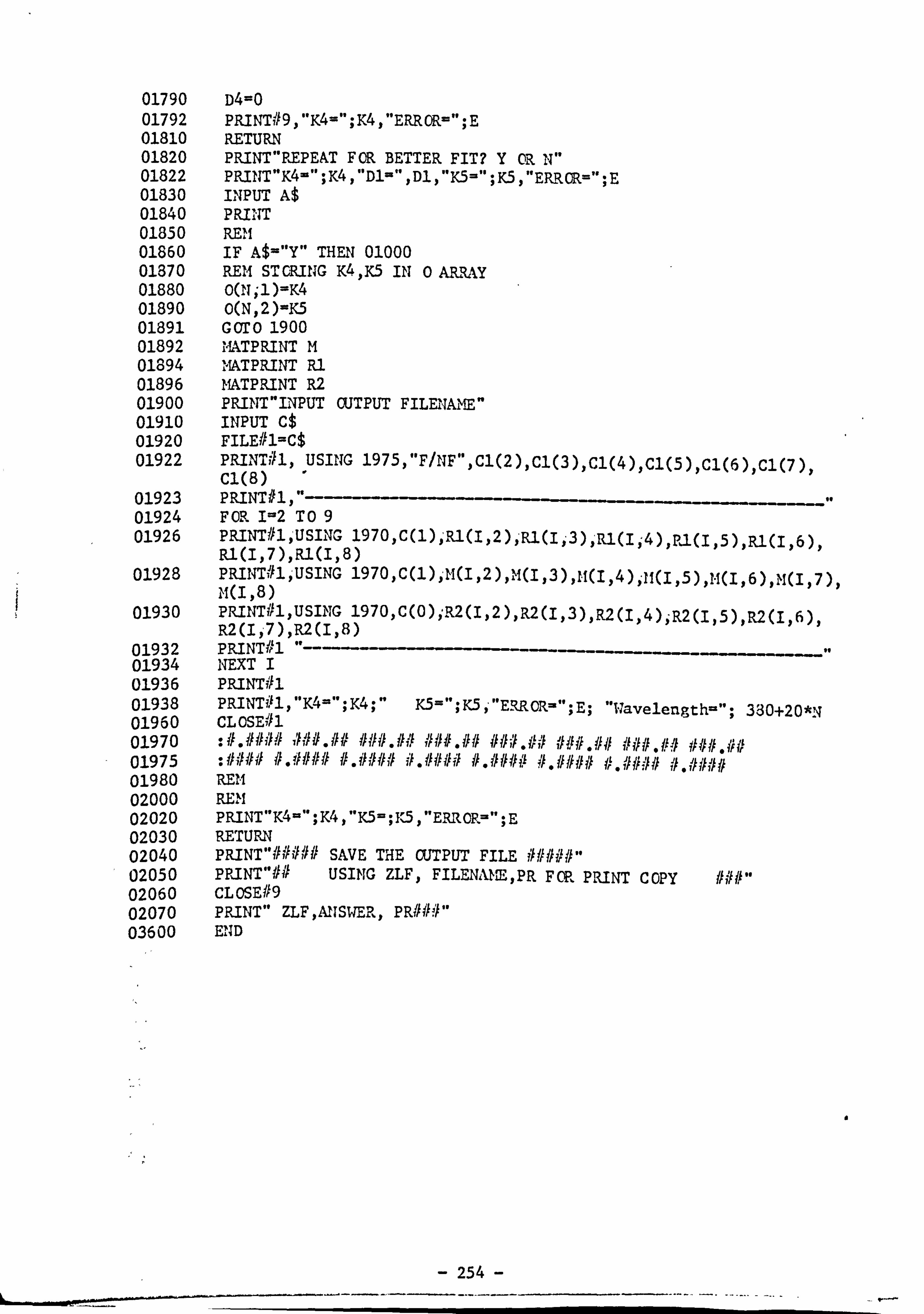
01790 01792 01810 01820 01822 01830 01840 01850 01860 01870 01880 01890 01891 01892 01894 01896 01900 01910 01920 01922
01923 01924 01926
01928
01930
01932 01934 01936 01938 01960 01970 01975 01980 02000 02020 02030 02040 02050 02060 02070 03600
D4=0 PRINT#9, "KW'; K4, "ERROR="; E RETURN PRINT"REPEAT FOR BETTER FIT? Y OR N" PRINT'*K4="; K4, "Dl=", Dl ý "K5="; K5, "ERROR="; E INPUT A$ PRINT RE'll IF Ato"Y" THEN 01000 REM STCRING K4, K5 IN 0 AB-RAY O(N; 1)=K4 O(N, 2)-K5 GOTO 1900 MATPRINT M MATPRINT Rl MATPRINT R2 PRINVINPUT OUTPUT FILENAIME" INPUT C$ FILE#1=C$ PRINTill, USING 1975, "F/NF", Cl(2), Cl(3), Cl(4), Cl(5), Cl(6), Cl(7), C1(8) PRINT#l, of FOR 1-2 TO 9 PRINT#lt'USING 1970, C(1)9'ýRl(I, 2)y-Rl(Ip3), 'RI(Ij, 4), PI(I, 5), RI(I, 6), Rl(I, 7), Rl(I, 8) PRINT#lpXSING 1970, C(l)), M(I, 2), M(I, 3), I. I(I)4)pll(I, 5)pl. I(I, 6), M(I, 7), -kl(I, 8) PRINT#lpUSING 1970, C(O); R2(I, 2), R2(I, 3), R2(I, 4))-R2(I, 5), R2(I, 6), R2(I)-7), R2(I, 8) PRINT#l NEXT I PRINT#1 PRINT#l, "K4="; K4; " K5= of ; K5j, "E-UCR="; E; "Wavelength="; 330+20*N CLOSE#l : #. #### J7##. ## ###. ## , 'i##. ## M1.0 ###. ## ###. #! I ###. ## : #il## #. #### #. #### #. #### #. #### #. #### #. #### #. #### REM REIM PRINT"K4='l; K4 0'*K5-; lC5, "E. RROR="; E RETURN PRINVOM SAVE THE CUTPUT FILE ##M" PRINT"## USING ZLFj FILENMM, PR FCR PRINT Copy CLOSE#9 PRINT" ZLF, AITSWER, PR##! I" Ell ID
#1/ #"
- 254 -
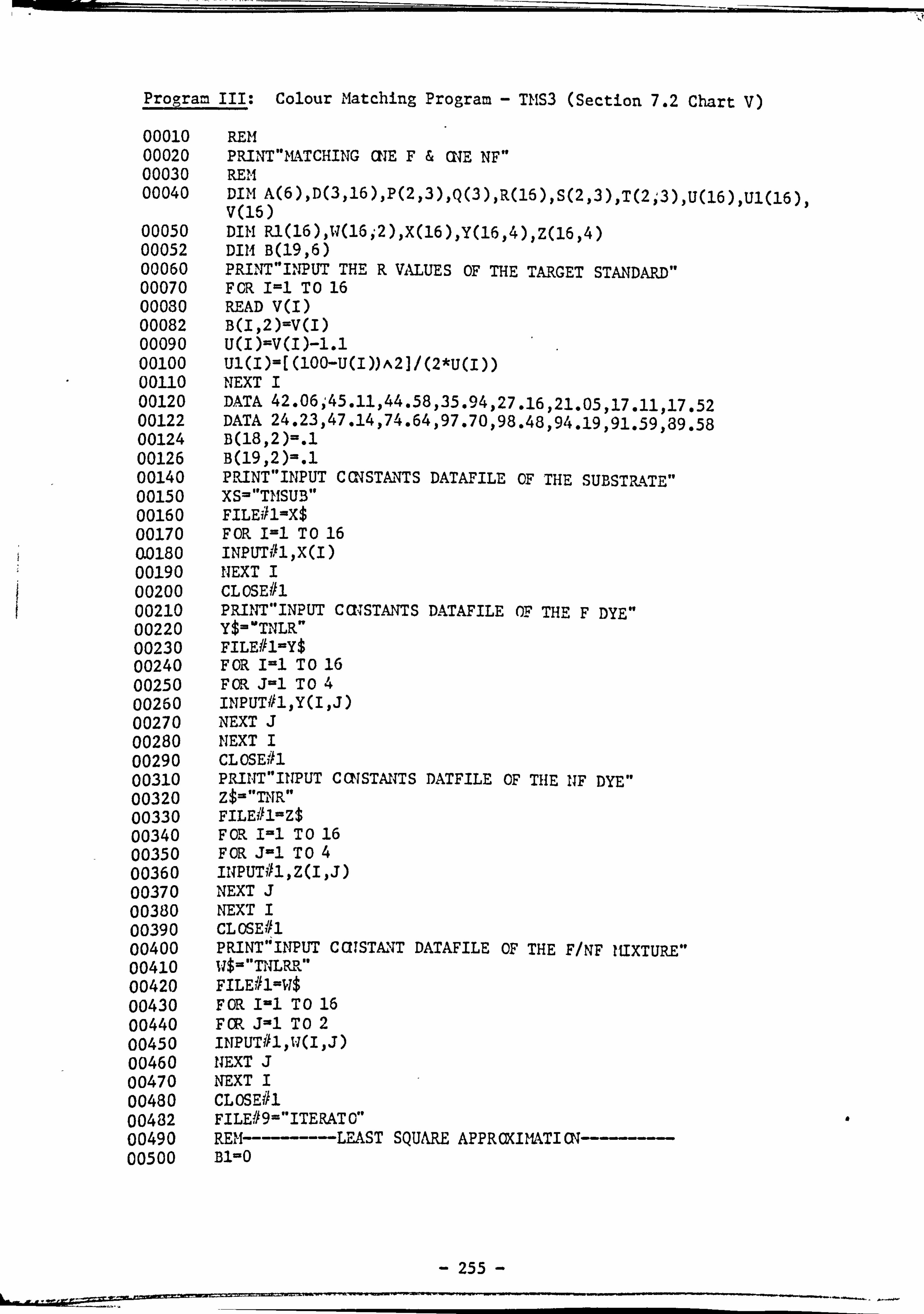
Program III: Colour Matching Program - TMS3 (Section 7.2 Chart V)
00010 REM 00020 PRINIT"MATCHING CUE F& WE NF" 00030 REM 00040 DIM A(6), D(3,16), P(2)3), Q(3), R(16), S(2,3), T(2; 3), U(16), Ul(16),
V(16) 00050 DIM Rl(16), W(16; 2), X(16), Y(16,4), Z(16,4) 00052 DI14 B(19,6) 00060 PRINVINýPUT THE R VALUES OF THE TARGET STANDARD" 00070 FOR I=l TO 16 00080 READ V(I) 00082 B(I, 2)=V(I) 00090 U(I)=V(I)-1.1 00100 Ul(j)=[(100-U(I))A2]/(2*U(I)) 00110 NEXT I
00120 DATA 42.06; 45.11,44.58,35.94,27.16,21.05,17.11,17.52 00122 DATA 24.23,47.14,74.64,97.70,98.48,94.19,91.59,89.58 00124 B(18,2)=. l 00126 B(19,2)=. l 00140 PRINVINPUT CWSTANTS DATAFILE OF THE SUBSTRATE" 00150 XS="TMSUB" 00160 FILE#1=X$ 00170 FOR I=l TO 16 0.0180 INPUT#1ýX(I) 00190 NEXT I 00200 CLOSE#l 00210 PRINT"INPUT CCUSTANTS DATAFILE OF THE F DYE" 00220 Y$-"TNLR" 00230 FILE#1=Y$ 00240 FOR I=l TO 16 00250 FORI J=l To 4 00260 INPUT#ljY(I, J) 00270 NEXT J 00280 NEXT I 00290 CLOSE#1 00310 PRINVINPUT CaISTAIITS DATFILE OF THE NF DYE" 00320 Z$="TNR" 00330 FILE#1=Z$ 00340 F OR I-1 T0 16 00350 F OR J=l T04 00360 IIIPUT#1, Z(I, J) 00370 NEXT J 00380 NEXT I 00390 CLOSE#l 00400 PRINT"INPUT CCITSTANT DATAFILE OF THE FINF MIXTURE" 00410 W$="TNLRR" 00420 FILE#1=W$ 00430 FOR 1-1 TO 16 00440 FOR J-1 To 2 00450 INPUT#l, W(I, J) 00460 NEXT J 00470 NEXT I 00480 CLOSE#l 00482 FILE#9="ITERATO" 00490 REM -------- LEAST SQUARE APPRCKIMATICN- 00500 Bl=O
- 255 -
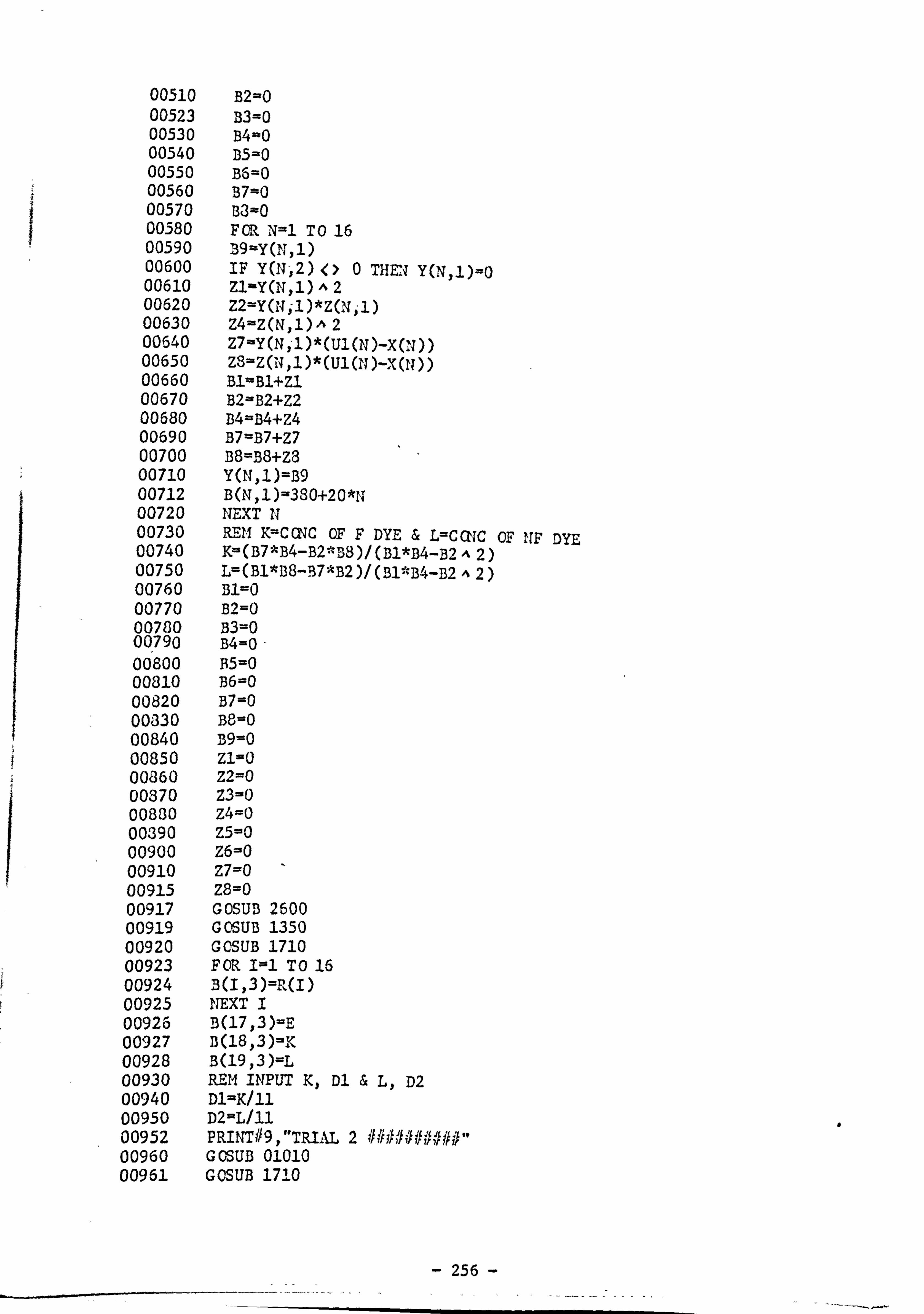
00510 B2=0 00523 B3-0 00530 B4-0 00540 B5=0 00550 BG=O 00560 B7=0 00570 B3=0 00580 FMI N=l To 16 00590 Bg-Y(N, l) 00600 IF Y(N-, 2) <> 0 THEN Y(N, 1)=o 00610 ZJ-Y(N, I) A2 00620 Z2-Y(N; 1)*Z(Njj) 00630 Z4=Z(N, 1)A 2 00640 V =Y (N y'l )* (Ul (N )-X (14 00650 Z3=Z(! l)1)*(Ul(N)-X(N)) 00660 BI-Bl+Zl 00670 B2=B2+Z2 00680 B4-B4+Z4 00690 VýV+V 00700 B8=B8+Z3 00710 Y(Ný1)=Bq 00712 B(N, 1)=380+20*N 00720 NEXT N 00730 REM K--CCUC OF F DYE & L=CCUC OF UF DYE 00740 K--(B7*B4-B2"BS)/(Bl*B4-B2 A 2) 00750 L=(Bl*B8-B7*B2)/(BM4-B2 A 2) 00760 B1-0 00770 B2=0 00780 B3=0 00790 B4=0- 00800 B5=0 00810 B6=0 00820 B7=0 00330 B8=O 00840 B9=0 00850 zi=o 00860 z2=0 00370 Z3=0 00830 z4=0 00390 Z5=0 00900 Z6=0 00910 Z7=0 00915 za=o 00917 GOSUB 2600 00919 GOSUB 1350 00920 GOSUB 1710 00923 FOR I=l TO 16 00924 B(i$3)=R(I) 00925 NEXT I 00926 B(17,3)=E 00927 B(18., 3)=K 00928 B(19,3)=L 00930 REM INPUT K, DI & L, D2 00940 Dl=K/11 00950 D2-L/11 00952 PRINT# 9, "TRIAL 2 ####iHf####" 00960 GOSUB 01010 00961 GOSUB 1710
- 256 -
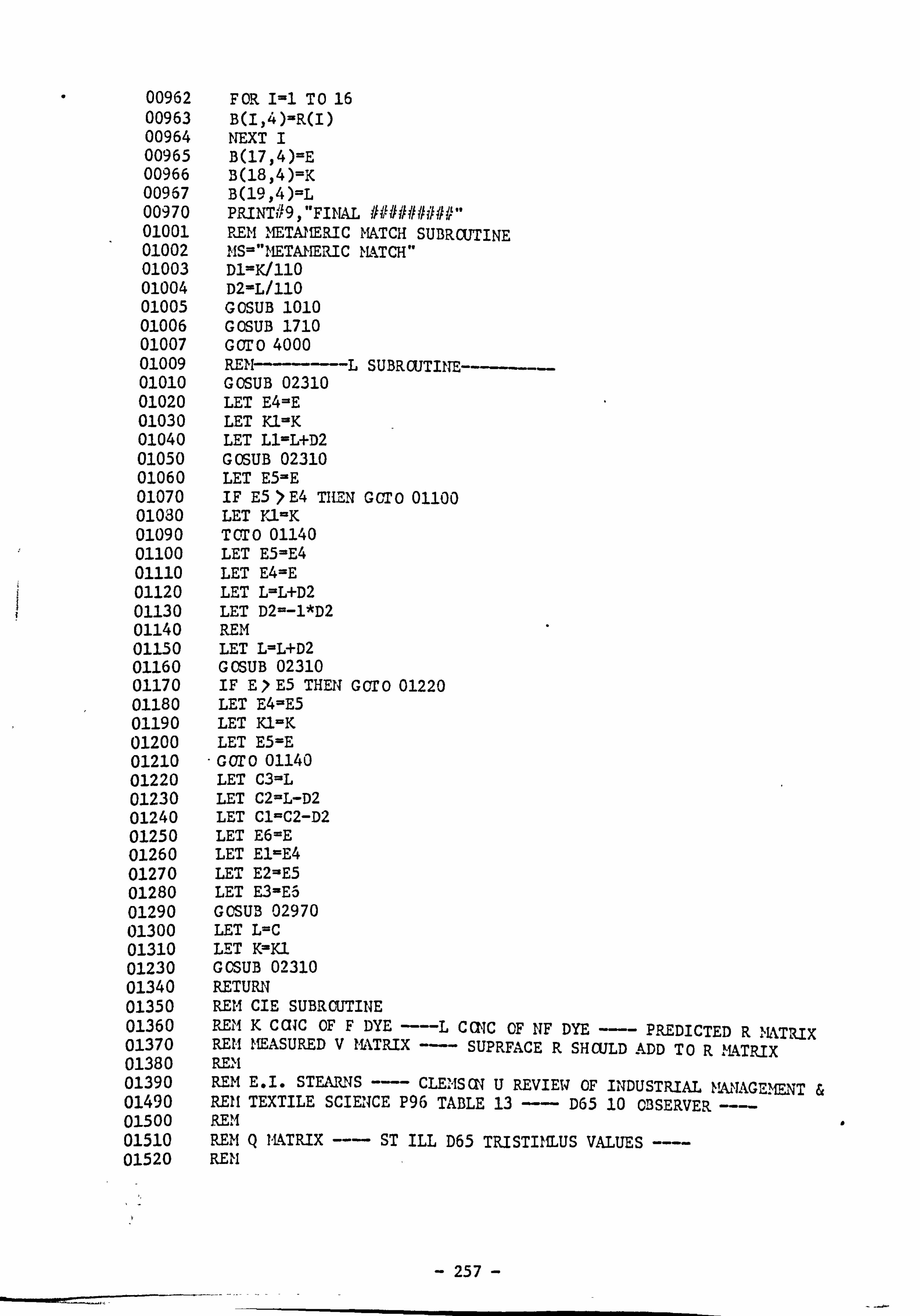
00962 FOR I=l TO 16 00963 B(1ý4)-R(I) 00964 ITEXT I 00965 B(17,4)=E 00966 B(18,4)ýK 00967 B(19,4)=L 00970 PRINTi#9, "FINAL #########" 01001 REM METATIERIC MATCH SUBRCUTINE 01002 11S="METAMERIC ILkTCH" 01003 Dl=K/110 01004 D2-L/110 01005 GOSUB 1010 01006 GOSUB 1710 01007 Goro 4000 01009 REN----L SUBRCUTINE----- 01010 GOSUB 02310 01020 LET E4=E 01030 LET Kl-K 01040 LET Ll-L+D2 01050 GOSUB 02310 01060 LET E5=E 01070 IF E5 >E4 THEN GCTO 01100 01080 LET Y, 1=K 01090 TOTO 01140 01100 LET E5=E4 01110 LET E4=E 01120 LET L=L+D2 01130 LET D2=-l*D2 01140 REM 01150 LET L=L+D2 01160 GOSUB 02310 01170 IF E> E5 THF14 GCTO 01220 01180 LET E4=E5 01190 LET Kl-K 01200 LET E5=E 01210 GOTO 01140 01220 LET C3=L 01230 LET C2=L-D2 01240 LET Cl=C2-D2 01250 LET E6=E 01260 LET El=E4 01270 LET E2-E5 01280 LET E3-E5 01290 GCSUB 02970 01300 LET L=C 01310 LET K-KI 01230 GCSUB 02310 01340 RETURN 01350 RE14 CIE SUBRCLJTI14E 01360 REM K CC11C OF F DYE ---L CGIC OF NF DYE PREDICTED R 'MATTRIX 01370 REM MEASURED V M&TRIX --- SUPRFACE R SHCULD ADD TO R 'tkTRIX 01380 REM 01390 REM E. I. STEAILIIIS --- CLEMSCK U REVIEW OF INDUSTRIAL =NAGEMENT & 01490 REM TEXTILE SCIENCE P96 TABLE 13 -- D65 10 OBSERVER 01500 REM 01510 REM Q I-L&TRIX --- ST ILL D65 TRISTI11LUS VALUES ---- 01520 REN
A
- 257 -
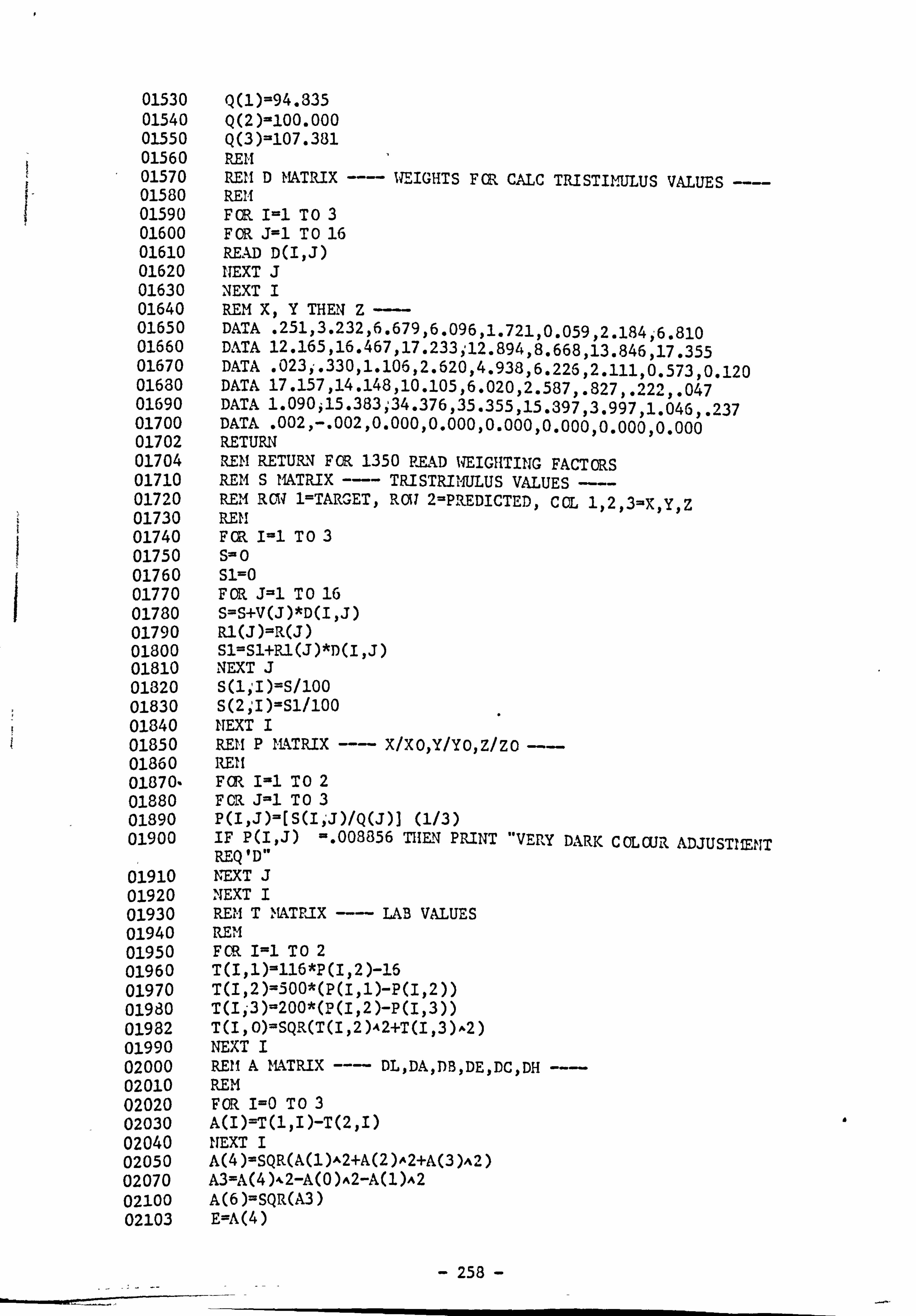
I
01530 01540 01550 01560 01570 01580 01590 01600 01610 01620 01630 01640 01650 01660 01670 01630 01690 01700 01702 01704 01710 01720 01730 01740 01750 01760 01770 01780 01790 01300 01810 01820 01830 01840 01850 01860 01870- 01880 01890 01900
01910 01920 01930 01940 01950 01960 01970 01980 01982 01990 02000 02010 02020 02030 02040 02050 02070 02100 02103
Q(1)=94.335 Q(2)-100.000 Q(3)=107.331 REM REM D MATRIX ---- IFEIGHTS FCR CALC TRISTIMULUS VALUES REM FCR I=l TO 3 F OR J-1 TO 16 READ D(I, J) ITEXT J 'ýHXT I REM X, Y THEI, 4 Z DATA . 251,3.232,6.679,6.096,1.721,0.059,2.184i6.810 DATA 12.165,16.467,17.233; 12.894,8.668,13.846217.355 DATA . 023i. 330,1.106,2.62OY4.938,6.226y2.111,0.573,0.120 DATA 17.157,14.148,10.105p6.020,2.587ý. 827,. 222y. 047 DATA l. 09Oil5.383; 34.376y35.355,15.397,3.997,1.046,. 237 DATA . 002, -. 002,0.000,0.000,0.000,0. oooyo. oooyo. ooo RETURN REM RETURN FOR 1350 READ 14EIGIITIIIG FACTORS REM S MATRIX --- TRISTRIIIHULUS VALUES -- REM ROW I=TARGET, Ral 2=PTREDICTED, CCL 1,2y3=X, Y, Z REM FCR 1=1 To 3 S=O Sl=O F OR J=l T0 16 S2'-S+V(J)*D(I, J) Rl(J)=R(J) Slý-Sl+Rl(J)*D(I, J) NEXT J S(1; I)=S/100 S(2; I)=Sl/100 ITEXT I REM P IATRIX --- X/XO, Y/YO, Z/zo RETI FCR I-1 TO 2 F OR J-1 TO 3 P(I, J)=[S(I)'J)/Q(J)l (1/3) IF P(I, J) =. 008856 THEIN PRINT REQ'D" NEXT J NEXT I REM T LAB VALUES REM FOR I=l TO 2 T(Ixl)=116*P(I, 2)-16 T(Ij2)ý300*(P(I, 1)-P(I, 2)) T(I , -3)-200*(P(Iý2)-P(I, 3)) T(I, O)=SQR(T(I, 2)A2+T(I, 3),. 2) NEXT I
"VERY DARK CCLaJR ADJUSTMENT
REII A MATRIX --- DL, DA, DB, DE, DC, DH REM FOR I=O To 3 A(I)=T(1, I)-T(29I) NEXT I A(4)-SQR(A(1)A2+A(2)ot2+A(3)A2) A3=A(4). %2-A(O)A2-A(1)A2 A(6)=SQR(A3) E=A(4)
- 258 -

02104 PRIllT#9j"CF="; Ki ýIF="; Lý" DE="; E "Cl 02105 RETUllLN 02310 REI1,1-----K--- --SUBRCAJTINE 02320 GOSUB 02600 02330 LET El=E 02340 LET K7-K+Dl 02350 GOSUB 02600 02360 LET E2=E 02370 IF E2>El THEN GOrO 02390 02380 GOTO 02430 02390 LET E2=El 02400 LET El=E 02410 LET K=K-Dl 02420 LET Dl=-l*Dl 02430 REM 02440 LET K7-K+Dl 02450 GOSUB 02600 02460 IF E> E2 THEN GOTO 02500 02470 LET El=E2 02480 LET -r2=E 02490 GCrO 02430 02500 LET C3-K 02510 LET C2=K-Dl 02520 LET Cl=C2-Dl 02530 LET E3=E 02540 GOSUB 02970 02550 LET K=C 02560 LET Dl=K/11 02570 GOSUB 02600 02590 RETUPUT 02600 REM MATCHING SUBROUTINE 02610 FOR M=l TO 16 02620 IF W(N, 1)=O THEN GOTO 02840 02630 REM NFIF FOlU4ULAE 02640 IF K40 THEN Dl=-K/15 02642 IF K <0 THEN K-. 00001 02653 IF L< 0 THEN D2-L/15 02655 IF L< 0 THEN L-. 00001 02660 Zl=Y(N)4)*K*(EXP((KAY(11,2))*Y(tl, 3))) 02670 Z3=li(N)2)*(Zl*((l/(1+1-/(N, 1)*L))^ ((K)A (-. 2)))) 02630 Z2-X(N)+Y(1411)*K+Z(N, -l)*L 02685 IF Z2 40 THEN Z2=. 0000000001 02690 Z2-(100+Z2)-SQR((100+Z2)^ 2-10000) 02700 R(N)=Z2+Z3 02710 zi=o 02720 Z2=0 02730 Z3=0 02740 GOTO 02880 02840 REM K/S CALC 02850 Zl-X(-N)+R*Y(N, 1)+L*Z(N, l) 02852 IF Zl< 0 THEN Zl=. 0000000001 02860 R(,. 11)=(100+Zl)-SQR((100+Zl) #% 2-10000)+J. l 02870 zi=o 02830 NEXT N 02882 IF If$ "MEETAME'11,11C MATCH" THEll GCTO 2890 02884 GOSUB 1710 02886 GOTO 2950 02890 FOR 11=1 T016 02900 Zl=V(N)-R(N)
- 259 -

02910 E=E+Zl A2 02920 NEXT N 02930 E=SQR(E/16) 02932 PRINT#9, IOCF= .1 ; K, "CNF='*; L)ý"ERR0R="; E 02940 zl--O 02950 RETURN 02960 REM 02970 REM Q FIT --- --SUBROUTINE 02980 LET Al=(E2-El)*(C3-Cl)-(E3-El)*(C2-Cl) 02990 LET A2=(C2A2-ClA2)*(C3-Cl)-(C3^ 2-Cl A2)*(C2-Cl) 03000 LET A--Al/A2 03010 LET B=((E3-El)-A*(C3A2-CJA2))/(C3-Cl) 03020 LET C=-B/(2*A) 03030 'RETURN 04000 PRINT"##### PREDICTED RECIPE , #####" 04001 FOR I=l TO 16 04002 B(Iý6)=R(I) 04003 NEXT I 04004 B(17ý6)=E 04005 B(18,6)=K 04006 B(19,6)=L 04010 PRINT 04020 PRINT"CCN. OF F DYE="; K, "CON. OF NF DYE=*'; L 04030 PRINT 04040 PRINT"R. -EFLECTICK VALUES" 04050 FOR I=l TO 6 04060 PRINT Rl(I), 04070 NEXT I 04075 PRINT 04080 PPII-IT"DE="; A(4), "DL="; A(l) '*DA7-"; A(2)j"DB="; A(3) 2 04090 PRINT "DC="; A(O), "Dll="; A(6) 04100 PRINT"INPUT FILNAIIE FOR OUTPUT" 04120 INPUT B$ 04104 FILE#1=B$ 04106 PRINT#1; USING 4600, "14AVELFI-IGTH")"TARGET"I"TRIAL 1", TRIAL 2", "FINAL'* 04110 FOR I=l TO 16 04112 PRINT#1, USING 4500, B(1; 1), B(I, -2), B(I; 3)ýB(I; 4)-, B(I. 6) 04114 NEXT I 04116 PRINT#1, USING 4500, "DE CIELAB'*, B(Iy--2), B(Iy3), -B(I, -4), B(I. 6) 04118 I=I+l 04120 PRIjrr#l, USING 4500, " F DYE "yB(I)2), B(I, -3), B(I, 4), B(I, 6) 04122 I=I+l 04124 PRINT#1, USING 4500, " NF DYE ", B(I, 2)yB(I,, 3)yB(1,4), B(IY6) 04500 : ######### ###. ### ###. ###
### ### ### # 1### 1# ## Ir #11f 04600 li 05000 CLOSEi#9 05010 PRINT" ZLF , ITERATE, PR 06000 END
- -260

C2 Data (The measurement and calibration contants for L. Red G and Red 3BEL)
Table C2.1 Reflectance Values of the Substrate
rim
400 '70.90 420 77.15 440 80.39 460 82.01 480 82.88 500 82.93 520 82.89 540 83.13 560 83.22 580 83.38 600 83.83 620 84.15 640 84.74 660 85.69 680 86.38 700 86.57
Table C2.2 Total Radiance Factors of Dyei gs of Palanil Lumnious Red G
Concentration of Lumnious Red G
nm . 005 . 01 . 025 . 05 .1 . 25 .5 1.0
400 68.060 66.170 60-. 820 55.190 46-350 35-510 25.950 18.320 420 73.830 71.670 65.390 60.010 51.090 39.020 23.680 20.450 440 76.850 74.500 68.480 62.210 53.040 40.490 29.600 20.930 460 75.600 71.560 62.790 54.280 44.010 31.120 21.440 14.360 480 71.990 65.890 54.600 44-550 34.040 22.090 14.050 8.790 500 67.720 60.070 47.330 36.870 26.860 16.270 9.720 5.800 520 63.890 55.220 41.820
. 31.400 22.070 12.640 7.170 4.190
540 65.010 56.650 43.530 33.210 23.740 13.990 8.150 4.860 560 74.850 59.390 58.940 49.350 38.930 26.680 17.920 11.860 580 95.420 99.370 103.490 102.980 96.820 33.820 69.020 53.980 600 98.020 106.310 120.380 131.430 138.190 140.910 135.920 122.480 620 96.920 104.660 113.830 131.210 141.200 151.140 155.180 150.110 640 93.110 97.990 107.640 116.350 123.500 132.090 . 137.840 137.360 660 90.690 93.470 99.210 104.400 103.040 112.380 115.580 115.370 680 89.450 91.120 94.730 97.950 99.800 101.970 103.740 103.230 700 88.400 39.380 91.750 93.810 94.690 95.900 97.200 96.780
- 261 -

Table C2.3 Total Radiance Factors of Dyeings of Palanil Red 5BEL
Concentration of, Red 5BEL
rim . 005 . 01 . 025 . 05 .1 . 25 .5 1.0
400 70.470 68.050 60.620 58.560 53.840 44.130 35.690 27.620 420 76.340 73.590 64.980 61.730 57.530 45.610 36.410 27.750 440 73.020 74.600 63.070 59.140 54.590 41.410 31.700 23.180 460 77.080 72.610 57.080 52.610 47.590 33.840 24.420 16.830 480 74.330 69.290 50.080 45.420 40.100 26.670 13.120 11.780 500 72.590 66.040 44.110 39.360 34.060 21.380 13.790 8.520 520 70.940 63.520 39.960 35.160 30.050 18.110 11.260 6.730 540 71.040 63.400 39.010 34.110 29.100 17.370 10.700 6.340 560 72.300 64.910 40.700 35.690 30.650 18.620 11.640 6.990 580 75.400 . 69.200 47.450 42.450 37.310 24.300 16.160 10.310 600 30.640 77.070 63.730 59.860 55.180 42.080 31.920 23.190 620 83.670 81.920 78.390 77.020 74.080 66.340 58.110 48.360 640 85.050 83.780 83.760 83.580 81.990 78.900 74.870 69.210 660 86.130 34.970 85.610 85.630 84.500 82.870 80.530 76.940 680 86.910 85.660 86.470 86.520 85.530 84.440 82.600 79.730 700 87.070 85.860 86.670 36.750 85.890 85.020 83.400 80.910
-Table C2.4 Total Radiance Factors of Dyeings of . 005. A*' L. 'led G and Red 5BEL
Concentration of Red 5BEL
nm . 005 . 01 . 025 . 05 1 . 25 .5 1.0
400 65.980 63.540 63.850 60.550 54.860 45.730 36.390 27.520 420 71.350 69.240 63.470 64.340 57.720 47.280 37.050 27.590 440 73.900 70.850 68.460 63.000 54.920 43.110 32.340 23.000 460 71.290 67.620 63.740 56.960 47.620 35.260 24.910 16.650 480 66.700 62.550 57.600 49.890 39.850 27.800 18.520 11.620
61.710 57.380 51.990 43.840 33.620 22.300 14.110 8.380 520 57.440 53.140 47.820 39.600 29.460 18.380 11.520 6.590
, 540 58.200 53.680 47.910 39.210 28.730 13.170 10.970 6.220 560 67.160 61.540 53.560 43.120 31.230 19.700 11.990 6.860 580 87.100 79.540 66.890 53.750 39.770 26.160 16.780 10.200 600 94.610 89.040 30.660 70.470 58.490 44. -550 32.920 23.100 620 96.310 92.640 89.870 84.490 77.840 68.710 59.370 43.920 640 92.830 90.180 90.130 37.630 84.700 30.430 75.830 69.520 660 90.950 89.200 89.520 38.100 86.490 34.080 111.370 77.450 680 90.080 89.110 89.200 88.280 37.120 85.480 83.270 80.210 700 39.100 83.420 88.600 87.960 37.080 35.320 83.950 81.280
- 252 -
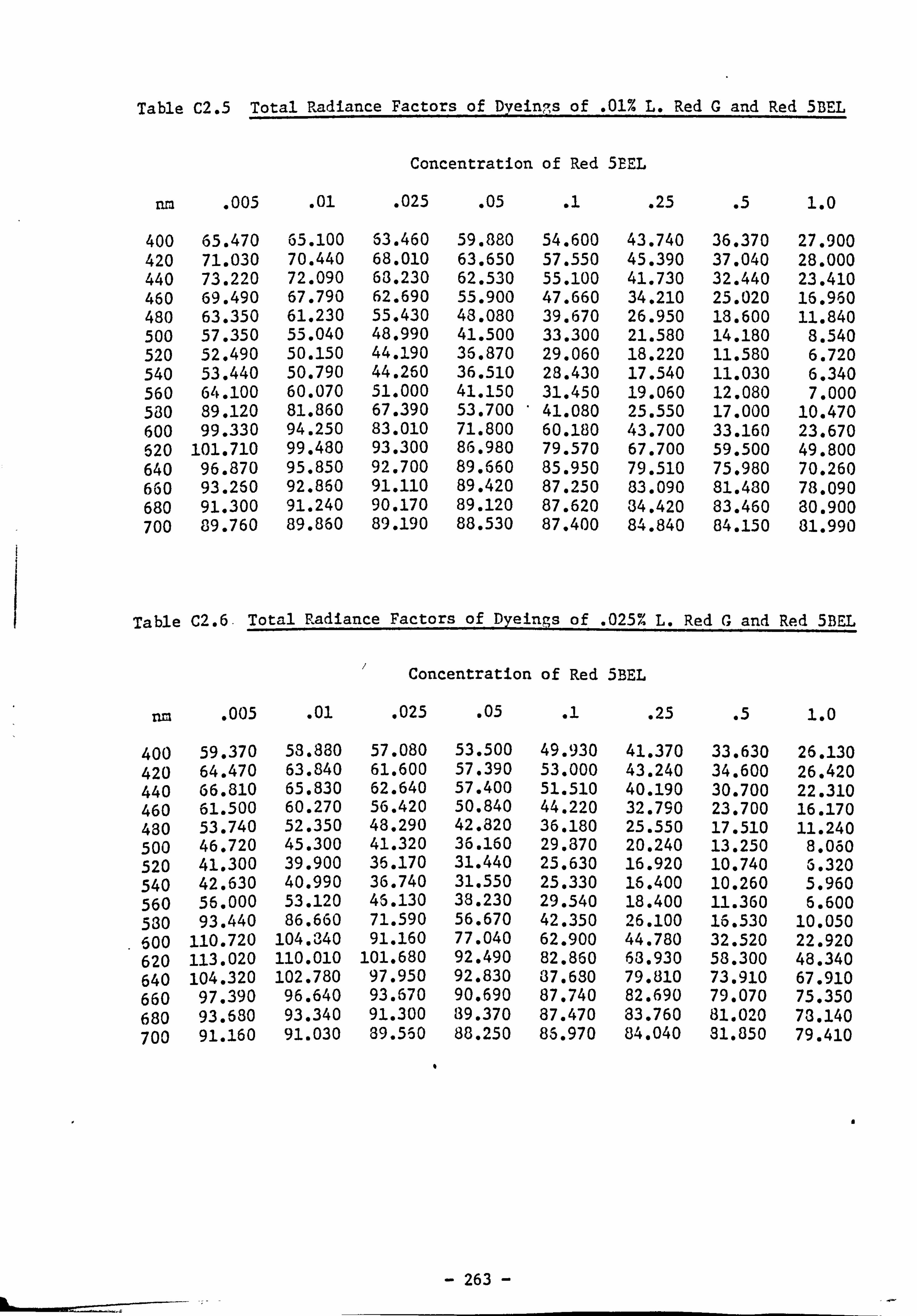
Table C2.5 Total Radiance Factors of Dyeinpýs of . 01% L. Red G and Red 5BEL
Concentration of Red 5EEL
nm . 005 . 01 . 025 . 05 .1 . 25 .5 1.0
400 65.470 65.100 63.460 59.880 54.600 43.740 36.370 27.900 420 71.030 70.440 68.010 63.650 57.550 45.390 37.040 28.000 440 73.220 72.090 63.230 62.530 55.100 41.730 32.440 23.410 460 69.490 67.790 62.690 55.900 47.660 34.210 25.020 16.960 480 63.350 61.230 55.430 48.080 39.670 26.950 18.600 11.840 500 57.350 55.040 48.990 41.500 33.300 21.580 14.180 8.540 520 52.490 50.150 44.190 36.870 29.060 18.220 11.580 6.720 540 53.440 50.790 44.260 36.510 28.430 17.540 11.030 6.340 560 64.100 60.070 51.000 41.150 31.450 19.060 12.080 7.000 530 89.120 81.860 67.390 53.700 , 41.080 25.550 17.000 10.470 600 99.330 94.250 83.010 71.800 60.180 43.700 33.160 23.670 620 101.710 99.480 93.300 86.980 79.570 67.700 59.500 49.800 640 96.870 95.850 92.700 89.660 85.950 79.510 75.980 70.260 660 93.260 92.860 91.110 89.420 87.250 33.090 81.430 78.090 680 91.300 91.240 90.170 89.120 87.620 34.420 83.460 80.900 700 89.760 89.860 89.190 88.530 87.400 84.840 84.150 81.990
Table C2.6. Total Radiance Factors of Dyeings of . 025% L. Red G and Red 5BEL
Concentration of Red 5BEL
nm . 005 . 01 . 025 . 05 .1 . 25 .51.0
400 59.370 53.880 57.080 53.500 49.930 41.370 33.630 26.130 420 64.470 63.840 61.600 57.390 53.000 43.240 34.600 26.420 440 66.810 65.830 62.640 57.400 51.510 40.190 30.700 22.310 460 61.500 60.270 56.420 50.840 44.220 32.790 23.700 16.170 430 53.740 52.350 48.290 42.820 36.180 25.550 17.510 11.240 500 46.720 45.300 41.320 36.160 29.370 20.240 13.250 8.060 520 41.300 39.900 36.170 31.440 25.630 16.920 10.740 G. 320 540 42.630 40.990 36.740 31.550 25.330 16.400 10.260 5.960 560 56.000 53.120 45.130 38.230 29.540 18.400 11.360 5.600
. 530 93.440 86.660 71.590 56.670 42.350 26.100 10.530 10.050 600 110.720 104.340 91.160 77.040 62.900 44.780 32.520 22.920 620 113.020 110.010 101.680 92.490 82.860 63.930 58.300 48.340 640 104.320 102.780 97.950 92.830 37.630 79.810 73.910 67.910 660 97.390 96.640 93.670 90.690 87.740 82.690 79.070 75.350 680 93.680 93.340 91.300 39.370 87.470 83.760 20 81.0ý 73.140 700 91.160 91.030 39.550 88.250 86.970 84.040 81.850 79.410
- 263 -
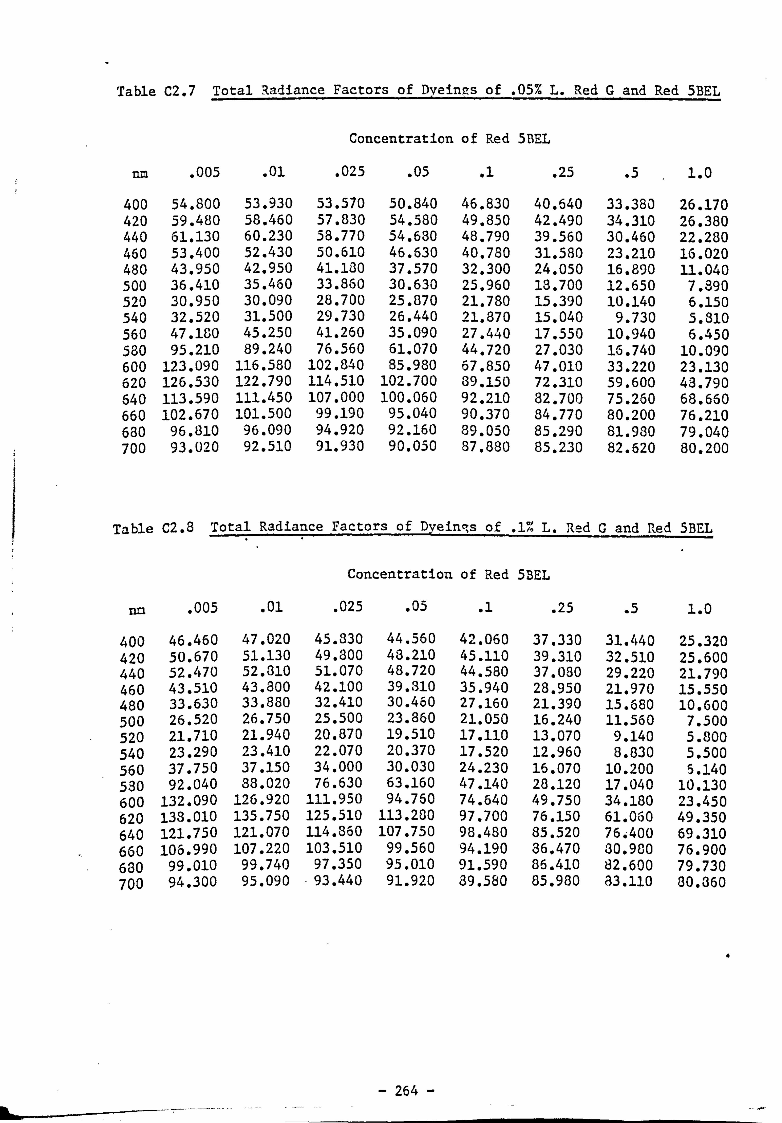
Table C2.7 Total Radiance Factors of Dyeings of . 05% L. Red G and Red 5BEL
Concentration of Red 5BEL
nm . 005 . 01 . 025 . 05 .1 . 25 .5 1.0
400 54.800 53.930 53.570 50.840 46.830 40.640 33.380 26.170 420 59.480 58.460 57.830 54.580 49.850 42.490 34.310 26.380 440 61.130 60.230 58.770 54.630 48.790 39.560 30.460 22.280 460 53.400 52.430 50.610 46.630 40.780 31.580 23.210 16.020 480 43.950 42.950 41.130 37.570 32.300 24.050 16.890 11.040 500 36.410 35.460 33.860 30.630 25.960 18.700 12.650 7.890 520 30.950 30.090 28.700 25.870 21.780 15.390 10.140 6.150 540 32.520 31.500 29.730 26.440 21.870 15.040 9.730 5.810 560 47.180 45.250 41.260 35.090 27.440 17.550 10.940 6.450 580 95.210 89.240 76.560 61.070 44.720 27.030 16.740 10.090 600 123.090 116.580 102.840 85.980 67.850 47.010 33.220 23.130 620 126.530 122.790 114.510 102.700 39.150 72.310 59.600 48.790 640 113.590 111.450 107.000 100.060 92.210 82.700 75.260 68.660 660 102.670 101-500 99-190 95.040 90.370 84.770 80.200 76.210 680 96.810 96.090 94.920 92.160 89.050 85.290 81.980 79.040 700 93.020 92.510 91.930 90.050 87.880 85.230 82.620 80.200
Table C2.8 Total Radiance Factors of Dyeincýs of . 1% L. Red G and red 5BEL
Concentration of Red 5BEL
rm . 005 . 01 . 025 . 05 .1 . 25 .5 1.0
400 46.460 47.020 45.830 44.560 42.060 37.330 31.440 25.320 420 50.670 51.130 49.800 43.210 45.110 39.310 32-510 25.600 440 52.470 52.310 51.070 48.720 44.580 37.080 29.220 21.790 460 43.510 43.800 42.100 39.310 35.940 28.950 21.970 15.550 480 33.630 33.880 32.410 30.460 27.160 U. 390 15.680 10.600 500 26.520 26.750 25.500 23.860 21.050 16.240 11.560 7.500 520 21.710 21.940 20.870 19.510 17.110 13.070 9.140 5.800 540 23.290 23.410 22.070 20.370 17.520 12.960 8.830 5.500 560 37.750 37.150 34.000 30.030 24.230 16.070 10.200 5.140 530 92.040 88.020 76.630 63.160 47.140 28.120 A. 040 10.130 600 132.090 126.920 111.950 94.760 74.640 49.750 34.180 23.450 620 133.010 135.750 125.510 113.280 97.700 76.150 61.060 49.350 640 121.750 121.070 114.360 107.750 98.480 85.520 76300 69.310 660 106-990 107.220 103.510 99.560 94.190 86.470 30.980 76.900 630 99.010 99.740 97.350 95.010 91.590 86.410 82.600 79.730 700 94.300 95.090 . 93.440 91.920 89.580 85.980 83.110 80.360
- 264 -
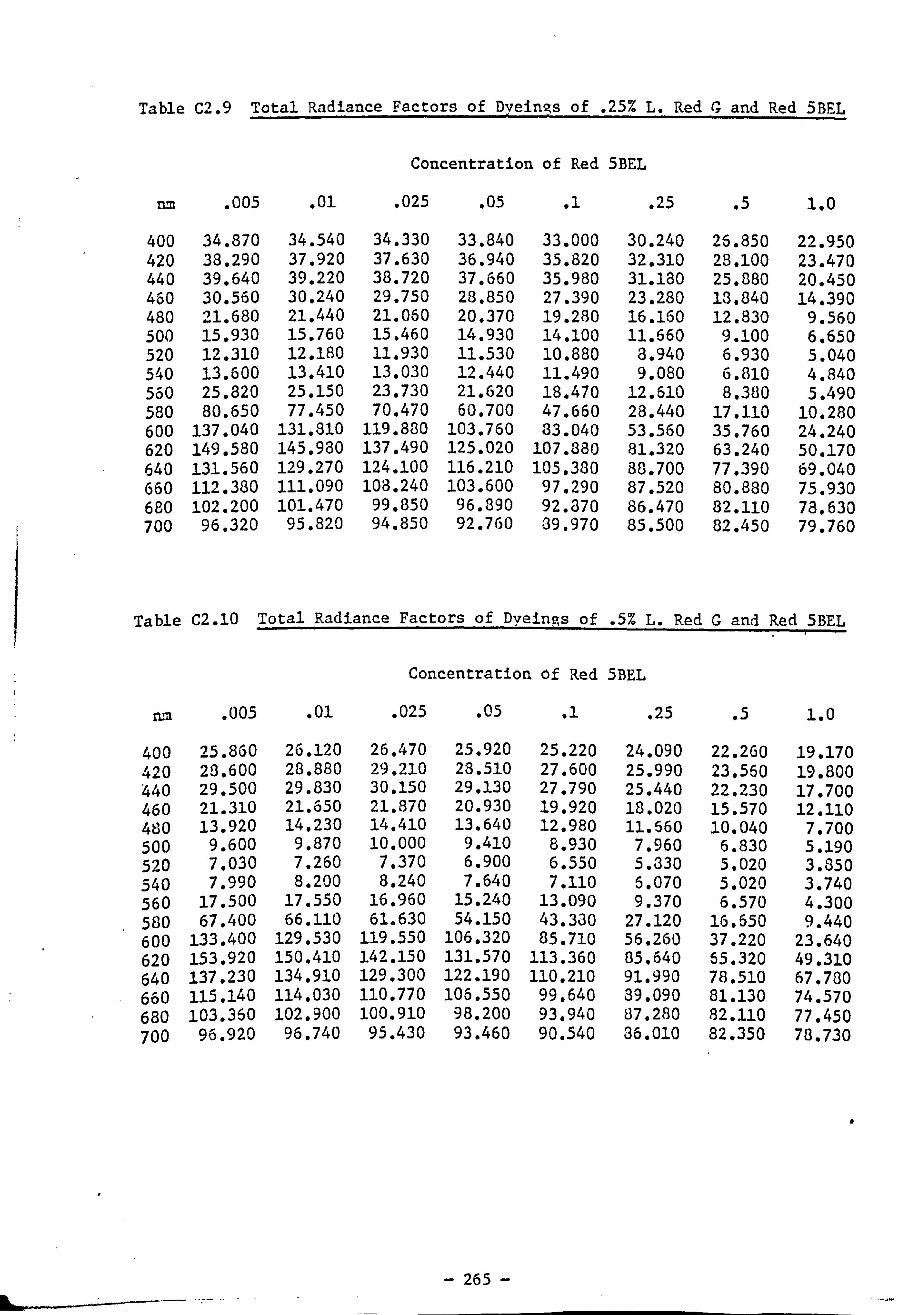
Table C2.9 Total Radiance Factors of Dyeings of . 25% L. Red G and Red 5BEL
Concentration of Red 5BEL
rLm . 005 . 01 . 025 . 05 .1 . 25 .5 1.0
400 34.870 34.540 34.330 33.840 33.000 30.240 26.850 22.950 420 38.290 37.920 37.630 36.940 35.820 32.310 2S. 100 23.470 440 39.640 39.220 38.720 37.660 35.980 31.180 25.880 20.450 460 30.560 30.240 29.750 28.850 27.390 23.280 13.840 14.390 480 21.680 21.440 21.060 20.370 19.280 16.160 12.830 9.560 500 15.930 15.760 15.460 14.930 14.100 11.660 9.100 6.650 520 12.310 12.180 11.930 11.530 10.880 3.940 6.930 5.040 540 13.600 13.410 13.030 12.440 11.490 9.080 6.810 4.840 560 25.820 25.150 23.730 21.620 18.470 12.610 8.380 5.490 580 80.650 77.450 70.470 60.700 47.660 23.440 17.110 10.280 600 137.040 131.310 119.830 103.760 33.040 53.560 35.760 24.240 620 149.580 145.980 137.490 125.020 107.380 81.320 63.240 50.170 640 131.560 129.270 124.100 116.210 105.380 88.700 77.390 69.040 660 112.380 111.090 108.240 103.600 97.290 87.520 80.880 75.930 680 102.200 101.470 99.850 96.890 92.370 86.470 82.110 78.630 700 96.320 95.820 94.850 92.760 39.970 85.500 82.450 79.760
Table C2.10 Total Radiance Factors of Dyeings of . 5% L. Red G and Red 5BEL
Concentration Of Red 5BEL
. 005 . 01 . 025 . 05 . 25 .5 1.0
400 25.860 26.120 26.470 25.920 25.220 24.090 22.260 19.170 420 28.600 28.880 29.210 28.510 27.600 25.990 23.560 19.800 440 29.500 29.830 30.150 29.130 27.790 25.440 22.230 17.700 460 21.310 21.650 21.870 20.930 19.920 18.020 15.570 12.110 480 13.920 14.230 14.410 13.640 12.980 11.560 10.040 7.700 500 9.600 9.870 10.000 9.410 8.930 7.960 6.830 5.190 520 7.030 7.260 7.370 6.900 6.550 5.330 5.020 3.850 540 7.990 8.200 8.240 7.640 7.110 5.070 5.020 3.740 560 17.500 17.550 16.960 15.240 13.090 9.370 6.570 4.300 580 67.400 66.110 61.630 54.150 43.330 27.120 16.650 9.440 600 133.400 129.530 119.550 106.320 85.710 56.260 37.220 23.640 620 153.920 150.410 142.150 131.570 113.360 85.640 55.320 49.310 640 137.230 134.910 129.300 122.190 110.210 91.990 78.510 67.780 6060 115.140 114.030 110.770 106.550 99.640 39.090 81.130 74.570 680 103.360 102.900 100.910 98.200 93.940 87.280 82.110 77.450 700 96.920 96.740 95.430 93.460 90.540 36.010 82.350 78.730
- 265 -

Table C2.11 Total Radiance Factors of Dyeings of 1.0% L. Red G and Red 5BEL
Concentration of Red 5BEL
. 005 . 01 . 025 . 05 .1 . 25 .5 1.0
400 17.640 17.690 17.590 17.640 17.400 16.910 16.280 14.740 420 19.870 19.990 19.890 19.260 19.720 18.680 17.630 15.530 440 20.440 20.630 20.410 18.540 20.590 13.560 16.960 14.290 400 13.940 14.040 13.900 12.140 14.220 12.500 - 11.330 9.420 480 8.480 8.540 3.440 7.210 8.720 7.540 6.830 5.630 500 5.550 5.580 5.530 4.690 5.710 4.930 4.480 3.760 520 3.960 3.980 3.940 3.400 4.050 3.530 3.250 2.800 540 4.680 4.670 4.580 3.970 4.460 3.770 3.320 2.770 560 11.910 11.780 11.140 9.690 9.150 6.510 4.680 3.280 580 54.100 53.240 49.370 43.960 36.450 23.540 14.690 3.500 600 122.680 120.440 111.470 102.420 82.460 55.000 36.590 23.270 620 151.150 148.870 140.730 134.820 112.130 84.840 64.760 48.620 640 138.000 136-230 130.530 126.270 110.350 90.930 77.240 66.100 660 115.400 114.330 111.040 109.250 98.700 87.360 79.340 72.540 680 103.200 102.540 100.510 100.350 92.280 85.520 80.360 75.650 700 96.720 96.340 94.920 95.090 89.020 84.340 80.680 77.160
Table C2.12 Calibration Data for the Substrate - TMSUB (Eq. 37)
nm K/ S
400 6.53324 420 3.77122 440 2.70465 460 2.25206 480 2.07953 500 2.01729 520 2.02717 540 1.96831 560 1.94651 530 1.90811 600 1.80257 620 1.7297 640 1.60001 660 1.40364 680 1.27039 700 1.23506
- 266 -

Table C2.13 Calibration Data for Mixture Dyeings of L Red G and Red 5BEL - rITLRR (Eq. 54)
K4 K5 400 . 00000 . 0000 420 . 00000 . 0000 440 . 00000 . 0000 460 . 00000 . 0000 480 . 00000 . 0000 500 . 00000 . 0000 520 . 00000 . 0000 540 . 00000 . 0000 560 . 00000 . 0000 580 13.16093 1.10768 600 12.09643 1.08317 620 9.52011 1.06806 640 9.85932 1.07680 660 10.73548 1.08858 680 11.53035 1.10717 700 13.37949 1.14146
Table C2.14 Calibration Data for Self-colour of the Red 5BEL (Eq. 38)
rm K/A K L m
400 100.13071 . 00000 . 00000
. 00000 420 101.39974 . 00000
. 00000 . 00000
440 140.00596 . 00000 . 00000
. 00000 460 230.91186 . 00000
. 00000 . 00000
430 330.54415 . 00000 . 00000
. 00000 500 582.72784 . 00000
. 00000 . 00000
520 790.64548 . 00000 . 00000
. 00000 540 354.12314 . 00000
. 00000 . 00000
560 752.81069 . 00000 . 00000
. 00000 580 455.10488 . 00000
. 00000 . 00000 600 140.44303 . 00000 . 00000 . 00000 620 27.45235 . 00000
. 00000 . 00000 640 5.92683 . 00000
. 00000 . 00000
660 2.44915 . 00000 . 00000 . 00000
680 1.62356 . 00000 . 00000
. 00000 700 1.30729 . 00000
. 00000 . 00000
- 267 -
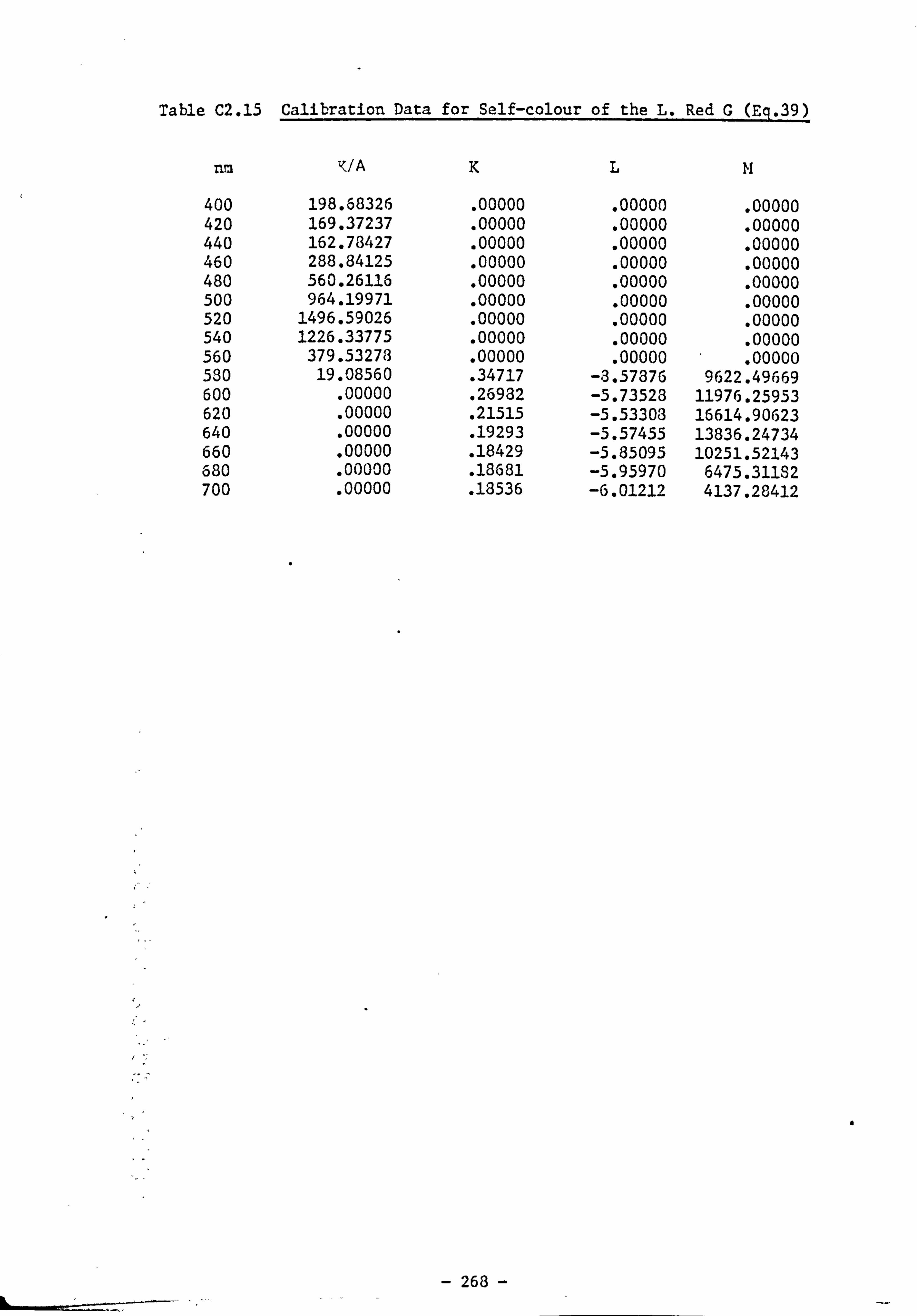
Table C2.15 Calibration Data for Self-colour of the L. Red G (Eq. 39)
nm K/A
400 198.68326 420 169.37237 440 162.78427 460 288.84125 480 560.26116 500 964.19971 520 1496.59026 540 1226.33775 560 379.53273 530 19.08560 600 . 00000 620 . 00000 640 . 00000 660 . 00000 680 . 00000 700 . 00000
K
. 00000
. 00000
. 00000
. 00000
. 00000
. 00000
. 00000
. 00000
. 00000
. 34717
. 26932
. 21515
. 19293
. 18429
. 18681
. 18536
LH
. 00000 . 00000
. 00000 . 00000
. 00000 . 00000
. 00000 . 00000
. 00000 . 00000
. 00000 . 00000
. 00000 . 00000
. 00000 . 00000
. 00000 . 00000 -3.57376 9622.49669 -5.73523 11976.25953 -5.53303 16614.90623 -5.57455 13836.24734 -5.85095 10251.52143 -5.95970 6475.31182 -6.01212 4137.28412
a
- 268 -
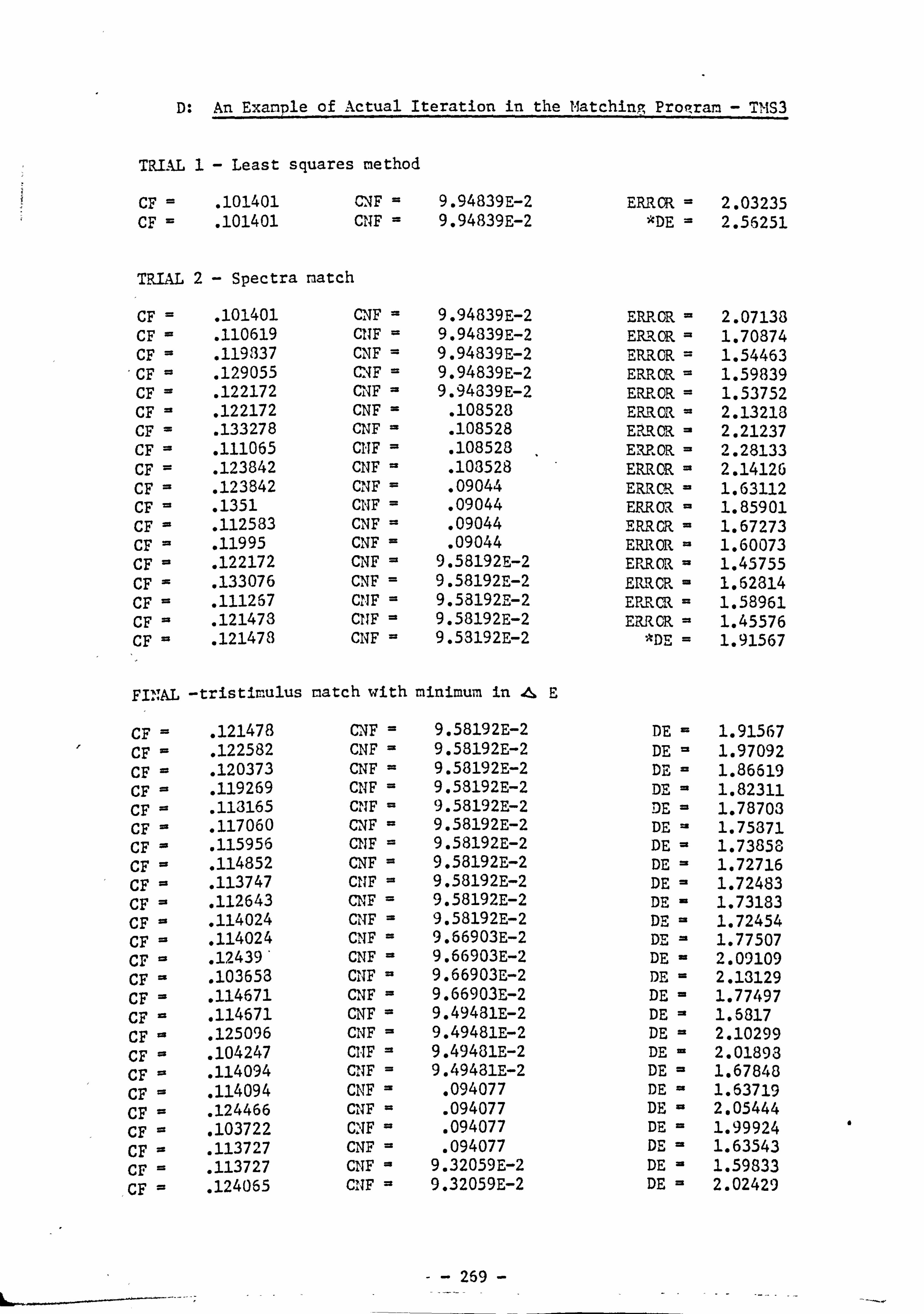
An Example of Actual Iteration in the Matching-ProRram - TMS3
TRIAL 1- Least squares method
CF = . 101401 CNF = 9.94839E-2 ERROR = 2.03235 CF ý . 101401 CNF = 9.94839E-2 *DE m 2.56251
TRIAL 2- Spectra match
CF = . 101401 CNF = 9.94839E-2 ERROR = 2.07138 CF = . 110619 CIIF = 9.94339E-2 ERROR = 1.70874 CF = . 119337 CNF = 9.94339E-2 ERROR = 1.54463 CF = . 129055 CNF = 9.94839E-2 ERROR. = 1.59839 CF . 122172 CNF = 9.94339E-2 ERROR = 1.53752 CF = . 122172 CNF = . 108528 ERROR - 2.13213 CF = . 133278 CNF = . 108528 ERROR = 2.21237 CF = . 111065 CNF = . 108523 E U, OR = 2.28133 CF = . 123842 CNF - . 103528 ERROR = 2.14126 CF = . 123842 CNF = . 09044 ERRC-R = 1.63112 CF = . 1351 CNF = . 09044 ERROR, = 1.85901 CF - . 112533 CNF = . 09044 ERRCR - 1.67273 CF = . 11995 CNF = . 09044 ERROR = 1.60073 CF - . 122172 CNF = 9.58192E-2 ERROR, = 1.45755 CF = . 133076 CNF = 9.58192E-2 ERROR = 1.62314 CF = . 111257 Q'IF = 9.58192E-2 ERROR = 1.58961 CF = . 121473 CITF = 9.58192E-2 ERROR = 1.45576 CF - . 121478 CNF = 9.53192E-2 *DE = 1.91567
FI'. KT, AL -tristirulus match with minimum in &
CF = . 121478 C. NF = 9.58192E-2 DE - 1.91567 CF . . 122582 CNF = 9.58192E-2 DE = 1.97092 CF - . 120373 CNF = 9.58192E-2 DE = 1.86619 CF - . 119269 CNF = 9.58192E-2 DE - 1.82311 CF - . 113165 CllTF - 9.58192E-2 DE = 1.78703 CF - . 117060 CNF = 9.58192E-2 DE - 1.75371 CF - . 115956 CNF = 9.58192E-2 DE - 1.73858 CF - . 114852 CNF = 9.58192E-2 DE = 1.72716 CF = . 113747 CNF = 9.58192E-2 DE = 1.72483 CF - . 112643 CNF = 9.58192E-2 DE - 1.73183 CF - . 114024 CLITF = 9.58192E-2 D lE - 1.72454 CF - . 114024 CLNF = 9.66903E-2 DE = 1.77507 CF - . 12439' CNF - 9.66903E-2 DE - 2.09109 CF - . 103658 CNF = 9.66903E-2 DE - 2.13129 CF - . 114671 CNF - 9.66903E-2 DE = 1.77497 CF - . 114671 CNF - 9.49481E-2 DE - 1.6817 CF - . 125096 CNF - 9.49481E-2 DE - 2.10299 CF - . 104247 CI-IF = 9.49481E-2 DE - 2.01893 CF - . 114094 CINF = 9.49481E-2 DE = 1.67848 CF - . 114094 CNF = . 094077 DE - 1.63719 CF - . 124466 CNF = . 094077 DE - 2.05444 CF = . 103722 CýNF = . 094077 DE - 1.99924 CF - . 113727 CNF = . 094077 DE - 1.63543 CF = . 113727 CNF - 9.32059E-2 DE - 1.59833 CF = . 124065 CINF = 9.32059E-2 DE - 2.02429
a
269 -

CF = . 103388 CNF = 9.32059E-2 DE = 1.97004 CF = . 113375 NIF = 9.32059E-2 DE = 1.59661 CF . 123682 CNF = 9.23349E-2 DE 1.99932 CF . 103068 CNF = 9.23349E-2 DE 1.94377 CF . 113024 CNF = 9.23349E-2 DE 1.56242 CF . 113024 CINF = 9.14638E-2 DE 1.53516 CF . 123293 CNF - 9.14638E-2 DE 1.97863 CF = . 102749 CNF = 9.14638E-2 DE 1.92172 CF = . 112671 CNF = 9.14638E-2 DE 1.53332 CF = . 112671 CNF = 9.05927E-2 DE 1.51164 CF - . 122914 CNF = 9.05927E-2 DE 1.96253 CF = . 102428 CITF = 9.05927E-2 DE 1.90424 CF = . 112317 CNF = 9.05927E-2 DE 1.50973 CF = . 112317 CNF = 8.97216E-2 DE 1.49405 CF - . 122528 CNIF = 8.97216E-2 DE 1.95109 CF = . 102106 CNF = 8.97216E-2 DE = 1.8916 CF - . 111962 CNF = 8.97216E-2 DE = 1.4921 CF - . 111962 CNF - 8.88505E-2 DE = 1.43278 CF - . 12214 CNF = 8.88505E-2 DE = 1.94454 CF = . 101783 CNF = 8.83505E-2 DE = 1.88403 CF = . 111605 CNITF = 8.88505E-2 DE = 1.48078 CF - . 111605 CNF - 8.79794E-2 DE - 1.47314 CF - . 121751 QIF - 8.79794E-2 DE - 1.94309 CF - . 101459 CNF - 8.79794E-2 DE = 1.88172 CF = . 111246 CilF = 8.79794E-2 DE = 1.47609 CF = . 111246 CNF - 8.71034E-2 DE = 1.48036 CF - . 121360 CNF = 8.71084E-2 DE = 1.94685 CF - . 101123 CNF = 3.71084E-2 DE = 1.38484 CF = . 1101885 CNF = 8.71084E-2 DE 1.47828 CF - . 111246 CNF = 8.78211E-2 DE 1.47626 CF = . 121327 CNF = 8.78211E-2 DE 1.91791 CF - . 101166 CNT F = 3.78211E-2 DE 1.90079 CF - . 111147 CIT = 8.78211E-2 DE 1.47534 CF - . 111147 CNF - 8.73211E-2 *DE 1.47584
- 270 -
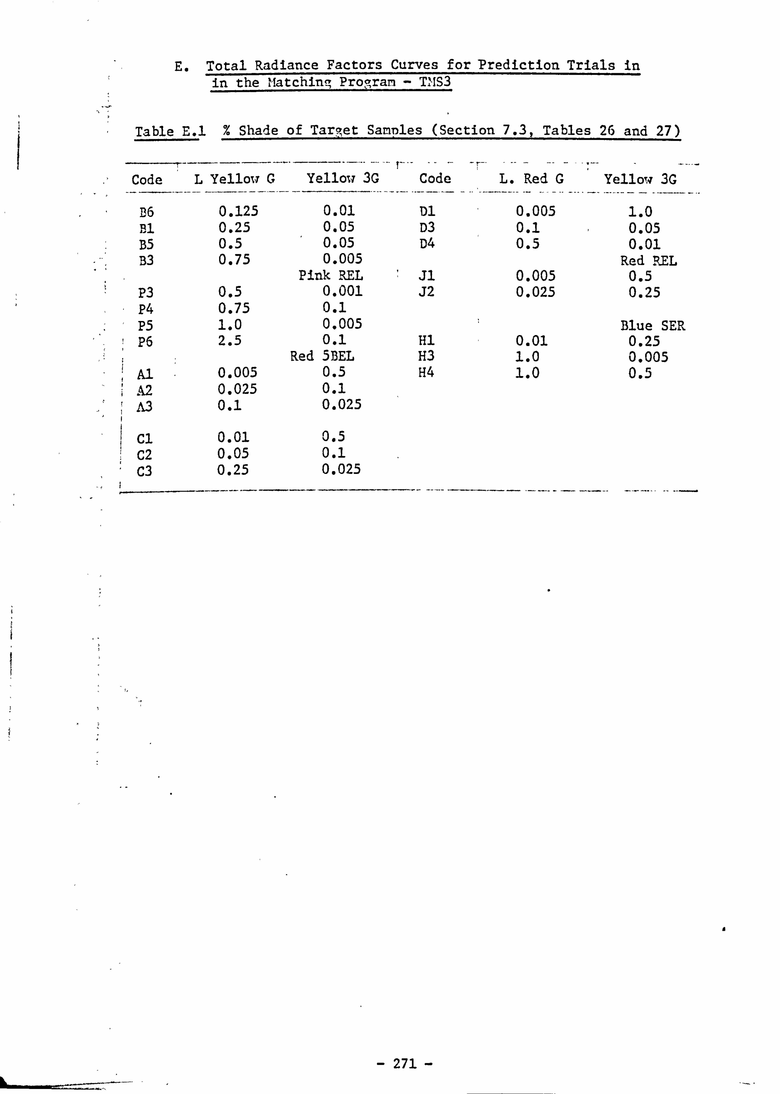
E. Total Radiance Factors Curves for Prediction Trials in in the Matching Program - TIM
Table E. 1 % Shade of Target Samples (Section 7.3, Tables 26 and 27)
Code L Yellow G Yellow 3G Code L. Red G Yellow 3G
D6 0.125 0.01 Dl 0.005 1.0 p1l 0.25 0.05 D3 0.1 0.05 B5 0.5 0.05 D4 0.5 0.01 B3 0.75 0.005 Red REL
Pink REL il 0.005 0.5 P3 0.5 0.001 J2 0.025 0.25 P4 0.75 0.1 P5 1.0 0.005 Blue SER P6 2.5 0.1 Hl 0.01 0.25
Red 5BEL H3 1.0 0.005 Al 0.005 0.5 H4 1.0 0.5 A2 0.025 0.1 A3 0.1 0.025
C, 0.01 0.5 C2 0.05 0.1 C3 0.25 0.025
8
- 271 -
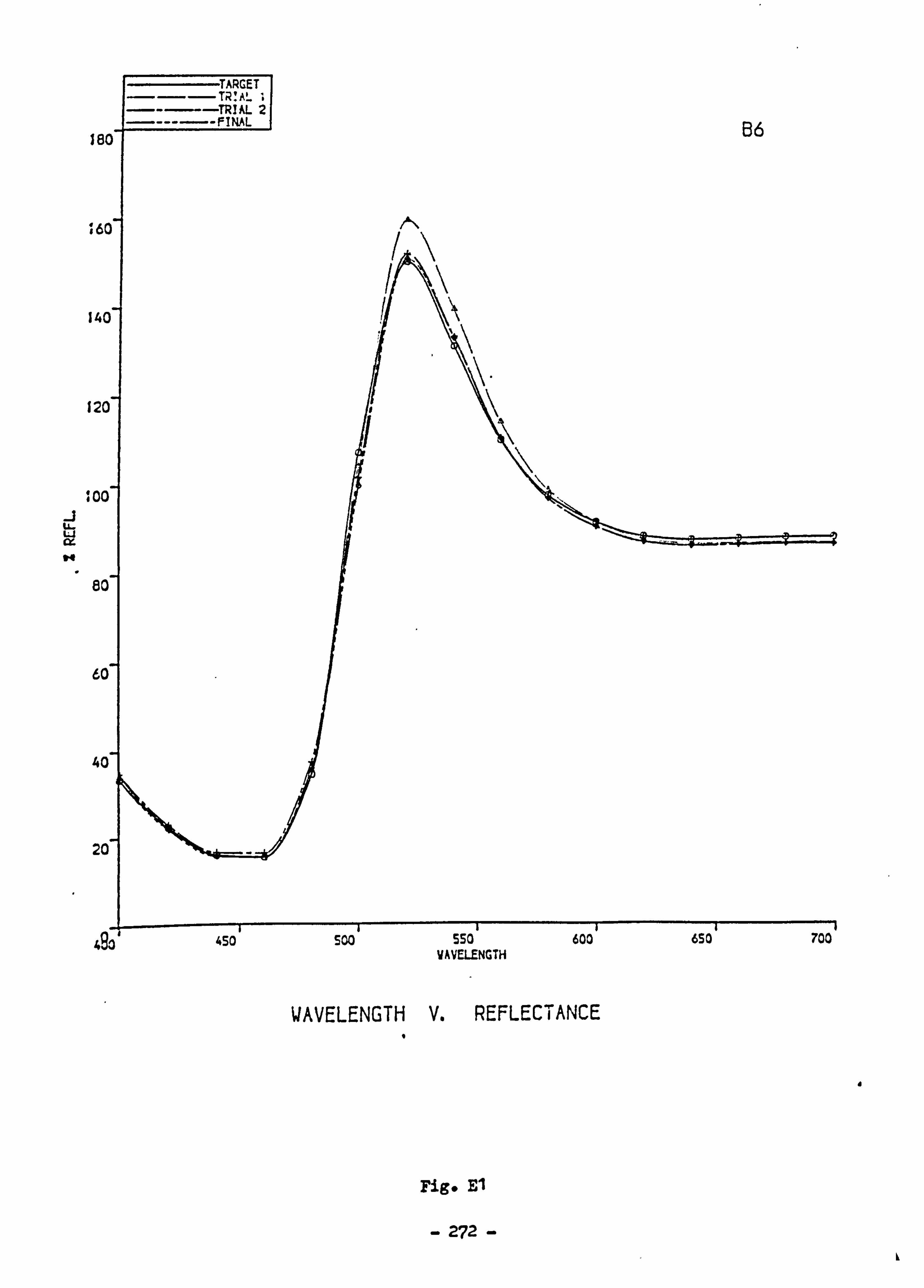
IN
s6C
14C
120
4 too
Li cx
80
60
40
20
WAVELENGTH V. REFLECTANCE I
rig* El
- 272 -
4
k
493,450' 500' 550 600 650 700 WAVELENGTH
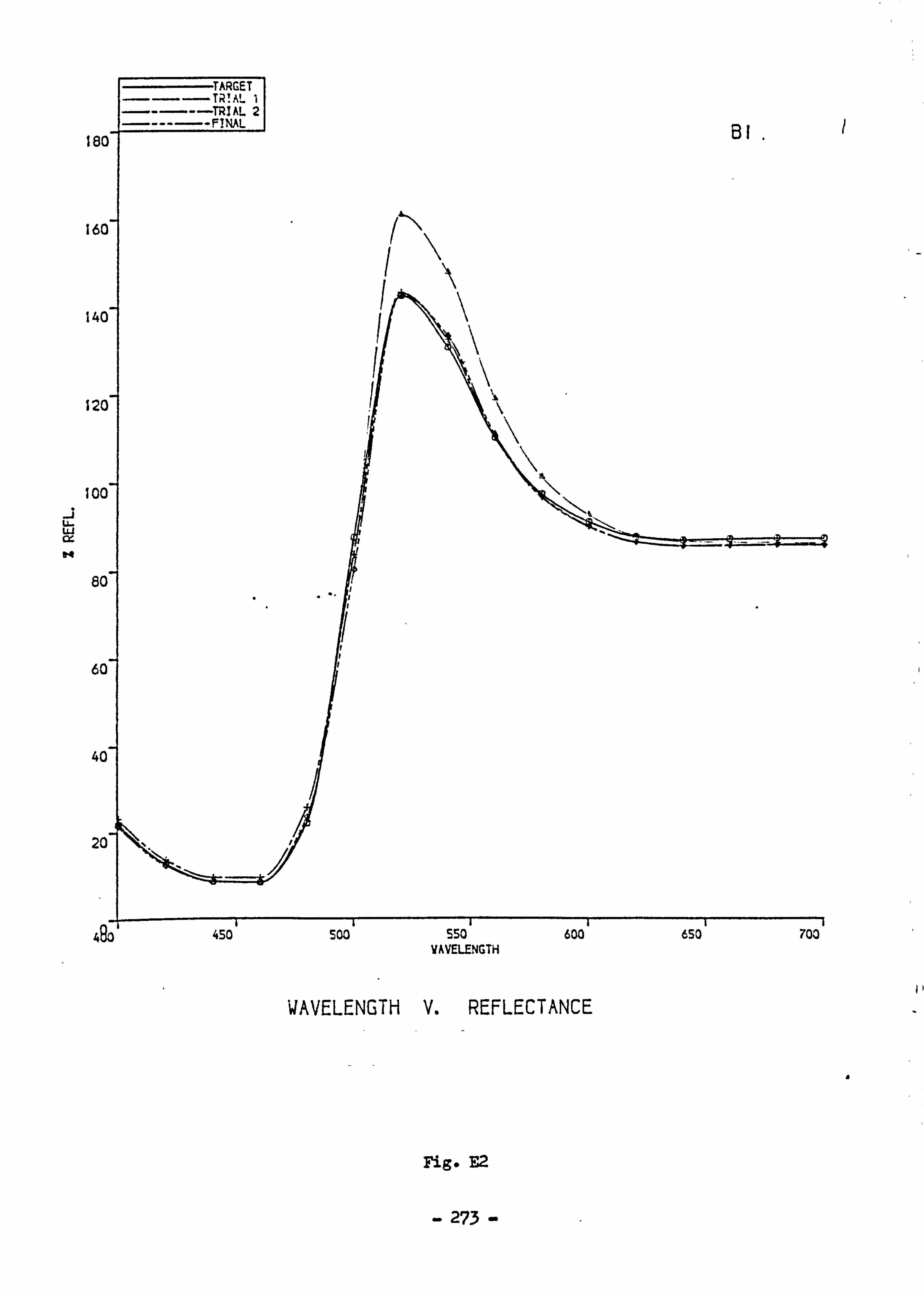
lec
160
140
120
100
-j U- uj aq
80
60
40
20
WAVELENGTH V. REFLECTANCE
Fig. E2
a
- 273 -
490' 450' 500' 550' 600' 650' 700 VAVELENGTH

180
160
140
120
too
U- uj
80
60
40
20
WAVELENGTH V. REFLECTANCE
a
Fig- E3
- 274 -
490' 450' sw, sso, 600,650" 700 VAVELENGTH

I ec
16C
14C
120
loo
-j LL-
t4
80
60
40
20
WAVELENGTH V. REFLECTANCE
a
Fig. E4
-275 -
490' 450' 500' SSO' 600 650 700 VAVELENGTH
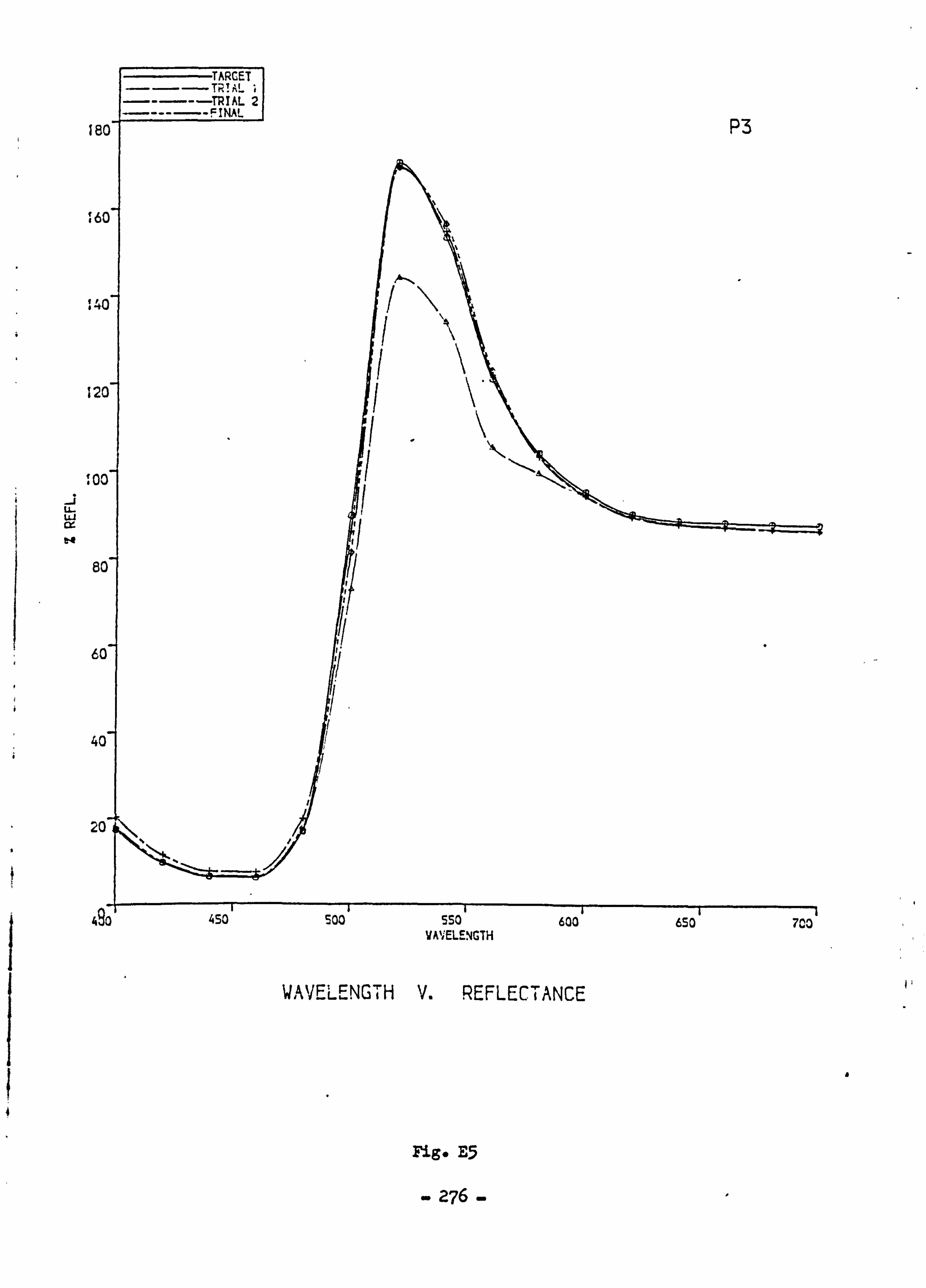
18(
114(
12C
f Or
uj 8c
M
40
20
a
Fig* E5
-276-
490' 450' SOO' 550' 600 650 700 VAVELENGTH
WAVELENGTH V. REFLECTANCE
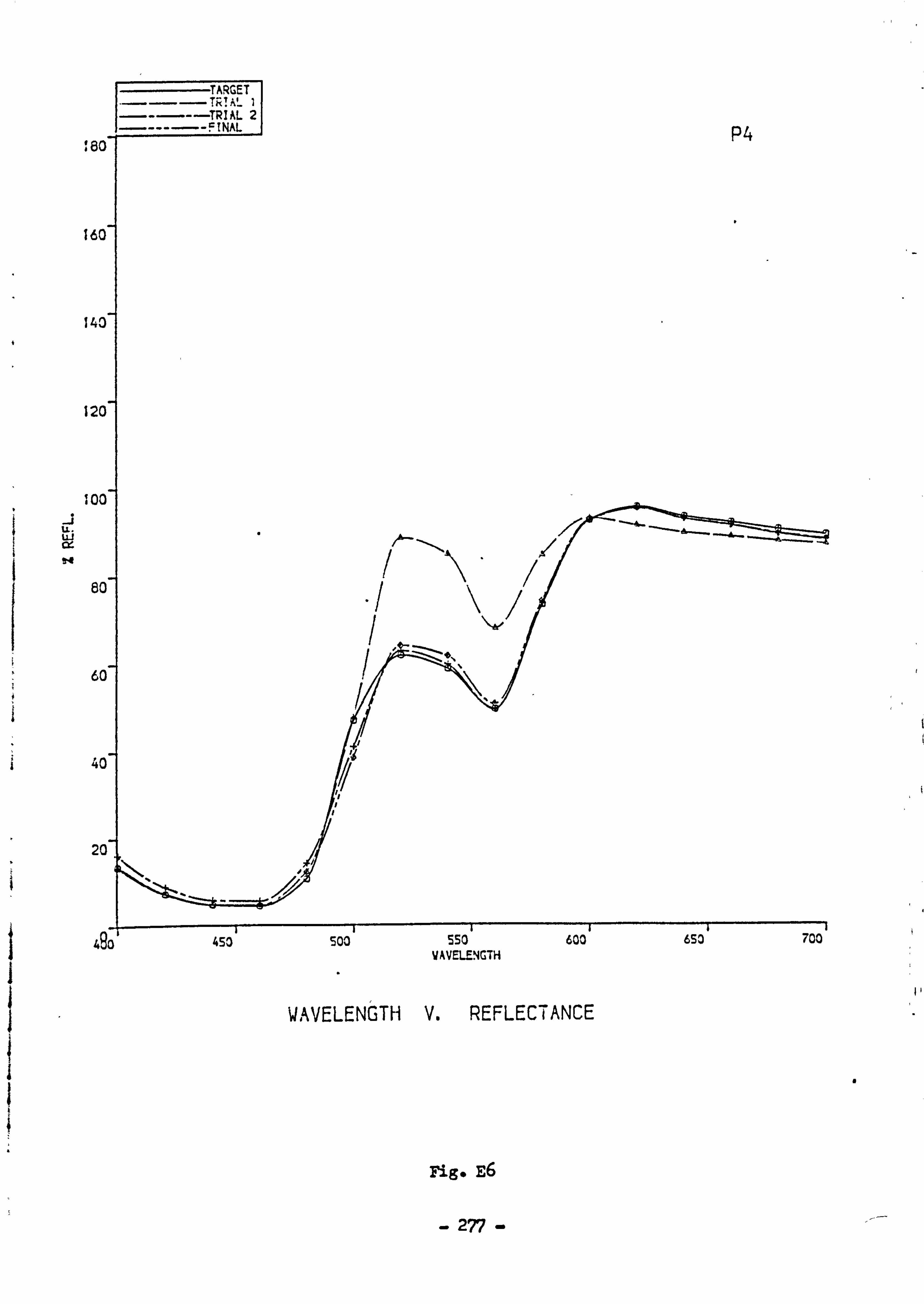
180
160
140
120
100
ui cy t4
60
60
40
20
a
Fig* E6
- 277 -
490' 450' 500" 550 600 6so 700 VAVELENGTH
WAVELENdTH V. REFLECTANCE
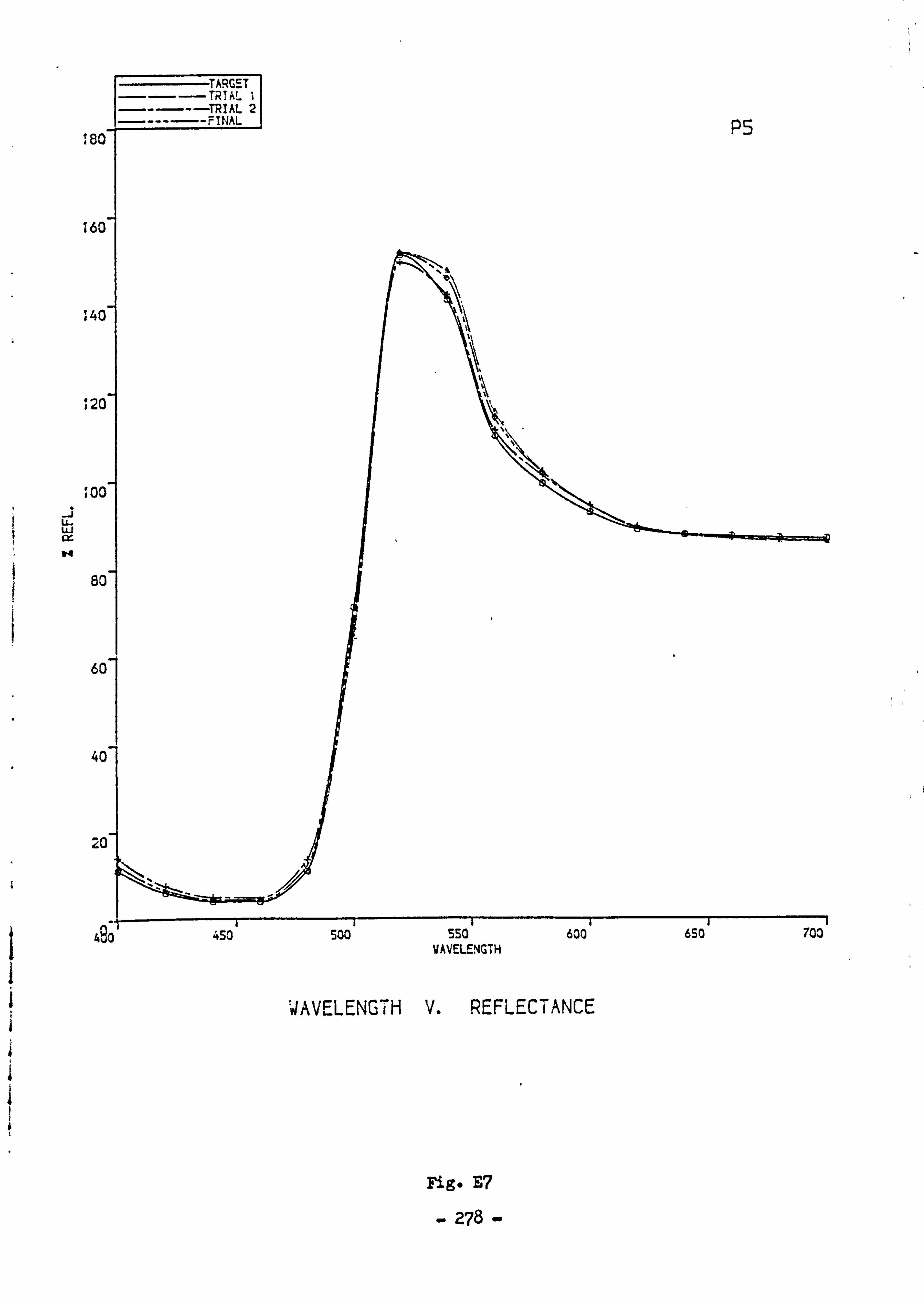
180
160
, 40
s20
loo
-i U- uj
80
60
40
20
I I I
Fig. E7
- 278 -
4901 450' 500' 550' 600' 650' 700 VAVELENGTH
TANCE TH V. REFLECI WAVELENGI
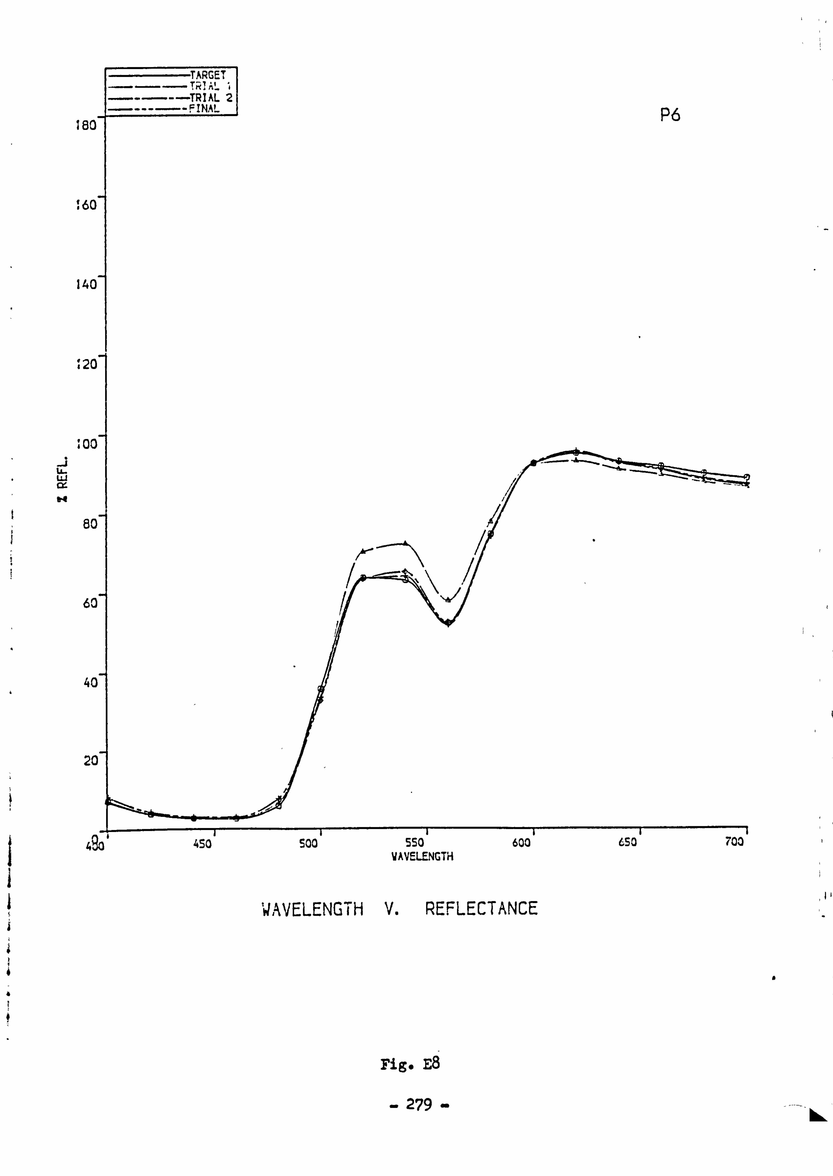
160
. 60
140
, 20
loo
LU CY-
60
40
20
ri g. F, 8
- 279 -
a
490' 4SO' 500' sso- 600' 650- 700 WAVELENGTH
WAVELENGTH V. REFLECTANCE
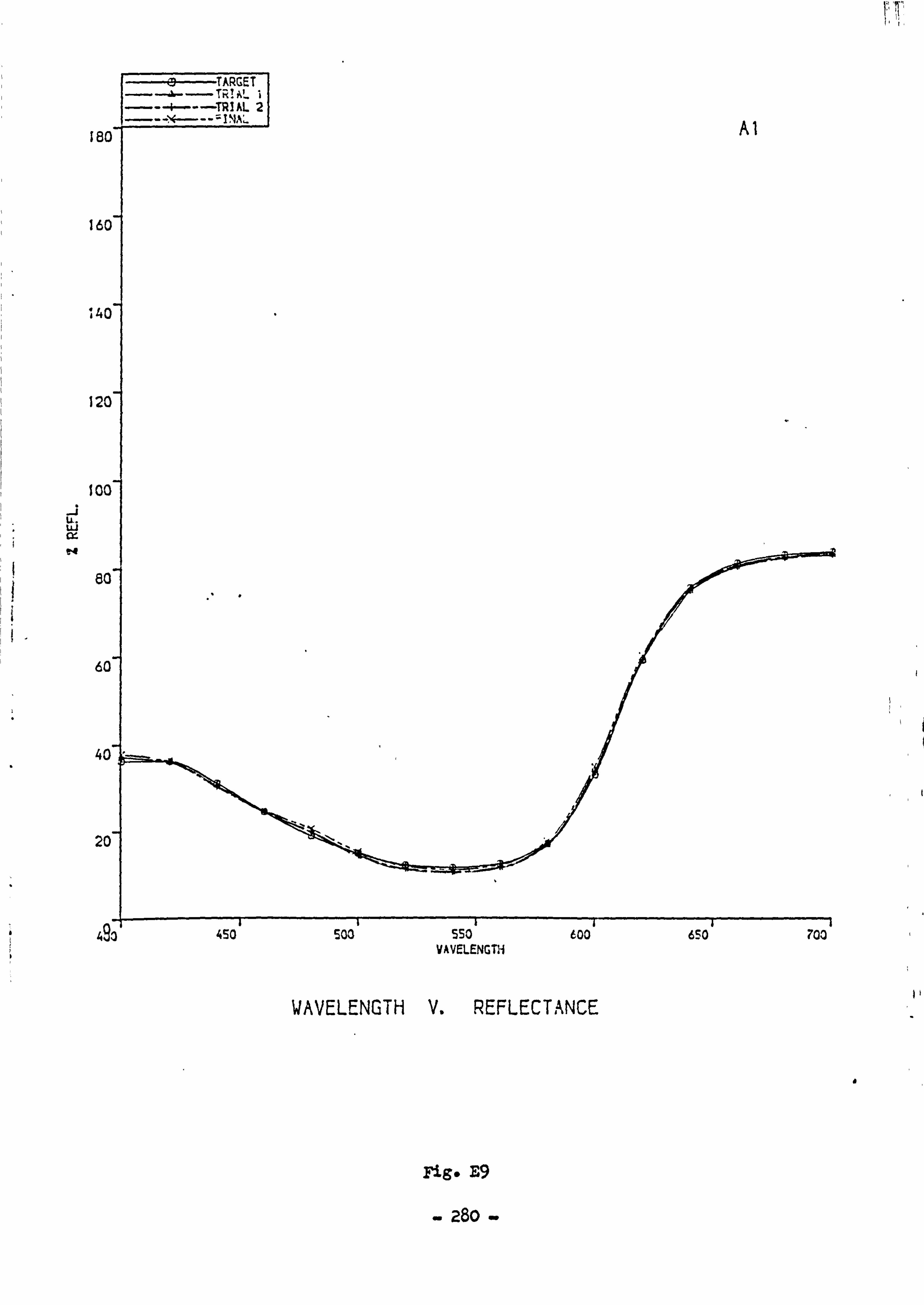
lac
160
140
120
100
U. uj M r4
80
60
40
20
a
Fig. E9
- 280 -
493' 450' 500' SSO' 600' 650' 700 VAVELENGTH
WAVELENGTH V. REFLECTANCE
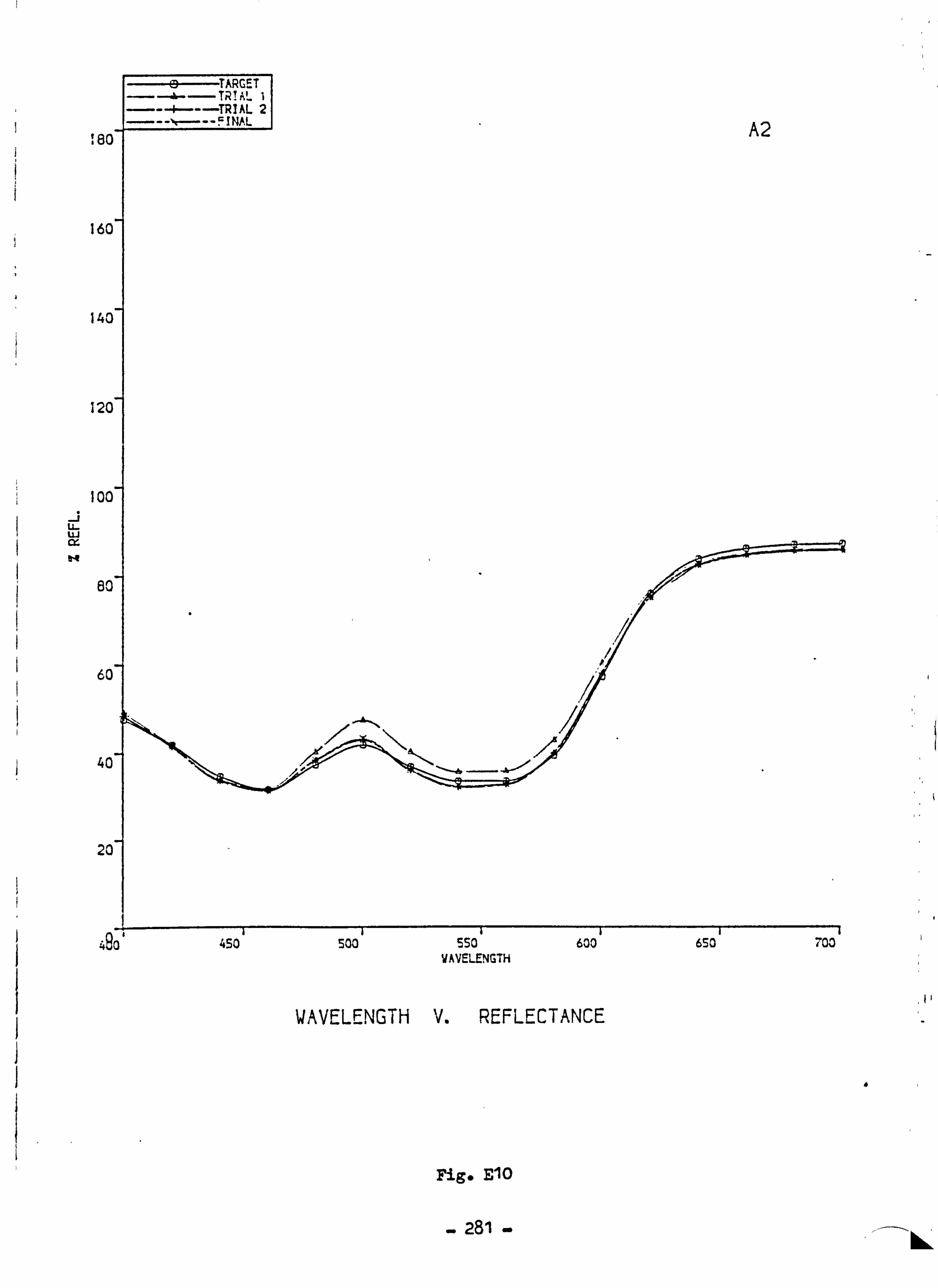
! 80
160
140
120
100
60
60
40
20
4
Fig. Elo
- 281 -
490' 450' 500' SSO' 600' 650' 700 WAVELENGTH
WAVELENGTH V. REFLECTANCE
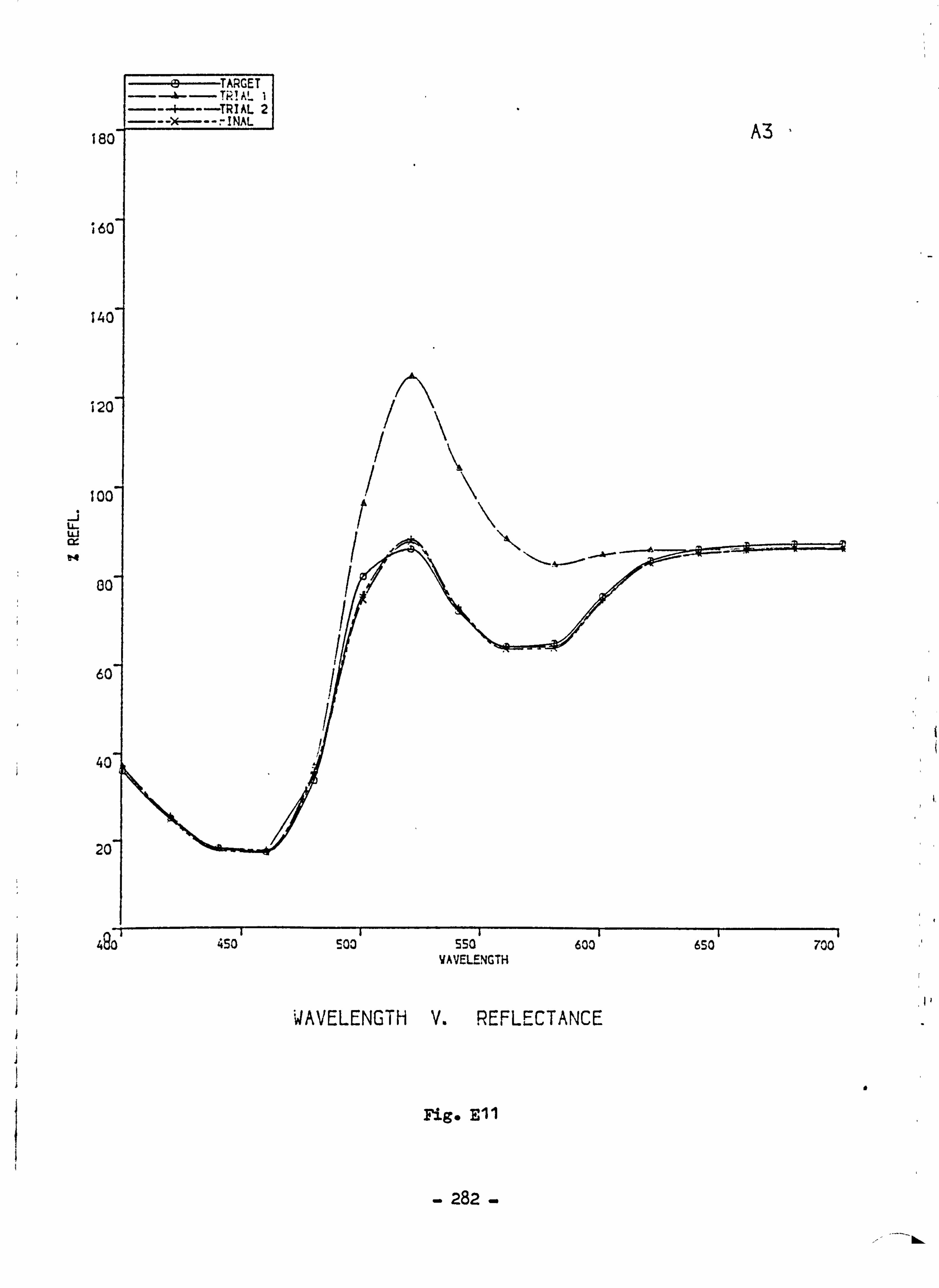
1 8c
16C
14C
12C
100
-j ti- uj cx
00
60
40
20
WAVELENGTH V. REFLECTANCE
Fig. El 1
- 282 -
a
490 450 Soo 550 600 650 700 WAVELENGTH
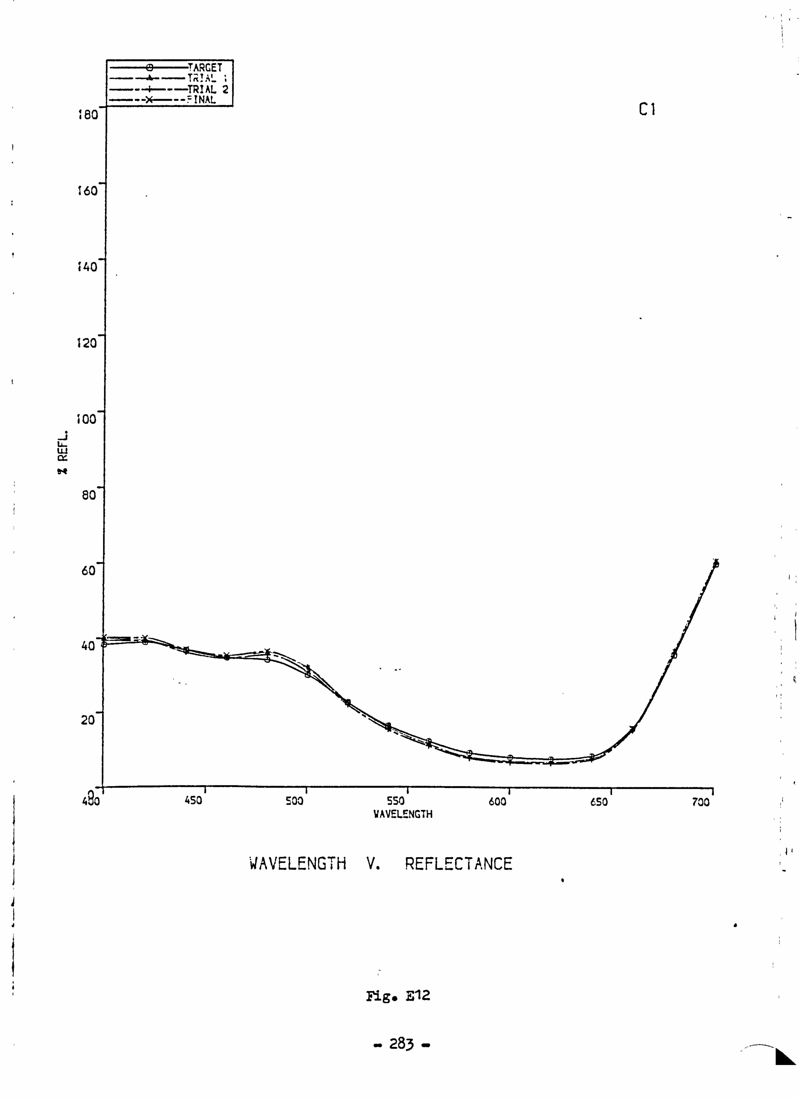
lac
16C
14C
12C
, 00
-j Li- ul cr-
94
80
60
40
20
I
Fig* E12
ý 283 -
490' 450' Soo 1
550' 600 1
6so 1
700 VAVELENGTH
WAVELENGTH V. REFLECTANCE

180
160
140
120
loo
-j U- uj
6c
6C
40
20
493
Fig. E13
- 284 -
450 500 bbu 6uu VAVELENGTH
EFLECTANCE WAVELENGTH V. RE
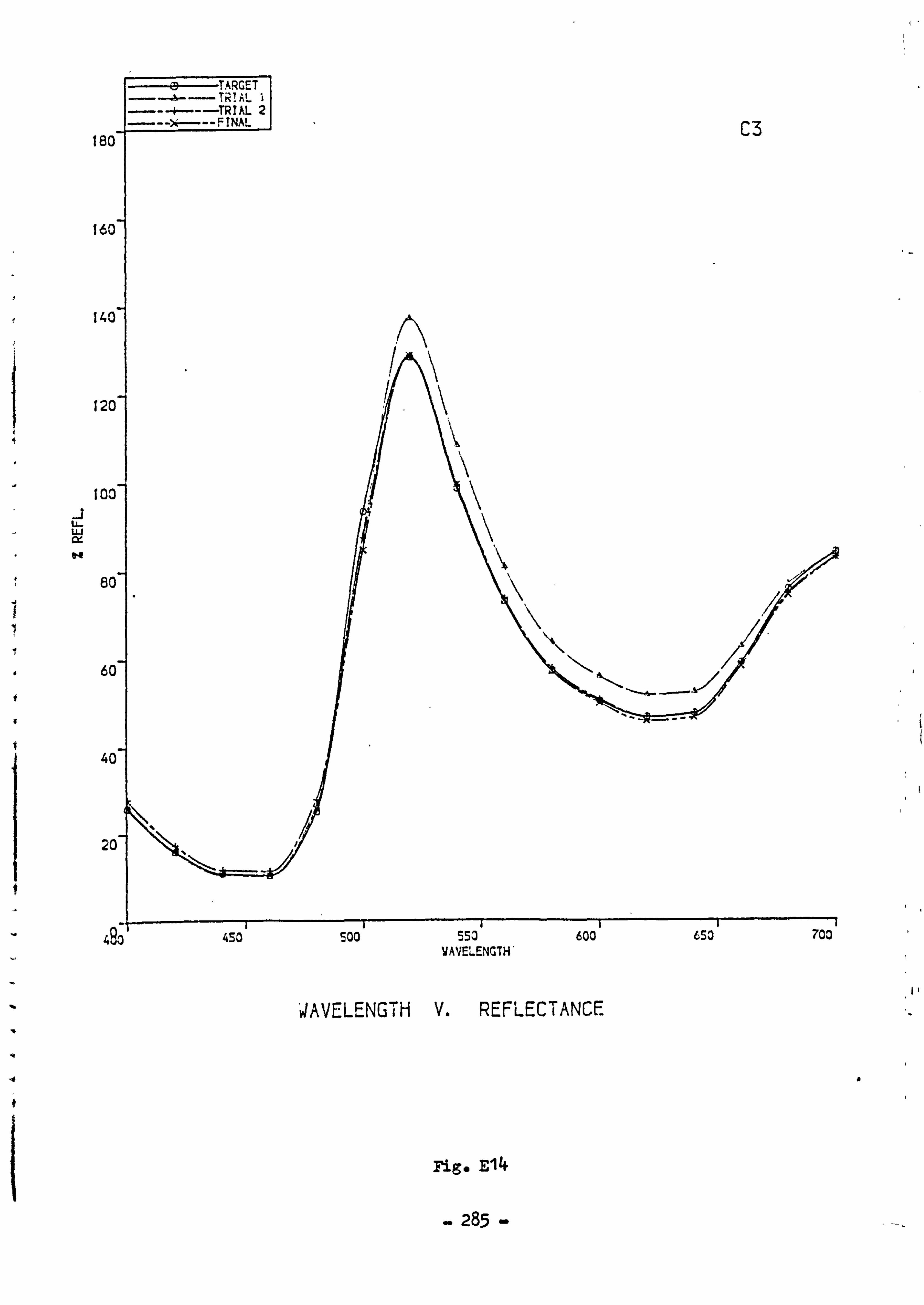
180
160
140
120
i0a
LLJ
t4
80
60
40
2C
rig. F, 14
- 285 -
490' 450' 500' 553' 600' 650' 700 VAVELENGTH'
'JAVELENGTH V. REFLECTANCE

18C
160
140
120
100
-i tL LU cy.
80
60
40
20
WAVELENGTH V. REFLECTANCE
Fig. E15
- 286
a
-- 111h
4906 453' SOO' 550' 600 650 700 VAVELENG7H
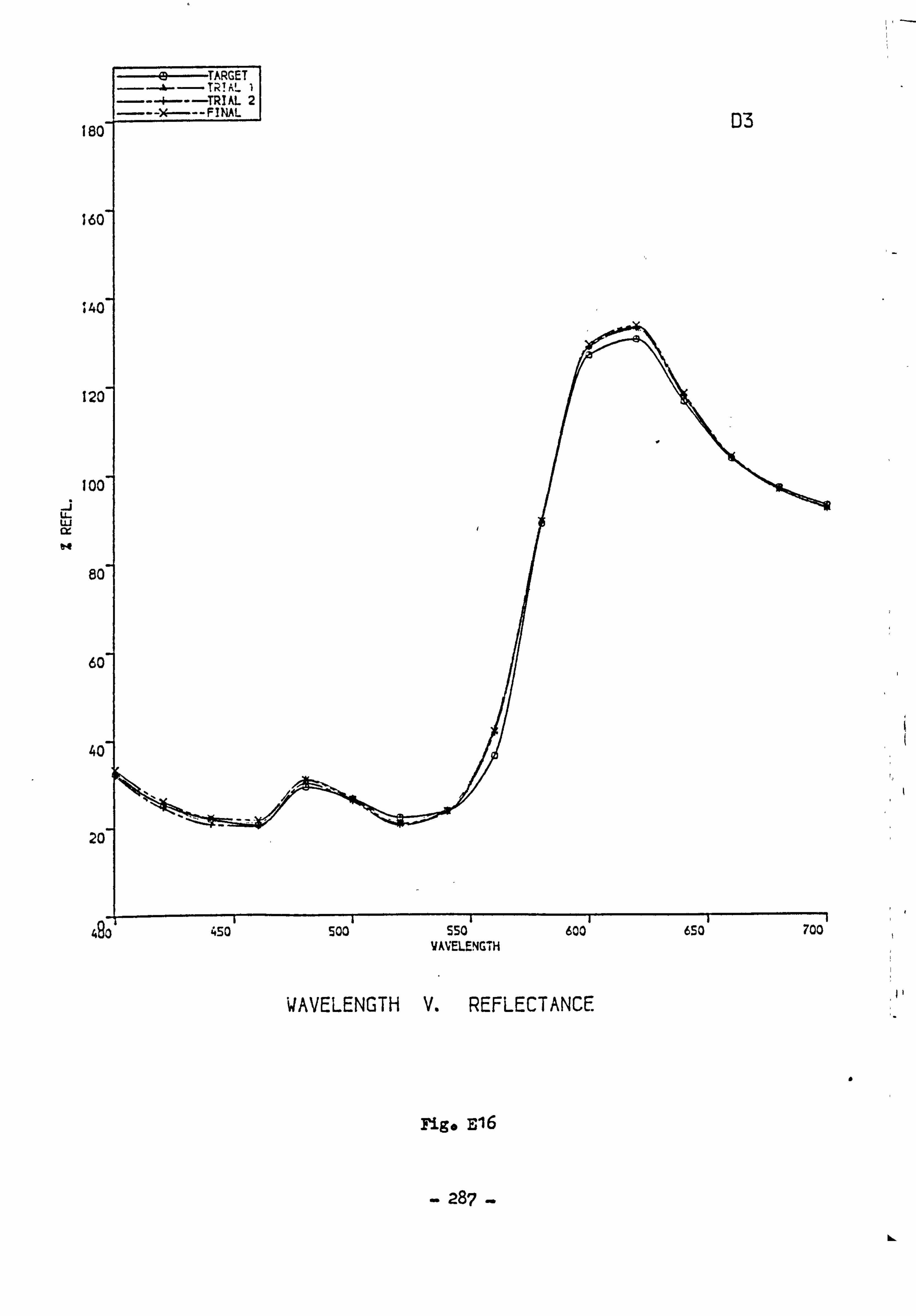
160
160
s40
120
loo
-i U-
80
60
40
20
rig* E16
- 287 -
a
Lý
490' 450' 500' SSO' 600' 650' 700 VAVELENGTH
WAVELENGTH V. REFLECTANCE
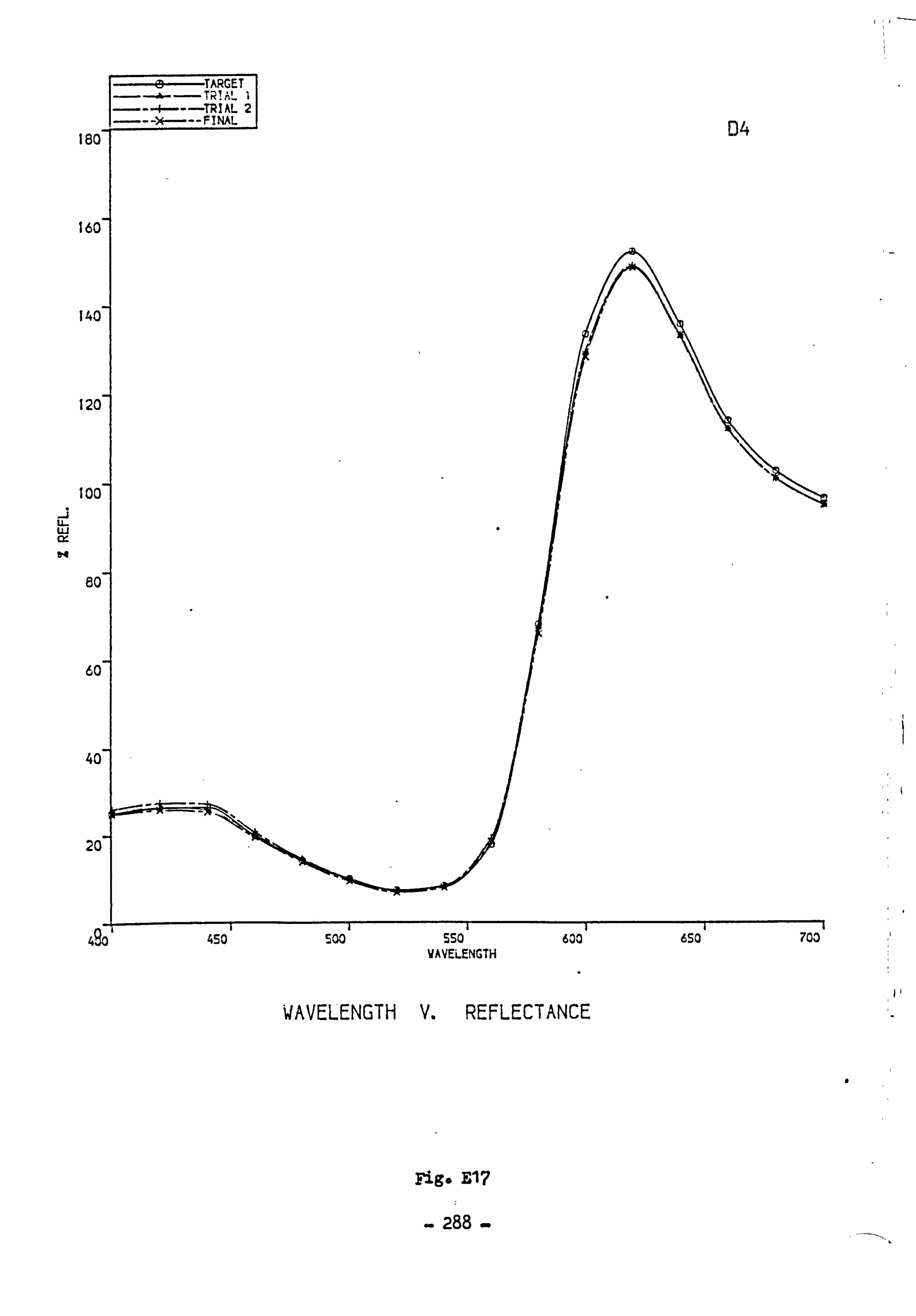
180
160
140
120
too
-i U- ui cr
80
60
40
20
S
Fig. E17
- 288 -
490' 450' Soo 550' 600' 650 700 WAVELENGTH
WAVELENGTH V. REFLECTANCE

160
160
140
#20
loo
-i U- LU
tq
80
60
40
20
Fig. E18
- 289 -
490' 450' 500' 550' 600' 6so, 700 VAVELENGTH
WAVELENGTH V. REFLECTANCE

160
160
140
120
100
LU im
80
60
4C
2c
rig. E19
- 290 -
a
490' 450' Soo* SSO' 600 650 700 WAVELENGTH
WAVELENGTH Vý REFLECTANCE
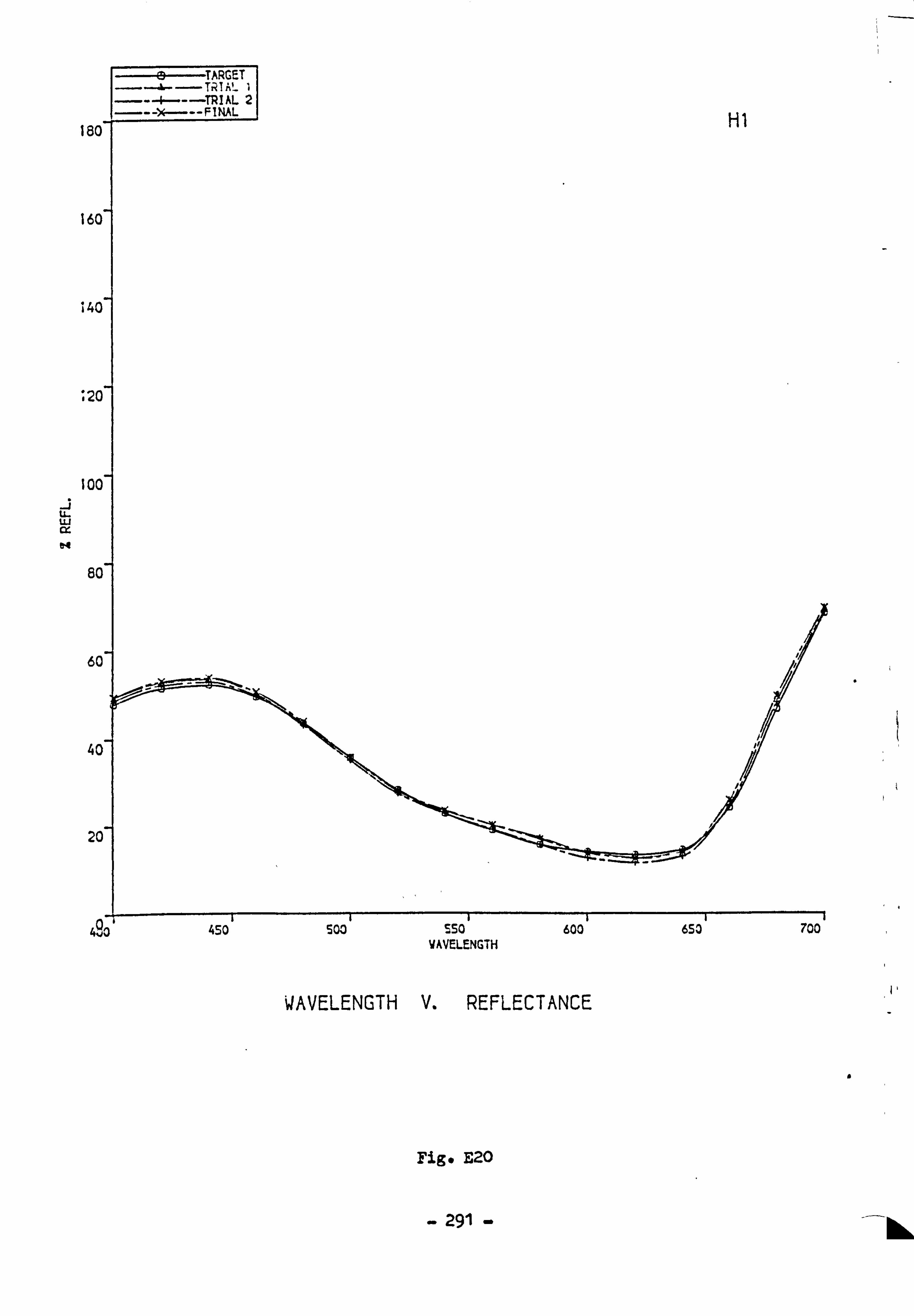
160
160
M
. 20
100
-i U- uj cx
60
60
40
20
a
Fig* E20
- 291 - --1116
01 4, jO 450 Soo sso 600 650 700 WAVELENGTH
WAVELENGTH V. REFLECTANCE

fac
16C
14C
120
100
-j U- LU M
80
60
40
20
a
Fig@ E21
-292-
4906 4SO' 500' SSO' 600 653 700 WAVELENGTH
VAVELENGTH V. REFLECTANCE
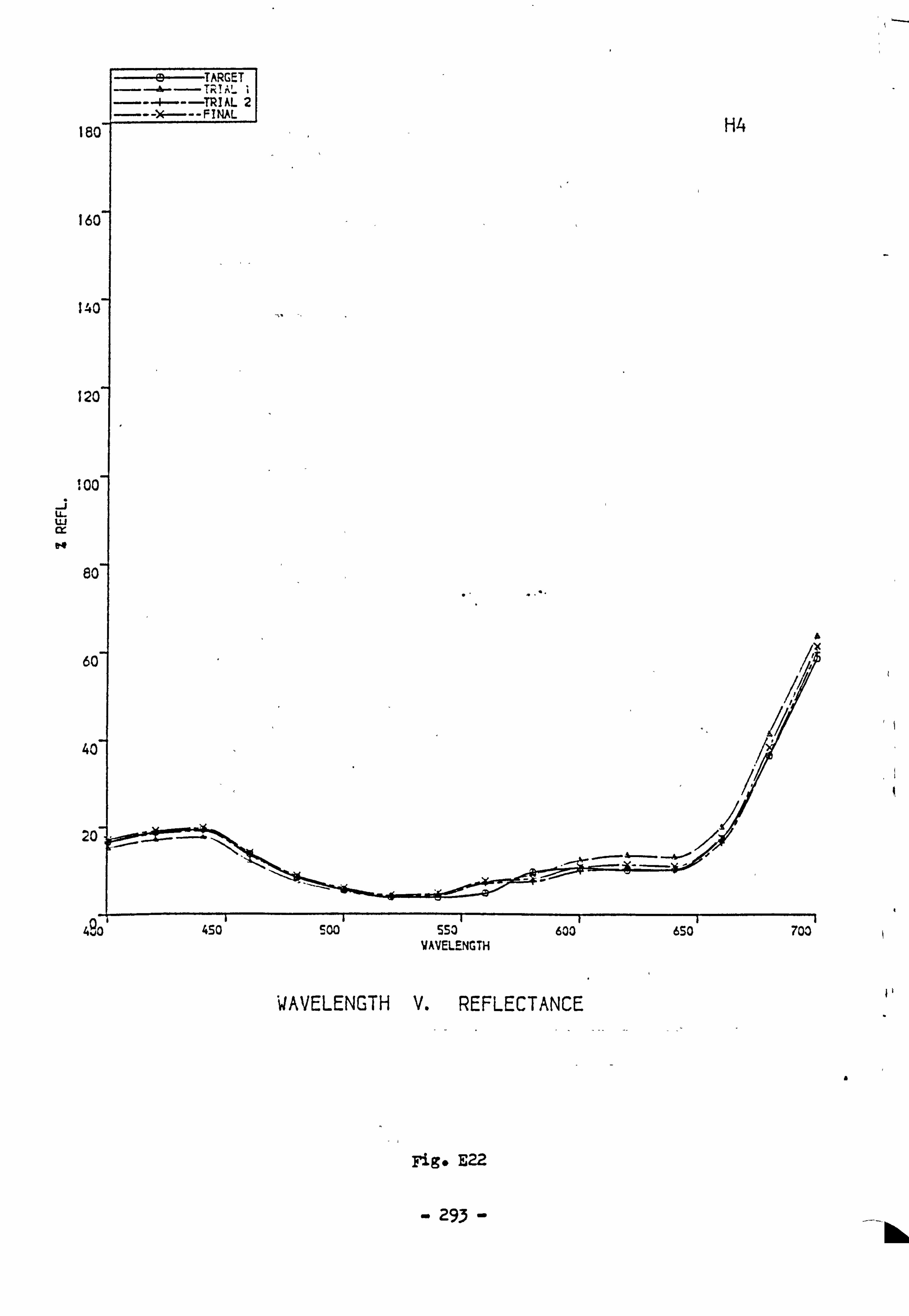
18c
16C
14C
12C
I loc
ui (X
80
60
40
20
49 ZO 450 Soo 550 600 650 VAVELENGTH
WAVELENGTH V. REFLECTANCE
Fig- E22
- 293 -
703
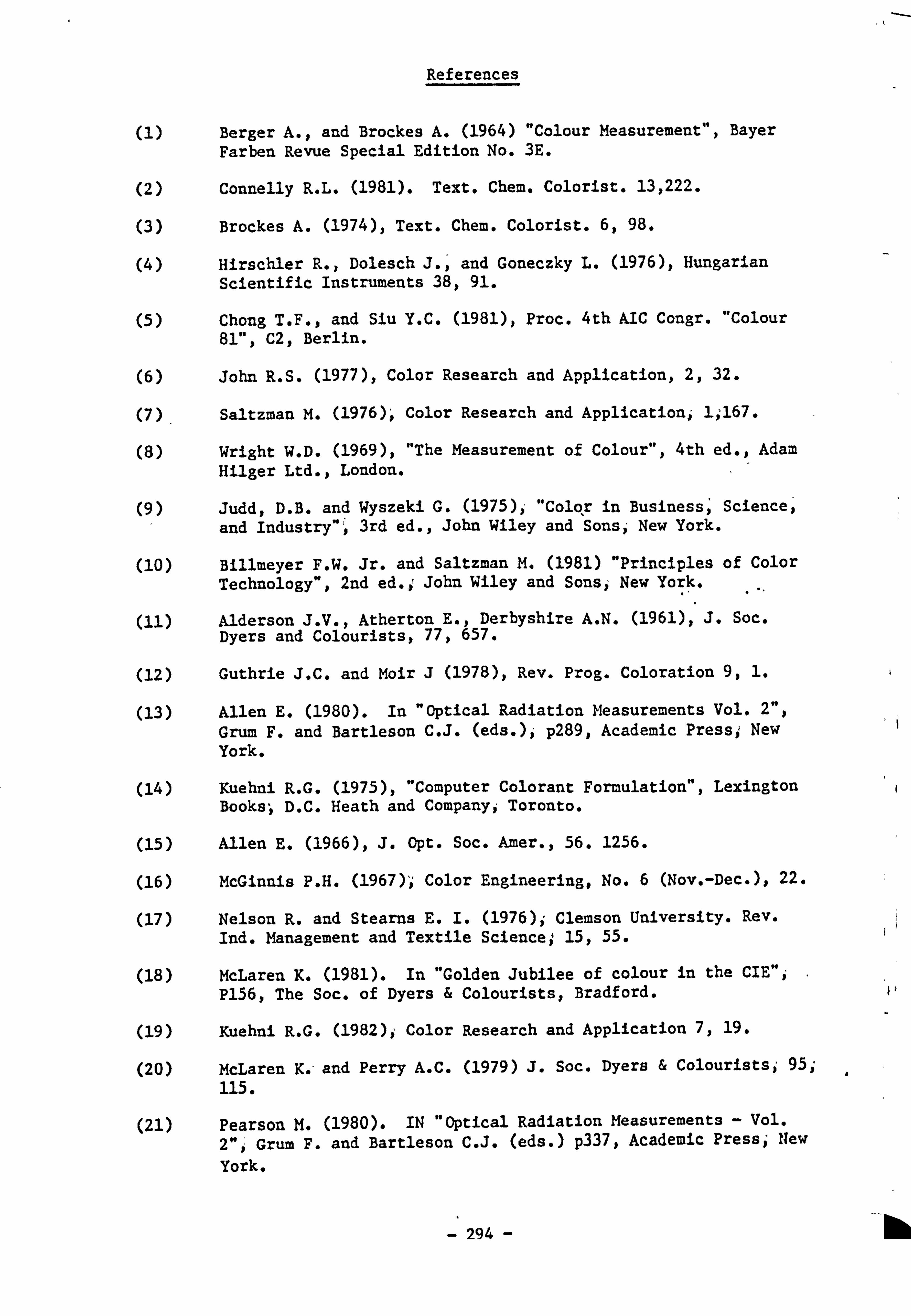
References
Berger A., and Brockes A. (1964) "Colour Measurement", Bayer Farben Revue Special Edition No. 3E.
(2) Connelly R. L. (1981). Text. Chem. Colorist. 13,222.
(3) Brockes A. (1974), Text. Chem. Colorist. 6,98.
(4) Hirschler R., Dolesch J., and Goneczky L. (1976), Hungarian Scientific Instruments 38,91.
(5) Chong T. F. ý and Siu Y. C. (1981), Proc. 4th AIC Congr. "Colour 81", C2, Berlin.
(6) John R. S. (1977), Color Research and Application, 2,32.
(7) Saltzman M. (1976), ' Color Research and Applicationi 1; 167.
(8) Wright W. D. (1969), "The Measurement of Colour", 4th ed., Adam Hilger Ltd., London.
(9) Judd, D. B. and Wyszeki G. (1975). "Colqr in Business, Sciencet and Industry"', 3rd ed., John Wiley and Sons, - New York.
(10) Billmeyer F. W. Jr. and Saltzman M. (1981) "Principles of Color Technology", 2nd ed.,, John Wiley and Sonsi New York.
(11) Alderson J. V., Atherton E., Derbyshire A. N. (1961)p J. Soc. Dyers and Colourists, 77ý 657.
(12) Guthrie J. C. and Moir J (1978), Rev. Prog. Coloration 9,1.
(13) Allen E. (1980). In "Optical Radiation Measurements Vol. 2", Grum F. and Bartleson C. J. (eds. ), p289, Academic Press, New York.
(14) Kuehni R. G. (1975), "Computer Colorant Formulation", Lexington Booksý, D. C. Heath and Companyi Toronto.
(15) Allen E. (1966), J. Opt. Soc. Amer., 56. 1256.
(16) McGinnis P. H. (1967)'; Color Engineering, No. 6 (Nov. -Dec. ), 22.
(17) Nelson R. and Stearns E. 1. (1976); Clemson University. Rev. Ind. Management and Textile Science; 15,55.
(18) McLaren K. (1981). In "Golden Jubilee of colour in the CIE"i - P156, The Soc. of Dyers & Colourists, Bradford.
(19) Kuehni R. G. (1982)i Color Research and Application 7,19.
(20) McLaren K. -and Perry A. C. (1979) J. Soc. Dyers & Colouristsi 95; 115.
(21) Pearson M. (1980). IN "Optical Radiation Measurements - Vol. 2"i Grum F. and Bartleson C. j. (eds. ) p337, Academic Press, New
York.
294
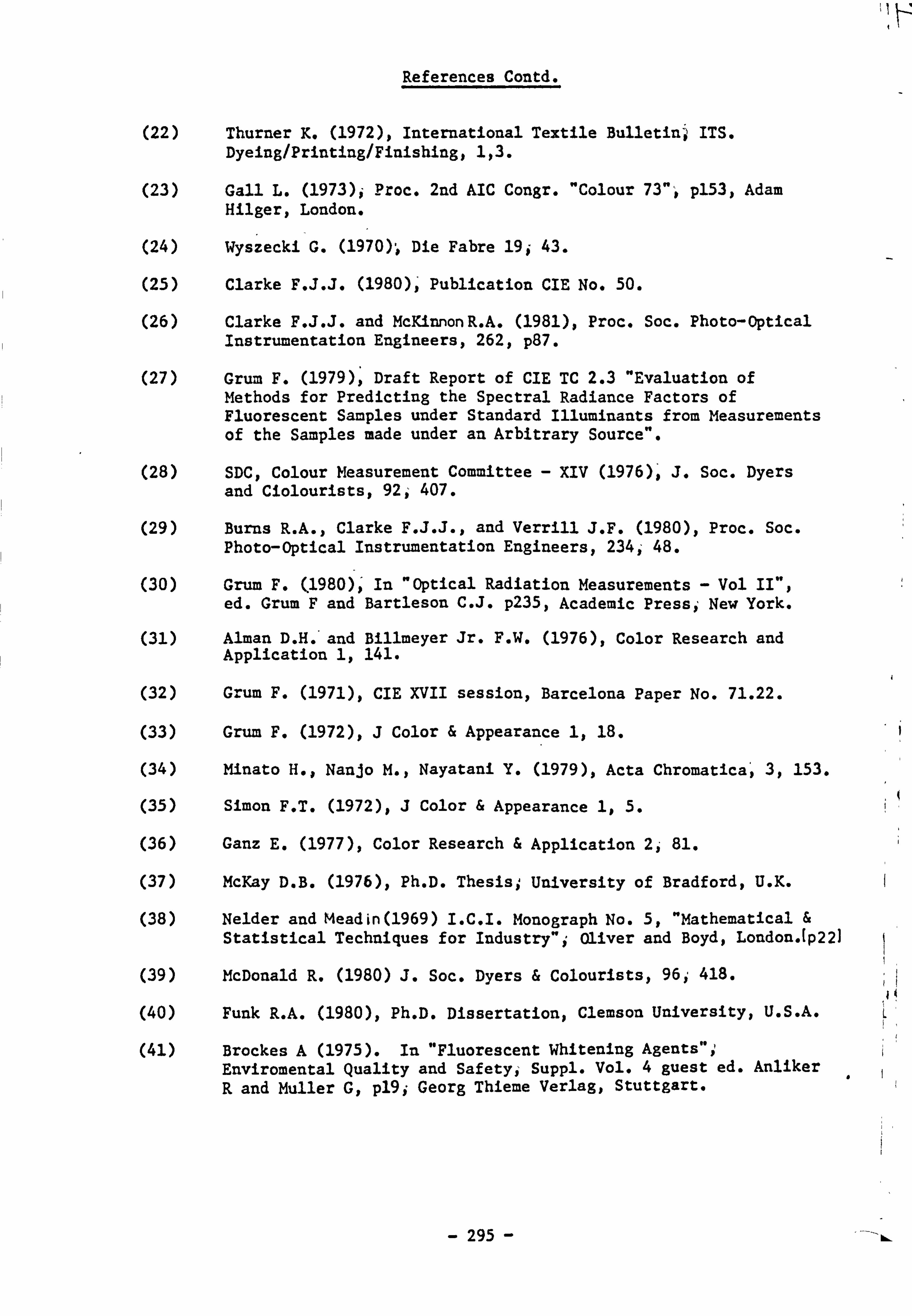
References Contd.
(22) Thurner K. (1972), International Textile Bulletin' ITS. Dyeing/Printing/Finishingt lt3.
(23) Gall L. (1973)i Proc. 2nd AIC Congr. "Colour 73"', p153, Adam Hilger, London.
(24) Wyszecki G. (1970),, Die Fabre 19i 43.
(25) Clarke F. J. J. (1980)o Publication CIE No. 50.
(26) Clarke F. J. J. and McKinnonR. A. (1981), Proc. Soc. Photo-optical Instr=entation Engineers, 262, p87.
(27) Grum F. (1979), Draft Report of CIE TC 2.3 "Evaluation of Methods for Predicting the Spectral Radiance Factors of Fluorescent Samples under Standard Illuminants from Measurements of the Samples made under an Arbitrary Source".
(28) SDC, Colour Measurement Committee - XIV (1976)s J. Soc. Dyers and Ciolourists, 921 407.
(29) Burns R. A., Clarke F. J. J., and Verrill J. F. (1980), Proc. Soc. Photo-optical Instrumentation Engineers, 234, ý 48.
(30) Grum, F. (1980)p' In "Optical Radiation Measurements - Vol II", ed. Grum F and Bartleson C. J. p235j Academic Pressi New York.
(31) Alman D. H. *and Billmeyer Jr. F. W. (1976), Color Research and Application 1,141.
(32) Grum F. (1971)0 CIE XVII session; Barcelona Paper No. 71.22.
(33) Grum F. (1972),, J Color & Appearance 1,18.
(34) Minato H. . Nanjo M. , Nayatani Y. (1979), Acta Chromatica') 3,153.
(35) Simon F. T. (1972)p J Color & Appearance 1,5.
(36) Ganz E. (1977), Color Research & Application 23- 81.
(37) McKay D. B. (1976), Ph. D. Thesis, University of Bradford, U. K.
(38) Nelder and Meadin(1969) I. C. I. Monograph No. 5, "Mathematical & Statistical Techniques for Industry"; Oliver and Boyd, London. lp221
(39) McDonald R. (1980) J. Soc. Dyers & Colourists, 96i 418.
(40) Funk R. A. (1980), Ph. D. Dissertation; Clemson University, U. S. A.
(41) Brockes A (1975). In "Fluorescent Whitening Agents"pl Enviromental Quality and Safetyj SuPPl- V01- 4 guest ed. Anliker R and Muller G. pl9j Georg Thieme Verlag, Stuttgart.
- 295 kh,

References Contd.
. 42) Sharpe L. T. and Lakowski R (1977), Proc. 3rd AIC Congr. "Colour 77'*pz p300i Adam Helger Ltd. j London.
(43) DIN 6172 (1971), Metameric Index.
(44) X. Mclaren (1976), J. Soc. Dyers and colourists, 92,338.
(45) Rigg. B (1981), J.. Soc. Dyers and Colourists, 97,504.
(46) Clarum, S. N. and Penner S. E. (1954), Amer. Dyestuff Rep.; 43, 310.
(47) Schulman S. G. (1976), "Fluorescence and Phosphorescence spectroscopy: Physicochemical Principles and Practice", p104.
(48) Cheung M. (1984)p Ph. D Thesis, University of Bradford, U. K.
(49) AATCC Technica Manual (1980), Vol/ 56; plll.
t
- 296 -
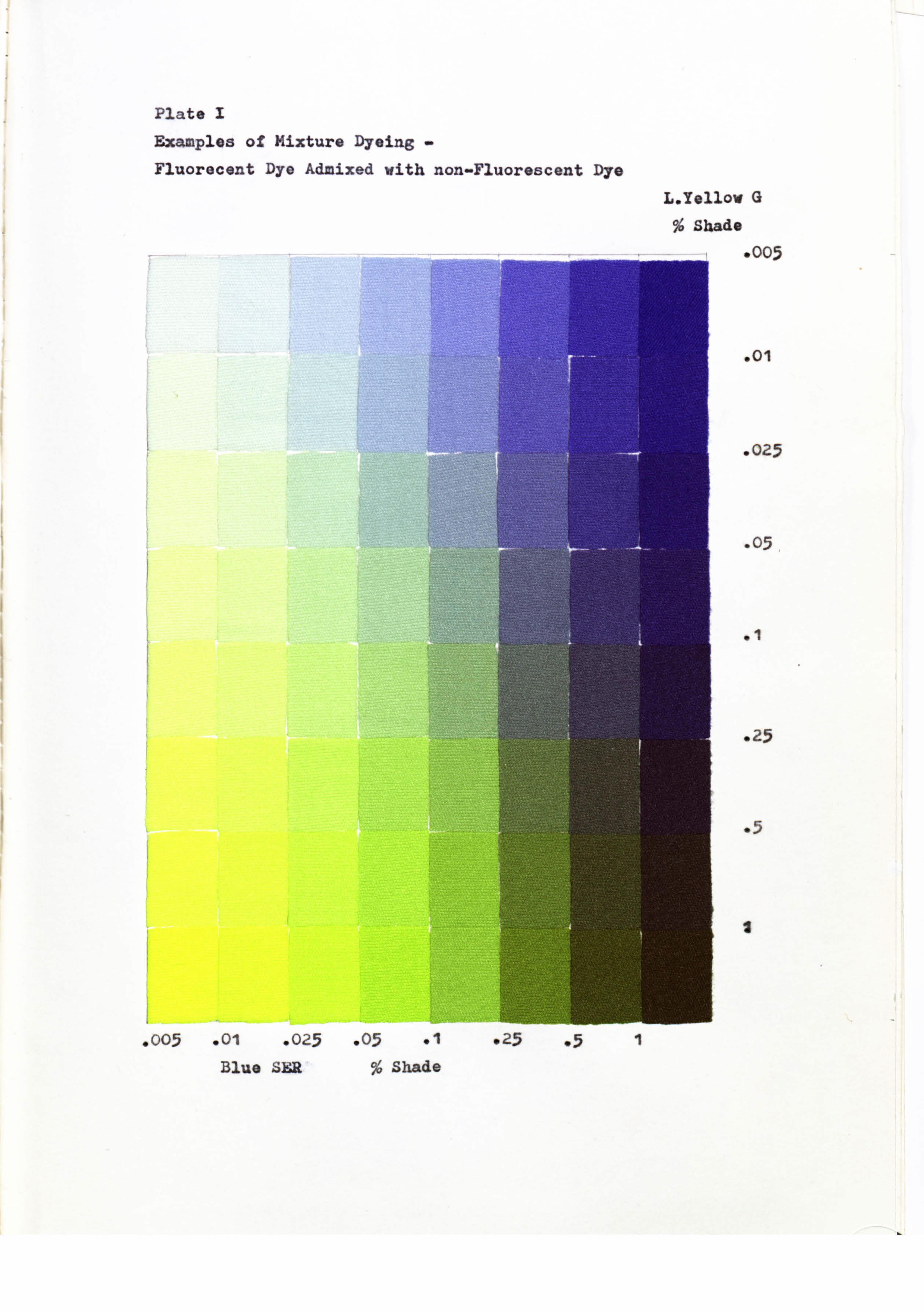
Plate I
Examples of Mixture Dyeing
Fluorecent Dye Admixed with non-Fluorescent Dye
L. Yellow G
% Shade
'005
001
. 025
. 05
01
. 25
.5
I
. 005 . 01 . 025 . 05 ol Blus SER % Shade
*25 05 1
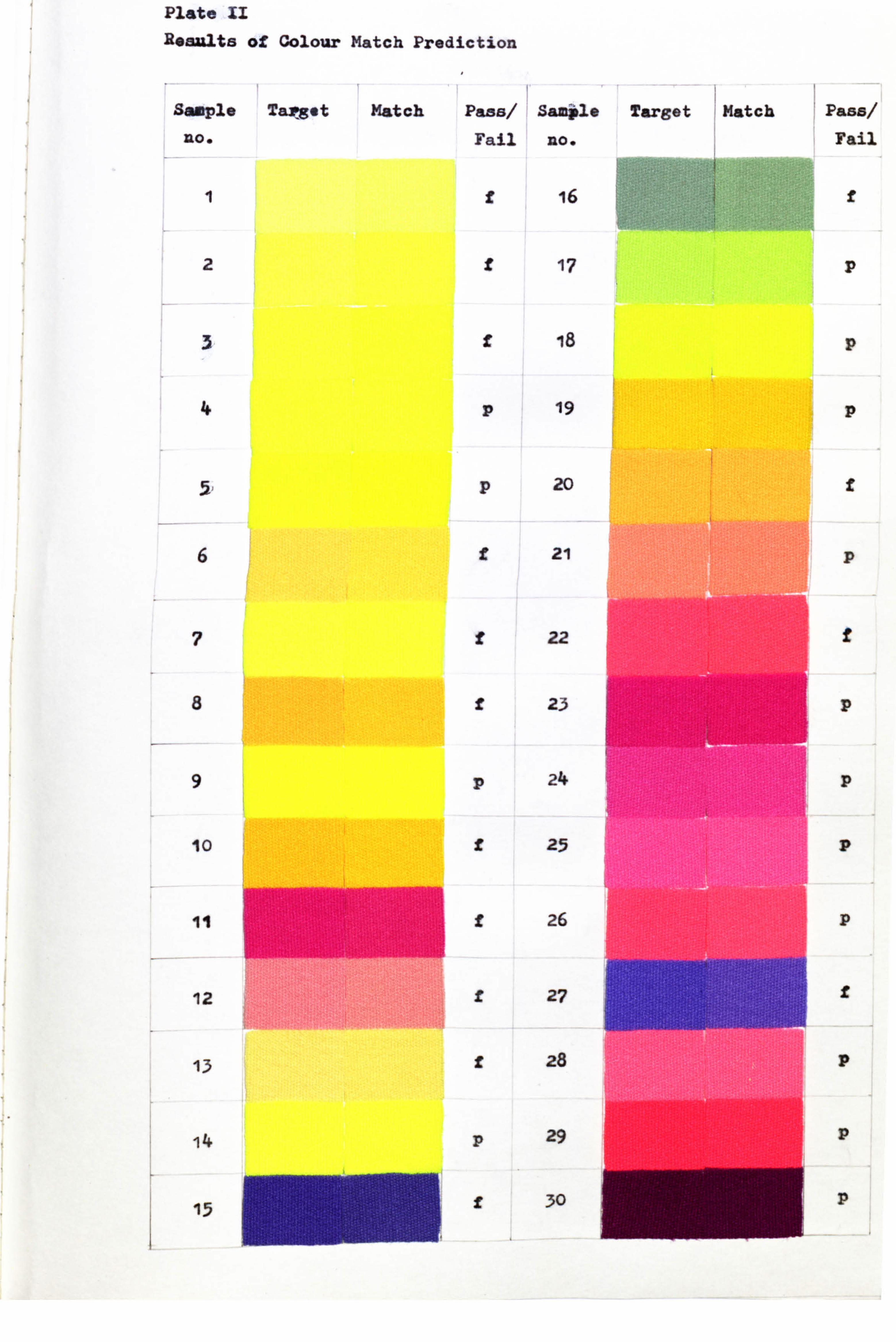
Plate 11
Results of Golour Match Prediction
Sample Targot Match Pass/ SAIM*l* Target Match Pass/
noo Fail no* Fail
1f 16 f
2f 17
f 18
4P 19 P
20
6p
7 f
8
f __ _____
14 p
15
22 _ýý Mmm M- :t
23
24
25
p
p
26
27
28
29
30
p
f


