3

Seasonal Reflectance Courses of Forests

Tiit Nilson1, Miina Rautiainen2, Jan Pisek1 and Urmas Peterson1 1Tartu Observatory

2University of Helsinki, Department of Forest Sciences 1Estonia

2Finland

1. Introduction

Studies on the seasonal changes in plant morphology and productivity, also known as phenology, have applied a multitude of methods for detecting changes in the start of spring or length of growing period. Global-scale plant phenology observation is needed, for example, to understand the seasonality of biosphere-atmosphere interactions (e.g. Moulin et al., 1997). Traditional species-specific in situ records of leafing and fruiting (e.g. Menzel et al., 2006), monitoring of atmospheric carbon dioxide as an indicator of photosynthesis (e.g. Keeling et al., 1996) and remote sensing of vegetation reflectance (e.g. Zhou et al., 2001) have all been used in attempts to understand the consequences of the changing climate on primary production and global vegetation cover.

Satellite remote sensing enables continuous monitoring of vegetation status (and potentially also physiological processes of plants), and thus, it is not limited to conventional, single-date phenological metrics such as budburst or flowering. Using remote sensing also enables a wider perspective to vegetation dynamics: at its best it can reveal large-scale phenological trends that would not be possible to detect from the ground. Monitoring phenological phases of vegetation using remote sensing has made significant progress during the past decade due to an increased global coverage of satellite images, development of reflectance metrics describing seasonality, and evolution of methods for calibrating time series of remotely sensed data sets. In addition, operational satellite products for monitoring phenology from space have been designed (e.g. Ganguly et al., 2010; Zhang et al., 2003).

Despite rapid progress, remote sensing also faces a multitude of both scientific and technical challenges before reliable phenological statistics with global coverage can be obtained. Firstly, compared to traditional phenological observations, a satellite pixel typically covers a larger area. Therefore, phenological information obtained from remote sensing (especially from satellite images) is aggregated data covering a heterogeneous landscape and requires new interpretation of phenological metrics. Hence, the concept of “land surface phenology” (Friedl et al., 2006) is often used to describe the seasonal pattern of variation in vegetated land surfaces observed from remote sensing. Secondly, coarse scale remotely sensed data sets cannot necessarily differentiate all phenological processes occurring in a fragmented landscape. Thus, the validation of phenological metrics has taken a new meaning: conventional ground measurements (typically made from a few individual plants) need to

New Advances and Contributions to Forestry Research

34

be upscaled to the level of satellite pixels. Finally, the physical processes driving the seasonal reflectance dynamics observed in satellite images are not yet well known; until now only a few pioneering studies linking forest reflectance seasonality to seasonal changes in forest structure and biochemistry have been carried out.

In this chapter, we review remote sensing of the seasonal dynamics of forest reflectance as well as highlight future challenges in the development of methodologies needed for interpreting seasonal reflectance courses at forest stand level (Section 2: Literature review). In addition, using empirical data from European hemiboreal and boreal forests, we demonstrate how seasonal reflectance courses of forests can be obtained from satellite remote sensing and how they can be used to examine the cyclic changes taking place in the vegetation (Section 3: Case study).

2. Literature review

In the following section, we will briefly outline the most common seasonal reflectance changes observed in remotely sensed datasets and discuss their driving factors in forests. Next, we will describe forest reflectance models as a tool for linking reflectance data to stand structure. Finally, we will explain how calibrated time series of satellite data can be created from multi-year image archives. The literature review focuses on forest stand-level phenomena i.e. global or large-scale monitoring of vegetation phenology is not covered.

2.1 Seasonal reflectance changes in satellite images

It is commonly understood that the seasonal reflectance course of deciduous forests is more pronounced than that of coniferous forests (e.g. Peterson, 1992). The phenology of evergreen coniferous species is more difficult to monitor from satellite images than that of deciduous species due to the smaller changes in foliage i.e. because new shoots account for only a small part of the green biomass. Jönsson et al. (2010) have estimated that seasonal changes in typically used spectral vegetation indices are actually more related to snow dynamics than to changes in needle biomass in coniferous forests.

The differences in seasonal reflectance dynamics between forests ultimately arise from the differences in their canopy structure and understory vegetation. In the same tree species, reflectance differences may be due to, for example, site fertility (e.g. Nilson et al., 2008) or topographical elevation (e.g. Guyon et al., 2011). Currently, there is only a limited understanding of reflectance seasonality and its driving factors at forest stand level: seasonal reflectance variation has preliminarily been linked to changes in stand structure (e.g. Kobayashi et al., 2007; Kodani et al., 2002; Nilson et al., 2008; Rautiainen et al., 2009; Suviste et al., 2007) or variation in leaf spectra resulting from, for example, climatic-elevational factors and site quality (e.g. Richardson & Berlyn, 2002; Richardson et al., 2003). The seasonal reflectance course of a forest results from the temporal reflectance cycles of the tree canopy and understory (also occasionally called forest floor or background) layers and the presence of snow. Seasonal reflectance changes of the two layers, in turn, are explained by changes in biochemical properties of plant elements and geometrical structure (e.g. crown shape, leaf area index, canopy cover) of the different plant species. In addition, the seasonal and diurnal variation in solar illumination influences forest reflectance (e.g. Sims et al., 2011): often a forest may exhibit a clear seasonal reflectance course even if there were no phenological changes occurring in the vegetation cover (Nilson et al., 2007).

Seasonal Reflectance Courses of Forests

35

The main drivers of the seasonal course of forest reflectance are found from the tree canopy layer. The amount of foliage, also characterized by leaf area index (LAI) (Chen & Black, 1992; Watson, 1947), undergoes significant seasonal changes in deciduous species and much smaller changes in coniferous species throughout the growing period (Rautiainen et al., 2011a). Phenological greening (an increase in LAI) or senescence (a decrease in LAI) influence both the scattering process in the tree canopy volume as well as have an indirect impact on canopy cover (and hence, the visibility of the understory layer or forest floor to the satellite sensor). The relationship of LAI and forest reflectance is complicated and somewhat species-specific: an increase in LAI may result both in an increase or decrease in forest reflectance, depending on the geometric arrangement of the canopy, optical properties of single leaves and optical properties of the understory layer. Theoretical studies have shown that the relationship of LAI and canopy reflectance depends on viewing and illumination angles as well as the absolute value of LAI and canopy cover (e.g. Gastellu-Etchegorry et al., 1999; Knyazikhin et al., 1998; Myneni et al., 1992; Rautiainen et al., 2004). In empirical studies, shortwave spectral bands typically have a decreasing trend when canopy LAI increases (e.g. Brown et al., 2000; Nilson et al., 1999; Stenberg et al., 2004; Stenberg et al., 2008a).

The contribution of leaf optical properties to stand reflectance is the greatest in dense stands with closed canopies (e.g. Eklundh et al., 2001). The optical properties of single leaves (or coniferous needles) change through the growing season due to physiological processes (e.g. Middleton et al., 1997). For example, Demarez et al. (1999) reported for temperate tree species that the seasonal course of leaf albedos (especially in the green and SWIR bands) is characterized by a decrease at the beginning of the growing season, a relatively constant value during summer and finally an increase towards the end of the growing season. Currently, there is no public database covering the seasonality of leaf spectra. Leaf optical properties models, such as the widely used PROSPECT model (e.g. Jacquemoud & Baret, 1990), enable us to predict quantitatively the seasonal changes in leaf reflectance and transmittance spectra, if the changes in leaf biochemical parameters (contents of various leaf pigments, water, organic compounds, etc.) are known. However, there are too few systematic investigations to prove the validity of leaf reflectance models in the seasonal context and to describe quantitatively changes in leaf biochemical parameters throughout the growing season. Further, the leaf optical properties are also affected by less predictable attacks of insects and diseases, typically in the second half of the vegetation.

Understory vegetation contributes significantly to forest reflectance (e.g. Eriksson et al., 2006; Spanner et al., 1990); the contribution of understory in sparse canopies can overrule the contribution from the tree canopy layer. In addition, if the temporal cycles of the tree canopy and understory layers differ considerably (Richardson et al., 2009), the greening of the understory prior to the tree canopy may complicate interpreting the budburst date for the region from satellite images (Ahl et al., 2006). The seasonal variability of understory reflectance is biome- and site type-specific (e.g. Miller et al., 1997; Shibayama et al., 1999). For example, most boreal forest understory layers have strong seasonal dynamics during their short snow-free growing period. Their seasonal course of understory reflectance is very characteristic of stand type, and the reflectance differences between stands tend to become more pronounced as the growing period progresses (Miller et al., 1997). Furthermore, Rautiainen et al. (2011b) reported that the spectral differences between and within boreal understory types are the largest at the peak of the growing season whereas in the beginning

New Advances and Contributions to Forestry Research

36

and end of the growing season the differences between the understory types are marginal. They also noted that understory vegetation growing on fertile sites had the brightest near infrared (NIR) spectra throughout the growing season whereas infertile sites appeared darker in NIR. It is very likely that the relative contributions of the understory and tree canopy layers to forest reflectance change as the growing season proceeds. Thus, separating the biophysical properties of the tree canopy layer from remote sensing data is further complicated.

Finally, the presence of snow significantly influences the seasonal course of forest reflectance, especially in the visible part of the spectrum. According to Manninen & Stenberg (2009), the presence of snow on the forest floor significantly increases forest albedo in sparse canopies (i.e. tree canopy LAI < 3). Furthermore, they reported that snow or hoar frost on trees alters the red band forest albedo completely. In addition, forest reflectance may vary when snow melts even though there are no changes in canopy leaf area index (e.g. Dye & Tucker, 2003).

The basic idea how to link a seasonal series of satellite images to phenology is to determine key moments of the season from the image series. Different physical quantities derived from the satellite images could be used to plot the time series; however, the most feasible is to use top-of-canopy (TOC) reflectance factors or multispectral indices derived from the TOC reflectance factors. Thus, pre-processing of the images that includes the absolute calibration and atmospheric correction of the images is needed. In addition, if the images in the series are acquired at variable view angles, the so-called BRDF (bidirectional reflectance distribution function) correction should be applied to reduce the reflectance factors to a fixed (e.g. nadir) direction. For instance, such image processing is included in the MODIS nadir reflectance product chain. The most popular multispectral index used to link to the phenology is NDVI, which is defined as

NDVI = (RNIR-RRED)/(RNIR+RRED), (1)

where RNIR and RRED are TOC reflectance factors in the NIR and red spectral region.

Fig. 1. A typical seasonal course of NDVI during the snow-free period with key phenology moments

Seasonal Reflectance Courses of Forests

37

Several authors have defined many parameters defining the shape of the seasonal curve (Crist, 1984; Jönsson & Eklundh, 2002, among others). A typical NDVI seasonal profile of green vegetation with indicated key moments of the season is shown in Fig. 1. A very important quantity is the integral of NDVI over the growing season. This integral is assumed to be proportional to the fraction of absorbed PAR over the season and, according to Kumar & Monteith (1981), linearly related to annual net primary production (NPP). The beginning of the active season could be defined as the moment when the first derivative of the NDVI differs reliably from zero. The moment when the maximum NDVI value is reached could be interpreted as the moment when the maximum leaf area is attained. The end of the growing season, also known as the beginning of dormancy, is assumed to start when a stable minimum NDVI value is measured, e.g. when the NDVI derivative has reached the stable value of zero. It is important to note that the spring minimum NDVI value and the minimum reached in fall after the active vegetation period is over does not necessarily have to be the same. According to our own experience from the hemiboreal region, the fall minimum is typically higher than in the spring for deciduous dominated stands. Several reasons could be responsible for this: there are still some leaves left on trees in the fall; on average the ground is wetter in spring compared to conditions in fall; and the layer of fresh leaf litter in the fall is brighter than the old decomposed litter after snowmelt in spring.

In practice, instead of a smooth NDVI curve we have a scattered series of points, because the image calibration and atmospheric procedures inevitably cause errors in the TOC reflectance values and vegetation indices. Thus the first task is to smooth the series. Several methods have been proposed for smoothing (e.g. TIMESAT, Jönsson & Eklundh, 2002). The problem is further complicated by the fact that most of the key parameters should be determined from an analysis of the first (sometimes second) derivative of the time course. The problem of estimating the derivatives from an empirical curve has been long known as a difficult task.

Another question is how are the important moments of phenological development of plants related to the seasonal curves of reflectance or vegetation indices? Determining the beginning or end of the green development is more or less clear. However, it is not as evident for another important phenological phase, the flowering.

The detection of flowering is an important phenology-related application of remote sensing. For instance, estimates of phenological phases derived from satellite images can be used in honeybee management to detect blooming of major honey plants (e.g. Nightingale et al., 2008), to estimate crop pollination by honeybees, to estimate honeybee nectar flow, etc. An option is to use an indirect way to detect the beginning of the vegetation period and then predict the flowering dates from the known meteorological data.

The possibility to detect flowering in visible spectral bands depends on the colour of flowers and on the cover fraction of flowers exposed in the view (nadir) direction. To detect flowering, a rather frequent temporal reflectance sampling is needed. In the NIR region, the pigments causing the coloration of flowers do not have a primary effect on reflectance. However, the scattering properties of leaves and flowers could be different in the NIR band as well, mostly because of their different structure. Floral reflectance databases are available on the Web, such as the FReD http://www.reflectance.co.uk//. Typically, these databases

New Advances and Contributions to Forestry Research

38

do not contain data in the NIR region or for the main tree species of the boreal and temperate region.

Detection of flowering by coarse resolution satellite scanners can be successful, if the cover fraction of flowers in the pixel is sufficiently large, which seems to be a rather hopeless task. On a subpixel scale, it is also possible to detect flowering if a linear unmixing method (Singer and McCord, 1979) is used and the spectral signatures of the flowers are known to define the respective endmember.

2.2 Seasonal forest reflectance modeling

Analyzing the role of each of the contributing factors (see Section 2.1) can only be achieved by linking stand-level forest reflectance modelling to empirical reflectance and forest inventory data sets. Forest reflectance models are parameterized using mathematical descriptions of tree canopy and understory structure and optical properties of plant elements to produce spectral signatures of the canopy leaving radiation field (see Stenberg et al., 2008b or Widlowski et al., 2007 for an overview of canopy reflectance models). Forest reflectance simulations can be applied, for example, (1) to understand how the spectral signature of a stand is formed, (2) to investigate quantitative relationships between remotely sensed reflectance data and forest attributes, and (3) to simulate seasonal and age courses in forest reflectances (Nilson et al., 2003). Even though forest reflectance models have existed for three decades, there is a lack of detailed in situ ground reference data sets for the validation of the seasonal simulation results. Thus, many quantitative links between seasonal changes in canopy structural and biochemical properties and forest reflectance are yet to be established.

Currently, there are only a handful of published studies, which have applied forest reflectance models to analyze the driving factors of reflectance seasonality. Based on empirical reflectance data and radiative transfer modelling, Kobayashi et al. (2007) reported that seasonal changes in a larch forest understory (or forest floor) influence both the absolute values of reflectance and seasonal reflectance trajectories even if the LAI of the tree layer remains constant. Next, Nilson et al. (2008) and Suviste et al. (2007) reported that in sparse stands (e.g. peatlands), the seasonal course of Sun elevation can be a significant contributing factor to reflectance seasonality i.e. the continuous change in Sun angle typically results in a bell-shaped seasonal reflectance trajectory for a forest. In addition, they reported that the typical seasonal course of canopy LAI results in a bowl-shaped seasonal reflectance trajectory in the visible bands. Most recently, Rautiainen et al. (2009) studied hemiboreal birch forests and concluded that the main driving factors in forest reflectance seasonality in the red and green bands were stand LAI and leaf chlorophyll content, in the NIR band stand LAI, and in the shortwave infrared (SWIR) band LAI and general water content. Furthermore, they suggested that future work on detecting boreal forest phenological phases from satellite images should be focused on quantifying the role of debris and forest floor water on stand reflectance during the early phases of leaf development in the spring, and better characterizing the highly variable surface roughness of the understory layer.

A general challenge in studies which link forest reflectance modeling to seasonal reflectance changes is that expert guesses and interpolation often need to be used to determine many of

Seasonal Reflectance Courses of Forests

39

the input parameters (e.g. biochemical changes in leaves during the growing season, structural changes in forest understory plants), and thus only preliminary conclusions can be drawn from the simulations.

2.2.1 Boreal and temperate forests as multi-component plant communities

Boreal and temperate forests should be treated as multi-component plant communities in forest reflectance modelling. To understand how the seasonal changes in reflectance of forest communities are formed one should be able to describe the seasonal changes occurring in all of the community components. A complete structural model of a typical forest community as an input for a forest reflectance model should include a quantitative description of the following components:

1. The first (dominating) tree layer, separately for all (main) tree species; 2. The second (and possibly third) tree layer, separately for all species; 3. Understory vegetation, including the tree regeneration, shrub and ground layer

vegetation (different herbs, dwarf shrubs, lichens, mosses); 4. Soil surface including the layer of litter on the surface;

Each of the vegetative components changes its appearance through the growing season. From the optical point-of-view, the changes in phenology induce the following structural and optical changes:

1. Growth of new leaf area, stems and branches, emergence of flowers and fruits, as well as senescence and dying of leaves and other components or whole plants in overstory and understory. It results mainly in changes of cover fraction of different components (through the effects of mutual shadowing) as seen from the view direction of the satellite sensor;

2. Changes in leaf inclination and orientation along with the growth of new leaves and branches. This has an effect on redistribution of radiation within the plant community and on scattering properties of canopy elements;

3. Changes in colour and surface structure of leaves and other organs mainly due to changes in pigmentation or in other optically active chemical compounds (water, organic compounds);

4. Changes in soil optical properties mainly due to changes in ground surface wetness, appearance of new litter on soil surface and decay of old litter;

5. Changes in spatial distribution of plants and their elements, clumping or surface roughness in overstory, understory and soil.

This is a complex set of changes. Although all these changes are known in principle, reliable data for their quantitative description are typically lacking. In addition, successional transitions and disturbance-caused changes contribute to the seasonal course as well.

2.3 Creating seasonal time series of higher resolution satellite images

Interpreting seasonal reflectance dynamics of forests from satellite images requires processing multitemporal satellite images to create a smoothed time series of reflectance factors. Several coarse resolution satellite scanners, such as MODIS, MERIS, etc. provide multispectral reflectance data that can be arranged into seasonal series and analysed in

New Advances and Contributions to Forestry Research

40

terms of changes in phenology and view geometry. Because of coarse spatial and temporal resolution, these data are well fitted to analyse seasonal changes at global and regional scales. However, we also need to study seasonal changes at much finer scales, e.g. at a forest stand level. Due to relatively low revisit capability of most popular scanners (Landsat TM and ETM+, SPOT) and frequent occurrence of clouds, the reconstruction of reliable seasonal courses of reflectance in different spectral bands in boreal and temperate regions is practically impossible during a particular growing season. New emerging higher-resolution satellite-borne scanner systems have higher revisit frequency, and thus, could provide high spatial resolution seasonal reflectance time series in the near future.

Currently, the only feasible alternative is to derive the seasonal reflectance series averaged over a certain period of years, and to produce a seasonal series called the “climatological” mean seasonal reflectance course. It is possible to accumulate cloudless images over several years covering the whole vegetation period. Using this method, it is possible to create a time series for, for example, middle-aged and mature forests, since there is a long period of stand age when the reflectances are stable (Nilson & Peterson, 1994). A natural way to produce the time series is to calibrate all the images into the units of TOC reflectance factors by making use of the absolute calibration and atmospheric correction of images. In spite of apparent success in the atmospheric correction procedures, the resulting time series is typically scattered and may need some additional smoothing.

Nilson et al. (2007) proposed a method for smoothing such multi-year time series using the assumption that some forest types have smooth average seasonal reflectance curves during the snowless period of the year. A smoothing procedure was used to correct the two calibration coefficients defining the linear relation between TOC reflectance and the digital number (DN) representation for each image in each spectral band. The corrected calibration coefficients were selected so that the squared sum of residuals between the smoothed seasonal curve and initial TOC reflectance values for a selected sample set of stands was minimized. The selected stands in Nilson et al. (2007) included middle-aged and mature forests growing on fertile sites as dark targets and a selection of pine bogs as a bright target. Next, the corrected calibration constants were applied to the time series of images for all the study stands.

When images from multiple years are used, a problem of phenology differences between the years arises. To account for the interannual differences in meteorological conditions, a concept of accumulated or growing degree-days (GDD) or temperature (also called as physiological or phenological) time has often been used. There are several methods to calculate GDD. Here we use a simple method where daily mean air temperatures from the nearest meteorological station exceeding a predetermined level (5ºC in our case) are cumulated starting from the day when the daily mean air temperature permanently exceeds the 5ºC level. Using GDD as the time axis reduces the air temperature differences between years; however, the differences in precipitation and air humidity remain.

To test which time axis should be preferred in analyzing the resulting time series, Nilson et al. (2008) applied the smoothing procedure in two different ways: one version when the GDD time axis was used, and the second version with the day of year (DOY) used as the seasonal time axis. When describing the quality of smoothing by the residual standard deviation of measured reflectance factors with respect to the smoothed curve, it appeared

Seasonal Reflectance Courses of Forests

41

that both methods gave nearly the same value of standard deviation. However, the GDD time axis seemed to perform somewhat better in the first half of the vegetation period. According to phenological observations of the Estonian Plant Breeding Institute (L. Keppart, pers. comm.) in Jõgeva (60 km away from the main study site in Järvselja, Estonia), a considerable variation in arrival dates of main phenophases of tree species have been observed during 1986-2003. For instance, on average DOY=129 was the beginning of flowering in Silver birch and the standard deviation of that date was 7.4 days. When recalculated into GDD, the average flowering date was at GDD=87 degree days, the standard deviation being 27. Since the mean daily contribution into GDD for that period of time is 5ºC, the standard deviation of the flowering date is about 5.4 days. This confirms that the use of GDD axis to plot the seasonal reflectance series is preferable at least in the first half of the vegetation period.

After the smoothed calibration coefficients have been determined for all images in the seasonal series, it is possible to analyse the “average” seasonal reflectance courses of different forest types. Here we can make use of potential forestry databases over the study area. By queries from these databases it is possible to extract forests with similar site type and site index, age class, species composition, etc. Using a digital map of the forest area, the pixels corresponding to the query results can be extracted from the images. Next, the pixel values can be converted from the original DN format into physical radiance units, and finally, via atmospheric correction into the TOC reflectance factors. Aggregation of pixels leads to smoother seasonal curves. If a sufficiently large total area of forests is queried from the database, one can expect smooth seasonal curves (Nilson et al., 2008). However, as can be seen in our case study (Section 3), more or less smooth seasonal curves can be obtained even to describe the average (“climatological”) seasonal course of an individual forest stand.

3. Case study

The aim of the case study is to demonstrate how seasonal reflectance courses of forests can be obtained from high and coarse resolution satellite images and how they can be used to examine the phenological changes taking place in hemiboreal and boreal forests. First, we examine stand-level seasonal courses of reflectance and spectral vegetation indices for several forest types in Estonia during the snow-free period (typically from April/May until October). Next, we look at seasonal reflectance changes of typical hemiboreal understory communities, interpret the changes in the community by changes of aspecting species and discuss the problems of flowering detection. Finally, we examine landscape-level dynamics of forest reflectance seasonality using MODIS data from Estonia and Finland.

3.1 Study areas

In this case study, we have two study areas. The first study area is located in Järvselja Training and Experimental Forestry District (Estonia, 58.15°N, 27.28°E), a representative of the lush hemiboreal zone forest. The dominating tree species are Silver birch, Scots pine, and Norway spruce. The site types vary over a large range from fertile types to infertile transitional and raised bogs and lowland mires (Nilson et al., 2007). The Järvselja area is used in all parts of the case study. In addition, ground-based radiometric measurement data from Peterson (1989-1990) is on grass communities of clearcut forests in the Konguta Forest District, Estonia (relatively close to Järvselja) are included.

New Advances and Contributions to Forestry Research

42

The second study area is located in Hyytiälä (Finland, 61.83º N, 24.28º E) and represents typical southern boreal vegetation. The stands range from herb-rich Silver birch forests to xeric Scots pine forests with understory dominated by lichens and heather. A more detailed description of the Hyytiälä forest is available in Rautiainen et al. (2011b). The Hyytiälä area is used only in the landscape-level analysis of MODIS data (Section 3.5).

3.2 Stand-level seasonal reflectance courses of forests

3.2.1 Creating a time series of Landsat and SPOT images

From the time period extending from 1986 to 2007, a total of 34 Landsat and SPOT images over the Järvselja area covering practically the whole growing season were collected. The aim was to produce a smooth time series of reflectances, to apply the time series in change detection and to study the primary productivity of different forest types by applying the Monteith hypothesis (Kumar & Monteith, 1981). The data set is described in detail by Nilson et al. (2007).

Scanner and channel Wavelength region Wavelength range, nm TM1 blue TM: 450-520 TM2 and XS1 green TM: 520-600, XS 500-590 TM3 and XS2 red TM: 630-690, XS 610-680 TM4 and XS3 near infrared (NIR) TM: 780-900, XS 780-890 TM5 and XS4 shortwave infrared (SWIR1) TM: 1550-1750, XS 1580-1750 TM7 shortwave infrared (SWIR2) TM: 2080-2350

Table 1. Satellite sensors and spectral bands used to form a time series of forest reflectance for the Järvselja site. [TM = Landsat channels, XS = SPOT channels].

Using the previously described (Section 2.3.1) method of smoothing the image calibration coefficients, seasonal courses of reflectance in six spectral bands corresponding to Landsat TM and ETM+ scanner were produced (Table 1).

After the smoothed calibration coefficients for the whole set of 34 images had been identified, it was possible to study the seasonal course of reflectance and various multispectral indices at different levels of pixel aggregation starting from sample plots covering 1 ha up to areas corresponding to MODIS pixels. Alternatively, queries from the forestry database were used to select forests of the same dominating species, age, site quality, etc.

We demonstrate the seasonal changes in two commonly used multispectral indices (normalized difference vegetation index NDVI (Eq.1) and normalized difference water index NDWI), and two linear indices (Greenness, Wetness). NDWI was calculated as

NDWI = (RNIR –RSWIR1)/(RNIR+RSWIR1). (2)

The linear indices were defined similar to the tasselled cap transformation by Kauth & Thomas (1976); however, the coefficients of the transformation were calculated for the TOC reflectance factor in all six reflective bands of Landsat TM or four bands of SPOT. The formulas to calculate the indices were for Landsat TM and ETM+ as follows:

Greenness = -0.0912 R1-0.1614 R2-0.4214 R3+0.8045 R4-0.2242 R5-0.3009 R7 (3)

Seasonal Reflectance Courses of Forests

43

Wetness = 0.5078 R1+0.421 R2+0.4407 R3+0.1019 R4-0.4682 R5-0.3755 R7+0.1, (4)

where Ri is the TOC reflectance factor in Landsat band i. The formulas to calculate the indices are scanner-specific. For the SPOT4 images they were defined as

Greenness = -0.2100 R1-0.5031 R2+0.7745 R3-0.3209 R4 (5)

Wetness = 0.4984 R1+0.4807 R2+0.1555 R3-0.7045 R4+0.1, (6)

where Ri is the TOC reflectance factor in SPOT4 band i. For SPOT3 images, these indices were not calculated. The value 0.1 was added to the Wetness index to obtain typically positive values of the index.

3.2.2 A comparison of reflectance seasonality in coniferous and deciduous stands

We show the climatological average seasonal course of reflectance in six Landsat bands as functions of the GGD (temperature time) for three different forest types: a Scots pine, Norway spruce and Silver birch forest representing typical hemiboreal vegetation in Järvselja (Fig. 2). A description of the stands is provided in Table 2. The pine and birch stands also serve as test stands within the RAMI-IV (RAdiation transfer Model Intercomparison) effort (Widlowski et al., 2007) (http://rami-benchmark.jrc.ec.europa.eu/ HTML/RAMI-IV/RAMI-IV.php).

According to previous studies (see Section 2 for review), the seasonal course of forest reflectance in the visible bands is primarily controlled by changes in the amount of pigments (mainly chlorophyll) per ground area in the tree layer and understory. In other words, the main driving factor of reflectance seasonality in the visible bands is the green LAI. NIR region is considered to be sensitive to the total amount of leaf tissue or LAI, and SWIR bands to the total amount of water in leaves per ground area.

In general the seasonal curves in Fig. 2 are in agreement with the theory. The seasonal reflectance changes in the two evergreen forest plots, spruce and pine, are less pronounced than in the birch plot. However, the reflectance factors of the two coniferous stands are not constant during the season. There are deciduous species present in the spruce stand (approximately 25 % of trees), so some features of their seasonal course are evident. In general, the seasonal changes of reflectance in pure spruce forests should be smaller than what was observed for the spruce-dominated stand in this case study (Fig. 2). This highlights how the species composition, especially the presence of deciduous species in a coniferous forest, influences stand reflectance and its seasonal trends.

In the deciduous birch stand, the most notable seasonal courses of reflectance are related to emergence of new leaves in spring. In the visible bands a decreasing trend of reflectance is seen mainly caused by growing of green LAI. The seasonal course in the NIR region follows the development of total LAI (canopy + understory). The expected loss of chlorophyll during the second half of the vegetation period is hardly notable. The scatter of points in Fig. 2 is larger during late summer and fall if compared with midsummer. This possibly refers to problems with the atmospheric correction of the images during the period or to the fact that the GDD time axis fails to represent adequately the phenological time. The seasonal trends in the SWIR1 and SWIR2 regions should be explained by changes in the total amount

New Advances and Contributions to Forestry Research

44

of water in leaves of canopy and understory, and to some extent by moisture conditions of soil surface and litter. In addition, these spectral regions are somewhat sensitive to organic compounds (cellulose, proteins, lignin) in leaves and litter (Asner, 1998; Jacquemoud & Baret, 1990). As the effect of variable atmospheric conditions on the blue band is probably not too reliably eliminated by the atmospheric correction of the images, we have not further analyzed the seasonal course in the blue band.

Fig. 2. Seasonal course of reflectance in six spectral bands and three multispectral vegetation indices for three 100x100m sample plots of different dominating tree species (Norway spruce, Scots pine, Silver birch, Table 2) in Järvselja, Estonia. The time axis is in growing degree days (GDD): A - blue band, B – green, C – red, D – NIR, E – SWIR1, F – SWIR2, G – NDVI, H – Greenness, I – Wetness index. Reflectance data for the birch stand after the thinning in 2004 are shown by empty symbols

In the birch-dominated stand, we can see some changes in reflectance caused by thinning during the following years and a stabilization of reflectance after 2-3 years. After the thinning reflectance increased in the visible bands (especially the red band) and decreased in the NIR band. The thinning has changed the absolute values of reflectance in a few spectral bands, but the overall seasonal shape of the curve remained the same.

Seasonal Reflectance Courses of Forests

45

Some of the seasonal reflectance changes are not easy to explain. What is the reason for the rather pronounced bell-shaped seasonal changes of reflectance in the visible and SWIR bands of the two coniferous stands? This could be partly explained by the dependence of forest reflectance on solar elevation and by seasonal change of the Sun angle during the image acquisition. Why is there a reflectance decrease in the SWIR2 band and almost no change in the SWIR1 band in spring? SWIR bands, especially SWIR1 should be less sensitive to the forest understory than the visible and NIR band (Brown et al., 2000). Leaf water is added along with the development of new leaves, so the reflectance decrease in the springtime is expected. Ground surface moisture is expected to decrease after snowmelt in spring and this effect should be better seen in leafless deciduous forests. Soil surface is drying while new leaves containing water are added, and to some extent these factors cancel out. It is also somewhat problematic to explain why the changes in SWIR2 are more pronounced than in SWIR1. The linear wetness index has a slight increasing trend, and the reason for such a trend is difficult to explain. The autumn coloration of birch leaves is not clearly observed in this dataset, yet in the coarser MODIS data (see below Section 3.5) and in the selection of birch forests (Fig. 3 below) it is clearly seen. Presently, it is difficult to conclude if these seasonal changes are real or if they are partly results of the applied calibration and smoothing procedure.

Stand name

Dominating tree species in upper

layer

Tree species in

lower layer

Stand age (years) in

2007

Site type (Paal, 1997) and fertility

Understory and soil layer

Other remarks

Pine site

Pinus sylvestris none 124

transitional bog

infertile (H100 = 10.8m)

Ledum palustre, Eriophorum vaginatum,

Sphagnum ssp.

Spruce site

Picea abies Betula

pendula 59

Oxalis-Vaccinium myrtillus,

fertile (H100 = 28.1m)

mosses (Hylocomium

splendens, Pleurozium schreberi)

High canopy cover (0.89), thus sparse understory

Birch site

Betula pendula

Tilia Cordata,

Picea abies 49

Aegopodium fertile

(H100 = 28.7m)

several grass species

Thinned in 2004 fall

Table 2. Characteristics of three study sites (100-m x 100-m) in the Järvselja area used to examine climatological average seasonal courses of reflectance (Fig. 2). For more details on these stands see Kuusk et al. (2008, 2009).

The seasonal courses of reflectance and multispectral indices for these forests are similar to those previously averaged over a large number of stands from the Järvselja area (Nilson et al., 2008; Rautiainen et al., 2009). In other words the selected three stands represent well the forest types over the whole study area. The scatter of points in the seasonal curves for these sample plots is somewhat higher than for the respective selection of forest of the same type from the database due to considerable differences in the number of pixels used in averaging. There are minor differences, but these are rather systematic differences in the absolute reflectance values than in the general shape of the seasonal reflectance curves. No time lags

New Advances and Contributions to Forestry Research

46

in the major developmental phases between the different stands of the same species and site fertility class are notable. For instance, the spruce stand seems to have more chlorophyll and water in tree leaves compared to the selection of spruce forests of the same site index from a local forestry database, but the shape of the seasonal reflectance curve is similar.

3.2.3 Seasonal reflectance courses of birch forests

Next, we used the same time series of Landsat and SPOT images (see Section 3.2.1) to study the pronounced seasonal reflectance courses of deciduous forests in more detail. Our aim was to evaluate the influence of site fertility on reflectance seasonality of birch forests. We selected 145 birch (Betula sp.) dominated, approximately 50 year-old stands from the Järvselja area from a database collected by a local forest inventory company (Metsaekspert OÜ in 2001). We grouped the stands into seven classes based on the fertility (so-called Orlov’s index) of the site type. More details about the stands can be obtained from Rautiainen et al. (2009).

Fig. 3. Seasonal course of reflectance in the red (A) and NIR (B) bands and of the indices NDVI (C) and NDWI (D) for the selection of birch-dominated forests growing on sites of different fertility from Järvselja, Estonia. Site fertility is shown by the Orlov site index: 1a - the most fertile, 5a - most infertile

Our results showed that the more fertile the site type, the lower the reflectance of the stand in the red band and the higher in the NIR band, with the relative differences being larger in

Seasonal Reflectance Courses of Forests

47

the red band (Fig. 3). Among the birch stands of different fertility, the shapes of the NDVI curves are similar, yet some time lag in the green development in the poorest sites can be observed in the spring. Also, the maximum NDVI value is reached later among the forests growing on poor sites. The seasonal integrals of NDVI (see Fig. 1) over the vegetation period can be interpreted as being proportional to the yearly net primary production (NPP), thus confirming the hypothesis by Kumar & Monteith (1981).

3.3 Seasonal reflectance changes in understory vegetation

In a community consisting of several species (e.g. the understory layer of a forest), the seasonal course of a reflectance factor or a multispectral index is formed by the reflectance spectra of all components. Due to extremely high variability of irradiance at the ground level it is difficult to obtain reliable measured reflectance spectra and their seasonal trends for understory vegetation. Typically, pure patches of understory vegetation have been measured (Miller et al., 1997; Peltoniemi et al., 2005; Rautiainen et al., 2011b). As a first approximation, the linear mixture approach can be used with cover fractions of community components serving as weights of the components. According to theory, linear approximation should work better in the visible and SWIR bands, where the first-order scattering with its linear nature is dominating. In the NIR region, because of non-linear effects in reflectance, mostly due to multiple scattering of radiation within the plant community, the reflectance spectrum of a community is not exactly a linear mixture of the spectra of its components.

If the aim of the analysis is to estimate the roles of different components in the community in forming the spectrum of reflected radiation, it is logical to use different linear multispectral indices, such as the Brightness, Greenness, Wetness etc. indices suggested by Kauth & Thomas (1976). Linear multispectral indices preserve all linear features if they exist at a single band level.

To demonstrate this we present results of ground-based spectral reflectance measurements conducted by Peterson (1989) with a four-channel field radiometer in a species-rich grass ground-elder (Aegopodium podagraria) dominated community growing on a fresh boreo-nemoral (Paal, 1997) site in a four-year-old clearcut in Konguta, south-central Estonia.

The same sample plots (ca 2m2) were measured throughout the whole growing season. The cover fractions of individual species were visually estimated three times during the season. Following the ideas by Kauth & Thomas (1976) the index Greenness was defined for the four-channel field radiometer used in these measurements as follows:

Greenness = -0.2923 R1-0.2773 R2-0.5775 R3+0.7101 R4, (7)

where R1, R2, R3 and R4 are the reflectance factors in bands 1 - blue (480 nm), 2 - green (553 nm), 3 - red (674 nm) and 4 - near infrared (780 nm). The cover fractions were used as weights to linearly mix the Greenness values of different aspecting species as measured from the pure plots.

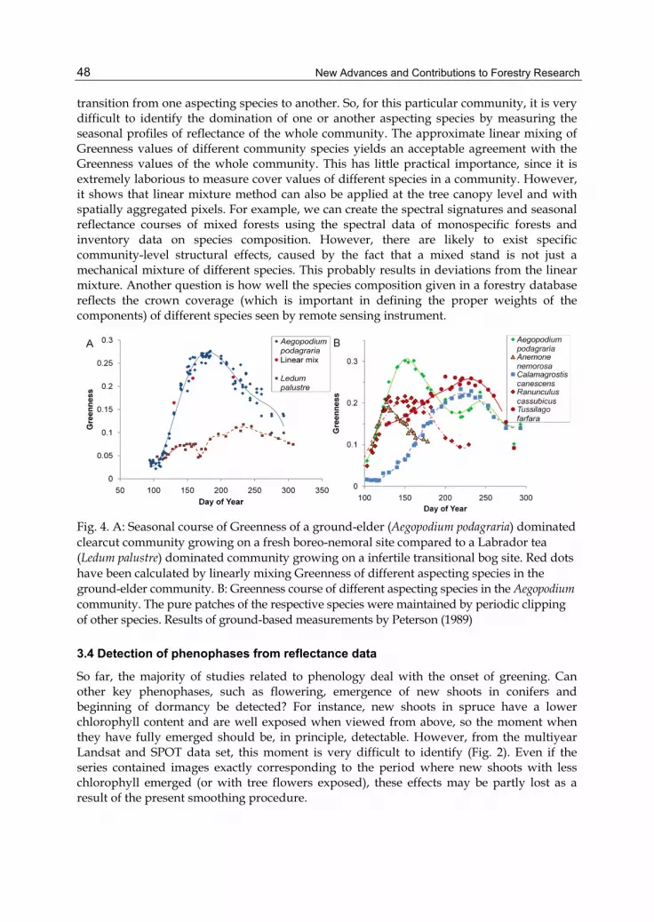
The contribution of different aspecting species to the seasonal profile of the Greenness index is shown in Fig. 4 (reproduced from Peterson, 1989). This example shows us that the whole-community Greenness course may be more or less a smooth curve, in spite of the gradual

New Advances and Contributions to Forestry Research

48

transition from one aspecting species to another. So, for this particular community, it is very difficult to identify the domination of one or another aspecting species by measuring the seasonal profiles of reflectance of the whole community. The approximate linear mixing of Greenness values of different community species yields an acceptable agreement with the Greenness values of the whole community. This has little practical importance, since it is extremely laborious to measure cover values of different species in a community. However, it shows that linear mixture method can also be applied at the tree canopy level and with spatially aggregated pixels. For example, we can create the spectral signatures and seasonal reflectance courses of mixed forests using the spectral data of monospecific forests and inventory data on species composition. However, there are likely to exist specific community-level structural effects, caused by the fact that a mixed stand is not just a mechanical mixture of different species. This probably results in deviations from the linear mixture. Another question is how well the species composition given in a forestry database reflects the crown coverage (which is important in defining the proper weights of the components) of different species seen by remote sensing instrument.

Fig. 4. A: Seasonal course of Greenness of a ground-elder (Aegopodium podagraria) dominated clearcut community growing on a fresh boreo-nemoral site compared to a Labrador tea (Ledum palustre) dominated community growing on a infertile transitional bog site. Red dots have been calculated by linearly mixing Greenness of different aspecting species in the ground-elder community. B: Greenness course of different aspecting species in the Aegopodium community. The pure patches of the respective species were maintained by periodic clipping of other species. Results of ground-based measurements by Peterson (1989)

3.4 Detection of phenophases from reflectance data

So far, the majority of studies related to phenology deal with the onset of greening. Can other key phenophases, such as flowering, emergence of new shoots in conifers and beginning of dormancy be detected? For instance, new shoots in spruce have a lower chlorophyll content and are well exposed when viewed from above, so the moment when they have fully emerged should be, in principle, detectable. However, from the multiyear Landsat and SPOT data set, this moment is very difficult to identify (Fig. 2). Even if the series contained images exactly corresponding to the period where new shoots with less chlorophyll emerged (or with tree flowers exposed), these effects may be partly lost as a result of the present smoothing procedure.

Seasonal Reflectance Courses of Forests

49

As detecting flowering of tree species from satellite images has been shown to be difficult, we will examine next if it would be possible to identify the moment of flowering of smaller plants from high resolution data collected at the ground level. A radiometer was used to measure the reflectance of a Labrador tea (Ledum palustre) dominated grass community in four spectral bands (Peterson, 1989). The community was located in a forest clear cut in a wet oligotrophic site in Konguta, Estonia. The size of the measured plot was ca 2 m2, and thus, the detection of flowering was conducted at an extremely high spatial resolution.

At DOY≈170 a significant peak is clearly seen in all the three visible bands confirming the visual impression of mass flowering (Fig. 5). The flowers of Labrador tea are white, so the peak in all visible bands was expected. In the NIR band a simultaneous slight reflectance decrease during intensive flowering can be noticed; it is likely that Labrador tea flowers scatter less radiation in the NIR band than the leaves. In this particular case, the estimated fraction of flowers at the peak time of flowering was 21% while the total coverage by Labrador tea was 66%. Taking into account that reflectance of white flowers can exceed that of green leaves up to ten times in the visible bands, a detectable signal from flowers can happen at rather low cover values of flowers. However, the temporal frequency of acquiring images must be high enough to catch the peak of flowering.

Fig. 5. The seasonal reflectance course of a Ledum palustre dominated clearcut community. The effect of flowering on is clearly seen at DOY≈170 as a significant peak in the visible bands (Peterson, 1989)

Is it possible to detect the mass flowering of the same Labrador tea community through the canopy of pine trees (as it could be for our pine stand discussed previously in Fig. 2, Table 2)? This is extremely difficult to achieve when the “climatological” seasonal series are used, as it is the case in this study. From model simulations by the forest reflectance model FRT (Kuusk & Nilson, 2000), we can conclude that even if the understory reflectance in the red band increased by 50% (like in Fig. 5) because of flowering of Labrador tea, the nadir reflectance of the stand would increase only by 22%. Although the measured canopy cover of the stand was rather high – (0.74), the pine crowns were relatively transparent, and the total gap fraction in the vertical direction in the canopy was 0.46. So, the understory contributes considerably to the reflected signal from the nadir in the stand. If the cover of Labrador tea were 100%, its flowering could be detectable through the pine canopy. However, in reality, although Labrador tea is the dominating species in the understory of

New Advances and Contributions to Forestry Research

50

the pine stand, its cover fraction is less than 0.20. So, even its mass flowering is extremely difficult to detect from satellite data, since the expected change is of the same order of magnitude with the reflectance measurement error.

3.5 Landscape-level seasonal reflectance courses of forests

A landscape-level analysis of reflectance seasonality was carried out with MODIS data. The MODIS BRDF/Albedo Product (MCD43A1, version 5) (Lucht et al., 2000; Schaaf et al., 2002) was used to reconstruct the nadir reflectances every 8 days at 500 m resolution over Järvselja and Hyytiälä areas in 2006 (dry summer) and 2010 (normal summer). The sun zenith angle was determined for each day for 6:15 GMT i.e. roughly corresponding to the Landsat overpass time. Only the best quality retrievals (QA=0 in the associated MCD43A2 product) were used. Additionally, phenology dates (greenness increase, maximum, decrease, and minimum) were obtained from MODIS MCD12Q2 product for year 2006. Our aim was to use these data to compare the seasonal reflectance curves in two different locations with supposed time lags in phenology and to compare seasonal curves in two years with different precipitation. The idea of comparing the seasonal reflectance courses from MODIS data and from Landsat/SPOT series was to show the reliability of image calibration and to examine the effects of spatial averaging in a fragmented landscape on the seasonal reflectance profiles.

Fig. 6. Comparison of Järvselja (blue squares) and Hyytiälä (purple squares) seasonal reflectance curves for MODIS pixels with birch (A, C) and pine dominated stands (B,D) for years 2006 (dry summer-empty symbols) and 2010 (typical summer-filled symbols). If available, the phenology dates (greenness increase, maximum, decrease, and minimum) from MODIS MCD12Q2 product for year 2006 are also marked (Järvselja - empty triangles; Hyytiälä - empty circles)

Seasonal Reflectance Courses of Forests

51

First, no clear time lag in the green development can be observed from MODIS reconstructed retrievals between Järvselja and Hyytiälä (Fig. 6). This may be partly due to rather long compositing period of the MODIS BRDF product (16 days). The green development at Järvselja preceded Hyytiälä by around 10 days in 2006 according to the MODIS MCD12Q2 phenology product. Järvselja stands also show more rapid reflectance change in early spring, and greater differences in the absolute values of reflectance between the year with dry (2006) and typical (2010) summer (Fig. 6). The more southerly Järvselja stands thus appear to be more sensitive to the variation in available moisture than Hyytiälä. The pronounced difference in amplitude between the birch dominated stands in Järvselja and Hyytiälä in the NIR band (Fig. 6C) is due to the higher share of coniferous stands in the Hyytiälä MODIS pixel. Finally, the differences in the red band (Fig. 6A,B) indicate the general higher vegetation abundance in the Järvselja stands.

Fig. 7. Comparison of Landsat-SPOT red and NIR band time series (purple triangles) and average MODIS seasonal curves for period 2000-2010 (blue diamonds) for a few typical MODIS pixels from Järvselja. A, B, C – red band; D, E, F – NIR band

A comparison of MODIS seasonal curves and Landsat-SPOT time series for a few typical MODIS pixels from Järvselja is shown in Fig. 7. The course of seasonal curves may agree quite well, as in case of the fertile deciduous black alder and birch dominated stand (Fig. 7A, D). The rapid reflectance increase in red band (Fig. 7A) during the fall (DOY 280-300) is due to the loss of chlorophyll in broadleaf trees and understory. A similar increase can also be observed for averaged MODIS reflectances over a pine bog (Fig. 7B). Most of the MODIS retrievals over the pine bog during the fall period have been flagged to be of low quality and were subsequently left out of the averaging procedure, while the remaining retrievals sometimes indicated even early presence of snow. The effect of spatial averaging can be illustrated over the pine bog stand as well. MODIS does not sample from the same footprint every time it passes over, which increases the uncertainty quite considerably (Tan et al., 2006). In fact, a single pixel value may have been obtained from up to 4 different pixels. This complicates the situation particularly in heterogeneous areas in visible bands (Fig. 7B). In the NIR band, the differences are usually smaller due to the weaker contrast and stronger multiple scattering effect

New Advances and Contributions to Forestry Research

52

(Fig. 7E,F) (Pinty et al., 2002). As for the lowland mires, the large scattering in the red band of Landsat-SPOT time series (Fig. 7C) is caused by water level, which varies a lot in Järvselja from year to year, especially in the first half of the vegetation period.

The heterogeneity of the landscape seems to be the main reason why, for some other MODIS pixels in Järvselja such as a treeless bog (results not shown here), the comparison between the MODIS-retrieved seasonal reflectance courses and that derived from the Landsat/SPOT series showed systematic differences. Pixels with typically high reflectance (especially in the visible bands, such as treeless bogs) are extremely sensitive with respect to possible contribution by neighbouring dark forest areas. Such contaminating effects can influence not only the absolute reflectance values at different moments of the season, but can modify the seasonal curves as well and even cause shifts in the key phenology dates determined from the seasonal reflectance curves.

Thus, at the landscape level, the seasonal course of a forest pixel depends much on the share of coniferous and deciduous forests and of treeless (e.g. clear-cut areas, meadows, agricultural land) areas within the pixel. Once again, to explain the seasonal course of reflectance in mixed pixels a linear mixture approach is possible.

4. Future perspectives and conclusions

Until now, most remote sensing studies have concentrated on detecting the onset of greening from satellite data. Now is the time to move beyond the spring-summer time period i.e. to include the full growing period of forests in the analyses, as shown in our case study. In this way, we can develop satellite-based monitoring methods for forest phenology to link the observed changes in reflectance and phenological development of different species to, for example, carbon stocking and photosynthesis.

The main future challenges in monitoring seasonal changes of forests using reflectance data are related to the methods used for interpreting satellite data. As we have shown in this chapter, the theoretical understanding of the physical phenomena is not yet mature enough even though the key driving factors of forest reflectance seasonality have been qualitatively identified. Detecting short phenological phases (e.g. flowering) or phenological phases that are fragmented in the landscape (e.g. yellowing of leaves) is not trivial. Currently, the onset of greening seems to be the easiest, yet still not routinely successful, to detect.

Another challenge is related to data sets. We need to generate spatially and temporally continuous and consistent time series of satellite data for monitoring the seasonal changes. However, the temporal resolution of satellite images is often poor due to the presence of clouds. This has consequences in understanding the seasonality of primary production in regions with a persistent cloud cover, such as boreal and tropical forests. In addition, we need to develop a method for validating the seasonal changes observed in satellite images. Currently, there are no (global) landscape-level ground reference data for validating remotely sensed seasonal courses - maybe the RGB-analysis of landscape-level photos (e.g. automatically taken by webcams in flux towers) will be a step forward?

5. Acknowledgment

The support by Estonian Science Foundation grants no ETF8290 and ETF7725, ESA/ESTEC contract number 4000103213/11/NL/KML, Academy of Finland, University of Helsinki

Seasonal Reflectance Courses of Forests

53

Research Funds and Emil Aaltonen Foundation is acknowledged. MODIS MCD43 and MCD12Q2 product tiles were acquired from Land Processes Distributed Active Archive Center (LP DAAC).

6. References

Ahl, D.; Gower, S.; Burrows, S.; Shabanov, N.; Myneni, R. & Knyazikhin, Y. (2006). Monitoring spring canopy phenology of a deciduous broadleaf forest using MODIS. Remote Sensing of Environment, Vol. 104, pp. 88−95, ISSN 0034-4257

Asner, G.P. (1998) Biophysical and biochemical sources of variability in canopy reflectance. Remote Sensing of Environment, Vol. 64, pp. 234-253.

Brown, L.; Chen, J.M.; Leblanc, S.G. & Cihlar, J. (2000). A Shortwave Infrared Modification to the Simple Ratio for LAI Retrieval in Boreal Forests: An Image and Model Analysis. Remote Sensing of Environment, Vol. 71, pp. 16–25, ISSN 0034-4257

Chen, J.M. & Black, T. (1992). Defining leaf area index for non-flat leaves. Plant, Cell and Environment, Vol. 15, pp. 421-429, ISSN 0140-7791

Crist, E.P. (1984). Effects of cultural and environmental factors on corn and soybean spectral development patterns. Remote Sensing of Environment, Vol. 14, pp. 3-13, ISSN 0034-4257

Demarez, V.; Gastellu-Etchegorry, J.P.; Mougin, E.; Marty, G.; Proisy, C.; Dufrene, E. et al. (1999). Seasonal variation of leaf chlorophyll content of a temperate forest. Inversion of the PROSPECT model. International Journal of Remote Sensing, Vol. 20, pp. 879−894, ISSN 0143-1161

Dye, D. & Tucker, C. (2003). Seasonality and trends of snow-cover, vegetation index, and temperature in northern Eurasia. Geophysical Research Letters, Vol. 30, No. 7, pp. doi:10.1029/2002GL016384, ISSN 0094-8276

Eklundh, L.; Harrie, L. & Kuusk, A. (2001). Investigating relationships between Landsat ETM+ sensor data and leaf area index in a boreal conifer forest. Remote Sensing of Environment, Vol. 78, pp. 239-251, ISSN 0034-4257

Eriksson, H.; Eklundh, L.; Kuusk, A. & Nilson, T. (2006). Impact of understory vegetation on forest canopy reflectance and remotely sensed LAI estimates. Remote Sensing of Environment, Vol. 103, pp. 408—418, ISSN 0034-4257

Friedl, M. et al. (2006). Land surface phenology NASA white paper. In: NASA documents, 15.8.2011, Available from :

http://landportal.gsfc.nasa.gov/Documents/ESDR/Phenology_Friedl_ whitepaper.pdf.

Ganguly, S. et al. (2010). Land surface phenology from MODIS : Characterization of the Collection 5 global land cover dynamics product. Remote Sensing of Environment, Vol. 114, pp. 1805-1816, ISSN 0034-4257

Gastellu-Etchegorry, P.; Guillevic, P.; Zagolski, F.; Demarez, V.; Trichon, V.; Deering, D. & Leroy, M. (1999). Modeling BRF and radiation regime of boreal and tropical forests : I. BRF. Remote Sensing of Environment, Vol. 68, 281-316, ISSN 0034-4257

Guyon, D.; Guillot, M.; Vitasse, Y.; Cardot, H.; Hagolle, O.; Delzon, S. & Wigneron, J.-P. (2011) Monitoring elevation variations in leaf phenology of deciduous broadleaf

New Advances and Contributions to Forestry Research

54

forests from SPOT/VEGETATION time-series. Remote Sensing of Environment, Vol. 115, pp. 615-627, ISSN 0034-4257

Jacquemoud, S. & Baret, F. (1990). PROSPECT: a model of leaf optical properties spectra. Remote Sensing of Environment, Vol. 34, pp. 75-91, ISSN 0034-4257

Jönsson, P. & Eklundh, L. (2002). Seasonality extraction by function fitting to time series of satellite sensor data. IEEE Transactions on Geoscience and Remote Sensing, Vol. 40, pp. 1824−1832, ISSN 0196–2892

Jönsson, A.; Eklundh, L.; Hellström, M.; Bärring, L. & Jönsson, P. (2010) Annual changes in MODIS vegetation indices of Swedish coniferous forests in relation to snow dynamics and tree phenology. Remote Sensing of Environment, Vol. 114, pp. 2719-2730, ISSN 0034-4257

Kauth, R.J. & Thomas, G.S. (1976). The tasseled cap --a graphic description of the spectral-temporal development of agricultural crops as seen in Landsat. Proceedings on the Symposium on Machine Processing of Remotely Sensed Data, West Lafayette IN, June 29 -- July 1, 1976, pp. 41-51.

Keeling, C. et al. (1996). Increased activity of northern vegetation inferred from atmospheric CO2 measurements. Nature, Vol. 382, pp. 146-149, ISSN 0028-0836

Knyazikhin, Y.; Martonchik, J.; Myneni, R.; Diner, D. & Running, S. (1998). Synergistic alogorithm for estimating vegetation canopy leaf area index and fraction of absorbed photosynthetically active radiation from MODIS and MISR data. Journal of Geophysical Research, Vol. D103, pp. 32 257-32 275, ISSN 0148-0227

Kobayashi, H.; Suzuki, R. & Kobayashi, S. (2007). Reflectance seasonality and its relation to the canopy leaf area index in an eastern Siberian larch forest: Multi-satellite data and radiative transfer analysis. Remote Sensing of Environment, Vol. 106, pp. 238-252, ISSN 0034-4257

Kodani, E.; Awaya, Y.; Tanaka, K. & Matsumura, N. (2002). Seasonal patterns of canopy structure, biochemistry and spectral reflectance in a broad-leaved deciduous Fagus crenata canopy. Forest Ecology and Management, Vol. 167, pp. 233-249, ISSN 0378-1127

Kumar, M. & Monteith, J.L. (1981). Remote sensing of crop growth. In: Plants and the daylight spectrum, Smith (ed), pp. 133–144, Academic Press, London

Kuusk, A.; Lang, M.; Kuusk, J.; Lükk, T.; Nilson, T.; Mõttus, M. et al. (2008). Database of optical and structural data for the validation of radiative transfer models. Technical Report. Tartu Observatory, 52 pp, Retrieved from http://www.aai.ee/bgf/jarvselja db/jarvselja db.pdf.

Kuusk, A.; Kuusk, J. & Lang, M. (2009). A dataset for the validation of reflectance models. Remote Sensing of Environment, Vol. 113, pp. 889–892, ISSN 0034-4257

Kuusk, A. & Nilson, T. (2000). A directional multispectral forest reflectance model. Remote Sensing of Environment, Vol. 72, pp. 244−252, ISSN 0034-4257

Lucht, W.; Schaaf, C.B. & Strahler, A. H. (2000). An algorithm for the retrieval of albedo from space using semiempirical BRDF models. IEEE Transactions on Geoscience and Remote Sensing, Vol. 38, pp. 977−998, ISSN 0196–2892

Manninen, T. & Stenberg, P. (2009). Simulation of the effect of snow covered forest floor on the total forest albedo. Agricultural and Forest Meteorology, Vol. 149, pp. 303-319, ISSN 0168-1923

Seasonal Reflectance Courses of Forests

55

Menzel et al. (2006). European phenological response to climate change matches the warming pattern. Global Change Biology, Vol. 12, pp. 1969-1976, ISSN 1354- 1013

Middleton, E.; Sullivan, J.; Bovard, B.; Deluca, A.; Chan, S. & Cannon, T. (1997). Seasonal variability in foliar characteristics and physiology for boreal forest species at the five Saskatchewan tower sites during the 1994 Boreal Ecosystem-Atmosphere Study. Journal of Geophysical Research, Vol. 102, No. D24, (December 1997), pp. 28831-28844, ISSN 0148-0227

Miller, J.; White, P.; Chen, J.M.; Peddle, D.; McDemid, G.; Fournier, R.; Shepherd, P.; Rubinstein, I.; Freemantle, J.; Soffer, R. & LeDrew, E. (1997). Seasonal change in the understory reflectance of boreal forests and influence on canopy vegetation indices. Journal of Geophysical Research, Vol. 102, No. D24, (December 1997), pp. 29475 – 29482, ISSN 0148-0227

Moulin, S.; Kergoat, L.; Viovy, N. & Dedieu, G. (1997). Global-Scale Assessment of Vegetation Phenology Using NOAA/AVHRR Satellite Measurements. Journal of Climate, Vol. 10, pp. 1154-1170, ISSN 0894-8755

Myneni, R.; Asrar, G.; Tanré, D. & Choudhury, B. (1992). Remote sensing of solar radiation absorbed and reflected by vegetated land surfaces. IEEE Transactions on Geoscience and Remote Sensing, Vol. 30, No. 2, pp. 302-314, ISSN 0196-2892

Nightingale, J.; Esaias, W.; Wolfe, R.; Nickeson, J. & Ma, P. (2008). Assessing honey bee equilibrium range and forage supply using satellite-derived phenology. Proceedings of IEEE International Geoscience and Remote Sensing Symposium, Boston, MA, July 7-11, 2008, pp. III-763-766, doi:10.1109/IGARSS.2008.4779460.

Nilson, T.; Anniste, J.; Lang, M. & Praks, J. (1999). Determination of needle area indices of coniferous forest canopies in the NOPEX region by ground-based optical measurements and satellite images. Agricultural and Forest Meteorology, Vol. 98-99, pp. 449-462, ISSN 0168-1923

Nilson, T.; Kuusk, A.; Lang, M. & Lükk, T. (2003). Forest reflectance modeling : theoretical aspects and applications. Ambio, Vol. 33, No. 8, (December 2003), pp. 534-540, ISSN 0044-7447

Nilson, T.; Lükk, T.; Suviste, S.; Kadarik, H. & Eenmäe, A. (2007). Calibration of time series of satellite images to study the seasonal course of forest reflectance. Proceedings of the Estonian Academy of Sciences, Biology / Ecology. Vol. 56, pp. 5-18, ISSN 1406-0914

Nilson, T. & Peterson, U. (1994). Age dependence of forest reflectance: Analysis of main driving factors. Remote Sensing Environment, Vol. 48, pp. 319-331, ISSN 0034-4257

Nilson, T.; Suviste, S.; Lükk, T. & Eenmäe, A. (2008). Seasonal reflectance course of some forest types in Estonia from a series of Landsat TM and SPOT images and via simulation. International Journal of Remote Sensing, Vol. 29, No. 17-18, pp. 5073-5091, ISSN 0143-1161

Paal, J. (1997). Classification of the Estonian vegetation site types, Estonian Environment Information Centre, ISBN 9985-9072-8-0, Tallinn (in Estonian)

Peltoniemi, J.I.; Kaasalainen, S.; Näränen, J.; Rautiainen, M.; Stenberg, P.; Smolander, H.; et al. (2005). BRDF measurement of understory vegetation in pine forests: Dwarf

New Advances and Contributions to Forestry Research

56

shrubs, lichen, and moss. Remote Sensing of Environment, Vol. 94, pp. 343−354, ISSN 0034-4257

Peterson, U. (1989). Seasonal reflectance profiles for forest clearcut communities at early stages of secondary succession. Academy of Sciences of the Estonian SSR, Section of Physics and Astronomy, Preprint A-5 (1989), Tartu

Peterson, U. (1992). Seasonal reflectance factor dynamics in boreal forest clear-cut communities. International Journal of Remote Sensing, Vol. 13, pp. 753-772, ISSN 0143-1161

Pinty, B.; Widlowski, J.L.; Gobron, N.; Verstraete, M.M. & Diner, D.J. (2002). Uniqueness of multiangular measurements – Part 1: An indicator of subpixel surface heterogeneity from MISR. IEEE Transactions on Geoscience and Remote Sensing, Vol. 40, pp. 1560-1573, ISSN 0196-2892

Rautiainen, M.; Heiskanen, J. & Korhonen. L. (2011a). Seasonal changes in canopy leaf area index and MODIS vegetation products for a boreal forest site in central Finland. Boreal Environment Research, in press, ISSN 1239-6095

Rautiainen, M.; Mõttus, M.; Heiskanen, J.; Akujärvi, A.; Majasalmi, T. & Stenberg, P. (2011b). Seasonal reflectance dynamics of common understory types in a northern European boreal forest. Remote Sensing of Environment, Vol. 115, pp. 3020-3028, ISSN 0034-4257

Rautiainen, M.; Stenberg, P.; Nilson, T. & Kuusk, A. (2004). The effect of crown shape on the reflectance of coniferous stands. Remote Sensing of Environment, Vol. 89, pp. 41-52, ISSN 0034-4257

Rautiainen, M.; Nilson, T. & Lükk, T. (2009). Seasonal reflectance trends of hemiboreal birch forests. Remote Sensing of Environment, Vol. 113, pp. 805–815, ISSN 0034- 4257

Richardson, A. & Berlyn, G. (2002). Spectral reflectance and photosynthetic properties of Betula papyrifera (Betulaceae) leaves along an elevational gradient on Mt. Mansfield, Vermont, USA. American Journal of Botany, Vol. 89, pp. 88−94, ISSN 0002-9122

Richardson, A.; Berlyn, G. & Duigan, S. (2003). Reflectance of Alaskan black spruce and white spruce foliage in relation to elevation and latitude. Tree Physiology, Vol. 23, pp. 537-544, ISSN 0829-318X

Richardson A. & O'Keefe J. (2009). Phenological differences between understory and overstory: a case study using the long-term Harvard Forest records, In: Phenology of Ecosystem Processes, A. Noormets (Ed.), 87–117, Springer Science + Business Media, ISBN 978-0-4419-0025-8, New York, USA.

Schaaf, C.B.; Gao, F.; Strahler, A.H.; Lucht, W.; Li, X.; Tsang, T. et al. (2002). First operational BRDF albedo, nadir reflectance products from MODIS. Remote Sensing of Environment, Vol. 83, pp. 135−148, ISSN 0034-4257.

Shibayama, M.; Salli, A.; Häme, T.; Iso-Iivari, L.; Heino, S.; Alanen, M.; Morinaga, S.; Inoue, Y. & Akiyama, T. (1999). Detecting phenophases of subarctic shrub canopies by using automated reflectance measurements. Remote Sensing of Environment, Vol. 67, pp. 160–180, ISSN 0034-4257

Singer, R.B. & McCord, T.B. (1979). Mars: Large scale mixing of bright and dark surface materials and implications for analysis of spectral reflectance. Proceedings of the

Seasonal Reflectance Courses of Forests

57

10th Lunar Planetary Science Conference, Houston TX, March 19-23, 1979, pp. 1835–1848.

Sims, D.; Rahman, A.; Vermote, E. & Jiang, Z. (2011). Seasonal and inter-annual variation in view angle effects on MODIS vegetation indices at three forest sites. Remote Sensing of Environment, in press, ISSN 0034-4257

Spanner, M.; Pierce, L.; Peterson, D. & Running, S. (1990). Remote sensing of temperate coniferous forest leaf area index: the influence of canopy closure, understory vegetation and background reflectance. International Journal of Remote Sensing, Vol. 11, No. 1, pp. 95-111, ISSN 0143-1161

Stenberg, P.; Mõttus, M. & Rautiainen, M. (2008b). Modeling the spectral signature of forests: application of remote sensing models to coniferous canopies, In: Advances in Land remote Sensing: System, Modeling, Inversion and Application, S. Liang, (Ed.), 147-171, Springer-Verlag, ISBN 978-1-4020-6449-4, New York, USA.

Stenberg, P.; Rautiainen, M.; Manninen, T.; Voipio, P. & Mõttus, M. (2008a). Boreal forest leaf area index from optical satellite images: model simulations and empirical analyses using data from central Finland. Boreal Environment Research, Vol. 13, pp. 433-443, ISSN 1239-6095

Stenberg, P.; Rautiainen, M.; Manninen, T.; Voipio, P. & Smolander, H. (2004). Reduced simple ratio better than NDVI for estimating LAI in Finnish pine and spruce stands. Silva Fennica, Vol. 38, pp. 3-14, ISSN 0037-5330

Suviste, S.; Nilson, T.; Lükk, T. & Eenmäe, A. (2007). Seasonal reflectance course of some forest types in Estonia from multi-year Landsat TM and SPOT images and via simulation. Proceedings of the International Workshop on the Analysis of Multi-temporal Remote Sensing Images (MultiTemp 2007), 5 p. doi:10.1109 /MULTITEMP.2007.4293068, ISSN 1-4244-0846-6, Leuven, Belgium, July 18-20, 2007.

Tan, B.; Woodcock, C.E.; Hu, J.; Zhang, P.; Ozdogan, M.; Huang, D.; Yang, W.; Knyazikhin, Y. & Myneni, R.B. (2006). The impact of gridding artifacts on the local spatial properties of MODIS data: Implications for validation, compositing, and band-to-band registration across resolutions. Remote Sensing of Environment, vol.105, pp. 98−114, ISSN 0034-4257

Watson, D. (1947). Comparative physiological studies in the growth of field crops. I. Variation in net assimilation rate and leaf area between species and varieties, and within and between years. Annales Botanicales, Vol. 11, pp. 41-76.

Widlowski, J-L.; Taberner, M.; Pinty, B.; Bruniquel-Pinel, V.; Disney, M.; Fernandes, R.; Gastellu-Etchegorry, J-P.; Gobron, N.; Kuusk, A.; Lavergne, T.; Leblanc, S.; Lewis, P.; Martin, E.; Mõttus, M.; North, P.R.J.; Qin, W.; Robustelli, M.; Rochdi, N.; Ruiloba, R.; Soler, C.; Thompson, R.; Verhoef, W.; Verstraete, M. & Xie, D. (2007). The third RAdiation transfer Model Intercomparison (RAMI) exercise: Documenting progress in canopy reflectance models. Journal of Geophysical Research – Atmospheres, Vol. 112, No, D09111, pp : doi:10.1029/2006JD007821, ISSN 0148-0227

Zhang, X. et al. (2003). Monitoring vegetation phenology using MODIS. Remote Sensing of Environment, Vol. 84, pp. 471-475, ISSN 0034-4257

New Advances and Contributions to Forestry Research

58

Zhou, L. et al. (2001). Variations in northern vegetation activity inferred from satellite data of vegetation index during 1981 to 1999. Journal of Geophysical Research - Atmospheres, Vol. 106, pp. 20069-20083, ISSN 0148-0227