Instrumentation-related uncertainty of reflectance and transmittance measurementswith a two-channel spectrophotometerChristian Peest, Carsten Schinke, Rolf Brendel, Jan Schmidt, and Karsten Bothe

Citation: Review of Scientific Instruments 88, 015105 (2017);View online: https://doi.org/10.1063/1.4973633View Table of Contents: http://aip.scitation.org/toc/rsi/88/1Published by the American Institute of Physics

Articles you may be interested in Photon counting phosphorescence lifetime imaging with TimepixCamReview of Scientific Instruments 88, 013104 (2017); 10.1063/1.4973717

Note: A high-performance, low-cost laser shutter using a piezoelectric cantilever actuatorReview of Scientific Instruments 88, 016102 (2017); 10.1063/1.4973774

Continuous time of flight measurements in a Lissajous configurationReview of Scientific Instruments 88, 013301 (2017); 10.1063/1.4971305

Thermoelectric characterization of flexible micro-thermoelectric generatorsReview of Scientific Instruments 88, 015103 (2017); 10.1063/1.4973417

Simple quadratic magneto-optic Kerr effect measurement system using permanent magnetsReview of Scientific Instruments 88, 013901 (2017); 10.1063/1.4973419

Simultaneous measurement of in-plane and through-plane thermal conductivity using beam-offset frequencydomain thermoreflectanceReview of Scientific Instruments 88, 014902 (2017); 10.1063/1.4973297

REVIEW OF SCIENTIFIC INSTRUMENTS 88, 015105 (2017)

Instrumentation-related uncertainty of reflectance and transmittancemeasurements with a two-channel spectrophotometer

Christian Peest,1,a) Carsten Schinke,1,2 Rolf Brendel,1,2 Jan Schmidt,1,2 and Karsten Bothe11Institute for Solar Energy Research Hamelin (ISFH), Am Ohrberg 1, 31860 Emmerthal, Germany2Leibniz University of Hanover (LUH), Institute for Solid State Physics, Appelstr. 2, 30167 Hanover, Germany

(Received 29 June 2016; accepted 22 December 2016; published online 12 January 2017)

Spectrophotometers are operated in numerous fields of science and industry for a variety of appli-cations. In order to provide confidence for the measured data, analyzing the associated uncertaintyis valuable. However, the uncertainty of the measurement results is often unknown or reduced tosample-related contributions. In this paper, we describe our approach for the systematic determina-tion of the measurement uncertainty of the commercially available two-channel spectrophotometerAgilent Cary 5000 in accordance with the Guide to the expression of uncertainty in measurements.We focus on the instrumentation-related uncertainty contributions rather than the specific applicationand thus outline a general procedure which can be adapted for other instruments. Moreover, wediscover a systematic signal deviation due to the inertia of the measurement amplifier and developand apply a correction procedure. Thereby we increase the usable dynamic range of the instrumentby more than one order of magnitude. We present methods for the quantification of the uncertaintycontributions and combine them into an uncertainty budget for the device. Published by AIP Publish-ing. [http://dx.doi.org/10.1063/1.4973633]

I. INTRODUCTION

Spectrophotometry is a widely used measurement tech-nique in many fields of natural and life science.1–3 Usually,it is believed to be a very accurate and reliable measurementtechnique. Thus, most published uncertainty considerationsfocus on the impact of sample-related contributions to theuncertainty budget, whereas the impact of the instrumentationis believed to be of minor significance and is therefore notconsidered.4,5 However, in order to obtain accurate and reliabledata, a comprehensive analysis not only of the sample undertest but also of the spectrophotometer itself as well as the mea-surement procedure is required. The ASTM standard “Esti-mating Uncertainty of Test Results Derived from Spectropho-tometry,”6 subdivided into instrument, operator, and unifor-mity uncertainty contributions, can be regarded as a guidelinefor such an analysis. Some of the mentioned contributions arediscussed in Ref. 7.

This paper focuses on the experimental determination ofthe uncertainty contributions caused by the instrumentation.We consider a widely used commercially available spectro-photometer, the Agilent Cary 5000 UV-VIS-NIR. This de-vice is used world wide for research and development, forquality assurance as well as for calibration measurements.We present methods for the quantitative estimation of theinstrument-related uncertainty contributions, taking into ac-count that such a commercially available system providesonly limited access to the parameters required for a compre-hensive uncertainty analysis. In accordance with the Guideto the expression of uncertainty in measurement (GUM),8

the different contributions are combined into an uncertainty

a)Now with Sterrenkundig Observatorium, Universiteit Gent, Krijgslaan 281S9, 9000 Gent, Belgium; Electronic mail: christian.peest@ugent.be

budget. For specific applications, sample and measurementprocedure related contributions have to be added to this budget.However, the number of applications is numerous and can thusnot be treated in a general way. As an example, we show anuncertainty analysis for reflectance and transmission measure-ments on planar silicon wafers in Section V, which also takessample-related contributions to the uncertainty budget intoaccount.

II. METHODOLOGY

The analysis presented in this work is based on an exten-sive characterization of an Agilent Cary 5000 spectropho-tometer. We apply the methodology specified in the GUM,8

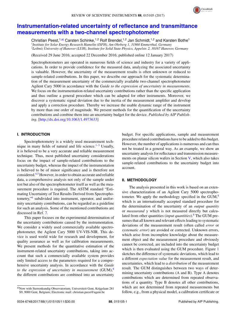
which is an internationally accepted standard procedure forthe determination of the uncertainty of an output quantityor measurand y which is not measured directly but calcu-lated from other quantities (input quantities).8 The GUM pre-sumes that all known and relevant effects leading to systematicdeviations of the measurement result (often called error orsystematic error) are avoided or corrected. Unknown errors,which arise from incomplete knowledge about the measure-ment object and the measurement procedure and obviouslycannot be corrected, are included into the uncertainty budgetwhich is then evaluated using the GUM procedure. Figure 1sketches the difference of systematic deviations, which lead toa different expectation value for the measurement result, anduncertainties, which lead to a distribution of the measurementresult. The GUM distinguishes between two ways of deter-mining uncertainty contributions (A and B). Type A denotescontributions which are determined from repeated observa-tions of a quantity. Type B denotes all other contributions,which are not determined from repeated measurements butfollow, e.g., from a physical model, a calibration certificate or

0034-6748/2017/88(1)/015105/11/$30.00 88, 015105-1 Published by AIP Publishing.

015105-2 Peest et al. Rev. Sci. Instrum. 88, 015105 (2017)

FIG. 1. Visualization of the terms systematic deviation and uncertainty.

scientific experience. The nomenclature does not refer to thetreatment of the uncertainty contributions, which is equal forboth types. Note that type A and B must not be confused withthe familiar terms systematic error and random error, whichdescribe the nature of the error. Each determination type (A orB) can in principle be used to determine the uncertainty due toerrors of both types.

The core part of an uncertainty analysis in accordancewith the GUM is the process equation f , which defines thefunctional relationship between the measurand y and inputquantities x1, x2, . . . , xN ,

y = f (x1, x2, . . . , xN). (1)

The combined standard uncertainty u2c(y) of the measur-

and y is then given by

u2c(y) =

Ni=1

Nj=1

∂ f∂xi

∂ f∂x j

u�xi, x j

�. (2)

If the xi are uncorrelated, which means that the values of the xi

are not affected by the values of the other x j,i, this simplifiesto

u2c(y) =

Ni=1

(∂ f∂xi

)2

u2(xi) =Ni=1

c2iu

2i , (3)

with the sensitivity coefficients ci = ∂ f/∂xi and the uncertaintyof the input quantities u(xi) ≡ ui. The case of uncorrelatedinput quantities is assumed throughout this paper due to thephysical origin of the uncertainty contributions or the quanti-fication method (see comments in Section IV).

The formulation of the complete process equation is acritical part of the evaluation of measurement uncertainty, as itmust include all relevant effects that could lead to systematicdeviations of the measurement result, as mentioned above.Alternatively, corrections can directly be applied to the inputquantities, and a simpler process equation (without correctionterms) can be used. It is obvious that both approaches areequivalent. Furthermore, the uncertainty distributions of theinput quantities need to be determined. Recurrent distributionsare the normal and the rectangular distribution (see Fig. 1).The first describes values randomly scattered around the meanvalue, whereas the latter is used when the exact distribution isunknown but the upper and lower boundaries are known, inbetween which the true value lies.

For all mentioned distributions, the best estimate of thetrue value is the arithmetic mean of a number N of repeatedmeasurements. For the normal distribution (ND), the uncer-tainty of the estimated value is given by

u2ND =

σ2

√N − 1

, (4)

with the variance σ2 of the arithmetic mean. Note that inprinciple, a limited number of measurements is described bythe Student’s t-distribution rather than the normal distribu-tion. For a large number of measurements, however, the t-distribution approaches the normal distribution. (see Sec. IV Aand GUM Annex C). The rectangular distribution represents auniform probability density (UD) of width 2a. The associateduncertainty is

u2UD =

a2

3. (5)

The true value lies within the interval±uc around the measuredvalue with a probability of approximately 68%. The expandeduncertainty U for the coverage factor k is defined as

U = k · uc. (6)

In this paper, all given expanded uncertainties refer to acoverage factor of k = 2, i.e., they encompass the true valuewith a probability of about 95%.

III. MEASUREMENT SETUP

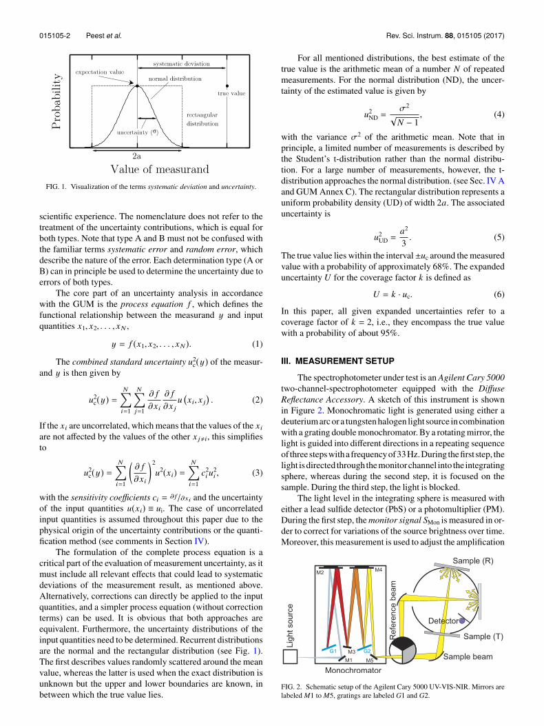
The spectrophotometer under test is an Agilent Cary 5000two-channel-spectrophotometer equipped with the DiffuseReflectance Accessory. A sketch of this instrument is shownin Figure 2. Monochromatic light is generated using either adeuterium arc or a tungsten halogen light source in combinationwith a grating double monochromator. By a rotating mirror, thelight is guided into different directions in a repeating sequenceof threestepswitha frequencyof33Hz.During thefirst step, thelight isdirected through themonitorchannel into the integratingsphere, whereas during the second step, it is focused on thesample. During the third step, the light is blocked.

The light level in the integrating sphere is measured witheither a lead sulfide detector (PbS) or a photomultiplier (PM).During the first step, the monitor signal SMon is measured in or-der to correct for variations of the source brightness over time.Moreover, this measurement is used to adjust the amplification

FIG. 2. Schematic setup of the Agilent Cary 5000 UV-VIS-NIR. Mirrors arelabeled M1 to M5, gratings are labeled G1 and G2.

015105-3 Peest et al. Rev. Sci. Instrum. 88, 015105 (2017)

factor gamp of the measurement amplifier. During the secondstep, the sample signal SSam is measured. In the third step, thebaseline signal SBas is measured, which contains detector andelectronic offsets and stray light.

In order to determine the reflectance of a sample, threemeasurements are combined: One measurement with a cali-brated standard on the reflection port (RN), one with the sam-ple in the same position (RS), and a baseline measurementwith the reflection port open to a darkened room (RB). RBdetermines the amount of light that is reflected back into theintegrating sphere at the edge of the reflectance port, and RN isused to normalize the measurement of the sample, so that thereflectivity of the sample can be calculated with the tabulatedreflectivity RStd of the standard,

R =RS − RB

RN − RBRStd. (7)

For transmittance measurements, this procedure is simpli-fied. The baseline measurement, a measurement with a beamtrap, is omitted. This is possible due to an internal baselinecorrection (see Eq. (9)). For the measurements considered inthis paper (wavelength range 250 nm–1450 nm), the absorp-tion of light in air is negligible; therefore an empty transmis-sion port replaces the measurement of a calibrated standard.Hence, only two measurements are required: one measurementwith the sample in the transmission port of the integratingsphere (TS) and one with an empty transmission port (TN). Thetransmittance of the sample is then given by

T =TS

TN. (8)

Each of the input quantities S ∈ {TN,TS,RB,RN,RS} is given by

S =SSam − SBas

SMon − SBas, (9)

where SMon, SSam, and SBas denote the detector signal dur-ing the mentioned three steps (illumination of monitor chan-nel, illumination of sample channel, baseline measurement),respectively. These quantities are not accessible to the oper-ator and the calculation of S is carried out internally by theinstrument.

A. Settings for data acquisition

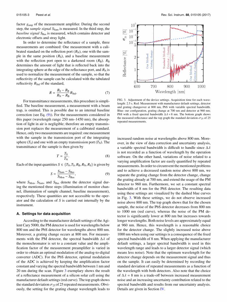
According to the manufacturer default settings of the Agi-lent Cary 5000, the PM detector is used for wavelengths below800 nm and the PbS detector for wavelengths above 800 nm.Moreover, a grating change occurs at 800 nm. For measure-ments with the PM detector, the spectral bandwidth ∆λ ofthe monochromator is set to a constant value and the ampli-fication factor of the measurement preamplifier is varied inorder to obtain an optimal modulation of the analog-to-digitalconverter (ADC). For the PbS detector, optimal modulationof the ADC is achieved by keeping the amplification factorconstant and varying the spectral bandwidth between 1 nm and20 nm during the scan. Figure 3 exemplary shows the resultof a reflectance measurement of a silicon solar cell using themanufacturer default settings (red curve). The top graph showsthe standard deviationσ25 of 25 repeated measurements. Obvi-ously, the setting for the grating change wavelength leads to

FIG. 3. Adjustment of the device settings. Acquisition time for each wave-length: 2.5 s. Red: Measurement with manufacturer default settings, detectorand grating changeover at 800 nm, PbS with variable spectral bandwidth.Blue: our configuration, grating change at 700 nm and detector at 960 nm;PbS with a fixed spectral bandwidth ∆λ = 8 nm. The bottom graph showsthe measured reflectance and the top graph the standard deviation σ25 of 25repeated measurements.

increased random noise at wavelengths above 800 nm. More-over, in the view of data correction and uncertainty analysis,a variable spectral bandwidth is difficult to handle since ∆λis not recorded as a function of wavelength by the operationsoftware. On the other hand, variations of noise related to avarying amplification factor are easily quantified by repeatedmeasurements. In order to circumvent the mentioned problemsand to achieve a decreased random noise above 800 nm, weseparate the grating change from the detector change, changethe grating already at 700 nm, and extend the usage of the PMdetector to 960 nm. Furthermore, we set a constant spectralbandwidth of 8 nm for the PbS detector. The resulting datausing these settings are visualized by the dashed blue curvesin Fig. 3. With these settings, we do not observe increasednoise above 800 nm. The top graph shows that for the chosensample, the noise of the PbS detector decreases from 800 nmto 1000 nm (red curve), whereas the noise of the PM de-tector is significantly lower at 800 nm but increases towardslonger wavelengths. Both noise levels are approximately equalat 960 nm. Hence, this wavelength is a reasonable choicefor the detector change. The slightly increased noise above1000 nm when using our settings is a consequence of the fixedspectral bandwidth of 8 nm. When applying the manufacturerdefault settings, a larger spectral bandwidth is used in thiswavelength range and leads to a larger detector signal (whichmeans less noise). Note that the optimum wavelength for thedetector change depends on the measurement signal and thuson the sample. It can easily be determined by recording thestandard deviation of repeated measurements as a function ofthe wavelength with both detectors. Also note that the choiceof ∆λ = 8 nm is a trade-off between increased measurementnoise and an increasing uncertainty contribution related to thespectral bandwidth and results from our uncertainty analysis.Details are given in Section IV.

015105-4 Peest et al. Rev. Sci. Instrum. 88, 015105 (2017)

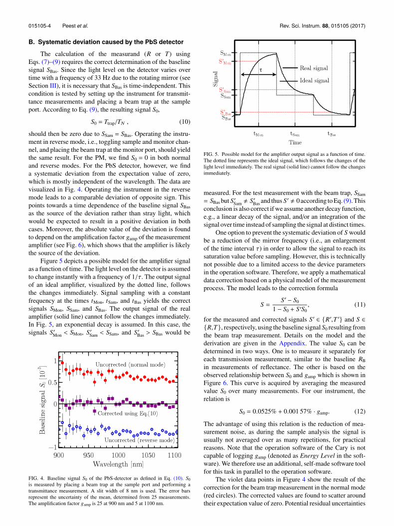
B. Systematic deviation caused by the PbS detector

The calculation of the measurand (R or T) usingEqs. (7)–(9) requires the correct determination of the baselinesignal SBas. Since the light level on the detector varies overtime with a frequency of 33 Hz due to the rotating mirror (seeSection III), it is necessary that SBas is time-independent. Thiscondition is tested by setting up the instrument for transmit-tance measurements and placing a beam trap at the sampleport. According to Eq. (9), the resulting signal S0,

S0 = Ttrap/TN , (10)

should then be zero due to SSam = SBas. Operating the instru-ment in reverse mode, i.e., toggling sample and monitor chan-nel, and placing the beam trap at the monitor port, should yieldthe same result. For the PM, we find S0 = 0 in both normaland reverse modes. For the PbS detector, however, we finda systematic deviation from the expectation value of zero,which is mostly independent of the wavelength. The data arevisualized in Fig. 4. Operating the instrument in the reversemode leads to a comparable deviation of opposite sign. Thispoints towards a time dependence of the baseline signal SBasas the source of the deviation rather than stray light, whichwould be expected to result in a positive deviation in bothcases. Moreover, the absolute value of the deviation is foundto depend on the amplification factor gamp of the measurementamplifier (see Fig. 6), which shows that the amplifier is likelythe source of the deviation.

Figure 5 depicts a possible model for the amplifier signalas a function of time. The light level on the detector is assumedto change instantly with a frequency of 1/τ. The output signalof an ideal amplifier, visualized by the dotted line, followsthe changes immediately. Signal sampling with a constantfrequency at the times tMon, tSam, and tBas yields the correctsignals SMon, SSam, and SBas. The output signal of the realamplifier (solid line) cannot follow the changes immediately.In Fig. 5, an exponential decay is assumed. In this case, thesignals S′Mon < SMon, S′Sam < SSam, and S′Bas > SBas would be

FIG. 4. Baseline signal S0 of the PbS-detector as defined in Eq. (10). S0is measured by placing a beam trap at the sample port and performing atransmittance measurement. A slit width of 8 nm is used. The error barsrepresent the uncertainty of the mean, determined from 25 measurements.The amplification factor gamp is 25 at 900 nm and 5 at 1100 nm.

FIG. 5. Possible model for the amplifier output signal as a function of time.The dotted line represents the ideal signal, which follows the changes of thelight level immediately. The real signal (solid line) cannot follow the changesimmediately.

measured. For the test measurement with the beam trap, SSam= SBas but S′Sam , S′Bas and thus S′ , 0 according to Eq. (9). Thisconclusion is also correct if we assume another decay function,e.g., a linear decay of the signal, and/or an integration of thesignal over time instead of sampling the signal at distinct times.

One option to prevent the systematic deviation of S wouldbe a reduction of the mirror frequency (i.e., an enlargementof the time interval τ) in order to allow the signal to reach itssaturation value before sampling. However, this is technicallynot possible due to a limited access to the device parametersin the operation software. Therefore, we apply a mathematicaldata correction based on a physical model of the measurementprocess. The model leads to the correction formula

S =S′ − S0

1 − S0 + S′S0, (11)

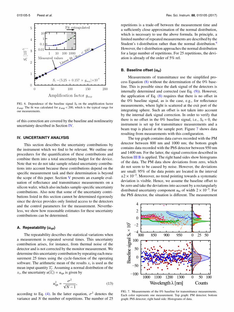
for the measured and corrected signals S′ ∈ {R′,T ′} and S ∈{R,T}, respectively, using the baseline signal S0 resulting fromthe beam trap measurement. Details on the model and thederivation are given in the Appendix. The value S0 can bedetermined in two ways. One is to measure it separately foreach transmission measurement, similar to the baseline RBin measurements of reflectance. The other is based on theobserved relationship between S0 and gamp which is shown inFigure 6. This curve is acquired by averaging the measuredvalue S0 over many measurements. For our instrument, therelation is

S0 = 0.0525% + 0.001 57% · gamp. (12)

The advantage of using this relation is the reduction of mea-surement noise, as during the sample analysis the signal isusually not averaged over as many repetitions, for practicalreasons. Note that the operation software of the Cary is notcapable of logging gamp (denoted as Energy Level in the soft-ware). We therefore use an additional, self-made software toolfor this task in parallel to the operation software.

The violet data points in Figure 4 show the result of thecorrection for the beam trap measurement in the normal mode(red circles). The corrected values are found to scatter aroundtheir expectation value of zero. Potential residual uncertainties

015105-5 Peest et al. Rev. Sci. Instrum. 88, 015105 (2017)

FIG. 6. Dependence of the baseline signal S0 on the amplification factorgamp. The fit was calculated for gamp < 200, which is the typical range forour measurements.

of this correction are covered by the baseline and nonlinearityuncertainty described in Section IV.

IV. UNCERTAINTY ANALYSIS

This section describes the uncertainty contributions bythe instrument which we find to be relevant. We outline ourprocedures for the quantification of these contributions andcombine them into a total uncertainty budget for the device.Note that we do not take sample related uncertainty contribu-tions into account because these contributions depend on thespecific measurement task and their determination is beyondthe scope of this paper. Section V presents an example eval-uation of reflectance and transmittance measurements on asilicon wafer, which also includes sample-specific uncertaintycontributions. Also note that some of the uncertainty contri-butions listed in this section cannot be determined rigorouslysince the device provides only limited access to the detectorsand the control parameters for the measurement. Neverthe-less, we show how reasonable estimates for these uncertaintycontributions can be determined.

A. Repeatability (urpt)

The repeatability describes the statistical variations whena measurement is repeated several times. This uncertaintycontribution arises, for instance, from thermal noise of thedetector and is not corrected by the monitor measurement. Wedetermine this uncertainty contribution by repeating each mea-surement 25 times using the cycle-function of the operatingsoftware. The arithmetic mean of the results xi is used as themean input quantity xi. Assuming a normal distribution of thexi, the uncertainty u(xi) = urpt is given by

u2rpt =

σ2

√N − 1

, (13)

according to Eq. (4). In the latter equation, σ2 denotes thevariance and N the number of repetitions. The number of 25

repetitions is a trade-off between the measurement time anda sufficiently close approximation of the normal distribution,which is necessary to use the above formula. In principle, alimited number of repeated measurements are described by theStudent’s t-distribution rather than the normal distribution.9

However, the t-distribution approaches the normal distributionfor a large number of repetitions. For 25 repetitions, the devi-ation is already of the order of 5% rel.

B. Baseline offset (ubl)

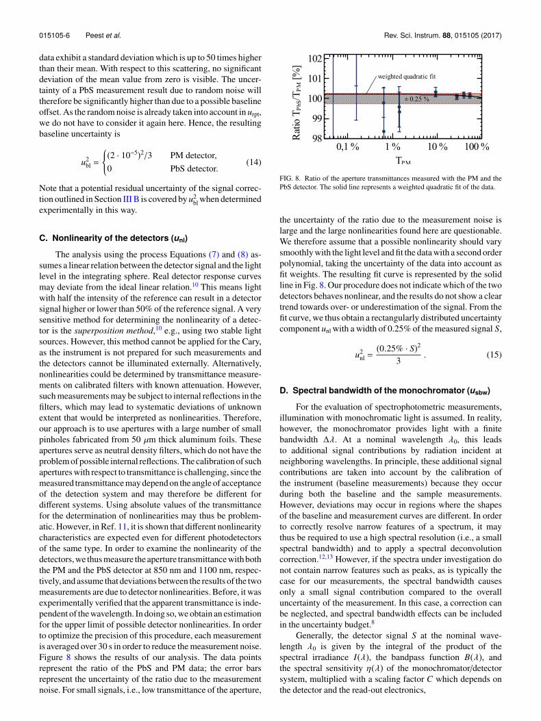
Measurements of transmittance use the simplified pro-cess Equation (8) without the determination of the 0% base-line. This is possible since the dark signal of the detectors isinternally determined and corrected (see Eq. (9)). However,the application of Eq. (8) requires that there is no offset inthe 0% baseline signal, as is the case, e.g., for reflectancemeasurements, where light is scattered at the exit port of theintegrating sphere. Such an offset is not taken into accountby the internal dark signal correction. In order to verify thatthere is no offset in the 0% baseline signal, i.e., S0 = 0, theinstrument is set up for transmittance measurements and abeam trap is placed at the sample port. Figure 7 shows dataresulting from measurements with this configuration.

The top graph contains data curves recorded with the PMdetector between 800 nm and 1000 nm; the bottom graphcontains data recorded with the PbS detector between 950 nmand 1400 nm. For the latter, the signal correction described inSection III B is applied. The right hand sides show histogramsof the data. The PM data show deviations from zero, whichdo not seem to be caused by noise. However, the deviationsare small: 95% of the data points are located in the interval±2 × 10−5. Moreover, no trend pointing towards a systematicdeviation is visible. Hence, we assume the baseline offset tobe zero and take the deviations into account by a rectangularlydistributed uncertainty component ubl of width 2 × 10−5. Forthe PbS detector, the situation is different. The measurement

FIG. 7. Measurements of the 0% baseline for transmittance measurements.Each color represents one measurement. Top graph: PM detector; bottomgraph: PbS detector; right hand side: Histograms of data.

015105-6 Peest et al. Rev. Sci. Instrum. 88, 015105 (2017)

data exhibit a standard deviation which is up to 50 times higherthan their mean. With respect to this scattering, no significantdeviation of the mean value from zero is visible. The uncer-tainty of a PbS measurement result due to random noise willtherefore be significantly higher than due to a possible baselineoffset. As the random noise is already taken into account in urpt,we do not have to consider it again here. Hence, the resultingbaseline uncertainty is

u2bl =

(2 · 10−5)2/3 PM detector,0 PbS detector.

(14)

Note that a potential residual uncertainty of the signal correc-tion outlined in Section III B is covered by u2

bl when determinedexperimentally in this way.

C. Nonlinearity of the detectors (unl)

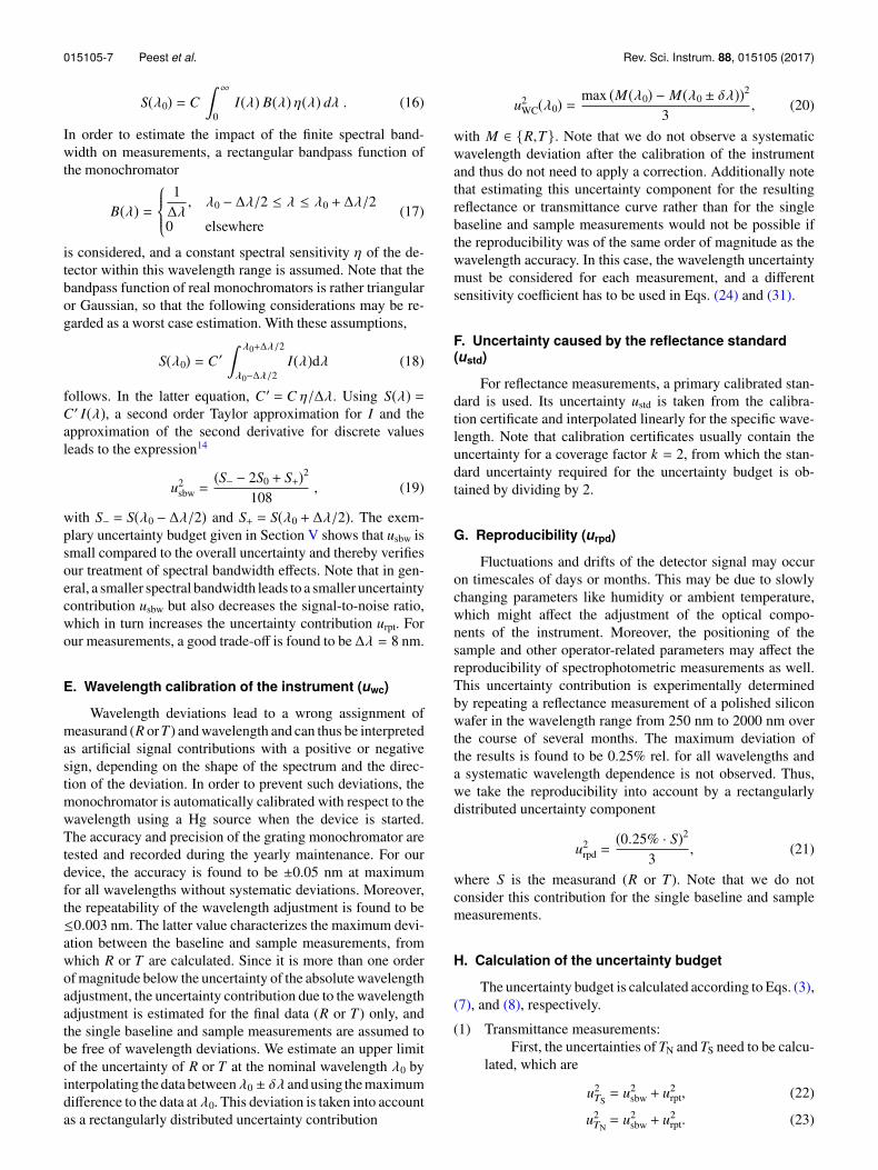
The analysis using the process Equations (7) and (8) as-sumes a linear relation between the detector signal and the lightlevel in the integrating sphere. Real detector response curvesmay deviate from the ideal linear relation.10 This means lightwith half the intensity of the reference can result in a detectorsignal higher or lower than 50% of the reference signal. A verysensitive method for determining the nonlinearity of a detec-tor is the superposition method,10 e.g., using two stable lightsources. However, this method cannot be applied for the Cary,as the instrument is not prepared for such measurements andthe detectors cannot be illuminated externally. Alternatively,nonlinearities could be determined by transmittance measure-ments on calibrated filters with known attenuation. However,such measurements may be subject to internal reflections in thefilters, which may lead to systematic deviations of unknownextent that would be interpreted as nonlinearities. Therefore,our approach is to use apertures with a large number of smallpinholes fabricated from 50 µm thick aluminum foils. Theseapertures serve as neutral density filters, which do not have theproblem of possible internal reflections. The calibration of suchapertures with respect to transmittance is challenging, since themeasured transmittance may depend on the angle of acceptanceof the detection system and may therefore be different fordifferent systems. Using absolute values of the transmittancefor the determination of nonlinearities may thus be problem-atic. However, in Ref. 11, it is shown that different nonlinearitycharacteristics are expected even for different photodetectorsof the same type. In order to examine the nonlinearity of thedetectors, we thus measure the aperture transmittance with boththe PM and the PbS detector at 850 nm and 1100 nm, respec-tively, and assume that deviations between the results of the twomeasurements are due to detector nonlinearities. Before, it wasexperimentally verified that the apparent transmittance is inde-pendent of the wavelength. In doing so, we obtain an estimationfor the upper limit of possible detector nonlinearities. In orderto optimize the precision of this procedure, each measurementis averaged over 30 s in order to reduce the measurement noise.Figure 8 shows the results of our analysis. The data pointsrepresent the ratio of the PbS and PM data; the error barsrepresent the uncertainty of the ratio due to the measurementnoise. For small signals, i.e., low transmittance of the aperture,

FIG. 8. Ratio of the aperture transmittances measured with the PM and thePbS detector. The solid line represents a weighted quadratic fit of the data.

the uncertainty of the ratio due to the measurement noise islarge and the large nonlinearities found here are questionable.We therefore assume that a possible nonlinearity should varysmoothly with the light level and fit the data with a second orderpolynomial, taking the uncertainty of the data into account asfit weights. The resulting fit curve is represented by the solidline in Fig. 8. Our procedure does not indicate which of the twodetectors behaves nonlinear, and the results do not show a cleartrend towards over- or underestimation of the signal. From thefit curve, we thus obtain a rectangularly distributed uncertaintycomponent unl with a width of 0.25% of the measured signal S,

u2nl =

(0.25% · S)23

. (15)

D. Spectral bandwidth of the monochromator (usbw)

For the evaluation of spectrophotometric measurements,illumination with monochromatic light is assumed. In reality,however, the monochromator provides light with a finitebandwidth ∆λ. At a nominal wavelength λ0, this leadsto additional signal contributions by radiation incident atneighboring wavelengths. In principle, these additional signalcontributions are taken into account by the calibration ofthe instrument (baseline measurements) because they occurduring both the baseline and the sample measurements.However, deviations may occur in regions where the shapesof the baseline and measurement curves are different. In orderto correctly resolve narrow features of a spectrum, it maythus be required to use a high spectral resolution (i.e., a smallspectral bandwidth) and to apply a spectral deconvolutioncorrection.12,13 However, if the spectra under investigation donot contain narrow features such as peaks, as is typically thecase for our measurements, the spectral bandwidth causesonly a small signal contribution compared to the overalluncertainty of the measurement. In this case, a correction canbe neglected, and spectral bandwidth effects can be includedin the uncertainty budget.8

Generally, the detector signal S at the nominal wave-length λ0 is given by the integral of the product of thespectral irradiance I(λ), the bandpass function B(λ), andthe spectral sensitivity η(λ) of the monochromator/detectorsystem, multiplied with a scaling factor C which depends onthe detector and the read-out electronics,

015105-7 Peest et al. Rev. Sci. Instrum. 88, 015105 (2017)

S(λ0) = C ∞

0I(λ) B(λ) η(λ) dλ . (16)

In order to estimate the impact of the finite spectral band-width on measurements, a rectangular bandpass function ofthe monochromator

B(λ) =

1∆λ

, λ0 − ∆λ/2 ≤ λ ≤ λ0 + ∆λ/2

0 elsewhere(17)

is considered, and a constant spectral sensitivity η of the de-tector within this wavelength range is assumed. Note that thebandpass function of real monochromators is rather triangularor Gaussian, so that the following considerations may be re-garded as a worst case estimation. With these assumptions,

S(λ0) = C ′ λ0+∆λ/2

λ0−∆λ/2I(λ)dλ (18)

follows. In the latter equation, C ′ = C η/∆λ. Using S(λ) =C ′ I(λ), a second order Taylor approximation for I and theapproximation of the second derivative for discrete valuesleads to the expression14

u2sbw =

(S− − 2S0 + S+)2108

, (19)

with S− = S(λ0 − ∆λ/2) and S+ = S(λ0 + ∆λ/2). The exem-plary uncertainty budget given in Section V shows that usbw issmall compared to the overall uncertainty and thereby verifiesour treatment of spectral bandwidth effects. Note that in gen-eral, a smaller spectral bandwidth leads to a smaller uncertaintycontribution usbw but also decreases the signal-to-noise ratio,which in turn increases the uncertainty contribution urpt. Forour measurements, a good trade-off is found to be ∆λ = 8 nm.

E. Wavelength calibration of the instrument (uwc)

Wavelength deviations lead to a wrong assignment ofmeasurand (R orT) and wavelength and can thus be interpretedas artificial signal contributions with a positive or negativesign, depending on the shape of the spectrum and the direc-tion of the deviation. In order to prevent such deviations, themonochromator is automatically calibrated with respect to thewavelength using a Hg source when the device is started.The accuracy and precision of the grating monochromator aretested and recorded during the yearly maintenance. For ourdevice, the accuracy is found to be ±0.05 nm at maximumfor all wavelengths without systematic deviations. Moreover,the repeatability of the wavelength adjustment is found to be≤0.003 nm. The latter value characterizes the maximum devi-ation between the baseline and sample measurements, fromwhich R or T are calculated. Since it is more than one orderof magnitude below the uncertainty of the absolute wavelengthadjustment, the uncertainty contribution due to the wavelengthadjustment is estimated for the final data (R or T) only, andthe single baseline and sample measurements are assumed tobe free of wavelength deviations. We estimate an upper limitof the uncertainty of R or T at the nominal wavelength λ0 byinterpolating the data between λ0 ± δλ and using the maximumdifference to the data at λ0. This deviation is taken into accountas a rectangularly distributed uncertainty contribution

u2WC(λ0) = max (M(λ0) − M(λ0 ± δλ))2

3, (20)

with M ∈ {R,T}. Note that we do not observe a systematicwavelength deviation after the calibration of the instrumentand thus do not need to apply a correction. Additionally notethat estimating this uncertainty component for the resultingreflectance or transmittance curve rather than for the singlebaseline and sample measurements would not be possible ifthe reproducibility was of the same order of magnitude as thewavelength accuracy. In this case, the wavelength uncertaintymust be considered for each measurement, and a differentsensitivity coefficient has to be used in Eqs. (24) and (31).

F. Uncertainty caused by the reflectance standard(ustd)

For reflectance measurements, a primary calibrated stan-dard is used. Its uncertainty ustd is taken from the calibra-tion certificate and interpolated linearly for the specific wave-length. Note that calibration certificates usually contain theuncertainty for a coverage factor k = 2, from which the stan-dard uncertainty required for the uncertainty budget is ob-tained by dividing by 2.

G. Reproducibility (urpd)

Fluctuations and drifts of the detector signal may occuron timescales of days or months. This may be due to slowlychanging parameters like humidity or ambient temperature,which might affect the adjustment of the optical compo-nents of the instrument. Moreover, the positioning of thesample and other operator-related parameters may affect thereproducibility of spectrophotometric measurements as well.This uncertainty contribution is experimentally determinedby repeating a reflectance measurement of a polished siliconwafer in the wavelength range from 250 nm to 2000 nm overthe course of several months. The maximum deviation ofthe results is found to be 0.25% rel. for all wavelengths anda systematic wavelength dependence is not observed. Thus,we take the reproducibility into account by a rectangularlydistributed uncertainty component

u2rpd =

(0.25% · S)23

, (21)

where S is the measurand (R or T). Note that we do notconsider this contribution for the single baseline and samplemeasurements.

H. Calculation of the uncertainty budget

The uncertainty budget is calculated according to Eqs. (3),(7), and (8), respectively.

(1) Transmittance measurements:First, the uncertainties of TN and TS need to be calcu-

lated, which are

u2TS= u2

sbw + u2rpt, (22)

u2TN= u2

sbw + u2rpt. (23)

015105-8 Peest et al. Rev. Sci. Instrum. 88, 015105 (2017)

TABLE I. Uncertainty contributions due to properties of our instrument for measurements of transmittance (T )and reflectance (R).

T /R Description Symbol Our value Distribution Sens. coeff.

R Refl. standard ustd (2.981 to 3.664) × 10−3a Normal — / cRStd

T /R Nonlinearity unl 1.443 × 10−3Sa Rectangular 1 / 1T /R Reproducibility urpd 1.443 × 10−3Sa Rectangular 1 / 1T /R Repeatability urpt,S Eq. (13)a Normal cTS / cRS

R Repeatability urpt,B Eq. (13)a Normal — / cRB

T /R Repeatability urpt,N Eq. (13)a Normal cTN / cRN

T /R Spectr. bandwidth usbw,S ∆λ = 8 nm, Eq. (19)a Rectangular cTS / cRS

T /R Wavelength cal. uwc δλ = 0.05 nm, Eq. (20)a Rectangular 1 / 1T /R Spectr. bandwidth usbw,N ∆λ = 8 nm, Eq. (19)a Rectangular cTN / cRN

T Baseline ubl 1.155 × 10−5 rectangular 1 /—

aTo be calculated for each wavelength.

With this and Eq. (8), the uncertainty of T follows as

u2T = c2

TS· u2

TS+ c2

TN· u2

TN+ u2

rpd + u2nl + u2

wc + u2bl, (24)

with the sensitivity coefficients

c2TS=

1TN

2 , (25)

c2TN=

TS2

TN4 . (26)

(2) Reflectance measurements:The uncertainties of the input quantities are

u2RS= u2

sbw + u2rpt, (27)

u2RN= u2

sbw + u2rpt, (28)

u2RB= u2

rpt, (29)

u2RStd= u2

std. (30)

With Eq. (7), the uncertainty of R is then

u2R = c2

RS· u2

RS+ c2

RN· u2

RN+ c2

RB· u2

RB+

+ c2RStd· u2

RStd+ u2

rpd + u2nl + u2

wc, (31)

with the sensitivity coefficients

c2RS=

(1

RN − RBRStd

)2

, (32)

c2RN=

(RS − RB

(RN − RB)2 RStd

)2

, (33)

c2RB=

(RS − RN

(RN − RB)2 RStd

)2

, (34)

c2RStd=

(RS − RB

RN − RB

)2

. (35)

Table I summarizes the uncertainty contributions as deter-mined in this work. Uncertainties related to the specific prop-erties of the sample add to the total uncertainty and need tobe considered as well for a complete analysis of a specificmeasurement.

V. EXAMPLE UNCERTAINTY ANALYSIS

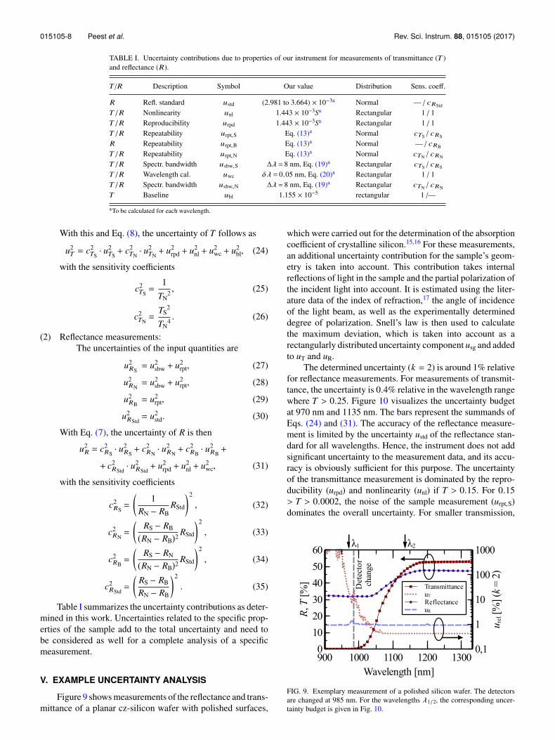
Figure 9 shows measurements of the reflectance and trans-mittance of a planar cz-silicon wafer with polished surfaces,

which were carried out for the determination of the absorptioncoefficient of crystalline silicon.15,16 For these measurements,an additional uncertainty contribution for the sample’s geom-etry is taken into account. This contribution takes internalreflections of light in the sample and the partial polarization ofthe incident light into account. It is estimated using the liter-ature data of the index of refraction,17 the angle of incidenceof the light beam, as well as the experimentally determineddegree of polarization. Snell’s law is then used to calculatethe maximum deviation, which is taken into account as arectangularly distributed uncertainty component usg and addedto uT and uR.

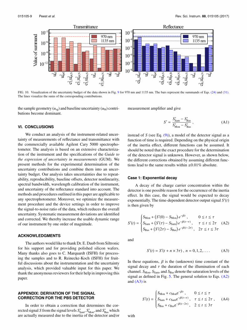
The determined uncertainty (k = 2) is around 1% relativefor reflectance measurements. For measurements of transmit-tance, the uncertainty is 0.4% relative in the wavelength rangewhere T > 0.25. Figure 10 visualizes the uncertainty budgetat 970 nm and 1135 nm. The bars represent the summands ofEqs. (24) and (31). The accuracy of the reflectance measure-ment is limited by the uncertainty ustd of the reflectance stan-dard for all wavelengths. Hence, the instrument does not addsignificant uncertainty to the measurement data, and its accu-racy is obviously sufficient for this purpose. The uncertaintyof the transmittance measurement is dominated by the repro-ducibility (urpd) and nonlinearity (unl) if T > 0.15. For 0.15> T > 0.0002, the noise of the sample measurement (urpt,S)dominates the overall uncertainty. For smaller transmission,

FIG. 9. Exemplary measurement of a polished silicon wafer. The detectorsare changed at 985 nm. For the wavelengths λ1/2, the corresponding uncer-tainty budget is given in Fig. 10.

015105-9 Peest et al. Rev. Sci. Instrum. 88, 015105 (2017)

FIG. 10. Visualization of the uncertainty budget of the data shown in Fig. 9 for 970 nm and 1135 nm. The bars represent the summands of Eqs. (24) and (31).The lines visualize the sums of the corresponding contributions.

the sample geometry (usg) and baseline uncertainty (ubl) contri-butions become dominant.

VI. CONCLUSIONS

We conduct an analysis of the instrument-related uncer-tainty of measurements of reflectance and transmittance withthe commercially available Agilent Cary 5000 spectropho-tometer. The analysis is based on an extensive characteriza-tion of the instrument and the specifications of the Guide tothe expression of uncertainty in measurements (GUM). Wepresent methods for the experimental determination of theuncertainty contributions and combine them into an uncer-tainty budget. Our analysis takes uncertainties due to repeat-ability, reproducibility, baseline offsets, detector nonlinearity,spectral bandwidth, wavelength calibration of the instrument,and uncertainty of the reflectance standard into account. Themethods and procedures outlined in this paper are applicable toany spectrophotometer. Moreover, we optimize the measure-ment procedure and the device settings in order to improvethe signal-to-noise ratio of the data, which reduces the overalluncertainty. Systematic measurement deviations are identifiedand corrected. We thereby increase the usable dynamic rangeof our instrument by one order of magnitude.

ACKNOWLEDGMENTS

The authors would like to thank Dr. E. Daub from Siltronicfor his support and for providing polished silicon wafers.Many thanks also goes to C. Marquardt (ISFH) for process-ing the samples and to R. Reinecke-Koch (ISFH) for fruit-ful discussions about the instrumentation and the uncertaintyanalysis, which provided valuable input for this paper. Wethank the anonymous reviewers for their help in improving thispaper.

APPENDIX: DERIVATION OF THE SIGNALCORRECTION FOR THE PBS DETECTOR

In order to obtain a correction that determines the cor-rected signal S from the signal levels S′Sam, S′Mon, and S′Bas whichare actually measured due to the inertia of the detector and/or

measurement amplifier and give

S′ =S′Sam − S′Bas

S′Mon − S′Bas, (A1)

instead of S (see Eq. (9)), a model of the detector signal as afunction of time is required. Depending on the physical originof the inertia effect, different functions can be assumed. Itshould be noted that the exact procedure for the determinationof the detector signal is unknown. However, as shown below,the different corrections obtained by assuming different func-tions lead to the same results within ±0.01% absolute.

Case 1: Exponential decay

A decay of the charge carrier concentration within thedetector is one possible reason for the occurrence of the inertiaeffect. In this case, the signal would be expected to decayexponentially. The time-dependent detector output signal S′(t)is then given by

S′(t) =

SMon +�S′(0) − SMon

�e−βt , 0 ≤ t ≤ τ

SSam +�S′(τ) − SSam

�e−β(t−τ) , τ ≤ t ≤ 2τ

SBas +�S′(2τ) − SBas

�e−β(t−2τ) , 2τ ≤ t ≤ 3τ

(A2)

and

S′(t) = S′(t + n × 3τ) , n = 0,1,2, . . . . (A3)

In these equations, β is the (unknown) time constant of thesignal decay and τ the duration of the illumination of eachchannel. SMon, SSam, and SBas denote the saturation levels of thesignal as defined in Fig. 5. The general solution to Eqs. (A2)and (A3) is

S′(t) =

SMon + cMone−βt , 0 ≤ t ≤ τ

SSam + cSame−β(t−τ) , τ ≤ t ≤ 2τSBas + cBase−β(t−2τ) , 2 ≤ t ≤ 3τ

, (A4)

with

015105-10 Peest et al. Rev. Sci. Instrum. 88, 015105 (2017)

cMon =SSam − SMon + (SBas − SMon)e−βτ

1 + e−βτ + e−2βτ , (A5)

cSam =SBas − SSam + (SMon − SSam)e−βτ

1 + e−βτ + e−2βτ , (A6)

cBas =SMon − SBas + (SSam − SBas)e−βτ

1 + e−βτ + e−2βτ . (A7)

A reasonable assumption would be that the detector signalis integrated over a period of time in order to reduce themeasurement noise. In general, the signal is integrated fromt1 to t2, where

n τ ≤ t1 ≤ t2 ≤ (n + 1) τ , n = 0,1,2 . (A8)

This leads to

S′Mon =

t2

t1

S′(t) dt , (A9)

S′Sam =

τ+t2

τ+t1

S′(t) dt , (A10)

S′Bas =

2τ+t2

2τ+t1S′(t) dt . (A11)

Combining Eqs. (A2)–(A8) leads to

S′Mon = SMon(t2 − t1)τ + cMon

β

(e−βτt1 − e−βτt2

), (A12)

S′Sam = SSam(t2 − t1)τ + cSam

β

(e−βτt1 − e−βτt2

), (A13)

S′Bas = SBas(t2 − t1)τ + cBas

β

(e−βτt1 − e−βτt2

). (A14)

The case of signal sampling at distinct times tMon, tSam, and tBas,which is considered in Fig. 5 for the purpose of simplicity, is

contained in these equations as the special case t2 → t1. Notethat for an instant change of the signal level, i.e., β → ∞, thesecond terms on the right hand sides disappear and the terms(t2 − t1)τ cancel out when inserting the results into Eq. (A2) or(9), respectively, which is the correct result for this case, wherea correction is not required. Inserting Eqs. (A12)–(A14) intoEq. (A1) leads to

S′ =SSam − SBas + K (cSam − cBas)SMon − SBas + K (cMon − cBas) , (A15)

with

K =e−βt1τ − e−βt2τ

β(t2 − t1)τ . (A16)

The equation can further be simplified by recognizing thatthe constant signal offset described by the baseline signalSBas is also contained in SMon and SSam. As Eq. (A15) onlycontains signal differences, any constant offset cancels out andSBas = 0 can be assumed without loss of generality. Moreover,the two-channel measurement technique only considers theratio of SSam to SMon but not the absolute values of thesequantities. Therefore, we can scale both SSam and SMon witha scaling factor such that SMon = 1 without changing the resultof Eq. (A15). Hence, the equation can be simplified further bysetting SMon = 1.

With these simplifications, Eq. (A15) contains two un-knowns, namely, SSam, which is to be determined, and thefactor K which accounts for the integration limits and the timeconstant β. The quantity S′ is known from the measurement.In order to obtain SSam, a measurement of the 0% baseline S0using a beam trap is required. For this situation, SSam = SBas= 0 holds and Eq. (A15) becomes

S′ = S0 =(e−βτ − 1)(e−βt1τ − e−βt2τ)

(1 + e−βτ + e−2βτ βτ)(t2 − t1) − (e−βτ + 2)(e−βt1τ − e−βt2τ) . (A17)

Combining Eqs. (A15) and (A17) yields

SSam =S′ − S0

1 + S0 (S′ − 1) . (A18)

Since we assumed SBas = 0 and SMon = 1,

S = SSam (A19)

holds according to Eq. (9), which finally leads to

S =S′ − S0

1 + S0 (S′ − 1) , (A20)

which is the correction formula Eq. (11).

Case 2: Linear decay

Inertia of the measurement amplifier is another possiblereason for the occurrence of the inertia effect. In this case, alinear signal decay with constant slope would be expected.The dependence of the measured 0% baseline signal on the

amplification factor points towards the measurement amplifieras the origin of the effect. Assuming that the detector signal isgiven by the integral over the period τ, the signal levels S′Mon,S′Sam, and S′Bas follow as

S′Mon = SMon τ + (SBas − SMon) ∆t1

2, (A21)

S′Sam = SSam τ + (SMon − SSam) ∆t2

2, (A22)

S′Bas = SBas τ + (SSam − SBas) ∆t3

2. (A23)

Since the signal decay is linear with constant slope a,

∆y = a ∆t (A24)

holds where ∆y denotes the amplitude of the signal change.Combining the latter equations yields

015105-11 Peest et al. Rev. Sci. Instrum. 88, 015105 (2017)

FIG. 11. Comparison of the correction formulas for exponential and lineardecay, expressed as the absolute difference between both corrections as afunction of the uncorrected signal S′. On the right axis, the significance ofthe correction is shown.

S′Mon = SMon τ −(SBas − SMon)2

2a, (A25)

S′Sam = SSam τ +(SMon − SSam)2

2a, (A26)

S′Bas = SBas τ +(SSam − SBas)2

2a. (A27)

Inserting this result into Eq. (A1) and following the derivationoutlined above, the correction formula

S =

(1 − 4S′)S0

2 + (4S′2 − 2)S0 + 1 + S0 − 1

2 S′S0(A28)

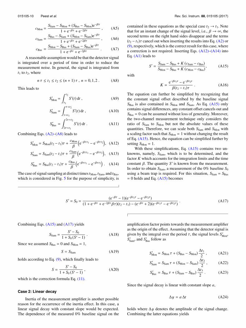
is obtained.A comparison of the correction formulas Eqs. (A20) and

(A28) for exponential or linear decay, respectively, is shownin Fig. 11. Figure 11 shows the absolute deviation betweenthe corrected values using the correction for the exponentialor linear decay, respectively, as a function of the measured(uncorrected) signal S′. It can be seen that the absolute devia-

tion between both corrections is below 0.01% for signal levelsbelow 10%, where the correction has a significant impact, i.e.,S′/S > 1. Compared to the uncertainty of the measured data,this deviation can be neglected, i.e., both corrections yieldthe same results. For the purpose of simplicity, the correctionformula for the exponential decay is thus used in this work.

1H.-H. Perkampus, H.-C. Grinter, and T. L. Threlfall, UV-VIS Spectroscopyand its Applications (Springer, 1992).

2J. Workman, Jr. and A. Springsteen, Applied Spectroscopy: A CompactReference for Practitioners (Academic Press, 1998).

3K.-E. Peiponen, R. Myllylä, and A. V. Priezzhev, Optical MeasurementTechniques: Innovations for Industry and the Life Sciencess (Springer,2009), Vol. 136.

4J. Dobiliene, E. Raudiene, and R. P. Zilinskas, Measurement 43, 113 (2010).5P. S. Ramanjaneyulu, Y. S. Sayi, and K. L. Ramakumar, Indian J. Chem.Technol. 17, 468 (2010), available at http://nopr.niscair.res.in/handle/123456789/10721?mode=full.

6ASTM International, Standard Practice for Estimating Uncertainty of TestResults Derived from Spectrophotometry, 10.1520/E2867-13, 2013.

7L. Sooväli, E.-I. Rõõm, A. Kütt, I. Kaljurand, and I. Leito, Accredit. Qual.Assur. 11, 246 (2006).

8Joint Committee for Guides in Metrology, JCGM, 100, 2008.9B. J. Winer, D. R. Brown, and K. M. Michels, Statistical Principles inExperimental Design Vol. 2 (McGraw-Hill, New York, 1971).

10S. Yang, I. Vayshenker, X. Li, and T. R. Scott, “Accurate measurementof optical detector nonlinearity,” Technical Report (National Institute ofStandards and Technology, 1994).

11W. Budde, Appl. Opt. 18, 1555 (1979).12E. R. Woolliams, R. Baribeau, A. Bialek, and M. G. Cox, Metrologica 48,

164 (2011).13S. Eichstädt, F. Schmähling, G. Wübbeler, K. Anhalt, L. Bünger, U. Krüger,

and C. Elster, Metrologica 50, 107 (2013).14I. Bronstein and K. Semendjaev, Taschenbuch der Mathematik (Verlag Harri

Deutsch, 2001).15C. Schinke, K. Bothe, P. C. Peest, J. Schmidt, and R. Brendel, Appl. Phys.

Lett. 104, 081915 (2014).16C. Schinke, P. C. Peest, J. Schmidt, R. Brendel, K. Bothe, M. R. Vogt, I.

Kröger, S. Winter, A. Schirmacher, S. Lim, H. Nguyen, and D. MacDonald,AIP Adv. 5, 067168 (2015).

17M. A. Green, Sol. Energy Mater. Sol. Cells 92, 1305 (2008).