FLIGHT CONTROL DEVELOPMENT FOR THE ARH-70 ARMED RECONNAISSANCE HELICOPTER PROGRAM

Kevin T. Christensen Kip G. Campbell Carl D. Griffith KChristensen@bellhelicopter.textron.com KGCampbell@bellhelicopter.textron.com CGriffith@bellhelicopter.textron.com Sr Engineering Specialist Principal Engineer Sr Staff Engineer

Bell Helicopter Textron Inc., Fort Worth, Texas

Christina M. Ivler Mark B. Tischler CIvler@mail.arc.nasa.gov MTischler@mail.arc.nasa.gov San Jose State University Foundation Sr Scientist

Aeroflightdynamics Directorate U.S. Army Aviation and Missile Command, Moffett Field, California

Jeffrey W. Harding

Jeffrey.W.Harding@us.army.mil Harding Consulting, Inc.

Aviation Engineering Directorate U.S. Army Aviation and Missile Command, Redstone Arsenal, Alabama

ABSTRACT

In July 2005, Bell Helicopter won the U.S. Army’s Armed Reconnaissance Helicopter competition to produce a replacement for the OH-58 Kiowa Warrior capable of performing the armed reconnaissance mission. To meet the U.S. Army requirement that the ARH-70A have Level 1 handling qualities for the scout rotorcraft mission task elements defined by ADS-33E-PRF, Bell equipped the aircraft with their generic automatic flight control system (AFCS). Under the constraints of the tight ARH-70A schedule, the development team used modern parameter identification and control law optimization techniques to optimize the AFCS gains to simultaneously meet multiple handling qualities design criteria. This paper will show how linear modeling, control law optimization, and simulation have been used to produce a Level 1 scout rotorcraft for the U.S. Army, while minimizing the amount of flight testing required for AFCS development and handling qualities evaluation of the ARH-70A.

1

INTRODUCTION

The Armed Reconnaissance Helicopter, ARH-70A, shown in Fig. 1, is currently under development by Bell Helicopter to perform the armed reconnaissance role for the US Army as a replacement for the OH-58 Kiowa Warrior. The ARH-70A acquisition strategy was to modify a commercial-off-the-shelf aircraft, the Bell 407, to meet military requirements. Some of the changes to the Bell 407 include a more powerful engine, a bigger tail rotor, and improved avionics.

The US Army handling qualities requirements for the ARH-70A include the following:

Presented at the American Helicopter Society 63rd Annual Forum, Virginia Beach, VA, May 1–3, 2007. Copyright © 2007 by the American Helicopter Society International, Inc. All rights reserved.

The Armed Reconnaissance Helicopter shall have Level 1 handling qualities for all Scout Rotorcraft Category Mission Task Elements as defined by ADS-33E-PRF, Table I. In order to provide the ARH-70A with the response-types required by ADS-33E-PRF (Ref. 1) for Level 1 handing qualities in both good visual environment (GVE) and degraded visual environment (DVE) conditions, Bell Helicopter has equipped the aircraft with their generic automatic flight control system (AFCS). The AFCS control laws provide multiple levels of stabilization from unaugmented basic aircraft up to hover stabilization with absolute height, heading, and inertial position hold. The ARH-70A AFCS development effort was conducted by Bell Helicopter engineers with the support of the Aeroflightdynamics and Aviation Engineering Directorates of the US Army Aviation and Missile Command. By using modern parameter identification techniques, the development team was able to optimize the AFCS gains to simultaneously meet multiple handling qualities design criteria. Preliminary optimization of the AFCS gains was based on a flight test identified linear model of the Bell 407.

2

Once the ARH-70A entered its flight test phase, the linear model was updated and the AFCS gain optimization was repeated. The specifications used for gain optimization included control sensitivity, system stability, disturbance rejection, and the ADS-33E-PRF Level 1 handling qualities design criteria. Preliminary testing of the optimized AFCS gains in both the aircraft and simulator has produced promising results. By optimizing the initial set of AFCS gains for the Bell 407 linear model, the development team was able to clear the ARH-70A for the US Army’s Limited User Test (LUT) in less than one third of the flight test time that had been originally planned for AFCS development. Thus far in the flight test program, the gains optimized for the ARH-70A linear model have only been tested for one mode of the AFCS. Preliminary test results show that the dynamic aircraft response in the stability and control augmentation system (SCAS) mode meets the handling qualities design criteria. The handling qualities test plan calls for a similar validation of the optimized AFCS gains for the other AFCS modes. The final validation of this flight control development process will come when the final set of AFCS gains are evaluated on the ADS-33E-PRF MTE courses in both GVE and DVE conditions. This paper will show how linear modeling, control law optimization, and simulation were used to minimize the amount of flight testing required for AFCS development and handling qualities evaluation of the ARH-70A. The paper will provide an overview of the ARH-70A flight control system design, and then proceed into a discussion of the techniques used for model identification and AFCS gain optimization. Next, the paper will discuss the preliminary test results and plans for future testing. Finally, this paper will conclude with a presentation of the lessons learned thus far from the ARH-70A flight control development effort.

FLIGHT CONTROL SYSTEM

The ARH-70A flight control system combines the basic mechanical flight control system of the Bell 407 with Bell Helicopter’s generic AFCS. The four-axis, non-redundant, limited authority AFCS is comprised of qualified, off-the-shelf components currently used in a wide range of commercial helicopters. Mechanical Controls

The ARH-70A mechanical flight controls, depicted in Fig. 2, are traditional single rotor helicopter flight controls, incorporating hydraulically boosted lateral and longitudinal cyclic stick, collective stick, and anti-torque pedals. The mechanical control system also includes a Watt’s linkage

which mixes the longitudinal cyclic input into the lateral axis. Although the mixing relationship is not linear over the full range of the longitudinal cyclic, in the predominately linear midrange, a forward cyclic input will transmit a left lateral input to the swashplate. The Watt’s linkage essentially allows the pilot to takeoff from hover with less left lateral cyclic required to hold a level attitude. Three electromechanical actuators are mounted in series along the control rods for the longitudinal cyclic, lateral cyclic, and pedal to augment the pitch, roll, and yaw controls, respectively. The flight control computer (FCC) sends signals to these series actuators to provide stability and control augmentation of the pilot’s direct input. Since a failure within the AFCS could command a full travel hardover of a series actuator, the maximum allowable travel of each actuator is mechanically limited. This, in turn, limits the control authority available for the AFCS to effect aircraft handling qualities. The maximum series actuator control authority is limited to about 15-20% of the total control authority for each axis. Four additional electromechanical actuators are mounted in parallel along the control rods for each axis to provide the ARH with a force trim system. The trim detent positions can be manually adjusted through the use of beep switches for each of the four axes. Additionally, the pilot can completely disengage the trim clutches to reposition the trim detent through the use of force trim release switches. When the trim clutch is disengaged, a viscous damper in each trim actuator resists control movement to limit control jump as the control forces return to zero. In addition to providing the pilot with a manual force trim system, the trim actuators also provide information to the AFCS. The control monitoring transducers (CMTs) mounted in each trim actuator provide the AFCS with control positions, while sensors in each trim actuator detect whether the pilot has moved a control out of the trim detent. With this information, the AFCS has the capability to automatically adjust the trim detent positions, thus providing the ARH-70A with the automatic trim capability required by the AFCS hold modes. Automatic Flight Control System

An overview of the AFCS can be found in Fig. 3. At the heart of the AFCS, the FCC receives data from other aircraft systems and then sends commands to the flight control actuators. Inertial data (attitude, attitude rate, heading, acceleration, and velocity) are received from the embedded global positioning system/inertial navigation system (EGI), while air data (barometric altitude, altitude rate, and airspeed) are received from the air data computer. Radar

3

altimeter data are pulled off the aircraft data bus by the control display units and then sent to the FCC. Cockpit switch actions are provided to the FCC through discrete interfaces. Commands to the series actuators are via the data busses, while commands to the trim actuators are provided via pulse-width modulated analog signals. Control positions are sent to the FCC via analog signals from the trim actuator CMTs. The trim detent status of each trim actuator is returned to the FCC via discrete interface. The inner loop AFCS modes include the SCAS mode and the attitude hold mode. The SCAS mode also includes turn coordination and a stability augmentation system sub-mode for failures in any of the CMTs. The attitude hold mode includes a heading hold feature in all phases of flight. The outer loop modes are speed hold, hover hold, and altitude hold. The SCAS mode operates through the series actuators independent of the trim actuators to provide the pilot with a rate command maneuvering response. It uses pitch, roll, and yaw rate feedback for dynamic stabilization and control position feed-forward to adjust control sensitivity and quickness. Additionally, the SCAS mode incorporates limited lagged rate feedback for short-term attitude stabilization. At forward flight conditions, the SCAS mode provides turn coordination though computed yaw rate command and lateral acceleration feedback. The attitude hold mode also operates through the series actuators. However, with controls in the trim detent, it will automatically back drive the trim actuators, moving the cockpit controls, to keep the series actuators within their limits. In the pitch and roll axes, this mode provides the pilot with a rate command, attitude hold response type. In forward flight conditions at bank angles below 5º, the heading hold feature of attitude hold operates through the roll series actuator. In hover and low speed conditions, heading hold operates through the yaw series actuator to provide the pilot with a rate command, direction hold response type. The heading reference can be adjusted by either moving the pedals out of the trim detent position or by beeping heading left or right with the yaw beep switch. This low speed heading hold also includes collective position crossfeed to minimize torque-induced heading changes. The speed hold mode provides an acceleration command, speed hold response type through the attitude hold loops. In forward flight conditions, airspeed error commands pitch attitude to hold airspeed. Airspeed is filtered with longitudinal acceleration aiding to smooth out airspeed changes due to turbulence. In hover and low speed flight conditions, groundspeed error commands both pitch and roll attitudes to hold groundspeed. Moving the cyclic out of the trim detent position will command a constant acceleration

rate, within the limits of the series actuators. The speed reference can also be adjusted by using the cyclic beep switch. The altitude hold mode uses altitude error feedback to the collective trim actuator to provide the pilot with a rate command, height hold response type. In forward flight conditions, this mode holds barometric altitude, while in hover and low speed conditions, it holds radar altitude. Altitude is filtered with vertical acceleration aiding to smooth out altitude changes due to turbulence or rugged terrain. Radar altitude hold also uses pressure altitude data in filtering to further smooth out commands over rugged terrain. The altitude reference can be adjusted either by moving the collective out of the trim detent position or by beeping altitude up or down with the collective beep switch. The hover hold mode provides a translational rate command, position hold response type through the attitude hold loops. This mode also uses the collective trim actuator to control radar altitude and the yaw series actuator for heading hold. Upon engagement, hover hold automatically commands a descent and deceleration to a 50-foot hover on a glide path of no greater than 6º. Once established in hover, moving the cyclic out of the trim detent position commands a constant translational groundspeed, within the limits of the series actuators. Hover position can also be adjusted by using the cyclic beep switch.

MODEL IDENTIFICATION

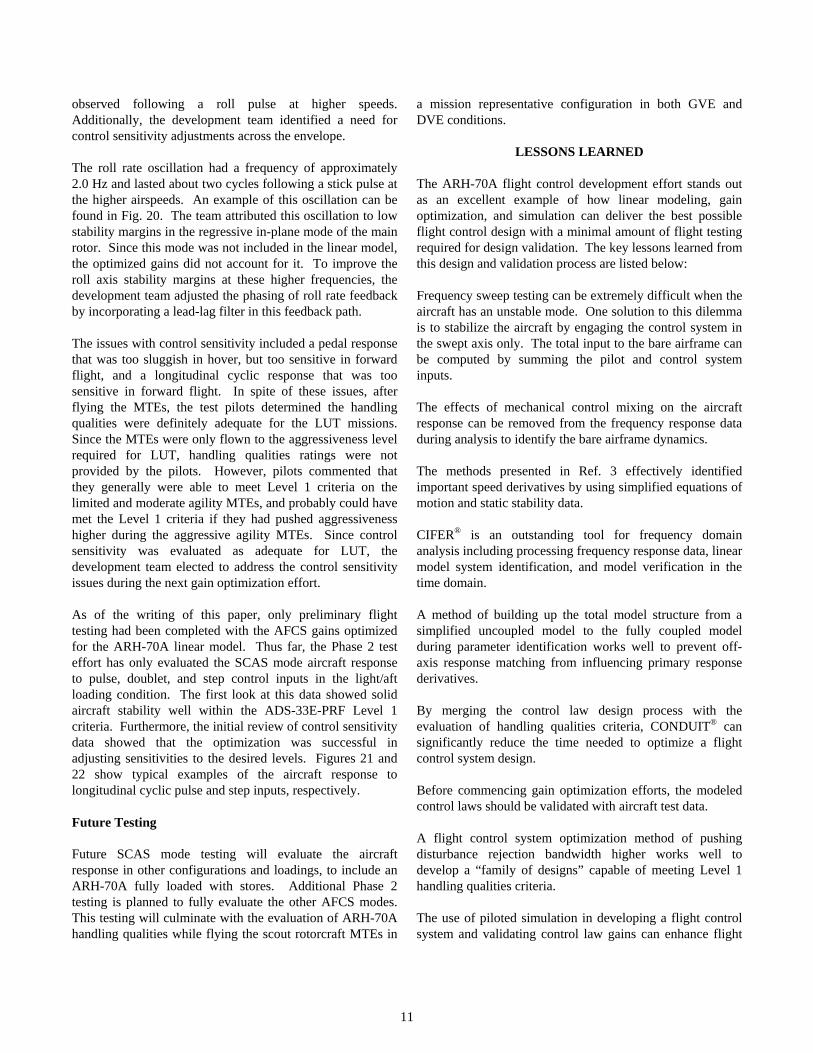
Identification of the ARH-70A linear dynamic model was completed using frequency response parameter identification techniques applied to a six degree of freedom (6-DOF), rigid-body aircraft model. The stability and control derivatives used in this model are listed below in Table 1.

Table 1. Linear model stability and control derivatives

The longitudinal and lateral flapping modes were modeled by an equivalent time delay (τflap) applied to both the longitudinal and lateral cyclic inputs. Similarly, the engine governor and main rotor RPM dynamics were modeled by an equivalent time delay (τcol) applied to the collective input for aircraft response in the rotational degrees of freedom (p, q, and r). Finally, tail rotor dynamics were modeled by an equivalent time delay (τped) applied to the pedal input. The frequency responses needed to identify the parameters in this 6-DOF model included those for each control input in both the rotational and translational degrees of freedom. The rotational frequency response data came from the

4

aircraft’s angular rate response (p, q, and r) for each control axes. The translational data came from the body axis acceleration response (ax, ay, and az). Since air data is generally poor at low speeds and at frequencies above 1 radian per second (rad/sec), the rate of change of the body axis airspeeds ( u& , v& , and w& ) were computed and used instead. Thus, with four control inputs and nine aircraft response outputs, a total of 36 frequency responses were available for the parameter identification effort. Flight Testing

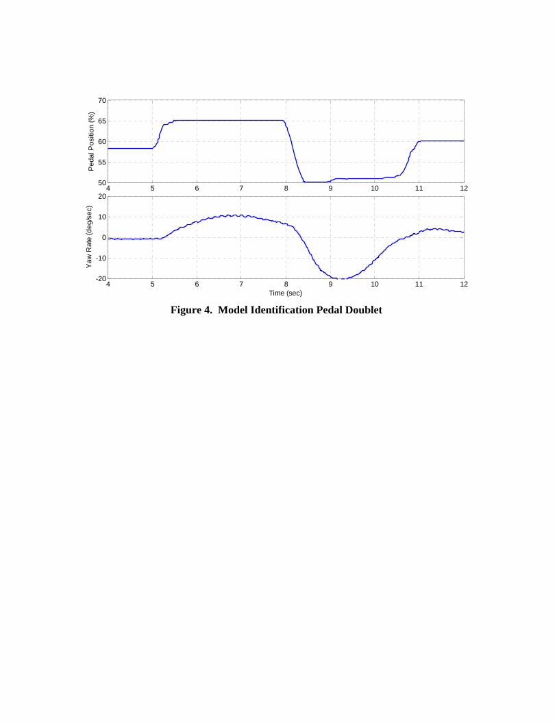
A linear model of the Bell 407 was identified to perform preliminary flight control optimization work until the ARH-70A entered flight testing. The Bell 407 testing was accomplished for two loading conditions, one with a light gross weight and aft center of gravity (light/aft) and the other with a heavy gross weight and forward center of gravity (heavy/forward). For each loading condition, model identification test points were completed at three different flight conditions: hover out of ground effect, level flight at the maximum rate of climb airspeed, and level flight at 90% of the maximum speed with maximum continuous power. The AFCS development team elected to use the heavy/forward Bell 407 model for the initial optimization of the AFCS gains since this was closest to the nominal ARH-70A loading condition. Additionally, since the ARH-70A has a bigger tail rotor than the Bell 407, the Bell 407 pedal control derivatives in the linear model were increased by the appropriate scale factor. An early goal of the ARH-70A flight test program was to obtain the flight test data needed to identify the linear model. To aid in comparison, these model identification test points were flown at the same speeds that were flown in the Bell 407. In order to ensure that the ARH-70A was capable of meeting the handling qualities requirement over a wide spectrum of aircraft loadings and configurations, the development team elected to optimize the AFCS for a nominal loading with a middle of the envelope gross weight and center of gravity (mid/mid). Therefore, all ARH-70A model identification test points were flown in the mid/mid loading condition. The model identification test points consisted of frequency sweeps and doublets flown in each of the four control axes. The frequency sweeps followed the flight test technique guidance contained in Ref. 2. The doublets were flown to provide time history data for model verification purposes. To fully record the aircraft’s response to control inputs during these doublets, the aircraft response rate was allowed to peak before reversing the control input. An example doublet is depicted in Fig. 4.

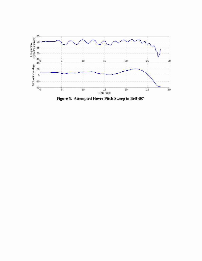
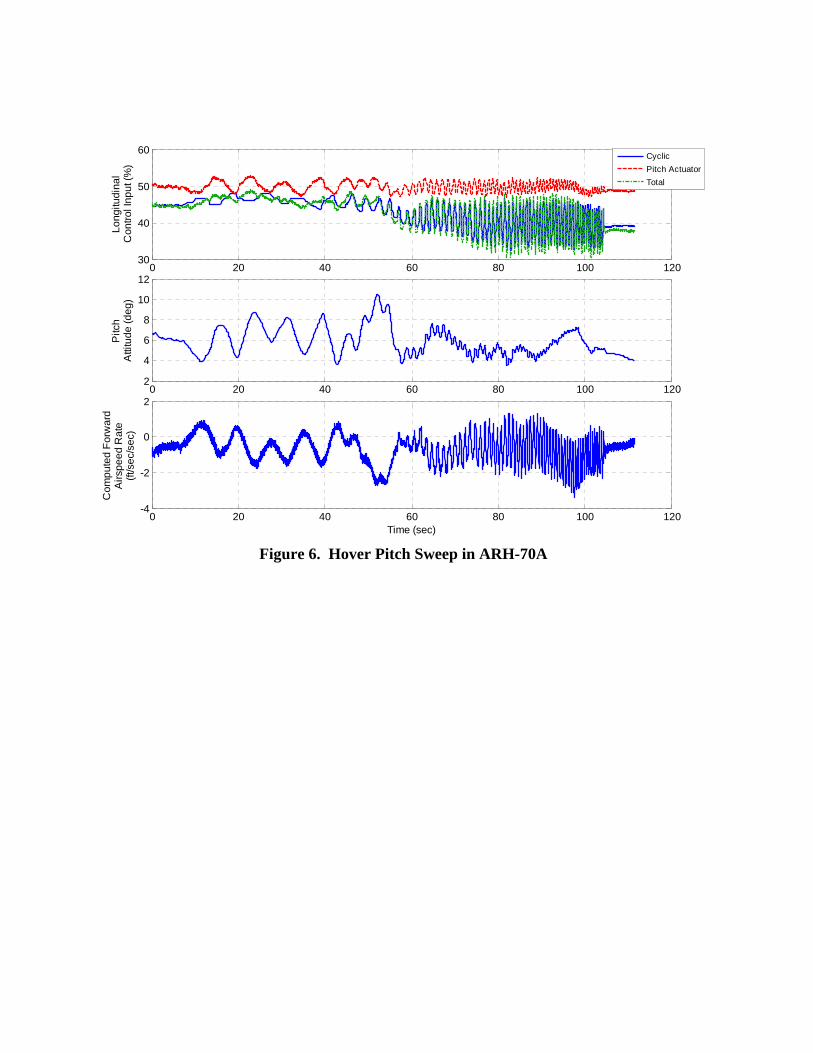
During the Bell 407 hover pitch and roll frequency sweeps, the unstable long term coupled pitch and roll mode made it very difficult for the test pilot to stay within test point tolerances, especially at low frequencies. Figure 5 shows an example of how this hover instability caused one of the Bell 407 pitch sweeps to be aborted. To overcome this problem in the ARH-70A, the hover pitch and roll frequency sweeps were flown with the SCAS mode engaged in the input axis only. During the processing of this data, the appropriate series actuator output was added to the pilot’s input to get the total input to the aircraft dynamic system. Figure 6 shows how this technique enabled the pilot to collect pitch sweep data, even at the lower frequencies, while keeping pitch within test point tolerances. This SCAS mode stabilization was not needed during the frequency sweeps flown at forward flight airspeeds. Frequency Response Data

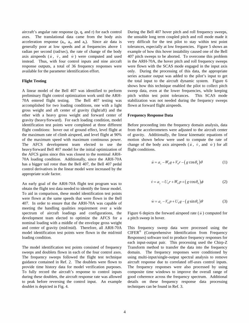
Before proceeding into the frequency domain analysis, data from the accelerometers were adjusted to the aircraft center of gravity. Additionally, the linear kinematic equations of motion shown below were used to compute the rate of change of the body axis airspeeds ( u& , v& , and w& ) for all flight conditions.

( )0 0 0cosxu a W q V r g θ θ= − + −& (1)

( )0 0 0cosyv a U r W p g θ φ= − + +& (2)

( )0 0 0sinzw a V p U q g θ θ= − + −& (3)

Figure 6 depicts the forward airspeed rate ( u& ) computed for a pitch sweep in hover. This frequency sweep data were processed using the CIFER® (Comprehensive Identification from Frequency Responses) software tool to produce frequency responses for each input-output pair. This processing used the Chirp-Z Transform method to transfer the data into the frequency domain. The frequency responses were conditioned by using multi-input/single-output spectral analysis to remove aircraft response due to correlated off-axes control inputs. The frequency responses were also processed by using composite time windows to improve the overall range of good coherence across the frequency spectrum. Additional details on these frequency response data processing techniques can be found in Ref. 3.

5

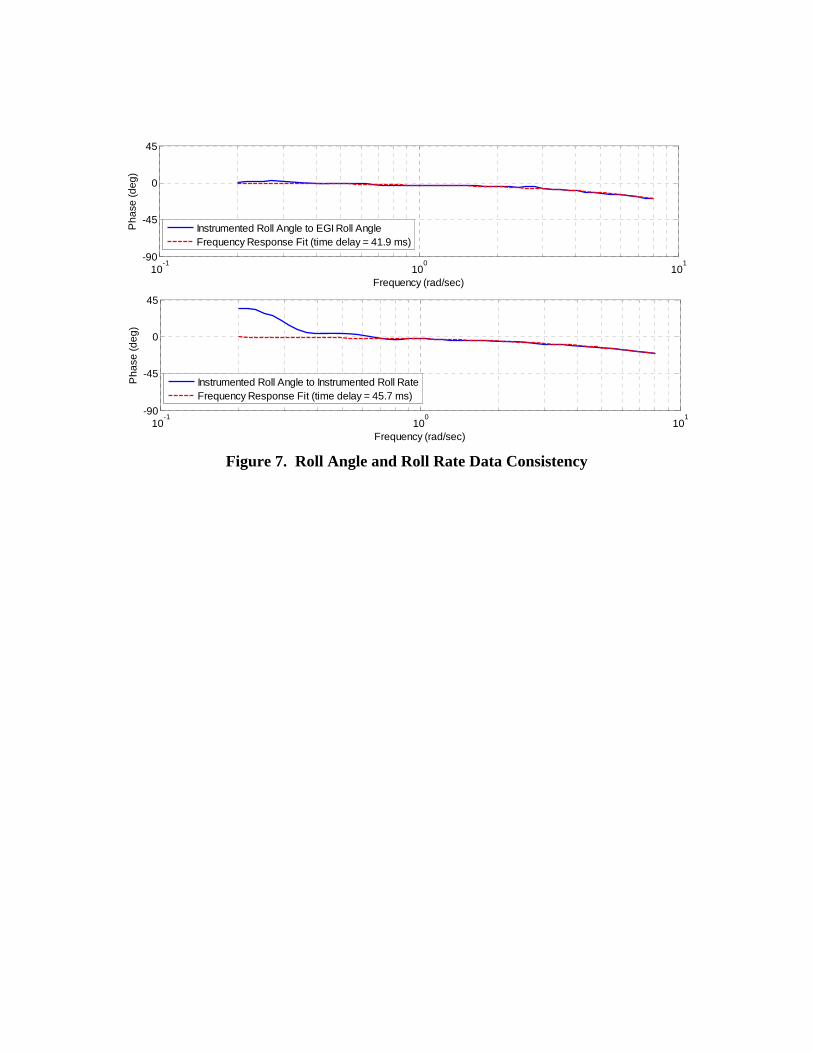
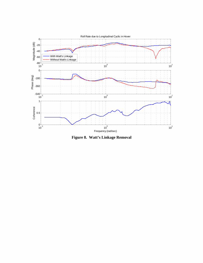
To ensure the best possible data were used for parameter identification, the frequency sweep data were first evaluated for consistency. The development team compared instrumentation data and aircraft bus data from the EGI with the kinematic equations of motion in both the time and frequency domains to look for biases and time shifts. Likewise, the instrumented control positions were compared with bus data from the CMTs. As an example, Fig. 7 shows how a frequency response fit was used to determine that both the EGI roll attitude and the instrumented roll rate lagged the instrumented roll attitude by about 40 to 45 milliseconds. Additional analysis led the development team to conclude that the EGI provided the best source of angular data for the parameter identification effort. Before beginning the parameter identification portion of this analysis, one more adjustment needed to be made to the frequency response data. As mentioned earlier in the Flight Control System section, the Watt’s linkage mixes longitudinal cyclic into the lateral axis. Since the pitch series actuator outputs do not get mixed into the lateral axis, the flight control development team decided that the most accurate model for AFCS gain optimization would be one with the effects of the Watt’s linkage removed. Frequency response arithmetic using Equation 4 below enabled the removal of the roll rate response due to the Watt’s linkage from the longitudinal frequency responses.

wattslon lon latnew old

p p pKδ δ δ

⎛ ⎞ ⎛ ⎞ ⎛ ⎞= −⎜ ⎟ ⎜ ⎟ ⎜ ⎟

⎝ ⎠ ⎝ ⎠ ⎝ ⎠ (4)

The Kwatts term in this equation is the ratio of longitudinal input mixed into the lateral axis to the total longitudinal input. Figure 8 shows how removing Watt’s linkage affected this frequency response in hover. As expected, the Watt’s linkage had a significant effect on the coupled response at the higher frequencies. A similar approach was used to remove the effect of the Watt’s linkage from other longitudinal frequency responses. Parameter Identification

Once the selection and processing of the appropriate frequency responses was complete, the next task was to select the portion of the frequency response data that could positively contribute to the parameter identification effort. Using the guidance from Ref. 3, the development team selected frequency response data with coherence greater than a threshold of 0.5. Since the team planned to use coherence weighting during the parameter identification, data with dips in coherence below the threshold were also included. Frequency responses that peaked only momentarily above the threshold were disregarded. As a guide, the maximum frequency with coherence above the threshold had to be at

least twice the minimum frequency to be included. To avoid higher frequency main rotor dynamics and stay within the applicable range of the 6-DOF model, the frequency responses were cutoff at 12 rad/sec. In the collective axis, the translational frequency responses ( u& , v& , w& , ax, ay, and az) were cut off at 8 rad/sec to avoid the mean dynamic inflow dynamics which were not part of the model structure. Table 2 shows the frequency responses and ranges of data chosen for use in the identification of the hover model. Of the original 36 frequency responses generated, 10 were dropped due to poor coherence. The bold frequency ranges show the primary aircraft response for each control axis.

Table 2. Initial frequency response data selection for hover

Identification of the ARH-70A stability and control derivatives was completed using the CIFER® program as described in Ref. 3. In order to accurately identify the linear model derivatives to best match the frequency response data, CIFER® used a weighted frequency response cost function to converge on a least cost solution. The 6-DOF state space model was set up based on the following equations:

x Ax Bu= +& (5)

1 2y H x H x= + & (6)

Equation 6 can be converted to the standard state space format shown in Equation 7 by using the conversions in Equation 8 and 9.

y Cx Du= + (7)

1 2C H H A= + (8)

2D H B= (9)

The state vector (x) was made up of the translational and rotational rates (u, v, w, p, q, and r), plus pitch and roll angle (φ and θ) in order to account for the gravity terms in the equations of motion. The state equation matrices (A and B)

6

contained the stability and control derivatives as well as the kinematic and gravity terms from the linear equations of motion (Equations 1 through 3). Additionally, the last two rows of the stability matrix (A) were built using the linear kinematic equations of motion for roll and pitch shown below.

( )0tanp rφ θ= +& (10)

qθ =& (11)

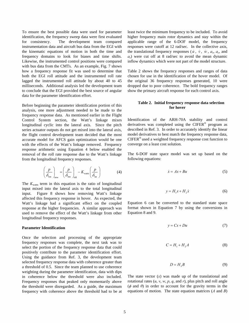
The output vector (y) was made up of the state vector and the body axis accelerations (ax, ay, and az). The acceleration portion of the output equation matrices (H1 and H2) was built for each flight condition by solving the linear kinematic equations of motion (Equations 1 through 3) for the accelerations (ax, ay, and az). The initial derivative values that were used in the state equation matrices (A and B) were obtained from Bell Helicopter’s proprietary COPTER (Comprehensive Program for Theoretical Evaluation of Rotorcraft) program. This non-linear, blade element based rotorcraft model used small perturbations from trim to compute the linear model stability and control derivatives. Before attempting to converge the model on a solution to match the frequency response data, selected stability and control derivatives were zeroed out based on the frequency responses being matched. If a frequency response had no data that met the coherence threshold criteria previously discussed, then it was assumed that control input and primary aircraft responses from that input had no effect on the output response for that frequency response. Therefore, the input control derivative and primary stability derivatives could be zeroed out in the non-responsive equation of motion. For example, Table 2 shows that in hover the lateral acceleration response to longitudinal cyclic (ay/δlon) did not meet the coherence threshold criteria previously discussed. This indicates that the longitudinal cyclic had no effect on lateral acceleration. Furthermore, since the primary aircraft responses due to longitudinal cyclic were forward speed (u) and pitch rate (q), it can be assumed that changes to these states also had no effect on lateral acceleration. Therefore, the corresponding derivatives in the lateral equation of motion (Yu, Yq, and Ylon) could be fixed at zero. To further narrow down the number of derivatives to be identified, two other rules of thumb were applied. In general, the speed derivatives (u, v, and w) contribute to the aircraft response at lower frequencies, below about 1

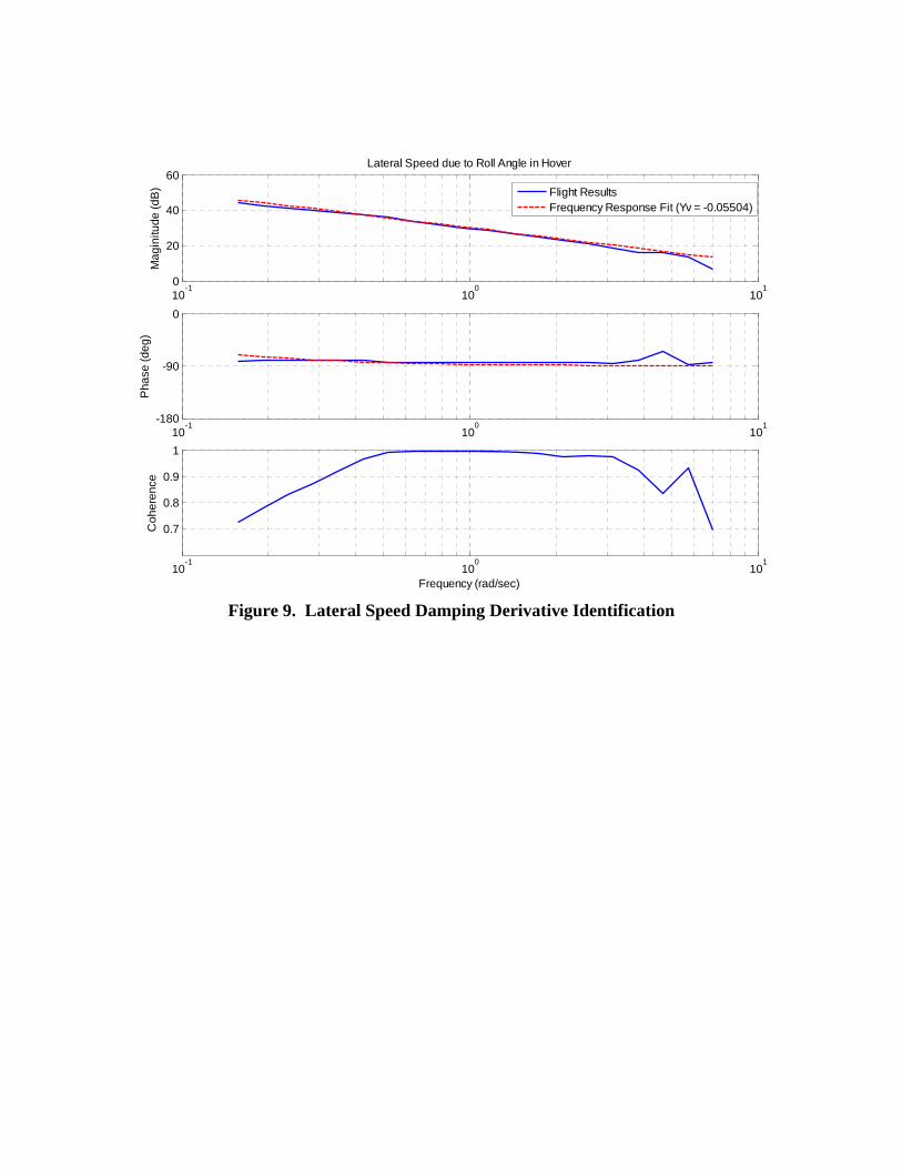
rad/sec, while the control and angular rate derivatives contribute to aircraft response at the higher frequencies, above about 1 rad/sec. Therefore, if an off-axis frequency response only had coherent data at lower frequencies, then the corresponding control and angular rate derivatives could be zeroed out. As an example from Table 2, since the vertical acceleration response to longitudinal cyclic (az/δlon) only showed coherence at lower frequencies, the corresponding control and pitch rate derivatives (Zlon and Zq) could be fixed at zero. Likewise, if the off-axis frequency response only had coherent data at the higher frequencies, the corresponding speed derivative could be zeroed out. Also from Table 2, since the roll rate response to collective (p/δcol) only showed coherence at higher frequencies, the corresponding vertical speed derivative (Lw) could be fixed at zero. Using these rules of thumb, approximately sixteen stability derivatives and six control derivatives were fixed at zero leaving a total of forty-two unknown parameters to be identified including twenty stability derivatives, eighteen control derivatives, and three time delays. As predicted in Ref. 3, due to poor low-frequency excitation and high cross-control correlation in the frequency responses, several of the significant on-axis speed derivatives could not be identified using the methods discussed thus far. To identify the speed damping derivatives (Xu and Yv), the simplified longitudinal and lateral translation equations of motion shown below were used.

( )0cosuu X u g θ θ= −& (12)

( )0cosvv Y v g θ φ= +& (13)

The longitudinal speed damping derivative (Xu) was identified by fitting the frequency response of longitudinal speed due to pitch angle (u/θ), while the lateral speed damping derivative (Yv) was identified with the lateral speed due to roll angle (v/φ) frequency response. Figure 9 shows an example of how this method was used to identify the lateral speed damping derivative in hover. The other parameters that were sometimes difficult to identify were the speed stability derivatives (Lv, Mu, and Nv). As described in Ref. 3, these derivatives were identified by using static stability data. The equations below were derived from the simplified static stability equations and show how the static stability control gradients can be combined with other identified derivatives to compute the speed stability derivatives.

7

pedlatlat pedvL L L

v vδδ⎡ ⎤Δ⎛ ⎞Δ⎛ ⎞= − +⎢ ⎥⎜ ⎟⎜ ⎟Δ Δ⎝ ⎠⎢ ⎥⎝ ⎠⎣ ⎦

(14)

lonlon

uu w

w

ZM M M

u Zδ ⎛ ⎞Δ⎛ ⎞= − + ⎜ ⎟⎜ ⎟Δ⎝ ⎠ ⎝ ⎠

(15)

pedpedvN N

vδΔ⎛ ⎞

= − ⎜ ⎟Δ⎝ ⎠

(16)

Although these derivatives can be constrained to be automatically computed during the convergence of the model, this has a tendency to pull the other derivatives off. The approach used here was to compute these derivatives after the first convergence and then fix them in the subsequent model convergence. One of the major advantages of using CIFER® for model identification was its ability to easily transition a newly identified model into the time domain for verification. Each model’s time domain response to the flight test doublet control inputs was compared to the actual inflight response. Since the Watt’s linkage had been removed from the model, this control mixing was added back into the lateral cyclic input before running it through the model. Model Buildup Approach

Time domain verification allowed the development team to determine that using the entire set of coupled frequency response data shown in Table 2 caused some of the derivatives to be pulled off. To overcome this problem, the linear model was built from the uncoupled model by adding one off-axis frequency response at a time. The initial uncoupled model included all of the derivatives for the primary frequency responses, with the other derivatives fixed at zero. As an example from Table 2, since the pitch rate response to longitudinal cyclic (q/δlon) is a primary response, the pitch moment longitudinal control derivative (Mlon), as well as the pitch moment stability derivatives that correspond the primary longitudinal responses (Mu and Mq), were freed in the initial model. This initial uncoupled hover model used ten frequency responses to identify ten stability derivatives, six control derivatives, and two time delays, and served as the foundation from which to build on. As each successive off-axis frequency response was added with its corresponding stability and control derivatives, it was evaluated to determine if it added value to the model or not. If the newly converged model did not provide an accurate fit to the new frequency response without pulling off the other frequency responses, then that response either

had its frequency range cut back to only include the portion that provided a good fit, or it was removed completely. Since the addition of other derivatives might allow a better fit of the marginal frequency responses, they were given one last chance, after all of the other frequency responses had been tested, to see if they could bring any additional value to the model. Likewise, each stability and control derivative that was added had to earn its way into the model in both the frequency and time domains. In the frequency domain, if the model was insensitive to the new derivative, or if the parameter had an excessive Cramer-Rao bound, then it could be dropped from the model without having a big impact on the frequency response cost function. In the time domain, comparing the verification cost functions between a new and previous model determined if the newly added derivatives improved or hurt the model. If the cost function increased, then the new derivative was reset to zero to determine if it was the cause. In some cases, the new derivatives actually improved the model even though the verification cost function had increased. This was caused by other derivatives being pulled off by the new frequency response data. To identify the offending derivatives, each derivative in the old model was replaced one at a time to determine which of the new derivatives caused the verification cost function to jump. Once the inaccurate derivatives were singled out, the model was reconverged with these derivatives fixed at their previous value. After attaining the best possible coupled model, one additional step was taken to possibly improve the model even further. All of the derivatives that had been previously fixed to keep them from being pulled off were once again freed. If these derivatives continued to be pulled off, then the offending frequency response data was removed and its corresponding derivatives were fixed before attempting to converge the model again. This step enabled the most accurate identification of the uncoupled derivatives for the final coupled model. Table 3 shows the final set of frequency data that were used to identify the ARH-70A hover model.

Table 3. Final frequency response data used for hover

The model buildup approach described in this paper added data from eight of the off-axis frequency responses to the hover model. This data allowed the identification of thirteen coupled derivatives in addition to the sixteen derivatives that were identified from the primary, uncoupled frequency response data. Additionally, this data enabled identification

8

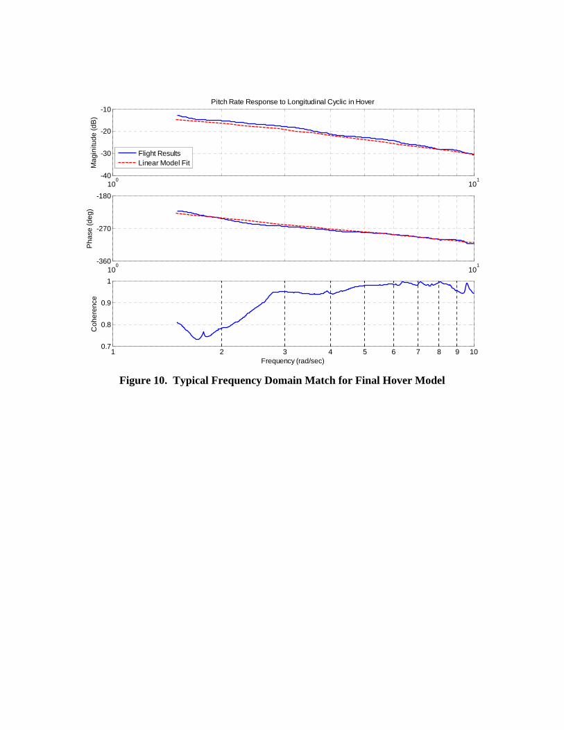
of the equivalent time delay for the collective into the rotational axes (τcol). Figures 10 and 11 show some typical results for the final ARH-70A hover model. By using the frequency response based model buildup approach, the development team was able to identify an ARH-70A model that provided the best possible match to flight data in both the frequency and time domains. With the model identification complete, the development team next set out to optimize the AFCS gains.

GAIN OPTIMIZATION

This optimization was completed by using the CONDUIT® (The Control Designer’s Unified Interface) software tool (Ref. 5). The CONDUIT® program proved to be a valuable design tool, because it merged the control law design process with the evaluation of handling qualities criteria and other flight control system specifications. Faced with a very tight ARH-70A schedule, this synergy enabled the development team to significantly reduce the time needed to optimize the AFCS to meet the US Army’s handling qualities requirements. CONDUIT® also reduced the redesign cycle time by providing the team with the ability to rapidly evaluate and re-optimize any design changes. Control Law Validation

In order to optimize the AFCS gains for the ARH-70A linear model, the AFCS control laws first had to be modeled accurately. From the master generic AFCS control law design, simplified block diagrams were programmed using the SIMULINK® software tool to model the AFCS. Having an accurate model of the aircraft control laws was essential to ensure that the predicted aircraft handling qualities and stability margins would realized in flight. As a vital step before commencing the gain optimization efforts, the modeled control laws were validated with ground and flight test data. Control law model validation was completed by comparing the frequency responses from the actual on-aircraft AFCS with those from the simulation environment. Figure 12 provides a schematic of the data flow for generating these frequency responses. For the ARH-70A SCAS mode, the output for each frequency response was the SCAS command being sent to each of the three series actuators (pitch, roll, and yaw). The frequency response inputs were the CMT values for the feed-forward paths and the angular rates for the feedback paths. For feed-forward path validation, frequency sweeps were conducted on the ground in the three series actuator axes. This prevented the series actuator commands from being influenced by aircraft response through the feedback loops. Similarly, the feedback path

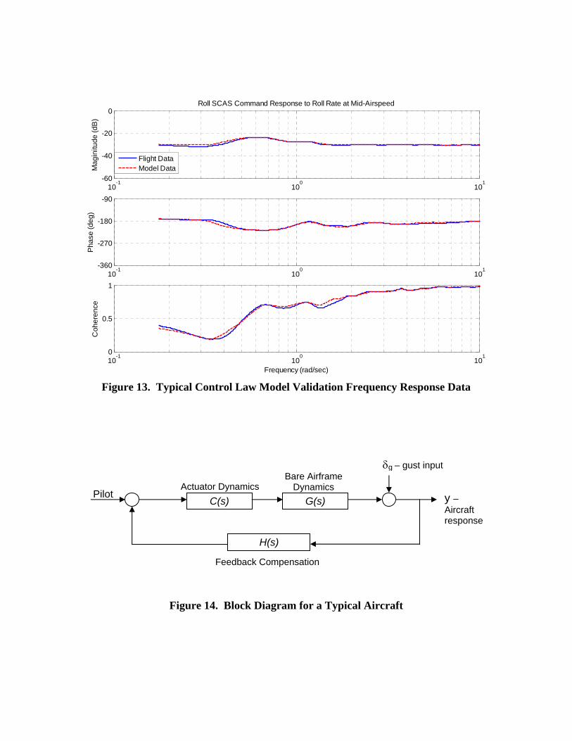
validation was completed by using a rotor exciter system to automatically generate frequency sweeps through each of the series actuators. These automatic sweeps generated aircraft response without having any of the pilot’s inputs influence the series actuator commands through the feed-forward paths. To validate gain scheduling and control law changes with airspeed, the automatic sweeps were flown at the same three speeds that were flown during model identification test points. As depicted in Fig. 12, the modeled control law frequency sweeps were generated using the input signals from the on-aircraft testing. This method was preferred over using the linear model (LINMOD) feature of SIMULINK® since it included the effects of the non-linear functions in the ARH-70A SCAS model. Once this frequency sweep data were obtained, CIFER® was used to generate the frequency responses for both the aircraft and model control laws. Figure 13 shows a near perfect match between the aircraft and model frequency responses for the automatic roll sweep at the mid-airspeed flight condition. Since the frequency response data from the other control axes and flight conditions also displayed excellent consistency, the modeled SCAS control laws were considered validated as a match with the actual AFCS. Design Constraints

Within the CONDUIT® design environment, a comprehensive set of specifications were chosen to drive the optimization of the control laws. Specifications were chosen such that adequate stability and handling qualities would be achieved. Most of the chosen specifications were based on ADS-33E-PRF (Ref. 1). The required stability margin was based on the military specification for flight control systems, MIL-F-9490 (Ref. 5). The selected specifications fell into three different categories within the optimization scheme: hard constraints, soft constraints, and summed objective constraints. The hard constraints included specifications considered critical for aircraft stability. During Phase 1 of the optimization, these hard constraints were optimized to the Level 1 (desirable) region before the other requirements were considered. Phase 2 of the gain optimization considered the soft constraints. These specifications were important for the handling qualities of the system, but were not vital to the stability of the system. Once all of the hard and soft constraints were met, the optimization entered Phase 3. During this phase, the set of summed objective constraints was minimized while maintaining all hard and soft constraints within the Level 1 region. An example of a summed objective constraint is the actuator root mean squared (RMS)

9

specification, which looks at the amount of series actuator activity for a given flight control design. Table 4 shows the specifications that were used in the optimization of the ARH-70A flight control laws.

Table 4. ARH-70A flight control optimization specifications

Design Approach

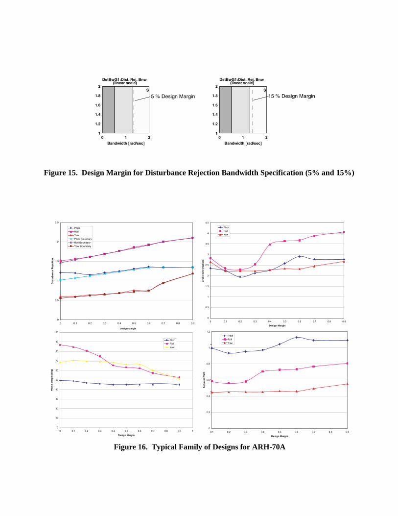
The design approach used by the development team was to optimize the system for the best disturbance rejection characteristics. A similar approach was implemented in the AH-64D Apache flight control law design (Ref. 6). This methodology ensured good command response tracking and performance of the hold functions in turbulent flight conditions. To aid in understanding disturbance rejection bandwidth, a typical aircraft block diagram is shown in Fig. 14. The sensitivity function for this block diagram is the transfer function which maps the gust input to the aircraft response as shown in Equation 17. Disturbance rejection bandwidth is defined as the frequency at which the Bode magnitude plot of the sensitivity function crosses the -3 dB line.

( ) ( )( ) ( ) ( ) ( )

11g

y sS s

s G s C s H sδ= =

+ (17)

The goal of the ARH-70A optimization strategy was to find a solution that had high disturbance rejection bandwidth, yet still maintained reasonable stability margin, cross-over frequency, and actuator RMS. The development team used an incremental method of increasing disturbance rejection bandwidth and then produced an optimized design at each point. The following list summarizes this optimization approach:

1. Set disturbance rejection bandwidth “Level 1” boundary at roughly 70% of baseline performance. All other Level 1 specifications are default based on industry, MIL-F-9490, and ADS-33E-PRF standards.

2. Optimize all specifications to Level 1 through Phase 3.

3. Incrementally increase the design margin for

disturbance rejection bandwidth specifications only. This moves the “Level 1” boundary incrementally higher as shown in Fig. 15.

4. Re-optimize at each increment through Phase 3.

5. When one axis has reached its maximum, fix the “Level

1” boundary for that axis at its disturbance rejection

maximum. Then, continue to increment the disturbance rejection design margin in the other axes and re-optimize at each increment through Phase 3.

6. Continue to incrementally increase the disturbance

rejection design margin until all axes have reached their maximum values. This results in a “family of designs” ranging from conservative to “maxed out” disturbance rejection, crossover, and actuator RMS. Often stability margins will be at the Level 1 boundary (45 deg) for the “maxed out” design.

7. Make graphs that show the progression of disturbance

rejection bandwidth, stability margin, crossover frequency, and actuator RMS. Choose a design that demonstrates a reasonable balance between all of these important stability and handling qualities parameters.

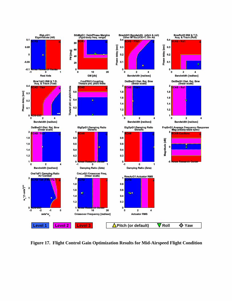
To automate this process, the development team used a batch mode optimization feature in CONDUIT® called Design Margin Optimization. This feature automated the process of advancing the disturbance rejection bandwidth design margin and then re-optimizing the solution at each point. Figure 16 shows a “family of designs” that resulted from this optimization strategy. The disturbance rejection bandwidth plot compares the disturbance rejection “Level 1” boundary versus the disturbance rejection bandwidth of the optimized solution. The corresponding cross-over frequency plot indicates that, in general, the cross-over frequency increased with disturbance rejection bandwidth. Actuator activity also increased with improved disturbance rejection, as indicated by the actuator RMS plot, while phase margin generally decreased with disturbance rejection bandwidth. These charts clearly show the design tradeoffs for the system and were instrumental in choosing a solution that balanced stability, disturbance rejection, and actuator activity. The suggested approach for choosing one gain set within this “family of designs” finds the point where disturbance rejection is as large as possible, but still maintains Level 1 phase margin requirements with an appropriate cross-over frequency to ensure that actuator activity is reasonable. The 0.7 design margin case in Fig. 16 would be a good choice for this example case. This design maintains reasonable cross-over frequencies for a helicopter the size of the ARH-70A (approximately 2.5 rad/sec for pitch and yaw, 3.7 rad/sec for roll), has nearly maximized disturbance rejection bandwidth, and meets Level 1 stability margin requirements. The actuator RMS is also reasonable because it increased only slightly from the previous design point due to the increased actuator activity associated with improved disturbance rejection.

10

Design Comparisons

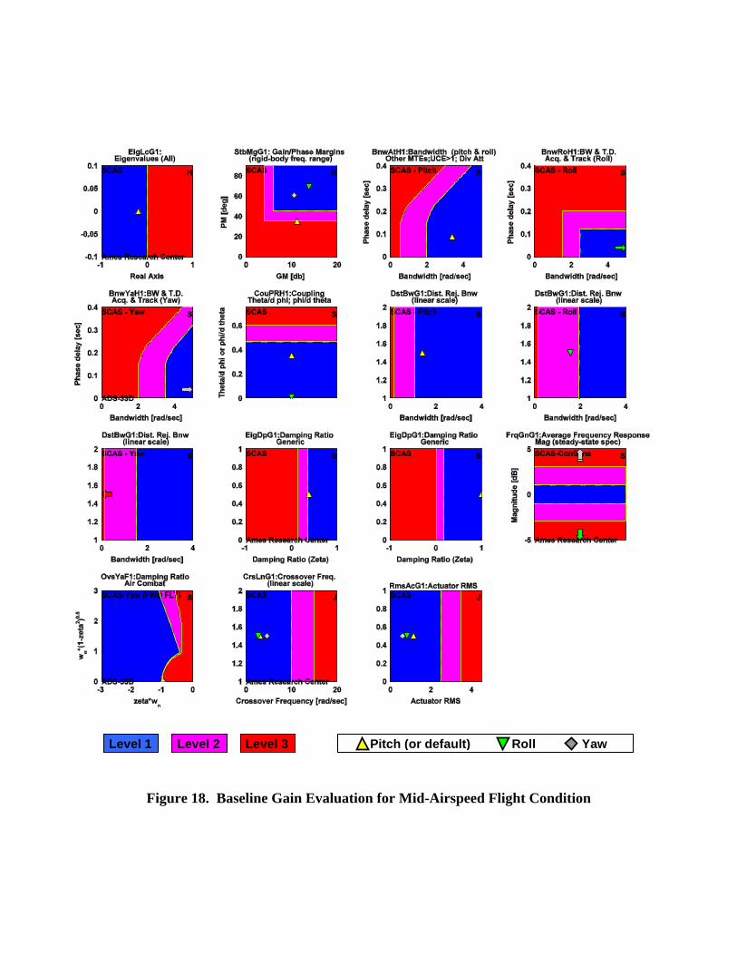
Figure 17 shows how this gain optimization strategy produced a gain set that met all of the Level 1 handling qualities design criteria. At this mid-airspeed flight condition, optimization of the SCAS mode gains resulted in a design which maximized the disturbance rejection bandwidth with minimum possible actuator activity and good cross-over frequency characteristics. All of this was attained while maintaining stable Eigenvalues, damping ratios not less than 0.45, and phase margins of at least 45 degrees. Finally, this optimization tuned the cyclic and pedal sensitivities to their desired values. If this optimization effort had not been completed, the ARH-70A would have entered flight test with a baseline set of generic AFCS gains. Figure 18 shows how these baseline SCAS gains fared against the handling qualities criteria. Table 5 compares the results of the control sensitivity optimization with the un-optimized baseline design.

Table 5. ARH-70A control sensitivity at mid-airspeed

Overall, the baseline design was deficient in pitch phase margin, yaw disturbance rejection, and control sensitivity in all axes. Even after extensive inflight tuning of this baseline gain set, the ARH-70A still would probably not have been able to deliver the Level 1 handling qualities required by the US Army. This comparison truly drives home the importance of completing flight control optimization to minimize flight testing while delivering a helicopter capable of meeting and exceeding the customer’s requirements.

TEST RESULTS

Testing of the optimized flight control gains has been completed in both the piloted simulator and the test aircraft. Based on our design strategy of optimizing the gains for a flight test identified linear model, the AFCS development test effort primarily called for validating the design process rather than tuning the system inflight one gain at a time. Although only preliminary AFCS testing has been completed thus far in the ARH-70A program, the results have been very promising. The initial set of SCAS and Attitude Hold gains, optimized using the Bell 407 linear model, needed only minor tuning before being cleared for the US Army’s Limited User Testing (LUT). Furthermore, the SCAS gains optimized for the ARH-70A linear model have been flown on the test aircraft and demonstrated compliance with stability and control sensitivity design criteria.

Simulation

The ARH-70A simulator is shown in Fig. 19. The non-linear ARH-70A COPTER model was run real-time to enable piloted evaluation of handling qualities in the simulator. This model was updated and validated using flight test data from the ARH-70A. The AFCS control laws were integrated with the COPTER model to enable development and evaluation of each of the AFCS control modes. The ARH-70A simulator cockpit was designed to duplicate the control characteristics, switches, displays, and outside visibility of the actual ARH-70A aircraft. This fixed cockpit was “flown” in a dome with a 270º wrap-around, out-the-window visual. Each of the ADS-33E-PRF MTE courses was modeled in the visual database to enable the evaluation of handling qualities while flying the scout helicopter MTEs. The ARH-70A simulator proved to be a valuable tool in developing the AFCS and validating the flight control gains before flying them on the aircraft. Use of the simulator not only enhanced flight safety, but also reduced the overall scope of the flight test effort. Both Bell Helicopter and US Army pilots evaluated handling qualities while flying the MTEs in the simulator. Overall, the pilots were very pleased with the way the AFCS performed. Although several of the MTEs were given Level 2 handling qualities ratings, this could be directly attributed to the limited visual cueing and lack of motion cues inherent in the simulation. Therefore, no changes were made to the AFCS gains based on piloted simulation. Flight Testing

The initial flight testing of the ARH-70A AFCS used the gains that were optimized for the Bell 407 linear model. The purpose of this Phase 1 testing was to ensure that the handling qualities of the SCAS and attitude hold modes were adequate for the US Army to complete LUT. The evaluation of these modes was completed by looking at the aircraft response to control pulse, doublet, and step inputs in the mid/mid LUT configuration at speeds across the flight envelope. Additionally, the test pilots evaluated handling qualities while flying the MTE courses during the day and at night while flying with night vision goggles. Overall, the ARH-70A development team was very encouraged by the results of this Phase 1 test effort. The team had planned on 15 hours of flight testing in order to tune the SCAS and attitude hold modes for LUT. As a result of the gain optimization effort, these modes were evaluated and adjusted in under five flight hours. Two issues were identified. First, a high frequency roll rate oscillation was

11

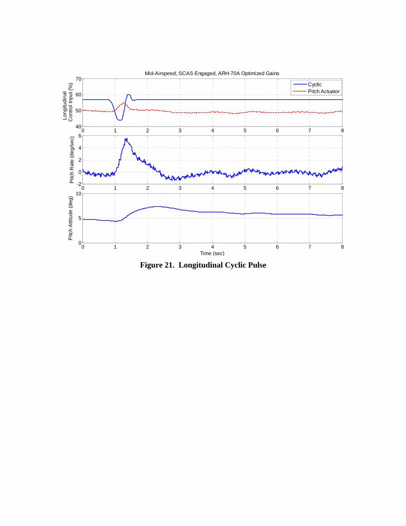
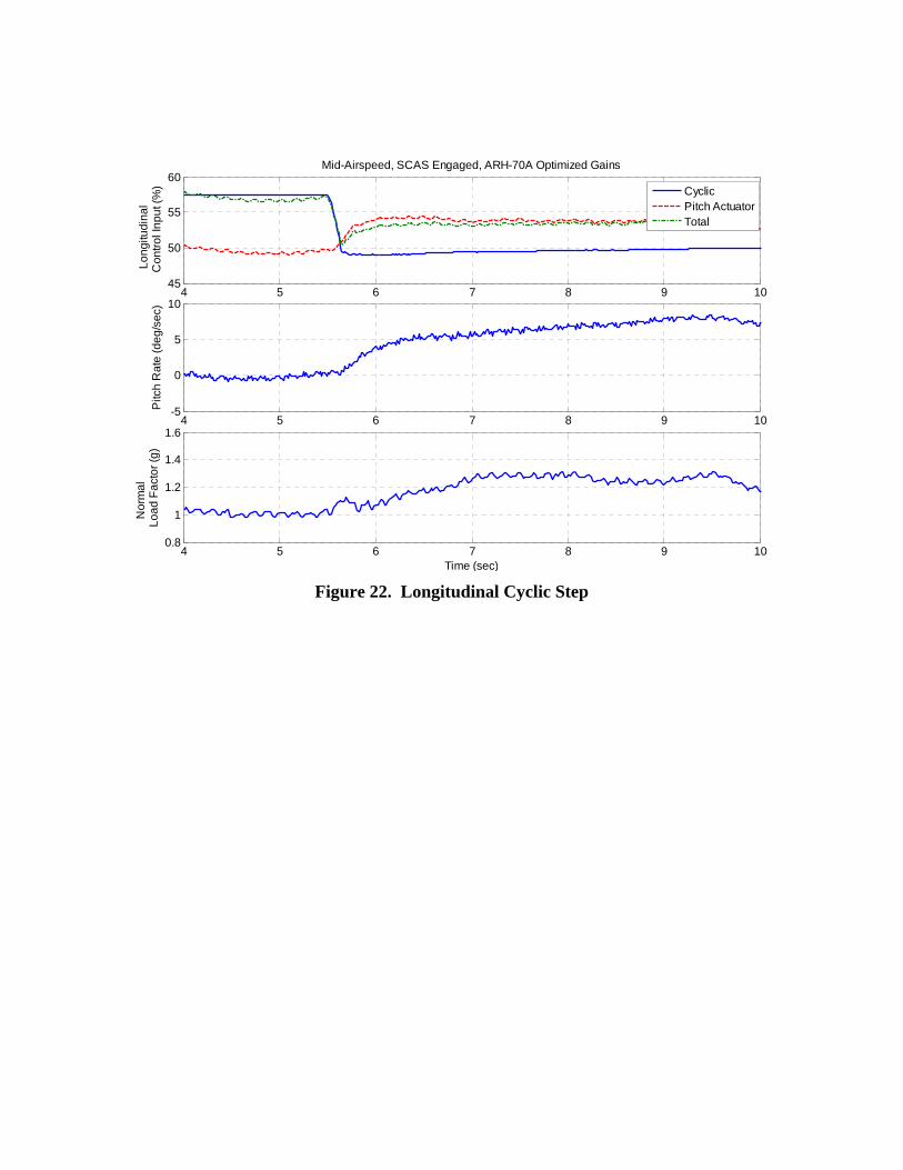
observed following a roll pulse at higher speeds. Additionally, the development team identified a need for control sensitivity adjustments across the envelope. The roll rate oscillation had a frequency of approximately 2.0 Hz and lasted about two cycles following a stick pulse at the higher airspeeds. An example of this oscillation can be found in Fig. 20. The team attributed this oscillation to low stability margins in the regressive in-plane mode of the main rotor. Since this mode was not included in the linear model, the optimized gains did not account for it. To improve the roll axis stability margins at these higher frequencies, the development team adjusted the phasing of roll rate feedback by incorporating a lead-lag filter in this feedback path. The issues with control sensitivity included a pedal response that was too sluggish in hover, but too sensitive in forward flight, and a longitudinal cyclic response that was too sensitive in forward flight. In spite of these issues, after flying the MTEs, the test pilots determined the handling qualities were definitely adequate for the LUT missions. Since the MTEs were only flown to the aggressiveness level required for LUT, handling qualities ratings were not provided by the pilots. However, pilots commented that they generally were able to meet Level 1 criteria on the limited and moderate agility MTEs, and probably could have met the Level 1 criteria if they had pushed aggressiveness higher during the aggressive agility MTEs. Since control sensitivity was evaluated as adequate for LUT, the development team elected to address the control sensitivity issues during the next gain optimization effort. As of the writing of this paper, only preliminary flight testing had been completed with the AFCS gains optimized for the ARH-70A linear model. Thus far, the Phase 2 test effort has only evaluated the SCAS mode aircraft response to pulse, doublet, and step control inputs in the light/aft loading condition. The first look at this data showed solid aircraft stability well within the ADS-33E-PRF Level 1 criteria. Furthermore, the initial review of control sensitivity data showed that the optimization was successful in adjusting sensitivities to the desired levels. Figures 21 and 22 show typical examples of the aircraft response to longitudinal cyclic pulse and step inputs, respectively. Future Testing

Future SCAS mode testing will evaluate the aircraft response in other configurations and loadings, to include an ARH-70A fully loaded with stores. Additional Phase 2 testing is planned to fully evaluate the other AFCS modes. This testing will culminate with the evaluation of ARH-70A handling qualities while flying the scout rotorcraft MTEs in

a mission representative configuration in both GVE and DVE conditions.

LESSONS LEARNED

The ARH-70A flight control development effort stands out as an excellent example of how linear modeling, gain optimization, and simulation can deliver the best possible flight control design with a minimal amount of flight testing required for design validation. The key lessons learned from this design and validation process are listed below: Frequency sweep testing can be extremely difficult when the aircraft has an unstable mode. One solution to this dilemma is to stabilize the aircraft by engaging the control system in the swept axis only. The total input to the bare airframe can be computed by summing the pilot and control system inputs. The effects of mechanical control mixing on the aircraft response can be removed from the frequency response data during analysis to identify the bare airframe dynamics. The methods presented in Ref. 3 effectively identified important speed derivatives by using simplified equations of motion and static stability data. CIFER® is an outstanding tool for frequency domain analysis including processing frequency response data, linear model system identification, and model verification in the time domain. A method of building up the total model structure from a simplified uncoupled model to the fully coupled model during parameter identification works well to prevent off-axis response matching from influencing primary response derivatives. By merging the control law design process with the evaluation of handling qualities criteria, CONDUIT® can significantly reduce the time needed to optimize a flight control system design. Before commencing gain optimization efforts, the modeled control laws should be validated with aircraft test data. A flight control system optimization method of pushing disturbance rejection bandwidth higher works well to develop a “family of designs” capable of meeting Level 1 handling qualities criteria. The use of piloted simulation in developing a flight control system and validating control law gains can enhance flight

12

safety while reducing the overall scope of the flight test effort. Higher frequency dynamics associated with the main rotor can have an adverse affect on control system stability. Limitations in the analysis due to unmodeled dynamics are often revealed only during flight test.

REFERENCES

1. “Aeronautical Design Standard, Handling Qualities Requirements for Military Rotorcraft,” USAAMCOM ADS-33E-PRF, U.S. Army Aviation and Missile Command, Huntsville, Alabama, March, 2000.

2. Tischler, M. B., Williams, J. N., Ham, J. A., “Flight Test Manual, Rotorcraft Frequency Domain Testing,” US Army Aviation Technical Test Center, Edwards AFB, California, September 1995.

3. Tischler, M. B. and Remple, R. K., “Aircraft and Rotorcraft System Identification: Engineering Methods With Flight Test Examples,” AIAA 2006.

4. “CONDUIT® Version 4.1 User’s Guide,” Raytheon, Report. ITSS 41-071403, Moffett Field, CA, July 2003.

5. “Military Specification, Flight Control Systems – General Specification for Design, Installation and Test of Piloted Aircraft,” MIL-F-9490D (USAF), June 6, 1975.

6. Harding, J.W., Moody, S.J., Jeram, G.J., Mansur, M.H., Tishcler, M.B., “Development of Modern Control Laws for the AH64D in Hover/Low Speed Flight,” American Helicopter Society 62nd Annual Forum, Phoenix, Arizona, May 9-11, 2006.

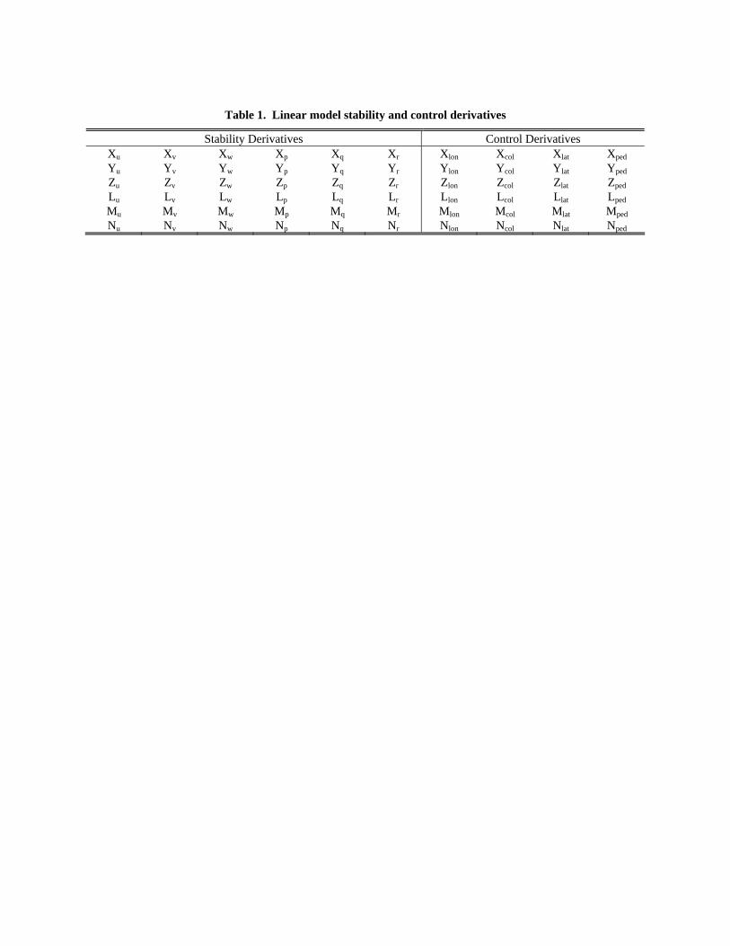
Table 1. Linear model stability and control derivatives

Stability Derivatives Control Derivatives Xu Xv Xw Xp Xq Xr Xlon Xcol Xlat Xped Yu Yv Yw Yp Yq Yr Ylon Ycol Ylat Yped Zu Zv Zw Zp Zq Zr Zlon Zcol Zlat Zped Lu Lv Lw Lp Lq Lr Llon Lcol Llat Lped Mu Mv Mw Mp Mq Mr Mlon Mcol Mlat Mped Nu Nv Nw Np Nq Nr Nlon Ncol Nlat Nped

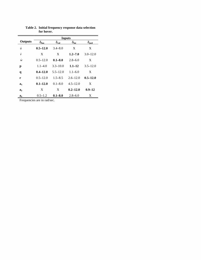
Table 2. Initial frequency response data selection for hover.

Inputs Outputs δlon δcol δlat δped

u& 0.5–12.0 3.4–8.0 X X

v& X X 1.2–7.0 3.0–12.0

w& 0.5–12.0 0.1–8.0 2.8–6.0 X

p 1.1–4.0 3.3–10.0 1.1–12 3.5–12.0

q 0.4–12.0 5.5–12.0 1.1–6.0 X

r 0.5–12.0 1.5–8.5 2.6–12.0 0.5–12.0

ax 0.1–12.0 0.1–8.0 4.5–12.0 X

ay X X 0.2–12.0 0.9–12

az 0.5–1.2 0.1–8.0 2.8–6.0 X Frequencies are in rad/sec.

Table 3. Final frequency response data used for hover.

Inputs Outputs δlon δcol δlat δped

u& 3.2–12.0 3.4–8.0 X X

v& X X 1.2–7.0 3.0–12.0

w& X 0.1–8.0 X X

p 1.1–4.0 3.3–10.0 1.1–12 X

q 1.5–12.0 X 1.1–6.0 X

r X 1.5–8.5 2.6–12.0 0.5–12.0

ax 0.1–12.0 0.1–8.0 X X

ay X X 0.2–12.0 0.9–12

az X 0.1–8.0 X X Frequencies are in rad/sec.

Table 4. ARH-70A flight control optimization specifications

CODUIT® Code Specification Description Constraint Type Axes

StbMgG1 Gain and Phase Margin (45 deg, 6 dB) Hard Pitch, Roll, Yaw EigLcG1 Stable Eigenvalues Hard All EigDpG1 Generic Damping Ratio (must be greater than 0.45

for SCAS) Soft All

OvsYaF1 Dutch Roll Damping (forward flight only) Soft Yaw BnwAtH1 Pitch Bandwidth for Other MTEs Soft Pitch BnwRoH1 Roll Bandwidth for Acquisition and Tracking Soft Roll BnwYaH1 Yaw Bandwidth for Acquisition and Tracking Soft Yaw CouPRH1 Coupling Between Pitch and Roll Soft Pitch/Roll DstBwG1 Disturbance Rejection Bandwidth Soft Pitch, Roll, Yaw FrqGnG1 Average Frequency Response (at low frequency to

minimize steady-state error) Soft Pitch, Roll, Yaw

FrqGnG1 Stick Sensitivity Soft Pitch, Roll, Yaw RisLoG1 Rise Time Specification (Lower Order Equivalent

System) Soft Pitch, Roll, Yaw

CrsLnG1 Cross-over Frequency Summed Objective Pitch, Roll, Yaw RmsAcG1 Actuator RMS Summed Objective Pitch, Roll, Yaw

Table 5. ARH-70A control sensitivity at mid-airspeed.

Axis Control Sensitivity Desired Baseline Gains Optimized

Gains Pitch Nz (g/in) 0.33 0.53 0.36 Roll p (deg/sec)/(in) 14.0 7.2 13.7 Yaw β (deg/in) 5.0 15.8 5.5

Figure 1. Armed Reconnaissance Helicopter, ARH-70A

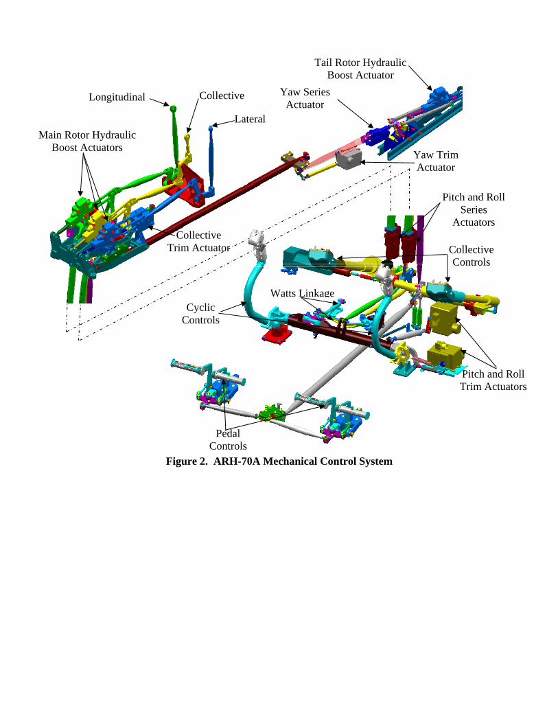
Figure 2. ARH-70A Mechanical Control System

Main Rotor Hydraulic Boost Actuators

Longitudinal Collective

Lateral

Yaw Series Actuator

Tail Rotor Hydraulic Boost Actuator

Yaw Trim Actuator

Collective Trim Actuator

Pitch and Roll Series

Actuators

Pitch and Roll Trim Actuators

Watts Linkage

Collective Controls

Cyclic Controls

Pedal Controls

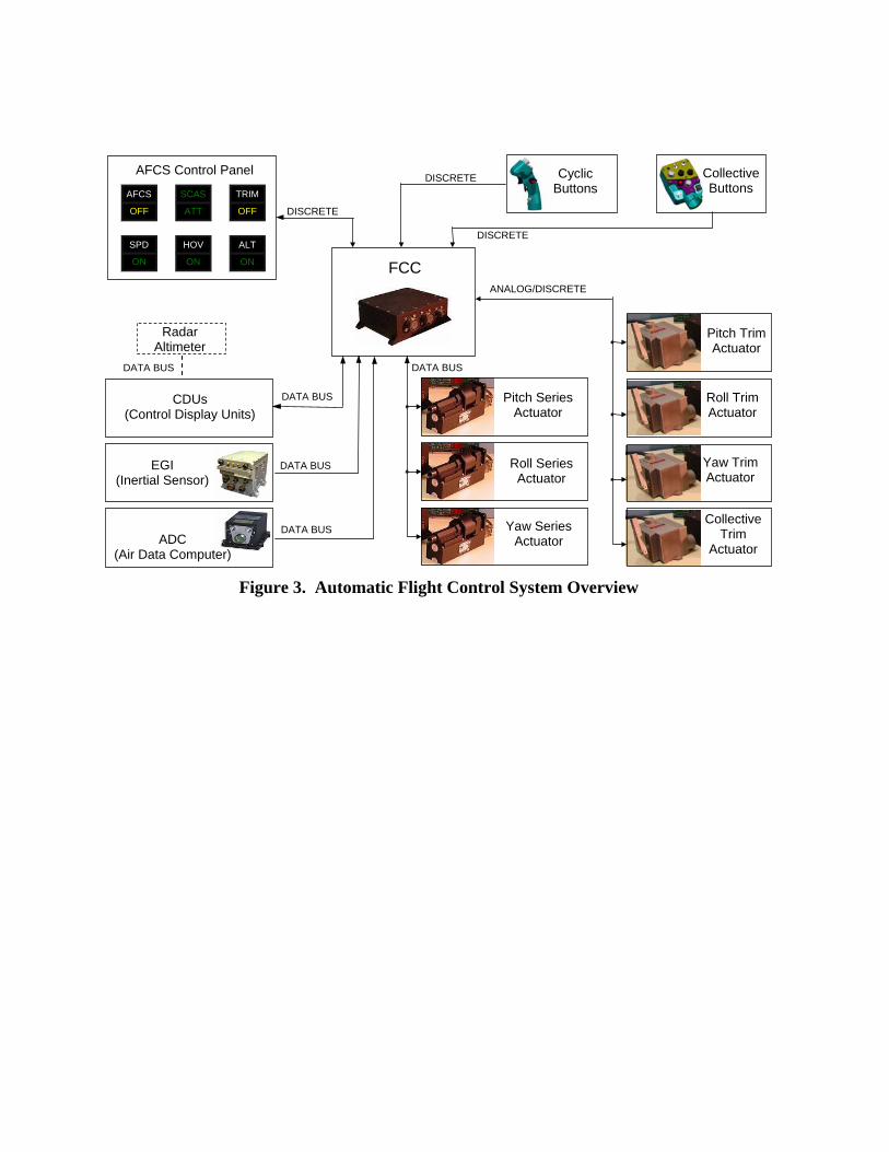
Figure 3. Automatic Flight Control System Overview

ANALOG/DISCRETE

FCC

AFCS Control Panel

TRIM OFF AFCS

OFF SCAS ATT

SPD ON ALT

ON HOV ON

CDUs (Control Display Units)

ADC (Air Data Computer)

EGI (Inertial Sensor)

Radar Altimeter

DATA BUS

Yaw SeriesActuator

Roll SeriesActuator

Pitch SeriesActuator

Roll TrimActuator

Pitch TrimActuator

Yaw TrimActuator

CollectiveTrim

Actuator DATA BUS

DATA BUS

DATA BUS

DATA BUS

DISCRETE

CyclicButtons

CollectiveButtons

DISCRETE

DISCRETE

4 5 6 7 8 9 10 11 1250

55

60

65

70P

edal

Pos

ition

(%)

4 5 6 7 8 9 10 11 12-20

-10

0

10

20

Time (sec)

Yaw

Rat

e (d

eg/s

ec)

Figure 4. Model Identification Pedal Doublet

0 5 10 15 20 25 3045

50

55

60

65

Long

itudi

nal

Cyc

lic P

ositi

on (%

)

0 5 10 15 20 25 30-40

-20

0

20

40

Time (sec)

Pitc

h A

ttitu

de (d

eg)

Figure 5. Attempted Hover Pitch Sweep in Bell 407

0 20 40 60 80 100 12030

40

50

60

Long

itudi

nal

Con

trol I

nput

(%)

CyclicPitch ActuatorTotal

0 20 40 60 80 100 120-4

-2

0

2

Time (sec)

Com

pute

d Fo

rwar

dA

irspe

ed R

ate

(ft/s

ec/s

ec)

0 20 40 60 80 100 1202

4

6

8

10

12

Pitc

hA

ttitu

de (d

eg)

Figure 6. Hover Pitch Sweep in ARH-70A

10-1

100

101

-90

-45

0

45

Frequency (rad/sec)

Pha

se (d

eg)

Instrumented Roll Angle to EGI Roll AngleFrequency Response Fit (time delay = 41.9 ms)

10-1

100

101-90

-45

0

45

Frequency (rad/sec)

Pha

se (d

eg)

Instrumented Roll Angle to Instrumented Roll RateFrequency Response Fit (time delay = 45.7 ms)

Figure 7. Roll Angle and Roll Rate Data Consistency

10-1

100

101

0

0.5

1

Frequency (rad/sec)

Coh

eren

ce

10-1

100

101

-80

-60

-40

-20

0Roll Rate due to Longitudinal Cyclic in Hover

Mag

initu

de (d

B)

10-1

100

101-540

-360

-180

0

Pha

se (d

eg)

With Watt's LinkageWithout Watt's Linkage

Figure 8. Watt’s Linkage Removal

10-1

100

101

0.7

0.8

0.9

1

Frequency (rad/sec)

Coh

eren

ce

10-1

100

1010

20

40

60Lateral Speed due to Roll Angle in Hover

Mag

initu

de (d

B)

10-1

100

101

-180

-90

0

Pha

se (d

eg)

Flight ResultsFrequency Response Fit (Yv = -0.05504)

Figure 9. Lateral Speed Damping Derivative Identification

1 102 3 4 5 6 7 8 90.7

0.8

0.9

1

Frequency (rad/sec)

Coh

eren

ce

100

101

-40

-30

-20

-10Pitch Rate Response to Longitudinal Cyclic in Hover

Mag

initu

de (d

B)

100

101

-360

-270

-180

Pha

se (d

eg)

Flight ResultsLinear Model Fit

Figure 10. Typical Frequency Domain Match for Final Hover Model

0 2 4 6 8 10-20

-10

0

10

20Longitudinal Cyclic Doublet in Hover

Pitc

h R

ate

(deg

/sec

)

0 2 4 6 8 10-10

0

10

20

Rol

l Rat

e (d

eg/s

ec)

0 2 4 6 8 10-20

-10

0

10

20

30

Time (sec)

Pitc

h A

ttitu

de (d

eg)

0 2 4 6 8 10-20

-10

0

10

20

Time (sec)R

oll A

ttitu

de (d

eg)

Flight DataLinear Model Fit

Figure 11. Typical Time Domain Match for Final Hover Model

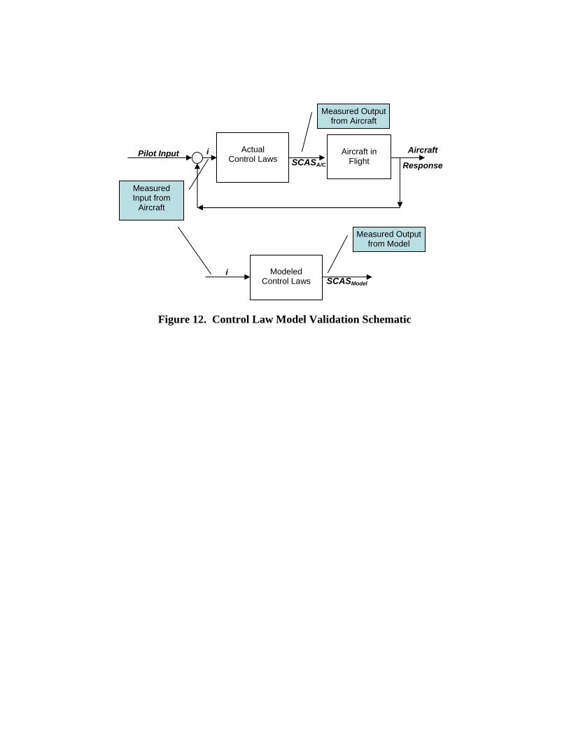
Figure 12. Control Law Model Validation Schematic

Aircraft in

Flight

Modeled

Control Laws

Actual

Control Laws

Aircraft

Response Pilot Input

Measured Input from

Aircraft

Measured Output from Aircraft

Measured Output from Model

i

i

SCASA/C

SCASModel

10-1

100

101-60

-40

-20

0Roll SCAS Command Response to Roll Rate at Mid-Airspeed

Mag

initu

de (d

B)

10-1

100

101

-270

-180

-90

-360

Pha

se (d

eg)

Flight DataModel Data

10-1

100

101

0

0.5

1

Frequency (rad/sec)

Coh

eren

ce

Figure 13. Typical Control Law Model Validation Frequency Response Data

Figure 14. Block Diagram for a Typical Aircraft

H(s)

C(s) G(s)

δg – gust input

y – Aircraft response

Pilot Actuator Dynamics

Bare Airframe Dynamics

Feedback Compensation

0 1 21

1.2

1.4

1.6

1.8

2

Bandwidth [rad/sec]

(linear scale)DstBwG1:Dist. Rej. Bnw

S

5 % Design Margin

0 1 2

1

1.2

1.4

1.6

1.8

2

Bandwidth [rad/sec]

(linear scale)DstBwG1:Dist. Rej. Bnw

S

15 % Design Margin

Figure 15. Design Margin for Disturbance Rejection Bandwidth Specification (5% and 15%)

0

0.5

1

1.5

2

2.5

0 0.1 0.2 0.3 0.4 0.5 0.6 0.7 0.8 0.9

Design Margin

Dis

turb

ance

Rej

ectio

n

Pitch

Roll

Yaw

Pitch Boundary

Roll Boundary

Yaw Boundary

0

10

20

30

40

50

60

70

80

90

100

0 0.1 0.2 0.3 0.4 0.5 0.6 0.7 0.8 0.9 1

Design Margin

Phas

e M

argi

n (d

eg)

Pitch

Roll

Yaw

0

0.5

1

1.5

2

2.5

3

3.5

4

4.5

0 0.1 0.2 0.3 0.4 0.5 0.6 0.7 0.8 0.9

Design Margin

Cro

ss-o

ver (

rad/

sec)

Pitch

Roll

Yaw

0

0.2

0.4

0.6

0.8

1

1.2

0.1 0.2 0.3 0.4 0.5 0.6 0.7 0.8 0.9

Design Margin

Act

uato

r RM

S

Pitch

Roll

Yaw

Figure 16. Typical Family of Designs for ARH-70A

Level 1 Level 2 Level 3 Pitch (or default) Roll Yaw

Figure 17. Flight Control Gain Optimization Results for Mid-Airspeed Flight Condition

Level 1 Level 2 Level 3 Pitch (or default) Roll Yaw

Figure 18. Baseline Gain Evaluation for Mid-Airspeed Flight Condition

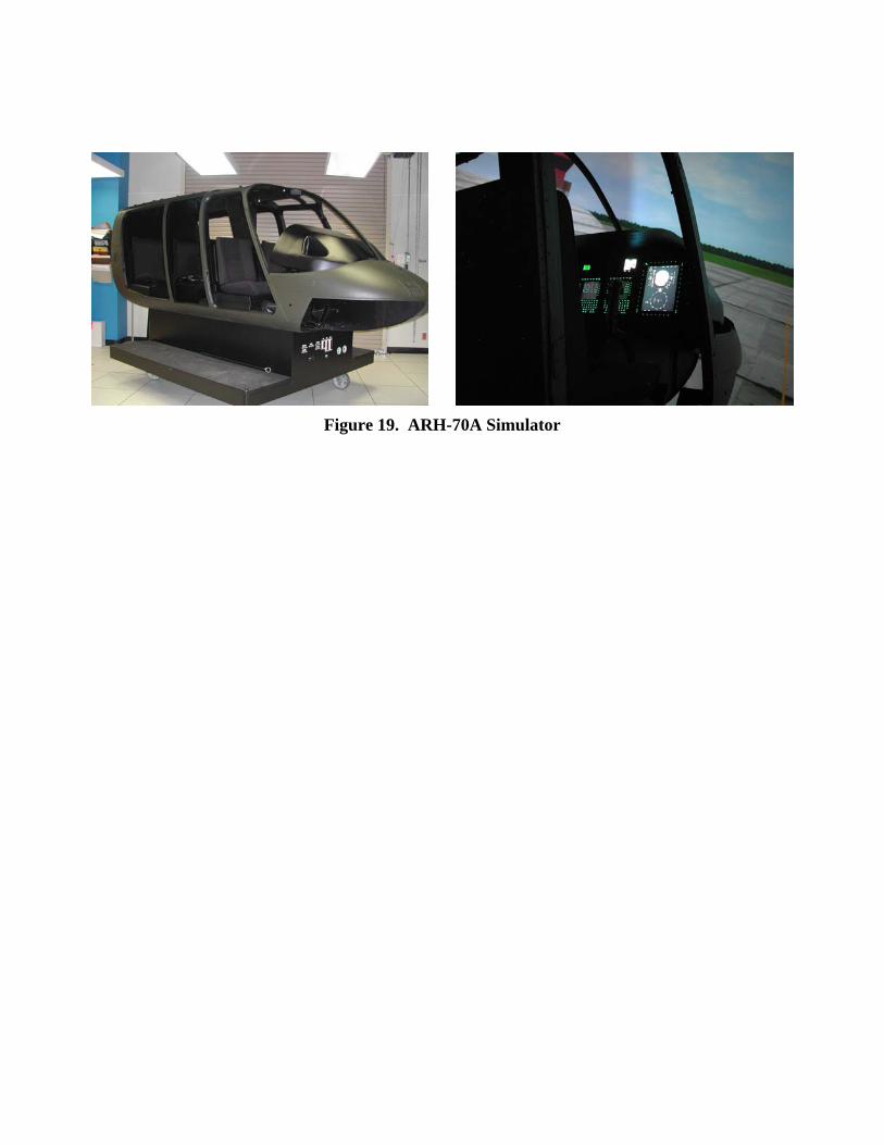
Figure 19. ARH-70A Simulator

2 2.5 3 3.5 4 4.5 5-15

-10

-5

0

5

Time (sec)

Rol

l Rat

e (d

eg/s

ec)

2 2.5 3 3.5 4 4.5 540

50

60

70

80High Airspeed, SCAS Engaged, Bell 407 Optimized Gains

Late

ral

Con

trol I

nput

(%)

CyclicRoll ActuatorTotal

Figure 20. Roll Rate Oscillation

0 1 2 3 4 5 6 7 8-2

0

2

4

6

Pitc

h R

ate

(deg

/sec

)

0 1 2 3 4 5 6 7 80

5

10

Time (sec)

Pitc

h A

ttitu

de (d

eg)

0 1 2 3 4 5 6 7 840

50

60

70Mid-Airspeed, SCAS Engaged, ARH-70A Optimized Gains

Long

itudi

nal

C

ontro

l Inp

ut (%

)

CyclicPitch Actuator

Figure 21. Longitudinal Cyclic Pulse

4 5 6 7 8 9 10-5

0

5

10

Pitc

h R

ate

(deg

/sec

)

4 5 6 7 8 9 100.8

1

1.2

1.4

1.6

Time (sec)

Nor

mal

Lo

ad F

acto

r (g)

4 5 6 7 8 9 1045

50

55

60Mid-Airspeed, SCAS Engaged, ARH-70A Optimized Gains

Long

itudi

nal

C

ontro

l Inp

ut (%

)

CyclicPitch ActuatorTotal

Figure 22. Longitudinal Cyclic Step