STABILITY OF INTERCELULAR EXCHANGE OFBIOCHEMICAL SUBSTANCES AFFECTED BY VARIABILITY

OF ENVIRONMENTAL PARAMETERS

DRAGUTIN T. MIHAILOVI , IGOR BALAZ

1Faculty of Agriculture, University of Novi Sad, Dositej Obradovic Sq. 8, Novi Sad21000, Serbia, E – mail:ibalaz@polj.uns.ac.rs, guto@polj.uns.ac.rs

Abstract. Communication between cells is realized by exchange of biochemical substances.Due to internal organization of living systems and variability of external parameters, the exchange isheavily influenced by perturbations of various parameters at almost all stages of the process. Sincecommunication is one of essential processes for functioning of living systems it is of interest toinvestigate conditions for its stability. Using previously developed simplified model of bacterialcommunication in a form of coupled difference logistic equations we investigate stability of exchangeof signaling molecules under variability of internal and external parameters.

Keywords: Intercellular communication; substances exchange; coupled logistic equations;synchronization, robustness.

1. INTRODUCTION

Process of communication between cells is an excellent example ofrobustness in living systems. Despite heavy influence of perturbations of variousinternal and external parameters, it is able to maintain its functionality. Moreover itseems that living systems evolved toward ability to function undisturbed by smallor moderate parameter fluctuations. It is not surprising since significant amount offluctuations is of internal origin, due to protein disorder [1,2] and so called intrinsicnoise [3,4]. Finally, due to thermal and conformational fluctuations, biochemicalprocesses are inherently random [5]. However, it is surprising that some elaboratedformal treatments of this problem are still in infancy [6,7]. It is argued here thatrobustness is a measure of feature persistence in systems that compels us to focuson fluctuations, and often assemblages of perturbations, qualitatively di erent innature from those addressed by stability theory. Moreover, to address featurepersistence under these sorts of perturbations, we are naturally led to study issuesincluding: the coupling of dynamics with organizational architecture, implicitassumptions of the environment, the role of a system’s evolutionary history indetermining its current state and thereby its future state, the sense in whichrobustness characterizes the fitness of the set of ”strategic options” open to the

system and the capability of the system to switch among multiple functionalities[8,9]. In this paper, the following de nition will be used - “robustness” is aproperty that allows a system to maintain its functions against internal and externalperturbations. It is important to realize that robustness is concerned withmaintaining functions of a system rather than system states, which distinguishesrobustness from stability or homeostasis [7].

Previously, we developed simplified model of bacterial communication inorder to investigate synchronization of substances exchange between abstract cells[10]. Since our model is inspired by a general scheme of intercellularcommunication, it naturally does not allow detailed modeling of some concrete,empirically verifiable intercellular communication process. Instead, it is designedto be a starting tool in a general investigation of robustness in mutually stimulativepopulations.

In this paper, our focus is only on question how the oscillating system whichis basically stochastic, and is inherently influenced by internal and externalperturbations, can maintain its functioning? In Section 2, using bacterialcommunication as an example, we give a short description of the model,representing cooperative communication process. In Section 3 we investigatesynchronization of the model and its sensitivity to fluctuations of environmentalparameters. Concluding remarks are given in Section 4.

2. DESCRIPTION OF THE INTERCELLULAR EXCHANGE MODEL

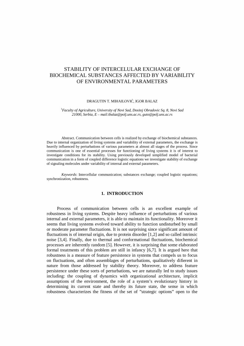
Signaling molecules are ones which are deliberately extracted by the cell intointracellular environment, and which can affect behavior of other cells of the sameor different type (species or phenotype) by means of active uptake and subsequentchanges in genetic regulations. Once appeared in intercellular environment, theycan be transported to other cells that can be affected. Let us note that the termenvironment, in this paper, comprises both (i) intracellular environment (inside thecell) and (ii) intercellular environment (that surrounds cells). Since active uptake isone of the milestones of the process, a very important factor in establishingcommunication is a current set of receptors and transporters in cellular membrane,during the communication process. At the same time they constitute backbone ofthe whole process, while simultaneously are very important source of perturbationsof the process due to protein disorder and intrinsic noise. Another important factoris intercellular environment which could interfere with the process of exchange. Itincludes: distance between cells, mechanical and dynamical properties of the fluidwhich serves as a channel for exchange and various abiotic and biotic factorsinfluencing physiology of the involved cells. Finally, in order to define exchangeprocess as communication, received molecules should induce change in geneticregulations. Therefore, concentration of signaling molecules inside of the cell, thatare destined to be extracted, can serve as an indicator of dynamics of the wholeprocess of communication. Additionally, the influence of affinity in functioning ofliving systems is also an important issue. In this case, it can be divided intofollowing aspects: (a1) affinity of genetic regulators towards arriving signals whichdetermine intensity of cellular response and (a2) affinity for uptake of signalingmolecules. First aspect is genetically determined and therefore species specific.

Second aspect is more complex and is influenced by: affinity of receptors tobinding specific signaling molecule, number of active receptor and theirconformational fluctuations (protein disorder).

As it is obvious from the empirical description, we can infer successfulnessof the communication process by monitoring: (i) number of signaling molecules,both inside and outside of the cell and (ii) their mutual influence. Concentration ofsignaling molecules in intercellular environment is subject to variousenvironmental influences, and taken alone often can indicate more about state ofthe environment then about the communication itself. Therefore, we choose tofollow concentration of signaling molecules inside of the cell as the main indicatorof the process. In that case, parameters of the system are: (i) affinity p by whichcells perform uptake of signaling molecules (a2), that depends on number and stateof appropriate receptors, (ii) concentration c of signaling molecules in intercellularenvironment within the radius of interaction, (iii) intensity of cellular response (a1)

nx and ny and (iv) influence of other environment factors which can interfere withthe process of communication. In this case we postulate parameter r , that can betaken collectively for intra- and inter- cellular environment, inside of the onevariable, indicating overall disposition of the environment to the communicationprocess.

Figure 1. Schematic representation of intercellular communication, taken from [10]. Here, crepresents concentration of signaling molecule in intercellular environment coupled with intensity ofresponse they can provoke while r includes collective influence of environment factors which caninterfere with the process of communication. xn and yn represent concentration of signaling moleculesin cells environment, while p denotes cellular affinity to uptake the substances.

The time development ( n is the number of time step) of the concentration incells ( , )n nx y can be expressed as

1 (1 ) ( ) ( ( ))n n nx c x h y , (1a)

1 (1 ) ( ) ( ( ))n n ny c x h x . (1b)

The map, h represents the flow of materials from cell to cell, and ( )h x and ( )h yare defined by a map that can be approximated by a power map,

( ) ~ ph x cx , (2a)( ) ~ qh y cy . (2b)

If ( ) ~ ph x cx and ( ) ~ qh y cy , the interaction is expressed as a nonlinear couplingbetween two cells. The dynamics of intracellular behavior is expressed as a logisticmap (e.g., [11,12]),

( ) (1 )n n nx r x x , (3a)( ) (1 )n n ny r y y . (3b)

Since concentration of signaling molecules can be regarded as theirpopulation for fixed volume, and since we are focused on mutual influence of thesepopulations, it points out to use the coupled logistic equations. Instead ofconsidering cell-to-cell coupling of two explicit n-gene oscillators [13] we considergeneralized case of gene oscillators coupling. In that case investigation ofconditions under which two equations are synchronized and how thissynchronization behaves under changes of intra- and inter- cellular environment,can give some answers on the question of maintaining functionality in the system.Therefore, having in mind that (i) cellular events are discrete [14] and (ii) theaforementioned reasoning, we consider system of difference equations of the form

1 ( ) ( ) ( )X F X L X P Xn n n n , (4)

with notation

1( ) ((1 ) (1 ),(1 ) (1 )), ( ) ( , )L X P X p pn n n n n n n nc rx x c ry y cy cx , (5)

where ( , )Xn n nx y is a vector representing concentration of signaling moleculesinside of the cell, while ( )P Xn denotes stimulative coupling influence of membersof the system which is here restricted only to positive numbers in the interval (0,1).The starting point 0X is determined so that 0 0( , ) (0,1)x y . Parameter (0,4)r isso-called logistic parameter, which in logistic difference equation determines an

overall disposition of the environment to the given population of signalingmolecules and exchange processes. Affinity to uptake signaling molecules isindicated by p . Let us note that we require that sum of all affinities of cells ipexchanging substances has to satisfy condition 1i

i

p or in the case of two cells

1p q . Since fixed point is (0) 0F , in order to ensure that zero is not at thesame time the point of attraction, we defined (0,1)p as an exponent. Finally, crepresents coupling of two factors: concentration of signaling molecules inintracellular environment and intensity of response they can provoke. This form istaken because the effect of the same intracellular concentration of signalingmolecules can vary greatly with variation of affinity of genetic regulators for thatsignal, which is further reflected on the ability to synchronize with other cells.Therefore, c influence both, rate of intracellular synthesis of signaling molecules,as well as synchronization of signaling processes between two cells, so theparameter c is taken to be a part of both ( )L Xn and ( )P Xn . However, relativeratio of these two influences depends on current model setting. For example, if forboth cells Xn is strongly influenced by intracellular concentration of signals, whilethey can provoke relatively smaller response then the form of equation will be

1 (1- ) (1- ) pn n n nx c rx x cy , (6a)

11 (1 ) (1 ) p

n n n ny c ry y cx . (6b)

We now analyze our coupled system given by (6a)-(6b). For 0 1x and0 1p we have 0 1px x . So, for small c , the dynamic of our investigatedsystem is similar to the dynamic of the following systems obtained byminorization, i.e.

1

1

(1 ) (1 ),(1 ) (1 ),

n n n

n n n

x c rx xy c ry y

(7)

and

1

1

(1 ) (1 ) ,(1 ) (1 ) .

n n n n

n n n n

x c rx x cyy c ry y cx

(8)

If we apply a majorization the considered system becomes

1

1

(1 ) (1 ) ,(1 ) (1 ) ,

n n n

n n n

x c rx x cy c ry y c

(9)

For all of those systems is obvious that they do not depend on parameter p .Because of ( , ) ( , )f x y g y x , where, ,f g are components of F in (4), theirdynamics are symmetric to the diagonal , {( , ) : }x y y x , as it was analyzedin [15]. This symmetry we also have for system (6a)-(6b) if 0.5p .

Having in mind the aforementioned conditions for p , x and px we consideronly systems (7) and (9) since the behavior of the system (6a)-(6b) comes from theproperties of the mentioned ones. It is seen that the systems (7) and (9) consist ofuncoupled logistic maps, in (7), on the interval (0,1) , while in (9) on the interval( ,1 ) , where 0 is the smaller solution of the equation

(1 ) (1 ) ,x c rx x c i.e.

2[(1 ) 1 [ (1 ) 1)] 4 (1 )] / [2 (1 )]c r c cr c r c . (10)

From the property of the logistic equation we get the following expression

[ (1 ) 4 4 ] / (1 2 )r c c , (11)

where in system (9) taking the role of (1 )r c in (7). Comparing (1 )r c with(11) we can conclude that the expression (11) is always greater, that implies thatbifurcations and chaos first appears for system (7) and than for (9). Finally,combining expressions (10) and (11) we get

2 2 2

2

(1 ) 4 (1 ) 2 (1 ) 2 2 [ (1 ) 1] 4 (1 )

1 [ (1 ) 1] 4 (1 )

r c cr c r c r c cr cr c cr c

(12)

3. A NONLINEAR DYNAMICS-BASED ANALYSIS OF THE COUPLEDMAPS REPRESENTING THE INTERCELLULAR EXCHANGE OF

SUBSTANCES

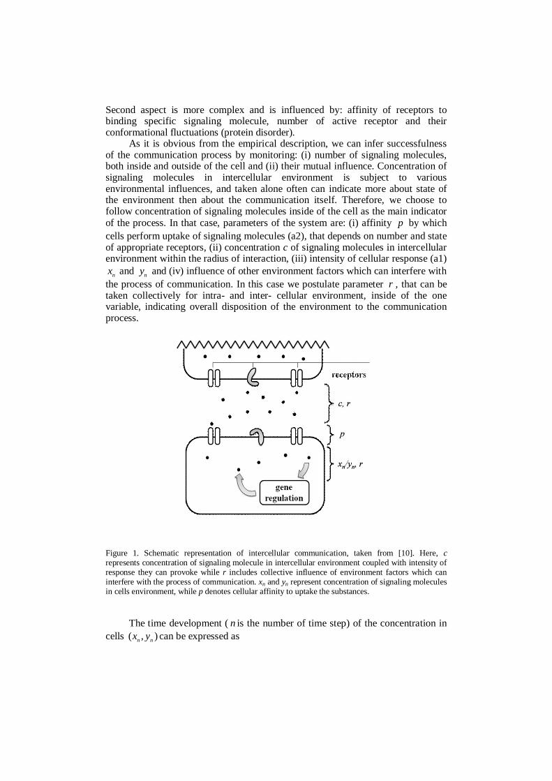
In order to further investigate the behavior of the coupled maps, we performa numerical analysis of the coupled system (6) throuhg its parameters c , r and p ,using the largest Lyapunov exponet as measure of the chaotic behaviour and borderbetween synchronized and nonsynchronized system states in intercellular exchangeof substances.

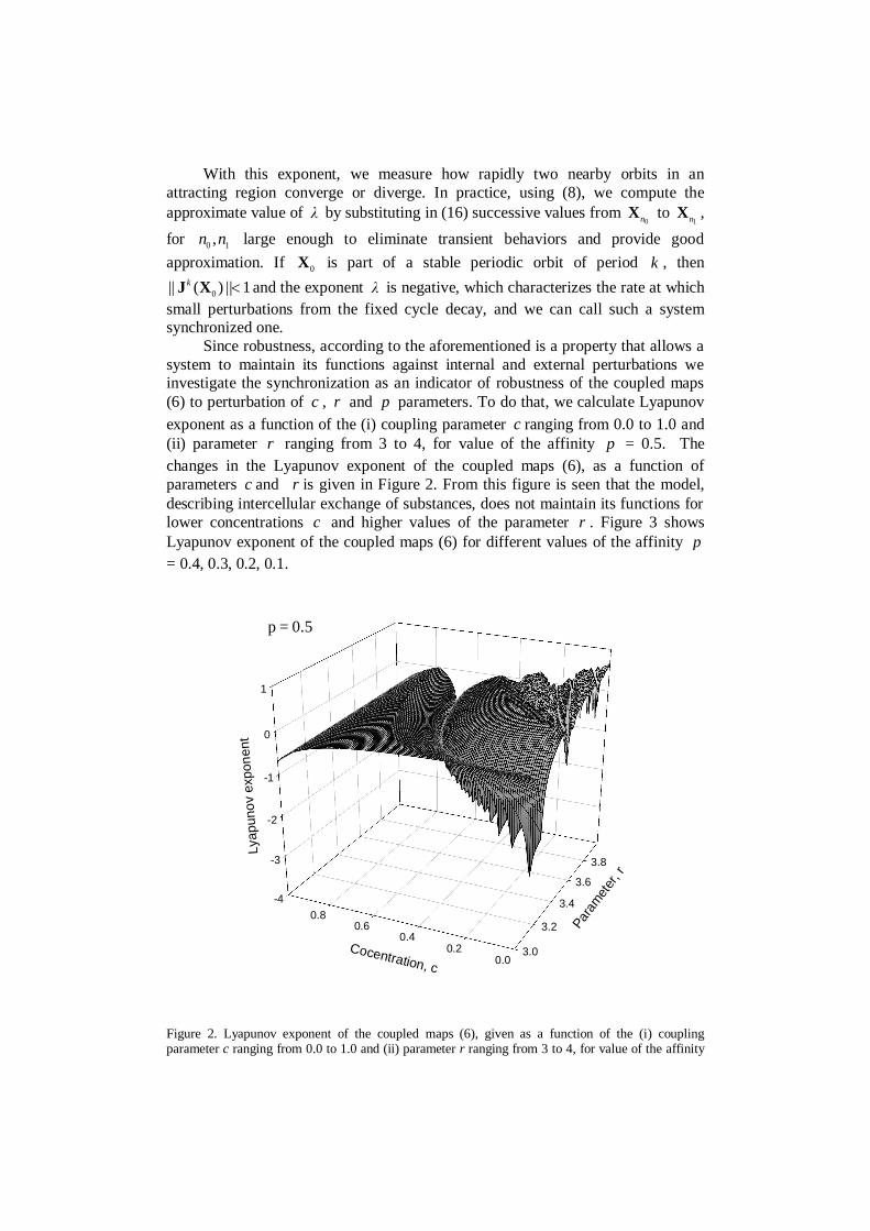
Previously [10] we showed that for fixed value of r (in our case 3.95)Lyapunov exponent of the coupled maps, given as a function of the coupling

parameter c ranging from 0 to 1.0, for different values of the affinity p gives aborder in values of concentration c (around 0.4), that split domain of concentrationinto two regions. The first one, is located between 0 and 0.4, with the nonsinchronyzed states including sporadical windows where synchronization isreached. In contrast to that, the second region (between 0.4 and 1.0) is regionwhere process of ehcange between two cells is fully synchronized.

We calculate Lyapunov exponent by analysis of orbits. The orbit of the point0X is the sequence 0 0 0, ( ),..., ( ),...X F X F Xn where 0

00( )F X X and for 1n ,

10 0( ) ( ( ))F X F F Xn n . We say that the orbit is periodic with period k if k is the

smallest natural number such that 0 0( )F X Xk . If 1k , then the point 0X is thefixed point. The periodic point 0X with period k is an attraction point if the normof the Jacobi matrix for the mapping ( ) ( ( , )), ( ( , ))F Xk

k kf x y g x y is less than one,i.e., 0|| ( ) || 1J Xk , where

0( )

0X X

J X

k k

k

k k

f fx yg gx y

. (13)

Here, we define 0|| ( ) ||J Xk as max 1 2{| |,| |} , where 1 and 2 are theeigenvalues of the matrix. It is worth noting that

0 1 1 0( ) ( ) ( )... ( ) ( )J X J X J X J X J Xk kk k , (14)

where

1(1 ) (1 2 )( ) .

(1 ) (1 ) (1 2 )J X

p

p

c r x cpyc p x c r y

(15)

In particular, for the scalar equation 1 ( )n nx d x the norm is

0 1 1 0| ( ( )) ' | | '( )... '( ) '( ) |kx x nd x d x d x d x , where 1'( ) (1 2 ) pd x r x cpx . In order to

characterize the asymptotic behavior of the orbits, we need to calculate the largestLyapunov exponent, which is given for the initial point 0X in the attracting regionby

lim(ln || ( ) || / )n0J X

nn . (16)

With this exponent, we measure how rapidly two nearby orbits in anattracting region converge or diverge. In practice, using (8), we compute theapproximate value of by substituting in (16) successive values from

0Xn to

1Xn ,

for 0 1,n n large enough to eliminate transient behaviors and provide goodapproximation. If 0X is part of a stable periodic orbit of period k , then

0|| ( ) || 1J Xk and the exponent is negative, which characterizes the rate at whichsmall perturbations from the fixed cycle decay, and we can call such a systemsynchronized one.

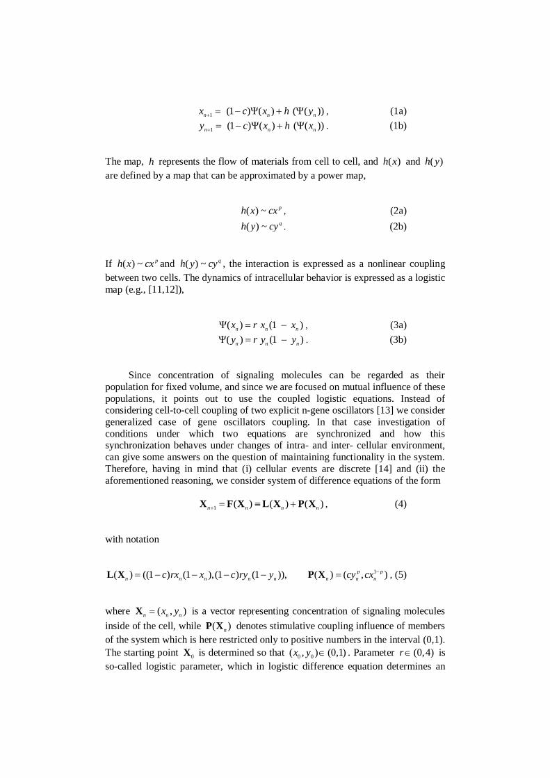
Since robustness, according to the aforementioned is a property that allows asystem to maintain its functions against internal and external perturbations weinvestigate the synchronization as an indicator of robustness of the coupled maps(6) to perturbation of c , r and p parameters. To do that, we calculate Lyapunovexponent as a function of the (i) coupling parameter c ranging from 0.0 to 1.0 and(ii) parameter r ranging from 3 to 4, for value of the affinity p = 0.5. Thechanges in the Lyapunov exponent of the coupled maps (6), as a function ofparameters c and r is given in Figure 2. From this figure is seen that the model,describing intercellular exchange of substances, does not maintain its functions forlower concentrations c and higher values of the parameter r . Figure 3 showsLyapunov exponent of the coupled maps (6) for different values of the affinity p= 0.4, 0.3, 0.2, 0.1.

-4

-3

-2

-1

0

1

3.0

3.2

3.4

3.6

3.8

0.00.2

0.40.6

0.8

Lyap

unov

exp

onen

t

Para

meter,

r

Cocentration, c

Figure 2. Lyapunov exponent of the coupled maps (6), given as a function of the (i) couplingparameter c ranging from 0.0 to 1.0 and (ii) parameter r ranging from 3 to 4, for value of the affinity

p = 0.5

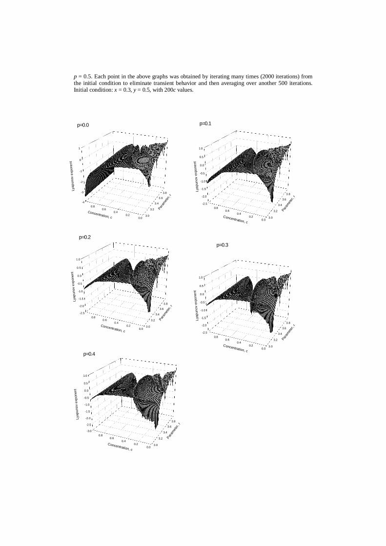
p = 0.5. Each point in the above graphs was obtained by iterating many times (2000 iterations) fromthe initial condition to eliminate transient behavior and then averaging over another 500 iterations.Initial condition: x = 0.3, y = 0.5, with 200c values.

p=0.0

-2.5

-2.0

-1.5

-1.0

-0.5

0.0

0.5

1.0

3.0

3.2

3.4

3.6

3.8

0.00.2

0.40.6

0.8

Lyap

unov

exp

onen

t

Para

meter,

r

Concentration, c

p = 0.1

-2.5

-2.0

-1.5

-1.0

-0.5

0.0

0.5

1.0

3.0

3.2

3.4

3.6

3.8

0.00.2

0.40.6

0.8

Lyap

unov

exp

onen

t

Param

eter,

r

Concentration, c

c = 0.2

-2.5

-2.0

-1.5

-1.0

-0.5

0.0

0.5

1.0

3.0

3.2

3.4

3.6

3.8

0.00.2

0.40.6

0.8

Lyap

unov

exp

onen

t

Para

meter,

r

Concentration, c

c = 0.3

-3.0

-2.5

-2.0

-1.5

-1.0

-0.5

0.0

0.5

1.0

3.0

3.2

3.4

3.6

3.8

0.00.2

0.40.6

0.8

Lyap

unov

exp

onen

t

Param

eter,

r

Concentration, c

-4

-3

-2

-1

0

1

3.0

3.2

3.4

3.6

3.8

0.00.2

0.40.6

0.8

Lyap

unov

exp

onen

t

Para

meter,

r

Concentration, c

p =0.0p=0.0 p=0.1

p=0.2

p=0.4

p=0.3

Figure 3. Lyapunov exponent of the coupled maps, given as a function of the (i) coupling parameter cranging from 0.0 to 1.0 and (ii) parameter r ranging from 3 to 4, for different values of the affinity p.The same graphs will be able to obtained for values p = 0.6, 0.7, 0.8, 0.9 and 1.0 corresponding tothose for p = 0.4, 0.3, 0.2, 0.1 and 0.0. Each point in the above graphs was obtained by iterating manytimes (2000) from the initial condition to eliminate transient behavior and then averaging overanother 500 iterations. Initial condition: x = 0.3, y = 0.5, with 200c values.

4. CONCLUSIONS

In this paper, our focus is on investigating stab ty of ntercelular exchangeof b ochem cal substances affected by var ab ty of env ronmental parameters. Weidentified main parameters of the process of cellular communication and using asystem of two coupled logistic equations we investigated synchronization of themodel and its sensitivity to fluctuations of environmental parameters. Results showexistence of stability regions where noise in the form of fluctuations inconcentration of signaling molecules in intercellular environment and fluctuationsin affinity for uptake these molecules cannot interfere with the process ofexchange. Since our model is insipred by the general scheme of intercellularcommunication, it naturally does not allow detailed modelling of some concrete,emiprically verifable intercellular communication process. Instead, it is designed toserve as a starting tool in general investigation of robustness in mutuallystimulative populations which can be readily extended to investigation ofsynchronization in larger networks of interacting entities [16,17].

Acknowledgments. The research work described here has been funded bythe Serbian Ministry of Science and Technology under the project “Numericalsimulation and monitoring of climate and environment in Serbia”, for 2011-2014.

REFERENCES

1. A. K. Dunker, J.D. Lawson, C.J.Brown, R.M. Williams, P. Romero, J. S. Oh, C. J. Oldfield, A.M. Campen, C. M. Ratliff, K. W. Hipps, J. Ausio, M. S. Nissen, R. Reeves, C. Kang, C. R.Kissinger, R. W. Bailey, M. D. Griswold, W. Chiu, E. C. Garner, Z. Obradovic, J. Mol. Graph.Model. 19, 26-59 (2001)

2. A. K. Dunker, C.J.Brown, J.D. Lawson, L. M. Iakoucheva, Z. Obradovic, Biochemistry 41,6573–6582 (2002)

3. M. B. Elowitz, A. J. Levine, E. D. Siggia, P. S. Swain, Science 297, 1183-1186 (2002)4. P. S. Swain, M. B. Elowitz, E. D. Siggia, PNAS 99, 12795-12800 (2002).5. D. Longo, J. Hasty, Mol. Syst. Biol. 2, 64 (2006)6. H. Kitano, Nat. Rev. Genet. 5, 826–837 (2004)7. H. Kitano, Mol. Syst. Biol. 3, 137 (2007)8. E. Jen: Stable or robust? What’s the difference? Complexity 8, 12-18 (2003)9. M. B. Kennel, R. Brown, H. D. I. Abarbanel, Phys. Rev. A 45, 3403–3411 (1992)10. I. Balaz, D.T. Mihailovic, Arch. Biol. Sci. Belgrade (2010) - submitted11. L. Deverney: An Introduction to Chaotic Dynamical Systems. Benjamin/ Cummings Comp,

Boston (1986)12. Y. – P. Gunji, M. Kamiura, Physica. D 198, 74-105 (2004)

13. E. Ullner, A. Koseska, J. Kurths, E. Volkov, H. Kantz, J. Garcia-Ojalvo, Phys. Rev. E 78,031904 (2008)

14. N. Barkai, B.- Z. Shilo, Mol. Cell 28, 755-760 (2007)15. D. T. Mihailovi , M. Budin evi , I. Balaz, M. Periši , In Mihailovi D.T., Lali B. (eds.)

Advances in environmental modelling and measurements, pp. 89-100. Nova SciencesPublishers, New York (2010)

16. R. E. Amritkar, S. Jalan, Physica A 321, 220-225 (2003)17. S. Jalan, R. E. Amritkar, C. – K. Hu, Phys. Rev. E 72, 016211 (2005)