Equilibrium properties of liquids containing supercritical substances

Equilibrium Properties of Liquids Containing Supercritical Substances

A two-parameter, corresponding-states form for direct correlation function integrals in liquids is applied to many types of systems with one substance being supercritical. This gives a quantitative correlation for volumetric behavior, pure and mixed solvent Henry’s constants, and Henry’s Law deviations over wide ranges of conditions using only pure- component information and a single binary parameter. Details of the method and results are given for H,, N,, CO, CH,, and other gases in pure and mixed simple, polar, and aqueous solvents and coal oils. Because of its reliable predictive capability, the present approach can serve as a generator of data for parameter estimation by other models such as equations of state.

E. A. Campanella, P. M. Mathias, J. P. O’Connell

Department of Chemical Engineering University of Florida

Gainesville, FL 3261 1

Introduction Current design practice for high-pressure chemical process-

ing and multisolvent gas absorption requires increasingly better correlations of physical properties of systems containing species a t temperatures above their critical point. Treatments for systems containing H,, N,, CO, CH,, or other gases, such as pro- posed by Soave ( 1 9721, Peng and Robinson (1 976), and Brule e t al. (1982), generally rely on a complete equation of state, such as the Redlich-Kwong equation. Others, such as Prausnitz and Chueh (1 968), describe deviations of the liquid phase from Hen- ry’s Law. Both treatments have been of limited value when applied to liquids containing highly polar species such as ammonia, water, and alcohols. In particular, activity coefficient and pressure contributions to the supercritical component fugacities tend to compensate, so their product may be poorly described. Also, even in binary solvents, Henry’s constant is often poorly predicted from pure-component solubilities and solvent properties.

The present work applies a general formulation of the problem using the fluctuation solution theory of statistical mechan- ics. Expressions can be written for derivatives of the activity coefficient and of the pressure with respect to the concentrations of the species. Using expressions for the direct correlation function integrals (DCFI) in terms of concentrations, these derivatives can then be integrated from any liquid reference state to any desired final state. Deviations from Henry’s Law in pure

Correspondence concerning this paper should be addressed to J. P. O’Connell. The oresent affiliation of E. A. Camoanella is Univ. Nac. del Literal. Santa Fe, ArRentina.

The pr&ent affiliation of P. M. Mathias is Air Products and Chemicals, Inc., Allentow< PA.

and mixed solvents are one kind of application. Another is prediction of Henry’s constants of a solute in pure or mixed solvents using a known Henry’s constant of the same solute in another solvent. Extension to multiple solutes is also straightforward and these ideas can be applied to a diverse set of systems including hydrocarbon, polar, aqueous, and coal oil solutions of the above gases.

The result of this work is a practical and accurate method for describing the component fugacities and volumetric behavior of nonelectrolyte liquids containing supercritical components, re- gardless of the complexity of the intermolecular forces in the system. The DCFI have been correlated with density and temperature using two-parameter corresponding states. Parameters are given for over 55 substances, including gases, small and large hydrocarbons, polar and hydrogen-bonding solvents, and mixed coal oils. Comparisons are made for 33 high-pressure systems with excellent results. Procedures are described for obtain- ing parameters for other components from liquid density data. For pure or pseudopure (e.g., coal oil) solvents, analytical expressions are used to calculate changes in volume and in component fugacities as the composition and pressure are changed from the liquid reference state of Henry’s Law to the system conditions. While a binary constant is used, the results are generally insensitive (kO.1) to its value. For many systems, such as H, in coal oils, NH,, and methanol, pure-solvent saturation pressure and density along with a single fitted gas-solvent binary parameter are sufficient information to accurately correlate behavior over the entire range of available conditions.

For gas solubility in mixed solvents the present method appears to be the most generalized and reliable available, as

AIChE Journal December 1987 Vol. 33, No. 12 2057

shown by comparisons with 50 nonaqueous and 24 aqueous binary mixtures and one aqueous ternary system. In addition to the parameters, pure-solvent Henry's constants and densities and-particularly for aqueous systems-binary solvent densities are needed as input.

The present paper shows how this generalized technique can be used in its present form for even the most complex systems; the only additional requirement is an easily available vapor- phase model, for example, that of Nakamura et al. (1976). In addition, the method can generate reliable data for fitting parameters of sophisticated full equations of state for use in the critical region or in higher order multicomponent systems containing supercritical components.

Basic Expressions We use a liquid reference state, plus a vapor equation of state

and activity coefficient model rather than a single equation of state for both phases. Prausnitz and Chueh (1968), Van Ness and Abbott (1962), and Prausnitz et al. (1986) have described this most extensively. The liquid fugacity is given as:

In Eq. 1, the final state fugacityx. is obtained from the reference state fugacity ( i / x i ) ' by a two-step thermodynamic process: A change in composition a t constant reference pressure to obtain the activity coefficient, yi, followed by a change in pressure to the final value using the exponential Poynting correction. The reference state for the subcritical component is the pure- component, saturated liquid, so ( f i / x i ) r is 4 p P?'. The value of ( f i / x i ) ' for the supercritical solute is Henry's constant, Hi, the fugacity of the hypothetical pure liquid corresponding to the ideal dilute solution at the reference pressure.

P-P'

The quantity in braces in Eq. 1 represents the total deviation from ideality. For low-pressure, subcritical systems, the Poynt- ing correction is small while the (usually) large activity coefficient can be modeled by excess free energy expressions (Praus- nitz et al., 1986). For systems with supercritical components, the pressure correction is large and the activity correction is small for the solvent components, while the two effects cancel to a significant extent for the supercritical solutes (Mathias, 1978; Mathias and O'Connell, 1981). Figure 1 shows this for the system hydrogen-methanol.

Thus, when supercritical components are present, the liquid fugacity can advantageously be written with the deviations com- bined into a single quantity, -y{,

We have found that an accurate value for y{ can be obtained from fluctuation solution theory, which uses integrals of the statistical mechanical direct correlation function (DCFI). These are insensitive to the nature of the intermolecular forces in the

2058 December 1987

9

In (2) 8

8

CALCULATED Ik ,,= 0.01 - DATA OF KRICHEVSKII.eI el.

/ 363.15 K

/ 413.15

I I I I 0.075 0.025 0.050

x " *

Figure 1. Fugacity of hydrogen(1) in methanol(%) at vari- ous temperatures.

~ calculated; -. -. - Henry's Law; --- Poynting correction only

fluid (Brelvi and O'Connell, 1972, 1975a, b, c; Gubbins and O'Connell, 1974), so two-parameter corresponding states can be applied to predict the integrals of these correlation functions as a function of reduced temperature and reduced density. Because the theory yields the concentration derivatives of both the activity coefficient and the pressure, values of y{can be obtained for systems where the solvent is present. Further, by proper manipu- lation (OConnell, 1981), it can be found for cases where the reference state solvent does not actually appear in the solution of interest. This potentially powerful concept takes advantage of the generality of Eq. 3 by using it in the limit of infinite dilution of component i when the solvent composition is changed from a pure reference solvent (x, - 1) to any other solvent composition. Thus, if ( J l x , ) ' = HIR, then y{ = H,,(T,Pf,$F)/H,R where H,, is Eq. 2 in a mixed solvent a t the same temperature and the solute-free composition is :SF. Because of this flexibility, as well as its general insensitivity to binary parameter values, the technique may considerably reduce the data requirements for accurate modeling of systems with supercritical components, particularly in mixed solvents.

The present paper describes extensive, but not exhaustive, applications of the method. The following sections include basic expressions, DCFI model equations, pure-liquid properties and parameter evaluation, high-pressure binary system correlation and prediction, mixed-solvent applications including Henry's constants, and improvements and extensions.

The DCFI between species i and j , C,,, can be related to derivatives of the activity coefficient of Eq. 3 (Mathias, 1978;

Vol. 33, No. 12

k- l

AIChE Journal

The Gibbs-Duhem equation, together with Eq. 4, yields

As described by O'Connell (1981), if the system changes from thestate (T,P',x') = (T,p') to the state (T,P',X/) = ( T , d ) , Eq. 4 and 5 can be integrated to provide values for the changes in activity coefficient and pressure. For example, if P',?', Pf,$,pr are known, integration of Eq. 5 for all components i yields p'. Integration of Eq. 4 for all components j yields values of In 7;.

DCFl Model The basis of the model in corresponding states is described

elsewhere (Mathias and O'Connell, 1981). The result is an expression based on hard spheres and is of the van der Waals form

This form has been used previously in a different context (Bien- kowski et al., 1973). The expressions we use for Cp, djj and BF are given in the Appendix. There are two pure-component parameters, Ti* and VF, and a binary constant k,, which appears only in kij. This allows the integrations of Eqs. 4 and 5 to be carried out analytically.

Thus, pfcan be found directly by solving

M M + [p{pbf - pjpbf] [d,V$ - B F ] (7)

i-1 j - l

Then the activity coefficient can be calculated from

M

+ 2 x (p$ - ps) [&V$ - B t ] (8)

and used in Eq. 3. Equation 8 with its implied single integral should be compared to Eq. 1, in which there are two steps, an integral over pressure and an activity coefficient. As noted previously (Mathias and OConnell, 1981), these two cancel significantly for a supercritical component. Because the Cij values are considerably different, the results from Eqs. 7 and 8 are not highly sensitive to errors in their modeling.

Application to Pure-Liquid Properties and Parameter Evaluation

j - I

In the case of pure liquids, Eq. 7 becomes

- pr[i + (w4 - 2(5:)31/[1 - 5:i4 + (diiG- B;)[(P')' - (P')~I (9)

Using volumetric data for compressed liquids over a range of temperatures, a least-squares fit can be made to obtain V: and

T i . While the functional form chosen for Cii describes simple fluids over all conditions of states, the correlation will work well for other substances only for p > 1.5 pe when T < 2T,. As the temperature is raised, the density limit falls. We have systemati- cally excluded all data where T/T, is within 0.05 of unity and where V/V, < 1.3 except if T/T, > 3. Table I of the supplementary material (SM) shows values obtained from compression data for 59 different substances, including inorganics, hydrocarbons, polar organics, and coal oils. In general, the values of T: and V:are near the critical values for nonpolar species (this fact has been used for coal oils), but are significantly less for polar components. The results are not particularly sensitive to the value of T:, so reasonably close estimates are satisfactory. How- ever, the sensitivity to V$ may preclude estimating this value; only experimental compression data accurate to within a few percent in the compressibility

are sufficient. Equation 9 represents an isothermal equation of state in the

same spirit as that used by Brelvi and OConnell (1975b, c) for liquids and liquid mixtures in the reduced density range from 1.5 to 3.65 or higher. For mixed liquids, the pseudocharacteris- tics, such as

* (TiT;)"2(l - kjj ) /V; ( l lb )

should be somewhat more accurate in Eq. 9 than the earlier Brelvi method. However, we have not tested this extensively because only a small improvement in accuracy would be obtained from increased complexity. In addition, a much more accurate method has recently been developed (Huang, 1986).

Application to High-pressure Binary Systems- Correlation

For systems with a supercritical component 1 and a subcritical component 2, we choose the reference state as the pure saturated solvent (2) at the temperature of interest. Equation 3 is then

f z ( T , P f , x { ) = (1 - x~)~Y"' (T)P:P ' (T)y l (T ,P ' ,x { ) (12b)

The values of the 7; can be obtained from Eqs. 7 and 8 (P' = P y f ) , the parameters, and the solvent density (p' = p?'). If a vapor equation of state is available to calculate vapor fugaci- tiesfl (T , Pf, yl) andfz( T, Pf, y l ) at the conditions, vapor-liquid equilibria can be calculated by setting the vapor fugacities equal to the righthand sides of Eqs. 12a and 12b. Here we input T , Pf, and solve for x{ and y , in order to compare results with the most sensitive liquid property, x{. The vapor equations we use are those of Prausnitz and Chueh (1968), Nakamura et al. (1976). or Hayden and OConnell(1975), depending on the system.

AIChE Journal December 1987 Vol. 33, No. 12 2059

If only high-pressure data are available, the Henry's constant is normally not known except by extrapolation to low pressure. In such cases our correlation procedure has been to use Eqs. 8 and 9 to determine yf and to find the parameters a,, a,, a2 in such equations as

In H I , = a, + a,T + a2T2 (13)

by minimizing the sum of errors squared Z(x;"" - ~ f " ) ~ for all measured points. The results of fitting a variety of systems with H2, CO, N2, CH4, and C 0 2 in 15 nonpolar, three polar, and three associating solvents (H20, NH,, CH.,O) are shown in Table I1 and columns 1-10 of Table I11 of the supplementary material. In general, the R M S errors in x, are of the order of 1% with maxima of less than 4%. We believe that some of the error comes from inadequate vapor phase equations and the liquid description appears to be very precise. [An example is the H2- C6H6 system, where the present values for yi agree better with the values of Connolly (1962) than do values of $I:.] The binary parameter values are subjectively chosen to give good agreement, but the results are sufficiently insensitive to k , that any value within +0.03 of the value cited would yield comparable correlations. In most cases, variations of up to 0.1 or more would not even double the error. Thus, if only the low-pressure solubility (Henry's constant) had been known, we are confident that conditions for the high-pressure systems could have been predicted successfully using an estimated value of k,,. Note that negative values are used for water, ammonia, and methanol.

Figures 1 and 2 show the results for the systems with hydrogen; the extensive volumetric and phase behavior data of Con- nolly (1962) allowed us to make detailed analysis of calculated and experimental solution molar volumes. Comparisons with the properties tabulated by Connolly show that most of our error is in the vapor phase. In this case, as shown before (Mathias and OConnell, 1981), if only the Poynting correction had been included (the Krichevskii-Kasarnovsky method; see Prausnitz et al., 1986), there would be far too positive a correction from the ideal solution.

Figure 3 shows similar results for the system nitrogen-water. The correlated values are within 0.0001 mole fraction for pressures up to 300 bar with a binary constant k , , = 0, even though the best fit is with k , , = -0.25.

463.15 K 3 %za 0.05 433.15 K 0.10

0.10 0.0

Figure 2.

xH2. MOLE FRACTION HYDROGEN

Molar volumes of hydrogen( l)-benzene(2) liquid solutions. - calculated Data of Connolly (1962)

r I I I I

I I I I

x N 2 . MOLE FRACTION NITROGEN o m 1 0.002

Figure 3. Pressure-liquid composition relations for nitrogen(1) with water(2). Data of Saddington and Krase (1934)

Application to Binary Systems- Prediction One use of Eq. 8 is for the variation of solute fugacity from

infinite dilution in one solvent ( R ) to infinite dilution in another (2), that is, prediction of H12 knowing HLR at the same temperature. This follows from

In (Hl2/HIR) lim In ($/x,) - lim In ( f l / x , ) X2-l x,- I

= In yf ( T , pf = p?', p' = p?) (14)

With values of H I R , H I 2 , pg', pSp', and the pure-component parameters, Eq. 14 is a connection of k l R to kIz ( w e have chosen the particular form of Eq. 14 to ensure symmetry with respect to either solvent as the reference.) This means that once a k l R value is chosen for a solute ( 1 ) in a particular solvent ( R ) , the values for that solute in all other solvents (2,3, . . .) will be fixed by the Henry's constant ratio of Eq. 14. To the degree that the model is successful, the k , values will be independent of temperature. Over a considerable range this is true for hydrogen, so predictions of entire systems of H2 in coal oils are described in Table IIISM. The RMS and maximum errors in the predicted values of xI are no worse than twice those of the fitted values. Here quinoline is the reference solvent, although its binary parameter is consistent with benzene through their Henry's constants in Eq. 14. The tabulations of Table IISM and the left side of Table IIISM have not been constrained to meet the consistency requirement, so adjustments in kI2 must be made for the systems in Table IISM before prediction of HI, can be made. An example of results when a reference solvent is used is shown in Figure 4, where high-pressure phase behavior for the hydrogen( 1)-methanol(2) system (data of Krichevskii et al., 1937) are obtained with benzene as the reference solvent ( R ) . The values from fitting the parameters in Eq. 16 are substantially the same as the predicted values on the graph (RMS deviation in x1 = 0.0018 predicted vs. 0.0012 fitted). The results are reasonably good considering that k,, was obtained by fitting only the methanol Henry's constant data over the temperature range, not the full set of phase equilibria.

The sensitivity of the Henry's constant to the value of k , , is the only apparent limitation in this predictive method. It must be specified to about 0.01 to 0.001 to achieve 1% accuracy in H,2

2060 December 1987 Vol. 33, No. 12 AIChE Journal

o v I I I I I OM 0.08

xi, MOLE FRACTION HYDROGEN

Figure 4. Pressure-liquid composition relations for hydrogen(1) In methanoi(2). Prediction using Henry’s constants from hydrogen(1) in bcn- zene(R) Data of Krichcvskii et al. (1937)

from H I R and klR. It is unlikely that this can be predicted accurately enough, so it may be necessary to measure the low-pressure solubility of solute 1 in solute 2 to find HI* and obtain k I 2 . In addition, for many systems constant binary parameters will not completely reproduce the temperature dependence of the Henry’s constants even though the solvent densities are used. This appears to be more of a problem for polar solvents and for gases with T, > 150 K.

As expected, nonpolar systems show the best agreement. Fig- ure 5 shows the carbon monoxide( l)-n-octane(2) system (Con- nolly and Kandalic, 1977) predicted from the carbon monoxide( 1)-benzene(R) system. The prediction is effectively as good as the fitting (RMS deviation in xI = 0.00026 for prediction, 0.00016 for fitting).

A case of particular interest is the phase behavior of hydrogen with heavy aromatic species that appear in coal hydrogenation processes. We have fitted Henry’s constant parameters to the

I I I I

xi, MOLE FRACTION CO 0.050 o m

Figure 5. Pressure-liquid composition relations for carbon monoxide(1) in moctane(2). Prediction using Henry’s constants for carbon monoxide( 1) in bcn- zene(R) Data of Connolly (1977)

data for each binary and correlated the properties of the systems using only Henry’s constant for hydrogen( 1) in quinoline(R) and k l R while fitting k I 2 . Table IIISM shows the results for several of the systems measured by Chao and coworkers (Sebastian et al., 1981). In the absence of reliable solvent densities and isothermal compressibilities, the characteristic parameters were obtained from their estimated critical values. Table IIISM and the present Figure 6 for the hydrogen-m-cresol system show that the predicted results are nearly as good as the fitted ones, with RMS deviation in xH2 around 1-2%. The resulting deviations in K-factors are less than 5%, but our vapor phase equation probably contributes much of the error.

Applications- Mixed Solvents While detailed discussion of the formulation of this problem is

given elsewhere (Mathias and OConnell, 1981), we outline here the basic approach for predicting the vapor-liquid equilibrium in two kinds of systems. In one, the solvent is a mixture of components of approximately the same volatility, so it can be treated as a pseudocomponent. In the second, the properties of the individ- ual solvents [ T*, V*, p“( T), F‘( T ) ] and their mixture [ G E ( T, Pr, x’”), VE( T, $’)I are known and at least one Hen- ry’s constant for the supercritical species is available at the temperature of interest. A coal hydrogenation recycle solvent is rep- resentative of the former, while a Fischer-Tropsch solvent and mixed solvent absorbers may be typical of the latter.

The first case is most easily treated with the solvent assumed to be a single pseudocomponent. Experimental phase and volumetric behavior and an estimate of the molecular weight of the liquid alone should be measured to obtain Py‘, p i , Tp*, and V:p. Except for the hydrogen systems where the data base of Tables IISM and IIISM can provide an adequate estimate, at least one low-pressure solubility measurement should be made for the supercritical component to obtain k,,. Finally, the calculation of r{-Eqs. 6 and 8-is made for use in Eq. 3. This has been done successfully for the two “CLPP’ Exxon Donor solvent coal oils cited in Table IIISM. It i s also possible to mix the parameters, as is done in Eq. 11 with k,, = 0, if the solvent components are

PO

c W

ln ln W

a a

E 10

- PWUIOIM Uslng

0 0 D I 8 01 SlmnlcU. *I_

nl(ri . (kltndmun) v.1.

0 0 O.> 0.2

xi, MOLE FRACTION HYDROGEN

Figure 6. Pressure-liquid composition relations for hydrogen( 1) in mcresol(2). Prediction using Henry’s constants from hydrogen(1) in quinoline(R) Data of Sebastian et al. (1981)

AIChE Journal December 1987 Vol. 33. No. 12 2061

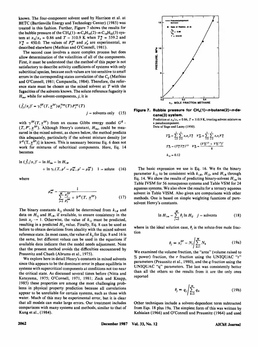
known. The four-component solvent used by Harrison et al. at BETC (Bartlesville Energy and Technology Center) (1 985) was treated in this fashion. Further, Figure 7 shows the results for the bubble pressure of the CHI( 1)-n-C4Hlo(2)-n-CloHzz(3) system at x 2 / x , - 0.86 and T = 310.9 K when Tp* = 559.2 and V z = 450.0. The values of PFf and p;l are experimental, as described elsewhere (Mathias and OConnell, 1981).

The second case involves a more complex process but does allow determination of the volatilities of all of the components. First, it must be understood that the method of this paper is not satisfactory to describe activity coefficients of systems with only subcritical species, because such values are too sensitive to small errors in the corresponding states correlation of the C,, (Mathias and OConnell, 198 1; Campanella, 1984). Therefore, the reference state must be chosen as the mixed solvent at T with the fugacities of the solvents known. The solute reference fugacity is H,,, while for solvent-components,j, it is

= Y ; F ( ~ , zsF)4iy”’(~) P ~ ( T )

j = solvents only (1 5)

with ySF(T, xsF) from an excess Gibbs energy model G E - (T, P’, x“). Although Henry’s constant, H,,, could be measured in the mixed solvent, as shown below, the method predicts this adequately, particularly if the solvent mixture density [or VE(T, zsF)] is known. This is necessary because Eq. 6 does not work for mixtures of subcritical components. Here, Eq. 14 becomes

1

2 ‘

3

1 J C

u) W C n

- p”udacarnwm 8olr.nl

0 MW n nnnnr. a .I.

XI T . 3101u

I I I I I 0.2 0.4

x,, MOLE FRACTION METHANE

Figure 7. Bubble pressure for CH,( l)-mbutane(2)-rrde cane(3) system. Prediction at x,/x, - 0.86, T - 310.9 K, treating solvent mixture as a pseudocomponent. Data of Sage and Lacey ( I 950).

kl, - 0.12

In ( j l / x l y = In H,, - In H~~

+ In YI ( T , P’ = P:‘, p‘ - P:‘) 1 = solute (16)

where

The binary constants k l j should be determined from k l R and data on HI, and H I R , if available, to ensure consistency in the limit x j - 1. Otherwise, the value of k , , must be predicted, resulting in a predicted HI, value. Finally, Eq. 8 can be used as before to obtain deviations from ideality with the mixed solvent reference state. In most cases, the value of kij for Eqs. 8 and 16 is the same, but different values can be used in the equations if available data indicate that the model needs adjustment. Note that the present method avoids the difficulties encountered by Prausnitz and Chueh (Abrams et al., 1975).

We explore here in detail Henry’s constants in mixed solvents since this appears to be the dominant error in phase equilibria in systems with supercritical components at conditions not too near the critical state. As discussed several times before (Nitta and Katayama, 1975; O’Connell, 1971, 1981; Zeck and Knapp, 1985) these properties are among the most challenging problems in physical property prediction because all correlations appear to be unreliable for certain systems, such as those with water. Much of this may be experimental error, but it is clear that all models can make large errors. Our treatment includes comparisons with many systems and methods, similar to that of Kung et al., (1984).

2062 December 1987

The basic expression we use is Eq. 16. We fix the binary parameter k , , to be consistent with k l R , H12, and HIR through Eq. 14. We show the results of predicting binary-solvent H,, in Table IVSM for 56 nonaqueous systems and Table VSM for 24 aqueous systems. We also show the results for a ternary aqueous solvent in Table VISM. Also given are comparisons with other methods. One is based on simple weighting functions of pure- solvent Henry’s constants.

M

In H~,,, = e, in H,, j = solvents (18) j -2

where in the ideal solution case, 0, is the solute-free mole fraction

We examined the volume fraction, the “area” (volume raised to y3 power) fraction, the r fraction using the UNIQUAC “r” parameters (Prausnitz et al., 1980), and the q fraction using the UNIQUAC “q” parameters. The last was consistently better than all the others so the results from it are the only ones reported

Other techniques include a solvent-dependent term subtracted from Eqs. 18 plus 19a. The simplest form of this was written by Kehiaian (1966) and OConnell and Prausnitz (1964) and used

VOl. 33, No. 12 AICbE Journal

by Prausnitz and Chueh (1968) where the solvent G E / R T was subtracted. O’Connell(l971) and Kung et al. (1984) show that this is less satisfactory than their methods. At this time, the comparisons of Kung et al. imply that their method is probably the most accurate for nonaqueous solvents. However, they needed a different expression to get agreement within 15% for aqueous systems.

For nonaqueous binary solvents, the present method is as good as that of Kung et al., and relatively little accuracy is sacri- ficed when YE is ignored in Eq. 17. Thus, for 267 data of 56 systems, the average error is 5% with nonzero YE and 7% with zero YE. For the 124 data of 30 systems we could compare with Kung et al., their error was 5% while the present method gave 5% error with nonzero YE and 6% with zero YE. For aqueous solvents the present method works well only if the excess volume is included. This is because the large negative YE is significant compared to the small water molar volume. Thus, for 598 data of 67 systems, the average error was 8% with nonzero V E and 24% for zero YE. For the 346 data on 33 systems where the special method of Kung et al. achieved 11% error, the present model gave 7% errors for nonzero YE and 22% error with zero YE. While agreement for these systems is probably not within experimental error, the trends are generally followed to a greater accuracy and reliability than with other models. Figure 8 shows comparisons for two systems that show average deviations for the methods used. Table VISM shows that the agreement for the ternary aqueous solvent of Zeck and Knapp (1985) is the same as for the binary aqueous solvents.

Improvements and Computational Aspects Despite the extensive comparisons we have made, there are

several aspects that have been incompletely covered. These include other components of interest, convergence characteris- tics of our calculations, consistency of binary parameters between Henry’s constant and nonideality correlations, excess volumes and mixed solvent Henry’s constants, multiple solutes,

0.2 1 1 I I I I I 1 I

and utilization to generate data for other correlations. We dis- cuss these here.

1. The pure-component parameters in Table ISM are only a few of those for which the correlation could be used. The greatest source of liquid compression data is the work of Huang (1986), which collects data on over 250 substances and fits them to a more accurate form than Eq. 6. However, his correlation could also be used to generate data to obtain values of T* and V* for the present model. Obviously many other supercritical substances and solvents are of interest; Tables IISM and IIISM are only intended to assist users in judging the potential utility of the correlation for their purposes. I t should be noted that as T* of the solute increases, sensitivity to k l z values increases. Since we ignored reactions, the possibility of partial solute dissociation will also affect the accuracy of the results,

2. Some of the systems cited in Tables IISM and IIISM had a few more data points than we were able to use. In most cases, we were limited by the validity of the vapor equation of state chosen and the convergence in calculating x, and yI from T and P. In general, we could obtain good results up to solute amounts where y/x of the solvent component went through its minimum (50-90% of critical solute mole fraction). Such information might be useful to guide complete equations of state closer to the critical point. They certainly would not have the convergence problems of the present treatment. Also, in some of the high- pressure systems, we found that the best fit k, , depended on ini- tial guess, primarily because of scatter in the data and insensitivity to the k l z value.

3. The optimal k , , value for binary high-pressure data is often different from that to predict consistent Henry’s constants; that is, Table IISM gives different values than used for Tables IVSM and VSM. Since the results for y are less sensitive to k, , , the values from Henry’s constants are to be preferred. The most accurate results would be found by using different k, , values for y and H12 in Eq. 12a when HI, is found from Eq. 14 and y from Eq. 7. In this case, even though the k 1 2 for H , , may depend on temperature when k , , is fixed, a constant k12 can be used for y. Table VIISM shows the binary parameters we have found.

4. Solvent excess volume data can be difficult to obtain. As Table IVSM shows, they may not be necessary for nonaqueous systems, but Table VSM shows that water systems must include such input. We have found as a rule of thumb that each 0.1% change in solution density changes H , , by 1%. If density data are not available but H I , data are, it is possible to obtain VEas a function of composition and then construct a correlation such as Handa and Benson (1979) used. For ternary and higher order solvents, the additivity of binary YE values seem adequate. We have compared experimental results for acetone-chloroform- benzene (Campbell et al., 1966), benzene-cyclohexane-n-hexane (Ridgway and Butler, 1967) and several ternaries with naphthenic, aromatic and pyridinic rings, and halogenated paraffins (Singh and Sharma, 1985), and water, methanol, and

rn COlloluendAnlllne - o1 n,opropanolrwa,er -

st 293.15K

/‘ , st 298.15K . , .’ ‘.____-c

-0.6 - I I I I 1 1 I I

0 0.2 0.4 0.6 0.8 1 1 acetone (Zeck and Knapp, 1985) with the equation x 2 , SOLVENT MOLE FRACTION

1 ,

Figure 8. Excess Henry’s constant for “average” systems.

v;,, = 2 2 v; i- l j - l

a where YE is the binary i-j solution excess volume calculated

such as those Of Hands and (1979)’ (Note that from the ternary mole fractions xi and xi in model expressions

xi + x j f 1 .) The errors are rarely over 0.1 cm3/gmol.

EXCOSS Henry’s conetant:

Systems: CO(1) in tolunene(2)/aniline mixtures at 298.15 K and

HL - In H , ~ - 1 xy In H,, /-I

0,(1) in isopropanol(2)/water mixtures at 293.15 K

December 1987 Vol. 33, No. 12 2063 AIChE Journal

5. For multiple solutes, the only modification to the above formulation involves Eqs. 6 and 7, with p j for all solutes equal to zero. Comparisons with data for the system H2-CH,-tetralin (Simnick et al., 1980) and H,-CO-methanol (Krichevskii et al., 1937) show good results and essentially complete insensitivity to the value of solute-solute binary constants.

6. New equations of state are sufficiently powerful that it is usually not necessary to choose separate models for the vapor and liquid to achieve good results as we have done here. How- ever, such equations often require extensive data in order to choose proper mixing rules and values of the binary parameters for accuracy in the region of interest. Because of its reliability for the liquid, the present model may provide a basis to use a minimum of more readily accessible information (principally pure-solvent densities, vapor pressures, and low-pressure solubilities) to generate such data for fitting to a desired equation of state form.

Acknowledgment E.A. Campanella is grateful to the Consejo Nacional de Investiga-

ciones Cientificas y Tecnicas de la Republica Argentina for a fellowship. The other authors are grateful to the National Science Foundation for financial assistance; to the Northeast Regional Data Center of the State University System of Florida for use of its facilities; to E. Buck, T. Krol- ikowski Buck, and H.C. Van Ness for helpful discussions; to J.F. Con- nolly for making his data available; and to J.C. Telotte and S. Skjold- Jorgensen for computational assistance.

Notation uo, u,, u2 = parameters in Henry’s constant correlation, Eq. 13

B = reduced second virial coefficient, Eq. A7 B” = hard-sphere second virial coefficient, Eq. A10 C,L = integral of direct correlation function for species i and j

= fugacity of component i, bar G E = excess Gibbs energy, J/gmol Hi = Henry’s constant, Eq. 2, bar k , = binary constant, Eqs. 11 b and A 8 M = number of components in system N = number of moles P = absolute pressure, bar q = UNIQUAC parameter R = universal gas constant = 83.143 cm3 . bar/gmol . K r = UNIQUAC parameter

SM = supplementary material T = absolute temperature, K V = molar volume, cm3/gmol V, = partial molar volume of component i , cm’/gmo~

V E = excess volume, cm3/grnol x i = liquid mole fraction of component i

Greek letters y, = activity coefficient of component i 6, = Kronecker delta; = 1 if i = j, = 0 if i # j Oi = solute-free composition, Eqs. 18-1 9 zT = isothermal compressibility, bar-’ pi = chemical potential of component i, J/gmol 5, = reduced density, Eq. AS, a = 0, I , 2, 3 p = molar density of solution, gmol/cm’

pi = molar density of component i, g/mol/cm’ = x i p ul = hard sphere diameter, Eq. A10

$: = vapor fugacity coefficient of component i

Subscripts c = critical property m = mixed solvent p = pseudocomponent species (mixed solvent) R = reference solvent - = (underline) set of values for all components

Superscripts calc = calculated value using theory exp = experimental value f = final state

r = reference state hs = hard sphere expression

sat = saturated liquid condition SF - solute-free solvent mixture

* = characteristic property ~ - reduced property

Appendix Listed below are the expressions for the quantities used in

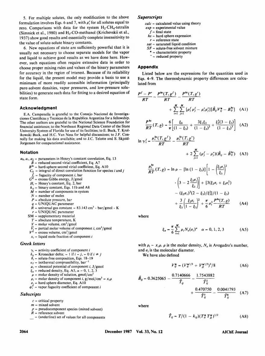
Eqs. 4-9. The thermodynamic property differences are calculated from

In =

P:“ - (T ,p) = Inp - [ln(1 - 1 3 ) ] RT

where

with pi = xip. p is the molar density, No is Avogadro’s number, and ni is the molecular diameter.

We have also defined

0.7140666 1.7543882 hij = 0.3625065 - -

f i j f; 0.470750 0.0041793 +-- (A7) T i f;

where

f‘v = T/(1 - kij)(T$ T;)”, (A81

AIChE Journal 2064 December 1987 Vol. 33, No. 12

Further, Isothermal Equation of State for Liquid Mixtures,” AIChE J. , 21, 1024 (197%).

B i = ( i f V: + it 5 ) / 2 (A9)

where 8: and ui are related to reduced temperature and Va

27T - N,U?

- 0.65386227/( T/T$)0.1MM7976 &=-- 3 V:

T/T: t 0.73

= 0.807662393 exp [ -0.22010926(T/Ti:)]

T/T: 5 0.73

From Eq. 4

Cij( T, p) = c: - 2 p [d, v; - $1

(AlOa)

(AlOb)

(A1 1)

In the limiting case of a pure fluid, Eq. A12 reduces to

Fortran computer subprograms for evaluating the pressure-density relation of Eqs. AI and A2 and the activity coefficient-density relation of Eqs. A3 and A4 are available from J. P. O’Con- nell.

Literature Cited Abrams, D. S., F. Seneci, P-L. Chueh, and J. M. Prausnitz, “Thermody-

namics of Multicomponent Liquid Mixtures Containing Subcritical and Supercritical Components,” Ind. Eng. Chem. Fundam., 14, 52 (1975).

Bienkowski, P. R., H. S. Denenholz, and K-C. Chao, “A Generalized Hard-Sphere Augmented Virial Equation of State,” AIChE J. , 19, 167 (1973).

Brelvi, S. W., and J. P. OConnell, “Corresponding States Correlation for Liquid Compressibility and Partial Molar Volumes of Gases at Infinite Dilution in Liquids,” AIChE J., 18, 1239 (1972).

, “Prediction of Unsymmetric Convention Liquid-Phase Activity Coefficients of Hydrogen and Methane,” AIChE J . . 21, 157 (1975a).

, “A Generalized Isothermal Equation of State for Dense Liq- uids,” AIChE J., 21, 17 1 ( 1 975b).

, “Generalized Prediction of Isothermal Compressibilities and an

AIChE Journal December 1987

Brule, M. R., C. T. Lin, L. L. Lee, and K. E. Starling, “Multiparameter Corresponding States Correlation of Coal-Fluid Thermodynamic Properties,” AfChEJ. , 28,616 (1982).

Campanella, E. A., “Some Applications of Fluctuation Solution Theory to Multiphase Systems of Nonelectrolytes,” Ph.D. Diss., Univ. Flor- ida (1984).

Campbell, A. N., E. M. Kartzmark, and R. M. Chatterjee, “Excess Vol- umes, Vapor Pressures and Related Thermodynamic Properties of the System Acetone-Chloroform-Benzene and Its Component Binary Systems,” Can. J . Chem., 44, 1183 (1966); supplementary material.

Connolly, J. F., J. Chem. Phys., 36,2897 (1 962). Connolly, J. F., and G. A. Kandalic, Amoco Research Company, Naper-

ville, IL, personal communication (1977). Gubbins, K. E., and J. P. OConnell, “Isothermal Compressibility and

Partial Molal Volume for Polyatomic Liquids,” J . Chem. Phys., 60, 3449 (1974).

Handa, Y. P., and G. C. Benson, “Volume Changes on Mixing Two Liq- uids: A Review of the Experimental Techniques and the Literature Data,” Fluid Phase Equil., 3, 185 (1979).

Harrison, R. H., S. E. Scheppele, G. P. Sturm, Jr., and P. L. Grizzle, “Solubility of Hydrogen in Well-Defined Coal Oils,” J . Chem. Eng. Data, 30, 183 (1985).

Haydens, J. G., and J. P. O’Connell, “A Generalized Method for Second Virial Coefficients,” Ind. Eng. Chem. Process Des. Dev., 14, 209 (1975).

Huang, Y. H., “Thermodynamic Properties of Compressed Liquids and Liquid Mixtures from Fluctuation Solution Theory,” Ph.D. Diss., Univ. Florida (1986).

Kehiaian, H., “Solubility of Nonelectrolytes in Systems Characterized by Kohler’s Equation,’’ Bull. Acad. Polon. Sci. Ser. Sci. Chem., 14, 153 (1966).

Krichevskii, I. R., N. M. Zhavoronkov, and P. S. Tsiklis, “Solubility of Hydrogen, Carbon Monoxide, and Their Mixtures in Methanol U n - der Pressure,” Zhur. Fiz. Khim., 9,317 (1937).

Kung, J. K., F. N. Nazario, J. Joffe, and D. Tassios, “Prediction of Hen- ry’s Constants in Mixed Solvents from Binary Data,” Ind. Eng. Chem. Process Des. Dev., 23, 170 ( 1 984).

Mathias, P. M., “Thermodynamic Properties of High-pressure Liquid Mixtures Containing Supercritical Components,” Ph.D. Diss., Univ. Florida (1978).

Mathias, P. M., and J. P. O’Connell, “Molecular Thermodynamics of Solutions Containing Supercritical Components,” Chem. Eng. Sci., 36, 1123 (1981).

Nakamura, R., G. T. F. Breedveld, and J. M. Prausnitz, “Thermody- namic Properties of Gas Mixtures Containing Common Polar and Nonpolar Components,” Ind. Eng. Chem. Process Des. Dew. 15, 557 (1976).

Nitta, T., and T. Katayama, “Thermodynamics of Solubilities in Mixed Solvents,” J . Chem. Eng. Japan, 8, 175 (1975).

OConnell, J. P. “Molecular Thermodynamics of Gases in Mixed Sol- vents,”AIChE J., 17,658 (1971).

, “Thermodynamic Properties of Solutions and the Theory of Fluctuations,” Fluid Phase Equil., 6,21 (1981).

OConnell, J. P., and J. M. Prausnitz, “Thermodynamics of Gas Solubil- ity in Mixed Solvents,” Ind. Eng. Chem. Fundam., 3,347 (1964).

Peng, D. Y., and D. B. Robinson, “A New Two-Constant Equation of State,” Ind. Eng. Chem. Fundam.. 15, 59 (1976).

Prausnitz, J. M., T. F. Anderson, E. A. Grens, C. A. Eckert, R. Hsieh, and J. P. O’Connell, Computer Calculations of Multicomponent Vapor-Liquid and Liquid-Liquid Equilibria. Prentice-Hall, Engle- wood Cliffs, NJ (1980).

Prausnitz, J . M., and P-L. Chueh, Computer Calculations of High- Pressure Vapor-Liquid Equilibrium, Prentice-Hall, Englewood Cliffs, NJ (1968).

Prausnitz, J. M., R. N. Lichtenthaler, and E. G. Azevedo, Molecular Thermodynamics of Fluid-Phase Equilibria, 2nd ed., Prentice-Hall, Englewood Cliffs, NJ (1986).

Ridgway, K., and V. A. Butler, “Some Physical Properties of the Ter- nary System Benzene-Cyclohexane-n-Hexane,” J . Chem. Eng. Data, 12,509 (1967).

Saddington, A. W., and N. W. Krase, “Vapor-Liquid Equilibrium in the System Nitrogen-Water,’’ J , Amer. Chem. Soc.. 56, 353 (1934).

Vol. 33, No. 12 2065

Sage, B. A., and W. N. Lacey, Thermodynamic Properties of the Lighter Hydrocarbons and Nitrogen, Amer. Pet. Inst., New York (1950).

Sebastian. H. M., H-M. Lin, and K-C. Chao, “Correlation of Solubility of Hydrogen in Hydrocarbon Solvents,” AIChE J., 27,138 (1981).

Simnick, J. J., H. M. Sebastian, H-M. Lin, and K-C. Chao, “Vapor- Liquid Phase Equilibria in the Ternary System Hydrogen-Methane- Tetralin,” J. Chem. Eng. Data, 25, 147 (1980).

Singh, P. P., and S. P. Sharma, “Molar Excess Volumes of Ternary Mixtures of Nonelectrolytes at 308.15 K,” J. Chem. Eng. Data, 30, 477 (1 985).

Soave, G., “Equilibrium Constants from a Modified Redlich-Kwong Equation of State,” Chem. Eng. Sci., 27, 1197 (1972).

Van Ness, H. C., and M. M. Abbott, Classical Thermodynamics of Nonelectrolyte Solutions, McGraw-Hill, New York (1982).

Zeck, S., and H. Knapp, “Solubilities of Ethylene, Ethane, and Carbon Dioxide in Mixed Solvents of Methanol, Acetone, and Water,” Int. J. Thermophys., 6,643 (1985).

Manuscript received Sept. 23, 1986. and revision received May 26,1987.

See NAPS document no. 04542 for 17 pages of supplementary material. Order from NAPS c/o Microfiche Publications, P.O. Box 3513, Grand Central Station, New York, NY 10163. Remit in advance in U.S. funds only $7.75 for photocopies or $4.00 for microfiche. Outside the U.S. and Canada, add postage of $4.50 for the first 20 pages and $1.00 for each of 10 pages of material thereafter, $1.50 for microfiche postage.

2066 December 1987 Vol. 33, No. 12 AIChE Journal

Documents

Equilibrium properties of liquids containing supercritical substances