On the stability and Hopf-bifurcation of a multi-delayed competitive population system affected by toxic substances with imprecise biological parameters

ORIGINAL ARTICLE

On the stability and Hopf-bifurcation of a multi-delayedcompetitive population system affected by toxic substanceswith imprecise biological parameters

D. Jana1 • P. Dolai2 • A. K. Pal3 • G. P. Samanta2

Received: 20 May 2016 / Accepted: 4 June 2016

� Springer International Publishing Switzerland 2016

Abstract In this paper we have analyzed the stability and

Hopf-bifurcation behaviors of a multi-delayed two-species

competitive system affected by toxic substances with

imprecise biological parameters. We have exercised a

method to handle these imprecise biological parameters by

using parametric form of interval numbers. We have

studied the feasibility of various equilibrium points and

their stability. In case of toxic stimulatory system, the delay

model exhibits a stable limit cycle oscillation due to vari-

ation in the delay parameters which lead to Hopf-bifurca-

tion. Numerical simulations with a hypothetical set of data

have been done to support the analytical findings.

Keywords Competing species � Imprecise parameters �Interval number � Multiple-delay � Hopf-bifurcation

Introduction

Environmental pollution has emerged with it adversities to

the modern civilization dwarfing the advantages to such a

great extent of technological achievements. Since, indus-

trialization contributes a lot to the economy of a nation, a

massive resource is being invested in national industrial-

ization. As a consequence, the industrial discharges con-

tribute to a huge amount of contamination to the both

aquatic and terrestrial environmental components (Jensen

and Marshall 1982; Nelson 1970). A large amount of

toxicant in the discharge makes it very difficult for that

much species to exist on this earth. The poison inclines in

the discharges, as a consequence, compels many species to

go into extinction. Therefore, a circumstantial query is

needed to put into the nature and activity of the discharged

particles to combat with the situation and to our environ-

ment from these toxicant.

Mathematical models, here, can play a vital role to

measure and minimize the aggression of the toxic elements

in the environment and draw a sustainable atmosphere. The

deterministic dynamic models with the effect of toxic

substances on various ecosystems is studied by Hallam

et al. (1983a, b), Hallam and Luna (1984), Luna and Hal-

lam (1987), Freedman and Shukla (1991), Ghosh et al.

(2002), He and Wang (2007), Das et al. (2009) and many

others. Researchers, in course of their study over the effect

and nature of the toxic elements come to an important

observation that the enhanced population of one species

might affect or control the growth of another or several

other species through the production of allelopathic toxins

or stimulants, thus influencing seasonal succession (Rice

1984). Unicellular green alga, chlorella Vulgaris can

control the growth of their population and inhibit the

growth of planktonic algae Asterionella formosa and

& G. P. Samanta

[email protected]; [email protected]

D. Jana

[email protected]

P. Dolai

[email protected]

A. K. Pal

[email protected]

1 Department of Zoology, Ecological Modelling Laboratory,

Visva Bharati University, Santiniketan 731235, India

2 Department of Mathematics, Indian Institute of Engineering

Science and Techology, Shibpur, Howrah 711103, India

3 Department of Mathematics, S. A. Jaipuria College,

Kolkata 700005, India

123

Model. Earth Syst. Environ. (2016) 2:110

DOI 10.1007/s40808-016-0156-0

http://crossmark.crossref.org/dialog/?doi=10.1007/s40808-016-0156-0&domain=pdf

http://crossmark.crossref.org/dialog/?doi=10.1007/s40808-016-0156-0&domain=pdf

Nitzschia frustrum (Bacillareae) with the toxin produced by

themselves (Pratt 1940; Pratt and Fong 1940; Rice 1954).

Toxic inhibition of phytoplankton by other phytoplankton

has been observed by several researchers. In addition to

that, it is also observed that some of the algae produce

auxin that enhances the stimulation towards the growth of

the other algae (Anderson 1989). These types of allelo-

pathic stimulators and inhibitors play deciding role in

moulding algal succession, blooms and pulses by creating

or causing stimulated (inhibited) species to have a selective

advantage or disadvantage in question of existence (Rice

1984; Berglund 1969).

In reality, time delays occur in almost every ecological

situation and assume to be most of the reasons of regular

fluctuations on population biomass. Kuang (1993) men-

tions that animals must take time to digest their food before

further activities and responses take place and hence any

model of species dynamics without delays is an approxi-

mation at best. Therefore, time delays can be included in

the mathematical population model due to various ways

such as maturation time, capturing time and other reasons.

Moreover, existence of time delays is frequently a source

of instability in some way. To make a more realistic bio-

logical model, many researchers (Maiti et al. 2008, 2008;

Celik 2008; Gopalsamy 1992; MacDonald 1989; Xua et al.

2009; Liu 1994; Chen et al. 2007; Song et al. 2004) have

incorporated time delay in their respective models.

Several researchers in theoretical ecology have consid-

ered their models based on the assumption that the bio-

logical parameters are precisely known. But in reality, the

values of all the biological parameters can not be deter-

mined precisely for the lack of information and data,

mistakes in the measurement process and determining the

initial conditions. To overcome these difficulties in the

field of mathematical biology, imprecise model is more

realistic. Environmental fluctuations or imprecise biologi-

cal phenomenon are the important causes of the impre-

ciseness of the bio-mathematical model. There are many

approaches to handle such models with imprecise param-

eters such as stochastic approach, fuzzy approach, fuzzy

stochastic approach etc. In stochastic approach the impre-

cise parameters are replaced by random variables with

known probability distributions. In fuzzy approach the

imprecise parameters are replaced by fuzzy sets with

known membership functions. In fuzzy stochastic approach

some parameters are as fuzzy in nature and rest of the

parameters are taken as random variables. However it is

very difficult to draw a suitable membership function or a

suitable probability distribution for each of the imprecise

biological parameters. Recently researchers have intro-

duced fuzzy models in prey-predator system such as Bas-

sanezi et al. Bassanezi et al. (2000), Peixoto et al. Peixoto

et al. (2008) and Guo et al. Guo et al. (2003), etc. Pal et al.

(2012, (2014, (2013) have considered an optimal harvest-

ing prey-predator system with imprecise biological

parameters and they have also discussed bio-economic

equilibrium and optimal harvesting policy.

In this paper, we have introduced a multi-delayed two

species competitive system which is affected by toxicant. To

make the delay model more realistic, we have considered

imprecise biological parameters as interval numbers. We

present the interval numbers in parametric function form and

study the parametric model Maynard-Smith (1975). The

dynamical behavior of the parametric model is investigated

for several values of the parameter p 2 ½0; 1�: In Sect. 2, we

discuss some basic definitions on interval numbers. In

Sect. 3, we represent mathematical form of two species

competitive system with time delays. Section 4 briefly states

the delayed two species competitive system with imprecise

parameters. Then parametric form of the systems is formu-

lated to study the different behaviors of the model. Section 5

deals with the equilibrium points of the systems, their

existence and stability analysis. Our important analytical

results are numerically verified in Sect. 6. Finally, Sect. 7

contains the general discussion of the paper.

Basic definitions

In this section we discuss some basic definitions of the

interval number and interval-valued function which have

been used to study the imprecise competition model.

Definition 1 (Interval number) An interval number A is

represented by closed interval ½al; au� and defined by

A ¼ ½al; au� ¼ fx : al � x� au; x 2 Rg, where R is the set

of real numbers and al, au are the lower and upper limits of

the interval number, respectively.

So, every real number can also be presented by the

interval number [a, a], for all a 2 R.

Definition 2 (Interval-valued function) Let us consider

the interval [a, b] where a[ 0. The interval [a, b] can be

expressed as a function /ðpÞ ¼ að1�pÞbp for p 2 ½0; 1�. Thisfunction is called interval-valued function.

Now we present some arithmetic operations on interval-

valued functions. Let A ¼ ½al; au� and B ¼ ½bl; bu� be two

interval numbers, then

Addition Aþ B ¼ ½al; au� þ ½bl; bu� ¼ ½al þ bl; au þ bu�.The interval-valued function for the interval Aþ B is given

by /ðpÞ ¼ að1�pÞL a

pU where aL ¼ al þ bl and aU ¼ au þ bu.

Subtraction A� B ¼ ½al; au� � ½bl; bu� ¼ ½al � bu; au � bl�,provided al � bu [ 0. The interval-valued function for the

interval A� B is given by /ðpÞ ¼ bð1�pÞL b

pU where bL ¼

al � bu and bU ¼ au � bl.

110 Page 2 of 16 Model. Earth Syst. Environ. (2016) 2:110

123

Scalar multiplication jA ¼ j½al; au� ¼½jal; jau�; if j� 0

½jau; jal�; if j\0

�; provided al [ 0. The interval-

valued function for the interval jA is given by /ðpÞ ¼cð1�pÞL c

pU if j� 0

�dð1�pÞU d

pL if j\0

(; where cL ¼ jal; cU ¼

jau; dL ¼ jjjal; dU ¼ jjjau.

Basic mathematical model

Maynard-Smith (1975) have considered a two species

competing system:

dN1

dt¼ N1½K1 � a1N1 � b12N2 � c1N1N2�;

dN2

dt¼ N2½K2 � a2N2 � b21N1 � c2N1N2�;

ð1Þ

with initial data

N1 0ð Þ� 0; N2 0ð Þ� 0: ð2Þ

Here N1ðtÞ; N2ðtÞ denote the population biomass of two

competing species at time t, having common food resour-

ces; K1;K2; a1; a2; b12; b21; c1; c2 are positive constants.

Here Ki is the intrinsic growth rate of species i, ai repre-sents the interspecies competition coefficient of species i,

bij denotes the inter-species competition rate of jth species

upon the ith species and ci denotes the toxic inhibition rate

of the ith species ði 6¼ j; i; j ¼ 1; 2Þ. Samanta (2010) also

analyze dynamical behaviors of such model where a toxic

substance is produced at a constant rate. When the toxic

coefficients ci [ 0 ði ¼ 1; 2Þ, the model (1) represents

toxic inhibited species system. If we assume

ci ¼ �c0i ði ¼ 1; 2Þ, where c0i [ 0, then the model 1 rep-

resents toxic stimulated system. We assume that each

species produces a substance toxic to the other, but only

when the other is present. Further, it is also reasonable to

assume such model where a toxic substance is produced to

the competing species will not be instantaneous and takes

discrete time lag which is regarded as maturity period of

the species. Here we introduce the time lag siði ¼ 1; 2Þ forthe maturity of the species Niði ¼ 1; 2Þ. Then the system 1

reduces to

dN1

dt¼ N1½K1 � a1N1 � b12N2 � c1N1N2ðt � s2Þ�;

dN2

dt¼ N2½K2 � a2N2 � b21N1 � c2N1ðt � s1ÞN2�:

ð3Þ

The initial condition for the model 2 takes the form N1ðhÞ¼ w1ðhÞ� 0; N2ðhÞ ¼ w2ðhÞ� 0; h 2 ½� min fs1; s2g; 0�;w1ð0Þ[ 0; w2ð0Þ[ 0; ðw1ðhÞ;w2ðhÞÞ 2 ðCð½�s; 0�;RþÞ:

Positivity and boundedness of the delayed system

In theoretical ecology, positivity and boundedness of a

system implies that the system is biologically well

behaved. What we mean that for any system, it should have

these restrictions (positivity and boundedness) as far as

biological aspects are concerned. The following proposi-

tion ensures the positivity and boundedness of the delayed

system 3.

Proposition 1 Each and every component of the solution

of the delayed system 3 is positive and bounded for all

t� 0.

Proof Since the right hand side of the system 3 is com-

pletely continuous and locally Lipschitzian on C, the

solution ðN1ðtÞ;N2ðtÞÞ of 3 exists and is unique on ½0; nÞ,where 0\n 6 1 (Hallam and Luna 1984). From system 3,

we have

N1ðtÞ ¼ N1ð0ÞZ t

0

ðK1 � a1N1ðsÞ � b12N2ðsÞ � c1N1ðsÞN2ðs� s2ÞÞds� �

[ 0;

N2ðtÞ ¼ N2ð0ÞZ t

0

ðK2 � a2N2ðsÞ � b21N1ðsÞ � c2N1ðs� s1ÞN2ðsÞÞds� �

[ 0:

Therefore, N1ðtÞ[ 0; N2ðtÞ[ 0 8 t > 0: Now we

assume,

W ¼ N1ðtÞ þ N2ðtÞ:

Then,

dW

dt6� a1 N1 �

K1

a1

� �2

�a2 N2 �K2

a2

� �2

þK21

a1

þ K22

a2� K1N1 � K2N2

6l� mW ; where l ¼ K21

a1þ K2

2

a2and

m ¼ min K1;K2f g:

Therefore,

dW

dtþ mW 6 l:

Applying a theorem on differential inequalities (Birkhoff

and Rota 1982), we obtain

0\WðN1;N2Þ 6lmþWðN1ð0Þ;N2ð0ÞÞ

emt

and for t ! 1;

0\W 6lm:

Thus, entire solutions of the system 3 enter into the region

B ¼ ðN1;N2Þ : 0\W\lmþ e for any e[ 0

n o:

This proves the theorem. h

Model. Earth Syst. Environ. (2016) 2:110 Page 3 of 16 110

123

Imprecise competition model

All the parameters of the competition model 3 are positive

and precise. But due to lack of proper information of the data,

the parameters are not always precise. Now if any of the

parameters Ki; ai; bij; ci ði 6¼ j; i; j ¼ 1; 2Þ is imprecise,

i.e., if any parameter is interval number rather than a single

value, then it becomes difficult to convert the equation to the

standard form and analyze the dynamical behavior of the

system. For imprecise parameters, we present the system 3

with interval parameters as described below:

Competition model with interval parameters

Case I: Toxic inhibition

Let Ki; ai; bij; ci ði 6¼ j; i; j ¼ 1; 2Þ be the interval coun-

terparts of Ki; ai; bij; ci respectively. Then the imprecise

competition delay model 3 becomes

dN1

dt¼ N1½K1 � a1N1 � ^b12N2 � c1N1N2ðt � s2Þ�;

dN2

dt¼ N2½K2 � a2N2 � ^b21N1 � c2N1ðt � s1ÞN2�;

ð4Þ

where Ki ¼ ½Kil;Kiu�; ai ¼ ½ail; aiu�; bij ¼ ½bijl; biju�; ci ¼½cil; ciu�; and Kil [ 0; ail [ 0; bijl [ 0; cil [ 0 ði 6¼ j;

i; j ¼ 1; 2Þ:Case II: Toxic stimulation

In this case, c1 ¼ �c01 and c2 ¼ �c02 where c01 ¼ ½c01l; c01u� and

c02 ¼ ½c02l; c02u� and c01l [ 0; c02l [ 0, i.e., the last term in the

Eq. (4) give apositive effect insteadofnegative effect as in case

I. Then the imprecise competition delay model 3 becomes

dN1

dt¼ N1½K1 � a1N1 � ^b12N2 þ c1N1N2ðt � s2Þ�;

dN2

dt¼ N2½K2 � a2N2 � ^b21N1 þ c2N1ðt � s1ÞN2�:

ð5Þ

Competition model with parametric interval

parameters

For fixed m, we are considering the interval-valued function

/mðpÞ ¼ að1�pÞm bpm forp 2 ½0; 1� for an interval ½am; bm�. Since

/pm is a strictly increasing and continuous function, the sys-

tem 4 and 5 can be written in the parametric form as follows:

dN1ðt; pÞdt

¼ N1

hðK1lÞð1�pÞðK1uÞp � ða1lÞð1�pÞða1uÞpN1

� ðb12lÞð1�pÞðb12uÞpN2 � ðc1lÞð1�pÞðc1uÞpN1N2ðt � s2Þi;

dN2ðt; pÞdt

¼ N2

hðK2lÞð1�pÞðK2uÞp � ða2lÞð1�pÞða2uÞpN2

� ðb21lÞð1�pÞðb21uÞpN1 � ðc2lÞð1�pÞðc2uÞpN1ðt � s1ÞN2

i

ð6Þ

and

dN1ðt; pÞdt

¼ N1½ðK1lÞð1�pÞðK1uÞp � ða1lÞð1�pÞða1uÞpN1

� ðb12lÞð1�pÞðb12uÞpN2 þ ðc1lÞð1�pÞðc1uÞpN1N2ðt � s2Þ�;dN2ðt; pÞ

dt¼ N2½ðK2lÞð1�pÞðK2uÞp � ða2lÞð1�pÞða2uÞpN2

� ðb21lÞð1�pÞðb21uÞpN1 þ ðc2lÞð1�pÞðc2uÞpN1ðt � s1ÞN2�;ð7Þ

where p 2 ½0; 1�.

Equilibria and local stability of the delayedsystem

Toxic inhibition

The system 6 has four positive steady states, namely (i)

E0ð0; 0Þ, the trivial equilibrium, (ii) E1ð �N1; 0Þ and

E2ð0; �N2Þ, the axial equilibrium, where

�N1 ¼ðK1lÞð1�pÞðK1uÞp

ða1lÞð1�pÞða1uÞp[ 0ðalwaysÞ;

�N2 ¼ðK2lÞð1�pÞðK2uÞp

ða2lÞð1�pÞða2uÞp[ 0ðalwaysÞ for all p 2 ½0; 1�

ð8Þ

and (iii) E� ¼ ðN�1 ;N

�2Þ, the interior equilibrium, where

N�1 ; N�

2 can be determined by

aijN�2i þ bijN

�i þ cij ¼ 0; i 6¼ j; i; j ¼ 1; 2 ð9Þ

where

aij ¼ ðbijlÞð1�pÞðbijuÞpðcilÞð1�pÞðciuÞp

� ðailÞð1�pÞðaiuÞpðcjlÞð1�pÞðcjuÞp;bij ¼ ðKilÞð1�pÞðKiuÞpðcjlÞð1�pÞðcjuÞp

� ðKjlÞð1�pÞðKjuÞpðcilÞð1�pÞðciuÞp

� ðailÞð1�pÞðaiuÞpðajlÞð1�pÞðajuÞp

þ ðbijlÞð1�pÞðbijuÞ

pðbjilÞð1�pÞðbjiuÞ

p;

cij ¼ ðKilÞð1�pÞðKiuÞpðajlÞð1�pÞðajuÞp

� ðKjlÞð1�pÞðKjuÞpðbjlÞð1�pÞðbjuÞp;

ð10Þ

for all p 2 ½0; 1�: Then

N�i ¼ 1

2aij�bij �

ffiffiffiffiffiffiffiffiffiffiffiffiffiffiffiffiffiffiffiffiffiffib2ij � 4aijcij

q� ; i; j ¼ 1; 2 ð11Þ

exist with the conditions

aij 6¼ 0; b2ij � 4aijcij � 0: ð12Þ

The variational matrix of the system 6 at E0ð0; 0Þ is given by


123

V E0ð Þ ¼ ðK1lÞð1�pÞðK1uÞp 0

0 ðK2lÞð1�pÞðK2uÞp

" #:

Clearly, E0ð0; 0Þ is a unstable node.

The variational matrix of the system 6 at E1ð �N1; 0Þ is

given by

then the eigenvalues are k1 ¼ �ða1lÞð1�pÞða1uÞp�N1\0ðalwaysÞ and k2 ¼ ðK2lÞð1�pÞðK2uÞp � ðb21lÞð1�pÞ

ðb21uÞp �N1. Therefore the equilibrium point E1ð �N1; 0Þ is

asymptotically stable ifðK1lÞð1�pÞðK1uÞp

ðK2lÞð1�pÞðK2uÞp[ ða1lÞð1�pÞða1uÞp

ðb21lÞð1�pÞðb21uÞpand

unstable (saddle point) if

ðK1lÞð1�pÞðK1uÞp

ðK2lÞð1�pÞðK2uÞp\

ða1lÞð1�pÞða1uÞp

ðb21lÞð1�pÞðb21uÞp: ð13Þ

Again, the variational matrix of the system 6 at E2ð0; �N2Þ isgiven by

then the eigenvalues are k1 ¼ �ða2lÞð1�pÞða2uÞp�N2\0ðalwaysÞ and k2 ¼ ðK1lÞð1�pÞðK1uÞp � ðb12lÞð1�pÞ

ðb12uÞp �N2. Therefore the equilibrium point E2ð0; �N2Þ is

asymptotically stable ifðK2lÞð1�pÞðK2uÞp

ðK1lÞð1�pÞðK1uÞp[ ða2lÞð1�pÞða2uÞp

ðb12lÞð1�pÞðb12uÞpand

unstable (saddle point) if

ðK2lÞð1�pÞðK2uÞp

ðK1lÞð1�pÞðK1uÞp\

ða2lÞð1�pÞða2uÞp

ðb12lÞð1�pÞðb12uÞp: ð14Þ

Hence, combining 13 and 14, the condition requires for the

persistence of both the species is

ðKilÞð1�pÞðKiuÞp

ðKjlÞð1�pÞðKjuÞp\

ðailÞð1�pÞðaiuÞp

ðbjilÞð1�pÞðbjiuÞpði 6¼ j; i; j ¼ 1; 2Þ

for all p 2 ½0; 1�: ð15Þ

Condition (15) gives cij [ 0 in Eq. (9). Then the system 6

has unique positive equilibrium if

aij\0 i.e., ifðailÞð1�pÞðaiuÞp

ðbjilÞð1�pÞðbjiuÞp[

ðcilÞð1�pÞðciuÞp

ðcjlÞð1�pÞðcjuÞp

ði 6¼ j; i; j ¼ 1; 2Þ for all p 2 ½0; 1�:ð16Þ

So combining Eq. (15) and (16), we have,

ðailÞð1�pÞðaiuÞp

ðbjilÞð1�pÞðbjiuÞp[ max

�ðcilÞð1�pÞðciuÞp

ðcjlÞð1�pÞðcjuÞp;ðKilÞð1�pÞðKiuÞp

ðKjlÞð1�pÞðKjuÞp

ði 6¼ j; i;j¼1;2Þ for all p2 ½0;1� ð15Þ

as the condition of existence of unique positive interior

equilibrium of the system 6. Now to investigate the local

stability of the interior equilibrium E�ðN�1 ;N

�2Þ, we lin-

earize the system 6 by using transformation

N1 ¼ N�1 þ n1; N2 ¼ N�

2 þ n2:

Linearizing the system 6 at E�ðN�1 ;N

�2Þ and its corre-

sponding characteristic equation is given by

k2 þ Akþ Bþ ðC1kþ D1Þe�ks1 þ ðC2kþ D2Þe�ks2

þ Ee�kðs1þs2Þ ¼ 0; ð18Þ

where A ¼ �ða11 þ a22Þ, D1 ¼ a22b11, C1 ¼ �b11,

D2 ¼ a11c22, C2 ¼ �c22, E ¼ b11c22, B ¼ ða11a22�a12a21Þ, a11 ¼ �fða1lÞð1� pÞða1uÞp þ ðc1lÞð1� pÞðc1uÞpN�2gN�

1 , a12 ¼ �ðb12lÞð1� pÞðb12uÞpN�1 , a21 ¼ �ðb21lÞ

ð1� pÞðb21uÞpN�2 , a22 ¼ �fða2lÞð1� pÞða21uÞp þ ðc2lÞ

ð1� pÞðc2uÞpN�1gN�

2 , b11 ¼ ðc2lÞð1� pÞ ðc2uÞpN�22, c22 ¼

ðc1lÞð1� pÞðc1uÞ

pN�12:

Case 1 s1 ¼ 0 ¼ s2In case of s1 ¼ 0 ¼ s2, the Eq. (18) becomes

k2 þ ðAþ C1 þ C2Þkþ ðBþ D1 þ D2 þ EÞ ¼ 0: ð19Þ

All roots of the Eq. (19) have negative real parts if and

only if

V E1ð Þ ¼ �ða1lÞð1�pÞða1uÞp �N1 � ðb12lÞð1�pÞðb12uÞ

p �N1 � ðc1lÞð1�pÞðc1uÞ

p �N21e

�ks

0 ðK2lÞð1�pÞðK2uÞp � ðb21lÞð1�pÞðb21uÞp �N1

" #

V E2ð Þ ¼ ðK1lÞð1�pÞðK1uÞp � ðb12lÞð1�pÞðb12uÞ

p �N2 0

�ðb21lÞð1�pÞðb21uÞ

p �N2 � ðc2lÞð1�pÞðc2uÞ

p �N22e

�ks � ða2lÞð1�pÞða2uÞp �N2

" #


123

Aþ C1 þ C2 [ 0 and Bþ D1 þ D2 þ E[ 0: ð20Þ

Theorem 2.1 If s1 ¼ s2 ¼ 0, then interior equilibrium

point E�ðN�1 ;N

�2Þ of system (6) exists and asymptotically

stable if condition (16) and (20) hold simultaneously.

Case 2 s1 ¼ 0 and s2 6¼ 0

If s1 ¼ 0 and s2 6¼ 0. In this case, the characteristic

Eq. (18) becomes

k2 þ ðAþ C1Þkþ Bþ D1 þ ðC2kþ D2 þ EÞe�ks2 ¼ 0: ð21Þ

Let ixðx[ 0Þ be a root of the Eq. (21). Then we have,

ðD2 þ EÞ cosxs2 þ C2x sinxs2 ¼ x2 � ðBþ D1Þ;C2x cosxs2 � ðD2 þ EÞ sinxs2 ¼ �ðAþ C1Þx:

ð22Þ

This leads to

x4 � ½C22 � ðAþ C1Þ2 þ 2ðBþ D1Þ�x2

þ ðBþ D1Þ2 � ðD2 þ EÞ2 ¼ 0:ð23Þ

It follows that the Eq. (23) has no positive roots if the

following conditions are satisfied:

ðAþ C1Þ2 � C22 � 2ðBþ D1Þ[ 0 and

ðBþ D1Þ2 � ðD2 þ EÞ2 [ 0:ð24Þ

Hence, all roots of the Eq. (23) will have negative real

parts when s2 2 ½0;1Þ if conditions of the Theorem 2.1

and (24) are satisfied. Let

ðBþ D1Þ2 � ðD2 þ EÞ2\0: ð25Þ

If Theorems 2.1 and (25) hold then the Eq. (23) has a

unique positive root x20. Substituting x2

0 into Eq. (22), we

have

s2n ¼1

x0

cos�1 ðD2 þ EÞðx20 � B� D1Þ � ðAþ C1ÞC2x2

0

C22x

20 þ ðD2 þ EÞ2

" #

þ 2npx0

; n ¼ 0; 1; 2; . . .

Let,

C22 � ðAþ C1Þ2 þ 2ðBþ D1Þ[ 0;

ðBþ D1Þ2 � ðD2 þ EÞ2 [ 0

and

C22 � ðAþ C1Þ2 þ 2ðBþ D1Þ

h i2[ 4 ðBþ D1Þ2 � ðD2 þ EÞ2

h i:

ð26Þ

If Theorem 2.1 and (26) hold then Eq. (23) has two posi-

tive roots x2þ and x2

�. Substituting x� into Eq. (22), we

get

s�2k ¼1

x�cos�1 ðD2 þ EÞðx2

� � B� D1Þ � ðAþ C1ÞC2x2�

C22x

2� þ ðD2 þ EÞ2

" #

þ 2kpx�

; k ¼ 0; 1; 2; . . .

If kðs2Þ be the root of Eq. (21) satisfying Rekðs2nÞ ¼ 0

(respectively, Rekðs�2kÞ ¼ 0) and Imkðs2nÞ ¼ x0 (respec-

tively, Imkðs�2kÞ ¼ x�), we get

d

ds2Re ðkÞ

� �s2¼s20 ;x¼x0

¼ x4 þ ðD2 þ EÞ2 � ðBþ D1Þ2

x2ðC22x

2 þ ðD2 þ EÞ2Þ

[x2

C22x

2 þ ðD2 þ EÞ2[ 0 ðby ð25ÞÞ:

Similarly, we can show that

d

ds2Re ðkÞ

� �s2¼sþ

2k;x¼xþ

[ 0;

d

ds2Re ðkÞ

� �s2¼s�

2k;x¼x�

\0:

From Corollary (2.4) in Ruan and Wei (2003), we have the

following conclusions.

Theorem 2.2 Assume s1 ¼ 0; s2 6¼ 0 and conditions of

the Theorem 2.1 are satisfied, then the following conclu-

sions hold:

(i) If (24) holds then the equilibrium E�ðN�1 ;N

�2Þ is

asymptotically stable for all s2 � 0:

(ii) If (25) holds then the equilibrium E�ðN�1 ;N

�2Þ is

conditionally stable. It is locally asymptotically

stable for s2\s20 and unstable for s2 [ s20 .Furthermore, the system (6) undergoes a Hopf

bifurcation at E�ðN�1 ;N

�2 Þ when s2 ¼ s20 , where

s20 ¼1

x0


0

C22x

20 þ ðD2 þ EÞ2

" #:

(iii) If (26) holds then there is a positive integer m

such that the equilibrium is stable when s2 2½0; sþ20Þ [ ðs�20 ; s

þ21Þ [ ::: [ ðs�2m�1

; sþ2mÞ and unsta-

ble when s2 2 ½sþ20 ; s�20Þ [ ðsþ21 ; s

�21Þ [ :::[ ðsþ2m�1

;

s�2m�1Þ [ ðsþ2m ;1Þ. Furthermore, the system under-

goes a Hopf bifurcation at E�ðN�1 ;N

�2Þ when

s2 ¼ sþ2m ;m ¼ 0; 1; 2; :::

Case 3 s1 6¼ 0 and s2 6¼ 0

We consider Eq. (18) with s2 in its stable interval ðs2 2½0; s20ÞÞ and regard s1 as a parameter ðs1 2 ð0;1ÞÞ.Without loss of generality, we consider that the system


123

parameters satisfy Theorem 2.1 and (25). Let ixðx[ 0Þ bea root of Eq. (18) and we obtain

x4 þ eAx2 þ B2 þ D22 � D2

1 � E2

þ 2eB sinxs2 þ 2eC cosxs2 ¼ 0;ð27Þ

where

eA ¼ A2 þ C22 � 2B� C2

1;eB ¼ xC1E � x3C2 � xAD2 þ xBC2 and

eC ¼ �D1E � x2D2 þ BD2 þ x2AC2:

We define,

FðxÞ ¼ x4 þ eAx2 þ B2 þ D22 � D2

1

� E2 þ 2eB sinxs2 þ 2eC cosxs2

and assume that

ðBþ D2Þ2 � ðD1 þ EÞ2\0: ð28Þ

Then it is easy to check that Fð0Þ\0 and Fð1Þ ¼ 1.

Thus, (27) has finite positive roots x1;x2; . . .;xk. For

every fixed xi; i ¼ 1; 2; . . .; k, there exists a sequence

fs j1i jj ¼ 1; 2; . . .g, where,

s j1i ¼1

xi

� �cos �1 M1

N1

� �þ 2ip

xi

;

i ¼ 1; 2; . . .; k; j ¼ 1; 2; . . .

where,

M1 ¼ P1S1 þ P2T1 þ ðQ1S1 þ R1T1Þ cos xis2þ ðR1S1 � Q1T1Þ sin xis2;

N1 ¼ S21 þ T21 ; P1 ¼ �x2

i þ B; P2 ¼ Axi;

Q1 ¼ D2; R1 ¼ C2xi;

S1 ¼ �ðE cos xis2 þ D1Þ; T1 ¼ E sin xis2 � C1xi;

i ¼ 1; 2; :::; k:

Let s10 ¼ minfs j1i ji ¼ 1; 2; :::; k; j ¼ 1; 2; :::g. Define the

function hðs1Þ 2 ½0; 2pÞ such that coshðs1Þ is given by the

right-hand sides of the last equation. In the following, we

assume that

d

ds1ðRekÞ

� �k¼ix0

6¼ 0: ð29Þ

Therefore, by the general Hopf bifurcation theorem, we

have the following result on the stability and bifurcation of

the system (6).

Theorem 2.3 For the system (6), suppose the parameters

satisfy the conditions of the Theorem 2.1, 25 and 29 and

s2 2 ½0; s20Þ, then the equilibrium E�ðN�1 ;N

�2Þ is asymptot-

ically stable when s1 2 ð0; s10Þ, unstable when s1 [ s10 anda Hopf bifurcation occurs when s1 ¼ s10 .

Case 4 s1 6¼ 0 but s2 ¼ 0

Next, we assume that s1 6¼ 0 but s2 ¼ 0. The proof is

similar to the Case 2 and we only summarize the results

below.

Theorem 2.4 Assume Theorem 2.1 is satisfied, then the

following conclusions hold:

(i) If

ðAþ C2Þ2 � C21 � 2ðBþ D2Þ[ 0;

Bþ D2Þ2 � ðD1 þ EÞ2 [ 0ð30Þ

hold, then the equilibrium E�ðN�1 ;N

�2Þ is locally

asymptotically stable for all s1 � 0.

(ii) If

ðBþ D2Þ2 � ðD1 þ EÞ2\0 ð31Þ

holds, then the equilibrium E�ðN�1 ;N

�2 Þ is locally

asymptotically stable for s1\~s10 and unstable for

s1 [ ~s10 . Furthermore, the system (6) undergoes a

Hopf bifurcation at E�ðN�1 ;N

�2Þ when s1 ¼ ~s10 ,

where

~s1p ¼1

x0


0

C21x

20 þ ðD1 þ EÞ2

" #

þ 2ppx0

; p ¼ 0; 1; 2; . . .

(iii) If C21 � ðAþ C2Þ2 þ 2ðBþ D2Þ[ 0; ðBþ D2Þ2 �

ðD1 þ EÞ2 [ 0 and

½C21 � ðAþ C2Þ2 þ 2ðBþ D2�2 [ 4½ðBþ D2Þ2 � ðD1 þ EÞ2�

ð32Þ

hold, there is a positive integer l such that the equilib-

rium is stable when s1 2 ½0; ~sþ10Þ [ ð~s�10 ; ~sþ11Þ [ :::[

ð~s�1l�1; ~sþ1lÞ; and unstable when s1 2 ½~sþ10 ; ~s

�10Þ [ ð~sþ11 ; ~s

�11Þ [

::: [ ð~sþ1l�1; ~s�1l�1

Þ [ ð~sþ1l ;1Þ: Furthermore, the system

undergoes a Hopf bifurcation at ðN�1 ;N

�2Þ when

s1 ¼ ~sþ1l ; l ¼ 0; 1; 2; :::

Case 5 s1 6¼ 0 and s2 6¼ 0

Table 1 Stable equilibrium points of toxic inhibited system for dif-

ferent p

p Equilibrium points Fig. 1

0.0 (31.5810, 4.8369) a

0.3 (26.8610, 4.1779) b

0.5 (24.1373, 3.7626) c

0.8 (20.6083, 3.1699) d

1.0 (18.5878, 2.7915) e


123

0 10 20 30 40 50 60 70 80 90 1000

5

10

15

20

25

30

35

time(t)

popu

latio

n(N

1,N2)

p=0.0

N1

N2

0 10 20 30 40 50 60 70 80 90 1000

5

10

15

20

25

30

time(t)

popu

latio

n(N

1,N2)

p=0.3

N1

N2

0 10 20 30 40 50 60 70 80 90 1000

5

10

15

20

25

time(t)

popu

latio

n(N

1,N2)

p=0.5

N1

N2

0 10 20 30 40 50 60 70 80 90 1000

5

10

15

20

25

time(t)

popu

latio

n(N

1,N2)

p=0.8

N2

N1

0 10 20 30 40 50 60 70 80 90 1000

2

4

6

8

10

12

14

16

18

20

time(t)

popu

latio

n(N

1,N2)

p=1.0

N1

N2

0 0.1 0.2 0.3 0.4 0.5 0.6 0.7 0.8 0.9 10

5

10

15

20

25

30

35

p

popu

latio

n(N

1,N2)

N1

N2

a b

c d

e f

Fig. 1 Behavior of the toxic inhibited species with time by using the

imprecise parameters values and initial conditions ðN1ð0Þ;N2ð0ÞÞ ¼ð1:0; 1:0Þ for p ¼ 0:0; 0:3; 0:5; 0:8; 1:0 and Fig. 1f shows the

dynamical behavior of the two species population ðN1;N2Þ with

respect to p when the values of the other parameters are same


123

Finally, we assume that both the prey and predator are

harvested selectively then s1 6¼ 0 and s2 6¼ 0. We consider

Eq. (18) with s1 in its stable interval and regard s2 as a

parameter. The proof is similar to the Case 3 and we only

summarize the results below.

Theorem 2.5 For the system (6), suppose the parameters

satisfy the conditions of the Theorem 2.1, (25) and (29) and

s1 2 ½0; s10Þ. Then the equilibrium E�ðN�1 ;N

�2Þ is locally

asymptotically stable when s2 2 ð0; st2sÞ, unstable when

s2 [ st2s and a Hopf bifurcation occurs when s2 ¼ st2s ,

where,

st2s ¼1

xs

� �cos �1 M2

N2

� �þ 2sp

xs

;

s ¼ 1; 2; . . .; q; t ¼ 1; 2; . . .

where,

M2 ¼ P1S2 þ P2T2 þ ðQ2S2 þ R2T2Þ cos xss1þ ðR2S2 � Q2T2Þ sin xss1;

N2 ¼ S22 þ T22 ; P1 ¼ �x2

s þ B; P2 ¼ Axs;

dQ2 ¼ D1; R2 ¼ C1xs;

S2 ¼ �ðE cos xss1 þ D2Þ; T2 ¼ E sin xss1 � C2xs;

s ¼ 1; 2; . . .; q:

Toxic stimulation

In this case, we study the system (7), which is same as the

system (6) unless in the last term, where the toxic inhibi-

tion rate ci ði ¼ 1; 2Þ are negative i.e., either species pro-

duces auxin which stimulate the growth of the other

species. Here the local stability analysis of the system (7)

remains same as in case I for the trivial and axial equi-

librium points and so as the criteria for persistence of both

the species. Now we study the local stability of the system

(7) for the interior equilibrium point E0�ðN 0�1 ;N

0�2 Þ which is

also asymptotically stable.

Numerical Illustration

Analytical studies can never be completed without numeri-

cal verification of the results. In this section we present

computer simulation of some solutions of the system (6) and

(7). Beside verification of our analytical findings, these

numerical solutions are very important from practical point

of view. Let us consider a set of imprecise biological values

of parameters as follows in appropriate units: K1 ¼½1:5; 2:0�; K2 ¼ ½0:8; 1:2�; a1 ¼ ½0:04; 0:09�; a2 ¼ ½0:05;0:1�; ^b12 ¼ ½0:03; 0:08�; ^b21 ¼ ½0:008; 0:03�; c1 ¼½0:0006; 0:002�; c2 ¼ ½0:002; 0:007� and p 2 ½0; 1�. Also

for the purpose of the execution of delayed system (6), we

take a particular example when s1 ¼ s2 ¼ s (say), then we

get the following numerical results:

Case I: Toxic inhibition

Using the parametric form of interval numbers and

assuming the initial condition ðN1ð0Þ;N2ð0ÞÞ ¼ ð1:0; 1:0Þ,we find the conditions given in (19) are satisfied, which

imply that the unique interior equilibrium point E�ðN�1 ;N

�2Þ

exist of the system (6) for all values of p 2 ½0; 1�. FromTable 1 we observe that for different values of the

parameter p, the system (6) corresponds a unique positive

equilibrium point which are locally asymptotically stable.

We present the dynamics of the model for different values

of p ðp ¼ 0:0; 0:3; 0:5; 0:8; 1:0Þ in Fig. 1a–e. These fig-

ures show that the interior equilibrium E� exist and

asymptotically stable for all values of p 2 ½0; 1�. But thevalues are different for different values of p. Figure 1f

shows that both the species population decrease with

increasing p, but N1 species is decreasing rapidly where as

N2 species decreasing slowly. However, in this case, ana-

lytically we have already shown that the system is always

stable for all s� 0.

Case II: Toxic stimulation

Here also we consider the same parametric form of

interval numbers and assuming the initial condition

ðN 01ð0Þ;N 0

2ð0ÞÞ ¼ ð1:0; 1:0Þ, we find the conditions given in

(29) are satisfied which imply that the unique interior

equilibrium point E0�ðN 0�1 ;N

0�2 Þ exist of the system (7) for

all values of p 2 ½0; 1�. Also when the delay value s ¼ 0,

the condition (33) is satisfied and the interior equilibrium

point E0� is locally asymptotically stable. From Table 2, we

Table 2 Stable equilibrium points of toxic stimulated system for

different p

p Equilibrium points Fig. 2

0.0 (16.9842, 41.4162) a

0.3 (13.4222, 33.1089) b

0.5 (11.4207, 28.6961) c

0.8 (8.8834, 23.3342) d

1.0 (7.4548, 20.4188) e

Table 3 Critical values of time delay ðs�Þ and transversality condi-

tion (TC) of toxic 6 system for different p

p 0.0 0.3 0.5 0.8 1.0

s� 0.9294 0.9788 1.0101 1.0585 1.0944

TC 0.5E-04 0.0003 0.1892 0.7332 1.0668


123

0 10 20 30 40 50 60 70 80 90 1000

10

20

30

40

50

60

70

80

time(t)

p=0.0po

pula

tion(

N’ 1,N

’ 2)

N’2

N’1

0 10 20 30 40 50 60 70 80 90 1000

10

20

30

40

50

60p=0.3

time(t)

popu

latio

n(N

’ 1,N’ 2)

N’2

N’1

0 10 20 30 40 50 60 70 80 90 1000

5

10

15

20

25

30

35

40

45

time(t)

popu

latio

n(N

’ 1,N’ 2)

p=0.5

N’1

N’2

0 10 20 30 40 50 60 70 80 90 1000

5

10

15

20

25

30

35p=0.8

time(t)

popu

latio

n(N

’ 1,N’ 2)

N’1

N’2

0 10 20 30 40 50 60 70 80 90 1000

5

10

15

20

25

30p=1.0

time(t)

popu

latio

n(N

’ 1,N’ 2)

N’2

N’1

0 0.1 0.2 0.3 0.4 0.5 0.6 0.7 0.8 0.9 15

10

15

20

25

30

35

40

45

p

popu

latio

n(N

’ 1,N" 2)

N’1

N’2

a b

c d

e f

Fig. 2 Behavior of the toxic inhibited species with time by using the

imprecise parameters values and initial conditions ðN 01ð0Þ;N 0

2ð0ÞÞ ¼ð1:0; 1:0Þ for p ¼ 0:0; 0:3; 0:5; 0:8; 1:0 and Fig. 1f shows the

dynamical behavior of the two species population ðN 01;N

02Þ with

respect to p when the values of the other parameters are same


123

0 100 200 300 400 500 600 700 800 900 10000

20

40

60

80

100

120

time(t)

popu

latio

n(N

’ 1,N

’ 2)

p=0.0,τ=0.9<τ*

N’1

N’2

0 100 200 300 400 500 600 700 800 900 10000

5

10

15

20

25

30

35

time(t)

N’ 1

p=0.0, τ=0.95>τ*

0 100 200 300 400 500 600 700 800 900 10000

20

40

60

80

100

120

140

time(t)

N’ 2

p=0.0, τ=0.95>τ*

0 100 200 300 400 500 600 700 800 900 10000

20

40

60

80

100

120

time(t)

popu

latio

n(N

’ 1,N’ 2

)

p=0.3, τ =0.95< τ *

N’2

N’1

0 100 200 300 400 500 600 700 800 900 10000

5

10

15

20

25

30

time(t)

N’ 1

p=0.3, τ =1.0> τ *

0 100 200 300 400 500 600 700 800 900 10000

20

40

60

80

100

120

time(t)

N’ 2

p=0.3, τ =1.0> τ *

a b

Fig. 3 Time course of two competitive species variation when s\s� and s[ s� with same imprecise parameter values for

p ¼ 0:0; 0:3; 0:5; 0:8; 1:0


123

0 100 200 300 400 500 600 700 800 900 10000

10

20

30

40

50

60

70

80

90

100

time(t)

popu

latio

n(N

’ 1,N’ 2)

p=0.5, τ=0.98<τ*

N’2

N’1

0 100 200 300 400 500 600 700 800 900 10000

5

10

15

20

25

time(t)

N’ 1

p=0.5, τ=1.05>τ*

0 100 200 300 400 500 600 700 800 900 10000

20

40

60

80

100

120

time(t)

N’ 2

p=0.5, τ=1.05>τ*

0 100 200 300 400 500 600 700 800 900 10000

10

20

30

40

50

60

70

80

time(t)

popu

latio

n(N

’ 1,N’ 2)

p=0.8, τ=1.0<τ*

N’2

N’1

0 100 200 300 400 500 600 700 800 900 10000

2

4

6

8

10

12

14

16

18

20

time(t)

N’ 1

p=0.8, τ=1.1>τ*

0 100 200 300 400 500 600 700 800 900 10000

10

20

30

40

50

60

70

80

90

time(t)

N’ 2

p=0.8, τ=1.1>τ*

c d

Fig. 3 continued


123

observe that for different values of the parameter p, the

system (7) corresponds a unique positive equilibrium point

which are locally asymptotically stable. we present the

dynamics of the model for different values of p ðp ¼0:0; 0:3; 0:5; 0:8; 1:0Þ in Fig. 2a–e. These figures show that

the interior equilibrium E0� exist and asymptotically

stable for all values of p 2 ½0; 1�. But values are different

for different values of p. Figure 2f shows that both the

species population decrease at more or less same rate with

increasing p.

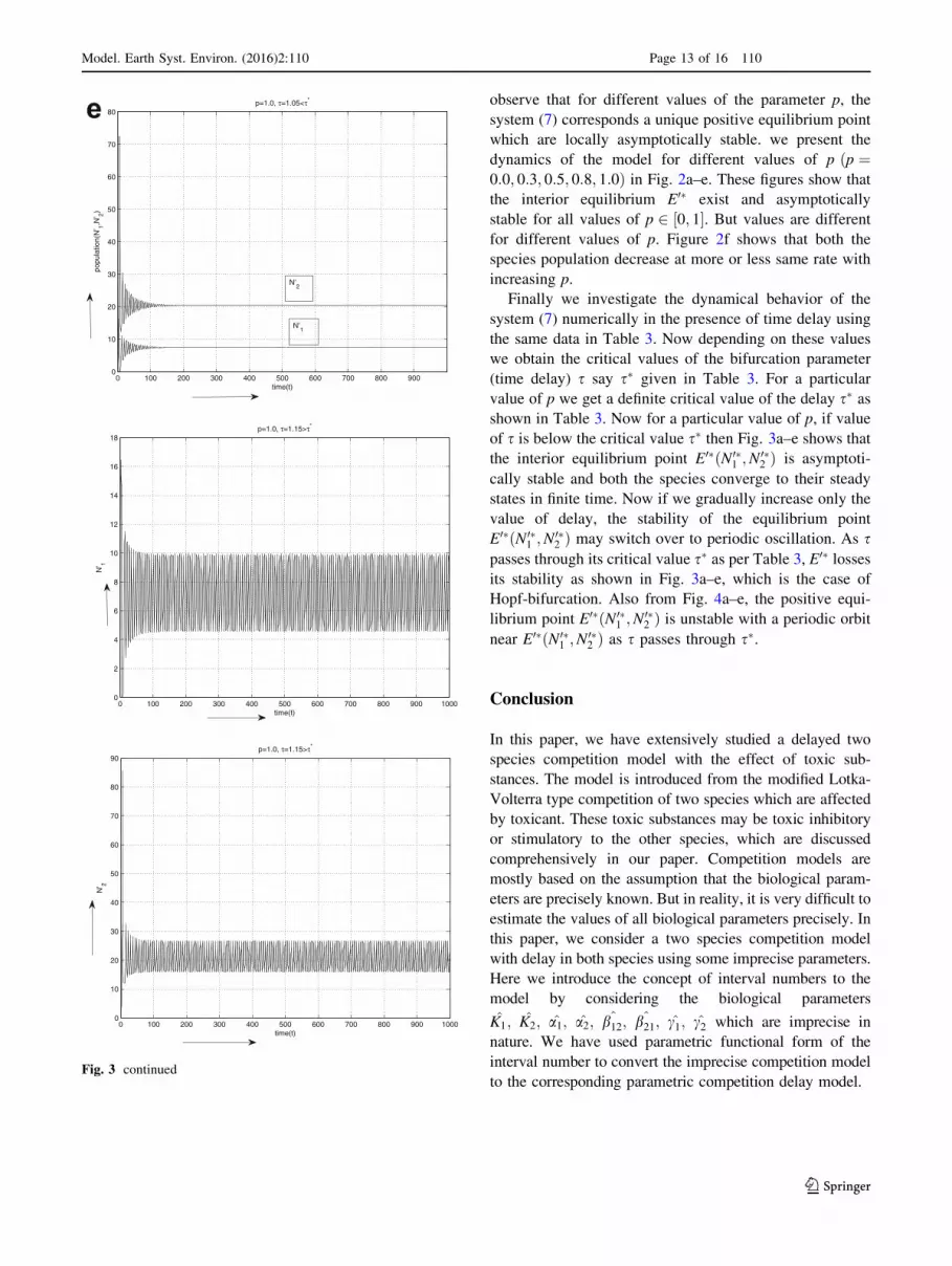
Finally we investigate the dynamical behavior of the

system (7) numerically in the presence of time delay using

the same data in Table 3. Now depending on these values

we obtain the critical values of the bifurcation parameter

(time delay) s say s� given in Table 3. For a particular

value of p we get a definite critical value of the delay s� asshown in Table 3. Now for a particular value of p, if value

of s is below the critical value s� then Fig. 3a–e shows that

the interior equilibrium point E0�ðN 0�1 ;N

0�2 Þ is asymptoti-

cally stable and both the species converge to their steady

states in finite time. Now if we gradually increase only the

value of delay, the stability of the equilibrium point

E0�ðN 0�1 ;N

0�2 Þ may switch over to periodic oscillation. As s

passes through its critical value s� as per Table 3, E0� lossesits stability as shown in Fig. 3a–e, which is the case of

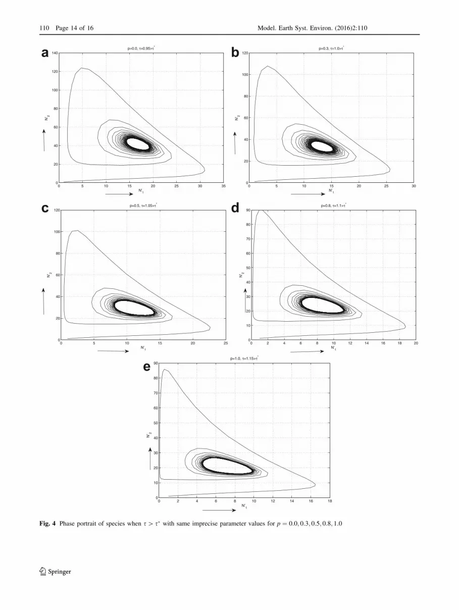
Hopf-bifurcation. Also from Fig. 4a–e, the positive equi-

librium point E0�ðN 0�1 ;N

0�2 Þ is unstable with a periodic orbit

near E0�ðN 0�1 ;N

0�2 Þ as s passes through s�.

Conclusion

In this paper, we have extensively studied a delayed two

species competition model with the effect of toxic sub-

stances. The model is introduced from the modified Lotka-

Volterra type competition of two species which are affected

by toxicant. These toxic substances may be toxic inhibitory

or stimulatory to the other species, which are discussed

comprehensively in our paper. Competition models are

mostly based on the assumption that the biological param-

eters are precisely known. But in reality, it is very difficult to

estimate the values of all biological parameters precisely. In

this paper, we consider a two species competition model

with delay in both species using some imprecise parameters.

Here we introduce the concept of interval numbers to the

model by considering the biological parameters

K1; K2; a1; a2; ^b12; ^b21; c1; c2 which are imprecise in

nature. We have used parametric functional form of the

interval number to convert the imprecise competition model

to the corresponding parametric competition delay model.

0 100 200 300 400 500 600 700 800 9000

10

20

30

40

50

60

70

80

time(t)

popu

latio

n(N

’ 1,N’ 2)

p=1.0, τ=1.05<τ*

N’2

N’1

0 100 200 300 400 500 600 700 800 900 10000

2

4

6

8

10

12

14

16

18

time(t)

N’ 1

p=1.0, τ=1.15>τ*

0 100 200 300 400 500 600 700 800 900 10000

10

20

30

40

50

60

70

80

90

time(t)

N’ 2

p=1.0, τ=1.15>τ*

e

Fig. 3 continued


123

0 5 10 15 20 25 30 350

20

40

60

80

100

120

140

N’1

N’ 2

p=0.0, τ=0.95>τ*

0 5 10 15 20 25 300

20

40

60

80

100

120

N’1

N’ 2

p=0.3, τ=1.0>τ*

0 5 10 15 20 250

20

40

60

80

100

120

N’1

N’ 2

p=0.5, τ=1.05>τ*

0 2 4 6 8 10 12 14 16 18 200

10

20

30

40

50

60

70

80

90

N’1

N’ 2

p=0.8, τ=1.1>τ*

0 2 4 6 8 10 12 14 16 180

10

20

30

40

50

60

70

80

90

N’1

N’ 2

p=1.0, τ=1.15>τ*

a b

c

e

d

Fig. 4 Phase portrait of species when s[ s� with same imprecise parameter values for p ¼ 0:0; 0:3; 0:5; 0:8; 1:0


123

Dynamical behavior of both the cases, toxic inhibitory

and stimulatory model system are examined rigorously in

absence as well as presence of time delay for different

values of the parameter p 2 ½0; 1�. We have discussed the

existence and stability of various equilibrium points of both

the systems. We obtain different equilibrium points of the

species and the critical value of the time delay depending

upon values of the parameter p. Analytically it is observed

that the time delay does not affected the stability on the

toxic inhibited system. But in case of toxic stimulatory

system, it is observed that the system becomes unstable at

different time delay for different value of the parameter

p and leads to stable limit cycle periodic solutions through

Hopf-bifurcation.

All our important mathematical findings for the

dynamical behavior of the two species competition model

affected by toxic substances are also numerically verified

and graphical representation of a variety of solutions of

system (6) and (7) are depicted by using MATLAB with

some imprecise parameter values. These numerical results

are very important to understand the system in both

mathematical and ecological point of view. Finally, we

conclude that impreciseness of biological parameters has

great impact on the behavior of the delay model. We use

the concept of interval number to present imprecise com-

petition modeling, which makes the system more realistic

as always it is difficult to know the parameter values pre-

cisely. Here we consider all the biological parameters are

imprecise, except the delay parameters. The delay model

can be made more realistic when incorporated with

impreciseness in the delay terms, it makes the model more

interesting and is left for future work.

References

Anderson DM (1989) Toxic algae blooms and red tides : a global

perspective. Environmental science and toxicology. Elsevier,

New York

Bassanezi RC, Barros LC, Tonelli A (2000) Attractors and asymptotic

stability for fuzzy dynamical systems. Fuzzy Sets Syst

113:473–483

Berglund H (1969) Stimulation of growth of two marine algae by

organic substances excreted by Enteromorpha linza in unialgal

and axeniccultures. Physicol Plant 22:1069–1078

Birkhoff G, Rota GC (1982) Ordinary differential equations. Ginn,

Boston

Celik C (2008) The stability and Hopf bifurcation for a predator-prey

system with time delay. Chaos Solitons Fractals 37(1):87–99

Chen Y, Yu J, Sun C (2007) Stability and Hopf bifurcation analysis in

a three-level food chain system with delay. Chaos Solitons

Fractals 31(3):683–694

Das T, Mukherjee RN, Chaudhuri KS (2009) Harvesting of a prey-

predator fishery in the presence of toxicity. Appl Math Model

33:2282–2292

Freedman HI, Shukla JB (1991) Models for the effect of the toxicant

in single species and predator-prey system. J Math Biol

30:15–30

Ghosh M, Chandra P, Sinha P (2002) A mathematical model to study

the effect of toxic chemicals on a prey-predator type fishery.

J Biol Syst 10:97–105

Gopalsamy K (1992) Stability and oscillation in delay-differential

equations of population dynamics. Kluwer, Dordrecht

Guo M, Xu X, Li R (2003) Impulsive functional differential

inclusions and fuzzy populations models. Fuzzy Sets Syst

138:601–615

Hallam TG, Clark CE, Jordan GS (1983a) Effects of toxicants on

population :a qualitative approach II. First-order kinetics. J Math

Biol 18:25–37

Hallam TG, Clark CE, Lassiter RR (1983b) Effects of toxicants on

population :a qualitative approach I. Equilibrium environmental

exposure. Ecol Model 18:291–304

Hallam TG, Luna JTD (1984) Effects of toxicants on population :a

qualitative approach III. Environmental and food chain path-

ways. J Theor Biol 109:411–429

He J, Wang K (2007) The survival analysis for a single-species

population model in a polluted environment. Appl Math Model

31:2227–2238

Jensen AL, Marshall JS (1982) Application of a surplus production

model to assess environmental impacts on exploited populations

of Daphina pluex in the laboratory. Environ Pollut Ser A

28:273–280

Kuang Y (1993) Delay differential equations with applications in

population dynamics. Academic Press, New York

Liu WM (1994) Criteria of Hopf bifurcations without using eigen

values. J Math Anal Appl 182(1):250–256

Luna JTD, Hallam TG (1987) Effect of toxicants on population: a

qualitative approach IV. Resource-consumer-toxicants models.

Ecol Model 35:249–273

MacDonald M (1989) Biological delay system: linear stability theory.

Cambridge University Press, Cambridge

Maiti A, Pal AK, Samanta GP (2008) Effect of time-delay on a food

chain model. Appl Math Comp 200:189–203

Maiti A, Pal AK, Samanta GP (2008) Usefulness of biocontrol of

pests in tea: a mathematical model. Math Model Nat Phenon

3(4):96–113

Maynard-Smith J (1975) Models in ecology. Cambridge University

Press, Cambridge

Nelson SA (1970) The problem of oil pollution in the sea In: Russell

FS, Yonge M (eds) Adv. in Marine Biol. Academic Press,

London, pp 215–306

Pal D, Mahapatra GS, Samanta GP (2012) A proportional harvesting

dynamical model with fuzzy intrinsic growth rate and harvesting

quantity. Pac Asian J Math 6:199–213

Pal D, Mahapatra GS, Samanta GP (2013) Optimal harvesting of

prey-predator system with interval biological parameters: a

bioeconomic model. Math Biosci 241:181–187

Pal D, Mahapatra GS, Samanta GP (2014) Bifurcation analysis of

predator-prey model with time delay and harvesting efforts using

interval parameter. Int J Dynam Control

Peixoto M, Barros LC, Bassanezi RC (2008) Predtor-prey fuzzy

model. Ecol Model 214:39–44

Pratt R (1940) Influence of the size of the inoculum on the growth of

Chlorella vulgaris in freshly prepared culture medium. Am J Bot

27:52–56

Pratt R, Fong J (1940) Studies on Chlorella vulgaris, II. Further

evidence that chlorella cells form a growth-inhibiting substance.

Am J Bot 27:431–436

Rice EL (1984) Allelopathy, 2nd edn. Academic Press, New York

Rice TR (1954) Biotic influences affecting population growth of

planktonic algae. US Fish Wildl Serv Fish Bull 54:227–245


123

Samanta GP (2010) A two-species competitive system under the

influence of toxic substances. Appl Math Comp 216:291–299

Song Y, Han M, Peng Y (2004) Stability and Hopf bifurcations in a

competitive Lotka-Volterra system with two delays. Chaos

Solitons Fractals 22(5):1139–1148

Xua R, Gan Q, Ma Z (2009) Stability and bifurcation analysis on a

ratio-dependent predator-prey model with time delay. J Comp

Appl Math 230:187–203


123

Documents

On the stability and Hopf-bifurcation of a multi-delayed competitive population system affected by toxic substances with imprecise biological parameters