Embed Size (px)
Citation preview

Working Paper Series
Bank Size, Leverage, and FinancialDownturns
Chacko GeorgeFederal Deposit Insurance Corporation
First Version: October 2013Current Version: March 2015
FDIC CFR WP 2015-01fdic.gov/cfr
NOTE: Staff working papers are preliminary materials circulated to stimulate discussion and criticalcomment. The analysis, conclusions, and opinions set forth here are those of the author(s) alone and donot necessarily reflect the views of the Federal Deposit Insurance Corporation. References in publicationsto this paper (other than acknowledgment) should be cleared with the author(s) to protect the tentativecharacter of these papers.

Bank Size, Leverage, and Financial Downturns ∗
Chacko George †
First Draft: October 2, 2013
This Draft: March 30, 2015
Abstract
I construct a macroeconomic model with a heterogeneous banking sector and an
interbank lending market. Banks differ in their ability to transform deposits from
households into loans to firms. Bank size differences emerge endogenously in the model,
and in steady state, the induced bank size distribution matches two stylized facts in the
data: bigger banks borrow more on the interbank lending market than smaller banks,
and bigger banks are more leveraged than smaller banks.
I use the model to evaluate the impact of increasing concentration in US banking
on the severity of potential downturns. I find that if the banking sector in 2007 was
only as concentrated as it was in 1992, GDP during the Great Recession would have
declined by much less than it did, and would have recovered faster.
Keywords: Financial crisis, interbank lending, concentration
JEL Classifications: E02, E44, E61, G01, G21
Opinions expressed in this paper are those of the author and not necessarily
those of the FDIC.
∗Thanks to Matthias Kehrig, Olivier Coibion, Andrew Glover, Jacek Rothert, and David Kendrick for alltheir guidance, and to Rudiger Bachmann, John Fernald, Francois Gourio, Chris House, Nobuhiro Kiyotaki,and Ariel Zetlin-Jones for all their helpful comments and suggestions. Thanks also to the seminar participantsat the Federal Reserve Bank of Dallas and the University of Texas for their questions and suggestions.†FDIC, Center for Financial Research, 550 17th St NW, Washington, DC 20429, email:
1

1 Introduction
The Great Recession of 2007-2009 began in the housing sector but ultimately resulted in a
decrease in employment and output in many sectors of the economy. One theory suggests
that the financial sector seems played a crucial role in transmitting weakness from one part
of the economy to another. The initial weakness in the housing sector decreased the value
of mortgages and their derivatives, decreasing the value of the asset side of their balance
sheets. Financial institutions then engaged in a deleveraging process which reduced their
investments in other sectors of the economy, driving an economy-wide recession.
If this theory is true, then the industrial characteristics of the banking sector - the
number of banks, their size, the functions they engage in, and the way they interact - should
matter a great deal for macroeconomic volatility. This paper explores the relationship
between one such characteristic, concentration in terms of asset size, and the depth of
recessions. At the most basic level, I ask: can a change in the distribution of bank sizes
affect the depth of recessions? If so, how?
I address this question theoretically by building a macroeconomic model with a het-
erogeneous banking sector and an interbank lending market. Banks are endowed with the
ability to transform deposits from households into loans to firms, but they differ in this abil-
ity endowment. From these ability differences, bank size differences emerge endogenously
in the model. In steady state, the induced bank size distribution qualitatively matches two
stylized facts in the data: bigger banks borrow more on the interbank lending market than
smaller banks, and bigger banks are more leveraged than smaller banks.
In order to study downturns, I introduce an exogenous shock that destroys the value
of net worth of all banks. In a downturn, the average ability of borrowing banks falls,
worsening the extensive margin, and with it, the misallocation of funds across banks. At
the same time, borrowing constraints tighten as bank net worth falls, reducing size on
the intensive margin. In the typical case, both effects combine to prolong and deepen
downturns. Bank heterogeneity in the model enables us to examine the difference in the
impact of downturns on individual banks. The differences qualitatively match what we see
in the data: the collapse in interbank lending disproportionately hurts large banks, large
banks de-lever and lose more in downturns, and firm investment financed by large banks
falls more than investment financed by small banks. It will also turn out that asset size
concentration will primarily depend on the concentration in the underlying intermediation
ability distribution.
After calibrating the model economy to match the pre-crisis economy and banking sector
2

of 2007, I induce a shock which results in a drop in output similar to that seen in 2007/08
financial crisis. I then consider the counterfactual: if the banking sector in 2007 had only
been as concentrated as it was in 1992, would the same shock produce a smaller drop in
output? I adjust banking sector size concentration by adjusting the underlying intermedi-
ation ability distribution. I find that the answer is yes, the same shock produces a 40%
smaller drop in output in the less concentrated economy. Further, output recovers to its
steady state level almost twice as quickly.
Why worry about the size distribution of banks? First, the financial crisis showed us that
there may be good reasons to think that big banks may matter a lot for the macroeconomy
purely because of their size. The knock-on effects from the failures of large banks and the
potential moral hazard problems generated by large bank bailouts have been pointed out
as inherently de-stabilizing to the system. More recently Bremus et al. (2013) points out
that, just because of their size, the largest banks are so large that their individual failures
can influence the macroeconomy.
Second, there are good reasons to think that big banks operate in qualitatively different
ways than small banks. Big banks are more leveraged, lose more in downturns, and rely
more on interbank lending to finance their day-to-day operations. There is some evidence
to suggest that big banks may benefit from economies of scale.
Rezitis (2006) considers the production of assets from deposits, labor, and capital in the
Greek banking sector, and finds that large banks enjoy higher productivity than small banks.
Hughes and Mester (2013) views bank productivity as the quantity of assets and deposits
generated for a given level of labor hours and capital, and finds that banks enjoy economies
of scale in this type of production. Kovner et al. (2014) finds that bank holding company
size increases with noninterest expense, suggesting that large bank holding companies have
lower operating costs. On the other hand, because of their systemic importance, big banks
may receive a “too-big-to-fail” implicit guarantee of government bailouts, allowing them to
operate with riskier balance sheets. Some of the apparent scale benefits may actually come
from a “too-big-to-fail” funding advantage for larger banks. Recent work (e.g. Tsesmelidakis
and Merton (2012) and Jacewitz and Pogach (2014)) has uncovered empirical evidence for
this advantage.
Last, the size distribution has transformed in recent decades. Over the last 40 years,
the concentration of the banking system has increased dramatically, as shown in figure 1.
Higher concentration means that big banks make up a larger share of the banking sector
than in the past, and therefore the actions taken by big banks, and the interactions between
big and small banks, matter more for outcomes in the banking sector.
3

Whether this trend has affected the economy negatively is still a topic of debate. One
view in the literature is that concentration makes the economy less prone to crises because
large banks are also more diversified, and are therefore better able to maintain the credit
they provide to firms in the event of a downturn. For example, Beck et al. (2007) perform a
reduced-form, cross-country study using a global dataset of banks, finding that concentra-
tion is associated with fewer crises (though they do not find evidence specifically supporting
the diversification theory). At the same time, other research supports the idea that large
banks are less disciplined by competition than smaller banks, make poorer lending choices,
and lose more in downturns. The model of Boyd and De Nicolo (2005) predicts that banks
in less competitive environments charge higher interest rates to firms, which induces firms
to take on greater risk and default more often. Supporting this hypothesis, De Nicolo et al.
(2004) performs a cross-country study using a dataset of large banks, and finds that higher
concentration is associated with higher fragility of the largest five banks in a given country.
In some ways, this division in the research still persists. Corbae and D’Erasmo (2010) builds
a two-tiered model of the banking sector, where a few dominant banks interact with a com-
petitive fringe. They find evidence that an increase in banking concentration (implemented
as an increase in entry costs) has offsetting effects: bank exit decreases, increasing stability,
while interest rates increase, decreasing stability as in Boyd and De Nicolo (2005).
Mechanically, this paper follows a strand of literature in macroeconomics that considers
the impact of information frictions in the financial sector on financial crises. The model in
this paper builds on the model of Gertler and Kiyotaki (2011), who incorporate an interbank
lending market in a macroeconomic model with a banking sector composed of identical
banks. The agency problem in that model keeps aggregate investment below its efficient level
in normal times, and amplifies the adverse effects of financial shocks in downturns. Boissay
et al. (2013) consider the effects of this agency problem with a heterogeneous banking sector,
and are able to create an economy in which banking crises arise endogenously.1
My paper adds two elements to this strand of literature. First, my focus is different: I am
more interested in the connection between banking industry characteristics and downturns,
and as such, I restrict my attention to the analysis of industry trends. Second, my model is
1This paper is also related to a broader literature considering the quantitative effects of financial frictionsin macroeconomic models. Carlstrom and Fuerst (1997) implement a friction generated by costly monitoringof borrowers, and focus on the effects of a shock to net worth, as in this paper. Jermann and Quadrini(2012) consider the effects of a friction generated by the possibility of default by firms, similar to the frictionconsidered here, and find that the addition of this friction is important in explaining dynamics during thecrisis. Christiano et al. (2010) find a more general result, weighing the quantitative effects of several frictionsin the literature, finding their addition to generally improve the output of this class of models. For a goodreview of this literature, see Christiano et al. (2010) and Christiano and Ikeda (2011).
4

Figure 1: Concentration in the US Banking Sector
Note: Share of assets held by largest 1% of banks calculated for all commercial banks from1976 to 2010. Data from call reports (forms FFIEC 031 and 041), retrieved from FederalReserve Bank of Chicago (2013).
different: leverage, or the assets banks hold per dollar net worth, will differ with size. This
margin will generate a connection between the depth of downturns and the variance of the
size distribution - the larger the highest bank is relative to the smallest, the more output
declines in response to a given decrease in liquidity, the deeper the recession.
The paper proceeds as follows. I begin by presenting some stylized facts about the
banking sector. The second section presents the model framework, describing its solution
and discussing its general properties. The third section presents the counterfactual exer-
cise described above, namely, to consider how the economy in 2007 may have responded
differently if the banking sector had only been as concentrated as it was in 1992. A fourth
section concludes.
2 Banking Facts
All banks are not the same, and size appears to be a key determinant of differences in bank
behaviors. In this section, I document three trends in banking which relate to size and play
a central role in my model. I then revisit concentration in the US banking sector, along
5

with two related trends that will be important for quantitative analysis.
First, big banks make a lot more loans and deposits than small banks. The first row of
table 1 shows the differences in the volume of loans performed by banks of different sizes
calculated from Federal Reserve Economic Data, where large is defined as the largest 25
banks by asset size. With respect to commercial and industrial loans in isolation or all loans
and leases in general, the largest banks lend twice as much as the smallest. On the deposit
side, banks also perform more intermediation activity than small banks. Again, large banks
receive twice as many deposits as small banks.
Second, bigger banks tend to be more leveraged than smaller ones. Table 1 shows the
inverse of the Tier 1 leverage ratio, calculated for all bank holding companies by the Federal
Reserve Bank of New York (2009). This measure is the ratio of the bank’s risk-weighted
assets, where assets are weighted by their credit risk, to the bank’s tier 1 capital, which
consists of a bank’s equity and its retained earnings. Larger values of this ratio imply that
less of a bank’s asset holdings are funded through the bank’s equity. In this sense, leverage
is a measure of the bank’s vulnerability to downturns. Both before and after the onset
of the financial crisis, large banks were more leveraged than smaller banks. In the run
up to the financial crisis, leverage increased for all banks, and in the midst of the crisis,
leverage decreased substantially. This partly reflects the tightening of borrowing constraints
(margins) banks faced when the value of many assets was deemed uncertain.2
Third, big banks tend to rely more on short-term liquidity markets than small banks
do. Banks rely on interbank lending and short-term debt to fund their day-to-day opera-
tions. With respect to interbank lending, there are several studies that indicate that when
interbank liquidity markets stop functioning, existing credit relationships are interrupted,
causing damage to the real economy. Ivashina and Scharfstein (2010) finds that banks that
relied less on interbank liquidity reduced their lending to nonbank borrowers in the wake of
the financial crisis. Puri et al. (2011) find that banks that were affected worse by liquidity
shortages rejected more potential borrowers than banks that weren’t.
The importance of these markets depends on bank size. With respect to interbank
lending, Furfine (1999) finds that net borrowers of Fed funds tend to be larger in asset size
than net lenders of funds. Cocco et al. (2009) uncovers a similar result in the Portuguese
interbank lending market, finding that larger banks borrow more often and borrow more
when they do. With respect to repo, a form of securitized lending banks use in a similar
way as interbank loans, Fecht et al. (2011) find that, in auctions for repo, banks that bid
for repo were larger than non-bidders.
2See Brunnermeier (2009) for a detailed explanation of this mechanism and its consequences.
6

Table 1: Large and Small Bank Differences: Intermediation Volume and Leverage
Volume of Intermediation
Measure Large Banks Small Banks Ratio Large to Small
All Loans 2314 1210 1.91Commercial and Industrial Loans 497 244 2.00
Total Deposits 2516 1318 1.90
Leverage
Measure Large Banks Small Banks
Assets/Equity
Average - All Years 13.1 11.01992 17.0 13.02007 10.0 9.50
Assets/Tier 1 Capital
Average - All Years 15.4 12.71996 14.8 11.92007 17.0 14.3
Note: Top panel: loans, deposits, and interbank loans in units of billions of US dollars for largeand small commercial banks, where large is defined as the largest 25 banks by asset size. Averagescalculated from monthly data over the period April 1988 Q1 to 2013 Q3. Recessions are defined byNBER recessions. Data are also displayed in 1992 and 2007, the reference years considered in thequantitative analysis, to show the effects of industry trends.Bottom panel: ratio of total assets to equity for large and small commercial banks, where large isdefined as banks with asset size larger than $20 B, for quarterly data over the period April 1985to September 2013. Next, ratio of risk-weighted assets to tier 1 capital for large and small banks,where large is defined as all banks with asset size larger than $500 B, for quarterly data from 1996Q1 to 2013 Q2.Sources: (Label - Series Name)Top Panel: All Loans - Loans and Leases from Bank Credit, Large/Small Domestically CharteredBanks; C+I Loans - Commercial and Industrial Loans, Large/Small Domestically Chartered Banks;Total Deposits - Deposits, Large/Small Domestically Chartered BanksBottom Panel: Assets/Equity Large - inverse of Total Equity/Total Assets, Banks with Total Assetsover $20 B [EQTA5]; Assets/Equity Large - Total Equity/Total Assets, Banks with Total Assetsless than $20B [EQTA1-4]Data from Board of Governors of the Federal Reserve System, retrieved from Federal Reserve Bankof St. Louis (2013).
Assets/Tier 1 Capital - inverse of leverage ratio, from Federal Reserve Bank of New York (2009).
7

Industry-wide, banking sector concentration has increased, which has changed the re-
lationship of large banks to small banks over time. A primary objective of this paper is
to understand whether concentration has made downturns worse or better. The answer, it
turns out, will depend on how concentration manifests itself.
Increasing concentration is typically characterized by an increase in the share of assets
held by the largest banks, but this increase in share can arise in a number of ways. In the
US data, the increase occurred for two reasons. First, banks have become more dispersed
by asset size - the size of the biggest and smallest banks have become more extreme relative
to the mean. Second, there are relatively more big banks in the banking sector today - the
bank size distribution has become more skewed to the right.
Though it has changed over time, the distribution has maintained two typical character-
istics: it has a large mass of small banks, so the left side of the distribution is heavy, and it
has a long right tail, representing a few very large banks. Figure 2 is a histogram of banks
in 2007 by the logarithm of their asset size. Janicki and Prescott (2006) considers similar
bank size distributions over time, and conclude that the distribution is best captured by a
lognormal distribution with a Pareto tail.
Figure 2: Log Bank Size Distribution
Note: Frequency plot of banks by their log (asset size) in 2007, where asset size is measuredin thousands of US dollars. Calculated from call reports FFIEC 031 and 041, retrieved fromthe Federal Reserve Bank of Chicago (2013).
In answering this question, I examine the banking sector in two reference years, one to
8

represent a low concentration year, another to represent a high concentration year. I choose
1992 as the reference low concentration year for several reasons.3 I choose 2007 as the high
concentration year for comparison to the financial crisis.
Table 2 gives several measures of concentration. This increase corresponds to an increase
in the share of total assets held by the top banks. The overall upward trend is robust to
changes in the definition of concentration; as we see in the table, whether measured by the
top 1% share, top 10% share, or the GINI coefficient, concentration has increased.
Table 2: Increasing Concentration and Related Trends
Concentration
Measure 1992 2007
Top 1% Share of Assets 0.47 0.72Top 10% Share of Assets 0.81 0.91
GINI Coefficient 0.85 0.92
Dispersion
Coeff. of Variation 7.65 15.6Interquartile Range 97063 180933
Right Tail
Skewness 33.7 39.5
Note: Measures of concentration, dispersion, and skewness calculated from the distributionof total assets across banks in 1992 and 2007. Assets and interquartile range measured inthousands of US dollars. (Interquartile range in 2007 adjusted to 1992 dollars using seriesGDP Implicit Price Deflator in the United States, from OECD, retrieved from FederalReserve Bank of St. Louis (2013).) Data from call reports FFIEC 031 and 041, retrievedfrom Federal Reserve Bank of Chicago (2013).
As the banking sector has become more concentrated, it has also become more dispersed
and heavier in the right tail. Dispersion is quantified in two ways in the table: first, in the
coefficient of variation, or the ratio of the standard deviation to the mean, and second,
in the interquartile range, or the difference in size between the banks at the 25th and 75th
3In figure 1, we saw that the share of assets held by the largest 1% of banks slightly decreases over the1976-1992 period, and then increases until 2010. This apparent trend break in concentration is accompaniedby trend breaks in dispersion, or the standard deviation relative to the mean, and skewness/kurtosis, whichfor the bank size distribution are synonymous with an increase in the fatness of the right tail. In both cases,these roughly move with concentration over the period - between 1976 and 1992, these measures decrease,while between 1992 and 2010, these measures increase. Historically, this roughly coincides with the end ofthe savings and loan crisis, which took place during the mid-1980s and early 1990s. During this period,many smaller commercial banks faced competitive pressure from savings and loans, leading to a reductionin the number of small banks.
9

percentiles in size.4 Both measures have increased, indicating that banks have become more
dispersed over time. The number of large banks has also increased relative to the number
of smaller banks. This is indicated by an increase in skewness of the size distribution
over the period. Throughout the period, the bank size distribution has a long right tail;
therefore, the increase in skewness indicates an increase in the mass of the right tail of the
size distribution.
3 Model
I consider an infinite-horizon economy composed of a continuum of islands a ∈ [0, 1]. On
each island, there are many households that supply labor and save funds, many firms that
produce consumption goods from capital goods and labor, and many banks that interme-
diate funds from households and lend them to the firms. Households and firms will be
identical across islands, but banks will not.
Following Gertler and Kiyotaki (2011) and Gertler and Karadi (2011), households and
bankers on each island will belong to the same family, or economy-wide household. This
induces two desirable features in the model. First, households will own banks, and receive
dividends that bankers pay out. Second, households will insure one another against con-
sumption risk across islands. This setup is maintained to ensure that we can represent the
household side of the model with a single representative household. All the heterogeneity
in the model will be isolated in the banking sector.
Banks will differ in a single dimension, intermediation ability, defined as the quantity of
assets they can produce for each dollar of liabilities. Ability differences will generate differ-
ences in investment demands across islands, which will be satisfied through the reallocation
of funds through an interbank lending market. Reallocation will be imperfect, however, and
this imperfection will generate size differences between banks. In order to abstract away
any distributional consequences other than what I am interested in, I will specify the model
in a way that the size distribution does not endogenously evolve over time.
I will denote a single island by a, and an ability type by κ. I will refer to the quantity x
on island a with x(a). The mass of any set of islands A will be given by the measure µ(A).
4Because banks are generally larger today than in the past, the variance has increased over time, theinterquartile range (measured in units of dollars of assets) has increased much more than the coefficient ofvariation (a unitless quantity).
10

3.1 Banks
There are many potentially infinitely lived, risk-neutral banks on each island. These banks
raise deposits from households on the same island, raise interbank loans from banks on all
other islands, and invest in the firms on the same island. All banks on the same island are
identical, but banks on different islands are not.
Banks in this model are intermediaries, that is, they take deposits from households
and invest them as loans to firms. Banks will be heterogeneous in their ability to perform
this task. We can think of intermediation ability as a productivity term in a simple bank
production function, so that if banks are producing assets S valued at price Q from net
worth N :
QS = κN (1)
After they receive deposits but before they borrow interbank loans, all the banks on an
island a receive a random, iid ability draw κ(a). Draws are assumed to be distributed with
cumulative distribution function κ(a) ∼ F (·), with bounded support [κ, κ].
Banks raise deposits in an economy-wide deposit market. Each bank offers a common
deposit rate Rt to households for a one-period deposit. This means that for each dollar
deposited in period t, the household will be repaid Rt dollars in period t + 1. I denote
the total deposits raised by all banks on each island in time t by dt. Deposits are written
without an island identifier because they raise identical quantities of deposits.5
Banks on any island are able to borrow or lend to banks on any other island. Since there
are many banks on each island, instead of characterizing loans between individual banks, I
will be interested in the net loans made between all banks on one island with all banks on
another. Ability and amount borrowed are observable, so we can characterize all interbank
loans with a contract specifying the interest rate and the borrowing quantity, (Rbt, bt(a)),
where a is the island where the borrower banks live.6
5Banks receive their ability draw after they raise deposits, and ability draws are iid. Therefore, if thebanks on any given island a raise dt(a), and banks on another island raise dt(a
′), then dt(a) = dt(a′). I refer
to this common quantity as dt = dt(a) = dt(a′).
6Technically, an interbank loan contract is bilateral. Therefore, we should specify an interbank lendingrate for each lender-borrower pair, or (Rbt(a, a
′), bt(a, a′)), where a, a′ are the island where the borrower
and lender banks live, respectively. It will turn out that the only rates we observe in equilibrium willbe both borrower and lender independent, however. The rate is lender-independent because there are acontinuum of potential lenders; since lenders compete with each other for borrowers across all islands, andloan contracts are identical to borrowers, only one lending rate will prevail. The borrowed amount will beborrower-dependent because of the financial friction I describe below. Then the debt contract will have theproperty that (Rbt(a, a
′), bt(a, a′)) = (Rbt, bt(a)).
11

Banks lend a mixture of capital and consumption goods to the firms on the same island.
Firms can use these loans to buy new capital goods in period t, and then use the old and
any new capital to produce consumption goods in period t + 1. The firm then gives the
bank its output (less wages) along with any undepreciated capital goods, also at time t+ 1.
Banks are potentially infinitely-lived, but face an incentive constraint that I will present
below. To prevent the bank from saving its way out of this constraint, a constant proportion
σ of banks on each island exit every period. Upon exit, a bank transfers its earnings to the
household on its island. Second, new banks enter to replace the old banks. To ensure that
these new banks have something to invest with, they receive a ”start-up transfer” equal to
a constant fraction ξ of the total assets held by all banks on the island.
Banks carry wealth from period to period in the form of net worth, defined as the payoff
from assets less deposits and interbank loans. The net worth of the island a representative
bank at time t is given by:
nt(a) = [Zt + (1− δ)Qt(a)]ψt(σ + ξ)st−1(a)−Rt−1dt−1(a)−Rbt−1bt−1(a) (2)
The first term gives the bank’s returns on investments in the firm: Zt is the economy-
wide representative firm’s gross profits from investments (per unit invested), Qt(a) is the
price of capital on island a, and st−1(a) is the units of capital held by the firm in period t−1.
The second term gives the bank’s repayments for deposits and interbank loans: bt−1(a) are
the funds borrowed on the interbank market in the last period, and dt−1(a) are the deposits
made by households in the last period.
ψt is the “quality of capital”; we can view this as an underlying asset value. This
variable will be the key shock in this model. This type of shock behaves differently from a
shock to total factor productivity. Most important, a shock to capital quality exogenously
affects the value of net worth; because the price of capital is endogenous to this model,
this shock will also exogenously decrease asset prices. This type of shock has been used in
recent work, including Gertler and Kiyotaki (2011), because it mimics a financial crisis - a
shock to capital quality mimics an unforeseen drop in asset values (e.g. housing crisis).
We can now revisit the balance sheet of the bank with the new variable descriptions in
hand. Banks balance assets against the intermediated value of liabilities and equity, which
in this case is the sum of net worth, deposits, and interbank borrowing. We can summarize
the balance sheet of the bank with a flow of funds constraint:
Qt(a)st(a) = κt(a) [nt(a) + dt + bt(a) ] (3)
12

In every period, banks are supposed to repay depositors and banks they borrowed from
in the previous period. Instead of repayment, however, banks can choose to default on their
loans, in which case they take a fraction θ ∈ [0, 1] of the total funds Qt(a)st(a) and exit
forever. If a bank chooses to default, it does so at the end of a period, and sells its shares
to another bank on the island.7 On the other hand, there will be no friction between banks
and firms on the same island - banks will be able to enforce full repayment of loans made
to firms.
We can now state the bank’s maximization problem. Bank managers choose a quantity of
deposits, loans to firms, and interbank loans today to maximize the expected present value
of future dividends. Households are bank owners, and the banker internalizes this when
calculating the expected value of dividends, discounting it by Λt,t+i, the stochastic discount
factor of the economy-wide representative household.8 At time t, the bank formulates a
plan for the path of deposits, assets, and interbank loans. The plan is state-contingent, so
that it chooses a different level of deposits dt for each value of aggregate shock it faces in
that period, ψt, and a different level of st(a) and bt(a) for each level of aggregate shock and
ability shock κt(a) it receives in that period.
Vt(dt−1, st−1(a), bt−1(a)) = maxdt+i,(st+i(ai))a,(bt+i(a))a∞i=0
Et
∞∑i=1
(1− σ)σi−1Λt,t+int+i(at+i)
s.t. Vt ≥ θQt(a)st(a) (4)
Note that nt(a) in (4) is a state variable here. At the time the bank makes its deposit
demand decision, it only knows the expected value of its net worth. However, at the time
it makes its asset and interbank loan decisions, it knows its net worth precisely.
The constraint in the above problem is an incentive constraint imposed by the bank’s
ability to default. In equilibrium, the continuation value of staying on the equilibrium path
has to exceed the dollar value of assets the bank can run away with.
We can rewrite the above problem in a Bellman equation:
Vt = maxdt
Et maxst(a),bt(a)
Et,aΛt,t+1
[(1− σ)nt+1(a) + σ max
dt+1
(max
st+1(a),bt+1(a)Vt+1
)]s.t. Vt ≥ θQt(a)st(a) (5)
7I interpret this ”running away” as capturing a bankruptcy cost: if a borrower bank decides to declarebankruptcy, creditors can capture some, but probably not all, of the repayments they are owed.
8As mentioned in the setup, households insure one another against differences in consumption acrossislands.
13

3.1.1 Additional Assumptions
I make two additional assumptions to ensure a tractable solution to the model. First, even if
ability draws are independent across periods, the interbank loans from the previous period
will make the expected returns from assets, or the ratio of net worth to capital, unequal. In
this case, the history of previous draws will matter for bank returns today. To prevent this,
I follow Gertler and Kiyotaki (2011) and allow individual banks to arbitrage these return
differences away, before their new ability type is realized:
Assumption 1. At the beginning of a period, banks can move between islands to equalize
expected returns on assets.
Consider two islands, aL and aH . aL has low expected returns when it enters the
period, that is, the representative bank has high interbank debt obligations, and aH has
high expected returns. When given the opportunity, an individual bank on aL decides to
move to aH . It currently holds assets (investments) in firms on aL, interbank debt to banks
on aH , and deposits (economy-wide). Before it moves, it trades its assets with another bank
on aL for more interbank debt to aH . It then takes its net worth and deposits and moves;
this reduces the individual bank’s interbank debt of aL to aH but maintains the total asset
held in aL firms. This process continues until returns are equalized.
The second assumption has to do with the capital goods that carry over from previous
periods. Intermediation ability also applies to the undepreciated capital that banks carry
between periods - banks will reallocate (or re-intermediate) the undepreciated portion of
the capital stock among firms on the same island. Re-intermediation of capital will leave
some islands with higher production capacity than others. To ensure that we can maintain
a simple law of motion for capital, I assume that these changes to production capacity can
be realized as gains in the output of firms in the same period:
Assumption 2. When an island’s existing capital kt(a) is intermediated, any gains (losses)
in the production possibilities of that capital are realized as an increase (decrease) in output
of all island firms yt(a) in the same period.
3.2 Households
Households on each island a are infinitely-lived, supply up to one unit of labor per period,
save in the form of deposits, and consume consumption goods. The household makes its
deposit and labor supply decisions before the banks on its island realize their ability. Because
households across islands are members of the same family and insure one another against
14

consumption shocks, we can represent the decisions of each household with an economy-wide
representative household.
Households on each island save by making riskless one-period depositsDt in the economy-
wide deposit market9 at the interest rate Rt. Deposits made in the last period are repaid
at the beginning of this period.
I make another simplifying assumption on labor:
Assumption 3. Workers can supply labor on any island.
With the above, wages will be identical across islands. Let’s call this economy-wide
wage Wt. The household also owns the bank, and receives dividends from exiting banks
every period Πt. Then the household’s budget constraint is
Ct = WtLt + Πt +Rt−1Dt−1 −Dt (6)
The household’s maximization problem becomes
max(Ct,Lt,Dt)∞t=0
Et
∞∑i=0
βi[ln(Ct+i − γCt+i−1)−
χ
1 + ϕ(Lt+i)
1+ϕ
]s.t. Ct = WtLt + Πt +Rt−1Dt−1 −Dt (for each t) (7)
where β ∈ (0, 1) is the discount factor and γ ∈ [0, 1) is a habit formation parameter10.
ϕ is the inverse Frisch elasticity of labor supply.
Taking first order conditions, we first work out a condition for aggregate deposits:
Rt(EtΛt,t+1) = 1 (8)
and a condition for aggregate labor:
WtEt(uCt) = χ(Lt)ϕ (9)
where uCt ≡ (Ct− γCt−1)−1− βγ(Ct+1− γCt)−1 is the marginal utility of consumption
and Λt,t+1 ≡ β uCt+1
uCtis defined as the household’s stochastic discount factor.
9We could alternatively restrict the household to only making deposits in the banks on their island; withthe timing assumptions below, nothing about the model changes. I maintain this formulation for ease ofexplanation.
10These preferences exhibit habit formation when γ ∈ (0, 1), a feature that is included for comparison toother models in the literature. The model is not fundamentally different when we turn off habit formation,i.e. set γ = 0.
15

3.3 Firms
There are many identical, competitive firms on each island. Immediately after the bank’s
ability is realized, the firm uses the capital it held from the last period to produce output.
It makes its loan repayment to the bank, and the bank then makes its loan to the firm for
next period production.
Coming into period t, there is capital kt(a) on island a. The firm’s problem is then
reduced to one of choosing how much labor to input. The representative firm on island a
chooses lt(a) to maximize:
yt(a) = Atkt(a)αlt(a)1−α (10)
where At is the (economy-wide) total factor productivity of the firm.11 Since labor is
mobile, firms on every island face the same wage Wt. Firms will choose labor to equate the
economy-wide wage with the marginal product of labor:
Wt = (1− α)
(yt(a)
lt(a)
)= (1− α)
YtLt
(11)
where the second equality follows from the fact that the ratio of capital to labor is
constant across islands. Thus, to find the optimal capital/labor ratio on each island, we
only need to solve the economy-wide representative firm’s problem:
Yt = AtKαt L
1−αt (12)
Even though the ratio of net worth to capital is identical across islands by assumption
1, the capital on each island is unknown. As a result, the size distribution of firms across
islands in equilibrium will be indeterminate. (In the solution below, I will show that despite
this, we can still pin down the size distribution of firms in a meaningful way.)
After production happens, capital depreciates, leaving (1−δ)kt(a) on the island. As part
of the repayment to banks, firms transfer ownership of this capital to banks. Banks then
decide on the loan package st(a), which comprises this undepreciated capital and (possibly)
of cash (basic goods) for new investment, which I denote by it(a). This implies that
st(a) = (1− δ)kt(a) + it(a) (13)
11This will be constant and equal to 1 throughout the paper, though TFP shocks can be induced in themodel through this channel.
16

3.4 Capital Goods Producers
When firms decide to expand their existing capital stock, they travel to a central (economy-
wide) market for new capital. The market is perfectly competitive, but all producers face
adjustment costs. Capital goods producers sell new capital to firms for the price Qit. These
producers then choose It to maximize
Et
∞∑τ=t
QiτIτ −(
1 + f(IτIτ−1
)
)Iτ (14)
From the first order condition for this profit maximization problem, the new capital
price should satisfy
Qit = 1 + f
(ItIt−1
)+
(ItIt−1
)f ′(
ItIt−1
)− EtΛt,t+1
(It+1
It
)2
f ′(It+1
It
)(15)
I’ll add another assumption to ensure that the law of motion for capital has a simple
form. With this assumption, banks will always find it optimal to reinvest their capital stock.
Assumption 4. Once installed, existing capital cannot be used on any other island.
3.5 Market Clearing Conditions
When we combine the household budget constraint with the equation for firm output and
new capital, we can write an economy-wide resource constraint for basic goods:
Yt = Ct +
(1− f
(ItIt−1
))It (16)
With the assumptions above, we can write a simple law of motion for capital:
Kt+1 = ψt+1 (It + (1− δ)Kt) (17)
A period is divided into two parts: before and after intermediation ability is realized.
Figure 3 gives the timing of the model. First, the aggregate shocks ψt and At are realized.
Banks then move to equalize expected returns, and some banks exit exogenously. Banks then
pay dividends to households, and new banks enter in their place. Deposits and interbank
loans are then repaid, and households make their deposit and labor supply decisions.
The second half of the period begins when intermediation ability types are realized.
Firms borrow from banks, and use household labor and existing capital to produce output.
They then pay profits Zt to banks and wages Wt to workers. Those firms that want to
17

Figure 3: Timing
expand their capital stock for next period’s production use the loans to purchase capital
from the capital goods producers (in the central new capital market). Simultaneously, banks
borrow from other banks. Banks then make their plan for the future, deciding in the process
whether to default before the next period.
As mentioned above, the size distribution of firms across islands will be indeterminate in
equilibrium. In what follows, I will first define and solve the model aggregated to the level
of ability type. To make things easier, I will first characterize the solution to the bank’s
maximization problem.
3.6 Bank Optimization
The bank on island a maximizes net worth, which itself is a linear function of assets,
deposits, and loans. Because of this linearity, we’ll guess and verify (details are left to the
appendix) that the bank’s value function will also be linear. The problem then boils down
to solving for the coefficients of a linear value function.
First, guess that in every period a bank maximizing a linear function of shares, deposits,
and interbank loans will maximize its expected net worth. Specifically, this function will
take the following form:
Vt = νstst(a)− νbtbt(a)− νtdt (18)
In what follows, I restrict attention to equilibria with interior solutions to the above
18

guess, so that banks can only hold nonzero quantities of all choice variables - only these
equilibria will have positive volumes of interbank lending.
Next, use the guess to set up a Lagrangian for the bank’s problem. First, substitute the
flow of funds constraint into the guess to reduce the number of choice variables to two:
V (dt, st(a), bt(a)) = νstst(a)− νtdt − νbtbt(a)
=κ(a)νstQt(a)
(nt(a) + dt + bt(a))− νtdt − νbtbt(a)
=κ(a)νstQt(a)
nt(a) + (κ(a)νstQt(a)
− νt)dt + (κ(a)νstQt(a)
− νbt)bt(a) (19)
Note again that nt(a), the bank’s net worth, is a state variable. Next, substitute the
guess into the incentive constraint, and use it to construct a Lagrangian:
L(dt, bt(a)) =
((1 + λt(a))
κ(a)νstQt(a)
− λt(a)κ(a)θ
)nt(a)
+
((1 + λt(a))(
κ(a)νstQt(a)
− νt)− λt(a)κ(a)θ)
)dt
+
((1 + λt(a))(
κ(a)νstQt(a)
− νbt)− λt(a)κ(a)θ
)bt(a)
λt(a) is the multiplier on the incentive constraint in period t for the representative bank
from island a.
We obtain the following first order conditions for dt and bt(a):
νt = νbt (20)
κ(a)θλt(a)
1 + λt(a)= κ(a)
νstQt(a)
− νbt (21)
Using the above, we can also rearrange the borrowing constraint:
bt(a) ≤ φt(a)nt(a)− dt(a) (22)
where
φt(a) =
κ(a)νstQt(a)
− κ(a)θ
νbt − κ(a)νstQt(a)
+ κ(a)θ(23)
φt(a) will be a useful quantity throughout the paper. It is related to the leverage ra-
tio, denoted Lt(a), or the ratio of shares held to net worth; Lt(a) = κ(a)(1 + φt(a)). The
19

leverage ratio Lt(a) is an increasing and convex function of κ. Convexity arises because
intermediation ability makes asset purchases easier for banks in two ways. First, interme-
diation ability decreases the cost of assets directly through its effect on the flow of funds
constraint. Second, ability decreases the value to running away by increasing the returns
to borrowing on the interbank market, which in turn loosens the borrowing constraint.
We can use the form of the linear solution to characterize the price of capital on each
island. Recall that, after production happens, the bank receives ownership of the existing
capital stock, which it can then re-lend to the firms as part of a loan package st(a). Islands
that are not borrowing constrained have λt(a) = 0, which implies that they are indifferent
between lending on the interbank market and re-lending to firms. Faced with indifference
between these choices, I will impose that the bank will always reinvest the existing capital
stock on its island. The following assumption states this formally.
Assumption 5. st(a) ≥ (1− δ)kt(a) ∀a
It will be convenient to group islands based on the borrowing activity of their banks
(recall that all banks on a single island are identical) . If the banks on island a are borrowing
constrained we will say that the island is part of the set B, and if banks on island a are not
borrowing constrained, we say that the island is part of the set L.
Further, if banks on island a are not borrowing constrained, λt(a) = 0. Then from
equation (21) it follows that
Qt(a)
κ(a)=νstνbt≡ Qnt ∀a ∈ L (24)
Assumption 4 also implies that the price of capital on each island is free to adjust to a
different value on each island. Here we make another guess that we can verify later:
Qt(a) = κ(a)νstνbt
= κ(a)Qnt ∀a ∈ L (25)
where L is the set of ability types for which banks are not borrowing constrained. This
price is related to the shadow cost of re-lending existing capital - if a bank on island a were
given an extra unit of basic good, it could either lend it on the interbank market, earning
the bank νbt, or it could turn it into κ(a) 1Qt(a)
units of capital, earning it κ(a) νstQt(a)
worth
of value.
We can also characterize the price of capital on islands with banks that are borrowing
constrained. The FOC for bt(a) also tells us that constrained banks view assets as more
valuable than interbank lending, implying that these banks also desire higher investment.
20

If these banks were indifferent between investing in assets and lending on the interbank
market, the price Qt(a) would get very large, as banks would demand ever higher returns
per unit capital.
No firm on any island will ever allow the price of capital Qt(a) to exceed the price for
new capital in the economy-wide new capital market, Qit. To see this, imagine a bank that
wants to lend a unit of existing capital to a firm, but demands repayment Qt(a) > Qit for
a unit of this capital. Rather than agreeing to these terms, the firm instead threatens to
go to another bank on the island to get a loan, which it could then use to buy new capital
at the lower price Qit. Since there are many potential lenders on the island, the threat is
credible, and the bank should drop the price of the existing capital to Qit as well. Thus, the
price of capital on borrowing constrained islands gets pinned down:
Qt(a) = Qit ∀a ∈ B (26)
where B is the set of islands on which banks are borrowing constrained.
Some sets of parameters will not admit equilibria with positive lending. I make two
restrictions on parameters to prevent these cases. I will choose parameters so that these
restrictions hold in steady state, and in the quantitative analysis below, I will choose the
level of the shock to be small enough to ensure that the restrictions hold in the impulse
responses.
It will turn out that intermediation ability will have a simple relationship with borrowing
behavior. Banks with ability high enough will borrow, and be borrowing constrained, while
low ability banks will lend. I show this in the next proposition.
Proposition 1. Consider an equilibrium with a strictly positive volume of interbank lending.
In each period t, there exists a κ∗t such that:
• for all banks with κ(a) < κ∗t , bt(a) = −(nt(a) + dt − Qnt kt(a)), that is, the bank will
lend all of its net worth and deposits less the cost of refinancing the entire existing
capital stock on its island.
• for all banks with κ(a) > κ∗t , bt(a) = bt(a), that is, the bank will borrow up to its
borrowing constraint and use the funds to purchase assets.
Proof. Consider the term for borrowing in equation (19), and let us first assume
(κ(a)νstQt(a)
− νbt) > 0
21

In this case, the bank gets positive value for every dollar it borrows, and it will choose
to borrow as much as it can. This bank will therefore run into its borrowing constraint,
i.e. until bt(a) = bt(a). Because all constrained banks face capital prices Qt(a) = Qit, this
implies that (κνstQit− νbt) > 0, or after rearranging, κ > νbt
νstQit.
If ( κνstQt(a)
− νbt) ≤ 0, the bank gets positive value for every dollar it lends (negative value
for every dollar it borrows). This implies that the bank will lend as many funds as it can.
Assumption 5 requires that the bank re-invest its entire existing capital stock; thus, the
funds the bank actually lends out on the interbank lending market will be limited to those
left over after this re-investment. These remaining funds are bt(a) = −(nt(a)+dt−Qnt kt(a)).
Further, we know that capital prices on these islands are smaller than the new capital market
price, so Qt(a) ≤ Qit. Since ( κνstQt(a)
− νbt) ≤ 0 implies that κ ≤ νbtνstQt(a), it must also be that
κ ≤ νbtνstQt(a) ≤ νbt
νstQit.
Call κ∗ ≡ νbtνstQit. Then, for any bank with ability κ > κ∗, borrowing and investing is
strictly more profitable than lending on the interbank market. For any bank with ability
κ ≤ κ∗, lending is (weakly) more profitable than borrowing.
The above proposition shows that an island a will fall into one of the two sets introduced
above: either banks on the island borrow from the interbank lending market, in which case
the island is in the set B, or banks on the island lend to the interbank lending market,
in which case the island is in the set L. Moreover, the proposition tells us that we can
summarize these sets with one object, the ability cutoff.
It will also turn out that lower ability interbank lenders will lend less than higher ability
interbank lenders. I show this in the next proposition.
Proposition 2. Consider two banks on different islands a, a′ with types κ(a) and κ(a′) and
bt(a), bt(a′) < 0. If κ(a) < κ(a′), then bt(a) < bt(a
′).
Proof. The cost of refinancing the entire existing capital stock kt(a), net of the benefit
derived in the form of net worth, is given by
Qt(a)
κ(a)kt(a)−Qt(a)kt(a)
Because of assumption 2, any differences in refinancing costs are reflected in output
in the same period. This allows banks to lend the consumption good equivalent of the
differences.
22

For unconstrained (lending) islands, this simplifies to
Qnt kt(a)(1− κ(a))
This is a decreasing function of κ. Thus, for interbank lenders the cost of refinancing
the capital stock is decreasing in κ. By the flow of funds constraint, the amount left over
for lending to other islands is then increasing in κ.
Since banks on islands with the same ability draw κ(a) will make the same choices for
dt and bt(a), this result extends to all banks with the same ability κ.
Figure 4: Ability Cutoff
κ (Intermediation Ability)
Mar
gina
l Val
ue
κ*
Value from Investment (lending to firms)
Value from Interbank Lending
Note: Marginal value from interbank borrowing (green dash) and marginal value fromholding shares (blue solid) versus intermediation ability. The intersection of the two linesmarks the ability cutoff κ∗. Above the cutoff, banks act as net borrowers on the interbanklending market, while below the cutoff, banks act as net lenders.
Figure 4 is a visualization of proposition 1. It diagrams the marginal value from lending
on the interbank market (dash line) and the marginal value from investing in firms in a
typical steady state. The value of lending is the same for all banks since all banks receive
the same interest rate for loans of any size. The value from investing/lending to firms,
on the other hand, increases with bank intermediation ability. In any equilibrium with
23

positive lending, the two lines have to cross - if the interbank lending line was always under
the investment line, no bank would be willing to lend, and if the interbank lending line
was always above the investment line, no bank would be willing to borrow. The ability
level at which these two lines cross is the ability cutoff κ∗ - for any bank with ability above
the cutoff, the marginal value from investing is higher than the value from lending, so it
becomes profitable for the bank to borrow and invest.
3.7 Equilibrium in Ability Types
The quantity of capital installed on each island in period t depends on the quantity of
capital installed in period t− 1. Since each island gets a new ability draw every period, the
only way to determine the capital on each island is to keep track of the history of all ability
draws over time. This requirement makes computing an equilibrium very difficult. In this
section, I introduce an alternative, aggregated equilibrium concept that is much easier to
solve, but still preserves the heterogeneity across banks.
In this alternative equilibrium concept, I will solve for prices and total quantities for
groups of islands with the same ability draw, e.g. instead of solving for the quantity of
interbank loans made by banks on a single island, I will determine the sum total value of
interbank loans made by all banks on every island with the same ability draw. Aggregating
the model in this way will lend itself to a tractable solution concept which still preserves
heterogeneity across banks. For the remainder of the paper, the quantity x on all islands
with the same ability type (a sum across individual islands) is called x(κ), that is, x(κ) =∫Aκx(a)da, where Aκ = a : κ(a) = κ.For any island receiving ability draw κ, there will be a positive measure of islands with
the same ability draw.12 Since the distribution is assumed to be iid across periods, any
positive measure of islands will be representative of the entire economy in the previous
period; the net interbank loan repayment in this measure will be 0, and the total capital
installed last period will just be a fraction of aggregate capital: bt−1(κ) = 0, st−1(κ) =
p(κ)Kt.
On each island, banks choose deposits dt identically, before uncertainty is realized.
Banks choose st(a) and bt(a) differently across islands, but two islands with the same ability
12To be more precise, we can justify this with the following setup: specify the set of islands over the space[0, 1]× [0, 1], where a specific island is referred to by two coordinates, a = (a1, a2). Now assume that in evenperiods, all islands with same first coordinate receive the same draw, and in odd periods, all islands withthe same second coordinate receive the same draw. Then for any island with a given level of κ, there will bea positive measure of islands with the same level of κ. Since [0, 1]× [0, 1] has the same cardinality as [0, 1],this same argument will work for the model in the main text. For ease of exposition, I leave this setup outof the main text.
24

type will choose identical values of st(a) and bt(a). This means that banks on all islands
with the same ability type will either all be borrowing constrained or not. This implies,
then, that the price of capital on islands with the same ability type will be identical, that
is, Qt(a) = Qt(a′) for all a, a′ with κ(a) = κ(a′). This can also be shown for the quantity
φt(a) as well.
We can use these facts to write an equation for the aggregate net worth of all banks
with the same ability type, which I label nt(κ), and the aggregate quantity of loans made
by all banks with the same ability type, which I label st(κ):
nt(κ) = [Zt + (1− δ)Qt(κ)]ψt(σ + ξ)p(κ)Kt − p(κ)σRt−1Dt−1 (27)
st(a) =κ(a)
Qt(a)(1 + φt(a))nt(a) (28)
The first term in equation (27) gives the representative bank’s returns on investments in
the firm: Zt is the economy-wide representative firm’s gross profits from investments (per
unit invested), Qt(κ) is the price of capital on all islands with ability κ, and Kt is the capital
installed by all firms in the economy at the beginning of period t. The second term gives
the bank’s repayments for deposits and interbank loans: bt−1 is the funds borrowed on the
interbank market last period, and dt−1 is the deposits made by households last period.
Since the quantities Qt(a), φt(a), and κ(a) are identical for any islands with the same
ability type, we can also write down an ability type level flow of funds constraint:
st(κ) =κ
Qt(κ)(1 + φt(κ))nt(κ) (29)
We can use this to solve for the ability type aggregates for banks with the maximization
problem
Vt = maxdt+i,(st+i(κt+i))κ,(bt+i(κt+i))κ∞i=0
Et
∞∑i=1
(1− σ)σi−1Λt,t+int+i(κt+i) (30)
s.t. Vt ≥ θQt(κ)st(κ) (31)
On the firm side, since net worth is pinned down for each ability type, and the rationt(a)kt(a)
is equal for each island by assumption 1, we can pin down the quantities kt(κ) and
it(κ) for each ability type. These will take the form
25

kt(κ) = p(κ)Kt (32)
it(κ) = st(κ)− (1− δ)kt(κ) (33)
Second, even though firms on each island may have different sizes, when we aggregate
them to the ability type level, all firms on islands with the same ability type will choose
ability type aggregate labor lt(κ) to maximize:
yt(κ) = Atkt(κ)αlt(κ)1−α (34)
With these in hand, we can describe the size distribution of firms across ability types.
Since the household was already represented by an economy-wide single representative
agent, we can define the aggregated equilibrium concept, equilibrium in ability types:
Definition 1. A recursive competitive equilibrium in ability types consists of a sequence
of economy-wide prices Pt ≡ (Rt+i, Rbt+i,Wt+i, Zt+i, Qit+i)
∞i=0 , a sequence of type-specific
prices Pκt ≡ (Qt+i(κ))∞i=0,
a sequence of economy-wide quantities Qt ≡ (Kt+i, Ct+i, It+i, Yt+i, Lt+i, Lt+i, Dt+i)∞i=0,
a sequence of type-specific quantities Qκt ≡ (bt+i(κ), st+i(κ), dt+i(κ), it+i(κ))∞i=013 such that:
(Individual Optimization) for each t,
• (dt, bt(κ), st(κ) maximizes the representative bank’s expected value (30) subject to their
flow of funds constraint (3) for each ability type κ
• (kt(κ), lt(κ)) maximizes the representative firm’s profits (34) for each ability type κ
• (Ct, Lt, Dt) maximizes the economy-wide representative household’s expected utility
(7)
• It maximizes capital goods producer profits (14)
(Market Clearing) and for each t, these markets clear
• deposits: Dt =∫κ dt(κ)p(κ)dκ
• labor: Lt =∫κ lt(κ)p(κ)dκ
• interbank loans:∫κ bt(κ)p(κ)dκ = 0
13Note that type-specific quantities are functions xt(κ) : [0, 1]→ R
26

• new capital, so that It =∫κ it(κ)p(κ)dκ
• assets (for each ability type): st(κ) = (1− δ)kt(κ) + it(κ)
The full set of equilibrium equations is given in the appendix.
3.8 Discussion
There are several qualitative properties of the model that are worth discussing here, mainly
because they are important for understanding the dynamics in the next section, but also
because they illustrate the model’s mechanics.
First, bank asset size increases with intermediation ability. To see this, first note that
interbank activity increases with the intermediation ability of a bank. From proposition
1 above in the previous section, the higher a bank’s intermediation ability, the more it
borrows from the interbank lending market if it is a borrower, and the more it lends to the
interbank lending market if it is a lender.
If a bank borrows from the interbank lending market, as it borrows more intensively,
the liabilities side of their balance sheet becomes larger. Through the bank’s “production
function” (3), larger liabilities are transformed into larger assets. Banks which lend to the
interbank market behave identically in terms of asset size. In the discussion in proposition
2, I note that all banks which lend hold exactly the same quantity of assets (equal to
Qnt kt(κ)(1− κ)). Thus, as intermediation ability increases, asset size either stays the same
(when intermediation ability is below the cutoff) or increases (if intermediation ability is
above the cutoff). Figure 5 diagrams this relationship.
Note here that borrowing banks are significantly larger than lending banks. The bor-
rowing banks in this models are the real drivers of the economy in this model; they are
responsible for the bulk of aggregate investment in the economy.
To further illustrate the mechanics of the model, let us consider how worsening financial
frictions affect the interbank lending market in steady state. Recall that financial frictions
are introduced into the model through the θ parameter in interbank borrowing constraint.
The worse the financial friction, the higher the value of θ, the tighter the borrowing con-
straint for all banks.
If there were no financial friction in the model, no bank would be constrained in its
borrowing. Depositors would make deposits in all banks as before, but once ability is
realized, the interbank lending market would funnel all deposits to the most able bank.
This bank would transform these loans into assets, which firms would use to purchase the
highest amount of capital possible.
27

Figure 5: Interbank Borrowing, Asset Size, and Intermediation Ability
Intermediation Ability
Inte
rban
k B
orro
win
g
Intermediation Ability
Inve
stm
ent
borrowing ofleast ableborrower
cost ofreinvestment
of existingcapital stock
cost of newcapital
purchases ofleast ableborrower
lending ofmost able
lender
Note: Interbank borrowing (left) and asset size (right) versus intermediation ability.
A positive value for the friction limits the maximum the most able bank can borrow
through the interbank lending market. By limiting the maximum the bank can borrow,
interbank loans that would go to the most able bank are redistributed to less able banks.
All else equal, as shown in equation (23), less able banks face tighter borrowing constraints
than more able ones. Thus, even though less able banks still invest in assets, because they
can only borrow significantly less, economy-wide investment is lower than in the frictionless
case.
An increase in the value of the friction pushes this redistribution further. We can
decompose the effects of increasing the friction into two components: an “intensive” and
an “extensive” effect. The intensive effect is a tightening of borrowing constraints: as the
friction θ increases, the value of φt(a) decreases, so any borrower that continues to be a
borrower will face a tighter constraint on the level of their borrowing, and thus will not be
able to invest as much. The extensive effect is the pure redistribution of interbank loans to
less able banks: as the friction increases and demand for interbank loans drops, the price of
borrowing decreases (relative to the value of lending to firms). This decrease in price causes
some banks that were lenders on the interbank market to become borrowers and invest.
28

Figure 6 diagrams the relationship between interbank borrowing and intermediation in
steady state for different levels of financial friction. In the frictionless case (red dot-dash),
only banks with the highest ability level borrow, while all other banks lend; this can be
seen in the diagram as negative borrowing (lending) by banks with ability less than the
maximum, and a straight vertical line at the maximum. The remaining lines diagram
the same relationship for low friction (solid green) and high friction (dashed blue) cases.
Increasing the friction results in an intensive effect, a decrease in the level of borrowing for
all borrowing banks, and an extensive effect, an increase in borrowing by less able banks.
Figure 6: Borrowing and Financial Friction
Intermediation Ability
Inte
rban
k B
orro
win
g
Low FrictionHigh FrictionFrictionless
Lenders BecomeBorrowers
BorrowingConstraintsTighten
κ*
Note: Steady state interbank borrowing in model with low friction (dash), high friction(solid), and frictionless (dash-dot) by banks of different abilities. Ability cutoff κ∗ is largestfor the frictionless case, then the low friction, then the high friction case.
The net effect of a given increase in the level of the financial friction on economy-wide
investment depends on the level of the friction. The intensive effect tends to decrease
aggregate investment because of the brake it puts on the borrowing taken by individual
banks, while the extensive effect tends to increase aggregate investment as more banks are
engaged in borrowing and investing (recall that borrowing banks are responsible for most
of aggregate investment). We can establish that the intensive effect tends to be much larger
29

than the extensive effect when the initial level of the friction is small, for example near the
frictionless case. The opposite seems to be true when the initial value of the friction is large.
4 Quantitative Effects of Rising Concentration
In this section, I use the model to analyze the impact of changes to the asset size distri-
bution that resulted from the increase in US banking sector concentration from 1992 to
2007. I calibrate the model to match the bank asset size distribution in 2007, and ask the
counterfactual: if the banking sector were only as concentrated as it was in 1992, would
downturns be less severe? If so, by how much?
Concentration is defined here as the share of assets (or more generally, output) held by
the largest firms in an industry. An increase in concentration can happen for many reasons.
For example, either an increase in the asset size of the largest bank in the industry or a
decrease in the asset size of the smallest bank would cause the share of all assets held by
the top 1 percent of banks to increase.
The concentration increase in the US banking sector took a specific form. First, the
variance of bank asset sizes increased. Second, the skewness of asset sizes (asymmetry of
the distribution toward higher values) increased. These two changes together will necessarily
lead to an increase in concentration; an increase in variance puts more weight in the tails
of the distribution, while an increase in skewness will ensure that the right tail gets more of
the extra weight than the left tail. In what follows, I produce an increase in concentration
in the model just as we see in the data, through an increase in the variance and skewness
of the size distribution.
4.1 Calibration
The model requires the choice of nine parameters, the adjustment costs function, and the
distribution of ability types. Five of the parameters control the standard preference and
technology shocks from from the literature: the discount rate β, the habit parameter γ, the
utility weight of labor χ, the share of capital in production α, and the depreciation rate δ.
These parameters are drawn from Gertler and Kiyotaki (2011) and Christiano et al. (2005)
and are given in Table 3 below.
The parameter ϕ, the inverse elasticity of labor supply, is chosen so that the Frisch
elasticity is 10. This choice is made to induce realistic labor responses in a model with
no other labor market frictions. The parameter ξ - the start-up transfer to new bankers -
governs the average spread between the interbank lending rate and the average return on
30

assets. The parameter σ, the exogenous probability of exit by a bank, is chosen so that the
average bank survives for approximately 15 years. The parameter θ, the financial friction
parameter, is chosen (along with the intermediation ability distribution) so that the average
leverage ratio across all banks in the model matches the data.
Adjustment costs take the quadratic form:
f
(ItIt−1
)=cI2
(ItIt−1
− 1)2 (35)
The distribution of ability types can take any shape, but will always be bounded. In
what follows, the distribution of ability types will take the form of a bounded Pareto dis-
tribution.14 This distribution has a pdf, given by
p(x) =ρκρκρ
κρ − κρx−ρ−1 (36)
where κ and κ are the lower and upper bounds of the distribution. In accordance with
the assumptions in the model, the parameters of the distribution will always be chosen so
that the distribution has a mean of 1.
In accordance with the assumptions in the model, the parameters of the distribution
will always be chosen so that the distribution has a mean of 1. The level of θ, the bounds
of the distribution κ and κ, and the shape parameter ρ will be adjusted to match the size
concentration (measured by the share of assets held by the top 10 percent of banks) and
the average leverage ratio in 1992 and 2007.
Table 4 shows how the calibrated model performs. Concentration is measured in the first
column, by the share of assets held by the top 10 percent of banks. Both model rows show
concentration measures for the steady state asset size distribution of the model calibrated
to the 1992 and 2007 banking sectors. The model generates significantly less concentration
than we see in the data, but significantly more leverage. This trade-off exists for a wide
range of parameters.
4.2 Crisis Response
The 2008 financial crisis, and banking crises more broadly, have their roots in more fun-
damental weaknesses in the wider economy. I want to focus on how the banking sector
propagates and amplifies weaknesses. To this end, I initiate a downturn in the calibrated
14Janicki and Prescott (2006) suggests that the tail of the bank size distribution is best modeled with aPareto distribution, while the remainder is best modeled with a lognormal distribution.
31

Table 3: Calibration - Parameters
Parameter Value Target/Source
Inverse Elasticity of Labor Supply ϕ 0.33 Gertler/Kiyotaki (2011)Start-up Transfer ξ 0.002 Gertler/Kiyotaki (2011)
Probability of Bank Exit σ 0.982 Average Bank Age - 2007Discount Factor β 0.99 Gertler/Kiyotaki (2011)Habit Parameter γ 0.8 Christiano, Eichenbaum, Evans (2005)
Depreciation Rate δ 0.025 Christiano, Eichenbaum, Evans (2005)Effective Capital Share α 0.36 Christiano, Eichenbaum, Evans (2005)Utility Weight of Labor χ 5.584 Gertler/Kiyotaki (2011)
Adjustment Cost Parameter cI 1.5 Gertler/Kiyotaki (2011)
Low Concentration Scenario
Parameter Value Target/Source
Friction θ 0.3 Average Leverage Ratio - 1992Min Ability κ 0.81 Asset Size Distribution - 1992Max Ability κ 2.15 Asset Size Distribution - 1992
Shape ρ 7 Asset Size Distribution - 1992
High Concentration Scenario
Parameter Value Target/Source
Friction θ 0.3 Average Leverage Ratio - 2007Min Ability κ 0.835 Asset Size Distribution - 2007Max Ability κ 2.8 mean(productivity distribution) = 1
Shape ρ 6 Asset Size Distribution - 2007
Note: Parameters chosen for quantitative analysis. Low and High Concentration scenarioparameters chosen to match characteristics of the asset size distribution in 1992 and 2007,respectively.
32

Table 4: Calibration - Performance
Top 10% Share Coeff of Variation Avg Leverage
Model - 1992 (Low Concentration) 36% 1.1 6.6Data - 1992 81% 7.65 6.6
Model - 2007 (High Concentration) 58% 2.1 14Data - 2007 91% 15.6 6.6
Note: Performance of calibrated model. Model - 1992 and Model - 2007 rows show concen-tration measures for steady state asset size distribution of model calibrated to each of thoseyears, respectively. Top 10% measures concentration as the percentage share of all assetsheld by top 10% of banks.
steady state economies with an exogenous shock to capital quality. This shock represents
an unexpected fall in the underlying value of all assets in the economy. (With respect to the
2008 recession, this shock could capture the unexpected fall in underlying collateral values
of mortgage-backed securities.) Since banks in the model derive their net worth partly from
the capital investments they’ve already made, this shock to capital translates to a shock to
the net worth of all banks.
Specifically, I first calculate the non-stochastic steady state of the model, and then
use the software package Dynare15 to calculate a second-order approximation of the model
around the steady state. I then initiate a crisis in the model with a 5 percent shock to the
capital quality ψt - the level is chosen to initiate a drop in output similar to that seen during
the 2008 crisis. The shock has a persistence of 0.8, so that it returns to its steady state
value after five years. I calculate the impulse responses to the shock in the approximated
model, again using Dynare.
The impulse responses for these cases are given in figure 7. The high concentration
response is the dotted line, while the low concentration response is the solid line. Notably,
output decreases more, in percentage terms, in the high concentration economy. Output
in the high concentration economy falls to a minimum that is 1.66 times the minimum of
the low concentration economy; thus, if the high concentration case represents the economy
just before the financial crisis, the economy would have experienced a downturn that was
only 60 percent as deep.
In both scenarios, the initial fall in capital quality produces the same qualitative changes
in the model. First, the shock destroys capital on impact, immediately reducing the stock
15For more details regarding this software, see ?.
33

Figure 7: Impulse Responses: High and Low Concentration
Note: Impulse responses to a negative 5 percent financial shock for high concentration(dotted, red) and low concentration (solid, blue) banking sector. Responses are expressedin percentage deviations. Responses are calculated for a second-order approximation to themodel using the software package Dynare.
34

of assets, K, invested in the economy. We can see this in the panel for capital - in both
cases, there is an initial drop in the first period. Output Y falls, and because the marginal
productivity of labor falls upon impact, demand for labor falls. Wages fall as well, so
the labor supply curve shifts inward, and employment falls. The decrease in wages and
employment forces households to save less today, leading to lower supply of deposits in
both cases.
Second, on the bank side, because capital is held as assets by banks, the decline in
capital quality leads to a significant decrease in bank net worth. This is seen in the bottom
left panel. A decline in capital quality decreases net worth in two ways. First, a decline in
capital quality destroys the value of assets held by the bank from last period, which directly
decreases net worth. Second, the decline in capital quality reduces the price of capital,
which indirectly decreases the value of the bank’s assets.
Because their net worth has decreased, borrowing banks must reduce their asset positions
further to satisfy their borrowing constraint. As a result, investment I falls - this is depicted
in the panel labeled I. In addition, adjustment costs help keep investment low for many
periods after the initial shock.
In addition, because their net worth has decreased and because households supply fewer
deposits, the supply curve of interbank loans shifts inward, and the quantity of loans made
decreases. However, the interest rate on deposits and interbank loans, R, also falls. Banks
are responsible for this, preventing households from dropping the supply of deposits even
further than it was already.
Though banks de-lever and reduce their assets after their net worth decreases, the lever-
age ratio for every bank increases in a downturn, that is, leverage ratios are countercyclical.
This is shown in the panel labeled average leverage. Leverage ratios are countercyclical
because the value from holding assets increases more than the value of default on inter-
bank loans; since capital quality shocks induce de-leveraging, the value from holding assets
increases as the shock dissipates.
Dispersion can amplify the effects of financial frictions. The banking sector of the high
concentration economy is more dispersed than the banking sector of the low concentration
economy. Because more able banks are more leveraged, and because leverage increases
at an increasing rate with intermediation ability, average leverage gets larger as disper-
sion increases. A larger portion of steady state investment is funded through interbank
borrowing; if the net worth decreased by the same amount in both the heterogeneous and
homogeneous bank models, investment decreases more in the heterogeneous case. In the fig-
ure, we actually see that net worth decreases more in the heterogeneous case, exacerbating
35
this difference.
The decrease in the interbank lending rate causes less able banks to switch from lending
to borrowing on the interbank lending market. This corresponds to a decrease in the ability
cutoff, shown in the panel labeled cutoff. These new borrowers act as a stabilizing force
in the interbank lending market, pushing up the interest rate and the volume of interbank
lending above what it would be otherwise. These new borrowers are also less leveraged
when they do borrow. Their entrance brings down the average leverage in the economy.
Heterogeneity among lenders also affects impulse responses. When faced with the same
shock to net worth, more able lenders decrease their lending more than less able ones,
making the average lender response in percentage terms larger in the heterogeneous banks
case. Thus, the volume of interbank lending decreases by more in the homogeneous banks
case.
Second, output in the high concentration economy returns to steady state much more
slowly than in the low concentration economy. Though not pictured, output in the high
concentration economy takes twice as many quarters to return to its steady state level than
in the low concentration economy.
The difference on impact of output in the two economies is because of the initial dif-
ference in the response of employment. As shown in the top right panel, employment falls
much farther in the high concentration than the low concentration economy. Since the high
concentration economy is more dispersed, all banks know there is a high chance of being
very productive tomorrow. This makes the value of net worth in the high concentration
economy higher on average today than in the low concentration economy. Thus, as capital
gets scarce, even though the marginal product of labor decreases in both economies, firms
want capital more in the high concentration economy, and shift their capital/labor ratio
toward capital more than in the low concentration economy. As a result, employment falls
further initially, and output falls with it.
Net worth decreases more in the high concentration case because the net profits from
firms decrease more, which occurs because output Y falls more. Thus, the relationship
between investment today and net worth tomorrow produces a feedback effect that amplifies
the shock.
The average leverage of borrowing banks is higher. These effects tend to worsen the
de-leveraging borrowing banks do in response to a shock, as the more concentrated sector
contains very leveraged banks.
In addition to dispersion, the mass of the right tail has increased over time. This has two
effects. First, since the number of leveraged banks increases, more banks de-leverage, and
36

the overall effect of de-leveraging on output worsens. Second, since the number of leveraged
banks increases, the same changes to the interbank lending rate produce larger swings in
the ability cutoff - for a given change in interest rate, there are more banks that respond to
the change.
These leverage differences are responsible for the very slow recovery of the high concen-
tration economy. Though both economies initially drop by similar amounts, total borrow-
ing, investor net worth, and investment in the high concentration economy stays much lower
than in the high concentration economy after a year or so. This occurs despite the fact that
leverage, both of the average bank and the most able, is more strongly countercyclical in
the high concentration than the low concentration economy.
Another contributing factor to the deeper downturn in the high concentration economy
is the smaller extensive effect of banks switching from lending to borrowing. The net worth
of banks in the high concentration economy decreases less than in the low concentration
economy, while the volume of interbank borrowing decreases more. Both the supply and de-
mand for interbank loans decreases. At first, this restricts demand, but because supply falls
farther, there is a net positive effect on the value that banks can receive from interbank
lending in both cases. This negative effect drives more banks into switching from lend-
ing to borrowing, pushing down the cutoff in the low concentration economy farther, and
dampening the negative effects of de-leveraging relative to the high concentration economy.
As shown above, the banks that switch from lending to borrowing stabilize the inter-
bank lending market, partly offsetting the negative effects of deleveraging - the extensive
effect of switching opposes the intensive effect of deleveraging. As a result, even though am-
plification occurred for this parameterization, there are other parameterizations for which
bank heterogeneity dampens downturns. Generally, amplification will occur for cases where
cutoffs are already relatively low. The cutoff will not move much after a capital shock, and
thus extensive switching effects are small.
5 Conclusion
In this paper, I construct a macroeconomic model with a heterogeneous banking sector, and
show that heterogeneity has consequences for downturns. In particular, mean-independent
changes in the distribution of bank sizes can mirror the effects of financial frictions, and as
a result, changes to the bank size distribution qualitatively similar to those that occurred
with the rising banking sector concentration observed in the US make potential downturns
more severe today.
37

The model in this paper puts us in the unique position to consider targeted macro-
prudential policies in a general macroeconomic framework. One such policy taken up by
the US Treasury and the Federal Reserve was embodied in broad targeted asset purchases
like the TARP, which in some cases equated to the government taking up partial ownership
positions in some banks. In the context of this model, this would lessen the borrowing con-
straint target banks face and essentially reduce the financial friction for the whole economy.
If the economy is in really bad shape, however, the economy starts at a high level of friction,
extensive effects can dominate. Loosening the friction will increase the interbank interest
rate, drawing some banks into interbank lending. However, the banks to which this lending
goes to are still so constrained that they don’t expand their investment enough. They get
an extra dollar of loan, but at a higher interest rate not offset by the change in the friction.
In this case, offering a targeted program which doesn’t affect the interbank market would
improve welfare more than one which did affect the interbank market.
Despite the stylized assumptions in the model, the environment is rich, and I see three
avenues worth pursuing in future work. First, the model has difficulty generating the ex-
treme bank size inequality we see in the data. This problem is partly due to the sharp
transition from lending to borrowing banks make as their ability increases. If banks calcu-
lated their net worth as a strictly convex, rather than linear, combination of deposits, assets
and interbank loans, their value functions would also be convex in these three quantities,
and banks would smoothly transition from lending to borrowing as ability increased. With
this, we could more easily generate high inequality.
Second, dropping assumption 1 will cause bank size next period to depend on its size
this period. This will induce an endogenously evolving size distribution, which may itself
uncover some interesting dynamics. For example, if ability tomorrow doesn’t depend on
ability today, but size carries to next period, large banks can use their assets as a buffer
against poor ability draws, but small banks would be more sensitive to such changes. As
a result, the average value of interbank lending would not adjust as much as in the case of
this model.
Third, if we modify the model by restricting the loans banks make to a subset of all
banks, we can create an environment where network effects are important. Relationships
matter in interbank lending (and other short-term debt, e.g. repo), with banks borrowing
from a partner in one period only to lend to the same partner in the next. Bank A’s failure
will matter more for bank B if the two were lending partners. As a result, some network
structures of lending relationships will transmit downturns better than others, just as a
more concentrated banking sector seems to transmit crises better in this model.
38

This project is a small step in a larger agenda of analyzing the macroeconomic impli-
cations of industry-wide trends (not just size differences) in banking. So far, research in
this field has not placed much emphasis on the characteristics of individual banks and the
dynamic consequences from changes in those characteristics. Research in this vein may be
especially informative for the conduct of unconventional monetary policy.
References
Beck, T., A. Demirguc-Kunt, and R. Levine (2007). Bank Concentration and Fragility. The
Risks of Financial Institutions, 193.
Boissay, F., F. Collard, and F. Smets (2013). Booms and Systemic Banking Crises. ECB
Working Paper, No. 1514 .
Boyd, J. H. and G. De Nicolo (2005). The Theory of Bank Risk Taking and Competition
Revisited. Journal of Finance 60 (3), 1329–1343.
Bremus, F., C. Buch, K. Russ, and M. Schnitzer (2013). Big Banks and Macroeconomic
Outcomes: Theory and Cross-Country Evidence of Granularity. (w19093).
Brunnermeier, M. K. (2009). Deciphering the Liquidity and Credit Crunch 2007-2008.
Journal of Economic Perspectives 23 (1), 77–100.
Carlstrom, C. T. and T. S. Fuerst (1997). Agency Costs, Net Worth, and Business Fluc-
tuations: A Computable General Equilibrium Analysis. American Economic Review ,
893–910.
Christiano, L., R. Motto, and M. Rostagno (2010). Financial Factors in Economic Fluctu-
ations.
Christiano, L. J., M. Eichenbaum, and C. L. Evans (2005). Nominal rigidities and the
dynamic effects of a shock to monetary policy. Journal of Political Economy 113 (1),
1–45.
Christiano, L. J. and D. Ikeda (2011). Government Policy, Credit Markets and Economic
Activity. NBER Working Paper (w17142).
Cocco, J. F., F. J. Gomes, and N. C. Martins (2009). Lending Relationships in the Interbank
Market. Journal of Financial Intermediation 18 (1), 24–48.
39

Corbae, D. and P. D’Erasmo (2010). A Quantitative Model of Banking Industry Dynamics.
Technical report.
De Nicolo, G., P. Bartholomew, J. Zaman, and M. Zephirin (2004). Bank Consolidation,
Internationalization, and Conglomeration: Trends and Implications for Financial Risk.
Financial Markets, Institutions & Instruments 13 (4), 173–217.
Fecht, F., K. G. Nyborg, and J. Rocholl (2011). The Price of Liquidity: the Effects of
Market Conditions and Bank Characteristics. Journal of Financial Economics 102 (2),
344–362.
Federal Reserve Bank of Chicago (2013). Commercial Bank Data. Available on-
line at www.chicagofed.org/webpages/banking/financial_institution_reports/
commercial_bank_data.cfm.
Federal Reserve Bank of New York (2009). Quarterly Trends for Consolidated US Banking
Organizations. Technical report, Federal Reserve Bank of New York.
Federal Reserve Bank of St. Louis (2013). Assets and Liabilities of Commercial Banks in the
United States. Available online at http://research.stlouisfed.org/fred2/release?
rid=22.
Furfine, C. H. (1999). The Microstructure of the Federal Funds Market. Financial Markets,
Institutions & Instruments 8 (5), 24–44.
Gertler, M. and P. Karadi (2011). A Model of Unconventional Monetary Policy. Journal
of Monetary Economics 58 (1), 17–34.
Gertler, M. and N. Kiyotaki (2011). Financial intermediation and credit policy in business
cycle analysis. Handbook of Monetary Economics 3 (3), 547–599.
Hughes, J. P. and L. J. Mester (2013). Who said large banks don’t experience scale
economies? evidence from a risk-return-driven cost function. Journal of Financial Inter-
mediation 22 (4), 559–585.
Ivashina, V. and D. Scharfstein (2010). Bank Lending during the Financial Crisis of 2008.
Journal of Financial Economics 97 (3), 319–338.
Jacewitz, S. and J. Pogach (2014). Deposit rate advantages at the largest banks. Technical
report, Federal Deposit Insurance Corporation.
40

Janicki, H. and E. Prescott (2006). Changes in the Size Distribution of US banks: 1960-2005.
Federal Reserve Bank of Richmond Economic Quarterly 92 (4), 291–316.
Jermann, U. and V. Quadrini (2012). Macroeconomic Effects of Financial Shocks. The
American Economic Review 102 (1), 238–271.
Kovner, A., J. I. Vickery, and L. Y. Zhou (2014). Do big banks have lower operating costs?
Economic Policy Review .
Puri, M., J. Rocholl, and S. Steffen (2011). Global Retail Lending in the Aftermath of
the US Financial Crisis: Distinguishing between Supply and Demand Effects. Journal of
Financial Economics 100 (3), 556–578.
Rezitis, A. N. (2006). Productivity Growth in the Greek Banking Industry: a Non-
parametric Approach. Journal of Applied Economics 9 (1), 119–138.
Tsesmelidakis, Z. and R. C. Merton (2012). The value of implicit guarantees. Available at
SSRN 2231317 .
A Bank Value Function Derivation
In the main text, I guess that we can solve the bank’s optimization problem with a linear
value function. Here I verify that this solution does indeed solve the bank’s problem in
detail.
First, recall the guess that in every period a bank guided by some linear function of
shares, deposits, and interbank loans will maximize its expected net worth:
Vt = νstst(a)− νbtbt(a)− νtdt (37)
If the guess is correct, the coefficients νst and νbt will be equal to the marginal value of
shares and interbank loans. Shares produce profits from firms tomorrow, which increases
the value of tomorrow’s net worth. Deposits and interbank loans today reduce tomorrow’s
net worth through repayment. Because net worth is a linear function of each of these
quantities, this marginal value will be constant. Calculating the value of these coefficients
amounts to calculating the marginal effect of increasing these quantities on net worth.
41

Note that the above Lagrangian is also equal to the bank’s maximized value written in
terms of net worth. Substituting the FOCs into the Lagrangian, we get
Vt = (1 + λt(a))νbtnt(a) (38)
If we iterate this one period forward and then plug this into the Bellman equation, we
obtain:
νstst(a)− νtdt − νbtbt(a) = Et,a′Λt,t+1(1− σ)nt+1(a′) + σ(1 + λt+1(a
′))νbt+1nt+1(a′) (39)
We can obtain the value of each coefficient by taking the partial derivatives of both sides
of the above equation with respect to each of the variables bt(a), dt, st(a):
νbt = RbtEt,a′Λt,t+1Ωa′t+1 (40)
νt = RtEt,a′Λt,t+1Ωa′t+1 (41)
νst = Et,a′Λt,t+1ψt+1(Ωa′t+1(Zt+1 + (1− δ)Qa′t+1) (42)
where
Ωa′t+1 = 1− σ + σ(1 + λt+1(a
′))νbt+1 (43)
As long as ability draws next period are independent of the draw this period, these
coefficients do not depend on ability type or level of either of the choice variables. They
also maximize the value of the original objective function (4):
Vt = Et,a′∞∑i=1
(1− σ)σi−1Λt,t+int+i(a′) (44)
To see this, consider the effect of a decrease dt on equation (4). dt only affects the
bank objective when the bank exits. A fraction (1 − σ) of banks exit from each island
every period. An increase in dt affects net worth in period t+ 1 directly, by increasing the
repayment in that period. Thus, banks that exit in period t+ 1 will have lower net worth.
The decrease in t+ 1 net worth decreases st+1 through the flow of funds constraint, which
turn reduces the net worth in period t+ 2; if banks exit then, they will also have lower net
worth. The full effect of the change in deposits can then be written as
42

dVtddt
= (1− σ)∂nt+1
∂dt+ σ(1− σ)
∂nt+1
∂dt
∂st+1
∂nt+1
∂nt+2
∂st+1
+ σ2(1− σ)∂nt+1
∂dt
∂st+1
∂nt+1
∂nt+2
∂st+1
∂st+2
∂nt+2
∂nt+3
∂st+2+ ... (45)
The partial effects ∂st+i∂nt+i
are captured by the quantity (1 + λt+i(a′))νbt+i. This means
that the coefficient νt completely summarizes the direct effect of dt on the island objective
function. The same argument holds for bt(a). Because of this, we can conclude that
dVtddt
= νt (46)
dVtdbt
= −νbt = νt (47)
Thus, if we solved the bank’s optimization problem by taking first-order conditions
directly on the objective function Vt with respect to each of the bank’s choice variables, we
would obtain the same first-order conditions as we obtain from the linear guess. Moreover,
given that the marginal effects are constant, we can say that:
Proposition 3. A set of choices (d∗t+i, b∗t+i(a))∞i=0 that maximizes the linear value function
guess (37) for each i will also maximize the bank objective (44).
B Equilibrium Conditions
In this section, I list the full set of equations that describes equilibrium. Before proceeding,
I make a few simplifications to the model. First, let’s simplify the interbank lending market
clearing condition. Note that clearing the interbank market automatically clears the market
for deposits. Call B the set of ability types with representative banks that borrow, and L
the set of all types that lend. The sum of all interbank lending by types in L should equal
the sum of all interbank borrowing by types in B:∫κ∈B
b(κ)p(κ)dκ =
∫κ∈B
b(κ)p(κ)dκ =
∫κ∈B
(φt(κ)nt(κ)− dt(κ)) dκ
= −∫κ∈L
b(κ)p(κ)dκ =
∫κ∈L
(nt(κ) + dt −Qt(κ)kt(κ)) dκ (48)
With this in hand, we can rewrite the interbank lending market condition in terms of
43

aggregates:
Dt =
∫ κ
κ∗p(κ)φt(κ)((Zt + (1− δ)Qit)Kt(σ + ξ)− σRt−1Dt−1)dκ
−∫ κ∗
κp(κ)((Zt + (1− δ)Qt(a))Kt(σ + ξ)− σRt−1Dt−1)dκ
+
∫ κ∗
κp(κ)
Qt(a)
κ(a)(1− δ)Ktdκ (49)
Where Dt is aggregate deposits and Kt is the aggregate capital stock.
In order to pin down investment, we need to consider the market for new capital alone.
We know that the aggregate investment and existing capital held by firms on borrower
islands is equal to It + (1 − δ)Kt
∫ κκ∗ p(κ), and that capital is demanded in the form of
interbank borrowing and deposits. Noting that borrowing islands will borrow the maximum
possible, we can replace the borrowing constraint into the flow of funds equation:
st(κ) = it(κ) + kt(κ) =κ
Qt(κ)(nt(κ) + dt(κ) + bt(κ))
=κ
Qit(1 + φt(κ))nt(κ) ∀κ ∈ [κ∗, κ] (50)
Finally, integrate both sides over the set B to get the condition in terms of aggregates:
Qit
(It + (1− δ)Kt
∫ κ
κ∗p(κ)
)=
∫ κ
κ∗κ(1 + φt(κ))nt(κ)dκ (51)
44
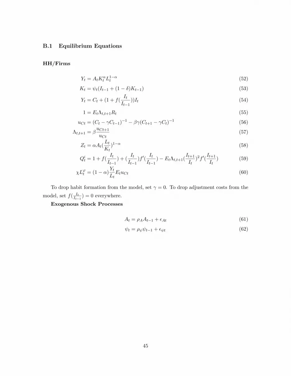
B.1 Equilibrium Equations
HH/Firms
Yt = AtKαt L
1−αt (52)
Kt = ψt(It−1 + (1− δ)Kt−1) (53)
Yt = Ct + (1 + f(ItIt−1
))It (54)
1 = EtΛt,t+1Rt (55)
uCt = (Ct − γCt−1)−1 − βγ(Ct+1 − γCt)−1 (56)
Λt,t+1 = βuCt+1
uCt(57)
Zt = αAt(LtKt
)1−α (58)
Qit = 1 + f(ItIt−1
) + (ItIt−1
)f ′(ItIt−1
)− EtΛt,t+1(It+1
It)2f ′(
It+1
It) (59)
χLϕt = (1− α)YtLtEtuCt (60)
To drop habit formation from the model, set γ = 0. To drop adjustment costs from the
model, set f( ItIt−1
) = 0 everywhere.
Exogenous Shock Processes
At = ρAAt−1 + εAt (61)
ψt = ρψψt−1 + εψt (62)
45

Bank Optimization
Qt(κ) =κ
κctQit ∀κ ∈ L (63)
νt = νbt (64)
νbt =κctQitνst (65)
λt(κ) =(κ− κct)νst
κθQit − (κ− κct)νst∀κ ∈ B (66)
λt(κ) = 0 ∀κ ∈ L (67)
Ωt(κ) = 1− σ + σνbt(1 + λt(κ)) (68)
φt(κ) =κ(νst − θQit)
νbtQit − κ(νst − θQit)
(69)
νbt = EtRtΛt,t+1(1− σ + σνbt+1) + EtRtΛt,t+1σνbt+1G0 (70)
νst = EtΛt,t+1Ψt+1[(1− σ + σνbt+1 + σνbt+1G0)Zt+1
+ (1− σ + σνbt+1)(1− δ)Qit+1(
∫ κ
κct+1
p(κ)dκ) + σνbt+1G0(1− δ)Qit+1
+ (1− σ + σνbt+1)(
∫ κct+1
κp(κ)κdκ)(1− δ)Qnt+1] (71)
G0 =
∫ κ
κct+1
p(κ)λt+1(κ) dκ (72)
Securities Market
Qit(It + (1− δ)Kt
∫ κ
κct
p(κ)dκ) = ((Zt + (1− δ)Qit)(σ + ξ)Kt − σRt−1Dt−1)G1 (73)
G1 =
∫ κ
κct
p(κ)κ(1 + φt(κ)) dκ (74)
Deposit Market
46

Dt = (Zt + (1− δ)Qit)(σ + ξ)Kt − σRt−1Dt−1)G2
− (Zt − σRt−1Dt−1)(
∫ κct
κp(κ)dκ)
− (1− δ)Qnt (σ + ξ)Kt(
∫ κct
κp(κ)κdκ) +Qnt (1− δ)Kt(
∫ κct
κp(κ)dκ) (75)
G2 =
∫ κ
κct
p(κ)φt(κ) dκ (76)
B.2 Steady State
HH
I = δK (77)
C = [A(L
K)1−α − δ]K (78)
χLϕ = (1− α)A(L
K)−α
1− βγ1− γ
1
C(79)
L = (Z
αA)
11−αK (80)
R =1
β(81)
Λ = β (82)
Qi = 1 (83)
Bank Optimization
λ(κ) =(κ− κc)νs
κθ − (κ− κc)νs∀κ ∈ B (84)
λ(a) = 0 ∀a ∈ L (85)
φ(κ) =κ(νs − θ)
νb − κ(νs − θ)(86)
Qn =1
κc(87)
1
κc= νs(1−
σ
1− σG0) (88)
νb = κcνs (89)
47

Z =νsβνb− 1− δ
νb
((1− σ + σνb)(
∫ κ
κcp(κ)dκ) + σνbG0
)− (1− δ)Qn
νb
((1− σ + σνb)(
∫ κc
κp(κ)κdκ)
)(90)
Securities Market
σ
β
D
K= (Z + 1− δ)(σ + ξ)−
δ + (1− δ)(∫ κκc p(κ)dκ)
G1
(91)
Deposit MarketN i
K= (Z + 1− δ)(σ + ξ)− σ
β
D
K(92)
D
K=N i
KG2 +Qn(1− δ)
(∫ κc
κp(κ)dκ
)−(Z(σ + ξ)− σ
β
D
K
)(∫ κc
κp(κ)dκ
)− (1− δ)Qn(σ + ξ)
(∫ κc
κp(κ)κdκ
)(93)
G0 =
∫ κ
κct+1
p(κ)(κ− κct+1)νst+1
κθQit+1 − (κ− κct+1)νst+1dκ (94)
G1 =
∫ κ
κct
p(κ)κκctνstκctνst − κνst + κθQit
dκ (95)
G2 =
∫ κ
κct
p(κ)κ(νst − θQit)κctνst − κνst + κθQit
dκ (96)
G0 =
∫ κ
κc
p(κ)(κ− κc)νsκθ − (κ− κc)νs
dκ (97)
G1 =
∫ κ
κc
p(κ)κκcνsκcνs − κνs + κθ
dκ (98)
G2 =
∫ κ
κc
p(κ)κ(νs − θ)κcνs − κνs + κθ
dκ (99)
To solve the model, I first guess a productivity cutoff κc. Then the value from interbank
48

lending νb = κcνs, and the equation for interbank lending above becomes an equation in
one variable, which we can solve for parameters. We can then use the equation for νs to get
Z, and use the investing islands securities market equation to get DK . With this in hand, we
can test the deposit market clearing condition, by calculating both the right and left hand
sides of equation (21).
49