Embed Size (px)
Citation preview

©International Monetary Fund. Not for Redistribution
World Economic and Financial Surveys
WORLD ECONOMIC OUTLOOK SUPPORTING STUDIES
International Monetary Fund 2000
©International Monetary Fund. Not for Redistribution
© 2000 International Monetary Fund
Production: lMF Graphics Section Cover & Design: Luisa Menjivar-Macdonald
Figures: Theodore F. Peters, Jr. Typography: Julio R. Prego
ISBN l-55775-893-X ISSN 0258-7440
Price: US$25.00 (US$20.00 to full-time faculty members and
students at universities and colleges)
Please send orders to: International Monetary Fund, Publication Services
700 19th Street, N.W., Washington, D.C. 20431, U.S.A. Tel.: (202) 623-7430 Telefax: (202) 623-720 I
E-mail: [email protected] Internet: bttp://www.imf.org
recycled paper
©International Monetary Fund. Not for Redistribution
CONTENTS
Preface
Chapter I. Globalization and Growth in the Twentieth Century
Nicholas Cmfts
What Has Twentieth Century Economic Growth Delivered? Globalization Then and Now An End-of-the-Century Perspective References
Chapter II. The International Monetary System in the (Very) Long Run
Barry Eichengreen and Nathan Sussman
Early Monetary Arrangements: Private Money Monetary Stability and Monetary Integration Rise of the State: Monetary Sovereignty The Political Economy of Inflation The International Monetary Landscape Paper Money: Beginnings The Nineteenth Century System Stability of the Gold Standard End of the Gold Standard Rebirth of the Gold Standard? Demise of Bretton Woods Recent Developments in Millennia! Perspective References
Chapter Ill. Currency Crises: In Search of Common Elements
Jahangir Aziz, Francesco Cammazza, and Rani[ Salgado
Identifying Crises: Methodology and Data The Correlates of Financial Crises The Macroeconomy Before a Crisis Outcomes of Crises Costs of Crises Conclusions Appendix 3.1. Banking Crises References
Chapter IV. Business Cycle Influences on Exchange Rates: Survey and Evidence
Ronald MacDonald and Phillip Swagel
Exchange Rate Models: Some Scaffolding and an Overview A Review of the Empirical Evidence
ix
1
2
19
26
44
52
53
56
57
58
63
64
65
68
70
74
76
79
82
86
87
90
92
121
124
125
126
127
129
129
133
iii
©International Monetary Fund. Not for Redistribution
iv
CONTENTS
New Empirical Evidence Conclusions References
Chapter V. The Great Contractions in Russia, the Baltics, and the Other Countries of the Former Soviet Union: A View from the Supply Side
Mark De Broeck and Vincent Koen
Background Considerations Selected Stylized Features Inputs and Outputs: Contraction Accounting Sectoral Reallocation Conclusions Appendix 5.1. Data Description Appendix 5.2. Alternative Summary Statistics for Aggregate Output References
Chapter VI. EMU Challenges to European labor Markets
R·udiger Soltwedel, Dirk Dohse, Christiane Krieger-Boden, and the IMF Research Department
The Optimum Currency Area Criteria The Regional Perspective Enlarging Institutional and Regional Diversity Conclusions References
Tables
l . l . The Human Development Index and Its Components: Long-Run Estimates 1.2. The Human Development Index and Its Components in the Recent Past 1.3. Catching Up and Falling Behind 1.4. Weighted Averages of HDJ 1.5. Growth Rates of Real GDP per Person 1.6. Growth Rates Acljusted for Hours Worked and Mortality 1.7. Annual Hours Worked per Head of Population 1.8. Growth Accounting: Comparisons of Sources of Growth 1.9. Ratios of Merchandise Exports to GOP and to Merchandise Value-Added
1.10. Composition of\1\lorld Merchandise Trade 1.11. Foreign Investment 1.12. Barriers to Trade: Average Tariffs on Manufactures and Import Coverage of 1.13. Immigration to the United States 1.14. The Structure of Employment in Five Leading Economies, 1900-95
l.l5. Sectoral Productivity Growth Rates, 1950-95
1.16. Government Expenditures/GOP, 1870-1998
1.17. Compatisons of Institutional Quality
3.1. Costs of Crises in Lost Output Relative to Trend
4.1. Cointegration Results for the Monetary Model 4.2. Estimates of the Real Exchange Rate-Real Interest Rate Relationship
TBs
142
156
157
161
161
163
166
170
173
175
176
181
184
184
193
199
206
207
7
8
9
9
II
14
15
17
20
21
21
22
23
27
28
35
39
125
135
137
©International Monetary Fund. Not for Redistribution
CONTENTS
4.3. Permanent and Transitory Variance Ratios for the Real Exchange Rate 139 4.4. Business Cycle Components of Real Exchange Rates and Real Interest Rate Differentials 151 4.5. Variance Decompositions for the Real E-xchange Rate from the Structural VAR 152
5.1. Contraction Length 164
5.2. Contraction Depth 165
5.3. Depth of the Contractions in Industrial Omput 166
5.4. Length of the Con tractions in Industrial Output 167
5.5. Fall in Industrial Output Across Regions During the First Half of the 1990s 168
5.6. Output and TFP Growth, Period Averages 169 5.7. Contribution of Sectoral Reallocation to TFP Growth 171
5.8. Total Employment Shifts 172
5.9. Total Investment Shifts 173
5.10. Industrial Employment Shifts 173 5.11. Industrial Investment Shifts 174 5.12. Yearly TFP Growth Rates 176
5.13. Cumulative Decline in Measured Real GDP and Electricity Consumption 178
6.1. Coefficients of Specialization in Manufacture, EU Countries, 1980-93 191
6.2. Total and Structural Unemployment in EU Member Countries, 1997 193
6.3. Monetary Union and Labor Market Risks for EU Countries 194
6.4. EU Regions with the Highest/Lowest Unemployment Rates, April 1997 194
6.5. EU Regions with the Highest/Lowest Yolllh Unemployment Rates, April 1997 195 6.6. Unemployment Disparities by Region 1985, 1990, 1995-97 196
6.7. Persistence of Regional Unemploymem Differentials: Rank-Order Correlations,
1985-97 197 6.8. Italian Mezzogiorno and East Germany Compared, 1995 198
6.9. Labor Costs and Labor Productivity Relative to the Rest of the Country 199
Figures
2.1. Percentage of Countries with Fiat Currencies, 1870-1998
2.2. Debasement Minting, Dauphine, 1417-22
2.3. Value of English Currency and the Price Level, 1265-1500
2.4. Value of Silver Currency in Terms of Gold Florin
2.5. Restrictions on Capital Account
2.6. Percentage of Countries with Pegged Exchange Rates, 1870-1988
3.1. Incidence of Currency Crises
3.2. Real Effective Exchange Rates
3.3. Export Growth
3.4. Trade Balance
3.5. Terms of Trade
3.6. Inflation
3.7. Nominal M l Growth
3.8. Nominal M2 Growth
3.9. ominal Domestic Credit Growth
3.10. Real M l Growth
3.11. Real M2 Growth
53
59
60
62
76
80
89
95
97 98
99
100
102
103
104
105
106
v
©International Monetary Fund. Not for Redistribution
vi
CONTENTS
3.12. Real Domestic Credit Growth 107
3.13. Real Interest Rate 108
3.14. Change in Real Stock Prices 110
3.15. Change in Stock Prices (Valued in Foreign Currency) 111
3.16. Change in Foreign Reserves 112
3.17. M2-to-Reserves Ratio 113
3.18. Change in M2-to-Ml Ratio 115
3.19. Output Growth 116
3.20. World Real Interest Rate 117
3.21. Change in the Unemployment Rate 118
3.22. Current Account Balance 119
3.23. Fiscal Balance 120
3.24. Short Term Capital 1n11ows 122
4.1. Germany: Real Bilateral Exchange Rate and Interest Rate 143
4.2. Japan: Real Bilateral Exchange Rate and Interest Rate 143
4.3. United Kingdom: Real Dollar Exchange Rate and Interest Rate Differential 144
4.4. Germany: Real Effective Exchange Rate and Interest Rate Differential 145
4.5. Japan: Real Effective Exchange Rate and Interest Rate DilTerential 145
4.6. United Kingdom: Real Effective Exchange Rate and Interest Rate Differential 146
4.7. United States: Real Effective Exchange Rate and Interest Rate Differential 146
4.8. Germany: Band-Pass Filter of Real Bilateral Exchange Rate and Interest Rate Differential 147
4.9.Japan: Band-Pass Filter of Real Bilateral Exchange Rate and Interest Rate Differential 148
4.10. United Kingdom: Band-Pass Filter of Real Bilateral Exchange Rate and Interest Rate
Differential 148
4.11. Germany: Band-Pass Filter of Real Effective Exchange Rate and Interest Rate Differen tiaJ 149
4.12. Japan: Band-Pass Filter of Real Effective Exchange Rate and Interest Rate Differential 149
4.13. United Kingdom: Band-Pass Filter of Real Effective Exchange Rate and Interest Rate Differential 150
4. 14. United States: Band-Pass Filter of Real Effective Exchange Rate and Interest
Rate Differential 150
4.15. Real Bilateral Exchange Rate: Response to Shocks 153
4.16. Structtu·al VAR: Real Bilateral Exchange Rate 154
4.17. Response of Real Effective Exchange Rate to Shocks 155
4.18. Real Effective Exchange Rate 156
5.1. Finland: Real GDP and Overall Electricity Consumption 179
5.2. Finland: Real GDP and Total Freight Turnover 180
5.3. Finland: Real GDP and Mail 181
6.1. Integration, Specialization, and Asymmetric Shocks 190
6.2. Determination of Labor Market Flexibility 19�
Boxes
1.1. Measuring Long-Run Growth in Living Standards
1.2. Financial Crisis in 1930s America 1.3. Computers and Productivity Growth
3 29
33
©International Monetary Fund. Not for Redistribution
2.1. Financial Crises: Continuity and Change
2.2. Monetary Developments Beyond Europe 2.3. The Future of the International Monetary System
6.1. Exchange Rates as Shock Absorbers: Italy and Finland
6.2. Euro Area's Most Prominent Problem Regions
6.3. Trends in Business Organization
The following symbols have been used throughout this volume:
to indicate that dat a are not available;
to indicate that the figure is zero or less than half the final digit shown, or that the ite m does n ot exist; between years or months ( for example, 1997-99 or J anuary-June) to indicate the years or months covered, including the beginning and ending years or months;
between years (for example, 1998/99) to indicate a fiscal or financial year.
"Billion" means a thousand million; "trillion" means a thous and billion.
"Basis points" refer to hundredths of I percentage point (for example, 25 ba sis points are equivalent to \1.1 of l percentage poin t).
"n.a." means not applicable.
Minor discrepancies between constituent figures and tot als are due to rounding.
As used in this volume the term "country" does n ot in all cases refer to a territorial entity that is a state as understood by international Jaw and practice. As used here, the tenn also covers some territorial entities that are not states but for which statistical data are maintained on a separate and independent basis.
C ONTENTS
54 55
82
186
188 200
vii

©International Monetary Fund. Not for Redistribution
Fhispage intentionally left hlank
©International Monetary Fund. Not for Redistribution
PREFACE
Supporting Studies for the World Eronomic Outlook contains background analyses for the World Economic
Outlook exercise carried out by staff in the IMF's Research DepartmenL and by visiting scholars. The
May 2000 World Economic OutlcJok editions for which these papers were prepared were directed by Flemming Larsen, former Deputy Direcwr of the Research Department, together with Graham Hacche and Tamim Bayoumi, former and current Chiefs of the World Economic Studies Division.
The papers have benefited from comments by colleagues throughout the TMF and, in some cases, by
the IMF's Executive Directors. However, the views presented in the papers are those of the authors and
should not be interpreted as representing the views of the Internalional Monetary Fund. The authors
would like to thank Gretchen Byrne and Toh Kuan for research assis1.ance and Lisa Nugent., Marlene
George, Patricia Medina, and ]emilie Tumang for word processing. James McEuen and Jeanette
Morrison of the External Relations Department edited the manuscripts and coordinated production of the publicalion.
ix

©International Monetary Fund. Not for Redistribution
Fhispage intentionally left hlank
©International Monetary Fund. Not for Redistribution
GLOBALIZATION AND GROWTH IN THE TWENTIETH CENTURY Nicholas Crafts
This chapter reviews the experience of
economic growth during the twentieth
century in the context of trends in glob
alization and with a view to highlighting
implications relevant to early twenty-first century
policymakers. The first section provides a de
scriptive analysis of trends in growth and living
standards during the century, which highlights
differences between periods and across coun
tries. The next section looks at the rollercoaster
progress of globalization both in trade and capi
tal flows since the late nineteenth century, with
particular emphasis on explanations for the pro
longed reverse w globalization from the back
lash of the interwar years. The final section uses
the building blocks of the earlier analysis w pro
vide an end-of-century perspective on growth
prospects and the extent to which they are likely
to be:: enhanced by improved policies, technolog
ical progress, and globalization.
The first section presents a basic quantifica
tion of growth during the twentieth century
dra\ving on the economic history literature. The
ccnu·al themes that emerge include the massive
and unprecedented divergence in income levels
and growth performance across countries, espe
cially between the OECD and many developing
countries in both the first and second halves of
the century. The consequences in terms of in
come forgone of poor policy and/or inadequate
institutions were much more serious than in ear
lier centuries. evenheless, a g1·eat deal of
progress has been made everywhere in terms of
the Human Development Index (see UNDP,
1998), and the spectacular improvements in
mortality that have taken place are a major rea
son to believe that historical national income ac
counts tend to underestimate growth in living
standards. The contribution of technological
progress to economic growth both in the ad
vanced and the developing world has varied sub
stantially over time for reasons that are not fully
understood either by growth theorists or eco
nomic historians.
The second section spells out what is known
about the dimensions of globalization over time.
In many respects, the information is patchy, but
a clear pattern emerges of increases in trade
flows and stocks of capital assets relative to levels
of CDP before World War I and in recent
decades, with the opposite characterizing the
1920s through the 1950s. Many aspects of the
current situation are shown to be unprece
dented, driven not only by changes in technol
ogy but also in economic policy. The retreat of
globalization in the interwar period was, of
course, driven by policy not technology and was,
in large part, a response to the Great
Depression. A review of recent historical re
search concludes that a combination of macro
economic policy errors and structural faults in
bankjng systems and labor markets rather than
globalization per se provoked the slump.
ln the final section the historical experience is
linked to insights from modern applied growth
economics to examine growth potential after the
liberalization and globalization of the recent
past. It is argued that globalization itself could be
subject to a renewed backlash either, as in the
1930s, in the event of a major world recession or
in a new context of the impossibility of govern
ments continuing to meet increased demands for
economic security in a world of severe tax com
petition. In a less apocalyptic scenario, the im
pact of globalization on fiscal policy could ad
dress some of the growth-inhibiting effects of the
late t:wemieth century expansion of the public
sector in OECD Europe. Prospects for catch-up
growth and an escape from the divergence in in
comes that has characterized the twentieth cen
tury are argued to depend very largely on pol
icy/institutional reform in the developing world
to reduce problems of agency costs, rent-seeking,
asymmetric information, and opportunism,
©International Monetary Fund. Not for Redistribution
2
CHAPTER I GLOBALIZATION AND GROWTH IN THE TWENTIETH CENTURY
thereby facilitating financial development, invest
ment, and innovation. The present policy con
sensus in favor of markets and outward orienta
tion in the developing world potentially
represents a significant improvement from the
state-led industJ·ialization stance that was preva
lent 25 years ago, but the political economy of
supply-side policy is central to further progress
yet little understood. Despite the confidence of
many stock market players, long-run growth
prospects for the United States are particularly
hard to predict, both because theory suggests
that they depend crucially on scale effects in in
novation on which the jury is still out, and also
because at this point of history it t·emains unclear
whether the information and communications
technology revolution will eventually deliver a
major boost to total factor productivity equiva
lent or superior to that of the era of electricity.
What Has Twentieth Century Economic Growth Delivered?
Since World War U, trend growth of real GDP
per person has become a key policy objective in
virtually all counu·ies. This is not surpt·ising since
it is usually thought to be central to raising living
standards and because, despite doubts raised by
economic theorists, it is generally believed that
government policy can influence long-run
growth outcomes. The twentieth century has
seen unprecedented economic growth in many
parts of the world, but the benefits of growth
have often been quite unequally distributed
both between and within countries, and growth
rates have exhibited considerable vat;ation over
time. Moreover, it is now frequently suggested
that GDP growtl1 is a poor, or perhaps quite mis
leading, indicator of changing well-being and,
even within the national accounts framework, it
has become widely accepted that important
measurement issues have to be addressed, partic
ularly when considering the long run.
In this section, experience of economic
growth in me twentieth century is assessed born
in terms of its impact on standards of Jiving and
also with a view to extracting the lessons mat it
can offer on why growth rates differ. Two ques
tions are of central concern:
• What has been the relationship between
economic growth and changes in living
standards?
• What explains me uneven pace and spread
of economic growth ?
The renaissance of research in growth eco
nomics since the mid-1980s makes iliis a good
time to conduct such a survey. So also does the
proliteration of alternatives to national income
accounting for the measurement of standards of
living (Box 1.1). In addition, however, the end
century vantage point suggests answers to these
questions that are somewhat different from ear
lier conventional wisdom simply as a result of re
cent economic history.
Trends in the Human Development Index
One of the most widely discussed measures of
the impact of economic development on well
being is the Human Development Index (l-ID I).
This has been designed to facilitate long-run
comparisons and is a measure of tl1e distance
traveled from minimwn ro maximum develop
ment in tet·ms of iliree components: education,
income, and longevity (see Box 1.1). The focus
of HDI is on the escape from poverty. Human
development is regarded as a process of expand
ing people's choices; income is assumed to im
pact on tl1is primarily at low levels of material
well-being and, above a threshold level, is consid
ered to make a sharply diminishing contribu
tion, eventually tailing off to nothing. Life ex
pectancy and education are taken to be cenu·al
to tl1e enhancement of human capabilities but
not generally dependent on private income,
given tl1e important role that public services usu
ally play in these aspects.
"Vhile, as noted in Box 1.1, there are serious
index number problems associated with the
HDI, it offers an important perspective on
changing living standards to be considered to
geilier wiili me evidence on growili in real GDP
per person. UNDP (1998) provides estimates
only for me period since 1960, but it is possible
©International Monetary Fund. Not for Redistribution
WHAT HAS TWENTIETH CENTURY ECONOMIC GROWTH DELIVERED?
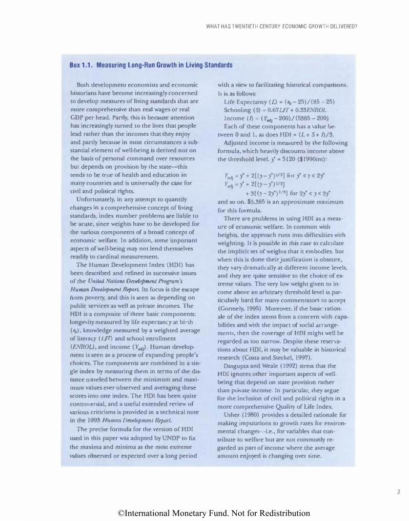
Box 1.1. Measuring long-Run Growth in living Standards
Both development economists and economic
historians have become increasingly concerned
to develop measures of li\ing standards that are
more comprehensive than real wages or real
GOP per head. Partly, this is because attention
has increasingly turned to the lives that people
lead rather than the incomes that the} enjo)
and partly because in most circumstances a sub
stantial element of well-being is derived not on
the basis of personal command over resources
but depends on provision by the state--this
tends to be true of health and education in
many countries and is universally the case for
civil and political rights.
Unfortunately. in any attempt to quantif)
changes in a comprehcnsive concept of lhing
standards, index number problems are liable to
be acute, since weights ha\e to be developed for
the various components of a broad concept of
economic welfare. In addition, some important
aspects of well-being may not lend themselves
readily to cardinal measurement.
The Human Development Index (HDI) has
been described and refined in successi\'e issue�
of the Uml£d fo\atumJ DfVflopmml Program's Human Det>tlqpmnlf RL>port. Its focus is the �ape
from poverty, and this is seen a'> depending on
public service� as well as private incomes. The
HDI is a compo�ite of three basic components:
longevity measured by life expectancy at birth
(e0), knowledge measured by a weighted average
of literacy ( U1) and school enrollment
(ENROL). and income ( �'dJ). Human develop
ment is seen a� a procec;s of expanding people\
choices. The componcn� are combined in a sin
gle index by mea,uring them in terms of the di�
tance traveled between the minimum and maxi
mum values ever observed and averaging t.hese
scores into one index. The HDl has been quite
controversial, and a useful extended review of
various criticisms is provided in a technical note
in the 1993 1/umrm Df!Jrlopmml RRport. The precise formula for the version of HOI
used in this paper was adopted by UNDP to ftx the maxima and minima as the most extreme
values observed or expected over a long period
with a view to facilitating histOrical comparisons.
h is as follows:
Life Expectancy ( L) = ( 'o -25) I (85 - 25) Schooling (S) = 0.67 UT + 0.33ENROL Income (I) = ( Y .WJ- 200) I (5385 -200) Each of these componen� ha� a value be-
tween 0 and 1, as does HOI= (L + S + 1)13. Adjusted income is measured b) the following
formula, which heavily di�count.s income above
the threshold level, i' = 5120 CS1990int):
t-:l(lj = y" t 2[ (y -/) l/2) f(u y' < ) < 2i
YadJ = i + 2[(y-'f) l!:Z) +3[(y-2y")1 'J tor2y'<y<3l
and � on. $5,385 i� an approximate ma.ximum
for this formula.
There are problems in using 1101 as a meas
ure of economic welfare. In common \vith
heights, the approach runs into difficulties with
weighting. It is possible in this case to calculate
the implicit set of weighL\ that it embodies, but
when this is done their justification is obscure,
they vary dramatically at diflerent income levels,
and they are quite sensitive to the choice of ex
treme values. The very low wetght given to in
come above an arbitr<�ry threshold level is par
ticular)> hard for man) commentators to accept
(Gormcly, 1995). Moreo,er. if the basic ration
ale of the index stems ft·om a concern with capa
bilities and with the impact of social at-range
mcnts, then the coverage of liD I might well be
rt·garded as too narrow. Despite these reserva
tions about HDI, it may be valuable in historical
research (Costa and Steckel, 1997). Dasgupta and Weale ( 1992) stre'' that the
HOI ignores other important aspects of well
being that depend on sLate pro.,.ision rather
than private income. In particular, they argue
for the inclusion of civil and political rights in a
more comprehensive Quality of Life Index.
Usher ( 1980) provides a detailed r-ationale for
making imputations to growU1 r-ates for environ
mental changes--i.e., for variables that con
tribute to welfare but are not commonly re
garded as part of income where the average
amount enjoyed � changing over time.
3
©International Monetary Fund. Not for Redistribution
4
CHAPTER I GLOBALIZATION AND GROWTH IN THE TWENTIETH CENTURY
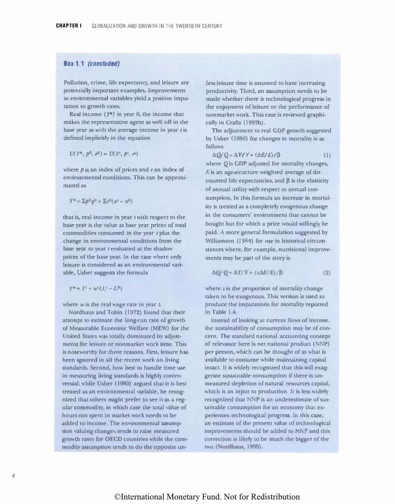
Box 1.1 (concluded)
Pollution, crime, life expectancy, and leisure are potentially important examples. Improvements in environmental variables yield a positive imputation to growth rates.
Real income ( Y*) in )Car 0, the income that makes the representative agent as weU off in the base year as \\ith the average income in year tis defined implicitly in the equation
U(Y*, po, eO)= U( )'1, p•, t1)
where pis an index of prices and tan index of environmental conditions. Tltis can be approximated as
that is, real income in year t with respect to the base year is the value at base year prices of total commodities consumed in the year t plus the change in environmental conditions from the base year to year t e,�aluated at the shadow
prices of the base year. In the case where only
leisure is considered a.<, an environmental variable, Usher suggc�ts the formula
Y*= }'l + w1(L1- LO)
where w is the real wage rate in year t. Nordhaus and Tobin (1972) found that their
attempt ro estimate the long-nm rate of growth
of Measurable Economic Welfare (MEW) for the United States w� totally dominated by adjustments for leLmre or nonmarket work time. This is noteworthy for three reasons. First, leisure ha.� been ignored in all the recent work on living �tandard�. Second, how be. t to handle time use
in measuring living standards is highly controversial; while Usher ( 1980) argued that it is best treated as an environmental variable, he recognized that others might prefer to see it as a regular commodity, in which case the total value of hours not spent in market work needs to be added to income. The environmental assumption valuing change� tend to raise measured growth rates for OECO countries while the commoditv assumption tends to do the opposite un-
less leisure time is assumed to have increasing productivity. Third, an a.�sumption needs to be made whether there is technological progress in the enjoyment of leisure or the performance of non market work. This case is re,'iewed graphlcallv in Crafts (1997b).
The adjustment to real GOP growth suggested by Usher (1980) for changes in monality is as follows
b.QIQ= b.Y/Y+ (b.£/E)/13 (1) where Q is GOP adjusted for mortality changes,
E is an age-structure weighted average of discounted life ex-pectancies, and 13 is the elasticity
of annual utility \vith respect to annual con
sumption. In this formula an increase in mortal
ity is treated as a completely exogenous change
in the consumers' environment that cannot be
bought but for which a price would willing!) be
paid. A more general formulation suggested by
Williamson ( 1984) for usc in historical circum
stances where, for e-xample, nutritional improve
ments may be part of the stOry is
(2)
where z is the proportion of mortaJity change taken to be exogenous. Tl1is ver ion b ltsed to produce the imputations for mortality reported in Table 1.4.
Instead of looking at current flows of income, the sustainability of consumption may be of concern. The standard national accounting concept of relevance here is net national product (N1\rp) per person, which can be thought of as what is available to consume while maintaining capital intact. It is widely recogniLed that this will exag
gerate sustainable consumption if there is unmeasured depletion of natural reoources capital, which is an input to production. It is less widely recognized that NNP is an underestimate of sustainable consumption for an economy that experiences technological progress. In this case,
an estimate of the present value of technological improvements should be added to P and this correction b likely to be much the bigger of the two ( 'ordbaus, 1995).
©International Monetary Fund. Not for Redistribution
NNP can be thought of as the annuity equivalent of future consumption. Weitzman (1999) notes that this is calculated as if the present consumption of exhaustible resources will be available indefinitely at mday's real extraction cost, whereas in fact conventional NNP includes an element that is a form of temporary income based on the use of a finite stock that can be measured in principle as (price minus marginal extraction cost} times resource use. This amount expressed as a percentage of NNP represents the required correction.
The implications of future technological progress for sustainable consumption should
to extend this back to 1950 for many countries
and earlier than that for a few cases. These long
run HDI estimates, reported in Table 1.1, pro
vide a comparative context in which to place re
cent Third World development and, taken
together, Tables 1.1 and 1.2 offer a different an
gle on divergence between the First and Third
Worlds from that which emerges from historical
national accounting.
Using these tables, comparisons across coun
tries can be made both of levels of HDJ and also
of the speed of reduction in the distance from
maximum development in different eras. In ad
dition, HDI gaps between advanced and devel
oping countries can be considered. There are, of
course, data problems, but the broad outlines of
the estimates in Tables 1.1 and 1.2 are robust
enough for present purposes (Crafts, 1997a).
The coverage of the tables is determined by data
availability.
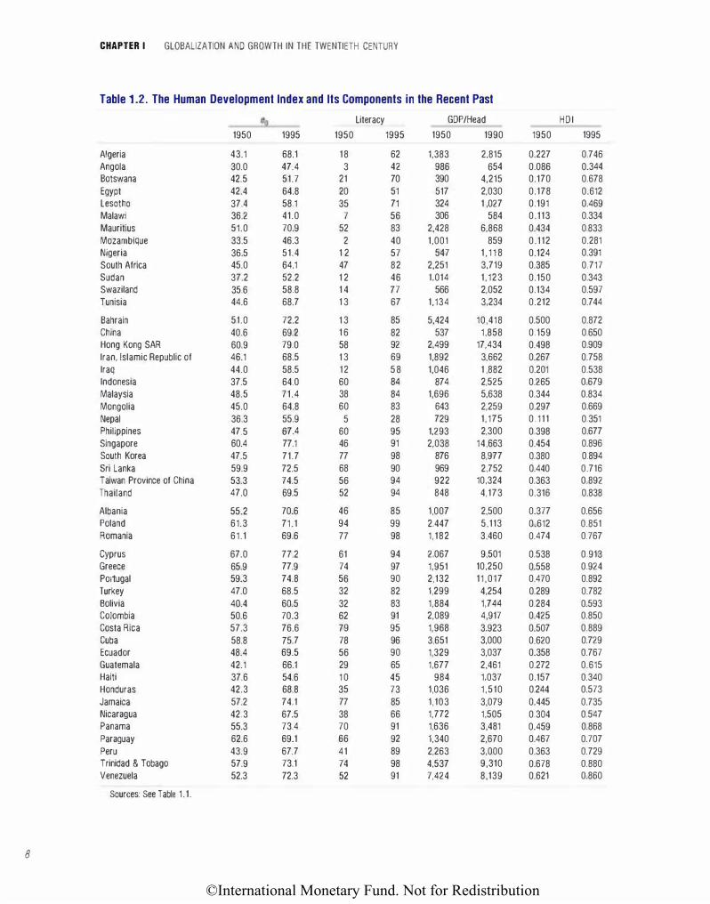
The most striking feature of these tables is
that the 1995 HDI scores for poor developing
countries in Table 1.2 are well ahead of the 1870
scores for the leading countries of that time
shown in Table 1.1. Australia's score of 0.539 in
1870 would rank 127th in the world in 1995.
Conversely, Mozambique's 1995 score of 0.281
(166th in the world) is distinctly above the levels
achieved in some parts of Europe (for example,
WHAT HAS TWENTIETH CENTURY ECONOMIC GROWTH DELIVERED?
also be recognized. TFP growth will raise production and thus consumption possibilities. If the average since 1950 were used as a projection for future TFP growth in the United States, then this would raise the annuity equivalent of future consumption to about40 percent above NNP (Weitzman, 1999). This suggests that the ntture productivity of R&D expenditures is critical and that the decline in TFP growth in the last quarter of the twentieth century may well have a big
ger impact on estimates of sustainable consumption than imminent exhaustion of raw materials supplies.
ll:aly and Spain) in 1870. At the same time, as
suming that the HDI score of 0.055 for India in
1913 represents the lowest level, the absolute
HDI gap of 0. 775 in 1995 between the best and
worst in the world (UNDP, 1998) is slightly big
ger than Ln 1913. Since 1950, however, there has
been a substantial fall in the gap between aver
age HDI in Africa and in the advanced counu·ies
of western Europe, Nonh Ameiica, and
Oceania-from 0.608 to 0.391.
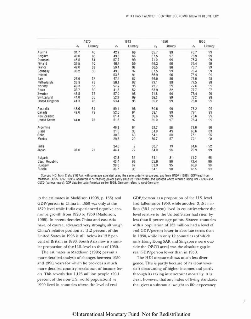
Looking at the components of HDl, the low
level of life expectancy at birth (e0) in leading
countries in 1870 is apparent witl1 the highest
figure at only 49.3 years, a level that has now
been exceeded by almost all counu·ies.
Research in historical demography long ago
confirmed that, during the twentieth cenrury,
improvements in mortality resulting from ad
vances in medical science and public health
measur·es have been largely independent of
changes in real income (Preston, 1975). The
levels of life expectancy (and HDI) now en
joyed by countries like Algeria and Tunisia were
simply not attainable in 1870 for any country
given the state of medical technology. By con
trast, levels of literacy, which in 1950 were still
very low in much of Africa and India. still com
pare unfavorably in many cases with tl1e leading
countries of 1870.
5
©International Monetary Fund. Not for Redistribution
6
CHAPTER I GLOBALIZATION AND GROWTH IN THE TWENTIETH CENTURY
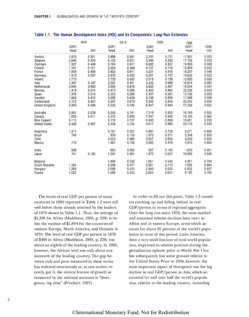
Table 1.1. The Human Development Index (HOI) and Its Components: Long-Run Estimates
1870
GOP/ GOP/ Head HOI Head
Austria 1,875 0.261 3,488 Belgium 2,640 0.429 4,130 Denmark 1,927 0.448 3,764 Finland 1,107 0.151 2,050 France 1,858 0.400 3,452 Germany 1,913 0.397 3,833 Ireland 1,773 2,733 Italy 1,467 0.187 2,507 Netherlands 2,640 0.450 3,950 Norway 1,416 0.374 2,473 Spain 1,376 0.219 2,255 Sweden 1,664 0.412 3,096 Switzerland 2,172 0.457 4,207 United Kingdom 3,263 0.496 5,032
Australia 3,801 0.539 5,505 Canada 1,620 0.411 4,213 New Zealand 3,115 5,178 United States 2,468 0.467 5,330
Argentina 1,311 3,797 Brazil 740 839 Chile 2,653 Mexico 710 1,467
India 558 663 Japan 741 0.160 1,334
Bulgaria 1,498 Czech Republic 1,164 2,096 Hungary 1,269 2,098 Russia 1,023 1,488
The levels of real GDP per person of many countries in 1990 reported in Table 1.2 were still well below those already attained by the leaders of 1870 shown in Table 1.1. Thus, the average of $1,336 for Africa (Maddison, 1995, p. 228) is below the median of $1,894 for the countries of western Europe, North America, and Oceania in 1870. The level of real GDP per person in 1870
of $480 in Africa (Maddison, 1995, p. 228) was about an eighth of the leading country. In 1990,
however, the African level was only about onesixteenth of the leading cou.!)try. The gap between rich and poor measured in these terms has widened enormously or, as one author recently put it, the central feature of growtl1 as measured by the national accounts is "divergence, big time" (Pritchett, 1997).
1913 1950 1996 GOP/ GOP/ 1995
HOI Head HOI Head HOI
0.501 3,731 0.731 17,951 0.933 0.621 5,346 0.833 17,756 0.933 0.677 6,683 0.857 19,803 0.928 0.389 4,131 0.740 15,864 0.942 0.611 5,221 0.818 18,207 0.946 0.632 4,281 0.787 19,622 0.925 0.563 3,518 0.736 15,820 0.930 0.441 3,425 0.666 16,814 0.922 0.676 5,850 0.867 18,504 0.941 0.588 5,403 0.862 22,256 0.943 0.368 2,397 0.581 13,132 0.935 0.628 6,738 0.858 17,566 0.936 0.679 8,939 0.843 20,252 0.930 0.730 6,847 0.844 17,326 0.932
0.781 7,218 0.853 18,169 0.932 0.682 7,047 0.842 19,109 0.960 0.797 8,495 0.868 15,621 0.939 0.733 9.617 0.866 23,719 0.943
0.521 4,987 0.758 8,271 0.888 0.159 1,673 0.371 5,346 0.809 0.360 3,827 0.620 9,250 0.893 0.182 2,085 0.418 4,979 0.855
0.055 597 0.160 1,643 0.451 0.381 1,873 0.607 19,582 0.940
0.332 1,651 0.540 4,301 0.789 0.471 3,501 0.713 7,595 0.884 0.431 2,480 0.634 5,852 0.857 0.252 2,834 0.651 4,120 0.769
In order to fill out this point, Table 1.3 considers catching up and falling behind in real GDP /person in terms of regional aggregates. Over the long run since 1870, the most marked and sustained relative declines have been in Africa and in eastern Europe, areas which account for about 20 percent of the world's population in most of this period. Latin America, then a very small fraction of total world population, improved its relative position during the globalization episode prior to World War I but has subsequently lost some ground relative to tl1e United States. Prior to 1950, however, the most important aspect of divergence was the big decline in real GDP /person in Asia, which accounted for well over half the world's population, relative to the leading country. According
©International Monetary Fund. Not for Redistribution
WHAT HAS TWENTIETH CENTURY ECONOMIC GROWTH DELIVERED?
1 870 1913 1950 1955
eo Literacy eo Literacy eo Literacy eo literacy
Austria 31.7 40 42.2 66 65.7 99 76.7 99 Belgium 40.0 66 49.6 86 67.5 97 76.9 99 Denmark 45.5 81 57.7 99 71.0 99 75.3 99 Finland 36.5 1 0 46.2 59 66.3 90 76.4 99 France 42.0 69 50.4 92 66.5 96 78.7 99 Germany 36.2 80 49.0 97 67.5 99 76.4 99 Ireland 53.8 91 66.9 96 76.4 99 Italy 28.0 32 47.2 62 66.0 86 78.0 98 Netherlands 38.9 78 56.1 97 72.1 99 77.5 99 Norway 49.3 55 57.2 98 72.7 99 77.6 99 Spain 33.7 30 41.8 52 63.9 82 77.7 97 Sweden 45.8 75 57.0 98 71.8 99 78.4 99 Switzerland 41.0 85 52.2 99 69.2 99 78.2 99 United Kingdom 41 .3 76 53.4 96 69.2 99 76.8 99
Australia 48.0 64 59.1 96 69.6 99 78.2 99 Canada 42.6 79 52.5 94 69.1 99 79.1 99 New Zealand 61 .4 95 69.6 99 76.6 99 United States 44.0 75 51 .6 92 69.0 97 76.4 99
Argentina 46.3 64 62.7 86 72.6 96 Brazil 31.0 35 51.0 49 66.6 83 Chile 30.3 63 54.1 80 75.1 95 Mexico 29.5 29 50.7 57 72.1 90
India 24.8 9 38.7 19 61.6 52 Japan 37.0 21 44.4 72 64.0 98 79.9 99
Bulgaria 42.3 53 64.1 81 71.2 98 Czech Republic 42.4 92 65.9 96 72.4 99 Hungary 39.5 87 63.9 95 68.9 99 Russia 36.7 38 64.1 90 65.5 99
Sources: HOI from Crafts (1997a), with coverage extended using the same underlying sources, and from UNOP (1998): GOP/head from Maddison (1995, 1997, 1998) measured in purchasing power parity adjusted 1990 dollars and updated where required using IMF (1999) and OECO (various years); GOP data for Latin America are for 1995; Germany refers to west Germany.
w the estimates in Maddison (1998, p. 158) real
GDP/person in China in 1950 was only at the
1870 level while India experienced negative eco
nomic growth from 1920 to 1950 (Maddison,
1995). In recent decades China and east Asia
have, of course, advanced very strongly, although
China's relative position at 11.2 percent of the
United States in 1996 is still below its 13.2 per
cent of Britain in 1890. South Asia now is a simi
lar proportion of the U.S. level to that of 1950.
The estimates in Maddison (1995) permit a
more detailed analysis of changes between 1950
and 1990, years for which he provides a much
more detailed country breakdown of income lev
els. This reveals that 1,123 million people (20.1
percent of the non-U.S. world population) in
1990 lived in countries where the level of real
GDP /person as a proportion of the U.S. level
had fallen since 1950, while another 3,151 mil
lion (56.1 percent) lived in countries where the
level relative to the United States had risen by
less than 5 percentage points. Sixteen countries
with a population of 165 million had a level of
real GDP /person lower in absolute terms than
in 1950, while in only 12 countries (of which
only Hong Kong SAR and Singapore were out
side the OECD area) was the absolute gap in
real GDP I person lower than in 1950.
The HOI measure shows much less diver
gence. This is partly because of its (controver
sial) discounting of higher incomes and partly
through its taking inlO account mortality. ll is
clear, however, that any index of living standards
that gives a substantial weight to life expectancy
1
©International Monetary Fund. Not for Redistribution
8
CHAPTER I GLOBALIZATION AND GROWTH IN THE TWENTIETH CENTURY
Table 1.2. The Human Development Index and Its Components in the Recent Past
eo Literacy GOP/Head
1950 1995 1950 1995 1950 1990
Algeria 43.1 68.1 18 62 1,383 2,815 Angola 30.0 47.4 3 42 986 654 Botswana 42.5 51.7 21 70 390 4,215 Egypt 42.4 64.8 20 51 517 2,030 Lesotho 37.4 58.1 35 71 324 1 ,027 Malawi 36.2 41.0 7 56 306 584 Mauritius 51.0 70.9 52 83 2,428 6,868 Mozambique 33.5 46.3 2 40 1,001 859 Nigeria 36.5 51.4 1 2 57 547 1 ,118 South Africa 45.0 64.1 47 82 2,251 3.719 Sudan 37.2 52.2 1 2 46 1,014 1,123 Swaziland 35.6 58.8 1 4 77 566 2,052 Tunisia 44.6 68.7 13 67 1,134 3,234
Bahrain 51.0 72.2 13 85 5,424 10,418 China 40.6 69.2 16 82 537 1,858 Hong Kong SAR 60.9 79.0 58 92 2,499 17,434 Iran, Islamic Republic of 46.1 68.5 13 69 1,892 3,662 Iraq 44.0 58.5 12 58 1,046 1 ,882 Indonesia 37.5 64.0 60 84 874 2,525 Malaysia 48.5 71.4 38 84 1,696 5,638 Mongolia 45.0 64.8 60 83 643 2,259 Nepal 36.3 55.9 5 28 729 1,175 Philippines 47.5 67.4 60 95 1,293 2,300 Singapore 60.4 77.1 46 91 2,038 14,663 South Korea 47.5 71.7 77 98 876 8,977 Sri Lanka 59.9 72.5 68 90 969 2.752 Taiwan Province of China 53.3 74.5 56 94 922 10,324 Thailand 47.0 69.5 52 94 848 4,173
Albania 55.2 70.6 46 85 1,007 2,500 Poland 61.3 71.1 94 99 2.447 5,113 Romania 61.1 69.6 77 98 1,182 3,460
Cyprus 67.0 77.2 61 94 2.067 9,501 Greece 65.9 77.9 74 97 1,951 10,250 Portugal 59.3 74.8 56 90 2,132 11,017 Turkey 47.0 68.5 32 82 1,299 4,254 Bolivia 40.4 60.5 32 83 1,884 1,744 Colombia 50.6 70.3 62 91 2,089 4,917 Costa Rica 57.3 76.6 79 95 1,968 3,923 Cuba 58.8 75.7 78 96 3,651 3,000 Ecuador 48.4 69.5 56 90 1,329 3,037 Guatemala 42.1 66.1 29 65 1,677 2,461 Haiti 37.6 54.6 10 45 984 1,037 Honduras 42.3 68.8 35 73 1,036 1,510 Jamaica 57.2 74.1 77 85 1,103 3,079 Nicaragua 42.3 67.5 38 66 1,772 1,505 Panama 55.3 73.4 70 91 1,636 3,481 Paraguay 62.6 69.1 66 92 1,340 2,670 Peru 43.9 67.7 41 89 2,263 3,000 Trinidad & Tobago 57.9 73.1 74 98 4,537 9,310 Venezuela 52.3 72.3 52 91 7,424 8,139
Sources: See Table 1.1.
HOI
1950 1995
0.227 0.746 0.086 0.344 0.170 0.678 0.178 0.612 0.191 0.469 0.113 0.334 0.434 0.833 0.112 0.281 0.124 0.391 0.385 0.717 0.150 0.343 0.134 0.597 0.212 0.744
0.500 0.872 0.159 0.650 0.498 0.909 0.267 0.758 0.201 0.538 0.265 0.679 0.344 0.834 0.297 0.669 0.111 0.351 0.398 0.677 0.454 0.896 0.380 0.894 0.440 0.716 0.363 0.892 0.316 0.838
0.377 0.656 0.612 0.851 0.474 0.767
0.538 0.913 0.558 0.924 0.470 0.892 0.289 0.782 0.284 0.593 0.425 0.850 0.507 0.889 0.620 0.729 0.358 0.767 0.272 0.615 0.157 0.340 0.244 0.573 0.445 0.735 0.304 0.547 0.459 0.868 0.467 0.707 0.363 0.729 0.678 0.880 0.621 0.860
©International Monetary Fund. Not for Redistribution
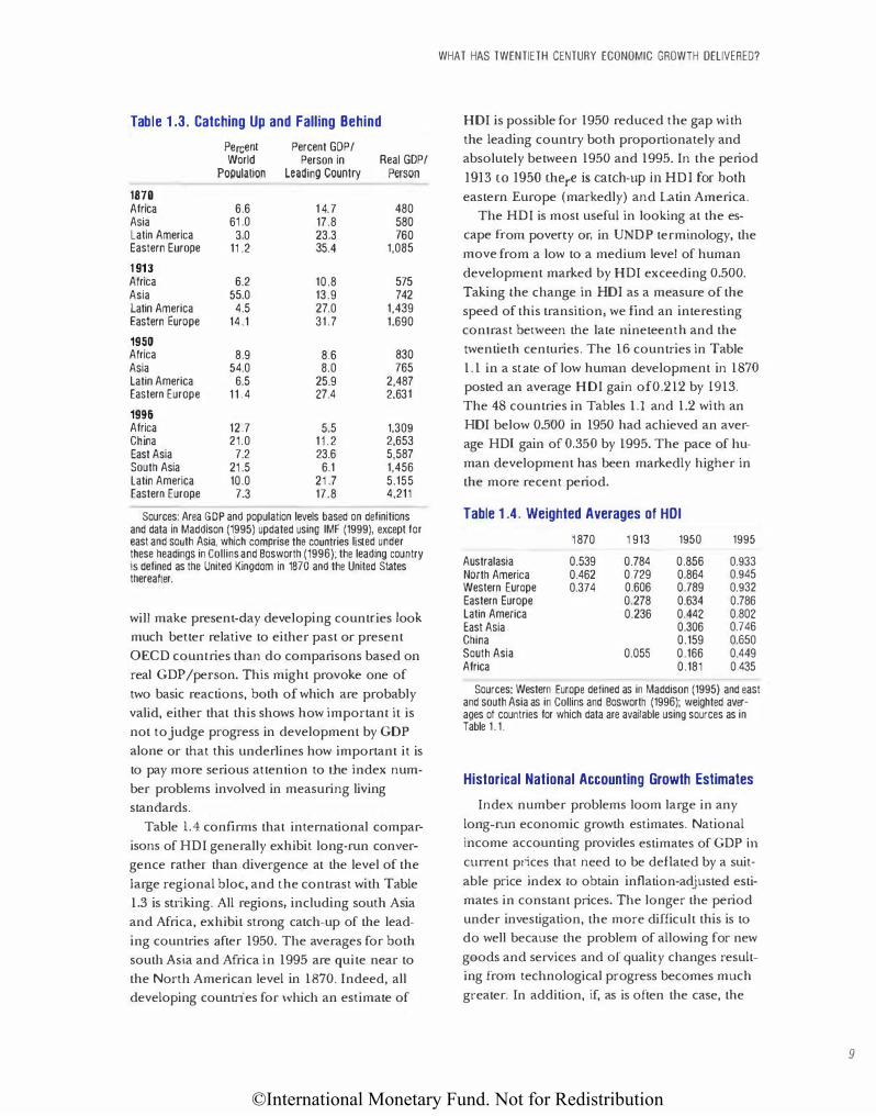
Table 1 .3. Catching Up and Falling Behind
Percent Percent GOP/ World Person in Real GOP/
Population Leading Country Person
1870 Africa 6.6 1 4.7 480 Asia 61 .0 17.8 580 Latin America 3.0 23.3 760 Eastern Europe 11.2 35.4 1,085
1 913 Africa 6.2 10.8 575 Asia 55.0 13.9 742 Latin America 4.5 27.0 1,439 Eastern Europe 14.1 31.7 1,690
1950 Africa 8.9 8.6 830 Asia 54.0 8.0 765 Latin America 6.5 25.9 2,487 Eastern Europe 1 1 . 4 27.4 2,631
1996 Africa 12.7 5.5 1,309 China 21.0 11.2 2,653 East Asia 7.2 23.6 5,587 South Asia 21 .5 6.1 1,456 Latin America 10.0 21.7 5,155 Eastern Europe 7.3 17.8 4,211
Sources: Area GOP and population levels based on definitions and data in Maddison (1995) updated using IMF (1999), except for east and south Asia, which comprise the countries listed under these headings in Collins and Bosworth (1996): the leading country Is defined as the United Kingdom in 1870 and the United States thereafter.
will make present-day developing countries look
much better relative to either past or present
OECD countries than do comparisons based on
real GDP/person. This might provoke one of
two basic reactions, both of which are probably
valid, either that this shows how important it is
not to judge progress in development by GDP
alone or that this underlines how important it is
to pay more serious attention to the index num
ber problems involved in measuring living
standards.
Table 1.4 confirms that international compar
isons of HDI generally exhibit long-run conver
gence rather than divergence at the level of the
large regional bloc, and the contrast with Table
1.3 is suiking. All regions, including south Asia
and Africa, exhibit strong catch-up of the lead
ing countries after 1950. The averages for both
south Asia and Africa in 1995 are quite near to
the North American level in 1870. Indeed, all
developing countries for \Vhich an estimate of
WHAT HAS TWENTIETH CENTURY ECONOMIC GROWTH DELIVERED?
HDI is possible for 1950 reduced the gap with
the leading country both proportionately and
absolutely between 1950 and 1995. In the period
1913 to 1950 there is catch-up in HDI for both
eastern Europe (markedly) and Latin America.
The HDI is most useful in looking at the es
cape from poverty or, in UNDP terminology, the
move from a low to a medium level of human
development marked by HDI exceeding 0.500.
Taking the change in HDI as a measure of the
speed of this transition, we find an interesting
contrast between the late nineteenth and the
twentieth centuries. The 16 countries in Table
1.1 in a state of low human development in 1870
posted an average HDI gain of0.212 by 1913.
The 48 countries in Tables 1.1 and 1.2 with an
HDI below 0.500 in 1950 had achieved an aver
age HDI gain of 0.350 by 1995. The pace of hu
man development has been markedly higher in
the more recent period.
Table 1 .4. Weighted Averages of HOI
Australasia North America Western Europe Eastern Europe Latin America East Asia China South Asia Africa
1870
0.539 0.462 0.374
1913
0.784 0.729 0.606 0.278 0.236
0.055
1950
0.856 0.864 0.789 0.634 0.442 0.306 0.159 0.166 0.181
1995
0.933 0.945 0.932 0.786 0.802 0.746 0.650 0.449 0.435
Sources: Western Europe defined as in Maddison (1995) and east and south Asia as in Collins and Bosworth (1996); weighted averages of countries for which data are available using sources as in Table 1.1 .
Historical National Accounting Growth Estimates
Index number problems loom large in any
long-run economic growth estimates. National
income accounting provides estimates of GDP in current pt;ces that need to be deflated by a suit
able price index to obtain inflation-adjusted esti
mates in constant prices. The longer the period
under investigation, the more difficult this is to
do well because the problem of allowing for new
goods and services and of quality changes result
ing from technological progress becomes much
greater. In addition, if, as is often the case, the
9
©International Monetary Fund. Not for Redistribution
10
CHAPTER I GLOBALIZATION AND GROWTH IN THE TWENTIETH CENTURY
reason for making the growth estimate is to pro
vide information on changes in living standards, it will be necessary to take account of aspects of
well-being that are omitted from GDP such as
changes in leisure or longevity, and it may also be appropriate to consider the sustainability of
consumption (see Box 1 .1 and the section on
globaJization, below).
It is generally accepted that, in advanced west
ern economies in the recent past, inflation has been exaggerated by conventional measurement
techniques and thus the growth rate of real GDP
has been understated. This has been studied in
tensively for the United States, and in a recem
survey of the evidence, Shapiro and Wilcox (1996) argue that the present-day bias is proba
bly somewhere between 0.6 and 1.5 percentage
points per year. The problem is not new, al
though it has probably become more selious
during the past hundred years as the composi
tion of GDP has moved away from run-of-themill commodities toward services that are more
difficult to measure-government activities, and
durable goods. By conu·ast, in communist coun
tries it is common for official statistics to underestimate inflation; for example, the recent study by Maddison (1998) finds it necessary to reduce
officiaJ estimates of Chinese growth since 1978
by about 2 percent per year-a correction that is
incorporated into the tables in this chapter.
Leaving aside the index number problems for
the moment, Table 1.5 reports the available estimates and changes the focus from levels to
growth rates. The table is based on the peri
odization in Maddison ( 1995), which is useful
for OECD countries in particular for separating
out the disturbed years around the depression
and the two World Wars (1913-50) and what is
often termed the Golden Age of growth plior to
the first OPEC shock (1950-73). Obviously, for
some cow1tries and some purposes, for example,
an examination of the impact of communism on eastern European growth or of reform on
Chinese growth, this &·amework is not so suit
able. Nor is this design set up to highlight shorter-run fluctuations in growth rates such as
the collapse of the early 1930s.
The first point to note from Table 1 .5 is that
twentieth century growth has generally been
much stronger than that prior to 1870. Thus, regions like India and Latin America where citi
zens are perhaps disappointed not to have
matched the east Asian growth rates of the last
four decades have nevertheless performed much
better than in the mid-nineteenth century, and
over the whole period since 1950 they have
grown faster than did the United Kingdom and the United States between 1820 and 1870.
Under mid- and even late nineteenth century
conditions, 1.5 to 1.8 percent a year was about
the maximum growth rate except in a few "re
gions of recent settlement" such as Argentina
and Canada. This, however, represented a major break
through from pre-Indusu·ial Revolution growth
capabilities, where long-run growth at 0.2 per
cent a year was a good resul L. Recen L research
has established that, even during the First
Industrial Revolution, Blitain achieved a growth
rate of real GDP per person no higher than
about 0.4 percent a year between 1780 and 1830
(Crafts and Harley, 1992). Indeed, the experi
ence of Industrial Revolution Britain, while rep
resenting a major breakthrough from the past in
terms of technological advance and resulting in
extremely rapid industrialization and urbaniza
tion, is also remarkable, viewed through a modern lens, for what it reveals about the limits to
growth in the leading economy of the midnineteenth century.
By modern standards, Industrial Revolution
Britain had a very modest growth potential.
Investment rates and formal schooling were
very low relative to twentieth century levels, and
research and development spending was negligible. Market sizes were still small, and tradi
tional rent-seeking occupations absorbed much
of the talent in the economy. The costs both of
inventing and protecting the profits from inven
tion were relatively high compared with later periods. Growth was based on quite different
foundations from those charactelizing success stories during the twentieth century(Crafts,
1998).
©International Monetary Fund. Not for Redistribution
WHAT HAS TWENTIETH CENTURY ECONOMIC GROWTH DELIVERED?
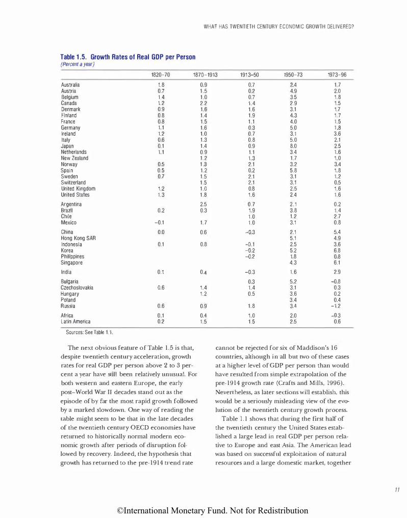
Table 1.5. Growth Rates of Real GOP per Person (Percent a year)
1820-70 187Q-1913 191 3-50 1950-73 1973-96
Australia 1.8 Austria 0.7 Belgium 1.4 Canada 1.2 Denmark 0.9 Finland 0.8 France 0 8 Germany 1.1 Ireland 1.2 Italy 0.6 Japan 0.1 Netherlands 1.1 New Zealand Norway 0.5 Spain 0.5 Sweden 0.7 Switzerland United Kingdom 1.2 United States 1.3
Argentina Brazil 0.2 Chile Mexico -0.1
China 0.0 Hong Kong SAR Indonesia 0.1 Korea Philippines Singapore
India 0.1
Bulgaria Czechoslovakia 0.6 Hungary Poland Russia 0.6
Africa 0.1 Latin America 0.2
Sources: See Table 1.1.
The next obvious feature of Table 1.5 is that,
despite twentieth century acceleration, growth
rates for real GDP per person above 2 to 3 per
cent a year have stiU been relatively unusual. For
both western and eastern Europe, the early
post-World War n decades stand out as the
episode of by far the most rapid growth followed by a marked slowdown. One way of reading the
table might seem to be that in the late decades
of the LWentieth century OECD economies have
returned to historically normal modern eco
nomic growth after periods of disruption followed by recovery. Indeed, the hypothesis that
growth has returned to the pre-1914 u·end rate
0.9 1.5 1.0 2.2 1.6 1.4 1.5 1.6 1.0 1.3 1.4 0.9 1.2 1.3 1.2 1.5 1.5 1.0 1.8
2.5 0.3
1.7
0.6
0.8
0.4
1.4 1.2
0 9
04 1.5
0.7 2.4 1.7 0.2 4.9 2.0 0.7 3.5 1.8 1.4 2.9 1.5 1.6 3.1 1.7 1.9 4.3 1.7 1.1 4.0 1.5 0.3 5.0 1 .8 0.7 3.1 3.6 0.8 5.0 2.1 0.9 8.0 2.5 1.1 3.4 1.6 1.3 1.7 1.0 2.1 3.2 3.4 0.2 5.8 1.8 2.1 3.1 1.2 2.1 3.1 0.5 0.8 2.5 1.6 1.6 2.4 1.6
0.7 2.1 0.2 1.9 3.8 1.4 1.0 1.2 2.7 1.0 3.1 0.8
-o.3 2.1 5.4 5.1 4.9
-o.1 2.5 3.6 -o.2 5.2 6.8 -Q.2 1.8 0.8
4.3 6.1
-0.3 1.6 2.9
0.3 5.2 -0.8 1.4 3.1 0.3 0.5 3.6 0.2
3.4 0.4 1.8 34 -1.2
1.0 2.0 -D.3 1.5 2.5 0.6
cannot be rejected for six of Maddison's 16
countries, although in all but LWo of these cases
at a higher level of GDP per person than would
have resulted from simple extrapolation of the pre-1914 growth rate (Crafts and Mills, 1996).
Nevertheless, as later sections will establish, this
would be a seriously misleading view of the evo
lution of the LWentieth century growth process.
Table 1 .1 shows that during the first half of
the twentieth century the Urrited States established a large lead in real GDP per person rela
tive to Europe and east Asia. The American lead
was based on successful exploitation of natural
resources and a large domestic market, together
11
©International Monetary Fund. Not for Redistribution
12
CHAPTER I GLOBALIZATION AND GROWTH IN THE TWENTIETH CENTURY
with prowess in high technology based on terti
ary education, that other countries found hard
to emulate. Also, the World Wars did not dam
age the American economy, as they did Germany
and Japan. Since 1950, many western European and east Asian countries have considerably re
duced the percentage (if not the absolute) gap
with the United States. Thus, in 1950 levels of
GDP per person in France and South Korea
were 54 and 9 percent, respectively, of that in
the United States, but 77 and 54 percent, respectively, in 1996 and 1969, and 21 percent for both
in 1900. While the gap between the richest and poorest has continued to widen, there has been
a significant catch-up with the leader by OECD
and "Tiger" economies. The fastest growth has been achieved by
economies that are successfully catching up from
well behind the leader, such as high-performing
east Asian economies in recent decades, while the United States has not exceeded 2.4 percent a
year in any of these periods. The fast growth in
postwar Europe also benefited from catch-up
and seems to owe a good deal to the reduction
in bar.-iers to the emulation of American technology, as well as the reversal of earlier policy er
rors and the return to peacetime. Nelson and
Wright ( 1 992) stress the reduction in the advan
tage that America had gained from cheap natu
ral resources and a large domestic market as
u·ansport costs fell and European integration
and trade liberalization proceeded. Investment�
by Europeans in human capital and in research
and development (R&D) facilitated the codifica
tion and spread of technological know-how,
while high volumes of physical investment were achieved on either side of the Iron Curtain.
Growth, however, slowed down again well before
the Europeans (or the japanese) had completed
their catch-up with the United S tates.
This is especially true of the communist coun
tries, which in the 1960s were sometimes
thought likely to overtake the United States be
fore the end of the twentieth century. Although
they mobilized huge investment programs, capital accumulation ran into severely diminishing
returns, and incentive structures under commu-
nism were not conducive to sustaining hlgh rates of innovation (Easterly and Fischer, 1995). Had
catch-up been as successful as in western
Europe, countries like the Czech Republic and
Hungary could have been expected to have GDP
per person in 1996 at around the level of Auso·ia
or Italy-that is, at least $10,000 (1990 interna
tional) higher (Fischer and others, 1998).
Table 1.5 reports striking differences in
growth performance among the now advanced
economies, which have been reflected in relative
advance and decline in levels of real GDP per
person. The United Kingdom, which in 1900 still
had the highest real GDP per person, was by
1996 only thirteeth of the countries listed and
had been overtaken by most European and several Asian couno·ies, including Hong Kong SAR and Singapore. Conversely, japan ranks eighth
in 1996 but in 1900 had an income level below
that of Russia. The damage done by communism
is underlined by comparing the post- 1950 per
formance of former Czechoslovakia and
Hungary (data refer to the area of those coun
tries as in 1990) with that of Austria and Italy.
At first glance, Table 1.5 may seem to suggest that there was more r·eason to be bullish about
1:\'lentieth century growth in 1973 than now. The obstacles of colonialism, the World Wars, and
the Depression seemed to be in the past and to
many it seemed reasonable to suppose that rapid
catch-up growth might spread much more
widely. For the West, the power of technology, and th.e computer revolution in particular,
seemed to promise sustained fast growth. Clearly, there has been a substantial slowdown in
world growth in the last quarter century from which only Asia (until recently) ha.s largely
escaped.
So the growth experience of the last quarter
century has produced several puzzles for growth
economists. One is to produce an adequate ac
count of the reasons for very strong growth in
east Asia while many other regions, including
most of Afr-ica, have had a dismal growth failure.
It seems clear that a full explanation of these
contrasting outcomes requires something more
than can be found in conventional growth mod-
©International Monetary Fund. Not for Redistribution
els, and this has promoted investigations of what,
following Abramovi tz ( 1 986), might be termed
"social capability" for catch-up growth. Another
new issue that has emerged following the devel
opment of endogenous growth models is to ex
plain the failure of growth to accelerate in the
United States despite increased investment in
human capital and R&D (Jones, 1995).
Adjusted GOP as a Guide to long-Run living Standards
During the twentieth century there have been
big changes in hours spent on market work and
in mortality in the countries for which we have
long-run estimates. Table 1 . 1 showed that aver
age life expectancy at birth has roughly doubled
since 1870 in leading OECD economies. In the
same period, hours worked per person em
ployed have roughly halved (Maddison, I 995).
Both of these are aspects of improved living stan
dards that would not have been captured by
growth in real GOP. Usher (1980) argues that it
is both possible and desirable to augment meas
ures of economic g1·owth to include these com
ponents of well-being (see Box 1 . 1 ) . Although
there is no consensus on exactly how best to ac
complish imputations of this kind, it is useful to
consider illustrative calculations along the lines
proposed by Usher simply because the changes
have been so great.
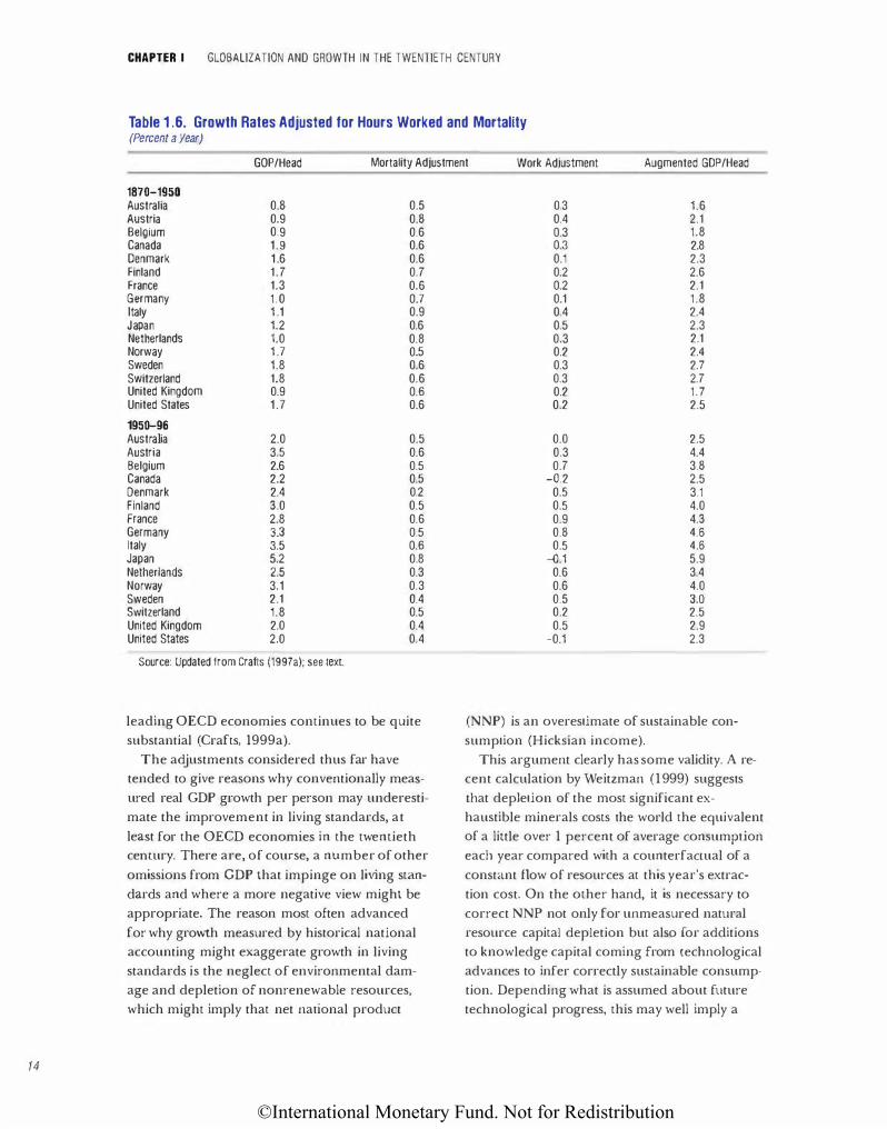
Crafts ( 1 997a) explains in detail the method
used to obtain the undeniably crude estimates in
Table 1.6, which are almost certainly underesti
mates of the imputations that should be made
for changing market work hours and mortality.
Improvements in life expectancy that are unre
lated to personal consumption expenditure are
valued on a willingness to pay basis based on
nineteenth century rather than twentieth cen
tury behavior, which would yield much bigger
welfare gains (Nordbaus, 1998), while reduc
tions in market work, valued using wages for
gone, ignore the possibility of technical progress
in nonmarket work. Even so, the results raise
growth rates an.d, in some cases, by a substantial
amount. Applications of this methodology would
WHAT HAS TWENTIETH CENTURY ECONOMIC GROWTH DELIVERED?
not always give this result-for example, in
Industrial Revolution Britain there may well
have been periods when the adjustment would
tend to reduce growth (Crafts, 1999b).
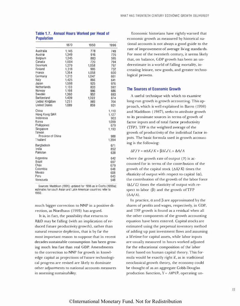
Table 1.7 highlights the variability of hours
worked per person over time and across coun
tries. These differences result partly from demo
graphic factors, partly from female labor force
participation, and partly from hours worked per
employee. With regard to this last, Latin
American and east Asian countries are now simi
lar to western Europe in the 1950s and the
1920s, respectively, but work years in both re
gions are well below the level of almost 3,000
charactel"istic of late nineteenth century
Europe.
Labor inputs per person are reported in Table
1.7 for Latin America in 1992 to be much lower
t11an for western Europe in 1870. This has im
portant implications for comparative productiv
ity performance as well as for welfare compar
isons. Thus, while t11e real GDP per person in
Latin America in 1996 of$5,155 reported in
Table 1.3 is less than 60 percent ahead of the U.K. level of $3,263 in 1870, real output per
hour worked was over three times that of the
U.K. level in 1870. The gap in real GDP per per
son clearly hugely understates the extent to
which economic welfare in Latin America has
outstripped the level attained in Britain in 1870,
not only because life expectancy is so much
higher but also because labor inputs are so
much lower.
Differences in the age structure of the popula
tion or in hours worked per person employed
per year can also mean that comparative real
GDP per person is a poor indicator of labor pro
ductivity in the present day. This turns out tO matter most when comparisons are made be
tween east Asia and Europe. Thus, wbereas by
1996 the leading Tiger economies, Hong Kong
SAR and Singapore, had overtaken most of west
ern Europe in real GOP per person, there was
still a substantial gap in terms of labor productiv
ity. Their continued fast growth prior to the re
cent Asian crisis is less paradoxical when it is rec
ognized that their scope for catch-up of the
13
©International Monetary Fund. Not for Redistribution
14
CHAPTER I GLOBALIZATION AND GROWTH IN THE TWENTIETH CENTURY
Table 1 .6. Growth Rates Adjusted for Hours Worked and Mortality (Percent a year)
GOP/Head Mortality Adjustment Work Adjustment Augmented GOP/Head
1870-1950 Australia 0.8 0.5 Austria 0.9 0.8 Belgium 0.9 0.6 Canada 1.9 0.6 Denmark 1 .6 0.6 Finland 1.7 0.7 France 1.3 0.6 Germany 1 .0 0.7 Italy 1 .1 0.9 Japan 1.2 0.6 Netherlands 1.0 0.8 Norway 1 .7 0.5 Sweden 1.8 0.6 Switzerland 1.8 0.6 United Kingdom 0.9 0.6 United States 1 .7 0.6
1950-96 Australia 2.0 0.5 Austria 3.5 0.6 Belgium 2.6 0.5 Canada 2.2 0.5 Denmark 2.4 0.2 Finland 3.0 0.5 France 2.8 0.6 Germany 3.3 0.5 Italy 3.5 0.6 Japan 5.2 0.8 Netherlands 2.5 0.3 Norway 3.1 0.3 Sweden 2.1 0.4 Switzerland 1.8 0.5 United Kingdom 2.0 0.4 United States 2.0 0.4
Source: Updated from Crafts (1997a); see text.
leading OECD economies continues to be quite
substantial (Crafts, 1999a).
The adjustments considered thus far have tended to give reasons why conventionally meas
ured real GDP growth per person may underesti
mate the improvement in living standards, at
least for the OECD economies in the twentieth cemury. There are, of course, a number of other
omissions from GDP that impinge on living stan
dards and where a more negative view might be
appropriate. The reason most often advanced
for why growth measured by historical national accounting might exaggerate growth in living
standards is the neglect of environmental dam
age and depletion of nonrenewable resources,
which might imply that net national product
0.3 1.6 0.4 2.1 0.3 1.8 0.3 2.8 0.1 2.3 0.2 2.6 0.2 2.1 0.1 1.8 0.4 2.4 0.5 2.3 0.3 2.1 0.2 2.4 0.3 2.7 0.3 2.7 0.2 1.7 0.2 2.5
0.0 2.5 0.3 4.4 0.7 3.8
-o.2 2.5 0.5 3.1 0.5 4.0 0.9 4.3 0.8 4.6 0.5 4.6
-D.1 5.9 0.6 3.4 0.6 4.0 0.5 3.0 0.2 2.5 0.5 2.9
-0.1 2.3
(NNP) is an overestimate of sustainable con
sumption (Hicksian income).
This argument clearly has some validity. A recent calculation by Weitzman (1999) suggests
that depletion of the most significant ex
haustible minerals costs the world the equivalent of a little over 1 percent of average consumption
each year compared with a counterfaccual of a
constant flow of resources at this year's extrac
tion cost. On the other hand, it is necessary to
correct NNP not only for unmeasured natural
resource capital depletion but also for additions
to knowledge capital coming from technological
advances to infer correctly sustainable consump
tion. Depending what is assumed about future
technological progress, this may well imply a
©International Monetary Fund. Not for Redistribution
Table 1.7. Annual Hours Worked per Head of Population
1870 1950 1996
Australia 1,145 778 749 Austria 1,349 916 725 Belgium 1,245 883 595 Canada 1,004 720 794 Denmark 1,279 1,058 797 Finland 1,318 995 732 France 1,364 1,058 600 Germany 1,213 1,047 661 Italy 1,425 866 641 Japan 1,598 925 976 Netherlands 1,133 833 592 Norway 1,198 996 686 Sweden 1,360 952 693 Switzerland 1,439 1,022 874 United Kingdom 1,251 989 764 United States 1,089 859 931
China 1 '11 0 Hong Kong SAR 1,127 Indonesia 903 Korea 1,099 Philippines 679 Singapore 1,193 Taiwan
Province of China 988 Thailand 1,394
Bangladesh 671 India 852 Pakistan 638
Argentina 642 Brazil 697 Chile 679 Colombia 648 Mexico 608 Peru 643 Venezuela 548
Sources: Maddison (1995) updated for 1996 as in Crafts (1999a); estimates for south Asian and Latin American countries refer to 1992.
much bigger correction to NNP in a positive di
rection, as Nordhaus ( l 995) has argued.
It is, in fact, the possibility that returns to
R&D may be falling (with an implication of re
duced future productivity growth), rather than
natural resource depletion, that is by far the
most important reason to suppose that in recent
decades sustainable consumption has been grow
ing much less fast than real GOP. Amendments
to the correction to NNP for growth in knowl
edge capital as projections of fuLUre technologi
cal progress are revised are likely to dominate
other adjustments to national accounts measures
in assessing sustainability.
WHAT HAS TWENTIETH CENTURY ECONOMIC GROWTH DELIVERED?
Economic historians have rightly warned that
economic growth as measured by historical na
tional accounts is not always a good guide to the
rate of improvement of average livi11g standards.
For most of the twentieth century, it seems likely
that, on balance, GDP growth has been an un
derestimate in a world of falling mortality, in
creasing leisure, new goods, and greater techno
logical prowess.
The Sources of Economic Growth
A useful technique with which to examine
long-run growth is growtJ1 accounting. This ap
proach, which is well explained in Sarro ( 1998)
and Maddison ( 1987), seeks to attribute growth
to its proximate sources in terms of growth of
factor inputs and of total factor productivity
(TFP). TFP is the weighted average of the
growili of productivity of the individual factor in
puts. The basic formula used in growth accoum
ing is the following:
.:lY/ Y= a.AK/ K+ �llL/ L + M/ A
where ilie growth rate of output ( Y) is ac
counted for in terms of tJ1e contribution of ilie
growth of the capital stock (.:lK/ K) times the
elasticity of output wiili respect to capital (<X), ilie contribution of the growili of the labor force
(M/ L) times the elasticity of output with re
spect to labor (�) and the growili ofTFP
(.:lA/ A). In practice, <X and � are approximated by the
shares of profits and wages, respecdvely, in GDP,
and TFP growth is found as a residual when all
the other components of ilie growth accounting
equation have been entered. Capital stocks are
estimated using the perpeLUal inventory method
of adding up past investment nows and assuming
a lifetime for capital assets, while labor inputs
are usually measured in hours worked adjusted
for the educational composition of the. labor
force based on human capital theory. This for
mula would be exactly right if, as in traditional
neoclassical growth tl1eory, tl1e economy could
be iliought of as an aggregate Cobb-Douglas
production function, Y = A�l.J. operating un-
15
©International Monetary Fund. Not for Redistribution
/6
CHAPTER I GLOBALIZATION AND GROWTH IN THE TWENTIETH CENTURY
der conditions of perfect competition and con
stant returns to scale. The parameter A would re
flect the state of technology, and TFP growth
would measure exogenous (Hicks-neutral) tech
nological change.
Caution is required before assuming that
residual TFP growth actually measures the con
tribution of technological change to economic
growth. According to traditional analysis, the
bias may go in either direction. First, technologi
cal change may be less than TFP growth if there
are scale economies or improvements in the effi
ciency with which resources are used or if im
provements in the quality of factors of produc
tion are underestimated, for example due to
unmeasured human capital accumulation
(Abramovitz, 1993). Second, if the elasticity of
substitution between factors of production is less
than 1 and technological change has a Hicks
labor-saving bias, as many analysts think is the
case, then conventional TFP growth underesti
mates the contribution of technological change
and the mismeasurement increases with the
growth in the capital to labor ratio, the degree
of labor-saving bias, and the inelasticity of substi
tution (Rodrik, 1997a).
Faster technological change raises the steady
state rate of growth of the capital stock in a tra
ditional neoclassical growth model, and so part
of its impact on growth compared with the coun
terfactual of no technological change shows up
in capital's measured contribution. The advent
of endogenous growth theory strengthens this
kind of reason to believe that the contribution
of technological change exceeds TFP growth.
Thus, in models that envisage endogenous inno
vation driving growth through expanded vari
eties of capital inputs, a fraction of the contribu
tion of the growth in varieties of capital
facilitated by R&D accrues to capital and is not
captured by the Solow residual. The undermea
surement will be greater the larger the endoge
nous component in technological progress
(Barro, 1998).
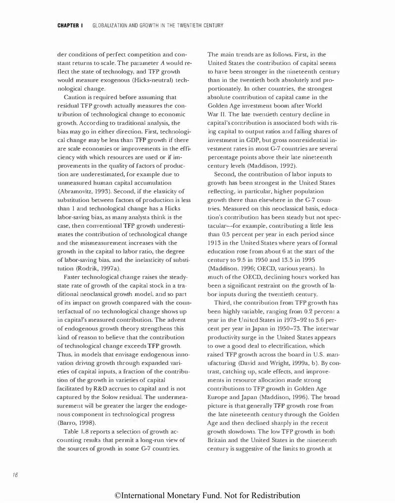
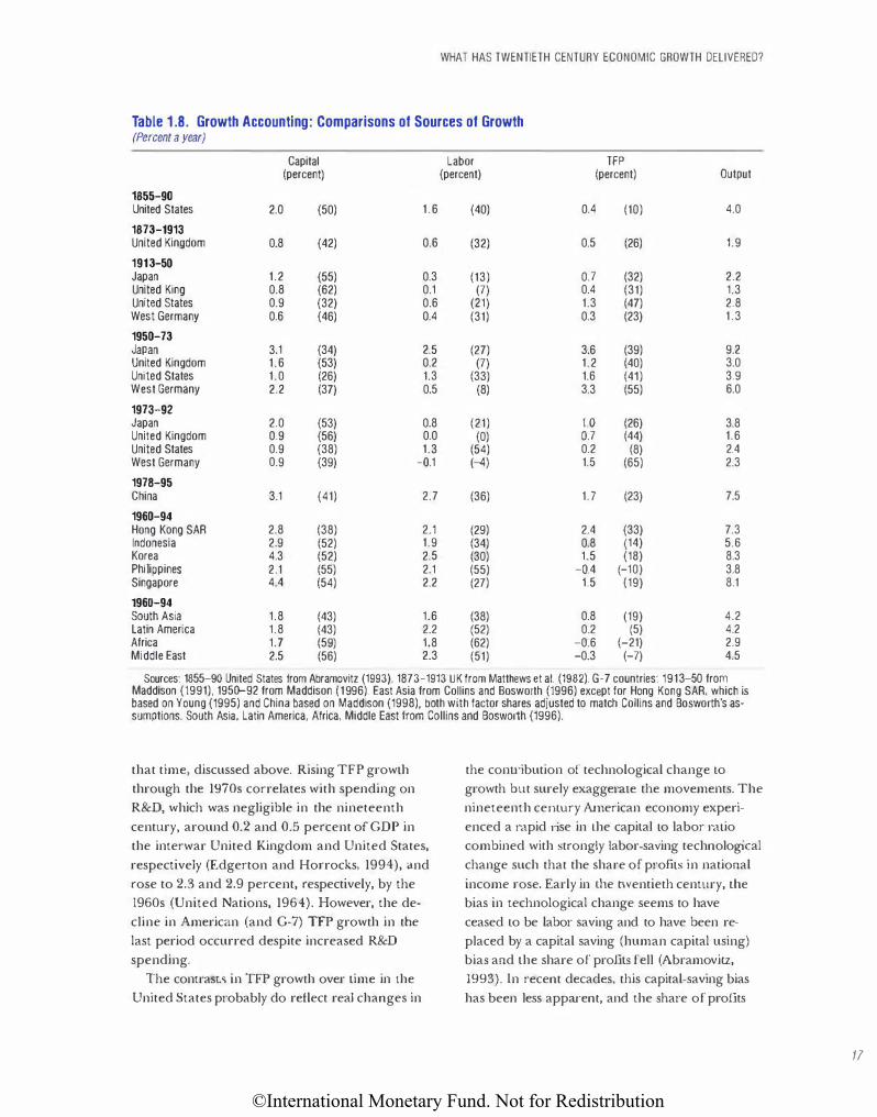
Table 1.8 reports a selection of growth ac
counting results that permit a long-run view of
the sources of growth in some G-7 counu·ies.
The main u·ends are as follows. First, in the
United States the contribution of capital seems
to have been stronger in the nineteenth century
than in the twentieth both absolutely and p•·o
portionately. In other countries, the strongest
absolme contribution of capital came in the
Golden Age investmem boom after World
War n. The late twenti.eth century decline in
capital's conu·ibution is associated both with ris
ing capital to output ratios and falling shares of
investment in GDP, but gross nonresidential in
vestment rates in most G-7 counu·ies are several
percentage points above their late nineteenth
century levels (Maddison, 1992).
Second, the contribution of labor inputs to
growth has been strongest in the United States
reflecting, in particular, higher population
growth there than elsewhere in the G-7 coun
tries. Measured on this neoclassical basis, educa
tion's contribution has been steady but not spec
tacular-for example, contributing a little less
than 0.5 percent per year in each period since
1913 in the United States where years of formal
education rose from about 6 at the stan of the
century to 9.5 in 1950 and 13.5 in 1995
(Maddison, 1996; OECD, various years). ln
much of the OECD, declining hours worked has
been a significant restraint on the growth of la
bor inputs during the twentieth century.
Third, the contribution from TFP growth has
been highly va•·iable, ranging from 0.2 percent a
year in the United States in 1973-92 to 3.6 per
cent per year in japan in 1950-73. The interwar
productivity surge in the United States appears
to owe a good deal to electrification, which
raised TFP growth across the board in U.S. man
ufacturing (David and Wright, 1999a, b). By con
trast, catching up, scale effects, and improve
ments in resource allocation made strong
contributions to TFP growth in Golden Age
Europe and Japan (Maddison, 1996). The broad
picture is that generally TFP growth rose from
the late nineteenth century through the Golden
Age and then declined sharply in the recent
grO\vth slowdown. The low TFP growth in both
Britain and the United States in the nineteenth
century is suggestive of the limits to growth at
©International Monetary Fund. Not for Redistribution
WHAT HAS TWENTIETH CENTURY ECONOMIC GROWTH DELIVERED?
Table 1 .8. Growth Accounting: Comparisons of Sources of Growth (Percent a year)
Capital Labor TFP (percent) (percent) (percent) Output
1855-90 United States 2.0 (50) 1 .6 (40) 0.4 (10) 4.0
1873-1913 United Kingdom 0.8 (42) 0.6 (32) 0.5 (26) 1.9
1913-50 Japan 1.2 (55) 0.3 (13) 0.7 (32) 2.2 United King 0.8 (62) 0.1 (7) 0.4 (31) 1.3 United States 0.9 (32) 0.6 (21) 1.3 (47) 2.8 West Germany 0.6 (46) 0.4 (31) 0.3 (23) 1 .3
195D-73 Japan 3.1 (34) 2.5 (27) 3.6 (39) 9.2 United Kingdom 1.6 (53) 0.2 (7) 1.2 (40) 3.0 United States 1 .0 (26) 1.3 (33) 1.6 (41) 3.9 West Germany 2.2 (37) 0.5 (8) 3.3 (55) 6.0
1973�92 Japan 2.0 (53) 0.8 (21) 1.0 (26) 3.8 United Kingdom 0.9 (56) 0.0 (0) 0.7 (44) 1.6 United States 0.9 (38) 1.3 (54) 0.2 (8) 2.4 West Germany 0.9 (39) -o.1 (-4) 1.5 (65) 2.3
1978-95 China 3.1 (41) 2.7 (36) 1.7 (23) 7.5
196D-94 Hong Kong SAR 2.8 (38) 2.1 (29) 2.4 (33) 7.3 Indonesia 2.9 (52) 1.9 (34) 0.8 (14) 5.6 Korea 4.3 (52) 2.5 (30) 1.5 (18) 8.3 Philippines 2.1 (55) 2.1 (55) -o.4 (-10) 3.8 Singapore 4.4 (54) 2.2 (27) 1.5 (19) 8.1
196D-94 South Asia 1.8 (43) 1.6 (38) 0.8 (19) 4.2 Latin America 1.8 (43) 2.2 (52) 0.2 (5) 4.2 Africa 1.7 (59) 1.8 (62) -0.6 (-21) 2.9 Middle East 2.5 (56) 2.3 (51) -0.3 (-7) 4.5
Sources: 1855-90 United States from Abramovitz (1993). 1873-1913 UK from Matthews et al. (1982). G-7 countries: 1913-50 from Maddison (1991), 195�92 from Maddison (1996). East Asia from Collins and Bosworth (1996) except for Hong Kong SAR, which is based on Young (1995) and China based on Maddison (1998), both with factor shares adjusted to match Collins and Bosworth's as-sumptions. South Asia, Latin America, Africa, Middle East from Collins and Bosworth (1996).
that time, discussed above. Rising TFP growth
through the 1970s correlates with spending on
R&D, which was negligible in the nineteenth
century, around 0.2 and 0.5 percent of GDP in
the interwar United Kingdom and United States,
respectively (Edgerton and Horrocks, 1994), and
rose to 2.3 and 2.9 percent, respectively, by the
1960s (United Nations, 1964). However, the de
cline in American (and G-7) TFP growth in the
last period occurred despite increased R&D
spending.
The contrasts in TFP growth over time in the
United States probably do reflect real changes in
the contribution of technological change to growth but surely exaggenue the movements. The
nineteenth century American economy experi
enced a rapid dse in 1.he capital to labor ratio
combined with strongly labor-saving technological
change such that the share of profits in national
income rose. Early in the twentieth century, 1.he
bias in technological change seems to have
ceased to be labor saving and to have been re
placed by a capital saving (human capital using)
bias and the share of profits fell (Abramovitz,
1993). In recent decades, this capital-saving bias
has been less apparent, and the share of profits
11
©International Monetary Fund. Not for Redistribution
18
CHAPTER I GLOBALIZATION AND GROWTH IN THE TWENTIETH CENTURY
has fluctuated with no su·ong trend. In the light
of the earlier discussion, it seems probable that
conventionally measmed TFP growth significantly
understates the role of technological change in
the nineteenth century and overstates it between the 1920s and the 1960s. The recent decline in
TFP growth in the United States appears paradox
ical in the light of the computer revolution and
this has prompted many to suspect that it may be, at least to some extent, a statistical artifact (G1;liches, 1994). We return to this issue in the
next section.
The developing world clearly offers some
striking comparisons with the advanced world,
although data limitations resu·ict measurement
LO the post-1960 period. The starLiing contrasts
in this period are between the much faster
growth in east Asia in a still to be completed
process of catching up with the OECD and the
growth failure in Mrica, which has fallen fur
ther behind and has seen real GDP per person
in the continent declining in the last quarter
century. Table 1 .8 shows negative TFP growth for
Mrica in the period 1960-94, and contributions
from factor inputs that look respectable until it
is recalled that population growth was nearly
3 percent a year. Probing behind these numbers,
the invesunem rate in Mrica has been held
down in real terms by the very high price of cap
ital goods in highly protectionjst economies, and
educational levels have remained low, rising
from 1.6 years in 1960 to only 3.5 years in 1994
(Collins and Bosworth, 1996). In east Asia the
invesunent rate has been high relative to histori
cal norms and has translated into a strong con
tribution from the capital stock because of un
usually low capital to output ratios (Fukuda,
1999). The contribution from labor inputs has
been boosted by a favorable demographic transi
tion and rapid increases in schooling, from an
average of 2.7 years in 1960 to 7.2 years in 1994
(Collins and Boswo1·th, 1996). The stronger TF P
growth in east Asia may partly reflect effective
ness in technology transfer that compares very favorably with other Third World experience
(Dahlman, 1994).
Comparisons of east Asian with European
g1·owth in the recem past are somewhat beside
the point given the differences in capital tO out
put ratios, scope for catch-up in TFP, and de
mography. Examining differences in tbe sources
of recent fast growth in east Asia and of 1·apid
growth in Europe during catch-up in the 1950s
and 1960s is instructive, however. Here, the obvi
ous point to stand out from Table 1.8 is that east Asian growth has relied much more heavily on
factor inputs, boLI1 labor and capital, and less on
TFP growth than that of Golden Age western
Germany. Although measurement error occa
sioned by factor-saving bias may exaggerate the TFP growth difference somewhat, the conclusion
that east Asian TFP growth has been outstanding relative LO that of Afr·ica but not so impressive by earlier European standards seems robust (Crafts,
1999a).
Convergence and Divergence
The large divergence in income levels and
growth rates that has emerged since L11e stan of modern economic growth seems hard to square
wiLI1 the traditional neoclassical growL11 model
that assumed constant returns to scale, diminish
ing returns to capital accumulation, and univer
sal technology that improved like manna from
heaven. Although some early work in the growth
regressions literature argued that differences in
income levels across the world could largely be
explained by human and physical capital per
worker (Mankiw, Romer, and Weil, 1992) and
tended to interpret P-convergence (i.e., the neg
ative relationship between growth rates and ini
tial labor productivity levels found in cross
section regressions when enough conditioning
variables are included) as consistem with the
augmemed-Solow growth model with conver
gence at 2 percent per year (Barro and
Sala-i-Martin, 1991), these interpretations are
now generally rejected (Temple, 1999).
Economic historians reviewing the experience
have tended to stress L11e importance of techno
logical congruence and social capability
(Abramovitz and David, 1996). The former re-
©International Monetary Fund. Not for Redistribution
lates to the profitability of using technology de
veloped in the leader(s) in potemial follower
countries with different factor endowments and
demand conditions. Thus, in the first half of the
twentieth century, U.S. technolog)', which was
natural-resource-intensive, physical capital-using,
and scale-dependent, was frequently not the op
timal choice of technique in European condi
tions. Greater integration of world markets and
reductions in the cost advantages of domestic
natural resource endowments combined with in
creased importance of intangible capital (R&D and education) subsequently reduced the obsta
cles to catch-up first within the OECD and later
elsewhere in east Asia. Social capability refers to
a counu-y's culture, institutions, and policy
framework tl1at influence the attractiveness of in
vestment and innovative activity and the effi
ciency with which technological possibilities are
exploited. The productivity gap with the leader
informs the potential for rapid catch-up growth
but catching up is not automatic. This coheres
with the more recent econometric evidence.
Prescott ( 1998) explores the possibilities of
calibrating a neoclassical production function to
account for cross-country labor productivity dif
ferences in terms of human and physical capital
per worker with TFP common to all countries
and concludes tl1at the evidence is not remotely
consistent with this hypothesis. While economet
ric evidence strongly supports diminishing re
turns to (broad) capital accumulation, estimates
of rates of conditional convergence are now
known to be highly sensitive to econometric
specification and there appears to be strong evi
dence both of differences in levels or rates of
growth ofTFP across countries. This strongly
suggests tllat both policy and institutions matter
for growth performance (Temple, 1999).
Globalization Then and Now
Many economists have discussed the twentieth
century in terms of a phase of globalization end
ing with World War [, followed by a phase of dis
integration through and until the reconstruction
after World War H. The past 50 years is then
GLOBALIZATION THEN AND NOW
seen in terms of a gradual liberalization of trade and capital flows followed by a new and deeper
version of globalization in the last quarter cen
rury or so. In both the OECD and the Third
World, perspectives on the advantage of outward
orientation have clearly varied dramatically over
time, as has the impetus to globalization from
technological change. The objectives of this sec
tion are to establish some of the key dimensions
of globalization and to explain why the process
was reversed in tl1e interwar period as govern
ments retreated to fmancial autarchy and trade
protectionism.
Globalization in Trade and Factor Flows
I t is widely known that for many coumries the
proponion of merchandise trade to GDP has
now returned to levels quite similar to those at
the start of the cenwry. At first glance, it might
appear tllat the world economy has simply re
turned to its old level of economic integration
and that international trade has merely resumed
its earlier importance. As has increasingly been
recognized, however, that view is seriously mis
leading. The nature of international trade is in
several respects quite differem now compared
with a hundred years ago, and it plays a much
larger part in world economic activity (Bordo,
Eichengreen, and Irwin, 1999).
Table 1.9 reports ratios of world merchandise
trade relative to world GDP and largely matches
the stylized facrs set out above. The trade ratio
was increasing rapidly before World War l, did
not exceed the 1913 level until the late 1960s,
and has risen sharply in recent decades.
However, the present level is unprecedentedly
high and represents both a massive increase over
the estimate of 1 percent for 1820 and a near
doubling of the 7 percent eslimated for 1950
(Maddison, 1995, p. 233). On tl1e other hand, in
the United Kingdom, the leading player in the
global economy of the late nineteenth century,
merchandise trade is now a much smaller pro
portion of GDP than it was then, and for the
United States the increase in the tTade ratio is
quite modest.
19
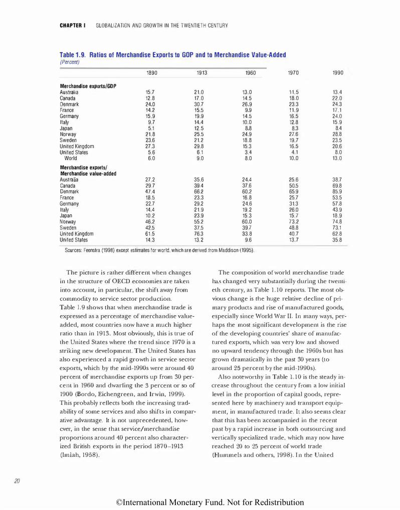
©International Monetary Fund. Not for Redistribution
20
CHAPTER I GLOBALIZATION AND GROWTH IN THE TWENTIETH CENTURY
Table 1 .9. Ratios of Merchandise Exports to GOP and to Merchandise Value-Added (Percent)
1890 1913 1960 1970 1990
Merchandise exports/GOP Australia 15.7 21.0 13.0 11.5 13.4 Canada 12.8 17.0 14.5 18.0 22.0 Denmark 24.0 30.7 26.9 23.3 24.3 France 14.2 15.5 9.9 11.9 17.1 Germany 15.9 19.9 14.5 16.5 24.0 Italy 9.7 14.4 10.0 12.8 15.9 Japan 5.1 12.5 8.8 8.3 8.4 Norway 21.8 25.5 24.9 27.6 28.8 Sweden 23.6 21.2 18.8 19.7 23.5 United Kingdom 27.3 29.8 15.3 16.5 20.6 United States 5.6 6.1 34 4.1 8.0
World 6.0 9.0 8.0 10.0 13.0
Merchandise exports/ Merchandise value-added Australia 27.2 35.6 244 25.6 38.7 Canada 29.7 39.4 37.6 50.5 69.8 Denmark 47.4 66.2 60.2 65.9 85.9 France 18.5 23.3 16.8 25.7 53.5 Germany 22.7 29.2 24.6 31.3 57.8 Italy 14.4 21.9 19.2 26.0 43.9 Japan 10.2 23.9 15.3 15.7 18.9 Norway 46.2 55.2 60.0 73.2 74.8 Sweden 42.5 37.5 39.7 48.8 73.1 United Kingdom 61.5 76.3 33.8 40.7 62.8 United States 14.3 13.2 9.6 13.7 35.8
Sources: Feenstra (1998) except estimates for world, which are derived from Maddison (1995).
The picture is rather different when changes
in the structure of OECD economies are taken
into account, in particular, the shift away from
commodity to service sector production.
Table 1.9 shows that when merchandise trade is
expressed as a percentage of merchandise value
added, most countries now have a much higher
ratio than in 1913. Most obviously, this is true of
the United States where the trend since 1970 is a
su·iking new development. The United States has
also experienced a rapid growth in service seclOr
exports, which by the mid-1990s were around 40
percent of merchandise exports up from 30 per
cent in 1960 and dwarfing the 3 percent or so of
1900 (Bordo, Eichengreen, and Irwin, 1999).
This probably reflects both the increasing tract
ability of some services and also shifts in compar
ative advantage. It is not unprecedented, how
ever, in the sense that service/merchandise
proportions around 40 percent also character
ized British exports in the period 1870-1913
(Im1ah, 1958).
The composition ofworld merchandise u·ade
has changed very substantially during the twenti
eth century, as Table 1.10 reports. The most ob
vious change is the huge relative decline of pri
mary products and rise of manufactured goods,
especially since World War II. In many ways, per
haps the most significant development is the rise
of the developing countries' share of manufac
tured exports, which was very low and showed
no upward tendency through the 1960s but has
grown dramatically in the past 30 years (to
around 25 percent by the mid-1990s).
Also notewonhy in Table 1 . 10 is the steady increase throughout the century from a Low initial
level in the proportion of capital goods, repre
sented here by machinery and transport equip
ment, in manufactured trade. It also seems clear
that this has been accompanied in the recent
past by a rapid increase in both outsourcing and
vertically specialized trade, which may now have
reached 20 to 25 percent of world u·ade
(Hummels and others, 1998). I n the United
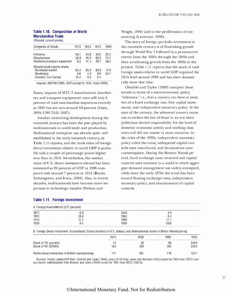
©International Monetary Fund. Not for Redistribution
Table 1 .1 0. Composition of World Merchandise Trade (Percent, current prices)
Categories of Goods 1913 1955
Primaries 64.1 54.8 Manufactures 35.9 45.2 Machinery/transport equipment 6.3 17.5
Manufactured exports shares Developed market 95.4 85.2 Developing 4.6 4.4 (Former) Iron Curtain 10.4 9.5
1973 1994
39.5 25.3 60.5 74.7 28.7 38.3
83.9 72.9 6.6 24.7 2.4
Sources: UNCTAO (1983, 1997) except for 1913: Yates (1959).
States, imports of SITC 7 manufactures (machin
ery and transport equipment) were still only 5
percent of total merchandise imports as recently
as 1955 but are now around 50 percent (Yates,
1959; UNCTAD, 1997).
Another interesting development dltring the
twentieth century has been the part played by
multinationals in world trade and production.
Multinational enterprise was already quite well
established in the early twentieth century, as
Table 1 . 11 reports, and the book value of foreign
direct investment relative to world GDP is proba
bly only a couple of percentage points higher
now than in 1914. Nevertheless, the market
value of U.S. direct investment abroad has been
estimated as 20 percent of GNP in 1996 com
pared with around 7 percent in 1914 (Bordo,
Eichengreen, and Irwin, 1999). Also, in recent
decades, multinationals have become more im
portant in technology transfer (Nelson and
Table 1 .11 . Foreign Investment
A. Foreign Assets/World GOP (percent)
1870 6.9 1900 18.6 1914 1�5 1930 8.4
GLOBALIZATION THEN AND NOW
Wright, 1992) and in the proliferation of out
sourcing (Lawrence, 1 996).
The story of foreign portfolio investment in
the twentieth century is of flourishing growth
through World War I followed by a pronounced
retreat from the 1930s through the 1950s and
then accelerating growth from tl1e 1960s to the
present. Table 1 . 1 1 repons that the stock of total
foreign assets relative to world GDP regained the
1914 level around 1980 and has risen dramati
cally since that time.
Obstfeld and Taylor ( 1999) interpret these
trends in terms of a macroeconomic policy
''Lrilemma," i.e., that a counu·y can have at most
two of a ftxed exchange rate, free capital move
ments, and independent monetary policy. At the
start of the century, the advanced counu·y norm
was to eschew the last of these in an era when
politicians denied responsibility for the level of
domestic economic activity and working class
votes still did not matter in most countries. In
the crisis of the 1930s, independent monetary
policy ruled the roost, widespread capital con
trols were introduced, and devaluations were
commonplace. During the Bretton Woods pe
riod, fixed exchange rates returned and capital
conu·ols were retained in a world in which aggre·
gate demand management was widely attempted,
while since the early 1970s the trend has been
toward floating exchange rates, independent
monetary policy, and abandonment of capital
controls.
1945 1960 1980 1995
4.9 6.4
17.7 568
B. Foreign Direct Investment Accumulated Stocks (millions of U.S. dollars) and Multinationals Active in British Manufacturing
Stock of FDI (current) Stock of FD I ($1990)
Multinational enterprises in British manufacturing
1914
14 153
1 1 1
1938
26 350
361
1960
66 362
718
1995
2464 2053
1507
Sources: Foreign assets/GOP lrom Obstfeld and Taylor (1999); stock of FOI from Jones and Schroter (1993) except for 1995 from OECO (vari· ous years); multinationals from Bostock and Jones (1994) except for 1995 from OECO (1997b).
21
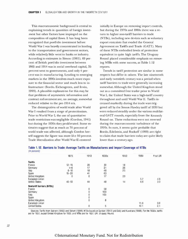
©International Monetary Fund. Not for Redistribution
22
CHAPTER I GLOBALIZATION AND GROWTH IN THE TWENTIETH CENTURY
This macroeconomic background is central to
explaining trends in quantities of foreign invest
ment but other factors have impinged on the
composition of capital flows. It has long been
recognized that portfolio investment before
World War I was heavily concentrated in lending
to the transportation and government sectors,
while relatively little went to banks or industry.
According to estimates in Simon (1967), 69 per
cent of British portfolio investment between
1865 and 1914 was in social overhead capital, 35
percent went to governments, and only 4 per
cent was in manufacturing. Lending to emerging
markets in the 1990s involves much more expo
sure to the financial sector and much less to in
frastructure (Bordo, Eichengreen, and Irwin,
1999). A plausible explanation for this may be
that problems of asymmetric information and
contract enforcement are, on average, somewhat
reduced relative to the pre-1914 era.
The disintegration of world trade after World
War I resulted from a surge of protectionism.
Prior to World War I, the use of quantitative
trade restrictions was negligible (Gordon, 1941)
but during the 1930s they proliferated. Some estimates suggest that as much as 70 percent of
world u·ade was affected, although Gordon her
self suggests the figure was more like 50 percent.
Trade liberalization after World War II centered
initiaJJy in Europe on removing import conu·ols,
but during the 1970s and 1980s there was a re
turn to higher non-tariff barriers to trade
(NTBs), including new devices such as voluntary
export resu·aints that evaded the General
Agreement on Tariffs and Trade (GATT). Many
of these NTBs embodied levels of protection
equivalent to quite high tariffs. The Uruguay
Round placed considerable emphasis on remov
ing NTBs with some success, as Table 1 . 12
reports.
Trends in tariff protection are similar in some
respects but differ in others. The late nineteenth
and early twentieth century was a period when
tariff barriers to trade were generally increasing
somewhat. Although the United Kingdom stood
out as a committed free trader prior to World
War I, the United States was a high-tariff country
throughout and until World War ll. Tariffs in
creased markedly during the trade wars trig
gered off by the Smoot-Hawley tariff of 1930 but
were reduced steadily under the various multilat
eral GATT rounds, especially from the Kennedy
Round on. These reductions were not reversed
during the macroeconomic turbulence of the
1970s. In sum, it seems quite probable that
Bordo, Edelstein, and Rockoff (1999) are 1ight
to claim that trade barriers today are quite likely
lower than a century ago.
Table 1 .12. Barriers to Trade: Average Tariffs on Manufactures and Import Coverage of NTBs (In percent)
1875 1913 1930s 1950 1989 Post UR
Tariffs France 12-15 20 30 18 Germany 4-6 17 21 26 Italy 8-10 18 46 25 Spain 15-20 41 63 United Kingdom 0 0 17 23 European Union 5.7 4.6 United States 40-50 44 48 14 4.6 3.0
Nontariff barriers (NTBs) France 0 58 Germany 0 100 Italy 0 100 Spain 0 United Kingdom 0 8 European Union 11.6 3.8 United States 0 5 10.1 2.1
Sources: Tariffs from Bairoch (1993) and Schott (1994); NTBs based on Gordon (1941) and Daly and Kuwahara (1998). For the 1930s, tariffs are for 1931. except United Kingdom for 1932. and NTBs are for 1937. UR, Uruguay Round.
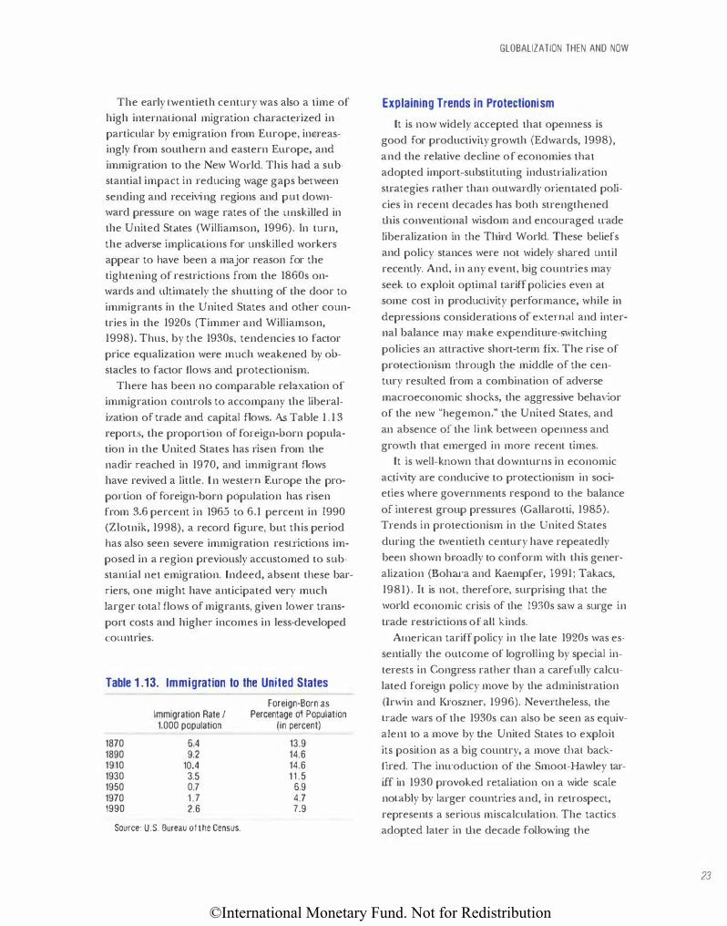
©International Monetary Fund. Not for Redistribution
The early twentieth century was also a time of
high international migration characterized in
particular by emigration from Europe, increas
ingly from southern and eastern Europe, and
immigration to the New World. This had a sub
stantial impact in reducing wage gaps between
sending and receiving regions and put down
ward pressure on wage rates of the Lmskilled in
the United States (Williamson, 1996). Tn turn,
the adverse implications for unskilled workers
appear to have been a major reason for the
tightening of restrictions from the 1860s on
wards and ultimately the shutting of the door to
immigrants in the United States and other coun
tries in the 1920s (Timmer and Williamson,
1998). Thus, by the 1930s, tendencies to factor
price equalization were much weakened by ob
stacles to factor flows and protectionism.
There has been no comparable rei<Lxation of
immigration controls to accompany the liberal
ization of trade and capital flows. As Table 1 . 1 3
reports, the proportion of foreign-born popula
tion in the United States has risen from the
nadir reached in 1970, and immigrant flows
have revived a little. In western Europe the pro
ponion of foreign-born population has risen
from 3.6 percent in 1965 to 6.1 percent in 1990
{Ziotnik, 1998), a record figure, but this period
has also seen severe immigration restrictions im
posed in a region previously accustomed to sub
stantial net emigration. Indeed, absent these bar
riers, one might have anticipated very much
larger co tal flows of migrants, given lower trans
port costs and higher incomes in less-developed
countries.
Table 1 .13. Immigration to the United States
1870 1890 1910 1930 1950 1970 1990
Immigration Rate I 1.000 population
6.4 9.2
10.4 3.5 0.7 1.7 2.6
Source: U.S. Bureau of the Census.
Foreign-Born as Percentage of Population
(in percent)
13.9 14.6 14.6 11.5
6.9 4.7 7.9
GLOBALIZATION THEN AND NOW
Explaining Trends in Protectionism
It is now widely accepted that openness is
good for productivity growth {Edwards, 1998),
and the relative decline of economies that
adopted import-substituting industrialization
strategies rather than outwardly oriemated poli
cies in recent decades has both strengthened
this conventional wisdom and encouraged u·ade
liberalization in the Third World. These beliefs
and policy stances were not widely shared until
recently. And, in any event, big countries may
seek to exploit optimal tariff policies even at
some cost in productivity performance, while in
depressions considerations of external and inter
nal balance may make expenditure-switching
policies an attractive short-term fix. The rise of
protectionism Lhrough the middle of the cen
tury resulted fi·om a combination of adverse
macroeconomic shocks, the aggressive behavior
of the new "hegemon," the United States, and
an absence of the link between openness and
growth that emerged in more recent times.
It is well-known that downturns in economic
activity are conducive to protectionism in soci
eties where governments respond to the balance
of interest group pressures (Gallarotti, 1985).
Trends in protectionism in the United States
during the twentieth century have repeatedly
been shown broadly to conform with this gener
alization (Bohara and Kaempfer, 1991; Takacs,
1981). It is not, therefore, surprising that the
world economic crisis of the 1930s saw a surge in
trade restrictions of aJI kinds.
American tariff policy in the late 1920s was es
sentially the outcome of logrolling by special in
terests in Congress rather than a carefully calcu
lated foreign policy move by the administration
(Irwin and Kroszne1� 1996). Nevertheless, the
trade wars of the 1930s can also be seen as equiv
alent to a move by the United States to exploit
its position as a big country, a move that back
fired. The inu·oduction of the Smoot-Hawley tar
iff in 1930 provoked retaliation on a wide scale
notably by larger countries and, in retrospect,
represents a serious miscalculation. The tactics
adopted later in the decade follo\ving the
23
©International Monetary Fund. Not for Redistribution
24
CHAPTER I GLOBALIZATION AND GROWTH IN THE TWENTIETH CENTURY
Reciprocal Trade Agreements Amendment were
a better way of seeking optimal tariffs that effec
tively distinguished between countries of rela
tively high and low bargaining power
(Conybeare, 1987). During the Pax Americana
after World War II, the United States moved to
ward subordinating trade policy to foreign pol
icy, and this aided considerably the shift back to
ward trade liberalization.
In recent decades protectionism seems to
have reduced growth rates as a consequence of
the distortions to which it gave rise. A detaiJed
analysis of long-run Latin American growth per
formance by Taylor ( 1 998) found that the key
impact worked through a whole series of distor
tions that raised the price of capital goods rather
than high tariffs per se. Similarly, Ades and di
Tella (1997) have argued that there are serious
adverse impacts of industrial policy from the cor
ruption that it generally spawns, which is fos
tered by protected markets.
In the early twentieth century, the inverse cor
relation between tariffs and growth was absent. A
careful study by O'Rourke (1997), which uses all
the obvious controls, confirms the intuitions of
earlier writers like Bairoch (1993). The reason
for this result may well be that, in general, tariffs
at this time tended to reduce the relative price
of capital goods and thus to stimulate rather
than to discourage real investment. This is sug
gested by the evidence in Collins and
Williamson ( 1 999) who found that prior to 1950
tariffs tended to lower the price of capital goods
relative to consumer goods. More speculatively,
it may also be that in an era when "industrial
policy" was in its infancy there was less reason to
associate protection with additional distortions.
Origins and Nature of the Great Slump
The tendency to disintegration of the world
economy in the interwar period was hugely exac
erbated by the slump of the early 1930s. I t seems
highly probable that a return to global economic
crisis of similar proportions would provoke simi
lar antipathy to international capital mobility and
free trade leading to widespread adoption of
policies aimed at reimposing controls.
Understanding the reasons for the depression, in
particular of the parts played by structural faults
and policy errors, is central to assessing the risk
of a repeat and is thus a key building block in
weighing up the likelihood of a future backlash
against globalization. Also, understanding the
propagation of the initial adverse shocks is fun
damental to averting a repetition of a major
slump and an associated retreat from openness.
The traditional literature on the Great
Depression stressed catasu:opbic errors in
Ame1ican monetary policy, which provoked a
huge aggregate demand shock that reduced out
put and prices both domestically and then,
through secondary effects, in the rest of the
world (Friedman and Schwartz, 1963). This is
still a valid, but now clearly incomplete, picture
as more recent research has brought out the im
portance of wage stickiness and aggregate supply
in real output falls, of the operation of the newly
restored gold standard in the inadequacy of the
world macroeconomic policy response, and of
the fragility of banking systems in the onset of fi
nancial crisis.
Those who argue for the fragility of the world
economy prior to the depression are typically
pointing to various legacies of World War T such
as adjustment problems linked to world agricul
tural overproduction and loss of export markets
by European counu·ies (Kindleberger, 1973).
Their claims are not that the world economic
crisis was inherent in early twentieth century
globalization but that the shock delivered by the
wa1· seliously impaired subsequent macro
economic policymaking, led to increased pres
sures for protection, or had adverse implications
for the volatility of capital Oows. Indeed, the
main line of argumen t is now that the war shock
was primarily responsible for the instability of
the interwar gold standard, but the significance
of the changed economic environment was per
ceived too late (Temin, 1989).
Eichengreen ( 1992) established a picture of
the pre- 1 9 1 4 Gold Standard as an era in which
Britain was frequently able to operate as a
Stackelberg leader because of sterling's reserve
©International Monetary Fund. Not for Redistribution
currency role and as a world in which interna
tional cooperation sustained the system when
under pressure. The pdority given to gold con
vertibility coexisted with quite high volatility in
domestic levels of economic activity but domes
tic politics permitted neglect of internal balance
objectives. By the 1920s all this had changed
wilh the rise of New York as a financial center,
the differing views of major players on the ap
propriate conduct of monetary policy, and the
pursuit of working-class votes. American mone
tary policy first provoked a general world tightening and then presided over a sensational col
lapse in the domestic money supply and output.
This episode is discussed in detail below.
A substantial rise in real interest rates and real
wages ensued in the economically advanced
world. Newell and Symons (1988) estimated that
in the representative European counu·y, real
wages rose by 13.8 percent and the real interest
rate increased by 7.2 percentage points between
1928 and 1931, while the price of traded goods
fell by 27.2 percent and domestic p1;ces by 15.2
percent. The prices of primary goods fell dra
matically from an index value of 28.01 in 1928 to 10.15 in 1932 compared with 48.31 in 1920
(Grilli and Yang, 1988). The terms of trade
moved very sharply against primary producers
in Latin America by about 32 percent between
1929 and 1931. Capital flows from First to Third
World ceased and were then reversed; capital ex
ports of $355 million in 1929 became inflows or
$1.4 billion and $1.7 billion in 1931 and 1932
(Maddison, 1985). Currency and debt crises followed for many Third World countries.
The depression was also notable for financial
crises in many advanced countries featuring significant bank failures, switches from bank money
into cash, and drying up of the supply of bank
loans (Bemanke andjames, 1991) . The most
spectacular of these debacles was in the United
States (Box 1.2). Here research has established
that a badly regulated banking system had en
gaged in excessive risk taking in the boom years
preceding the depression and that the interrup
tion to supplies of credit in the financial crisis of
lhe early 1930s added extra deflationary pres-
GLOBALIZATION THEN AND NOW
sure to lhat expected from a conventional nega
tive money supply shock ( Calomiris, 1993).
Money wages generally proved to be very
sticky downwards such that during 1931-34 real
wages were 20 to 40 percent above the 1929 level
in mosl countries. Estimated wage acljustment
equations for a panel of 22 countries confirm
that wages generally reacted very sluggishly to
price declines (Bernanke and Carey, 1996). This
ensur·ed that the deflationary shocks were trans
lated into output reductions. In some cases, like
that of Britain, the spread of collective bargain
ing arrangements and the implications of unem
ployment benefits in placing a floor under nomi
nal wages may partly explain this (Crafts, 1989).
The stickiness of money wages remains quite
puzzling, however, especially in view of the much
greater flexibility that they displayed both in
Britain and the United States in the early 1920s.
Calibrations of a Taylor overlapping-conu·acts
model for lhe United States indicate that a
change to much slower wage adjustment in the
eal"ly 1930s than a decade earlier is implied, and
the explanation of this is not yet clear (Bordo
and others, 1997).
Recent r·esearch has placed the operation of
the noncooperative interwar gold standard at
the heart of tJ1e problems of d1e early 1930s. In
the absence of cooperative monetary expansion,
the fLXed exchange rate regime buttressed by fis
cal orthodoxy ensured that the representative
counu·y faced adverse aggregate demand shocks
to which there was no effective policy remedy.
It has also become clear that leaving the gold standard was the key to early recovery, which was
associated with the pursuit of independem mon
etary policies (which mitigated price declines
and thus real wage increases) besides having
more conventional implications for aggr-egate
demand (Campa, 1990; Eichengreen and Sachs,
1985). Early devaluation also helped prevent
currency crises, which translated i.nto banking
crises (Grossman, 1994). At the same time, im
posing capital controls and erecting barriers to
trade were seen as attractive ways to escape from
conflicts of external and internal balance; in ef
fect, openness was increasingly seen as an obsta-
25
©International Monetary Fund. Not for Redistribution
26
CHAPTER I GLOBALIZATION AND GROWTH IN THE TWENTIETH CENTURY
cle to prosperity at least in the short term. Even
in the hitherto staunchly free-trade United
Kingdom the macroeconomic downturn
prompted the imposition of the General Tariff
as long-standing protectionist interest groups
seized their moment (Rooth, 1992).
lf, ex post, the interwar gold standard turned
out so badly, why ex ante did so many counnies
seek to return to gold after World War I?
Obviously, a major reason was that the pre-1914
system had operated as an effeCLive commitment
technology for many countries (Bordo and
Kydland, 1995), and the advantage of a rules
based system for macroeconomic policy was
highly valued-as Montague Norman said it was
"knave proof." Recent research has also stressed
the role of gold standard membership as the
best available signal to capital markets of finan
cial rectitude and thus as a means to borrowing
from abroad at substantially lower interest rates
(Bordo, Edelstein, and Rockoff, 1999). In this
way, globalization was tied to the gold standard
and thus, given the international economic pol
icy context of the early 1930s, carried with it the
seeds of its own demise.
The upshot of this research is to highlight
three key ingredients of the Great Depression
inappropriate international monetary and ex
change rate policy, frag.ile banking systems, and
inflexible labor markets. The chances of avoiding
a replay of the 1930s will be better the less these
apply in f·uture. As noted above, the solution to
the policy trilemma increasingly is to drop the
fLXed exchange rate, and this removes a key as
pect of the 1930s crisis. I t might also be noted
that in a world of floating exchange rates the G-7
response to the stock market crash of 1987 indi
cates that policymakers were both alive to the les
sons of history and able to take appropriate ac
tion. Inflexible labor markets seem to remain a
problem, notably in Europe. The reasons for
wage stickiness in the 1930s are not yet under
stood and are a priority for further research. At
present, it is unclear whether there would now
be greater downward wage flexibility in response
to deflationary pressure, but it would be unwise
to rely on it (Ak.erlof and others, 1996).
The Asian crisis in 1997-98 is a reminder of
the acute problems that can be created by the
policy trilemma in the face of inadequately su
pervised and regulated banking systems.
Attempts to use interest rate policy for domestic
demand management with a pegged exchange
rate were counterproductive in the face of capi
tal inflows, and the excessive •·isk taking tJnt en
sued threatened financial stability (Mishkin,
1999). In turn, as bank balance sheets deterio
rated sharply, the fiscal implications of implicit
goven1ment guarantees risked a currency crisis
that itself would exacerbate the banking crisis
(Burnside and others, 1999). The unholy combi
nation of inapp.-opriate monetary and exchange
rate policy together •Nith a fragile banking sys
tem, is quite reminiscent of 1930s America. As
with that episode, ex post, these errors seem to
be widely recognized and improvements in the
design of policy can be expected.
In sum, the message from the interwar period
is that economic policymaking rather than glob
alization per se was the root of the Great
Depression. Accordingly, tl1ere seem to be rea
sons to be optimistic both that a similar down
turn can be averted in future and, if so, the
probability of a reversal of globalization is lower.
An End-of-the-Century Perspective
The Paradoxical OECD Growth Slowdown
One of the most discussed aspects of twentieth
century economic growth is the productivity
slowdown of tl1e past quarter century in the
OECD economies, and especially in the United
States. In tl1e context of the information and
communications technology revolution, this has
been seen by many as a considerable puzzle. The
episode raises a number of important issues
both for economic poUcymakers and growth
economists. These include
• Is sn·uctural change responsible for slower
OECD growth?
• Is there a post-Golden Age hangover effect?
• ls the growth slowdown sufficient to refute
the endogenous growt11 hypothesis?
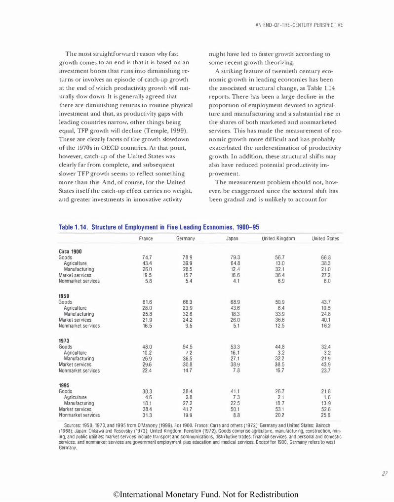
©International Monetary Fund. Not for Redistribution
The most straightforward reason why fast growth comes to an end is that it is based on an investment boom that runs inw diminishing returns or involves an episode of catch-up growth at the end of which productivity growth will natUJ·ally slow down. It is generally agreed that there are diminishing .returns to routine physical investment and that, as productivity gaps with leading countries narrow, other things being equal, TFP growth will decline (Temple, 1999). These are clearly facets of the growth slowdown of the 1970s in OECD countries. At that point, however, catch-up of the United States was clearly far from complete, and subsequent slower TFP growth seems to reflect something more than this. And, of course, for the United States itself the catch-up effect carries no weight, and greater investments in innovative activity
AN END-OF-THE-CENTURY PERSPECTIVE
might have led to faster growth accorcting to some recent growth theorizing.
A SITiking feature of twentieth century economic g1·owth in leading economies has been the associated structural change, as Table 1.14
reports. There has been a large decline in the proportion of employment devoted to agriculture and manufacturing and a substantial rise in the shares of both marketed and nonmarketed services. This has made the measurement of economic growth more difficult and has probably exacerbated the underestimation of productivity growth. In addition, these structural shifts may also have reduced potential productivity improvement.
The measurement problem should not, however, be exaggerated since the sectoral shift has been gradual and is unlikely to account for
Table 1 .14. Structure of Employment in Five Leading Economies, 190D-95
France Germany Japan United Kingdom United States
Circa 1900 Goods 74.7 78.9 79.3 56.7 66.8
Agriculture 43.4 39.9 64.8 13.0 38.3 Manufacturing 26.0 28.5 12.4 32.1 21.0
Market services 19.5 15.7 16.6 36.4 27.2 Nonmarket services 5.8 5.4 4.1 6.9 6.0
1950 Goods 61.6 66.3 68.9 50.9 43.7
Agriculture 28.0 23.9 43.6 6.4 10.5 Manufacturing 25.8 32.6 18.3 33.9 24.8
Market services 21.9 24.2 26.0 36.6 40.1 Nonmarket services 16.5 9.5 5.1 12.5 1 6.2
1973 Goods 48.0 54.5 53.3 44.8 32.4
Agriculture 10.2 7.2 16.1 3.2 3.2 Manufacturing 26.9 36.5 27.1 32.2 21.9
Market services 29.6 30.8 38.9 38.5 43.9 Non market services 22.4 14.7 7.8 16 7 23.7
1995 Goods 30.3 38.4 41.1 26.7 21.8
Agriculture 4.6 2.8 7.3 2.1 1.6 Manufacturing 18.1 27.2 22.5 18.7 13.9
Market services 38.4 41.7 50.1 53.1 52.6 Non market services 31.3 19.9 8.8 20.2 25.6
Sources: 1950, 1973, and 1995 from O'Mahony (1999). For 1900, France: Carre and others (1972); Germany and United States: Bairoch (1968); Japan: Ohkawa and Rosovsky (1973); United Kingdom: Feinstein (1972). Goods comprise agriculture, manufacturing, construction, min-ing, and public utilities; market services include transport and communications, distributive trades, financial services, and personal and domestic services; and non market services are government employment plus education and medical services. Except for 1900, Germany refers to west Germany.
27
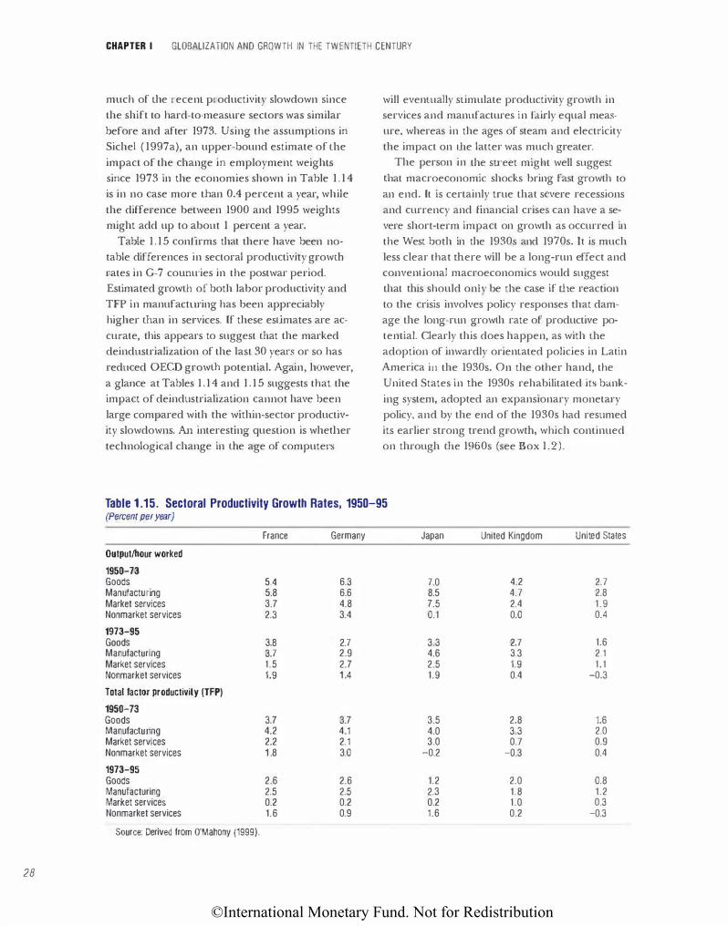
©International Monetary Fund. Not for Redistribution
28
CHAPTER I GLOBALIZATION AND GROWTH IN THE TWENTIETH CENTURY
much of the recenL productivity slowdown since
the shift to hard-to-measure sectors was similar
before and after 1973. Using the assumptions in
Sichel ( 1997a), an upper-bound estimate of l11e
impact of the change in employment weights
since 1973 in the economies shown in Table 1 . 1 4
is in no case more than 0.4 percent a year, while
the difference between 1900 and 1995 weights
might add up to about 1 percent a year.
Table 1 . 15 confirms that there have been no
table differences in sectoral productivity growm
rates in G-7 cotmu·ies in the postwar period.
Estimated growm of both labor productivity and
TFP in manufacn.1ring has been appreciably
higher than in services. If these estimates are ac
curate, this appears to suggest that the marked
deindustrialization of the last 30 years or so has
reduced OECD growt.h potential. Again, however,
a glance at Tables 1 . 1 4 and 1 . 1 5 suggests that the
impact of deindustrialization cannot have been
large compared with fue within-sector productiv
ity slowdowns. An interesting question is whel11er
technological change in fue age of computers
will eventually stimulate productivity growth in
services and manufactures in fairly equal meas
ure, whereas in the ages of steam and electricity
the impact on l11e latter was much greater.
The person in the su·eet might well suggest
fuat macroeconomic shocks bring fast growth to
an end. It is certainly true that severe recessions
and currency and financial crises can have a se
vere short-term impact on growth as occurred in
the West both in the 1930s and 1970s. Il is much
less clear that mere will be a long-run effect and
conventional macroeconomics would suggest
that fui.s should only be d1e case if fue reaction
to the crisis involves policy responses that dam
age the long-run growth rate of productive po
tential. Clearly this does happen, as with d1e
adoption of inwardly orientated policies in Latin
America in the 1930s. On the other hand, the
United States in fue 1930s rehabilitated its bank
ing system, adopted an expansionary monetary
policy, and by the end of the 1930s had resumed
its earlier strong trend growfu, which continued
on through the 1960s (see Box 1.2).
Table 1 .15. Sectoral Productivity Growth Rates, 1950-95 (Percent per year)
France Germany Japan United Kingdom United States
Output/hour worked
195D-73 Goods 5.4 6.3 7.0 4.2 2.7 Manufacturing 5.8 6.6 8.5 4.7 2.8 Market services 3.7 4.8 7.5 2.4 1 .9 Nonmarket services 2.3 3.4 0.1 0.0 0.4
1973-95 Goods 3.8 2.7 3.3 2.7 1.6 Manufacturing 3.7 2.9 4.6 3.3 2.1 Market services 1.5 2.7 2.5 1.9 1.1 Nonmarket services 1.9 1 .4 1.9 0.4 -0.3
Total factor productivity (TFP)
1950-73 Goods 3.7 3.7 3.5 2.8 1.6 Manufacturing 4.2 4.1 4.0 3.3 2.0 Market services 2.2 2.1 3.0 0.7 0.9 Nonmarket services 1 .8 3.0 -0.2 -o.3 0.4
1973-95 Goods 2.6 2.6 1.2 2.0 0.8 Manufacturing 2.5 2.5 2.3 1.8 1.2 Market services 0.2 0.2 0.2 1.0 0.3 Nonmarket services 1.6 0.9 1.6 0.2 -0.3
Source: Derived from O'Mahony (1999).
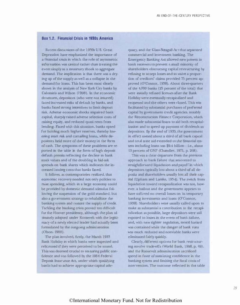
©International Monetary Fund. Not for Redistribution
Box 1.2. Financial Crisis In 1930s America
Recent discussions of the 1930s U.S. Great
Depression have emphasized the importance of
a financial crisis in which the role of asymmetric
infom1ation was central rather than treating the
event simply as a monetar}· shock to aggreg-cue
demand. The implication is that there was a dry
ing up of the supply as well as a collapse in the
demand for loans. This has been most clearly
shown in the analysis of New York City banks by
Calomiris and Wilson (1998). In the economic
downturn, depositors (who were not insured)
faced increased risks of default by banks, and
banks faced strong incentives to limit deposit
risk. Adverse economic shocks impaired bank
capital, sharph· raised adverse selection costs of
raising equily, and reduced quasi rents from
lending. Faced with this situation, banks opted
for holding much higher reserves, thereby low
ering asset risk and curtailing loans, while de-
positors held more of their moner in the form
of cash. The symptoms of these problems are re
ported in the table in the form of high deposit
defauh premia reflecting the decline in bank
stock values and of the doubling in bid-ask
spreads on bank shares which indicates the in
creased issuing costs that banks faced.
It follows, as contemporaries realized, that
economic recovery needed not only policies to
raise spending, which in a large economy could
be provided by domestic demand stimulus fol·
lo\\ing the suspension of the gold standard. but
also a gO\·ernment strategy to rehabilitate the
banking system and rt:SLore t11e supply of credil.
Tackling the banking crisis proved too difficult
for the Hoover presidency. although the plan ul
timately adopted under Rooseveh with the legiti·
maC} of a newly elected leader had actually been
formulated by the outgoing administration
(Olson. 1988). The plan involved, firstly. the March 1933
Bank Holiday in which banks were inspected and
relicerued if they were perceived to be :.ound.
This was deemed crucial to re�toring public con
fidence and was followed b) the 1934 Federal
Deposit Insurance Act, under which qualifYing
banks had to achieve appropriate capital adc-
AN END-OF-THE-CENTURY PERSPECTIVE
quacy, and tlte Class-Steagall Act that separated
commercial and investment banking. The
Emergency Banking Act allowed new powers to bank recei,·ers to pre,ent a small minority of
shareholder� obstructing capital restructuring by
refusing to accept losses and to waive a propor
tion of creditors' claims pro\'ided 75 percent ap
proved (O'Connor, 1938). About three--quarters
of the 4,000 banks (25 percent of the total) that
were initially refused Jicen�es after the Bank
Holiday were eventually recapitalized and
reopened and the others were dosed. This was
facilitated by substantial purcha�cs of preferred
capital by government credit agencies. notabl}
the Reconstruction Finance Corporation, which
also made substantial loans to aid both recapital
ization and to speed up papucnt of di\idends to
depositors. By the end of 1935, the government
in effect owned about a third of all bank capital
and total state aid extended to the financial sys
tem including loans was $9.-.1 hillion-i.e., about
13 percent of GNP (Chandler, 1971, p. 268). This was a clear departure from the previous
approach to bank failure that amounted to
�traightfonvard liquidation and payoff in \\hich
depositors typically lost about a third of all dc
posiL<> and shareholden; usually lost all their cap
i tal (Upham and Lamke, 1934). The switch from
liquidation toward recapitali7ation was not, how
ever, a bailout and the government appears to
ha\'e suffered no overall losses on its temporary
banking investments and loans (O'Connor,
1938). Shareholders were.' usually called upon to
make as substantial a contribution to the recapi
tali.t.ation as possible, large depositors were still
exposed to los.�es in the event of bank failure,
and, with new tighter regulation, moral hazard
was contained while the danger of bank runs
was much red\lced and nonviable banks were
eliminated fairly quickly.
Clearly, difTerent options for bank restructur
ing involve trade-ofls (\\TorJd Bank, 1998. p. 19), and the Roosevelt administration sacrificed
speed in favor of sustaining conlidence in the
banking !))'stem and limiting the fiscal coM.:. of
intervention. The outcome reflected in the table
29
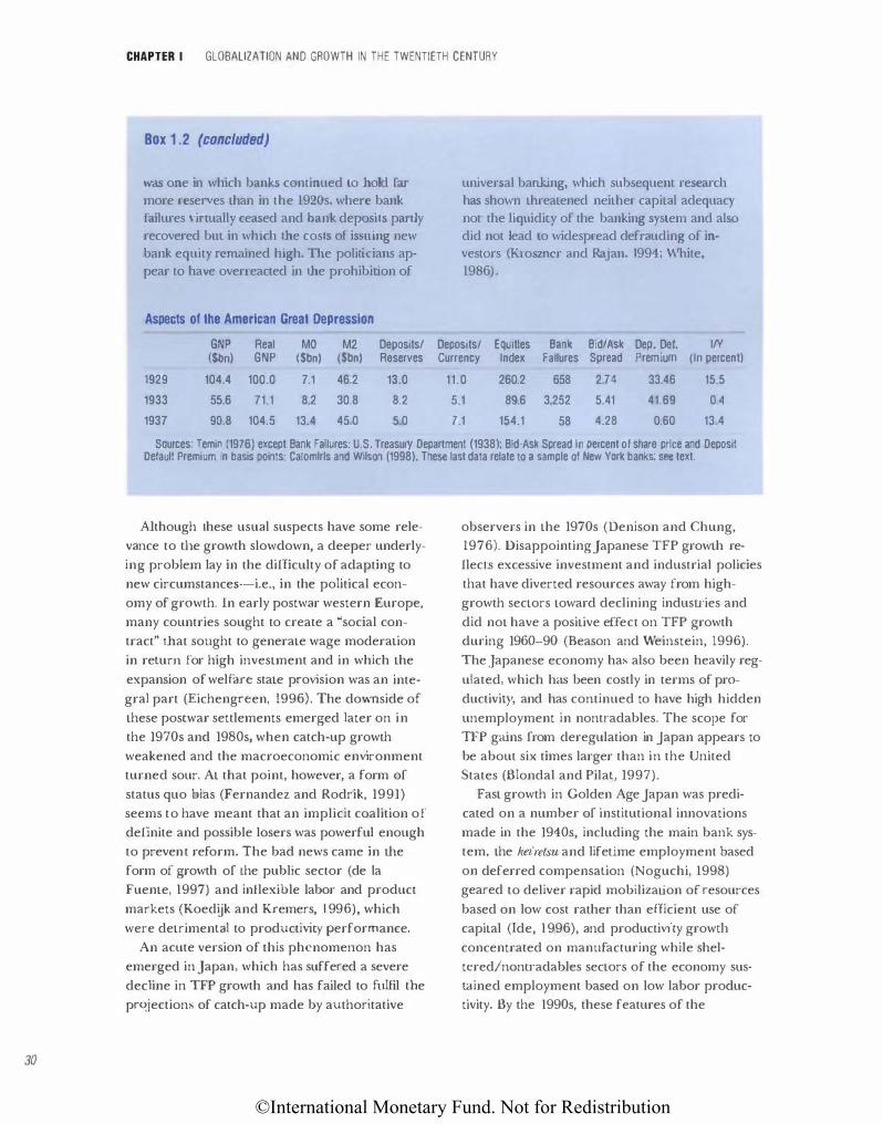
©International Monetary Fund. Not for Redistribution
30
CHAPTER I GLOBALIZATION AND GROWTH IN THE TWENTIETH CENTURY
Box 1 .2 (concluded)
was one in which banks continued to hold far more resenes than in the 1920s, where bank failures \'inuall) ceased and bank deposits parlly recovered but in whkh the costs of issuing new bank equity remained high. The politicians appear to have overreacted in Lhe prohibition of
Aspects of the American Great Depression GNP Real MO M2 Deposits/ {$bn) GNP ($bn) ($bn) Reserves
1929 104.4 100.0 7.1 46.2 13.0
1933 55.6 71.1 8.2 30.8 8.2
1937 90.8 104.5 13.4 45.0 5.0
universal ban.lJng, which subsequent research has shown threatened neither capital adequacy not the liquidit) of the banking system and also did not lead to widespread defrauding of investors (K.rosmcr and Rajan. 1994; White. 1986) .
Deposits/ EqUJties Bank Bid/Ask Dep. Del. IN Currency Index Failures Spread Premium (In percent)
11.0 260.2 658 2.74 33.46 15.5
5.1 89.6 3,252 5.41 41.69 0.4
7.1 154.1 58 4.28 0.60 13.4
Sources: Temin (1976) except Bank Fallures: U.S. Treasury Department (1938); Bid-Ask Spread In percent of share price and Deposit Default Premium in basis points: Calomlrls and Wilson (1998). These last data relate to a sample of New York banks; see text.
Although these usual suspects have some rele
vance to the growth slowdown, a deeper underly
ing problem lay in the difficulty of adapting to
new circumstances--i.e., in the political econ
omy of growth. In early postwar western Europe,
many countries sought to create a "social con
tract" that sought to generate wage moderation
in return for high investment and in which the
expansion of welfare state provision was an inte
gral part (Eichengreen, 1996). The downside of
these postwar settlements emerged later on in
the 1970s and 1980s, when catch-up growth
weakened and the macroeconomic environment
turned sour. At that point, however, a form of
status quo bias (Fernandez and Rodrik, 1991)
seems to have meant that an implicit coalition of
definite and possible losers was powerful enough
to prevent reform. The bad news came in the
form of growth of Lhe public sector (de Ia
Fuente, 1997) and intlexible labor and product
markets (KoedUk and Kremers, 1 996), which
were detrimental to productivity performance.
An acute version of this phenomenon has
emerged in Japan, which has suffered a severe
decline in TFP growth and has failed to fulfil tl1e
prqjections of catch-up made by authoritative
observers in the 1970s (Denison and Chung,
1976). Disappointing japanese TFP growth re
flects excessive investment and industrial policies
that have diverted resources away from high
growth sectors toward declining industries and
did not have a positive effect on TFP growth
during 1960-90 (Beason and Weinstein, 1996).
The Japanese economy has also been heavily reg
ulated, which has been costly in terms of pro
ductivity, and has continued to have high hidden
unemployment in nontradables. The scope for
TFP gains from deregulation in Japan appears to
be about six times larger than in the United
States (Blondal and Pilat, 1997).
Fast growth in Golden Age Japan was predi
cated on a number of institutional innovations
made in the 1940s, including the main bank sys
tem, the keiretsu and lifetime employment based
on deferred compensation (Noguchi, 1998)
geared to deliver rapid mobi.lizal.ion of resources
based on low cost rather than efficient use of
capital (Ide, 1 996), and productivity growd1
concentrated on manufacturing while shel
tcred/nono·adables sectors of the economy sus
tained employment based on low labor produc
tivity. By the 1990s, these features of the
©International Monetary Fund. Not for Redistribution
Japanese economy were increasingly seen as ob
stacles to further catch-up with the United States
but very difficult politically to reform (Ito,
1996). Japan is perhaps a good example of both
of the need for and rhe difficulties of transition
from the institutions designed to achieve a
Gerschenkronian escape from backwardness
(see below).
The issue of endogenous growth continues lO excite economists. It seems increasingly clear
that the study of (conditional) convergence
based on the Summers- Reston data set cannot
provide answers. The common finding that
growth is inversely related to the initial income
level or labor productivity gap does not discrimi
nate well between rival growth models even
though this clearly is a prediction of the neoclas
sical Solow or augmented-Solow growth models.
For example, if there are obstacles lO technologi
cal diffusion, then should the costs of technol
ogy transfer fall, there may be periods of catch
up even when the underlying growth process is
endogenous and long-run growth rates show no
tendency to equalize across counu·ies (Sala-i
Martin, 1996). In fact, this seems a possible in
terpretation of recent OEGD experience, given
that time-series analysis of the Maddison data set
rejects the hypotheses that long-run forecasts of
differences in output per person tend to zero or
are proportional with a single long-term u·end
(Mills and Crafts, 1999).
Jones (1995) argues that long-run time-series
evidence is indeed the key to evaluarjng the en
dogenous growth hypothesis. He stresses that the
failure of OECD, and especially U.S. trend
growth rates to acceleraLe in recent decades ap
pears to contradict the predictions of endoge
nous growth models that increased investments
in human capital and R&D will permanently
raise the growth rate, and thus also calls into
question the central claim of endogenous
growth, namely that good policy can raise the
growth rate rather than merely have a levels ef
fect as in the Solow model.
The growth accounting estimates discussed
earlier provide a useful input tO this discussion.
It has already been noted that the changes over
AN END-OF-THE-CENTURY PERSPECTIVE
time in measured TFP growth, which inform the
discussion in .Jones (1995), are not necessarily a
good gLLide to the rate of technological change
and so a fortiori need not be a good guide to
the rare of endogenous innovation. Indeed, the
TFP growth exhibited by the United States at
mid-century is "too good to be true" in the sense
that it would imply a phenomenal rate of return
on the R&D expenditure of the time. This opens
the possibility that TFP growth may have slowed
down for reasons other than declining reLUrns to
innovative effort. Economeu·ic investigation of
the TFP growth slowdown in American manufac
turing in the 1960s and 1970s su·engthens this
suspicion, since it finds that the underlying rate
of technological change (which accounted for
less than half of conventionally measured TFP
growth) did not decline, but productivity im
provement from economics of scale fell substan
tially (Morrison, 1992).
lf there arc diminishing returns to research
effort, then increases in the share of national in
come devoted to R&D will raise 1he level of GDP
per person and will have a transitory but not a
permanent positive effect on the growth rate,
which in the long run will be determined by the
exogenous natural rate-i.e., we are back in an
augmented-Solow world. This can be illustrated
by the following simplified model (Jones, 1999):
Y= flaLY where A is the s1ock of ideas and L_'" is labor used
in goods production;
LlA = 8LAM where <P < 1 .
In the steady stale, M/ fl and thus the growth
of income pe•· head is n/ ( 1 - cp), where n is the
population rate and is independent of the allo
cation of labor to research.
Modelers have also discussed the impact of a
proliferation of product varieties. Suppose
LlA/ A = 8LA/ V, where Vis the variety of products
available: then, Lhc nature of scale effects will de
pend on whether the number of varieties grows
more or less rapidly than population. The
growth rate will depend only on allocation of la
bor w research and not on scale when popula
tion and variety grow at the same rate.
31
©International Monetary Fund. Not for Redistribution
32
CHAPTER I GLOBALIZATION AND GROWTH IN THE TWENTIETH CENTURY
Jones ( 1 997) claimed that not only is this permutatjon on the augmented-Solow model the best available interpretation of the long-run data on productivity growth but also, since investment
in R&D and human capital have been r·ising rela
tive to U.S. GDP, the economy must have been growing above the steady-state rate. He therefore projected a substantial slowdown when this transition phase is complete. A long-run perspective suggests, however, that the historical experience has been variable and would inrucate some caution before accepting jones's projection.
In particular, the impact of innovative effort on overall TFP growth seems to depend on whether it results in the invention of new gen
eral purpose technologies such as electricity in the early twentieth century (David and Wright, l999a) or unconnected real costs reductions in individual sectors as in recent decades (Harberger, 1998). In Harberger's striking metaphor, the former is a yeast-type growth process, and the latter is a mushroom-type
growth. Moreover, general purpose technologies are also thought by some economists to be likely to involve a productivity slowdown prior to a subsequent acceleration as a result of the adjust
ment costs of the new opportunities. The information and communications tech
nology revolution is clearly the big technological development of the late twentieth century. At least until quite recently, however, it has not had dramatic effects on either labor productivity or TFP growth, and economists' assessments of its likely impact have tended to be skeptical (Gordon, 1999).
Growth accounting estimates suggest that this is because computers remain a relatively small, although fast-growing, component of the capital stock and because there appears to be relatively little evidence of strong spillover effects (Jorgenson and Stiroh, 1999) (Box 1.3). This will not surprise new economic historians, since a staple finding in the cliometric literature is that even dramatic changes in technology like railways or the steam engine have modest effecL� on overall GDP growth, especially in the early clays (Fogel, 1964; von Tunzelmann, 1978).
1 evertheless, the long-run TFP implications of changes in technology are often unclear initially. Thus, while American productivity surged in the 1920s \Vhen electrification was developed
as a general purpose technology, this was fully 40 years after electricity was first commercially generated (David, 199 1 ) . On this analogy, it is
too soon to assess the productivity implications of the computer revolution. Moreover, it seems likely that well-informed observers at the end of either the eighteenth or nineteenth centuries would have failed to predict subsequent productivity improvement given the very limited implications of steam and electricity at those junctures. If, howeve1� substantial yeast-like
implications for TFP growth are to come from the computer revolution, it will need to progress
to a new phase, such as a massive increase in teleworkjng, that has substantial implications for capital saving in terms of transport infrasu·ucture and commercial buildings (David and Wright, 1999b).
The bottom line of this review of the OECD productivity slowdown is tl1at only a small pan seems to be due to the impact of su·uctural change including associated increases in meas
urement error. The end of the Golden Age left a legacy of much expanded public sectors that probably has reduced growth rates somewhat (see below). The modest impact of the information and communications technology revolution on economic growth thus far is not surprising from a growth accounting perspective. The growth slowdown is paradoxical in the light of some endogenous growth theorizing and it remains unclear whether the long-run rate of pro
ductivity improvment from technological progress will respond positively to more innovative effort. Depending on one's prior views about scale effects in innovalion, a case can be made that OECD growth in the first quarter of the next century is about to speed up as the delayed effects of greater spending on R&D feed through or slow down as u·ansitional dynamics unwind.
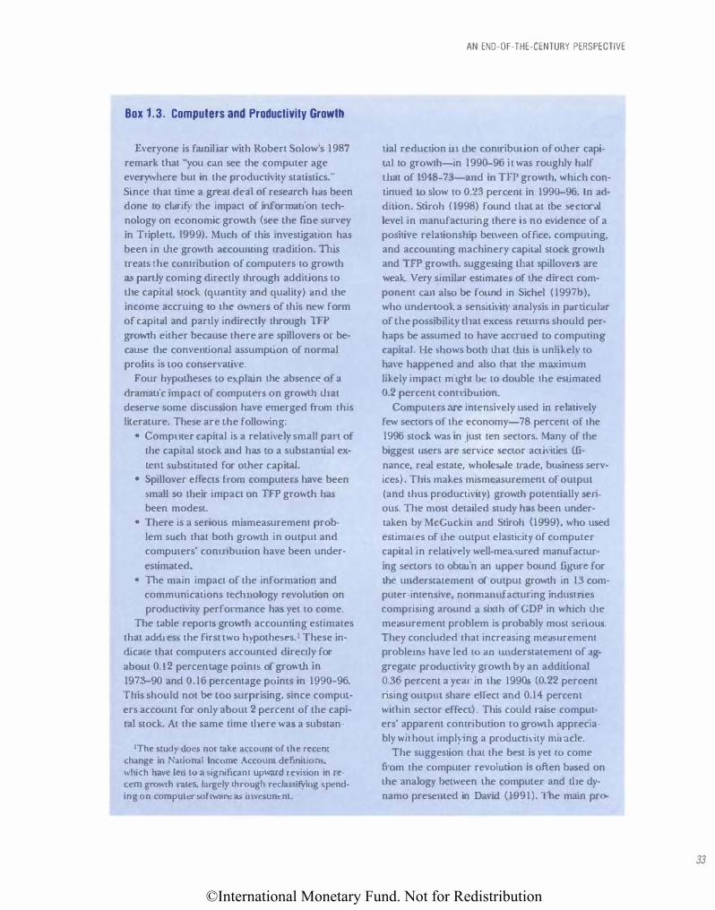
©International Monetary Fund. Not for Redistribution
Box 1.3. Computers and Productivity Growth
Everyone is familiar with Robert Solow's 1987 remark that ''you can see the computer age
everywhere but in the productivity statistics.··
Since that lime a great deal of research has been
done to clari1} the impact of information tech
nology on economic growth (see the fme survey
in Tripleu. L999). Much of this investigation has
been in the growth accounting tradition. This treats the contribution of computers to growth
as partly coming directly through additions to
Lhe capital �tock (quantity and quality) and tl1e
income accruing to t11c owners of this new form
of capital and partly indirectly through TFP
growth either because there are spillovers or be
cause the conventional assumption of normal
profits is too conservative.
Four hypo theses to explain the absence of a
dramaLic impact of computers on growth that
deserve some discussion have emerged from this
literature. These are the following:
• Computer capital is a relatively small pan of
the capital stock and has to a substantial ex
tent substituted for other capi taL • Spillover effects from computers have been
�mall so their impact on TFP growth has
been modesL
• There is a serious mismeasurement prob
lem such that both growLh in output and
compmers' contribution have been under
estimated.
• The main impact of the information and
communications technology revolution on
productivity perfonnance has yet to come.
The table reports growth accounting estimates
that address the first two hypotheses. I These in
ctica£C that computers accounted directly for
about 0.12 percen tage points of growth in
1973-90 and 0.16 percentage points in 1990-96. This should not be too surprising, since comput
ers accoum for only about 2 percent of tile capi
tal stock. At the same time tllere was a substan-
'The �tudy does not take account of the recent change in National Income Accowll definitions. which have led to a signilicam upward revision in reccm growlh ratcs, largely through reclassifying �pending on computer softw·<�re ru. im..:.o.unent.
AN END-OF-THE-CENTURY PERSPECTIVE
tial reduction in tile contribution of other capi
tal to growth-in 1990-96 it was roughly half
tllat of 1948-73-and in TFP growth, which con
tinued to slow to 0.23 percent in 1990-96. Jn ad
dition. Stiroh ( 1998) found tllat at tbe l;ectoral
level in manufacturing there is no evidence of a
positive relationship between office, compming.
and accounting machinery capital stock growtll
and TFP growth, suggesting tllat spillovers are
weak. Very similar estimates of the direct com
ponent can also be found in Sichel ( l 997b), who undenook a sensitivity analysis in particular
of tile possibility tllat excess rewrns should per
haps be assumed to have accn1ed to computing
capitaL He shows botll that this is unllkelv to
have happened and also rhat the ma.ximum
likely impact might be to double the estimated
0.2 pcrcem contribution.
Computers are intensively used in relatively
few sectors of the economy-78 percem of the
1996 stock was in just ten sectors. Many of the
biggest users are service secwr activities (finance, real estate, wholcS<tle trade, business serv
ices) . This makes mismcasuremcm of output
(and thus productivity) growth potentially serious. The most detailed study hru. been under
taken by McGuckin and Stiroh (1999), who used
estimates of the output elasticity of computer
capital in relatively well-measured manufactur
ing sectors to obtain an upper bound figure for
the understatement of output growth in 13 com
puter-intensive, nonmanufacturing industries
comprising around a sixth of GDP in which the
measurement problem is probably most seriouJ>.
They concluded that increasing measurement
problems have led LO an understatement of aggregate productivity growth by an additional
0.36 percent a ycru in the 1990s (0.22 percent
rising ourpm share ellect and 0.14 percem
within sector effecL) . This could raise comput
ers' apparent contribution to growt11 apprecia
bly wit.hom implying a productivity miracle.
The suggestion that the best is yet to come
from the computer revolution is often based on
lhe analogy between t11e computer and tl1e dy
namo presented in David (1991). The main pro-
33
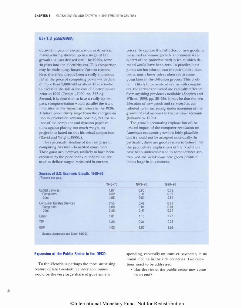
©International Monetary Fund. Not for Redistribution
34
CHAPTER I GLOBALIZATION AND GROWTH IN THE TWENTIETH CENTURY
Box 1.3 (concluded)
duclivity impact of electriiicalion in American manufacturing showed up in a surge ofTFP growth that was delayed until the 1920s, some
40 yearl> imo the electricity era. Thii> comparison may be misleading, however, for two reasons. First, there has already been a really enormous fall in the price of computing power-a decline of more than 2,000-fold in about 45 years--far
in excess of Lhe fall in the cost of clecuic power prior to 1920 (Triplett, J 999. pp. 323-4) . Second, it is clear that to have a really big impact, computerization would parallel the lransformalion in the American factoq• in the 1920s. A future productivity surge from the reorganization in production remains possible, but the author of the computer and dynamo paper cautions against placing too much weight on
projections based on this historical comparison (David and Wright., 1999b).
The spectacular decline of the real price of computing has surely benefited consumers. Their gains are, however, unlikely to have been
captured by the price index numbers that are used to deflate output measured in current
Sources of U.S. Economic Growth, 1948-96 (Percent per year)
Capital Services Computers Other
Consumer Durable Services Computers Other
Labor
TFP
GOP
Source: Jorgenson and Stiroh (1999)
Expansion of the Public Sector in the OECD
1948-73
1.07 0.02 1.05
0.55 0.00 0.55
1.01
1.39
4.02
To the Victorians perhaps the most surprising
feaLUre of late twentieth century economies
would be the very large share of government
prices. To captw·e the full effect of new goods in
measured economic growth, an estimare is required of the (nonobscn•ed) plice at which demand would have been zero. ln practice, new goods arc inu·oduced into the price index number at much lower prices ob erved at some
point later in the diffUsion process. This problem is likely to be acute where, as with complllcrs, the services delivered are radically different from anything previously available (Shapiro and Wilcox, 1996, pp. 25-36) . It may be that Lhe proliferation of new goods and services has con
tributed tO an increasing understatement of Lhe growth of real incomes in the national accountS (Nakamura, 1995).
The growth accounting explanation of the
limited impact of the computer revolution on Amedcan economic growth is fairly plausible but it should not be accepted uncritically. In
particular, there are good reasons to believe that
the producti\�t)' implications of the r('vohHion have been underestimated in some services ec
tors. and the well-known new goods problem looms large in this context.
1973-90 199Q-96
0.95 0.63 0.11 0.12 0.84 0.51
0.42 0.28 0.01 0.04 0.41 0.24
1.15 1.22
0.34 0.23
2.86 2.36
spending, especially on transfer paymentS, in na
tional income in the rich cotmtries. Two ques
Lions need to be addressed:
• Has the rise of the public sector now come
to an end?
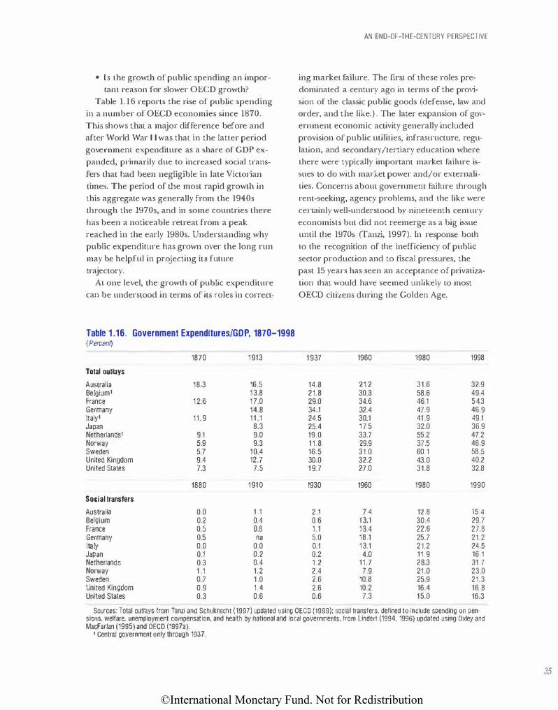
©International Monetary Fund. Not for Redistribution
• Is the growth of public spending an important reason for slower OECD growth?
Table 1.16 reports the rise of public spending in a number of OECD economies since 1870.
This shows that a major difference before and after World War l l was that in the latter period government expenditure as a share of GDP expanded, primarily due to increased social trans
fers that had been negligible in late Victorian times. The period of the most rapid growth in this aggregate was generally from the 1940s through the 1970s, and in some countries there has been a noticeable retreat from a peak reached in the early 1980s. Understanding why public expenditure has grown over the long run may be helpful in projecting its future trajectory.
At one level, the growth of public expenditure can be understood in terms of its roles in correct-
Table 1 .16. Government Expenditures/GOP, 187D-1998 (Percent)
1870 1913
Total outlays
Australia 18.3 16.5 Belgium I 1 3.8 France 1 2.6 1 7.0 Germany 14.8 ltaly1 11.9 11 .1
Japan 8.3
Netherlands I 9.1 9.0 Norway 5.9 9.3 Sweden 5.7 10.4 United Kingdom 9.4 12.7
United States 7.3 7.5
1880 191 0
Social transfers
Australia 0.0 1 .1
Belgium 0.2 0.4
France 0.5 0.8 Germany 0.5 na Italy 0.0 0.0
Japan 0.1 0.2 Netherlands 0.3 0.4
Norway 1 .1 1.2
Sweden 0.7 1 .0
United Kingdom 0.9 1.4 United States 0.3 0.6
AN END-OF-THE-CENTURY PERSPECTIVE
ing market failure. The urst of these roles predominated a century ago in terms of the provision of the classic public goods (defense, law and order, and the like.) . The later expansion of government economic activity generally included provision of public utilities, infrasu·uctw·e, regulation, and secondary/tertiary education where there were typically important market failure issues to do with market power and/or externalities. Concerns about government failure through
rent-seeking, agency problems, and the like were certainly well-understood by nineteenth century economists but did not reemerge as a big issue until the 1970s (Tanzi, 1997). In response both lo the recognition of the inefficiency of public sector production and to fiscal pressures, the past 15 years has seen an acceptance of privatization that would have seemed unlikely w most OECD citizens during the Golden Age.
1 937 1960 1980 1998
14.8 21.2 31.6 32.9 21.8 30.3 58.6 49.4 29.0 34.6 46.1 543
34.1 32.4 47.9 46.9 24.5 30.1 41 .9 49.1 25.4 1 7.5 32.0 36.9 19.0 33.7 55.2 47.2
11 .8 29.9 37.5 46.9 16.5 31.0 60.1 58.5 30.0 32.2 43.0 40.2 1 9.7 27.0 31.8 32.8
1930 1960 1980 1990
2.1 7.4 12.8 15.4 0.6 1 3.1 30.4 29.7
1.1 1 3.4 22.6 27.8 5.0 18.1 25.7 21.2
0.1 1 3.1 21.2 24.5 0.2 4.0 11.9 16.1
1.2 11.7 28.3 31 .7
2.4 7.9 21 .0 23.0
2.6 10.8 25.9 21.3 2.6 10.2 16.4 16.8 0.6 7.3 15.0 16.3
Sources: Total outlays from Tanzi and Schuknecht (1997) updated using OECD (1999): social transfers, defined to include spending on pen-sions. welfare, unemployment compensation. and health by national and local governments. from Lindert (1994, 1996) updated using Oxley and MacFarlan (1995) and OECD (1997a).
1 Central government only through 1937.
35
©International Monetary Fund. Not for Redistribution
36
CHAPTER I GLOBALIZATION AND GROWTH IN THE TWENTIETH CENTURY
As the privatization movement suggests, the claim ofWagner's Law-that there is an income elastici ty for government real output greater than unity-is rejected empirically in time-series tests (Gemmell, 1990). There has, however, been a powerful impetus to the growth of the ratio of
government consumption to overall activity, especially since the 1950s, from the relative price effect first brought to prominence by Baumol (1967). This is not surprising given the large share of wages in the public sector and the relative productivity performance reponed in Table l . l5.
Another type of market failure (for example, due to severe problems of adverse selection and
moral hazard) is associated with government's increased role in protecting people against risk. Here, however, considerations of redistributing income and vote seeking were also prominent. Rodrik (1997a) showed that there is a strong correlation in OECD countries in recent times between the exposure of an economy to external risk and the amount of government spending on social security and welfare systems. The interwar
period plainly saw very large shocks from the international economy both through trade and capital Oows. It is perhaps not surprising, therefore, that postwar attempts to restore international economic integration were accompanied by much stronger government efforts to reduce the risks to citizens-an undertaking that was to prove very expensive in some countries, for example, Sweden, in the renewed economic turbulence of the 1970s.
An econometric study of the growth of social u·ansfers reported in Lindert ( 1994) found that the most important influences through 1930 were the extension of the electoral franchise, which in some countries profoundly altered the identity of the median voter, and the aging of the population. For the 1960s to the 1980s, when democracy was already mature, population age structure was by far the dominant factor in explaining the rise of social spending over time (Linden, 1996). In both periods there was also evidence of a weak Wagner's Law effect.
If Lindert's model is used to project the future course of social spending, then the rise in social spending as a share of OECD GDP is forecast to cease at about present levels because many OECD countries have reached the point (285 elderly per 1,000 adults aged 20-64) at which the further aging of their populations is estimated to stop raising social spending (Linden, 1996, p. 14, 31). There are, however, built-in increases in state spending on pensions in all OECD countries, which result from the interaction of demographics and pay-as-you-go pension schemes established several decades ago (Roscveare and others, 1 996). These entail rises from the 1995 level that, with entitlements unchanged, will by 2030 raise pension expendiLUres by about 7 percentage points of GDP in Finland, Germany, Italy, Japan, and Portugal, the counu·ies where the impact will be largest, but by only 1 percentage point in the United Kingdom as a result of its greater reliance on private pensions
and the reduced generosity of its scheme stemming from the Thatcher years. The policy response to tl1is problem in a period that is likely to experience increased tax competition between countries will be intriguing.
The implications of fiscal policy for economic growth remain quite controversial. Theoretical predictions are sensitive to model specification, particularly in terms of the magnitude of effects, while empirical studies vary considerably in their
conclusions (Tanzi and Zee, 1997). Nevertheless, there are good reasons to suppose that in general governmenL capital spending has a positive but diminishing impact through raising expected returns to private investment while taxation does the opposite. This implies that, eventually, tl1e disincentive effects of tl1e taxes dominate. Economeu·ic modeling by Dowrick ( 1996) found that OECD countries are already
past tl1e break-even point. The general tendency of recent empirical
work has been that larger governmem budgets and their associated tax burdens have had a negative effect on growth in OECD countries. Based on growth regressions, de Ia Fuente ( 1 997) estimated that a reduction of 5 percentage points in
©International Monetary Fund. Not for Redistribution
government C\.IITent spending would raise the growth rate by 0.6 percentage points. A slightly smaller effect is suggested by Engen and Skinne1· (1996). Their "bottom-up" aggregation of the U.S. evidence argued for impacts on human capital formation, physical investment, and R&D such that a reduction of 2.5 percentage points in the average tax rate from a 5 percentage poinr cut in all marginal tax rates would raise growth by about 0.2 percentage points. Taken together, this evidence suggests that the increase of about 15 percentage points in the ratio of government
spending to GDP in the average OECD counu·y since 1960 may well have reduced the OECD
growth rate by 1 percentage point or more.
Will Rapid Catch-Up Growth Become More Widespread?
This section considers growt11 prospects for regions that have missed out on rapid catch-up
growth in recent decades-Africa, eastern Europe, India, and Latin America. Two questions are considered:
• Is growt11 severely constTained by geography or history?
• Will institutional quality be conducive to rapid catch-up growth?
Earlier sections stressed two important aspects of twentieth century economic growth: tJ1at the
long-run experience has mostly been of divergence rather than convergence, and iliat achiev
ing rapid catch-up growth is relatively rare and has required social capabiUty that derives from appropriate policies and institutions. Two kinds of society appear to have been especially disadvanr.aged, colonies and communist couno·ies. Postcolonial experiences have been very different thus far-compare South Korea with Angola-and early signs are that ilie same may be true for the former communist bloc-compare Poland with Ukraine.
Economic historians have always stressed ilie importance of institutions for growth outcomes. The huge literature on the rise of the West has traditionally pointed to its relative success in containing rent seeking and enJorcing well-defined
AN END-OF-THE-CENTURY PERSPECTIVE
property lights, which promoted market-based activities and innovation on an increasingly wide scale (Rosenberg and Bi1·dzell, 1986). North ( l 990) has developed these ideas the furthest. He argues that well-defined, enforceable property rights that ensure low transactions costs and limit opportunism and that. are predicated on strong but limited government are the central underpinnings of growth capability. Transactions costs are seen as still much greater in the Third World than in the earlier history of OECD counu·ies. North also points out., however, that what is much less well understood is t.he political economy of successful insitutional reform.
In practice, the optimal solution t.o u·ansac
tions costs problems may well diffe1· in the early stages of development. and later on in ilie catchup process. The developmental state approach to industrialization adopted in some east Asian countries (Amsden, 1989; Wade, 1990) and, indeed, the ·well-known Gerschenkronian schema for escape from economic backwardness
(Gerschenkron,l962) through investment. banking, state-directed investment, vertically integrated enterprises, and weak antitrust policy can be iliought of as the rational substitution of hier
archies for markets to cope witJ1 initially severe problems of asset specificity, moral hazard, and unreliable legal systems. At the same time, these market-substituting arrangements have a downside in terms of dulling incentives to productivity improvement. and may be highly vulnerable to capture by rent-seeking groups. In practice, outside east Asia, this seems to have been the typical outcorne.
Since the mid-1990s the growth regressions literature has followed the lead given by North and other economic historians and has tended to emphasize the role of social capability (both through institutional quality and policy choice) in growth outcomes with impacts both through investment and TFP growth. 111e variance in these characteristics across countries means that
recent experience has offered some interesting experiments from which to make inferences about these aspects of growth. Broadly speaking, it seems clear t11at strong commitment to en-
37
©International Monetary Fund. Not for Redistribution
38
CHAPTER I GLOBALIZATION AND GROWTH IN THE TWENTIETH CENTURY
forcement of property lights, the development
of a legal system that reduces moral hazard and
opportunism and policies of openness tOward in
ternational trade are all positive for growth
(Edwards, 1998; Knack and Keefer, 1995; Levine,
1998; Sachs and Warner, 1995) .
Equally clearly, east Asian countlies have on
average scored far better on all these aw·ibutes
than do countries fi·om regions of the world in
which catch-up has been relatively weak such as
Africa (Collier and Gunning, 1999), India
(B�pal and Sachs, 1996), or Latin America
(Burki and Perry, 1997). The vast m�jority of
countries in these regions from the 1950s
through the 1980s sought economic develop
ment through heavy reliance on the state to
promote industrialization while paying relatively
little auention to strengthening the micro
economic institutions required to sustain
market-based growth, perhaps reflecting an un
derstandable suspicion of governments and
multinational enterprises in the advanced world.
The potential for rapid catch-up growth depends
on the size of the productivity gap. Since this has
become much larger in recent decades, the
penalties in terms of forgone growth for having
infelior institutions and policies and attempting
state-led industrialization have become much
greater.
Civil war also has a severe impact on growth
outcomes. By reducing expected returns and
the security of property lights, it lowers the de
sired capital stock and promotes capital flight.
vVhether there is a postwar boost to growth
turns on the extent to which, in the new peace
environment, investment is revitalized by mak
ing good some or all of the wartime reduction
in capital conditional on expectations of sus
tained peace and renewed enforceability of
property rights. Growth regressions reponed in
Collier ( 1999) predict a growth reduction of
over 2 percent a year during the war and, in the
case of short wars, tor a further five years after
ward. Only in the case of long wars (five years or
over) does the estimated model predict that
postwar growth will be higher than the peace
time norm.
The message of these growth regressions rein
forces a central theme of the new growth eco
nomics-that incentive structures that affect ex
pected rewrns to investment or to innovation
matter for growth. Given the sunk-cost nature of
much of this activity, it is crucial that holdup
threats, whether by plivatc agents or by govern
ment, are kept in check. Similarly, it is impera
tive that a solution be found to problems atising
from asymmeuic information that may otherwise
vitiate the financing of investment and innova
tion. IL is also clear, however, that productivity
outcomes depend on how well agency problems
in large organizations in both public and private
sectors are mitigated and it seems likely that this
also depends both on institUtional design and
the extent to which competition can operate.
Recent developmentS in the growth regres
sions literature have taken inw account both the
impact of natural resource endowments, climate,
and ease of access to sea transport on the one
hand and the policy framework reflected in
openness, property rights, and t11e legal infra
su·ucture on the otl1er. Two points emerge, both
of which resonate with nineteenth century eco
nomic history (Morris and Adelman, 1988): ge
ography can indeed be a handicap, but its ef�
fects are quite small relative to tl1e difference
made by good policy choices. Thus, Sachs and
Warner (1997, p. 357) found that the contribu
tion of policy and institutions to slow African
growth has been more than six times large•- and
their results imply that, vviLh appropliate re
forms, African countries could achieve per
capita income growth of 5 percent or more (as
suming tl1at demographic transition ensues).
Analysis of growth in other regions comes to
rather similar conclusions. Progress in reform in
the transition economies has been a more im
portant determinant of growth outcmnes than
the initial economic su·ucture or institutional
legacy, the impact of which has been weakening
steadily (de Melo and others, 1997). India's
weak productivity performance from the 1950s
through the 1980s has reflected rent seeking
(HamillOn and others, 1 988) and protectionism
(Ahluwalia, 1991), both ofwhich persisted in the
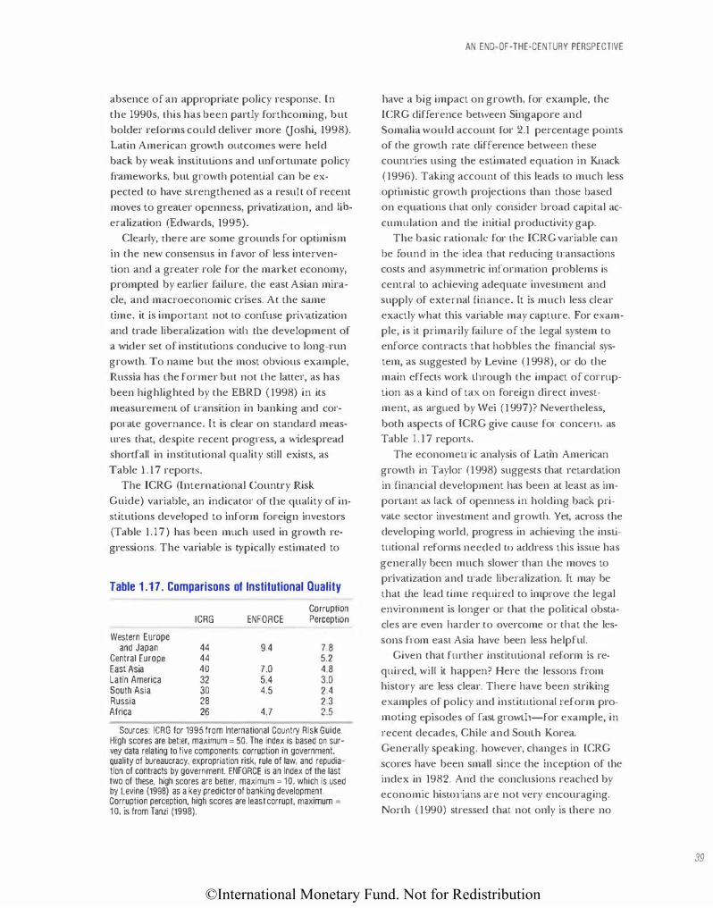
©International Monetary Fund. Not for Redistribution
absence of an appropriate policy response. In the 1990s, lhis has been partly forthcoming, but bolder ref<)rms could deliver more Uoshi, 1998). Latin American growth outcomes were held back by weak institutions and unfortunate policy frameworks, but growth potential can be expected to have strengthened as a result of recent moves to greater openness, privatization, and liberalization (Edwards, 1995).
Clearly, there are some grounds for optimism in the new consensus in favor of less intervention and a greater role for the market economy, prompted by earlier failure, the east Asian miracle, and macroeconomic crises. At the same time, it is important not w confuse privatization and trade liberalization witl1 t11e development of a wider set of institutions conducive to long-run growth. To name but the most obvious example, Russia has tl1e former but not the latter, as has been highlighted by the EBRD ( 1998) in its
measurement of transition in banking and corporate governance. It is clear on standard measures that, despite recent progress, a widespread shortfall in institutional quality still exists, as Table 1 . 17 report5.
The TCRG (International Country Risk Guide) variable, an indicator of t1·1e quality of institutions developed to inform foreign investors (Table 1 .17) has been much used in growth regressions. The variable is typically estimated to
Table 1 .17. Comparisons of Institutional Quality
Corruption ICRG ENFORCE Perception
Western Europe and Japan 44 9.4 7.8
Central Europe 44 5.2 East Asia 40 7.0 4.8 Latin America 32 5.4 3.0 South Asia 30 4.5 2.4 Russia 28 2.3 Africa 26 4.7 2.5
Sources: ICRG for 1995 from International Country Risk Guide. High scores are better, maximum = 50. The index is based on sur· vey data relating to five components: corruption in government. Quality of bureaucracy, expropriation risk, rule of law, and repudiation of contracts by government. ENFORCE is an Index of the last two of these, high scores are better, maximum = 10, which is used by Levine (1998) as a key predictor of banking development. Corruption perception, high scores are least corrupt, maximum =
1 D. is from Tanzi (1998).
AN END-OF-THE-CENTURY PERSPECTIVE
have a big impact on growth, for example, the ICRG difference bet\veen Singapore and Somalia would account for 2.1 percentage points of the growth rate difference between these countries using the estimated equation in Knack ( 1996). Taking account of this leads w much less optimistic growth projections than those based on equations Lhat only consider broad capital ac
cumulation and the initial productivity gap. The basic rationale for lhc TCRG variable can
be found in the idea that reducing u·ansactions costs and asymmetric information problems is central to achieving adequate inveslmenl and supply of external finance. It is much less clear exactly what this variable may capture. For example, is it primarily failure of the legal system to enforce contracts that hobbles the financial system, as suggested by Levine ( 1 998), or do tl1e main effects work tl1rough the impact of corruption as a kind of tax on foreign direct investment, as argued by Wei ( 1 997)? Nevertheless,
both aspects of JCRG give cause for concern, as Table 1 . 1 7 report�.
The economeu·ic analysis of Latin American
growth in Taylor (1998) suggests that retardation in financial development has been at least as important as lack of openness in holding back private sector investment and growth. Yet, across the developing world, progress in achieving t11e institutional reforms needed to address this issue has generally been much slower than the moves to privatization and u·ade liberalization. It may be tl1at lhe lead time required to improve the legal environment is longer or that the political obstacles are even harder to overcome or that the lessons from east Asia have been less helpful.
Given that further institutional reform is required, will it happen? Here the lessons from history are less clear. There have been striking examples of policy and institutional reform promoting episodes of fast growt11-for example, in recent decades, Chile and South Korea. Generally speaking, however, changes in ICRG scores have been small since the inception of the index in 1982. And the conclusions reached by economic hisro1ians are not very encouraging. North (1990) su·essed that not only is lhere no
39
©International Monetary Fund. Not for Redistribution
40
CHAPTER I GLOBALIZATION AND GROWTH IN THE TWENTIETH CENTURY
natural selection process that ensures the replacement of inefficient with efficient institutions but that network externalities, informal constraints, and the vested interests that surround existing arrangements tend to make institutional change a slow, incremental process and give it a path-dependent character.
What Future for the East Asian Developmental State?
The assessment in World Bank ( 1993) has been highly influential. High-performing east Asian economies were seen as benefiting from excellent TFP growth linked to their outwardly oriented policies and their unusual success was attributed to governmental success in solving coordination problems while adopting policy frameworks that contained rent seeking and were generally market-friendly. Rapid deepening of financial markets was taken to be a big stimulus to investment and growth, while industrial and directed credit policies were not seen as
damaging. These countries have rightly been praised for thei1· policies to foster human capital accumulation and high domestic savings rates, and for the quality of their government bureaucracies. Country dummy variables in growth regressions suggested that these economies had outperformed the world sample by about 1.7 percent a year compared with underperformance signaled by Latin American and African dummies of 1.3, and 1.0 percent, respectively (World Bank, 1993, p. 54).
To the economist in the street brought up on 'The East Asian Miracle," the trauma that began in 1997 and brought growth in many countries to an abrupt halt must have come as a dreadful surprise. Two questions arise:
• Were there aspects of the east Asian development model that exposed the region to the crisis?
• How should the crisis affect assessments of east Asian growth?
Economic history offers many examples of financial crises occurring in basically sound and strong economies with high growth potential but
exposed to macroeconomic shocks where the banking system was fragile, for example, in nineteenth and early twentieth century America, and most notoriously in the American Great Depression of the 1930s.
Recent appraisals of east Asian banking systems have commented on a number of serious weaknesses that were common, although with differing severity, through much of the region. These include low capital-adequacy ratios of banks, excessive exposure of banks to single borrowers, unduly lenient provisioning rules for nonperforming loans, weak supervision, absence of proper auditing and accounting, and so on that, combined witl1 high leverage of the corporate sector, have implied vulnerability to financial shocks (World Bank, 1998). The implication of these weak balance sheets was a high risk of financial crisis with mounting asymmetric information problems if the macroeconomic environment turned difficult (Mishkin, 1999). Financial liberalization in many east Asian countries overburdened the regulatory authorities and incurred a high risk of a subsequent financial crisis.
What then does the current crisis tell us about the preceding east Asian growth process? It should not be taken to suggest that several decades of strong growth should be seen as some sort of mirage. Rather, it reminds us that a key lesson of history is that, without adequate
regulation of the banking system, severe disruptions to economic growth are always likely. It probably reinforces suggestions that capital has been badly used in some counu;es. lt need not, however, imply that, in general, long-term growth potential is weak or has been permanently damaged. Favorable features of east Asian growth noted by the World Bank such as high savings, strong human capital formation, and effective technology u·ansfer mechanisms are unlikely to be damaged by the financial crisis.
Indeed, the 1 930s American experience (see
Box 1.2) may have some optimistic implications for Asian crisis countries. In the long run, the trend rate of growth was unaffected despite the severity of the economic shock (Ben David and Papell, 1995). While this example suggests that
©International Monetary Fund. Not for Redistribution
even a massive financial crisis need not damage long-term growth potential provided that the banking system is rehabilitated and reregulated, this does not detract from the case for widerranging reforms to the conduct of both firms and governments in east Asia if future growth potential is to be fully realized.
From Table 1.8, it is clear that east Asian growth has relied much more on the contribution of rapid factor accumulation, of both capital and labor, than did Europe's fast growth during its Golden Age. Normalizing for the opportunities for catch-up presented by the ini
tial productivity gaps and levels of education, the Tigers' TFP growth seems rather disappointing (Crafts, 1999a). Growth accounting reveals that Lhe east Asian dummies in the World Bank's growth regressions were largely the result of favorable demography and initial capital to output ratios rather than superior policy.
The east Asian developmental states delivered
a long period of high investment and very rapid growth bur their policy prescriptions appear to have been much more successful in promoting high levels of investment than in achieving exceptional productivity performance. Recent econometric studies have found that selective interventions on balance retarded rather than stimulated growth. ln Korea, directed loans and the clout of the chaebols appear to have distorted credit flows to the detriment both of profitability and productivity growth (Borensztein and Lee, 1999). An analysis of industrial productivity growth across sectors in Korea dwing 1963-83 found that tax and financial incentives did not enhance productivity growth, while NTBs re
duced both capital accumulation and TFP growth (Lee, 1995). A comprehensive review of industrial policy in east Asian countries concluded that government intervention has generally had adverse effects (Smith, 1995).
In the absence of effective conu·ol by shareholders, the best restraint on inefficient management of firms is competition (Nickell, 1996). Yet competition policy in east Asia has been seriously neglected; for example, ASEAN counu·ies with the exception of Thailand do not have anti-
AN END-OF-THE-CENTURY PERSPECTIVE
trust laws, and in the Thai case the law has been used as an instrument of price control rather than to promote economic efficiency (Lall, 1 997). This is also an area where reform seems to be urgently required.
I n the longer term, it seems likely that in the later stages of developmem it will be desirable for east Asian countries to move away from bankdominated finance and to develop better methods of corporate governance. In most cases, this
will entail the establishment of better legal rights for outside shar·eholders and will be facilitated by the emergence of ownership characterized by large and powerful investors (La Porta and other·s, 1997). The importance of investor protec
tion and availability of equity finance appears to be especially important in fostering growth in R&D-intensive activities, which are starting to be important in the leading Tiger economies (Carlin and Mayer, 1998).
The industrial poljcy prescriptions of the de
velopmental state, which are liable to result in the support of declining industries at the expense of the rapid exploitation of new service sector opportunities, ar·e likely to be still less helpful to funher catch-up in east Asia. Su·onger market disciplines are likely to be conducive to better productivity performance.
Recognizing both the need for and some of the difficulties of a move back [rom hierarchies toward markets to strengthen productivity performance as development progresses is dearly
important in refining perspectives on the east Asian developmental state. Nevertheless, these are, in an important sense, problems of success and still appear to leave the Asian developmental state as an escape route out of economic back"wardness. The deeper problem for other counu·ies may be tl1at tl1is model is hard to replicate in that po)jtical economy will pervert its interventions much further in the direction of rent seeking and wasteful investment.
Is Another Globalization Backlash likely?
The retreat from globalization in the interwar period was much accelerated by the depression.
41
©International Monetary Fund. Not for Redistribution
42
CHAPTER I GLOBALIZATION AND GROWTH IN THE TWENTIETH CENTURY
At the same time, there were other forces that
pulled in the same direction. Losers from the
operation of free world markets put pressure on
governments to protect them, and trade wars
loomed la1·ge in any case. Clearly, similar issues
have surfaced in the context of the renewed
globalization of recent decades. There have
been fears that increasing regionalism will give
rise to u·ade hostilities and that the consensus in
favor of free u-ade in OECD countries, especially
the United States, might evaporate in the face of
the problems of sunset indusu·ies and unskilled
workers.
A new focal point for unease in First World
countries is the suggestion that, in a world of
greatly increased capital mobility, tax competi
tion may jeopardize the provision of social insur
ance just when the external economy is seen as a
source of increased risk exposure. In the Third
World, whjle the evidence of recent times has
persuaded most policymakers that greater open
ness is conducive to faster economic growth in
the long run, there may yet be risks that old na
tionalist resentments directed at perceived ex
ploitation by multinational enterprises return
and obstacles to foreign direct investment are re
instated, especially in counu·ies where the in
come gap with the rich continues to grow.
The early twenty-first century differs from the
1930s in several important respects. There was
no equjvalent to the GATT /WfO with tariff
binding in place then. The range of policy in
struments with which to shield losers is rather
wider now in many countries. Globalization has
much deeper roots. The egregious macroeco
nomic policy errors of the interwar period are
widely recognized, and lessons have been learnt.
It is generally agreed among "informed econo
mists" that the problems of unskilled workers in
the OECD countries are very largely due to skill
biased technological change rather than factor
price equalization through trade (Slaughter,
1999). So, at first glance, there may be less risk
of a backlash. Nevertheless, the pressure points
highlighted above deserve some consideration.
It is well-known that larger countries typically
will have higher optimal tariffs in a noncoopera-
tive u·ade environment. Retaliatory trade policy
was a distinct feature of the 1930s retreat from
globalization. ll does not, however, follow rJ1at
end-century moves toward greater regionalism
imply a retun1 to the trade wars of the interwar
period, especially given the results of that
episode. ll might be argued that, at the intergov
ernmental level, the current situation is more
akin to an infinitely repeated game in which co
operation is preserved by the prospect of future
payoffs (Perroni and Whalley, 1996).
Nevertheless, the circumstances that gave rise
to unequivocal support for freer trade in early
postwar U.S. policymaking have been eroded.
Changing patterns of comparative advantage
and the catching up of other countries have in
creased the number of indusu·ies that fear for
eign competition; organized labor and a signifi
cant part of the Democratic Party has become
protectionist as many workers' real wage rates
have stagnated; and the elite consensus that
arose as a foreign policy reaction to the 1930s
has evaporated (Destler, 1992). To many interest
groups, protectionism is attractive. Similar con
siderations have informed the European
Commission's use of non tariff barriers such as
antidumping measures in tl1e recem past
(Tharakan, 1991).
The policy processes at work in the earlier re
treat from globalization in the United States
have been the object of a good number of de
tailed analyses. These tend to emphasize the im
portance of shifting coalitions in Congress as
well as political responses to substantial numbers
of losers. Thus, Goldin ( 1994) found both that
immigration impacted heavily on unskilled
wages and that trends in wages informed the
votes of legislators on immigration policy i11 the
early twentieth cemury. But she also found that
the coalition that eventually was formed to pass
the acts of the 1920s depended on the South's
urge to protect its relalive population share and
political clout and a growing antipathy to immi
gration by other rural Americans who were not
threatened in any direct way.
The Fordney-McCumber ( 1 922) and the
Smoot-Hawley (1930) tariffs offer similar lessons.
©International Monetary Fund. Not for Redistribution
The former exhibits a clear pauern of protec
tion for labor-intensive indusu·ies, industries that
were geographically concentrated or produced
agriculturally based consumer goods products
(Hayford and Pasurka, 1992). The latter pro
vided relief for agricultural distress in a log
rolling coalitions process that also raised tat;ffs
for specific industrial inte1·ests (Eichengreen,
1989; and Irwin and Kroszner, 1996). The impli
cation of these examples is that, absent the early
postwar consensus, American trade policy is li
able to be unpredictable. Although the represen
tatives of unskilled labor have been unable to
prevent NAITA, there may yet be new protec
tionist coalitions.
RodriJ< ( 1997a) pointed to the danger of an
eventual globalization backlash as a result of the
tension between its implications of, on the one
hand, increased demands for social protection
of workers and, on the other hand, reduced abil
ity to finance these from taxes on capital. He
supported this argument empirically by suggest
ing that capital taxes have been reduced in the
face of increased capital mobility and that, other
things equal, exposure to terms of u·ade volatil
ity is correlated with greater social insurance ex
penditure by governments. This would hardly
have been an issue in the 1920s when govern
ments generally relied very little on direct taxes
other than those on real estate and when social
transfers were very modest (see Table 1.16).
While Rodrik's regressions point to a potential
problem, the experience of OECD countries thus
far appears more benign. The evidence reviewed
in Schulze and Ursprung ( 1999) does confirm
that capital tax rates started to decline modeJ·
ately from the early 1980s but also shows that cap
ital tax revenues have been stable and that capital
market integration effects depend heavily on po
litical institutions with a tendency to increase so
cial transfers in corporatist, high consensus
democracy countries. They conclude that global
ization so far has had its main impact in terms of
a modification of tl1e tax structure rather than
through reu·enchment of the weliare state. Detailed empirical research on the impact of
fiscal policy on growth in advanced countries for
AN END-OF-THE-CENTURY PERSPECTIVE
the 1970-95 period has con firmed that "produc
tive expenditures" by government on infrastruc
ture, education, etc. are growth enhancing while
distortionary (direct) taxation is growth reduc
ing (Kneller and others, 1999). II might be ex
pected that competition fo1· footloose investment
'��11 tend to push governments both to reduce
distortionary taxes and to raise expenditures
that encourage private capital formation. The
implication may be tl1at tl1e pressures of global
ization are actually helpful in steering Ciscal pol
icy to a more pro-growth stance.
Although tl1ere is clear evidence in both Latin
America (Taylor, 1998) and Africa (Collier and
Gunning, 1999) that closed economy develop
ment strategies have been expensive failw-es,
there is a danger that recent liberalizations may
deliver less than their proponents expect and
tl1at, at some point, there will be a backlash. For
example, there is no evidence that abolishjng
capital conu·ols per se raises the rate of growth
(Grilli and Milesi-Feretti, 1995) but quite good
reason to believe that financial liberalization sig
nificantly increases Lhe risk of a subsequent fi
nancial or currency crisis (Kaminsky and
Reinhart, 1 999). As recent Malaysian experience
testifies, tl1is may undermine support for liberal
ization. The issue is perhaps one of sequencing,
but history suggests that there may have been a
tendency to premature reform in the absence of
adequate financial supervision and regulation.
Similarly, earlier nationalist critics probably
were right to question the impact of multina
tional enterp1;ses on host developing counu·ies.
A recem summary of tl1e evidence in Caves
( 1 996) concluded that both theory and empiri
cal evidence is ambiguous as to t11e implications
of multinationals for host country growth.
Positive spillovers and crowding ouL can both be
envisaged. In the case of exu-active industry in
particular, linkage effects may be weak and repa
triated profits high (Rodriguez-Clare, 1996).
Moreover, indiscriminate attraction of foreign di
rect investment can be welfare reducing when it
is based on tariff protection (Encarnalion and
Wells, 1986). Thus, despite the potential advan
tages of multinational enterprise as a vehicle for
43
©International Monetary Fund. Not for Redistribution
44
CHAPTER I GLOBALIZATION AND GROWTH IN THE TWENTIETH CENTURY
technology transfer, it would not be surprising to find some of the resentments that were so evident in the 1950s through the 1970s resurfacing.
Conclusions
The preceding material contains a great deal of detail and will not be summadzed here. Rather, the opportunity will be taken to underline a few central arguments around the general theme that an assessment of fumre growth prospects now must be less confident (in both
senses-less optimistic and less precise) than would have been the case 30 years ago. Now, there is much less consensus among mainstream
growth economists and we arc more aware of the transience of epochs in world economic development
Three points from the evidence explored in this section deserve to be underlined. First, and foremost, is that policy matters for growth outcomes. This is most obviously true and has the largest impact on growth outcomes in developing economies, but it is also evident in the OECD, as is confirmed by the contrasting fortunes of Ireland and Sweden since the end of
the Golden Age. Second, this is a point at which there are wildly different beliefs about the likely future growth of the leading economy. While the new paradigmists and some believers in endogenous growth theory seem to imagine that the information and communications technology revolution will lead to much-enhanced producti,rity growth, many economic historians and those still wedded to some version of the augmented-So low
growth model are unconvinced. At the very least, the next two or three decades should be an interesting test for competing ideas in growth theory.
Finally, it should be recognized that the analysis in this section is quite skeptical of the projections of future growth performance that international organizations such as OECD seem to favor (Richardson, 1997). In the view developed here, sustaining strong catch-up growth performance is seen as rather difficult and dependent on unpredictable success in achieving policy reform
and institutional innovation as the economy de
velops. Thus, China faces the problems of moving on from initial success that have caused
Japan to falter. We know that policy reform can turn around "basket cases" and that crises can initiate long-needed reform or encourage seriously growth-retarcljng policy responses, as in Lhe 1930s. These decisions lie fundamentally in the realm or political economy and we still know remarkably little about what determines the outcomes.
References
Abramovitz, M., 1986, "Catching Up, Forging Ahead,
and Falling Behind," }ottnwl of Economic Hi.�tmy, Vol.
36, pp. 385-406.
_, 1993, "The Search for the Sources of Growth:
Areas of Ignorance, Old and New," journal of
Ecrmmnic History, Vol. 53, pp. 2 1 7-43.
_, and P. David, 1996, "Convergence and
Deferred Catch-Up: Productivity Leadership and
the Waning of Ame1·ican "Exceptionalism," in R.
Landau, T. Taylor. and C. Wright (eds.) , The Mosrtir
of Ecouomic Growth (Stanford: Stanford Unive;:rsity
Press), pp. 21-62.
Ades, A., and R. di Tella, 1997, "National Champions
and CorrupLion: Some Unpleasam Interventionist
Arithmetic," Brmwmic jounwl, Vol. I 07,
pp. I 023-42.
Ahluwalia, I.J., 1991, Productivity ant/ Growth in f11dian Manufacl�tring (Delhi: Oxford University P1·ess).
Akedol: C.A., W.T. Dickens, and C.L. Perry, 1996,
"The Macroeconomics of Low Inflation," Brookings
Papers on l!'conomic Attivity. Vol. I , pp. 1-76.
Amsden, A.l-1., 1989, Asia 's Nrxl Ciani (New York:
Oxford Uuiversity Press). Bairoch. P., 1993, Erouomics and World History: Myths
and Paradoxes (London: Harvester Wheatshea(). Bajpal. N., and J.D. Sachs, 1996, "India's Economic
Reforms: The Steps Ahead," Harvard lnstitltte for
Economic Development Discussion Paper No. 532
(Camb1·idge, Massachuseus) . Barro, RJ., 1998, "Notes on Crowlh Accounting,''
National Bureau of Economic ReseRrch Working
Paper No. 6654 (Cambridge, Massachusetts) . __ , and X. Sala-i-Martin, 1991, "Convergence in
S tates and Regions," Bmol<ings PafJers on Economic
Activity, Vol. 1 , pp. J 07-82.
©International Monetary Fund. Not for Redistribution
Baumol, WJ., 1967, "Macroeconomics of Unbalanced
Growth: The Anatomy of Urban Crisis,'' Ame1ican
Economic Review, Vol. 57, pp. 415-26.
Beason, R., and D.E. Weinstein, 1996, "Growth,
Economies of Scale and Targeting in Japan,
1955-1990,'' Review of Economics and Statistics, Vol.
78, pp. 286-95.
Ben-David, D., and D.H. PapeU, 1995, "The Great
Wars, the Great Crash and Steady-State Growth:
Some New Evidence About an Old Stylized Fact,"
jou.nwl of Monetary Ecmwmics, Vol. 36, pp. 453-77.
Bemanke, B.S., and K. Carey, 1996, "Nominal Wage
Stickiness and Aggregate Supply in the Great
Depression,'' Qum-terlyjou.rnal of Economics, Vol. 1 1 1 ,
pp. 853-84.
Bernanke, B.S., and H. James, 1991, "The Gold
Standard, Deflation, and Financial Crisis in the
Great Depression: An International Comparison,"
in R. C. Hubbard (eel.), Financial Mad1ets and
Financial C1ises (Chicago: University of Chicago
Press), pp. 33-68.
Bohara, A.K., and W.H. Kaempfer, 1991, "A Test of
TariffEndogeneity in the United States,'' Ame1ican
Econom.ic Review, Vol. 81, pp. 952-60.
Bordo, M., and F.E. Kydland, 1995, 'The Cold
Standard as a Rule: An Essay in Exploration,"
Explorations in Economic History, Vol. 32, pp. 423-64.
Bordo, M., CJ. Erceg, and C.L Evans, 1997, "Money,
Sticky Wages, and the Great Depression,'' Board of
Governors of the Federal Reserve System
international Finance Discussion Paper No. 591
(Washington).
Bordo, M., B. Eichengreen, and D.A. Irwin, 1999. "ls
Clobali.zation Today Really Different Than
Globalization a Hundred Years Ago?" National
Bureau of Economic Research Working Paper o.
7185 (Cambridge, Massachuseus).
Bordo, M., M. Edelstein, and H. Rockoff, 1999, ''\>Vas
Adherence to the Gold Standard a 'Good
Housekeeping Seal of Approval' During the
Interwar Period?" National Bureau of Economic
Research Working Paper No. 7186 (Cambridge,
Massachusetts).
Bot·ensztein, E., and J-W. Lee, 1999, "Credit Allocation
and financial Crisis in Korea," lMF Working Paper
No. 99/20 (Washington).
Boswck, F .. and C. jones, 1994. "Foreign
Multinationals in British Manufacturing,
1850-1962," Business History, Vol. 36, pp. 89-126.
REFERENCES
Blondal, S., and D. Pilat. 1997, 'The Economic
Benel1ts of Regulatory Reform,'' OECD Economic
Studies, Vol. 28(1), pp. 7-45.
Burki, SJ, and G. E. Perry, 1997, The Long Mmdt: A Riform Agenda for Latin Amm·ica and the Catibbean in
the Next Decade (Washington: World Bank).
Burnside, C., M. Eichenbaum, and S. Rebelo, 1999.
"Prospective Deficits and the Asian Currency
Crisis," World Bank PoliC)' Research Working Paper
No. 2174 (Wa�hington).
Calomiris, C.W., 1993, "Financial Factot'S in the Great
Oept·ession," joumal of Economic Perspectives, Vol.
7(2), pp. 61-85.
Calomiris, C.W., and B. Wilson, 1998, "Bank Capital
and Portfolio Management: The 1930s 'Capital
Crunch' and So-amble to Shed Risk," National
Bureau of Economic Research Working Paper No.
6649 (Can1bridge, Massachusetts) .
Campa,j.M., 1990, ''Exchange Rates and Economic
Recovery in the 1930s: An Extension to Larin
America,"journa/ ofEcOIW'IIIic History, Vol. 50,
pp. 677-82.
Caprio, G., 1998, "Banking on Ctises: Expen.�ive
Lessons from Recent Financial Crises." World Bank
Policy Research Working Papet· No. 1979
(Washington).
Carlin, W., and C. Mayer, 1998, "Finance, Investment
and Cr·owth," Universit)' College of London
Department of Economics Discussion Paper 98-09.
Caves, It E .. 1996, Mullinational Enterprise cmd Economic
Anal)'sis (Cambridge: Cambl"idge University Press).
Chandler. LV., 1971, Amnicrm MonPlary Polic)', 1928-1941 (New York: Harper and Row).
Collier, P., 1999, "On the Economic Consequences of
Civil War." Oxjmrl Economic Paf;ers, Vol. 5 1 ,
pp. 168-83.
Collier, P., andj.W. Cunning, 1999, "Explaining
Africa's Economic Performance, .. .foumal of Economir
Litemtw·e, Vol. 37. pp. 67-1 1 1 .
Collins, S.M., and B.P. Boswonh, 1996, "Economic
Growth in East Asia: AccumulaLion Versus
Assimilation," Bmohings Patm:5 on Economic ilctivity,
Vol. 2. pp. 135-91.
Collins, WJ., andJ.G. Williamson, 1999, "Capital
Goods Prices, Global Capital Markets, and
Accumulation, 1870-1950," National Bureau of
Economic Research Working Paper No. 7145
(Cambridge. Massachuseus).
Conybeare,j.AC., J987, TradP Wars (New York:
Columbia University Press).
45
©International Monetary Fund. Not for Redistribution
46
CHAPTER I GLOBALIZATION AND GROWTH IN THE TWENTIETH CENTURY
Costa, D.L., and R.H. Steckel, 1997, "Long-Term
Trends in Health, Welfare, and Economic Growth
in the United States," in R. H. Steckel and R. Floud
(eds.), Health and Welfare Dwing Industrialization
(Chicago: University of Chicago Press) , pp. 47-89.
Crafts, N.F.R., 1989, "Long-Term Unemployment and
the Wage Equation in Britain, 1925-1939,"
Economica, Vol. 56, pp. 247-54.
__ . l997a, "The Human Development Index and
Changes in Standards of Living: Some 1-1 isto•·ical
Compa1isons," Eu·ropean Review of Economic HistCft')',
Vol. 1 , pp. 299-322.
__ , 1997b, "Economic Growth in East Asia and
Western Europe Since 1950: Implications for Living
Standards," National Institute Economic Revi11w, Vol.
162, pp. 75-84.
__ , 1998, "Forging Ahead and Falling Behind: The
Rise and Relative Decline of the First T ndustrial
Nation," }otmUJ.l of Economic Perspectives, Vol. 12 (2) ,
pp. 193-210.
__ , l999a, "East Asian Growth Before and After the
Crisis," JJ'vfF Sta!J Papers, Vol. 46, pp. 139- 66.
__ , 1999b, "Development History," LSE
Department of Economic History Working Paper
(London: London School of Economics and
Political Science).
_, and C.K. Harley, 1992, "Output Growth and the
British Industrial Revolution: A Restatement of tl1e
Crafts-Harley View," I::wnomic Histor)' Review, Vol. 45,
pp. 703-30.
__ , and T.C. Mills, 1996, "Europe's Golden Age: An
Econometric Investigation of Changing Trend Rates
of Growth," in B. van Ark and N. F. R. Crafts (eds.),
Quantitatiw Aspects of Postwar Ew·opean economic
Growth (Cambridge: Cambridge University Press),
pp. 413-3 1 .
Dahlman, CJ., 1994, "Technology Strategy i n East
Asian Developing Countries." joumaL of Asian
Economics, Vol. 5, pp. 541-72.
Daly, M., and 1-1. Kuwahara, 1998, "The Impact of lhe
Uruguay Round on Tariff and Non-Tari1J Barriers
to Trade in the 'Quad,"' The World Economy, Vol. 2 1 ,
pp. 207-34.
Dasgupta, P., and M. Weale, 1992, "On Measuring tl1e
Quality of Life," World Development, Vol. 20,
pp. 1 1 9-31.
David, P.A., 1991, "Computer and Dynamo: The
Modern Productivity Paradox in a Not-Too-Distant
Mirror," in OECD, Technology and P1·oductivit)' (Paris:
OECD), pp. 315-48.
� and G. Wright, 1999a, "General Purpose
Technologies and Surges in Productivity: Historical
Reflections on the Ftnure of the ICT Revolution,"
paper presented to the Conference on Economic
Challenges of the 21st Century in Historical
Perspective, Oxford.
� 1 999b, "Early Twcntieth-Centur)' Productivity
Growtl1 Dynamics,'' paper presented to tl1e
Economic History Society Conference, Oxford.
de Ia Fuente, A .. 1997. "Fiscal Polky and Growth in
the OECD," Ccnu·e for Economic Policy Research
Discussion Paper 1o. 1755 (London).
de Melo, M., C. Denize•·, A. Gelb, and S. Tenev, 1997.
"Circumstance and Choice: the Role of Initial
Conditions and Policies in Transition Economies,"
Wo.-Id Bank Policy Research Wodung Paper No.
1866 (Washington).
Denison, E. F., and W. Chung, 1976, How }afJan 's Eronomy G1·ew So Fast (Washington: Brookings).
De;:stler. l.M., 1992, ilnmican Trade Politics (Washington:
Institute fo•· Inte;:rnational Economics).
Dowrick, S., 1996, "Estimating the Impact of
Gove1·nment Consumption on Growth: Growth
Accounting and Endogenous Growtl1 Models," in S.
Durlauf,J. Helliwell, and B. Raj (eels.), Long-1?-un
Economic Growth (Heidelberg: Physica-Verlag).
pp. 163-84.
Easterly, W., and S. Fischer. 1995, 'The Soviet
Economic Decline," World Bank I::ronomir Revil!w,
Vol. 9, pp. 341-71 .
Easterly, W., and R. Levine, 1997, "Africa's Growth
Tragedy: Policies and Ethnic Divisions," QuarterLy
journaL of Economics, Vol. 1 1 2, pp. 1203-49.
Edgerton, D.E.I-1., and S.M. Hor.-ocks, 1994, "British
TndtlSu·ial Research and Development Before 1945,"
l!'couomir History Review, Vol. 47, pp. 213-38.
Edwards, S., 1995, G1isis and Rejol'm in Latin Ametica
(New York: Oxford University Press).
__ . 1 998, "Openness, ProducLivity, and Growth:
'V\fhat Do \Ale Really Know?" EconomicJoumal, Vol.
I 08, pp. 383-98.
Eichengreen, B., 1989, 'The Political Economy of 1he
Smoot-Hawley TariiJ," Research in Economic HislOI)'•
Vol. 12, pp. 1-43.
__ , 1992, Golden Fellers: 17!e Colli Standard aud the
Oreal Depression, 1919-1939 ( ew York: Oxford
University Press) .
_, 1996, "Institutions and Economic Growth:
Europe After World War 11," in N.F.R. Crafts and G.
Toniolo (e;:ds.), Economic Growth in EuTojJe Since 1945
©International Monetary Fund. Not for Redistribution
(Cambt·idge: Cambridge University Press),
pp. 38-72.
__ , andj. Sachs, 1985, "Exchange Rates and
Economic Recovery in Lhe 1930s," journal of
Economic History, Vol. 45, pp. 925-46.
Encarnation, OJ., and LT. Wells, 1986, "Evaluating
Foreign Investment," in T. H. Moran (ed.), Investing
in Develofnnenl: New Roles for Ptivate Capital (New
Brunswick, New Jersey: Transaction Books),
pp. 61-86.
Engen, E. M., anclj. Skinner, 1996, "Taxation and
Economic Growth," National Bureau of Economics
Working Paper No. 5826 (Cambridge,
Massachuseus).
European Bank of Reconstruction and Development
(EBRD), 1998, Transition RefJorl (London).
Feenstra, R. C., 1998, "Integration ofTrade and
Disintegration of Production," journal of Economic
Perspectives, Vol. 12(3), pp. 31-50.
Fernandez, R., and D. Rodrik, 1991, "Resistance tO
Reform: Status-Quo Bias in the Presence of
l ndivid ual-Speci lie U n cen.ai n ty," American Economic
Review, Vol. 81, pp. 1 1 46-55.
Fischer, S., R. Sahay, and C.A. Vegh, 1998, ''How Far Is
Eastern Europe from Brussels?" TMF Working Paper
No. 98/53 (Washington).
Fogel, R. W., 1964, Railroads and American Economic
Growth: Essays in Economet-ric History (Baltimore,
Maryland: Johns Hopk.ins University Press).
Friedman, M., and A. Schwartz, 1963, A Monetary
History of the United States, 1867-1960 (Princeton,
New Jersey: Princeton University Press) .
Fukuda, S., 1999, "Sources of Economic Growth in
East Asian Economies: Why Did Capital Stock Grow
So Rapidly?" in OECD, Stru.ctuml Aspects of the East
Asian C1isis (Paris: OECD), pp. 29-56.
Gallarotti, M., 1985, ''Toward a Business-Cycle Model
of Tariffs," International Organization, Vol. 39,
pp. 155-87.
Gemmell, N., 1990, ''Wagner's Law, Relative Prices and
the Size of the Public Sector," Tlte Manchester School,
Vol. 58, pp. 361-77.
Gerschenkron, A., 1962, Economic Badtwardness in
Historical Pmpective (Cambridge, Massachusetts:
Belknap Press).
Goldin, C., 1994, ''The Political Economy of
Immigration Resu·iction in the United States, 1890
to 1921," in C. Goldin and G. Libecap (eels.}, The
Regulated Ecorwm:y (Chicago: University of Chicago
Press) , pp. 223-57.
REFERENCES
Gordon, M., 1941, Bm·rie1:� to World 1h'ulP (New York:
Macmillan).
Gordon, RJ., 1999, "U.S. Economic Growth Since
1870: One Big Wave?" Ame�ican Economic Review
Papers and Procee(lings, Vol. 89 (2), pp. 123-28.
Gormely, PJ., 1995, ''The Human Development Index
in 1994: Impact oflncomc on Country Rank,"
journal of Economic and Social Meflsuremenl, Vol. 21,
pp. 253-67.
Grilli. E.R., and M.C. Yang, 1988, ·'Primary
Commodity Prices, Manufacwred Goods Prices,
and the Terms of Trade of Developing Counu·ies:
What the Long Run Shows," World Ban/1 Ecouomir
Review, Vol. 2, pp. 1-47.
Grilli, V., and G.M. Milesi-Ferretti, 1995, "Economic
Effects and Su·ucwral Determinants of Capital
Controls,� !MF Stajf Papers, Vol. 42, pp. 51 7-52.
Griliches, Z., 1994, ·'Productivity, R & D, and the Data
Consu·aint," American Ecouomic Review, Vol. 84,
pp. 1-23.
Gt·ossman. R.S., 1994, "The Shoe That Didn't Drop:
Explaining Banking Stability During the Great
Depression,·· .founwl of Economic HistOI)'. Vol. 54,
pp. 654-82.
Hamilton, B., S. Mohammad, and.J. Whalley, 1988,
"Applied General Equilibrium Analysis and
Perspective on Growth Performance," jottr11al of
Polic)' Modeling, Vol. 10, pp. 281-97.
Harberget·, A. C., 1998, ''Two Visions of the Growtl1
Process," f1n1Prica11 Economic Revi ew, Vol. 88,
pp. 1-32.
Ha)'ford, M., and C.A. Pasurka, 1992, "The PoliLical
Economy of the Fordncy-McCumber and Smoot
Hawley TariiT Acts." E).plomtions in Economic History,
Vol. 29, pp. 30-50.
Hummels, D., D. Rapaport, and K-M.Yi, 1998, "Vertical
Specialization and the Changing Nature of World
Trade," Federal Reserve Bank of New York &' View,
pp. 79-99.
lde, M., 1996, ''The Financial System and Corporate
Competitiveness," in P. Sheard (eel.), japa11ese Firms, Finance, tL11d Marltets (New York: Addison-Wesley),
pp. 191-221.
lmlah, A., 1958, Economit: Elements in I hi! Pax Blillanica
(Cambridge, Massachusetts: Harvard University
Press).
International Monetar)' Fund, 1999, World Economir
Outlooll (Washington).
Irwin, D.A, and Kroszner, R., 1996, ·'Log-Rolling and
Economic lnterests in Lhe Passage of the Smoot-
41
©International Monetary Fund. Not for Redistribution
48
CHAPTER I GLOBALIZATION AND GROWTH IN THE TWENTIETH CENTURY
Hawley Tariff," National Bureau of Economic
Research Working Paper No. 5510 (Cambridge,
Massachusens).
Ito, T., 1996, 'Japan and Lhe Asian Economies: A
'Miracle' in Transition," Bmo/cin.gs Papers on Econmnir
Activity, Vol. 2, pp. 205-72.
jones, C.l., 1995, "Time Series Tests of Endogenous
Growth Models," Qum·terly journal of Economics, Vol.
1 1 0, pp. 495-525.
__ , 1997, 'The Upcoming Slowdown in U.S.
Economic Growth," National Bureau of Economic
Research Working Paper No. 6284 (Cambridge.
Massachusetts).
_, 1999, ''Growth: With or Without Scale Effects,"
American Economic Review Papers and Proceedings, Vol.
89(2), pp. 139-44.
Jones, G., and H.G. Schroter, 1993, "Continental
European Multinationals, 1850-1992," in G. Jones
and H.G. Schroter (eels.), The Rise of Mult·inationafs
in Continental Europe (AldeJ·shot, United Kingdom:
Edward Elgar), pp. 3-27.
jorgenson, D.W., and KJ. Stiroh, 1999, "Information
Technology and Growth," American Eco1wmic Review
Papers and Proceedings, Vol. 89, pp. 109-15.
Joshi, V., 1998, "India's Economic Reforms: Progress,
Problems, Prospects," Oxford Development Studies, Vol.
26, pp. 333-50.
Kaminsky, G.L., and C.M. Reinhart, 1999, "The Twin
Crises: The Causes orBanJdng and .Balance of
Payments Problems, " Americrtn Economic Review, Vol.
89, pp. 473-500.
Kindleberger, C. P., 1973, Tile World in Depression,
1929-1939 (Berkeley: University of California
Press) .
Knack, S., 1996, "Institutions and t11e Convergence
Hypothesis: Cross-Country Tests Using Alternative
Institutional Measures," Public Choice, Vol. 87,
pp. 207-28.
__ , and P. Keefer, 1995, "lnsLiwtions and Economic
Performance: Cross-Counu·y Tes1s Using Alternative
Instiwt.ional Measures," Economics mui Politics, VoL 7,
pp. 207-27.
Kneller, R., M. B\eaney, and N. Gemmell, 1999, ''Fiscal
Policy and Growth: Evidence from OECD
Countries," journal of Public Economics, Vol. 74,
pp. 1 71-90.
Koedijk, K., and J. Kremers, 1996, "Markel Opening,
Regulation and Economic Crowlh in Europe,"
Economic Policy, Vol. 23, pp. 445-67.
Kroszner, R.S., and R.C. Ra,jan, 1994, "Is the Class
Steagall Act justified ? A Study of the U. S.
Experience wilh Universal Banking Before 1933,"
American E=wmic Review, Vol. 84, pp. 8 10-32.
Lall, A., 1997, "ASEAN Approacl1es tO Competition
Policy," in F. Flatters and D. Gillen (eds.),
Competition and Regulation: hnplictttions of
Globalization for Malaysia and Thailand (Kingston:
Queen's University Press), pp. 7-32.
La Porta, R, F. Lope:.:-de-Silanes, A. Shleifer, <mel R.W.
Vishn)'• 1997, "Legal Determinants of External
Finance," journal of Finance, Vol. 52, pp. 1 131-50.
Lawrence, R.Z., 1996, Single World, Divided Nations?
(Pal-is: OECD) .
Lee,.J-W., 1995, "Government lmerventions and
Productivity Growth in Korean ManufactuJ-ing
Industries,·· National Bureau of Economic Research
Work.ing Paper No. 5060 (Cambridge,
Massachusetts).
Levine, R., 1998, 'The Legal Environment, Banks and
Long-Run Economic Growth,"jo-mw.al ofMone)',
C1-edit, and Banking, Vol. 30, pp. 596-6 1 1 .
Lindert, P. H., 1994, 'The Rise of Social Spending,
1880-1930," Expwrations in Economic History, Vol. 31,
pp. 1-37
__ , 1996, 'What Limits Social Spending?"
E>.ploralions in Economir Histqry, Vol. 33, pp. 1-34.
McGuckin, R. H., and K.j. Stiroh, 1999, "Do
Computers Make Output Harder to Measure?"
(unpublished; ew York: The Conference Board) .
Maddison, A., 1985, Two Ctises: Latin America rmd Asi(l
1929-38 and 1 973-83 (Paris: OEGO).
__ , 1987, "Growth and Slowdown in Advanced
Capitalist Economies: Techniques of Quanlitative
Assessment," joumal of Economic Literature, Vol. 25,
pp. 649-98.
__ , 1991, Dynamic Forces in Capitalist Developmmt
(Oxford: Oxford University Press).
__ , 1992, "A Long-Run Perspective on Savings."
Sertndinavian journal of Economics, Vol. 94,
pp. 181-96.
__ , 1995, Monitoring /he WorldEconom)', 1820-1992 (Paris: O£CO).
__ , J 996, "Macroeconomic Accounts for European
Countries," i11 B. van Ark and N.F.R. Crafts (eds.),
Quantitrttive Aspects of Postwm· Eur·opean Economic
Growth (Cambridge: Camb,·idge University Press),
pp. 27-83.
©International Monetary Fund. Not for Redistribution
__ , 1997, The Natu1·e and Functioning of EumjJean
Capitalism: A Historical and Comparative Per�jJective
(Croningen: Growth and Development Centre).
_. 1998, Chinese Economic Pnjormcmcr in lhe Long
Run (Paris: OECD).
Mankiw, N.C., D. Romer, and D. Wei!, 1992. "A
Contribution to the Empirics of Economic Growth,"
Qum·terly jounwl of Economics, Vol. 107, pp. 407-38.
Mills, T.C., and N.F.R. Crafts, 1999, "After the Colden
Age: A Long-Run Perspective on Growth Rates That
Speeded Up, Slowed Down, and Still Differ," The Manchester School.
Mishkin, ·F., 1999, "Lessons from the Asian Crisis,·
National Bureau of Economic Research Working
Paper No. 7102 (Cambridge, Massachusetts) .
Morris, C.T., and I. Adelman, 1988, ComjJamtive
Patterns of Economic Develcpment 1850-1914
(Baltimore: johns Hopkins University Press).
Morrison, CJ, 1992, "Unraveling the Productivity
Growth Slowdown in t.he United Suues, Canada,
and Japan: The Effects of Subequilibrium, Scale
Economies and Markups," .Re()iew of Economics and
Statistics, VoL 74, pp. 381-93.
Nakamura, L.l., 1995, "Is U.S. Economic Perfor·mance
Really That Bad?" Federal Reserve Bank of
Philadelphia Working Paper No. 95-21
(Philadelphia).
Nelson, R.R., and C. Wright, 1992, "The Rise and Fall
of American Technological Leadership," j&m'11al of
Econmnic Literature, Vol. 30, pp. 1931-64.
Newell, A., andJ.S.V. Symons, 1988, "The
Macroeconomics of the Interwar Years:
International Comparisons," in B. Eichengrecn and
T.J. Hatton (eds.). Interwar Unemployment in
International Perspective (Dordrecht, Netherlands:
Martinus-NUhoH).
Nickell, SJ, I 996, ''Competition and Corporate
Performance," jounwl of Political Economy, Vol. I 04,
pp. 724-46.
Noguchi, Y., 1998, "The 1940 SysLCm:Japan Under t.he
Wartime Economy," Amm·ican Economic Riroiew Papers
and Pmceedings , Vol. 88, pp. 404-07.
Nordhaus, W.O., 1995, "How Should We Measure
Sustainable Income?'' Cowles Foundation
Discussion Paper No. 1 1 0 1 .
_, 1998, "The Health of Nations: Irving Fisher and
the Conu-ibution of Improved Longevity to Living
Standards," Cowles Foundation Discussion Paper
No. 1200.
REFERENCES
__ , andJ. Tobin, 1972, Is Orowth Obsolete? (New
York: Columbia University Press).
North, D.C., 1990, Institutions, Institutional Change, and
Economic Performana (Cambridge: Cambridge
University Press).
Obstfcld, M., and A.M. Taylor, 1999, Global Capital
Markets: Integration, Clisis and Orowth (Cambridge:
Cambridge University Press).
O'Connor,.J.F.T., 1938, The Banking C1·isis and Recovery
Under the Rooswelt J!dministration (Chicago:
Callaghan).
Organization for Economic Cooperation and
Developmem (OECD), 1997a, Historical Statistics,
1990-1995 (Paris).
__ , 1997b, Activities of Foreign Affiliates in OECD
Cownlries (Paris) .
__ , 1998a, Natio1utl Accounts Stalistics (Paris).
__ , J998b, Human Capital investment: An
1nternalional ComjJa·rison (Paris).
__ , various years, lnterna.tionttl Direct Investment
Statistics Yearbook (Paris).
__ , 1999, Economic Outlook (Paris).
Olson, .J. W., 1988, Saving Capitalism: The .Reconstr·uction
Fina·ncr Col'jJoration and the Nm Deal, 1933-1940
(Princeton, New jersey: Princeton University
Press).
O'Rourke, K.l-l., 1997, 'Tari(fs and Growth in the Late
1 ineteenth Century," Cenu·e for Economic Policy
Research Discussion Paper No. 1700 (London).
Oxley, 1-1., and M. Macfarlan, 1995, "Health Care
Reform: Conu·olling Spending and Increasing
Efficiency," OECD Economir Studies, Vol. 24( I ) ,
pp. 7-55.
Perroni, C., andj. Whalley, 1996, "How Severe Is
Global Retaliation Risk Under Increasing
Regionalism?'' Amerir.an Et:onomic Review Papers rmd
Proaedings, Vol. 86, pp. 57-61.
Prescott, E.C., 1998, "Needed: A Theory of Total
Factor Productivity," International Economic Riroiew,
Vol. 39, pp. 525-5 1 .
Preston, S.H., 1975, 'The Changing Relation Between
Mortality and Level of Economic Developmem,"
Population Studies, Vol. 29, pp. 231-48.
Pritchett, L., 1997, "Divergence, Big Time,'' jcnwnal of
Economic Perspectives, Vol. I I (3), pp. 3-17.
Richardson, P., 1997, "Globalization and Linkages:
Macroeconomic Challenges and Opponunities,"
OECD Economks Deparunem Working Paper
No. 181 (Pal-iS).
49
©International Monetary Fund. Not for Redistribution
50
CHAPTER I GLOBALIZATION AND GROWTH IN THE TWENTIETH CENTURY
Rodrigue;r.-Clare, A., J 996, "Multinationals, Linkages,
and Economic Development," American Eronomir
Review, Vol. 86, pp. 852-73.
Rodrik, D., 1997a, Has Globalization Gone Too Far?
(WashingLOn: Institute for International
Economics).
__ , 1997b, "TFPG Controversies, Institutions and
Economic Performance in East Asia," Centre for
Economic Policy Research Discussion Paper
No. 1587 (London).
Rooth, T., 1992, 'The Political Economy of
Protectionism in Britain, 1919-32",journal of
EttTOjJean Economic History, Vol. 21, pp. 47-97.
Rosenberg, N., and L.E. Birdzell, 1986, How the West
Grew Rich (London: Tauris) .
Roseveare, D., W. Leibfritz, D. Fore, and E. Wurzel,
1996, "Ageing Populations, Pension Systems and
Government Budgets: Simulations for 20 OECD
Countries,'" OECD Economics Department Working
Paper No. 168 (Paris) .
Sachs, J.D., and A.M. Warner, 1995, "Economic
Reform and the Process of Global Integration,"
Broo!tin� Papm on Economic Jtctivily, Vol. I ,
pp. 1-118.
_ , 1997, "Sources of Slow Growth in African
Economies," jomnal of African Economie.s, Vol. 6,
pp. 335-76.
Sala-i-Martin, X., 1996, "Regional Cohesion: Evidence
and Theories of Regional Growth and
Convergence," Europecm Economic Revh"w, Vol. 40,
pp. 1325-52.
Schou,JJ., 1994, The Umguay Round: An Assessment.
(Washington: Institute for International
Economics) .
Schulze, G.G., and H.W. Ursprung, 1999,
"GiobaUsation of the Economy and the Nation
State," World Economy, Vol. 22, pp. 295-352.
Shapiro, M.D., and D.W. Wilcox, 1996,
"Mismeasuremenl in lhe Consumer Price Index: An Evaluation," National Bureau of Economic
Research Working Paper No. 5590 (Cambridge,
Massachusetts) .
Sichel, O.E., 1997a, 'The Productivity Slowdown: 1s a
Growing Unmeasurable Sector the Culprit?" Review
of Economics and Statistics, Vol. 79, pp. 367-70.
__ , 1997b, Tlte Computer Revolution: An Economic
Perspective (Washington: Brookings).
Simon, M., 1967, 'The Pattern of ew British Portfolio
Investment, 1865-1914," in .J. H. Adler (cd.), Capital
Movements and Eamomic Develop·ment (London:
Macmillan) .
Slaughter·, M., 1999, "Giobalisation and Wages: A Talc
of Two Perspectives," W01-ld Economy, Vol. 22,
pp. 609-29.
Smith, H., 1995, "Industry Policy in East Asia," Asian
Pacific Economir. Literature, Vol. 9, pp. 17-39.
Stiroh, I<J., 1998, "Computers, Productivity, and Input
Substitution," Economit:lnquiry, Vol. 36, pp. 175-91.
Takacs, W.A., 1981, "Pressures for Protectionism: An Empir·ical Analysis," Eronomic Inquiry, Vol. 19,
pp. 687-93.
Tanzi, V., 1997, "The Changing Role of the State in
the Economy: A HisLOrical Perspective," IMF
Wor·kiug Paper No. 97/114 (Washington).
__ , 1998, "Corruption Around the World: Causes,
Consequences, Scope, and Cures,'' IMF Working
Paper No. 98/63 (Washington) .
__ , and L. Schuknecht, 1997, ''Reforming
Government: An Overview of Reccm Experience," EuroJJetm jounwl of Politiml Eronomy, Vol. 13,
pp. 395-417.
Tangi, V. and H.H. Zec, 1997, "Fiscal Policy and Long
Run Growt.h," lMF Staff Prtfm-s, Vol. 44,
pp. 179-209.
Taylor, A.M., 1998, ··on the Costs of Inward-Looking
Development: Price Distortions, Growth, and
Divergence in Latin America," jonmal of Economir
History, Vol. 58, pp. 1-28.
Temin, P., 1976, Did Monela7)' Forres Cause the Great
Depression? (New York: Norton).
__ , 1989, Lessons from the Oreal Depression
(Cambl'idgc, Massachusetts: MIT Press).
Temple,]., 1999, 'The cw Growth Evidence,"joumal
of Economir Literature, Vol. 37, pp. L 12-56.
Thru·akan, P.K.M., 1991, 'The Political Economy of
Anti-Dumping Undertakings in lhe European
Communities," Emvpean Economic Review, Vol. 35,
pp. 1341-59.
Timmer, A., and.J.C. Williamson, 1998, "Immigration
Policy Prior to tJ1e 1930s: Labor Markets, Polic)'
1meractions, and Globalization Backlash,"
Population and DeveloJnnenl Review, Vol. 24,
pp. 739-71.
Tripleu,J.E., 1999, 'The Solow Productivity Paradox:
What Do Computer-s Do to Productivity?" Canadian
joumal of Economics. Vol. 32, pp. 309-34.
UNCTAD, 1983, Handbook of Jnterrwtional Trade and
Develo-pment Statistics (New York).
_, 1997, Handbooh of international Tmlle mul Development Statistics (New York).
United Nations, 1964, Some Factors in the Economic
Orowth ofEurofJe Dming the 1950s (Geneva).
©International Monetary Fund. Not for Redistribution
United Nations Developmem Program (UNDP), 1998,
Human DeveLopment Report (New York: Oxford
University Press) .
United States Treasury Department, 1938, 76th Annual
Report of the Comptroller of the Currency (Washington).
Upham, C. B., and E. Lamke, 1934, CLosed and Di.stresse(l
Banks (Washington: Brookings).
Usher, D., 1980, The MeasU?·ement of Economic Orowth
(Oxford: Blackwell).
von Tunzelmann, G.N., 1978, Sl.eam Power and British
lndusl1ia limtion to 1860 (Oxford: Clarendon) .
Wade, R., 1990, G(ft)eming the Market (Princeton:
Princeton University Press).
Wei, S-J., 1997, "How Taxing Is Corruption on
International lnvestOJ-s?" National Bureau of
Economic Research Working Paper No. 6030
(Cambridge, Massachusetts}.
'.Veitzman, M., 1999, "Prici11g the Limits to Growth
from Minerals Depletion," Quarterly journal of
Economics, Vol. 114, pp. 691-706.
White, E.N., 1986, "Before 1.he Glass-Steagall Act: AJ1
Analysis of the Invesunen1. Banking Activities of
REFERENCES
National Banks," Explon.ttions in Economic History,
Vol. 23, pp. 33-55.
Williamson,j.G., 1984, "British Monality and the
Value of Life," PojJulation Studies, Vol. 38.
pp. 157-72.
__ , 1996, "Globalization, Convergence, and
History," jounwl of Economic History, Vol. 56,
pp. 277-306.
World Bank, 1993, TJw Enst Asian Mimc/P (New York:
Oxford University Press).
_, 1998. East Asia: The !Wad to Rerover)•
(Washington).
Ymes, P.L., 1959, Forty Yem.- of Foreign Trade (London:
Allen and Unwin).
Young, A., 1995, "The Tynmny of Numbers:
Confronting Lhe Statistical Rea liLies or the East
Asian Growth Experience," Qtwl·terlyjou,·rwl of
Economics, Vol. I 10, pp. 641-80.
Zlowik, H., 1998, "International Mignuion,
1965-1996: An Overview," Popul.alion and
Development Reuiew, Vol. 24 ( l ) , pp. 429-68.
51
©International Monetary Fund. Not for Redistribution 52
THE INTERNATIONAL MONETARY SYSTEM IN THE (VERY) LONG RUN Barry Eichengreen and Nathan Sussman
The dawn of the new millennium is an appropriate time to take stock of the evolution of the international monetary system. In most of the literature on this
subject, a long view is any1.hing thai. considers the behavior of exchange rates and associated policies pdor to the breakdown of the Bretton Woods System of par values in 1973. Thus, Baxter and Stockman ( I 989), in a widely cited swdy of exchange rate regimes, extend their data set all the way back 1.0 1960!
In this chapter we go to the other extreme, and analyze exchange ra1.es and monetary relations over the last thousand years. I It is not clear how to think about the domestic and international monetary systems over such a long period. Some would emphasize the trend from commodity money to fiat money, from market-determined money supplies to government-determined money supplies, and from price stability to innalion. The exchange rates between national currencies were not actively managed by governmental authorities in the commodity-money world that prevailed for more than 90 percent of the past millennium; rather, the exchange rate was a corollary of the metallic basis of the circulation (typic.:llly silver or gold, although other metals were also used) and 1.he fineness (thai. is, the purity) of the circulating coins. Two gold coins of equal weight and fmeness u-aded for one another at a fixed •-ate of one to one. Two gold coins of differem weight or fineness traded for one another at a differenl but still fixed rate of exchange. In contrast, the rate of exchange between gold- and silver-based monies fluctuated
with the relative price of the two metals. This makes it tempting to think of earlier international monetary arrangements in terms of a pair of gold- and silver-based monetary blocs.
With the transition to fiat money, the rate of exchange came to depend on the relative supplies and demands of the national monies that central banks and governments now actively managed. Those exchange rates could be pegged, if the authorities chose to adjust policies accordingly, or be allowed to float if other policy objectives took precedence. Because changes in economic theory, economic policy, and domestic politics increasingly caused other objectives to take precedence, we observe over time a shift from fixed to flexible rates.
In fact, this simple story begs as many questions as it answers. It ignores the fact that the governments could and did debase the coinage in the age of commodity money. 1t ignores that there were pe1;ods of inflation coinciding with these episodes of debasement and that price levels were far from stable even while gold and silver convertibility prevailed. l t does not explain the deeper factors that account for the shift from silver to gold in the nineteenth century and from gold Lo fiat money in the twentieth (summarized in Figure 2.1) .2 ll does not explain why we currently appear to be witnessing a "return to the past," with declining inflation and the reemergence of monetary blocs.
In this chapter we present a more elaborate analysis of these issues designed to place recent international monetary developments in their (very) long-run context.3 At the outset, it is
1We are conscious thai the coverage is necessarily selective, both geographicaUy and themalically, reflecting the limits of our own expertise.
2For purposes of Figure 2.1, we define countries "�th fia1 currenc-ies as those not on a gold �tandard, no1 dollarized, and not having a currency board. Thus, for present purposes we take the alternath·e 10 fiat money not as commodity money but as any hard-and-fast monetary rule (where a simple exchange r.lle peg does not quality).
'The sntdy covers a lo1 of ground and tma,·oidably skims over a variety of important topics. While we hope to answer some of the questions previously begged, it is ine,�table that we also leave important issues unresolved.
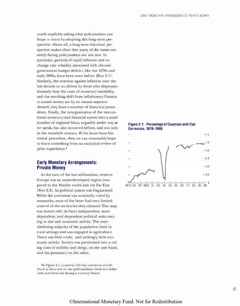
©International Monetary Fund. Not for Redistribution
worth explicitly asking what policymakers can
hope LO Jearn by adopting mis long-term per
spective. Above all, a long-term hisLOrical per
spective makes clear that many of me issues cur
rently facing policymakers are not new. In particular, periods of rapid inflation and ex
change rate volatility associated with chronic
government budget deficits, like the 1970s and
early 1980s, have been seen before (Box 2.1 ).
Similarly, the reaction against inflation over the
last decade or so, driven by those who dispropor
tionately bear the costs of monetary instability,
and the resulting shift from inflationary finance
to sound money are by no means unprece
dented; they have a number of historical prece
dents. Finally, the reorganization of the interna
tional monetary and financial system into a small
number of regional blocs, arguably under way as
we speak, has also occurred before, and not only
in the twentieth century. If the issues have his
totical precedent, then we can reasonably hope
to learn somemmg from an analytical review of
prior experience.4
Early Monetary Arrangements: Private Money
At the turn of the last millennium, western
Europe was an underdeveloped region com
pared to tl1e Muslim world and me Far East
(Box 2.2). Its political system was fragmented.
While me continent was nominally ruled by
monarchs, most of the latter had very limited
conu·ol of tl1e territories they claimed. The map
was dotted witll de facto independent, semj
dependent, and dependent political units vary
ing in size and economic activity. The over
whelming majority of the population lived in
rural settings and was engaged in agriculture.
There was little trade, and strikingly little eco
nomic activity. Society was partitioned into a rul
ing class of nobility and clergy, on the one hand,
and the peasantry on the other.
41n Figure 2.1, countries with fiat currencies are defined as those not on the gold standard, those not dollarized, and tl1ose not having a currency board.
EARLY MONETARY ARRANGEMENTS: PRIVATE MONEY
Figure 2 .1. Percentage of Countries with Fiat Currencies, 187D-1998
-1.2 - 1 .0 � -0.8 -0.6 - 0.4
=-:C:_.___.____.__.____._..____.__--L...-..J...___.______.'----'----.J-1 0.: 1870 80 90 1900 10 20 30 40 50 60 70 80 90 98
53
©International Monetary Fund. Not for Redistribution
54
CHAPTER II THE INTERNATIONAL MONETARY SYSTEM IN THE (VERY) LONG RUN
Box 2.1. Financial Crises: Continuity and Change
Financial mania, crises, and panics are as old as financial markets. as Kindleberger (1978) has amply demonstrated. The tendency for asset valuesincluding the value of the assets to which the monetary circulation is linked-to reach unsustainable levels before adjusting downward will1 a crash is no new phenomenon. From the modern poim of view, however, the question is whether the sharp recessionary effects of currency and fi
nancial clises, which have been so disruptive in recem years, are also a historical constanL
This is not a question on whose answer historians agree. But it is reasonable that lhese effects were smaller prior to the eighteenth century, when the monetary system was to a large extent (in any case, to a greater extent than today) disconnected from the real economy. Many producers and consumers transacted in nonmonetized segments of the economy. (Recall for example the importance of feudal dues paid in kind.) In western E.w·ope, litis siwation changed with the Commercial Revolution and the rise of long-distance u-ade. Both events increased the
The monetary system was based on a single
denomination silver coin, the penny (or denier) ,
a descendent of the Carolingian monetary re
form." The mints that sprung up with the revival
of trade in the tenth century produced an array
of penny coins ranging from the almost pure
sterling penny to the impure, low-weight coins of
northern ltalian cities. The monetary systems of
the m(\jor political unjts varied in size, scope,
and control, although they all shared a relatively
high degree of decentralization, reflecting Lhe
weakness of state authority and bureaucratic
monetization of the economy, then gave birth to banks. and finally encouraged the development of markets on which securitized financial assets were traded. Governments' increasing reliance on debt to .finance wars created u1creasingly deep and liquid government debt markets. The great trading companies (the Dutch and English East fndia Companies and the Bank of England) were the fu·st commercial concerns that issued debt and equity (with the aid of officially sanctioned monopolies). The emergence of this secondary market set the stage for rhe first financial bubbles and cr-ashes, witll significant consequences for the real economy: the Soulh Sea and Mississippi Bubbles of tl1e begimting of the eighteenth century (see above), the collapse of both of which was widely thought to have had depressing effects on the real economy. Ultimately, however, thls crisis ushered a wave of regulation that on tile one hand enhanced the stability for the markets and on the other band promotC'd financial deepening and econontic development.
control. On the other hand, broad differences
among major political and economic units can
be discerned. In England, for example, the mint
system was directed by the crown, and all mints
issued the same coin, whereas in France there
existed a multitude of issuing authorities, coins,
and accounting systems, and Italy's largely au
tonomous cities all issued their own coins.6
The seignorage from coin production was a
feudal right and an important source of rev
enue.? Mints had to compete with each other for
silver and seignorage. The industry can best be
5The mouetary reform of 794 consti tutes the issuing of a heavy bodied (1.7 grams) silver penny that circulated throughout Charlemagne's empire.
6The industrial organization of coin production was broadly similar throughout western Europe. The production process was catTied out in mints operated by mint masters and supervised by wardens. Coins were su·uck from dies using a manual production process that allowed substantial variability in their weight and fineness. Fineness refers to the pu.-ity of tl1e silver content of the coin. Unlike contemporary monetary arrangements. most mints did not mint on state account. Coins were minted from privately supplied silver, either from silver bullion or used coins. The merchant would bring lO t11e mint the bullion which he desired to coin. The mim would charge a fee-seignorage-for tl1is service.
7As we shall see later, it was also the impetus for commodity money inflation.
©International Monetary Fund. Not for Redistribution
Box 2.2. Monetary Developments Beyond Europe1
The monetary experiences of Asia, the Middle
East, and Africa share both similarities and differences with that of western Europe. A promi
nent element in common was the association of
fiscal and political crises with episodes of de
basements, inflation, and stabilization. Perhaps
the most important difference was that most of
the money-issuing authorities were large central
ized states, in some cases empires that spanned
wide geographical areas. These states tended to
monopolize minting activity and in most cases
were the dominant suppliers of precious metal
to the mints. The more economicaJJy advanced and com
mercialized economies of the Muslim and
Byzantine world had highly monetized
economies and were able to circulate gold cur
rencies-the bezam and dinar, respectively
well in advance of Europe. Eventually the politi
cal and military decay of the Byzantine Empire
led to debasements of its gold coinage, leaving
the dinar the leading international currency. In
J I 09 Saladin shifted the monetary standard to
ward the silver coin-the dirham-which be
came the unit of account. Again, political de
cline led to currency instability. Substitution
toward now more stable and prized European
gold coins proved iJTeversible for many cen
turies. Even the Ottoman Empire, which en
joyed substantial political and military success
for three centuries, failed to develop a monetary
system comparable to that of Western Europe;
its circulation was dominated by foreign coins.
for during periods of war the sultan (the main
is.�uer of coins) debased the silver currency.
ln India and southeast Asia the degree of
monetization was less. These regions were heav
ily agricultw·al and supported mainly local mar
kets. As was true also of most of Africa, mone·
tary requirements were fulfilled by perty
currency: cowry shells in Bengal and copper in
LThis box is largely based on articles in Richards (1983). The space consrrainlS allow us only to state the most salient faclS, doing considerable injustice to the complex historical development.
EARLY MONETARY ARRANGEMENTS: PRIVATE MONEY
Asia, including China and Japan. Monetary sys
tems of the sort that had developed in Europe
and the Middle East did not exist. Gold and sil
ver were mainly hoarded ramer than used in monetary exchange (although they were also
used to settle international trade deficits). V.'ben
used in domestic exchange, they circulated ac
cording to weight rather than tale. The Japanese
also used copper coinage until the seventeenth
century. The silver they mined was largely ex
ported to China in return for Chinese copper
coins. The only marked change occurred in India with the Muslim conquest that brought
with it the monetary practices of the Muslim
world.
The Chinese story is one of innovation on Lhe
one hand and underdevelopmem on the other.
By the sixteenth century, as in many other as
pects of economic growth and technological in
novation, the forces of relative decline came to
dominate. Since the Chinese economy was heav
ily agricultural, most of the circulation took the
form of copper coins suited for small transac
tions. Gold and silver were hoarded and used at
weight value, uncoined, in large transactions. A
key difference with Europe was that while coins
were used as a medium of exchange, they were
not generally accepted by the government in payment of taxes, a practice that tended to rein·
force the low degree of monetization of the
Chinese economy.
Interestingly, China pioneered the usc of pa
per money. The sheer size of the empire encour
aged the use of paper to minimize shipments of
precious metal. By 800, some 400 years before
Europe, China had developed a system of bills
of exchange. Unlike Europe, the government as
sumed responsibility for the note issue relatively
early. Less than a quarter of a cemury after pa·
per money, backed by silver, was first issued by
private merchants (around 1000). the govern
ment took over paper money production. The
monetary system thus was composed of copper
coins and silver-backed paper money. Evenrua!Jy,
military conflicts, especially the struggle with tl1e
Mongols, led to larger note issues which re--
55
©International Monetary Fund. Not for Redistribution
56
CHAPTER II THE INTERNATIONAL MONETARY SYSTEM IN THE (VERY) LONG RUN
Box 2.2 (concluded) suited in accelerating inflation as the end of the
Chin dynasty neared. The fuan dynasty managed to issue stable paper cu•-rency for a short
while and subsequently gave paper money fiat status by demonetizing precious metal allogether. From 1280 to 1350, the money supply
characterized, except perhaps in England, in
terms of monopolistic competition. a Each mint
would offer a "mint price" for silver in terms of
newly minted coins, and competition yielded
high- and low-quality coins and both stable and
unstable currencies. The variety and uncertain
quality of coins made it inefficient to use a coin
outside the immediate area in which it was is
sued-a situation that was perhaps tolerable so
long as trade volumes were low and economies
were relatively autarkic. Once trade revived, how
ever, the eJdsting monetary system proved inade
quate, creating an opportunity for emerging
cenu·alized monarchies.
The international monetary system was a hy
brid of fixed and flexible exchange rates, not
unlike our current system (in this respect at
least) .9 The dual nature of the exchange rate system followed from the dual nature of the unit of
account. On the one hand, a monetary system
based on a commodity such as silver or gold
made it relatively easy to arrive at a system of
fixed exchange rates between different coins.
Private and official money changers set ex-
was controlled in such a way as to generate mild
inflation. The system finally collapsed in the
mid-ftfteenth century, after which silver cur
rency came to dominate. Thus, at the very time Europe was starting to experiment with paper money, China ironically decided to abandon it.
change rates between the coins on the basis of
their precious metal content.IO On the other
hand, there existed a flexible exchange rate be
tween silver or gold and the unit of account, and
consequently between two countries' monies.
In addition, the fact that the media of ex
change-the coins-were valued independently
of the unit account or the price level made them
closer substitutes than modern fiat currencies.
Throughout most of the period, foreign coins
circulated side by side witl1 domestic ones.
"CwTency substitution" was a prevalent
phenomenon.
Monetary Stability and Monetary Integration
The commercial revolution that started
around 1 1 00 ushered in a period of trade expan
sion, urbanization, and growth. Regional and
long-distance trade and the establishment of the
first Europe-wide u·ade fairs in Champagne cre
ated demand for additional money.l l The re
sponse was not only an expansion of the existing
8£ngland was geographically compact and, being insular, offered the crown easier conrrol over imported bullion. The Saxon conquest of Danish-held lands allowed 1.he crown to impose its coinage. The Norman conquest also allowed the im· position of a monetary order.
9ln its modern usage, the "exchange rate" relates to the relative price of t:wo currencies--the relative price of the numeraire in two economies. Bl!t defining the numeraire in the medieval period is problematic. Before the elevemh century, all coins were valued at one penny in a different money of accoum, and these coins had varying silver comem; was the numeraire therefore the penny or the silver? For presem purposes it is convenient to take the numeraire as the penny and to think of silver as being valued (or measured) , like any other commodity, in terms of the prevailing money of account. We adopt this convention in what follows.
tOModified by the variability of that contem and the cost of minting them. 110ne is reminded of modern arguments that European integ1·ation, by stimulating inu·a-European u-ade, su·engthened
the demand for a single European money. We return to this below. It is also likely that the ino·eased demand for silver for monetary uses associated with this revival of n-ade led to the discovery of silver mines in cenrral Emope that irrigated the arteries of western Ew·ope's economies.
©International Monetary Fund. Not for Redistribution
monetary system as a number of new mints
sprang up, but also a demand for a more uni
form currency. This led to a consolidation phase
in which the more efficient and reputable mints
exploited economies of scale and reputation w drive their less efficient rivals out of business. I 2
The provision of this widely accepted medium of
exchange required its producers to guarantee its
quality-that is, its metallic content. To supply
the growing needs of merchants for a variety of
denominations and handle large volumes of
minting, minting became an industry character
ized by large factories with multiple furnaces
and many workers. This undertaking required
capital and an ability to produce reputation by
creating a monitoring and enforcement mecha
nism to combat fraud and counterfeiting. IS
Consolidation was carried out mainly by mar
ket forces rather than .fiat. The mints that pre
vailed were those that produced trustworthy
coins at low cost. At the risk of sounding
anachronistic, we can say that the dynamics of
Darwinian selection and survival of mints and
coins guaranteed, along its path, monetary poli
cies that benefited consumers, namely, policies
that conduced to monetary stability and mone
tary integration. Similar to the current establish
ment of the euro, a variety of currency areas
formed in medieval Europe, each based on a sin
gle or set of mints that issued a stable, reputable
coin. A key difference from the present day was
that the medieval system was allowed to emerge
endogenously, through the operation of market
forces.14
While commodity money was hardly unique to
Europe, the institutional arrangements support
ing it were. The overwhelming majority of
RISE OF THE STATE: MONETARY SOVEREIGNTY
commodity-based monetary systems, from the
Roman Empire to the Ottoman Empire to
China, involved substantial minting of state
owned precious metal, in contrast to Europe
where much of the metal was privately owned.
Consequently, the Roman, Ottoman, and
Chinese states all had a high degree of control
over the money supply. Western European states,
in contrast, did not have sufficient amounts of
precious metal to afford them direct control
over the quantity of coins they issued. The au
thorities may have set tl1e mint price, but the
quantity of money and seignorage were deter
mined endogenously, forcing western European
rulers to stay closely attnned to market signals.
That states operated in a competitive, market
driven environment helps to explain Europe's
development of a vibrant market economy and,
in particular, a relatively sophisticated financial
system.
Rise of the State: Monetary Sovereignty
The most likely candidate to take advantage of
these opportunities was the state. The state en
joyed several advantages in the provision of a
universally accepted medium of exchange.
Under feudal law, only the king e1�oyed seignor
age in all the kingdom, while local authorities
(dukes, bishops, and cities) enjoyed seignorage
rights only in those regions falling directly under
their jurisdiction. Hence the state was in an ad
vantageous position in a competition character
ized by economies of scale in enforcement and
monitoring.l5 The state also enjoyed supreme le
gal authority throughout the area it controlled,
allowing it to prosecute counterfeiters and re--
12"fhe elimination of smaller mints and reduction in the variety of circulating coins can be understood in terms of modern models of media of exchange (Kiyotaki and Wright, 1989, and Sargent and Smith, 1997). These models predict that a universally accepted, stable medium of exchange will be dominant. They also suggest that there are multiple equilibria of commodity money circulation in some of which Gresham's law prevails and in others just the opposite.
LSGandal and Sussman (1997) treat the issue of monitoring and quality control during the medieval commodity money regime.
L4We do not claim that market power was unimportanl. Nonetheless, while sovereigns always enjoyed legal superiority and were allowed to mint and circulate coins in all parts of their realms, they had (except, perhaps, in England) limited power to exercise these rights.
15Another \vay of putting the poim is that only the state could efficiently defray the high fiXed costs associated with operating a monetary bureaucracy.
57
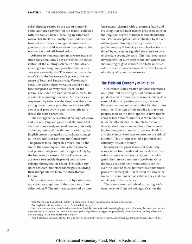
©International Monetary Fund. Not for Redistribution
58
CHAPTER II THE INTERNATIONAL MONETARY SYSTEM IN THE (VERY) LONG RUN
solve disputes related to the use of money. It
could authorize payment of the taxes it collected
with the coins it issued, creating an automatic
market for the latter. Finally, as an independent
issuer of a currency, it mitigated moral hazard
problems that could arise when one party to the
transaction used self-issued coins.
Advisors to medieval monarchs were aware of
these considerations. They advocated the consol
idation of the minting system, with the idea of
creating a minting monopoly (in other words,
monetary sovereignty) . This would enhance the
state's (and the bureaucrats') power at the ex
pense of local and feudal rivals. Viewed nar
rowly, the state's objective was to acquire a tax
base composed of every coin (user) in the
realm. The wider the circulation of its coins, the
greater its seignorage tax base. A broader view
(expressed by writers at the time) was that mon
etizing the economy promised to increase effi
ciency and productivity and incidentally to in
crease the state's revenues.
The emergence of a national coinage was slow
and uneven. England pioneered the successful
circulation of a u·uly national currency. As early
as the beginning of the thirteenth century, the
English crown managed to consolidate coinage
in the two mints of London and Canterbury.
The process took longer in France, due lO the
size of the economy and the lesser economic
and political integration of its regions. Only by
the fourteenth century did the French crown
achieve a reasonable degree of control over
coinage throughout its realm. The Italian city
states achieved monetary sovereignty following
their independence from the Holy Roman
Empire.
Most state-run mints were run by a mint mas
ter, either an employee of the crown or a fran
chise holder. 16 The mint was supervised by state
bureaucrats charged with preventing fraud and
ensuring that the mint master produced coins of
the requisite degree of fineness and standardiza
tion. Public acceptance was cultivated by the rep
utation ( commitment)-creating mechanism of
public assaying.17 Assaying a sample of coins pro
duced by state mints signaled the state's resolve
to circulate reputable coins. The final step in the
development of European monetary systems was
the minting of gold coins.18 The high inu·insic
value of such coins encouraged the development
of strict quality control measures.
The Political Economy of Inflation
Centralized states created national currencies
not by fiat but by driving out of business inde
pendent coin producers and cotmterfeiters. As a
result of this competitive pressure, western
European money remained stable for almost two
centut;es. One sign of this stability is that most
people, most of the time, appear to have traded
coins at face value.I9 Another is the tendency of
feudal landlords and the church to commute
dues in kind into monetary dues. But by enter
ing into long-term nominal contracts, landlords
and the chtu·ch were later exposed to the risk of
inflation. This in turn created a powerful con
stituency for stable money.
So long as this process was still under way,
competition from lords and counterfeiters pro
vided a source of market discipline that miti
gated the state's commitment problem. Once
the state acquired near monopolistic control
over the issue of coins, however, its commitmen t
problem reemerged. Rulers faced the choice be
tween the maintenance of stable money and ma
nipulation of the currency.
There were two methods of extracting addi
tional revenue from the coinage. One was the
16See Mayhew and SpufJord ( 1988) for discussion of mint organization in medieval Europe. 17[n England this was referred to as "the trial of the pyx." 18As trade volumes increased and transactions (mainly international) involving large sums of money became prevalent, a
need for coins of greater intrinsic value emerged and gold coins began supplementing silver coins as the large-denomination currency in the mid-thirteenth century.
19See Sussman and Zeira (1999) for a model of commodity money that assumes that agentS trade coins at face v-alue.
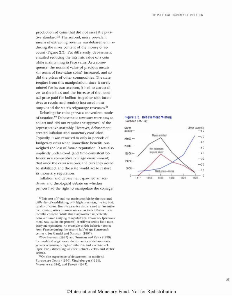
©International Monetary Fund. Not for Redistribution
production of coins that did not meet the puta
tive standard.2o The second, more prevalent
means of extracting revenue was debasement: re
ducing the silver content of the money of ac
count (Figure 2.2). Put differently, debasement
entailed reducing the intrinsic value of a coin
while maintaining its face value. As a conse
quence, the nominal value of precious metals
(in terms of face-value coins) increased, and so
did the prices of other commoclities. The state
benefited from this manipulation: since it rarely
minted for its own account, it had to attract sil
ver to the mints, and the increase of the nomi
nal price paid for bullion (together with incen
tives to recoin and remint) increased mint
output and the state's seignorage revenues.2t
Debasing the coinage was a convenient mode
of taxation.22 Debasement revenues were easy to
collect and clid not require the approval of the
representative assembly. However, debasement
created inflation and monetary confusion.
Typically, it was resoned to only in periods of
budgetary crisis when immediate benefits out
weighed the loss of future reputation. It was also
implicitly understood (and time-consistent be
havior in a competitive coinage environment)
that once the crisis was over, the currency would
be stabilized, and the state would act to restore
its monetary reputation.
Inflation and debasemem spawned an aca
demic and theological debate on whether
princes had the right to manipulate the coinage.
20'fhis sort of fraud was made possible by tl1e cost and difficulty of establishing, wit:h high precision, tlle intrinsic quality of coins. But tllis practice also created an incentive for private parties to assay coins so as to determine tlleir metallic content. While tllis assay worked imperfect!)'• however, since assaying dissipated real resources (precious me tal was lost in tlle process), it still worked to limit monetary manipulation. An example of tl1is behavior comes from France during tlle second half of tJ1e fourteentJ1 cemury. See Gandal and Sussman (1997).
2tSee Sussman (1993) and Sussman and Zeira (1 999) for models tl1at generate tlle dynamics of debasements: greater seignorage. highe•· inflation, and eventual collapse. For a dissenting view see Rolnick, Velde, and Weber (1996).
22Qn the experience of debasement in medieval Europe see Gould (1970), Kindleberger (1991),
MotOmura (1984), and Pamuk (1997).
THE POLITICAL ECONOMY OF INFLATION
Figure 2.2. Debasement Minting (Dauphine: 1417-22)
Mares 30000-
25000 -
20000 -
15000-
10000-
5000-
1417
Uvres tournois -80
-70
-60
-50
-40
-30
-20
- 1 0
0
59
©International Monetary Fund. Not for Redistribution
60
CHAPTER II THE INTERNATIONAL MONETARY SYSTEM IN THE (VERY) LONG RUN
Figure 2.3. Value of English Currency and the Price level , 1265-1500
-250
Price index
- 50
1265 85 1305 25 45 65 85 1405 25 45 65 85 99 0
On the one hand, feudal taw allowed the king LO
charge and profit from seignorage; on the other
hand, it was claimed that the currency was a pub
lic good, which the prince was responsible for ad
ministering for the benefit of his subjects.23
Predating the bullionist controversy of the nine
teenth century, other aspects of this academic de
bate related to pioneering formulations of the
quantity equation linking the money supply to
the level of prices, and an early analysis of the
shoe-leather costs of inflation. Periods of rapid
inflation also introduced indexation to the ac
counting system, to contracts, and even to wages
(see Sussman, 1993). In many respects, political,
academic, and market responses to debasements
were direct precursors of modern developments.
The inflation caused by the debasements re
distributed income from creditors to debtors, ad
versely affecting the landowning elite and the
church and raising transaction costs for mer
chants, creating repeated public outcries against
debasement and inflation. In some stares, no
tably England, representative assemblies struck a
deal trading off stable money in return for
higher taxation. In France, the elites Jacked the
cohesion to gram the king alternative sources of
finance.24 As a result, England enjoyed monetary
stability for centuries, whereas France suffered
from instability and bursts of inflation.
The competitive nature of the commodity
money system and the threat of currency substi
tution disciplined rulers more effectively than le
gal, theological, and political constraints.
Nevertheless, the tensions between monetary sta
bility and inflation were as prevalent in early
modern Europe as they are today. The resulting
monetary regimes can be divided into four
types. The first, that of England, was strictest in
terms of stability. The English currency was sta
ble for very long periods (on average, more than
60 years; Figure 2.3). The currency was debased
23The most famous of these protests was that of Oresme
Uobnson, 1956), who argued that debasements violated the public's property rights and inu·oduced injus[ices and inefficiencies.
24Qn the politics of F1·ench debasement, see Miskimin (1984}.
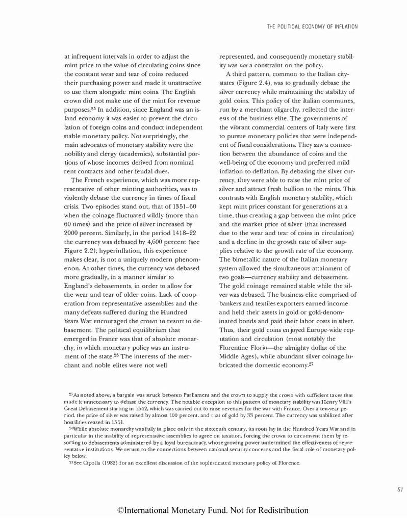
©International Monetary Fund. Not for Redistribution
at infrequent intervals in order to adjust the
mint price to the value of circulating coins since
the constant wear and tear of coins reduced
their purchasing power and made it unattractive
to use them alongside mint coins. The English
crown did not make use of the mint for revenue
purposes.25 In addition, since England was an is
land economy it was easier tO prevent the circu
lation of foreign coins and conduct independent
stable monetary policy. Not surprisingly, the
main advocates of monetary stability were the
nobility and clergy (academics), substantial por
tions of whose incomes derived from nominal
rent contracts and other feudal dues.
The French experience, which was more rep
resentative of other minting authorities, was to
violently debase the currency in times of fiscal
crisis. Two episodes stand out, that of 1351-60
when the coinage fluctuated wildly (more than
60 times) and the price of silver increased by
2000 percent. Similarly, in the period 1418-22
the currency was debased by 4,600 percent (see
Figure 2.2); hyperinflation, this experience
makes clear, is not a uniquely modern phenom
enon. At other times, the currency was debased
more gradually, in a manner similar to
England's debasements, in order to allow for
the wear and tear of older coins. Lack of coop
eration from representative assemblies and the
many defeats suffered during the Hundred
Years War encouraged the crown to resort to de
basement. The political equilibrium that
emerged in France was that of absolute monar
chy, i�n which monetary policy was an instru
ment of the state.26 The interests of the mer
chant and noble elites were not well
THE POLITICAL ECONOMY OF INFLATION
represented, and consequently monetary stabil
ity was not a constraint on the policy.
A tl1ird pattern, common to the Italian city
states (Figure 2.4), was to gradually debase the
silver currency while maintaining the stability of
gold coins. This policy of the Italian communes,
run by a merchant oligarchy, reflected the inter
ests of the business elite. The governments of
the vibrant commercial centers of Italy were first
to pursue monetary policies that were independ
ent of fiscal considerations. They saw a connec
tion between the abundance of coins and the
well-being of the economy and preferred mild
inflation to deflation. By debasing the silver cur
rency, they were able to raise the mint price of
silver and attract fresh bullion to the mints. This
contrasts with English monetary stability, which
kept mint prices constant for generations at a
time, thus creating a gap between the mint price
and the market price of silver (that increased
due to the wea1· and tear of coins in circulation)
and a decline in the growth rate of silver sup
plies relative to the growth rate of the economy.
The bimetallic nature of the Italian monetary
system allowed the simultaneous attainment of
two goals--currency stability and debasement.
The gold coinage remained stable while the sil
ver was debased. The business elite comprised of
bankers and textiles exporters earned income
and held their assets in gold or gold-denom
inated bonds and paid their labor costs in silver.
Thus, their gold coins enjoyed Europe-wide rep
utation and circulaLion (most notably the
Florentine Florin-the almighty dollar of the
Middle Ages), while abundant silver coinage lu
bricated the domestic economy.27
25As noted above, a bargain was struck between Parliament and the crown to supply the crown with sufficient taxes that made it unnecessary to debase the currency. The notable exception to this pattern of monetary stability was Henry VIITs Great Debasement starting in 1542, which was carried out to raise revenues for the war with France. Over a ten-year period, the price of silver was raised by almost 100 percent, and t.hat of gold by 33 percent.. The currency was stabilized after hostilities ceased in 1551.
26While absolute monarchy was fully in place only in the sixteent.h cenrury, its roots lay in t11e Hundred Years War and in particular in the inability of representative assemblies to agree on LaXation, forcing the crown to circumvent them by resorting to debasements administered by a loyal bureaucracy, whose growing power undermined the effectiveness of representative institutions. We return 1.0 the connections between national security concerns and the fiscal role of monetary policy below.
27See Cipolla (1982) for an excellent discussion of the sophisticat.ed monetary policy of Florence.
61
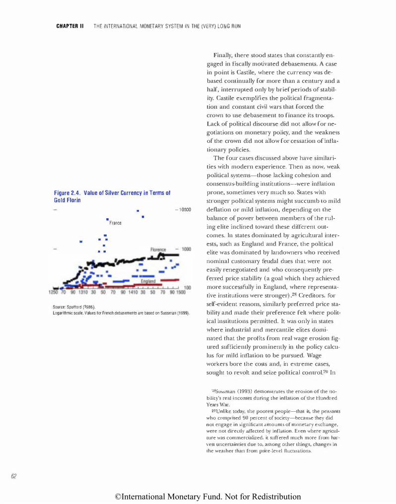
©International Monetary Fund. Not for Redistribution
62
CHAPTER II THE INTERNATIONAL MONETARY SYSTEM IN THE (VERY) LONG RUN
Figure 2.4. Value of Silver Currency in Terms of Gold Florin
•
Source: Spufford (1986).
•
• • •
• • •
• •
France
-10000
logarithmic scale. Values tor French debasements are based on Sussman (1999).
Finally, there stood states that constantly engaged in fiscally motivated debasements. A case in point is Castile, where the currency was debased continually for more than a century and a half, interrupted only by brief periods of stability. Castile exemplifies the political fragmentation and constant civil wars that forced the crown to use debasement to finance its troops. Lack of political discourse did not allow for negotiations on monetary policy, and the weakness of the crown did not allow for cessation of inflationary policies.
The four cases discussed above have similarities with modern experience. Then as now, weak political systems-those lacking cohesion and consensu s-building institutions-were inflation prone, sometimes very much so. States with su·onger political systems might succumb to mild deflation or mild inflation, depending on the balance of power between members of the ruling elite inclined toward these differem outcomes. ln states dominated by agricultural interests, such as England and France, the political elite was dominated by landowners who received nominal customary feudal dues that were not easily renegotiated and who consequently preferred price stabili ty (a goal which they achieved more successfully in England, where representative institutions were stronger) .28 Creditors, for self-evident reasons, similarly preferred price stability and made their preference felt where political institutions permitted. It was only in states where industrial and mercantile elites dominated that the profits from real wage erosion figured sufl1ciently prominently in the policy calculus for mild inflation to be pursued. Wage workers bore the costs and, in exu·eme cases, sought to revolt and seize political comrot.29 In
28Sussman (1993) demonstrates the erosion of the nobility's real incomes during the inflation of the Hundred Years War.
29Unlike today, the poorest people-Lhat is, the peasants who comp.-ised 90 percent of society-because they did not engage in significant amountS of monetary exchange, were not direcLiy affected by inflation. Even where agricui[Ure was commercialized, it suffered much more from harvest uncertainties due to, among oL11er things, changes in 1.he weather than from p!'ice-level fluctuations.
©International Monetary Fund. Not for Redistribution
Florence, a compromise was reached between
these competing interests: gold remained stable,
but silver was debased.
The International Monetary Landscape
The monetary scene during the Middle Ages
and the early modern pet;od reflected
Europe's political fragmentation. With the ex
ception of England, each region was dotted
with issuing authorities: monarchies, city-states,
towns, and dukedoms. Over 100 different silver
currencies existed in Europe before 1500, com
pared with 38 at the beginning of the nine
teenth century.30 This situation resulted in high
u·ansaction costs as reflected by the growing in
dustry of money changers and exchange manu
als that helped merchants classify and u·ade the
various coins.
Despite the proliferation of silver currencies,
the heavyweight players were those authorities
that could circulate gold coins. The club of gold
issuing states included only 32 political entities,
of which 12 were Italian city-states. The only
truly international currencies were the
Florentine Florin and the Venetian Ducat, al
though the French Ecu and the German cities'
Rhinegeld eftioyed wide circulation in their own
areas. Much like during the gold standard era,
the gold-issuing countries were the economicaUy
advanced ones, which enjoyed superior u·ade
and credit facilities.31 Moreover, there existed a
close connection between financial supremacy,
as measured in number of banks and amount of
international lending, and the circulation of an
internationally renowned gold coin. Like
London in the nineteenth century, Florence in
THE INTERNATIONAL MONETARY LANDSCAPE
the fourteenth and fifteenth centuries issued the
reserve currency of the Middle Ages and was
Europe's leading financial center.
Medieval Europe was composed of a set of
small open economies.32 The share of manufac
tures and luxury good production that was
u·aded was relatively high. While capital flows
were low, they were unrestricted and since most
regions did not have gold or silver mines, the
money supply was determined almost exclusively
in the international money market. Therefore
states could not sterilize or impose exchange
controls, as their nineteenth and cwentieth cen
tury successors were able to do, nor did they
have the luxury of suspending convertibility in
the face of a bullion drain, making it impossible
to conduct an independcm mone tary policy for
any substantial length of time.33 Intentional or
unintentional deviations of the official gold-to
silver ratio at the mint from the international ra
tio sent one metal abroad, leaving in circulation
the less (relatively) valued one. During debase
ments, states increased the price of silver at the
mint to attract foreign silver, which entered the
mints and provided seignorage, while gold that
yielded little in terms of seignorage was ex
ported. When one of the warring parties de
based the currency in an attempt to draw silver
to its mint, its opponents had to reciprocate.
Monetary wars were part of the war effort, in
deed, at times victory in the monetary war was
more important, or a necessary condition to win
ning on tl1e battle£ield.34 During peace times, for
eign coin invasion that resulted from misalign
ment of silver coins could undermine the
monetary policy of even the strongest financial
center in Europe.35
goBased on the currencies listed in Spufford ( 1986). For the nineteenth century. see Lhe article on coins in McCulloch (1837).
:�•or Lhe 33 s tates that. issued gold coins in the early nineteenth century, 17 had already issued gold coins in the Middle Ages.
32See Munro (1979) on bullionistic measures in medieval Britain. :!:�Sussman ( 1998) provides a model of commodity money based on the monetary appmach to the balance of paymems. !14See Sussman (1993) for analysis of the comribuLion of success of the French in winning the moneta�·y war with
England and Burgundy to their ability to prevail in the Hundred Years War. See also Wervcke (1948) for analysis of the monetat-y wars between France and Flanders.
3SSee Cipolla ( 1982) for discussion or the quatt.rini affair-in which Florence was inV"".tded by Pisan quattrinis leading w a debasement. of Florentine silver currency. The episode is also analyzed in Sargent and Smith (1997).
63
©International Monetary Fund. Not for Redistribution
64
CHAPTER II THE INTERNATIONAL MONETARY SYSTEM IN THE (VERY) LONG RUN
The exposure of the Em·opean economy to
capital and monetary flows is best exemplified in
two related episodes-the Bullion Famine and
the Price Revolution. During the Bullion
Famine, which is said by scholars of the subject
to have lasted from 1380 to 1460, bullion was ex
ported to the East to cover trade deficits result
ing from the Black Death. The decline in the
money supply sent the economies into a severe
and prolonged recession.36 The flow reversed di
rection following Europe's discovery of America,
which set in motion flows of silver and gold to
Europe. These flows generated what is termed
the Price Revolution, when prices increased at
an average rate of 1 percent per annum for
more than a hundred years. After centuries of
price stability, Europe experienced its first long
period of inflation.
Paper Money: Beginnings
The development of banking in the Middle
Ages and the early modern period led to the in
troduction of new monetary instruments, start
ing with the bill of exchange (a kind of a
banker's draft) and ending with paper money
backed by fractional reserves. Banks settled their
bills in gold or silver. Though the danger of
bank runs limited the tendency to over-issue
notes, the use of bills of exchange became in
creasingly prevalent, preparing the ground for
the eventual introduction of inconvertible paper
currency. In the absence of well-developed bond
markets, private banks and bankers lent to gov
ernments and popes. Default on some of these
debts led to the bankruptcy of some of the lead
ing banking houses of the time.
A prerequisite for the circulation of fiat paper
currency was the establishment of a central
bank. These banks were mostly private but pos
sessed a degree of monopoly power over note is-
sue, which was conferred in return for services
provided in managing tl1e public debt. The cur
rency bills issued by these banks were convert
ible into gold or silver (except in times of crisis).
As with debasements, the issue of inconvertible
paper was in most cases an expedient related to
war. Moreover, each of these episodes, as during
the earlier commodity-money regimes, ended
with stabilization and return to convertibility.
One notable exception was the first experiment
with the large·scale issuance of inconvertible pa
per: the infamous Law affair in France in
1716-20. John Law founded the Banque Generate, which received privileges similar to those of the
Bank of England in return for offering the
crown similar services. I L issued notes re
deemable in specie. In practice, however, note is
sue increased well beyond its assets.37 More than
a few of tl1e notes issued by this bank were used
to purchase the Mississippi Company stock. A fa
mous bubble developed, with Mississippi
Company stock appreciating in price and note
issues ever increasing, until November 1720, when the bubble burst and the bank could not
make specie payments in return for notes.
l t is thus tempting to suggest that central
banking and fiat money emerged as by-products
of state finance. The impetus for granting mo
nopoly power to these private banks was the de
sire to have access to cheap, dependable sources
of funding for the governmenl and to obviate
the need to rely excessively on the market.
Ultimately, these mounting debt burdens ended
up in the lap of the central bank, in episodes of
monetization that occasioned Europe's ftrsl ex
periments with inconvertible fiat currency.
Another episode of inconvertible paper cur
rency occurred in Sweden from 1745 to 1762, where the cenu-al bank (the first government-run
central bank in Ettrope) issued currency to fi
nance a Keynesian type expansionary policy tbat
S6See Sussman ( 1998) for a model of the bullion famine and critique of its assumptions, empirical evideuce, and conclusions. The analysis and data there suppon the hypothesis lhat the decline in minting was a result of fall in economic activity that followed the Black Dealh, which wiped out a third of Europe's population. This created large surpluses of precious metals lhat were hoarded and exponed in return for goods and services.
37Jn 1718 the Banque Generale was taken over by the king and renamed Banquc Royale.
©International Monetary Fund. Not for Redistribution
resulted in inflation and depreciation of the ex
change rate (Kindle berger, 1984). Inconvertible
money was also imroduced during the American
War of Independence ( 1776-80) and during the
French Revolution (the Assignat inflation of
1790-94), during which inflation reached 36 per
cent a montJ1.
The British Suspension ofl797-1821 was
probably the most famous such episode. Its im
portance lies both in its duration and in the the
oretical debate it spawned, which laid the foun
dations for classical monetary economics. l l
started with a run on the Bank of England in
1 797, precipitated by fears of a French invasion.
The suspension of specie payments was initially
scheduled to last six months but was repeatedly
extended, ending only in 1821. Unlike its conti
nental counterparts, the Bank of England was
able to manage the money supply to limit infla
tion. This is another indication of tJ1e power of
the stable-money interest that had prevailed in
England for centuries which 'vas strengthened
during tJ1e Glorious Revolution.
High inflation mreatened only in 1809-10,
which brought about the appoinunem of me
Bullion Committee to investigate the causes of
the pound's depreciation. The Bullion
Controversy generated a lively economic debate,
whose participants included ThornLOn and
Ricardo. While the conclusions of Bullion
Report were rejected by Parliament, me politicaJ
and economic debate it spawned acted to disci
pline the Bank of England until convertibility
was resumed in 1821.
Ln me episodes described above, inconvertibil-
ity ,vas not deliberate. It 'vas the inadvertent re
sult of excessive note issue in response to crisis
conditions, typically \var. It was well understood
that inconvertibility 'vas only temporary.
Nevermeless, the adverse consequences of those
unintentional inconvertibility crises strengm
ened me parties advocating specie standards and
price stability at least up to World War J.38
THE NINETEENTH CENTURY SYSTEM
The Nineteenth Century System
The nineteenth century was an era of peace
compared w what came before and went after.
ln 1815, Russia, Austria, Prussia, and Britain
formed the Quadruple AJiiance, agreeing to
meet periodically to discuss meir common inter
est in peace and security. To be sure, this so
called Concert of Europe did not prevent lim
ited conflicts, from tJ1e Crimean War to the
Franco-Prussian War to the Spanish-American
War. But the Congress of Vienna inaugurated a
century when me world was spared a global or
even cominent-wide conflict.
Peace and security provided a favorable con
text for growth. This was the century when the
industrial revolution spread from an isolated
corner of normwest Europe to omer parts of the
globe. It \vaS me century in which trade grew
even faster man output, fueling me increase in
agricultural and industrial production:
Maddison's (1995) estimates suggest mat mer
chandise exports rose from 1 percent of GOP in
1820 to 5 percent in 1870 and approached 10
percent in 1913. [t was a period of rising interna
tional capital flows. The favorable political cli
mate helps to explain mese outcomes. So do the
rapid declines in transportation and communi
cations costs associated with railroadization, the
shift from sailing ships to steam ships. the tele
graph, and the u·ans-oceanic cable.
Exchange rate stability was integral to this
process. For me first two-thirds of the century,
national monetary systems were divided into
three blocs: a gold bloc composed of Britain,
Portugal, and most ofBritain's dominions and
colonies; a silver bloc made up of most of the
German states, Austria, the Netherlands,
Denmark, Norway, Sweden, Mexico, China,
India, and japan; and a group of bimetallic (or
"double standard") countries including France,
Belgium, ltaJy, Switzerland, and the United
States. The adoption of a common monetary
standard by the members of each of these blocs
sssee Sussman ( !997) for discussion of Lhe role of policyrnakcrs in establishing what is now termed "British Monet:.ry Orthodoxy" as a reaction to the convertibility suspension of 1797-1821.
65
©International Monetary Fund. Not for Redistribution
66
CHAPTER II THE INTERNATIONAL MONETARY SYSTEM 1N THE (VERY) LONG RUN
(together with their inability to prevent the
inter-circulation of their jJartners' coins) made
for exchange rate stability within the group.
More su-i king still is the stability of the ex
change rates between them_ The relative price
of gold and silver and hence the exchange rate
between gold and silver coins of comparable
weight and fineness held stable around 15\/z to
1 from the early nineteenth century to the
1870s (at which point the price of silver took
of£) .39 This stability is all the more remarkable
given the magnitude of the shocks to world
gold and silver supplies and hence the potential
for the market and mint prices of the metals to
diverge. Typically, these shocks took the form of
the discovery of gold or silver deposits in the
course of agticultural and pastoral penetration
of sparsely settled regions: they included gold
discoveries in California in 1848 and eastern
Australia in 1851 (which together raised world
production of gold tenfold) and the Comstock
Lode silver discovery in Nevada in 1859. The
stability of exchange rates in the face of these
disturbances is typically ascribed to the stabiliz
ing properties of bimetallism.40 \1\lhen the sup
ply of newly mined gold rose, as it did in the
1850s, and its price began to drop (relative to
that of silver), the cheap metal flowed toward
the members of the bimetallic bloc, where it
was coined, and the scarce metal (silver) was
melted down and exported.41 Conversely, when
the supply of silver rose, as it did in the 1860s,
the bimetallic countries imported silver and ex
ported gold, allowing the former to displace
the latter in domestic circulation.42 Mid-century
flows of newly mined gold and silver may have
been large as far as flows go, but they were
small relative to the stocks of the two metals
that circulated in the bimetallic counu-ies. So
long as stocks dominated flows and the commit
ment to bimetallism was su-ong, exchange rates
remained stable. The system operated like a sta
bilizing target zone: the knowledge that France
and its bimetallic paru1ers would absorb one
metal and disgorge the other as soon as their
relative price in tl1e market diverged from their
relative price in the mint (by more than the
narrow margins allowed for by transactions
costs) prevented the market price from hitting
those reflecting barriers.'13
Given the stability of the bimetallic standard,
tl1e speed with which it crumbled after the 1860s
is something of a paradox. Flandreau ( 1 994) dis
tinguishes four explanations for this u·ansforma
tion. The "structural" explanati.on of
Kindleberger ( 1 984) and others points to silver
discove•-ies in Nevada and Mexico and the in
crease in newly minted silver in the 1860s and
1870s. Risil'tg silver output meant falling silver
prices and inflaLion and exchange rate deprecia
tion for silver-standard counuies, undesirable
consequences that pushed them onto gold. But
it is not clear why the same argument that ap
plied to the pre-1870 period (flow supplies of
the two metals, while large, were small relative to
the stocks circulation in the bimetallic coun
tdes) did not also apply to tl1e post-1870 years.
In fact, the rise in silver production in me late
1860s and 1870s was small compared tO the
surge in gold production after 1848:1-1
39We argue in a moment that this stability reflected the operation of systemic factors. 40See, for example, Flandreau (1995). 41The markets responded in this fashion because the governmems of officially bime tallic countries pegged the relative
price of gold and silver at a constant price. (ln practice, countries like the United S tates mjght alter that relative price periodically, but those changes were few and far between.)
42flandreau (1994) estimates that for every dollar of one met<ll added to the world stock, France and its partners absorbed 60 cents, while disgorging 40 cents worth of the other.
43The target-zone model is applied 10 nineteenth cenr.ury bimetallism by Oppers (1995). 44A variation on this theme is the "chain-gang" hypothesis of Gallarotti ( 1995): by purchasing gold and selling silve1�
Germany added to the incipient disequilibrium caused by the Comstock Lode and Mexican silver discoveJ-ies, thereby threatening the bimetallic system. The objection is again the same, namely, that German gold purchases and silver sales, while working in the posited direction, were too limited to undermine the viability of French bimetallism (Oppers, 1996). Oppers calculates that Germany's demonetization of silver would have reduced 1he share of gold in the money supplies of the bimetallic countries from 57 percem in 1873 to 48 percent in 1879, bm that the 15\-1 to 1 mint ratio would not have been threatened.
©International Monetary Fund. Not for Redistribution
The second explanation focuses on the mone
tary consequences of rising living standards,
technological progress, and expanding trade.
Prior to the nineteenth century, the smallest
gold coin was still too valuable for everyday use.
One of the attractions of bimetallism was that it
provided a supply of low-value silver coins that
were practical for domestic transactions, along
with more valuable gold coins that were conven
ient for larger transactions, international trans
actions in particular. As trade and living stan
dards rose, the balance shifted bet\veen these
two needs. The problem of producing small
denomination token coins that might circulate
alongside the gold coinage used in large u·ansac
tions, without incurring the risk of significant
counterfeiting, was solved once steam power
came to the mint and token coins could be pro
duced at a higher level of uniformity.45 A gold
based standard consequently became more
attractive.
While there is surely something to this expla
nation, its power should not be exaggerated.
Half a century and more passed between the ad
vent of steam-powered machinery and the shift
to gold. Differences in the cost of settling large
transactions by shipping gold and silver bet\veen
countries were a negligible share of the u·ansac
tions involved. Something else is needed to ac
count for the timing of the event and the simul
taneous adoption of the gold standard in a large
number of different countries.
One possible "something else" is politics. The
expansion of industry relative to agriculture
muted the voice of farmers, a debtor class that
preferred rising prices and declining mortgage
debts, relative to financial interests who pre
ferred stable money. Thus, the final defeat of
the "free silver" lobby in the United States in the
1890s is typically described as the triumph of
creditors over debtors and of the advocates of
stable money over inflationists.46 Again, there is
surely something to this interpretation. After all,
45See the discussion in Redish (1990). 4GSee, for example, Frieden (1994).
THE NINETEENTH CENTURY SYSTEM
the new system would not have been adopted in
the absence of political support. But, as typicaJiy
told, this story neglects the influence of the
lobby with the most to lose in the event of silver
demonetization, namely, the silver lobby itself,
which grew in numbers as the volume of silver
mining continued to expand. Its proponents ap
ply to other countries the American political
constellation, in which the yeoman farmer
played a powerful role, whereas in other coun
tries land was held in large blocs by an aristoc
racy not similarly encumbered. It tends to inter
pret the 1870s and 1880s in terms of a debate
that really only came to a head in the 1890s after
more than two decades of deflation.
The fourth and final explanation (to which we
are inclined) is network effects. With the growth
of international trade and lending, it became in
creasingly convenient to operate the same mone
tary standard as one's neighbors. Transaction
costs and exchange rate uncertainty between the
gold and silver blocs may have been small, but
even small costs mattered with the expansion of
international trade and lending. British investors
understandably preferred foreign investments
denominated in sterling; Madden (1985,
pp. 255) describes as "common knowledge" 1.hat
British investors viewed securities issued by coun
tries not on the gold standard as riskier than
those of countries that were, and that they lent
accordingly. The convenience of a common stan
dard was conducive to trade; Flandreau (1993)
shows that countries sharing a common standard
traded disproportionately with one another even
after conu·oUing for incomes, proximity, and ad
jacency. Thus, the fact that Britain was then a
leading commercial and financial nation for
much of the nineteenth century encouraged
other countries to link up to her monetary stan
dard. And t11ese network effects were reinforced
when the world's two other leading industrial
economies, Germany and the United States,
went over to the gold standard in the 1870s.47
47Meissner (1999) estimates a model of tl1e timing of the adoption of tl1e gold standard in various counu-ies, obtaining some econometric evidence of the importance of tl1ese network effects.
67
©International Monetary Fund. Not for Redistribution
68
CHAPTER II THE INTERNATIONAL MONETARY SYSTEM IN THE (VERY) LONG RUN
Finally, the suspicion, however nebulous, that
the gold standard had been an ingredient of
Britain's industrial success encouraged its adop
tion. That Britain had been the first country to
go onto the gold standard and also the first
country to industrialize encouraged the view of
the gold standard as a progressive and modern
monetary arrangement.
In the event, silver and bimetallism were aban
doned ad seriatim, as one country after another
went over to gold. Newly unified Germany led
the way in 1871, using the indemnity it received
as victor in the Franco-Prussian war to carry out
a monetary reform. Otber silver-standard coun
tries that traded heavily with Germany-the
Netherlands, Denmark, Norway, and Sweden
among them-followed suit. France and her
partners in the Latin Monetary Union, Belgium,
Switzeriand, Italy, and Greece, abandoned bimet
allism for gold.48 When the United States com
pleted its recovery from the Civil War and offi
cially restored convertibility in 1879, it did so on
gold rather than a bimetallic basis.49 Once
Russia and Japan adopted gold convertibility in
the 1890s, the gold-standard system of fixed ex
change rates between national currencies was
truly global in scope.
A limited number of countries never went
onto the gold standard prior to 1913. China re
mained on the silver standard, as did a number
of central American countries (Guatemala,
Honduras, and El Salvador). Persia's officially
bimetallic system was effectively silver based. But
by the first decade of the twentieth century, the
largest part of the world was on gold.
Stability of the Gold Standard
Many commentators have noted the striking
stability of the nineteenth-century gold standard
system. To be sure, payments pressures occasion
ally forced countries to suspend convertibility,
most frequently in "emerging markets" at the pe-
riphery of the international system. And banking
and financial crises were not uncommon (as we
describe below). Almost without exception, how
ever, gold convertibility was restored subse
quently, generally at the previously prevailing
rate of exchange. And the leading industrial and
commercial powers remained on gold without
interruption for fully a third of a century up to
World War I . As enumerated above, a few coun
tries in Central and South America and Asia (no
tably China) did not join the gold standard club,
preferring to cling to silver, but they became an
increasingly isolated minority as the period
progressed.
A reasonable degree of price stability was a
corollary of the operation of this system. In t11e
same way that national money supplies were
linked to national stocks of gold, the world
money supply was linked to the world gold
stock. 50 The commitment to gold convertibility
deterred governments from manipulating
money supplies in ways iliat destabilized the
price level. And ilie operation of t11e market
induced changes in the world gold stock to ac
commodate changes in world money demand.
As the world economy expanded, commodity
prices tended to fall (given the more-or-less con
stant supply of money), which raised ilie real
price of gold (since governments were pegging
the nominal price of the latter). The gold-min
ing industry responded with increased supply,
which boosted money supplies and neutralized
the fall in the price level (Barro, 1979). The
mechanism might work slowly, allowing deflation
to persist (as between the mid-1870s and mid-
1890s), but work it did.
From an end-of-millennium perspective, ilie
most remarkable feature of this system was the
success with which it reconciled capital mobility
with exchange rate stability. Today, international
capital mobility is seen as posing an impossible
challenge to countries seeking w hold their ex
change rates stable and at the same time to pur-
48The Latin Union was an arrangement negotiated to harmonize the coinage in these closely linked countries. 49Although limited amounts of silver coinage continued until ll1e passage of the Gold Standard Act of 1900. 50The velocity of circulation fell slowly for most of the period (Bordo andjonung, 1997), but rrends were not large.
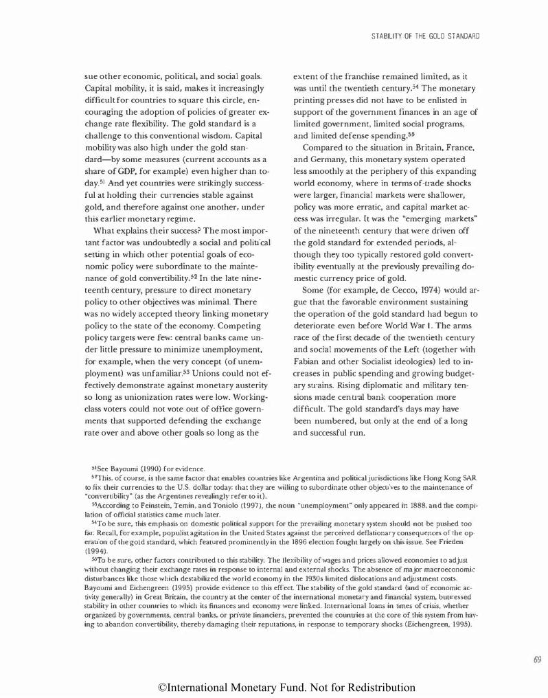
©International Monetary Fund. Not for Redistribution
sue other economic, political, and social goals.
Capital mobility, it is said, makes it increasingly
difficult for countries to square this circle, en
couraging the adoption of policies of greater ex
change rate flexibility. The gold standard is a
challenge to this conventional wisdom. Capital
mobility was also high under the gold stan
dard-by some measures (current accounts as a
share of GDP, for example) even higher than to
day. 51 And yet countries were strikingly success
ful at holding their currencies stable against
gold, and therefore against one another, under this earlier monetary regime.
What explains their success? The most impor
tant factor was undoubtedly a social and political
setting in which other potential goals of eco
nomic policy were subordinate to the mainte
nance of gold convertibility. 52 In the late nine
teenth century, pressure to direct monetary
policy to other objectives was minimal. There
was no widely accepted theory linking monetary
policy to the state of the economy. Competing policy targets were few: central banks came un
der little pressure to minimize unemployment,
for example, when the very concept (of unem
ployment) was unfamiliar.ss Unions could not ef
fectively demonstrate against monetary austerity
so long as unionization rates were low. Working
class voters could not vote out of office govern
ments that supported defending the exchange
rate over and above other goals so long as the
5ISee Bayoumi (1990) for evidence.
STABILITY OF THE GOLO STANDARD
extent of the franchise remained limited, as it was until the twentieth century.54 The monetary
printing presses did not have to be enlisted in
support of the government finances in an age of
limited government, limited social programs,
and limited defense spending.55
Compared to the situation in Bt;tain, France,
and Germany, this monetary system operated less smoothly at the periphery of this expanding
world economy, where in terms-of-trade shocks
were larger, financial markets were shallower,
policy was more erratic, and capital market ac
cess was irregular. It was the "emerging markets"
of the nineteenth century that were driven off
the gold standard for extended periods, al
though they too typically restored gold convert
ibility eventually at the previously prevailing do
mestic currency price of gold.
Some (for example, de Cecco, 1974) would ar
gue that the favorable environment sustaining
the operation of the gold standard had begun to
deteriorate even before World War I . The arms
race of the first decade of the twentieth century and social movements of the Left (together with
Fabian and other Socialist ideologies) led to in
creases in public spending and growing budget
ary so·ains. Rising diplomatic and military ten
sions made cenu-al bank cooperation more
difficult. The gold standard's days may have
been numbered, but only at the end of a long and successful run.
5lrfhis, of course, is Lhe same factor that enables countries like Argentina and political jurisdictions like Hong Kong SAR to fix their currencies to the U.S. dollar today: Lhat they are willing to subordinate other objectives to the maintenance of "convertibility" (as the Argentines revealing!)' refer tO it).
�3According to Feinstein, Temin, and Toniolo (1997), the noun "unemployment" only appeared in 1888, and tl1e compilation of official statistics came much later.
54To be sure, this emphasis on domestic political suppon for the prevailing monetary system should not be pushed too far. Recall, for example, populist agitation in the United States against the perceived deflationary consequences of the operation of the gold standard, which featured prominently in the 1896 election fought largely on tl1is issue. See Frieden (1994).
5!>To be sure, other factors contributed to this stability. The flexibility of wages and prices allowed economies to adjust without changing their exchange rates in response to internal and external shocks. The absence of major macroeconomic disturbances like those which destabilized the world economy in the 1930s limited dislocations and adjustment costs. Bayoumi and Eichengreen (1995) provide evidence to this effect. The stability of the gold standard (and of economic activity generally) in Great Brita.in, the country at Lhe center of the international monetary and financial system, buttressed stability in other countries to which its finances and economy were linked. International loans in times of crisis, whetl1er organized by governments, central banks, or private financiers, prevented the counu·ies at the core of this system from having to abandon convertibility, !hereby damaging tl1eir reputations, in response to temporary shocks (Eichengreen, 1995).
69
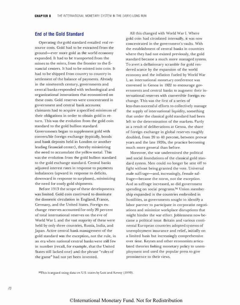
©International Monetary Fund. Not for Redistribution
10
CHAPTER II THE INTERNATIONAL MONETARY SYSTEM IN THE (VERY) LONG RUN
End of the Gold Standard
Operating the gold standard entailed real re
source costs. Gold had to be extracted from the
ground-ever more gold as the world economy
expanded. lL had to be transported from the
mines to the mints, from the frontier to the fi
nancial centers. It had to be minted into coin. It
had to be shipped from country to country in
settlement of the balance of payments. Already
in the nineteenth century, governments and
central banks responded with technological and
organizational innovations that economized on
these costs. Gold reserves were concentrated in
government and central bank accounts;
claimants had to acquire a specified minimum of
their obligations in order to obtain gold in re
turn. This was the evolution from the gold coin
standard to the gold bullion standard.
Governments began to supplement gold with
convenible foreign exchange (typically, bonds
and bank deposits held in London or another
leading financial center) , thereby minimizing
the need to accumulate the yellow metal. This
was the evolution from the gold bullion standard
to the gold exchange standard. Central banks
adjusted interest rates in response to payments
imbalances (upward in response to deficits,
downward in response to surpluses) , minimizing
the need for costly gold shipments.
Before 1913 the scope of these developments
was limited. Gold coin continued to dominate
the domestic circulation in England, France,
Germany, and the United States. Foreign ex
change reserves accounted for only 20 percent
of total international reserves on the eve of
World War I, and the vast majority of these were
held by only three countries, Russia, India, and
Japan. Active central bank management of the
gold standard \vas the exception, not the rule, in
an era when national central banks were still few
in number (recall, for example, that the United
States still lacked one) and the phrase "rules of
the game" had not yet been invented.
AU this changed with World War I. Where
gold coin had circulated internally, it was now
concentrated in the governmem's vauJts. With
the establishment of central banks in countries
where they had not existed previously, the gold
standard became a much more managed system.
To avert a deflationary scramble for gold ren
dered scarce by the expansion of the world
economy and the inflation fueled by World War
l, an international monetary conference was
convened in Genoa in 1922 to encourage gov
ernments and central banks to augment their in
ternational reserves with convertible foreign ex
change. This was the first of a series of
less-than-successful efforts to collectively manage
the supply of international liquidity, something
that under the classical gold standard had been
left to the determination of the markets. Partly
as a result of deliberations at Genoa, the share
of foreign exchange in global reserves roughly
doubled, from 20 to 40 percent, between prewar
)'Cars and the late 1920s, the practice becoming
much more general than before.
Moreover, the war undermined the political
and social foundations of the classical gold stan
dard system. Men could no longer be sent off to
fight witl1out being granted tl1e vote. Universal
male suffrage-and, increasingly, female suf
frage-became t11e norm, not the exception.
And as suffrage increased, so did governmenr
spending on social programs.56 Union member
ship expanded in the countries embroiled in
hostilities, as governments sought to identify a
labor partner to participate in corporatist negoti
ations and minimize workplace disruptions that
might hinder the war effort. joblessness now be
came a political issue. Bdtain and various conti
nental European countries adopted systems of
unemployment insurance and relief, initially on
a limited basis but increasingly comprehensive
over time. Keynes and other economists articu
lated theories linking monetary policy to unem
ployment and used the popular press to give
prominence to their views.
56Th is is argued using dat.a on U.S. states by Lou and Kenny ( 1999).
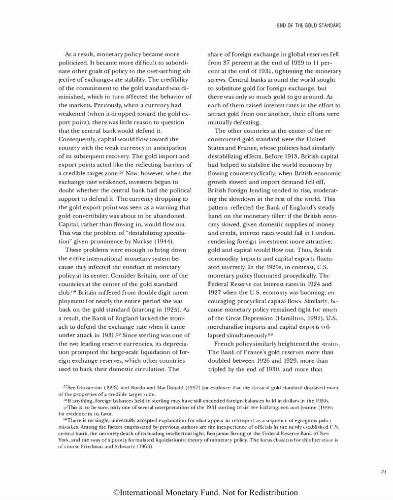
©International Monetary Fund. Not for Redistribution
As a result, monetary policy became more
politicized. It became more difficult to subordi
nate other goals of policy to the over-arching ob
jective of exchange-rate stability. The credibility
of the commitment to the gold standard was di
minished, which in turn affected the behavior of
the markets. Previously, when a currency had
weakened (when it dropped toward the gold ex
port point), there was little reason to question
that the central bank would defend it.
Consequently, capital would flow toward the
country with the weak currency in anticipation
of its subsequent recovery. The gold import and
export points acted like the reflecting barriers of
a credible target zone. 57 Now, however, when the
exchange rate weakened, investors began to
doubt whether the central bank had the political
support to defend it. The currency dropping to
the gold export point was seen as a warning that
gold convertibility was about to be abandoned.
Capi tal, rather than flmving in, would flow out.
This was the problem of "destabilizing specula
tion" given prominence by Nurkse ( 1944).
These problems were enough to bring down
the enti•-e international monetary system be
cause they infected the conduct of monetary
policy at its center. Consider Britain, one of the
countries at the center of the gold standard
club.f•>� Britain suffered from double-digit unem
ployment for nearly the entire period she was
back on the gold standard (starting in 1925). As a result, the Bank of England lacked the stom
ach to defend the exchange rate when it came
under attack in 1931 .59 Since sterling was one of
the two leading reserve currencies, its deprecia
tion prompted the large-scale liquidation of for
eign exchange reserves, which other countries
used to back their domestic circulation. The
END OF THE GOLD STANDARD
share of foreign exchange in global reserves fell
from 37 percent at the end of 1929 to 1 1 per
cent at the end of 1931, tightening the monetary
screws. Central banks around the world sought
to substitute gold for foreign exchange, but
there was only so much gold to go around. As each of them raised interest rates in the effort to
attract gold from one another, their efforts were
mutually defeating.
The other countries at the center of the re
constructed gold standard were the United
States and France, whose policies had similarly
destabilizing effects. Before 1913, British capital
had helped to stabilize the world economy by
flowing countercyclically: when British economic
growth slowed and import demand fell off,
British foreign lending tended to rise, moderat
ing the slowdown in the rest of the world. This
pattern reflected the Bank of England's steady
hand on the monetary tiller: if the British econ
omy slowed, given domestic supplies of money
and credit, interest rates would fall in London,
rendering foreign investment more attractive;
gold and capital would flow out. Thus, British
commodity imports and capi tal exports lluctu
ated inversely. ln the 1920s, in contrast, U.S.
monetary policy fluctuated procyclically. The
Federal Reserve cut interest rates in 1924 and
1927 when the U.S. economy was booming. t"n
couraging procyclical capital flows. Similarly, be
cause monetary policy remained tight f()r much
of the Great Depression (Hamilton, 1992), U.S.
merchandise imports and capital exports col
lapsed simultaneously.'i0
French policy similarly heightened the strains.
The Bank of France's gold reserves more than
doubled between 1926 and 1929, more than
tripled by the end of 1930, and more than
'•7See Giovannini ( 1993) and Bordo and MacDonald ( 1997) for evidence that the clas.�ical g-old �tandard displayl·d man1· or the properties of a credible target zone.
<•HLf anything, foreign balances held in sterling may have still exceeded fi>reign balances ht:ld in dollars in the I \l20s. !>!Yfhis is, to be sure, only one of several interpretations of the 1931 sterling crisis; sec I::ichengJ·ecn and .Jeanne ( I \J\l!l)
f(H· evidence in ilS favor. '�'There is no single, universally accepted explanation for what appear in retrospt·ct as a sequence or eg-regious pol in
mistakes. Among the factors emphasized by previous authors are the inexperience of officials in the newly es tablished L" .S. cenu·al bank, the untimely death of iL� leading intellectual light, Benjamin Strong of the Federal Reserve Bank of New York, and the sway of a poorly formulated liquidationist theory of monetary policy. The lorus classicus fi1r this literatun· is of course Friedman and Schwarl'l. ( 1963).
71
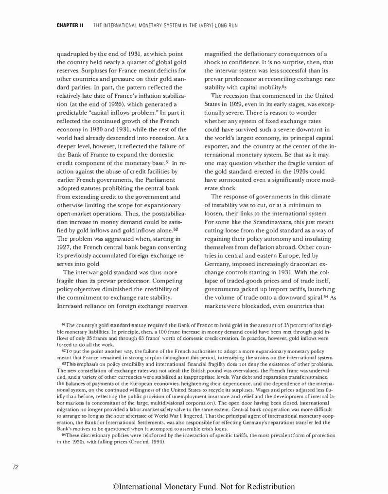
©International Monetary Fund. Not for Redistribution
72
CHAPTER II THE INTERNATIONAL MONETARY SYSTEM IN THE (VERY) LONG RUN
quadrupled by the end of 1931, at which point
the country held nearly a quarter of global gold
reserves. Surpluses for France meant deficits for
other counuies and pressure on their gold stan
dard parities. In part, the pattern reflected the
relatively late date of France's inflation stabiliza
tion (at the end of 1926), which generated a
predictable "capital inflows problem." In part it
reflected the continued growth of the French
economy in 1930 and 1931, while the rest of the
world had already descended into recession. At a
deeper level, however, it reflected the failure of
the Bank of France to expand the domestic
credit component of the monetary base.61 In re
action against the abuse of credit facilities by
earlier French governments, the Parliament
adopted statutes prohibiting the central bank
from extending credit to the government and
otherwise limiting the scope for expansionary
open-market operations. Thus, the poststabiliza
tion increase in money demand could be satis
fied by gold inflows and gold inflows alone. 52
The problem was aggravated when, starting in
1927, the French central bank began converting
its previously accumulated foreign exchange re
serves into gold.
The interwar gold standard was thus more
fragile than its prewar predecessor. Competing
policy objectives dimjnished the credibiljty of
the commitment to exchange rate stability.
Increased reliance on foreign exchange reserves
magnified the deflationary consequences of a
shock to confidence. It is no surprise, then, that
the interwar system was less successful than its
prewar predecessor at reconciling exchange rate
stability with capital mobility.63
The recession that commenced in the United
States in 1929, even in its early stages, was excep
tionally severe. There is reason to wonder
whether any system of fixed exchange rates
could have survived such a severe downturn in
the world's largest economy, its principal capital
exporter, and the country at the center of the in
ternational monetary system. Be that as it may,
one may question whether the fragile version of
the gold standard erected in the 1920s could
have surmounted even a significantly more mod
erate shock.
The response of governments in this climate
of instability was to cut, or at a minimum to
loosen, their links to the international system.
For some like the Scandinavians, this just meant
cutting loose from the gold standard as a way of
regaining their policy autonomy and insulating
themselves from deflation abroad. Other coun
tlies in central and eastern Europe, led by
Germany, imposed increasingly draconian ex
change controls starting in 1931. With the col
lapse of traded-goods prices and of trade itself,
governments jacked up import tariffs, launching
the volume of trade onto a downward spiral.64 As markets were blockaded, even countries that
61The coumry's gold standard statute required the Bank of France to hold gold i n the amoum of 35 percem of its eligible mone!al'y liabilities. Jn principle, then, a 100 franc increase in money demand could have been met through gold inflows of only 35 francs and through 65 francs' worth of domestic c1·edit creation. In practice, however, gold inflows were forced to do all the work.
62'fo pm the point another way, the failure of the French authorities to adopt a more expansionary monetary policy meant that France remained in su·ong surplus throughom Lhis period, imensifying the strains on the intemational system.
6S'fhis emphasis on policy credibility and international financial fragility does not deny the existence of other problems. The new constellation of exchange rates was not ideal: the British pound was overvalued, the French franc was undervalued, and a variety of other currencies were stabilized at inappropriate levels. War debt and reparation transfers strained the balances of payments of the European economies, heightening their dependence, and the dependence of the imernational system, on the continued willingness of the United States to recycle its surpluses. Wages and prices adjusted Jess fluidly than before, reflecting the public provision of unemployment insurance and relief and the developmem of internal labor markets (a concomitant of the large, multidivisional corporation). The open door having been closed, international migration no longer provided a labor-market safety valve to the same extent. Ceno·al bank cooperation was more difficult to arrange so long as the sour aftertaste of World War I lingered. That the principal agent of international monetary cooperation, the Bank for International Settlements, was also responsible for effecting Germany's reparations transfer led the Bank's motives to be questioned when it attempted to assemble crisis loans.
&!These discretionary policies were reinforced by the interaction of specific tariffs, the most prevalent form of protection i.n the 1930s, wid1 falling prices (Crucini, 1994).
©International Monetary Fund. Not for Redistribution
wished to maintain their gold parities found it difficult to generate foreign exchange. And as capital markets closed down, developing countries suspended payments on their external debts; in the absence of new lending, the incen
tive to keep current on their external financial obligations was greatly reduced. In these ways the collapse of the international monetary sys
tem reinforced, and in turn was reinforced by, the collapse of international trade and finance.
To be sure, not all countries were equally
ready to cut their international links. Bri tain's Commonwealth and Empire, along with her
principal European trading partners (Portugal, for example), sought to maintain their u·adi
tional commercial and financial ties, forming the sterling area and pursuing policies of imperial preference. 65 France and several of her
neighbors, including Belgium, the Netherlands, and Switzerland, clung to the gold standard as
long as possible, seeking to maintain an increasingly isolated gold bloc. Germany elaborated her system of exchange control and bilateral clearing into a closed Reichsmark bloc.
A striking aspect of this pattern is how
strongly it resembled the tripartite monetary world of the mid-nineteenth century, with one bloc centered on Britain, another organized around France, and a third around Germany,
and with many of the same countries linked to these three centers as a century before.
Monetary history, it would seem, casts a long shadow. Past monetary history shaped subsequent trade patterns and diplomatic relations, which in turn encouraged countries to coordi
nate their monetary arrangements even in as turbulent a period as the 1930s.
Another striking aspect of this period, in contrast to both the 1920s and 1970s, is that fiat money did not produce fiat money inflation. To
be sure, going off the gold standard and regain-
END OF THE GOLD STANDARD
ing control of mone tary policy allowed central banks and governments to halt deflation. They lowered interest rates and injected additional liquidity into the economy via the discount window. But despite the unemployment crisis that created intense political pressure to get the
economy moving again, few governments used the autonomy they enjoyed as a result of the
shift to flexible exchange rates to aggressively expand their money supplies or increase govern
ment spending. Monetary and fiscal expansion remained tentative, despite an unemployment rate that might exceed 20 percent. This was the downside of the policies of the 1930s, that more was not done to bring down high unemployment. But there was also an upside-that, in contrast to the 1970s (following the next collapse of a pegged-rate system), runaway inflation
did not result. From today's perspective (and with the con
trast with the 1970s in mind), the interesting question is why the inflation problem did not run out of conu·ol. The answer plausibly has three parts. First, Keynesian-style theories of the concerted use of monetary and fiscal policies were still in their very early stages of dissemination. Second, looking back at their experience in the early 1920s (before the gold standard had been restored), when the combination of large budget deficits and monetary autonomy had
proved a recipe for hyperinflation, governments
and central banks were understandably reluctant to simply let policy "rip." Any sign that they were
about to push hard on the monetary and fiscal accelerator might precipitate capital flight, since these same memories were foremost in the minds of investors as well as officials. 56 And third, central banks and governments did not develop an alternative monetary policy operating su·ategy to be substituted for the currency
peg, which might reconcile policy autonomy
00Thus, 1.he members of the Commonwealth and Empire enjoyed preferential access to both British commodity and fi. nancial markets.
66This problem of investor confidence was readily evident in France after 1937, not coincidentally since France had been one of the countries with chronic inflation problems in the first half of the 1920s. More gene1-ally, the proliferation of controls on capital flows limited the extent of this problem, although they did not remove it. Thus, not even countries adopt· ing exchange controls (aside from cases like Japan and Germany where macroeconomic policy was subordinated to rear· mament) engaged in aggressive monetary and fiscal expansion (Eicbengreen, 1992).
73
©International Monetary Fund. Not for Redistribution
14
CHAPTER II THE INTERNATIONAL MONETARY SYSTEM IN THE (VERY) LONG RUN
with credibility and confidence. Sweden, which
developed an explicit price-level targeting rule,
was a prominent counterexample. 57 But else
where, central banks and governments failed to
articulate comparable confidence-inspiring
rules. In their absence, aggressive expansion
threatened to excite capital flight. And with this
specter looming, the scope for reflationary ac
tion remained limited.
Rebirth of the Gold Standard?
The United States never entirely abandoned
the gold standard in the 1930s. Franklin Delano
Roosevelt took the dollar off gold in 1933 but
repegged it in january 1934 (in the meantime
having pushed up the dollar price of gold from
$20.66 to $35.00). Clearly, the resumption rule
was no more.68 In an era when unemployment
was a dominant political and economic concern,
pushing down p1;ces in order to restore precrisis
exchange rates and gold prices, at the risk of fur
ther aggravating unemployment, was no longer a
politically viable public-policy strategy.
As the United States recovered from the Great
Depression, gold flowed in to accommodate the
increased demand for money and credit. As an
other war loomed on the horizon, capital flight
from Europe further augmented American re
serves. America's European allies then used
much of the gold they retained to purchase the
supplies needed to sustain their war effort. For
all these reasons, when World War II drew to a
close, the United States possessed a majority of
the (non-Soviet) world's monetary gold.
Given this fact, it is not surprising that the
United States and the countries with which it ne
gotiated the post-World War II monetary order
had different views of the role of gold in the in
ternational system. The United States preferred
a system that resembled the arrangements that
had prevailed for the better part of the previous
century. The dollar was to remain convertible
into gold at $35 an ounce, the rate that had pre
vailed since 1934. Stable exchange rates were ro
be restored, since currency stability was essential
to the reconstruction of trade, which U.S. offi
cials viewed as an economic and political imper
ative. The foreign counterparts to the United
States delegation at Bretton Woods, including
the Keynes-led British delegation, were more
skeptical of both exchange rate stability and free
trade, free trade because they anticipated chronic deficits vis-a-vis the United States, the ex
change rate commitment because they worried
that their efforts to bring down unemploymem
would be hamstrung. The compromise involved
the three key innovations of the Bretton Woods
Agreement. First, exchange rates, although
pegged, could now be adjusted in the event of
fundamental disequilibrium. Second, govern
ments that wished to gain room for maneuver to address domestic problems and w avoid a replay
of the interwar experience with "destabilizing
speculation" were expressly permitted to resort
to capital controls. And third, the International
Monetary Fund was created as a way of placing
international monetary cooperation at one re
move from domestic politics.
Thus, to say that Bretton Woods sealed the
shift from commodity money to fiat money is too
simple. The dollar remained convertible into
gold, although not until the end of the 1950s
did that constraint bind the United States. Other
currencies remained convertible into dollars (for
purposes of current account transactions). Thus,
commodity money was not entirely out of the
picture. Again, the continuity in the structure of
the international monetary system is striking.
Although exchange rates could be adjusted,
adjusunents were infrequent. There was a gen
eral realignment of European currencies in 1949
(accompanied by devaluations by the members
of the sterling area and three of Britain's long-
6i'fhere, it can be argued, economic theory played an important role. Theoris!S like Wick.sell had developed models of
potential conflic!S between exchange rate stability and price stability and played a prominem role in the policy debate. See Berg andJonung (1999).
68Similarly, none of the other counuies that abandoned gold convertibility and depreciated their currencies starting in 1931 restored convertibility subsequently at the previously prevailing rate.
©International Monetary Fund. Not for Redistribution
standing trading parUlers-Argentina, Canada,
and Egypt), designed to get the Bretton Woods
System on its feet. Other realignments included
the French franc devaluations of 1957, 1958, and
1969, the sterling devaluation of l967, and the
deutsche mark revaluations of 1961 and 1969.
There were 69 major stepwise devaluations by
(politically independent) developing countries
between 1949 and 1971 .69 Thus, while the
Bretton Woods System was characterized by a
greater degree of exchange rate flexibility than
its predecessors, the extent of that flexibility was
still, in an important sense, limited.
The explanation is not hard to find. The
1920s and 1930s had not enamored officials and
others (aside from a few academic dissenters) of
the me•its of flexible rates. Describing floating
exchange rates in the 1920s, Nurkse had written
of "cumulative and self-aggravating" movements
(Nurkse, 1944). Floating in the 1930s was associ
ated with the collapse of trade and output, al
though the direction of causality could fairly be
regarded as a question. After World War II, gov
ernments did not develop alternative monetary
anchors like monetary targeting or inflation tar
geting. Th•·ough process of elimination, ex
change rate policy became the cornerstone of
their entire economic policy strategy-the sym
bol of their commitment to sound and stable
policies. To devalue cast doubt over that strategy
REBIRTH OF THE GOLD STANDARD?
and over the competence of its framers. 70 And to revalue, as Germany and the Netherlands came
under pressure to do, threatened the postwar so
cial compact which rested on an agreement to
pursue export-led growtb.71
Exchange rate stability was possible because
the economic environment was again favorable.
The world economy was growing rapidly-by 5
percent a year, according to Maddison's esti
mates, more than twice as fast as between 1870
and 1913. This alleviated the pressure to de
value as a way of boosting growth. Commodity
markets were not disturbed by large price move
ments, either upward as in the 1970s or down
ward as in the 1920s and 1930s.72 Wage pres
sures were moderate, reflecting the impact on
labor markets of memories of high unemploy
ment in the 1930s. Cyclical stability was en
hanced by this combination of rapid growth and
stable prices: while Europe expetienced growth
recessions (declines in the positive rate of
growth) between 1950 and 1971, there was no
year in which the output of the continent as a
whole turned negative in absolute-value terms
(Van der Wee, 1986, p. 62). The stability of the
macroeconomy limited the need to use active
monetary and fiscal measures fot- countercycli
cal purposes. With monetary and fiscal policies
steady, policy-induced dislocations to the bal
ance of payments were less.
69"fhis calculation is from Edwards and Samaella (1994), who define a major stepwise devaluation as an adjustment of the official rate of at least 14 percent, following a period of at least two years of fixing the exchange rate. Roughly half of the total took place in the context ofTMF Slalld-By programs starting in 1952.
'1Yfhis is one interpre tation of Richard Cooper's ( 1971) famous finding that currency devaluation typically precipitated the dismissal of the finance minister.
71And, more concretely, to excite the opposition of producers in the export indusu·ies. In addition, the United States would have faced a tech_nical problem had it sought to devalue the dollar. If the U.S. government raised the dollar pdce of gold, which was the only instrument it in fact controlled, other governments would also raise the domestic-curren<.")' ptice of gold, leaving exchange rates and U.S. international competitiveness unchanged_ EUJ-ope and Japan, for all the aforementioned reasons, were reluctant tO see the competitiveness of their exports erode. Export inten:!Sts would scream if their governments acquiesced in policies ''�th this effect, and they were too important to ignore. Germany might agree, under tllC most intense pressure, to revalue, but only to a very limited extent. Moreover, the structure of the Bretton Woods System made more than their mere acquiescence necessary; positive steps on their pan were required in order fo1· the dollar to be devalued against their currencies, given that they had declared par values in terms of the dollar. If the dollar depreciated against gold. non action on their part meant that their currencies would depreciate along with the dollar. There would be no benefits fo1· U.S. competitiveness. And given thei1· domestic political situation, nonacLion was the likely outcome. This was what Treasury Secretary Fowler presumably meant when he said that "the U.S. under the present rules cannot change its own parity." Cited in Duncan, PatLerson, and Yee (1999), p. 604.
72Bayoumi and Eichengreen ( 1994) attempt to recover aggregate-supply and aggregate-demand shocks from time series
on output and prices for a number of OECD countries, and show that these were smaller under Bretton Woods than in the periods tl1at went before and came after.
15
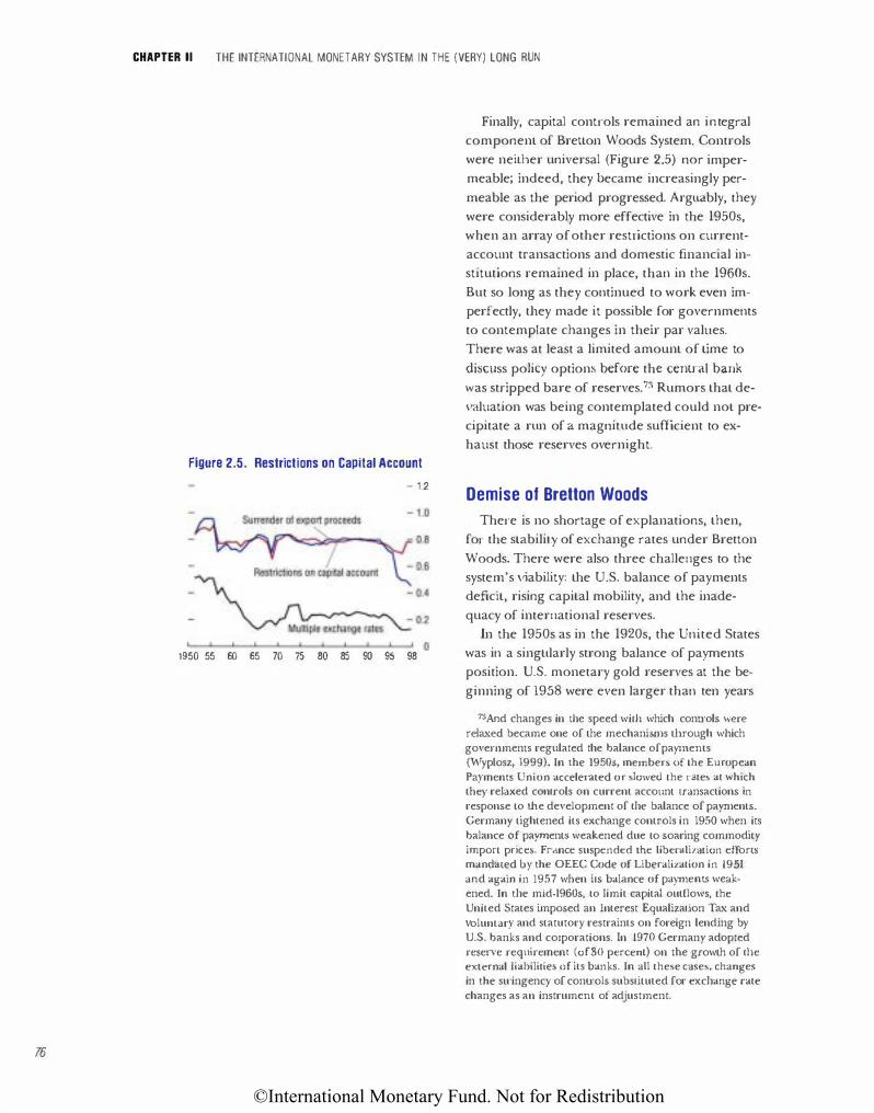
©International Monetary Fund. Not for Redistribution
76
CHAPTER II THE INTERNATIONAL MONETARY SYSTEM IN THE (VERY) LONG RUN
Figure 2.5. Restrictions on Capital Account
- 1.2
1950 55 60 65 70 75 80 85 90 95 98
Finally, capital contr·ols remained an integral
component of Bretton Woods System. Controls
were neither universal (Figure 2.5) nor imper
meable; indeed, they became increasingly per
meable as the period progressed. Arguably, they
were considerably more effective in the 1950s,
when an array of other restrictions on current
account u·ansactions and domestic fmancial in
stitutions remained in place, than in the 1960s.
But so long as they continued to work even im
perfectly, they made it possible for governments
to contemplate changes in their par values.
There was at least a limited amount of time to
discuss policy options before the central bank was sttipped bare of reserves.73 Rumors that de
valuation was being contemplated could not pre
cipitate a run of a magnitude sufJicient to ex
haust those reserves overnight.
Demise of Bretton Woods
Ther·e is no shortage of explanations, then,
for the stability of exchange rates under Bretton
Woods. There were also three challenges to the
system's viability: the U.S. balance of payments
deficit, rising capital mobility, and the inade
quacy of international reserves.
In the 1950s as in the 1920s, the United States
was in a singttlarly strong balance of payments
position. U.S. monetary gold reserves at the be
ginning of 1958 were even larger than ten years
73And changes in 1.he speed wii.h which conu·ols were relaxed became one of the mechanisms through which governments regulated the balance ofpaymems (Wyplosz, 1999). In i.he 1950s, members of the European Payments Union accelerated or slowed the rates at which they relaxed controls on current account transactions in response to i.he development of the balance of payments. Germany tightened its exchange controls in 1950 when its balance of payments weakened due to soaring commodity import prices. France suspended i.he liberalization efforts mandated by the OEEC Code of Liberalization in 195 I and again in 1957 when its balance of payments weakened. In the m.id-1960s, to limit capital outflows, the United States imposed an Interest Equalization Tax and voluntary and statutory restraints on foreign lending by U.S. banks and corporations. [n 1970 Germany adopted reserve requirement (of30 percent) on i.l1e growth of i.l1e external Liabilities of its banks. In all these cases, changes in the su·ingency of controls substituted for exchange rate changes as an instrumcm of adjustment.
©International Monetary Fund. Not for Redistribution
before. This was the period of the dollar short
age. But it was not to last. The U.S. current ac
count remained in surplus through most of the
1960s, but not by a margin sufficient to finance
the country's foreign investment. Rapid eco
nomic growth abroad attracted foreign direct in
vestment by American corporations and portfo
lio lending by Unlted States banks. As early as
1960, U.S. foreign dollar liabilities exceeded
U.S. gold reserves, raising fears for the stability
of the dollar. In pan, such fears reflected the un
willingness of U.S. officials to subordinate other
goals of policy to the maintenance of the dollar
peg. Other objectives-the New Society and the
Vietnam War, but above all demand-driven
growth-were allowed to take precedence. And
with the rest of the industrial world pursuing
other economic and political priorities
(Germany attached greater importance to infla
tion control, for example, while France was a
less than enthusiastic support of America's for
eign policy goals), diverging fundamentals pro
duced diverging balance of payments out
comes.74 The Kennedy, Johnson, and Nixon
administrations resorted to differential tax u·eat
ment of domestic and foreign investments, re
ductions in the value of the goods American
tourists could bring into the country, and tied
foreign aid, among other devices, in an effort to
remedy the balance of payments problem and
free up monetary and fiscal poUcies for the pur
suit of domestic objectives. But these expedients
failed to address the fundamental conflict be
tween "external pressw·es for higher [interest]
rates and the needs of the domestic economy for
monetary expansion," as the point was put in
the report of the President's Task Force on
Foreign Economic Policy in 1964.75
Devaluing the dollar would have been one way
of squaring the circle. It would have enhanced
the competitiveness of U.S. exports, improved
the u·ade balance (given sufficient time), and al
tered the direction of foreign investment flows
by raising the profitabiUty of domestic produc-
DEMISE OF BRETION WOODS
tion •·elative to foreign production. Why then
was the option shunned? One explanation is
fear that devaluation would damage the credibil
ity of the Bretton Woods System and, perhaps of
more relevance to U.S. officials, of the dollar it
self. Unilateral devaluation would have also an
tagonized the United States' allies and trading
partners, who saw themselves as possessing a col
lective interest in the maintenance of this inter
national monetary system which offered them a
favorable climate for export-led growth. It wouJd
have frayed lhe Western a!Jiance at a time when
Cold War tensions were high. It would have
thrown a w1·ench in the works of ongoing GATT
negotiations. Finally, there was the possibility
that if the U.S. govemment raised the dollar
price of gold, which was the only instrument it
in fact controlled, other governments would also
raise the domestic-currency price of gold, leav
ing exchange rates and U.S. international com
petitiveness unchanged. Authors like Genberg
and Swoboda ( 1994) emphasize this fundamen
tal asymmetry, arising out of these multiple ob
stacles to dollar devaluation, as a further fatal
weakness of the Bretton Woods System.
The pressures emanating from the divergent
stance of macroeconomic policies in the United
States and other industrial countries grew all the
more intense with declining effectiveness of capi
tal controls. The restoration of current account
convertibility allowed individuals engaged in le
gitimate, trade-related transactions to exploit
leads and lags as a way of shifting capital across
borders. And with the gradual relaxation of the
tight controls imposed on domestic financial in
stitutions and markets in the 1930s and 1940s,
market participants found new ways around the
remaining conu·ols; the development of the
Eurodollar market in response to the U.S.
Interest Equalization Tax is a case in point. The
amount of time the government of a deftcit coun
try could take to contemplate policy options, be
fore it was overwhelmed by market pressures,
shrank with the growing permeability of conu·ols.
7'1Both the political context and macroeconomic consequences are ably described by Genberg and Swoboda (1994). 75Reprimed in Dw1ean and others (1999), p. 39.
77
©International Monetary Fund. Not for Redistribution
18
CHAPTER II THE INTERNATIONAL MONETARY SYSTEM IN THE (VERY) LONG RUN
And with the declining effectiveness of controls, even a hint that devaluation was under consideration could now lmleash a tidal wave of anticipatory speculation; hence, governments grew loath to consider the option, rendering the system of par values increasingly rigid and brittle.
As controls weakened, con taining and adjust
ing to payments p1·essures both became more difficult. As the British appreciated when they compared the 1967 sterling crisis with its predecessors in 1947 and 1949, capital flows now could force the issue more quickly than before (Cairncross and Eichengreen, 1983, Chapter 3). Even contemplating a change in par values was problematic, for mere rumor tl1at devaluation was in the offing could now precipitate massive capital flight.
It is tempting to tell the story of the collapse of Bretton Woods in terms of this combination of declining U.S. competitiveness and rising capital mobility. There was a third element, of course, namely the inadequacy of international reserves. The 1960s was a decade of rapid expansion i.n Europe, .Japan, and much of the develop
ing world. Countries needed additional international liquidity to buffer their economies from trade-related shocks and therefore sought to run surpluses against the United States. But while integral to the operation of Bretton Woods, this pattern also heightened the fragility of the system, since foreign holders of dollars could "run on" U.S. gold reserves at any time. Seen in this perspective, the problem was less that the dollar was overvalued relative to the yen and the European currencies; it was more that the dollar was overvalued relative to gold, reflecting the inelasticity of monetary gold supplies and the growing stock of foreign do !Jar balances.
This problem of an inadequately elastic supply of international liquidity was not new, of course. It had been evident in the deflationary 1870s and 1880s, in response to which Russia, India,
Japan, and other countries had accumulated
bonds and bank balances denominated in sterling, francs, and marks. I t had been on the minds of the delegates to the Genoa Conference, in response to which governments and central banks had been encouraged to elaborate the practice. It had been on Keynes's mind when he had proposed giving his Clea,;ng Union the power to create a synthetic reserve asset (a recommendation that was not taken up). Unfortunately, the policymakers' solution, the creation of Special Drawing Rights, came tOO late to salvage the Bretton Woods System.
A more comprehensive solution, however, was at hand. As the international monetary system evolved away from a fixed link between the reserve currencies and gold, away from pegged rates, and away from capital controls, it became both feasible and atu-active for central banks to satisfy t.heir demands for reserves by holding diversified portfolios of dollars, pounds, deutsche marks, francs, and otl1er convertible currencies. They could augment those holdings by running current accolmt surpluses or borrowing abroad, depending on need. [n the end, the solution to
the problem of an elastic supply of in ternationaJ reserves was provided through evolution rather than creationism.
The breakdown of Bretton Woods opened the door to the high-inflation 1970s and 1980s, out of which the world economy is now only finally emerging. Cut free from the fixed exchange rate anchor, central banks stepped hard on the monetary accelerator. Budget deficits widened significantly in the 1970s and 1980s, bequeathing a chronic problem of high public debts. While monetary stability and fiscal sustainability were restored at different times in different counu;es, it is a fair generalization that some two decades had to pass before these policy imbalances were significantly brought under control.
Why such a different response from the last
time an international system of fixed rates had collapsed, in the 1930s?76 One can point to sev-
76Conventional explanations point to the two OPEC oil shocks as creating imbalances and worsening unemploymcm, which required governments tO respond aggressively. But the supply and demand shocks and the unemployment of the late 1920s and early 1930s were if anything more pronounced. Hence, the macroeconomic disturbances of the 1970s do not provide a convincing explanadon for the contrast.
©International Monetary Fund. Not for Redistribution
era! factors. Keynesian ideas, that fiscal and mon
etary policies should be used to counter unem
ploymem, had gained considerable currency. In
many countries, policies to main tain full employ
ment were an explicit element of the postwar so
cial compaCl of equity and shared growth, leaving
governments no choice but to respond aggres
sively to the rise in unemployment.77 Moreover,
after two decades of stability, the fear that aggres
sive countercyclical action would excite inflation
and capital flight was considerably subdued.
Given that they were entering uncharted terri
tory, it is not surprising that policymakers did not
anticipate the markets' reaction. As governments
responded more aggressively to unemployment,
the markets responded more aggressively to pol
icy. Removing the exchange rate anchor and put
ting nothing in its place fed inflationary expecta
tions. It caused the familiar Phillips Curve
relationship to be replaced with the inflation-aug
mented Friedman-Phelps Phillips Curve. So long
as the framework for policy had been provided by
the commitment to maintain pegged exchange
rates, a total loss of inflationary comrol had not
been regarded as likely. Only under exceptional
circumstances-in response to exceptional prob
lems-would the authorities stimulate demand,
which would therefore mainly boost output
rather than fuel inflation. Because the additional
demand stimulus was regarded as temporary (for
otherwise it could come in to conflict with the ex
change rate commitment), it did not provoke
sharp increases in wage demands and translate
mainly into additional inflation.78 But once that
anchor was lifted, additional inflationary pressure
today simply incited fears of additional inflation
ary pressure tomorrow. Demand stimulus pro
duced mainly inflation rather than additional out
put and employment as wages and p1ices
responded more quickJy to policy (Alogoskoufis
and Smith, 1992). Consequently, as governments
77See, for example, Boltho (1982) on the European cases.
RECENT DEVELOPMENTS IN MILLENNIAL PERSPECTIVE
pushed harder on their policy l.evers, those levers
grew increasingly ineffectual.
Solving this problem-eliminating chronic
policy imbalances and establishing a new
monetary-policy operating framework to replace
the earlier exchange rate-centered policy
regime-has occupied the advanced induso·ial
and developing countries alike for the better
part of the past 20 years. ln some cases, high
costs in terms of growth foregone have been in
curred as a result of the high-interest-rate poli
cies to extinguish inflation.
Recent Developments in Millennia! Perspective
Many accounts have been written of the devel
opment of the international monetary system
over the past 25 years, emphasizing rising capital
mobility, greater exchange rate flexibility
(Figure 2.6), and the declining monetary role of
gold. By way of conclusion, it may be useful to
inquiJ-e how these trends appear when placed in
their long-term context.
SeveJ-al points stand ouL One is the reluctance
of governments to embrace radical changes in
international monetary relations. For example,
European governments responded to the col
lapse of Bretton Woods by seeking to establish a
regional monetary arrangement in the image of
Bretton Woods, complete with capital conu-ols
and Bretton Woods-style fluctuation margins. ln
much of the developing world, they responded
to the collapse of Bretton Woods' par values by
substituting unilateral dollar pegs. Similarly,
while the monetary role of gold was officially
abolished in 1977, central banks continued to
hold substantia.! gold reserves, once again indi
cating their commitment to traditional values. ln
many respects, then, continuity has remained
the order of the day.79
78in other words, occasional recourse to demand slimulus, like temporary suspensions under the gold sJandard, was stabilizing because it occurred in a framework within which there existed a credibility-enhancing nominal anchor.
7\JWhere countries have moved to new arrangements, they have generally done so under duress-that is, when market pressures have left them no choice. See the evidence in Eichengreen and Masson and others (1998).
79
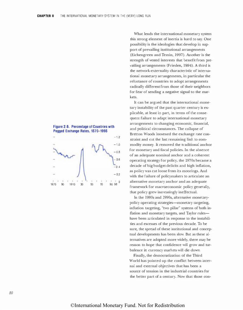
©International Monetary Fund. Not for Redistribution
80
CHAPTER II THE INTERNATIONAL MONETARY SYSTEM IN THE (VERY) LONG RUN
Figure 2.6. Percentage of Countries with Pegged Exchange Rates, 1870-1998
1870 90 1910 30 50 70
- 1 . 2
- 1 .0
- 0.8
- 0.6
-0.4
- 0.2
0 90 98
What lends the international monetary system
this strong element of inertia is hard to say. One
possibility is the ideologies that develop in sup
port of prevailing institutional arrangements
(Eichengreen and Temin, 1997). Another is the
strength of vested interests that benefit from pre
vailing arrangements (Frieden, 1994). A third is
the network-externality characteristic of interna
tional monetary arrangements, in particular the
reluctance of countries to adopt arrangements
radically different from those of their neighbors
for fear of sending a negative signal to the mar
kets.
It can be argued that the international mone
tary instability of the past quarter century is ex
plicable, at least in part, in terms of the conse
quent failure to adapt international monetary
arrangements to changing economic, financial,
and political circumstances. The collapse of
Bretton Woods loosened the exchange rate con
straint and cut the last remaining link to com
modit)' money. It removed the o·aditional anchor
for monetary and fiscal policies. In the absence
of an adequate nominal anchor and a coherent
operating su·ategy for policy, the 1970s became a
decade of big budget deficits and high inflation,
as policy was cut loose from its moorings. And
with the failure of policymakers to articulate an
alternative monetary anchor and an adequate
framework for macroeconomic policy generally,
that policy grew increasingly ineffectual.
ln the 1980s and 1990s, alternative monetary
policy operating strategies-monetary targeting,
inflation targeting, "two pillar" systems of both in
flation and monetary targets, and Taylor rules
have been articulated i.n response to the instabili
ties and excesses of the previous decade. To be
sme, the spread of these institmional and concep
tual developments has been slow. But as these al
ternatives are adopted more widely, there may be
reason to hope that confidence will grow and tur
bulence in currency markets will die down.
Finally, the democratization of the Third
World has pointed up the conflict between inter
nal and external objectives that has been a
source of tension in the induso;al countries for
the better part of a century. Now that those con-
©International Monetary Fund. Not for Redistribution
cerned with unemployment and distributive poli
cies can make their priorities known via the bal
lot box, it has become harder for governments
to subordinate all other goals of policy to stabi
lizing the exchange rate. As exchange rate policy
has come into conflict with other priorities, it
has lost credibility. But as they gain experience
with democracy, a growing number of societies
have come to recognize the risks associated with
the politicization of macroeconomic policy. They
have responded with institutional reforms, for
example, strengthening the independence of
their central banks and adopting fiscal rules, in
the effort to better insulate policy and the for
eign exchange market from day-to-day political
pressures. An extreme example is the currency
board, an alternative to floating exchange rates
that appears to be gaining adherents by the day,
which is in a sense a throwback to the gold
standard-style exchange rate arrangements of
previous centuries.
There is a sense in which these recent devel
opments represent a turn back from the govern
ment-run international monetary system of the
twentieth century to the more market-based sys
tem that characterized the better part of the pre
ceding millennium. Governments were never en
tirely out of the picture in the age of commodity
money, to be sure, but markets played a more
prominent role in regulating money supplies,
u·ansferring capital across borders, and deter
mining exchange rates. In a sense, the weakness
of governments-in particular, their limited abil
ity to regulate financial transactions and even to
cono·ol the circulation-gave markets the upper
hand. With the development in the nineteenth
century of new military technologies, which im
plied the need to mobilize resources for total
war, governments were forced to develop new
means of commanding and conu·olling re
sources. The levers of monetary control were
placed squarely in the hands of the central bank.
The state bureaucracy, especially its ability to tax,
was elaborated. The banking system was enlisted
RECENT DEVELOPMENTS IN MILLENNIAL PERSPECTIVE
to promote economic development
( Gerschenkron, 1962). This process culminated
in the Great War of 19 13-18, in which the mone
tary printing press, the domestic banking system ,
and tax system were utilized as never before.
And in response to the instabilities of the 1920s and 1930s, government regulation of financial
markets was tightened and macropolicy was ma
nipulated even more actively. Relative to the ear
lier situation, governments had gained the up
per hand.
Today, technology has struck back. The infor
mation and communication revolutions, which
worked in the nineteenth century to strengthen
the state relative to the market, today have the
opposite effect. The high fixed costs characteris
tic of nineteenth and twentieth century informa
tion and communications technologies, which
gave governments an advantage relative to indi
vidual market participants, have no analog in
the electronic age. In the age of the Internet,
controls on private financial transactions be
come increasingly easy to evade. In the age of
cheap international transportation, supporting
relatively inefficient national industries becomes
increasingly expensive. And if a century of wat·
has really drawn to a close (Mazower, 1999), then the willingness of the public to tolerate ex
tensive government intervention in the name of
national security may be less. While the insecuri
ties of globalization continue to fuel the demand
for government social programs to provide in
surance against the uncertainties created by
open international markets (Roclrik, 1997), the
scope for individuals to obtain such insurance
pdvately, on financial markets, is ever growing.
These are reasons for thinking that a century of
dirigisme, which looks increasingly Like an aber
ration in the long sweep of history, may be draw
ing to a close. Markets, by regaining the upper
hand in determining exchange rates and capital
flows, will only then have restored the status quo
ante that prevailed for most of the past
millennium (Box 2.3).
81
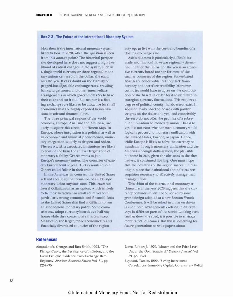
©International Monetary Fund. Not for Redistribution
82
CHAPTER II THE INTERNATIONAL MONETARY SYSTEM IN THE (VERY) LONG RUN
Box 2.3. The Future of the International Monetary System
How then is the international monetary system likely to look in 2020, when the question is seen from this vantage point? The historical perspective developed here does not suggest a high likelihood of radical changes in the system, such as a single world currency or three regional monetary unions centered on the dollar, d1e ew·o, and the yen. It casts doubt on the viability of pegged-but-a�justable exchange rates, crawling banks, target zones, and other intermediate arrangements in which governments try to have their cake and eat it too. But neither is a floating exchange rate likely to be alu-aclive for small economies that are highly exposed to international u-ade and rmancial nows.
The three ptincipal regions of the world economy, Europe, Asia, and the Americas, are likely to square this circle in different ways. In Europe, where integration is a political as well as an economic and financial phenomenon, monetary integration is likely to deepen and widen. The euro and its associated institutions are likely to provide the basis for an ever larger zone of monetary stability. Greece wants to join Europe's monetary union. The countries of eastern Europe want to join. Turkey wants to join. Others could follow in their train.
In the Americas, in contrasl, the United States will not accede to the formation of an EU-style monetary union anytime soon. This leaves unilateral dollarization as an option, which is likely to be most attractive for small countries with particularly strong economic and financial links to me United States that find it difficult to run an autonomous monetary policy. Some counaies may adopt currency boards as a half-way house while they contemplate this [mal step. Meanwhile, the larger, more economic;ally and financially diversified countries of the region
References
Alogoskoufis, George, and Ron Smith, 1992, 'The Phillips Curve, the Persistence of Inflation, and the Lucas Critique: Evidence from Exchange Rate
Regimes," American EconQmic Review, Vol. 81, pp.
1254-75.
may opt to live \vilh the costs and benefits of a floating exchange rate.
Asia's dilemma is particularly difficult. Its u-ade and financial flows are regionally diversified: neither the dollar nor the yen is an attractive currency-board anchor for most of the smaller counu·ies of the region. Basket-based boards are conceivable, but they lack trans
parency and therefore credibility. Moreover, cOtmaies would have to agree on the composition of the basket in order for it to minimize intraregion currency fluctuations. This requires a degree of political comity that does not exisL In addition, basket-backed boards with positive weights on the dollar, the yen, and conceivably the euro do not offer the promise of a subsequent transition to monetary union. That is to say, it is not dear whether such a country would logically proceed to monetary unification with the United States, Europe, or Japan. Hence, while Europe is likely to solve the currency conundrum through monetary unification and the Americas through dollruization, the plausible outcome in Asia, given the obstacles to d1e alternatives, is continued floating. One must hope that the countries of the region succeed in putting in place the institutional and political prerequi�ites necessary to effectively manage their managed float.
This vision of the international monetary architecture in the year 2020 suggests that the currency conundrum will not be solved by some grand design adopted at a new Bretton Woods Conference. It will be solved in a market-driven fashion, with arrangements evolving in clifferem ways in different parts of the world. Looking even further down the road, it is possible to envisage more radical outcomes. But this is something for future generations to write papers about.
Bat'I'O, Robenj., I 979, "Money and the Price Level Under the Gold Standard," Economicjourna4 Vol.
89, pp. 13-3 1.
Bayoumi, Tamim, 1990. "Saving-lnvesunem
Correlations: Immobile Capital, Government Policy.
©International Monetary Fund. Not for Redistribution
or Endogenous Behavior?" IMF Staff Papers, Vol. 37,
pp. 360-87.
Bayoumi, Tamim, and Barry Eichengreen, 1994,
"Macroeconomic Adjusunem Under Bretton Woods
and the Post-Bretton Woods Float," Economic
journal, Vol. 14, pp. 813-827.
--,1995, 'The Stability of the Gold Standard and
the Evolution of the International Monetary
System," in Tamim Bayoumi, Barry Eichengreen,
and Mark Taylor (eds.), 1\tfodern Perspectives on the
Gold Staru/a·rd (Cambridge: Cambi;dge University
Press) , pp. 165-88.
Berg, Claes, and Larsjonung, 1999, "Pioneering Price
Level Targeting: The Swedish Experience
1931-1937," Journal of Monetar)' Economics, Vol. 43,
pp. 525-51.
Boltho, Andrea, 1982, "Inu·oduction," in Andrea
Boltho (ed.), The European Econon�y: Growth and
Crisis (Oxford: Clarendon Press).
Bordo, Michael, and Barry Eichengreen, 1999, "Is Our
Current International Economic Environment
Unusually C•·isis Prone?" in CapitalFwws and the
httemationalFinancial System (Sydney: Reserve Bank
of Australia), pp. 18-74.
Bordo, Michael, and Larsjonung, 1997, "Institutional
Change and the Velocity of Money: A Century of
Evidence," Economic l7Ufui1y, Vol. 35, pp. 710-24.
Bordo, Michael, and Ronald MacDonald, 1997,
"Violations of the 'Rules of the Game' and the
Credibility of the Classical Gold Standard,
1880-1914," NBER Working Paper No. 6115
(Cambridge, Massachusetts) .
Cairncross, Alec, and Barry Eichengreen, 1983, Sterling
in Decline: The Devaluations of 1931, 194 9 and 1967
(Oxford: Blackwell).
Cipolla, Carlo M., 1982, Tlte Monetary Poli�y of
Fourteenth CenturyFl01-ence (Berkeley: University of
California Press).
Cooper, Richard, 1971, "Currency Devaluation in
Development Countries," Princeton Essays in
International Finance No. 86 (International
Finance Section, Deparunent of Economics,
Princeton University).
Crucini, Mario, 1994, "Sources of Variation in Real
Tariff Rates: The United States 1900-1940,"
American Economic Review, Vol. 84, pp. 932-43.
de Cecco, Marcello, 1974, Money and Empire: The
International Gold Standard (London: Blackwell).
Duncan, Evan, David Patterson, and Carolyn Vee
(eds.), 1999, F01·eign Relations of the United States,
REFERENCES
1964-1968, Volume VIII: lnternationalMonetmy and
Trade Policy (Washington: GPO).
Edwards, Sebastian, andjulio Santaella, 1994,
"Devaluation Conu·oversies in the Developing
Countries: Lessons from the Bretton Woods Era," in
Michael D. Bordo and BarryEichengreen (eds.), A
Retrospective on the 81-etton Woods S)'Siem (Chicago:
University of Chicago Press), pp. 405-55.
Eichengreen, Barry, 1992, Golden Fellet-s: Tlte Gold
Standard awl the Great Dejmssion (New York: Oxford
University Press) .
_, and Olivier Jeanne, 1999, "Currency Crisis and
Unemployment: Sterling in 1931," NBER Working
Paper No. 6563 (Cambridge, Massachusetts) .
Eichengreen, Barry, and Paul Masson, with othe rs,
1998, "Exit Su-ategies: Policy Options for Countries
Seeking Greater Exchange Rate Flexibility,"
Occasional Paper No. 168 (Washington, D.C.:
IMF).
Eichcngreen, Barry, and BetJ1 Simmons, 1995a,
"lmernational Economics and Domestic Politics:
Notes on the 1920s," in Charles Feinstein (ed.),
Banking, C1trrmcy and Finance in Eumpe Between the
Wt'trs (New York: Oxford University Press),
pp. 131-50.
_, 1995b, "Exchange Rate Commitments and
Central Bank Cooperation: The Classical and
Interwar Gold Standards Compared," Financial
Histor)' Review.
Eichen green, Barry, and Peter Ternin ( 1997), 'The
Gold Standard and the Great Depression," NBER
Working Paper No. 6060 (Cambridge,
Massachusetts).
Feinstein, Charles, Peter Temin, and Gianni Toniolo,
1997, The European Econ01ny Between the Wars
(Oxford: Oxford University Press) .
Flandreau, Marc, 1993, 'Trade, Finance and Currency
Blocs in Nineteenth Cenmry Europe: Was the Latin
Monetary Union a Franc Zone?" (unpublished;
University of California at Berkeley and DELTA,
Paris).
_, 1994, "An Essay on the Emergence of the
lntemational Gold Standard" (unpublished;
Stanford University).
_, 1995, L'or du monde: la F1·ance et la stabilite du sys
tem monetaire international, 1848-1873 (Paris:
L'Harmattan).
Frieden, jeffry, 1994, "Greenback, Gold and Silver:
The Politics of American Exchange Rate Policy,
1870-1913," CIBER Working Paper No. 91-04 (Los
83
©International Monetary Fund. Not for Redistribution
84
CHAPTER II THE INTERNATIONAL MONETARY SYSTEM IN THE (VERY) LONG RUN
Angeles: Anderson School of Management,
UClA).
Friedman, Milton, and AnnaJ. Schwartz, 1963, A
Monetary Hist01y of the United States, 1863-1960
(Princeton: Princeton University Press).
Gallarotti, G.M., 1995, The Anatomy of an International
Monetary Regime: The Classical Gold Standard,
1880-1914 (New York: Oxford University Press).
Caudal, Neil, and Nathan Sussman, 1997, "Asymmetric
Information and Commodity Money: Tickling the
Tolerance in Medieval France,journal of Money Credit
and Banking, Vol. 29, pp. 440-57.
Genberg, Hans, and Alexander Swoboda, 1994, 'The
Provision of Liquidity in the Bretton Woods System,"
in Michael D. Bordo and Barry Eichengreen (eds.),
A Retrospective on the Bretton Woods System (Chicago:
University of Chicago Press), pp. 269-316.
Gerschenkron, Alexander, 1962, Economic Backwardness
in Hist01ical Perspective (Cambridge, Massachusetts:
Harvard Unive rsity Press).
Giovannini, Alberto, 1993, "Bretton Woods and lts
Precursors: Rules versus Discretion in the History of
International Monetary Regimes," in Michael Bordo
and Barry Eichengreen (eds.), A Retrospective on the Bretton Woods System (Chicago: University of Chicago
Press), pp. 109-54.
Goodhart, Charles, and PJ.R. DeLargy, 1999,
"Financial Crises: Plus <:a change, plus c'est Ia meme
chose," LSE Financial Markets Group Special Paper
No. 108 (London).
Gould, John D., 1970, The Great Debasement (New York:
Oxford University Press).
Hamilton,James, 1992, "Was the Deflation During the
Great Depression Anticipated? Evidence from the
Commodity Market," American Economic Review, Vol.
82, pp. 157-78.
Johnson C., I 956, The De Moneta of Nicholas Oresme and
English Mint Documents (London).
Kindleberger, Charles P., 1978, Manias, Panics and
Crashes (New York: Basic Books).
_, 1984, A Financial History of Western J:.:urope
(London: Allen & Unwin).
_, 1991, 'The Economic Crisis of 1619 to 1623,"
Journal of Economic History, Vol. 51, pp. 149-75.
Kiyotaki, Nobuhiro, and Randall Wright, 1989, "On
Money as a Medium of Exchange," journal of Political
Economy, Vol. 97, pp. 927-55.
Lott,John R., and Lawrence W. Kenny, 1999, "Did
Women's Suffrage Change the Size and Scope of
Government?" Journal of Political Economy, Vol. 107,
pp. 1 1 63-98.
Madden, John J., 1985, British Investment in the United
States, 1860-1880 (New York: Garland Publishing).
Maddison, Angus, 1995, Monitoring the World Economy
1820-1992 (Paris: OECD).
Mayhew Nicholas, and Peter Spufford, 1988, Later
Medieval Mints: Organization, Administration and
Technique, BAR International Series 389.
Mazower, Mark, 1999, Dark Continent (New York:
Knopf).
McCuUoch,John R., 1837, Dictionary, Practica�
Theoretical and Historical of Commerce and Commercial
Navigation (London).
Meissner, Chris, 1999, "Why the World Went to Gold:
An Empirical Inquiry into the Emergence of the
Gold Standard, 1870-1913" (unpublished;
University of California, Berkeley) .
Miskimin, Harry A., 1984, Money and Power in Fifteenth
Century France (New Haven: Yale University Press).
Mitchell, Brian R., 1988, British Histmical Statistics
(Cambridge: Cambridge University Press).
Motomura, Akira, 1994, "The Best and Worst of
Currencies: Seigniorage and Currency Policy in
Spain, 1597-1650," joumal of Economic History,
Vol. 54, pp. 104-27.
Munro, John, 1979, "Bullion ism and the Bill of
Exchange in England, 1276-1663: A Study in
Monetar}' Management and Popular Prejudice," in
The Dawn of Modern Banking (New Haven: Yale
University Press) , pp. 169-239.
Nurkse, Ragnar, 1944, lntemational Currency Experience
(Geneva: League of Nations).
Oppers, Stefan, 1995, "A Model of the Bimetallic
System," IMF Working Paper WP/95/144
(Washi.ogton).
__ , 1996 "Was the Worldwide Shift to Gold
Inevitable? An Analysis of the End of Bimetallism,"
Joumal of Monetary Economics, Vol. 37, pp. 143-62.
Pamuk, Sevket, 1997, "In the Absence of Domestic
Currency: Debased Emopean Coinage in the
Seventeenth-Century Ottoman Empire," journal of
Economic History, Vol. 57, pp. 345-66.
Redish, Angela, 1990, 'The Evolution of the Gold
Standard in England," journal of Economic History\
Vol. 50, pp. 789-805.
Rodrik, Dani, 1997, 'Trade, Social Insurance, and the
Limits to Globalization," NBER Working Paper
No. 5905 (Cambridge, Massachusetts: National
Bureau of Economic Research) .
Rolnick, Arthur J., Francois R. Vel de, and Warren E.
Weber, 1996, 'The Debasement Puzzle: An Essay on
©International Monetary Fund. Not for Redistribution
Medieval Monetary History," joumal of Economic
History•, Vol. 56, pp. 789-808.
Sargent, Thomas]., and Bruce D. Smith, 1997,
"Coinage, Debasements, and Gresham's Laws,"
Economic Theory, Vol. 10, pp. 198-226.
Shaw, William A., 1895, The History of Currency,
1252-1894 (London: Wilson & Milne).
Spufford, Peter, 1986, Handbook of Medieval Exchange
(London).
__ , 1988, Money and Its Use in Medieval Europe
(Cambridge: Cambridge University Press).
Sussman, Nathan, 1993, ''Debasements, Royal
Revenues, and Inflation in France During the
Hundred Years' War, 1415-1422,"joumal of Economic
History) Vol. 53, pp. 44-70.
__ , 1997 "Wi.lliam Huskisson and the Bullion
Controversy-1810," Europeanjoumal of the HistrJry rJf
Ec()tlmnic Thought, pp. 237-57.
REFERENCES
__ , 1998, "The Bullion Famine Reconside1·ed-A
Monetary Approach to the Balance of Payments
Analysis: Evidence from France 1360-1415," joumal
rJf Economic History, Vol. 58, pp. 126-55.
_, and joseph Zeira, 1999, "Commodity Money
Inflation: Theory and Evidence from France,
1350-1436," (unpublished;Jerusalem: Hebrew
University).
Werveke, Hans van, 1948, "Currency Manipulations in
the Middle Ages: The Case of Louis Male, Count of
Flanders," Transactions of the !Wyal Historical Society,
4th series, Vol. 31, pp. 115-27.
Wyplosz, Charles, 1999, "Financial Restraints and
Liberalization in Postwar Europe" (unpublished;
Geneva: Graduate Institute of International Smdies,
University of Geneva).
85
©International Monetary Fund. Not for Redistribution 86
CURRENCY CRISES: IN SEARCH OF COMMON ELEMENTS Jahangir Aziz, Francesco Caramazza, and Ranil Salgado
The financial crisis that erupted in east
Asia in Lhe second half of 1997 was Lhe
latest in a series of currency crises that
at various times in Lhe post-Bretton
Woods period have engulfed emerging market
economies and industrial coumries alike.
Financial innovations and the increased interna
tional integration of financial markets appear to
have altered the naLUre of these crises in recent
years; in particular, the spillover effects and the
contagious spread of crises seem to have become
both more pronounced and far-reaching. At a
fundamental level, however, many of the same
forces have often been at work in different
crises. This chapter is concerned with these com
mon characteristics. It examines a large number
of currency crises in an effort to identify similari
ties in the behavior of a variety of macroeco
nomic and financial variables around Lhe times
of crises. The sample spans the period 1975-97 for 50 industrial countries and emerging market
economies. It covers crises that culminated in
large currency depreciation as well as those in
which there was a substantial loss of foreign re
serves. The analysis involves comparing the
monthly or annual pattern of movement of the
various macroeconomic and financial variables
around the time of crisis to their behavior dur
ing tranquil periods. The robustness of the re
sults is tested by subdividing the sample into dif
ferent types of currency crises and carrying out a
similar analysis for each. The paper also exam
ines the behavior of the various variables in the
aftermath of a crisis and assesses the costs of
crises in terms of lost output.
Following Frankel and Rose (1996), the paper
poses the question: Are currency crises aJI alike?
But it differs from that study in several respects.
Whereas Frankel and Rose focused exclusively
on currency crashes characterized by large ex
change rate depreciations, this study instead
considers currency crises that involve both large
depreciations or substantial losses in reserves, or
both. Another difference is that the earlier pa
per analyzed Lhe experience of developing coun
tries only, using annual data, while the sample of
countries in this study comprises both industrial
and emerging market economies. Furthermore,
most of the analysis is carried out using monthly
data, which allows for a more precise dating of
crises and which, given the nature of currency
crises, may be mot·e revealing than annual data.
Annual data is used, nonetheless, both to com
plement the monthly analysis and when variable
of particular interest are not available on a
montJ1ly frequency.
The methodology used is similar to that of
Eichengreen, Rose, and Wyplosz (1995) and
Frankel and Rose (1996). Essentially, for each
variable of interest a graphical "event study" is
conducted to see whether its average pattern of
movement bolh before and after a ct·isis (tJ1e
event) is different from its behavior during nor
mal or tranquil periods. The differences in be
havior between crisis and tranquil periods are
tested for statistical significance. Since the
graphical technique docs not impose any para
metric structure on the data and because tJ1e sta
tistical tests require less demanding assumptions
about the distribution of tJ1e variables, this
methodology has the advantage of often being
more informative in extracting behavioral pat
terns over a longer period of time than formal
econometric procedures. However, the analysis
remains intrinsically univariate. "While many
studies have supplemented the univariate analy
sis with more rigorous multivariate regression
analyses, these have not been fully satisfactory
for a variety of reasons (discussed in "The
Macroeconomy Before a Crisis," below).
Graphical event studies have drawbacks too,
however. For instance, unlike in regression
analysis where various sen itivity tests can be em
ployed to check the robustness of results, there
©International Monetary Fund. Not for Redistribution
are no such standard diagnostics available in
graphical analysis. To overcome this problem, in
this paper the robustness of the results are
checked by examining how the average behavior
of different variables changes for different types
of currency crises. In panicular, the sample of
158 currency crises identified in this study was divided into various subgroups: crises in indus
trial countries, crises in emerging market coun
tries, crises characterized mainly by currency
crashes, crises characterized mainly by reserve
losses, "severe" crises, "mild" crises, crises associ
ated with serious banking sector problems, crises
with fast recoveries, and crises with slow recover
ies.' For each of these subgroups, the same
variable-by-variable event study was conducted
and the behavior of these variables was com
pared across the various groupings. Behavioral
characteristics of variables that displayed largely
similar patterns across these groupings were con
sidered to be robust.
To summarize very briefly the main findings,
typically prior to a crisis tbe economy was over
heated, with monetary policy significantly expan
sionary, strong domestic credit growth, an over
valued currency, and in many cases high
inflation. The economy was also increasingly fi
nancially vulnerable, with rising liabilities of the
banking system not backed by foreign reserves
and falling asset prices. Furthermore, some
event, such as an increase in world interest rates
or a deterioration in the terms of trade, usually
exacerbated the vulnerability of the economy to
crisis.
Identifying Crises: Methodology and Data
Financial crises may be grouped into three
broad categories: currency crises, banking crises,
and foreign debl crises. 2 A currency crisis may be
said to occur when a speculative attack on the
IDENTIFYING CRISES: METHODOLOGY AND DATA
exchange value of a currency results in a devalu
ation (or sharp depreciation) of the currency,
or forces the authorities to defend the currency
by expending large volumes of international re
serves or sharply raising interest rates. A banking
crisis generally refers to a situation in which ac
tual or potential bank runs or failures induce
banks to suspend the internal convertibility of
their liabilities or which compels the govern
ment to intervene to prevent tl"lis by extending
assistance on a large scale.3 A foreign debl crisis is
usuaJiy described as a situation in which a coun
try cannot service its foreign debt, whether sov
ereign or private.
This study focuses on currency crises. ln many
instances, however, elements of ctu·rency, bank
ing, and debt crises may be present simultane
ously, as in the recent east Asian crises and in
the Mexican 1994-95 crisis. In contrast, the ERM
1992-93 crises were essentially currency crises,
even though the Nordic countries that experi
enced currency crises also had domestic banking
crises at around d1e same time. Furthermore,
what may start out as one type of crisis may de
velop into other kinds as well. Banking crises
have often preceded currency crises, especially
in developing couni.Jies-for instance, as in
Turkey and Venezuela in the mid-1990s. Banking
problems have preceded debt crises too, as in
Argentina and Chile in 198 1-82. The converse
also has occurred, as in Colombia, Mexico, Peru,
and Uruguay, where the withdrawal of external
financing in 1982 precipitated banking crises.
More recently, what began as currency crises in
some east Asian countries metastasized into
banking and debt crises, as illustrated most
clearly by lndonesia. That one type of crisis pre
cedes another does not necessarily imply causal
ity, however. For instance, when the financial sec
tor is poorly supervised and regulated, banking
system fragilities may be fully revealed only after
1The procedure used in identifying the crises is described in detail and the crisis subgroups are defined later in this chapter.
2This definition follows Bordo (1985), Caprio and Klingebiel ( 1997), and Eichengreen and Rose (1997). 3Not all financial disturbances are viewed as true tinancial crises. Financial disturbances that do not impinge on the pay·
ments mechanism and do not have potentially damaging consequences for economic activity have been characterized as "pseudo-financial crises"-see Mishkin (1994) and Schwartz (1985).
81
©International Monetary Fund. Not for Redistribution
88
CHAPTER Ill CURRENCY CRISES
a run on the currency has undermined confidence more generally and precipitated speculative shifts that expose and exacerbate banking and debt problems. This has clearly been a feature of the east Asian crises. Consequently, although banking and debt crises are not analyzed directly in this study, many cases of such crises, such as those of the Latin American debt crisis of the early 1980s and others that involved currency crises, are considered indirectly.
The measurement and dating of currency crises pose various difficulties. In this paper, following procedures adopted in the literature, episodes of significant foreign exchange market pressures are identified and dated using statistical criteria. This approach, while capturing the more serious currency crises, inevitably also
picks up episodes where there were significant but less than critical foreign exchange market pressures. This should be borne in mind in interpreting the results and drawing inferences of general applicability.
A currency crisis could be defmed simply as a substantial nominal currency devaluation or de
preciation.4 This criterion, however, would exclude instances where a currency came under severe pressure but the authorities successfully defended it by intervening heavily in the foreign exchange market, or by raising interest rates sharply, or by other means. An alternative approach is to construct an index of speculative pressure that takes into account not only exchange rate changes, but also movements in international reserves or interest rates that absorb pressure and thus moderate the exchange rate changes. For example, Eichengreen, Rose, and Wyplosz ( 1 996) use a weighted average of changes in the exchange rate, foreign reserves, and interest rates, relative to Germany, the refer-
ence country, to examine currency crises in industrial countries. Crises are then identified as extreme values of the speculative pressure index. Ctises identified using such an index would therefore include not only those occasions in which the currency depreciated significantly, but also occasions where actions by the authorities averted a large devaluation or the abandonment of an exchange rate peg.
For this study, currency crises were identified for a group of 50 countries for the period 1975-97. The group included 20 industrial countries and 30 developing countries. The developing country group consisted mainly of countries commonly referred to as emerging market economies.5 Germany and the United States served as the reference countries for the
European and the non-European countries, respectively.
For each country, an index of foreign exchange market pressure was constructed as a weighted average of (detrended) monthly exchange rate changes and reserve changes. The weights were chosen so as to equalize the vari
ance of the two components, thus avoiding the possibility of one of the two components dominating the index. Interest rates were not included in the index owing to the paucity of comparable, market-determined interest rate data for many developing countries over the sample period. Occasions when values of the index ex
ceeded a specified threshold-set to 1 Y2 times the pooled standard deviation of the calculated index plus the pooled mean of the index-were classified as crises. Weights and thresholds were calculated separately for periods of high inflation, which were defined as periods with 12-
month inflation rates greater than 80 percent. For any one country, crises identified v.rithin
4For example frankel and Rose (1996) ddine a "currency crash" as a nominal depreciation of the currency of at least 25
percent in a year, along with a 10 percent increase from the previous year in the rate of depreciation. The latter condition is included so as lO omit from ctu-rency crashes the large u·end depreciations of high-inflation countries.
5The industrial countries in the sample were Australia, Austria, Belgium, Canada, Denmark, Finland, France, Greece, Iceland, Ireland, ltaly,Japan, the Netherlands, New Zealand, Norway, Portugal, Spain, Sweden, Switzerland, and the United Kingdom. The emerging 1TU11·ket ec(»wmies were Argentina, Bangladesh, Brazil, Chile, China, Colombia, Cos ta Rica, Ecuador, Egypt, India, Indonesia, Israel, jamaica, Korea, Malaysia, Mexico, Nigeria, Pakistan, Paraguay, Peru, the Philippines, Singapore, South Africa, Sri Lanka, Taiwan Province of China, Thailand, Turkey, Uruguay, Venezuela, and Zimbabwe
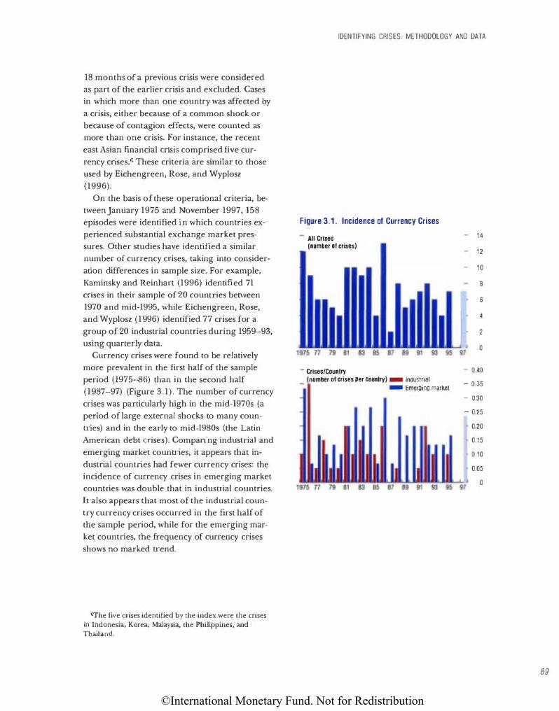
©International Monetary Fund. Not for Redistribution
18 months of a previous crisis were considered as part of the earlier crisis and excluded. Cases in which more than one country was affected by a crisis, either because of a common shock or because of contagion effects, were counted as more than one crisis. For instance, the recent
east Asian fmancial crisis comprised five currency crises.6 These criteria are similar to those used by Eichengreen, Rose, and Wyplosz
(1996).
On the basis of these operational criteria, between January 1975 and November 1997, 158 episodes were identified in which countries experienced substantial exchange market pressures. Other studies have identified a similar number of currency crises, taking into consideration differences in sample size. For example,
Kaminsky and Reinhart (1996) identified 71 crises in their sample of 20 countries between
1970 and mid-1995, while Eichengreen, Rose, and Wyplosz (1996) identified 77 crises for a group of 20 industrial countries during 1959-93, using quarterly data.
Currency crises were found to be relatively more prevalent in the first half of the sample period (1975-86) than in the second half (1987-97) (Figure 3.1). The number of currency crises was particularly high in the mid-1970s (a period of large external shocks to many coun
tries) and in the early to mid-l980s (the Latin American debt crises). Comparing industria] and emerging market counuies, it appears that in
dustrial countries had fewer currency crises: the incidence of currency crises in emerging market countries was double that in industrial countries.
It also appears that most of the industrial country currency crises occurred in the first half of the sample period, while for the emerging market countries, the frequency of currency crises
shows no marked u·end.
6The five crises identified by the index were the crises in Indonesia, Korea, Malaysia, the Philippines, and Thailand.
IDENTIFYING CRISES: METHODOLOGY AND DATA
Figure 3.1 . Incidence of Currency Crises
All Crises (number of crises)
- Crises/Country number of crises per country) - Industrial
- Emerging market
- 14
- 12
- 10
8
6
4
2
0
- 0.40
- 0.35
- 0.30
- 0.25
0.20
0.15
0.10
0.05
0
89
©International Monetary Fund. Not for Redistribution
90
CHAPTER Ill CURRENCY CRISES
The Correlates of Financial Crises
Having elated the currency crises, the next step was to choose the set of variables whose behavior could be expected a priori to systemati
cally differ during episodes of intense exchange market pressures from that in tranquil times.
The set of variables chosen was partly determined by the empirical implications of theOt·eti
cal models of exchange rate and balance of payments crises, the literature on "early warning
signals," and previous empirical studies of fmancial crises.
The early literature on currency crises-usually referred to as the "first-generation mod
els"-developed notably by Krugman ( 1979) and Flood and Garber ( 1984)-stressed the role played by economic fundamentals in causing crises. These models typically explained crises as
the result of fundamental inconsistencies in domestic policies, such as a persistent money
financed fiscal deficit and a commitment to a
pegged exchange rate. Such inconsistencies can for·a time be overlooked, as long as the central bank has sufficiently large foreign exchange reserves. But when official reserves fall to a critically low level and are perceived by the market
as insufficient, there will be a sudden speculative attack on the currency. These first-generation
models, therefore, predicted that a deterioration in the fundamentals would be indjcated prior to
a crisis by developments such as high or growing fiscal budget deficits, high rates of monetary
growth, high inOation, overvalued real exchange rates, large current accounr and trade defici£S,
sharp declines in international reserves, and rising domestic interest rates.
The role of domestic macroeconomic imbalances in generating currency crises in first
generation models has been evident in quite a few specific siwations. Overly expansionary mon
etary and fiscal policies have spurred lending booms, excessive debt accumulation, and over
investment in real assets, which have d1;ven up equity and real estate prices to unsustainable levels. The evenwal tightening of policies to contain inOation and facilitate tl1e adjusunent of ex-
ternal positions, and the inevitable correction of asset prices, have then led to a slowdown in economic activily, debt-servicing difficulties, declining collateral values and net worth, and rising
levels of non performing loans that threaten bank solvency. Macroeconomic factors, especially lending booms, have been found to play an important role in creating financial sector vulnerabilit)' in many Latin American countries (Gavin and 1lausmann, 1996, and Sachs, Tornell, and Velasco, 1996) and in other emerging market economies as well.
A drawback of first-generation models was that they represented policy in an essemially unidimensional and mechanical manner-the government automatically monetized all budget deficits while the central bank accommodated the pres
sures on the exchange rate by selling reserves without regard to other developments in the economy. Clearly, the range of policy options available even when budget defici£S are persist
ent goes beyond simply monetizing the deficit. When governments have multiple objecti,,es, however, almost all policy options involve some form of trade-off. Second-generation crisis models (Obstfcld, 1986 and 1994) exploit the tradeoffs among altermnive policies and the tensions in the governmem's objectives to generate mutu
ally conflicting incentives on the part of the authorities both to abandon an exchange rate peg and to defend it. In addition to tl1is policy uncertainty, if the cost of defending the peg is
likely to rise when agents expect the peg to be abandoned, then the exchange market could be subject to self-fulfilling expectations. 1f investors expect that despite sound fundamentals the government would abandon the peg if a specuJative
attack were severe enough, then by acting on those beliefs, investors may force the government to sacrifice the peg. For example, indi,�dual investors may believe a country to haYe generally sound fundamentals, so that there is no
reason for them to withdraw their funds from the country solely on the basis of the fundamentals. llowever, if a sufficient mtmber of other investors withdraw their funds from the country and thus increase the likelihood tl1at t11e govern-
©International Monetary Fund. Not for Redistribution
ment would be forced to abandon the peg, then
even the investors who were initially confident
that the country's fundamentals were sound may
also withdraw their investments rather than risk
losses from a devaluation. This, in turn, would
further increase the likelihood that the peg
would be abandoned. Ln such a case, if some
event or shock caused a critical mass of investors
to sell a country's currency, an exchange crisis
could ensue.
While theoretically it is possible that com
pletely extrinsic events ("sunspots») can trigger a
crisis-so that the economy is subject to multiple
equilibria, some involving crises and others
not-it is almost always the case that this possi
bility holds true only for certain ranges of the
fundamentals. There are no equilibrium models
of currency crises that generate sunspot equilib
ria for almost all possible ranges of the funda
mentals, such that sunspot-driven crises are not
generic. Consequently, even in second-genera
tions models, some fundamentals, such as the
composition of external debt (Masson, 1998,
and Cole and Kehoe, 1998) ultimately play the
critical role in generating crises. The role played
by such fundamentals, however, is more su·uc
turaJ than behavioral, in contrast to first
generation models.
A related but separate explanation of crises fo
cuses on contagion effects, where a crisis in one
country triggers crises in others. Contagion ef
fects can be transmitted through u·ade or finan
cial linkages, or may be a result of similarities in
macroeconomic fundamentals. For example, if a
group of countries are closely related through
trade, then a devaluation in one country can
force the others to devalue to maintain price
competitiveness. Also, owing to interdependen
cies in creditors' portfolios, iiJiquidity in one
market can force investors to liquidate assets in
other markets to cover losses or to meet liquidity
needs (Goldfajn and Valdez, 1997). Contagion
effects can also be transmitted through commit
ment costs. For a country, the costs of abandon-
THE CORRELATES OF FINANCIAL CRISES
ing a peg fall if neighboring countries (in an
economic sense, which in most cases is also in
the geographic sense) also abandon their pegs.
The waves of currency crises in the 1990s have
generated a lot of interest in contagion effects
and there is some evidence (e.g., Eichengreen,
Rose, and Wyplosz, 1996, and Glick and Rose,
1999) that they may be an important cause of
crises. Both theoretical and empirical studies of
contagion are silent, however, on why a crisis
originates in a specific countTy among a group
of vulnerable countries. Thus, even if contagion
plays a role in transmitting crises across coun
tries, it is still important to understand the role
played by funclan1entals in precipitating crises in
the first place.7
Another set of studies point to external condi
tions as the pivotal elements in fiJlancial crises,
especially in emerging market economies. Most
notable have been sudden, large shifts in lhe
terms of trade and in world interest rates that
have affected a large number economies simulta
neously (sometimes referred to as ''monsoonal
effects," Masson and Mussa, 1995). An unantici
pated drop in export prices, for instance, can
impair lhe capacity of domestic firms to service
their debts and result in a deterioration in t11e
quality of banks' loan portfolios. Movements in
interest rates in the major industrial coumries
have become increasingly important to emerg
ing market economies worldwide, reflecting the
increasing integration of world capital markets
and the globalization of investment. The sensitiv
ity of capital flows to developing counu·ies to
changes in world interest rates has been empha
sized by an1ongst others, Calvo, Leiderman, and
Reinhart ( 1993, 1996) and Taylor and Sarno
(1997). While sustained declines in world inter
est rates have induced surges in capital flows to
emerging market economies, an abrupt rise in
industrial country interest rates can lead to the
reversal of those flows. The rise in interest rates
not only increases the cost to domestic banks
(and firms) of funding themselves offshore, but
7For an empirical investigation of the role of Lraclc and financial linkages as well as external, domestic, and financial weakness in inducing financial crises, see Caramazza, Ricci, and Salgado (2000).
91
©International Monetary Fund. Not for Redistribution
92
CHAPTER Ill CURRENCY CRISES
also worsens adverse selection and moral hazard
problems and the fragility of the financial sys
tem.s Changes in global financial conditions,
therefore, are another possible factor behind
banking crises in emerging market economies
see Eichengreen and Rose (1997) for supporting
empirical evidence.
This paper does not study contagion effects; it
concentrates instead on investigating whether
countries' macroeconomic and financial charac
teristics during periods of crisis differ systemati
cally from those during noncrisis per·iods.
Consequently, the emphasis is mostly on vari
ables of the type suggested by first-generation
models and only to a lesser extent on those sug
gesting second-generation models. Variables em
ployed in the empirical literature on "early warn
ing signals,''9 such as measures of financial
liberalization, tl1e money multiplier, and credit
growth; proxies for investor confidence in the
domestic currency; the ratio of broad money to
international reserves; and the growth in asset
prices, are also analyzed.
The Macroeconomy Before a Crisis
Methodology
The methodology used in this paper is a mod
ified version of that adopted in other studies of
currency crises, such as those of Eichengreen,
Rose, and Wyplosz (1996) and Frankel and Rose
(1996). The approach employed in those papers
was a version of the "event study" methodology
where for each variable the sample was divided
into crisis windows and tranquil periods. A crisis
window was defined as some number of periods
centered around each crisis date. After all the
observations in each of the crisis windows were
taken out of the sample for a particular variable,
the remaining noncrisis observations were col
lectively deemed to be the sample of tranquil pe
riod observations. Having separated the sample
into crisis and tranquil observations, we com
puted the average across all the separate crisis
events for each period in the crisis window.
These averages for the crisis window were then
ploued against the average for the entire tran
quil period. The pattern displayed in the crisis
window was taken to be the average behavior of
the variable during crises. For the monthly data
in this paper, we considered a 49-month period
centered around each of the 158 crisis dates to be the crisis window. In the case of annual data,
five-year windows centered on the crisis dates
were used.
There are both advantages and drawbacks to
this methodology. The advantages lie largely in
the simplicity of the procedure. Since the graph
ical technique does not impose any parametric
structure on the data, it is more informative in
extracting patterns of behavior. Moreover, since
for this methodology statistical tests require less
demanding assumptions about the dist1ibutions
of the variables, the technique does not run into
a problem commonly encountered in more for
mal econometric procedures-namely the inva
lidity of statistical inferences owing to untenable
assumptions regarding the properties of the un
derlying data.
Among the drawbacks, perhaps the most sig
nificant is that the teclmique is intrinsically uni
variate. As a result it is often difficult to extract
the degree to which a particular pattern dis
played by a variable, before and after a crisis, is
influenced by me behavior of other variables.
Some studies have supplemented tl1e univariate
analysis with more r·igorous multivariate regres
sion analyses, but these have been unsatisfactory for a variety of reasons. The most appropriate
technique to use is a probit or logit-type panel
regression model with a sufficient number of
lags and leads (for example, in this paper it
would have 24 lags and 24 leads for the monthly
data) for the set of control variables. Typically,
this would involve estimates with too few degrees
8The linJ.;s between increases in interest rates and adverse selection and moral hazard problems, and financial ctises have been described in Mishkin (1996).
9See, for example, Goldstein (1996) and Kaminsky, Lizondo, and Reinhart ( 1997).
©International Monetary Fund. Not for Redistribution
of freedom even when the number of control
variables is kept small, since for most countries the required data are available only from the
mid-1970s. Because crises are relatively "rare"
events (typically, less than 2 percent of all obser
vations) panel regressions of this sort thus are
likely to encounter overfilling problems. In most
studies, therefore, either panel restrictions are
not respected or a very small number of lags are
used. In both cases, the additional information
has marginal benefit.
A second drawback of the graphical event
study technique is that typically a large number
of diverse countries are included in the sample,
making it difficult to draw conclusions from the
average behavior of variables. In this paper, this
problem is circumvented by standardizing vari
ables with respect to their counu·y-specific
means and standard deviations. This filters coun
try-specific characteristics that affect long-run
levels and volatility (for example, because of dif
ferent levels of development or differences in institutional structures-particularly in the finan
cial sector-some countries may have inherently
higher growth rates or more volatile paths for
monetary variables). It also partly addresses data
problems that may occur because of differences
in measurement and data collection across coun
tries. To some extem, using country-specific
standardized variables is similar to using panel
regressions with fixed and random effects.
A third drawback is that even if the countries
in the sample are similar (for example, all industrial countries or all developing countries), the
crisis situations may not be. For instance, some
variables may have behaved differently in more
severe crises than in the less severe crises, or in
crises where the economic recovery was faster than in crises where the recovery was relatively
slower, and crises involving only reserves losses
could be inherently different from those with
large devaluations. Consequently, while looking
for common behavior across many different
kinds of crises is informative, it can also be misleading-in that some particular type of crises could be dominating the common pattern. To
address this problem, the sample of 158 identi-
THE MACROECONOMY BEFORE A CRISIS
fied crises was djvided into various subgroups:
crises in industrial countries, crises in emerging
market countries, crises characterized mainly by currency crashes, crises characterized mainly
by reserve losses, "severe" crises, "mild" crises,
crises associated with serious banking sector
problems, crises with fast recoveries, and crises
with slow recoveries. For each of these sub
groups, the same variable-by-variable evem study was conducted and the behavior of these vari
ables was compared across the various groupings to verify whether the behavioral patterns of vari
ables in some crisis categories dominated the
overall average behavior. This subgrouping of
crises also provided a check for robustness. If a
variable's behavior remained largely similar
across the different subgroups then it can be
claimed with some degree of confidence that
such behavior was in fact a common feature of
currency crises.
Finally, to test whether the behavior of the var
ious v-ariables differed significantly during peri
ods of crisis from that during tranquil periods,
for each variable the two-standard error bands
for the difference between the average value of the variable during the crisis period and its u·an
quil period average were also drawn in the event-study charts. Following standard t-tests, if
the error band was different from zero, tl1e dif�
ference in behavior was claimed to be significant
at tl1e 95 percent confidence level. As can be
seen in the figures, the standard error bands are
wider tl1an in most other studies. The reason
may be that while other papers (for example,
Frankel and Rose, 1996) show only the error
bands for the crisis period and the value of the
tranquil period average-the implicit assump
tion being that the tranquil period observations
have no sampling error-this paper assumes that
both the crisis and tranquil-period observations
are subject to sampling errors. Consequently, the
appropriate standard errors for the differences be
tween crisis and tranquil period averages are the
square-root of the sum of the squared standard
errors fo1· the crisis and tranquil-period averages. While, this clearly bas the effect of widening the
error bands, it is tl1e right procedure to follow if
93
©International Monetary Fund. Not for Redistribution
94
CHAPTER Ill CURRENCY CRISES
inferences regarding the statistical significance of differences between crisis and noncrisis period behavior are to be made.
Antecedents of Crises
Figures 3.2-3.20 portray the behavior of various macroeconomic and financial variables in the run-up to currency crises and in their aftermath. Each figure includes ten panels, with each panel depicting the average behavior of a variable (denoted by a solid line) from 24 months before to 24 months after the crisis date compared LO its average level during tranquil or· normal times. Since each variable was standardized, units are in terms of country-specific standard
deviations-so that each panel shows the difference in the number of standar·d deviations by which the variable deviated from its countryspecific mean during crisis and tranquil periods. Although this way of presenting the data makes it difficult to interpret the differences in absolute or percentage terms, it goes a long way toward addressing the problems associated with pooling a large number of heterogeneous countries, as discussed in the previous section. The dotted lines display the two-times standard error bands of the differences between crisis and tranquil period behavior. If for any period, the error band does not intersect the zero line, then one car1 infer the difference to be significant at the 95 percent confidence level.
In each figure, the top row, left panel shows d1e difference in average behavior of a variable
during the 49-month crisis window compared to tranquil periods for the overall crisis sample. The oilier nine panels plot the results for various country and analytical groupings of the full sarnple, with a view to checking the robustness of the aggregate results. These groupings in
clude industrial count1·y crises; emerging market countY)' crises; crises mainly attributable to a sharp fall in the exchange rate (currency "crashes"); crises mainly attributable to a sizable decline in reserves ("reserves crises"); currency cr·ises associated with banking crises; relatively
··severe" crises; relatively "mild" crises; crises with fast recoveries; and crises with slow recoveries. JO
Generally, for all crisis groupings (excluding "high-inilation" crises1 1 ) , prior to the outbreak of a crisis the real foreign currency value of the domest.ic currency was significar1tly higher than itS mean during tranquil periods (Figure 3.2). At the beginning of the crisis window, around 24 mond1s before a crisis, the real ejjective exchange
m/.e was about 0.4 standard deviations higher than its u-anquil per-iod level. Although in some
cases the exchange rate declined slightly in the
subsequent two years, the overvaluation re·
mained significant dur-ing most of the precrisis
period. This pattern of real exchange rate overvalua
tion in the period leading up to a crisis was observed for all of the analyt.ical categories. I t
10Cunency "cr,\shes" are crises where the currency component of the exchange market pressure index account� for 75 per·cent of the index when the index signals a crisis. Reserves crises are crises where the reserves component of the exchange market pressure index accor.LntS for 75 percent of t.he index when the index signals a crisis. Currency crises associated with banking crises (also referred lO as banking and currency crises) are occurrences where a banking crisis occurs within two years (before or afler)-see the appendix to tl1is chapter for the definition and description of the incidence of banking crises. Severe crises are identified by increa;;ing the threshold of the exchange market pressure index w three times the pooled standard deviation plus tl1e pooled mean instead of 1.5 Limes the pooled standard deviation. For the severe crises, the tranquil periods are different from that of tl1e full crisis sample as tl1ey are recalculated as periods outside tl1e 49-monLh severe crisis window. Mild crises are those crises in which tl1e tbreshold is between 1.5 and 2.0 times the pooled standar·d deviation plus the pooled mean. For mild crises, tJ1e tranquil periods are the same as those for the full sample. Crises with fast recover-ies are those crises in which GOP returns to trend within two years after the outbreak of the crisis, while crises witl1 slow recoveries are those in which GOP returns to trend after tl1ree years or more. Based on these definitions, tl1ere were 42 industtiaJ country crises, 116 emerging market crises, 55 currency crashes, 55 reserves cr·ises, 45 banking and currency crises, 52 severe crises, 84 mild crises, 98 crises \\�th fast recoveries, and 60 crises witl1 slow recoveries.
1 '"1-ligh-inflation'' crises were defined as crises in which the pr·eceding 12-month inflation rate exceeded 80 percent.
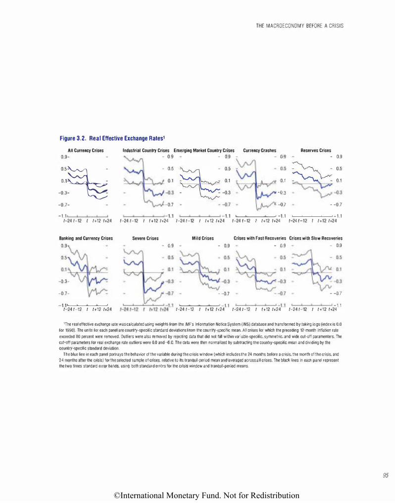
©International Monetary Fund. Not for Redistribution
THE MACROECONOMY BEFORE A CRISIS
Figure 3.2. Real Effective Exchange Rates1
All Currency Crises
0.9-
0.5�-
0.1- -
-{).3- -
-{).7-
Industrial Country Crises Emerging Market Country Crises Currency Crashes - 0.9 - 0.9 - - 0.9
- 0.5
�-� 0.1
� -{).3
0.1 0.1
-{).3
-{)_7 -{).7
Reserves Crises - 0.9
� 0.5
��: - -{).7
-1.1 -1.1 -1.1 ...._......__.__....__, -1.1 -1.1 1-24 t-12 I 1+12 1+24 1-24 t-12 I 1+12 1+24 1-24 t-12 I 1+12 1+24 1-24 t-12 1+12 1+24 1-24 t-12 I 1+12 1+24
Banking and Currency Crises
0.9
0.5
-{).3-
-{).7-
-1.1l--'----'--L--' 1-24 t-12 I 1+12 1+24
Severe Crises - 0.9
Mild Crises Crises with Fast Recoveries Crises with Slow Recoveries
- 0.9 - 0.9 - 0.9
- -{).7 - -{},7
..___..___,_....____, -1.1 1.1 -1.1 1-24 t-12 I 1+12 1+24 1-24 t-12 I 1+12 1+24 1-24 t-12 I 1+12 1+24
'The real effective exchange rate was calculated using weights from the IMF's Information Notice System (INS) database and transfonned by taking logs (index is 0.0 for 1990). The units for each panel are country-specific standard deviations from the country-specific mean. All crises lor which the preceding 12-month Inflation rate exceeded 80 percent were removed. Outliers were also removed by rejecting data that did not fall within variable-specific, symmetric, and wide cut-off paramenters. The
cut-off parameters lor real exchange rate outliers were 6.0 and -6.0. The data were then normalized by subtracting the country-specific mean and dividing by the country-specific standard deviation.
The blue line in each panel portrays the behavior of the variable during the crisis window (which includes the 24 months before a crisis, the month of the crisis, and
24 months after the crisis) for the selected sample of crises, relative to its tranquil-period mean and averaged across all crises. The black lines In each panel represent
the two times standard error bands. using both standard errors for the crisis window and tranquil-period means.
95
©International Monetary Fund. Not for Redistribution
96
CHAPTER Ill CURRENCY CRISES
ranged from about 0.3 standard deviations above
normal around two years prior to emerging mar
ket crises and cdses with slow recoveries to as
much as 0.6 standard deviations for industrial
country crises. It should be noted that these re
sults do not imply, however, that the overvalua
tion was higher in an absolute or percentage
sense in industrial countries, because average ex
change rates in crisis and tranquil periods are
calculated after removing country-specific means
and variance and these are higher for emerging
market countries. In fact, in percentage terms,
24 months prior to a crisis real exchange rates in
indusu·ial countries were on average only about 10 percent higher than in tranquil times com
pared to about 25 percent for developing
couno·ies.
Although the measured real exchange rate
overvaluation was statistically significant at the
95 percent significance level at the beginning of
the crisis window for all of the analytical cate
gories, it was not so throughout the precdsis pe
riod for some of the subgroups. Specifically, for
crises associated with serious banking sector
problems as well as for reserves crises-and to a
lesser extent for emerging market crises and for
crises with fast recoveries-the overvaluation was
not statistically significant in the year preceding
a crisis. For these categories, the real exchange
rate generally depreciated throughout the pre
crisis pe1iod. The real exchange rate overvalua
tion was generally statistically signi1icant at the
90 percent level, however. It is interesting to
note that the relative overvaluation of the real
exchange rate provided little information on the
severity of the crisis or the time it took on aver
age to recover from a crisis, as the precrisis be
havior of the real exchange rate was broadly sim
ilar for severe crises, mild crises, crises with fast
recoveries, and crises with slow recoveries.
It is of course not altogether surprising that
the real exchange rate tended to be appreciated,
relative to its norm, prior to a crisis, since most
currency crises involved significant nominal de
preciations. What this analysis reveals is that al
though real exchange rate overvaluation was a
dominant featw·e in the precrisis phase of most
currency crises, it was by no means present in
all. In particular, for crises that involved banking
sector problems and in those associated with
large reserves losses, the overvaluation was not
significant.
Typically, the real exchange rate appreciation
in precrisis periods was accompanied by a deteri
oration in exjJart performance, especially in tl1e
12 months or so preceding the outbreak of a cri
sis (Figure 3.3). However, the difference be
tween crisis and tranquil period behavior was sta
tistically significant-at the 95 percent
confidence level-only in the four months prior
to a crisis for the full sample of crises, and was
not statistically significant for some crisis group
ings, such as industrial country crises and crises
with large reserves losses. Similarly, the trade bal
ance did not display any significant differences in
behavior in the precrisis period except for a
slight deterioration near the outbreak of a crisis
(Figure 3.4). The terms of trade generally wors
ened in the precrisis period, but differed signifi
cantly from the tranquil pe1iod only in the final
few months before a crisis (Figure 3.5). For
emerging-market counu·y crises and cunency
crises associated with serious banking sector
problems, however, the terms of u·ade were wors
ened sigrlificantly starting almost a year prior to the crisis. In swn, although poor export per
formance, which resulted partly from a loss of
competitiveness owing to an overvalued ex
change rate and deteriorating terms of trade, ap
pears to have played a role in many crises, it was
not a common feature across all crises.
Inflation was significantly higher in precrisis pe
riods than in tranquil periods for the entire sam
ple of crises and for several of the analytical cate
gories (Figl.�re 3.6). Remarkably, for indusuial
counu;es the deviation of the rate of inflation
from its tranquil period level was greater t11an for
emerging market countries. However, this was
tl1e case only for comparisons that abstract from
country-specific means and variances. In absolute
terms, on average for emerging market countries
the inflation rate was 10-15 percent above its
tranquil period mean during the two years lead
ing up to a crisis, but for the industrial counu·ies
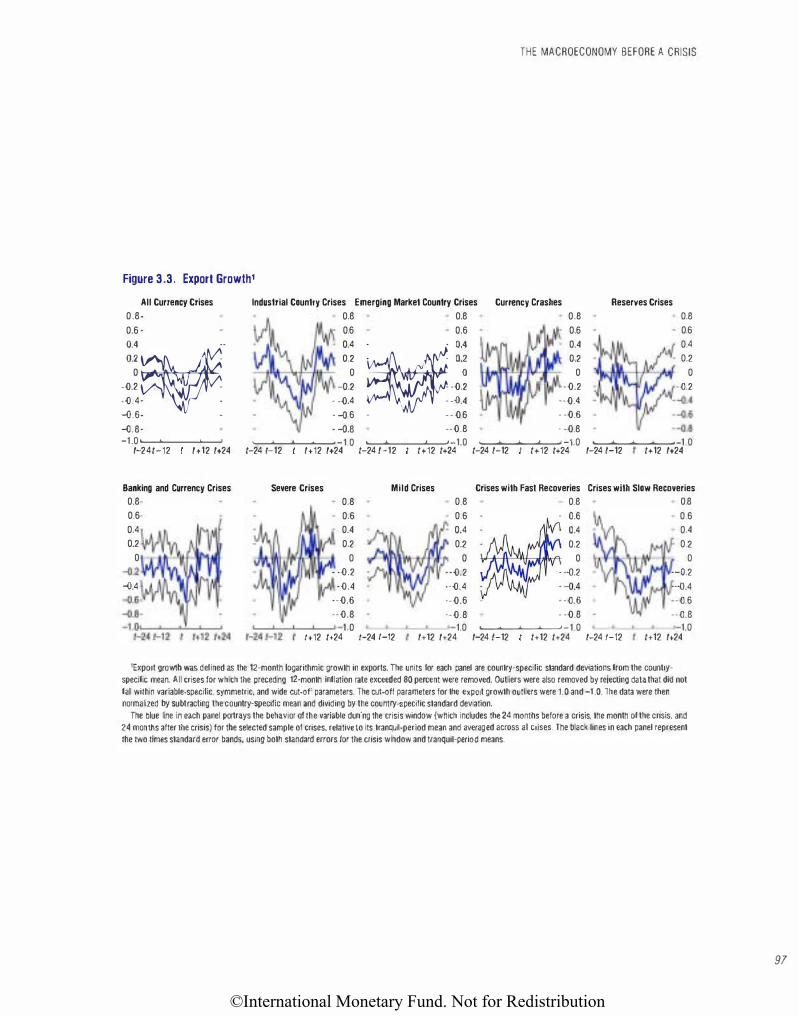
©International Monetary Fund. Not for Redistribution
THE MACROECONOMY BEFORE A CRISIS
Figure 3.3. Export Growth,
All Currency Crises
0.8· Industrial Country Crises Emerging Market Country Crises Currency Crashes Reserves Crises
0.6
·
�:: ¥
·
:
0 -o.2 . -D.4· . -o.6· . -o.8.
0.8 0.8 0.6 0.4 0.2
0 -0.2
. -o.4 · -D 6 - -o.8
0.6
�:: -o.2 -0.4
. --o6 --o.8
0.8 0.6 0.4 0.2
0 -o.2
--oA - -o.s - -o.8
0.8 0.6 0.4 0.2
0 -o.2
-1.0 '---'--'--'---' '---'--'---'---' -1.0 '----'---'--'----' -1.0 ,___.___,__..____, -1.0 ,___.___,__..____,_1_0 1-241-12 1+12 1+24 1-24 t-12 1+12 1+24 1-24 t-12 1+12 1+24 1-24 t-12 1+12 1+24 1-24 t-12 1+12 1+24
Banking and Currency Crises
0.8· 0.6· 0.4 0.2
0 1-r·tll-'-'l*HP<HII--Q.4
Severe Crises
0.8 0.6 0.4 0.2
0 . -o.2
-o.4 --o.s --o.8
1.0
Mild Crises Crises with Fast Recoveries Crises with Slow Recoveries
0.8 0.6 0.4 0.2
0.8 0.8
0 ·-D.2 ·-D.4 --o.6 �. - �::
. 0.2 . 0
. -o.2 - • -D.4 - - -o.s
--o.8 - -o.8 1.0 '----'---'--'---' -1.0
0.6 0.4 0.2
0 --o.2 --o.4 --o.6 --o.8
1+12 1+24 1-24 t-12 1+12 1+24 1-24 t-12 1+12 1+24 1-24 t-12 1.0
1+12 1+24
'Export growth was defined as the 12-monlh logarithmic growth in exports. The units for each panel are country-specific standard devlations from the countryspecific mean. All crises for which the preceding 12-month inflation rate exceeded 80 percent were removed. Outliers were also removed by rejecting data that did not
fall within variable-specific, symmetric, and wide cut·off parameters. The cut-off parameters for the export growth outliers were 1.0 and -1.0. The data were then normalized by subtracting the country-specific mean and dividing by the country-specific standard deviation.
The blue line in each panel portrays the behavior of the variable during the crisis window (which includes the 24 months before a crisis, the month of the crisis. and 24 months after the crisis) for the selected sample of crises, relative to its tranquil-period mean and averaged across all crises. The black lines in each panel represent
the two times standard error bands, using both standard errors for the crisis window and tranquil-period means.
91
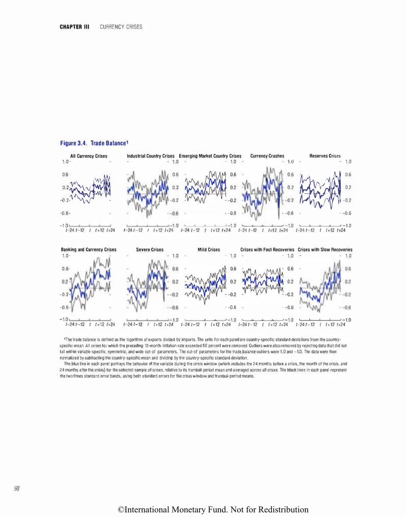
©International Monetary Fund. Not for Redistribution
98
CHAPTER Ill CURRENCY CRISES
Figure 3.4. Trade Balance,
All Currency Crises 1.0-
Industrial Country Crises Emerging Markel Country Crises Currency Crashes Reserves Crises 1.0 - 1.0 1.0 1.0
0.6�-
0.2-
-o.2. .
-o.s.
0.6
0.2
-o.2
� n 1 n
�� 0.6
�-::
0.6
0.2
-o.2
- -0.6 - -o.s
� 0 6
0 2
-o.2
- -o.6
1.0 .___.__.__...___, -1.0 '---'---'-----"'--.J -1.0 1-24 t-12 I 1+12 1+24 1-24 t-12 I 1+12 1+24 1-24 t-12 1+12 1+24 1-24 t-12 1+12 1+24 1-24 t-12 lt12 1+24
Banking and Currency Crises Severe Crises 1.0-
0.6-
-o.2·
-o.6-
1.0
Mild Crises Crises with Fast Recoveries Crises with Slow Recoveries - 1.0 - 1.0 1.0
�� ::: � :.: �·_,, �_,, - -o.s - -o.s
-1.0 -1.0 .___.__.__...___, -1.0 .___.__.__...___, -1.0 .____..___, _ _,___J -1.0 1-24 t-12 I 1+12 1+24 1-24 t-12 I lt12 1+24 1-24 t-12 1+12 1+24 1-24 t-12 1+12 1+24 1-24 t-12 1+12 lt24
1The trade balance is defined as the logarithm of exports divided by imports. The units for each panel are country-specific standard deviations from the country· specilic mean. All crises lor which the preceding 12·month lnllation rate exceeded 80 percent were removed. Outliers were also removed by rejecting data that did not fall within variable-specific. symmetric, and wide cut-off parameters. The cut-off parameters lor the trade balance oulliers were 1.0 and -1.0. The data were then normalized by subtracting the country-specific mean and dividing by the country-specific standard deviation.
The blue line in each panel portrays the behavior of the variable during the crisis window (which includes the 24 months before a crisis. the month of the crisis, and 24 months after the crisis) lor the selected sample of crises, relative to its tranquil-period mean and averaged across all crises. The black lines in each panel represent the two times standard error bands, using both standard errors for the crisis window and tranquil-period means.
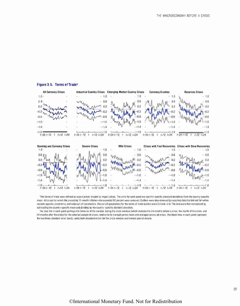
©International Monetary Fund. Not for Redistribution
THE MACROECONOMY BEFORE A CRISIS
Figure 3.5. Terms of Tradel
All Currency Crises 1.0 . Industrial Country Crises Emerging Mark.et Country Crises Currency Crashes Reserves Crises
0.6.
��� -1 0 · -1.4· -1 .8 '----'--'---''---' r-24 1-12 !t 12 !t24 Banking and Currency Crises 1.0·
�::� -o.2� �:� -1 .8 '----'--'---''---' 1-24 1-12 I It 12 lt24
. 1.0 . 1.0 �.11� 0.6
��: . ·-1.0 ·-1.4
�� �:: ��
-o.2 �-.lf\V A AA ·_r M. �:� : �lf''y :-_1.4
L--....L..--'--'---'-1.8 .___.....___,__....____, -1.8 t-24 1-12 1+12 !+24 1-24 1-12 !+12 1+24 Severe Crises Mild Crises
1.8 1-24 1-12 t 1+12 1+24 1-24 t-12 . -1.4 1.8 lt12 1+24
1.0 0.6 0.2
-1.0 .__,___,__....____,_1.8 --1.4
,___.__..___.___, -1.8 1-24 1-12 It 12 1+24 1-24 1-12 1+12 lt24 Crises with Fast Recoveries Crises with Slow Recoveries . 1.0 . 1.0
�# �:: ���:: � -o2 � -o2
��: ��: -�.4 . -�.4 1-24 t-12 1 � 1 � 1+12 1+24 1-24 t-12 I 1+12 lt24
'The terms of trade were defined as export prices divided by import prices. The units for each panel are country-specific standard deviations from the country-specific
mean. All crises for which the preceding 12-month inflation rate exceeded 80 percent were removed. Outliers were also removed by rejecting data that did not fall within variable-specific, symmetric, and wide cut·off parameters. The cut-oft parameters for the terms of trade outliers were 2.0 and -2.0. The data were then normalized by
subtracting the country-specific mean and dividing by the country-specific standard deviation.
The blue line in each panel portrays the behavior of the variable during the crisis window {which includes the 24 months before a crisis, the month of the crisis. and 24 months after the crisis) for the selected sample of crises, relative to its tranquil-period mean and averaged across all crises. The black lines in each panel represent
the two times standard error bands, using both standard errors for the crisis window and tranquil-period means.
99
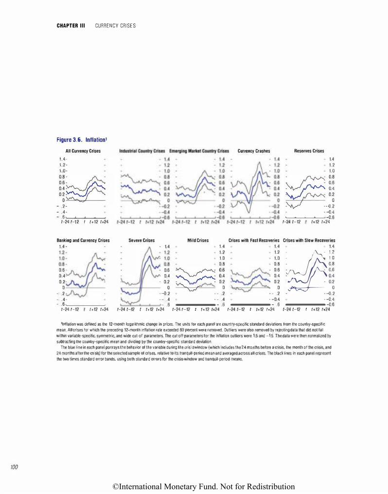
©International Monetary Fund. Not for Redistribution
100
CHAPTER Ill CURRENCY CRISES
Figure 3.6. lnflation1
All Currency Crises
1.4. 1.2. 1.0.
! l� o Y\c....,.,.�
-o. 2 · -o.4. -o.6 '---'----'---''---'
1-24 t-12 1+12 1+24
Banking and Currency Crises Severe Crises 1.4 . . • • 1.4
0 6 · . • 0 6 0.4. . . . 0 4 0.2. . . 0 2
0 0 -o 2 . . . . -o.2
Mild Crises 1.4 1.2 1.0 0.8
� 0.6
��� 0.4 �A �-�-A • 0,2 � � 0 'C.J.7
- -o.2
Currency Crashes
Crises with Fast Recoveries 1.4 1.2 1.0 0.8 0.6 0.4 0.2
0 - -o.2
Reserves Crises
1.4 1.2 1.0 �· 0.8 0.6
-'v.../ � 0.4 �� 0.2
\A? --o.� . -o.4
L-....L..--'--'---'-o.6 t-24 t-12 1+12 1+24
Crises with Slow Recoveries 1.4
�?dfj�li . 0.4
. 0.2 0
. . -o.2 -o.4· . -o.4 . -o.4 . -0.4 . -o.4 -o.6 '---'-___.__.....___, '-..:J.....---'-_..___, -o.6 '---'-----'---''-----' -o.s '---'-___.__.....___, -o.s '---'---'--'-----' -o.s
1-24 t-12 I+ 12 1+24 t-24 t-12 t 1+12 lt24 1-24 t-12 lt12 lt24 t-24 t-12 lt12 lt24 t-24 t-12 1+12 tt24
'Inflation was defined as the 12·month logarithmic change in prices. The units for each panel are country-specific standard deviations from the country-specific
mean. All crises for which the preceding 12·month Inflation rate exceeded 80 percent were removed. Outliers were also removed by rejecting data that did not fall within variable-specific, symmetric, and wide cut·off parameters. The cut·off parameters for the Inflation outliers were 1.5 and -1.5. The data were then normalized by
subtracting the country-specific mean and dividing by the country-specific standard deviation. The blue line in each panel portrays the behavior of the variable during the crisis window (which Includes the 24 months before a crisis, the month of the crisis, and
24 months after the crisis) for the selected sample of crises. relative to its tranquil-period mean and averaged across all crises. The black lines in each panel represent
the two times standard error bands, using both standard errors for the crisis window and tranquil-period means.
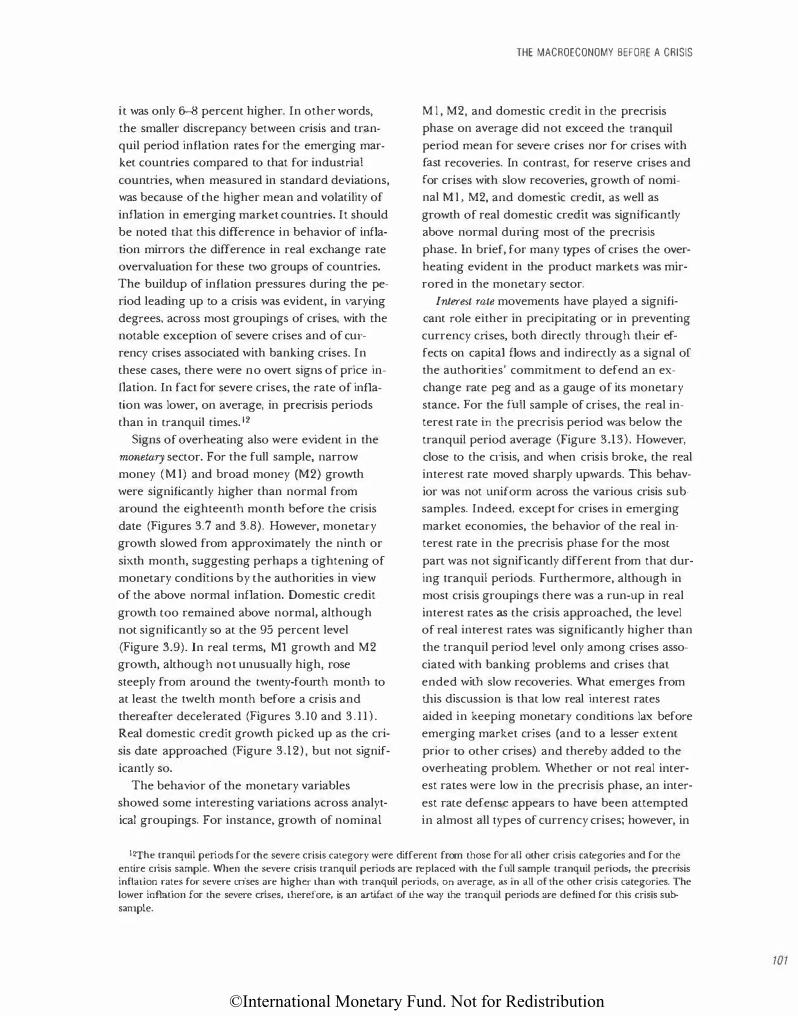
©International Monetary Fund. Not for Redistribution
it was only 6-8 percent higher. In other words,
the smaller discrepancy between crisis and tran
quil period inflation rates for the emerging mar
ket countries compared to that for industrial
countries, when measured in standard deviations,
was because of the higher mean and volatility of
inflation in emerging market countries. It should
be noted that this difference in behavior of infla
tion mirrors the difference in real exchange rate
overvaluation for these two groups of countries.
The buildup of inflation pressures during the pe
riod leading up to a crisis was evident, in varying
degrees, across most groupings of crises, with the
notable exception of severe crises and of cw·
rency crises associated with banking crises. In
these cases, there were no overt signs of price in
flation. In fact for severe crises, the rate of infla
tion was lower, on average, in precrisis periods
than in tranquil times. l2
Signs of overheating also were evident in the
monetary sector. For the full sample, narrow
money (Ml) and broad money (M2) growth
were significantly higher than normal from
around the eighteenth month before the crisis
date (Figures 3.7 and 3.8). However, monetary
growth slowed from approximately the ninth or
sixth month, suggesting perhaps a tightening of
monetary conditions by the authorities in view
of the above normal inflation. Domestic credit
growth too remained above normal, although
not significantly so at tl1e 95 percent level
(Figure 3.9). ln real terms, Ml growth and M2
growth, although not unusually high, rose
steeply from around the twenty-fourth month to
at least the twelth month before a crisis and
thereafter decelerated (Figures 3.10 and 3.11) .
Real domestic credit growth picked up as the cri
sis date approached (Figure 3.12), but not signif
icantly so.
The behavior of the monetary variables
showed some interesting variations across analyt
ical groupings. For instance, growth of nominal
THE MACROECONOMY BEFORE A CRISIS
M l , M2, and domestic credit in the precrisis
phase on average did not exceed the tranquil
period mean for seve1·e crises nor for crises with
fast recoveries. In contrast, for reserve crises and
for crises with slow recoveries, growth of nomi
nal Ml, M2, and domestic credit, as well as
growth of real domestic credit was signi:fican tly
above normal during most of the precrisis
phase. In brief, for many types of crises the over
heating evident in the product markets was mir
rored in the monetary sector.
Interest rate movements have played a signifi
cant role either in precipitating or in preventing
currency crises, both directly through tlleir ef
fects on capital flows and indirectly as a signal of
the authorities' commitment to defend an ex
change rate peg and as a gauge of its monetary
stance. For the full sample of crises, the real in
terest rate in the precrisis period was below the
tranquil period average (Figure 3.13). However,
close to the ci;sis, and when crisis broke, the real
interest rate moved sharply upwards. This behav
ior was not uniform across the various crisis sub
samples. Indeed, except for crises in emerging
market economies, the behavior of the real in
terest rate in the precrisis phase for the most
part was not significantly different from that dur
ing tranquil periods. Furthermore, although in
most crisis groupings there was a run-up in real
interest rates as the crisis approached, the level
of real interest rates was significantly higher than
the tranquil period level only among crises asso
ciated with banking problems and crises tl1aL
ended with slow recoveries. What emerges from
this discussion is that low real interest rates
aided in keeping monetary conditions lax before
emerging market crises (and to a lesser extent
pdor to other crises) and thereby added to the
overheating problem. Whether or not real inter
est rates were low in the precrisis phase, an inter
est rate defense appears to have been attempted
in almost all types of currency crises; however, in
12"fhe tranquil periods for the severe crisis category were different from those for all other crisis categories and for the entire crisis sample. When the severe crisis tranquil periods are replaced with the full sample tranquil periods, the precrisis inflation rates for severe crises are higher than with tranquil periods, on average, as in ail of the other crisis categories. The lower inflation for the severe crises, therefore, is an artifact of the way the tranquil periods ru·e defined for this crisis subsrunple.
101
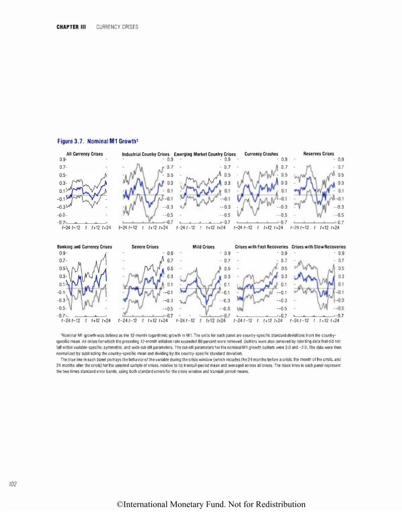
©International Monetary Fund. Not for Redistribution
102
CHAPTER Ill CURRENCY CRISES
Figure 3.7. Nominal M1 Growth1
All Currency Crises 0.9-0.7-
�:��- N«'' !. 0.1)1"""'1�� -o.1 · .
-o.3 . -o.s-
Industrial Country Crises Emerging Market Country Crises Currency Crashes Reserves Crises � - � � �
- - 0.5 . fvv... • � 0.5 . . 0.5 . 0.5 . 0.7 - - 0.7 J:N:!J 0.7 - - 0.7 0.3 JMM '1./V,v jt o.3 0.3 - 0 3
--o.3 --o 3 - --o.3 - --o.3 . -o.s . . -o.s --o.s - --o.s -o.7.__-'-__.__..___, '---''----'---'-L--1-Q} '---'----'--'-----'-0. 7 -o. 7 -Q.7 1-24 t-12 1+12 1+24 1-24 t-12 1+12 1+24 1-24 t-12 1+12 1+24 1-24 t-12 I 1+12 1+24 1-24 t-12 I 1+12 1+24 Banking and Currency Crises Severe Crises
E� . M Ari �:! o.3�:11VNA
vf1 0.3
0.1 · 0.1 -\-1---;-IHf\-f-''-,.,tt -o.1· ·-Q.1 -o.3- ·-Q.3 -o.s- --o.s -o. 7.___.___,__..__....J l.:.--''---'---'---'-o. 7
Mild Crises
1-24 t-12 1+12 1+24 1-24 t-12 1+12 1+24 1-24 1-12
0.9 0.7 0.5 0.3 0.1 --0.1 --o.3 --o.s
Crises with Fast Recoveries Crises with Slow Recoveries 0.9 0.9
'Wfi�I-..P..-!L
0.7 0.5 0.3 0.1 --o.1 ·-Q.3
·-0.5
0.7 0.5 0.3
'---'---'--'----'-o. 7 .___.___,__..__....J-o. 7 /-24 t-12 I 1+12 1+24 1-24 t-12 1+12 1+24
'Nominal M1 growth was defined as the 12·month logarithmic growth in Ml. The units for each panel are country-specific standard deviations from the country·
specific mean. All crises lor which the preceding 12·month Inflation rate exceeded 80 percent were removed. Outliers were also removed by rejecting data that did not
fall within variable-specific. symmetric, and wide cut·off parameters. The cut-ofl parameters for the nominal Ml growth outliers were 2.0 and -2.0. The data were then
normalized by subtracting the country-specific mean and dividing by the country-specific standard deviation. The blue line in each panel portrays the behavior of the variable during the crisis window (which includes the 24 months before a crisis, the month of the cnsis, and
24 months after the crisis) for the selected sample of crises, relative to its tranquil-period mean and averaged across all crises. The black lines in each panel repres.ent
the two times standard error bands, using both standard errors for the crisis window and tranquil-period means.
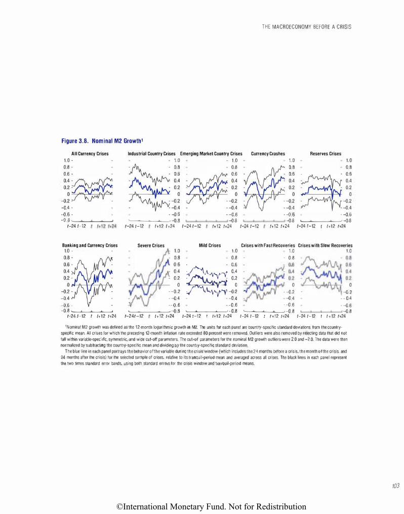
©International Monetary Fund. Not for Redistribution
THE MACROECONOMY BEFORE A CRISIS
Figure 3.8. Nominal M2 Growtht
All Currency Crises 1.0 -0.8 . 0.6 . : :� -o.2 . . -Q.4 . -o.6 --o.8 .____.___._____,'--_,
1-24 t-12
Banking and Currency Crises 1.0 .
�r�� -o.4 . -o.6 - .
-o.8 .____._____.__..__, 1-24 t-12 I I+ 12 lt24
Industrial Country Crises Emerging Market Country Crises Currency Crashes Reserves Crises
1.0 - 1.0 1.0 1.0 � :: . � J\i-- :: . I"\ )1/: :: . . :: ��; ��; ��; ��; . -o.6 . -o.6 . -o.6 . -o.6 .____.____.__..__. -o 8 -o.8 -o.8 .____.____.__..__, -o.s
1-24 1-12 I+ 12 1+24 1-24 1-12 It 12 1+24 t-24 t-12 I+ 12 1+24 1-24 t-12 I+ 12 1+24
Severe Crises Mild Crises Crises with Fast Recoveries Crises with Slow Recoveries 1.0 0.8 0.6 0.4 0.2 0
1.0 0.8
�
ll . -o.2 -o.2 . -o.4 . . -Q.4
--o.6 . -o.6 .____.____._�.....__, -o.8 '----'---'-�'---' -o.8
1-241-12 1+12 lt24 1-24 t-12 lt12 1+24
1� 1� . · 0.8 � 08
��· :: ���:; - 0 0 . · -Q2 . -o 2 - . -Q 4 - - o 4
. -o.6 . -o.6 ,__.____.__..__, -o.8 -o.8
1-24 1-12 1+12 lt24 1-24 1-12 1+12 1+24
1 Nominal M2 growth was defined as the 12-month logarithmic growth In M2. The units for each panel are country-specific standard deviations from the country
spec�ic mean. All crises for which the preceding 12·month Inflation rate exceeded 80 percent were removed. Outliers were also removed by rejecting data that did not fall within variable·specific, symmetric, and wide cut-oft parameters. The cut-off parameters for the nominal M2 growth outliers were 2.0 and -2.0. The data were then normalized by subtracting the country-specific mean and dividing by the country-specific standard deviation.
The blue line in each panel portrays the behavior of the variable during the crisis window (which includes the 24 months before a crisis, the month of the crisis, and 24 months after the crisis) for the selected sample of crises, relative to its tranquil-period mean and averaged across all crises. The black lines in each panel represent
the two times slandard error bands, using both standard errors for the crisis window and tranquil-period means.
103
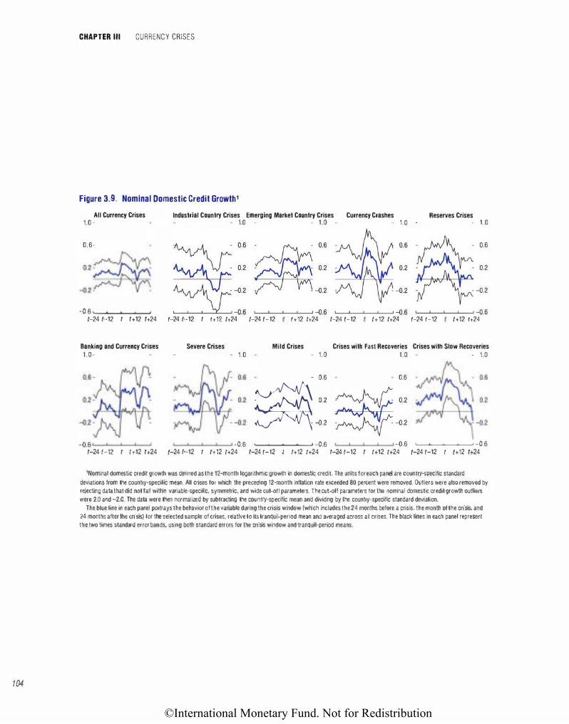
©International Monetary Fund. Not for Redistribution
104
CHAPTER Ill CURRENCY CRISES
Figure 3.9. Nominal Domestic Credit Growth,
All Currency Crises 1.0 .
0.6-
-o.6 L-....L---'--'---' 1-24 t-12 I 1+12 1+24
Banking and Currency Crises 1.0-
Industrial Country Crises Emerging Market Country Crises Currency Crashes Reserves Crises 1.0 1.0 1.0 1.0
� :: � :: W :: 4 :: �:: �:.: �:: �:.:
1-24 t-12 I 1+12 1+24 1-24 t-12 1+12 1+24 1-24 t-12 1+12 1+24 1-24 1-12 1+12 1+24
Severe Crises 1.0
Mild Crises Crises with Fast Recoveries Crises with Slow Recoveries 1.0 1.0 . 1.0
- 0.6 0.6
��: � 0.2
� "" -_A��VJr. 1--. ·vv "'V . -o.2
-o.6 -o.6 L--'---'----''--' -o.6 -o.6 '---'----'---'---' -o.6 1-24 t-12 I lt12 1+24 1-24 t-12 I lt12 1+24 1-24 t-12 1+12 1+24 1-24 t-12 I 1+12 1+24 1-24 t-12 1+12 1+24
'Nominal domestic credit growth was defined as the 12·month logarithmic growth in domestic credit. The units for each panel are country-specific standard deviations from the country·specific mean. All crises for which the preceding 12·month inflation rate exceeded 80 percent were removed. Outliers were also removed by rejecting data that did not fall within variable-specific. symmetric, and wide cut-off parameters. The cut·off parameters lor the nominal domestic credit growth outliers were 2.0 and -2.0. The data were then normalized by subtracting the country-specific mean and dividing by I he country-specific standard deviation.
The blue line in each panel portrays the behavior of the variable during the crisis window (which includes the 24 months before a crisis, the month of the crisis. and 24 months after the crisis) for the selected sample of crises, relative to Its tranquil-period mean and averaged across all crises. The black lines In each panel represent the two times standard error bands, using both standard errors for the crisis window and tranquil-period means.
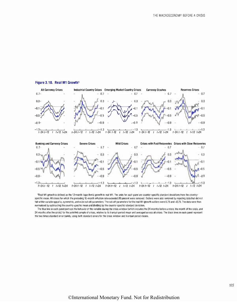
©International Monetary Fund. Not for Redistribution
THE MACROECONOMY BEFORE A CRISIS
Figure 3.1 0. Real M1 Growth,
All Currency Crises
0.7.
�:ru �.5v� �.9·
Industrial Country Crises Emerging Marltet Country Crises
0.7 . 0.7
0.3 ��.1
. -�.5
. -�.9 �=: -�.9
Currency Crashes Reserves Crises
0.7
-1.3 1.3 ',.--....L...--L--'---' -1.3 1.3 1.3 It 12 lt24 1-24 t-12 I lt12 lt24 t-24 t-12 I lt12 lt24 1-24 t-12 lt12 1+24 1-24 t-12 t lt12 lt24 1-24 t-12
Banking and Currency Crises Severe Crises 0.7.
0.3
. 0.7 Mild Crises Crises with Fast Recoveries Crises wilh Slow Recoveries
. 0.7 . 0.7 0.7
0.3
�.5
�.9
-1.3 -1.3 .__.....__.__..___, _1.3 -1.3 '---'---'--.I<.L.......J -1.3 1-24 t-12 I 1+12 1+24 1-24 t-12 t 1+12 1+24 1-24 t-12 1+12 1+24 1-24 t-12 I lt12 1+24 t-24 t-12 lt12 1+24
'Real Mt growth is defined as lhe 1 2-month logarithmic growth in real M1. The units for each panel are country-specific standard deviations from the country· specific mean. All crises for which the preceding 12-month inflation rate exceeded 80 percent were removed. Outliers were also removed by rejecting data that did not fall within variable-specific, symmetric, and wide cut-off parameters. The cut-off parameters for the real M1 growth outliers were 0.75 and �.75. The data were then normalized by subtracting the country-specific mean and dividing by the country-specific standard deviation.
The blue line in each panel portrays the behavior of the variable during the crisis window (which includes the 24 months before a crisis, the month of the crisis. and 24 months after the crisis) for the selected sample of crises. relative to its tranquil-period mean and averaged across all crises. The black lines in each panel represent the two times standard error bands, using both standard errors for the crisis window and tranquil-period means.
105
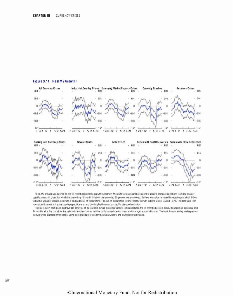
©International Monetary Fund. Not for Redistribution
106
CHAPTER Ill CURRENCY CRISES
Figure 3.11 . Real M2 Growtht
All Currency Crises 0.8 °
Industrial Country Crises Emerging Market Country Crises Currency Crashes Reserves Crises
-1.2 '----'-----'---'-----' 1-24 1-12 I 1+12 1+24
Banking and Currency Crises 0.8 .
0.8 ° 0.8 • 0.8 0.8
'----'-----'---'-----' -1 2
0.4 0.4 0.4
1.2 -1.2 -1.2 1-24 1-12 I 1+12 1+24 1-24 t-12 1+12 1+24 1-24 1-12 1+12 1+24 1-24 1-12 t 1+12 1+24
Severe Crises 0.8
0.4
Mild Crises Crises with Fast Recoveries Crises with Slow Recoveries · M M M
0.4 0.4
. -o.8
'----'---'--'----' -1.2 '---'--'---'----' -1.2 I 1+12 1+24 1-24 1-12 t 1+12 1+24 1-24 1-12 1+12 1+24 1-24 1-12 t
1 Real M2 growth was deli ned as the 12·month logarithmic growth in real M2. The units for each panel are country-specific standard deviations from the country·
specific mean. All crises for which the preceding 12·month inflation rate exceeded 80 percent were removed. Outliers were also removed by rejecting data that did not
fall within variable-specific, symmetric, and wide cut-off parameters. The cut-off parameters for the real M2 growth outliers were 0.75 and -o.75. The data were then
normalized by subtracting the country-specific mean and dividing by the country-specific standard deviation.
The blue line in each panel portrays the behavior of the variable during the crisis window (which includes the 24 months before a crisis, the month of the crisis, and
24 months after the crisis) for the selected sample of crises, relative to its tranQuil-period mean and averaged across all crises. The black lines in each panel represent
the two times standard error bands, using both standard errors for the crisis window and tranQuil-period means.
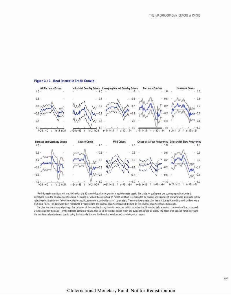
©International Monetary Fund. Not for Redistribution
THE MACROECONOMY BEFORE A CRISIS
Figure 3.1 2. Real Domestic Credit Growth1
All Currency Crises 1.0 .
Industrial Country Crises Emerging Market Country Crises 1.0 . 1 .0
�:� ��: ��: Currency Crashes
1.0
0.6
0.2
�.6�'\f: �A\t�.6 . - � 6
-1.0 � -1.0 -1.0 .___.___.__..__,_1.0
·-0.6
Reserves Crises 1.0
0.6
0.2
�.2
�.6
t-24 t-12 I 1+12 1+24 1-24 t-12 I 1+12 1+24 1-24 t-12 I 1+12 1+24 1-24 1-12 1+12 1+24 1-24 1-12 1.0
1+12 1+24
Banking and Currency Crises 1.0 .
0.6 .
0.2.
-0.6 .
Severe Crises 1.0
0.6
0.2
�.2
�.6
�n �n
Mild Crises 1.0
0.6 � 0 2
-02
. -�.6
1.0
Crises with Fast Recoveries Crises with Slow Recoveries 1.0 1.0
0.6 0.6
�=: 0.2
- �.2
- -o.6
1.0 1.0 1-24 1-12 I 1+12 1+24 1-24 1-12 I 1+12 1+24 1-24 1-12 1+12 1+24 1-24 1-12 1+12 1+24 1-24 t-12 I 1+12 1+24
'Real domestic credit growth was defined as the 12·month logarithmic growth in real domestic credit. The units tor each panel are country-specilic standard deviations from the country-specific mean. All crises for which the preceding 12-month inflation rate exceeded 80 percent were removed. Outliers were also removed by rejecting data that did not fall within variable-specific, symmetric. and wide cut-off parameters. The cut·off parameters for the real domestic credh growth outliers were
0.75 and �.75. The data were then normalized by subtracting the country-specific mean and dividing by the country-specific standard deviation.
The blue line in each panel portrays the behavior of the variable during the crisis window (which Includes the 24 months before a crisis, the month of the crisis, and 24 months after the crisis) for the selected sample of crises, relative to its tranquil-period mean and averaged across all crises. The black lines in each panel represent
the two times standard error bands, using both standard errors lor the crisis window and tranquil-period means.
101
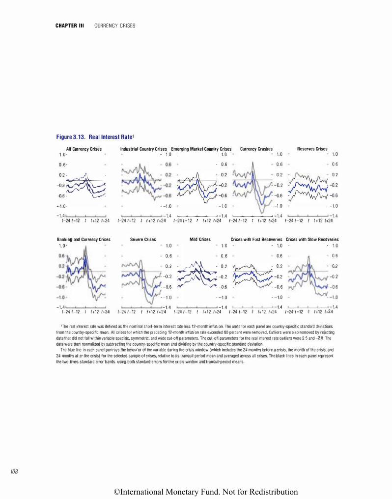
©International Monetary Fund. Not for Redistribution
108
CHAPTER Ill CURRENCY CRISES
Figure 3.13. Real Interest Ratet
All Currency Crises 1.0.
Industrial Country Crises Emerging Market Country Crises . 1.0 1.0
0.6. • 0.6
::� ��: l\-' . �-o.6 -1.0- . -1 .0 . -1.0
Currency Crashes 1.0
0.6
0.2
. -o.2
. -o.6
. -1 .0
Reserves Crises 1.0
0.6
J"vv-v... . /\ , 0.2
� -o.2
� -o.s
. -1.0
-1.4 -1.4 ......__._____.,__,___, -1.4 ....___.__,__.______, -1.4 1.4 1-24 t-12 I 1+12 t+24 1-24 t-12 t 1+12 1+24 1-24 t-12 1+12 1+24 1-24 t-12 1+12 1+24 1-24 t-12 t 1+12 1+24
Banking and Currency Crises Severe Crises Mild Crises Crises with Fast Recoveries Crises with Slow Recoveries
1.0· 1.0
0.6
1.0 • 1.0 . 1.0
0.6 0.6 •
0.2 -� 0.2 � 0.2
. -o.2 . . -o.2 �� -o.2
· -o.6 · -Q.6 · yv �- -o.6
--1.0 . -1.0
-1.4 -1.4 -1.4 1-24 1-12 I 1+12 1+24 1-24 1-12 t 1+12 lt24 1-24 1-12 t lt12 1+24 1-24 t-12
. -1.0
1.4 It 12 lt24 1-24 1-12
0.6
0.2
-o.2
-o.s
1.4 1+12 1+24
1The real interest rate was defined as the nominal short-term interest rate less 12-month inflation. The units for each panel are country-specific standard deviations
from the country-specific mean. All crises for which the preceding 12-month inflation rate exceeded 80 percent were removed. Outliers were also removed by rejecting
data that did not fall within variabte-specitic, symmetric, and wide cut-off parameters. The cut-off parameters for the real interest rate outliers were 2.5 and -2.5. The
data were then normalized by subtracting the country-specific mean and dividing by the country-specific standard deviation. The blue line in each panel portrays the behavior of the variable during the crisis window (which includes the 24 months before a crisis, the month of the crisis. and
24 months after the crisis) for the selected sample of crises, relative to its tranquil-period mean and averaged across all crises. The black lines in each panel represent
the two times standard error bands. using both standard errors for the crisis window and tranquil-period means.
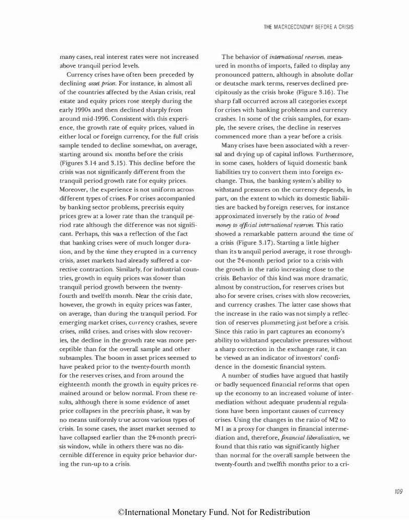
©International Monetary Fund. Not for Redistribution
many cases, real interest rates were not increased
above tranquil period levels.
Currency crises have often been preceded by
declining asset prices. For instance, in almost all
of the countries affected by the Asian crisis, real
estate and equity prices rose steeply during the
early 1990s and then declined sharply from
around mid-1996. Consistent with this experi
ence, the growth rate of equity prices, valued in
either local or foreign currency, for the full crisis
sample tended to decline somewhat, on average,
starting around six months before the crisis
(Figures 3.14 and 3.15). This decline before the
crisis was not significantly different from the
tranquil period growth rate for equity prices.
Moreover, the experience is not uniform across
different types of crises. For crises accompanied
by banking sector problems, precrisis equity
prices grew at a lower rate than the tranquil pe
riod rate although the difference was not signifi
cant. Perhaps, this was a reflection of the fact
that banking crises were of much longer dura
tion, and by the time they erupted in a cunency
crisis, asset markets had already suffered a cor
rective contraction. Similarly, for industrial coun
tries, growth in equity prices was slower tl1an
tranquil period growth between the twenty
fourth and twelfth month. Near the crisis date,
however, the growth in equity prices was faster,
on average, than during the tranquil period. For
emerging market crises, currency crashes, severe
crises, mild crises, and crises with slow recover
ies, me decline in the growth rate was more per
ceptible man for me overaJJ sample and other
subsamples. The boom in asset prices seemed to
have peaked prior to tl1e twenty-fourth monm
for the reserves crises, and from around the
eighteenm month the growth in equity prices re
mained around or below normal. From these re
sults, almough tl1ere is some evidence of asset
price collapses in the precrisis phase, it was by
no means uniformly true across various types of
crisis. In some cases, the asset market seemed to
have collapsed earlier than the 24-month precri
sis window, while in others there was no dis
cernible difference in equity price behavior dur
ing the run-up to a crisis.
THE MACROECONOMY BEFORE A CRISIS
The behavior of international reserves, meas
ured in months of imports, failed to display any
pronounced pattern, although in absolute dollar
or deutsche mark terms, reserves declined pre
cipitously as the crisis broke (Figure 3.16). The
sharp fall occurred across all categories except
for crises with banking problems and currency
crashes. ln some of the crisis samples, for exam
ple, the severe crises, the decline in reserves
commenced more than a year before a crisis.
Many crises have been associated wim a rever
sal and d1·ying up of capital inflows. Furthermore,
in some cases, holders of Uquid domestic bank
liabilities try to convert them into foreign ex
change. Thus, the banking system's ability to
wimstand pressures on the currency depends, in
part, on the extent to which its domestic liabili
ties are backed by foreign reserves, for instance
approximated inversely by the ratio of broad
money to official international reserves. This ratio
showed a remarkable pattern around the time of
a crisis (Figure 3.17). Starting a little higher
than its u·anquil period average, it rose through
out me 24-month period prior to a crisis with
the growth in the ratio increasing close to the
crisis. Behavior of mis kind was more dramatic,
almost by construction, for reserves crises but
also for severe crises, crises with slow recoveries,
and currency crashes. The latter case shows that
th.e increase in the ratio was not simply a reflec
tion of reserves plumrneting just before a crisis.
Since this ratio in part captures an economy's
ability to witl1stand speculative pressures without
a sharp correction in me exchange rate, it can
be viewed as an indicator of investors' confi
dence in the domestic financial system.
A number of studies have argued that hastily
or badly sequenced financial reforms that open
up the economy to an increased volume of inter
mediation without adequate prudential regula
tions have been important causes of currency
crises. Using the changes in the ratio of M2 to
M l as a proxy for changes in frnancial interme
diation and, therefore, financial liberalization, we
found that this ratio was significantly higher
man normal for the overall sample between the
twenty-fourtl1 and twelfm monms prior to a cri-
109
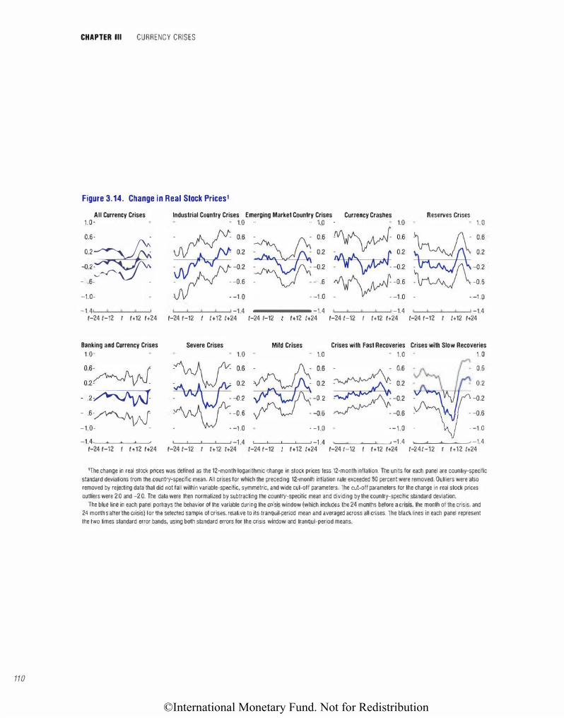
©International Monetary Fund. Not for Redistribution
110
CHAPTER Ill CURRENCY CRISES
Figure 3.14. Change in Real Stock Prices1
All Currency Crises 1.0·
�:� -o.6· .
-1.0·
Industrial Country Crises Emerging Market Country Crises Currency Crashes Reserves Crises 1.0 1.0 1.0 1.0
?:: � � :: �:: N :: Y
-o.2 � -o.2 _, \f0_--o.2 ��
(\\-o.2
. . -o.6 . v . -o.6 N\.A. A J\r. -o.6 . \JwvJ \ -o.6 -�� - �� . w �v·· - �� - � �
-1.4 -1.4 '--'---'--'-----'-1.4 -1.4 -1.4 1-24 t-12 I 1+12 1+24 1-24 t-12 I 1+12 1+24 1-24 t-12 1+12 1+24 1-24 t-12 I 1+12 1+24 1-24 t-12 I 1+12 1+24
Banking and Currency Crises
1.0·
o.s- .A.. {\ _ • r o.2.!' ... � V\J.
-o.2�
-o.6�
-1.0· .
-1.4'---'---'----'---' 1-24 1-12 r 1+12 1+24
Severe Crises Mild Crises Crises with Fast Recoveries Crises with Slow Recoveries
1.0 1.0 1.0 1 .0
�:: ��:·: • . A - -A 'vvJ � -Q.2 . -Q.2 A 11. A w f'v. -o.s . -o.6 . v � � - �� - �� ,_.....___. _ _._____, -1.4 ,_.....___. _ _._____, -1.4
1-24 t-12 I 1+12 lt24 1-24 t-12 1+12 1+24
0 6
� 0 2
�� -02
� v: -os
·-1.0
'---'---'---'--....) -1.4 1-24 1-12 r 1+12 1+24
0.6
0.2
�\;!/(�:: . '\) · -1.0
.__.__,__.___, -1.4 1-241-12 r 1+12 1+24
'The change in real stock pnces was defined as the 12·month logarithmic change in stock prices less 12·month inflation. The units for each panel are country-specific
standard deviations from the country-specific mean. All crises for which the preceding 12·monlh inflation rate exceeded 80 percent were removed. Outliers were also removed by rejecting data that did not fall within variable-specific. symmetric. and wide cut·off parameters. The cut·off parameters for the change in real stock prices
outliers were 2.0 and -2.0. The data were then normalized by subtracting the country-specific mean and dividing by the country-specific standard deviation. The blue line in each panel portrays the behavior of the variable during the crisis window (which includes the 24 months before a crisis. the month of the crisis. and
24 months alter the crisis) lor the selected sample of crises. relative to its tranquil-period mean and averaged across all crises. The black lines in each panel represent the two times standard error bands. using both standard errors for the crisis window and tranquil-period means.
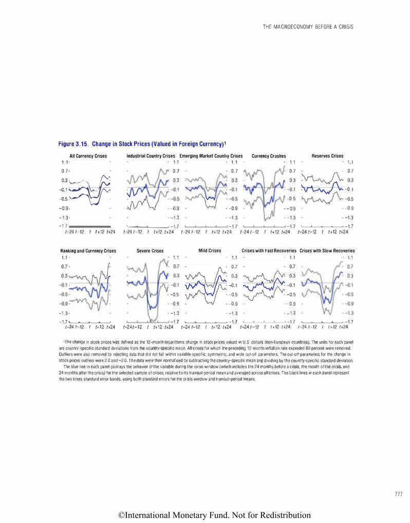
©International Monetary Fund. Not for Redistribution
THE MACROECONOMY BEFORE A CRISIS
Figure 3.15. Change in Stock Prices (Valued in Foreign Currency)1
All Currency Crises 1.1• 0.7.
�:� -o.9·
-1.3-
-1.7 '----'----'--'-----'
1-24 1-12 tt12 1+24
Banking and Currency Crises
1.1 -
�::��N
�:�
Industrial Country Crises Emerging Market Country Crises Currency Crashes • 1.1 • 1.1 1.i
- 0.7 - . 0.7 • 0.7
0.3 - - 0 3 - 0 3
yv ·11'-./fV_ -os :-..��Ufv'. _os - - -o s JVY v - -o.9 . � w - -o.9 . --o9
Reserves Crises 1.1
• . 0.7 � 0.3 V'\AJ\.Yl"' -o.1
� -o.s
- -o.9
- -1.3 - -1 3 . · -1.3 · -1.3 .___.__..__..____, -1.7 -1.7 -1.7 '---'----'--.1...---' -1.7
1-24 1-12 1+12 1+24 1-24 1-12 tt12 1+24 1-24 1-12 lt12 1+24 1-24 1-12 1+12 1+24
Severe Crises
1.1
Mild Crises Crises with Fast Recoveries Crises with Slow Recoveries . 1.1 - 1.1 1.1
'-""�:A�-h,.-1: iA�k 1i �1: · -o.s -o.s � -o.s
- -o.9 - . -o 9 - - -o 9
0.7
0.3
-1 .3 · • -1.3 - -1.3 • -1.3
-1.7 '---'--'---'---' '---'--l..L.='-'----' -1 .7 '---'----'--'---' -1.7 1.7 .___.____,__..____, -1.7 1-24 1-12 1+12 1+24 1-241-12 1+12 1+24 1-24 1-12 1+12 t+24 1-24 1-12 1+12 1+24 1-24 1-12 1+12 lt24
1The change in stock prices was delined as the 12-month logarithmic change in stock prices valued in U.S. dollars {non-European countries). The units for each panel
are country-specific standard deviations from the country-specific mean. All crises for which the preceding 12-month inflation rate exceeded 80 percent were removed.
Outliers were also removed by rejecting data that did not fall within variable-specific, symmetric, and wide cut-off parameters. The cut-off parameters for the change In
stock prices outliers were 2.0 and -2.0. The data were then normalized by subtracting the country·spetific mean and dividing by the country-specific standard deviation.
The blue line in each panel portrays the behavior of the variable during the crisis window {which includes the 24 months before a crisis, the month of the crisis, and
24 months after the crisis) for the selected sample of crises, relative to its tranquil-period mean and averaged across all crises. The black lines in each panel represent
the two times standard error bands, using both standard errors for the crisis window and tranquil-period means.
111
©International Monetary Fund. Not for Redistribution
112
CHAPTER Ill CURRENCY CRISES
Figure 3.16. Change in Foreign Reserves,
All Currency Crises 1.0 .
Industrial Country Crises Emerging Marl!et Country Crises Currency Crashes
�:� -o.6ry : -1.0. -
1.0 1 .0 1.0
0.6
0.2
0.6
0.2
0.6
0 2
--1.0 - -1.0
Reserves Crises 1.0
0.6
0.2
-1.4 '----'----'--.L....-' 1.4 1.4 '--....L..----'---'----' -1.4 '----'----'--...___--' -1.4 1-24 1-12 I 1+12 1+24 1-24 1-12 1+12 1+24 1-24 1-12 1+12 1+24 1-24 1-12 1+12 1+24 1-24 1-12 1+12 1+24
Banking and Currency Crises
1.0 •
Severe Crises Mild Crises Crises with Fast Recoveries Crises with Slow Recoveries
1.0
0.6
0.2
1.0
0.6
0.2
1.0
0.6
0.2
1.0
0.6
0.2
. -o.2
. -o.6
. -1.0
. -o.2
. -o.6
• -1.0 . -1.0
-1.4 -1.4 .._____.._____,_--'----' -1.4 -1.4 1-24 1-12 I 1+12 1+24 1-24 1-12 I 1+12 1+24 1-24 1-12 1+12 1+24 1-24 1-12 I 1+12 1+24 t-24 1-12
. -1.0
1.4 1+12 1+24
1The change in foreign reserves was defined as the 12-month logarithmic change in reserves valued in U.S. dollars (non-European countries) or deutsche mark (European countries). The units for each panel are country-specific standard deviations from the country-specific mean. All crises for which the preceding 12-month Inflation rate exceeded 80 percent were removed. Outliers were also removed by rejecting data that did not fall within variable-specific. symmetric, and wide cut·oH parameters. The cut-off parameters for the change in foreign reserves outliers were 1.5 and -1.5. The data were then normalized by subtracting the country-specific
mean and dividing by the country-specific standard deviation.
The blue line in each panel portrays the behavior ot the variable during the crisis window (which Includes the 24 months before a crisis, the month of the crisis, and
24 months alter the crisis) for the selected sample of crises, relative to its tranquil-period mean and averaged across all crises. The black lines in each panel represent
the IWo times standard error bands, using both standard errors tor the crisis window and tranquil-period means.
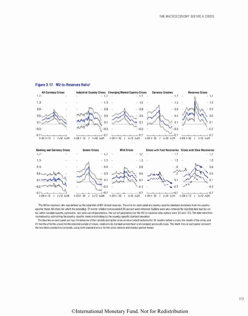
©International Monetary Fund. Not for Redistribution
THE MACROECONOMY BEFORE A CRISIS
Figure 3.17. M2-to-Reserves Ratio1
All Currency Crises 1 . 7 .
1 . 3 -
Industrial Country Crises Emerging Marlcet Country Crises Currency Crashes 1.7 1.7
1.3 1.3
1.7
1.3
0.9
0.5
0.1
Reserves Crises 1.7
1.3
0.9
0.5
0.1
--o.3
-o.7 -o.7 -o.7 -o.7 -o.7 1-24 t-1 2 I 1+12 1+24 1-24 1-12 t 1+12 1+24 1-24 1-12 I 1+12 1+24 1-24 1-12 I 1+12 1+24 1-24 1-12 I 1+12 1+24
Banking and Currency Crises
1.7'
1.3-
0.9-
0.5� 0.1 �
-o.3 �� -o.7 '-�--'--'---'----'
1-24 1-12 I 1+12 1+24
Severe Crises
1.7
1.3
0.9
0.5
0.1
--o.3
'---'--'---'---' -o. 7 1-241-12 I 1+12 1+24
Mild Crises Crises with Fast Recoveries Crises with Slow Recoveries
1.7 1.7 - 1.7
1.3 1.3 - 1.3
�:::: ��:: ·�: :.: � 0.1 0.1 - - 0.1
- . -o.3 - - -o.3 - -o 3
.___.___.__..___, -o. 7 -o.7 -o. 7 1-24 1-12 I 1+12 1+24 1-24 1-12 I 1+12 1+24 1-24 1-1 2 I 1+12 1+24
'The M2-to-reserves ratio was defined as the logarithm of M2 divided reserves. The units for each panel are country-specific standard deviations from the countryspecific mean. All crises for which the preceding t2-month inflation rate exceeded SO percent were removed. Outliers were also removed by rejecting data that did not fall within variable-specific, symmetric. and wide cut-off parameters. The cut·off parameters for the M2·to-reserves ratio outliers were 5.0 and -5.0. The data were then normalized by subtracting the country-specific mean and dividing by the country-specific standard deviation.
The blue line in each panel portrays the behavior of the variable during the crisis window (which includes the 24 months before a crisis, the month of the crisis, and 24 months after the crisis) for the selected sample of crises. relative to its tranquil-period mean and averaged across all crises. The black lines in each panel represent the two times standard error bands, using both standard errors for the crisis window and tranquil-period means.
113
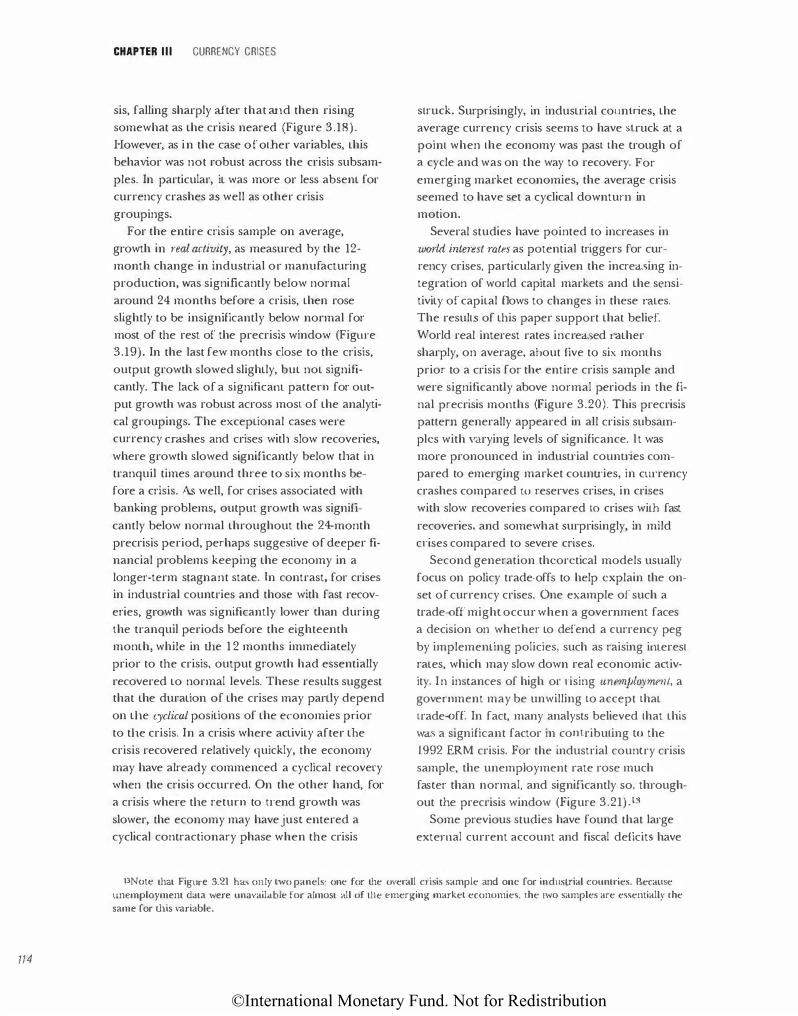
©International Monetary Fund. Not for Redistribution
114
CHAPTER Ill CURRENCY CRISES
sis, falling sharply after that and then rising
somewhat as the crisis neared (Figure 3.18).
However, as in the case of other variables, this
behavior was not robust across the crisis subsam
ples. In particular, it was more or less absent for
currency crashes as well as other crisis
groupings.
For the entire crisis sample on average,
growth in teal activit)', as measured by the 12-
month change in industrial or manufacturing
production, v.ras significantly below normal
around 24 months before a crisis, then rose
slightly to be insignificantly below normal for
most of the rest of the precrisis window (Figw·e
3.19). In the last few months close to the crisis,
output growth slowed slightly, but not signifi
cantly. The lack of a significant pattern for out
put growth was robust across most of the analyti
cal groupings. The exceptional cases were
currency crashes and crises witl1 slow recoveries,
where growth slowed significantly below tl1at in tranquil times around three to six months be
fore a crisis. As well, for crises associated with
banking problems, output growth was signifi
cantly below normal throughout the 24-month
precrisis period, perhaps suggestive of deeper fi
nancial problems keeping the economy in a
longer-term stagnant state. in contrast, for crises
in industrial countries and those with fast recov
eries, growth was significantly lower than during
the tranquiJ periods before the eighteenth
month, while in the 1 2 months immediately
prior to the crisis, output growth had essentially
recovered to normal levels. These results suggest that the duration of the crises may partly depend
on tile �yclical positions of the economies pdor
to tile crisis. In a crisis where activity after tJ1e
crisis recovered relatively quickly, the economy
may have already commenced a cyclical recovery
when the crisis occurred. On the other hand, for
a crisis where tile return to u·end growth was
slower, the economy may have just entered a
cyclicaJ contractionary phase when the crisis
struck. Surpdsingly, in industriaJ counuies, the
average currency crisis seems to have Slruck at a
point when the economy was past the trough of
a cycle and was on the way to recovery. For
emerging market economies, the average crisis
seemed to have set a cyclical downturn in
motion.
Several studies have pointed to increases in
world interest mtes as potential triggers for cur
rency crises, particularly given the increasing in
tegration of world capital markets and the sensi
tivity of capital flows to changes in these rates.
The results of this paper support that belief.
World real interest rates increased rather
sharply, on average, about five to six months
prior to a crisis for the entire crisis sample and
were significantly above normal periods in the fi
nal precrisis months (Figure 3.20). This pre crisis
pattern generally appeared in all crisis subsam
ples with varying levels of significance. lt was
more pronounced in indusu·ial counuies com
pared to emerging market countries, in ctu-rency
crashes compared to reserves crises, in crises
with slow recoveries compared LO crises witJ1 fast
recoveries, and somewhat surprisingly, in mild
c•·ises compared to severe crises.
Second generation theoretical models usua!Jy
focus on poljcy trade-offs to help explain the on
set of currency crises. One example of such a
trade-off might occur when a government faces
a decision on whether to defend a currency peg
by implementing policies, such as raising interest
rates, which may slow down real economic activ
ity. In instances of high or •·ising ·unemplo)'menl, a
government may be unwilling to accept that
trade-off. In fact, many analysts believed that this
was a significant factor in comributing to the
1992 ERM crisis. For the industrial country crisis
sample, the unemployment rate rose much
faster than normal, and significantly so, thTough
out tl1e precrisis window (Figure 3.21) .L!l
Some previous studies have found that laTge
external current account and fiscal deficitS have
13Note that Figu•·e 3.21 has only two panels: one for the overall c•-isis sample and one for industrial countries. Because unemployment data were unavailable for almost all of 1J1e emerging market economies, the two samples are essentially the same for this variable.
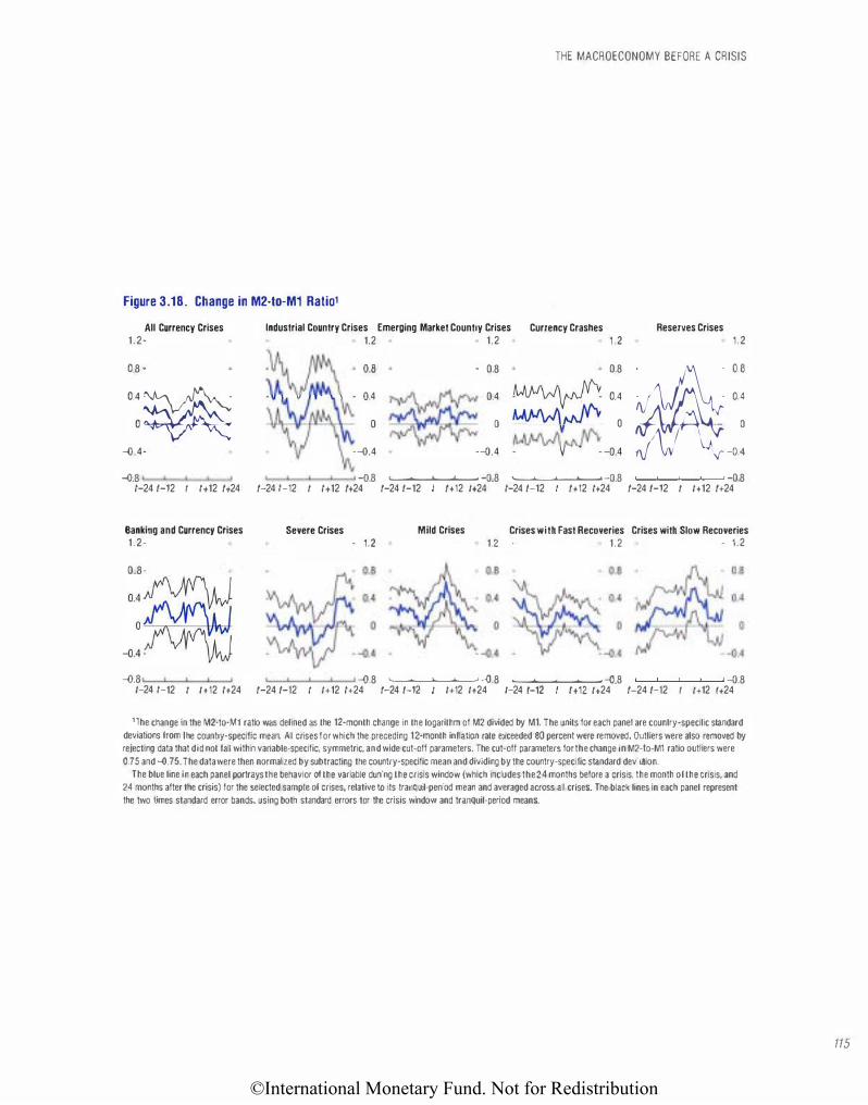
©International Monetary Fund. Not for Redistribution
Figure 3.18. Change in M2·to·M1 Ratiot
All Currency Crises 1.2.
08 .
0.4�
0� --{).4.
Industrial Country Crises
� . .
1.2
0.8
0.4
0
---{).4
THE MACROECONOMY BEFORE A CRISIS
Emerging Market Country Crises Currency Crashes Reserves Crises 1.2 1.2 1 .2
• 0.8 0.8
Mt�·� � 0.4 � 0.4
0 UJ.!'v/\� 0
� ---{).4 • ---{).4
--{).8 --{).8 ,__.....__..._.....__,--{),8 ,__.....__..._..____,--{),8 -0.8 1-24 t-12 I 1+12 1+24 1-24 t-12 I 1+12 1+24 1-24 t-12 1+12 1+24 1-24 t-12 1+12 1+24 1-24 t-12 I 1+12 1+24
Banking and Currency Crises 1.2-
0.8-
,,� --{).:�
Severe Crises Mild Crises • 1.2
Crises with Fast Recoveries Crises with Slow Recoveries 1.2 1.2 - 1.2
--{).8 -().8 .__.....__..._.....___, _0.8 .__.....__...._..____,-()_8 --{).8 1-24 t-12 I 1+12 1+24 1-24 t-12 I 1+12 1+24 1-24 t-12 1+12 1+24 1-24 t-12 lt12 lt24 1-24 t-12 I lt12 lt24
'The change in the M2-to·M1 ratio was defined as the 12-month change in the logarithm of M2 divided by M1. The units for each panel are counlry-specilic slandard
deviations from I he country-specific mean. All crises for which the preceding 12-month inflation rate exceeded 80 percent were removed. Outliers were also removed by rejecting data that did not fall within variable-specific. symmetric, and wide cut-off parameters. The cut-off parameters for the change in M2-to-M1 ratio outliers were
0.75 and --{).75. The data were then normalized by subtracting the country-specific mean and dividing by the country-specific standard deviation.
The blue line in each panel portrays the behavior of the variable during the crisis window (which includes the 24 months before a crisis, the month of the crisis, and 24 months after the crisis) for the selected sample of crises, relative to its tranquil-period mean and averaged across all crises. The black lines in each panel represent
the two times standard error bands, using both standard errors tor the crisis window and tranquil-period means.
115
©International Monetary Fund. Not for Redistribution
116
CHAPTER Ill CURRENCY CRISES
Figure 3.19. Output Growtht
All Currency Crises
1.1 •
Industrial Country Crises Emerging Martcet Country Crises Currency Crashes Reserves Crises
0.7. �:�� -Q.S�v-: -Q.9·
1.1 • 1.1
0.7 . 0.7 � 0.3 � 0.3
��: ���:
1 . 1
0.7
0.3
-Q.1
1.1
0.7 �.� 0.3 ��-Q.1 �-Q.S
·-Q.9
� � 1� 1� �� 1 � 1-24 t-12 I 1+12 1+24 1-24 t-12 I 1+12 1+24 1-24 t-12 I 1+12 1+24 1-24 t-12 I 1+12 1+24 1-24 t-12 I 1+12 1+24
Banking and Currency Crises
1 . 1 ·
Severe Crises
• 1.1
Mild Crises Crises with Fast Recoveries Crises with Slow Recoveries
1.1 . 1.1 • 1.1
-1.3 -1.3 -1.3 -1.3 1.3 1-24 t-12 I 1+12 1+24 1-24 t-12 I 1+12 1+24 1-24 t-12 I 1+12 1+24 1-24 t-12 I 1+12 1+24 1-24 t-12 I 1+12 1+24
'Output growth was defined as the 12·month logarithmic growth in industrial or manufacturing output. The units for each panel are country-specific standard deviations from the country-specific mean. All crises for which the preceding 12·month inflation rate exceeded 80 percent were removed. Outliers were also removed by
rejecting data that did not fall within variable-specific, symmetric, and wide cut·off parameters. The cut·off parameters for the output growth outliers were 0.5 and -{).5. The data were then normalized by subtracting the country-specific mean and dividing by the country-specific standard deviation.
The blue line in each panel portrays the behavior of the variable during the crisis window (which includes the 24 months before a crisis, the month of the crisis, and 24 months after the crisis) for the selected sample of crises, relative to its tranquil-period mean and averaged across all crises. The black lines in each panel represent the two limes standard error bands. using both standard errors for the crisis window and tranquii·period means.
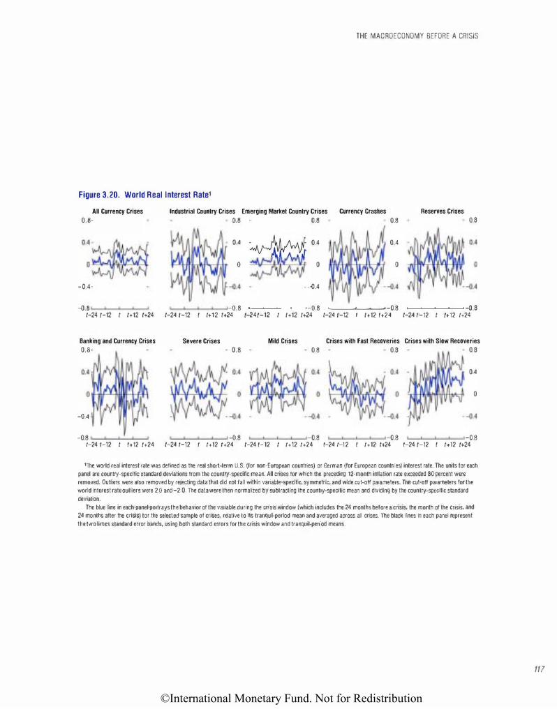
©International Monetary Fund. Not for Redistribution
THE MACROECONOMY BEFORE A CRISIS
Figure 3.20. World Real Interest Rate1
All Currency Crises
0.8.
Industrial Country Crises Emerging Market Country Crises Currency Crashes Reserves Crises
�8 �8 0.8 0.8
0.4 � 0.4 0.4
0 � 0 0
-o.4. - -o.4
-0.8 -o.8 -o.8 .___.___.__.__-J-o.8 -o.8 1-24 t-12 I 1+12 lt24 1-24 t-12 I 1+12 lt24 1-241-12 I 1+12 1+24 1-24 t-12 1+12 1+24 1-24 t-12 I 1+12 lt24
Banking and Currency Crises Severe Crises Mild Crises Crises with Fast Recoveries Crises with Slow Recoveries
0.8. 0.8 0.8 0.8 0.8
0.4
0
-Q.4
-o.8 o.8 -o.8 -o.8 -o.8 1-24 t-12 I 1+12 lt24 1-24 t-12 I lt12 lt24 1-24 1-12 I lt12 lt24 1-24 1-12 I lt12 1+24 1-24 t-12 I lt12 lt24
'The world real interest rate was defined as the real short-term U.S. (for non-European countries) or German (for European countries) interest rate. The units tor each
panel are country-specific standard deviations from the country-specific mean. All crises for which the preceding 12-month inflation rate exceeded 80 percent were
removed. Outliers were also removed by rejecting data that did not fall within variable-specific, symmetric, and wide cut-oH parameters. The cut-oH parameters for the
world Interest rate outliers were 2.0 and -2.0. The data were then normalized by subtracting the country-specific mean and dividing by the country-specific standard
deviation.
The blue line in each panel portrays the behavior of the variable during the crisis window (which includes the 24 months before a crisis. the month of the crisis, and
24 months after the crisis) tor the selected sample of crises. relative to Its tranquil-period mean and averaged across all crises. The black lines In each panel represent
the two limes standard error bands, using both standard errors for the crisis window and tranquil-period means.
111
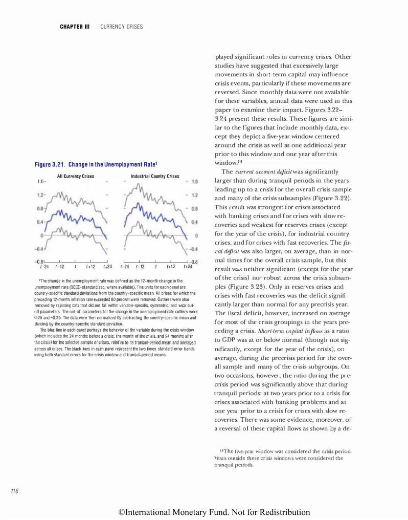
©International Monetary Fund. Not for Redistribution
118
CHAPTER Ill CURRENCY CRISES
Figure 3.21 . Change in the Unemployment Rate1
All Currency Crises Industrial Country Crises 1.6-
-o.a<---"'----'-_.....__ _ _, L---'---L---'----' -o.a /-24 t-12 1+12 1+24 /-24 t-12 /+12 /+24
'The change in the unemployment rate was defined as the 12·month change in the unemployment rate (OECD·standardized. where available). The units for each panel are country·specific standard deviations from the country·specific mean. All crises for which the
preceding 12·month inflation rate exceeded 80 percent were removed. Outliers were also removed by rejecting data that did not fall within variable·specific, symmetric. and wide cut· off parameters. The cut·off parameters for the change in the unemployment rate outliers were 0.25 and -o.25. The data were then normalized by subtracting the country-specific mean and dividing by the country-specific standard deviation.
The blue line in each panel portrays the behavior of the variable during the crisis window (which includes the 24 months before a crisis. the month of the crisis, and 24 months after
the crisis) for the selected sample of crises, relative to its tranquil-period mean and averaged across all crises. The black lines in each panel represent the two times standard error bands. using both standard errors for the crisis window and tranquil-period means.
played significant roles Ln currency crises. Other
studies have suggested that excessively large
movements in short-term capital may influence
crisis events, particularly if these movements are
reversed. Since monthly da ta were not available
for these variables, annual data were used in this
paper to examine their impact. Figures 3.22-3.24 present these results. These figures are simi
lar to the figures that include monthly data, ex
cept they depict a five-year window centered
around the crisis as well as one additional year
prior to this window and one year after this
window.14
The current account dejicit was significantly
larger than during tranquil periods in the years
leading up to a crisis for the overall crisis sample
and many of the cri.sis subsamples (Figure 3.22).
This result was strongest for crises associated
with banking crises and for crises with slow re
coveries and weakest for reserves crises (except
for the year of the crisis), for industrial country
crises, and for crises with fast recoveries. The fis
cal deficit was also larger, on average, than in nor
mal times for the overall c1·isis sample, but this
result was neither significant (except for the year
of the crisis) nor robust across the crisis subsam
ples (Figure 3.23). Only Ln reserves crises and
crises with fast recoveries was the deficit signifi
cantly larger than normal for any precrisis year.
The fiscal deficit, however, increased on average
for most of the crisis groupings in the years pre
ceding a crisis. Shart-term capital inflows as a ratio
to GDP was at or below normal (though not sig
nificantly, except for tl1e year of the crisis), on
average, during the precrisis pe1iod for the over
all sample and many of the crisis subgroups. On
two occasions, howeve•·, the ratio during the precrisis period was significantly above that during
tranquil periods: at two years prior to a crisis for
crises associated with banking problems and at
one year prior to a crisis for crises with slow re
coveries. There was some evidence, moreover, of
a reversal of tl1ese capital Oows as shown by a de-
14The five-year window was considered the crisis period. Years outside these crisis windows were considered the tranquil pe•·iods.
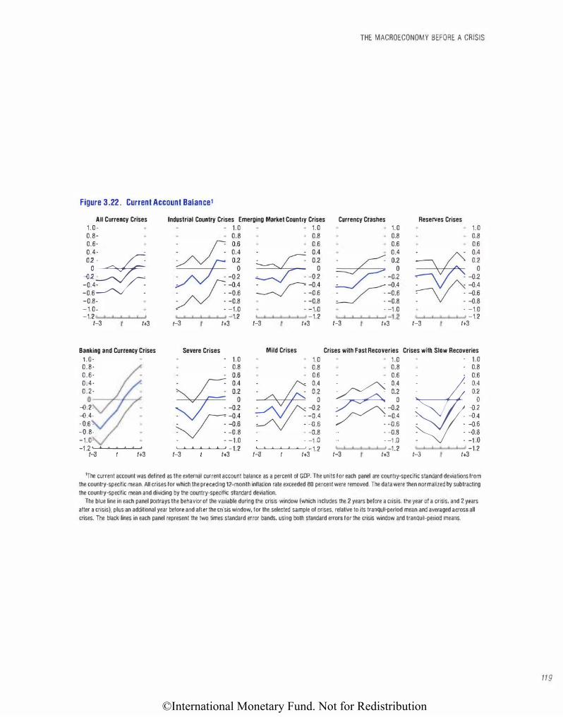
©International Monetary Fund. Not for Redistribution
THE MACROECONOMY BEFORE A CRISIS
Figure 3.22. Current Account Balance1
All Currency Crises Industrial Country Crises Emerging Market Country Crises Currency Crashes Reserves Crises 1.0· 0.8. 0.6. 0.4. -
�:� -Q.4. . -o.6 .
-o.8. -1.0· -1.2
1-3 1+3
Banking and Currency Crises 1.0· 0.8. 0.6. 0.4. 0.2.
0 ----;>'�-...,,L -o.2. -D.4. -o.6 . -o.8. -1.0· -1.2 L.......I._J__J_.L......J.-1
1-\3 1+3
1.0 0.8
� 0.6 0.4
� '' -o.�
��· -o.6 -o.8 -1.0
t-3
Severe Crises
-1.2 1+3
. 1.0
. 0.8
�L �:�
0=�l -:-y . -o.8 - . -1.0 L......l--'--'--'-.J.......J -1.2
1-3 1+3
1.0 1.0 1.0 0.8 0.8 0.8 0.6 0.6 0.6
� :l 0.4 � OA 7 ': 0.2
��! -o.2 -o.2
� -Q.4 � -o.4
1-3
-o.6 -o.6 . -o.8 -o.8 . -1.0 . -1 .0 - -1.0
-1.2 1.2 -1.2 1+3 1-3 1+3 1-3 1+3
Mild Crises Crises with Fast Recoveries Crises wllh Slow Recoveries
1.0 1.0 . 1.0 0.8 0.8 . 0.8 0.6 0.6 �- . 0.6
W� �i B00��i �· j -0.4 . . -o.4 . . -o.4
. . -o.s - -o.s . . -o.s . . -0.8 . -o.8 · · -o.s
- � n - � n . - �n L......l--'--'--'-.J.......J -1.2 1.2 -1.2
1-\3 1+3 1-\3 1+3 1-3 1+3
1The current account was defined as the external current account balance as a percent of GOP. The units for each panel are country-specific standard deviations from the country-specific mean. All crises for which the preceding 12·month inflation rate exceeded 80 percent were removed. The data were then normalized by subtracting
the country-specific mean and dividing by the country-specific standard deviation.
The blue line in each panel portrays the behavior of the variable during the crisis window (which includes the 2 years before a crisis, the year of a crisis, and 2 years
after a crisis). plus an additional year before and after the crisis window, tor the selected sample of crises, relative to its tranqull·perlod mean and averaged across all
crises. The black lines in each panel represent the two times standard error bands, using both standard errors for the crisis window and tranquil-period means.
119
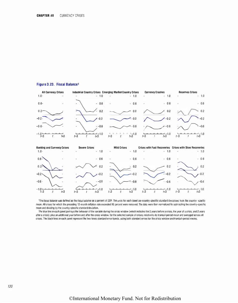
©International Monetary Fund. Not for Redistribution
120
CHAPTER Ill CURRENCY CRISES
Figure 3.23. Fiscal 8alance1
All Currency Crises Industrial Country Crises Emerging Maltet Country Crises Currency Crashes
1.0·
0.6·
0.2�0�
-o.2 �
-o.6�
-1 .0 L-J.-'--'-J.......L--' 1-3 lt3
Banking and Currency Crises 1.0·
0 6� 0.2. .
� 2� -o.s - .
-1.0 1-3 1+3
1.0
�:: . -o.2
� -o.6
t.-1.--'--'--J........I.--' -1.0 1-3 lt3
Severe Crises 1.0
0.6
� 0.2
/--JV -G.2
. . -o.s
� -1.0 1-3 I 1+3
1.0
0.6
� 0.2
�-o.2
� - o.6
1-3
Mild Crises
1.0 lt3
1.0
0.6 � 0.2
-o.2
� -o.s
1-3 -1.0 lt3
1.0
0.6
� 0.2
� -o.2
� -o.6
.._.___._........._...___.__, -1.0 1-3 lt3
Crises with Fast Recoveries 1.0
0.6
� r- 0.2 ........., �-o.2
�-o.s 1-3 1+3 1.0
Reserves Crises 1.0
0.6
� ;---- 0.2
� -o.2
� -o.6
.._.___._........._...___.__, -1.0 1-3 1+3
Crises with Slow Recoveries 1.0
0.6 � 0 2
-o.2
�-o.s -1.0 1-3 1+3
1The fiscal balance was defined as the fiscal balance as a percent of GOP. The units lor each panel are country-specific standard deviations from the country·specific
mean. All crises for which the preceding 12-month Inflation rate exceeded 80 percent were removed. The data were then norma.lized by subtracting the country-specific mean and dividing by the country-specific standard deviation.
The blue line in each panel portrays the behavior of the variable during the crisis window (which Includes the 2 years before a crisis. the year of a crisis, and 2 years after a crisis). plus an additional year before and after the crisis window. for the selected sample of crises. relative to its tranquil-period mean and averaged across all crises. The black lines in each panel represent the two limes standard error bands. using both standard errors tor the crisis window and tranquil-period means.
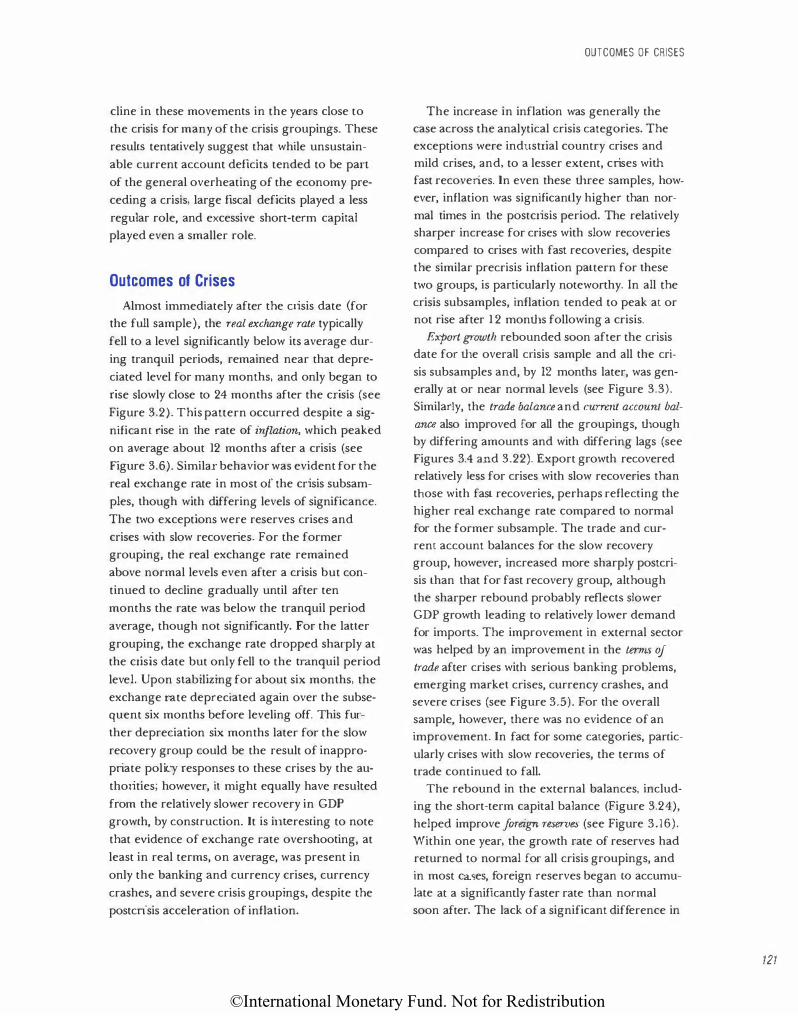
©International Monetary Fund. Not for Redistribution
cline in these movements in the years close to
the crisis for many of the crisis groupings. These
results tentatively suggest that while unsustain
able current account deficits tended to be pan
of the general overheating of the economy pre
ceding a crisis, large fiscal deficits played a less
regular role, and excessive short-term capital
played even a smaller role.
Outcomes of Crises
Almost immediately after the crisis date (for
the full sample), the real exchange rate typically
fell to a level significantly below its average dur
ing tranquil periods, remained near that depre
ciated level for many months, and only began to
rise slowly close to 24 months after the crisis (see
Figure 3.2). This pattern occurred despite a sig
nificant rise in the rate of inflation, which peaked
on average about 12 months after a crisis (see
Figure 3.6). Similar behavior was evident for the
real exchange rate in most of the crisis subsam
ples, though with differing levels of significance.
The two exceptions were reserves crises and
crises with slow recoveries. For the former
grouping, the real exchange rate remained
above normal levels even after a crisis but con
tinued to decline gradually until after ten
months the rate was below the tranquil period
average, though not significantly. For the latter
grouping, the exchange rate dropped sharply at
the crisis date but only fell to the tranquil period
level. Upon stabilizing for about six months, the
exchange rate depreciated again over the subse
quent six months before leveling off. This fur
ther depreciation six months later for the slow
recovery group could be the result of inappro
priate policy responses to these crises by the au
thorities; however, it might equally have resulted
from the relatively slower recovery in GDP
growth, by construction. It is interesting to note
that evidence of exchange rate overshooting, at
least in real terms, on average, was present in
only the banking and currency crises, currency
crashes, and severe crisis groupings, despite the
postcrisis acceleration of inflation.
OUTCOMES OF CRISES
The increase in inflation was generally the
case across the analytical crisis categories. The
exceptions were industrial country crises and
mild crises, and, to a lesser extent, crises with
fast recoveries. In even these three samples, how
ever, inflation was significantly higher than nor
mal times in the postcrisis period. The relatively
sharper increase for crises with slow recoveries
compared to crises with fast recoveries, despite
the similar precrisis inflation pattern for these
two groups, is particularly noteworthy. In all the
crisis subsamples, inflation tended to peak at or
not rise after 1 2 months following a crisis.
Export growth rebounded soon after the crisis
date for the overall crisis sample and all the cri
sis subsamples and, by 12 months later, was gen
erally at or near normal levels (see Figure 3.3).
Similarly, the trade balance and curnmt account bal
ance also improved for all the groupings, though
by differing amounts and with differing lags (see
Figures 3.4 and 3.22). Export growth recovered
relatively less for crises with slow recoveries than
those with fast recoveries, perhaps reflecting the
higher real exchange rate compared to normal
for the former subsample. The trade and cur
rent account balances for the slow recovery
group, however, increased more sharply postcri
sis than that for fast recovery group, although
the sharper rebound probably reflects slower
GDP growth leading to relatively lower demand
for imports. The improvement in external sector
was helped by an improvement in the tenns of
trade after crises with serious banking problems,
emerging market crises, currency crashes, and
severe crises (see Figure 3.5). For tl1e overall
sample, however, there was no evidence of an
improvement. ln fact for some categories, partic
ularly crises with slow recoveries, the terms of
trade continued to fall.
The rebound in the external balances, includ
ing the short-term capital balance (Figure 3.24),
helped improve foreign 1-eserves (see Figure 3.16).
Within one year, the growth rate of reserves had
returned to normal for all crisis groupings, and
in most cases, foreign reserves began to accumu
late at a significantly faster rate than normal
soon after. The lack of a significant difference in
121
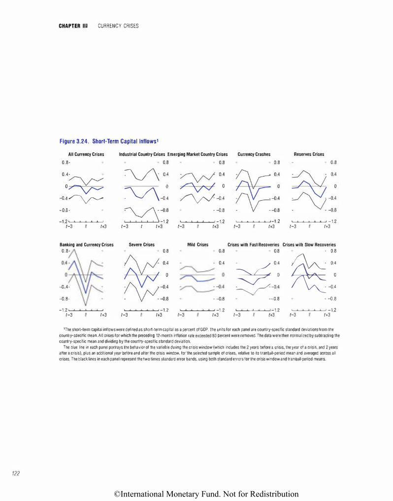
©International Monetary Fund. Not for Redistribution
122
CHAPTER Ill CURRENCY CRISES
Figure 3.24. Short-Term Capital lnflows1
All Currency Crises
0.8. Industrial Country Crises Emerging Market Country Crises Currency Crashes Reserves Crises
0.4. 0�
7 v-v--�.4�
-{).8.
-1.2 L.......I.....L...J.......L....J.......J 1-3 1+3
Banking and Currency Crises
0.8.
�.4-
�.8-
-1 .2 L.......I--L-'-...L....J.......J 1-3 1+3
0.8 0.8 � 0.4
��.:
� 0.4 _,.-"\ - / 0 7\/V ��.4
��8 I..�...L.....I......L......l--L....J -1 .2
- �.8 L......l....J..-'--'---'--' -1.2
1-3 I 1+3 1-3 1+3
Severe Crises Mild Crises
0.8 0.8
- �.8
�;J 04
�::
0.4
....._._,__._....__....__, -1.2 .._._.__.__,_....__, -1 .2 1-3 1+3 1-3 1+3
0.8 0.8 �� 04 � OA
�:: J'\::1:: L......l--'--'--'-J......J -1.2 L.......I.....L...J.......L....J.......J -1.2
1-3 1+3 1-3 1+3
Crises with Fast Recoveries Crises wilh Slow Recoveries
0.8 . 0.8
�
04 � OA
��: � �: --0.8 . �.8
1........1.--'--'---l........L....J-1.2 L......J.....J......J_.L....J._J -1.2 1-3 1+3 1-3 1+3
'The short-term capital inflows were defined as short-term capital as a percent of GOP. The units for each panel are country-specific standard deviations from the country-specific mean. All crises for which the preceding 12-month inflation rate exceeded 80 percent were removed. The data were then normalized by subtracting the country"specific mean and dividing by the country-specific standard deviation.
The blue line in each panel portrays the behavior of tile variable during the crisis window (which includes the 2 years before a crisis, the year of a crisis, and 2 years after a crisis). plus an additional year before and after the crisis window. for the selected sample of crises, relative to Its tranquil-period mean and averaged across all crises. The black tines in each panel represent the two times standard error bands, using both standard errors for the crisis window and tranquil-period means.
©International Monetary Fund. Not for Redistribution
short-term capital flows between crises \vith fast
recoveries and those with slow recoveries is sur
prising given the poorer growth recovery in the
latter as well as significantly higher warld interest
rates, on average, after crises >vith slow recoveries
(see Figure 3.20) .15
After a crisis, monetary growth, particularly in
real terms, contracted relatively sharply. Real M l
and M2 growth remained significantly below
tranquil period averages for at least the first year
of the postcrisis period in every crisis subsample
(see Figures 3.10 and 3.11), despite reductions
in the real interest rate to levels significantly below
normal (see Figure 3.13). The contraction also
occurred for real domestic credit growth in all
the categories, but growth was not significantly
less than normal, except for a few months, in
the postcrisis period in many of these categories
(see Figure 3.12). Because inflation rates also
generally rose in the frrst 12 months after a cri
sis, the evidence of a monetary slowdown was
weaker for nominal M1, M2, and domestic credit
growth (see Figures 3.7, 3.8, and 3.9).
It is interesting to compare the behavior of
the monetary variables, the real interest rate,
and inflation between crises with fast recoveries
and those with slow recoveries. For crises with
fast recoveries, real interest rates were lowered
less, inflation rose less, and nominal Ml, M2,
and domestic credit growth remained near nor
mal. As a result, the real money supply did not
contract significantly. For the crises with slow re
coveries, tl1e real money supply contracted
more, despite lower real interest rates, because
inflation rose much more. This may have caused
GOP growth to recover more slowly.
The decline in broad money along with the
improving foreign reserves position caused the
ratio of broad money to foreign reserves to return to
more normal levels in ilie postcrisis period (see
Figure 3.17). As this ratio fell, confidence in ilie
domestic currency was restored, leading to a
more s table currency. It is notewortl1y that in
crises with faster recoveries, this ratio was back
OUTCOMES OF CRISES
to normal within six months after the outbreak
of crisis, but for crises wiili slower recoveries, tl1e
ratio was not back to normal, on average, even
after two years.
By construction, industrial o·utput growth de
clined much more following crises with slow re
coveries than those with fast recoveries (see
Figure 3.19). In fact, for the latter group, output
growili was not significantly different from nor
mal. For the overall crisis sample and most of
the otl1er subsamples, output was significantly
below normal at some stage during the postcrisis
period, although the timing and duration of the
below normal output varied by group. The two
exceptions were industrial country crises, for
which output increased, on average, after a crisis
and was at or above normal times, and currency
crashes, where output also increased after a crisis
but remained insignificantly below normal for
about six months.
The output slowdown, along with the decline
in confidence in the currency, led to stock prices
growing more slowly than normal, on average,
after a crisis (see Figures 3.14 and 3.15). By con
struction, the decrease in stock prices was larger,
and generally significant, when valued in foreign
currency. Tn domestic currency, however, stock
price growtl1 was insignificantly different from
normal generally, except for after crises with
slow recoveries. In fact, stock prices continued to
grow at normal rates, on average, for indusuial
country crises and crises with fast recoveries.
Lastly, the .fiscal balance, typically, deteriorated
on the crisis date and remained weak, though
not always significantly, for the entire crisis sam
ple and most of the crisis subsamples in tl1e post
crisis period (see Figure 3.23). For crises with
slow recoveries, tlle fiscal deficit grew larger,
though this might be more a result of, rather
ilian a cause of, relatively slower GDP growth, as
well as a result of tl1e greater costs of financial
and economic resu·ucturing after a relatively
deeper crisis. After a reserves crisis, ilie postcrisis
fiscal balance generally improved.
15 ote that in every other subsample and the full sample, the postcdsis world interest rates are no1 significantly different from normal.
123
©International Monetary Fund. Not for Redistribution
124
CHAPTER Ill CURRENCY CRISES
Costs of Crises
Financial crises can be very costly, both in
terms of the fiscal and quasi-fiscal costs of re
structuring the financial sector and more
broadly in terms of the effect on economic activ
ity of the inability of financial markets to func
tion effectively. In particular, financial crises may
lead to misallocation and underutilization of re
sources, and thus to losses of real outpul. In
some instances, however, crises may not have led
to output losses, such as when a crisis simply
brought about a needed correction of a mis
aligned exchange rate. To provide a rough as
sessment of the costs in terms of lost output,
GDP growth after a crisis was compared to trend
GDP growth. The cost in lost output was then es
timated by adding up the differences between
trend growth and actual growth in the years fol
lowing the crisis until the time when annual out
put growth returned to its trend. It is important
to note that the results presented below were for
the group of countries and time period used in
the analysis in this paper; results will obviously
differ from case to case.
For the entire sample of currency crises, on
average, output growth returned to trend in a
little over 1 Y2 years, and the cumulative loss in
output growth per crisis was almost 4!12 percent
age points (relative to trend) (Table 3.1).16 For
approximately 40 percent of the currency crises,
there were no significant output losses estimated
using this technique.l7 Although the average re
covery time was shorter in emerging market
counu·ies than in industrial countries, the cumu-
lative output loss \Vas on average larger. The dif
ferences in recovery time and cumulative output
losses may have resulted, in part, from the
higher mean and variance of output growth in
emerging market countries compared to indus
trial countries.18 The recovery time and output
losses were similar on average in currency
crashes and reserves crises (respectively, two
years and 7 percentage points, on average) .
However, in a relatively larger proportion o f re
serves crises (about 40 percent compared to 30
percent for currency crashes) , countries suffered
no output losses.
Cunency crises that occurred within two years
of banking crises, not surprisingly, were more
prolonged and more costly than those not asso
ciated with banking crises: on average it took 2!12
years for output growth to return to trend and
the average cumulative loss in output growth was
9 percentage points.l9 Although this may seem
intuitively convincing, some caution is in order,
since the criteria used to identify banking crises
may tend to select occasions when financial sec
tor problems were severe, whereas the statistical
criteria used to identity currency crises are inde
pendent of such judgments. Similarly, in severe
ctises output losses were higher on average (8\/t
percentage points) than in mild crises (5 per
centage points ) , although average recovery
times were similar (2\/t years for severe crises and
2 years for mild crises). By construction, crises
with fast recove1ies had shorter average recovery
times and smaller average output losses than
crises with slow recoveries.
16This cost estimate may be biased downward because instances where output growth did not return to trend over the sample period were excluded from the calculation.
17Th is may be, in part, because in some cases it took several years for the consequences of financial sector weaknesses to materialize or because the ··crisis" brought about a much-needed correction of the exchange rate.
IS'fhe mean and standard deviation of output growth were 4.5 percem and 3.7 percent, respectively, for emerging market countries, while they were 2.7 percent and 2.3 percent, respectively, for indusu·ial counu·ies.
19Th is should be viewed only as indicative of the macroeconomic costs associated with banking crises and not as suggesting that the banking crises caused these output losses. Recessions may give rise to banking crises. which then amplify the recessions. Furthermore the magnitude of output losses fo1· different couJltries may depend on their specific cyclical positions prior to the crisis. While it is, in principle, possible to derive output losses correcting for each country's cyclical position, since the cyclical positions of the 50 countries in the sample have not been closely synchroni.zed, the effect of the correction on average losses will be limited.
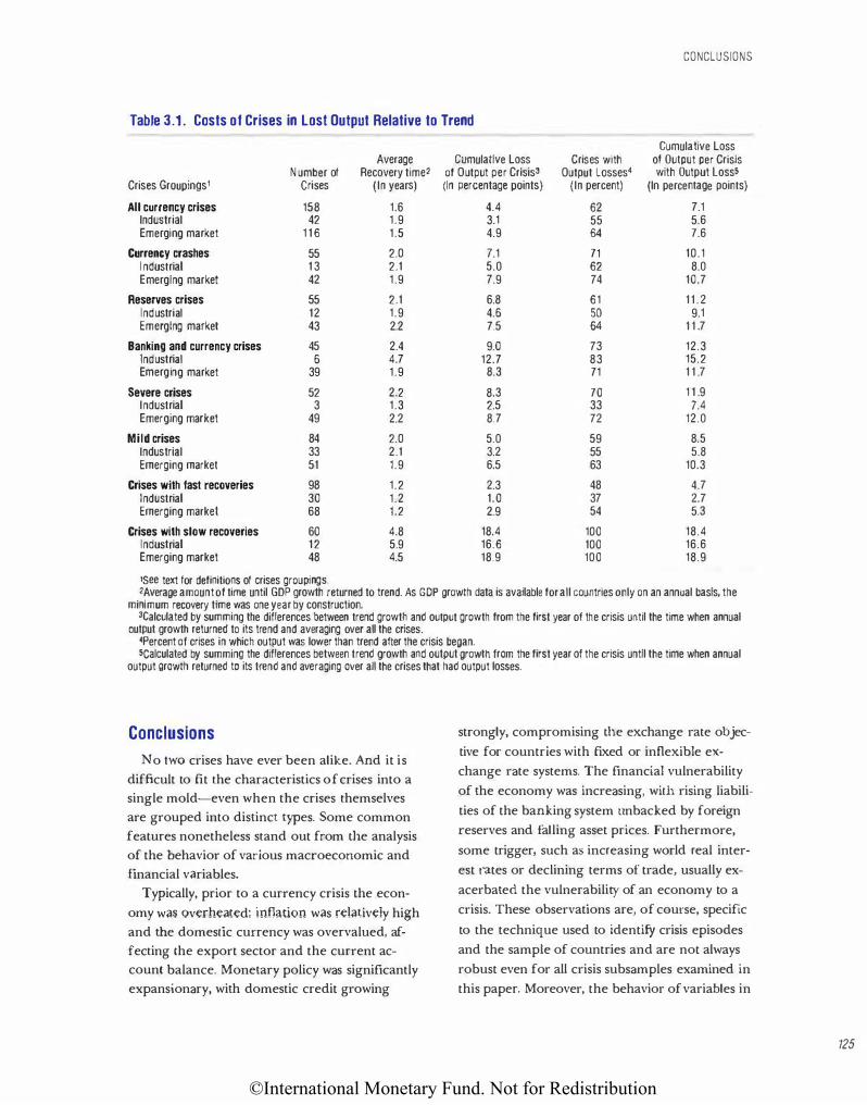
©International Monetary Fund. Not for Redistribution
CONCLUSIONS
Table 3.1. Costs of Crises in Lost Output Relative to Trend
Cumulative loss Average Cumulative loss Crises with of Output per Crisis
Number of Recovery time2 of Output per Crisis3 Output Losses4 with Output losss Crises Groupings1 Crises (In years) (In percentage points) (In percent) (In percentage points)
All currency crises 158 1.6 4.4 62 7.1 Industrial 42 1.9 3.1 55 5.6 Emerging market 1 16 1.5 4.9 64 7.6
Currency crashes 55 2.0 7.1 71 10.1 Industrial 13 2.1 5.0 62 8.0 Emerging market 42 1.9 7.9 74 10.7
Reserves crises 55 2.1 6.8 61 11 .2 Industrial 12 1.9 4.6 so 9.1 Emerging market 43 2.2 7.5 64 1 1 .7
Banking and currency crises 45 2.4 9.0 73 12.3 Industrial 6 4.7 12.7 83 15.2 Emerging market 39 1.9 8.3 71 1 1 .7
Severe crises 52 2.2 8.3 70 1 1 .9 Industrial 3 1.3 2.5 33 7.4 Emerging market 49 2.2 8.7 72 12.0
Mild crises 84 2.0 5.0 59 8.5 Industrial 33 2.1 3.2 55 5.8 Emerging market 51 1.9 6.5 63 10.3
Crises with fast recoveries 98 1.2 2.3 48 4.7 Industrial 30 1.2 1.0 37 2.7 Emerging market 68 1.2 2.9 54 5.3
Crises with slow recoveries 60 4.8 18.4 100 18.4 Industrial 12 5.9 16.6 100 16.6 Emerging market 48 4.5 18.9 100 18.9
1See text for definitions of crises groupings. 2Average amount of time until GOP growth returned to trend. As GOP growth data is available for all countries only on an annual basis, the
minimum recovery time was one year by construction. 3Calculated by summing the differences between trend growth and output growth from the first year of the crisis until the time when annual
output growth returned to its trend and averaging over all the crises. 4Percent of crises in which output was lower than trend after the crisis began. scalculated by summing the differences between trend growth and output growth from the first year of the crisis until the time when annual
output growth returned to its trend and averaging over all the crises that had output losses.
Conclusions
No two crises have ever been alike. And it is
difficult to fit the characteristics of crises into a
single mold-even when the crises themselves
are grouped into distinct types. Some common
features nonetheless stand out from the analysis
of the behavior of various macroeconomic and
financial variables.
Typically, prior to a currency crisis the econ
omy was overheated: inflation was relatively high
and the domestic currency was overvalued, af
fecting the export sector and the current ac
count balance. Monetary policy was significantly
expansionary, with domestic credit growing
strongly, compromising the exchange rate objec
tive for countries with fixed or inflexible ex
change rate systems. The financial vulnerability
of the economy was increasing, with rising liabili
ties of the banking system unbacked by foreign
reserves and falling asset prices. Furthermore,
some trigger, such as increasing world real inter
est rates or declining terms of trade, usually ex
acerbated the vulnerabilily of an economy to a
crisis. These observations are, of course, specific
to the technique used to identify crisis episodes
and the sample of countries and are not always
robust even for all crisis subsamples examined in
this paper. Moreover, the behavior of variables in
125
©International Monetary Fund. Not for Redistribution
126
CHAPTER Ill CURRENCY CRISES
particular crises has, on many occasions, differed
from this average pattern-to take one example,
in a number of the Asian countries affected by the recent crisis, inflation was relatively low.
Crises in emerging market economies have
tended to be deeper than crises in industrial
countries, but recoveries have tended to be
faster. Generally, faster recoveries have been as
sociated with stronger rebounds in export
growth. While currency crises can be very costly
in terms of lost output, not all are-output
losses are more likely in crises in which the cur
rency "crashes" than in those in which exchange
market pressures are reflected mainly in large re·
serves losses. Most costly and most prolonged
are currency crises accompanied by banking sec
tor difficulties.
Appendix 3.1 . Banking Crises
Banking crises are more difficult to identify
empirically, partly because of the nature of the
problem and partly because of the lack of rele
vant data. While data on bank deposits are read
ily available for most countries, and thus could
be used to identify crises associated with runs on
banks, most banking problems today do not
originate on the liabilities side of banks' balance
sheets. Thus, among the industrial counoies,
neither the banking crises in Finland, Norway,
and Sweden in the late 1980s and early 1990s,
nor the earlier banking problems in several
other countries, such as in Spain in the early
1980s, nor t11e more recent banking problems in
Japan were associated with runs on deposits.
Among the developing countries, large with
drawals of deposits and runs on banks have been
more frequent-for instance, t11e banking crises
in the 1980s and 1990s in Argentina, the
Philippines, Thailand, Turkey, Uruguay, and
Venezuela were associated with bank runs. A fail
ure to roll over interbank deposits, as in Korea
during the 1997-98 Asian crisis, can have results
similar to those of a run on banks. Instances of
Large deposit witl1drawals, however, as in the re
cent financial crisis in Indonesia, have tended to
follow the disclosure of difficulties on the assets
side or widespread uncertainty as tO whether the
currency would maintain its value. Generally,
runs on banks are the result rather than the
cause of banking problems.
Banking crises generally stem from tl1e assets
side of banks' balance sheets-from a protracted
deterioration in asset quality. This suggests that
variables such as tile share of non performing
loans in banks' portfolios, large fluctuations in
real estate and stock prices, and indicators of
business failures could be used to identifY crisis
episodes. The difficulty is tl1at data for such vari
ables are not readily available for many develop
ing countries or are incomplete, as wi th data on
non performing loans in many counu·ies. In
cases where central banks have detailed informa
tion on nonperforming loans, it is usually laxity
in the analysis of, and in follow-up action in re
sponse to, the data that allows the situation to
deteriorate to the poi1u of ciisis.
Reflecting these limitations, banking crises
have usually been dated by researchers on the
basis of a combination of events-such as the
forced closure, merger, or government take over
of financial institutions, runs on banks, or the
extension of government assistance to one or
more financial institutions-or in-depth assess
ments of financial conditions, as in many case
studies. As a result of this methodology, the dat
ing of banking crises is much more approximate
than that of currency crises as it depends on the
occurrence of "events" such as the closure or
governmem takeover of financial institutions,
bank runs, etc. There is therefore a greater risk
of dating crises either "too late"-as financial
problems usually begin well before bank closures
or bank runs occur-or "too early," since the
peak of a crisis is generally reached much later.
Banking crises were compiled from previous
studies for the analysis in this paper. The list of
banking crises was compiled from Caprio and
Klingebiel ( 1 996), Kaminsky and Reinhart
( 1 996), and Demirguc-Kunl and Detragiache
(1997).
Between 1975 and 1997, the sample of 50
counoies had 54 banking clises. Of these, 12
©International Monetary Fund. Not for Redistribution
occurred in industrial countries while 42 were in
developing counu·ies. Forty-five of the banking
crises were within two years of currency crises.
Twelve were contemporaneous with currency
crises20 and another 12 preceded currency crises
by one year, while 10 others preceded them by
two years. In 7 cases currency crises were fol
lowed in one year by a banking crisis, while in 4
instances currency crises preceded banking
crises by two years. This evidence, while sugges
tive, should be interpreted with caution in view
of the difficulties in dating the beginning of
banking crises.21
References
Bordo, Michael D., 1985, "Financial Crises, Banking
Crises, Stock Market Crashes and the Money
Supply: Some International Evidence, 1870-1933,"
in Forrest Capie and Geoffrey Wood (eds.),
Financial Crises in tile World Banking System ( ew
York: SL Martin's).
Calvo, Guillermo A., Leonardo Leiderman, and
Carmen M. Reinhart, 1993, "Capital Inflows and
Real Exchange Rate Appreciation in Latin America:
The Role of External Factors," //IfF Staff Papers, Vol.
40 (March), pp. 108-51.
__ , 1996, "Inflows of Capital to Developing
Countries in the 1990s," journal of Economic Perspectives, Vol. 10, No. 2, pp. 123-39.
Caprio,jr., Ccrnrd, and Daniela Klingebiel, 1996,
"Bank Insolvencies: Cross-Country Experience,"
Policy Research Working Paper No. 1620
(Washington: The World Bank, july).
_, 1997, "Banking Insolvency: Bad Luck, Bad
Policy, or Bad Banking," in Ann·ual World Bank
C011jerence on DI!Velopment Economics 1996
(Washington: The World Bank).
Caramaua, Francesco, Luca Ricci, and Rani! Salgado,
2000, "Trade and Financial Contagion in Currency
Crises," IMF Working Paper 00/55 (Vhshington).
Cole, Harold L., and Timothy J. Kehoe, 1998, "SelfFulfiUing Debt Crises," Federal Reserve Bank of
Minneapolis, Staff Report No. 211 Quly).
REFERENCES
Demirguc-Kunt, Asli, and Enrica Detragiache. 1997.
'The Determinants of Banking Crises: Evidence
from Developing and Developed Countries," IMF
Working Paper 97/106 (Washington).
Eichengreen, Barry, and Andrew K. Rose, 1997,
"Staying Afloat When the Wind Shifts: External
Factors and Emerging-Market Banking Crises"
(unpublished; IMF, UCLA, and UC Berkeley).
Eichengreen, Barry, Andrew K. Rose, and Charles
Wyplosz, 1995, "Exchange Market Mayhem: The
Antecedents and Aftermath of Speculative Auacks," Eccnomic Policy: A European Fomm (U.K.), No. 21,
pp. 249-312.
__ , 1996, "Contagious Currency Crises: First Tests,"
Scandinavian joumal �f t:conomics. Vol. 98. No. 4,
pp. 463-84.
Flood, Roben, and Peter Garber, 1984, "Collapsing
Exchange-Rate Regimes: Some Linear Examples,"
joumt1l of lntematitmal Econumics, Vol. 17, pp. 1-13.
Frankel, Jeffrey A., and Andrew K. Rose, 1996,
"Currency Crashes in Emerging Markets: Empirical
Indicators," NBER Working Paper No. 5437
(Can1bridge, Massachusetts: National Bureau of
Economic Research).
Gavin, Michael, and Ricardo Hausmann, 1996, 1be
Roots of Banking Crises: The Macroeconomic
Context,- in R. Hausmann and L. Rojas.Suarez
(eds.), Banking Grists i11 Latin America (WashingtOn:
Inter-American Developmem Bank),
Click, Reuven. and Andrew K. Rose, 1999, "Contagion
and Trade: Why Are Currency Crises Regional?"
juurnal of International Money and Finance (U.K),
Vol. 18, No. 4, pp. 603-17.
Coldfajn, Ilan, and Rodrigo 0. Valdes, 1997, "Capital
Flows and the Twin Crises: The Role of Liquidity,"
JMF Working Paper 97/87 (Washington).
Goldstein. Morris, 1996. "Presumptive Indicators/
Early Waming Signals of Vulnerability lO Financial
Crises in Eme1'ging Market Economies" (unpub
lished; WashingtOn: Institute for International
Economics, January) .
Kaminsky, Crnciela L., Saul Lizondo, and Carmen Yl.
Reinhart, 1997, "Leading Indicators of Currency
Crises," IMF Working Paper 97/79 (Washington).
Kaminsky, Graciela L., and Carmen M. Reinhart, 1996,
'The Twin Crises: The Causes of Banking and
20Currency and banking crises seem to have become more contemporaneous since the late 1980s: 10 of 12 instances in which banking and currency crises occurred in the same year have taken place since 1989.
21Qthers have found evidence that banking crises are statistically significant in helping to predict currency crises, but not conversely. See Kaminsky and Reinhan (1996), for example.
127

©International Monetary Fund. Not for Redistribution
128
CHAPTER Ill CURRENCY CRISES
Balance-of-Payments Problems," International
Finance Discussion Paper No. 544 (Washington:
Board of Governors of the Federal Reserve System,
March).
Krugman, Paul, 1979, "A Model of Balance of
Payments Crises," journal of Money, Credit, and
Banking, Vol. 1 1, pp. 3 1 1-25.
Lindgren, Carl:Johan, GiLJjan Garcia, and Matthew [.
Saal, 1996, Bank Soundness and Macroeconomic Policy
(Washington: International Monetary Fund).
Masson, Paul, 1998, "Contagion: Monsoonal Effects,
Spillovers, and jumps Between Multiple Equilibria,"
IMF Working Paper 98/1 42 (Washington).
Masson, Paul, and Michae.l Mussa, 1995, "The Role of the IMF: Financing a11d Its lntetactions 1vith Adjustment and SurveilJance," Pamphlets Series
No. 50 (Washington: International Monetary Fund).
Mishkin, Frederic S., 1994, "Preventing Financial C1·ises:
An International Perspecti.ve," NBER Working Paper
No. 4636 (Cambridge, Massachusetts: National
Bureau of Economic Research).
__ , 1996, "Understanding Financial Crises: A
Developing Country Perspective," NBER Working
Paper No. 5600 (Cambridge, Massachusetts:
National Bureau of Economic Research).
Obstfeld, Maurice, 1986, "Rational and Self-Fulfilling
Balance of Payments Crises." American Economic
Review, Vol. 76 (March), pp. 72-81 .
_, 1994, 'The Logic of Currency Crises," Cahiers
Economiques et Monetaires, Vol. 43, pp. 89-123.
Sachs, Jeffrey, Aaron Tornell, and Andres Velasco,
1996, "Financial Crises in Emerging Markets: The
Lessons from 1995," Bn>okings Papers on Economic
Activity, Vol. l , pp. 147-98.
Schwartz, Anna, 1985, "Real and Pseudo-:Financial
Crises," in Forrest Capie and Geoffrey E. Wood
( eds.), Financial C1ises in the Wm·ld Ban/ling System
(New York: St. Martin's Press) .
Taylor, Mark P., and Lucio Sarno, 1 997, "Capital Flows
to Developing Countries: Long- and Short-Term
Determinants," The Wo1'ld Bank Econo111ic Review,
Vol. 1 1 (September) , pp. 451-70.
©International Monetary Fund. Not for Redistribution
BUSINESS CYCLE INFLUENCES ON EXCHANGE RATES: SURVEY AND EVIDENCE Ronald MacDonald and Phillip Swagel
This chapter examines the relationship
between exchange rates and the busi
ness cycle. A principal goal is to assess
the extent to which exchange rate
movements reflect countries' relative positions
over the business cycle. Are the influences simi
lar across coumries and at different points in
time? The importance of this question is high
lighted by the late 1990s conjuncture of low in
flation, sustained economic growth, and appreci
ated currencies in the United States and United
Kingdom compared to relatively slack conditions
in continen tal Europe and a weak euro. The
conclusion of the research summarized in this
paper is that cyclical movements in activity have
substantial effects on exchange rates, though
these are of course not the only or at all times
the most important innuence on currencies.
There are a number of potential reasons why
the United Kingdom and United States may be
enjoying such a fortuitous inflation/growth com
bination, including productivity improvements
associated with information technology and the
relatively slow growth in competing countries
that has kept a lid on prices of raw materials.
Additionally, the exchange rate may play an im
portant role, with the appreciating currencies in
the United States and UniLed Kingdom helping
to attenuate inflation in each country, both be
cause of the direct effect on the cost of primary
inputs and importables, and from the
feedthrough to the nonu-aded goods sector via
the wage bargaining process. In recent years, the
exchange rate-business cycle link appears to
have worked to the advantage of policymakers in
the United Kingdom and United States, while
the corresponding depreciation of the yen may
also be viewed as beneficial to the Japanese
economy given that country's relatively weak
growth performance.
The srudy first reviews the literature on the
determinants of exchange rates and the relation-
ship with business cycles, and then presents di
rect empirical evidence on the connection.
Somewhat surprisingly, there is liule work that
looks directly at the exchange rate-business cycle relationship. Because of this, a principal fo
cus in this survey is on the role of asset yields
and the corresponding interest rate differemials
between countries and maturities; these are then
used to examine the relationship between ex
change rate movements and the business cycle.
This mechanism and related analytical frame
works are discussed in the econd section, after
which the existing empirical evidence is re
viewed. The next section provides new empirical
evidence, first on tl1e link between real ex
change rates and real interest rate differentials
for a number of key bilateral and effective ex
change 1-ates over the post-1973 period of float
ing exchange rates, and then on the decomposi
lion of exchange rate movements into a
permanent component and business-<:ycle move
ments. The chapter ends by drawing
conclusions.
Exchange Rate Models: Some Scaffolding and an Overview
In thinking about the relationship between
the economic cycle and the exchange rate, it is
instructive to stan with a discussion of models of
nominal and real exchange rates. Since these
arc comprehensively surveyed elsewhere-see,
for example, MacDonald ( 1988), MacDonald
and Taylor (1992), and Frankel and Rose
( 1995 )-the discussion here is not intended to
be exhaustive or rigo1·ous but, rather, to focus on
implicalions for the relalionship between the
business cycle and exchange rates and then to
motivate the empirical work that follows.
Perhaps the simplest nominal exchange rate
model is purchasing power parity (PPP), in
which the equilibrium level of an exchange rate
129
©International Monetary Fund. Not for Redistribution
130
CHAPTER IV BUSINESS CYCLE INFLUENCES ON EXCHANGE RATES
is determined by relative prices-absolute PPPor relative PPP, where the exchange rate changes
in response to inflation differentials. Although PPP in itself has limited applicability for the cen
tral focus of this study, it is helpful in motivating the decomposition of real exchange rates into the permanent and transitory components that
are taken to correspond to long-run and cyclical
movements, respectively. Absolute PPP, which relies on arbitrage in the trade account, may be stated as:
(1 )
where s1 denotes the nominal exchange rate (domestic price of a unit of foreign exchange) at time t, fJ1 is the domestic price level, fJt is the for
eign price level (as usual, an asterisk denotes a
foreign variable), and all variables are expressed as natural logarithms. If absolute PPP holds ex
actly, the logarithm of the real exchange rate, q1 = s,-P1 + p�, always equals zero, though of course there is overwhelming evidence against a su·ict version of this model. Rather, what may be refeJ-red to as a traditional PPP view would be that real exchange rates are mean-reverting, or revert to some trend in the presence of a productivity growth differential. This suggests that real exchange rate movements are dominated by the
transitory component, qT, the reversions back to trend. Efficient markets PPP, which relies on capital account arbitrage, posits that the real ex
change rate follows a random walk and therefore all of the exchange rate movements are driven purely by permanent components. Problems and pitfalls in constructing data to examine equation (1) and the empirical evidence are discussed in MacDonald ( 1995a).
Since price and inflation movements are
linked to the business cycle-although there has been widespread discussion of whether in the
current phase of the cycle in the United
Kingdom and United States there has been a decoupling of this relationship-PPP could be
used in a limited sense to address the central issue of this paper. However, since it excludes the variables central to the business cycle-namely, output and interest yields-PPP alone has only limited applicability to the task at hand and is therefore not a direct focus in this survey.
Perhaps the most useful general model in the current context is the two-counu·y open econ
omy TS-LM model with rational expectations, in
which capital is assumed to be perfectly mobile and prices are sticky in the short run, with the cenu·al feature that the exchange rate moves to clear both goods and asset markets. This model is usually referred to as the extended, or eclectic, Mundeli-Fleming modeJ.l This model has been set forth by various authors, including inter alia,
Dornbusch (1976), Frankel (1979), Flood
(1981), and Mussa (1982). Obstfeld (1985) provides a synthesis in a deterministic setting, while Clarida and Gali (1994) present a version with stochastic shocks.
From the perspective of this paper, the key component of the model is the condition of uncovered interest rate parity which governs relative nominal interest rates between countries:
(2)
where E;1st+k denotes the expected change in the exchange rate between periods t and t + k, i1 denotes a nominal interest rate with maturity k, an asterisk denotes a foreign magnitude, a "prime"
( ' ) indicates that a variable is defined as home relative to counu·y (e.g., x' = x - xj, and all variables apart from interest rates are in logs. Using
the standard Fisher decomposition to define the real interest rate, r;, equation (2) can be rewritten as:
where i� is the nominal interest rate difierential,
E,.1jJ[+ 1 = Elp;+ 1 - fJ�), and fit is the relative p1ice level.
1Extended because of the inclusion of forward-looking expectations and an explicit supply side relationship, both of which a1·e feattares missing from the original Mundell-Fleming model.
©International Monetary Fund. Not for Redistribution
Equation (2) can also be rewritten in terms of
the real exchange rate as:
E1L1q1+k = r;, (3)
This shows that a relatively lower domestic
real interest rate must be compensated by the
expectation of a real appreciation.
The demand for home output relative to for
eign output, 'f{, is specified an increasing func
tion of the real exchange rate, an aggregate de
mand shock, g;, and a negative function of the
real interest rate:
A price setting equation captures short-run
price inertia:
(4)
(5)
Equation (5) states that the price level in period
t is an average of the market-cleruing price ex
pected at time t-1 to prevail at time t, E,_l'J!!; , and
the price which would actually clear the output
market at time t, pe;. With e = 1 , prices are fully
flexible and output is supply determined, while
with e = 0, prices are fixed and predetermined
one period in advance. Values of() between 0
and 1 impart some short-run price stickiness.
The relative money market equilibrium condi
tion between the home and foreign country is
given by:
(6)
where m' denotes the relative money supply, a is
the income elasticity of demand for money, and
f3 is the interest rate semi-elasticity (the equation
is defined so that a and f3 are positive ) .
In the presence of less than fully flexible
prices, an exogenous fall in aggregate demand
that pushes output below its trend will lead,
other things being equal, to a relatively lower in
terest rate, a capital outflow, and an exchange
rate depreciation (both real and nominal). For
EXCHANGE RATE MODELS: SOME SCAFFOLDING AND AN OVERVIEW
the lower interest rate to be consistent with inter
est parity, the cw-rency must be expected to ap
preciate in both real and nominal terms; this ap
preciation takes place as demand returns w trend. The dynamic path of the exchange rate is
the path that coincides with an increasing rela
tive interest rate-the traditional capital Oow re
lationship between the exchange rate and rela
tive interest rates. Indeed, this is likely to be
compounded if monetary authorities have an ex
plicit reaction function in which interest rates are
raised to attenuate inflationary pressure. If the
recession is instead caused by an adverse supply
shock, this would lead to an initial rise in the in
terest rate (real and nominal) and a currency ap
preciation (both real and nominal), with the
consequent expectation of a currency deprecia
tion being translated into an actual depreciation
as supply retw-ns to trend, with relative interest
rates similarly falling. If a monetru·y tightening is
the source of the recession (either through a fall
in the supply of money or increased demand for
money) , interest rates would initially rise and the
real exchange rate would appreciate on impact,
eventually depreciating back to trend as output
adjusted. The similarity of the effects of these
two shocks means that it is in practice difficult to
distinguish between their relative importru1ce
without imposing restrictions on the causal rela
tionships between the variables, such as in
Clarida and Cali (1994).
Although the Mundeii-Fieming model stresses
the importance of both goods and asset markets
in determjning exchange rates, it does not take
into account stock-flow implications of asset ac
cumulation or allow for time-varying exchange
risk premia.
The "flexible price monetary model of ex
change rates" (FPMM) can be derived from the
above framework by assw-ning that prices are
continuously flexible, purchasing power parity
holds at all times, output is fixed at the full em
ployment level, and there are no demru1d
shocks:2
Zfhis framework can also be derived f1·om the generalj7.ed asset pricing model of Lucas ('1982).
131
©International Monetary Fund. Not for Redistribution
132
CHAPTER IV BUSINESS CYCLE INFLUENCES ON EXCHANGE RATES
, • • f3. /3 •.• s1 = m 1 - ay1 + a y 1 + z1 - z ,. (7)
Equation (7) asserts that in a flexible price equi
)jbrium, an exchange rate is driven purely by
conditions of asset market equilibrium (relative
excess money supplies) , with goods market con
ditions having no independent influence. In the
flexible price variant of the monetary model,
equation (7) is assumed to hold continuously in
both the short and long run-see, among
others, Bilson (1978), Frenkel (1978) and
Hodrick ( 1987), while in the sticky price variant
(SPMM) it holds only in the long run (see
Dornbusch ( 1976) and Frankel ( 1979).
How useful is equation (7) from the perspec
tive of thinking about business cycle issues? A
stylized fact is that a currency typically appreci
ates in the upS\ving of an economic cycle and de
preciates in the downswing. Equation (7} neatly
captures this effect: higher income increases
money demand and thus leads to an apprecia
tion of the nominal exchange rate (and vice
versa in a slump). This is consistent with a de
mand shock in the generalized model but not a
supply shock. Since in the FPMM, output
changes are driven only by supply side effects,
the difference in the sign here relates to the fact
that output affects the exchange rate only
through the demand for assets, with relative
prices moving to satisfy asset market equilibrium,
and not through interest rates, which simply
equal expected inflation. The FPMM must thus
be regarded as having limited applicability for
the task at hand since it ignores the relationship
between asset yields and output.
Of course, equation (7) is usually estimated as
a reduced form that could also be consistent
with the more general eclectic model-for ex
ample, if interest rates are given a capital flow in
terpretation. That is, the domestic and foreign
interest rates would, respectively, have negative
and positive signs, and income a positive sign in
the forecasting equation for the nominal ex
change rate. This is brought out clearly by
Frankel (1979) in a real interest differential
(RID) variant of the monetary model. This as.
sumes a form of regressive expectations in which
the exchange rate is expected to change in pro
portion to the gap between the equilibrium and
actual exchange rate and the expected inflation
differential:
M1 - qJ(S,- sJ + (t1P' - t1fj'*),..1, O«p<l. (8)
Equation (8} indicates that in long-run equi
librium, when s; • s, the exchange rate is ex
pected to change by an amount equal to the ex
pected inflation differential. Substituting
equation (8} into the UIP condition (2) gives
the key RID relationship:
s, = s; - qrt [ ( i1 - E,1p,..k) - ( i•, - E,1p•,+«)]. (9)
This indicates that whether s1 is above or be
low s; depends on the real interest differential;
that is, if the domestic real interest rate is above
the foreign rate, the exchange rate appreciates
relative to its Long-run value. Equation (9) there
fore illustrates, in a single equation comext, the
traditional capital account interpretation of the
exchange rate/business cycle relationship re
ferred to above.
The RID model may be thought of as relaxing
the assumption of the FPMM that the expecta
tions model of the term structure holds, replac
ing it instead with an assumption of market seg
mentation, so that a monetary impulse can have
different effects on short and long interest rates.
ln particular, a monetary tightening can increase
the short rate through the liquidity effect, while
at the same time decreasing the long rate
through an expected inflation effect. To the ex
tent that the output expansion emanates from
the supply side and thereby has a moderating in
fluence on inflation (price movements), the
business cycle could have an effect on exchange
rates that is separate from that of interest yields.
This effect relies on price flexibility, and would
thus not be present in the case of sticky prices.
Assuming s; in (9) is determined by equation (7)
and that long rates proxy for expected inflation
and short rates proxy for real interest rates gives
a reduced form of the RID model:
s1 = rp1 m, - Cf'-lm;- (j)3Yt + (/)4]; - f1>5i: + rp6i',"+ <P?�- fPsit;+e, (10)
©International Monetary Fund. Not for Redistribution
where the s and l superscripts denote short- and
long-term interest rates, respectively. Although
the RID reduced form is in the spirit of the
eclectic Mundell-Fleming model, in terms of the
relative interest rate effects, it nevertheless con
strains output to have a purely asset market role
in the exchange rate equilibrium process; as in
the FPMM, increased output has a negative in
fluence on the exchange rate. Indeed, this
model has a long-run solution that is equivalent
to that of the FPMM.
The above models all assume that non-money
assets are perfect substitutes. However, propo
nents of the portfolio balance approach-Allen
and Kenen (1980), Branson (1977), and
Dornbusch and Fischer (1980)-argue that non
money assets are likely to be imperfect substi
tutes across countries, so that equation (8) holds
only on a risk-adjusted basis. Dooley and Isard
( 1982) demonstrate that in a model in which
there are two types of money (home and for
eign) and two bonds (home and foreign), the
risk premium, ()1, may be defined by the follow
ing expression (see also Frankel (1983)):
( 1 1 )
where B denotes domestic non-money assets and
B* foreign non-money assets.
In the context of the above framework,
Frankel (1983) and Hooper and Morton (1982)
demonstrate that a reduced form in the spirit of
the portfolio balance approach is:
s1 = m; - ay1 t ay�- f3i11 + Wi·'7 + A.i11- A. *i1; +e1• (12)
Equation (12) is usually referred to as a hy
brid model monetary-portfolio balance reduced
form.3 The relationship between the net supply
of non-money assets (effectively net foreign as
sets) and the risk premium is assumed to be pos
itive in the portfolio model: an increased risk
premium requires a currency depreciation to
equilibrate asset markets. It is not entirely clear
if the adctition of a risk premium to equation (7)
A REVIEW OF THE EMPIRICAl EVIDENCE
or (10) gives much insight with respect to the
impact of the business cycle on the exchange
rate. One way in which risk premia could be re
lated to business cycles is through effects of the
economic cycle on countries' fiscal positions and
thereby relative debt stocks. For example, gov
ernments often use the upswing of a cycle, and
associated buoyant tax revenues, to repatriate
government debt and, conversely, downswings
often have implications for increased govern
ment debt as increased fiscal deficits drive up
the outstanding stock of debt.
A Review of the Empirical Evidence
This section reviews empirical evidence on the
exchange rate-business cycle relationship.
Evidence on the factors that influence nominal
exchange rates is examined first, followed by sev
eral strands of the literature on the influences of
real exchange rates.
Nominal Exchange Rates and the Business Cycle
The most general monetary approach equa
tion may be expressed as a reduced form:
st = <t>t mt + <t><lm*t + <t>sYt + q>4y•t + q>5it +q>6i7 +Et> (13)
where the q>'s are parameters to be estimated
and e1 is a disturbance term. The su·ict form of
the monetary model implies q>1 = -<t><l = 1, while
q>3 and q>4 should take on values that are close to
estimated income elasticities from money de
mand functions, and <t>5 and q>6 should take on
values close to interest rate semi-elasticities also
from money demand functions. The hypothe
sised values of unity for q>1 and <t>2 are those ex
pected, in equilibrium at least, from either the
flex-price and fix-price monetary models.
However, it is important to note that even within
the monetary tradition there is a view that these
coefficients may be less than one in absolute
value; see, for example, Mussa (1979). There is a
3Strictly speaking, this relationship relies for its derivation on a short-long distinction that is not made in tl1is paper.
133
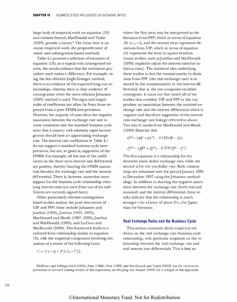
©International Monetary Fund. Not for Redistribution
134
CHAPTER IV BUSINESS CYCLE INFLUENCES ON EXCHANGE RATES
large body of empirical work on equation (13)
and variants thereof; MacDonald and Taylor
(1993) provide a survey.4 The focus here is on recent empirical work, the preponderance of
which uses cointegration-based methods. Table 4.1 presents a selection of estimates of
equation (13); as is typical with co integrated sys
tems, the results indicate that the estimation procedure used makes a difference. For example, us
ing the less efficient Engle-Granger method, there is no evidence of the expected long-run re
lationships, whereas there is clear evidence of
cointegration when the more efficientjohansen (1995) method is used. The signs and magnitudes of coefficients are often far from those ex
pected from a pure FPMM interpretation. However, the majority of cases show the negative
association benveen the exchange rate and income consistent with the standard business cycle
story that a country with relatively rapid income
growth should have an appreciating exchange rate. The interest rate coefficients in Table 4.1 do not support a standard business cycle inter
pretation, but are, in general, supportive of the FPMM. For example, all but one of the coefficients on the short term interest rate differential
are positive, thereby favoring the FPMM association benveen the exchange rate and the interest differential. There is, however, somewhat more support for the business cycle relationship when
long interest rates are used (four out of six coefficients are correctly signed here).
Other particularly relevant cointegration
based studies analyze the joint interaction of UIP and PPP; these include Johansen and
Juselius ( l 992),Juselius (1991, 1995), MacDonald and Marsh (1997, 1999), Juselius and MacDonald (1999), and La Cour and MacDonald (2000). This framework leads to a reduced form relationship similar to equation (9), with the empirical component involving esti
mation of a vector of the following form:
x'1 = [(s1 -P1 + p*1) ,(i1 - i*1) ] ,
where the first term may be interpreted as the deviation from PPP, which in terms of equation (9) is s1- Sv and the second term represents de
viations from UIP, which in terms of equation (9) represents the term in square brackets
(some studies, such asJuselius and MacDonald (1999) explicitly adjust the interest rates for in
flation rates). The statistical idea underlying these studies is that the nonstationarity in deviations from PPP (the real exchange rate) is re
moved by the nonstationarity in the interest dif
ferential; that is, the two composite variables cointegrate. It turns out that nearly all of the
studies that combine VIP and PPP in this way produce an association bet\veen the nomina] ex
change rate and the interest differential which is negative and therefore supportive of the interest rat�exchange rate linkage referred to above.
Two sets of results from MacDonald and Marsh (1999) illustrate this:
st?M = ( p!I,"' + P'f'") - 0.132 ( 14"- i�"')'
sYEN = ( <hiPm + P"''") - 0.318(iifm - i"'). I rj 1 I I The first equation is a relationship for the deutsche mark-dollar exchange rate, while the
second is for the yen-dollar rate. Both relation
ships are estimated over the period January 1983
to December 1997 using the Johansen methodology. In addition to showing the negative associ
ation benveen the exchange rate (both real and nominal) and the interest differential, these re
sults indicate that the relationship is much
stronger-by a factor of about 2lh-for Japan than for Germany.
Real Exchange Rates and the Business Cycle
This section examines direct empirical evidence on the real exchange rate-business cycle relationship, with particular emphasis on the relationship between the real exchange rate and real interest rate differentials. This is best ex-
4Hoffman and Schlagenhauf (1983), Finn (1986), Woo (1985) and MacDonald and Taylor (1993) test the rational expectations or forward looking version of this expression; see Dejong and Husted (1995) for a critique of this approach.
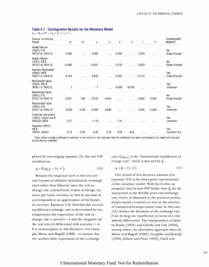
©International Monetary Fund. Not for Redistribution
A REVIEW OF THE EMPIRICAL EVIDENCE
Table 4.1 . Cointegration Results for the Monetary Model S1 = m1 + m* I + J1 + y• I + i1 + i* I Source, Currencies, Cointegrated? Period m m· y y· ;s ;s· jl ,,. Method?
Baillie-Selover (1987); ¥·$ No 1973:3 to 1983:12 0.065 0.458 0.005 0.035 Engle·Granger
Baillie-Selover (1987); C$-$ No 1973:3 to 1983:12 -o.466 -0.047 0.010 . . . -0.003 Engle-Granger
Kearney-MacDonald ( 1990); A$-$ Yes 1984:1 to 1988:12 0.186 0.946 0.022 . . . -Q.Q12 Engle-Granger
MacDonald-Taylor (1993); OM-$ Yes 1976:1 to 1990:12 -1 0.049 -0.050 Johansen
MacDonald-Taylor (1994); £-$ No 1976:1 to 1990:12 -0.471 1.06 -0.733 -o.284 . . . -0.052 0.004 Engle-Granger
MacDonald-Taylor (1994); £-$ Yes 1976:1 to 1990:12 0.209 -o.49 -o.098 0.646 0.035 0.086 Johansen
Cushman and others (1997); Turkish lira-$ Yes 198103-9204 0.21 -1.13 1.14 Johansen
Kouretas (1997); C$·$ Yes 1970:6-1994:5 -0.12 -o.79 -0.32 0.32 0.08 -o.02 Dynamic OLS
Note: When a single coefficient is reported in two columns, this indicates that the coefficient has been constrained to be equal and opposite across the two variables.
plored by rearranging equation (3), the real UIP
condition as:
(14)
Because the empirical work in the next sec
tion focuses on effective (multilateral) exchange
rates rather than bilateral rates, the real ex
change rate is henceforth written as foreign cur
rency per home currency, so that an increase in
q corresponds to an appreciation of the domes
tic currency. Equation (14) describes the cunent
equilibrium exchange rate as determined by two
components, the expectation of the real ex
change rate in period t + k and the (negative of)
the real interest differential with maturity l + k.
It is commonplace in this literature-for exam
ple, Meese and Rogoff (1988)-to assume that
the unobservable expectation of the exchange
rate, E,(q,+k), is the "fundamental equilibrium exchange rate," which is denoted by 7j1:
(15)
One strand of this literature assumes that
equation (15) is the sticky-price representation of the monetary model. With the further assumption that ex ante PPP holds, then 7j1 can be interpreted as the flexible price real exchange
rate, which, as discussed in the previous section,
simply equals a constant or zero in the absence
of transaction/transportation costs. In this case,
(15) defines the deviation of the exchange rate from its long-run equilibrium in terms of a real
interest differential. This interpretation is taken
by Baxter (1994) and Clarida and Gali (1994), among others. An alternative approach taken by Meese and Rogoff (1988), Coughlin and Koedjik
(1990), Edison and Pauls (1993), Clark and
135
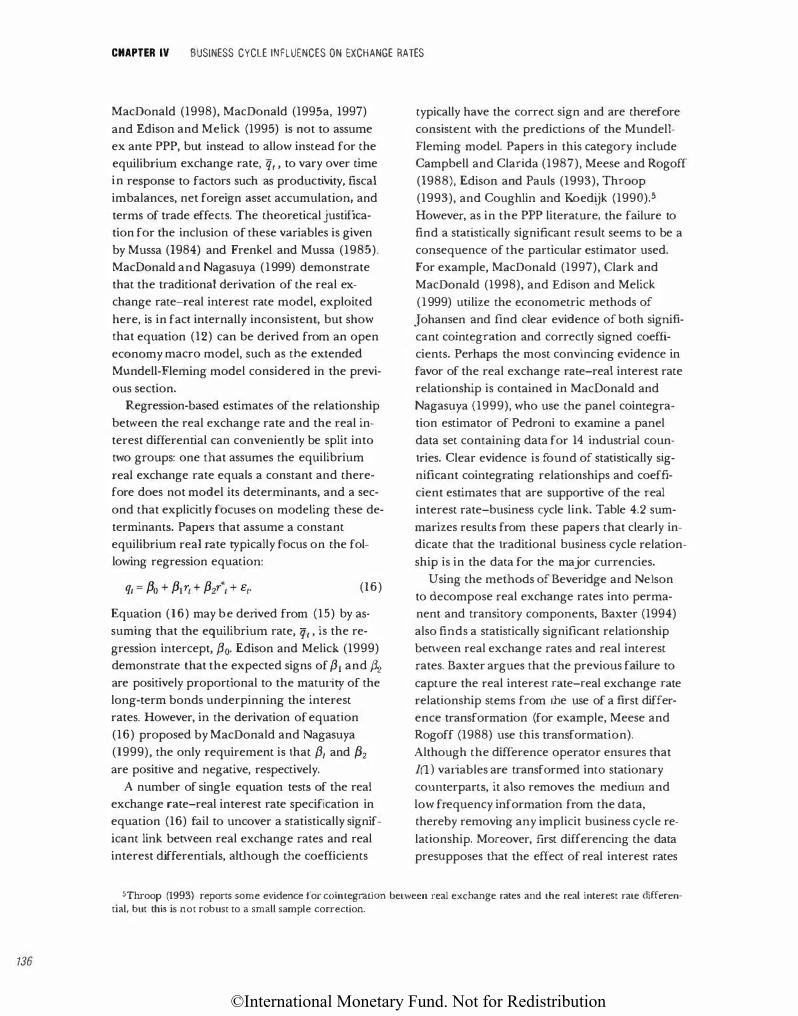
©International Monetary Fund. Not for Redistribution
136
CHAPTER IV BUSINESS CYCLE INFLUENCES ON EXCHANGE RATES
MacDonald (1998), MacDonald (1995a, 1997) and Edison and Melick (1995) is not to assume ex ante PPP, but instead to allow instead for the equilibrium exchange rate, q1 , to vary over time in response to factors such as productivity, fiscal imbalances, net foreign asset accumulation, and terms of trade effects. The theoretical justification for the inclusion of these variables is given by Mussa (1984) and Frenkel and Mussa (1985). MacDonald and Nagasuya (1999) demonstrate that the traditional derivation of the real exchange rate-real interest rate model, exploited here, is in fact internally inconsistent, but show that equation (12) can be derived from an open economy macro model, such as the extended Mundeli-Fleming model considered in the previous section.
Regression-based estimates of the relationship between the real exchange rate and the real interest differential can conveniently be split into two groups: one that assumes the equilibrium real exchange rate equals a constant and therefore does not model its determinants, and a second that explicitly focuses on modeling these determinants. Papers that assume a constant equilibrium real rate typically focus on the following regression equation:
(16)
Equation (16) may be derived from (15) by assuming that the equilibrium rate, q1 , is the regression intercept, {30• Edison and Melick (1999) demonstrate that the expected signs of /31 and � are positively proportional to the maturity of the long-term bonds underpinning the interest rates. However, in the derivation of equation (16) proposed by MacDonald and Nagasuya (1999), the only requirement is that /31 and /32 are positive and negative, respectively.
A number of single equation tests of the real exchange rate-real interest rate specification in equation (16) fail to uncover a statistically significant link between real exchange rates and real interest differentials, although the coefficients
typically have the correct sign and are therefore consistent with the predictions of the MundellFleming model. Papers in this category include Campbell and Clarida (1987), Meese and Rogoff (1988), Edison and Pauls (1993), Throop (1993), and Coughlin and Koedijk (1990).5 However, as in the PPP literature, the failure to find a statistically significant result seems to be a consequence of the particular estimator used. For example, MacDonald (1997), Clark and MacDonald (1998), and Edison and Melick (1999) utilize the econometric methods of
Johansen and find clear evidence of both significant cointegration and correctly signed coefficients. Perhaps the most convincing evidence in favor of the real exchange rate-real interest rate relationship is contained in MacDonald and Nagasuya (1999), who use the panel cointegration estimator of Pedroni to examine a panel data set containing data for 14 industrial countries. Clear evidence is found of statistically significant cointegrating relationships and coefficient estimates that are supportive of the real interest rate-business cycle link. Table 4.2 summarizes results from these papers that clearly indicate that the traditional business cycle relationship is in the data for the major currencies.
Using the methods of Beveridge and Nelson to decompose real exchange rates into permanent and u·ansitory components, Baxter (1994) also finds a statistically significant relationship between real exchange rates and real interest rates. Baxter argues that the previous failure to capture the real interest rate-1·eal exchange rate relationship stems from the use of a first difference transformation (for example, Meese and Rogoff (1988) use this transformation). Although the difference operator ensures that 1(1) variables are u·ansformed into stationary cow1terparts, it also removes the meditun and low frequency information from the data, thereby removing any implicit business cycle relationship. Moreover, first differencing the data presupposes that the effect of real interest rates
5Throop (1993) reports some evidence for cointegration between real exchange rates and the real interest rate differential, but this is not robust to a small sample correction.
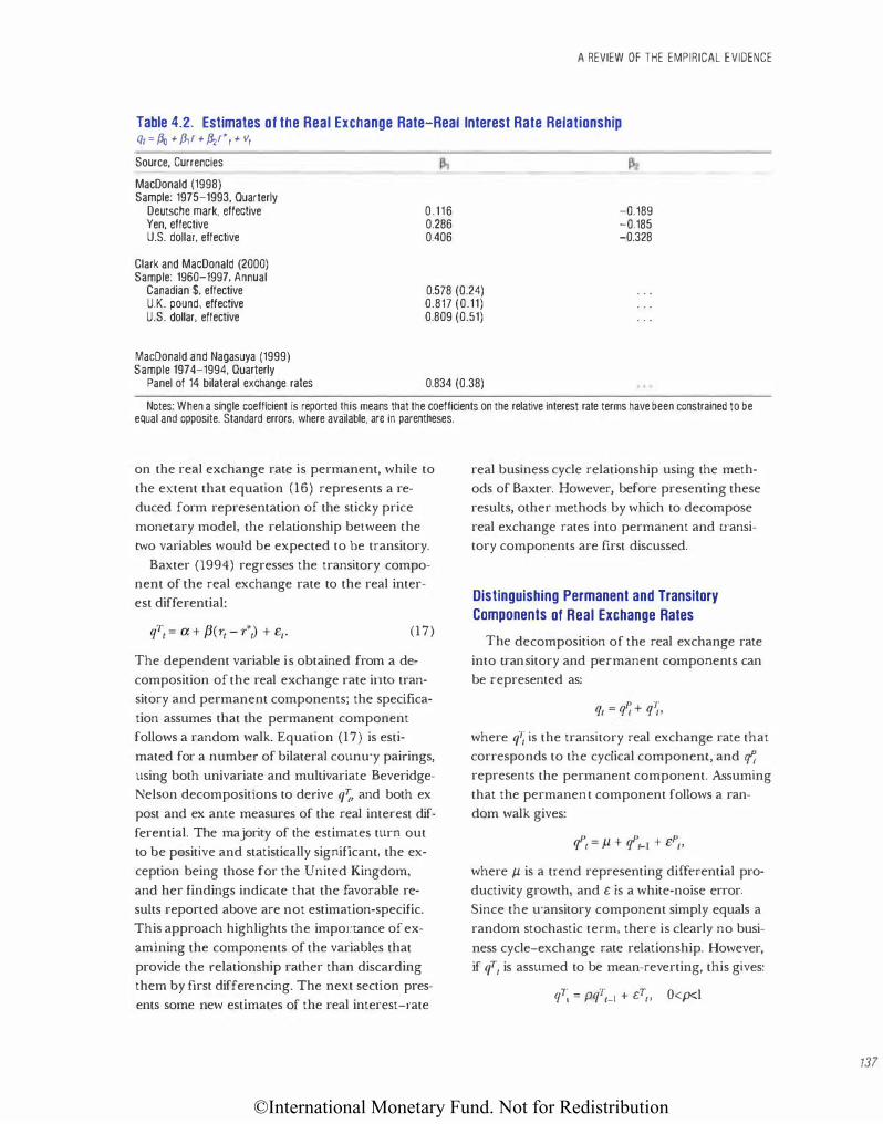
©International Monetary Fund. Not for Redistribution
A REVIEW OF THE EMPIRICAL EVIDENCE
Table 4.2. Estimates of the Real Exchange Rate-Real Interest Rate Relationship q1 = fJo + {31 r + {J.zr* 1 + v1 Source, Currencies
MacDonald (1998) Sample: 1975-1993, Quarterly
Deutsche mark, effective Yen, effective U.S. dollar, effective
0.116 0.286 0.406
-0.189 -0.185 -0.328
Clark and MacDonald (2000) Sample: 1960-1997, Annual
Canadian $, effective U.K. pound, effective U.S. dollar, effective
0.578 (0.24) 0.817 (0.11) 0.809 (0.51)
MacDonald and Nagasuya (1999} Sample 1974-1994, Quarterly
Panel of 14 bilateral exchange rates 0.834 (0.38)
Notes: When a single coefficient is reported this means that the coefficients on the relative interest rate terms have been constrained to be equal and opposite. Standard errors, where available, are in parentheses.
on the real exchange rate is permanent, while to
the extent that equation (16) represents a re
duced form representation of the sticky price
monetary model, the relationship between the
tvvo variables would be expected to be transitory.
Baxter (1994) regresses the transitory compo
nent of the real exchange rate to the real inter
est differential:
(17)
The dependent variable is obtained from a de
composition of the real exchange rate into tran
sitory and permanent components; the specifica
tion assumes that the permanent component
follows a random walk. Equation (17) is esti
mated for a number of bilateral counu·y pairings,
using both univariate and multivariate Beveridge
Neisen decompositions to derive q·�, and both ex
post and ex ante measures of the real interest dif
ferential. The majority of the estimates turn out
to be positive and statistically significant, the ex
ception being those for the United Kingdom,
and her findings indicate that the favorable re
sults reported above are not estimation-specific.
This approach highlights the importance of ex
amining the components of the variables that
provide the relationship rather than discarding
them by first differencing. The next section pres
ents some new estimates of the real interest-rate
real business cycle relationship using the meth
ods of Baxter. However, before presenting these
results, other methods by which to decompose
real exchange rates into permanent and transi
tory components are first discussed.
Distinguishing Permanent and Transitory Components of Real Exchange Rates
The decomposition of the real exchange rate
into u-ansitory and permanent components can
be represented as:
,p T q, = v, + q "
where q7; is the transiLOry real exchange rate that
corresponds to the cyclical component, and q�
represents the permanent component. Assuming
that the permanent component follows a ran
dom walk gives:
where f.L is a trend representing differential pro
ductivity growth, and £ is a white-noise error.
Since the u·ansitory component simply equals a
random stochastic term, there is dearly no busi
ness cycle-exchange rate relationship. However,
if qT1 is assumed to be mean-reverting, this gives:
7' 7' T q ' = pq 1-1 + £ ,. Oqxl
731
©International Monetary Fund. Not for Redistribution
138
CHAPTER IV BUSINESS CYCLE INFLUENCES ON EXCHANGE RATES
ln this case, the real exchange rate has a tran
sitory, mean-reverting component that may be
interpreted as the part of the exchange rate re
lated to the business cycle. The next section dis
cusses methods used to carry out this decompo
sition, followed by a review of empirical results.
Methods to Separate Permanent and Transitory Exchange Rate Movements
Perhaps the most popular method of decom
posing real exchange rates (and indeed a range
of other macro series) into permanent and tran
sitory components is the ARIMA based (time
domain) procedure of Beveridge and Nelson
(1981; henceforth BN). An ARIMA model of the
first difference of the relevant series is estimated,
and then the coefficients used to calculate the
long-run multiplier, C(1). This facilitates con
struction of the permanent component which is
in turn used to derive the cyclical component
from the actual data.
Baxter and King (1995) discuss an alternative
to the BN decomposition into permanent and
u·ansitory components, which is to use band-pass
(BP) filters to decompose a series into compo
nents of movements within specific bands of fre
quencies. For example, Baxter (1994) decom
poses the real exchange rate into three
components: the trend, or long-term, component
corresponding to movements with frequencies of
greater than 32 quarters; the business cycle com
ponent of movements with frequencies bet<.veen
6 and 32 quarters; and the irregular component of high frequency fluctuations (from 2 to 5 quar
ters). Statistical analysis can then be performed
using only the business cycle components or
only the trend/permanent components or some
mix of these, with the aim of allowing a direct
comparison of the business cycle elements of the
various series. A further advantage of the BP fil
ter over the BN decomposition is that it does not
rely on the first difference operator, which as dis
cussed by Baxter removes the frequencies in the
data that are typically interpreted as correspon
ding to the cycle-in quarterly data, for exam
ple, movements with frequencies of 6 quarters or
more.
While the BP ftlter and BN decomposition are
both univariate in nature, there are a number of
multivariate methods of extracting the business
cycle component. The first is the multivariate
version of the BN decomposition, which involves
estimating a VAR model for two or more series
and using matrix of long-run multipliers to ex
u·act the permanent and transitory components
in a manner analogous to the univariate BN ap
proach. An interesting conclusion to emerge
from the widespread use of this method-see
Evans (1989), Cochrane (1990), and King and
others (1991)-is that if the information set in
cludes variables that Granger-cause subsequent
changes in the variable of interest, then the vari
ance of the transitory component derived from
such a system must exceed the ratio of the tran
sitory component to the permanent component
derived from a univariate BN decomposition.
Both the multivariate and univariate BN models
start by first differencing the data. In the pres
ence of cointegrated variables, however, a VAR system constructed using only differences of vari
ables will be misspecified since it fails to incorpo
rate the stationary interactions of the levels of
the variables. Such misspecifications can have
important and significant implications for im
pulse response analysis. Gonzalo and Granger
( 1995) demonstrate how a vector of variables
that exhibit cointegration may be decomposed
into permanent and temporary components.
Empirical Results A useful starting point in testing for the im
portance of permanent components in real ex
change rates are the tests of the time-series prop
erties of real exchange rates using unit root
testing methods. MacDonald (1999) surveys this
literature, finding that real exchange rates typi
cally do contain a unit root, implying that there
is no significant transitory component in real ex
change rates. However, it is well known that such
tests have low power to reject the null of a unit
run when it is in fact false. Using the variance ra
tio test, Huizinga (1987) argues that, on average,
over 10 (industrial) currencies and 11 years of
adjustment, around 60 percent of the variance
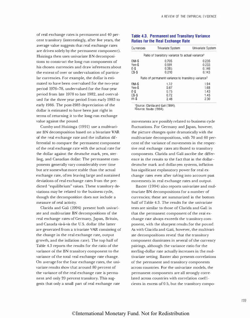
©International Monetary Fund. Not for Redistribution
of real exchange rates is permanent and 40 per
cent u·ansitory (interestingly, after five years, the
average value suggests that real exchange rates
are driven solely by the permanent component).
Huizinga then uses univariate BN decomposi
tions to construct the long-run components of
his chosen currencies and draw inferences about
the extent of over or undervaluation of particu
lar currencies. For example, the dollar is esti
mated to have been overvalued for the two-year
period 1976-78, undervalued for the four-year
period from late 1978 to late 1982, and overvalued for the three year period from early 1983 to
early 1986. The post-1985 depreciation of the dollar is estimated to have been just right in
terms of returning it to the long-run exchange
value against the pound.
Cumby and Huizinga (1991) use a multivari
ate BN decomposition based on a bivariate VAR
of the real exchange rate and the inflation dif
ferential to compare the permanent component
of the real exchange rate with the actual rate for
lhe dollar against the deutsche mark, yen, ster
ling, and Canadian dollar. The permanent com
ponents generally vary considerably over time but are somewhat more stable than the actual
exchange rate, often leaving large and sustained
deviations of real exchange rates from the pre
dicted "equilibrium" values. These transitory de
viations may be related to the business cycle,
lhough the decomposition does not include a
measure of real activity. Clarida and Cali ( 1994) present both univari
ate and multiv-.u-iate BN decompositions of the
real exchange rates of Germany, Japan, Britain,
and Canada vis-a-vis the U.S. dollar (the latter
are generated from a u·ivariate VAR consisting of
the change in the real exchange rate, output
growth, and the inflation rate). The top half of Table 4.3 reports the results for the ratio of the
variance of the BN transitory component to the
variance of the total real exchange rate change. On average for the four exchange rates, the univariate results show that around 80 percent of
the variance of the real exchange rate is perma
nent and only 20 percent transitory. This sug
gests that only a small part of real exchange rate
A REVIEW OF THE EMPIRICAL EVIDENCE
Table 4.3. Permanent and Transitory Variance Ratios for the Real Exchange Rate
Currencies Trivariate System Univariate System
Ratio of transitory variance to actual variance'
OM-$ Yen·$ £-$ C$-$
0.705 0.591 0.385 0.210
0.235 0.233 0.146 0.143
Ratio of permanent variance to transitory variance2
OM-$ 1.72 1.94 Yen-$ 0.67 1.68 £-$ 0.75 1.43 C$-$ 0.72 1.45 FF-$ 2.48 2.30
'Source: Clarida and Gali (1994). 2Source: Baxter (1994).
movements are possibly related to business cycle
fluctuations. For Germany and japan, however,
the picture changes quite dramatically with the
multivariate decompositions, with 70 and 60 per
cent of the variance of movements in the respec
tive real exchange rates atu·ibuted to transitory
components. Clarida and Gali ascribe the differ
ence in the results to the fact that in the dollardeutsche mark and dollar-yen systems, inflation
has significant explanatory power for real ex
change rates even after taking into account past movements in real exchange rates and output
Baxter (1994) also reports univariate and mul
tivariate BN decompositions for a number of
currencies; these are summarized in the bottom
half of Table 4.3. The results for the univariate
tests are similar to those of Clarida and Cali in
that the permanent component of the real ex
change rate always exceeds the u-ansitory com
ponent, with the sharpest results for the pound. As with Clarida and Cali, however, the multivari
ate decompositions reveal that the transitory component dominates in several of the currency
pairings, although the variance ratio for the
sterling-dollar rate actually increases in the mul
tivariate setting. Baxter also presents correlations
of the permanent and transitory components
across countries. For the univariate models, the
permanent components are all strongly correlated across countries with correlation coeffi
cients in excess of 0.5, but the transitory compo-
139
©International Monetary Fund. Not for Redistribution
140
CHAPTER IV BUSINESS CYCLE INFLUENCES ON EXCHANGE RATES
nents show no such dear-cut pattern, with posi
tive correlations for the deutsche mark-Swiss
franc and French franc-Swiss franc rates (both
vis-a-vis the dollar), but zero or negative correla
tions for most other currencies. The multivariate
correlations, however, reveal much stronger evi
dence of positive correlations across counu·ies;
interestingly, the only currency pairings to pro
duce negative correlations are those involving
sterling. In summary, multivariate anaJysis ap
pears to be necessary to provide substantial evi
dence of a business cycle component in real ex
change rates.
"Direct" Empirical Evidence
The identification scheme proposed by
Clarida and Gali (1994) introduces structural
shocks of supply, demand, and nominal ("mone
tary") into the Mundell-Fleming framework. In
the long run, the real equilibrium exchange rate
is a function of demand and supply shocks,
while in the short run, the existence of price
stickiness means that the real exchange rate re
sponds to nominal shocks as well as to demand
and supply shocks. A positive supply side shock
that boosts U.S. output relative to foreign output
is predicted to produce a real depreciation of
the dollar, a fall in U.S. prices, and higher U.S.
output. A positive permanent demand shock
leads to a permanent real appreciation of the
dollar, a higher price level, and increased output
to the extent that prices are sticky. A negative
U.S. money supply shock results in a nominal
dollar depreciation, higher U.S. price level, and
increased U.S. output with sticky prices. If the
nominal shock is permanent, it leads to a perma
nent dollar depreciation as well, but by consu·uc
tion not a permanent real depreciation. Clarida
and GaJi (1994) estimate the model using a
structural VAR along the lines of Blanchard and
Quah in which restrictions are placed on the
permanent effects of shocks on certain variables
while leaving the transitory, or short-term, effects
unconstrained. The focus is on the sources of
real exchange rate fluctuations since the incep
tion of floating exchange rates for the bilateral
exchange rates between the dollar and lhe
deutsche mark, yen, pound, and Canadian dol
lar ove1- the period 1974:Ql tO 1992:Q1. The im
posed restrictions are that nominal shocks affect
the price level in the long run but have only
transitory effects on the real exchange rate and
output; supply and demand shocks have perma
nent effects on the real exchange rate, but only
supply shocks affect the long-run level of (rela
tive) output. This approach has become increas
ingly popular, with additional exchange rates
and variations on the included variables being
estimated by (among many others) Chadha and
Prasad (1997) for Japan, Astley and Gan-ett
(1996) for the United Kingdom, and Thomas
( 1 997) f01· Sweden.
Clarida and GaJi find that at a horizon of 4
quarters, nominaJ shocks account for about 50
and 30 percent of the variance of the mark and
yen rates, respectively, with the effect evenrually
diminishing to zero at longer horizons. However,
nominal shocks have only a small influence on
exchange rates for Canada and tl1e United
Kingdom, accounting for only around 1 percent
of the movements in these currencies against the
U.S. dollar. For all four real exchange rates, de
mand shocks account for virtually all of the re
maining variance, leaving little role for supply
shocks.
The impulse response analysis for the
dollar-deutsche mark exchange rate suggests
that the real exchange rate depreciates by 3.8
percenl (the nominal rate overshoots by 4 per
cent) in response to a one standard deviation
nominaJ shock, while U.S. output rises relative to
German output by 0.5 percent and U.S. inflation
rises relative to German inflation by 0.3 percent.
The output and real exchange rate effects of a
nominal shock last for 16 to 20 quarters. In re
sponse to a one standard deviation shock to rela
tive demand, the dollar appreciates in real terms
by 4 percent vis-a-vis the deutsche mark, U.S. rel
ative output rises by 0.36 percent, and there is a
0.44 percent rise in U.S. inflation relative to
Germany. The effect of the demand shock on
the exchange rate is permanent, with a 6 per
cent real appreciation after 20 quarters. A one
©International Monetary Fund. Not for Redistribution
standard deviation relative supply shock pro
duces a (wrongly signed) 1 percent dollar appre
ciation in quarter 2, but this quickly goes to
zero, with the appreciation after 20 quarters only
0.2 percent above the initial exchange rate.
Chadha and Prasad (1997) apply the Clarida
Cali approach to the yen-dollar real exchange
rate over the period 1975-96. Supply shocks are
found to account for two-thirds of the variance
in japanese output growth relative to the United
States, with demand shocks explaining one-third,
and nominal shocks playing only a very small
role (this is the case for forecast horizons
through 40 quarters) . Mter around 8 quarters,
supply and demand shocks each account for
roughly one quarter of the forecast error vari
ance of the real exchange rate, leaving the re
maining 50 percent explained by nominal
shocks. Chadha and Prasad interpret this as sug
gesting that monetary and fiscal policy have a
substantial effect on the dollar-yen real ex
change rate over the business cycle (the transi
tOry fluctuations), with only a small role for sup
ply shocks such as innovations in productivity
shocks. Although this result suggests that supply
shocks have not been pervasive, it is also fow1d
that these shocks are important when they do
occur, as a "typical" supply shock (that is, a
shock of one standard deviation in magnitude)
leads to a permanent real exchange rate depre
ciation of around 8 percent, while a demand
shock leads to a permanent appreciation, also of
around 8 percent. A nominal shock leads to an
initial real depreciation, but this is eventually off
set with the real rate exchange rate returrung to
the initial level by the end of two years.
Although the approach of Clarida and Cali
and others is insightful and certainly in the spirit
of the relationship between exchange rates and
the business cycle, as discussed by Stockman
(1994), it nonetheless suffers from a number of
important problems. First, the identification pro
cedure forces all temporary shocks that are com-
A REVIEW OF THE EMPIRICAL EVIDENCE
mon to the three variables of output, inflation,
and exchange rates to have a nominal origin, so
that the transitory effects of events such as oil
price shocks and changes in fiscal policy are sub
sumed under nominal shocks. A similar argu
ment holds for temporary demand shocks.
Second, in setting up the identifying assump
tions, it is assumed that the innovations to de
mand and supply are uncorrelated, which, for a
variety of reasons, seems implausible (i.e., a posi
tive shock to aggregate demand spurs invest
ment, which increases the capital stock and thus
aggregate supply). Third, the finding that nomi
nal shocks generally account for only a small
part of movements in relative output raises the
question of whether this is due to the way nomi
nal shocks are specified.6
The empirical work on real exchange rate re
lationships can be summarized in the following
way. The real exchange rates of leading indus
trial countries have important transitory compo
nents, the magnitude of which depends on the
particular currency and the methods used to de
compose permanent and u·ansitory fluctuations.
In the applications so far, the richer the informa
tion set in terms of the nwnber of variables
used, the larger is the transitory component rel
ative to the permanent component.
Irrespective of the methods used, empirical evi
dence based on the real exchange rate-real inter
est rate model points to the importance of transi
tory components such as business cycle
fluctuations in explaining movements in real ex
change rates. This is particularly the case for the
deutscbe mark and yen, but less so for the pound.
However, these findings are based in a sense on
averages constructed from data for the post-1973
period of floating rates, which could possibly dis
guise important regime shifts such as financial
deregulation that occurred in the 1980s. This
deregulation potentially increased the mobility of
capital and thus affected the relationship between
interest rates and exchange rates.
6Sarte (1994) demonsmnes that identification in structural VARs is sensitive to the assumed restrictions.
141
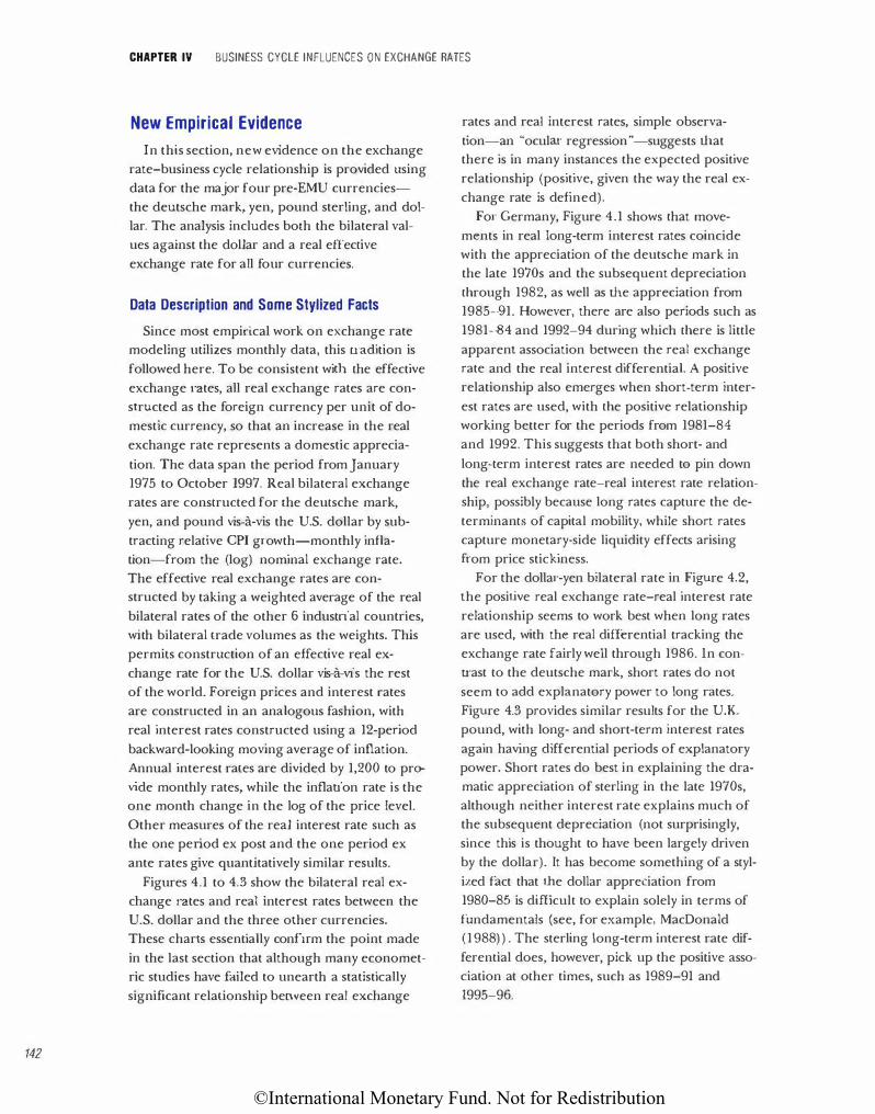
©International Monetary Fund. Not for Redistribution
142
CHAPTER IV BUSINESS CYCLE INFLUENCES ON EXCHANGE RATES
New Empirical Evidence
In this section, new evidence on the exchange
rate-business cycle relationship is provided using
data for the major four pre-EMU currencies
the deutsche mark, yen, pound sterling, and dol
lar. The analysis includes both the bilateral val
ues against the dollar and a real effective
exchange rate for all four currencies.
Data Description and Some Stylized Facts
Since most empirical work on exchange rate
modeling utilizes monthly data, this n-adition is
followed here. To be consistent with the effective
exchange rates, all real exchange rates are con
structed as the foreign currency per unit of do
mestic currency, so that an increase in the real
exchange rate represents a domestic apprecia
tion. The data span the period from january
1975 to October 1997. Real bilateral exchange
rates are constructed for the deutsche mark,
yen, and pound vis-a-vis the U.S. dollar by sub
tracting relative CPI gt·owth-monthly infla
tion-from the (log) nominal exchange rate.
The effective real exchange rates are con
structed by taking a weighted average of the real
bilateral rates of the other 6 industrial countries,
with bilateral trade volumes as the weights. This
permits construction of an effective real ex
change rate for the U.S. dollar vis-a-vis the rest
of the world. Foreign prices and interest rates
are constructed in an analogous fashion, with
real interest rates constructed using a 12-period
backward-looking moving average of inflation.
Annual interest rates are divided by 1,200 to pro
vide monthly rates, while the inflation rate is the
one month change in the log of the price level.
Other measures of the real interest rate such as
the one period ex post and the one period ex
ante rates give quantitatively similar results.
Figures 4.1 to 4.3 show the bilateral real ex
change rates and real interest rates between the
U.S. dollar and the three other currencies.
These charts essentially confirm the point made
in the last section that although many economet
ric studies have failed to unearth a statistically
significant relationship between real exchange
rates and real interest rates, simple observa
tion-an "ocular regression "-suggests that
there is in many instances the expected positive
relationship (positive, given the way the real ex
change rate is defined).
Fot· Germany, Figure 4.1 shows that move
ments in real long-term interest rates coincide
with the appreciation of the deutsche mark in
the late 1970s and the subsequent depreciation
through 1982, as well as the appreciation from
1985-91. However, there are also periods such as
1981-84 and 1992-94 during which there is little
apparent association between the real exchange
rate and the real interest differential. A positive
relationship also emerges when short-term inter
est rates are used, with the positive relationship
working better for the periods from 1981-84
and 1992. This suggests that both short- and
long-term interest rates are needed to pin down
the real exchange rate-real interest rate relation
ship, possibly because long rates capture the de
terminants of capital mobility, while short rates
capture monetary-side liquidity effects arising
from price stickiness.
For the dollat·-yen bilateral rate in Figure 4.2,
the positive real exchange rate-real interest rate
relationship seems to work best when long rates
are used, with the real differential tracking the
exchange rate fairly well through 1986. In con
u·ast to the deutsche mark, short rates do not
seem to add explanatory power to long rates.
Figure 4.3 provides similar results for the U.K. pound, with long- and short-term interest rates
again having differential periods of explanatory
power. Short rates do best in explaining the dra
matic appreciation of sterling in the late 1970s,
although neither interest rate explains much of
the subsequent depreciation (not surprisingly,
since this is thought to have been largely driven
by the dollar). It has become something of a styl
ized fact that the dollar appreciation from
1980-85 is difficult to explain solely in terms of
fundamentals (see, for example, MacDonald
(1988)) . The sterling long-term interest rate dif
ferential does, however, pick up the positive asso
ciation at other times, such as 1989-91 and
1995-96.
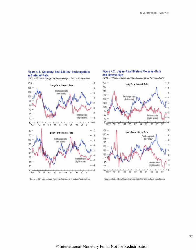
©International Monetary Fund. Not for Redistribution
Figure 4.1 . Germany: Real Bilateral Exchange Rate and Interest Rate (1975 = 100 for exchange rate; in percentage points for Interest rate) 130-
long· Term Interest Rate
70 -
60 -
- 10
- 8
50 -40 �-L��-L��-L��-L��-L��� � 1977 79 81 83 85 87 89 91
130 -120 -
100 -90 80
60-50 -40 I I
1977 I I I I
79 81
Short· Term Interest Rate
I I I I I I I I 83 85 87 89 91
93 95 97
I I I I 93 95 97
- 10
- 8
- 6
4
2
0
- -4 · �
Sources: IMF. lntemational Financial Statistics; and authors· calculations.
NEW EMPIRICAL EVIDENCE
Figure 4.2. Japan: Real Bilateral Exchange Rate and Interest Rate (1975 = 100 for exchange rate; In percentage points for interest rate)
250 -230 -210 -1 90 -
150-130-110 90 70 -
long· Term Interest Rate - 10 - 8
- 6
- 4
2 0
501�97=-=7�79:-'-'L::-81�'::-83:-'-'L::-85::'---"L::-87::'---l'-:-89�'-:-91�'-:-93�'-:-95�'-97� �
250 -230 -210-190 -
110 90 -70 -
Short· Term Interest Rate
Exchange rate (left scale)
- 10
- 8 - 6
- 4 2
0
50 1'::97=-=7�79:;-l-'::81�'::83:;-l-'::85:;-L-L::-87:;-L-L::-89:;-l-'::91�'-:-93�'-:-95�L-'-� �
Sources: IMF. lntemational Financial Statis tics; and authors' calculations.
143
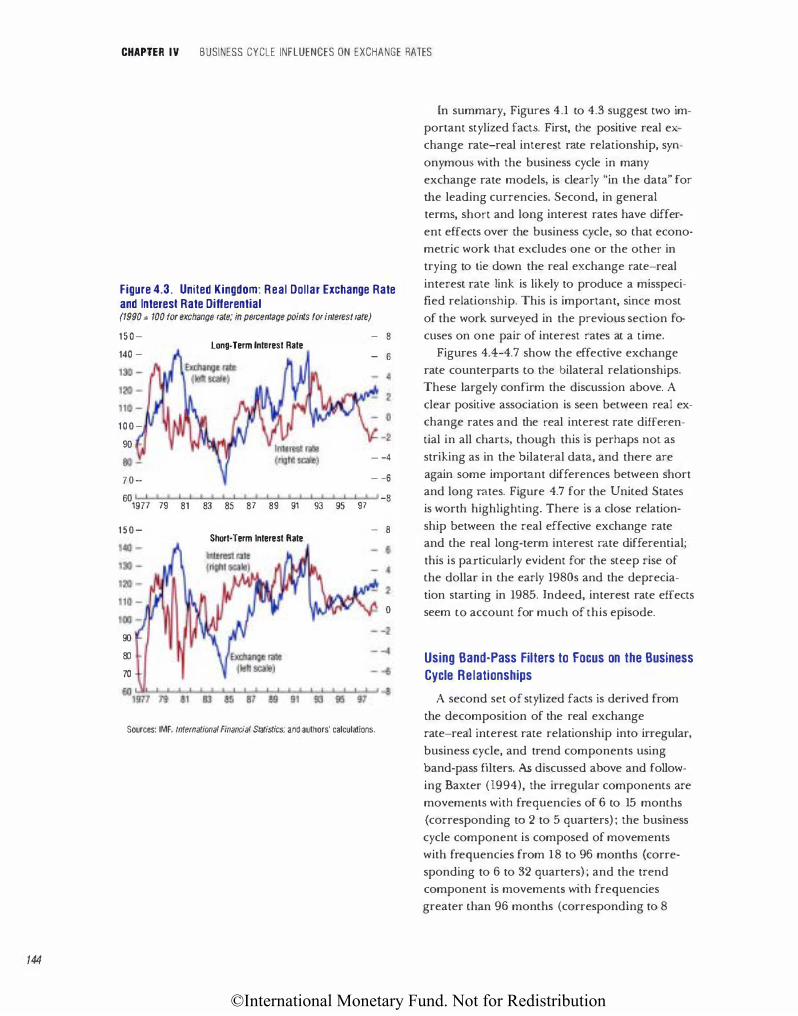
©International Monetary Fund. Not for Redistribution
144
CHAPTER IV BUSINESS CYCLE INFLUENCES ON EXCHANGE RATES
Figure 4.3. United Kingdom: Real Dollar Exchange Rate and Interest Rate Differential (1990 = 100 tor exchange rate; in percentage points tor interest rate)
150- - 8
140 -
100-
90
long-Term Interest Rate - 6
-2
- -4
ro- -� 60 -8
1977 79 81 83 85 87 89 91 93 95 97
150- - 8 Short-Term Interest Rate
[n summary, Figures 4.1 to 4.3 suggest two im
portant stylized facts. First, the positive real ex
change rate-real interest rate relationship, syn
onymous with the business cycle in many
exchange rate models, is clearly "in the data" for
the leading currencies. Second, in general
terms, short and long interest rates have differ
ent effects over the business cycle, so that econo
metric work that excludes one or the other in
trying to tie down the real exchange rate-real
interest rate link is likely to produce a misspecified relationship. This is important, since most
of the work surveyed in the previous section fo
cuses on one pair of interest rates at a time.
Figures 4.4-4.7 show the effective exchange
rate counterparts to the bilateral relationships.
These largely confirm the discussion above. A clear positive association is seen between real ex
change rates and the real interest rate differen
tial in all charts, though this is perhaps not as
striking as in the bilateral data, and there are
again some important differences between short
and long rates. Figme 4.7 for the United States
is worth highlighting. There is a close relation
ship between the real effective exchange rate
and the real long-term interest rate differential;
this is particularly evident for the steep rise of
the dollar in the early 1980s and the deprecia
tion starting in 1985. Indeed, interest rate effects o seem to account for much of this episode.
90
80
70
Sources: IMF, International Financial Statistics; and authors' calculations.
Using Band-Pass Filters to Focus on the Business Cycle Relationships
A second set of stylized facts is derived from
the decomposition of the real exchange
rate-real interest rate relationship into irregular,
business cycle, and trend components using
band-pass filters. As discussed above and follow
ing Baxter (1994), the irregular components are
movements with frequencies of 6 to 15 months
(corresponding to 2 to 5 quarters) ; the business
cycle component is composed of movements
with frequencies from 18 to 96 months (corre
sponding to 6 to 32 quarters) ; and the trend
component is movements with frequencies
greater than 96 months (corresponding to 8
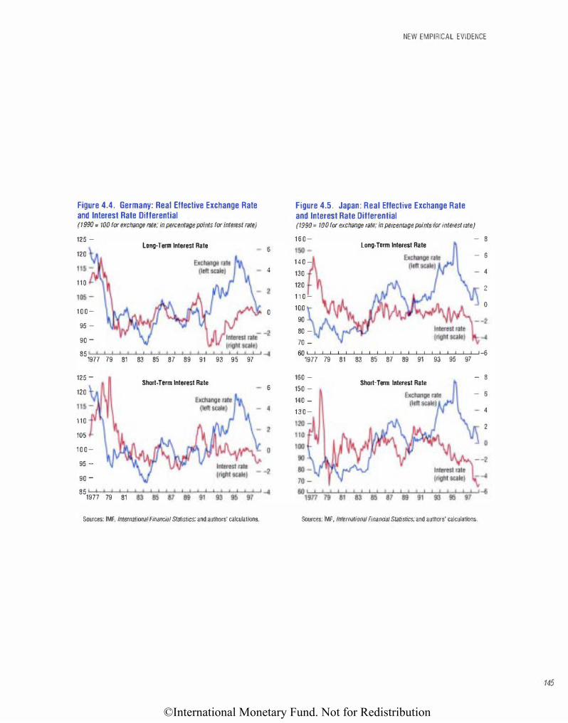
©International Monetary Fund. Not for Redistribution
Figure 4.4. Germany: Real Effective Exchange Rate and Interest Rate Differential (1990 = 100 for exchange rate; in percentage points for interest rate)
125 -
120
110
1 0 0 -
95 -
90 -
85 1977
125 -
120
110
105 1 0 0 -
95 -
90 -
85 1977
79 81
79 81
Long· Term Interest Rate
83 85 87 89 91 93 95 97
Short· Term Interest Rate
Sources: IMF, International Financial Statistics; and authors· calculations.
6
4
0
-4
6
NEW EMPIRICAL EVIDENCE
Figure 4.5. Japan: Real Effective Exchange Rate and Interest Rate Differential (1990 = 100 for exchange rate; in percentage points for interest rate)
1 6 0 -
1 4 0 -
130
120
1 1 0 -
100
90
80 -
- 8 long· Term Interest Rate
- 6
4
2
0
70 -
60�-L��-L��-L��-L��_L���
-4
-6 1977 79 81 83 85 87 89 91
160 -
150 -
140 -
1 3 0 -
Short· Term Interest Rate
93 95 97
- 8
- 6
4
2
Sources: IMF, International Financial Statistics; and authors' calculations.
145
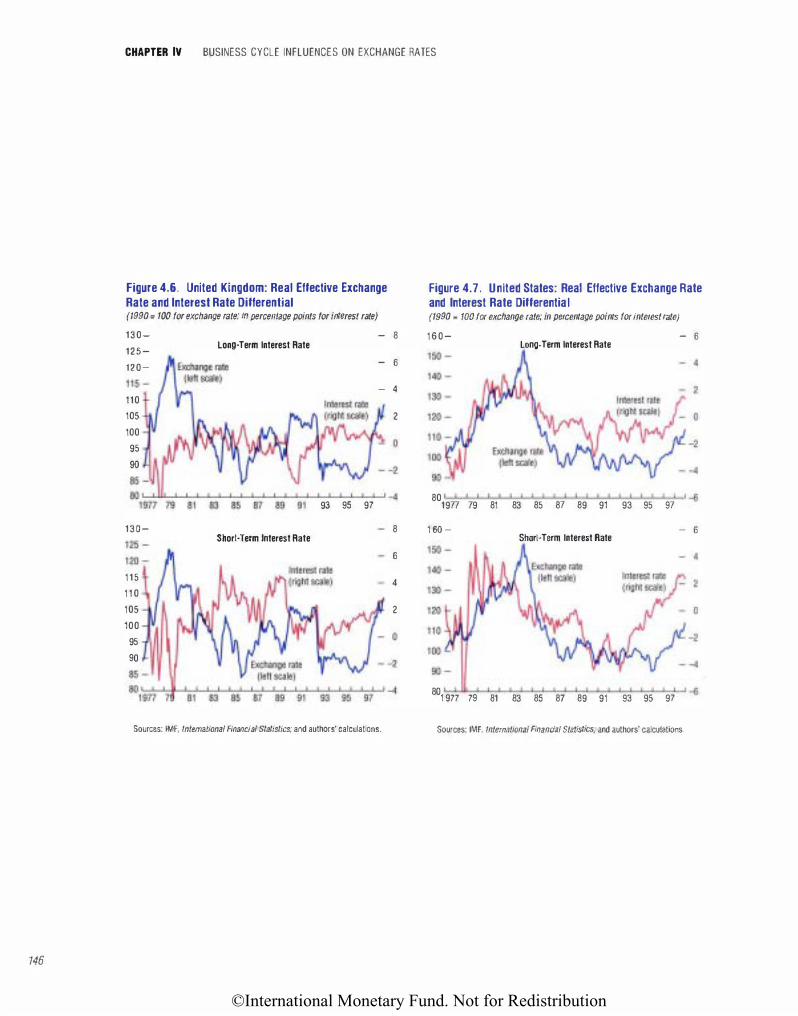
©International Monetary Fund. Not for Redistribution
146
CHAPTER IV BUSINESS CYCLE INFLUENCES ON EXCHANGE RATES
Figure 4.6. United Kingdom: Real Effective Exchange Rate and Interest Rate Differential (1990 = 100 for exchange rate; in percentage points tor interest rate)
130-125-120-
110 105 100 95 90
130-
115 110 105 100 95 90
long· Term Interest Rate
93 95 97
Short· Term Interest Rate
- 8
- 6
- 4
2
8
6
4
2
Sources: IMF, International Financial Statistics; and authors' calculations.
Figure 4.7. United States: Real Effective Exchange Rate and Interest Rate Differential (1990 = 100 for exchange rate; in percentage points for interest rate)
160- - 6 long-Term Interest Rate
801977 79 81 83 85 87 89 91 93 95 97 -6
1 60 - - 6 Short-Term Interest Rate
801977 79 81 83 85 87 89 91 93 95 97 -6
Sources: IMF, International Financial Statistics; and authors' calculations.
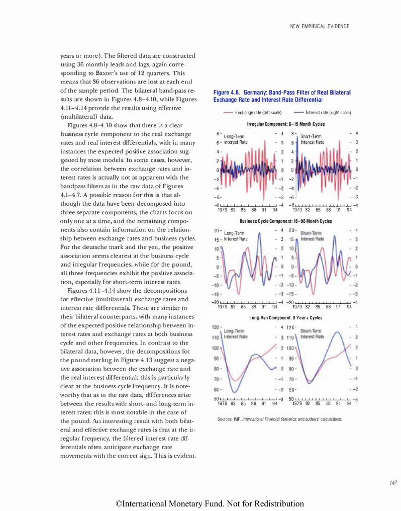
©International Monetary Fund. Not for Redistribution
years or more). The filtered data are constructed
using 36 monthly leads and lags, again corre
sponding to Baxter's use of 12 quarters. This means that 36 observations are lost at each end
of the sample period. The bilateral band-pass re
sults are shown in Figures 4.8-4.10, while Figures
4.11-4.14 provide the results using effective
(multilateral) data.
Figures 4.8-4.10 show that there is a clear
business cycle component to the real exchange
rates and real interest differentials, with in many
instances the expected positive association sug
gested by most models. In some cases, however,
the correlation between exchange rates and in
terest rates is actually not as apparenl with the
bandpass filters as in the raw data of Figures
4.1-4.7. A possible reason for this is that al
though the data have been decomposed into
three separate components, the charts focus on
only one at a time, and the remaining compo
nents also contain information on the relation
ship between exchange rates and business cycles.
For the deutsche mark and the yen, the positive
association seems clearest at the business cycle
and irregular frequencies, while for the pound,
all three frequencies exhibit the positive associa
tion, especially for short-term interest rates.
Figures 4.1 1-4.14 show the decompositions
for effective (multilateral) exchange rates and
interest rate differentials. These are similar to
their bilateral counterparts, with many instances
of the expected positive relationship between in
terest rates and exchange rates at both business
cycle and other frequencies. In contrast to the
bilateral data, however, the decompositions for
the pound sterling in Figure 4.13 suggest a nega
tive association between the exchange rate and
the real interest differential; this is particularly
clear at the business cycle frequency. It is note
worthy that as in the raw data, differences arise
between the results with short- and long-term in
terest rates; this is most notable in the case of
the pound. An interesting result with both bilat
eral and effective exchange rates is that at the ir
regular frequency, the filtered interest rate dif
ferentials often anticipate exchange rate
movements with the correct sign. This is evident,
NEW EMPIRICAL EVIDENCE
Figure 4.8. Germany: Band-Pass Filter of Real Bilateral Exchange Rate and Interest Rate Differential
-- Exchange rate (left scale) - Interest rate (right scale)
Irregular Component: 6-15 Month Cycles
8 • Long· Term
- 4 8 -Short-Term
- 4
6 - Interest Rate
4 -
2
0
-2
- 4 -
-6-
- 3
- -3
6 Interest Rate
4
2
0
-2
-4 -6
- 3
0
-1
- -3 -8 I I I I I I I I I I I I I I I I I -4 -8t I I I I I I I I I I I I I I I I -4
1979 82 85 88 91 94 1979 82 85 88 91 94
Business Cycle Component: 18-96 Month Cycles
20 • Long· Term 15 - Interest Rate
- 4 20-
- 3 15
10
- 4
-20 I I I I I I I I I I I I I I I I I -4 -20 I I I I I I I I I I I I I I I I I -4 1979 82 85 88 91 94 1979 82 85 88 91 94
Long-Run Component: 8 Year+ Cycles
- 4 120-
110
100
60-
- 4
- -2
50 I I I I I I I I I I I I I I I I I -3 1979 82 85 88 91 94
50 I ! I I I I I I I I I I I I I I I -3 1979 82 85 88 91 94
Sources: IMF, International Financial Statistics; and authors' calculations.
141
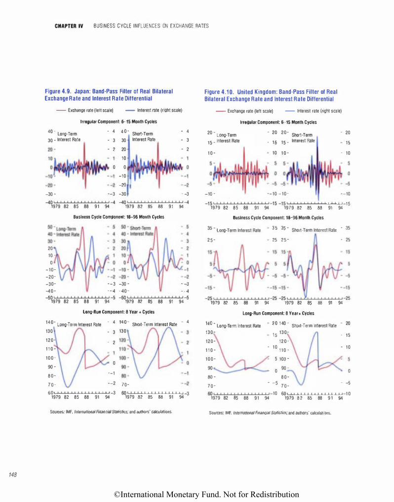
©International Monetary Fund. Not for Redistribution
148
CHAPTER IV BUSINESS CYCLE INFLUENCES ON EXCHANGE RATES
Figure 4.9. Japan: Band-Pass Filter of Real Bilateral Exchange Rate and Interest Rate Differential
-- Exchange rate (left scale) -- Interest rate (right scale)
Irregular Component: 6-15 Month Cycles
40 - Long-Term
30 - Interest Rate
-30 -
- 4
- 3 - 2
0
--3
4 0 -Short-Term
30 Interest Rate
20 10
0 -10 -20
-30
- 4 - 3 - 2
- -3 -40 I I I I I I I I I I I I I I I I I -4 -40 I I I I I I I I I I I I I I I I I -4
1979 82 85 88 91 94 1979 82 85 88 91 94
20 10 -
0 -10--20--30-
Buslneu Cycle Component: 18-96 Month Cycles
--3 -30 - - -3 -40- --4 -40- - - 4 -50 I I I I I I I I I I I I I I I I I -5 -50 I I I I I I I I I I I I I I I I I -5
1979 82 85 88 91 94 1979 82 85 88 91 94
Long-Run Component: 8 Year + Cycles
140- Long· Term Interest Rate
130 120-1 1 0 -100-
90 -80-70-
- 4
- 3
- 2
0
--1
--2
140- Short-Term Interest Rate
130
70-
- 4
--2 60, I It! I ! I I I I I I I I I ,_3 60• I I I I I I I I I I I I I I I , _3
1979 82 85 88 91 94 1979 82 85 88 91 94
Sources: IMF, Jnternatiooal Rnancial Statis tics; and author$' caltulations.
Figure 4.10. United Kingdom: Band-Pass Filter of Real Bilateral Exchange Rate and Interest Rate Differential
-- Exchange rate (left scale) -- Interest rate (right scale)
Irregular Component: 6-15 Month Cycles
20 • Long-Term
15 _ Interest Rate
1 0 -
-10 -
- 20 20-Short-Term
_ 15 15 _ Interest Rate
10 1 0 -
--10 -10-
- 20
15
- 10
--10 -15 1 I I I I 1 1 1 1 I I I I I I I 1-15 -15 I I I I I I I I I I I I I I I I 1-15
1979 82 85 88 91 94 1979 82 85 88 91 94
Business Cycle Component: 1&-96 Month Cycles
35 • Lono·Term Interest Rate
2 5 -
3 5 35 - Short-Term Interest Rate - 35
25 25- - 25
-25 I I I I I I I I I I I I I I I I I -25 -25 I I I I I I I I I I I I I I I I 1 -25 1979 82 85 88 91 94 1979 82 85 88 91 94
Long-Run Component: 8 Year+ Cycles
140 -Long· Term Interest Rate
130-120-1 1 0 -100-
90 80 -70-
20 140 - Short-Term Interest Rate 20
1 5 130' - 15
120-- 10 110 - - 10
- 5 100 -
0 90 - 0 80-
- -5 70- - -5 601 I I I I I I I I I I I I I I I I 10 601 I I I I I I I I I I I I I I I I 1 0
1979 82 85 88 91 94 1979 82 85 88 9 1 94
Sources: IMF, lntemational Financial Statistics; and author$' calculations.
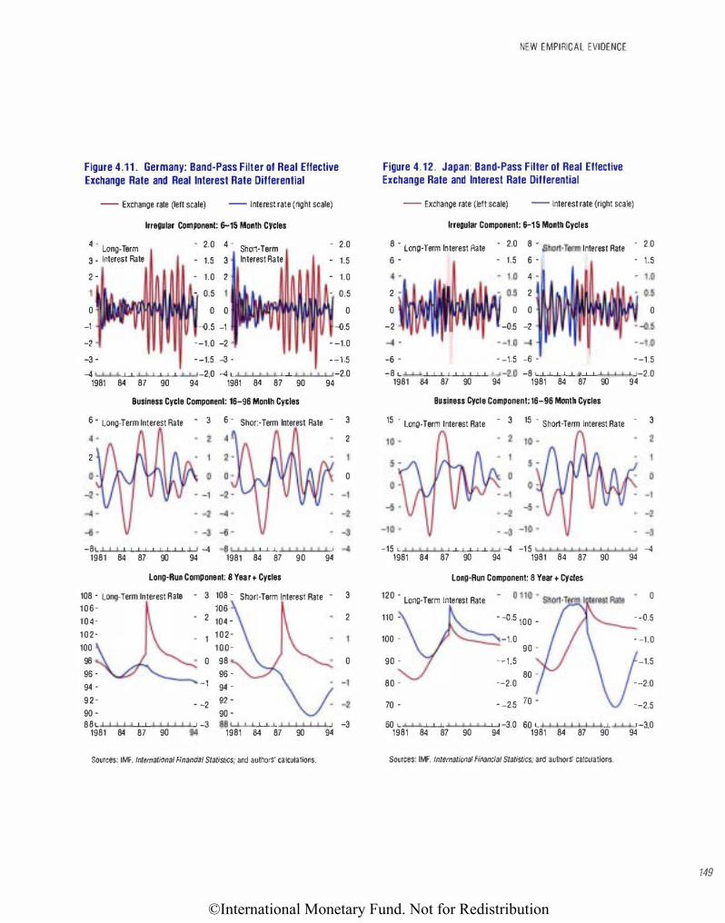
©International Monetary Fund. Not for Redistribution
Figure 4.11 . Germany: Band-Pass Filler of Real Effective Exchange Rate and Real Interest Rate Differential
-- Exchange rate (left scale) -- Interest rate (right scale)
4 - Long· Term
3 - Interest Rate
2 -
0 -1 -2
Irregular Component: 6-15 Month Cycles
- 2.0 4 --
--
1.5 3 1.0 2
0.5 0 0
-o.5 -1 --1.0 -2
Short-Term Interest Rate
- 2.0 - 1.5 - 1.0 - 0.5
0 -o.5
--1.0 -3 - --1.5 -3 · --1.5 -4 I I I I I I I I I I I I I I -2.0 -4 I I I I I I I I I I I I I I -2.0
1981 84 87 90 94 1981 84 87 90 94
Business Cycle Component: 16-96 Month Cycles
6 • Long-Term Interest Rate • 3 6 · Short· Term Interest Rate - 3
2
2
0
-8t I I I I I I I I I I I I I -4 -8 1 I I J I I I I I I I -4 1981 84 87 90 94 1981 84 87 90 94
Long-Run Component: 8 Year+ Cycles
108 • Long-Term Interest Rate - 3 108 - Short· Term Interest Rate - 3 106- 106 104- - 2 104 - 2 102- - 1 102-100 100-98 - 0 98 0 96 - 96 -94 -
-1 94 -92- - -2 92 -90 - 90 -88t I I I I I I I I 1 -3 881 I I I I I I I I -3
1981 84 87 90 94 1981 84 87 90 94
Sources: IMF, International Financial Statistics; and authors' calculations.
NEW EMPIRICAL EVIDENCE
Figure 4.12. Japan: Band-Pass Filter of Real Effective Exchange Rate and Interest Rate Differential
-- Exchange rate (left scale) -- Interest rate (right scale)
Irregular Component: 6-15 Month Cycles
8 - Long-Term Interest Rate - 2.0 8 -
Interest Rate . 2.0
6 - - 1.5 6 - - 1.5 4 .
2 2 0 0 0 0
-2 -o.5 -2
-4
-6 - --1.5 -6 - --1.5 -8 I I I I I I I I I I I I I l-2.0 -8 I I I I I I I I I I I I 1-2.0
1981 84 87 90 94 1981 84 87 90 94
Business Cycle Component: 16-96 Month Cycles
15 · long-Term Interest Rate - 3 15 · Short-Term Interest Rate · 3
-15 I I I I I I I I I I I I I -4 -15 -4 1981 84 87 90 94 1981 84 87 90 94
Long-Run Component: 8 Year + Cycles
120 -long-Term Interest Rate
0
110 - • -o.5 100 - --o.5
100 - -1.0 - -1.0 90 -
90 - --1.5 -1.5 80 -
80 - --2.0 --2.0
70 - --2.5 70 - --2.5
60 I I I I I I I I I I l-3,0 60 I I I I I I I I I I 1-3.0 1981 84 87 90 94 1981 84 87 90 94
Sources: IMF, International Financial Statistics; and authors' calculations.
149
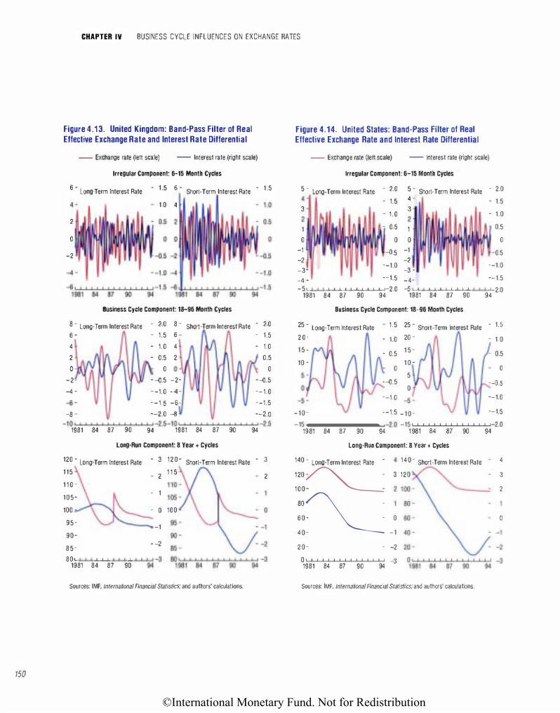
©International Monetary Fund. Not for Redistribution
150
CHAPTER IV BUSINESS CYCLE INFLUENCES ON EXCHANGE RATES
Figure 4.13. United Kingdom: Band-Pass Filter of Real Effective Exchange Rate and Interest Rate Differential
- Exchange rate (left scale) -- Interest rate (right scale)
Irregular Component: 6-15 Month Cycles
6 · Long-Term Interest Rate • 1·5 6 • Short-Term Interest Rate • 1·5
1.0 4
2
0
-2
Business Cycle Component: 18-96 Month Cycles
8 - Long· Term Interest Rate - 2.0 8 - Short-Term Interest Rate - 2·0
6 · 4 2
o -
-2-
-4 -
-6 -
-8 --101 I I I
1981 84 87 90
- 1.5 6 -
- 1.0 4 - 0.5 2
0 - -o.5 -2---1.0 -4-·-1.5 -6-
--2.0 -8 11 2.5-1011 II 94 1981 84 87 90
Long-Run Component: 8 Year + Cycles
120 · Long-Term Interest Rate
115
1 1 0 -
105-
100 -
95-
90-
8 5 -801 I I I I I I I I I
1981 84 87 90
- 3 120- Short-Term Interest Rate
2 1 1 5
- 1
- 0 100
-1
- -2
Sources: 1Mf1 International Financial Statistics; and authors' calculations.
- 1.5 - 1.0
0.5 0
--o.5
--1.0 --1.5
--2.0
I I 2.5 94
- 3
2
Figure 4.14. United States: Band-Pass Filter of Real Effective Exchange Rate and Interest Rate Differential
- Exchange rate (left scale) -- Interest rate (right scale)
Irregular Component: 6-15 Month Cycles
5 - Long-Term Interest Rate - 2.0 5 - Short-Term Interest Rate - 2.0 4 - - 1.5 4 - 1.5 3
1.0 3
1.0 - -2
1 - 0.5 1 0.5
0 0 0 0 -1 -o.5 -1 -0.5 -2 -2 -3-
--1.0 -3 -
--1.0
-4 · --1.5 -4· --1.5
-51 I I I I I I I I I I I I 1-2.0 -5 1 I I I I I I I I I I I I 1-2.0 1981 84 87 90 94 1981 84 87 90 94
Business Cycle Component: 18-96 Month Cycles
25 • Long-Term Interest Rate 1.5 25 • Short-Term Interest Rate •
1.S
2 0 - - 1.0 20 - - 1.0 1 5 -
10 -- 0.5 1 5 - - 0.5
1 0 -0 0
5 --o.5 --o.s
0 --1.0 --1.0
-10- --1.5 -10- --1.5
-15 L..L.J....L..J....L..J....l-L..JW...L..J...J.J 2.0 -15 L..L.J....L..J....L-':-'-L..J':-:'-L..J...J.J-2.0 1981 84 87 90 94 1 981 84 87 90 94
Long-Run Component: 8 Year + Cycles
140 - Long-Term Interest Rate - 140- Short-Term Interest Rate
120� 3 120
100- -80� 60- -
40-
0
-1
20- - -2
Q t I I I I I I I I I I I -3 1981 84 87 90 94
Sources: IMF, International Financial Statistics; and authors' calculations.
4
3
2
0
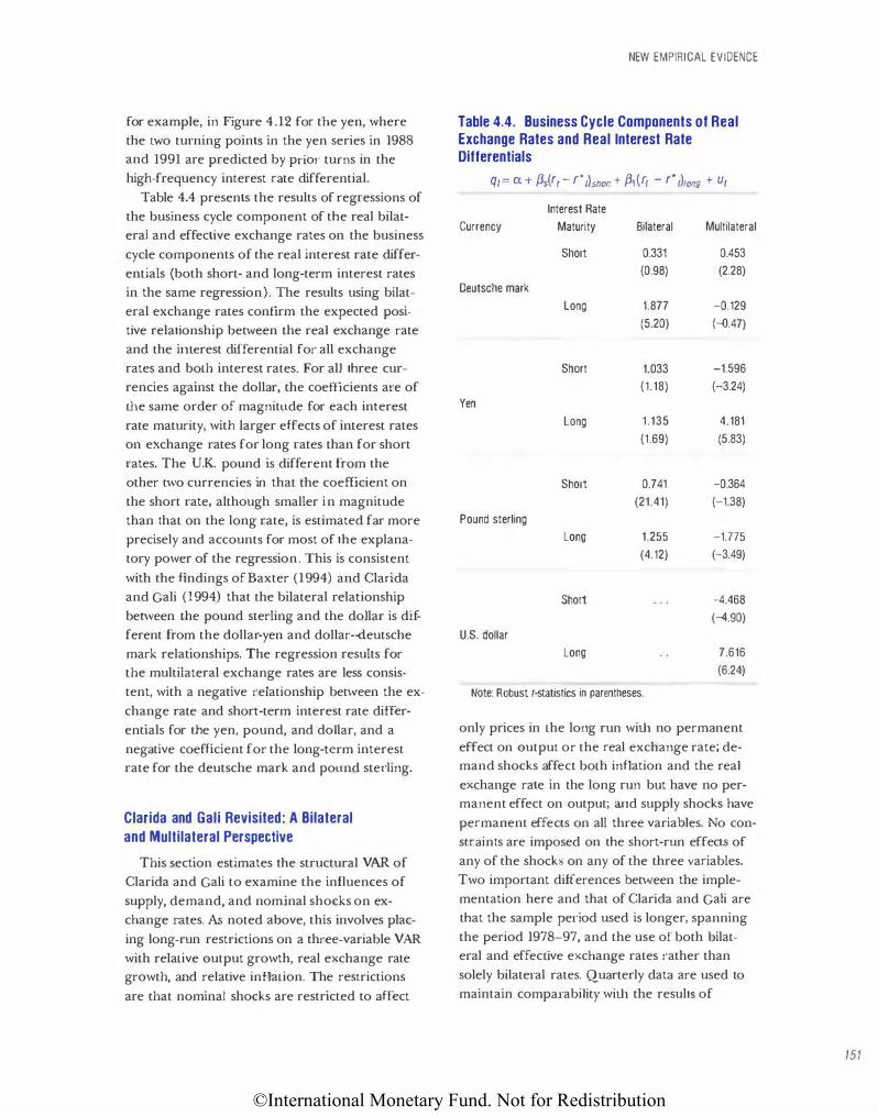
©International Monetary Fund. Not for Redistribution
for example, in Figure 4.12 for the yen, where
the n ... o turning points in the yen series in 1988 and 1991 are predicted by pdo1· turns in the
high-frequency interest rate differential.
Table 4.4 presents the results of regressions of
the business cycle component of the real bilat
eral and effective exchange rates on the business
cycle components of the real interest rate differ
entials (both short- and long-term interest rates
in the same regression). The results using bilat
eral exchange rates confirm the expected posi
tive relationship ben...een the real exchange rate
and the interest differential for all exchange
rates and both interest rates. For all three cur
rencies against the dollar, the coefficients are of
the same order of magnitude for each interest
rate maturity, with larger effects of interest rates
on exchange rates for long rates than for short
rates. The U.K pound is different from the
other n...o currencies in that the coefficient on
the short rate, although smaller in magnitude
than that on the long rate, is estimated far more
precisely and accounts for most of the explana
tory power of the regression. This is consistent
with the findings of Baxter (1994) and Clarida
and Cali (1994) that the bilateral relationship
between the pound sterling and the dollar is dif
ferent from the dollar-yen and dollar-deutsche
mark relationships. The regression results for
the multilateral exchange rates are less consis
tent, with a negative relationship benveen the ex
change rate and short-term interest rate differ
entials for the yen, pound, and dollar, and a
negative coefficient for the long-term interest
rate for the deutsche mark and pound sterling.
Clarida and Gali Revisited: A Bilateral and Multilateral Perspective
This section estimates the structural VAR of
Clarida and Cali to examine the influences of
supply, demand, and nominal shocks on ex
change rates. As noted above, this involves plac
ing long-run restrictions on a three-variable VAR
with relative output growth, real exchange rate
growth, and relative inflation. The restrictions
are that nominal shocks are restricted to affect
NEW EMPIRICAL EVIDENCE
Table 4.4. Business Cycle Components of Real Exchange Rates and Real Interest Rate Differentials
ql = C1. + f3s(r, - r*t)short + {3,(rt - r• tllong + Ut
Interest Rate
Currency Maturity Bilateral Multilateral
Short 0.331 0.453
(0.98) (2.28)
Deutsche mark
long 1.877 -0.129
(5.20) (-Q.47)
Short 1.033 -1.596
(1.18) (-3.24)
Yen
long 1.135 4.181
(1.69) (5.83)
Short 0.741 -0.364
(21.41) (-1.38)
Pound sterling
Long 1.255 -1.775
(4.12) (-3.49)
Short -4.468
(-4.90)
U.S. dollar
Long 7.616
(6.24)
Note: Robust t·statistics in parentheses.
only prices in the long run with no permanent
effect on output or the real exchange rate; de
mand shocks affect both inflation and the real
exchange rate in the long run but have no per
manent effect on output; and supply shocks have
permanent effects on all three variables. No con
straints are imposed on the short-run effects of
any of the shocks on any of the three variables.
Two important differences ben.,een the imple
mentation here and that of Clarida and Cali are
that the sample pel"iod used is longer, spanning
the period 1978-97, and the use of both bilat
eral and effective exchange rates rather than
solely bilateral rates. Quarterly data are used to
maintain comparability with the results of
151
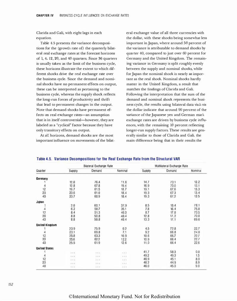
©International Monetary Fund. Not for Redistribution
152
CHAPTER IV BUSINESS CYCLE INFLUENCES ON EXCHANGE RATES
Clarida and Gali, with eight lags in each
equation.
Table 4.5 presents the variance decomposi
tions for the (growth rate of) the quarterly bilat
eral real exchange rates at the forecast horizons
of 1, 4, 12, 20, and 40 quarters. Since 36 quarters
is usually taken as the limit of the business cycle,
these horizons illustrate the extent to which dif
ferent shocks drive the real exchange rate over
the business cycle. Since the demand and nomi
nal shocks have no permanent effects on output,
these can be interpreted as pertaining to the
business cycle, whereas the supply shock reflects
the long-run forces of productivity and thrift
that lead to permanent changes in the output.
Note that demand shocks have permanent ef
fects on real exchange rates-an assumption
that is in itself controversial-however, they are
labeled as a "cyclical" factor because they have
only transitory effects on output.
At all horizons, demand shocks are the most
important influence on movements of the bilat-
eral exchange value of all three currencies with
the dollar, with these shocks being somewhat less
important in Japan, where around 50 percent of
the variance is attributable to demand shocks by
quarter 40, compared to just over 60 percent for
Germany and the United Kingdom. The remain
ing variance in Germany is split roughly evenly
between the supply and nominal shocks, while
for Japan the nominal shock is nearly as impor
tant as the real shock. Nominal shocks hardly
matter in the United Kingdom, a result that
matches the findings of Clarida and Gali.
Following the interpretation that the sum of the
demand and nominal shock represents the busi
ness cycle, the results using bilateral data vis-a-vis
the dollar indicate that around 90 percent of the
variance of the Japanese yen and German mark
exchange rates are driven by business cycle influences, with the remaining 10 percent reflecting
longer-run supply factors. These results are gen
erally similar to those of Clarida and Gali, the
main difference being that in their results the
Table 4.5. Variance Decompositions for the Real Exchange Rate from the Structural VAR
Bilateral Exchange Rate Multilateral Exchange Rate
Quarter Supply Demand Nominal Supply Demand Nominal
Germany 1 12.0 76.4 11.6 14.7 73.1 12.2 4 12.8 67.8 19.4 16.9 70.0 13.1
12 19.7 61.5 18.7 19.1 67.6 13.3 20 20.6 61.0 18.4 19.3 67.3 13.4 40 20.7 60.9 18.4 19.3 67.2 13.5
Japan 1 2.0 60.1 37.9 8.5 13.4 78.1 4 6.2 58.7 35.1 7.8 16.4 75.8
12 8.4 51.3 40.3 8.7 17.8 73.5 20 8.8 50.8 40.4 12.8 17.2 70.0 40 8.8 50.8 40.4 13.3 17.1 69.6
United Kingdom 1 23.9 75.9 0.2 4.5 72.8 22.7 4 23.1 69.8 7.1 9.2 66.8 24.0
12 25.8 63.3 10.9 10.6 66.7 22.7 20 25.6 62.2 1 2.2 10.9 66.4 22.7 40 25.5 61.9 12.6 11.0 66.4 22.6
United States 1 41.7 58.3 0.0 4 49.2 49.3 1.5
12 46.9 45.1 8.0 20 46.2 44.9 8.9 40 46.0 45.0 9.0
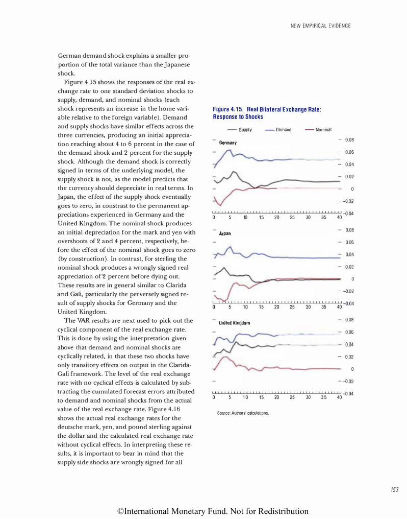
©International Monetary Fund. Not for Redistribution
German demand shock explains a smaller pro
portion of the total variance than the Japanese
shock.
Figure 4.15 shows the responses of the real ex
change rate to one standard deviation shocks to
supply, demand, and nominal shocks (each
shock represents an increase in the home variable relative to the foreign variable). Demand
and supply shocks have similar effects across the
three currencies, producing an initial apprecia
tion reaching about 4 to 6 percent in the case of
the demand shock and 2 percent for the supply
shock. Although the demand shock is correctly
signed in terms of the underlying model, the
supply shock is not, as the model predicts that
the currency should depreciate in real terms. In
Japan, the effect of the supply shock eventually
goes to zero, in constrast to the permanent ap
preciation:; experienced in Germany and the
United Kingdom. The nominal shock produces
an initial depreciation for the mark and yen with
overshoots of 2 and 4 percent, respectively, be
fore the effect of the nominal shock goes to zero
(by construction). In contrast, for sterling the
nominal shock produces a wrongly signed real
appreciation of 2 percent before dying out.
These results are in general similar to Clarida
and Cali, particularly the perversely signed re
sult of supply shocks for Germany and the
United Kingdom.
The VAR results are next used to pick out the
cyclical component of the real exchange rate.
This is done by using the interpretation given
above that demand and nominal shocks are
cyclically related, in that these two shocks have
only transitory effects on output in the Clarida
Cali framework. The level of the real exchange
rate with no cyclical effects is calculated by su�
tracting the cumulated forecast errors attributed
to demand and nominal shocks from the actual
value of the real exchange rate. Figure 4.16
shows the actual real exchange rates for the
deutsche mark, yen, and pound sterling against
the dollar and the calculated real exchange rate
witl10ut cyclical effects. In interpreting these re
sults, it is important to bear in mind that the
supply side shocks are wrongly signed for all
NEW EMPIRICAL EVIDENCE
Figure 4.15. Real Bilateral Exchange Rate: Response to Shocks
- Supply - Demand - Nominal
Germany - 0.08
- 0.06
- 0.04
- 0.02 -------
0
- -Q.02
I I I! I I I ! I! 1! I I I I I I I I I I I I I I I I It I It I I I I I I I I I -o.04 0 5 10 15 20 25 30 35 40
Japan 0.08
0.06
0.04
- 0.02
0
- -o.02
0 I I I I 15 I I I I � 0 I I I ; 5 I I I :1o I I I 25 I I I so I I I 35 I I I �0 -o 04
United Kingdom 0.08
0.06
0.04 - 0.02
0
--Q.02
t I I I 1 I I I It! It I I I I I I I I I I I I I I I I I It I I I I I I I I I ' -G 04 0 5 1 0 15 20 25 30 3 5 40
.
Source: Authors· calculations.
153
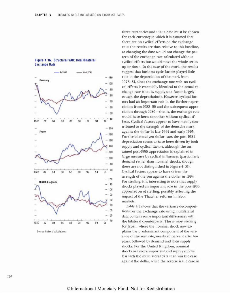
©International Monetary Fund. Not for Redistribution
154
CHAPTER IV BUSINESS CYCLE INFLUENCES ON EXCHANGE RATES
Figure 4.16. Structural VAR: Real Bilateral Exchange Rate
- Actual - No cycle
Germany - 110
three currencies and that a date must be chosen
for each currency in which it is assumed that
there are no cyclical effects on the exchange
rate; the results are thus relative to this baseline,
as changing the date would not change the pat
tern of the exchange rate calculated without
cyclical effects but would move the whole series
up or down. In the case of the mark, the results
suggest that business cycle factors played little
1980 32 84 86 88 90 92 94 96 40
role in the depreciation of the mark from
1978-81, since the exchange rate with no cycli
cal effects is essentially identical to the actual ex
change rate (that is, supply side factor largely
caused tl1e depreciation). However, cyclical fac
tors had an important role in the further depre
ciation from 1982-85 and the subsequent appre
ciation through 1986-that is, the exchange rate
would have been smoother without cyclical ef
fects. Cyclical factors appear to have mainly con
tributed to the strength of the deutsche mark
against the dollar in late 1994 and early 1995.
For the bilateral yen-dollar rate, the post-1981
depreciation seems to have been driven by both
1980 82 84 86 88 90 92
United Kingdom
1980 82 84 86 88 90 92
Source: Authors' calculations.
94
94
- 200
140 supply and cyclical factors, although the sus
96 60
- 120
- 1 10
- 100
- 90
80
- 60
- 50
96 40
tained post-1985 appreciation is explained in
large measure by cyclical influences (particularly
demand rather than nominal shocks, though
these are not distinguished in Figure 4.16).
Cyclical factors appear to have driven the
strength of the yen against the dollar in 1994.
For sterling, it is interesting to note that supply
shocks played an important role in the post-1986
appreciation of sterling, possibly reflecting the
impact of the Thatcher reforms in labor markets.
Table 4.5 shows that the variance decompositions for the exchange rate using multilateral
data contain some important differences with
tl1e bilateral counterparts. This is most striking
for Japan, where the nominal shock now ex
plains the predominant component of the vari-
ance of the real rate, nearly 70 percent after ten
years, followed by demand and then supply
shocks. For the United Kingdom, nominal
shocks are more important and supply shocks
less with the multilateral data than was the case
against the dollar, while the reverse is the case in
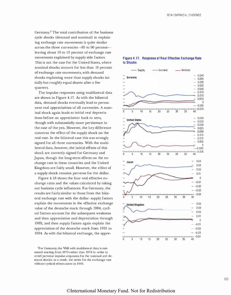
©International Monetary Fund. Not for Redistribution
Germany.' The total contribution of the business
cycle shocks (demand and nominal) in explain
ing exchange rate movements is quite similar
across the three currencies-85 to 90 percent
leaving about 10 to 15 percent of exchange rate
movements explained by supply side factors.
This is not the case for the United States, where nominal shocks account for less than 10 percent
of exchange rate movements, with demand
shocks explaining more than supply shocks ini
tially but roughly equal shares after a few
quarters.
The impulse responses using multilateral data
are shown in Figure 4.17. As ·with the bilateral data, demand shocks eventually lead to perma
nent real appreciations of all currencies. A nom
inal shock again leads to initial real depreda
tions before an appreciation back to zero,
though with substantially more persistence in
the case of the yen. However, the key difference
concerns the effect of the supply shock on the
real rate. In the bilateral case this was wrongly
signed for all three currencies. With the multilateral data, however, the initial effects of this
shock are correctly signed for Germany and
Japan, though the long-term effects on the ex
change rate in these countries and the United
Kingdom are fairly small. However, the effect of
a supply shock remains perverse for the dollar.
Figure 4.18 shows the four real effective exchange rates and the values calculated by taking
out business cycle influences. For Germany, the
results are fairly similar to those from the bilat
eral exchange rate with the dollar: supply factors
explain tl1e movements in the effective exchange
value of the deutsche mark through 1984, cycli
cal factors account for the subsequent weakness
and then appreciation and depreciation through 1989, and then supply factors again explain the
appreciation of the deutsche mark from 1991 to 1994. As with tl1e bilateral exchange, the appre-
7For Germany, the VAR with multilateral data is esti· mated starting from 1979 rather than 1978 in order to avoid perverse impulse-responses for the nominal and demand shocks; as a result, the series for the exchange rate without cyclical effects starts in 1981.
NEW EMPIRICAL EVIDENCE
Figure 4.17. Response of Real Effective Exchange Rate to Shocks
- Supply - Demand - Nominal
Germany - 0.040
- 0.035
- 0.030
- 0.025
- 0.020
- 0.015
________ _,_ 0.010
- 0.005
��==���======� 0 - -o.oos
I I I I I I I I I I I I 1 I I I I 1 I 1 I 1 I 1 I I 1 I I I I I I I I I I 1 I I I I -o.010 0 5 10 15 20 25 30 35 40
0
United States
5 10
- Japan
- 0.040
- 0.035
--------- 0.030
- 0.025
-------------,_ 0.020
15 20 25 30 35
- 0.015
- 0.010
- 0.005
0
--0.005
0.010 40
- 0.04
--------- 0.03
- 0.02
-
: - 0.01
� ..... } �� 0 5 1 0 1 5 20 25 30 35 40
- 0.04
- 0.03
- 0.02
- 0.01
0
- -o.01
- -o.02
- -{).03
-o.04 0 5 1 0 1 5 20 25 30 35 40
155
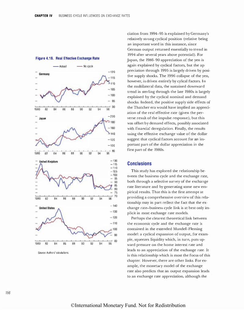
©International Monetary Fund. Not for Redistribution
CHAPTER IV BUSINESS CYCLE INFLUENCES ON EXCHANGE RATES
ciation from 1994-95 is explained by Germany's
relatively strong cyclical position (relative being
an important word in this instance, since German output returned essentially to trend in
Figure 4.1 8. Real Effective Exchange Rate 1994 after several years above potential). For
Japan, the 1986--90 appreciation of the yen is
- Actual - No cycle again explained by cyclical factors, but the ap-
-120 predation through 1995 is largely driven by posi-
tive supply shocks. The 1996 collapse of the yen,
110 however, is driven entirely by cylical factors. In the multilateral data, the sustained downward
u·end in sterling through the late 1980s is largely
explained by the cyclical nominal and demand
shocks. Indeed, the positive supply side effects of
1980 82 84 86 88 90 90 the Thatcher era would have implied an appreci-
92 94 96 ation of the real effective rate (given the per-
Japan -200 verse result of the impulse response), but this
was offset by demand effects, possibly associated
with financial deregulation. Finally, the results 140 using the effective exchange value of the dollar
-120 suggest that cyclical factors account for an im-
-100 portant part of the dollar appreciation in the
80 first part of the 1980s. 1980 82 84 86 88 90 92 94 96
- United Kingdom - 1 20 Conclusions - 115
- 1 1 0 -105 This study has explored the relationship be--100 t\'leen the business cycle and the exchange rate, - 95 - 90 both through a selective survey of the exchange
85 rate literature and by generating some new em-- 80 - 75 pirical results. That this is the first attempt at
1980 82 84 86 88 90 92 94 96 70 providing a comprehensive overview of this rela-
- 140 tionship may in part reflect the fact that the ex-
change rate-business cycle link is at best only im-plicit in most exchange rate models.
Perhaps the dearest theoretical link between
the economic cycle and the exchange rate is
contained in the extended Mundeii-Fieming
model: a cyclical expansion of output, for exam-
80 pie, squeezes liquidity which, in turn, puts up-1980 82 84 86 88 90 92 94 96 ward pressure on the home interest rate and
Source: Authors' calculations. leads to an appreciation of the exchange rate. It
is this relationship which is most the focus of this
chapter. However, there are other links. For ex-
ample, the monetary model of the exchange
rate also predicts that an output expansion leads
to an exchange rate appreciation, although the
156
©International Monetary Fund. Not for Redistribution
channel is more direct: prices must fall to main
tain money market equilibrium and, through
PPP, this leads to an exchange rate appreciation.
In the portfolio balance model, a risk premium
is also an important influence on the exchange
rate, and risk premia could be related to busi
ness cycles through the effect of the cycle on
countries' fiscal positions and thereby relative
debt stocks. However, evidence of a foreign ex
change risk premium is weak at best, so that this
avenue is not explored in this chapter.
Empirical evidence generally supports the the
oretical connection between business cycles and
exchange rates. This is true both for the direct
connection between output and exchange rates
as in the monetary approach, and for the more
general link between exchange rates and interest
rates. This is particularly the case when interest
rates and exchange rates are decomposed into
u·ansitory and permanent components, as is
done in this paper with band-pass filters. Finally,
evidence from structural VARs shows that busi
ness cycle factors are the dominant factor in ac
counting for recent exchange rate movements in
the United States, Germany,Japan, and United
Kingdom.
The existence of a relationship between busi
ness cycles and exchange rates has important im
plications for policy and multilateral surveil
lance. When business cycles are not
synchronized across countries, variations in ex
change rates can play a useful stabilizating role,
especially when economies are open and inter
nationally integrated. The link between ex
change rates and business cycles means that the
existence of desynchronized expansions across
countries in effect provides a "safety valve" for
inflationary pressures, as changes in exchange
rates can lead to a redistribution of demand
from countries near the top of their business cy
cles to those where demand is weak and there is
spare capacity. A challenge for policy evaluation
is to distinguish exchange rate movements war
ranted by international cyclical divergences from
movements due to changes in medium-term fun
damentals or episodes of overshooting or gross
misalignments.
REFERENCES
References
Allen, P.R., and P.B. Kenen, 1980, Asset Markets,
Exchange Rates, and Economic Integration: A Synthesis
(Cambridge: Cambridge University Press).
Astley, M., and A. Garrett, 1996, "Exchange Rates and
Prices: Sources of Sterling Real Exchange Rate
Fluctuations 1973-94," Bank of England Working
Paper (London).
BaiiJie, R., and D. Selover, I 987, "Coiotegration and
Models of Exchange Rate Determination,"
lnternal'ional journal of Farecasting. Vol. 3, No. 1 ,
pp. 43-51.
BaxLer, M., 1994, "Real Exchange Rates and Real
Interest Rate Differentials: Have We Missed the
Business Cycle Relationship?" j(ntmal of Monetm·y
Eronomics, Vol. 33 (February), pp. 5-37.
--, and R. King, 1995, "Measuring Business Cycles:
Approximate Band-Pass Filters for Economic Time
Series," NBER Working Paper 5022 (Cambridge,
Massachusetts: National Bureau of Economic
Research).
Beveridge, S., and C.R. Nelson, 1981, "A New
Approach to the Decomposition of Economic Time
Series into Permanent and Transitory Components,
with Particular Attention to the Measurement of
Business Cycles," journal of Monetary Economics,
Vol. 7, pp. 151-74.
Bilson,j., 1978, "Ralional Expectations and the
Exchange Rate," in jacob A. Frenkel and Harry G.
Johnson (eds.), The Economics of Exchange Rates:
Selected Studies, (Reading, Massachusetts: Addison
Wesley), pp. 75-96.
Branson, W.H., 1977, "Asset Markets and Relative
Prices in Exchange Rate Determination,"
Sozialwissenschaftliche Annalen, Band 1.
Campbell,j.Y, and R.H. Clarida, 1987, 'The Dollar
and Real Interest Rates," Camegi�EWchester Conference
Series on Public Policy, Vol. 27 (Autumn), pp. 103-40.
Chadha, B., and E. Prasad, 1997, "Real Exchange Rate
Flucruations and tl1e Business Cycle," IJ\tfF Staff
Papers, Vol 44, No. 3, pp. 328-55.
Clarida, R., and j. Cali, 1994, ''Sources of Real
Exchange Rate Fluctuations: How Imponam Are
Nominal Shocks?" Carnegie-Rochester Series on Public
Policy, Vol. 41, pp. 1-56.
Clark, P.B., and R. MacDonald, 1998, "Exchange Rates
and Economic Fundamentals: A Metl1odological
Comparison of BEERs and FEERs," IMF Working
Paper 98/67 (Washington).
151
©International Monetary Fund. Not for Redistribution
158
CHAPTER IV BUSINESS CYCLE INFLUENCES ON EXCHANGE RATES
Cochrane,]., 1990, uUnivariaLe vs. MultivariaLC
ForecastS of GNP Growth and Stock Returns,"
NBER Working Paper No. 3427 (Cambridge,
Massachusetts: National Bureau of Economic
Research).
Coughlin, Clews C., and Kees Koedijk, 1990, "What
Do We Know AboUl the Long-Run Real Exchange
Rate?" St. Louis Federal Reserve Bank Revie-w, Vol. 72
(January/February), pp. 36-48.
Cumby, R., andj. Huizi11ga, 1991, 'The Predictability
of Real Ex.change Rate Changes in the Short Run
and in the Long Run," japan and the World Economy,
Vol. 3, No. 1, pp. 17-38.
Cushman, D.A, S.S. Lee, and T. Thorgeirsson, 1996,
"Maximum Likelihood Estimation of Cointegration
in Exchange Rate Models for Seven Inflationary
Countries," journal of lnternaliona.l Money and
Finance, Vol.l5, pp. 337-68.
Dejong, D., and S. Husted, 1995, 'The Forward
Looking Monetary Model: A Ctitical Perspective"
(unpublished; University of PittSburgh).
Dooley, M., and P. Isard, 1982, "A Portfolio-Balance
Rational-Expectations Model of the Dollar-Mark
Exchange Rate," jaurnal of International Econmnics,
Vol. 12, pp. 257-76.
Dor·nbusch, Rudiger, 1976, "Expectations and
Exchange Rate Dynamics," Journal of Political
Economy, Vol. 84 (December) , pp. 1 161-76.
---, and S. Fischer, 1980, "Exchange Rates and the
Current Account," Ameriwn Economic Revie·w, Vol.
70, pp. 960-7l.
Edison, HJ., and B. Diane Pauls, 1993, "A Re
Assessment of the Relationship Be tween Real
Exchange Rates and Real Interest Rates: 1974-90,"
Journal of Monelc�ry Economics, Vol. 31 (April),
pp. 165-87.
Edison, HJ. and W.R. Melick, 1995, "Alternative
Approaches to Real Exchange Rates and Real
Interest Rates: Three Up and Three Down," Board
of Governors of the Federal Reserve System,
International Finance Discussion Paper No. 518
(Washington).
Evans, C., 1989, "A Measure of the U.S. Output Gap,"
l:."conmnics Letters, Vol. 29, No. 4, pp. 285-89.
Finn, M., 1986. "Forecasting the Exchange Rate: A
Monetary or Random Walk Phenomenon?" Journal
of International M(tney and Finance, Vol. 5 (June),
pp. 181-93.
Flood, Robert, 1981, "Explanations of Exchange-Rate
Volatility and Other Empirical Regularities in Some
Popular Models of the Foreign Exchange Market,"
Camegie-Rochesler Se1ies on Public Policy, Vol. 15,
pp. 219-50.
Frankel, J ., 1979, "On the Mark: A Theory of Floating
Exchange Rates Based on Real Interest
Differen lials," American Economic Revil!W, Vol. 69,
pp. 601-22.
---, 1983, "Monetary and Portfolio-Balance
Models of Exchange Rate Determination," in j.S.
Bhandari, B.H. Putnam, and J.H. Levin ( eds.),
Economic hrterd ependence and Flexible Exchange Rales
(Cambridge. Massachusetts: MIT Press).
---, and A. Rose, 1995, "A Survey of Empirical
Research on Nominal Exchange Rates," in S.
Grossman and K. Rogoff, (eds. ) , The Handbook of
International Econamics, Vol. 3 (Amsterdam: North
Holland).
Frenkel, J., 1978, "A Monetary Approach to the
Exchange Rate: Doctorinal Aspects and Emprical
Evidence," Scandinavianjoumal of Economics, Vol. 78,
pp. 200-24.
---, and Michael L. Mussa, J 985, "Asset MarketS,
Exchange Rates, and the Balance of Payments," in
R.jones and P. Ke11en (eds.), Handbook of
lntemationaiEconomics, Vol. 2 (Amsterdam: orrh
Holland), Chapter 14.
Conzalo,J., and C.W. Granger, 1995, "Estimation of
Common Long-Memory Components in
Cointegrated Systems," journal of Business Economics
and Statistics, Vol.13, pp. 27-35.
Rodrick, Robert]., 1978, "An Empirical Analysis of'
the Monetary Approach to the Determination of
the Exchange Rate," in jacob A. Frenkel and Harry
C . .Johnson ( eds.), The Economics of Exclwnge &tes,
(Reading, MassachusettS: Addison-Wesley),
pp. 97-1 16.
---, 1987, The Empirical Evidence on the Efficiency of
Forwm-d andFtttm-es M.w·kets (London: Harwood).
Hoffman, D., and 0. Schlagenhauf, 1983, uRational
Expectations and Monetary Models of Exchange
Rate Determination: An Empirical Examination,··
journal of Monetary Economics, Vol. I I (March),
pp. 247-60.
Hooper, P., and]. Morton, 1982, "Fluctuations in the
Dollar: A Model of Nominal and Real Exchange
Rate Determination," journal of lntemational Money
mul Fincmce, Vol. l (April), pp. 39-56.
Huizinga,John, 1987, "An Empirical Investigation of
the Long-Run Behavior of Real Exchange Rates,"
©International Monetary Fund. Not for Redistribution
Cam.egie-Rnchester Conference SCiies on Public Policy,
Vol. 27 (Autumn), pp. 149-214.
Johansen, S., 1995, Likelihood-Based lnfermce in
Coint.egrated Vector Aut01·egressive Models (New York
and Oxford: Oxford University Press) .
Johansen, S., and K.Juselius, 1992, "Testing Structural
Hypotheses in a Multivariate Coimegration Analysis
of PPP and UIP for the UK." journal of Eccmomet1·ics,
Vol. 53, pp. 21 1-44.
.Juselius, K., 1991, "Long-Run Relations in a Well
Defined Statistical Model for the Data Generating
Process: Cointegration Analysis of the PPP and UIP
Relations Between Denmark and Germany," inJ.
Gruber (ed.), Economet1ic Decision Mod.els: New
Methods of Modeling and Applications (New York:
Springer Verlag).
---, 1995, "Do Purchasing Power Parity and
Uncovered Interest Rate Parity Hold in the Long
Run? An Example of Likelihood Inference in a
Multivariate Time-Series Model," ]O'UT1Utl of
Econometrics, Vol. 69, pp. 21 1-40.
---, and R. MacDonald, 2000, "Jmernational Parity
Relationships Between Germany and the United
States: Ajoint Modelling Approach" (unpublished;
European University lnstitute).
Kearney, C., and R. MacDonald, 1988, "Rational
Expectations, Bubbles and Monetary Models of the
Exchange Rate: The Australian/U.S. Dollar Rate
During the Recent Float," Austmlian Economic
Papers, Vol. 44, pp. 1-20.
King, R., C. Plosser, j. Stock, and M. Watson, 1991,
"Stochastic Trends and Economic FlucLUations,"
American Economic Revil!1.u, Vol. 81 (September),
pp. 819-40.
Kouretas, G., 1997, ''IdentifYing Linear Restrictions on
the Monetary Exchange Rate Model and the
Uncovered Interest Pal'ity: Cointegration Evidence
from the Canadian-U.S. Dollar," umadianjoumal of
Economics, VoL 30 (November), pp. 875-90.
La Cour, L., and R. MacDonald, 2000, "Modelling the
ECU Against the Dollar: A Su·uctural Monetary
Approach," Journal of Business Economics and.
Statistics.
Lucas, R.E., 1982, "lnterest Rates and Currency Prices
in a Two-Country World," journal of Moneta1')'
Economics, Vol. 10, pp. 335-60.
MacDonald, R., 1988, Floating Exchange Rates: Theories
and Evidence (London: Unwin-Hyman) .
REFERENCES
---, 1990, "Exchange Rate Economics,'' in G. Bird
(ed.), The lntmtalional Financial Regime (London:
Academic).
---, 1995a, "Long-Run Exchange Rate Modeling: A
Survey of the Recent Evidence," 11\lfF Staff Papers,
Vol. 42, No. 3, pp. 437-89.
---, 1995b, "Asset Market and Balance of Payments
Characteristics: An Eclectic Exchange Rate Model
for tbe Dollar, Mark, and Yen," li\{F Working Paper
95/55 (Washington) .
---, 1997, "What Determines Real Exchange
Rates? The Long and the Short of lL," Joum.al of
lnternatiO'nal Fin.ancial lvJa,-kets, Institutions and
Money.
---, and Marsh, LW, 1997, "On Fundamentals and
Exchange Rates: A Cassel ian Perspective," Reuil!1.u of
Eronomics and Statistics, Vol. 78, pp. 655-64.
---, 1999, "Currency Spillovers and Tri-Polarity: A
Simultaneous Model of the U.S. Dollar, German
Mark and japanese Yen," CEPR Discussion Paper
2210 (London).
MacDonald, R., andJ. Nagasuya, 1999, 'The Long-Run
Relationship Between Real Exchange Rates and
Rea\ Interest Rate Differelllials-A Panel Study,"
lM.F Working Paper 99/37 (Washington).
MacDonald, R .. and M.P. Taylor. 1992, "Exchange Rate
Economics: A Survey," TMF Staff Papers, Vol. 39,
pp. 1-57.
---, 1993, 'The Monetary Approach to the
Exchange Rate: Rational Expectations, Long-Run
Equilibrium and Forecasting," 1MF Staff Papers, Vol.
40, pp. 89-107.
Meese, R., and K. Rogoff, 1988, "Was It Real? The
Exchange Rate-Interest Differential Relation Over
the Modern Floating-Rate Period," journal of
Finance, VoL 43, pp. 933-48.
Mussa, M., 1979, "Empi1ical Regula1ities in the
Behavior of Exchange Rates and Theories of the
Foreign Exchange Market," Carnegie-Rod1ester
Confertnce Sl!lies on Public Policy, Vol. 11, pp. 9-57.
---, 1982, "A Model of Exchange Rate Dynamics,"
joumal of Political Economy, Vol. 90, pp. 74-104.
---, 1984, 'The Theory of Exchange Rate
Determination," inJ.F.O. Bilson and R.C. Marston
(eds.), Exchange Rate Theory and Practice, NBER
Conference Report (Chicago: University of Chicago
Press) .
---. 1986, "Nominal Exchange Rate Regimes and
the Behavior of Real Exchange Rates: Evidence and
159
©International Monetary Fund. Not for Redistribution
160
CHAPTER IV BUSINESS CYCLE INFLUENCES ON EXCHANGE RATES
Implications," Carnegie-Rochester Conference Series on
Pttblic Polit)', Vol. 26.
Obstfeld, M., 1985, "Floating Exchange Rates:
Experiences and Prospects," Brookings Papers (tn
Economic Activity, Vol. 2, pp. 369-450.
Sarte, P., 1997, "On the Identification of StructW'a1
Vector Autoregressions," Economic Quarterly, Federal
Reserve Bank of Richmond, Vol. 83 (Summer),
pp. 45-67.
Stockman, A., 1995. "Sources of Real Exchange-Rate
Fluctuations: A Comment," Carnegie Rochester Ccnference Series on Public Policy, Vol. 41, pp. 57-65.
Thomas, Alun, 1997, "Is the Exchange Rate a Shock
Absorber? The Case of Sweden," lMF Working
Paper 97/176 (Washington).
Throop, A., 1993, "A Generalized Uncovered Interest
Parity Model of Exchange Rates," Economic Review,
Fede1·a1 Rese1·ve Bank of San Francisco, No. 2,
pp. 3-16.
Woo, W.T., 1985, "The Monetary Approach to
Exchange Rate Determination Under Rational
Expectations: The Dollar-Deutschemark Rate,"
journal of International Economics, Vol. 18, pp. 1-16.
©International Monetary Fund. Not for Redistribution
THE GREAT CONTRACTIONS IN RUSSIA, THE BALTICS, AND THE OTHER COUNTRIES OF THE FORMER SOVIET UNION: A VIEW FROM THE SUPPLY SIDE Mark De Broeck and Vincent Koen
The early years of u-ansition from a com
mand to a market-based economy in
central and eastern Europe have typi
cally wi tnessed considerable output
drops, at least according to official national sta
tistics. Output comractions were even more pro
nounced in the Baltics, Russia, and the other
countries of the former Soviet Union. By 1997, growth had resumed in the vast majority of tran
sition countries. Even though a number of them
faced renewed output declines in 1998, mainly
associated with the financial crisis in Russia, it
appears that the bulk of the transitional reces
sion is now over in most cases. With the benefit
of hindsight, this sLUdy attempts to put the con
tractions endured in the Baltics as well as in
Russia and the other countries of the
Commonwealth of Independent States (CIS) in
perspective, examining them from several
angles.
A first and obvious que Lion arises as to their
magnitude. On many scales, it seems to be very
large. While this impression can be corroborated
in a number of ways, quantification has been,
and remains, a m<Uor challenge because of the
poor quality of available statistics. In fact, be
cause of these uncertainties, any point estimate
is likely to be misleading. Bearing this caveat in
mind, a second issue is how to evaluate the wel
fare consequences of the e contractions. All too
often, the magnitude of the output decline is
equated, at least implicilly, with that of the wel
fare loss. On reflection, however, it turns out
that there is no straightforward, one-to-one, rela
tionship between the former and the latter, as
welfare measures reflect the type of social wel
fare function used.
ext, the stylized features of the contractions
in the Baltics and the CIS countries are de
scribed and contrasted with the experience of se
lected central European transition economies.
While many studies tend to focus on the depth
of the contractions, their length and breadth are
also highlighted here, and performance is set
against countries' longer-run growth record.
The contractions have been ascribed a variety
of causes in the literaLUre, including the disloca
tion of traditional domestic and international
links, fiscal retrenchment, and credit crunches,
with the relative importance of these factors dif
fering across countries. 1 This study does not con
sider such a broad range of factors, but instead
focuses on changes in inputs and the evolution
of productivity to interpret the observed decline
in output, in line with earlier work by Easterly
and Fischer (1994). lt also sheds light on the re
allocation of inputs across seCLors.
Background Considerations
Starting in the late 1980s or early 1990s, offi
cial measures of output and value added de
clined precipitously in the Baltics, Russia, and
the other countries of the CIS. The size of the
actual conu·actions, however, is hard to gauge.
On the one hand, pan of the falling activity
reflected the replacemem of the previous incen
tive to report the (over-) fulfillment of plan tar
gets by the incentive to avoid the scrutiny of the
tax and other authorities (Koen, 1994).
Anecdotal evidence of L11e dynamism of under
ground businesses abounds, at least in some sec
tors. In L11e early years of transition, statistical of
fices generally did not have at their disposal the
1For an empirical cross-country study, see for instance Berg and otl1ers ( 1999) and 1-la\'l')'I)"Shyn and others (2000) and
lhe references lherein. For an in-depth country-specific anai)"Sis. see for instance the anal)-sis by De Broeck and Kostial ( 1998) on Kazakhstan and by ZeLLelmeyer ( 1998) on Uzbekistan. Analytical reviews of the causes of lhe outpm decline are presemed in Conw·ay (forthcoming) and Mundell ( 1997).
161
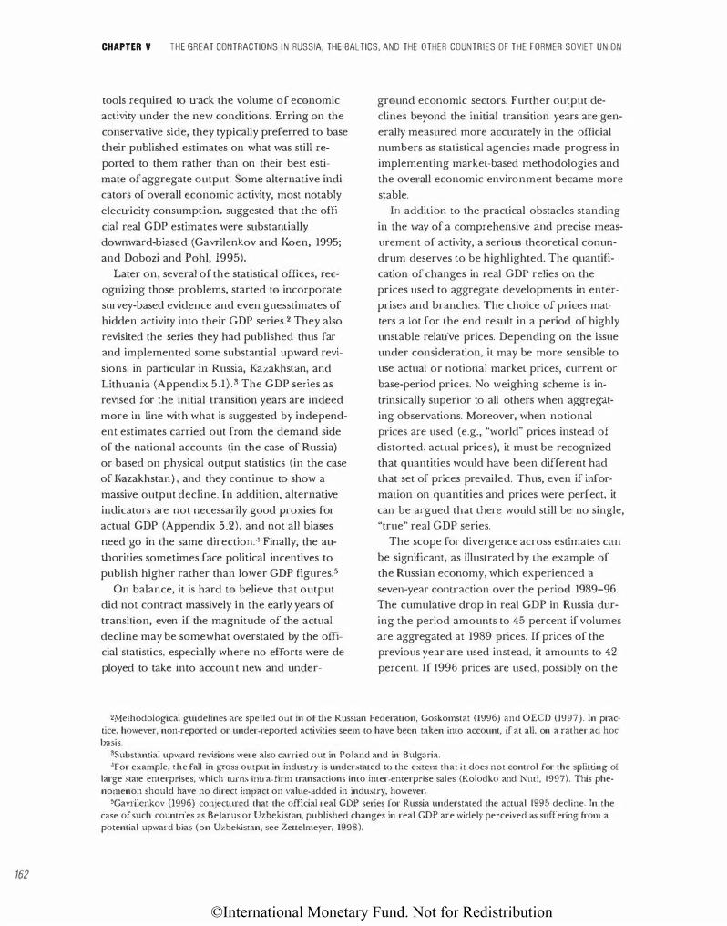
©International Monetary Fund. Not for Redistribution
162
CHAPTER V THE GREAT CONTRACTIONS IN RUSSIA, THE BALTICS, AND THE OTHER COUNTRIES OF THE FORMER SOVIET UNION
tools required to track the volume of economic
activity under the new conditions. Erring on the
conservative side, they typically preferred to base
their published estimates on what was still re
ported to them rather than on their best esti
mate of aggregate output. Some alternative indi
cators of overall economic activity, most notably
electricity consumption, suggested that the offi
cial real GDP estimates were substantially
downward-biased (Gavrilenkov and Koen, 1995;
and Dobozi and Pohl, 1995).
Later on, several of the statistical offices, rec
ognizing those problems, started to incorporate
survey-based evidence and even guesstimates of
hidden activity into their GDP series.2 They also
revisited the series they had published thus far
and implemented some substantial upward revi
sions, in particular in Russia, Kazakhstan, and
Lithuania (Appendix 5.1).3 The GDP series as
revised for the initial transition years are indeed
more in line with what is suggested by independ
ent estimates carried out from the demand side
of the national accounts (in the case of Russia)
or based on physical output statistics (in the case
of Kazakhstan) , and they continue to show a
massive output decline. In addition, alternative
indicatOrs are not necessarily good proxies for
actual GDP (Appendix 5.2), and not all biases
need go in the same direction.'1 Finally, the au
thorities sometimes face political incentives to
publish higher rather than lower GDP figures.5
On balance, it is hard to believe that output
did not contract massively in the early years of
transition, even if the magnitude of the actual
decline may be somewhat overstated by the offi
cial statistics, especially where no efforts were de
ployed to take into account new and under-
ground economic sectors. Further output de
clines beyond the initial transition years are gen
erally measured more accurately in the official
numbers as statistical agencies made progress in
implemenling market-based methodologies and
the overall economic environment became more
stable.
In addition to the practical obstacles standing
in the way of a comprehensive and precise meas
urement of activity, a serious theoretical conun
drum deserves to be highlighted. The quantifi
cation of changes in real GDP relies on the
prices used to aggregate developments in enter
prises and branches. The choice of prices mat
ters a lot for the end result in a period of highly
unstable relative prices. Depending on the issue
under consideration, it may be more sensible to
use actual or notional market prices, currem or
base-period prices. No weighing scheme is in
trinsically superior to all others when aggregat
ing observations. Moreover, when notional
prices are used (e.g., "world" prices instead of
distOrted, actual prices), it must be recognized
that quantities would have been different had
that set of prices prevailed. Thus, even if infor
malion on quantities and prices were perfect, it
can be argued that there would still be no single,
"true" real GDP series.
The scope for divergence across estimates can
be significant, as illustrated by the example of
the Russian economy, which experienced a
seven-year conu-action over the period 1989-96.
The cumulative drop in real GDP in Russia dur
ing the period amounts to 45 percent if volumes
are aggregated at 1989 prices. If prices of the
previous year are used instead, it amounts to 42
percent. If 1996 prices are used, possibly on the
2Methodological guideHnes are spelled out in of the Russian Federation, Goskomstat (1996) and OECD (1997). ln practice, however, non-reported or under-reponed activities seem to have been taken into account, if at all, on a rather ad hoc basis.
3Substantial upward revisions were also carried out in Poland and in Bulgaria. •1For example, the fall in gross output in industry is understated to the extent that it does not control for the spliuing or
large state enterprises, which turns intra-finn transactions into inter-enterprise sale::s (Kolodko and Nuti, 1997). This phenomenon should have no direct impact on v-alue-added in industry, however.
5Gavrilcnkov (1996) conjecwred that the official real GDP series for Russia understated the actual 1995 decline. In the case of such countries as Belarus or Uzbekistan, published changes in real GDP are widely perceived as suffering from a potential upwat·d bias (on Uzbekistan, see Zettelmeyer, 1998).
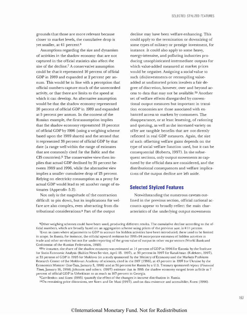
©International Monetary Fund. Not for Redistribution
grounds rbat those are more relevant because
closer to market levels, the cumulative drop is
yet smaller, at 41 percent.6
Assumptions regarding the size and dynamism
of activities in the shadow economy that are not
captured in the official statistics also affect the
size of the decline.7 A conservative assumption
could be that it represented 10 percent of official
GDP in 1989 and expanded at 2 percent per an
num. This would be in line with a perception that
official numbers capture much of the unrecorded
activity, or that there are limits to the speed at
which it can develop. An alternative assumption
would be that the shadow economy represented
20 percent of official GDP in 1989 and expanded
at 5 percent per annum. In the context of the
Russian example, the first assumption implies
that the shadow economy represented 18 percent
of official GDP by 1996 (using a weighing scheme
based upon the 1989 shares) and the second that
it represented 38 percent of official GDP by that
date (a range well within the range of estimates
that are commonly cited for the Baltic and the
CIS countries) .s The conservative view then .im
plies that actual GDP declined by 35 percent be
tween 1989 and 1996, while the alternative view
implies a smaller cumuJative drop of 23 percent.
Relying on electricity consumption as a proxy for
actual GDP would lead to yet another range of es
timates (Appendix 5.2).
Not only is the magnitude of the contraction
difficult to pin down, but its implications for wel
fare are also complex, even abstracting from dis
tributional considerations.9 Part of the output
SELECTED STYLIZED FEATURES
decline may have been welfare-enhancing. This
could apply to the termination or downsizing of
some types of miHtary or prestige investment, for
instance. It could also apply to some heavy,
energy-intensive, and polluting industties pro
ducing unsophisticated intermediate outputs for
which value-added measured at market prices
would be negative. Assigning a social value to
such {dis) investments or recompiling value
added at undistorted prices involves a fair de
gree of discretion, however, over and beyond ac
cess to data that may not be available. tO Another
set of welfare effects disregarded by conven
tional OU[put measures but important in u·ansi
tion economies are those associated with en
hanced access to markets by consumers. The
disappearance, or at least lessening, of ratjoning
and queuing, as well as the increased variety on
offer are tangible benefits that are not directly
reflected in real GDP measures. Again, the size
of such offsetting welfare gains depends on the
type of social welfare function used, but it can be
consequential (Roberts, 1997). In the subse
quent sections, only output movements as cap
tured by the official data are considered, and the
distributional consequences and welfare implica
tions of the output decline are left aside.
Selected Stylized Features
otwithstanding the numerous caveats out
lined in the previous section, official national ac
counts appear to broadly reflect the main char
acteristics of the underlying output movemems
6(}t.her weighing schemes could have been used, producing different. results. The cumulative decline according to the official numbers, which are broadly based on an aggregation scheme using pt·ices of the previous year, is 4 1 'h percent..
7Even in cases where adjustments tO GOP to account fot· hidden activities have been introduced, these Lend to be limited in scope. In Russia, for instance, the ollicial upward revisions for 1991-94 i.ncorporate estimates of hidden activities in trade and other services bm not for underreporting of the gross value of output in other major sectors (World Bank and Goskoms tat of the Russian Federation, 1995).
8Fot· instance, the share of the shadow economy was estimated at 14 percent of GOP in 1996 for Estonia by the Institute for Socio-Economic Analysis (Baltics News Service, April l3, 1997). at 30 percent in 1997 for Kazakhstan (Kulekeev, 1997). at 33 percent of GOP in 1995 for Moldova (in a study sponsot·ed by the Ministry of Economy and the Markets Pt·oblems Research Center ohhe Moldovan Academ)' of sciences, cited in tJ1e IMF (1998), at 43 percent in 1997 for Ukraine by t.he Economics Minist.er (!tar-Tass, January 3, 1998) and at 50 percent. for Russia by a U.S. Treasw·y sponsored repon (Finaucial Times, January 16, 1998).Johnson and others. (1997) estimate tllal in 1995 the shadow economy ranged from as litt.le as 7 percent of official GOP in Uzbekistan to as much as 167 percent in Georgia.
9Gavrilenkov and Koen (1995) quantify the effect of t.he changes in income distribution in Russia. lOOn remaining price distortions, see Koen and De Masi (1997), and on data existence and accessibility, Koen ( 1996) .
163
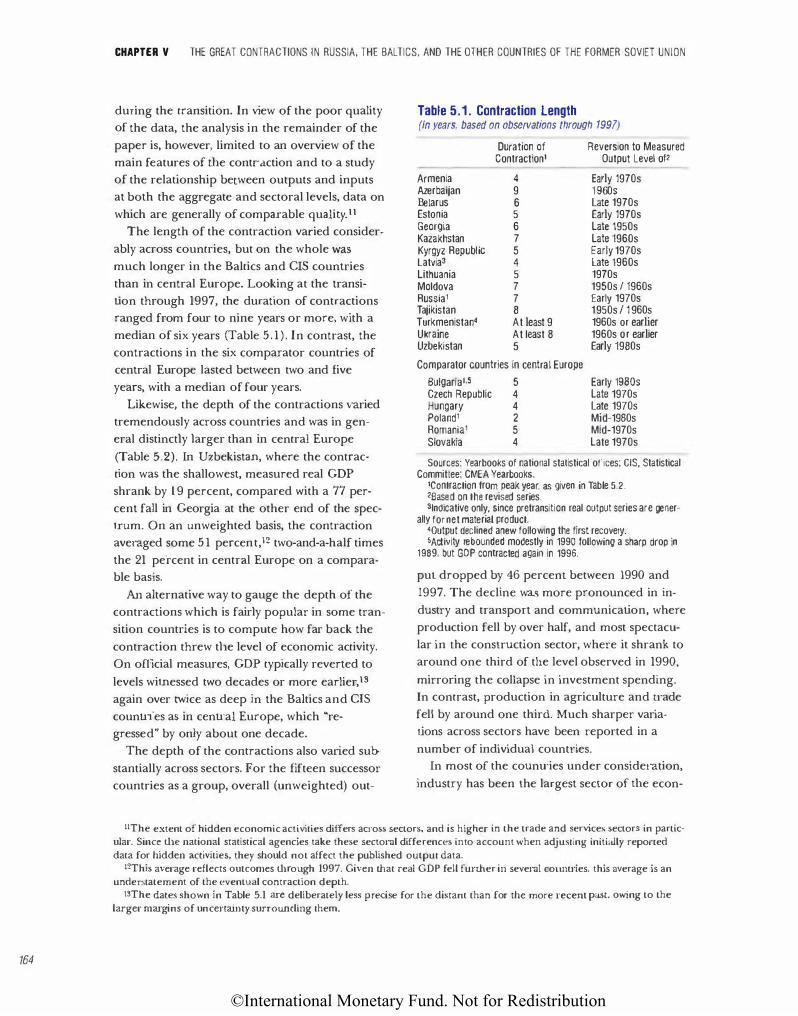
©International Monetary Fund. Not for Redistribution
164
CHAPTER V THE GREAT CONTRACTIONS IN RUSSIA, THE BALTICS, AND THE OTHER COUNTRIES OF THE FORMER SOVIET UNION
during the transition. In view of the poor quality
of the data, the analysis in the remainder of the
paper is, however, limited to an overview of the
main features of the contraction and to a study
of the relationship between outputs and inputs
at both the aggregate and sectoral levels, data on
which are generally of comparable quality. II
The length of the contraction varied consider
ably across countries, but on the whole was much longer in the Baltics and CIS countries
than in central Europe. Looking at the transi
tion through 1997, the duration of contractions
ranged from four to nine years or more, with a
median of six years (Table 5.1) . In contrast, the
contractions in the six comparator countries of
central Europe lasted between two and five
years, with a median of four years.
Likewise, the depth of the contractions varied
tremendously across countries and was in gen
eral distinctly larger than in central Europe
(Table 5.2). In Uzbekistan, where the contrac
tion was the shallowest, measured real GDP
shrank by 19 percent, compared with a 77 per
cent fall in Georgia at the other end of the spec
trum. On an unweighted basis, the contraction
averaged some 51 percent,12 two-and-a-half times
the 21 percent in central Europe on a compara
ble basis.
An alternative way to gauge the depth of the
contractions which is fairly popular in some tran
sition countries is to compute how far back the
contraction threw tl1e level of economic activity.
On official measures, GDP typically reverted to
levels witnessed two decades or more earlier,13
again over twice as deep in the Baltics and CIS
countries as in central Europe, which "re
gressed" by only about one decade.
The depth of the contractions also varied sub
stantially across sectors. For the fifteen successor
countries as a group, overall (unweighted) out-
Table 5.1 . Contraction Length (In years, based on observations through 1997)
Armenia Azerbaijan Belarus Estonia Georgia Kazakhstan Kyrgyz Republic Latvia3 Lithuania Moldova Russia' Tajikistan Turkmenistan4 Ukraine Uzbekistan
Duration of Contraction'
4 9 6 5 6 7 5 4 5 7 7 8 At least 9 At least 8 5
Comparator countries in central Europe
Bulgaria1.5 5 Czech Republic 4 Hungary 4 Poland' 2 Romania' 5 Slovakia 4
Reversion to Measured Output Level of2
Early 1970s 1 960s Late 1970s Early 1970s Late 1950s Late 1960s Early 1970s Late 1960s 1970s 1950s / 1960s Early 1970s 1950s / 1 960s 1960s or earlier 1960s or earlier Early 1980s
Early 1980s Late 1970s Late 1970s Mid-1980s Mid-1970s Late 1970s
Sources: Yearbooks of national statistical offices; CIS, Statistical Committee; CMEA Yearbooks.
1Contraction from peak year, as given in Table 5.2. 2Based on the revised series. 31ndicative only, since pretransition real output series are gener
ally for net material product. 40utput declined anew following the first recovery. SActivity rebounded modestly in 1990 following a sharp drop in
1989. but GOP contracted again in 1996.
pul dropped by 46 percent between 1990 and
1997. The decline was more pronounced in in
dustry and transport and communication, where
production fell by over half, and most spectacu
lar in the construction sector, where it shrank to
around one third of tl1e level observed in 1990,
mirroring the collapse in investment spending.
In contrast, production in agriculture and o·ade
fell by around one third. Much sharper varia
tions across sectors have been reported in a
number of individual countries.
In most of the counu·ies under consideration,
industry has been the largest sector of me econ-
11The extent of hidden economic activities differs across sectors, and is higher in the trade and services sectors in particular. Since the national statistical agencies take these sectoral differences in to account when adjusting initially reponed data for hidden activities, they should not affect the published oULput data.
12This average reflects outcomes through 1997. Given mat real GDP fell funher in several coLmu·ies, this average is an understatement of the eventual contraction depth.
13The dates shown in Table 5.1 are deliberately less precise for the distant than for the more recent past, owing to the larger margins of uncertainty surrow1eling them.
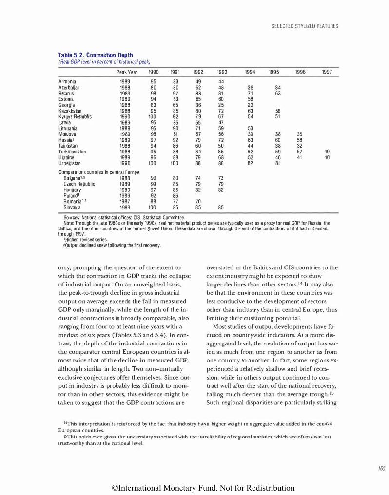
©International Monetary Fund. Not for Redistribution
SELECTED STYLIZED FEATURES
Table 5.2. Contraction Depth (Real GOP level in percent of historical peak)
Peak Year 1990 1991 1992 1993 1994 1995 1996 1997
Armenia 1989 95 83 49 44 Azerbaijan 1988 80 80 62 48 38 34 Belarus 1989 98 97 88 81 71 63 Estonia 1989 94 83 65 60 58 Georgia 1988 83 65 36 25 23 Kazakhstan 1988 95 85 80 72 63 58 Kyrgyz Republic 1990 100 92 79 67 54 51 Latvia 1989 95 85 55 47 Lithuania 1989 95 90 71 59 53 Moldova 1989 98 81 57 56 39 38 35 Russia1 1989 97 92 79 72 63 60 58 Tajikistan 1988 94 86 60 50 44 38 32 Turkmenistan 1988 95 88 84 85 62 59 57 49 Ukraine 1989 96 88 79 68 52 46 41 40 Uzbekistan 1990 100 100 88 86 82 81
Comparator countries in central Europe Bulgaria, .2 1988 90 80 74 73 Czech Republic 1989 99 85 79 79 Hungary 1989 97 85 82 82 Poland, 1989 92 86 Romania1.2 1987 88 77 70 Slovakia 1989 100 85 85 85
Sources: National statistical offices; CIS, Statistical Committee. Note: Through the late 1980s or the early 1990s, real net material product series are typically used as a proxy for real GOP for Russia, the
Baltics, and the other countries of the Former Soviet Union. These data are shown through the end of the contraction, or if it had not ended, through 1997.
1Higher, revised series. 2Qutput declined anew following the first recovery.
omy, prompting the question of the extent to
which the contraction in GDP tracks the collapse
of industrial output. On an unweighted basis,
the peak-to-trough decline in gross industrial
output on average exceeds the fall in measured
GDP only marginally, while the length of the in
dustrial contractions is broadly comparable, also
ranging from four to at least nine years with a
median of six years (Tables 5.3 and 5.4). In con
trast, the depth of the industrial contractions in
the comparator central European countries is al
most twice that of the decline in measured GDP,
although similar in length. Two non-mutually
exclusive conjectures offer themselves. Since out
put in industry is probably less difficult to moni
tor than in other sectors, this evidence might be
taken to suggest that the GDP contractions are
overstated in the Baltics and CIS countries to the
extent industry might be expected to show
larger declines than other sectors.14 It may also
be that the environment in these countries was
less conducive to the development of sectors
other than industry than in central Europe, thus
limiting their cushioning potential.
Most studies of output developments have fo
cused on countrywide indicators. At a more dis
aggregated level, the evolution of output has var
ied as much from one region to another as from
one country to another. In fact, some regions ex
perienced a relatively shallow and brief reces
sion, while in others output continued to con
tract well after the start of the national recovery,
falling much deeper than the average trough.15
Such regional disparities are particularly su·ik.ing
14This interpretation is reinforced by the fact that industry has a higher weight in aggregate value-added in the cenU'lll European countries.
15Th is holds even given the uncertainty associated with r.he unreliability of regional statistics, which are often even less trustworthy than at the national level.
165
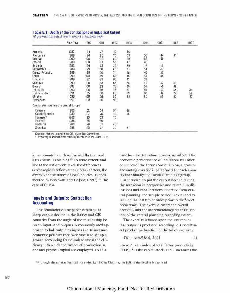
©International Monetary Fund. Not for Redistribution
166
CHAPTER V THE GREAT CONTRACTIONS IN RUSSIA, THE BALTICS, AND THE OTHER COUNTRIES OF THE FORMER SOVIET UNION
Table 5.3. Depth of the Contractions in Industrial Output (Gross industrial output level in percent of historical peak)
Peak Year 1990 1991
Armenia 1987 84 77 Azerbaijan 1989 94 98 Belarus 1990 100 99 Estonia 1989 100 91 Georgia 1989 94 73 Kazakhstan 1989 99 100 Kyrgyz Republic 1989 99 100 Latvia 1990 100 99 Lithuania 1989 97 92 Moldova 1990 100 93 R ussia 1989 100 92 Tajikistan 1990 100 96 Turkmenistan 1 1991 95 100 Ukraine 1989 100 95 Uzbekistan 1991 98 100
Comparator countries in central Europe
Bulgaria 1988 82 64 Czech Republic 1989 97 76 Hungaryz 1988 96 83 Poland2 1988 75 69 Romania 1988 79 61 Slovakia 1988 95 77
Sources: National authorities; CIS, Statistical Committee. 1Temporary rebounds were officially recorded in 1993 and 1996.
in vast countries such as Russia, Ukraine, and
Kazakhstan (Table 5.5).16 To some extent, and
like at the nationwide level, the differences
across regions reflect, among other factors, the
diversity in the stance of local policies, as docu
mented by Berkowitz and Dejong (1997) in the
case of Russia.
Inputs and Outputs: Contraction Accounting
The remainder of the paper explores the
sharp output decline in the Baltics and CIS
countries from the angle of the relationship be
tween inputs and outputs. A commonly used ap
proach to link output to inputs and to measure
economic performance over time is to set up a
growth accounting framework lO assess the effi
ciency with which the factors of production la
bor and physical capital are employed. To illus-
1992
40 75 89 58 39 83 74 65 66 68 75 73 85 89 93
54 70 75
48 70
1993 1994 1995 1996 1997
36 69 53 44 41 80 66 58 47 46 29 17 16 71 51 47 55 40 33 45 40 38 43 31 68 49 47 43 65 51 50 48 67 51 43 35 34 89 66 62 74 52 82 60 53 50 49
48 66
67
trate how the transition process has affected the
economic performance of the fifteen transition
counu·ies of the former Soviet Union, a growth
accounting exercise is performed for each coun
try individually and for all fifteen as a group.
Furthermore, to put the output decline during
the transition in perspective and relate it to dis
LOrtions and misallocations inherited from cen
tral planning, the sample period is extended to
include the last two decades prior to the Soviet
breakdown. The exercise covers the overall
economy and the aforementioned six main sec
tors of the cenu·al planning recording system.
The exercise is based upon the assumption
that output is produced according to a neoclassi
cal production function of the following form,
Y( t) = A ( t) f1 K( t), L( t) ] , ( 1 )
where A is an index of total factor productivity
(TFP), K is the capital stock, and L measures the
16AJthough the contraction had not ended by 1997 in Ukraine, the bulk of the decline is captu,·ed.
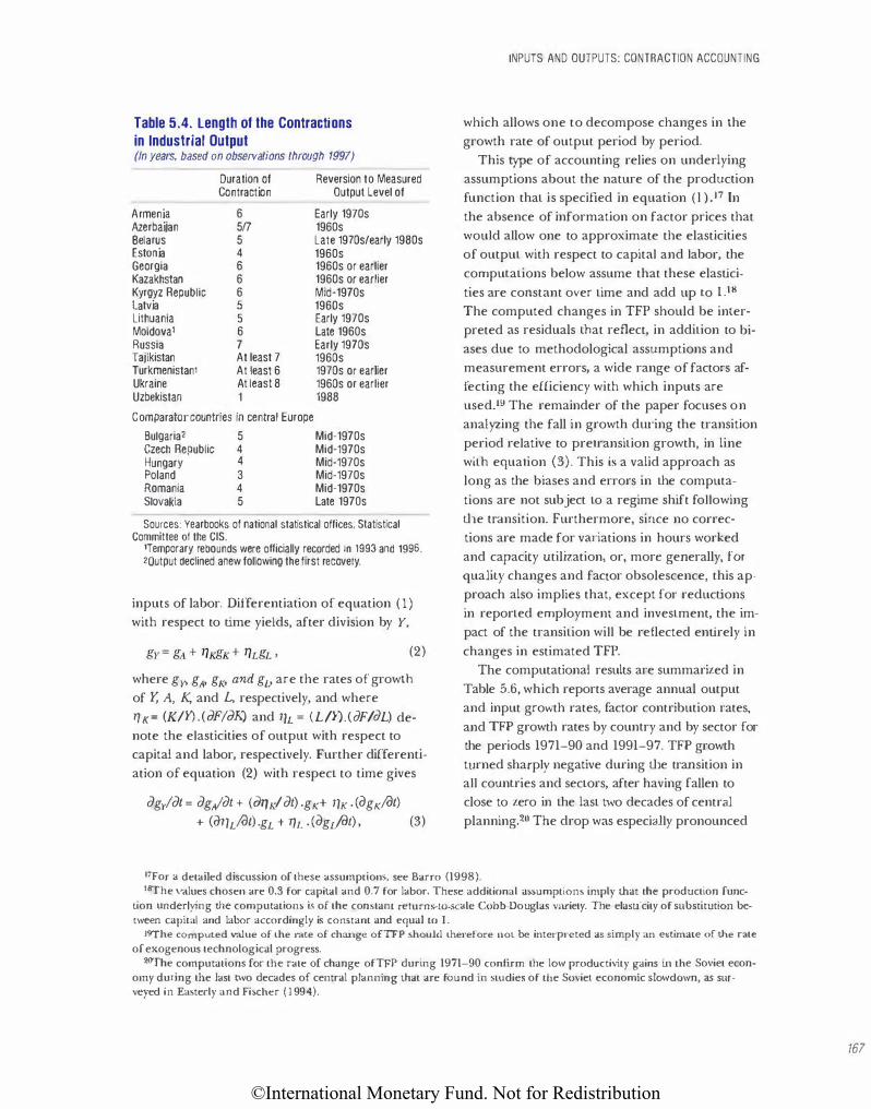
©International Monetary Fund. Not for Redistribution
Table 5.4. Length of the Contractions in Industrial Output (In years, based on observations through 1997)
Duration of Contraction
Reversion to Measured Output Level of
Early 1970s 1960s
Armenia Azerbaijan Belarus Estonia
6 5/7 5 4
Late 1970s/early 1980s 1960s
Georgia Kazakhstan Kyrgyz Republic Latvia Lithuania Moldova! Russia Tajikistan Turkmenistan1 Ukraine Uzbekistan
6 6 6 5 5 6 7 At least 7 At least 6 At least 8 1
Comparator countries in central Europe
Bulgaria2 5 Czech Republic 4 Hungary 4 Poland 3 Romania 4 Slovakia 5
1960s or earlier 1960s or earlier Mid-1970s 1960s Early 1970s Late 1960s Early 1970s 1960s 1970s or earlier 1960s or earlier 1988
Mid-1970s Mid-1970s Mid-1970s Mid-1970s Mid-1970s Late 1970s
Sources: Yearbooks of national statistical oHices; Statistical Committee of the CIS.
1Temporary rebounds were oHicially recorded in 1993 and 1996. 20utput declined anew following the first recovery.
inputs of labor. Differentiation of equation (l ) with respect to time yields, after division by Y,
(2)
where gy, g11, gK, and g1_, are the rates of growth
of 1� A, K, and L, respectively, and where
17K= (K/Y) .(()Fj()K) and 17L = (L!Y).(()Fj()L) denote the elasticities of output with respect to
capital and labor, respectively. Further differenti
ation of equation (2) with respect to time gives
dgl,fdt = dgA/dt + (dTJKf' dt) .gK+ 1JK . (iJgK/()t) + (o1JL/()t) .gL + 17t . (iJgL/()t), (3)
INPUTS AND OUTPUTS: CONTRACTION ACCOUNTING
which allows one to decompose changes in the
growth rate of output period by period.
This type of accounting relies on underlying
assumptions about the nature of the production
function that is specified in equation ( l ) .11 In
the absence of information on factor prices that
would allow one to approximate the elasticities
of output with respect to capital and labor, the
computations below assume that these elastici
ties are constant over time and add up to LIS
The computed changes in TFP should be inter
preted as residuals that reflect, in addition to bi
ases due to methodological assumptions and
measurement errors, a wide range of factors af
fecting the efficiency with which inputs are
used.l9 The remainder of the paper focuses on
analyzing the fall in growth dw-ing the transition
period relative to pretransition growth, in line
with equation (3). This is a valid approach as
long as the biases and errors in the computa
tions are not subject to a regime shift following
the transition. Furthermore, since no correc
tions are made for vru.iations in hours worked
and capacity utilization, or, more generally, for
quality changes and facror obsolescence, this ap
proach also implies that, except for reductions
in reported employment and investment, the im
pact of the transition will be reflected entirely in
changes in estimated TFP.
The computational results are summarized in
Table 5.6, which reports average annual output
and input growth rates, factor contribution rates,
and TFP growth rates by country and by sector for
the periods 1971-90 and 1991-97. TFP growth
turned sharply negative during the transition in
all countries and sectors, after having fallen to
close to zero in the last two decades of central
planning.20 The drop was especially pronounced
1iFor a detailed discussion of these assumpLions, see Barro (1998). 'liThe v-alues chosen are 0.3 for capital and 0.7 for labor. These additional assumptions imply Lhat the production func
tion underlying the computations is of the constant return s-to-scale Cobb-Douglas variety. The elasticity of substitution between capital and labor accordingly is constant and equal to I.
19The computed value of the rate of change ofTFP should therefore not be inte•-p.-cted as simply an estimate of the rate of exogenous technological progress.
2<Yfhe computations for the rate of change ofTFP during 1971-90 confirm the low productivity gains in the Soviet economy during the last two decades of central planning tJ1at are found in swdies of the Soviet economic slowdown, as surveyed in Easterly and Fischer ( 1 994).
161
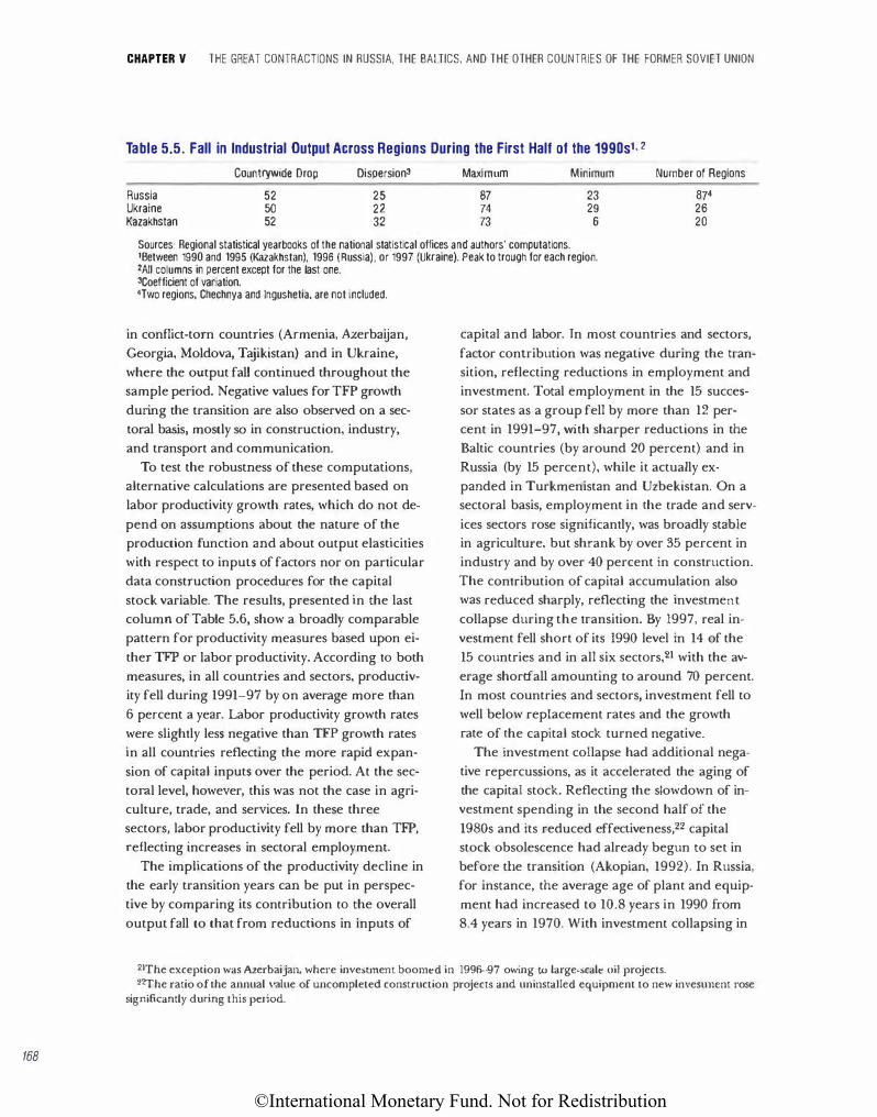
©International Monetary Fund. Not for Redistribution
168
CHAPTER V THE GREAT CONTRACTIONS IN RUSSIA, THE BALTICS, AND THE OTHER COUNTRIES OF THE FORMER SOVIET UNION
Table 5.5. Fall in Industrial Output Across Regions During the First Half of the 1990s1• 2
Russia Ukraine Kazakhstan
Countrywide Drop
52 50 52
Dispersion3
25 22 32
Maximum
87 74 73
Minimum
23 29
6
Number of Regions
874
26 20
Sources: Regional statistical yearbooks of the national statistical offices and authors' computations. !Between 1990 and 1995 (Kazakhstan), 1996 (Russia) , or 1997 (Ukraine). Peak to trough for each region. 2AII columns in percent except for the last one. 3Coefficient of variation. 4Two regions, Chechnya and lngushetia, are not included.
in conflict-torn countries (Armenia, Azerbaijan,
Georgia, Moldova, Tajikistan) and in Ukraine,
where the output fall continued throughout the
sample peiiod. Negative values for TFP growth
during the transition are also observed on a sec
toral basis, mostly so in construction, industry,
and transport and communication.
To test the robustness of these computations,
alternative calculations are presented based on
labor productivity growth rates, which do not de
pend on assumptions about the nature of the
production function and about output elasticities
with respect to inputs of factors nor on particular
data construction procedures for the capital
stock variable. The results, presented in the last
column of Table 5.6, show a broadly comparable
pattern for productivity measures based upon ei
ther TFP or labor productivity. According to both
measures, in all countries and sectors, productiv
ity fell during 1991-97 by on average more than
6 percent a year. Labor productivity growth rates
were slightly less negative than TFP growth rates
in all countries reflecting the more rapid expan
sion of capital inputs over the period. At the sec
toral level, however, this was not the case in agri
culture, trade, and services. In these three
sectors, labor productivity fell by more than TFP,
reflecting increases in sectoral employment.
The implications of the productivity decline in
the early transition years can be put in perspec
tive by comparing its contribution to the overall
output fall to that from reductions in inputs of
capital and labor. In most countries and sectors,
factor contribution was negative during the tran
sition, reflecting reductions in employment and
investment. Total employment in the 15 succes
sor states as a group fell by more than 12 per
cent in 1991-97, with sharper reductions in the
Baltic countries (by around 20 percent) and in
Russia (by 15 percent), while it actually ex
panded in Turkmenistan and Uzbekistan. On a
sectoral basis, employment in the trade and serv
ices sectors rose significantly, was broadly stable
in agriculture, but shrank by over 35 percent in
industry and by over 40 percent in construction.
The contribution of capital accumulation also
was reduced sharply, reflecting the investment
collapse during the transition. By 1997, real in
vestment fell short of its 1990 level in 14 of the
15 countries and in all six sectors,21 with the av
erage shortfall amounting to around 70 percent.
In most countries and sectors, investment fell to
well below replacement rates and the growth
rate of the capital stock turned negative.
The investment collapse had additional nega
tive repercussions, as it accelerated the aging of
the capital stock. Reflecting the slowdown of in
vestment spending in the second half of the
1980s and its reduced effectiveness,22 capital
stock obsolescence had already begun to set in
before tl1e transition (Akopian, 1992). In Russia,
for instance, the average age of plant and equip
ment had increased to 10.8 years in 1990 from
8.4 years in 1970. With investment collapsing in
21The exception was Azerbaijan, where invesunem boomed in 1996-97 owing to large-scale oil projects. 22'fhe ratio of the annual value of uncompleted construction projectS and uninstaUed equipment to new invesunent rose
significantly dudng this period.
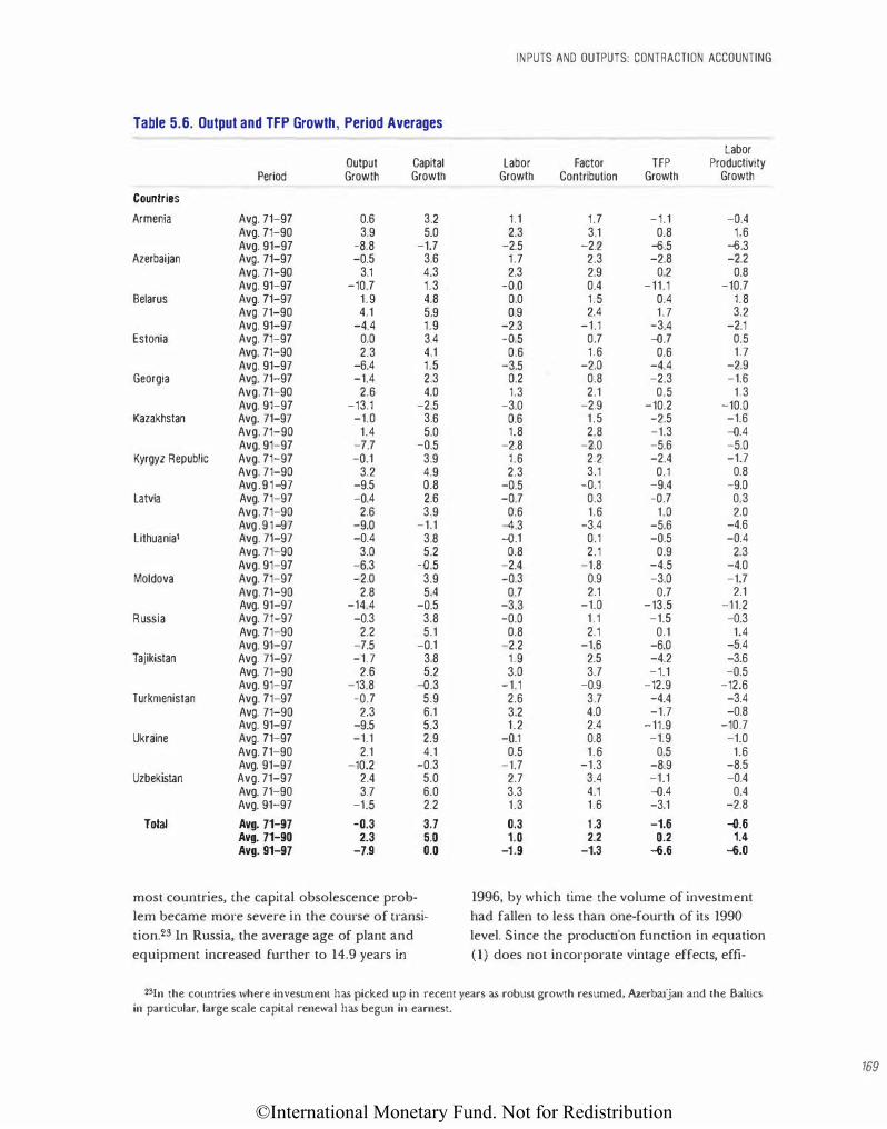
©International Monetary Fund. Not for Redistribution
INPUTS AND OUTPUTS: CONTRACTION ACCOUNTING
Table 5.6. Output and TFP Growth, Period Averages
Labor Output Capital Labor Factor TFP Productivity
Period Growth Growth Growth Contribution Growth Growth
Countries
Armenia Avg. 71-97 0.6 3.2 1.1 1.7 -1.1 -0.4 Avg. 71-90 3.9 5.0 2.3 3.1 0.8 1.6 Avg. 91-97 -8.8 -1.7 -2.5 -2.2 �.5 -6.3
Azerbaijan Avg. 71-97 -0.5 3.6 1.7 2.3 -2.8 -2.2 Avg. 71-90 3.1 4.3 2.3 2.9 0.2 0.8 Avg. 91-97 -10.7 1.3 -o.o 0.4 -11.1 -10.7
Belarus Avg. 71-97 1.9 4.8 0.0 1.5 0.4 1.8 Avg. 71-90 4.1 5.9 0.9 2.4 1.7 3.2 Avg. 91-97 -4.4 1.9 -2.3 -1.1 -3.4 -2.1
Estonia Avg. 71-97 0.0 3.4 -o.5 0.7 -Q.7 0.5 Avg. 71-90 2.3 4.1 0.6 1.6 0.6 1.7 Avg. 91-97 -6.4 1.5 -3.5 -2.0 -4.4 -2.9
Georgia Avg. 71-97 -1.4 2.3 0.2 0.8 -2.3 -1.6 Avg. 71-90 2.6 4.0 1.3 2.1 0.5 1.3 Avg. 91-97 -13.1 -2.5 -3.0 -2.9 -10.2 -10.0
Kazakhstan Avg. 71-97 -1.0 3.6 0.6 1.5 -2.5 -1.6 Avg. 71-90 1.4 5.0 1.8 2.8 -1.3 -Q.4 Avg. 91-97 -7.7 -Q.5 -2.8 -2.0 -5.6 -5.0
Kyrgyz Republic Avg. 71-97 -Q.1 3.9 1.6 2.2 -2.4 -1.7 Avg. 71-90 3.2 4.9 2.3 3.1 0.1 0.8 Avg.91-97 -9.5 0.8 -o.5 -0.1 -9.4 -9.0
Latvia Avg. 71-97 -Q.4 2.6 -Q.7 0.3 -0.7 0.3 Avg. 71-90 2.6 3.9 0.6 1.6 1.0 2.0 Avg.91-97 -9.0 -1.1 -4.3 -3.4 -5.6 -4.6
lithuania' Avg. 71-97 -0.4 3.8 -0.1 0.1 -Q.5 -Q.4 Avg. 71-90 3.0 5.2 0.8 2.1 0.9 2.3 Avg. 91-97 -6.3 -Q.5 -2.4 -1.8 -4.5 -4.0
Moldova Avg. 71-97 -2.0 3.9 -Q.3 0.9 -3.0 -1.7 Avg. 71-90 2.8 5.4 0.7 2.1 0.7 2.1 Avg. 91-97 -14.4 -o.5 -3.3 -1.0 -13.5 -11.2
Russia Avg. 71-97 -0.3 3.8 -0.0 1 . 1 -1.5 -0.3 Avg. 71-90 2.2 5.1 0.8 2.1 0.1 1.4 Avg. 91-97 -7.5 -0.1 -2.2 -1.6 -6.0 -5.4
Tajikistan Avg. 71-97 -1.7 3.8 1.9 2.5 -4.2 -3.6 Avg. 71-90 2.6 5.2 3.0 3.7 -1.1 -Q.5 Avg. 91-97 -13.8 -0.3 -1.1 -0.9 -12.9 -12.6
Turkmenistan Avg. 71-97 -0.7 5.9 2.6 3.7 -4.4 -3.4 Avg. 71-90 2.3 6.1 3.2 4.0 -1.7 -0.8 Avg. 91-97 -9.5 5.3 1.2 2.4 -11.9 -10.7
Ukraine Avg. 71-97 -1.1 2.9 -D.1 0.8 -1.9 -1.0 Avg. 71-90 2.1 4.1 0.5 1.6 0.5 1.6 Avg. 91-97 -10.2 -0.3 -1.7 -1.3 -8.9 -8.5
Uzbekistan Avg. 71-97 2.4 5.0 2.7 3.4 -1.1 -0.4 Avg. 71-90 3.7 6.0 3.3 4.1 -Q.4 0.4 Avg. 91-97 -1.5 2.2 1.3 1.6 -3.1 -2.8
Total Avg. 71-97 -{).3 3.7 0.3 1 .3 -1.6 -{).6 Avg. 71-90 2.3 5.0 1.0 2.2 0.2 1.4 Avg. 91-97 -7.9 0.0 -1.9 -1.3 �.6 �.0
most countries, the capital obsolescence prob- 1996, by which time the volume of investment
\em became more severe in the course of transi- had fallen to less than one-fourth of its 1990
tion.23 In Russia, the average age of plant and level. Since the production function in equation
equipment increased further to 14.9 years in (l) does not incorporate vintage effects, effi-
2SJn the cotmtries where investment has picked up in recent years as robust growth resumed, AzerbaUan and the Baltics in particular, large scale capital renewal has begun in earnest.
169
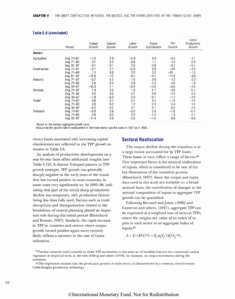
©International Monetary Fund. Not for Redistribution
110
CHAPTER V THE GREAT CONTRACTIONS IN RUSSIA, THE BALTICS, AND THE OTHER COUNTRIES OF THE FORMER SOVIET UNION
Table 5.6 (concluded)
labor Output Capital labor Factor TFP Productivity
Period Growth Growth Growth Contribution Growth Growth
Sectors
Agriculture Avg. 71-97 -1.5 2.9 -o.4 0.9 -2.4 -1.1 Avg. 71-90 0.1 5.0 -o.6 1.1 -1.0 0.6 Avg. 91-97 -B.1 -3.1 0.0 -0.9 -5.2 -B.1
Construction Avg. 71-97 -3.7 3.7 -o.5 0.8 -4.5 -3.2 Avg. 71-90 1.2 5.5 2.2 3.2 -20 -1.0 Avg.91-97 -17.6 -1.2 -8.1 -B.1 -11.6 -9.5
Industry Avg. 71-97 -o.7 4.3 -1.0 0.6 -1.3 0.3 Avg. 71-90 2.8 5.4 0.8 2.2 0.6 1.8 Avg. 91-97 -10.5 1.1 -B.2 -4.0 -6.5 -4.3
Services Avg. 71-97 1 .4 3.2 1.5 2.1 -0.6 -Q.1 Avg. 71-90 2.5 4.5 2.1 2.8 -0.3 0.5 Avg. 91-97 -1.8 -0.3 0.0 -o.1 -1.7 -1.8
Trade2 Avg. 71-97 0.9 3.7 2.1 2.4 -1.5 -1.2 Avg. 71-90 2.8 5.0 1.2 2.3 0.4 1.6 Avg. 91-97 -4.2 -0.2 3.1 2.1 -6.3 -7.4
Transport Avg. 71-97 -0.8 3.9 -o.5 0.8 -1.6 -o.2 Avg. 71-90 2.9 5.0 0.2 1.6 1.3 2.7 Avg. 91-97 -11.4 0.9 -2.5 -1.5 -9.9 -8.9
I Based on the revised aggregate growth rates. 2Assuming the growth rate of employment in the trade sector was the same in 1997 as in 1996.
ciency losses associated with increasing capital
obsolescence are reflected in the TFP growth es·
timates in Table 5.6.
An analysis of productivity developments on a
year·by·year basis offers additional insights (see
Table 5.12). A distinct V·shaped pattern in TFP
growth emerges. TFP growth was generally
sharply negative in the early years of the transi·
tion but turned positive in most countries, in
some cases very significantly so, by 1995-96, indi
cating that part of the initial sharp productivity
decline was temporary, witl1 production factors
being less than fully used. Factors such as trade
disruptions and disorganization related to the
breakdown of central planning played an impor
tant role during this initial period (Blanchard
and Kremer, 1997). Similarly, the rapid increase
in TFP in countries and sectors where outpm
growth turned positive again more recently
likely reflects a recovery in the rate of facto1·
utilization.
Sectoral Reallocation
The output decline during the u-ansition is to
a large extent accounted for by TFP losses.
These losses in turn reflect a range of factors.24
One important factor is tl1e sectoral reallocation
of inputs, which is considered to be one of tl1e
key dimensions of the transition process
(Blanchard, 1997). Since the output and input
data used in this study are available on a broad
sectoral basis, the contribution of changes in the
sectoral composition of inputs to aggregate TFP
growth can be quantified.
Following Bernard and jones ( 1996) and
Cameron and others. (1997), aggregate TFP can
be expressed as a weighted sum of sectoral TFPs,
where the weights are ratios of an index of in
puts in each sector to an aggregate index of
inputs.25
24Further research could consider to relate TFP movements to the same set of variables that are now commonly used as regressors in empirical work, in the vein of Berg and others (1999), for instance, on output movements during the transition.
25This expression assumes that the produCLion process in each sector j is characterized by a common, time-invariaiH. Cobb-Douglas production technology.
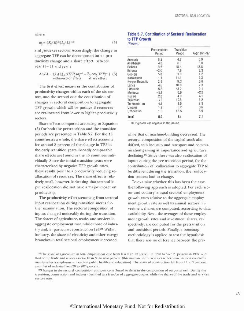
©International Monetary Fund. Not for Redistribution
where
(4)
and j indexes sectors. Accordingly, the change in
aggregate TFP can be decomposed into a pro
ductivicy change and a share effect. Between
year ( t - 1) and year l
L1A/ A = 1/ A lLj L\Tf'J�.ro.t' + L1 L\O>_j.1Fijl-l) (5} withjn-sector effect share effect
The first effect measures the contribution of
productivicy changes within each of the six sec
tors, and the second one the contribution of
changes in sectoral composition to aggregate
TFP growth, which will be positive if resources
are reallocated from lower to higher-productivity
sectors.
Share effects computed according to Equation
(5) for both the pretransition and the transition
periods are presented in Table 5.7. For the 15 countries as a whole, the share effect accounts
for around 8 percent of the change in TFP in
the early transition years. Broadly comparable
share effects are found in the 15 countries indi
\ri.dually. Since the initial u·ansition years were
characterized by negative TFP growth rates,
these results point to a productivity reducing re
allocation of resources. The share effect is rela
tively small, however, indicating that sectoral in
put reallocation did not have a major impact on
productivity.
The productivity effect stemming from sectoral
input reallocation during u·ansition merits fur
ther examination. The sectoral composition of
inputs changed noticeably during the transition.
The shares of agriculture, trade, and services in
aggregate employment rose, while those of indus
try and, in particular, construction feJl.26 Within
industry, the share of electricicy and other energy
branches in total sectoral employment increased,
SECTORAL REALLOCATION
Table 5. 7. Contribution of Sectoral Reallocation to TFP Growth (Percent)
Pretransition Transition Period Period' Avg.1 971-97
Armenia 8.2 4.7 5.9 Azerbaijan 4.8 0.9 3.0 Belarus 9.6 18.4 12.8 Estonia -2.0 7.9 3.3 Georgia 5.8 3.0 4.2 Kazakhstan -1.1 11.1 2.3 Kyrgyz Republic 2.9 9.3 6.6 Latvia 4.6 10.0 7.3 Lithuania 5.3 13.2 9.1 Moldova -5.1 0.9 -2.2 Russia 2.8 4.9 4.1 Tajikistan -1.2 10.5 6.2 Turkmenistan 4.5 1.6 2.9 Ukraine 1.2 0.2 0.6 Uzbekistan 1.0 1 5.5 5.9
Total 5.0 8.1 7.1 1TFP growth was negative in this period.
while that of machine-building decreased. The
sectoral composition of the capital stock also
shifted, with indusu·y and transport and commu
nication gaining in importance and agriculture
declining.27 Since there was also reallocation or
inpms during the pre-transition period, for the
conu·ibution of r·eallocation to aggregate TIP tO
be different during the transition, the realloca
rion process had to change.
To examine whether this has been the case,
the following approach is adopted. For each sec
tor and counu·y, annual sectoral employment
growth rates relative to the aggregate employ
ment growth rate as well a� annual sectoral in
vestment shares are computed, according to data
availability. ext, the averages of these employ
ment growth rates and investment shares, re
spectively, are computed for the pretransition
and u-ansition periods. Finally, a bootso-ap
methodology is applied to test the hypothesis
that there was no difference between the pre-
2GThe share of agriculture in total employmem rose from less than 19 percent in 1990 tO over :.11 percent in 1997, and that of the u-ade and services sec LOr from 38 to 46!h percent (this increase in the services sector sh;u·c in most countries mainly refleclS employment u·ends in public health and education). The share or construction fel l from I I to 7 percent, and lhat of industry from 28 to 20'h percent.
27Changes in the sectoral composition of in puiS contributed to shift:. in the composition of our pur as well. During the transition, construction and industry declined as a fmction of aggregate output, while the shares of the trade and sen;ces sectors rose.
171
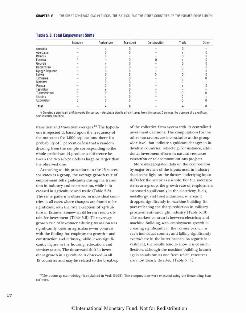
©International Monetary Fund. Not for Redistribution
172
CHAPTER V THE GREAT CONTRACTIONS IN RUSSIA, THE BALTICS, AND THE OTHER COUNTRIES OF THE FORMER SOVIET UNION
Table 5.8. Total Employment Shifts1
Industry Agriculture Transport Construction Trade Other
Armenia + 0 0 Azerbaijan 0 0 + 0 Belarus 0 0 0 Estonia 0 0 0 + 0 Georgia + 0 0 0 Kazakhstan 0 0 0 0 Kyrgyz Republic 0 0 0 0 Latvia 0 0 0 0 0 Lithuania 0 0 0 0 Moldova 0 0 0 Russia 0 0 + 0 Tajikistan + 0 Turkmenistan 0 0 0 0 0 0 Ukraine + 0 0 + Uzbekistan 0 0 0 0 0
Total + 0 + 0 1+ Denotes a significant shift towards the sector; - denotes a significant shift away from the sector; 0 denotes the absence of a significant
shift in either direction.
transition and u·ansition averages.2s The hypoth
esis is rejected if, based upon the frequency of
the outcomes for 1,000 replications, there is a
probability of 1 percent or less that a random
drawing from the sample corresponding to the
whole period would produce a difference be
tween the two sub-periods as large or larger than
the observed one.
According to this procedure, in the 15 successor states as a group, the average growth rate of
employment fell significantly during the transi
tion in industry and construction, while it in
creased in agriculture and trade (Table 5.8).
The same pattern is observed in individual coun
tries in all cases where changes are found to be
significant, with the rare exception of agri.cul
ture in Estonia. Somewhat different results ob
tain for investment (Table 5.9). The average
growth rate of invcstmen t during transition was
significantly lower in agriculture-in contrast
with the finding for employment growth-and
construction and industry, whjle it was signill
cantly higher in the housing, education, and
services sector. The downward shift in invest
ment growth in agriculture is observed in all
15 countries and may be related to the break-up
of the collective farm system with its centralized
investment decisions. The computations for the
other two sectors are inconclusive at the group
wide level, but indicate significant changes in in
dividual countries, reflecting, for instance, addi
tional investment efforts in natural resources
extraction or telecommunications projects.
More disaggregated data on the composition
by major branch of the inputs used in industry shed some light on the factors underlying input
shifts for the sector as a whole. For the successor
states as a group, the growth rate of employment
increased significantly in the electricity, fuels,
metallurgy, and food indusu·ies, whereas it
dropped significantly in machine-building (in
part reflecting the sharp reduction in mili tary
procurement) and light industry (Table 5.10).
The starkest contrasl is bet\veen electricity and
machine-building, with employmenl growth in
creasing significantly in the former branch in
each indjvidual country and falling significantly
everywhere in the latter branch. As regards in
vestment, the results tend to show Jess of an in
flection, although the machine-building branch
again stands out as one from which resources
are most clearly diverted (Table 5.1 1 ) .
28"fhe bootstrap methodology is explained in Veall (1998). The computations were executed using the Resampling S taL� software.
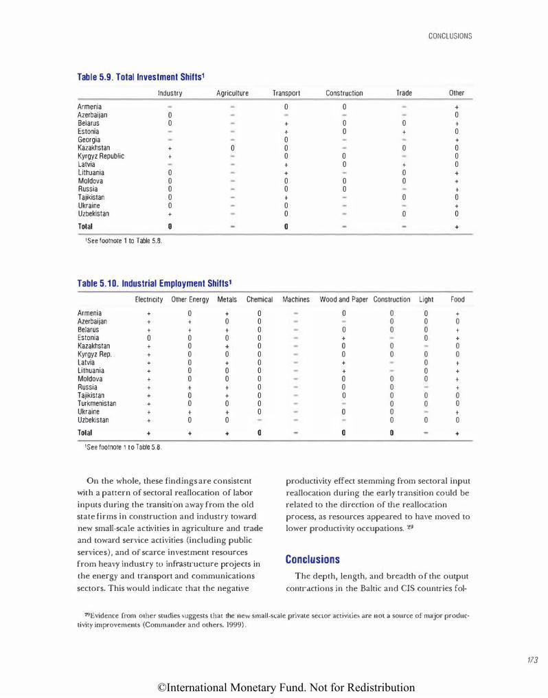
©International Monetary Fund. Not for Redistribution
CONCLUSIONS
Table 5.9. Total Investment Shifts1
Industry Agriculture Transport Construction Trade Other
Armenia 0 0 + Azerbaijan 0 0 Belarus 0 + 0 0 t Estonia t 0 t 0 Georgia 0 t Kazakhstan t 0 0 0 0 Kyrgyz Republic t 0 0 0 Latvia t 0 + 0 lithuania 0 t 0 + Moldova 0 0 0 0 t Russia 0 0 0 t Tajikistan 0 t 0 0 Ukraine 0 0 t Uzbekistan t 0 0 0
Total 0 0 +
'See footnote 1 to Table 5.8.
Table 5.10. Industrial Employment Shifts1
Electricity Other Energy Metals Chemical Machines Wood and Paper Construction Light Food
Armenia t 0 t 0 Azerbaijan t t 0 0 Belarus t t t 0 Estonia 0 0 0 0 Kazakhstan t 0 + 0 Kyrgyz Rep. t 0 0 0 Latvia t 0 t 0 Lithuania t 0 0 0 Moldova t 0 0 0 Russia t t t 0 Tajikistan t 0 t 0 Turkmenistan t 0 0 0 Ukraine t t + 0 Uzbekistan t 0 0
Total + + + 0
1See footnote 1 to Table 5.8.
On the whole, these findings are consistent with a pattern of sectoral reallocation of labor inputs during the transition away from the old state firms in construction and industry toward new small-scale activities in agriculture and trade and toward service activities (including public
services), and of scarce investment resources from heavy industry to infrastructure projects in the energy and transport and communications
sectors. This would indicate that the negative
0 0 0 t 0 0 0
0 0 0 t
t 0 t 0 0 0 0 0 0 0 t 0 t t 0 t 0 0 0 t 0 0 t
0 0 0 0 0 0 0
0 0 t 0 0 0
0 0 +
productivity effect stemming from sectoral input reallocation during the early o·ansition could be related to the direction of the reallocation process, as resources appeared to have moved to lower productivity occupations. 29
Conclusions
The depth, length, and breadth of the output
contractions in the Baltic and CIS countries fol-
29.Evidence from olher studies suggests that the new small-scale private sector acth�ties are not a source of major productivity improvements (Commander and others, 1999) .
113
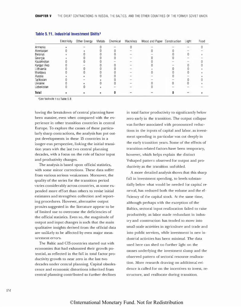
©International Monetary Fund. Not for Redistribution
114
CHAPTER V THE GREAT CONTRACTIONS IN RUSSIA, THE BALTIC$, AND THE OTHER COUNTRIES OF THE FORMER SOVIET UNION
Table 5.11. Industrial Investment Shifts1
Electricity Other Energy Metals Chemical
Armenia + 0 Azerbaijan 0 + 0 0 Belarus + 0 0 0 Georgia + 0 0 0 Kazakhstan 0 0 0 Kyrgyz Rep. 0 0 0 Lithuania 0 0 0 0 Moldova 0 0 0 0 Russia + + 0 0 Tajikistan 0 + 0 Ukraine 0 + 0 0 Uzbekistan 0 0 +
Total + + + 0
1see footnote 1 to Table 5.8.
lowing the breakdown of central planning have
been massive, even when compared with the ex
perience in other transition countries in central
Europe. To explore the causes of these particu
larly sharp conu·actions, the analysis has put out
put developments in these 15 countries in a
longer-run perspective, linking the initial transi
tion years with the last two central planning
decades, with a focus on the role of factor input
and productivity changes.
The analysis is based upon official statistics,
with some minor corrections. These data suffer
from various serious weaknesses. Moreover, the
quality of the series for the transition period
varies considerably across countries, as some ex
pended more effort than others to revise initial
estimates and strengthen collection and report
ing procedures. However, alternative output
proxies suggested in the literature appear to be
of limited use to overcome the deficiencies of
the official statistics. Even so, the magnitude of
output and input changes is such that the main
qualitative insights derived from the official data
are unlikely to be affected by even m�jor meas
urement en-ors.
The Baltic and CIS countries started out with
economies that had exhausted their growth po
tential, as reflected in the fall in total factor pro
ductivity growth to near zero in the last two
decades under central planning. Capital obsoles
cence and economic distOrtions inherited from
central planning contributed tO fw·ther declines
Machines Wood and Paper Construction Light Food
0 0 0 0
0 0 + 0 0 0 0 0 0 0 + 0 0 + 0 0 0 +
0 + 0 0
0 0 0 + 0
0 +
in total factor productivity to significantly below
zero early in the transition. The output collapse
was further associated with pronounced reduc
tions in the inputs of capital and labor, as invest
ment spending in panicular was cut deeply in
Lhe early transition years. Some of the effects of
transition-related factors have been temporary,
however, which helps explain the distinct
V-shaped pattern observed for output and pro
ductivity as the transition unfolded.
A more detailed analysis shows that this sharp
faU in investment spendjng, to levels substan
tially below what would be needed for capital re
newal, has reduced both the volume and the ef
ficiency of the capital stock. At the same time,
although perhaps with the exception of the
Baltics, sectoral input reallocation failed to raise
productivity, as labor made redundant in indus
u·y and consu·uction has tended to move into
small-scale activities in agriculture and trade and
into public services, while investment in new in
dustrial activities has been minimal. The data
used here can shed no further light on the
causes underlying the investment slump and the
observed pattern of sectoral resource realloca
tion. More research drawing on additional evi
dence is called for on the incentives to invest, re
structure, and reallocate during transition.
©International Monetary Fund. Not for Redistribution
Appendix 5.1 . Data Description3o
National Accounts
The series for output, labor, and the capital
stock are built up starting from the data set used
by Easterly and Fischer ( 1994), covering
1970-89. The data have been cross-checked
against series on the same variables provided by
the Statistical Committee of the CIS for 1980-90,
and some minor corrections introduced. Output
and capital data for the pretransition period are
level data and are expressed in "comparable
prices," a price concept that is considered not to
fully adjust for inflation. An adjustment has been
applied following Unites States Congress, joint
Economic Committee (1990), Kellogg (1990),
and Noren and Kurtzwcg (1993). Labor data re
fer to total employment numbers, unadjusted
for variations in hours worked.
This amended data set is supplemented for
more recem years by information drawn from
national statistical yearbooks (in particular for
the Baltics) , from various publications of the
Statistical Committee of the CIS (notably its CD
ROM Official Statistics of the CIS Countries, various
issues of The Statistical YeadJook of the CIS, The World in Figures (1992) and its foroughtly
Bulletin) and from the World Bank's Statistical
Handboolt, Stales of the Fonner USSR; in a few cases,
data have been obtained directly from the cen
u·al statistical offices (data from these various
sources may differ from the estimates used by
lMF country desks and appearing in the IMF's
World Economic Outloolt or in IMF Staff Country
Reports).
The output, labor, and capital stock data for
the transition period are constructed to ensure
consistency with the 1970-89 series. Output level
data for this period are extrapolated from the
preu-ansition period using information on real
growth rates. Labor data for the period 1990-97
continue to refer to total employment nwnbers,
which in most cases arc broadly consistent with
the pretransition numbers (with the possible ex-
APPENDIX 5.1
ception or employment da ta in the u-ade and
services sectors in 1996-97, which in a number
of counu·ics appear to reflect reclassification of
occupations) . The capital stock data for tl1e tran
sition period arc obtained using 1990-97 gross
investment data and applying depreciation rates
that are impmed from 1970-89 capital stock and
investment data and from information in
Kellogg (1990).
A number of countries have substantially re
vised their COP and sectoral output series, in
cluding Russia (World Bank and the Russian
Federation, Goskomstat 1995), Kazakhstan
(World 13ank, 1997), and Lithuania (for the ag
gregate output series only). ln such cases, the re
vised series are used.
TFP computaLions, in addiLion to data on out
put and inputs of labor and capi tal, require
proxies for the elasticities of output with respect
to capital and labor (Table 5.12). For this pur
pose, observed shares of factOr payments in total
product are commonly used. Reported factor
share data for the 15 countries in the sample
are, however, incomplete and, except for the
most recent yea.-s, do not reflect market
determined factor payments. Share esLimates
that could approximate elasticities of output
with respect to capital and labor can only be ob
tained on the basis of detailed adjustments and
additional information on wages and rentals, as
in Bergson ( 1 978). Rather than ino·oducing
such adjustments, output elasticities with regard
to capital and labor arc posited to equal 0.3 and
0.7 respectively, for all countries, sectors, and
years.
Finally, the statistical yearbooks of the Council
for Mutual Economic Assistance (CMEA) are
used for prctransition data on ceno-al European
comparators when no national yearbooks were
available.
Alternative Measures of Output
Elecu·icity consumption data are taken from
various publications of the International Energy
SOData referred to btl! not displayed in this paper are available from tlle authors on request.
175
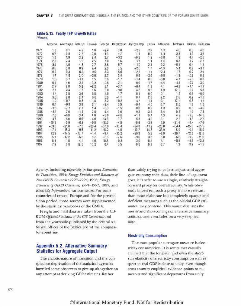
©International Monetary Fund. Not for Redistribution
176
CHAPTER V THE GREAT CONTRACTIONS IN RUSSIA, THE BALTIC$, AND THE OTHER COUNTRIES OF THE FORMER SOVIET UNION
Table 5. 12. Yearly TFP Growth Rates (Percent)
Armenia Azerbaijan Belarus Estonia Georgia Kazakhstan
1971 1.8 0.1 4.2 1.8 -2.4 0.0 1972 0.6 -0.5 2.7 -2.0 -1.3 4.7 1973 1.8 1.9 3.2 2.4 2.7 -3.2 1974 2.8 7.4 1.9 2.5 7.0 -1.6 1975 3.1 1.0 4.8 2.7 2.8 -5.7 1976 0.5 3.8 0.9 2.4 2.8 3.5 1977 0.2 0.3 -0.3 -0.5 3.3 -8.0 1978 1.7 1.9 2.0 -3.6 2.7 5.4 1979 1.6 3.7 -1.1 1.5 5.6 -1.7 1980 0.4 4.0 -2.1 -0.3 -0.6 -2.1 1981 2.7 2.8 5.3 -2.2 3.1 -3.7 1982 -2.1 -2.4 -1.7 1 .6 -3.0 -9.0 1983 -1.4 -2.5 3.6 0.8 1.0 1.7 1984 3.0 2.0 2.1 0.6 3.8 -4.1 1985 1.9 -0.7 0.8 -1.8 2.2 -0.2 1986 0.1 -0.9 3.9 2.1 -2.4 0.5 1987 -1.5 -7.7 2.7 1.4 -3.3 -1.5 1988 -4.1 7.0 -1.2 2.5 4.4 2.0 1989 7.5 -9.8 3.4 4.8 -3.8 -4.6 1990 -4.7 -8.0 -0.6 -4.0 -14.3 0.7 1991 -10.2 -7.9 -0.2 -9.8 -18.3 -4.8 1992 -59.0 -21.0 -7.3 -28.4 -37.0 -10.4 1993 -7.4 -18.3 -9.6 -11.2 -18.2 -4.5 1994 1 2.9 -17.5 -16.7 -1.4 -9.4 -15.2 1995 5.7 -12.2 -6.5 5.7 -5.6 -7.6 1996 5.1 -1.5 4.1 4.0 10.8 -0.2 1997 7.2 0.6 12.5 10.2 6.4 3.5
Agency, including Electricity in European Economies in Transition, 1994; Energy Statistics and Balances of Non-OECD Countries 1993-1994, 1996; Energy Balances ofOECD Countries, 1994-1995, 1997; and
Electricity lnfrmnation, various issues. For some
countries of cenu·al Europe and for the preu·an
sition period, those sources were supplemented
by the statistical yearbooks of the CMEA. Freight and mail data are taken from the CD
ROM Official Statistics of the CIS Countries, and
from the yearbooks published by the central sta
tistical offices of the Baltics and of the compara
tor countries.
Appendix 5.2. Alternative Summary Statistics for Aggregate Output
The chaotic nature of transition and the con
spicuous deprivation of the statistical agencies
have led some observers to give up altogether on
any attempt at deriving GDP estimates. Rather
Kyrgyz Rep. Latvia Lithuania Moldova Russia Tajikistan
-2.9 2.9 1.3 4.0 0.0 4.3 1.4 0.9 1.4 -2.8 -1.3 -3.2
-0.5 1.2 -0.8 1.9 4.4 -2.5 -1.1 1.1 1.0 -o.8 1.7 2.1 -1.0 2.1 2.2 -Q.4 0.4 1.2 -2.0 1.7 -1.3 5.4 0.2 -3.1 -2.5 -1.4 -2.4 -1.7 0.2 -2.4
0.8 -2.5 -0.8 -1.8 -0.8 0.2 -1.4 0.5 -3.0 4.7 -2.0 0.3
0.9 -1.7 -4.4 -4.2 -0.7 3.0 -0.4 1.9 4.1 -4.9 -1.1 -1.7 -4.6 -0.6 1.9 12.2 -0.7 -5.3
5.1 0.9 -0.1 1.5 0.5 -0.9 0.7 2.8 2.2 2.0 0.2 -1.2
-4.7 -1.4 -3.1 -12.1 0.5 -1.1 -0.4 4.0 5.7 8.5 1.8 1.5
0.0 0.9 4.3 0.9 0.6 -4.6 9.3 3.6 5.4 0.2 1.9 7.5
-1.1 6.4 1.3 4.2 -2.3 -14.5 5.8 -4.2 3.1 -2.2 -1.2 -2.2
-6.9 -3.2 -5.9 -21.4 -4.4 -7.6 -24.8 -41.9 -28.0 -34.4 -15.0 -25.5 -10.7 -14.5 -33.9 8.9 -9.1 -18.9 -26.3 5.3 -8.9 -36.7 -12.8 -12.5
-9.6 3.3 5.0 -6.6 -1.2 -11.0 3.0 5.1 4.1 -5.4 -2.3 -13 2 9.6 6.9 8.7 1.3 3.2 -1.2
than vainly trying to collect, adjust, and aggregate economy-wide data, their line of argument
goes, it is safer to use a single, relatively straight
forward proxy for overall activity. While obvi
ously imperfect, such a proxy is more relevant
than more elaborate but completely opaque and
de-ficient measures such as the official GDP estimates, they contend. This annex discusses the merits and shortcomings of alternative summary statistics, and concludes on a very skeptical
note.
Electricity Consumption
The most popular surrogate measure is elec
u·icity consumption. I t is sometimes casually
claimed that the long-run and even the short
run elasticity of electricity consumption with re
spect to real GDP is close to unity, even though cross-country empirical evidence points to nu
merous and significant departures from unity
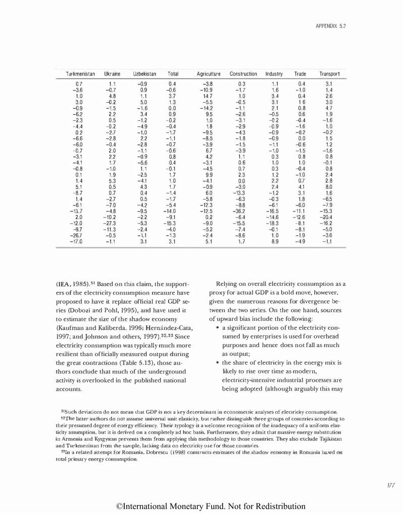
©International Monetary Fund. Not for Redistribution
Turkmenistan Ukraine Uzbekistan Total
0.7 1.1 -0.9 0.4 -3.6 -0.7 0.9 -0.6
1.0 4.8 1 .1 3.7 3.0 -o.2 5.0 1.3
-0.9 -1.5 -1.6 0.0 -6.2 2.2 3.4 0.9 -2.3 0.5 -1.2 -o.2 -4.4 -0.2 -4.9 -0.4
0.2 -2.7 -1.0 -1.7 -6.6 -2.8 2.2 -1.1 -6.0 -0.4 -2.8 -0.7 -0.7 2.0 -1.1 -o.6 -3.1 2.2 -o.9 0.8 -4.1 1.7 -5.6 0.4 -o.8 -1.0 1 .1 -o.1
0.1 1.9 -2.5 1.7 1.4 5.3 -4.1 1.0 5.1 0.5 4.3 1.7
-8.7 0.7 0.4 -1.4 1.4 -2.7 0.5 -1.7
-6.1 -7.0 -4.2 -5.4 -13.7 -4.8 -9.5 -14.0
2.0 -10.2 -2.2 -9.1 -12.0 -27.3 -5.3 -15.3
-9.7 -11.3 -2.4 -4.0 -26.7 -0.5 -1.1 -1.3 -17.0 -1.1 3.1 3.1
(lEA, 1985).31 Based on this claim, the support
ers of the electricity consumption measure have
proposed to have it replace official real GDP se
ries (Dobozi and Pohl, 1995), and have used it
to estimate the size of the shadow economy
(Kaufman and Kaliberda, 1996; Hermindez-Cata,
1997; and johnson and others, 1997).32,33 Since
electricity consumption was typically much more
resilient than officially measured output during
the great contractions (Table 5.13), those au
thors conclude that much of the underground
activity is overlooked in the published national
accounts.
APPENDIX 5.2
Agriculture Construction Industry Trade Transport
-3.8 0.3 1 .1 0.4 3.1 -10.9 -1.7 1.6 -1.0 1.4
14.7 1.0 3.4 0.4 2.6 -5.5 -o.5 3.1 1.6 3.0
-14.2 -1.1 2.1 0.8 4.7 9.5 -2.6 -0.5 0.6 1 .9 1.0 -3.1 -0.2 -Q.4 -1.6 1.8 -2.9 -0.9 -1.6 1.0
-9.5 -4.3 -0.9 -o.2 -0.2 -8.5 -1.8 -0.9 0.0 1 .5 -3.9 -1.5 -1.1 -o.6 1.2
6.7 -3.9 -1.0 -1.5 -1.6 4.2 1 .1 0.3 0.8 0.8
-3.1 0.6 1.0 1.0 -0.1 -4.5 0.7 0.3 -Q.4 0.8
9.9 2.3 1.2 -1.0 2.4 -4.1 0.0 2.2 0.7 2.8 -o.9 -3.0 2.4 4.1 8.0
6.0 -13.3 -1.2 3.1 1.6 -5.8 -6.3 -o.3 1.8 -6.5
-12.3 -8.8 -6.1 -6.0 -7.9 -12.5 -36.2 -16.5 -11.1 -15.3
0.2 -6.4 -14.6 -12.6 -20.4 -9.0 -15.5 -18.3 -8.1 -16.2 -5.2 -7.4 -o.1 -8.1 -5.0 -2.4 -8.6 1 .0 -1.9 -3.6
5.1 1.7 8.9 -4.9 -1.1
Relying on overall electricity consumption as a
proxy for actual GDP is a bold move, however,
given the numerous reasons for divergence be
tween the two series. On the one hand, sources
of upward bias include the following:
• a significant portion of the electricity con
sumed by enterprises is used for overhead
purposes and hence does not fall as much
as output;
• the share of electricity in the energy mix is
likely to rise over time as modern,
electricity-intensive industrial processes are
being adopted (although arguably this may
SISuch deviations do not mean that GDP is not a key determinant in econometric analyses of electricity consumption. S2"fhe Iauer· authors do not assume universal unit elasticity, but rather distinguish three groups of countries according to
their presumed degree of energy efficiency. Their typology is a welcome recognition of t11e inadequacy of a uniform elasticity assumption, but it is derived on a completely ad hoc basis. FurtJ1ennore, t11ey admit t11at massive energy substitution in Armenia and K)'l·gystan prevents them from applying t11is metJ1odology to t11ose countries. They also exclude Tajikis tan and Turkmenistan from the sample, lacking data on electricity use for those countries.
ssrn a related auempt for Romania, Dobrescu (1998) constructs estimates of the shadow economy in Romania based on total pr·imary energy consumption.
177
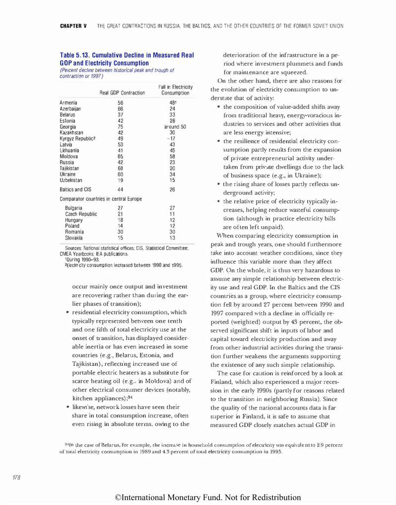
©International Monetary Fund. Not for Redistribution
178
CHAPTER V THE GREAT CONTRACTIONS IN RUSSIA, THE BALTIC$, AND THE OTHER COUNTRIES OF THE FORMER SOVIET UNION
Table 5.13. Cumulative Decline in Measured Real GOP and Electricity Consumption (Percent decline between historical peak and trough of contraction or 1997)
Fall in Electricity Real GOP Contraction Consumption
Armenia 56 481 Azerbaijan 66 24 Belarus 37 33 Estonia 42 28 Georgia 75 around 50 Kazakhstan 42 30 Kyrgyz Republic2 49 -17 Latvia 53 43 Lithuania 41 45 Moldova 65 58 Russia 42 23 Tajikistan 68 20 Ukraine 60 34 Uzbekistan 1 9 15
Baltics and CIS 44 26
Comparator countries in central Europe
Bulgaria 27 27 Czech Republic 21 1 1 Hungary 1 8 12 Poland 14 12 Romania 30 30 Slovakia 15 13
Sources: National statistical offices; CIS, Statistical Committee; CMEA Yearbooks; lEA publications.
1Quring 199G-93. 2Eiectricity consumption increased between 1990 and 1995.
occur mainly once output and investment
are recovering rather than during the ear
lier phases of transition);
• residential electricity consumption, which
typically represented between one tenth
and one ftfth of total electricity use at the
onset of transition, has displayed consider
able inertia or has even increased in some
countries (e.g., Belarus, Estonia, and
Tajikistan), reflecting increased use of
portable electric heaters as a substitute for
scarce heating oil (e.g., in Moldova) and of
other electrical consumer devices (notably,
kitchen appliances) ;34.
• likewise, network losses have seen their
share in total consumption increase, often
even rising in absolute terms, owing to the
deterioration of the infrastructure in a pe
riod where investment plummets and funds
for maintenance are squeezed.
On the other hand, there are also reasons for
the evolution of electricity consumption to un
derstate that of activity:
• the composition of value-added shifts away
from traditional heavy, energy-voracious in
dustries to services and other activities that
are less energy intensive;
• the resilience of residential electricity con
sumption partly results from the expansion
of private entrepreneurial activity under
taken from private dweJlings due to the lack
of business space (e.g., in Ukraine);
• the rising share of losses partly reflects un
derground activity;
• the relative price of electricity typically in
creases, helping reduce wasteful consump
tion (alLhough in practice electricity bills
are often left unpaid).
When comparing electricity consumption in
peak and trough years, one should furthermore
take into account weather conditions, since tl1ey
influence this variable more than they affect
GDP. On the whole, it is thus very hazardous to
assume any simple relationship between electric
ity use and real GDP. In the Baltics and the CIS
countries as a group, where electricity consump
tion fell by around 27 percenl between 1990 and
1997 compared with a decline in officially re
ported (weighted) output by 43 percent, the ob
served significant shift in inputs of labor and
capital toward electricity production and away
from other industrial activities during the o·ansi
tion further weakens the arguments supporting
the existence of any such simple relationship.
The case for caution is reinforced by a look at
Finland, which also experienced a major reces
sion in the early 1990s (partly for reasons related
to the transition in neighboring Russia). Since
the quality of the national accounts data is far
superior in Finland, it is safe to assume that
measured GDP closely matches actual GDP in
S4]n the case of Belarus, for example, the increase in household consumption of elecuicity was equivalemw 2.9 percent of rotal electricity consumption in 1989 and 4.3 percent of total elecu·icity consumption in 1995.
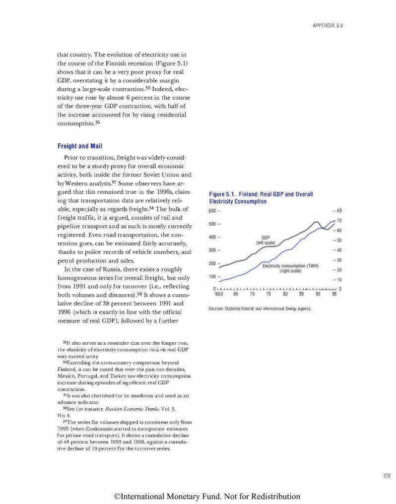
©International Monetary Fund. Not for Redistribution
that country. The evolution of electricity use in
the course of the Finnish recession (Figure 5.1)
shows that it can be a very poor proxy for real
GDP, overstating it by a considerable margin
during a large-scale contraction.35 Indeed, elec
tricity use rose by almost 6 percent in the course
of the three-year GDP contraction, with half of
the increase accounted for by rising residential
consumption. 36
Freight and Mail
Prior to transition, freight was widely consid
ered to be a sturdy proxy for overall economic
activity, both inside the former Soviet Union and
by Western analysts.37 Some observers have ar
gued that this remained true in the 1990s, claim
ing that transportation data are relatively reli
able, especially as regards freight.38 The bulk of
freight trafftc, it is argued, consists of rail and
pipeline transport and as such is mostly correctly
registered. Even road transportation, the con
tention goes, can be estimated fairly accurately,
thanks to police records of vehicle numbers, and
peu·ol production and sales.
In the case of Russia, there exists a roughly
homogeneous series for overall freight, but only
from 1991 and only for turnover (i.e., reflecting
both volumes and distances) .39 It shows a cumu
lative decline of 38 percent between 1991 and
1996 (which is exactly in line with the official
measure of real GDP), followed by a further
S5[t also serves as a reminder that over the longer nm, the elasticity of electricity consumption vis-a-vis real GDP may exceed unity.
S6£xtending the cross<ountry comparison beyond Finland, it can be noted that over the past two decades, Mexico, Portugal, and Turkey saw electricity consumption increase during episodes of significant real GDP con traction.
37ft was also cherished for its timeliness and used as an advance indicator.
38See for instance Russian Economic Trends, Vol. 5,
No.4.
39J'he series for volumes shipped is consistent only from 1993 (wben Goskomstat started to incorporate estimates for private road transpon). It shows a cumulative decline of 44 percent between 1993 and 1996, against a cumulative decline of 19 percent for the turnover series.
Figure 5.1 . Finland: Real GOP and Overall Electricity Consumption
600 -
APPENDIX 5.2
- 80
0 I I I I I I I I I I I I I I I I I I I I I I I I I I I I I I I I I I I I I 0 1960 65 70 75 80 85 90 95
Sources: Statistics Finland: and International Energy Agency.
179
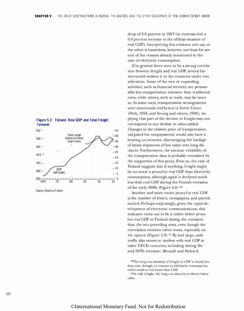
©International Monetary Fund. Not for Redistribution
180
CHAPTER V THE GREAT CONTRACTIONS IN RUSSIA, THE BALTICS. AND THE OTHER COUNTRIES OF THE FORMER SOVIET UNION
Figure 5.2. Finland: Real GOP and Total Freight Turnover
550 -
500 -
450 -
400--
350 -
Source: Statistics Finland.
Total freight (billion tonsfkm)
(right scale)
I I 85
I I 90
-45
-25
-20
-15
-10
- 5 I I 0
95
drop of 3.6 percent in 1997 (in contrast with a
0.8 percent increase in the official measure of real GDP). Interpreting this evidence one way or
the other is hazardous, however, not least for sev
eral of the reasons already mentioned in the case of electricity consumption.
If in general there were to be a strong correla
tion between freight and real GDP, several fac
tors would weaken it in the countries under con
sideration. Some of the new or expanding
activities, such as financial services, are presum
ably less transportation intensive than traditional
ones, while others, such as trade, may be more
so. In some ways, transportation arrangements
were notoriously inefficient in Soviet Union
(Holt, 1993; and Strong and others, 1996), im
plying that part of the decline in freight may not
correspond to any decline in value·added.
Changes in the relative price of transportation
(adjusted for nonpayments) would also have a
bearing on turnover, discouraging the haulage
of heavy shipments of low value over long dis
tances. Furthermore, the intrinsic reliability of
the transportation data is probably overstated by
the supporters of this proxy. Even so, the case of
Finland suggests that if anything, freight might
be no worse a proxy for real GDP than electricity
consumption, although again it declined much
less than real GDP during the Finnish recession
of the early 1990s (Figure 5.2) .10
Another and more exotic proxy for real GDP
is the number of letters, newspapers, and parcels
mailed. Perhaps surprisingly, given the rapid de
velopment of electronic communications, this
indicator turns out to be a rather better proxy
for real GDP in Finland dUTing the recession
than the two preceding ones, even though the
correlation remains rather loose, especially on
the upturn (Figure 5.3) .11 By and large, mail
traffic also moves in tandem with real GDP in
other OECD coumries, including during the
mid-1970s recession (Bonsall and Rickard,
40Thc long-run elasticity of freight to GDP is clearly less than one, though, in contrast to electricity consumption, which tends to rise faster than GDP.
41As with freight, the long-nm elasticity is clearly below unity.
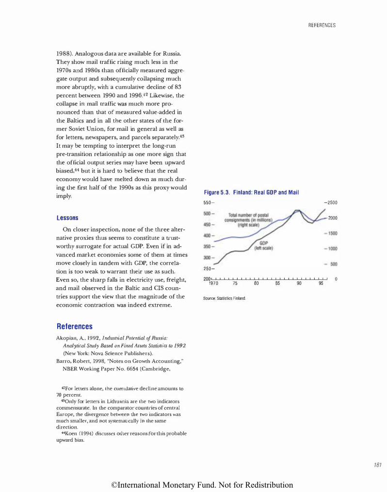
©International Monetary Fund. Not for Redistribution
1988). Analogous data are available for Russia. They show mail traffic rising much less in the 1970s and 1980s than officially measured aggregate output and subsequently collapsing much more abruptly, with a cumulative decline of 83 percent between 1990 and 1996.42 Likewise, the collapse in mail traffic was much more pronounced than that of measured value-added in
the Baltics and in all the other states of the former Soviet Union, for mail in general as well as for letters, newspapers, and parcels separately.43
It may be tempting to interpret the long-run pre·transition relationship as one more sign that the official output series may have been upward biased,44 but it is hard to believe that the real economy would have melted down as much during the first half of the 1990s as this proxy would imply.
Lessons
On closer inspection, none of the three alternative proxies thus seems to constitute a u·ustworthy surrogate for actual GDP. Even if in ad
vanced market economies some of tl1em at times move closely in tandem with GDP, the correlation is too weak to warrant their use as such. Even so, the sharp falls in electricity use, freight, and mail observed in the Baltic and CIS countries support tile view that the magnitude of the economic contraction was indeed extreme.
References
Akopian, A., 1992, Industrial Potential of Russia:
Analytical Study Based on Fixed Assets Statistics to 1992
(New York: Nova Science Publishers).
Barro, Robert, 1998, "Notes on Growth Accounting,"
NBER Working Paper No. 6654 (Cambridge,
�2For letters alone, the cumulative decline amounts to 70 percent.
·13Qnly for letters in Lithuania are the two indicators commensurate. ln tlte comparator countries of central Europe, the divergence between the two iJldicators was much smaller, and not systematically in the same direction.
�Koen (1994} discusses oilier reasons for tllis probable upward bias.
REFERENCES
Figure 5.3. Finland: Real GOP and Mail
550-
250-
-2500
2000
200 1LL1�LL�'�'LL����������� ������������ 0 1970 75 80 85 90 95
Source: Statistics Finland.
181
©International Monetary Fund. Not for Redistribution
182
CHAPTER V THE GREAT CONTRACTIONS IN RUSSIA, THE BALTICS, AND THE OTHER COUNTRIES OF THE FORMER SOVIET UNION
Massachusetts: National Bureau of Economic
Research) .
Berg, Andrew, Eduardo Borensztein, Ratna Sahay, and
jeromin Zettelmeyer, 1999, 'The Evolution of
Output in Transition Economies-Explaining the
Differences," fMF Working Paper 99/73
(Washington).
Bergson, Abram, 1978, Prod:uctivity and the Social S)•Stem:
The USSR and the West (Cambridge, Massachusetts:
Harvard University Press).
Berkowitz, Daniel, and David Dejong, 1997,
"Accounting for Growth in Post-Soviet Russia,"
University of Pittsburgh Working Paper No. 318.
Bernard, Andrew, and Charles jones, 1996,
"Productivity Across Industries and Countries: Time
Series Theory and Evidence," Review of Econo·mics and
Statistics, Vol. 78 (No.1), pp. 135-46.
Blanchard, Olivier, 1997, The Economics of Post
Communist Transition (Oxford: Clarendon Press).
___ , and Michael Kremer, 1997, "Disorganization,"
Qy,arterly journal of Economics, Vol. 1 1 2 (No. 4),
pp. 1091-1126.
Bonsall, Peter, and john Rickard, 1988, Prediction of UK
Letter Mail Traffic (Aldershot, U.K.: Avebmy).
Cameron, Gavin, James Proudman, and Stephen
Redding, 1997, "Deconstructing Growth in UK
Manufacturing," Bank of England Working Paper
No. 73 (London).
Central Intelligence Agency, 1990, Measuring Soviet
GNP: Problems cmd Solutions-/\ Confenmce Report,
SOV 90-10038 (Langley, Virginia: Directorate of
Intelligence).
Commander, Simon, Mark Dutz, and Nicholas Stern,
l 999, "Restructuring in Transition Economies:
Ownership, Competition and Regulation," paper
prepared for the Annual World Bank Conference
on Development Economics, April 28-30
(Washington).
Commonwealth of Independent Sta tes (CIS),
Statistical Committee, 1997, "Production and
Consmnption of Electrical Energy in CIS
Cot!ntries," Bulletin,June 1 1.
Conway, Patrick, forthcoming C1isis, Stabiliwtion and
Growth in Transition Economies.
De Broeck, Mark, and Kristina Kostial, 1998, "Output
Decline in Transition: The Case of Kazakhstan," [MF
Working Paper 98/45 (Washington).
Dobozi, Istvan, and Gerhard Pohl, 1995, "Real Output
Decline in Transition Economies-Forget GOP, Try
Power Consumption Data," 1'm.nsition, Vol. 6 (No.
1-2), pp. 17-18.
Dobrescu, Emilian, 1998, "Essai d'estimer !'economic
non comptabilisee," paper presented at the Seventh
National Accounts Colloquium, january 28-30
(Pa1·is) .
Easterly, William, and Stanley Fischer, 1994, "The
Soviet Economic Decline: Historical and Republican
Data," World Bank Policy Research Working Paper
No. 1284, subsequently published as "The Soviet
Economic Decline," The World Bank Economic Review, Vol. 9 (September 1995), pp. 341-71.
Gavrilen kov, Evgeny, 1996, "Macroeconomics of the
Arrears C1isis in Russia," Hitotsubashi jotwnaL of Economics, Vol. 37 (No. l ) , pp. 59-67.
Gavrilenkov, Evgeny, and Vincent Koen, 1995, "How
Large Wal; the Output Collapse in Russia?
Alternative Estimates and Welfare Implications,"
Staff Studies for the Wodd Economic Outlook
(Washington: International Monetary Fund),
pp. 106-19.
Havrylyshyn, Oleh, Thoma� Wolf, and others, 2000,
"Growth Experience in Transition Economies,
1990-98," IMF Occasional Paper 184 (Washington).
Hermindez-Cata, Ernesto, 1997, "Liberalization and
the Behavior of Output During the Transition from
Plan to Market," fMF Working Paper 97/53
(Washington).
Holt, Jane, 1993, Transport Strategies Jm· the Russian
Federation, Studies of Economies in Transformation
(Washington: World Bank) .
International Energy Agency, 1985, Electri,ity in TEA
Counl1ies: Issues and Outlook (Paris).
International Monetary Fund, Economic Reviews and
IMF Staff Country RejJorts (Washington).
_, 1998, "Republic of Moldova-Recent
Economic Developments," IMF Staff Counu·y
Reporr 98/58 (Washington).
_, World Bank, Organization for Economic
Cooperation and Development, and European Bank
for Reconstruction and Development, 1991, A Study
of the Soviet Economy (Washington).
Johnson, Simon, Daniel Kaufman, and Andrei
Schleifer, 1997, "The Unofficial Economy in
Transition," Bmokings Papers on Economic Activit)\
Vol. 2, pp. 159-239.
Joint Economic Committee, 1990, Measw·es of Soviet
National Product in 1982 Prices (Washington: U.S.
Congress) .
©International Monetary Fund. Not for Redistribution
Kaufman, Daniel, and Aleksander Kaliberda, 1996,
"Integrating the Unofficial Economy into the
Dynamics of Post-Socialist Economies: A Framework
of Analysis and Evidence," World Bank Policy
Research Working Paper 1691 (Washington).
Kellogg, Robert, 1990, "Lnnauon in Soviet lnvestmem
and Capital Stock Data," in Central lntelligence
Agency, 1990, Measwing Soviet GNP: hob/ems and
Solutions-A Conference Report, SOY 90-10038,
(Langley, Virginia: Directorate of Intelligence)
pp. 103-58.
Koen, Vincent, 1994, "Measuring the Transition: A
User's View of National Accounts in Russia," L'viF
Working Paper 94/6 (WashingtOn).
___ , 1996, "Russian Macroeconomic Data:
Existence, Access, Interpretation," Communist
Economies and Economic Transformation, Vol. 8
( 0. 3), pp. 321-33.
_, and Paula De Masi, 1997, "Prices in the
Transition: Ten Stylized Facts," Staff Studies fm· the
World Economic Outlook (Washington: International
Monetary Fund), pp. 128-43.
Kolodko, G•-t.egorz, and Mario Nuti, 1997, "The Polish
Alternative: Old Myths, Hard Facts and New
Strategies in the Successful Transformation of the
Polish Economy," WIDER Research for Action, No. 33.
Kulekcev, Zhaksybek, 1997, "Shadow Economy in
Kazakhstan," paper presented at the Economic
Development Institute Conference on
"Understanding the Transition in Central Asia."
Washington D.C.,June.
Mundell, Robert, 1997, 'The Great Conu·actions in
Transition Economies," in Mario Blejer and Marko
Skreb (eds.), Macroeconomic Stallilization in Tmnsition
REFERENCES
Economies (Cambridge and New York: Cambridge
University Press), pp. 73-99.
Noren, .James, �mel Lauric Kurtzweg, J 993, 'The Soviet
Economy Unravels: 1985-1991," in Richard
Kaufman and john Hardt for the joint Economic
Committee, Congress of the United States, The
Forme1· Soviet Union in Transition (Armonk, New
York: M.E. Sharpe), pp. 8-33.
Organization for Economic Cooperation and
Development (OECD), 1997, FTameworli for flu• Mea.sumnent of Unrecorded Economic /\clivi ties in
Tmnsition Economies, CCET. OCDE/GD(97) 177
(Paris).
Roberts. Bryan, 1997. "Welfare Change and
Elimination of the Shortage Economy in Rus.sia:
Some Representative-Household Results," Economics ofTmnsition, Vol. 5, No. 2, pp. 427-51 .
Russian Federation, Goskomstat, 1996, Melhodowgittt! Regulations for Su.ttistics (Moscow) ; in Russian.
Su·ong,John,John Meyer, Clell Harral, and Graham
Smith, 1996. Moving to Nla1ket: Restructwing
Transport ·in the Former Soviet Union (Cambridge,
Massachusetts: Harvard Institute for International
Development, Harvard University Press).
Veall, Michael, 1998, ''Applications of the Bootsu·ap in
Econometrics and Economic Statistics," in Aman
Ullah and David Giles, Handbook of lljJJJlied Economir Statistics (New York: Marcel Dekker) , pp. 419-63.
World Bank and Russian Federation Goskomstat,
1995, Russian Federation: Report on tlw Nalional
Accounts (Washington and Moscow).
World Bank, 1997, Kazakhstan: RejJort on the National
Accounts (Washington).
Zettelmeyer,Jeromin, 1998, "The Uzbek Growth
Puzzle," IMJ: Working Paper 98/133 (Washington).
183
©International Monetary Fund. Not for Redistribution
184
EMU CHALLENGES TO EUROPEAN LABOR MARKETS Rudiger Soltwedel, Dirk Dohse, Christiane Krieger-Boden, and the IMF Research Department
0 n "E-day,"January 1 , 1999, phase 3 of
the Economic and Monetary Union
EMU for shon1-became realicy. The
euro area comprises all European
Union member states and Sweden, Denmark,
and the United Kingdom, which voluntarily
abstained.
In the run-up to the !ormation of monetary
union, questions of ftscal convergence, the ade
quacy of the conversion exchange rates, and the
stabilicy of the euro have been predominant in
the currency union debate. By contrast, relatively
little attention has been paid to the labor market
implications of EMU. This is all the more strik
ing since labor market performance in the euro
area is crucial for the long-run success or failure
of the monetary union: with the introduction of
the euro, the exchange rate and monetary poli
cies will no longer be available at the country
level as tools for macroeconomic adjustmem.
Furthermore, fiscal policy has been constrained
by the Pact on Stabilicy and Growth. The only
way to avoid (or at least reduce) undesirable
quanticy adjustments to shocks is to make mar
kets more flexible. The formation of EMU thus
adds urgency to the need tor structural reform.
A currency area as large and heterogeneous as
the euro area requires a high degree of flexibil
ity to successfully exploit the potential efficiency
effects of the monetary union. That market flexi
bilicy has been seriously deficient in the past,
though, is apparent in the high level and re
gional concentration of unemployment in most
EU member coumric . In this chapter, we focus
on the regional problems of EMU, with "re
gions" referring not only to member states but,
importantly, also to the subnational regions, and
we discuss ways of coping with the adjustment re-
quirements in the various regions of t.he eut·o
area.
We will start our analysis by reviewing the sta
lllS quo in the euro area from the perspective of
optimum currency area (OCA) theory. This fa
ciJitates identifying those countries that may run
into difficulties under the regime of EMU (first.
section) . We will then describe that European
unemployment is to a large extent a regional
problem within counu·ies. This aspect has as yet
not been given much attention in the debat.e on
monetary union. We will argue that any auempt.
to successfully reform European labor markets
and "make them fit for EMU" has to take the re
gional perspective and even a more decentral
ized, firm perspective imo account (second sec
tion). Therefore, structural labor market reform
may also have to bling about a greater institu
tional diversity to deal with the growing need for
choice in employment relationships and tO allow
greater scope for the exploitation of murually
profitable contracts between labor and firms
(third section). The final section presents
conclusions.
The Optimum Currency Area Criteria
Exchange Rates and Asymmetric Shocks
We can be brief on the often described upside
of the prospects for employment: A single cur
rency reduces the transaction costs between
agents in diffe•·ent EMU countries, and hence
raises the static efficiency of the economy. lt
eliminates the exchange rate lisk as well as d1e
costs of currency exchange and hedging, which
is just another way of saying that the reaJ re
sources employed in foreign-exchange u·ading
1Throughout Lhis paper we use the abbreviation EMU for the Economic and :\1onetary Union, following its widespread use in Lhe literature (see Alsopp and Vines, 1998; Calmfors. 1998; Eichengreen, 1998; OECD. 1999; Mauro, Prasad. and Spilimbergo, 1999).
©International Monetary Fund. Not for Redistribution
can be shifted to other productive uses (Kenen,
1997, p. 212). Furthermore, transparency in
creases and this increases the intensity of compe
tition in goods and factor markets, raising also
the dynamic efficiency of the economy. This in
turn stimulates innovation, investment, trade,
and growth, thereby improving employment
prospects.
On the downside, monetary union heightens
labor market risks. The Lheary of optimal currency
areas establishes that exchange rates are a useful
tool for macroeconomic adjustment in the case
of asymmetric shocks. Exogenous demand and
supply shocks that hit countries asymmetrically
require a response of real exchange rates be
tween these countries in order to adjust relative
real wages between these countries. This could
be accomplished either by adjusting nominal ex
change rates or else by adjusting nominal goods
and factor prices in one country relative to the
other country-otherwise such asymmetric
shocks might result in an increase in unemploy
ment. Nominal exchange rates can therefore be
seen as "a device whereby depreciation can take
the place of unemployment when the external
balance is in deficit, and appreciation can re
place inflation when it is in surplus" (Mundell,
1961, p. 657). A member of a currency union
loses this device for a spontaneous (in the case
of flexible exchange rates) or discretionary (in
the case of fixed exchange rates) macroeco
nomic response to shocks. Hence, asymmetric
shocks in a currency union exert increased pres
sure on national labor markets and entail a sub
stantial risk of rising unemployment.2 A rise in
unemployment due to the loss of exchange rate
flexibility can only be excluded if (at least) one
of the following three conditions holds:
• the exchange rate mechanism between EMU
countlies does not work in the shock absorb-
THE OPTIMUM CURRENCY AREA CRITERIA
ing way predicted by theory, so that nothing
would be lost by giving up this device, or
• there is little probability that members of
EMU are hit by asymmetric shocks, or
• labor markets are flexible enough to adjust lO
asymmetric shocks without a rise in
unemployment.
With respect to the ftrst condition, there is a
controversy in the literature over whether nomi
nal exchange rates really do act as shock ab
sorbers in the way predicted by OCA theory. An
immediate response of the nominal exchange
rates to a shock cannot be taken for granted, it is
argued, because apart from trade flows a great
number of other factors influence nominal ex
change rates, making their movements look like
a "random walk." Moreover, since the deprecia
tion of a currency leads to an import-price in
duced rise in inflation, domestic workers might
try to raise t.l1eir nominal wages in order to com
pensate for the real wage loss, thereby offsetting
the shock-absorbing effects of the depreciation.
There is evidence that exchange rates be
tween EU member states in the past have in vari
ous instances played an important role as shock
absorbers (with the experiences of Italy and
Finland in the early 1990s as conspicuous cases
in point; see Box 6.1) .3This empitical evidence
is in line with mainstream economic reasoning,
which holds that exchange rates provide a useful
tool for macroeconomic adjustment if
• the change in the nominal exchange rate
leads to the required change in the real ex
change rate, or
• such adjustments do not happen too often
(since they require a certain degree of ex
change rate illusion), or
• the exchange rate adjustment is accompanied
by a credible policy change addressing the
2Shocks can be temporary or pcrmanem, on the demand or supply side, and sector, region, or COlllltry specific. Permanent shocks are typically supply side related, whereas temporary shocks are typically demand side or policy induced (OECD, 1999, p. 91). Thus. when speaking about shocks in the monetary union, we usually have supply side shocks in mind. Nevenheless, one should be aware that even temporary (region-specific) shocks may have long-run effecLS on output if hysteresis effects are evident (OECD, 1999, p. 113; Mauro, Prasad, and Spilimbergo, 1999, pp. 5-11 ).
3More evidence on successful-as well as less successful--currency devaluarions is given in Dohse and Krieger-Bod en (1998, pp. 30-32). See also De Grauwe (1994, 1996) and Dornbusch (1996).
185
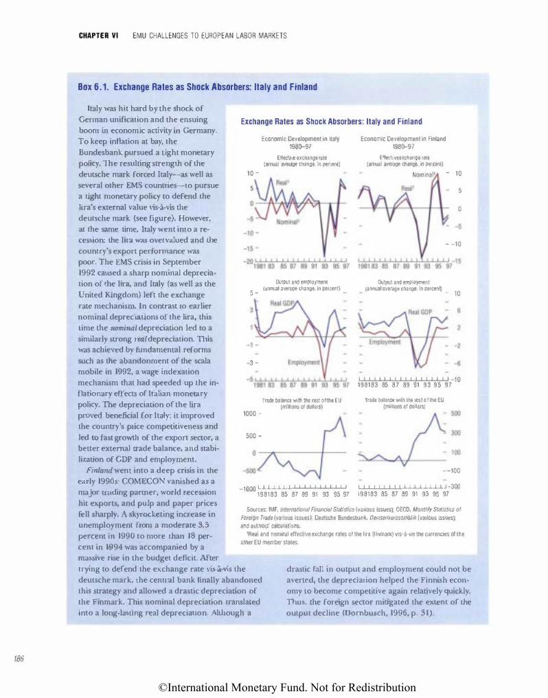
©International Monetary Fund. Not for Redistribution
186
CHAPTER VI EMU CHALLENGES TO EUROPEAN LABOR MARKETS
Box 6.1. Exchange Rates as Shock Absorbers: Italy and Finland
Italy was hit hard by the shock of
German unification and the ensuing
boom in economic activity in Germany. To keep inflation at bay, the
Bundesbank pursued a Light monetary
policy. The resulting strength of the
deutscbe mark forced Italy-as well as
several other EMS countries--to pursue a tight monetary policy to defend the
lira's external value \ois-a-vis the
deutsche mark (see figure). However,
at the same Lime, Italy went into a re
cession: the lira was ovet·vaJued and the
country's export perfunnance was poor. The EMS crisis in September 1992 caused a sharp nominal deprecia
tion of the lira, and Italy (as well as the
United Kingdom) left the exchange
rate mechanism. In contrast ro earlier
nominal depreciations of the lira, this
Lime the nominal depreciation led to a
similarly strong real depreciation. This was achieved by fundamental reforms
such as the abandonment of the scala mobile in 1992, a wage indexation
mechanjsm that had speeded up the inflationary effects of Italian monetary policy. The depreciation of the lira
proved beneficial for Italy: it improved the country's price competitiveness and
led to fast growth of the export sector, a better external trade balance, and stabi
li7.ation of GDP and employment.
Finland wem into a deep crisis in the
early 1990s: COMECON vanisbed as a major o-ading partner, world recession
hir exports, and pulp and paper prices
fell sharply. A skyrocketing increase in unemployment from a moderate 3.5
percent in 1990 to more than 18 per
cent in 1994 was accompanied by a massive rise in the budget deficit. After
Exchange Rates as Shock Absorbers: Italy and Finland
10 -
5
Economic Development in Italy 198D-97
Effective exchange rate (annual average change, In pen:ent)
Output and employment
5 _ (annual average change. in percent)
3
-3 -
Trade balance with the rest ott he EU (millions of dollars)
1000 -
500 -
-500
Economic Development in Finland 198o-97
Effective exchange rate (annual average change, in percent)
Nominal' - 10
5
0
- -10
Output and employment (annual average change. In percent)
_ 10
I I I I I I I I I I I I I I I I I ' -1Q 198183 85 87 89 91 93 95 97
Trade balance with the rest of the EU (millions of dollars)
--100
-1QQQ I I I I I I I I I I I I I I I I I I I I I I I I I I I I I I I I I I I t-300
198183 85 87 89 91 93 95 97 t98183 85 87 89 91 93 95 97
Sources: IMF, lntematronal Rnancl81 Statistics (various issues): OECD, Monthly Stallstlcs of
Foreign Trade (various issues): Deutsche Bundesbank, Devisenkursstatistik (various issues):
and authors' calculations.
'Real and nominal effectrve exchange rates of the lira (llnmark) vts·:l-vts the currencres of the other EU member states.
trying to defend the exchange rate vis-a-vis the
deutsche mark, the central bank finally abandoned
this strategy attd allowed a drastic depreciation of
the Finmark. This nominal depreciation translated
into a long-lasting real depreciation. Although a
drastic fall in output and employment could not be
averted, the depreciarion helped the Finnish econ
omy LO become competitive again relatively quickly.
Thus. the foreign sector mitigated the extem of the
ouLput decline (Dornbusch, 1996, p. 31).
©International Monetary Fund. Not for Redistribution
root causes of the problems that necessi tate
the need for adjustment.
Hence, we conclude that the exchange rate
mechanism did work as an effective "absorber"
for asymmetric shocks on several occasions in
the past.
However, will there still be much need for
shock-absorbing mechanisms in the euro area?
Sometimes it is argued that the problem of asym
metric shocks will no longer be of much rele
vance because the major sources of asymmetric
shocks have been eliminated (Emerson and oth
ers, 1990): there will be no more country
specific shocks from inconsistent national mone
tary policies or from speculative attacks on
national exchange rates; moreover, the scope for
destabilizing national fiscal policy is constrained.
However, even a common monetary policy in
the euro area may be a source of asymmeu·ic
shocks to member countries (and their regions).
In the case of the U.S., for exan1ple, the federal
monetary policy has been found to create asym
metric shocks to U.S. regions because of struc
tural differences of their economies (Box 6.2; see also Carlino and DeFina, 1998 and 1999;
Ramaswamy and Sloek, 1997).4 Numerous empirical studies have dealt with
the probability of asymmeu·ic shocks in EMU,
analyzing the variability of output fluctuations as
well as real exchange rate va1iability in the past.
In these studies, the experiences of EU member
states have been compared to those of existing
single currency areas such as the United States
and Canada or to those of European regions,
THE OPTIMUM CURRENCY AREA CRITERIA
taking pre-euro individual EU countries as cur
rency unions . .? In a nutshell, the result of these
studies is:
• variations of output are more synchronized
among EU member states Lhan among re
gions within individual member states, and
• va1·iations of real exchange rates are smaller
among EU member states Lhan among re
gions within individual member states.
This evidence suggests that several EU mem
ber states have been hit by various asymmetric
shocks in the past and did adjust to them by a
price response (parlicuJarly by a change of the
nominal exchange rate) rather than by a quan
tity (output) response. In a core group of coun
tries-Germany, France, the Benelux countries,
Austria, and Denmark-asymmetric shocks have
been relatively rare as variations of output and of
real exchange rates were quite similar; by con
Lrast, the incidence of asymmetric shocks has
been rather high for Porntgal, Greece, Spain,
ltaly, the United Kingdom, u·eland, Sweden, and
Finland.6
However, these historic patterns of susceptibil
ity to shocks may not persist in the euro area.
The future probability of asymmetric shocks will
depend upon the underlying economic sLruc
tures of the counu-ies participating in the cur
··ency union. The critical question is how EMU
will affect this structure and what the impacr. will
be on the synchronization of their respective cy
cles. Two alternative tendencies are discussed in
the literature:
4ft has also been argued Lhat lixing the enu·y exchange rate at too high a level may represent a shock with long enduring effects that are difficult to overcome (Barrell and Pain, 1998). The decision of Britain in the mid-1920s to return to its prewar gold standard parity may come to mind in lhis context, as well as the case of' cast Germany in the process of reunilica· Lion (see below in Box 6.2). RecenLI)'• Wolf' (1999) has argued along these lines that Germany, by picking roughly the EMS exchange rate, was locked into an overvaluation lhat reduced Lhe competitiveness of the economy, given the wide gap in unit labor cosrs compared to major euro-area countries. However, lhe deutsche mark-ECU exchange rate has prevailed for quite a long time without markets betting on an imminent German devaluation during L11e EMS period.
5See for instance De Grauwe and Vanhavcrbeke (1991), Bayoumi and Eichengreen (1993), Decressin and Fa tas (1995); for an overview see Dohse and Krieger-Boden ( 1998, pp. 19-21).
6These empirical results are in line with standard open-economy macroeconomic 1·easoning that predicts that lhe small. open economies in the EU are subject to asymmetric shocks to a greater extent than the larger economies. The reason is twofold. Small economies are typically less diversified L11ar1 large economies, so lhat indusu·r- or secLOHpecific shocks affect a small economy more su·ongly thar1 a large economy. Moreover, lhe small economics at the periphery of the EU are more exposed to shocks from outside the EU than the economies a1 lhe center-for example, Germany or France (see Hagen and Hammond, 1998, p. 337).
181
©International Monetary Fund. Not for Redistribution
188
CHAPTER VI EMU CHALLENGES TO EUROPEAN LABOR MARKETS
Box 6.2. Euro Area's Most Prominent Problem Regions1
Germany's "Neue Lander"
In unifYing with west Germany, east
Germany's economy was hit by a conversion
shock: wages, rents, and pensionl. were converted at a rate I :1 from eastern marks into
deutsche mark. This political!) dctennined con
version rate rranslated imo wage costs explosion
for cast German producers exceeding product.iv
it) levels by far. (Based on productivity levels, a
conversion rate of 4:1 or even 5: I would have
been adequate.) The effect was a strong real ap
preciation, sharply raising the prices of e�t
Germany's output and thus jeopardizing the
manufactudng sector's competitiveness. A mas
sh·e deindustrialization took place to an extem
that was unique among the transition countries
in cenu·al and eastern Europe: within one vear
following the economic, social, and mone�y
union in 1990, industrial production dropped to
one-third of its 1989 volume and GDP dropped
by one quarter. In the transition process from a
socialist economy to a market economy a large
part of the east German capital stock became
obsolete.
The problems were aggravated by the fact
that-under the impression that mass migration
might be flooding west German} (in 1989 as
well as in 1990 cast German} lost abom 5 per
cent of its population)2__Lhe east German wage
rates were rapidly adapted to western lew b. im
plying that wages in the east rose much faster
than productivity. The consequence was a fm
t.her loss of competitiveness and a subsequent rise in unemployment. In the second quaner of
1990, monthly wages and salades per employee
were, on average. 20 percent higher than in the
roECD. Eammmc Sun�s (various 1$.\Ues): Boltho and others ( 1997): OIW, IIW and IWII (various i� sues): Fairu and others ( 1997); Gerling and Schmidt (1997): Schau and Schmidt (1992): Soltwedcl (1998a and 1998b).
2J lowevcr, after it became clear that "the dour would remain open" net-migration decreased marked!) and did �tabilizc at a low lc\CI after m•d-1991.
fourth quarter of 1989 and 26 percent higher
than in the third quarter. Funhennore, the west
German wage bargaining system, cllaraClerized
b) its COT.) corporatbm, was extended to east
Germany with the Treaty for an Economic,
Monetary and Social Union that took t'ffect as
of July I, 1990. The combination of ccmraJized
wage bargainmg, too-high aggregate wage levels,
and massive income transfers from the west to the cast has prevented a market re pon� to the
growing labor market disequilibdum and hin
dered the economic reco,·ery of the German
east.
Arguably, it was the combination or conver
sion, wage explosion, and immediate and com
plete opening of the east GermaJl market to
western producers that caused the collapse of
ea�t German manufacturing. A more gradual
process of integration-if possible at all-might have been less costly by allowing a more gradual
adjttstmenL \imilar to the proce...ses in other
highly indu\trialized transition economies.
lta�-y :S Mez.:.ol(iorno hair is used to ha,ing substanual regional dis
parities in employment and income. The north
ern parts of the country are traditionally more
prosperous than the \Outhern rt•gions. It is now
worthy, however, that during the last dl!cadc re
gional unemploymen1 dispadties have in
cre�cd. The observer is confromed with an
empirical puulc, as faJiing migration goes hand
in hand \\ith growing unemplo\mcnt difTeren
tials among Italian regions. What are the reasons for the low and falling labor mobility in
Italy? According to Faini and others (1997) it is a combination of high mobility co�ts. incfficiem
regional matching, and demographic factors. The authors find that the main rc ponsibilit)• for
the high mobility cosL� lies with the housing
market, which is heavily curtailed by rent con
trols and high taxation of housing tran-.action .
Furthermore, large welfare payments and inter
regional transfers reduce the interregional dis
parities in real income, inducing the unemployed to stay in their horne region. The
©International Monetary Fund. Not for Redistribution
inefficient matching is due to a peculiarity of the Italian labor market: compared to other countries, Italy's unemployed tend to rely to a disproportionate extent on networks of family and friends in their job search activities. Since these are typically local networks, they don't provide information on job opportunities in
other regions. The aging of the society may be a
Frankel and Rose (1998) argue that an in
creasing synchronization of business cycles
within EMU may be expected, because trade
lirtkages between European regions are likely to
increase further. Any shock that will hit a certain
region or couno·y will thus be passed on quickly
to all other regions and countries by way of
trade linkages. Moreover, it is reasoned that the
tighter international trade linkages between the
participating counu·ies will make their economic
structures and their business cycles more similar
and asymmetric shocks less likely. Such an out
come is considered to be most relevant if de
mand shocks (or other common shocks) pre
dominate or if intraindustry trade accounts for
most of trade.
An opposite line of reasoning has been devel
oped by Krugman (1993) 7 who argues that the
enhanced integration triggered by the monetary
union (and even before by the Single Market)
will entail an increasing specialization of coun
tries (and their regions) that will, in tum, in
crease the likelihood that a given shock will have
asymmetric effects on different regions because
of differences in their production structure. The
Krugman argument focuses on new opportuni
ties for the exploitation of scale economies (e.g.,
localized knowledge spillovers) that foster the
spatial concentration of industries.8 In this case,
THE OPTIMUM CURRENCY AREA CRITERIA
further reason for the observed reduction in mobility.
National (sectoral) wage bargaining impedes regional wage flexibilicy and, furthermore, there exists a large informal sector in Italy, such that part of the labor market adjustmenL does not occtJr in Lhe "official" economy but rather outside in the economia sommersa.
EMU will increase sectoral and regional special
ization in Europe, such that the probability of
asymmetric shocks will not necessarily decrease,
but may even increase as a result of EMU (see
Figure 6.1 for a stylized description of the two
lines of reasoning).
On theoretical grounds both hypotheses seem
equally plausible, and the empirical evidence is
inconclusive so far. Frankel and Rose (1998)
present economeu·ic evidence on synchroniza
tion of business cycles using data for 20 industri
alized countries covering a 30 year period.9
Krugman (1991) presents empirical evidence
that the currency union in the U.S. entailed
more regional divergence rather than more ho
mogeneity. For Europe, evidence is scarce and
does not provide clear-cut results. Our estimates
suggest that in the early 1980s regional special
ization increased in most EU countries, whereas
particularly in the early 1990s it decreased in
most counoies (Table 6. 1 ) . A.miti (1997) and
Brulhart ( 1998), too, find evidence of an in
crease in regional specialization within Europe
in the period of l 980-90.
In models of the "new economic geography"
(see Krugman and Venables, 1995) it is even ar
gued that in the long run the relationship be
tween integration and regional concentration
may be nonlinear and possibly reversing.
7DeCrauwe and Vanhaverbeke (I 99 I ) argue along similar lines. 8 Jaffee and olhers (1993) presem empi.-ical evidence on localized knowledge spillovers. 9frankel and Rose (1998) found increasing S)'llChronization in a sample of20 countries including the U.S., Canada, and
Japan. However, !.hey did not go as far as to suggest a currency union for all countries in their sample.
189
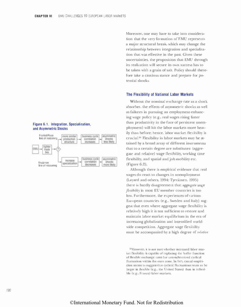
©International Monetary Fund. Not for Redistribution
190
CHAPTER VI EMU CHALLENGES TO EUROPEAN LABOR MARKETS
Figure 6.1 . Integration, Specialization, and Asymmetric Shocks
FrankeVRose line of reasoning
Krugman line of reasoning
Moreover, one may have to take into considera
tion that t.he very formation of EMU represen 1..s a major structural break, which ma)' change the
relationship between integration and specializa
Lion that was effective in the past. Given these
uncertain Lies, t.he proposition that EMU through
its realization will secure its own success has to
be taken with a grain of sail. Policy should there
fore take a cautious stance and prepare for potential shocks.
The Flexibility of National Labor Markets
Without the nominal exchange nue as a shock
absorber. the effects of asymmetric shocks as well
as failures in pursuing an employmem-enhanc
ing wage policy (e.g., real wages rising faster
than productivity in the face of persistent unem
ployment) will hit t.he labor markets more heav
ily than before; hence, labor market flexibility is
cruciat.tu Flexibility i11 labor markets may be at
tained by a broad array of different insu·umems
that to a certain degree are substitmes: (aggre
gate and relative) wage Oexibility, working time flexibility, and spatial and job mobility etc.
(Figure 6.2).
AlLhough there is empirical evidence t11at real
wages do react to changes in uncmploymem
(Larard and others, 1994; Tyrvai nen, 1995)
there is hardly disagreement that agJ.f''l'gate wage jlRxibility in most EU member counu·ies is too
low. Furthermore, the experiences ofvalious
European countries (e.g., Sweden and hal)') sug
gest that even where aggregate wage Oexibility is
relatively high it is not sufficient to resLOre and maintain labor market equilibrium in the era of
increasing global i7.ation and intensified \\'Oriel
wide competition. Aggregate wage flexibility
must be accompanied by a high degree of relative
tol lowevcr, it is not sure whether increased labnr marker !lexibiliry is capable of replacing the buffer function of flexible exchange rates for tmsrnchroni7.ed cyclical fluctuation within tlw euro zone. In fact, casual empiricism seems to suggest that cyclical nuctuations seem to be larger in llexible (e.g., the United States) than in inflexible (e.g .. Fraucc) labor markets.
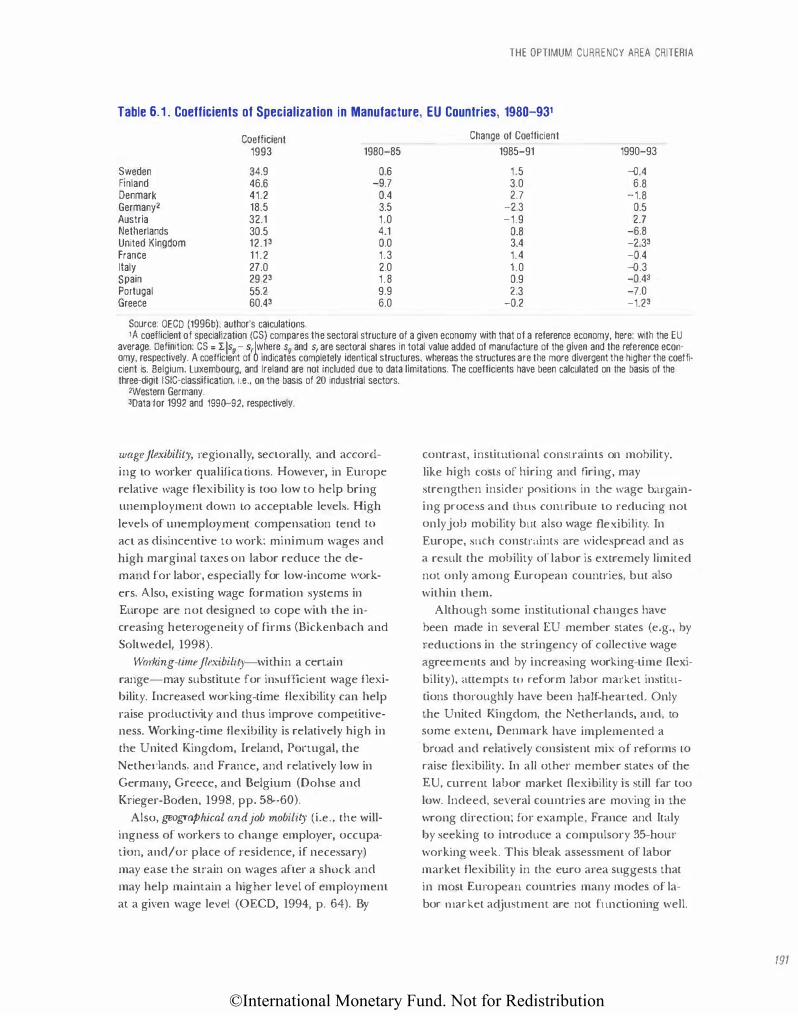
©International Monetary Fund. Not for Redistribution
THE OPTIMUM CURRENCY AREA CRITERIA
Table 6.1 . Coefficients of Specialization in Manufacture, EU Countries, 1980-931
Sweden Finland Denmark Germanyz Austria Netherlands United Kingdom France Italy Spain Portugal Greece
Coefficient 1993
34.9 46.6 41.2 18.5 32.1 30.5 12.13 11.2 27.0 29.23 55.2 60.43
Source: OECO (1996b), author's calculations.
1980-85
0.6 -9.7
0.4 3.5 1.0 4.1 0.0 1.3 2.0 1.8 9.9 6.0
Change of Coefficient
1985-91
1.5 3.0 2.7
-2.3 -1.9
0.8 3.4 1.4 1.0 0.9 2.3
-0.2
1990-93
-Q.4 6.8
-1.8 0.5 2.7
-6.8 -2.33 -0.4 -o.3 -0.43 -7.0 -1.23
1A coefficient of specialization (CS) compares the sectoral structure of a given economy with that of a reference economy, here: with the EU average. Definition: CS = l:!sg- s,lwhere Sg and s, are sectoral shares in total value added of manufacture of the given and the reference economy, respectively. A coettic1ent of 0 indicates completely identical structures. whereas the structures are the more divergent the higher the coeffi· cient is. Belgium, Luxembourg, and Ireland are not included due to data limitations. The coefficients have been calculated on the basis of the three-digit I SIC-classification, I.e., on the basis of 20 industrial sectors.
2Western Germany. 30ata for 1992 and 1990-92, respectively.
wage jlexibiliLy, regionally, sectorally, and accord
ing to worker qualifications. However, in Europe
relative wage flexibility is too low to help bring
unemployment down lO acceptable levels. High
levels of unemployment compensation tend LO act as disincentive to work; minimum wages and
high marginal taxes on labor reduce the de
mand for labor, especially for low-income work
ers. Also, existing wage formation systems in
Europe are not designed to cope with the in
creasing heterogeneity of firms (Bickenbach and
Soltwedel, 1998).
WoTking-Lime jlexibilil)�within a certain
range-may substitute for insufficient wage flexi
bility. Increased working-time flexibility can help
raise productivity and thus improve competitiveness. Working-time flexibility is relatively high in
the United Kingdom, Ireland, Portugal, the
Netherlands, and France, and relatively low in
Germany, Greece, and Belgium (Dohse and
Krieger-Boden, 1998, pp. 58-60).
Also, geographical and job mobility (i.e., the will
ingness of workers to change employer, occupa
tion, and/ or place of residence, if necessary)
may ease the strain on wages after a shock and
may help maintain a higher level of employment
at a given wage level (OECD, 1994, p. 64). By
contrast, instimtionaJ constraints on mobility.
like high costs or hiring and firing, may
strengthen insider positions in the wage b<u·gaining process and Lints comribULe to reducing not
only job mobility but also wage flexibility. In
Europe, such constraints are widespread and as
a result the mobility of labor is extremely limited
not only among European countries, but also
within them.
Although some institutional changes have
been made in several EU member states (e.g., by
reductions in the stringency of collective wage
agreements and by increasing working-time Oexi
bility), attempts to reform labor market instiLU
tions thoroughly have been half-hearted. Only
the United Kingdom, the Netherlands, and, to
some extent, Denmark have implemented a
broad and relatively consistent mix of reforms LO raise flexibility. In all other member states of the
EU, current labor market Oexibility is still far too
low. Indeed, several countries are moving in the
wrong direction; for example, France and Italy
by seeking to introduce a compulsory 35-hour
working week. This bleak assessment of labor
market flexibility in the euro area suggests that
in most European countries many modes of la
bor market adjustment are not functioning well.
191
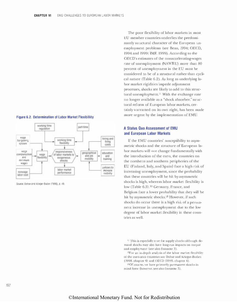
©International Monetary Fund. Not for Redistribution
192
CHAPTER VI EMU CHALLENGES TO EUROPEAN LABOR MARKETS
Figure 6.2. Determination of labor Market Flexibillity
wage bargaining
system 1------, wage
compensation and
minimum wages
Source: Dohse and Krlejjer-Boden (1998). p. 49
policies to L-----1 increase mobility
The poor flexibility of labor markets in most EU member countries underlies the predominamly su·uctural character of the European unemployment problems (see Bean, 1994; OECD, 1994 and l999;' IMF, 1999). According to the OECD's estimates of the nonaccelerating-wages rate of unemployment (NAWRU) more Lhan 80
percent of unemployment in the EU must be considered to be of a structural rather than cyclical nature (Table 6.2). As long as underlying labor market rigidilics impede adjustment processes, shocks are likely to add to Lhis su·uctural unemployment." \o\1ith the exchange rate no longer available as a "shock absorber," su·uctural reform of European labor markets, certainly warranted on its own right, has been made more urgent by the implementation of EMU.
A Status Quo Assessment of EMU and European labor Markets
If the EMU countries' susceptibility to asymmetric shocks and the structure of European labor markets will 1101. change fundamentally with the introduction of the curo, the countries on the northern and southern pet;phcries of the EU (Finland, Italy, and Spain) face a high risk of increasing unemployment, since the probability that these counu·ies will be hit by asymmetric shocks is high, whereas labor market nexibility is low (Table 6.3) .12 Germany, France, and Belgium face a lower probability that they will be hit by asymmetric shocks.t3 However, if such shocks do occur t11ere is a high risk of a penn anent. increase in unemployment due to the low degree of labor market flexibility in these countries as well.
1 1 This is especially true for supply shocks although demand shocks ma)' also ha\·e long-run impacts on ompu1 and emplormen l (see also foomote 3).
12Fm- an in-depLh ana.lrsis of Lhe labor market nexibilitv or t.hc euro-area countries see Dohse and Krieger-Bodt'n ( 1998, chapLer 4) and OECD (1999, chapter 4).
13Qf course, we have primadly permanem shocks in mind here (however. see also foomow 3).
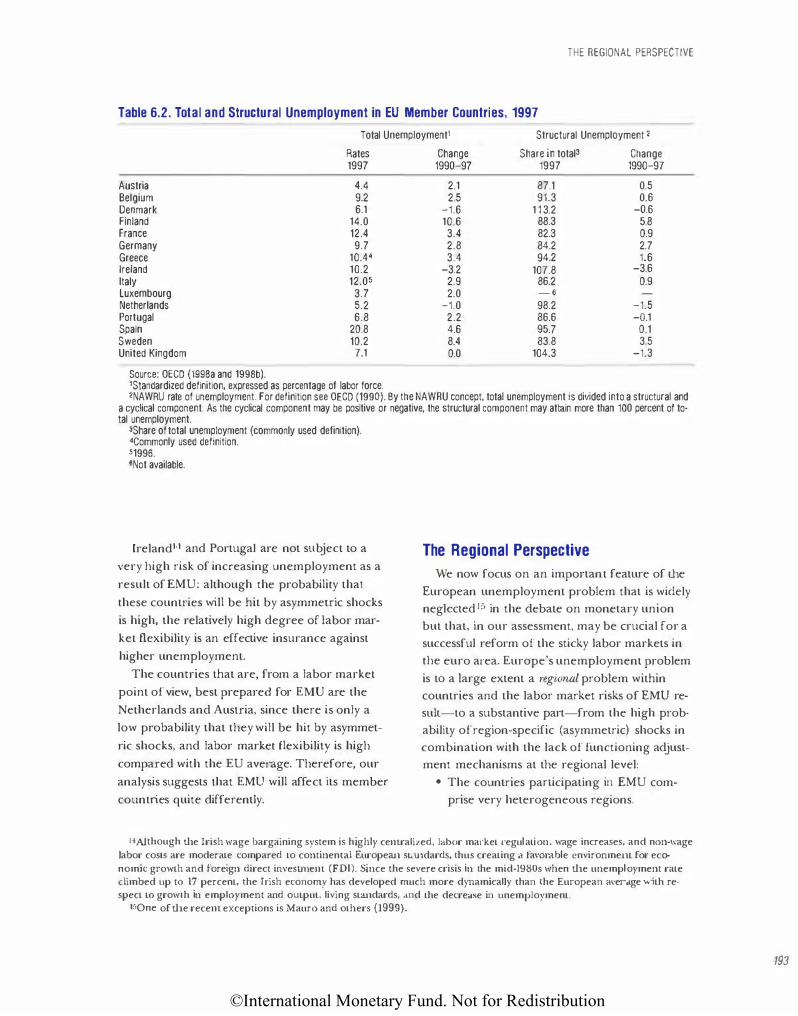
©International Monetary Fund. Not for Redistribution
THE REGIONAL PERSPECTIVE
Table 6.2. Total and Structural Unemployment in EU Member Countries, 1997
Total Unemployment, Structural Unemployment 2 Rates Change Share in total3 Change 1997 199Q-97 1997 1990-97
Austria Belgium Denmark Finland France Germany Greece Ireland Italy Luxembourg Netherlands Portugal Spain Sweden United Kingdom
Source: OECD (1998a and 1998b).
4.4 9.2 6.1
14.0 12.4 9.7
10.44 10.2 12.05
3.7 5.2 6.8
20.8 10.2
7.1
I Standardized definition, expressed as percentage of labor force.
2.1 2.5
-1.6 10.6
3.4 2.8 3.4
-3.2 2.9 2.0
-1.0 2.2 4.6 8.4 0.0
87.1 0.5 91.3 0.6
1 1 3.2 -o.6 88.3 5.8 82.3 0.9 84.2 2.7 94.2 1.6
107.8 -3.6 86.2 0.9 - 6 98.2 86.6 95.7 83.8
104.3
-1.5 -o.1
0.1 3 5
-1.3
2NAWRU rate of unemployment. For definition see OECD (1990). By the NAWRU concept, total unemployment is divided into a structural and a cyclical component. As the cyclical component may be positive or negative, the structural component may attain more than 100 percent of total unemployment.
3Share of total unemployment (commonly used definition). 4Commonly used definition. 51996. SNot available.
Jreland1•1 and PortugaJ are not subject to a
very high risk of increasing unemployment as a
result of EMU: although the probability that
these countries will be hit by asymmeo·ic shocks
is high, the relatively high degree of labor mar
ket flexibility is an effective insurance against
higher unemployment.
The countries that are, from a labor market
point of view, best prepared for EMU are the
Netherlands and Austria, since there is only a
low probability that they will be hit by asymmet
ric shocks, and labor market flexibility is high
compared with the EU average. Therefore, our
analysis suggests that EMU will affect its member
countries quite differently.
The Regional Perspective
We now focus on an important feature of the
European unemployment probJem that is widely
neglected 15 in the debate on monetary union
but that, in our assessment, may be crucial for a
successful reform of the sticky labor markets in
the euro area. Europe's unemployment problem
is to a Jarge extent a 1'egional problem within
countries and the labor market risks of EMU re
suiL-to a substantive part-from the high prob
ability of region-specific (asymmetric) shocks in
combination with the lack of functioning adjust
ment mechanisms at the regional level:
• The countries panicipating in EMU com
prise very heterogeneous regions.
14AJthough the Irish wage bargaining system is highly cemralized, labor market regulation. wage increases, and non-wage labor costs are moderate compared to continental European standards, thus creating a favorable e::nvironmelll for economic growth and foreign direct invesunem (FDl). Since the severe crisis in the mid-1980s when the unemployment rate climbed up tO 17 percent, the Irish economy has developed much more dynamically than the European <�ver.tge with respect tO growth in employment and output. living standards, and the decrease in unemployment.
150ne of the recem exceptions is Mauro and others (1999).
193
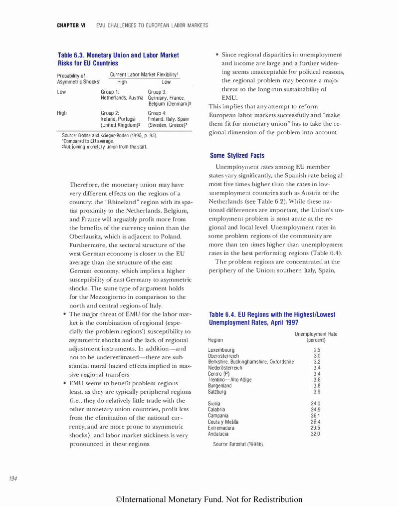
©International Monetary Fund. Not for Redistribution
194
CHAPTER VI EMU CHALLENGES TO EUROPEAN LABOR MARKETS
Table 6.3. Monetary Union and labor Market Risks for EU Countries
Probability of Asymmetric Shocks1
Current Labor Market Flexibility!
High Low
Low
High
Group 1: Netherlands. Austria
Group 2: Ireland, Portugal (United Kingdom)2
Group 3: Germany, France, Belgium (Denmark)2
Group 4: Finland, Italy, Spain (Sweden, Greece)2
Source: Dohse and Krieger·Boden (1998, p. 95). 1Compared to EU average. 2Not joining monetary union from the start.
Therefore, the monetary union may have
very different effects on the regions of a
country: the "Rhineland" region with its spa
tiai proximity to the Netherlands, Belgium,
and France will arguably profit more from
the benefits of the currency union than the
Oberlausitz, which is adjacent to Poland.
Furthermore, the sectoral structure of the
west German economy is closer r.o the EU
average than the structure of the east
German economy, which implies a higher
susceptibility of east Germany w asymmetric
shocks. The same type of argument holds
for the Mezzogiorno in comparison to the
north and central regions of italy. • The major threat of EMU for the labor mar
ket is the combination ofregional (espe
cially the problem regions') susceptibility to
asymmetric shocks and the lack of regional
adjustment instruments. In addition-and
not to be underestimated-there are sub
stantial moral hazard effects implied in mas
sive regional transfers.
• EMU seems to benefit problem regions
least, as they are typically peripheral regions
(i.e., they do relatively little trade with the
other monetary union countries, profit less
from the elimination of the national cw·
rency, and are more prone to asymmeu·ic
shocks), and labor market stickiness is very
pronounced in these regions.
• Since regional disparities in unemployment
and income are large and a further widen
ing seems unacceptable for political reasons,
the regional problem may become a m�jor
threat w the long-run sustainability of
EMU.
This implies that any attempt LO reform
European labor markets successfully and "make
them fit tor monetary union" has to take the re
gional dimension of the problem into account.
Some Stylized Facts
Unemployment rates among EU member
states vary significantly, the Spanish rate being al
most five times higher than the rates in low
unemployment countries such as Austria or the
Netl1erlands (see Table 6.2). While these na
tional differences are important, the Union's un
employmem problem is most acUle at the re
gional and local level. Unemployment rates in
some problem regions of the community are
more than ten limes higher than unemployment
rates in the best performing regions (Table 6.4). The problem regions are concemratecl at the
periphery of the Union: southern Italy, Spain,
Table 6.4. EU Regions with the Highest/lowest Unemployment Rates, April 1997
Region
Luxembourg Oberosterreich Berkshire, Buckinghamshire, Oxfordshire Niederosterreich Centro (P) Trentino-Aito Adige Burgenland Salzburg
Sicilia Calabria Campania Ceuta y Melilla Ex1remadura Andalucia
Source: Eurostat (199Bb).
Unemployment Rate (percent)
2.5 3.0 3.2 3.4 3.4 3.8 3.8 3.9
24.0 24.9 26.1 26.4 29.5 32.0
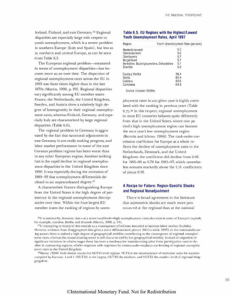
©International Monetary Fund. Not for Redistribution
Ireland, Finland, and east Germany. 16 Regional
disparities are especially large with respect to
youth unemployment, which is a severe problem
in southern Europe (Italy and Spain) , but less so
in northern and central Europe, as can be seen
from Table 6.5.
The European regional problem-measured
in terms of unemployment disparities-has be
come more acute over time. The dispersion of
regional unemployment rates across the EU in
1995 was three times higher than in the late
1970s (Martin, 1998, p. 20). Regional disparities
vary significantly among EU member states:
France, the Netherlands, the United Kingdom,
Sweden, and Austria show a relatively high de
gree of homogeneity in their regional unemploy
ment rates, whereas Finland, Germany, and espe
cially Italy are characterized by large regional
disparities (Table 6.6).
The regional problem in Germany is aggra
vated by the fact that sLructural adjusLrnent in
east Germany is not really making progress, and
labor market performance in some of the east
German problem regions has been worse than
in any other European region. Another striking
fact is the rapid decline in regional unemploy
ment disparities in the United Kingdom since
1990. It was especially during the recession of
1989-93 that unemployment differentials de
clined to an unprecedemed degree. 17
A characteristic feature distinguishing Europe
from the United States is the high degree of per
sistence in the regional unemployment discrep
ancies over time. Within the four largest EU
member states the ranking of regions by unem-
THE REGIONAL PERSPECTIVE
Table 6.5. EU Regions with the Highest/lowest Youth Unemployment Rates, April 1997
Region Youth Unemployment Rate (percent)
Niederosterreich 5.0 Obertisterreich 5.0 Oberbayern 5. 7 Burgenland 5.7 Berkshire, Buckinghamshire, Oxfordshire 5.7 Drenthe 5.9
Ceuta y Melilla Sicilia Calabria Campania
Source: Eurostat (1998b).
58.4 60.4 62.6 64.9
ployment rates in any given year is highly corre
lated with the ranking in previous years (Table
6.7).18 Tn this respect, regional unemployment
in most EU countries behaves quite differently
from that in the United States, where one pe
riod's high unemployment region can become
the next year's low unemployment region
(Bertola and lchino, 1996). The rank-order cor
relation coefficient for Europe as a whole re
flects the decline of unemployment rates i_n the
Netherlands, Denmark, and the United
Kingdom: the coefficient did decline from 0.96
for 1985-90 to 0.78 for 1985-97, which neverthe
less remains markedly above the U.S. coefficients
of about 0.50.
A Recipe for Failure: Region-Specific Shocks
and Regional Nonadjustment
There is broad agreement in the literature
that asymmeu-ic shocks are much more pro
nounced at the regional than at the national
161L is noteworthy, however, that-at a more local level-high unemployment rates also exist in some of Europe's capitals. for example, London, Berlin, and Brussels (Martin, 1998, p. 18).
171t is tempting to interpret this cnl.irely as a consequence of reforms intended to increase labor market llexibilit)'·
However, evidence from disaggregated da ta gives a more ditferentiated picture (McCormick, 1997): in the nonmanufacturing sectors 1J1ere is indeed a high degree of geographical mobility contributing to the convergence of regional unemployment rates, whereas the manufacturing sector is still charactel"ized by low geographical mobility. Instead of migration or significam '"a•·iacions in relative w·..�ges there has been a tendency for manufactwing l<1bor force participation rates tO decline in comracting regions, which-togel.ber with mjgt·ation by non manuals-explains lhc leveling of regional Lulemploy
ment rates in the United Kingdom. 18M arlin ( 1998) finds similar results for NUTS !-level regions. NUTS is lhe nomenclature of territorial units for staListics
compiled by Eurost.at. Level I (NUTSl) is lhe largest., NUTS2 the medium, and NUTS3 the smallest level of regional disaggregation.
795
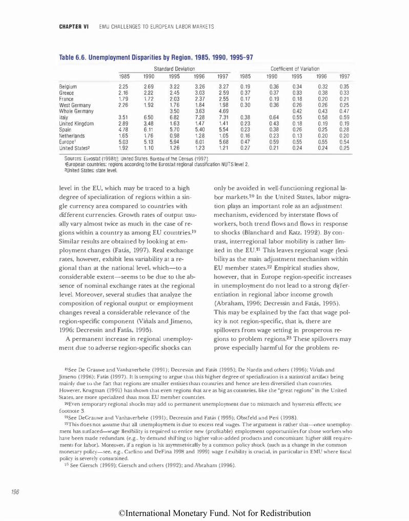
©International Monetary Fund. Not for Redistribution
196
CHAPTER VI EMU CHALLENGES TO EUROPEAN LABOR MARKETS
Table 6.6. Unemployment Disparities by Region, 1985, 1990, 1995-97
Standard Deviation Coefficient of Variation
1985 1990 1995 1996 1997 1985 1990 1995 1996 1997
Belgium 2.25 2.69 3.22 3.26 3.27 0.19 0.36 0.34 0.32 0.35 Greece 2.16 2.22 2.45 3.03 2.59 0.37 0.37 0.33 0.38 0.33 France 1.79 1.72 2.03 2.37 2.55 0.17 0.19 0.18 0.20 0.21 West Germany 2.26 1.92 1.76 1.84 1.98 0.30 0.36 0.26 0.26 0.25 Whole Germany 3.50 3.63 4.69 0.42 0.43 0.47 Italy 3.51 6.50 6.82 7.28 7.31 0.38 0.64 0.55 0.58 0.59 United Kingdom 2.89 3.48 1.63 1.47 1.41 0.23 0.43 0.18 0.19 0.19 Spain 4.78 6.11 5.70 5.40 5.54 0.23 0.38 0.26 0.25 0.28 Netherlands 1.65 1.76 0.98 1.28 1.05 0.16 0.23 0.13 0.20 0.20 Europel 5.03 5.13 5.94 6.01 5.68 0.47 0.59 0.55 0.55 0.54 United States2 1.92 1.10 1.26 1.23 1.21 0.27 0.21 0.24 0.24 0.25
Sources: Eurostat (1998b); United States, Bureau of the Census (1997). 1European countries: regions according to the Eurostat regional classification NUTS level 2. 2United States: state level.
level in the EU, which may be u·aced to a high
degree of specialization of regions within a sin
gle currency area compared to countries with
different currencies. Growth rates of output usu
ally vary almost twice as much in the case of re
gions within a country as among EU countries.19
Similar results are obtained by looking at em
ployment changes (Fariis, 1997). Real exchange
rates, however, exhibit less variability at a re
gional than at the national level, which-to a
considerable extent-seems to be due to t.he ab
sence of nominal exchange rates at the regional
level. Moreover, several studies that analyze the
composition of regional output or employment
changes reveal a considerable relevance of the
region-specific component (Vinals and Jimeno,
1996; Decressin and Fariis, 1995).
A permanent increase in regional unemploy
ment due to adverse region-specific shocks can
only be avoided in well-functioning regional la
bor markets.20 ln the United States, labor migra
tion plays an important role as an adjustment.
mechanism, evidenced by interstate flows of
workers, both trend flows and flows in response
to shocks (Blanchard and Katz, 1992). By con
trast, interregional labor mobility is rather lim
ited in the EU.21 This leaves re!,>ional wage flexi
bility as the main adjustment mechanism within
EU member states.22 Empirical studies show,
however, that in Europe region-specific increases
in unemployment do not lead to a strong differ
entiation in regional labor income growth
(Abraham, 1996; Decressin and Fariis, 1995).
This may be explained by the fact that wage pol
icy is not region-specific, that is, there are
spillovers from wage setting in prosperous re
gions to problem regions.23 These spillovers may
prove especially harmful for the problem re-
19See De Grauwe and Vanhaverbeke (1991 ); Decressin and Fallis (1995); De Nard is and others ( 1996); Vii1als and Jimeno ( 1996): Fallis (1997). It is tempting to argue that this higher degree of specialization is a statistical ani fact being mainly due tO the fact that regions are smaller entities than coumries and hence are less diversified than coumries. However, Krugman (1991) has shown that even regions that are as big as cotult.ries, like the "great regions" in the United States, are more specialized than most EU member countries.
20E\•en temporary regional shocks may add to permanelll unemploymem due to mismatch and hysteresis effects; sec footnote 3.
21See DeGrauwe and Vanhaverbeke (1991); Decressin and Fallis ( 1995); Obstfeld and Peri ( 1998). 22Th is does not assume that all unemployment is due to excess real wages. The argumem is rather that-once unemploy
ment has surfaced-wage llexibility is required to entice new (profitable) employmem opponunities for those workers who have been made redundant (e.g .. by demand shifting to higher value-added products and concomitant higher skill requirements for labor). Moreover, if a region is hit asymmetrically by a common policy shock (such as a change in the common monetary policy-see. e.g., Carlino and DeFina 1998 and 1999) wage flexibility is crucial, in particular in EMU where fiscal policy is severely consuained.
23 See Giersch ( 1969): Giersch and others (1992); and Abraham ( 1996).
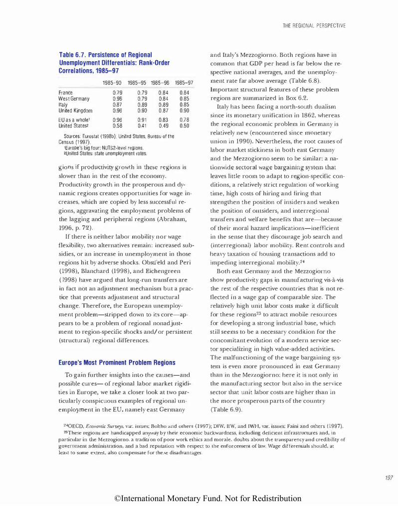
©International Monetary Fund. Not for Redistribution
Table 6.7. Persistence of Regional Unemployment Differentials: Rank-Order Correlations, 1985-97
1985-90 1985-95 1985-96 France 0.79 0.79 0.84 West Germany 0.96 0 79 0.84 Italy 0.87 0.89 0.89 United Kingdom 0.96 0.90 0.87
EU as a whole, 0.96 0.91 0.83 United States2 0.58 0.41 0.49
Sources: Eurostat (19981>); United States, Bureau of the Census (1 997).
1Europe's l>ig four: NUTS2-Ievel regions. 2United States: state unemployment rates.
1985-97 0.84 0.85 0.85 0.90 0.78 0.50
gions if productivity gTowth in these regions is
slower than in the rest of the economy.
Productivity growth in the prosperous and dy
namic regions creates opportunities for wage in
creases, which are copied by less successful re
gions, aggravating the employment problems of
the lagging and peripheral regions (Abraham,
1996, p. 72).
If there is neither labor mobility nor wage
flexibility, two alternatives remain: increased sub
sidies, or an increase in unemployment in those
regions hit by adverse shocks. Obstfeld and Peri
(1998), Blanchard (1998), and Eichengreen
( 1998) have argued that long-run transfers are
in fact not an adjustment mechanism but a prac
tice that prevents adjustment and structural
change. Therefore, the European unemploy
ment problem-stripped down to its core-ap
pears to be a problem of regional nonadjust
ment to region-specific shocks and/ or persistent
(structural) regional differences.
Europe's Most Prominent Problem Regions
To gain further insights into the causes-and
possible cw·es- of regional labor market rigidi
ties in Europe, we take a closer look at two par
ticularly conspicuous examples of regional un
employment in the EU, namely east Germany
THE REGIONAL PERSPECTIVE
and Italy's Mezzogiorno. Both regions have in
common that GDP per head is far below the re
spective national averages, and the unemploy
ment rate far above average (Table 6.8).
Important structural features of these problem
regions are summarized in Box 6.2.
Italy has been facing a north-south dualism
since its monetary unification in 1862, whereas
the regional economic problem in Germany is
relatively new (encountered since monetary
union in 1990). Nevertheless, the root causes of
labor market stickiness in bolh east Germany
and the Mezzogiorno seem to be similar: a na
tionwide sectoral wage bargaining system that leaves little room to adapt to region-specilic con
ditions, a relatively su-ict regulation of working
time, high costs of hiring and firing that
strengthen the position of insiders and weaken
the position of omsiders, and interregional
transfers and welfare benefits that are-because
of their moral hazard implications-inefficient
in Lhe sense dtat they discourage job search and
(interregional) labor mobility. Rent controls and
heavy taxation of housing u-ansactions add to
impeding interregional mobility.24
Both east Germany and the Mezzogiorno
show productivity gaps in manufacturing vis-a-vis
the rest of tl1e respective countries that is not re
flected in a wage gap of comparable size. The
relatively high unit labor costs make it difficult
for these regions25 to attract mobile resources
for developing a strong industrial base, which
still seems to be a necessary condition for the
concomitant evolution of a modern service sec
tor specializing in high value-added activities.
The malfunctioning of the wage bargaining sys
tem is even more pronounced in east Germany
than in the Mezzogiorno: here it is not only in
the manufacturing sector but also in the service
sector that unit labor costs are higher than in
the more prosperous parts of the country
(Table 6.9).
240ECD, Economic Survll)'>, var. issues; Boltho and others (1 997); OlW, IIW, and LWH, var. issues; Faini and others ( 1997). 2;These regions are handicapped anyway by their economic backwardness, including defic:iem tnfrastmctures and, in
particular in the Mezzogiorno, a tradition of poor work ethics and morale, doubts abom the transparency and credibilit)' of government adminisu·ation, and a bad reputation with respect to the enforcement of law. Wage differentials should, at least to some extent, also compensate for these disadvantages.
197
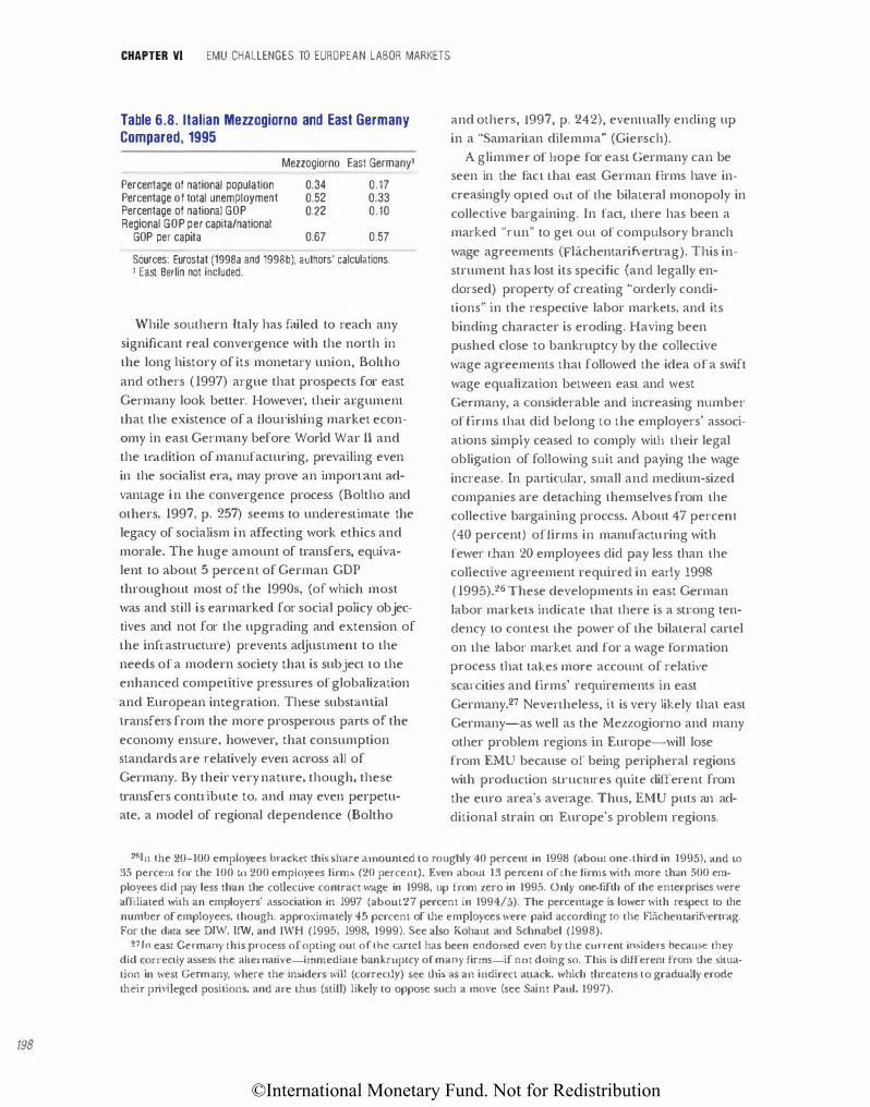
©International Monetary Fund. Not for Redistribution
198
CHAPTER VI EMU CHALLENGES TO EUROPEAN LABOR MARKETS
Table 6.8. Italian Mezzogiorno and East Germany Compared, 1995
Mezzogiorno East Germanyl
Percentage of national population 0.34 0.17 Percentage of total unemployment 0.52 0.33 Percentage of national GOP 0.22 0.10 Regional GOP per capita/national
GOP per capita 0.67 0.57
Sources: Eurostat (1998a and 1998b): authors' calculations. 1 East Berlin not included.
While southern Italy has failed to reach any
significant real convergence with the north in the long history of its monetary union, Boltho
and others ( 1997) argue that prospects for east
Germany look better. Howeve1� their argument
that the existence of a flow·ishing market econ
omy in east Germany before World War II and
the tradition of manufacturing, prevailing even
in the socialist era, may prove an important ad
vantage in the convergence process (Boltho and
others, 1997, p. 257) seems to underestimate the
legacy of socialism in affecting work ethics and
morale. The huge amount of transfers, equiva
lent to about 5 percent of German GDP
throughout most of the 1990s, (of which most
was and still is earmarked for social policy objec
tives and not for the upgrading and extension of
the infrastructure) prevents adjustmem to the
needs of a modern society that is subject to the
enhanced competitive pressures of globalization
and European integration. These substamial
transfers from the more prosperous parts of the
economy ensure, however, that consumption
standards are relatively even across all of
Germany. By their very nature, though, these
transfers conu·ibute to, and may even perpetu
ate, a model of regional dependence (Boltho
and others, 1997, p. 242), eventually ending up
in a "Samaritan dilemma" (Giersch).
A glimmer of hope for east Germany can be
seen in the fact that east German firms have in
creasingly opted out of the bilateral monopoly in
collective bargaining. In fact, there has been a
marked "run" to get our of compulsory branch
wage agreements (FHichentarifveru·ag). This in
strument has lost its specific (and legally en
dorsed) property of creating ''orderly condi
tions" in the respective labor markets, and its
binding character is eroding. Having been
pushed close to bankruptcy by the collective
wage agreements that followed the idea of a swift
wage equalization between east and west
Germany, a considerable and increasing number
of firms that did belong to the employers' associ
ations simply ceased to comply with their legal
obligation of following suit and paying the wage
increase. In particular, small and medium-sized
companjes are detaching themselves from the
collective bargaining process. About 47 percem
(40 percent) offirms in manufacturing with
fewer than 20 employees did pay less than the
collective agreement required in early 1998
( 1995).26 These developments in east German
labor marketS indicate that there is a su·ong ten
dency to concest the power of the bilateral cartel
on the labor market and for a wage formation
process that takes more account of relative
scarcities and firms' requirements in east
Germany.27 Nevertheless, it is very likely that east
Germany-as well as the Mezzogiorno and many
other problem regions in Europe-will lose
from EMU because of being peripheral regions
with production su·ucLUres quite different from
the euro area's average. Thus, EMU puts an ad
ditional strain on Europe's problem regions.
26Jn the 20-100 employees bracket this share amounted to roughly 40 percent in 1998 (about one-third in 1995), and w 35 percent for Lhe 100 LO 200 employees firms (20 percent). Even about 13 percent of Lhe firms with more Lhan 500 employees did pay less Lhan Lhe collecLive conLract wage in 1998, up from zero in 1995. Only one-fifth of Lhe enterprises were afJiliated with an employe1·s' association in 1997 (aboUL27 percem in 1994/5). The percentage is lower with respect to Lhe number of employees. though: approximately 45 percem of the employees were paid according lO the f'lachemarifVenrag. For the data see DT\oV, J!W, and IWH (1995, 1998, 1999). See also Kohaut and Schnabel (1998).
2i.Lo cast Germany this process of opting out of the cartel has been endo rsed even by the current insiders because they did con·ectly assess Lhe alternative-immediate bankruptcy of many firms-if not doing so. This is diiTerent from the siwalion in west Germany, where the insiders will (correcll)') see Lhis as an indirecL attack, which threatens to gradually erodt: L11cir privileged positions, and are L11us (still) likely to oppose such a move (see Saint Paul. 1997).
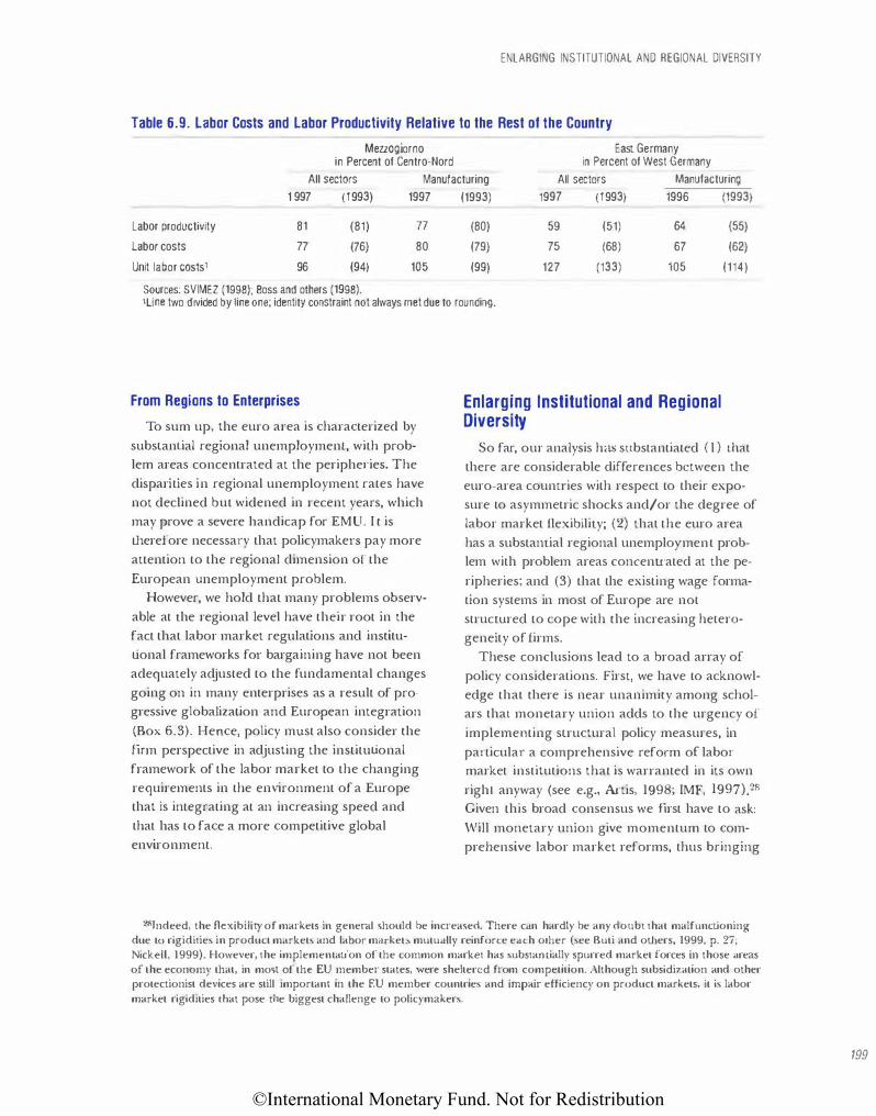
©International Monetary Fund. Not for Redistribution
ENLARGING INSTITUTIONAL AND REGIONAL DIVERSITY
Table 6.9. Labor Costs and Labor Productivity Relative to the Rest of the Country
Mezzogiorno East Germany in Percent of Centro-Nord in Percent of West Germany
All sectors Manufacturing All sectors Manufacturing
1 997 (1993) 1997 (1993) 1997 (1993) 1996 (1993)
Labor productivity 81 (81) 77 (80) 59 (51) 64 (55)
labor costs 77 (76) 80 (79) 75 (68) 67 (62)
Unit labor costsl 96 (94) 105 (99) 127 (133) 105 (114)
Sources: SVIMEZ (1998); Boss and others (1998). 1Une two divided by line one; identity constraint not always met due to rounding.
From Regions to Enterprises
To sum up, the euro area is characterized by
substanlial regional unemployment, with prob
lem areas concentrated at the periphet-ies. The
disparities in regional unemployment rates have
not declined but widened in recent years, which
may prove a severe handicap for EMU. I t is
therefore necessary that policymakers pay more
attention to the regional dimension of the
European w1employment problem.
However, we hold that many problems observ
able at the regional level have their root in the
fact that labor market regulations and institu
tional frameworks for bargaining have not been
adequately adjusted to the fundamental changes
going on in many enterprises as a result of pro
gressive globalization and European integration
(Box 6.3). Hence, policy must also consider the
firm perspective in adjusting the institutional
framework of the labor market to the changing
requirements in the environment of a Europe
that is integrating at an increasing speed and
that has to face a more competitive global
environment.
Enlarging Institutional and Regional Diversity
So far, our analysis has substantiated ( l ) that
there are considerable differences between the
euro-area counu·ies with respect to their expo
sure to asymmetric shocks and/or the degree of
labor market flexibility; (2) that the euro area
has a substantial regional unemployment prob
lem with problem areas concenu·ated at the pe
ripheries; and (3) that the existing wage forma
tion systems in most of Europe are not
strucmred to cope with the increasing hetero
geneity of firms.
These conclusions lead to a broad array of
policy considerations. First, we have to acknowl
edge that there is near unanimity among schol
ars that monetary union adds to the urgency of
implementing structural policy measures, in
particular a comprehensive reform of labor
market institutions that is warranted in its own
righ l anyway (see e.g., Artis, 1998; IMF, 1997). 28
Given this broad consensus we first have to ask:
Will monetary union give momentum to com
prehensive labor market reforms, thus bringing
28Indeed. the Oexibility of markets in general should be increased. There can hardly be any doubt that malfunctioning due tO rigidities in product markets and labo1· mm·kets mutually reinforce each other (see Buti and others, 1999, p. 27; Nickell. 1 999). However, the implementation of the common market has substamially spurred market forces in those areas of the economy that, in most of the EU member states, were sheltered from competition. Although subsidization and other protectionist devices are still important in the EU member countries and impair efficiency on product markets, it is labor market rigidities that pose the biggest challenge to policymakers.
199
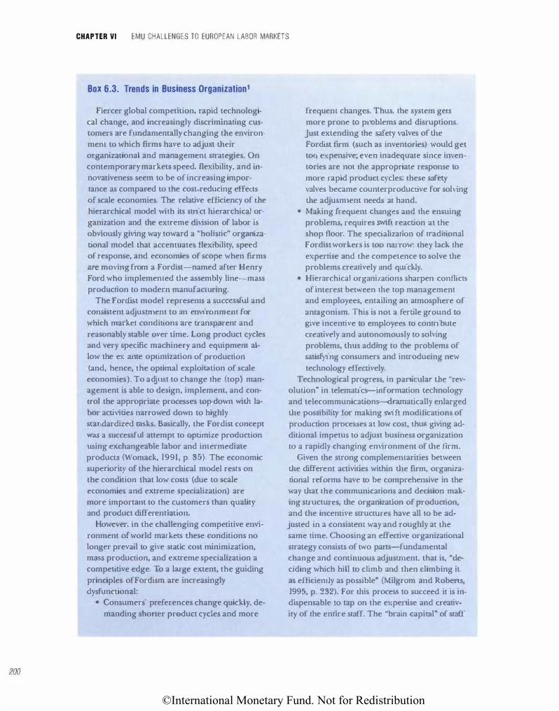
©International Monetary Fund. Not for Redistribution
200
CHAPTER VI EMU CHALLENGES TO EUROPEAN LABOR MARKETS
Box 6.3. Trends in Business Organization1
Fiercer global competition, rapid technological change, and increasingly discriminating customers are fundamentally changing the environmem to which firms have to adjust their organizational and managemem strategies. On contemporary markets speed, flexibility, and innovativeness seem to be of increasing importance as compared to the cost-reducing effects of scale economies. The relative efficiency of the hierarchical model with its strict hierarchical organization and the extreme division of labor is obviously giving way toward a �holistic" organizational model that accentuates flexibility. speed of response, and economies of scope when firms are moving from a Fordist-named after Henry Ford who implememed the assembly line--mass production to modern manufacmring.
The Forclist model represenrs a successful and consistent adjustment to an environment for which market conditions are transparenr and
reasonably stable over time. Long product cycles and very specific machinery and equipment allow the ex ante optimization of production
(and, hence, the optimal exploitation of scale economies). To adjust to change the (top) management is able to design, implement, and control the appropriate processes top-down with labor activities narrowed down to highly startdardized casks. Basically, the Fordist concept was a successful attempt to optimize production using exchangeable labor and imermediate products (Womack, 1991, p. 35). The economic superiority of the hierarchical model resrs on the condition that low costs (due to scale economies and extreme specialization) are more important to the customers than quality and product differenliation.
Howe�rer, in the challenging competitive environment of world markets these conditions no longer prevail to give static cost minimization, mass production, and extreme specialization a competitive edge. To a large extent, the guiding principles ofFordism are increasingly dysfunctional:
• Consumers· preferences change quickly, demanding shoner product cycles and more
frequem changes. Thus, the system gets
more prone to problems and disruplions. just extending the safety valves of the Fordist firm (such as inventories) would get too e.xpensive; even inadequate since inventOries are not the appropriate response to more rapid product cycles; these safety valves became counterproductive for solving the adjusm1ent needs at hand.
• Making frequent cl1angcs and the ensuing problems, requires swift reaction at the shop floor. The specialization of traditional Fordist workers is too narrow: they lack the
expertise and the competence to solve the problems creatively and quickly.
• Hierarchical organizations sharpen conflicts of interest between the lop management and employees, entaiJjng an atmosphere of
antagonism. This is not a fertile ground to give incentive to employees to contribute creatively and autonomously to soh�ng problems, thus adding to the problems of satisfying consumers and introducing new
technology effectively. Technological progress, in particular the "rev
olution" in telematics-information technology and telecommunications-dramatically enlarged the possibility for making swift modifications of production processes at low cost, thu giving additional impetus to adjust business organization ro a rapidly changing environment of the firm.
Given the strong complememarities between the different activities within the firm, organizational reforms have to be comprehensive in the way that the communications and decision making structures, the organization of production, and the incentive structures have all to be adjusted in a consistem way and roughly at the same time. Choosing an effective organizational strategy consists of two parts-fundamental change and continuous adjustment, that is, "cl� ciding which hill to cJjmb and then climbing il
as efficiently as possible" (Milgrom and Roberts, 1995, p. 232). For this process to succeed it is indispensable to tap on the e>.:pertise and creativity of the entire staff. The "brain capital� of staff
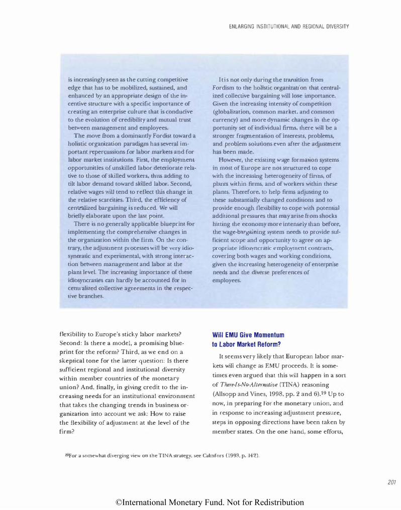
©International Monetary Fund. Not for Redistribution
is increasingly seen as the cutting competitive
edge that has to be mobilized, sustained, and enhanced by an appropriate design of the incentive structure with a specific importance of creating an enterprise culture that is conducive to the evolution of credibility and murual trust between management and employees.
The move from a dominantly Fordist toward a holistic organization paradigm has several important repercussions for labor markets and for labor market institutions. First, the employmem opporrunities of unskilled labor deteriorate relative to those of skilled workers, thus adding to tilt labor demand toward skilled labor. Second, relative wages will tend to reflect this change in the relative scarcities. Third, the efficiency of centralized bargaining is reduced. We will briefly elaborate upon the last point.
There is no generally applicable blueprint for implementing the comprehensive changes in the organization within the firm. On the contrary, the adjustment processes will be very idio
syncratic and experimental, with strong interac
tion between management and labor at the plant level. The increasing importance of these idiosyncrasies can hardly be accounted for in cenu-alized collective agreements in the respective branches.
flexibility to Europe's sticky labor markets?
Second : Is there a model, a promising blueprint for the reform? Third, as we end on a
skeptical tone for the latter question: Is there
sufficient regional and institutional diversity
within member countries of the monetary
union? And, finally, in giving credit to the in
creasing needs for an institutional environment
that takes the changing trends in business or
ganization into account we ask: How to raise
the flexibility of adjustment at the level of the
firm?
ENLARGING INSTITUTIONAL AND REGIONAL DIVERSITY
Itis not only during the tranSition from Fordism to the holistic organization that centralized collective bargaining will lose importance. Given the increasing intensity of competition (globalization, common market. and common currency) and more dynamic changes in the opportunity set of individual firms, there will be a stronger fragmentation of interests, problems, and problem solutions even after the adjustment has been made.
However, the existing wage formation systems in most of Europe are not structured to cope with the increasing heterogeneity of firms, of plants within firms, and of workers within these plants. Therefore, to help firms adjusting to these substantially changed conditions and to provide enough (]exibility to cope with potential additional pressures that may arise from shocks
hitting the economy more intensely than before, the wage-bargaining system needs to provide sufficient scope and opportunity to agree on appropriate idiosyncratic employment contracts,
covering both wages and working conditions,
given the increasing heterogeneity of emerprise needs and the diverse preferences of employees.
Will EMU Give Momentum
to labor Market Reform?
It seems very likely that European labor mar
kets will change as EMU proceeds. It is some
times even argued that this will happen in a son
of There-Is-No-Alternative (TINA) reasoning
(Allsopp and Vines, 1998, pp. 2 and 6).29 Up to
now, in preparing .tor the monetary union, and
in response to inCJ·easing adjustment pressure,
steps in opposing directions have been taken by
member states. On the one hand, some efforts,
29for a somewhat diverging view on the TINA strategy, see Calmfors ( 1998, p. 142).
201

©International Monetary Fund. Not for Redistribution
202
CHAPTER VI EMU CHALLENGES TO EUROPEAN LABOR MARKETS
particularly at the European level, tend to stifle
competition and might easily lead to a "vicious
circle." The completion of the Single Market,
the globalization of markets, and the inu·oduc
tion of EMU, it is often argued by politicians,
unions, and interest groups, require a "social di
mension" for the EU to protect Emopeao work
ers against "unfair" competition and "wage
dumping." In this vein the EU opted for the in
troduction of European minimum standards for
working conditions,30 for example, the initiatives
based on the Social Charter and it.s accompany
ing Action Program (Addison and Siebert,
1997) .31 Our assessment is that these standards
reduce the flexibility of labor markets. Moreover,
they are costly, particularly for those member
counu·ies in which standards are comparatively
low. As differences in productivity are likely to
persist for some time to come, more uniform
minimum standards may lead to increased un
employment in low-productivity countries
(Paque, 1997; Solr:wedel, 1997b). High and in
creasing regional unemployment might then
raise demands for more EU regional assistance,
and financing these subsidies is likely to reslrain
the economic dynamics of the remaining areas
(Kronberger Kreis, 1996).
On the other hand, there are indications of a
possible "virtuous circle," as several EU member
states have, though at rather different speeds
and with variations in scope, implemented meas
ures to decentralize and deregulate their
economies and to increase the flexibility of their
labor markets. Other countries may imitate the
examples of the United Kingdom and the
Netherlands who have gone farthest clown that
road and, subsequently, experienced a marked
decline in unemployment. Moreover, in most
member s tates (with the exception of lreland)32
there has been a tendency toward decentralizing
the process of collective bargaining.
It is difficult to assess which of these two diver
gent tendencies will dominate in the long run. In
support of the virtuous circle hypot11esis, one
may argue that by joining EMU tl1e member
coumries did submit themselves to an external
pressure shaping adjustment needs tl1at one
country on its own cannot resist. This may help
remove the roadblocks to political action for
comprehensive labor marker reform. That exter
nal pressure may be conducive to this end be
came apparent in the process of liberalization in
the run-up to t11e completion of the Single
Market. By pointing to the commitment of the
respective governments to the higher-ranking ob
jectives of "European Integration" and the
"Single Market," politicians had an opportunity
to resist the influence of well-organized and pow
erful interest groups and to make successful in
roads into their privileges and exemptions from
competition, for example, in the areas of trans
portation and telecommunications. Likewise, the
convergence of inflation rates through the 1 990s
may be read as a result of the political commit
ment to EMU that allowed national central banks
to resist pressure groups urging a permissive
monetary policy (SVR, 1996, par. 434; Mussa,
1997). Thus, member governments might use
the implementation of the monetary union as
the basis for an (implicit) agreemem ro cut back
on the exuberant welfare state and to bring t11e
incentive structures more into line with eco
nomic sustainability in order lo foster market dy
namics (McKinnon, 1997, p. 228; Salvatore, 1997,
S(T[here is a broad consensus in democratic societies that JJ1ere are unalienable human rights (such as JJ1e prohibition of slavery) and other basic rights (such as union formation). Furthermore, UlCre are some areas where the existence of negative extemalities may warrarH national, or even supranational, minimum standards (such as job safety provisions). However, it has to be taken into account that the quantitative v-aluation of these externaJities as well as the definition of specific dghts (such as the prohibition of child labor) may have to take country-specific idiosyncrasies into accounL in order not to email a substantial net burden for the respective cownries.
3r$eemingly, the European Commission acts as an "agent'' of the social partners. Although unions and employers' associations have been given "voice" i.n the Maasr.richt treaty, no European wage bargaining and no European collective agreement� on common standards are to be expected in the foreseeable future.
32See above, foomote 15.

©International Monetary Fund. Not for Redistribution
p. 225). Thus, the inu·oduction ofEMU could facilitate a reduction in the high costs of regulation and of social protection. However, there is no room for complacency that the circle will automatically be virtuous. Policy has to take the initiative and cannot rely upon the monetary union automatically uiggering a process of fundamental reform.
Is There a Blueprint for Reform?
There can hardly be any doubt that tl1e OECD Jobs Strategy currently provides the most scholarly, comprehensive, and consistent labor market reform program, and, as a matter of fact, all OECD member counu·ies did commit themselves to it, albeit without really taking S\Vift action (see IMF, 1999, p. 75). We do not wam to go into tlle details of tlle Jobs Su·ategy in !llis paper. Instead, alluding to tlle argument tllat the various elements of labor market f1exibitity, that is, wage flexibility, working-time flexibility, and geographical mobility (see Figure 6.2), are (to a certain degree) substitutes, we would like to su·ess that tllere is no need for all counu·ies to follow the same reform model to attain higher overall labor market flexibility.33 Country-specific preferences may lead to differem mixes of flexibility characteristics with broadly similar efficiency properties. Nevertheless, we have to take into consideration tl1e "all or notlling" warning issued by Coe and Snower (1997). They argue that piecemeal labor market reforms may have had so little success in reducing unemployment in the past because complementaiities that operate when a broad range of policies is implemented are lost sight of. Hence, what is needed is a fundamental labor market reform tllat is both broad and deep.
ENLARGING INSTITUTIONAL AND REGIONAL DIVERSITY
National governments, !lle EU, and, above all, employers and employees have to be committed
w institutional reform for m�jor progress in reducing unemployment to be achieved (Siebert, 1998). Hence, there is urgent need for an appropriate assignment of responsibilities.3-l
The main responsibitil)' for establishing the rules or the game is with national governments.
Government has to provide an efficient institutional and legal framework within which labor market agents can act. This framework has to make it uncompromisingly clear to employers and employees that they have to take account of market conditions in their negotiating and contracting in the broad area of working conditions and pay. Furthermore, legal statutes that drive up the costs of employment have to be scniti
nized, made more flexible, or even eliminated.
National govemments have to be alen Lhat the EU level is not grasping more competencies
than is proper under the subsidiarity principle.
The Need for More Regional
and Institutional Diversity
Against the background of widely divergent economic (and social) conditions between countries as well as within countries it seems appropriate not only that reform packages be countryspecific but that a country-specific package pays tribute to the importance of the regional (i.e.,
intranational) dimension. The importance of
the regional perspective has, to our knowledge, hardly ever been given auention in the discus
sion of labor market reform (even the OECD Jobs Strategy does not explicitly tackle tlle regional perspective) or in the discussion of the consequences of EMU.
33for a provocative essay on the "War of tJ1c Models" see Freeman (1998). 34Th is assignmem can, but need not, be accomplished by a consensus between the major relevant groups (as was obvi·
ously the case, e.g., in lhe Netherlands); however, a determined government can by itself and rather abntptJy change the institutional environment so lhat the interest groups have to adjust and take on their responsibility as was lhe;: case, for example, in New Zealand. Note, however, that in the case of 1ew Zealand's refom1 pn)cess there also was a broad (implicit) consensus among the political partie� and social gmups not to initially change the basic institutional framework of lhe labor market. It ""as only after the failure of the sweepiJ1g reform process to reduce unemployment and enhance employment prospecL� tJ1at tJ1e Employment Contracts Act was implemented in 1991 against the opposition of the nnions (Kasper, 1995).
203

©International Monetary Fund. Not for Redistribution
204
CHAPTER VI EMU CHALLENGES TO EUROPEAN LABOR MARKETS
There is a pervasive lack of institutional vari
ety within national employment systems that
does not allow for the appropriate dynamic reac
tion to idiosyncratic shocks. Institutions such as welfare and unemployment benefit systems, min
imum wages (where they apply) , dismissal pro
tection laws, even working-hours regulations, are mostly shaped at the national level and are usu
ally uniform within a given country. Critical cases
in point are housing market regulations and the
taxation of housing transactions, which form im
portant obstacles to interregional mobility.
There are also a lot of regulations outside labor
markets (e.g., shopping hours) that often apply
nationwide and, void of any economic justilka
tion, allow hardly any regional differentiation.
The hjgh degree of institutional homogene
ity, prevailing in most EMU countries, may en
tail a mismatch between institutions and the
economic conditions that prevail in the problem regions. The greater clifferentiation that ex
ists across European regions than within any in
dividual country strengthens our concern that
pressures toward greater uniformity of labor
market institutions or wage equalization follow
ing monetary union would raise the risk of in
creasing institutional mismatch and hence jeop
ardize the efficiency gains expected from the
implementation of t11e monetary union (see
also Buti and ot11ers, 1998; Mauro, Prasad, and
Spilimbergo, 1999, p. 43). To achieve a broader
regional diversity it should be considered
whether opt-out clauses could be amended to
nationwide regulations that resu·ain regional ad
justment capabilities in the case of asymmetric
shocks. More interregional variety is also a precondi
tion for more effective interregional competition. We view interregional competition as a
competition among regions struggling to design
the most favorable institutional and legal envi-
ronment for employment and growth. Such a
competition may help find innovative institu
tional arrangements facilitating rather than hin
dering adaptation to modern production
processes, to break up "bureaucratic sclerosis,"
to reshape t11e regional production system, and to contest the cartel of the "distributive coali
tions" (Olson, 1982). In t11at sense, interregional
competition can be looked at from t11e perspec
tive of "competition as a discovery procedure"
(Hayek, 1968, 1978).
Furthermore, the policy objective that became
known under the heading of "Europe of the
Regions" (and t11at has been given more promi
nence and clout in the Maastricht Treacy) does
reflect that more institutional variety is an indis
pensable instrument for regions to sharpen their
ow11 profiles in a competitive environment
where national boundaries lose importance be
cause of the completion of the Common Market
and of EMU, and because of me increasing pace
of the international integration of markets.
However, on tl1e rat11er pessimistic assumption that regional nonadjustment will persist or that
there will at least be substantial inertia in effec
tively tackling t11e paramount regional problems,
a discussion is evolving about alternative, non
market mechanisms to protect the regions
against adverse consequences of asymmetric
shocks. Several proposals have been made to set
up an insurance mechanism, designed to chan
nel income from countries (or regions) in a
boom relative to t11e EU average w countries (or
regions) in a relative u·ough.35 It has been
shown, however, that the proposed insurance
mechanisms do not meet basic efficiency re
quirements (Hagen and Hammond, 1998).3<; So
there is no easy escape from the need for struc
tw·al labor market reform in order to improve
the regions' adjustment capabilities in t11e case
of asymmetric shocks.
35See .Belke and Gros (1998) for a recent proposal and Hagen and Hammond (1998) for a critical evaluation of different insurance approaches.
36Basic efficiency requirementS imply that there is significant insurance against asymmetric shocks, no permanent transfers are generated, and that there are no lasting ex ante distributi<>nal consequences.
©International Monetary Fund. Not for Redistribution
More Freedom of Contract at the Firm Level
To keep wages in line with productivity at high
levels of employment and to agree on labor mar
ket conditions that are conducive to full employ
ment should be the main responsibility of emj>loy
ers' associations and lmde unions in most EU
member states given their corporatist institu
Lional environment.37 The academic discussion
about the appropriate model for the institutions
of wage policy has long been dominated by the
Calmfors-Drifill (C-D) hypothesis ( 1988), accord
ing to which labor markets work best in those
countt-ies with either very decentralized or very
cenu·alized wage formation systems. However,
the C-D hypothesis seems at odds with recent ex
periences: countries with decentralized wage ne
gotiations have proved more successful than oth
ers with respect to labor market performance in
the last decade (Berthold and Fehn, 1996;
Dohse, 1999).38
Collective bargaining may be even more diffi
cult in the more transparent environment of a
monetary union. German political and eco
nomic unification provides an inu·iguing exam
ple for a "wage and welfare benefit unification."
The implementalion of the west German collec
tive bargaining system with its tight and cozy cor
poratism aiming at swift wage equalization
turned out to be harmful for east German em
ployment: wage policy was decoupled from pro
ductivity developments and turned east
Germany into a high-cost location with unit la
bor costs considerably exceeding those in west
Germany throughout most of the 1990s. In re
cent years, more and more east German firms
are trying-quite successfully-to get out of the
cost-enhancing collective bargaining system (see
ENLARGING INSTITUTIONAL AND REGIONAL DIVERSITY
above), fostering a fundamental shake-up of the
system also in west Germany toward a more ap
propriate decenu·alized wage-setting
mechanism.
Cenu·alized collective bargaining, guided by
politically induced objectives for wage policy, is
not only inappropriate in situations of widely dif
fering conditions in regional labor markets-as
is the case for EMU member countries-but also
inconsistent with the above-mentioned trends in
business organization (see Box 6.3). The para
digm shift from the su·ictly hierarchical toward a
holistic organization implies that efficient agree
ment<; between employers and employees be
come more complex and diverse and, thus, in
creasingly information-intensive. At the same
time, implicit contracL<; gain in importance and
require more mutual trust and cooperative in
dustrial relations. Standardized problems and so
lutions (such as standardized wage structures
that cover most of an industry) that can be de
termined at a centralized level by employers' as
sociations will be increasingly rare.
Collective norms that are defined at the cen
tral level impede firms in their efforts to provide
effective wage incentives for their employees.
Likewise, firms may feel resu·ained from invest
ing efficiently in the human capital of theit· staff
by an individual mix of formal and informal
measures and a regular rotation of activities.
Firms need considerable room for maneuver for
the adjusm1e1u and specification of tasks, remu
neration systems, and qualificalion policies.
Howeve1� existing wage formation systems in
most of Europe are not su·uctured to cope with
the increasing heterogeneity of firms and jobs.
Therefore, to help firms aqjust to these substan-
37In a totally decentralized institutional environmem where firms arc free to martage, wages will always be "in line" with productivity. To stimulate job creation, wage flexibility will bring the aspiration wage of the unemployed "in line" with profitable employmenL Once full employment is reached employment growth is required only if the labor force is gro"�ng, which need not be the case in £urope in the medium run.
38The Calmfors-Driffil hypothesis as well as the positions mentioned above reflect average relaLionships to which some exceptions stand out such as [reland and the Netherlands. Note that Ireland was not included in the iniLiaJ Calmfors-Driffil paper and, therefore, not in Dohse (1999) . The case of the Netherlands gives a flavor of the difficulties to rank countries along the centrali?.ed-intermediate-decentralized criteria: although the corporatist tradition, in particular in the mid-1980s, has a strong centralist character, the ease at which firms can su·ike a deal on a decentralized level in case of difficulties suggests putting the Netherlands imo the intermediate category (Hartog and Theeuwes, 1997).
205
©International Monetary Fund. Not for Redistribution
206
CHAPTER VI EMU CHALLENGES TO EUROPEAN LABOR MARKETS
tially changed conditions and to provide enough
flexibility to cope with potential additional pres
sures that may arise from shocks hitting the econ
omy more heavily than before, the wage-bargain
ing system needs to provide sufficient scope and
opportunity for agreement on appropriate idiosyn
cratic employment contracts, covering both wages
and working conditions. Shaping pay systems in a
more performance-oriented way, organizing work
ing hours more flexibly, forging agreements and
contracts on employment and locational security,
and adopting measures for a long-term-oriemed
manpower policy-all of this can be done most ef�
ficiently at tl1e enterprise level.
Conclusions
Without major changes in the instilntional
framework of labor markets in the majo•·ity of
member counuies, EMU may contribute to ag
gravating the unemployment problems in the
euro area. The appropriate response is struc
tural reforms, such as those proposed in the
OECD .Jobs Strategy, to enhance the flexibility of
labor markets. But in addition, considering that
regional nonadjustrnent is the main reason for
EU member counuies' swbborn regional unem
ployment problems, policies are needed that al
low a decentralization of competencies and a
broader diversity of labor market outcomes.
Such diversity is instrumental to interregional
(or locational) competition.
The subsidiarity principle that has gained in
importance in EU politics under the Maasu·icht
Treaty gives more prominence to institutional di
versity. Furthermore, the Amsterdam Treaty gave
labor market policy more prominence at the EU
level. From our perspective, there is an upside
and a downside to these recent changes in the
allocation of competencies.
The Eurapean aut/unities (Cm.tnr:i� Commission,
and Parliament), being emit.led to issue binding
guidelines and directives, can and do play an im
portant role in assisting member s tates to stimu
late competition at the national levels and thus
in increasing the flexibility of their labor mar
kets. EU member governments should be urged
t.o acknowledge their obligations resulting from
endorsement of the OECD Jobs Strategy. To this
end, the European Commission should make de
termined use of its competencies acquired in the
Amsterdam Treaty to embark on a peer pressure re
vieru j>rocedure for surveiJlance of progress with
su·uctural reform in labor markets. The
Commission could benefit from the expedence
of the OECD's Economir Development Review CommiUee (EDRC) and its ongoing review
process.
The European Commission could spur institu
tional reform by setting incentives for a decen
tralized experimentation in implementing its di
rectives at the national level. This would add
substance to the p•inciple of subsidiarity.
There may be a temptation for the European
Commission and nmional governments to ab
sorb increasing adjustmenL pressure at the
European border, or to follow a centralized pol
icy of handing om regional subsidies in order to
make the necessary adjustments more "socially
acceptable.·· Trade unions and employers' associ
ations usually endorse such action. They might
feel taken off the hook to meet the challenges of
the increased competition engendered by glob
alization and monetary union. From this per
spective, there is a risk that the enlarged compe
tencies for employment policies at the EU level
(created by the employment chapter of t.he
Amsterdam treaty) could be used as a protecrive
device. Such a shift of competencies could
su·engthen the zeal of Lhe European
Commission to get additional own funds (in L11e
form of taxing autl1ority or own credit facilities
on capital markets). The member states should
oppose any attempt to implement such an "ac
tive employment policy" at the European level
since Ll1is goes in the wrong direction. More cen
u·alization implies less regional and institutional
dive•·sity that is, as has been argued in this paper,
crucial for the regions' ability to adjust to asym
metric shocks. In this sense, one may argue that
it is the furtl1er evolution of the institmional
framework of European labor markets that will
be decisive for the long-run success or the fail
ure of EMU.
©International Monetary Fund. Not for Redistribution
References
Abraham, Filip, 1996, "Regional Adjusuuent and Wage
Flexibility in the European Union," Regional Scil'net•
nnd Urlxm Economics, Vol. 26 (1), pp. 51-75.
Addison, John T., and W. Stanley Siebert, 1997, "The
Course of European-Level Labour MarkeL
Regulation," in John T. Addison and W. S tanley
Siebert (eds.), Labour Markets in Europe: Issues of
Harmonhalion and Regulation (London: Dryden
Press).
Allsopp, Christopher, and David Vines, 1998, ''The
Assessment: Macroeconomic Policy After EMU,"
Oxford l�m1iew of l:.' couomic Policy, Vol. 14 (3), pp.
1-23.
Amiti, Mary, 1997. "Spccialisa1ion Patterns in Europe."
CEPR Discussion Paper No. 363 (London: Centre
for Economic PerFormance) .
Artis, Mike J., 1998, "The U nemplo)�llCDL Problem,"
Oxford Rroil'w of Economic Polil)) Vol. 14 (3), pp.
98-109.
Barrell, Ray, and Nigel Pain, 1998. "Real Exchange
Rates, Agglomerations, and lneven;ibilities:
Macroeconomic Policy and FDI in EMU," Oxford
Rroll'lll ofi:COnomic PoliC)\ Vol. 1 4 (3). pp. 152-67.
Bayoumi, Tamim, and Barry Eichengreen, 1993,
''Shocking Aspects of European Monetary
Integration," in Francisco Torres and Francesco
GiavatJ.i (eels.), lldjustmmt and Growth in the
l�uropean Moul'tary Union (Cambridge: Cambddge
University Press).
Bean, Charl<'s R., 1994, "European Unemployment: A
Survey;· ThP joumal ofEronomic Literature, Vol. 32
(2). pp. 573-619.
Belke, Ansgar, and Daniel Gros, 1998. "Asymmetric
Shocks and EMU: Is There a Need for a Stability
Fund?" lnterrconomics, Vol. 33 (6), pp. 274-88.
Berthold, Norhcn, ;md Rainer Fehn, 1996, "Evolution
von Lohnverhandlungssystemen-MachL ode•·
okonomisches Gesetz?" in ·werner ZohlnhOfer
(ed.). Dil' Tmifautonomie auf dem Priifstand. Schdften
des \'creins fi'u· Socialpolitik. Bd. 244 (Berlin:
Duncker & llumblot).
Bertola, Giu�cppe, and Andrea lchino, 1996, "\\'age
lncqualitr and UnempiO)"mcnt: U.S. \'S. Europe,�
CEPR Obcussion Paper 'o. 1 186 (London: Cemrc
fo• Economic Policy Research) .
Bickcnbach, Frank, and Ri'•diger Soltwcdel. 1998.
"Procluktionssr�tcm, Arbeitsorganisalion und
Anreitstrukturen: Ocr Paradigmenwechsel in der
Untcrnchmensorganisalion unci seine
REFERENCES
Kon�cquentcn filr die Arbcitsmarktverfa-;sung," in
Dieter Ca�el (eel.), 50 jalu'l' Sozwle Marktwirtschaft.
Ord 11111/�lhror'l'tirrltl' Gntmllagm, RFalisimtngspmbleml'
wul lukrmftsfll'll/JI'ktivrn riner wirtschaflsp()[itisdrm
1\onuplion chriftl·n t.u Orclnuugsfragcn der
WirL�chaft 57 (Stuttgart: Lucius <md Lucius) .
Blanchard, Oli\CI J.. 1998, "Discussion on Obstfeld
ancl Peri ( 1998): in Klaus F. Zimmennann, David
Bcgg,Ji'•rgcn, von l lagen. Charles A. Wyplosz,
(eels.). EMU: ProsfJect\ mul Clwllen�res for the EURO
(Ox1'01·d: Blackwell).
___ . and Lawrence F. Kav., 1992, "Regional
Evoltuiuns," flroolting Ptt/JI'I:I 011 Economic ActiviL)\
(Vol. 1), pp. 1-75.
Bohho, Andr<'a, Wendy Carlin, and Pasquale
ScaramoLZino. 1997, "Will East Germany Become a
cw Mct.t.ogiomo?".Jourual of Comparative Eronomirr,
Vol. 24 (3), pp. �41-6-1.
Boss, Alfrcd,Jorg Dopke,Jan Gottschalk. Enno
Langfcldr . .Joachim Schcidc. Rainer Schmid4 and
Hubert Smwl3, 1998. "Bundesrepublik
Deurschlancl: r<·mpo des Aufschwungs bleibt ger
ing,· Otl' I \'rltwtrt:.dwft, ( I ) . pp. 22-41.
Brt•lhart, Madu,, 199R, "Trading Places: lndustdal
Spccialitation in the European Union,"joumal of
Common J\lmktt St udie�. Vol. 36 (3). pp. 319-46.
Buti. Marco. Daniele Franco. and Hcdwigc Ongcna.
1998. "Fiscal Di,<·ipline and Flexibilit)' in Et\IU: The
lmplemcmation of the Stability and Growth Pact,"
Oxford Rt�li t•w of /:'c()lwmir Pofil)', Vol. 1 4 (3), pp.
S l-97.
Buti. Marco. Lucio R. Pcnch, aud Paolo Sestito. 1999.
1\uro/JNIII llnnnfllO)'IIIPIII: Conlt•nding Tlu>orifs ant!
111.1/itutiOII(I/ ComfJll'xilil'\ (LllXl'lll bourg: Center ror
Financial Studies, EtOIIUillic and Financial
Reports).
Calmfor�. L<irs. 1998, "Macroccouomic Policy, Wage
Setting. and Emplorment-What Difference Docs
EMU Make?" O:..jord l ?l'tlinu of Economic PoliC)', Vol. 14
(3), pp. 125-5 1 .
__ , and John Drifill. 1988. "Bm-gaining Structure.
Coq>oratbm and Macroeconomic Per·formance,"
h'ronomic Polil)'. Vol. 3 (6), pp. 13-61.
Carlino, Gerald. and Robert Defina, 1998, "The
Difli.·reutial Regional EITects of Moneta•·y Policy.·
Rrom11 ofF.conomtrf anrl Statistics, Vol. 80 (4), pp. 572-87.
__ . 1999, "The DifT<·remial Regional EfTccts of
Monetary Polic}: Evidence from the U.S. States,·
joumal of RPgioual Srimcf, Vol. 39 (2), pp. 339-58.
207
©International Monetary Fund. Not for Redistribution
208
CHAPTER VI EMU CHALLENGES TO EUROPEAN LABOR MARKETS
Coe, David T., and DennisJ. Snower, 1997, "Policy
Complememarities: The Case tor Fundamental
Labor Market Reform," IMF Stl!ff Papers, Vol. 44 ( 1 ) ,
pp. 1-35.
Decressin,jorg, and Antonio Fatas, 1995, "Regional
Labor Market Dynamics in Europe," European
Economic Review, Vol. 39 (9), pp. 1627-55.
De Grauwe, Paul, 1994, The Econmnics of Monetary
Integration (Oxford: Oxford University Pt·ess).
_, 1996, International Money (Oxford: Oxford
University Press, 2nd. eel.).
__ , and Wim Vanhaverbeke, 1991, "'s Europe an
Optimum Cun·ency Area? Evidence from Regional
Data," CEPR Discussion Paper No. 555 (London:
Centre for Economic Policy Research).
De Nardis, Sergio, Alessandro Goglio, and Marco
Malgarini, 1996, "Regional Specialization and
Shocks in Europe: Some Evidence from Regional
Data," Weltwirt.schaflliches Mchiv, Vol. 132 (2), pp.
197-214.
DlW, HW, und IWI-1 (Oeu!Sches !nstitut fi:lr
Wirtschaftstorschung, lnstitut fitr Weltwirtschaft,
und lnstitut fUr Wirtschaf!Sforschung Halle), 1995,
"Gesamtwirtschaftliche und untemehmedsche
Anpassungsfor!Schri tte in Ostdeu!Schland.
Dreizehnter Bericht," Kiel Discussion Papers No.
256/257 (Kiel: Kiel Institute ofWorld Economics).
_ , 1998, "Gesamtwir!Schaflliche unci un
ternehmerische Aupassungsfortschritte in
Ostdeutschland. Achtzehmer Bericht," Kiel
Discussion Papers No. 322/323 (Kiel: Kicl fnstilute
ofWorld Economics) .
_, 1999, " Gesamtwirtschaftliche und un
ternehmerische Anpassungsfor!Schritte in
Ostdeutschland. Neunzehnter Bericht," Kiel
Discussion Papers No. 346/347 (Kiel: Kiel Institute
of World Economics).
Dohse, Dirk, 1999, "Charakteristika von
Lohnverhandlungssystemen tmd makrookonomis
che Performance," (unpublished; Kiel: Kiel
Institute of World Economics).
__ , and Christiane Kriegcr-Boden, 1998,
"vVahrungsunion und Arbeitsmarkt. Auftakt zu un
abdingbarcn Reformen," Kieler Studien No. 290
(Tubingen: Mohr).
Dornbusch, Rudiger, 1996, "The Effectiveness of
Exchange-Rate Changes," Oxford Review of EconO'mic
Policy, Vol. 12 (3), pp. 26-38.
Eichengreen, Barry, 1998, "European Monetary
Unification: A Tour D'Horizon," Oxford Revinv of
Economic Policy, Vol. 1 4 (3), pp. 24-40.
Emerson, Michael, and others, 1990, "One Market,
One Money: An Ev-aluation of the Potential Benefits
and Costs of Forming an Economic and Monetary
Union," E�mrpecm Econmn)\ Vol. 44.
Euros tat, l998a, "Das BlP pro Kopf 1995 in nal1ezu
jeder 4. Region unter 75 % des EU-Durchschnit!S,"
Suttistik lnmgeja.s.st. Regimum, Vol. 1.
__ , 1998b, "Weiterhin groBe regionale
Schwankungen der Arbeitslosigkeit in der
Europaischen Union," Statistik lcm·zgeja.sst, Regionen,
Vol. 3.
Faini, Ricardo, 1996, ''European Migr·an!S: An
Endangered Species?" CEPR Conference on
Regional Integration, La Coruna, April 25-26
(London: Center for Economic Policy Research).
_, Giancarlo Galli, Pieu·o Gennari, and Franco
Rossi, 1997, �An Empirical Puzzle: falling Migration
and Growing Unemployment Differentials An1ong
Italian Regions," Eu·rcrpean Economic Review, Vol. 41
(3/5), pp. 571-79.
Fatas. Amonio, 1997, "EMU: Countries or Regions?
Lessons from the EMS Expe•-ience," CEPR
Discussion Paper No. 1558 (London: Ccnu·e for
Economic Policy Research).
Frankel, jeffrey A., and Andrew K. Rose, 1998, "The
Endogcneity of tl1c Optimum Currency Area
Criteria," The Economic journal, Vol. I 08 ( 449), pp.
1009-25.
Freeman, Richard B., 1998, ''War of lhe Models:
Which Labour Market Institutions for the 21st
Century?" La.bmaEconomics, Vol. 5 ( 1 ) , pp. 1-24.
Gerling, KatJa, and Klaus-Dieter Schmidt, 1997,
"Restructuring and Competitiveness in the
Transition Process: Evidence From an Eastern
German Firm Panel,'' Kiel Working Paper 791 (Kiel:
Kiel lnstitu!S fUrs Weltwit·tschaft).
Giersch, Herbert, L969. "The Economics of Regional
Policy," The German Economic Review, Vol 3, pp.
13-24.
__ , Kari-Hein;(. Paque, and Holger Schmieding,
I 992, The Fading Mimde: FoU1· Decades of Markel
Economy in Germany (Cambridge: Cambridge
University Press),
Hagen,Jiirgen V., and Georg W. Hammond, 1998,
"Regional Insurance Against Asymmeu·ic Shocks:
An Empirical Swdy for Lhe European Communit)',"
The Manchester School, Vol. 66 (3), pp. 331-53.
©International Monetary Fund. Not for Redistribution
Hartog,joop, and jules Theeuwes, 1997, 'The Dutch
Response tO Dynamic Challenges in the Labor
Market," in Horst. Siebert (ed.), St?'Uctural Change
and Labor Market Flexibility (Stuttgart: Mohr
Siebeck).
Hayek, Friedrich A., 1968, "Wettbewerb als
Entdeckungsverfahren," Kieler Vortriige N.F. 56
(Kiel: Kiel Institme ofWorld Economics).
__ , 1978, Competition as a Discover)' .Procedure,
(Chicago: University of Chicago Press)
Imernational Monetary Fund (IMF), 1997, World
Economic Outlook (Washington).
_, 1999, World Economic Outlook (Washington).
Jaffe, Adam, Manuel Trajtenberg, and Rebecca
Henderson, 1993, "Geographic Localization of
Knowledge Spillovers as Evidenced by Patent
Citations," Quarterly j&urnal of Economics, Vol. 108
(3), pp. 577-98.
Kasper, Wolfgang, 1995, "Liberating Labor-The New
Zealand Employment Contracts Act," Kiel Working
Papers No. 694 (Kiel: Kiel Institute of World
Economics).
Kenen, Peter B., 1997, "Preferences, Domains, and
Sustainability," American Ec(Jl!omic Reuiw, PafJers aud
Proceedings, Vol. 87 (2), pp. 21 1-13.
Kohatlt, Susanne, and Claus Schnabel, 1998,
"Fliichentarifvertrag im Westen sehr viel weiter ver
breitet als im Osten: Ergebnisse aus dem lABBetriebspanel," IAB-Ku·rzbericht, 19 (Niirnberg).
Kronberger Kreis, 1996, "Sozialunion fi:tr Europa?"
Schriftem·eihe des Frankjitrter lnstituts, 31.
Krugman, Paul, 1991, Geography and Trade
(Cambridge, Massachusetts: MIT Press).
__ , 1993, "Lessons ofMassachusetts for EMU," in
Francisco Torres and Francesco Giavazzi (eds.),
Adjustment and Growth in the European Monetary
Union (Cambridge and New York: Cambl'idge
University Press) .
__ , and Anthony J. Venables, 1995, "Globalisation
and the Inequality of Nations," Qtwrterlyjoumal of
Economics, Vol. llO (4), pp. 857-80.
Layard, Richard, Stephen Nickell, and Richard
Jackman, 1994, Unemployment: Macroeconomic
Petjonnance and the Labo·ur Market (Oxford: Oxford
University Press).
Martin, Ron, 1998, "Regional Dimensions of Europe's
Unemployment Crisis," in Paul Lawless (ed.),
Unemj>lo)'ment and Social Exclusion: LandscafJes of
Labour Inequality, Regional Studies Association
(London: Kingsley).
REFERENCES
Mauro, Paolo, Eswar Prasad, and Antonio
Spilimbergo. 1999, "Perspectives on Regional
Unemployment in Europe," Occasional Paper 177
(Washington: IMF).
McCormick, Barry, 1997, "Regional Unemployment
and Labom Mobility in the U.K.," European
Economic Reuiew, Vol. 41 (3/5), pp. 581-89.
McKinnon, Ronald 1., 1997, "EMU as a Device for
Collective Fiscal Retrenchment," American Economic
Reuiw, Pafms and Proceedings, Vol. 87 (2),
pp. 227-29.
Milgrom, Paul, and john Roberts, 1995, ··continuous
Adjustment and Fundamental Change in Business
Su·ategy and Organization," in Horst Siebert (ed.),
Trends in B1tsiness Organization: Do Participation and
Cooperation Increase Competitiveness? (Tiibingen:
Mohr).
Mundell, Robert A., 1961, "A Theory of Optimum
Currency Areas," A metican Economic Reuiew, Vol. 51,
pp. 657-65.
Mussa, Michael, 1997, "Political and institutional
Commitmem to a Common Currency," American
Ewnomic Reviw, Papers mul hoceed.ings, Vol. 87 (2),
pp. 217-20.
Nickell, Stephen, 1999, ·'Product Markets and Labour
Markets," Labou1·Economics, Vol. 6 ( I ) , pp.l-20.
Obstfeld, Maurice, and Giovanni Peri, 1998,
"Asymmetric Shocks, Regional Non-Adjustment and
Fiscal Policy," iJl David Begg,Jiirgen. von Hagen,
Charles A. Wyplosz, Klaus F. Zimmermann (eds.),
EMU: Prospects and Challenges for the EURO (Oxford:
Blackwell).
Organization for Economic Cooperation and
Development (OECD), 1990, The !W le oflndicators in
Structuml Surveillance, Economics and Statistics
Depanment Working .Paper 72 (Pads: OECD).
_, 1994, The OECD.fobs Stud)'-Evidence and
Explanations (Paris: OECD).
___ , l998a, Economic Outlook (Paris: OECD).
_, 1998b, 'The OECD Jobs Strategy: Progress
Report on Implementation of Coumry-specitlc
Recommendations," Economics Department
Working Paper 196 (Paris: OECD).
_, 1999, EMU-Facts, Challenges and Policies
(Paris: OECD).
___ (vat·ious issues), Indust1'ial St1'Uclltre Statistics,
CD-ROM OSC.
__ (various issues), OECD Economic Surveys
Germany (Paris: OECD).
209
©International Monetary Fund. Not for Redistribution
210
CHAPTER VI EMU CHALLENGES TO EUROPEAN LABOR MARKETS
___ (var·ious issues) , OECD Economic SuTVC)'S-IIaly
(Paris: OECD).
Olson, Mancur·, 1982, 'the Rise and the Dedine of Natio-ns:
Economic Gmwtlz, Stagflation and Social Rigidities (New
Haven, London: Yale University Press).
Paque, Karl-Heinz. 1997, "Does Europe's Common
Market Need a 'Social Dimension'? Some Academic
ThoughLS on a Popular· Theme," in john T. Addison
and W. Stanley Sieben (eds.), Labottr Mmitets in
l:.'ttrope-lssues of 1-lcmnonization and Regulation
(London: Dryden Press) .
Ramaswamy, Ramana, and Torsten Sloek, 1997, "The
Real Effects of Monetary Policy in the European
Union: What Are the Differences?n lMF Working
Paper 97/160 (Washington).
SVR (Sachvers tandigenrar. zur Begutachtung der·
gesam twi rLSchaftJ ichen Emwickl u ng) , 1996,
Reformen vomnlningen, jahresgutachten 1996/1997
(Stuttgart: Metzler-Poeschel).
Saint Paul, Gilles, 1997, "High Unemployment from a
Political Economy Perspective," in Dennis Snower
and Guillermo de Ia Dehesa (eds.), Unemployment
Polic)' -Govenmumt Options f01· the LabOT Mmiwt
(Cambridge and New York: Cambridge University
Press) , pp. 54-73.
Salvatore, Dominick, 1997, 'The Common Unr·esolvcd
Problem with the EMS and EMU," American
Eco-nomic Review, Papers and Proceedings, Vol. 87 (2),
pp. 224-26.
Schatz, Klaus Werner, and Klaus-Dieter Schmidt, 1992,
"Real Economic Adjustment of the Eastern German
Economy in the Short and in the Long Run,·· in
Horst Siebert (ed.), The Transformation of Socialist
Ec01wmies, Symposium I 99] (Tubingen: Mohr).
Siebert, Horst, 1998, 'The Euro: A Dozen Do's and
Don'LS." Kiel Discussion Papers No. 3 1 2 (Kiel: Kiel
Institute ofWorld Economics).
Soltwedel, Rudiger, l997a, "Dynamik der Markle
Soliditiit des Sozialen. Leillinien fUr e'ine Reform
der Institutionen," Kicl Discussion Papers No.
297/298 (Kiel: Kicl Institute of World Econornics) .
__ , I997b, "Social Engineering in Europe: A
German Perspective," in john T. Addison and W.
Stan ley Sieben ( cds.) , Labour Marhets in Etrrope
lsrues of Hannoni:;;ation mul Regulativn (London:
Dryden) .
__ ,1998a, "Restructuring the Manufacturing
Sector: The Experience from United Germany," in
II SaKong and Kwang Suk Kim (eds.), Policy Priorities
for the Unified Korean Economy (Seoul: Institute for
Global Economics) .
__ , 1998b, ''The Threm of Migration-Can It Be
Contained? Lesson for Korea from German
Unification?" Kiel Working Papers No. 898 (Kiel:
Kiel lnstitute of World Economics).
SVIMEZ (Associazione per lo sviluppo dell' indusu·ia
nel Mezzogiorno), 1998, ''Rappono 1998 sull'
economia del Mezzogiorno."
Tyrvainen. Timo, 1995, "Wage Determination in the
Long Run, Real Wage Resistance and
Unemployment: Multivariate Analysis of
Coimegration Relations in 10 OECD Economies,"
Discussion Papers No. 95, 12 (Helsinki: Bank of
Finland)
United States, Bureau of the Census, 1997, Stat isti('([l
Abstrart of the United St(ltes 117 (Washington) .
Vinals,.Jose, and Juan F.Jimeno, 1996, "Monetary
Union and European Unemployment," Documento
de Trabajo No. 9624 (Madrid: Banco de Espai'la).
Wolf, M., 1999, ·'German Handicap,·· Financial Times
(London), March 31.
Womack, james P., 1991, Die z.weite Revolution in der
Autoi.ndtLStrie (Frankfurt: Campus- Verlag) .

©International Monetary Fund. Not for Redistribution
World Economic and Financial Surveys Thls series (ISSN 0258-7440) contains biannual, annual, and periodic studies covering monetary and financial issues of importance to Lhe global economy. The core elements of the series are the Wodd Economic Outlook report, usually published in May and October, and the annual repon on International Capital Markets. Other studies assess international trade policy, private market and official financing for developing countries, exchange and payments systems, export credit policies, and issues discussed in Lhe Wo1·ld Economic Outlook. Please consult the IMF Publications Catalog for a complete listing of currently available World Economic
and Financial Surveys.
World Economic Outlook: A Survey by the Staff of the International Monetary Fund
The World Economic Outlook, published £\\rice a year in English, French, Spanish, a11d Arabic, presents IMF staff economists' analyses of global economic developments during Lhe near and medium term. Chapters give an overview of the world economy; consider issues affecting industrial countries, developing coumries, and economies in tranSition to the market; and address topics of pressing current interest. ISSJ\1 025&-6877. $42.00 (acndemk rn�e: S!l5.00); paper. 2000. (Ocl.}. ISBN 1-55775-97�. Stock #WEO £A 0022000. 2000. (:.fay). ISBN 1-55775-936-7 Stock IIW£0 £A 012000. 1999. (Oct.). ISBN 1-55775-839-ii. Stock #WEO £A 299. 1999. (May). ISBN t-55775-809-3. Stock #WE0-199.
Official Fmancing for Developing Countries by a staff team in the !J\IIF's Policy Development and &vi£w Department led b)• tlntltony R. Boote and Doris C. Ross
This study provides informadon on official financing for developing countries, wilh the focus on low-income countries. IL updates the 1995 edition and reviews developments in direct financing by official and multilateral sources. $25.00 (ncadernic rnte: $20.00): f>ilper. 199!!. ISBN 1-ii577!>-702-X. Stock IIWE0-1397. 1995. ISBN l-55775-527-l!. Stock #WE0-1395.
Exchange Rate Arrangements and Currency Convertibility: Developments and ISsues by a .ftaff team led by R. Barry Johnston
A principle force dri,ing the growt.h in international trade and invesm1ent has been the liberalization of financial transactions, including the liberalization of tr-ade and exchange controls. Thls study reviews the developments and issues in the exchange arr3l1gements and currency convertibility of IMF members. S20.00 (;�cademic rate: $12.00); pap<:•� 1999. ISBN 1-55775-795-X. Stock #WEO EA0191999.
World Economic Outlook: Supporting Studies
These studies, supporting analyses and scenarios of the World &onomu Outlook, provide a detail ed examination of Lheory and evidence on major issues currently affecting Lhe global economy.
-$25.00 (academic rnu:: $20.00): paper. 2000. ISBI\ 1-55775-893-X. Stock IIWEO EA 0032000.
International Capital Markets: Developments, Prospects, and Key Policy Issues b)• a staff team led by Dunaldj Mathieson and C'.arr)•j Schinasi
This year's International Capital Markets report assesses recent developments in mauue and emerging financial markets and analyzes key systemic issues affecting global financial marketS. The report discusses the main risks in the period ahead; identifies sources of, and possible measw·es to avoid, instability in OTC derivatives markets; reviews initiatives to "involve"the p1;vate sector in preventing and resolving crises, and discusses the role of foreign-owned banks in emerging markets. $42.00 (academic rate: $35.00): paper 2000. (Scp.). ISBN 1-5577:>-94.9-9. Stock #WEO £A 0062000 1999. (Sep.). ISBN 1-55775-852-2. Stock #WEO EA 699. 1998. (Sep.). ISBN 1-55775-770-4. Stock IIWE0-698
Toward a Framework for Fmancial Stability by a staff team led by David Follrerts-umdatt and Carlrjolum Lindgren
This study outlines the broad principles and characteristics of stable and sound fmancial systems, to facilitate lMF surveillance over banking sector issues of macroeconomic significance and to contribute to the general international effort to reduce t.he likelihood and diminish the intensity of future financial sector crises. $25.00 (academic rate: S20.00l; paper. 1998. 1SBN 1-55775-706-2. Stock IIWE0-016.
Thade Liberalization in IMF-Supported Programs by a staff team led by Robt>Tt Sharer
This study assesses trade liberali7.ation in programs supported by the IMF by reviewing multiyear arrangementS in the 1990s and six detailed case studies. £1. also discusses the main economic factors affecting trade policy targets. $25.00 (academic rate: $20.00): paper.
1998. ISBN 1-55775-707.0. Stock #WE0-1897.
Private Market Fmancing for Developing Countries by a staff team f1"om the IMF's Policy Development and Review Department led by Stevm Dunaway
This study surveys recent trends in flows to developing countries through banking and securities markets. It also analyzes the institutional and regulatory framework for developing country finance; institutional investor behavior and pricing of developing country stocks; and progress in commercial bank debt restructuring in low-income countries. $20.00 (academic rate: $12.00): paper. 1995. ISBN 1-55775-526-4. Stock IIWE0-1595.
Available by series sttbsmptwn or .ringle title (including back i.mte5); academic rate available only to fuU.-timt university faculty and students. For earlier editions please inquire about prices.
The IMF Catalog of Publications is available on-line at the lntemet address listed below.
Please send orders and inquiries to: International Monetary Fund, Publication Services, 700 19Lh Street, N.W.
Washington, D.C. 20431, U.S.A. Tel.: (202) 623-7430 Telefax: (202) 623-7201
E-maJ1: [email protected] lnteme1: http://www.imf.org