Embed Size (px)
Citation preview
UNIVERSIDADE FEDERAL DE VIÇOSADepartamento de Economia Rural
WORKING PAPERS IN APPLIEDECONOMICS
Simulating Brazilian Electricity DemandUnder Climate Change Scenarios
Ian Michael Trotter, José Gustavo Féres, Torjus Folsland Bolkesjø andLavínia Rocha de Hollanda
WP – 01/2015
Viçosa, Minas GeraisBrazil
1
Simulating Brazilian Electricity Demand Under
Climate Change Scenarios
Ian M. Trotter∗ José Gustavo Féres† Torjus Folsland Bolkesjø‡
Lavínia Rocha de Hollanda§
3rd September 2015
Abstract
Long-term load forecasts are important for planning the development of the elec-
tric power infrastructure. We present a methodology for simulating ensembles of
daily long-term load forecasts for Brazil under climate change scenarios. For certain
applications, it is important to choose an ensemble approach in order to estimate
the (conditional) probability distribution of the load. High temporal resolution is
necessary in order to preserve key features of the electricity demand that are par-
ticularly important in the face of increasing penetration of intermittent renewable
power generation.
Keywords: long-term load forecast, climate change.
∗(Corresponding Author) Universidade Federal de Viçosa, Department of Agricultural Economics.E-mail: [email protected].†Institute for Applied Economic Research (IPEA), Department of Macroeconomic Policies and Studies
(DIMAC). E-mail: [email protected].‡Norwegian University of Life Sciences, Department of Ecology and Natural Resource Management.
E-mail: [email protected].§Fundação Getulio Vargas, Centro de Estudos de Energia. E-mail: [email protected].
2
1 Introduction
The electric power sector in Brazil is particularly exposed to weather risk, since hydroelec-
tric power generation accounts for about 80% of total power generation (U.S. Energy In-
formation Administration, 2013) and the electricity consumption for cooling purposes
is significant and growing rapidly. The Brazilian electric power sector will therefore be
particularly severely impacted by the changes that are expected to occur in the Earth’s
climatic system over the next few decades (Intergovernmental Panel on Climate Change,
2013).
In this study, we create electric load simulations with high temporal resolution for
the distant future. Such simulations can be useful for studying the properties of the
electric load under a variety of future conditions, and are essential for the purposes of
long-term generation capacity planning, especially in the presence of an increasing share
of intermittent renewable power generation. We will use the approach to characterise
the likely impacts of climate change on the distribution of the system load of the electric
system in Brazil, which will be compared to results from other studies.
The connection between weather and consumption of electric power is well established,
and weather variables have been extensively used for forecasting electricity demand for
many decades already. Dryar (1944) noted that electric system load was influenced by
weather conditions and radio programs of “unusual interest”. In the following decades,
the use of weather variables for short-term load forecasting gained popularity and became
important in the day-to-day operations of the power system and in production scheduling
(Gillies et al., 1956; Davies, 1959; Clair and Einwechter, 1961; Heinemann et al., 1966;
Matthewman and Nicholson, 1968a,b; Lijesen and Arvanitidis, 1970). Edwin and Elsayed
(1980) showed how the errors of short-term load forecasts affected the operating costs and
that higher accuracy of load forecasts could lead to more cost-efficient operation of the
electric power system. Although primarily used in the daily operations of utilities, the
relationship between weather conditions and electric system load also started receiving
more attention in the context of long-term load forecasting and system planning (Stanton
et al., 1969; Davey et al., 1973; Clayton et al., 1973; Asbury, 1975; Thompson, 1976; Rao
3
and Singh, 1980; Kandil et al., 1981).
In the following period, timeseries methods with integrated weather variables grad-
ually became common for short-term load forecasting, as they were able to account for
inertia in the load response and complex serial correlation in the load (Christiaanse, 1971;
Gupta and Yamada, 1972; Keyhani and Daniels, 1976; Keyhani and Rad, 1978; Phi et al.,
1978; Abou-Hussien et al., 1981; Nakamura and Miyano, 1983; Bolzern and Fronza, 1986;
Vemuri et al., 1986; Costin et al., 1987; Campo and Ruiz, 1987; Matthews et al., 1988).
Barakat and Eissa (1989) studied the dynamic properties of electricity demand in a fast
growing utility, and used a logistic model to represent a trend component with a satu-
ration point. Timeseries approaches were also adapted to longer-term load forecasting,
where the importance economic and demographic factors was also recognised and included
(Uri, 1977, 1978a,b, 1979; Cardelli et al., 1980).
As personal computers became more widespread, they naturally became very popular
in the field of load forecasting, and eventually became deeply integrated into the daily
power system operations (Takenawa et al., 1980; Lajda and Reichert, 1981; Keyhani and
Miri, 1983; Laing and Metcalfe, 1986; Jabbour et al., 1988; Wen and Jiang, 1988; Rahman
and Baba, 1989). Multiple linear regression was originally the most common method, but
with the increased availability of computational power, researchers started exploring the
application of machine learning techniques to load forecasting (Shu-Ti, 1981; Nemeth
and Nagy, 1981; Lajda, 1981; Dehdashti et al., 1982; Rahman and Bhatnagar, 1988;
Lebby, 1990; Chen et al., 1991). Machine learning techniques, particularly neural networks
applied to short-term load forecasting, gained tremendous popularity for load forecasting
purposes in the following period. Bansal and Pandey (2005) performed a more thorough
review of 265 papers on the topic, and research in this area has remained very active
since the review was written. Although machine learning techniques usually perform well
within the range of their training sample, they have been applied much less frequently
to the problem of long-term load forecasting due to concerns that they may be poor
for extrapolation. However, severeal studies have successfully applied machine learning
techniques to long-term load forecasting (Kermanshahi, 1998; Kermanshahi and Iwamiya,
4
2002; Dalvand et al., 2008; Xia et al., 2010; Adam et al., 2011). In addition to neural
networks, researchers have also applied many other machine learning techniques to the
problem, such as Kalman filters, data mining techniques, fuzzy logic, self-organizing maps
and support vector machines (Al-Hamadi and Soliman, 2004; Liuzhang and Lin, 2004;
Wang et al., 2005; Bao et al., 2005; Fan et al., 2005; Al-Hamadi and Soliman, 2006;
Pan et al., 2007; ul Asar and Amjad, 2008; Chang-chun and Min, 2008; Guo, 2009).
Decomposition techniques, primarily based on wavelet theory and Fourier transforms,
have also been widely applied to load forecasting (Kim et al., 2000; Zheng et al., 2000;
Yu, 2000; Degaudenzi and Arizmendi, 2000; Huang and Yang, 2001; Zhang et al., 2007;
Zheng et al., 2008; Truong et al., 2008; Bashir and El-Hawary, 2009; Kelo and Dudul,
2010; Chauhan and Hanmandlu, 2010; Pandey et al., 2010; Bahrami et al., 2014).
A number of studies have focused on predicting the load for “special events”, such
as holidays, unusual weather patterns or extraordinary political events, for which the
statistical models have traditionally performed badly due to low number of observations
on which they can be calibrated (Lambert-Torres et al., 1991; Liu et al., 1992; Moharari
and Debs, 1993; Park et al., 1993; Rahman et al., 1993; Srinivasan et al., 1995; Song
et al., 2002; Yong, 2003; Ding et al., 2005; Qza et al., 2005; Li et al., 2006; Hor et al.,
2008; Quansheng et al., 2009; Li and Gao, 2011; Akdemir and Çetinkaya, 2012; Wi et al.,
2012; Li et al., 2013; Raza et al., 2014). In a particularly curious study, Yu et al. (2007)
shows that text mining and sentiment analysis of news articles can be used to improve
energy demand forecasts during abnormal events.
Some research has also been dedicated to distributions of load forecasts rather than
simple point forecasts, mainly in order to more clearly understand the uncertainty of
the forecasts, the effect of uncertainty in the parameters on the forecasts and the conse-
quences of uncertainty in the forecasts (Adams et al., 1991; Mumford et al., 1991; Belzer
and Kellogg, 1993; Ranaweera et al., 1995; Miyake et al., 1995; Ranaweera et al., 1996;
Charytoniuk and Niebrzydowski, 1998; Douglas et al., 1998a,b; Charytoniuk et al., 1999;
Zhengling and Kongyuan, 2002; Taylor and Buizza, 2002, 2003; Teisberg et al., 2005;
Yang et al., 2007; Chaoyun and Ran, 2007; Hor et al., 2008; Hong et al., 2010; Fay and
5
Ringwood, 2010; Ziser et al., 2012; Zhang et al., 2013; Abdel-Karim et al., 2014).
Another modeling approach that has grown increasingly popular – in particular in
the context of so-called smart grids – is attempting to create the load forecast bottom-
up by modeling the end-use of the consumers (Noureddine et al., 1992; Bartels et al.,
1992; Wu and Wong, 1993; Pratt et al., 1993; Harris and Liu, 1993; Rastogi and Roulet,
1994; Levi, 1994; Yan, 1998; Tao and Shen, 2006; Frąckowiak and Tomczykowski, 2007;
Tiedemann, 2008; Beccali et al., 2008; Ali et al., 2011; Penya et al., 2011; Mao et al., 2011;
Peng and Wei, 2011; Nejat and Mohsenian-Rad, 2012; Shen et al., 2012; Marinescu et al.,
2013; Bacher et al., 2013; Sun et al., 2013; Hovgaard et al., 2013; Palchak et al., 2013;
Bagnasco et al., 2014; Powell et al., 2014; Sandels et al., 2014; Horowitz et al., 2014; Lü
et al., 2015). Some recent studies have also discussed how the proliferation of smart grid
or microgrid technologies may influence consumer behaviour (Schachter and Mancarella,
2014; Jin et al., 2014; Mirowski et al., 2014).
Recognising that low-quality inputs can be detrimental to the forecast accuracy, some
researchers focused on improving the accuracy of the inputs to the load forecasts. Khotan-
zad et al. (1996) and Seerig and Sagerschnig (2009) discuss how to upsample weather data
in order to improve high-resolution load forecasts. Savelieva et al. (2000) have treated the
problem of missing weather data and varying economic conditions. Challa et al. (2005)
and Cao et al. (2012) discuss how to incorporate real-time weather data in the forecasthing
process, and Jiao et al. (2012) discusses strategies for constructing training samples for
support vector machines with the purpose of forecasting electric system loads.
In the context of load forecasting, one year is often considered “long-term”. McSharry
et al. (2005) and Pezzulli et al. (2006) created forecasts using simulated weather. Mi-
rasgedis et al. (2006) and Apadula et al. (2012) built long-term models for Greece and
Italy, respectively, using multiple linear regression. Hyndman and Fan (2010) created
a long-term forecast for Australia, developing a very interesting resampling approach
to generate simulated weather paths. Pielow et al. (2012) built long- and short-term
models for USA, explicitly considering short-run price elasticities. Hong et al. (2014b)
made long-term probabilistic forecasts with hourly information. De Felice et al. (2015)
6
discussed the use of seasonal climate forecasts for medium-term electricity demand fore-
casting. Although one year forecasts may be sufficient for many operational tasks, such
as production scheduling, it is insufficient capacity expansion planning – in particular at
the time horizon in which climate change becomes important, several decades.
Since electricity demand is affected by weather conditions, it will naturally be in-
fluenced by changing climatic conditions. Mideksa and Kallbekken (2010) performed a
review of the literature on the impacts of climate change on the electricity market, not-
ing that most of the reviewed studies predict a net increase in electricity demand due
higher temperatures and more use of air conditioning and further that more research
was needed on the demand-side impacts in Latin America. Schaeffer et al. (2012) also
summarise a number studies on the impact of climate change on energy demand. Further-
more, Zachariadis (2010) and Zachariadis and Hadjinicolaou (2014) studied the impacts
of climate change on electricity use on Cyprus. Kaufmann et al. (2013) note that utilising
hourly temperature and a flexible cut-off point for calculating heating degrees allows for
improving the accuracy of models for electricity consumption.
In the specific case of Brazil, most of the published studies ignore the effects of weather
on electric system load. Zebulum et al. (1995) and Carpinteiro et al. (2004) studied the
use of neural networks for short- and medium-term load forecasting, respectively, for small
regions of Brazil, although no weather data included. Several studies estimate the price-
and income-elasticity of electricity in Brazil, and demonstrate how this may be used
to forecast electricity demand, but do not consider the influence of weather conditions
(Andrade and Lobão, 1997; Schmidt and Lima, 2004; Mattos and Lima, 2005; Camargo,
2007). Further studies have experimented with load forecasting based on various time-
series methods for various regions of Brazil, but again weather conditions have not been
included in the analysis (Soares and Souza, 2006; Soares and Medeiros, 2008; Castro and
Montini, 2010; Neto et al., 2006; Viana and Silva, 2014). Siqueira et al. (2006) and Irffi
et al. (2009) made forecasts for the North-East region of Brazil, but fail to take weather
conditions into account. Campos (2008) studied several techniques for long-term load
forecasting for the state of Minas Gerais, but did not consider weather conditions. On
7
the other hand, Schaeffer et al. (2008) conducted a comprehensive study of the impacts
of climate change on the Brazilian electric energy sector, including long-term electricity
demand projections. Caldas and Santos (2012) developed a simple multiple regression
model for forecasting long-term residential consumption in the city of Petrolina, which
included temperature. Migon and Alves (2013) experimented with a multivariate dy-
namic regression model on the hourly electricity loads of the Brazilian South-East region,
considering trends, calendar effects, short-term dynamics and non-linear cooling effects.
Using a dynamic panel approach, dos Anjos Rodrigues et al. (2014) also used weather
variables to show that climate change is likely to cause a significant increase in residential
electricity consumption in Brazil in the long term.
The strategic planning and expansion of the Brazilian electricity supply infrastructure
is largely guided by the research conducted by Empresa de Pesquisa Energética (EPE).
Some of the main reports created by EPE include an annual ten-year expansion plan
(EPE-PDE, 2014), and an occasional longer-term plan – the latest of which is currently
under development and will treat the period until 2050 (EPE-PNE, 2014). These reports
are instrumental to the development of the Brazilian electricity supply infrastructure and
naturally contain demand projections.
However, in the context of climate change, a somewhat longer planning horizon is
required. The IPCC generally develops scenarios whose span reaches up to year 2100
and forecasts the most severe weather effects to occur beyond year 2050 (Intergovern-
mental Panel on Climate Change, 2013). Therefore, a time horizon up to about year
2100 appears more adequate for analysing climate risk. Traditionally, the reports pub-
lished by EPE have also not excplicitly treated climate uncertainty, although the climate
uncertainty and weather risk are of great interest the context of climate change.
This study will make several important contributions. Firstly, our research will con-
tribute to the understanding of how weather conditions affect electricity demand in Brazil,
which has received little attention in the existing literature. Secondly, realistic long-term
load simulations with high temporal resolution for Brazil do not appear to have been
created before, and are essential for long-term system planning. Thirdly, we will provide
8
a desperately needed updated assessment of the impacts of climate change on electricity
demand in Brazil, using the latest available results and data. And finally, the chosen
approach will enable us to discuss the probability distribution of the forecasts for electric
system load, in contrast to the existing literature which only provides point forecasts.
Ferreira et al. (2015) calls for more research on the stochastic modelling of the Brazilian
Electric Power Sector, and this study provides a probabilistic long-term electricity demand
forecast through simulation.
This paper is structured as follows: the following section discusses and justifies the
selection and treatment of input variables, the appropriate data sources and applicable
calibration methods for building the load model. Section 3 presents the methodology
framework, whereas section 4 present the load model and the results of calibrating the
model on historical data, and compares some of the fitted model parameters with results
from earlier studies. Section 5 presents the approach that will be used for performing load
simulations for the future, as well as results and insights gained from performing these
simulations. Finally, section 6 briefly summarises the main findings of this study.
2 Data Description and Analysis
2.1 Electricity Demand
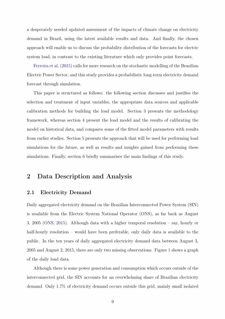
Daily aggregated electricity demand on the Brazilian Interconnected Power System (SIN)
is available from the Electric System National Operator (ONS), as far back as August
3, 2005 (ONS, 2015). Although data with a higher temporal resolution – say, hourly or
half-hourly resolution – would have been preferable, only daily data is available to the
public. In the ten years of daily aggregated electricity demand data between August 3,
2005 and August 2, 2015, there are only two missing observations. Figure 1 shows a graph
of the daily load data.
Although there is some power generation and consumption which occurs outside of the
interconnected grid, the SIN accounts for an overwhelming share of Brazilian electricity
demand. Only 1.7% of electricity demand occurs outside this grid, mainly small isolated
9
2006 2008 2010 2012 2014
1000
1600
GW
h/da
y
Figure 1: Daily Aggregated Load of the Brazilian Interconnected Power System (SIN)Source: Brazilian Independent System Operator (ONS, 2015)
systems in the Amazon region. Our study therefore only considers the electricity demand
served by the SIN.
In principle, there may be some advantages to separating the demand between various
sectors and modelling them individually, since for example the residential, commercial and
industrial sectors can have very different demand patterns. In some cases, it might also
be interesting to divide even further, for example distinguish between various industries
(steel and pulp, for example) or different classes of residential customers (for example
based on income). We do not, however, have access to daily data at this level of detail.
Essentially, this means that our modelling approach will be in large part a top-down
approach where we focus on aggregate behaviour, rather than a bottom-up approach
where one would concentrate on smaller units. Although daily demand data is available
for four geographically separated subsystems of the SIN, our main focus remains on the
daily total demand of the system. It might be possible to improve on our results by
modelling each geographical region separately, although our approach – simply modelling
the aggregate – hopefully benefits somewhat from the law of large numbers.
10
2.2 Weather Data
The main purpose of this study is to determine the behaviour of electricity demand under
changing climatic conditions. Therefore, it is important that we first and foremost consider
the impact of weather variables on the electricity demand.
The Integrated Surface Database (ISD) from the National Oceanic and Atmospheric
Administration (NOAA) contains quality-controlled weather observations from 490 weather
stations on Brazilian territory (NOAA, 2015). However, only 28 of these weather stations
have less than 10% missing hourly observations in the ten-year period between August 3,
2005 and August 2, 2015. We initially focus on this subset of weather stations.
For simplicity, we consider only the temperature rather than a wider set of weather
variables. Although humidity, cloud coverage and wind most likely also affect electricity
demand, temperature is generally considered to be by far the most important single
weather variable.
Since the temperature observations contain missing values, we replace the missing
values with artificial values imputed by the procedure described by Josse and Husson
(2011). The temperature observations contain few missing values in addition to a sub-
stantial amount of both temporal and geographical regularity, which is why we believe
that a PCA-based imputation method is well suited for our purposes.
We assume that when average daily temperature (that is, daily maximum temperature
plus daily minimum temperature, divided by two) is below a certain base temperature,
TH , then electricity demand increases for heating purposes. When the temperature is
above a certain base temperature, TC , electricity demand increases for cooling purposes,
and when the temperature is above an even higher base temperature TCA, then electricity
demand for cooling purposes increases at a higher rate. Altogether, this means that we
estimate a piecewise linear temperature response curve with knots at TH , TC and TCA, and
which is flat between TH and TC . The base temperatures are chosen by simply scanning
over the base temperatures and selecting the base temperatures that minimise an out-of-
model error measure, that is, we selected the base temperatures that appeared to provide
the best forecasting performance. This procedure lead to a base temperature for heating
11
at 18◦C, a base temperature for cooling at 25◦C, and a base temperature for accelerated
cooling at 28◦C. Each of these three base temperatures will give rise to a linear term in
the model.
In order to select a smaller subset of stations with the highest impact on electricity
demand, we employ a variation of the procedure suggested by Hong et al. (2015) for
selecting weather stations. The framework proposed by Hong et al. (2015) first ranks in-
dividual weather stations based on a goodness-of-fit measure when including each station
individually in a simple model, then selects a composite weather variable containing the
highest ranking weather stations such that a given model error measure is minimised. We
depart slightly from the proposed framework by avoiding the construction of a composite
weather variable and instead including all the highest ranking weather variables individ-
ually in the model. This procedure results in a selection of 18 weather terms pertaining
to 13 different weather stations.
For the selected weather variables, autoregressive and lagged terms are also included in
order to account for inertia (that is, serial correlation) and accumulative weather effects,
as discussed by Li et al. (2009). By scanning over various lagged and autoregressive terms
and calculating out-of-model error measures, we chose to include the 9-day moving average
of the weather variables (average of ten days earlier up until and including yesterday) and
the value of yesterday’s weather variable.
Since this can give rise to a large number of weather-related variables in the model, we
also perform a backwards stepwise regression at the end using the Bayesian Information
Criterion to select a more parsimonious model (Hyndman and Athanasopoulos, 2014).
After this pruning, only nine weather variables from eight weather stations is included in
the model: heating degree days from a single weather station (number of degrees below
18◦C), accelerated cooling degree days from a single weather station (number of degrees
above 28◦C), and regular cooling degree days from seven weather stations (number of
degrees above 25◦C).
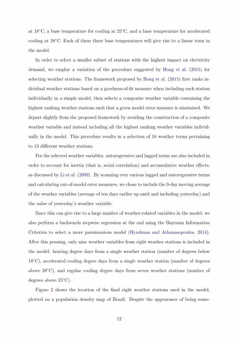
Figure 2 shows the location of the final eight weather stations used in the model,
plotted on a population density map of Brazil. Despite the appearance of being some-
12
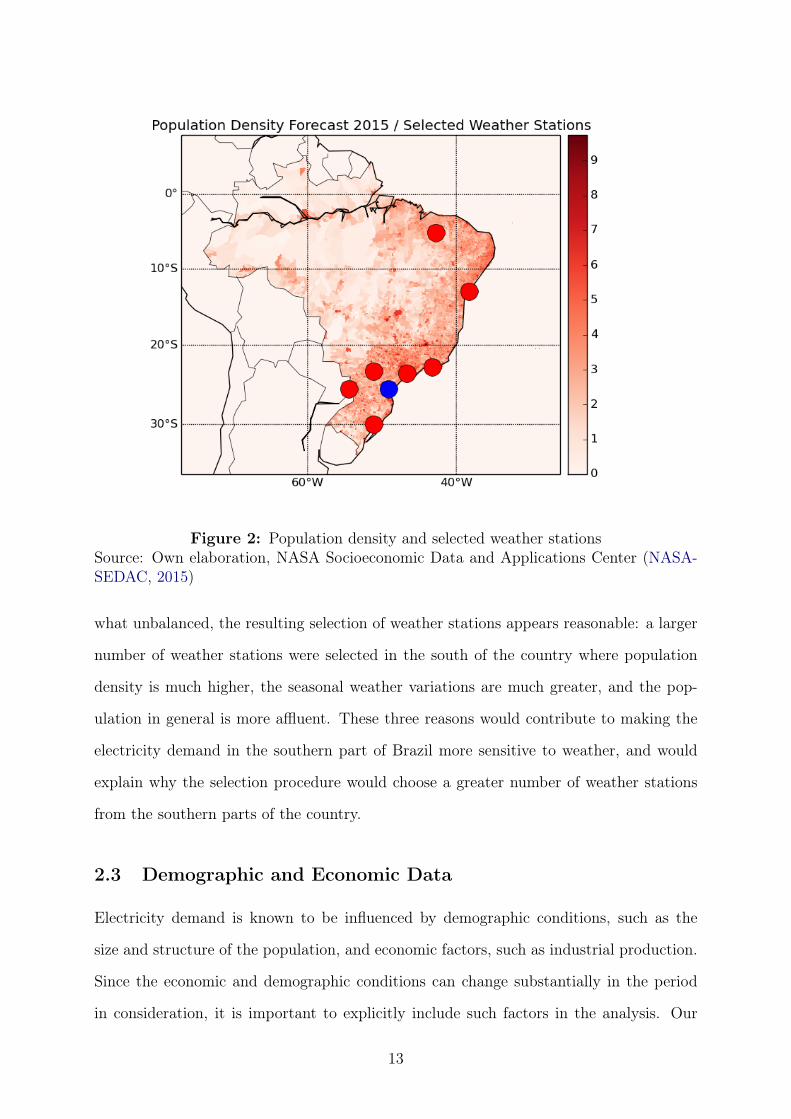
Figure 2: Population density and selected weather stationsSource: Own elaboration, NASA Socioeconomic Data and Applications Center (NASA-SEDAC, 2015)
what unbalanced, the resulting selection of weather stations appears reasonable: a larger
number of weather stations were selected in the south of the country where population
density is much higher, the seasonal weather variations are much greater, and the pop-
ulation in general is more affluent. These three reasons would contribute to making the
electricity demand in the southern part of Brazil more sensitive to weather, and would
explain why the selection procedure would choose a greater number of weather stations
from the southern parts of the country.
2.3 Demographic and Economic Data
Electricity demand is known to be influenced by demographic conditions, such as the
size and structure of the population, and economic factors, such as industrial production.
Since the economic and demographic conditions can change substantially in the period
in consideration, it is important to explicitly include such factors in the analysis. Our
13
2006 2008 2010 2012 2014
240
280
GD
P, b
illio
ns o
f BR
L (1
995)
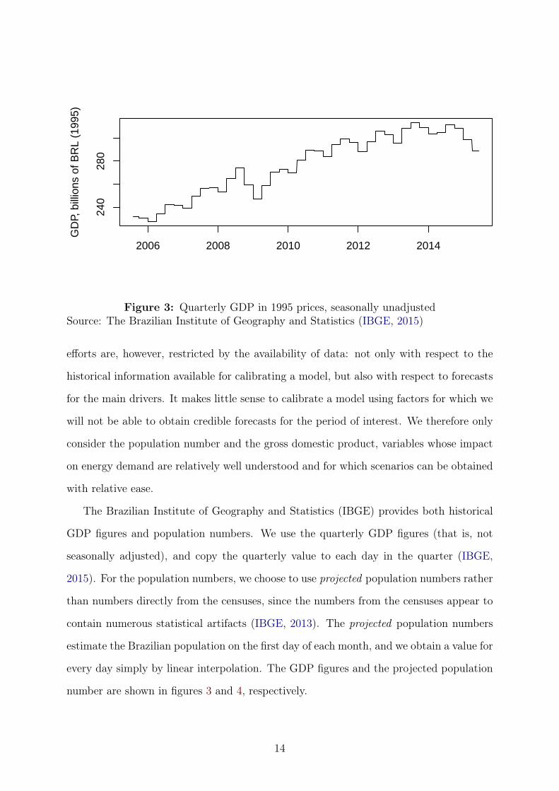
Figure 3: Quarterly GDP in 1995 prices, seasonally unadjustedSource: The Brazilian Institute of Geography and Statistics (IBGE, 2015)
efforts are, however, restricted by the availability of data: not only with respect to the
historical information available for calibrating a model, but also with respect to forecasts
for the main drivers. It makes little sense to calibrate a model using factors for which we
will not be able to obtain credible forecasts for the period of interest. We therefore only
consider the population number and the gross domestic product, variables whose impact
on energy demand are relatively well understood and for which scenarios can be obtained
with relative ease.
The Brazilian Institute of Geography and Statistics (IBGE) provides both historical
GDP figures and population numbers. We use the quarterly GDP figures (that is, not
seasonally adjusted), and copy the quarterly value to each day in the quarter (IBGE,
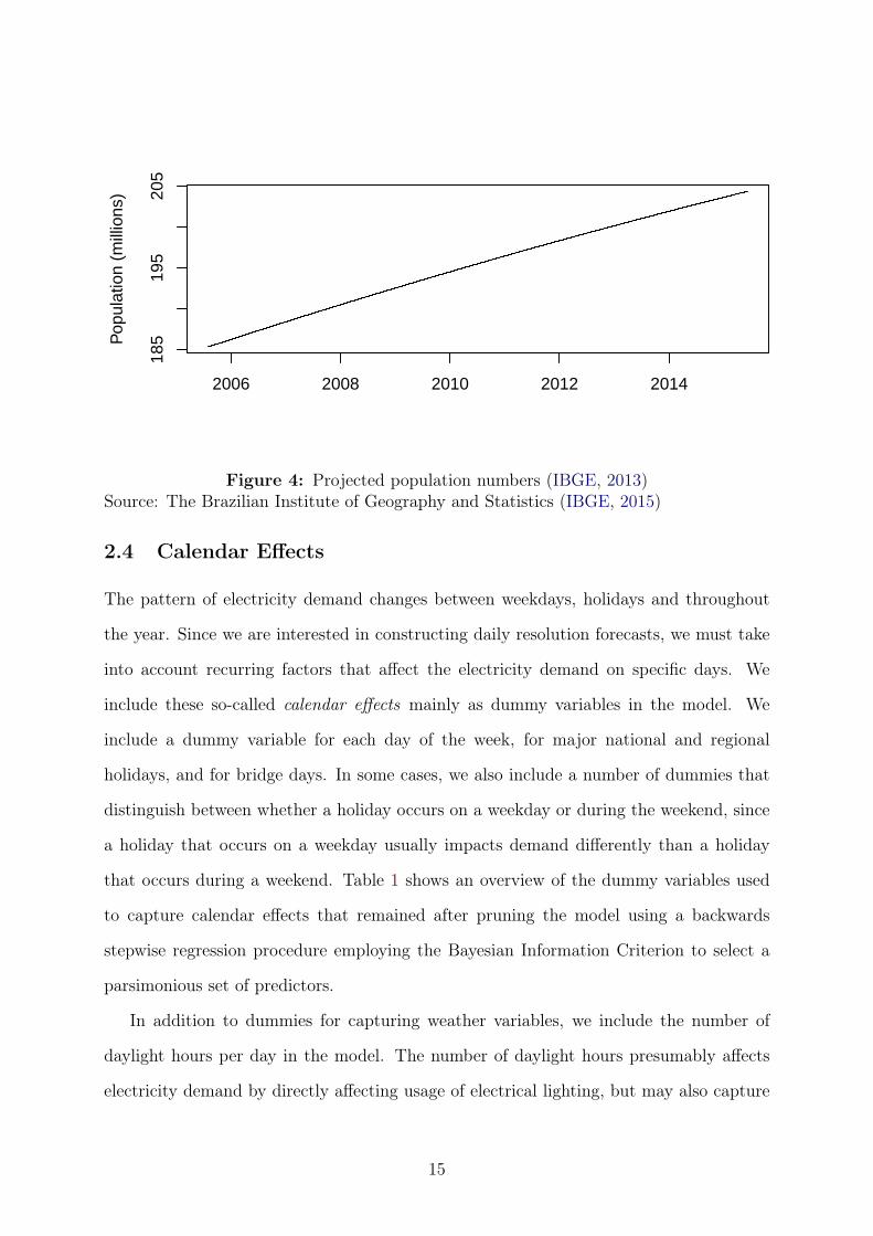
2015). For the population numbers, we choose to use projected population numbers rather
than numbers directly from the censuses, since the numbers from the censuses appear to
contain numerous statistical artifacts (IBGE, 2013). The projected population numbers
estimate the Brazilian population on the first day of each month, and we obtain a value for
every day simply by linear interpolation. The GDP figures and the projected population
number are shown in figures 3 and 4, respectively.
14
2006 2008 2010 2012 2014
185
195
205
Pop
ulat
ion
(mill
ions
)
Figure 4: Projected population numbers (IBGE, 2013)Source: The Brazilian Institute of Geography and Statistics (IBGE, 2015)
2.4 Calendar Effects
The pattern of electricity demand changes between weekdays, holidays and throughout
the year. Since we are interested in constructing daily resolution forecasts, we must take
into account recurring factors that affect the electricity demand on specific days. We
include these so-called calendar effects mainly as dummy variables in the model. We
include a dummy variable for each day of the week, for major national and regional
holidays, and for bridge days. In some cases, we also include a number of dummies that
distinguish between whether a holiday occurs on a weekday or during the weekend, since
a holiday that occurs on a weekday usually impacts demand differently than a holiday
that occurs during a weekend. Table 1 shows an overview of the dummy variables used
to capture calendar effects that remained after pruning the model using a backwards
stepwise regression procedure employing the Bayesian Information Criterion to select a
parsimonious set of predictors.
In addition to dummies for capturing weather variables, we include the number of
daylight hours per day in the model. The number of daylight hours presumably affects
electricity demand by directly affecting usage of electrical lighting, but may also capture
15
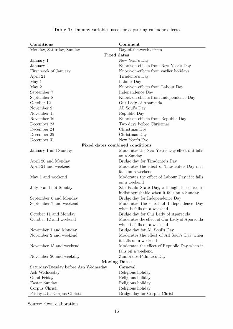
Table 1: Dummy variables used for capturing calendar effects
Conditions CommentMonday, Saturday, Sunday Day-of-the-week effects
Fixed datesJanuary 1 New Year’s DayJanuary 2 Knock-on effects from New Year’s DayFirst week of January Knock-on-effects from earlier holidaysApril 21 Tiradente’s DayMay 1 Labour DayMay 2 Knock-on effects from Labour DaySeptember 7 Independence DaySeptember 8 Knock-on effects from Independence DayOctober 12 Our Lady of AparecidaNovember 2 All Soul’s DayNovember 15 Republic DayNovember 16 Knock-on effects from Republic DayDecember 23 Two days before ChristmasDecember 24 Christmas EveDecember 25 Christmas DayDecember 31 New Year’s Eve
Fixed dates combined conditionsJanuary 1 and Sunday Moderates the New Year’s Day effect if it falls
on a SundayApril 20 and Monday Bridge day for Tiradente’s DayApril 21 and weekend Moderates the effect of Tiradente’s Day if it
falls on a weekendMay 1 and weekend Moderates the effect of Labour Day if it falls
on a weekendJuly 9 and not Sunday São Paulo State Day, although the effect is
indistinguishable when it falls on a SundaySeptember 6 and Monday Bridge day for Independence DaySeptember 7 and weekend Moderates the effect of Independence Day
when it falls on a weekendOctober 11 and Monday Bridge day for Our Lady of AparecidaOctober 12 and weekend Moderates the effect of Our Lady of Aparecida
when it falls on a weekendNovember 1 and Monday Bridge day for All Soul’s DayNovember 2 and weekend Moderates the effect of All Soul’s Day when
it falls on a weekendNovember 15 and weekend Moderates the effect of Republic Day when it
falls on a weekendNovember 20 and weekday Zumbi dos Palmares Day
Moving DatesSaturday-Tuesday before Ash Wednesday CarnevalAsh Wednesday Religious holidayGood Friday Religious holidayEaster Sunday Religious holidayCorpus Christi Religious holidayFriday after Corpus Christi Bridge day for Corpus Christi
Source: Own elaboration
16
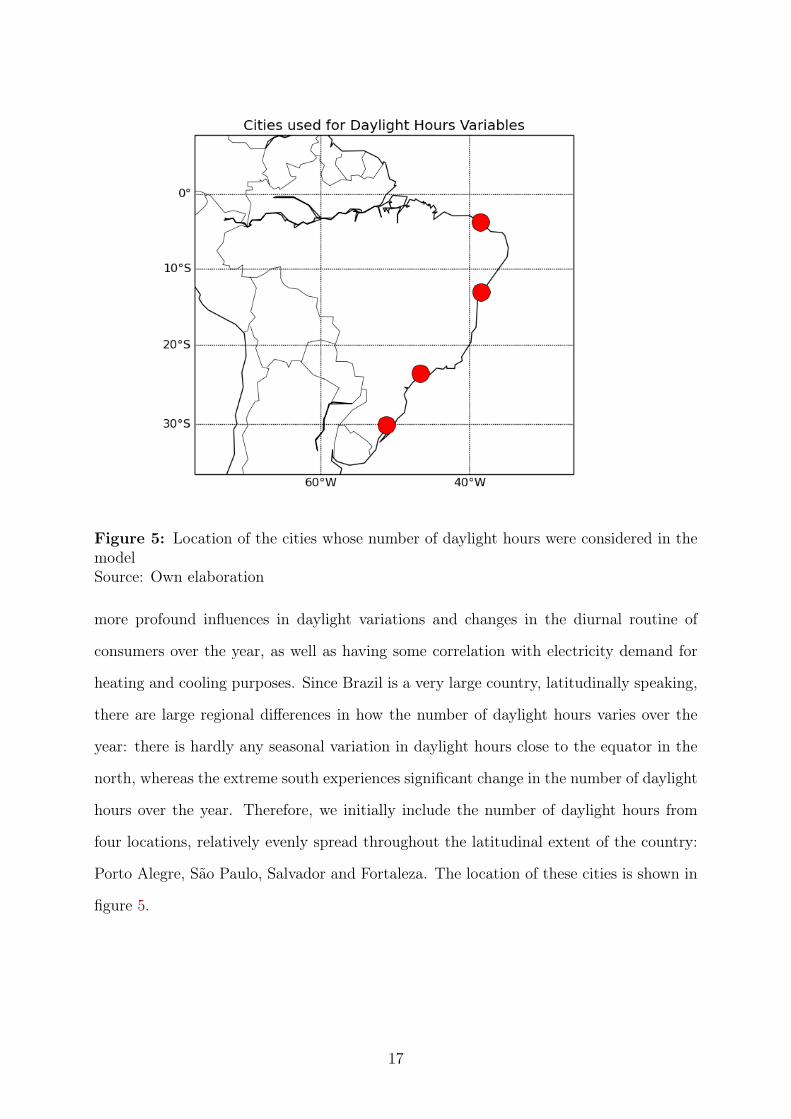
Figure 5: Location of the cities whose number of daylight hours were considered in themodelSource: Own elaboration
more profound influences in daylight variations and changes in the diurnal routine of
consumers over the year, as well as having some correlation with electricity demand for
heating and cooling purposes. Since Brazil is a very large country, latitudinally speaking,
there are large regional differences in how the number of daylight hours varies over the
year: there is hardly any seasonal variation in daylight hours close to the equator in the
north, whereas the extreme south experiences significant change in the number of daylight
hours over the year. Therefore, we initially include the number of daylight hours from
four locations, relatively evenly spread throughout the latitudinal extent of the country:
Porto Alegre, São Paulo, Salvador and Fortaleza. The location of these cities is shown in
figure 5.
17
2.5 Special events
Special rare or irregular events can also affect electricity consumption. Although it would
be difficult to obtain forecasts for these events in the remote future, it is necessary to
include known historical events for the calibration of the model. When creating forecasts
with the model, there is some comfort in knowing that these types of events normally
infrequent. In this respect, in our demand model we include a dummy variable to mark
the weekdays on which the Brazilian national team played matches in the FIFA World
Cups in 2006, 2010 and 2014.
2.6 Error Term
The error of the model is likely to contain residual amounts of serial correlation. We
model the error term as an ARMA process, and use a Ljung-Box test to show that the
residuals from the ARMA process are uncorrelated. Modelling the error term thusly will
help us create probabilistic forecasts that recreate the serial correlation characteristics of
the original series during the simulation step.
2.7 Intentionally Omitted Drivers
Electricity demand is affected by a greater number of factors than those mentioned until
now. Although the following factors have not been included in the model for practical
reasons, they have not been forgotten.
Technological change, for instance, is an important determinant of electricity demand.
However, new technology may both increase and decrease electricity demand through
creating new ways of using electricity or replacing current uses of electricity. Also the
proliferation of important existing technologies, such as air conditioning, is something
that could have been explicitly included in the model, especially considering that many
technologies in Brazil are far from their saturation point. Some of these developments,
however, are somewhat accounted for by including the GDP.
Intermittent renewable electricity generation, such as solar or wind power, is frequently
modelled as “negative demand”, since electricity from these sources could substitute elec-
18
tricity from the national grid with local sources of electricity. Although this might in-
crease in importance in the future, we do not include this in the model. Although these
are weather-dependent, thus apparently of great interest in this study, we consider these
as sources of supply in this context, rather than sources of “negative demand”.
Perhaps the most ominous omission is the price of electricity. Firstly, however, several
studies on the household sector in Brazil assert that at least price elasticity in that partic-
ular sector is low, much lower than income elasticity (Andrade and Lobão, 1997; Schmidt
and Lima, 2004; Mattos and Lima, 2005). Secondly, demand is a crucial component to
price formation, which means that it would be necessary to forecast demand in order to
forecast price, but we would also need a price forecast to construct a demand forecast.
As such, this would lead to a circular problem, or at best a simultaneous problem, which
is beyond the scope of this study.
These factors have been omitted partially in an effort to keep the assumptions neces-
sary for simulation step as simple as possible: including even a small number of additional
factors can dramatically increase the number of possible scenarios that need to be con-
sidered, as well as create consistency problems, since creating scenarios that accurately
reflect the appropriate conditional probabilities can be exceptionally complicated. In
many cases, there is also little current or historical information to base forecasts of the
factors on.
The factors that have been omitted are also presumably of lower importance than
the variables already included. If the selection of predictors already included provides
sufficiently pleasing results, there is little incentive to complicate the model further. At
best, including these factors would provide marginal benefits in return for a substantial
increase in complexity, typically showing diminishing returns in response to the effort.
3 Methodology Framework
The methodology follows the same three basic steps as Hyndman and Fan (2010): first a
statistical demand model is calibrated using the available historical data described above,
then the demand model is used to forecast future demand by combining temperature and
19
residual simulation with future assumed demographic and economic scenarios, and finally
the results and the forecasting performance will be evaluated critically.
The statistical model of demand is constructed using multiple linear regression. Al-
though more complex approaches have been explored in the literature, such as machine
learning, Hong et al. (2014a) argue that multiple linear regression approaches often prove
superior to machine learning approaches, in addition to being considerably simpler to op-
erationalise. The resulting models are also more defensible, in the sense that the influence
of each factor is directly and explicitly quantified, which is not the case for most ma-
chine learning based approaches. The weather variables of the model are selected using a
slightly modified version of the approach developed by Hong et al. (2015). Final predictor
selection is performed by backwards stepwise regression, using the Bayesian Information
Criterion (BIC) in order to indicate a preference for parsimonious models (Hyndman and
Athanasopoulos, 2014).
Future demand scenarios are constructed through repeatedly creating point forecasts
with the calibrated model by applying it to simulated residuals, simulated future tem-
peratures, and assumed future economic and demographic scenarios. After choosing the
correct timeseries model for the residual, residual simulation can be performed by a simple
bootstrapping method. Future temperatures are provided by global circulation models
MIROC5 and HadGem3 that simulate the climate. However, the climate simulations do
not provide a sufficient number of weather scenarios for assessing the entire probability
distribution, and because of this we will apply a bootstrapping method to the climate
simulation results in order to generate a much greater number of realistic weather scenar-
ios. For assumed future values of demographic and economic drivers, we will use selected
scenarios from the Shared Socioeconomic Pathways (SSP) database (O’Neill et al., 2014a).
In the final step, the forecasting performance is evaluated and the forecasts are com-
pared to forecasts provided in the existing literature. An idea of the performance can be
obtained by checking the forecasting performance of the calibrated model on an out-of-
sample validation set, paying close attention to the differences between the ex-ante and
ex-post forecasts. We also compare results with electricity demand forecasts developed in
20
other reports, such as the Brazilian official ten-year plan (EPE-PDE, 2014), the Brazil-
ian official long-term plan (EPE-PNE, 2014), and the demand projections developed by
Schaeffer et al. (2008).
4 Model Establishment
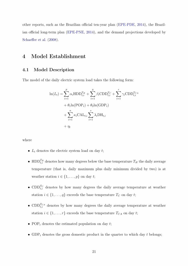
4.1 Model Description
The model of the daily electric system load takes the following form:
ln(Lt) =
p∑i=1
αiHDDTHt,i +
q∑i=1
βiCDDTCt,i +
r∑i=1
γiCDDTCAt,i
+ θ1ln(POPt) + θ2ln(GDPt)
+n∑
i=1
κiCALt,i
s∑i=1
λiDHt,i
+ ηt
where
• Lt denotes the electric system load on day t;
• HDDTHt,i denotes how many degrees below the base temperature TH the daily average
temperature (that is, daily maximum plus daily minimum divided by two) is at
weather station i ∈ {1, . . . , p} on day t;
• CDDTCt,i denotes by how many degrees the daily average temperature at weather
station i ∈ {1, . . . , q} exceeds the base temperature TC on day t;
• CDDTCAt,i denotes by how many degrees the daily average temperature at weather
station i ∈ {1, . . . , r} exceeds the base temperature TCA on day t;
• POPt denotes the estimated population on day t;
• GDPt denotes the gross domestic product in the quarter to which day t belongs;
21
• CALt,i is a set of dummies marking calendar effects and the occurrence of special
events;
• DHt,i is the number of hours of daylight on day t at location i ∈ {1, . . . , s};
• ηt denotes the model error on day t, which can be serially correlated and is modelled
by an ARMA process.
The model is formulated in terms of the natural logarithm of demand, as such the
effects of weather and calendar dummies are multiplicative in this model. The demo-
graphic and economic variables, population and gross domestic product, also appear as
natural logarithms, so they are modelled as having a constant elasticity rather than a
constant marginal effect. In addition to being a reasonable modelling choice (a change
in the GDP of one percent increases the electricity demand by a determined percentage),
an advantage of this choice is that the elasticities can be easily compared to estimates of
elasticities found in the existing literature.
4.2 Variable Selection
The set of weather variables was chosen using a method similar to the one developed by
Hong et al. (2015). The final set of predictors were selected using backwards stepwise
regression (Hyndman and Athanasopoulos, 2014).
4.3 Model Fitting
We divided our sample into two parts: a training sample and a test sample. The model
parameters are calibrated using the training sample, and an ex-post forecast on the val-
idation sample gives an impression of how the model performs for forecasting purposes,
disconsidering uncertainty in the predictor variables.
The results of the model calibration are shown in appendix A. The mean absolute
percentage error (MAPE) of the training sample is 1.64%, whereas the MAPE of the
ex-post forecast (i.e. given the observed historical value of all the predictors) on the test
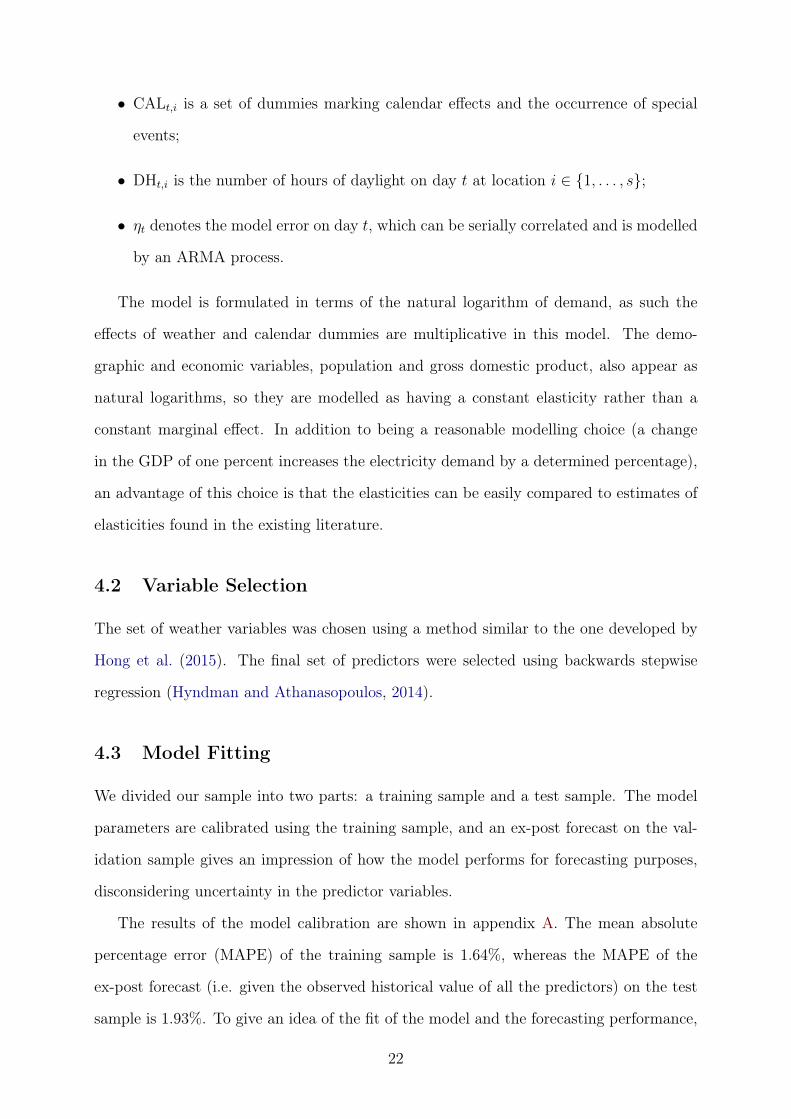
sample is 1.93%. To give an idea of the fit of the model and the forecasting performance,
22
5 10 15 20 25 30
1000
1400
1800
January 2014
GW
h
LoadForecast
Figure 6: In-sample forecast, January 2014Source: Own elaboration, Brazilian Independent System Operator (ONS, 2015)
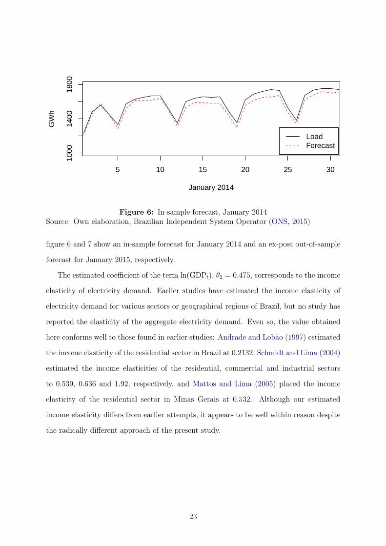
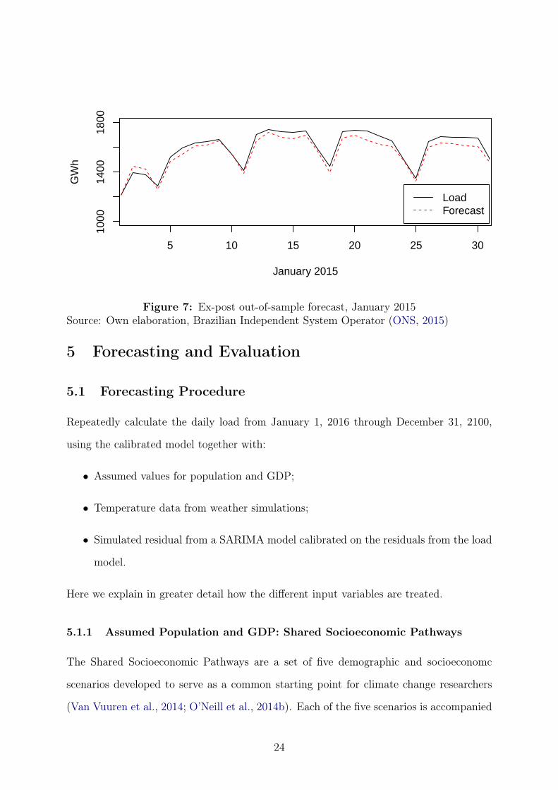
figure 6 and 7 show an in-sample forecast for January 2014 and an ex-post out-of-sample
forecast for January 2015, respectively.
The estimated coefficient of the term ln(GDPt), θ2 = 0.475, corresponds to the income
elasticity of electricity demand. Earlier studies have estimated the income elasticity of
electricity demand for various sectors or geographical regions of Brazil, but no study has
reported the elasticity of the aggregate electricity demand. Even so, the value obtained
here conforms well to those found in earlier studies: Andrade and Lobão (1997) estimated
the income elasticity of the residential sector in Brazil at 0.2132, Schmidt and Lima (2004)
estimated the income elasticities of the residential, commercial and industrial sectors
to 0.539, 0.636 and 1.92, respectively, and Mattos and Lima (2005) placed the income
elasticity of the residential sector in Minas Gerais at 0.532. Although our estimated
income elasticity differs from earlier attempts, it appears to be well within reason despite
the radically different approach of the present study.
23
5 10 15 20 25 30
1000
1400
1800
January 2015
GW
h
LoadForecast
Figure 7: Ex-post out-of-sample forecast, January 2015Source: Own elaboration, Brazilian Independent System Operator (ONS, 2015)
5 Forecasting and Evaluation
5.1 Forecasting Procedure
Repeatedly calculate the daily load from January 1, 2016 through December 31, 2100,
using the calibrated model together with:
• Assumed values for population and GDP;
• Temperature data from weather simulations;
• Simulated residual from a SARIMA model calibrated on the residuals from the load
model.
Here we explain in greater detail how the different input variables are treated.
5.1.1 Assumed Population and GDP: Shared Socioeconomic Pathways
The Shared Socioeconomic Pathways are a set of five demographic and socioeconomc
scenarios developed to serve as a common starting point for climate change researchers
(Van Vuuren et al., 2014; O’Neill et al., 2014b). Each of the five scenarios is accompanied
24
by a narrated storyline (O’Neill et al., 2012), and several teams of researchers have per-
formed simulations to quantify key economic and demographic variables for each of the
scenarios (IIASA, 2015).
For our work, we have selected three of the five scenarios:
SSP1: Global Sustainable Development
SSP2: Business As Usual
SSP5: Conventional Development/Economic Optimism
We have chosen to use the quantifications that have been created by the OECD and
are available in the SSP Database, since these are considered illustrative (IIASA, 2015).
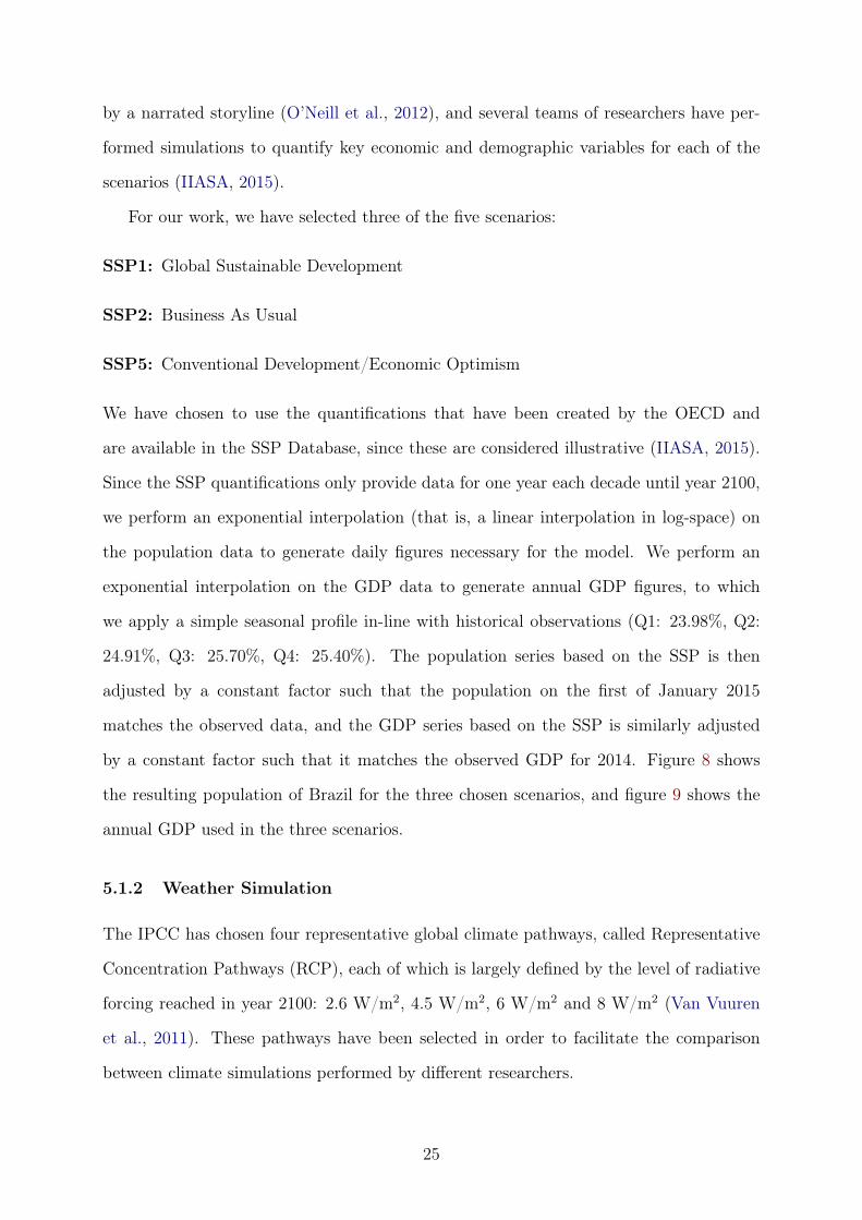
Since the SSP quantifications only provide data for one year each decade until year 2100,
we perform an exponential interpolation (that is, a linear interpolation in log-space) on
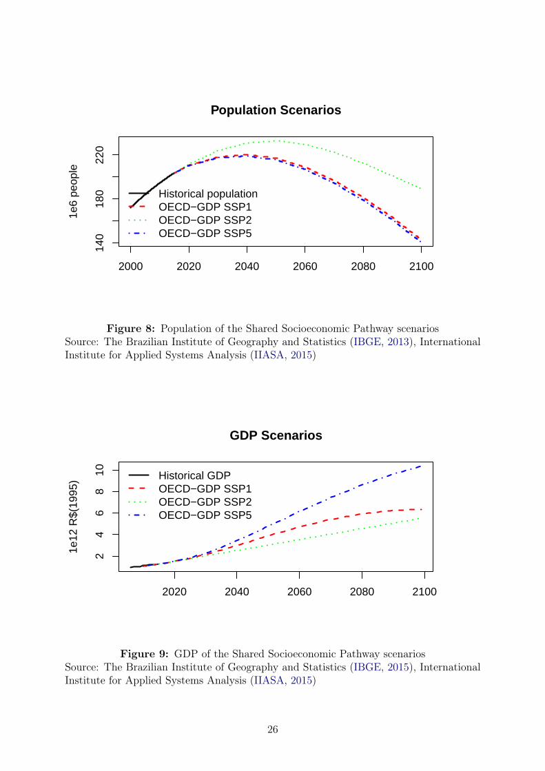
the population data to generate daily figures necessary for the model. We perform an
exponential interpolation on the GDP data to generate annual GDP figures, to which
we apply a simple seasonal profile in-line with historical observations (Q1: 23.98%, Q2:
24.91%, Q3: 25.70%, Q4: 25.40%). The population series based on the SSP is then
adjusted by a constant factor such that the population on the first of January 2015
matches the observed data, and the GDP series based on the SSP is similarly adjusted
by a constant factor such that it matches the observed GDP for 2014. Figure 8 shows
the resulting population of Brazil for the three chosen scenarios, and figure 9 shows the
annual GDP used in the three scenarios.
5.1.2 Weather Simulation
The IPCC has chosen four representative global climate pathways, called Representative
Concentration Pathways (RCP), each of which is largely defined by the level of radiative
forcing reached in year 2100: 2.6 W/m2, 4.5 W/m2, 6 W/m2 and 8 W/m2 (Van Vuuren
et al., 2011). These pathways have been selected in order to facilitate the comparison
between climate simulations performed by different researchers.
25
2000 2020 2040 2060 2080 2100
140
180
220
1e6
peop
le
Population Scenarios
Historical populationOECD−GDP SSP1OECD−GDP SSP2OECD−GDP SSP5
Figure 8: Population of the Shared Socioeconomic Pathway scenariosSource: The Brazilian Institute of Geography and Statistics (IBGE, 2013), InternationalInstitute for Applied Systems Analysis (IIASA, 2015)
2020 2040 2060 2080 2100
24
68
10
1e12
R$(
1995
)
GDP Scenarios
Historical GDPOECD−GDP SSP1OECD−GDP SSP2OECD−GDP SSP5
Figure 9: GDP of the Shared Socioeconomic Pathway scenariosSource: The Brazilian Institute of Geography and Statistics (IBGE, 2015), InternationalInstitute for Applied Systems Analysis (IIASA, 2015)
26

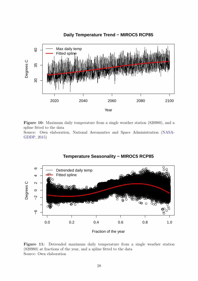
The National Aeronautics and Space Administration (NASA) has created global daily
downscaled climate projections for two of the RPCs, RCP4.5 and RCP8.5, using 21 dif-
ferent climate models (NASA-GDDP, 2015). With a spatial resolution of 0.25 degrees,
these projections are considered appropriate for climate change impact studies on local
and regional scales. From the NASA-GDDP dataset, we obtained the daily maximum and
minimum temperature projections for each weather station used in our calibrated model
from the MIROC5 global circulation model for the two available RCPs (Watanabe et al.,
2010).
This temperature data is then used to simulate a large number of weather paths, which
enables us to estimate the impact of weather uncertainty on the electricity demand. The
simulated weather paths are created using the following procedure:
1. A trend spline and a seasonal spline are fitted to the data for each variable from
each weather station, as illustrated for a single weather variable in figures 10 and
11;
2. A trend spline and a seasonal spline are fitted to the annual and daily standard
deviations of the detrended and deseasonalised temperature data for each variable
from each weather station, as illustrated for a single weather variable in figures 12
and 13;
3. A normalised, detrended and deseasonalised residual is created for each variable from
each weather station by subtracting the trend and seasonal splines, then dividing
by the trend and seasonal splines that were fitted to the standard deviation, as
illustrated for a single weather variable in figure 14;
4. The normalised residual is resampled (with replacement) in blocks containing a
random number of days between 180 and 545, and containing all weather variables.
This procedure is intended to capture trends in the weather variables, as well as preserve
the temporal and spatial correlation present in the dataset. The last step of the procedure
is repeated 500 times in order to generate 500 weather simulations for each of the two
selected RCPs. Figures 15 and 16 illustrate the results of this procedure for the maximum
27
2020 2040 2060 2080 2100
3035
40Daily Temperature Trend − MIROC5 RCP85
Year
Deg
rees
C
Max daily tempFitted spline
Figure 10: Maximum daily temperature from a single weather station (820980), and aspline fitted to the dataSource: Own elaboration, National Aeronautics and Space Administration (NASA-GDDP, 2015)
●●
●
●●
●●●●●●●●●●●●
●
●●●●
●●●●●●
●●●
●●●●●●
●●●●●●●●●●●
●
●●●●●
●
●●●●●●●●
●●●●●
●●●●●●
●●●●
●●
●●●●●●●●●●●●●
●●●●●●●●●●●●
●●●●●●●●
●●●●●●●
●
●●●●●●
●
●●●●●●●
●●●●●
●●●●●●
●●●●●●●●●●●●●●●●●●●
●●●●●●●●●●●●●●●●
●●●●●●●●●●●●●●●●●●●●●●●●●●●
●●●●●●●●●●●●●●
●
●
●
●
●●●●
●
●●●●
●●●
●
●
●●●●
●●
●●●
●●●●●
●
●●●●
●
●●
●●
●●
●
●●●
●
●
●
●
●●●●●●
●●●
●
●●
●●
●●
●
●●
●
●●●●
●
●●
●
●●
●●●●●
●●
●
●●
●
●
●
●
●
●
●●
●
●
●
●
●●
●
●
●
●●●●●
●
●
●●
●
●●●●●●●●●●●●●
●●●●●●
●
●
●●●●
●●●●●●
●●●●●●●●
●●●●●●●●●●●●●
●●●●●●●
●●●●●●●●
●●●●●●●
●●●●●●●●●●●●●●●●●●●●●●●●●●
●●●●●●
●●●●●●
●●●●●●●●●●●●●
●●●●●
●●●●●●●●●●●●●●
●●●●●●●●●●
●●●●●●●●●●●●●●●●●●●●●●
●●
●●●●●●●●
●●●●●●
●●●●●●●●●●●●●●●
●●●●●●●●●●●●●●●●●●●●●●●●●
●●
●●●●●●●●●●●●●●●
●●
●
●
●●●●
●●●
●●●●
●●●
●●
●●●●●
●●
●
●●●●
●●
●
●
●
●●
●●
●
●●●
●●
●
●
●
●●●
●●●●●●
●
●
●
●●●
●
●
●
●
●
●
●
●
●
●●●●●
●
●
●
●●
●●
●●
●●●●●
●●
●●
●●●●●●●
●
●●●●
●
●●●●
●
●
●●●●
●●●
●●
●
●●
●●●●●●●
●●●●●●●●
●●●●●●●●●●●●●●●●●
●●●●●●●●●
●●●●●●●●●●●●
●●●●●●●●●●●●
●●●●●●
●
●●●●●●●
●●●●●●●
●●●●●●●●●●●●●●●●●●●●●●●●●●●●●
●●●●●●●●●●●●●●●
●●●
●●●●●●
●●●●●●●●●
●●
●●●●●●●●●●●●●●●●
●●
●●●●●●●●●●
●●●●●●●●●●●
●●●●●●●●●●●●●●●●●●●●●●●
●●●●●●●●●●
●●●●●●
●●●●●●●●
●●●●
●●●●●●●●●
●●●
●
●
●●●●●●●
●●●●
●●●
●
●
●●●
●●
●●
●
●●
●
●●
●●●
●
●●
●
●●
●
●
●
●
●
●
●
●●
●●
●●
●●●
●
●●
●
●●
●●●●
●
●
●●●●●
●
●●●
●
●
●●●
●●
●
●●
●●●●●●●●
●
●
●●
●
●●
●●●●●●
●
●
●●●
●●●●●●●●●
●●●●
●●
●●●
●
●●●●●●●●
●●●●●●●●●●
●
●●●●●●●●●●●●●●●●●●
●●●●●●●●●●
●●
●●●●●●●●●●●●●●
●●●●●●●●●●●●●●●●●●●●●
●●●
●●●●●●●
●●●●●●●●●●●●●●●●●●●●
●●●●●●●●●
●●●●●●●●●
●●●●●●●●●●●●●
●●●●●●●●●●●
●●●●●●●●●●●●●●●●●●●●
●●●●●●●●●●●●●●●●●●●●●●●●●●
●●
●
●
●●●●
●
●●
●●●●
●●●●●●●
●
●●
●
●●
●●●
●●●●●
●●●
●●
●
●●
●
●
●
●
●●●●●
●
●●
●●●●●●●●●
●●●
●
●●●●
●
●
●●●
●●●●●●●
●●●●●
●●
●
●
●
●
●
●
●
●
●●●
●
●
●
●●●
●
●●●
●
●●
●
●
●
●
●
●●●●●
●
●●
●●
●●
●●●●●●
●
●●●
●●
●
●
●●
●
●●
●
●
●●●
●
●●●
●●●
●●
●●
●●
●
●●●
●●
●
●●●
●
●●●
●
●●●
●●●●●●
●
●●●●●●
●●
●●●●●
●●
●●●●●●●●
●●●●●●●●●●●●●
●●●●●●●●●
●●●●●●●●
●●●●●●●●●●●●●●●●●●●●●
●●●●●●●●●●●●●
●●●●●●●●●●●●●●●●●
●●●●●●●●●●●●●●
●●●●
●
●●●●●
●●●●●●●●●●●●●●●
●●●●●●●●●●●●●●●●●●●
●●●●●
●
●
●●
●●
●●●
●
●●●
●
●●●●●●●●●●
●
●
●
●●●●
●
●
●
●
●●
●●●●●●●●
●●
●●●●●●●●●
●●
●●●●
●●●●
●●●●
●
●
●●●●●●
●●
●●●
●●●●●
●●●
●
●●●●●●
●
●
●
●●●
●
●
●
●
●
●●
●●●
●
●●●●
●
●
●
●
●
●●
●●●●
●●●●●●●
●
●●
●
●
●●
●
●
●
●●●
●●●
●●●●●●●●
●●
●●●●●●●●
●
●●●●●●●●●
●●●●
●
●
●●●●●●●●●●●●●●●●●●●●●●●●●●●●●●
●●●●●●
●●●●●●●●●●●●
●●●●●●●●●●●●●●●●
●●●●●●●
●●●●●●●●●●
●●●●●●●●●●●●●●●●●●
●●●●●●●●●●●●●
●●●●●●
●●●●●●●●●●●●●●
●●●●●●●●●●●●●●●●●●
●●●●●●●●
●●●●●●●●●●●●●●●
●●●●●●
●●●●●●
●
●●●●●●●
●●●●●●●●●●●●●●●
●●
●●
●●●
●●
●●●
●●●
●
●●
●
●
●●
●●
●●●
●●●
●●
●●
●●
●
●
●●
●
●●●
●
●●●●
●●●●
●●
●●
●
●●●
●
●●●
●●
●
●●
●
●
●
●
●●
●●●
●●
●●●●
●
●
●
●●
●●
●
●
●●
●●
●●
●
●
●
●
●
●●●●
●
●
●●●●
●●
●●●●●●●
●
●●
●●●●
●
●
●●●●●●●
●
●●●●
●●●
●●●●●●●●
●●
●●
●●●●●●●●
●●●●●●●●●●●●●●●●
●●●●●●●●●●●●
●●●●
●●●●●●
●●●●●●●●●●●●●●●●●●●
●●●●●●●●
●●●●●●
●●●●●●●●●●●●
●●●●●●●●●●
●●●●●●●●●●●●●●●●●●●
●●●●●●●●●●●●●
●
●
●●●●●●
●
●●●●●●●●●●●●●●●●●
●●●●
●●●●●●●
●●●●●●●●
●●
●
●●●●●●
●●●
●
●●●●●●
●
●●●
●●
●
●
●●
●
●●
●●●●
●
●
●
●●●●●
●
●
●●●
●
●●●●
●
●
●●●●●●●
●●
●●●●
●
●
●
●●●
●●
●
●●●●
●●●●●
●●
●●
●
●
●●●●●
●●
●
●
●
●
●●
●
●●●●
●
●
●●●●●●●●●
●
●
●
●
●
●●
●
●
●●●●
●●●●
●●●●●●●●●●●
●●
●
●
●●●
●
●●●●●●
●●●●
●●
●●●●●●
●●●●●●●●●●●●●●●●●
●●●●●●●●●●●●●●
●●●●●●●●●●
●●●●●●●●
●●●●●●●●●●●●●●●●●
●●●●●●●●●●●●●
●●●●●●
●●●●●●●●●●●
●●●●●●●●●
●●●●●●●
●●●●●●●●●●
●●●●●●●●
●
●●●●●
●●●●●●●●
●●
●●●●●●●●●●●●●●●●●●●●
●●
●●●●●●●●
●●●●●●●●●●●●●
●
●
●●
●●
●●
●
●
●
●●●●●●●
●●●
●●●●
●
●●●●●
●●●●●
●●
●
●
●
●●●●
●●
●
●
●●
●●
●●●●
●●●
●●●●●●
●●
●●●●●●●●
●
●
●●●●●●●
●●●
●
●
●
●
●
●
●●
●
●●
●●●●
●●
●
●
●
●
●
●●
●
●
●
●
●●
●●●
●
●
●●●
●●●
●
●
●●●
●●
●
●
●●●
●●
●
●
●●
●●●
●●
●●
●●●●●
●
●●
●
●
●
●
●●●
●●
●
●●●●●●●●
●●●
●●●●●●●●●●●●●●●●●●●
●●●●●●●●●●●●●
●
●●●●●●●●
●●●●●●●●●
●●●●●●●●●●●●●●●●●
●●●●●●●●●
●●●●●●●●●●●●●●●●●●
●●●●●●●●●●●●●●
●
●●●●●●●
●●●●●●●
●●●
●●●●●●●●●●●
●●●●●●●●●●
●●●●
●●●●●●
●●●●●●●
●●●●●●●
●●●●●●
●●
●●●●●
●
●
●●●●●●●●●●
●
●●●●●●●●●●●●●●●●●
●●
●
●
●●●●●
●●
●
●●
●●●
●
●●
●
●
●●
●
●●●●●●●●
●●●●●●●
●●
●
●●●
●●●●●●●
●
●●●
●
●●
●●●
●
●
●●
●
●
●
●
●●
●●
●●
●●
●
●●●
●
●●●●●
●
●
●
●
●●
●
●
●●●
●●
●
●
●
●●
●●
●●●
●
●
●
●
●●
●●
●●
●
●
●
●
●●●
●
●
●●
●●
●
●●●●●●●●●●
●●●●●
●
●●●●●●●●●●●●●●●●●●
●●●●●●
●●●●●
●●●●●●●●●●●●●
●●●
●
●●●●●●●●●●
●●●●●●●●
●
●●●
●●●●●●●●●●●●●●●●●●●●●●●●
●●●●●●●●●●●●
●●●●●●●●●●●
●●●●●●●●●●●●●●●●●●
●●●●●●●●●●●●●●●●●●●●●●●●
●●●●●
●●●●●●●●●
●●●●●●●●●●●●●●●●●●●●●
●●●●●●
●●●●●●
●●
●●
●
●●●●●●●●●●●
●
●
●
●●●
●
●●
●●●●●●●
●
●
●●
●●●●●
●
●●●●●
●●
●●●
●
●●
●
●
●●
●
●
●●●●●
●●●●●
●
●●●
●
●●●●
●
●●●
●
●●
●●●●
●
●
●
●●
●●●
●●
●
●●●
●●●●●●
●
●●●
●
●●
●
●
●●
●●●
●
●
●●
●●●
●●
●
●●
●
●●
●
●
●●●●
●●●●●●
●●●●●●●●●●●●●●●●●●●●
●●
●
●●●●●●●●●●●●●●●●●●●●●●●●●
●●●●●●●●●●
●●●●●●●●●●●●●●●●●●●●●●●●●●●●
●●●●●●●●●●●●●●●
●●●●●●●●●●●●●●●●●●●●●
●●●●●●●●●
●●●●●●
●●●●●●
●●●●●●●●●●●●●
●●●●
●●●●●
●
●●●●●
●
●●●●●●●●
●●●●
●●●●●
●
●●●●●●●
●●
●
●●●●
●●●●●
●●●●●
●●●
●●●●●
●
●
●●
●●
●
●●●●●
●●●●
●●
●
●
●●●
●●
●
●
●
●●
●●●●
●
●
●●
●
●
●●●
●
●●
●●
●
●●●
●●
●
●●●●●
●●●●
●
●●
●●
●●●●
●
●
●●●
●●
●●●●●●
●
●
●
●●
●●●●
●
●
●
●
●
●●●●●
●
●
●●
●●●
●●●●●●
●●●●●●
●
●●●●●
●●●●●●
●●●●●●●●●
●●●●●●●●●●
●●●●●●●●●●●●●●●
●●●●●●●●●
●●●●●●●●
●●●●●●●●●●●●●●●●
●●●●●●●●●●●●●●
●●●●●●●●●●●●●●●●●●
●
●
●●●●●●●●
●●●●●●●●●
●●●●●●●●●●●●●●●
●●●
●
●
●●●●
●●●●●●●●●●●●●●●●●●●●●●●
●●●●●●●●●●●●●●●
●●●●●●●●●●
●●●●●●●●●
●●●●●●
●●
●
●
●
●●●●
●●
●●●
●●
●
●
●●
●
●
●●
●
●●
●●
●
●
●
●
●●
●
●●
●
●●●
●
●
●
●
●●●●
●●●●●●
●●
●●
●
●
●●●
●●●
●
●
●
●
●
●
●
●
●●
●●
●
●
●
●
●
●
●
●●●
●●●●
●
●
●●●●●●
●
●●●
●
●
●●●●●
●●●●
●
●●
●
●
●
●
●
●●
●●
●●●●
●●●●●●●●●●
●
●●●
●
●●
●
●●
●●
●●
●●
●●
●●●
●●●●●●●●●●●●●●●●●●●●●●●●●
●●●●●●●●●●●●
●●●●●●●●
●●●●●●
●●●●●●●●
●●●●●●●●
●●
●●
●●●
●●●●●●●●●●●●●
●●●●●●●●●●●●●●●●
●●●●●●●●●●●●●●●●●●●●
●●●●●●●●●●●
●●●●
●●●●●
●
●●●●●●●●●
●
●●●●●●●●●●
●●●●●●●●●●●●●●●●●●●●●●●●●
●●●●●●●●●●●●●
●●●
●●●●●●●●●●●●
●
●
●
●●
●●●
●●●
●
●●
●
●●
●●
●
●
●●●
●
●
●●●
●
●●●●●
●●●
●
●
●
●●●●●●
●
●●●
●
●
●
●
●
●●
●●●
●●●
●
●
●●
●
●●
●
●
●
●
●
●●
●
●
●
●
●
●●
●
●●●
●
●
●
●
●
●
●●
●
●
●●
●●●●
●
●
●●
●●●
●
●
●●
●
●
●●
●●●
●●●●
●●●
●●●
●
●
●
●●●
●
●●●●●●●●●
●●●●●
●●●●
●●●●●
●●●●●●●●●●●●●●
●●
●
●●●●●●●
●●●●●●●●●●●
●●●●●●●●●●●●
●●●●●●●●
●●●●●●●●
●●●●●●●●●
●●
●●●●●●●●●●●
●●●●●●●●●
●●●●●●●●●●●●
●●●●●●●●
●●●●●●●●●●●●●●●
●●●●●
●●●
●●
●●●●●●●●●
●●●●●●●●●●●●●
●●●●●●●
●●●●●●●●●●●●●●
●
●●●●●●●●●●●●●●●●●●●●●
●●●●●●
●●●
●
●
●●
●●●●●
●
●
●●●●●●●●●
●
●
●●
●●●
●●●●●●
●
●●
●
●
●
●●
●●●●●●●●
●●●●
●●
●●
●
●●
●
●●●
●●
●●●●●●
●●
●●●●
●●●
●
●
●
●
●●●●●
●
●●
●
●
●
●●
●
●●
●●
●●
●
●
●
●
●●
●●
●
●●
●
●●
●
●●
●●
●●
●●●●
●
●●
●●●●●●●●●●●●●●
●●●●
●
●●●●
●●●
●●●
●●
●●●●
●
●●●●●●●
●●●●●●●●
●●
●●●
●●●●●
●●
●●●●●●●●●●●●●●●●●●●●
●●●●●●●●●●●
●●
●●●●●●●●●●●
●●●●●●●●●●●
●●●●●●●
●●●●●●●
●●●●●●●●●●●●●
●●●●●●●●●●●●●●●●●●●●
●●●●●●●●●●●●●●●
●●●●●●●●●●●●
●●●●●●●●●●●●●●
●
●●●
●●●●●
●
●
●
●
●●●●●●●●●●●●●
●
●
●
●
●
●●●
●●●
●●●●●●
●●●
●●
●
●●●●●●●●
●
●
●
●
●●
●●
●●
●
●●●
●●●
●●
●
●
●
●
●●●
●
●
●
●●
●●
●●●●●
●●●●
●
●●
●
●
●
●
●
●
●
●
●
●
●●
●●
●●
●
●
●●
●●
●
●●●
●
●
●●
●
●●
●●●●
●●●●●●●
●●●
●●
●●●
●
●
●
●
●●
●
●
●●
●●
●
●
●●●●
●
●
●
●
●●
●
●
●
●●
●●●●
●●●●●
●●●
●
●●●●●●●●●●●●●●●●●●●●●●
●●●●●●●●●●
●●●●●●●●
●●●●●●●●●
●●●●●●●●●●●●●●
●●●●●●●●●●
●●●●●●●●●●●●●●●●●●●●●●●●●
●●●●●●●●●●●●●●●
●
●●●●●●
●●●●●●●●●●●●
●●●●●
●●●●●●●●●●●●
●
●●●●●●●
●●●●
●
●●●●●●●
●
●●●●●
●●●
●
●●
●●●●
●●●
●●
●●●●
●●
●
●
●
●
●●●●
●
●●●●●
●●
●●●
●●●●
●
●●
●
●
●●●●
●
●●
●
●●
●
●
●●●
●●
●
●●●
●●
●
●●●
●
●●●
●
●
●●●●●
●●
●
●
●
●●
●
●
●●●●●
●
●
●
●
●
●
●
●
●
●●●●●●●
●●
●●●
●
●●●
●●
●
●●●●●●●
●●
●●
●
●●
●●
●●
●●●
●
●●
●●●●●●●
●●●●●●●●●●●
●●
●●●●●
●●●●●●●●●●●●●●
●●●●●●●
●●●●●●●●●●●●
●●●●●●●●●●●●
●●●●●●●●●●●●●●●●●
●●●●●●●●●●●●●●●●●●●●
●●●●●●●
●●●●
●●●●●
●●●●●●●●●●●●●●
●●●
●●●●●●
●●●●●●
●●●●
●●●●●●●●●●●●●●●●●
●●●●●●●●●●●●●●●
●●●●●
●●●●
●●●●●●
●●●●
●●●●
●
●●●●
●
●●
●●●●●●●
●●
●
●
●●●●●
●●●●●●
●
●●
●
●
●●
●●
●●●
●
●
●
●
●
●●●●
●●●●●
●●●●●●●●●●●
●●
●
●●●●●●
●●
●
●●●●●●
●
●
●
●
●●●
●
●●●●
●
●
●●●●
●
●
●●●●
●
●
●
●●●●●●●●●●
●●●●
●●●●
●●●●●●
●
●●●●●●●●●●
●●●●●●●●●●●●●●
●●●●●●
●●●●●●●●●●●●●●●●●●●●●●●
●●●●●●●●●●●
●●●●●●●●●●●●●●●
●●●●●●●●●●
●●●●●●●●
●●●●●●●●●●●●●
●●●●●●●●●●●
●●●●●●●●●●●●●●●●●●●●●●
●●●●●●●●●
●●●●●●●
●●●●●●●●●●●●
●
●●●●●●●●●●●
●●●●●●●●
●●●●●●●●●●●●●●●
●●●●●●●●●●
●●●●●●●
●
●
●●●●●●●●●●
●●●●●●●
●●●
●●●●●●●●●●●●●●
●
●●
●
●
●
●●●●●●
●●●●●●●
●●
●
●●●●●
●●●●
●●●●●
●
●●●●
●●
●●
●
●
●●
●
●
●●
●●●●●●
●●
●●
●●
●●●
●
●
●●
●●
●
●●●●●●●●
●
●
●●
●●
●●●●
●●
●
●
●●
●●
●●●●
●●
●
●●●
●●●●●●●●
●●●●
●●●●●●●●●●
●●●●●●●●●●●
●●●●●●●●●●●●
●●●●●●●●●●●●●●●●●●●●●
●●●●●●●●●
●●●●●●
●●●●●●●
●●●●
●●●●●●●●
●●●●●●●●●●●●●●
●●●●●●●●●●●●●●●
●●●●●●●●
●●●●●●●●●●●●
●●●●●●●●●●●●●●
●●●●●●●●●●●
●●●●●●
●●●●●●
●●●●●
●
●●●●●●●●●●●●
●●●●●
●●●●●●●●●●●
●●
●●●●●
●
●●●
●
●
●●●●
●●
●
●
●●
●●●
●●●●●●●●
●
●
●●
●●
●●●●
●●●
●
●●●
●
●●
●●●
●
●●●●●
●
●
●●
●●
●
●●●●●
●●
●●●●
●
●●●
●●●●●●
●
●
●●●
●
●
●
●
●
●●
●●●●●
●●
●●●●
●
●●
●●●●
●●●●
●
●
●●
●
●
●●
●●
●
●●●●
●
●
●
●
●●
●●●●
●●
●
●●
●●
●
●●
●
●
●●●●●●
●●
●
●●
●
●●
●
●
●
●●●
●
●
●●
●●●●●
●
●●
●●
●
●●●●
●
●●
●
●
●
●
●●●
●●
●●●
●
●
●●●●●●●●●
●
●●●●●●●
●
●●●●●●
●●●
●●●●●●●●●●●●●●●●●●●●●●●●●
●●●●●●●●●●●●●●●●●●●●●
●●●●●●●●
●●●●●●●●●●●
●●●
●●●●●
●●●●●●
●●●●●●●
●●●●●●●●●●●
●●●●●●
●●●●●●●●
●
●●●●●●
●●●●●
●●●
●
●●●
●
●●
●●
●●●●
●
●●●
●
●
●
●
●●●●●●●●●●●●●●●●●●●
●●●●●
●
●●●●●
●
●●●
●●●●
●
●
●●
●●
●
●●●●●●●
●●
●
●
●
●●
●●
●●
●●
●
●●●
●
●●●
●
●
●●
●●●
●
●●
●
●
●
●
●●●●●●
●●●●
●●●
●●
●
●
●
●●
●
●
●
●
●
●●●●●
●
●●
●
●
●
●
●●●●
●●●●
●●●●●●●●●●●●●●●●●●●●●●●●●●●●●●●●●●●●●●●●
●●●●●●●●●
●●
●●●●●●●●
●●●●●●●●●
●●●●●
●●●●●●●●●●
●●●●●●●
●●●●●●
●●●●●●●●●●●●●●
●●●●●●
●●●●●●●●●●●●●●
●●●●●●●●●●
●●●●●●
●
●●●●●●●●●●●●●●●●
●●●●●
●●●●
●●●●●●●●●●●●●
●●●●●
●
●●●●●●●
●●●●●●●●●
●
●●●●●
●●
●
●●●
●
●●●●●●
●●
●
●
●●●
●●●●●
●
●
●
●●
●●
●●●●
●●
●●●●●●
●●●
●
●
●●●
●
●
●●●
●
●
●
●●●
●●
●
●●
●●●●●●●
●
●●●●●
●●
●●●●
●●
●●
●
●●●●●●
●
●
●●
●
●
●
●
●
●
●
●
●
●
●
●
●
●
●
●●
●●●●●
●
●●
●●
●●
●
●
●
●●●
●●●
●
●●
●
●●
●●●●●●●
●
●●●●●
●
●●●
●●●●●●●●●●●●●●●
●●●
●
●●●●●●●●
●●●
●●●●●●●●●●●●●●●●●●●●
●●●●
●●●●●●
●●
●
●
●●●●●
●●●●●
●●●●
●●●●●●●●●
●●●●●●●●●●●●●●●●
●●●●●●●●●●●●●
●●
●●●●●●
●●
●●●●●●●●●●●●●●●
●●●●●●●●●●●●●●
●●●●●●●●●●●●●●●●●
●●●●●●●●●●●●●●
●●●●●●
●●●
●●●●
●
●●●
●
●
●●
●●
●●●●●●
●
●
●●●●●
●
●●
●●●
●
●
●●
●●●●●●●●●
●
●●
●
●●●
●
●
●
●
●
●
●
●●
●●
●
●●●
●
●
●●●●
●●●
●●●●●●
●
●
●
●
●●●
●
●●●●●●
●
●●●
●
●●
●●
●●
●
●
●
●●●
●
●
●●
●●
●●●●
●
●
●●
●●
●●●
●●●●●
●
●●
●●
●
●
●●
●
●●
●●●●●●●●●●
●●
●●●●●●
●●●●
●●●●●●●●●●●●●●●●●●●●
●●●●●●●●
●●●●
●
●●●●
●●●●●●●
●●●●●●●●●●●●●●●●●●
●●●●●●●
●
●●●●●●
●●●●●●●●
●●●●●●●●●●●●●●●
●●●●●●●●●●●
●●●●●●●●●●●●●●●●
●●●●
●●●●●
●●●●●●●●●●●●●●●●
●●●●●●●●●
●●●●●●●●●●●●●●●●●●●●●●
●●
●
●●●●●●●●●●●
●●●
●●●
●●●●●●●●
●
●●●●●●●●●
●
●
●●●
●●●
●●
●●●
●●●●●●●●●●●
●
●●●●
●●●
●●
●●
●●
●●●
●●●●●
●●●
●
●●
●
●
●●●
●
●●
●●
●
●●
●●●
●
●●
●●●
●●
●
●
●
●
●●
●●
●●●
●●●
●
●
●●
●●
●
●
●●●●
●●●
●●
●
●●
●●●●●
●●●●●●●●●●
●●●
●●●●●●●●●
●●●●●
●●●●●
●●●●●●
●●●●●●●●●●●●
●●●●●●●●●●●●
●●●●●●●●●●
●●●●●●●●●●●●●●●●●
●●●●●●●●●
●●●●●●●●●●●
●●●●●●●
●●●●●●●●●●●●●●●●●●●●●●●●●●●●●
●●●●●●●●●●●●●●●●●●●●
●
●●●●●●●●●●●
●●●●
●●●●●●●●●●●●●●●●●●
●●
●
●●●●●●●●●
●●●●
●●●●●●
●●●●●●●●●
●●●●●●●●●●●●
●●
●●●●
●
●●
●●
●
●●
●
●
●
●
●
●
●
●●
●
●
●
●●●●
●●
●
●
●
●
●●
●
●
●
●
●
●
●●●
●●●●●●
●●●
●●
●●●●●●
●
●●
●
●●
●
●●
●
●●
●●
●
●●
●
●
●
●
●
●●●●
●●
●
●
●
●●●
●●
●●●
●●●
●●●
●●
●●
●●
●
●
●
●
●
●
●
●
●●●
●●
●●●
●●●●●
●●●●
●
●●●●●●●
●
●●
●
●●
●●●●●●
●●●●●●●●●●●●●●●
●
●●●●●●
●●●●●●●●●●●●●●●●●●●●
●●●●●
●●●●●●●●●●●●●●
●●●●●●●●
●●●●●●
●●●●●●●●●●●●●●●●●
●●●●●●●●●●
●●●●●●●●●●●●●●●●●●●●
●●●●●●●●●●●●
●
●●
●●
●●●●
●●●●●●●
●●●●●●●●●●●●●●
●●●
●●●●●●
●
●●●
●
●●●●●●●●
●●●●●●●●
●
●●●●●●●
●
●●●
●●●
●●
●●●●
●●
●●
●
●●●
●
●
●
●●●
●
●●
●
●
●●●
●●
●●●
●●
●
●
●●●●
●●●●
●
●
●●
●●●
●
●●
●
●
●
●●
●
●
●
●
●
●●
●●
●
●
●●●
●
●
●●
●●
●●
●
●
●
●
●●●
●●●●
●●
●
●
●
●●●●
●●●●●
●●●●●●●
●
●●●●●●
●
●
●
●
●
●●
●●●●●●●●●
●●●
●●●
●●●●●●●●●●●●●●●
●●●●●●
●●●●●●●●
●●●●●●●●●●●●●●●●●●●
●●●●●●●●
●●●●●●
●●●●●●●●●●●●●●●●●●●
●●●●●●●●●●●●●
●
●●●●●●●
●●●●●●●●●●●●●●
●●●
●●●●●●●●●●
●●●●●●●●●●●
●●●●●
●●●●●●
●●●●●●●●●●●●●●●●●●●●●●●
●●●●●●●●●●●●
●●●●
●●●●●●●●●●●●●
●
●
●●●●●
●●●●●●●●●
●●●●
●●●●●●●
●
●●
●●●●●●
●●●
●
●●
●●●
●
●●
●●●
●●
●●●●
●●●●●
●●
●●●●●
●●●●●
●
●●
●
●●●
●
●●●●
●●
●
●
●
●●
●
●
●
●●●●●●
●
●
●
●
●●●●
●
●
●
●●●●
●●●●●●
●
●
●
●
●●●●●●●●●
●●
●
●●●●●●●●
●
●
●
●●
●●
●●●●●●●●●●●
●
●●●
●●●
●●●●●●●●●●●●
●●●●●●●
●●●●●●●●●●●●
●●●●●●●●●●
●●●●●●●●●●●●●●●●●●●●●●
●
●●●●●●●●●●●
●●●●●●●●●●●●●●●●●●●●
●
●●●●●●●●●●●●●●●●●●●●●●●●●●●●●●●
●●●●●●●●●
●●●●●●●●●●●●●●●
●●●●●●●●●●●●●
●●●●●
●
●●●●●●
●●●●●●●
●●●●●●●●
●
●●
●●●●●●●●
●●●●●●●●●
●
●●
●●●●●●
●●
●●
●
●●●
●●●●
●●●●
●●
●●●
●
●●
●●
●●●●●
●
●
●
●
●●●
●
●
●●●●●
●
●
●●●
●
●●●
●●
●
●●
●●●●
●●
●
●●
●
●●
●
●
●●
●
●●●
●
●
●●
●●
●●●
●●
●●●●●●●●
●●●
●
●●
●●
●●●
●
●●
●
●
●
●●●●●●
●●●●●
●●
●
●
●
●●●●
●
●
●●●●●●●●●●●●●●●●●●●●●●●●●
●●●●●●
●●●●●●
●●●●●●●●●●●●
●●●●●●●●●●
●●●●●●●●●●
●●●●●●●●●●●●
●●●●●●●●●●●●●●●●●●●
●●●●●●
●●●●●●●●●●●●●●●●●●●●●●●
●●●●●●●●
●●●
●●●●●●●●●●●
●●●●●●●●
●●●
●
●●
●●●●●●●●●●●●●
●●
●●●●●●●●
●●●●●●●●●●●
●●●●●●●●
●
●●●●●●
●●●●●●●●
●●●
●●●●●
●
●●●●
●●●
●
●
●●●●●●
●
●●
●●●●●●
●●
●●●●●●●●●●
●●●●
●●●●
●
●●
●
●
●
●
●●●
●
●
●
●
●●
●
●
●
●●●●
●
●
●●●
●●
●
●
●
●
●
●
●●●
●●●●●●
●●
●●●●
●
●●
●●●●
●●
●
●
●
●
●
●
●
●●
●
●
●
●
●
●
●
●●●
●●●●●●
●●●●●
●●
●●●
●●●●●●●●●●●
●
●●●●
●
●●
●●●
●●●●●
●●●●●●
●●●●●●●●●●
●●●●●●●●●●●
●●●●
●
●●●●●●●●●●●●●●●
●●●●●●●●●●●
●●●●●●●●●●
●●●●●●●●●●●●●●
●●●●●●●●●●●●●●●●●●
●●
●
●●●●●●●
●●●●●●●●●●
●●●●●●●●●●●●●
●●●●●●●
●●●●●
●
●●●●●●●●●●●●●
●●●●
●
●
●
●●●●●●●
●●
●●●●
●●●●●●
●●
●●●●●
●●●●●●●●●
●●●
●
●●●●●●●●●●
●●●●●●●●●●
●
●
●●●●●●
●
●●●●●
●●●●
●●
●
●
●
●
●●
●●
●
●●
●●●●
●
●
●
●
●
●
●●
●●●●●●●●●●
●
●
●●
●●●
●●
●
●●●
●●●
●
●●●
●
●●
●●
●●●●
●●●●
●
●●●●●
●●●
●
●●
●●
●●●
●●
●
●●●●●●●●●●●●●●●●
●
●●●●●●●●
●
●
●●●●●●●●
●●●●●●
●●●●●●●●●●
●●●●●
●●●●●●●●●●
●●●●●
●●
●●●●●●●●●●●
●●●●●●●
●●●●●●●●
●●●●●●●●●●●●●
●●●●●●●●●●●
●●●●●●●●●●●●
●●●●●●●●
●●●●●●●●●●●●
●
●●●●●●
●
●●●●●
●●
●●
●●●●●●●●●●●●●●●●●●●●●●●●●●
●●
●●●●●●●
●
●●
●
●●
●●
●
●●
●●●●●●●●
●
●●●●●
●●
●●●●●●
●
●
●●
●●
●●●●●
●
●●
●
●●
●●●●●●●
●●
●●●●●
●●
●●●
●●●●●●●
●
●
●
●
●
●
●●
●●●
●
●●
●
●●●
●
●
●●
●●●●
●
●
●
●●●
●
●
●
●●●●
●
●●
●●●
●
●
●
●●●●
●
●
●
●●
●
●●
●
●
●
●
●
●●●
●
●●
●●●●●●●●●●●
●●●●●●●●●●●●●●●●●
●●
●●●●●●●●●●●●
●●●●●●●●●●●●●●●
●●●●
●●●●●●●●●●●●
●
●●●●●●●●●●●●●●●●
●●●●●●●
●●●●●●●●●●●●●●●
●●●●
●●●●●●●●●
●●●●●●●●●●●●●●●●●●
●
●●●●●●●●●
●●●●●●
●●●●
●●●●●●●●
●
●●●●●●●●●
●●●●●●●●●●●
●●●●●●●●●●
●●●●●●●●
●
●●●●●●●●●●●
●●●●
●
●●●●
●●●
●●●
●
●
●
●
●●
●●●●●●●
●●●
●●
●●●●●●●●●●●
●●●●●
●
●
●●
●●
●●
●
●●
●●
●●●
●
●
●●●●●
●
●●
●
●
●
●
●●●
●
●
●●
●
●●●
●●
●
●●
●●●
●●●●
●●●
●●●
●
●
●●●●●
●
●●
●●●●●
●●
●
●
●●
●●●●
●●●●●●●●
●●●
●
●●●●●●●●●●●●●●●●●●●
●●●●●●●●●●●●●●●●
●●●●●●
●●●●●●●●●●●●●●●●●●●●●●●●●●●●
●●●●●●●●●●●●●●●●●●●●
●●●●●●●●●●
●
●●●●●●●●●●●
●●●●●●●●●●●●●
●●●
●●●●●●●●
●●●●●●●●●●●●●●●●
●●●●●●●●●●
●●●●●
●
●●●●●●●●
●●
●●●●●●●●●●●●●●●●●●
●●●●●
●●●●●●●●●●●●●
●●●●●●●
●
●
●
●●●●●●
●
●●●●●●
●●
●●●●
●●●●●●
●
●
●●
●
●●●●●
●●
●●●
●
●●●●
●
●●●
●
●
●●
●●●
●
●●
●
●
●●●●●
●●
●
●●●
●
●●●
●
●
●
●
●
●
●●●
●
●●
●
●
●
●●●●●●
●
●●
●
●●
●●●
●
●●●●●●
●●●●●●
●●●
●●●●●
●●●
●
●
●
●●
●●●
●
●●●●
●●●●●●●●●●●●●
●●●
●●●●●●●●●●●
●
●●●●●●●●●●●
●●●●●●●●●●●●●●●●●●●●●●●●●●●
●●●●●●●●●●
●●●●●●●
●●●●●●
●●●●●●●●●
●●●●●●●●●●●●●●●
●●●●●●●●●●●●
●●●●●●●
●●●
●
●●
●●●●●●
●●
●●●●●●●●●●●
●●●●●
●
●●
●●●●●●●●●
●●●●●●
●●
●●●●
●
●●●●●●●●●●
●●●●●●●●●●
●●●●●●●
●●●●●●●
●●●●●
●●●●●
●●
●●
●
●●●●
●●●
●
●
●●●●●●
●
●●●●
●
●
●●
●●●●●●●
●●●●
●
●●
●
●
●●
●●●●●
●
●
●
●
●
●●
●●●●●
●●●●
●●●
●●●
●●●●●●●●
●
●
●
●
●●
●
●
●
●
●
●●
●●
●●
●
●●
●
●
●
●●●●●
●
●
●
●
●
●
●
●●●●●●
●
●
●●
●
●
●
●●●●●
●●
●
●
●●●●●
●
●
●
●●●
●
●
●
●●●
●●
●●●●
●●●●●●●
●●●●●●●●
●●●●●●●●●●●●●●●
●●●●●●●
●●●●●●●●●●●●●
●●●●●
●●●●●●●●●
●●
●●●●●●●●●●●●●●●●
●●●●●●●●
●●●●●●●●●●●●●●●●●●●●
●●●●●●●●
●●●
●●●●●●●●
●●
●●●●●●●●●
●●●●●●●●
●●●●●●●●●●●
●
●
●●●●●●●●●●
●●●●●
●●●●●●●●●●●●●●●
●●●
●●●●●●●
●●●
●
●●
●
●●●
●
●●●
●
●●●●
●
●
●●●●
●●●●●
●●●●
●●●●●●●
●●
●
●
●●
●●●●
●
●●
●●●●●●●
●●●●
●●
●●
●●●
●
●
●
●
●●
●●●
●
●●●
●●●●
●●
●
●
●●●
●●●●●●
●
●
●
●●●
●●●
●
●
●
●●●●
●●
●
●●●●●●
●
●●
●
●●●●●●
●●●●
●
●●●
●
●●●
●●
●
●●
●
●●●●●●●●
●●●●●●●
●●●●●●●●●●●●●●●●●●●●
●●●●●●●
●●●●●●●●●●●●●●
●●●●●●●●
●●
●●●●●●●●●●●●
●●●●
●
●●●●●●●●
●●●●●●●●●●●
●●●●●●●●●●●●●●●●●
●●●●●●●●●●●●●●●
●●●●●●●●●●●
●●●●●●●●●●●●●●●●●●
●●
●●●●●●●
●●
●●●●●●●●●●
●
●●●●●●●
●
●
●●
●
●●●
●
●●
●
●
●●
●
●
●●
●●●●●
●
●●
●●●●
●
●
●●●●●
●
●
●
●
●●●●●●●●
●●
●
●
●
●●
●
●●
●
●●
●
●●●
●
●
●●
●●
●●
●
●
●
●●
●
●●
●
●●
●
●●
●●●●
●●●
●●
●●●●●
●●●
●●
●
●
●
●●
●
●●
●
●
●
●
●
●
●
●
●
●
●●●●
●
●●
●
●
●
●
●
●●●
●
●
●
●
●
●●●●
●
●
●●
●
●
●
●●●
●
●●
●●●●●●●●●●●●●●●●●●
●●●●●●●●●●●●●●
●●●●●●●●
●●●●●●●●
●●●●●●●
●
●●●●●●●
●●●●●●●●●●
●●●●●●●●●●●●●●●●
●●●●●●●●●●●●●●
●●●●●●●●●●●●●●●●●
●●●●●●●●●●●●●
●●●●●●
●●
●●●
●●●●●●●
●●
●●●●●●●●
●
●●●●●●
●●●●●
●●●●●●●●●●●●●●
●●●●
●●●
●●
●●●●●●●●●
●●●●●
●●●
●●
●●●●
●
●●
●
●●
●●
●●●●
●
●
●●●
●●●●●
●
●
●●●●
●
●
●●
●
●●●
●
●●●●
●
●●●
●●●●●
●●
●
●●●●
●
●
●●●
●●
●●
●
●●●●●●
●●
●
●●
●●
●
●
●
●
●
●
●●
●
●●
●
●
●
●●
●●
●●●
●●●
●●
●
●●●
●
●●●
●●
●●
●
●
●
●●
●●
●
●
●●
●
●
●
●
●
●
●
●
●
●●●
●
●●●●
●●●●●●●●
●●
●●●●●●●●●●
●●●●●●●
●●●●●●●●●●●●●●
●●●●●
●●●●●●●●●●
●●●●●●●●
●●●●●●●●●●●●
●●●●●●●
●●●●●●●●●●●●●●●●●●
●●●●●●●●●●●●●
●●●●●
●●●●●●●●●●●●●●●●
●●●●●●●●
●●●●●●
●●●●●
●●●●●●
●●●
●●●●●●●●
●●●●●
●●●●●●●●●●
●●●●●●●●●●●●●●
●●
●●
●●●●●
●
●●●
●●●●●
●●
●●●
●
●●●●●●●●●●●
●●●●●●●●
●●
●
●●●●●●
●●●
●●●●●●●●
●
●
●●●
●●
●●●●●
●●
●
●
●●●●
●
●●●●●●●
●●
●
●●●●
●●●●
●●
●●●
●
●●
●
●
●
●●●●●
●●●
●●
●
●
●●●
●
●●●●●●●●●●
●
●
●●
●●●
●●
●
●●●
●●●●●●●●●
●●●
●
●●●●●●●●●●●●●●●●●●
●●●●●●●●●
●●●●●●
●●●●●●●
●●●●●●●●●●●●●●●●●●●●●●●●●●●
●●
●●●●●●●
●●●●●●●●●●
●●●●●●●●●●
●●●●●●●●
●●●●●●●●●●
●●●●●●●●●●●●●●●●●●●●
●
●●●●●●●●●●●●●●
●●●●●●●●●●●
●●●●●●●●●
●●●●●●●●●
●●●●●●●●
●●●●●●●●●●●
●●●●●●●●
●●
●
●●●●●
●●●●●●
●●
●
●●●●●
●●●●●●●●●●●●●●
●●●●
●●
●
●
●●
●●●
●●●●●●●●●
●
●●●
●
●
●●
●●●●●●●●●●
●
●●●
●
●●
●
●
●
●
●●●
●●
●
●●
●●●●
●●
●
●
●
●●●
●●
●●●●●
●●●
●
●●●●
●●●
●●
●●
●●●●
●●
●
●●
●
●
●
●●●
●
●●●
●●●●
●
●●
●●●●●●●●●
●
●●●●
●●●●●●
●
●
●
●
●●●●●●●●●●●●●
●●
●●●●●●●●
●
●●●●●●●●●
●●●●●●●
●●●●
●●●●●●●●●
●●●●●●●●●●●●●●
●●●●●●●●●●●●●●●●●●●●●●●
●●●●●●
●●●●●●●●●●●●●●●●●●●●
●●●●●●●●
●●●●●●●●●●●
●●●●●●●●●
●●●●●●●●●●●●●●●●●●
●●●●●●●●●●
●●●●●●●●●
●●
●●
●
●●●●●●●●
●
●
●●●●●●●●●●
●
●
●●
●
●●
●●
●●●
●●
●●●●●
●
●●●
●●
●●●●●●
●
●
●●●
●
●
●●●
●●
●●
●
●●
●●
●●●●●●
●
●●●
●●
●●●
●●
●●●●●●●
●●●●●
●
●
●
●
●●●
●●●●●
●
●
●
●
●
●
●
●●●●
●●●●
●●
●
●●●●
●
●●
●
●●●●
●
●
●
●●●
●
●●●
●●
●
●●
●
●●●●●●
●●
●●
●
●●●●●●
●●●●●●●●●●●●●●●●●
●●●●●●●●●●●●●
●●●●●●●●●●●●●●
●●●●●●●●●●●●●●●●●●●●●
●●●●●●●●●
●●●●●●●●
●●●●●●
●●●●●●●●●●●●
●
●●●●●●●
●●●●●●●●●●●●●
●●●●●●●●
●●●●●●●●●●●●●●●
●●●●●●●●●●
●
●●●●
●
●
●
●●●●●●●●●●●●●●
●●●●●●●●●●●
●●●●●●
●●
●●
●●●
●●
●
●●●●●
●
●●●
●
●●●●●●
●●●●●
●●●●
●
●●
●
●●●●●●
●●●●●
●●●●●●
●
●
●●
●●
●
●●
●●●●●
●
●●●●●●●●●●
●
●●
●
●●
●
●
●
●
●●
●
●
●
●
●
●●●●●●●●
●●
●
●●
●
●
●
●
●
●●
●
●
●
●●●●
●●
●
●
●
●
●
●
●
●●●●●●●●●●●
●●●●●●
●●●●●
●●●●●●●●
●●●●●●●●●●●●●●●
●●●●●●●
●●●●●●●●●
●●●●●●●●
●●●●●●●●●●●
●●●●●
●●●●●
●●●●●●●
●
●●●●
●●●●●●●
●●●●●●●●
●●●●●●●●●●
●●●●●●●●●●●●●●●●
●●●●●●●●●●●●●●
●●●●●●●●
●●●●●●●●
●●●●●●●●
●●●●●●●●●●●●●
●●●●●●●●●●
●●●●●●●
●●●●●●
●●●●●●●●●●
●●●●●●●●
●
●●
●●
●●
●●●●●●
●
●●●●●●
●
●
●●
●●●●●●●●●●●●
●●●●●●
●●
●●
●●●●●●●
●
●●
●
●●●
●●●
●
●●●●●
●●●●
●●●
●●
●●
●
●●
●
●
●
●
●
●●
●●
●
●●●
●
●
●
●●
●
●●
●
●
●●●●
●●●●
●
●
●
●●●
●
●●●●
●
●●
●●
●●
●
●
●●
●●
●
●
●
●
●●●●●
●
●
●●●
●●●●●
●●
●●●●●●●
●●●●●●●●●●
●●●●●●●●●●●●●●●●
●●●●●●
●●●●●●●●●●●●●●
●●●●●
●●●●●●●●
●●●●●●●●
●●●●●●●●●
●●●●●●●●●●●
●
●●●●●●●●●●●●
●●●●●●●●
●●
●●●●●●●●●●●●●●
●●●●
●●●●
●●
●
●●●●●●●●●●●
●
●●●●●●●●●●●●●
●●●●●●●●●●
●●●
●●●●●●●●●●●●●
●●●●●●●●●
●●●●●●●●
●●●●●
●
●●●●●
●●
●●●●●
●
●●
●●
●
●●
●
●
●●●●●●●●
●●
●
●●●
●●●●●●
●●
●●
●●●
●●●●●●●
●●
●●●
●
●
●
●
●●●●
●●●
●
●●●●●
●
●●
●
●●●●
●●●●
●●
●
●●●
●
●
●●
●
●
●●
●
●
●●
●●●
●
●
●
●
●●●●
●●●
●
●●●
●
●●
●●
●
●●
●
●
●
●●●●●
●
●●
●●●●●●●
●●●●●●●●●●●●●●●●●●●●
●●●●●●●●●●●●
●●●●●●●●
●●●●●●●●●
●●●●●●●●●
●●
●●●●●●●●●●●
●●●●●●●●●●●●●●●
●●●●●●●●
●●
●●
●●●●●●●●●●●
●●
●●●●●●●●●●
●●●●●●●●●
●
●●●●●●●●●
●●●●●●
●
●●●
●
●●●●●●●●●●●●●●●●
●●●●●●●●●●●
●●●●●●
●●●●●●●●●
●●●●●●●●●●
●●●●●●
●
●●●●
●
●●●
●
●
●●
●
●
●
●●
●
●●
●●●●●●●
●●●
●
●
●●
●●●
●
●●
●
●
●●●●
●
●
●
●
●●
●●●●
●●
●
●●
●
●
●●
●
●
●●●
●
●
●
●
●
●
●●
●
●●●
●●
●
●
●
●
●
●●●●
●●●
●●●
●
●
●●
●
●
●
●●
●●
●●
●
●
●●
●●●●●●
●●
●●●●●●●●●●●
●●●●●●●●●●●
●
●●●●●
●●●●●●●
●●●●●●●●●●●●●●●●
●●●●●●●●●●●●●●●
●●●●●
●●●●●●●●●●●●●●
●●●●●●●●●●
●●●●●●●●●●●
●●●●●●●●●●●
●●●
●●●●●●●●●●●
●●●●●●●●●●
●●●●●●●●●
●●●●●●●
●●●●●●●●●●
●●●●●●●●●●●●●●●
●●●●●●●●
●●●●●●●
●●●●●●●●●
●●●
●
●●●●●
●●●
●●●●●●●
●
●●
●
●●●●●●●●●
●●●
●●●●●●●
●
●
●●
●
●●●●●
●
●●
●●●●
●●
●
●●●●
●
●
●●●●●●●
●●
●
●
●
●
●●●●●
●●
●
●●
●●
●●
●●
●
●
●
●
●
●
●●
●●●●
●●●●
●
●●●●
●●●●●●
●
●●
●
●●●●
●
●
●
●●●
●
●
●●
●
●●●●●●●
●
●
●●●
●
●●●●●●
●●●●●
●●●●●
●●
●●●
●●●●
●●
●●●●●●
●●●●●●●
●●●●●●●●
●●●●
●●●●●●●●●●●●●●●●●●●●●●●●●●●●●●
●●●●●●
●●●●●
●●●●●●●●●●●●●●●●●●●●●●●●●●●●●●
●●●●●●●●●
●●●
●●●●●●
●●●●●●●●●●●●●●●●●●●●●
●●●●●
●●●●●●●●●●●
●
●●●●●●●
●●●●●●
●
●●●●●●●●
●●●●●●●
●●●●●●
●●●●●●●●●●●●●●●●●●●
●●●●●
●
●●●●●●●●●●●
●
●●
●●●●
●
●
●●
●●●●●●●●●●●
●●●
●
●
●●
●●●
●●●●
●●●●●●●●●●
●●
●●●
●●●●●
●
●
●●●
●
●●
●
●
●
●
●●
●●
●
●
●
●
●●
●
●●
●
●
●
●
●
●●
●
●●●
●
●
●
●●●
●
●
●●●●
●●●
●
●
●●
●●
●
●
●●
●●
●●●
●
●●
●
●
●●
●
●
●
●
●●●
●●
●●
●
●●●●●●
●●●
●●●●
●●●●●●●●●●
●●●●●
●●●●●●●●●●●●●●
●●●●●●●●
●●
●●●●●●●●●●●●●●
●●●
●●
●●●●●
●
●
●●
●●●●●●●
●●●●●●●●●●
●●●●●●●●●
●
●●●●●●●●●●●●
●●●●●●●●●●●●●●●●●●●●●●
●
●●●●●●●●●
●
●●●
●●●●●●●●
●●●●●●●
●●●●●●●●●●●●●
●●●●●●●●●●●●●●
●●●●●●
●
●●
●●
●●●●●●●●●●
●●●●●●●●●●●●
●●
●●●
●●
●●●●
●●●
●●●
●
●
●●●●●
●
●●
●●
●●●●●●●●●●●●●●●
●
●
●●●●●●
●●
●
●
●
●●●●●●●
●●●●
●
●●●
●●●
●●●●●●
●●●
●
●
●
●
●
●
●●
●●●●
●●
●
●●
●●
●
●●●
●
●●
●
●●●●●●●●
●●●●●●
●●●●
●●
●●●●●●●●
●●●●
●●●●●●●
●●●●●●●●●●●●●
●●●
●●●●●●●●●●●●●●●●●●
●●●●●●
●●●●●●●●●●
●●●●●●●●●●●●●●●●●●●●●●●●
●●●●●
●●●●
●●●●●●●
●●●●●●●●●●●●●●●●
●●●●●●
●●●●●●●●●●●●●●●●●●
●●●●●●●
●
●●●●●●●●●●●●●●●●
●●●
●●●●●●●●●●●●●●
●●●●
●
●●●●●●●●
●●●●●
●
●
●●
●●●●
●●●●●
●●
●●●●●●●●
●●
●●●
●●
●
●●●
●●●●●●
●
●●
●
●●●●●
●
●●●●●●
●
●
●
●
●
●●●●
●
●
●●●●●●
●
●●●●●
●●
●
●●
●
●
●●
●●
●
●
●
●●
●
●●
●●●●●●
●●
●●
●
●
●●●●●●●●●●●
●
●
●●
●
●●
●●
●●
●
●
●
●●
●●
●
●
●
●
●●●●
●●
●●
●●●
●●
●●●●●
●●
●
●●●●●●●●●●
●●●●●●●●●●●●●●●
●●●●●●●
●●●●●●●●●●●
●●●●●●●●●●
●●●●●●●●●●●
●●●●●●●●●●●●●●●●●●●●●●●●●●●
●●●●●●●●●●●●●●
●●●●●●●●●●●●●●●●●●
●●●●●●●
●●●●●●
●●
●●●●●●●
●●●●●●
●●●●●●●●●●●●●●●●●
●●●●●●●●●●●●●●●●●●●●●
●●●●●●●
●●●●●
●
●●●●●●●●●●
●
●●
●●●●●●
●●
●
●●●●●●
●●●
●●
●
●●●●
●●●●●●●
●●●●
●●●●
●
●●
●●●●●●●●
●●●●
●●
●
●●●
●
●
●●
●
●
●
●
●●
●
●
●●●
●●
●●●●●
●
●●
●
●●
●
●●●
●
●
●●●●
●
●●●
●●
●●●●
●●
●●
●●
●
●
●●●
●
●●●●
●
●●
●
●●●●●●●●●●●
●●●●●●●●●●●●●●●●●●●●●●●●●
●●●●●●●●●●●●●●●●●●●●●●
●●●●●●●●●●●●●●●●●●●●●●●
●●●●●●●
●
●
●●●●●●●●●●●●●●●●●●●
●●●●●●●●●
●●●●●●●●●●●●
●●●●●●●●●●●●
●●●●●●●●●●
●●●●●●●
●●●●●
●●●●●●●●●●●●●●●●●●●
●●●●●●
●●●●●●●●●●●
●●●●
●
●●●●●●●●●●●●●●●
●●●●
●
●●●●●
●
●●●●●●●
●●●●●●●
●
●●
●●
●●
●●●
●
●●
●
●●●●●
●
●●●
●●
●●●●●●●
●
●
●●
●
●●
●●●●
●
●
●
●
●●●●
●
●●●
●
●
●●
●
●
●
●●
●
●●●
●
●
●●
●
●
●●
●●
●
●
●●
●
●●
●●
●●
●
●●●●●
●●●
●●
●
●●
●
●
●
●●●●●●
●●●
●●●
●
●●●
●●
●●
●
●
●●●
●●●●
●
●
●●●●
●●●●●●●
●
●
●●●●●●
●
●●●●●●●●●●●●●●●●
●●●●●●●●●●●
●●●●●●●●
●●●●●●●●●●●●●●
●●●●●●●●●●●●●●●●●●●●●●
●●●●●●●●●●●●●●●●●●
●●●●●●●●●●●●●●●●●●●
●●●●●●●●●●
●●●●●●
●●●●●
●●●●●●●●
●
●●●●●●
●●●●●●
●
●●●●●●●●●●●●●●
●●●●●●●●●●●●●●●
●●
●●●●●●●●●
●●●●
●●
●●●●●
●
●●●●
●
●●
●●●●
●
●
●
●
●●●
●●
●●●
●●●●
●
●●●●●●●
●
●●
●
●●●
●
●
●●●●
●●●
●●
●●●
●
●
●
●●
●●●
●●
●●●
●●●●●
●●●
●
●●●●
●
●
●●
●●●
●●
●
●
●
●●
●●●●
●
●●●
●●
●●
●●
●
●
●●●
●●
●●
●●
●
●●
●●
●●
●●●
●
●
●
●
●●
●●●●●●●●●●●●●●●
●●●●●
●
●
●●●●●●●●●●●●●●●●
●●●●●●●
●●●●
●
●
●●●
●●●●
●●●●●●●●
●●●●●●●●●●●●●
●●●●●●●●●●●●
●●●●●
●
●●●●●●●●●
●●●●●●●●●●●●●●
●●●●●●
●●●●●●●●●●●●●●
●●
●●
●●●●●●●●●●●
●●●●●●●●
●
●●●●●●●●●●●●●●
●●●●●●●●●●●●●●●●●
●
●●●●●●●●
●●●●●●●●●●●●●
●●●●●●
●●●●●●●●
●
●●●●●
●
●
●
●●●●●
●
●●
●●●●
●●●●
●●
●●●
●●●
●
●●●●●●●
●●●●●●●●●
●●●
●
●●●
●●●
●
●●●●
●●●●
●●
●●
●
●
●
●
●●●●●●
●
●●
●●
●
●
●●●
●
●
●●●●
●
●●●●
●
●
●●
●
●●
●
●●●●●●●
●●●
●
●
●
●●
●
●
●●●●
●
●
●
●●
●
●●●●●
●
●●●●●
●●●●
●●
●
●●●
●●
●●●●●●●●●●●●●●
●
●●●
●●●●●●●
●●●●●●
●●●●
●●●●●●●●●●●●●●●●
●●●
●●●●●●●
●●●●●●●●●●●●●●●
●
●●●●●
●●●●●●●●
●●●
●●●
●●●●●●●●●●●●●●●●
●●●●●●
●●
●●●●●●●●●●●●●●●
●●●●●●●●●●●●●●
●
●●●●●●●●●●●●●
●●●●●●●●●●●●●●●●●●●
●●●
●●●●
●●●●●●
●
●
●●
●●●●●●●●●●●
●
●
●●
●●●●
●
●
●
●●
●●
●
●●
●
●●●
●
●
●●●●●
●●
●●●●●●
●●
●●
●●●●●●
●●●
●
●
●●
●●●
●●●●
●
●
●●●●
●●
●
●●
●
●●●●●●
●
●●●
●
●
●●●
●●
●
●●
●
●●
●
●
●●
●
●●
●
●●
●●
●
●
●●
●
●●
●
●●
●
●
●
●●
●
●
●
●●●●●●
●
●●●
●●●●●●●●●●●
●●●●●
●●●●●●●●●●●●
●●
●●●●●●●●●●●●●●●●●●●●●●●●
●●●●●●●●●●●●●●●●
●●●●●●●●●●●●●●●●●●●●●●●●●●●●●●●●●●●●●●●
●●●●●●●●●●●●●●●
●●
●●●
●●●●●●●●●●
●●
●●
●
●●●●●
●●●●●
●●●●●●●●●●
●●●●●
●●●●●●●●●
●●●●●●●●●
●
●●
●●●●●●●●●
●
●●
●
●●●●●●●
●●●●●
●
●
●●
●●
●
●
●
●●●
●
●●
●●
●●●●
●
●●●●●
●
●●●
●
●
●●●
●
●●●●●
●
●
●●●
●●●●
●●●
●
●
●●●
●●●●
●●●
●●●
●
●
●
●
●
●
●
●●
●●●●●●●●
●
●●●●●
●●●●●
●
●
●●
●
●
●
●
●
●
●
●
●
●●●
●
●●●●●●●
●●
●
●●
●●●
●●
●
●●●●●●●
●●●●●●
●●●
●●●●●●
●●●●●●●●●●●●●●
●●●●●●
●●●●●●●●●●●●●●●●●●●●●●●●●
●●●●●
●●●●
●●●●●●●●●●●●
●●●●●●●●
●●●●●●●●●●●●●
●●●●●●●●●●●
●
●●●●
●●●●●●●
●●●●●●●●●●●●●●●
●●●●●●●●●●●●●
●●●●●●●●●●●
●●
●●●●●●●●●
●
●●●●●
●●●●●●
●●●●●●
●●●●●●●●●
●●●●●
●●●●●
●
●●●●●●
●●●●●
●●●●
●●●
●
●●●●●●
●●●
●●
●●●●●●●
●
●
●
●
●
●
●●
●
●●
●●●●●●●●
●●●
●●
●
●●●
●●
●
●
●
●●●●●
●●
●
●●
●
●●●●
●●●
●
●●
●●●
●●●●
●
●
●
●
●
●
●●
●●
●
●
●●●●●●●●
●
●
●●●
●●
●●
●●●●
●●●●●●●●●
●
●●
●●●●
●●●●●
●●
●●
●
●●●
●●●
●●●●●●●●●●●●
●●●●●●●●●●●●●●●●●
●●●●●●●●●●●●
●●●●●●●
●●●●●●
●●●●●●●●
●●●●●●●●●●●●●
●●●●●●●●●●●●●●●●●●●●●
●●●●●●●●●●●●●●●●●
●●●●●●●●●●●●●●
●●●●●●●●●●
●●●●
●●●●●●●●●●●●
●●●●
●●●●●●●●
●●●●●
●●●●●●●●●●●●●
●●●●●●●●●
●●●●●●●●●
●
●●●●●●●●●●
●●●●●●●●
●
●●
●
●
●●●●●●
●●●
●●
●
●
●
●
●●
●●
●
●
●
●
●●
●●●●●
●
●●●●
●●
●●
●
●
●●
●
●●●●
●●
●
●
●●
●
●●
●
●●
●
●●
●
●●●●
●
●
●
●●●●●●●●
●
●
●●
●●
●●●
●
●●
●
●●●
●●
●●●
●●●●
●●
●
●●●
●●●●
●
●
●●●●●●●
●●
●●●●●●●
●●●●●●●●●
●●●●●●●●●●
●●●●●●●●●●●●●●
●●●●●●●●●●●●
●●●●●●●●●●●●●
●●●●●
●●●●●●●●
●●●●●●●●
●●●●●●●●●●●
●●●●●●●●●●●●●●●●●
●●●●●●●●
●●●●●●●
●●
●●●●
●●
●
●●●●●●
●●●●
●●●●●
●●
●●●●●●●●●●●●●●●●●●●●
●●●●●●●
●●●●●
●●●
●●●●●●●●●●●●
●●●●●
●●●●●●●●●
●
●●●●●●
●●●
●
●
●●●●
●●●●●
●
●●●●●●●●●●
●
●●
●
●●●●●●
●
●●
●
●●●
●●
●●●●●
●●
●●
●●
●●●●●
●●
●●●●●●●●
●●
●
●
●
●
●●
●
●●
●
●●
●●●●
●●
●
●●●●
●●
●
●●●●●
●
●●
●●
●●●●●
●
●
●
●
●
●●●●●
●●
●●●●
●●
●
●
●
●●
●●
●●●●
●
●●
●
●●●●
●
●
●
●●
●
●
●
●
●
●●●●●●
●●●●●
●●●●●●●●●
●
●●●●●●●●●●
●●●●●●●●●●●●
●
●●●●●●
●
●●●●●●
●
●●●●●
●
●●●●●●●●●●●●●●●●●●●
●●●●●●●●●●●●●●●●●
●●●●●●
●●●●●●●
●●●●●●●●
●●●●●●●
●●●●
●●●●●
●●●●●●●●●●●●
●●●●●●●●
●●●
●
●●●●●●
●●●●●●●●●●
●●●●●●●●●●●●●●●●●●●●●
●●●●●●●●●
●●●
●●●●●●●
●●●●●●●●●●●●●●●
●●
●●●
●●●
●●
●●●●●
●
●●●
●●●
●
●●●
●●
●●●●●
●●●
●●
●
●
●●
●
●
●●●●●
●●
●●
●
●●●
●
●●●●
●●●
●●●●●
●
●
●
●●
●
●●
●●●●
●●
●●
●
●
●
●●
●●●●
●
●
●
●●
●
●
●●
●●
●
●●●●
●
●
●
●
●
●●●
●●●●●●●
●
●●
●
●
●●●●●●●●●●●●●●
●●●●●●
●
●●●●●●●●●●●●●●●●●●●
●●●●●●●●●●
●●●●
●●●●●●●●
●●●●●●●●
●●●●●●●●●
●●●●●●●●
●●●●●●●●●●●●●●●●●●●
●●●●●●●●●●●●●●●●●●●
●●
●●●●●●●●●●●●
●
●●●●●●●●●●●●
●
●
●●●
●●
●●
●●●●●●●●
●
●
●●●●●●●●●●●
●●●●●●●●●●●●●●
●●●●●●●●
●
●●
●●
●●●●●
●●●
●●●●●
●
●●
●
●
●●
●
●●
●●●●
●●
●●●●●●●●●●●●●●
●
●
●●
●●●●
●●●●
●●●●●●●
●●
●
●●
●
●
●
●●●●
●●
●
●
●●●●
●●
●
●
●
●
●●
●●
●
●●●
●●
●●
●
●●●●●
●
●
●
●
●
●
●
●
●●●●
●●●
●●
●
●
●
●
●●
●
●
●
●
●●
●
●
●●●
●
●
●●●●●●●
●●
●●●●●●●●●●●●●●●●●●●●●●
●●●●●●●●●●
●●●●●
●●●●●●●●●●●●●●●
●●●●●●●●●●●●●●●●●●●●●●●●●●
●●●●●●●●●●●●●●●●●●
●●●●●●●●●●●●●●
●●●●●●●●●●●●●●●●●●●●●●
●●●●●●●●●●●●●
●●●●●●●
●●●●●●●
●●●●●●
●
●●●
●●●●●●
●●●●
●●●●●●●●●●●●●
●●●●●●●●●●●●●●●●●●●●●
●●●
●
●●●●●●
●●●●●●●●
●●●●●
●●●
●●●
●●●●●
●
●●●●●
●●
●●●
●
●
●●
●●●
●●●●
●●
●●
●
●●●●
●
●
●
●●
●●●●
●
●
●
●●
●●●●
●
●●
●●
●●●●
●
●
●
●●
●
●●
●
●
●
●
●
●●
●
●
●●
●●●●●●
●●
●
●
●
●●●●
●
●
●
●
●
●●
●●
●
●●●
●●●●●●●
●
●●●●●
●
●●●●●●●●●●●●●●●
●●●●●●●●●●●●
●●●●●●●●●●●●●●●●●●●●
●●●●●●●●●●●●●●●●●●●●●●●●●●●●●●
●●●●●●●●●●●●●●●●
●●●●●●●●●●●●●
●●●●●●●●●
●●●●●●●
●●●●●
●
●●●●●●●●
●●●
●●●●●●●●●
●●
●●●●●●●●●●●●●●●●
●●●●●●●
●●●●●●●●●
●●●●●●
●●●●●●●●●●●●●●●
●●●●●
●
●
●
●●●●●●●●●
●●●●●●●
●●●●●●●●●●●
●●
●
●●●●●●●●●
●
●●●●
●●●●●●●●●●
●
●
●●●
●
●
●●
●
●
●
●●●
●
●●
●
●●
●●
●●
●
●●
●
●
●
●
●●
●
●●
●
●
●
●●●●
●●●●●●●●●●
●
●●
●
●
●
●●●
●●●●●●
●●
●●
●
●●
●
●
●
●
●●●●●●●●●●●●●
●●●●●●●●●●
●●●●●●●●●●
●●●●●●●●●
●●●●●●●
●
●●●●●●●●●
●●●●●●●●●
●
●●●
●●●●●●●●●
●●
●●●●●●●●●●●●●●●●●●●●●●
●●●●●●
●
●●●●●●●●●●
●●●●●●●●●
●●●●●●●●●●
●●●●●●●●●●●●●
●●●●●●●●
●●
●●●●●●●●●
●●●●
●●●●●●●●●●
●●●●●●●●●●●●●●●●●●●●
●●●●●●
●●●●●●●●●●●●●●●●●●●●●●
●●●●●●●●●●●●
●●●
●●●●●●●●
●●
●●●
●●
●●●●
●●
●
●
●
●
●
●
●●●
●
●
●●●
●
●●
●
●
●●●●●●
●
●●●●●●●●
●
●●●
●●●●●●
●
●
●
●
●
●●●
●
●●●
●●
●●●
●
●
●
●
●●●
●
●●●●
●●●
●
●●
●●●●●●
●
●●
●
●●
●
●
●
●●●
●
●
●●●●●●
●●●●●
●
●
●●●●●●●●●●●●
●●
●
●●●●●●●●●●●●●
●●●
●●●●●●●●●●●●●●●●
●●●●●●●●●●●
●●●●●●●
●●●●
●●●
●●●●●●
●
●●●●●●●●●●●●
●●●●●●●●●●●●●●●●
●●●●●●●●●
●●●
●●●●●●●●●●
●●●●●●●●●●●●●●
●●●●●
●●●●●●●●
●●●●●●●●●●●●
●●●●●●●●●●
●●●●●●●
●●●●●●●●●●●●●●●●●●●●●●●
●●●●●●
●●●●●●●●●●●●●●
●●●●
●
●
●●●●●
●●●●●●●●●●●
●●●●●●
●●●●
●
●●●●●●●
●●●●
●●●●●●●●●●
●●
●
●
●
●●●
●●●●
●
●●
●●
●
●
●●
●
●●●●
●●●
●●●
●
●●
●
●
●●
●
●●
●
●
●
●●●●
●●
●
●●
●●
●
●
●●
●●
●
●
●
●
●
●●
●●
●
●●●●●
●●●
●●●
●
●
●
●●●
●
●●●
●
●
●●●●
●
●●●
●●●●
●●
●●
●●
●
●●●
●●●●●●●●●●●●●●●●
●
●
●
●●
●●●
●●●●●●
●●
●
●●
●●●●●●●●●●
●●●
●●●●●
●●●●●●●●●●
●●●●●●●●●●●●●●●●●
●●●●●●●●●●●●●
●●●●●
●●●●●●●●●
●●●●●●
●●●●●●●●●●●●
●●●●●●●●●●●●
●●●●●●●
●●●●●
●●●●●●
●●●●●●●●
●●●●●●●●●●●
●
●●●
●●●
●
●●●
●●●●●
●
●
●
●
●●●●●
●●●●
●●●●●●●●
●
●
●
●●●●●●●●●
●●
●
●●●
●
●●
●●
●
●●●
●●●
●●●
●
●
●
●●●●●●
●●●
●●
●●●●
●
●●●
●●
●●
●
●
●
●
●●●
●
●
●●
●
●
●●
●
●
●
●
●●
●
●
●●●
●
●
●
●
●●●
●
●
●
●●●
●●●●
●
●●●●
●●●●●●
●●
●●●●
●
●●●●●●●●●
●●●
●●●
●●●●●●●●●●●
●●●●●●●
●●●●●●●●●●●●●●
●●●●●●●●●●●
●●●●●●●●●●●●●●
●●
●●●●●●●●●●●●
●●●●●●
●●●●●●●
●●●●●●●●●●●●●●
●●●●●●
●●●●●●●●●●
●●●●●●●●
●●●●●●●●●●●●●●●
●●●●●●●●
●●●●●
●
●●●●●●
●●●●●
●●●●●●●●●
●●●●●●
●
●●●●●●●●●
●●●●●●
●●●●●●●●●●●●●●●
●
●
●●●
●●●●●●●●●●●●
●●●●●
●
●●●●●●●●●●
●●●●●●●
●●●●●
●●●●●●●
●●
●●●●●●●●●●
●●●●●●●
●●●●●●●●●
●
●
●
●●●
●●●●
●●
●
●
●●
●●●
●●
●
●●
●●
●●
●●●●
●●●●●
●●
●
●●●●●●●●
●
●●
●●
●●●●
●●●
●●●●●●●●●●●●
●●●●●●●●●●●
●●●●●●●●●●●●●
●●●●●●●●●●
●●●●●●●●●●●
●●●●●●●●●●●●●●●●●●●●●●●●●●
●●●●●●●●●●●●●●●●●●●
●●●●●●●●●●●●●●●●
●●●●●●●●●●●●
●●●●●●●
●
●●
●●●●●●●●●
●
●●
●●●●●●●●●●●●●●●●●●●●●●●●●●●●
●
●
●●●●●●●
●●●●●●●●●●●
●●●●●●●●
●●●●●
●
●
●
●●●●●●●
●●●●●●●●
●●
●
●●
●●●●
●●
●●●●●●●●●
●
●
●
●
●●
●●●
●
●●●
●
●●●●●●●
●
●
●●
●●
●
●
●
●●●
●
●●●●●
●
●●
●●
●
●●
●●
●
●
●
●
●●
●●
●
●
●
●●
●●
●
●●
●●
●●●●●
●●●●●●●
●
●●
●
●●
●
●
●●
●●
●
●
●●
●
●
●●
●●
●
●●●●
●●
●
●
●●
●
●●●●●●●●●●●●●●●●
●
●●●●●●●●●
●●●●●●●
●●●●●●●●●●
●
●●●●●●●●●●●
●●●●●●●●
●●●●●●●●●●●●
●●●●●●●●●●●●●
●●●●●●●●●●●●●●●●●●●●●●
●●●●●●●●●●
●●●●●●●●●●●●●●
●●●●●●●●●●●●●●●
●●●●●●●●●●●●●●
●●●●●●●●●●●●●●●
●
●●●●●●●●●●
●●●●●●
●●●●●●●●●●●●●●●●
●●●●●●●●●●●
●●●●
●
●●●●●●●●●
●●●●●●●●●●●●
●
●●●
●
●●●●
●
●●●
●
●●●
●●
●●●
●●●●
●
●
●
●●●
●●●
●●●
●
●
●●●●●●
●
●●●
●●
●
●
●
●
●
●●
●
●●●●●
●
●
●
●
●●
●
●
●
●●
●
●
●●
●
●●
●
●●●●●●
●
●
●●●●
●
●
●●●●
●●●●
●
●
●●
●●
●●●●●
●
●●●●●●
●
●●●●●●●●●●●●●●●●●●●●
●●●●●
●●●●●●●●
●●●●●●●●●●●●●●●●●●●●●●●●●●●●
●●●●●●●●●●
●●●●●●●
●●●●●●●●●●●
●●●●●●●
●●●●●●●●●●●●●●●●●●●●●●●●●●
●●●●●●●●●●●●
●●●●●●●
●●●●●●●●
●●●●●●
●●●●●●●●●●●●●
●●●●●●●●●●●●●●
●●●●
●●●●●●●●●●●●●●
●●●●●●●●●●●●●●●●
●●●●●●●●●●●●●●●●
●
●●●
●●●●
●●
●
●●●●●●
●●●●●●●●●●●
●●●●●●●
●●
●●●
●
●●●
●
●
●●●
●●
●●
●
●●●
●
●●●●●●●
●
●
●
●●
●
●●
●
●
●
●●
●●
●
●●
●●●
●
●
●
●●●●
●●
●●
●●
●
●
●
●
●●
●
●●●●
●
●●
●●●
●
●
●
●
●●●
●●●●
●
●●●●●●
●●●●●●
●●
●
●
●●●●●●●
●●●
●●●●●●●●●●●●●
●●●●●●●
●●●●●●●●
●●
●●●
●●●●●●●●●●
●●●
●●●●
●●
●●●●●●●●●●●●●●
●●●●●●●●●●●●●●
●●●●
●
●
●●●●●●●●●●●●●●●●●●
●●●●●●●●●●●●●●
●
●●●●●●●●●●●●●●●●●●●●●●●●●●
●●●●●●
●●●●●●●●●●●
●
●●●
●●●●●●
●
●●●●
●●
●●●●●
●
●●●●
●
●
●●
●
●●
●●●●●●●
●●●●●●●
●●●●
●
●●●
●●●●
●
●●
●
●●●●●
●
●●
●●●
●●●●●
●●●●●●
●
●●●
●
●●●
●
●●●
●
●
●●●
●●●●●●●●
●●●●●
●●●●●●
●
●
●
●●●●
●
●
●
●●
●
●
●
●●
●●
●
●
●
●●●
●●●●●
●
●
●●
●
●●
●
●●
●●
●
●●
●
●●
●
●●
●
●●●
●
●
●●●
●
●●●
●●
●
●
●
●
●
●●●●●
●●
●
●●●●
●●●●●●●●●●
●●●●●●●●●●●●●●●●●●●
●●●●●●●●●●●●
●●●●●●●●●●
●●●●●●●●●●
●
●●●●●●●●●
●●●●●●●
●●●●●●●●●●●●
●●●●●●●
●●●●●●●●●
●●●●●●
●●●●●●
●●●●●●●●
●●
●●●●●●
●●●●●
●●●●●●●●●
●●●●●●●●●
●●●●●●●●●●●●●●●●
●●●●●●●●●●●●●●●●●●●●
●●●●●●●
●
●
●
●
●●●●●●
●
●
●
●
●●
●
●●●●
●●●●●●●●●●●
●●●●●●●●●●●●
●
●
●●●●
●●
●
●●●●●
●
●
●●
●●●
●●●●
●●
●
●●●
●
●
●●●
●●
●
●
●
●
●
●
●
●
●
●
●●
●
●
●
●
●
●●
●
●
●
●●
●●
●
●●●●●
●
●●●
●
●
●●●
●
●
●●●●
●
●●●●●●●●●
●
●●●●●●●●●●●●
●●●●●
●●●●●●●●●●●
●●●●●●●●●●●●
●●●●●●●●●●●●●
●●●●●●
●●●●●●●●●●●●●
●●●●●●●●●
●●●●●●●●●●●●●
●●●●●●●●
●●●●●●●●●●
●●●●●●●
●●●
●●●●●●
●
●●●
●
●●●●●●●●●●●
●●●●
●●●●●●●●●
●●●●●●●●●●●●●●●●●●●●●●●●
●●●
●●●●●●●●●●●●●●●
●●●●●●●●●●●●●●●
●●
●
●●●●●
●●
●●●
●
●
●●
●
●●●
●●●
●
●●
●●
●
●●●●
●●●●●●●
●●●●●●●●●
●●●
●
●
●●
●
●
●●
●●●
●●●●●●
●●
●
●
●
●
●
●
●●
●
●
●
●●●●
●
●
●
●●
●
●
●
●
●●●●●
●●
●
●●
●●●
●●
●
●
●●
●
●●
●●●●●
●●●●
●
●●
●●●●
●
●
●●●●●●●●●
●
●●
●●●
●●●●●●
●●●●●
●●●●●●●●
●●
●●●●●●●
●●●
●●●●●●●●●●
●●●●●●●●●●●●●●●●●●●●
●●●●●●●●●●●●●
●●●●●●●●●●●●●
●●●●●
●●●●●●●●●●●●●
●●●●●●●●●●
●●●●●●●●●
●●●●●●
●●
●●●●●●●●
●●●●●
●●●●●●
●●●●●●●●●●●●●
●●●●●●●●
●●●●●●●●●
●
●●●●●●●●●●●●●●●●●
●●●●
●
●●●●●●●●
●●
●●
●●●●●●
●●●●●●
●●●●
●
●
●
●
●●
●
●
●●●
●●
●●
●
●●
●●●
●●
●
●●
●●●●
●
●●●●●
●●●
●●●
●●●
●
●●
●
●
●●●
●●●
●
●●
●
●●●●●
●
●
●●●
●●●
●
●
●
●
●●
●●●
●●●
●●●●●
●
●●●●●
●●●
●
●●
●●●
●●●●●
●●●●●●●●●●●●●●
●●
●●●●●●●●●●●●●●●●●●●●●●●●●●●
●●●●
●●●●●●●●
●●●●●●●
●
●●●●●●●●●●●●●●●●
●●●●
●●●●●●●
●●
●●●●●●●
●●●●●●●●●●●●●●●●●●●●
●
●
●●●●●
●●●
●●●●●●●●●●●●●●●●●●●
●●●●●●●●●●●●●●
●
●●●●
●●●●●●●
●●●●●
●
●●●●●●●●●●●●●●●●●
●●●●●●●●●
●●●●●●●●●●●●●●●●●
●●●●●●●●●
●●●●●●●●●●●●●●●●●●●●●●●●
●●●●●●●
●●
●●●
●●●●●●●●
●
●
●●
●●
●●●●●●●●●●●
●
●
●●●●
●●
●
●●●●●
●
●●
●
●
●●
●●
●
●
●●
●●
●
●
●●
●
●
●
●
●
●●●
●●
●
●
●
●
●
●
●●
●●●
●●
●
●●●●●
●●●●
●●
●
●●●
●●●●●●●
●●●
●
●
●●
●
●
●
●
●●●
●
●●●●●
●●●●●●●●●●●●●●●●●●
●●●●
●●●●●●●●●●●●●●●●●●●●
●●●●●●●●●●●●●●
●●●●●●●●●●
●●●●●●●●●●●●●●●●●●●●
●●●●
●●●●
●●●●●
●●●●●●●●●●●●
●●●●●●●●●●●
●●●●
●●●●
●●●●●●●●●●●●●●●
●●●●
●●
●●●●●●●●●●●●
●●●●●●●
●●●●●●●●●●
●●●●●●●●●●●
●●●●●●●●●●●●●●
●●●●●●●●●●●●●●●
●●●●
●●●●●●
●●●
●●●●●●
●●
●
●●
●●
●
●●●●
●
●●●●
●●●●
●●
●●●●●
●●●
●●
●
●●●
●
●
●
●
●●
●
●
●
●●
●
●
●
●
●
●●
●
●
●
●
●●
●
●●●●
●
●●
●
●
●
●●
●●●●●
●
●●
●●
●●●●●
●
●
●
●
●●
●●
●
●●●●●
●●
●
●
●
●
●
●
●●●●
●●●●●
●
●●
●●●●●●●
●●
●●●
●●
●●●●●●●●
●●●●●●●●●●
●●●●●●
●●●●●●●
●●●●●●●●●●●●●●●●●●●●●
●●●●●●●●●●●●●●●
●●●
●●●●●●●
●
●●●●●●●●●●●●
●●●●●●●
●●●●●●●●
●●●●●●●●
●●●●●●
●●●●●●●●●●●●●●
●●●●●●●●●●●
●●●●●●●●●●●●●●●●●●●●●●●●●
●●●●●●●●●●●●
●
●●●●●●●●
●●
●
●●●
●
●●●●●●●●●●●
●●●●
●●●
●
●●●
●●●
●
●●●●●●●
●●●●
●●●
●
●●●●
●●●●●●●●●●
●●●●
●
●●●●●●●●●●●●●●●●
●
●
●
●
●●
●
●
●
●●●
●
●
●
●
●●
●
●
●
●
●●
●●●
●●
●●●●
●
●
●●●●
●
●
●
●●●●
●
●●
●
●●
●●
●
●
●
●
●●●●
●●
●●●●●●●●●
●●●●●●●
●●●●●
●●●●●●●●●●●●
●●●●●●●●
●
●●●●●●
●●●●●●●●●●●●●●●●●●●●●●●●●●●●
●●●●●●●●●●●●●
●●●●●
●●●●●●●●
●●●●●●●●
●●●●●●
●●●●●●●●●●●●
●●●●●●●●
●●●●●●●●
●●●
●●●●●●●●●●●●●●●●●●●●●●
●●●●●●●●
●●●●●
●●●●●●
●●●●●●●
●●●●●●●●●●●
●●●
●●●●●●●●●
●●●
●●
●●
●●●
●
●●●●●
●
●
●●●●
●
●●
●
●
●
●
●
●
●●●
●
●
●
●●●●●
●
●
●●●●●
●
●●
●●
●
●●●
●
●
●●●●●●●●
●●●
●
●●●●●
●●●
●●●●
●●
●●
●
●
●
●●
●
●●
●
●●
●
●
●
●●●
●
●
●●●
●●
●
●
●
●
●●●●
●●●
●●●
●
●
●
●●
●●●●
●●●●
●●●
●●●
●●●
●●●●●●●
●●●●●●●●●●●●●
●
●●●●●●
●●●●●●●●
●●●●●●●●
●●●●●●●●●●●
●●●●●●●●●●●●●
●●●●●●
●●●●●●●●●
●●●●●●●●●●●●●●●●
●●●●●●●●
●●
●
●●●
●
●●●●●●●
●●●●●
●●●●●●●●●●●●●●●●●●●●●●●
●●●●●●●
●●●●●●●
●●
●●
●●●●●
●●●●●●
●●●
●●●●●●●
●●●●●●●●●●●●●●●●●●●●●●●●●●●●
●●●
●●●●●●●●●●
●●●●●●
●●
●
●●●●●●
●●●●
●
●
●
●●●●●●
●●
●
●
●●
●
●●●●
●
●●●●●●
●●●●●●●●
●
●
●●●●●
●●●
●
●●
●
●
●
●●●●
●
●
●●
●
●
●
●
●
●●
●
●
●
●●
●
●
●
●●
●
●
●●
●
●●
●●●●●
●
●
●
●
●
●
●
●●
●
●
●●
●●●●●●
●
●
●
●
●
●
●●
●●●
●
●
●
●●
●
●●
●
●
●●●●●●●●
●
●●●
●
●●
●●●●●●●
●●●●●●●●
●●●●●●●●●●●●
●●●●●●●●●●●●●
●●●●●
●●●●●●●●●●●●●●●●●
●●●●●●●●●●●●●●●●●●●●●●●●●●●●●●
●●●●●●●●●●●
●●●●●●●●●
●●●●●●●●●●●●●●●●●
●●●
●●●●
●●●●●●●●
●●●●●●●●●
●●●●●●●●
●●●●●
●
●●●●●●●●●●●●●●●●●●●●●●●●
●●●●●●●●●
●●●
●●●
●●●●
●●●
●●●●●●●●●●
●●
●●
●
●●●●
●
●
●●
●●●●●●●●
●●●
●●●●
●●●
●●
●
●●●
●●
●●●●
●●
●●●
●
●●
●
●●
●●
●
●
●
●
●
●
●●●
●
●●
●
●
●●●
●●●
●
●●
●●
●
●
●●
●●
●
●●●●
●
●
●
●●
●
●●●
●●●
●
●
●
●
●
●
●
●
●●●
●
●●●●●●●
●●●●●
●●
●
●
●●
●
●●●
●
●
●
●
●
●●
●●
●●●
●●
●
●●●●●●
●●●●
●●●
●●●●●●●
●●●●●●●
●●●●●●●●●●●●●
●●●●●
●●●●●●●●●●●●●●
●●●●●●●●●●●●●●
●●●●●●●●●
●●●●●●●●
●●●●●●●●●●●
●●●●
●●
●●●
●●●●
●●
●
●●●●●
●●●●●●
●●●
●●●●●●●●●●●●●●●●
●
●●
●
●●●●●●●●●●●
●●●●●●●●●●●●●●
●●●●●●●
●●●●●●●●
●●●●●●●
●
●●
●
●
●●●●●
●●●●●●
●●●●
●●●●●●
●
●●●
●●●●●●●●●●
●●
●●●
●●
●
●●●●●●●●●●
●●
●
●●●
●
●●●●
●●●
●●●
●●
●
●
●●●●
●
●
●●●
●
●
●
●●
●●
●●●
●
●●
●
●●
●
●●
●
●●
●
●●●
●
●●●●●●
●●
●
●
●●
●
●
●●
●
●
●
●●
●●
●●●
●
●
●
●●
●●●
●
●●
●●●
●●
●●●●●●●●●●●●●
●●●●●●●●●●●●●
●●●●●●●●●●●
●●●●●●●●●●
●●●●●●●●●●●
●●●●●●●●●●●●
●●●●●●●●
●●●●●●●●●●
●●●●●●●●●●●●●●●●●●
●●●●●
●●●●●●●●
●
●●●●●●●●●●●
●
●●●
●●●
●
●●●●●●●●
●
●●●
●●●●●
●●●●●●●●
●●●●●●●●●
●●●●●●●●●●●●
●●●●●●●
●●●
●●●
●
●
●
●●
●●
●●●●
●
●●●
●●
●
●
●
●●
●
●
●
●
●
●
●
●
●●
●
●
●
●
●●
●
●
●●●
●
●●●●●●●
●
●●●●●●●
●
●●
●
●●●●●●
●●●
●●●●
●
●●●
●●
●●●
●
●
●
●●
●
●●●●
●●
●●
●●●
●
●
●●
●●
●
●
●●
●●●
●
●●●●●
●●●●●●●●
●
●
●●
●●
●
●
●●●●
●●●●
●
●●●
●●●●●●
●●●●
●●●●●●●●●
●●●
●●●●●●
●●●●●●●●●●●●
●●●●●●●●
●●●●●
●
●●●●●●●●●●●
●●●●●
●●●●●●●●●
●●●●●●●
●●●●●●
●●●●●●●●●●●●●●●
●●●●●●●●
●●●●
●●●●●●
●●●●
●●●●●
●●●●●●●●●
●●●●●●
●●●●●
●●●●●●
●●●●●●
●●●●●●●●●●●●●●●●●●●
●●●●●
●●●●●
●●●●●●●●●
●●
●
●●●
●●
●
●●
●●●●
●
●●●●●●
●
●
●
●
●●●●
●●●●●●●●●
●●●●
●
●
●●
●●●●●
●
●●
●●●
●
●●
●
●●
●●●●
●
●●
●●
●
●
●●
●
●●
●●
●
●●●
●
●●
●
●●
●
●
●
●●
●
●
●●●●
●
●●●
●
●●
●
●
●●●
●●●
●●
●●●
●
●●
●●●
●●
●●●
●●
●
●
●
●
●●●●●
●●●
●●
●●●●●●●●
●●●●●●●
●●●●●●●
●●●
●●●●●●●●●●●●●●●●
●●●●●●●●●
●●●●●●●●●
●●●●●●●●
●●
●●●●●●●●●●
●●●●●●
●●●●●●●●
●●●●●●●●●●●
●●●●●●●●●●●
●●●●●●●●●
●●●●●
●●●●●●●●●●●
●●●●●●●●●●
●●●●●●●●●●●
●●●●●
●
●
●●●●●●●●
●●●●●●●●●●●●●●●
●●●●●●●●●
●●●●●●●●●
●●●●●●●●●●●
●●
●●●●●●
●●●●●●●
●●
●●
●●●●●
●●●
●●●●●
●●
●
●●●●
●●
●●●
●●
●●●●●●●
●
●●●
●
●●●
●●●●
●
●
●
●●
●
●
●●●●●●
●
●●
●●
●●●●
●●
●
●●●
●
●●
●●
●
●●●
●●
●
●●
●●●
●
●●
●
●●●
●
●
●
●●●
●●●
●●●●●●●●
●
●●
●●
●
●
●●
●
●
●
●●●
●●●
●●●●●●●
●●
●●●
●●●●●●●●●●●●●
●●●●●●●●●●●●●●●●●●
●●●●●●●●●●●●●●●
●●●●●●●●●●●●
●●●●●●●●●●●●
●●●●●●●●●●
●●●●
●●●●●●●
●●●●●●●●●●●●
●●●●●●●●●●●●●
●●●●●
●●●●●●●●●●●●●●●●●●●●●●
●●●
●●●●●●●●●●●●●●●●●●●●●●●●●●●
●●●●●●●●●●●
●●●●●●●●●●●
●●●●●●●●●●●
●●
●●●●
●
●●●●●●
●●●●
●●●●●●●●
●●●●●●
●●●●●●
●●●●
●●●●
●
●
●
●
●
●
●
●
●
●●●
●
●
●
●
●
●●●●●
●●●
●
●●●●●●
●●●●
●
●
●●
●●●
●
●●
●●
●
●
●
●
●
●
●●●
●●
●●
●
●●●
●●
●
●
●
●
●
●●●
●●●●
●●●
●
●●
●
●
●●
●●
●●●●
●●●
●
●
●
●●
●●●●
●
●●●●●
●●●●
●●●●●●●●●●●●●
●●●
●●●●●●●●
●●●●●●●●●
●●●●●●●●●●●●●●●
●●●●●●●●●●●●●●
●●●●●●●●●
●●●●●●●●
●●●●●●●●●●●●●●
●●●●●●●●●●●
●●●
●●
●●●●●●●●
●●●●●●●●●●●
●●●
●●●
●●●●●●
●●●●●●
●
●●●●●●
●●●●●●●●
●●●●●●●●●●●●●●●●●●
●●●●●●●●
●●●●●●●●●●
●●●●
●●●●●●●●●●●●●●
●●●
●●
●●●●●●●●
●●●●
●●●●●●
●
●
●●●
●●●●●
●
●
●
●●●●●●●●●●●
●
●
●
●
●●●●
●●●
●
●
●●●●
●
●●
●
●
●●●●
●●●
●
●
●
●
●
●
●
●
●
●
●
●●
●
●
●
●●
●
●●●
●
●●
●
●●
●●
●●
●
●
●●
●●●●
●●
●
●
●●
●●
●●●
●
●●●
●●
●
●
●●
●
●
●
●
●●●●
●
●
●●
●●
●●●
●
●●
●●
●●●
●●●●●
●●
●
●●●●●●●●●●●
●●●
●●●●
●●
●●●●●
●●
●
●●
●●
●
●●●●●
●
●●●
●●●●●●
●●●●●●●
●●●●
●●●●●●●●
●●
●●●●
●●
●●●●●●●●●●●●
●
●●●●●●●●●●●
●●●●●●●●●
●●●●●●●●●●●●
●●●●●●
●●●●●
●●●●●●
●●●
●
●●●●●●●●●●●●●●●●●●●●●●●
●●
●
●●●●●●●●●●●●
●●●
●
●
●●
●●
●●●●●●●●●●●●●
●●
●●
●
●
●●●●●●
●●●●●●
●●●●●
●
●
●
●●●
●●●●
●
●●●
●●●●●
●
●
●●●
●
●
●●●
●
●●●●●
●
●●●
●●●●●
●
●●
●●●●●
●
●
●●●
●●●●
●●●
●●
●
●●●
●
●●●●●●●●
●
●●
●
●●●●
●
●
●
●
●●
●
●●
●●
●●
●●●
●
●●●●●
●
●●●
●●
●●●●●
●●
●●●●●●
●●●●
●●●●●●●●●●●●
●●●●●●●●●●
●●●●●
●●●●●●●●●●●●●●●●●●
●●●●
●●●●●●●●●
●●●●●●●●●●●●●●●●●●
●●●●●●●●●●●●●●●●●●●●●
●●●●●●●●●●
●●●●●●●●●●
●
●
●●●●●●●●●●●●●●●
●●●●●●●●
●●●●●
●●●●●●●●●●●●
●●●●●●●●●●●
●●●●●●●●●●●
●●●●●●●●●●
●●●●●●●●●●
●
●
●
●
●●●●●●
●●●
●
●●●●●
●●
●●●●
●
●●
●●●
●●
●●
●●●
●
●●●●
●
●●
●
●
●●●●
●●●
●●●
●●
●●●
●
●●
●
●●
●
●●●●●●
●●
●●
●
●●●
●
●
●●
●
●
●●
●●●●
●●
●●
●●●
●
●●●●
●
●●●●
●●●
●
●●●
●
●●
●●●●●●
●●●●●
●
●
●
●●●●●
0.0 0.2 0.4 0.6 0.8 1.0
−6
−2
02
46
Temperature Seasonality − MIROC5 RCP85
Fraction of the year
Deg
rees
C
Detrended daily tempFitted spline
Figure 11: Detrended maximum daily temperature from a single weather station(820980) at fractions of the year, and a spline fitted to the dataSource: Own elaboration
28
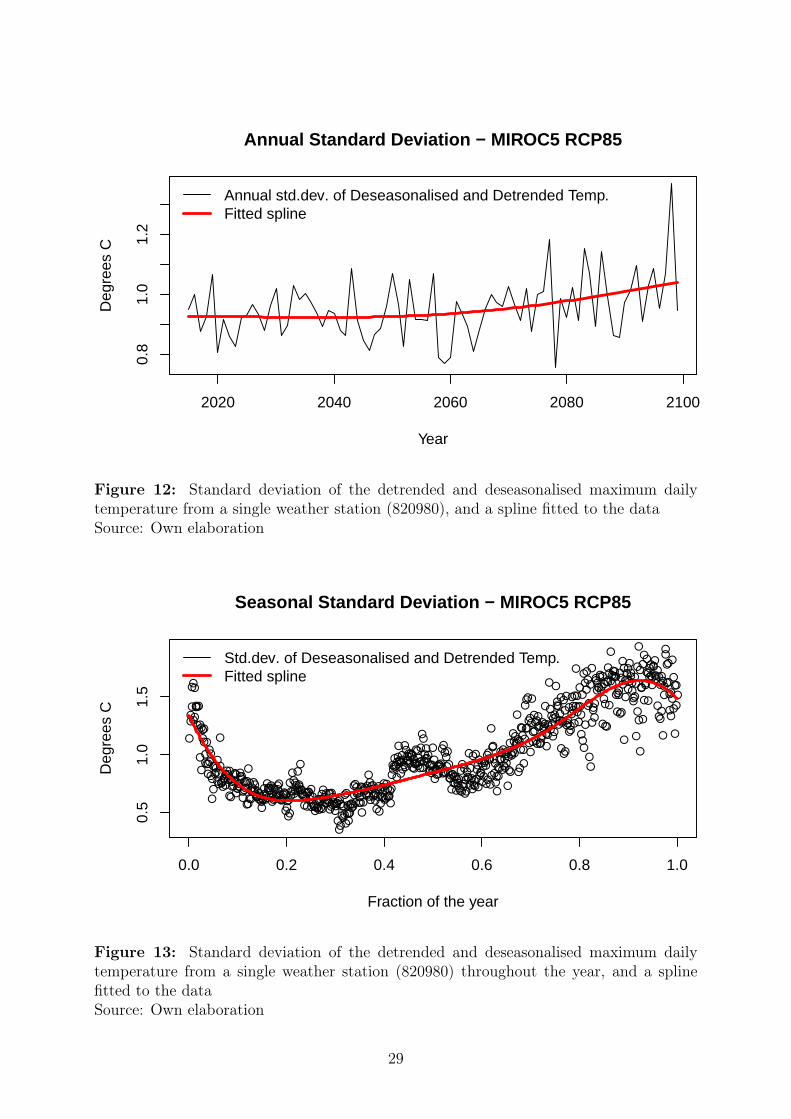
2020 2040 2060 2080 2100
0.8
1.0
1.2
Annual Standard Deviation − MIROC5 RCP85
Year
Deg
rees
C
Annual std.dev. of Deseasonalised and Detrended Temp.Fitted spline
Figure 12: Standard deviation of the detrended and deseasonalised maximum dailytemperature from a single weather station (820980), and a spline fitted to the dataSource: Own elaboration
●
●
●
●●●●●
●●●
●
●
●
●●●
●
●●●●●
●
●●●●●●●
●●●●●
●●●●
●●●●
●
●●●●●
●●●●
●●●●
●●●●●●●
●●●●●●
●●●●
●●●●●●●●●●●●●
●●●●●●●●
●●●●●●●●●●●●
●●●●●●●●
●●
●●●●●●●●●●●●●●
●●●●●●●●●●●●●
●●●●●●
●●●●●
●
●●●●●●●●●●●●
●●●●●●●●●●●●●●●●●●●●●●●
●●●●●●●●●●●●●
●
●●●●●●●●●
●●
●●●●●
●●●
●
●
●●
●●●
●●●●●●●
●●●●●●●●●
●
●●●●●●●
●
●●●●●
●●●●●●●
●●
●●
●
●●
●
●
●
●●
●
●
●
●
●●
●
●●●
●
●
●
●●●●
●
●
●
●●
●
●●●
●
●
●●
●●
●
●●●●●
●
●
●●
●●
●●●
●●●
●
●●
●
●
●
●
●●
●
●●●●●
●●
●●●●●●
●
●●
●
●●
●
●●●●
●
●●●
●
●●
●
●
●●
●●●
●
●
●●
●●●
●
●
●●●●●●
●●●●
●
●●●●●
●●●
●●●●●●●
●●●●●●●●●●●●●●●
●●●●●●●
●●●●
●
●●●●
●
●
●
●●
●
●
●
●●●●●●●●●●●●●●●●
●●●●●●
●●●●●●●●●●●●
●●●●●●●●
●●●●●●●●●●
●
●●●●●●●●
●●
●●●●
●●
●
●●
●●●●●●
●●●●●●
●
●●
●●
●●●●
●
●●●●●●
●●●●●
●
●●
●●●●●●
●●
●●●
●
●
●●
●
●
●
●
●
●●●●
●
●●
●
●●
●
●●●
●
●●●●●●
●
●●
●
●
●●
●
●●
●●
●
●●●
●●
●
●●●●
●
●●
●●
●
●
●
●
●●●●
●
●
●●
●
●
●●
●●●●
●
●
●
●
●●
●
●●●
●
●
●
●●
●
●●
●●●
●
●
●
●
●●
●●
●
●●●
●●●
●●
●
●
●
●
●
●●
●●●
●
●●
●
●
●
●
●
●
●
●●
●●●●
●●●●
●
●
●
●
●
●●
●●
●
●
0.0 0.2 0.4 0.6 0.8 1.0
0.5
1.0
1.5
Seasonal Standard Deviation − MIROC5 RCP85
Fraction of the year
Deg
rees
C
Std.dev. of Deseasonalised and Detrended Temp.Fitted spline
Figure 13: Standard deviation of the detrended and deseasonalised maximum dailytemperature from a single weather station (820980) throughout the year, and a splinefitted to the dataSource: Own elaboration
29
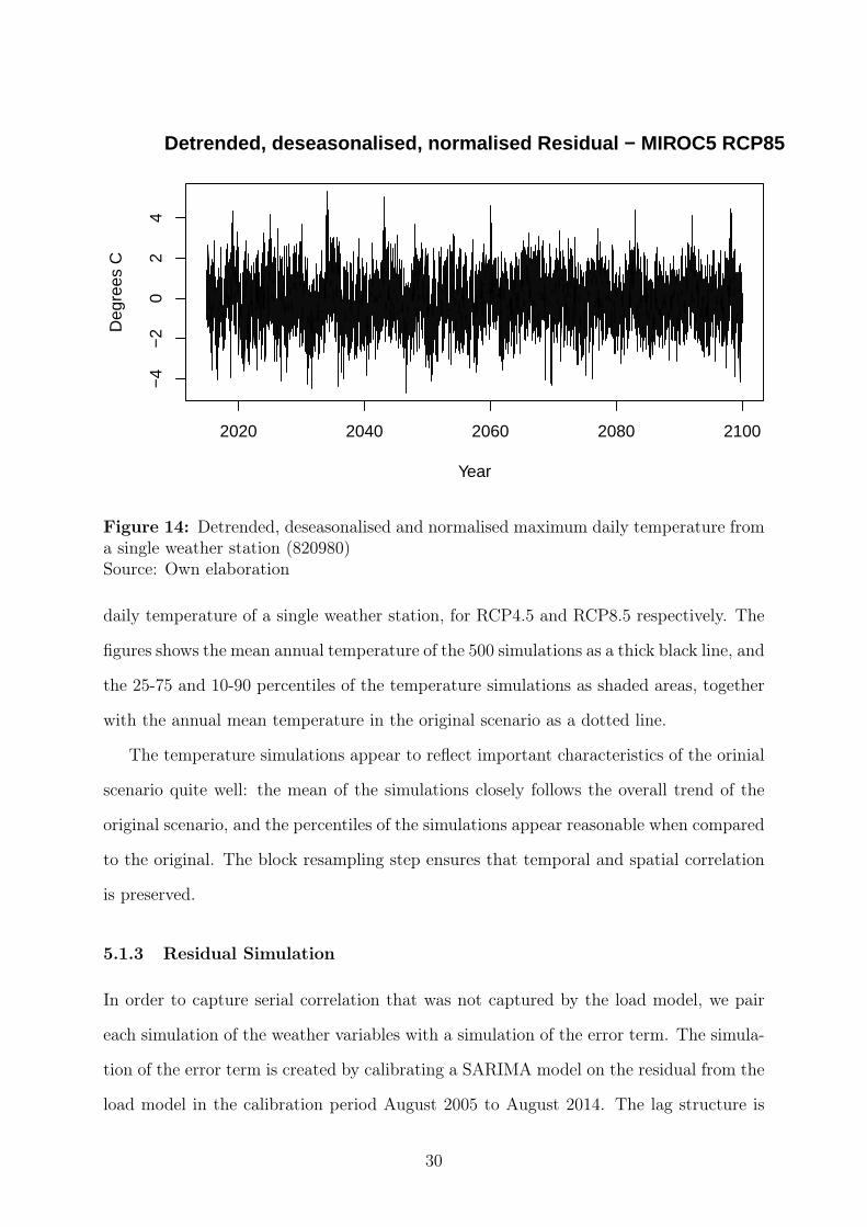
2020 2040 2060 2080 2100
−4
−2
02
4Detrended, deseasonalised, normalised Residual − MIROC5 RCP85
Year
Deg
rees
C
Figure 14: Detrended, deseasonalised and normalised maximum daily temperature froma single weather station (820980)Source: Own elaboration
daily temperature of a single weather station, for RCP4.5 and RCP8.5 respectively. The
figures shows the mean annual temperature of the 500 simulations as a thick black line, and
the 25-75 and 10-90 percentiles of the temperature simulations as shaded areas, together
with the annual mean temperature in the original scenario as a dotted line.
The temperature simulations appear to reflect important characteristics of the orinial
scenario quite well: the mean of the simulations closely follows the overall trend of the
original scenario, and the percentiles of the simulations appear reasonable when compared
to the original. The block resampling step ensures that temporal and spatial correlation
is preserved.
5.1.3 Residual Simulation
In order to capture serial correlation that was not captured by the load model, we pair
each simulation of the weather variables with a simulation of the error term. The simula-
tion of the error term is created by calibrating a SARIMA model on the residual from the
load model in the calibration period August 2005 to August 2014. The lag structure is
30
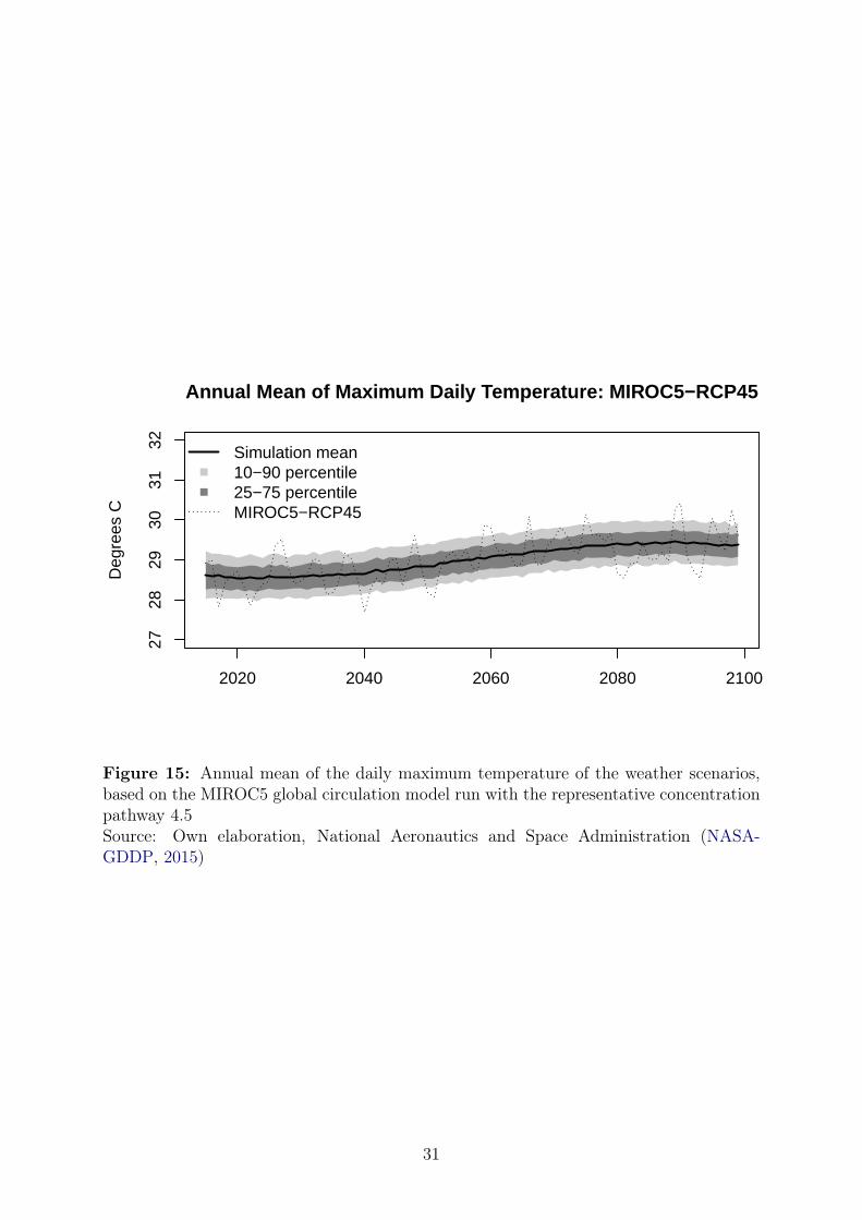
2020 2040 2060 2080 2100
2728
2930
3132
Deg
rees
C
Annual Mean of Maximum Daily Temperature: MIROC5−RCP45
Simulation mean10−90 percentile25−75 percentileMIROC5−RCP45
Figure 15: Annual mean of the daily maximum temperature of the weather scenarios,based on the MIROC5 global circulation model run with the representative concentrationpathway 4.5Source: Own elaboration, National Aeronautics and Space Administration (NASA-GDDP, 2015)
31
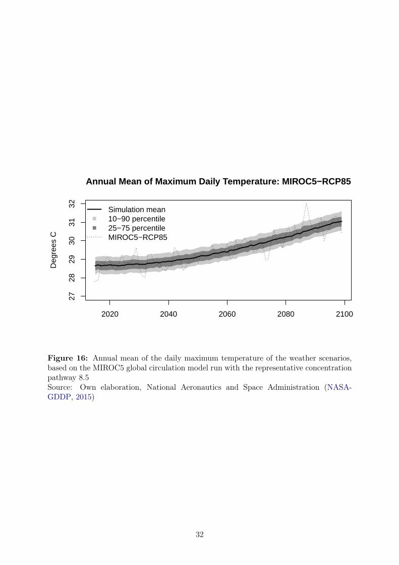
2020 2040 2060 2080 2100
2728
2930
3132
Deg
rees
C
Annual Mean of Maximum Daily Temperature: MIROC5−RCP85
Simulation mean10−90 percentile25−75 percentileMIROC5−RCP85
Figure 16: Annual mean of the daily maximum temperature of the weather scenarios,based on the MIROC5 global circulation model run with the representative concentrationpathway 8.5Source: Own elaboration, National Aeronautics and Space Administration (NASA-GDDP, 2015)
32
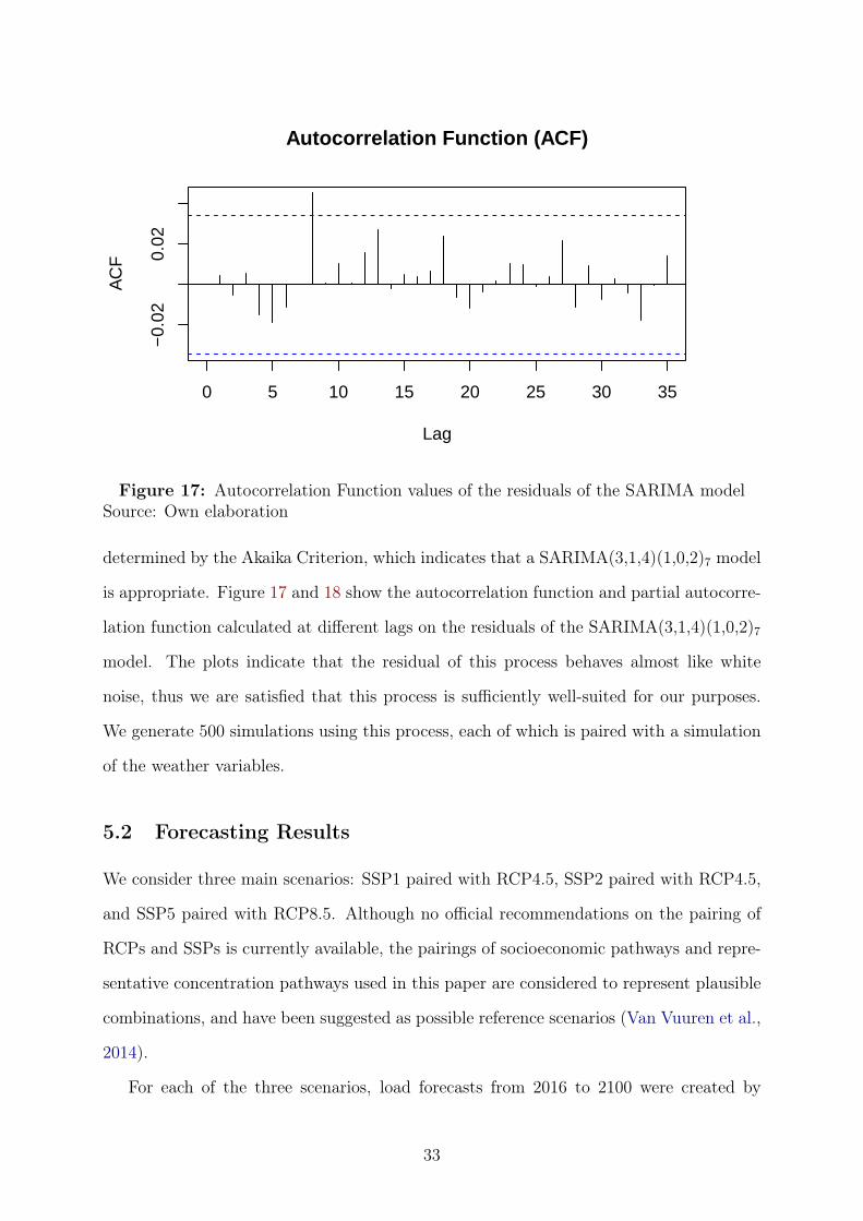
0 5 10 15 20 25 30 35
−0.
020.
02
Lag
AC
FAutocorrelation Function (ACF)
Figure 17: Autocorrelation Function values of the residuals of the SARIMA modelSource: Own elaboration
determined by the Akaika Criterion, which indicates that a SARIMA(3,1,4)(1,0,2)7 model
is appropriate. Figure 17 and 18 show the autocorrelation function and partial autocorre-
lation function calculated at different lags on the residuals of the SARIMA(3,1,4)(1,0,2)7
model. The plots indicate that the residual of this process behaves almost like white
noise, thus we are satisfied that this process is sufficiently well-suited for our purposes.
We generate 500 simulations using this process, each of which is paired with a simulation
of the weather variables.
5.2 Forecasting Results
We consider three main scenarios: SSP1 paired with RCP4.5, SSP2 paired with RCP4.5,
and SSP5 paired with RCP8.5. Although no official recommendations on the pairing of
RCPs and SSPs is currently available, the pairings of socioeconomic pathways and repre-
sentative concentration pathways used in this paper are considered to represent plausible
combinations, and have been suggested as possible reference scenarios (Van Vuuren et al.,
2014).
For each of the three scenarios, load forecasts from 2016 to 2100 were created by
33
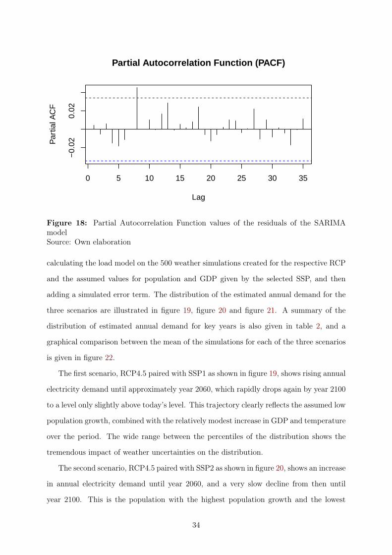
0 5 10 15 20 25 30 35
−0.
020.
02
Lag
Par
tial A
CF
Partial Autocorrelation Function (PACF)
Figure 18: Partial Autocorrelation Function values of the residuals of the SARIMAmodelSource: Own elaboration
calculating the load model on the 500 weather simulations created for the respective RCP
and the assumed values for population and GDP given by the selected SSP, and then
adding a simulated error term. The distribution of the estimated annual demand for the
three scenarios are illustrated in figure 19, figure 20 and figure 21. A summary of the
distribution of estimated annual demand for key years is also given in table 2, and a
graphical comparison between the mean of the simulations for each of the three scenarios
is given in figure 22.
The first scenario, RCP4.5 paired with SSP1 as shown in figure 19, shows rising annual
electricity demand until approximately year 2060, which rapidly drops again by year 2100
to a level only slightly above today’s level. This trajectory clearly reflects the assumed low
population growth, combined with the relatively modest increase in GDP and temperature
over the period. The wide range between the percentiles of the distribution shows the
tremendous impact of weather uncertainties on the distribution.
The second scenario, RCP4.5 paired with SSP2 as shown in figure 20, shows an increase
in annual electricity demand until year 2060, and a very slow decline from then until
year 2100. This is the population with the highest population growth and the lowest
34
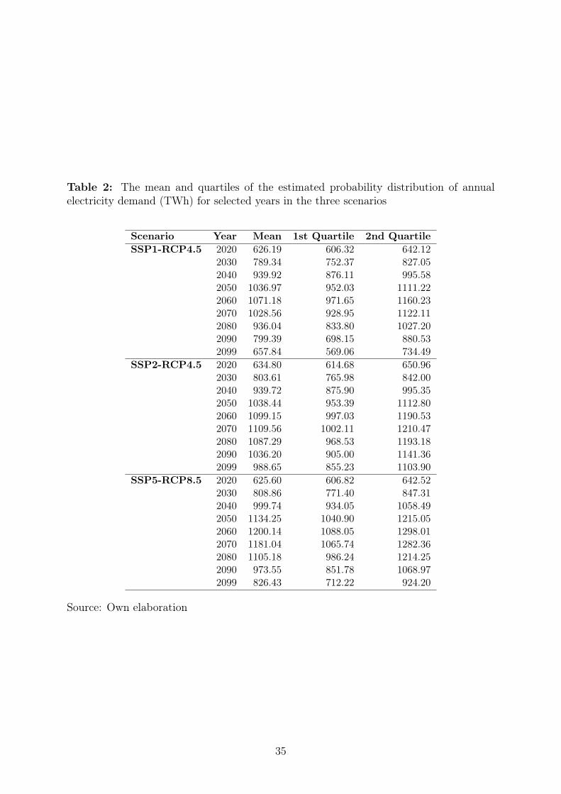
Table 2: The mean and quartiles of the estimated probability distribution of annualelectricity demand (TWh) for selected years in the three scenarios
Scenario Year Mean 1st Quartile 2nd QuartileSSP1-RCP4.5 2020 626.19 606.32 642.12
2030 789.34 752.37 827.052040 939.92 876.11 995.582050 1036.97 952.03 1111.222060 1071.18 971.65 1160.232070 1028.56 928.95 1122.112080 936.04 833.80 1027.202090 799.39 698.15 880.532099 657.84 569.06 734.49
SSP2-RCP4.5 2020 634.80 614.68 650.962030 803.61 765.98 842.002040 939.72 875.90 995.352050 1038.44 953.39 1112.802060 1099.15 997.03 1190.532070 1109.56 1002.11 1210.472080 1087.29 968.53 1193.182090 1036.20 905.00 1141.362099 988.65 855.23 1103.90
SSP5-RCP8.5 2020 625.60 606.82 642.522030 808.86 771.40 847.312040 999.74 934.05 1058.492050 1134.25 1040.90 1215.052060 1200.14 1088.05 1298.012070 1181.04 1065.74 1282.362080 1105.18 986.24 1214.252090 973.55 851.78 1068.972099 826.43 712.22 924.20
Source: Own elaboration
35
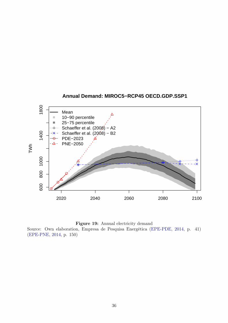
2020 2040 2060 2080 2100
600
800
1000
1400
1800
TW
h
Annual Demand: MIROC5−RCP45 OECD.GDP.SSP1
●
●
●
●
Mean10−90 percentile25−75 percentileSchaeffer et al. (2008) − A2Schaeffer et al. (2008) − B2PDE−2023PNE−2050
Figure 19: Annual electricity demandSource: Own elaboration, Empresa de Pesquisa Energética (EPE-PDE, 2014, p. 41)(EPE-PNE, 2014, p. 150)
36
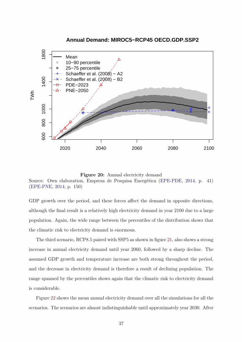
2020 2040 2060 2080 2100
600
800
1000
1400
1800
TW
h
Annual Demand: MIROC5−RCP45 OECD.GDP.SSP2
●
●
●
●
Mean10−90 percentile25−75 percentileSchaeffer et al. (2008) − A2Schaeffer et al. (2008) − B2PDE−2023PNE−2050
Figure 20: Annual electricity demandSource: Own elaboration, Empresa de Pesquisa Energética (EPE-PDE, 2014, p. 41)(EPE-PNE, 2014, p. 150)
GDP growth over the period, and these forces affect the demand in opposite directions,
although the final result is a relatively high electricity demand in year 2100 due to a large
population. Again, the wide range between the percentiles of the distribution shows that
the climatic risk to electricity demand is enormous.
The third scenario, RCP8.5 paired with SSP5 as shown in figure 21, also shows a strong
increase in annual electricity demand until year 2060, followed by a sharp decline. The
assumed GDP growth and temperature increase are both strong throughout the period,
and the decrease in electricity demand is therefore a result of declining population. The
range spanned by the percentiles shows again that the climatic risk to electricity demand
is considerable.
Figure 22 shows the mean annual electricity demand over all the simulations for all the
scenarios. The scenarios are almost indistinguishable until approximately year 2030. After
37
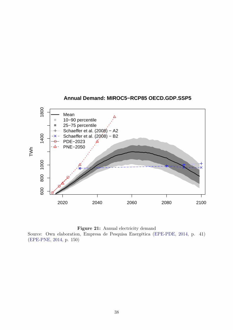
2020 2040 2060 2080 2100
600
800
1000
1400
1800
TW
h
Annual Demand: MIROC5−RCP85 OECD.GDP.SSP5
●
●
●
●
Mean10−90 percentile25−75 percentileSchaeffer et al. (2008) − A2Schaeffer et al. (2008) − B2PDE−2023PNE−2050
Figure 21: Annual electricity demandSource: Own elaboration, Empresa de Pesquisa Energética (EPE-PDE, 2014, p. 41)(EPE-PNE, 2014, p. 150)
38
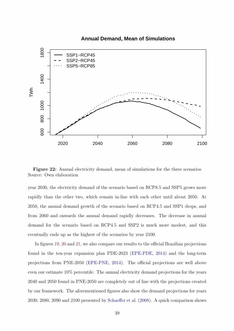
2020 2040 2060 2080 2100
600
800
1000
1400
1800
TW
h
Annual Demand, Mean of Simulations
SSP1−RCP45SSP2−RCP45SSP5−RCP85
Figure 22: Annual electricity demand, mean of simulations for the three scenariosSource: Own elaboration
year 2030, the electricity demand of the scenario based on RCP8.5 and SSP5 grows more
rapidly than the other two, which remain in-line with each other until about 2050. At
2050, the annual demand growth of the scenario based on RCP4.5 and SSP1 drops, and
from 2060 and onwards the annual demand rapidly decreases. The decrease in annual
demand for the scenario based on RCP4.5 and SSP2 is much more modest, and this
eventually ends up as the highest of the scenarios by year 2100.
In figures 19, 20 and 21, we also compare our results to the official Brazilian projections
found in the ten-year expansion plan PDE-2023 (EPE-PDE, 2014) and the long-term
projections from PNE-2050 (EPE-PNE, 2014). The official projections are well above
even our estimate 10% percentile. The annual electricity demand projections for the years
2040 and 2050 found in PNE-2050 are completely out of line with the projections created
by our framework. The aforementioned figures also show the demand projections for years
2030, 2080, 2090 and 2100 presented by Schaeffer et al. (2008). A quick comparison shows
39
that the projections for year 2030 are significantly above all three scenarios considered
here. The projections for year 2080 for both the A2 and B2 scenarios are more or less
in line with all three of our scenarios, and their projections for years 2090 and 2100 are
quite close to our results for both the RCP4.5-SSP2 and RCP8.5-SSP5 scenarios. Their
projections for year 2090 and 2100 for both the A2 and B2 scenarios are considerably
above the results of our RCP4.5-SSP1 scenario.
5.3 Model Evaluation
The framework we have used to create electricity demand projections contains a few
critical limitations that must be taken into consideration.
Firstly, the procedure made no explicit allowance for structural and/or technological
change, for example widespread adoption of electrical vehicles or deployment of electricity
storage technology that would radically change the determinants of electricity demand.
Calibrating a model on a decade of historical data, then subsequently using the model
to make demand projections for the next 85 years, may seem like little more than a shot
in the dark to some and pure madness to others. We recognise this limitation, and even
though the next 85 years certainly will be very different from the last ten, we still believe
that the demand projections provide some guidance. It is a very brave assumption, but
every attempt to avoid it would perhaps be equally brave. In essence, all forecasts are
wrong, but they can still be useful.
Secondly, we did not allow for uncertainty in the GDP and population numbers. Al-
though this could be incorporated in principle, our main focus was on climatic risks and
therefore we concentrated on weather uncertainty.
Thirdly, we have also disregarded the uncertainty in the model parameters. That is,
the calibration of the model was considered to be absolutely accurate. This is unrealistic,
but again this assumption allowed us to focus on climate risk and weather uncertainty.
These shortcomings discussed here are clear, and although they are cause to be cau-
tious, they do not invalidate the results. Taking into consideration the radically different
framework in this study and the different datasets used during both calibration and fore-
40
casting, it is comforting that our projections share some characteristics with the results
presented in the existing literature. All in all, the projections seem quite reasonable in
general.
6 Conclusion
We have provided electricity demand projections for Brazil for three climate change sce-
narios, with probability distributions illustrating the climatic risk that the electricity
demand is exposed to. We have improved on the existing literature in three important
ways: firstly, we have applied a probabilistic approach to Brazilian electricity demand
forecasting. Since forecasting is essentially a stochastic problem, this is very appropriate,
although no such approach appears to have been considered yet in the existing litera-
ture. Secondly, we provide updated demand projections for climate change scenarios in
light of the new climatic, demographic and macroeconomic simulations accompanying
the IPCC AR5 report, using the latest available data. This is important, because much
has happened since the last comprehensive electricity demand projections that explicitly
considered climate change scenarios were published in 2008. And finally, by creating the
electricity demand projections using a model for daily electricity demand, our framework
gives easy access to an unprecedented amount of detail about the Brazilian electricity de-
mand. Such a level of detail, for instance being able to retrieve the probability distribution
of the maximum daily demand of a year, can be very valuable for planning purposes.
Acknowledgments
The author would like to thank the Brazilian agency CAPES (Coordenação de Aper-
feiçoamento de Pessoal de Nível Superior) for the scholarship BEX 10893-14.
41
References
Abdel-Karim, N., Nethercutt, E. J., Moura, J. N., Burgess, T., Ly, T. C., 2014. Effect of
load forecasting uncertainties on the reliability of north american bulk power system.
In: PES General Meeting| Conference & Exposition, 2014 IEEE. IEEE, pp. 1–5.
Abou-Hussien, M., Kandlil, M., Tantawy, M., Farghal, S., Sept 1981. An accurate model
for short-term load forecasting. Power Apparatus and Systems, IEEE Transactions on
PAS-100 (9), 4158–4165.
Adam, N. B., Elahee, M., Dauhoo, M., 2011. Forecasting of peak electricity demand
in mauritius using the non-homogeneous gompertz diffusion process. Energy 36 (12),
6763–6769.
Adams, G., Allen, P. G., Morzuch, B. J., 1991. Probability distributions of short-term
electricity peak load forecasts. International Journal of Forecasting 7 (3), 283–297.
Akdemir, B., Çetinkaya, N., 2012. Importance of holidays for short term load forecasting
using adaptive neural fuzzy inference system. In: Advanced Materials Research. Vol.
433. Trans Tech Publ, pp. 3959–3963.
Al-Hamadi, H., Soliman, S., 2004. Short-term electric load forecasting based on kalman fil-
tering algorithm with moving window weather and load model. Electric Power Systems
Research 68 (1), 47–59.
Al-Hamadi, H., Soliman, S., 2006. Fuzzy short-term electric load forecasting using kalman
filter. IEE Proceedings-Generation, Transmission and Distribution 153 (2), 217–227.
Ali, M. T., Mokhtar, M., Chiesa, M., Armstrong, P., 2011. A cooling change-point model
of community-aggregate electrical load. Energy and Buildings 43 (1), 28–37.
Andrade, T. A., Lobão, W. J., 1997. Elasticidade renda e preço da demanda residencial
de energia elétrica no brasil.
Apadula, F., Bassini, A., Elli, A., Scapin, S., 2012. Relationships between meteorological
variables and monthly electricity demand. Applied Energy 98, 346–356.
42
Asbury, C., 1975. Weather load model for electric demand and energy forecasting. IEEE
Transactions on Power Apparatus and Systems 94 (4), 1111–1116.
Bacher, P., Madsen, H., Nielsen, H. A., 2013. Online load forecasting for supermarket
refrigeration. In: Innovative Smart Grid Technologies Europe (ISGT EUROPE), 2013
4th IEEE/PES. IEEE, pp. 1–5.
Bagnasco, A., Saviozzi, M., Silvestro, F., Vinci, A., Grillo, S., Zennaro, E., 2014. Artificial
neural network application to load forecasting in a large hospital facility. In: Proba-
bilistic Methods Applied to Power Systems (PMAPS), 2014 International Conference
on. IEEE, pp. 1–6.
Bahrami, S., Hooshmand, R.-A., Parastegari, M., 2014. Short term electric load forecast-
ing by wavelet transform and grey model improved by pso (particle swarm optimization)
algorithm. Energy 72, 434–442.
Bansal, R., Pandey, J., 2005. Load forecasting using artificial intelligence techniques: a
literature survey. International journal of computer applications in technology 22 (2/3),
109–119.
Bao, Z., Pi, D., Sun, Y., 2005. Short-term load forecasting based on self-organizing map
and support vector machine. In: Advances in Natural Computation. Springer, pp. 688–
691.
Barakat, E., Eissa, M., 1989. Forecasting monthly peak demand in fast growing electric
utility using a composite multiregression-decomposition model. In: Generation, Trans-
mission and Distribution, IEE Proceedings C. Vol. 136. IET, pp. 35–41.
Bartels, R., Fiebig, D. G., Garben, M., Lumsdaine, R., 1992. An end-use electricity load
simulation model: Delmod. Utilities Policy 2 (1), 71–82.
Bashir, Z., El-Hawary, M., 2009. Applying wavelets to short-term load forecasting using
pso-based neural networks. Power Systems, IEEE Transactions on 24 (1), 20–27.
43
Beccali, M., Cellura, M., Brano, V. L., Marvuglia, A., 2008. Short-term prediction of
household electricity consumption: Assessing weather sensitivity in a mediterranean
area. Renewable and Sustainable Energy Reviews 12 (8), 2040–2065.
Belzer, D., Kellogg, M., 1993. Incorporating sources of uncertainty in forecasting peak
power loads-a monte carlo analysis using the extreme value distribution. Power Systems,
IEEE Transactions on 8 (2), 730–737.
Bolzern, P., Fronza, G., 1986. Role of weather inputs in short-term forecasting of electric
load. International Journal of Electrical Power & Energy Systems 8 (1), 42–46.
Caldas, A. A. S. e., Santos, E. F. N., 2012. Previsão de consumo de energia elétrica em
petrolina-pe. Revista Brasileira de Energia 18 (1), 129–141.
Camargo, I. M. d. T., 2007. Panorama da oferta e do consumo de energia elétrica no brasil
para os próximos anos. Revista Brasileira de Energia 13 (1), 1–10.
Campo, R., Ruiz, P., Aug 1987. Adaptive weather-sensitive short term load forecast.
Power Systems, IEEE Transactions on 2 (3), 592–598.
Campos, R. J., 2008. Previsão de séries temporais com aplicações a séries de consumo de
energia elétrica. Ph.D. thesis, Universidade Federal de Minas Gerais.
Cao, Y., Zhang, Z. J., Zhou, C., 2012. Data processing strategies in short term electric
load forecasting. In: Computer Science & Service System (CSSS), 2012 International
Conference on. IEEE, pp. 174–177.
Cardelli, E., Beichert, K., Marks, M., 1980. Impact of weather on power system loads.
In: Proc. Am. Power Conf.;(United States). Vol. 42. Am Electr Power Serv Corp, New
York, NY.
Carpinteiro, O. A., Reis, A. J., da Silva, A. P., 2004. A hierarchical neural model in
short-term load forecasting. Applied Soft Computing 4 (4), 405–412.
Castro, J. B., Montini, A. A., 2010. Previsão do consumo residencial de energia elétrica
no brasil: aplicação do modelo arx. XII SEMEAD.
44
Challa, B. P., Challa, S., Chakravorty, R., Deshpande, S. K., Sharma, D., 2005. A novel
approach for electrical load forecasting using distributed sensor networks. In: Intelligent
Sensing and Information Processing, 2005. ICISIP 2005. Third International Conference
on. IEEE, pp. 189–194.
Chang-chun, C., Min, W., 2008. Support vector machines with similar day’s training
sample application in short-term load forecasting. In: Electric Utility Deregulation
and Restructuring and Power Technologies, 2008. DRPT 2008. Third International
Conference on. IEEE, pp. 1221–1225.
Chaoyun, A., Ran, L., 2007. Study on short term load forecast based on cloud model. In:
Power Tech, 2007 IEEE Lausanne. IEEE, pp. 1797–1801.
Charytoniuk, W., Chen, M.-S., Kotas, P., Van Olinda, P., 1999. Demand forecasting in
power distribution systems using nonparametric probability density estimation. Power
Systems, IEEE Transactions on 14 (4), 1200–1206.
Charytoniuk, W., Niebrzydowski, J., 1998. Confidence interval construction for load fore-
cast. Electric power systems research 48 (2), 97–103.
Chauhan, B. K., Hanmandlu, M., 2010. Load forecasting using wavelet fuzzy neural net-
work. International Journal of Knowledge-Based and Intelligent Engineering Systems
14 (2), 57–71.
Chen, D., Chen, B., Li, T., 1991. An expert system for short-term load forecasting. In:
Advances in Power System Control, Operation and Management, 1991. APSCOM-91.,
1991 International Conference on. IET, pp. 330–334.
Christiaanse, W., 1971. Short-term load forecasting using general exponential smoothing.
IEEE Transactions on Power Apparatus and Systems (2), 900–911.
Clair, S., Einwechter, W., 1961. The weather and daily forecasting of philadelphia electric
system loads. Proceedings of the American Power Conference 23, 853–859.
45
Clayton, R., Priest, K., Truex, C., 1973. Load model sensitive to weather data. Electrical
World 179 (6), 96–98.
Costin, E., Sandulescu, M., Herscovici, S., Sufan, N., 1987. Short term model forecasting
of the required electric power and energy, taking into account the weather conditions
and other influences. Buletinul Institutului de Studii si Proiectari Energetice 30 (1),
25–32.
Dalvand, M. M., Azami, S., Tarimoradi, H., 2008. Long-term load forecasting of iranian
power grid using fuzzy and artificial neural networks. In: Universities Power Engineering
Conference, 2008. UPEC 2008. 43rd International. IEEE, pp. 1–4.
Davey, J., Saacks, J., Cunningham, G., Priest, K., 1973. Practical application of weather
sensitive load forecasting to system planning. IEEE Transactions on Power Apparatus
and Systems (3), 971–977.
Davies, M., 1959. The relationship between weather and electricity demand. Proceedings
of the IEE-Part C: Monographs 106 (9), 27–37.
De Felice, M., Alessandri, A., Catalano, F., 2015. Seasonal climate forecasts for medium-
term electricity demand forecasting. Applied Energy 137, 435–444.
Degaudenzi, M., Arizmendi, C., 2000. Wavelet-based fractal analysis of electrical power
demand. Fractals 8 (03), 239–245.
Dehdashti, A., Tudor, J. R., Smith, M., Sept 1982. Forecasting of hourly load by pattern
recognition a deterministic approach. Power Apparatus and Systems, IEEE Transac-
tions on PAS-101 (9), 3290–3294.
Ding, Q., Zhang, H., Huang, T., Zhang, J., 2005. A holiday short term load forecasting
considering weather information. In: Power Engineering Conference, 2005. IPEC 2005.
The 7th International. IEEE, pp. 1–61.
dos Anjos Rodrigues, L., Féres, J. G., de Mattos, L. B., 2014. Aquecimento global e a
demanda residencial de energia elétrica no brasil.
46
Douglas, A. P., Breipohl, A. M., Lee, F. N., Adapa, R., 1998a. The impacts of temperature
forecast uncertainty on bayesian load forecasting. Power Systems, IEEE Transactions
on 13 (4), 1507–1513.
Douglas, A. P., Breipohl, A. M., Lee, F. N., Adapa, R., 1998b. Risk due to load forecast
uncertainty in short term power system planning. Power Systems, IEEE Transactions
on 13 (4), 1493–1499.
Dryar, H. A., 1944. The effect of weather on the system load. Electrical Engineering
63 (12), 1006–1013.
Edwin, K., Elsayed, M., 1980. Load curve forecasting for operation planning of power-
systems. ETZ Archiv 2 (6), 171–176.
EPE-PDE, 2014. Empresa de Pesquisa Energética. Plano Decenal de Expansão de Energia
2023. Accessed: 2015-07-31.
URL http://www.epe.gov.br/Estudos/Paginas/default.aspx?CategoriaID=345
EPE-PNE, 2014. Empresa de Pesquisa Energética. Plano Nacional de Energia 2050. Ac-
cessed: 2015-07-31.
URL http://www.epe.gov.br/Estudos/Paginas/default.aspx?CategoriaID=346
Fan, S., Mao, C., Chen, L., 2005. Peak load forecasting using the self-organizing map. In:
Advances in Neural Networks–ISNN 2005. Springer, pp. 640–647.
Fay, D., Ringwood, J. V., 2010. On the influence of weather forecast errors in short-term
load forecasting models. Power Systems, IEEE Transactions on 25 (3), 1751–1758.
Ferreira, P. G. C., Oliveira, F. L. C., Souza, R. C., 2015. The stochastic effects on the
brazilian electrical sector. Energy Economics 49, 328–335.
Frąckowiak, R., Tomczykowski, J., 2007. Modelling of the household lighting-related load.
International Journal of Electrical Power & Energy Systems 29 (8), 580–588.
47
Gillies, D., Bernholtz, B., Sandiford, P., 1956. A new approach to forecasting daily peak
loads. Transactions of the American Institute of Electrical Engineers. Part III: Power
Apparatus and Systems 3 (75), 382–387.
Guo, Y.-C., 2009. Knowledge-enabled short-term load forecasting based on pattern-base
using classification & regression tree and support vector regression. In: Natural Com-
putation, 2009. ICNC’09. Fifth International Conference on. Vol. 3. IEEE, pp. 425–429.
Gupta, P., Yamada, K., 1972. Adaptive short-term forecasting of hourly loads using
weather information. IEEE Transactions on Power Apparatus and Systems (5), 2085–
2094.
Harris, J. L., Liu, L.-M., 1993. Dynamic structural analysis and forecasting of residential
electricity consumption. International Journal of Forecasting 9 (4), 437–455.
Heinemann, G., Nordmian, D., Plant, E., 1966. The relationship between summer weather
and summer loads-a regression analysis. IEEE Transactions on Power Apparatus and
Systems (11), 1144–1154.
Hong, T., Pinson, P., Fan, S., 2014a. Global energy forecasting competition 2012. Inter-
national Journal of Forecasting 30 (2), 357–363.
Hong, T., Wang, P., Pahwa, A., Gui, M., Hsiang, S. M., 2010. Cost of temperature history
data uncertainties in short term electric load forecasting. In: Probabilistic Methods
Applied to Power Systems (PMAPS), 2010 IEEE 11th International Conference on.
IEEE, pp. 212–217.
Hong, T., Wang, P., White, L., 2015. Weather station selection for electric load forecast-
ing. International Journal of Forecasting 31 (2), 286–295.
Hong, T., Wilson, J., Xie, J., 2014b. Long term probabilistic load forecasting and nor-
malization with hourly information. Smart Grid, IEEE Transactions on 5 (1), 456–462.
Hor, C., Watson, S., Infield, D., Majithia, S., 2008. Assessing load forecast uncertainty
using extreme value theory. 16th PSCC, Glasgow.
48
Horowitz, S., Mauch, B., Sowell, F., 2014. Forecasting residential air conditioning loads.
Applied Energy 132, 47–55.
Hovgaard, T. G., Boyd, S., Larsen, L. F., Jørgensen, J. B., 2013. Nonconvex model
predictive control for commercial refrigeration. International Journal of Control 86 (8),
1349–1366.
Huang, C.-M., Yang, H.-T., 2001. Evolving wavelet-based networks for short-term load
forecasting. IEE Proceedings-Generation, Transmission and Distribution 148 (3), 222–
228.
Hyndman, R. J., Athanasopoulos, G., 2014. Forecasting: principles and practice. OTexts.
Hyndman, R. J., Fan, S., 2010. Density forecasting for long-term peak electricity demand.
Power Systems, IEEE Transactions on 25 (2), 1142–1153.
IBGE, 2013. The Brazilian Institute of Geography and Statistics. Projecao da População.
Accessed: 2015-07-08.
URL http://www.ibge.gov.br/home/estatistica/populacao/projecao_da_
populacao/2013/default.shtm
IBGE, 2015. The Brazilian Institute of Geography and Statistics. Contas Nacionais
Trimestrais.
URL http://www.ibge.gov.br/home/estatistica/indicadores/pib/defaultcnt.
shtm
IIASA, 2015. International Institute for Applied Systems Analysis. Shared Socioeconomic
Pathways Database. Accessed: 2015-07-28.
URL https://tntcat.iiasa.ac.at/SspDb
Intergovernmental Panel on Climate Change, 2013. Climate Change 2013: The Physical
Science Basis. Geneva: Intergovernmental Panel on Climate Change.
Irffi, G., Castelar, I., Siqueira, M. L., Linhares, F. C., 2009. Previsão da demanda por
49
energia elétrica para classes de consumo na região nordeste, usando ols dinâmico e
mudança de regime. Economia Aplicada 13 (1), 69–98.
Jabbour, K., Riveros, J. F. V., Landsbergen, D., Meyer, W., 1988. Alfa: Automated load
forecasting assistant. IEEE Transactions on Power Systems 3 (3), 908–914.
Jiao, R., Mo, R., Lin, B., Su, C., 2012. Construction of training sample in a support
vector regression short-term load forecasting model. In: Computational Intelligence and
Design (ISCID), 2012 Fifth International Symposium on. Vol. 2. IEEE, pp. 339–342.
Jin, L., Cong, D., Guangyi, L., Jilai, Y., 2014. Short-term net feeder load forecasting
of microgrid considering weather conditions. In: Energy Conference (ENERGYCON),
2014 IEEE International. IEEE, pp. 1205–1209.
Josse, J., Husson, F., 2011. missmda: a package to handle missing values in and with
multivariate exploratory data analysis methods. In: The R User Conference, useR!
2011 August 16-18 2011 University of Warwick, Coventry, UK. p. 100.
Kandil, M., El-Maghraby, M., El-Dosouky, H., 1981. A proposed methodology for
medium-range maximum demand anticipation and application. Electric Power Systems
Research 4 (1), 29 – 35.
URL http://www.sciencedirect.com/science/article/pii/037877968190033X
Kaufmann, R. K., Gopal, S., Tang, X., Raciti, S. M., Lyons, P. E., Geron, N., Craig, F.,
2013. Revisiting the weather effect on energy consumption: Implications for the impact
of climate change. Energy Policy 62, 1377–1384.
Kelo, S. M., Dudul, S. V., 2010. Short-term load prediction with a special emphasis on
weather compensation using a novel committee of wavelet recurrent neural networks
and regression methods. In: Power Electronics, Drives and Energy Systems (PEDES)
& 2010 Power India, 2010 Joint International Conference on. IEEE, pp. 1–6.
Kermanshahi, B., 1998. Recurrent neural network for forecasting next 10 years loads of
nine japanese utilities. Neurocomputing 23 (1), 125–133.
50
Kermanshahi, B., Iwamiya, H., 2002. Up to year 2020 load forecasting using neural nets.
International Journal of Electrical Power & Energy Systems 24 (9), 789–797.
Keyhani, A., Daniels, H., 1976. Real time load modeling technique an application to short
term load prediction. In: 1976 Control of Power Systems Conference and Exposition.
pp. 132–136.
Keyhani, A., Miri, S., 1983. On-line weather-sensitive and industrial group bus load fore-
casting for microprocessor-based applications. IEEE Transactions on Power Apparatus
and Systems (12), 3868–3876.
Keyhani, A., Rad, T. E., 1978. Simulation study for recursive prediction of hourly load
demands. In: IEEE Transactions on Power Apparatus and Systems. Vol. 97. pp. 318–
318.
Khotanzad, A., Davis, M. H., Abaye, A., Maratukulam, D. J., 1996. An artificial neural
network hourly temperature forecaster with applications in load forecasting. Power
Systems, IEEE Transactions on 11 (2), 870–876.
Kim, C., Yu, I., Song, Y., 2000. Evaluation of mother wavelets for the short-term load
forecasting. UPEC.
Laing, W., Metcalfe, M., 1986. Computer-assisted demand forecasting for power-system
control. Water Power and Dam Construction, 28–36.
Lajda, P., 1981. Short-term operation planning in electric power systems. Journal of the
Operational Research Society, 675–682.
Lajda, P., Reichert, K., 1981. An interactive short-term load forecasting program. In:
Proceedings of the Seventh Power Systems Computation Conference. pp. 553–558.
Lambert-Torres, G., Traore, C., Lagace, P., Mukhedkar, D., 1991. A knowledge engineer-
ing tool for load forecasting. In: Circuits and Systems, 1990., Proceedings of the 33rd
Midwest Symposium on. IEEE, pp. 144–147.
51
Lebby, G., 1990. Power system load modeling using a statistically trained gmdh network.
In: Proceeding of the Second IASTED International Symposium. Expert Systems and
Neural Networks. IASTED, pp. 12–15.
Levi, V. A., 1994. A medium-term probabilistic model for forecasting loads with a small
proportion of air conditioners. Electric power systems research 29 (1), 57–67.
Li, C., Yang, P., Liu, W., LI, D., WANG, Y., 2009. An analysis of accumulative effect of
temperature in short-term load forecasting. Automation of Electric Power Systems 9,
023.
Li, M., Gao, J., 2011. An ensemble data mining and flann combining short-term load
forecasting system for abnormal days. Journal of Software 6 (6), 961–968.
Li, M., Wang, Z.-l., Yang, X.-y., Chen, Z.-h., 2006. Short-term load forecasting for abnor-
mal changes and its application. Automation of Electric Power Systems 10, 021.
Li, X.-Y., Wen, F.-s., Lu, E., Li, J.-l., Liu, S.-j., 2013. Short-term load forecasting in
typhoon periods based on load modification of similar days. Proceedings of the Chinese
Society of Universities for Electric Power System and its Automation 3, 018.
Lijesen, D., Arvanitidis, N., 1970. Short-term load forecasting in power systems. In: Ad-
vances in Instrumentation: Proceedings of the 25th Annual ISA Conference. Vol. 25.
Instrument Society of America.
Liu, X., Powell, R., Hartley, J., 1992. Using data and knowledge: an architecture for
implementing load forecasting systems. In: Artificial Intelligence in Civil Engineering,
IEE Colloquium on. IET, pp. 4–1.
Liuzhang, Z., Lin, Y., 2004. Short-term load forecasting by use of decision support objects.
Power System Technology-Beijing 28 (6), 59–62.
Lü, X., Lu, T., Kibert, C. J., Viljanen, M., 2015. Modeling and forecasting energy con-
sumption for heterogeneous buildings using a physical–statistical approach. Applied
Energy 144, 261–275.
52
Mao, Y., Tang, S., Zhang, B., 2011. New extended short-term load forecasting method
consideration of human body amenity. In: Proceedings of the CSU-EPSA. Vol. 23.
Editorial Board of Proceedings of the CSU-EPSA, School of Electrical & Automation
Engineering Tianjin 300072 China, pp. 106–110.
Marinescu, A., Harris, C., Dusparic, I., Clarke, S., Cahill, V., 2013. Residential electri-
cal demand forecasting in very small scale: An evaluation of forecasting methods. In:
Software Engineering Challenges for the Smart Grid (SE4SG), 2013 2nd International
Workshop on. IEEE, pp. 25–32.
Matthewman, P., Nicholson, H., 1968a. Predicting day to day power demand. Electrical
Times 154 (4015), 793–796.
Matthewman, P., Nicholson, H., 1968b. Techniques for load prediction in electricity-supply
industry. Proceedings of The Institution of Electrical Engineers – London 114 (10), 1451.
Matthews, A., Russell, L., Carpinella, C., 1988. Weather-normalized intermediate term
capacity forecasting: a procedural innovation. IEEE Transactions on Power Systems
3 (3), 1291–1297.
Mattos, L. B. d., Lima, J. E. d., 2005. Demanda residencial de energia elétrica em minas
gerais: 1970-2002. Nova Economia 15 (3), 31–52.
McSharry, P. E., Bouwman, S., Bloemhof, G., 2005. Probabilistic forecasts of the mag-
nitude and timing of peak electricity demand. Power Systems, IEEE Transactions on
20 (2), 1166–1172.
Mideksa, T. K., Kallbekken, S., 2010. The impact of climate change on the electricity
market: A review. Energy Policy 38 (7), 3579–3585.
Migon, H. S., Alves, L. C., 2013. Multivariate dynamic regression: modeling and forecast-
ing for intraday electricity load. Applied Stochastic Models in Business and Industry
29 (6), 579–598.
53
Mirasgedis, S., Sarafidis, Y., Georgopoulou, E., Lalas, D., Moschovits, M., Karagiannis,
F., Papakonstantinou, D., 2006. Models for mid-term electricity demand forecasting
incorporating weather influences. Energy 31 (2), 208–227.
Mirowski, P., Chen, S., Kam Ho, T., Yu, C.-N., 2014. Demand forecasting in smart grids.
Bell Labs Technical Journal 18 (4), 135–158.
Miyake, T., Murata, J., Hirasawa, K., 1995. One-day-through seven-day-ahead electrical
load forecasting in consideration of uncertainties of weather information. Electrical
engineering in Japan 115 (8), 22–32.
Moharari, N. S., Debs, A. S., 1993. An artificial neural network based short term load
forecasting with special tuning for weekends and seasonal changes. In: Neural Networks
to Power Systems, 1993. ANNPS’93., Proceedings of the Second International Forum
on Applications of. IEEE, pp. 279–283.
Mumford, L. G., Schultz, D. E., Troutt, M. D., 1991. Using spreadsheet simulation to gen-
erate a distribution of forecasts for electric power demand. Journal of the Operational
Research Society, 931–939.
Nakamura, M., Miyano, T., 1983. Application of an mras identifier to one-day-ahead
load forecasting. Transactions of the Society of Instrument and Control Engineers 19,
787–793.
NASA-GDDP, 2015. National Aeronautics and Space Administration. NASA Earth Ex-
change Global Daily Downscaled Projections. Accessed: 2015-07-28.
URL https://cds.nccs.nasa.gov/nex-gddp/
NASA-SEDAC, 2015. NASA Socioeconomic Data and Applications Center. Gridded Pop-
ulation of the World (GPW), v3. Accessed: 2015-07-31.
URL http://sedac.ciesin.columbia.edu/data/collection/gpw-v3
Nejat, A., Mohsenian-Rad, H., 2012. Electric load forecasting: A multi-agent systems
approach. In: Intelligent Transportation Systems (ITSC), 2012 15th International IEEE
Conference on. IEEE, pp. 863–869.
54
Nemeth, A., Nagy, I., 1981. Short term load forecasting of the hungarian load dispatching
center. In: Proceedings of the Seventh Power Systems Computation Conference. pp.
520–525.
Neto, J. C. d. L., Correia, J. d. C., Parente, R. C. P., Pereira, J. R. G., 2006. Modelo
de projeção para o consumo de energia elétrica e óleo diesel no interior do estado do
amazonas. Revista Brasileira de Energia 12 (1).
NOAA, 2015. National Oceanic and Atmospheric Administration. Integrated Surface
Database Lite. Accessed: 2015-07-09.
URL https://www.ncdc.noaa.gov/isd
Noureddine, A., Alouani, A., Chandrasekaran, A., 1992. A new technique for short-term
residential electric load forecasting including weather and lifestyle influences. In: Cir-
cuits and Systems, 1992., Proceedings of the 35th Midwest Symposium on. IEEE, pp.
1419–1427.
ONS, 2015. Brazilian Independent System Operator. Boletím Diário de Operação. Ac-
cessed: 2015-07-09.
URL http://www.ons.org.br/resultados_operacao/boletim_diario/index.htm
O’Neill, B., Carter, T., Ebi, K., Edmonds, J., Hallegatte, S., Kemp-Benedict, E., Kriegler,
E., Mearns, L., Moss, R., Riahi, K., et al., 2012. Meeting report of the workshop on the
nature and use of new socioeconomic pathways for climate change research, boulder, co,
november 2–4, 2011. In: Workshop report, Boulder: National Center for Atmospheric
Research.
O’Neill, B. C., Kriegler, E., Riahi, K., Ebi, K. L., Hallegatte, S., Carter, T. R., Mathur,
R., van Vuuren, D. P., 2014a. A new scenario framework for climate change research:
the concept of shared socioeconomic pathways. Climatic Change 122 (3), 387–400.
O’Neill, B. C., Kriegler, E., Riahi, K., Ebi, K. L., Hallegatte, S., Carter, T. R., Mathur,
R., van Vuuren, D. P., 2014b. A new scenario framework for climate change research:
the concept of shared socioeconomic pathways. Climatic Change 122 (3), 387–400.
55
Palchak, D., Suryanarayanan, S., Zimmerle, D., 2013. An artificial neural network in
short-term electrical load forecasting of a university campus: A case study. Journal of
Energy Resources Technology 135 (3), 032001.
Pan, F., Chu, L.-l., Zhang, Y.-j., 2007. Application of weather factor-considered svm
method to short-term load forecast. East China Electric Power 11, 020.
Pandey, A. S., Singh, D., Sinha, S. K., 2010. Intelligent hybrid wavelet models for short-
term load forecasting. Power Systems, IEEE Transactions on 25 (3), 1266–1273.
Park, D., Mohammed, O., Merchant, R., Dinh, T., Tong, C., Azeem, A., Farah, J.,
Drake, C., 1993. Forecasting abnormal load conditions with neural networks. In: Neural
Networks to Power Systems, 1993. ANNPS’93., Proceedings of the Second International
Forum on Applications of. IEEE, pp. 73–78.
Peng, W. X. S. W. G., Wei, Z., 2011. Short-term load forecasting of air-conditioning
systems using similar day searching. Journal of Huazhong University of Science and
Technology (Natural Science Edition) 12, 029.
Penya, Y. K., Borges, C. E., Agote, D., Fernández, I., 2011. Short-term load forecasting in
air-conditioned non-residential buildings. In: Industrial Electronics (ISIE), 2011 IEEE
International Symposium on. IEEE, pp. 1359–1364.
Pezzulli, S., Frederic, P., Majithia, S., Sabbagh, S., Black, E., Sutton, R., Stephenson, D.,
2006. The seasonal forecast of electricity demand: A hierarchical bayesian model with
climatological weather generator. Applied Stochastic Models in Business and Industry
22 (2), 113–125.
Phi, D., Austin, T., McAllister, G., Thorne, D., Patterson, w., 1978. Adaptive forecast-
ing of electric demands in new brunswick. In: Canadian Communications & Power
Conference. IEEE, pp. 200–203.
Pielow, A., Sioshansi, R., Roberts, M. C., 2012. Modeling short-run electricity demand
with long-term growth rates and consumer price elasticity in commercial and industrial
sectors. Energy 46 (1), 533–540.
56
Powell, K. M., Sriprasad, A., Cole, W. J., Edgar, T. F., 2014. Heating, cooling, and
electrical load forecasting for a large-scale district energy system. Energy 74, 877–885.
Pratt, R., Ross, B., Sandusky, W., 1993. Analysis of water heater standby energy con-
sumption from elcap homes. Energy and buildings 19 (3), 221–234.
Quansheng, D., Guanyu, P., Zhongzhi, S., Bin, Y., 2009. Knowledge extraction model for
power load characteristics of special days and extreme weather. In: Intelligent Comput-
ing and Intelligent Systems, 2009. ICIS 2009. IEEE International Conference on. Vol. 1.
IEEE, pp. 496–499.
Qza, D., Zhang, H., Zhang, J.-y., 2005. Temperature sensitive method for short term load
forecasting during holidays. Automation of Electric Power Systems 17, 022.
Rahman, S., Baba, M., May 1989. Software design and evaluation of a microcomputer-
based automated load forecasting system. Power Systems, IEEE Transactions on 4 (2),
782–788.
Rahman, S., Bhatnagar, R., May 1988. An expert system based algorithm for short term
load forecast. Power Systems, IEEE Transactions on 3 (2), 392–399.
Rahman, S., Drezga, I., Rajagopalan, J., 1993. Knowledge enhanced connectionist models
for short-term electric load forecasting. In: Neural Networks to Power Systems, 1993.
ANNPS’93., Proceedings of the Second International Forum on Applications of. IEEE,
pp. 401–406.
Ranaweera, D. K., Karady, G. G., Farmer, R., 1995. A probabilistic approach to handle
uncertainties in load forecasting. American Power Conference, Chicago, IL (United
States).
Ranaweera, D. K., Karady, G. G., Farmer, R. G., 1996. Effect of probabilistic inputs on
neural network-based electric load forecasting. Neural Networks, IEEE Transactions on
7 (6), 1528–1532.
57
Rao, S., Singh, S., 1980. Statistical correlation method to predict peak demand. Journal
of the Institution of Engineers (India).: Electrical Engineering Division 61, 189.
Rastogi, S., Roulet, G., 1994. Effect of weather on rural electric cooperative demand. In:
Rural Electric Power Conference, 1994. Papers Presented at the 38th Annual Confer-
ence. IEEE, pp. A3–1.
Raza, M. Q., Baharudin, Z., Badar-Ul-Islam, B.-U.-I., Nallagownden, P., et al., 2014.
A comparative analysis of neural network based short term load forecast models for
anomalous days load prediction. Journal of Computers 9 (7), 1519–1524.
Sandels, C., Widén, J., Nordström, L., 2014. Forecasting household consumer electricity
load profiles with a combined physical and behavioral approach. Applied Energy 131,
267–278.
Savelieva, E., Kravetski, A., Chernov, S., Demyanov, V. V., Timonin, V., Arutyunyan,
R. V., Bolshov, L. A., Kanevski, M. F., 2000. Application of mlp and stochastic simu-
lations for electricity load forecasting in russia. In: ESANN. pp. 413–418.
Schachter, J., Mancarella, P., 2014. A short-term load forecasting model for demand
response applications. In: European Energy Market (EEM), 2014 11th International
Conference on the. IEEE, pp. 1–5.
Schaeffer, R., Szklo, A., Lucena, A., Souza, R., Borba, B., Costa, I., Pereira Jr, A., Cunha,
S. H. F. d., 2008. Mudanças climáticas e segurança energética no brasil. Tech. rep.
Schaeffer, R., Szklo, A. S., de Lucena, A. F. P., Borba, B. S. M. C., Nogueira, L. P. P.,
Fleming, F. P., Troccoli, A., Harrison, M., Boulahya, M. S., 2012. Energy sector vul-
nerability to climate change: a review. Energy 38 (1), 1–12.
Schmidt, C. A. J., Lima, M. A., 2004. A demanda por energia elétrica no brasil. Revista
Brasileira de Economia 58 (1), 68–98.
Seerig, A., Sagerschnig, C., 2009. Using discrete online weather forecasts for building
services applications and load management. Bauphysik 31 (1), 42–50.
58
Shen, Y., Yang, Y., Yu, G.-Q., Liu, J., Zang, J.-B., Wang, Y.-W., 2012. Influencing
factors and demand forecast model for residential electricity consumption in shanghai.
East China Electric Power 40 (10), 1763–1766.
Shu-Ti, F., 1981. A pragmatic approach for short-term load forecasting using learning-
regression method. In: Proceedings of the Seventh Power Systems Computation Con-
ference. pp. 581–587.
Siqueira, M. L., Cordeiro Jr, H., Castelar, I., 2006. A demanda por energia elétrica
no nordeste brasileiro após o racionamento de 2001-2002: previsões de longo prazo.
Pesquisa e planejamento econômico 36 (1), 137–178.
Soares, L. J., Medeiros, M. C., 2008. Modeling and forecasting short-term electricity load:
A comparison of methods with an application to brazilian data. International Journal
of Forecasting 24 (4), 630 – 644, energy Forecasting.
URL http://www.sciencedirect.com/science/article/pii/S0169207008000915
Soares, L. J., Souza, L. R., 2006. Forecasting electricity demand using generalized long
memory. International Journal of Forecasting 22 (1), 17–28.
Song, K.-B., Ku, B.-S., Baek, Y.-S., 2002. An improved algorithm of the daily peak load
forecasting for the holidays. Transactions - Korean Institute of Electrical Engineers A
51 (3), 109–117.
Srinivasan, D., Chang, C., Liew, A., 1995. Demand forecasting using fuzzy neural com-
putation, with special emphasis on weekend and public holiday forecasting. Power Sys-
tems, IEEE Transactions on 10 (4), 1897–1903.
Stanton, K., Gupta, P., El-Abiad, A., 1969. Long range demand forecasting for the electric
utility industry. In: Proc. 6th Power Industries Computer Applications Conf, Denver,
Colo. Vol. 565. p. 571.
Sun, Y.-y., Zhao, Y.-h., Wang, W., Jia, H., 2013. Application study of air conditioning
system operational load prediction based on grnn. Journal of Beijing University of
Technology 7, 020.
59
Takenawa, T., Schneider, A. M., Schiffman, D. A., 1980. A computer program for 24-hour
electric utility load forecasting. Energy 5 (7), 571 – 585.
URL http://www.sciencedirect.com/science/article/pii/0360544280900389
Tao, Y., Shen, Y., 2006. Influence of summer weather condition on regional air condition-
ing loads. East China Electric Power 10, 007.
Taylor, J. W., Buizza, R., 2002. Neural network load forecasting with weather ensemble
predictions. Power Systems, IEEE Transactions on 17 (3), 626–632.
Taylor, J. W., Buizza, R., 2003. Using weather ensemble predictions in electricity demand
forecasting. International Journal of Forecasting 19 (1), 57–70.
Teisberg, T. J., Weiher, R. F., Khotanzad, A., 2005. The economic value of tempera-
ture forecasts in electricity generation. Bulletin of the American Meteorological Society
86 (12), 1765–1771.
Thompson, R. P., 1976. Weather sensitive electric demand and energy analysis on a large
geographically diverse power system: Application to short term hourly electric demand
forecasting. IEEE Transactions on Power Apparatus and Systems 95 (1), 385–393.
Tiedemann, K., 2008. Statistical modelling of residential electricity consumption and elec-
tricity savings by end-use. In: Proceedings of the 19th IASTED International Confer-
ence. Vol. 620. p. 414.
Truong, N.-V., Wang, L., Wong, P. K., 2008. Modelling and short-term forecasting of
daily peak power demand in victoria using two-dimensional wavelet based sdp models.
International Journal of Electrical Power & Energy Systems 30 (9), 511–518.
ul Asar, A., Amjad, U., 2008. Application of data mining techniques in the identification
of key weather parameters affecting electric load patterns. In: DMIN. pp. 355–361.
Uri, N., 1977. A hybrid econometric-time series approach to forecasting peak system load.
In: International Conference on Cybernetics and Society. IEEE, pp. 704–706.
60
Uri, N., 1978a. Forecasting peak system load using a combined time series and econometric
model. Applied Energy 4 (3), 219 – 227.
URL http://www.sciencedirect.com/science/article/pii/0306261978900041
Uri, N. D., 1978b. A mixed approach to forecasting peak system load. Electric Power
Systems Research 1 (3), 213–223.
Uri, N. D., 1979. An integrated model for forecasting system load. Applied Mathematical
Modelling 3 (1), 37–40.
U.S. Energy Information Administration, 2013. Brazil analysis brief.
URL http://www.eia.gov/countries/analysisbriefs/brazil/brazil.pdf
Van Vuuren, D. P., Edmonds, J., Kainuma, M., Riahi, K., Thomson, A., Hibbard, K.,
Hurtt, G. C., Kram, T., Krey, V., Lamarque, J.-F., et al., 2011. The representative
concentration pathways: an overview. Climatic change 109, 5–31.
Van Vuuren, D. P., Kriegler, E., O’Neill, B. C., Ebi, K. L., Riahi, K., Carter, T. R., Ed-
monds, J., Hallegatte, S., Kram, T., Mathur, R., et al., 2014. A new scenario framework
for climate change research: scenario matrix architecture. Climatic Change 122 (3),
373–386.
Vemuri, S., Hoveida, B., Mohebbi, S., 1986. Short term load forecasting based on weather
load models. In: Power Systems & Power Plant Control: Proceedingsof the IFAC Sym-
posium, Beijing, China, 12-15 August 1986. Elsevier, pp. 315–320.
Viana, G. I. M. N., Silva, A. L. M., 2014. Um modelo para projeções para demanda
por energia elétrica, 2009-2017 para o setor residencial no brasil. Revista Brasileira de
Energia 20 (1), 107–126.
Wang, Z., Guo, C., Cao, Y., 2005. A new method for short-term load forecasting integrat-
ing fuzzy-rough sets with artificial neural network. In: Power Engineering Conference,
2005. IPEC 2005. The 7th International. IEEE, pp. 1–173.
61
Watanabe, M., Suzuki, T., O’ishi, R., Komuro, Y., Watanabe, S., Emori, S., Takemura,
T., Chikira, M., Ogura, T., Sekiguchi, M., et al., 2010. Improved climate simulation by
miroc5: mean states, variability, and climate sensitivity. Journal of Climate 23 (23),
6312–6335.
Wen, Y. Y., Jiang, Z. H., 1988. A practical model of daily power load forecasting based on
weather variables. In: Systems, Man, and Cybernetics, 1988. Proceedings of the 1988
IEEE International Conference on. Vol. 1. IEEE, pp. 310–313.
Wi, Y.-M., Joo, S.-K., Song, K.-B., 2012. Holiday load forecasting using fuzzy polyno-
mial regression with weather feature selection and adjustment. Power Systems, IEEE
Transactions on 27 (2), 596–603.
Wu, C., Wong, Y., 1993. Estimating residential air conditioner loads using consumer sur-
vey information. In: Advances in Power System Control, Operation and Management,
1993. APSCOM-93., 2nd International Conference on. IET, pp. 962–966.
Xia, C., Wang, J., McMenemy, K., 2010. Short, medium and long term load forecast-
ing model and virtual load forecaster based on radial basis function neural networks.
International Journal of Electrical Power & Energy Systems 32 (7), 743–750.
Yan, Y. Y., 1998. Climate and residential electricity consumption in hong kong. Energy
23 (1), 17–20.
Yang, Z., Wang, W., Cao, D., Zhang, J., Chen, X., 2007. Ensemble chaotic forecasting
method in short term load forecasting. Automation of Electric Power Systems 23, 009.
Yong, J., 2003. Load characteristics analysis and load forecasting during spring festival in
nanjing district. Power System Technology-Beijing 27 (5), 72–74.
Yu, W.-B., Lea, B.-R., Guruswamy, B., 2007. A theoretic framework integrating text
mining and energy demand forecasting. International Journal of Electronic Business
Management 5 (3), 211–224.
62
Yu, Chang-Il Kim, Y. S. I.-K., 2000. A novel short-term load forecasting technique using
wavelet transform analysis. Electric Machines &Power Systems 28 (6), 537–549.
Zachariadis, T., 2010. Forecast of electricity consumption in cyprus up to the year 2030:
The potential impact of climate change. Energy Policy 38 (2), 744–750.
Zachariadis, T., Hadjinicolaou, P., 2014. The effect of climate change on electricity needs–
a case study from mediterranean europe. Energy 76, 899–910.
Zebulum, R., Vellasco, M., Pacheco, M., Guedes, K., 1995. A multi-step hourly load
forecasting system using neural nets. In: Circuits and Systems, 1995., Proceedings.,
Proceedings of the 38th Midwest Symposium on. Vol. 1. IEEE, pp. 461–464.
Zhang, K., Yao, J.-g., Li, W., He, H., 2007. Short-term load forecasting based on power
spectrum decomposition and hourly weather factors. Power System Technology 23, 012.
Zhang, T., Sheng, W., Song, X., Meng, X., Shi, C., 2013. Probabilistic modelling and
simulation of stochastic load for power system studies. In: Computer Modelling and
Simulation (UKSim), 2013 UKSim 15th International Conference on. IEEE, pp. 519–
524.
Zheng, T., Girgis, A. A., Makram, E. B., 2000. A hybrid wavelet-kalman filter method
for load forecasting. Electric Power Systems Research 54 (1), 11–17.
Zheng, Y.-k., Chen, W.-r., Dai, C.-h., 2008. Short-term load forecasting based on wavelet
support vector machine and phase space reconstruction [j]. Relay 7, 011.
Zhengling, Y., Kongyuan, L., 2002. Discussion on causes of chaos in load records of power
systems. Automation of Electric Power Systems 26 (10), 18–22.
Ziser, C., Dong, Z., Wong, K., 2012. Incorporating weather uncertainty in demand fore-
casts for electricity market planning. International Journal of Systems Science 43 (7),
1336–1346.
63
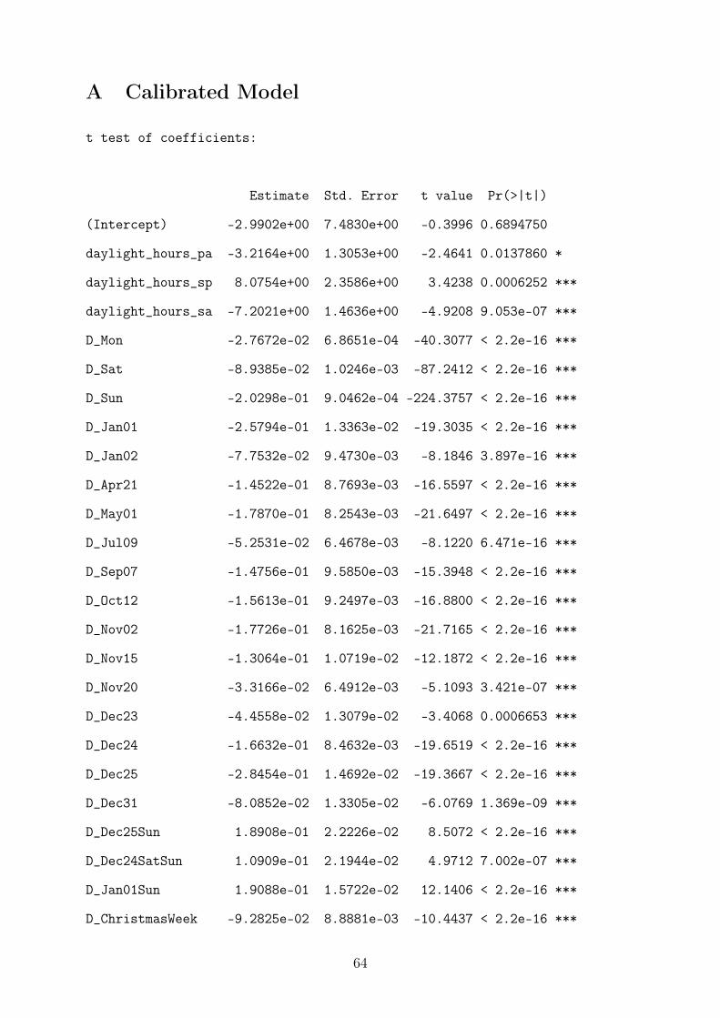
A Calibrated Model
t test of coefficients:
Estimate Std. Error t value Pr(>|t|)
(Intercept) -2.9902e+00 7.4830e+00 -0.3996 0.6894750
daylight_hours_pa -3.2164e+00 1.3053e+00 -2.4641 0.0137860 *
daylight_hours_sp 8.0754e+00 2.3586e+00 3.4238 0.0006252 ***
daylight_hours_sa -7.2021e+00 1.4636e+00 -4.9208 9.053e-07 ***
D_Mon -2.7672e-02 6.8651e-04 -40.3077 < 2.2e-16 ***
D_Sat -8.9385e-02 1.0246e-03 -87.2412 < 2.2e-16 ***
D_Sun -2.0298e-01 9.0462e-04 -224.3757 < 2.2e-16 ***
D_Jan01 -2.5794e-01 1.3363e-02 -19.3035 < 2.2e-16 ***
D_Jan02 -7.7532e-02 9.4730e-03 -8.1846 3.897e-16 ***
D_Apr21 -1.4522e-01 8.7693e-03 -16.5597 < 2.2e-16 ***
D_May01 -1.7870e-01 8.2543e-03 -21.6497 < 2.2e-16 ***
D_Jul09 -5.2531e-02 6.4678e-03 -8.1220 6.471e-16 ***
D_Sep07 -1.4756e-01 9.5850e-03 -15.3948 < 2.2e-16 ***
D_Oct12 -1.5613e-01 9.2497e-03 -16.8800 < 2.2e-16 ***
D_Nov02 -1.7726e-01 8.1625e-03 -21.7165 < 2.2e-16 ***
D_Nov15 -1.3064e-01 1.0719e-02 -12.1872 < 2.2e-16 ***
D_Nov20 -3.3166e-02 6.4912e-03 -5.1093 3.421e-07 ***
D_Dec23 -4.4558e-02 1.3079e-02 -3.4068 0.0006653 ***
D_Dec24 -1.6632e-01 8.4632e-03 -19.6519 < 2.2e-16 ***
D_Dec25 -2.8454e-01 1.4692e-02 -19.3667 < 2.2e-16 ***
D_Dec31 -8.0852e-02 1.3305e-02 -6.0769 1.369e-09 ***
D_Dec25Sun 1.8908e-01 2.2226e-02 8.5072 < 2.2e-16 ***
D_Dec24SatSun 1.0909e-01 2.1944e-02 4.9712 7.002e-07 ***
D_Jan01Sun 1.9088e-01 1.5722e-02 12.1406 < 2.2e-16 ***
D_ChristmasWeek -9.2825e-02 8.8881e-03 -10.4437 < 2.2e-16 ***
64
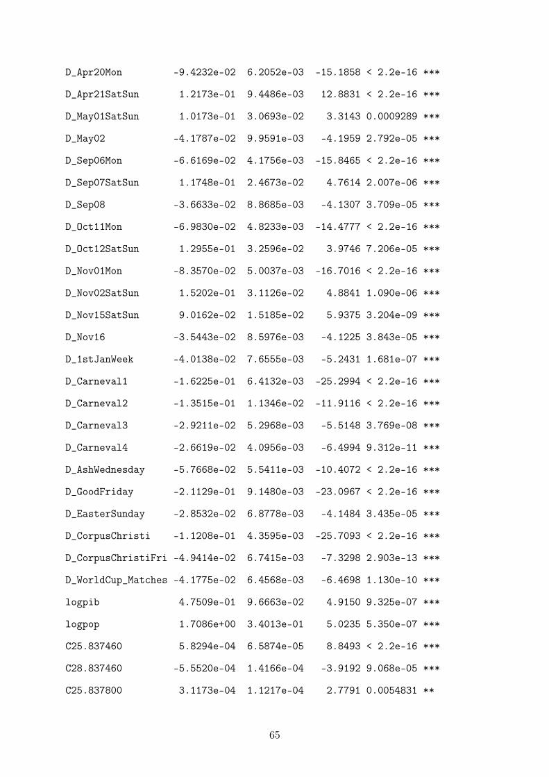
D_Apr20Mon -9.4232e-02 6.2052e-03 -15.1858 < 2.2e-16 ***
D_Apr21SatSun 1.2173e-01 9.4486e-03 12.8831 < 2.2e-16 ***
D_May01SatSun 1.0173e-01 3.0693e-02 3.3143 0.0009289 ***
D_May02 -4.1787e-02 9.9591e-03 -4.1959 2.792e-05 ***
D_Sep06Mon -6.6169e-02 4.1756e-03 -15.8465 < 2.2e-16 ***
D_Sep07SatSun 1.1748e-01 2.4673e-02 4.7614 2.007e-06 ***
D_Sep08 -3.6633e-02 8.8685e-03 -4.1307 3.709e-05 ***
D_Oct11Mon -6.9830e-02 4.8233e-03 -14.4777 < 2.2e-16 ***
D_Oct12SatSun 1.2955e-01 3.2596e-02 3.9746 7.206e-05 ***
D_Nov01Mon -8.3570e-02 5.0037e-03 -16.7016 < 2.2e-16 ***
D_Nov02SatSun 1.5202e-01 3.1126e-02 4.8841 1.090e-06 ***
D_Nov15SatSun 9.0162e-02 1.5185e-02 5.9375 3.204e-09 ***
D_Nov16 -3.5443e-02 8.5976e-03 -4.1225 3.843e-05 ***
D_1stJanWeek -4.0138e-02 7.6555e-03 -5.2431 1.681e-07 ***
D_Carneval1 -1.6225e-01 6.4132e-03 -25.2994 < 2.2e-16 ***
D_Carneval2 -1.3515e-01 1.1346e-02 -11.9116 < 2.2e-16 ***
D_Carneval3 -2.9211e-02 5.2968e-03 -5.5148 3.769e-08 ***
D_Carneval4 -2.6619e-02 4.0956e-03 -6.4994 9.312e-11 ***
D_AshWednesday -5.7668e-02 5.5411e-03 -10.4072 < 2.2e-16 ***
D_GoodFriday -2.1129e-01 9.1480e-03 -23.0967 < 2.2e-16 ***
D_EasterSunday -2.8532e-02 6.8778e-03 -4.1484 3.435e-05 ***
D_CorpusChristi -1.1208e-01 4.3595e-03 -25.7093 < 2.2e-16 ***
D_CorpusChristiFri -4.9414e-02 6.7415e-03 -7.3298 2.903e-13 ***
D_WorldCup_Matches -4.1775e-02 6.4568e-03 -6.4698 1.130e-10 ***
logpib 4.7509e-01 9.6663e-02 4.9150 9.325e-07 ***
logpop 1.7086e+00 3.4013e-01 5.0235 5.350e-07 ***
C25.837460 5.8294e-04 6.5874e-05 8.8493 < 2.2e-16 ***
C28.837460 -5.5520e-04 1.4166e-04 -3.9192 9.068e-05 ***
C25.837800 3.1173e-04 1.1217e-04 2.7791 0.0054831 **
65
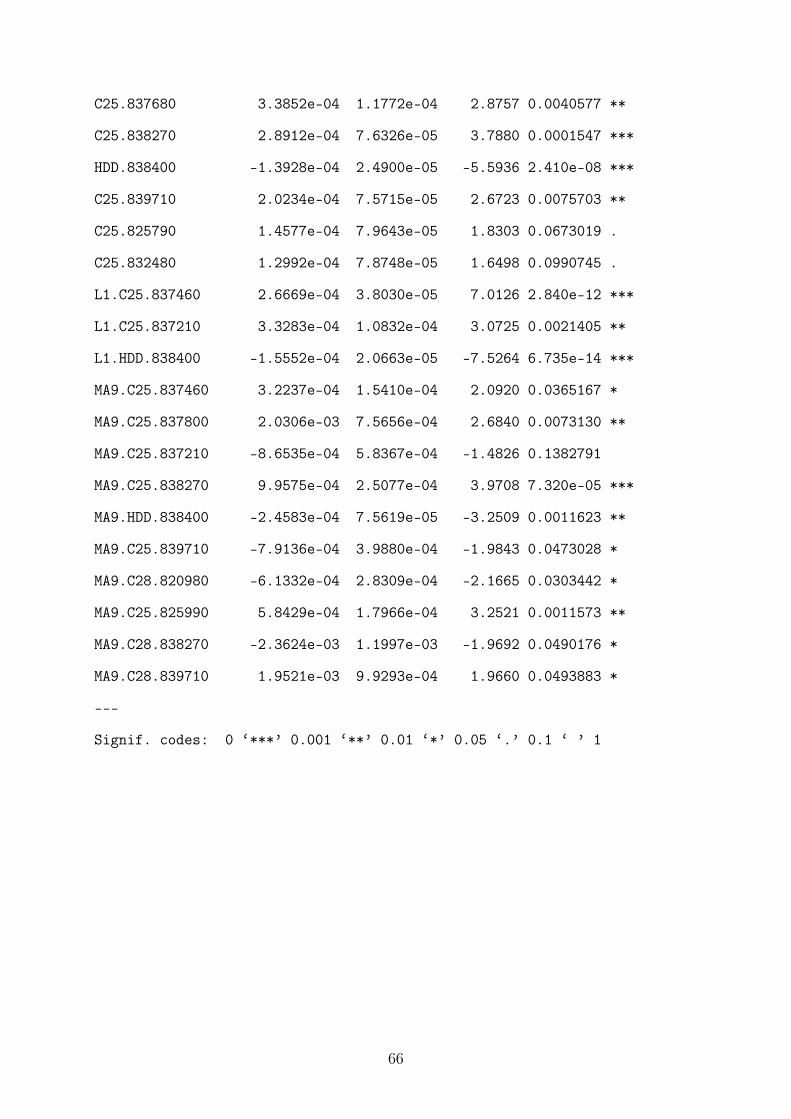
C25.837680 3.3852e-04 1.1772e-04 2.8757 0.0040577 **
C25.838270 2.8912e-04 7.6326e-05 3.7880 0.0001547 ***
HDD.838400 -1.3928e-04 2.4900e-05 -5.5936 2.410e-08 ***
C25.839710 2.0234e-04 7.5715e-05 2.6723 0.0075703 **
C25.825790 1.4577e-04 7.9643e-05 1.8303 0.0673019 .
C25.832480 1.2992e-04 7.8748e-05 1.6498 0.0990745 .
L1.C25.837460 2.6669e-04 3.8030e-05 7.0126 2.840e-12 ***
L1.C25.837210 3.3283e-04 1.0832e-04 3.0725 0.0021405 **
L1.HDD.838400 -1.5552e-04 2.0663e-05 -7.5264 6.735e-14 ***
MA9.C25.837460 3.2237e-04 1.5410e-04 2.0920 0.0365167 *
MA9.C25.837800 2.0306e-03 7.5656e-04 2.6840 0.0073130 **
MA9.C25.837210 -8.6535e-04 5.8367e-04 -1.4826 0.1382791
MA9.C25.838270 9.9575e-04 2.5077e-04 3.9708 7.320e-05 ***
MA9.HDD.838400 -2.4583e-04 7.5619e-05 -3.2509 0.0011623 **
MA9.C25.839710 -7.9136e-04 3.9880e-04 -1.9843 0.0473028 *
MA9.C28.820980 -6.1332e-04 2.8309e-04 -2.1665 0.0303442 *
MA9.C25.825990 5.8429e-04 1.7966e-04 3.2521 0.0011573 **
MA9.C28.838270 -2.3624e-03 1.1997e-03 -1.9692 0.0490176 *
MA9.C28.839710 1.9521e-03 9.9293e-04 1.9660 0.0493883 *
---
Signif. codes: 0 ‘***’ 0.001 ‘**’ 0.01 ‘*’ 0.05 ‘.’ 0.1 ‘ ’ 1
66