Embed Size (px)
Citation preview

Working Paper Series
An Econometric Analysis of Brand Level Strategic Pricing Between Coca Cola and Pepsi Inc.
by
Tirtha P. Dhar1
Jean-Paul Chavas2
Ronald W. Cotterill3
Brian W. Gould4
Ψ This research was supported by a USDA CSRS grant 2002-06090 to the Food System Research Group, University of Wisconsin-Madison and USDA CSRS Grant 00-34178-9036 to the Food Marketing Policy Center, University of Connecticut. The authors are greatly indebted to the FMPC- University of Connecticut for providing access to data used in the analysis. Any errors and omissions are the sole responsibility of the authors. A version of the paper was presented at the 5th INRA-IDEI conference on Industrial Organization and Food Processing Industries, Toulouse-France, June-20002. 1 Contacting Author, Research Associate, Food System Research Group, Dept. of Agricultural and Applied Economics; University of Wisonsin-Madison. 2 Professor, Dept. of Agricultural and Applied Economics; University of Wisconsin-Madison. 3 Professor and Director of Food Marketing Policy Center, Dept. Agricultural and Resource Economics; University of Connecticut. 4 Senior Scientist, Wisconsin Center for Dairy Research and the Department of Agricultural and Applied Economics; University of Wisconsin-Madison.

Abstract: Market structure and strategic pricing for leading brands sold by Coca Cola and
Pepsi Inc. are investigated in the context of a flexible demand specification and structural price equations. This approach is more general than prior studies that rely upon linear approximations and interactions of an inherently nonlinear problem. We test for Bertrand equilibrium, Stackelberg equilibrium, collusion, and a general conjectural variation (CV) specification. This nonlinear Full Information Maximum Likelihood (FIML) estimation approach provides useful information on the nature of imperfect competition and the extent of market power.
Keywords: Market structure, strategic pricing, conjectural variations, price reaction, carbonated soft drinks.

Title: An Econometric Analysis of Brand Level Strategic Pricing Between
Coca Cola and Pepsi Inc.
I. Introduction
Analysis of strategic behavior of firms using structural models is widely used in the
New Empirical Industrial Organization (NEIO) literature. The basic approach is to specify
and estimate market level demand and cost specifications after taking into account specific
strategic objectives of firms. The empirical implementation of these models can be
complex due to highly non-linear nature of flexible demand and cost functions and the
specification of strategic firm behavior. As a result, researchers have tended to simplify the
structural model by specifying ad-hoc or approximated demand specifications, and reduced
form conditions of the firm’s objectives. In this paper we attempt to overcome some of
these shortcomings.
In strategic market analysis estimated demand parameters play a crucial role as the
estimation of market power and strategic behavior depends crucially on the estimated price
and expenditure elasticities. For example, Gasmi, Laffont and Vuong (1992) (hereafter
GLV) and Golan, Karp and Perloff (2000) have used ad-hoc linear demand specifications.
A major problem with ad-hoc demand specifications is that they do not satisfy all the
restrictions of consumer theory. As a result estimated parameters may imply violation of
basic tenets of economic rationality. Even under a correct specification of strategic game,
any misspecification of demand may generate spurious results and incorrect policy
prescriptions due to incorrect elasticity estimates.
Researchers have tried to overcome these shortcomings of demand specification by
specifying flexible demand functions based on well-behaved utility functions. For
1
example, Hausman, Leonard and Zona (1994) and Cotterill, Dhar and Putsis (2000) use a
linear approximation to the Almost Ideal Demand System (LA-AIDS; see Deaton and
Muellbauer, 1980a). The problem with LA-AIDS is that the validity of its elasticity
estimates is subject to debate in the economic literature (e.g., Green and Alston 1990;
Alston et al., 1994; Buse, 1994; Moschini, 1995). As a result, there is no clear consensus
on the right way to estimate elasticities with LA-AIDS. For example, Hahn (1994) argues
that LA-AIDS violates the symmetry restrictions of consumer demand.1 This suggests that
it is desirable to avoid approximation to the AIDS since such approximation imposes
restrictions on price effects.
To avoid such approximated and ad-hoc demand specification, there is another
strand of the NEIO literature that uses characteristic based demand system based on
random utility model. Nevo (2000), Vilas-Boas and Zhao (2001) and others use
characteristic-based demand system. Empirically this approach is appealing due to
parsimonious description of the parameter space. However, the specification of random
utility models often imposes restrictions that may not be implied by general utility theory.
In a recent paper Bajari and Benkard (2001) show that many standard discrete choice
models have the following undesirable properties: as the number of product increases, the
compensating variation for removing all of the inside goods tends to infinity, all firms in a
Bertrand-Nash pricing game have markups that are bounded away from zero, and for each
good there is always some consumer that is willing to pay an arbitrarily large sum for the
good. These properties also imply discrete choice demand curve is unbounded for any
price level. To avoid this problem, Hausman (1997) uses linear and quadratic
approximations to the demand curve in order to make welfare calculations (e.g., multi
2
stage demand system with LA-AIDS at the last stage), favoring them over the CES
specification, which has an unbounded demand curve.
In terms of specifying behavioral rules for a firm, two broad approaches can be
found in the empirical literature. GLV (1992), Kadiyali, Vilcassim and Chintagunta (1996)
and Cotterill and Putsis (2001) have derived and estimated profit maximizing first-order
conditions under the assumption of alternative games (e.g., Bertrand or Stackelberg) along
with their demand specifications. However these studies derive estimable first-order
conditions based on ad-hoc demand specifications. Cotterill, Putsis and Dhar (2000) use
the more flexible LA-AIDS but they approximate the profit maximizing first-order
condition with a first-order log linear Taylor series expansion. Implications of using such
approximated first-order conditions have not been fully explored. In the other strand of
empirical literature, researchers have relied on instrumental variable estimation of the
demand specification (e.g., Hausman, Leonard and Zona 1994; and Nevo, 2000). The
advantage of this approach is that it avoids the pitfall of deriving and estimating
complicated first-order conditions. But in terms of estimating market power and merger
simulation, this approach restricts itself to Bertrand conjectures and the assumption of
constant marginal costs (Warden, 1998).
In this paper we overcome some of these shortcomings by specifying a fully
flexible ‘representative consumer model’ based nonlinear Almost Ideal Demand
Specification (AIDS) and structural first-order conditions for profit maximization. Unlike
Cotterill, Putsis and Dhar (2000), our derived first-order conditions are generic and avoid
the need for linear approximation. As a result they can be estimated with any flexible
demand specification that has closed form analytical elasticity estimates. We propose to
3
estimate our system (i.e., the demand specification and first-order conditions) using full
information maximum likelihood (FIML).
In this paper, we also test for different stylized strategic games, namely: Nash
equilibrium with Bertrand or Stackelberg conjectures, and Collusive games. In empirical
analysis of market, the correct strategic model specification is just as critical as the demand
and cost specification. Until now most antitrust analysis of market power has tended to
assume Bertrand conjectures (Cotterill, 1994a; Warden, 1998). One exception is Dhar,
Putsis and Cotterill (2000), who test for Bertrand and Stackelberg game at the product
category level. They test within a product category (e.g., breakfast cereal) for Stackelberg
and Bertrand game between two aggregate brands: private label and national brand. As a
result, their analysis is based on ‘two player game’. Similarly, GLV (1992) estimates and
test for strategic behavior of Coke and Pepsi brands. In this paper, we consider games with
multi firms and multi brands. In such a market, a firm may dominate a segment of the
market with one brand and then follow the competing firm in another segment of the
market with another brand. So, the number of possible games that needs to be tested
increases greatly. To the best of our knowledge this is the first study to test for strategic
brand level competition between firms.
In this paper, we also control for expenditure endogeneity in the demand
specification. Most papers in the industrial organization literature have failed to address
this issue. Dhar, Chavas and Gould (2002) and Blundell and Robin (2000) have found
evidence that expenditure endogeneity is significant in demand analysis and can have large
effects on the estimated price elasticities of demand.
4

Empirically we study the nature of price competition between four major brands
marketed by Pepsi and Coca Cola Inc. GLV (1992) was one of the first papers to estimate
a structural model for the carbonated soft drink industry (CSD). They developed a strategic
model of pricing and advertising between Coke and Pepsi using demand and cost
specification. Compared to the GLV study, our database is more disaggregate. As a result
we are able to control for region specific unobservable effect on CSD demand. Also, we
incorporate two other brands produced by Coca Cola and Pepsi Inc.: Sprite for Coca Cola,
and Mountain Dew for Pepsi. Of the four brands, three are Caffeineted (Coke, Pepsi and
Mt. Dew) and one is a clear non-caffeineted drink (Sprite). Characteristically, Mountain
Dew is quite unique. In terms of taste it is closer to Sprite but due to caffeine content,
consumers can derive alertness response similar to Coke and Pepsi.2 These four brands
dominate the respective portfolio of the two firms.
In the present study, unlike the GLV (1992) and Golan, Karp and Perloff (2000)
study, we do not model strategic interactions of firms with respect to advertising. Due to
lack of city and brand specific data on advertising we ignore strategic interactions in
advertisement (although we do control for the cost of brand promotion in our structural
model). Our analysis is based on quarterly IRI (Information Resources Inc.)-Infoscan
scanner data of supermarket sales of carbonated non-diet soft drinks (hereafter CSD) from
1988-Q1 to 1989-Q4 for 46 major metropolitan cities across USA.3
The paper is organized as follows. First, we present our conceptual approach.
Second, we discuss our model selection procedures. Third, we present our empirical model
specification. Fourth, econometric and statistical test results are presented. And finally we
draw conclusions from this study.
5
II. Model Specification
We specify a brand level non-linear Almost Ideal Demand System (AIDS) model.
We then derive first-order conditions of profit maximization under alternative game
theoretic assumptions using AIDS. Finally, we estimate the model using full information
maximum likelihood procedure.
a. Overview of the AIDS Demand Specification
This is the first study to use nonlinear AIDS in analyzing strategic brand level
competition between firms. So in this section we describe the derivation of AIDS in details
for interested readers.
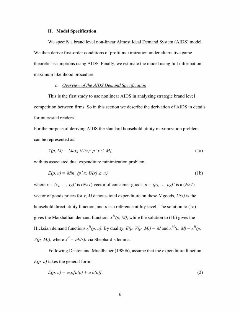
For the purpose of deriving AIDS the standard household utility maximization problem
can be represented as:
V(p, M) = Maxx {U(x): p’ x ≤ M}, (1a)
with its associated dual expenditure minimization problem:
E(p, u) = Minx {p’ x: U(x) ≥ u}, (1b)
where x = (x1, …, xN)’ is (N×1) vector of consumer goods, p = (p1, …, pN)’ is a (N×1)
vector of goods prices for x, M denotes total expenditure on these N goods, U(x) is the
household direct utility function, and u is a reference utility level. The solution to (1a)
gives the Marshallian demand functions xM(p, M), while the solution to (1b) gives the
Hicksian demand functions xH(p, u). By duality, E(p, V(p, M)) = M and xM(p, M) = xH(p,
V(p, M)), where xH = ∂E/∂p via Shephard’s lemma.
Following Deaton and Muellbauer (1980b), assume that the expenditure function
E(p, u) takes the general form:
E(p, u) = exp[a(p) + u b(p)], (2)
6
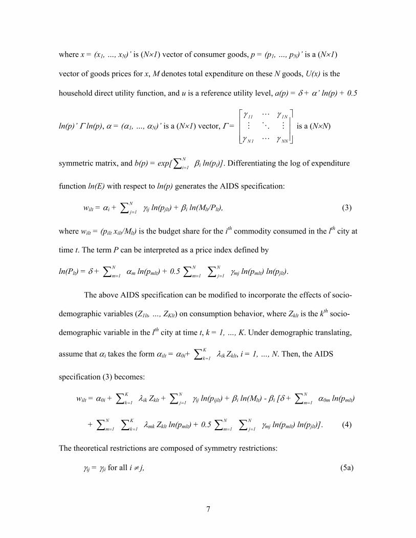
where x = (x1, …, xN)’ is (N×1) vector of consumer goods, p = (p1, …, pN)’ is a (N×1)
vector of goods prices for x, M denotes total expenditure on these N goods, U(x) is the
household direct utility function, and u is a reference utility level, a(p) = δ + α’ ln(p) + 0.5
ln(p)’ Γ ln(p), α = (α1, …, αN)’ is a (N×1) vector, Γ = is a (N×N)
symmetric matrix, and b(p) = exp[
NN1N
N111
γγ
γγ
∑ =
N
1iβi ln(pi)]. Differentiating the log of expenditure
function ln(E) with respect to ln(p) generates the AIDS specification:
wilt = αi + ∑ =
N
1jγij ln(pjlt) + βi ln(Mlt/Plt), (3)
where wilt = (pilt xilt/Mlt) is the budget share for the ith commodity consumed in the lth city at
time t. The term P can be interpreted as a price index defined by
ln(Plt) = δ + α∑ =
N
1m m ln(pmlt) + 0.5 ∑ =
N
1m ∑ =
N
1jγmj ln(pmlt) ln(pjlt).
The above AIDS specification can be modified to incorporate the effects of socio-
demographic variables (Z1lt, …, ZKlt) on consumption behavior, where Zklt is the kth socio-
demographic variable in the lth city at time t, k = 1, …, K. Under demographic translating,
assume that αi takes the form αilt = α0i+ ∑ =
K
1kλik Zklt, i = 1, …, N. Then, the AIDS
specification (3) becomes:
wilt = α0i + λ∑ =
K
1k ik Zklt + ∑ =
N
1jγij ln(pijlt) + βi ln(Mlt) - βi [δ + α∑ =
N
1m 0m ln(pmlt)
+ λ∑ =
N
1m ∑ =
K
1k mk Zklt ln(pmlt) + 0.5 ∑ =
N
1m ∑ =
N
1jγmj ln(pmlt) ln(pjlt)]. (4)
The theoretical restrictions are composed of symmetry restrictions:
γij = γji for all i ≠ j, (5a)
7
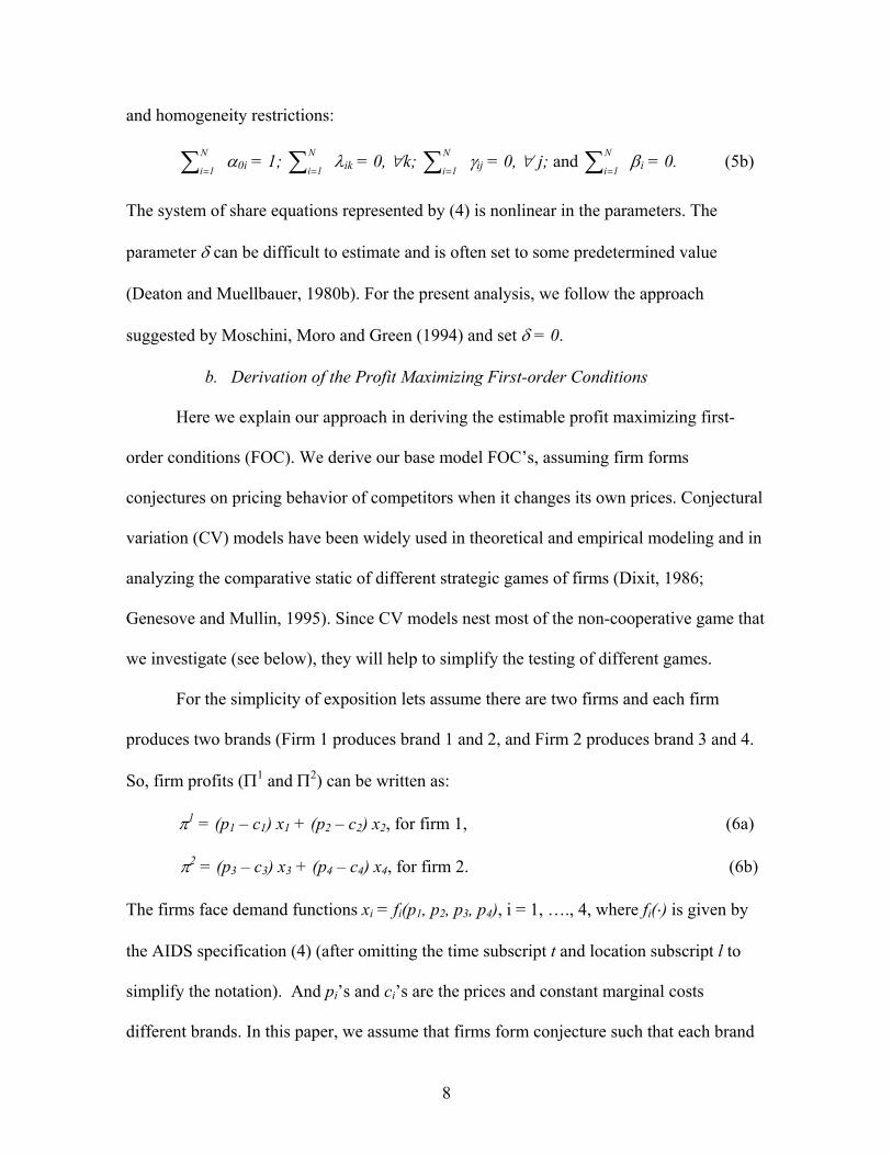
and homogeneity restrictions:
∑=
N
1iα0i = 1; λ∑ =
N
1i ik = 0, ∀k; ∑=
N
1iγij = 0, ∀ j; and ∑=
N
1iβi = 0. (5b)
The system of share equations represented by (4) is nonlinear in the parameters. The
parameter δ can be difficult to estimate and is often set to some predetermined value
(Deaton and Muellbauer, 1980b). For the present analysis, we follow the approach
suggested by Moschini, Moro and Green (1994) and set δ = 0.
b. Derivation of the Profit Maximizing First-order Conditions
Here we explain our approach in deriving the estimable profit maximizing first-
order conditions (FOC). We derive our base model FOC’s, assuming firm forms
conjectures on pricing behavior of competitors when it changes its own prices. Conjectural
variation (CV) models have been widely used in theoretical and empirical modeling and in
analyzing the comparative static of different strategic games of firms (Dixit, 1986;
Genesove and Mullin, 1995). Since CV models nest most of the non-cooperative game that
we investigate (see below), they will help to simplify the testing of different games.
For the simplicity of exposition lets assume there are two firms and each firm
produces two brands (Firm 1 produces brand 1 and 2, and Firm 2 produces brand 3 and 4.
So, firm profits (Π1 and Π2) can be written as:
π1 = (p1 – c1) x1 + (p2 – c2) x2, for firm 1, (6a)
π2 = (p3 – c3) x3 + (p4 – c4) x4, for firm 2. (6b)
The firms face demand functions xi = fi(p1, p2, p3, p4), i = 1, …., 4, where fi(⋅) is given by
the AIDS specification (4) (after omitting the time subscript t and location subscript l to
simplify the notation). And pi’s and ci’s are the prices and constant marginal costs
different brands. In this paper, we assume that firms form conjecture such that each brand
8
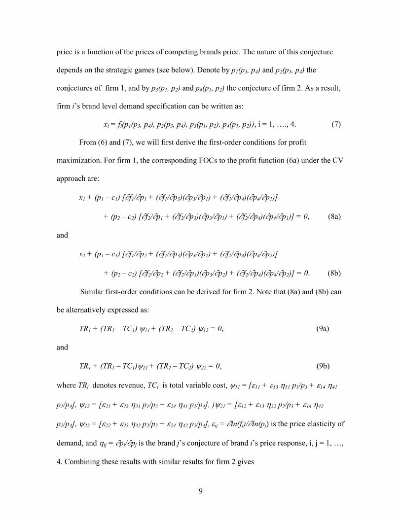
price is a function of the prices of competing brands price. The nature of this conjecture
depends on the strategic games (see below). Denote by p1(p3, p4) and p2(p3, p4) the
conjectures of firm 1, and by p3(p1, p2) and p4(p1, p2) the conjecture of firm 2. As a result,
firm i’s brand level demand specification can be written as:
xi = fi(p1(p3, p4), p2(p3, p4), p3(p1, p2), p4(p1, p2)), i = 1, …., 4. (7)
From (6) and (7), we will first derive the first-order conditions for profit
maximization. For firm 1, the corresponding FOCs to the profit function (6a) under the CV
approach are:
x1 + (p1 – c1) [∂f1/∂p1 + (∂f1/∂p3)(∂p3/∂p1) + (∂f1/∂p4)(∂p4/∂p1)]
+ (p2 – c2) [∂f2/∂p1 + (∂f2/∂p3)(∂p3/∂p1) + (∂f2/∂p4)(∂p4/∂p1)] = 0, (8a)
and
x2 + (p1 – c1) [∂f1/∂p2 + (∂f1/∂p3)(∂p3/∂p2) + (∂f1/∂p4)(∂p4/∂p2)]
+ (p2 – c2) [∂f2/∂p2 + (∂f2/∂p3)(∂p3/∂p2) + (∂f2/∂p4)(∂p4/∂p2)] = 0. (8b)
Similar first-order conditions can be derived for firm 2. Note that (8a) and (8b) can
be alternatively expressed as:
TR1 + (TR1 – TC1) ψ11 + (TR2 – TC2) ψ12 = 0, (9a)
and
TR1 + (TR1 – TC1)ψ21 + (TR2 – TC2) ψ22 = 0, (9b)
where TRi denotes revenue, TCi is total variable cost, ψ11 = [ε11 + ε13 η31 p1/p3 + ε14 η41
p1/p4], ψ12 = [ε21 + ε23 η31 p1/p3 + ε24 η41 p1/p4], )ψ21 = [ε12 + ε13 η32 p2/p3 + ε14 η42
p2/p4], ψ22 = [ε22 + ε23 η32 p2/p3 + ε24 η42 p2/p4], εij = ∂ln(fi)/∂ln(pj) is the price elasticity of
demand, and ηij = ∂pi/∂pj is the brand j’s conjecture of brand i’s price response, i, j = 1, …,
4. Combining these results with similar results for firm 2 gives
9
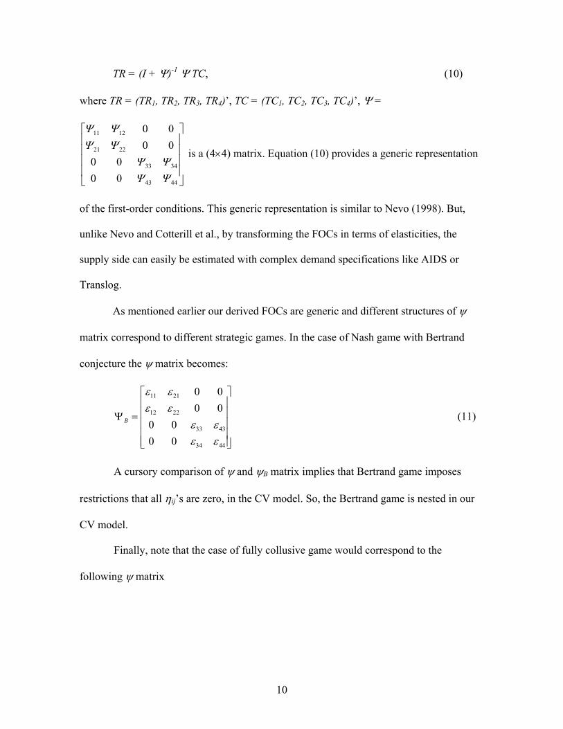
TR = (I + Ψ)-1 Ψ TC, (10)
where TR = (TR1, TR2, TR3, TR4)’, TC = (TC1, TC2, TC3, TC4)’, Ψ =
is a (4×4) matrix. Equation (10) provides a generic representation
of the first-order conditions. This generic representation is similar to Nevo (1998). But,
unlike Nevo and Cotterill et al., by transforming the FOCs in terms of elasticities, the
supply side can easily be estimated with complex demand specifications like AIDS or
Translog.
4443
3433
2221
1211
0000
0000
ΨΨΨΨ
ΨΨΨΨ
As mentioned earlier our derived FOCs are generic and different structures of ψ
matrix correspond to different strategic games. In the case of Nash game with Bertrand
conjecture the ψ matrix becomes:
11 21
12 22
33 43
34 44
0 00 0
0 00 0
B
ε εε ε
ε εε ε
Ψ =
(11)
A cursory comparison of ψ and ψB matrix implies that Bertrand game imposes
restrictions that all ηij’s are zero, in the CV model. So, the Bertrand game is nested in our
CV model.
Finally, note that the case of fully collusive game would correspond to the
following ψ matrix
10
11 21 31 41
12 22 32 42
13 23 33 43
14 24 34 44
COL
ε ε ε εε ε ε εε ε ε εε ε ε ε
Ψ =
. (12)
Note that, when collusion is defined over all brands, then the (I+ψ) matrix
becomes singular due to Cournot aggregation condition. In this paper, we do not
investigate a fully collusive game. Rather, we estimate partial brand level collusion, such
as: collusive pricing between Coke and Pepsi with Sprite and Mountain Dew playing
Bertrand game. Given the historic rivalries between Coca Cola and Pepsi, strategic
collusion in pricing is not realistic. Below, we estimate this collusive model mainly for the
purpose of test and comparison with other estimated models.
c. Reduced Form Expenditure Equation
Similar to Blundell and Robin (2000), we specify a reduced form expenditure
equation where household expenditure in the lth city at time t is a function of median
household income and a time trend:
Mlt = f(time trend, income). (13)
Blundell and Robin (2000), and Dhar, Chavas and Dhar (2002) found expenditure
endogeneity to significantly impact parameter estimates in AIDS.
III. Model Selection Procedures
The analysis by GLV (1992) was one of the first to suggest procedures to test
appropriate strategic market models given probable alternative cooperative and non-
cooperative games. They use both likelihood ratio and Wald tests to evaluate different
model specification. Of the two types of tests, the Wald test procedure is sensitive to
functional form of the null hypothesis. Also, the Wald test can only be used in situations
11

where models are nested in each other. As such, GLV (1992) suggest estimating alternative
models assuming different pure strategy gaming structures and then testing each model
against the other using nested and non-nested likelihood ratio tests.
In our view this is a suitable approach only in the case where the numbers of firms
and products are few (preferably not more than two) and the demand and cost specification
are not highly non-linear. Otherwise as the number of products or firms increases, the
number of alternative models to be estimated also increases exponentially. This is due to
the fact that a firm may play different strategies for different brands. One brand of the firm
may be a Stackelberg leader but the other brand may have a price followship strategy.
It is even possible that firms may be collusive for some brands and at the same time
plays non-collusive Stackelberg or Bertrand games on other brands. For each brand,
managers of Coca Cola and Pepsi can choose from four stylized pure strategies. These
strategies are Stackelberg leadership, Stackelberg followship, non-cooperative Betrand and
collusion. For each brand this implies four conceivable pure strategies in pricing against
each of the competing brands. In Table 1, we diagrammatically present the strategy profile
for each brand. With four brands and four pure strategies in pricing, there are 256 (i.e.,
four firms with four strategies: 44) pure strategy equilibrium. Given the large numbers of
pure strategy games and highly non-linear functional forms of our models, use of
likelihood ratio based tests is not very attractive for our analysis. Indeed, we would need to
estimate 256 separate models to test each models against the other. Out of sample
information may help us to eliminate some of the games.
In Table 2, we present a sample of 12 representative games based on pure
strategy pricing as described in Table 1. Of all the probable games, only the collusive game
12
[1] is not nested in our CV model derived earlier. So, except in the case of collusive model,
we can test games by testing the statistical significance of the restrictions imposed by the
game on the estimated CV parameters.
We follow Dixit (1986) to develop null hypothesis in testing nested models. Dixit
(1986) shows that most pure strategy games can be nested in a CV model. As a result CV
approach provides a parsimonious way of describing different pure strategy games.
Following Dixit (1986), CV parameters can be interpreted as fixed points that establish
consistency between the conjecture and the reaction function associated with a particular
game. In this paper we use our estimated CV model to test the different market structures
presented in Table 1. For example, if all the estimated CV parameters were zero, then the
appropriate game in the market would be Bertrand (game 2 in Table 2). This generates the
following null hypothesis (which can be tested using a Wald test):
[ηC,P ηC,MD ηS,P ηS,MD ηP, C ηP,S ηMD, P ηMD, S]′ = [0]′ (14)
where C stands for Coke, P for Pepsi, S for Sprite and MD for Mountain Dew.
In the case of any Stackelberg game, Dixit (1986) have shown that at equilibrium,
the conjectural variation parameter of a Stackelberg leader should be equal to the slope of
the reaction function of the follower, and followers CV parameter should be equal to zero.
Thus, in a game where Coca Cola’s brands leads Pepsi’s brands (i.e., game 6 in Table 2:
both Coke and Sprite leads Pepsi and Mountain Dew), parametric restrictions genereates
the following null hypothesis:
[ηC,P ηC,MD ηS,P ηS,MD ηP, C ηP,S ηMD, P ηMD, S]′ = [RP,C RMD,C RP,S RMD,S 0 0 0 0]′ (15)
where Ri,j’s are estimated slope of the reaction function of brand i of the follower to a price
change in j of the leader. For the rest of the games (as in Table 2), we can generate similar
13
restrictions and test for them using a Wald test. We estimate the slope of the reaction
functions by totally differentiating the derived first order conditions.
We propose a sequence of test in the following manner. First we test our non-nested
and partially nested models against each other using Vuong test (1989). In the present
paper, our collusive model and CV model are partially nested. One major advantage of
Vuong test is that it is directional. This implies that the test statistic not only tells us
whether the models are significantly different from each other but also the sign of the test
statistic indicates which model is appropriate. If we reject the collusive model, then the rest
of the pure strategy models can be tested using Wald tests because they are nested in our
CV model.
IV. Database
Table 3 provides brief descriptive statistics of all the variables used in the analysis.
Figure 1 plots prices of the four brands. During the period of our study, Mountain Dew
was consistently the most expensive, followed by Coke, Pepsi and Sprite. Figure 2 plots
volume sales by brands. In terms of volume sales Coke and Pepsi were almost at the same
level, Sprite and Mountain Dew’s sales were significantly lower than Coke and Pepsi’s
sales.
V. Empirical Model Specification
As noted above, we modify the traditional AIDS specification with demographic
translating. As a result, our AIDS model incorporates a set of regional dummy variables
along with selected socio-demographic variables. Many previous studies using multi-
market scanner data, including Cotterill (1994), Cotterill, Franklin and Ma (1996), and
Hausman, Leonard and Zona (1994) use city specific dummy variables to control for city
14
specific fixed effects for each brand. Here we control for regional differences by including
nine regional dummy variables.4
Our AIDS specification incorporates five demand shifters, Z, capturing the effects
of demographics across marketing areas. These variables include: median household size,
median household age, percent of household earning less than $10,000, percentage of
household earning more the $50,000, and supermarket to grocery sales ratio. Also to
maintain theoretical consistency of the AIDS model, the following restrictions based on (5)
are applied to the demographic translating parameter α0i:
α0i = d9
1r=∑ ir Dr, d9
1r=∑ ir = 1, i = 1,…, N. (16)
where dir is the parameter for the ith brand associated with the regional dummy variable Dr
for the rth region. Note that as a result, our demand equations do not have intercept terms.
We assume constant linear marginal cost specification. Such cost specification is quite
common and performs reasonably well in structural market analysis (e.g., Kadiyali,
Vilcussim and Chintagunta, 1996; GLV, 1992; Cotterill, Putsis and Dhar, 2000). The total
cost function is:
T_Cost =Ui + Mcostilt * xilt (17)
Where Ui is the brand specific unobservable (by the econometrician) cost component and
assumed not to vary at the mean of the variables. Mcostilt is the observable cost component
and we specify it as:
MCostilt = θi1 UPVilt + θi2 MCHilt (18)
where UPVilt in is the unit per volume of the ith product in the lth city at time t and
represents the average size of the purchase. For example, if a consumer purchases only
one-gallon bottles of a brand, then units per volume for that brand is one. Alternatively, if
15
this consumer buys a half-gallon bottle then the unit per volume is 2. This variable
captures packaging-related cost variations, as smaller package size per volume implies
higher costs to produce, to distribute and to shelve. The variable MCHilt measures
percentage of a CSD brand i sold in a city l with any type of merchandising (e.g., buy one
get one free, cross promotions with other products, etc.). This variable captures
merchandising costs of selling a brand. For example, if a brand is sold through promotion
such as: ‘buy one get one free’, then the cost of providing the second unit will be reflected
in this variable.
Following Blundell and Robin (2000), to control for expenditure endogeneity, the
reduced form expenditure function in (13) is specified as:
Mlt = η Trendt + ∑ δ9
1r= r Dr + φ1 INClt + φ2 INClt2, t = 1,…, 8, (19)
where Trendt in (19) is a linear trend, capturing any time specific unobservable effect on
consumer soft-drink expenditure. The variables Dr’s are the regional dummy variables
defined above and capture region specific variations in per capita expenditure. The variable
INClt is the median household income in city l and is used to capture the effect of income
differences on CSD purchases.
We estimate the system of three demand and four FOCs using FIML estimation
procedure. One demand equation drops out due to aggregation restrictions of AIDS. The
variance-covariance matrix and the parameter vector are estimated by specifying the
concentrated log-likelihood function of the system. The Jacobian of the concentrated log-
likelihood function is derived based on the models seven endogenous variablesl: 3 quantity
demanded variables (e.g. xi’s), 4 price variables (e.g. pi’s) and the expenditure variable (e.g.
M). Note that in the process of estimation we have one less quantity demanded variables
16

than price variables. This is due to the fact that we can express the demand for the fourth
brand as function of rest of the endogenous variables: x4 = M – (p1x1 + p2x2 + p3x3) / p4.
VI. Regression Results and Test of Alternative Models
We estimate three alternative models: (1) collusive oligopoly where the two firms
colludes on the price of Coke and Pepsi, (2) Bertrand model, and (3) the conjetctural
variation model.5
We assume that the demand shifters and the variables in the cost and expenditure
specification are exogenous. In general the reduced form specifications (i.e. equation (17)
and (19)) are always identified. The issue of parameter identification in non-linear
structural model is rather complex.6 We checked the order condition for identification that
would apply to a linearized version of the demand equations (4) and found it to be
satisfied. Finally, we did not uncover numerical difficulties in implementing the FIML
estimation and our estimated results are robust to iterative process of estimation. As
pointed out by Mittelhammer, Judge and Miller (2000, pages 474-475) in nonlinear full
information maximum likelihood estimation, we interpret this as evidence that each of the
demand equations is identified.7
Table 4 presents system R2 based on McElroy (1977). In terms of goodness of fit
the full CV model fits the best and collusive model fits the least. However, goodness of fit
measure in nonlinear regression may not be the appropriate tool to choose among models.
To test for an appropriate nesting structure and to select the best model we run further tests
based on likelihood ratio and Wald test statistics.
17
As mentioned earlier we estimate only one game with collusion. From the pure
strategy profile in Table 1 if we eliminate collusive strategy then we will be left with
eighty-one (i.e., four brands with three strategies each: 34) probable games.8 Of these
games full Bertrand model discussed above is one of them. So, in this paper in total we
test for eighty-two games, including a collusive game.
Collusion (game 1 in Table 2): As mentioned before we test only one game with
collusion. Existing literature and anecdotal evidence do not suggest any significant level
of collusion between Coca Cola and Pepsi Inc. Our collusion model where Coca Cola and
Pepsi Inc. collude on pricing of Coke and Pepsi is partially nested within our full CV
model. So, following GLV we use a modified likelihood ratio test based on Vuong (1989).
The test statistic is –3.56. Under a standard normal distribution, the test statistic is highly
significant. And the sign of the test provides strong evidence that the full CV model is
more appropriate than the collusive model.
Bertrand Game (game 2 in Table 2): Nash equilibrium with Bertrand conjectures has been
widely used in the NEIO literature for market power analysis (e.g., Nevo, 2001). This
motivated us to estimate this model separately so that we can test this model rigorously
against our alternative estimated models. We first use our estimated full CV model to test
for Bertrand conjecture. In the case of Nash equilibrium with Bertrand conjecture all the
estimated CV parameters should be not significantly different from zero. At 95%
significance level, 7 out of 8 CV parameter estimates are significant (Table 5). To provide
additional information, we first used a Wald test to investigate formally the null hypothesis
that all the CV parameters are zero. The estimated Wald test statistic is 4211.24. Under a
chi-square distribution, we strongly reject the null hypothesis of Bertrand conjectures. Note
18
that, unlike the likelihood ratio test, the Wald test can be specification sensitive
(Mittelhammer, Judge and Miller, 2000). So, we also conducted a likelihood ratio test of
the Bertrand model versus the full CV model. Testing the null hypothesis that restrictions
based on Bertrand conjectures are valid, we also strongly reject this null hypothesis with a
test statistic of 865.78. In conclusion, all our tests suggest overwhelmingly that the
Bertrand conjecture is not a valid conjecture in this market.
Test of other Games: Except for the collusive and the full Bertrand model, we use our
estimated CV model to test for rest of the game.
In the case of Stackelberg games, only the leader forms conjectures. The necessary
and sufficient condition for Stackelberg leadership is that such conjectures should be
positive and consistent with the associated reaction functions, and follower’s conjectures
should be zero. In the case of estimated full CV model we do not observe any such patterns
of significance, where one brand’s conjectures are positive and significant and the
competing brand’s conjectures are insignificant.
Table 5 presents estimated CV parameters and estimated slope of the reaction
functions at the mean. For any two brands to have Stackelberg leader-follower relationship
estimated CV parameters of the leader should be equal to the estimated reaction slope of
the follower. For example, for Coke to be the Stackelberg leader over Pepsi, Cokes
estimated conjecture over Pepsi’s price (i.e., 0.4126) should be equal to the estimated
reaction function slope of Pepsi (i.e. -0.3599). This is a sufficient condition. In addition,
Pepsi’s conjecture on Coke’s price (i.e. –0.3232) should be equal to zero. Assuming that
rest of the brand relationship is Bertrand our Wald test of the game investigates the
empirical validity of these restrictions. The other games are tested in a similar fashion,
19
using the restrictions on CV estimates and estimated reaction function slopes. We reject all
the games at the 5% level of significance.9 Using Wald test we fail to accept any of the
other probable games.10
Consistency of Conjectures: We fail to accept any of the game with Stackelberg
equilibrium. So, we test for less restrictive sufficient condition of Stackelber leadership.
That is we test for consistency of estimated conjectures. Consistency of conjectures implies
a firm behaves as if it is a Stackelberg leader even though there may not be any firm
behaving as Stackelberg follower. Results of the test of consistent conjectures are
presented in Table 6. In general, our estimated reaction function slopes at the mean are
quite different from the corresponding conjectures. This helps explain the overwhelming
rejection of all the game scenarios with Stackelberg conjectures. Only Pepsi has a
consistent conjecture with respect to Sprite at 1% level of significance.
Failure to accept any specific nested games implies CV model is the most
appropriate and general model. So, we focus our further analysis on our CV model. First,
we explore the issue of estimating elasticities and Lerner Index using alternative models.
The Lerner Index is defined as (Price-Marginal cost)/Price and calculated using the
estimated FOCs. One of the main reasons to estimate a structural model is to estimate price
and expenditure elasticities, and associated indicators of market power (e.g., Lerner Index).
We evaluate the impact of alternative model specifications on elasticity and market power
estimates. Table 7 and 8 present price and expenditure elasticity estimates for the full CV
model.
20
Dhar, Chavas and Gould (2001) and Vilas-Boas and Winer (1999) found that after
controlling price and expenditure endogeneity, efficiency of the elasticity estimates
improve dramatically. This study also finds significant improvements in terms of the
efficiency of our elasticity estimates.11
In our CV model the estimated own price elasticities have the anticipated signs, and
own and cross price elasticities satisfy all the basic utility theory restrictions (namely
symmetry, Cournot and Engel aggregation). Also, all the estimated cross and own price
elasticities are highly significant suggesting rich strategic relationships between brands.
Our estimated expenditure elasticities are all positive and vary between 0.74 to 1.85, with
Pepsi being the most inelastic and Mountain Dew being the most elastic brand.
Table 9 presents Lerner indices. Each is an estimate of price-cost margin for the
entire soft drink marketing channel, i.e. it includes margins of the manufacturers,
distributors and retailers. Using our CV model, Pepsi has the lowest price-cost margin and
Mountain Dew has the highest. This is consistent with the fact that Mountain Dew is the
fastest growing carbonated soft drink brand, with a higher reported profit margin than most
brands.12
For the purpose of evaluating the impact of model specification, we also estimate
the Lerner Index for the Bertrand and collusive games. Our estimated Lerner Index from
the CV model, Bertrand, and collusive games are quite different. To compare them, we
calculated the average absolute percentage differences (APD) among the estimated Lerner
Indices, where APD between any two estimates (ε* and ε**) is defined as:
APD = {100 |ε* - ε**|}/{0.5 |ε* + ε**|}.
21
The average APD between Lerner Index estimates from the CV and the full Bertrand game
is 19.14. Between the CV and the collusive model it is 57.92. Such large differences in
estimated Lerner Index across models indicate that appropriate model specification is
important for empirical market power analysis.
VII. Concluding Remarks
In this paper we analyze the strategic behavior of Coca Cola and Pepsi Inc. in the
carbonated soft drink market. This is the first study to use the flexible nonlinear AIDS
model within a structural econometric model of firm (brand) conduct. Also, we derive
generic first-order conditions under different profit maximizing scenario that can be used
with most demand specifications and to test for strategic games. This approach avoids
linear approximation of the demand and/or first-order conditions.
In this paper we test for brand level alternative games between firms. Most of the
earlier studies in differentiated product oligopoly either tested for games at the aggregate
level (i.e., Cotterill, Putsis and Dhar, 2000) or between two brands (Golan, Karp, and
Perloff, 2000; and GLV, 1992). Given that most oligpolistic firms produces different
brands, test of brand level strategic competition is more realistic.
We first test our partially nested collusive model against our CV model. We find
statistical evidence that the CV model is more appropriate than the collusive model. The
remaining stylized games considered in this paper are in fact nested in the CV model. Our
tests for specific stylized multi brand multi firm market pure strategy models (relying on
Wald tests) are attractive because of its simplicity. Treating each game as a null
hypothesis, we reject all null hypotheses. Our overall test results imply that the pricing
22
game being played in this market is much more complex than the stylized games being
tested.
However, we have not considered all possible games. It may well be that some
complex game not considered in this paper would appear consistent with the CV model. As
a result, if the researcher do not have any specific out of sample information on specific
game being played then it is appropriate to estimate CV model.
We use estimated parameters from different models to estimate elasticities and
Lerner Index. We find these estimates to be quite sensitive to model specifications. The
empirical evidence suggests that the CV model is the most appropriate.
One of the shortcomings of this paper is that we do not consider mixed strategy
games as in Golan, Karp and Perloff (2000). The pure strategy games considered here are
degenerate mixed strategy games. It is possible that actual game involve games with mixed
strategies. Additional research is needed to consider such models with flexible demand
specification such as AIDS.
23
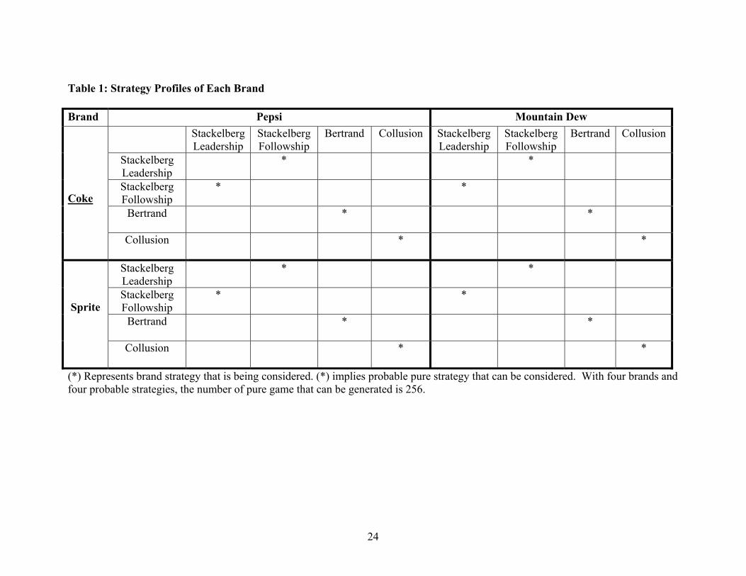
Table 1: Strategy Profiles of Each Brand
(*) Represents brand strategy that is being considered. (*) implies probable pure strategy that can be considered. With four brands and four probable strategies, the number of pure game that can be generated is 256.
Brand Pepsi Mountain DewStackelbergLeadership
Stackelberg Followship
Bertrand Collusion StackelbergLeadership
Stackelberg Followship
Bertrand Collusion
Stackelberg Leadership
* *
Stackelberg Followship
* *
Bertrand * *
Coke
Collusion * *
Stackelberg Leadership
* *
Stackelberg Followship
* *
Bertrand * *
Sprite
Collusion * *
24

Table 2: Probable Pure Strategy Games€
Game Set 1: Game estimated and tested against CV model using likelihood ratio test:
1 Collusive Game: Coke and Pepsi are the collusive brands. And Sprite and Mountain Dew uses Bertrand conjecture.
2 Full Bertrand Game: Both the firms use Bertrand conjecture over all brands.
Game Set 2: To Test following strategic games we used Wald test procedure:
3 Mixed Stackelberg and Bertrand Game 1: Coke leads Pepsi in a Stackelberg game. Rest of the brand relationship is Bertrand.
4 Mixed Stackelberg and Bertrand Game 2: Coke leads Mountain Dew in a Stackelbarg game. Rest of the brand relationship is Bertrand.
5 Mixed Stackelberg and Bertrand Game 3: Coke leads both Pepsi and Mountain Dew in a Stackelberg game. Rest of the brand relationship is Bertrand.
6 Mixed Stackelberg and Bertrand Game 4: Coke leads Pepsi and Mountain Dew, and Sprite leads Pepsi and Mountain Dew in a Stackelberg game.
7 Mixed Stackelberg and Bertrand Game 5: Coke leads Pepsi and Mountain Dew leads Sprite. Rest of the brand relationship is Bertrand.
8 Mixed Stackelberg and Bertrand Game 7: Sprite leads Mountain Dew in a Stackelberg game. Rest of the brand relationship is Bertrand.
9 Mixed Stackelberg and Bertrand Game 9: Pepsi leads Coke in a Stackelberg game. Rest of the brand relationship is Bertrand.
10 Mixed Stackelberg and Bertrand Game 11: Pepsi leads Coke and Moutain Dew leads Sprite in a Stackelberg game. Rest of the brand relationship is Bertrand.
11 Mixed Stackelberg and Bertrand Game 15: Mountain Dew leads Sprite in a Stackelberg game. Rest of the brand relationship is Bertrand.
12 Mixed Stackelberg and Bertrand Game 15: Pepsi leads Coke and Sprite leads Mountain Dew in a Stackelberg game. Rest of the brand relationship is Bertrand.
€ A sample list of pure strategy pricing Games. A detailed list of pure strategy game with three strategy is presented in Appendix Table A1.
25
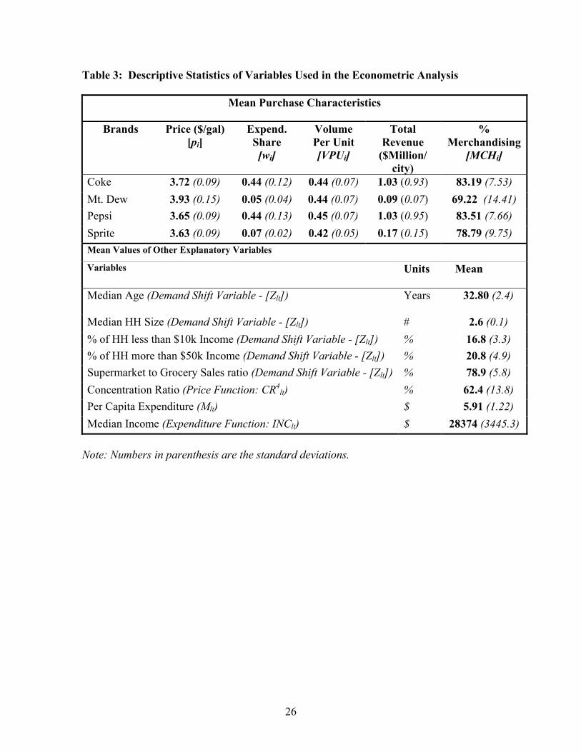
Table 3: Descriptive Statistics of Variables Used in the Econometric Analysis
Mean Purchase Characteristics
Brands Price ($/gal) [pi]
Expend. Share [wi]
Volume Per Unit [VPUi]
Total Revenue
($Million/ city)
% Merchandising
[MCHi]
Coke 3.72 (0.09) 0.44 (0.12) 0.44 (0.07) 1.03 (0.93) 83.19 (7.53) Mt. Dew 3.93 (0.15) 0.05 (0.04) 0.44 (0.07) 0.09 (0.07) 69.22 (14.41) Pepsi 3.65 (0.09) 0.44 (0.13) 0.45 (0.07) 1.03 (0.95) 83.51 (7.66) Sprite 3.63 (0.09) 0.07 (0.02) 0.42 (0.05) 0.17 (0.15) 78.79 (9.75) Mean Values of Other Explanatory Variables
Variables Units Mean
Median Age (Demand Shift Variable - [Zlt]) Years 32.80 (2.4)
Median HH Size (Demand Shift Variable - [Zlt]) # 2.6 (0.1) % of HH less than $10k Income (Demand Shift Variable - [Zlt]) % 16.8 (3.3) % of HH more than $50k Income (Demand Shift Variable - [Zlt]) % 20.8 (4.9) Supermarket to Grocery Sales ratio (Demand Shift Variable - [Zlt]) % 78.9 (5.8) Concentration Ratio (Price Function: CR4
lt) % 62.4 (13.8) Per Capita Expenditure (Mlt) $ 5.91 (1.22) Median Income (Expenditure Function: INClt) $ 28374 (3445.3)
Note: Numbers in parenthesis are the standard deviations.
26
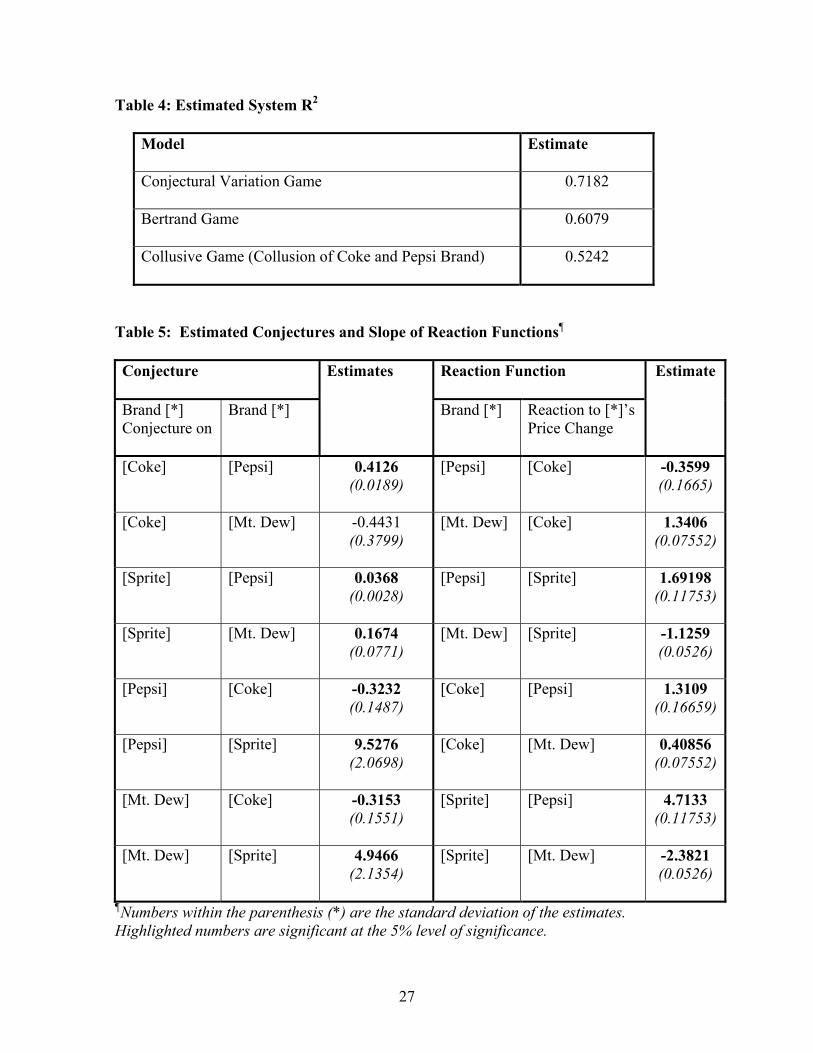
Table 4: Estimated System R2
Model Estimate
Conjectural Variation Game 0.7182
Bertrand Game 0.6079
Collusive Game (Collusion of Coke and Pepsi Brand) 0.5242
Table 5: Estimated Conjectures and Slope of Reaction Functions
Conjecture
Reaction Function
Brand [*] Conjecture on
Brand [*]
Estimates
Brand [*] Reaction to [*]’s Price Change
Estimate
[Coke] [Pepsi] 0.4126 (0.0189)
[Pepsi] [Coke] -0.3599 (0.1665)
[Coke] [Mt. Dew] -0.4431 (0.3799)
[Mt. Dew] [Coke] 1.3406 (0.07552)
[Sprite] [Pepsi] 0.0368 (0.0028)
[Pepsi] [Sprite] 1.69198 (0.11753)
[Sprite] [Mt. Dew] 0.1674 (0.0771)
[Mt. Dew] [Sprite] -1.1259 (0.0526)
[Pepsi] [Coke] -0.3232 (0.1487)
[Coke] [Pepsi] 1.3109 (0.16659)
[Pepsi] [Sprite] 9.5276 (2.0698)
[Coke] [Mt. Dew] 0.40856 (0.07552)
[Mt. Dew] [Coke] -0.3153 (0.1551)
[Sprite] [Pepsi] 4.7133 (0.11753)
[Mt. Dew] [Sprite] 4.9466 (2.1354)
[Sprite] [Mt. Dew] -2.3821 (0.0526)
¶Numbers within the parenthesis (*) are the standard deviation of the estimates. Highlighted numbers are significant at the 5% level of significance.
27
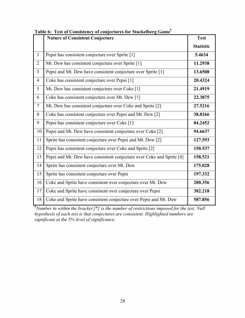
Table 6: Test of Consistency of conjectures for Stackelberg Game¶ Nature of Consistent Conjecture Test
Statistic
1 Pepsi has consistent conjecture over Sprite [1] 5.4634
2 Mt. Dew has consistent conjecture over Sprite [1] 11.2938
3 Pepsi and Mt. Dew have consistent conjecture over Sprite [1] 13.6508
4 Coke has consistent conjecture over Pepsi [1] 20.4324
5 Mt. Dew has consistent conjecture over Coke [1] 21.4919
6 Coke has consistent conjecture over Mt. Dew [1] 22.3875
7 Mt. Dew has consistent conjecture over Coke and Sprite [2] 27.5216
8 Coke has consistent conjecture over Pepsi and Mt. Dew [2] 38.8266
9 Pepsi has consistent conjecture over Coke [1] 84.2452
10 Pepsi and Mt. Dew have consistent conjecture over Coke [2] 94.6637
11 Sprite has consistent conjecture over Pepsi and Mt. Dew [2] 127.593
12 Pepsi has consistent conjecture over Coke and Sprite [2] 150.537
13 Pepsi and Mt. Dew have consistent conjecture over Coke and Sprite [4] 158.521
14 Sprite has consistent conjecture over Mt. Dew 175.028
15 Sprite has consistent conjecture over Pepsi 197.332
16 Coke and Sprite have consistent over conjecture over Mt. Dew 200.356
17 Coke and Sprite have consistent over conjecture over Pepsi 382.218
18 Coke and Sprite have consistent conjecture over Pepsi and Mt. Dew 587.856 ¶Number in within the bracket [*] is the number of restrictions imposed for the test. Null hypothesis of each test is that conjectures are consistent. Highlighted numbers are significant at the 5% level of significance.
28
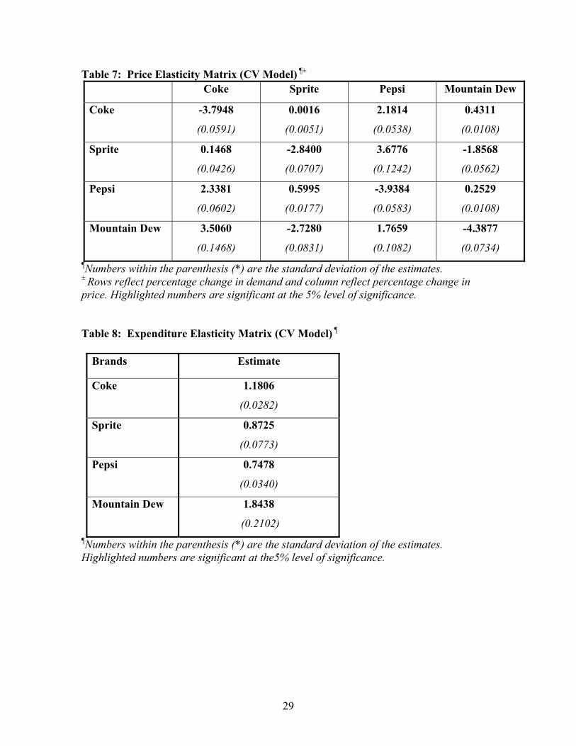
Table 7: Price Elasticity Matrix (CV Model) ¶± Coke Sprite Pepsi Mountain Dew
Coke -3.7948
(0.0591)
0.0016
(0.0051)
2.1814
(0.0538)
0.4311
(0.0108)
Sprite 0.1468
(0.0426)
-2.8400
(0.0707)
3.6776
(0.1242)
-1.8568
(0.0562)
Pepsi 2.3381
(0.0602)
0.5995
(0.0177)
-3.9384
(0.0583)
0.2529
(0.0108)
Mountain Dew 3.5060
(0.1468)
-2.7280
(0.0831)
1.7659
(0.1082)
-4.3877
(0.0734) ¶Numbers within the parenthesis (*) are the standard deviation of the estimates. ± Rows reflect percentage change in demand and column reflect percentage change in price. Highlighted numbers are significant at the 5% level of significance.
Table 8: Expenditure Elasticity Matrix (CV Model) 
Brands Estimate
Coke 1.1806
(0.0282)
Sprite 0.8725
(0.0773)
Pepsi 0.7478
(0.0340)
Mountain Dew 1.8438
(0.2102) ¶Numbers within the parenthesis (*) are the standard deviation of the estimates. Highlighted numbers are significant at the5% level of significance.
29
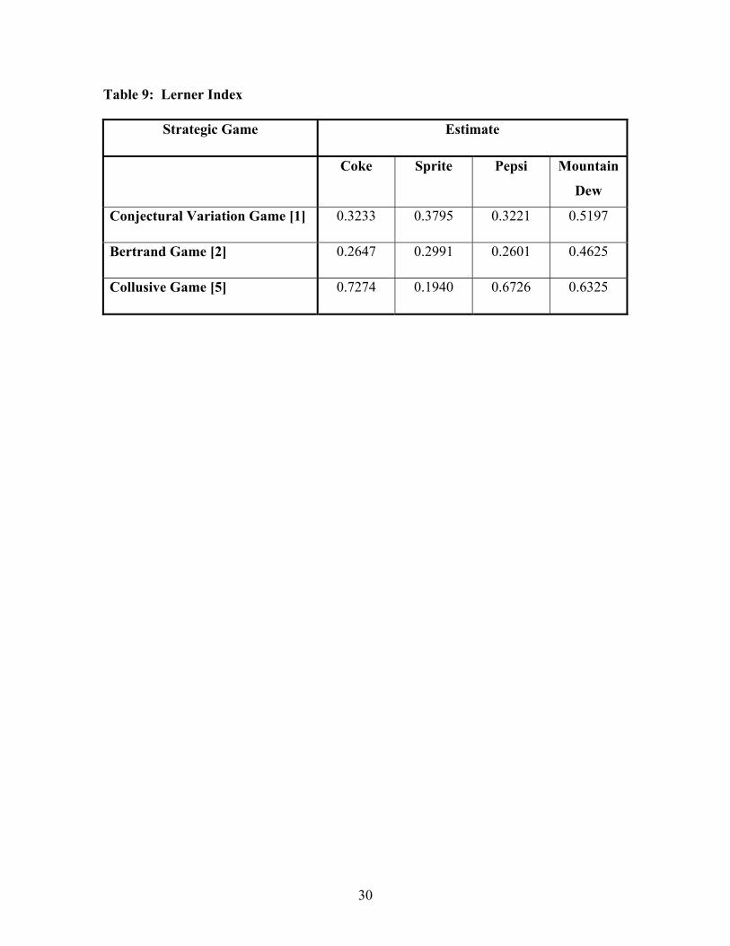
Table 9: Lerner Index
Strategic Game Estimate
Coke Sprite Pepsi Mountain
Dew
Conjectural Variation Game [1] 0.3233 0.3795 0.3221 0.5197
Bertrand Game [2] 0.2647 0.2991 0.2601 0.4625
Collusive Game [5] 0.7274 0.1940 0.6726 0.6325
30
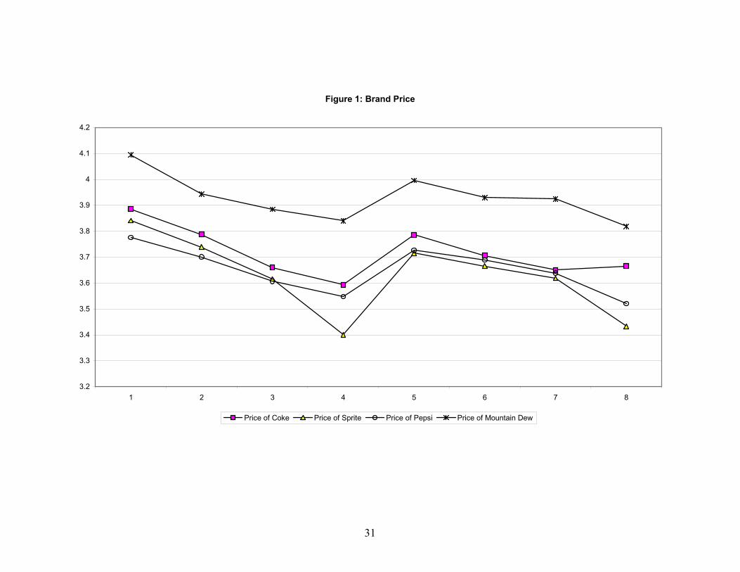
Figure 1: Brand Price
3.2
3.3
3.4
3.5
3.6
3.7
3.8
3.9
4
4.1
4.2
1 2 3 4 5 6 7 8
Price of Coke Price of Sprite Price of Pepsi Price of Mountain Dew
31
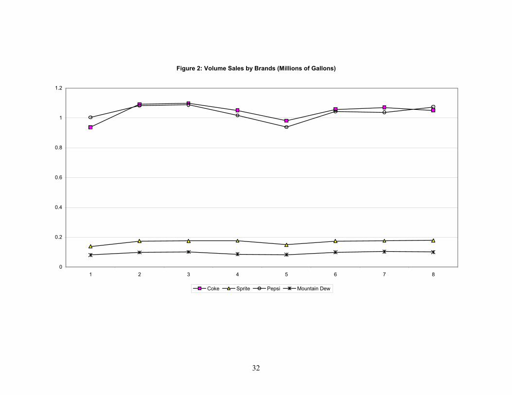
Figure 2: Volume Sales by Brands (Millions of Gallons)
0
0.2
0.4
0.6
0.8
1
1.2
1 2 3 4 5 6 7 8
Coke Sprite Pepsi Mountain Dew
32
References
Alston, J.M., Foster, K.A., Green R.D., 1994. “Estimating Elasticities with the Linear
Approximate Almost Ideal Demand System: Some Monte Carlo Results.” Review
of Economic Statistics.
Bajari, P. and C.L. Benkard, “Discrete Choice of Models of Structural Models of Demand:
Some Economic Implications of Common Approaches.” Stanford University
Department of Economics Working Paper; October, 2001.
Berry, S. T. “Estimating Discrete-Choice Models of Product Differentiation.” Rand
Journal of Economics 25(Summer 1994): 242-62.
Blundell, R. and J. M. Robin. “Latent Separability: Grouping Goods without Weak
Separability.” Econometrica 68(January 2000): 53-84.
Buse, A. 1996. “Testing Homogeneity in the Linearized Almost Ideal Demand System.
American Journal of Agricultural Economics 76, 781-793.
Buse, A. and W.H. Chan., “Invariance, Price Indices and Estimation in Almost Ideal
Demand System.” Empirical Economics 25(2000): 519-539.
Chen, K.Z. 1998., “The Symmetric Problem in the Linear Almost Ideal Demand System.”
Economic Letters, 59, pages 309-315.
Cotterill, R. W., A. W. Franklin and L. Y. Ma. “Measuring Market Power Effects in
Differentiated Product Industries: An Application to the Soft Drink Industry.”
Research Report, Food Marketing Policy Center, University of Connecticut, Storrs;
CT, 1996.
Cotterill, R. W., W. P. Putsis Jr. and R. Dhar. “Assessing the Competitive Interaction
between Private Labels and National Brands.” Journal of Business 73 (January
2000): 109-37.
Cotterill, R.W. “Scanner Data: New Opportunities for Demand and Competitive Strategy
Analysis.” Agricultural and Resource Economics Review 23(2): 125-139, 1994.
Cotterill, R.W. and W.P. Putsis, Jr., “Testing the Theory: Assumptions on Vertical
Strategic Interaction and Demand Functional Form,” Journal of Retailing,
77(2001): 83-109.
33
Cotterill, R.W., (1994a) “An Econometric Analysis of the Demand for RTE Cereal:
Product Market Definition and Unilateral Market Power Effects” Exhibit C in
Affidavit of R.W. Cotterill, 9/6/1994, State of New York v Kraft General Foods et
al., 93 civ 0811. (reprinted as University of Connecticut Food Marketing Policy
Center Research Report No.35.
Deaton, A. S. and J. Muellbauer. “An Almost Ideal Demand System.” American Economic
Review 70(June 1980b): 312-26.
Deaton, A. S. and J. Muellbauer. Economics and Consumer Behavior. New York:
Cambridge University Press, 1980a.
Dhar T., J.P. Chavas and B. W. Gould. “An Empirical Assessment of Endogeneity Issues
Dixit, Avinash. “Comparative Statics for Oligopoly,” International Economic Review
27(1986): 107-122.
Gasmi, F., J. J. Laffont and Q. Vuong. “A Structural Approach to Empirical Analysis of
Collusive Behavior.” European Economic Review; 34(2-3), May 1990, pages 513-
23.
Gasmi, F.; J. J. Laffont and Q. Vuong, “Econometric Analysis of Collusive Behavior in a
Soft-Drink Market.” Journal of Economics and Management Strategy; 1(2),
Summer 1992, pages 277-311.
Genesove, D., and W.P. Mullin., “Validating the Conjectural Variation Method: The Sugar
Industry, 1890-1914.” NBER Working Paper 5314, OCT 1995.
Golan, Amos, Larry S. Karp, Jeffrey M. Perloff, "Estimating Coke and Pepsi's Price and
Advertising Strategies," Journal of Business & Economic Statistics, 18(4), October
2000: 398-409.
Green, R., Alston J.M. 1990. “Elasticities in AIDS Models.” American Journal of
Agricultural Economics 72, 442-977.
Hahn, W., 1994. “Elasticities in AIDS Models: Comments. American Journal of
Agricultural Economics 72, pages 874-875.
Hausman, J., G. Leonard and J. D. Zona. “Competitive Analysis with Differentiated
Products.” Annales D’Economie et de Statistique 34(1994): 159-180.
in Demand Analysis for Differentiated Products.” Food System Research Group-
Working Paper, University of Wisconsin-Madison; 2001.
34
Kadiyali, V., N. J. Vilcassim and P. K. Chintagunta. “Empirical Analysis of Competitive
Product Line Pricing Decisions: Lead, Follow, or Move Together?” Journal of
Business 69(October 1996): 459-87.
McElroy, M. (1977) “Goodness of Fit for Seemingly Unrelated Regressions: Glahn’s R2yx
and Hooper’sr2.” Journal of Econometrics, 6, pp. 381-387.
Mittelhammer, R.C., G.G. Judge and D.J. Miller. “Econometric Foundations.” 1st Edition.
Cambridge University Press: UK, 2000.
Moschini, G., 1995. “Units of Meausurement and the Stone Index in Demand System
Estimation. American Journal of Agricultural Economics 77, 63-68.
Moschini, G., D. Moro and R. D. Green. “Maintaining and Testing Separability in Demand
Systems.” American Journal of Agricultural Economics 76(February 1994): 61-73.
Nevo, A. “Measuring Market Power in the Ready-to-Eat Cereal Industry.” Econometrica
69 (March 2001): 307-42.
Nevo, A. “Mergers with Differentiated Products: The Case of the Ready-to-Eat Cereal
Industry.” RAND Journal of Economics 31(Autumn 2000): 395-421.
Nevo, Aviv. "Identification of the Oligopoly Solution Concept in a Differentiated-Products
Industry." Economics Letters; 59(3) June 1998: pages 391-95.
Villas-Boas, J. M. and Y. Zhao. “The Ketchup Marketplace: Retailer, Manufacturers, and
Individual Consumers.” Unpublished Mimeo, University of California, Berkeley,
January 2001.
Villas-Boas, J.M. and R. Winer. “Endogeneity in Brand Choice Model.” Management
Science 45(1999): 1324-1338.
Vuong, Quang H. "Likelihood Ratio Tests for Model Selection and Non-nested
Hypotheses." Econometrica; 57(2), March 1989, pages 307-33.
Warden, G. (1996) “Demand Elasticities in Antitrust Analysis.” Economic Analysis Group
Discussion Paper; US D.O.J. EAG 96-11 (November).
35
Footnotes
1 For a detailed discussion on problems with LA-AIDS please refer to Chen (1998), Buse
and Chan (2000).
2 During the period of our study, Coca Cola Inc. did not have any specific brand to
compete directly against Mountain Dew. Only in 1996 they introduced the brand Surge to
compete directly against Mountain Dew.
3 Information Resources Inc., collects data from supermarkets with more than $2 million in
sales from major US cities. The size of supermarket accounts for 82% of grocery sales in
the US.
4 A list of the cities and definitions of the nine regions used in our analysis can be obtained
from the authors upon request. Our region definitions are based on census definition of
divisions.
5 A regression result of the CV model is presented in the Appendix.
6 For a detailed discussion please refer to Mittelhammer, Judge and Miller (2000, pages
474-475).
7 Due to space limitations, we report only related econometric results. More complete
reports of the results are available from the authors on request.
8 A detailed list of all the games with three pure strategies is presented in Appendix Table
A1.
9 Detail test procedures and statistics are available from the authors on request.
10 A list of probable games and detailed test statistics of all the games tested is available
from the authors on request.
11 Detailed results of models without controlling for endogeneity are available from the
authors on request.
36
37
12 According to Andrew Conway, a beverage analyst for Morgan Stanley & Company:
"Mountain Dew gives Pepsi about 20 percent of its profits because it's heavily skewed
toward the high-profit vending-machine and convenience markets. In these channels,
Mountain Dew is rarely sold at a discount." (New York Times, Dec 16, 1996).

Appendix for the Reviewers
Appendix for the Reviewers
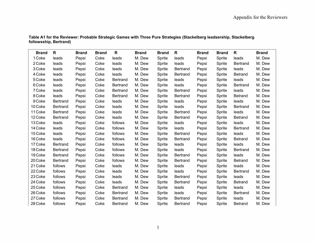
Table A1 for the Reviewer: Probable Strategic Games with Three Pure Strategies (Stackelberg leadsership, Stackelberg followsship, Bertrand) Brand R Brand Brand R Brand Brand R Brand Brand R Brand
1 Coke leads Pepsi Coke leads M. Dew Sprite leads Pepsi Sprite leads M. Dew2 Coke leads Pepsi Coke leads M. Dew Sprite leads Pepsi Sprite Bertrand M. Dew3 Coke leads Pepsi Coke leads M. Dew Sprite Bertrand Pepsi Sprite leads M. Dew4 Coke leads Pepsi Coke leads M. Dew Sprite Bertrand Pepsi Sprite Betrand M. Dew 5 Coke leads Pepsi Coke Bertrand M. Dew Sprite leads Pepsi Sprite leads M. Dew6 Coke leads Pepsi Coke Bertrand M. Dew Sprite leads Pepsi Sprite Bertrand M. Dew7 Coke leads Pepsi Coke Bertrand M. Dew Sprite Bertrand Pepsi Sprite leads M. Dew8 Coke leads Pepsi Coke Bertrand M. Dew Sprite Bertrand Pepsi Sprite Betrand M. Dew 9 Coke Bertrand Pepsi Coke leads M. Dew Sprite leads Pepsi Sprite leads M. Dew
10 Coke Bertrand Pepsi Coke leads M. Dew Sprite leads Pepsi Sprite Bertrand M. Dew11 Coke Bertrand Pepsi Coke leads M. Dew Sprite Bertrand Pepsi Sprite leads M. Dew12 Coke Bertrand Pepsi Coke leads M. Dew Sprite Bertrand Pepsi Sprite Betrand M. Dew 13 Coke leads Pepsi Coke follows M. Dew Sprite leads Pepsi Sprite leads M. Dew14 Coke leads Pepsi Coke follows M. Dew Sprite leads Pepsi Sprite Bertrand M. Dew 15 Coke leads Pepsi Coke follows M. Dew Sprite Bertrand Pepsi Sprite leads M. Dew 16 Coke leads Pepsi Coke follows M. Dew Sprite Bertrand Pepsi Sprite Betrand M. Dew 17 Coke Bertrand Pepsi Coke follows M. Dew Sprite leads Pepsi Sprite leads M. Dew 18 Coke Bertrand Pepsi Coke follows M. Dew Sprite leads Pepsi Sprite Bertrand M. Dew 19 Coke Bertrand Pepsi Coke follows M. Dew Sprite Bertrand Pepsi Sprite leads M. Dew 20 Coke Bertrand Pepsi Coke follows M. Dew Sprite Bertrand Pepsi Sprite Betrand M. Dew 21 Coke follows Pepsi Coke leads M. Dew Sprite leads Pepsi Sprite leads M. Dew22 Coke follows Pepsi Coke leads M. Dew Sprite leads Pepsi Sprite Bertrand M. Dew 23 Coke follows Pepsi Coke leads M. Dew Sprite Bertrand Pepsi Sprite leads M. Dew 24 Coke follows Pepsi Coke leads M. Dew Sprite Bertrand Pepsi Sprite Betrand M. Dew 25 Coke follows Pepsi Coke Bertrand M. Dew Sprite leads Pepsi Sprite leads M. Dew 26 Coke follows Pepsi Coke Bertrand M. Dew Sprite leads Pepsi Sprite Bertrand M. Dew 27 Coke follows Pepsi Coke Bertrand M. Dew Sprite Bertrand Pepsi Sprite leads M. Dew 28 Coke follows Pepsi Coke Bertrand M. Dew Sprite Bertrand Pepsi Sprite Betrand M. Dew
1

Appendix for the Reviewers
29 Coke Bertrand Pepsi Coke Bertrand M. Dew Sprite leads Pepsi Sprite leads M. Dew30 Coke Bertrand Pepsi Coke Bertrand M. Dew Sprite leads Pepsi Sprite Bertrand M. Dew31 Coke Bertrand Pepsi Coke Bertrand M. Dew Sprite Bertrand Pepsi Sprite leads M. Dew32 Coke Bertrand Pepsi Coke Bertrand M. Dew Sprite Bertrand Pepsi Sprite Betrand M. Dew33 Coke leads Pepsi Coke leads M. Dew Sprite follows Pepsi Sprite follows M. Dew 34 Coke leads Pepsi Coke leads M. Dew Sprite follows Pepsi Sprite Bertrand M. Dew 35 Coke leads Pepsi Coke leads M. Dew Sprite Bertrand Pepsi Sprite follows M. Dew 36 Coke leads Pepsi Coke leads M. Dew Sprite Bertrand Pepsi Sprite Betrand M. Dew 37 Coke leads Pepsi Coke Bertrand M. Dew Sprite follows Pepsi Sprite follows M. Dew 38 Coke leads Pepsi Coke Bertrand M. Dew Sprite follows Pepsi Sprite Bertrand M. Dew 39 Coke leads Pepsi Coke Bertrand M. Dew Sprite Bertrand Pepsi Sprite follows M. Dew 40 Coke leads Pepsi Coke Bertrand M. Dew Sprite Bertrand Pepsi Sprite Betrand M. Dew 41 Coke Bertrand Pepsi Coke leads M. Dew Sprite follows Pepsi Sprite follows M. Dew 42 Coke Bertrand Pepsi Coke leads M. Dew Sprite follows Pepsi Sprite Bertrand M. Dew 43 Coke Bertrand Pepsi Coke leads M. Dew Sprite Bertrand Pepsi Sprite follows M. Dew 44 Coke Bertrand Pepsi Coke leads M. Dew Sprite Bertrand Pepsi Sprite Betrand M. Dew 45 Coke leads Pepsi Coke follows M. Dew Sprite follows Pepsi Sprite follows M. Dew46 Coke leads Pepsi Coke follows M. Dew Sprite follows Pepsi Sprite Bertrand M. Dew 47 Coke leads Pepsi Coke follows M. Dew Sprite Bertrand Pepsi Sprite follows M. Dew 48 Coke leads Pepsi Coke follows M. Dew Sprite Bertrand Pepsi Sprite Betrand M. Dew 49 Coke Bertrand Pepsi Coke follows M. Dew Sprite follows Pepsi Sprite follows M. Dew50 Coke Bertrand Pepsi Coke follows M. Dew Sprite follows Pepsi Sprite Bertrand M. Dew 51 Coke Bertrand Pepsi Coke follows M. Dew Sprite Bertrand Pepsi Sprite follows M. Dew 52 Coke Bertrand Pepsi Coke follows M. Dew Sprite Bertrand Pepsi Sprite Betrand M. Dew 53 Coke follows Pepsi Coke leads M. Dew Sprite follows Pepsi Sprite follows M. Dew54 Coke follows Pepsi Coke leads M. Dew Sprite follows Pepsi Sprite Bertrand M. Dew 55 Coke follows Pepsi Coke leads M. Dew Sprite Bertrand Pepsi Sprite follows M. Dew 56 Coke follows Pepsi Coke leads M. Dew Sprite Bertrand Pepsi Sprite Betrand M. Dew 57 Coke follows Pepsi Coke Bertrand M. Dew Sprite follows Pepsi Sprite follows M. Dew58 Coke follows Pepsi Coke Bertrand M. Dew Sprite follows Pepsi Sprite Bertrand M. Dew 59 Coke follows Pepsi Coke Bertrand M. Dew Sprite Bertrand Pepsi Sprite follows M. Dew 60 Coke follows Pepsi Coke Bertrand M. Dew Sprite Bertrand Pepsi Sprite Betrand M. Dew
2

Appendix for the Reviewers
61 Coke Bertrand Pepsi Coke Bertrand M. Dew Sprite follows Pepsi Sprite follows M. Dew 62 Coke Bertrand Pepsi Coke Bertrand M. Dew Sprite follows Pepsi Sprite Bertrand M. Dew63 Coke Bertrand Pepsi Coke Bertrand M. Dew Sprite Bertrand Pepsi Sprite follows M. Dew64 Coke Bertrand Pepsi Coke Bertrand M. Dew Sprite Bertrand Pepsi Sprite Betrand M. Dew65 Coke leads Pepsi Coke leads M. Dew Sprite leads Pepsi Sprite follows M. Dew66 Coke leads Pepsi Coke leads M. Dew Sprite follows Pepsi Sprite leads M. Dew67 Coke leads Pepsi Coke Bertrand M. Dew Sprite leads Pepsi Sprite follows M. Dew 68 Coke leads Pepsi Coke Bertrand M. Dew Sprite follows Pepsi Sprite leads M. Dew 69 Coke Bertrand Pepsi Coke leads M. Dew Sprite leads Pepsi Sprite follows M. Dew 70 Coke Bertrand Pepsi Coke leads M. Dew Sprite follows Pepsi Sprite leads M. Dew 71 Coke leads Pepsi Coke follows M. Dew Sprite leads Pepsi Sprite follows M. Dew 72 Coke leads Pepsi Coke follows M. Dew Sprite follows Pepsi Sprite leads M. Dew 73 Coke Bertrand Pepsi Coke follows M. Dew Sprite leads Pepsi Sprite follows M. Dew 74 Coke Bertrand Pepsi Coke follows M. Dew Sprite follows Pepsi Sprite leads M. Dew 75 Coke follows Pepsi Coke leads M. Dew Sprite leads Pepsi Sprite follows M. Dew 76 Coke follows Pepsi Coke leads M. Dew Sprite follows Pepsi Sprite leads M. Dew 77 Coke follows Pepsi Coke Bertrand M. Dew Sprite leads Pepsi Sprite follows M. Dew 78 Coke follows Pepsi Coke Bertrand M. Dew Sprite follows Pepsi Sprite leads M. Dew 79 Coke Bertrand Pepsi Coke Bertrand M. Dew Sprite leads Pepsi Sprite follows M. Dew 80 Coke Bertrand Pepsi Coke Bertrand M. Dew Sprite follows Pepsi Sprite leads M. Dew 81 Coke Bertrand Pepsi Coke Bertrand M. Dew Sprite Bertrand Pepsi Sprite Bertrand M. Dew
Note: Here follows implies Stackelberb followsship; leads implies Stackelberg leadsership, Bertrand implies Bertrand Nash equilibrium.
3

Appendix for the Reviewers
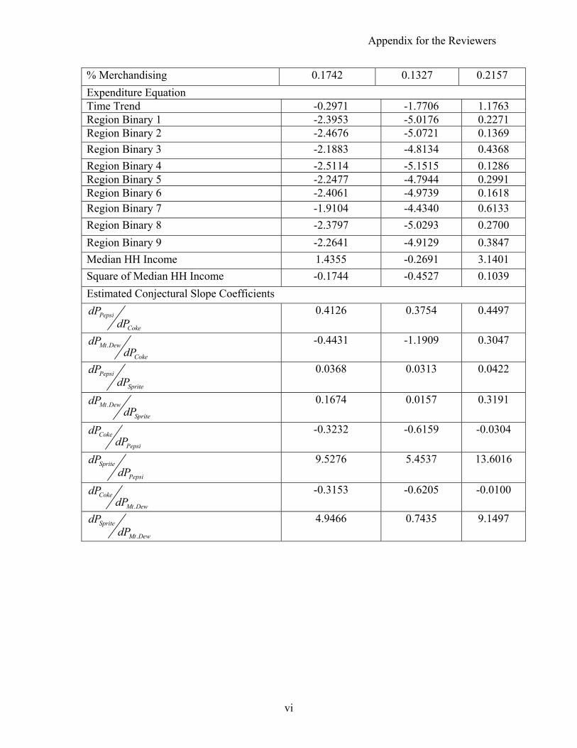
Table A2 for the Reviewer: Regression Results (CV Model): Variable Value Confidence Interval (95%)
Coke Lower Upper Region Binary 1 0.4449 0.5015 0.3882 Region Binary 2 0.3095 0.3549 0.2640 Region Binary 3 0.3926 0.4251 0.3601 Region Binary 4 0.3710 0.4145 0.3275 Region Binary 5 0.5511 0.5810 0.5211 Region Binary 6 0.5998 0.6410 0.5585 Region Binary 7 0.7025 0.7387 0.6663 Region Binary 8 0.3073 0.3692 0.2453 Region Binary 9 0.3793 0.4208 0.3377 Median Age 0.1464 0.5724 -0.2796 Median Household Size 0.8413 1.4682 0.2144 % of HH earning less than $10,000 0.0486 0.1018 -0.0046 % of HH earning more than $50,000 0.1068 0.1906 0.0230 Supermarket to grocery sales ratio 0.0573 0.2010 -0.0864 Total Expenditure on Softdrinks 0.0788 0.0545 0.1031 Price of Coke -1.1842 -1.2316 -1.1369 Price of Sprite 0.0063 0.0019 0.0108 Price of Pepsi -0.1314 -0.1413 -0.1215 Sprite Region Binary 1 0.0907 0.0808 0.1006 Region Binary 2 0.0632 0.0526 0.0739 Region Binary 3 0.0547 0.0477 0.0618 Region Binary 4 0.0458 0.0392 0.0525 Region Binary 5 0.0832 0.0762 0.0901 Region Binary 6 0.0915 0.0839 0.0991 Region Binary 7 0.1004 0.0943 0.1065 Region Binary 8 0.0661 0.0559 0.0762 Region Binary 9 0.0629 0.0537 0.0721 Median Age 0.1221 0.0347 0.2095 Median Household Size 0.2546 0.1255 0.3837 % of HH earning less than $10,000 -0.0024 -0.0156 0.0108 % of HH earning more than $50,000 0.0211 0.0063 0.0360 Supermarket to grocery sales ratio 0.0243 -0.0044 0.0530
iv

Appendix for the Reviewers
Total Expenditure on Softdrinks -0.0091 -0.0199 0.0018 Price of Coke Price of Sprite 0.9848 0.9376 1.0321 Price of Pepsi 0.2576 0.2415 0.2736 Sprite Region Binary 1 0.4220 0.3638 0.4802 Region Binary 2 0.5499 0.4938 0.6060 Region Binary 3 0.4567 0.4198 0.4936 Region Binary 4 0.5015 0.4528 0.5501 Region Binary 5 0.3099 0.2712 0.3486 Region Binary 6 0.2718 0.2101 0.3334 Region Binary 7 0.1812 0.1406 0.2219 Region Binary 8 0.5786 0.5071 0.6502 Region Binary 9 0.4942 0.4472 0.5412 Median Age -0.3002 -0.7958 0.1955 Median Household Size -1.1276 -1.8641 -0.3911 % of HH earning less than $10,000 -0.0435 -0.1092 0.0222 % of HH earning more than $50,000 -0.1025 -0.1985 -0.0066 Supermarket to grocery sales ratio -0.0531 -0.2181 0.1118 Total Expenditure on Softdrinks -0.1117 -0.1414 -0.0820 Price of Coke Price of Sprite Price of Pepsi -1.3475 -1.3988 -1.2962
Cost Side Variables Coke Intercept 0.0984 0.0871 0.1098 Volume per Unit 3.9901 3.7042 4.2761 % Merchandising 0.2982 0.2783 0.3181 Sprite Intercept 0.0191 0.0172 0.0209 Volume per Unit 2.9059 2.5447 3.2672 % Merchandising 0.2663 0.2440 0.2887 Pepsi Intercept 0.1314 0.1247 0.1381 Volume per Unit 3.0537 2.8704 3.2371 % Merchandising 0.3287 0.3142 0.3431 Mountain Dew Intercept 0.0104 0.0077 0.0132 Volume per Unit 5.6314 4.8186 6.4442
v
Appendix for the Reviewers
vi
% Merchandising 0.1742 0.1327 0.2157 Expenditure Equation Time Trend -0.2971 -1.7706 1.1763 Region Binary 1 -2.3953 -5.0176 0.2271 Region Binary 2 -2.4676 -5.0721 0.1369 Region Binary 3 -2.1883 -4.8134 0.4368 Region Binary 4 -2.5114 -5.1515 0.1286 Region Binary 5 -2.2477 -4.7944 0.2991 Region Binary 6 -2.4061 -4.9739 0.1618 Region Binary 7 -1.9104 -4.4340 0.6133 Region Binary 8 -2.3797 -5.0293 0.2700 Region Binary 9 -2.2641 -4.9129 0.3847 Median HH Income 1.4355 -0.2691 3.1401 Square of Median HH Income -0.1744 -0.4527 0.1039 Estimated Conjectural Slope Coefficients
Pepsi
Coke
dPdP
0.4126 0.3754 0.4497
.Mt Dew
Coke
dPdP -0.4431 -1.1909 0.3047
Pepsi
Sprite
dPdP
0.0368 0.0313 0.0422
.Mt Dew
Sprite
dPdP 0.1674 0.0157 0.3191
Coke
Pepsi
dPdP -0.3232 -0.6159 -0.0304
Sprite
Pepsi
dPdP
9.5276
5.4537
13.6016
.
Coke
Mt Dew
dPdP -0.3153
-0.6205 -0.0100
.
Sprite
Mt Dew
dPdP
4.9466 0.7435 9.1497