Embed Size (px)
Citation preview
=
UNIVERSITY OF MICHIGAN
=
=
==
Working Paper ==
Integrated Optimization of Procurement, Processing and Trade of Commodities
Sripad K. Devalkar Stephen M. Ross School of Business
at the University of Michigan
Ravi Anupindi
Stephen M. Ross School of Business at the University of Michigan
Amitabh Sinha
Stephen M. Ross School of Business at the University of Michigan
Ross School of Business Working Paper Series
Working Paper No. 1095 August 2007
This paper can be downloaded without charge from the
Social Sciences Research Network Electronic Paper Collection: http://ssrn.com/abstract=1004742
Integrated Optimization of Procurement, Processing and Trade of
Commodities
Sripad K Devalkar, Ravi Anupindi, Amitabh Sinha
Stephen M. Ross School of Business, University of Michigan, Ann Arbor, MI 48109
[email protected], [email protected], [email protected]
August 2007
Abstract
We consider an integrated optimization problem for a firm involved in procurement, process-
ing and trading of commodities. We first derive optimal policies for a risk-neutral firm, when
the processed commodity(ies) are sold using futures instruments. We find that the optimal pro-
curement quantity is governed by a threshold policy, where the threshold is independent of the
starting inventory level, and it is optimal to postpone all processing till the last possible period.
We extend the model to include risk-averse firms, using a Value-at-Risk constraint on the total
expected profits. We show that the optimal procurement quantity for a risk-averse firm is never
greater than that for a risk-neutral firm and a risk-averse firm may find it optimal to process
and sell the output commodity in earlier periods. We conduct numerical studies to quantify the
benefit from integrated decision making and the impact of risk-aversion on expected profits.
Keywords: Integrated Optimization; Commodities; Risk; Value-at-Risk
1 Introduction
Consider a firm that procures an input commodity, processes it into one or more output commodi-
ties, and trades both input and output commodities for profit. For such firms, there are three
critical decision-making stages: the procurement of the input commodity, the commitment of the
input commodity to processing (an irreversible transformation of the input commodity into output
commodities), and the trading of the input and output commodity(ies). Examples of such input-
output commodity sets include corn and ethanol; soybean and soymeal/oil; oranges and orange
juice; crude oil and refined petroleum products; etc. The firm’s objective of profit maximization is
affected by the interplay of decisions in all three stages: procurement, processing and trading. In
the literature (reviewed in §2), however, typically these stages are analyzed independently of one
another, leading to possibly sub-optimal strategies for the overall integrated problem. While the
processing costs may be somewhat well-predictable or deterministic, the procurement costs and
revenues from trading are driven by spot and futures prices of the commodities in international
exchanges, as well as local prices (trading with small-scale farmers or independent users of the
commodities), which are stochastic and not predictable with certainty.
An additional level of complexity is added when firms’ risk profile is considered. Commodity
prices are time-varying and stochastic, and the correlation between prices of the input and output
commodities are not perfect. The stochastic prices result in the potential for huge downside losses
if, for example, commodity prices fall after the input commodity has already been procured and
held in inventory for processing and /or trading at a later point in time. Naturally, firms wish to
guard against such downside risk by adopting risk-averse behavior strategies, which further modify
the optimal policies for the three stages of procurement, processing and trading.
Traditional research in operations management has addressed the problem in each of the decision
stages independently, usually under the assumption of risk neutrality. Resultantly, the overall
integrated optimization problem presents both an interesting challenge and an opportunity to fill
a substantial gap in the literature. This paper seeks to fill some of the gap by deriving integrated
optimal policies across the three decision stages under different scenarios of the general problem.
1.1 Our Contributions
We consider a firm that earns revenues by procuring and processing an input commodity, and
committing to sell the output of the processing in a futures contract and/or salvaging the input
1
inventory in a spot market at the end of the horizon. We begin with the study of a risk-neutral
firm and find that the optimal procurement policy is a threshold policy, where the threshold is
independent of the starting inventory level. We also find that it is optimal for a risk-neutral firm to
postpone the processing and sale of the output using a futures contract until the last period before
the maturity of the futures contract.
When risk-averse behavior is considered, however, the firm may in fact find it optimal to commit
to sell the output in periods other than the last. However, these commitments are solely to manage
its risk and result in lower expected profits. The procurement policy is still a threshold policy, but
the threshold may depend on the starting inventory level.
We also conduct a numerical study, highlighting the impact of risk-averse behavior as well as
the benefits of integrated decision making. While firms not practicing integrated decision-making
can and do follow a variety of different operational strategies, we compare the benefits with respect
to a specific policy1 we term the ‘full-commitment’ policy, described in §3.1.1. We find that there
is a significant difference in expected profits between the optimal and full-commitment policies,
and risk-aversion plays a significant role in optimal policies and expected profits, confirming the
theoretical results.
Finally, we also consider the case of a firm that has access to multiple futures contracts for the
output. For a risk-neutral firm, the structure of the procurement policy is unchanged. However, it
may be optimal to commit to process before the end of the horizon. If this is done, the commitment
is always in a period just before the expiration of a futures contract and only if the margin from
the expiring contract exceeds the maximum expected margin of retaining unprocessed inventory.
Furthermore, if such an option is exercised, all available inventory is committed.
1.2 Motivation
The original motivation for this work comes from the innovative practices of one of India’s largest
private sector companies, The ITC Group (www.itcportal.com). While ITC is a diversified com-
pany, the International Business Division (IBD) of ITC exports agricultural commodities such as
soybean meal, rice, wheat and wheat products, etc. As a buyer of these agricultural commodities,
ITC-IBD faced the consequences of an inefficient farm-to-market supply chain amidst increasing
competition in a liberalized economy. In response, in the year 2000 ITC-IBD (hereafter referred to
as ITC) embarked on an initiative to deploy information and communication technology (ICT) to1This policy is used by The ITC Group, the firm that motivated this research, as described in §1.2.
2
Trade of
output
(soymeal
& oil)
Trade
of input
(soybean)
Processing
Storage
Hub
Hub
Hub
Input
(soybea
n)
e-Choupals
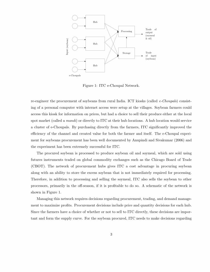
Figure 1: ITC e-Choupal Network.
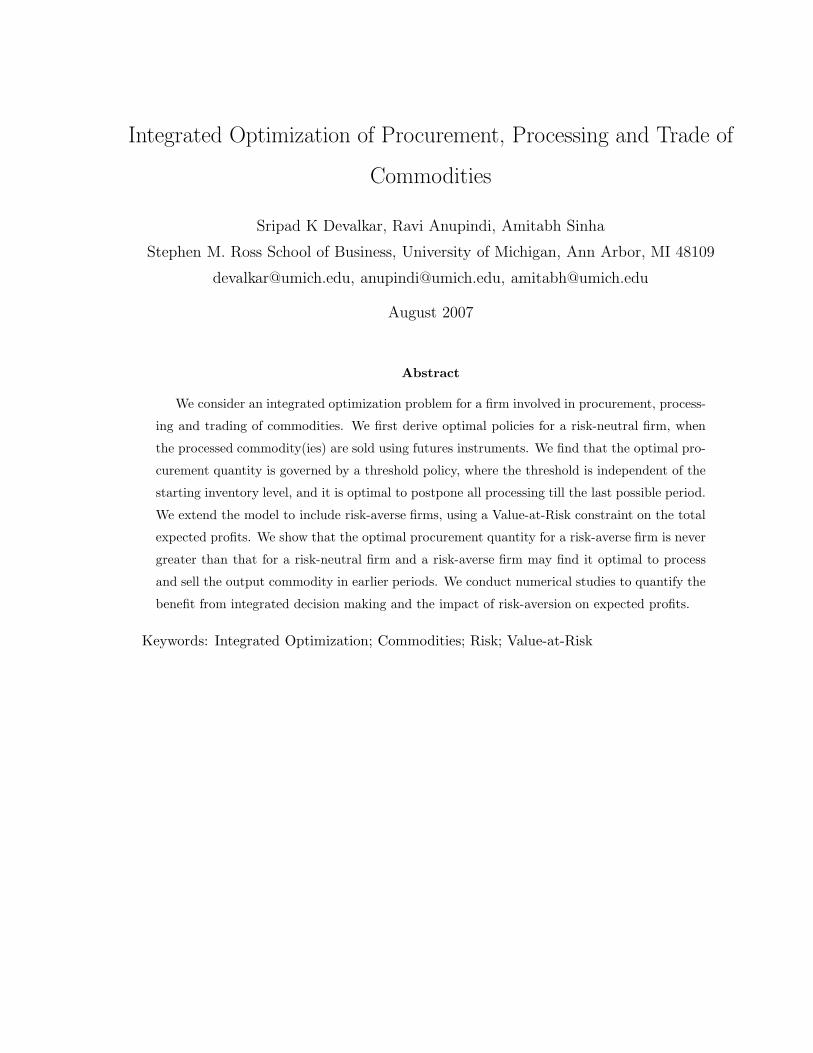
re-engineer the procurement of soybeans from rural India. ICT kiosks (called e-Choupals) consist-
ing of a personal computer with internet access were setup at the villages. Soybean farmers could
access this kiosk for information on prices, but had a choice to sell their produce either at the local
spot market (called a mandi) or directly to ITC at their hub locations. A hub location would service
a cluster of e-Choupals. By purchasing directly from the farmers, ITC significantly improved the
efficiency of the channel and created value for both the farmer and itself. The e-Choupal experi-
ment for soybeans procurement has been well documented by Anupindi and Sivakumar (2006) and
the experiment has been extremely successful for ITC.
The procured soybean is processed to produce soybean oil and soymeal, which are sold using
futures instruments traded on global commodity exchanges such as the Chicago Board of Trade
(CBOT). The network of procurement hubs gives ITC a cost advantage in procuring soybean
along with an ability to store the excess soybean that is not immediately required for processing.
Therefore, in addition to processing and selling the soymeal, ITC also sells the soybean to other
processors, primarily in the off-season, if it is profitable to do so. A schematic of the network is
shown in Figure 1.
Managing this network requires decisions regarding procurement, trading, and demand manage-
ment to maximize profits. Procurement decisions include price and quantity decisions for each hub.
Since the farmers have a choice of whether or not to sell to ITC directly, these decisions are impor-
tant and form the supply curve. For the soybean procured, ITC needs to make decisions regarding
3
whether to trade the bean (typically at the end of the planning horizon, which is the off-season
for procurement but may still have processing activity arising from other firms) or process it and
trade the oil and meal. Finally, the procurement decision needs to be integrated with the decision
to manage the demand in terms of the form of output commodity and channels to trade in. Based
on our extensive discussions with ITC, we observe that the decisions of procurement, allocation,
and sale are not coordinated. This disconnect is also seen in the literature, with relatively little
academic work on the integrated optimization problem.
While the ITC e-choupal network was our introduction to the area and our initial motivation,
the model we analyze is quite generic and applies to other contexts as well. Any firm engaged in
the procurement of an input commodity with a choice of whether, and when, to irreversibly process
it into an output commodity faces such a decision-making problem. For instance, the increasing
use of ethanol as an alternative to fossil fuels presents a similar optimization problem for corn
producers and procurers. The model can also be extended in a variety of other directions, some of
which are discussed in the conclusion of the paper.
1.3 Outline
In §2 we review the literature related to commodity procurement and processing, and joint opera-
tional and financial hedging. §3 describes the mathematical model for the integrated optimization
problem. We derive optimal policies for a risk-neutral and risk-averse firm when there is a single
futures contract available for trading the output in §3.1 and §3.2 respectively. Numerical calcu-
lations for the single futures case are presented in §3.3. We also consider the optimal policy for
a risk-neutral firm in the presence of multiple futures contracts with different maturities in §4.Conclusions and open research questions are discussed in §5.
2 Literature Review
The trading of commodities is a fairly old economic activity, and a steady stream of literature has
developed on the modeling of commodity prices and derivatives and their trading. Working (1949)
is one of the earliest to study the relation between storage decisions and commodity prices and
introduced the idea of convenience yield2. Geman (2005) is a recent and comprehensive book on2The return on storage, or the convenience yield, is the benefit of avoiding frequent deliveries and frequent
production schedule changes to meet demand, when one has stock of the commodity available.
4
commodity prices, including agricultural commodities. Other recent papers on pricing commodities
in the spot and futures markets include Gibson and Schwartz (1990), Pindyck (2001), Routledge
et al. (2000) and Routledge et al. (2001). The work of Gibson and Schwartz (1990) was general-
ized by Schwartz and Smith (2000), who use a general two-factor model comprised of a long-run
equilibrium as well as short-term mean-reverting fluctuations. We use a variation of this model in
our preliminary numerical analysis to validate our findings. We observe here that all these papers
(with the exception of Routledge et al. (2001)) focus on single commodities, and do not model the
relationship between the prices of two commodities, one of which is an input to and the other the
output of some process.
The widespread use of futures markets to trade and hedge risk has led to a substantial body of
associated literature as well. Working (1953) is among the earliest papers to study the use of futures
markets for trading and hedging. Risk management in agriculture was studied by Goy (1999), who
explores various hedging strategies available to farmers in the U.S. Anderson and Danthine (1995),
Tsang and Leuthold (1990) and Dahlgran (2002), among others, study a single period problem
of hedging positions in multiple commodities using futures instruments while Myers and Hanson
(1996) consider the problem of dynamical hedging the risk from a single commodity over multiple
periods. It has been observed that commodity processing decisions in the aggregate are correlated
with output commodity prices; an exploration of this phenomenon in the soybean crushing industry
by Plato (2001) finds some empirical evidence that firms strategically use the commodity markets
to optimally time their operational (processing) decisions. Most of the papers mentioned above
consider either a single commodity or single period in their analysis, but not both. In contrast, we
study the dynamic hedging and optimization of multiple commodities over a horizon.
In the past few years, a series of papers in the operations literature have begun to focus on
using financial hedging strategies to mitigate inventory and other operational risks. These include
Caldentey and Haugh (2006), who view the operations of the firm as an asset for investment and use
portfolio analysis techniques; Gaur and Seshadri (2005), who study the hedging of inventory risk in a
newsvendor setting; and Zhu and Kapuscinski (2006) and Chowdhry and Howe (1999), who consider
operational and financial hedging for multinational firms facing exchange rate risk in addition to
uncertain demand. Perhaps most closely related to our work is the recent work of Goel and Gutierrez
(2006), who analyze the integration of spot and futures markets for optimal procurement strategies
of commodities in a multi-period setting. All of these papers, however, continue to focus on trade
on only one side: either the input (procurement) or the output commodity, without analyzing the
5
integrated decision of optimizing strategies over both commodities.
As can be seen by the literature survey above, there is substantial academic work on the
individual pieces of the decision making involved in the type of firm we study, such as procurement
over spot and futures markets, hedging inventory with markets, etc. However, there are no studies
that we are aware of, which look at the integrated problem of of procuring, processing and trading
of commodities. It is this gap in the literature that we hope to address in the current paper.
3 Model Description
We consider a finite horizon model for the integrated procurement and processing decisions of a
firm that maximizes discounted expected profit over the horizon. The firm may be risk-neutral or
risk-averse and the two cases are analyzed in §3.1 and §3.2 respectively.
The time periods are indexed by n = 1, 2, . . . , N − 1, N , with n = 1 being the first decision
period. In any period n, let Sn denote the spot market price for the input commodity. The firm
sells all the processed product (output) using futures contracts that are traded on an exchange.
A futures contract is an agreement between two parties to buy or sell a certain quantity of a
commodity at a certain time in the future for a certain price (Hull 1997). Futures contracts are
normally traded on an exchange, with the exchange specifying certain standardized features of the
contract, such as the quality and delivery location. The price specified on the futures contract at
which the commodity (the processed product or output in the current model) can be sold or bought
is known as the futures price and this price changes over time. Let F ln denote the futures price on
a futures contract l for the output, with maturity Nl > n. We assume that there are L futures
contracts, with maturities Nl, l = {1, 2, . . . ,K} with Ni < Nj for i < j.
Any leftover inventory of the input at the end of the horizon is salvaged at the prevailing
spot price in the last period, SN . In the ITC context, the planning horizon can be considered as
the procurement season, when bulk of the procurement happens. The end of the horizon can be
thought of as the off-season, when most of the trading of the input (soybean) occurs. Therefore,
SN models the off-season trading price for the input and it may be substantially different from
the spot prices during the procurement season. Under certain conditions, the margins from just
holding the input inventory and trading it at the end of the horizon might result in significantly
higher profits. Considering this potential for trade is critical in our integrated decision-making.
Let In denote all the relevant information regarding the spot market prices, futures prices and
6
the end of the horizon salvage value available to the firm in period n. Thus, In includes the realized
spot market price, futures prices and could include other information like aggregate inventory levels
of the commodities, inventory levels with other processors, etc. A definition of In at this general
level is sufficient for the purposes of model being considered.
The availability of labor, handling equipment and other operational constraints at the procure-
ment hub impose a restriction on the amount of the input commodity that can be procured in any
given period. For simplicity, we assume that the procurement capacity in every period is the same
and let K > 0 denote the maximum quantity of the input that can be procured in any given period
at the hub; i.e., xn ≤ K for all n ≤ N − 1. We later show, in §3.1.3, that relaxing this assumption
does not alter the structural results obtained.
Thus, in each period n, based on In, the firm decides the quantity of input, xn, to be procured
and the quantity of the processed product, qln, to be committed for sale using a futures contract l,
with the revenues being realized in period Nl. Any leftover inventory of the input at the end of the
horizon is sold to other firms, at a per-unit salvage value of SN .
Naturally, a commitment to sell the output can be made only using a futures contract that
matures later in the horizon; i.e., qln makes sense only when n < Nl. Furthermore, since we
consider a situation where sales of a futures contract are settled by actual delivery of the processed
product, it is costly to reverse a commitment. Therefore, we require that at the time of expiration
of a futures contract, the total amount committed does not exceed the total amount procured:
l∑j=1
Nj−1∑i=1
qji ≤
Nl−1∑i=1
xi ∀ l ≤ L (1)
However, temporary over-commitment is allowed: the firm at an intermediate point of time may
have more commitments than the available inventory, as long as the shortfall is made up before
expiration of the futures contract.
We assume that there are no processing capacity restrictions and the quantity committed is
limited only by the total amount procured. This assumption is made for analytical tractability
and to focus attention on the value of integrated decision making. Observe that infinite processing
capacity implies that the firm would never process the input without a commitment to sell the
output.
The firm also has an endogenous procurement cost function C(Sn, xn), which is the total cost
incurred to procure xn units if the spot price is Sn. In the simplest case (that of constant marginal
costs), C(Sn, xn) is simply Sn × xn, but in general, the cost of procurement may be increasing and
7
convex due to market factors. An alternative view of this cost function is in the context of ITC;
ITC announces a one-day forward price for input procurement directly at its hubs. The resulting
supply is a function of the price announced by ITC as well as the prevailing spot price. Inverting
this supply function results in the cost function C(Sn, xn).
For ease of exposition and without loss of generality, we assume there is no discounting and
that the physical costs of holding inventory are negligible3. The firm, however, incurs a processing
cost of p per unit of input that is processed.
Input
Inven
tory
,C
om
mit
men
ts
Uncommittedinput inventory
Processingcommitment
1 k NjN
Time period n
Nj − 1 N − 1
xn,q n
Procurement xn Commitment qn
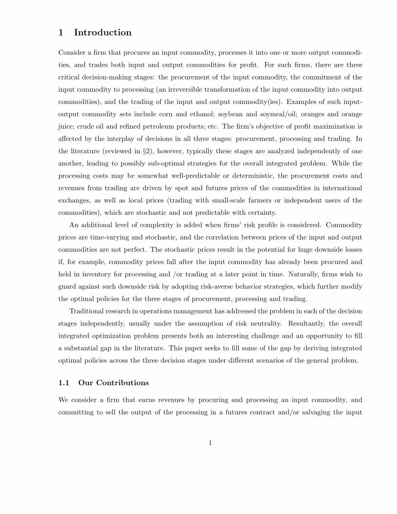
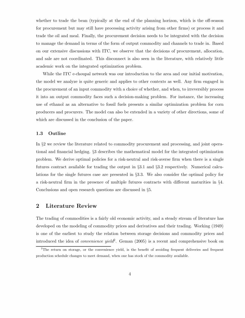
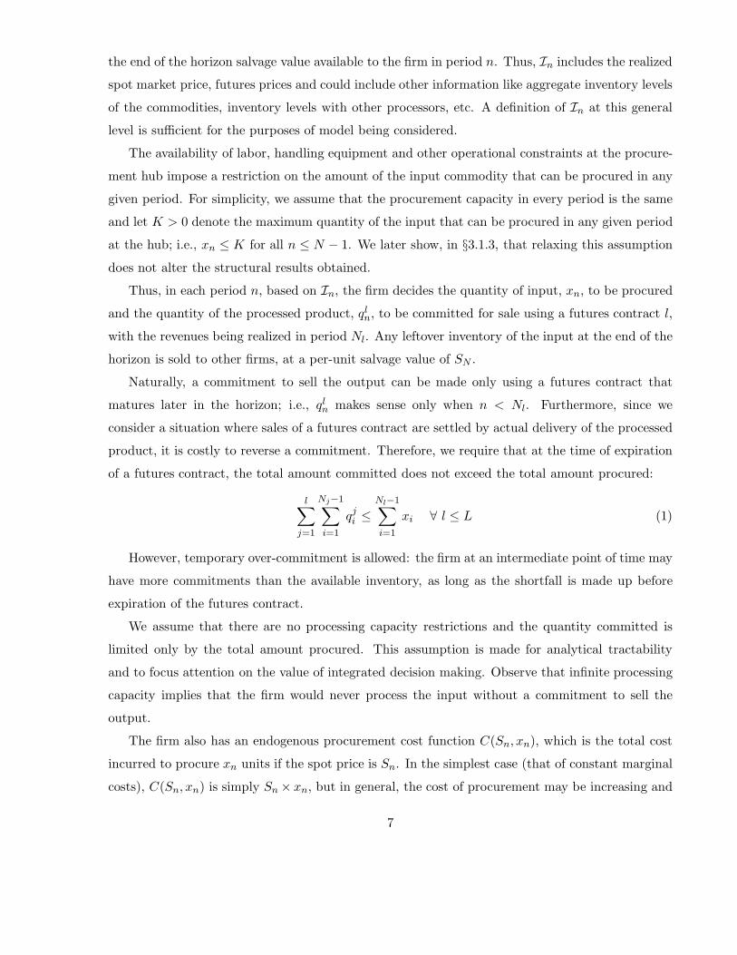
Figure 2: Sample Path for Inventory and Processing Commitment.
A theoretical sample path for the input inventory and processing commitments is shown in
Figure 2. The top portion shows the net input inventory after commitments and the cumulative
commitments against contract j, expiring in period Nj . Period N is the end of the horizon (begin-
ning of the off-season) and period N−1 is the last period in which any procurement or commitments
can be made. The bottom portion of the figure shows the procurement and commitment (against
futures contract j), xn and qjn, in each period n. Above, the firm has an over-commitment at the
end of period k. However, because of (1), the firm can additionally commit only a small quantity3From the analysis that follows, assuming a discount factor α < 1 and imposing a positive holding cost on inventory
does not alter the structure of the optimal policy discussed below and hence these assumptions are not restrictive.
8
in the last period, Nj − 1, before the contract expires.
3.1 Single Futures Contract: Risk-neutral Firm
We begin by considering the case when the firm is risk-neutral and a single futures contract is
available for selling the processed product; later we extend the analysis to include risk-aversion and
multiple futures contracts.
Since there is only one futures contract, we drop the superscript l in the notation for the rest of
this section. W.l.o.g., we assume the futures contract expires in the last period, N , and Fn denotes
the futures price on the contract in period n. If the firm decides to commit qn to be sold against the
futures contract in period n, the revenue realized (at the end of the horizon) is given by (Fn −p)qn.
Let en denote the cumulative excess (or shortfall) of the input commodity over commitments
already made at the beginning of period n. That is, en = e1 +∑n−1
i=1 xi −∑n−1
i=1 qi, where e1 is
the quantity of the input available at beginning of period 1. Only the uncommitted inventory at
the beginning of period n is relevant for the procurement and processing decisions in period n.
Therefore, the pair (en,In) is sufficient to describe the state at period n.
We consider an efficient market for all commodities, i.e., a market without arbitrage opportuni-
ties. A well known result in the financial literature is that in a risk-neutral world, the futures price
in any period is equal to the expected spot price of the commodity at maturity (see Hull (1997)
sec. 3.9, Bjork (2004) sec. 7.6). That is, Fn = E[YN |In], where E[·] denotes the expectation oper-
ator, YN is the spot price of the commodity underlying the futures contract at maturity. It follows
that Fn+1 = E[YN |In+1], and E[Fn+1|In] = E[E[YN |In+1]|In] = E[YN |In] = Fn. Therefore, the
following assumption holds for the remaining analysis in this section.
Assumption 1 The markets for the input and output commodities are efficient and the futures
prices for the output satisfy the following property: E[Fn+1|In] = Fn for n = 1, 2, . . . , N − 1.
Let Vn(en,In) denote the optimal expected profit starting from period n; i.e., if (en,In) is the
state at the start of period n, then Vn(en,In) denotes the additional maximal expected profits that
the firm can earn if optimal decisions are made in period n and all subsequent periods.
For en ≥ 0, n = 1, 2, . . . , N − 1, define Jn(en, qn, xn,In) as follows:
Jn(en, qn, xn,In) = (Fn − p)qn − C(Sn, xn) + EIn [Vn+1(en + xn − qn,In+1)] (2)
Vn(en,In) then satisfies the following dynamic programming equation:
Vn(en,In) = maxqn≥0, 0≤xn≤K
{Jn(en, qn, xn,In)} (3)
9
and VN (eN ,IN ) =
⎧⎨⎩
SNeN if eN ≥ 0
−∞ if eN < 0
The definition of VN (eN ,IN ) implies that we do not allow the total commitment to exceed the
total available inventory of the input when the futures contract expires, as required by (1).
Consider the period n = N − 1. When eN−1 ≥ 0, the marginal revenue from committing
to sell a unit of the input as processed product against the futures contract is FN−1 − p. The
marginal revenue from holding unprocessed inventory and salvaging it at the end of the horizon is
EIN−1[SN ]. We define processing margin as the expected margin from selling the output using the
futures contract and trade margin as the margin from holding unprocessed inventory and salvaging
it at the end of the horizon. We see that it is optimal to commit to sell the output only if the
processing margin is at least as much as the expected trade margin; i.e., FN−1 − p ≥ EIN−1[SN ].
Because of the convex cost of procurement, the total quantity to procure is given by the standard
first order condition where marginal cost of procurement is equal to the marginal revenue.
The following theorem formalizes this intuition and describes the optimal policy for n = N − 1.
Proofs for all the theorems are given in §A in the e-companion.
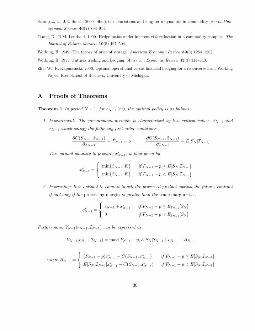
Theorem 1 In period N − 1, for eN−1 ≥ 0, the optimal policy is as follows.
1. Procurement: The procurement decision is characterized by two critical values, x̂N−1 and
x̃N−1 which satisfy the following first order conditions.
∂C(SN−1, x̂N−1)∂xN−1
= FN−1 − p∂C(SN−1, x̃N−1)
∂xN−1= E[SN |IN−1]
The optimal quantity to procure, x∗N−1, is then given by
x∗N−1 =
⎧⎨⎩
min{x̂N−1,K} if FN−1 − p ≥ E[SN |IN−1]
min{x̃N−1,K} if FN−1 − p < E[SN |IN−1]
2. Processing: It is optimal to commit to sell the processed product against the futures contract
if and only if the processing margin is greater than the trade margin; i.e.,
q∗N−1 =
⎧⎨⎩
eN−1 + x∗N−1 if FN−1 − p ≥ EIN−1
[SN ]
0 if FN−1 − p < EIN−1[SN ]
Furthermore, VN−1(eN−1,IN−1) can be expressed as
VN−1(eN−1,IN−1) = max{FN−1 − p,E[SN |IN−1]}.eN−1 + BN−1
10
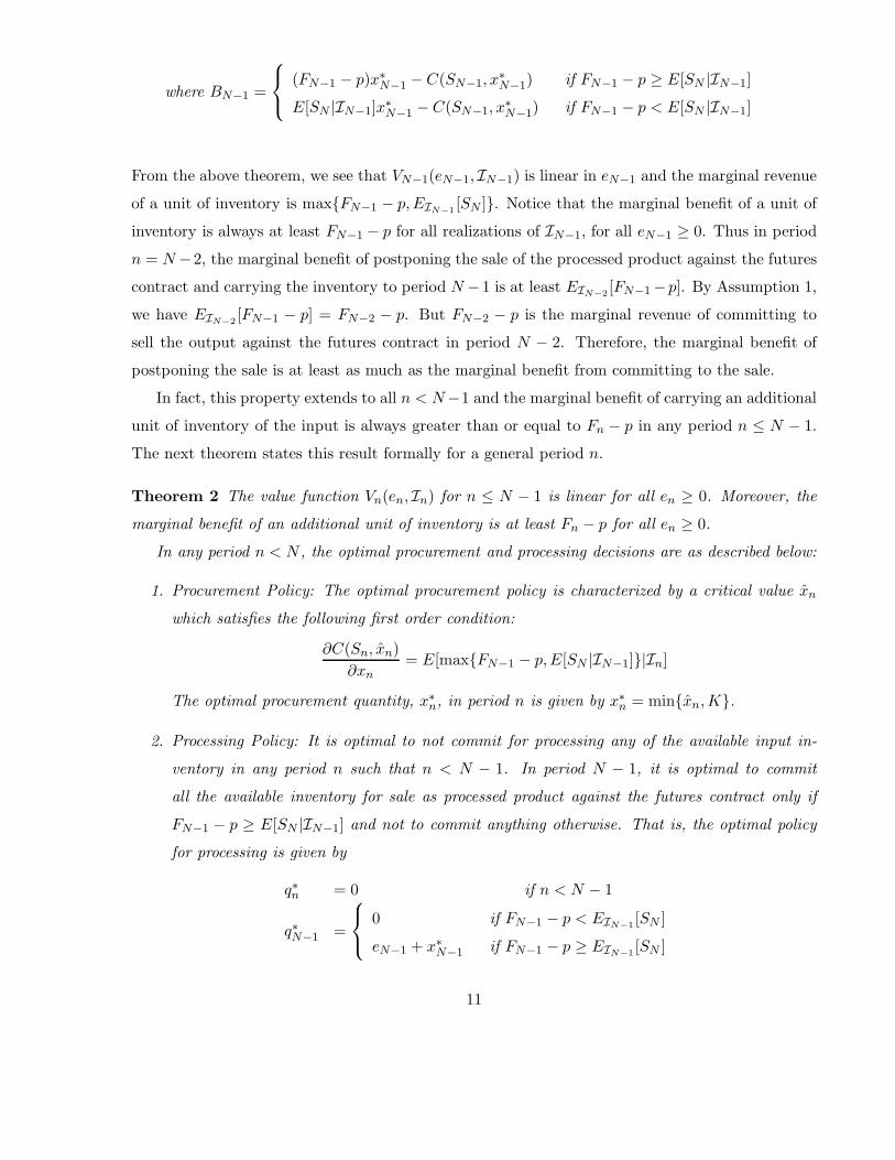
where BN−1 =
⎧⎨⎩
(FN−1 − p)x∗N−1 − C(SN−1, x
∗N−1) if FN−1 − p ≥ E[SN |IN−1]
E[SN |IN−1]x∗N−1 − C(SN−1, x
∗N−1) if FN−1 − p < E[SN |IN−1]
From the above theorem, we see that VN−1(eN−1,IN−1) is linear in eN−1 and the marginal revenue
of a unit of inventory is max{FN−1 − p,EIN−1[SN ]}. Notice that the marginal benefit of a unit of
inventory is always at least FN−1 − p for all realizations of IN−1, for all eN−1 ≥ 0. Thus in period
n = N −2, the marginal benefit of postponing the sale of the processed product against the futures
contract and carrying the inventory to period N −1 is at least EIN−2[FN−1 −p]. By Assumption 1,
we have EIN−2[FN−1 − p] = FN−2 − p. But FN−2 − p is the marginal revenue of committing to
sell the output against the futures contract in period N − 2. Therefore, the marginal benefit of
postponing the sale is at least as much as the marginal benefit from committing to the sale.
In fact, this property extends to all n < N−1 and the marginal benefit of carrying an additional
unit of inventory of the input is always greater than or equal to Fn − p in any period n ≤ N − 1.
The next theorem states this result formally for a general period n.
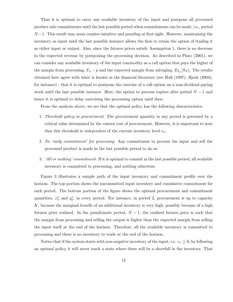
Theorem 2 The value function Vn(en,In) for n ≤ N − 1 is linear for all en ≥ 0. Moreover, the
marginal benefit of an additional unit of inventory is at least Fn − p for all en ≥ 0.
In any period n < N , the optimal procurement and processing decisions are as described below:
1. Procurement Policy: The optimal procurement policy is characterized by a critical value x̂n
which satisfies the following first order condition:
∂C(Sn, x̂n)∂xn
= E[max{FN−1 − p,E[SN |IN−1]}|In]
The optimal procurement quantity, x∗n, in period n is given by x∗
n = min{x̂n,K}.
2. Processing Policy: It is optimal to not commit for processing any of the available input in-
ventory in any period n such that n < N − 1. In period N − 1, it is optimal to commit
all the available inventory for sale as processed product against the futures contract only if
FN−1 − p ≥ E[SN |IN−1] and not to commit anything otherwise. That is, the optimal policy
for processing is given by
q∗n = 0 if n < N − 1
q∗N−1 =
⎧⎨⎩
0 if FN−1 − p < EIN−1[SN ]
eN−1 + x∗N−1 if FN−1 − p ≥ EIN−1
[SN ]
11
Thus it is optimal to carry any available inventory of the input and postpone all processed
product sale commitments until the last possible period when commitments can be made, i.e., period
N −1. This result may seem counter-intuitive and puzzling at first sight. However, maintaining the
inventory as input until the last possible instance allows the firm to retain the option of trading it
as either input or output. Also, since the futures prices satisfy Assumption 1, there is no decrease
in the expected revenue by postponing the processing decision. As described in Plato (2001), we
can consider any available inventory of the input commodity as a call option that pays the higher of
the margin from processing, Fn − p and the expected margin from salvaging, EIn [SN ]. The results
obtained here agree with what is known in the financial literature (see Hull (1997), Bjork (2004),
for instance) - that it is optimal to postpone the exercise of a call option on a non-dividend paying
stock until the last possible instance. Here, the option to process expires after period N − 1 and
hence it is optimal to delay exercising the processing option until then.
From the analysis above, we see that the optimal policy has the following characteristics:
1. Threshold policy in procurement: The procurement quantity in any period is governed by a
critical value determined by the convex cost of procurement. However, it is important to note
that this threshold is independent of the current inventory level en.
2. No ‘early commitment’ for processing: Any commitment to process the input and sell the
processed product is made in the last possible period to do so.
3. ‘All or nothing’ commitment: If it is optimal to commit in the last possible period, all available
inventory is committed to processing, and nothing otherwise.
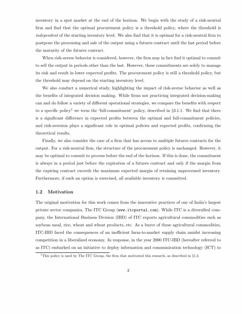
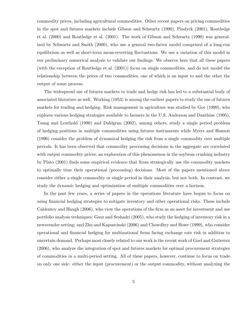
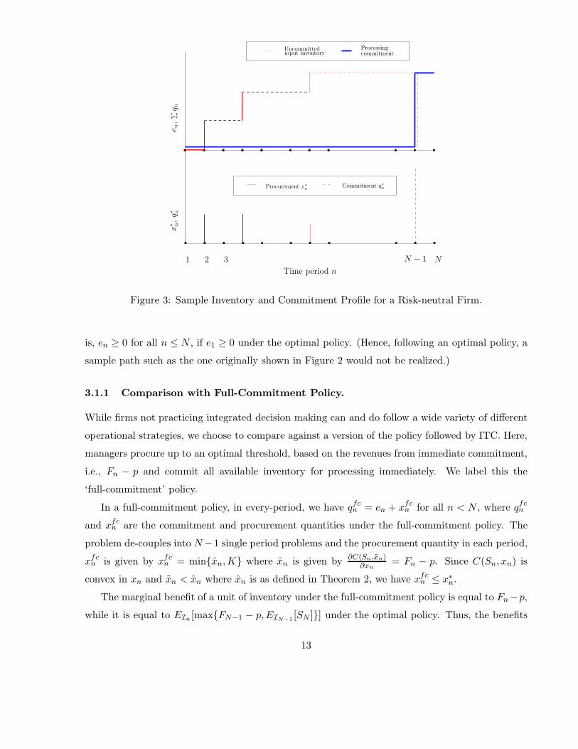
Figure 3 illustrates a sample path of the input inventory and commitment profile over the
horizon. The top portion shows the uncommitted input inventory and cumulative commitment for
each period. The bottom portion of the figure shows the optimal procurement and commitment
quantities, x∗n and q∗n, in every period. For instance, in period 2, procurement is up to capacity
K, because the marginal benefit of an additional inventory is very high, possibly because of a high
futures price realized. In the penultimate period, N − 1, the realized futures price is such that
the margin from processing and selling the output is higher than the expected margin from selling
the input itself at the end of the horizon. Therefore, all the available inventory is committed to
processing and there is no inventory to trade at the end of the horizon.
Notice that if the system starts with non-negative inventory of the input, i.e. e1 ≥ 0, by following
an optimal policy it will never reach a state where there will be a shortfall in the inventory. That
12
Uncommittedinput inventory
Processingcommitment
e n,
∑q n
1 3 N
Time period n
N − 12
x∗ n,q∗ n
Procurement x∗n
Commitment q∗n
Figure 3: Sample Inventory and Commitment Profile for a Risk-neutral Firm.
is, en ≥ 0 for all n ≤ N , if e1 ≥ 0 under the optimal policy. (Hence, following an optimal policy, a
sample path such as the one originally shown in Figure 2 would not be realized.)
3.1.1 Comparison with Full-Commitment Policy.
While firms not practicing integrated decision making can and do follow a wide variety of different
operational strategies, we choose to compare against a version of the policy followed by ITC. Here,
managers procure up to an optimal threshold, based on the revenues from immediate commitment,
i.e., Fn − p and commit all available inventory for processing immediately. We label this the
‘full-commitment’ policy.
In a full-commitment policy, in every-period, we have qfcn = en + xfc
n for all n < N , where qfcn
and xfcn are the commitment and procurement quantities under the full-commitment policy. The
problem de-couples into N −1 single period problems and the procurement quantity in each period,
xfcn is given by xfc
n = min{x̃n,K} where x̃n is given by ∂C(Sn,x̃n)∂xn
= Fn − p. Since C(Sn, xn) is
convex in xn and x̃n < x̂n where x̂n is as defined in Theorem 2, we have xfcn ≤ x∗
n.
The marginal benefit of a unit of inventory under the full-commitment policy is equal to Fn−p,
while it is equal to EIn [max{FN−1 − p,EIN−1[SN ]}] under the optimal policy. Thus, the benefits
13
from the optimal policy over the full-commitment policy accrue from (a) higher marginal benefit
for every unit of inventory and (b) higher procurement quantity in every period.
3.1.2 Special Case: Constant Marginal Costs.
As a further illustration of our findings, consider the special case of constant marginal costs of pro-
curement, i.e., C(Sn, xn) = Snxn. Since the marginal benefit of a unit of inventory is not dependent
on the procurement cost structure (when we start from non-negative inventory of the input), the
marginal benefit of inventory in any period n is still given by EIn [max{FN−1 − p,EIN−1[SN ]}].
The optimal processing policy remains the same as the one described in Theorem 2. The procure-
ment policy is much simpler and is given by an ‘all or nothing’ policy; that is, if EIn [max{FN−1 −p,EIN−1
[SN ]}] ≥ Sn, then it is optimal to procure up to the procurement capacity K in period n
and 0 otherwise.
3.1.3 General Procurement Capacities.
While we have assumed that the procurement capacity per period is a constant K, we show here that
relaxing this assumption is fairly straightforward. From the analysis above, the marginal benefit of
inventory is not dependent on the level of inventory. Therefore, even if the procurement capacity
is not the same in every period, the optimal processing policy still remains the same. The only
modification will be that the optimal procurement quantity would be given by x∗n = min{x̂n,Kn}
where Kn is the procurement capacity in period n and x̂n is as described in Theorem 2.
3.2 Single Futures Contract: Risk-averse Firm
Notice that the optimal policy in §3.1 requires the firm to keep the entire input inventory uncom-
mitted till the last possible period. Thus, there is significant uncertainty in the profits realized and
the firm is exposed to substantial down-side risk if prices fall. Typically, firms in the commodities
business have limited appetite for such risk. In this section, we explore how the optimal policy
changes when risk-aversion is incorporated as a constraint.
Risk aversion has been modeled in many different ways in the financial and agricultural eco-
nomics literature; Goy (1999) provides a good discussion on different approaches to modeling risk
and risk management tools that have been developed in the context of agricultural producers.
There are two major approaches to modeling risk attitude: (a) Value-at-Risk (VaR), and (b) vari-
ous forms of utility functions. VaR is defined as the maximum loss of value that a firm can incur
14
for a given confidence level and a time interval. Linsmeier and Pearson (2000) provide a discussion
on the concept of VaR and describe various methods used for computing it. VaR is widely used in
practice; for instance, Manfredo and Leuthold (1999) provide an analysis of VaR and its potential
applications for firms involved in the procurement and processing of agricultural commodities. We
also found that ITC uses a VaR measure to manage risk in their agribusiness. Based on all these
factors, we choose to model risk-aversion by using a VaR constraint.
The VaR constraint is characterized by a critical level of wealth, VaR, and a probability α. The
VaR constraint requires that the probability of wealth at the end of the time interval being below
the critical value VaR is no more than α. In our multi-period problem, in each period optimal
xn and qn values need to be computed which account for this critical level, given profits already
accumulated from past actions (which are deterministic and known). Therefore, we have a period-
specific value for the critical level, V aRn, (which incorporates past actions and revenues) which
only constrains actions taken in present and future periods.
In general, under a risk-averse probability measure, the futures price might not necessarily be
equal to the expectation of the future spot price. However, Assumption 1 (E[Fn+1|In] = Fn) is
often made in the literature (see Myers and Hanson (1996), Dahlgran (2002), e.g.). Therefore,
Assumption 1 continues to hold in our model as well.
Recall that Vn(en,In) represents the total expected profits to go from period n until the end of
the horizon. If we define wealth at the end of period n as the sum of the immediate profits from
actions in period n plus the total expected profits from period n + 1 onwards, the VaR constraint
for period n can then be expressed as P{(Fn − p)qn − C(Sn, xn) + Vn+1(en + xn − qn,In+1) ≤V aRn|In} ≤ α, where α is the maximum allowable probability that the total wealth at the end
of the period will be less than the critical level, and the probability measure is over all future
realizations of spot and futures prices of the two commodities.
The dynamic programming formulation for a risk-averse firm becomes
Vn(en,In) = max(qn≥0, 0≤xn≤K)
{Jn(en, qn, xn,In)} (4)
s.t. P{(Fn − p)qn − C(Sn, xn) + Vn+1(en + xn − qn,In+1) ≤ V aRn|In} ≤ α (5)
In the last period, since there is no uncertainty in profits, the VaR constraint is irrelevant. Thus
the profit function is given by VN (eN ,IN ) = SNeN if eN ≥ 0 and −∞ otherwise.
A commitment to process the input and sell the output in period n gives a risk-free marginal
revenue of Fn − p per unit. Carrying uncommitted inventory to the end of the horizon gives an
15
expected marginal revenue of E[SN |In] per unit. However, the realized marginal revenue from
uncommitted inventory is uncertain and hence risky. Thus, we can consider a commitment to
process as an investment in a risk-free asset while carrying uncommitted inventory of the input is
analogous to investing in a risky asset.
In a financial portfolio investment problem, for a risk-averse investor, the parameters of the VaR
constraint are such that investing all the available wealth into the risk-free asset will satisfy the
VaR constraint (see Arzac and Bawa (1977) e.g.). In the our model, this means that committing to
process all available inventory in any given period should satisfy the VaR constraint (5). Indeed,
the problem would be meaningless if this were not the case, because no combination of procurement
and processing quantities would meet the VaR constraint. We therefore assume that the following
holds throughout this section.
Assumption 2 The VaR constraint, equation (5), is always satisfied by committing to process
all the available inventory. That is, for all n < N , we have P{(Fn − p)(en + xn) − C(Sn, xn) +
Vn+1(0,In+1) ≤ V aRn|In} ≤ α for all xn ≥ 0 and all realizations of In.
At n = N − 1, the firm’s problem can be formulated as
VN−1(eN−1,IN−1) = maxqN−1≥0, 0≤xN−1≤K
{JN−1(eN−1, qN−1, xN−1,IN−1)} (6)
s.t. P{(FN−1 − p)qN−1 − C(SN−1, xN−1) + SN (eN−1 + xN−1 − qN−1) ≤ V aRN−1|IN−1} ≤ α (7)
Define SαN as follows: P{SN ≤ Sα
N |IN−1} = α. That is, SαN is the value of SN corresponding
to the critical fractile, α. (Since the distribution of SN is dependent on IN−1, the value SαN is a
function of IN−1. We suppress this dependence for notational convenience.) The following theorem
characterizes VN−1(eN−1,IN−1) and gives the optimal policy for n = N − 1.
Theorem 3 VN−1(eN−1,IN−1) is concave in eN−1 and such that ∂VN−1(eN−1,IN−1)∂eN−1
≥ FN−1 − p.
The optimal processing and procurement policy is as described below:
1. Procurement Policy: The optimal procurement quantity is characterized by two critical values,
x̂N−1 and x̃N−1, which satisfy the following first order conditions
∂C(SN−1, x̂N−1)∂xN−1
= FN−1 − p∂C(SN−1, x̃N−1)
∂xN−1= E[SN |IN−1]
16
respectively, and the optimal procurement quantity is given by
x∗N−1 =
⎧⎪⎪⎪⎪⎪⎪⎪⎪⎪⎪⎪⎪⎪⎪⎨⎪⎪⎪⎪⎪⎪⎪⎪⎪⎪⎪⎪⎪⎪⎩
min{x̂N−1,K} if FN−1 − p ≥ E[SN |IN−1]
min{x̂N−1,K} if FN−1 − p < E[SN |IN−1],
and SαN (eN−1 + x∗
N−1) − C(SN−1, x∗N−1) < V aRN−1
min{x̃N−1,K} if FN−1 − p < E[SN |IN−1],
and SαN (eN−1 + x∗
N−1) − C(SN−1, x∗N−1) ≥ V aRN−1
2. Processing Policy: The optimal quantity to commit for processing is given by
q∗N−1 =
⎧⎪⎪⎪⎪⎪⎪⎪⎪⎪⎪⎪⎪⎪⎪⎪⎪⎪⎪⎪⎪⎨⎪⎪⎪⎪⎪⎪⎪⎪⎪⎪⎪⎪⎪⎪⎪⎪⎪⎪⎪⎪⎩
eN−1 + x∗N−1 if FN−1 − p ≥ E[SN |IN−1]
V aRN−1−[SαN (eN−1+x∗
N−1)−C(SN−1,x∗N−1)]
(FN−1−p)−SαN
if FN−1 − p < E[SN |IN−1],
and SαN (eN−1 + x∗
N−1)
−C(SN−1, x∗N−1) < V aRN−1
0 if FN−1 − p < E[SN |IN−1],
and SαN (eN−1 + x∗
N−1)
−C(SN−1, x∗N−1) ≥ V aRN−1
From the above theorem, we find that in period N − 2, the marginal revenue from committing
to process a unit of input inventory, FN−2 − p, is less than the expected marginal revenue from
carrying the inventory into period N − 1, since EIN−2[∂VN−1(eN−1,IN−1)
∂eN−1] ≥ FN−2 − p. Therefore,
any commitment to process in period N − 2 reduces the expected profits, while increasing the
certainty of the profits (committing to process results in a known revenue of FN−2 − p for every
unit committed to be sold as the output). Thus, it is optimal to commit to process only the
minimum quantity required to meet the VaR constraint and carry the rest as uncommitted input
inventory.
From the definition of SαN , we have that P{VN (eN ,IN ) ≤ Sα
NeN |IN−1} = α. Therefore, SαNeN
can be interpreted as the value of VN (eN ,IN ) corresponding to the α fractile. For any general
period n, we define V αn (en) as the value of Vn(en,In) corresponding to the α fractile. That is,
P{Vn(en,In) ≤ V αn (en)|In−1} = α. (As in the case of Sα
N , we suppress the dependence of V αn (en)
17
on In−1 for notational convenience.) The next theorem describes the optimal policy for a risk-averse
firm in any period n < N − 1.
Theorem 4 For all n < N −1 and en ≥ 0, the value function Vn(en,In) is concave and increasing
in en, for all realizations of In and the marginal benefit of an unit of uncommitted inventory is
always greater than or equal to the processing margin; i.e., ∂Vn(en,In)∂en
≥ Fn − p. The optimal
procurement and processing policy is as given below
1. Procurement Policy: The optimal procurement quantity is characterized by two critical values,
x̂n and x̃n, which satisfy the following first order conditions
∂C(Sn, x̂n)∂xn
= Fn − p∂C(Sn, x̃n)
∂xn= E
[∂Vn+1(en + x̃n)∂en+1
|In
]
respectively, and the optimal procurement quantity is given by
x∗n =
⎧⎪⎪⎨⎪⎪⎩
min{x̂n,K} if V αn+1(en + x∗
n) − C(Sn, x∗n) < V aRn
min{x̃n,K} if V αn+1(en + x∗
n) − C(Sn, x∗n) ≥ V aRn
2. Processing Policy: The optimal quantity to commit for processing is given by
q∗n =
⎧⎪⎪⎨⎪⎪⎩
V aRn−[V αn+1(en+x̃n−q∗n)−C(Sn,xn)]
(Fn−p) if V αn+1(en + x∗
n) − C(Sn, x∗n) < V aRn
0 if V αn+1(en + x∗
n) − C(Sn, x∗n) ≥ V aRn
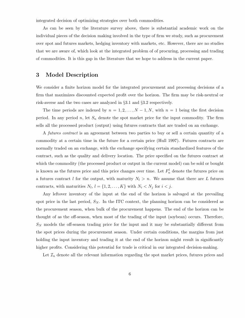
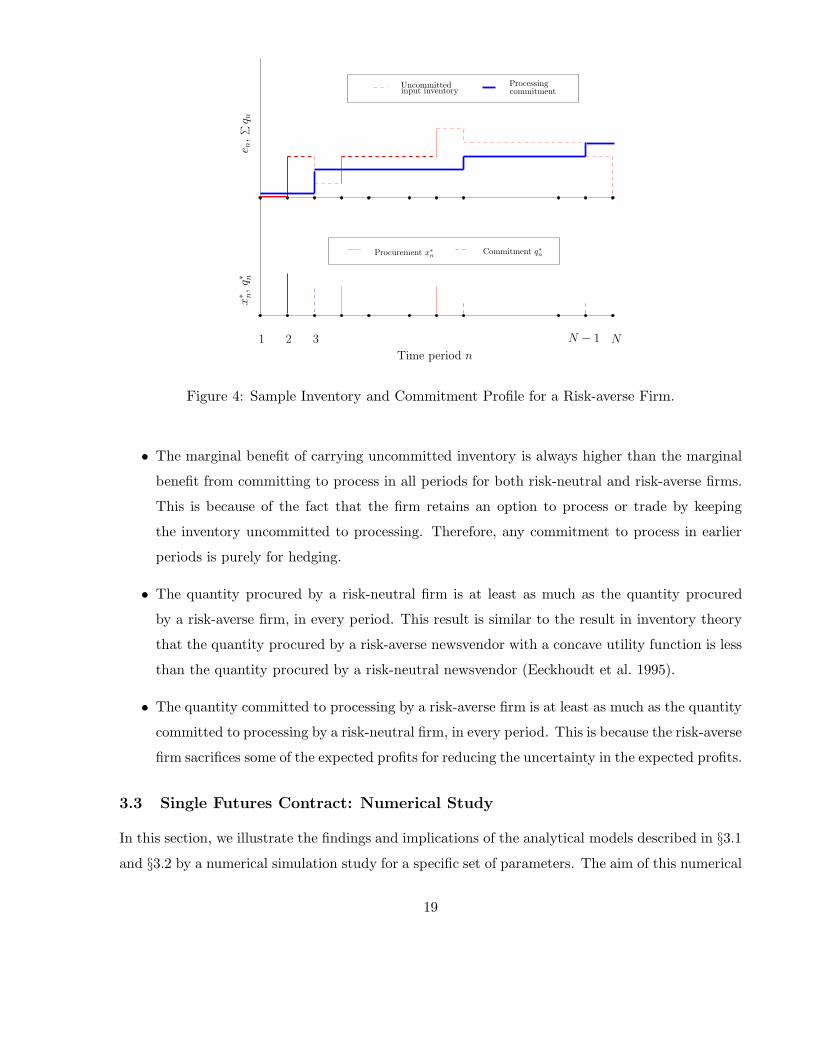
Figure 4 shows a sample path for the commitment and uncommitted input inventory profile.
From the figure, in period 3 the firm needs to commit a portion of the available input inventory
for processing to reduce the uncertainty in profits. Also, in the penultimate period, N − 1, the
expected margin from trading is higher than the margin from processing. Hence the firm finds it
optimal to commit only a portion of the available inventory to meet its VaR constraint and trade
the rest as input at the end of the horizon. Similarly, the marginal cost of procurement is high
enough in intermediate periods that there is almost zero procurement in those periods.
3.2.1 Comparison with Risk-neutral Case.
We note the following observations in comparing the findings of the risk-neutral and risk-averse
cases:
18
Uncommittedinput inventory
Processingcommitment
e n,
∑q n
x∗ n,q∗ n
1 3 N
Time period n
N − 12
Procurement x∗n
Commitment q∗n
Figure 4: Sample Inventory and Commitment Profile for a Risk-averse Firm.
• The marginal benefit of carrying uncommitted inventory is always higher than the marginal
benefit from committing to process in all periods for both risk-neutral and risk-averse firms.
This is because of the fact that the firm retains an option to process or trade by keeping
the inventory uncommitted to processing. Therefore, any commitment to process in earlier
periods is purely for hedging.
• The quantity procured by a risk-neutral firm is at least as much as the quantity procured
by a risk-averse firm, in every period. This result is similar to the result in inventory theory
that the quantity procured by a risk-averse newsvendor with a concave utility function is less
than the quantity procured by a risk-neutral newsvendor (Eeckhoudt et al. 1995).
• The quantity committed to processing by a risk-averse firm is at least as much as the quantity
committed to processing by a risk-neutral firm, in every period. This is because the risk-averse
firm sacrifices some of the expected profits for reducing the uncertainty in the expected profits.
3.3 Single Futures Contract: Numerical Study
In this section, we illustrate the findings and implications of the analytical models described in §3.1and §3.2 by a numerical simulation study for a specific set of parameters. The aim of this numerical
19
study is two-fold:
1. Quantify benefit from integrated decision making: As mentioned in §1, the decision-making
of the three stages of procurement, processing and trading are often done in isolation, in the
literature and in practice. One of the aims of this paper is to develop an integrated decision-
making policy, raising the question of how much better (w.r.t. expected profits) the integrated
policy is compared to the full-commitment policy (one of the many possible non-integrated
policies).
2. Quantify the impact of the VaR constraint: Imposing a VaR constraint on the expected profits
limits the probability of making severe losses. However, this reduction in the downside comes
at the cost of sacrificing some of the expected profits from waiting to commit until the end,
which is the optimal risk-neutral policy. The numerical study will help quantify the impact
of the VaR constraint on the expected profits and the distribution of profits by comparing
the optimal policies for a risk-neutral and risk-averse firm.
3.3.1 Implementation.
The implementation study was conducted on a specific chosen set of parameters, described below.
The optimal policy was calculated for each period for each combination of (en, Sn, Fn) over a range of
values of these three quantities, for every n = 1, 2, . . . , N . (For the purposes of this study, In consists
of just the spot and futures prices realized in the current period.) The distribution of (Sn+1, Fn+1),
given (Sn, Fn) for every pair (Sn+1, Fn+1) was estimated using the price process described in
§B in the electronic companion. The distribution thus generated was then used to estimate
EIn [Vn+1(en,In+1)] and V αn+1(en+1), given Vn+1(en+1,In+1) for each combination of (en+1,In+1),
in the range. Once EIn [Vn+1(en,In+1)] and V αn+1(en+1) are known, Vn(en,In), x∗
n(en,In) and
q∗n(en,In) can be calculated for each combination of (en,In) using the optimality equations (4) and
(5). Thus, starting with VN (eN ,IN ) = SNeN , the quantitities Vn(en,In),x∗n(en,In) and q∗n(en,In)
were estimated for each value of (en,In) in the range.
Once the policy parameters x∗n(en,In) and q∗n(en,In) were calculated, forward simulation runs
were implemented. Let Π(e1,I1) denote the profit over the entire horizon, for one sample path,
starting from an initial state of (e1,I1). The expectation of Π(e1,I1) over multiple sample paths
gives V1(e1,I1). The forward simulation runs were conducted in the following manner.
1. Set Π(e1,I1) = 0.
20
2. For n �= N , for a starting value of (en,In), choose x∗n and q∗n.
3. Update en+1 = en +x∗n− q∗n and n = n+1 and Π(e1,I1) = Π(e1,I1)+(Fn−p)q∗n−C(Sn, x∗
n).
4. For the given values of (Sn, Fn), generate the next period prices (Sn+1, Fn+1).
5. Repeat steps 2 to 4 until n = N .
6. For n = N , set Π(e1,I1) = Π(e1,I1) + SNeN and stop.
The optimal policies were computed for a horizon with N = 5 periods. With each period in
the model corresponding to 15 real days, a horizon of N = 5 models a significant portion of the
procurement season. The procurement capacity in each period, K, was normalized to 1 unit. The
uncommitted inventory levels, e, ranged from 0 to N ∗ K = 5, in steps of 0.1. The processing cost
was set to p = 5 per-unit. A procurement cost function, C(Sn, xn) = Snx1.5n was used.
For scaling purposes, in the numerical study, the long term equilibrium value of the input spot
price was set to 25. Correspondingly, the long run equilibrium of the output was scaled to 31. With
these values, policies were computed over a input spot price range of [10, 40] and output futures
price range of [11, 51], both in increments of 0.25. These limits were chosen such that the realized
spot and futures prices over the horizon would fall within the range 95% of the time. Observe also
that a processing cost of p = 5 corresponds to an expected processing margin of 1 (approximately
3.3%) which allows us to model situations when the actual realized processing margin may be large,
marginal or negative.
While this numerical study is based on specific values, we note that it is for illustration only.
If different parameters are chosen, the analysis in §3.1 and §3.2 shows that the broad conclusions
(greater profit with integrated decision-making, and risk-reward tradeoff with incorporation of risk-
aversion) will continue to hold; only their magnitudes will change.
3.3.2 Benefit from Integrated Optimization.
Optimal policies were calculated for the risk-neutral case and a total of 10, 000 simulation runs
were conducted using the optimal policy parameters generated. To exclude boundary effects, only
those simulation runs where the maximum futures price realized across the horizon is less than or
equal to 42 were considered from these simulation runs (At the boundary of the range of futures
price, Assumption 1 is violated and hence the optimal policies and the simulation run results
corresponding to these boundary values were not considered.). Similar, independent simulation
21
1 2 3 40.46
0.48
0.5
0.52
0.54
0.56
0.58
0.6
0.62
0.64
0.66
Period n
E[x
∗ n]
Optimal Policy
Full-Commitment Policy
1 2 3 40
0.2
0.4
0.6
0.8
1
1.2
1.4
Period n
E[q
∗ n]
Optimal Policy
Full-Commitment Policy
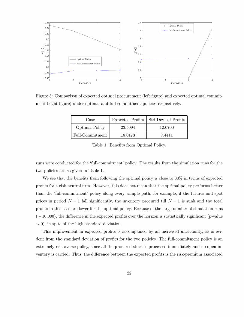
Figure 5: Comparison of expected optimal procurement (left figure) and expected optimal commit-
ment (right figure) under optimal and full-commitment policies respectively.
Case Expected Profits Std Dev. of Profits
Optimal Policy 23.5094 12.0700
Full-Commitment 18.0173 7.4411
Table 1: Benefits from Optimal Policy.
runs were conducted for the ‘full-commitment’ policy. The results from the simulation runs for the
two policies are as given in Table 1.
We see that the benefits from following the optimal policy is close to 30% in terms of expected
profits for a risk-neutral firm. However, this does not mean that the optimal policy performs better
than the ‘full-commitment’ policy along every sample path; for example, if the futures and spot
prices in period N − 1 fall significantly, the inventory procured till N − 1 is sunk and the total
profits in this case are lower for the optimal policy. Because of the large number of simulation runs
(∼ 10,000), the difference in the expected profits over the horizon is statistically significant (p-value
∼ 0), in spite of the high standard deviation.
This improvement in expected profits is accompanied by an increased uncertainty, as is evi-
dent from the standard deviation of profits for the two policies. The full-commitment policy is an
extremely risk-averse policy, since all the procured stock is processed immediately and no open in-
ventory is carried. Thus, the difference between the expected profits is the risk-premium associated
22
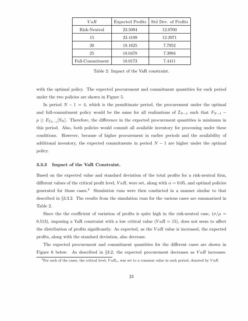
V aR Expected Profits Std Dev. of Profits
Risk-Neutral 23.5094 12.0700
15 23.4109 12.2971
20 18.1625 7.7952
25 18.0478 7.3994
Full-Commitment 18.0173 7.4411
Table 2: Impact of the VaR constraint.
with the optimal policy. The expected procurement and commitment quantities for each period
under the two policies are shown in Figure 5.
In period N − 1 = 4, which is the penultimate period, the procurement under the optimal
and full-commitment policy would be the same for all realizations of IN−1 such that FN−1 −p ≥ EIN−1
[SN ]. Therefore, the difference in the expected procurement quantities is minimum in
this period. Also, both policies would commit all available inventory for processing under these
conditions. However, because of higher procurement in earlier periods and the availability of
additional inventory, the expected commitments in period N − 1 are higher under the optimal
policy.
3.3.3 Impact of the VaR Constraint.
Based on the expected value and standard deviation of the total profits for a risk-neutral firm,
different values of the critical profit level, V aR, were set, along with α = 0.05, and optimal policies
generated for those cases.4 Simulation runs were then conducted in a manner similar to that
described in §3.3.2. The results from the simulation runs for the various cases are summarized in
Table 2.
Since the the coefficient of variation of profits is quite high in the risk-neutral case, (σ/μ =
0.513), imposing a VaR constraint with a low critical value (V aR = 15), does not seem to affect
the distribution of profits significantly. As expected, as the V aR value is increased, the expected
profits, along with the standard deviation, also decrease.
The expected procurement and commitment quantities for the different cases are shown in
Figure 6 below. As described in §3.2, the expected procurement decreases as V aR increases.4For each of the cases, the critical level, V aRn, was set to a common value in each period, denoted by V aR.
23
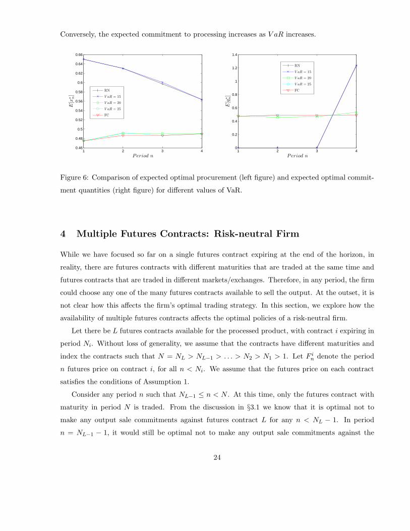
Conversely, the expected commitment to processing increases as V aR increases.
1 2 3 40.46
0.48
0.5
0.52
0.54
0.56
0.58
0.6
0.62
0.64
0.66
Period n
E[x
∗ n]
RN
V aR = 15
V aR = 20
V aR = 25
FC
1 2 3 40
0.2
0.4
0.6
0.8
1
1.2
1.4
Period n
E[q
∗ n]
RN
V aR = 15
V aR = 20
V aR = 25
FC
Figure 6: Comparison of expected optimal procurement (left figure) and expected optimal commit-
ment quantities (right figure) for different values of VaR.
4 Multiple Futures Contracts: Risk-neutral Firm
While we have focused so far on a single futures contract expiring at the end of the horizon, in
reality, there are futures contracts with different maturities that are traded at the same time and
futures contracts that are traded in different markets/exchanges. Therefore, in any period, the firm
could choose any one of the many futures contracts available to sell the output. At the outset, it is
not clear how this affects the firm’s optimal trading strategy. In this section, we explore how the
availability of multiple futures contracts affects the optimal policies of a risk-neutral firm.
Let there be L futures contracts available for the processed product, with contract i expiring in
period Ni. Without loss of generality, we assume that the contracts have different maturities and
index the contracts such that N = NL > NL−1 > . . . > N2 > N1 > 1. Let F in denote the period
n futures price on contract i, for all n < Ni. We assume that the futures price on each contract
satisfies the conditions of Assumption 1.
Consider any period n such that NL−1 ≤ n < N . At this time, only the futures contract with
maturity in period N is traded. From the discussion in §3.1 we know that it is optimal not to
make any output sale commitments against futures contract L for any n < NL − 1. In period
n = NL−1 − 1, it would still be optimal not to make any output sale commitments against the
24
futures contract L, which matures in period N . However, there is also another futures contract
that expires in period NL−1 that is available, against which potential commitments could be made.
The marginal benefit of committing a unit of available inventory of the input against the futures
contract maturing at NL−1 is FL−1NL−1−1 − p. The marginal benefit of carrying this inventory to
the next period is given by EINL−1−1[max{FL
N−1 − p,EIN−1[SN ]}]. Therefore, it is optimal to
commit to sell the processed product against the futures contract maturing at NL−1 only when
FL−1NL−1−1−p ≥ EINL−1−1
[max{FLN−1 −p,EIN−1
[SN ]}]. Unlike the single-contract case, it is possible
that FL−1NL−1−1 − p ≥ EINL−1−1
[max{FLN−1 − p,EIN−1
[SN ]}], as we are comparing the futures price
on contracts with different maturities, possibly traded on different exchanges. Thus, it may be
optimal to commit against a futures contract for n < N − 1.
The presence of multiple futures contracts thus affects the marginal benefit of a unit of inventory.
However, the optimal procurement quantity would still be governed by a threshold such that the
marginal cost of procurement at the threshold is equal to the marginal benefit from an additional
unit of inventory. As in the single futures case, this threshold would not depend on the current
level of inventory and the optimal procurement quantity would be the lesser of this threshold value,
x̂n, and the procurement capacity, K, in any period n.
The next theorem formalizes the intuition described in the previous paragraphs and shows that
it is never optimal to commit against a futures contract i in a period n for which n �= Ni − 1.
We assume that e1 ≥ 0; that is, the initial uncommitted inventory of the input commodity is
non-negative. Define
Mn = EIn [max{F i+1Ni+1−1 − p,EINi+1−1
[max{. . . max{FLN−1 − p,EIN−1
[SN ]} . . .}]}]
Theorem 5 When multiple futures contracts of the output commodity are available, the marginal
benefit of inventory is given by max{F iNi−1 − p,EINi−1
[MNi ]} when n = Ni − 1 for some i and Mn
otherwise. The optimal policies are as described below:
1. Procurement Policy: The optimal procurement quantity is characterized by a critical value x̂n
which satisfies the following first order condition
∂C(Sn, x̂n)∂xn
=
⎧⎨⎩
Mn if Ni ≤ n < Ni+1 − 1
max{F iNi−1 − p,EINi−1
[MNi ]} if n = Ni − 1
and the optimal procurement quantity x∗n is given by x∗
n = min{x̂n,K}.
25
2. Processing Policy: The optimal quantity of output to process and sell against any futures
contract i is given by
qi∗n =
⎧⎪⎪⎨⎪⎪⎩
0 if n �= Ni − 1
0 if n = Ni − 1 and F iNi−1 − p < EINi−1
[MNi ]
en + x∗n if n = Ni − 1 and F i
Ni−1 − p ≥ EINi−1[MNi ]
Notice that EINi−1[MNi ] ≥ EINi−1
[F jNj−1 − p] for all j = i + 1, i + 2, . . . , L. Therefore, the
condition in the above theorem includes the intuitive condition that it is never optimal to commit
to a futures contract i when there exists a contract j, with Nj > Ni and F jNi−1 > F i
Ni−1.
Mn, the expected marginal benefit of inventory in period n, where Ni ≤ n < Ni+1 − 1, is
analogous to the marginal benefit of inventory in the case of a single futures contract given by
EIn [max{FN−1 − p,EIN−1[SN ]}]. This marginal benefit of inventory accounts for the fact that
there are multiple processing margins (through the multiple futures contracts) available. As in the
case with a single futures contract, the expected marginal benefit of a unit of inventory is at least
as much as the marginal benefit from committing to sell the output using any of the remaining
futures contracts.
4.1 Comparison with Single Futures Case
The multiple futures contracts case can be treated as one where each unit of inventory is a call
option on all the processing margins from futures contracts that are yet to expire and the salvage
margin. Looking at it from this perspective, the optimal procurement and processing policy is a
direct extension of the result in §3.1 for a single futures contract and exhibit similar properties as
in the single futures case.
It is optimal to make a commitment against a specific futures contract only if the processing
margin from the contract is at least as much as the maximal expected benefit from all the futures
contracts that are yet to expire and the salvage value; i.e., the value from exercising the option is at
least as much as the value from waiting. The value from waiting is nothing but the marginal benefit
of inventory, EINi−1[MNi ], which is at least as much as max{F j
Ni−1−p} for all j = i+1, i+2, . . . , L.
Therefore we see that the simple condition, F iNi−1 ≥ F j
Ni−1, is not enough to commit against futures
contract i in period Ni − 1.
26
5 Conclusions
In this paper we study the integrated procurement, processing and trading decisions for a firm
dealing in commodities. We first analyzed the case when a risk-neutral firm has a single futures
contract available for trading the processed product. We find that the available inventory of the
input commodity can be considered as a call option on the processing margin and the optimal
policy is to postpone the decision to process and sell the output until the last possible period in
which the output can be sold. When the procurement costs are convex, the optimal procurement
policy is governed by a threshold that is independent of the current inventory level and it is optimal
to procure up to the threshold quantity.
We then considered a risk-averse firm which has a Value-at-Risk (VaR) constraint. In this case,
we find that the risk-averse firm finds it optimal to trade some portion of the available inventory as
processed product in every period. The quantity to process is dependent on the starting inventory
level and the processing decision is purely for managing risk and satisfying the VaR constraint.
The procurement policy is again governed by a threshold value, but the threshold is not necessarily
independent of the starting inventory levels. Moreover, the quantity procured in any period is no
greater than that procured by a risk-neutral firm.
Finally, we look at optimal policies for a risk-neutral firm when there are multiple futures
contract with different maturities that are traded. The optimal policies in this case are very similar
to those in the single futures case. We find it is optimal to postpone selling the output against any
futures contract until the last period in which a sale can be made against that contract. The optimal
procurement policy is again a threshold policy, where the procurement threshold is independent of
the starting inventory level.
In summary, we find that incorporating ideas from the financial world into operational prob-
lems provides significant insights in the analysis of integrated problems such as the one we consider.
Furthermore, this yields significant managerial insights and decision support tools to improve per-
formance in a variety of contexts. For example, our finding that it is optimal for a risk-neutral
firm to postpone the processing and sale of the output until the last possible opportunity provides
a practical guideline for managerial decision making. Similarly, managers can adopt operational
strategies to manage risk, supplementing financial risk management.
27
5.1 Future Research
While this paper provides a start towards analyzing integrated decision making for firms involved
in the commodities business, there is much work that remains. We highlight some of the open
questions and future research directions in which the results in the paper can be extended. In
particular, the cases of a risk-averse firm trading in multiple futures contracts as well incorporating
finite processing capacities is work in progress.
Agricultural input commodities like soybean and corn are grown in farms spread over large
geographic areas, the firm’s processing capabilities may be in factories in fixed locations, and
the output commodity(ies) may need to be delivered to specific locations such as ports of trade.
The opportunity to maximize profit is affected by the network characteristics such as distances,
capacities and transportation times and the firm needs to consider the network effects while deciding
on its procurement and processing decision.
This paper only considers a single input commodity being processed into a single output com-
modity. In some industries, the firm can choose what output to process the input commodity into.
For example, corn can be processed into ethanol or cornmeal. In a similar manner, the firm might
have a choice in terms of the input commodity. We believe our research has the potential for
spurring further research into these and other related problems.
6 Acknowledgment
The authors gratefully acknowledge the collaboration and support of The ITC Group. Their
generous hospitality and access to key personnel and data greatly enhanced this research.
References
Anderson, R.W., J. Danthine. 1995. Hedging and joint production: Theory and illustrations. The Journal
of Finance 35(2) 487–498.
Anupindi, R., S. Sivakumar. 2006. Supply chain re-engineering in agri-business: A case study of ITC’s
e-choupal. Hau L. Lee, Chung-Yee Lee, eds., Supply Chain Issues in Emerging Economies. Elsevier-
Springer.
Arzac, E.R., V.S. Bawa. 1977. Portfolio choice and equilibrium in capital markets with safety-first investors.
Journal of Financial Economics 4 277–288.
Bjork, T. 2004. Arbitrage Theory in Continuous Time. Oxford University Press, New York.
28
Caldentey, R., M. Haugh. 2006. Optimal control and hedging of operations in the presence of financial
markets. Working Paper, Stern School of Business, New York University.
Chowdhry, B., J.T.B. Howe. 1999. Corporate risk management for multinational corporations: Financial
and operational hedging policies. European Finance Review 2 229–246.
Dahlgran, R.A. 2002. Inventory and transformation risks in soybean processing. Paper presented at the NCR-
134 Conference on Applied Commodity Price Analysis, Forecasting, and Market Risk Management.
Eeckhoudt, L., C. Gollier, H. Schlesinger. 1995. The risk-averse (and prudent) newsboy. Management Science
41(5) 786–794.
Gaur, V., S. Seshadri. 2005. Hedging inventory risk through market instruments. Manufacturing and Service
Operations Management 7(2) 103–120.
Geman, H. 2005. Commodities and Commodity Derivatives: Modeling and Pricing for Agriculturals, Metals
and Energy. Wiley.
Gibson, R., E.S. Schwartz. 1990. Stochastic convenience yield and the pricing of oil contingent claims.
Journal of Finance 45(3) 959–976.
Goel, A., G.J. Gutierrez. 2006. Integrating commodity markets in the optimal procurement policies of a
stochastic inventory system. Working Paper, Management Department, University of Texas at Austin.
Goy, B.A. 1999. Essays on agricultural risk management and agribusiness marketing. Ph.D. thesis. Purdue
University.
Hull, J.C. 1997. Options, Futures and Other Derivatives. Prentice Hall, Upper Saddle River, New Jersey.
Linsmeier, T.J., N.D. Pearson. 2000. Value at risk. Financial Analysts Journal 56(2) 47–67.
Manfredo, M.R., R.M. Leuthold. 1999. Value-at-risk analysis: A review and the potential for agricultural
applications. Review of Agricultural Economics 21(1) 99–111.
Myers, R.J., S.D. Hanson. 1996. Optimal dynamic hedging in unbiased futures markets. American Journal
of Agricultural Economics 78(1) 13–20.
Pindyck, R.S. 2001. The dynamics of commodity spot and futures markets: A primer. Energy Journal 22(3)
1–29.
Plato, G. 2001. The soybean processing decision: Exercising a real option on processing margins. Elec-
tronic Report from the Economic Research Service, Technical Bulletin Number 1897, United States
Department of Agriculture.
Routledge, B.R., D.J. Seppi, C.S. Spatt. 2000. Equilibrium forward curves for commodities. Journal of
Finance 55(3) 1297–1338.
Routledge, B.R., D.J. Seppi, C.S. Spatt. 2001. The spark spread: An equilibrium model of cross-commodity
price relationships in electricity. Working Paper, Tepper School of Business, Carnegie Mellon University.
29
Schwartz, E., J.E. Smith. 2000. Short-term variations and long-term dynamics in commodity prices. Man-
agement Science 46(7) 893–911.
Tsang, D., R.M. Leuthold. 1990. Hedge ratios under inherent risk reduction in a commodity complex. The
Journal of Futures Markets 10(5) 497–504.
Working, H. 1949. The theory of price of storage. American Economic Review 39(6) 1254–1262.
Working, H. 1953. Futures trading and hedging. American Economic Review 43(3) 314–343.
Zhu, W., R. Kapuscinski. 2006. Optimal operational versus financial hedging for a risk-averse firm. Working
Paper, Ross School of Business, University of Michigan.
A Proofs of Theorems
Theorem 1 In period N − 1, for eN−1 ≥ 0, the optimal policy is as follows.
1. Procurement: The procurement decision is characterized by two critical values, x̂N−1 and
x̃N−1 which satisfy the following first order conditions.
∂C(SN−1, x̂N−1)∂xN−1
= FN−1 − p∂C(SN−1, x̃N−1)
∂xN−1= E[SN |IN−1]
The optimal quantity to procure, x∗N−1, is then given by
x∗N−1 =
⎧⎨⎩
min{x̂N−1,K} if FN−1 − p ≥ E[SN |IN−1]
min{x̃N−1,K} if FN−1 − p < E[SN |IN−1]
2. Processing: It is optimal to commit to sell the processed product against the futures contract
if and only if the processing margin is greater than the trade margin; i.e.,
q∗N−1 =
⎧⎨⎩
eN−1 + x∗N−1 if FN−1 − p ≥ EIN−1
[SN ]
0 if FN−1 − p < EIN−1[SN ]
Furthermore, VN−1(eN−1,IN−1) can be expressed as
VN−1(eN−1,IN−1) = max{FN−1 − p,E[SN |IN−1]}.eN−1 + BN−1
where BN−1 =
⎧⎨⎩
(FN−1 − p)x∗N−1 − C(SN−1, x
∗N−1) if FN−1 − p ≥ E[SN |IN−1]
E[SN |IN−1]x∗N−1 − C(SN−1, x
∗N−1) if FN−1 − p < E[SN |IN−1]
30
Proof: By substituting for VN (eN ,IN ), we have
VN−1(eN−1,IN−1) = maxqN−1≥0, 0≤xN−1≤K
{(FN−1 − p)qN−1 − C(SN−1, xN−1)
+ EIN−1[SN (eN−1 + xN−1 − qN−1)]} (8)
Observe that the expression to be optimized above is linear in qN−1. Therefore, for a given
xN−1, the contribution of qN−1 is maximized at the boundary; that is, the optimal processing
decision is given by
q∗N−1 =
⎧⎨⎩
eN−1 + xN−1 if FN−1 − p ≥ EIN−1[SN ]
0 if FN−1 − p < EIN−1[SN ]
(9)
Thus, (8) can be written as
VN−1(eN−1,IN−1) =
⎧⎪⎪⎪⎪⎪⎪⎪⎪⎪⎨⎪⎪⎪⎪⎪⎪⎪⎪⎪⎩
maxxN−1
{(FN−1 − p)eN−1
+ (FN−1 − p)xN−1 − C(SN−1, xN−1)} if FN−1 − p ≥ EIN−1[SN ]
maxxN−1
{EIN−1[SN ]eN−1
+ EIN−1[SN ]xN−1 − C(SN−1, xN−1)} if FN−1 − p < EIN−1
[SN ]
Because of the convexity of C(SN−1, xN−1), both the functions to be maximized above are
concave in xN−1 and have unique maximizers, x̂N−1 and x̃N−1, satisfying the respective first order
conditions.
The rest of the theorem follows from the above results. �
Theorem 2 The value function Vn(en,In) for n ≤ N − 1 is linear for all en ≥ 0. Moreover, the
marginal benefit of an additional unit of inventory is at least Fn − p for all en ≥ 0.
In any period n < N , the optimal procurement and processing decisions are as described below:
1. Procurement Policy: The optimal procurement policy is characterized by a critical value x̂n
which satisfies the following first order condition:
∂C(Sn, x̂n)∂xn
= E[max{FN−1 − p,E[SN |IN−1]}|In]
The optimal procurement quantity, x∗n, in period n is given by x∗
n = min{x̂n,K}.
2. Processing Policy: It is optimal to not commit for processing any of the available input in-
ventory in any period n such that n < N − 1. In period N − 1, it is optimal to commit
31
all the available inventory for sale as processed product against the futures contract only if
FN−1 − p ≥ E[SN |IN−1] and not to commit anything otherwise. That is, the optimal policy
for processing is given by
q∗n = 0 if n < N − 1
q∗N−1 =
⎧⎨⎩
0 if FN−1 − p < EIN−1[SN ]
eN−1 + x∗N−1 if FN−1 − p ≥ EIN−1
[SN ]
Proof: We prove the theorem by induction. As the basis for induction, we know from Theorem 1
that the above holds for n = N − 1. Suppose it is true for period n + 1 ≤ N − 1. Then, Vn+1 can
be expressed in linear form as follows:
Vn+1(en+1,In+1) = An+1en+1 + Bn+1 (10)
where An+1 and Bn+1 are functions of In+1 alone and An+1 ≥ Fn+1 − p.
From (3), we have
Vn(en,In) = maxqn≥0, 0≤xn≤K
{Ln(en, qn, xn,In)}
where Ln(en, qn, xn,In) = (Fn − p)qn − C(Sn, xn) + EIn [An+1(en + xn − qn) + Bn+1].
Consider the coefficient of qn in Ln(·). We have
Fn − p − EIn [An+1] ≤ Fn − p − EIn [Fn+1 − p]
= Fn − p − Fn − p
= 0
The inequality above is by the induction hypothesis and the first equality due to Assumption
1. Therefore, it is optimal to have qn = 0. We can then write the maximization as
Vn(en,In) = maxxn
{EIn [An+1](en + xn) + EIn [Bn+1] − C(Sn, xn)}
The function to be maximized is concave in xn and has a unique maximizer, x̂n which satisfies
the first order condition,
∂C(Sn, x̂n)∂xn
= EIn [An+1] (11)
The optimal procurement quantity is therefore given by x∗n = min{x̂n,K}. Substituting, we get
Vn(en,In) = EIn [An+1]en + EIn [An+1]x∗n + EIn [Bn+1] − C(Sn, x∗
n) (12)
32
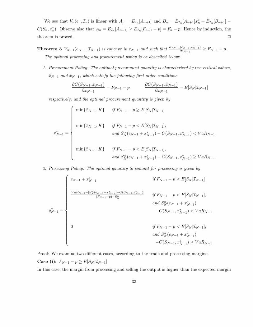
We see that Vn(en,In) is linear with An = EIn [An+1] and Bn = EIn [An+1]x∗n + EIn [Bn+1] −
C(Sn, x∗n). Observe also that An = EIn [An+1] ≥ EIn [Fn+1 − p] = Fn − p. Hence by induction, the
theorem is proved. �
Theorem 3 VN−1(eN−1,IN−1) is concave in eN−1 and such that ∂VN−1(eN−1,IN−1)∂eN−1
≥ FN−1 − p.
The optimal processing and procurement policy is as described below:
1. Procurement Policy: The optimal procurement quantity is characterized by two critical values,
x̂N−1 and x̃N−1, which satisfy the following first order conditions
∂C(SN−1, x̂N−1)∂xN−1
= FN−1 − p∂C(SN−1, x̃N−1)
∂xN−1= E[SN |IN−1]
respectively, and the optimal procurement quantity is given by
x∗N−1 =
⎧⎪⎪⎪⎪⎪⎪⎪⎪⎪⎪⎪⎪⎪⎪⎨⎪⎪⎪⎪⎪⎪⎪⎪⎪⎪⎪⎪⎪⎪⎩
min{x̂N−1,K} if FN−1 − p ≥ E[SN |IN−1]
min{x̂N−1,K} if FN−1 − p < E[SN |IN−1],
and SαN (eN−1 + x∗
N−1) − C(SN−1, x∗N−1) < V aRN−1
min{x̃N−1,K} if FN−1 − p < E[SN |IN−1],
and SαN (eN−1 + x∗
N−1) − C(SN−1, x∗N−1) ≥ V aRN−1
2. Processing Policy: The optimal quantity to commit for processing is given by
q∗N−1 =
⎧⎪⎪⎪⎪⎪⎪⎪⎪⎪⎪⎪⎪⎪⎪⎪⎪⎪⎪⎪⎪⎨⎪⎪⎪⎪⎪⎪⎪⎪⎪⎪⎪⎪⎪⎪⎪⎪⎪⎪⎪⎪⎩
eN−1 + x∗N−1 if FN−1 − p ≥ E[SN |IN−1]
V aRN−1−[SαN (eN−1+x∗
N−1)−C(SN−1,x∗N−1)]
(FN−1−p)−SαN
if FN−1 − p < E[SN |IN−1],
and SαN (eN−1 + x∗
N−1)
−C(SN−1, x∗N−1) < V aRN−1
0 if FN−1 − p < E[SN |IN−1],
and SαN (eN−1 + x∗
N−1)
−C(SN−1, x∗N−1) ≥ V aRN−1
Proof: We examine two different cases, according to the trade and processing margins:
Case (i): FN−1 − p ≥ E[SN |IN−1]
In this case, the margin from processing and selling the output is higher than the expected margin
33
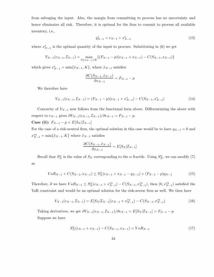
from salvaging the input. Also, the margin from committing to process has no uncertainty and
hence eliminates all risk. Therefore, it is optimal for the firm to commit to process all available
inventory, i.e.,
q∗N−1 = eN−1 + x∗N−1 (13)
where x∗N−1 is the optimal quantity of the input to procure. Substituting in (6) we get
VN−1(eN−1,IN−1) = max0≤xN−1≤K
{(FN−1 − p)(eN−1 + xN−1) − C(SN−1, xN−1)}
which gives x∗N−1 = min{x̂N−1,K}, where x̂N−1 satisfies
∂C(SN−1, x̂N−1)∂xN−1
= FN−1 − p
We therefore have
VN−1(eN−1,IN−1) = (FN−1 − p)(eN−1 + x∗N−1) − C(SN−1, x
∗N−1) (14)
Concavity of VN−1 now follows from the functional form above. Differentiating the above with
respect to eN−1 gives ∂VN−1(eN−1,IN−1)/∂eN−1 = FN−1 − p.
Case (ii): FN−1 − p < E[SN |IN−1]
For the case of a risk-neutral firm, the optimal solution in this case would be to have qN−1 = 0 and
xrnN−1 = min{x̃N−1,K} where x̃N−1 satisfies
∂C(SN−1, x̃N−1)∂xN−1
= E[SN |IN−1]
Recall that SαN is the value of SN corresponding to the α fractile. Using Sα
N , we can modify (7)
as
V aRN−1 + C(SN−1, xN−1) ≤ SαN (eN−1 + xN−1 − qN−1) + (FN−1 − p)qN−1 (15)
Therefore, if we have V aRN−1 ≤ SαN (eN−1 + xrn
N−1) − C(SN−1, xrnN−1), then (0, xrn
N−1) satisfied the
VaR constraint and would be an optimal solution for the risk-averse firm as well. We then have
VN−1(eN−1,IN−1) = E[SN |IN−1](eN−1 + xrnN−1) − C(SN−1, x
rnN−1) (16)
Taking derivatives, we get ∂VN−1(eN−1,IN−1)/∂eN−1 = E[SN |IN−1] > FN−1 − p.
Suppose we have
SαN (eN−1 + xN−1) − C(SN−1, xN−1) < V aRN−1 (17)
34
for all xn ≥ 0. By Assumption 2, full-commitment satisfies the VaR constraint; i.e.,
(FN−1 − p)(eN−1 + xN−1) − C(SN−1, xN−1) ≥ V aRN−1
Therefore, there exists a q̃N−1 such that
(FN−1 − p)q̃N−1 + SαN (eN−1 + xN−1 − q̃N−1) − C(SN−1, xN−1) = V aRN−1 (18)
That is, if committing nothing does not meet the VaR constraint but committing everything
does, then there exists an intermediate value of the committment amount that satisfies the VaR
constraint exactly. (Notice that assumption 2 is satisfied only if SαN < FN−1 − p.)
The quantity to process, q̃N−1, is therefore given by
q̃N−1 =V aRN−1 + C(SN−1, xN−1) − Sα
N (eN−1 + xN−1)(FN−1 − p) − Sα
N
(19)
Notice that the quantity to commit is a function of the quantity procured, xN−1. Substituting
this in the maximization problem, (6), we have
VN−1(eN−1,IN−1) = max0≤xN−1≤K
{(FN−1 − p)(q̃N−1) − C(SN−1, xN−1)
+ E[SN |IN−1](eN−1 + xN−1 − q̃N−1)}
The function to be maximized is concave and has a unique maximum. The maximizer, x̂N−1
satisfies the following first order condition
(FN−1 − p)∂q̃N−1
∂xN−1− ∂C(SN−1, xN−1)
∂xN−1+ E[SN−1|IN−1]
(1 − ∂q̃N−1
∂xN−1
)∣∣∣xN−1=x̂N−1
= 0 (20)
Substituting ∂q̃N−1/∂xN−1 from (19) and simplifying the above equation gives
∂C(SN−1, xN−1)∂xN−1
∣∣∣xN−1=x̂N−1
= FN−1 − p (21)
Thus we have x∗N−1 = min{x̂N−1,K} and q∗N−1 = max{q̃N−1, 0}. Thus, we have
VN−1(eN−1,IN−1) = (FN−1 − p)(q̃N−1) − C(SN−1, x∗N−1)
+ E[SN |IN−1](eN−1 + x∗N−1 − q̃N−1) (22)
Taking partial derivatives, we have
∂VN−1(eN−1,IN−1)∂eN−1
= (FN−1 − p)E[SN |IN−1] − Sα
N
(FN−1 − p) − SαN
We find that VN−1(eN−1,IN−1) is concave ∂VN−1(eN−1,IN−1)/∂eN−1 ≥ FN−1 − p for all cases
considered. �
35
Theorem 4 For all n < N −1 and en ≥ 0, the value function Vn(en,In) is concave and increasing
in en, for all realizations of In and the marginal benefit of an unit of uncommitted inventory is
always greater than or equal to the processing margin; i.e., ∂Vn(en,In)∂en
≥ Fn − p. The optimal
procurement and processing policy is as given below
1. Procurement Policy: The optimal procurement quantity is characterized by two critical values,
x̂n and x̃n, which satisfy the following first order conditions
∂C(Sn, x̂n)∂xn
= Fn − p∂C(Sn, x̃n)
∂xn= E
[∂Vn+1(en + x̃n)∂en+1
|In
]
respectively, and the optimal procurement quantity is given by
x∗n =
⎧⎪⎪⎨⎪⎪⎩
min{x̂n,K} if V αn+1(en + x∗
n) − C(Sn, x∗n) < V aRn
min{x̃n,K} if V αn+1(en + x∗
n) − C(Sn, x∗n) ≥ V aRn
2. Processing Policy: The optimal quantity to commit for processing is given by
q∗n =
⎧⎪⎪⎨⎪⎪⎩
V aRn−[V αn+1(en+x̃n−q∗n)−C(Sn,xn)]
(Fn−p) if V αn+1(en + x∗
n) − C(Sn, x∗n) < V aRn
0 if V αn+1(en + x∗
n) − C(Sn, x∗n) ≥ V aRn
Proof: We prove the theorem by induction. Suppose the claim in the theorem is true for periods
n + 1, n + 2, . . . , N − 1.
The VaR constraint, (5), can be written as
V aRn + C(Sn, xn) ≤ V αn+1(en + xn − qn) + (Fn − p)qn (23)
For a risk-neutral firm, by the induction hypothesis, it would never be optimal to commit any
quantity for processing in period n. Also, in the risk-neutral case, it would be optimal to procure
xrnn = min{x̃n,K} where x̃n satisfies
∂C(Sn, x̃n)∂xn
= E[∂Vn+1(en + x̃n,In+1)
∂en+1
∣∣∣In
](24)
So, if V αn+1(en + xrn
n ) − C(Sn, xrnn ) ≥ V aRn, then the risk-neutral optimal solution would also
be optimal for the risk-averse firm and we would have
Vn(en,In) = E[Vn+1(en + xrnn ,In+1)|In] − C(Sn, xrn
n ) (25)
36
Concavity and continuity of Vn follows from the induction hypothesis. Taking partial derivatives,
we have
∂Vn(en,In)∂en
= E[∂Vn+1(en + xrn
n ,In+1)∂en+1
∣∣∣In
]
≥ E[Fn+1 − p|In]
= Fn − p
where the inequality follows from the induction hypothesis and the last equality from the assumption
about the futures prices. The interchange of the derivative and expectation in the above equation
is justified by the Lebesgue Dominated Convergence Theorem.
Now suppose
V αn+1(en + xn) − C(Sn, xn) < V aRn (26)
for any xn ≥ 0. By Assumption 2, we have
V αn+1(0) − C(Sn, xn) + (Fn − p)(en + xn) ≥ V aRn (27)
By continuity of all the terms in the above equation, there exists at least one qn ≤ en +xn such
that
V αn+1(en + xn − qn) − C(Sn, xn) + (Fn − p)qn = V aRn (28)
Let q̃n be the smallest value satisfying the following equation
q̃n =V aRn + C(Sn, xn) − V α
n+1(en + x̃n − qn)(Fn − p)
(29)
Consider ε1 > 0, where qn = en + xn − ε1 such that
V αn+1(ε1) − C(Sn, xn) + (Fn − p)(en + xn − ε1) ≥ V aRn
Consider the derivative of the left hand side with respect to ε1. If this derivative is non-negative,
i.e., if ∂V αn+1(ε1)/∂en+1 ≥ (Fn − p), then by increasing ε1 (reducing the quantity committed for
processing), the VaR constraint can still be satisfied. However, since q̃n satisfies (28), there must
be a ε2 < en + xn − q̃n such that
∂V αn+1(ε2)∂en+1
< Fn − p
37
(Otherwise, we can find a qn < q̃n for which the VaR constraint is satisfied and the firm will find
it optimal to reduce the quantity committed for processing.) Therefore, ∂V αn+1(en+xn−q̃n)/∂en+1 <
Fn − p.
Substituting (29) into the optimality equation, we have
Vn(en,In) = max0≤xn≤K
{(Fn − p)q̃n − C(Sn, xn) + E[Vn+1(en + xn − q̃n,In+1)|In]} (30)
The optimal procurement quantity is given by x∗n = min{x̂n,K} where x̂n satisfies the following
first order condition
(Fn − p)∂q̃n
∂xn− ∂C(Sn, xn)
∂xn+ E
[∂Vn+1(en + xn − q̃n,In+1)∂en+1
∣∣∣In
](1 − ∂q̃n
∂xn
)∣∣∣xn=x̂n
= 0 (31)
Taking partial derivative with respect to xn for equation (29) we have
∂q̃n
∂xn=
∂C(Sn,xn)∂xn
− ∂V αn+1(en+xn−q̃n)
∂en+1
(Fn − p) − ∂V αn+1(en+xn−q̃n)
∂en+1
(32)
Substituting into (31) and simplifying, we get[E[V(n+1,e)|In] − V α
(n+1,e)
][(Fn − p) − ∂C(Sn, xn)
∂xn
]∣∣∣xn=x̂n
= 0 (33)
where V(n+1,e) = ∂Vn+1(en + xn − q̃n,In+1)/∂en+1 and V α(n+1,e) = ∂V α
n+1(en + x∗n − q̃n)/∂en+1.
Because we have ∂V αn+1(en +xn− q̃n)/∂en+1 < Fn−p ≤ E[∂Vn+1(en +xn− q̃n,In+1)/∂en+1|In],
it follows that x̂n satisfies
∂C(Sn, x̂n)∂xn
= Fn − p (34)
Therefore, we have
Vn(en,In) = (Fn − p)q̃n − C(Sn, x∗n) + E[Vn+1(en + x∗
n − q̃n,In+1)|In]
Taking partial derivatives, we have
∂Vn(en,In)∂en
= (Fn − p)E[V(n+1,e)|In] − V α
(n+1,e)
(Fn − p) − V α(n+1,e)
From the above equation, we see that ∂Vn(en,In)/∂en ≥ Fn − p. Taking the second order
partial derivative and simplifying, we have
∂2Vn(en,In)∂e2
n
= (Fn − p)[E[V(n+1,ee)](Fn − p − V α
(n+1,e))
((Fn − p) − V α(n+1,e))
2
+V α
(n+1,ee)(E[V(n+1,e)|In] − Fn − p)
((Fn − p) − V α(n+1,e))
2
]
≤ 0
38
where E[V(n+1,ee)] = E[∂2Vn+1(en + xn − q̃n,In+1)/∂e2n+1|In] and V α
(n+1,ee) = ∂2V αn+1(en + x∗
n −q̃n)/∂e2
n+1. �
Theorem 5 When multiple futures contracts of the output commodity are available, the marginal
benefit of inventory is given by max{F iNi−1 − p,EINi−1
[MNi ]} when n = Ni − 1 for some i and Mn
otherwise. The optimal policies are as described below:
1. Procurement Policy: The optimal procurement quantity is characterized by a critical value x̂n
which satisfies the following first order condition
∂C(Sn, x̂n)∂xn
=
⎧⎨⎩
Mn if Ni ≤ n < Ni+1 − 1
max{F iNi−1 − p,EINi−1
[MNi ]} if n = Ni − 1
and the optimal procurement quantity x∗n is given by x∗
n = min{x̂n,K}.
2. Processing Policy: The optimal quantity of output to process and sell against any futures
contract i is given by
qi∗n =
⎧⎪⎪⎨⎪⎪⎩
0 if n �= Ni − 1
0 if n = Ni − 1 and F iNi−1 − p < EINi−1
[MNi ]
en + x∗n if n = Ni − 1 and F i
Ni−1 − p ≥ EINi−1[MNi ]
Proof: From Theorem 2 when en ≥ 0, we have from equation (12)
An = EIn [An+1]
= EIn [EIn+1 [An+2]]...
= EIn [. . . EIN−2[AN−1]]
= EIn [max{FN−1 − p,EIN−1[SN ]}]
(35)
for the case when only a single futures contract is available.
For any n such that NL−1 ≤ n < N −1, where NL−1 is the period in which the futures contract
with second longest maturity expires, the situation is the same as if there was only a single futures
contract. Therefore, the above equation holds for all n such that NL−1 ≤ n < N − 1.
In period n = NL−1 − 1, we know from Theorem 2 that it is not optimal to commit against
the futures contract maturing in period N . However, committing against the futures contract
maturing at NL−1 gives a marginal benefit of FL−1NL−1−1 − p per unit of soybean inventory, while not
39
committing and carrying inventory into the future gives a marginal benefit of EINL−1−1[AN−1] per
unit. Therefore, at n = NL−1 − 1, the marginal benefit of a unit of soybean inventory is given by
max{FL−1NL−1−1 − p,EINL−1−1
[max{FLN−1 − p,EIN−1
[SN ]}]} (36)
Denote this marginal benefit by MNL−1−1. Notice that MNL−1−1 ≥ FL−1NL−1−1−p and also MNL−1−1 ≥
FLNL−1−1 − p.
Now, for any n such that NL−2 ≤ n < NL−1 − 1, the marginal benefit from committing against
futures contract L or L−1 is less than the marginal benefit of carrying uncommitted inventory into
the next period. For n = NL−2 − 1, we have, the marginal benefit of a unit of soybean inventory is
MNL−2−1 = max{FL−2NL−2−1 − p,EINL−2−1
[MNL−1−1]}= max{FL−2
NL−2−1 − p,EINL−2−1[max{FL−1
NL−1−1 − p,
EINL−1−1[max{FL
N−1 − p,EIN−1[SN ]}]}]}
Extending this argument, for any period n such that Ni ≤ n < Ni+1−1, it is not optimal to commit
against any futures contract i + 1, i + 2, . . . , L. For any such period n, the marginal benefit of a
unit of inventory is given by
Mn = EIn [max{F i+1Ni+1−1 − p,EINi+1−1
[max{. . . max{FLN−1 − p,EIN−1
[SN ]} . . .}]}]
Therefore, in any period n such that n = Ni−1, it is optimal to commit against futures contract
i only if F iNi−1 − p ≥ EINi−1
[MNi ].
The optimal procurement policy described in the theorem follows as x̂n and x̂Ni−1 are the
threshold values at which the marginal cost of procurement is equal to the marginal revenue in the
respective periods. �
B Price Model for Numerical Study
B.1 Input Spot Price
We use a two-factor model for the input spot price in the spirit of Schwartz and Smith (2000). The
spot price St is modeled as ln St = Xt + μt, where Xt represents the short-term deviation in prices
and μt the equilibrium price level. Since the period of interest in our model is a single season, we
assume μt to be fixed for all t to a constant value, μ. (This is unlike the model in Schwartz and
Smith (2000) where μt follows a Brownian motion process). Xt follows a mean-reverting process
40
given by dXt = −κXtdt + σxdW xt , where dW x
t is the increment of a standard Brownian motion
and κ is the mean-reversion coefficient.
Using Ito’s lemma and integrating the above equation gives:
XT = e−κ(T−t)Xt + σx
√1 − e−2κ(T−t)
√2κ(T − t)
(W xT − W x
t )
Discretizing this equation, we get Xt+1 = e−κXt + σx
√1−e−2κ√
2κζx, where ζx is a random variable
with a standard normal distribution.
Finally, substituting in the two-factor spot price model, we get St+1 = exp{Xt+1 + μ} =
exp{
e−κXt + σx
√1−e−2κ√
2κζx + μ
}= exp
{(1 − e−κ)μ + e−κ ln St + σx
√1−e−2κ√
2κζx
}.
B.2 Estimating the parameters
From the expression for St+1 derived above, we have ln St+1 = (1−e−κ)μ+e−κ ln St+σx
√1−e−2κ√
2κζx.
Thus, by fitting a linear regression model on lnSt and ln St+1, one can estimate the value of
the parameters μ, κ and σx. (Note that St+1 is the next period price, where a period can be
appropriately chosen and not necessarily the immediate next day price.)
Based on the National Commodities and Derivatives Exchange Ltd. (NCDEX)5 data on soybean
spot prices for the period of 1st August, 2006 to 30th December, 2006, prices with a 15 day lag
(i.e., St+1 = St+15 regressed with St) show a fit with a R2 = 0.424 and an adjusted R2 = 0.419. By
considering a period in our model to correspond to 15 actual days (i.e., procurement and processing
decisions are made once every two weeks), we can use the results from this data for modeling the
spot price process.
B.3 Output Futures Price
For the model studied in this paper, the processed product is sold entirely using futures contracts.
However, there was no reliable data available on the futures prices of soymeal and soyoil on the
NCDEX. (the futures markets are illiquid and there are very few trades that happened on these
markets.)
In order to overcome this deficiency and to serve the purposes of this numerical study, we
assume that the futures prices are equal to the expected spot prices at maturity. We consider a5A commodities exchange in India, http://www.ncdex.com/Market Data/hist spot price 2006.aspx, retrieved July
2007.
41
model for the spot prices of soymeal and soyoil and then derive the futures price from those spot
prices. We consider a simple case of a single output commodity in this paper. Hence, we model the
total output, soymeal and soyoil, as a single output commodity and model the price of a composite
ouput.
The output spot price is modeled as λ ∗ Mt + (1 − λ) ∗ Ot where λ is the amount of soymeal
produced from a unit of soybean (and the remaining is assumed to be soyoil), Mt is the spot price
of soymeal and Ot is the spot price of soyoil. Considering this composite output as a commodity,
we use the same model as for the input for these prices. Therefore we have ln St = Yt +μc, where St
is the spot price of the composite, Yt is the short term deviation in the price of the composite and
μc is the long run equilibrium price level of the composite product. Yt has the following dynamics:
dYt = −κyYtdt + σydW yt .
Along similar lines as before, we have, upon integration:
YT = e−κy(T − t)Yt + σy
√1 − e−2κy(T−t)
√2κy(T − t)
(W yT − W y
t )
Discretizing as before, we have Yt+1 = e−κyYt + σy
√1−e−2κy√
2κyζy, where ζy is a standard normal
random variable. Moreover, ζx and ζy are correlated with a correlation coefficient ρ.
From the equations above we have ST = exp{
(1−e−κy(T−t))μy+e−κy(T−t) ln St+σy
√1−e−2κ(T−t)√
2κyζy
}
and St+1 = exp{
(1−e−κy)μy +e−κy ln St +σy
√1−e−2κ√
2κyζy
}. The parameters μy, κy, σy can again be
estimated from a linear regression model with St+1 against St as described in the section on input
spot prices.
Based on the NCDEX data on soymeal and soyoil spot prices for the period of 1st August, 2006
to 30th December, 2006, prices with a 15 day lag (i.e., St+1 = St+15 regressed with St) show a fit
with a R2 = 0.484 and an adjusted R2 = 0.479. (As in the case of the input spot prices, we can
consider a single period in the model to correspond to 15 real days and hence these results can be
used for the purposes of this paper.)
To derive the futures price process for the output, we assume that the rational expectation
hypothesis holds and the futures price F Tt for a contract maturing in period T , is an unbiased
estimator for the future spot price ST in period T. Therefore, we have F Tt = E[ST |St] = exp{(1 −
e−κy(T − t))μy + e−κy(T−t) ln St + σ2y
(1−e−2κ(T−t))4κy
}.We need to be able to express F T
t+1 in terms of F Tt to generate the probability distribution of the
next period futures price, given the current period futures price. Through algebraic manipulation,
42
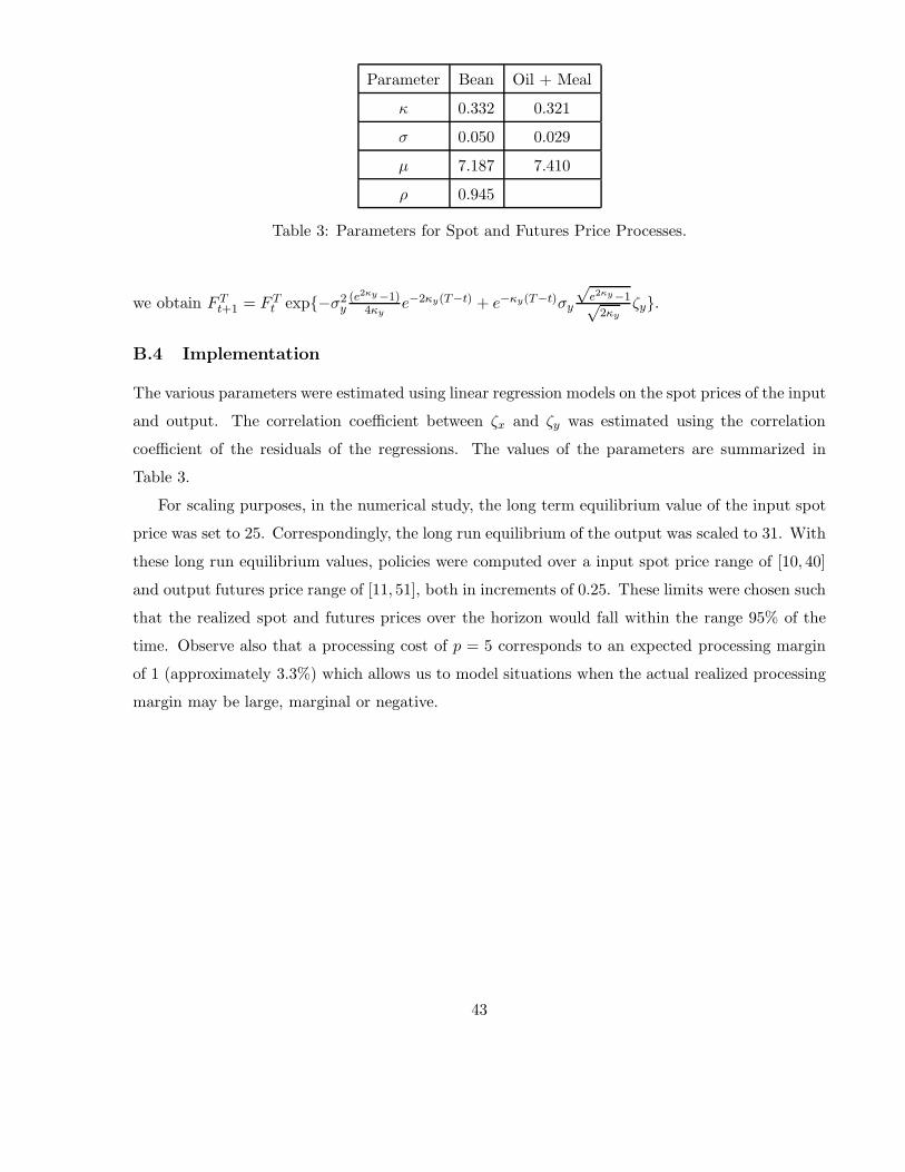
Parameter Bean Oil + Meal
κ 0.332 0.321
σ 0.050 0.029
μ 7.187 7.410
ρ 0.945
Table 3: Parameters for Spot and Futures Price Processes.
we obtain F Tt+1 = F T
t exp{−σ2y
(e2κy−1)4κy
e−2κy(T−t) + e−κy(T−t)σy
√e2κy−1√
2κyζy}.
B.4 Implementation
The various parameters were estimated using linear regression models on the spot prices of the input
and output. The correlation coefficient between ζx and ζy was estimated using the correlation
coefficient of the residuals of the regressions. The values of the parameters are summarized in
Table 3.
For scaling purposes, in the numerical study, the long term equilibrium value of the input spot
price was set to 25. Correspondingly, the long run equilibrium of the output was scaled to 31. With
these long run equilibrium values, policies were computed over a input spot price range of [10, 40]
and output futures price range of [11, 51], both in increments of 0.25. These limits were chosen such
that the realized spot and futures prices over the horizon would fall within the range 95% of the
time. Observe also that a processing cost of p = 5 corresponds to an expected processing margin
of 1 (approximately 3.3%) which allows us to model situations when the actual realized processing
margin may be large, marginal or negative.
43


