MICROTHERMAL DEVICES FOR FLUIDIC ACTUATION BY MODULATION OF SURFACE TENSION

by

Amar Sarbbesesh Basu

A dissertation submitted in partial fulfillment of the requirements for the degree of

Doctor of Philosophy (Electrical Engineering)

in The University of Michigan 2008

Doctoral Committee: Professor Yogesh B. Gianchandani, Chair Professor Ronald G. Larson Professor Khalil Najafi Associate Professor Shuichi Takayama Assistant Professor Michel M. Maharbiz

© Amar Sarbbasesh Basu 2008

ii

DEDICATION

To my loyal friends and extended family who have made life rich & fulfilling,

and have been there for me through the years. To Dada, my source of wisdom and

strength. To Ma, my emotional rock and supporter. And to Baba, my educator, who

sacrificed his own doctoral studies so he could better teach to his two sons.

iii

ACKNOWLEDGEMENTS

First and most of all, I would like to thank the support of my advisor, Professor

Yogesh Gianchandani, without whom this work would not be possible. Professor

Gianchandani, thank you for taking the risks in letting me choose my research project,

and encouraging me to pursue the initial discoveries that led to this thesis. You have

worked me hard, challenged me, and pushed me towards success. Thank you for keeping

me out of the dreaded “analysis paralysis”, and thank you for your patience at times when

I have needed it.

Thank you to my committee members, Professor Khalil Najafi, Professor Ronald

Larson, Professor Michel Maharbiz, and Professor Shuichi Takayama for your input,

guidance, and support.

Thank you to Dr. Shamus McNamara (now at the University of Louisville) for

your mentoring during my first two years as a graduate student and your assistance in

fabricating the thermal probes. Thank you to Angelo Gaitas (Picocal, Inc.) for our

enjoyable collaborations on the thermal probes, and to Seowyuen Yee for your helpful

assistance in experiments and characterization. Thank you to the WIMS and SSEL staff

for endless administrative and technical support. This work would not have been

possible without your help.

Special thanks to all the people who have made my experience in graduate school

worthwhile and pleasant. To all of my labmates in the YG Research group and the

iv

WIMS ERC, thank you for your friendship and the many good memories of graduate

school. I can’t even begin to list everyone because I know I will leave many out, so I will

say you know who you are. Finally, I’d like to thank my EECS 514 and EECS 515 class

for their patience and enthusiasm in my first year teaching.

v

TABLE OF CONTENTS

DEDICATION ii

ACKNOWLEDGEMENTS iii

LIST OF FIGURES vii

LIST OF TABLES xiii

LIST OF APPENDICES xiv

ABSTRACT xv

CHAPTER 1: INTRODUCTION 1

1. MICROFLUIDICS FOR MINIATURIZED CHEMICAL ASSAYS 1

2. USING THE MARANGONI EFFECT FOR MICROFLUIDIC ACTUATION 3

3. CONTINUOUS FLOW MICROFLUIDIC SYSTEMS 10

4. MICRODROPLET-BASED “DIGITAL” MICROFLUIDICS 12

5. ORGANIZATION OF DISSERTATION 21

CHAPTER 2: VIRTUAL MICROFLUIDIC TRAPS, FILTERS, CHANNELS, AND PUMPS

USING MARANGONI FLOWS 23

1. INTRODUCTION 24

2. THEORETICAL MODEL OF MARANGONI FLOWS 25

3. SIMULATION RESULTS 31

4. EXPERIMENTAL RESULTS 41

5. DISCUSSION 54

6. SUMMARY 57

CHAPTER 3: HIGH SPEED DOUBLET FLOW 59

1. BACKGROUND 59

2. TEMPERATURE GRADIENT THEORY 61

vi

3. SOURCE/SINK THEORY 63

4. EXPERIMENTAL CHARACTERIZATION 70

5. SUMMARY 76

CHAPTER 4: A PROGRAMMABLE ARRAY FOR CONTACT-FREE MANIPULATION OF

FLOATING DROPLETS BY MODULATION OF SURFACE TENSION 78

1. INTRODUCTION 79

2. THEORETICAL 82

3. SYSTEM DESIGN AND EXPERIMENTAL SETUP 91

4. EXPERIMENTAL RESULTS 94

5. DISCUSSION 102

6. SUMMARY 106

CHAPTER 5: CONCLUSIONS 107

APPENDICES 112

BIBILIOGRAPHY 134

vii

LIST OF FIGURES

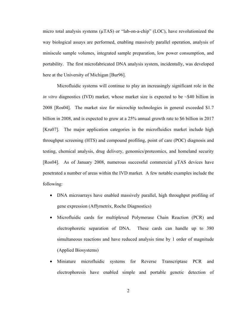
Figure 1.1: Comparison of conventional, multicellular Marangoni convection versus the present

approach. (a) Schematic of multicellular Marangoni flow occurring when a thin liquid layer is isothermally heated from below. (b) Top view of hexagonal convection cells resulting from conventional Marangoni convection (from [Mar07]). (c) Local, unicellular Marangoni convection initiated by a heat source placed above the liquid layer ....................................... 5

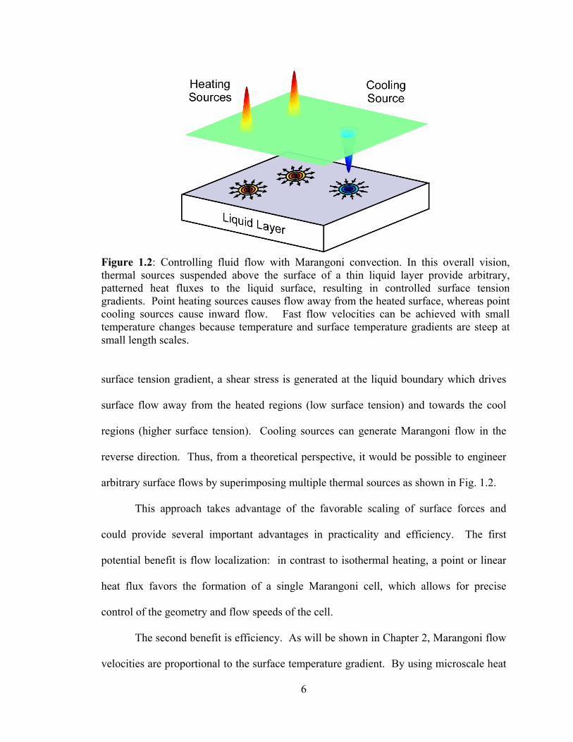
Figure 1.2: Controlling fluid flow with Marangoni convection. In this overall vision, thermal sources suspended above the surface of a thin liquid layer provide arbitrary, patterned heat fluxes to the liquid surface, resulting in controlled surface tension gradients. Point heating sources causes flow away from the heated surface, whereas point cooling sources cause inward flow. Fast flow velocities can be achieved with small temperature changes because temperature and surface temperature gradients are steep at small length scales..................... 6

Figure 1.3: Comparison of non-mechanical microfluidic pumping methods. (a) Flow velocities (in continuous flow systems) or droplet velocities (in discrete fluidic systems) as a function of substrate complexity for various pumping methods. (b) Flow/droplet velocities versus the required drive voltage for the same pumping methods. Abbreviations and references for each pumping method are as follows: Ma, Marangoni flow (this work) [Bas05A, Bas05B]; OT, Optical Tweezers [Kat01, Sas92]; ET, Electrostatic tip [Kats99]; Th-Ma, Thermal Marangoni effect on droplet interfaces using lasers [Kot04]; OEW, Optoelectrowetting [Chi03]; OET, Optoelectrostatic tweezers [Chi04]; AC-EW, AC Electrowetting [Cho02]; DC-EW, DC Electrowetting [Cho03]; EHD, Electrohydrodynamic pumping [Fuh92, Ahn98]; EO, Electroosmotic pumps, [Har91,Che02]; and MHD, Magnetohydrodynamic [Lem00]................................................................................................................................... 8

Figure 1.4: Comparison of continuous flow microfluidic systems and droplet systems. ............. 13 Figure 1.5: Illustration of droplet unit operations. ....................................................................... 15 Figure 1.6: Illustration of various techniques used from droplet manipulation, including the

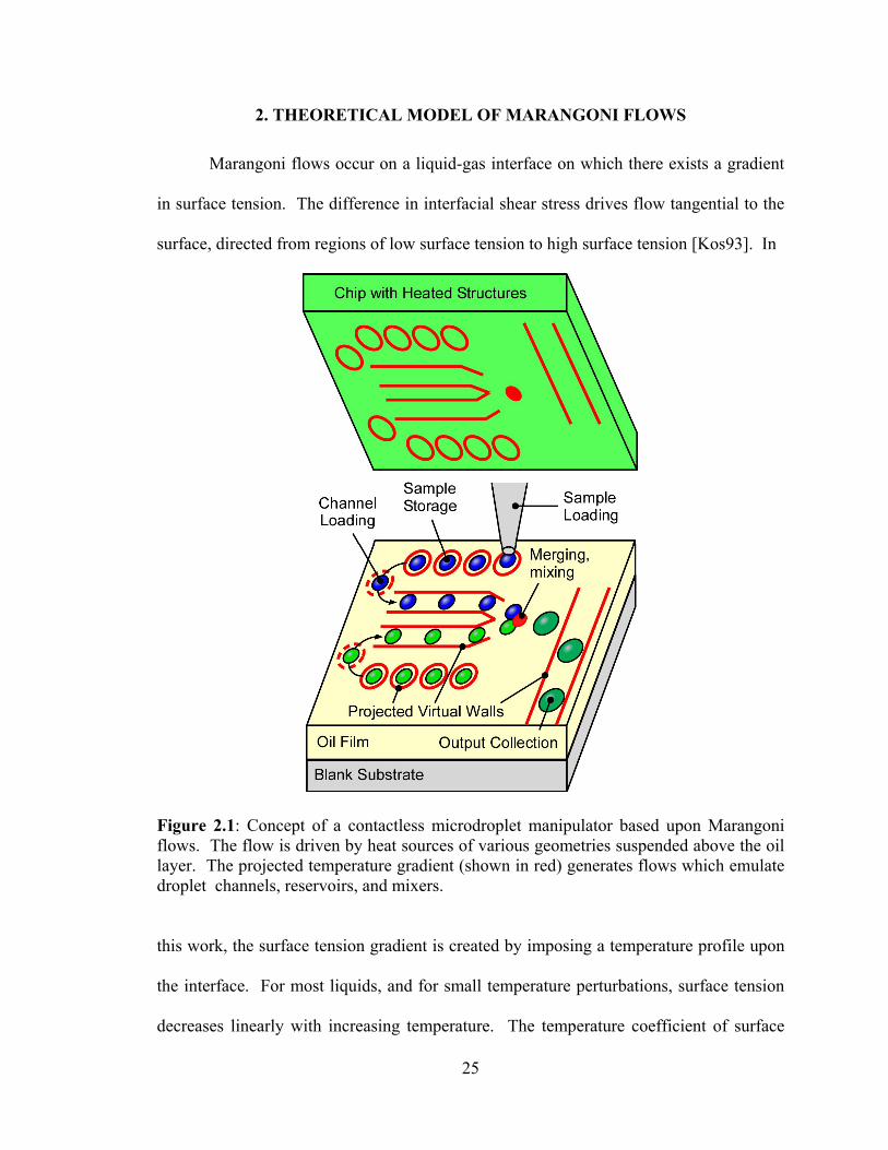
Marangoni flow technique to be presented in this thesis. ..................................................... 17 Figure 2.1: Concept of a contactless microdroplet manipulator based upon Marangoni flows.

The flow is driven by heat sources of various geometries suspended above the oil layer. The projected temperature gradient (shown in red) generates flows which emulate droplet channels, reservoirs, and mixers. .......................................................................................... 25

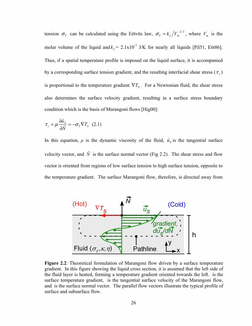
Figure 2.2: Theoretical formulation of Marangoni flow driven by a surface temperature gradient. In this figure showing the liquid cross section, it is assumed that the left side of the fluid layer is heated, forming a temperature gradient oriented towards the left. is the surface temperature gradient, is the tangential surface velocity of the Marangoni flow, and is the surface normal vector. The parallel flow vectors illustrate the typical profile of surface and subsurface flow. .................................................................................................................... 26

Figure 2.3: A microfluidic trap generated by a point heat source. (a) schematic showing the suspended heat source, the projected Gaussian heat flux profile, and the toroidal flow region in the oil layer. (b-c) Thermal CFD simulation results showing flow resulting from a Gaussian heat flux with amplitude qo = 6 mW/mm2 and ro = 40 µm applied to a 140 µm-thick layer of mineral oil with surface tension coefficient -0.16 mN/m-K. (b) Contours of

viii

stream function, illustrating pathlines in the oil layer. The 20 contours are equally spaced between 0 and 1.5x10-9 kg/s. (c) Temperature profile in the oil layer, again with 20 equally spaced contours between 300K and 301.4K. ........................................................................ 33

Figure 2.4: Simulated spatial velocity profile at various depths of the liquid for the simulation shown in Fig. 2.3. .................................................................................................................. 34

Figure 2.5: (a) Three dimensional thermal fluid simulation showing the interaction of a microfabricated thermal probe held above a layer of mineral oil. The numerical value of the temperature contours depends on the applied power as shown in part (b); however, the shapes of the contours do not change. Inset shows the qualitative surface heat flux resulting from the probe held at a 30° angle. (b) Maximum temperature increase on the liquid surface (∆TMAX) vs. separation between the probe and the liquid surface. (c) Maximum surface temperature gradient vs. gap. In (b,c), the diamonds represent simulation results. The lines are a 1/x best fit. .................................................................................................................... 35

Figure 2.6: Virtual droplet channels generated by parallel, linear heat sources. The channel boundaries are defined by the heat flux projected by two heated wires with separation s held parallel to the liquid surface. Target-sized droplets are pulled into the channel by the subsurface flows; others are excluded. Marangoni flows are shown in green and with arrows.................................................................................................................................... 37

Figure 2.7: Simulations of virtual channels formed by either two parallel heat fluxes with spacing s, or, alternatively, a single linear source with width w. (a,c) show the temperature profile and flow vectors for 2 parallel linear heat sources with a spacing s = 900 µm. (b,d) shows the same for a single line heat source with width w = 350 µm. In each case, surface temperature profiles are drawn above the flow vectors. Simulations assume a 200 µm-thick mineral oil layer with a surface tension coefficient -0.16 mN/m- K. Heat flux amplitudes are Gaussian with amplitude 6 mW/mm2 and radius 40 µm. uMAX is the maximum horizontal flow velocity, and ∆TMAX is the maximum surface temperature change................................ 38

Figure 2.9: Control of flow velocities with toroidal flows generated by a microfabricated point heat source. (a) Flow velocity vs. input power to the thermal probe plotted for three different separation distances. Also shown are simulated flow velocities as a function of input power. In the simulation, a Gaussian heat flux of increasing amplitude was applied to a 2D, axisymmetric fluid layer. (b) Experimental flow velocity vs. separation with experimental conditions as shown. A 140 µm layer of mineral oil was used in all experiments and simulations. ........................................................................................................................... 43

Figure 2.10: (a) Cold probe experimental setup. (b) Collection of particles using reverse Marangoni flow..................................................................................................................... 44

Figure 2.11: Effect of fluid depth. a) Radius of the convective region as a function of fluid depth. b) Peak radial velocity as a function of fluid depth. In both graphs, experimental conditions are as follows: probe type (R01, 35 Ω), input power=18 mW, air gap=100 µm, and the liquid is mineral oil. Simulation conditions: q0 = 6000 W/m2, r0 = 50 µm, and mineral oil properties are used. ............................................................................................. 45

Figure 2.12: Applications of the toroidal flow pattern in particle and droplet collection. (a) Schematic showing the heat source, XY scanning stage, toroidal flow patterns, and particles trapped within the collection area. Collection of (b) weed pollen in 125 µm mineral oil, and (c) 1 second exposure fluorescent image illustrating the movement of water microdroplets containing fluorescent dye. ................................................................................................... 46

Figure 2.13: Collection of 25 µm weed pollen using local toroidal flows. (1) The heat source is first advanced towards the particles. (2) When the heat source reaches the area above the particles, the particles are swept into the vortex and trapped. (3-4) The trapped particles are moved to a new location and released by turning off the heater. .......................................... 47

ix

Figure 2.14: Droplet merging of four droplets with (φ = 200-400 µm). (0s) The droplets are trapped in the self-circulating convective flow. (2s-9s) The droplets merge together, one by one, eventually forming a single, φ = 600 µm droplet. ......................................................... 48

Figure 2.15: Droplet rotation and mixing. (a) Schematic showing Marangoni flows around a suspended droplet which can rotate the droplet. (b) Experimental results showing single axis rotation up to 300 µm/s obtained when a 650 µm diameter tip is placed near a droplet of approx. the same dimensions. The tip temperature was ≈40°C. Flow patterns are visualized using immersed fluorescein particles and a 0.5 second CCD exposure with 490 nm/500 nm excitation/emission filters. .................................................................................................... 50

Figure 2.16: Size selective filtration of droplets in virtual channels. (a) Micrographs showing two 500 µm-diameter droplets (circle) entering the channel while a smaller one (square) is rejected. (b) Histogram showing the size selectivity of two droplet channels with 600 µm and 970 µm spacing. Droplet statistics were compiled over video clips spanning 40 minutes. Bins are in 100 µm increments. ............................................................................. 51

Figure 2.17: Single droplet trapping with an annular heat flux. (a) Schematic illustrating the annular heat flux projected on the surface, the trapped droplet, and the exclusion of larger or smaller droplets. (b) CFD Simulation. The shaded contours represent the surface temperature gradient, with evenly spaced contours and a maximum temperature increase ∆TMAX = 6°C. White arrows represent the subsurface flow at 140 µm depth beneath the surface. The two regions of flow are marked with dashed lines. (c) Micrographs showing strong affinity of a 1 mm droplet to the annular heat source (T≈120°C). Gap is ≈200 µm. 53

Figure 2.18: Guidewire pump emulated by a tapered heat source. (a) Schematic showing the orientation of the triangular heat flux projected on the fluid surface, and a droplet being pulled in along its longitudinal axis. (b) CFD Simulation. Shaded contours represent the surface temperature gradient, and white arrows represent the subsurface flow (140 µm depth) which pushes the droplet from left to right. (c) Micrographs illustrating movement of a droplet at 196 µm/s driven by a suspended heat source (T≈130°C) with 10° lateral taper and a 5° taper in vertical spacing. Gap is ≈200 µm.............................................................. 54

Figure 3.1: Schematic of doublet flow generation. The heated thermal probe, when suspended above a liquid, induces a high-speed doublet flow pattern at the surface. ............................ 60

Figure 3.2: Simulation of doublet flow due to surface momentum. ............................................. 62 Figure 3.3: Theoretical doublet model. (a) Schematic of doublet geometry illustrating a sink to

the left of the origin and a source to the right of the origin. Velocity is calculated at an observation point P. (b) Streamlines of a doublet with dipole moment 25x10-6, plotted using Eq. 3.4. (c) Contours of x velocity for the same doublet, plotted usinq Eq. 3.5. .................. 65

Figure 3.4: Simulation results of a doublet caused by a thermal dipole on the liquid surface. (a) Contours of the heat flux supplied to the surface of a 50 µm thick layer of water. The cold spot is on the left, hot spot on the right. Separation is 20 µm. (b) Velocity vectors, showing 5 mm/s flow to the left of the sink. (c) Contours of velocity in the +x direction.................. 69

Figure 3.5: High-speed doublet flow is illustrated in 4 sequential micrographs taken at 1/30 second intervals. Polystyrene beads are used to visualize the flow. .................................... 70

Figure 3.6: Control of flow velocities. (a,b) Peak linear flow velocity as a function of (a) input power, and (b) air gap. (c) Rotation rate in the eddies, as a function of air gap. (d) Flow velocity vs air gap repeated for three different ambient liquid temperatures. Experimental conditions are shown. The lines in (a) are a linear fit, and the lines in (b,c) are a fit to 1/x2................................................................................................................................................ 71

Figure 3.7: Flow reversal. The direction of the flow can be reversed by changing the angle of the heater. For example, using probe R02 at a 15° tilt, 15 mW input power, and a ~15 µm air gap, the doublet flows left to right, and the rotation in the vortices is counter-clockwise (left). Increasing the angle to 30° while keeping all other parameters constant reverses the

x

direction of the flow and rotation and shifts the location of the vortices to the left of the cantilever (right).................................................................................................................... 73

Figure 3.8: Uniform flow generated with a linear array of doublets. (a) Theoretical streamlines of flow generated by an array of 8 doublets with 85 µm spacing obtained by summing the respective stream functions. (b) Linear flow generation using an 8-probe array, numbered 1-8 from the top down. The array was placed ~15-20 µm above the liquid surface, held at a 15° tilt, and biased with a total power of 92 mW. Probes 1 and 4 were nonfunctional. Trajectories for 3 particles are marked with a square, triangle, and circle on micrographs taken at 3 second intervals. ................................................................................................... 74

Figure 3.9: (a) Schematic of subsurface particle flow (80 µm below the surface). Particles flow radially inward towards the area underneath the microheater tip. Upon reaching this point, they are immediately propelled upwards to the surface. (b) Sequential micrographs show three particles (marked respectively with a square, triangle, and circle) converge towards the center and then disappear from the field of view as they are propelled upwards.................. 76

Figure 4.1: A complete system for programmable, non-contact droplet actuation based on Marangoni flows, including a 128-pixel array of resistive heaters suspended above the oil layer, control circuitry, and a graphical user interface. ......................................................... 81

Figure 4.2: Results from a computational fluid dynamics simulation (FLUENT 6.0). (a) Surface temperature contours generated by an active heater and velocity vectors of the surface and sub-surface Marangoni flows. (b) Flow velocity vs. peak surface temperature change for 100 µm, 200 µm, and 500 µm gap between the heater and liquid. CR represents the coupling ratio, which is defined as the ∆T on the liquid surface divided by the ∆T in the heater. .................................................................................................................................... 84

Figure 4.3: 3-D CFD simulation of push and pull mode actuation on a Ф=200µm and Ф=800µm droplet, respectively. The droplet volumes were meshed as an immiscible spherical volume within the fluid layer. (a) Flow vectors showing pressure and viscous forces on a 200 µm droplet offset 1 mm from the center of the heat source. (b) Moment force on an 800 µm droplet offset 500 µm from the center of the heat source. (c) A trapped 800 µm droplet after it has been pulled into the center of the heat source.............................................................. 85

Figure 4.4: Simulated results. Forces acting on a Ф=800 µm and Ф=200 µm droplet, taken from the simulation in Fig. 4.3. (a) Moment force on the two sizes of droplets at various lateral offset distances from the center of the heat source. (b) Lateral pressure force (directed away from the heat source) for the two droplets, also at various distances from the heat source. . 87

Figure 4.5: Micrograph of heater array ......................................................................................... 91 Figure 4.6: Experimental setup, showing the heater array above a glass slide on which the liquid

samples are placed................................................................................................................. 92 Figure 4.7: (a) Schematic of logic and driver electronics. There are 128 joule heaters, and one

D-latch and driver for each (these elements are represented by the <128>). The remaining components are shared. The forward slash indicates a multi-line bus, and the number beneath indicates the number of lines on the bus. (b) Timing diagram, showing the serial input scheme for toggling heaters on and off. ....................................................................... 93

Figure 4.8: Experimental results. (a) Temperature of an active heater (TH) vs. input power. Also shown is the temperature increase one pixel away (T1), two pixels away (T2), and on the substrate 2 cm away (TS). (b) Flow velocity (25 µm pollen) and droplet velocity (Ф=300 µm droplet) vs. input power and heater temperature. This experiment used Dow Corning 550 silicone oil and a heater-liquid gap of ~100 µm. (c) Comparison of maximum flow velocities obtained with 4 fluids including mineral oil, Dow Corning 550 and 704 silicone oils, and Fluorinert FC-3283 dielectric liquid. Calculated figures of merit for each fluid are given in the figure. ................................................................................................................ 95

Figure 4.9: Push-mode actuation. (a) Surface Marangoni flows create a droplet force (FD) oriented away from the active heater. (b-e) A Ф=900 µm floating droplet is moved along a

xi

square path by activating multi-heater configurations sequentially. Active heaters are shaded. PH=1 W/heater, gap≈400 µm, and the fluid is DC-550 silicone oil. ....................... 99

Figure 4.10: Pull-mode actuation and droplet merging. (a) Subsurface Marangoni flows create a force on the droplet (FD) toward the active pixel. (b-e) Droplet merging with pull-mode actuation. Two droplets (Ф=600 µm) are merged through sequential activation of the heaters. Active heaters are shaded. PH=1 W/heater, gap≈300 µm, and the fluid is DC-550 silicone oil. .......................................................................................................................... 100

Figure 4.11: Preventing droplet evaporation. Measurements showing variation of droplet size over time (log scale) for a Ф=650 µm droplet in single and double layer oil system. The single layer oil system consists of DC-550 silicone oil, and two layer system consists of DC-550 and mineral oil.............................................................................................................. 101

Figure 4.12: Scaling study (simulation). (a) The surface temperature gradient and corresponding shear stress is plotted at various length scales. In all cases, the absolute temperature change on the liquid surface (∆TS) is 10°C. (b) Flow velocity (blue diamond) and flow reversal depth (red square) plotted for each length scale, under the same condition of ∆TS= 10°C.105

Fig. A1.1: The microfabricated thermal probe which is used to generate flow. (a) Schematic showing a polyimide cantilever overhanging the edge of a silicon substrate. The integrated heater is located on the cantilever just beneath the tip. The shading along the length of the cantilever indicates the thermal gradient that is present when the heater is powered. (b) Scanning electron micrograph of the fabricated thermal probe, with inset showing the pyramidal tip (from [Li03])................................................................................................. 112

Fig. A1.2: Scanning electron micrograph of a microfabricated thermal probe array [McN04B] used to generate flow. The inset shows the scanning tip with approximately 100 nm tip diameter............................................................................................................................... 113

Fig. A1.3: Fabrication process. Details are given in the text. ...................................................... 114 Fig. A1.4: Temperature characterization of the R01 type thermal probe. The three lines show the

fractional resistance change of probe R01 as the input power was ramped under various conditions. The probe is connected to a wheatstone bridge circuit which supplies measures the probe resistance. tip temperature is calculated by the resistance change ..................... 116

Fig. A1.5: Thermal time constant of a typical probe. The x axis shows time in 1 ms divisions, and the y axis shows the voltage, with 50 mV/division. The time constant is approximately 5 ms. ....................................................................................................................................... 117

Fig. A2.1: Schematic of simulation model, showing the thermal probe is held in air above a liquid film. Symmetry is used to simplify the simulation so that only ½ of the model is solved. All perpendicular field gradients are set to null at the mirror symmetry plane................... 118

Fig. A2.2: Typical heat flux and temperature profiles on the liquid surface driven by the probe. (left) A composite image showing qualitative heat flux and temperature contours on the fluid surface. (right) This graph shows the parallel cross section of a heat flux profile supplied by the thermal probe to the liquid surface under typical conditions. An approximate Gaussian fit is shown...................................................................................... 119

Fig. A2.3: Side view of simulation results, showing qualitative temperature contours in the probe and the liquid surface. The magnitude of temperature depends on the input power applied; however the contour shapes remain the same. .................................................................... 120

Fig. A2.4: Heat flux supplied to the liquid surface from the probe at various attack angles. (simulation). The probe is suspended 15 µm above the liquid surface and is angled at 15, 30, and 45 degrees with respect the liquid plane. These contours are qualitative; their magnitudes scale with the amount of input power. The line across the middle of the heat flux plots represents the probe axis. .................................................................................... 121

Fig. A3.1: Process flow for scanning thermal lithography of AZ5214E resist. (a) Flood exposure generates photoacids. (b) Spatially localized thermal cross-linking occurs under the heated

xii

probe tip (inset) as a result of the photoacids and elevated temperatures. (c) The insoluble cross-linked region remains after development in TMAH developer. ................................ 124

Fig A3.2: (a) Schematic of the micromachined single probe, and (b) SEM of the 8-probe array surface micromachined from polyimide on a Si substrate. Thin film resistors integrated on the tip of the cantilevers allow the individual probes in the array to be heated independently of one another...................................................................................................................... 125

Fig. A3.3: Dot sizes can be controlled by the heating times as well as heating power. (a) Reduction in size with shorter heating times using a probe biased at 18 mW on 450 nm resist. (b) Dot sizes vs. heating time for 18 mW and 13.5 mW power.............................. 129

Fig A3.4: (a) Finite element simulations with photoresist thicknesses of 1.4 µm, 450 nm, and 100 nm show that the geometry of heat flow becomes vertical as the photoresist is thinned below the diameter of the tip, resulting in smaller features. (b) Dots obtained after fully developing 1400 nm and 450 nm resist follow the same trend. The roughened surfaces in the micrographs are due to an Au/Pd layers sputtered for SEM. ........................................ 131

Fig. A3.5: (a,b) Lines of 500 nm width written by patterning successive dots with 200 nm spacing (1 s heating per dot) can be seen after partial development of the photoresist. (c,d) Parallel lithography is demonstrated where two adjacent probes in the 8 probe array simultaneously generate the same pattern. ................................................................................................... 132

xiii

LIST OF TABLES

Table 1.1: Techniques for microdroplet manipulation. An ‘X’ is placed in the column if the technique offers the feature indicated on the top of the respective column .......................... 20

Table 4.1: Material properties for 3 liquids used in generating Marangoni flows. Values marked with a * are calculated using the Eötvös law, and those marked with ** are estimated from similar fluids.......................................................................................................................... 90

xiv

LIST OF APPENDICES

APPENDIX 1: STRUCTURE, FABRICATION, AND OPERATION OF THERMAL PROBES 112

1. STRUCTURE 113

2. FABRICATION 114

3. OPERATIONAL CHARACTERISTICS 115

APPENDIX 2: INTERACTION OF PROBES WITH THE LIQUID SURFACE 118

APPENDIX 3: SCANNING THERMAL LITHOGRAPHY - MASKLESS, SUBMICRON

THERMO-CHEMICAL PATTERNING OF PHOTORESIST BY ULTRACOMPLIANT PROBES

122

1. INTRODUCTION 122

2. PROCESS AND DEVICE CONCEPTS 125

3. EXPERIMENTAL RESULTS 127

xv

ABSTRACT

Fluid manipulation at the micrometer scale has traditionally involved the use of

batch-fabricated chips containing miniature channels, electrodes, pumps, and other

integrated structures. This dissertation explores how liquids on non-patterned substrates

can be manipulated using the Marangoni effect. By placing miniature heat sources above

a liquid film, it is possible to generate micro-scale surface temperature gradients which

results in controlled Marangoni flow. A variety of useful flow patterns can be designed

by tailoring the geometry of the heat source.

As a surface tension-based phenomenon, the Marangoni effect is an efficient

actuation mechanism at submillimeter dimensions. With optimized liquid carriers, flow

velocities >10 mm/s can be generated with only small perturbations in surface

temperature (<10 K). Thermally efficient microfabricated heat sources, such as

polyimide thermal probes, can produce >1700 µm/s flow velocity in mineral oil while

consuming <20 mW of power. In water films, the probes can generate surface doublets

with linear velocities up to 5 mm/sec and rotational velocities up to 1300 rpm, making

them potentially useful for active mixing.

The utility of Marangoni flows is demonstrated within the context of digital

microfluidic systems. In contrast to conventional microfluidics, where samples are

flowed through microchannels, digital microfluidic systems contain liquid samples in

micro and nanoliter-sized droplets suspended in an immiscible oil layer. Marangoni

xvi

flows generated in the oil layer can manipulate droplets without any physical structures,

thus avoiding surface contamination. By using point, linear, annular, and tapered heat

source geometries, it is possible to engineer Marangoni flows which mimic the

functionality of droplet channels, mixers, size-selective filters, and pumps. Arbitrary,

two-dimensional actuation of droplets (Ф=400-1000 µm) can also be achieved using an

array of heaters suspended above the oil layer. The 128-pixel heater array incorporates

addressing logic and a software interface which allows it to programmatically transport

and merge multiple droplets through the sequential activation of heaters.

The appendices outline other aspects of thermal probes, including i) the structure,

fabrication, and operational characteristics of single probes and probe arrays, and ii)

scanning thermal lithography, a technique for nanoscale patterning of thin films with

heat.

1

CHAPTER 1:

INTRODUCTION

1. MICROFLUIDICS FOR MINIATURIZED CHEMICAL ASSAYS

Richard Feynmann, in his famous 1959 speech [Fey59], proclaimed that “there is

plenty of room at the bottom”, encouraging leading scientists to explore a new field of

science and engineering at micrometer and nanometer length scales. Among the several

intriguing possibilities he described, Feynman noted “The Marvelous Biological

System”, referring to microorganisms which move, interact, and store information at

small length scales. He challenged scientists to build precision instruments that would be

able to study and interact with these systems at the same length scales. Forty five years

later, Feynman’s vision has now grown into one of the most promising areas of

engineering and biomedical research.

One of the primary drivers behind the renewed interest is microfabrication

technology, which allows us to manufacture micrometer scale, planar structures using the

combined technologies of thin film deposition, photolithography, as well as chemical and

plasma etching [Mad02]. These techniques, borrowed from the semiconductor industry,

can be used to produce small microchips containing 1) various fluid channels, pumps, or

valves for handling liquid samples of cells and molecules, and ii) sensors, heaters, and

other instruments for performing sample analysis. The devices, collectively termed

2

micro total analysis systems (µTAS) or “lab-on-a-chip” (LOC), have revolutionized the

way biological assays are performed, enabling massively parallel operation, analysis of

miniscule sample volumes, integrated sample preparation, low power consumption, and

portability. The first microfabricated DNA analysis system, incidentally, was developed

here at the University of Michigan [Bur96].

Microfluidic systems will continue to play an increasingly significant role in the

in vitro diagnostics (IVD) market, whose market size is expected to be ~$40 billion in

2008 [Ros04]. The market size for microchip technologies in general exceeded $1.7

billion in 2008, and is expected to grow at a 25% annual growth rate to $6 billion in 2017

[Kru07]. The major application categories in the microfluidics market include high

throughput screening (HTS) and compound profiling, point of care (POC) diagnosis and

testing, chemical analysis, drug delivery, genomics/proteomics, and homeland security

[Ros04]. As of January 2008, numerous successful commercial µTAS devices have

penetrated a number of areas within the IVD market. A few notable examples include the

following:

• DNA microarrays have enabled massively parallel, high throughput profiling of

gene expression (Affymetrix, Roche Diagnostics)

• Microfluidic cards for multiplexed Polymerase Chain Reaction (PCR) and

electrophoretic separation of DNA. These cards can handle up to 380

simultaneous reactions and have reduced analysis time by 1 order of magnitude

(Applied Biosystems)

• Miniature microfluidic systems for Reverse Transcriptase PCR and

electrophoresis have enabled simple and portable genetic detection of

3

microorganisms (Handylab)

• Integrated, sample-to-answer genetic detection systems using microfluidic cards

can perform sample preparation, PCR, electrophoretic separations, and molecular

purification in portable, highly parallel format with low reagent consumption

(Agilent Technologies, Caliper Life Sciences).

• Portable blood analyzers have enable point of care (POC) testing of various

biological markers (Honeywell, Siloam Biosciences)

• Microfabricated glucose monitors have provided a portable and less invasive

option for diabetics to monitor their blood sugar (TheraSense)

2. USING THE MARANGONI EFFECT FOR MICROFLUIDIC ACTUATION

In his speech, Richard Feynman noted that the physics of nature changes at small

lengths scales [Fey59]. In microfluidic systems, physical scaling laws enhance surface

phenomena and diminish the importance of pressure, inertia, gravity, and other

volumetric forces. As a result, many pumping techniques developed for conventional

length scales become less effective. For example, microfluidic channels have a large

hydraulic resistance due to their small cross sections, and require larger pressures from

external pumps. At the same time, other physical phenomena, such as surface-based

phenomena, tend to become more efficient at small length scales. One such example is

the Marangoni effect, the topic of this thesis.

Marangoni flow, the movement of liquids due to surface tension gradients, is

responsible for many common phenomena. These include, for example, the dispersion of

oils in dishwater upon the addition of detergent [Her96], and the rotating flow of particles

4

below a candle wick [Adl70]. Nevertheless, at macroscopic length scales, the Marangoni

effect is not a practical mechanism for fluidic actuation because surface forces are

typically weak compared to pressure, inertial, and other body force mechanisms.

However, like other surface phenomena, it scales favorably to the micrometer regime. If

l is considered the length scale, surface tension forces are proportional to l, pressure

forces are proportional to l2, and inertial forces are proportional to l3. Thus, at small

length scales, surface tension forces become increasingly significant compared to the

other two. Furthermore, the high ratio of surface-area to volume present in microscale

devices suggests that the Marangoni effect could be useful for microfluidic actuation.

The traditional, “macroscopic” approach for generating Marangoni flow is via

isothermal heating (Fig 1.1a). A thin liquid layer is heated uniformly from below, and

the resulting flow is a pattern of hexagonal convection cells (Fig. 1.1b) [Mar07, Kos93].

This multicellular flow, first observed by Henri Bénard in the late 1800’s [Bén00], was

originally thought to be due to natural convection, and was later attributed to the

Marangoni effect by Brock and Pearson in the 1950’s [Blo56, Pea58, Mar07]. Since

then, it has been the subject of several efforts to mathematically analyze fluid stability

[Kos93]. From a practical standpoint, however, the geometry and stability of the flow is

very sensitive to the fluid container and the thermal boundary conditions. Therefore,

isothermally-generated Marangoni flows provide little opportunity for localized fluidic

manipulation in the context of an automated system.

5

This dissertation focuses on a localized approach for generating Marangoni flow:

by imposing micrometer scale temperature gradients on the surface [Bas07B]. This can

be done by suspending small heat sources just above the liquid surface (Fig. 1.1c). The

heat flux supplied to the surface causes localized variation in surface temperature. This,

in turn, causes a corresponding surface tension gradient due to the inverse relation

between surface tension and temperature that exists for most liquids. In the presence of a

Figure 1.1: Comparison of conventional, multicellular Marangoni convection versus the present approach. (a) Schematic of multicellular Marangoni flow occurring when a thin liquid layer is isothermally heated from below. (b) Top view of hexagonal convection cells resulting from conventional Marangoni convection (from [Mar07]). (c) Local, unicellular Marangoni convection initiated by a heat source placed above the liquid layer

6

surface tension gradient, a shear stress is generated at the liquid boundary which drives

surface flow away from the heated regions (low surface tension) and towards the cool

regions (higher surface tension). Cooling sources can generate Marangoni flow in the

reverse direction. Thus, from a theoretical perspective, it would be possible to engineer

arbitrary surface flows by superimposing multiple thermal sources as shown in Fig. 1.2.

This approach takes advantage of the favorable scaling of surface forces and

could provide several important advantages in practicality and efficiency. The first

potential benefit is flow localization: in contrast to isothermal heating, a point or linear

heat flux favors the formation of a single Marangoni cell, which allows for precise

control of the geometry and flow speeds of the cell.

The second benefit is efficiency. As will be shown in Chapter 2, Marangoni flow

velocities are proportional to the surface temperature gradient. By using microscale heat

Figure 1.2: Controlling fluid flow with Marangoni convection. In this overall vision, thermal sources suspended above the surface of a thin liquid layer provide arbitrary, patterned heat fluxes to the liquid surface, resulting in controlled surface tension gradients. Point heating sources causes flow away from the heated surface, whereas point cooling sources cause inward flow. Fast flow velocities can be achieved with small temperature changes because temperature and surface temperature gradients are steep at small length scales.

7

sources it is possible to achieve sharp temperature gradients which enable faster

velocities while minimizing the absolute changes in surface temperature. An important

aspect of this technique is that the heat sources used to generate flow are suspended

above the oil. Benefiting from the low thermal conductivity of air, this approach creates

sharp surface temperature gradients which would not be possible were the heat source

embedded in the fluid. Embedded heaters would also cause significant heating in the

bulk fluid which is undesirable for bio-analytical microsystems.

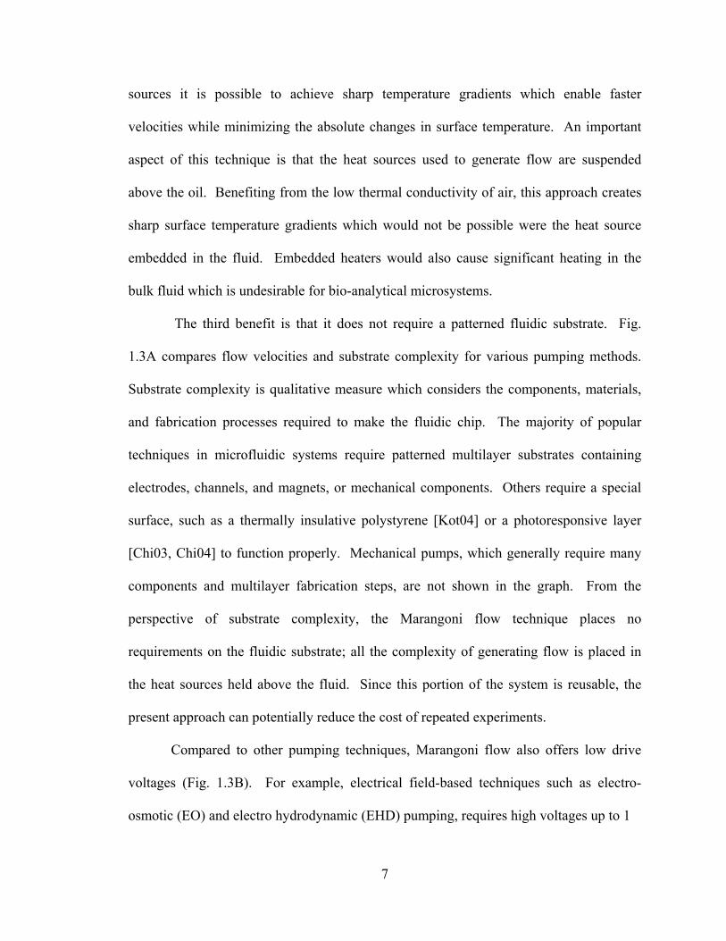
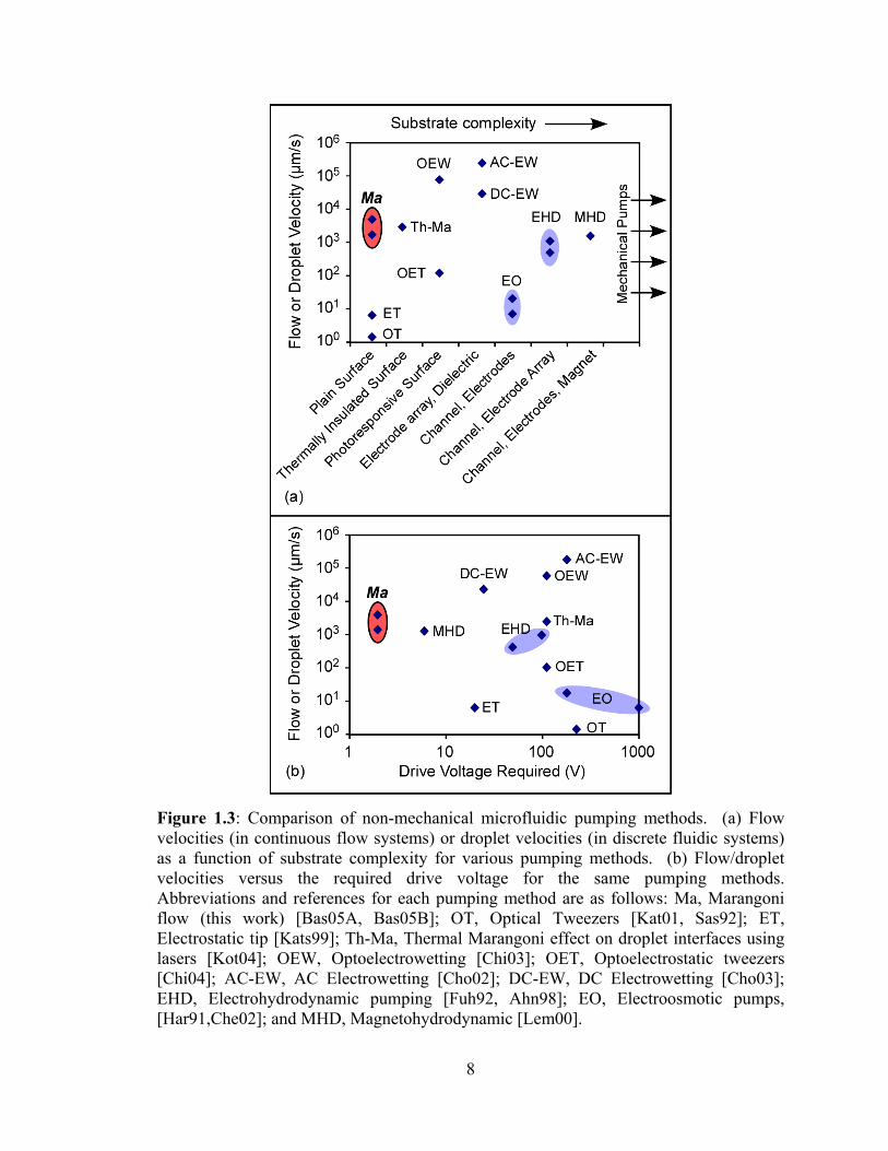
The third benefit is that it does not require a patterned fluidic substrate. Fig.

1.3A compares flow velocities and substrate complexity for various pumping methods.

Substrate complexity is qualitative measure which considers the components, materials,

and fabrication processes required to make the fluidic chip. The majority of popular

techniques in microfluidic systems require patterned multilayer substrates containing

electrodes, channels, and magnets, or mechanical components. Others require a special

surface, such as a thermally insulative polystyrene [Kot04] or a photoresponsive layer

[Chi03, Chi04] to function properly. Mechanical pumps, which generally require many

components and multilayer fabrication steps, are not shown in the graph. From the

perspective of substrate complexity, the Marangoni flow technique places no

requirements on the fluidic substrate; all the complexity of generating flow is placed in

the heat sources held above the fluid. Since this portion of the system is reusable, the

present approach can potentially reduce the cost of repeated experiments.

Compared to other pumping techniques, Marangoni flow also offers low drive

voltages (Fig. 1.3B). For example, electrical field-based techniques such as electro-

osmotic (EO) and electro hydrodynamic (EHD) pumping, requires high voltages up to 1

8

Figure 1.3: Comparison of non-mechanical microfluidic pumping methods. (a) Flow velocities (in continuous flow systems) or droplet velocities (in discrete fluidic systems) as a function of substrate complexity for various pumping methods. (b) Flow/droplet velocities versus the required drive voltage for the same pumping methods. Abbreviations and references for each pumping method are as follows: Ma, Marangoni flow (this work) [Bas05A, Bas05B]; OT, Optical Tweezers [Kat01, Sas92]; ET, Electrostatic tip [Kats99]; Th-Ma, Thermal Marangoni effect on droplet interfaces using lasers [Kot04]; OEW, Optoelectrowetting [Chi03]; OET, Optoelectrostatic tweezers [Chi04]; AC-EW, AC Electrowetting [Cho02]; DC-EW, DC Electrowetting [Cho03]; EHD, Electrohydrodynamic pumping [Fuh92, Ahn98]; EO, Electroosmotic pumps, [Har91,Che02]; and MHD, Magnetohydrodynamic [Lem00].

9

kV, although newer methods like electrowetting-on-dielectric (EWOD) have reduced this

requirement to 20 V. The presence of high electric fields, particularly DC fields, can lead

to electrolysis which degrades electrodes and also causes bubble formation in channels.

As a thermal actuation technique, Marangoni flows are generated by electrically heating a

source. By using an efficient microfabricated heat source with <40 Ω resistance, flow

velocities up to >5 mm/s can be achieved with voltages <2 V and input powers <25 mW.

This is due not only to the efficient design of the heat source, but also the efficient

conversion of heat to mechanical energy at small length scales. Thus, this technique has

potential for enabling low power, reconfigurable microfluidic systems.

A fifth benefit is the lack of physical contact between the heat source and the

liquid sample, which eliminates contamination of the device and cross-contamination

between samples. A previous approach to using Marangoni flow for fluidic actuation

requires electrochemically generated surfactants [Gal99], which causes ionic

contamination of the sample. Temperature gradients generated by substrate heaters

[Dar03] or external lasers [Kot04] have also been used to initiate Marangoni flow and

move a liquid droplet or film on a substrate. Both these approaches, however, require

that the liquid sample be in contact with the substrate.

In this approach, aqueous samples are contained in droplets which are suspended

in a high-density, immiscible oil layer. Due to the high density of the oil, the droplets

float near the surface, away from the actuator and the substrate below, and they can

manipulated using Marangoni flows generated by the heat sources from above. This

approach to fluidic manipulation is less prone to contamination than those mentioned

10

above, as well as other popular techniques for droplet manipulation, such as

electrowetting [Cho03, Yoo03].

The last benefit is the central theme of this dissertation: the ability to engineer

Marangoni flows. Using microscale heat sources of various geometries, it is possible to

shape the surface temperature gradient and the resulting Marangoni flow. These flows

can be used to manipulate liquids, particles, and droplets without any physical structures

in the liquid film. Microdroplets, in particular, have potential applications in microfluidic

biochemical assays.

3. CONTINUOUS FLOW MICROFLUIDIC SYSTEMS

In general, microfluidic sample handling can be categorized into two broad

categories. The early generations of microfluidic chips have been primarily “continuous

flow” systems. In other words, reagents and samples are flowed through microchannels

formed on the fluidic substrate. These channels can be formed in a number of ways,

including bulk micromachining of silicon [Che97], chemical etching of glass [Har92,

Sei93], parylene deposition with a sacrificial photoresist layer [Man97], and

micromolding with a silicone elastomer [Xia98]. Due to the small cross section and

length of the fluidic channels, small amounts of liquids are consumed, and flows are

primarily laminar in nature [Tak01], resulting in predictable flow and mixing profiles.

Mechanical actuators, similar to conventional pumps, can be used to generate

pressure and flow of liquids through microchannels. The most common implementation

is a peristaltic membrane pump, driven by integrated thermopneumatic, electrostatic, and

piezoelectric actuators, or by off-chip pressure driven sources [Gro99, Xie04, Ung00].

11

Since these devices often require moving parts with out of plane deflection, device

reliability and fabrication complexity is often a concern for mechanical pumps.

Several non-mechanical methods, which take advantage of surface and capillary

effects in small channels, are also effective in controlling fluids without moving parts.

These include electro-osmotic [Har91, Che02], electrohydrodynamic [Fuh92, Ahn98],

thermocapillary [Sam99A, Sam99B], and magnetohydrodynamic pumps [Lem00], along

with many more. These pumps generally rely on the interaction of electromagnetic fields

with mobile charges in the fluid, and often require large field strengths in order to

function. However, they are more amenable to integration because their fabrication

complexity tends to be simpler. For example, electro-osmotic pumps require only two

electrodes aligned in the channel [Har91]. For a review of micropump technologies, the

reader is referred to [Ngu02].

Although the continuous flow systems are appropriate for many assays, users seek

several areas of improvement. First of all, due to the high hydraulic resistances of the

microchannels, pumps must generate large pressure heads in order to achieve reasonable

flow rates. The presence of moving parts is a concern for mechanical pumps, and in

nonmechanical pumps, high field strengths can cause undesirable effects such as

electrolysis.

Another issue is reconfigurability. Early in the years of digital electronics,

application specific IC’s (ASICs) were designed to perform specific computing tasks.

ASICs were eventually replaced by a more versatile microprocessor chip which could be

reprogrammed to perform a wide range of general computations. Similarly, the first

generation of fluid handling chips have been designed with fixed geometries for use in a

12

specific assay. While this is sufficient if the fluid handling protocol is fixed, it does

present a problem if flexibility in the handling of reagents is required [Gas04, Cho03].

With a fixed geometry, each assay requires its own chip design and fabrication, resulting

in non-recurring engineering (NRE) costs and effort.

Still another issue with continuous flow systems, arguably the most significant, is

the problem of surface adsorption. Hydrophobic proteins and DNA have low surface

hydration energies [Gas04], making it likely that any contact to a solid surface will result

in nonspecific adsorption; thus, any degree of contact or wetting between a liquid sample

and the channels walls can result in surface adsorption. Most channel materials,

particularly hydrophibic materials such as Teflon, Parylene, and Polydimethylsiloxane

(PDMS) are particularly susceptible to such adsorption [Yoo03, Sia03, Son03]. In

microchannels, the adsorption of proteins and cellular debris leads not only to

contamination, but can also cause channel blockages [McC03]. More importantly,

contamination eliminates the possibility of reusing the device, and the sample loss due to

adsorption can make it difficult to detect low concentration samples [Lin06].

4. MICRODROPLET-BASED “DIGITAL” MICROFLUIDICS

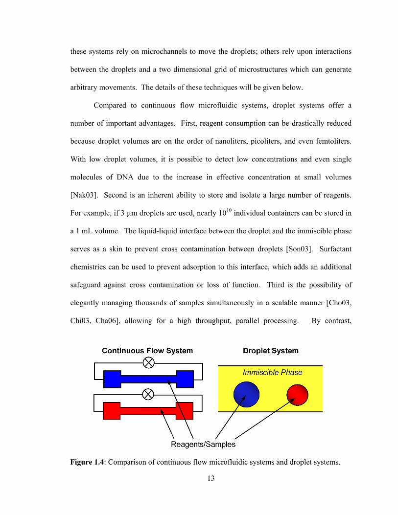
Digital microfluidic systems offer an elegant alternative to continuous flow

microfluidics (Fig 1.4). In these systems, liquid samples are handled in the form of

compartmentalized droplets. Specifically, aqueous microdroplets immersed in an

immiscible phase serve to encapsulate reagents and to function as microscale reaction

containers. Precise, user-defined chemical reactions may be achieved by transporting

and merging droplets containing the appropriate samples and reagents [Son03]. Some of

13

these systems rely on microchannels to move the droplets; others rely upon interactions

between the droplets and a two dimensional grid of microstructures which can generate

arbitrary movements. The details of these techniques will be given below.

Compared to continuous flow microfluidic systems, droplet systems offer a

number of important advantages. First, reagent consumption can be drastically reduced

because droplet volumes are on the order of nanoliters, picoliters, and even femtoliters.

With low droplet volumes, it is possible to detect low concentrations and even single

molecules of DNA due to the increase in effective concentration at small volumes

[Nak03]. Second is an inherent ability to store and isolate a large number of reagents.

For example, if 3 µm droplets are used, nearly 1010 individual containers can be stored in

a 1 mL volume. The liquid-liquid interface between the droplet and the immiscible phase

serves as a skin to prevent cross contamination between droplets [Son03]. Surfactant

chemistries can be used to prevent adsorption to this interface, which adds an additional

safeguard against cross contamination or loss of function. Third is the possibility of

elegantly managing thousands of samples simultaneously in a scalable manner [Cho03,

Chi03, Cha06], allowing for a high throughput, parallel processing. By contrast,

Figure 1.4: Comparison of continuous flow microfluidic systems and droplet systems.

14

continuous flow systems require complex valving for isolating multiple reagent streams

[Tho03].

From an application standpoint, microdroplet-based systems have been

successfully employed in a number of biochemical assays. The low volumes and fast

diffusive mixing rates allow the study of enzyme kinetic reactions in real time [Son03].

The ability to screen a large number of droplets, each with a different composition, has

been shown to be indispensable in optimizing protein crystallization conditions [Zhe03].

PCR amplification in droplets allows the detection of single molecules of DNA [Nak03].

Droplets can be used to preconcentrate and isolate solutes [He04], and they also offer a

controlled, low-volume microenvironment of droplets for the culture and study of single

cells [He05]. The absence of dilution in the encapsulated environment enables

quantitative measurements of intra and extracellular secretions [Iri04]. Given the large

number of applications and the advancement of droplet system technology, it is likely

that the use of droplets in biochemical assays will grow rapidly in the next several years.

In order to mirror the complete set of fluidic operations that would be conducted

on a laboratory benchtop, the ideal digital microfluidic device should be able to perform

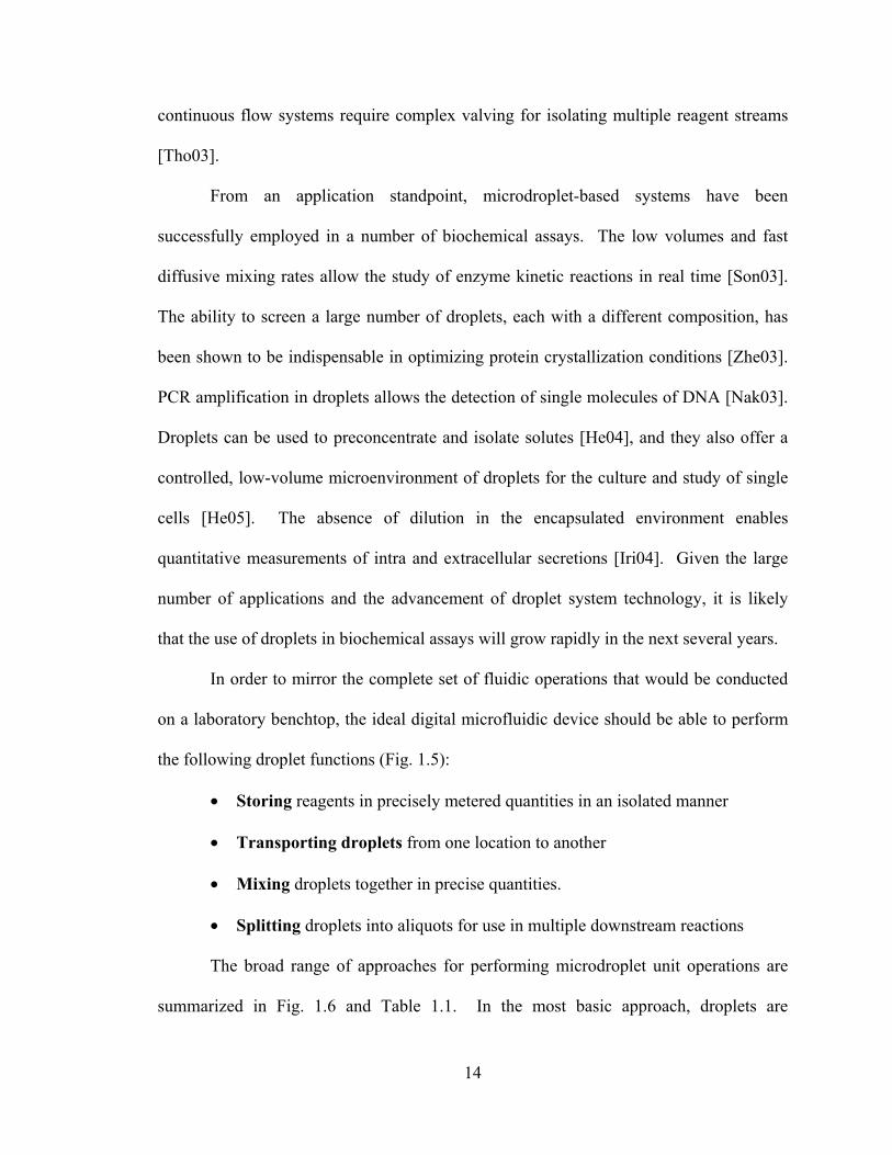
the following droplet functions (Fig. 1.5):

• Storing reagents in precisely metered quantities in an isolated manner

• Transporting droplets from one location to another

• Mixing droplets together in precise quantities.

• Splitting droplets into aliquots for use in multiple downstream reactions

The broad range of approaches for performing microdroplet unit operations are

summarized in Fig. 1.6 and Table 1.1. In the most basic approach, droplets are

15

transported through microchannels in the form of plugs. Various channel structures such

as T-junctions can be used to generate, mix, split, and merge droplets [Son03]. The

disadvantage of this approach is that it requires external pumps to generate flow in

channels. A somewhat surprising advantage to using droplet channels is that there is no

contact between the droplet and the channel walls. The hydrophobic carrier fluid

surrounding the droplets forms a thin boundary which separates and isolates the droplet

from the wall [Son03]. Therefore, this technique avoids surface adsorption. However,

the drawback is its lack of programmability because the channel geometries are fixed.

Electrowetting on dielectric (EWOD), perhaps the most popular technique for

droplet manipulation, uses voltages on a two dimensional grid of electrodes to control the

movement of droplets [Pol02]. An aqueous droplet is sandwiched between an upper and

lower surface. The lower surface contains a grid of control electrodes coated with a

hydrophobic surface, while the upper surface contains one large electrode which serves

as the ground plane. When a voltage is applied to one of the control electrodes, the

surface becomes hydrophilic, and the droplet is attracted to the surface. By activating

adjacent electrodes in a sequential manner, it is possible to create surface energy

gradients which can move droplets from one electrode to the next. Other activation

patterns can split, cut, merge, and dispense droplets via electronic control [Cho03].

Figure 1.5: Illustration of droplet unit operations.

16

Optoelectrowetting, a similar technique, also relies on switching surface energies of

electrodes, but the switching is done via optical means, thus avoiding the need to

electronically address each electrode [Chi03].

Although both electro and optoelectrowetting can perform a wide range of

operations, perhaps the most fundamental limitation with these techniques is that they

require the droplet to wet the surface. The avoidance of surface contact cannot be under-

emphasized, and it is a serious concern if the system is to be reusable or able to detect

small amounts of reagents. Due to its high hydrophobicity, Teflon is particularly

susceptible to adsorption. It is possible to reduce adsorption by maintaining an acidic pH

in the droplet, reducing the duration of inactive time, or by the use of plasma deposited

fluoropolymer coatings [Bay07, Yoo03]. It has also been suggested that if silicone oil is

used as the encapsulating medium, the droplet may be separated from the Teflon surface

by a thin film of oil [Sri04]; however, the effectiveness of the technique depends

significantly on the interfacial tension between the oil and the protein concentration in the

droplet. None of these techniques for avoiding adsorption are 100% effective, as would

be required for a robust, reusable device. Adsorption can also render hydrophobic

surfaces hydrophilic, which results in contact angle hysteresis and interferes with the

EWOD actuation [Yoo03].

Optical tweezers (lasers) rely on radiation pressure which acts on the liquid-liquid

interface of the droplets [Ash80, Kat01, Sas92, Chi07]. Since the typical forces are fairly

small, optical traps work with small droplets with volumes on the order of femtoliters.

Unfortunately, optical tweezers can only attract particles which have a higher refractive

index than the surrounding media. The index of refraction in aqueous droplets (n = 1.33),

17

is always lower than that of the surrounding oil; therefore, the laser spot repels droplets

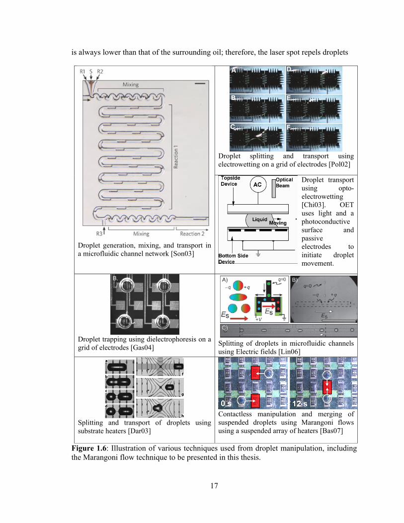
Droplet splitting and transport using electrowetting on a grid of electrodes [Pol02]

Droplet generation, mixing, and transport in a microfluidic channel network [Son03]

Droplet transport using opto-electrowetting [Chi03]. OET uses light and a photoconductive surface and passive electrodes to initiate droplet movement.

Droplet trapping using dielectrophoresis on a grid of electrodes [Gas04] Splitting of droplets in microfluidic channels

using Electric fields [Lin06]

Splitting and transport of droplets using substrate heaters [Dar03]

Contactless manipulation and merging of suspended droplets using Marangoni flows using a suspended array of heaters [Bas07]

Figure 1.6: Illustration of various techniques used from droplet manipulation, including the Marangoni flow technique to be presented in this thesis.

18

rather than attracts them. To overcome this issue, the laser beam must be scanned to

create a cage-like optical profile, requiring a more complex setup.

Dielectrophoresis (DEP) is a promising approach which uses non-uniform AC

electric fields acting on the liquid-liquid interface of a droplet. Positive DEP forces can

attract a droplet, avoiding the problem of having to create cages as with optical traps.

Moreover, greater forces are possible with DEP, allowing the manipulation of droplets up

to 100 nL [Gas04]. Using a two dimensional grid of electrodes, droplets can be

manipulated and merged arbitrarily. Although DEP devices do not rely on surface

contact, in most cases droplets sit on the substrate. It is not clear whether this technique

will result in contamination.

DC and pulsed electric fields acting on the liquid-liquid interface can also be used

to perform a wide range of operations. Weitz et al. demonstrated the use of both DC and

pulsed fields to dispense and split droplets inside microchannels [Lin06].

A DC electric field at a channel bifurcation can be used to split a droplet into two

daughter droplets with a positive and negative charge, respectively. The existence of

charge allows further electrical manipulation by electric fields; however, the droplets lose

charge over time and must be recharged. This approach allows some degree of

programmatic control, but due to fixed channel geometries it cannot perform arbitrary

routing in a 2D grid. It does, however, avoid surface adsorption since it does not rely on

surface wetting.

Magnetic fields, generated by a two dimensional array of coils, can be used to

manipulate droplets in a programmable manner. Superparamagnetic beads or

nanoparticles are embedded in each of the droplets, and the local magnetic fields induced

19

by the coils can transport and split droplets [Leh07]. In addition to having large forces

and long throw, an advantage of this approach is that the beads can be functionalized for

capturing DNA, viral RNA [Pip07], or for other solid phase extraction. The concern with

magnetic beads and fields is whether or not they are scalable and reusable. In these

systems, the droplets also contact the surface, which results in adsorption.

A final technique reviewed is thermocapillary flow, which is related, but not

identical, to the approach mentioned in this thesis. The thermocapillary approach uses

microheaters patterned on a substrate [Dar03]. When a finger shaped-film of liquid is

placed near an active heater, the boundary of the liquid tends to move away from the

heater (towards the cooler region) due to thermocapillary stresses in the liquid film. This

technique can be used to transport and split liquid films and droplets; however, in order to

localize the liquids on the substrate, hydrophilic strips must be patterned on the substrate,

which causes surface wetting and can result in contamination. A variant of this technique

uses an external laser [Kot04] for heating, which simplifies the fluidic substrate, but still

requires droplet/surface contact.

The technique that will be discussed in this dissertation is the use of Marangoni

flows for manipulating droplets suspended in oil [Bas07A-C]. As mentioned earlier,

surface Marangoni flows at small length scales can be created by placing small heat

sources above the fluid surface. Droplets suspended near the surface of the oil layer can

be manipulated using these flows. Although this technique does not offer the ability to

split droplets, it avoids all surface contact between the droplets and the system. Having

the heaters above the fluid surface allows the formation of sharp temperature gradients of

various shapes, which can generate a number of useful flow patterns for advanced droplet

20

control.

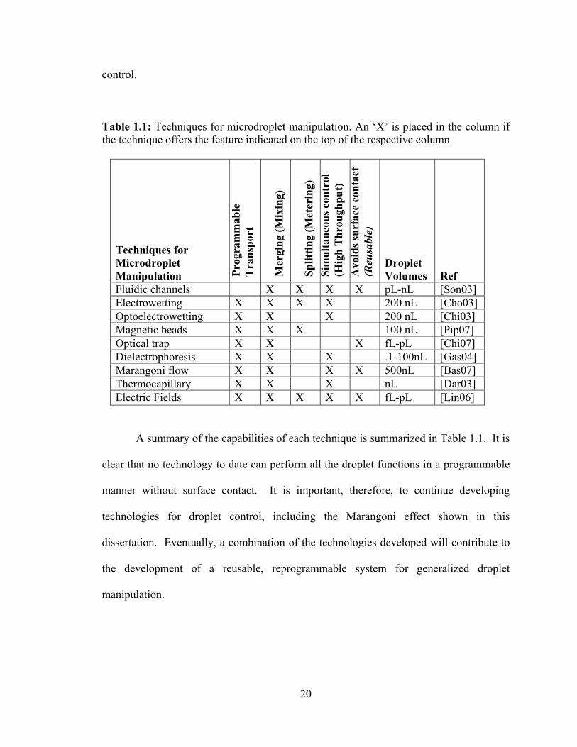
Table 1.1: Techniques for microdroplet manipulation. An ‘X’ is placed in the column if the technique offers the feature indicated on the top of the respective column

Techniques for Microdroplet Manipulation Pr

ogra

mm

able

T

rans

port

Mer

ging

(Mix

ing)

Split

ting

(Met

erin

g)

Sim

ulta

neou

s con

trol

(H

igh

Thr

ough

put)

A

void

s sur

face

con

tact

(R

eusa

ble)

Droplet Volumes Ref

Fluidic channels X X X X pL-nL [Son03] Electrowetting X X X X 200 nL [Cho03] Optoelectrowetting X X X 200 nL [Chi03] Magnetic beads X X X 100 nL [Pip07] Optical trap X X X fL-pL [Chi07] Dielectrophoresis X X X .1-100nL [Gas04] Marangoni flow X X X X 500nL [Bas07] Thermocapillary X X X nL [Dar03] Electric Fields X X X X X fL-pL [Lin06]

A summary of the capabilities of each technique is summarized in Table 1.1. It is

clear that no technology to date can perform all the droplet functions in a programmable

manner without surface contact. It is important, therefore, to continue developing

technologies for droplet control, including the Marangoni effect shown in this

dissertation. Eventually, a combination of the technologies developed will contribute to

the development of a reusable, reprogrammable system for generalized droplet

manipulation.

21

5. ORGANIZATION OF DISSERTATION

Chapter 2 of this thesis explores the effect of the heat source geometry on

Marangoni flow. It is shown that a number of useful flow patterns can be obtained in thin

layers of oil using simple geometries such as point heat sources, lines, rings, and tapered

shapes. These flows can emulate droplet traps, channels, filters, and pumps, all

accomplishing their functionality without physical structures. Chapter 3 focuses on a

specific pattern called the doublet, which occurs if a sharp linear gradient is imposed on a

low viscosity liquid such as water. This flow can be used for microfluidic mixing.

Chapter 4 demonstrates a complete system for droplet manipulation using the Marangoni

effect. This system can achieve arbitrary two dimensional control of droplets using a grid

of heaters suspended above the oil layer. This system demonstrates simultaneous control

of multiple droplets, as well as droplet merging. In all of the cases, it is shown that

droplet velocity can be controlled by adjusting the power to the heat source. In addition

to experimental results, this dissertation presents a supporting simulation model which

reveals the mechanism of operation, and also gives a methodology for predicting

behavior of Marangoni flow at other geometries and length scales.

The three appendices in this thesis describe the microfabricated thermal probes

and probe arrays which were used as heat sources in this work. In addition to their use in

fluidic actuation, these probes are useful in several other areas as well, including

nanoscale imaging and lithography. These were part of early research efforts which are

not in the scope of this thesis, but nevertheless showcase the versatility of the devices

which were designed and fabricated as part of this effort. Appendix 1 describes the probe

[Li03], including its structure, fabrication, and integrated features which allow it to

22

perform a wide variety of thermal functions. An array of thermal probes [McN04A,

McN04B], fabricated in the same process, is also described. Appendix 2 presents

simulations which show the thermal interactions between the probe and the liquid

surface, included as supplementary material to the simulations in Chapters 2-4.

Appendix 3 describes a new technique to pattern thin films with high resolution using

heat [Bas04A, Bas04B]. Here, the probe acts as a localized heat source, causing an

irreversible chemical reaction on the surfaces which comes in contact with the heated tip.

This technique is the first demonstration of thermochemical patterning with a heat source,

and it has potential application in maskless lithography.

23

CHAPTER 2:

VIRTUAL MICROFLUIDIC TRAPS, FILTERS, CHANNELS, AND

PUMPS USING MARANGONI FLOWS

This chapter describes several microfluidic components, including traps,

channels, filters, and pumps, for manipulating aqueous droplets suspended in a film of oil

on blank, unpatterned substrates. These are “virtual” devices because they have no

physical structure; they accomplish their function entirely by localized variations in

surface tension (Marangoni flows) created in a non-contact manner by heat sources

suspended just above the liquid surface. Various flow patterns can be engineered through

the geometric design of the heat sources on size scales ranging from 10-1,000 µm. A

point source generates toroidal flows which can be used for droplet merging and mixing.

Virtual channels and traps, emulated by linear and annular heat fluxes respectively,

demonstrate nearly 100% size selectivity for droplets ranging from 300-1,000 µm. A

source of heat flux that is parallel to the surface and is triangular with a 10° taper, serves

as a linear pump, translating droplets of about the same size at speeds up to 200 µm/s.

The chapter includes simulations that illuminate the working principle of the devices.

Models show that Marangoni flows scale favorably to small length scales. By using

microscale thermal devices delivering sharp temperature gradients, it is possible to

generate mm/s flow velocities with small increases (<10°) in liquid temperature.

24

1. INTRODUCTION

The primary topic of this thesis is the ability to engineer Marangoni flows to

perform various fluidic manipulations. Using microscale heat sources of different

geometries, it is possible to shape the surface temperature gradient and the resulting

Marangoni flow. This chapter shows that a number of useful flow patterns can be

obtained in thin layers of oil using simple geometries such as point heat sources, lines,

rings, and tapered shapes.

With respect to lab-on-a-chip systems, the purpose of these flows is to enable the

manipulation of microdroplets in an oil layer. The flows demonstrated are capable of

emulating the function of droplet traps, channels, filters, and pumps. It is envisioned that

these virtual components could be integrated into a noncontact microfluidic system

driven only by heat fluxes (Fig 2.1).

Section 2 outlines general theoretical models of Marangoni flow. Section 3 gives

simulation results focusing on each geometry of flow: a point heat source, which

generates toroidal flows useful for trapping particles and droplets; linear heat sources

emulating virtual channels and filters; ring heat sources acting as single droplet traps; and

tapered heat sources emulating a pump. Section 4 presents experimental data for each

type of flow, and Section 5 discusses design and experimental considerations.

25

2. THEORETICAL MODEL OF MARANGONI FLOWS

Marangoni flows occur on a liquid-gas interface on which there exists a gradient

in surface tension. The difference in interfacial shear stress drives flow tangential to the

surface, directed from regions of low surface tension to high surface tension [Kos93]. In

Figure 2.1: Concept of a contactless microdroplet manipulator based upon Marangoni flows. The flow is driven by heat sources of various geometries suspended above the oil layer. The projected temperature gradient (shown in red) generates flows which emulate droplet channels, reservoirs, and mixers.

this work, the surface tension gradient is created by imposing a temperature profile upon

the interface. For most liquids, and for small temperature perturbations, surface tension

decreases linearly with increasing temperature. The temperature coefficient of surface

26

tension Tσ can be calculated using the Eötvös law, 32 /mT Vkγσ = , where mV is the

molar volume of the liquid and γk = 2.1x10-7 J/K for nearly all liquids [Pil51, Eöt86].

Thus, if a spatial temperature profile is imposed on the liquid surface, it is accompanied

by a corresponding surface tension gradient, and the resulting interfacial shear stress ( sτ )

is proportional to the temperature gradient ST∇ . For a Newtonian fluid, the shear stress

also determines the surface velocity gradient, resulting in a surface stress boundary

condition which is the basis of Marangoni flows [Hig00]:

STS

s TNu

∇−=∂∂

= σµτ r

r

(2.1)

In this equation, µ is the dynamic viscosity of the fluid, Sur is the tangential surface

velocity vector, and Nr

is the surface normal vector (Fig 2.2). The shear stress and flow

vector is oriented from regions of low surface tension to high surface tension, opposite to

the temperature gradient. The surface Marangoni flow, therefore, is directed away from

Figure 2.2: Theoretical formulation of Marangoni flow driven by a surface temperature gradient. In this figure showing the liquid cross section, it is assumed that the left side of the fluid layer is heated, forming a temperature gradient oriented towards the left. is the surface temperature gradient, is the tangential surface velocity of the Marangoni flow, and is the surface normal vector. The parallel flow vectors illustrate the typical profile of surface and subsurface flow.

27

the heat source. It is accompanied by subsurface flow, oriented in the opposite direction,

which provides the return path needed to maintain fluid continuity. The depth at which

the subsurface flow reaches maximum velocity, defined as the inversion depth, depends

on the length scale of the flow and the depth of the liquid. Together, the surface and

subsurface flows create a recirculating cell which is the basis for the all the microfluidic

components to be discussed in this chapter.

To determine the specific geometry and velocity of flow requires a model which

couples the basic fluid mechanics and the temperature gradients. Higuera [Hig00],

Taslim [Tas89], and Lai [Lai86] have formulated the problem of Marangoni flow in a

thin fluid layer resulting from a surface heat flux. The problem is posed in either planar

or cylindrical coordinates, where x represents the radial distance from the heat source,

and y the vertical position in the fluid of depth h. The two-dimensional, incompressible

flow is governed by the continuity equation (2.2), the Navier-Stokes equations (2.3-2.4),

and the energy equation (2.5):

( ) 01 =∂∂+

∂∂

⎟⎠⎞

⎜⎝⎛

yvux

xxj

j

(2.2)

uxp

yuv

xuu 2∇+

∂∂−=⎟⎟

⎠

⎞⎜⎜⎝

⎛∂∂+

∂∂ µρ

(2.3)

vgyp

yvv

xvu 2∇+−

∂∂−=⎟⎟

⎠

⎞⎜⎜⎝

⎛∂∂+

∂∂ µρρ

(2.4)

TCy

TvxTu

P

2∇=∂∂+

∂∂

ρκ

(2.5)

The horizontal velocity, vertical velocity, and temperature are denoted by u, v, and T

respectively. Liquid properties include the density ρ, viscosity µ, thermal conductivity κ,

and specific heat CP. The constant g is the acceleration due to gravity. The constant j is

28

set to 0 if cylindrical coordinates are used, or 1 in a planar coordinate system. In low

Reynolds number flows, which can be assumed at submillimeter length scales, the inertial

terms in the momentum equations are typically small compared to the viscous terms, so

the left hand side of eq. (2.3-2.4) can usually be ignored. The gravitational term in eq.

(2.4), which represents natural convection, is also insignificant as it is known that

Marangoni effect dominates natural convection by one to two orders of magnitude in thin

(<1 mm) films of liquid [Kos93]. Finally, it can be assumed that there is negligible

curvature at the liquid interface, which is valid for small values of capillary number

[Hig00].

Dimensional analysis can be useful for gaining intuition and predicting general

trends in the behavior of convective flows without the need for simulations. Convective

flow in thin liquid layers, driven by buoyancy and surface tension, can be reformulated

using the Boussinesq approximation [Hig00], a slight variation to the conventional form

of the constitutive fluid equations. The dimensionless forms of the equations (in planar

coordinates) are as follows:

( ) 01 =∂∂+

∂∂

yvxu

xx (2.6)

uxp

yuv

xuu 2

PrMa ∇+

∂∂−=⎟⎟

⎠

⎞⎜⎜⎝

⎛∂∂+

∂∂ (2.7)

θMaRa

PrMa 2 +∇+

∂∂−=⎟⎟

⎠

⎞⎜⎜⎝

⎛∂∂+

∂∂ v

yp

yvv

xvu (2.8)

θθθ 2Ma ∇=⎟⎟⎠

⎞⎜⎜⎝

⎛∂∂+

∂∂

yv

xu (2.9)

The physical parameters and their dimensionless counterparts are listed below.

29

Parameter Characteristic Value Dimensionless Variable

Temperature khqT 0

0 =∆ ( ) 0TTT AABSOLUTE −=θ

Velocity µ

σ 00

TTu

∆∂∂=

0/ uuu ABSOLUTE=

0/ vvv ABSOLUTE=

Pressure hv

p Cµ=0 0/ ppp ABSOLUTE=

Position d dyydxx

ABSOLUTE

ABSOLUTE

//

==

The four dimensionless numbers which govern the geometry and onset of flow include

the Marangoni number, the Rayleigh number, dynamic Bond number, the Prandtl

number, and the Reynolds number.

ckhqT

2

20Ma

µσρ ∂∂

= (2.10)

ck /Pr µ= (2.11)

ckhqg

2

40

2

Raµ

βρ= (2.12)

Thg∂∂

==σ

βρ 2

MaRaBo (2.13)

PrMaRe = (2.14)

The Marangoni number (Ma) indicates the relative strength of surface tension

driven flow, whereas the Rayleigh (Ra) number is an indicator of buoyancy driven flow.

The ratio of the Rayleigh and Marangoni numbers, the dynamic Bond number (Bo), tells

30

which of the two forces is dominant. The Reynolds number (Re), equal to Ma/Pr,

indicates the relative strength of the inertial terms in the Navier-Stokes equations. In

microfluidic laminar flows, where Re is low, inertial terms can typically be ignored. In

this set of experiments, where heat fluxes on the order of 104 W/m2 are applied to mineral

oil layers approximately 100 µm thick, the typical values for the Marangoni, Rayleigh,

Bond, Prandtl, and Reynolds numbers are, respectively, 88, 0.028, 3x10-4, and 370, and

0.24. This indicates that, under typical experimental conditions, 1) Marangoni

convection (surface tension driven force) largely supercedes buoyancy driven effects, and

2) the flow is laminar.

In addition to the well known parameters for dimensional analysis, Lai [Lai86]

determined the following relations for estimating the radial extent of the flow region (L)

and the change in surface temperature (∆T0).

4/10

4/12 )(~ qLhMaAL R∝ (2.15)

4/30

4/120 )(~ qLTMaAT RR ∝∆∆ − (2.16)

Here, h is the fluid depth, qo is the peak value of the gaussian heat flux, and LR is its

characteristic radius. The radial extent of the flow is a strong function of the liquid depth,

and a weak function of the temperature and diameter (~LR) of the heat source. The

surface temperature increase, meanwhile, depends a combination of the heat flux

amplitude and its width. Both are confirmed in simulations and experimental data.

31

3. SIMULATION RESULTS

In general, the Marangoni flow resulting from a given geometry and magnitude of

heat flux can be computed numerically using a thermal computational fluid dynamics

solver (FLUENT6, Fluent Corp., Lebanon, NH). The simulation model is planar or

axisymmetric as described above, or a full 3 dimensional model as necessitated by the

symmetry of the input heat flux. The software determines the Marangoni flows from a

given heat flux using an iterative procedure which includes the following steps: 1)

calculation of the surface temperature profile gradient using a heat conduction simulation,

2) equating the surface temperature gradient to surface shear stress, and 3) solving the

Navier Stokes and continuity equations with the shear stress as a boundary condition.

The alteration in the temperature profile as a result of the convective flow is reflected in

the following iteration. The process repeats until the both sets of equations converge.

To model the heat transfer from the suspended heat source, a heat flux is applied

at the fluid surface. For example, in a 2D simulation, a heat flux q(x) is applied to the

surface y = h, forcing a vertical temperature gradient κ/)(/ xqdydT −= at the interface.

The lateral temperature gradient resulting from the heating is equated to a surface stress

boundary condition using eq. (2.1). Next, according to the kinematic boundary condition,

the normal velocity at the interface is set to zero. At the bottom surface of the fluid layer,

an isothermal ambient temperature TA = 300K is specified, along with a no-slip boundary

condition. The same condition is applied in the lateral far field boundaries. If an

axisymmetric, planar, or 3D symmetric model is used to model the fluid, then symmetry

boundary conditions apply at plane of symmetry. These conditions nullify the orthogonal

32

flow velocities as well as the orthogonal field gradients. For example, in the case of a 2D

simulation, 0// === dxdTdxdvu .

Mineral oils are chosen as the carrier fluids due to their low thermal conductivity

and low volatility. Material properties used in the simulations are as follows [Ber03,

Lai86]: ρ = 886 kg/m3, µ = 0.026 Pa-s, k = 0.12 W/K, CP = 1700 J/kg-K, and T∂∂ /σ =

16x10-5 N/m-K.

Simulations were carried out for each of the four heat flux geometries explored in

this effort, including 1) a point heat source, 2) a parallel, linear heat source, 3) a ring-

shaped heat source, and 4) a tapered heat source. Each geometry represents a specific

microfluidic component, and each is discussed in turn.

The point heat source, the most basic geometry, serves as a fluidic trap. The point

source generates radial surface temperature gradients and Marangoni flow directed

outward on the surface, and inward below. In three dimensions, the combined flow

resembles a toroid (Fig. 2.3) which can trap particles and droplets. Due to the axial

symmetry, the point heat source is modeled in a 2-D geometry as shown in Fig. 2.3a.

The fluid layer is meshed with 5 µm square elements, with refinements at the surface

thermal boundary layer, and the symmetry axis. A Gaussian heat flux

( )20

20 /exp)( rxqxq −= is applied to the upper surface to represent the heating from the

point heat source. The heat flux is given a peak amplitude q0 = 6 mW/mm2 and a

characteristic radius ro = 40 µm, corresponding to 20 µW total power at the surface.

These values are chosen to model flow velocities obtained in experiments. The liquid

film is assumed to be 140 µm thick mineral oil with the properties indicated above.

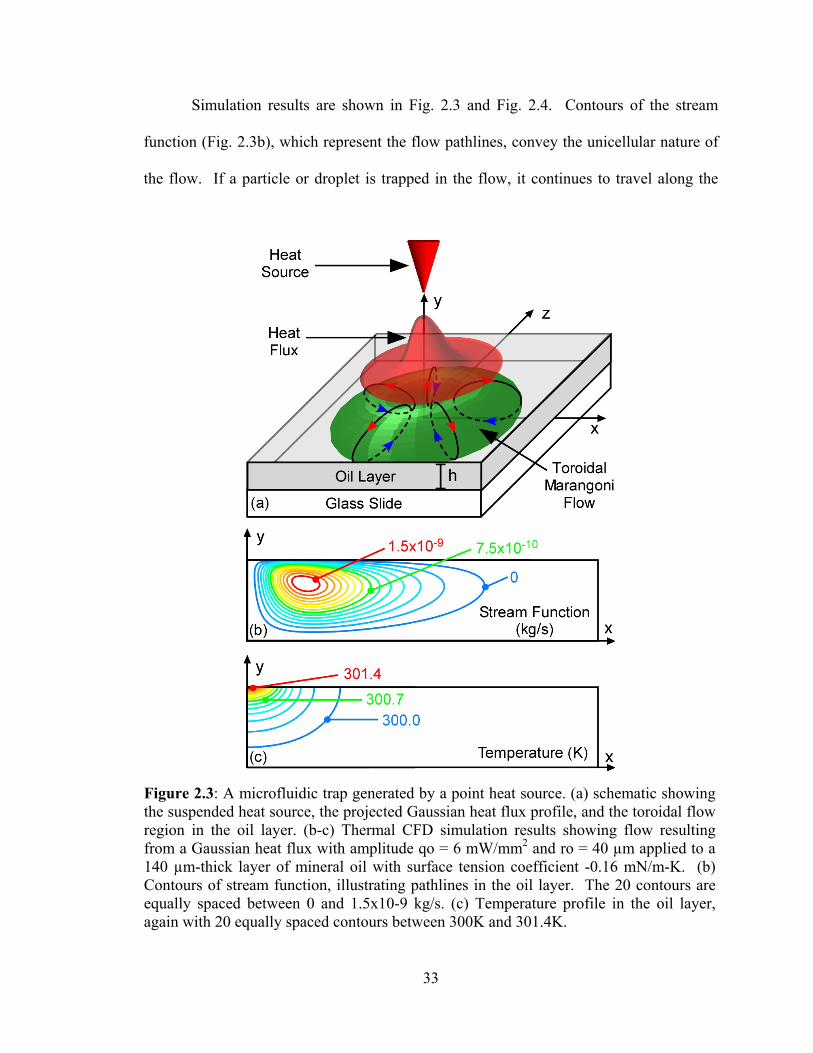
33

Simulation results are shown in Fig. 2.3 and Fig. 2.4. Contours of the stream

function (Fig. 2.3b), which represent the flow pathlines, convey the unicellular nature of

the flow. If a particle or droplet is trapped in the flow, it continues to travel along the

Figure 2.3: A microfluidic trap generated by a point heat source. (a) schematic showing the suspended heat source, the projected Gaussian heat flux profile, and the toroidal flow region in the oil layer. (b-c) Thermal CFD simulation results showing flow resulting from a Gaussian heat flux with amplitude qo = 6 mW/mm2 and ro = 40 µm applied to a 140 µm-thick layer of mineral oil with surface tension coefficient -0.16 mN/m-K. (b) Contours of stream function, illustrating pathlines in the oil layer. The 20 contours are equally spaced between 0 and 1.5x10-9 kg/s. (c) Temperature profile in the oil layer, again with 20 equally spaced contours between 300K and 301.4K.

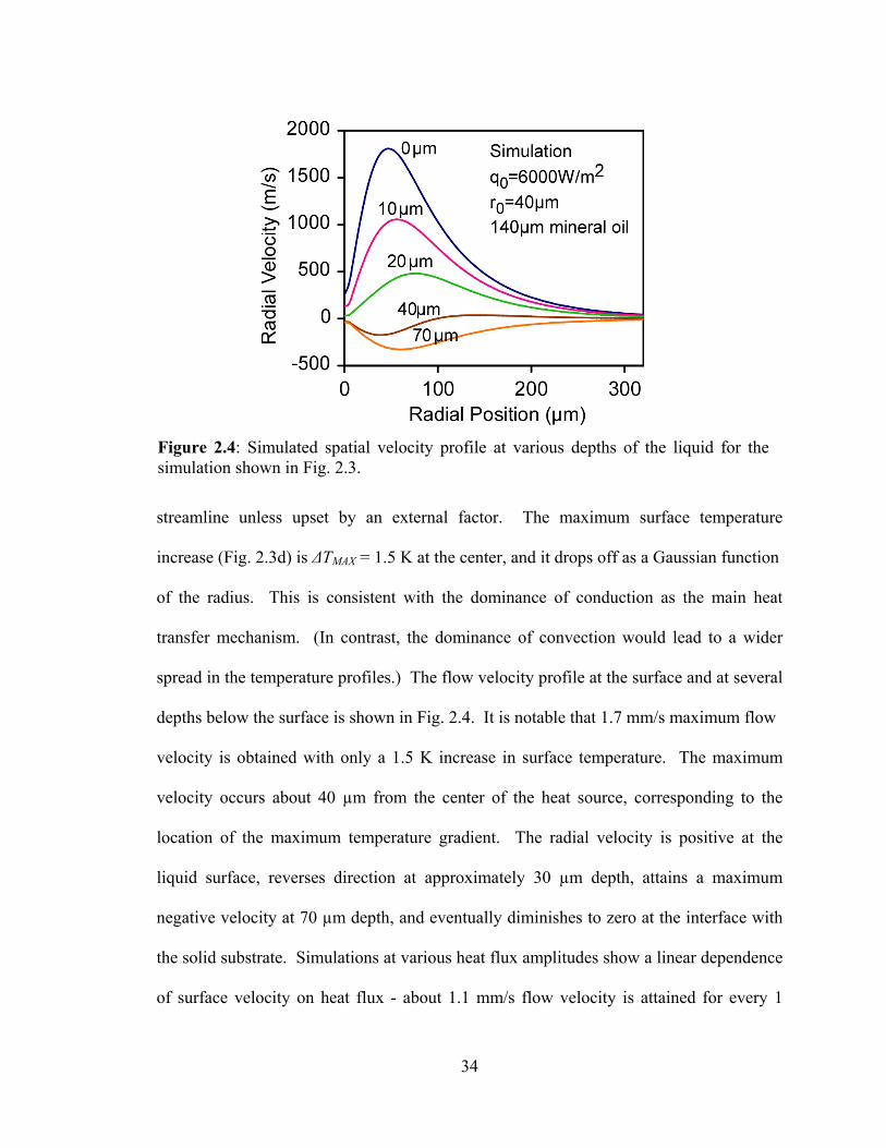
34

streamline unless upset by an external factor. The maximum surface temperature

increase (Fig. 2.3d) is ∆TMAX = 1.5 K at the center, and it drops off as a Gaussian function

of the radius. This is consistent with the dominance of conduction as the main heat

transfer mechanism. (In contrast, the dominance of convection would lead to a wider

spread in the temperature profiles.) The flow velocity profile at the surface and at several

depths below the surface is shown in Fig. 2.4. It is notable that 1.7 mm/s maximum flow

velocity is obtained with only a 1.5 K increase in surface temperature. The maximum

velocity occurs about 40 µm from the center of the heat source, corresponding to the

location of the maximum temperature gradient. The radial velocity is positive at the

liquid surface, reverses direction at approximately 30 µm depth, attains a maximum

negative velocity at 70 µm depth, and eventually diminishes to zero at the interface with

the solid substrate. Simulations at various heat flux amplitudes show a linear dependence

of surface velocity on heat flux - about 1.1 mm/s flow velocity is attained for every 1

Figure 2.4: Simulated spatial velocity profile at various depths of the liquid for the simulation shown in Fig. 2.3.

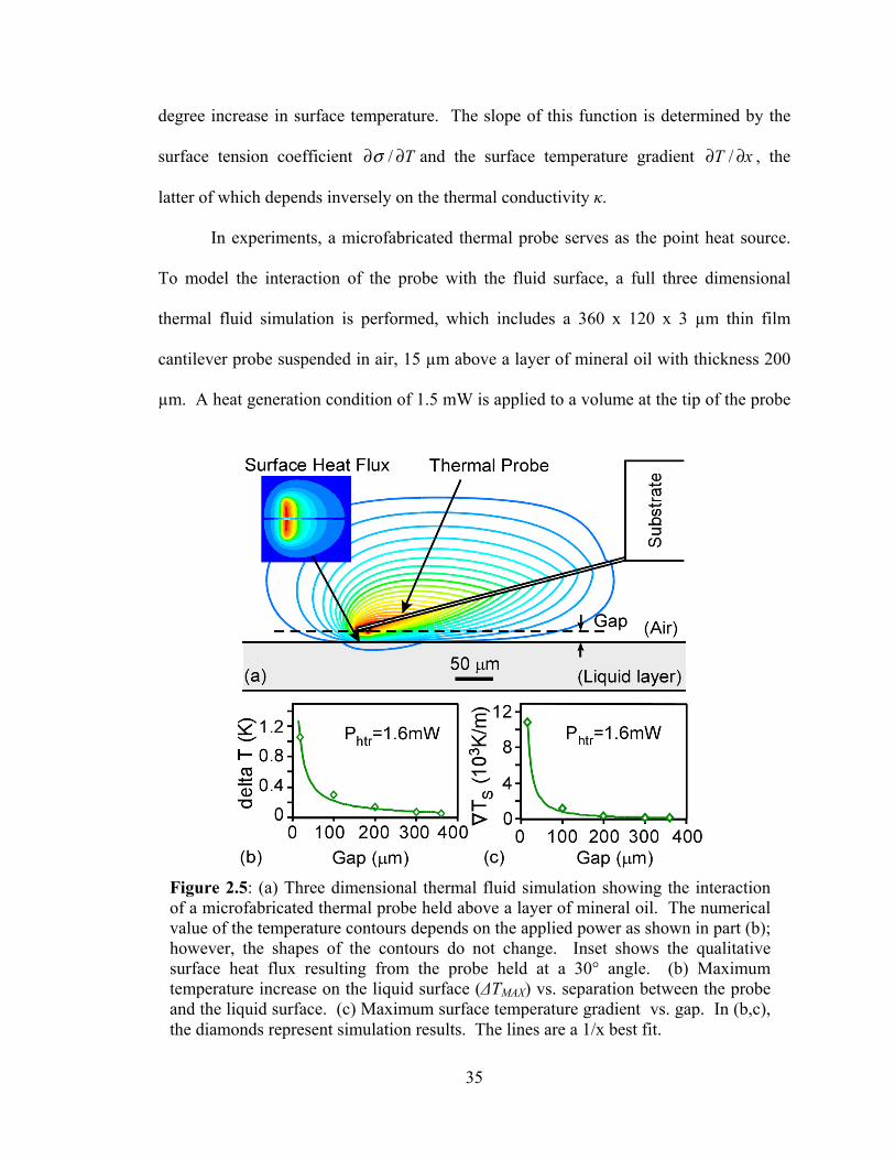
35

degree increase in surface temperature. The slope of this function is determined by the

surface tension coefficient T∂∂ /σ and the surface temperature gradient xT ∂∂ / , the

latter of which depends inversely on the thermal conductivity κ.

In experiments, a microfabricated thermal probe serves as the point heat source.

To model the interaction of the probe with the fluid surface, a full three dimensional

thermal fluid simulation is performed, which includes a 360 x 120 x 3 µm thin film

cantilever probe suspended in air, 15 µm above a layer of mineral oil with thickness 200

µm. A heat generation condition of 1.5 mW is applied to a volume at the tip of the probe

Figure 2.5: (a) Three dimensional thermal fluid simulation showing the interaction of a microfabricated thermal probe held above a layer of mineral oil. The numerical value of the temperature contours depends on the applied power as shown in part (b); however, the shapes of the contours do not change. Inset shows the qualitative surface heat flux resulting from the probe held at a 30° angle. (b) Maximum temperature increase on the liquid surface (∆TMAX) vs. separation between the probe and the liquid surface. (c) Maximum surface temperature gradient vs. gap. In (b,c), the diamonds represent simulation results. The lines are a 1/x best fit.

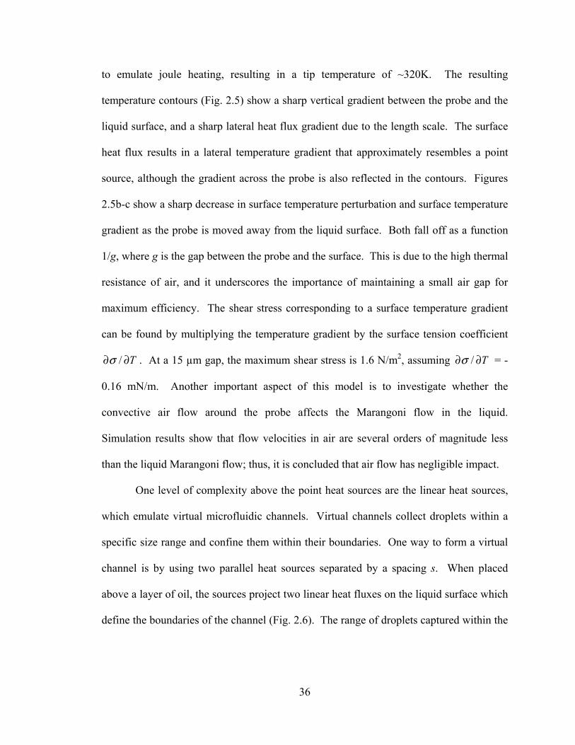
36

to emulate joule heating, resulting in a tip temperature of ~320K. The resulting

temperature contours (Fig. 2.5) show a sharp vertical gradient between the probe and the

liquid surface, and a sharp lateral heat flux gradient due to the length scale. The surface

heat flux results in a lateral temperature gradient that approximately resembles a point

source, although the gradient across the probe is also reflected in the contours. Figures

2.5b-c show a sharp decrease in surface temperature perturbation and surface temperature

gradient as the probe is moved away from the liquid surface. Both fall off as a function

1/g, where g is the gap between the probe and the surface. This is due to the high thermal

resistance of air, and it underscores the importance of maintaining a small air gap for

maximum efficiency. The shear stress corresponding to a surface temperature gradient

can be found by multiplying the temperature gradient by the surface tension coefficient

T∂∂ /σ . At a 15 µm gap, the maximum shear stress is 1.6 N/m2, assuming T∂∂ /σ = -

0.16 mN/m. Another important aspect of this model is to investigate whether the

convective air flow around the probe affects the Marangoni flow in the liquid.

Simulation results show that flow velocities in air are several orders of magnitude less

than the liquid Marangoni flow; thus, it is concluded that air flow has negligible impact.

One level of complexity above the point heat sources are the linear heat sources,

which emulate virtual microfluidic channels. Virtual channels collect droplets within a

specific size range and confine them within their boundaries. One way to form a virtual

channel is by using two parallel heat sources separated by a spacing s. When placed

above a layer of oil, the sources project two linear heat fluxes on the liquid surface which

define the boundaries of the channel (Fig. 2.6). The range of droplets captured within the

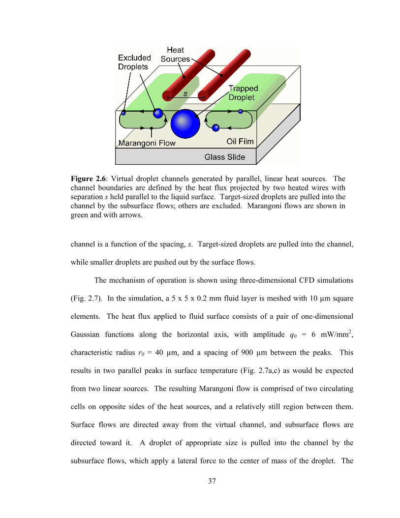
37

channel is a function of the spacing, s. Target-sized droplets are pulled into the channel,

while smaller droplets are pushed out by the surface flows.

The mechanism of operation is shown using three-dimensional CFD simulations

(Fig. 2.7). In the simulation, a 5 x 5 x 0.2 mm fluid layer is meshed with 10 µm square

elements. The heat flux applied to fluid surface consists of a pair of one-dimensional

Gaussian functions along the horizontal axis, with amplitude q0 = 6 mW/mm2,

characteristic radius r0 = 40 µm, and a spacing of 900 µm between the peaks. This

results in two parallel peaks in surface temperature (Fig. 2.7a,c) as would be expected

from two linear sources. The resulting Marangoni flow is comprised of two circulating

cells on opposite sides of the heat sources, and a relatively still region between them.

Surface flows are directed away from the virtual channel, and subsurface flows are

directed toward it. A droplet of appropriate size is pulled into the channel by the

subsurface flows, which apply a lateral force to the center of mass of the droplet. The

Figure 2.6: Virtual droplet channels generated by parallel, linear heat sources. The channel boundaries are defined by the heat flux projected by two heated wires with separation s held parallel to the liquid surface. Target-sized droplets are pulled into the channel by the subsurface flows; others are excluded. Marangoni flows are shown in green and with arrows.

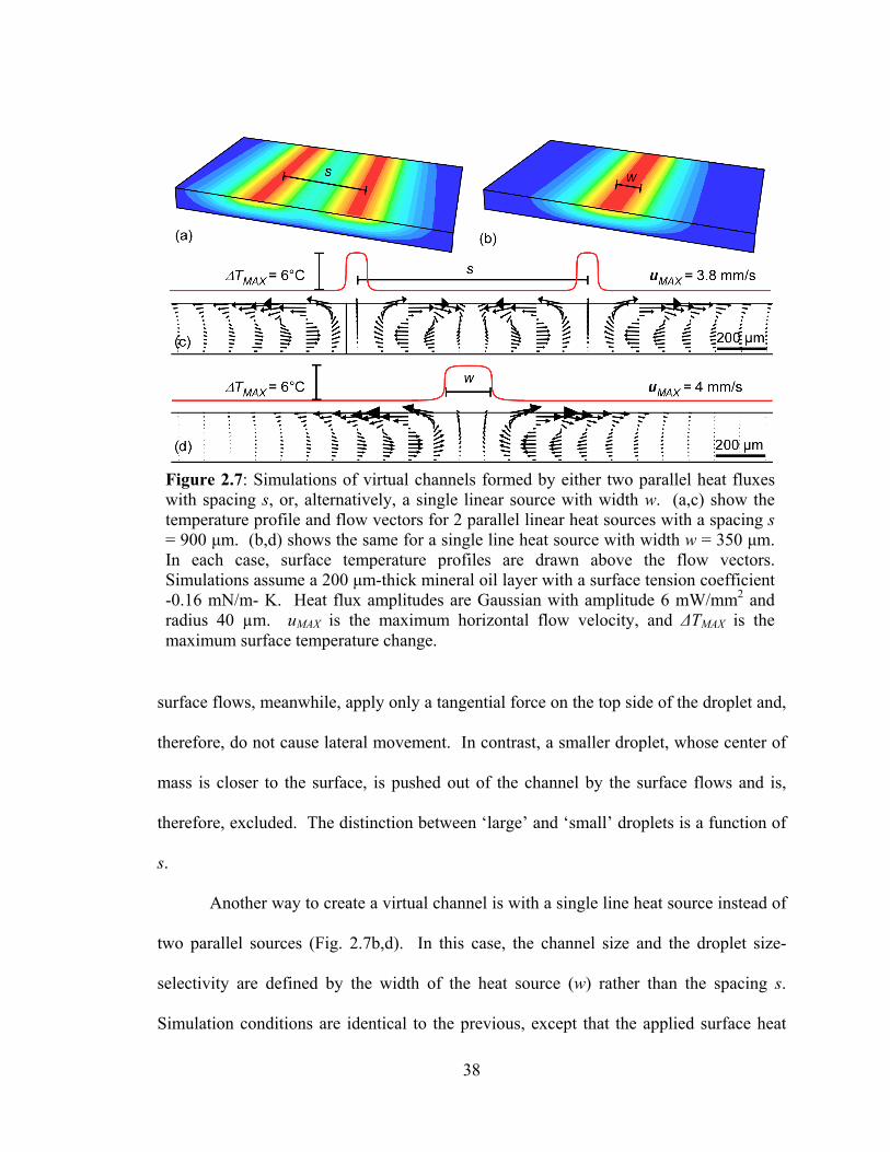
38

surface flows, meanwhile, apply only a tangential force on the top side of the droplet and,

therefore, do not cause lateral movement. In contrast, a smaller droplet, whose center of

mass is closer to the surface, is pushed out of the channel by the surface flows and is,

therefore, excluded. The distinction between ‘large’ and ‘small’ droplets is a function of

s.

Another way to create a virtual channel is with a single line heat source instead of

two parallel sources (Fig. 2.7b,d). In this case, the channel size and the droplet size-

selectivity are defined by the width of the heat source (w) rather than the spacing s.

Simulation conditions are identical to the previous, except that the applied surface heat

Figure 2.7: Simulations of virtual channels formed by either two parallel heat fluxes with spacing s, or, alternatively, a single linear source with width w. (a,c) show the temperature profile and flow vectors for 2 parallel linear heat sources with a spacing s = 900 µm. (b,d) shows the same for a single line heat source with width w = 350 µm. In each case, surface temperature profiles are drawn above the flow vectors. Simulations assume a 200 µm-thick mineral oil layer with a surface tension coefficient -0.16 mN/m- K. Heat flux amplitudes are Gaussian with amplitude 6 mW/mm2 and radius 40 µm. uMAX is the maximum horizontal flow velocity, and ∆TMAX is the maximum surface temperature change.

39

flux includes only a single peak, and the characteristic radius is increased (ro = 175 µm)

to represent a wider heat source. Simulation results illustrate the differences in flow

patterns of the double and single line heat sources. The recirculating flows present inside

the double line channel do not appear in the single line version; however, these internal

flows do not affect the trapping capability of the channel. The double line heat source

offers some flexibility in that the virtual channel region can be easily tuned wider than

the single line channel for trapping larger droplets. It is notable that in both cases, up to 4

mm/s surface velocities can be obtained with <6 °C change in surface temperature, again

illustrating the potential efficiency of Marangoni flows. The subsurface flows are only

about 1/3rd the velocity of the surface flows, but they are sufficient to pull in selected

droplets. Experimental results will be discussed in the following section.

A single droplet trap can be implemented using an annular heat source (Fig. 2.17).

Compared to the parallel heat sources, the cross section of the flow vectors are identical;

however, when viewed from above, the flow pattern is axially-symmetric about the heat

source. With respect to droplet manipulation, the primary difference between this

component and the channel is that the droplet can be confined in both lateral dimensions.

The trap is useful as a reservoir for holding single droplets, and for moving droplets if the

heat source is translated laterally. On a broader note, a particularly interesting aspect of

this flow pattern is the isolation of the fluid region within the confines of the ring.

Simulations and experimental results show that the fluid within the ring boundary

circulates independently and does not flow into the outer bulk fluid. In a sense, the inner

and bulk fluid are doubly separated by two walls of co-rotating flows. This suggests that

a ring heat source may have potential use as a fluid isolator outside the context of droplet

40

systems.

In the simulation model, the heat flux profile is an axisymmetric ring shape, the

cross section of which consists of Gaussian peaks at a radius of 300 µm. The amplitude

and characteristic width of the Gaussian profile is maintained at the same values as prior

simulations (q0 = 6 mW/mm2 and ro = 40 µm). Figure 2.17b shows the surface

temperature profile (∆TMAX = 6°C) and flow resulting from a ring-shaped heat source in a

200 µm-thick layer of mineral oil. For clarity, the arrows show only the subsurface flows

(140 µm beneath the surface) since they are the ones for droplet trapping. The flow can

be divided into two distinct regions. Flow vectors outside the perimeter of the ring are

oriented inward, and these flows push the droplet to the center. The maximum flow

velocity in this region is 1.3 mm/s. Inside the perimeter of the ring, the subsurface flows

are oriented outward, reaching a peak velocity of 0.8 mm/s; however, these flows do not

affect the trapped droplet because the lateral forces they impart on a trapped droplet are

symmetric and therefore cancel each other. Target-sized droplets, therefore, remain

stable at the center of the ring. Like the earlier geometries, smaller droplets are rejected

from the trap by the surface flows (not shown), which are oriented opposite the

subsurface flows. Thus, the size exclusion capability applies to the annular geometry as

well.

A fundamental component of any fluidic system is a pump. With noncontact

Marangoni flows, pumping or actuation of droplets can be accomplished by two methods.

The first is simply a consequence of the trapping: the heat source projecting a channel or

a trap can be translated physically with respect to the substrate, and the trapped droplets

follow it. However, droplet actuation can be also accomplished by steady-state,

41

motionless heating provided by a tapered shape and angled spacing (Fig. 2.18). The

tapered geometry provides a triangular heat flux on the fluid surface and a temperature

gradient oriented in the direction of increasing width. It can be simulated by applying a

triangular heat flux with amplitude 6 mW/mm2 and a 10° tip angle on a 500 µm square,

140 µm-thick layer of mineral oil. This results in a triangular temperature profile with a

maximum temperature increase of ∆TMAX = 5°C on the fluid surface. The resulting

subsurface flows (Fig. 2.18b) are biased in the direction of increasing taper, and can pull

appropriately sized droplets along the length of the guidewire. The maximum subsurface

flow velocity of 1.5 mm/s can be found near the tip of the guidewire. The surface flows

(not shown) have velocities roughly 3x larger than the subsurface flows and are biased in

the opposite direction. As before, the surface flows affect only the small droplets,

rejecting them from the guidewire.

4. EXPERIMENTAL RESULTS

Marangoni flows from point heat sources were obtained with a micromachined

polyimide-shank thermal probe [Li03] which provides high thermal efficiency, sharp

temperature gradients, and controllable temperatures. The probe consists of a 40 x 360 x

3.5 µm polyimide cantilever with a thin film heater near the tip which provides control of

the probe power and temperature. The probe was mounted on a motorized

micromanipulator stage (MP-285, Sutter Instruments, Novato, CA) and suspended above

a 140 µm thick layer of mineral oil (Mineral Oil USP, Rite Aid Corp., Harrisburg, PA).

The thickness of the oil was measured optically. Flow velocities were measured at input

powers ranging from 5-20 mW and at air gaps ranging from 20-320 µm. Weed pollen

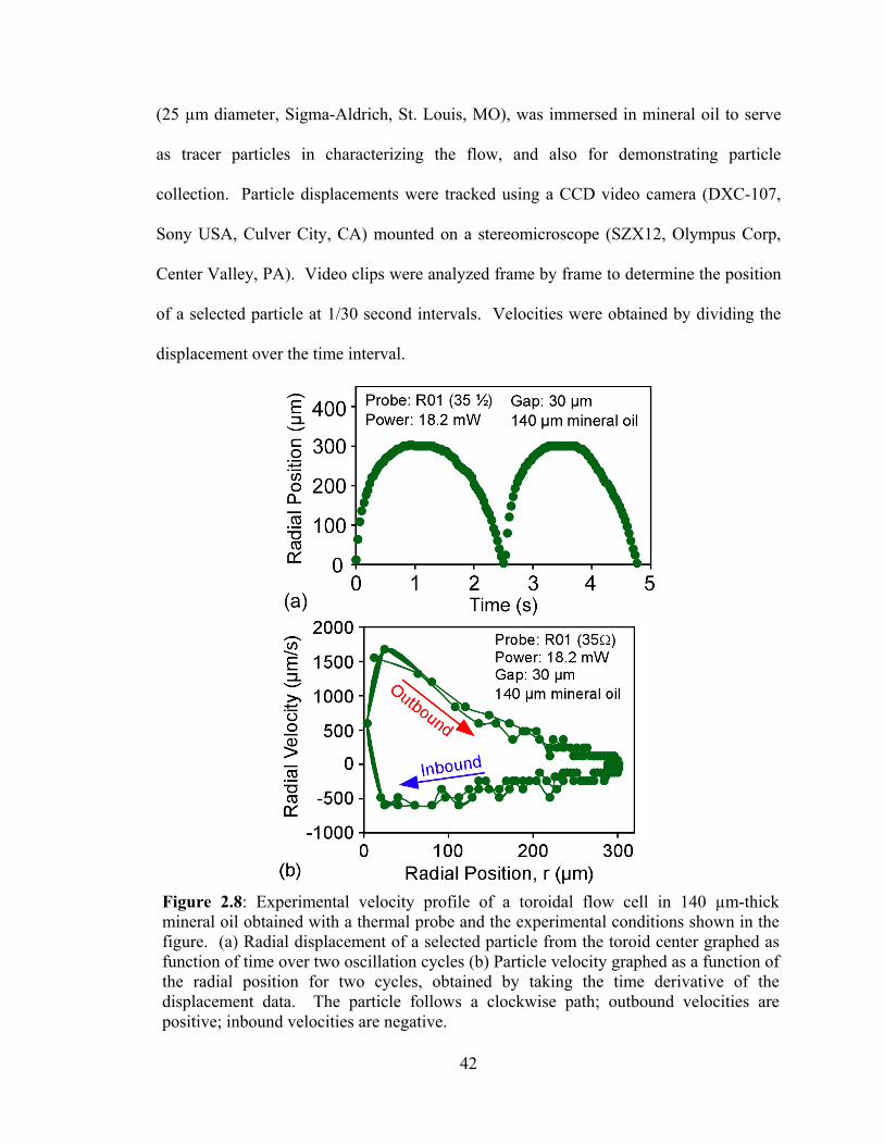
42

(25 µm diameter, Sigma-Aldrich, St. Louis, MO), was immersed in mineral oil to serve

as tracer particles in characterizing the flow, and also for demonstrating particle

collection. Particle displacements were tracked using a CCD video camera (DXC-107,

Sony USA, Culver City, CA) mounted on a stereomicroscope (SZX12, Olympus Corp,

Center Valley, PA). Video clips were analyzed frame by frame to determine the position

of a selected particle at 1/30 second intervals. Velocities were obtained by dividing the

displacement over the time interval.

Figure 2.8: Experimental velocity profile of a toroidal flow cell in 140 µm-thick mineral oil obtained with a thermal probe and the experimental conditions shown in the figure. (a) Radial displacement of a selected particle from the toroid center graphed as function of time over two oscillation cycles (b) Particle velocity graphed as a function of the radial position for two cycles, obtained by taking the time derivative of the displacement data. The particle follows a clockwise path; outbound velocities are positive; inbound velocities are negative.

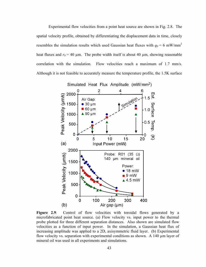
43

Experimental flow velocities from a point heat source are shown in Fig. 2.8. The

spatial velocity profile, obtained by differentiating the displacement data in time, closely

resembles the simulation results which used Gaussian heat fluxes with q0 = 6 mW/mm2

heat fluxes and r0 = 40 µm. The probe width itself is about 40 µm, showing reasonable

correlation with the simulation. Flow velocities reach a maximum of 1.7 mm/s.

Although it is not feasible to accurately measure the temperature profile, the 1.5K surface

Figure 2.9: Control of flow velocities with toroidal flows generated by a microfabricated point heat source. (a) Flow velocity vs. input power to the thermal probe plotted for three different separation distances. Also shown are simulated flow velocities as a function of input power. In the simulation, a Gaussian heat flux of increasing amplitude was applied to a 2D, axisymmetric fluid layer. (b) Experimental flow velocity vs. separation with experimental conditions as shown. A 140 µm layer of mineral oil was used in all experiments and simulations.

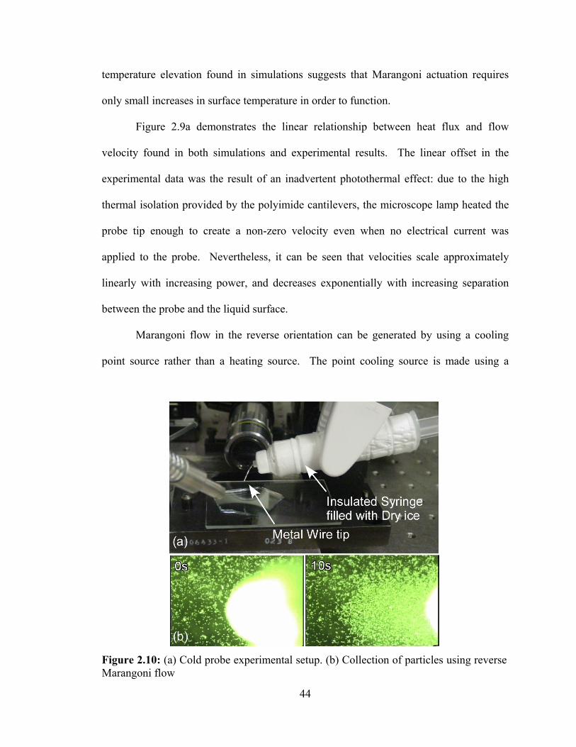
44

temperature elevation found in simulations suggests that Marangoni actuation requires

only small increases in surface temperature in order to function.

Figure 2.9a demonstrates the linear relationship between heat flux and flow

velocity found in both simulations and experimental results. The linear offset in the

experimental data was the result of an inadvertent photothermal effect: due to the high

thermal isolation provided by the polyimide cantilevers, the microscope lamp heated the

probe tip enough to create a non-zero velocity even when no electrical current was

applied to the probe. Nevertheless, it can be seen that velocities scale approximately

linearly with increasing power, and decreases exponentially with increasing separation

between the probe and the liquid surface.

Marangoni flow in the reverse orientation can be generated by using a cooling

point source rather than a heating source. The point cooling source is made using a

Figure 2.10: (a) Cold probe experimental setup. (b) Collection of particles using reverse Marangoni flow

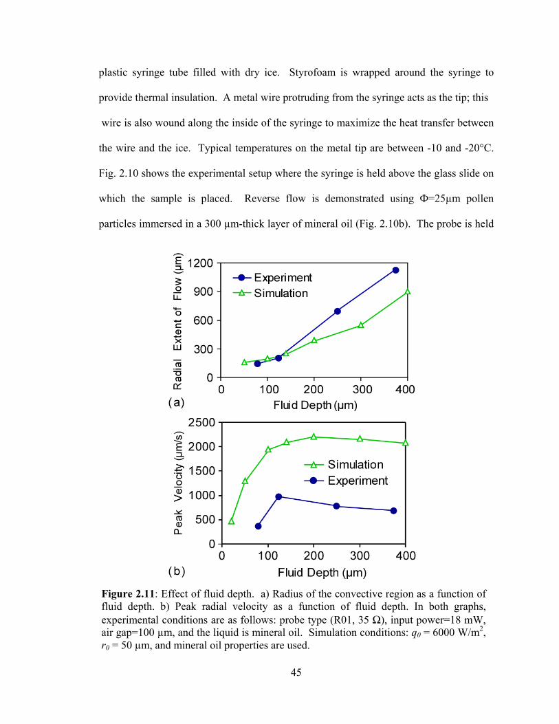
45

plastic syringe tube filled with dry ice. Styrofoam is wrapped around the syringe to

provide thermal insulation. A metal wire protruding from the syringe acts as the tip; this

wire is also wound along the inside of the syringe to maximize the heat transfer between

the wire and the ice. Typical temperatures on the metal tip are between -10 and -20°C.

Fig. 2.10 shows the experimental setup where the syringe is held above the glass slide on

which the sample is placed. Reverse flow is demonstrated using Ф=25µm pollen

particles immersed in a 300 µm-thick layer of mineral oil (Fig. 2.10b). The probe is held

Figure 2.11: Effect of fluid depth. a) Radius of the convective region as a function of fluid depth. b) Peak radial velocity as a function of fluid depth. In both graphs, experimental conditions are as follows: probe type (R01, 35 Ω), input power=18 mW, air gap=100 µm, and the liquid is mineral oil. Simulation conditions: q0 = 6000 W/m2, r0 = 50 µm, and mineral oil properties are used.

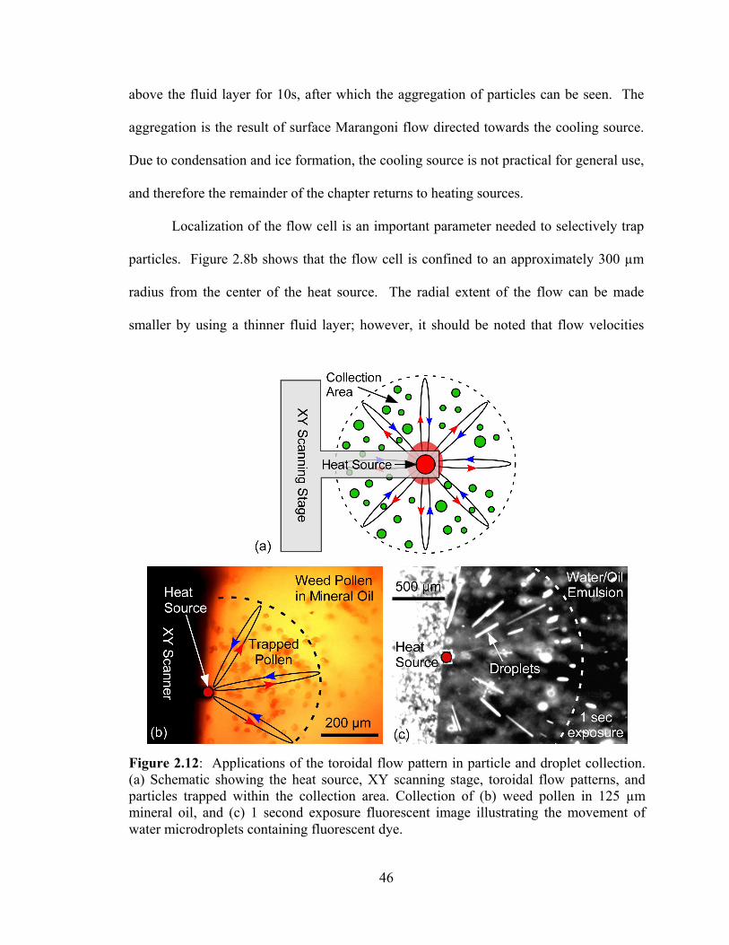
46

above the fluid layer for 10s, after which the aggregation of particles can be seen. The

aggregation is the result of surface Marangoni flow directed towards the cooling source.

Due to condensation and ice formation, the cooling source is not practical for general use,

and therefore the remainder of the chapter returns to heating sources.

Localization of the flow cell is an important parameter needed to selectively trap

particles. Figure 2.8b shows that the flow cell is confined to an approximately 300 µm

radius from the center of the heat source. The radial extent of the flow can be made

smaller by using a thinner fluid layer; however, it should be noted that flow velocities

Figure 2.12: Applications of the toroidal flow pattern in particle and droplet collection. (a) Schematic showing the heat source, XY scanning stage, toroidal flow patterns, and particles trapped within the collection area. Collection of (b) weed pollen in 125 µm mineral oil, and (c) 1 second exposure fluorescent image illustrating the movement of water microdroplets containing fluorescent dye.

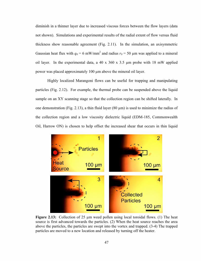
47

diminish in a thinner layer due to increased viscous forces between the flow layers (data

not shown). Simulations and experimental results of the radial extent of flow versus fluid

thickness show reasonable agreement (Fig. 2.11). In the simulation, an axisymmetric

Gaussian heat flux with q0 = 6 mW/mm2 and radius r0 = 50 µm was applied to a mineral

oil layer. In the experimental data, a 40 x 360 x 3.5 µm probe with 18 mW applied

power was placed approximately 100 µm above the mineral oil layer.

Highly localized Marangoni flows can be useful for trapping and manipulating

particles (Fig. 2.12). For example, the thermal probe can be suspended above the liquid

sample on an XY scanning stage so that the collection region can be shifted laterally. In

one demonstration (Fig. 2.13), a thin fluid layer (80 µm) is used to minimize the radius of

the collection region and a low viscosity dielectric liquid (EDM-185, Commonwealth

Oil, Harrow ON) is chosen to help offset the increased shear that occurs in thin liquid

Figure 2.13: Collection of 25 µm weed pollen using local toroidal flows. (1) The heat source is first advanced towards the particles. (2) When the heat source reaches the area above the particles, the particles are swept into the vortex and trapped. (3-4) The trapped particles are moved to a new location and released by turning off the heater.

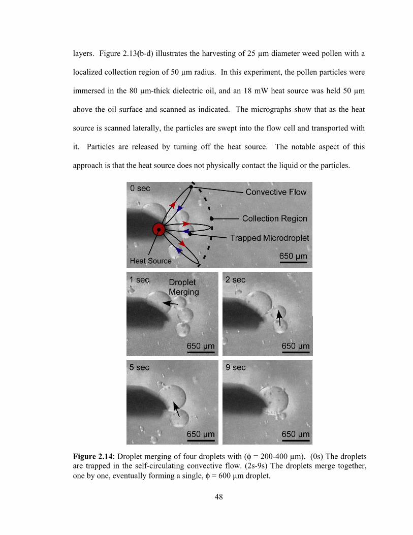
48

layers. Figure 2.13(b-d) illustrates the harvesting of 25 µm diameter weed pollen with a

localized collection region of 50 µm radius. In this experiment, the pollen particles were

immersed in the 80 µm-thick dielectric oil, and an 18 mW heat source was held 50 µm

above the oil surface and scanned as indicated. The micrographs show that as the heat

source is scanned laterally, the particles are swept into the flow cell and transported with

it. Particles are released by turning off the heat source. The notable aspect of this

approach is that the heat source does not physically contact the liquid or the particles.

Figure 2.14: Droplet merging of four droplets with (φ = 200-400 µm). (0s) The droplets are trapped in the self-circulating convective flow. (2s-9s) The droplets merge together, one by one, eventually forming a single, φ = 600 µm droplet.

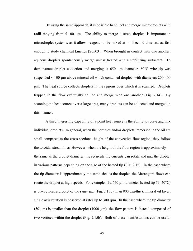
49

By using the same approach, it is possible to collect and merge microdroplets with

radii ranging from 5-100 µm. The ability to merge discrete droplets is important in

microdroplet systems, as it allows reagents to be mixed at millisecond time scales, fast

enough to study chemical kinetics [Son03]. When brought in contact with one another,

aqueous droplets spontaneously merge unless treated with a stabilizing surfactant. To

demonstrate droplet collection and merging, a 650 µm diameter, 80°C wire tip was

suspended < 100 µm above mineral oil which contained droplets with diameters 200-400

µm. The heat source collects droplets in the regions over which it is scanned. Droplets

trapped in the flow eventually collide and merge with one another (Fig. 2.14). By

scanning the heat source over a large area, many droplets can be collected and merged in

this manner.

A third interesting capability of a point heat source is the ability to rotate and mix

individual droplets. In general, when the particles and/or droplets immersed in the oil are

small compared to the cross-sectional height of the convective flow region, they follow

the toroidal streamlines. However, when the height of the flow region is approximately

the same as the droplet diameter, the recirculating currents can rotate and mix the droplet

in various patterns depending on the size of the heated tip (Fig. 2.15). In the case where

the tip diameter is approximately the same size as the droplet, the Marangoni flows can

rotate the droplet at high speeds. For example, if a 650 µm-diameter heated tip (T≈40°C)

is placed near a droplet of the same size (Fig. 2.15b) in an 800 µm-thick mineral oil layer,

single axis rotation is observed at rates up to 300 rpm. In the case where the tip diameter

(50 µm) is smaller than the droplet (1000 µm), the flow pattern is instead composed of

two vortices within the droplet (Fig. 2.15b). Both of these manifestations can be useful

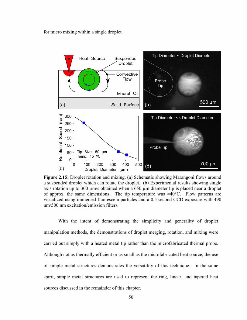
50

for micro mixing within a single droplet.

With the intent of demonstrating the simplicity and generality of droplet

manipulation methods, the demonstrations of droplet merging, rotation, and mixing were

carried out simply with a heated metal tip rather than the microfabricated thermal probe.

Although not as thermally efficient or as small as the microfabricated heat source, the use

of simple metal structures demonstrates the versatility of this technique. In the same

spirit, simple metal structures are used to represent the ring, linear, and tapered heat

sources discussed in the remainder of this chapter.

Figure 2.15: Droplet rotation and mixing. (a) Schematic showing Marangoni flows around a suspended droplet which can rotate the droplet. (b) Experimental results showing single axis rotation up to 300 µm/s obtained when a 650 µm diameter tip is placed near a droplet of approx. the same dimensions. The tip temperature was ≈40°C. Flow patterns are visualized using immersed fluorescein particles and a 0.5 second CCD exposure with 490 nm/500 nm excitation/emission filters.

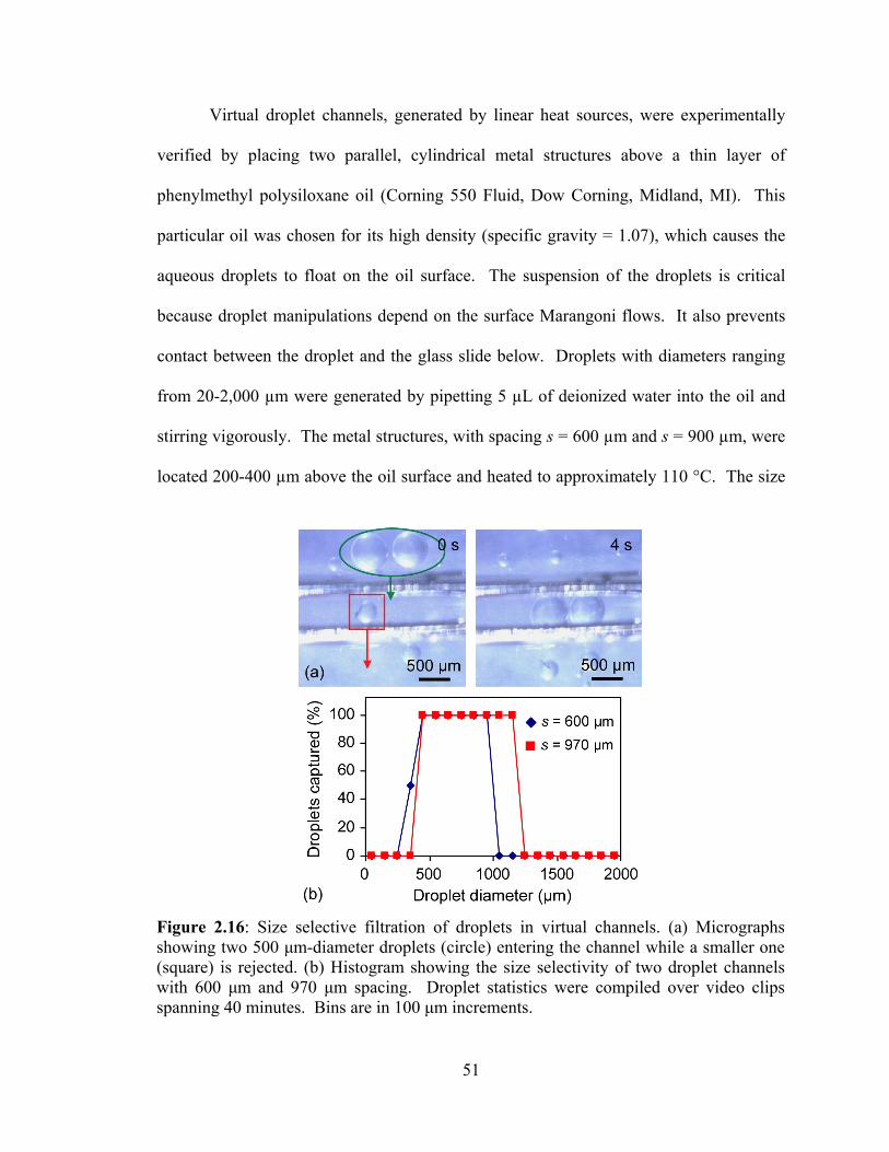
51

Virtual droplet channels, generated by linear heat sources, were experimentally

verified by placing two parallel, cylindrical metal structures above a thin layer of

phenylmethyl polysiloxane oil (Corning 550 Fluid, Dow Corning, Midland, MI). This

particular oil was chosen for its high density (specific gravity = 1.07), which causes the

aqueous droplets to float on the oil surface. The suspension of the droplets is critical

because droplet manipulations depend on the surface Marangoni flows. It also prevents

contact between the droplet and the glass slide below. Droplets with diameters ranging

from 20-2,000 µm were generated by pipetting 5 µL of deionized water into the oil and

stirring vigorously. The metal structures, with spacing s = 600 µm and s = 900 µm, were

located 200-400 µm above the oil surface and heated to approximately 110 °C. The size

Figure 2.16: Size selective filtration of droplets in virtual channels. (a) Micrographs showing two 500 µm-diameter droplets (circle) entering the channel while a smaller one (square) is rejected. (b) Histogram showing the size selectivity of two droplet channels with 600 µm and 970 µm spacing. Droplet statistics were compiled over video clips spanning 40 minutes. Bins are in 100 µm increments.

52

selectivity is demonstrated by time-lapse images in Fig. 2.16, which show that droplets

within a specific size range move into the channel, while smaller droplets are actively

removed by the Marangoni flows. Very large droplets are unaffected by the flows, and

therefore are not actively recruited into the channel.

The ability to tailor the size selectivity of the channels is quantitatively shown in

Fig. 2.16b. A histogram of droplet capture vs. droplet size is shown for the two channels

with different spacings (s). When s = 600 µm, the minimum diameter for entry into the

channel is 250 µm, and when s = 970 µm, the minimum diameter is 350 µm. A sharp

transition can be seen in both cases, and nearly 100% exclusion of off-sized droplets is

shown. Therefore, these channels inherently provide a size-based filtration capability.

Figure 2.17c shows experimental results for the annular heat source functioning as

a droplet trap. A rectangular ring-shaped metal pin (T ≈ 120°C, s = 600 µm) was

suspended 200-400 µm above the oil layer to approximate an annular heat flux. The

micrographs show that a 700 µm-diameter droplet is actively pulled into the trap, driven

by the subsurface flows directed into the center of the trap. If the trap boundary is moved

(by the translation of the substrate or heat source), the droplet follows it. The process is

repeatable, and the droplet velocity, as it enters the trap, is approximately 200 µm/s.

Experimental confirmation of the guidewire pump (tapered heat source) is shown

in Fig. 2.18c. To create the surface heat flux, a steel needle (T≈130°C) with 10° lateral

taper, and a 5° taper in vertical spacing was placed ≈200 µm above the fluid surface.

Time lapse images show a 523 µm-diameter droplet pulled along the axis by virtue of the

Marangoni flows. The droplet moves quickly when first approaching the tip of the heat

flux and continues to move in the direction of increasing taper, achieving a maximum

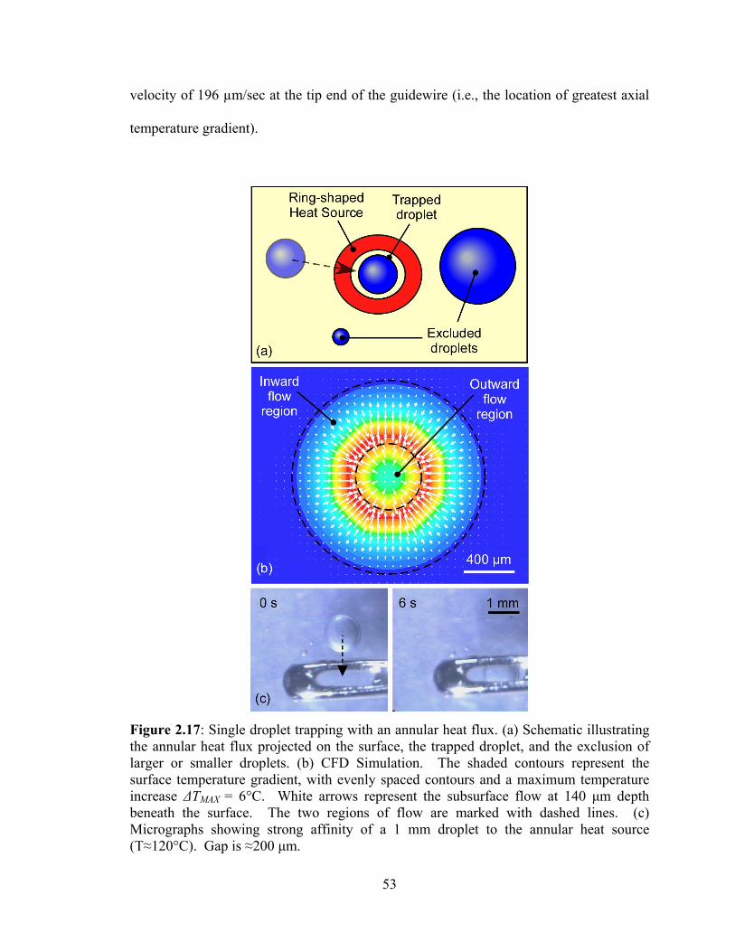
53

velocity of 196 µm/sec at the tip end of the guidewire (i.e., the location of greatest axial

temperature gradient).

Figure 2.17: Single droplet trapping with an annular heat flux. (a) Schematic illustrating the annular heat flux projected on the surface, the trapped droplet, and the exclusion of larger or smaller droplets. (b) CFD Simulation. The shaded contours represent the surface temperature gradient, with evenly spaced contours and a maximum temperature increase ∆TMAX = 6°C. White arrows represent the subsurface flow at 140 µm depth beneath the surface. The two regions of flow are marked with dashed lines. (c) Micrographs showing strong affinity of a 1 mm droplet to the annular heat source (T≈120°C). Gap is ≈200 µm.

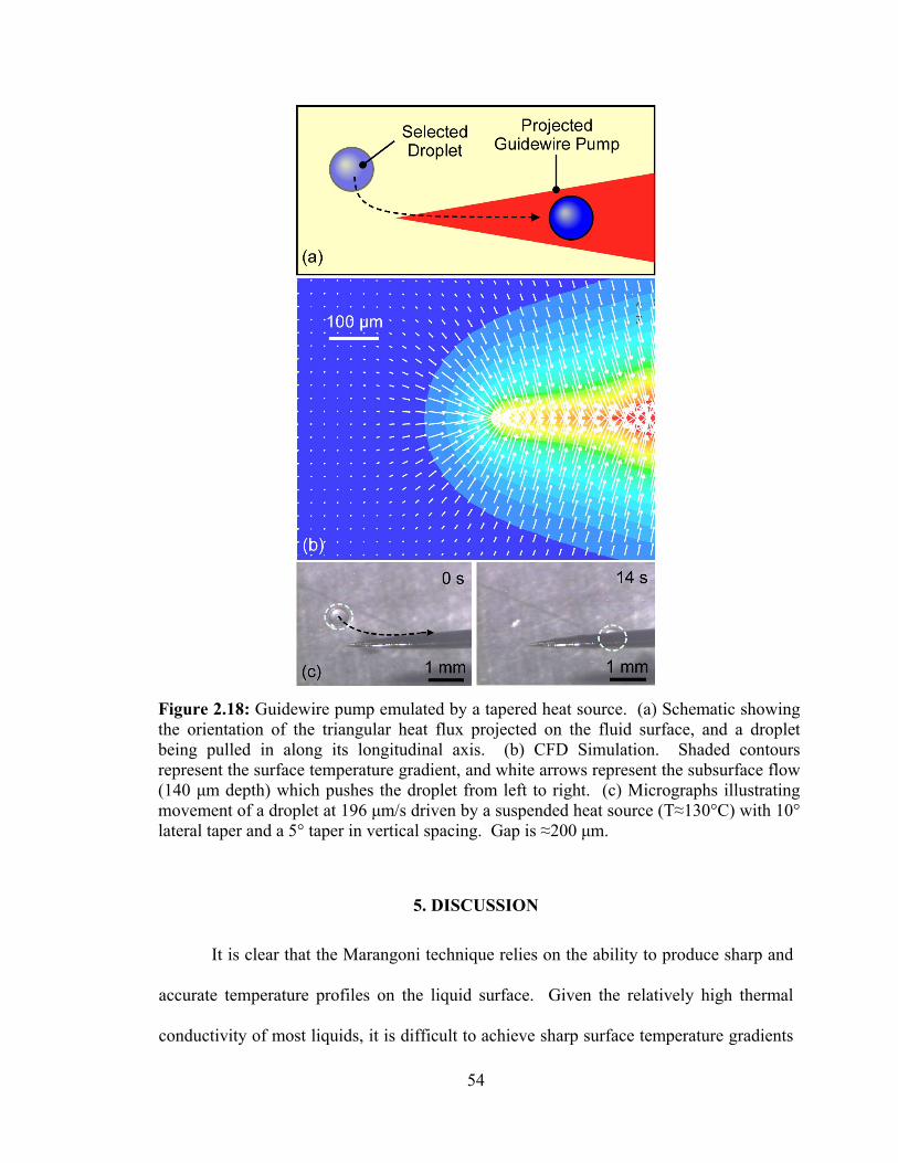
54

5. DISCUSSION

It is clear that the Marangoni technique relies on the ability to produce sharp and

accurate temperature profiles on the liquid surface. Given the relatively high thermal

conductivity of most liquids, it is difficult to achieve sharp surface temperature gradients

Figure 2.18: Guidewire pump emulated by a tapered heat source. (a) Schematic showing the orientation of the triangular heat flux projected on the fluid surface, and a droplet being pulled in along its longitudinal axis. (b) CFD Simulation. Shaded contours represent the surface temperature gradient, and white arrows represent the subsurface flow (140 µm depth) which pushes the droplet from left to right. (c) Micrographs illustrating movement of a droplet at 196 µm/s driven by a suspended heat source (T≈130°C) with 10° lateral taper and a 5° taper in vertical spacing. Gap is ≈200 µm.

55

if the heaters are embedded within the fluid. By contrast, placing the heat sources above

the liquid benefits from the low thermal conductivity of air, which is nearly an order of

magnitude less than oil. This limits lateral heat conduction and allows the formation of

sharp surface temperature gradients at the resolution needed to obtain shaped temperature

profiles at the sub-millimeter scale. An added benefit is that the heaters do not contact

the sample, obviating contamination concerns.

With regards to reconfigurability, one of the projected advantages of this type of

approach is that the substrate itself remains unpatterned. The complexity and burden of

the fluid actuation is essentially placed to the suspended heating structures rather than the

fluidic substrate. Since the heating structure can be reused and reconfigured, this can

lower the overall cost of repeated experiments.

To achieve the sharpest temperature gradients on the liquid surface, it is important

to place the heat sources as close to the surface as possible, since heat spreads

isotropically in the air gap. Typical gaps on the order of 100-400 µm can be obtained by

visual estimation during the approach of the heat source to the sample surface. An

automated technique which would allow for small air gaps would greatly benefit

efficiency, as simulations indicate that when the gap is less than 100 µm, both the surface

temperature gradient and resulting velocity sharply increases.

Another benefit of placing the probes close to the surface is lower power

operation. Although the low thermal conductivity of air helps achieve a sharp lateral

gradient, it also reduces the heat transfer from the heat source to the liquid surface.

Experimental results with the microfabricated thermal probe show that approximately 10

mW of heat power must be dissipated in order to generate 1 mm/s flow velocity.

56

Simulations, however, indicate that <0.2 mW of surface heat flux is needed to generate

the same flow velocity. The discrepancy between the two arises due to the poor heat

transfer between the probe and the liquid surface. Three dimensional heat conduction

simulations of the probe above the liquid surface show that at a 100 µm separation, the

surface temperature rise is only 1.3% that of the probe. This figure drops to only 0.3% if

the gap is 300 µm. As shown earlier (Fig. 2.5), there is an approximate 1/x dependence

on the surface temperature rise vs. the probe-liquid separation.

An equally important way to improve efficiency is by optimizing the heat source.

Microfabricated heaters with well-designed thermal isolation can achieve thermal

resistances in the range of 10,000 K/W [Li03], and thermal masses of only 10-9 J/K. This

enables temperatures of 100 °C with <10 mW of input power, and dynamic heating times

on the order of 10 ms. In these probes, the relatively small thermal losses are due to

conduction through the probe shank. Thus, the efficiency can be further improved by

using a thinner cantilever or lower thermal conductivity materials in its fabrication. With

the existing devices, the best power efficiency, obtained experimentally at a 30 µm gap,

is about 1 mm/s per milliwatt input power, reaching a maximum liquid velocity of 1700

µm/s with < 20 mW input power to the probe.

The ability to localize flow is an important aspect as well. Fig. 2.11 shows that

the radius of the collection region scales with the thickness of the liquid layer, and

intuitively, it would also scale with the size of the heat source. The former approach is

simpler, but the latter offers the ability to accommodate a larger range of droplet sizes.

The smallest flow cell observed was a 50 µm diameter toroidal flow, obtained using a

thermal probe above 80 µm thick low viscosity oil.

57

Another purpose of this effort was to show that even simple metal tools can be

used to generate Marangoni flow which can emulate microfluidic components. Because

these components are larger in size (a few mm) than the microfabricated probe (< 100

µm), they cannot generate as sharp a gradient. Thus, a larger absolute increase in

temperature is needed to drive flows at the same rate. In the case of the tapered, ring, and

linear geometries, the heat source temperatures are between 80-120°C, and the liquid

surface temperatures are measured to be 10-40° above ambient. This temperature

requirement can be reduced by scaling the heat sources to smaller sizes.

Overall, scaling down to smaller length scales can potentially provide significant

performance benefits. For example, the microfabricated thermal probe used in this work

obtains temperature gradients of up to 1 K/µm (106 K/m) along a 200 µm-long cantilever.

Experimental and simulation data using this probe show that on the liquid surface, the

typical temperature gradient ranges from 1-10 K/mm, resulting in shear stresses between

0.1-1 N/m2 and velocities between 1-10 mm/s on a 200 µm thick oil layer.

Hypothetically, if the thermal gradients on the microfabricated probe (up to 106 K/m)

could be directly transferred to the fluid surface without loss, this could result in shear

stresses up to 100 N/m2, and theoretical velocities above 10 cm/s (if viscous resistance

can be minimized). Although this is not possible in the existing setup, it does illustrate

the favorable scaling of this technique, and the potential to achieve high speed flow.

6. SUMMARY

This chapter has shown that microfluidic Marangoni flows can be engineered

through the geometric design of the heat flux. A surprising number of microdroplet

58

operations, including mixing, confining, filtering, trapping, and pumping, can be

emulated through the creative use of surface and subsurface flows. As a noncontact

technique, these virtual components avoid many of the contamination issues which limit

many microfluidic technologies. The future direction of this research is to integrate

several of these components into a usable system for droplet manipulation. A system

with programmable heat fluxes may also be useful for research applications which

require flexibility and reusability over portability.

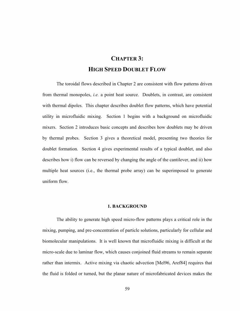
59

CHAPTER 3:

HIGH SPEED DOUBLET FLOW

The toroidal flows described in Chapter 2 are consistent with flow patterns driven

from thermal monopoles, i.e. a point heat source. Doublets, in contrast, are consistent

with thermal dipoles. This chapter describes doublet flow patterns, which have potential

utility in microfluidic mixing. Section 1 begins with a background on microfluidic

mixers. Section 2 introduces basic concepts and describes how doublets may be driven

by thermal probes. Section 3 gives a theoretical model, presenting two theories for

doublet formation. Section 4 gives experimental results of a typical doublet, and also

describes how i) flow can be reversed by changing the angle of the cantilever, and ii) how

multiple heat sources (i.e., the thermal probe array) can be superimposed to generate

uniform flow.

1. BACKGROUND

The ability to generate high speed micro-flow patterns plays a critical role in the

mixing, pumping, and pre-concentration of particle solutions, particularly for cellular and

biomolecular manipulations. It is well known that microfluidic mixing is difficult at the

micro-scale due to laminar flow, which causes conjoined fluid streams to remain separate

rather than intermix. Active mixing via chaotic advection [Mel96, Aref84] requires that

the fluid is folded or turned, but the planar nature of microfabricated devices makes the

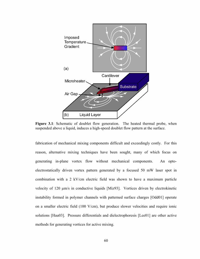
60

fabrication of mechanical mixing components difficult and exceedingly costly. For this

reason, alternative mixing techniques have been sought, many of which focus on

generating in-plane vortex flow without mechanical components. An opto-

electrostatically driven vortex pattern generated by a focused 50 mW laser spot in

combination with a 2 kV/cm electric field was shown to have a maximum particle

velocity of 120 µm/s in conductive liquids [Miz93]. Vortices driven by electrokinetic

instability formed in polymer channels with patterned surface charges [Odd01] operate

on a smaller electric field (100 V/cm), but produce slower velocities and require ionic

solutions [Hau03]. Pressure differentials and dielectrophoresis [Lee01] are other active

methods for generating vortices for active mixing.

Figure 3.1: Schematic of doublet flow generation. The heated thermal probe, when suspended above a liquid, induces a high-speed doublet flow pattern at the surface.

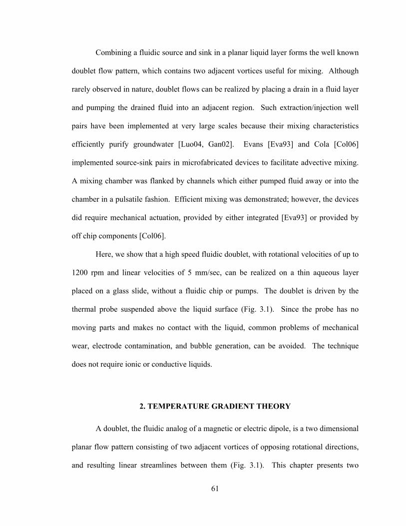
61

Combining a fluidic source and sink in a planar liquid layer forms the well known

doublet flow pattern, which contains two adjacent vortices useful for mixing. Although

rarely observed in nature, doublet flows can be realized by placing a drain in a fluid layer

and pumping the drained fluid into an adjacent region. Such extraction/injection well

pairs have been implemented at very large scales because their mixing characteristics

efficiently purify groundwater [Luo04, Gan02]. Evans [Eva93] and Cola [Col06]

implemented source-sink pairs in microfabricated devices to facilitate advective mixing.

A mixing chamber was flanked by channels which either pumped fluid away or into the

chamber in a pulsatile fashion. Efficient mixing was demonstrated; however, the devices

did require mechanical actuation, provided by either integrated [Eva93] or provided by

off chip components [Col06].

Here, we show that a high speed fluidic doublet, with rotational velocities of up to

1200 rpm and linear velocities of 5 mm/sec, can be realized on a thin aqueous layer

placed on a glass slide, without a fluidic chip or pumps. The doublet is driven by the

thermal probe suspended above the liquid surface (Fig. 3.1). Since the probe has no

moving parts and makes no contact with the liquid, common problems of mechanical

wear, electrode contamination, and bubble generation, can be avoided. The technique

does not require ionic or conductive liquids.

2. TEMPERATURE GRADIENT THEORY

A doublet, the fluidic analog of a magnetic or electric dipole, is a two dimensional

planar flow pattern consisting of two adjacent vortices of opposing rotational directions,

and resulting linear streamlines between them (Fig. 3.1). This chapter presents two

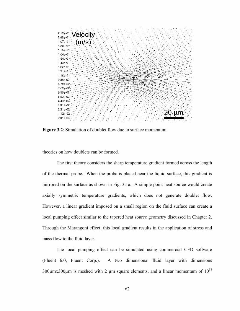
62

theories on how doublets can be formed.

The first theory considers the sharp temperature gradient formed across the length

of the thermal probe. When the probe is placed near the liquid surface, this gradient is

mirrored on the surface as shown in Fig. 3.1a. A simple point heat source would create

axially symmetric temperature gradients, which does not generate doublet flow.

However, a linear gradient imposed on a small region on the fluid surface can create a

local pumping effect similar to the tapered heat source geometry discussed in Chapter 2.

Through the Marangoni effect, this local gradient results in the application of stress and

mass flow to the fluid layer.

The local pumping effect can be simulated using commercial CFD software

(Fluent 6.0, Fluent Corp.). A two dimensional fluid layer with dimensions

300µmx300µm is meshed with 2 µm square elements, and a linear momentum of 1018

Figure 3.2: Simulation of doublet flow due to surface momentum.

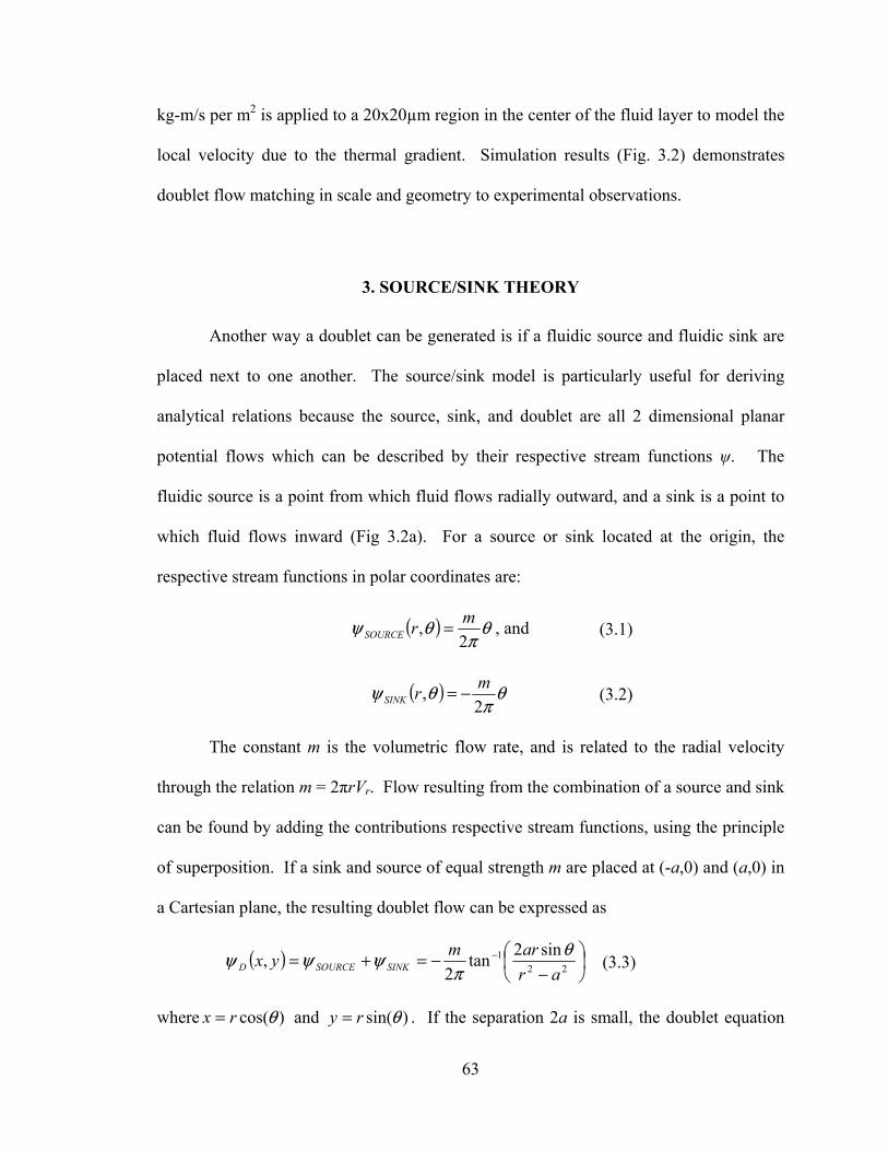
63

kg-m/s per m2 is applied to a 20x20µm region in the center of the fluid layer to model the

local velocity due to the thermal gradient. Simulation results (Fig. 3.2) demonstrates

doublet flow matching in scale and geometry to experimental observations.

3. SOURCE/SINK THEORY

Another way a doublet can be generated is if a fluidic source and fluidic sink are

placed next to one another. The source/sink model is particularly useful for deriving

analytical relations because the source, sink, and doublet are all 2 dimensional planar

potential flows which can be described by their respective stream functions ψ. The

fluidic source is a point from which fluid flows radially outward, and a sink is a point to

which fluid flows inward (Fig 3.2a). For a source or sink located at the origin, the

respective stream functions in polar coordinates are:

( ) θπ

θψ2

, mrSOURCE = , and (3.1)

( ) θπ

θψ2

, mrSINK −= (3.2)

The constant m is the volumetric flow rate, and is related to the radial velocity

through the relation m = 2πrVr. Flow resulting from the combination of a source and sink

can be found by adding the contributions respective stream functions, using the principle

of superposition. If a sink and source of equal strength m are placed at (-a,0) and (a,0) in

a Cartesian plane, the resulting doublet flow can be expressed as

( ) ⎟⎠⎞

⎜⎝⎛

−−=+= −

221 sin2tan

2,

ararmyx SINKSOURCED

θπ

ψψψ (3.3)

where )cos(θrx = and )sin(θry = . If the separation 2a is small, the doublet equation

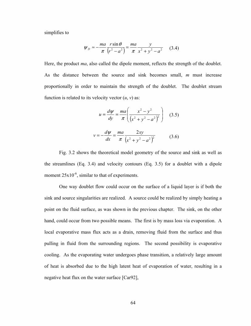
64

simplifies to

( ) 22222

sinayx

ymaar

rmaD −+

=−

−≈π

θπ

ψ (3.4)

Here, the product ma, also called the dipole moment, reflects the strength of the doublet.

As the distance between the source and sink becomes small, m must increase

proportionally in order to maintain the strength of the doublet. The doublet stream

function is related to its velocity vector (u, v) as:

( ) ⎟⎟⎠

⎞⎜⎜⎝

⎛

−+−== 2222

22

ayxyxma

dydu

πψ (3.5)

( )2222

2ayx

xymadxdv

−+=−=

πψ (3.6)

Fig. 3.2 shows the theoretical model geometry of the source and sink as well as

the streamlines (Eq. 3.4) and velocity contours (Eq. 3.5) for a doublet with a dipole

moment 25x10-6, similar to that of experiments.

One way doublet flow could occur on the surface of a liquid layer is if both the

sink and source singularities are realized. A source could be realized by simply heating a

point on the fluid surface, as was shown in the previous chapter. The sink, on the other

hand, could occur from two possible means. The first is by mass loss via evaporation. A

local evaporative mass flux acts as a drain, removing fluid from the surface and thus

pulling in fluid from the surrounding regions. The second possibility is evaporative

cooling. As the evaporating water undergoes phase transition, a relatively large amount

of heat is absorbed due to the high latent heat of evaporation of water, resulting in a

negative heat flux on the water surface [Car92],

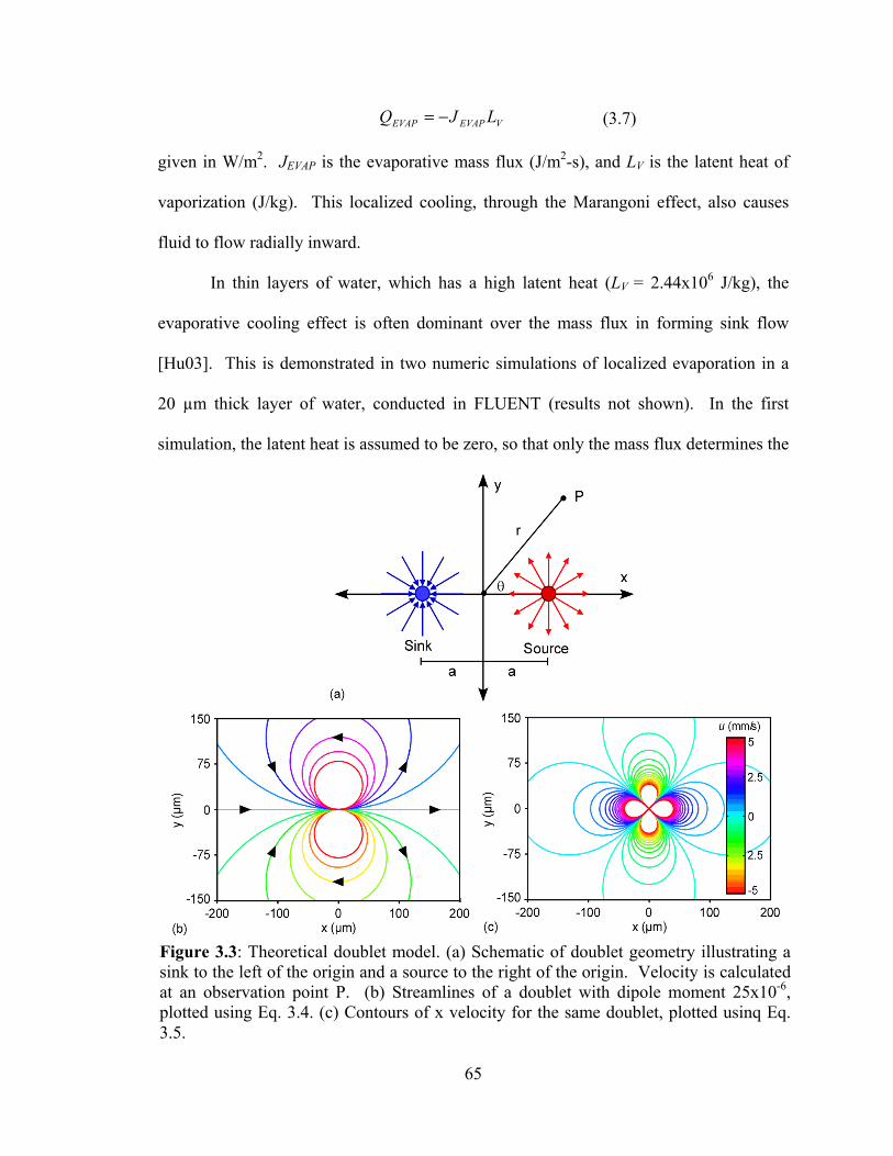
65

VEVAPEVAP LJQ −= (3.7)

given in W/m2. JEVAP is the evaporative mass flux (J/m2-s), and LV is the latent heat of

vaporization (J/kg). This localized cooling, through the Marangoni effect, also causes

fluid to flow radially inward.

In thin layers of water, which has a high latent heat (LV = 2.44x106 J/kg), the

evaporative cooling effect is often dominant over the mass flux in forming sink flow

[Hu03]. This is demonstrated in two numeric simulations of localized evaporation in a

20 µm thick layer of water, conducted in FLUENT (results not shown). In the first

simulation, the latent heat is assumed to be zero, so that only the mass flux determines the

Figure 3.3: Theoretical doublet model. (a) Schematic of doublet geometry illustrating a sink to the left of the origin and a source to the right of the origin. Velocity is calculated at an observation point P. (b) Streamlines of a doublet with dipole moment 25x10-6, plotted using Eq. 3.4. (c) Contours of x velocity for the same doublet, plotted usinq Eq. 3.5.

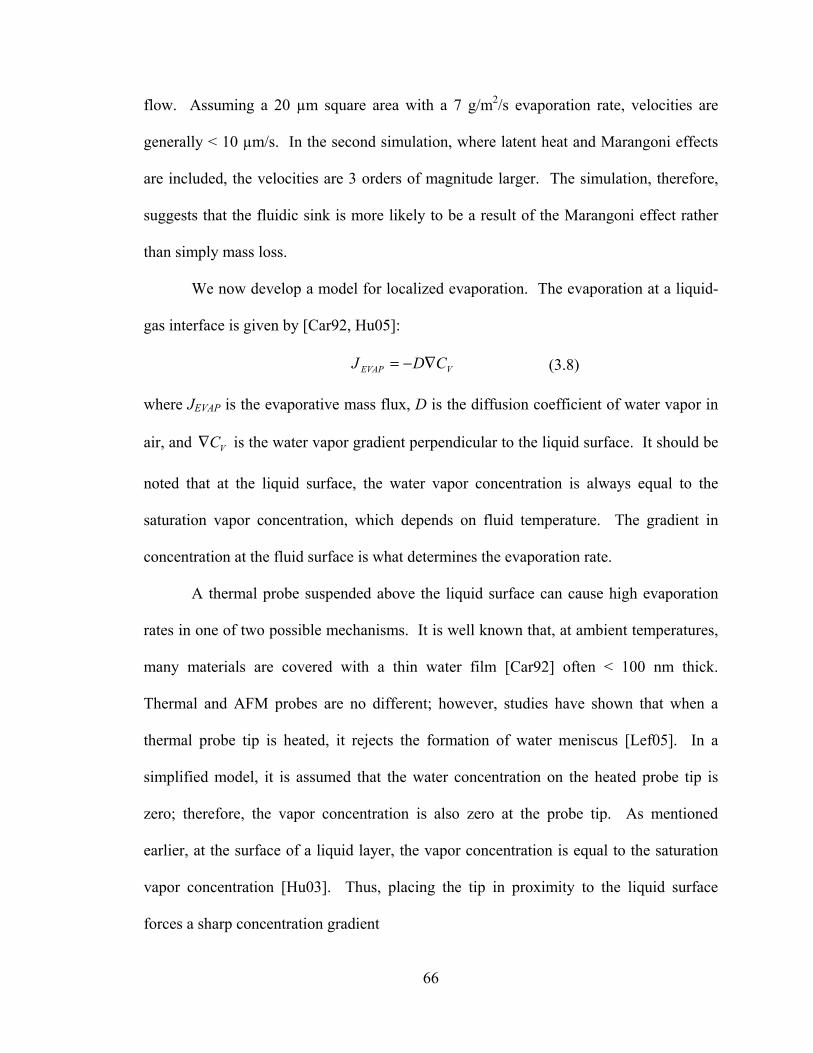
66

flow. Assuming a 20 µm square area with a 7 g/m2/s evaporation rate, velocities are

generally < 10 µm/s. In the second simulation, where latent heat and Marangoni effects

are included, the velocities are 3 orders of magnitude larger. The simulation, therefore,

suggests that the fluidic sink is more likely to be a result of the Marangoni effect rather

than simply mass loss.

We now develop a model for localized evaporation. The evaporation at a liquid-

gas interface is given by [Car92, Hu05]:

VEVAP CDJ ∇−= (3.8)

where JEVAP is the evaporative mass flux, D is the diffusion coefficient of water vapor in

air, and VC∇ is the water vapor gradient perpendicular to the liquid surface. It should be

noted that at the liquid surface, the water vapor concentration is always equal to the

saturation vapor concentration, which depends on fluid temperature. The gradient in

concentration at the fluid surface is what determines the evaporation rate.

A thermal probe suspended above the liquid surface can cause high evaporation

rates in one of two possible mechanisms. It is well known that, at ambient temperatures,

many materials are covered with a thin water film [Car92] often < 100 nm thick.

Thermal and AFM probes are no different; however, studies have shown that when a

thermal probe tip is heated, it rejects the formation of water meniscus [Lef05]. In a

simplified model, it is assumed that the water concentration on the heated probe tip is

zero; therefore, the vapor concentration is also zero at the probe tip. As mentioned

earlier, at the surface of a liquid layer, the vapor concentration is equal to the saturation

vapor concentration [Hu03]. Thus, placing the tip in proximity to the liquid surface

forces a sharp concentration gradient

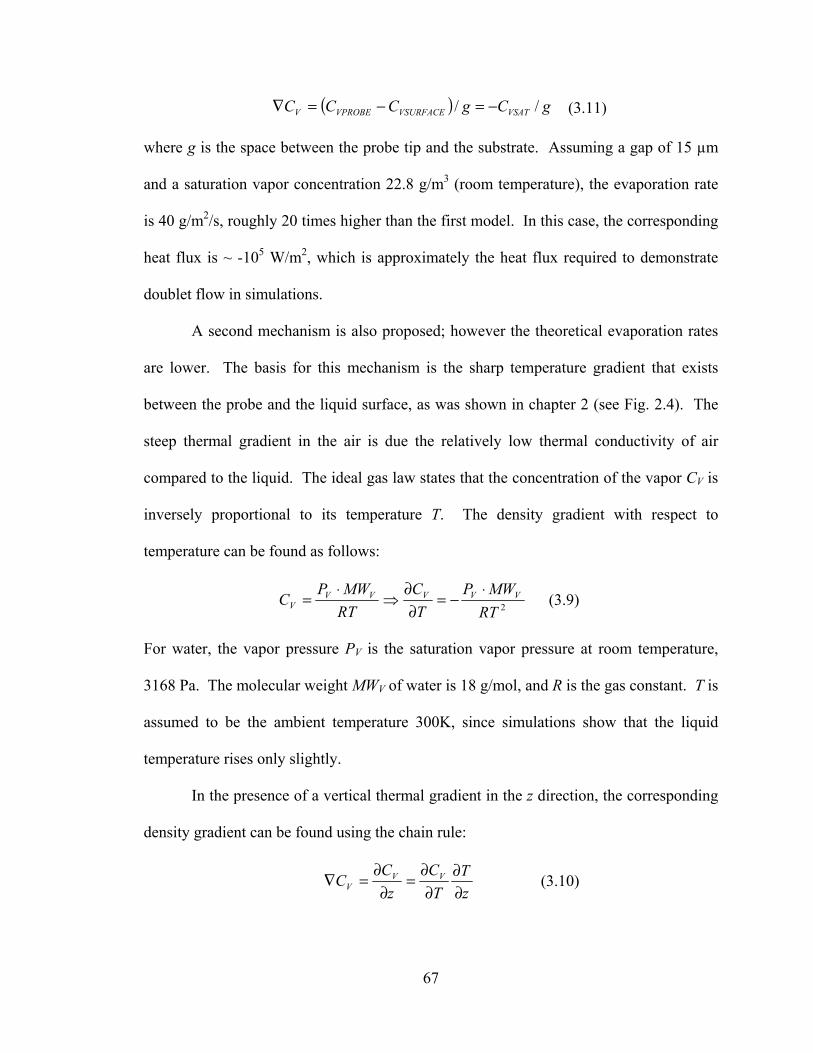
67

( ) gCgCCC VSATVSURFACEVPROBEV // −=−=∇ (3.11)

where g is the space between the probe tip and the substrate. Assuming a gap of 15 µm

and a saturation vapor concentration 22.8 g/m3 (room temperature), the evaporation rate

is 40 g/m2/s, roughly 20 times higher than the first model. In this case, the corresponding

heat flux is ~ -105 W/m2, which is approximately the heat flux required to demonstrate

doublet flow in simulations.

A second mechanism is also proposed; however the theoretical evaporation rates

are lower. The basis for this mechanism is the sharp temperature gradient that exists

between the probe and the liquid surface, as was shown in chapter 2 (see Fig. 2.4). The

steep thermal gradient in the air is due the relatively low thermal conductivity of air

compared to the liquid. The ideal gas law states that the concentration of the vapor CV is

inversely proportional to its temperature T. The density gradient with respect to

temperature can be found as follows:

2RTMWP

TC

RTMWP

C VVVVVV

⋅−=

∂∂

⇒⋅

= (3.9)

For water, the vapor pressure PV is the saturation vapor pressure at room temperature,

3168 Pa. The molecular weight MWV of water is 18 g/mol, and R is the gas constant. T is

assumed to be the ambient temperature 300K, since simulations show that the liquid

temperature rises only slightly.

In the presence of a vertical thermal gradient in the z direction, the corresponding

density gradient can be found using the chain rule:

zT

TC

zC

C VVV ∂

∂∂

∂=

∂∂

=∇ (3.10)

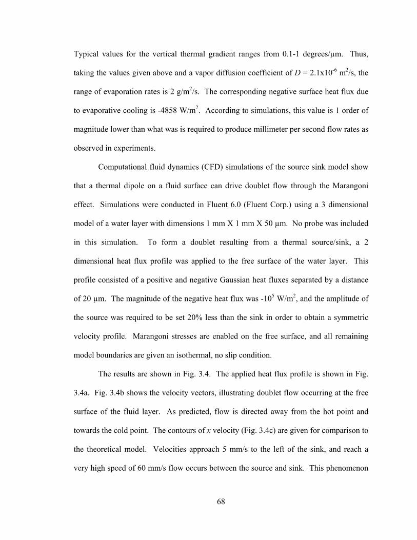
68

Typical values for the vertical thermal gradient ranges from 0.1-1 degrees/µm. Thus,

taking the values given above and a vapor diffusion coefficient of D = 2.1x10-6 m2/s, the

range of evaporation rates is 2 g/m2/s. The corresponding negative surface heat flux due

to evaporative cooling is -4858 W/m2. According to simulations, this value is 1 order of

magnitude lower than what was is required to produce millimeter per second flow rates as

observed in experiments.

Computational fluid dynamics (CFD) simulations of the source sink model show

that a thermal dipole on a fluid surface can drive doublet flow through the Marangoni

effect. Simulations were conducted in Fluent 6.0 (Fluent Corp.) using a 3 dimensional

model of a water layer with dimensions 1 mm X 1 mm X 50 µm. No probe was included

in this simulation. To form a doublet resulting from a thermal source/sink, a 2

dimensional heat flux profile was applied to the free surface of the water layer. This

profile consisted of a positive and negative Gaussian heat fluxes separated by a distance

of 20 µm. The magnitude of the negative heat flux was -105 W/m2, and the amplitude of

the source was required to be set 20% less than the sink in order to obtain a symmetric

velocity profile. Marangoni stresses are enabled on the free surface, and all remaining

model boundaries are given an isothermal, no slip condition.

The results are shown in Fig. 3.4. The applied heat flux profile is shown in Fig.

3.4a. Fig. 3.4b shows the velocity vectors, illustrating doublet flow occurring at the free

surface of the fluid layer. As predicted, flow is directed away from the hot point and

towards the cold point. The contours of x velocity (Fig. 3.4c) are given for comparison to

the theoretical model. Velocities approach 5 mm/s to the left of the sink, and reach a

very high speed of 60 mm/s flow occurs between the source and sink. This phenomenon

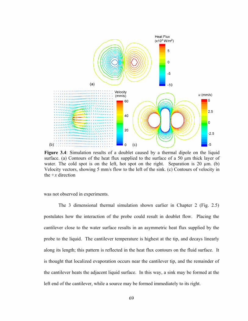
69

was not observed in experiments.

The 3 dimensional thermal simulation shown earlier in Chapter 2 (Fig. 2.5)

postulates how the interaction of the probe could result in doublet flow. Placing the

cantilever close to the water surface results in an asymmetric heat flux supplied by the

probe to the liquid. The cantilever temperature is highest at the tip, and decays linearly

along its length; this pattern is reflected in the heat flux contours on the fluid surface. It

is thought that localized evaporation occurs near the cantilever tip, and the remainder of

the cantilever heats the adjacent liquid surface. In this way, a sink may be formed at the

left end of the cantilever, while a source may be formed immediately to its right.

Figure 3.4: Simulation results of a doublet caused by a thermal dipole on the liquid surface. (a) Contours of the heat flux supplied to the surface of a 50 µm thick layer of water. The cold spot is on the left, hot spot on the right. Separation is 20 µm. (b) Velocity vectors, showing 5 mm/s flow to the left of the sink. (c) Contours of velocity in the +x direction

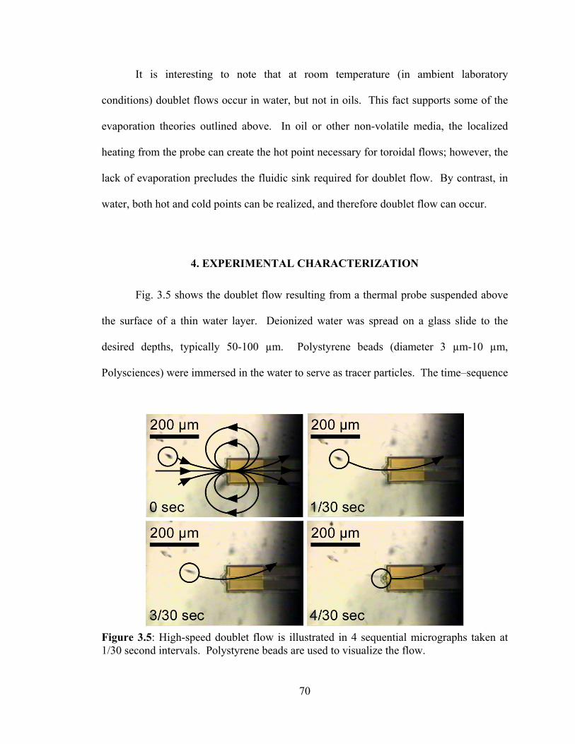
70

It is interesting to note that at room temperature (in ambient laboratory

conditions) doublet flows occur in water, but not in oils. This fact supports some of the

evaporation theories outlined above. In oil or other non-volatile media, the localized

heating from the probe can create the hot point necessary for toroidal flows; however, the

lack of evaporation precludes the fluidic sink required for doublet flow. By contrast, in

water, both hot and cold points can be realized, and therefore doublet flow can occur.

4. EXPERIMENTAL CHARACTERIZATION

Fig. 3.5 shows the doublet flow resulting from a thermal probe suspended above

the surface of a thin water layer. Deionized water was spread on a glass slide to the

desired depths, typically 50-100 µm. Polystyrene beads (diameter 3 µm-10 µm,

Polysciences) were immersed in the water to serve as tracer particles. The time–sequence

Figure 3.5: High-speed doublet flow is illustrated in 4 sequential micrographs taken at 1/30 second intervals. Polystyrene beads are used to visualize the flow.

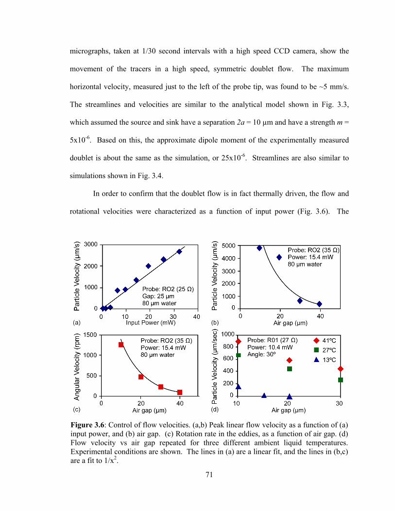
71

micrographs, taken at 1/30 second intervals with a high speed CCD camera, show the

movement of the tracers in a high speed, symmetric doublet flow. The maximum

horizontal velocity, measured just to the left of the probe tip, was found to be ~5 mm/s.

The streamlines and velocities are similar to the analytical model shown in Fig. 3.3,

which assumed the source and sink have a separation 2a = 10 µm and have a strength m =

5x10-6. Based on this, the approximate dipole moment of the experimentally measured

doublet is about the same as the simulation, or 25x10-6. Streamlines are also similar to

simulations shown in Fig. 3.4.

In order to confirm that the doublet flow is in fact thermally driven, the flow and

rotational velocities were characterized as a function of input power (Fig. 3.6). The

Figure 3.6: Control of flow velocities. (a,b) Peak linear flow velocity as a function of (a) input power, and (b) air gap. (c) Rotation rate in the eddies, as a function of air gap. (d) Flow velocity vs air gap repeated for three different ambient liquid temperatures. Experimental conditions are shown. The lines in (a) are a linear fit, and the lines in (b,c) are a fit to 1/x2.

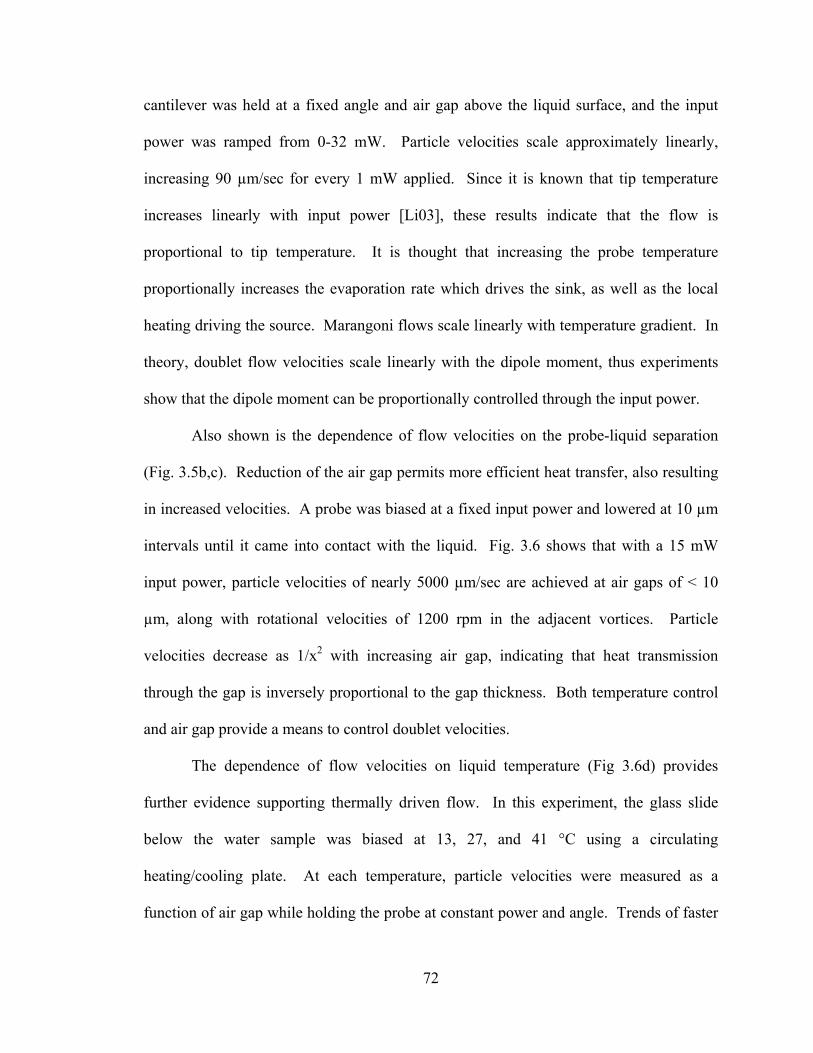
72

cantilever was held at a fixed angle and air gap above the liquid surface, and the input

power was ramped from 0-32 mW. Particle velocities scale approximately linearly,

increasing 90 µm/sec for every 1 mW applied. Since it is known that tip temperature

increases linearly with input power [Li03], these results indicate that the flow is

proportional to tip temperature. It is thought that increasing the probe temperature

proportionally increases the evaporation rate which drives the sink, as well as the local

heating driving the source. Marangoni flows scale linearly with temperature gradient. In

theory, doublet flow velocities scale linearly with the dipole moment, thus experiments

show that the dipole moment can be proportionally controlled through the input power.

Also shown is the dependence of flow velocities on the probe-liquid separation

(Fig. 3.5b,c). Reduction of the air gap permits more efficient heat transfer, also resulting

in increased velocities. A probe was biased at a fixed input power and lowered at 10 µm

intervals until it came into contact with the liquid. Fig. 3.6 shows that with a 15 mW

input power, particle velocities of nearly 5000 µm/sec are achieved at air gaps of < 10

µm, along with rotational velocities of 1200 rpm in the adjacent vortices. Particle

velocities decrease as 1/x2 with increasing air gap, indicating that heat transmission

through the gap is inversely proportional to the gap thickness. Both temperature control

and air gap provide a means to control doublet velocities.

The dependence of flow velocities on liquid temperature (Fig 3.6d) provides

further evidence supporting thermally driven flow. In this experiment, the glass slide

below the water sample was biased at 13, 27, and 41 °C using a circulating

heating/cooling plate. At each temperature, particle velocities were measured as a

function of air gap while holding the probe at constant power and angle. Trends of faster

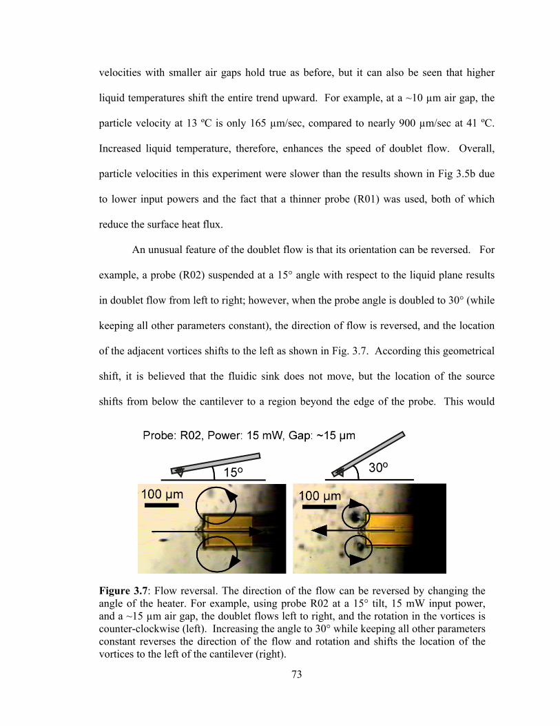
73

velocities with smaller air gaps hold true as before, but it can also be seen that higher

liquid temperatures shift the entire trend upward. For example, at a ~10 µm air gap, the

particle velocity at 13 ºC is only 165 µm/sec, compared to nearly 900 µm/sec at 41 ºC.

Increased liquid temperature, therefore, enhances the speed of doublet flow. Overall,

particle velocities in this experiment were slower than the results shown in Fig 3.5b due

to lower input powers and the fact that a thinner probe (R01) was used, both of which

reduce the surface heat flux.

An unusual feature of the doublet flow is that its orientation can be reversed. For

example, a probe (R02) suspended at a 15° angle with respect to the liquid plane results

in doublet flow from left to right; however, when the probe angle is doubled to 30° (while

keeping all other parameters constant), the direction of flow is reversed, and the location

of the adjacent vortices shifts to the left as shown in Fig. 3.7. According this geometrical

shift, it is believed that the fluidic sink does not move, but the location of the source

shifts from below the cantilever to a region beyond the edge of the probe. This would

Figure 3.7: Flow reversal. The direction of the flow can be reversed by changing the angle of the heater. For example, using probe R02 at a 15° tilt, 15 mW input power, and a ~15 µm air gap, the doublet flows left to right, and the rotation in the vortices is counter-clockwise (left). Increasing the angle to 30° while keeping all other parameters constant reverses the direction of the flow and rotation and shifts the location of the vortices to the left of the cantilever (right).

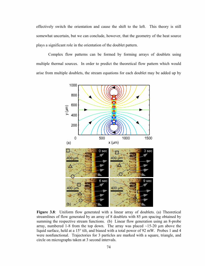
74

effectively switch the orientation and cause the shift to the left. This theory is still

somewhat uncertain, but we can conclude, however, that the geometry of the heat source

plays a significant role in the orientation of the doublet pattern.

Complex flow patterns can be formed by forming arrays of doublets using

multiple thermal sources. In order to predict the theoretical flow pattern which would

arise from multiple doublets, the stream equations for each doublet may be added up by

Figure 3.8: Uniform flow generated with a linear array of doublets. (a) Theoretical streamlines of flow generated by an array of 8 doublets with 85 µm spacing obtained by summing the respective stream functions. (b) Linear flow generation using an 8-probe array, numbered 1-8 from the top down. The array was placed ~15-20 µm above the liquid surface, held at a 15° tilt, and biased with a total power of 92 mW. Probes 1 and 4 were nonfunctional. Trajectories for 3 particles are marked with a square, triangle, and circle on micrographs taken at 3 second intervals.

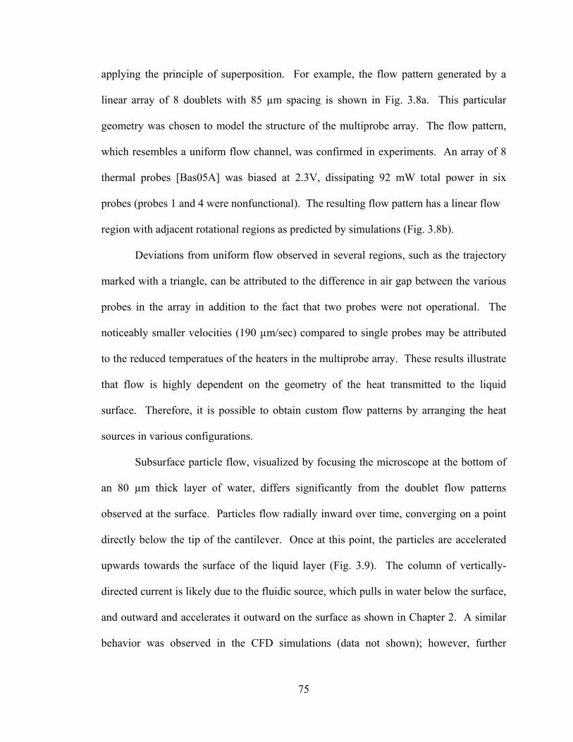
75

applying the principle of superposition. For example, the flow pattern generated by a

linear array of 8 doublets with 85 µm spacing is shown in Fig. 3.8a. This particular

geometry was chosen to model the structure of the multiprobe array. The flow pattern,

which resembles a uniform flow channel, was confirmed in experiments. An array of 8

thermal probes [Bas05A] was biased at 2.3V, dissipating 92 mW total power in six

probes (probes 1 and 4 were nonfunctional). The resulting flow pattern has a linear flow

region with adjacent rotational regions as predicted by simulations (Fig. 3.8b).

Deviations from uniform flow observed in several regions, such as the trajectory

marked with a triangle, can be attributed to the difference in air gap between the various

probes in the array in addition to the fact that two probes were not operational. The

noticeably smaller velocities (190 µm/sec) compared to single probes may be attributed

to the reduced temperatues of the heaters in the multiprobe array. These results illustrate

that flow is highly dependent on the geometry of the heat transmitted to the liquid

surface. Therefore, it is possible to obtain custom flow patterns by arranging the heat

sources in various configurations.

Subsurface particle flow, visualized by focusing the microscope at the bottom of

an 80 µm thick layer of water, differs significantly from the doublet flow patterns

observed at the surface. Particles flow radially inward over time, converging on a point

directly below the tip of the cantilever. Once at this point, the particles are accelerated

upwards towards the surface of the liquid layer (Fig. 3.9). The column of vertically-

directed current is likely due to the fluidic source, which pulls in water below the surface,

and outward and accelerates it outward on the surface as shown in Chapter 2. A similar

behavior was observed in the CFD simulations (data not shown); however, further

76

modeling and experimentation is needed to clarify the mechanism driving the surface and

subsurface flow patterns observed.

5. SUMMARY

This chapter has demonstrated surface doublets, a unique flow pattern which

occurs only in films of water when driven by a thermal probe. The supporting theory

suggests that a doublet can be generated by a fluidic source and sink in close proximity.

The latter can be caused by localized evaporation, due to the sharp concentration gradient

between the probe tip and the liquid surface. The orientation of the source and sink is

Figure 3.9: (a) Schematic of subsurface particle flow (80 µm below the surface). Particles flow radially inward towards the area underneath the microheater tip. Upon reaching this point, they are immediately propelled upwards to the surface. (b) Sequential micrographs show three particles (marked respectively with a square, triangle, and circle) converge towards the center and then disappear from the field of view as they are propelled upwards.

77

determined by the geometry and attack angle of the probe, suggesting that the

temperature gradient along the probe plays a significant role in generating doublet flow.

78

CHAPTER 4:

A PROGRAMMABLE ARRAY FOR CONTACT-FREE MANIPULATION

OF FLOATING DROPLETS BY MODULATION OF SURFACE

TENSION

One of the fundamental limitations of present programmable microdroplet

actuation systems is that they rely on the droplet’s interactions with a solid surface. Such

an approach leads to surface adsorption resulting in device contamination and sample

loss. This chapter presents a contactless droplet manipulation system which relies on

thermally generated Marangoni flows. Programmable, two dimensional control of

microdroplets suspended in an oil film is achieved using a 128-pixel heater array

suspended 100-500 µm above the oil layer. The heaters create surface temperature

perturbations, resulting in local Marangoni flows which can move droplets in either a

push or pull mode. Programmed movement is achieved by the sequential activation of

the heaters, with digital control circuitry and a graphical interface providing addressable

control of each heater. Droplets with diameters 300-1000 µm can be manipulated and

merged at speeds up to 140 µm/s. Several system level issues are discussed: surface

temperature elevation can be reduced from 25°C to <2.5°C by using fluids with low

thermal conductivity; thermal crosstalk and thermal time constants can be improved by

20% and 80%, respectively, by using a heat sink; evaporation rates can be reduced by

almost two orders of magnitude by using a two layer oil medium; and the choice of an

79

appropriate carrier fluid can achieve fluid velocities over 17,000 µm/s and reduces power

consumption to 30 mW/heater at moderate flow velocities. Microfabrication provides

added opportunities for power reduction and efficiency due to the favorable scaling of

Marangoni flows. The system provides a contactless platform for parallel droplet-based

assays.

1. INTRODUCTION

Digital microfluidic systems use microdroplets in an immiscible phase to

encapsulate reagents and to serve as reaction containers. Precise, user-defined chemical

reactions may be achieved by transporting and merging droplets containing the

appropriate samples and reagents [Son03A]. Compared to the traditional microfluidic

systems where samples are flowed through microchannels, digital microfluidics provides

an elegant approach to high throughput assays, offering inherent encapsulation, low

reagent consumption, and fast reaction times.

Programmable fluidic processors (PFPs) refer to systems which can dynamically

control the movement of droplets [Gas04, Sri04]. Droplets are manipulated in real time

on a 2-dimensional space using methods such as electrowetting-on-dielectric (EWOD)

[Cho03], optoelectrowetting [Chi03], dielectrophoresis (DEP) [Gas04], and magnetic

fields [Rid03]. As described in Chapter 2, all of these approaches, require a substrate

patterned with electrodes or coils, and the increased cost may not be suitable for a

disposable device.

A more important concern is that these approaches allow contact between the

droplet and the substrate. Any degree of contact or wetting between a liquid sample and

the substrate can result in surface adsorption. Proteins and other biomolecules readily

80

adsorb to hydrophobic surfaces like Teflon and PDMS as a result of hydrophobic

interactions [Yoo03, Sia03, Son03A]. In the traditional continuous flow devices, the

adsorption of proteins and cellular debris leads not only to contamination, but also causes

channel blockages [McC03]. In general, surface adsorption raises concerns for device

contamination, sample loss, and in most cases, makes device reuse impossible.

The problem of surface adsorption remains a concern with existing droplet

manipulation technologies because many of the current techniques rely on surface

interaction with the droplet. For example, EWOD applies voltages to a two-dimensional

grid of Teflon-coated electrodes to dynamically control surface energies. Due to its high

hydrophobicity, Teflon is particularly susceptible to adsorption. It has been suggested

that if silicone oil is used as the encapsulating medium, the droplet may be separated

from the Teflon surface by a thin film of oil [Sri04]; however, the effectiveness of the

technique depends significantly on the interfacial tension between the oil and the protein

concentration in the droplet. Protein adsorption can also render hydrophobic surfaces

hydrophilic, which interferes with EWOD and other surface based actuation techniques

[Sri04, Yoo03].

The best way to avoid surface adsorption is to keep the droplets away from any

walls or the solid substrate; however, there are presently no droplet manipulation

techniques which can avoid all surface contact. This chapter discusses a contactless,

programmable system for actuating droplets in which suspended droplets are manipulated

using Marangoni flows. Chapter 2 described the use of Marangoni flows of various

geometries for droplet mixing and control [Bas05B, Bas05C, Bas07A, Bas07B, Bas08A];

however, these flows were generated using fixed heat source geometries and were not

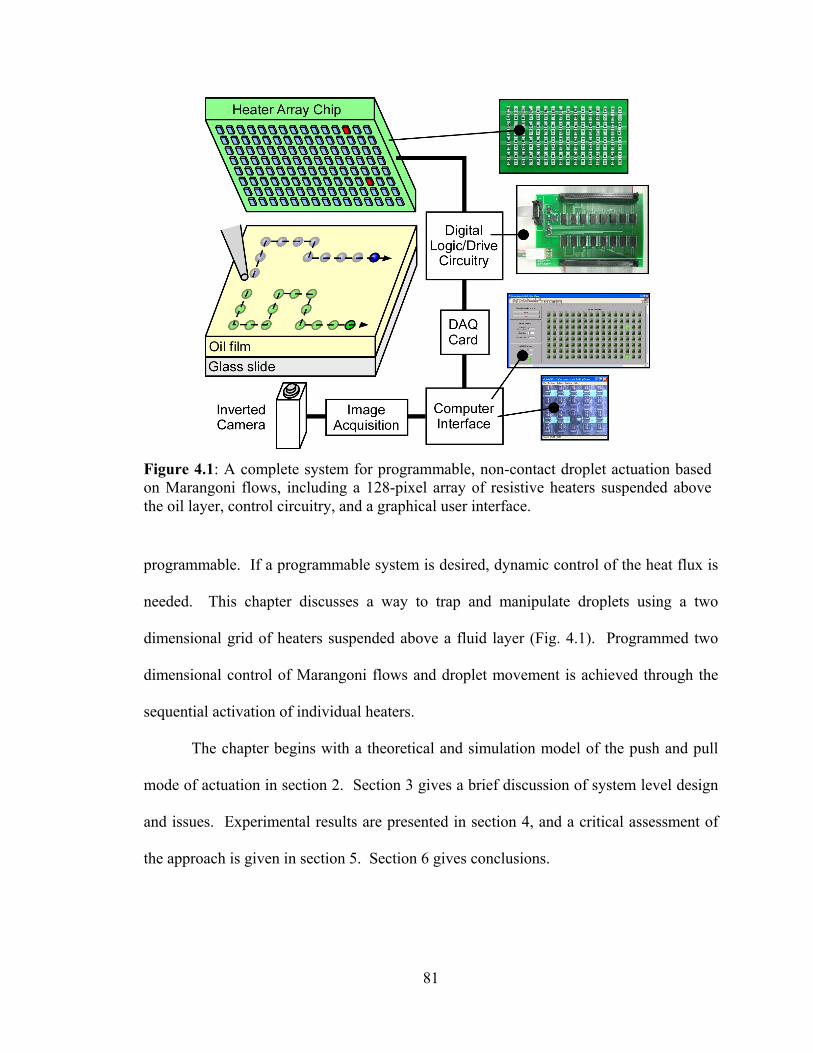
81

programmable. If a programmable system is desired, dynamic control of the heat flux is

needed. This chapter discusses a way to trap and manipulate droplets using a two

dimensional grid of heaters suspended above a fluid layer (Fig. 4.1). Programmed two

dimensional control of Marangoni flows and droplet movement is achieved through the

sequential activation of individual heaters.

The chapter begins with a theoretical and simulation model of the push and pull

mode of actuation in section 2. Section 3 gives a brief discussion of system level design

and issues. Experimental results are presented in section 4, and a critical assessment of

the approach is given in section 5. Section 6 gives conclusions.

Figure 4.1: A complete system for programmable, non-contact droplet actuation based on Marangoni flows, including a 128-pixel array of resistive heaters suspended above the oil layer, control circuitry, and a graphical user interface.

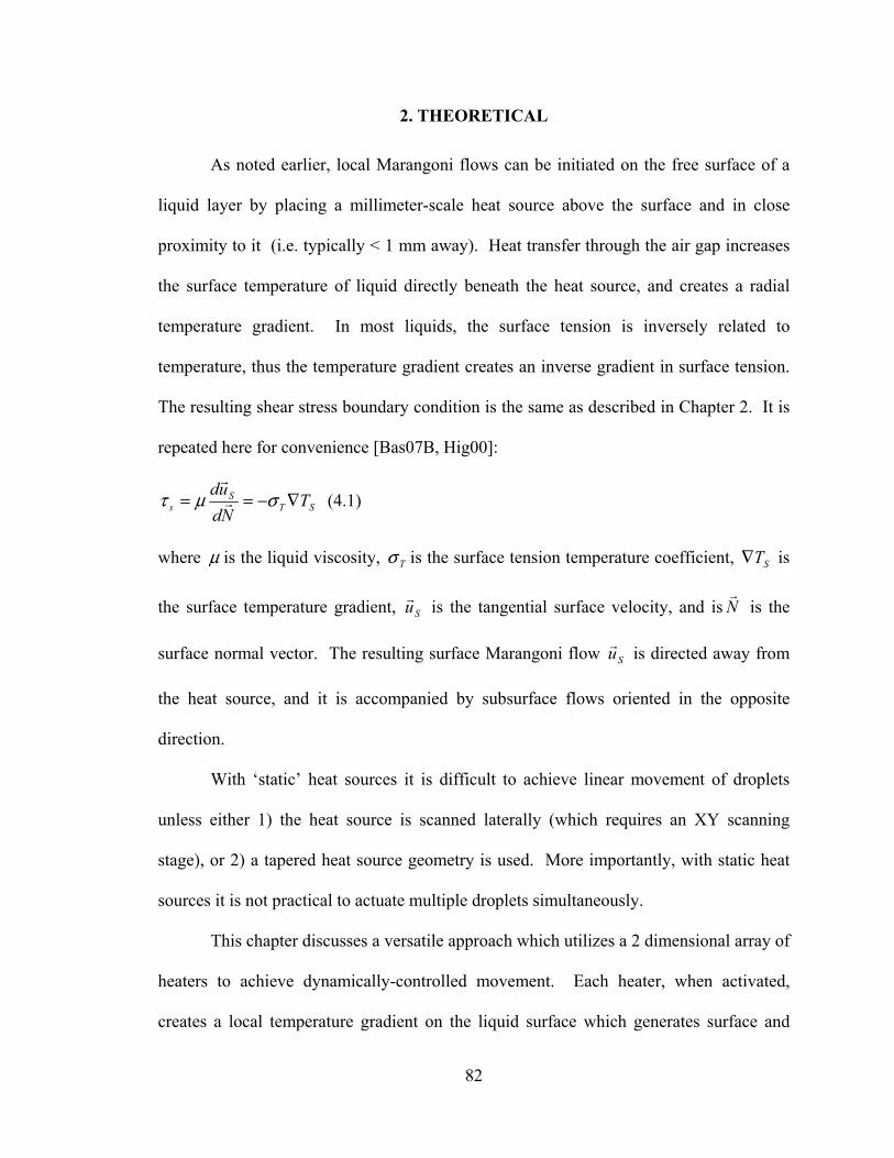
82

2. THEORETICAL

As noted earlier, local Marangoni flows can be initiated on the free surface of a

liquid layer by placing a millimeter-scale heat source above the surface and in close

proximity to it (i.e. typically < 1 mm away). Heat transfer through the air gap increases

the surface temperature of liquid directly beneath the heat source, and creates a radial

temperature gradient. In most liquids, the surface tension is inversely related to

temperature, thus the temperature gradient creates an inverse gradient in surface tension.

The resulting shear stress boundary condition is the same as described in Chapter 2. It is

repeated here for convenience [Bas07B, Hig00]:

STS

s TNdud

∇−== σµτ r

r

(4.1)

where µ is the liquid viscosity, Tσ is the surface tension temperature coefficient, ST∇ is

the surface temperature gradient, Sur is the tangential surface velocity, and is Nr

is the

surface normal vector. The resulting surface Marangoni flow Sur is directed away from

the heat source, and it is accompanied by subsurface flows oriented in the opposite

direction.

With ‘static’ heat sources it is difficult to achieve linear movement of droplets

unless either 1) the heat source is scanned laterally (which requires an XY scanning

stage), or 2) a tapered heat source geometry is used. More importantly, with static heat

sources it is not practical to actuate multiple droplets simultaneously.

This chapter discusses a versatile approach which utilizes a 2 dimensional array of

heaters to achieve dynamically-controlled movement. Each heater, when activated,

creates a local temperature gradient on the liquid surface which generates surface and

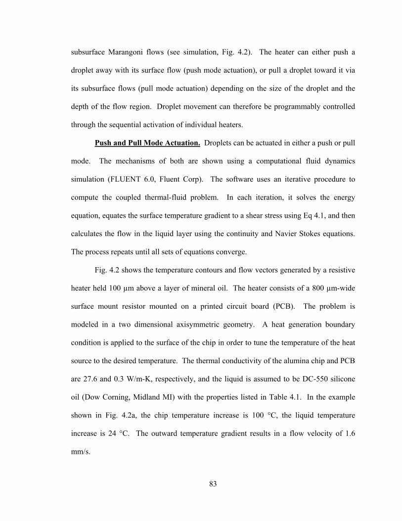
83

subsurface Marangoni flows (see simulation, Fig. 4.2). The heater can either push a

droplet away with its surface flow (push mode actuation), or pull a droplet toward it via

its subsurface flows (pull mode actuation) depending on the size of the droplet and the

depth of the flow region. Droplet movement can therefore be programmably controlled

through the sequential activation of individual heaters.

Push and Pull Mode Actuation. Droplets can be actuated in either a push or pull

mode. The mechanisms of both are shown using a computational fluid dynamics

simulation (FLUENT 6.0, Fluent Corp). The software uses an iterative procedure to

compute the coupled thermal-fluid problem. In each iteration, it solves the energy

equation, equates the surface temperature gradient to a shear stress using Eq 4.1, and then

calculates the flow in the liquid layer using the continuity and Navier Stokes equations.

The process repeats until all sets of equations converge.

Fig. 4.2 shows the temperature contours and flow vectors generated by a resistive

heater held 100 µm above a layer of mineral oil. The heater consists of a 800 µm-wide

surface mount resistor mounted on a printed circuit board (PCB). The problem is

modeled in a two dimensional axisymmetric geometry. A heat generation boundary

condition is applied to the surface of the chip in order to tune the temperature of the heat

source to the desired temperature. The thermal conductivity of the alumina chip and PCB

are 27.6 and 0.3 W/m-K, respectively, and the liquid is assumed to be DC-550 silicone

oil (Dow Corning, Midland MI) with the properties listed in Table 4.1. In the example

shown in Fig. 4.2a, the chip temperature increase is 100 °C, the liquid temperature

increase is 24 °C. The outward temperature gradient results in a flow velocity of 1.6

mm/s.

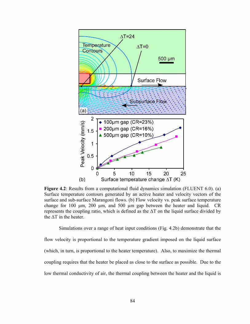
84

Simulations over a range of heat input conditions (Fig. 4.2b) demonstrate that the

flow velocity is proportional to the temperature gradient imposed on the liquid surface

(which, in turn, is proportional to the heater temperature). Also, to maximize the thermal

coupling requires that the heater be placed as close to the surface as possible. Due to the

low thermal conductivity of air, the thermal coupling between the heater and the liquid is

Figure 4.2: Results from a computational fluid dynamics simulation (FLUENT 6.0). (a) Surface temperature contours generated by an active heater and velocity vectors of the surface and sub-surface Marangoni flows. (b) Flow velocity vs. peak surface temperature change for 100 µm, 200 µm, and 500 µm gap between the heater and liquid. CR represents the coupling ratio, which is defined as the ∆T on the liquid surface divided by the ∆T in the heater.

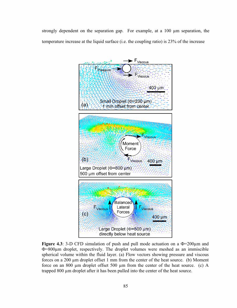
85

strongly dependent on the separation gap. For example, at a 100 µm separation, the

temperature increase at the liquid surface (i.e. the coupling ratio) is 23% of the increase

Figure 4.3: 3-D CFD simulation of push and pull mode actuation on a Ф=200µm and Ф=800µm droplet, respectively. The droplet volumes were meshed as an immiscible spherical volume within the fluid layer. (a) Flow vectors showing pressure and viscous forces on a 200 µm droplet offset 1 mm from the center of the heat source. (b) Moment force on an 800 µm droplet offset 500 µm from the center of the heat source. (c) A trapped 800 µm droplet after it has been pulled into the center of the heat source.

86

in the heat source. At a 500 µm gap, the coupling ratio falls to 10%. A small gap is also

important in maintaining a sharp lateral temperature gradient, which translates directly

into flow velocity. In this regard, the approach of having suspended heaters benefits from

the low thermal conductivity of air. Were the heaters embedded in the liquid, the

relatively high thermal conductivity would preclude the formation of sharp gradients,

limiting the velocity of Marangoni flow. Furthermore, it would cause undesirable heating

in the bulk fluid.

The interaction of droplets with the flow is shown in Fig. 4.3. This set of

simulations includes a 3-dimensional fluid layer with an embedded spherical volume to

represent the immiscible droplet. A surface heat flux of 50 mW/mm2 is added to a 1 mm

square region in the fluid layer to model the local heating. Assuming the properties of

DC-550 fluid, this results in a recirculating flow (maximum surface flow velocity of 6

mm/s) which applies pressure and viscous forces to a droplet. The lateral pressure and

viscous forces on the droplet were calculated by integrating the respective forces along

the surface area of the droplet, and moment forces were integrated in a similar manner

using the droplet centroid as the moment axis.

Qualitative results (Fig. 4.3a) demonstrate the operation of the push and pull

modes. A droplet < 200 µm in diameter gets pushed away from the active heater by

surface flows (push mode). In this case, the center of mass is near the fluid surface,

which is dominated by outward-directed surface Marangoni flows. A combination of

pressure and viscous forces (Fig. 4.3a) push the droplet outward. In contrast, a larger

droplet (for example, Ф=800 µm) tends to get pulled into the active heater. In this case,

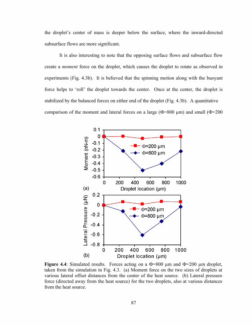
87

the droplet’s center of mass is deeper below the surface, where the inward-directed

subsurface flows are more significant.

It is also interesting to note that the opposing surface flows and subsurface flow

create a moment force on the droplet, which causes the droplet to rotate as observed in

experiments (Fig. 4.3b). It is believed that the spinning motion along with the buoyant

force helps to ‘roll’ the droplet towards the center. Once at the center, the droplet is

stabilized by the balanced forces on either end of the droplet (Fig. 4.3b). A quantitative

comparison of the moment and lateral forces on a large (Ф=800 µm) and small (Ф=200

Figure 4.4: Simulated results. Forces acting on a Ф=800 µm and Ф=200 µm droplet, taken from the simulation in Fig. 4.3. (a) Moment force on the two sizes of droplets at various lateral offset distances from the center of the heat source. (b) Lateral pressure force (directed away from the heat source) for the two droplets, also at various distances from the heat source.

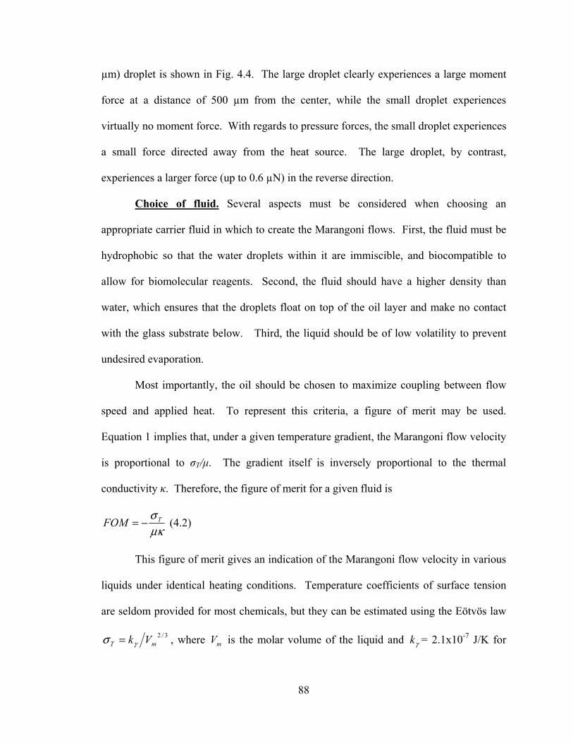
88

µm) droplet is shown in Fig. 4.4. The large droplet clearly experiences a large moment

force at a distance of 500 µm from the center, while the small droplet experiences

virtually no moment force. With regards to pressure forces, the small droplet experiences

a small force directed away from the heat source. The large droplet, by contrast,

experiences a larger force (up to 0.6 µN) in the reverse direction.

Choice of fluid. Several aspects must be considered when choosing an

appropriate carrier fluid in which to create the Marangoni flows. First, the fluid must be

hydrophobic so that the water droplets within it are immiscible, and biocompatible to

allow for biomolecular reagents. Second, the fluid should have a higher density than

water, which ensures that the droplets float on top of the oil layer and make no contact

with the glass substrate below. Third, the liquid should be of low volatility to prevent

undesired evaporation.

Most importantly, the oil should be chosen to maximize coupling between flow

speed and applied heat. To represent this criteria, a figure of merit may be used.

Equation 1 implies that, under a given temperature gradient, the Marangoni flow velocity

is proportional to σT/µ. The gradient itself is inversely proportional to the thermal

conductivity κ. Therefore, the figure of merit for a given fluid is

µκσ TFOM −= (4.2)

This figure of merit gives an indication of the Marangoni flow velocity in various

liquids under identical heating conditions. Temperature coefficients of surface tension

are seldom provided for most chemicals, but they can be estimated using the Eötvös law

32 /mT Vkγσ = , where mV is the molar volume of the liquid and γk = 2.1x10-7 J/K for

89

virtually all liquids [Pil51, Eöt86]. They can also be experimentally measured using the

DeNouy ring method [Nou19] or drop shape analysis [Son96]. Over the range of carrier

fluids examined in this work, the surface tension coefficients do not vary by more than 2-

5X.

Thermal conductivity data for fluids is typically available. Aqueous films, for

example, have relatively high thermal conductance (0.6 W/m-K) which limits the

formation of sharp surface temperature gradients. In contrast, typical mineral and

silicone oils have conductivity only 20% that of water, and also have fairly low vapor

pressures to reduce evaporative effects. Fluorinated organic liquids function as suitable

carrier fluids for Marangoni flows, due primarily to their low thermal conductivity on the

order of 0.06 W/m-K; however, their evaporation rates are somewhat higher than mineral

oils.

Given the diverse set of requirements, three oils are chosen. The first is mineral

oil (USP, Rite Aid Pharmacy), a biocompatible, transparent oil often used in biochemical

assays for reagent encapsulation (for example, to encapsulate embryos, and high

throughput assays). This oil is less dense than water, so it is used primarily for

characterization and for particle experiments. The second group of fluids includes high

density silicone oils which allow the droplets to float on the surface. These include DC-

550 and DC-704 fluids (Dow Corning). The last fluid is FluorinertTM (FC-3283, 3M

Corp.), a fully fluorinated dielectric fluid which has low very thermal conductivity, low

miscibility to water, and high density. FC-3283 has often been used as a carrier fluid in

microdroplet systems [Son03A]. Material properties for each of these fluids are given in

the Table 4.1.

90

Liquid Parameter Symbol Units Mineral Oil USP

DC550 Silicone oil

DC704 Silicone oil

FC-3283 dielectric liquid

Density ρ kg/m3 886 1070 1070 1820 Surface tension coefficient

σT mN/m-K

-0.220 -0.069** -0.036 * -0.410 *

Thermal Conductivity

κ W/m-K 0.12 0.1463 0.16 ** 0.066

Viscosity µ kg/m-s 0.026 0.134 0.042 0.0014 Figure of Merit

|σT/κµ| 7.1x10-2 3.5x10-3 5.3x10-3 4.44

References [Sam99A, Ber03]

[DC98A, Van97]

[DC98B, Ber03]

[3M01]

Table 4.1: Material properties for 3 liquids used in generating Marangoni flows. Values marked with a * are calculated using the Eötvös law, and those marked with ** are estimated from similar fluids.

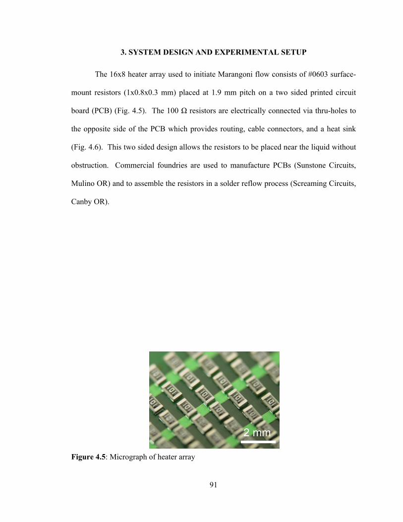
91

3. SYSTEM DESIGN AND EXPERIMENTAL SETUP

The 16x8 heater array used to initiate Marangoni flow consists of #0603 surface-

mount resistors (1x0.8x0.3 mm) placed at 1.9 mm pitch on a two sided printed circuit

board (PCB) (Fig. 4.5). The 100 Ω resistors are electrically connected via thru-holes to

the opposite side of the PCB which provides routing, cable connectors, and a heat sink

(Fig. 4.6). This two sided design allows the resistors to be placed near the liquid without

obstruction. Commercial foundries are used to manufacture PCBs (Sunstone Circuits,

Mulino OR) and to assemble the resistors in a solder reflow process (Screaming Circuits,

Canby OR).

Figure 4.5: Micrograph of heater array

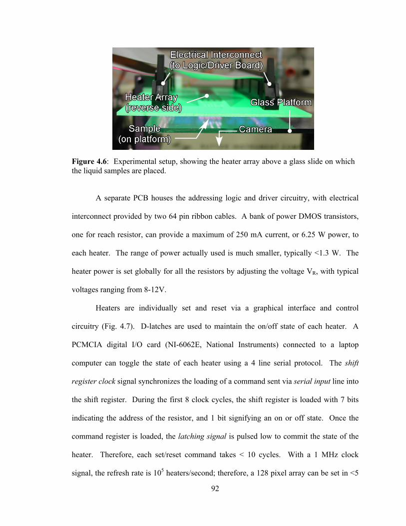
92

A separate PCB houses the addressing logic and driver circuitry, with electrical

interconnect provided by two 64 pin ribbon cables. A bank of power DMOS transistors,

one for reach resistor, can provide a maximum of 250 mA current, or 6.25 W power, to

each heater. The range of power actually used is much smaller, typically <1.3 W. The

heater power is set globally for all the resistors by adjusting the voltage VR, with typical

voltages ranging from 8-12V.

Heaters are individually set and reset via a graphical interface and control

circuitry (Fig. 4.7). D-latches are used to maintain the on/off state of each heater. A

PCMCIA digital I/O card (NI-6062E, National Instruments) connected to a laptop

computer can toggle the state of each heater using a 4 line serial protocol. The shift

register clock signal synchronizes the loading of a command sent via serial input line into

the shift register. During the first 8 clock cycles, the shift register is loaded with 7 bits

indicating the address of the resistor, and 1 bit signifying an on or off state. Once the

command register is loaded, the latching signal is pulsed low to commit the state of the

heater. Therefore, each set/reset command takes < 10 cycles. With a 1 MHz clock

signal, the refresh rate is 105 heaters/second; therefore, a 128 pixel array can be set in <5

Figure 4.6: Experimental setup, showing the heater array above a glass slide on which the liquid samples are placed.

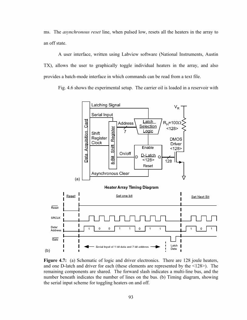
93

ms. The asynchronous reset line, when pulsed low, resets all the heaters in the array to

an off state.

A user interface, written using Labview software (National Instruments, Austin

TX), allows the user to graphically toggle individual heaters in the array, and also

provides a batch-mode interface in which commands can be read from a text file.

Fig. 4.6 shows the experimental setup. The carrier oil is loaded in a reservoir with

(a)

(b)

Figure 4.7: (a) Schematic of logic and driver electronics. There are 128 joule heaters, and one D-latch and driver for each (these elements are represented by the <128>). The remaining components are shared. The forward slash indicates a multi-line bus, and the number beneath indicates the number of lines on the bus. (b) Timing diagram, showing the serial input scheme for toggling heaters on and off.

94

a transparent bottom so that droplet motion can be imaged from below with a CCD

camera. The reservoir is placed on a glass platform which is actively cooled with a

circulating refrigerated water bath (Neslab Endocal). The purpose of the water bath is to

prevent heating of the bulk fluid which can reduce the surface temperature gradients

needed for Marangoni flow and also can cause loss of function or other damage to

thermally-sensitive samples such as enzymes and other biomolecules. Droplet samples

are deposited directly into the oil using a micropipette. The heater array, with the chip

resistors facing the oil sample, is then lowered to within 100 µm above the liquid surface

using a micromanipulator. Parallel alignment and leveling of the glass platform and the

heater array board must be done prior to the experiment to help ensure that heater-liquid

separation is uniform through the entire array. (A bubble alignment tool is useful for this

purpose.)

4. EXPERIMENTAL RESULTS

Test Setup and Characterization. Individual heaters were first characterized for

thermal efficiency by using a fine gauge thermocouple (CHAL-0005, Omega

Engineering) to measure the temperature as a function of input power. The typical

thermal isolation of each heater is ≈120 K/W, and a maximum temperature of 175°C

(Fig. 4.8a) can be achieved without burnout. The parasitic temperature on an adjacent

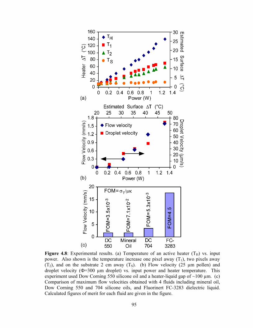
95

Figure 4.8: Experimental results. (a) Temperature of an active heater (TH) vs. input power. Also shown is the temperature increase one pixel away (T1), two pixels away (T2), and on the substrate 2 cm away (TS). (b) Flow velocity (25 µm pollen) and droplet velocity (Ф=300 µm droplet) vs. input power and heater temperature. This experiment used Dow Corning 550 silicone oil and a heater-liquid gap of ~100 µm. (c) Comparison of maximum flow velocities obtained with 4 fluids including mineral oil, Dow Corning 550 and 704 silicone oils, and Fluorinert FC-3283 dielectric liquid. Calculated figures of merit for each fluid are given in the figure.

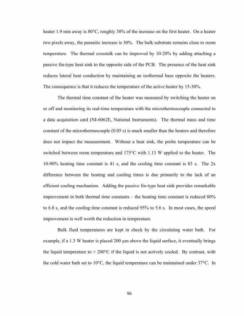
96

heater 1.9 mm away is 80°C, roughly 38% of the increase on the first heater. On a heater

two pixels away, the parasitic increase is 30%. The bulk substrate remains close to room

temperature. The thermal crosstalk can be improved by 10-20% by adding attaching a

passive fin-type heat sink to the opposite side of the PCB. The presence of the heat sink

reduces lateral heat conduction by maintaining an isothermal base opposite the heaters.

The consequence is that it reduces the temperature of the active heater by 15-30%.

The thermal time constant of the heater was measured by switching the heater on

or off and monitoring its real-time temperature with the microthermocouple connected to

a data acquisition card (NI-6062E, National Instruments). The thermal mass and time

constant of the microthermocouple (0.05 s) is much smaller than the heaters and therefore

does not impact the measurement. Without a heat sink, the probe temperature can be

switched between room temperature and 175°C with 1.13 W applied to the heater. The

10-90% heating time constant is 41 s, and the cooling time constant is 83 s. The 2x

difference between the heating and cooling times is due primarily to the lack of an

efficient cooling mechanism. Adding the passive fin-type heat sink provides remarkable

improvement in both thermal time constants – the heating time constant is reduced 80%

to 6.8 s, and the cooling time constant is reduced 95% to 5.6 s. In most cases, the speed

improvement is well worth the reduction in temperature.

Bulk fluid temperatures are kept in check by the circulating water bath. For

example, if a 1.3 W heater is placed 200 µm above the liquid surface, it eventually brings

the liquid temperature to > 200°C if the liquid is not actively cooled. By contrast, with

the cold water bath set to 10°C, the liquid temperature can be maintained under 37°C. In

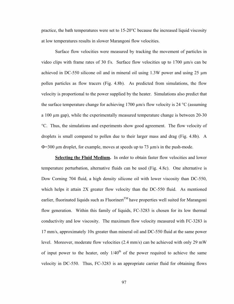
97

practice, the bath temperatures were set to 15-20°C because the increased liquid viscosity

at low temperatures results in slower Marangoni flow velocities.

Surface flow velocities were measured by tracking the movement of particles in

video clips with frame rates of 30 f/s. Surface flow velocities up to 1700 µm/s can be

achieved in DC-550 silicone oil and in mineral oil using 1.3W power and using 25 µm

pollen particles as flow tracers (Fig. 4.8b). As predicted from simulations, the flow

velocity is proportional to the power supplied by the heater. Simulations also predict that

the surface temperature change for achieving 1700 µm/s flow velocity is 24 °C (assuming

a 100 µm gap), while the experimentally measured temperature change is between 20-30

°C. Thus, the simulations and experiments show good agreement. The flow velocity of

droplets is small compared to pollen due to their larger mass and drag (Fig. 4.8b). A

Ф=300 µm droplet, for example, moves at speeds up to 73 µm/s in the push-mode.

Selecting the Fluid Medium. In order to obtain faster flow velocities and lower

temperature perturbation, alternative fluids can be used (Fig. 4.8c). One alternative is

Dow Corning 704 fluid, a high density silicone oil with lower viscosity than DC-550,

which helps it attain 2X greater flow velocity than the DC-550 fluid. As mentioned

earlier, fluorinated liquids such as FluorinertTM have properties well suited for Marangoni

flow generation. Within this family of liquids, FC-3283 is chosen for its low thermal

conductivity and low viscosity. The maximum flow velocity measured with FC-3283 is

17 mm/s, approximately 10x greater than mineral oil and DC-550 fluid at the same power

level. Moreover, moderate flow velocities (2.4 mm/s) can be achieved with only 29 mW

of input power to the heater, only 1/40th of the power required to achieve the same

velocity in DC-550. Thus, FC-3283 is an appropriate carrier fluid for obtaining flows

98

with low power and low temperature elevation to the fluid. The consequence is its higher

evaporation rate compared to the silicone oils.

Another challenge with using FC-3283 is the instability of droplets within the

hydrophobic fluid. Aqueous droplets deposited at the center of the fluid reservoir tend to

move to the edges of the reservoir where they eventually attach to the reservoir wall. The

stabilization problem is solved by adding the fluorous surfactant 1H,1H,2H,2H-perfluoro-

1-octanol (PFO, Sigma-Aldrich) to the FC-3283 carrier fluid in a 1:10 v/v ratio. The

surfactant molecules, which are soluble only in the fluorous phase, assemble at aqueous-

fluorous interface and stabilize the droplet [Roa05]. No droplet instability is observed

after adding the surfactant.

Push and Pull Mode of Actuation of Droplets. Droplets immersed in the carrier

fluid can be actuated in either the push or pull mode. The push-mode of actuation occurs

in single layers of DC-550 fluid when the center of gravity of the droplet is near the

surface. This can be ensured in one of two ways: 1) by pipetting the droplets above the

surface of the liquid so that the droplet floats on top of the surface, or 2) by using small

droplets (Ф<200 µm). In this mode, surface Marangoni flows drive the droplet away

from the active heaters (Fig. 4.9). Multi-heater configurations may be used to direct a

droplet in the desired direction. For example, two adjacent heaters activated next to a

droplet push the droplet in a straight line, while a right-angle turn can be accomplished

using three heaters in an L-shape. Arbitrary movements at speeds up to 200 µm/s can be

generated with sequential activation of such configurations.

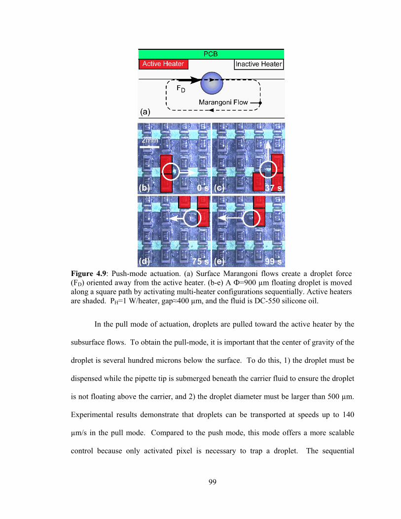
99

In the pull mode of actuation, droplets are pulled toward the active heater by the

subsurface flows. To obtain the pull-mode, it is important that the center of gravity of the

droplet is several hundred microns below the surface. To do this, 1) the droplet must be

dispensed while the pipette tip is submerged beneath the carrier fluid to ensure the droplet

is not floating above the carrier, and 2) the droplet diameter must be larger than 500 µm.

Experimental results demonstrate that droplets can be transported at speeds up to 140

µm/s in the pull mode. Compared to the push mode, this mode offers a more scalable

control because only activated pixel is necessary to trap a droplet. The sequential

Figure 4.9: Push-mode actuation. (a) Surface Marangoni flows create a droplet force (FD) oriented away from the active heater. (b-e) A Ф=900 µm floating droplet is moved along a square path by activating multi-heater configurations sequentially. Active heaters are shaded. PH=1 W/heater, gap≈400 µm, and the fluid is DC-550 silicone oil.

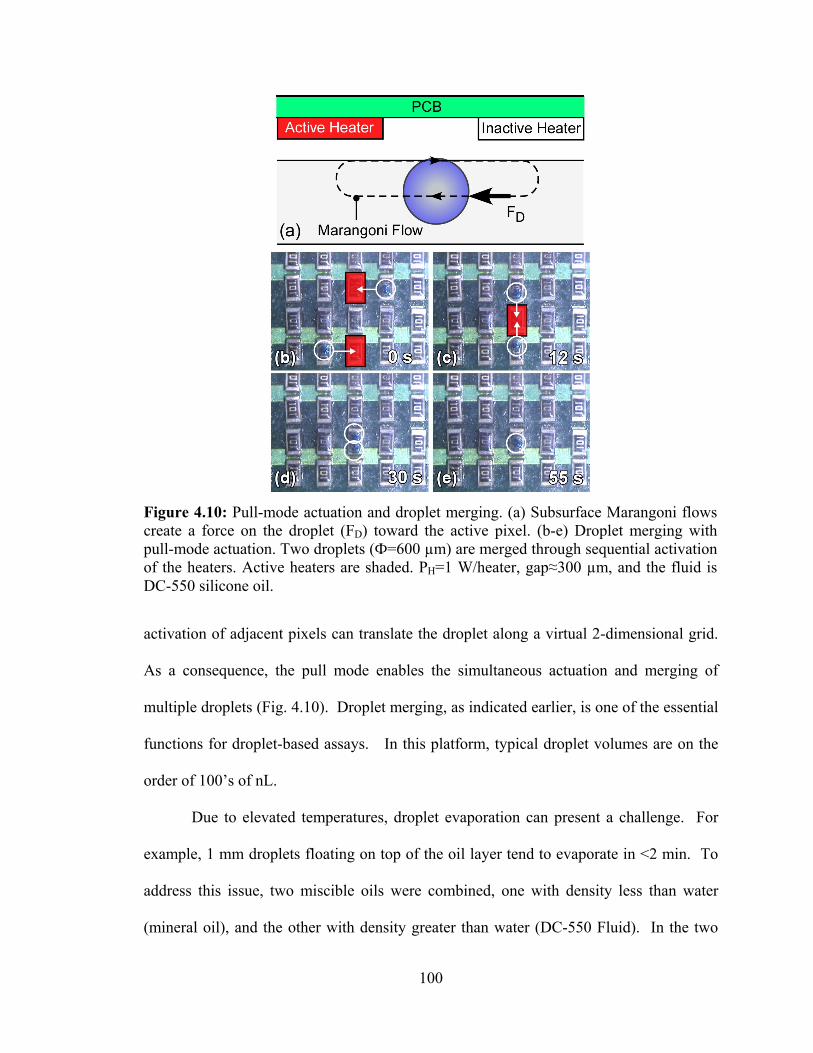
100

activation of adjacent pixels can translate the droplet along a virtual 2-dimensional grid.

As a consequence, the pull mode enables the simultaneous actuation and merging of

multiple droplets (Fig. 4.10). Droplet merging, as indicated earlier, is one of the essential

functions for droplet-based assays. In this platform, typical droplet volumes are on the

order of 100’s of nL.

Due to elevated temperatures, droplet evaporation can present a challenge. For

example, 1 mm droplets floating on top of the oil layer tend to evaporate in <2 min. To

address this issue, two miscible oils were combined, one with density less than water

(mineral oil), and the other with density greater than water (DC-550 Fluid). In the two

Figure 4.10: Pull-mode actuation and droplet merging. (a) Subsurface Marangoni flows create a force on the droplet (FD) toward the active pixel. (b-e) Droplet merging with pull-mode actuation. Two droplets (Ф=600 µm) are merged through sequential activation of the heaters. Active heaters are shaded. PH=1 W/heater, gap≈300 µm, and the fluid is DC-550 silicone oil.

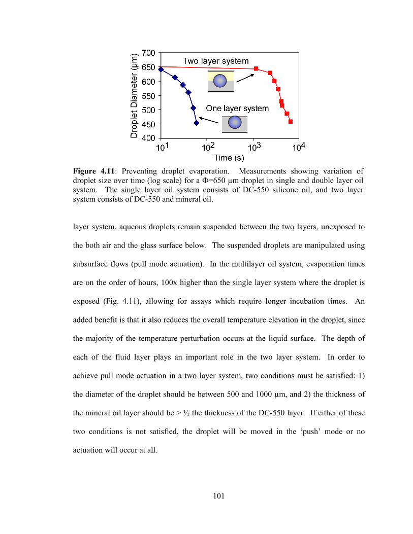
101

layer system, aqueous droplets remain suspended between the two layers, unexposed to

the both air and the glass surface below. The suspended droplets are manipulated using

subsurface flows (pull mode actuation). In the multilayer oil system, evaporation times

are on the order of hours, 100x higher than the single layer system where the droplet is

exposed (Fig. 4.11), allowing for assays which require longer incubation times. An

added benefit is that it also reduces the overall temperature elevation in the droplet, since

the majority of the temperature perturbation occurs at the liquid surface. The depth of

each of the fluid layer plays an important role in the two layer system. In order to

achieve pull mode actuation in a two layer system, two conditions must be satisfied: 1)

the diameter of the droplet should be between 500 and 1000 µm, and 2) the thickness of

the mineral oil layer should be > ½ the thickness of the DC-550 layer. If either of these

two conditions is not satisfied, the droplet will be moved in the ‘push’ mode or no

actuation will occur at all.

Figure 4.11: Preventing droplet evaporation. Measurements showing variation of droplet size over time (log scale) for a Ф=650 µm droplet in single and double layer oil system. The single layer oil system consists of DC-550 silicone oil, and two layer system consists of DC-550 and mineral oil.

102

5. DISCUSSION

The design issues with Marangoni flow-based droplet manipulation include 1)

coupling efficiency (maintaining fast droplet flow velocities while minimizing the

temperature perturbation and power consumption), and 2) scaling to small length scales.

Efficiency. The efficiency of the Marangoni technique depends on the system

providing a sharp temperature gradient at the fluid interface, and then translating that

gradient into a high speed flow. To do this, one must first choose a liquid with a high

figure of merit, as demonstrated in Fig. 4.8c. Fluorinated carrier fluids, with their

relatively high surface tension coefficient and low thermal conductivity, make them a

good carrier fluid for Marangoni flows, giving 10X higher velocities at the same power,

and 1/40th the power consumption at the same velocity; however, one must be careful to

use appropriate surfactants to stabilize the droplets. Furthermore, they are immiscible to

many oils, which makes it difficult to create multilayer oil systems for evaporation

reduction.

Efficiency can also be improved by placing the heat sources as close to the

surface as possible. This not only increases the coupling ratio (∆TSurface/∆THeater), but it

also increases the lateral temperature gradient necessary for producing flow. With an

array of heaters, the challenge is to keep the heater-liquid separation small and equal for

all of the heaters in the array. The present approach can obtain gaps as low as 100-200

µm; but this can be improved by using an optical feedback system or a more precise

leveling system.

Finally, one can increase the efficiency of the heater itself. Microfabricated

devices with thermally insulative materials and small cross sections provide high

103

efficiency and fast time constants. For example, a polyimide cantilever with an

integrated heater can achieve 100 °C temperature while dissipating only 10 mW of

applied power [Li03]. Such heaters would reduce power consumption by up to 2 orders

of magnitude, which is important especially if the number and density of the heaters in

the array is scaled up.

In order to allow localized control, thermal crosstalk between heaters is a concern.

Present experiments show a crosstalk ratio of 35% between adjacent pixels (Fig. 4.8) due

to parasitic heat flow through the PCB board. As shown earlier, a 10-20% improvement

can be obtained by placing a heat sink on the backside of the array. Additional

improvements can be made by a number of means, such as using a thinner PCB board,

removing portions of the board to decrease conduction, or by placing a thermally

insulative barrier between the heaters and the PCB (while maintaining electrical

conductivity).

An alternative is to use a lithographic process to batch fabricate high density

arrays. Thin film devices with small cross sections would improve the thermal isolation

between heaters and reduce power consumption. Integrated addressing electronics, such

as those found in commercial active pixel bolometers [Col98], could also be leveraged to

provide electronic control of large arrays. However, one of the challenges of a

microfabricated array is placing the heaters on relief structures in order to facilitate local

heat transfer to the liquid surface. An alignment process to ensure an equal gap between

the heaters and the liquid surface is especially important for all the elements in the array.

Scaling Study. In general, as a surface dependent phenomena, the Marangoni

effect scales favorably to small length scales when compared to body-force driven

104

mechanisms. Therefore, the possibility of downscaling this technique merits a theoretical

study. To do this, simulation models spanning a large range of length scales were created

and analyzed for trends. Both the size of the heater and the gap between the heater and

liquid are varied over two orders of magnitude: the heater radius is scaled from 1 mm to

10 µm, and gap is correspondingly scaled from 500 µm down to 5 µm, while keeping a

constant ratio between the radius and gap. The liquid depth remains constant in order to

avoid the increased viscous effects in thin layers. In all of the simulations, the heater

power is tuned in order to get a liquid temperature change of 10 K. This is done to

compare the effects of downscaling. Fig. 4.12a shows an important result: the

temperature gradient increases at smaller length scales. Eq. 4.1 suggests that this should

result in faster flow velocities however, it is also necessary to consider the increasing

viscous forces when scaling down. Fig. 4.12b shows that the flow reversal depth

becomes smaller at the smaller length scales. In other words, the cross-sectional

thickness of the flow region decreases with the size of the heat source. This increases the

viscous forces between the flow layers, resulting in smaller surface velocities. As a

result, the Marangoni flow velocities begin to fall at length scales below 100 µm. As

such, it is concluded that 100 µm heaters are a suitable size scale for maximum

efficiency. It should also be noted that the range of droplets which can be trapped

depends on the flow reversal depth. At the present length scale (2 mm), droplets with

diameter 400-1000 µm (30-500 nL) can be efficiently actuated in the pull mode. At a

100 µm length scale, with a flow reversal depth is 80 µm, it is estimated that 80-100 µm-

diameter (~200-500 pL) can be efficiently actuated in the pull mode. Overall, scaling to

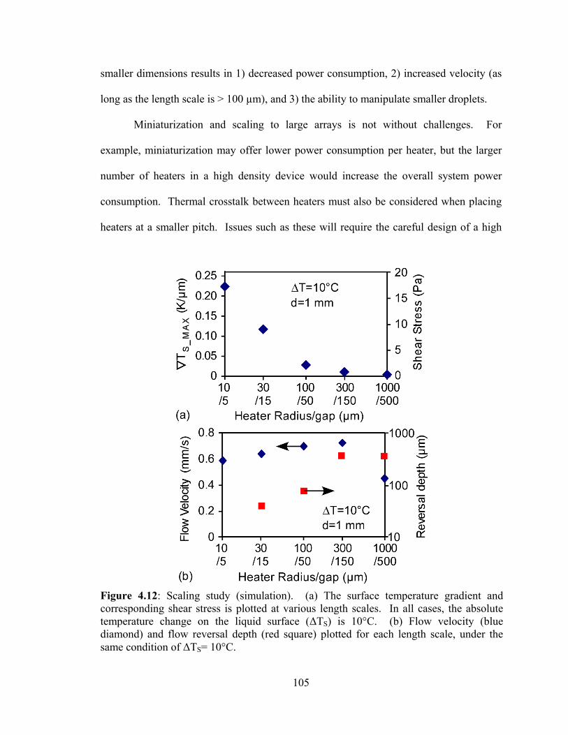
105

smaller dimensions results in 1) decreased power consumption, 2) increased velocity (as

long as the length scale is > 100 µm), and 3) the ability to manipulate smaller droplets.

Miniaturization and scaling to large arrays is not without challenges. For

example, miniaturization may offer lower power consumption per heater, but the larger

number of heaters in a high density device would increase the overall system power

consumption. Thermal crosstalk between heaters must also be considered when placing

heaters at a smaller pitch. Issues such as these will require the careful design of a high

Figure 4.12: Scaling study (simulation). (a) The surface temperature gradient and corresponding shear stress is plotted at various length scales. In all cases, the absolute temperature change on the liquid surface (∆TS) is 10°C. (b) Flow velocity (blue diamond) and flow reversal depth (red square) plotted for each length scale, under the same condition of ∆TS= 10°C.

106

density array and appropriate heat sinking in order to deliver efficient, isolated

temperature perturbations on the liquid surface.

6. SUMMARY

This chapter explores how Marangoni flows can be deliberately controlled by

creating dynamic temperature profiles on the liquid surface. A contactless,

programmable droplet manipulation system which utilizes the Marangoni effect is

described. The distinguishing feature of the approach is that the droplets are suspended

can be controlled without contact with solid surfaces, thus preventing contamination.

Furthermore, there is no complexity in the substrate. Programmable manipulation and

merging of multiple droplets was demonstrated using a system with 128 heaters and a

software controlled interface. One of the challenges of the technique, particularly for

biomedical assays, is the temperature change required in the liquid. Initial experiments

using common silicone oils have shown a 20-30K elevation. However, it was shown that

the temperature change and power consumption can be reduced by a factor of 40 by using

a fluid such as Fluorinert which has a high figure of merit. Scaling to smaller sizes does

not increase flow speeds; however, it does reduce power consumption, and allows digital

control of smaller droplets. The future direction of this work is to develop a

microfabricated heater array which will achieve these performance improvements, and

also allow high throughput manipulation of a larger number of droplets.

107

CHAPTER 5:

CONCLUSIONS

This thesis has explored the use of the Marangoni effect for fluidic actuation at

small length scales. By placing small heat sources < 1 mm above a thin liquid layer,

sharp temperature gradients can be generated at the fluid surface. Due to the inverse

relation between surface tension and temperature, shear stresses are generated at the

surface, inducing local flow which travels away from the heat source on the surface, and

in the opposite direction below the surface. At submillimeter length scales, it is possible

to efficiently generate flow due to the sharp temperature gradients and the strong viscous

coupling at low Reynold’s numbers. With regards to microfluidic systems, the advantage

of this approach is that flow can be generated without contact to the liquid sample

(avoiding contamination), and without any components in the fluidic substrate (reducing

cost).

By engineering the shape of the heat source, it is possible to generate unique

Marangoni flow patterns which can manipulate microdroplets suspended in an oil layer.

As discussed in Chapter 2, the point, linear, annular, and tapered geometries generate

flows emulating (respectively) droplet collectors, channels, traps, and pumps. The

advantage of these virtual components is that they have no physical structures, and can

accomplish their function entirely by virtue of the interaction of the flows with the

droplets. Many of these flows have a size selectivity as well, allowing for the possibility

108

of droplet sorting. The simulation model described in this thesis illustrates each of these

flows and gives an understanding of the mechanism of operation.

The doublet pattern (described in chapter 3) is another type of surface flow which

is achieved by placing a thermal probe near a layer of water. This type of flow achieves

5 mm/s linear velocity and 1300 rpm rotational velocity, making it useful as an in-plane

mixer. It is notable that doublet flow occurs in water, a liquid of high thermal

conductivity, but this flow pattern cannot be achieved in oil. The toroidal flows, on the

other hand, occur in oil but not in water. Doublet flow is consistent with a thermal dipole

on the fluid surface, and the directionality of the temperature gradient across the probe

appears to play a major role in this type of flow pattern.

Programmable actuation of droplets using Marangoni flows can be achieved with

dynamic heat fluxes rather than static heat fluxes. Chapter 4 discusses a two-dimensional

actuation system which consists of an array of heaters suspended above the surface. The

system can push and pull droplets (depending on their size) from place to place through

the sequential activation of heaters, rather than by scanning the heaters themselves. The

pull mode proves to be more useful than the push mode because only one active heater is

needed per droplet. Using the pull mode, the simultaneous control and merging of two

400 nL droplets is demonstrated at speeds up to 200 µm/s. Power consumption required

for flow generation can be as little as 30 mW/heater if a low thermal conductivity fluid

such as Fluorinert is used, and up to 1 W/heater for other fluids such as mineral oil.

Thermal crosstalk is 35% in the present implementation, which uses surface mount

resistors on a printed circuit board at a 2 mm pitch. Both power consumption and

109

crosstalk can be greatly improved by using microfabrication to make thermally isolated

heat sources which consume less power.

In general, the efficiency of this technique relies on having a thermally efficient

heat source and maximizing the coupling between temperature gradient and flow.

Microfabricated heat sources, with thermal efficiency of 10,000 K/W, offer nearly two

orders of magnitude lower power compared to surface mount resistors. For example,

Marangoni flows of 1,700 µm/s can be achieved in mineral oil with <20 mW power if a

microfabricated thermal probe is used. By combining the probe heat source with an

optimized carrier fluid, power consumption could potentially be reduced to < 1 mW.

Maximizing the surface temperature gradient requires that 1) the heat sources are

suspended in air above the sample (rather than embedded within the fluid), and 2) a low

thermal conductivity liquid is used. In order to maximize the coupling between

temperature gradient and flow, the liquid should have a high temperature coefficient of

surface tension and low viscosity. As mentioned above, flow velocities can be improved

nearly 10 fold, and required powers can be reduced by >10 fold if a low thermal

conductivity, low viscosity carrier fluid such as Fluorinert is used. In addition to these

material properties, the liquid must be of high density (to allow droplets to float) and

should have low volatility.

Other issues to consider include liquid heating and evaporation. Long-term

heating of the fluid can be prevented by actively cooling the liquid with a water bath

underneath the liquid sample. However, it is important to note that the viscosity of the

fluid will increase at lower temperatures, and this will decrease flow speeds. Evaporation

of droplets can be reduced by two orders of magnitude by using a multilayer oil system.

110

An immediate possibility for future work is reducing the size of the heater array

by one order of magnitude using microfabrication. As shown in Chapter 4, this will give

benefits in terms of power consumption, because thin film heaters have better power

efficiency and thermal isolation as mentioned above. A smaller flow cell also allows

manipulation of smaller droplets, which reduces reagent consumption and allows for

higher density processing. Downscaling, does, however, have some implications. While

it is possible to generate sharper temperature gradients and large shear stress at smaller

length scales, absolute flow velocities do not improve at length scales below 100 µm due

to the increased viscous resistance in small convection cells. Therefore, downscaling

beyond one order of magnitude may not be beneficial.

A second area of future work is the general design and application of Marangoni

flows. Chapter 2 demonstrated the fundamental flow patterns resulting from point, line,

annular, and tapered heat sources, but it is clear that more complex flow patterns can

generated by using other geometries, or combinations of them. Future research could

design complex flow patterns and investigate their application to droplet manipulation

and other areas. This thesis provides a simulation model which can be used to design

these flow patterns from a hypothesized heat flux. Such flow patterns could prove to be

useful in the trapping, filtering, separating, or manipulation of particles for various assay

protocols. Physical heat sources of various shapes can be used to supply the heat flux; or,

alternatively, optical approaches may offer a more scalable approach. Infrared lasers

have been shown to generate Marangoni flows [Sur04], and these methods could be

extended to design Marangoni flows for droplet manipulation and other applications.

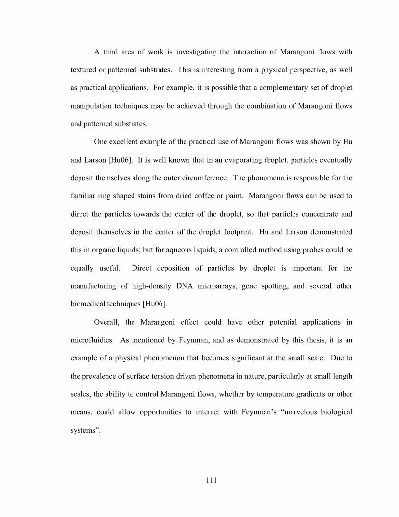
111

A third area of work is investigating the interaction of Marangoni flows with

textured or patterned substrates. This is interesting from a physical perspective, as well

as practical applications. For example, it is possible that a complementary set of droplet

manipulation techniques may be achieved through the combination of Marangoni flows

and patterned substrates.

One excellent example of the practical use of Marangoni flows was shown by Hu

and Larson [Hu06]. It is well known that in an evaporating droplet, particles eventually

deposit themselves along the outer circumference. The phonomena is responsible for the

familiar ring shaped stains from dried coffee or paint. Marangoni flows can be used to

direct the particles towards the center of the droplet, so that particles concentrate and

deposit themselves in the center of the droplet footprint. Hu and Larson demonstrated

this in organic liquids; but for aqueous liquids, a controlled method using probes could be

equally useful. Direct deposition of particles by droplet is important for the

manufacturing of high-density DNA microarrays, gene spotting, and several other

biomedical techniques [Hu06].

Overall, the Marangoni effect could have other potential applications in

microfluidics. As mentioned by Feynman, and as demonstrated by this thesis, it is an

example of a physical phenomenon that becomes significant at the small scale. Due to

the prevalence of surface tension driven phenomena in nature, particularly at small length

scales, the ability to control Marangoni flows, whether by temperature gradients or other

means, could allow opportunities to interact with Feynman’s “marvelous biological

systems”.

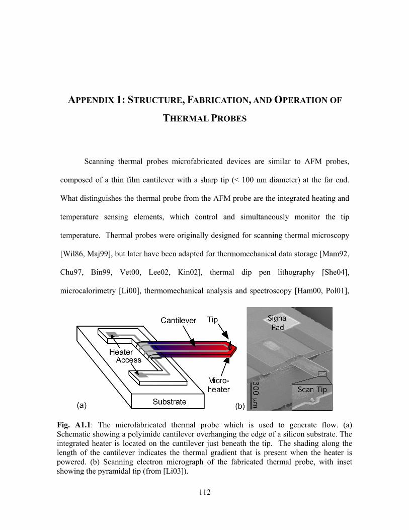
112

APPENDIX 1: STRUCTURE, FABRICATION, AND OPERATION OF

THERMAL PROBES

Scanning thermal probes microfabricated devices are similar to AFM probes,

composed of a thin film cantilever with a sharp tip (< 100 nm diameter) at the far end.

What distinguishes the thermal probe from the AFM probe are the integrated heating and

temperature sensing elements, which control and simultaneously monitor the tip

temperature. Thermal probes were originally designed for scanning thermal microscopy

[Wil86, Maj99], but later have been adapted for thermomechanical data storage [Mam92,

Chu97, Bin99, Vet00, Lee02, Kin02], thermal dip pen lithography [She04],

microcalorimetry [Li00], thermomechanical analysis and spectroscopy [Ham00, Pol01],

Fig. A1.1: The microfabricated thermal probe which is used to generate flow. (a) Schematic showing a polyimide cantilever overhanging the edge of a silicon substrate. The integrated heater is located on the cantilever just beneath the tip. The shading along the length of the cantilever indicates the thermal gradient that is present when the heater is powered. (b) Scanning electron micrograph of the fabricated thermal probe, with inset showing the pyramidal tip (from [Li03]).

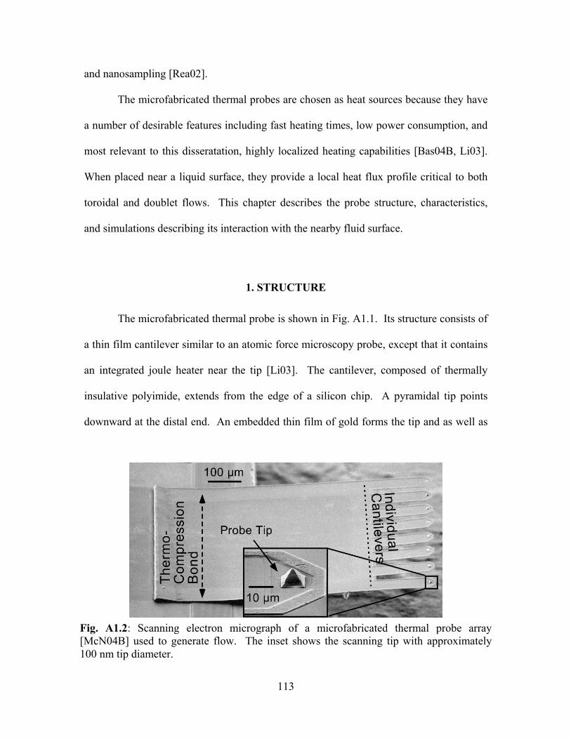
113

and nanosampling [Rea02].

The microfabricated thermal probes are chosen as heat sources because they have

a number of desirable features including fast heating times, low power consumption, and

most relevant to this disseratation, highly localized heating capabilities [Bas04B, Li03].

When placed near a liquid surface, they provide a local heat flux profile critical to both

toroidal and doublet flows. This chapter describes the probe structure, characteristics,

and simulations describing its interaction with the nearby fluid surface.

1. STRUCTURE

The microfabricated thermal probe is shown in Fig. A1.1. Its structure consists of

a thin film cantilever similar to an atomic force microscopy probe, except that it contains

an integrated joule heater near the tip [Li03]. The cantilever, composed of thermally

insulative polyimide, extends from the edge of a silicon chip. A pyramidal tip points

downward at the distal end. An embedded thin film of gold forms the tip and as well as

Fig. A1.2: Scanning electron micrograph of a microfabricated thermal probe array [McN04B] used to generate flow. The inset shows the scanning tip with approximately 100 nm tip diameter.

114

the adjacent heater. The heater, which contributes the majority of the probe’s resistance,

also functions as a thermistor to monitor tip temperature. Electrical interconnect is

provided by thicker metal lines extending the length of the cantilever. The length and

width of the cantilever as well as probe resistance vary depending on the type of probe.

In this work, two probe geometries are used: R01 (length 360 µm, width 42 µm,

resistance 25-40 Ω), and R02 (length 360 µm, width 120 µm, resistance 20-35 Ω). In

addition to the single probes, an 8-probe array reported in [McN04B] is also used to drive

multipole flow patterns. These probes are spaced 85 µm apart along a common shank

and can be heated individually.

2. FABRICATION

Both single probes and multiprobe arrays are fabricated in the same low-cost, 7-

Fig. A1.3: Fabrication process. Details are given in the text.

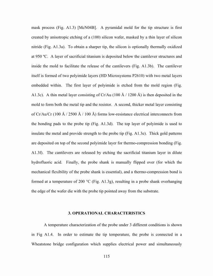
115

mask process (Fig. A1.3) [McN04B]. A pyramidal mold for the tip structure is first

created by anisotropic etching of a (100) silicon wafer, masked by a thin layer of silicon

nitride (Fig. A1.3a). To obtain a sharper tip, the silicon is optionally thermally oxidized

at 950 ºC. A layer of sacrificial titanium is deposited below the cantilever structures and

inside the mold to facilitate the release of the cantilevers (Fig. A1.3b). The cantilever

itself is formed of two polyimide layers (HD Microsystems P2610) with two metal layers

embedded within. The first layer of polyimide is etched from the mold region (Fig.

A1.3c). A thin metal layer consisting of Cr/Au (100 Å / 1200 Å) is then deposited in the

mold to form both the metal tip and the resistor. A second, thicker metal layer consisting

of Cr/Au/Cr (100 Å / 2500 Å / 100 Å) forms low-resistance electrical interconnects from

the bonding pads to the probe tip (Fig. A1.3d). The top layer of polyimide is used to

insulate the metal and provide strength to the probe tip (Fig. A1.3e). Thick gold patterns

are deposited on top of the second polyimide layer for thermo-compression bonding (Fig.

A1.3f). The cantilevers are released by etching the sacrificial titanium layer in dilute

hydrofluoric acid. Finally, the probe shank is manually flipped over (for which the

mechanical flexibility of the probe shank is essential), and a thermo-compression bond is

formed at a temperature of 200 °C (Fig. A1.3g), resulting in a probe shank overhanging

the edge of the wafer die with the probe tip pointed away from the substrate.

3. OPERATIONAL CHARACTERISTICS

A temperature characterization of the probe under 3 different conditions is shown

in Fig A1.4. In order to estimate the tip temperature, the probe is connected in a

Wheatstone bridge configuration which supplies electrical power and simultaneously

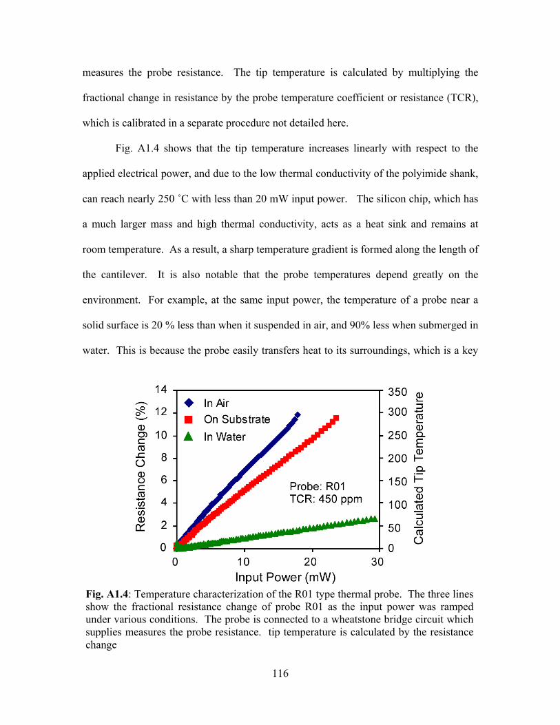
116

measures the probe resistance. The tip temperature is calculated by multiplying the

fractional change in resistance by the probe temperature coefficient or resistance (TCR),

which is calibrated in a separate procedure not detailed here.

Fig. A1.4 shows that the tip temperature increases linearly with respect to the

applied electrical power, and due to the low thermal conductivity of the polyimide shank,

can reach nearly 250 ˚C with less than 20 mW input power. The silicon chip, which has

a much larger mass and high thermal conductivity, acts as a heat sink and remains at

room temperature. As a result, a sharp temperature gradient is formed along the length of

the cantilever. It is also notable that the probe temperatures depend greatly on the

environment. For example, at the same input power, the temperature of a probe near a

solid surface is 20 % less than when it suspended in air, and 90% less when submerged in

water. This is because the probe easily transfers heat to its surroundings, which is a key

Fig. A1.4: Temperature characterization of the R01 type thermal probe. The three lines show the fractional resistance change of probe R01 as the input power was ramped under various conditions. The probe is connected to a wheatstone bridge circuit which supplies measures the probe resistance. tip temperature is calculated by the resistance change

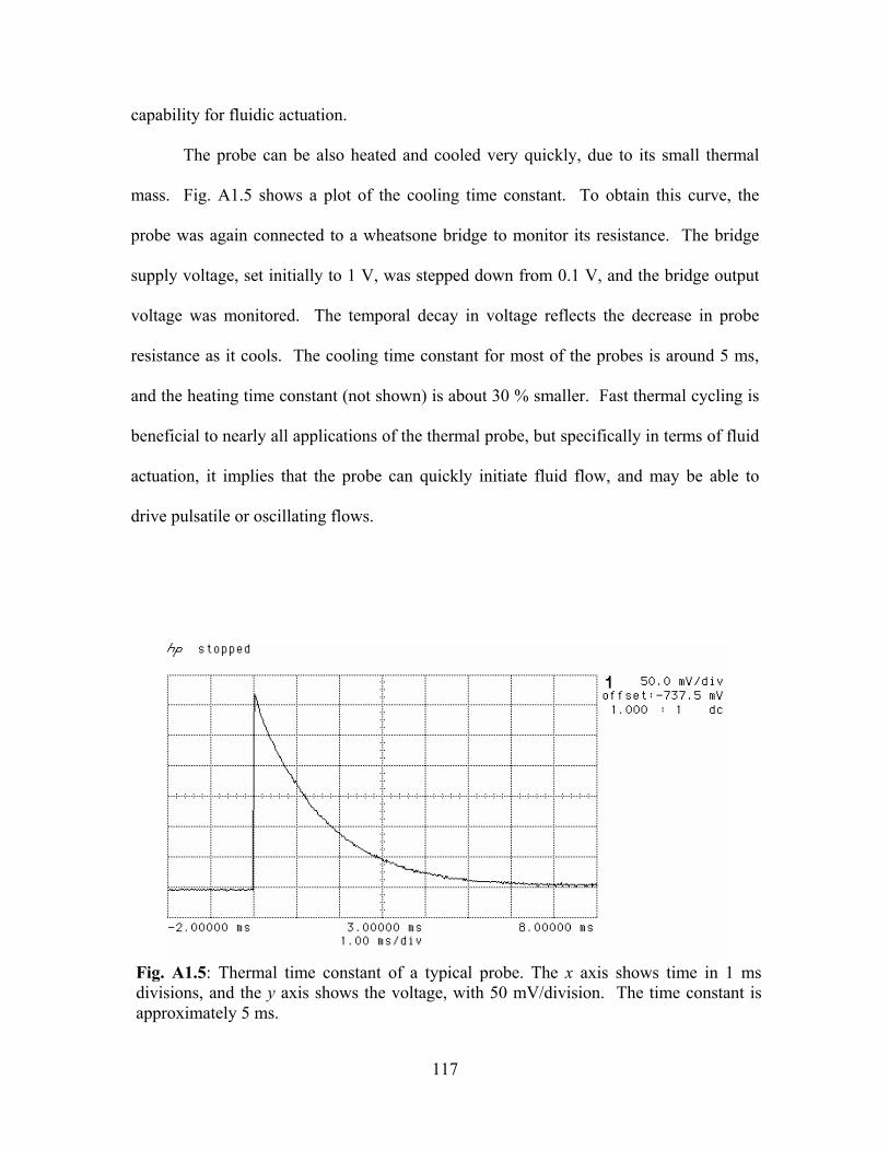
117

capability for fluidic actuation.

The probe can be also heated and cooled very quickly, due to its small thermal

mass. Fig. A1.5 shows a plot of the cooling time constant. To obtain this curve, the

probe was again connected to a wheatsone bridge to monitor its resistance. The bridge

supply voltage, set initially to 1 V, was stepped down from 0.1 V, and the bridge output

voltage was monitored. The temporal decay in voltage reflects the decrease in probe

resistance as it cools. The cooling time constant for most of the probes is around 5 ms,

and the heating time constant (not shown) is about 30 % smaller. Fast thermal cycling is

beneficial to nearly all applications of the thermal probe, but specifically in terms of fluid

actuation, it implies that the probe can quickly initiate fluid flow, and may be able to

drive pulsatile or oscillating flows.

Fig. A1.5: Thermal time constant of a typical probe. The x axis shows time in 1 ms divisions, and the y axis shows the voltage, with 50 mV/division. The time constant is approximately 5 ms.

118

APPENDIX 2:

INTERACTION OF PROBES WITH THE LIQUID SURFACE

When placed near the surface of a thin liquid layer, the probes locally heat the

surface, providing the basis for both toroidal and doublet flow patterns. Due to their

bolometer-like design, the probes are not perfectly symmetric point heat sources;

however, this asymmetry proves to be particularly important in the orientation of doublet

flows. To study the interaction of the probes with the liquid surface, a 3 dimensional

model of the probe was constructed in Fluent 6.0 (Fluent Corp.), a finite element software

for computational fluid dynamics and heat transfer. In this model (Fig. A2.1), a 360 µm

Fig. A2.1: Schematic of simulation model, showing the thermal probe is held in air above a liquid film. Symmetry is used to simplify the simulation so that only ½ of the model is solved. All perpendicular field gradients are set to null at the mirror symmetry plane

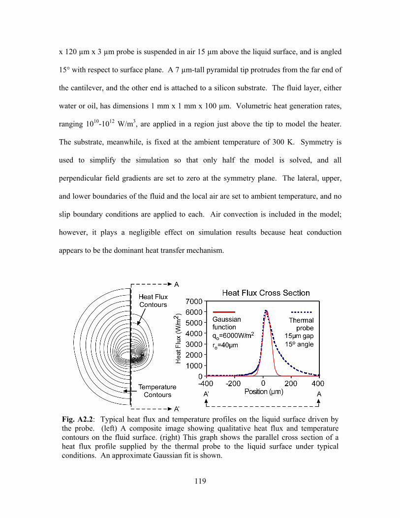
119

x 120 µm x 3 µm probe is suspended in air 15 µm above the liquid surface, and is angled

15° with respect to surface plane. A 7 µm-tall pyramidal tip protrudes from the far end of

the cantilever, and the other end is attached to a silicon substrate. The fluid layer, either

water or oil, has dimensions 1 mm x 1 mm x 100 µm. Volumetric heat generation rates,

ranging 1010-1012 W/m3, are applied in a region just above the tip to model the heater.

The substrate, meanwhile, is fixed at the ambient temperature of 300 K. Symmetry is

used to simplify the simulation so that only half the model is solved, and all

perpendicular field gradients are set to zero at the symmetry plane. The lateral, upper,

and lower boundaries of the fluid and the local air are set to ambient temperature, and no

slip boundary conditions are applied to each. Air convection is included in the model;

however, it plays a negligible effect on simulation results because heat conduction

appears to be the dominant heat transfer mechanism.

Fig. A2.2: Typical heat flux and temperature profiles on the liquid surface driven by the probe. (left) A composite image showing qualitative heat flux and temperature contours on the fluid surface. (right) This graph shows the parallel cross section of a heat flux profile supplied by the thermal probe to the liquid surface under typical conditions. An approximate Gaussian fit is shown.

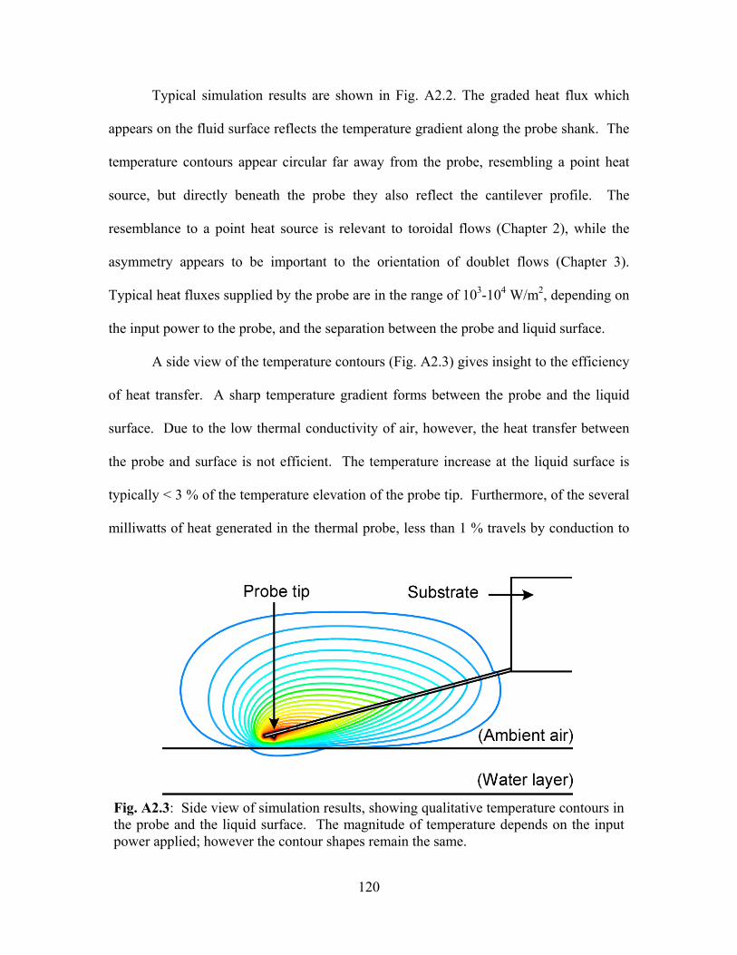
120

Typical simulation results are shown in Fig. A2.2. The graded heat flux which

appears on the fluid surface reflects the temperature gradient along the probe shank. The

temperature contours appear circular far away from the probe, resembling a point heat

source, but directly beneath the probe they also reflect the cantilever profile. The

resemblance to a point heat source is relevant to toroidal flows (Chapter 2), while the

asymmetry appears to be important to the orientation of doublet flows (Chapter 3).

Typical heat fluxes supplied by the probe are in the range of 103-104 W/m2, depending on

the input power to the probe, and the separation between the probe and liquid surface.

A side view of the temperature contours (Fig. A2.3) gives insight to the efficiency

of heat transfer. A sharp temperature gradient forms between the probe and the liquid

surface. Due to the low thermal conductivity of air, however, the heat transfer between

the probe and surface is not efficient. The temperature increase at the liquid surface is

typically < 3 % of the temperature elevation of the probe tip. Furthermore, of the several

milliwatts of heat generated in the thermal probe, less than 1 % travels by conduction to

Fig. A2.3: Side view of simulation results, showing qualitative temperature contours in the probe and the liquid surface. The magnitude of temperature depends on the input power applied; however the contour shapes remain the same.

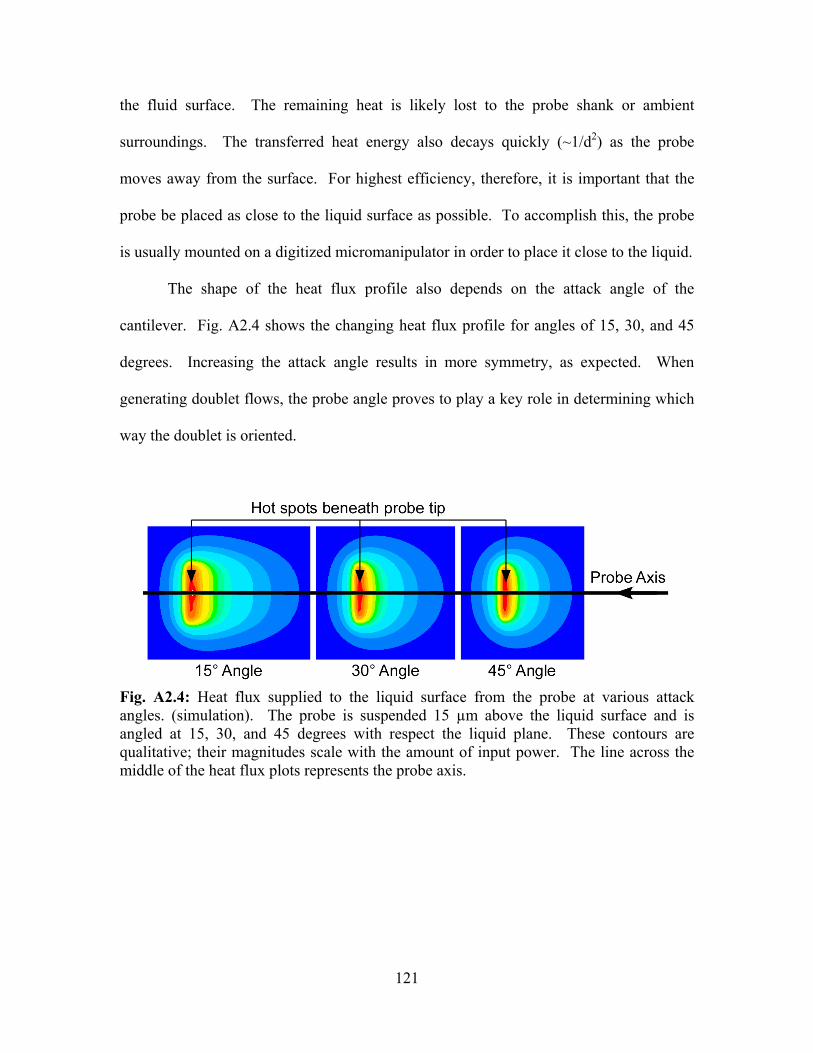
121

the fluid surface. The remaining heat is likely lost to the probe shank or ambient

surroundings. The transferred heat energy also decays quickly (~1/d2) as the probe

moves away from the surface. For highest efficiency, therefore, it is important that the

probe be placed as close to the liquid surface as possible. To accomplish this, the probe

is usually mounted on a digitized micromanipulator in order to place it close to the liquid.

The shape of the heat flux profile also depends on the attack angle of the

cantilever. Fig. A2.4 shows the changing heat flux profile for angles of 15, 30, and 45

degrees. Increasing the attack angle results in more symmetry, as expected. When

generating doublet flows, the probe angle proves to play a key role in determining which

way the doublet is oriented.

Fig. A2.4: Heat flux supplied to the liquid surface from the probe at various attack angles. (simulation). The probe is suspended 15 µm above the liquid surface and is angled at 15, 30, and 45 degrees with respect the liquid plane. These contours are qualitative; their magnitudes scale with the amount of input power. The line across the middle of the heat flux plots represents the probe axis.

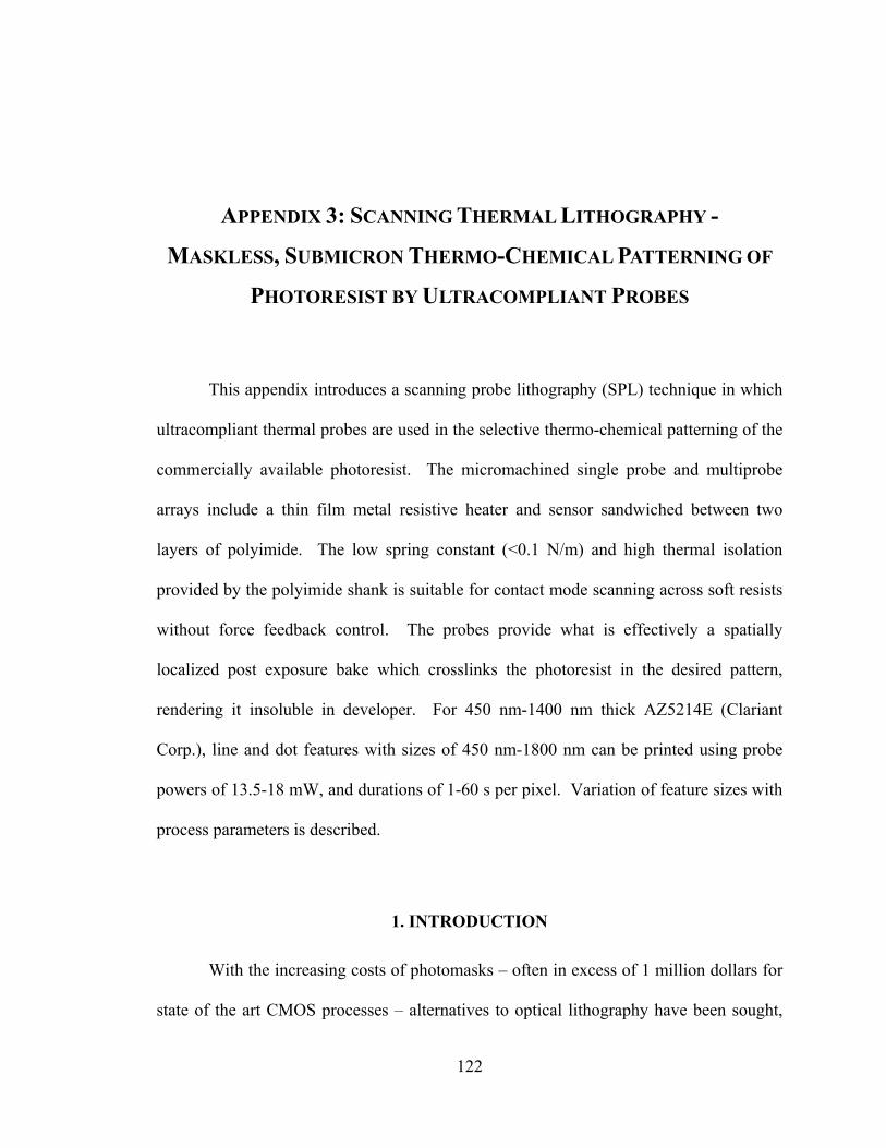
122

APPENDIX 3: SCANNING THERMAL LITHOGRAPHY -

MASKLESS, SUBMICRON THERMO-CHEMICAL PATTERNING OF

PHOTORESIST BY ULTRACOMPLIANT PROBES

This appendix introduces a scanning probe lithography (SPL) technique in which

ultracompliant thermal probes are used in the selective thermo-chemical patterning of the

commercially available photoresist. The micromachined single probe and multiprobe

arrays include a thin film metal resistive heater and sensor sandwiched between two

layers of polyimide. The low spring constant (<0.1 N/m) and high thermal isolation

provided by the polyimide shank is suitable for contact mode scanning across soft resists

without force feedback control. The probes provide what is effectively a spatially

localized post exposure bake which crosslinks the photoresist in the desired pattern,

rendering it insoluble in developer. For 450 nm-1400 nm thick AZ5214E (Clariant

Corp.), line and dot features with sizes of 450 nm-1800 nm can be printed using probe

powers of 13.5-18 mW, and durations of 1-60 s per pixel. Variation of feature sizes with

process parameters is described.

1. INTRODUCTION

With the increasing costs of photomasks – often in excess of 1 million dollars for

state of the art CMOS processes – alternatives to optical lithography have been sought,

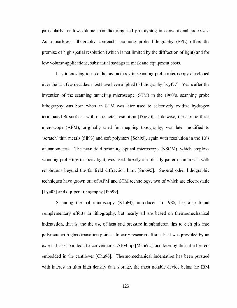
123

particularly for low-volume manufacturing and prototyping in conventional processes.

As a maskless lithography approach, scanning probe lithography (SPL) offers the

promise of high spatial resolution (which is not limited by the diffraction of light) and for

low volume applications, substantial savings in mask and equipment costs.

It is interesting to note that as methods in scanning probe microscopy developed

over the last few decades, most have been applied to lithography [Nyf97]. Years after the

invention of the scanning tunneling microscope (STM) in the 1960’s, scanning probe

lithography was born when an STM was later used to selectively oxidize hydrogen

terminated Si surfaces with nanometer resolution [Dag90]. Likewise, the atomic force

microscope (AFM), originally used for mapping topography, was later modified to

‘scratch’ thin metals [Sil93] and soft polymers [Soh95], again with resolution in the 10’s

of nanometers. The near field scanning optical microscope (NSOM), which employs

scanning probe tips to focus light, was used directly to optically pattern photoresist with

resolutions beyond the far-field diffraction limit [Smo95]. Several other lithographic

techniques have grown out of AFM and STM technology, two of which are electrostatic

[Lyu03] and dip-pen lithography [Pin99].

Scanning thermal microscopy (SThM), introduced in 1986, has also found

complementary efforts in lithography, but nearly all are based on thermomechanical

indentation, that is, the the use of heat and pressure in submicron tips to etch pits into

polymers with glass transition points. In early research efforts, heat was provided by an

external laser pointed at a conventional AFM tip [Mam92], and later by thin film heaters

embedded in the cantilever [Chu96]. Thermomechanical indentation has been pursued

with interest in ultra high density data storage, the most notable device being the IBM

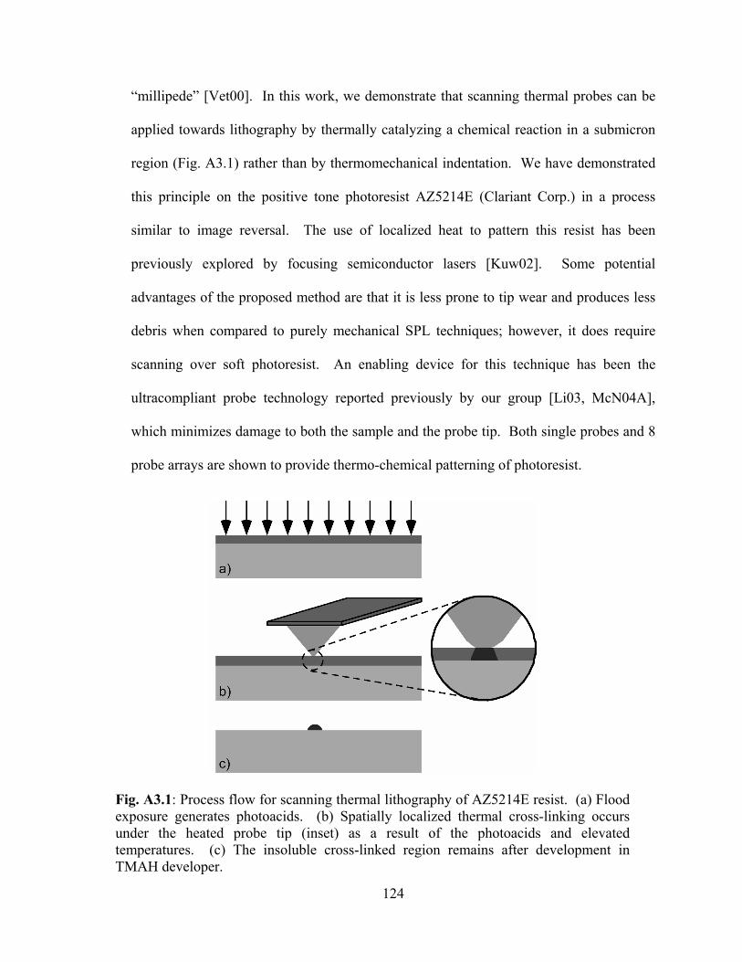
124

“millipede” [Vet00]. In this work, we demonstrate that scanning thermal probes can be

applied towards lithography by thermally catalyzing a chemical reaction in a submicron

region (Fig. A3.1) rather than by thermomechanical indentation. We have demonstrated

this principle on the positive tone photoresist AZ5214E (Clariant Corp.) in a process

similar to image reversal. The use of localized heat to pattern this resist has been

previously explored by focusing semiconductor lasers [Kuw02]. Some potential

advantages of the proposed method are that it is less prone to tip wear and produces less

debris when compared to purely mechanical SPL techniques; however, it does require

scanning over soft photoresist. An enabling device for this technique has been the

ultracompliant probe technology reported previously by our group [Li03, McN04A],

which minimizes damage to both the sample and the probe tip. Both single probes and 8

probe arrays are shown to provide thermo-chemical patterning of photoresist.

Fig. A3.1: Process flow for scanning thermal lithography of AZ5214E resist. (a) Flood exposure generates photoacids. (b) Spatially localized thermal cross-linking occurs under the heated probe tip (inset) as a result of the photoacids and elevated temperatures. (c) The insoluble cross-linked region remains after development in TMAH developer.

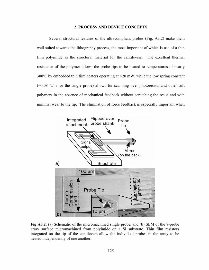
125

2. PROCESS AND DEVICE CONCEPTS

Several structural features of the ultracompliant probes (Fig. A3.2) make them

well suited towards the lithography process, the most important of which is use of a thin

film polyimide as the structural material for the cantilevers. The excellent thermal

resistance of the polymer allows the probe tips to be heated to temperatures of nearly

300ºC by embedded thin film heaters operating at <20 mW, while the low spring constant

(~0.08 N/m for the single probe) allows for scanning over photoresists and other soft

polymers in the absence of mechanical feedback without scratching the resist and with

minimal wear to the tip. The elimination of force feedback is especially important when

Fig A3.2: (a) Schematic of the micromachined single probe, and (b) SEM of the 8-probe array surface micromachined from polyimide on a Si substrate. Thin film resistors integrated on the tip of the cantilevers allow the individual probes in the array to be heated independently of one another.

126

scaling to arrays of probes. If rigid cantilevers are used, tip height non-uniformity across

the array can result in significant variation in contact force when it is lowered to the

substrate, necessitating feedback control at the probe level to prevent excessive force in

any one tip. The low spring constant in the ultracompliant array passively accomplishes

the same function, thus eliminating the need for force feedback. An additional feature of

the array is that each probe has individual heater control which can allow for independent

patterning if desired.

Both single probes and multiprobe arrays are fabricated in the same low-cost

micromachining process in which a thin film metal bolometer is sandwiched between two

insulating layers of polyimide. The thin metal film, consisting of 300-1200Å Au between

two adhesion layers of 100Å Cr, is molded into an anisotropically wet-etched notch in the

Si substrate to form the scanning tip. Two lines extending outwards from the tip region

form the heating element. Electrical connection to the bolometer is provided by thicker

metal lines extending the length of the cantilever. The total resistance ranges from 20-

200 ohms depending on design and process parameters. The probe is then released from

the substrate, flipped out over the die edge, and held in place by a thermo-compression

bond between two thin films of Au.

With regard to the patterning of the sample by the probes, the photoresist

AZ5214E is one of the very few positive tone photoresists that can function as a negative

tone resist by a process called image reversal. Conventional image reversal begins with a

patterned UV exposure which generates photoacids in unmasked regions. A subsequent

post exposure bake (PEB) thermally activates a crosslinking reaction catalyzed by the

photoacids in the previously exposed regions [Gij86]. The crosslinked regions become

127

insoluble in alkali developer, and insensitive to any further UV processing. The substrate

is then flood exposed to solubilize all non-crosslinked regions. Development in tetra-

methyl ammonium hydroxide (TMAH) leaves a negative photoresist image.

3. EXPERIMENTAL RESULTS

Temperature calibration of the single probe is relatively straightforward because

the fractional change in the probe resistance (∆R/R) is directly proportional to the

increase in tip temperature (∆T) by a constant K. The thin film heater accounts for the

majority of the probe’s resistance and results in a linear relationship between the

measured resistance and tip temperature. To determine the constant K, the single probe

cantilever was immersed in water and the current was ramped until bubble formation and

rapid evaporation was observed. Water was found to boil at a 2.16% increase in probe

resistance, and by correlating this to a 75ºC increase in tip temperature, K was found to

be 288 ppm/ºC. Repeating the same experiment with isopropyl alcohol (boiling point

85ºC) resulted in a virtually identical figure. Using the above calibration, the tip

temperature can be correlated to the measured resistance during probe operation. The

probes can be heated to approximately 300ºC before high temperatures begin to damage

the cantilever structures. It should be noted that the temperature vs. power relationship

differs depending on the degree of thermal isolation from the surrounding environment.

A probe operating in proximity or in contact with the substrate requires about 30% more

power than when suspended in air due to the heat loss to the substrate. Nevertheless, the

typical input powers needed to reach temperatures in excess of 250ºC while in contact

was <20mW.

128

The scanning thermal lithography (Fig. A3.1) proposed for this effort is similar to

the conventional process, except that it involves patterning the post exposure bake instead

of the initial exposure. AZ5214E photoresist at full concentration was spun on Si wafers

to obtain a thickness of 1.4 µm, and diluted 50% with PGMEA solvent (Nano EBR,

Clariant Corp.) to obtain 450 nm thickness. Further dilution resulted in poor uniformity;

however, in general it is expected that thinner resists will permit smaller feature sizes to

be patterned (discussed later in this report). After softbaking, the resist was flood

exposed to generate photoacids globally. The heated thermal probes were then scanned

across the surface point-by-point, each point being heated anywhere between 1 and 60 s.

Regions under the probe tip crosslink and become alkali insoluble. The resist was

developed in diluted TMAH (0.21N) in order to maintain the highest contrast between

crosslinked and noncrosslinked regions [Spa85].

To fully crosslink AZ5214E requires temperatures of about 90ºC, but it was found

that simply biasing the probe tip at this temperature was inadequate due to the thermal

contact resistance between the tip and the photoresist. Except where indicated, the single

probe was biased at 18 mW, corresponding to a tip temperature of 275ºC. In addition, the

substrate was biased at 45ºC using a hot plate in order to further reduce the amount of

heat that the probe needed to provide. Tests showed that when the contact force was

made excessively high by flexing the cantilever towards the substrate, the increased

pressure in combination with the high tip temperature resulted in thermomechanical

indentations penetrating all the way through the resist, and no thermal patterns were

observed after development. Conversely, weak contact forces resulted in poor thermal

contact, also resulting in no pattern formation. An intermediate contact force of about

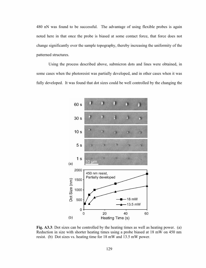
129

480 nN was found to be successful. The advantage of using flexible probes is again

noted here in that once the probe is biased at some contact force, that force does not

change significantly over the sample topography, thereby increasing the uniformity of the

patterned structures.

Using the process described above, submicron dots and lines were obtained, in

some cases when the photoresist was partially developed, and in other cases when it was

fully developed. It was found that dot sizes could be well controlled by the changing the

Fig. A3.3: Dot sizes can be controlled by the heating times as well as heating power. (a) Reduction in size with shorter heating times using a probe biased at 18 mW on 450 nm resist. (b) Dot sizes vs. heating time for 18 mW and 13.5 mW power.

130

probe temperature as well as the heating times (Fig. A3.3). Using an 18 mW bias on 450

nm resist resulted in features that ranged from 400 nm-1800 nm as heating times were

increased from 1-60 s. Reducing the power to 13.5 mW power resulted in the same

feature sizes, but required longer heating times. The above results were found after

partially developing the 450 nm photoresist. Features patterned at 18 mW for longer than

30 s remained after full development of both 1.4 µm and 450 nm resist (Fig. A3.4).

Biasing at high powers and heating for longer times results in a higher degree of

crosslinking because the crosslinking reaction is, in effect, both temperature and time

dependent.

Feature sizes shrink with photoresist thickness due to the decreased lateral flow of

heat. Two dimensional ANSYS heat flow models (Fig. A3.4a) qualitatively show that as

the thickness of the resist is reduced below the diameter of the scanning tip, the

cylindrical flow of heat results in features of approximately the same size as the tip. A

thick resist permits the heat to spread laterally, increasing feature sizes. For example,

using identical heating powers and times (18 mW, 30 s) on both 1.4 µm and 450 nm

resist produced dot sizes of 590 nm and 450 nm after full development of the photoresist

(Fig. A3.4b). The use of a thick resist also runs the risk of creating reentrant cross

sectional profiles which can be undercut during development.

The 450 nm dot size was the minimum feature size obtained in fully developed

dot patterns in our process using photoresist of approximately the same thickness.

Further scaling down of features sizes for the purposes of lithography can be

accomplished by using sharper tips and thinner resists, particularly those which are

chemically amplified (chemical amplification can also help to reduce heating times and

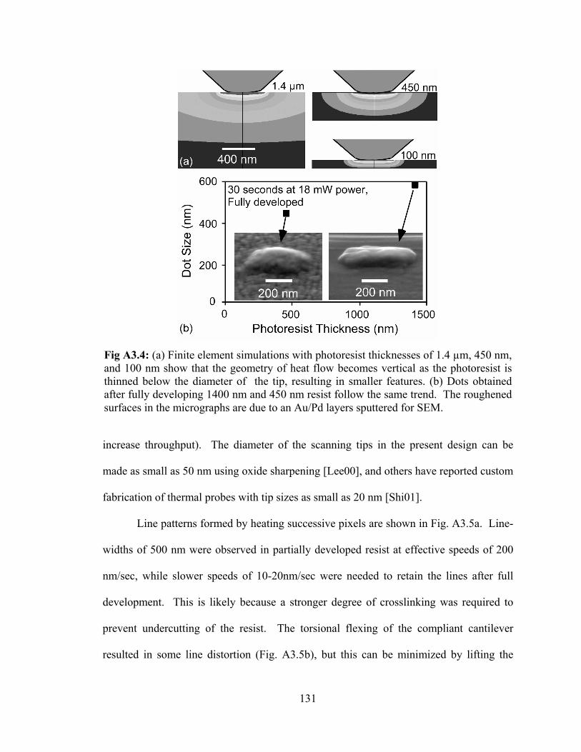
131

increase throughput). The diameter of the scanning tips in the present design can be

made as small as 50 nm using oxide sharpening [Lee00], and others have reported custom

fabrication of thermal probes with tip sizes as small as 20 nm [Shi01].

Line patterns formed by heating successive pixels are shown in Fig. A3.5a. Line-

widths of 500 nm were observed in partially developed resist at effective speeds of 200

nm/sec, while slower speeds of 10-20nm/sec were needed to retain the lines after full

development. This is likely because a stronger degree of crosslinking was required to

prevent undercutting of the resist. The torsional flexing of the compliant cantilever

resulted in some line distortion (Fig. A3.5b), but this can be minimized by lifting the

Fig A3.4: (a) Finite element simulations with photoresist thicknesses of 1.4 µm, 450 nm, and 100 nm show that the geometry of heat flow becomes vertical as the photoresist is thinned below the diameter of the tip, resulting in smaller features. (b) Dots obtained after fully developing 1400 nm and 450 nm resist follow the same trend. The roughened surfaces in the micrographs are due to an Au/Pd layers sputtered for SEM.

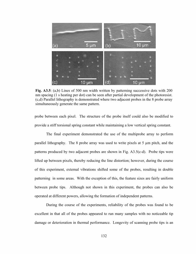
132

probe between each pixel. The structure of the probe itself could also be modified to

provide a stiff torsional spring constant while maintaining a low vertical spring constant.

The final experiment demonstrated the use of the multiprobe array to perform

parallel lithography. The 8 probe array was used to write pixels at 5 µm pitch, and the

patterns produced by two adjacent probes are shown in Fig. A3.5(c-d). Probe tips were

lifted up between pixels, thereby reducing the line distortion; however, during the course

of this experiment, external vibrations shifted some of the probes, resulting in double

patterning in some areas. With the exception of this, the feature sizes are fairly uniform

between probe tips. Although not shown in this experiment, the probes can also be

operated at different powers, allowing the formation of independent patterns.

During the course of the experiments, reliability of the probes was found to be

excellent in that all of the probes appeared to run many samples with no noticeable tip

damage or deterioration in thermal performance. Longevity of scanning probe tips is an

Fig. A3.5: (a,b) Lines of 500 nm width written by patterning successive dots with 200 nm spacing (1 s heating per dot) can be seen after partial development of the photoresist. (c,d) Parallel lithography is demonstrated where two adjacent probes in the 8 probe array simultaneously generate the same pattern.

133

important aspect to consider if they are to be used in a manufacturing process.

In conclusion, this effort has demonstrated that scanning thermal probes can be

used, both singly and in parallel, in the thermo-chemical patterning of AZ5214E. While

the resolution of this technique can be scaled down in a relatively straightforward

manner, the lessons are: first, the throughput can be addressed to some degree by the use

of multiprobe arrays; second, pixel sizes can be controlled by heating times and powers,

and finally, the procedure is less costly in the sense that it does not require photomasks or

optics, nor does it require a vacuum or UV filtered environment. Ultimately, the

resolution and throughput of this technique are determined by the size of the tips, the

number of probes that can be scanned in parallel, and the thickness and thermal

sensitivity of the resist. In a broader sense, this work has shown that scanning thermal

lithography can be used for patterning any thin film for semiconductor and biological

applications or for triggering a chemical reaction at the surface of a material.

134

BIBILIOGRAPHY

[3M01] FluorinertTM Electronic Liquid FC-3283, 3M Specialty Materials, St. Paul MN, 2001. [Adl70] J. Adler, “Fluid Mechanics of a Shallow Fuel Layer Near a Burning Wick,” Combust. Sci. Tech, Vol. 2, November 1970, pp. 105 – 113. [Ahn98] S.H. Ahn and Y.K. Kim, “Fabrication and Experiment of a Planar Micro Ion Drag Pump,” Sens Actuators A, 70, pp. 1-5, Oct.1998. [Alb02] B. Alberts, Molecular biology of the cell. New York: Garland Science, 2002. [Aref84] H. Aref, “Stirring by chaotic advection,” J Fluid Mech, vol. 143, pp. 1-21, June 1984. [Ash80] A. Ashkin, “Application of radiation pressure,” Science, vol. 210, pp. 1081-1087, Dec. 1980. [Bas04A] A.S. Basu, S. McNamara, and Y.B. Gianchandani, “Maskless Lithography by Patterned Heating of Photoresist Using Ultracompliant Thermal Probe Arrays,” Proc. Electron, Ion, Photon Beam Technology and Nanofabrication, Jun. 2004, pp. 109-111. [Bas04B] A.S. Basu, S. McNamara, and Y.B. Gianchandani, “Scanning Thermal Lithography: Maskless, Submicron Thermo-Chemical Patterning of Photoresist by Ultracompliant Probes,” J Vac Sci Technol B Microelectron Nanometer Struct, vol. 22, pp. 3217-3220, Nov. 2004. [Bas05A] A.S. Basu and Y.B. Gianchandani, “High Speed Microfluidic Doublet Flow in Open Pools Driven by Non-Contact Micromachined Thermal Sources,” Proc. IEEE Int Conf Micro Electro Mech Syst (MEMS), 2005, pp. 666-669. [Bas05B] A.S. Basu and Y.B. Gianchandani, “Trapping and Manipulation of Particles and Droplets Using Micro-Toroidal Convection Currents,” Digest Tech Papers Int Conf Solid-State Sensors Actuat Microsyst (Transducers), 2005, pp. 85-88. [Bas05C] A.S. Basu and Y.B. Gianchandani, “Microthermal Techniques for Mixing, Concentration, and Harvesting DNA and Other Microdroplet Suspensions,” Proc Int Conf on Miniaturized Systems for Chemistry and Life Sciences (µTAS), 2005, pp. 131-134.

135

[Bas07A] A.S. Basu, Seow Yuen Yee, and Y.B. Gianchandani, “Virtual Components for Droplet Control Using Marangoni Flows: Size-Selective Filters, Traps, Channels, and Pumps,” Proc. IEEE International Conference on Micro Electro Mechanical Systems (MEMS), Jan. 2007, Kobe, Japan, pp. 401-404. [Bas07B] A.S. Basu and Y.B. Gianchandani, “Shaping High-Speed Marangoni Flow in Liquid Films by Microscale Perturbations in Surface Temperature,” Applied Physics Letters, vol. 90, pp. 03410/1-03410-3, 2007. [Bas07C] A.S. Basu and Y.B. Gianchandani, “A 128-Pixel Digitally Programmable Microfluidic Platform for Non-Contact Droplet Actuation Using Marangoni Flows,” Proc. Intl. Conference on Solid State Sensors, Actuators, and Microsystems (Transducers), June 2007, Lyon, France, pp. 771-774. [Bas08A] A.S. Basu and Y.B. Gianchandani, “Virtual Microfluidic Traps, Filters, Channels, and Pumps using Marangoni Flows,” submitted. [Bas08B] A.S. Basu and Y.B. Gianchandani, “A Programmable Array for Contact-free Manipulation of Floating Droplets by Modulation of Surface Tension,” submitted. [Bay07] P. Bayiati, A. Tserepia, P. S. Petrou, S. E. Kakabakos, K. Misiakos and E. Gogolides, “Electrowetting on plasma-deposited fluorocarbon hydrophobic films for biofluid transport in microfluidics,” Jour Applied Physics, Vol. 101, 103306 2007. [Bén00] H. Bénard, “Les tourbillons cellulaires dans une nappe liquide,” Rev. Gén. Sci. Pure Appl., vol. 11, pp. 1261–71, 1900. [Ber03] Y. Bertrand, and L.C. Hoang, “Vegetal Oils as Substitute for Mineral Oils,” Proc IEEE Int Conf Prop Appl Dielectr Mater, June 2003, pp. 491-494. [Bin99] G. Binnig, M. Despont, U. Drechsler, W. Haberle, M. Lutwyche, P. Vettiger, H. J. Mamin, B.W. Chui, and T.W. Kenny, “Ultra High-Density AFM Data Storage with Erase Capability,” Appl Phys Lett, vol. 74, pp. 1329 –1331, Mar. 1999. [Blo56] J.M. Block, “Surface tension as the cause of Benard cells and surface deformation in a liquid,” Nature, vol. 178, pp. 650–651, 1956. [Bur96] M.A. Burns, C. H. Mastrangelo, T.S. Sammarco, F.P. Man, J.R. Webster, B.N. Johnson, B. Foerster, D. Jones, Y. Fields, A.R. Kaiser, and D. T. Burke, "Microfabricated Structures for Integrated DNA Analysis," Proceedings of the National Academy of Science, 93, 5556-5561 (1996). [Car92] V.P. Carey, Liquid-vapor Phase-change Phenomena. Washington D.C.: Hemisphere Publishing, 1992.

136

[Cha92] M.K. Chaudhury and G.M. Whitesides, “How to make water run uphill,” Science, vol. 256, pp. 1539–1541, June 1992. [Cha06] Y.-H. Chang, G.B. Lee, F.-C. Huang, Y.-Y. Chen, L. Lin, “Integrated polymerase chain reaction chips utilizing digital microfluidics,” Biomed Microdevices, Vol. 8, pp. 215-225, 2006. [Che97] J. Chen and K.D. Wise, “A High-Resolution Silicon Monolithic Nozzle Array for Inkjet Printing,” IEEE Transactions on Electron Devices, vol. 44, pp. 1401-1409, Sept. 1997. [Che02] C.-H. Chen and J.G. Santiago, “A Planar Electroosmotic Micropump,” J Microelectromech Syst, vol. 11, pp. 672-683, Dec. 2002. [Chi03] P.Y. Chiou, Z. Chang, and M.C. Wu, “Light actuated microfluidic devices,” in Proc IEEE Micro Electro Mech Syst MEMS, 2003, pp. 355-358. [Chi04] P.Y. Chiou, A.T. Ohta, and M.C. Wu, “Toward all optical lab-on-a-chip system: Optical manipulation of both microfluid and microscopic particles,” Proc SPIE Int Soc Opt Eng, 2004, pp. 73-81. [Chi07] D.T. Chiu, “Aqueous Droplets as Single-Molecule Reaction Containers,” Proc. Transducers, June 2007, Lyon, France, pp 465-468. [Cho02] S.K. Cho, S.-K. Fan, H. Moon, and C.-J. Kim, “Towards digital microfluidic circuits: Creating, transporting, cutting and merging liquid droplets by electrowetting-based actuation,” Proc IEEE Micro Electro Mech Syst MEMS, 2002, pp. 32-35. [Cho03] S.K. Cho, H. Moon and C.-J. Kim, “Creating, transporting, cutting, and merging liquid droplets by electrowetting-based actuation for digital microfluidic circuits,” J Microelectromech Syst, vol. 12, pp. 70-80, Feb. 2003. [Chu96] B.W Chui, T.D. Stowe, Y.S. Ju, H.T. Soh, S.C. Minne, K.E. Goodson, C.F. Quate, T.W. Kenny, H.J. Mamin, B.D. Terris, R.P. Pied, and D. Rugar, “Improved cantilevers for AFM thermomechanical data storage,” Proc. Solid-State Sensor and Actuator Workshop, June 1996, pp. 219-224. [Chu97] B. W. Chui, H. J. Mamin, B. D. Terris, D. Rugar, K. E. Goodson, and T. W. Kenny, “Micromachined Heaters with 1-µs Thermal Time Constants for AFM Thermomechanical Data Storage,” Proc Int Conf Solid-State Sensors Actuate Microsyst, June 1997, pp. 1085–1088. [Col06] B.A. Cola, D.K. Schaffer, T.S. Fisher, and M.A. Stremler, “A Pulsed Source-Sink Fluid Mixing Device,” J Microelectromech Sys, vol. 15, pp 259-266, Feb. 2006.

137

[Col98] D.E. Cole, “Monolithic Two-Dimensional Arrays of Micromachined Microstructures for Infrared Applications,” Proc. IEEE, vol. 86, pp. 1679-1686, Aug. 1998. [Dag90] J.A. Dagata, J. Schneir, H.H. Harary, C.J. Evans, M.T. Postek, and J. Bennett, “Selective-area epitaxial growth of gallium arsenide on silicon substrates patterned using a scanning tunneling microscope operating in air,” Appl. Phys. Lett., vol. 56, pp. 2437-2439, 1990. [Dar03] A.A. Darhuber, J.P. Valentino, J.M. Davis, S.M. Troian, and S. Wagner, “Microfluidic actuation by modulation of surface stresses,” Appl Phys Lett, vol. 82, pp. 657-659, Jan. 2003. [DC98A] Dow Corning Corporation, Information about Dow Corning 510, 550, 710 fluids, Dow Corning Corporation, Midland MI, 1998. [DC98B] Dow Corning Corporation, Information about Dow Corning 704 Diffusion Pump Fluid, Dow Corning Corporation, Midland MI, 1998. [Dee97] R.D. Deegan, O. Bakajin, T.F. Dupont, G. Huber, S.R. Nagel, T.A. Witten, “Capillary flow as the cause of ring stains from dried liquid drops,” Nature, vol. 389, pp. 827 – 829, Oct. 1997. [Eöt86] R. Eötvös, “Ueber den Zusammenhang der Oberflächenspannung der Flüssigkeiten mit ihrem Molecularvolumen,” Annalen der Physik, vol. 263, pp.448-459, 1886. [Eva97] J. Evans, D. Liepmann, and A.P. Pisano, “Planar laminar mixer,” Proc IEEE Micro Electro Mech Syst (MEMS), 1997, pp. 96–101. [Fey59] R. Feynman, “There’s Plenty of Room at the Bottom,” J Microelectromech Syst, vol. 1, pp. 60-66, Mar. 1992. [Transcript from Annual Meeting of the American Physical Society, Pasadena CA, 1959.] [Flo94] E.L. Florin, V.T. Moy, and H.E. Gaub, “Adhesion forces between individual ligand-receptor pairs,” Science, vol. 264, pp. 415-417, Apr. 1994. [Fuh92] G. Fuhr, R. Hagedorn, T. Muller, W. Benecke, and B. Wagner, “Microfabricated electrohydrodynamic (EHD) pumps for liquids of higher conductivity,” J Microelectromech Syst, vol. 1, pp. 141-146, Sep. 1992. [Gal99] B.S. Gallardo, V.K. Gupta, F.D. Eagerton, L.I. Jong, V.S. Craig, R.R. Shah, and N.L. Abbott, “Electrochemical principles for active control of liquids on submillimeter scales,” Science, vol. 283, pp. 57-60, 1999.

138

[Gan02] R.K.Gandhi, G.D Hopkins, M.N. Goltz, S.M. Gorelick, and P.L. McCarty, “Full-scale demonstration of in-situ cometabolic biodegradation of trichloroethylene in groundwater, 1: dynamics of a recirculating well system,” Water Resour Res, vol. 38, pp. 10.1–10.16, Apr. 2002. [Gas04] P.R.C. Gascoyne et al, “Dielectrophoresis-based programmable fluidic processors,” Lab on a chip, vol. 4, pp. 299-309, 2004. [Get03] A.V. Getling and O. Brausch, “Cellular flow patterns and their evolutionary scenarios in three-dimensional Rayleigh-Benard convection”, Phys Rev E, vol. 67, pp. 46313/1-46313/4, Apr. 2003. [Gia97] Y.B. Gianchandani and K. Najafi, “Silicon micromachined scanning thermal profiler with integrated elements for sensing and actuation,” IEEE Trans Electron Devices, vol. 44, pp. 1857-1868, Nov. 1997. [Gij86] R.M.R. Gijsen, H.J.J. Kroon, F.A. Vollenboek, and R. Vervoordeldonk, “A quantitative assessment of image reversal, a candidate for a submicron process with improved linewidth control,” Proc Advances in Resist Technology and Processing, Santa Clara, CA, pp. 108-116, 1986. [Gra04] D.S. Gray, J.L. Tan, J. Voldman, and C.S. Chen, “Dielectrophoretic registration of living cells to a microelectrode array,” Biosens Bioelectron, vol. 19, p 771-80, Feb. 2004. [Gro99] C. Grosjean and Y.-C. Tai, “A thermopneumatic peristaltic micropump,” Proc Int Conf on Solid-State Sensors and Actuators (Transducers’99), Sendai, Japan, 1999. [Hab91] W. Haberle, J.K.H. Horber, and G. Binnig, “Force microscopy on living cells,” J Vac Sci Technol B, vol. 9, pp. 1210-13, Mar. 1991. [Ham00] A. Hammiche, A. L. Bozec, M. Conroy, H.M. Pollock, G. Mills, J.M.R. Weaver, D.M. Price, M. Reading, D.J. Hourston, and M. Song, “Highly localized thermal, mechanical, and spectroscopic characterization of polymers using miniaturized thermal probes,” J Vac Sci Technol B Microelectron Nanometer Struct, vol. 18, pp. 1322-1332, May 2000. [Har91] D.J. Harrison, A. Manz, and P.G. Glavina, “Electroosmotic Pumping Within a Chemical Sensor System Integrated on Silicon,” Digest Tech Papers Int Conf Solid-State Sensors Actuat Microsyst (Transducers), 1991, pp. 792–795. [Har92] D. J. Harrison, A. Manz, Z. Fan, H. Luedi, and H. M. Widmer, “Capillary electrophoresis and sample injection systems integrated on a planar glass chip,” Anal. Chem., vol. 64, pp. 1926–1932, 1992.

139

[Hau03] W.L.W. Hau, L.M. Lee, Y.K. Lee, M. Wong, and Y. Zohar, “Experimental Investigation of Electrokinetically Generated In-Plane Vorticity in a Microchannel,” Digest Tech Papers Int Conf Solid-State Sensors Actuat Microsyst (Transducers), June 2003, pp. 651-654. [He04] M. He, C. Sun, and D.T. Chiu, “Concentrating solutes and nanoparticles within individual aqueous microdroplets,” Anal. Chem., vol. 76, pg. 1222-1227, Mar. 2004. [He05] M. He, J.S. Edgar, G.D.M. Jeffries, R.M. Lorenz, J.P. Shelby, and D.T. Chiu, “Selective encapsulation of single cells and subcellular organelles into picoliter and femtoliter-volume droplets” Anal. Chem. 77, pp. 1539–1544, 2005. [Hen92] E. Henderson, P.G. Haydon, D.S. Sakaguchi, “Actin filament dynamics in living glial cells imaged by atomic force microscopy,” Science, vol. 257, pp. 1944-1945, Sep. 1992. [Her96] K.E. Herold, R. Radermacher, and S.A Klein, Absorption Chillers and Heat Pumps. Boca Raton: CRC Press, 1996. [Hig00] F.J. Higuera, “Steady thermocapillary-buoyant flow in an unbounded liquid layer heated nonuniformly from above”, Phys Fluids, vol. 12, pp. 2186-2197, Sept. 2000. [Hu02] H. Hu and R.G. Larson, “Evaporation of a Sessile Droplet on a Substrate”, J Phys Chem B , vol. 106, pp. 1334-1344, Feb. 2002. [Hu05] H. Hu and R.G. Larson, “Analysis of the effects of Marangoni stresses on the microflow in an evaporating sessile droplet,” Langmuir, vol. 21, pp. 3972-3980, Apr. 2005. [Iri04] D. Irimia, R.G. Tompkins, and M. Toner, “Single-Cell Chemical Lysis in Picoliter-Scale Closed Volumes Using a Microfabricated Device,” Anal. Chem., vol. 76, pp. 6137 -6143, 2004. [Ise98] G. Isenberg, Modern optics, electronics, and high precision techniques in cell biology. New York: Springer-Verlag, 1998. [Jon01] T.B. Jones, M. Gunji, M. Washizu, and M.J. Feldman, “Dielectrophoretic liquid actuation and nanodroplet formation,” J Appl Phys, vol. 89, pp. 1441-1448, Jan. 2001. [Kat01] S. Katsura, A. Yamaguchi, H. Inami, S. Matsuura, K. Hirano, and A. Mizuno, “Indirect micromanipulation of single molecules in water-in-oil emulsion,” Electrophoresis, vol. 22, pp. 289-293, Jan. 2001. [Kata99] D.E. Kataoka and S.M. Troian, “Patterning liquid Flow on the microscopic scale,” Nature, vol. 402, pp. 794 – 797, Dec. 1999.

140

[Kats99] S. Katsura, A. Yamaguchi, N. Harada, K. Hirano, and A. Mizuno, “Micro-reactors based on water-in-oil emulsion,” Conf Rec IAS Annu Meet, 1999, pp. 1124-1129. [Kin02] W.P. King, T.W. Kenny, K.E. Goodson, G.L.W. Cross, M. Despont, U.T. Durig, H. Rothuizen, G. Binnig, and P. Vettiger, “Design of atomic force microscope cantilevers for combined thermomechanical writing and thermal reading in array operation,” J Microelectromech Syst, vol. 11, pp. 765-774, Dec 2002. [Kos93] E.L. Koschmieder, Bénard Cells and Taylor Vortices. New York: Cambridge University Press, 1993. [Kot04] K.T. Kotz, K.A. Noble, and G.W. Faris, “Optical microfluidics,” Appl Phys Lett, vol. 85, pp. 2658-2660, Sept. 2004. [Kru07] K. Krul and S. Heffner, Analytical Chip Technology Markets. New York: Kalorama Information, Nov. 2007 [Kuw02] M. Kuwahara, C. Mihalcea, N. Atoda, J. Tominaga, H. Fuji, and T. Kikukawa, “Thermal lithography for 0.1 µm pattern fabrication,” Microelectronic Engineering, vol. 61, 415-421, 2002. [Lai86] C.-L. Lai and A.-T. Chai, “Surface temperature distribution along a thin liquid layer due to thermocapillary convection,” Acta Astronaut, vol. 13, pp. 655-659, Nov 1986. [Lee00] M.H. Lee, J.J. Wu, and Y.B. Gianchandani, “High performance scanning thermal probe using a low temperature polyimide-based micromachining process,” Proc. IEEE International Conference on Micro Electro Mechanical Systems, Miyazaki, Japan, Jan. 2000, pp. 763-768. [Lee01] Y.-K. Lee, J. Deval, P. Tabeling, and C.-H. Ho, “Chaotic Mixing in Electrokinetically and Pressure Driven Micro Flows,” Proc IEEE Micro Electro Mech Syst (MEMS), pp 483-486, 2001. [Lee02] D.W. Lee, T. Ono, T. Abe, and M. Esashi, “Microprobe array with electrical interconnection for thermal imaging and data storage,” J Microelectromech Syst, vol. 11, pp. 215-221, June 2002. [Lef05] S. Lefevre, S. Volz, and P.-O. Chapuis, “Nanoscale heat transfer at contact between a hot tip and a substrate,” Int J Heat Mass Transf, vol. 49, pp. 251-258, Jan. 2006. [Lem00] A.V. Lemoff and A.P. Lee, “AC magnetohydrodynamic micropump,” Sens Actuators B Chem, vol. 63, pp 178-185, May 2000.

141

[Li00] M.-H. Li and Y.B. Gianchandani, “Microcalorimetry applications of a surface micromachined bolometer-type thermal probe,” J Vac Sci Technol B Microelectron Nanometer Struct, vol. 18, pp. 3600-3603, Nov. 2000. [Li03] M.H. Li and Y.B. Gianchandani, “Applications of a Low Contact Force Polyimide Shank Bolometer Probe for Chemical and Biological Diagnostics,” Sens Actuators A Phys, vol. 104, pp. 236-245, May 2003. [Lin99] X. Lin, T.A. Reponen, K. Willeke, S.A. Grinshpun, K.K. Foarde, and D.S. Ensor, “Long-term sampling of airborne bacteria and fungi into a non-evaporating liquid,” Atmos Environ, vol. 33, pp. 4291-4298, Nov.1999. [Lin06] D.R. Link, E. Grasland-Mongrain, A. Duri, F. Sarrazin, Z. Cheng, G. Cristobal, M. Marquez, and D.A. Weitz, “Electric Control of Droplets in Microfluidic Devices,” Angew. Chem. Int. Ed., vol. 45, pp. 2556 –2560, 2006. [Luo04] J. Luo, and P.K. Kitanidis, “Fluid residence times within a recirculation zone created by an extraction–injection well pair,” J Hydrol, vol. 295, pp. 149-162, Aug 2004. [Lyu03] S.F. Lyuksyutov, R.A. Vaia, P.B. Paramonov, S. Jhul, L. Waterhouse, R.M. Ralich, G. Sigalov, and E. Sancaktar, “Electrostatic nanolithography in polymers using atomic force microscopy,” Nature Materials, vol. 2, pp. 468-472, 2003. [Mad02] M.J. Madou, Fundamentals of Microfabrication. CRC Press: New York 2002. [Maj99] A. Majumdar, “Scanning thermal microscopy,” Annu Rev Mater Sci, vol. 29, pp. 505-585, 1999. [Mam92] H.J. Mamin and D. Rugar, “Thermomechanical Writing with an Atomic Force Microscope Tip,” Appl Phys Lett, vol. 61, pp. 1003–1005, Aug. 1992. [Man97] P.F. Man, D.K. Jones, and C.H. Mastrangelo, “Microfluidic plastic capillaries on silicon substrates: a new inexpensive technology for bioanalysis chips,” Proc IEEE Micro Electro Mechanical Systems, Jan. 1997, pp. 311-316. [Mar07] J.A. Maroto, V. Pérez-Muñuzuri, and M.S. Romero-Cano, “Introductory analysis of Bénard–Marangoni convection,” Eur. J. Phys., vol. 28, pp 311–320, 2007. [McC03] M.A. McClain, C.T. Culbertson, S.C. Jacobson, N.L. Allbritton, C.E. Sims, and J.M. Ramsey, “Microfluidic Devices for the High-Throughput Chemical Analysis of Cells,” Anal. Chem., Vol. 75, pp. 5646 -5655, 2003. [McN04A] S. McNamara, A.S. Basu, and Y.B. Gianchandani, “Ultracompliant, Passively Decoupled Thermal Probe Arrays: Large Area Mapping of Non-Planar Surfaces Without Force Feedback,” Proc. IEEE Int Conf Micro Electro Mech Syst (MEMS), Jan. 2004, pp. 825-828.

142

[McN04B] S. McNamara, A.S. Basu, and Y.B. Gianchandani, “Ultracompliant Thermal Probe Arrays,” J Micromech Microengineering, vol. 15, pp. 237-243, Jan. 2004. [Miz93] A. Mizuno, M. Nishioka, Y. Ohno, and L. Dascalescu, “Liquid Micro-Vortex Generated around a Laser Focal Point in an Intense High-frequency Electric Field,” Conf Rec IAS Annu Meet, 1993, pp. 1774-1778. [Nak03] M. Nakano, J. Komatsu, S. Matsuura, K. Takashima, S. Katsura, and A. Mizuno, “Single-molecule PCR using water-in-oil emulsion,” Journal of Biotechnology, vol 102, pp. 117-124, April 2003. [Ngu02] N.T. Nguyen, X.Y. Huang, and T.K. Chuan, “MEMS-micropumps: A review,” J Fluid Eng-T ASME, vol. 124, pp 384-392, June 2002. [Nou19] P. Lecomte du Noüy, “A New Apparatus for Measuring Surface Tension,” J. Gen. Physiol., vol. 1, pp. 521-524, May 1919. [Nyf97] R.M. Nyffenegger and R.M. Penner, “Nanometer-scale surface modification using the scanning probe microscope: progress since 1991,” Chem. Rev., vol. 97, pp. 1195-1230, 1997. [Oddy01] M.H. Oddy, J.G. Santiago, and J.C. Mikkelson, “Electrokinetic instability micromixing,” Anal Chem, vol. 73, pp. 5822–32, Dec. 2001. [Pas93] J. Passonneau and O. Lowry, Enzymatic Analysis, A Practical Guide. Totowa: Humana Press 1993. [Pea58] J.R.A. Pearson, “On convection cells induced by surface tension,” J. Fluid Mech. vol. 4, pp. 489–500, 1958. [Pil51] S.R. Palit, “Thermodynamic Interpretation of the Eötvös Constant,” Nature, vol. 177, pp. 1180, June 1956. [Pin99] R. Piner, J. Zhu, F. Xu, S. Hong, and C. Mirkin, “Dip Pen Nanolithography,” Science, vol. 283, pp. 661-663, 1999. [Pip07] J. Pipper, M. Inoue, L. Ng, P. Neuzil, Y. Zhang, and L.L. Novak, “Catching bird flu in a droplet,” Nature, vol. 13, pp. 1259-1263, 2007. [Pol00] M.G. Pollack, R.B. Fair, and A.D. Shenderov, “Electrowetting-based actuation of liquid droplets for microfluidic applications,” Appl Phys Lett, vol. 77, pp. 1725–1726, Sep. 2000. [Pol01] H.M. Pollack and A. Hammiche, “Micro-thermal analysis: techniques and applications,” J Phys D, vol. 34, pp. 23-53, May 2001.

143

[Pol02] H.M. Pollack, A.D. Shenderov, and R.B. Fair, “Electrowetting-based actuation of droplets for integrated microfluidics,” Lab on a chip, vol. 2, pp. 96-101, 2002. [Pur04] D. Purves, G. J. Augustine, D.D. Fitzpatrick, L.C. Katz, A.-S. LaMantia, and J.O. McNamara, and S.M. Williams, Neuroscience, Third Edition. Sunderland, MA: Sinauer Associates 2004. [Rad92] M. Radmacher, R.W. Tillman, M. Fritz, and H.E. Gaub, “From molecules to cells. Imaging soft samples with the atomic force microscope,” Science, vol. 257, pp. 1900-1905, Sep. 1992. [Rea02] M. Reading, D. Grandy, A. Hammiche, L. Bozec, and H.M. Pollock, “Thermally assisted nanosampling and analysis using micro-IR spectroscopy and other analytical methods,” Vib Spectrosc, vol. 29, p 257-260, Jul. 2002. [Rid03] A. Rida, V. Fernandez, and M.A. Gijs, “Long-range transport of magnetic microbeads using simple planar coils placed in a uniform magnetostatic field,” Appl. Phys. Lett., vol. 83, pp. 2396-2398, 2003. [Roa05] L.S. Roach, H. Song, and R.F. Ismagilov, “Controlling Nonspecific Protein Adsorption in a Plug-Based Microfluidic System by Controlling Interfacial Chemistry Using Fluorous-Phase Surfactants,” Anal Chem., Vol. 33, pp. 785–796, 2005. [Ros04] S. Rosen, and S. Heffner. The Worldwide Market for In Vitro Diagnostic Tests, 4th Edition. New York: Kalorama Information, 2004 [Sam99A] T.S. Sammarco, “A Microfluidic Thermocapillary Pumping System for Microfabricated Analysis Devices,” Ph.D. Dissertation, University of Michigan, 1999. [Sam99B] T.S. Sammarco and M.A. Burns, “Thermocapillary pumping of discrete drops in microfabricated analysis devices,” AIChE J, vol. 45, pp. 350-366, Feb. 1999. [Sas92] K. Sasaki, M. Koshioka, H. Misawa, N. Kitamura, and H. Masuhara, “Optical trapping of a metal particle and a water droplet by a scanning laser beam,” Appl Phys Lett, vol. 60, pp. 807-809, Feb. 1992. [Sei93] K. Seiler, D. J. Harrison, and A. Manz, “Planar glass chips for capillary electrophoresis: Repetitive sample injection, quantitation, and separation efficiency,” Anal. Chem., vol. 65, pp. 1481–1488, 1993. [She04] P.E. Sheehan, L.J. Whitman, W.P. King, and B.A. Nelson, “Nanoscale deposition of solid inks via thermal dip pen nanolithography,” Appl Phys Lett, vol. 85, pp. 1589-1591, Aug. 2004.

144

[Shi01] L. Shi, O. Kwon, A.C. Miner, and A. Majumdar, “Design and batch fabrication of probes for sub-100 nm scanning thermal microscopy,” Journal of Microelectromechanical Systems, vol. 10, pp. 370-378, Sept. 2001. [Sia03] S.K. Sia and G.M. Whitesides, “Microfluidic devices fabricated in poly(dimethylsiloxane) for biological studies,” Electrophoresis, vol. 24, pp. 3563-3576, 2003. [Sil93] L.A. Silva, P. Laitenberger, and R.E. Palmer, “Nanofabrication of metal structures in gold films deposited on mica,” J. Vac. Sci. Technol. B, vol. 11, pp. 1192-1999, 1993. [Smo95] I.I. Smolyaninov, D.L. Mazzoni, and C.C. Davis, “Near-field direct-write ultraviolet lithography and shear force microscopic studies of the lithographic process,” Appl. Phys. Lett., vol. 67, pp. 3859-3861, 1995. [Soh95] L.L. Sohn and R.L. Willett, “Fabrication of nanostructures using atomic-force-microscope-based Lithography,” Appl. Phys. Lett., vol. 67, pp. 1552-1554, 1995. [Son96] Bihai Song and Jürgen Springer, “Determination of Interfacial Tension from the Profile of a Pendant Drop Using Computer-Aided Image Processing 1. Theoretical,” Journal of Colloid and Interface Science, vol. 184, pp. 64-76, December 1996. [Son03A] H. Song, J.D. Tice, and R.F. Ismagilov, “Reactions in Droplets in Microfluidic Channels,” Angew. Chem. Int. Ed., vol. 42, pp. 768-772, 2003. [Son03B] H. Song and R.F. Ismagilov, “Millisecond kinetics on a microfluidic chip using nanoliters of reagents. J Am Chem. Soc, vol. 125, pp. 14613–14619, Nov. 2003. [Spa85] M. Spak, D. Mammato, S. Jain, and D. Durham, “Mechanism and Lithographic Evaluation of Image Reversal in AZ 5214 Photoresist,” Proc. Soc. Plastics E, 1985, pp. 247-267. [Sri04] V. Srinivasan, V.K. Pamula, and R.B. Fair, “An integrated digital microfluidic lab-on-a-chip for clinical diagnostics on human physiological fluids,” Lab on a Chip, vol. 4, pp. 310-315, 2004. [Sur04] J. Sur, T.P. Witelski, and R.P. Behringer, “Steady-Profile Fingering Flows in Marangoni Driven Thin Films,” Physical Review Letters, Vol. 93, No. 4, pp. 247803/1 - 247803/1, 2004. [Tak01] S. Takayama, E. Ostuni, P. LeDuc, K. Naruse, D.E. Ingber, and G.M. Whitesides, “Laminar flows: Subcellular positioning of small molecules,” Nature, vol. 411, pp. 1016-1016, Jun. 2001.

145

[Tas89] M.E. Taslim, U. Narusawa, and H. Rifiotis, “Thermocapillary Flow Induced by a Surface Heat Flux Variation,” ASME Heat Transfer Div Publ HTD, vol. 113, pp. 85-93, Aug. 1989. [Tru03] V.N. Truskett and K.J Stebe, “Influence of surfactants on an evaporating drop: Fluorescence images and particle deposition patterns,” Langmuir, vol. 19, pp. 8271-8279, Sep. 2003. [Ung00] M. Unger, H. Chou, T. Thorsen, A. Scherer, and S. Quake, “Monolithic microfabricated valves and pumps by multilayer soft lithography,” Science, vol. 288, pp. 113–116, 2000. [Van97] S.J. VanHook, M.F. Schatz, J.B. Swift, W.D. McCormick, and H.L. Swinney, “Long-wavelength surface-tension-driven Benard convection: experiment and theory,” Jour. Fluid Mech., vol. 345, pp. 45-78, 1997. [Vet00] P. Vettiger, M. Despont, U. Drechsler, U. Durig, W. Haberle, M.I. Lutwyche, H.E. Rothuizen, R. Stutz, R. Widmer, and G.K. Binnig, “Millipede-more than one thousand tips for future AFM data storage,” IBM J Res Dev, vol. 44, pp. 323-40, May 2000. [Wil86] C.C. Williams and H.K. Wickramsinghe, “Scanning thermal profiler,” Appl Phys Lett, vol. 49, pp. 1587-1589, Dec. 1986. [Xia98] Y. Xia and G.M. Whitesides, “Soft Lithography,” Angewandte Chemie International Edition, vol. 37, pp. 550-575, Dec. 1998. [Xie04] J. Xie, J. Shih, Q.A. Lin, B.Z. Yang, and Y.C. Tai, “Surface micromachined electrostatically actuated micro peristaltic pump,” Lab on a Chip, vol. 4, pp. 495-501, 2004. [Yoo03] J.-Y. Yoon and R.L. Garrell, “Preventing Biomolecular Adsorption in Electrowetting-Based Biofluidic Chips,” Anal Chem, vol. 75, pp. 5097-5102, 2003. [Zhe03] B. Zheng, L. S. Roach, and R.F. Ismagilov, “Screening of Protein Crystallization Conditions on a Microfluidic Chip Using Nanoliter-Size Droplets,” J. Am. Chem. Soc., vol 125, pp. 11170-11171, 2003.