DECENTRALIZED TOMATO PROCESSING: - AgEcon Search

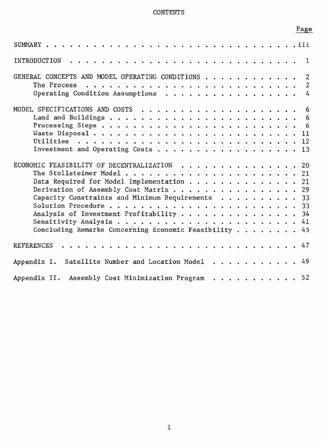
DECENTRALIZED TOMATO PROCESSING: Plant Design, Costs, and Economic Feasibility

by E. V. Jesse, W. G. Schultz, and J. L. Bomben

OFFICE

JUICE LOADING

HOT BREAK

4 PULPER FINISHER

SORT RINSE FLOOD WASH

TOMATO UNLOADING

United States Department of Agriculture Economic Research Service Agricultural Economic Report No. 313

DECENTRALIZED TOMATO PROCESSING: Plant Design, Costs, and Economic Feasibility

by E. V. Jesse, W. G. Schultz, and J. L. Bomben

JUICE LOADING

OFFICE

HOT BREAK

PULPER/FINISHER

SORT/RINSE FLOOD WASH i

TOMATO UNLOADING

Û 4U 60 80

United States Department of Agriculture Economic Research Service Agricultural Economic Report No. 313

CONTENTS

Page

SUMMARY iii

INTRODUCTION , 1

GENERAL CONCEPTS AND MODEL OPERATING CONDITIONS 2 The Process 2 Operating Condition Assumptions 4

MODEL SPECIFICATIONS AND COSTS 6 Land and Buildings 6 Processing Steps , . 6 Waste Disposal 11 Utilities 12 Investment and Operating Costs 13

ECONOMIC FEASIBILITY OF DECENTRALIZATION .20 The Stollsteimer Model 21 Data Required for Model Implementation 21 Derivation of Assembly Cost Matrix 29 Capacity Constraints and Minimum Requirements 33 Solution Procedure . 33 Analysis of Investment Profitability 34 Sensitivity Analysis . 41 Concluding Remarks Concerning Economic Feasibility .45

REFERENCES 47

Appendix I. Satellite Number and Location Model 49

Appendix II. Assembly Cost Minimization Program . 52

SUMMARY

The report considers decentralized or satellite plant processing of tomatoes as an alternative to conventional processing methods. An acreage distribution pattern typifying conditions for a California plant determined that cost savings exceeding $200,000 could be achieved by initially processing a portion of total raw product requirements at one optimally-located satellite. Addition of subsequent satellites yielded successively smaller cost reductions.

Savings resulted from reduced assembly costs, due largely to two factors: (1) A reduction in ton-miles hauled, and (2) reduced losses from raw product deterioration *

Investment and operating costs for satellite processing were estimated using a model firm or synthetic cost approach. A model satellite unit was designed after consulting with tomato processors. The model plant receives graded tomatoes at the rate of 50 tons per hour and produces a nonsterile single- strength juice which is shipped to an existing central cannery for product formulation into catsup, paste, puree, etc. Solid wastes are returned to harvested fields or hauled to sanitary landfills. Spray irrigation is used for liquid waste disposal.

Estimated plant establishment costs were approximately $1.2 million as of early 1974, while variable operating charges (labor and supplies) were about $150 per hour at capacity operation. Comparing cost savings with establisîiment costs for a model plant indicates an investment recovery period of about 5-1/2 years, and an internal annual rate of return of 12.7 percent for one satellite if satellite capacity replaces existing plant capacity. Return on investment is more attractive if satellites are used to expand productive capacity.

Ill

DECENTRALIZED TOMATO PROCESSING: PLANT DESIGN, COSTS, AND ECONOMIC FEASIBILITY

by

E.V. Jesse, W.G. Schultz, and J.L. Bomben*

INTRODUCTION

^Decentralized or satellite tomato processing is defined as performing initial processing steps at or near the point of harvest. Fruit is inspected, washed, sorted, macerated, broken, and finished at a location close to harvested fields. Juice from the process is then transported to an existing central cannery for product formulation. 1/ Decentralized processing contrasts with conventional processing methods, wherein all processing steps are carried out at the central cannery.

'There are several incentives for satellite processing. Disposing of cull tomatoes, seeds, and skins close to the point of harvest results in reduced volume and thus reduced fruit hauling costs. Satellite processing can decrease elapsed time between harvest and initial processing, thereby lessening physical deterioration as well as viscosity losses. All solid wastes and most liquid wastes from tomato product processing can be recycled to harvested fields under field processing arrangements. _2/

Several disincentives to adoption of satellite or field processing are also evident. An inherent problem is decentralization of management control, because field units are separated from central canneries. Physical coordination problems are also introduced; central canneries must construct and maintain facilities for receiving juice from satellite units, as well as for receiving tomatoes to be processed in the central plant. Possibly the major disincentive is the substantial new investment required to build satellite units.

* E.V. Jesse is an agricultural economist. Commodity Economics Division, Economic Research Service, stationed at the Department of Agricultural Economics, University of California, Davis, Calif. W.G. Schultz is a research mechanical engineer, and J.L. Bomben is a research chemical engineer, both located at the Western Regional Research Laboratory, Agricultural Research Service, U.S. Department of Agriculture, Berkeley, Calif.

1/ Juice from satellite units can be fabricated into tomato juice, catsup, tomato sauce, puree, paste, and other concentrated products. Whole peeled tomatoes and other whole products (sliced, diced, stewed wedges, etc.) cannot be processed at the satellite.

_2/ This advantage of satellite processing gains special significance in light of current and proposed effluent guidelines for fruit and vegetable processing. It can reasonably be expected that waste disposal costs for tomato canneries using in-plant treatment facilities or municipal sewerage systems will increase dramatically. Adoption of satellite processing represents one way these plants might mitigate the impact of waste quality standards.

while the technical feasibility of field processing tomatoes is generally accepted, _3/ public information regarding its economic feasibility has not been wholly developed. kj This study has three objectives:

(1) To design a model satellite tomato processing unit with commercial applicability,

(2) To estimate investment and operating costs for the model unit, and

(3) To define conditions under which satellite processing represents an economically feasible alternative to conventional processing methods.

Operating constraints and guidelines for plant design were established after extensive consultation with canners. The model satellite unit considered here incorporates plant and equipment items in line with these guidelines. This report synthesizes fixed and variable cost components given the model specifications. Finally, the optimal number and location of satellites is evaluated for a specific case study.

GENERAL CONCEPTS AND MODEL OPERATING CONDITIONS

The Process

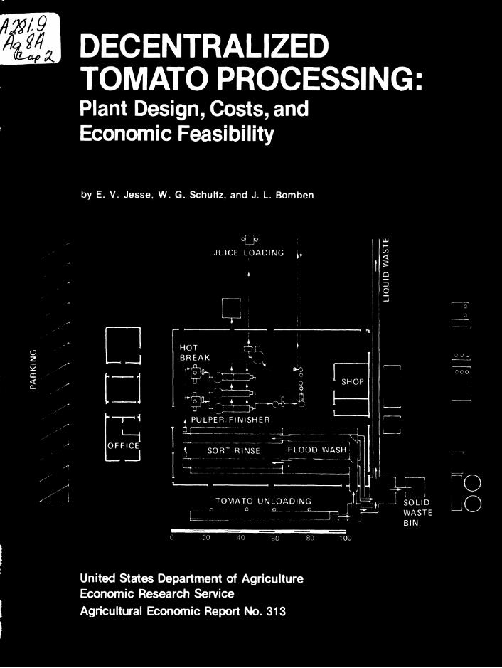
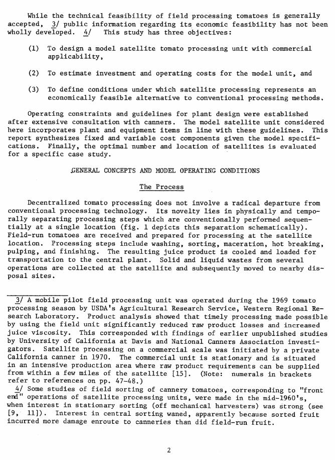
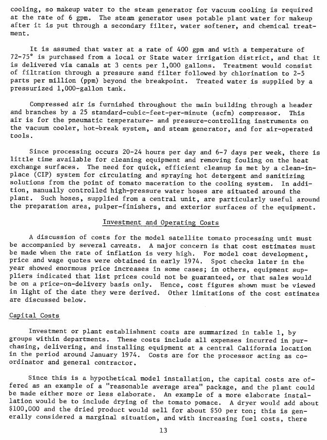
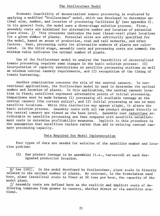
Decentralized tomato processing does not involve a radical departure from conventional processing technology. Its novelty lies in physically and tempo- rally separating processing steps which are conventionally performed sequentially at a single location (fig. 1 depicts this separation schematically). Field-run tomatoes are received and prepared for processing at the satellite location. Processing steps include washing, sorting, maceration, hot breaking, pulping, and finishing. The resulting juice product is cooled and loaded for transportation to the central plant. Solid and liquid wastes from several operations are collected at the satellite and subsequently moved to nearby disposal sites.

3^/ A mobile pilot field processing unit was operated during the 1969 tomato processing season by USDA*s Agricultural Research Service, Western Regional Re- search Laboratory. Product analysis showed that timely processing made possible by using the field unit significantly reduced raw product losses and increased juice viscosity. This corresponded with findings of earlier unpublished studies by University of California at Davis and National Canners Association investi- gators. Satellite processing on a commercial scale was initiated by a private California canner in 1970. The commercial unit is stationary and is situated in an intensive production area where raw product requirements can be supplied from within a few miles of the satellite [15], (Note: numerals in brackets refer to references on pp. 47-48.)

kj Some studies of field sorting of cannery tomatoes, corresponding to "front end" operations of satellite processing units, were made in the mid-1960*s, when interest in stationary sorting (off mechanical harvesters) was strong (see [9, 11]). Interest in central sorting waned, apparently because sorted fruit incurred more damage enroute to canneries than did field-run fruit.

PROCESS OPERATION IN SATELLITE TOMATO UNIT

Receiving Dump

At field i site

Disposal Liquid waste

Wash

Solid waste

Hot-break Pu I per

Disposal

Cooling Loading

Unload Regular plant operations

Figure 1.

At the central plant, the processed juice is unloaded and heated. Follow- ing this step, the juice undergoes further treatment along with juice initially processed at the central plant and loses its identity as a separate product.

Given that satellite processing is technologically similar to present prac- tices, what are the reasons for adoption? There are two basic economic incentives for considering processing decentralization. The first concerns waste management. The processing steps which can be performed at satellites generate heavy wasteloads. It is estimated that 5 to 25 percent of the weight of the tomato crop is lost in processing [1]. These wastes are largely cull tomatoes, seeds, skins, and dirt. Estimates of waste water production per ton of tomatoes processed range from AOO to 2,000 gallons [2, 6, 8, 10], Most of this waste water comes from raw product fluming, washing, and peeling, and it has been estimated to have a Biochemical Oxygen Demand (BOD) of 14 pounds per ton [10].

Locating satellites in rural areas simplifies both solid and liquid waste disposal. Solids can be returned to harvested fields and disked under with field trash. Land treatment of liquid wastes is feasible in nonresidential locations. But many existing tomato canneries, located in large cities, do not have access to this relatively inexpensive disposal technique.

The second economic incentive for adopting decentralized processing concerns transportation costs. With the expansion of the tomato processing industry, primarily in California, acreage has been contracted in new production areas some distance from established growing centers. By 1973, the average one- way haul from field to cannery in California was estimated to be 100 miles [3, p. 127]. Decentralized processing cannot reduce the total mileage fruit must be hauled, but it can reduce product weight considerably. Furthermore, product deterioration can be halted by timely processing.

Operating Condition Assumptions

Meetings were held with several California tomato processors to discuss appropriate operating assumptions for commercially feasible satellite units. These meetings, and discussions with regulatory agencies, led to the following set of operating conditions that were established for the model satellite.

Capacity

Maximum input was specified as 50 tons per hour (T/hr.) of paid weight tomatoes (net of culled fruit) containing an average of 5.9 percent total solids on a weight basis. This input level was considered the minimum necessary to ef- fectively utilize certain equipment items and processes. A scale much larger than this would suggest construction of a complete plant (central cannery with evaporation, canning, and warehousing facilities).

Given this input capacity, maximum feed rates at sequential points in the processing operation are as follows:

Stage Maximum flow

Receive/dump 55 tons per hour Paid weight 50 tons per hour Single strength juice 46.5 tons per hour

Shipping 41.6 tons per hour

Remarks

Raw tons dumped less graded defects Average 7 percent processing weight loss Average 10.5 percent evaporation (concentration due to evaporative cooling)

Mobility

Early in the study, the possibility of using a mobile unit capable of being moved three to four times during the tomato processing season was explored. This was deemed impractical by canners. The possible advantages of mobility (extension of season length) were believed to be outweighed by costs of moving the heavy equipment and time delays incurred by setting up and dismantling the unit. Hence, the model satellite is stationary with buildings having a useful life of 25 years. >.

Transport

All fruit would be bulk-hauled to satellite units. Field-run tomatoes are received in double gondolas with a total load of 20-25 tons of paid weight per vehicle.

Pasteurized juice is shipped in bulk tanks of 10 tons (2,400 gallons) each. These are either stainless or fiberglass-reinforced plastic, either mounted permanently or demountable on flatbed truck and trailer combinations.

It is assumed that shipping raw tomatoes or juice is done on a contractual basis, with the hauler owning the equipment.

Grading

Tomatoes received at the satellite are assumed to have been inspected and passed by the California State tomato grading system on a contractual basis at existing grading stations. The 50-ton-per-hour volume does not appear to jus- tify a separate on-site grading facility.

Product

The product resulting from satellite operations is a nonsterile single- strength juice finished through a 0.030 screen. Shipping temperature is approximately 75°F, with slightly higher or lower temperatures possible depending upon fruit quality and elapsed time between loading and receipt at the central cannery. At shipping, the juice contains 6.6 percent total solids.

Labor

Satellite plant operations were classed as industrial processing. Hence, plant labor is assumed to be unionized and union wage scales are used to determine labor costs.

Waste Disposal

The bulk of solid wastes generated by the satellite are temporarily held in watertight truck beds and periodically hauled to harvested fields, where they are dumped and disked under the soil with ordinary field trash from harvesting operations. This is considered feasible since solid wastes from processing are small relative to the volume of unpicked tomatoes and vines remaining in the field after harvest.

Several means of handling liquid wastes were considered, ranging from dumping wastes into irrigation district canals to using sophisticated bio- logical treatment facilities. Spray irrigation was selected as a low cost, versatile waste disposal method consistent with existing and anticipated Environmental Protection Agency (EPA) regulations.

MODEL SPECIFICATIONS MD COSTS

This section outlines specific characteristics of the model satellite processing unit; it describes features of the plants equipment specifications, and product and water flows, and then summarizes investment and operating costs.

Land and Buildings

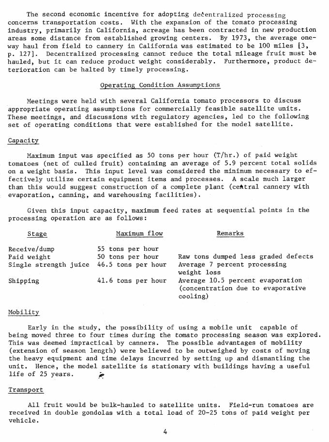
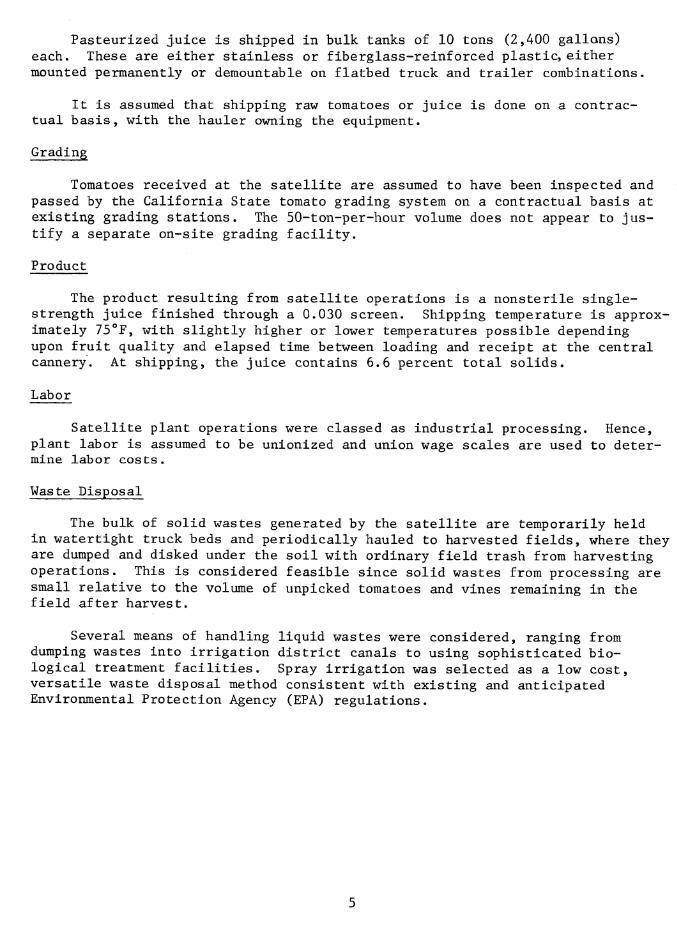
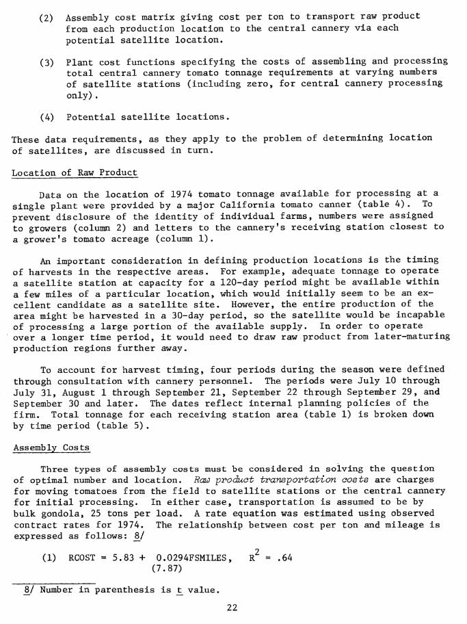
Figure 2 is a diagram of the overall satellite site (65 acres) with a liquid waste disposal field (57,6 acres) and the factory and settling pond areas (7,4 acres). The surplus area is not charged against the initial plant establishment because it would remain as farmland. Figure 3 diagrams a possible floor plan and layout for product and supply flows..

The factory site is on level ground with soil characteristics consistent with the carrying capacity needed for the building, equipment, and vehicle traffic. The period of processing is during the dry season, so no special provision has been made for rain beyond showers that can be expected in October. The vehicle areas in the yard require a smooth surface with a firm base. To minimize costs, a rock base and gravel surface is provided. The tomato unloading and juice shipping areas, and the area between the two buildings is concrete, because of the presence of water and dirt.

The basic factory building, measuring 90 by 110 feet, is a steel structur- al frame covered with sheet metal. It is of prefabricated construction with four vertical sides and a pitched roof. Plastic panel's replace one out of 20 metal roof sheets to provide daylight. Motor-driven roof fans are used to reduce heat and moisture buildup. The floor is concrete with floor gutters and poured concrete foundations for the heavier equipment.

The second, auxiliary building measures 20 by 80 feet (fig. 3). Con- structed of concrete blocks, it is separated from the main building to provide an office and rest area away from the factory noise, heat, and vibration. The office handles local receiving, shipping, personnel, and utility bookkeeping records. Basic information would be transmitted to the central cannery office for general accounting. The bulk of this building is occupied by a lunch room with adjoining wash and toilet facilities. Coin operated machines for hot and cold drinks can be readily situated in this area.

Processing Steps

Receiving and Washing

Tomatoes are unloaded by water flooding out of gondolas directly into a water-filled dump tank. The dump tank cushions the falling tomatoes and pro- vides an initial wash to separate fruit from rocks, sticks, dirt clods, foliage, and general trash. Tomatoes are elevated out of the first tank into a second wash tank, then elevated into a flood washer, and finally through a spray wash and a visual inspection. The water flow through this wash system is counter- current, with potable water entering at the final rinse. The wash operations use about 300 gallons of fresh water per ton of tomatoes, or 250 gallons per minute (gpm). This step is the primary user of water in the plant and the primary source of liquid waste.

PLANT SITE AND SPRAY IRRIGATION FIELD

LIQUID WASTE DISPOSAL

SPRAY PATTERN

UNUSED AREA

SETTLING POND

m

DQÍ PLANT

YARD

200 400 600 800 1000 FEET

Figure 2. 7

PLANT FLOOR PLAN AND LAYOUT/MODEL SATELLITE TOMATO PROCESSING UNIT

00

LUNCH ROOM

[WASH RMS

, LAB

•-1 I 1 OFFICE

JUICE LOADING

POMACE BIN

STEAM GENERATOR & WATER TREAT

ELECTRIC POWER

WASTE SUMP

SOLID WASTE

NAT'L GAS

FUEL OIL

FUEL OIL

CHLORINATOR

\J WATER /--s SUPPLY

Figure 3.

Typically, a 20-ton load of tomatoes can be positioned, unloaded, and cleared from the dump in 10-15 minutes.

Processing

After the final rinse, clean tomatoes are ready to be crushed, heated, screened, and cooled. Tomatoes are macerated by a chopper and pumped directly into an atmospheric IWF hot-break tank of the rotary coil type. Heat is supplied by steam, and the condensate is returned to the steam generator.

The hot-break macerate is pumped into a holding tank which gravity-feeds into paddle-type pulpers (extractors) with 0.12-inch screen holes and then into paddle finishers with 0.030-inch screen holes to produce a medium-fine textured juice. The screen sizes can be changed for chili sauce material in which the seeds are to be retained, or other intermediate products. 5_/

There are three sets of pulpers and finishers to provide reserve capacity. A reserve is needed when changing screens while the plant is onstream. Perhaps more important, an overloaded finisher produces a wetter waste, which could require a secondary pressing operation. A 60-percent moisture content for tomato waste pomace is acceptable, while a 70-percent or higher moisture level is not. The third pulper-finisher set reduces the possibility of high pomace moisture levels.

Cooling

Two methods used for cooling the tomato juice are vacuum cooling, which takes advantage of the sensible heat of the tomato juice to remove more than 10 percent of the water, or a surface heat exchanger. The 10-percent water removal with vacuum cooling reduces costs, since it gives a shipping weight reduction for juice that is destined for further concentration at the central cannery. Initial equipment cost for vacuum cooling is roughly three times that for a surface heat exchanger. On the other hand, a heat exchanger requires 800 gpm of water with a discharge temperature of 105°F. This large flow of water would require either a liquid waste treatment system about three times larger than that provided in the model, or else a means of recycling this water through the cooling system. While part of this water flow can be recycled, its volume and temperature exceed that needed elsewhere in the plant. Further- more, the vacuum cooling system can give the tomato juice a temperature of from 80°F to 45°F by changing the amount of steam put through the ejectors. The lowest temperature possible with the heat exchanger is about 75°F, due to the temperature of the water supply.

5^/ Optionally, pulping and finishing operations could be done at the central plant. However, a macerate is more difficult to cool than finished juice. Fur- thermore, tomato pomace resulting from pulping and finishing constitutes about 5 percent of the solid wastes in processing, which can be more easily disposed at the satellite site.

In summary, to provide product concentration,«flexibility in cooling temperature, and independence from water supply and discharged water, the vacuum cooling system was chosen for the model. For steam economy, the vacuum cooling system employed a two-chamber vessel with vapor recompression between the first and second stages of the three-vapor ejectors. The juice temperature would be sufficient to hold juice quality stable until it was reheated at the central cannery. For example, a 150-mile shipping distance with 5 hours elapsed time would require a juice temperature of 70°F.

Vapor-ejector condenser water could be handled in either of two ways. The water could be recycled through a cooling tower, or it could flow counter-current through the plant processes. The spray condensers use about 2,200 gpm of recycled water, which greatly exceeds water requirements for washing, preparation and steam generation. Hence it was decided to use a water cooling tower (as illustrated in fig. 4).

SETTLING POND AND WATER-COOLING TOWER LAYOUT

TO LtQUiD ¡ ^ WASTE DISPOSAL

PUMPÙi

n SETTLING POND

WATER COOLING

TOWER O il Figure 4.

Loading

Tank trucks arrive at the satellite clean and ready to load. The loading area has room for two trucks, so that during normal situations the juice will be pumped directly out of the vacuum cooling vessel into the trucks. These trucks consist of tractor-trailer units with either integral stainless tanks or demountable plastic tanks on flat beds, and they carry a net load of about 20 tons. Hauling will be contractual for both transport and rolling equipment.

10

From the time the tomatoes are dumped, processing requires a half hour at the 50-ton-per-hour dump rate; juice loading takes about a half hour. Transport takes about 2 hours for a 100-mile trip. At the central plant, another half hour is required to connect, unload, and reheat the juice.

Central Cannery Receiving

Upon arrival at the central cannery, the tomato juice is immediately unloaded and heated to 212°F by a steam-heated tubular heat exchanger. The juice then goes into the regular processing system for production of tomato catsup, puree, paste, or sauces. Unloading takes 15-20 minutes, after which the truck tanks are washed, sanitized, and rinsed. To even out juice flow into the central cannery, a 2,000-gallon holding tank is provided.

Waste Disposal

The prime objective of the waste disposal methods for the model satellite is to provide environmentally sound treatment and disposal of wastes at low cost. Both solid and liquid wastes are handled in the model in such a way as not to create a secondary problem by altering the ground water or providing a media for insects and rodents. Solid and liquid wastes are both deposited on agricultural fields—solid wastes are buried and liquids are sprayed onto the soil surface. A major attraction of processing at a field site is that a major- ity of the wastes are kept near their origin. This saves transporting an appreciable amount of the tomato weight to the central cannery.

Solid Wastes

There are two types of solid wastes. First, solid waste from tomato washing contains sticks and rocks which, along with factory debris such as papers and metals, are not compatible with cropland disposal; these must be disposed of in sanitary landfills, by incineration, or by hauling to a commercial dump. The second type of waste is rejected tomatoes, dirt, foliage, and pulper- finisher pomace, all of which can be plowed into cropland. These are hauled, spread, and plowed under on a contractual basis, much as described by Reed et al. [13]. The advantage of recycling these solid wastes to agricultural land is that the land is scheduled for cultivation soon after tomatoe¡s are harvested, so timing of waste disposal is appropriate and equipment is àt hand.

Liquid Wastes

Since a satellite plant is located in an agricultural area, the availability of large tracts of land at relatively low cost makes land treatment of the waste water the best choice. Also, land disposal meets the requirement for "zero discharge" by 1983 of the Federal Water Pollution Act Amendment of 1972 [20].

There are many factors to consider when designing a land treatment system for waste water [4, 10, 14]. For a specific site, the design of the land treatment system would have to account for soil type, soil drainage, subsurface conditions, topography, and climatic conditions. Once these conditions are established, the lowest cost land treatment technique can be chosen.

11

For the model described here, spray irrigation was chosen because it is most universally adaptable to different land iionditions. Infiltration-percola- tion techniques generally cost less to construct and operate, but they require a highly permeable soil [4], Overland flow systems can be constructed on soils of low permeability, but they generally cost more to construct [4], Either spray or surface distribution is suitable for the sites envisioned for the satellite processing plants; but spray distribution is the more widely used means of distributing waste water on land.

The system of spray irrigation designed for the model is illustrated in figs. 2 and 4. A canal carries the waste water, generated mostly by the washing operation, to a settling pond (fig. 4); from there the water is pumped through a typical portable spray irrigation system. The fields are assumed to be cropland, so they require little preparation for installing portable irrigation pipe. Using an average application rate of 0.5 inches per day, the waste water flow of 350 gpm (washing + 100 gpm. for other operations) requires 57.6 acres of land (including 25 percent excess for dikes, buffer zone, access roads, and future expansion). Average application rates of 0.34 and 0.67 inches per day have been reported for tomato waste water [4]. Using an automatic control system, waste water is applied to different sections, providing suitable rest periods for the land, usually one week [10]. This hydraulic loading of the soil is too large for valuable crops such as corn or alfalfa; the most that can be grown on the spray irrigation field is hay from a water-tolerant grass during the operating season and one crop of barley during the off-season,

A septic tank and drain field are provided for sanitary waste water from the satellite washrooms.

Utilities

Water, electricity, and natural gas are available as part of the site. The general needs are 400 gpm of water, 600 kilovolt-amps (kva), and 215 therms of natural gas per hour.

Electical power is purchased as three-phase power from a utility company and reduced to 440 volts which is the basic power for the larger motors. Major power users are the cooling tower fan, the water circulation pump supplying the spray condensers on the vacuum cooler, and the spray irrigation pump.

Both natural gas and fuel oil are needed for the dual fuel steam generator. Fuel oil is priced about 50 percent higher than natural gas, but is needed as a standby fuel because natural gas is only available on an interruptible basis to large consumers. Two underground 10,000-gallon fuel oil tanks are provided. These supply fuel for about 5 days operation at peak capacity for 24 hours.

Steam is supplied by a self-contained package steam generator capable of producing 20,000 pounds of steam per hour at 120 pounds per square inch (psi) under full load. Normal rate of operation would be 17,000 pounds per hour. Fuel consumption at normal operating levels is 21,450 cubic feet per hour (cfh) of natural gas or 153 gallons of fuel oil per hour. The hot-break system uses 13,500 pounds of steam per hour and the vacuum cooler uses 2,900 pounds per hour. Condensate is returned from the hot-break system, but not from vacuum

12

cooling, so makeup water to the steam generator for vacuum cooling is required at the rate of 6 gpm. The steam generator uses potable plant water for makeup after it is put through a secondary filter, water softener, and chemical treatment.

It is assumed that water at a rate of 400 gpm and with a temperature of 72-75** is purchased from a local or State water irrigation district, and that it is delivered via canals at 3 cents per 1,000 gallons. Treatment would consist of filtration through a pressure sand filter followed by chlorination to 2-5 parts per million (ppm) beyond the breakpoint. Treated water is supplied by a pressurized 1,000-gallon tank.

Compressed air is furnished throughout the main building through a header and branches by a 25 standard-cubic-feet-per-minute (scfm) compressor. This air is for the pneumatic temperature- and pressure-controlling instruments on the vacuum cooler, hot-break system, and steam generator, and for air-operated tools.

Since processing occurs 20-24 hours per day and 6-7 days per week, there is little time available for cleaning equipment and removing fouling on the heat exchange surfaces. The need for quick, efficient cleanup is met by a clean-in- place (CIP) system for circulating and spraying hot detergent and sanitizing solutions from the point of tomato maceration to the cooling system. In addition, manually controlled high-pressure water hoses are situated around the plant. Such hoses, supplied from a central unit, are particularly useful around the preparation area, pulper-finishers, and exterior surfaces of the equipment.

Investment and Operating Costs

A discussion of costs for the model satellite tomato processing unit must be accompanied by several caveats. A major concern is that cost estimates must be made when the rate of inflation is very high. For model cost development, price and wage quotes were obtained in early 19 74. Spot checks later in the year showed enormous price increases in some cases; in others, equipment sup- pliers indicated that list prices could not be guaranteed, or that sales would be on a price-on-delivery basis only. Hence, cost figures shown must be viewed in light of the date they were derived. Other limitations of the cost estimates are discussed below.

Capital Costs

Investment or plant establishment costs are summarized in table 1, by groups within departments. These costs include all expenses incurred in pur- chasing, delivering, and installing equipment at a central California location in the period around January 1974. Costs are for the processor acting as co- ordinator and general contractor.

Since this is a hypothetical model installation, the capital costs are offered as an example of a "reasonable average area" package, and the plant could be made either more or less elaborate. An example of a more elaborate installation would be to include drying of the tomato pomace. A dryer would add about $100,000 and the dried product would sell for about $50 per ton; this is generally considered a marginal situation, and with increasing fuel costs, there

13

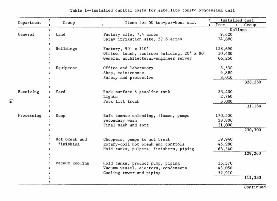
Table 1—Installed capital costs for satellite tomato processing unit

Department ] Group Items for 50 ton-per-hour unit ' Installed cost Item : Group

General ; Land Factory site, 7.4 acres Spray irrigation site, 57,6 acres

Dollars 9,620 74,880

: Buildings Factory, 90' x 110' Office, lunch, restroom building, 20' x 80' General architectural-engineer survey

128,690 30,400 66,250

: Equipment Office and laboratory Shop, maintenance Safety and protective

5,530 9,880 3,010

328,260

Receiving : Yard Rock surface & gasoline tank Lights Fork lift truck

23,400 2,760 5,000

31,160

Processing : Dump Bulk tomato unloading, flumes, pumps Secondary wash Final wash and sort

170,500 28,800 31,000

230,300

: Hot break and : finishing

Choppers, pumps to hot break Rotary-coil hot break and controls Hold tanks, pulpers, finishers, piping

19,940 45,980 63,340

129,260

: Vacuum cooling Hold tanks, product pump, piping Vacuum vessel, ejectors, condensers Cooling tower and piping

35,370 43,050 32,910

111,330

Continued

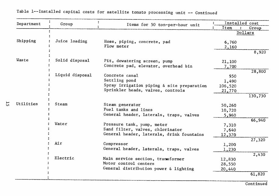
Table 1—Installed capital costs for satellite tomato processing unit — Continued

Department

Shipping

Waste

Ln Utilities

Group

Juice loading

Solid disposal

Liquid disposal

Steam

Water

Air

Electric

Items for 50 ton-per-hour unit

Hose, piping, concrete, pad Flow meter

Pit, dewatering screen, pump Concrete pad, elevator, overhead bin

Concrete canal Settling pond Spray irrigation piping & site preparation Sprinkler heads, valves, controls

Steam generator Fuel tanks and lines General header, laterals, traps, valves

Pressure tank, pump, meter Sand filter, valves, chlorinator General header, laterals, drink fountains

Compressor General header, laterals, traps, valves

Main service section, transformer Motor control centers General distribution power & lighting

Installed cost Item Group

Dollars

6,760 2,160

21,100 7,700

950 1,490

106,520 21,770

50,260 10,720 5,960

7,310 7,640

12,370

1,200 1,230

12,830 28,550 20,440

8,920

28,800

130,730

66,940

27,320

2,430

61,820

Continued

Table 1—Installed capital costs for satellite toinato processing unit — Continued

Department ] Group • • • Items for 50 ton-per-hour unit : Installed cost

: Item : Group

: Cleaning

Receiving

' Total installed

Clean-in-place system for process equip. Multi-station hi-press detergent system Cold water hoses, garbage cans

Truck unloading, hose, pipe Hold tank and piping Heat exchanger and controls Piping to plant processing

cost

Dollars

32,000 10,650

610

Central plant 11,470 7,350

11,500 5,720

43,260

36,040

1,236,570

does not seem to be iiranediate justification for adding this in initial installation. At additional cost, the spray irrigatiou system could be put underground or other provision made for harvesting a crop without moving the spraying system. However, the basic need is to dispose of plant liquid wastes, and until the soil and water conditions are fixed, there are too many uncertainties to say whether a crop is a viable alternative. For a less elaborate installation the office-lunchroom building could be incorporated under the factory roof, an unlined ditch could be used to carry the liquid waste from the factory to the settling pond, a flooded field disposal of liquid waste could be substituted for the spray system, or the cooling tower could be installed near the vacuum cooler condensers. The $1.2 million installation cost is, therefore, offered as an estimate rather than a recommended plant design.

Variable Operating Costs

To staff the model plant (table 2), there are 22 people per 8-hour shift plus one superintendent per day, giving a total of 67 employees for a 24-hour day. Some of these (the three-shift foremen, superintendent, and mechan- ics) would probably be permanent employees, to provide a year-to-year nucleus. These employees would spend approximately 6 months on-site, depending on the amount of off-season maintenance and refurbishing required. Based on the time required to start up and shut down the plant, the balance of the work force would be brought on gradually before the season and would be tapered off near the end of the season.

Wage rates were prevailing January 1974 union scale for cannery workers in northern California (International Brotherhood of Teamsters) [7]. Half the hourly cost is associated with receiving-preparation areas. Eight sorters are proposed, with two of these floating between sorting and inspection or reliev- ing the other six. Three laborers unload the trucks and do general cleanup. The receiving-preparation supervisor coordinates the overall plant operations. Two process operators oversee the flow from the choppers at the end of the sort-rinse belts through to the loading area; they monitor flow and temperatures, lubricate the equipment, and change the pulper-finisher screens. The actual connecting of the hoses to the trucks is done by the truckdrivers. The spray irrigation field is remote and the operator is designated to check on water distribution and sprinkler control, clear clogged nozzles, and in general assure an orderly flow to the field. Lab space is provided for production personnel to measure consistency and solids and to store samples of the product, but final quality control is handled by the central cannery.

Miscellaneous supplies, while crucial in the day-to-day operation of the facility, constitute only a small portion of total costs (table 3). Fuel and electricity account for 90 percent of the cost of consumables; water, chlorine, office and janitorial supplies, safety equipment, and cleaning materials account for the remaining 10 percent. The amounts required of these items, as well as o£ electricity, vary somewhat with production rate. Steam use is almost directly proportional to production.

17

Table 2—Personnel costs, model satellite processing unit

Personnel : Department : Personnel per

8-hour shift Wage : 2

Cost : Dept. : cost

: Type : No. : Dollar s per hour

Direct : Receiving and preparation

Supervisor Sorter Laborer

1 8 3

4.12 3.50 3.50

5.15 4.38 4.38

53.33 Process & ship Operator 2 4.12 5.15

10.30 • Waste disposal Operator 1 4.65 5.81

5.81 Central plant Operator 1 4.12 5.15

5.15

Indirect Maintenance Supervisor Mechanic

1 2

5.28 4.65

6.60 5.81

18.22 Office Clerk 2 3.78 4.73

9.46 Superintendence : General Foreman

Superinten- dent

1

1/3

7.20

9.60

9.00

12.00 13.00

\ Factory Total 22- ■1/3 115.27

Basic straight-time hourly wage or equivalent for 40-hour work week,

'Wage plus 25 percent fringe benefits.

18

Table 3—Cost of expendable supplies for satellite operation

Item : Use rate Cos t

: Percent : supply : Unit cost

I

Cost/hour : of total cost

Dollars Percent

Fuel: Natural gas #2 fuel oil :

: 21,452 cfh 153 gph

0.80/1000 cu. 0.17/gal

ft. 17.162 2/

50.1

3 Steam generation supplies . — 0.345 1.0

Water : 400 gpm 0.03/1000 gal. 0.720 2.1

Electricity : 600 kw 0.02/kw 13.200 38.5

Chlorine : 1.0 Ibs/hr. 0.10/lb. 0.100 .3 4

Miscellaneous ; — — 2.754 8.0

Total Supplies : 34.281 100.0

Use rate and cost per hour at capacity operation.

Fuel oil is used in the model only as an emergency backup fuel; both fuels are not used simultaneously.

Water softener resin, regeneration salt, feed-water chemical additive.

Office, lab, janitorial, and cleanup supplies, expendable safety items.

ECONOMIC FEASIBILITY OF DECENTRALIZATION

Discussion of economic feasibility necessarily entails a good deal of gen- eralization. Whether satellite tomato processing is feasible for a particular firm depends on a host of factors, many of which are immeasurable, or at best difficult to quantify. Critical physical factors in assessing the feasibility of satellite processing include the magnitude and expected location of production, the availability of potential satellite sites, and the probable allocation of raw product among finished tomato prodîcts. Financial considerations play a major role. Probable costs and cost savings must be viewed in light of firms' equity positions. Managerial goals, progressiveness, and market share objectives typify even more subjective factors in evaluating feasibility.

Taking this array of influencing factors into consideration, this section outlines a technique a tomato processing firm can apply to its particular situation to assess the economic feasibility of satellite processing. A general model is developed and empirically applied. Possible savings are outlined for ranges of conditions in the illustrative situation, and compared with establishment and operating costs developed in the preceding section. Then, investment recovery periods and net annual returns under alternative conditions are defined.

Just as in synthesizing costs, a number of critical assimptions are made in order to estimate returns. These are based on research findings and consultation with cannery representatives. While they generally reflect overall industry conditions, modifications can easily be made to fit individual firm conditions. Steps in the analytical process, assumptions, and computer programs employed are clearly outlined to facilitate evaluation for specific applications.

Subjective, firm-specific elements in investment decision-making cannot be captured in a model of the type developed here. However, the results of the sample application can suggest whether more comprehensive considerati^Dn is warranted.

The example situation analyzed in this section involves satellites shipping single-strength juice to a single central cannery. Costs of transporting tomatoes to satellites and processed juice to the central cannery are compared with costs of direct shipments of tomatoes from growers' fields to the central cannery. The latter, conventional method entails hauls ranging from 25 to more than 200 miles. The central cannery is assumed to possess sufficient capacity to process the entire tonnage available in the production area. All tonnage not routed through satellites is assigned to the central cannery.

The example closely reflects a real-life situation. Data pertaining to grower location and tonnage available were obtained from a major California tomato processor. Certain figures were modified to prevent disclosure of pro- prietary information, but such modifications do not seriously impair the empirical nature of the results.

20

The Stollsteímer Model

Economic feasibility of decentralized tomato processing is evaluated by applying a modified "Stollsteimer" model, which was developed to determine optimal size, number, and location of processing facilities j6/ (see Appendix I). In its general form, the model uses a three-stage solution process. First, assembly costs are minimized for alternative number and location of potential plant sites. Ij This procedure indicates the best (least-cost) plant locations for a given number of plants. Potential sites are arbitrarily specified for the model, based on areas of production, road and rail networks, and other factors. Next, processing costs for alternative numbers of plants are calculated. In the third stage, assembly costs and processing costs are summed; the minimum value indicates the optimal number of plants.

Use of the Stollsteimer model to analyze the feasibility of decentralized tomato processing requires some changes in the basic solution process: (1) incorporation of capacity restrictions on satellite processing stations as well as minimum central cannery requirements, and (2) recognition of the timing of tomato harvesting.

Another complication concerns the role of the central cannery. In conventional applications, the Stollsteimer model is used to determine the optimal number and location of plants. In this application, the central cannery location is fixed; satellites represent alternative points of initial processing. Comparisons must be made between (1) processing all available tonnage at the central cannery (the current policy), and (2) initial processing at one or more satellite locations. While this distinction may appear slight, it alters the basic solution process. Assembly costs with all raw product shipped directly to the central cannery are viewed as the base level. Assembly cost reductions attributable to satellite processing aré then compared with satellite establishment costs to determine profitability measures. Implicit in this procedure is the assumption that satellites replace rather than add to existing central cannery processing capacity.

Data Required for Model Implementation

Four types of data are needed for solution of the satellite number and location problem:

(1) Raw product tonnage to be assembled (i.e., harvested) at each designated production location.

6^/ See [18]]. In the model developed by Stollsteimer, plant scale is directly related to the optimal number of plants. By contrast, in the formulation used here, plant (satellite) scale is fixed at 50 tons per hour, the capacity o£ the model plant.

_7/ Assembly costs are defined here as the explicit and implicit costs of delivering tomatoes from grower to cannery, whether direct or via satellite stations.

21

(2) Assembly cost matrix giving cost per ton to transport raw product from each production location to the central cannery via each potential satellite location.

(3) Plant cost functions specifying the costs of assembling and processing total central cannery tomato tonnage requirements at varying numbers of satellite stations (including zero, for central cannery processing

only).

(4) Potential satellite locations.

These data requirements, as they apply to the problem of determining location of satellites, are discussed in turn.

Location of Raw Product

Data on the location of 1974 tomato tonnage available for processing at a single plant were provided by a major California tomato canner (table 4). To prevent disclosure of the identity of individual farms, numbers were assigned to growers (column 2) and letters to the cannery's receiving station closest to a grower's tomato acreage (column 1).

An important consideration in defining production locations is the timing of harvests in the respective areas. For example, adequate tonnage to operate a satellite station at capacity for a 120-day period might be available within a few miles of a particular location, which would initially seem to be an ex- cellent candidate as a satellite site. However, the entire production of the area might be harvested in a 30-day period, so the satellite would be incapable of processing a large portion of the available supply. In order to operate over a longer time period, it would need to draw raw product from later-maturing production regions further away.

To account for harvest timing, four periods during the season were defined through consultation with cannery personnel. The periods were July 10 through July 31, August 1 through September 21, September 22 through September 29, and September 30 and later. The dates reflect internal planning policies of the firm. Total tonnage for each receiving station area (table 1) is broken down by time period (table 5).

Assembly Costs

Three types of assembly costs must be considered in solving the question of optimal number and location. ROIA) product transportation costs are charges for moving tomatoes from the field to satellite stations or the central cannery for initial processing. In either case, transportation is assumed to be by bulk gondola, 25 tons per load. A rate equation was estimated using observed contract rates for 1974. The relationship between cost per ton and mileage is expressed as follows: 8j

(1) RCOST = 5.83 4- 0.0294FSMILES, R^ = .64 (7.87)

8^/ Number in parenthesis is t_ value.

22

Table 4—Tonnage by grower and mileage from field to nearest receiving station

Receiving station Grower * Tonnage

1 2 3 4 5 6 7 8

9 10 11 12 13 14 15 16

17 18 19 20 21

22 23 24 25 26 27 28

29 30 31 32 .33 34 35 36 37 38 39

Tons

9,000 1,500 7,000 2,500 1,000 1,000 2,240 1,120

2,500 2,500 2,500 2,750 1,000 3,750 1,250

16,250

2,000 6,900 3,750 6,300

16,000

5,600 5,750 1,150 2,200 6,875

13,750 2,940

2,000 2,750 2,250 3,584 1,250 6,250 1,760 1,000 1,000 8,400 2,500

Average distance to receiving station

Miles

20.5 24.5 16.5 8.0

26.0 27.0 18.0 15.0

14.7 14.1 12.3 13.8 14.3 7.8 9.3 4.0

9.0 16.0 6.7

12.0 23.1

12.0 12.0 8.0

12.0 38.0 20.0 25.0

7.0 12.0 4.0 2.0 6.0 7.0

26.0 10.0 10.0 7.0

15.0

Continued

23

Table 4—Tonnage by grower and mileage from field to nearest receiving station—Continued

. : Average distance to Receiving station ] Grower * Tonnage : receiving station

Tons Miles

E (cont'd) : 40 4,200 14.0 41 1,750 8.0 42 1,500 20.0 43 3,360 17.0 44 1,000 6.0

F : 45 6,000 2.5 46 1,400 3.0 47 4,900 12.0 48 800 5.5 49 1,000 6.0 50 462 4.5

: 51 462 4.5 52 1,144 20.5 53 3,125 4.5

: 54 2,200 13.0 55 1,408 6.0

: 56 3,280 5.0 : 57 4,356 4.5 : 58 1,000 22.0

59 480 15.0 : 60 3,816 15.0

61 1,080 6.0 62 1,000 6.0

: 63 2,200 4.0 : 64 1,408 3.5

G : 65 2,200 9.0 : 66 1,210 20.0 : 67 4,785 32.0 : 68 300 22.5 : 69 1,848 13.5 : 70 660 14.0 : 71 924 21.5 : 72 3,300 22.0 : 73 4,004 6.0 : 74 2,600 15.0 : 75 2,200 1.0

24

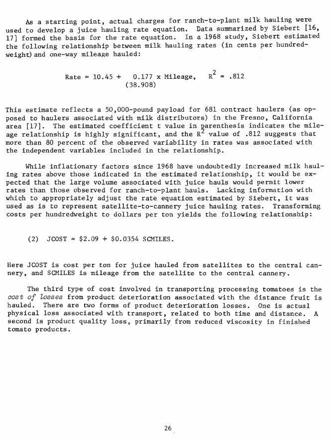
Table 5—^Tomato tonnage harvested per time period, by receiving station area

Receiving Time period Total station : 7/10-7/31 : 8/1-9/21 : 9/22-9/29 : 9/30 + :

Tons

A ; 16,907 8,453 0 0 25,360

B : 21,667 10,833 0 0 32,500

C : 15,494 19,456 0 0 34,950

D : 6,811 25,752 4,056 1,646 38,265

E : 7,530 30,118 3,787 3,119 44,554

F 0 21,953 10,592 9,056 41,601

G 0 14,971 6,032 3,028 24,031

Total : 68,409 131,536 24,467 16,849 241,261

RCOST is cost per ton in dollars and FSMILES is estimated road mileage between the point of harvest and the point of initial processing, _9/

2 The low R value (.64) indicates substantial residual variability in rates

after accounting for distance hauled. It is apparent that factors other than distance enter into hauling rate negotiations. However, experimentation with alternative functional forms failed to show that a curvilinear relationship between hauling cost and distance would be more appropriate than the linear form estimated in equation (1).

Juiae hauling costs are for transporting juice from satellites to the central cannery. In this example, stainless steel bulk milk trailers are employed for juice hauling. It could not be definitely ascertained whether satellite- produced juice would be considered an exempt agricultural commodity for the purpose of rate specification. The product is a raw agricultural product in one sense—it has not been containerized or compositionally altered. On the other hand, a form of processing has been carried out.

9_/ Definitions of equation terms are reviewed in Appendix I,

2 5

As a starting point, actual charges for ranch-to-plant milk hauling were used to develop a juice hauling rate equation. Data sunmiarized by Siebert [16, 17] formed the basis for the rate equation. In a 1968 study, Siebert estimated the following relationship between milk hauling rates (in cents per hundredweight) and one-way mileage hauled:

Rate = 10.45 + 0.177 x Mileage, R^ = .812 (38.908)

This estimate reflects a 50,000-pound payload for 681 contract haulers (as op- posed to haulers associated with milk distributors) in the Fresno, California area [17]. The estimated coefficient t value in parenthesis indicates the mileage relationship is highly significant, and the R value of .812 suggests that more than 80 percent of the observed variability in rates was associated with the independent variables included in the relationship.

While inflationary factors since 1968 have undoubtedly increased milk hauling rates above those indicated in the estimated relationship, it would be expected that the large volume associated with juice hauls would permit lower rates than those observed for ranch-to-plant hauls. Lacking information with which to appropriately adjust the rate equation estimated by Siebert, it was used as is to represent satellite-to-cannery juice hauling rates. Transforming costs per hundredweight to dollars per ton yields the following relationship:

(2) JCOST = $2.09 + $0.0354 SCMILES.

Here JCOST is cost per ton for juice hauled from satellites to the central cannery, and SCMILES is mileage from the satellite to the central cannery.

The third type of cost involved in transporting processing tomatoes is the cost of tosses from product deterioration associated with the distance fruit is hauled. There are two forms of product deterioration losses. One is actual physical loss associated with transport, related to both time and distance. A second is product quality loss, primarily from reduced viscosity in finished tomato products.

26

Some information has been developed on the relationship between product losses and elapsed time between fruit harvest and initial processing. Pub- lished and unpublished data from the University of California at Davis show that increases in Class III damage (i.e., when the seed locules or chambers are broken through or exposed) between field and cannery for bulk loads, relate to several factors, including position of fruit in the load, time of harvest (both within season and within day), and elapsed time. For 180 bulk loads sampled in 1972, Class III damage increased by an average of about 1.4 percent between field and grading station and another 6.2 percent between grading station and cannery for a total weight loss of 7.6 percent [12]. Assuming all Glass III damaged fruit is culled, this represents a loss of 152 pounds per ton or, at 1974 contract prices of $55 per ton, a monetary loss of $4.18 per ton harvested (this is net of the cost of transporting the culled fruit).

Experimental evidence is not available on the magnitude of product quality losses related to hauling distances. Even with such information, attaching a dollar cost to quality losses would be difficult without detailed buyer prefer- ence data. Nonetheless, the viscosity losses related to field-to-cannery distance are generally recognized by tomato processors, and are usually considered detrimental.

Specification of a functional relationship between distance hauled and cost of product loss entails substantial subjectivity, due to the nature of available information on the magnitude of these losses. At the outset, a cost of 4.64 cents per mile is used to reflect product losses (i.e., LCOST = .0464 FSMILES). This is based on the increase in Class III damage observed in the study cited above, where one-way field-to-cannery hauling distances averaged 90 miles. Note that this cost does not include viscosity losses, and therefore might be considered a low estimate. On the other hand, not all Class III damaged fruit would necessarily be culled when the fruit was destined for maceration. Product loss costs per mile are subsequently ranged above and below this level to ex- plore the sensitivity of total assembly costs to this parameter.

Satellite Establishment Costs

A crucial factor in determining optimal number of satellites is the cost of plant establishment, particularly if variable operating costs are similar for both satellite and central cannery. In that case, if satellite processing capacity replaces existing central cannery processing capacity, the cost of establishing the first satellite must be less than the cost savings attributable to using the satellite. The same relationship must hold for each additional satellite considered. However, if variable processing costs are less for satellites, or if the capacity of satellites is viewed as added rather than replac- ment capacity, then conditions of feasibility are less restrictive.

Investment and operating costs incurred in satellite station operation were outlined in the preceding section. Fixed cost components, reflecting establishment costs, are summarized in table 6. A total of $1,236,570 is considered the added cost of satellite processing if satellite capacity is considered replacement capacity.

27

Table 6—Total and annual establishment costs for satellite tomato processing units

00

Capital Installed cost

; Life Annual costs

item : Dep reciation : Int. on inv.

' 3 : RPT

• Total • • Dollars Years Dollars

Land : 84,500 A/ 0 8,450 845 9'r^95

Buildings : 225,340 20 11,267 9,014 5,633 25,914

Equipment : 926,730 10 92,673 37,069 32,436 162,178

Total : 1,236,570 103,940 54,533 38,914 197,387

Straight-line method, no salvage value,

"At 8 percent interest opportunity cost on one-half installed cost (4 percent annual rate) for buildings and equipment, full purchase price for land.

Repairs, taxes, and insurance at 3-1/2 percent of installed cost for equipment, 2-1/2 percent for buildings, and 1 percent for land.

No land appreciation or depreciation assumed.

Specification of Potential Satellite Locations

Criteria for selection of potential* satellite locations are few. Both raw product and juice move by truck, so sites must be adjacent to paved roads. Land requirements for spray irrigation of liquid wastes necessitate rural locations. Access to large quantities of fuel, water, and power is also required.

The number of sites which satisfy these criteria is infinite, and some means must be used to limit potential candidates. For several reasons, consideration was limited to existing receiving stations (receiving stations A through G in tables 4 and 5). For the most part, these sites are already either owned or leased by the cannery. In most cases, water, fuel, and electricity are readily accessible. All are located in rural areas adjacent to paved roads. Finally, the receiving stations are generally situated in areas of concentrated production.

Derivation of Assembly Cost Matrix

The next step in implementing the satellite number and location model is to compute all field-to-satellite and satellite-to-cannery distances. A provision in current grower-processor contracts simplifies this step. Con- tracts specify that tomatoes shall be weighed and inspected at the cannery's receiving station nearest the point of harvest; that is, fruit allocated to a satellite site must first be delivered to the closest receiving station for weighing and grading.

Given this restriction, a mileage matrix showing all field-to-satellite distances can be derived (table 8) from data in table 4 plus information on inter-satellite distances (table 7). Mileage for direct routes between a grower and the closest potential satellite is taken directly from table 4. For other routes, mileage is the distance between a grower and the closest satellite site plus the inter-satellite distance (table 7).

Table 7—Distances among potential satellites and between satellites and central cannery

Potential : satellite : site :

A B C D E F G Central cannery

Miles A ; ■ 92 138 150 209 186 230 206 B : - 50 84 114 120 147 112 C - 30 72 80 124 81 D - 41 50 94 50 E - 82 126 25 F - 44 103 G — 156

29

Table 8—Mileage matrix; distances among growers, satellite sites, and central cannery

Grower ' Satellite site % Central

A B C D E F G : cannery Miles

1 : 20.5 112.5 158.5 170.5 229.5 206.5 250.5 226.5 2 : 24.5 116.5 162.5 174.5 233.5 210.5 254.5 230.5 3 : 16.5 108.5 154.5 166.5 225.5 210.5 246.5 222.5 4 : 8.0 100.0 146.0 158.0 217.0 194.0 238.0 214.0 5 : : 26.0 118.0 164.0 176.0 235.0 212.0 256.0 232.0 6 : 27.0 119.0 165.0 177.0 236.0 213.0 257.0 233.0 7 : 18.0 110.0 156.0 168.0 227.0 204.0 248.0 224.0 8 : 15.0 107.0 153.0 165.0 224.0 201.0 245.0 221.0 9 , 106.7 14.7 64.7 98.7 128.7 134. 7 161.7 126.7

10 : 106.1 14.1 64.1 98.1 128.1 134.1 161.1 126.1 11 : 104.3 12.3 62.3 96.3 126.3 132.3 159.3 126.3 12 : 105.8 13.8 63.8 97.8 127.8 133.8 160.8 125.8 13 ! 106.3 14.3 64.3 98.3 128.3 134.3 161.3 126.3 14 : 99.8 8.7 57.8 91.8 121.8 127.8 154.8 119.8 15 I : 101.3 9.3 59.3 93.3 123.3 129.3 156.3 121.3 16 : 96.0 4.0 54.0 88.0 118.0 124.0 151.0 116.0 17 : 157.0 59.0 9.0 39.0 81.0 89.0 133.0 90.0 18 : 154.0 66.0 16.0 46.0 88.0 96.0 140.0 97.0 19 : 144.7 56.7 6.7 36.7 78.7 86.7 130.7 87.7 20 150.0 62.0 12.0 42.0 84.0 92.0 136.0 93.0 21 : 161.1 73.1 23.1 53.1 95.1 103.1 147.1 104.1 22 : 162.0 96.0 42.0 12.0 53.0 62.0 106.0 62.0 23 : 162.0 96.0 42.0 12.0 53.0 62.0 106.0 62.0 24 : 158.0 92.0 38.0 8.0 49.0 58.0 102.0 58.0 25 : 162.0 96.0 42.0 12.0 53.0 62.0 106.0 62.0 26 : 188.0 122.0 68.0 38.0 79.0 88.0 132. Ô 88.0 27 : 170.0 104.0 50.0 20.0 61.0 70.0 114.0 70.0 28 : 175.0 109.0 55.0 25.0 66.0 75.0 119.0 75.0 29 : 216.0 121.0 79.0 48.0 7.0 89.0 133.0 32.0 30 : 221.0 126.0 84.0 53.0 12.0 94.0 138.0 37.0 31 : 213.0 118.0 76.0 45.0 4.0 86.0 130.0 29.0 32 : 211.0 116.0 74.0 43.0 2.0 84.0 128.0 27.0 33 : 215.0 120.0 78.0 47.0 6.0 88.0 132.0 31.0 34 : 213.0 118.0 76.0 45.0 7.0 86.0 130.0 29.0 35 : 235.0 140,0 98.0 67.0 26.0 108.0 152.0 51.0 36 : 219.0 124.0 82.0 51.0 10.0 92.0 136.0 35.0 37 : 219.0 124.0 82.0 51.0 10.0 92.0 136.0 35.0 38 : 216.0 121.0 79.0 48.0 7.0 89.0 133.0 32.0 39 : 224.0 129.0 87.0 56.0 15.0 97.0 141.0 40.0 40 : 223.0 128.0 86.0 55.0 14.0 96.0 140.0 39.0 41 : 217.0 122.0 80.0 49.0 8.0 90.0 134.0 33.0 42 : 229.0 134.0 92.0 61.0 20.0 102.0 146.0 45.0 43 : 226.0 131.0 89.0 58.0 17.0 99.0 143.0 42.0

Continued

30

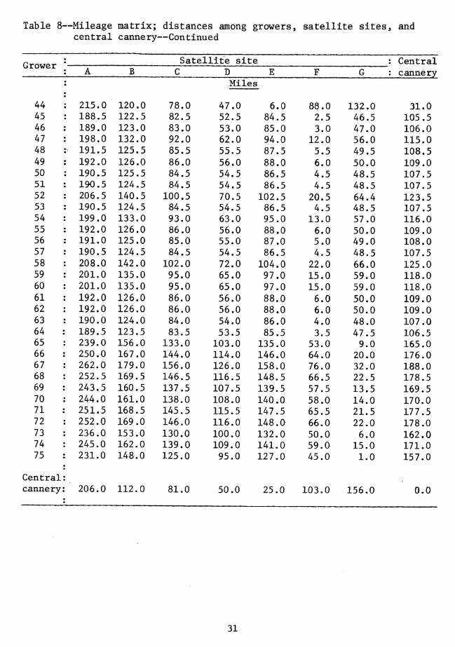
Table 8—Mileage matrix; distances among growers, satellite sites, and central cannery—Continued

Grower Satellite site _: Central : A B C D E F G : cannery

Miles

44 : 215.0 120.0 78.0 47.0 6.0 88.0 132.0 31.0 45 : 188.5 122.5 82.5 52.5 84.5 2.5 46.5 105.5 46 : 189.0 123.0 83.0 53.0 85.0 3.0 47.0 106.0 47 : 198.0 132.0 92.0 62.0 94.0 12.0 56.0 115.0 48 : 191.5 125.5 85.5 55.5 87.5 5.5 49.5 108.5 49 : 192.0 126.0 86.0 56.0 88.0 6.0 50.0 109.0 50 : 190.5 125.5 84.5 54.5 86.5 4.5 48.5 107.5 51 : 190.5 124.5 84.5 54.5 86.5 4.5 48.5 107.5 52 : 206.5 140.5 100.5 70.5 102.5 20.5 64.4 123.5 53 : 190.5 124.5 84.5 54.5 86.5 4.5 48.5 107.5 54 : 199.0 133.0 93.0 63.0 95.0 13.0 57.0 116.0 55 : 192.0 126.0 86.0 56.0 88.0 6.0 50.0 109.0 56 : 191.0 125.0 85.0 55.0 87.0 5.0 49.0 108.0 57 : 190.5 124.5 84.5 54.5 86.5 4.5 48.5 107.5 58 : 208.0 142.0 102.0 72.0 104.0 22.0 66.0 125.0 59 : 201.0 135.0 95.0 65.0 97.0 15.0 59.0 118.0 60 : 201.0 135.0 95.0 65.0 97.0 15.0 59.0 118.0 61 : 192.0 126.0 86.0 56.0 88.0 6.0 50.0 109.0 62 : 192.0 126.0 86.0 56.0 88.0 6.0 50.0 109.0 63 : 190.0 124.0 84.0 54.0 86.0 4.0 48.0 107.0 64 : 189.5 123.5 83.5 53.5 85.5 3.5 47.5 106.5 65 • 239.0 156.0 133.0 103.0 135.0 53.0 9.0 165.0 66 : 250.0 167.0 144.0 114.0 146.0 64.0 20.0 176.0 67 : 262.0 179.0 156.0 126.0 158.0 76.0 32.0 188.0 68 , 252.5 169.5 146.5 116.5 148.5 66.5 22.5 178.5 69 : 243.5 160.5 137.5 107.5 139.5 57.5 13.5 169.5 70 : 244.0 161.0 138.0 108.0 140.0 58.0 14.0 170.0 71 : 251.5 168.5 145.5 115.5 147.5 65.5 21.5 177.5 72 : 252.0 169.0 146.0 116.0 148.0 66.0 22.0 178.0 73 236.0 153.0 130.0 100.0 132.0 50.0 6,0 162.0 74 245.0 162.0 139.0 109.0 141.0 59.0 15.0 171.0 75 ; 231.0 148.0 125.0 95.0 127.0 45.0 1.0 157.0

Central cannery: 206.0 112.0 81.0 50.0 25.0 103.0 156.0 0.0

31

Raw product hauling, juice hauling, and product deterioration functions specified earlier are applied to the mileage matrix (table 8) to derive an assembly cost matrix. Combining the three types of costs yields the following relationship between total assembly cost (TACOST) and mileages:

'(3) TACOST. . = RCOST. . + LCOST. . + ÀJCOST. „. i»J i,J i,J J,8

The subscript i (i=l,2,...,75) designates grower; j (j=l,2,...,8) designates point of first processing, either satellite (J=l,2,...,7) or central cannery (j=8).

The parameter, À, reflects the reduction in product weight associated with satellite processing. This weight reduction is due to elimination of cull tomatoes, seeds, and skins at the field location and evaporation losses.

Cullable defects not associated with distance hauled are assumed to be 4 percent of the gross weight received. Juice recovery is specified at 93 percent of net weight (less culls). Vacuum cooling water loss is specified at 10.54 percent of processed juice weight. Hence, without considering transport-related losses, "out the door" or shipping weight is 79.85 percent of weight received.

In the study discussed above, Class III damage associated with transport and waiting time was shown to average 7.6 percent for an average haul of 90 miles, or .084 percent per mile. Combining "normal" weight loss (20,15 percent derived above) and damage losses related to the distance fruit is hauled, the value of X can be expressed as

(4) A = .8946(.93(.96 - .0008 FSMILES. .))

= .8320(.96 - .0008FSMILES. .)

Given X, equation (3) can be rewritten as

(5) TACOST. . = (5,83 + 0.0294FSMILES. ,) -h .0464FSMILES. .

+ .8320(.96 - .0008FSMILES. .)(2.09 + .0354SCMILES. J

For direct fieId-to-cannery hauls, the last expression in equation (5) is equal to zero, since juice hauling costs are not incurred (JCOST =0.0). In that case, total assembly costs are: '

(6) TACOST. = 5.83 -h (0.0294 + .0464)FSMILES. ^

= 5.83 + 0.0758FSMILES. ^. 1,8

Combining terms in equation (5), assembly costs for shipments through satellites can be written as:

(7) TACOST. . = 7.50 + 0,0743FSHILES. . + SCMILES. „('0283 -

- .000025FSMILES. .) lO

32

The assembly cost matrix is derived from the mileage matrix in table 5 by applying equations (6) and (7) to the appropriate entries.

Capacity Constraints and Minimum Requirements

In its general form, the Stollsteimer model yields minimum assembly costs without consideration of plant capacities. Plant size is arbitrarily specified as the scale necessary to process the tonnage resulting from the minimum-cost allocation. In this example, satellite size is restricted to the model plant defined earlier, that is, with a maximum capacity of 50 tons per hour. Further- more, the central cannery has a minimum tonnage requirement which must be considered along with the satellite capacity restrictions.

The model satellite plant synthesized.earlier, with a maximum dumping capacity of 50 tons per hour, operates 20 hours per day, implying a peak daily load of 1,000 tons. Discussion with cannery personnel indicated a minimum central cannery requirement in the example case of 1,125 tons per day. This quantity is needed to provide whole pack raw product needs, to operate existing juice lines at minimum levels, and to allow limited intercannery shipments. Maximum and minimum loads by period are shown in table 9. For the first three periods, plants were assumed to operate 6 days per week. For the open-ended last period (September 30 and later), a total of 6 operating days was assumed.

Solution Procedure

Imposition of these two constraints, maximum satellite capacity and minimum cannery requirement, alters the method of minimizing assembly costs. The problem could be handled as a special case of the transportation problem, for which there exist relatively simple linear programming solution techniques (see for example [5]). However, with 75 production locations and four separate time periods, the number of activities and constraints is enormous. This, coupled with the large number of possible satellite combinations possible, could make the use of programming methods prohibitively expensive. For example, consideration of three sites among seven possible sites would require 35 separate programming solutions, each with 300 production constraints, 16 capacity constraints, and 1,200 activities.

An alternative assembly cost minimization algorithm was developed which results in solutions similar to those obtained using linear programming. Its major advantages over linear programming are (1) solutions are generated at substantially lower cost, (2) cost comparisons with nonoptimal plant combinations are obtained, and (3) much less time is required for preparation of input data. However, except for the case of one satellite, it is possible that the routing pattern generated by the algorithm may not be optimal; that is, a linear programming transportation model could yield a pattern resulting in larger cost savings. The sub-optimal nature of the solution procedure used is not deemed a serious shortcoming for two reasons. First, the solution is optimal for one satellite, and it is likely that only a single site would initially be considered by firms planning satellite operations. Second, certain tests suggest that the degree of sub-optimality is quite small.

33

Instructions for using the minimization algorithm and the FORTRÁl^ program employed are presented in Appendix II, Figure 5 is a flow chart summarizing the program. Basically, the program uses a multiple iterative procedure to calculate and compare minimum costs with various combinations of plant sites. For any combination of n possible satellites (n=l,2,...,7 in the example case), the cost matrix cell with the largest cost advantage over direct grower-to- central cannery hauling is selected as the first grower-satellite route. Sup- pose this cell represents the route grower i through satellite j. Production from i is then allocated to j for each time period. The next step selects the second largest cost advantage and allocates accordingly. This process continues until a maximum constraint (satellite capacity) or a minimum constraint (central cannery requirement) is encountered for one of the time periods. Allocations violating the constraints are subsequently suppressed in further iterations and the procedure continues until one of the following situations occurs: (1) no further cost savings are possible (i.e., shipments via satellites are more costly than direct shipments); (2) all satellites considered are operating at capacity in each time period; or (3) all remaining production must be allocated to the central cannery in order to meet minimum requirements. The same procedure is repeated for each combination.

Output of the assembly cost minimization program is as follows:

(1) Assembly cost matrix with entries expressed as deviations from the costs of direct grower-to-central cannery hauls.

(2) Production by grower by period. (3) Cost reduction for each combination of n satellites. (4) For the combination yielding the largest cost reduction (i.e., the

minimum assembly costs):

a) Production for each grower during each period allocated to each satellite and to the central cannery,

b) Total satellite and central cannery receipts, both absolute and as a percent of maximum/minimum.

It should be noted that this particular assembly cost minimization program can only be applied in the case of a single receiving cannery. Scheduling com- plexities introduced in multiplant operations would necessitate use of a substantially more elaborate solution procedure. While multiplant tomato processing firms are common, restricting consideration to the single plant case is not viewed as a serious shortcoming. It is anticipated that multiplant firms con- templating satellite establishment would likely consider only one receiving plant at the outset.

Analysis of Investment Profitability

Least-Gost Satellite Locations

The assembly cost minimization program run for the example problem yielded the results summarized in tables 10 and 11. When a single satellite location is considered, site A yields the largest cost savings, $209,000. Site A is the most remote location, situated 206 miles from the central cannery. It is also isolated from other potential satellite sites—92 miles from the nearest and 230

34

FLOW CHART FOR ASSEMBLY COST MINIMIZATION PROGRAM

Read: \

Cost parameters i Constraints Production matr Mileage matrix

Calculate:

Cost matrix

Write:

Cost matrix Production matri>

Increment:

Number of Satellites

Allocate:

Reduce allocation to meet constraint

Increment:

Satellite combination

Select:

Least-cost route

Allocate:

Period produce

Allocate:

Remaining tons to centrai cannery

Write: '

Iteration number Cost savings

Save:

Allocation scheme Cost savings

Write:

Maximum cost savings Allocation scheme

Update:

Cost savings

Figure 5. 35

Table 9—Maximum satellite capacity and minimum central cannery requirements by period, raw ton basis

Item Period

7/10-7/31 • 8/1-9/21 : 9/22-9/29 : 9/30 + Tons

Maximum satellite capacity : 18,000 43,000 6,000 6,000

Minimum central cannery requirement : 20,250 48,375 6,750 6,750

Total tonnage available : 68,409 131,536 24,467 16,849

Table 10—Minimum assembly costs for alternative numbers of satellites

Number of Ltes Sites Cost reduction

satell] Total : 2

Marginal

Dollars

1 : A 209,022 209,022

2 : A, F 389,921 180,899

3 : A, B, F 496,309 106,388

4 • A, B, C, F 569,656 73,347

5 A, B, C, F, G 639,480 69,824

6 A, B, C, D, F, G 643,608 4,128

7 3 , (Same as for 6)

Assembly cost savings compared with direct grower-to- central cannery shipments.

2 Cost savings attributable to adding each additional satellite.

3 Location E is not a feasible satellite site.

36

Table 11—^Satellite and central cannery tonnage receipts, minimum assembly cost combinations

Satellites : Optimal : sites

: Time period . Total considered : 7/10- -7/31 8/1-9/21 9/22- -9/30 9/30 -1- : received

Tons % of max/min Tons % of

max/mln Tons % of Tons % of

Tons max/min max/min

1 : A 16,908 93.9 8,542 19.7 0 0.0 0 0.0 25,360 : Cent. can. 51,506 254.4 123,086 254.4 24,470 362.5 16,855 249.7 215,917

2 : A 16,908 93.9 8,452 19.7 0 0.0 0 0.0 25,360 : F 0 0.0 36,928 85.9 6,000 100.0 6,000 100.0 48,928 : Cent- can. 51,506 254.4 86,158 178.1 18,470 273.6 10,855 160.8 166,989

3 : A 16,908 93.9 8,452 19.7 0 0.0 0 0.0 25,360 : B 18,000 100.0 10,833 25.2 0 0.0 0 0.0 28,833 : r 0 0.0 36,928 85.9 6,000 100.0 6,000 100.0 48,928 : Cent. can. 33,506 165.5 75,325 155.7 18,470 273.6 10,855 160.8 138,156

4 : A 16,908 93.9 8,452 19.7 0 0.0 0 0.0 25,360 : B 18,000 100.0 10,833 25.2 0 0.0 0 0.0 28,833 : C 13,256 73.6 19,456 45.2 0 0.0 0 0.0 32,712 F 0 0.0 36,928 85.9 6,000 100.0 6,000 100.0 48,928 Cent. can. 20,250 100.0 55,869 115.5 18,470 273.6 10,855 160.8 105,444

5 A 16,908 93.9 8,452 19.7 0 0.0 0 0.0 25,360 B 18,000 100.0 10,833 25.2 0 0.0 0 0.0 28,833 C 13,256 73.6 19,456 45.2 0 0.0 0 0.0 32,712 F 0 0.0 21,955 51.1 6,000 100.0 6,000 100.0 33,955 G 0 0.0 14,973 34.8 6,000 100.0 3,029 50.5 24,002

1 • Cent. can. 20,250 100.0 55,869 115.5 12,470 184.7 7,826 115.9 96,415 6&7 : A 16,908 93.9 8,452 18.7 0 0.0 0 0.0 25,360

B 18,000 100.0 10,833 25.2 0 0.0 0 0.0 28,833 C 13,256 73.6 19,456 45.2 0 0.0 0 0.0 32,712 D 0 0.0 0 0.0 2,741 45.7 1,076 17.9 3,817 F 0 0.0 21,955 51.1 6,000 100.0 6,000 100.0 33,955 G 0 0.0 14,973 34.8 6,000 100.0 3,029 50.5 24,002

-1

Cent. can. 20,250 100.0 55,869 115.5 9,729 144.1 6,750 100.0 92,598

Optimal sites, cost reduction, and allocations are identical for 6 and 7 satellites

miles from the most distant. As a consequence, it receives tonnage only from adjacent growers, operating during the periods from July 10 to 31 and August 1 to September 21. No capacity or minimum requirement constraints are applicable.

Sites A and F are the satellite locations when two sites are considered. The marginal or additional cost saving over site A alone is $181,000. Site F is 103 miles from the central cannery and 44 miles from site G, the closest other potential satellite location. The satellite at F receives tonnage from the adjacent area as well as from growers shipping through the receiving station at site G. It operates at full capacity during the last two periods and at 86 percent of maximum capacity during the period August 1 to September 21. Total tonnage processed at F is nearly twice that processed at A (48,928 vs. 25,360).

Sites B, C, G, and D are included sequentially in subsequent iterations, yielding decreasingly smaller marginal cost savings. Site E is not a feasible location, even when seven possible sites are considered. Site E is so close to the central cannery (25 miles) that no assembly cost reduction can be achieved by locating a satellite at that point.

A minimum central cannery requirement constraint is reached in the fourth iteration (four satellites considered) for the July 1-31 period, and in the sixth iteration for the period after September 30. Satellite capacity constraints are met in the first, third, and fourth time periods for some of the satellite combinations considered. They are especially important in the two shorter (6-day) periods near the end of the processing season. Neither maximum nor minimum constraints are binding in the lengthy August 1 to September 21 period.

Return on Investment and Investment Recovery Periods There are several ways to evaluate the profitability of investment. Three

approaches considered here are: (1) comparison of annual investment cost with annual return (annual return on investment method); (2) assessment of the amount of time required for accumulated returns to exceed investment costs (recovery period method); and (3) calculation of the rate of interest implicit from the investment (internal rate of return method).

Each of these methods is based on a different viewpoint with respect to re- quisite profitability and alternative investment opportunities. Method (1) uses a prevailing long-term market interest rate as a comparison base; net returns from the proposed investment must equal or exceed what the capital could earn in conventional lending markets. The evaluation may be done on an annual basis if depreciation is accounted for (i.e., the annual net change in investment), or a "planning horizon" may be defined and the evaluation done on a present value basis. The former method is used here.

The recovery period method presupposes an inherent rule that an investment must be paid off (by increased revenue or reduced costs) within a certain period of time. The length of the payoff period depends on many factors and is highly variable among industries as well as firms within industries. A "satisfactory" recovery period may be as short as 2 years or as long as 7 or 8 years.

38

The internal rate of return approach involves comparison of the rate of return for the proposed investment with probable rates of return for alternative investments. If the alternative is investment in the money market, the internal rate of return and annual return on investment approaches are similar. Usually, the internal rate of return must exceed prevailing interest rates by a substantial margin for an investment to be considered feasible.

Use of these methods is confounded in the example case because of the lack of knowledge concerning variable processing costs for the central cannery. Fur- thermore, unit variable processing costs for satellites are not precisely defined—variable-length processing seasons would have some impact on hourly tonnage receipts, and consequently on utilization of labor and utilities. To circumvent this problem, comparison of variable operating costs between satellites and the central cannery is made on a relative basis. Specifically, three situations are evaluated: satellites possess a $2.50 per ton cost advantage, zero advantage, and a $2.50 disadvantage. 10/

Which of these situations would be most likely is difficult to assess. De- centralization of control inherent in satellite processing would tend to elevate variable processing costs. Crew scheduling problems might be severe, particularly if fruit flow was variable. The short processing season indicated for some satellites could present problems in recruiting and retaining labor. Fuel and electricity costs per ton processed would also be higher íf a satellite was forced to operate intermittently at levels well below capacity.

Economies of waste management would be the most important factor contribut- ing to a possible operating cost advantage for satellites. Liquid waste spray irrigation entails a large capital outlay, but operating expenses are small, particularly when compared with secondary treatment facilities or municipal treatment charges. Solid waste removal costs would also likely be smaller for satellites.

Values for the three evaluative methods are summarized %n table 12. An- nual return on investment is calculated as net cost reduction less total annual costs expressed as a percent of total investment. In essence, this is a measure of the annual return over and above that possible for money market investment. Net cost reduction is marginal assembly cost reduction from the last column of table 10 less the difference between total variable operating costs for the satellite and operating costs if the same tonnage were processed in the central cannery (i.e., zero, or + $2.50 times tonnage received by one or more satellite). These reflect an annual interest charge of 8 percent.

10/ If processing cost differences were known or ranges of values were esti- mable, it would be more appropriate to include differences in the assembly cost functions prior to solution of the minimum cost program, and, in fact, the results would be altered in the example case. As suggested in table 11, site F would be the least-cost location for one satellite if satellite processing costs were $2.50 less than central cannery costs. This procedure was not followed because the probable difference in processing costs was highly uncertain. But in specific empirical applications, it is recommended that adjustment for likely processing cost differences be made in the assembly cost function.

39

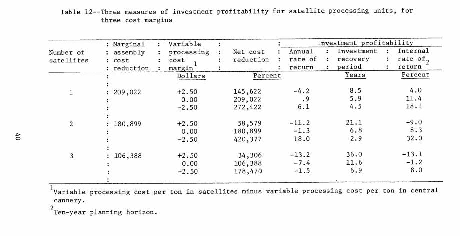
o

Table 12—Three measures of investment profitability for satellite processing units, for three cost margins

Number of satellites

Marginal : Variable assembly : processing cost : cost

: margin reduction Dollars

209,022 +2.50 0.00

-2.50

180,899 +2.50 0.00

-2.50

106,388 +2.50 0.00

-2.50

Net cost reduction

Percent

145,622 209,022 272,422

58,579 180,899 420,377

34,306 106,388 178,470

Investment profitability Annual rate of return

-4.2 .9

6.1

-11.2 -1.3 18.0

-13.2 -7.4 -1.5

Investment recovery period

Years

8.5 5.9 4.5

21.1 6.8 2.9

36.0 11.6 6.9

Internal rate of„ return Percent

4.0 11.4 18.1

-9.0 8.3 32.0

-13.1 -1.2 8.0

variable processing cost per ton in satellites minus variable processing cost per ton in central cannery.

"Ten-year planning horizon.

Investment recovery periods are simply total capital investment ($1,236,570) divided by net annual cost reduction. The internal rate of return (1ER) is calculated by solving the following formula:

Total capital investment = Annual net cost reduction

X Z 1 , Salvage Value

t=l (l+IRR)^ (l+IRR)-^°

A 10-year planning horizon with net cost reduction identical in each year is assumed. Salvage values are estimated at zero for equipment and buildings, and 100 percent of purchase price for land.

Table 12 indicates that when the variable processing cost margin is set at zero, only the first satellite yields a net annual return greater than annual investment cost. The annual rate of return for one satellite is less than 1 percent, assuming an 8 percent rate as an opportunity interest charge. This implies that'investment in the first satellite yields a return slightly better than current bond market rates. Depending on the proportion of owned and borrowed capital and the interest rate on borrowed capital, this return may or may not reflect a reasonable investment opportunity. The investment recovery period for one satellite with no difference in variable processing costs is 5.9 years, while the internal rate of return is 11.4 percent. Neither of these measures reflects a sterling investment opportunity. It should be noted, however, that the internal rate of return would increase if a longer planning horizon was utilized.

Addition of satellites beyond the first is shown to be less profitable. For both the second and third satellite, net cost reduction with no difference in processing cost is less than annual costs. Investment recovery periods are 6.8 years for the second satellite and 11.6 years for the third. A negative internal rate of return is observed for the third satellite. Additions beyond the third are not shown, since they yield even smaller cost reductions.

Processing cost differences have a strong influence on the profitability of satellite investment. For example, a $2.50 processing cost advantage for the first satellite yields an internal rate of return of 18.1 percent, or an increase of almost 7 percent over the case of no processing cost difference. A comparable processing cost disadvantage yields an internal rate of return of only 4 percent. The effect of processing costs is even more dramatic for the second satellite, which receives nearly twice the tonnage as the first. A $2.50 advantage for the second satellite yields an attractive 32 percent internal rate of return.

Sensitivity Analysis

Assembly Cost Parameter Ranging

While the parameters used in deriving the assembly cost matrix reflect reasonable assumptions and real-life observations, they are subject to consider- able variability over individual conditions. The effects of alternative levels

41

of raw product hauling, juice hauling, and product loss costs on satellite in^- vestment profitability were explored by ranging these costs and re-solving the assembly cost minimization program. The variable portions of these components used in the initial solution (2.94 cents per mile for raw product hauling, 3.54 cents per mile for juice hauling, and 4.64 cents per mile for product loss) were specified as base values, and levels from 50 percent below to 100 percent above the base values were subsequently substituted in deriving the assembly cost matrix.

The results of this cost ranging procedure are summarized in table 13. The top row reproduces the results of table 10, and the base values of the three cost components. The other rows show optimal cost reductions for assembly cost components at levels -50%, -25%, +25%, +50%, and +100% of each of the base values! Marginal cost reductions resulting in investment recovery periods of 5 years or less are indicated by boxes.

Some patterns are evident from table 13. As juice hauling costs drop, and as raw product hauling and product loss costs increase, satellite investment becomes more profitable. Investment profitability is particularly sensitive to changes in the product loss component. With a 25-percent increase above the base level in the dollar cost per mile attributable to product damage, cost reductions for both the first and second satellites yield investment recovery periods of less than 5 years. With product losses 25 percent below the base, even the first satellite generates savings well below annual investment charges.

Effect of Allocation Constraints

The effect of satellite capacity restrictions and minimum central cannery requirements on investment profitability was explored by dropping these constraints and re-solving the assembly cost minimization program. Comparisons of the results obtained with those from the constrained case are shown in table 14.

Optimal locations for the first two satellites are altered when the constraints are removed, and larger cost reductions are achieved. Site F yields the maximum savings, $26,000 more than site A. However, to achieve this level of savings, the satellite would require twice the assumed capacity of 50 tons per hour in the period after September 30, and nearly three times the initial capacity in the period September 22-29. Furthermore, the minimum central cannery constraint is also violated after September 30. Sites B and F are optimal for two locations in the unconstrained case. The satellite at B would have to possess hourly dumping capacity of 107 tons per hour to process the indicated tonnage in the July 10-31 period. Beyond two satellites, optimal sites are the same for both the constrained and unconstrained case. The cost of the constraints (i.e., the difference in cost reduction between the constrained and unconstrained solutions) is greatest for two satellites.

The primary conclusion regarding the constraints is that they have a limited effect on satellite investment profitability. While imposition of constraints does reduce costs savings, it is expected that the additional capital investment necessary to boost capacity would more than offset these savings.

42

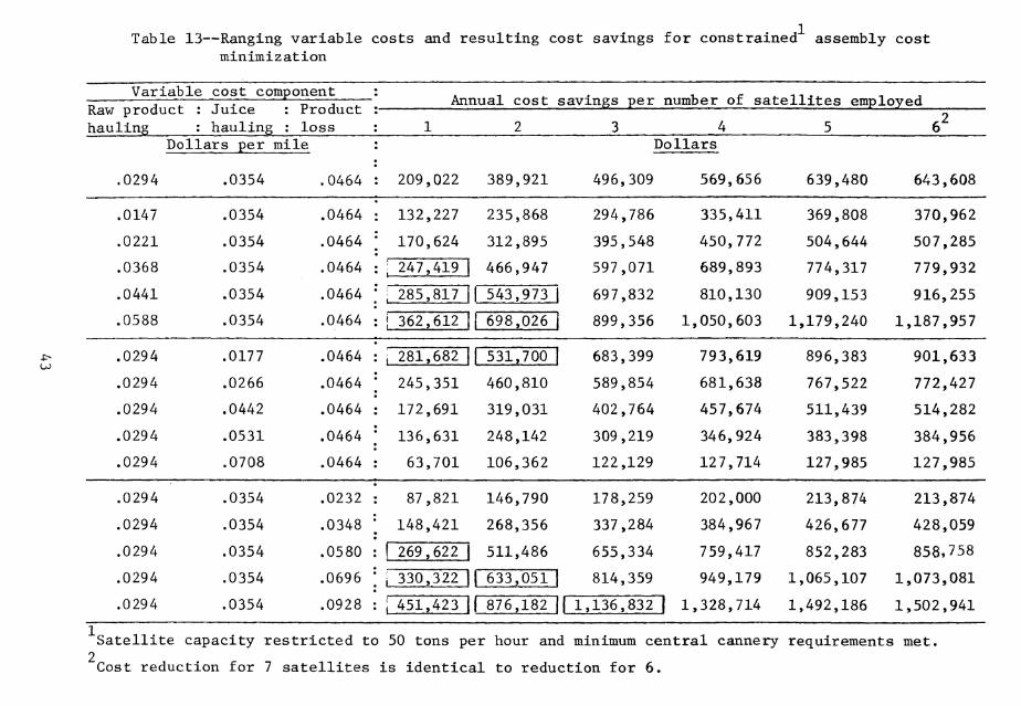
Table 13—Ranging variable costs and resulting cost savings for constrained assembly cost minimization

Variable cost component Annual cost savings per number of satellites employ rÂ

Raw product : hauling

Juice hauling

: Product : loss

ea

; 1 2 3 4 5 6^ Dollars per mile

.0294 .0354 .0464 : 209,022 389,921

Dollars

496,309 569,656 639,480 643,608

.0147

.0221

.0354

.0354

.0354

.0354

.0354

.0464

.0464

.0464

.0464

.0464

: 132,227

: 170,624

235,868

312,895

466,947

294,786

395,548

597,071

] 697,832

] 899,356

335,411

450,772

689,893

810,130

1,050,603 1

369,808

504,644

774,317

909,153

,179,240 1

370,962

507,285

.0368 : ; 247,419 779,932

.0441 • i 285,817 1 543,973 916,255

.0588 : 1 362,612 698,026 ,187,957

.0177

.0266

.0442

.0531

.0708

.0464

.0464

.0464

.0464

.0464 •

] 683,399

589,854

402,764

309,219

122,129

793,619

681,638

457,674

346,924

127,714

896,383

767,522

511,439

383,398

127,985

.0294 , 281,682 1 531,700 901,633

.0294

.0294

.0294

.0294

; 245,351

: 172,691

136,631

63,701

460,810

319,031

248,142

106,362

772,427

514,282

384,956

127,985

.0294

.0294

.0354

.0354

.0354

.0354

.0354

.0232 •

.0348 ;

.0580 :

.0696 ;

.0928 :

87,821

148,421

146,790

268,356

511,486

178,259

337,284

655,334

814,359

202,000

384,967

759,417

949,179

] 1,328,714

1

1

213,874

426,677

852,283

,065,107

,492,186

1

1

213,874

428,059

.0294 ! 269,622 858,758

.0294 1 330,322 1 633,051 ,073,081

.0294 ; 451,423 1 876,182 II 1,136,832 ,502,941

Satellite capacity restricted to 50 tons per hour and minimum central cannery requirements met,

'Cost reduction for 7 satellites is identical to reduction for 6.

.1/ Table 14—Comparison of constrained— and unconstrained assembly cost minimization

Number of optimal location : Cost reduction : Cost of 2/ satellites Constrained Unconstrained Constrained unconstrained : constraints—

Dollars

h'^ : A F*i/ 209,022 235,267 26,245

h : A, F F*, B* 389,921 463,518 73,597

h : A, B, F A, B*, F* 493,309 564,137 70,828

S A, B, c. F A, B*, C, F* 569,656 642,423 72,767

52 : A. B, c. F, G A, B*, C, F*, G* 639,480 682,826 43,346

^4 A, B, c, D, F, G A, B*, C, D, F*, G* 643,608 711,996 68,388

'4 : A, B, c, D, F, G A, B*, C, D, F*, G* 643,608 711,996 68,388

Constrained by satellite capacity restriction (50 tons per hour) and minimum central cannery requirements.

2 Cost of constraints is defined as the cost reduction for unconstrained assembly minimization (col. 5) minus the cost reduction for constrained minimization (col. 4).

3 The subscript on satellite numbers indicates the number of time periods during which a central cannery minimum tonnage requirement is exceeded in the unconstrained case .

Starred letters indicate a satellite is operating at greater than maximum capacity in the unconstrained case.

Concluding Remarks Concerning Economic Feasibility

The preceding exercise illustrated a method of ascertaining the feasibility of decentralized tomato processing. It was not intended to determine whether decentralized processing is profitable in general. However, some general con- clusions can be made.

The profitability of satellite processing depends heavily on the location of production. If a large share of contracted acreage is 100 miles or more from existing processing facilities, utilization of satellites can significantly reduce assembly costs. For growers located close to an existing cannery, the high fixed components of raw product and juice hauling charges preclude any assembly cost savings. The effect of distance on assembly cost reduction attributable to satellite processing is manifested in two ways. First, reduction in product weight from initial processing is substantial (20 percent or more), so total ton-miles can be much lower using satellite processing than central cannery processing. Second, long raw product hauls contribute to fruit deterioration, which can be cut by more timely processing closer to the point of harvest.

The relationship between raw product and juice hauling costs is crucial in assessing the feasibility of satellite investment. If per mile charges for hauling juice are high relative to raw product hauling costs, tne profitability of satellite processing is questionable. Because juice hauling on a commercial scale is not a common practice, there is a good deal of doubt about probable level of juice hauling costs. It is anticipated that juice shipments could be scheduled better than tomato shipments, as satellite juice output would be fairly constant. This would tend to lower juice hauling charges. However, more sophisticated equipment and cleaning methods are required for juice hauling than for raw product hauling. The question of ICC regulation of juice hauling rates must presently be left unresolved.

Because of the importance of transportation-induced fruit losses in assessing the potential value of satellite tomato processing, research concerning the measurement of these losses is highly recommended. Important questions in this respect include: What portion of Class III damage is unusable? What other types of damage can be traced to distance hauled or waiting time? What is the extent of solids loss through leaching in bulk hauling? Can the extent and economic cost of viscosity reduction be measured?

Problems were encountered in comparing processing costs in satellites with those in existing canneries. To be sure, economies of size in processing do exist, documented by the long-term industry trend toward fewer and larger plants. There is less certainty concerning what stages contribute most to these economies. If satellites operate over very limited time spans, it is doubtful that they could achieve processing costs comparable to those possible in 90- to 100-day seasons. On the other hand, decentralized processing would be particularly attractive to firms located in cities where waste treatment standards are expected to elevate central cannery processing costs.

Investment profitability measures calculated in the example case were con- servative in the sense that they considered satellites as replacing rather than

45

adding to existing plant processing capacity. Tomato processing satellites would represent a significantly more profitable venture compared with expansion of an existing central cannery« Establishment costs in that case would be marginal costs of satellite establishment over adding the same capacity in the central cannery. While the difference would surely be positive and likely be large, it would be far less than the gross investment figure used to calculate investment profitability in the example.

In conclusion5 there has been a strong incentive in the past to centralize tomato processing. Satellite processing represents a departure from this trend. While individual firms must evaluate the method in light of specific conditions, there appear to be sound economic reasons to perform this evaluation.

46

REFERENCES

1. Ben-Gara, Itamar, and Amihud Kramer, -"The Utilization of Food Industries Wastes," Advances in Food Research, Vol. 17, p. 77 (1959).

2. California, State of. Cannery Waste Treatment, Utilization and Disposal, No. 39, Resources Agency, State Water Resources Control Board, Sacramento, Calif. (1968).

3. Cervinka, et al.. Energy Requirements for California Agriculture, Joint Study, Calif. Dept. of Food and Agriculture and University of California, Davis (Jan. 1974).

4. Crites, R.W., CE. Pound, and R.G. Smith, "Experience with Land Treatment of Food Processing Wastewater," Proceedings, Fifth National Symposium on Food Processing Wastes, Monterey, Calif. Environmental Protection Tech- nology Series, EPA-660/2-74-058, p. 4 (1974).

5. Dorfman, R. , P.A. Smnuelson, and R.M. Solow, Linear Programming and Econom- ic Analysis, McGraw-Hill, N.Y. (1958).

6. Holdsworth, S.D., Effluents from Fruit and Vegetable Processing, Process Biochemistry 3 (6):27 (1968).

7. International Brotherhood of Teamsters, Northern California Wage Scale, Cannery Workers Union No. 750, Oakland, Calif.

8. Krochta, M.J., G.S. Williams, R.P. Graham, and D.F. Farkas, Reduced-Water Cleaning of Tomatoes, Food Processing Waste Management—Proceedings of the 1973 Cornell Agricultural Waste Management Conference and Proceedings for the National S3nnposium on Food Processing Wastes, Syracuse, N.Y. (March 26-28, 1973).

9. Mercer, W.A., and N.A. Olson, Tomato In-Field Washing Station Study, Final Report, National Canners Association Research Foundation^ (1969).

10. National Canners Association, Liquid Wastes from Canning and Freezing Fruits and Vegetables, Water Pollution Control Series, 12060 EBK 08/71 (1971) .

11. ___, Tomato In-Field Washing Station, National Canners Association Research Information No. 146, Berkeley, Calif. (Jan. 1969).

12. O'Brien, Michael, Agricultural Engineering Research Progress Report, Proces- sing Tomato: Subsampling for Color, Filling, Handling Damage, Grade Dis- tribution, Dept. of Agricultural Engineering, University of California, Davis (1972) [Processed].

13. Reed, A.D., W.E. Wildman, W.S. Seyman, R.S. Ayers, J.D. Prato, and R.S. Raushkolb, "Soil Recycling of Cannery Wastes," California Agriculture, 27(3): 6 (1973).

47

14. Sanborn, N.H., "Spray Irrigation as a Means of Cannery Waste Disposal," The Canning Trade 74, Mar. 3:17 (1952).

15. Schultz, W.G.; R.P. Graham, W.C. Rockwell, J.L. Bomben, J.C. Miers, and J.R'. Wagner, "Field Processing of Tomatoes. 1. Process and Design," Journal of Food Science, 36:397 (1971).

16. Siebert, Jerome B., Analysis of Milk Transportation Rates, Agricultural Extension Service, University of California, Berkeley (May 1969) [Mimeo.].

17. Siebert, Jerome B., J.N. Boles, and Miriam Revzan, Movements of Grade A Milk Supplies in California, Information Series Report No. 65-5, Giannini Foundation of Agricultural Economics, University of California (Dec. 1968).

18. Stollsteimer, John R., "A Working Model of Plant Numbers and Location," Journal of Farm Economics, Vol. XLV, pp. 631-45 (Aug. 1963),

19. USDA, Farm Real Estate Market Developments, Economic Research Service, Washington, D.C., July 1974.

20, U.S. Environmental Protection Agency, Development Document for Proposed Effluent Limitation Guidelines and New Source Performance Standards for the Citrus, Apple and Potato Segment of the Canned and Preserved Fruit and Vegetable Processing Point Source Category, EPA 440/1-73/027 (Nov. 1973).

48

APPENDIX I

SATELLITE NUMBER AND LOCATION MODEL

The model used to determine the preferred location of alternative numbers of tomato processing satellites and the resulting cost reduction is specified mathematically below. The process is based largely on Stollsteimer's model [18].

Define the following variables :

GTTONS = Total quantity of fieId-run tomatoes available for processing in the applicable region, period j

GTC = Total cost to assemble and process Z GTTONS, to 2 '

single-strength juice, dollars per year. GTC is delivered cost to the central cannery.

M

N

PROD. i.J

CAP j.k

= Number of satellite processing locations.

= Number of identifiable production locations.

= Production from the i .th

(i=l,2,...,N) during the j run tons.

production location

time period, field-

= Capacity of satellite k in the j run tons.

.th period, field-

MIN, J

= Minimum central cannery requirement, field-run tons per period.

■i,k = Total unit assembly cost for one field-run ton of tomatoes from production location i to the cen-

tral cannery via the k satellite (k=l,2,...,M, M+1, where k = M+1 designates direct shipment from production location to central cannery), in dollars. Note that T. , is assumed to be invari-

i k able over time. '

RT i,k = Raw product hauling charges from location i to

processing unit (satellite or central cannery) k, dollars per ton.

JT,

LT. . i,k

- Juice hauling charge from satellite location k to central cannery, dollars per ton of juice. JT, =

= 0 for k = M+1, direct central cannery shipment.

= Loss incurred in hauling fruit from production location i to processing unit k, dollars per ton shipped.

49

PRGOST = Unit processing cost at the k processing unit, dollars per ton.

■hVi

THAUL. . = Tonnage from the i production location in month ií3>^ th

j delivered to the k processing unit.

Several constraints and identities apply to the optimization problem. These are outlined in equations (1) through (6).

(1) E THAUL. . , = PROD. , (Total tonnage shipped from the i pro-

duction location is equal to tonnage available.)

(2) E THAUL. 1 CAP (Total tonnage shipped to the k satel- £ 3-,j ,k J >k

lite does not exceed monthly capacity. Con- straint does not apply to the central cannery, k = MH-1.)

(3) E THAUL. . ^,,^ > MIN. (Total tons delivered to the central cannery i i>l,M4-l - -j ^ is greater than or equal to minimum central can- ne ry req ui rement. )

(4) EEZ THAUL. . ^ GTTONS (Total of all deliveries equals total ton- ijk '^ * nage available.)

(5) T = RT + JT + LT (Unit assembly cost is the

sum of raw product hauling cost, juice hauling cost, and product loss cost.)

(6) EEE THAUL. . .XT. . + E PRCOST. XEE THAUL. . = GTG (Total cost is ijk k ij

the sum of assembly cost and processing cost.)

The objective is to minimize equation (6) subject to the constraints represented by equations (1), (2), (3), and (4) (the identity represented by equation (5) is definitional). Equation (6) possesses different minimum values for different values of M, the number of satellites considered. The first part of the equation, representing assembly costs, monotonically declines as satellite numbers increase, while the second part, reflecting processing costs, increases due to rising fixed costs if variable processing costs are assumed constant irrespective of satellite numbers. 11/ Hence, the optimization problem becomes multi-objective—finding the minimum value of equation (6) among all possible combinations of plant numbers and locations.

11/ Plant establishment costs are incurred upon the addition of each satellite.

50

Redefining M to represent the number of potential satellite sites and defining X^ as a specific locational configuration of K £ M satellites, the problem can be generalized as minimize

(7) GTC = EZE THAUL. . ,T. , i, + Z PRCOST ZZTHAUL (K\) ijk i,J,kx,k|A^ ^ k^. ±.3M\

Subject to the following constraints:

(8) E THAUL. . , < CAP., for all j,k

(9) E THAUL. . _^ > MIN. for all j

(10) Z THAUL, , , E PROD. . for all i,j

(11) THAUL, , , > 0 for all i,j,k

While equation (7) together with constraints (8) through (11) define the problem in general terms, the solution procedure outlined in the text does not involve straightforward minimization of equation (7) because certain com-

ponents of T_^ ^ and PRCOST^ cannot be clearly specified. In the procedure

used, ranges of values for the uncertain parameters included in T , are con- i,k

sidered to bound the conditions of economic feasibility. PRCOST is assumed to be constant for all i,j, and k in the initial solution process, and, consequently, the term E PRCOST^ ZE THAUL^ . î^ is also a constant and is ignored

k ij '~^ ' ' k in the solution process.

51

APPENDIX II

ASSEMBLY COST MINIMIZATION PROGRAM

The computer program used to determine minimum assembly costs for alternative numbers and locations of tomato processing satellites is listed on the following pages. The program is written in FORTRAN IV. Estimated core stor- age requirement is 7820 words. Format, read and print statements specific to the example problem can be altered to suit individual requirements. The program presently handles four separate production periods, but can be easily modified to handle more or fewer subperiods. Comment cards in the program indicate where alterations should be made and describe run control card for- mats. In solving the example program, the program required 2.76 minutes of processor time running on a Burroughs 6700 computer at the University of Calif- ornia, Davis, computer center.

52

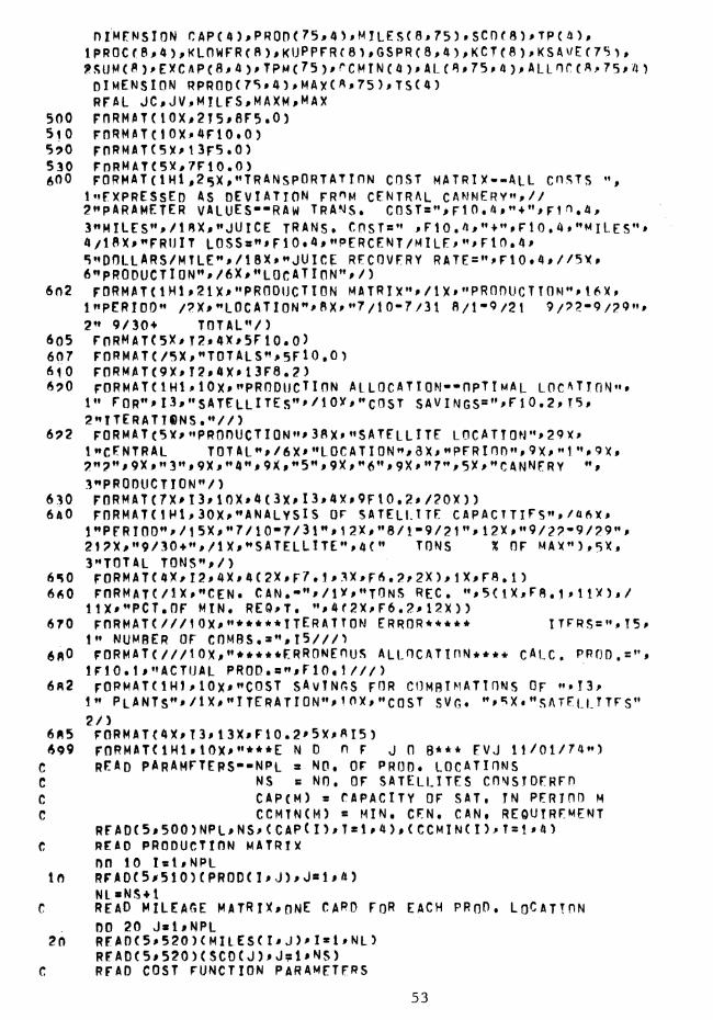
lPR0C(8>4),KLnwrR{fi)#KUPPrRr8)#GSPRC8,4)^KCT(B)íKSAy/EC7S>, ?>5;üM(í^)#EyCAP(8#A)#TPMC75>#rCMTM(4)f ALC8f 75*4)ÂLinrCí^^75#/n DIMENSION RPROO(7S#4)#MAXC8,75)#TSC4) RFAL JC#JV,MíLrS#MAXM^MAX

500 FnRMAT(lOX#2I5#eF5.0) 5l0 FORMATCíOX^4riO»0) 5^0 FnRMATC5XM3F5.0) 530 FDRMATC5X,7FíO,0) 600 F0RHAT(lHl,25X#"TRANSP0RTATinN COST MATRIX»«ALL Cn?^TS 'S

IMFXPRESSED AS DEVIATION FR'^H CENTRAL CAWNERY"*// ^«PARAMETER VALUES--RAW TRA^S* CnST = "# rl O • 4 ^ •' + »♦# Fl ^ • 4 , 3"MILES'N/ÍBX^"JUICE TRANS. COST«'' ^Fl O . 4^^ + 'NFÎ O • 4 f •'M iLES*'» 4/18X^♦'FRUIT L0SSs"tF10*4,"PERCENT/MlLFí"*Fl0,4# •Í^DOLLARS/MTLE^^/ISX^HJÜICE RECOVERY RATE = "JíF10# 4#//5Xf 6*^pR0DUCTl0N"#/6X#"L0rATl0N"#/)

602 FDRMATCÍHW21X> "PRODUCT ION MATRIX"^»/I X# "PRODUCT !0N"M6Xf INFERIDO« /?Xf*L0CATl0N"#8X#"7/10«7/31 8/1-9/21 9/72-9/2P"# 2'» 9/30+ TOTAL'V)

6o5 FORMÄT(5X#f2f4X#5F10.0) 607 FnRMATC/5X#"T0TAL$">5Fl0.0) 610 FnRMAT(9X#I2*4X*13F8.2) 6:>0 rORMATClHlulOXi'^PRODUCTION Al LOC AT I 0N-»OpT T MAL LOC^TTON"»

1" FOR^fn^^sATELLlTEs^'^^lOXí^cOST SAV I NGS = "Êi O • 2f T5# 2''TTERATTeNS**V/)

6P2 FORMAT (5X^ •♦PRODUCT 1 ON"# 38X» "SATELLITE LOC ATT0N"*29X# IwCENTRAL TOTAL"#/6X*"LOCATION''#3X*»'PERinD"#9X^"1"0 9X, 2*':?"#9Xf"3"#9Xj"4"#9Xf"5"f 9X^**6"#9X#"7"f5X^"ÇANNERY "f ^"PRODUCTION"/)

630 F0RMAT(7X#î3M0Xf4(3x#I3f4Xf9Fl0.Z#/20X)) 6A0 F0RMAT(1H1#30X#"ANÄLYSIS OF SATELLITE CAPACTTîFS"*/û6X>

l"PERIOD"#/l5X#"7/îO-7/3l"f 12X#"8/!*'9/2î"M2Xp"9/2»2-9/29"i 2î2X#"9/30+",/lX#"SATELLITE"^4(" TONS % OF MAX«)#5X, 3«T0TAL TONS"*/)

6S0 F0RMATC4X/I2#4X#4(2X,F7tî>3X*F6.2f2X)>1X#F8,Î) 660 FnRMÄTC/lXp"CENt C AN .••"#/l Xf "TONS REC "# 5< 1 X# F8 .1 # UX ) , /

ltX#"PCT,OF MIN. RE9#T. "#4f2X*F6.2M2X ) ) 670 FnRHAT(///îOX#"*****îTERATTON ERROR***** ÎTFRS="fî5#

1" NUMBER OF C0MBSta"#l5///) 680 FORMATC///10Xf"*****ERRONEnuS ALLOCATION**** CALC. PROD.s'îi

lFlOtl#"ÄCTUAL PR0Dto"fF10#î///) 682 FORMATCÎHÎ#10Xi'"COST SAvINGS FOR COMBlNATlONS OF »^J^P

!" PLANTS"'/1X#"ÏTERATI0N"*1OXJI"C0ST SVG« "'•îX."SATELLTTFS"

2/) 685 FORMÄT(4X#I3#13XfF10.2'5X#8I5) 699 FORMATdHlf ÎOX#''***E N D OF JO 8*** EVJ 11/01/74^)

C READ PARAMFTEPS--NPL a NO, OF PROD» LOCATIONS C NS « NO, OF SATELLITES CONSTDERFD C CAPCM) s CAPACITY OF SAT, IN PFRTOO M C CCMTN(M) = MIN, CEN, CAN, REQUIREMENT

READC5#500)NPL#NS#CCAP(n#T«î*4)#CCCMINCI)M = îi4) C READ PRODUCTION MATRIX

no 10 Isl*NPL to RFA0r5^510)tPR0D(I#J)#JBl#4)

NL«NS+l C READ MILEAGE MATRIXÔNE CARD FO« EACH PRoö, LQCATTON

DO 20 JaUNPL 20 RFAD(5Jí520)(MÍLES(Ií J)Î«1*NL)

REA0(5#520)(SC0(J)fJ?l^NS) C READ COST FUNCTION PARAMETERS

53

c c c c c c c

3n

50

57

5«

59 60

69

70

74

TA êO

SA

RPC RPV JC JV PIV PCTL

CALCUL nn 30 nn 30 MILES( l*MILrS no 40 MÎLESC EXPRFS

on 50 on 50 MÎLESC WRITE WRlTfC nn 55 WRîTrC nn 57 TP(M)s no 57 TP(M)is ATP«Ot on 56 GTpaST WRITE WRTTÜC nn 60 TPMCn on 59 TPMd) WRÏTEC WRiTrC

00 6? Nl«Nl* NCTsO NCTsNC ÎNÎTÎA

00 7?

fir«Ns- irCNr, N3»i on 74 N3«N3* NCOMsN r,n TO NCOMsl on 8ê KLOWER KÜPPER on 94 on 9?

«FIXED RAW HA »VARIABLE RAW «FIXED JUIOE »VARIARLE JUÎ «DOLLAR LOSS/ «PERCENT LOSS «JUICE RECOVE *530)RPC#RPVí ATE TRANSFER I«1>NS J«1#NPL liJ)=RPC+RPV* (IfJ>) *{JC4J I»1#NPL NL#n«(RPC*RP S COSTS AS OE

I«1#NL J«1#NPL I*J)«MILES(Nt TRANSFER COST 6#600)RPC^RPV J«Î#NPL 6#610)J#(MILE Mal#4 0.0 I«1#NPL TpCM)+PROOCIt 0 H8li4

P-^TPCM) PRODUCTION MA 6,6025 I«1#NPL a0»0 Mai,4 «TPMcn-^PRODC 6r605)I#(PR0D 6#607)(TPCj)i

IslfNS I

UllNG CnsT HAULINr, COST (PER MILE)

HAULING COST CF HAULING COST (PER MILE) MILE nUF TO FRUIT DAMAGE AND HOiniNG /MILE DUE TG FRUIT OftMAGF tHT) MOLOINQ RY RATE JC#JVfPI V#RR#PCTL COST MATRIX

MIL E S ( I. J ) + Ç R R * ( , 9 6 - PC T L / 10 0 » 0 ) V«SCD(n)4PLV*MILES(î,J)

V*MlLESfNLíI))+CPLV*MlLFSCNL*T)) VIATIONS FROM cENTAi. CANNERV CHSTS

*J)-^MUFS( WJ) MATRIX #JC#JV,PCTL,Pf V,RR

S(UJ)#I = !^NL>

M)

TRIX

I#M) CI#J),Jst,4),TPMCl) Jsl*45,GTP

T*l LIZE COMRINATION VARIARIES

IslíNCT I NCT EQ.OCO TO 76

I«t*NF I 1/CN:?*N3) ao

I alii NCT en«! CI)«NS-(NCT*I) Jsî#4 ISIJNS

54

97 GSPR(I*J)sO,0 94 r,SPR(NL*J)«TP(J)

GRTSeO.O ITFRsO.O Dn 100 J«t#NCT

100 KCT(J)«KLOWER(J) WRlTE(6i68?)NCT

102 ïTERelTFR^Î ; INITIALUE ITERATION VARIARLAS

TC»0.0 KCCTaO nn 700 Iel,NCT on 700 J«lfNPL KaKCTCn

700 MAX(K,J)«MTlESCKfJ) 00 705 !3l,NPL DO 705 M«1JI4

705 RPRODCIfM)3PR0D(I*M) on 707 M»W4 T5;(M)fi0.0 no 707 Isl#NL PRnC(I*M)»0,0 no 707 J»1#NPL

707 ÄLdf JíH)s0.0 : DFTERHîNE: LARGFST COST SAVTMGS ROUTE

7l0 MAXMBO.O T! SVsO nn 7?o islfNCT nn 7?o jsifNPi KeKCTCn TF CMAX(Kji»J).lF,MÄ>iM> GQ TO 720 MAXMsMAXCK^J) li SVsJ TSSVsK

7?o CONTINUF: C ASSIGNMENT

TFCILSV.FQ.O) GO TO Í2\ MAX(!SSV#îlSV)=-99 nn 740 Maîfa TF (RPROndLSVWn^FQ.O.O) Go Tn 740 Al CÎSSVilLSViM)sRPROnCÎlSV#M) PROCf ÎSSV*M)s=PROCCISSV'M) + RPRnO( ÎLSViM) TSCM>sTS(M)4RpR0DC!LSV#M) RPRQnClLSVfM)rO.O

c CHFCK FOR SAT. CAPACITY^ RFâSSîGN îF OVFR

îr(PROCCÎSSV#M),tE»CAP(M>) GD TO 730 EXsPROCCÎSSVfM)-CÂP(H)

GO TO 735 C CHFCK FOR CFN, CANNERY MÎN. REQT.i RFASSIGN IF UNCFR T:iO îr((TP{M)-TSCM)).GF»CCMîNCM)) GO TO 740

KCCT=KCCT41 FXsCCMÎN(M3-CTPiM5»TSCM))

7:^5 Al CISSV*ILSV#H)SÄLCISSV#IL5;V^M)-FX PRnCClSSV^M)sPROC(ISSV#M)-FX TSfM)=TSCM)-FX RPROOCllSViM)sRPRDDCÎLSVfM)+FX GO TO 730

740 CONTINUE nn 750 H=l,4

7S0 TCsTC4MîLESCISSVi ILSV)*AI (TSSVWLSV^M)

31)

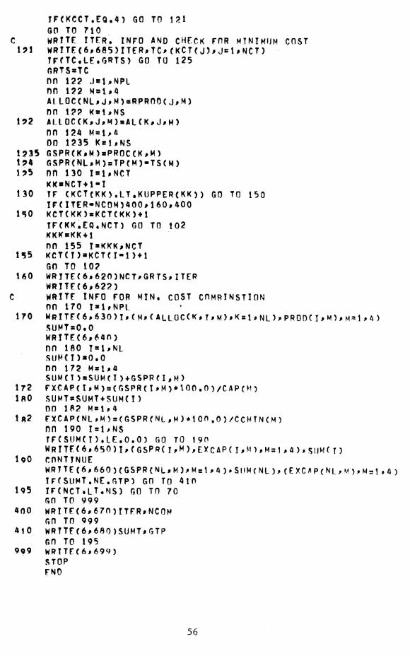
TFCKCCT.EQ.a) GO TO Í9A GO TO 710

C WRITF ITER. INFO ANO CHFCK FOR MlNlMiJN COST 1?1 WRlTF(6*685)nrRjTC#(KCT(j5#jBUNCT)

ÎFfTC.LF.GRTS) GO TO 125 fiRTS«TC on 122 JîßHPl nn 122 Matí4 ÄlLOC(NL*J#M)aRPRnnCJ#N) no 1?? K»i#NS

li>2 ÄLlOC(K^J,M)«AtCK#J#M) on 124 M=Wâ 00 1235 K«ÎjiNS

1?35 6SPR(KfM)sPR0CCK#M) ÎP4 GSPR<NL#M)sTP(M)-TSCM) 1:>5 on 130 IslfNCT

KK«NCT+1-I 130 TF <KCT(KK>.LT.KUPPER(KK)) GO TO 150

IFCITER«NCOM)400M60,400 mo KCT(KK)»KCTCKK) + 1

IFCKK.EQ.NCT) GO TO 102 KKKsKK+1 no 155 I»KKK^NCT

1"55 KCT(î)aKCT(î-î)tl GO TO 102

UO WRITF(6j620)NCT^GRTStlTER WRlTr(6^622)

:: WRITE INFO FOR MIN. COST COHRINSTION on iro laWNPi

170 WRlTFC6*630)I#CMi't ALLOC(Kiï,M)#K = l#NL)#PROnCliM>>M=l>/i) SUMTaO.O WRlTE(6#f4n} 00 180 laUNL SüM(n»0,0 DO 172 M»Ua SUMCT >aSUMÇl)4GSPRCI,M)

172 FXCAPCÎiM)={GSPRCl^H)*lOO,0)/CAPCM) 1«0 SUMTsSUMT'^SUMCn

00 162 H=l#4 lft2 F5iCAP(NL#M)a(GSPRCNL,M)*10n,0)/CCMTNCM)

on 190 lal^NS TFCSUM(T).LE.O.O) GO TO 190 WRlTE(6,650)I^(GSPRi I#M)ÊyCAP(I#M)^M=1,/|),snM(T)

IpO CONTINUE WRTTE(6#660)(GSPR(NL#M)#Ms:lM)#SllM(NL)^ C E XC AP (NL^ M ) * Msî . ¿i ) iFfSUMT.NE.GTP) GO TO 410

195 IFtNCT.LT.NS) GO TO 70 GO TO 999

400 WRlTF(é#670nTFR#NCOM GO TO 999

410 WRlTE(6#6aO)SÜMT*GTP GO TO 195

999 WRTTEC6#699) STOP FNO

56

Documents

DECENTRALIZED TOMATO PROCESSING: - AgEcon Search