ssssssras" - DTIC

°-'""~ " ISSN 0151 -1637

SCIENCE ET TECHNIQUE DU FROID COMPTES RENDUS

nt Kill - c(k i i> - i i i ~- ^ ^>; ex-, i

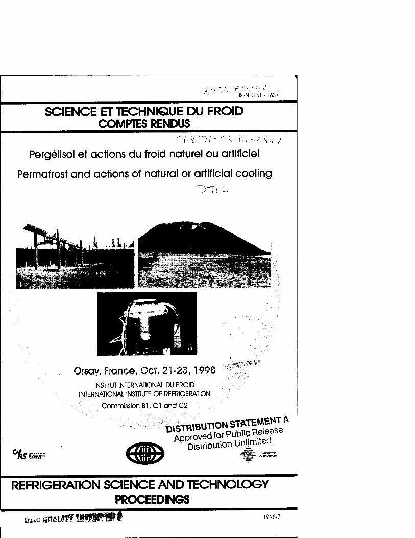
Pergelisol et actions du froid naturel ou artificiel

Permafrost and actions of natural or artificial cooling 91(c

°fx

Orsay, France, Oct. 21-23, 1998 INSTITUT INTERNATIONAL DU FROID

INTERNATIONAL INSTITUTE OF REFRIGERATION

Commission Bl, Cl and C2

• ..v^^'îÄ^V'

CÖHHENAUOJ1AL *7iifY*

■ssssssras" APPDistribution United

REFRIGERATION SCIENCE AND TECHNOLOGY PROCEEDINGS

DTio ®8Mm iwiw '« 1998/7

CAPTIONS OF THE PHOTOS ON THE COVER OF THESE PROCEEDINGS LEGENDES DES FIGURES DE LA COWERTVRE DE CE COMPTE RENDU

Photo 1: Arctic pipeline -Oleoduc arctique The Alaskan Pipeline between Prudhoe Bay and Puerto Valdez; length: 1200 km; pipe diameter: 1.22 m; temperature of the oil inside the pipe: 120°C; cost of the pipeline: 8 billion dollars (compared with a" projected cost of 900 million dollars); capacity: 2.5 million barrel per day (information provided by the Anchorage Museum, Alaska). Note the supporting piles: these piles also serve as heat pipes - the tops of the piles are fitted with heat exchangers in order to capture cold from the atmosphere in winter, ensuring that the ground remains super-frozen, increasing its bearing capacity. Note also the beams/runners system that prevents thermal dilatation and earthquake damage (Photo by J. Aguirre-Puente taken North of Fairbanks in July 1993). Oleoduc "Alaskan Pipeline" entre Prudhoe Bay et Puerto Valdez ; longueur, 1200 km ; diametre du conduit, 1,22 m ; temperature dupetrole ä l'interieur du conduit, 120°C ; coüt de l'ouvrage, 8 milliards de dollars contre 900 millions prevus ; capacite de transport, 2,5 millions de barils par jour (informations du Musee d'Anchorage, Alaska). On remarque les pieux qui supportent le conduit. Ces pieux sont en meme temps des caloducs, avec les echangeurs thermiques au sommet pour capturer le froid de l'atmosphere pendant l'hiver, de moniere ä surgeler le sol pour lui apporter de la portance. On note egalement le Systeme poutres/patins de glissement qui permet d'encaisser les dilatations thermiques et les deformations dues awe tremblements de terre (Photo J. Aguirre-Puente, au nord de Fairbanks, juillet 1993).

Photo 2 : Pingo One of the biggest pingos in the Toktoyaktuk Peninsula in Northern Canada (diameter: 600 m; height: about 48 m; age: several hundred years). Pingo: a periglacial geomorphological formation arising in certain zones with very specific characteristics; pingos arise where water is converted into ice under high hydrostatic pressure conditions (open system), due to a change in specific volume when water is converted into ice in confined talik domains and/or because cryogenic suction takes place (closed system) (Photo J. Aguirre- Puente). Un des plus grands "pingos" de la peninsule de Toktoyaktuk au Nord du Canada (diametre, 600 m ; hauteur : 48 m environ ; age : plusieurs centaines d'annees). Pingo : formation geomorphologique periglaciaire apparaissant dans certaines zones tres particulieres en raison de la transformation en glace de l'eau arrivant par pressions hydrostatiques elevees (systeme ouvert), en raison du changement de volume massique lors de la transformation de l'eau en glace dans des domaines de talik confines et/ou en raison de la succion cryogenique (systeme ferme) (Photo J. Aguirre-Puente).

Photo 3 : Experimental cell - Cellule experimentale First vizualization of ice lenses in the laboratory, during a freezing experiment under controlled conditions, with measurement of parameters exhibiting the behaviour of the frozen sample ("Freezing" Group of the Laboratoire d'Aerothermique, CNRS in the 1970s. Photo J. Aguirre-Puente). Premiere visualisation des lentilles de glace, en laboratoire, lors d'une experimentation de congelation sous des conditions contrölees, avec des mesures des parametres decrivant le comportement au gel de 1'echantillon (Groupe "Congelation" du Laboratoire d'Aerothermique du CNRS aux annees 70. Photo J. Aguirre-Puente).

ISBN n° 2-913149-04-9

For the full or partial reproduction of anything published in this book proper acknowledgment should be made to the original source. Any opinions expressed herein are entirely those of the authors.

La reproduction totale ou partielle de tout ce qui paraii dans ce livre est autorisee sous reserve de la citation precise de la source originale. Les opinions emises dans cettepublication n'engagent que leurs auteurs.

AD NUMBER DATE

REPORT IDENTIFYING INFORMATION

A. ORIGINATING AGENCY ^

B. REPORT TITLE ANO/OR NUMBER iäflmti FJiCS f

C. MONITOR REPORT NUMBER

DTIC ACCESSION NOTICE

D. PREPARED UNDER CONTRACT NUMBER

2. DISTRIBUTION STATEMENT

RPPROUED FOH PUBLIC HELEHSE

DISTRIBUTION UNLIMITED

PROCEEDINGS DTL

REQ

1. Pu on

2. Cot

3. Am m,

4. Us, in

5. Do k

Ml 1. A

2. R

cxj

DITIONS ARE OBSOLETE

rjff Tl\8$W.Gf$& %

REFRIGERATION SCIENCE AND TECHNOLOGY SCIENCE ET TECHNIQUE DU FROID

PERGELISOL ET ACTIONS DU FROID NATUREL OU ARTIFICIEL

PERMAFROST AND ACTIONS OF NATURAL OR ARTIFICIAL COOLING

Proceedings of the conference of: Compte rendu de la conference des .

Commissions Bl, Cl et C2 (October 21-23, 1998)

ORSAY, France 1998/7

DISTRIBUTION STATEMENT A Approved for Public Release

Distribution Unlimited

Issued by / Edite par

INTERNATIONAL INSTITUTE OF REFRIGERATION INSTITUT INTERNATIONAL DU FROID

177, boulevard Malesherbes - F-75017 PARIS, France Tel.: +33 1 4227 3235 -Fax: +33 1 4763 1798 -Web site: www.iifiir.org

20000616 079

!V\iirAr

Conference de l'lnstitut International du Froid (IIF/IIR) Conference of the International Institute of Refrigeration (IIF/IIR)

Commissions Bl, Cl, C2

PERGELISOL ET ACTIONS DU FROID NATUREL OU ARTIFICIEL PERMAFROST AND ACTIONS OF NATURAL OR ARTIFICIAL COOLING

21-23 octobre 1998 / October 21-23, 1998

Auditorium du Läboratoire de l'Accelerometre Lineaire Bat. 200 du Campus de l'Universite de Paris Sud, 91405 Orsay, France

Organise par le C.N.R.S. / Organized by the C.N.R.S.

UMR«) 8616"Orsayterre" CNRS/Universite de Paris Sud, 91405 Orsay, France

UMR 113 "Läboratoire des materiaux et de structures du genie civil", LCPC /CNRS, 77420 Champs sur Marne, France

GDR(2) 49"Recherches Arctfques", 25030 Besangon, France

avec / with

Association Francaise du Froid, Association Francaise du Pergelisol, Läboratoire Central des Ports et Chaussees (LCPC), Universite Pierre et Marie Curie, Universite de Paris Sud, Industrie

SPONSORS

-CAPRICELPrevoyance - Departement Scientifique SDU(3> - INSLK4) du CNRS - European Research Office of the US Army - GDR 49 du CNRS "Recherches Arctiques" - Groupe CRI - IRPELEC Prevoyance - Universite de Paris Sud

(3)

Unite Mixte de Recherche Groupe de Recherche Sciences de l'Univers Institut National des Sciences de l'Univers

TABLE DES MATIERES TABLE OF CONTENTS

Comite Scientifique / Scientific Committee 7 Liste des participants / List of participants 8 Foreword / Preface 10-11 Introduction 12

SECTION 1 COMPORTEMENT AU GEL DES

MILIEUX DISPERSES BEHA VIOUR OF FREEZING

DISPERSED MEDIA

RAMOS M, AGUIRRE-PUENTE J., SANZ P.D., POSADO CANO R, De ELVIRA C. - Solidification du cyclohexane par conduction de la chaleur pour des nombres de Stefan eleves Cyclohexane solidification by heat conduction for high Stefan numbers.

15

KIM H.K., FUKUDA M. - Experimental study on the evaluation of reducing method of total heave amounts using granulated tire-soil mixture 26 Etude experimentale d'une methode visant ä reduire les soulevements totaux et consistant ä melanger du caoutchouc granuleux au sol.

CHUVILIN EM., ERCHOV ED., MURASHKO A.A. - Transformation of sapropel in the process of freezing 34 Transformation du sapropel au cours du processus de congelation.

ISHIZAKIT. - Experimental study of frost deterioration process of porous materials during freezing 41 Etude experimentale du processus de deterioration du gel dans des materiaux poreux au cours de la congelation.

WHITE T.L., WILLIAMS P.J. - Soil microstructure, thermal, hydraulic and other properties and ground behaviour in cold regions 46 Microstructure du sol - proprietes thermiques, hydrauliques et autres et comportement du terrain dans les regions froides.

CHEN X., MITUNO T. - A new method to deal with the ice formation and melting on the simulation of the soil freezing and thawing processes infield 57 Une nouvelle methode pour integrer la formation et lafonte de la glace dans la simulation des processus de gel/degel du sol dans les champs.

GUY B. - Self-organized columnar morphology at millimeter scale of ice crystals frozen from mud: preliminary observations 65 Morphologie colonnaire ä Vechelle millimetrique de cristaux de glace formes par congelation de boue : observations priliminaires.

SECTION II PROCEDES, PROPRIETES PHYSIQUES

ET METROLOGIE PROCESSES, PHYSICAL PROPERTIES

AND METROLOGY

FROLOV A.D. - Plenary lecture: Prospects of various physical fields applications to study of frozen soils 73 Perspectives de plusieurs applications de champs physiques ä I 'etude des sols geles.

FROLOV A.D., FEDUKIN I.V., ZYKOV Y.D. - Main characteristics of saline frozen soils 79 Les particularites essentielles des sols salins geles.

DOMlNGUEZ M., PINILLOS J.M., GUTIERREZ P., LOPEZ N. - ADC: New system for the measure of specific heat, thermal conductivity and enthalpy (A.D.C.) 87 Nouveau Systeme de calorimetrie differentielle analogique (ADC) pour la mesure de la chaleur specifique, de la conducttviti thermique et de I 'enthalpie.

COTE H., THIMUS J.F. - Analysis of rocks behaviour at low temperature during Brazilian tests with ultrasonic waves Analyse du comportement des roches ä basses temperatures pendant un essai hresilien ä l'aide des signaux ultrasoniques.

95

CHEN X., HORINO H. - Three methods including TDR method to measure frozen or thawed depth of soil infield 104 Trois methodes, dont la methode TDR, pour mesurer la profondeur ä laquelle le sol gele ou degele dans les champs.

SHENG Y., FUKUDA M., INAMURA T. - The effect of unfrozen water content on dynamic properties of partially frozen soil 112 Effet d 'une teneur en eau non congelee sur les proprietes dynamiques d 'un sol. partiellement gele.

CHERVINSKAYA O.P., FROLOV A.D., ZYKOV Y.D. - On the acoustic testing of saline frozen soils strength characteristics 120 Methode acoustique de l'estimation de la solidite des sols salins geles.

BOREL S., BRZOSKA J.B. - Study of the behaviour of a snow layer deposited on the pavement: physical characterization of the snow/pavement interface 126 Caracterisation physique de Vinterface neige/chaussee ä partir de l'observation.

GOLUBEV V.N. - Ice formation in freezing of water-nonsaturated grounds 132 Formation de glace lors de la congelation des sols non satures en eau.

FROLOV A.D., GOLUBEV V.N. - Particularities of structure and some mechanical properties of ice frozen over the solids ; 139 Particularites de la structure et quelques proprietes mecaniques de I 'eau congelee formee sur des solides.

SECTION III

MODELISATION PHYSIQUE OU MATHEMATIQUE

PHYSICAL OR MATHEMATICAL MODELLING

DOMlNGUEZ M., ARIAS J.M., GARCJA C, BARRAGÄN M.V. - Solution of heat transmission equation including the phase change through computerized electrical analogy 149 Resolution de I 'equation de transmission de chaleur incluant le changement de phase par analogie electrique informatisee.

DJABALLAH-MASMOUDIN., AGUIRRE-PUENTE J. - Modelling and experimentation of the transfer mechanism in porous media during freezing 154 Modelisation et experimentation des mecanismes de transfert dans les milieux poreux au cours du gel.

POSADO CANO R, AGUIRRE-PUENTE J., COSTARD F. - Probleme de Stefan : une nouvelle methode approchee - Application au talik en zone periglaciaire 162 Problem of Stefan: a new approach method - Application to talik in periglacial areas.

POSADO CANO R, RAMOS M, AGUIRRE-PUENTE J. - Probleme de frontieres libres : modelisation, etudes experimentales, melanges eutectiques 171 Free boundary problems: modelling, experimental studies, binary eutectic mixtures.

CAMPANONE LA., SALVADOR! V.O., MASCHERONI R.H. - Modelling and

simulation of heat and mass transfer during freezing and storage of unpacked foods 180 Modelisation et simulation des transports de chaleur et de masse durant la congelation et le stockage de produits sans emballage.

GEOFFROY S., MERGUI S., BENARD C, GOBIN D. - Fusion de glace pure dans une solution saline 188 Melting of pure ice in an aqueous binary solution.

LASSOUED R., LABBE L., FREMOND M., DUPAS A. - Modelisation de la temperature de surface d'une Chaussee ä courte echeance 195 Modelling of the surface temperature of a pavement for a short lapse of time.

SECTION IV

PERGELISOL, POLLUTION ET CHANGEMENTS PLANETAIRES

PERMAFROST, CONTAMINATION AND GLOBAL CHANGE

LAD ANY B. - Plenary lecture: Effects of climate warming on engineering structures in permafrost regions 205 Effets du rechauffement du climat sur les structures d'ingenierie des regions avec pergelisol.

DYSLI M. - Loss of bearing capacity of roads during thaw and debris flows in mountain permafrost: the same phenomenon 208 Formation des laves torrentielles dans les pergelisols alpins et perte de portance au degel des fondations de routes : un meme phenomene.

GAYG., AZOUNI M.A. -An approach of soils cryoremediation 217 Approche de la cryo-depollution des sols.

ANISIMOVA N.P., KURCHATOVA A.N. - Changes in temperature regime and associated effects on anthropogenic salinity of permafrost (Central Yakutia) 225 Modifications du regime de temperature et effets associes sur la salinite anthropogenique du pergelisol (Yakutia central).

INSTANES D., INSTANES A. - Frozen ground temperature profiles at Svalbard airport, Spitsbergen 229 Profils de temperature du sol gele ä I 'aeroport de Svalbard, Spitsbergen.

MARCHAND Y., REES G. - Applications of remote sensing to oil contamination of frozen terrain 238 Applications de la teledetection au contröle de la pollution due aupetrole dans des terrains geles.

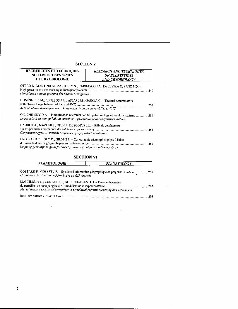
SECTION V

RECHERCHES ET TECHNIQUES SUR LES ECOSYSTEMES

ET CRYOBIOLOGEE

RESEARCH AND TECHNIQUES ON ECOSYSTEMS

AND CRYOBIOLOGY

OTERO L., MARTINO M., ZARITZKY N., CARRASCO JA., De ELVIRA C, SANZ P.D. - High pressure assisted freezing in biological products 249 Congelation ä haute pression des milieux biologiques.

DOMINGUEZ M., PINILLOS J.M., ARIAS J.M., GARCIA C. - Thermal accumulators with phase change between-21°C and40°C 253 Accumulateurs thermiques avec changement de phase entre -21 "C et 40°C.

GILICHINSKY DA. - Permafrost as microbial habitat: palaeontology of viable organisms 259 he pergelisol en tant qu 'habitat microbien : paleontologie des organismes viables.

BAUDOT A., MAZUER J., ODIN J., DESCOTES J.L. - Effet de confinement sur les proprietes thermiques des solutions cryoprotectrices 261 Confinement effect on thermal properties of cryoprotective solutions.

BROSSARD T., JOLY D., NILSEN L. - Cartographie geomorphologique ä l'aide debases dedonnees geographiques en haute resolution 269 Mapping geomorphological features by means of a high resolution database.

SECTION VI

| PLANETOLOGIE | PLANETOLOGY \

COSTARD F., GÖSSET J.P. - Systeme d'information geographique de pergelisol martien 279 Ground-ice distribution on Mars bases on GIS analysis.

MAKHLOUFIN, COSTARD F., AGUIRRE-PUENTE J. - Erosion thermique du pergelisol en zone periglaciaire : moderation et experimentation 287 Fluvial thermal erosion of permafrost in periglacial regions: modelling and experiment.

Index des auteurs / Authors Index 296

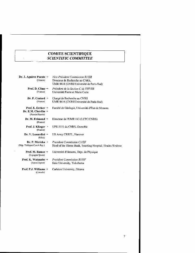
COMITE SCIENTIFIQUE SCIENTIFIC COMMITTEE

Dr. J. Aguirre Puente - (France)

Prof. D. Come (France)

Dr. F. Costard (France)

Prof. E. Erchov Dr. E.M. Chuvilin -

(Russie/Russia)

Dr. M. Fremond - (France)

Prof. J. Klinger - (France)

Dr. V. Lunardini - (USA)

Dr. P. Mericka (Rep. Tcheque/Czec/i Rep.)

Prof. M. Ramos - (Espagne/S/ram)

Prof. K. Watanabe - (Sapon/Japan)

Prof. P.J. Williams - (Canada)

Vice-President Commission BJ/IIR

Directeur de Recherche au CNRS, UMR 8616 (CNRS/Universite de Paris-Sud)

President de la Section C de l'IIF/IIR Universite Pierre et Marie Curie

Charge de Recherche au CNRS UMR 8616 (CNRS/Universite de Paris-Sud)

Faculte de Geologie, Universite d'Etat de Moscou

Directeur de l'UMR 113 (LCPC/CNRS)

UPR 5151 du CNRS, Grenoble

US Army CRREL, Hanover

President Commission Cl/IIF

Head of the Tissue Bank, Teaching Hospital, Hradec Kralove

Universite d'Henares, Dept. de Physique

President Commission Bl/IIF Keio University, Yokohama

Carleton University, Ottawa

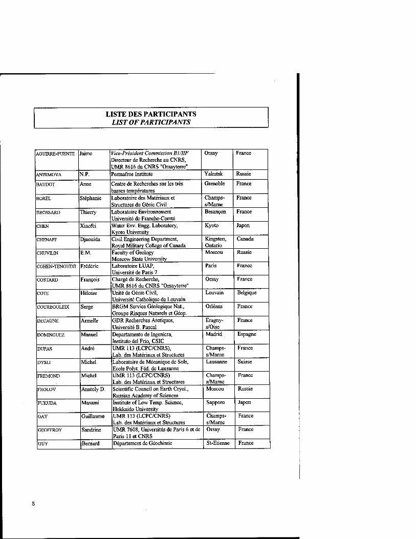
LISTE DES PARTICIPANTS LIST OF PARTICIPANTS

AGUIRRE-PUENTE Jaime Vice-President Commission Bl/IIF Directeur de Recherche au CNRS, UMR 8616 du CNRS "Orsayterre"

Orsay France

AN1SIMOVA N.P. Permafros Institute Yakutsk Russie

BAUDOT Anne Centre de Recherches sur les tres basses temperatures

Grenoble France

BOREL Stephanie Laboratoire des Materiaux et Structures du Genie Civil

Champs- s/Marne

France

BROSSARD Thierry Laboratoire Environnement Universite de Franche-Comte

Besancon France

CHEN Xiaofei Water Env. Engg. Laboratory, Kyoto University

Kyoto Japon

CHENAFF Djaouida Civil Engineering Department, Royal Military College of Canada

Kingston, Ontario

Canada

CHUVILIN E.M. Faculty of Geology Moscow State University

Moscou Russie

COHEN-TENOUDJ1 Frederic Laboratoire LUAP, Universite de Paris 7

Paris France

COSTARD Francois Charge de Recherche, UMR 8616 du CNRS "Orsayterre"

Orsay France

COTE Heloise Unite de Genie Civil, Universite Catholique de Louvain

Louvain Belgique

COURBOULEDC Serge BRGM Service Geologique Nat., Groupe Risques Natureis et Geop.

Orleans France

DECAUNE Armelle GDR Recherches Afctiques, Universite B. Pascal

Eragny- s/Oise

France

DOMTNGUEZ Manuel Departamento de Ingeniera, Instituto del Frio, CSIC

Madrid Espagne

DUPAS Andre UMR113(LCPC/CNRS), Lab. des Materiaux et Structures

Champs- s/Marne

France

DYSLI Michel Laboratoire de Mecanique de Sols, Ecole Polyt. Fed. de Lausanne

Lausanne Suisse

FREMOND Michel UMR113(LCPC/CNRS) Lab. des Materiaux et Structures

Champs- s/Marne

France

FROLOV Anatoly D. Scientific Council on Earth Cryol., Russian Academy of Sciences

Moscou Russie

FUKUDA Masami Institute of Low Temp. Science, Hokkaido University

Sapporo Japon

GAY Guillaume UMR113(LCPC/CNRS) Lab. des Materiaux et Structures

Champs- s/Marne

France

GEOFFROY Sandrine UMR 7608, Universites de Paris 6 et de Paris 11 et CNRS

Orsay France

GUY Bernard Departement de Geochimie St-Etienne France

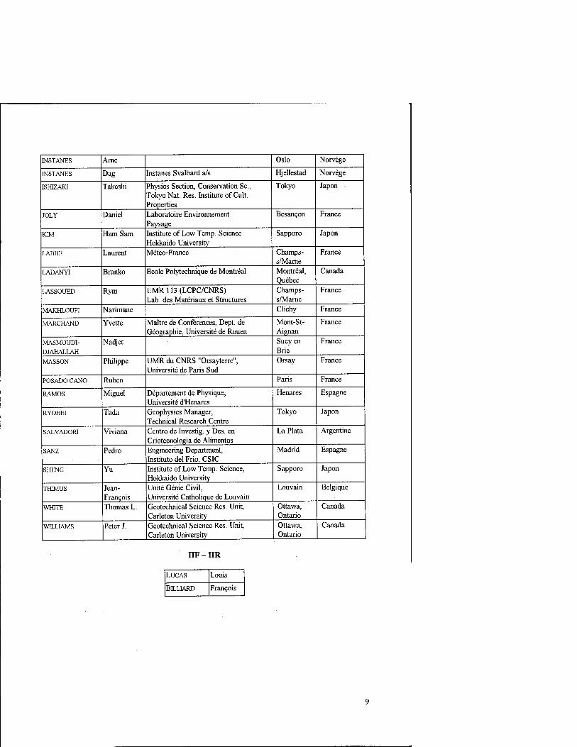
INSTANES Arne Oslo Norvege

INSTANES Dag Instanes Svalbard a/s Hjellestad Norvege

ISHIZAKI Takeshi Physics Section, Conservation Sc, Tokyo Nat. Res. Institute of Cult. Properties

Tokyo Japon

JOLY Daniel Laboratoire Environnement Paysage

Besancon France

KIM Ham Sam Institute of Low Temp. Science Hokkaido University

Sapporo Japon

LABBE Laurent Meteo-France Champs- s/Marne

France

LADANYI Branko Ecole Polytechnique de Montreal Montreal, Quebec

Canada

LASSOUED Rym UMR113(LCPC/CNRS) Lab. des Materiaux et Structures

Champs- s/Marne

France

MAKHLOUFI Narimane Clichy France

MARCHAND Yvette Maitre de Conferences, Dept. de Geographie, Universite de Rouen

Mont-St- Aignan

France

MASMOUDI-

DJABALLAH

Nadjet Sucy en Brie

France

MASSON Philippe UMR du CNRS "Orsayterre", Universite de Paris Sud

Orsay France

POSADO CANO Ruben Paris France

RAMOS Miguel Departement de Physique, Universite d'Henares

Henares Espagne

RYOHEI Tada Geophysics Manager, Technical Research Centre

Tokyo Japon

SALVADORI Viviana Centre de Investig. y Des. en Criotecnologia de Alimentos

La Plata Argentine

SANZ Pedro Engineering Department, Institute del Frio, CSIC

Madrid Espagne

SHENG Yu Institute of Low Temp. Science, Hokkaido University

Sapporo Japon

THMUS Jean- Francois

Unite Genie Civil, Universite Catholique de Louvain

Louvain Belgique

WHITE Thomas L. Geotechnical Science Res. Unit, Carleton University

Ottawa, Ontario

Canada

WILLIAMS Peter J. Geotechnical Science Res. Unit, Carleton University

Ottawa, Ontario

Canada

nF-nR

LUCAS Louis

BILLIARD Francois

FOREWORD

The idea of organizing a conference on natural freezing took shape within Commission Bl (Thermodynamics and transfer processes) of the IIR in 1995, during the 19th International Congress of Refrigeration held in The Hague, Netherlands. Following consultations with the management of the International Institute of Refrigeration and Presidents of Commissions and Section C, we decided to set up the scientific programme. Our aim was to keep this event as broad and focused as possible: we were aware that natural freezing and use of this phenomenon involved many scientific fields and technologies. We also knew that the use of natural freezing involved a wide range of problems that can only be addressed by acquiring basic knowledge.

The wide range of problems is obvious when one considers needs in terms of knowledge of freezing of dispersed water-containing media that are subjected to temperatures below 0°C in such widely different fields as geomorphology, civil engineering, food technology and cryosurgery. Moreover, it is increasingly becoming necessary to exploit energy resources in polar regions; however, a considerable degree of danger involved in such destruction of the environment because permanently frozen ground is present, and also because permafrost soil's thermomechanical equilibrium is fragile. The fragility of this medium, the extreme climatic conditions encountered in these regions and risk management are major stakes for industrial and governmental users.

Given this context and the complexity of the cryogenic phenomena encountered, we felt that it was vital to invite to this event industrialists, engineers, researchers, and persons involved in all other fields in which natural freezing needed to be addressed or in which natural or artificial freezing was required. Around forty-five specialists from the following countries attended the conference: Argentina, Belgium, Canada, France, Japan, Norway, Russia, Spain, Switzerland and United Kingdom. These proceedings contain 36 reports, of which summaries of plenary addresses given by globally renowned specialists: Anatoly Frolov, Branko Ladanyi and Philippe Masson. We seize this opportunity to thank them for their presentations and comments on current freezing-related issues: the use of physics in metrology in the frozen-ground field, the environment, the permafrost on Mars. We have placed papers in several chapters dealing with themes as varied as the behaviour of frozen ground, the effects of cold in civil engineering and planetology, as well as preservation of foodstuffs or biological tissues and physical, mathematical and digital modelling.

We would also like to seize this opportunity to cordially thank the management and staff at the International Institute of Refrigeration for their continual support and assistance enabling this event to be held, thus bringing together specialists in the field of freezing with a common cause. We are also extremely grateful for the promotion performed by the C.N.RS. (Centre National de Recherche Scientifique), the University and L.C.P.C, who, thanks to UMR "Orsayterre", the "Laboratoire des materiäux et de structures du Genie Civil [Civil-Engineering Materials and Structures Laboratory]" research unit and the "Recherches Arctiques [Arctic Research] " research unit, also promoted this conference. We would also like to thank the sponsors who contributed to the success of the event, particularly: Capricel Prevoyance, Departement Scientifique SDU-I.N.S.U. of the C.N.R.S., European Research Office of the US Army, GDR "Arctic Research]", Groupe CRI Irpelec Prevoyance and the Universite de Paris Sud.

Finally, I'd like to thank the colleagues and departments at our laboratory who made material contributions (in the field and during discussions) enabling this event to be held.

Jaime AGUIRRE-PUENTE Chairman of the Conference

10

PREFACE

L'idee d'organiser une conference sur le froid naturel s'est concretisee au sein de la Commission Bl (Thermodynamique et processus de transfert) de l'IIF, lors du 19°"* Congres International du froid qui s'est tenu ä La Haye (Pays-Bas) en 1995. Apres un travail de reflexion, en collaboration avec la Direction de l'lnstitut International du Froid et les Presidents des Commissions de la Section C, nous avons decide d'etablir le programme scientifique suivant une ligne directrice un tant soit peu ambitieuse. En effet, nous avons voulu teinter ce colloque d'un esprit multidisciplinaire et de synthese, inspire par le fait que dans beaucoup de disciplines scientifiques et techniques, le froid naturel d'une part, et l'utilisation du froid artificiel d'autre part, posent des problemes tres divers qui necessitent systematiquement des connaissances fondamentales.

La diversite des problemes est manifeste si l'on considere que les besoins de connaissance sur la congelation des milieux disperses contenant de l'eau et soumis ä des temperatures inferieure ä 0°C existent dans des domaines aussi diversifies que la geomorphologie, le genie civil, le genie agroalimentaire ou la cryochirurgie. Par ailleurs, l'exploitation des richesses energetiques des regions polaires devient de plus en plus necessaire, mais les dangers poses par la destruction de l'environnement sont considerables en raison de la presence de sols constamment geles et de l'equilibre thermomecanique precaire du pergelisol. Cette fragilite du milieu, les conditions climatiques extremes de ces regions et la maitrise des risques sont ä la base des grands enjeux des milieux industriels et gouvernementaux.

Compte tenu de ce contexte et de la complexity des phenomenes cryogeniques rencontres, il nous a paru indispensable d'inviter ä ce colloque les industriels, les ingenieurs, les chercheurs, et toutes les autres disciplines devant se defendre contre le froid naturel ou devant utiliser le froid naturel ou artificiel. L'Argentine, la Belgique, le Canada, l'Espagne, la France, le Japon, la Norvege, le Royaume-Uni et la Russie et la Suisse ont ete representes par 45 specialistes environ qui ont participe ä ce colloque. Ces comptes rendus contiennent les rapports de 36 communications dont des resumes etendus des conferences plenieres faites par des specialistes de renommee mondiale: Anatoly Frolov, Branko Ladanyi et Philippe Masson, que nous remercions pour leur disponibilite et leurs commentaires sur des problemes tres actuels concernes par le froid : Putilisation de la physique en metrologie des sols geles, l'environnement, le pergelisol martien. Nous avons groupe les contributions en plusieurs chapitres allant de la description du comportement des sols geles ä la presence du froid en Genie Civil ou en Planetologie, en passant par la conservation des denrees ou tissus biologiques et la modelisation physique, mathematique et numerique.

Nous remercions tres chaleureusement la direction et les equipes de l'lnstitut International du Froid qui nous ont toujours encourage dans notre projet et qui ont fourni une plate forme adequate pour la reunion de ce groupe de specialistes du froid animes par le meme esprit. Notre profonde reconnaissance est aussi dirigee vers le C.N.R.S., l'Universite et le L.C.P.C, qui, par intermediate de l'UMR « Orsayterre», l'UMR « Laboratoire des materiaux et de structures du Genie Civil» et le GDR « Recherches Arctiques », ont promu ce colloque. Nous remercions egalement les divers sponsors qui ont contribue ä la reussite de cette manifestation, en particulier : Capricel Prevoyance, Departement Scientifique SDU-I.N.S.U. du C.N.R.S., European Research Office of the US Army, GDR « Recherches Arctiques », Groupe CRI Irpelec Prevoyance et Universite de Paris Sud.

Enfin, merci ä tous nos collegues et services de notre laboratoire qui sur le terrain ou au cours des discussions, ont participe intellectuellement et materiellement ä la realisation de ce colloque.

Jaime AGUIRRE-PUENTE President de la Conference

11

INTRODUCTION

Ce document est le compte rendu de la Conference de la Commission Bl (Thermodynamique et processus de transfert), avec les Commissions Cl et C2 de 1'IIF, sur le theme "Pergelisol et actions du froid naturel et artificiel". C'est la premiere fois que 1'IIF organise une conference sur le pergelisol.

Ce sont des specialistes de 10 pays qui se sont reunis pendant 3 jours pour traiter: - du comportement au gel des milieux disperses ; - des proprietes des sols geles, des methodes de mesure et de nombreuses applications ; - de la modelisation de ces phenomenes ; - des effets du rechauffement de la planete et des pollutions diverses sur le pergelisol; - des problemes de cryobiologie lies au pergelisol; - et enfin de pergelisol sur la planete Mars. En definitive, ce sont 36 rapports qui, reunis dans ce compte rendu, presentent l'etat de l'art sur ce sujet eminemment important.

L'HF adresse au Professeur Jaime Aguirre Puente, President du Colloque et aujourd'hui Membre d'Honneur de 1'IIF, ä tous les organismes et aux personnes qui ont participe ä la reussite de cette conference, ses bien sinceres remerciements et ses chaleureuses felicitations. Ces remerciements vont aussi ä Louis Lucas, Directeur de 1'IIF lors de la tenue de cet evenement, qui avec M. Aguirre Puente, a eu l'idee du theme de cette conference.

Souhaitons que cette lere conference de 1'IIF sur le pergelisol soit ä l'origine d'une Serie de conferences tenues periodiquement sur le meme sujet.

Francois BILLIARD, Directeur de 1'IIF

This book comprises the proceedings of the conference on "Permafrost Soil and Natural Freezing" involving Commission Bl (Thermodynamics and transfer processes), with Commissions Cl and C2 of the IIR. This was the first conference on permafrost soil organized by the IIR.

Specialists from 10 countries took part in this 3-day event dealing with: - freezing of dispersed media: behaviour; - properties of frozen ground, measurement methods and numerous applications; - modelling of these phenomena; - effects of global warming and various types of pollution on permafrost soil; - cryological issues related to permafrost soil; - permafrost soil on Mars. The 36 papers comprising these proceedings represent the state of the art in this highly important field.

The IIR cordially thanks and warmly congratulates Professor Jaime Aguirre Puente, Chairman of this conference and now Honorary Member of the IIR, and all organizations and persons who ensured that this conference was successful. We also expend our thanks to Louis Lucas, Director of the IIR when this event was held; Louis Lucas and Prof. Aguirre Puente were the instigators of this conference.

Let's hope that this first IIR conference on permafrost soil will be the first in a series of events covering this field.

Francois BILLIARD, Director of the IIR

12

SECTION I

COMPORTEMENT AU GEL DES MILIEUX DISPERSES

BEHAVIOUR OF FREEZING DISPERSED MEDIA

SOLIDIFICATION DU CYCLOHEXANE PAR CONDUCTION DE LA CHALEUR POUR DES NOMBRES DE STEFAN ELEVES

RAMOS M. (1), AGUIRRE-PUENTE J. (3), SANZ P.D. (2), POSADO CANO R. (3), De ELVIRA C. (2)

(1) Departamento de Fisica, Universidad de Alcalä, 28871 Alcalä de Henares, Spain (2) Institute del Frio, C.S.I.C, Ciudad Universitaria, 28040 Madrid, Spain (3) Groupe de Planetologie, UMR 8616 du C.N.R.S. "OrsayTerre", 91405 Orsay, France

RESUME

On realise une &ude experimentale de la solidification unidimensionnelle du cyclohexane pour une geometrie plane semi-infmie avec une temperature constante sur la paroi froide en x=0. Le choix du cyclohexane permet d'&udier le ph^nomene de conduction de la chaleur avec changement d'etat pour des nombres de Stefan eleves, St e[0.96, 2.70]. L'etude experimental et numerique du processus de transfert de chaleur, fondamentalement par conduction, conduit ä des räsultats qui, de maniere surprenante, s'öcartent de ceux obtenus par la resolution exacte du Probleme de Stefano Cinq experiences de solidification distinctes sont presentees et la loi horaire, experimentale et numerique, ainsi qu'une discussion des rösultats obtenus. Finalement, on etablit, ä partir de considerations physiques, une fonction empirique du mouvement du front de solidification qui rend compte des resultats observes.

INTRODUCTION

L'&ude de la diffusion de la chaleur avec changement de phase et ses applications ont connu un sensible regain d'int&et pendant ces dernieres decennies (Lunardini, 1991). Du point de vue theorique, un effort a 6te fait pour r6soudre analytiquement certains problemes de changement de phase (Shamsundar and Sparrow, 1974, Oliver and Sunderland, 1987, Frederick and Greif, 1985, Tao, 1981, Cerrato et al, 1989) ainsi que pour developper des codes de calcul afin d'obtenir des resultats numenques approches (Hibbert et al, 1988, Wu et al, 1989, Raynaud and Beck, 1988). Le probleme des substances non pures, comme les substances eutectiques, est pos6 dans divers domaines tels que la metallurgie, le stockage d'energie thermique ou la congelation d'aliments (Sparrow et al, 1986, Beckerman and Viskanta, 1988, Gau and Viskanta, 1984, Burns et al, 1992). L'etude du changement de phase dans ces cas introduit un degre" de difficulte supplementaire. Meme avec des conditions aux limites et conditions initiales simples, il n'existe qu'un nombre tres reduit de solutions analytiques exactes (Lunardini, 1991, Ramos et al, 1994). II faut par consequent avoir pratiquement toujours recours aux solutions approchees ou ä des calculs numenques (Wu et al, 1989, Raynaud and Beck, 1988). Des etudes expenmentales de la solidification pour des diverses formes geometriques ont ete menees sur des substances pures pour des mecanismes de conduction (Saraf and Sharif, 1987, Christenson et al, 1989) ou de conduction et convection (Hale and Viskanta, 1980, Sparrow et al, 1986, Beckerman and Viskanta, 1988) et, par ailleurs, sur des substances eutectiques (Gau and Viskanta, 1984, Burns et al, 1992). L'effort le plus important a 6te porte sur des processus correspondant ä de faibles nombres de Stefan (St<0.5). Les experiences sont generalement effectuees avec des conditions aux limites du type Echelon de temperature en x=0 pour pouvoir contröler facilement les conditions aux limites et sur des substances pures dont on connait bien les proprieties thermo-physiques. Des formes geom&riques simples ont 6t6 adoptees pour lesquelles existent des solutions analytiques (Sparrow et al, 1986, Ramos et al, 1991, Clealand and Earle, 1982) et pouvoir eteblir ainsi des comparaisons entre les deux approches ou calibrer une experimentation (Ramos et al, 1991).

IIF-IIR - Commissions Bl, Cl and C2 - Orsay, France - 1998/7 15

Avec plus de difficultes, certains chercheurs ont effectue des experiences avec des geometries plus complexes : cavites rectangulaires, cylindres, spheres. Dans l'etude presentee ici, on s'est propose d'effectuer des processus de solidification, avec des experiences aussi simples que possible, sur des substances possedant des nombres de Stefan assez eleves, St e[0.96, 2.70]. On choisit une geometrie plane et semi-infinie, et des transferts de chaleur unidimensionnels. On considere une condition aux limites en x=0 de temperature constante Ts

(condition de quatrieme espece). La temperature initiale du Systeme ainsi que la temperature ä l'infini sont prises proches de la temperature de changement de phase Tf de la substance pendant toute la duree de l'experience. Par ailleurs, on utilise une substance pure, le Cyclohexane, possedant des proprietes thermo-physiques bien connues et un rapport chaleur massique/chaleur latente suffisamment grand pour atteindre des nombres de Stefan eleven dans l'intervalle de temperatures accessible en laboratoire. Dans ces conditions, on peut effectuer les comparaisons opportunes entre les resultats experimentaux et les solutions theoriques exactes. Outre cela, on doit, ä cause de la configuration experimentale adoptee, rejeter tout type de solution quasi-stationnaire puisque les processus etudies possedent des nombres de Stefan eleves, done hors du domaine de validite de la solution quasi- stationnaire. La position de l'interface solide/liquide X(t) est un parametre majeur dans ce type de processus et peut etre mesure sans grande difficulte avec une precision correcte. Le parametre de mesure dans toutes les experiences realisees a done ete le controle de revolution de l'interface, X(t) (loi horaire). Apres un rappel de la theorie du Probleme de Stefan, on presente une description des experiences, les resultats obtenus et les outils numeriques et theoriques utilises. La comparaison entre les resultats theoriques et experimentaux a mis en evidence un certain ecart qui ne peut etre attribue ä des pertes thermiques ou ä des elements non contröles dans 1'installation experimentale. Cet ecart reste tout de meme inferieur ä la difference entre les resultats obtenus du developpement theorique - basee dans le modele de Neumann -, et des calculs numeriques. Par ailleurs, on obtient un tres bon accord entre les solutions numeriques et les experimentales. Une discussion des resultats nous conduit ä proposer une formulation empirique permettant de decrire en general tous les resultats experimentaux obtenus.

1 BASES THEORIQUES

La plus remarquable des solutions exactes concernant les problemes de conduction de la chaleur avec changement d'etat est la solution de Neumann (Lunardini, 1991, Carslaw and Jaeger, 1982). Elle a ete etablie pour un Systeme unidimensionnel et semi-infini, initialement ä l'etat liquide et ä temperature uniforme et constante T0. Dans ce Systeme, on abaisse subitement la temperature de la surface situee en x=0 jusqu'ä la valeur Ts en dessous de la temperature de fusion Tf de la substance et on la maintient constante pendant tout le processus. La condition Ts < Tf < T0 conduit ä une extraction de chaleur ä travers la surface en x=0 ce qui provoque l'apparition d'une couche solidifiee qui croit avec le temps. Dans cet article, on ne considere pas de convection naturelle ou forcee et on suppose que pi = p2. La resolution du probleme consiste en l'application de la transformation de Boltzmann aux equations lineaires de diffusion de la chaleur dans les deux regions (1 : solide et 2 : liquide) (Lunardini, 1991) qui conduit ä deux equations differentielles ordinaires dont la solution est trivial. On peut remarquer que puisque le probleme admet la transformation de Boltzmann, une consequence immediate est que la loi horaire de la frontiere libre X(t) est proportionnelle ä Vt. De toute maniere, on retrouve ce resultat ä cause de la condition sur la frontiere libre de Ti = T2 pour x = X(t). On pose :

X(t) = 2yî, (1)

16 IIF-IIR - Commissions Bl, Cl and C2 - Orsay, France - 1998/7

oü y est wie constante qui s'obtient avec la condition de bilan des flux sur la frontiere mobile et ä partir de l'expression des champs de temperature dans les regions liquide et solide. On arrive ä l'equätion transcendante :

e-r' J2l^{T0-T/)e-"*'2 _ Ly^

erfr (7> - T.)erft{rtä) C{T} - Ts)

Si le liquide est initialement ä la temperature de solidification, on obtient la Solution de Stefan :

c (T,-Ts) y er erfy=——j=—. (3)

Nos experiences se placent dans le domaine des processus de solidification domines par la conduction, et l'equätion (3) reprösente le parametre primordial pour interpreter les resultats.

2 EXPERIMENTATION

2.1 Principe experimental Le nombre de Stefan, qui affecte le deuxieme membre de l'equätion (3), est donnee par :

S,= 'V 'L L (4)

Pour realiser des experiences avec des conditions correspondant ä des nombres de Stefan eleves, compris dans l'intervalle St e [0.96, 2.70] on peut agir sur les conditions imposees ä Techantillon et sur la substance ä experimenter. Plus la difference sera importante entre les de temperatures de la plaque froide et du changement d'&at de la substance (T/-TJ» 0, plus le Nombre se Stefan est significatif. Dans nos experiences cette difference a ete comprise entre 6 et 42 K environ. Mais on a notamment porte notre choix sur une substance possedant intrinsequement un rapport c,/L elev6 qui par ailleurs est caractens^ par une temperature de changement d'etat convenable pour les moyens

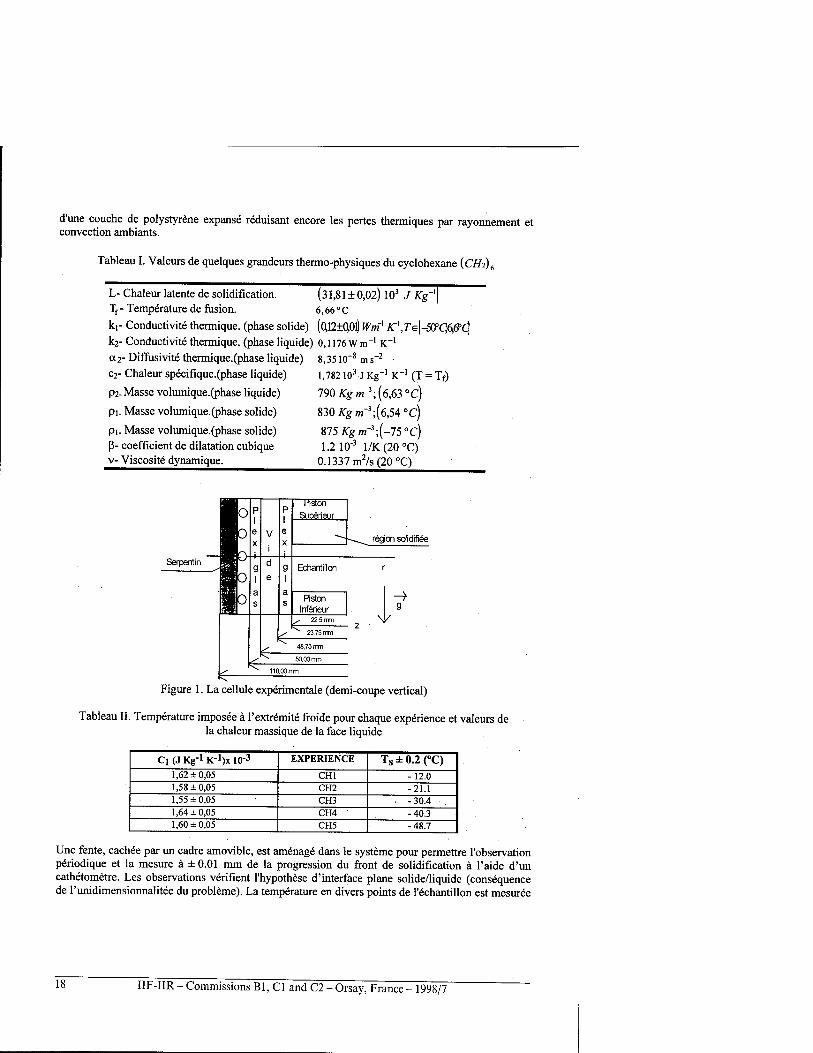
expenmentaux : le cyclohexane {CH2)6 qui est un compose organique possedant trois phases solides distinctes (Anderson, 1978) dont la phase cristalline II du diagramme des phases convient pour le type d'experiences envisagees (Tf = 6,66°C) (Tableau I). Nous avons construit une cellule experimental (Figure 1), fabriquee en Plexiglas (transparent et possedant des caracteristiques thermiques adequates). Elle permet de mesurer revolution temporelle du mouvement de la frontiere libre pendant la solidification. Cette cellule a ete calibree anteneurement avec de l'eau pure pour l'etude de la solidification des solutions salines (Ramos et al, 1991). Pendant l'experimentation, la substance est contenue dans un reservoir cylindrique, limite aux extremit6s supeneure et inferieure par deux pistons m&alliques connectes ä des cryostats agissant comme des sources de froid et contrölant leur temperature avec une precision de + 0,1 °C. Le Plexiglas des deux cylindres concentriques formant le corps de la cellule a une epaisseur de 1,25 mm. La chambre annulaire laissee entre ces deux cylindres est etanche et possede une epaisseur de 15 mm ; on y peut etablir un vide de l'ordre de 2 103 Pa grace ä une pompe ä vide rotatoire. Une grande partie des pertes thermiques laterales est ainsi de supprimee. En plus, autour de la cellule, une enveloppe thermostatee, pourvue d'un Serpentin oü circule un fluide caloporteur, maintient la paroi laterale ä la temperature du piston le plus chaud, celui qui se trouve ä l'extremite inferieure. Les pertes thermiques laterales etant sensiblement reduites, on respecte de pres l'hypothese de conduction de chaleur unidimensionnelle (Ramos et al, 1991). Finalement, la cellule est recouverte


d'une couche de polystyrene expanse reduisant encore les pertes thermiques par rayonnement et convection ambiants.

Tableau I. Valeurs de quelques grandeurs thermo-physiques du cyclohexane (CHi)

L- Chaleur latente de solidification. (31,81 + 0,02) 103 J Kg'l\ Tf- Temperature de fusion. 6,66 °C

ki- Conductivite thermique. (phase solide) (0,12±0,0l) Wnf Ar',7e[-5CPC;6,60C] k2- Conductivite thermique. (phase liquide) 0,1176 W m"1 K"1

a2- Diffusivite thermique.(phase liquide) 8,351(T8 m s"2

c2- Chaleur specifique.(phase liquide) 1,782 io3 J Kg-1 K"1 (T = Tf)

p2-Masse volumique.(phase liquide)

pi. Masse volumique.(phase solide)

pi. Masse volumique.(phase solide) ß- coefficient de dilatation cubique v- Viscosite dynamique.

790 Kgm-3; (6,63 °c)

830Xg/w-3;(6,54°c)

875ü:gm-3;(-750c) 1.2 10"3 1/K(20°C)

0.1337 m2/s (20 °C)

Serpentin

Piston

Superieur

region sdidifiee

Echantillon

Rston Inferieur g

\l/

K- Figure 1. La cellule experimentale (demi-coupe vertical)

Tableau II. Temperature imposee ä l'extremite froide pour chaque experience et valeurs de la chaleur massique de la face liquide

Ci (J Kg"1 K-!)x IO"3 EXPERIENCE TS±0.2(°C) 1,62*0,05 CHI - 12.0 1,58*0,05 CH2 -21.1 1,55 ±0,05 CH3 -30.4 1,64 ±0,05 CH4 - 40.3 1,60 ±0,05 CH5 - 48.7

Une fente, cachee par un cadre amovible, est amenage dans le Systeme pour permettre l'observation periodique et la mesure ä ± 0.01 mm de la progression du front de solidification ä l'aide d'un cathetometre. Les observations verifient l'hypothese d'interface plane solide/liquide (consequence de l'unidimensionnalitee du probleme). La temperature en divers points de l'echantillon est mesuree

IIF-IIR- Commissions Bl, Cl and C2-Orsay, France- 1998/7

ä l'aide de 6 thermocouples cuivre-constantan de 0,3 mm de diametre; ils sont places sur une meme generatrice de la paroi interieure de la cellule.

2.2 Obtention de la condition initiale. On rend d'abord uniforme la temperature de l'echantillon et aussi proche que possible de la temperature de changement d'etat de la substance Tf (6.8°C±0.2°C). Pour cela la temperature des deux pistons et de l'enveloppe thermostatee est portee ä la temperature d'equilibre solide/liquide Tf ; le Systeme est laisse dans cet etat pendant 14 heures environ, en suivant revolution de la distribution thermique au sein de l'echantillon jusqu'ä ce que l'equilibre thermique est atteint. Des lors que la temperature est statistiquement la meme dans tout l'echantillon, la temperature du piston superieur est abaissee brusquement jusqu'ä la valeur desiree Ts et maintenue constante. Le piston inferieur et l'enveloppe thermostatee sont maintenus ä la temperature de changement d'etat pendant toute la duree de l'experience.

2.3 Etablissement des conditions aux limites. Une fois atteinte la condition de temperature initiale, on maintient le piston inferieur et l'enveloppe thermostatee ä la temperature T£ grace ä un des deux cryostats. Cette derniere enveloppe garantie la condition de conduction de la chaleur unidimensionnelle (Ramos et al, 1991). Observons que puisque pendant le processus de solidification se fait avec la frontiere libre ä la temperature Tf, et que la substance dans la partie liquide et le piston inferieur sont ä cette temperature, il n'y a pas de transfert d'energie thermique dans la region liquide. En consequence, du point de vue thermique le Systeme est equivalent ä un milieu semi-infini comme il est suppose dans la solution de Stefan. Le second cryostat est utilise pour porter brusquement la temperature du piston superieur ä la temperature constante Ts. Le temps necessaire pour l'atteindre est approximativement de 5 minutes (la duree des experiences est superieure ä 3 heures). On montre dans le tableau II la temperature imposee en x=0 pour chaque experience ainsi que les valeurs de la chaleur massique respectives pour la phase liquide. II n'existe pas de convection puisque la temperature dans la region liquide est, aux imperfections experimentales pres, la meme que la temperature de changement d'etat de la substance. En definitive, on peut raisonnablement pretendre que le probleme de solidification etudie correspond bien ä celui sous-tendu par la solution de Stefan: conduction unidimensionnelle, domaine semi-infini, condition de temperature initiale constante et uniforme dans la region en phase liquide et une condition ä la limite en x=0 de temperature constante Ts<Tf.

3 RESULTATS EXPERIMENT AUX

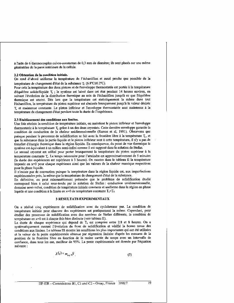
On a realise cinq experiences de solidification avec du cyclohexane pur. La condition de temperature initiale pour chacune des experiences est pratiquement la meme. Cependant, pour etudier des processus de solidification avec des nombres de Stefan differents, la condition de temperature en x=0 est ä chaque fois bien distincte (voir tableau II). La duree de chaque experience qui depend de Ts est comprise entre 2.8 et 8 heures. On a systematiquement mesure Involution du front de solidification et verifie la bonne tenue des conditions aux limites. Le tableau III montre les conditions les plus importantes qui ont ete utilisees et la valeur de la pente experimentale obtenue par regression lineaire d'apres les mesures de la position de la frontiere libre en fonction de la racine carree du temps avec un intervalle de confiance, dans tous les cas, meilleur de 95%. La pente experimentale est donnee par l'equation suivante :

x(t) = mM. (5)

IIF-IIR - Commissions B1, C1 and C2 - Orsay, France - 1998/7 19

On represente, dans la figure 2, les points experimental«, et la droite de regression pour l'experience CH3. L'ajustement lineaire tres convenable permet d'affirmer que, pour toutes les experiences, la position de la frontiere libre evolue proportionnellement ä la racine carree du temps.

Tableau III. Conditions experimentales et valeurs de la pente de la droite de regression.

EXPERIENCES [T,T0] "C U„ = 70 - T °C

i1, = UIICI/L m (mj-V^xlO4 AH

(KJ/Kg) ?

CHI [-12,0; 6,6] 18,6 0,96 3,61 ±0,08 41.3 0.989 CH2 [-21,1; 6,6] 27,6 1,41 4,7 ±0,1 36.1 0.998 CH3 [-30,4; 6,7] 37,1 1,87 5,4 ±0,1 36.8 0.997 CH4 [-40,3; 6,6] 46,9 2,33 5,95 ±0,05. 38.3 0.990 CH5 [-48,8; 6,8] 55,5 2,70 6,41 ±0,07 39.0 0.989

Experience CH3: Solidification Cyclohexane

S E

H Points expörimentaux m=5.4 E-4 (nVsqrt)

nnR !

0.07 ! ^^* nnR

n.ns \ 9» r*^

0.07 j jtf^^ n,m ■ .^*%*

«.^^

Racine carree de t (t en seconde).

Figure 2. Experience CH3, points expenmentaux et droite de regression

Puisque les experiences ont ete menees conformement aux conditions requises correspondant ä la solution de Stefan, on a resolu l'equation (3) en considerant les valeurs des proprietes thermo-physiques du cyclohexane consignees dans les tableaux I et II. On a ainsi obtenu la loi horaire theorique du mouvement de la frontiere libre pour chaque experience considered et en particulier la pente theorique m qui

thtonque ^ represente la constante de

proportionnalite qui affecte 4t ■ L'analyse des resultats obtenus (Posado, 1995) conduit ä mettre en evidence des hearts entre les valeurs experimentales de la constante de proportionnalite mexp et les valeurs theoriques mth4o. Le seul cas qui presente une erreur inferieure ä 3 % (erreur experimental) correspond ä l'experience menee avec le plus petit nombre de Stefan St=0,96. Pour les autres cas, les ecarts sont considerables et augmentent avec la valeur des nombres de St (jusqu'a 16 ä 17 % pour Ts = - 48.8°C). De la sorte, on a observe que, dans le processus de solidification reel, la vitesse du front de solidification est superieure ä ce qu'on est en mesure d'attendre d'apres les resultats theoriques. Rappelons qu'il n'y a pas de convection naturelle ni de pertes laterales importantes qui aurait eu tendance ä ralentir la progression du front. Par ailleurs, on a elabore un code de calcul simple qui permet de determiner quelle devrait etre la chaleur latente de la substance pour que la solution de l'equation transcendante donne la valeur de la pente experimentale mexp. La methode numerique utilisee est celle

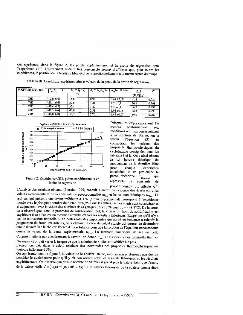
d'approximations par encadrement, ä savoir: on donne mexp et les valeurs des proprietes thermo- physiques et on fait varier L jusqu'ä ce que la solution de Stefan soit verifiee ä e pres. L'erreur cumulee dans le calcul resultant des incertitudes des proprietes thermo-physiques est toujours inferieure ä 5%. On represente dans la figure 3 la valeur de la chaleur latente, avec sa marge d'erreur, que devrait posseder le cyclohexane pour qu'il y ait bon accord entre les resultats theoriques et les resultats experimentaux. On observe que plus le nombre de Stefan est grand plus la valeur theorique s'ecarte

de la valeur reelle L = (31,81 ±0,02) 103 J Kg'\ Les valeurs theoriques de la chaleur latente etant


toujours inferieures ä la valeur reelle, le mouvement experimental de la frontiere libre est toujours plus rapide que celui estime theoriquement. Aux imperfections experimentales pres, on peut affirmer que les conditions experimentales reproduisent correctement les conditions du probleme de Stefan pour des processus de solidification avec de grands nombres de Stefan. Par ailleurs, on a justifie dans ces experiences la non-existence d'effets de convection ou d'autre nature qui eloigneraient les resultats de ceux des modeles indiques. Cependant, l'analyse des valeurs experimentales met en evidence des contradictions avec les valeurs theoriques de la solution a priori exacte du probleme. Puisque la solution theorique ne donne pas des resultats en accord avec les experiences effectuees, suite ä une reflexion concernant les valeurs experimentales on a trouve une solution empirique qui unifie toutes les valeurs du mouvement de la frontiere libre observees. Pour cela, on propose comme solution generique du mouvement du front de solidification une solution formellement identique ä la solution quasi-stationnaire du probleme (Sanz et al, 1996).

SdidficaBon du CYCLOHEXANE

Valeur de L selon la sduliori de Stefan

I

35 - 31,81

30 ■

25 . ■

20 . ■ ■ ■

15 .

m l i 1 1 , ,

Figure 3. Valeur de la chaleur latente de changement d'etat que devrait posseder le cyclohexane pour reproduire les pentes experimentales obtenues

On rappelle que la solution quasi-stationnaire n'est valable que pour les petits nombres de Stefan, cas contraire ä celui qui est le notre dans cette etude. Pour ce faire, on laisse libre le parametre correspondant ä la chaleur latente de fusion qui apparait dans la solution quasi-stationnaire. De sorte que cette grandeur energetique est ajustee dans les divers processus de solidification effectues. On prend done comme solution generique du mouvement de la frontiere libre l'expression suivante:

M-.P52ÜI Pi ~m (6)

oü AH represente la grandeur energetique qui est determinee ä partir des valeurs experimentales de

la pente m„p. A partir des equations (2) et (3), on trouve l'expression suivante pour AH,

AH = 2k, U0

Pi n»L (7)

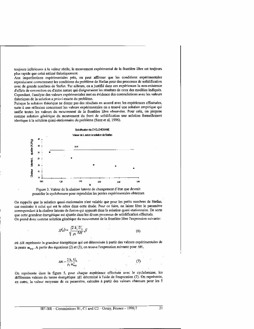
On represente dans la figure 5, pour chaque experience effectuee avec le cyclohexane, les differentes valeurs du terme energetique AH determine ä l'aide de l'expression (7). On represente, en outre, la valeur moyenne de ce parametre, calculee ä partir des valeurs obtenues pour les 5


experiences realisees. On peut constater sur cette figure qu'aux erreurs experimentales pres on peut considerer AH constant dans l'intervalle des mesures effectuees. De plus, on a represente sur ce meme graphique la valeur de la chaleur latente de solidification pour cette substance (tableau I).

Solidification Cyclohexane

3 40 +

I 35 ■■

30 ■■

25

i—r ¥-i

1.25 1.5 1

2.75

Exp. ■

St

-Moyenne Exp. ■ -Chaleur latente

Figure 5. Representation du terme energetique AH (7) en fonction du nombre de Stefan

Comme on peut le constater eile ne correspond pas aux valeurs de AH calculees ä partir des mesures experimentales. Finalement, on observe que la totalite des essais de solidification effectues peut etre interpreted correctement, aux erreurs experimentales pres, au moyen de la formulation semi-empirique (6) avec la valeur suivante du parametre energetique:

AH = 38 + 2 KJ Kg"1 pour Stes[l,3]

4 ANALYSE NUMERIQUE

On a fait diverses experiences numeriques pour etudier le probleme de la congelation du cyclohexane anterieurement propose. Le point de depart a ete le calcul bidimensionnel avec les dimensions de la cellule experimental (voir figure 2) pour comparer les resultats avec ceux correspondant au calcul unidimensionnel. La difference a ete toujours inferieure au 5%. La deuxieme etape a consiste dans l'application de diverses methodes de calcul numerique con9US pour l'etude de la solidification de l'eau avec de conditions particulieres du probleme de Stefan, et les comparer avec la solution exacte (3). Dans le tableau IV, on a represente les resultats obtenus. Dans ce cas, de faible nombre de Stefan, tous les calculs conduisent ä un resultat similaire. Le troisieme pas consiste en ['application des methodes numeriques ci-dessus (cas de l'eau, petit nombre de Stefan) au probleme de cyclohexane. On fait le calcul pour le cas plus defavorable, c'est ä dire, pour 1'experience 5 (Ts = - 48.8°C) qui correspond au nombre de Stefan le plus eleve St=2.7 (voir tableau V). Les resultats sont represented dans le tableau VI.


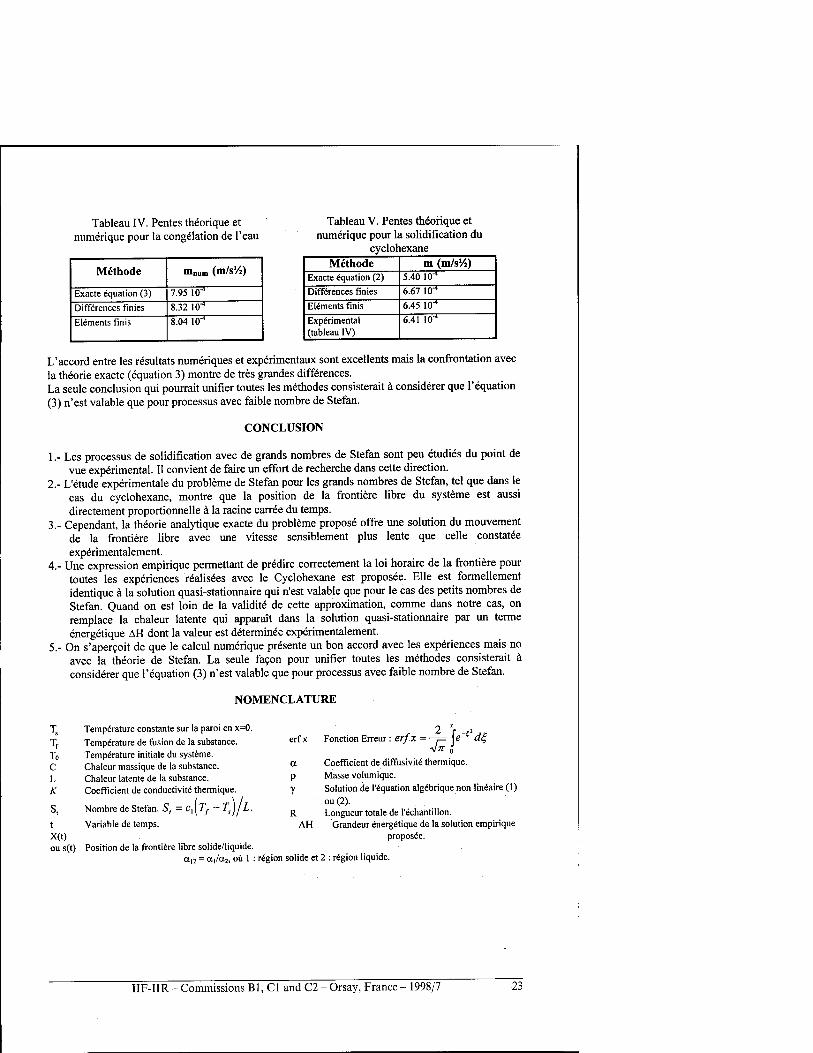
Tableau IV. Pentes theorique et numerique pour la congelation de l'eau

Tableau V. Pentes tbiorique et numerique pour la solidification du

cyclohexane

Methode ninura (m/s'/z)

Exacte Equation (3) 7.95 10-4

Differences finies 8.32 10"4

Elements finis 8.04 10-4

Methode m (mlsVi) Exacte equation (2) 5.40 10"4

Differences finies 6.67 10"4

Elements finis 6.45 10-"

Experimental (tableau IV)

6.41 10"4

L'accord entre les resultats numeriques et experimental sont excellents mais la confrontation avec la theorie exacte (equation 3) montre de tres grandes differences. La seule conclusion qui pourrait unifier toutes les methodes consisterait ä considerer que l'equation (3) n'est valable que pour processus avec faible nombre de Stefan.

CONCLUSION

1.- Les processus de solidification avec de grands nombres de Stefan sont peu etudies du point de vue experimental. II convient de faire un effort de recherche dans cette direction.

2.- L'etude experimentale du probleme de Stefan pour les grands nombres de Stefan, tel que dans le cas du cyclohexane, montre que la position de la frontiere libre du Systeme est aussi directement proportionnelle ä la racine carree du temps.

3.- Cependant, la theorie analytique exacte du probleme propose offre une solution du mouvement de la frontiere libre avec une vitesse sensiblement plus lente que celle constatee experimentalement.

4.- Une expression empirique permettant de predire correctement la loi horaire de la frontiere pour toutes les experiences realisees avec le Cyclohexane est proposee. Elle est formellement identique ä la solution quasi-stationnaire qui n'est valable que pour le cas des petits nombres de Stefan. Quand on est loin de la validite de cette approximation, comme dans notre cas, on remplace la chaleur latente qui apparait dans la solution quasi-stationnaire par un terme energetique AH dont la valeur est determined experimentalement.

5.- On s'apercoit de que le calcul numerique presente un bon accord avec les experiences mais no avec la theorie de Stefan. La seule facon pour unifier toutes les methodes consisterait ä considerer que l'equation (3) n'est valable que pour processus avec faible nombre de Stefan.

NOMENCLATURE

Ts Temperature constante sur la paroi en x=0. Tf Temperature de fusion de la substance. To Temperature initiale du Systeme. C Chaleur massique de la substance. L Chaleur latente de la substance. K Coefficient de conductivite thermique.

S, Nombre de Stefan. S, = c,(Tf - Ts)/L. t Variable de temps. X(t) ou s(t) Position de la frontiere libre solide/liquide.

a,2 = a,/a2, oil 1 :

erf x Fonction Erreur : erfx 2 'r

■J7)e d{ VTTO

a Coefficient de diffusivite thermique. p Masse volumique. y Solution de l'equation algebrique non lineaire (1)

ou(2). R Longueur totale de l'echahtillon.

AH Grandeur energetique de la solution empirique proposee.

region solide et 2 : region liquide.


BIBLIOGRAPHIE

1. Anderson, P., 1978, Thermal Conductivity and Heat Capacity of Cyclohexane under Pressure, J. Phys. Chem. Solids, vol. 39, p. 65-68.

2. Aston, J.G., Szasz, J.G. and Fink, H.L., 1943, The Heat Capacity and Entropy, Heats of Transition, Fusion and Vaporisation and the vapour Pressures of Cyclohexane, J Am Chem Soc. vol. 65, p. 1135-1139.

3. Beckermann, C, Viskanta, R., 1988, Natural Convection Solid/Liquid Phase Change in porous media, Int. J. Heat Mass Transfer,, vol. 31,1 p. 35-46.

4. Burns, A.S; Stickler, LA; Steward, W.E., 1992, Solidification of an Aqueous Salt Solution in a Circular Cylinder, Trans. ofASME,. vol. 114, p. 30-33.

5. Carslaw, H.S. and Jaeger, J.C., 1982, Heat Transfer in Solids,. University Press, Oxford, 6. Cerrato, Y., Gutierrez, J. and Ramos, M, 1989 Mathematical Study of the Solutions of a

diffusion Equation with Exponential Diffusion Coefficient, obtained by application of self- similar groups, J. Phys, A: Mat. Gen., 22, p. 132-140.

7. Christenson, M.S., Bennon, W.D., and Incopera, F.P., 1989 Solidification of an Aqueous ammonium chloride Solution in a rectangular cavity- II. Comparison of predicted and measured results., Int. J Heat Mass Transfer,, vol. 32,1, p 69-79.

8. Clealand, A.C. and Earle, R.L., 1982, A Simple Method for Prediction of Heating and Cooling rates in Solids of various Shapes, Int. J. of Refrigeration, 5, p. 98-106.

9. Frederick, D. and Greif, R. A., 1985, Methods for the Solution of Heat Transfer Problems with a Change of Phase, Trans. ofASME, vol. 107, p 520-525.

10. Gau, C. and Viskanta, R., Melting and Solidification of a Metal System in a rectangular Cavity".

11. Hale, N.W. and Viskanta, R., 1980, Solid-liquid Phase-Change Heat Transfer and Interface Motion in Materials Cooled or Heated from Above or Below, Int. J. Heat Mass Transfer, vol 23, p. 283-292.

12. Hibbert, S., Markatos, N.C. and Voller, V.R., 1988, Computer Simulation of Moving-interface, convective, phase-change process, Int. J. Heat Mass Transfer, vol. 31,9, p. 1785-1795.

13. Hirayama, F. and Lipsky, 1973, The effect of the Crystalline Phase on the Fluorescence Characteristic of Solids cyclohexane and Bicyclohexyl, Chem. Phys. Letters, vol. 22 1 p 173- 7.

14. Lunardini, V.J., 1991, Heat transfer with Freezing and Thawing,. Elsevier. 15. Oliver, D.L. and Sunderland, J.E., 1987, A phase Change Problem with Temperature-

Dependent Thermal Conductivity and Specific Heat,. Int. J. Heat Mass Transfer, vol. 30 12 p 2657-2661.

16. Posado Cano R., 1995, Probleme de Stefan, Etudes theoriques et experimental pour des substances pures et melanges eutectiques, These de Docteur de l'Universite Denis Diderot, Paris 7, soutenue le 30 octobre.

17. Ramos, M., Aguirre-Puente J. y Posado, R., (1991), Nueva Aproximacion al Estudio de los procesos de Congelaciön Mediante la definition de un Calor Latente efectivo, Anales de Fisica A, vol. 87, p. 92-108.

18. Ramos, M., Cerrato, Y., and Gutierrez, J., 1994, An Exact Solution for the Finite Stefan Problem with Temperature-Dependent Thermal Conductivity and Specific Heat, Int. J. of Refrigeration, vol. 7, Nr. 2, p. 130-134.

19. Raynaud, M. and Beck, J,V., 1988, Methodology for Comparison of Inverse Heat Conduction Methods, Trans. ASME, vol. 110, p. 30-37.

20. Ruehrwein, R.A. and Huffman, H.M., 1943, J. Am. Chemm. Soc., 65, p. 1620. 21. Sanz P.D., Ramos, M. and Mazheroni. R.H., 1996, Using Equivalent Volumetric Enthalpy

Variation to Determine the Freezing Time in Foods, J. Food Engineering, vol. 27, p. 177-190.


22. Saraf, G.R. and Sharif, K.A., 1987, Inward Freezing of Water in Cylinders, Int. J. Refrigeration, vol.10, p. 342-349.

23. Shamsundar, N. and Sparrow, E.M., 1974, Analysis of Multidimensional Conduction Phase Change Via the Enthalpy Model, J. of Heat Transfer, p. 333-339.

24. Sparrow, E.M., Gurtcheff, G.A. and Myrum, T.A., 1986, Correlation of Melting Results for Both Pure Substances and Impure Substances, J. of Heat Transfer, vol. 108, p 649-653.

25. Surin, V.G., Mogilevskii, B.M. and Chudnovskii, A.F., 1972, Effect of Additives on the Thermal Conductivity of Cyclohexane, J. Eng. Phys., vol. 23, p. 904-905.

26. Tao, N.L., 1981 The Exact Solutions of Some Stefan Problems with Prescribed Heat Flux, Trans. ofASME, Vol. 48, p. 732-736.

27. Wu, Y.K., Prud'homme, M. et Hung Nguyen, T., 1989, Etude Numerique de la Fusion autour d'un Cylindre Vertical soumis a deux Types de Conditions Limites, Int. J. Heat Mass Transfer. vol. 32, p 1927-1938.

CYCLOHEXANE SOLIDIFICATION BY HEAT CONDUCTION FOR HIGH STEFAN NUMBERS

SUMMARY: Experimental and numerical studies of one-dimensional freezing processes of a sample of cyclohexane for a semi-infinite region were performed. The substance was maintained at a fixed temperature on the surface located at x=0. The choice of cyclohexane allowed to exploration of the process of heat diffusion with phase change in the range of elevated Stefan numbers, St E [0.96, 2.70]. Surprisingly, the results are not in agreement with the theoretical ones obtained from the exact resolution of the Stefan problem. Experimental data and numerical modelling of the free boundary motion are given for five freezing experiments and the corresponding discussion is provided. An empirical function based on physical considerations and which verifies the experimental results is also given.


EXPERIMENTAL STUDY ON THE EVALUATION OF REDUCING METHOD OF TOTAL HEAVE AMOUNTS USING GRANULATED TD*E

SOIL MIXTURE

KIM H.K. and FUKUDA M. Institute of Low Temperature Science, Sapporo, 060-0819 Japan

ABSTRACT

The authors conducted the field experiments of frost heave as to evaluate reducing method of frost heave amount using granurated tire soil mixture. By mixing Tomakomai soil with granulated tire, a frost heave was decreased highly. From the results of the field experiment, it was confirmed that granulated tire was an excellent material in controlling the total heave amount. The efficiency for the reduction of the total heave amount by tire-soil mixture is discussed based on the segregation potential concepts.

INTRODUCTION

In cold regions, the ground is subjected to severe winter coldness and freezes into some depth. During soil freezing, frost heave tends to occur under specific conditions and soil types. Due to frost action, the roads are damaged by upheaval of the surface. Road, building, railway, pipeline and other infrastructures are required to be treated as to prevent from frost heave damage. In case of the protection methods for road frost heave, which results from formation of successive ice lenses in subgrade soils, replacing of the materials from frost susceptible to non-susceptible is most commonly adopted. However in some areas, it is difficult to supply enough amounts of sandy materials from local resources, and it makes the cost of road construction to be expensive. Therefore, there are some attempts to utilize the additional materials to original frost susceptible soil in-situ so that the road becomes to be frost tolerable. Fukuda et al (1991) used ordinal cement as mixing materials to silty soil. Thompson (1973) also reported the similar application. Alternative method is to install the geotextile in subgrade (Henry, 1990) or to embed the thermal insulating material as styrofoam into subgrade (Dunphy, 1973). There are some common disadvantages among these applications, which make the practical applications to be difficult. First, costs of the materials are higher than non-frost susceptible soil. Second new machinery or techniques for installation or mixing on the spot are still not well developed yet. Third the duration of effectiveness is not evaluated. Even considering these disadvantages, there is a demand for further application from industry and society as to improve the performance of the above-mentioned construction field. Recently huge amounts of discarded tires are flowing out due to the rapid trend of modernization. Adequate treatment of discarded tires is urgently requested as to recycle them in various ways. As mentioned above, one of application of discarded tire in the road is to embed it as insulation layer to limit the depth of frost penetration (Robert, 1994). However layered tire has problems which don't afford the overburden pressure derived from heavy vehicles, and give rise to a large settlement. For this reason, the authors propose a method of a new concept to improve these disadvantages. The new method mixes a soil with granulated tire as one part of replacement materials. By this mixture, it is expected not only the reduction of total heave due to high permeability and low surface activity of granulated tire but also the recycling of waste matters. With reduced frost heave, the life of all of structures could be extended. Therefore, the study focuses on evaluating the effectiveness of granulated tire in reducing method of frost heave amount and the efficiency for reduction of the total heave amount by granulated tire-soil mixture using segregation potential.

26 IIF-IIR - Commissions B1, C1 and C2 - Orsay, France - 1998/7

1 CONDITION OF TEST SITE

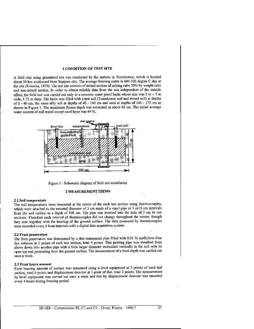
A field trial using granulated tire was conducted by the authors in Tomakomai, which is located about 50 km southward from Sapporo city. The average freezing index is 600-700 degree C day at the site (Kinosita, 1979). The test site consists of mixed section of mixing ratio 20% by weight ratio and non-mixed section. In order to obtain reliable data from the test independent of the outside effect, the field test was carried out only in a concrete water proof basin whose size was 5 m x 5 m wide, 1.75 m deep. The basin was filled with a test soil (Tomakomai soil and mixed soil) at depths of 0 - 40 cm, the same silty soil at depths of 40 - 140 cm and sand at depths of 140 - 175 cm as shown in Figure 1. The maximum frozen depth was estimated as about 40 cm. The initial average water content of soil tested except sand layer was 49 %.

frost line load cell

Figure 1 - Schematic diagram of field test installation

2 MEASUREMENT ITEMS

2.1 Soil temperature The soil temperatures were measured at the center of the each test section using thermocouples, which were attached to the external diameter of 3 cm made of a vinyl pipe at 5 orlO cm intervals from the soil surface to a depth of 100 cm. The pipe was inserted into the hole of 3 cm in test sections. Therefore each interval of thermocouples did not change throughout the winter, though they rose together with the heaving of the ground surface. The data measured by thermocouples were recorded every 4 hour intervals with a digital data acquisition system.

2.2 Frost penetration The frost penetration was determined by a thin transparent pipe filled with 0.01 % methylene blue dye solution at 3 points of each test section, total 6 points. This probing pipe was sheathed from above down into another pipe with a little larger diameter embedded vertically in the soil with its open top end protruding from the ground surface. The measurement of a frost depth was carried out once a week.

2.3 Frost heave amount Frost heaving amount of surface was measured using a level equipment at 3 points of each test section, total 6 points and displacement detector at 1 point ofthat, total 2 points. The measurement by level equipment was carried out once a week and that by displacement detector was recorded every 4 hours during freezing period.


3 FIELD RESULTS

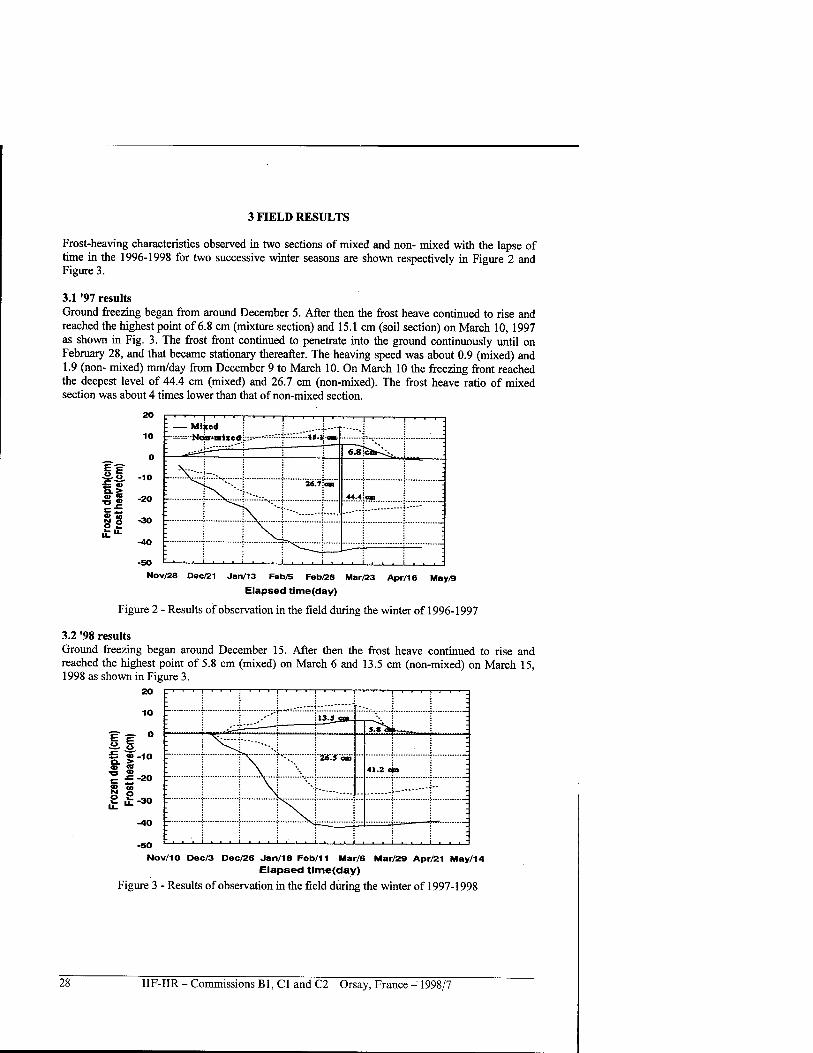
Frost-heaving characteristics observed in two sections of mixed and non- mixed with the lapse of time in the 1996-1998 for two successive winter seasons are shown respectively in Figure 2 and Figure 3.

3.1 '97 results Ground freezing began from around December 5. After then the frost heave continued to rise and reached the highest point of 6.8 cm (mixture section) and 15.1 cm (soil section) on March 10, 1997 as shown in Fig. 3. The frost front continued to penetrate into the ground continuously until on February 28, and that became stationary thereafter. The heaving speed was about 0.9 (mixed) and 1.9 (non- mixed) mm/day from December 9 to March 10. On March 10 the freezing front reached the deepest level of 44.4 cm (mixed) and 26.7 cm (non-mixed). The frost heave ratio of mixed section was about 4 times lower than that of non-mixed section.

• ■ ■ ■ ! • ' ■ 1 ■'-!-'- : Mined j...--, r--J^--N«r».,iirixe*j.-:"-—«r."i-.-.::.-.::."i5.*;.—.

■ ■ j • ' ■ 1 ' ' -■—

■ ~^r- r~ ; • 6.8!cn*^_ j

: V—L. j j ! j j ^*1 '--. ■ M.7;o»i

.44.4|«n J

- . . . i . . . i . . . i . . . i .

! ' ■

. . i . . . i . . . ■

•g-f. -10

|J -20 E-

|g -30 P ^ -40 f"

-50

Nov/28 Dec/21 Jan/13 Fob/5 Fob/28 Mar/23 Apr/16 May/9

Elapsed time(day)

Figure 2 - Results of observation in the field during the winter of 1996-1997

3.2 '98 results Ground freezing began around December 15. After then the frost heave continued to rise and reached the highest point of 5.8 cm (mixed) on March 6 and 13.5 cm (non-mixed) on March 15, 1998 as shown in Figure 3.

20

fc «,-10

S S St-30

-40 1

-50

_ ... j . ..]... I ... j ., , . . i j i . i j J . i ^

.•"'': \\3.i_sm-. "-. i •

■ --J—*—: ■ i 3.«o^—__

~ T T>T :*"-V Y'26'.'S'äm 41.2 <*n

: I ' I I N. i I 1 i :

• ■ ■ '■ -L ■ J ■ i ... i ... i ... i ... I ... i ... -

Nov/10 Dec/3 Dec/26 Jan/18 Feb/11 Mar/6 Mar/29 Apr/21 May/14 Elapsed tlme(day)

Figure 3 - Results of observation in the field during the winter of 1997-1998


By that time the frost front had reached 41.7 cm (mixed section) and 26.5 cm (non-mixed section). The frost front of mixed section passed deeper than that of non-mixed site. The difference of freezing front is thought that volumetric water content decreased by granulated tire-soil mixture has an effect on latent heat of mixed site caused by ice segregation. The heave ratio amounted to a value of 49%(non-mixed) and 14%(Mixed). The water level reached a depth of 45 cm below the initial ground surface inside Tomakomai soil layer on December 23 and reached the deepest of 150 cm below the initial ground surface on February 10. The heaving occurred with the growths of ice lenses segregated in the freezing front. The average heaving speed was about 2.1 mm/day from December 15 to February 17 (non-mixed) and 0.64 mm/day from December 15 to March 17 (mixed). The heaving process in mixed section was slower than that in non-mixed section, while the frost penetrated deeper.

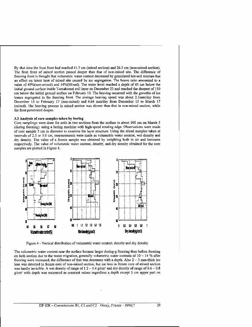
3.3 Analysis of core samples taken by boring Core samplings were done for soils in two sections from the surface to about 100 cm on March 5 (during freezing), using a boring machine with high-speed rotating edge. Observations were made of core sample 5 cm in diameter to examine the layer structure. Using the sliced samples taken at intervals of 2.5 or 5.0 cm, measurements were made as volumetric water content, wet density and dry density. The value of a frozen sample was obtained by weighting both in air and kerosene respectively. The value of volumetric water content, density, and dry density obtained for the core samples are plotted in Figure 4.

k » V

c |J30 Q

'' ' 111111111.11.11

«

09 1 l.t Ü U U \i

WetMyM

Ml f ■ ■ ' ' ■ ■ '

0 02 04 06 08 1

Figure 4 - Vertical distribution of volumetric water content, density and dry density

The volumetric water content near the surface became larger during-g freezing than before freezing on both section due to the water migration, generally volumetric water contents of 10 ~ 14 % after freezing were increased, the difference ofthat was decreases with a depth. Also 2-3 mm-thick ice lens was detected in frozen core of non-mixed section, but ice lens in frozen core of mixed section was hardly invisible. A wet density of range of 1.2 ~ 1.4 g/cm3 and dry density of range of 0.6 ~ 0.8 g/cm3 with depth was measured as constant values regardless a depth except 5 cm upper part on


both section. The radical decrease of densities in non-mixed soil was the result of oversaturation during the freezing.

4 DISCUSSION

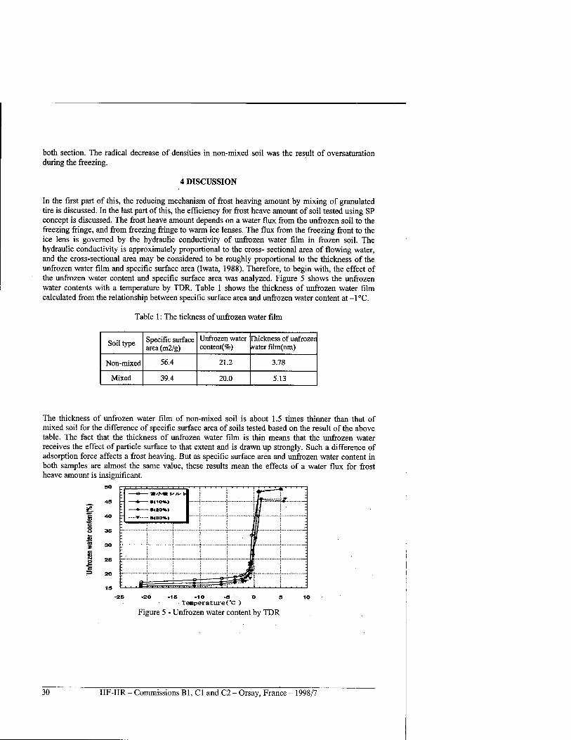
In the first part of this, the reducing mechanism of frost heaving amount by mixing of granulated tire is discussed. In the last part of this, the efficiency for frost heave amount of soil tested using SP concept is discussed. The frost heave amount depends on a water flux from the unfrozen soil to the freezing fringe, and from freezing fringe to warm ice lenses. The flux from the freezing front to the ice lens is governed by the hydraulic conductivity of unfrozen water film in frozen soil. The hydraulic conductivity is approximately proportional to the cross- sectional area of flowing water, and the cross-sectional area may be considered to be roughly proportional to the thickness of the unfrozen water film and specific surface area (Iwata, 1988). Therefore, to begin with, the effect of the unfrozen water content and specific surface area was analyzed. Figure 5 shows the unfrozen water contents with a temperature by TDR. Table 1 shows the thickness of unfrozen water film calculated from the relationship between specific surface area and unfrozen water content at -1°C.

Table 1: The tickness of unfrozen water film

Soil type Specific surface area (m2/g)

Unfrozen water content(%)

rhickness of unfrozer water film(nm)

Non-mixed 56.4 21.2 3.78

Mixed 39.4 20.0 5.13

The thickness of unfrozen water film of non-mixed soil is about 1.5 times thinner than that of mixed soil for the difference of specific surface area of soils tested based on the result of the above table. The fact that the thickness of unfrozen water film is thin means that the unfrozen water receives the effect of particle surface to that extent and is drawn up strongly. Such a difference of adsorption force affects a frost heaving. But as specific surface area and unfrozen water content in both samples are almost the same value, these results mean the effects of a water flux for frost heave amount is insignificant.

-1S -10 -5 TemperatureCc )

Figure 5 - Unfrozen water content by TDR


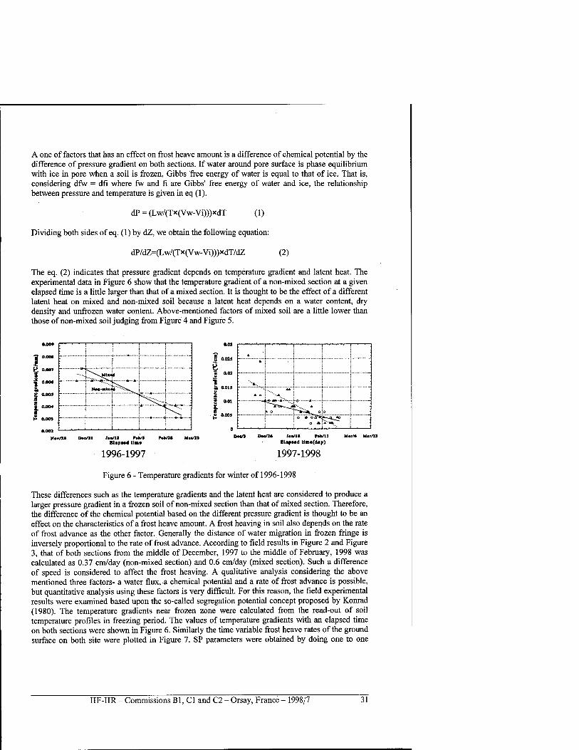
A one of factors that has an effect on frost heave amount is a difference of chemical potential by the difference of pressure gradient on both sections. If water around pore surface is phase equilibrium with ice in pore when a soil is frozen, Gibbs free energy of water is equal to that of ice. That is, considering dfw = dfi where fw and fi are Gibbs' free energy of water and ice, the relationship between pressure and temperature is given in eq (1).

dP = (Lw/(Tx(Vw-Vi)))xdT (1)

Dividing both sides of eq. (1) by dZ, we obtain the following equation:

dP/dZ=(Lw/(Tx(Vw-Vi)))xdT7dZ (2)

The eq. (2) indicates that pressure gradient depends on temperature gradient and latent heat. The experimental data in Figure 6 show that the temperature gradient of a non-mixed section at a given elapsed time is a little larger than that of a mixed section. It is thought to be the effect of a different latent heat on mixed and non-mixed soil because a latent heat depends on a water content, dry density and unfrozen water content. Above-mentioned factors of mixed soil are a little lower than those of non-mixed soil judging from Figure 4 and Figure 5.

0.0»

'S 0.000

g 0.007 • £ 0.00« m j» 0.003

S 0.0M

0.003

Nov/31

0.09

S 0.0U

£ O.« ■ 0.02

ft 0.013 u 3 3 0.01 S.

-,—,—,—|—,—,—,—,-

BlapM4 lls«

1996-1997

P«WU M«r/2S DM/3 DM04 !»•/!* BUpMd tfn*(day)

Mar/6 M*f/23

1997-1998

Figure 6 - Temperature gradients for winter of 1996-1998

These differences such as the temperature gradients and the latent heat are considered to produce a larger pressure gradient in a frozen soil of non-mixed section than that of mixed section. Therefore, the difference of the chemical potential based on the different pressure gradient is thought to be an effect on the characteristics of a frost heave amount. A frost heaving in soil also depends on the rate of frost advance as the other factor. Generally the distance of water migration in frozen fringe is inversely proportional to the rate of frost advance. According to field results in Figure 2 and Figure 3, that of both sections from the middle of December, 1997 to the middle of February, 1998 was calculated as 0.37 cm/day (non-mixed section) and 0.6 cm/day (mixed section). Such a difference of speed is considered to affect the frost heaving. A qualitative analysis considering the above mentioned three factors- a water flux, a chemical potential and a rate of frost advance is possible, but quantitative analysis using these factors is very difficult. For this reason, the field experimental results were examined based upon the so-called segregation potential concept proposed by Konrad (1980). The temperature gradients near frozen zone were calculated from the read-out of soil temperature profiles in freezing period. The values of temperature gradients with an elapsed time on both sections were shown in Figure 6. Similarly the time variable frost heave rates of the ground surface on both site were plotted in Figure 7. SP parameters were obtained by doing one to one


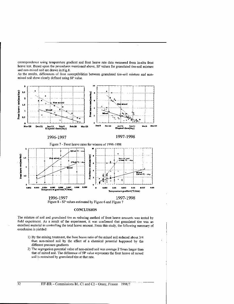
correspondence using temperature gradient and frost heave rate data measured from in-situ frost heave test. Based upon the procedures mentioned above, SP values for granulated tire-soil mixture and non-mixed soil are drawn in Fig.8. As the results, differences of frost susceptibilities between granulated tire-soil mixture and non- mixed soil show clearly defined using SP value.

2.5

*

1.5

S » tt

o No»/2»

■ 1 1 ,,,.,.,. J . . 1 j

* 1 '-..: A ;

i **'•-, ■

o '*-:4 Noil-mind ; ■

t^^mnk .*">.....*... {,. j ■ i ^^"S&c' : a: :

• o . ^^*-^-^' *•., ■

: j ^T»Ô^ ..„..„.... : : o ; .^^

. o"T© ,

Dee/21 Jan/13 Fcb/5 Feb/2* Elapsed time(diy)

D«c/S Dec/26 Jan/18 Feb/11 Elapsed tlme(<lay)

Mar/6 M«t/2S

1996-1997 1997-1998

Figure 7 - Frost heave rates for winters of 1996-1998

1

0

0.001

..,.,,., J , , , . J , . . i , , . . i J ■

* ■

i Non-iiix*d i .' 63&4^C ■ day;

' - ;.*...-*.-..£-.

-

: iW'ol " 1>^ ■"Slihwd: IMmrf/jC doy '

■ flit ° ? ■.». . i .. .. i

o ; ;

... i .... i . . . . i . !

0.003 0.004 0.005 0.006 0.007 0.00« 0.009 Temperature grid ten t(^C/mm)

0.005 0.01 0.015 0.02 0.025 Temperature gradIent(*C/mm)

1996-1997 1997-1998 Figure 8 - SP values estimated by Figure 6 and Figure 7

CONCLUSION

The mixture of soil and granulated tire as reducing method of frost heave amounts was tested by field experiment. As a result of the experiment, it was confirmed that granulated tire was an excellent material in controlling the total heave amount. From this study, the following summary of conclusion is yielded:

1) By the mixing treatment, the frost heave ratio of the mixed soil reduced about 3/4 than non-mixed soil by the effect of a chemical potential happened by the different pressure gradients

2) The segregation potential value of non-mixed soil was average 2 times larger than that of mixed soil. The difference of SP value represents the frost heave of mixed soil is restrained by granulated tire at that rate.


REFERENCES

l.Dunphy, W.J., 1973, Experimental insulation of a subgrade in Hampden, Maine, Proc. of Symposium on Frost Action on Roads, Oslo, O.E.C.D., vol.2, p. 329-338

2. Fukuda, M., Yamamoto, H. and Izuta, H., 1991, The evaluation of reducing method of total heave amounts using soil-cement mixtures, Ground Freezing, 91, p. 417 - 424

3. Henry, K.S., 1990, Laboratory investigation of the use of geotextile to mitigate frost heave. CRREL Report, 90-6, 28 p

4. Iwata, S., Tabuchi, T., and Warkentin, B.P., 1988, Soil water interactions-mechanisms and applications, 2nd edition, p. 20-121

5. Kinosita, S., 1979, Effects of initial soil-water conditions on frost heaving characteristics, Engineering Geology, 13, p. 41-52

6. Konrad, J.M. and Morgenstern, N. R., 1980, A mechanistic theory of ice lens formation in fine grained soils, Can. Geotehech. J.,\l, p. 473 -486

7. Robert, A.E., Richard, J.R. and Dwna, N.H., 1994, Fravel road test sections insulated with scrap tire chips, Special report, 94-21

8. Thompson, M.R.,1973, Durability and frost resistance of lime and cement stabilized soils, Proc. of Symposium on Frost action on Roads, vol. 2, p. 201-203

ETUDE EXPERIMENT ALE D'UNE METHODE VISANT A REDUIRE LES SOULEVEMENTS TOTAUX ET CONSISTANT A MELANGER DU CAOUTCHOUC GRANULEUX AU SOL

RESUME : Les auteurs ont effectue des experiences in situ sur le soulevement du gel, afin d'evaluer une methode visant ä reduire les quantites de soulevements, qui utilise un melange de sol et de caoutchouc sous forme de granules. En melangeant du caoutchouc en granules au sol de Tomakomai, le soulevement du sol a pu etre considerablement reduit. A partir des resultats de cette experience in situ, il a ete confirme que le caoutchouc en granules etait un excellent materiau pour la maitrise des soulevements totaux. En se fondant sur des concepts de puissance de segregation, les auteurs discutent de l'efficacite du melange caoutchouc-sol pour la reduction des soulevements du gel.


TRANSFORMATION OF SAPROPEL IN THE PROCESS OF FREEZING

CHUVILIN E.M., ERSHOV E.D., MURASHKO A.A. Department of Geocryology, Faculty of Geology, Vorobyevy Gory

Moscow State University, Moscow, Russia, 119899

ABSTRACT

The efficiency of the existing sapropel de-watering technology by means of freezing in precipitation tanks depends in a significant extent on the character of the transformation of sapropel texture in the process of freezing. In contrast to mineral soils the processes which occur in freezing sapropel have not been thoroughly studied. In this connection an analysis of structure and texture formation processes in freezing sapropel based on the lab modelling has been carried out in this paper. The whole experimentation let us define the optimum freezing regimes for the organogenic soils where the freezing process affects to the utmost extent on the organo-mineral and aggregation components of soil. It also allow to calculate the optimum depth of freezing for the purposes of industry where exists the high efficiency of cryogenic dehydration.

1. INTRODUCTION

Sapropels are lake deposits composed by plants and microorganisms with inclusions of mineral particles brought by water flow (Pidoplichko, 1975). They are valuable natural raw material using as medical mud, fertilisers and so on (Lopotko, 1974). Special parameter of sapropels is their high water content at natural conditions (up to 1000% and more). This requires development of drying technologies before transportation of the material. Conventional fields of sapropels are exhausted much, so there is need for development of new fields located in regions with winter freezing of ground. The most effective way of cryogenic drying of sapropels consists in the freezing of their settlements. Successful solution of this task is impossible without preliminary assessment of the processes of heat and mass exchange and cryogenic ground structure formation during freezing/thawing. These processes in organic soils are investigated weakly till now. Only limited number of data on mass exchange and structure formation processes within sapropels is available (Gamaunov et al, 1982, 1998). A row of problems needed to be investigated:

1. Mechanisms and regularities of cryogenic structure and texture formation; 2. Qualitative and quantitative interconnections of heät-mass transfer and cryogenic

structure and texture formation; 3. Prediction of soil structure and properties change during freezing; 4. Choice of optimal regimes of freezing.

A set of experimental studies conducted at Geocryology Department of Geologic Faculty of Moscow State University and in Peat Institute of Byelorussian Academy of Sciences on the study of cryogenic structure formation processes allows to define main factors influencing on the effectiveness of the drying technology.

2. TESTING PROCEDURE

Modelling of thermal- and mass-transfer processes, cryogenic texture- and structure formation in sapropel was conducted on the basis of use of a set of laboratory equipment and instruments. The main feature of this set was a laboratory installation (Brovka and Murashko, 1989). Its construction ensures maintaining one-dimension temperature field during freezing samples of ground with diameter of 140 mm and 300 mm in high. The installation allowed conducting comprehensive study


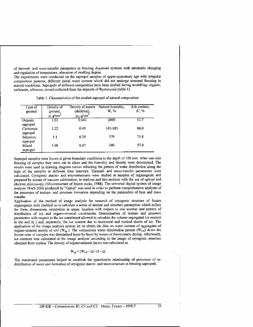
of thermal- and mass-transfer parameters in freezing dispersed systems with automatic changing and regulation of temperature, alteration of swelling degree. The experiments were conducted on the sapropel samples of upper-quaternary age with irregular composition patterns, different initial water content which did not undergo seasonal freezing in natural conditions. Sapropels of different composition have been studied during modelling: organic, carbonate, siliceous, mixed-collected from the deposits of Byelorussia (table 1).

Table 1. Characteristics of the studied sapropel of natural composition

Type of ground

Density of ground, p, g/cm3

Density of matrix (skeleton), pd, g/cm3

Natural humidity, W,%

Ash content, Ac, %

Organic 1.03 0.042 2000 12.7 sapropel Carbonate 1.22 0.49 142-183 84.0 sapropel Siliceous 1.1 0.39 379 75.8 sapropel Mixed 1.08 0.47 340 57.0 sapropel

Sapropel samples were frozen at given boundary conditions to the depth of 100 mm. After one-side freezing of samples they were cut in slices and the humidity and density were determined. The results were used in drawing diagram curves reflecting the pattern of water distribution along the high of the samples at different time intervals. Thermal- and mass-transfer parameters were calculated. Cryogenic macro- and microstructures were studied at samples of organogenic soil prepared by means of vacuum sublimation, in replicas and thin sections with the use of optical and electron microscopy (Microstructure of frozen rocks, 1988). The universal digital system of image analysis IBAS-2000 produced by "Opton" was used in order to perform comprehensive analysis of the processes of texture- and structure formation depending on the parameters of heat and mass transfer. Application of the method of image analysis for research of cryogenic structure of frozen organogenic soils enabled us to calculate a series of texture and structure parameters which reflect the form, dimensions, orientation in space, location with respect to one another and pattern of distribution of ice and organo-mineral constituents. Determination of texture and structure parameters with respect to the ice constituent allowed to calculate the volume segregated ice content in the soil (it) and, separately, the ice content due to horizontal and vertical sheets of ice. The application of the image analysis system let us obtain the data on water content of aggregates of organo-mineral matrix of soil (Wag). The voluminous water distribution pattern (Wvoi) down the frozen zone of samples was determined layer-by-layer by means of thermostatic drying. Afterwards, ice contents was calculated at the image analyser according to the image of cryogenic structure obtained from replica. The density of organo-mineral layers was calculated as

Wa6=(Wv„,-it)/(l-it).

The mentioned parameters helped to establish the quantitative relationship of processes of redistribution of water and formation of cryogenic macro- and microstructure at freezing sapropels.


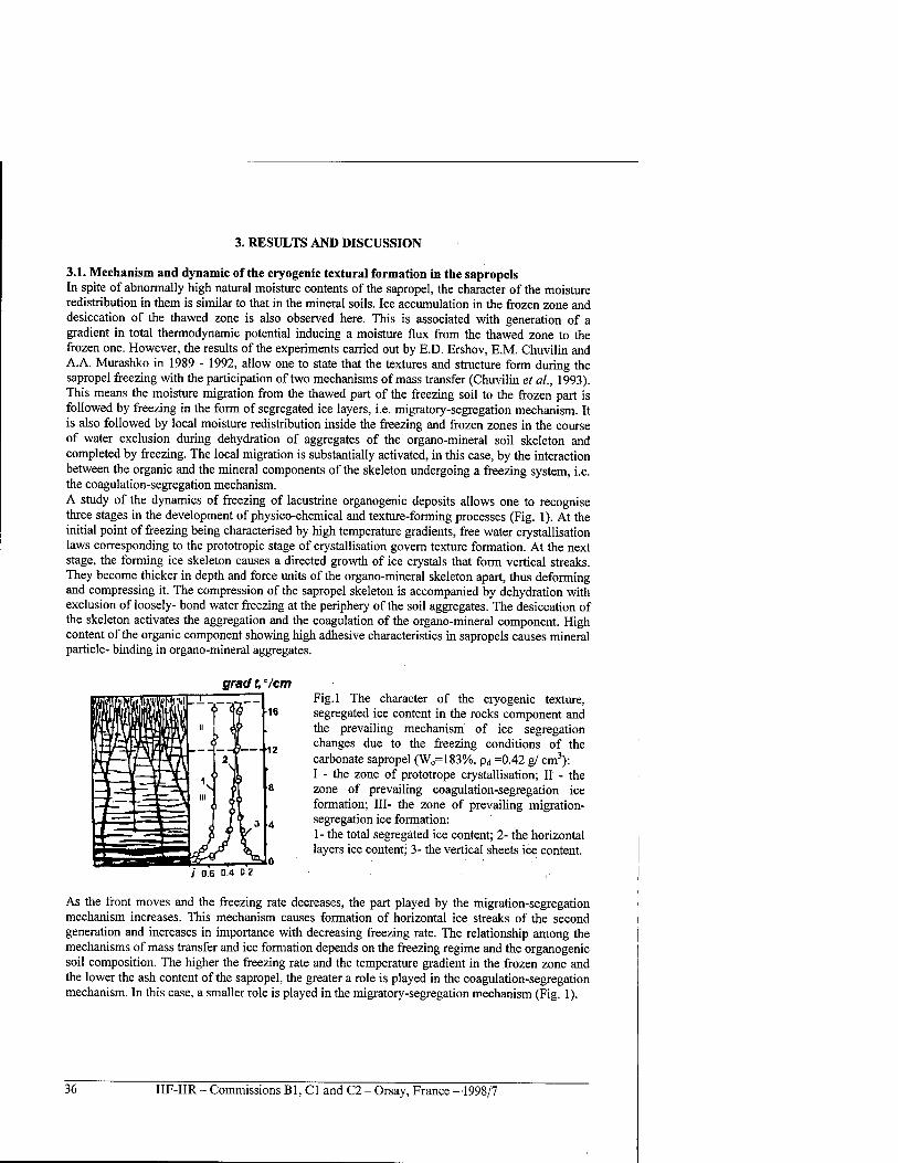
3. RESULTS AND DISCUSSION

3.1. Mechanism and dynamic of the cryogenic textural formation in the sapropels In spite of abnormally high natural moisture contents of the sapropel, the character of the moisture redistribution in them is similar to that in the mineral soils. Ice accumulation in the frozen zone and desiccation of the thawed zone is also observed here. This is associated with generation of a gradient in total thermodynamic potential inducing a moisture flux from the thawed zone to the frozen one. However, the results of the experiments carried out by E.D. Ershov, E.M. Chuvilin and A.A. Murashko in 1989 - 1992, allow one to state that the textures and structure form during the sapropel freezing with the participation of two mechanisms of mass transfer (Chuvilin et al, 1993). This means the moisture migration from the thawed part of the freezing soil to the frozen part is followed by freezing in the form of segregated ice layers, i.e. migratory-segregation mechanism. It is also followed by local moisture redistribution inside the freezing and frozen zones in the course of water exclusion during dehydration of aggregates of the organo-mineral soil skeleton and completed by freezing. The local migration is substantially activated, in this case, by the interaction between the organic and the mineral components of the skeleton undergoing a freezing system, i.e. the coagulation-segregation mechanism. A study of the dynamics of freezing of lacustrine organogenic deposits allows one to recognise three stages in the development of physico-chemical and texture-forming processes (Fig. 1). At the initial point of freezing being characterised by high temperature gradients, free water crystallisation laws corresponding to the prototropic stage of crystallisation govern texture formation. At the next stage, the forming ice skeleton causes a directed growth of ice crystals that form vertical streaks. They become thicker in depth and force units of the organo-mineral skeleton apart, thus deforming and compressing it. The compression of the sapropel skeleton is accompanied by dehydration with exclusion of loosely- bond water freezing at the periphery of the soil aggregates. The desiccation of the skeleton activates the aggregation and the coagulation of the organo-mineral component. High content of the organic component showing high adhesive characteristics in sapropels causes mineral particle- binding in organo-mineral aggregates.

grad t, °/cm Fig.l The character of the cryogenic texture, segregated ice content in the rocks component and the prevailing mechanism of ice segregation changes due to the freezing conditions of the carbonate sapropel (W0=183%, pd =0.42 g/ cm3): I - the zone of prototrope crystallisation; II - the zone of prevailing coagulation-segregation ice formation; III- the zone of prevailing migration- segregation ice formation: 1- the total segregated ice content; 2- the horizontal layers ice content; 3- the vertical sheets ice content.

i O.G D.4 0.2

As the front moves and the freezing rate decreases, the part played by the migration-segregation mechanism increases. This mechanism causes formation of horizontal ice streaks of the second generation and increases in importance with decreasing freezing rate. The relationship among the mechanisms of mass transfer and ice formation depends on the freezing regime and the organogenic soil composition. The higher the freezing rate and the temperature gradient in the frozen zone and the lower the ash content of the sapropel, the greater a role is played in the coagulation-segregation mechanism. In this case, a smaller role is played in the migratory-segregation mechanism (Fig. 1).

36 IIF-IIR - Commissions B1, C1 and C2 - Orsay, France -1998/7

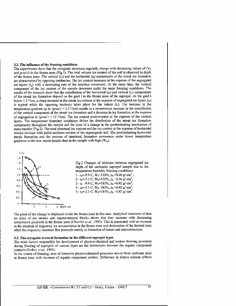
3.2. The influence of the freezing conditions The experiments show that the cryogenic structures regularly change with decreasing values of (Vf, and grad I) in the frozen zone (Fig.l). The total volume ice content of the soil is observed in depth of the frozen zone. The vertical (iv) and the horizontal (ih) components of the streak ice formation are characterised by opposing tendencies. The ice content increases at the expense of the segregated ice layers (ig) with a decreasing rate of the interface movement. At the same time, the vertical component of the ice content of the sample decreases under the same freezing conditions. The results of the research show that the contribution of the horizontal (ih) and vertical (iv) components of the streak ice formation depend on the grad t in the frozen zone of the sapropel. At the grad t below 1.5 %m, a sharp increase in the streak ice content at the expense of segregated ice layers (ih) is typical while the opposing tendency takes place for the values (iv). The increase in the temperature gradient up to (grad t > 1.5 7cm) results in a monotonous increase in the contribution of the vertical component of the streak ice formation and a decrease in ice formation at the expense of segregation at {grad t < 12 °/cm). The ice content predominates at the expense of the vertical layers. The temperature boundary conditions define the distribution of the streak ice formation components throughout the sample and the zone of a change in the predominating mechanism of mass transfer (Fig.2). The total structural ice content and the ice content at the expense of horizontal streaks increase with initial moisture content of the organogenic soil. The predominating horizontal streak formation and the process of structural formation commence under lower temperature gradients in the less- moist sample than in the sample with high (Win).

Fig.2 Changes of relations between segregated ice depth of the carbonate sapropel sample due to the temperature-humidity freezing conditions: 1 -10=-9.9 C, W0=l 10%, pd =0.60 g/ cm3; 2 -10=-5.1 C, W0=122%, pd =0.56 g/ cm3; 3 -10=-9.9 C, W0=183%, pd =0.42 g/ cmJ; 4 -10=-5.1 C, W0=183%, pd =0.42 g/ cm3; 5 -10=-2.1 C, W0=183%, pd =0.42 g/ cm3.

6 depth, cm

The point of the change is displaced inside the frozen zone in this case. Analytical treatment of data on sizes of ice streaks and organo-mineral blocks shows that they increase with decreasing temperature gradients in the frozen zone (Chuvilin et al, 1993). This is associated with an increase in the duration of migratory ice accumulation in the frozen zone and desiccation of the thawed zone when the migratory moisture flux proceeds mainly to formation of macro and microstructures.

3.3. The cryogenic textura) formation in the different sapropel types The main factors responsible for development of physico-chemical and texture forming processes during freezing of sapropels of various types are the distinctions between the organic component contents (Ershov et al, 1995). In the course of freezing, area of intensive physico-chemical processes moves from unfrozen zone to frozen zone with increase of organic component content. Difference in humus content reflects


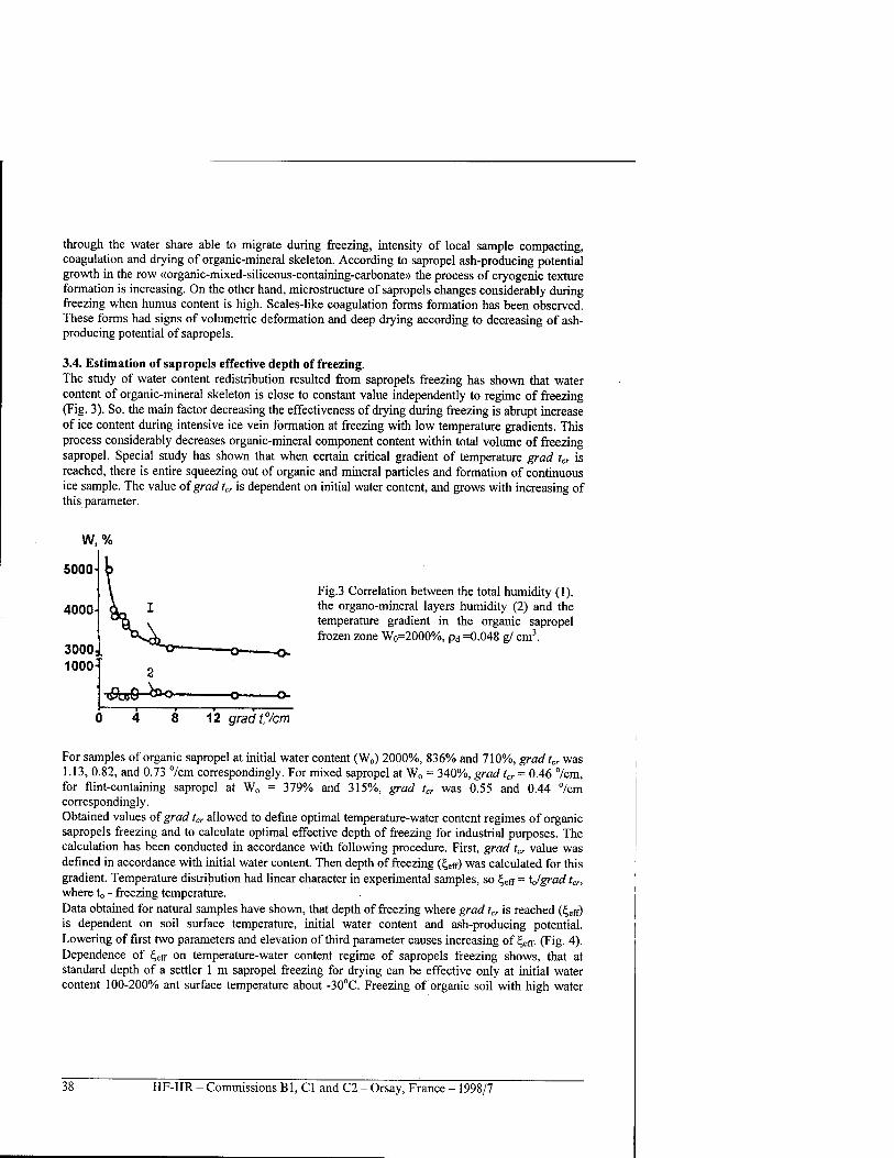
through the water share able to migrate during freezing, intensity of local sample compacting, coagulation and drying of organic-mineral skeleton. According to sapropel ash-producing potential growth in the row «organic-mixed-siliceous-containing-carbonate» the process of cryogenic texture formation is increasing. On the other hand, microstructure of sapropels changes considerably during freezing when humus content is high. Scales-like coagulation forms formation has been observed. These forms had signs of volumetric deformation and deep drying according to decreasing of ash- producing potential of sapropels.

3.4. Estimation of sapropels effective depth of freezing. The study of water content redistribution resulted from sapropels freezing has shown that water content of organic-mineral skeleton is close to constant value independently to regime of freezing (Fig. 3). So, the main factor decreasing the effectiveness of drying during freezing is abrupt increase of ice content during intensive ice vein formation at freezing with low temperature gradients. This process considerably decreases organic-mineral component content within total volume of freezing sapropel. Special study has shown that when certain critical gradient of temperature grad tcr is reached, there is entire squeezing out of organic and mineral particles and formation of continuous ice sample. The value of grad tcr is dependent on initial water content, and grows with increasing of this parameter.

W, %

5000

4000-

3000 1000

Fig.3 Correlation between the total humidity (1), the organo-mineral layers humidity (2) and the temperature gradient in the organic sapropel frozen zone W0=2000%, pd =0.048 g/ cm3.

0 4 8 12 gradt°/cm

For samples of organic sapropel at initial water content (W0) 2000%, 836% and 710%, grad tcr was 1.13, 0.82, and 0.73 %m correspondingly. For mixed sapropel at W0 = 340%, grad tcr = 0.46 7cm, for flint-containing sapropel at W„ = 379% and 315%, grad lcr was 0.55 and 0.44 7cm correspondingly. Obtained values of grad tcr allowed to define optimal temperature-water content regimes of organic sapropels freezing and to calculate optimal effective depth of freezing for industrial purposes. The calculation has been conducted in accordance with following procedure. First, grad tcr value was defined in accordance with initial water content. Then depth of freezing (£efr) was calculated for this gradient. Temperature distribution had linear character in experimental samples, so £eff = Xjgrad tcr, where to - freezing temperature. Data obtained for natural samples have shown, that depth of freezing where grad t„ is reached (i^ff) is dependent on soil surface temperature, initial water content and ash-producing potential. Lowering of first two parameters and elevation of third parameter causes increasing of £efr- (Fig. 4). Dependence of £,etr on temperature-water content regime of sapropels freezing shows, that at standard depth of a settler 1 m sapropel freezing for drying can be effective only at initial water content 100-200% ant surface temperature about -30°C. Freezing of organic soil with high water


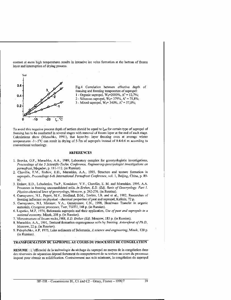
content at more high temperatures results in intensive ice veins formation at the bottom of frozen layer and interruption of drying process.

•Jeff

0.6

0.4

0.2

Fig.4 Correlation between effective depth of freezing and freezing temperature of sapropel: 1 - Organic sapropel, W0=2000%, Ac = 12,7%; 2 - Siliceous sapropel, W0= 379%, Ac = 75,8%; 3 - Mixed sapropel, W0= 340%, Ac = 57,0%;

-10 -20 L,"C

To avoid this negative process depth of settlers should be equal to i|eff for certain type of sapropel of freezing has to be conducted in several stages with removal of frozen layer at the end of each stage. Calculations show (Murashko, 1991), that layer-by- layer freezing even at average winter temperatures -3-H-5°C can result in drying of 5-7m of sapropels instead of 0.4-0.6 m according to conventional technology.

REFERENCES

1. Brovka, G.P., Murashko, A.A., 1989, Laboratory complex for geocryologistic investigations, Proceedings of the 5 Scientific-Techn. Conference, Engineering-geocryologist investigations on permafrost, Magadan, p. 111-112. (in Russian).

2. Chuvilin, E.M., Ershov, E.D., Murashko, A.A., 1993, Structure and texture formation in sapropels, Proceedings 6-th International Permafrost Conference, vol. 1, Beijing, China, p. 89- 93.

3. Ershov, E.D., Lebedenko, Yu.P., Kondakov, V.V., Chuvilin, E. M. and Murashko, 1995, A.A. Processes in freezing unconsolidated soils. In Ershov, E.D. (Ed), Basis of Geocryology. Part 1. Physico-chemical laws of geocryology, Moscow, p. 262-276. (in Russian).

4. Gamayunov, N.I., Popov, M.V., Stodland, D.M., Tovbin, LB. and et al., 1982, Researches of freezing influence on physical - chemical properties of peat and sapropel, Kalinin, 72 p.

5. Gamayunov, N.I, Mironov, V.A., Gamayunov, C.N., 1998, Heat/mass Transfer in organic materials, Cryogenic processes, Tver, TGTU, 148 p. (in Russian).

6. Lopotko, M.Z, 1974, Belorussia sapropels and their application, Use of peat and sapropels in a national economy, Minsk, 208 p. (in Russian).

7. Microstructure of frozen rocks,1988, E.D. Ershov (Ed), Moscow, 183 p. (in Russian). 8. Murashko, A.A., 1991, Textural formation organogenous soils by freezing. Avtoreferat of Ph.D.,

Moscow, 22 p. (in Russian). 9. Pidoplichko, A.P, 1975, Lake sediments of Belorussia, A science and engineering, Minsk, 120 p.

(in Russian).

TRANSFORMATION DU SAPROPEL AU COURS DU PROCESSUS DE CONGELATION

RESUME : L'efficacite de la technologie du sechage du sapropel au moyen de la congelation dans des reservoirs de separation depend fortement du comportement de sa texture au cours du processus impose pour obtenir sa solidification. Contrairement aux sols mineraux, la congelation du sapropel


n'a pas ete etudiee en detail. Sur ce theme, dans cette communication est presentee une analyse, basee sur des experiences conduites sur des modeles de laboratoire, de la transformation de la structure et de la texture du sapropel au cours de sa congelation. L'ensemble des experiences permet de definir les meilleurs regimes de congelation des sols organiques, pour lesquels le gel affecte fortement la plupart des composants organo-mineraux et agglomeres du sol. Les resultats permettent egalement la determination de la profondeur du gel pour des applications industrielles qui necessitent la meilleure efficacite des processus de cryo-deshydratation utilises.


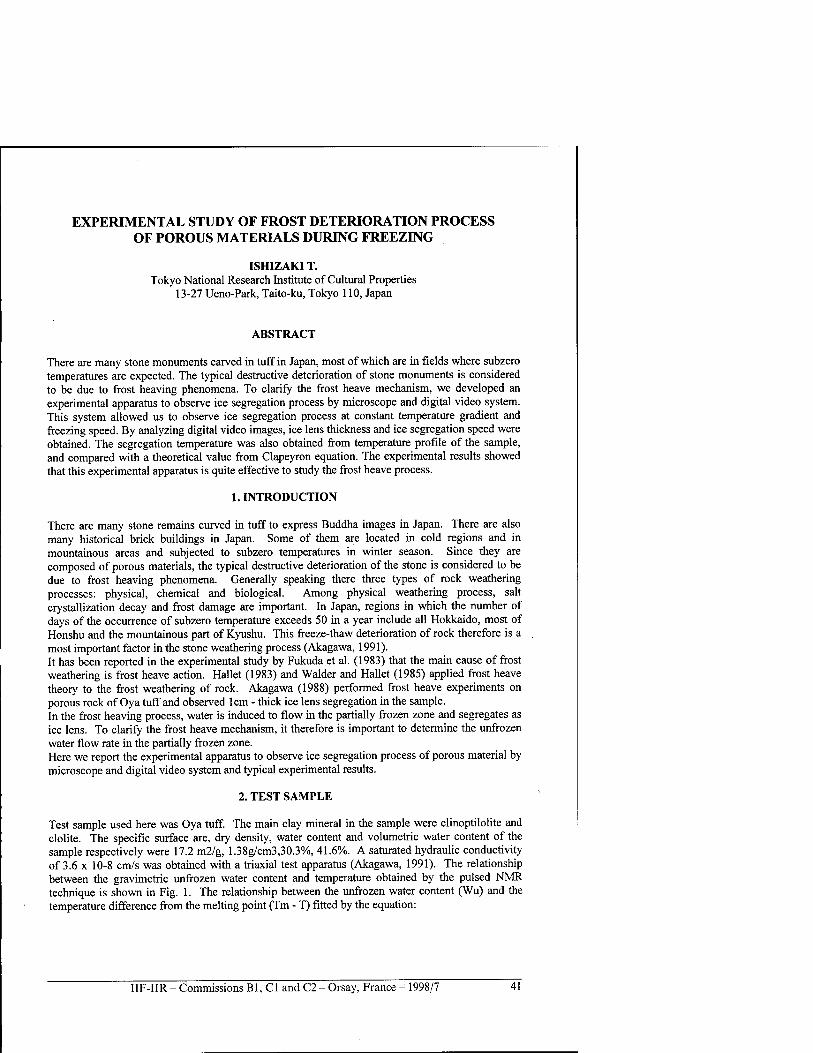
EXPERIMENTAL STUDY OF FROST DETERIORATION PROCESS OF POROUS MATERIALS DURING FREEZING

ISHIZAKIT. Tokyo National Research Institute of Cultural Properties

13-27 Ueno-Park, Taito-ku, Tokyo 110, Japan

ABSTRACT

There are many stone monuments carved in tuff in Japan, most of which are in fields where subzero temperatures are expected. The typical destructive deterioration of stone monuments is considered to be due to frost heaving phenomena. To clarify the frost heave mechanism, we developed an experimental apparatus to observe ice segregation process by microscope and digital video system. This system allowed us to observe ice segregation process at constant temperature gradient and freezing speed. By analyzing digital video images, ice lens thickness and ice segregation speed were obtained. The segregation temperature was also obtained from temperature profile of the sample, and compared with a theoretical value from Clapeyron equation. The experimental results showed that this experimental apparatus is quite effective to study the frost heave process.

1. INTRODUCTION

There are many stone remains curved in tuff to express Buddha images in Japan. There are also many historical brick buildings in Japan. Some of them are located in cold regions and in mountainous areas and subjected to subzero temperatures in winter season. Since they are composed of porous materials, the typical destructive deterioration of the stone is considered to be due to frost heaving phenomena. Generally speaking there three types of rock weathering processes: physical, chemical and biological. Among physical weathering process, salt crystallization decay and frost damage are important. In Japan, regions in which the number of days of the occurrence of subzero temperature exceeds 50 in a year include all Hokkaido, most of Honshu and the mountainous part of Kyushu. This freeze-thaw deterioration of rock therefore is a most important factor in the stone weathering process (Akagawa, 1991). It has been reported in the experimental study by Fukuda et al. (1983) that the main cause of frost weathering is frost heave action. Hallet (1983) and Wälder and Hallet (1985) applied frost heave theory to the frost weathering of rock. Akagawa (1988) performed frost heave experiments on porous rock of Oya tuff and observed 1cm - thick ice lens segregation in the sample. In the frost heaving process, water is induced to flow in the partially frozen zone and segregates as ice lens. To clarify the frost heave mechanism, it therefore is important to determine the unfrozen water flow rate in the partially frozen zone. Here we report the experimental apparatus to observe ice segregation process of porous material by microscope and digital video system and typical experimental results.

2. TEST SAMPLE

Test sample used here was Oya tuff. The main clay mineral in the sample were clinoptilolite and clolite. The specific surface are, dry density, water content and volumetric water content of the sample respectively were 17.2 m2/g, 1.38g/cm3,30.3%, 41.6%. A saturated hydraulic conductivity of 3.6 x 10-8 cm/s was obtained with a triaxial test apparatus (Akagawa, 1991). The relationship between the gravimetric unfrozen water content and temperature obtained by the pulsed NMR technique is shown in Fig. 1. The relationship between the unfrozen water content (Wu) and the temperature difference from the melting point (Tm - T) fitted by the equation:


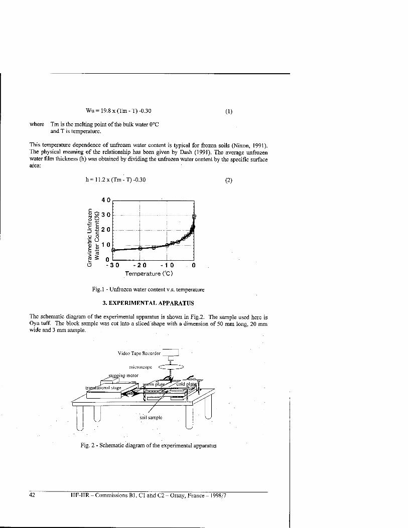
Wu = 19.8 x(Tm-T)-0.30 (1)

where Tm is the melting point of the bulk water 0°C and T is temperature.

This temperature dependence of unfrozen water content is typical for frozen soils (Nixon, 1991). The physical meaning of the relationship has been given by Dash (1991). The average unfrozen water film thickness (h) was obtained by dividing the unfrozen water content by the specific surface area:

h= 11.2 x(Tm-T) -0.30 (2)

-30 -20 - 1 0

Temperature (°C)

Fig. 1 - Unfrozen water content v.s. temperature

3. EXPERIMENTAL APPARATUS

The schematic diagram of the experimental apparatus is shown in Fig.2. The sample used here is Oya tuff. The block sample was cut into a sliced shape with a dimension of 50 mm long, 20 mm wide and 3 mm sample.

Video Tape Recorder

Fig. 2 - Schematic diagram of the experimental apparatus


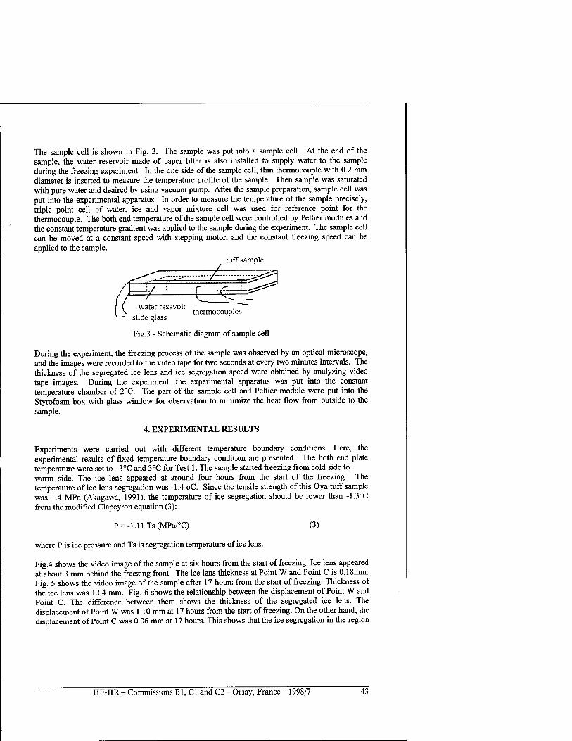
The sample cell is shown in Fig. 3. The sample was put into a sample cell. At the end of the sample, the water reservoir made of paper filter is also installed to supply water to the sample during the freezing experiment. In the one side of the sample cell, thin thermocouple with 0.2 mm diameter is inserted to measure the temperature profile of the sample. Then sample was saturated with pure water and deaired by using vacuum pump. After the sample preparation, sample cell was put into the experimental apparatus. In order to measure the temperature of the sample precisely, triple point cell of water, ice and vapor mixture cell was used for reference point for the thermocouple. The both end temperature of the sample cell were controlled by Peltier modules and the constant temperature gradient was applied to the sample during the experiment. The sample cell can be moved at a constant speed with stepping motor, and the constant freezing speed can be applied to the sample.

tuff sample ± water resevoir ,

thermocouples slide glass

Fig.3 - Schematic diagram of sample cell

During the experiment, the freezing process of the sample was observed by an optical microscope, and the images were recorded to the video tape for two seconds at every two minutes intervals. The thickness of the segregated ice lens and ice segregation speed were obtained by analyzing video tape images. During the experiment, the experimental apparatus was put into the constant temperature chamber of 2CC. The part of the sample cell and Peltier module were put into the Styrofoam box with glass window for observation to minimize the heat flow from outside to the sample.

4. EXPERIMENTAL RESULTS

Experiments were carried out with different temperature boundary conditions. Here, the experimental results of fixed temperature boundary condition are presented. The both end plate temperature were set to -3°C and 3°C for Test 1. The sample started freezing from cold side to warm side. The ice lens appeared at around four hours from the start of the freezing. The temperature of ice lens segregation was -1.4 oC. Since the tensile strength of this Oya tuff sample was 1.4 MPa (Akagawa, 1991), the temperature of ice segregation should be lower than -1.3°C from the modified Clapeyron equation (3):

P = -l.llTs(MPa/°C) (3)

where P is ice pressure and Ts is segregation temperature of ice lens.

Fig.4 shows the video image of the sample at six hours from the start of freezing. Ice lens appeared at about 3 mm behind the freezing front. The ice lens thickness at Point W and Point C is 0.18mm. Fig. 5 shows the video image of the sample after 17 hours from the start of freezing. Thickness of the ice lens was 1.04 mm. Fig. 6 shows the relationship between the displacement of Point W and Point C. The difference between them shows the thickness of the segregated ice lens. The displacement of Point W was 1.10 mm at 17 hours from the start of freezing. On the other hand, the displacement of Point C was 0.06 mm at 17 hours. This shows that the ice segregation in the region


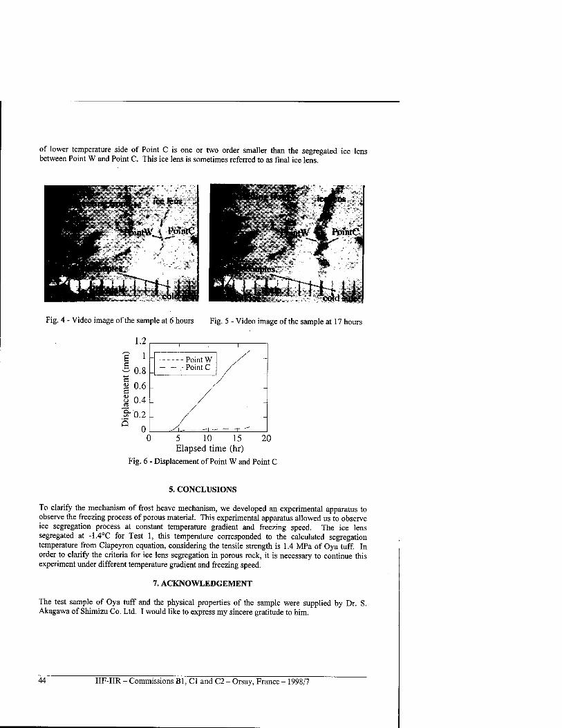
of lower temperature side of Point C is one or two order smaller than the segregated ice lens between Point W and Point C. This ice lens is sometimes referred to as final ice lens.

Fig. 4 - Video image of the sample at 6 hours Fig. 5 - Video image of the sample at 17 hours

1.2

? 1

§0.8

| 0.6

I 0.4

Q 0.2

0

Point W Point C /

/

/

0 5 10 15 20 Elapsed time (hr)

Fig. 6 - Displacement of Point W and Point C

5. CONCLUSIONS

To clarify the mechanism of frost heave mechanism, we developed an experimental apparatus to observe the freezing process of porous material. This experimental apparatus allowed us to observe ice segregation process at constant temperature gradient and freezing speed. The ice lens segregated at -1.4°C for Test 1, this temperature corresponded to the calculated segregation temperature from Clapeyron equation, considering the tensile strength is 1.4 MPa of Oya tuff. In order to clarify the criteria for ice lens segregation in porous rock, it is necessary to continue this experiment under different temperature gradient and freezing speed.

7. ACKNOWLEDGEMENT

The test sample of Oya tuff and the physical properties of the sample were supplied by Dr. S. Akagawa of Shimizu Co. Ltd. I would like to express my sincere gratitude to him.


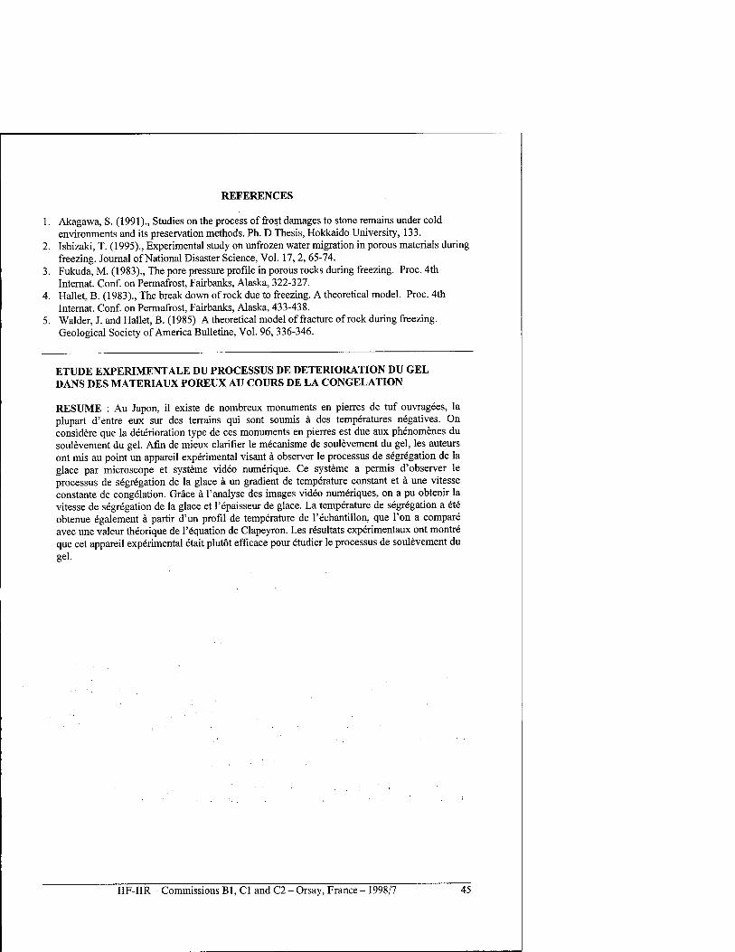
REFERENCES

1. Akagawa, S. (1991)., Studies on the process of frost damages to stone remains under cold environments and its preservation methods. Ph. D Thesis, Hokkaido University, 133.

2. Ishizaki, T. (1995)., Experimental study on unfrozen water migration in porous materials during freezing. Journal of National Disaster Science, Vol. 17, 2, 65-74.

3. Fukuda, M. (1983)., The pore pressure profile in porous rocks during freezing. Proc. 4th Internat. Conf. on Permafrost, Fairbanks, Alaska, 322-327.

4. Hallet, B. (1983)., The break down of rock due to freezing. A theoretical model. Proc. 4th Internat. Conf. on Permafrost, Fairbanks, Alaska, 433-438.

5. Wälder, J. and Hallet, B. (1985) A theoretical model of fracture of rock during freezing. Geological Society of America Bulletine, Vol. 96, 336-346.

ETUDE EXPERIMENT ALE DU PROCESSUS DE DETERIORATION DU GEL DANS DES MATERIAUX POREUX AU COURS DE LA CONGELATION

RESUME : Au Japon, il existe de nombreux monuments en pierres de tuf ouvragees, la plupart d'entre eux sur des terrains qui sont soumis ä des temperatures negatives. On considere que la deterioration type de ces monuments en pierres est due aux phenomenes du soulevement du gel. Afin de mieux clarifier le mecanisme de soulevement du gel, les auteurs ont mis au point un appareil experimental visant ä observer le processus de segregation de la glace par microscope et Systeme video numerique. Ce Systeme a permis d'observer le processus de segregation de la glace ä un gradient de temperature constant et ä une vitesse constante de congelation. Grace ä l'analyse des images video numeriques, on a pu obtenir la vitesse de segregation de la glace et l'epaisseur de glace. La temperature de segregation a ete obtenue egalement ä partir d'un profil de temperature de l'echantillon, que l'on a compare avec une valeur theorique de l'equation de Clapeyron. Les resultats experimentaux ont montre que cet appareil experimental etait plutot efficace pour etudier le processus de soulevement du gel.


SOIL MICROSTRUCTURE, THERMAL, HYDRAULIC AND OTHER PROPERTIES

AND GROUND BEHAVIOUR IN COLD REGIONS

WHITE T.L. and WILLIAMS P.J. Geotechnical Science Laboratories, Carleton University 1125 Colonel By Drive, Ottawa ON K1S 5B6 CANADA

ABSTRACT

The microstructure of freezing soils is largely responsible for their properties and behaviour. Experiments have shown how the microstructure is modified by freezing and, in turn, that the microstructure controls physical and geotechnical properties of the material. The microstructure of a soil controls the relative free energy of the soil water as a function of water content. This results in the dependence of unfrozen water content on temperature. These thermodynamic relations determine the thermal properties, strength and deformation, transport phenomena, hydrologic and other characteristics of frozen ground. The microstructure is thus ultimately responsible for the direction of geocryological processes at the macroscopic level. Consequently it is possible to predict the evolution of terrain conditions over periods of years. Such prediction is central to the solution of many geotechnical problems in the cold regions.

INTRODUCTION

The thermodynamic conditions within frozen ground at temperatures just below 0°C are such that there is a continuing translocation of water in conjunction with ice formation and displacement of soil particles. Van Vliet-Lanöe's (1985) review of frost effects summarised the major factors responsible for soil structure in cold environments, including ice lensing, frost heaving, soil solute concentration, and degree of cryodesiccation. Platy microstructure (Van Vliet-Lanöe, 1985; Gubin, 1993) is commonly associated with freeze- thaw processes and ice lens formation. Platy microstructure includes isoband and banded fabrics (Brewer and Pawluck, 1975; White, 1992, 1996; McMillan and Mitchell, 1953; Dumanski and St. Arnaud, 1966). Distinct fabric types for Turbic cryosols (Fox and Protz, 1981, Smith et al, 1991 and White and Fox, 1996) have been ascribed to the influence of cryogenic processes active in soils exposed to seasonal freezing and in permafrost. A fundamental consequence of the thermodynamic relations for freezing in porous media, is the development of cryosuction - a state of lowered pressure in the water phase which is responsible for water movements leading to frost heave, as well as for consolidation effects and the development of particle aggregates. This paper describes cryogenic fabric types which have developed in response to four prolonged periods of freezing (between 12 and 20 months) followed by periods of thaw (two to three months) in a silt used in a large scale ground freezing experiment. The experiment was to provide information on geotechnical consequences of freezing around a pipeline and included detailed monitoring of ground temperatures, frost heave, pipe displacement, soil moisture and density conditions, hydraulic conductivity and thermal properties. The observed reorganisation of soil fabric components has been analysed with respect to the cumulative effects of particle aggregation on unfrozen water content and thermal and mechanical properties.

1 METHODS AND MATERIALS

The Canada-France Pipeline Ground Freezing study (Burgess et al. 1982, Geotechnical Science Laboratories, 1988, Williams et al, 1993) was carried out in the controlled environment facility of the Centre de Geomorphologie, C.N.R.S., located in Caen, France. The refrigerated hall is 18 m


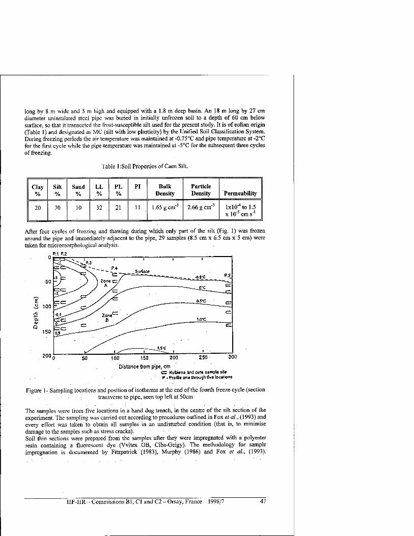
long by 8 m wide and 5 m high and equipped with a 1.8 m deep basin. An 18 m long by 27 cm diameter uninsulated steel pipe was buried in initially unfrozen soil to a depth of 60 cm below surface, so that it transected the frost-susceptible silt used for the present study. It is of eolian origin (Table 1) and designated as MC (silt with low plasticity) by the Unified Soil Classification System. During freezing periods the air temperature was maintained at -0.75°C and pipe temperature at -2°C for the first cycle while the pipe temperature was maintained at -5°C for the subsequent three cycles of freezing.

Table 1 :Soil Properties of Caen Silt.

Clay %

Silt %

Sand %

LL %

PL %

PI Bulk Density

Particle Density Permeability

20 70 10 32 21 11 1.65 gem"3 2.66 g cm'3 lxlO^tol.S x 10"5 cm s"1

After four cycles of freezing and thawing during which only part of the silt (Fig. 1) was frozen around the pipe and immediately adjacent to the pipe, 29 samples (8.5 cm x 6.5 cm x 5 cm) were taken for micrornorphological analysis.

P.t P.2

300

Distance -from pipe, cm CZ KuW«na and cure sampti sita P -ProSe on«Ihrough-fivs locations

Figure 1- Sampling locations and position of isotherms at the end of the fourth freeze cycle (section transverse to pipe, seen top left at 50cm

The samples were from five locations in a hand dug trench, in the centre of the silt section of the experiment. The sampling was carried out according to procedures outlined in Fox et al., (1993) and every effort was taken to obtain all samples in an undisturbed condition (that is, to minimise damage to the samples such as stress cracks). Soil thin sections were prepared from the samples after they were impregnated with a polyester resin containing a fluorescent dye (Vvitex OB, Ciba-Geigy). The methodology for sample impregnation is documented by Fitzpatrick (1983), Murphy (1986) and Fox et al, (1993).


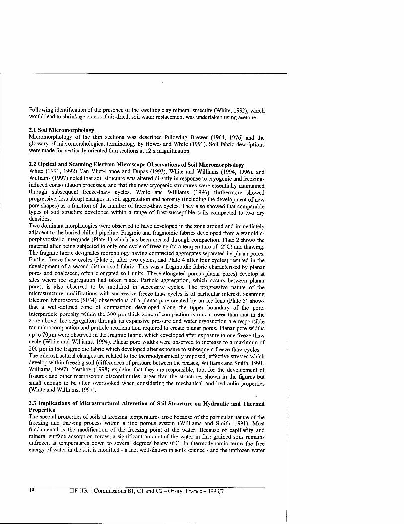
Following identification of the presence of the swelling clay mineral smectite (White, 1992), which would lead to shrinkage cracks if air-dried, soil water replacement was undertaken using acetone.

2.1 Soil Micromorphology Micromorphology of the thin sections was described following Brewer (1964, 1976) and the glossary of micromorphological terminology by Howes and White (1991). Soil fabric descriptions were made for vertically oriented thin sections at 12 x magnification.

2.2 Optical and Scanning Electron Microscope Observations of Soil Micromorphology White (1991, 1992) Van Vliet-Lanöe and Dupas (1992), White and Williams (1994, 1996), and Williams (1997) noted that soil structure was altered directly in response to cryogenic and freezing- induced consolidation processes, and that the new cryogenic structures were essentially maintained through subsequent freeze-thaw cycles. White and Williams (1996) furthermore showed progressive, less abrupt changes in soil aggregation and porosity (including the development of new pore shapes) as a function of the number of freeze-thaw cycles. They also showed that comparable types of soil structure developed within a range of frost-susceptible soils compacted to two dry densities. Two dominant morphologies were observed to have developed in the zone around and immediately adjacent to the buried chilled pipeline. Fragmic and fragmoidic fabrics developed from a granoidic- porphyroskelic intergrade (Plate 1) which has been created through compaction. Plate 2 shows the material after being subjected to only one cycle of freezing (to a temperature of -2°C) and thawing. The fragmic fabric designates morphology having compacted aggregates separated by planar pores. Further freeze-thaw cycles (Plate 3, after two cycles, and Plate 4 after four cycles) resulted in the development of a second distinct soil fabric. This was a fragmoidic fabric characterised by planar pores and coalesced, often elongated soil units. These elongated pores (planar pores) develop at sites where ice segregation had taken place. Particle aggregation, which occurs between planar pores, is also observed to be modified in successive cycles. The progressive nature of the microstructure modifications with successive freeze-thaw cycles is of particular interest. Scanning Electron Microscope (SEM) observations of a planar pore created by an ice lens (Plate 5) shows that a well-defined zone of compaction developed along the upper boundary of the pore. Interparticle porosity within the 300 um thick zone of compaction is much lower than that in the zone above. Ice segregation through its expansive pressure and water cryosuction are responsible for microcompaction and particle reorientation required to create planar pores. Planar pore widths up to 70um were observed in the fragmic fabric, which developed after exposure to one freeze-thaw cycle (White and Williams, 1994). Planar pore widths were observed to increase to a maximum of 200 um in the fragmoidic fabric which developed after exposure to subsequent freeze-thaw cycles. The microstructural changes are related to the thermodynamically imposed, effective stresses which develop within freezing soil (differences of pressure between the phases, Williams and Smith, 1991, Williams, 1997). Yershov (1998) explains that they are responsible, too, for the development of fissures and other macroscopic discontinuities larger than the structures shown in the figures but small enough to be often overlooked when considering the mechanical and hydraulic properties (White and Williams, 1997).

2.3 Implications of Microstructural Alteration of Soil Structure on Hydraulic and Thermal Properties The special properties of soils at freezing temperatures arise because of the particular nature of the freezing and thawing process within a fine porous system (Williams and Smith, 1991). Most fundamental is the modification of the freezing point of the water. Because of capillarity and mineral surface adsorption forces, a significant amount of the water in fine-grained soils remains unfrozen at temperatures down to several degrees below 0°C. In thermodynamic terms the free energy of water in the soil is modified - a fact well-known in soils science - and the unfrozen water

48 IIF-IIR - Commissions Bl, Cl and C2 - Orsay, France -1998/7

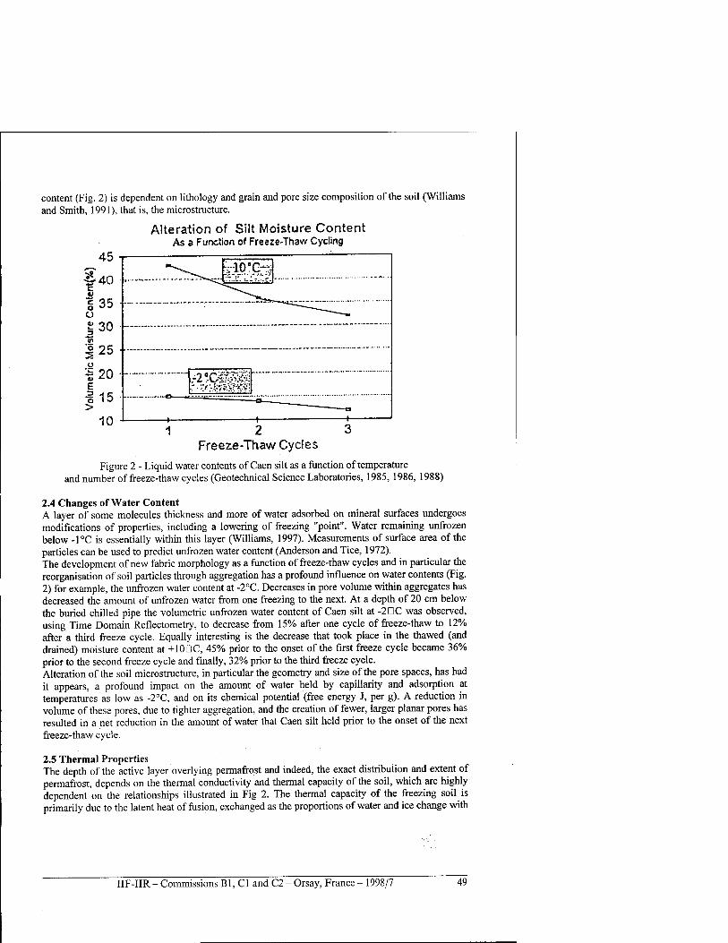
content (Fig. 2) is dependent on lithology and grain and pore size composition of the soil (Williams and Smith, 1991), that is, the microstructure.

Alteration of Silt Moisture Content As a Function of Freeze-Thaw Cycling

45

40

S35 o | 30 'S 125 o

'■5 20 e ü 15 >

10

Freeze-Thaw Cycles

Figure 2 - Liquid water contents of Caen silt as a function of temperature and number of freeze-thaw cycles (Geotechnical Science Laboratories, 1985, 1986, 1988)

2.4 Changes of Water Content A layer of some molecules thickness and more of water adsorbed on mineral surfaces undergoes modifications of properties, including a lowering of freezing "point". Water remaining unfrozen below -1°C is essentially within this layer (Williams, 1997). Measurements of surface area of the particles can be used to predict unfrozen water content (Anderson and Tice, 1972). The development of new fabric morphology as a function of freeze-thaw cycles and in particular the reorganisation of soil particles through aggregation has a profound influence on water contents (Fig. 2) for example, the unfrozen water content at -2°C. Decreases in pore volume within aggregates has decreased the amount of unfrozen water from one freezing to the next. At a depth of 20 cm below the buried chilled pipe the volumetric unfrozen water content of Caen silt at -2GC was observed, using Time Domain Reflectometry, to decrease from 15% after one cycle of freeze-thaw to 12% after a third freeze cycle. Equally interesting is the decrease that took place in the thawed (and drained) moisture content at +10DC, 45% prior to the onset of the first freeze cycle became 36% prior to the second freeze cycle and finally, 32% prior to the third freeze cycle. Alteration of the soil microstructure, in particular the geometry and size of the pore spaces, has had it appears, a profound impact on the amount of water held by capillarity and adsorption at temperatures as low as -2°C, and on its chemical potential (free energy J, per g). A reduction in volume of these pores, due to tighter aggregation, and the creation of fewer, larger planar pores has resulted in a net reduction in the amount of water that Caen silt held prior to the onset of the next freeze-thaw cycle.

2.5 Thermal Properties The depth of the active layer overlying permafrost and indeed, the exact distribution and extent of permafrost, depends on the thermal conductivity and thermal capacity of the soil, which are highly dependent on the relationships illustrated in Fig 2. The thermal capacity of the freezing soil is primarily due to the latent heat of fusion, exchanged as the proportions of water and ice change with


changing temperature. Figure 3 shows the position of the 0°C isotherm at Day 100 of the ground freezing experiment for the second, third and fourth freeze cycles in the silt adjacent to the buried chilled pipe. The figure shows that the depth of frost penetration from cycles two through four has increased. From this it may be inferred that the silt's thermal diffusivity has increased, thus giving faster penetration of the 0CC isotherm. The thermal conductivity increases from once cycle to the next in response to consolidation of the silt and intense ice segregation (ice has higher conductivity that water). Probably more important though, is the decrease in total moisture content and thus in the heat of fusion, giving smaller heat capacity.

■140 0.5 1 1.5

Distance from Pipe Axis (m)

Figure 3 - Position of 0°C isotherm in Caen silt, Day 100 of 2nd, 3rd and 4th freeze cycles (Geotechnical Science Laboratories, 1985, 1988)

2.6 Mechanical Properties The thermodynamic effects have equally fundamental consequences for the strength and creep properties of frozen ground, which have been elucidated only recently (Ladanyi and Shen, 1989, Williams and Smith, 1991). For these macroscopic effects to be large enough to affect engineered structures such as the buried chilled pipe used in the ground freezing experiments the soil must undergo the demonstrated changes in its internal microscopic structure. Pipe stresses observed on Day 350 for the second, third and fourth freeze cycles are shown in Figure 4. The evolution of pipe stresses can be explained from the changing soil structure. The consolidation and aggregation processes which reduce water content from one freeze-thaw cycle to the next also have a profound impact on the mechanical properties, including frost heave. It is the frost heave which is responsible for the pipe stresses.

2.7 Soil Microstructure as a Controlling Factor in Ground Surface Development The observations confirm what is intuitively reasonable. The soil microstructure, because it controls the fundamental thermodynamic behaviour of a freezing soil, and thus the soil's physical and geotechnical properties (density, frost heave, thermal properties etc.), controls the development of specific geocryological features. Depth of active layer, extent of permafrost, creep and solifluction and the forms of patterned ground are the soil's response to external conditions. The precise nature of the response is determined by the soil microstructure.


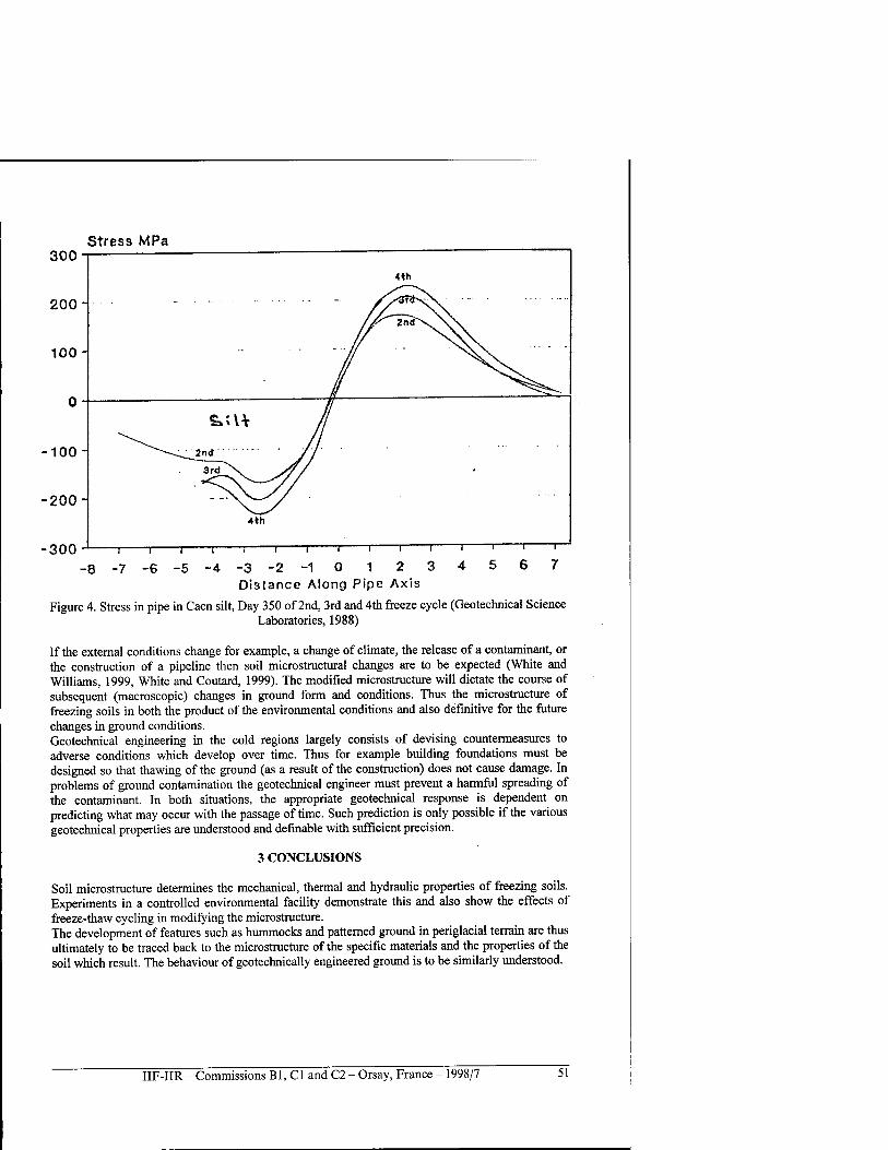
Stress MPa

-300

-8 -5 -4

T

-3 -2 -1 Distance Along Pipe Axis

Figure 4. Stress in pipe in Caen silt, Day 350 of 2nd, 3rd and 4th freeze cycle (Geotechnical Science Laboratories, 1988)

If the external conditions change for example, a change of climate, the release of a contaminant, or the construction of a pipeline then soil microstructural changes are to be expected (White and Williams, 1999, White and Coutard, 1999). The modified microstructure will dictate the course of subsequent (macroscopic) changes in ground form and conditions. Thus the microstructure of freezing soils in both the product of the environmental conditions and also definitive for the future changes in ground conditions. Geotechnical engineering in the cold regions largely consists of devising countermeasures to adverse conditions which develop over time. Thus for example building foundations must be designed so that thawing of the ground (as a result of the construction) does not cause damage. In problems of ground contamination the geotechnical engineer must prevent a harmful spreading of the contaminant. In both situations, the appropriate geotechnical response is dependent on predicting what may occur with the passage of time. Such prediction is only possible if the various geotechnical properties are understood and definable with sufficient precision.

3 CONCLUSIONS

Soil microstructure determines the mechanical, thermal and hydraulic properties of freezing soils. Experiments in a controlled environmental facility demonstrate this and also show the effects of freeze-thaw cycling in modifying the microstructure. The development of features such as hummocks and patterned ground in periglacial terrain are thus ultimately to be traced back to the microstructure of the specific materials and the properties of the soil which result. The behaviour of geotechnically engineered ground is to be similarly understood.


REFERENCES

1. Anderson, D.M., Tice, A.R., 1972, Predicting unfrozen water contents in frozen soils from surface area measurements. Highway Res. Rec. 393: 12-18.

2. Brewer, R. 1964, Fabric and Mineral Analysis of Soils, Wiley, New York. 3. Brewer, R. 1964 and Pawluk, S. 1975 Investigations of some soils developed in hummocks of

the Canadian sub-arctic and southern-arctic regions. Morphology and Micromorphology. Canadian Journal of Soil Science 55: p. 301 -319.

4. Burgess, M., Lemaire, G., Smith, M.W., Williams, P.J., 1982, Etude du gel des sols autour d'une conduite refroidie enterre dans une station experimentale. Phase I. Pour Le Ministere d'Energie, Mines et Resources, Direction de la Physique du Globe, 62 p.

5. Dumanski, J., St. Arnaud, R.J., 1966, A micropedological study of eluvial soil horizons. Canadian Journal of Soil Science 46, p. 287-292.

6. Fitzpatrick, E.A., 1983, The Morphology of Soils. New York: Chapman and Hall Ltd. 7. Fox, CA., 1993, Micromorphology of an orthic Turbic Cryosol - a permafrost soil. Soil

Micromorphology, Ed., P. Bullock and C.P. Murphy, vol. 2, p. 699-70. 8. Fox, CA., Protz, R., 1981, Definition of Fabric Distribution to Characterise the Rearrangement

of Soil Particles in Turbic Cryosols, Canadian Journal of Soil Science 61, 29-34. 9. Geotechnical Science Laboratories, 1983-88. Internal Reports, Canada- France Pipeline Ground

Freezing Project. 10. Gubin, S.V., 1993, Structure formation dynamics in Tundra Cryogenic Non-Gleyed Soils

(Tundra Cryozems). Joint Russia-America Seminar on Cryopedology and Global Change. Russian Academy of Science, p. 201-213.

11. Howes, J.E., White, T.L., 1991, Glossary of Terminology for Soil Micromorphology. Ottawa: Geotechnical Science Laboratories, 62 p.

12. Ladanyi, B., Shen, M., 1993, Freezing pressure development on a buried chilled pipeline. International Symposium on Frost in Geotechnical Engineering, Anchorage, Alaska, p. 23-34.

13. Murphy, C.P., 1986, Thin section preparation of soils and sediments. Berkhamsted, Herts, England: AB Academic Publishers.

14. Smith, C.A.S., Fox, CA., Hargrave, A.E., 1991, Development of soil Structure in some turbic cryosols in the Canadian low Arctic, Canadian Journal of Soil Science 71: p. 11-29.

15. Van Vliet-Lanöe, B., 1985, Frost Effects in Soils in Quaternary Landscape Evolution (J. Boardman, ed.). John Wiley and Sons Ltd., New York.

16. Van Vliet-Lanöe, B., Dupas, A., 1992, Development of soil fabric by freeze-thaw cycles. Its effects on frost heave. Proceedings of the Fifth International Symposium on Ground Freezing, Beijing, p. 189-195.

17. White, T.L., 1992, Cryogenic Alteration of a Frost Susceptible Soil. M.Sc. Thesis. Ottawa: Carleton University.

18. White, T.L., 1996, Cryogenic Alteration of Clay and Silt Microstructure, Implications for Geotechnical Properties. Ph. d. thesis. Ottawa: Carleton University.

19. White, T.L., Coutard, J-P., 1999, Modfication of silt microstructure by hydrocarbon contamination in freezing ground. Contamination in Freezing Ground, Proc. of Conf, Cambridge, 1997. Polar Record, vol. 35, no. 192, Jan 1999, p. 41-50.

20. White, T.L., Fox, CA., 1996, Comparison of cryogenic features dominant in soils affected by permafrost with those produced experimentally. Proceedings, 10th International Working Meeting of Soil Micromorphology, Moscow, July 1996.

21. White, T.L., Williams, P.J., 1994, Cryogenic alteration of frost susceptible soils. Proceedings of the 7th International Symposium on Ground Freezing, Nancy, France, 17-24.


22. White, T.L., Williams, P.J., 1996, The Role of Microstructure - Geotechnical Properties of Freezing Soils. Ottawa: Fifth International Symposium on Thermal Engineering and Science for Cold Regions, p. 415-426.

23. White, T.L., Williams, P.J., 1999, The influence of soil microstructure on hydraulic properties of hydrocarbon contaminated freezing ground. Seminar on Contaminants in freezing ground, Cambridge, July 1997. Polar Record, vol. 35, no. 192, Jan. 1999, p.25-32.

24. Williams, P.J., 1998, Frost heaving in frozen ground & Contaminants and microstructure in freezing ground. Proceedings: Nato Advanced Study Institute, Italy, Springer Verlag.29.

25. Williams, P.J., Riseborough, D.W., Smith, M.W. 1993. The France-Canada joint study of deformation of an experimental pipeline by differential frost heave. Int. Journ. Offshore and Petroleum Engineering vol.3, 1, p.56-60

26. Williams, P.J., Smith, M.W. 1991. The Frozen Earth. Fundamentals of Geocryology. Cambridge Univ. Press. 306 p.

27. Yershov, E.D., 1998, General Geocryology (Translation from the Russian, Nedra 1990). Cambridge University Press, 580 p.

MICROSTRUCTURE DU SOL - PROPRIETES THERMIQUES, HYDRAULIQUES ET AUTRES ET COMPORTEMENT DU TERRAIN DANS LES REGIONS FROIDES

RESUME : De la microstructure des sols congeles, dependent largement leurs proprietes et leur comportement. Des experiences ont montre comment la microstructure est modifiee par la congelation et, en retour, que la microstructure regit les proprietes physiques et geotechniques du materiau. La microstructure d'un sol regit l'energie libre relative de l'eau du sol en fonction de la teneur en eau, ce qui implique la dependance de la teneur en eau non congelee ä la temperature. Ces relations thermodynamiques determinent les proprietes thermiques, la resistance et la deformation, les phenomenes de transport, les caracteristiques hydrologiques et autres du sol congele. Par consequent, la microstructure est incontestablement responsable de l'orientation des processus geocryologiques ä un niveau macroscopique. II est done possible de prevoir revolution des conditions des terrains sur de nombreuses annees. Une teile prevision est essentielle pour la resolution de nombreux pföblemes geotechniques dans les regions froides.


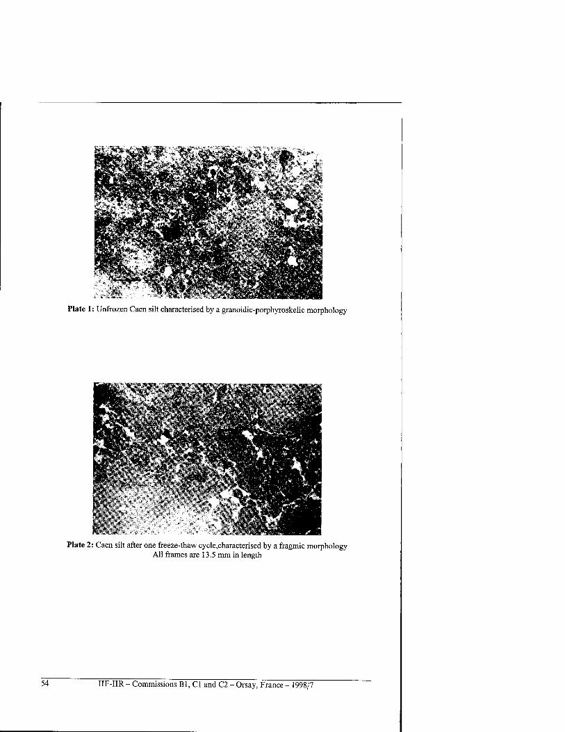
tftfc

Plate 1: Unfrozen Caen silt characterised by a granoidic-porphyroskelic morphology

Plate 2: Caen silt after one freeze-thaw cycle,characterised by a fragmic morphology All frames are 13.5 mm in length


..... . .*"• . ••■•■■

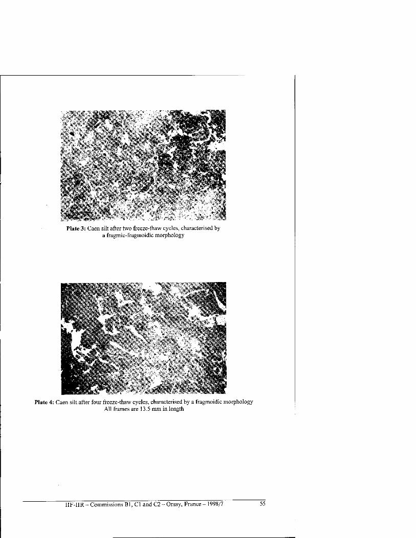
ft*-- "\. lift 1

Plate 3: Caen silt after two freeze-thaw cycles, characterised by a fragmic-fragmoidic morphology

Bl§4 .*"J."'-->i'-.":'. ,. .•'."V--. '■'7;.<i £,

m ;"■#

U m ■'..-*

Spil jd ̂ ^"

HP: '''

»§&?*£: £§£****?'■ ^^WaHi m» ^^

fyK5s&

M* ia

Plate 4: Caen silt after four freeze-thaw cycles, characterised by a fragmoidic morphology All frames are 13.5 mm in length


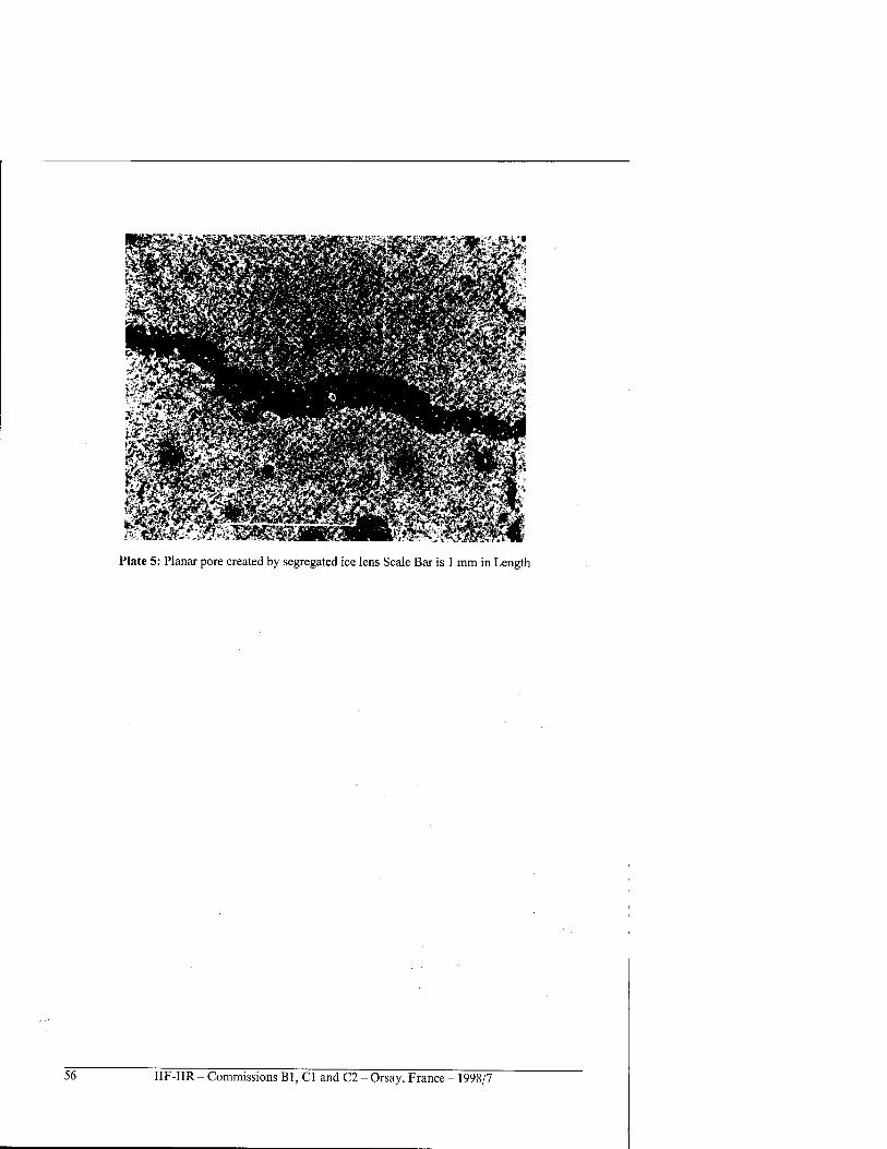
Plate 5: Planar pore created by segregated ice lens Scale Bar is 1 mm in Length


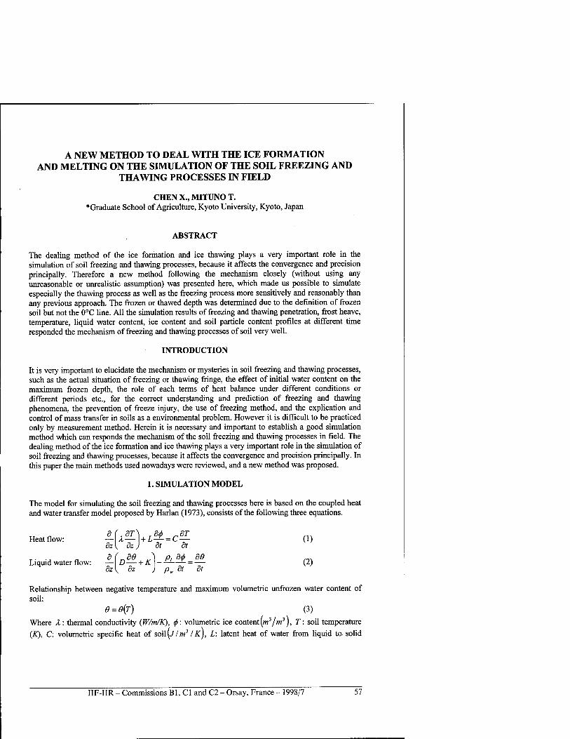
A NEW METHOD TO DEAL WITH THE ICE FORMATION AND MELTING ON THE SIMULATION OF THE SOIL FREEZING AND

THAWING PROCESSES IN FIELD

CHEN X., MITUNO T. ♦Graduate School of Agriculture, Kyoto University, Kyoto, Japan

ABSTRACT

The dealing method of the ice formation and ice thawing plays a very important role in the simulation of soil freezing and thawing processes, because it affects the convergence and precision principally. Therefore a new method following the mechanism closely (without using any unreasonable or unrealistic assumption) was presented here, which made us possible to simulate especially the thawing process as well as the freezing process more sensitively and reasonably than any previous approach. The frozen or thawed depth was determined due to the definition of frozen soil but not the 0°C line. All the simulation results of freezing and thawing penetration, frost heave, temperature, liquid water content, ice content and soil particle content profiles at different time responded the mechanism of freezing and thawing processes of soil very well.

INTRODUCTION

It is very important to elucidate the mechanism or mysteries in soil freezing and thawing processes, such as the actual situation of freezing or thawing fringe, the effect of initial water content on the maximum frozen depth, the role of each terms of heat balance under different conditions or different periods etc., for the correct understanding and prediction of freezing and thawing phenomena, the prevention of freeze injury, the use of freezing method, and the explication and control of mass transfer in soils as a environmental problem. However it is difficult to be practiced only by measurement method. Herein it is necessary and important to establish a good simulation method which can responds the mechanism of the soil freezing and thawing processes in field. The dealing method of the ice formation and ice thawing plays a very important role in the simulation of soil freezing and thawing processes, because it affects the convergence and precision principally. In this paper the main methods used nowadays were reviewed, and a new method was proposed.

1. SIMULATION MODEL

The model for simulating the soil freezing and thawing processes here is based on the coupled heat and water transfer model proposed by Harlan (1973), consists of the following three equations.

TT r, Sf.dT^ Td(j> _Sr ... Heat flow: — A— +L—= C— (1)

dz{ 8z) dt dt

Liquid water flow: *-(D™+K)-PL?* = M (2) 8z{ dz ) pw dt dt

Relationship between negative temperature and maximum volumetric unfrozen water content of soil:

e = 0(T) (3)

Where A: thermal conductivity {W/tn/K), $: volumetric ice content (m3/;n3), T: soil temperature (K), C: volumetric specific heat of soil(j/»23 IK), L: latent heat of water from liquid to solid


(J/m\ z: vertical position coordinate (m), D: hydraulic diffusivity (m2/sec), K: hydraulic conductivity (m/sec), p,: ice density (lffkg/m3), pw: water density, 0: liquid water content (m3/m3), t: time (sec).

2. DEALING METHODS OF ICE FORMATION AND THAWING

The dealing method of the ice formation and ice thawing plays a very important role in the simulation of soil freezing and thawing processes, because it affects the convergence and precision principally. The latent heat for the phase change from water to ice is so large, up to 160 times of the specific heat of frozen or unfrozen soil (Taylor and Luthin, 1978). Therefore even a small error of ice content calculation, will causes big error in the computing of soil temperature and unfrozen water content, furthermore affect the location of frozen-unfrozen interface and the result of the frost heave etc.. Various methods for dealing with the ice formation and thawing have been proposed. Three main methods of it will be reviewed as follows, and the new one presented in this paper will be described at last.

2.1 Method in Light of the Heat Flux Difference Since Taylor and Luthin (1978), a method in light of heat flux difference has been used by many researchers to simulate the freezing process in laboratory or in situ. It is a method that assume the difference of heat flux into and get off from a node is fully contributed to the ice formation or thawing around that node at first, and then revise it by changing the coefficient R until the precise of the iteration results of temperature and liquid water content become allowable. Equation estimating the heat flux difference at node "i" is as follows.

£(*-G'+I)-*-G"-I)) z„(|- + l)-*.(0. .(')-*.,0--i) (4)

Where At: time step (sec), R: adjusting coefficient, $(i): volumetric ice content, the subscript m indicates the former time step. When the difference of heat flux is too small, endless iteration will occurs, and causes instability and divergence. For this reason this method is inadequate for the thawing process where the temperature gradient is often gentle. In fact this method has been used only for the freezing process of soils.

2.2 Temperature Recovery Method As described by Nisigaki and Umeda (1993), the temperature recovery method is originally used for the calculation of metal solidifying. For the freezing of soil, instead of latent heat, take note of Ag,, the increase of proportion of the ice content over the initial water content, when the proportion rise to 1, the phase change finished around this node. The AQ of latent heat release from Ag, was expressed by the following equation.

AQ = pwxVxmxAgixL (5)

Where, m: total water content (ice+water, m3/m3), V: volume of soil bulk (m3). At beginning, set Ag; be 0, compute T by the heat flow equation, and the depression AT from the original freezing point TL, namely AT = Tv T. If A7'>0, indicates the ice content increased, calculate Ag by equation (6). Where p is the synthetic density (ICPkg/m3) of soil.


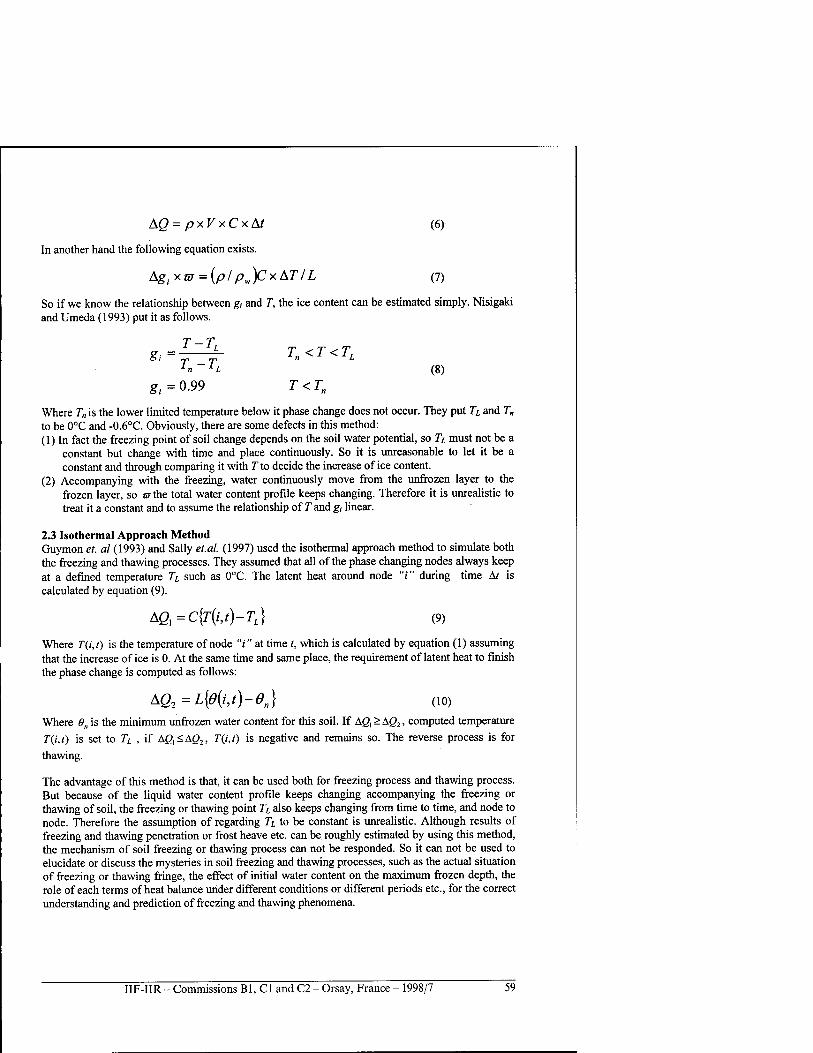
AQ = pxVxCxAt (6)

In another hand the following equation exists.

Agixm = {p/pw)CxAT/L (7)

So if we know the relationship between gt and T, the ice content can be estimated simply. Nisigaki and Umeda (1993) put it as follows.

T-T Z=-—— T<T<T,

ln~lL (8)

g,=0.99 T<Tn

Where T„ is the lower limited temperature below it phase change does not occur. They put TL and T„ to be 0°C and -0.6°C. Obviously, there are some defects in this method: (1) In fact the freezing point of soil change depends on the soil water potential, so TL must not be a

constant but change with time and place continuously. So it is unreasonable to let it be a constant and through comparing it with 7/to decide the increase of ice content.

(2) Accompanying with the freezing, water continuously move from the unfrozen layer to the frozen layer, so w the total water content profile keeps changing. Therefore it is unrealistic to treat it a constant and to assume the relationship of T and gt linear.

2.3 Isothermal Approach Method Guymon et. al (1993) and Sally et.al. (1997) used the isothermal approach method to simulate both the freezing and thawing processes. They assumed that all of the phase changing nodes always keep at a defined temperature TL such as 0°C. The latent heat around node "i" during time At is calculated by equation (9).

AQx=C{T(i,t)-TL) (9)

Where T(i,t) is the temperature of node "i" at time t, which is calculated by equation (1) assuming that the increase of ice is 0. At the same time and same place, the requirement of latent heat to finish the phase change is computed as follows:

*Q2=L{0{i,t)-e„} (10) Where 0„ is the minimum unfrozen water content for this soil. If AQl>AQ1, computed temperature T(i,t) is set to TL , if Aß,<A02, T(i,t) is negative and remains so. The reverse process is for

thawing.

The advantage of this method is that, it can be used both for freezing process and thawing process. But because of the liquid water content profile keeps changing accompanying the freezing or thawing of soil, the freezing or thawing point TL also keeps changing from time to time, and node to node. Therefore the assumption of regarding TL to be constant is unrealistic. Although results of freezing and thawing penetration or frost heave etc. can be roughly estimated by using this method, the mechanism of soil freezing or thawing process can not be responded. So it can not be used to elucidate or discuss the mysteries in soil freezing and thawing processes, such as the actual situation of freezing or thawing fringe, the effect of initial water content on the maximum frozen depth, the role of each terms of heat balance under different conditions or different periods etc., for the correct understanding and prediction of freezing and thawing phenomena.


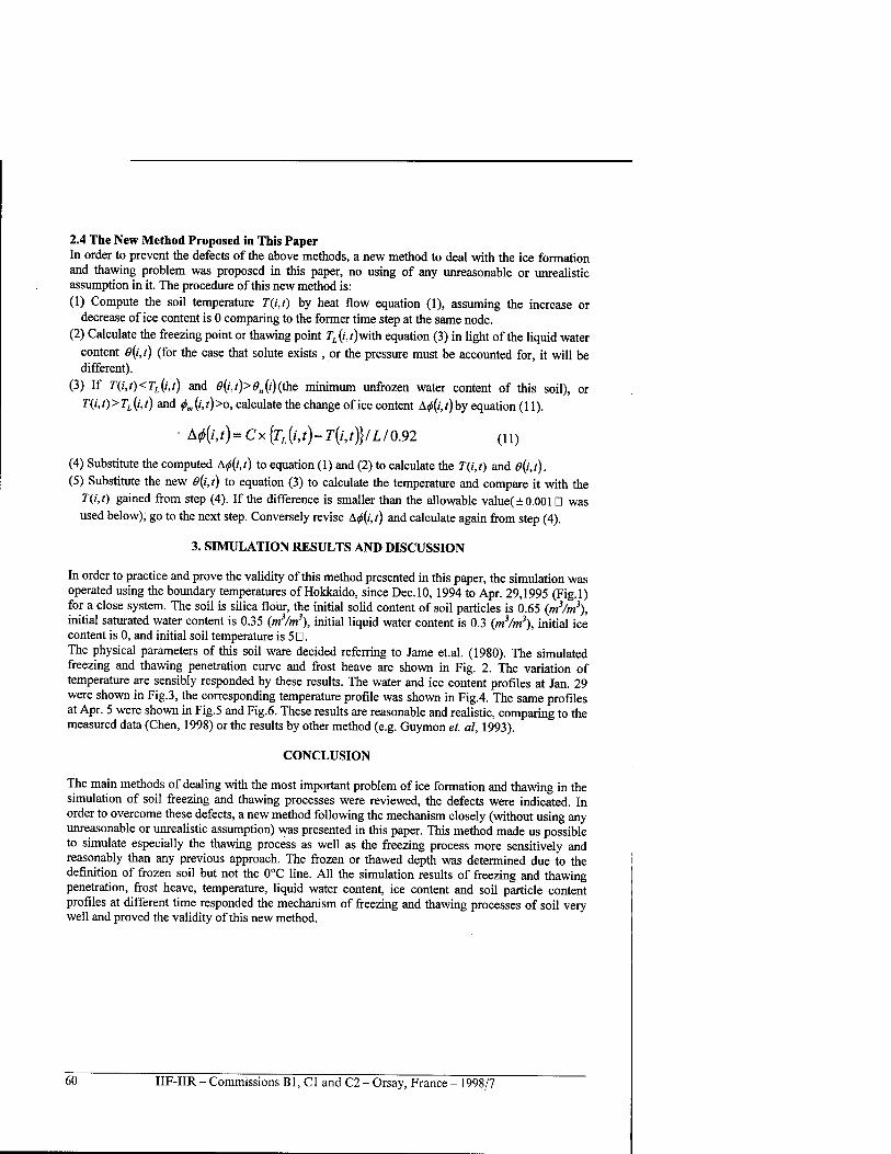
2.4 The New Method Proposed in This Paper In order to prevent the defects of the above methods, a new method to deal with the ice formation and thawing problem was proposed in this paper, no using of any unreasonable or unrealistic assumption in it. The procedure of this new method is: (1) Compute the soil temperature T(i,t) by heat flow equation (1), assuming the increase or

decrease of ice content is 0 comparing to the former time step at the same node. (2) Calculate the freezing point or thawing point rt(/,/)with equation (3) in light of the liquid water

content 9{i,t) (for the case that solute exists , or the pressure must be accounted for, it will be different).

(3) If T(i,t)<TL{i,t) and 0(i,/)>0„(i)(the minimum unfrozen water content of this soil), or T(i,t)>TL{i,t) and <j>m{i,t)>o, calculate the change of ice content A(S(;,f)by equation (11).

• A0{i,t) = Cx{TL{i,t)-T{i,t)}/LI 0.92 (ll)

(4) Substitute the computed A0{i,t) to equation (1) and (2) to calculate the T(i,t) and 0(i,t). (5) Substitute the new 9(i,t) to equation (3) to calculate the temperature and compare it with the

T(i,t) gained from step (4). If the difference is smaller than the allowable value(± 0.001 D was used below), go to the next step. Conversely revise A0{i,t) and calculate again from step (4).

3. SIMULATION RESULTS AND DISCUSSION

In order to practice and prove the validity of this method presented in this paper, the simulation was operated using the boundary temperatures of Hokkaido, since Dec. 10, 1994 to Apr. 29,1995 (Fig.l) for a close system. The soil is silica flour, the initial solid content of soil particles is 0.65 {m3/m\ initial saturated water content is 0.35 (m3/m3), initial liquid water content is 0.3 (m3/m3), initial ice content is 0, and initial soil temperature is 5D. The physical parameters of this soil ware decided referring to Jame et.al. (1980). The simulated freezing and thawing penetration curve and frost heave are shown in Fig. 2. The variation of temperature are sensibly responded by these results. The water and ice content profiles at Jan. 29 were shown in Fig.3, the corresponding temperature profile was shown in Fig.4. The same profiles at Apr. 5 were shown in Fig.5 and Fig.6. These results are reasonable and realistic, comparing to the measured data (Chen, 1998) or the results by other method (e.g. Guymon et. al, 1993).

CONCLUSION

The main methods of dealing with the most important problem of ice formation and thawing in the simulation of soil freezing and thawing processes were reviewed, the defects were indicated. In order to overcome these defects, a new method following the mechanism closely (without using any unreasonable or unrealistic assumption) was presented in this paper. This method made us possible to simulate especially the thawing process as well as the freezing process more sensitively and reasonably than any previous approach. The frozen or thawed depth was determined due to the definition of frozen soil but not the 0°C line. All the simulation results of freezing and thawing penetration, frost heave, temperature, liquid water content, ice content and soil particle content profiles at different time responded the mechanism of freezing and thawing processes of soil very well and proved the validity of this new method.


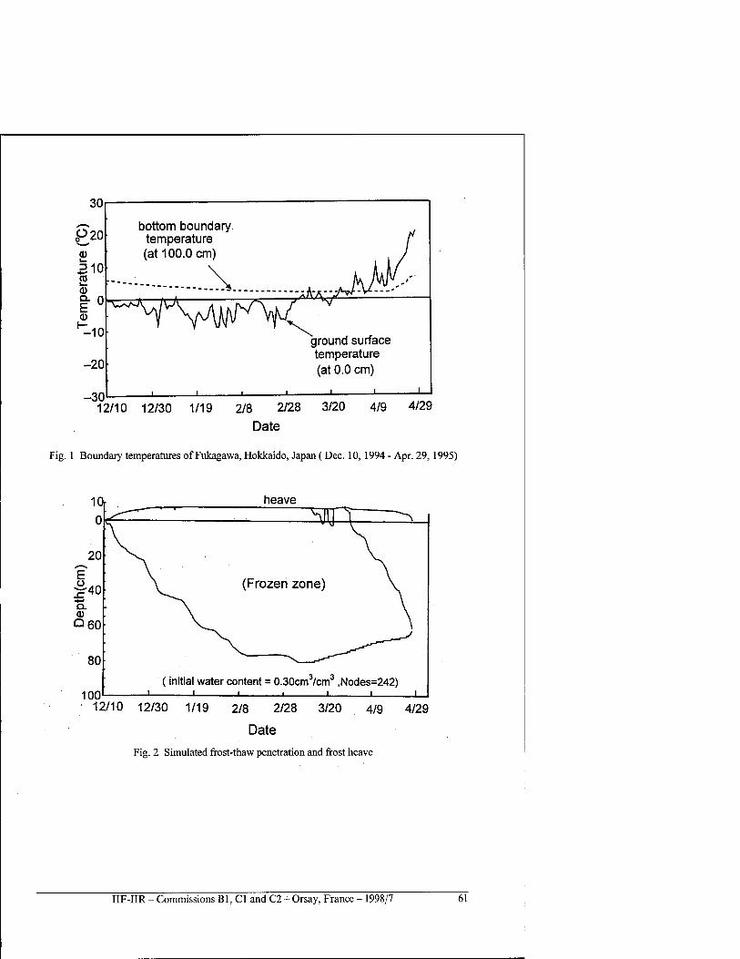
30

P20

= 10 CO

a)

1° CD H-10

-20

-30

bottom boundary temperature (at 100.0 cm)

^TVirv. ground surface temperature

. (at 0.0 cm)

12/10 12/30 1/19 2/8 2/28 3/20 4/9 4/29 Date

Fig. 1 Boundary temperatures of Fukagawa, Hokkaido, Japan ( Dec. 10, 1994 - Apr. 29, 1995)

100

heave

(Frozen zone)

3, 3 (initial water content = 0.30cm7cm ,Nodes=242)

12/10 12/30 1/19 2/8 2/28 3/20 4/9 4/29

Date

Fig. 2 Simulated frost-thaw penetration and frost heave


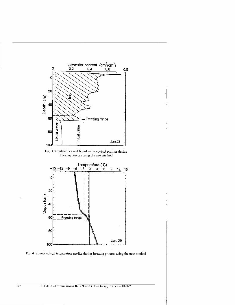
Ice+water content (cm3/cm3) 0.2 0.4 0.6 0.8

100

Fig. 3 Simulated ice and liquid water content profiles during freezing process using the new method

Temperature (°C) -15 -12 -9 -6 -3 0 3 6 9 12 15

100

Fig. 4 Simulated soil temperature profile during freezing process using the new method


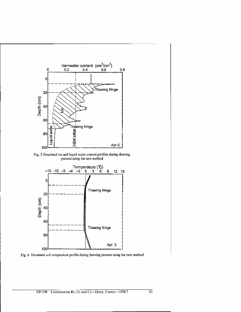
c Ice+water content (cm3/cm3)

) 0.2 0.4 0.6 0.8

0

20

? i3_

£ 40 CL 0) Q

I

t

_^<xS^ ̂Thawing fringe /\ \ \Tv v '\ X. X. X X f 1 x. x^ x. "x. >J

(X X. x. xj X. \

SxVxxS 0\\yi

60

80

•inn

*X^ X^ N^îJ*" i

!» \ \îhawinq f ringe

Apr.5 '

CO 5

CT _J In

itial

jvaj

ue

Fig. 5 Simulated ice and liquid water content profiles during thawing process using the new method

Temperature (°C) 15 -12 -9-6-3 0 3 6 9 12 15

Dep

th (

cm)

o

o

o

-

Thawing fringe

60

80

Thawing fringe

100 \ Apr. 5

Fig. 6 Simulated soil temperature profile during thawing process using the new method


REFERENCES

1. Chen, X. , 1998, Study on the Measurement and Analysis of Soil Freezing and Thawing Processes OPh. D thesis, Graduate School of Agriculture, Kyoto University, Kyoto, Japan

2. Gunman, G. L., Richard L. B. , and. Hromadka V., 1993, Mathematical Model of Frost Heave and Thaw Settlement in Pavements, CRREL Report, p. 93-2

3. Harlan, R.L. 1973, Analysis of Coupled Heat-flute Transport in Partially Frozen Soil, Water Resources Research, vol.9, p.1314- 1323

4. Jame, Y.W., Norum D. I., 1980, Heat and Mass Transfer in a Freezing Unsaturated Porous Medium, Water Resources Research, vol.16, p. 811-819

5. Nisigaki, M, Umeda, B. , 1993, Quantitative Evaluation and Controlling Method of the Soil Water Transport in Shallow Ground DP/iD thesis, Engineering Faculty, Okayama University, Japan

6. Sally A.S., Susan R.B., 1997, Moisture Migration During Freeze and Thaw of Unsaturated Soils: Modeling and large scale experiments, Cold Regions Science and Technology, vol. 25, p.33-45

7. Taylor G. S., Luthin J. N., 1978, A Model for Coupled Heat and Moisture Transfer During Soil Freezing, Can. Geoteck, ,7vol. 15, p.548-555

UNE NOUVELLE METHODE POUR INTEGRER LA FORMATION ET LA FÖNTE DE LA GLACE DANS LA SIMULATION DES PROCESSUS DE GEL/DEGEL DU SOL DANS LES CHAMPS

RESUME : La methode utilisee pour etudier la formation et la fönte de la glace joue un role important dans la simulation des processus de gel-degel du sol en agissant principalement sur la convergence et la precision du modele. Par consequent, une nouvelle methode plus fidele au mecanisme (ne faisant pas appel ä des hypotheses non realistes) est presentee ici. Cette methode a permis de simuler les processus de gel/degel d'une maniere plus rationnelle et plus sensible que toutes les approches proposees jusqu'ä present. Les profondeurs auxquelles le sol gele et degele, ont ete definies en utilisant comme reference, non pas la temperature de 0CC, mais la presence de glace. Tous les resultats des simulations concernant les profondeurs de gel/degel, la densite de la gelee, la temperature, la quantite d'eau liquide, de glace, et de particules dans le sol ä divers temps, sont en tres bon accord avec le mecanisme de gel/degel des sols.


SELF-ORGANIZED COLUMNAR MORPHOLOGY AT MILLIMETER SCALE OF ICE CRYSTALS FROZEN FROM MUD: PRELIMINARY OBSERVATIONS

GUYB. School of Mines,

158 Cours Fauriel, 42023 Saint-Etienne Cedex 2, France

ABSTRACT

The freezing of aqueous mud may lead to a separation of ice crystals from the mud, as it may be observed in nature. Ice crystals form regular needles parallel to each other; texture is similar to columnar jointing in volcanic rocks or to the so-called basaltic structure occurring during the solidification of alloys. The diameter of ice fibers is millimetric to inframillimetric and the length is centimetric to decimetric. The fibers develop perpendicular to the surface of the ground whether it is horizontal or with some slope. The pure ice crystals are covered by a dense mud cap. It is suggested that, during the freezing of mud, the ice cannot incorporate clays. A kind of constitutional supercooling applied to the solution water + clays, where the « solute » is here made up of the clays, may lead to the unstability of the planar freezing interface and may lead to the formation of regular ice needles. Further observational, experimental and theoretical works are needed to ascertain the conditions where such structure may develop, particularly in terms of thermal gradient and density of initial mud.

INTRODUCTION

The author is not a specialist of refrigeration. He is geologist, and, in the past, he has discussed some morphological aspects occurring during the solidification of volcanic rocks and compared them with the case of alloys (Guy and Lecoze, 1990). In the present text, he would like to discuss briefly some aspects occurring during the formation of ice crystals that he could observe in the French countryside in winter, and compare them with similar morphology in rocks and metals. A tentative mechanism is proposed. Although, after discussing the matter with the specialists of the refrigeration community, the author himself is not convinced by all what he proposed, the following text was written: it is a basis for organizing the argument and set the problem.

1. OBSERVATIONS

Extremely regular, pure ice, needles may sometimes be observed at the surface of the ground during winter; there are perpendicular to the ground surface whether it is horizontal or has some slope ; they are generally covered by a dense mud cap like shown in Figure 1. The length of the needles is centimetric to pluricentimetric and the diameter is approximately half a millimeter (Figure 2a). This diameter does not change along the needle. The needles are stuck together and form a regular carpet; sometimes the needles are separated into two or more zones, the limit of which is parallel to ground surface. More rarely, it may be observed that some amount of mud or pebbles is enriched between the needles and forms oscillatory bands (Figure 2b).

2. DISCUSSION

From the above observations it may be concluded that the ice needles cannot have crystallized from pure water (they are observed on slopes), and that the ice was separated from the mud during the


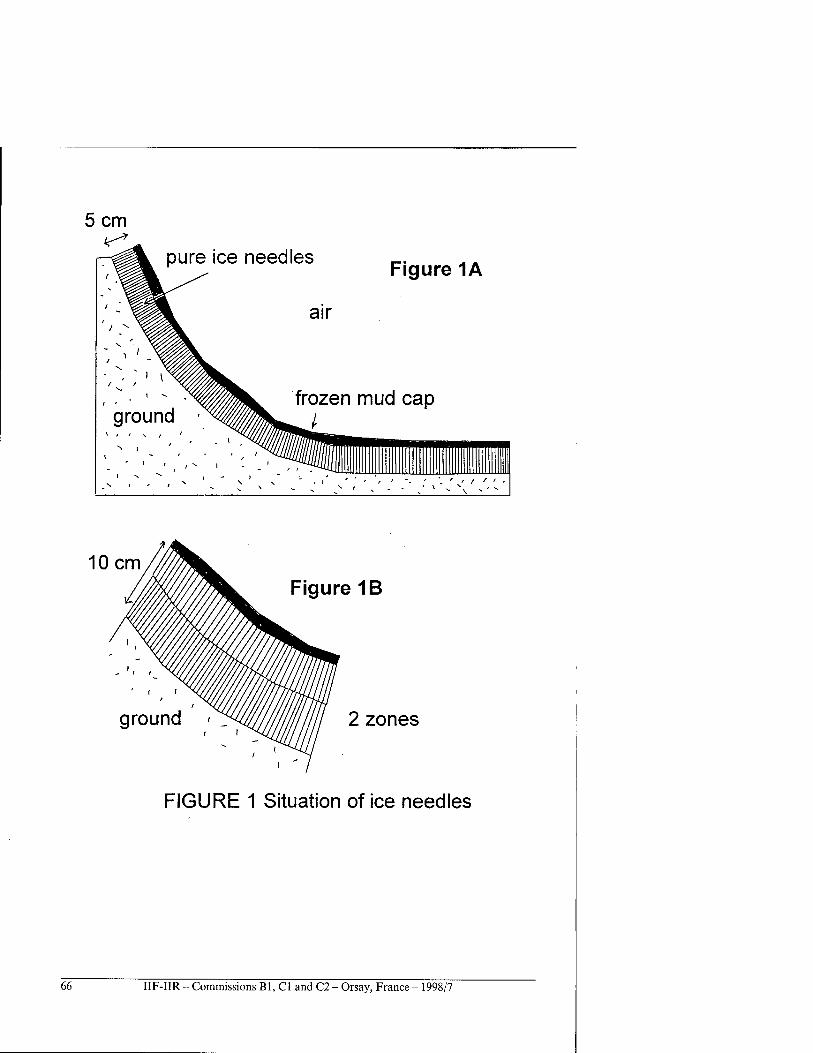
5 cm

ice needles Figure 1A

air

ground ' . i

|k frozen mi id cap

'- ' ' ' , ' - i : ;T/Äll||fl|I|^ llllilill

10 cm

ground

Figure 1B

2 zones

FIGURE 1 Situation of ice needles


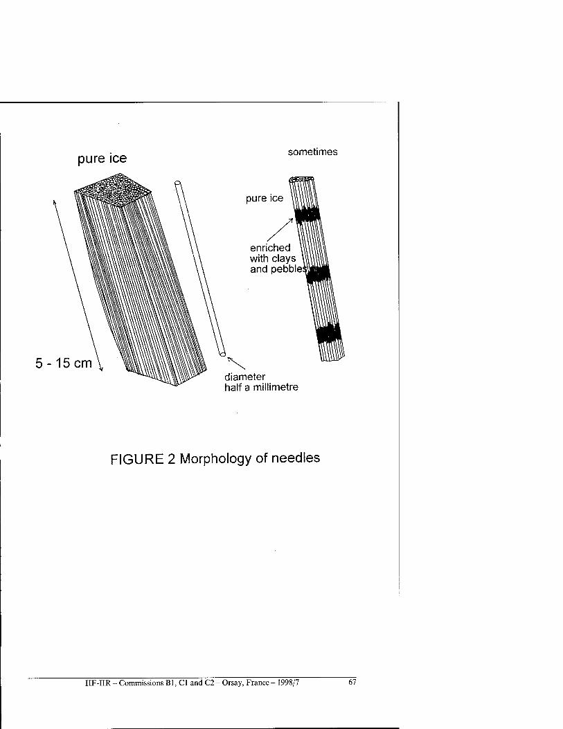
pure ice sometimes

5 -15 cm

pure ice

enriched with clays and pebble;

diameter half a millimetre

FIGURE 2 Morphology of needles

IIF-IIR - Commissions Bl, Cl and 01 - Orsay, France - 1998/7 67

freezing of mud. As was mentioned at the beginning of the text, regular needles are also observed in the ingots solidified from liquid metal at micron to millimeter scale, where the size of ingots is decimetric. In that case the constitutional supercooling of impure liquid solidification is the explanation proposed (Kurz and Fisher, 1989). Note that the composition difference between the solid and the liquid may be very small. In the case of rocks, regular columns are sometimes observed in the volcanic rocks (« columnar jointing »); the length of the columns is metric to decametric, the diameter is decimetric and the size of flows may be hectometric; together with a metallurgist colleague, the author proposed that constitutional supercooling could also play a role in the case of solidification of magmas (Guy and Lecoze, 1990); water and some chemical elements such as the alkalis would be expelled from the liquid. Recall briefly that the standard explanation of columnar jointing of volcanic rocks by mere contraction, because of cooling after solidification, is problematic: chemical differences across the columns are sometimes observed so as bubbles in bands parallel to the contact of the columns; this cannot be explained by a post solidification contraction. Note in addition that cooling contraction usually produces fractures parallel to the contacts of metal ingots and not perpendicular. One may also question the phenomenon that would be responsible for the formation of so well synchronized and so regular fractures.

In the case of mud freezing, one would be tempted in the above context to discuss a possible role of supercooling. It is well known that the presence of solutes or particles, even in small proportion, lowers the liquidus of water. When freezing, the ice expels these solutes or particles that are in greater amount in the liquid just close to the solid interface. Making use of the information on the liquidus decrease with composition, and that on the concentration profile in space, one can draw the liquidus temperature profile in space in the liquid close to the solid interface. It is also well known that thermal diffusivity is greater than matter diffusivity, so thermal gradient in the problem may be considered as imposed by the boundary conditions. Depending on conditions, supercooling may appear (so-called constitutional supercooling). This is the driving force for solidification. In this context, planar solidification is unstable because it can be shown that a little bump of the solidification front will see a higher supercooling : cellular morphology may develop and lead to a self-organized morphology (see mentioned authors). Optional fracturing may occur between the cells afterwards.

Taking as an hypothesis the supercooling explanation, one must discuss the size of ice needles as compared to that of metal and rock cells. Thermal diffusivity has the same order of magnitude for ice, metal and magma systems (102 cm2/s); solute diffusivity has also same order of magnitude for ice, metal and ice systems (10"5 cm2/s). Important differences in the three systems lie on the size of freezing systems and magnitude of temperature gradients. The empirical or semi-empirical equations that connect the parameters of the system show that the size of the cells is inversely proportional to the thermal gradient G times the solidification velocity V ; using the parameters of the system, this may roughly be expressed as X oc 12AT with X, size of cells, 1 size of freezing system and AT temperature difference between freezing system and external medium. All the relevant parameters are given in Table 1 : one sees that this approach does not give unreasonable results. Within the proposed explanation, predicted size of ice cells is in proportion to that in metals and rocks, taking into account the differences in the size of the systems and in the temperature contrasts.

CONCLUSION

The mechanism that is actually responsible for the formation of the ice needles may involve other phenomena that the author is not familiar with. In any case he will be interested to know about possible descriptions and discussions of similar ice needles in the literature. Before one is able to conclude, it

IIF-IIR - Commissions Bl, Cl and C2 - Orsay, France - 1998/7

be needed to assess the respective roles in the process of the possible mechanisms and discuss how these are able to produce this so regular features.

Table 1. Orders of magnitude of the parameters of the problem (case of metal, ice and magma freezing)

metal ice magma

AT (K): temperature difference 102tol03 10' 102to 103

1 (cm): size of freezing system 10 10 102to 10" ÄAmeiii : predicted size of cells 1 10'to 102 104to 106

observed size of cells (cm) 10"4to 10"' micron to millimeter

10"2to 10"1

millimeter 10 to 102

decimeter to metro

The author thanks Jaime Aguirre Puente for his welcoming in the refrigeration community and all the individuals with whom he could discuss the matter presented here.

REFERENCES

1. Guy B. and Lecoze J. (1990) Reflections on columnar jointing of basalts : the instability of the planar solidification front. C.R. Acad. Sei. Paris, t. 311, II, 943-949.

2. Kurz W. and FisherD.J. (1989) Fundamentals of solidification, Trans. Tech. Publications, 305 p.

DISCUSSION

FROLOV A.D. (Russia) You are looking for the analogy between igneous rocks solidification and moist soil freezing. It is very interesting and useful. But as it seems to me the case considered by you concerning ice needle crystals texture in frozen surface sediments is very particular caused by local thermodynamic conditions: temperature gradient and thermal properties, etc. There is a snow in the needle form also. In this field of analogies, there is the more interesting and general approach to consider a likeness between frozen grounds and igneous rocks with partially melted one of principal rock forming mineral. By using this approach, it will perhaps be possible to find new rules of physical forming and changing properties.

MORPHOLOGIE COLONNAIRE A L'ECHELLE MILLIMETRIQUE DE CRISTAUX DE GLACE FORMES PAR CONGELATION DE BOUE : OBSERVATIONS PRELIMINAIRES

RESUME : La congelation de la boue peut conduire ä une separation des cristaux de glace des particules minerales, comme on peut l'observer dans la nature. Les cristaux de glace forment des aiguilles regulieres paralleles les unes aux autres ; la texture est semblable aux orgues observees dans les roches volcaniques ou ä la structure « basaltique » apparaissant au cours de la solidification des alliages. Le diametres des fibres est millimetrique ou inframillimetrique et leur longueur est centimetrique ä decimetrique. Les fibres se developpent perpendiculairement ä la surface du sol, que celui-ci soit horizontal ou presente une certaine pente. Les cristaux de glace pure sont couverts d'une couche de boue dense. On suggere que, durant la congelation de la boue, la glace ne peut incorporer les particules minerales (argiles notamment). Une sorte de surfusion de constitution appliquee a la solution eau + argiles, ou les « solutes » sont ici les argiles, peut conduire ä l'instabilite du front plan de congelation et peut conduire ä la formation d'aiguilles regulieres de glace. Davantage d'observations, de travaux experimentaux et de modelisation sont necessaires pour s'assurer des conditions dans lesquelles une teile structure peut apparaitre, notamment en termes de gradient thermique et de densite de la boue initiale.


SECTION II

PROCEDES, PROPRIETES PHYSIQUES ET METROLOGIE

PROCESSES, PHYSICAL PROPERTIES AND METROLOGY

PLENARY LECTURE

PROSPECTS OF VARIOUS PHYSICAL FIELDS APPLICATIONS TO STUDY OF FROZEN SOILS

FROLOV A. D. Consolidated Scientific Counsil on Earth Cryology R.A.N.

Fersman St.l 1, Moscow 117289. Russia Fax: 7(095) 290-5072; E-mail: [email protected]

INTRODUCTION

Frozen soils are heterogeneous polyphase porous media or complex macrosystems. Physical model of such macrosystems may be founded on three main particularities of this media: a) the component composition, b) the spatial crystalline-coagulant cryogenic structure (SCCS), c) the physical subsystems determining the response of macrosystem on the external physical field

excitation. The main elements of this SCCS are: 1) grains (or aggregates of grains) of ice, 2) soil mineral matrix , 3) intergrains zones containing a liquidphase and impurities.

The physical subsystems are related with these main elements of SCCS and they can be: nuclear, electronic, dipolar, ionic etc. Moreover, each of them can be represented by several varieties according to the degrees of freedom of atoms, molecules, ions, electrons etc. movements. For instance the ionic subsystems (usually it is the main) can be "bounded", "semibounded" and "free". It means that the ions under the effect of external force fields can only oscillate or move progressively. In semibounded subsystems these progressive ion migrations are restricted by the size of liquid phase domains (Frolov, 1998) that determine the liquid phase energy state. In the time variable external fields the excitation and relaxation of the corresponding physical subsystems occur, which nature and peculiarities condition the values of complex conductivity, dielectric and magnetic permittivity, moduli of elasticity (or deformation), strength and other properties of the medium. The electric and mechanical properties of frozen soils are the moist sensitive to cryogenic changes and they vary considerably more then magnetic, thermal and others ones. For instance, in soil transition from thawed to frozen state their conductivity and dielectric permittivity change from tens to thousands, elastic moduli from tens to hundreds and velocities of electromagnetic and stress waves up to tens times. There are the definite particularities in the different frequency ranges of the physical fields and in the soils with dissimilar mineral matricies All the above cause the high resolution and effectivity of seismic-acoustic as well as electromagnetic methods and also the methods based on the measurements of electromechanical energy conversion to study the frozen soils.

1 SEISMIC-ACOUSTIC METHODS

These techniques are well known and used extensively in studies of the properties, states and structure of frozen soils in the field and laboratories. There is very important the possibility to apply these non-destructive methods to assess and monitor the strength and deformation properties of frozen soils using established correlations between them and wave propagation velocities or elastic


moduli (Voronkov, 1985; Zykov and Cherviskaya,1990; Goryainov, 1992; Frolov 1976, 1998 and others). Thereat the land seismic techniques, seismic and acoustic logging with registration of longitudinal and Rayleigh's waves are used sufficiently wide. The basis of these methods successful application for study the frozen massifs is the reliable information on the structure and other peculiarities of wave fields in the frozen medium. They are often characterized by space variability of velocities especially in the upper part of geocryological section, wide frequency range of seismic signals, presence of inversional velocity boundaries, divergence between average and effective velocities (the last is usually less), elastic property anisotropy, presence the inhomogeneities of different scales and genesis and some other. Firstly the data sistematized in this domain have been obtained by A. Shutkin on the base of long-term studies in the Vilui syneclise (Yakutiya), as a result of which the special procedures for deep seismic exploration by reflected P-waves in permafrost areas have been elaborated (Shutkin et al, 1979). Further, this direction was developed by many researchers in Russia (see Gennadinic, 1986) and also in Canada and partly in USA. Contemporary trend in this field is the preferable application of S-waves of various polarizations, especially of SH- kind (Burns et al, 1995; Skvortsov, 1997) for various studies of frozen soils. This is doubtless prospect in land engineering seismic prospecting as well as in seismic and acoustic logging to study the frozen sequences. The estimation of seismic danger of frozen grounds, a forecast seismic effects, the seismic microzoning of the territories and a seismic-acoustic local monitoring in ctyolithozone are also highly important applied directions (Pavlov, 1987; Goryainov, 1992; Dzhuric, 1996 and others).

2 PARTICULARITIES OF ELECTRIC PROPERTIES

As it is well known the main parameter characterized electromagnetic wave propagation is the complex permittivity or conductivity of medium, representing usually as:

e* = s -j- o7coe0 or cr* = o"+jö>e0s (1)

where e = XE and G = 2A

i.e. it is supposed that the properties of the medium are the additive functions of his component properties. However this approach is not adequate for multyphase heterogeneous media including frozen soils, that is not always one take into account. That is why we will enlarge a little this subject below. In the media above-mentioned which are usually the ionic imperfect conductors (thanks the presence a liquid phase and admixture pore ice), there are considerably diversity of the charge porter mobilities and restrictions of their space movements (Frolov, 1976, 1998). So, if this media is exited by an electromagnetic field, the nonideal electric condition and polarisation presence arise from the migration of charge porters (mostly ions). Each from there processes is characterised by wide range of phase delays with reference to the phase of applied force field. So, each process will be make of contribution both in synphase - conduction current and in quadrature-lagging one - displacement current. In this connection it should be noted that both s and o of such media are bounded to be the complex and frequently depended parameters:

CT = CT*(CO) = cr, (co)+jc'2(o)) and E = S*(G>) = £,((a)-js2((B) (2)

i.e. the measuring values of e and a should be effective. It signify that these values impossible to evaluate by use additive mixture formulae in comformity with volumetric content of the components. So, taking into account (2), it is easily be obtained (instead of (1)) that the real and imaginary parts of E*ef and a*ef are:

CT*ef(co) = o-'ef(a>) = o"i(co) + cos0E2(co) = (aE0s"ef(ca) (3)

S*ef(co) = E'ef(C0) = El(C0) + O-2(ö))/(ÖE0 = CT"ef((D)/ß)E0 (4)


where : a,(co) and s, (w) are the summary parameters of the proper conduction and polarization in the medium, e0 = 8,85 • 10'12 F/m. The seconds addends in (3) and (4) characterize the imperfection of conduction and polarization processes and their superposition, i.e. they are the peculiar interference terms, which values are conditioned by interaction of liquid and solid soil components. As is obvious from (3) and (4) at low frequences both effective parameters are determined by the imperfect conduction process:

o-el(co) = CTi(<°) and eef (co) = cr2(co) / ras0 (5)

By this it meant that physically the great polarization arises thanks of ion migratory displacements in limited liquid phase domains and of forming the electric macrodipoles. As a result the sef values can be much more greater then from the component composition. The experiments confirm this and have shown (Araki and Maeno, 1989; Frolov, 1976, 1998; Gurov, 1983; Olhoeft, 1977 and others) that at the frequencies 102 - 103 Hz the sef values for frozen sandy-clayey soils have attained ~ 102 - 10\ and at lower frequencies ~ 104 if not more. Experiments also have shown that at the frequencies ~ 105 - 106Hz the macrodipolar polarization in frozen soils sharply reduced and at high frequencies there are from (3) and (4):

aef(tt>) SCOE0E2(CO) and sef(co) = E,(w) (6)

According to experimental results of Delaney and Arcone 1978, Oliphant 1985 and others, the s' values for frozen soils at ~ 107 - 109 Hz are ~ 4 - 10 (depending on initial moisture and soil temperature) and e"« 10"' - 10 "2 . Moreover there is no frequency dispersion of permittivity in this frequency range. At more higher frequencies there is again the frequency dispersion range for s ef

and e"ef (~ 3 • 109 - 5 • 10"Hz) which is conditioned by various kinds of water molecular polarisation. Thus, from the about discussion it is clear that our model on electric properties of frozen soils is in a good accordance with the experimental data and it is necessary to take it into account in the applied engineering studies.

3 ELECTROMAGNETIC METHODS

Low frequency (<106 Hz) techniques, which presented themselves in a good light in the field studies of frozen soils in Russia, Canada and some other countries are: induced polarization (IP) transient, evaluative and frequency-distance EM soundings, dipolar, surface impedance, radio comparation and direction-finding (RCDF) EM profiling methods (Akimov et al, 1979; Kozhevnikov, 1991; Krylov and Bobrov, 1995; Scott et al, 1990, and others). For correct interpretation of the EM soundings results (using sufficiently wide frequency or trausient and evolution time ranges) the frequency dispersion of aef and Eef should be taken properly into account. But the optimum route of this account is discursive up to now (Krylov and Bobrov, 1996). For the studies of underground ices, cryopegs, structure of permafrost, mapping the thawed-frozen boundaries of taliks and frozen ground islands etc, one may to note as the most prospect methods are the frequency-distance soundings and mobile EM profiling techniques especially RCDF which use the fields of special and broadcasting radiostations in the ranges 10 - 30 Khz and 150 - 450 Khz. The primary advantages of this last profiling over others are high resolution and outputs, capacity to take measurements in summer and winter and under conditions of industrial interferences, capability to measure rapidly several intersupplementable components of radiostation magnetic field. There are some variants of this method with measurements both magnetic and electric fields. In high frequency domain (> 106 Hz) the most prospect methods for engineering-geocryologgical studies are: the radio wave cross-boreholes transmission, radiowave logging and radar method. The deep ( distance) of this methods is not great ( from several to tens metres), but for many engineering


tasks they are quite suitable and effective (Akimov et al, 1979; Arcone and Delaney, 1989; Nim et al, 1994; Scott et al, 1990 and others). For instance by land radar sounding it is possible to locate underground ice bodies, and frozen soils with high ice content, to determine the behaviour of the upper permafrost boundary, the thickness of snow cover etc. The testing of aerial variant of this method (including lateral scanning apparatus with synthetic aperture) have shown a good prospects in the permafrost mapping on mid scale ~ 1: 100000. To this group it is possible to assign the radiothermal, and infrared surveys as well as the method of heat fluxes, which have based on the studies of the natural Earth thermal field in the ranges 1 - 10GHz ~ (1 - 4) • 105 GHz. The aerial radiothermal mapping in Yakutiya, Yamal peninsula and other areas of Siberia have shown that the anomalies of radiobrightness temperature and it spectral changes provides the means for mapping the taliks, islands of frozen grounds, underground ices etc ( depth < 50 X). More valuable data are obtained usually in the winter. Infrared multispectral survey joint with spectrozone photography ( in the visible spectrum) also given a good results for purposes of permafrost territories zoning by thermal contrasts , especially in the tundra regions. And, at last, the studies of thermal fluxes in cryolithozone( remote, land and in boreholes) permit to achieve the geocryological zoning with evaluation of the permafrost states: degradational or aggradational. The magnitude of thermal flux, for instance in Siberian cryolithozone, changes from 0 to 150 mW/ m2 ( Devyatkin, 1993), which is to say that the remote measurements have a good prospects for various scientific and practical purposes in North regions.

4 UNFROZEN LIQUID PHASE CONTENT DETERMINATION

Principally for this aim these are the possibilities of both acoustic and electromagnetic methods (Frolov, 1976, 1998). However the elastic properties of frozen soils considerably depend on ice content that make difficult its application especially in the cases of small unfrozen water content in ice saturated frozen soils. So, the electromagnetic dielectric methods have better outlooks. The high frequency electrical capacity and T.D.R. methods of esef determination are of particular interest and wide use. Both techniques allow to determine E ef as well as a ef ( with much more difficulties), and consequently not only unfrozen liquid phase content can be determined but principally it mineralization also ( Van Loon, 1991). Comparison of the results on unfrozen water content determinations by NMR and TDR ( at frequencies 108 - 109 Hz) have shown its quite good accordance excluding very fine dispersed clays for which method TDR have given lesser values( Smith and Tice, 1988). Generally any high frequency (107 - 109 Hz) radiowave method can be used for the E values determination ( supposing that s'ef <<e"ef) by EM wave velocity measurements in the medium. But in the cases of small liquid phase volumetric content (< 2 % ) the resolution of high frequency methods sharply decrease and it is necessary pass to more complicated measurement in relaxation domain at low frequencies (~103-104 Hz) when at the same volumetric liquid phase content the Ä ef value is mach more greater thanks the macrodipolar polarization. By these measurements it is possible to evaluate the liquid phase content in frozen soils to 0,1 % and it changes in wide temperature interval up to the points practical full completion of the phase transformations ( Frolov, 1996, 1998 ). The last, according to our data, are for ; sand ~ -30°C, kaolin- -( 65-70)°C, heavy loam <-80°C and freshwater ice ~ -(5-8) °C.

5 ELECTROMECHANICAL ENERGY CONVERSION

There is highly promising method of exploring the liquid phase state and the kinetic of freezing especially in saline frozen soils which is based on the study of electromechanical energy conversion in frozen medium ( Frolov and Seguin,1993; Frolov, 1998 ). As is evident from our experiments in laboratory it is more simple and reliable to realize the study of this conversion in the variant of electric-acoustic (excitation by electromagnetic field) measurements, Whilst in field conditions


there are preferable the acoustic- electric ( or seismic-electric) technique. These techniques have been tested in the both cases and have given interesting and useful results.

6 CONCLUDING REMARKS

Taking into account all things considered above as well as high accuracy and reliability of modern radioelectronic apparatus the seismic-acoustic and electromagnetic methods are irreplaceable for ecological-geophysical monitoring in cryolithozone on diverse scales in relation to technogenic stresses as well as to probable global climatic and enviromental changes. Now, estimation of the state of permafrost( or seasonal frozen ground) based practically solely on temperature measurements. The reliability of this estimations is rather problematic especially in saline and clay soils or when solving the special engineering tasks ( Velikin et al, 1997). So, it is necessary to introduce seismic-acoustic and electromagnetic techniques foremost in local ecological-geophysical monitoring in cryolithozone. The monitoring systems of regional and global scales may be based only on remote sensing methods : EM, radar, radiothermal and possibly the heat flux measurements.

REFERENCES

1. Akimov A.T., Melnikov V.P., Frolov A.D. 1979. Geophysical methods to study of permafrost in USSR. ONTIVIEMS Press, Moscow, 51pp. (USA CRREL Draft Translation 707, 30 pp.).

2. Araki T., Maeno N., 1989. Measurements of dielectric properties of frozen soils. L.T.S., serA, Phys.Sci.' 48, p 27-40

3. Arcone S.A., Delaney A.J. 1989. Investigation of dielectric properties of some frozen materials using cross-borehole radiowave pulse transmission. USA CRREL Rep. 89-4, 19 pp.

4. Burns R.F., Goryainov N.N., Skvortsov A. G et al.1995. The results of joint Russia-Canada geophysical studies of Yamal peninsula permafrost. Geophys. Investig. of Cryogithozone, Trans., issue 1, RAN, Moscow, p 63-72.

5. Curov V.V. 1983. Technique and some results of experimental study of frozen soil dielectric properties.Merzlotnyeissledovaniya,issue21,Mosc.StateUniv.Press,p.l70-178.

6. Delaney A.J., Arcone S.A., 1982. Laboratory measurements of soil electric properties between 0,1-5 Ghz. USA CREEL Rep 82-10, 10 pp.

7. Devyatkin V. N. 1993. Heat flow of Siberia cryolithozone. Nauka Press, Navosibirsk, 164 pp. 8. Dzhurik V.l., 1996. The particularities of seismic effect forecast in cryolithozone conditions.

Geophys. Investig. of Gryolithozone,Trans.,issue 2, RAN, Moscow,p 53-59. 9. Frolov A.D. 1976. Electric and elastic properties of cryogenic rocks. Nedra Press, Moscow, 254

pp. 10. Frolov A.D. 1996. Dielectric moisture measurements in frozen soils. Proc. I Conf. of

geocryologists of Russia, Book 2, Moscow, p. 271 -279. 11. Frolov A.D. 1998. Elastic and electric properties of frozen earth materials. ONTI PNC RAN

Press, Pushchino, 515 pp. 12. Frolov A.D., Seguin M.K. 1993. Caracteristics de la cinetique de congelation des sols salins.

Permafrost and Periglac. Processes, v. 4 , p 311-325. 13. Gennadinik G.V. 1986 Geophysical investigations of frozen grounds and ices. Main Russian

Bibliography 1930.1985, (1339 titles). Inst. of permafrost, Yakutsk, 134 pp. 14. Goryainov N.N.- ed., 1992. Seismic-acoustic methods application in hydrogeology and

engineering geology, Nedra Press, Moscow, 260 pp. 15. Kozhevnikov N.O. 1991. Effect of dielectric permittivity frequency dispersion on the results of

measurements in transient method. Deponir. in VINITI, Moscow,' 882-B91, 20 pp. 16. Krylov S.S., Bobrov N. Yu. 1996. Anomalous polarizability and fractal models of permafrost.

Geophys. Investig. of Cryolithozone, Trans., issue 2 , p 123-135.


18. Nim Yu. A., Omelyanenko A.V., Stognij V.V., 1994. Impulse electrical prospecting of cryolithozone. Nauka Press, Novosibirsk, 190 pp.

19. Olhoeft G.R. 1977 . Electrical properties of natural clay permafrost. Canad J. Earth Sei. v. 14, p. 16-21.

20. Oliphant J.L. 1985. A model for dielectric constants of frozen soils. Freezing and thawing of soil- water system. Proc.Amer. Soc. of Civil Eng. N. Y. p. 46-56

21. PavlovO. V., 1987. Seismic danger of frozen soils. Nauka Press, Novosibirsk, 160 pp. 22. Scott W.J. , Sellmann P.V., Hunter JA., 1990. Geophysics in the study of permafrost. Ward

S.H.( ed-r),Geotechnical and Enviromental Geophysics, v.l,SEG,USA, p.355-383. 23. Shutkin A.E. et al., 1979. Methodical recommendations on deep seismic prospecting in the

permafrost areas. VNII Geophysika Press, Moscow, 84 pp. 24. Skvortsov A.G, 1997. Features of the elastic oscillation field structure in non-lithified frozen

grounds. Earth Cryosphere, v 1, ' 3 , p. 66-72. 25. Smith M.W., Tice AR. 1988 Measurement of the unfrozen water content of soils, Comparison

of NMR and TDR methods. USA CRREL Rep. 88-18, 11 pp. 26. Van Loon W.K.P., 1991. Heat and mass transfer in frozen porous media. Ph. D. Thesis,

A.U.W„Netherland, 200 pp. 27. Velikin S.A., Snegirev A.M., Frolov A.D., 1997. Local ecological-geophysical monitoring of the

cryolithozone. Proc. Intern. Symp. Engineering Geology and the Enviroment, Athens, Greece, Balkema Press, p 2559-2564.

28. Voronkov O.K. 1985. Recommendations to study by engineering seismic techniques of the static and dynamic deformation properties of hydrotechnical structures in the north building-climatic zone. VNIIIG Press, Leningrad, 101 pp.

29. Zykov Yu. D., Chervinskaya OP. 1990. Acoustical properties of icy soils and ices. Nauka Press, Moscow, 133 pp.

DISCUSSION

AGUIRRE PUENTE J. (France): Pouvez-vous parier des methodes utilisees sur le terrain dans les zones de pergelisol ?

FROLOV A. - There are many electromagnetic geophysical methods which are applied in the field studies of permafrost. Effectivity of them depends from the aims of application. For instance: 1/ Mapping of vertical boundaries frozen-thawed soils or taliks within permafrost: radio-wave profiling by measuring the local anomalies of broadcasting and special radio transmitters fields in LF and VLF ranges (ellips of polarization of H and E, amplitude and phase variations, surface impedance, etc.). 2/ Determination of underground ice and thickness of frozen soils, deepness of taliks, etc.: the electromagnetic soundings by transient method, by frequency and transmitter receiver distance variation, radar echo-soundings for small deepnesses, induced polarization (IP), etc. 3/ Electromagnetic bore-hole methods for study permafrost: dielectric logging, IP logging, magnetic susceptibility logging, radioscopy between holes, etc.

DUPAS A., France: You describe the high-frequency measuring methods, with frequencies expressed in KHZ. Apparently, these frequencies caracterize the frequency deterioration due to the media studied in the measuring capacitor. Isn'it?

FROLOV A. - Yes, it is.


MAIN CARACTERISTICS OF SALINE FROZEN SOILS

FROLOV A.D., FEDYUKIN I.V., ZYKOV Y.D. Consolidated Scientific Council on Earth Cryology Russian Academy of Sciences

Fersman St. 11,Moscow, Russia, Fax : 095 - 258 - 2463, E - mail: ipquis @ redline.ru

ABSTRACT

Analysis of the various physical and physical-chemical study results has led us to put in the forefront four most important distinguishing features of saline frozen soils: critical initial concentration of the saturating pore solution; phase composition peculiarities; specificity of the spatial crystalline-coagulant cryogenic structure; freezing kinetics particularities. In the paper all these features are described and discussed.

INTRODUCTION

The rise of frozen soil as a new polycrystall formation is primarily attributed to crystallization of ice, as the result of phase transformations in porous liquid at temperatures below 0°C .These transformations and cryogenic structure formation in natural soils are essentially processes of a solution freezing in heterogeneous pore-capillary medium. These processes are complicated and still not sufficiently studied. In cases that the soils are dispersible, such as fine clay, the effects of dispersion and coagulation, ionic exchange and adsorption, and also the existence of ultramicropores, significantly complicate the freezing process. Such a case also entails great diversity of porous liquid energy states hence a wide temperature range of freezing, even with small pore solution concentrations. In sandy soils these phenomena are almost absent, but the principal liquid phase changes (in the case of fresh water saturation) take place in a rather narrow range of negative temperatures near 0°C, that is difficult to study, Saline frozen sandy soils, depending on concentration and the composition of their pore solution, exhibit considerable specificity in freezing kinetics and wide phase change temperature range. Therefore such soils present a good research models for detecting the patterns of different frozen soil properties. Moreover, saline frozen soils are rather widespread in many regions of cryolithozone takes place thus the studies of these soils main characteristics are of great practical importance.

1 BACKGROUND

Any frozen soil contains some quantity of ice and unfrozen liquid as its distinguishing feature. No less important is the formation of a new structure that distinguishes a frozen soil from a thawed one. Using concepts of physics-chemical mechanics (Rebinder,1979) we have demonstrated that in the given case there is a Spatial Crystalline-coagulant Cryogenic Structure (SCCS). The main elements of SCCS are: a) ice grains (or aggregates of grains) - an ice matrix; b) silicate grains - a mineral matrix; c) intergrain (inter aggregates) zones containing unfrozen liquid, impurities, etc. - a matrix of "defects". The first two form a solid matrix in the frozen soil The third may be liquid or a mixture of solid and liquid. It is possible to define several stages of SCCS formation and consolidation (Frolov,1976; Frolov and Seguin, 1993). An increase in pore solution concentration and a decrease in soil temperature lead to increased superficial tension, deterioration of wettability, and discreteness of pore solution. The last is supported by the results of experiments on low frequency dielectric permittivity and electroacoustic conversion measurements ( Frolov, 1991) as well as on freezing water and solutions around small aluminium balls (Chellaiah and


Viscanta,1987). Ice formation in frozen soil is also diversified by grain (aggregate) sizes and forms as well as by degree of their admixing. In the case of high initial salinity, the SCCS of frozen saline soil differs considerably from nonsaline one and, as a result, sharp distinctions do exist in most of the physical, mechanical and other properties. So, there are two principal cases of forming SCCS hence all particularities of frozen soil properties: 1. Predomination of the mineral matrix influence on SCCS formation - case of a well known

nonsaline or freshwater saturated soils. 2. Predomination of the initial concentration and ionic composition of the saturating pore solution

impact on SCCS formation - saline soils. One bordering soil state must exist and be determined by some critical (limiting) concentration Ccr

of saturating pore solution.

2 PRINCIPAL CHARACTERISTICS OF SALINE FROZEN SOILS

It would be much more informative to have the data from joint studies (on the same soil matrix) of liquid phase content and several physical properties, as the functions of temperature, concentration and composition of saturating pore solution. Unfortunately these kinds of experiments haven't been realized yet. However, the results of some experiments, which have been conducted for other reasons, might be analyzed and compared in order to reveal some common characteristics of saline frozen soils. We have set of the following groups of such experiments : - Determination of the freezing beginning temperature and the unfrozen liquid phase content in frozen soils saturated with solutions of various concentrations and compositions (Ershov, 1995,1996; Grant,1993; Tice et al, 1984 and others). - Data obtained on the effects of salinity on electric, thermal, elastic and other properties of saline frozen soils as a function of temperature (Ershov, 1996; Fedyukin et al, 1979; Frolov, 1991; Frolov and Fedyukin 1983,1985; Frolov et al 1997; Zykov et al 1990]. - Studies of salinity's influence on physico-chemical processes in frozen soils such asxryogenic structure and texture formation (Chellaiach and Viscanta, 1987; Ershov, 1996; Khimencov and Minaev, 1990; Panchenko and Aksionov, 1990); ionic transfer (Ershov, 1995; Ostroumov, 1990); and electroacoustic conversion (Frolov,1991; Frolov and Seguin, 1993; Pavlov and Frolov, 1990). - Studies on deformation and the variability of strength properties for saline frozen soils ( Ershov, 1996; Roman et al,1994;Velli,1990; Yarkin,1990;Zykov and Chervinskaya,1995). On the basis of analysis of the results, four of the most important saline frozen soil distinguishing features are set forward and discussed below.

2.1 Critical Concentration The critical (limiting) initial concentration - Ccr of the soil saturating solution permit to distinguish a saline frozen sandy-clayey soil and practically nonsaline one from the standpoint of physical properties. The data available from indirect experiments obtained on different soil mineral matrices, moisture contents, and saturating solution compositions etc. Most of the experiments deal with saline frozen soils saturated with NaCl solutions, sometime with KC1 and CaCl2 ones and seldom other salts. Only a few authors addressed to the problem of obtaining critical concentration values whereas in most studies the salinity of soils were set, taking no into consideration of a probable critical concentration. But data analysis allows some deductions. For saline frozen quartz sand, the initial critical concentration for chloride salinity according to our results of dielectric spectroscopy and electroacoustic conversion experiments (Frolov and Fedyukin,1983; Frolov, 1991 and others) is: Ccr = (0.5 to 1) * 10"2 mole/1.


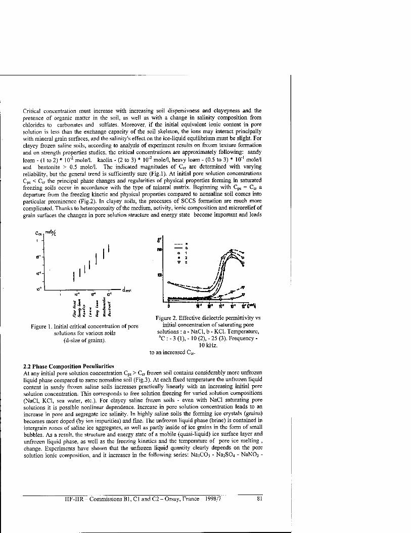
Critical concentration must increase with increasing soil dispersivness and clayeyness and the presence of organic matter in the soil, as well as with a change in salinity composition from chlorides to carbonates and sulfates. Moreover, if the initial equivalent ionic content in pore solution is less than the exchange capacity of the soil skeleton, the ions may interact principally with mineral grain surfaces, and the salinity's effect on the ice-liquid equilibrium must be slight. For clayey frozen saline soils, according to analysis of experiment results on frozen texture formation and on strength properties studies, the critical concentrations are approximately following: sandy loam - (1 to 2) * 10"2 mole/1, kaolin - (2 to 3) * 10"2 mole/1, heavy loam - (0.5 to 3) * 10"' mole/1 and bentonite > 0.5 mole/1. The indicated magnitudes of Ccr are determined with varying reliability, but the general trend is sufficiently sure (Fig.l). At initial pore solution concentrations CPs < Ccr the principal phase changes and regularities of physical properties forming in saturated freezing soils occur in accordance with the type of mineral matrix. Beginning with Cps = Ccr a departure from the freezing kinetic and physical properties compared to nonsaline soil comes into particular prominence (Fig.2). In clayey soils, the processes of SCCS formation are much more complicated. Thanks to heteroporosity of the medium, activity, ionic composition and microrelief of grain surfaces the changes in pore solution structure and energy state become important and leads

»"

l0%

10*

Figure 1. Initial critical concentration of pore solutions for various soils

(d-size of grains).

¥iHi Figure 2. Effective dielectric permittivity vs

initial concentration of saturating pore solutions : a - NaCl, b - KC1. Temperature, °C : - 3 (1), -10 (2), - 25 (3). Frequency -

10 kHz. to an increased Ccr.

2.2 Phase Composition Peculiarities At any initial pore solution concentration Cps > Ccr frozen soil contains considerably more unfrozen liquid phase compared to same nonsaline soil (Fig.3). At each fixed temperature the unfrozen liquid content in sandy frozen saline soils increases practically linearly with an increasing initial pore solution concentration. This corresponds to free solution freezing for varied solution compositions (NaCl, KC1, sea water, etc.). For clayey saline frozen soils - even with NaCl saturating pore solutions it is possible nonlinear dependence. Increase in pore solution concentration leads to an increase in pore and segregate ice salinity. In highly saline soils the forming ice crystals (grains) becomes more doped (by ion impurities) and fine. The unfrozen liquid phase (brine) is contained in intergrain zones of saline ice aggregates, as well as partly inside of ice grains in the form of small bubbles. As a result, the structure and energy state of a mobile (quasi-liquid) ice surface layer and unfrozen liquid phase, as well as the freezing kinetics and the temperature of pore ice melting , change. Experiments have shown that the unfrozen liquid quantity clearly depends on the pore solution ionic composition, and it increases in the following series: Na2C03 - Na2S04 - NaN03 -


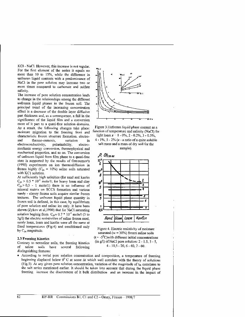
KC1 - NaCl. However, this increase is not regular. For the first element of the series it equals no more than 10 to 15%, while the difference in unfrozen liquid contents with a predominance of NaCl in the pore solution may increase two or more times compared to carbonate and sulfate salinity. The increase of pore solution concentration leads to change in the relationships among the different unfrozen liquid phases in the frozen soil. The principal trend of the increasing concentration effect is a decrease of the double layer diffusive part thickness and, as a consequence, a fall in the significance of the liquid film and a conversion more of it part to a quasi-free solution domains. As a result, the following changes take place: moisture migration to the freezing front and characteristic frozen structure formation, electro- and thermo-osmosis, variation in electroconductivity, polarizability, electro- mechanic energy conversion, thermophysical and mechanical properties, and so on. The conversion of unfrozen liquid from film phase to a quasi-free state is supported by the results of Ostroumov's (1990) experiments on ion thermodiffusion in frozen highly (Cps = 10%) saline soils saturated withKCl solution. At sufficiently high salinities (for sand and kaolin Cps > 0.5 * 10"' mole/1; for heavy loam and clay Cps > 0,5 - 1 mole/1) there is no influence of mineral matrix on SCCS formation and various sandy - clayey frozen soils acquire similar frozen textures. The unfrozen liquid phase quantity in frozen soil is defined, in this case, by equilibrium of pore solution and saline ice only. It have been shown (Zykov et al,1990) that for NaCl saturating solution beginig from Cps« 0.7 * 10"' mole/1 (3 to 5g/l) the electric resistivities of saline frozen sand, sandy loam, loam and kaolin were all the same at fixed temperatures (Fig.4) and conditioned only by Cps magnitude.

wuz

Figure 3.Unfrozen liquid phase content as a function of temperature and salinity (NaCl) for

light loam z = 1 - 0%, 2 - 0.2%, 3 - 0.5%, 4 -1%, 5 - 2% (z - a ratio of a quite soluble

salt mass and a mass of dry soil for the sample).

A Ohmm JO*

10* 5

5

10 5

1

0,5

Z___ —-*

- = = = =T _ _^ _—_—___ f

Sand SLcest Loam KaoHn

the freezing kinetics several following

Figure 4. Electric resistivity of moisture saturated (w = 30%) frozen saline soils

(t = -5°C)with different initial concentrations (in g/l) of NaCl pore solution: 2 - 1.5, 3 - 5,

4-10,5-20,6-40,7-60.

2.3 Freezing Kinetics Contrary to nonsaline soils, of saline soils have distinguishing features: • According to initial pore solution concentration and composition, a temperature of freezing

beginning displaced below 0° C at some At which well correlate with the theory of solutions (Fig.5). At any given pore solution concentration, variation of the magnitude of tth correlates to the salt series mentioned earlier. It should be taken into account that during the liquid phase freezing increase the discreteness of it bulk distribution and an increase in the impact of


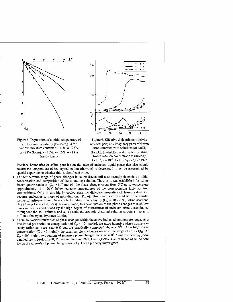
CS 1,0 1,5 it ZZ

-25 - 20

Figure 5. Depression of a initial temperature of soil freezing vs salinity (z - see fig.3) for

various moisture content: A -11%, o - 22%, x - 32% (loam); A - 10%, ■ -15%, • - 18%

(sandy loam).

Figure 6. Effective dielectric permittivity (e' - real part, e" - imaginary part) of frozen

sand saturated with solutions (a) NaCl, (b) KC1, (c) distilled water vs temperature.

Initial solution concentrations (mole/1): 1 - 10"', 2 - 10"3, 3 - 0; frequency =5 kHz.

interface boundaries of saline pore ice on the state of unfrozen liquid phase that also should causes the temperature of ice crystallization (thawing) to decrease. It must be ascertained by special experiments whether this is significant or no. The temperature range of phase changes in saline frozen soil also strongly depends on initial concentration and composition of the saturating solution. Thus, as it was established for saline frozen quartz sands at Cps > 10'1 mole/1, the phase changes occur from 0°C up to temperature approximately 15 - 20°C below eutectic temperatures of the corresponding ionic solution compositions. Only in this highly cooled state the dielectric properties of frozen saline soil become analogous to those of nonsaline one (Fig.6). This trend is correlated with the similar results of unfrozen liquid phase content studies in very highly (Cps = 10 - 20%) saline sand and clay (Zhang Lixin et al,1993). In our opinion, this continuation of the phase changes at such low temperatures is conditioned by the high degree of discreteness of unfrozen brine disseminated throughout the soil volume, and as a result, the strongly distorted solution structure makes it difficult the crystal hydrates forming. There are various intensities of phase changes within the above indicated temperature range. At a low initial pore solution concentration of Cps ~ 10"2 mole/1, the more intensive phase changes in sandy saline soils are near 0°C and are practically completed above -10°C. At a high initial concentration (Cps > 1 mole/1), the principal phase changes occur in the range of (0.3 - \)Uu- At Cps~ 10"' mole/1, two regions of intensive phase changes recur, near 0° C and rest near Uu (more detailed see in Frolov,1990; Frolov and Seguin, 1993; Frolov,1998). The influence of saline pore ice on the intensity of phase changes has not yet been properly investigated.


2.4 Specificity of SCCS. Specific distinctions of saline soil SCCS are determined by the processes of: dispersion and coagulation of mineral matrix grains, formation of saline ice matrix and modifications of the intergrain zones : • The salinity effect on mineral matrix leads to a change in the granulometric composition and

plasticity index of moist saturated soil. There were obtained (Ershov, 1995,1996) that an increase in pore solution concentration cause increase the intensity of clay particle coagulation and forms micro- and macroaggregates. This leads in turn to changes of media heteroporosity that influence the unfrozen liquid phase content temperature dependencies. The changes of soil microaggregate composition depend considerably on exchangeable ions. For instance, saturation of montmorillonite clay by Fe3+ ions leads to formation of aggregates which correspond by size to sandy fraction. Decrease of ion valence increase the soil dispersiveness that attaches more importance to ultramicropores in liquid phase distribution.

• The forming saline pore ice is much more fine crystalline compared to one in nonsaline soil. Initial pore solution concentration increase leads to a marked decrease in ice grain sizes. Thus, the change of solution concentration from 10"' to 1 mole/1 decreases the crystal sizes approximately in one order. So the ice matrix of saline frozen soil consists of doped crystals and aggregates of saline ice that must change the freezing kinetics and the energy state of the liquid phase as well as the physical properties of frozen soil.

• The third principal element of SCCS - intergrain zones in saline frozen soils are distinguished not only by high general unfrozen liquid content but also by their irregular discreteness of bulk distribution. The latter usually is not determined by known methods of unfrozen liquid phase contents studies. The presence of the discreteness effect was shown indirectly in our experiments (Frolov,1976;Frolov,1991) using two electrodynamics methods: low frequency spectroscopy and electroacoustic energy conversion. According to these experiments there are two maximums of unfrozen liquid discretization: at the initial freezing temperature and near the eutectic temperature of saturating pore solution Even at high initial soil salinity (Cps > 1 mole/1) there is a clear increase of liquid phase discreteness during a freezing. However, in this case the first maximum is not observed due to the low amount of porous ice formation during initial stage of freezing. Similar experiments for saline clayey soils have not been realized yet.

3 CONCLUSIONS

The results may be summarized as follows : 1. Saline soils are distinguished some critical initial pore solution concentration of Ccr. The Ccr

magnitude increases with increasing soil dispersiveness and clayeyness. In the case of chloride saturating solutions for quartz sand Ccr =(0,5-1,0) * 10"2 mole/1, and for bentonite it reaches 0,5 to 1 mole/1.

2. The initial.pore solution concentration increase causes approximately linear increase of unfrozen liquid phase content at fixed temperatures of saline frozen soil. Unfrozen liquid content depends on the pore solution ionic composition and it increases in the following order : carbonates-sulfates-nitrates-chlorides.

3. During saline soil freezing there is not only increasing a concentration, but also extent energy state diversity and discreteness in bulk distribution of unfrozen liquid phase. An extended temperature range of phase changes is common to all saline soils especially for sandy ones. For high saline sandy soils (Cps >10* mole/1) it runs up to the corresponding pore solution eutectic temperature and even 15 - 20 °C below it.

4. There are characteristic features in solid parts of SCCS of frozen saline soil: a) the ice matrix consists of fine crystallized saline ice with doped grains; b) the mineral matrix changes its granulometric composition and a degree of heteroporosity (pore distribution by sizes).

84 IIF-IIR - Commissions Bl, Cl and C2 -r Orsay, France - 1998/7

5. High liquid phase content in saline frozen soils causes the decrease of their thermal conductivity and diffusivity, acoustic, elastic and strength properties and vice versa the increase of electroconductivity, dielectric permittivity and Poisson's ratio compared to the same, but nonsaline soils.

6. Beginning with an initial saturating pore solution concentration of Cps «10"1 mole/1, soil mineral matrix composition has no practically impact on freezing kinetics, cryogenic structure and texture forming, electric resistivity and some other properties of most frozen soils (except heavy clays).

The indicated principal features are important for a better comprehension of the saline ( or generally polluted ) soil specificity compared to nonsaline one. In the future it is necessary to realize the joint experimental studies (on the same soils!) of liquid phase content and several electric and mechanical properties as the functions of temperature, composition and concentration of saturating solution. Note very interesting prospects to use a pure quartz sand and other simple granular media saturated with various solutions as the research models for detail imitation and study the regularities of various stages of phase transformations during freezing.

ACKNOWLEDGMENT

The study was supported in part by Russian Foundation of Fundamental Researches, Project Ks 97-05-64961.

REFERENCES

1. Chellaiah, S. and R. Viskanta,1987, Freezing of Water and Water-Salt Solutions around Aluminium Spheres," Int. Comm. in Heat and Mass 7hms.,vol.l4: p. 437-487.

2. Ershov, E.D.,Ed - r,1995, Fundamentals of Geocryology, vol I, Physics - chemical Bases of Geocryology. Mose.State Univ. Press, 367 p.

3. Ershov, E.D.,Ed-r,1996, Fundamentals of Geocryology, vol II, Lithogenous Geocryology, Mose. State Univ. Press, 365 p.

4. Fedyukin, I.V., Frolov A.D., Gussev,B.V.,1979, Salinity Influence on Electric Properties of Frozen Soils, Dokl. Acad Nauk, USSR, vol. 244: p. 941-944.

5. Frolov, A.D., 1976, Electric and Elastic properties of cryogenic grounds, Nedra Press, Moscow, 258 p.

6. Frolov,A.D., Fedyukin,I.V.,1983, Polarization of Frozen Soils in the Alternative Electromagnetic Fields, Izvestia VUZov, Geologiya i Razvedka, no, 6: p. 90-96,.

7. Frolov, A.D.,1991, Peculiarities of Phase Changes in Quartz Sand Saturated with Salt Solutions at 0°C -:- -40°C, Proc. Third Intern. Symp. On Cold Regions Heat Transfer, UAF, Fairbanks,Alaska,USA, p. 293- 302.

8. Frolov, A. D., Seguin,M.K., Caracteristiques de la Cinetique de Congelation de Sols Salins, Permafrost and Periglac, Processes, no. 4: p. 311-325.

9. Frolov, A.D. and I.V. Fedyukin, "Dielectric properties of saline frozen soils", Trans. Geophysical Investigations of Cryolithozone, 1,73-94,1995.

10. Frolov A.D., Chervinskaya O.P., Zykov Yu. D.,1997, Peculiarities of frozen saline soils electric and elastic properties, Proc.Int.Symp. Ground Freezing and Frost Action in Soils, Lulea, Sweeden. Balkema, p. 385-390.

11. Frolov,A.D.,1998, Electric and Elastic Properties of Frozen Earth Materials, ONTI PSC RAS Publisher, Pushchino, 515p.

12. Grant, G.A. et al.,1993, Unfrozen water content in caolinite, montmorilonite and sands saturated with NaCl solution at three concentrations, USA CRREL, Final Report, Contract DACA 89-92-M-2378, 52p.


13. Khimenkov, A.N., Minaev,A.N.,1990, Salinity Influence on Frozen Soils Cryostructure Formation, Coll. "Saline Frozen Soils as the Foundations of Constructions", Nauka, Press, Moscow, p.55-62.

14. Ostroumov, V.E.,1990, Salt Transfer in Frozen Soils Under Influence of a Temperature Gradient, Coll. "Saline Frozen Soils as the Foundations of Constructions", Nauka, Press, Moscow, p. 45-55.

15. Panchenko, N.I., Aksionov,V.I.,1990, Physics-chemical Approaches for Frozen Soils Classification by Salinity, Coll. "Saline Frozen Soils as the Foundations of Constructions", Nauka, Press, Moscow, p.70-73.

16. Pavlov, A.S. Frolov,A.D.,1990, On the Electroacoustic Effect Application for Study of Saline Soil Freezing, Coll. "Saline Frozen Soils as the Foundations of Constructions", Nauka, Press, Moscow, p. 136-143.

17. Rebinder P.A.,1979, Physics-chemical mechanics., Nauka, Press, Moscow 380p., 18. Roman L.D., Artyushina V.l., Ivanova L.G.,1994, Impact of pore liquid phase freesing begining

temperature of frozen saline soils strength, Ingineering Geology, Hydrogeology, Geocryology, Moscow, no.l: p.49-55.

19. Tice, A.R., Zhu Yuanlin, OHphant,I.L.1984, The Effects of Soluble Salts on the Unfrozen Water Contents of the Lanzhou PR.C. Silt, USA, CRREL Report 84-16.

20. Velli, Yu.Ya.,1990, Arctic Shore Saline Frozen Soil Studies (review), Coll. "Saline Frozen Soils as the Foundations of Constructions, Nauka, Press, Moscow,p. 9-20.

21. Yarkin, A.N.,1990, Influence of Salinity Type on the Strength and Rheological Properties of Frozen Soils, Coll. "Saline Frozen Soils as the Foundations of Constructions", Nauka, Press, Moscow, p. 103-107.

22. Zhang Lixin et al.,1993, Analysis of the Second Phase Transition of Sodium Chloride Solution in Freezing Soil, Proc. of VIInt. Conf. on Permafrost, Beijing, China, vol.1, p.773-777.

23. Zykov, Yu.D. et al.,1990, Electric and Acoustic Properties of Saline Frozen Soils, Coll. "Saline Frozen Soils as the Foundations of Constructions", Nauka, Press, Moscow, p. 128 - 136.

24. Zykov,Yu.D.,Chervinskaya,O.P.,1995, Estimation of Deformation and Strength Properties of Frozen Soils by Acoustic Method, Trans. Geophysical Investigations of Cryolithozone, issue 1, Moscow, p. 12-22.

LES PARTICULARITES ESSENTIELLES DES SOLS SALINS GELES

RESUME : L'analyse des resultats des differentes recherches physiques et physico-chimiques a permis d'etablir quatre particularites distinctives et les plus importantes pour les sols salins geles : 1) la concentration initiale critique des solutions saturantes des pores; 2) la composition de phase originale; 3) la structure spatiale cryogenique cristalline - coagulante specifique; 3) les traits caracteristiques de la cinetique de congelation. Toutes ces particularites sont decrites et discutees dans cet article.


ADC: NEW SYSTEM FOR THE MEASURE OF SPECIFIC HEAT, THERMAL CONDUCTIVITY AND ENTHALPY (A.D.C.)

DOMINGUEZ M., PINILLOS J.M., GUTIERREZ P., LOPEZ N. Instituto del Frio. C.S.I.C. Ciudad Universitaria .28040 Madrid.Spain

ABSTRACT

The Analogical Differential Calorimetry ADC. Is a new technique which exhibits many possibilities and advantages for the de measure of three thermophysical parameters like: thermal conductivity coefficient, specific heat and enthalpy. This are very important properties in the studies of freezing and thawing of food products, in order to increase quality, also in studies involving heat accumulators with phase change, and in freezing of porous media, like in polar regions, etc., where other techniques cannot yield information about said parameters or require much time or very costly equipment. The advantages is present , for instance, in the quality control of products where the coefficient of conductivity is important, as in the case of thermal insulating materials, as values can be obtained within minutes, which would require many hours with other techniques. Some of the results obtained, analysing the possibilities that it has in the study of freezing and thawing phenomena, are indicated.

INTRODUCTION

The knowledge of the thermophysical properties of the products as a function of temperature is very important in many applications, as can be in the study of the freezing and thawing of perishable products. It is possible to find in the literature techniques for measuring the thermal conductivity coefficient of insulating materials, for enclosures, based upon absolute calorimetric methods, and relative ones with heat flux measurers, in a stationary regime. In the case of applications for food products it is also possible to find others of transitory regime, based on the hot wire method which calculates the coefficient of diffusivity. In the case of metals, some very complex methods have been developed using thermal impulses, etc. There are few suppliers commercialising conductivity equipment, and the devices they offer are expensive and scarcely flexible. The measurement of the specific heat can be carried out by the law of mixtures in calorimeters or Dewar flasks or by microcalorimetry, which is an expensive but widely used technique, which also permits the determination of latent heats. Indirect methods for the measurement of conductivity and specific heat, by means of the coefficient of diffusivity, have been tested, but have not yielded the desired accuracy. There is therefore a great gap in the determination of these thermophysical properties which are of great importance in all heat transmission studies, for all kinds of products. On the other hand, in many materials, and especially in food products, the water content can be very large and the measuring problems become enormously more complicated, and problems of sub-cooling, historical differences, variations with the rates of cooling, possible mass transfer problems, etc, appear during the freezing process. Due to all of this, thought was put into the development of a new measuring technique which would permit the solution of many of these problems, which would adapt to the dimensions and requirements of food products, and the result obtained was the technique we have denominated Analogical Differential Calorimetry (ADC). The main stages followed are indicated in (1), (2) and (3) and the main results obtained are found in (4) and (5). Currently, after having constructed four prototypes, the technique is considered to be fully achieved, being it possible to move on to its commercialisation and widespread use.


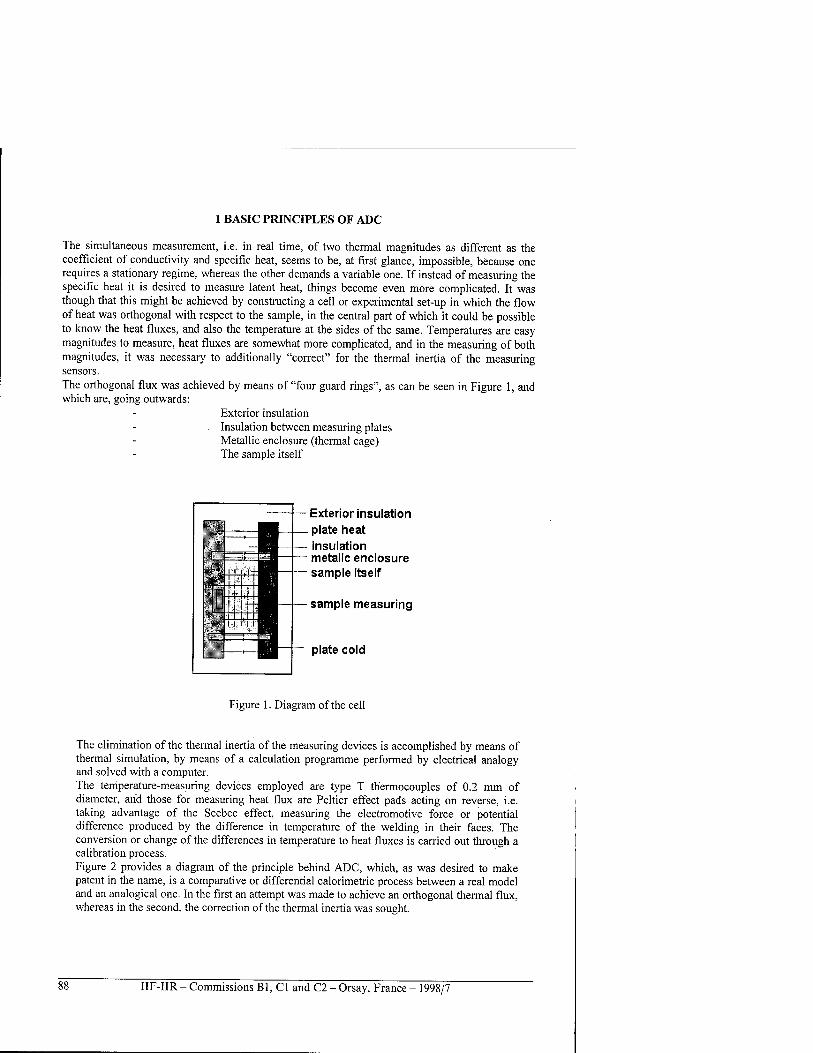
1 BASIC PRINCIPLES OF ADC

The simultaneous measurement, i.e. in real time, of two thermal magnitudes as different as the coefficient of conductivity and specific heat, seems to be, at first glance, impossible, because one requires a stationary regime, whereas the other demands a variable one. If instead of measuring the specific heat it is desired to measure latent heat, things become even more complicated. It was though that this might be achieved by constructing a cell or experimental set-up in which the flow of heat was orthogonal with respect to the sample, in the central part of which it could be possible to know the heat fluxes, and also the temperature at the sides of the same. Temperatures are easy magnitudes to measure, heat fluxes are somewhat more complicated, and in the measuring of both magnitudes, it was necessary to additionally "correct" for the thermal inertia of the measuring sensors. The orthogonal flux was achieved by means of "four guard rings", as can be seen in Figure 1, and which are, going outwards:

Exterior insulation Insulation between measuring plates Metallic enclosure (thermal cage) The sample itself

Exterior insulation plate heat insulation metalic enclosure sample itself

sample measuring

plate cold

Figure 1. Diagram of the cell

The elimination of the thermal inertia of the measuring devices is accomplished by means of thermal simulation, by means of a calculation programme performed by electrical analogy and solved with a computer. The temperature-measuring devices employed are type T thermocouples of 0.2 mm of diameter, and those for measuring heat flux are Peltier effect pads acting on reverse, i.e. taking advantage of the Seebec effect, measuring the electromotive force or potential difference produced by the difference in temperature of the welding in their faces. The conversion or change of the differences in temperature to heat fluxes is carried out through a calibration process. Figure 2 provides a diagram of the principle behind ADC, which, as was desired to make patent in the name, is a comparative or differential calorimetric process between a real model and an analogical one. In the first an attempt was made to achieve an orthogonal thermal flux, whereas in the second, the correction of the thermal inertia was sought.


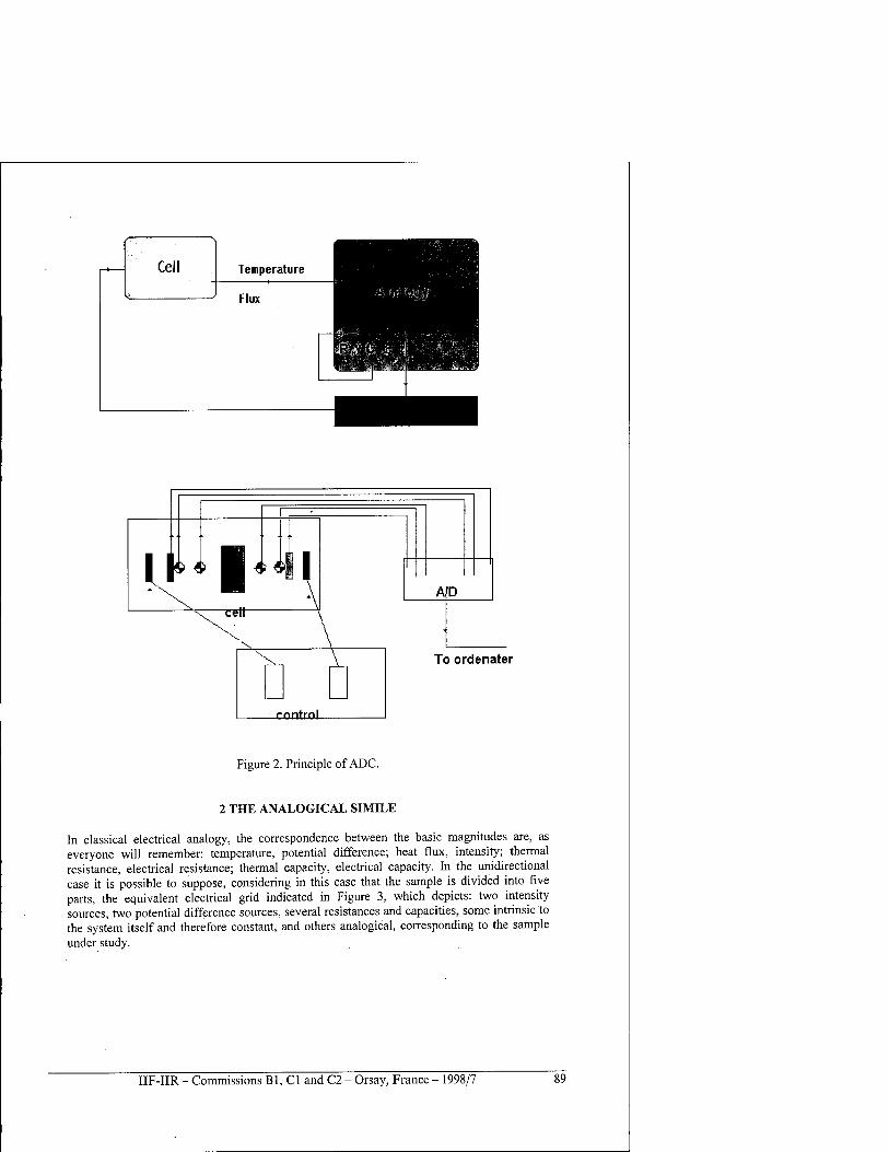
Temperature

Flux

Figure 2. Principle of ADC.

2 THE ANALOGICAL SIMILE

In classical electrical analogy, the correspondence between the basic magnitudes are, as everyone will remember: temperature, potential difference; heat flux, intensity; thermal resistance, electrical resistance; thermal capacity, electrical capacity. In the unidirectional case it is possible to suppose, considering in this case that the sample is divided into five parts, the equivalent electrical grid indicated in Figure 3, which depicts: two intensity sources, two potential difference sources, several resistances and capacities, some intrinsic to the system itself and therefore constant, and others analogical, corresponding to the sample under study.


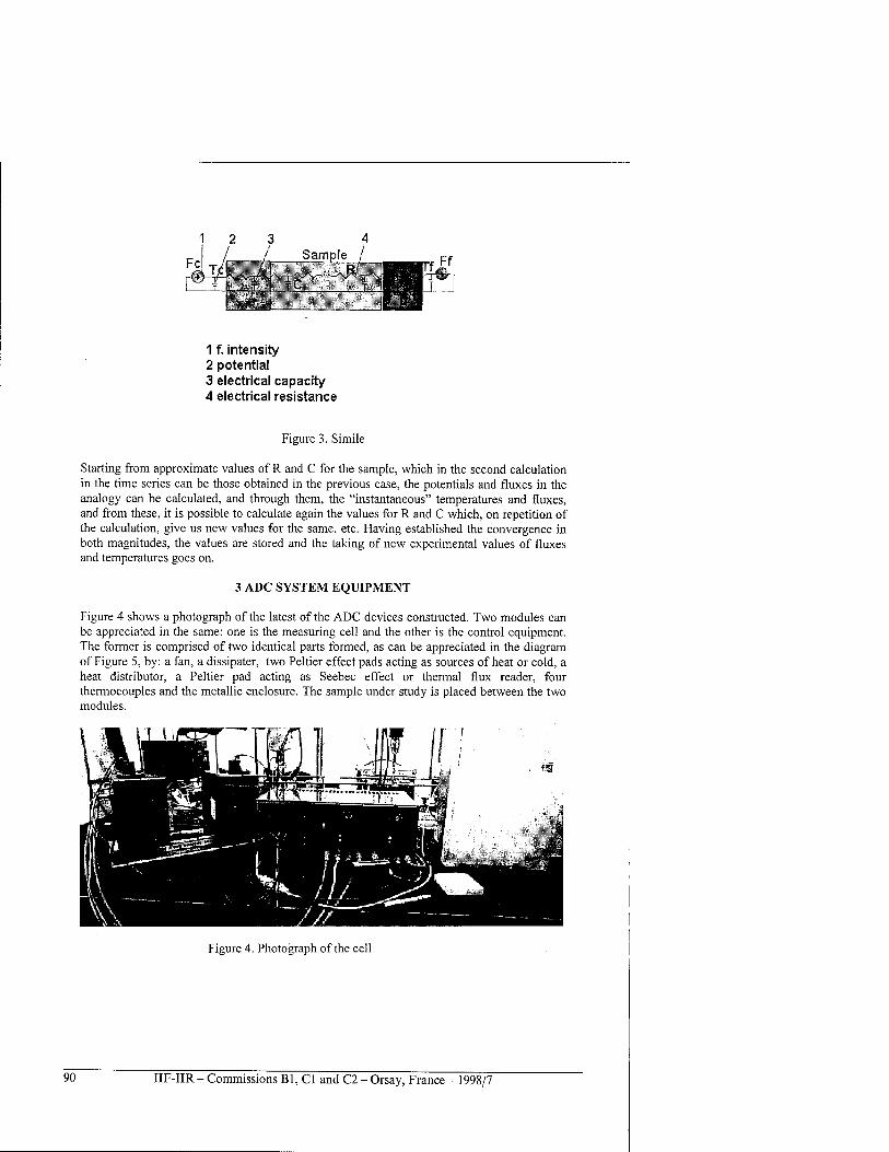
1 f. intensity 2 potential 3 electrical capacity 4 electrical resistance

Figure 3. Simile

Starting from approximate values of R and C for the sample, which in the second calculation in the time series can be those obtained in the previous case, the potentials and fluxes in the analogy can be calculated, and through them, the "instantaneous" temperatures and fluxes, and from these, it is possible to calculate again the values for R and C which, on repetition of the calculation, give us new values for the same, etc. Having established the convergence in both magnitudes, the values are stored and the taking of new experimental values of fluxes and temperatures goes on.

3 ADC SYSTEM EQUIPMENT

Figure 4 shows a photograph of the latest of the ADC devices constructed. Two modules can be appreciated in the same: one is the measuring cell and the other is the control equipment. The former is comprised of two identical parts formed, as can be appreciated in the diagram of Figure 5, by: a fan, a dissipater, two Peltier effect pads acting as sources of heat or cold, a heat distributor, a Peltier pad acting as Seebec effect or thermal flux reader, four thermocouples and the metallic enclosure. The sample under study is placed between the two modules.

Figure 4. Photograph of the cell


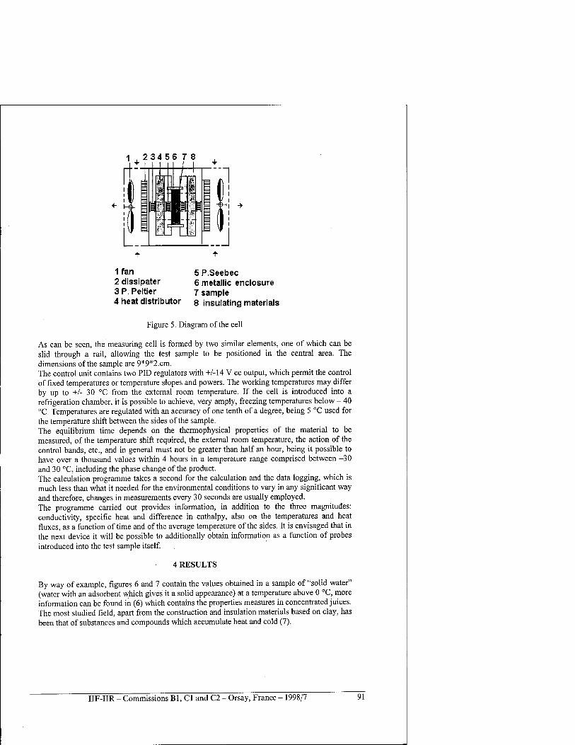
1 , 23456 7 8

1 fan 5 p.Seebec 2 dissipater 6 metallic enclosure 3 P. Peltier 7 sample 4 heat distributor Q insulating materials

Figure 5. Diagram of the cell

As can be seen, the measuring cell is formed by two similar elements, one of which can be slid through a rail, allowing the test sample to be positioned in the central area. The dimensions of the sample are 9*9*2.cm. The control unit contains two PID regulators with +/-14 V cc output, which permit the control of fixed temperatures or temperature slopes and powers. The working temperatures may differ by up to +/- 30 °C from the external room temperature. If the cell is introduced into a refrigeration chamber, it is possible to achieve, very amply, freezing temperatures below - 40 °C. Temperatures are regulated with an accuracy of one tenth of a degree, being 5 °C used for the temperature shift between the sides of the sample. The equilibrium time depends on the thermophysical properties of the material to be measured, of the temperature shift required, the external room temperature, the action of the control bands, etc., and in general must not be greater than half an hour, being it possible to have over a thousand values within 4 hours in a temperature range comprised between -30 and 30 °C, including the phase change of the product. The calculation programme takes a second for the calculation and the data logging, which is much less than what it needed for the environmental conditions to vary in any significant way and therefore, changes in measurements every 30 seconds are usually employed. The programme carried out provides information, in addition to the three magnitudes: conductivity, specific heat and difference in enthalpy, also on the temperatures and heat fluxes, as a function of time and of the average temperature of the sides. It is envisaged that in the next device it will be possible to additionally obtain information as a function of probes introduced into the test sample itself.

4 RESULTS

By way of example, figures 6 and 7 contain the values obtained in a sample of "solid water" (water with an adsorbent which gives it a solid appearance) at a temperature above 0 °C, more information can be found in (6) which contains the properties measures in concentrated juices. The most studied field, apart from the construction and insulation materials based on clay, has been that of substances and compounds which accumulate heat and cold (7).


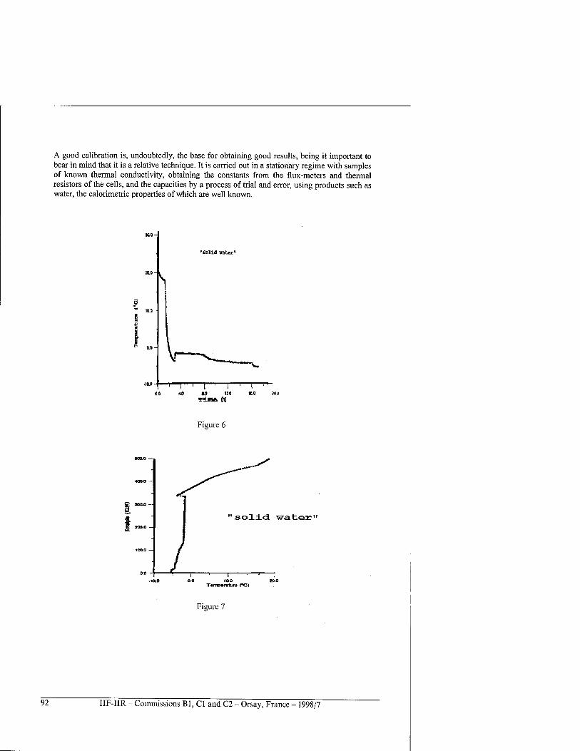
A good calibration is, undoubtedly, the base for obtaining good results, being it important to bear in mind that it is a relative technique. It is carried out in a stationary regime with samples of known thermal conductivity, obtaining the constants from the flux-meters and thermal resistors of the cells, and the capacities by a process of trial and error, using products such as water, the calorimetric properties of which are well known.

"S

KLB- ■

S a r

•10.0-• —X

F Solid VatBr"

V Co «.0 M 120 MO »u

vina (hi

Figure 6

L

solid water'

-]I|r—

0.0 100 TamD»tmtufte t*C\

Figure 7


5 DISCUSSION

ADC is considered to be a new measuring technique which exhibits many possibilities and advantages, for the measure of three very important properties in the studies of freezing and thawing of food products, studies involving accumulators of heat or cold with a phase change in studies in polar regions and of freezing of porous media, etc., where other techniques cannot yield information about said parameters or require much time or very costly equipment. The advantages it presents for the quality control of products where the coefficient of conductivity is important, as is the case of thermal insulating materials, as values can be obtained within minutes, which would require many hours with other techniques. The precision that can be obtained is a function of the initial calibration, and it has been seen that it does not vary unless the environmental conditions surrounding the cell are changed to a large extent. The programming in the microprocessors which are fitted in the prototypes constructed, has been seen to be less important than expected, being the oscillations in the results charts more affected than the values themselves. There will surely be a more comfortable and pleasant solution for each type of study, which can be found by acting upon them. The main source of error which has been appreciated is the determination of the thickness of the samples, and if these contain liquids, also due to the movement of these during the test. The liquid measuring cylinders are positioned vertically, horizontal ones could introduce problems related to air pockets which would complicate the measurements. In such a case the technique would have to be modified.

CONCLUSION

The new technique for the measure of the three thermophysical parameters: thermal conductivity coefficient, specific heat and enthalpy, which we have denominated ADC (Analogical Differential Calorimetry) is considered to have many possibilities for the study of freezing and thawing processes of perishable products, and in those involving the search of thermal accumulators with a change of phase and the control of material processes, in which conductivity is important, as it can be in the case of thermal insulation materials.

ACKNOWLEDGEMENTS

This work has been carried out within the "Development of new concentration technologies using heat by atomisation" program ALI 94-1044-C03-01, financed by the National Program of the Spanish International Science and Technology Commission, without the help of which this research would not have been possible.

REFERENCES

1. Dominguez M, Pinillos J.M., 1989, Principio y descripciön de una nueva celula de medida del coeficiente de conductividad termica con placas Peltier. Refigeraciön-Frial, no. 13: p. 5-10.

2. Dominguez M., Pinillos J.M., 1990, Determinaciön simultänea de calores especificos y conductividades termicas en una celula experimental, Refigeraciön-Frial, no. 14, Marzo 1990: p. 15-21.

3. Dominguez M., Barragän V.B., Pinillos J.M., Arias J.M., 1997, Sistema de medida simultänea de coeficiente de conductividad y calor especifico basado en la calorimetria diferencial analögica, XXVI Reunion Bienal R.S.FISICA Las Palmas de Gran Canarias, sep.1997: p. 625-626.


4. Domi'nguez M., Pinillos J.M., Ramos M. y Ortiz de Zärate J.M., 1991, International Congress on Refrigeration, Comission C2, Montreal, Agosto 1991.

5. Dominguez M., Pinillos J.M., Ramos M. y Ortiz de Zärate J.M., 1990, Aplicaciön de la calorimetria diferencial analögica en el estudio termico de la metilcelulosa, Refrigeraciön Frial no. 17: p. 5-10.

6. Dominguez M., Arias J.M., Pinillos J.M., 1997, Propiedades de zumo de naranja concentrado: conductividad, calor especifico, entalpia y viscosidad, Refrigeraciön Frial .no. 45: p. 35-39.

7. Dominguez; M., Pinillos J.M., Garcia, C, Arias J.M., Lopez N., 1998, Algunas propiedades termofisicas de "agua sölida", obtenida con la tecnica C.D.A., VII Encuentro delgrupo Especializado de Termodinämica de las R.S. E. de Fisicay Quimica, Tarragona, Juniol998,a3:p. 1-3.

NOUVEAU SYSTEME DE CALORIMETRIE DIFFERENTIELLE ANALOGIQUE (ADC) POUR LA MESURE DE LA CHALEUR SPECIFIQUE, DE LA CONDUCTIVITE THERMIQUE ET DE L'ENTHALPIE

RESUME : La calorimetrie differentielle analogique est une technique nouvelle qui offre nombre de possibilites et avantages pour la mesure de trois parametres thermophysiques tels que le coefficient de conductivity thermique, la chaleur specifique et l'enthalpie. Ce sont des proprietes ä prendre en compte dans l'etude de la congelation et de la decongelation des produits alimentaires, afin d'en ameliorer la qualite, mais aussi dans l'etude des accumulateurs de chaleur avec changement de phase et dans la congelation de milieux poreux tels que ceux rencontres dans les regions polaires ; pour ces cas lä, d'autres techniques ne sont pas en mesure de fournir une information sur les parametres mentionnes ci-dessus, ou encore exigent du temps ou sont coüteuses. Les avantages sont indeniables, notamment pour le controle de la qualite des produits dont le coefficient de conductivite est eleve (par exemple pour les materiaux d'isolation thermique) parce que les valeurs peuvent etre obtenues en quelques minutes, alors que d'autres techniques exigeraient plusieurs heures. On donne certains des resultats obtenus, en analysant les possibilites offertes pour l'etude des phenomenes de congelation et decongelation.


ANALYSIS OF ROCKS BEHAVIOUR AT LOW TEMPERATURE DURING BRAZILIAN TESTS WITH ULTRASONIC WAVES

COTE H., THIMUS J.-F. Unite Genie Civil, Universite catholique de Louvain, Place du Levant, 1

Louvain-la-Neuve, Belgium

ABSTRACT

When submitted to low temperatures, rock grains individual thermal deformation gives a stronger matrix. In saturated conditions, phase change involves ice participation to this improvement. Our aim is the characterisation of mechanical behaviour of frozen saturated rocks with non-destructive techniques. Ultrasonic waves P & S through rock sample give precious informations about the cracking process. Crack density leads to a decrease in measured velocity while saturation and confining involve velocity increase. Attenuation evaluated on entire ultrasonic signals (energy) is more sensitive for material deterioration analysis. P & S waves velocity and energy indicate that hard rocks behave in the same way at ambient and at low temperatures. Rocks with high porosity have a different behaviour which depends on temperatures, saturation and strain deformation.

INTRODUCTION

Technologies such as liquid gas storage in underground caverns are important challenges for artificial frozen rock engineering. Proper designs require a good knowledge of many parameters. Low temperatures induced by the cryo-liquid create complex thermal stresses, particularly for tensile stresses which is unfavourable for the cavern tightness.

Non-destructive techniques are often required for mechanical tests to provide information allowing the determination of failure process. This paper proposes a coupling study of indirect tensile tests with ultrasonic waves on frozen rocks with different porosity.

1 STATEMENT OF THE PROBLEM

1.1 Brazilian tests In brittle material mechanics, diametral compressive tests represent a solution to direct tensile test problems. A disc of diameter D and length L is compressed in the diametral axis between two surfaces. When the maximal stress Pmax is reached, the tensile strength is given by

2P„ <y, =

max (1)

TtDL

Hondros analytic model (1959) suggests a confining state at the rock-platen interfaces (fig.l). Maximum compressive principal stress component, a„ is compressive in all the sample and moreover near the interfaces. Minimum principal stress component, CT3, is also compressive close to the platens but tensional everywhere else with stronger stresses along the loading axis. This results in a strong confining pressure next to the platens. According material theories, final failure initiates at the center of this axis and propagates to the platens.


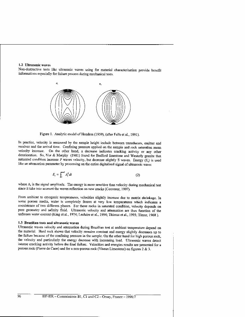
1.2 Ultrasonic waves Non-destructive tests like ultrasonic waves using for material characterisation provide benefit informations especially for failure process during mechanical tests.

Figure 1. Analytic model of Hondros (1959), (after Falls et al., 1991).

In practice, velocity is measured by the sample height include between transducers, emitter and receiver and the arrival time. Confining pressure applied on the sample and rock saturation mean velocity increase. On the other hand, a decrease indicates cracking activity or any other deterioration. So, Nur & Murphy (1981) found for Bedford limestone and Westerly granite that saturated condition increase P waves velocity, but decrease slightly S waves. Energy (Et) is used like an attenuation parameter by processing on the entire digitalised signal of ultrasonic wave:

peiu

Afdt (2)

where A, is the signal amplitude. The energy is more sensitive than velocity during mechanical test since it take into account the waves reflection on new cracks (Couvreur, 1997).

From ambient to cryogenic temperatures, velocities slightly increase due to matrix shrinkage. In some porous media, water is completely frozen at very low temperatures which indicates a coexistence of two different phases. For those rocks in saturated condition, velocity depends on pore geometry and salinity fluid. Ultrasonic velocity and attenuation are thus function of the unfrozen water content (King et al., 1974; Leclaire et al., 1994; Thimus et al, 1993; Timur, 1968 ).

1.3 Brazilian tests and ultrasonic waves Ultrasonic waves velocity and attenuation during Brazilian test at ambient temperature depend on the material. Hard rock shows that velocity remains constant and energy slightly decreases up to the failure because of the confining pressure in the sample. On the other hand for high porous rock, the velocity and particularly the energy decrease with increasing load. Ultrasonic waves detect intense cracking activity before the final failure. Velocities and energies results are presented for a porous rock (Pierre de Caen) and for a non-porous rock (Visean Limestone) on figures 2 & 3.


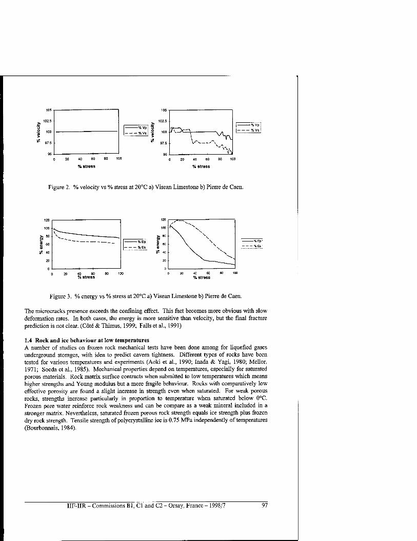
%Vp

% Vs

105

102.5

100

97.5

95 40 60 80 100

% stress

rocxv "^V -% Vp j

■ %VS !

20 40 60

% stress

Figure 2. % velocity vs % stress at 20°C a) Visean Limestone b) Pierre de Caen.

v. ̂ 100

X 80 X \ \

\ X 40 ■

\_\ 20

%Ep' % Es

% stress

Figure 3. % energy vs % stress at 20°C a) Visean Limestone b) Pierre de Caen.

The microcracks presence exceeds the confining effect. This fact becomes more obvious with slow deformation rates. In both cases, the energy is more sensitive than velocity, but the final fracture prediction is not clear. (Cote & Thimus, 1999; Falls et al., 1991)

1.4 Rock and ice behaviour at low temperatures A number of studies on frozen rock mechanical tests have been done among for liquefied gases underground storages, with idea to predict cavern tightness. Different types of rocks have been tested for various temperatures and experiments (Aoki et al., 1990; Inada & Yagi, 1980; Mellor, 1971; Soeda et al., 1985). Mechanical properties depend on temperatures, especially for saturated porous materials. Rock matrix surface contracts when submitted to low temperatures which means higher strengths and Young modulus but a more fragile behaviour. Rocks with comparatively low effective porosity are found a slight increase in strength even when saturated. For weak porous rocks, strengths increase particularly in proportion to temperature when saturated below 0°C. Frozen pore water reinforce rock weakness and can be compare as a weak mineral included in a stronger matrix. Nevertheless, saturated frozen porous rock strength equals ice strength plus frozen dry rock strength. Tensile strength of polycrystalline ice is 0.75 MPa independently of temperatures (Bourbonnais, 1984).


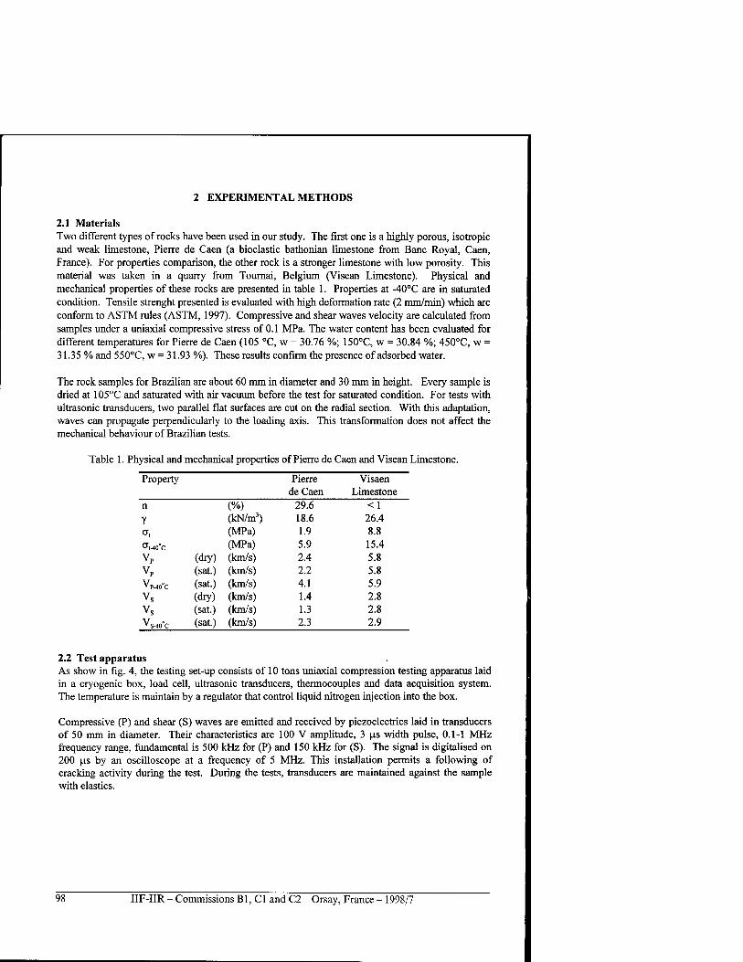
2 EXPERIMENTAL METHODS

2.1 Materials Two different types of rocks have been used in our study. The first one is a highly porous, isotropic and weak limestone, Pierre de Caen (a bioclastic bathonian limestone from Banc Royal, Caen, France). For properties comparison, the other rock is a stronger limestone with low porosity. This material was taken in a quarry from Tournai, Belgium (Visean Limestone). Physical and mechanical properties of these rocks are presented in table 1. Properties at -40°C are in saturated condition. Tensile strenght presented is evaluated with high deformation rate (2 mm/min) which are conform to ASTM rules (ASTM, 1997). Compressive and shear waves velocity are calculated from samples under a uniaxial compressive stress of 0.1 MPa. The water content has been evaluated for different temperatures for Pierre de Caen (105 °C, w = 30.76 %; 150°C, w = 30.84 %; 450°C, w = 31.35 % and 550°C, w = 31.93 %). These results confirm the presence of adsorbed water.

The rock samples for Brazilian are about 60 mm in diameter and 30 mm in height. Every sample is dried at 105°C and saturated with air vacuum before the test for saturated condition. For tests with ultrasonic transducers, two parallel flat surfaces are cut on the radial section. With this adaptation, waves can propagate perpendicularly to the loading axis. This transformation does not affect the mechanical behaviour of Brazilian tests.

Table 1. Physical and mechanical properties of Pierre de Caen and Visean Limestone.

Property Pierre de Caen

Visaen Limestone

n (%) 29.6 <1 Y (kN/m3) 18.6 26.4

a, (MPa) 1.9 8.8 CTM0°C (MPa) 5.9 15.4 vP (dry) (km/s) 2.4 5.8 vP (sat.) (km/s) 2.2 5.8 Vp-40°C (sat.) (km/s) 4.1 5.9 Vs (dry) (km/s) 1.4 2.8 Vs (sat.) (km/s) 1.3 2.8 *S-40°C (sat.) (km/s) 2.3 2.9

2.2 Test apparatus As show in fig. 4, the testing set-up consists of 10 tons uniaxial compression testing apparatus laid in a cryogenic box, load cell, ultrasonic transducers, thermocouples and data acquisition system. The temperature is maintain by a regulator that control liquid nitrogen injection into the box.

Compressive (P) and shear (S) waves are emitted and received by piezoelectrics laid in transducers of 50 mm in diameter. Their characteristics are 100 V amplitude, 3 (is width pulse, 0.1-1 MHz frequency range, fundamental is 500 kHz for (P) and 150 kHz for (S). The signal is digitalised on 200 |xs by an oscilloscope at a frequency of 5 MHz. This installation permits a following of cracking activity during the test. During the tests, transducers are maintained against the sample with elastics.


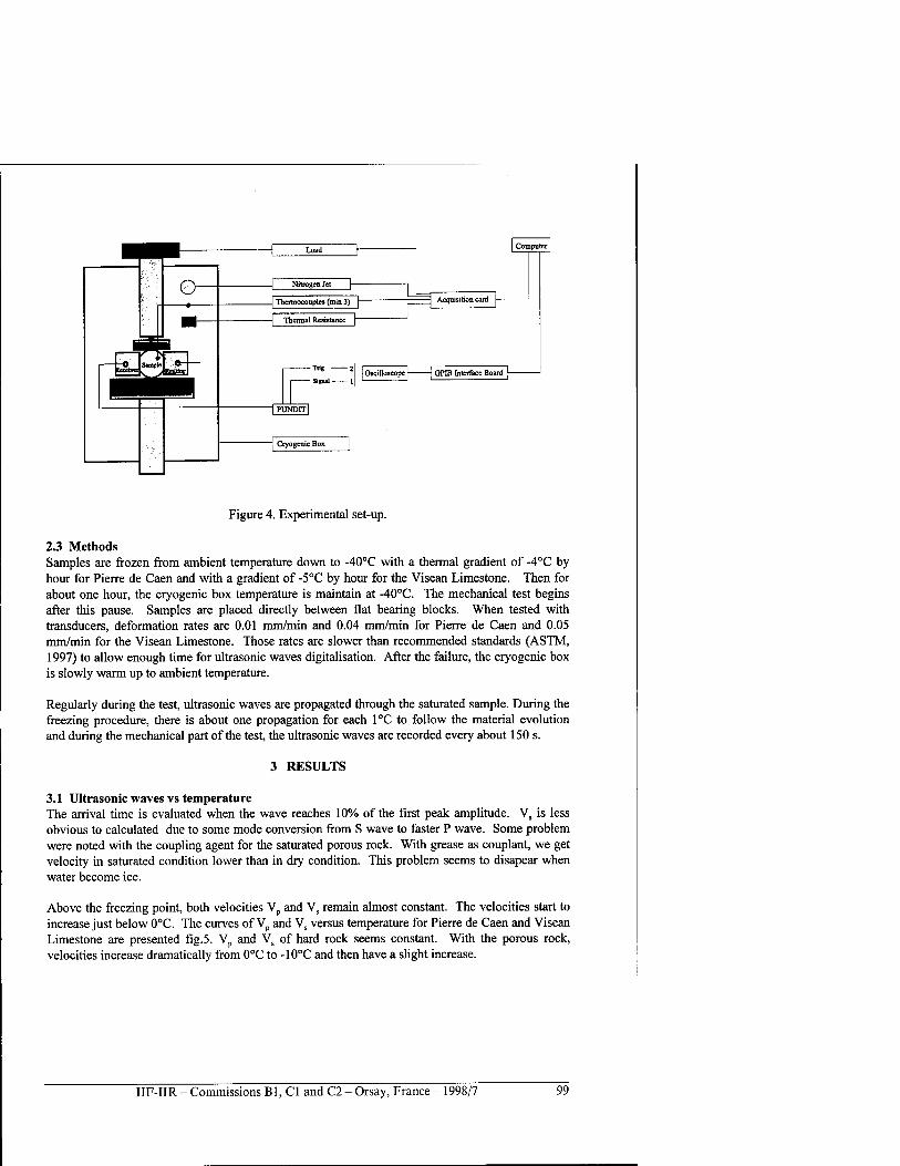
0-

I Computer ]

—| Nitrogen Jet \-

__| Thennocouples (min 3)

Thermal Resistance

Acquisition card I—

r Tug 2

Signal 1 | Oncillmcopej 1 GPIB Interface Board [

~| PUNDIT 1

Cryogenic Box

Figure 4. Experimental set-up.

2.3 Methods Samples are frozen from ambient temperature down to -40°C with a thermal gradient of -4°C by hour for Pierre de Caen and with a gradient of -5°C by hour for the Visean Limestone. Then for about one hour, the cryogenic box temperature is maintain at -40°C. The mechanical test begins after this pause. Samples are placed directly between flat bearing blocks. When tested with transducers, deformation rates are 0.01 mm/min and 0.04 mm/min for Pierre de Caen and 0.05 mm/min for the Visean Limestone. Those rates are slower than recommended standards (ASTM, 1997) to allow enough time for ultrasonic waves digitalisation. After the failure, the cryogenic box is slowly warm up to ambient temperature.

Regularly during the test, ultrasonic waves are propagated through the saturated sample. During the freezing procedure, there is about one propagation for each 1°C to follow the material evolution and during the mechanical part of the test, the ultrasonic waves are recorded every about 150 s.

3 RESULTS

3.1 Ultrasonic waves vs temperature The arrival time is evaluated when the wave reaches 10% of the first peak amplitude. Vs is less obvious to calculated due to some mode conversion from S wave to faster P wave. Some problem were noted with the coupling agent for the saturated porous rock. With grease as couplant, we get velocity in saturated condition lower than in dry condition. This problem seems to disapear when water become ice.

Above the freezing point, both velocities Vp and Vs remain almost constant. The velocities start to increase just below 0°C. The curves of Vp and Vs versus temperature for Pierre de Caen and Visean Limestone are presented fig.5. Vp and Vs of hard rock seems constant. With the porous rock, velocities increase dramatically from 0°C to -10CC and then have a slight increase.


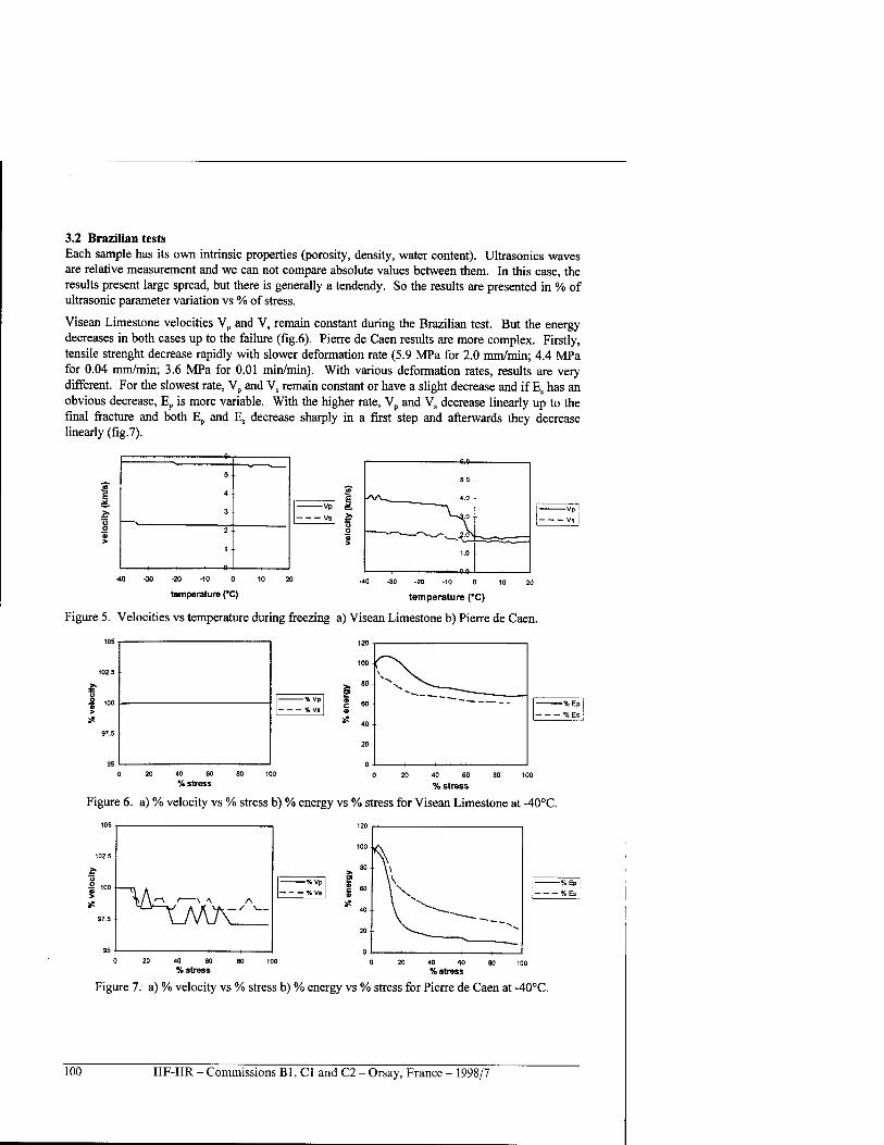
3.2 Brazilian tests Each sample has its own intrinsic properties (porosity, density, water content). Ultrasonics waves are relative measurement and we can not compare absolute values between them. In this case, the results present large spread, but there is generally a tendendy. So the results are presented in % of ultrasonic parameter variation vs % of stress.

Visean Limestone velocities Vp and Vs remain constant during the Brazilian test. But the energy decreases in both cases up to the failure (fig.6). Pierre de Caen results are more complex. Firstly, tensile strenght decrease rapidly with slower deformation rate (5.9 MPa for 2.0 mm/min; 4.4 MPa for 0.04 mm/min; 3.6 MPa for 0.01 min/min). With various deformation rates, results are very different. For the slowest rate, Vp and Vs remain constant or have a slight decrease and if Es has an obvious decrease, Ep is more variable. With the higher rate, Vp and Vs decrease linearly up to the final fracture and both Ep and Es decrease sharply in a first step and afterwards they decrease linearly (fig.7).

I — 6—

5--

4-

3

2 ■

1

1 1 1 »-•

Vp

--Vs

E je

5

5.0

4.0

'-^.O

———--W -W?-^

1.0

temperature (°C) temperature (°C)

Figure 5. Velocities vs temperature during freezing a) Visean Limestone b) Pierre de Caen.

120

100

c o

80

%Vp

S Vs 60

% stress

Figure 6. a) % velocity vs % stress b) % energy vs % stress for Visean Limestone at -40°C.

102.5

100 —*\ A W\ < \ <\

J AÄ 7 *-'Av_ 97.5 1 uv\l \

95

%Vp

% Vs %Ep

-— %Es

0 20 40 60 80 100 % stress % stress

Figure 7. a) % velocity vs % stress b) % energy vs % stress for Pierre de Caen at -40°C.


4 ANALYSIS

During the temperature variation, the velocity changes are associated to matrix shrinkage and the water content or water-ice proportion. For Pierre de Caen, the results indicate an obvious velocity increase on a large gradient. This fact involves adsorbed water in this rock. The evaluation of water content at different high temperatures confirms this. The pore water is completely frozen at about -10°C (same results as Letarvernier, 1984). For non-porous media, velocities increase slightly and generally the low water content has almost no effect on ultrasonic waves.

Theorically, slower deformation rates for mechanical tests give smaller strenght. But in the case of Pierre de Caen in saturated condition at low temperature, this rock has a greater sensitivity than at ambient temperature. Pore ice as a mineral component does not seem to be helpful at those rates. This situation is very interesting if we have to take into account natural behaviour which are much more slower than those in laboratory.

The results obtained (% velocity and % energy) for the Visean Limestone indicate that the mechanical behaviour is the same at both temperature. The only difference is the velocities for each temperature. Rock behaviour at low temperature becomes more fragile, but the present apparatus can not detect this fact. Maybe with faster ultrasonic digitalisation set-up it could be possible to see a difference at the very last moment before the failure.

Pierre de Caen behaves in different ways which depend on the deformation, in saturation condition and of course, temperature. If the velocities of compressive and shear waves decrease slightly in all cases, the energies show obvious differents which depend all parameters. Ambiant temperature is characterised by larger decreases with slower rates. At low temperature with high deformation rate, the energies show a sharp decrease in a first step and then a slight decrease. From this point of view, the participation of ice should be taking into account. With the first load step, local stress exceeds ice strenght which is crushing into the matrix. For a lower rate, the energies present various shapes without clear tendency. This phenomenon could be related to ice behaviour under creep: melting or recrystallisation, but it was never observed at this temperature for ice alone.

5 CONCLUSION

The use of ultrasonic waves during indirect tensile tests is a valuable technique to compare mechanical behaviour for different parameters. P & S waves velocities and more particularly energies are related to media damage during failure process. If non-porous rocks almost behave in the same way, results for porous rocks are more complex. Temperatures, saturation conditions and deformation rate variation lead to different observations. Ice pore gives stronger rock but still remain weak into the matrix.

ACKNOWLEDGEMENTS

Thanks are due to J.F. Couvreur and A. Van Hauwart for numerous discussions. The authors thank the Laboratoire du Genie Civil (UCL), especially E. Bouchonville, G. Henriet, this research would not be complete without their assistance. They also thank Dr J.C. Ozouf from Laboratoire de Morphodynamique continentale et cotiere of CNRS (Caen - France) and J.P. Jerome of C.C.B. (Tournai - Belgium) for giving rock samples.


REFERENCES

1. Aoki, K, Hibiya, K., Yoshida, T., 1990, Storage of refrigerated liquified gases in rocks caverns: characteristics of rock under very low temperatures, Tunnelling & Underground Space Technology, vol.5, no.4, p.319-325.

2. ASTM, 1997, Standard test method for splitting tensile strenght of intact rock core specimens. In Annual book of ASTM Standards, chapter 04.08(I)-D 3967-95a, p.404-406.

3. Bourbonnais, J., 1984, Etude du comportement des sols geles jusqu'aux temperatures cryogeniques, Ph.D. Thesis, Ecole Polytechnique de Montreal, 442 p.

4. Cote, H., Thimus, J.F., Ultrasonics waves velocity and attenuation during Brazilian tests, 9,h

International Congress on Rock Mechanics, 1999 (accepted for publication). 5. Couvreur, J.-F., 1997, Propagation d'ondes ultrasoniques dans des roches sedimentaires -

Etude de Vendommagement par traitement des signaux, Doctorat Thesis, Universite catholique de Louvain, 220 p.

6. Falls, S.D., Chow, T., Young, R.P., Hutchins, DA., 1991, Acoustic emission analysis and ultrasonics velocity imaging in the study of rock failure, Acoustic Emission: Current Practice and Future Directions, ASTM STP 1077, p.381-391.

7. Hondros, G., 1959, The evaluation of Poisson's ratio and the modulus of materials of a low tensile resistance by the Brazilian (Indirect tensile) Test with particular reference to concrete, Australian Journal of Applied Science, vol.10, p.243-268.

8. Inada, Y., Yagi, N., 1980, Mechanical characteristics of rocks at low temperatures, J. Soc. Mate. Sei. 29, p.67-73.

9. King, M.S., Bamford, T.S., Kurfürst, P.J., 1974, Ultrasonic velocity measurements on frozen rocks and soils, Proc. Symp. Permafrost Geophysics, NRCC Tech. Mem. no.l 13, p.35-42.

10. Leclaire, P., Aguirre-Puente, JA., Cohen-Tenoudji, F., 1994, Ondes elastiques dans les millieux poreux soumis au gel - Application ä 1'etude des sols et des roches poreuses, Ground Freezing'94, p. 175-179.

11. Letarvernier, G., 1984, La gelivite des roches calcaires - Relation avec la morphologie du milieu poreux, Doctorat Thesis, Universite de Caen, CNRS, 181 p.

12. Mellor, M., 1971. Strenght and deformability of rocks at low temperatures. U.S Army Corps of Engineers, CRREL Research rept. 294. Hanover, New Hampshire, 78 p.

13. Nur, A., Murphy, W., 1981, Wave velocities and attenuation in porous media with fluids, Brulin & Hsieh, eds., 4th Int. Conf. on Continuum Models of Discrete Systems, p.311-327.

14. Soeda, K, Nishismaki, H, Sekine, I, 1985, Mechanical characteristics of rock in refrigerated underground cavern, 4th Int. Symp.Ground Freezing, Sapporo, p.283-288.

15. Thimus, J.F., Aguirre-Puente, JA., Cohen-Tenoudji, F., Leclaire, P., 1993, Ultrasonic measurements in frozen soils to -120 °C: results and interpretation using different theoritical models, Proc. VI Int. Conf. on Permafrost, Beijing, p.611-616.

16. Timur, A., 1968, Velocity of compressional waves in porous media at permafrost temperatures, Geophysics, vol. 33, no.4, August 1968, p.584-595.

DISCUSSION

FROLOV A.D., Russia: This study is very interesting and prospective. For characterizing the different stages of stress-strain state of frozen rocks, it would be useful in future to apply statistical analysis in multiparameter space (for example a factor analysis, etc.). It is necessary, as the direct correlations between measuring physical parameters are usually not so informative compared to complex statistical parameters obtained by generalization of several parameters, to compare in details the phases of the variations of magnitudes P and S waves and intensity of acoustic emission,


especially close to the state of sample rupture. Of course, it would be nice to joint these studies with measuring of electromagnetic emission.

ANALYSE DU COMPORTEMENT DES ROCHES A BASSES TEMPERATURES PENDANT UN ESSAI BRESILIEN A L'AIDE DES SIGNAUX ULTRASONIQUES

RESUME : Lorsqu'une roche est soumise ä des basses temperatures, la deformation thermique de chacune de ses composantes implique un hausse de la resistance totale de la matrice En condition saturee, le changement de phase implique la participation de la glace lors d'efforts mecaniques Le but de cette etude est de caracteriser le comportement mecanique des roches gelees et saturees avec des techniques non-destructives. Les ondes ultrasoniques P et S donnent des informations importantes sur l'endommagement de la roche. D'une part, une augmentation de la vitesse peut provemr du confinement et aussi de la saturation du materiau. Tandis que la presence de fissures implique plutot la diminution de la vitesse. L'attenuation evaluee ä partir de l'entierete des signaux ultrasoniques (energie) se montre plus sensible pour l'analyse de l'etat d'endommagement du materiel. Les resultats demontrent que la vitesse et l'energie des ondes P et S se comportent de la meme facon ä differentes temperatures pour les roches dures. Ces parametres indiquent toutefois un comportement different pour les roches poreuses qui depend de la temperature du taux de deformation et de l'etat de saturation.


THREE METHODS INCLUDING TDR METHOD TO MEASURE FROZEN OR THAWED DEPTH OF SOIL IN FIELD

CHEN X., HORINO H. Graduate School of Agriculture, Kyoto University, Kyoto, Japan

ABSTRACT

It is necessary to measure the frozen or thawed depth accurately to deal with the problems related to soil freezing and thawing phenomena. In this paper, the time domain reflectometry (TDR) technique was applied to the measurement of frozen and thawed depths at a field lot in Hokkaido of Japan, with comparison of the conventional methylene blue frost-tube method (MBFT) and the temperature method using thermocouples (TMT). It was found that during freezing process the data of the three methods are approximately equal, but during the thawing process the TMT method is inadequate because of the very gentle temperature gradient of soil around 0°Cfurthermore the TDR method showed a higher precision than the MBFT and the TMT method.

INTRODUCTION

The frozen-unfrozen interface in soils is often referred to as the freezing front (frost line) or the thawing front and refers to the boundary between frozen and unfrozen soil. Location of the frozen- unfrozen interface is often of great importance to scientists and engineers. In permafrost regions, the depth of the active layer must be known and monitored for the construction and operation of buildings, pipelines, and roads. In temperate areas, the depth of frost penetration may need to be monitored around foundations and buried utilities. During the construction and repair of shafts and tunnels artificial freezing has been used to supply temporary structural support and to control water infiltration. In artificial freezing projects it is necessary to monitor the thickness of the frozen layer for safety and for economic reasons. Techniques most often used to determine the frozen-unfrozen interface are MBFT method and TMT method. But the precision of these two methods are limited by the defects of the unavoidable disturbance of soil when install the apparatus, the inability to respond the freezing point depression of soils etc.. The time-domain refletometry has been drawing public attention in the measurement of soil water content or electrical conductivity since 1980's. In addition it is capable to locate the soil frozen-unfrozen interface by a high precise and could avoid the mentioned defects of the above two conventional methods theoretically, for the TDR method is in light of the large difference of dielectric constants between water and ice. The use of TDR to locate the frozen-unfrozen interface has been attempted by Baker, et al. (1982), but they placed the probes horizontally to get the dielectric constant of frozen layer. For this reason, it is laborious and unable to avoid the disturbance of soil. Therefore, in this paper we used a series of probes with different length and put them perpendicularly in the field to determine the frozen-unfrozen interface in the freezing process, and the two interfaces in thawing process. Simultaneously the measurement of TDR was compared with the measurement of the thickness of the frozen zone determined by the TMT and MBFT methods.

1. TEMPERATURE METHOD (TMT)

As well discussed by Baker et al. (1982), the TMT method to locate the frozen-unfrozen interface is to measure the temperature profile and, by using a straight-line interpolation of temperatures between measured points, determine the position of the zero-degree isotherm. In some cases, the interface is not always located at the zero -degree isotherm. The temperature at which water freezes in soils may be below zero because of pressure, pore size, or the presence of impurities in the soil water. In coarse-grained soils (sands and gravels) and pure water, the zero-degree isotherm is


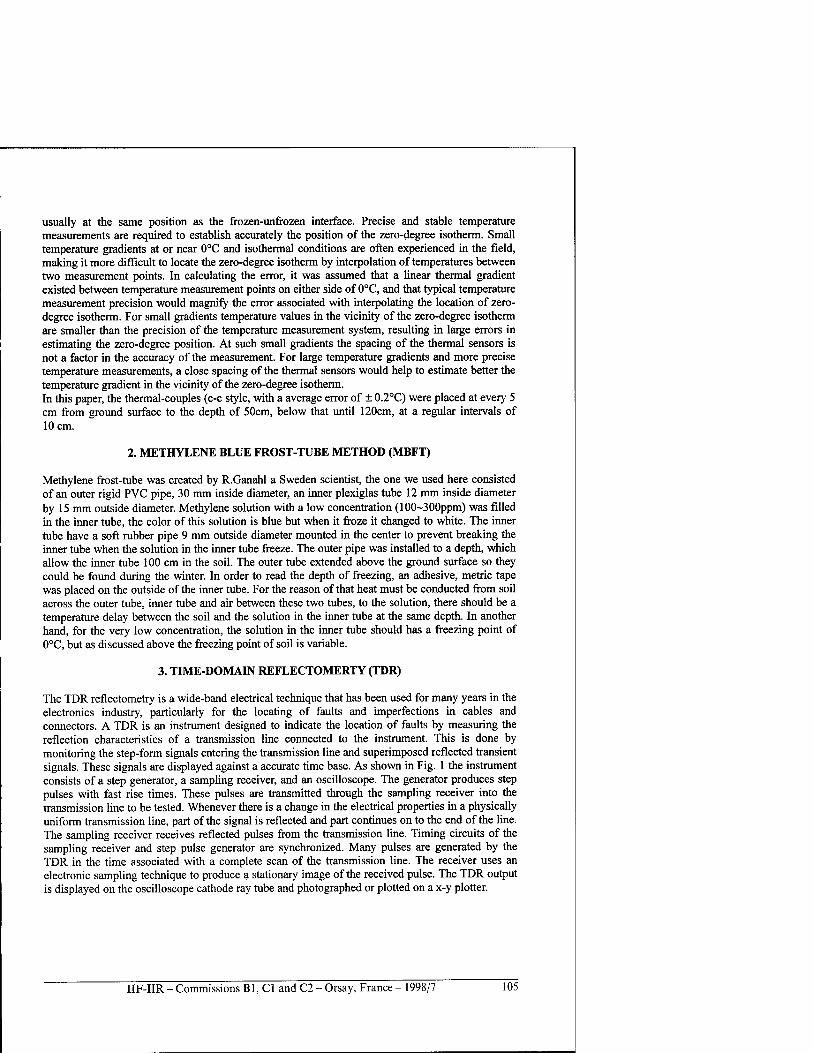
usually at the same position as the frozen-unfrozen interface. Precise and stable temperature measurements are required to establish accurately the position of the zero-degree isotherm. Small temperature gradients at or near 0°C and isothermal conditions are often experienced in the field, making it more difficult to locate the zero-degree isotherm by interpolation of temperatures between two measurement points. In calculating the error, it was assumed that a linear thermal gradient existed between temperature measurement points on either side of 0°C, and that typical temperature measurement precision would magnify the error associated with interpolating the location of zero- degree isotherm. For small gradients temperature values in the vicinity of the zero-degree isotherm are smaller than the precision of the temperature measurement system, resulting in large errors in estimating the zero-degree position. At such small gradients the spacing of the thermal sensors is not a factor in the accuracy of the measurement. For large temperature gradients and more precise temperature measurements, a close spacing of the thermal sensors would help to estimate better the temperature gradient in the vicinity of the zero-degree isotherm. In this paper, the thermal-couples (c-c style, with a average error of ± 0.2°C) were placed at every 5 cm from ground surface to the depth of 50cm, below that until 120cm, at a regular intervals of 10 cm.

2. METHYLENE BLUE FROST-TUBE METHOD (MBFT)

Methylene frost-tube was created by R.Ganahl a Sweden scientist, the one we used here consisted of an outer rigid PVC pipe, 30 mm inside diameter, an inner plexiglas tube 12 mm inside diameter by 15 mm outside diameter. Methylene solution with a low concentration (100~300ppm) was filled in the inner tube, the color of this solution is blue but when it froze it changed to white. The inner tube have a soft rubber pipe 9 mm outside diameter mounted in the center to prevent breaking the inner tube when the solution in the inner tube freeze. The outer pipe was installed to a depth, which allow the inner tube 100 cm in the soil. The outer tube extended above the ground surface so they could be found during the winter. In order to read the depth of freezing, an adhesive, metric tape was placed on the outside of the inner tube. For the reason ofthat heat must be conducted from soil across the outer tube, inner tube and air between these two tubes, to the solution, there should be a temperature delay between the soil and the solution in the inner tube at the same depth. In another hand, for the very low concentration, the solution in the inner tube should has a freezing point of 0°C, but as discussed above the freezing point of soil is variable.

3. TIME-DOMAIN REFLECTOMERTY (TDR)

The TDR reflectometry is a wide-band electrical technique that has been used for many years in the electronics industry, particularly for the locating of faults and imperfections in cables and connectors. A TDR is an instrument designed to indicate the location of faults by measuring the reflection characteristics of a transmission line connected to the instrument. This is done by monitoring the step-form signals entering the transmission line and superimposed reflected transient signals. These signals are displayed against a accurate time base. As shown in Fig. 1 the instrument consists of a step generator, a sampling receiver, and an oscilloscope. The generator produces step pulses with fast rise times. These pulses are transmitted through the sampling receiver into the transmission line to be tested. Whenever there is a change in the electrical properties in a physically uniform transmission line, part of the signal is reflected and part continues on to the end of the line. The sampling receiver receives reflected pulses from the transmission line. Timing circuits of the sampling receiver and step pulse generator are synchronized. Many pulses are generated by the TDR in the time associated with a complete scan of the transmission line. The receiver uses an electronic sampling technique to produce a stationary image of the received pulse. The TDR output is displayed on the oscilloscope cathode ray tube and photographed or plotted on a x-y plotter.


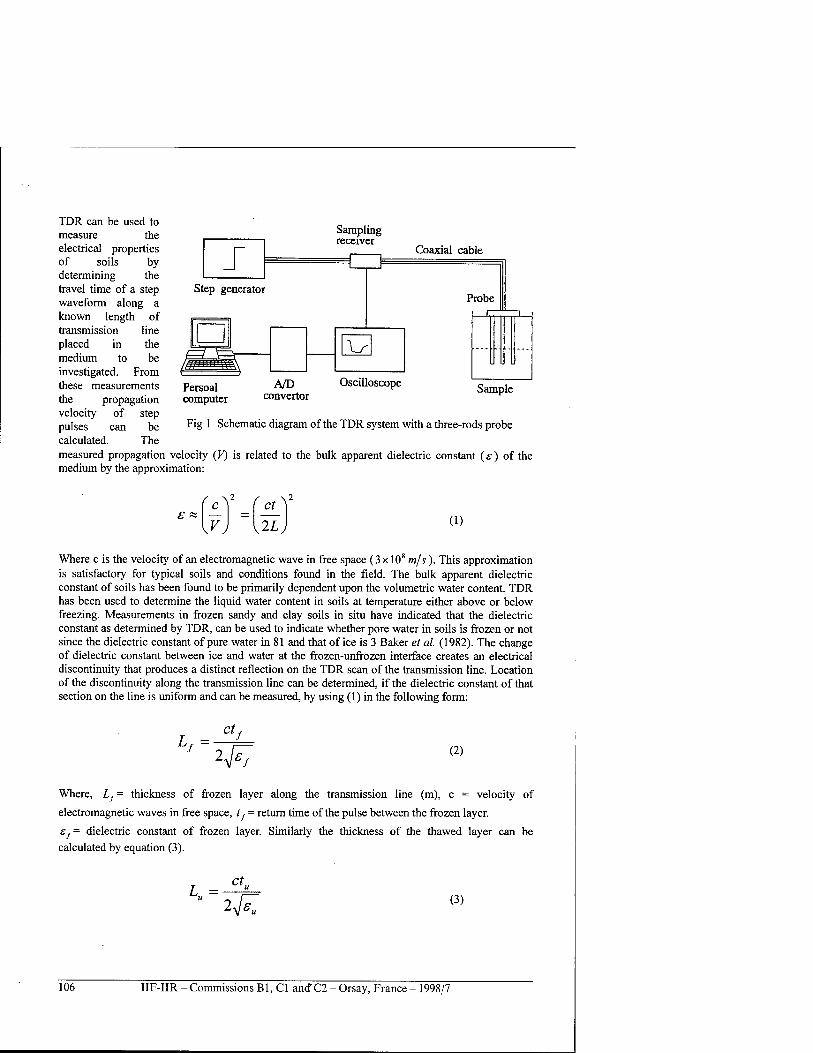
Sampling receiver

Coaxial cable

Probe

TDR can be used to measure the electrical properties of soils by determining the travel time of a step waveform along a known length of transmission line placed in the medium to be investigated. From these measurements the propagation velocity of step pulses can be calculated. The measured propagation velocity (V) is related to the bulk apparent dielectric constant (s) of the medium by the approximation:

Persoal computer

A/D converter

Oscilloscope Sample

Fig 1 Schematic diagram of the TDR system with a three-rods probe

'c>2

V J

ct

\2Lj (i)

Where c is the velocity of an electromagnetic wave in free space (3 x 108 m/s). This approximation is satisfactory for typical soils and conditions found in the field. The bulk apparent dielectric constant of soils has been found to be primarily dependent upon the volumetric water content. TDR has been used to determine the liquid water content in soils at temperature either above or below freezing. Measurements in frozen sandy and clay soils in situ have indicated that the dielectric constant as determined by TDR, can be used to indicate whether pore water in soils is frozen or not since the dielectric constant of pure water in 81 and that of ice is 3 Baker et al. (1982). The change of dielectric constant between ice and water at the frozen-unfrozen interface creates an electrical discontinuity that produces a distinct reflection on the TDR scan of the transmission line. Location of the discontinuity along the transmission line can be determined, if the dielectric constant of that section on the line is uniform and can be measured, by using (1) in the following form:

h = Ct.

2Je (2)

Where, Lf= thickness of frozen layer along the transmission line (m), c = velocity of

electromagnetic waves in free space, ts = return time of the pulse between the frozen layer.

Sj= dielectric constant of frozen layer. Similarly the thickness of the thawed layer can be calculated by equation (3).

L„ = ct,.

2^ (3)

106 IIF-IIR - Commissions Bl, Cl and"C2 - Orsay, France - 1998/7

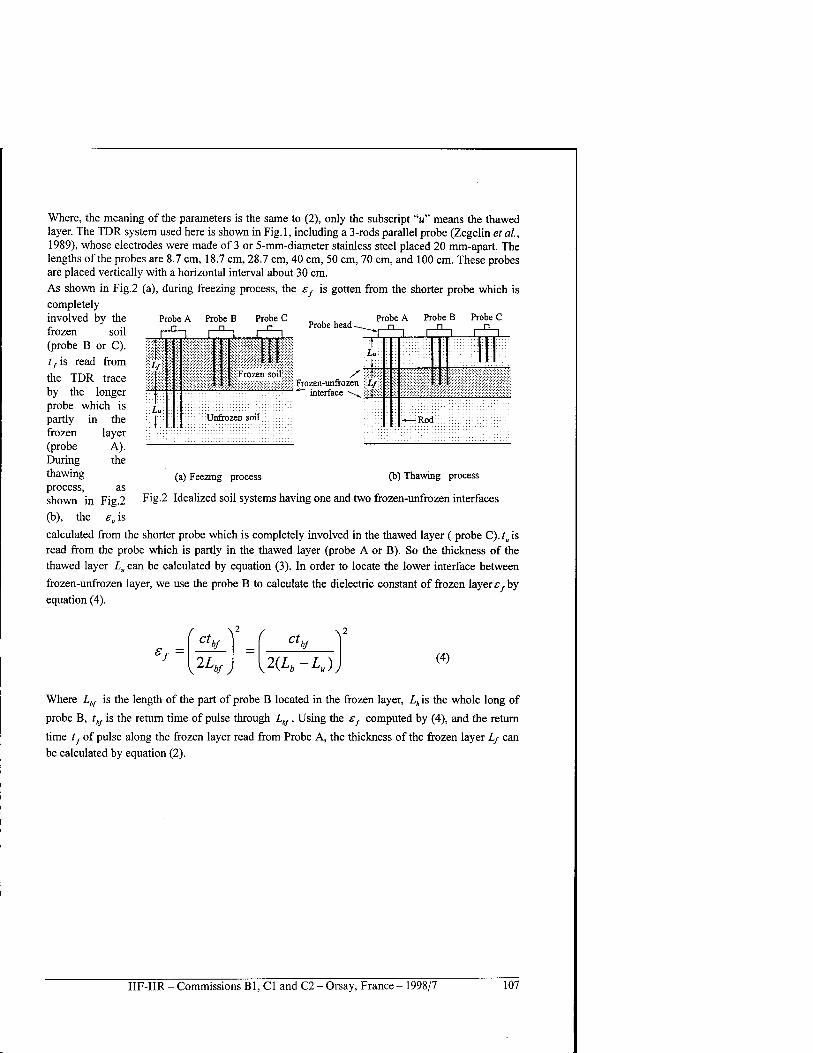
Where, the meaning of the parameters is the same to (2), only the subscript "u" means the thawed layer. The TDR system used here is shown in Fig.l, including a 3-rods parallel probe (Zegelin et al, 1989), whose electrodes were made of 3 or 5-mm-diameter stainless steel placed 20 mm-apart. The lengths of the probes are 8.7 cm, 18.7 cm, 28.7 cm, 40 cm, 50 cm, 70 cm, and 100 cm. These probes are placed vertically with a horizontal interval about 30 cm. As shown in Fig.2 (a), during freezing process, the ef is gotten from the shorter probe which is completely

Probe A Probe B Probe C , n , , n , , n ,

involved by the frozen soil (probe B or C). tfis read from the TDR trace by the longer probe which is partly in the frozen

Uri

layer A), the

as Fig.2 £„is

\\Frozen soil

Unfrozen soil

Probe A Probe B Pro Probe head — n n

be n

C

'1 1 1 1 1 1 t

La

zen-unfrozen Z,/:: :•. interface \^ :{:••■:

— Rod

(a) Feezing process (b) Thawing process

Fig.2 Idealized soil systems having one and two frozen-unfrozen interfaces

(probe During thawing process, shown in (b), the

calculated from the shorter probe which is completely involved in the thawed layer ( probe C). r„ is read from the probe which is partly in the thawed layer (probe A or B). So the thickness of the thawed layer Lu can be calculated by equation (3). In order to locate the lower interface between

frozen-unfrozen layer, we use the probe B to calculate the dielectric constant of frozen layer ef by equation (4).

£f =

Ct \

bf

2L v J

( ct bf

2(Lb-h). (4)

Where LbJ is the length of the part of probe B located in the frozen layer, Lh is the whole long of

probe B, thJ is the return time of pulse through LbJ. Using the sf computed by (4), and the return

time ts of pulse along the frozen layer read from Probe A, the thickness of the frozen layer Lj can be calculated by equation (2).


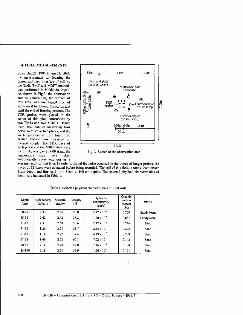
1.8m 4-Qm 12m

Plate and staff for frost heave

Ö..B

s--§ Ö

H Methylene blue

frost-tube

TDR _ _ probes _ _

H n—Thermocouple

_ for air temp.

4. FIELD MEASUREMENTS

Since Dec.21, 1994 to Apr.22, 1995, the measurement for locating the frozen-unfrozen interface of soil by the TDR, TMT and MBFT methods was performed in Hokkaido, Japan. As shown in Fig.3, the observation area is 7.0mx7.0m, the surface of this area was maintained free of snow on it by having the aid of tent until the end of freezing process. The TDR probes were placed in the center of this plot, surrounded by two TMTs and two MBFTs. Beside them, the units of measuring frost heave were set in two places, and the air temperature at 1.5m high from ground surface was measured by thermal couple. The TDR trace of each probe and the MBFT data were recorded every day at 9:00 A.m., the temperature data were taken automatically every one our as a average result ofthat hour. In order to dispel the noise occurred in the traces of longer probes, the traces of 32 times were averaged before being recorded. The soil of this field is sandy loam above 31cm depth, and fine sand from 31cm to 100 cm depths. The selected physical characteristics of them were indicated in Table 1.

Thermocouples for soil temp.

0.38m 0.46m Mil

2.4m

0.31m

773m

Fig. 3 Sketch of the observation area

Table 1 Selected physical characteristics of field soils

Depth (cm)

Bulk density (g/cm3)

Specific gravity

Porosity (%)

Hydraulic conductivity

(cm/s)

Organic carbon content

(%)

Texture

0-18 1.33 2.66 50.0 3.47 x 10"5 0.700 Sandy loam

18-31 1.62 2.62 38.2 1.60 xlO"6 0.631 Sandy loam

31-41 1.33 2.68 50.6 2.47 x 10^ 0.226 Sand

41-51 1.20 2.71 55.7 2.54 x 10~3 0.262 Sand

51-61 1.16 2.72 57.4 4.19 x 10"3 0.239 Sand

61-68 1.09 2.72 60.1 7.02 x 10~3 0.142 Sand

68-83 1.14 2.70 57.8 7.16 xlO"3 0.190 Sand

83-100 1.18 2.74 56.9 1.20 xlO"2 0.171 Sand


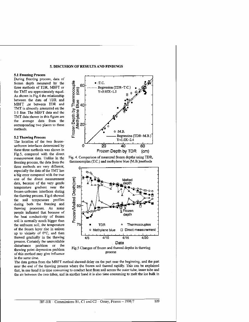
5. DISCUSION OF RESULTS AND FINDINGS

5.1 Freezing Process During freezing process, data of frozen depth measured by the three methods of TDR, MBFT or the TMT are approximately equal. As shown in Fig.4 the relationship between the data of TDR and MBFT ,or between TDR and TMT is almostly amounted on the 1:1 line. The MBFT data and the TMT data shown in this figure are the average data from the corresponding two places to these methods.

o :M.B. - Regression (TDR-M.B.)"

Y=1.0X-2.4

20 40 60 Frozen Depth by TDR (cm)

Fig. 4. Comparison of measured frozen depths using TDR, thermocouples (T.C.) and methylene blue (M.B.)methods

Or

£ /V*&„ Melted

5.2 Thawing Process The location of the two frozen- unfrozen interfaces determined by these three methods was shown in Fig.5, compared with the direct measurement data. Unlike in the freezing process, the data from the three methods are very different, especially the data of the TMT has a big error compared with the true one of the direct measurement data, because of the very gentle temperature gradient near the frozen-unfrozen interfaces during the thawing process. Fig.6 showed the soil temperature profiles during both the freezing and thawing processes. As some people indicated that because of the heat conductivity of frozen soil is normally much bigger than the unfrozen soil, the temperature of the frozen layer rise in unison up to vicinity of 0CC, and then thawed gradually in the thawing process. Certainly the unavoidable disturbance problem or the thawing point depression problem of this method may give influence in the same time. The data gotten from the MBFT method showed delay on the part near the beginning, and the part near the end of the thawing process where the frozen soil thawed rapidly. This can be explained that, in one hand it is time consuming to conduct heat from soil across the outer tube, inner tube and the air between the two tubes, and in another hand it is also time consuming to melt the ice bulk in

a <=n-

-rozen depth

■ TDR A Thermocouples o Methylene blue a Direct measurement

_L 4/5 4/10

J 1 I L. _1_ 4/20 4/15

. Date Fig.5 Changes of frozen and thawed depths in thawing

process


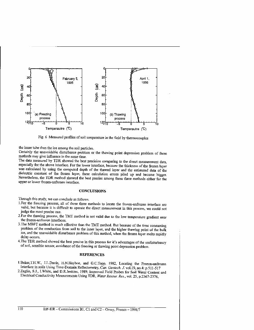
0

20

40

« 60

80h

a Q

February 5, 1995

100f '(a) Freezing process

120. -10 -5 0 5

Temperautre (°C)

10

i

20 April 1, ; 1995

§ 4° '

f 60 01 Q

i

80 V

100 (b) Thawing process

. . 1 . 1 . . . . -10 -5 0 ~ 5

Temperautre (°C)

10

Fig. 6 Measured profiles of soil temperature in the field by thermocouples

the inner tube than the ice among the soil particles. Certainly the unavoidable disturbance problem or the thawing point depression problem of these methods may give influence in the same time. The data measured by TDR showed the best precision comparing to the direct measurement data, especially for the above interface. For the lower interface, because the thickness of the frozen layer was calculated by using the computed depth of the thawed layer and the estimated data of the dielectric constant of the frozen layer, these calculation errors piled up and became bigger. Nevertheless, the TDR method showed the best precise among these three methods either for the upper or lower frozen-unfrozen interface.

CONCLUSIONS

Through this study, we can conclude as follows. l.For the freezing process, all of those three methods to locate the frozen-unfrozen interface are

valid, but because it is difficult to operate the direct measurement in this process, we could not judge the most precise one.

2.For the thawing process, the TMT method is not valid due to the low temperature gradient near the frozen-unfrozen interfaces.

3.The MBFT method is much effective than the TMT method. But because of the time consuming problem of the conduction from soil to the inner layer, and the higher thawing point of the bulk ice, and the unavoidable disturbance problem of this method, when the frozen layer melts rapidly delay occurs.

4.The TDR method showed the best precise in this process for it's advantages of the undisturbancy of soil, sensible sensor, avoidance of the freezing or thawing point depression problem.

REFERENCES

l.Baker,T.H.W., J.L.Davis, H.N.Hayboe, and G.C.Topp, 1982, Locating the Frozen-unfrozen Interface in soils Using Time-Domain Reflectometry, Can. Geotech. J. vol.19, no.4: p.511-517

2.Zegiin, S.J., I.White, and D.R.Jenkins, 1989, Improved Field Probes for Soil Water Content and Electrical Conductivity Measurements Using TDR, Water Resour. Res., vol. 25, p.2367-2376,


TROIS METHODES, DONT LA METHODE TDR, POUR MESURER LA PROFONDEUR A LAQUELLE LE SOL GELE OU DEGELE DANS LES CHAMPS

RESUME : Les profondeurs auxquelles le sol gele et degele doivent etre mesurees de maniere tres precise lorsque Ton s'interesse aux phenomenes de gel-degel. Dans ce papier, une technique utilisant un reflectometre (TDR) a ete utilisee pour mesurer ces profondeurs dans un champ de Lotin en Hokkaido. Les resultats obtenus ont ete compares ä ceux obtenus par les methodes conventionnelles basees sur l'utilisation du bleu de methylene (MBFT) ou de thermocouples (TMT). Les trois methodes donnent des resultats similaires en ce qui concerne le processus de gel. En revanche, la methode TMT n'est pas valide pour le processus de degel du fait d'un gradient de temperature tres faible aux environs de 0°C dans le sol. Des deux autres methodes, la methode TDR s'est revelee etre la plus precise pour l'etude du processus de degel.


THE EFFECT OF UNFROZEN WATER CONTENT ON DYNAMIC PROPERTIES

OF PARTIALLY FROZEN SOIL

*SHENGY., * FUKUDA M., **IMAMURA T. "Institute of Low Temperature Science, Hokkaido University, N19 W8 Kita-ku Sapporo 060 Japan ♦♦National Research Laboratory of Metrology, 1-1-4, Umezono, Tsukuba, Ibaraki 305-8563 Japan

ABSTRACT

Ultrasonic propagation velocities of both the dilatational and shear waves through water saturated frozen silt, and tire-mixed silt were measured under temperature condition of near subzero by means of sing-around method. Comparing the results with previously obtained data on unfrozen water content, a linear relations between velocities and unfrozen water content was performed with high coefficient value. Experimental results of two kinds of rather uniform materials, namely, glass-beads and silica micro-beads, testified the similar linear relations. In addition, the change rate of dilatational wave velocities with the change of volumetric unfrozen water content has tendency that this relation is not dependent on soil type. Although a rational theory of the ultrasonic velocities dependence to the unfrozen water content is not yet proposed, the presented empirical relationships may suggest not only the appropriate evaluation to the effect of unfrozen water on dynamic properties of frozen soil, but also a possible model as to estimate the unfrozen water content by means of high resolution velocity measurement such as the sing-around method.

INTRODUCTION

Dynamic properties of frozen soil are of important significance in cold regions engineering concerning with geophysical exploration for mineral, excavation by blasting, earthquake, vibrating machinery, and so on. Taking into the account of the advantage of being a quick, simple and non- destructive method, ultrasonic wave propagation has been employed to investigate the dynamic properties of frozen soil in both field work and laboratory test. Unlike other solid materials, such as metal and ice, in which ultrasonic velocity increases very slightly with descending temperature, the ultrasonic velocity in frozen soil performs a considerable change with temperature, especially at the vicinity of sub-zero. As a general explanation, this is considered to result from the change of unfrozen water amount in frozen soil, as well as ice content(Nakano,et.al,1972; Thimus, et.al,1991; Fukuda,1989). Many have made attempt to connect ultrasonic velocities with unfrozen water content by means of improving different models such as Timur's time distribution model, Wyllie's effective bulk moduli model (Deschatres,et.al,1988; Thimus,et.al,1991). Based on Biot's theory in porous media, Leclaire et.al. (1994) proposed an extension of wave propagation theory in frozen soil. A common point of the above models is that the dynamic properties of frozen soil are expressed as contributions of dynamic properties of constituents, namely soil particles, ice and unfrozen water, respectively in different ways. These studies have well developed our understandings to the role of unfrozen water amount in the dynamic properties of frozen soil. Simultaneously, they also induce a difficulty to determine dynamic parameters of soil particle which are usually unknown. As a simple and direct means, statistical method is available of evaluating the dynamic properties of frozen soil. The suggestion by Fukuda(1989) that dilatational wave velocity may be linearly related to unfrozen water content of frozen soil is one of the efforts. In the present paper, the authors developed Fukuda's model to both dilatational and shear waves, and proposed a limited range of the change rate of velocities with the change of volumetric


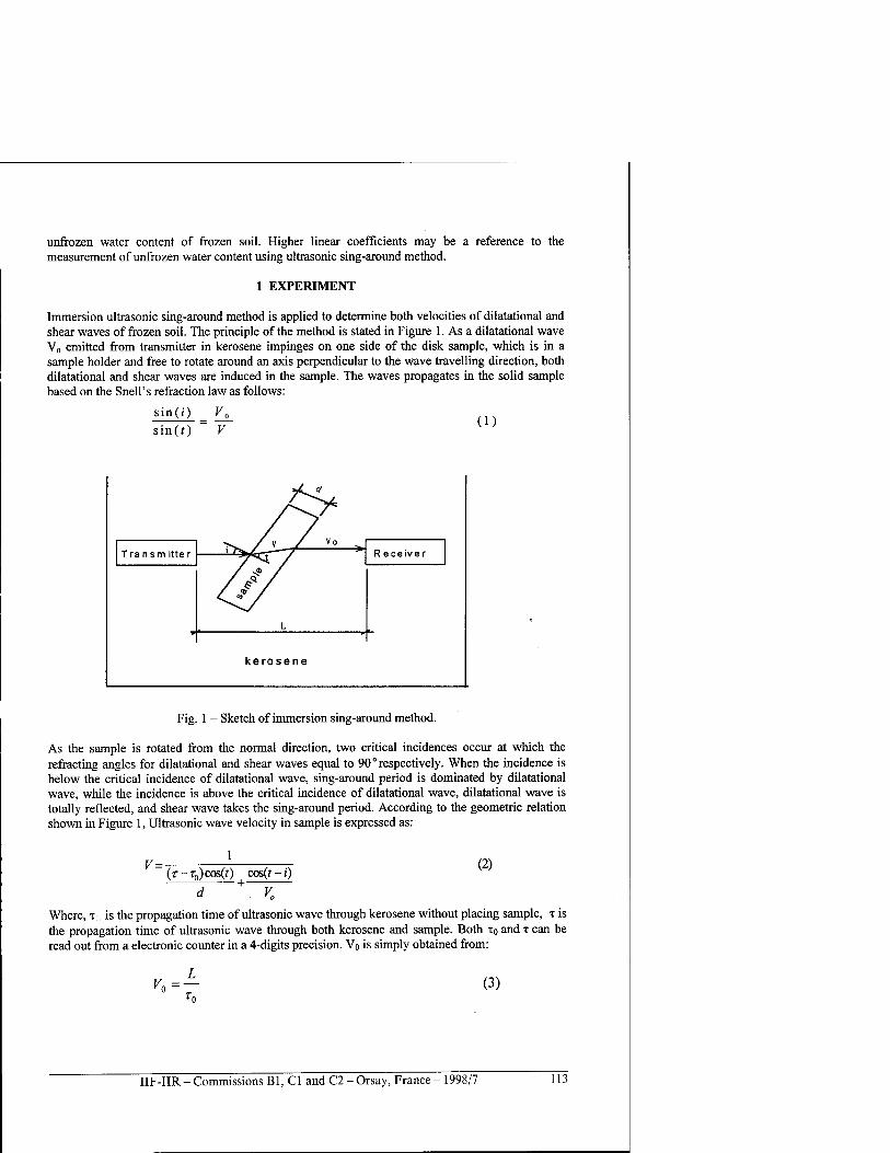
unfrozen water content of frozen soil. Higher linear coefficients may be a reference to the measurement of unfrozen water content using ultrasonic sing-around method.

1 EXPERIMENT

Immersion ultrasonic sing-around method is applied to determine both velocities of dilatational and shear waves of frozen soil. The principle of the method is stated in Figure 1. As a dilatational wave V0 emitted from transmitter in kerosene impinges on one side of the disk sample, which is in a sample holder and free to rotate around an axis perpendicular to the wave travelling direction, both dilatational and shear waves are induced in the sample. The waves propagates in the solid sample based on the SnelPs refraction law as follows:

sin(i) sin(0 V (1)

Tra nsm itter R e c e iv e r

kerosene

Fig. 1 - Sketch of immersion sing-around method.

As the sample is rotated from the normal direction, two critical incidences occur at which the refracting angles for dilatational and shear waves equal to 90"respectively. When the incidence is below the critical incidence of dilatational wave, sing-around period is dominated by dilatational wave, while the incidence is above the critical incidence of dilatational wave, dilatational wave is totally reflected, and shear wave takes the sing-around period. According to the geometric relation shown in Figure 1, Ultrasonic wave velocity in sample is expressed as:

1 (r-r0)cos(0 cos(f-0 (2)

Where, TC. is the propagation time of ultrasonic wave through kerosene without placing sample, T is the propagation time of ultrasonic wave through both kerosene and sample. Both to and T can be read out from a electronic counter in a 4-digits precision. Vo is simply obtained from:

L (3)


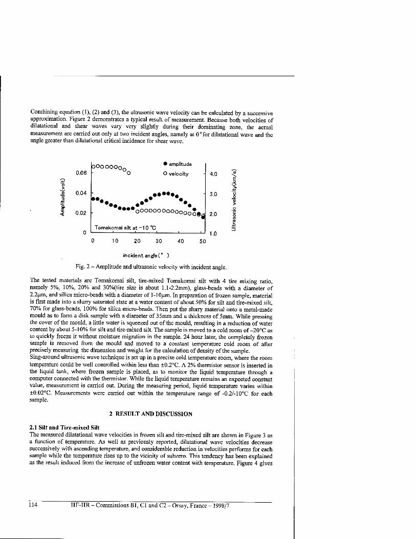
Combining equation (1), (2) and (3), the ultrasonic wave velocity can be calculated by a successive approximation. Figure 2 demonstrates a typical result of measurement. Because both velocities of dilatational and shear waves vary very slightly during their dominating zone, the actual measurement are carried out only at two incident angles, namely at 0°for dilatational wave and the angle greater than dilatational critical incidence for shear wave.

oooooo 0.06

4J

o

0.04 . 3

< 0.02

5°o, • amplitude

O velocity

'••••

.•••••«

ooooooooooooo Ofg

Tomakomai silt at -10 °C

4.0

3.0

2.0

1.0 10 20 30 40 50

incident angle(° )

Fig. 2 - Amplitude and ultrasonic velocity with incident angle.

The tested materials are Tomakomai silt, tire-mixed Tomakomai silt with 4 tire mixing ratio, namely 5%, 10%, 20% and 30%(tire size is about l.l-2.2mm), glass-beads with a diameter of 2.2um, and silica micro-beads with a diameter of 1-1 Oum. In preparation of frozen sample, material is first made into a slurry saturated state at a water content of about 50% for silt and tire-mixed silt, 70% for glass-beads, 100% for silica micro-beads. Then put the slurry material onto a metal-made mould as to form a disk sample with a diameter of 35mm and a thickness of 5mm. While pressing the cover of the mould, a little water is squeezed out of the mould, resulting in a reduction of water content by about 5-10% for silt and tire-mixed silt. The sample is moved to a cold room of-20°C as to quickly freeze it without moisture migration in the sample. 24 hour later, the completely frozen sample is removed from the mould and moved to a constant temperature cold room of after precisely measuring the dimension and weight for the calculation of density of the sample. Sing-around ultrasonic wave technique is set up in a precise cold temperature room, where the room temperature could be well controlled within less than ±0.2°C. A 2% thermistor sensor is inserted in the liquid tank, where frozen sample is placed, as to monitor the liquid temperature through a computer connected with the thermistor. While the liquid temperature remains an expected constant value, measurement is carried out. During the measuring period, liquid temperature varies within ±0.02°C. Measurements were carried out within the temperature range of -0.2/-10°C for each sample.

2 RESULT AND DISCUSSION

2.1 Silt and Tire-mixed Silt The measured dilatational wave velocities in frozen silt and tire-mixed silt are shown in Figure 3 as a function of temperature. As well as previously reported, dilatational wave velocities decrease successively with ascending temperature, and considerable reduction in velocities performs for each sample while the temperature rises up to the vicinity of subzero. This tendency has been explained as the result induced from the increase of unfrozen water content with temperature. Figure 4 gives


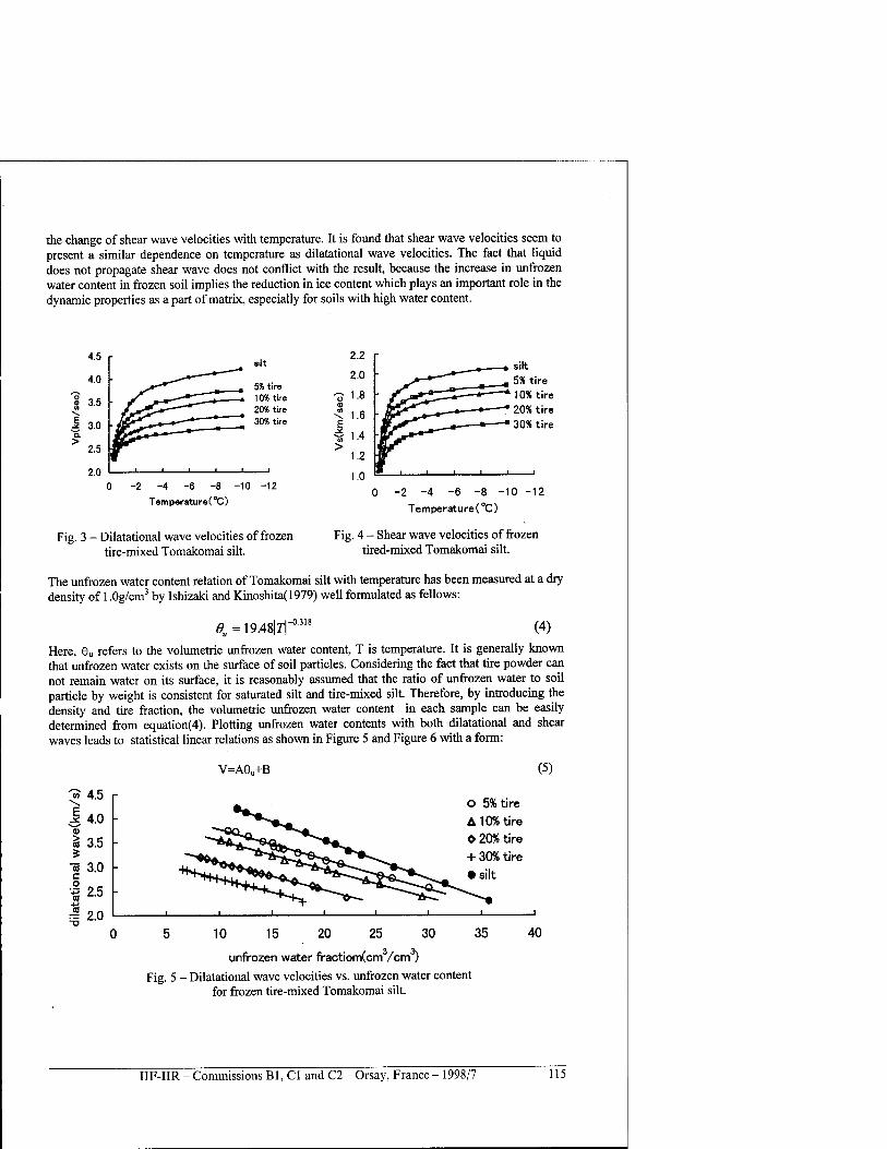
the change of shear wave velocities with temperature. It is found that shear wave velocities seem to present a similar dependence on temperature as dilatational wave velocities. The fact that liquid does not propagate shear wave does not conflict with the result, because the increase in unfrozen water content in frozen soil implies the reduction in ice content which plays an important role in the dynamic properties as a part of matrix, especially for soils with high water content.

4.5 silt

2.2

4.0 5* tire

2.0

8 35 10% tire 'S 1.8

1 3.0

2096 tire 30% tire < 1.6

E a. > 3M

2.5 > 1.2

2.0 , , , i ,

1.0 ( ) -2 -4 -6 -8 -10 -12

Temperature(°C) -2 -4 -6 -8 -10

Temperature(°C) -12

Fig. 3 - Dilatational wave velocities of frozen tire-mixed Tomakomai silt.

Fig. 4 - Shear wave velocities of frozen tired-mixed Tomakomai silt.

The unfrozen water content relation of Tomakomai silt with temperature has been measured at a dry density of 1.0g/cm3 by Ishizaki and Kinoshita(1979) well formulated as fellows:

0U = 19.48|7t (4)

Here, 9U refers to the volumetric unfrozen water content, T is temperature. It is generally known that unfrozen water exists on the surface of soil particles. Considering the fact that tire powder can not remain water on its surface, it is reasonably assumed that the ratio of unfrozen water to soil particle by weight is consistent for saturated silt and tire-mixed silt. Therefore, by introducing the density and tire fraction, the volumetric unfrozen water content in each sample can be easily determined from equation(4). Plotting unfrozen water contents with both dilatational and shear waves leads to statistical linear relations as shown in Figure 5 and Figure 6 with a form:

V=AGU+B (5)

-a 4.5 O 5% tire A 10% tire O 20% tire + 30% tire • silt

5 10 15 20 25 30

unfrozen water fractiom(cm /cm )

Fig. 5 - Dilatational wave velocities vs. unfrozen water content for frozen tire-mixed Tomakomai silt.


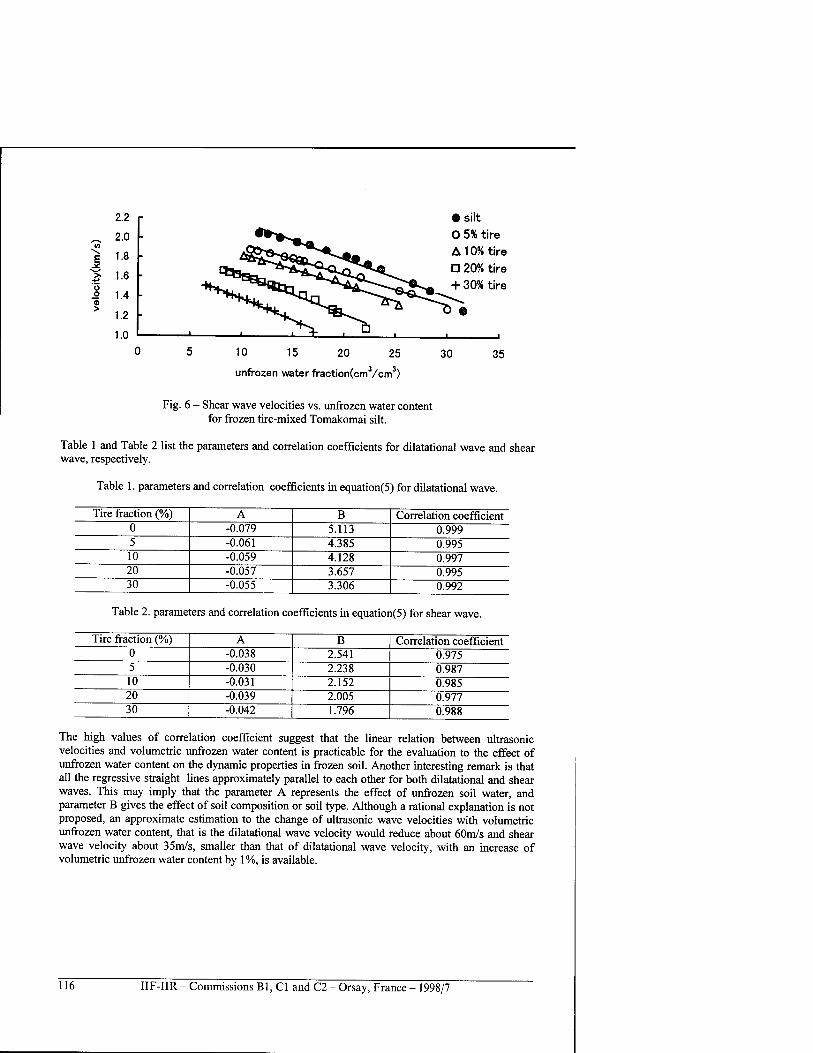
E

10 15 20 25

unfrozen water fraction(cm3/cm3)

• silt O 5% tire A 10% tire D 20% tire + 30% tire

30 35

Fig. 6 - Shear wave velocities vs. unfrozen water content for frozen tire-mixed Tomakomai silt.

Table 1 and Table 2 list the parameters and correlation coefficients for dilatational wave and shear wave, respectively.

Table 1. parameters and correlation coefficients in equation(5) for dilatational wave.

Tire fraction (%) A B Correlation coefficient 0 -0.079 5.113 0.999 5 -0.061 4.385 0.995 10 -0.059 4.128 0.997 20 -0.057 3.657 0.995 30 -0.055 3.306 0.992

Table 2. parameters and correlation coefficients in equation(5) for shear wave.

Tire fraction (%) A B Correlation coefficient 0 -0.038 2.541 0.975 5 -0.030 2.238 0.987 10 -0.031 2.152 0.985 20 -0.039 2.005 0.977 30 -0.042 1.796 0.988

The high values of correlation coefficient suggest that the linear relation between ultrasonic velocities and volumetric unfrozen water content is practicable for the evaluation to the effect of unfrozen water content on the dynamic properties in frozen soil. Another interesting remark is that all the regressive straight lines approximately parallel to each other for both dilatational and shear waves. This may imply that the parameter A represents the effect of unfrozen soil water, and parameter B gives the effect of soil composition or soil type. Although a rational explanation is not proposed, an approximate estimation to the change of ultrasonic wave velocities with volumetric unfrozen water content, that is the dilatational wave velocity would reduce about 60m/s and shear wave velocity about 35m/s, smaller than that of dilatational wave velocity, with an increase of volumetric unfrozen water content by 1%, is available.


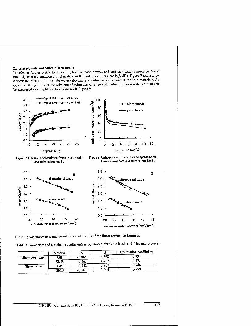
2.2 Glass-beads and Silica Micro-beads In order to further verify the tendency, both ultrasonic wave and unfrozen water content(by NMR method) tests are conducted in glass-beads(GB) and silica micro-beads(SMB). Figure 7 and Figure 8 show the results of ultrasonic wave velocities and unfrozen water content for both materials. As expected, the plotting of the relations of velocities with the volumetric unfrozen water content can be expressed as straight line too as shown in Figure 9.

4.0

3.5

3.0

E 2.5

1? 2.0 u o . | 1.5

1.0

0.5

-VpofGB ■

-Vpof SMB-

-VsofGB

-VsofSMB

-2 -4 -6 -8

Temperature(t)

-10 -12

Figure 7. Ultrasonic velocities in frozen glass-beads and silica micro-beads.

micro-beads

glass-be ads

0 -2 -4 -6 -8 -10 -12

temperature(°C)

Figure 8. Unfrozen water content vs. temperature in frozen glass-beads and silica micro-beads.

3.5 a

3.5 r b

3.0 *-#s-^ dilatational wave 3.0 ^^Qs_ dilatational wave

2.5

2.0 ^"^

(0

E 2.5

2.0 : ^

1.5 0"&^^ shear wave o <D >

1.5 ^"ÂSA shear wave

1.0

0.5 i i i i

1.0

0 5 i i i i 1

20 25 30 35 40 unfrozen water fraction(cm3/cm )

20 25 30 35 40 45

unfrozen water content(cm /cm )

Table 3 gives parameters and correlation coefficients of the linear regressive formulas.

Table 3. parameters and correlation coefficients in equation(5) for Glass-beads and silica micro-beads.

Material A B Correlation coefficient

Dilatational wave GB -0.065 4.568 0.997

SMB -0.063 4.482 0.975

Shear wave GB -0.052 2.857 0.948

SMB -0.061 3.044 0.979


It is found that the decreasing rates of dilatational wave velocity with the change in increasing volumetric unfrozen water content for both materials are similar to those for silt and tire-mixed silt, namely, about 60m/s. This may derive the conclusion that the effect of unfrozen water content on the dilatational wave velocity is not dependent on soil type. However, the decreasing rates of shear wave velocity exhibit values much greater than those of silt. A possible interpretation is that the behavior of the effect of unfrozen water content on the dynamic properties of frozen material might contribute to the role played by liquid water in dilatational wave and shear wave. On a view of wave propagation in porous media, the change of unfrozen water in frozen soil actually means changes in both porous liquid and solid matrix. The well sought relation for dilatational wave should be a comprehensive effect contributed by both water and ice. For a shear wave, the variation of velocity should be mainly governed by the change of solid matrix, namely ice in frozen material, while the unfrozen water may be less responsible for the shear wave velocity. Nevertheless, linear relations of both ultrasonic wave velocities with unfrozen water content with high correlation coefficient still suggest their utilizable point, that is to evaluate the dynamic properties of frozen soil under consideration of unfrozen water content and to develop a method to determine unfrozen water content of frozen soil by means of ultrasonic wave propagation, especially by the aid of dilatational wave velocity.

3 CONCLUSIONS

The present study experimented both dilatational and shear wave velocities in frozen soil with unfrozen water content by linear regressive relations with high correlation coefficients. Results suggest that the effect of unfrozen water content on the dilatational wave velocity may be evaluated by a decreasing rate of 60m/sec responding to a 1% increase of volumetric unfrozen water content without obviously depending on soil type. On the other hand, the change rate of shear wave velocity seems somewhat related to material type. Well established linear relations suggest the utilization in the evaluation to the dynamic properties of frozen soil considering the change of unfrozen water content, and determination of unfrozen water content by the aid of ultrasonic wave velocity.

ACKNOWLEDGEMENT

This experiment was conducted as the Joint Research Program of the Institute of Low Temperature Science. The authors wish to acknowledge Education Ministry of Japan for the financial fund and Japan Society for Promotion of Science for providing a chance of postdoctoral fellow to the first author, who came from State Key Laboratory of Frozen Soil Engineering, Lanzhou Institute of Glaciology and Geocryology, to engage in the research. Thanks also give to Dr. Kim, Dr. Muto and Mr. Hasekawa for their assistance in conducting experiments.

REFERENCES

1. Deschatres. M.H., Cohen-Tenoudji, F., Aguirre-Puente, J. and Khastou, B., 1988. Acoustics and unfrozen water content determination. In proceedings of the 5th International Conference on Permafrost. P324-328.

2. Fukuda, M., 1989. Measurement of ultrasonic velocity of frozen soil" near OD. Low Temperature Science. Ser.A 50, p83-86.

3. Ishizaki, T. and Kinoshita, S., 1979. Frost heave under overburden pressure. Low Temperature Science. Ser.A 38, pl69-178.

4. Leclaire, Ph., Cohen-Tenoudji, F. and Aguirre-Puente, J., 1994. Extension of Biot's theory of wave propagation to frozen porous media. J. Acoust. Soc. Am. 96(6), p3753-3768.

5. Nakano, Y., Martin III, R.J. and Smith, M., 1972. Ultrasonic velocities of the dilatational and shear waves in frozen soils. Water Resources Research. Vol.8, No.4. pl024-1030.


Thimus, J.Fr., Aguirre-Puente, J. and Cohen-Tenoudji. F., 1991. Determination of unfrozen water content of an overconsolidated clay down to -160° by sonic approaches -Comparison with classical method. In proceedings of the 6th International Symposium on Ground Freezing. P83-88.

EFFET D'UNE TENEUR EN EAU NON CONGELEE SUR LES PROPRIETES DYNAMIQUES D'UN SOL PARTIELLEMENT GELE

RESUME : Les vitesses de propagation ultrasonique des ondes de dilatation et de cisaillement, dans du Union gele sature en eau et dans du limon melange ä du caoutchouc, ont ete mesurees ä des temperatures proches du zero absolu par la methode dite "sing-around method" (methode de propagation ultrasonique dans un echantillon tournant en immersion). En comparant les resultats avec des donnees obtenues precedemment sur la teneur en eau non congelee, une relation lineaire entre vitesses et teneur en eau non congelee a ete obtenue avec une valeur de coefficient eleve. Des resultats experimentaux obtenus sur deux types de materiaux plutöt uniformes, ä savoir des perles de verre et des micro-billes de silice, ont confirme ces relations lineaires. En outre, la proportion de changement des vitesses des ondes de dilatation en fonction du changement de la teneur en eau non congelee volumetrique tend ä montrer que cette relation ne depend pas du type de sol. Bien qu'une theorie rationnelle concernant la dependance des vitesses ultrasoniques ä la teneur en eau non congelee ne soit pas encore proposee, les relations empiriques presentees pourraient suggerer non seulement 1'evaluation appropriee de l'effet de l'eau non congelee sur les proprietes dynamiques du sol gele, mais aussi un modele possible pour estimer la teneur en eau non congelee au moyen d'une mesure de la vitesse de haute resolution, teile que la "sing-around method".


ON THE ACOUSTIC TESTING OF SALINE FROZEN SOILS STRENGTH CHARACTERISTICS

*CHERVINSKAYA O.P., **FROLOV A.D., ***ZYKOV Y.D. ♦Research Institute of Engineering for Construction,

Okrushnoi passage 18, Moscow 105058, Russia. ♦♦Consolidated Scientific Counsil on Earth Cryology RAS,

Fersmann street 11, Moscow 117289, Russia, Fax: (095) 258-2463, E-mail: [email protected] ♦♦♦Geological Faculty, Moscow State University,

Vorobjovy Gory, Moscow 119899, Russia.

ABSTRACT

The results of joint laboratory studies on acoustic and strength properties of soils with various plasticity indexes saturated with solutions of different concentrations and ionic compositions at the temperatures from 0 to -20°C are presented and discussed in this paper. Using the experimental data we are established the sufficiently reliable correlations between compression wave velocities and cohesion parameter which give a practical possibility to apply an acoustic techniques for testing the strength of saline frozen soils. There was studied the impact of pore saturating solutions ionic composition on elastic wave velocities for sulfate, hydrocarbonate, chloride salinity and their mixtures in various proportions. Some corresponding features firstly obtained are presented and discussed also.

INTRODUCTION

From the basic concepts of physical-chemical mechanics (Rebinder,1979) it was shown that elastic, strength and other properties of frozen soils are chiefly controlled (Frolov,1976) by their peculiar spatial cryogenic crystalline-coagulant structure (SCCS). Saline frozen soils differ from nonsaline ones by lower temperature of phase transformations of pore solution and by higher contents of unfrozen liquid phase, which is usually distributed as semi- discrete accumulations in inter-grain zones, with an energy state undergoes changes. The ice matrix in saline frozen soils appears also essentially different: it comprises fine-crystalline saline ice consisted of doped crystals and contained inclusions of liquid phase (brine). These special features depend on many physics-chemical, structural, morphological and other factors (Frolov and Seguin, 1993; Frolov et al, 1998) which controls adsorptivity and are ultimately reflected in changes of strength and elasticity characteristics of the media under consideration. Two essentially different cases may occur if SCCS is formed in frozen soils with different initial concentration of saturating pore solution (Cps). In the first case (under low Cps) the soil mineral matrix is of dominant importance. This variant may be considered typical for nonsaline soils. In the second case all the properties of soil are greatly influenced by a considerably higher content of liquid phase (which depends on ionic composition and Cps) and the presence of saline ice. As a result, the soil mechanic properties, including a response to an external load applied, changes considerably. Such soils should be considered saline. It is reasonable that there must be some critical concentration (Ccr) which corresponds to a boundary state between these two cases. Such critical concentration of pore solution for various sandy-clayey soils must depends, first of all, on the soil lithology, as well as on pore solution ionic composition or on the type of frozen soils salinity: marine or continental. That is the reason why mechanical properties of saline frozen sands and clays call for special studies.

120 IIF-IIR-Commissions B1,C1 and C2-Orsay, France- 1998/7

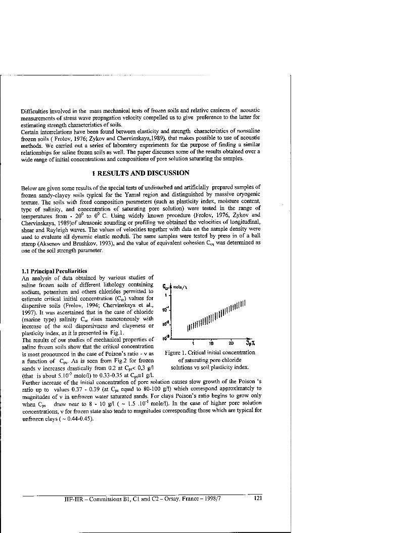
Difficulties involved in the mass mechanical tests of frozen soils and relative easiness of acoustic measurements of stress wave propagation velocity compelled us to give preference to the latter for estimating strength characteristics of soils. Certain interrelations have been found between elasticity and strength characteristics of nonsaline frozen soils ( Frolov, 1976; Zykov and Chervinskaya,1989), that makes possible to use of acoustic methods. We carried out a series of laboratory experiments for the purpose of finding a similar relationships for saline frozen soils as well. The paper discusses some of the results obtained over a wide range of initial concentrations and compositions of pore solution saturating the samples.

1 RESULTS AND DISCUSSION

Below are given some results of the special tests of undisturbed and artificially prepared samples of frozen sandy-clayey soils typical for the Yamal region and distinguished by massive cryogenic texture. The soils with fixed composition parameters (such as plasticity index, moisture content, type of salinity, and concentration of saturating pore solution) were tested in the range of temperatures from - 20° to 0° C. Using widely known procedure (Frolov, 1976, Zykov and Chervinskaya, 1989)of ultrasonic sounding or profiling we obtained the velocities of longitudinal, shear and Rayleigh waves. The values of velocities together with data on the sample density were used to evaluate all dynamic elastic moduli. The same samples were tested by press in of a ball stamp (Aksenov and Brushkov, 1993), and the value of equivalent cohesion Ceq was determined as one of the soil strength parameter.

Cw i mole/i

1

io-

10*

10'

1.1 Principal Peculiarities An analysis of data obtained by various studies of saline frozen soils of different lithology containing sodium, potassium and others chlorides permitted to estimate critical initial concentration (Ccr) values for dispersive soils (Frolov, 1994; Chervinskaya et al., 1997). It was ascertained that in the case of chloride (marine type) salinity Ccr rises monotonously with increase of the soil dispersivness and clayeness or plasticity index, as it is presented in Fig.l. The results of our studies of mechanical properties of saline frozen soils show that the critical concentration is most pronounced in the case of Poison's ratio - v as a function of Cps. As is seen from Fig.2 for frozen sands v increases drastically from 0.2 at Cps< 0,3 g/1 (that is about 5.10"3 mole/1) to 0.33-0.35 at Cpssl g/1. Further increase of the initial concentration of pore solution causes slow growth of the Poison 's ratio up to values 0.37 - 0.39 (at Cps equal to 80-100 g/1) which correspond approximately to magnitudes of v in unfrozen water saturated sands. For clays Poison's ratio begins to grow only when Cps draw near to 8 - 10 g/1 ( ~ 1.5 .10"1 mole/1). In the case of higher pore solution concentrations, v for frozen state also tends to magnitudes corresponding those which are typical for unfrozen clays ( ~ 0.44-0.45).

i 10 20 DPX

Figure 1. Critical initial concentration of saturating pore chloride

solutions vs soil plasticity index.


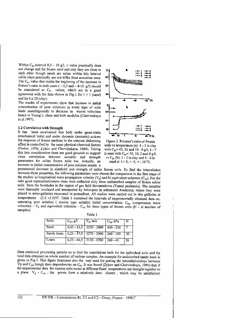
Within CpS interval 0,5-10 g/1, v value practically does not change and for frozen sand and clay they are close to each other though sands are saline within this interval while clays practically are not differ from nonsaline ones. The Cps value that marks the beginning of the increase in Poison's ratio in both cases ( ~ 0,3 and ~ 8-10 g/1) should be considered as Ccr values, which are in a good agreement with the data shown in Fig.l for I < 1 (sand) and for I = 20 (clay). The results of experiments show that increase in initial concentration of pore solutions in every type of soils leads unambiguously to decrease in waves velocities hence in Young's, shear and bulk modulus (Chervinskaya et al. 1997).

u v

V

■»i

m

v

-M «

vt

«H II tit* t VI

Figure 2. Poisson's ratio of frozen soils vs temperature (a): 1 - 3 is clay with Cps= 45, 30 and 10 - 0 g/1, 4 - 7 is sand with Cps= 30,10, 2 and 0 g/1; vs Cps (b): 1 - 3 is clay and 4 - 6 is

sand at t>0, = -5, = - 10 °C.

1.2 Correlation with Strength It has been ascertained that both under quasi-static (mechanical tests) and under dynamic (acoustic) actions the response of frozen medium to the external deforming affect is controlled by the same physical-chemical factors (Frolov, 1976; Zykov and Chervinskaya, 1989). Taking this into consideration there are good grounds to suggest close correlation between acoustic and strength parameters for saline frozen soils too. Actually, an increase in initial concentration of pore solution results a pronounced decrease in elasticity and strength of saline frozen soils. To find the interrelation between these properties, the following parameters were chosen for comparison in the first stage of the studies: a) longitudinal wave propagation velocity (Vp) and b) equivalent cohesion (Ceq). For the sake good representativeness there were collected sixty three undisturbed samples of frozen saline soils from the boreholes in the region of gas field Bovanenkovo (Yamal peninsula). The samples were thermally insulated and transported by helicopter in settlement Amderma, where they were placed in mine-galleries excavated in permafrost. All studies were carried out in this galleries at temperatures -(2.2 -=-3.5)°C. Table 1 contained the intervals of experimentally obtained data on: saturating pore solution ( marine type salinity) initial concentration- Cps, compression wave velocities - Vp and equivalent cohesion - Ceq for three types of frozen soils (N - is number of samples).

Table 1

Soils Cps, g/1 Vp, m/s Lêq, Ki 3. N

Sand 0,45 - 13,5 3550 - 2460 400-150 7

Sandy loam 0,25 - 17,0 3270 - 2090 240 -100 30

Loam 0,35 - 44,5 3130-1700 260 - 45 26

Data statistical processing permits us to find the correlations both for the individual soils and for total data obtained on whole number of various samples. An example for undisturbed sandy loam is given in Fig.3. This figure illustrates also the way used for getting the interrelationships between Vp and Ceq trough their dependencies on Cps. It was found (Zykov and Chervinskaya, 1995) that if the experimental data for various soils tested at different fixed temperatures are brought together to a plane Vp - Ceq , the points form a relatively dens cluster , which may be satisfactory


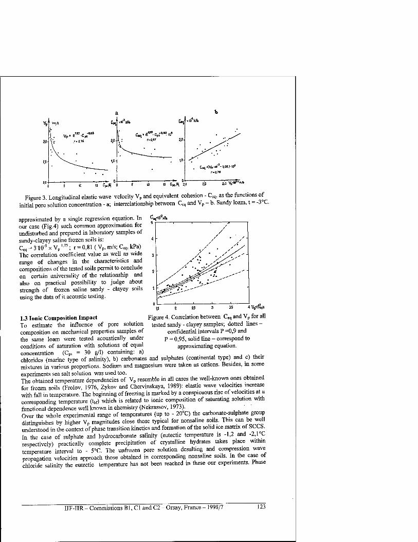
" .10*11

Cai-tV,-» -1.06)-10s

r.0.7«

15 Cw,?i 2,0 2.5 j,0 T^«-1»**

Figure 3. Longitudinal elastic wave velocity Vp and equivalent cohesion - Ceq, as the functions of itial pore solution concentration - a; interrelationship between Ceq and Vp - b. Sandy loam, t = -3°C initial pore

approximated by a single regression equation. In our case (Fig.4) such common approximation for undisturbed and prepared in laboratory samples of sandy-clayey saline frozen soils is: Ceq = 3T0"5 x Vp ''

75; r = 0,81 (Vp, m/s; Ceq, kPa) The correlation coefficient value as well as wide range of changes in the characteristics and compositions of the tested soils permit to conclude on certain universality of the relationship and also on practical possibility to judge about strength of frozen saline sandy - clayey soils using the data of it acoustic testing.

4 tyoiws

Figure 4. Correlation between Ceq and Vp for all tested sandy - clayey samples; dotted lines -

confidential intervals P =0,9 and P = 0,95, solid line - correspond to

approximating equation.

1.3 Ionic Composition Impact To estimate the influence of pore solution composition on mechanical properties samples of the same loam were tested acoustically under conditions of saturation with solutions of equal concentration (Cps = 30 g/1) containing: a) . chlorides (marine type of salinity), b) carbonates and sulphates (continental type) and c) their mixtures in various proportions. Sodium and magnesium were taken as cations. Besides, in some experiments sea salt solution was used too. . The obtained temperature dependencies of Vp resemble in all cases the well-known ones obtained for frozen soils (Frolov, 1976, Zykov and Chervinskaya, 1989): elastic wave velocities mcrease with fall in temperature. The beginning of freezing is marked by a conspicuous rise of velocities at a corresponding temperature (tbf) which is related to ionic composition of saturating solution with functional dependence well known in chemistry (Nekrassov, 1973). ' Over the whole experimental range of temperatures (up to - 20°C) the carbonate-sulphate group distinguishes by higher Vp magnitudes close those typical for nonsaline soils. This can be well understood in the context of phase transition kinetics and formation of the solid ice matrix of bCC5>. In the case of sulphate and hydrocarbonate salinity (eutectic temperature is -1,2 and -2,1 °C respectively) practically complete precipitation of crystalline hydrates takes place within temperature interval to - 5°C. The unfrozen pore solution desalting and compression wave propagation velocities approach those obtained in corresponding nonsaline soils. In the case of chloride salinity the eutectic temperature has not been reached in these our experiments. Phase


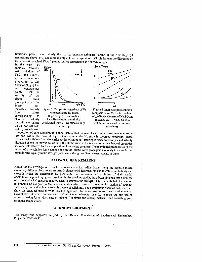
soil linearly values

Tip» ICf3 try's

2 "

transitions proceed more slowly then in the sulphate-carbonate group at the first stage (at temperature above -5°C) and more rapidly at lower temperatures. All this features are illustrated by the schematic graph of dVp/dt° plotted versus temperature as it shown in fig.5. In the case of samples saturated with solutions of NaCl and Na2S04

mixtures in various proportions it was obtained (Fig.6) that at temperatures below - 5°C the velocity of the elastic wave propagation at the frozen increases from corresponding to chloride salinity towards the values typical for sulphate and hydrocarbonate

20t*C

Figure 5. Temperature gradient of VP

vs temperature for loam. (Cps= 30 g/1). 1 - nonsaline,

2 - sulfate-carbonate salinity - continental type, 3 - chloride salinity -

marine type.

0 0.5

Figure 6. Impact of pore solution composition on Vp for frozen loam (Cps=30g/1). Content of Na2S04 in

mixed (NaCl + Na2S04) pore solutions presented in portions

(abscissa).

composition of pore solutions. It is quite natural that the rate of increase at lower temperatures is less and within the area of higher temperatures the Vp growth becomes nonlinear. These characteristics follow from the particularities of saline soil freezing kinetics for two types of salinity discussed above. In thawed saline soils the elastic wave velocities and other mechanical properties are very little affected by the composition of saturating solutions. The mentioned peculiarities of the impact of pore solution ionic composition on the elastic wave propagation velocity in saline frozen grounds refer equally to the strength parameters, though no direct measurements of there.

2 CONCLUDING REMARKS

Results of the investigations enable us to conclude that saline frozen soils are specific media essentially different from nonsaline ones in character of deformability and therefore in elasticity and strength which are determined by peculiarities of formation and evolution of their spatial crystalline-coagulant cryogenic structure. In the previous studies have been obtained that a number of various physical methods may be used to estimate the strength of frozen soils but the leading role should be assigned to the acoustic studies which permit to realize this testing of strength sufficiently fast and with a reasonable degree of reliability. The correlations obtained and discussed show the practical possibility to use this approach for saline frozen soils and similar media. Nevertheless, it seems necessary to continue the experiments in order to make the best use of acoustic testing for a wide range of mineral ( or tissue and others) matrices and saturating pore solutions compositions.

ACKNOWLEDGEMENT

This study was supported in part by the Russian Foundation of Fundamental Researches Project Ks 97-05-64961.


REFERENCES

1. Aksenov V.l. and Bruskov A.V., 1993, Plastic frozen (saline) soil as bases. Proceedings 6,k

International Conference on Permafrost, Beijing, China. South China University of Technology Press, Wushan, Guangzhou, China, p. 1-4.

2. Chervinskaya O.P., Zykov Yu.D. and Frolov A.D., 1997, The effect of pore solution concentration and composition upon the electric and elastic properties of frozen saline soils. Proceedings of the international symposium on physics, chemistry and ecology of seasonally frozen soils. Fairbanks, Alaska, CRREL spec. rep. 97-10, p.133-139.

3. Frolov A.D., 1976, Electric and elastic properties of cryogenic rocks. Nedra Press, Moscow , 254p.

4. Frolov A.D. and Seguin M.K., 1993, Caracteristiques de la cinetique de congelation des sol salins. Permafrost and Pereglacial Processes, 4, p.311-325.

5. Frolov A.D., 1994, Principal phase changes in saline frozen soils, Intern. Mech. Eng. Congress and Exhibition, Chicago, Illinois, Preprint, 8p.

6. Frolov A.D., Fedyukin I.V., Zykov Yu.D., 1998, Main characteristics of saline frozen soils. Paper of this meeting.

7. Nekrassov B. V., 1973, The principles of General Chemistry, Khimia Press, Moscow, 656 p. 8. Rebinder P.A., 1979, Selected works. Physics-Chemical mechanics, Nauka Press, Moscow,

381p. 9. Zykov Yu.D. and Chervinskaya O.P., 1989, Acoustic properties of icy soils and ice, Nauka

Press, Moscow, 132 p. 10. Zykov Yu.D. and Chervinskaya O.P., 1995, Deformation and strength properties evaluation by

acoustic method. In Frolov A.D. (ed-r.), Geophysical Investigations of Cryolithozone, Transactions, issue 1, ONTI PSC RAS Press, Moscow, p. 12-22.

11. Zykov Yu.D., Chervinskaya O.P. and Krasovsky A.G., 1996, The connection of geophysical parameters with salinity features of the frozen soils. In Frolov A.D. (ed-r), Geophysical Investigation of Cryolithozone, Transactions, issue 2, ONTI PAS RAS Press, Moscow, p. 108- 114.

METHODE ACOUSTIQUE DE L'ESTIMATION DE LA SOLIDITE DES SOLS SALINS GELES

RESUME : Dans cet article on donne et discute les resultats des etudes, menees conjointement, des parametres de solidite et des parametres acoustiques des sols, avec des nombres de plasticite divers, les milieux etant satures par des solutions de compositions et de concentrations differentes dans l'intervalle de temperature de 0 ä -20°C. L'analyse statistique des donnees experimentales a permis d'etablir des liaisons assez süres entre la vitesse des ondes de compression et les parametres de cohesion du sol gele, ce qui peut devenir la base physique de l'application de la methode acoustique de l'estimation de la solidite des sols salins geles. Les premieres experiences visant ä etudier l'influence de la composition des solutions saturantes sur la vitesse de la propagation des ondes de compression ont ete realisees. Les resultats obtenus, tenant compte des relations mentionnees plus haut, peuvent etre appliques aux parametres de la solidite de ces sols.


STUDY OF THE BEHAVIOUR OF A SNOW LAYER DEPOSITED ON THE PAVEMENT : PHYSICAL CHARACTERIZATION OF THE

SNOW/PAVEMENT INTERFACE

BOREL S., BRZOSKA J.B. Laboratoire des Materiaux et Structures du Genie Civil,

2 allee Kepler, 77 420 Champs sur Marne, France

ABSTRACT

This study is part of the French project called GELCRO''2,3 the aim of which is to develop a model enabling forecasting of the condition of a road surface before snow falls and monitoring of evolution following snowfall. The model is called GELCRO and is fruit of the linkage of two one- dimensional numerical models. In order to perform this study, an experimental site was selected. Snowfalls and highly changeable weather were the characteristics determining this selection. The site is equipped with six experimental sections of road representing widely used surfaces in France. Various probes are inserted in these sections. Manual measurements are made during or just after a snowfall and snow/road composite samples are taken. In order to preserve the snow microstructure on the section during sampling, pores are filled with diethyl phtalate (melting point -5°C) and the sample is refrozen. An original technique has been developed in a cold laboratory (-20°C) and enables the observation of the snow/pavement interfaces. This technique involves dry-cutting of the snow and the road simultaneously in order to obtain a vertical cross section. When examined under a microscope, the links between the snow and the road surface can be seen. The images of the interface obtained in this way will then be used in a two-dimensional code for steady-state thermal calculations, thus making it possible to calculate the thermal conductivity of the interface. The parameters of this thermal conductivity are then determined with respect to the characteristics of snow and pavement and then incorporated in the GELCRO model. Direct observation of snow/pavement interface at a microscopic level will enable the development of a realistic model of thermal bridge and capillary effects at the interface.

1. Laboratoire des Matenaux et Structures du Genie Civil (Civil Engineering Materials and Structures Laboratory) (LCPC, CNRS), Champs sur Marne, France

2. Meteo France, Centre d'Etude de la Neige (Snow Research Centre), Grenoble, France 3. Laboratoire Regional des Ponts et Chaussees (Regional Laboratory of Bridge and Road Engineering), Nancy,

France

INTRODUCTION

The goal of the French project GELCRO is to develop a model which will allow us to forecast the surface state of the road before a snowfall and the evolution of a snow layer deposited on the pavement. This system will improve efficiency of road winter maintenance service. The model named Gelcro is built from two one-dimensional coupled numerical models : ■ Crocus, Brun (1989), is a physically based model originally developed for operational avalanche

risk forecasting. It simulates snow cover evolution, ■ Gel 1D, Fremond (1979), calculates frost propagation in the pavement. Physical properties of the interface between snow and pavement have to be determined and introduced into the model.


For this study, an experimental site was chosen owing to its important snowfall frequency and the variety of meteorological situations. This site is equipped with six experimental pavements representative of present French building techniques. These pavements are fitted out with different sensors (snow height and temperatures sensors, video cameras) which allow us to observe pavement snowing up and to characterize snow evolution for different weather conditions. This site is also equipped with a complete weather station including specific snow cover measurements. So a data base is built to determine snow/road interface properties and to validate the model Gelcro.

1. FIELD EXPERIMENTS

Standard manual measurements are performed after each snowfall. They consist in measuring snow height on each pavement and snow density, describing the snow layer and sampling some grains preserved in isooctane (melting point -107°C). For the study of snow/road in cold laboratory, composite samples are taken on the field. One of the six experimental pavements is made of detachable samples of pavement. We describe here the procedure of sampling. We have to be very careful in order not to alter the interface. a) We take a core sample of snow on the pavement. b) We remove snow around the PVC core sampler. c) A thick cold (-40°C) copper cylinder is introduced around the PVC sampler to prevent liquid

phtalate leakage (an ice seal is made by pouring 0°C water with a syringe at the base of the cylinder).

d) Supercooled diethyl-phtalate at -10°C (melting point -5°C) is poured between the two core samplers in order to fill pore space of the snow. We freeze the whole with dry ice (solid C02). This provide a solid material ready for further cutting, Perla (1982).

e) The composite sample is taken from the field and then brought to the cold laboratory for thorough analysis.

2. METHODOLOGY IN COLD ROOM

Images of snow grains silhouette are recorded under transmitted light. Geometric characteristics are computed with a grains recognition program developed at CEN, Lesaffre (1997). Gelcro model will need this data for snow/road interface parametrization.

2.1 Snow/pavement section plane making To observe interfaces in composite snow/pavement samples, an original technique has been designed in cold laboratory. It allows to dry cut simultaneously snow and pavement providing a vertical section without local snow melt. We proceed in three stages. a) First we dry-cut the sample from the snow to pavement with a machine developed for this

experiment in cold room at -20°C. This machine is made up of: • a disk grinder monted on a stone frame and equipped with a diamond disk designed for asphalt

dry-cutting; • a XY displacement device to move the sample during cutting ; • a vice on the XY displacement device to fasten sample. The disk must always be carefully brushed during the cut by an operator. If the disk gets dirty, the heat produced by the friction could rapidly destroy the sample. At this stage the surface of the section is rough and contrast between ice and phtalate is not sufficient to observe ice-substrate bond structure. b) At this stage we enhance contrast using a technique adapted from CRREL's etch method.

Specimen is allowed to sublimate for 24-36 hours in cold room at -10°C. It results in small pits


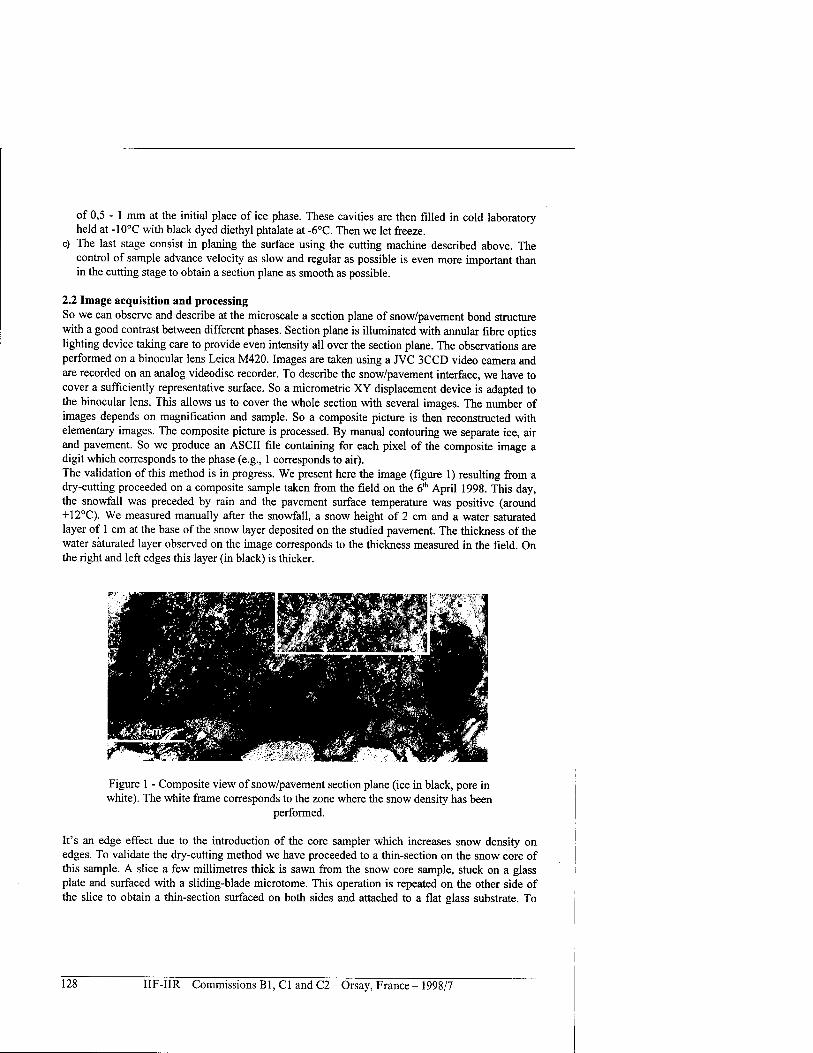
of 0,5 - 1 mm at the initial place of ice phase. These cavities are then filled in cold laboratory held at -10°C with black dyed diethyl phtalate at -6°C. Then we let freeze,

c) The last stage consist in planing the surface using the cutting machine described above. The control of sample advance velocity as slow and regular as possible is even more important than in the cutting stage to obtain a section plane as smooth as possible.

2.2 Image acquisition and processing So we can observe and describe at the microscale a section plane of snow/pavement bond structure with a good contrast between different phases. Section plane is illuminated with annular fibre optics lighting device taking care to provide even intensity all over the section plane. The observations are performed on a binocular lens Leica M420. Images are taken using a JVC 3CCD video camera and are recorded on an analog videodisc recorder. To describe the snow/pavement interface, we have to cover a sufficiently representative surface. So a micrometric XY displacement device is adapted to the binocular lens. This allows us to cover the whole section with several images. The number of images depends on magnification and sample. So a composite picture is then reconstructed with elementary images. The composite picture is processed. By manual contouring we separate ice, air and pavement. So we produce an ASCII file containing for each pixel of the composite image a digit which corresponds to the phase (e.g., 1 corresponds to air). The validation of this method is in progress. We present here the image (figure 1) resulting from a dry-cutting proceeded on a composite sample taken from the field on the 6th April 1998. This day, the snowfall was preceded by rain and the pavement surface temperature was positive (around +12°C). We measured manually after the snowfall, a snow height of 2 cm and a water saturated layer of 1 cm at the base of the snow layer deposited on the studied pavement. The thickness of the water saturated layer observed on the image corresponds to the thickness measured in the field. On the right and left edges this layer (in black) is thicker.

Figure 1 - Composite view of snow/pavement section plane (ice in black, pore in white). The white frame corresponds to the zone where the snow density has been

performed.

It's an edge effect due to the introduction of the core sampler which increases snow density on edges. To validate the dry-cutting method we have proceeded to a thin-section on the snow core of this sample. A slice a few millimetres thick is sawn from the snow core sample, stuck on a glass plate and surfaced with a sliding-blade microtome. This operation is repeated on the other side of the slice to obtain a thin-section surfaced on both sides and attached to a flat glass substrate. To


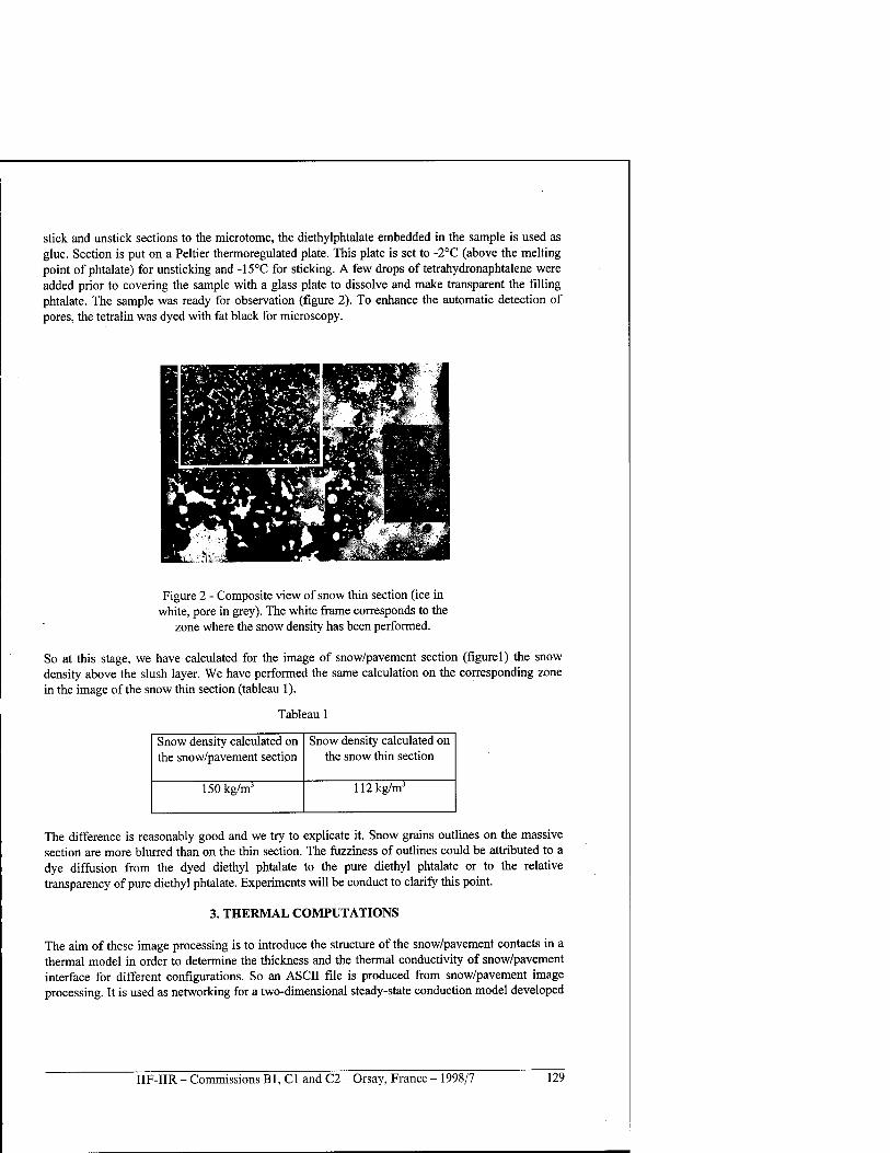
stick and unstick sections to the microtome, the diethylphtalate embedded in the sample is used as glue. Section is put on a Peltier thermoregulated plate. This plate is set to -2°C (above the melting point of phtalate) for unsticking and -15°C for sticking. A few drops of tetrahydronaphtalene were added prior to covering the sample with a glass plate to dissolve and make transparent the filling phtalate. The sample was ready for observation (figure 2). To enhance the automatic detection of pores, the tetralin was dyed with fat black for microscopy.

Figure 2 - Composite view of snow thin section (ice in white, pore in grey). The white frame corresponds to the

zone where the snow density has been performed.

So at this stage, we have calculated for the image of snow/pavement section (figure 1) the snow density above the slush layer. We have performed the same calculation on the corresponding zone in the image of the snow thin section (tableau 1).

Tableau 1

Snow density calculated on the snow/pavement section

Snow density calculated on the snow thin section

150kg/m3 112kg/m3

The difference is reasonably good and we try to explicate it. Snow grains outlines on the massive section are more blurred than on the thin section. The fuzziness of outlines could be attributed to a dye diffusion from the dyed diethyl phtalate to the pure diethyl phtalate or to the relative transparency of pure diethyl phtalate. Experiments will be conduct to clarify this point.

3. THERMAL COMPUTATIONS

The aim of these image processing is to introduce the structure of the snow/pavement contacts in a thermal model in order to determine the thickness and the thermal conductivity of snow/pavement interface for different configurations. So an ASCII file is produced from snow/pavement image processing. It is used as networking for a two-dimensional steady-state conduction model developed


at CRREL, Albert (1983), and adapted at Centre d'Etudes de la Neige for our specific use. We obtain a steady-state temperature distribution within the image. So we mean horizontally temperatures to obtain a one-dimensional vertical temperature profile and we deduce interface parameters (thickness, thermal conductivity).

CONCLUSION

These computations will be carried out for numerous sections plane corresponding to different types of snow (dry, wet) and different thermal state of pavement before the snowfall. The study of numerous cases will allow us to find a relationship between interfaces' thermal conductivity and snow and pavement features. Then the interfaces' thermal conductivity will be introduced in the model Gelcro. At the end the model will provide from meteorological conditions forecasted, an objective forecasting of the evolution of snow which arrive on the pavement.

REFERENCES

1. Albert, M.R., Phetteplace, G., 1983 : Computer models for two-dimensional steady-state heat conduction. CRREL Report 83-10.

2. Brun, E., and 4 others, 1989 : An energy and mass model of snow cover suitable for operational avalanche forecasting. J. Glaciol., 35(121).

3. Brzoska, J.B., Coleou, C, Lesaffre, B., 1998 :Thin-sectioning of wet snow after flash-freezing. J. Glaciol., 44(146), 54-62.

4. Fremond, M, Williams, P., 1979 : Gels des sols et des chaussees. Paris, Presse des Ponts et Chaussees.

5. Good, W., 1989 : Thin sections, serial cuts and 3-D analysis of snow. International Association of Hydrological Sciences Publication 162 (Symposium at Davos 1986 - Avalanche Formation, Movement and Effects), 35-48.

6. Lesaffre, B., Pougatch, E., Martin, E.,1998 : Objective determination of snow-grain characteristics from images. Annals of Glaciology, 26, 112-118.

7. Perla, R.I., 1982 : Preparation of section planes in snow specimens. J. Glaciol., 28(98),199-204.

ETUDE DU COMPORTEMENT D'UNE COUCHE DE NEIGE DEPOSEE SUR LA CHAUSSEE : CARACTERISTIQUES DE L'INTERFACE NEIGE/CHAUSSEE

RESUME : Ce travail fait partie du projet francais GELCRO''2,3 dont l'objectif est de developper un modele qui permettent de prevoir l'etat de surface de la chaussee avant une chute de neige et revolution de la couche de neige deposee. Ce Systeme permettra d'ameliorer l'efficacite des interventions des services d'exploitation hivernale. Le modele, nomme Gelcro, resulte du couplage de deux modeles numeriques unidimensionnels : ■ Gel ID' simule la propagation du gel dans la chaussee ; ■ Crocus2 est un modele physique initialement developpe pour la prevision du risque d'avalanche.

II simule revolution du manteau neigeux. Pour cette etude, un site experimental a ete choisi pour la frequence importante des chutes de neige et la diversite des situations meteorologiques. II est equipe de six planches experimentales de chaussee representatives des techniques francaises actuelles. Ces chaussees sont instrumentees avec differents capteurs ( capteurs de hauteurs de neige, sondes de temperatures et camera video) qui permettent d'observer lew enneigement et de caracteriser revolution de la neige pour differentes situations meteorologiques. Ce site dispose egalement d'une instrumentation meteorologique


complete incluant des mesures specifiques sur la neige. Des mesures manuelles sont aussi effectuees pendant ou juste apres une chute de neige et des echantillons composites neige/chaussee sont preleves. Pour preserver la microstructure de la neige sur la chaussee durant le prelevement, les pores sont remplis par du diethyl phtalate (point de fusion -5°C ) et l'echantillon est ensuite regele. Une technique originale a ete developpee en laboratoire froid ä -20°C pour observer les interfaces neige/chaussee sur ces echantillons. Cette technique consiste ä couper ä sec simultanement la neige et la chaussee pour obtenir une coupe verticale. La principale difficulte consiste ä minimiser au maximum l'echauffement. La coupe est ensuite traitee pour accentuer le contraste entre les grains de neige, le phtalate et la chaussee. On observe alors ä l'echelle microscopique sur la coupe les liaisons entre la neige et la chaussee. Les images d'interface obtenues sont alors utilisees dans un code bidimensionnel de calcul thermique en regime permanent afin de calculer la resistance thermique d'interface. Cette resistance thermique sera alors parametrisee en fonction des caracteristiques de la neige et de la chaussee puis introduites dans le modele Gelcro. L'observation directe ä l'echelle microscopique d'interface neige/chaussee permettra une modelisation realiste des ponts thermiques et des effets capillaires ä l'echelle de l'interface.

1. Laboratoire des Materiaux et Structures du Genie Civil (LCPC, CNRS), Champs sur Marne 2. M6t6o France, Centre d'Etude de la Neige, Grenoble 3. Laboratoire Regional des Ponts et Chauss6es, Nancy


ICE FORMATION IN FREEZING OF WATER-NONSATURATED GROUNDS

GOLUBEVV.N. Faculty of Geography, Moscow State University, Moscow, RUSSIA

E-mail: [email protected]

ABSTRACT

The ice formation in water-nonsaturated grounds during freezing is analyzed taking into account the impact of interfacial phenomena on water/ice - mineral boundaries. The influence of grounds water content and grain packing, physical and chemical properties, roughness of mineral particles surface and other factors on critical supercooling of water domain are discussed. Polydispersity and polyminerality of natural grounds follow to nonsynchronism in freezing of separate water domains. In result the phase transition of water in ice is spreading in time and space and a freezing zone is in water-nonsaturated grounds instead of freesing front. Ice nucleation is possible in any point inside this zone until the only condition is valid - negative temperature and conditioned by it supercooling of water domains.

INTRODUCTION

Water freezing in dispersed media is a some typical process of heterogeneous crystallization and it occurs very similarly to many other cases of ice formation on extraneous solids. However there are the specific features of ground freezing process, moisture migration and phase state, structure and composition of formed ice. These particularities are related with non-uniform distribution and even differences in chemical composition and energetic state of water; polydispersion, heteroporosity and various substantial composition of ground; polyminerality and polycrystallinity of ground particles. The freezing of water-nonsaturated ground represents the specific interest.

1 HETEROGENEOUS CRYSTALLIZATION OF WATER

The necessary condition of phase transition of water into ice is formation of the critical stable ice nucleus, which has size 2.6 nm and is a minimum quantity of crystal substance (Golubev 1986). Such crystallographically ideal ice nucleus is capable to a repeating growth and thermodynamically steady at temperatures below -38°C. This temperature corresponds to water threshold supercooling ATo at homogeneous nucleation and to temperature of spontaneous crystallization of water drops (Fletcher 1970, Golubev 1986). The ice appearance at higher temperatures is related to activating influence of mechanical impurities contained in water and is an example of heterogeneous nucleation process. The theory of activating influence of extraneous bodies is not developed. However a general theoretical reasons permit to suppose that the substances with crystal lattice parameters close to those for ice, with OH- group in composition, with small shear module and with uniform distribution of opposite charges on surface should have higher activating ability (Edwards et al. 1970, Fletcher 1970, Golubev 1981, Van-der-Merve 1966). The generalized characteristic of physical and chemical substance's properties can serve factor of ice-forming activation m, which is determined from energies on ice-water yiw, substrate-water ysw

and substrate-ice ysi interfaces (Fletcher 1970):

m=(y„-ysi)/ym (1)


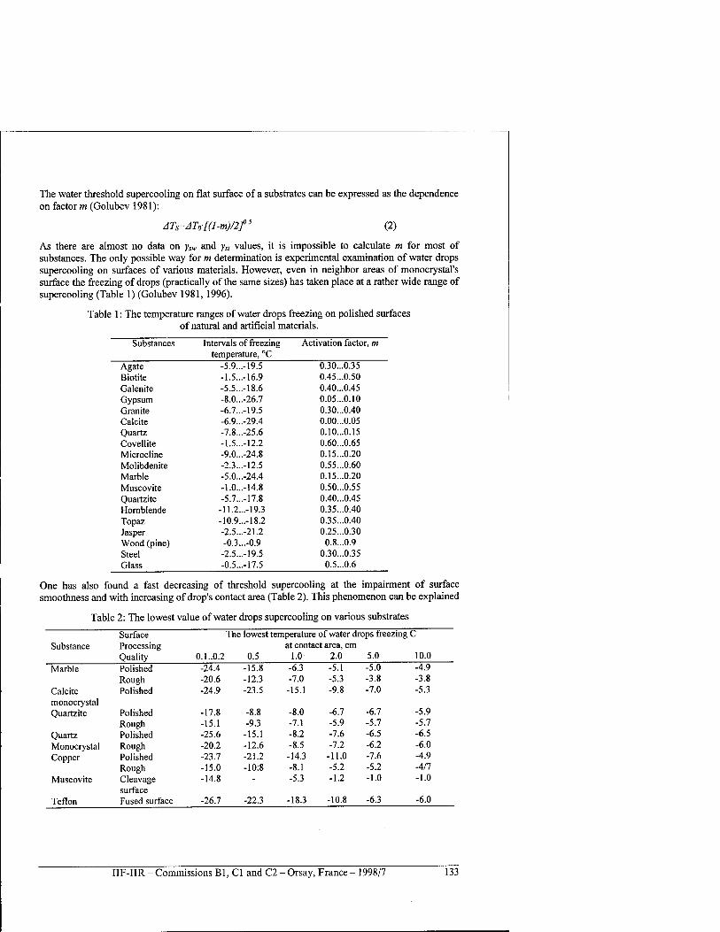
The water threshold supercooling on flat surface of a substrates can be expressed as the dependence on factor m (Golubev 1981):

ATs=ATo-[(l-m)/2fi (2)

As there are almost no data on ysw and ysi values, it is impossible to calculate m for most of substances. The only possible way for m determination is experimental examination of water drops supercooling on surfaces of various materials. However, even in neighbor areas of monocrystal's surface the freezing of drops (practically of the same sizes) has taken place at a rather wide range of supercooling (Table 1) (Golubev 1981, 1996).

Table 1: The temperature ranges of water drops freezing on polished surfaces of natural and artificial materials.

Substances Intervals of freezing temperature, °C

Activation factor, m

Agate -5.9...-19.5 0.30...0.35 Biotite -1.5...-16.9 0.45...0.50 Galenite -5.5...-18.6 0.40...0.45 Gypsum -8.0...-26.7 0.05...0.10 Granite -6.7...-19.5 0.30...0.40 Calcite -6.9...-29.4 0.00...0.05 Quartz -7.8...-25.6 0.10...0.15 Covellite -1.5...-12.2 0.60...0.65 Microcline -9.0...-24.8 0.15...0.20 Molibdenite -2.3...-12.5 0.55...0.60 Marble -5.0...-24.4 0.15...0.20 Muscovite -1.0...-14.8 0.50...0.55 Quartzite -5.7...-17.8 0.40...0.45 Hornblende -11.2...-19.3 0.35...0.40 Topaz -10.9...-18.2 0.35...0.40 Jasper -2.5...-21.2 0.25...0.30 Wood (pine) -0.3...-0.9 0.8...0.9 Steel -2.5...-19.5 0.30...0.35 Glass -0.5...-17.5 0.5...0.6

One has also found a fast decreasing of threshold supercooling at the impairment of surface smoothness and with increasing of drop's contact area (Table 2). This phenomenon can be explained

Table 2: The lowest value of water drops supercooling on various substrates

Surface The lowest temperature of water drops freezing C Substance Processing at contact area, cm

Quality 0.1..0.2 0.5 1.0 2.0 5.0 10.0

Marble Polished -24.4 -15.8 -6.3 -5.1 -5.0 -4.9 Rough -20.6 -12.3 -7.0 -5.3 -3.8 -3.8

Calcite Polished -24.9 -23.5 -15.1 -9.8 -7.0 -5.3 monocrystal Quartzite Polished -17.8 -8.8 -8.0 -6.7 -6.7 -5.9

Rough -15.1 -9.3 -7.1 -5.9 -5.7 -5.7 Quartz Polished -25.6 -15.1 -8.2 -7.6 -6.5 -6.5 Monocrystal Rough -20.2 -12.6 -8.5 -7.2 -6.2 -6.0 Copper Polished -23.7 -21.2 -14.3 -11.0 -7.6 -4.9

Rough -15.0 -10:8 -8.1 -5.2 -5.2 -4/7 Muscovite Cleavage

surface -14.8 - -5.3 -1.2 -1.0 -1.0

Teflon Fused surface -26.7 -22.3 -18.3 -10.8 -6.3 -6.0


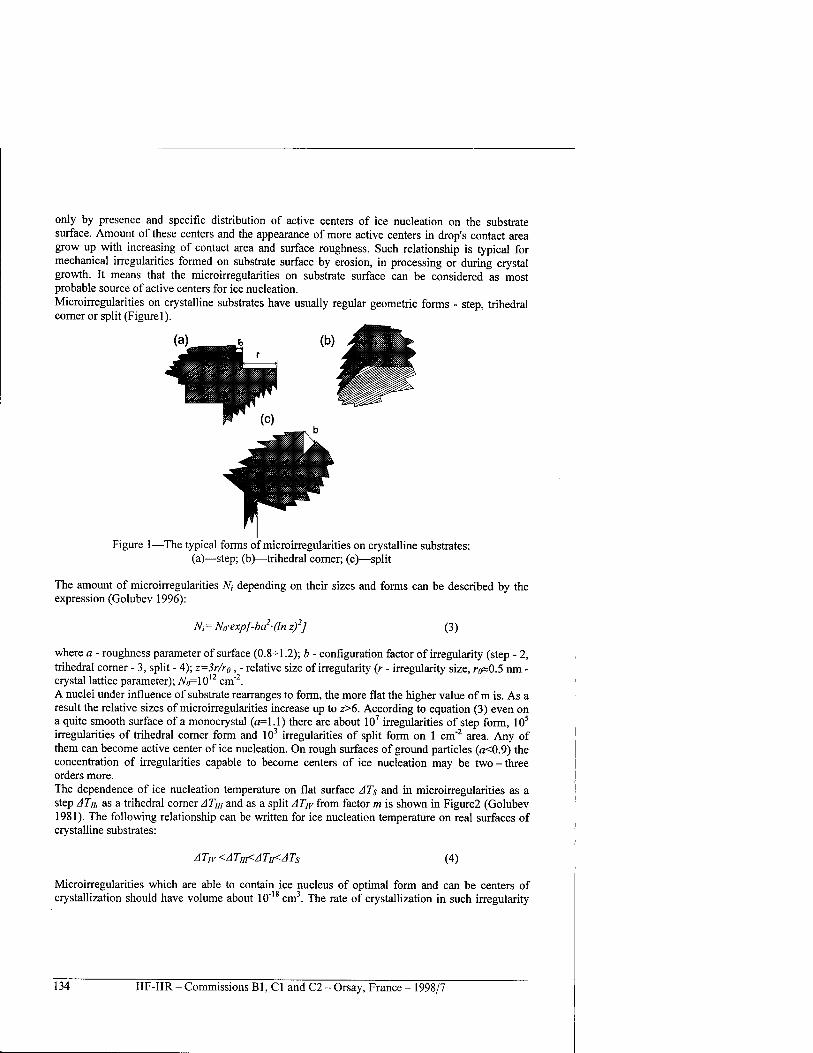
only by presence and specific distribution of active centers of ice nucleation on the substrate surface. Amount of these centers and the appearance of more active centers in drop's contact area grow up with increasing of contact area and surface roughness. Such relationship is typical for mechanical irregularities formed on substrate surface by erosion, in processing or during crystal growth. It means that the microirregularities on substrate surface can be considered as most probable source of active centers for ice nucleation. Microirregularities on crystalline substrates have usually regular geometric forms - step, trihedral corner or split (Figurel).

Figure 1—The typical forms of microirregularities on crystalline substrates: (a)—step; (b)—trihedral corner; (c)—split

The amount of microirregularities iV, depending on their sizes and forms can be described by the expression (Golubev 1996):

Ni=Nci-exp[-ba2-(lnz)2] (3)

where a - roughness parameter of surface (0.8-5-1.2); b - configuration factor of irregularity (step - 2, trihedral corner - 3, split - 4); z=3r/r0 , - relative size of irregularity (r - irregularity size, r0»0.5 nm - crystal lattice parameter); JVft=1012 cm"2. A nuclei under influence of substrate rearranges to form, the more flat the higher value of m is. As a result the relative sizes of microirregularities increase up to z>6. According to equation (3) even on a quite smooth surface of a monocrystal (a=l.l) there are about 107 irregularities of step form, 105

irregularities of trihedral corner form and 103 irregularities of split form on 1 cm'2 area. Any of them can become active center of ice nucleation. On rough surfaces of ground particles (a<0.9) the concentration of irregularities capable to become centers of ice nucleation may be two - three orders more. The dependence of ice nucleation temperature on flat surface AT$ and in microirregularities as a step ATn, as a trihedral corner ATm and as a split ATw from factor m is shown in Figure2 (Golubev 1981). The following relationship can be written for ice nucleation temperature on real surfaces of crystalline substrates:

AT,v<ATIII<AT1ÂTs (4)

Microirregularities which are able to contain ice nucleus of optimal form and can be centers of crystallization should have volume about 10"18 cm3. The rate of crystallization in such irregularity


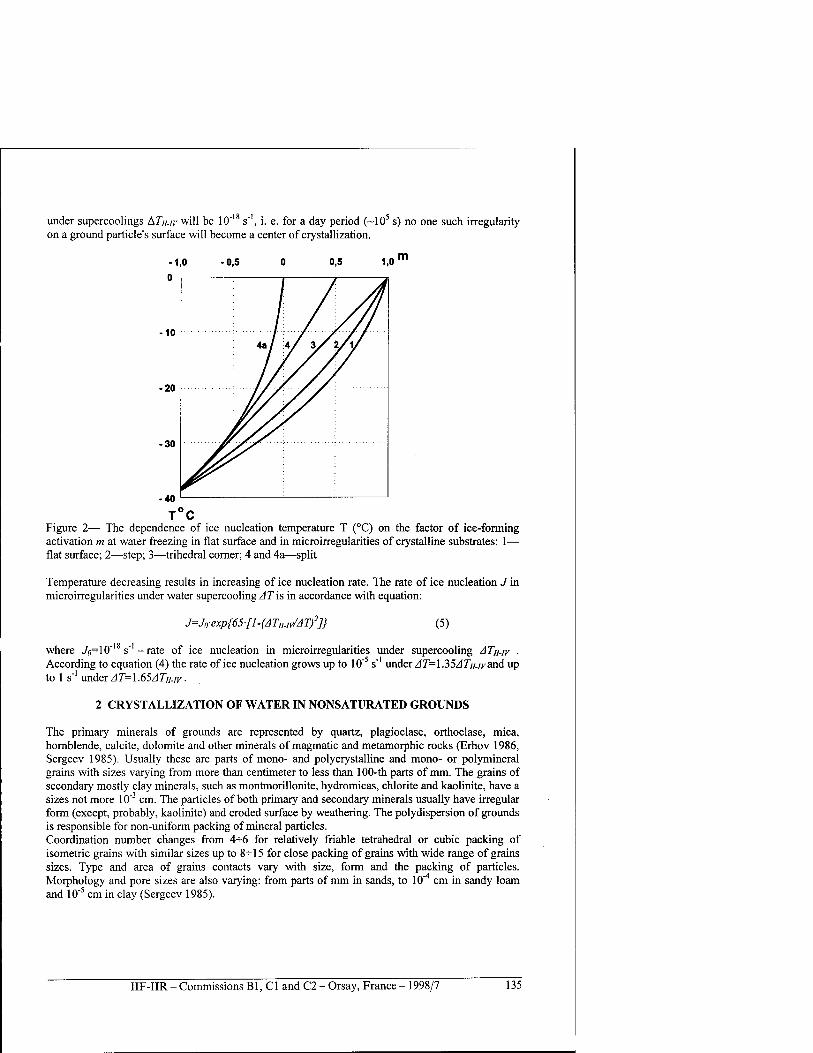
under supercoolings ATu-iv will be 10"18 s"', i. e. for a day period (~105 s) no one such irregularity on a ground particle's surface will become a center of crystallization.

■1,0

-10

-20

-30

-40

-0,5 0,5 1,0 m

4a/ v 3sYy

T°C Figure 2— The dependence of ice nucleation temperature T (°C) on the factor of ice-forming activation m at water freezing in flat surface and in microirregularities of crystalline substrates: 1— flat surface; 2—step; 3—trihedral corner; 4 and 4a—split

Temperature decreasing results in increasing of ice nucleation rate. The rate of ice nucleation J in microirregularities under water supercooling AT is in accordance with equation:

J=Jo-exp{65[l-(AT„.IV/AT)2]} (5)

where JQ= 10" s" -rate of ice nucleation in microirregularities under supercooling ATn.iy . According to equation (4) the rate of ice nucleation grows up to 10"5 s'1 under AT=\.35AT[/./y and up to 1 s"1 under AT=1.65ATu.iy.

2 CRYSTALLIZATION OF WATER IN NONSATURATED GROUNDS

The primary minerals of grounds are represented by quartz, plagioclase, orthoclase, mica, hornblende, calcite, dolomite and other minerals of magmatic and metamorphic rocks (Erhov 1986, Sergeev 1985). Usually these are parts of mono- and polycrystalline and mono- or polymineral grains with sizes varying from more than centimeter to less than 100-th parts of mm. The grains of secondary mostly clay minerals, such as montmorillonite, hydromicas, chlorite and kaolinite, have a sizes not more 10"3 cm. The particles of both primary and secondary minerals usually have irregular form (except, probably, kaolinite) and eroded surface by weathering. The polydispersion of grounds is responsible for non-uniform packing of mineral particles. Coordination number changes from 4-^-6 for relatively friable tetrahedral or cubic packing of isometric grains with similar sizes up to 8-M5 for close packing of grains with wide range of grains sizes. Type and area of grains contacts vary with size, form and the packing of particles. Morphology and pore sizes are also varying: from parts of mm in sands, to 10"4 cm in sandy loam and 10"5 cm in clay (Sergeev 1985).


The data shown in tables 1 and 2 and theoretical assumptions about a dependence of factor m on substrate structure (crystal lattice parameters and charge distribution), on substrate composition (presence of OH- groups) and properties (shear modulus) allow to assume that ice-forming activity of particles composed by quartz, plagioclase, gypsum or calcite is smaller than activity of particles composed by mica, clay minerals, hornblende and organic substance. Therefore ice nucleation in polymineral grounds has to begin on surfaces of the secondary minerals and organic substances. The ground dispersity exert an influence on water crystallization by the surface area of each particle. It can be either whole the surface of particle in case of smooth outlines or surface of one separate face on a particle's surface in case of angular, ribbed forms of ground grains. The areas of separate faces on particles of medium sand is about 10"2 cm2, but on particles of kaolin clay - only 10" cm . The probability of existence microirregularities of a optimal size and type on a grain face is decreasing with increase of ground dispersity. The influence of granulometric composition may to take into considerations if into equation (2) add average area of separate faces on a ground grain Sg(Golubevl996):

Ng=A-exp[-ba2(lnz/]-Sg, (6)

where Ng- the amount of microirregularities of given type and size on face area on a grain. In general case Sg=(0.5+\)-D2, where D-the average size of particles in ground or in separate granulometric or mineral fraction of ground. With^=1012 cm"2 and roughness parameter a=0.9 each grain face of medium sand can comprise only one or several microirregularities of split form with necessary dimensions for ice nucleation, up to 102 microirregularities of trihedral corner form and 10' microirregularities of step form. In the case of kaolinite with size 510"4 cm each particle there can be only two-three microirregularities of trihedral corner form and about 102 microirregularities of step form. The essential decreasing in possible spectrum of irregularities causes the water freezing in grounds composed by dusty particles under temperatures appropriate for ice nucleation in trihedral corner or step form irregularities, that makes possible significant supercooling of water. The deep and prolonged supercooling of ground water was repeatedly fixed in experimental works. The temperature -1°C was kept for several hours in water-saturated fine sand, while in kaolin clay the water did not freeze under -4°C during five days (Erhov 1986). It was also found that degree and duration of supercooling were the function of ground moisture and usually increased with water content decreasing. The ground granulometric composition can influence in full measure on process of water freezing only in water-saturated ground. In this case water in ground represents continuous medium or there are water "bridges" of sufficient thickness between relatively large meniscus nodules of water on ground grains. When moisture content of ground is less than 20% collar and meniscus formations on grain contacts can be separated from each other and the ground moisture is representing mostly capillary- disconnected water. The probability that the thin water films may be communications between separated water nodules is rather indefinite and also the ideas about nature and presence of such film were repeatedly reconsidered (Sergeev 1985). Crystal growth inside such film is even less possible . That is why the conditions of ground water freezing in water-nonsaturated grounds are more likely determined not by grain surface size but by contact area St of water nodulus and surface particle. For wettable isometric grains St corresponds to (Golubev 1996):

Sb =K-r2-(l-sinß) (7)

where K - form factor, equal to 2n in case of spherical particles; r - average radius of ground particles; ß - angle between grain surface and water nodule [Figure 3], related with ground water content, form and hydrophily of particles.

136 IIF-IIR-Commissions B1,C1 and C2-Orsay, France-1998/7

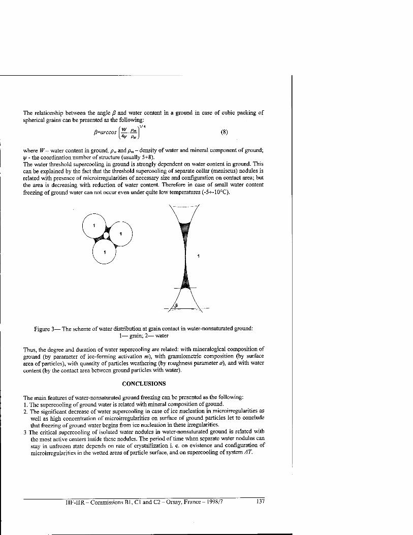
The relationship between the angle ß and water content in a ground in case of cubic packing of spherical grains can be presented as the following:

ß=arccos (^.PüL) (8) IV pw)

where W - water content in ground, pw and p,„ - density of water and mineral component of ground; y/ - the coordination number of structure (usually 5-^8). The water threshold supercooling in ground is strongly dependent on water content in ground. This can be explained by the fact that the threshold supercooling of separate collar (meniscus) nodules is related with presence of microirregularities of necessary size and configuration on contact area; but the area is decreasing with reduction of water content. Therefore in case of small water content freezing of ground water can not occur even under quite low temperatures (-5-^-10°C).

Figure 3— The scheme of water distribution at grain contact in water-nonsaturated ground: 1— grain; 2— water

Thus, the degree and duration of water supercooling are related: with mineralogical composition of ground (by parameter of ice-forming activation m), with granulometric composition (by surface area of particles), with quantity of particles weathering (by roughness parameter a), and with water content (by the contact area between ground particles with water).

CONCLUSIONS

The main features of water-nonsaturated ground freezing can be presented as the following: 1. The supercooling of ground water is related with mineral composition of ground. 2. The significant decrease of water supercooling in case of ice nucleation in microirregularities as

well as high concentration of microirregularities on surface of ground particles let to conclude that freezing of ground water begins from ice nucleation in these irregularities.

3 The critical supercooling of isolated water nodules in water-nonsaturated ground is related with the most active centers inside these nodules. The period of time when separate water nodules can stay in unfrozen state depends on rate of crystallization i. e. on existence and configuration of microirregularities in the wetted areas of particle surface, and on supercooling of system AT.

IIF-IIR-Commissions Bl, Cl and C2-Orsay, France- 1998/7 137

Freezing of water-nonsaturated ground is formed by ice formation in system consisting from many small separate water volumes contacting with unequal in area surfaces of ground particles, values of ice-forming activation factor m and degree of surface roughness for which may be distinguished. Isolation of water nodules determines the specificity of freezing of water-nonsaturated ground, namely probabilistic character of water nodules freezing related with probability of presence of an active center of ice nucleation on the wetted area of ground particle under present temperature. The polydispersity and polyminerality of natural grounds follow to nonsynchronism in freezing of separate meniscus nodules. This creates a "spreading" of phase transition in time and space. In other words, ground freezing takes place by numerous acts of ice crystals nucleation in separate nodules of ground water, resulting in appearance of not "front" of freezing but zone of phase transition. Ice nucleation is possible in any point inside this zone until the only condition is valid - negative temperature of ground and caused by it supercooling of water.

This research is supported RFBR (Project N 96-05-65445) and Program "Russian University — Basic Researches", direction 8.2.

REFERENCES

1. Edwards G. R., Evans L. F., Zipper A. F. 1970. Two-dimensional phase changes in water adsorbed on ice-nucleating substrates. - Trans. Faraday Soc, v.66, N 565, pp. 220-234.

2. Ershov E. D. 1986. Physics, chemistry and mechanics of frozen grounds. Moscow. MGU. 333 p.

3. Fletcher N. H. 1970. The chemical physics of ice. Cambridge. University press. 492 pp. 4. Golubev V. N. 1981. Conditions of ice nucleation on water-solid interface. - In: Glaciological

Study, N 26. Moscow. Radio, pp. 16-21. 5. Golubev V. N. 1986. Kinetics and mechanism of homogeneous crystallization of water. - In:

Prolems of engineering glaciology. Novosibirsk. Nauka. pp. 5-10. 6. Golubev V. N., 1996. Specific of water crystallization in grounds. - Moscow, MGU,

Proceedings of the 1-st Russian Conference of Geocriologists, Moscow, June 1996. Vol. 2. pp. 9-18.

7. Sergeev E.S. (Ed.), 1985. Theoretical basis of engineering geology. Physical and chemical basis. Moscow. Nedra. 288 p.

8. Van-der-Merve J. H., 1966. Discrepancy of crystal lattices and forces of connection on interface of oriented films-substrate. In: Monocrystal film. Moscow. Mir. pp. 215-232.

FORMATION DE GLACE LORS DE LA CONGELATION DE SOLS NON SATURES ENEAU

RESUME : Les auteurs analysent la formation de glace dans des terrains non satures en eau, au cours de la congelation, en tenant compte de l'effet des phenomenes d'interface sur les limites eau/glace-mineraux. Ils examinent l'influence de la teneur en eau des sols et de la densite des grains, des proprietes physiques et chimiques, de la durete superficielle des particules minerales, etc. sur la surfusion critique du domaine de l'eau. La polydiversite et la polymineralite des sols naturels entrainent une congelation asynchrone des domaines separes de l'eau. Ainsi, la transition de phase entre eau et glace s'etale dans le temps et dans l'espace, et une zone de congelation se trouve dans les sols non satures en eau et non dans un front de congelation. La nucleation de la glace est possible ä n'importe quel point ä l'interieur de cette zone, pourvu que la temperature y soit negative et que l'eau presente soit en surfusion.


PARTICULARITIES OF STRUCTURE AND SOME MECHANICAL PROPERTIES OF ICE FROZEN OVER THE SOLIDS

*FROLOV A.D. and **GOLUBEV V.N. »Consolidated Scientific Council on Earth Cryology, Russian Academy of Sciences,

Moscow; Russia, ** Geographical Department, Moscow State University, Moscow, Russia

ABSTRACT

The results of experimental studies of structure and elastic moduli of ice covers forming on solids are presented and discussed in the paper. It is established that the ice structure is depended on following factors: physical characteristics of substrate material, temperature of icing, water salinity. There were obtained also the freshwater and saline ice elastic moduli as a function of temperature (/=0°H--24°C) and salinity (2-10"2-^510"' mol/1). It is shown the considerable variations of studied parameters.

INTRODUCTION

The ice formations arisen on the solid surfaces differ from other natural ices by structure and properties because of specific thermodynamic conditions of their forming. Moreover the formation of contact layers of such ices occurs under strong influence of substrate surfaces. The special attention in our experiments has been given to study of ice structure as well as elastic modules and their salinity and temperature dependencies. These parameters are best to reflect the features of mechanical properties of ice and are useful as a basis for effective mechanism of ice covers removal from surfaces of solids. There are practically no data on the peculiarities of mechanical properties of these specific ice formations. Thus we suppose that the results described below clarify the principal characteristics and may be also usefull in the problems of environtment pollution.

1 TECHNIQUE OF EXPERIMENTAL RESEARCHES

The physical modeling of icing process has been conducted in a climatic chamber at the definite thermal and moisture conditions. The plates of steel, painted steel and wood have been fixed on a board, the inclination angle of which can be changed from 0° up to 90° relatively to a level. The temperature of the falling drops as well as the freezing surfaces was fixed by special systems of thermistors. The pulverizing device could automatically moved along two axes, owing to that each plate periodically (in 55 s) fell in a flow of drops during 5 s. There were realized 2 series of experiments at the temperatures of icing -15°C and -25°C. In each of these series were used the distilled water as well as NaCl solutions (with a concentration 2T0"2-510"' mol/1) preliminarily cooled up to 0°C. Pulverization have been carried out from distance 3.5 m, owing to that the drops of a water during the time of flight were in addition cooled up to temperature -1.3° and -3.5°C. Diameter of drops was 0.4^1.6 mm, but about 70% of a flow mass had the drop diameter 0.8-^1.2 mm. The rate of plate icing was about 1.1 cm/hour. Obtained ice cover samples have been subjected microstructural and ultrasonic studies. The structural studies included a determination of the form, sizes and orientation of crystals as well as a bulk distribution of brine. The salinity of obtained samples was usually two-three times smaller compared to the initial pulvarizated solutions. The moduli of elasticity-E, K, X, u and Poisson's ratios y were calculated from the values of the elastic wave propa-gation velocities: Vp (longitudinal), Vr (Relaygh) and Vs (shear). These velocity magnitudes have been determined by ultrasonic profiling technique (Frolov, 1976) at fixed


temperature of the ice cover samples. The frequency of registered signal in freshwater ice was 70 kHz and did not practically depend on temperature. For saline ices it was less and decrease up to 20-30 kHz with approach a temperature to ice melting point. The accuracy of elastic moduli evaluation was about 10%. For calculation there were used known formulas for elastic continuum isotropic medium, i.e. in the approximation of small wave attenuation. Such condition is appropriate to a freshwater ice. However, for a considera-bly saline ice especially in the state close to melting temperature there are significant increase of an attenuation factor and some increase of a prevailing wavelength of a registered pulse. Therefore a dynamic modulus values can be overestimated, as far as influence of viscosity (relaxation processes in elastic-viscous medium) grows. In this case the evaluation of elastic moduli requires one other technique of studies with due attention to a complex elastic moduli.

2 EXPERIMENTAL RESULTS AND DISCUSSION

3.1 Structural studies The ice cover structure is conditioned by active centers and thermal diffusivity of substrate as well as a supercooling of water and the growth rate of ice crystals (Golubev, 1981 a, b]. The dependence of crystal sizes on supercooling may be approximated by power function with exponent 0.3. In general case an increase of water salinity leads to a change of phase transition temperature and to decrease of crystal sizes. At small supercoolings (< 0,1 °C) the salinity dependence appears concerning weak, approximately linear. At higher supercoolings the dependence was power with exponent 1.5-3 (Golubev, 1971). It has been shown also that the ice crystal orientation on a very smooth substrates generally are vertical compared to surfaces whereas on rough surfaces any primary crystal orientations are accidental. The crystal sizes of saline ice near a substrate surface were 3-10"2-5T0"2 cm. The drops of fresh water and solution with concentration 3 10"2 mol/1 were supercooled at temperatures of icing -15°C and -25°C but of solutions with concentration 510° mol/1 — only at the temperature -25°C. As a consequence of this situation the average size of a crystals in ice formed from less concentrated solution were smaller (3-4-10"2 cm), than in the second case (4-6-10"2 cm). Basically, the ice crystal sections increase with a gradient 1,5-10"" cm2/K when a supercooling of water diminish. The crystal sizes in contact layer are defined also by thermal properties of the substrate material. For instance, an increase the substrate material thermal diffusivity in the case, when the substrate thermal diffusivity is higher than one for ice, lead to an increase of ice crystal sizes. As a result the sizes of ice crystals on the steel plate (thermal diffusivity is 0.12 cm2/s) were 20% less than one on the aluminum plate (thermal diffusivity is 0.92 cm2/s). But the surface smoothness (and consequently the concentration of active centers of ice nucleation) is the main parameter, which govern the ice structure. On carefully processed substrate surfaces the ice crystal sizes were 1.5-2 times greater than on rough surfaces (Golubev, 1992). Increase a distance from a substrate surface increase the sizes of crystals (10-30 %/cm) and change their forms from plates to pillars. The ice crystal's orientation near a substrate surface is random usually, however on a very smooth surfaces a many of crystals (40-50%) are directed almost vertically to surface. But for a distance 1-3 cm out a substrate surface up to 80% of crystals in a saline ice are directed parallel to surfaces. As a result of these changes of crystal's size and orientation the structure of ice for a distance 2-3 cm out a surface does not depend practically from substrate material and is defined by only thermodynamic conditions of icing. Therefore the features of structure of ice contact layer are essential only to adhesion of ice. Mechanical properties of the main part of freezing ice cover (strength, elastic moduli and others) are defined by thermodynamic conditions of icing, i.e.


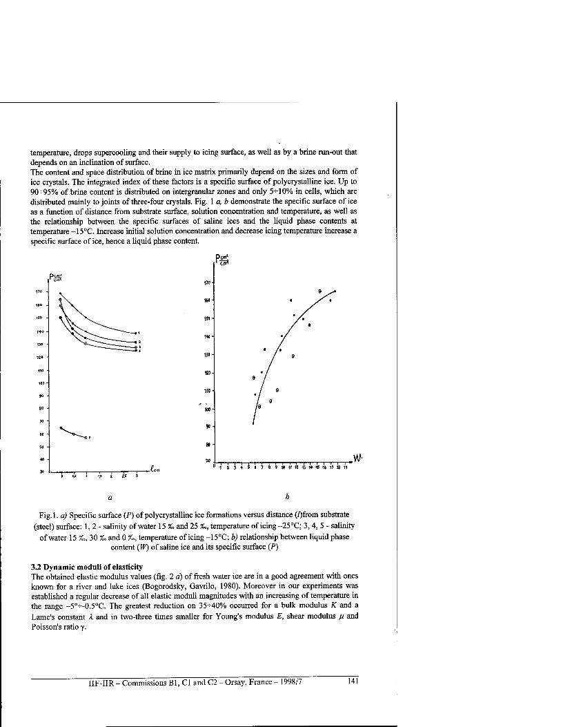
temperature, drops supercooling and their supply to icing surface, as well as by a brine run-out that depends on an inclination of surface. The content and space distribution of brine in ice matrix primarily depend on the sizes and form of ice crystals. The integrated index of these factors is a specific surface of polycrystalline ice. Up to 90-^95% of brine content is distributed on intergranular zones and only 5^-10% in cells, which are distributed mainly to joints of three-four crystals. Fig. 1 a, b demonstrate the specific surface of ice as a function of distance from substrate surface, solution concentration and temperature, as well as the relationship between the specific surfaces of saline ices and the liquid phase contents at temperature -15°C. Increase initial solution concentration and decrease icing temperature increase a specific surface of ice, hence a liquid phase content.

Pciti* 1 cm»

ISO

Y40

1» ■

«« -

110 -

' cm"

170-

9 /■*

160- • ^r |

1M- / •

1«- */

130- / e

«0- 9

• /

110- • / 9

100- 9

90-

80-

10 ( i' i 3 4 1 i 7 « ! « iUtld IS 16 17 18 U #

Fig.l. a) Specific surface (P) of polycrystalline ice formations versus distance (/)from substrate (steel) surface: 1,2- salinity of water 15 %, and 25 %., temperature of icing -25°C; 3, 4, 5 - salinity

of water 15 %„, 30 %, and 0 %,, temperature of icing -15°C; b) relationship between liquid phase content (W) of saline ice and its specific surface (P)

3.2 Dynamic moduli of elasticity The obtained elastic modulus values (fig. 2d) of fresh water ice are in a good agreement with ones known for a river and lake ices (Bogorodsky, Gavrilo, 1980). Moreover in our experiments was established a regular decrease of all elastic moduli magnitudes with an increasing of temperature in the range -5o-^-0.5°C. The greatest reduction on 35^-40% occurred for a bulk modulus K and a Lame's constant X and in two-three times smaller for Young's modulus E, shear modulus n and Poisson's ratio y-


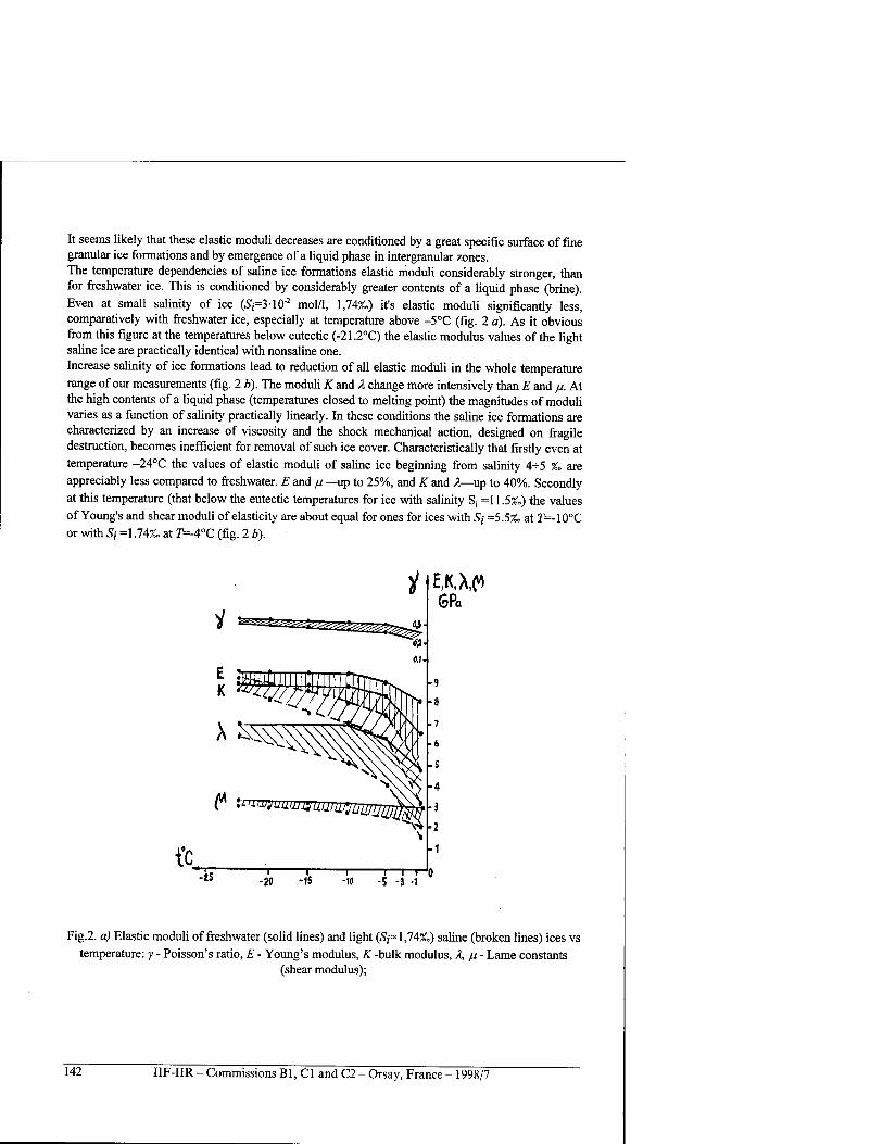
It seems likely that these elastic moduli decreases are conditioned by a great specific surface of fine granular ice formations and by emergence of a liquid phase in intergranular zones. The temperature dependencies of saline ice formations elastic moduli considerably stronger, than for freshwater ice. This is conditioned by considerably greater contents of a liquid phase (brine). Even at small salinity of ice (,S,-=3-10"2 mol/1, 1,74*.) it's elastic moduli significantly less, comparatively with freshwater ice, especially at temperature above -5°C (fig. 2 a). As it obvious from this figure at the temperatures below eutectic (-21.2°C) the elastic modulus values of the light saline ice are practically identical with nonsaline one. Increase salinity of ice formations lead to reduction of all elastic moduli in the whole temperature range of our measurements (fig. 2 b). The moduli AT and A change more intensively than E and fi. At the high contents of a liquid phase (temperatures closed to melting point) the magnitudes of moduli varies as a function of salinity practically linearly. In these conditions the saline ice formations are characterized by an increase of viscosity and the shock mechanical action, designed on fragile destruction, becomes inefficient for removal of such ice cover. Characteristically that firstly even at temperature -24CC the values of elastic moduli of saline ice beginning from salinity 4-^-5 %. are appreciably less compared to freshwater. E and fi —up to 25%, and K and X—up to 40%. Secondly at this temperature (that below the eutectic temperatures for ice with salinity S> =11.5%.) the values of Young's and shear moduli of elasticity are about equal for ones for ices with Sj =5.5*. at 7=-10°C or with S{ =1.74%. at T=-4°C (fig. 2 b).

t'c

1 GPa

-« -20 -15 T—r—t-'o •5 i -1

Fig.2. a) Elastic moduli of freshwater (solid lines) and light (iSj*l,74&) saline (broken lines) ices vs temperature: y - Poisson's ratio, E - Young's modulus, AT-bulk modulus, X, /u - Lame constants

(shear modulus);


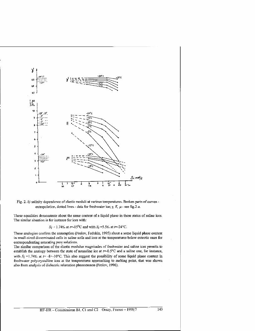
0.3 -T -of

0,4 -

0,1 -

3 Pa

10 - -24'-10"

-r -3;

8 - -oi-

? -

6 ■

S -

4 - -Z-V

J - ""□7s"

2

t

1

-24"C

f :---_:

Simot/t

3 17* 5,5

2 3 , 11.5 117«

Fig. 2. Ö) salinity dependence of elastic moduli at various temperatures. Broken parts of curves - extrapolation, dotted lines - data for freshwater ice; y, E, ju- see fig.2 a.

These equalities demonstrate about the same content of a liquid phase in these states of saline ices. The similar situation is for instance for ices with:

Si = 1.74%» at t=-\5°C and with Sj =5.5%. at /=-24°C.

These analogies confirm the assumption (Frolov, Fedukin, 1995) about a some liquid phase content in small-sized disseminated cells in saline soils and ices at the temperatures below eutectic ones for correspondenting saturating pure solutions. The similar comparison of the elastic modulus magnitudes of freshwater and saline ices permits to establish the analogy between the state of nonsaline ice at t=-0.5°C and a saline one, for instance, with Sj =1.74%» at t= -8-M0°C. This also suggest the possibility of some liquid phase content in freshwater polycrystalline ices at the temperatures approaching to melting point, that was shown also from analysis of dielectric relaxation phenomenon (Frolov, 1996).


CONCLUSIONS

Ice, formed during the icing of solids, is characterized by fast changes of all parameters of it structure (sizes, form and orientation of crystals) with an increase of distance from a substrate surface. At increase of water salinity the sizes of crystals decrease and they are directed basically parallel with icing surfaces. At an increase of temperature in the range -5-K)°C the elastic modulus magnitudes of freshwater polycrystalline ice decrease on 25-K35%, that is stipulated basically by changes of a various defect concentration in boundary zones between grains, as well as an arise of some liquid phase content At an increase of ice salinity the values of elastic moduli decrease that basically conditioned by corresponding increase of a liquid phase content and a degree of ice crystal admixture, presence of defects in a structure of boundary zones of crystal lattice of ice. The effective viscosity increases in this case also.

ACKNOWLEDGEMENTS

This research is supported RFBR (Project N 96-05-65445) and Program "Russian University — Basic Researches", direction 8.2.

REFERENCES

1. Bogorodsky V.V. and V.P.Gavrilo. (1980) Ice. Physical Properties. Modern Methods of Glaciology. 384, Hydromet Press, Leningrad,.

2. Frolov A.D. (1976) Electrical and Elastic Properties of Cryogenic Rocks, 253, Nedra Press Moscow 125 p.

3. Frolov A.D. and I.V.Fedukin. (1995) "Dielectric Properties of Saline Frozen Soils", Trans. Geophysical Investigations of Cryolithozone, 1, 73-94, SCEC, Moscow.

4. Frolov A.D. (1996) "Dielectric Moisturemetry of Frozen Soils". Proceedings of First Conference of Geocryologist of Russia, Moscow, Moscow State University, Book 2, 271-279

5. Golubev V.N. (1973) "Tne Dependence of Ice Structure from Water Salinity", Proceedings II Intern. Conf. on Permafrost, Yakutsk, 4, 180-184.

6. Golubev V.N. (1981) Conditions for the Appearance of Ice on the Solid - Water Boundary, Glaciological Researshes, 26, 16-21.

7. Golubev V.N. (1981) The Regularities of Ice Structure Formation during an Icing of Solids, Glaciological Researches, 26, 60-66.

8. Golubev V.N. (1992) The Ice Crystals Orientation on the Extraneous Bodies, Data of Glaciological Studies, 76, 203-210.

DISCUSSION

CHENAF D., Canada: What is the interest of relating the specific surface to the unfrozen water content?

FROLOV A.D. - This interest is connected with the problem: how influence the initial admixtures (or pollutions) on the structure and unfrozen water content of ice frozen on the solids. The data obtained are also useful to do the choice of the kind of mechanical effect for effective removal of ice cover.

FUKUDA M, Japan: is new method of TDEM (Time Domain Electric Magnetic) applied in Russia or not?

FROLOV A.D. - No attempts are made in Russia.

ISHIZAKI T., Japan: Why does specific surface increase with increasing water content (W)?


FROLOV A.D.- It is vice versa: the unfrozen liquid phase content (brine) in saline polycrystalline ice increases with decrease of grain sizes, hence with increasing of medium specific surface. Moreover, a fine crystalline ice consists in grains which are more admixting by strange ions and by small bubbles of brine, that also should influence on liquid phase freezing. But this effect is not yet studied in details.

RYOHEI T., Japan: How do you evaluate the elastic moduli from acoustic information? You estimate the specimen as homogeneous in order to get the elastic moduli, don't you? Can this homogeneity be acceptable for the models being considered the variations of grain size?

FROLOV A.D. -Yes, we consider the samples as quasi-homogeneous for evaluation of elastic moduli. In our ice samples, there were no real boundaries or layers of different grain sizes. Additionally, the grain and brine inclusion sizes were considerably less compared to sample size and the lengths of elastic waves. But, of course, the data obtained on elastic moduli are an average for all ice body of samples.

PARTICULARITES DE LA STRUCTURE ET QUELQUES PROPRIETES MECANIQUES DE L'EAU CONGELEE FORMEE SUR DES SOLIDES

RESUME : Les resultats d'etudes experimentales sur la structure et les modules d'elasticite des couvertures de glace formees sur des solides sont presented et expliques dans 1' article. II est etabli que la structure de la glace depend de plusieurs facteurs : caracteristiques physiques du substrat, temperature de glacage, salinite de l'eau. Ont ete egalement obtenus les modules d'elasticite'de la glace formee par de l'eau fraiche et de la glace formee par de l'eau saline en fonction de la temperature (t=0°+-24°C) et de la salinite (2.10"2 -5.10"1 mol/1). On montre les nombreuses variations entre les parametres etudies.


SECTION III

MODELISATION PHYSIQUE OU MATHEMATIQUE

PHYSICAL OR MATHEMATICAL MODELLING

SOLUTION OF HEAT TRANSMISSION EQUATION INCLUDING THE PHASE CHANGE THROUGH COMPUTERISED ELECTRICAL ANALOGY

DOMINGUEZ M., ARIAS J.M., GARCIA C, BARRAGÄN M.V. * Institute) del Frfo, Ciudad Universitaria, 28040 Madrid, Spain

*Departamento de Fisica Aplicada I, Facultad de Ciencias Fisicas, (UCM). Ciudad Universitaria, 28040 Madrid, Spain

ABSTRACT

A new simulation technique, based on computer assisted solution of the electrical analogy, is developed for the study of thermal problems, including the phase change. In this method the capacitor are substituted by equivalent resistors, which value is a function of the increase in the calculation time and of the capacity. The problem is reduced to the solution of the equation for the grids and nodes, the number of elements in the grid is fixed and the thickness is varied at each iteration. The results obtained in some cases of simulation are indicated and in some examples that have analytic solution compared. The conclusion is the new method is suitable for performing these studies.

INTRODUCTION

For many years now, it has been possible to find, several models, systems, etc. in the literature, to predict the time needed to freeze: a product, a cast of ice, a water pipe or the surface of a lake. The problem is mathematically complex and the assumptions made introduce a large degree of uncertainty. Even complex computer programmes have great difficulty to solve them. In all cases in which the issue of the time for freezing is discussed, it is necessary to begin from Fourier's heat analysis equation, which is valid when the medium is isotropic and continuous, which is something that does not occur when there is a phase change. For many years we used electrical analogy, which stopped being used when personal computers where developed. Later it was seen that by solving the analogical circuits with the aid of a computer, it could still be used advantageously in the solving of some problems. We made this public in several publications and was discussed in several congresses (Dominguez et al, 1991, Dominguez et al, 1995, Dominguez et al, 1997a). In the study carried out on the concentration of juices, the analogy was applied to freezing, with the introduction, in each iteration, of the variation curves for the thermophysical properties in relation to temperature (Dominguez et al, 1997b). We were left with doubts about the precision of the analogical method followed, and even more, of that employed in the phase change, and due to this, we sought exact solutions of the heat equation, so that they could serve as a method for comparison, as the experimental solutions could introduce an error equivalent to the degree of uncertainty. The precision of the computer assisted solution of the electrical analogy, with the programme employed, was demonstrated in works (Dominguez et al, 1997a) and (Barragän et al, in press a), and the possibility of the new simulation technique with a change of phase, in (Barragän et al, in press b). At this time we do not have the slightest doubt about the precision of the technique, and we consider it can be worthy of knowledge and discussion, in particular, in a forum such as this one, in which freezing problems are the object of the meeting.

1 PORTRAYAL OF COMPUTER ASSITED ELECTRICAL ANALOGY INCLUDING THE CHANGE OF PHASE.

The computer assisted solution of electrical analogy technique that we have developed is based upon substituting capacitors by equivalent resistors, the value of which is a function of the increase


in the calculation time dt and of the capacity C. They are calculated by means of the following equation:

R= dt/2.C

The problem is reduced to the solution of the equations for the grids and the nodes, i.e. solving simultaneous equations with the same number of unknowns. Up until , we had always made the media discrete, fixing the dimensions. In the case of the change of phase, it was thought that, in order to study these problems, it would be easier to discrete, a medium to be frozen, in constant parts and to vary its dimensions in each iteration. In the unidirectional case, it is easy to understand. Let us consider a sample of thickness E which is being frozen and that x is the thickness of the ice layer at a given instant. If we then divide each of the two areas into 5 parts we shall have the grid depicted in Figure 1, into which an additional element has been introduced corresponding to the interface layer. The basic idea of the method is to make equal, in each iteration, the heat that is eliminated or retained in the interface layer, to the heat necessary to freeze or thaw a specific thickness of liquid, whereby the calculated thickness adds on to engross the frozen layer and becomes subtracted from that of liquid.

Figure 1 s: solid, f: interface, 1: liquid

If we generalise it to a grid of i elements in each of the two areas, frozen or not, and if in each iteration we know the intensities in all of the resistors, or what is analogically the same, the heat fluxes, Y(i), corresponding to the i-th resistance, and if dt is the increase in the calculation time, the heat that will be released or will be used in the interface upon freezing or thawing will be:

(Y(i+2)-Y(i-l))*dt

and the thickness of the frozen layer will be:

x=(Y(i+2)-Y(i-l))*(dt/p.L)

being p the density of the liquid and L the latent heat. Figure 2 depicts the equivalent electric grid which, as can be seen, is formed by resistors in series and shunted capacities, with potential difference sources equivalent to the temperatures at the two ends and at the interface. More elements were used in the calculation than those shown in the previous figure, this number was of 50 in each of the two areas.

-c, c,, — o,-"-^, 51 ^93 ClOO c101-r-

T T TT T ■ TT T -10°C

Figure 2


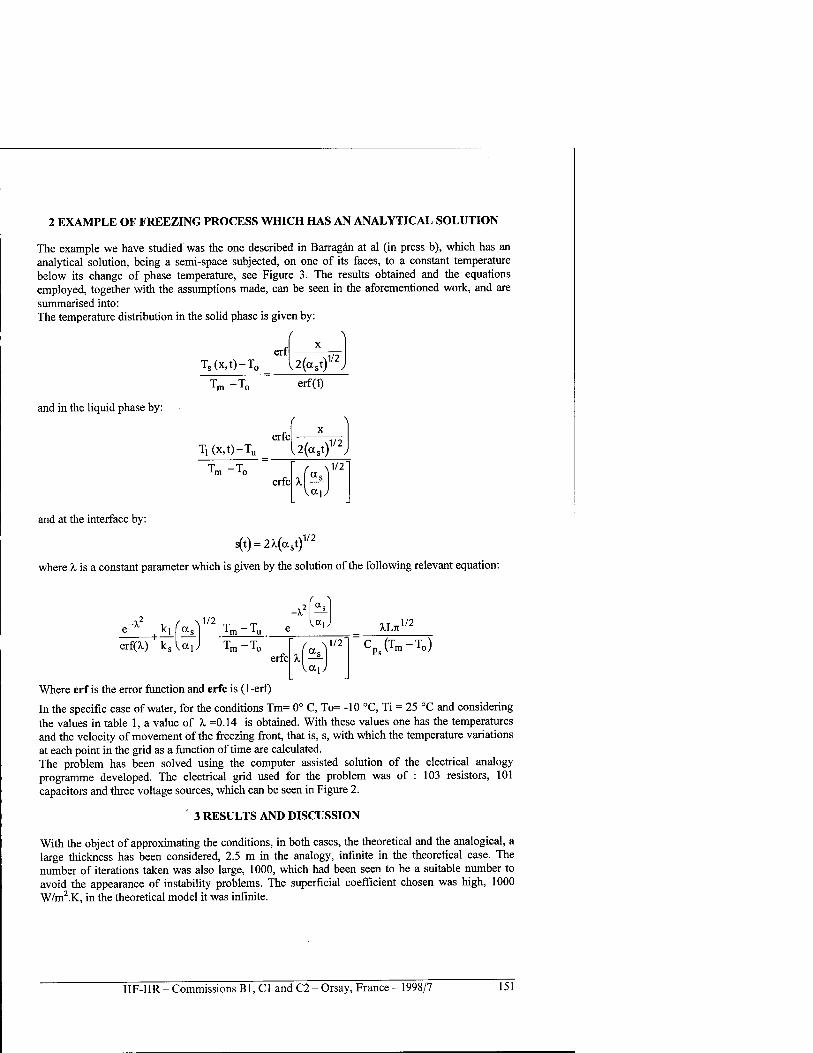
2 EXAMPLE OF FREEZING PROCESS WHICH HAS AN ANALYTICAL SOLUTION

The example we have studied was the one described in Barragän at al (in press b), which has an analytical solution, being a semi-space subjected, on one of its faces, to a constant temperature below its change of phase temperature, see Figure 3. The results obtained and the equations employed, together with the assumptions made, can be seen in the aforementioned work, and are summarised into: The temperature distribution in the solid phase is given by:

f \ x

erf Ts(x,t)-T0 2(<xst) 1/2

erf(1)

and in the liquid phase by:

erfc Ti (x,t)-Tu U(ast) 1/2

erfc X\^ a,

1/2

and at the interface by:

s(t) = 2H«st)1/2

where X is a constant parameter which is given by the solution of the following relevant equation:

erf(^) + ks «1

1/2 -X2 5L

Tm -T„ -T0

e ^J

Tm erfc if)

L J

XLn 1/2

Cp(Tm-T0)

Where erf is the error function and erfc is (1-erf)

In the specific case of water, for the conditions Tm= 0° C, To= -10 °C, Ti = 25 °C and considering the values in table 1, a value of X =0.14 is obtained. With these values one has the temperatures and the velocity of movement of the freezing front, that is, s, with which the temperature variations at each point in the grid as a function of time are calculated. The problem has been solved using the computer assisted solution of the electrical analogy programme developed. The electrical grid used for the problem was of : 103 resistors, 101 capacitors and three voltage sources, which can be seen in Figure 2.


With the object of approximating the conditions, in both cases, the theoretical and the analogical, a large thickness has been considered, 2.5 m in the analogy, infinite in the theoretical case. The number of iterations taken was also large, 1000, which had been seen to be a suitable number to avoid the appearance of instability problems. The superficial coefficient chosen was high, 1000 W/m2.K, in the theoretical model it was infinite.


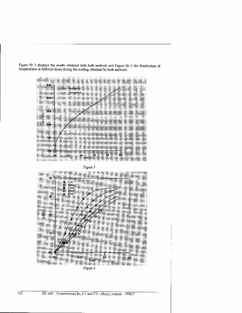
Figure Nr 3 displays the results obtained with both methods and Figure Nr 4 the distribution of temperatures at different times during the cooling, obtained by both methods.

oao Aflrtl&ftVAf

(MS

Tuputillâf

on .*>

04» -

004 -

" "'"' . 1 ■"" 1 ! 1 30

lida>>)

Figure 3

AS lail

06


It can be seen that during the first three days the agreement is very good, and it is considered that the differences at greater times are due to the different conditions indicated in the methods. It is thought that it would be convenient to increase the number of iterations with the increase in thickness, in order to avoid instability problems.

CONCLUSION

It is considered that: The new method developed for the study of thermal problems, including the phase change, of computer assisted solution of the electrical analogy, in which the number of elements in the grid is fixed and the thickness is varied in each iteration, is suitable for performing these studies.

ACKNOWLEDGEMENTS


REFERENCES

1. Dominguez M., Pinillos J.M., Sanz P.D., 1991, Proceedings of the XVIII Int. Cong, on Refrigeration, Montreal, Canada,. Vol. IV, p. 1898.

2. Dominguez M., Pinillos J.M., Arias J.M., Lopez N., 1995, Computerized electrical simulation of freezing processes, Proceedings of the XIX International Congress of Refrigeration, The Hague, The Nederlands, Vol. I, p. 45-51.

3. Dominguez M, Arias J.M., Fuentes R., Barragän V.M., 1997, Distribuciön de temperatura en placas con condiciones de contorno diversas. Solution con analogia electrica, Refrigeraciön - Frial, 42, 35, 40.

4. Dominguez M., Arias J.M., Pinillos J.M., 1997, Propiedades de zumo de naranja concentrado: conductividad, calor especifico, entalpia y viscosidad, Refrigeacion-Frial no. 45, p. 35-39.

5. Barragän V.M., Fuentes R., Dominguez M., Arias J.M., in press a, Testing the computer assisted solution of the electrical analogy in the temperature distribution on a square sheet with non homogeneous boundary conditions.

6. Barragän V.M., Arias J.M., Dominguez M., in press b, Testing computer assisted solution of the electrical analogy in a heat transfer processes with a phase change which has an analytical solution.

RESOLUTION DE L'EQUATION DE TRANSMISSION DE CHALEURINCLUANT LE CHANGEMENT DE PHASE PAR ANALOGIE ELECTRIQUE INFORMATISEE

RESUME : Une nouvelle technique de simulation, fondee sur la resolution assistee par ordinateur de l'analogie electrique, a ete mise au point pour etudier les problemes thermiques, notamment le changement de phase. Selon cette methode, la capacite est remplacee par des resistances äquivalentes, dont la valeur est fonction de 1'augmentation dans le temps de calcul et de la puissance. Le probleme se resume ä la resolution de 1'equation pour les grilles et les noeuds, le nombre des elements dans la grille est fixe et l'epaisseur varie ä chaque iteration. Les resultats obtenus dans ces cas de simulation sont presentes ; certains sont compares avec des resolutions analytiques. On conclut que cette methode est appropriee pour mener ce type d'etudes.


MODELLING AND EXPERIMENTATION OF THE TRANSFER MECHANISM IN POROUS MEDIA DURING FREEZING

DJABALLAH-MASMOUDI N., AGUIRRE-PUENTE J. UMR 8616 du C.N.R.S. "Orsayterre", Universite de Paris Sud, Bat. 504

91405 Orsay, France, and UPRES-A 6143 "Morphologie Continentale et Cötiere" (ex-Centre de Geomorphologie),

Universite de Caen/C.N.R.S., 14000 Caen, France

ABSTRACT

During the freezing of a water filled porous medium, several phenomena interact and control themselves: the heat transfer, the behaviour of interfaces in the pores, the mass transfer and the mechanical behaviour of the porous matrix. In order to predict and evaluate the consequences of this interaction (cryogenic suction and heave) a model of the "Coupled Stefan Problem" is proposed, allowing the coupling of the thermodynamics laws and the heat and mass transfer mechanisms. An experimental device allows the study of the evolution of a crack artificially created in a rock submitted to a freezing process. During the experiments, a vertical thermal gradient is imposed towards the bottom of the rock sample which is immersed in a continuous water flow. Measurements made during the experiment inform about the behaviour of the rock and their comparison with the theoretical estimates shows the validity of our approach for the two kinds of tested rocks: the "Lens" and the "Pierre de Caen".

INTRODUCTION

The objective of this paper is to present an original model of the Coupled Stefan Problem and the experimental studies made for its validation. Indeed, there are many mathematical and numerical models for the resolution of the only thermal Stefan Problem but few for the resolution of the Coupled Stefan Problem. In the first case, the non linearity of the problem already leads to high difficulties of resolution (Carslow and Jaeger, 1965, Neumann 1860 (Conference in Königsberg) in ibidem, Ramos et al, 1996) that need numerical calculations or simplifications whose consequence must be appreciated according to the kind of practical problem to resolve (Le Fur et al, 1964, Lunardini, 1991, Cames-Pintaux et Nguyen, 1986, Posado Cano, 1995). In the second case, i.e., when the substance filling a porous medium presenting a fine texture, the formation of ice/water interfaces in the small pores produces particular effects at the microscopic scale which need thermodynamic analyses. Physical modelling helps to understand the microscopic mechanism of freezing of one pore and the small capillary linking it to another (Everett and Heynes, 1965, Williams, 1967, Aguirre-Puente et al, 1973, Miller, 1973). These microscopic effects lead to a singular macroscopic behaviour of a porous medium undergoing freezing. The essential importance of the size of pores, pointed out by the microscopic studies, produces a very high degree of complexity of the macroscopic process of freezing of a fine dispersed medium. This is due to two reasons. The first is the very wide domain of pore sizes in a porous medium. The second is the very important role of the adsorbed water layer (Franks, 1975) in many aspects of the process but particularly in the hydraulic conductivity of the frozen medium. Many models are proposed in the literature but the most of them need simplifications which does not completely respect the physics of mechanisms (Aguirre-Puente and Fremond, 1975, O'Neil and Miller, 1980, Gilpin, 1980). Consequently, the use of them can not be universal from a fundamental point of view and frequently need more or less arbitrary empirical adjustments.


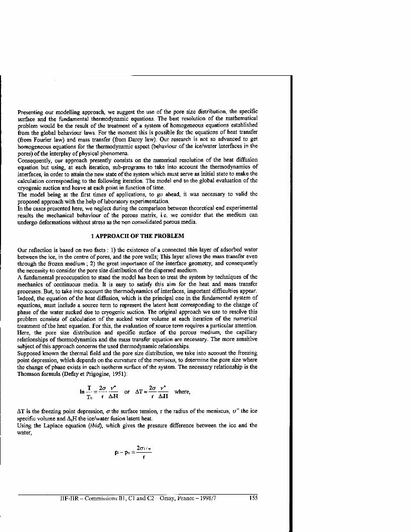
Presenting our modelling approach, we suggest the use of the pore size distribution, the specific surface and the fundamental thermodynamic equations. The best resolution of the mathematical problem would be the result of the treatment of a system of homogeneous equations established from the global behaviour laws. For the moment this is possible for the equations of heat transfer (from Fourier law) and mass transfer (from Darcy law). Our research is not so advanced to get homogeneous equations for the thermodynamic aspect (behaviour of the ice/water interfaces in the pores) of the interplay of physical phenomena. Consequently, our approach presently consists on the numerical resolution of the heat diffusion equation but using, at each iteration, sub-programs to take into account the thermodynamics of interfaces, in order to attain the new state of the system which must serve as initial state to make the calculation corresponding to the following iteration. The model end to the global evaluation of the cryogenic suction and heave at each point in function of time. The model being at the first times of applications, to go ahead, it was necessary to valid the proposed approach with the help of laboratory experimentation. In the cases presented here, we neglect during the comparison between theoretical end experimental results the mechanical behaviour of the porous matrix, i.e. we consider that the medium can undergo deformations without stress as the non consolidated porous media.

1 APPROACH OF THE PROBLEM

Our reflection is based on two facts : 1) the existence of a connected thin layer of adsorbed water between the ice, in the centre of pores, and the pore walls; This layer allows the mass transfer even through the frozen medium ; 2) the great importance of the interface geometry, and consequently the necessity to consider the pore size distribution of the dispersed medium. A fundamental preoccupation to stand the model has been to treat the system by techniques of the mechanics of continuous media. It is easy to satisfy this aim for the heat and mass transfer processes. But, to take into account the thermodynamics of interfaces, important difficulties appear. Indeed, the equation of the heat diffusion, which is the principal one in the fundamental system of equations, must include a source term to represent the latent heat corresponding to the change of phase of the water sucked due to cryogenic suction. The original approach we use to resolve this problem consists of calculation of the sucked water volume at each iteration of the numerical treatment of the heat equation. For this, the evaluation of source term requires a particular attention. Here, the pore size distribution and specific surface of the porous medium, the capillary relationships of thermodynamics and the mass transfer equation are necessary. The more sensitive subject of this approach concerns the used thermodynamic relationships. Supposed known the thermal field and the pore size distribution, we take into account the freezing point depression, which depends on the curvature of the meniscus, to determine the pore size where the change of phase exists in each isotherm surface of the system. The necessary relationship is the Thomson formula (Defay et Prigogine, 1951):

, T 2a v" ._ 2o- v" , In — = or AT« where,

To r AcH r AeH

AT is the freezing point depression, <rthe surface tension, r the radius of the meniscus, v" the ice specific volume and AeH the ice/water fusion latent heat. Using the Laplace equation (ibid), which gives the pressure difference between the ice and the water,

2<7i/w pi-p»=


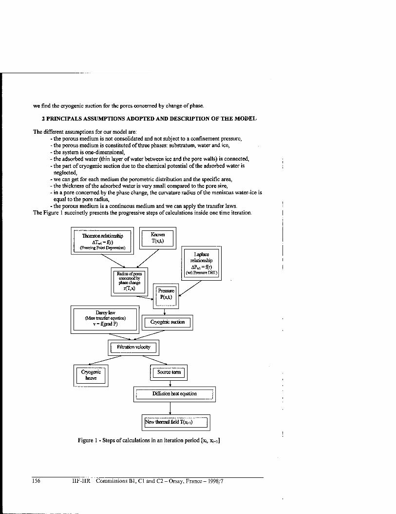
we find the cryogenic suction for the pores concerned by change of phase.

2 PRINCIPALS ASSUMPTIONS ADOPTED AND DESCRIPTION OF THE MODEL

The different assumptions for our model are: - the porous medium is not consolidated and not subject to a confinement pressure, - the porous medium is constituted of three phases: substratum, water and ice, - the system is one-dimensional, - the adsorbed water (thin layer of water between ice and the pore walls) is connected, - the part of cryogenic suction due to the chemical potential of the adsorbed water is

neglected, - we can get for each medium the porometric distribution and the specific area, - the thickness of the adsorbed water is very small compared to the pore size, - in a pore concerned by the phase change, the curvature radius of the meniscus water-ice is

equal to the pore radius, - the porous medium is a continuous medium and we can apply the transfer laws.

The Figure 1 succinctly presents the progressive steps of calculations inside one time iteration.

Thomson relationship ATvrt = f(r)

(Freezing Point Depression)

Known T(x,t,)

Radius of pores concerned by phase change

r(T,x)

Laplace relationship APw/i = f(r)

(w/i Pressure Diff)

Figure 1 - Steps of calculations in an iteration period [xi, Xj+i]


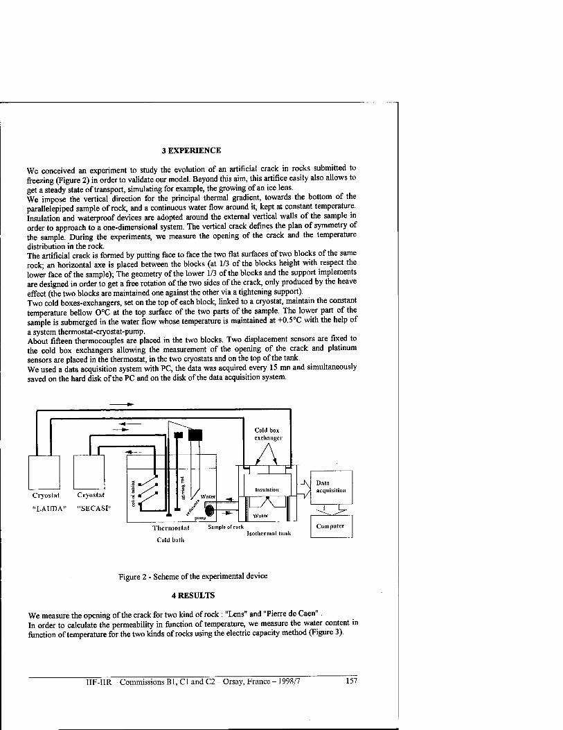
3 EXPERIENCE

We conceived an experiment to study the evolution of an artificial crack in rocks submitted to freezing (Figure 2) in order to validate our model. Beyond this aim, this artifice easily also allows to get a steady state of transport, simulating for example, the growing of an ice lens. We impose the vertical direction for the principal thermal gradient, towards the bottom of the parallelepiped sample of rock, and a continuous water flow around it, kept at constant temperature. Insulation and waterproof devices are adopted around the external vertical walls of the sample in order to approach to a one-dimensional system. The vertical crack defines the plan of symmetry of the sample. During the experiments, we measure the opening of the crack and the temperature distribution in the rock. The artificial crack is formed by putting face to face the two flat surfaces of two blocks of the same rock; an horizontal axe is placed between the blocks (at 1/3 of the blocks height with respect the lower face of the sample); The geometry of the lower 1/3 of the blocks and the support implements are designed in order to get a free rotation of the two sides of the crack, only produced by the heave effect (the two blocks are maintained one against the other via a tightening support). Two cold boxes-exchangers, set on the top of each block, linked to a cryostat, maintain the constant temperature bellow 0°C at the top surface of the two parts of the sample. The lower part of the sample is submerged in the water flow whose temperature is maintained at +0.5°C with the help of a system thermostat-cryostat-pump. About fifteen thermocouples are placed in the two blocks. Two displacement sensors are fixed to the cold box exchangers allowing the measurement of the opening of the crack and platinum sensors are placed in the thermostat, in the two cryostats and on the top of the tank. We used a data acquisition system with PC, the data was acquired every 15 mn and simultaneously saved on the hard disk of the PC and on the disk of the data acquisition system.

-* Cold box exchanger

A 'S

*i i r Insulation /.., , " -* L/vJ

Water "LAUDA" "SECASI" .. / •

nip —- 1 . * P>

Data acquisition

Thermostat

Cold bath

Sample of rock Isothermal tank

Computer

Figure 2 - Scheme of the experimental device

4 RESULTS

We measure the opening of the crack for two kind of rock : "Lens" and "Pierre de Caen". In order to calculate the permeability in function of temperature, we measure the water content in function of temperature for the two kinds of rocks using the electric capacity method (Figure 3).


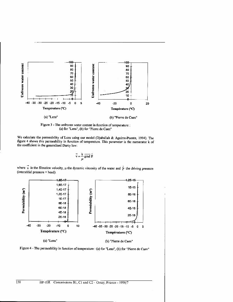
c o

N

i s s

1 we- 90 80 70 60 SO 40 30 /

ja/- 1 1 1 1 1 1 h-0-

* B U N e e P

I 4flO- 90 i 80 70 60 50] 40/

______^^20 - "~" 10 - 1 e_

-40 -35 -30 -25 -20 -15-10-5 0 5

Temperature (°C)

(a) "Lens"

-40 -20 0

Temperature (°C)

(b) "Pierre de Caen"

20

Figure 3 - The unfrozen water content in function of temperature : (a) for "Lens", (b) for "Pierre de Caen"

We calculate the permeability of Lens using our model (Djaballah & Aguirre-Puente, 1994). The figure 4 shows this permeability in function of temperature. This parameter is the numerator k of the coefficient in the generalised Darcy law:

-» k ■ A

v = — grad P M

where v is the filtration velocity, u the dynamic viscosity of the water and p the driving pressure (interstitial pressure + head).

E

.Q

a.

1.8E17

1.6E-17 -

1.4E-17 -

1.2E-17 - 1E-17

8E-18

6E-18

4E-18

2E-18 1 1 1 9-i

| 1.2E-15

1E-15 •

8E-16

6E-16

4E-16

2E-16J

—i 1 1 1—i—i—To -40 -30 -20 -10 0

Temperature (°C)

(a) "Lens"

10 -40 -35 -30 -25 -20 -15-10-5 0

Temperature (°C)

(b) "Pierre de Caen"

Figure 4 - The permeability in function of temperature : (a) for "Lens", (b) for "Pierre de Caen"


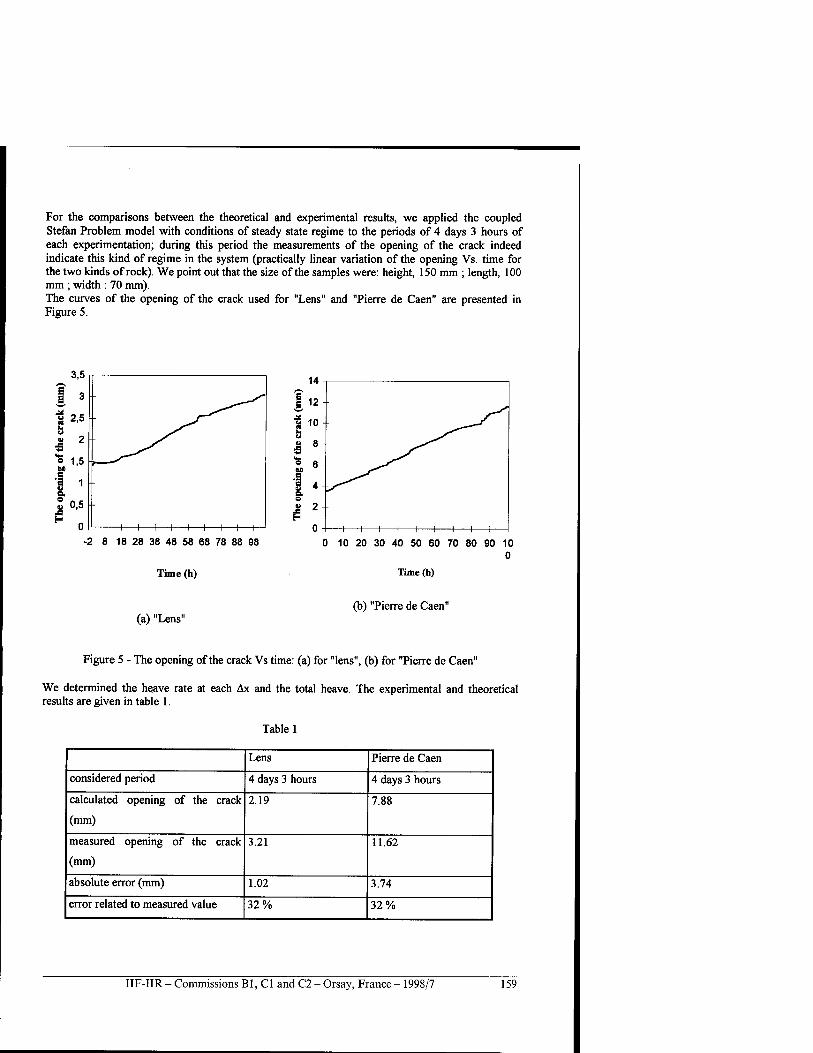
For the comparisons between the theoretical and experimental results, we applied the coupled Stefan Problem model with conditions of steady state regime to the periods of 4 days 3 hours of each experimentation; during this period the measurements of the opening of the crack indeed indicate this kind of regime in the system (practically linear variation of the opening Vs. time for the two kinds of rock). We point out that the size of the samples were: height, 150 mm ; length, 100 mm ; width : 70 mm). The curves of the opening of the crack used for "Lens" and "Pierre de Caen" are presented in Figure 5.

-2 8 18 28 38 48 58 68 78 88 98

Time (h)

10 20 30 40 50 60 70 80 90 10 0

Time (h)

(a) "Lens" (b) "Pierre de Caen"

Figure 5 - The opening of the crack Vs time: (a) for "lens", (b) for "Pierre de Caen"

We determined the heave rate at each Ax and the total heave. The experimental and theoretical results are given in table 1.

Table 1

Lens Pierre de Caen

considered period 4 days 3 hours 4 days 3 hours

calculated opening of the crack

(mm)

2.19 7.88

measured opening of the crack

(mm)

3.21 11.62

absolute error (mm) 1.02 3.74

error related to measured value 32% 32%


Taking into account the complexity of the problem, the experimental hazards and the fact that we exploited only few preliminary experiments, we consider this result as satisfactory. The experimental device and thermal-mechanical conditions placed to the sample was conceived in order to validate the approach we propose. The steady state regime was looked out to yield to easy numerical calculations. These calculations were made with the help of simple spreadsheet processing methods. But there are not fundamental obstacle to do calculations for other boundary and initial conditions and forms even with the use of the same kind of methods, waiting to put in service more elegant mathematical models.

CONCLUSION

The aim of this paper was to propose a method of modelling to study complex systems concerned by frozen soils and requiring urgent studies and its validation by experimental research in laboratory. The model tends to respect as near as possible the physics of the process. Several elementary phenomena interplaying all along the complex mechanism of change of phase, some simplifications was adopted to be able to resolve the problem. Nevertheless, the fundamental spirit of respect of the physics is kept. The progress of science, principally in knowledge of the adsoption of the water upon the solid matrix of porous media, will allow to get better results in the future. The originality of the model consists in the use of:

- fundamental thermodynamics laws in each pore (Thomson and Laplace relationships principally),

- classical properties of porous media as : distribution of the pore size curve; specific surface of the porous medium and water content in fonction of temperature bellow 0°C.

This is possible in numerical methods using sub-programs at each iteration to evaluate the source term of the discrete heat diffusion equation. The result of interpretations of the comparison between the theoretical and experimental results is enthusiastic, taking into account the experimental hazards and the estimated possible errors coming from the absence in calculations of certain physical aspects of the theoretical physical model (cryogenic suction produced by chemical potential in adsorbed water). One of the aspects of the future investigations is the research of the means to get homogeneous the behaviour equations of interfaces in the pores to treat more rigorous the whole system of mathematical equations and to do more easy its treatment, principally in the case of transient regimes.

REFERENCES 1. Aguirre-Puente J., Vignes M. and Viaud, P., 1973, Study of the Structural Changes in Soils

during Freezing, in Russian: Permafrost Second International Conference, Vol. 4 Yakutsk Institute, Aacademy of Sciences USSR, p. 161-175. (In English: USSR Contribution, Permafrost Second International Conference, National Academy of Sciences Washington, DC, 1978, p. 315-323).

2. Aguirre-Puente J. and Fremond M., 1976, Frost Propagation in Wet Porous Media, Lecture Notes in Mathematics, 503, Spingeer-Verlag, Berlin - Heidelberg - New York, 137-147.

3. Cames-Pintaux AM. and Nguyen-Lamba M; 1986, Finite-Element Enthalpy Method for Discrete Phase Change, Numerical Heat Tranfer, vol. 9, Hemisphere Publ. Corp., pp. 403-417.

4. Carslow H.S. and Jaeger J.C, 1965, Conduction of Heat in Solids, Second Ed., Oxford at the Carendon Press.

5. Defay R. et Prigogine I., 1951, Tension superfwielle et adsorption, Desoer, Liege - Dunod, Paris.


6. Djaballah N. et Aguirre-Puente I, 1994, Permeabilites des sols geles, approche theorique, premiere confrontation avec des mesures experimentales, Proceedings of the Seventh International Symposium on Ground Freezing, Nancy, pp. 69-74.

7. Everett D.H. and Heynes J.M., 1965 Capillary properties of some model pore systems with special reference to frost damage, Rillem Bulletin, No. 27, pp. 31-38

8. Franks F. (Ed.), 1975, Water, a Comprehensive Treatise, Vol. 5: Water in Dispersed Systems, Plenium Press. New York and London

9. Gilpin, R.R., 1980, A model for the Prediction of Ice Lensing and Frost Heave in soils, Water Resources Research, Vo; 16, Nr. 5, pp.918-930

10. Le Fur B., Bataille J. et Aguirre-Puente J., 1964, Etude de la congelation d'une lame plate dont une face est maintenue ä temperature constante, l'autre face etant soumise ä une temperature variable en fonction du temps (Probleme de Stefan Unidimensionnel), C.R. Acad. Sc, Paris, t. 252, 24 aoüt 1964, pp. 1483-1485.

11. Lunardini V.J., 1991, Heat Transfer With Freezing and Thawing, Developments in Geotechnical Engineering, 65 Elsevier, Amsterdam.

12. Miller R.D., 1973, Soil Freezing in Relation to Pore Water Pressure and Temperature, Permafrost Second International Conference, North American Contribution, National Academy of Sciences, Washington, D.C.

13. Neumann, F., 1860, Conference in Königsberg commented in ibidem Carslow and Jaeger, p. 282

14. O'Neill K. and Miller R.D., 1980, Numerical solutions for rigid ice model of Secondary Frost Heave, Second International Symposium on Ground Freezing, Norwegian Institute of Technology, pp. 656-684.

15. Posado Cano R, 1995, Probleme de Stefan: Etudes theoriques et experimentales pour des substances pures et des melanges eutectiques, These de Doctorat, Specialite Physique, Universite Denis Diderot Paris 7, pp. 141.

16. Ramos M., Aguirre-Puente J. and Posado Cano R. 1996, Soil Freezing Problem: an Exact Solution, Soil Technology, 9, Elsevier, pp. 29-38.

17. Williams, 1967, Unfrozen Water in Frozen Soils: Pore size - Freezing Temperature - Pressure Relationships, Norges Geotekniske Institut, Pub,. Nr. 72, Oslo, pp. 3748.

SIMULATION ET MESURES DES TRANSFERTS DE CHALEUR ET DE MASSE EN MILIEU POREUX PENDANT LA CONGELATION

RESUME : Pendant la congelation des milieux poreux ä texture fine contenant de l'eau, des comportements singuliers sont generes par des interactions des processus de transfert avec la physico-chimie des interfaces au cours du gel ou du degel. On groupe ce type des problemes sous la denomination de "Probleme de Stefan Couple". Un modele du "Probleme de Stefan Couple" est propose dans cette communication pour effectuer le couplage entre des phenomenes elementaires (transfert de chaleur, transfert de masse et lois de comportement des interfaces) considerant que le rayon de courbure du menisque eau-glace est un des parametres preponderants qui determinent le comportement du Systeme poreux subissant le gel. Pour valider le modele du "Probleme de Stefan Couple", une installation experimentale pour etudier le comportement du gel d'une fissure dans la röche a ete realisee pour deux types de roches, la Pierre de Caen et le Lens.


PROBLEME DE STEFAN : UNE NOUVELLE METHODE APPROCHEE Application au talik en zone periglaciaire

POSADO CANO R., AGUIRRE-PUENTE J. et COSTARD F. Groupe Planetologie U.M.R. 8616 du C.N.R.S. « ORSAYTERRE »,

Bätiment 504, Universite de Paris Sud, 91405 Orsay, France

RESUME

On regroupe sous la denomination de « probleme de Stefan» les problemes ayant en commun l'existence d'au moins deux phases en coexistence generalement separees deux ä deux par une interface bien definie ou non. Ces problemes sont bien connus pour etre d'une remarquable difficulte lorsqu'on cherche ä resoudre mathematiquement les equations liees aux modeles physiques decrivant ces phenomenes. On ne considere ici que des configurations qui rendent la conduction de la chaleur unidimensionnelle. On presente de nouveaux resultats theoriques concernant ces problemes pour des formes geometriques simples et possedant en outre une surface de changement de phase tranche. On s'interesse ä differents types de conditions parietales: condition de Neumann, condition de Dirichlet, condition de Fourier. On applique ces resultats theoriques ä la determination de la profondeur d'un talik en zone periglaciaire.

INTRODUCTION

On aborde le probleme de Stefan uniphasique1 par la methode de Green-Riemann. Cette theorie peut etre utilisee lorsque l'equation aux derivees partielles (E.D.P.) est lineaire. Elle s'appuie sur la connaissance de l'equation adjointe de l'E.D.P. et sur la formule de Green. Notre principale contribution s'articule alors sur l'expression des solutions exactes obtenues, on developpe, en effet, une nouvelle methode approchee pour resoudre les problemes de frontieres libres. Avec notre approche la loi horaires(?) approchee est donnee en tant que fonction implicite de la forme

*(') = /(f's(')) et l'obtention des valeurs s'effectue ä l'aide de techniques elementaires de l'analyse numerique. Les resultats numeriques montrent une superiority certaine de notre methode approchee par rapport aux methodes approchees traditionnelles (Lunardini, 1991) teile que, par exemple, les methodes polynomials (methode de Goodman, methode de Megerlin,...), les methodes variationnelles (quasi-variationnelle de Biot, principe de moindre action de Gauss,...).

1 SOLUTIONS EXACTES PAR LA METHODE DE GREEN-RIEMANN.

Les problemes de Stefan sont par essence des problemes couples car T(x,t) et s(t), sont liees par des conditions differentielles. La theorie de Green-Riemann permet de transformer ce probleme en un probleme d'equation integro-differentielle. Le resultat se presente sous la forme:

T(x,t) = jg[x,t,T,s{r)\iT et h(s(t),t)= jk[s(t),t,s(r),ds(r)/dT,r]dT (1) 0 0

Le probleme est totalement resolu si Ton sait resoudre exactement l'equation integro-differentielle (12). Actuellement, on ne sait resoudre de maniere exacte qu'un nombre tres restreintes d'equations integrales (Linz P., 1985), dans bien des cas, on est contraint d'utiliser des methodes ad hoc de l'analyse numerique pour les resoudre (F. de Hoog, Weiss R., 1974).

1 La methode s'&end sans difficult^ au probleme de Stefan biphasique


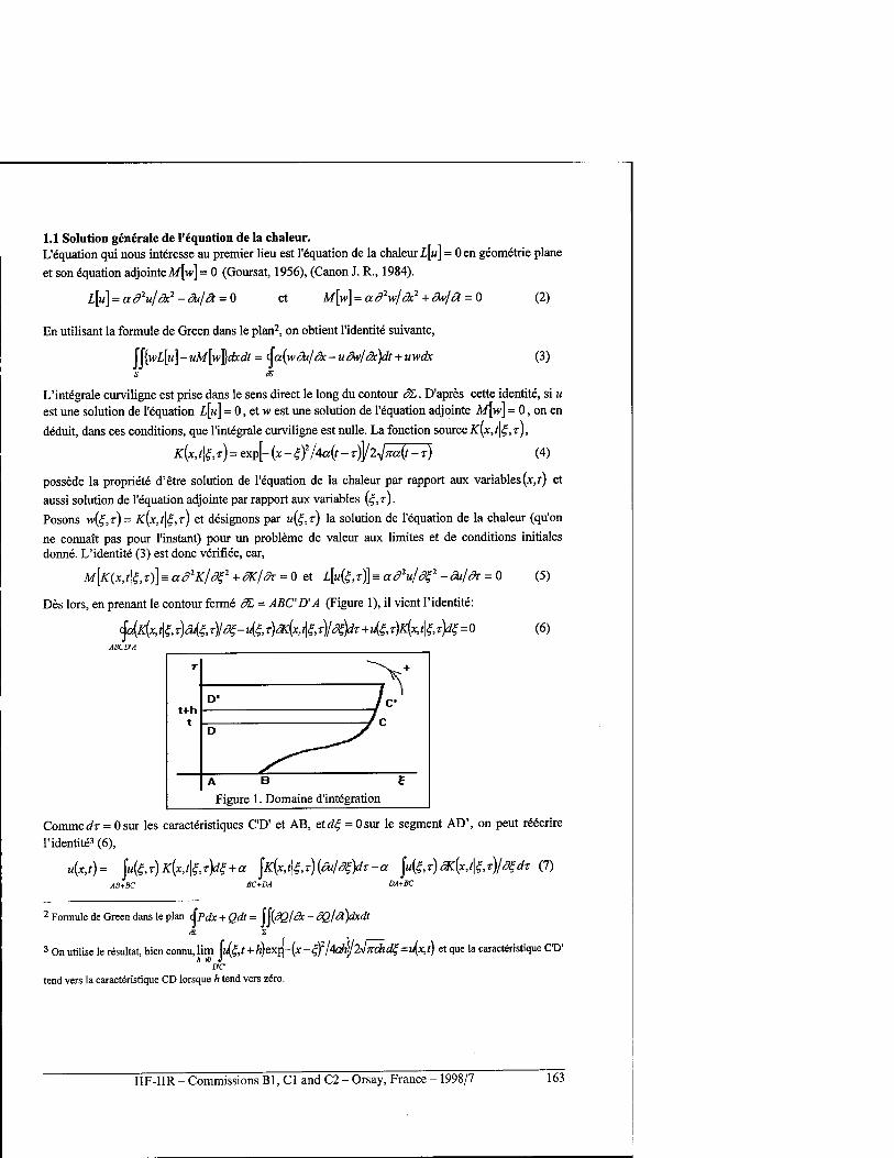
1.1 Solution generate de ('equation de la chaleur. L'equation qui nous interesse au premier lieu est l'equation de la chaleur L[u] = Oen geom&rie plane

et son equation adjointe M[w] = 0 (Goursat, 1956), (Canon J. R., 1984).

L[u) = ad2ulac2-äila = 0 et M[w] = ad2w/3c2 + äv/ä = 0 (2)

En utilisant la formule de Green dans le plan2, on obtient l'identite suivante,

J[{M'Z,[U]-KM[H']}C6C*= <\a{wdul'äc-uäv/'äc)dt + uwdx (3)

L'integrale curviligne est prise dans le sens direct le long du contour dL. D'apres cette identite, si u est une solution de l'equation L[u] = 0, et w est une solution de l'equation adjointe M[W] = 0, on en

deduit, dans ces conditions, que l'integrale curviligne est nulle. La fonction source K[x,t\^, r),

K{x,t%r) = exp[- {x - tf/4a(t - r)]/2â(t-r) (4)

possede la propriety d'etre solution de l'equation de la chaleur par rapport aux variables(x,t) et

aussi solution de l'equation adjointe par rapport aux variables (|,r).

Posons w(£,r) = K(x,t\^,r) et designons par U(^,T) la solution de l'equation de la chaleur (qu'on

ne connait pas pour l'instant) pour un probleme de valeur aux limites et de conditions initiales donne. L'identite (3) est done verifiee, car,

M[K(x,t\Z,T)] = ad2Kld? + dKldv = 0 et L[U(4,T)] = ad2u/%2 -dujdt = 0 (5)

Des lors, en prenant le contour ferme" dL = ABC DA (Figure 1), il vient l'identite:

T

>C t+h

t

D" / 1 / C

D y

A B 2 Figure 1. Domaine d'integration

Commerfr = 0 sur les caracteristiques CD' et AB, etrf£ = Osur le segment AD', on peut reecrire

l'identite3 (6),

u(x,t)= \u^,r)K{x,t%r)d4 + a J^(x,^,r)(^/'%)di-a \u{4,r)gK{x,t%T)ld^dr (7) AB+BC BC+DA

2 Formule de Green dans le plan Jpdx + Qdt = {[{<%)/<% - dQlä)dxdt m. r

3 On utilise le resultat, bien connu,lim U&+h)ex^(x-tf /4ch]/24xdd4=l(x,t) et que la caracteristique CD' DC

tend vers la caracteristique CD lorsque h tend vers zero.


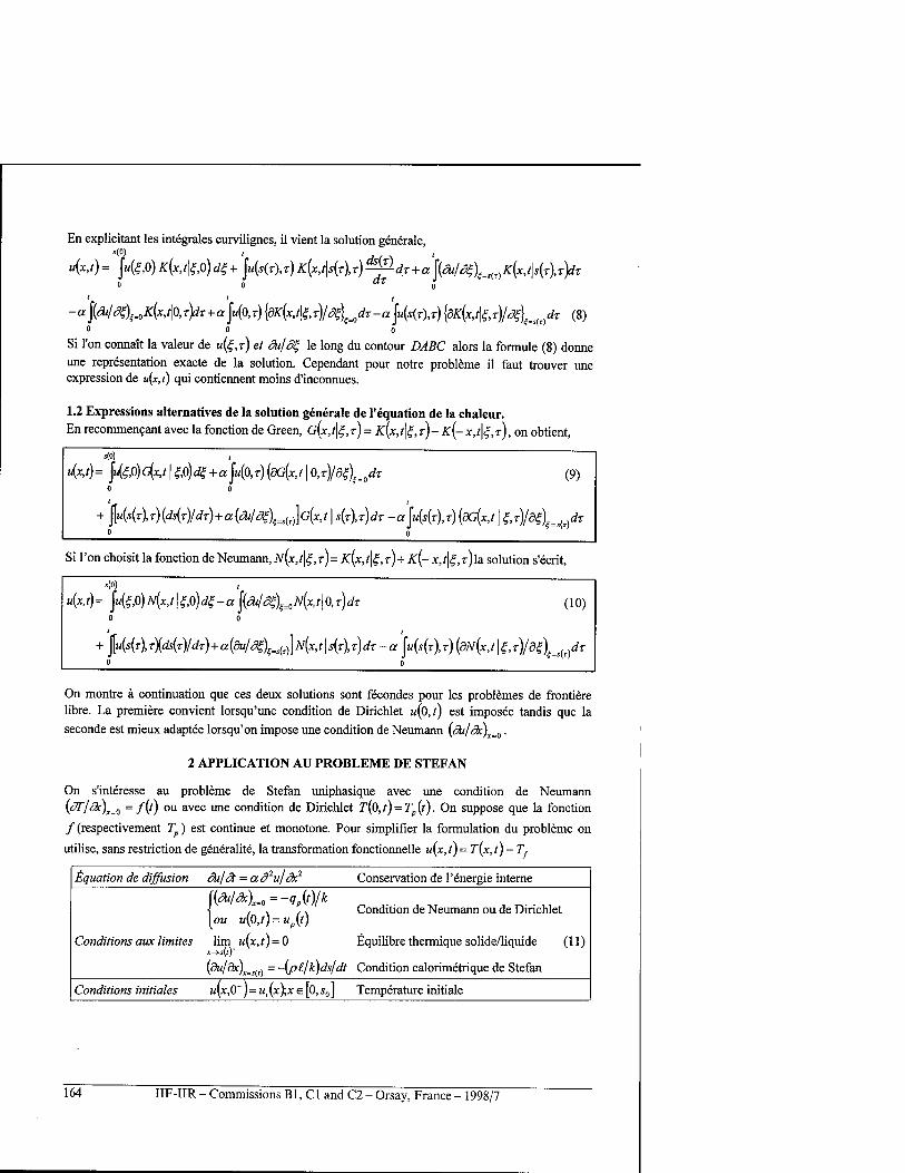
En explicitant les integrales curvilignes, il vient la solution generate, m ' '

u(x,t) = J«(£0) K{x,t\tß) d4 + ju(s(r),r) K{x,t\s(T),r) ^f-dr + a {{^1 d^\__s{r)K{x,t\s{r\t)dT 0 0 "r 0

' ' ; -aJ(^^4c,/|ar>/T+aJ"«(0,r) {dK{x,^,r)ld^\jt-a\u[s{r),r) {^^.rV^,,A (8)

0 0 0

Si 1'on connait la valeur de a(f ,r) er ^/<5£ le long du contour DABC alors la formule (8) donne une representation exacte de la solution. Cependant pour notre probleme il faut trouver une expression de u{x,t) qui contiennent moins d'inconnues.

1.2 Expressions alternatives de la solution generate de l'equation de la chaleur. En recommencant avec la fonction de Green, G(x,t\^,r) = K[X,^,T)- K(- x,t\^,r), on obtient,

u[x,t)= ji(^0)c{xt\^0)d4 + aju(0,T){dG{x,t\0,T)ld^\_0dr (9) 0 0

J[«^(4r)(rf5(r)/rfr)+«(^/^4=l(r)]G(x,? | s{t),r)dr -aju{s{r),r) {dG{x,t \^/d^^dr + o

Si Ton choisit la fonction de Neumann, jv(x,?|£,r)= K(x,t\^,r)+ K(- x,f|£,r)la solution s'ecrit,

u{x,t)= ju{^0)N{x,t\4fi)d^-aj{äi/^__0N{x,t\0,T)dT (10) 0 0

/ I

+ 0

On montre ä continuation que ces deux solutions sont fecondes pour les problemes de frontiere libre. La premiere convient lorsqu'une condition de Dirichlet u(0,t) est imposee tandis que la seconde est mieux adaptee lorsqu'on impose une condition de Neumann (dulck)x_0.

2 APPLICATION AU PROBLEME DE STEFAN

On s'interesse au probleme de Stefan uniphasique avec une condition de Neumann (dT/äc)x=0 =f(t) ou avec une condition de Dirichlet T(0,t)=Tp(t). On suppose que la fonction

/ (respectivement T ) est continue et monotone. Pour simplifier la formulation du probleme on

utilise, sans restriction de generality, la transformation fonctionnelle u(x, t) = T{x, t) - Tf

Equation de diffusion dujck = ad2ulck2 Conservation de l'energie interne

[(äi/&)]n0=-qf{t)/k \ , . ,, Condition de Neumann ou de Dirichlet [ou u(0,t)=up{t)

Conditions aux limites lim u(x,t)=0 Equilibre thermique solide/liquide (11)

{duldx)„<t) = -(p£/k)ds/dt Condition calorimetrique de Stefan

Conditions initiales u[x,0'j= u\x)f,x e [0,s0] Temperature initiale


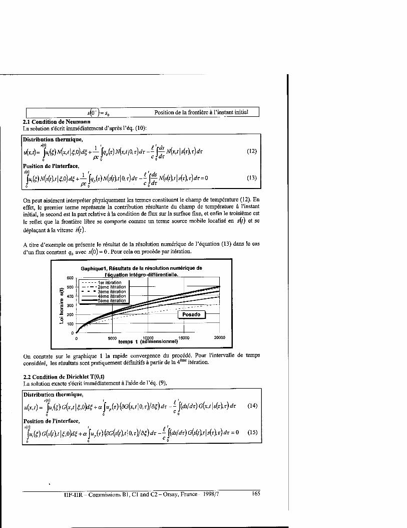
*(0')^ Position de la frontiere ä 1'instant initial

2.1 Condition de Neumann La solution s'ecrit immediatement d'apres l'eq. (10):

Distribution thermique,

Position de 1'interface, s(o) - t 0 * A

L{4)N(s(f\t\4fi)^+- [gp(r)N{s(t),t\0,r)dT -"- \^N{s{f\t\s{r\r)dT = Q o P0 o Co"r

(12)

(13)

On peut aisement interpreter physiquement les termes constituant le champ de temperature (12). En effet, le premier terme represente la contribution resultante du champ de temperature ä l'instant initial, le second est la part relative ä la condition de flux sur la surface fixe, et enfin le troisieme est le reflet que la frontiere libre se comporte comme un terme source mobile localise en s{f) et se

deplacant ä la vitesse s(t).

A titre d'exemple on presente le resultat de la resolution numerique de l'equation (13) dans le cas d'un flux constant q0 avec s(6) = 0. Pour cela on precede par iteration.

Gaphiquel, Resultats de la resolution numerique de l'equation integro-differentielle.

5000 10000 .15000 temps t (adimensionnel)

20000

On constate sur le graphique 1 la rapide convergence du precede. Pour l'intervalle de temps considere, les resultats sont pratiquement definitifs ä partir de la 4 me iteration.

2.2 Condition de Dirichlet T(0,t) La solution exacte s'ecrit immediatement ä l'aide de l'eq. (9),

Distribution thermique,

u{x,t) = J«,fe) G{x,t | e,6)d{ + a J«,(T) (dG{x,t 10, r)/3<?) dz — ]{ds/dr) G[x,t\ S(T),T) dr (14) 0 0 0

Position de I'interface, s(°) ' ('tis \u^)G{s{t),t\^)d^ + a\up{T) {dG(s(t),t\0,z)/d{)dT -"- \{dsl dr) G{s{f),t\s{^) ^ = 0 (15)


Le champ thermique (14) est la solution exacte du probleme. La loi horaire s(t) est donnee par la resolution de l'equation integro-differentielle (15) en utilisant par exemple des techniques numeriques similaires ä celles utilisees pour le flux constant. 2.3 Condition non-Iineaire sur la surface fixe - (dT/äc)xmB = f{f (t))

Considerons une substance qui est, ä l'instant initial, ä l'etat liquide et ä sa temperature de changement d'etat Tf. Supposons que le transfert de chaleur s'effectue ä cause d'une condition non

lineaire - (dr/dc)x^0 = f\Tp{t)). On peut citer de telles conditions rencontrees en physique,

Transfert de chaleur par convection naturelle: - k(dT/dx)^0 = h{fext - T (t)Jl4

Transfert de chaleur par rayonnement: - k(dT/dx)x=0 = aefy -T*(t))

Transfert de chaleur par convection forcee (condition de Fourier) - k(dT/dx)xx0 = hif^ - T (t)).

oil k xonductivite thermique, h : coefficient d'echange, Tm : temperature exterieur.a: Cte de Stefan-Boltzmann et e : l'emissivite.

Pour formuler le probleme de Stefan dans le cas d'un processus de solidification on considere que f(Tp(t)j est une fonction monotone et negative. En vertu de l'eq. (10), on ecrit directement le champ de temperature.

T{x,t)=T, +f )f{Tp(T))N{^0,T)dT+£- jjJvMsftr)* codT

(16)

Oü la temperature de paroi Tp(t) et la loi horaire s(t) sont determinees par la resolution du Systeme

d'equations integro-differentielles non-lineaires suivant,

Tp(t)=Tf+f)f^dr + t)±N(o,t\s(T),T)dT k UTVU-T) cidx

k IM^T) exp

4a(t - r) C » dT cidr

(17)

On a utilise l'approximation quasi-stationnaire de ce probleme avec une condition de Fourier pour interpreter certains aspects du relief martien (Aguirre-Puente J. etal, 1994).

3 UNE NOUVELLE METHODE APPROCHEE

On etablie notre methodologie pour une condition de Neumann, en sachant qu'il est aise de faire de meme pour une condition de Dirichlet. En partant de la solution exacte de la distribution thermique

u{x,t)=— {q(r)N{x,t\0,T)dT-- f— N{x,tU(r),r)rfr pc • c. * dr cfdr

(18)

"a I*.') g{*,l)

On constate que u0(x,t) n'est autre que la solution du probleme de conduction de la chaleur sans

changement de phase soumis ä la meme condition de flux. On peut done interpreter le termeg(x,/) comme une perturbation ä u0(x,t). En posant


En substituant dans 1'equation de la chaleur et en tenant compte des conditions aux limites, il vient

a0{t) = u0(s(tlt); al(t) = (du0/dxlMl) + (p£/k)'S{t) et-a a„^)=-än(t)+'s(t)anM"> 0 (20)

Par consequent, on obtient une nouvelle representation exacte de la solution, sous la forme,

i ' i 'f +0° u{x,t)= — Up(r)N[x,t\Q,r)dr \qp{r)N{s{t),t\0,r)dr -^>„M (21)

P°i , Pi , «-' "„(*.') Sow)

La contrainte pour determiners^)sera l'equation de conservation de l'energie entrex = Oetx = s(t).

1 ' s(2 ±S{t) = — \q{r)dr-C-\u{x,t)dx

P Z o K 0

(22)

(23)

(« + » si la densite de fiuxq(t) est positive et « - » dans le cas contraire) En substituant la solution exacte dans l'equation (22) il vient une nouvelle formule exacte,

± s(t) = — \q{r) erfc(s(t)/24i^)dr + - \g(x,t) dx P <■ o o

En approximant g(x,t) par g0(x,t) on obtient nos formules approchees,

1 ' 1 ' Champ de temperature approchee u{x,t)=— jqp{r)N{x,t\0,T)dT jqp(r)N{s(t),t\0,r)dT (24)

P° o P° 0 »o (■>,')

i V Equation de la hi horaire approchee ± s'(t) = —- \q (r) erfc M- dx +~s'(t) u0(s'(t),t) (25)

P " i \ 2\t — T) i

Cette relation definie, de maniere implicite, la loi horaire approchee /(f). II convient de souligner, qu'ä ce stade de 1'approximation, resoudre le probleme de Stefan uniphasique revient ä r£soudre le meme probleme sans changement de phase car il suffit de determiner u0(x,t). Mieux encore, dans

le cas oü Ton ne parvient pas ä dormer une expression exacte de u0(x,t), on peut employer sa forme integrale equivalente, de sorte que la formule approchee peut s'ecrire de maniere equivalente :

' '(f) ' ± s'(t) = — (Wr) G -4ML dr ou G(x) = erfc(x)+ê w oil p UV/-r) VTT

2 x

4 EXEMPLES

ao 9i ao

(26)

4.1 Flux constant: -k{dT/dx)x,0 =q0>0

ap2f , ap2l2 , / N ap£a{t') , A aplo-fr') _ En variables adimensionnelles: t = ^ t';r = r r';s(t) = ;s\r) = (.2.1)


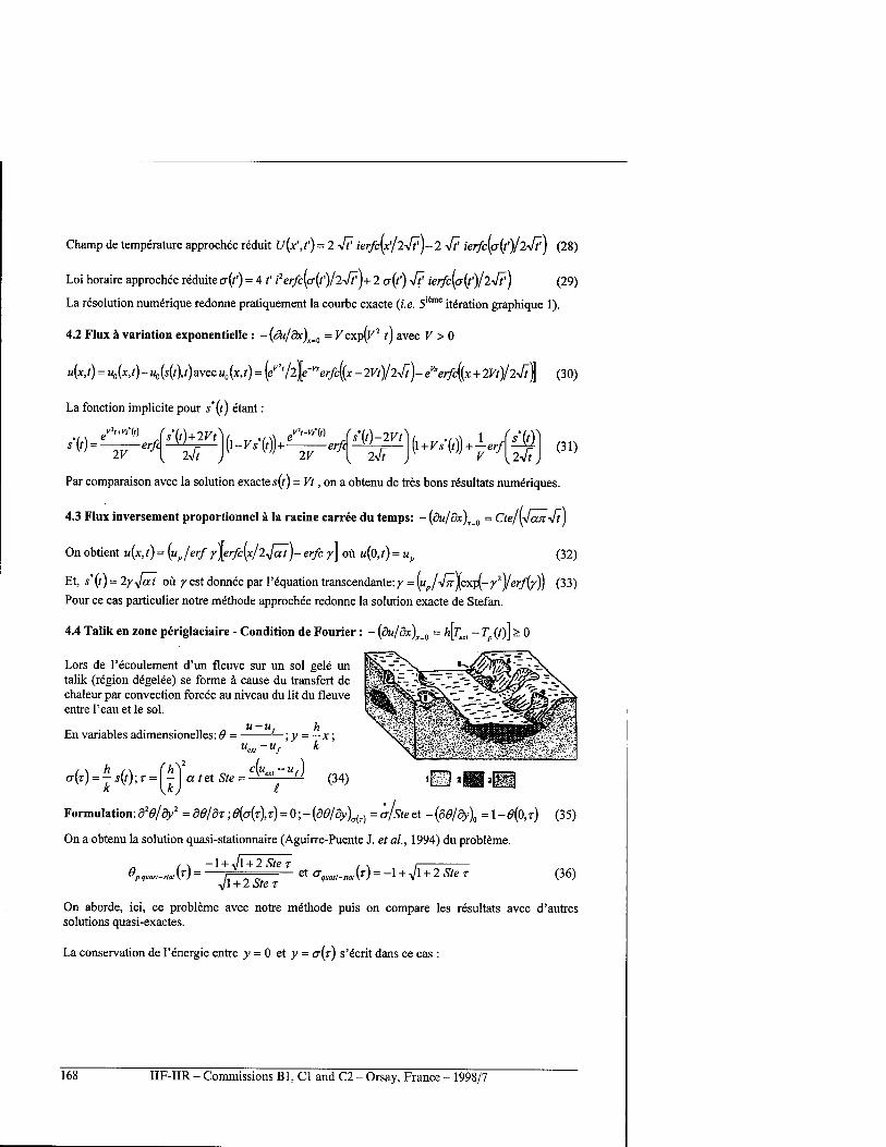
Champ de temperature approchee reduit U(x',f) =2 4? ierfc(x'/2j?)- 2 4? ierfc{p{t')l2-Jt') (28)

Loi horaire approchee reduite a(f) = 4 /' i2erfc[a(t')/2y[p)+ 2 cr(t') 4? ierfc(a(t')/24?) (29)

La resolution numerique redonne pratiquement la courbe exacte (i.e. 5l6me iteration graphique 1).

4.2 Flux ä variation exponentielle : -(ät/dx)x_0 = Vexpty2t) avec V > 0

u{x,t) = u0(x,t) -u0{s(t\t)avec u0{x,t) = [evh fyêrfc^x - 2Vt)/2^)- eVxerf\x + 2Vt)l24i\ (30)

La fonction implicite pour s'(t) etant:

-"ww rjs{f)+2Vi\ S'(t)-

2V -erfc

, ift V ; 2V J\ 2ft

[\+Vs{t)) + -erf 2 ft /

(31)

Par comparaison avec la solution exacte s(t) = Vt, on a obtenu de tres bons resultats numeriques.

4.3 Flux inversement proportionnel ä la racine carree du temps: -(du/dx)xs0 = Ctel\Icm4t)

Onobtient u(x,t) = (up/erf y\erfc[x/2fat)-erfc y\ oü u(0,t) = up (32)

Et, s'(t) = 2yfat oü yestdonn6e par l'equationtranscendante:y = \^p/^Jexp[-y2)/erfi/)) (33)

Pour ce cas particulier notre methode approchee redonne la solution exacte de Stefan.

4.4 Talik en zone periglaciaire - Condition de Fourier: - (du/dx)x=0 = h^, - Tp(t)\ > 0

Lors de l'ecoulement d'un fleuve sur un sol gele" un talik (region degelee) se forme ä cause du transfer! de chaleur par convection forcee au niveau du lit du fleuve entre l'eau et le sol.

En variables adimensionelles: 6 = - h

\y = -*\ u.„-Ur k »or "f

a(r)^ks(t);r = [f\antSte = C^^ (34) 'Pfi!?l

Formulation:d20/dy2 = 5<?/Sr; 0(o-(r),r) = 0; - (S6>/3yLr) = ä/steet -(d0/dy\=l-0(fi,r) (35)

On a obtenu la solution quasi-stationnaire (Aguirre-Puente J. et al, 1994) du probleme.

-1 + ^1 + 2 Sfer „w=- Vl + 2 Ste T

et ff^.-M.W = -1 + Vl + 2Äer (36)

On aborde, ici, ce probleme avec notre methode puis on compare les resultats avec d'autres solutions quasi-exactes.

La conservation de l'energie entre v = 0 et v = CT(T) s'ecrit dans ce cas :


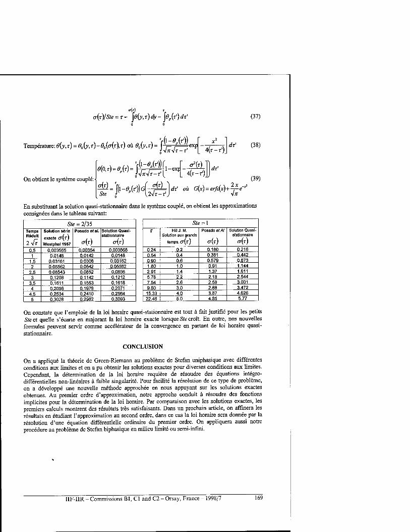
<r(r)

a{r)ISte = T - \e{y,r) dy - J0p(z') dx' (37)

1 (\-6 (r')) Temperature:öCv,r) = 6>0(y,r)-ö0(o-(r),r) oü 0o(y,x) = f\ ," (exp

4(r-r') dr'

On obtient le Systeme couple: Hnsx-x 4(r-r').

rfr1

Ste * \hlT-r) \n

(38)

(39)

En substituant la solution quasi-stationnaire dans le Systeme couple, on obtient les approximations consignees dans le tableau suivant:

Ste = 2/35 Temps Reduit

I4T

Solution serie

exacte G\t) Westphal 1967

Posadoefa/. Solution Quasi- stationnaire

0.5 0.003565 0.00354 0.003565 1 0.0148 0.0142 0.0148

1.5 0.03161 0.0308 0.03162 2 0.05562 0.0542 0.05562

2,5 0.08543 0,0852 0.0856 3 0.1208 0.1142 0.1212

3,5 0.1611 0.1553 0.1618 4 0.2056 0.1978 0.2071

4.5 0.2534 0.2410 0.2564 5 0,3028 0,2982 0.3093

Ste = l T Hill J. M.

Solution aux grands

temps. cr(r)

Posado et Al Solution Quasi- stationnaire

0.24 0.2 0.180 0.216 0.54 0.4 0.381 0.442 0.90 0.6 0.579 0.673 1.80 1.0 0.91 1.144 2.91 1.4 1.37 1.611 5.78 2.2 2.18 2.544 7.54 2.6 2.58 3.001 9.50 3.0 2.88 3.472 15.33 4.0 3.87 4.626 22.46 5.0 4.85 5.77

On constate que l'emploie de la loi horaire quasi-stationnaire est tout ä fait justifie pour les petits Ste et quelle s'ecarte en majorant la loi horaire exacte lorsque Ste croit. En outre, nos nouvelles formules peuvent servir comme accelerateur de la convergence en partant de loi horaire quasi- stationnaire.

CONCLUSION

On a applique la theorie de Green-Riemann au probleme de Stefan uniphasique avec differentes conditions aux limites et on a pu obtenir les solutions exactes pour diverses conditions aux limites. Cependant, la determination de la loi horaire requiere de resoudre des equations integro- differentielles non-lineaires ä faible singularity. Pour facilite la resolution de ce type de probleme, on a developpe une nouvelle methode approchee en nous appuyant sur les solutions exactes obtenues. Au premier ordre d'approximation, notre approche conduit ä resoudre des fonctions implicites pour la determination de la loi horaire. Par comparaison avec les solutions exactes, les premiers calculs montrent des resultats tres satisfaisants. Dans un prochain article, on affinera les resultats en etudiant l'approximation au second ordre, dans ce cas la loi horaire sera donnee par la resolution d'une equation differentielle ordinaire du premier ordre. On appliquera aussi notre procedure au probleme de Stefan biphasique en milieu limite ou semi-infini.

IIF-IIR- Commissions Bl, Cl and C2 - Orsay, France - 1998/7 169

BIBLIOGRAPHIE

1. Aguirre-Puente J., Costard F. and Posado-Cano R., 1994, Contribution to the study of thermal erosion on Mars, J. Geophysical Research, vol.99, no. 3, pp.5657-5667.

2. Canon J. R, 1984, The One-Dimensional Heat Equation, Encyclopedia of Mathematics and its Applications, Vol.23, Gian-Carlo Rota (Ed.), Addison-Wesley Publishing Company, 483 p.

3. Costard F., Aguirre-Puente J. and Posado-Cano R, 1995, Erosion thermique sur Mars, C.R Acad. Sei. Paris, t.320, serie II a, pp.151-155.

4. Goursat E., 1956, Cows d'Analyse Mathematique, Tome 3, Gauthier-Villars, Paris p 146 et p.287.

5. de Hoog F., Weiss R, 1974, High Order Methods for a Class of Volterra Integral Equations with Weakly Singular Kernels, SIAMJ. Num. Anal, vol.11, p.l 166-1181.

6. Lunardini V. J., 1991, Heat Transfer with Freezing and Thawing, Developments in Geotechnical Engineering, 65, Elsevier, Amsterdam, 437 p.

7. Linz P., 1985, Analytical and Numerical Methods for Volterra Equations, SIAM, Philadelphia, 227p.

THE STEFAN PROBLEM: A NEW APPROACH - Application to talik in the glacial zone.

SUMMARY: Stefan-like problems are those problems which admit at least two phases in equilibria usually separated by a sharp or extended front. It is well known that these problems are very difficult to solve from a mathematical view point due to inherent non-linearity induced by the free boundary. For convenience, we only consider monodimensional problems. We present new theoretical results for problems with tractable geometry and with phase change at fixed temperature. We consider some boundary conditions such as the Neumann condition, Dirichlet condition and Fourier condition. An application is made to estimate thickness of thawed ground beneath a river (talik).


PROBLEME DE FRONTIERES LIBRES : MODELISATION, ETUDES EXPERIMENTALES, MELANGES EUTECTIQUES

POSADO CANO R.,* RAMOS M. ** et AGUIRRE-PUENTE J. * *Groupe Planetologie U.M.R. 8616 du C.N.R.S. « ORSAYTERRE » Bätiment 504

Universite de Paris Sud 91405 Orsay- France **Departamento de Fi'sica, Universidad de Alcalä, Alcalä de Henares (Madrid), Espana

RESUME

On aborde ici une generalisation du probleme de Stefan classique en supposant que les phases peuvent presenter une zone de transition. On presente certains resultats theoriques obtenus dans le cas d'une forme geometrique plane concernant les problemes de solidification d'eutectiques. Les melanges eutectiques presentent la propriete de posseder une zone de transition delimitee par la surface liquidus et la surface solidus. En outre, le diagramme d'equilibre de phases de ces solutions binaires montre que la temperature de solidification est fonction de la concentration initiale en solute. On n'aborde que la condition parietale de Dirichlet avec une temperature constante et on modelise la region de changement de phase par une distribution de source de chaleur ce qui permet d'obtenir une solution similitude. On presente, en outre, les mesures experimentales obtenues lors de la solidification d'une solution saline aqueuse NaCl - H20.

INTRODUCTION

L'objectif est l'etude du processus de congelation d'une substance factice, dont les proprietes physiques sont reproductibles, pouvant representer des produits biologiques en contact avec les plaques planes d'un congelateur. Dans ce but, on se propose d'etudier la solidification d'un melange binaire sans diffusion de solute. Une hypothese fondamentale, dans le modele que nous exploitons, est que l'egalite des potentiels chimiques pour chaque espece chimique est instantanee, ce qui signifie qu'en un point jc„de la region biphasique ä l'instant / la temperature est T{xa,i). Le titre d'une espece chimique dans une phase donnee est determine par la lecture du diagramme des phases pour cette temperature.

1. INTERVALLE DE CHANGEMENT DE PHASE POUR LA SOLUTION NaCl - H20.

Le probleme de Stefan classique s'applique ä la solidification de materiaux pour lesquels la frontiere fibre est un front de solidification (fusion) bien defini separant la region liquide de la region solide. Or bien s'en faut pour que toutes les substances changent brutalement de phase avec apparition d'une frontiere fibre ä temperature constante. On entend par extension du probleme de Stefan classique l'etude de la solidification de substances qui possedent un intervalle de solidification limite par deux interfaces isothermes. On a de bonnes raisons de penser que la congelation de certains sols possedant une distribution porosimetrique raisonnable (pores ni trop petits comme l'argile ni trop gros comme le gravier) peut etre assimilee ä cette categorie de probleme. Les materiaux biologiques sont difficilement utilisables, lors de travaux experimentaux, ä cause de leurs compositions heterogenes et de leurs proprietes variables qui ne permettent pas l'obtention de mesures reproductibles et systematiques. A cet effet, on choisi la solution saline aqueuse NaCl - H20 comme modele de materiau ä changement de phase sur un intervalle de temperature. Le choix de cette substance permet de faire des mesures reproductibles et en outre les constituants chimiques NaCl etH20 qui sont les composants de base de la solution aqueuse sont tres abondants


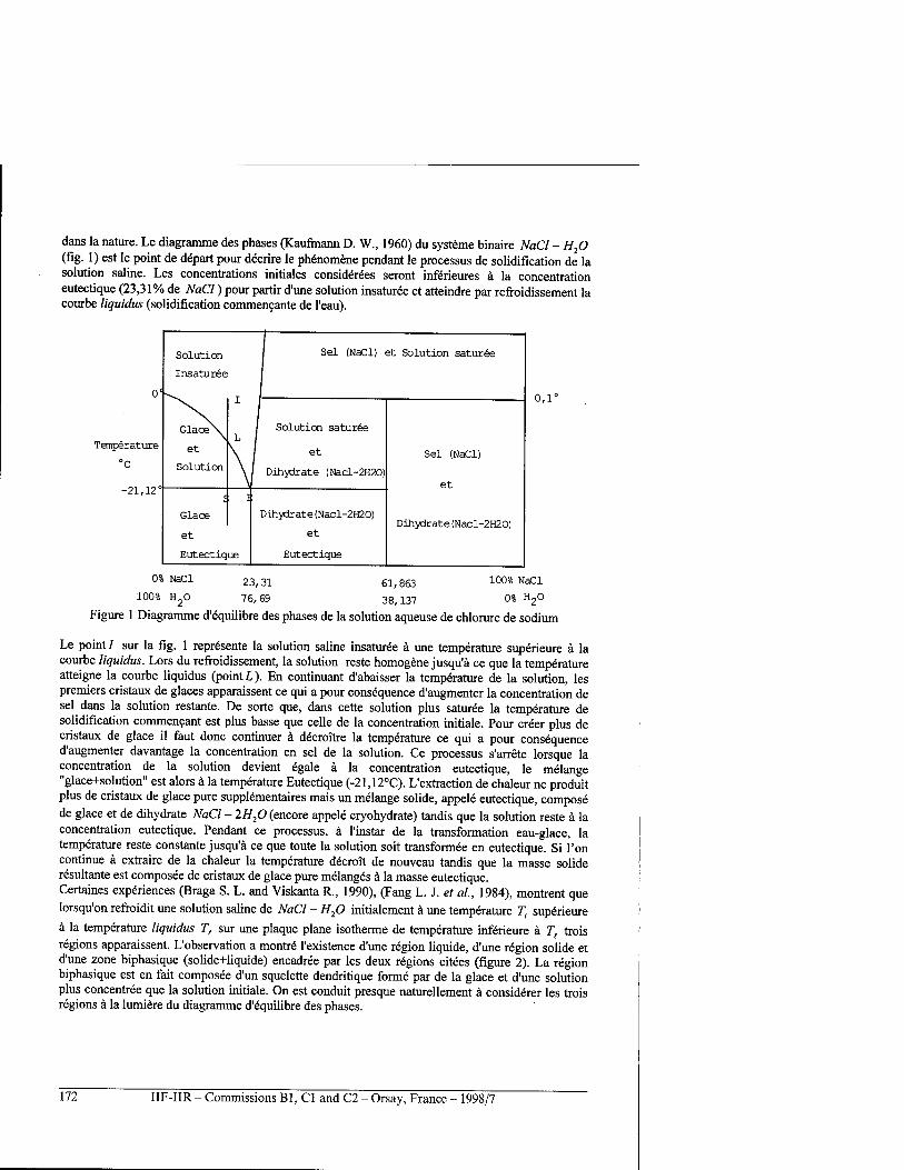
dans la nature. Le diagramme des phases (Kaufmann D. W., 1960) du Systeme binaire NaCl - H20 (fig. 1) est le point de depart pour decrire le phenomene pendant le processus de solidification de la solution saline. Les concentrations initiales considerees seront inferieures ä la concentration eutectique (23,31% de NaCl) pour partir d'une solution insaturee et atteindre par refroidissement la courbe liquidus (solidification commen9ante de l'eau).

Temperature

°C

-21,12'

Solution 1 Sei (NaCl) et Solution saturee

Insaturee

Glace\ L

/ Solution saturee

et \ J et Sei (NaCl)

Solution

\ Dihydrate (Nacl-2H20)

et c I

Glace

et

Dihydrate (Nacl-2H20)

et Dihydrate (Nacl-2H20)

Eutectique Eutectique

0,1°

0% NaCl 23,31 61,863 100i NaCl

100% H20 76,69 38,137 0% H2°

Figure 1 Diagramme d'equilibre des phases de la solution aqueuse de chlorure de sodium

Le point/ sur la fig. 1 represente la solution saline insaturee ä une temperature superieure ä la courbe liquidus. Lors du refroidissement, la solution reste homogene jusqu'ä ce que la temperature arteigne la courbe liquidus (pointL). En continuant d'abaisser la temperature de la solution, les premiers cristaux de glaces apparaissent ce qui a pour consequence d'augmenter la concentration de sei dans la solution restante. De sorte que, dans cette solution plus saturee la temperature de solidification commencant est plus basse que celle de la concentration initiale. Pour creer plus de cristaux de glace il faut done continuer ä decroitre la temperature ce qui a pour consequence d'augmenter davantage la concentration en sei de la solution. Ce processus s'arrete lorsque la concentration de la solution devient egale ä la concentration eutectique, le melange "glace+solution" est alors ä la temperature Eutectique (-21,12°C). L'extraction de chaleur ne produit plus de cristaux de glace pure supplementaires mais un melange solide, appele eutectique, compose de glace et de dihydrate NaCl - 2H20 (encore appele cryohydrate) tandis que la solution reste ä la concentration eutectique. Pendant ce processus, ä l'instar de la transformation eau-glace, la temperature reste constante jusqu'ä ce que toute la solution soit transformed en eutectique. Si Ton continue ä extraire de la chaleur la temperature decroit de nouveau tandis que la masse solide resultante est composee de cristaux de glace pure melanges ä la masse eutectique. Certaines experiences (Braga S. L. and Viskanta R., 1990), (Fang L. J. et al, 1984), montrent que lorsqu'on refroidit une solution saline de NaCl - H20 initialement ä une temperature T, superieure

ä la temperature liquidus Tt sur une plaque plane isotherme de temperature inferieure ä T, trois regions apparaissent. L'observation a montre l'existence d'une region liquide, d'une region solide et d'une zone biphasique (solide+liquide) encadree par les deux regions citees (figure 2). La region biphasique est en fait composee d'un squelette dendritique forme par de la glace et d'une solution plus concentree que la solution initiale. On est conduit presque naturellement ä considerer les trois regions ä la lumiere du diagramme d'equilibre des phases.


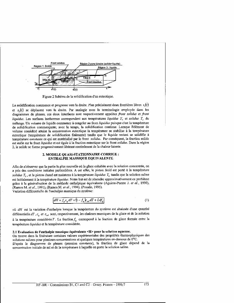
Front solidus Region 2:zone binaire (solide+liquide)

/ Region 3: liquide

Figure 2 Schema de la solidification d'un eutectique.

La solidification commence et progresse vers la droite. Plus precisement deux frontieres libres s,(f)

et s2(t) se deplacent vers la droite. Par analogie avec la terminologie employee dans les diagrammes de phases, ces deux interfaces sont respectivement appelees front solidus et front liquidus. Les surfaces isothermes correspondent aux temperatures liquidus T, et solidus Ts du melange. Un volume de liquide commence ä congeler au front liquidus puisque c'est la temperature de solidification commencante; avec le temps, la solidification continue. Lorsque l'element de volume considere atteint la concentration eutectique la temperature se stabilise ä la temperature eutectique (temperature de solidification finissante) tandis que le liquide restant se solidifie ä temperature constante ce qui est materialise par le front solidus. Par consequent, la fraction solide est nulle sur le front liquidus et est egale ä la fraction eutectique sur le front solidus. Dans la region 2, le solide se forme progressivement liberant continüment de la chaleur latente.

2. MODELE QUASI-STATIONNAIRE CORRIGE : ENTHALPIE MASSIQUE EQUIVALENTE

Afin de n'observer que la partie la plus nouvelle oü la glace cohabite avec la solution concentree, on a pris des conditions initiales particulieres. A cet effet, le piston froid est porte ä la temperature solidus Ts , et le piston chaud est maintenu ä la temperature liquidus TL tandis que la solution saline est initialement ä la temperature liquidus. Notre but est de resoudre approximativement ce probleme grace ä la generalisation de la methode enthalpique equivalente (Aguirre-Puente J. et al, 1990), (Ramos M. et al, 1991), (Ramos M. et al, 1994), (Posado, 1995). Variation differentielle de l'enthalpie massique du Systeme:

dH = fgcgdT + (1 - fX,dT + Ldfg (1)

oü dH est la variation d'enthalpie lorsque la temperature du Systeme est abaissee d'une quantite differentielle dT, cg et cml sont, respectivement, les chaleurs massiques de la glace et de la solution

ä la temperature considered 7\ La fraction/g correspond ä la fraction de glace formee entre la

temperature liquidus et la temperature consideree.

2.1 Evaluation de l'enthalpie massique equivalente <H> pour la solution aqueuse. On trouve dans la litterature certaines valeurs experimentales des proprietes thermophysiques des solutions salines pour plusieurs concentrations et quelques temperatures en-dessous de 0°C. D'apres le diagramme de phases (pression constante), la fraction de glace depend de la concentration initiale de sei et de la temperature ä laquelle on porte la solution saline.


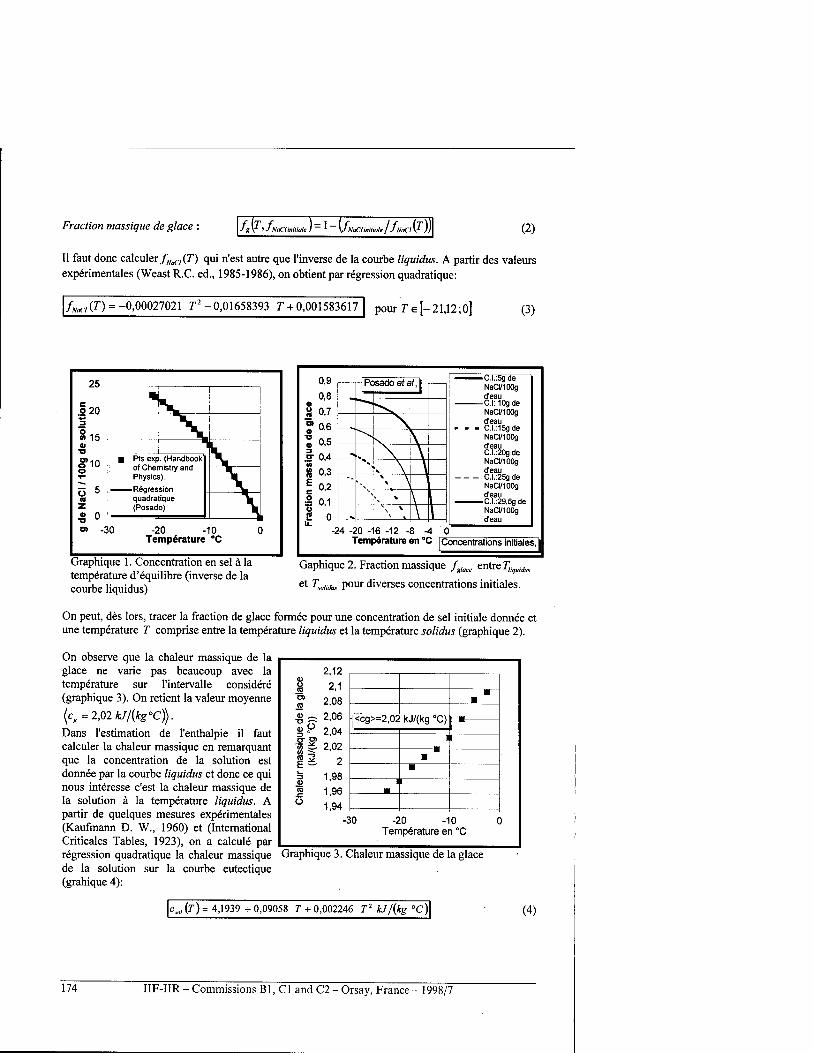
Fraction massique de glace : fg {T, fNaai„illale) = 1 - (fNaCIMiale /fNaC, (T)) (2)

II faut done calcvier fNaCJ(T) qui n'est autre que l'inverse de la courbe liquidus. A partir des valeurs experimentales (Weast R.C. ed., 1985-1986), on obtient par regression quadratique:

fmiV) = -0,00027021 T1 -0,01658393 T + 0,001583617 pour 7/e[-21,12; O] (3)

25

§20

S 15

SMo o

n 5

o •a a -30

:

■ Rs exp. (Handbook

Physics).

Regression quadratique (Posado)

-20 -10 Temperature "C

Graphique 1. Concentration en sei ä la temperature d'equilibre (inverse de la courbe liquidus)

0,9 0,8 0,7 0,6 0,5 0,4 0,3 0,2 0,1

0

N

s \

N \ \

*. \ V

« \

C.l.:5g de NaCI/100g d'eau

—C.I: 10gde NaCI/100g d'eau

- C.l.:15gde NaO/100g d'eau C.l.:20g de NaQ/100g d'eau

- C.l.:25gde NaCI/100g d'eau

—C.l.:29,5gde NaCI/100g d'eau

-24 -20 -16 -12 -8 -4 Temperature en °C Concentrations initiales,

Gaphique 2. Fraction massique fglace entreTlll/uidm

et Tmlidm pour diverses concentrations initiales.

On peut, des lors, tracer la fraction de glace formee pour une concentration de sei initiale donnee et une temperature T comprise entre la temperature liquidus et la temperature solidus (graphique 2).

On observe que la chaleur massique de la glace ne varie pas beaucoup avec la temperature sur l'intervalle considere (graphique 3). On retient la valeur moyenne

(c„ =2,02 kJ/{kg°C)).

Dans l'estimation de l'enthalpie il faut calculer la chaleur massique en remarquant que la concentration de la solution est donnee par la courbe liquidus et done ce qui nous interesse e'est la chaleur massique de la solution ä la temperature liquidus. A partir de quelques mesures experimentales (Kaufmann D. W., 1960) et (International Criticales Tables, 1923), on a calcule par regression quadratique la chaleur massique de la solution sur la courbe eutectique (grahique 4):

(D o J5

1? (0 3

2,12

2,1 2,08 2,06 2,04 2,02

2 1,98 1,96 1,94

II ■

j ^-y—'."i

l

■ u

I 1

-30 -20 -10 Temperature en °C

Graphique 3. Chaleur massique de la glace

Cw (T) =4,1939 +0,09058 T + 0,002246 T2 kJ/(kg °C) (4)


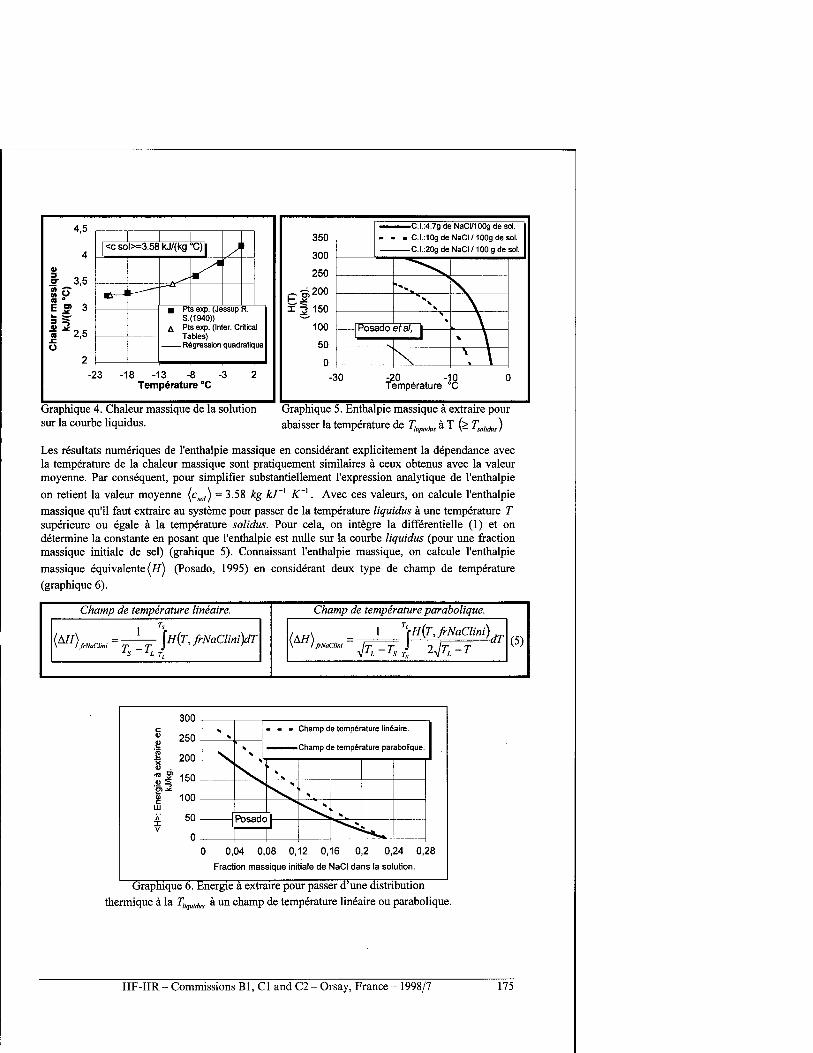
4,5

_3,5 O e

3 3

!2,5

2

Rs exp. (Jessup R S.(1940))

A Pts exp. (Inter. Critical Tables)

Regression quadratique

-23 -18 -13 -8 -3 Temperature °c

350

300

250

—C.l.:4.7g de NaCI/100g de sol.

■ C.I.:10gdeNaCI/100gdesol. —C.l.:20g de NaCI /100 g de sol.

-20 -IC Temperature

Graphique 4. Chaleur massique de la solution sur la courbe liquidus.

Graphique 5. Enthalpie massique ä extraire pour abaisser la temperature de TliqMu, ä T (> rW/ÄV)

Les resultats numeriques de l'enthalpie massique en considerant explicitement la dependance avec la temperature de la chaleur massique sont pratiquement similaires ä ceux obtenus avec la valeur moyenne. Par consequent, pour simplifier substantiellement l'expression analytique de l'enthalpie

on retient la valeur moyenne (c,0,) = 3.58 kg kJ'! K']. Avec ces valeurs, on calcule l'enthalpie massique qu'il faut extraire au Systeme pour passer de la temperature liquidus ä une temperature T superieure ou egale ä la temperature solidus. Pour cela, on integre la differentielle (1) et on determine la constante en posant que l'enthalpie est nulle sur la courbe liquidus (pour une fraction massique initiale de sei) (grahique 5). Connaissant l'enthalpie massique, on calcule l'enthalpie

massique equivalente (//) (Posado, 1995) en considerant deux type de champ de temperature (graphique 6).

Champ de temperature lineaire.

(AH) 1

frNaClini T,-T,

'S

JH{T,frNaClini)dT LTL

Champ de temperature parabolique.

(AH) ftNaClin -T.. J Vî Ts Ts

HJT, frNaClini) dT (5)

•<0 ff <u S

300

250

200

150

100

50

s Champ de temperature lineaire.

s ■■!■■ ■■'■ Champ de temperature parabolique.

. s i

s

,\ ^^ s

^ Posadc ̂ l r- r 0 0,04 0,08 0,12 0,16 0,2 0,24 0,28

Fraction massique initiale de NaCI dans la solution.

Graphique 6. Energie ä extraire pour passer d'une distribution thermique ä la Tliquidm ä un champ de temperature lineaire ou parabolique


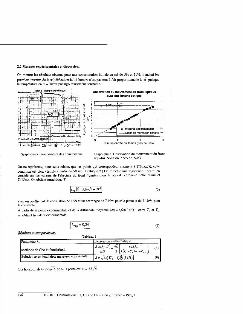
2.2 Mesures experimentales et discussion.

On montre les resultats obtenus pour une concentration initiale en sei de 5% et 10%. Pendant les

premiers instants de la solidification la loi horaire n'est pas tout ä fait proportionnelle ä -ft puisque la temperature enx = 0 n'est pas rigoureusement constante.

Piston ä latempSraturesolidiis Observation du mouvement du front liquidus avec une lunette optique

-■fc-hj-.iä 3ffäEti.-j 2(<fA?*£ii "| fp.'-r-*': J=Qi"~i:=t -i'*fei

Graphique 7. Temperature des deux pistons.

1 2 Racine carree du temps (t en heures)

Graphique 8. Observation du mouvement du front liquidus. Solution ä 5% de NaCl

On ne represente, pour cette raison, que les points qui correspondent vraiment ä T(0,t)=Ts; cette condition est bien verifiee ä partir de 50 mn (Grahique 7.) On effectue une regression lineaire en considerant les valeurs de l'abscisse du front liquidus dans la periode comprise entre 50mn et 5hl5mn. On obtient (graphique 8):

*=xP(')=5,09VF-10- (6)

avec un coefficient de correlation de 0,99 et un ecart type de 7.10"6 pour la pente et de 7.10-4 pom- la constante. A partir de la pente experimentale et de la diffusivite moyenne (a) = 5,610"7m2^"' entre TL et Tp,

on obtient la valeur experimentale:

Aexp=0,34

Resultats et comparaisons. Tableau 1

Loi horaire: s(t)=2Ä-Jat done la pente est m = 2X-[a

(7)

Parametre X. Expression mathematique.

Methode de Cho et Sunderland Aexp(-A2)_V^

erß 2 apLfm

Jc{TL-Ts) + apLfc„ (8)

Solution avec l'enthalpie massique equivalente. A = #)(^-^)J/[2(//)J (9)


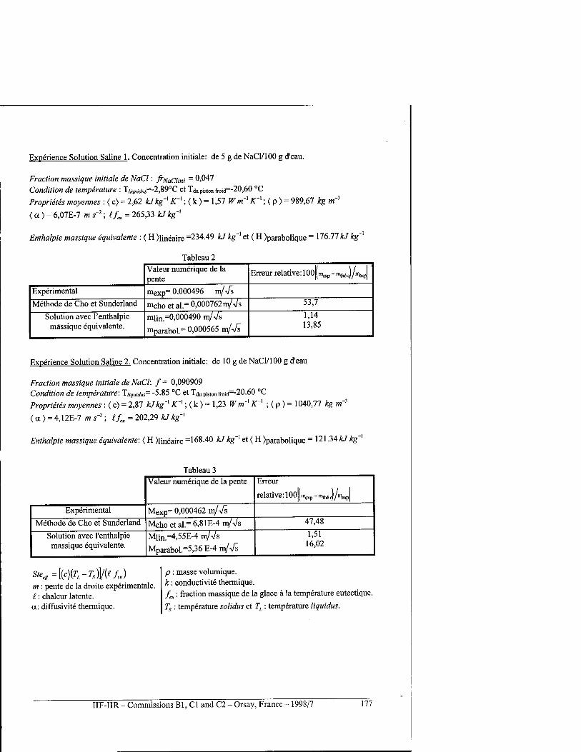
Experience Solution Saline 1. Concentration initiale: de 5 g de NaCl/100 g d'eau.

Fraction massique initiale de NaCl: frâCiim = 0,047 Condition de temperature : T;/,„waj=-2,89°C et Tdu piston froicT-20,60 °C

Proprietes moyennes : ( c) = 2,62 kJkg'x K']; < k ) = 1,57 W tnx K'1; ( p ) = 989,67 kg m'3

( a ) = 6,07E-7 m s'2; Hfm = 265,33 kJ kg'1

Enthalpie massique äquivalente : < H >Hneaire =234.49 kJ kg'' et ( H )parabolique = 176.77 kJ kg'

Tableau 2 Valeur numerique de la pente

Erreur relative: 100 imexp-mthäc)/n1exp

Experimental mexp= 0,000496 nV Vs Methode de Cho et Sunderland mcho et al.= 0,000762 m/Ä/s 53,7

Solution avec l'enthalpie massique equivalente.

mlin.=0,000490 m/Vs

mparabol.= 0,000565 m/Vs

1,14 13,85

Experience Solution Saline 2. Concentration initiale: de 10 g de NaCl/100 g d'eau

Fraction massique initiale de NaCl: f= 0,090909 Condition de temperature: TuqUidus= -5.85 °C et T<ju piston froid=-20.60 °C Proprietes moyennes : < c> = 2,87 kJkg'1 K']; < k > = 1,23 Wm'x K~] ; < p ) = 1040,77 kg m'3

< a > = 4.12E-7 m s'2; lfeu = 202,29 kJ kg'1

Enthalpie massique equivalente: ( H )lineaire =168.40 kJ kg'x et < H )parabolique = 121.34AJ kg'

Tableau 3 Valeur numerique de la pente Erreur

relative: 1 OOln^ - n^ J/n^l

Experimental Mexp= 0,000462 m/Vs Methode de Cho et Sunderland Mcho et al.= 6.81E-4 m/Vs 47,48

Solution avec l'enthalpie massique equivalente.

Miin.=4,55E-4 m/Vs

Mparabol.=5,36 E-4 m/Vs

1,51 16,02

Steeir=[(c){TL-Ts)]/(efJ m : pente de la droite experimentale. I: chaleur latente. a: diffusivite thermique.

p: masse volumique. k: conductivite thermique. feu: fraction massique de la glace ä la temperature eutectique.

Ts : temperature solidus et TL : temperature liquidus.


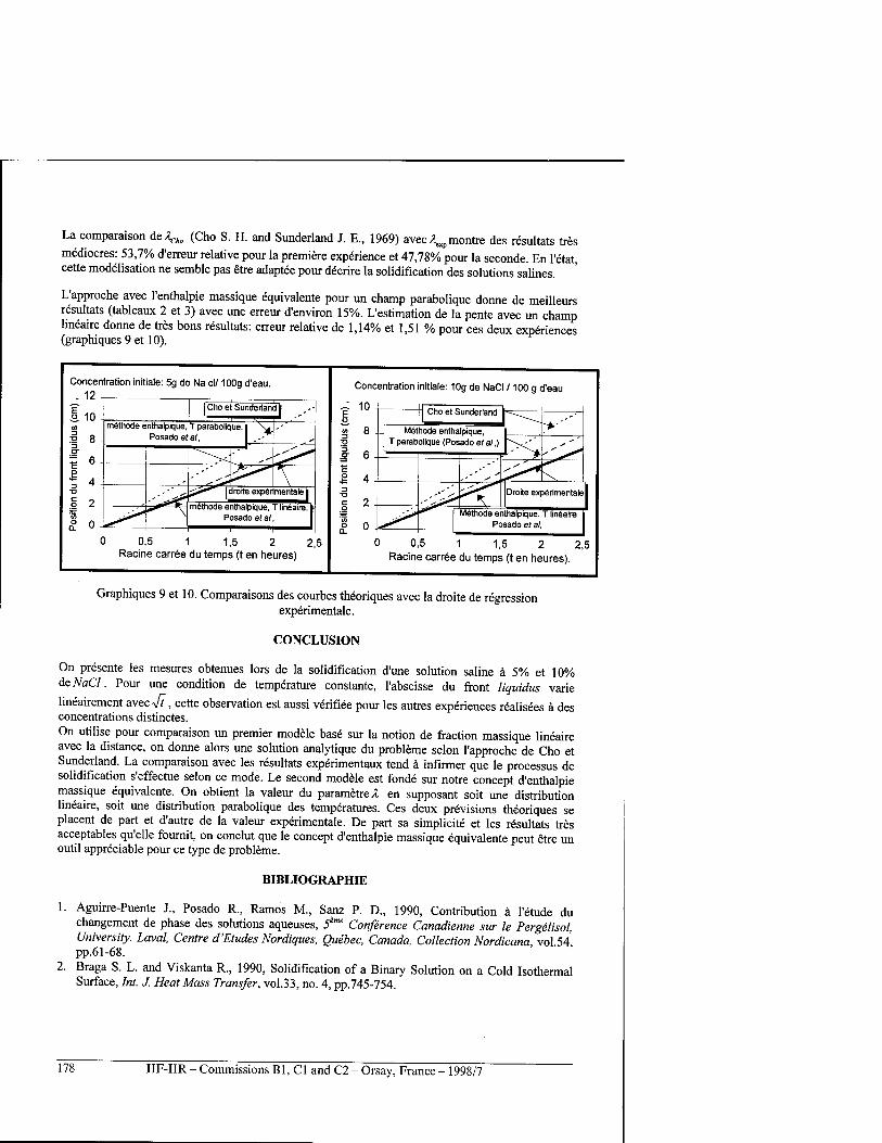
La comparison deACA„ (Cho S. H. and Sunderland J. E., 1969) avecA^montre des resultats tres mediocres: 53,7% d'erreur relative pour la premiere experience et 47,78% pour la seconde. En l'etat, cette moderation ne semble pas etre adaptee pour decrire la solidification des solutions salines.

L'approche avec l'enthalpie massique equivalente pour un champ parabolique donne de meilleurs resultats (tableaux 2 et 3) avec une erreur d'environ 15%. L'estimation de la pente avec un champ lineaire donne de tres bons resultats: erreur relative de 1,14% et 1,51 % pour ces deux experiences (graphiques 9 et 10).

Concentration initiate: 5g de Na cl/ 100g d'eau.

. 12

I 10 -. i Cho et Sunderland I

methode enthalpique, T parabolique. Posado eta/,

droite expenmentale

methode enthalpique, T lineaire. Posadoeta/,

0 0,5 1 1,5 2 2,5 Racine carree du temps (t en heures)

Concentration initiale: 10g de NaCI /100 g d'eau

10 Cho et Sunderland

Methode enthalpique, T lineaire Posado eta/,

0 0,5 1 1,5 2 2,5 Racine carree du temps (t en heures).

Graphiques 9 et 10. Comparaisons des courbes theoriques avec la droite de regression experimentale.

CONCLUSION

On presente les mesures obtenues lors de la solidification d'une solution saline ä 5% et 10% deNaCl. Pour une condition de temperature constante, l'abscisse du front liquidus varie

lineairement avec 4~t, cette observation est aussi verifiee pour les autres experiences realisees a des concentrations distinctes. On utilise pour comparaison un premier modele base sur la notion de fraction massique lineaire avec la distance, on donne alors une solution analytique du probleme selon l'approche de Cho et Sunderland. La comparaison avec les resultats experimentaux tend ä infirmer que le processus de solidification s'effectue selon ce mode. Le second modele est fonde sur notre concept d'enthalpie massique equivalente. On obtient la valeur du parametreA en supposant soit une distribution lineaire, soit une distribution parabolique des temperatures. Ces deux previsions theoriques se placent de part et d'autre de la valeur experimentale. De part sa simplicity et les resultats tres acceptables qu'elle fournit, on conclut que le concept d'enthalpie massique equivalente peut etre un outil appreciable pour ce type de probleme.

BIBLIOGRAPHIE

1. Aguirre-Puente J., Posado R, Ramos M., Sanz P. D., 1990, Contribution ä l'etude du changement de phase des solutions aqueuses, 5ime Conference Canadienne sur le Pergelisol, University. Laval, Centre d'Etudes Nordiques, Quebec, Canada, Collection Nordicana vol 54 pp.61-68. ' ' '

2. Braga S. L. and Viskanta R., 1990, Solidification of a Binary Solution on a Cold Isothermal Surface, Int. J. Heat Mass Transfer, vol.33, no. 4, pp.745-754.


3. Cho S. H. and Sunderland J. E., 1969, Heat-Conduction with Melting or Freezing, J. Heat Transfer, pp. 421-426.

4. Fang L. J., Cheung F. B., Linehan J. H., Pedersen D. R., 1984, Selective Freezing of a Dilute Salt Solution on a Cold Ice Surface, J. Heat Transfer, vol. 106, pp. 385-393.

5. International Critical Tables, 1923, M. Craw-Hill, NW, vol. Ill, pp.327-328 6. Kaufmann D. W., 1960, Sodium Chloride: The Production and Properties of Salt and Brine, Am.

Chem. Soc, Monograph Series, Reinhold Publishing Corporation, N.Y, 7. Posado Cano R. (1995), Probleme de Stefan: Etudes Theoriques et Experimentales pour des

Substances Pures et des Melanges Eutectiques, These, Universite Paris 7. 8. Ramos M., Aguirre-Puente J., Posado R., 1991, Nueva aproximaciön al estudio de los procesos

de congelaciön mediante la defmiciön de un calor latente efectivo, Anales defisica, vol. 87, pp. 92-107.

9. Ramos M., Sanz P. D., Aguirre-Puente J. and Posado R., 1994, Use of the equivalent volumetric enthalpy variation in non-linear phase-change processes: freezing-zone progression and thawing-time determination, Int. J. Refrig., vol.17, no.6, pp.374-380.

10. Weast R.C. ed., 1985-1986, Handbook of Chemistry and Physics, 66th edition, CRC Press, Florida.

FREE BOUNDARY PROBLEMS: MODELLING, EXPERIMENTAL STUDIES, BINARY EUTECTIC MIXTURES

SUMMARY: We study a generalisation of the classic Stefan problem by assuming that phases could admit an extended range of transition. We present some theoretical results in plane geometry for freezing eutectic problems. Eutectic mixtures exhibit a definite zone of phase change delimited by isothermal planes at the liquidus and solidus temperatures. An equilibrium phase diagram shows that these binary mixtures are function of the initial solute concentration. We only consider the Dirichlet condition with a constant wall temperature and we model the freezing zone by a uniform distribution of heat source which leads to a similarity solution of the problem. Finally, we compare theoretical results with experimental data obtain by solidification of an aqueous saline solution

NaCl-H20.


MODELLING AND SIMULATION OF HEAT AND MASS TRANSFER DURING FREEZING AND STORAGE OF UNPACKED FOODS

CAMPANONE L.A.1 '\ SALVADORI V.O.12, and MASCHERONI R.H.12

'CIDCA (Centro de Investigation y Desarrollo en Criotecnologia de Alimentos, UNLP-CONICET) 47 y 116 - (1900) La Plata, ARGENTINA

2MODIAL, Facultad de Ingenieria, Universidad National de La Plata, ARGENTINA e-mail: [email protected]

ABSTRACT

Dehydration of unwrapped foods occurs during freezing and frozen storage. Coupled heat and mass balances were proposed considering solidification of water and sublimation of ice. The mathematical model was solved using an Implicit Finite-Differences Method, with variable grid to follow the moving front of sublimation. The model enables to evaluate temperature and water concentration profiles and was used to predict kinetics of weight loss for different products.

INTRODUCTION

Weight losses occurs during freezing, storage and transport of foods in unwrapped state. Ice sublimation originates a dehydrated surface layer that changes appearance, colour, texture and taste. Furthermore in the industry it becomes an important economic factor. Ice sublimation has been surveyed by several authors in different systems: in freeze-drying (Mellor,1974; Kochs et al, 1990), in geomorphology (Aguirre Puente et al, 1978) and in the case of frozen products several experimental studies have been published: weight losses of lamb (Pham and Willix, 1984), tylose and beef (Sukhwal and Aguirre Puente,1983) and potatoes (Lambrinos and Aguirre Puente, 1983). Theoretical models were proposed but in most of the works semi-empiric models are used. Pham and Willix (1984) suggested the use of simple equations based on the drying theory and on the use of psycrometric chart to calculate weight loss. A description of the heat and mass balances were presented by Sukhwal and Aguirre Puente (1983). In this work the modelling of weight loss during freezing and frozen storage has been done. Coupled heat and mass balances were solved. The thermophysical properties were considered variables with the temperature and the state of the product (frozen, unfrozen and dehydrated). Two phase changes were included in the model: liquid to solid and solid to vapour. Solidification is considered through a variable apparent heat capacity and a numerical method that uses a fixed grid (Cleland, 1990). Meanwhile ice sublimation can be adequately modelled by a moving front and the same numerical method, but with variable grid, because of its very low displacement rate as compared to that of the solidification process (Marshall et al, 1986). The objective of this work is to develop a physical model and to implement the related numerical method that enable us to account for the influence of food characteristics and process variables on the freezing time, weight loss and on the growing rate of the dehydrated surface layer.

1 THEORY

Heat and mass transfer between food and environment, as both phase changes water-to-ice (freezing) and ice-to-water vapor (sublimation) are the main phenomena involved during food


freezing. From a physical point of view, food can be considered as a combination of a solid matrix, an aqueous phase and a gaseous phase (air and water vapor). Ice sublimation takes place within the frozen zone, leading to a dried layer with a porous structure. Thus, water vapor transfer to the surrounding medium occurs through this layer. It should be stressed, that part of the ice remains adsorbed to the food matrix depending on the local vapor-ice equilibrium conditions (Chumak and Sibiriakov, 1988). Vapor flow can be considered mainly as a diffusive flow passing throughout the dried layer, being the driving force the difference in water vapor pressure between the sublimation front and the environment. Fick's law was considered valid. According to the former system description, heat and mass balances can be stated in three zones: unfrozen, frozen and dehydrated zones. The analysis was performed for several geometries. For the unfrozen and frozen zones (0 < x < xi), the following energy balance was applied:

pCp*L=*JL*L + k*U- + IGL*L (i) H dt dx dx dx1 x dx

where x is the axial or radial coordinate, xi is the position of the sublimation front, p, k and Cp are, respectively, the density, thermal conductivity and apparent heat capacity of the food, which depend on temperature and composition. Apparent heat capacity involves both sensible specific heat and the enthalpy of ice fusion. IG is the geometric index, its value is zero for slabs, one for cylinders and two for spheres. For the dehydrated zone (xi < x < L) the following balance was applied:

p' Fd dt dx d x ' dx1 x dx where L is the half-thickness (slab) or radius (cylinder or sphere) of the product, pd, k<i and Cpa are the density, thermal conductivity and heat capacity of the dehydrated layer, which depend on temperature and composition. The microscopic mass balance applied to this zone was the following:

£?C^=^^+D f^+/G^f^, (3) dt dx dx " dx1 x dx

where e is the porosity of the dehydrated zone, Cra is the molar concentration of water vapor and Dv is the effective diffusion coefficient of water vapor in the porous medium, for which porosity and tortuosity factors are considered; Dv is also a function of temperature (Harper, 1962). For the energy balance the following boundary conditions can be stated:

x = 0 -*^=° ' (4) dx

x = L -kd^-=h(T-Ta) (5) dx

where h is the heat transfer coefficient and Ta is the bulk air temperature. Boundary conditions for the mass balance were:

* = *, Pva=Psa,(T) (6)

x = L -D,^=km(C„-C.) C7) dx

where km is the mass transfer coefficient, Ca is the molar concentration of vapor water in the air and Psat(T) is the vapor saturation pressure of ice, which depends on temperature. To better describe the physical situation, boundary conditions were stated at sublimation front (x = xi) as follows:

-k^L=LsmLd-f\-k/Ji (8)

dx s s\ dt) " dx


du _ t/,„+, - u, dt Ar

dU _ UM„X ~ £/,.,,.», + UM, - U,. dx 4 Ax

d'U _ UM„t + £/,.,,„„ - 2U,ntX + UMJ, + U,_,, - 2U,

_W^L=_^^ (9) * dt RT dx

»,=^>,0-/J (10) where y0 is the water content and w is the ice mass fraction (Mascheroni and Calvelo, 1978), which is a function of temperature, Ls is the heat of ice sublimation, f^ is the ice fraction (without sublimation) that remains adsorbed at the surface of dried fibers (Chumak and Sibiriakov, 1988) and dxi is the shift of sublimation front position with time. Balances were solved using different properties for unfrozen, frozen and dehydrated zones.

2 MATHEMATICAL MODEL

Equations (1), (2), (3) and (8) led to a system of coupled non-linear partial differential equations. The system is solved by an Implicit Finite-Differences Method (Crank-Nicolson centred method).A variable grid is applied to overcome the deformation of the original fixed grid due to the shift of the sublimation front. Finite differences generated are:

(11)

(12)

(13) dx' 2 Ax2

where U is temperature or concentration, i denotes the node position and n the time. Assuming that conductivity and the diffusion coefficient have a negligible change between times n and (n+1) At, one gets:

ßv V -V vv _ " I*'.K ''-'," (]4\

dx 2 Ax where V is thermal conductivity or diffusion coefficient. By replacing eqns. (11), (12), (13) and (14) in the energy balance (eq. (1)) the general equation to estimate temperatures of unfrozen, frozen was obtained. This equation is valid for 0 < i < m-2, being m the i value for the node that corresponds to the moving front. For the centre point (i=0), one fictitious point has to be evaluated. The boundary condition of eq. (4) was used to calculate the fictitious temperatures Ti_iin and THÎ.

In point (m-1) a discontinuity was produced because towards the frozen zone space increments were fixed (Ax), however towards the food surface, grid increments were variable since point m moved with time. Using a finite differences scheme which takes into account the variable increment the general expression was obtained. For the moving front (i=m), the discretization of the general equation showed two fictitious values, T i+ij, and T i+i,n+i; to evaluate them condition (8) was used. To solve the energy balance in the dehydrated zone (eq.(2) the partial derivatives should be replaced by the finite differences (11), (12), (13) and (14). Thus, the general equation for the intermediate points (m<i<b) was obtained. For the food surface (i = b), two fictitious points arose and were evaluated by means of boundary condition (5). To evaluate the vapor concentration profile within the dehydrated layer, the mass balance should be discretized using the finite differences (11),(12),(13) and (14). For the front of sublimation, the vapour pressure is the saturation pressure. At (i=b), the fictitious values (n+1) were evaluated using boundary condition (7). Campanone etal (1998) gives a detailed description of the whole system of equations. Finally, eq. (9) was discretized to calculate the moving front shift:


(*■„♦■ -*■.)

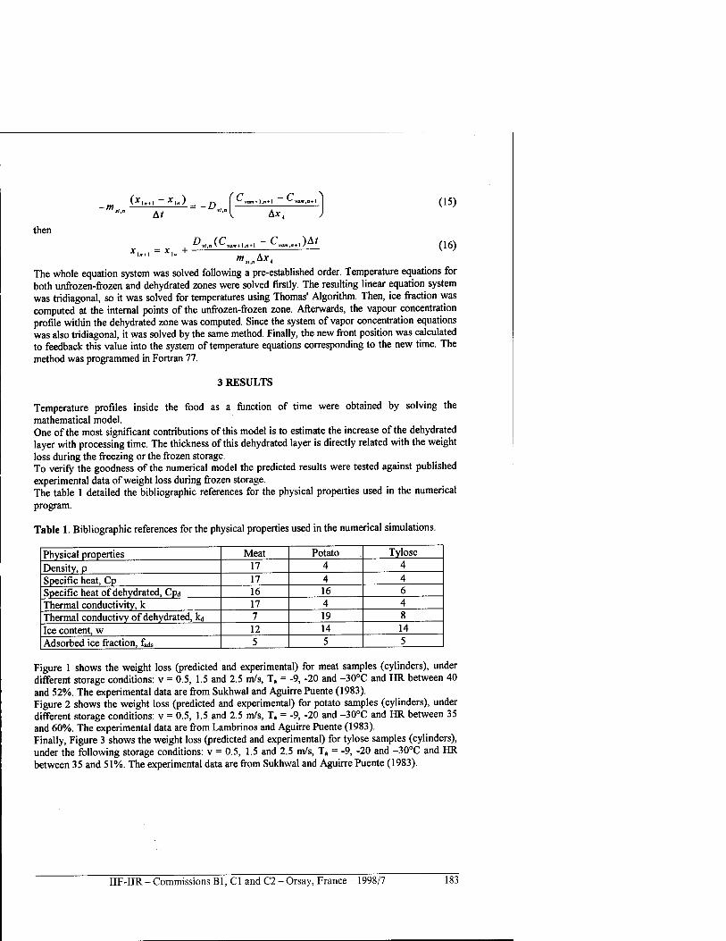
At

then

- D (C- -c

--D„,[ Ax4

D,,AC,^X -Cwtl)A/

(15)

(16) -1,1+1 --1» ,. i„

The whole equation system was solved following a pre-established order. Temperature equations for both unfrozen-frozen and dehydrated zones were solved firstly. The resulting linear equation system was tridiagonal, so it was solved for temperatures using Thomas' Algorithm. Then, ice fraction was computed at the internal points of the unfrozen-frozen zone. Afterwards, the vapour concentration profile within the dehydrated zone was computed. Since the system of vapor concentration equations was also tridiagonal, it was solved by the same method. Finally, the new front position was calculated to feedback this value into the system of temperature equations corresponding to the new time. The method was programmed in Fortran 77.

3 RESULTS

Temperature profiles inside the food as a function of time were obtained by solving the mathematical model. One of the most significant contributions of this model is to estimate the increase of the dehydrated layer with processing time. The thickness of this dehydrated layer is directly related with the weight loss during the freezing or the frozen storage. To verify the goodness of the numerical model the predicted results were tested against published experimental data of weight loss during frozen storage. The table 1 detailed the bibliographic references for the physical properties used in the numerical program.

Table 1. Bibliographic references for the physical properties used in the numerical simulations.

Physical properties Meat Potato Tylose

Density, p 17 4 4

Specific heat, Cp 17 4 4 Specific heat of dehydrated, Cpa 16 16 6 Thermal conductivity, k 17 4 4 Thermal conductivy of dehydrated, kd 7 19 8

Ice content, w 12 14 14

Adsorbed ice fraction, fads 5 5 5

Figure 1 shows the weight loss (predicted and experimental) for meat samples (cylinders), under different storage conditions: v = 0.5, 1.5 and 2.5 m/s, Ta = -9, -20 and -30°C and HR between 40 and 52%. The experimental data are from Sukhwal and Aguirre Puente (1983). Figure 2 shows the weight loss (predicted and experimental) for potato samples (cylinders), under different storage conditions: v = 0.5, 1.5 and 2.5 m/s, Ta = -9, -20 and -30°C and HR between 35 and 60%. The experimental data are from Lambrinos and Aguirre Puente (1983). Finally, Figure 3 shows the weight loss (predicted and experimental) for tylose samples (cylinders), under the following storage conditions: v = 0.5, 1.5 and 2.5 m/s, Ta = -9, -20 and -30°C and HR between 35 and 51%. The experimental data are from Sukhwal and Aguirre Puente (1983).


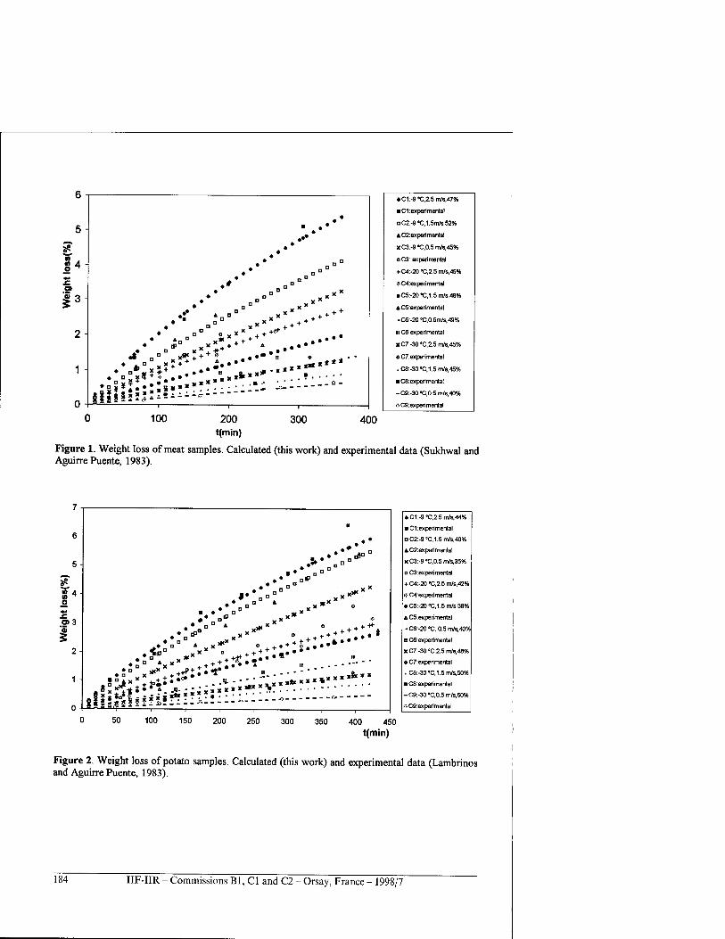
§4

| 3

* " «. *# ♦ « *** + + 4 .•••

«♦ „ D — * + * -•"

♦ C1:-9°C,2.5m/s,47%

■ C1 :experimental

aC2:-9cCl1.5m/s,52%

AC2:experimental

XC3:-9 »0,0.5 m/s,45%

o C3: experimental

+ C4:-20°C,2.5m/s,45%

* C4:experimental

• C5:-200C,1.5m/s,48%

AC5:experimental

-C6:-209C,0.5m/s,49%

:: C6:experimental

«C7:-30eC,2.5m/s,45%

o C7:experimental

.C8:-30eC,1.5m/s,45%

■ C8:experimental

-C9:-30*C,0.5m/s,40%

•"■C9:experimental

100 200 t(min)

300 400

Figure 1. Weight loss of meat samples. Calculated (this work) and experimental data (Sukhwal and Aguirre Puente, 1983).

• C1:-9'C.2.5 m/s,.|4%

■ C1 :experimental

nC2:-9,C,1.5m/s,40%

A C2:experimental

xC3:-9 '0,0.5 m/s, 35%

o C3:experimental

+ C4:-20'0,2.5 m/s,42%

• C4:expertmental

• C5:-20'0,1.5 m/s, 38%

& C5:experimental

• C6:-20*C 0.5m/s,40%

i: C6:experimental

xC7:-30'0,2.5 m/s,48%

»C7:experi mental

.C8:-30'0,1.5 m/s,50%

■ C8:experimental

-C9:-30"C,0.5m/s,60%

C9:experimental

150 200 250 300 350 400 450

t(min)

Figure 2. Weight loss of potato samples. Calculated (this work) and experimental data (Lambrinos and Aguirre Puente, 1983).


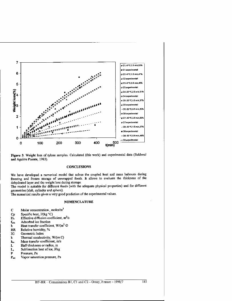
6-

«4 M o

»3 3

..n" XX

■ ♦*GD „XX

• O XX • a x

• a A vx

♦o° A" .4»**

♦SD xx *Aft»** 5P ,x? .^ft«*' 4T xx ° 4«^'

D X A ft A X «ft* » -""

X>C4i* »--■"'" -,«??"'

*** !;«:*■■■•••".— wgg** _ — •» ~ ~ ■^5"

100 200 300 400 „ .500 t(min)

♦ C1:-9*C,2.5m/s,53%

■ C1: experimental

nC2:-9'C,1.5m/s,47%

A C2:experimental

xC3:-9,C,0.5m/s,40%

o C3:experimental

AC4:-20,C.2.5m/s,51%

•:• C4:experimental

• C5:-20*C,1.5m/s,37%

A C5:experimental

-C6:-20*C,0.5m/s,35%

:: C6: experimental

*C7:-30 «0,2.5 m/s,50%

oC7:experimental

.C8:-30,C,1.5m/s,37«

■ C8:experimental

-C9:-30"C,0.5m/s,48%

* C9:experimental

Figure 3. Weight loss of tylose samples. Calculated (this work) and experimental data (Sukhwal

and Aguirre Puente, 1983).

CONCLUSIONS

We have developed a numerical model that solves the coupled heat and mass balances during freezing and frozen storage of unwrapped foods. It allows to evaluate the thickness of the dehydrated layer and the weight loss during storage. The model is suitable for different foods (with the adequate physical properties) and for different

geometries (slab, cylinder and sphere). The numerical results gives a very good prediction of the experimental values.

NOMENCLATURE

C Molar concentration, moles/m3

Cp Specific heat, J/(kg °C) Dv Effective diffusion coefficient, nrVs fads Adsorbed ice fraction h Heat transfer coefficient, W/(m2 © HR Relative humidity, % IG Geometric index k Thermal conductivity, W/(m.C) km Mass transfer coefficient, m/s L Half-thickness or radius, m Ls Sublimation heat of ice, J/kg P Pressure, Pa Psat Vapor saturation pressure, Pa


R Universal gas constant, 8.31 J/(mol K) t Time, s (or min) T Temperature, °C U Temperature or Concentration in eqns. (11), (12) and (13) V Air velocity, m/s V Thermal conductivity or diffussion coefficient in eq. (14) w Ice content, (kg of ice)/(kg of water) Wl Weight loss, % X Spatial coordinate, m Xl Moving front position, m yo Initial water content Ax Spatial increment, frozen zone, m At Time increment, s

Greek symbols P Density, kg/m 8 Porosity T Tortuosity

Subscripts a Air d Dehydrated

Initial va Water vapour

REFERENCES

1. Aguirre Puente, J., Fremond, M; Comini, G., 1978, Freezing of soils-Physical study and mathematical models, Int. J. Refrig, 1, 99-106.

2. Campanone, L.A., Salvadori, V.O., Mascheroni, R.H., 1998, Finite differences method to solve the coupled heat and mass balances during freezing with simultaneous surface dehydration, Proc Fourth World Congress of Computational Mechanics,! A.

3. Cleland, A.C., 1990, Food refrigeration processes. Analysis, design and simulation, Elsevier Applied Science Publishers Ltd, London.

4. Cleland, A.C., Earle, R.L., 1984, Assessment of freezing time prediction methods, J Food Sei, 49, 1034-1042.

5. Chumak, I.G., Sibiriakov, P.V., 1988, Influence of air parameters in a frigorific chamber on the humidity content of the surface of meat during refrigeration (Russian), Izvestia vuzov, Pischevaia tejnologuia, 2, 54-56.

6. Devres, Y.O., 1991, An analytical model for thermophysical properties of frozen foodstuffs, XVIIIInt. Congress. Refrig Proceedings, paper n° 367!

7. Harper, J., 1962, Transport properties of gases in porous media at reduced pressures with reference to freeze-drying, AIChEJ, 298-302.

8. Judson King, C, 1971, Freeze-drying of foods, CRC Press, California. 9. Kochs, M., Körber, Ch., Nunner, B., Heschel, I., 1990, The influence of the freezing process on

vapour transport during sublimation in vacuum-freeze-drying, Int. J. Heat Mass Transf 34, 2395-2408.

10. Lambrinos, G.P., Aguirre Puente ,1, 1983, Deshydratation des milieux disperses congeles. Influence des conditions d'entreposage sur les pertes de masse, XVI Int.Congress. Refrig Proceedings, Vol. II, 567-573.

11. Marshall, G., Rey, C, Smith, L., 1986, Metodos de Seguimiento de la Interfase para problemas


unidimensionales de frontera mövil II, Rev. Int. Met. Num. Cälculoy Dis. Ing, 2, 351-366. 12. Mascheroni, R.H., Calvelo, A., 1978, Modelo de descenso crioscopico en tejidos cameos, La

Alimentation Latinoamericana, 12, 34 42. 13. Mellor, J.D., 1974, Progress in the theoretical study of ice sublimation, IIF-IIR Commissions

Bl, CJ, C2, Bressanone, 121-129. 14. Miles, CA., 1974, Meat freezing-why and how?, Proc. Meat Research Inst Symposium, 15.1-

15.7. ' 15. Pham, Q.T., Willix, J., 1984, A model for food desiccation in frozen storage, J Food Sei, 49,

1275-1281. ' 16. Polley, S.L., Snyder, O.P., Kotnour, P., 1980, A compilation for thermal properties of foods,

Food Techn., 76-94. 17. Sanz, P.D., Dominguez, M., Mascheroni, R.H., 1989, Equations for the prediction of

thermophysical properties of meat products, Latin Am Appl Research, 19,15 5-163. 18. Sukhwal, R.N., Aguirre Puente, J., 1983, Sublimation des milieux disperses. Considerations

theoriques et experimentation, Rev Gen Therm Fr, 262, 663-673. 19. Wang, N., Brennan, J.G., 1992, Thermal conductivity of potato as a function of moisture

content JFoodEng, 17, 153-160.

MODELISATION ET SIMULATION DES TRANFERTS DE CHALEUR ET DE MATIERE DURANT LA CONGELATION ET LE STOCKAGE DE PRODUITS SANS EMBALLAGE

RESUME : Sans protection par un emballage, les produits alimentaires se deshydratent durant les phases de congelation et de stockage. Un modele des transferts couples de chaleur et de matiere (vapeur d'eau) est developpe. II integre la cristallisation de l'eau ainsi que sa sublimation. Le modele mathematique est resolu par la methode des differences finies (schema implicite) avec un maillage variable. Le modele represente bien les donnees experimentales de champ de distribution de temperature ainsi que les cinetiques globales de deshydratation.


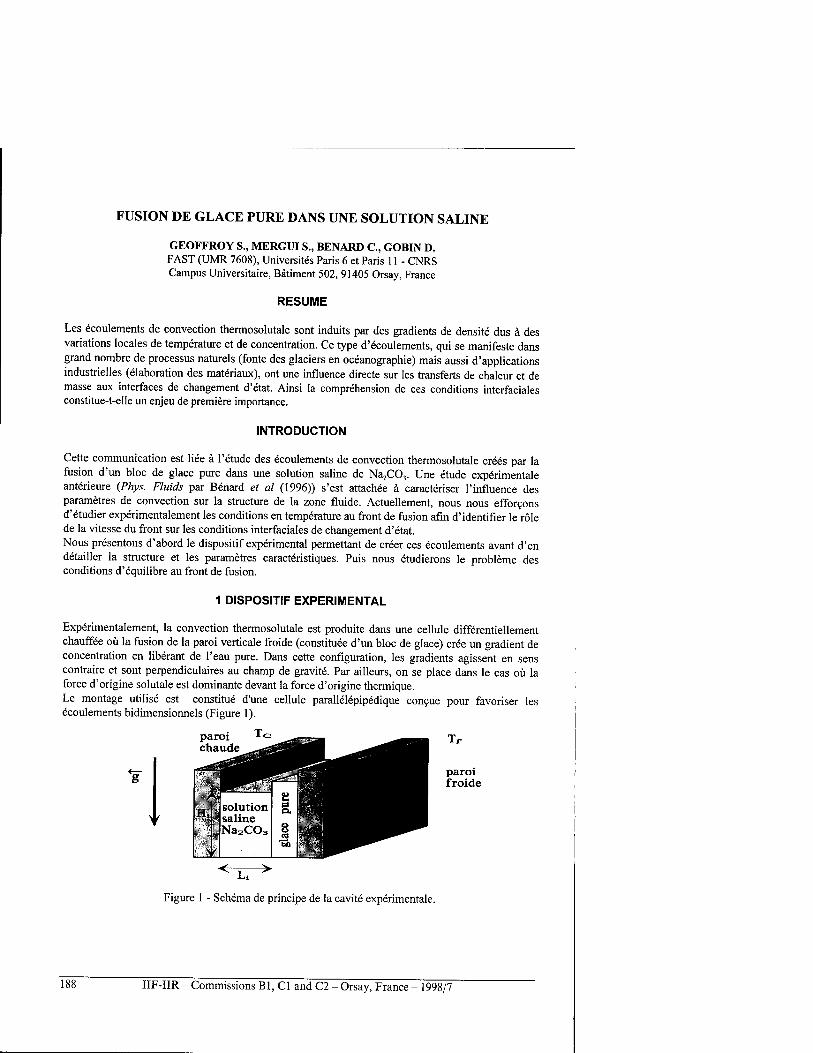
FUSION DE GLACE PURE DANS UNE SOLUTION SALINE

GEOFFROY S., MERGUI S., BENARD C, GOBIN D. FAST (UMR 7608), Universites Paris 6 et Paris 11 - CNRS Campus Universitaire, Bätiment 502, 91405 Orsay, France

RESUME

Les ecoulements de convection thermosolutale sont induits par des gradients de densite dus ä des variations locales de temperature et de concentration. Ce type d'ecoulements, qui se manifeste dans grand nombre de processus naturels (fönte des glaciers en oceanographie) mais aussi d'applications industrielles (elaboration des materiaux), ont une influence directe sur les transferts de chaleur et de masse aux interfaces de changement d'etat. Ainsi la comprehension de ces conditions interfaciales constitue-t-elle un enjeu de premiere importance.

INTRODUCTION

Cette communication est liee ä l'etude des ecoulements de convection thermosolutale crees par la fusion d'un bloc de glace pure dans une solution saline de Na2C03. Une etude experimentale anterieure (Phys. Fluids par Benard et al (1996)) s'est attachee ä caracteriser l'influence des parametres de convection sur la structure de la zone fluide. Actuellement, nous nous efforcons d'etudier experimentalement les conditions en temperature au front de fusion afin d'identifier le role de la vitesse du front sur les conditions interfaciales de changement d'etat. Nous presentons d'abord le dispositif experimental permettant de creer ces ecoulements avant d'en detailler la structure et les parametres caracteristiques. Puis nous etudierons le probleme des conditions d'equilibre au front de fusion.

1 DISPOSITIF EXPERIMENTAL

Experimentalement, la convection thermosolutale est produite dans une cellule differentiellement chauffee oü la fusion de la paroi verticale froide (constitute d'un bloc de glace) cree un gradient de concentration en liberant de l'eau pure. Dans cette configuration, les gradients agissent en sens contraire et sont perpendiculaires au champ de gravite. Par ailleurs, on se place dans le cas oü la force d'origine solutale est dominante devant la force d'origine thermique. Le montage utilise est constitue d'une cellule parallelepipedique concue pour favoriser les ecoulements bidimensionnels (Figure 1).

paroi chaude

sâtagi ^^^^" " ^^T'

1^ ^^üHH

A Hi i solution

saline WSgk ' T Na2C03 u $m i "3o

Iliill

paroi froide

Figure 1 - Schema de principe de la cavite experimentale.


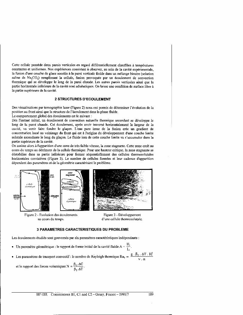
Cette cellule possede deux parois verticales en regard differentiellement chauffees ä temperatures constantes et uniformes. Nos experiences consistent ä observer, au sein de la cavite experimentale, la fusion d'une couche de glace accolee ä la paroi verticale froide dans un melange binaire (solution saline de Na2C03) remplissant la cellule, fusion provoquee par un ecoulement de convection thermique qui se developpe le long de la paroi chaude. Les autres parois verticales ainsi que la partie horizontale inferieure de la cavite sont adiabatiques. On laisse une condition de surface libre ä la partie superieure de la cavite.

2 STRUCTURES D'ECOULEMENT

Des visualisations par tomographie laser (Figure 2) nous ont permis de determiner revolution de la position au front ainsi que la structure de l'ecoulement dans la phase fluide. Le comportement global des ecoulements est le suivant: Des l'instant initial, un ecoulement de convection naturelle thermique ascendant se developpe le long de la paroi chaude. Cet ecoulement, apres avoir traverse horizontalement la largeur de la cavite, va venir faire fondre le glacon. L'eau pure issue de la fusion cree un gradient de concentration local au voisinage du front qui est ä l'origine du developpement d'une couche limite solutale ascendante le long du glacon. Le fluide issu de cette couche limite va s'accumuler dans la partie superieure de la cavite. On assiste alors ä l'apparition d'une zone de tres faible vitesse, la zone stagnante. Cette zone croit au cours du temps au detriment de la cellule thermique. Pour une hauteur critique, la zone stagnante se destabilise dans sa partie inferieure pour former sequentiellement des cellules thermosolutales horizontales corotatives (Figure 3). Le nombre de cellules formees et leur cadence d'apparition dependent des parametres et de la geometrie caracterisant le probleme.

;£."!,.* r*i\l cellule 1

fhermhftie 1 HHH

solution ' «qucuK c>0 r

V . J

roide

zone >w |H stagnante \^H

l^. cellules**] u B|

\t^mp&vliftales***t'

~\ glace pure

c"0 cellule I

lliennhlttc l\

V Ü Figure 2 - Evolution des ecoulements

au cours du temps. Figure 3 - Developpement

d'une cellule thermosolutale.

3 PARAMETRES CARACTERISTIQUES DU PROBLEME

Les ecoulements etudies sont gouvernes par six parametres caracteristiques independants :

H, Un parametre geometrique : le rapport de forme initial de la cavite fluide A:

Li

Les parametres de transport convectif: le nombre de Rayleigh thermique RaT =

et le rapport des forces volumiques N =

g . PT . AT . Hf

ßc-AC ßT.AT


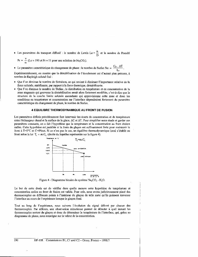
• Les parametres du transport diffusif : le nombre de Lewis Le = — et le nombre de Prandtl

Pr = - (Le : a

190 et Pr « 11 pour une solution de Na2C03).

Le parametre caracteristique du changement de phase : le nombre de Stefan Ste = CP. AT

LF ' Experimentalement, on montre que la destabilisation de l'ecoulement est d'autant plus precoce, ä nombre de Rayleigh solutal fixe :

• Que Ton diminue le nombre de flottaison, ce qui revient ä diminuer l'importance relative de la force solutale, stabilisante, par rapport ä la force thermique, destabilisante.

• Que Ton diminue le nombre de Stefan ; la distribution en temperature et en concentration de la zone stagnante qui gouverne la destabilisation serait alors fortement modifiee, c'est-a-dire que la structure de la couche limite solutale ascendante qui approvisionne cette zone et done les conditions en temperature et concentration sur 1'interface dependraient fortement du parametre caracteristique du changement de phase, le nombre de Stefan.

4 EQUILIBRE THERMODYNAMIQUE AU FRONT DE FUSION

Les parametres definis precedemment font intervenir les ecarts de concentration et de temperature entre l'echangeur chaud et la surface de la glace, AC et AT. Pour simplifier notre etude et garder ces parametres constants, on a fait l'hypothese que la temperature et la concentration au front etaient nulles. Cette hypothese est justifiee si la fönte du glacon est suffisamment forte pour maintenir le front ä T=0°C et C=0%wt. Si ce n'est pas le cas, un equilibre thermodynamique local s'etablit au front selon la loi TL = m.CL (droite du liquidus representee sur la figure 4).

<rc

-o,7*c

-U16*C

-2J'C

ure en "C

■-«■^^^ liquid tu

! „7T5*. 1

TL=m.CL

pente m—0JS4*C/%

1

1 1

1 pointi eutectiquc

Figure 4 - Diagramme binaire du Systeme Na2C03 - H,0.

Le but de cette etude est de verifier dans quelle mesure cette hypothese de temperature et concentration nulles au front de fusion est valide. Pour cela, nous avons judicieusement place des thermocouples en differents points ä l'interieur du glacon de teile sorte qu'ils puissent traverser l'interface au cours de Fexperience lorsque le glacon fond.

Tout au long de l'experience, nous suivons revolution du signal delivre par chaeun des thermocouples. Par ailleurs, une observation minutieuse permet de detecter ä quel instant les thermocouples sortent du glacon et done de determiner la temperature de l'interface, qui, grace au diagramme de phase, nous renseigne sur la valeur de la concentration.


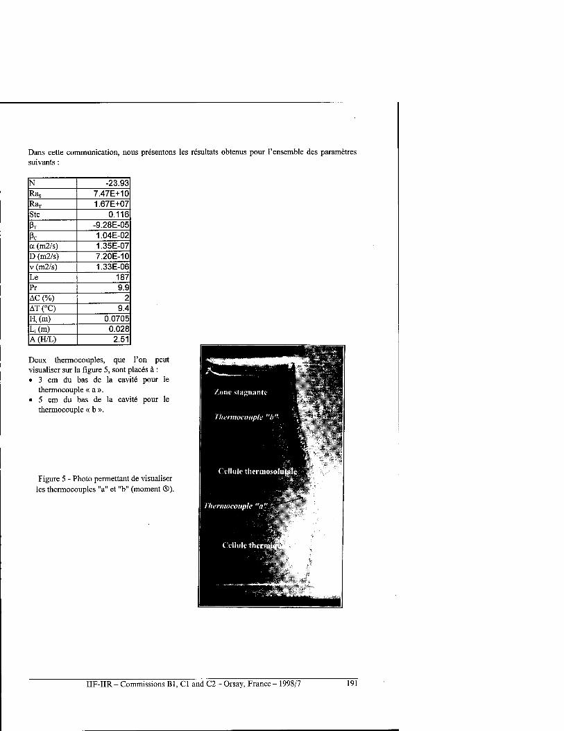
Dans cette communication, nous presentons les resultats obtenus pour l'ensemble des parametres suivants :

N -23.93 Ras 7.47E+10 RaT 1.67E+07 Ste 0.116 ßx -9.28E-05

ßc 1.04E-02 a (m2/s) 1.35E-07 D (m2/s) 7.20E-10 v (m2/s) 1.33E-06 Le 187 Pr 9.9 AC (%) 2 AT (°C) 9.4 H,(m) 0.0705 Li(m) 0.028 A(H/L) 2.51

Deux thermocouples, que l'on peut visualiser sur la figure 5, sont places ä : • 3 cm du bas de la cavite pour le

thermocouple « a ». • 5 cm du bas de la cavite pour le

thermocouple « b ».

Figure 5 - Photo permettant de visualiser les thermocouples "a" et "b" (moment ©).


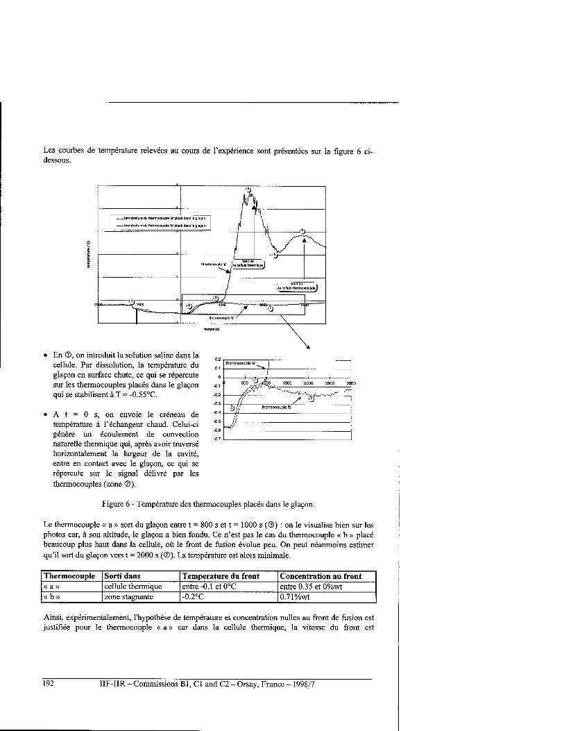
Les courbes de temperature relevees au cours de l'experience sont presentees sur la figure 6 ci- dessous.

—temperature du ttieimocouple 'a' place dans le glacon

—temperature du thermocouple V place dans le glacon

En ©, on introduit la solution saline dans la cellule. Par dissolution, la temperature du glacon en surface chute, ce qui se repercute sur les thermocouples places dans le glacon qui se stabilisent ä T = -0.55°C.

A t = 0 s, on envoie le creneau de temperature ä l'echangeur chaud. Celui-ci genere un ecoulement de convection naturelle thermique qui, apres avoir traverse horizontalement la largeur de la cavite, entre en contact avec le glacon, ce qui se repercute sur le signal delivre par les thermocouples (zone ©).

Figure 6 - Temperature des thermocouples places dans le glacon.

Le thermocouple « a » sort du glacon entre t = 800 s et t = 1000 s (®) : on le visualise bien sur les photos car, ä son altitude, le glacon a bien fondu. Ce n'est pas le cas du thermocouple « b » place beaucoup plus haut dans la cellule, oü le front de fusion evolue peu. On peut neanmoins estimer qu'il sort du glacon vers t = 2000 s (®). La temperature est alors minimale.

Thermocouple Sorti dans Temperature du front Concentration au front « a» cellule thermique entre-0.1 et0°C entre 0.35 et 0%wt « b » zone stagnante -0.2°C 0.71%wt

Ainsi, experimentalement, l'hypothese de temperature et concentration nulles au front de fusion est justifiee pour le thermocouple « a» car dans la cellule thermique, la vitesse du front est


suffisamment rapide pour que la fusion de la glace maintienne le front et son voisinage ä T=0°C et C=0%wt. Par contre, le thermocouple "b" sort dans la zone stagnante, au niveau de laquelle la vitesse du front est tres faible : un equilibre thermodynamique s'impose ä l'interface, nous eloignant ainsi de l'hypothese de temperature et concentration nulles au front de fusion. On se deplace alors sur la courbe du liquidus presentee sur la figure 4 : T < 0°C, C > 0%wt ; ceci a notamment pour

consequence de modifier le rapport de flottaison N = ßc-AC

ßT.AT'

CONCLUSION

Dans cette etude, nous nous sommes places dans le cas oü les ecoulements sont gouvernes par les forces d'Archimede d'origine thermique et solutale, avec force solutale dominante. Nous avons pu montrer que les conditions en temperature et en concentration sur 1'interface dependent de la zone dans laquelle on se place. Si on reste au niveau de la cellule thermique, oü les couches limites de convection sont tres actives et la vitesse du front rapide, la condition T = 0°C et C = 0%wt est une bonne approximation. En revanche, dans les zones oü la vitesse du front est faible et oü les phenomenes sont gouvernes de facon privilegiee par la diffusion, 1'approximation precedente n'est plus justifiee. A court terme, nous envisageons de faire varier les parametres caracteristiques afin d'en determiner 1'influence sur les conditions d'interface. D'autre part, une interaction entre experience et simulation numerique complete incluant le couplage entre convection thermosolutale instationnaire et deplacement du front de fusion nous permettra de mieux comprendre les phenomenes mis en jeu.

NOMENCLATURE

A Rapport de forme initial = H{ / Lt

CL Concentration de la phase liquide ä l'interface de fusion (%wt)

Cp Chaleur specifique (J.kg,0C-')

D Diffusivite massique (m2.s"')

H j Hauteur initiale de solution (m)

Le Nombre de Lewis = oc/D

LF Chaleur latente de fusion (J.kg1) de la glace

L, Largeur initiale de solution (m)

m Pente du liquidus (°C/%wt)

N Rapport des forces volumiques

Pr Nombre de Prandtl = u/oc

RaT Nombre de Rayleigh thermique

Ras Nombre de Rayleigh solutal

Ste Nombre de Stefan, rapport de la chaleur sensible et de la chaleur latente

TL Temperature de la phase liquide ä l'interface de fusion (°C)

symboles grecs

a Diffusivite thermique (m2.s"')

ßc Coefficient d'expansion massique ((wt%)"')

ßT Coefficient d'expansion thermique (°C')

AC Ecart de concentration (wt%) entre la solution et le front de fusion

AT Ecart de temperature entre l'echangeur chaud et la surface de la glace (°C)

u Viscosite cinematique du fluide (m2.s"')


BIBLIOGRAPHIE

Benard C, Benard R., Bennacer R, Gobin D., 1996 , Melting driven thermohaline convection,. Phys. Fluids, 8-1, p. 112-130. Mergui S., Joly D., Feroual B., Gobin D., Benard C, 16-19 septembre 1997 , Formation de cellules convectives induites par la fusion de la glace pure dans une solution binaire, Siemes Journees Europeennes de Thermodynamique Contemporaine, p. 123-130.

MELTING OF PURE ICE IN AN AQUEOUS BINARY SOLUTION

SUMMARY: Thermohaline convection flows are induced by density gradients due to local variations of temperature and concentration. This type of flow, which appears in many natural processes (melting of ice in oceanography) but also industrial applications (material processing), have a direct influence on heat and mass transfers to liquid-solid interfaces. Thus, the understanding of these interfacial conditions is very important.


MODELISATION DE LA TEMPERATURE DE SURFACE D'UNE CHAUSSEE A COURTE ECHEANCE

LASSOUED R.*, LABBE L.**, FREMOND M.*, DUPAS A.* * Laboratoire des Materiaux et des Structures du Genie Civil, UMR113 (LCPC/CNRS),

cite Descartes, 2, allee Kepler, 77420 Champs sur Marne, France ** Bureau d'Etude du Centre Inter-Regional Nord de METEO FRANCE,

18, rue Elisen Reclus, B.P. 7, 59651 Villeneuve d'Ascq Cedex, France

RESUME

Le programme COGEL modelise la temperature de surface d'une chaussee ä courte echeance en tenant compte des caracteristiques thermiques, hydriques et physiques de la chaussee ainsi que des conditions meteorologiques. COGEL est le resultat du couplage de deux modeles preexistants, le modele de chaussee GELID et le modele atmospherique COBEL.

INTRODUCTION

L'etat de surface de la route constitue pour l'usager l'un des facteurs importants pris en compte dans sa Strategie de conduite. En periode hivernale, cet etat evolue en fonction des conditions meteorologiques, des caracteristiques de la chaussee et des interventions realisees pour la viabilite. Les services Sexploitation cherchent ä maitriser ces etats de surface de maniere preventive ou curative : deneigement par evacuation et traitement de la neige, deverglacage ä l'aide de fondants, informations sur les conditions de circulation... Dans le cadre des recherches entreprises, un theme de recherche sur le comportement hivernal des chaussees a ete lance par le Laboratoire Central des Ponts et Chaussees en collaboration avec METEO-FRANCE (la Direction Inter-Regionale, DIR Lille et le Centre d'Etudes de la Neige, CEN Grenoble) et la Direction des Routes. Notre travail de recherche fait partie de ce theme et comporte trois parties :

1. Mise en oeuvre et evaluation du modele COGEL de prevision, ä courte echeance, de la temperature de surface d'une chaussee. Ce modele est base sur le couplage du modele de- chaussee GELID et du modele atmosphenque COBEL.

2. Mise en oeuvre et evaluation du modele GELCRO de prevision du comportement d'une couche de neige se deposant sur une chaussee. Ce modele est le fruit du couplage du modele de chaussee GELID et du modele Revolution du manteau neigeux CROCUS.

3. Extension de la prevision de temperature de surface d'une chaussee etablie par COGEL et GELCRO ä celle de l'etat de surface d'une chaussee en tenant compte des phenomenes thermiques suivants :

- echanges massiques et energetiques - changement de phase dans la structure routiere - discontinuite de la temperature ä l'interface chaussee-atmosphere.

On presente ci-dessous la moderation de la temperature de surface d'une chaussee ä courte echeance. Avant de presenter la methode adoptee pour la mise en oeuvre du modele COGEL, on presentera chacun des deux modeles GELID et COBEL.


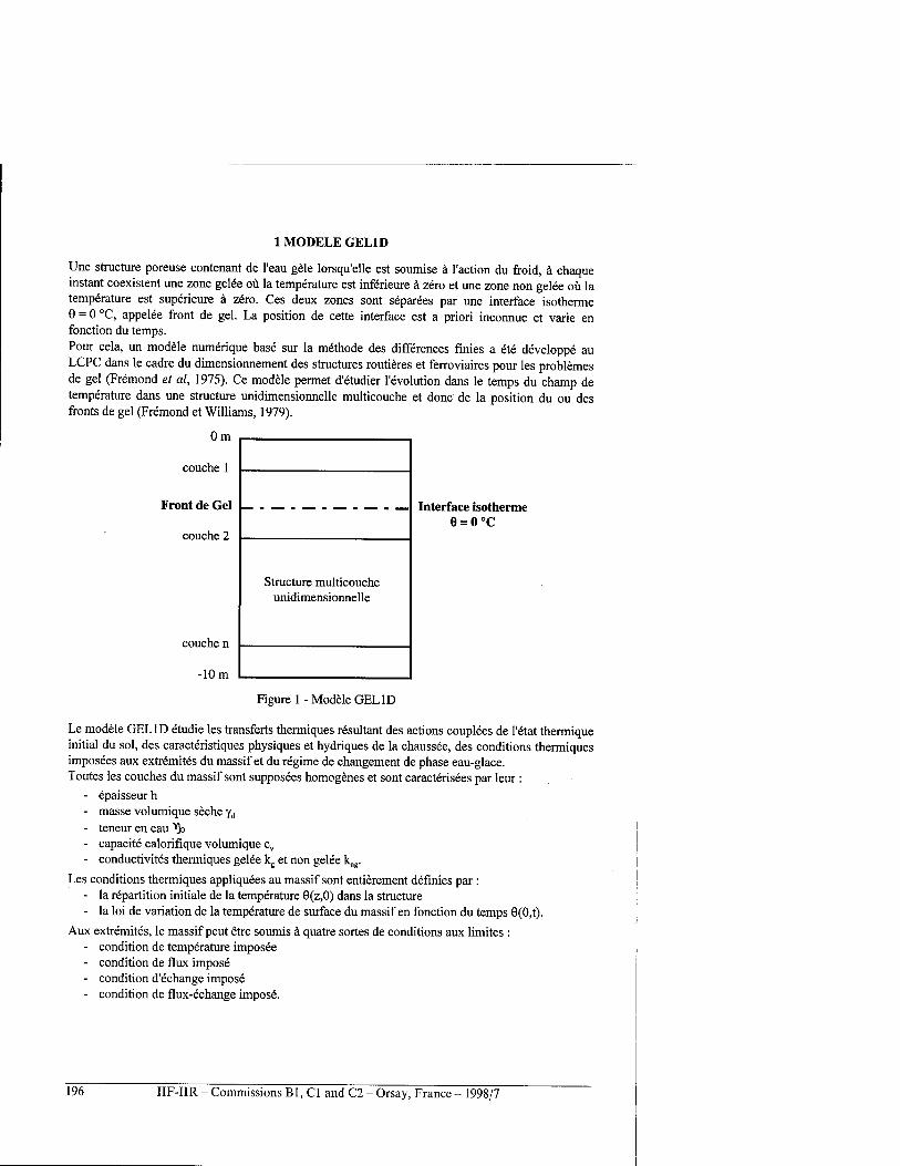
1 MODELE GELID

Une structure poreuse contenant de l'eau gele lorsqu'elle est soumise ä l'action du froid, ä chaque instant coexistent une zone gelee oü la temperature est inferieure ä zero et une zone non gelee oü la temperature est superieure ä zero. Ces deux zones sont separees par une interface isotherme 0 = 0 °C, appelee front de gel. La position de cette interface est a priori inconnue et varie en fonction du temps. Pour cela, un modele numerique base sur la methode des differences finies a ete developpe au LCPC dans le cadre du dimensionnement des structures routieres et ferroviaires pour les problemes de gel (Fremond et al, 1975). Ce modele permet d'etudier revolution dans le temps du champ de temperature dans une structure unidimensionnelle multicouche et done de la position du ou des fronts de gel (Fremond et Williams, 1979).

Om

couche 1

Front de Gel

couche 2

couche n

-10 m

Structure multicouche unidimensionnelle

Interface isotherme 6 = 0 °C

Figure 1 - Modele GELID

Le modele GELID etudie les transferts thermiques resultant des actions couplees de l'etat thermique initial du sol, des caracteristiques physiques et hydriques de la chaussee, des conditions thermiques imposees aux extremites du massif et du regime de changement de phase eau-glace. Toutes les couches du massif sont supposees homogenes et sont caracterisees par leur :

- epaisseur h - masse volumique seche yd

- teneur en eau ^ - capacite calorifique volumique cv

- conduetivites thermiques gelee kg et non gelee k,,6.

Les conditions thermiques appliquees au massif sont entierement definies par : - la repartition initiale de la temperature 6(z,0) dans la structure - la loi de variation de la temperature de surface du massif en fonction du temps 9(0,t).

Aux extremites, le massif peut etre soumis ä quatre sortes de conditions aux limites : - condition de temperature imposee - condition de flux impose - condition d'echange impose - condition de flux-echange impose.


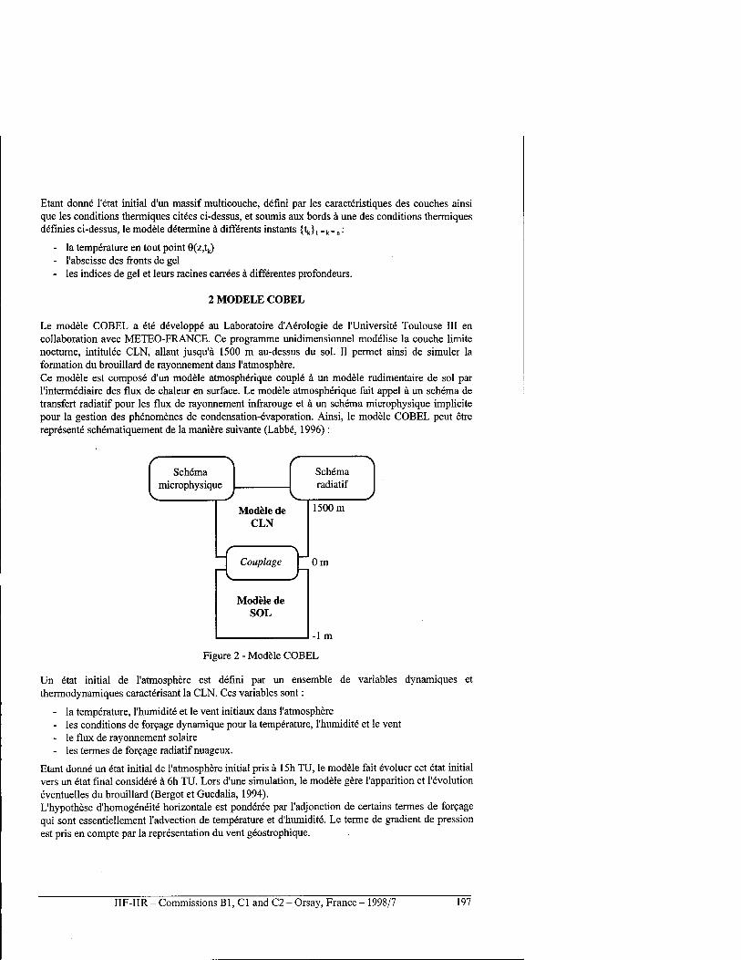
Etant donne l'etat initial d'un massif multicouche, defini par les caracteristiques des couches ainsi que les conditions thermiques citees ci-dessus, et soumis aux bords ä une des conditions thermiques definies ci-dessus, le modele determine ä differents instants {tk}, .k = n:

- la temperature en tout point 8(z,tk) - l'abscisse des fronts de gel - les indices de gel et leurs racines carrees ä differentes profondeurs.

2 MODELE COBEL

Le modele COBEL a ete developpe au Laboratoire d'Aerologie de l'Universite Toulouse III en collaboration avec METEO-FRANCE. Ce programme unidimensionnel modelise la couche limite nocturne, intitulee CLN, allant jusqu'ä 1500 m au-dessus du sol. II permet ainsi de simuler la formation du brouillard de rayonnement dans l'atmosphere. Ce modele est compose d'un modele atmospherique couple ä un modele radimentaire de sol par l'intermediaire des flux de chaleur en surface. Le modele atmospherique fait appel ä un schema de transfert radiatif pour les flux de rayonnement infrarouge et ä un schema microphysique implicite pour la gestion des phenomenes de condensation-evaporation. Ainsi, le modele COBEL peut etre represente schematiquement de la maniere suivante (Labbe, 1996):

Schema microphysique

Schema radiatif

Modele de CLN

Couplage

1500 m

0m

Modele de SOL

-Im

Figure 2 - Modele COBEL

Un etat initial de l'atmosphere est defini par un ensemble de variables dynamiques et thermodynamiques caracterisant la CLN. Ces variables sont:

- la temperature, l'humidite et le vent initiaux dans l'atmosphere - les conditions de forcage dynamique pour la temperature, l'humidite et le vent - le flux de rayonnement solaire - les termes de forcage radiatif nuageux.

Etant donne un etat initial de l'atmosphere initial pris ä 15h TU, le modele fait evoluer cet etat initial vers un etat final considere ä 6h TU. Lors d'une simulation, le modele gere l'apparition et revolution eventuelles du brouillard (Bergot et Guedalia, 1994). L'hypothese d'homogeneite horizontale est ponderee par l'adjonction de certains termes de forcage qui sont essentiellement l'advection de temperature et d'humidite. Le terme de gradient de pression est pris en compte par la representation du vent geostrophique.


Parmi ces termes de forcage figurent egalement les composantes atmospheriques qui ne peuvent etre gerees par le modele lui-meme, comme le rayonnement solaire ou la presence de nuages. En effet, une prevision du flux solaire et du flux nuageux est faite par METEO-FRANCE toutes les trois heures, ensuite un calcul par interpolation lineaire de ces flux est effectue par le programme COBEL ä chaque pas de temps. Le fonctionnement du modele se schematise ainsi:

Etat de l'atmosphere

ä 15h TU

1 1

Modele COBEL

Etat de l'atmosphere

ä6hTU +

Diagnostics du

brouillard

Figure 3 - Mode de fonctionnement du modele COBEL

3 COUPLAGE GEL1D-COBEL

Le modele COGEL, developpe ä l'UMR.113 en 1997, est le resultat du couplage des deux modeles GELID et COBEL decrits ci-dessus. COGEL permet de determiner la temperature de surface d'une chaussee ä courte echeance en tenant compte d'une part des caracteristiques thermiques, hydriques et physiques de la chaussee et d'autre part des conditions meteorologiques. La methode adoptee pour la mise en oeuvre du modele COGEL est une methode de couplage iterative implicite qui preserve globalement les structures des modeles GELID et COBEL et les traite par blocs. L'interface entre les deux modeles s'effectue ä l'aide d'un bilan de flux thermiques. Ce couplage a necessite des developpements algorithmiques et des parametrisations permettant de decoupler le modele atmospherique de COBEL de son modele rudimentaire de sol et d'integrer le modele GELID. Afin de raffiner le calcul du gradient de temperature ä l'interface sol-atmosphere, un nouveau niveau atmospherique situe ä 10 cm au-dessus du sol a ete cree. Le couplage effectue est base sur un bilan thermique ä l'interface sol-atmosphere (cf. figure 4). Les flux thermiques intervenant ä l'interface sont:

- les flux solaire et infrarouge - les flux de chaleur sensible et latente - le flux de conduction dans le sol.


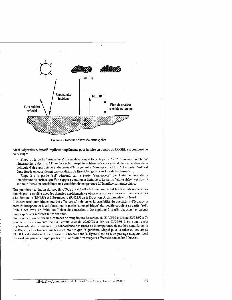
Flux solaire incident

Flux solaire röflechi

Flux IRj.

FluxIR1

Flux de chaleur sensible et latente

Figure 4 - Interface chaussee-atmosphere

Ainsi l'algorithme, iteratif implicite, implements pour la mise en oeuvre de COGEL est compose de deux etapes :

- Etape 1 : la partie "atmosphere" du modele couple force la partie "sol" du meme modele par l'intermediaire des flux ä l'interface sol-atmosphere schematises ci-dessus, de la temperature de la pellicule d'air superficielle et du terme d'echange entre l'atmosphere et le sol. La partie "sol" est done forcee en considerant une condition de flux-echange ä la surface de la chaussee. - Etape 2 : la partie "sol" retroagit sur la partie "atmosphere" par l'intermediaire de la temperature de surface que l'on suppose continue ä l'interface. La partie "atmosphere" est done ä son tour forcee en considerant une condition de temperature ä l'interface sol-atmosphere.

Une premiere validation du modele COGEL a ete effectuee en comparant les resultats numeriques donnes par le modele avec les donnees experimentales observees sur les sites experimentaux situes ä La Sentinelle (RN455) et ä Steenwoord (RN225) de la Direction Departementale du Nord. Plusieurs tests numeriques ont ete effectues afin de tester la sensibilite du coefficient d'echange a entre l'atmosphere et le sol fourni par la partie "atmospherique" du modele couple ä sa partie "sol". Suite ä ces tests, un faible coefficient de correction a ete applique ä a afin d'ajuster les calculs numeriques aux mesures faites sur sites. On presente dans ce qui suit les traces de temperature de surface du 21/03/97 ä 15h au 22/03/97 ä 6h pour le site experimental de La Sentinelle et du 02/02/98 ä 15h au 03/02/98 ä 6h pour le site experimental de Steenwoord. La concordance des traces de la temperature de surface simulee par le modele et celle observee sur les sites montre que l'algorithme adopte pour la mise en oeuvre de COGEL est satisfaisant. Le desaecord observe dans la figure 6 est du ä un passage nuageux local qui n'est pas pris en compte par les previsions du flux nuageux effectuees toutes les 3 heures.


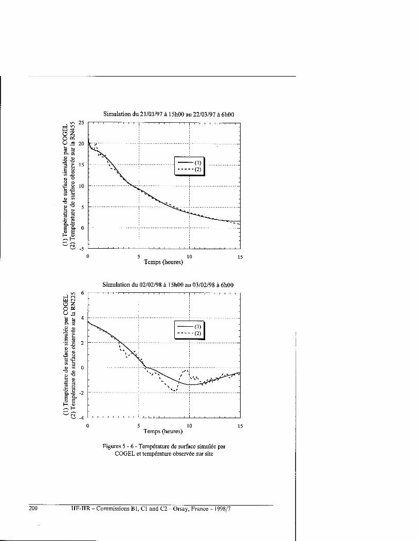
Simulation du 21/03/97 ä 15h00 au 22/03/97 ä 6h00

5 10 Temps (heures)

15

Simulation du 02/02/98 ä 15h00 au 03/02/98 ä 6h00

0 z, O 2 U ja

o. S ■8-8 1 £

ü O

'S 3 » s ü cn

ü *t3

II •Ö g E o- § E

,-^ H

0 -

-2 -'

; •

-^\ - (!) (2)

-

\ *^^^—

; "

5 10 Temps (heures)

15

Figures 5 - 6 - Temperature de surface simulee par COGEL et temperature observee sur site


CONCLUSION

Dans ce document nous avons presente l'etude relative ä la moderation de la temperature de surface d'une chaussee ä courte echeance (3 heures en avance). II s'agit de la mise en oeuvre et revaluation du modele COGEL. Les resultats numeriques obtenus par ce dernier montrent que la methode adoptee est satisfaisante. Des reception d'autres donnees experimentales relatives ä la Campagne hivernale 98-99, de nombreux tests seront effectues dans le cadre de la validation de ce modele.

BIBLIOGRAPHIE

1. Fremond, M., Caniard, L., Dupas, A., Levy, M., 1975, Comportement thermique d'une structure routiere soumise ä un cycle de gel-degel. Simulations experimentales et numeriques, Proa Vlleme congres international de lafondation Frangaise detudes nordiques.

2. Fremond, M.,Williams, P., 1979, Proc, Gel des sols et des chaussees, Presses des Ponts et Chaussees.

3. Labbe, L., 1996, COBEL : Description scientifique, Int. Note du BED, no. 5 : p. 1-33. 4. Bergot, T., Guedalia, D., 1994, Numerical forecasting of radiation fog. Part I : Numerical model

and sensitivity tests, Int. Monthly weather review, vol. 122 : p. 1218-1230.

DISCUSSION

DJABALLAH-MASMOUDIN. (France) - 1/ Quelle est la definition de la sensibilite du coefficient de transfert a ? 2/ Le facteur de correction introduit au niveau du coefficient de transfert a est-il general pour toutes les simulations ou est-il propre ä chaque simulation ?

LASSOUED R. - Le coefficient a est defini de facon ä permettre le calcul du flux de chaleur turbulent entre la surface de la chaussee et la couche superficielle atmospherique. II s'ecrit:

p-CpK a =

dz oü : p : densite de l'air (p = 1.22 kg/m3)

Cp : chaleur massique de l'air (Cp = 1005 J/kg.K) dz : distance separant la surface de la chaussee du premier niveau atmospherique (10 cm) K : coefficient d'echange turbulent variable en fonction du temps (m2/s).

Tester la sensibilite du coefficient a et l'effet de variation sur les resultats numeriques domes par le modele, c'est tester la sensibilite du coefficient d'echange turbulent K. Afin d'ajuster les calculs numeriques aux mesures experimentales faites sur sites, un faible coefficient de correction de temperature a ete applique ä K. Ce coefficient de correction est general ä toutes les simulations. Les valeurs de K dont nous disposons actuellement sont plutot du domaine de la thermique du bätiment.

CHENAF D. (Canada) - Comment definissez-vous le parametre a ? Signification physique ?

LASSOUED R. - Le coefficient a est un coefficient d'echange "convectif entre le sol et l'atmosphere. Ce coefficient intervient dans le calcul du flux de chaleur convective defini par :


Fa = <x3T = p-Cp-K— dz

oü aT = (T,ir-Tsuf) et K = coefficient d'echange turbulent (m2/s)

p = masse volumique de l'air (p = 1.22 kg/m3) Cp = chaleur specifique de l'air (Cp = 1005 J/kg°K) Tair = temperature de la pellicule d'air superficielle situee ä 10 cm au-dessus du sol

(dz=10cm) TSUIf = temperature de surface de la chaussee.

La variation du coefficient d'echange a suit la variation du coefficient K. Ce dernier caracterise l'activite de la turbulence et varie typiquement de lO3, \0A m2/s la nuit (turbulence faible) ä quelques m2/s le jour (turbulence forte).

MODELLING OF THE SURFACE TEMPERATURE OF A PAVEMENT FOR A SHORT LAPSE OF TIME

SUMMARY: The GOGEL model represents modelling of the surface temperature of a pavement for a short lapse of time. We take into account the thermal, the hydro and the physical characteristics of the pavement, as well as the meteorological conditions. This model is the result of the coupling of two previous models, one relative to the pavement and the other to the atmosphere.


SECTION IV

PERGELISOL, POLLUTION ET CHANGEMENTS PLANETAIRES

PERMAFROST, CONTAMINATION AND GLOBAL CHANGE

PLENARY LECTURE

EFFECTS OF CLIMATE WARMING ON ENGINEERING STRUCTURES IN PERMAFROST REGIONS

LADANYI Branko Professor Emeritus

Ecole Polytechnique, Montreal, C.P. 6079, Succ. Centre-Ville, Montreal, QC, H3C 3A7, Canada

ABSTRACT

The distribution and thickness of permanently frozen soils ("Permafrost") in circumpolar countries (e.g., Alaska, Canada, Russia, Norway) are controlled by climatic, hydrologic, geologic, topographic and biologic factors. Any change in the meteorological conditions, such as air temperature and snow cover, will result in the changes in the surface temperature of permafrost that are complex and difficult to predict. Impact of global warming is discussed.

The physical and mechanical properties of permafrost soils are generally temperature dependent and, at temperatures close to the melting point, they depend strongly on temperature. Most of the civil engineering concerns related to a climatic warming can be classified into those related to an increase in permafrost temperatures, those related to increases in the active layer thickness (annual thaw depth), and those related to the degradation of permafrost. Engineering concerns related to a general warming of the permafrost result primarily from the decrease of its mechanical strength in its frozen and eventually thawed state. Continued climatic warming will eventually cause much of the discontinuous permafrost to thaw, resulting in increasing rates of thaw settlement of structures in thaw-sensitive regions of the Arctic. Scenarios for possible future climate conditions are based on general circulation models (GMCs), which are large, complex, three-dimensional numerical models of the atmosphere and oceans. These models are generally given an impulsive change, like a C02 doubling, and are then integrated forward in time until a state of equilibrium is reached. However, the degree of uncertainty of these GMC- generated scenarios in unknown. The greatest uncertainty in the models relates to cloud, precipitation, sea-ice, air-sea interaction, albedos, and C02 feedback. Other uncertainties relate to the global carbon balance, future emissions, and transient versus equilibrium response While there is still a considerable disagreement among the climatologists about the most probable rate of future climate warming, it is nevertheless not too early to start thinking about the kind of effects a certain amount of warming would have on the behaviour and stability of natural and human-made structures in the North. In order to quantify the possible impacts, there has been a trend in recent years to establish the sensitivity of the physical, biological, social and economic systems to climate and changes in climate. In the area of permafrost science and engineering, there have been some proposals for estimating the sensitivity of predictions on: permafrost thermal regime, active layer thickness, and permafrost strength reduction. The potential effects of warming of the mean annual temperature on permafrost will be very different for continuous and discontinuous permafrost zones. In the continuous zones, the effect on the permafrost would be to warm it and possibly to change the depth of the active layer. Thawing at the base of permafrost would start several centuries later and would proceed at a rate of about a centimetre or more per year. In the discontinuous zone, the effects of a few degrees warming in the mean annual temperature of permafrost would be extremely serious. Since most of this permafrost is within a few degrees of thawing, it should eventually disappear. Although many centuries will be required for the permafrost to disappear entirely, increases in the active layer and thawing of the wannest permafrost


from the top could begin almost immediately. In two previous papers (Ladanyi, 1996, 1998), the author has attempted to quantify the sensitivity of frozen ground strength and creep rate to temperature increase, and proposed a simple strength-sensitivity index, that could be used for microzonation mapping of the zones of potentially stable and unstable permafrost. Permafrost sensitivity maps of this kind may become a useful basis for predicting the effect of climate warming on the existing constructed facilities in the Arctic, and for establishing guidelines for the design of the new ones. A proposal in this direction was made by Vyalov et al. (1993), who propose to establish a permafrost sensitivity zonation in the Arctic, based on the average annual ground temperature of permafrost. As for the effect of warming climate on particular construction elements, such as foundations, roads and dams, eventual design guidelines should first establish if and how much the present normal safety margins cover the effects of climate warming during the lifetime of the structure, and how and when the climate warming will become a decisive factor in the design.

CONCLUSIONS

1. Climate warming should be taken into account in engineering design where appropriate and where the effect would represent an important component of the geothermal design. 2. Climate warming could be introduced into a code or manual of practice, if necessary. 3. In engineering projects, climate warming may be a factor, if its effects go beyond those anticipated in an existing conservative approach. 4. Sensitivity maps for the loss of strength of permafrost due to climate warming can be established by using a simple strength sensitivity index, as the one proposed in Ladanyi (1996,1998).

REFERENCES

1. Ladanyi, B., 1996, A strength sensitivity index for assessing climate warming effects on permafrost, Proc. Eight Int. Conf. on Cold Regions Engineering, (R.F. Carlson, ed.), Fairbanks, Alaska, ASCE, New York, pp. 35-45.

2. Ladanyi, B., 1998, Geotechnical microzonation in the Arctic related to climate warming. In: "Geotechnical Hazards", Proc. Xlth Danube-European Conf. on SMFE, Porec, Croatia (Marie, Lisac & Szavits-Nossan, eds.), Balkema, Rotterdam, pp. 215-221.

3. Vyalov, S.S., Gerasimov, A.S., Zolotar, A.J. & Fotiev, S.M., 1993. Ensuring structural stability and durability in permafrost ground areas at global warming of the Earth's climate, Proc. 6th Int Permafrost Conf, Beijing, South China Univ. of Technology Press, pp. 955-960.

DISCUSSION

FUKUDA M. (Japan) - The socio-economical impacts due to the global warming in permafrost are the main objective of the International Arctic Research Centre, which is established jointly by Japan and USA. The program or action plan is now under the way to be published.

LADANYI B. - Thank you for your information. We are looking forward to see the activity of the International Arctic Research Centre in the area of socio-economic impacts due to the climate warming in permafrost regions.

INSTANES A. (Norway) - In order to take a possible climate warming into account in engineering design, it would be advantageous to treat climate warming as any other environmental load (earthquake, ocean waves, wind, etc.). This means that a certain climate warming scenario needs to be associated with a certain risk..

LADANYI B. - Thank you. This is an excellent suggestion we have recently produced in Canada a


environmental impacts of climate warming on present and future engineering facilities in permafrost regions.

FROLOV A.D., Russia: There are many scientists in the field of atmosphere physics and climatology who don't think that a menace of great climate warming is real now. What is your opinion on this situation?

LADANYI B. - Yes, I agree that the catastrophic climate warming is problematic. But it is necessary to organize systematically control to fix probable results of warming, especially in the permafrost regions. The most sensitive physical properties of frozen grounds relatively to variations of thermodynamic conditions are mechanic (strength, elastic, etc.) and particularly electric ones. Usually, a monitoring in cryolithozone consists of temperature measurements only.

FROLOV A.D. - Is it necessary to include in monitoring the control of stability (or instability) of electric and elastic properties of permafrost using corresponding geophysical methods?

LADANYI B. -1 think it would be very fruitful.

EFFETS DU RECHAUFFEMENT DU CLEMAT SUR LES STRUCTURES D'INGENIERIE DES REGIONS AVEC PERGELISOL

RESUME : La distribution et l'epaisseur des sols geles en permanence (« pergelisol»), dans les pays du cercle polaire (Alaska, Canada, Russie, Norvege, etc.), sont regies par des facteurs climatiques, hydrologiques, geologiques, topographiques et biologiques. Tout changement dans les conditions meteorologiques, au niveau de la temperature de l'air ou de la couverture neigeuse, est ä l'origine d'autres changements au niveau de la temperature superficielle du pergelisol, qui sont complexes et difficiles ä prevoir. L'article traite des consequences du rechauffement du climat.


LOSS OF BEARING CAPACITY OF ROADS DURING THAW AND DEBRIS FLOWS IN MOUNTAIN PERMAFROST: THE SAME PHENOMENON

DYSLIM. Soil Mechanics of the Swiss Federal Institute of Technology

EPF Ecublens, CH-1015 Lausanne

ABSTRACT

The present paper deals with the similitude between the loss of bearing capacity due to thawing in frost susceptible soils which form the subgrade of roads and railways and the formation of debris flows in mountain permafrost subjected to climatic warming up. It is especially shown that, at the thermal level as well as at the mechanical level, the phenomenon is the same and that the latent heat of fusion of the ice play a major role. This explains the brutality of these two phenomena which are both destructive and costly.

INTRODUCTION

A multidisciplinary approach is often the key to scientific and technical developments. In the domain of frost study, civil engineers today owe much to agronomists of the first half of this century. If the phenomenon of the loss of bearing capacity of frost susceptible soils of roads and railway foundations due to thawing is well known, mastered and even modelled today, this is in part thanks to these agronomists. Until approximately twenty years ago, permafrost, that is soils which are permanently frozen in depth and in which only their surface layer thaws between spring and autumn, were especially studied by geologists and geographers. These latter, often more naturalists than scientists, described the nature of permafrost rather than explained it, based on recognised physical models. However, civil engineers began to construct on permafrost, to tap petroleum deposits in the extreme north, for example, and they had to develop numerical models of the thermal and mechanical behaviour of these soils.

Concerning mountain permafrost, the tourist development in certain mountainous regions has led ski resort property developers to construct ski lifts at higher and higher altitudes and their civil engineers have thus been confronted with permafrost problems. In addition, climatic warming up is the cause of the melting of mountain permafrost which may produce debris flows with sometimes catastrophic consequences. The study of the behaviour of permafrost thus requires a more rational scientific approach based on sophisticated numerical models using the laws of the mechanics.

1 LOSS OF BEARING CAPACITY DURING THAW OF ROAD FOUNDATIONS

1.1 The phenomenon of the loss of bearing capacity during thaw and its measurement The loss of bearing capacity during thaw is a phenomenon which has been recognised for a long time, as MacAdam described it already in 1816. Its effects were, therefore, known long before it was possible to explain correctly the formation of ice lenses which, as they melt, are the cause of this loss of bearing capacity. In frost susceptible soils, the decrease or even the complete loss of bearing capacity due to thawing may occur during winter or spring, depending on the region. Several years ago, the soil mechanics laboratory of the Swiss Federal Institute of Technology in


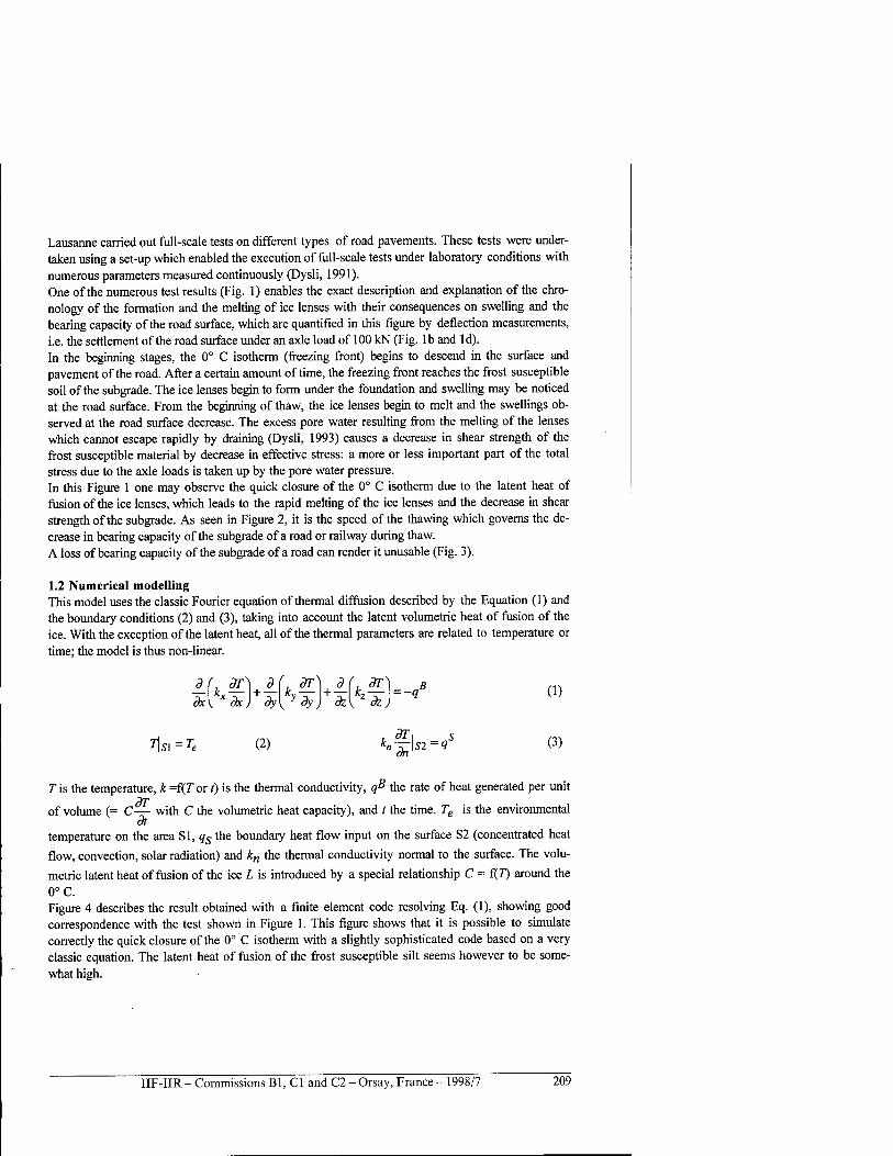
Lausanne carried out full-scale tests on different types of road pavements. These tests were undertaken using a set-up which enabled the execution of full-scale tests under laboratory conditions with numerous parameters measured continuously (Dysli, 1991). One of the numerous test results (Fig. 1) enables the exact description and explanation of the chro- nology of the formation and the melting of ice lenses with their consequences on swelling and the bearing capacity of the road surface, which are quantified in this figure by deflection measurements, i.e. the settlement of the road surface under an axle load of 100 kN (Fig. lb and Id). In the beginning stages, the 0° C isotherm (freezing front) begins to descend in the surface and pavement of the road. After a certain amount of time, the freezing front reaches the frost susceptible soil of the subgrade. The ice lenses begin to form under the foundation and swelling may be noticed at the road surface. From the beginning of thaw, the ice lenses begin to melt and the swellings observed at the road surface decrease. The excess pore water resulting from the melting of the lenses which cannot escape rapidly by draining (Dysli, 1993) causes a decrease in shear strength of the frost susceptible material by decrease in effective stress: a more or less important part of the total stress due to the axle loads is taken up by the pore water pressure. In this Figure 1 one may observe the quick closure of the 0° C isotherm due to the latent heat of fusion of the ice lenses, which leads to the rapid melting of the ice lenses and the decrease in shear strength of the subgrade. As seen in Figure 2, it is the speed of the thawing which governs the decrease in bearing capacity of the subgrade of a road or railway during thaw. A loss of bearing capacity of the subgrade of a road can render it unusable (Fig. 3).

1.2 Numerical modelling This model uses the classic Fourier equation of thermal diffusion described by the Equation (1) and the boundary conditions (2) and (3), taking into account the latent volumetric heat of fusion of the ice. With the exception of the latent heat, all of the thermal parameters are related to temperature or time; the model is thus non-linear.

T\Si=Te (2) knK\S2=qs (3)

T is the temperature, k =fiT or /) is the thermal conductivity, qB the rate of heat generated per unit ■yr

of volume (= C— with C the volumetric heat capacity), and t the time. Te is the environmental dt

temperature on the area SI, qs the boundary heat flow input on the surface S2 (concentrated heat

flow, convection, solar radiation) and kn the thermal conductivity normal to the surface. The volu-

metric latent heat of fusion of the ice L is introduced by a special relationship C = f(7) around the 0°C. Figure 4 describes the result obtained with a finite element code resolving Eq. (1), showing good correspondence with the test shown in Figure 1. This figure shows that it is possible to simulate correctly the quick closure of the 0° C isotherm with a slightly sophisticated code based on a very classic equation. The latent heat of fusion of the frost susceptible silt seems however to be somewhat high.

IIF-IIR - Commissions B1, C1 and C2 - Orsay, France -1998/7 209

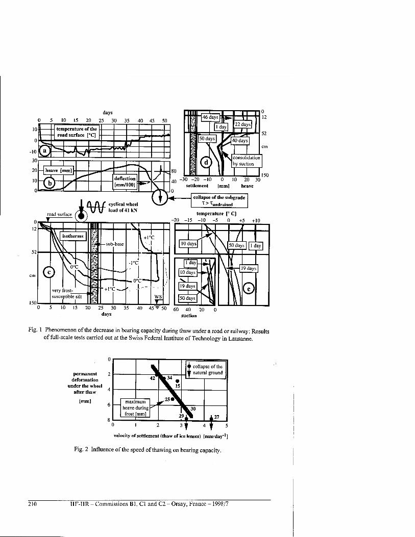
days

0 5 10 15 20 25 30 35 40 45 50

10

0

-10

30

H - road surface [°C]

W .„,/ k_ A f-~ —r r+*l S/'

30 -20 -10 0 10 20 30 settlement [mm] heave

I A A f cyclical wheel MJ \J\I load of 41 kN

road surface |A) T, , \9/

collapse of the subgrade t>T, undrained

temperature [° C] 20 -15 -10 -5 0 +5 +10

150 5 10 15 20 25 30 35 40 45 ~ 50 60 40 20

days suction

Fig. 1 Phenomenon of the decrease in bearing capacity during thaw under a road or railway: Results of full-scale tests carried out at the Swiss Federal Institute of Technology in Lausanne.

permanent 2 deformation

under the wheel after thaw

[mm]

0 1 2 3f 4 T 5

velocity of settlement (thaw of ice lenses) [mnrday"1]

Fig. 2 Influence of the speed of thawing on bearing capacity.


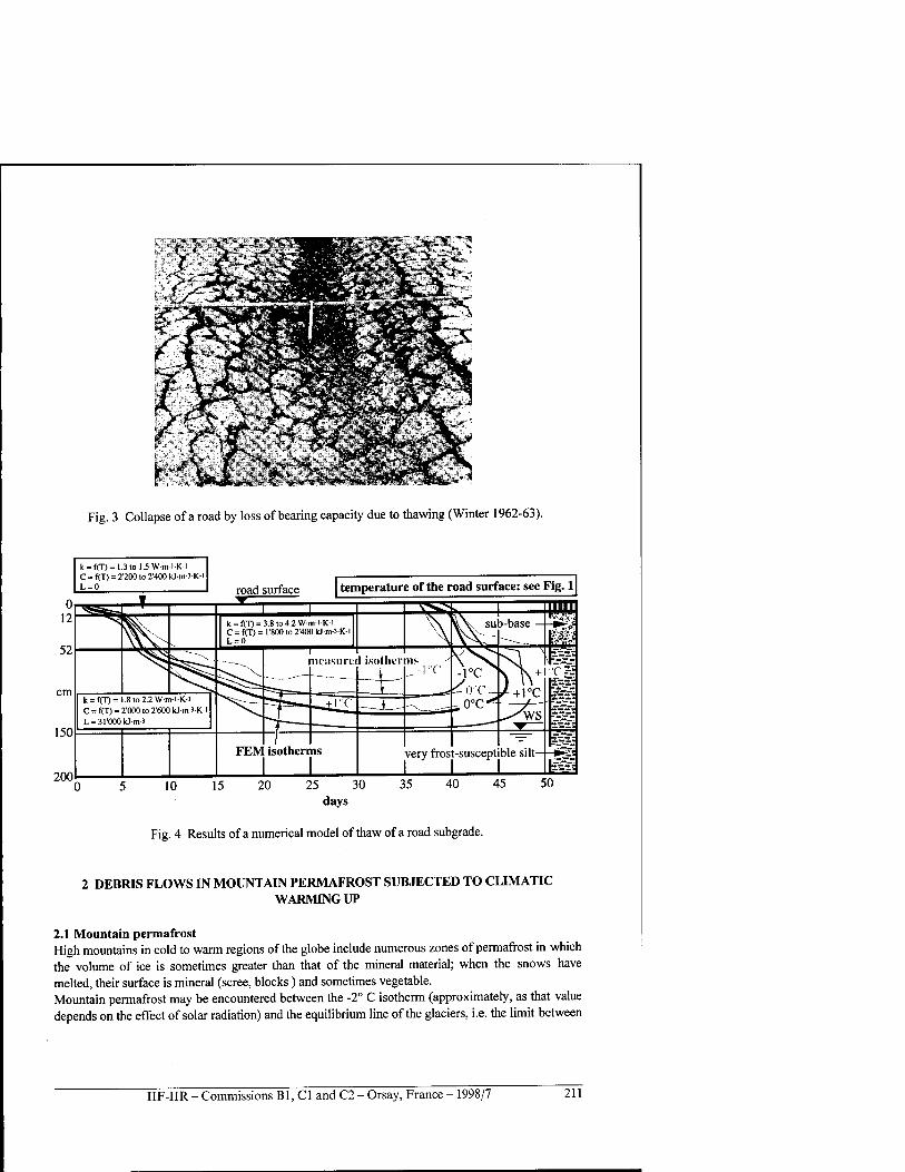
aJTv §F3

—«

*w-*-- V ">"^ j-*?- -V. P^

Fig. 3 Collapse of a road by loss of bearing capacity due to thawing (Winter 1962-63).

k = f(T)= 1.3to 1.5 Wm-l-K-l C = f(T) = 2'20O to 2400 kJ-m-3-K-l L = 0

I road surface temperature of the road surface: see Fig. 1

200

Fig. 4 Results of a numerical model of thaw of a road subgrade.

2 DEBRIS FLOWS IN MOUNTAIN PERMAFROST SUBJECTED TO CLIMATIC WARMING UP

2.1 Mountain permafrost High mountains in cold to warm regions of the globe include numerous zones of permafrost in which the volume of ice is sometimes greater than that of the mineral material; when the snows have melted, their surface is mineral (scree, blocks) and sometimes vegetable. Mountain permafrost may be encountered between the -2° C isotherm (approximately, as that value depends on the effect of solar radiation) and the equilibrium line of the glaciers, i.e. the limit between


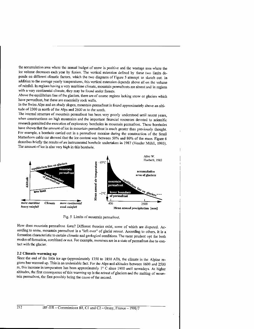
the accumulation area where the annual budget of snow is positive and the wastage area where the ice volume decreases each year by fusion. The vertical extension defined by these two limits depends on different climatic factors, which the two diagrams of Figure 5 attempt to sketch out. In addition to the average yearly temperatures, this vertical extension depends above all on the volume of rainfall. In regions having a very maritime climate, mountain permafrosts are absent and in regions with a very continental climate, they may be found under forests. Above the equilibrium line of the glaciers, there are of course regions lacking snow or glaciers which have permafrost, but these are essentially rock walls. In the Swiss Alps and on shady slopes, mountain permafrost is found approximately above an altitude of 2300 m north of the Alps and 2600 m to the south. The internal structure of mountain permafrost has been very poorly understood until recent years, when constructions on high mountains and the important financial resources devoted to scientific research permitted the execution of exploratory boreholes in mountain permafrost. These boreholes have shown that the amount of ice in mountain permafrost is much greater than previously thought. For example, a borehole carried out in a permafrost moraine during the construction of the Small Matterhorn cable car showed that the ice content was between 50% and 80% of the mass. Figure 6 describes briefly the results of an instrumented borehole undertaken in 1987 (Vonder Miihll, 1993). The amount of ice is also very high in this borehole.

glaciers

mountain permafrost

-15°C

a. E

tree limit -2°C

more maritime Climate more continental heavy rainfall weak rainfall

After W. Haeberli, 1983

accumulation area of glaciers

400 2500 Mean annual precipitation [mm]

Fig. 5 Limits of mountain permafrost.

How does mountain permafrost form? Different theories exist, some of which are disputed. Ac- cording to some, mountain permafrost is a "left over" of glacial retreat. According to others, it is a formation characteristic to certain climatic and geological conditions. The more prudent opt for both modes of formation, combined or not. For example, moraines are in a state of permafrost due to contact with the glacier.

2.2 Climatic warming up Since the end of the little ice age (approximately 1350 to 1850 AD), the climate in the Alpine regions has warmed up. This is an undeniable fact. For the Alps and altitudes between 1600 and 2500 m, this increase in temperature has been approximately 1° C since 1900 until nowadays. At higher altitudes, the first consequence of this warming up is the retreat of glaciers and the melting of mountain permafrost, the first possibly being the cause of the second.

212 IIF-IIR- Commissions Bl, Cl and C2 - Orsay, France - 1998/7

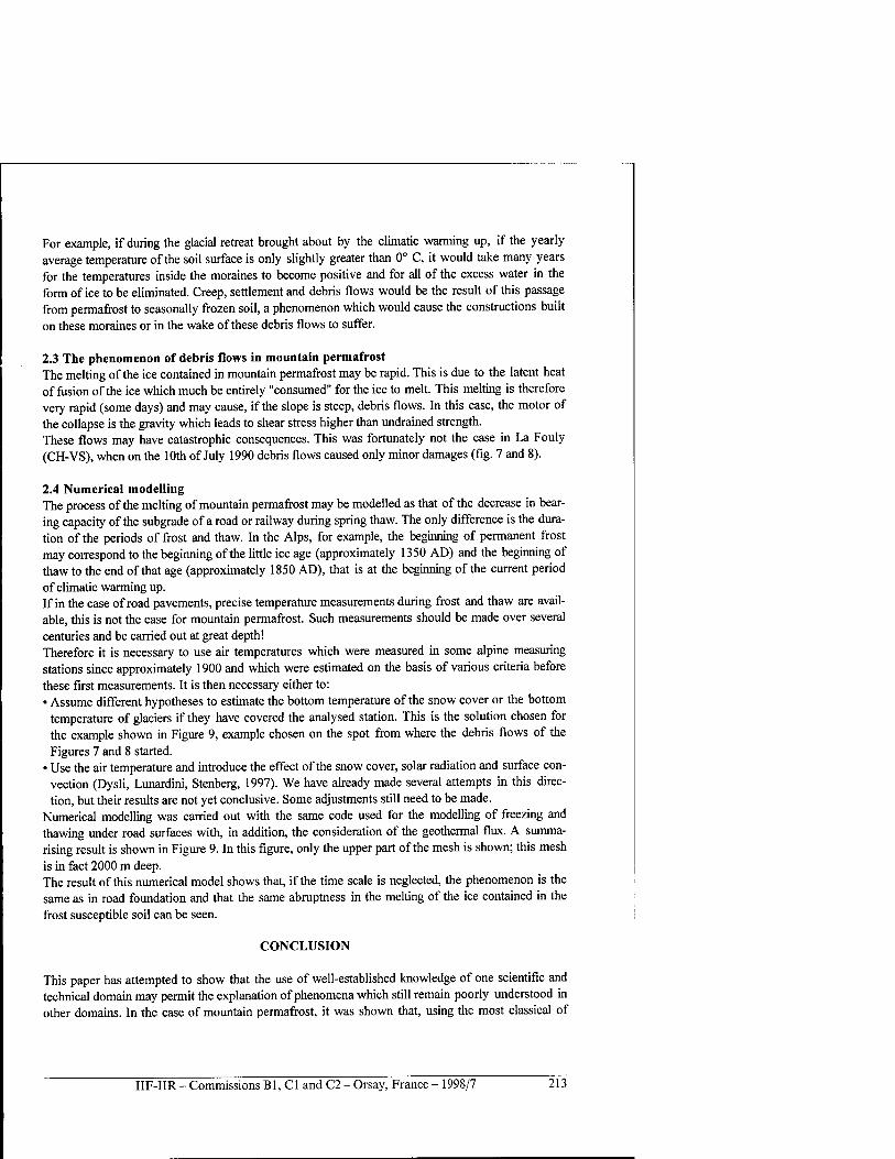
For example, if during the glacial retreat brought about by the climatic warming up, if the yearly average temperature of the soil surface is only slightly greater than 0° C, it would take many years for the temperatures inside the moraines to become positive and for all of the excess water in the form of ice to be eliminated. Creep, settlement and debris flows would be the result of this passage from permafrost to seasonally frozen soil, a phenomenon which would cause the constructions built on these moraines or in the wake of these debris flows to suffer.

2.3 The phenomenon of debris flows in mountain permafrost The melting of the ice contained in mountain permafrost may be rapid. This is due to the latent heat of fusion of the ice which much be entirely "consumed" for the ice to melt. This melting is therefore very rapid (some days) and may cause, if the slope is steep, debris flows. In this case, the motor of the collapse is the gravity which leads to shear stress higher than undrained strength. These flows may have catastrophic consequences. This was fortunately not the case in La Fouly (CH-VS), when on the 10th of July 1990 debris flows caused only minor damages (fig. 7 and 8).

2.4 Numerical modelling The process of the melting of mountain permafrost may be modelled as that of the decrease in bearing capacity of the subgrade of a road or railway during spring thaw. The only difference is the duration of the periods of frost and thaw. In the Alps, for example, the beginning of permanent frost may correspond to the beginning of the little ice age (approximately 1350 AD) and the beginning of thaw to the end ofthat age (approximately 1850 AD), that is at the beginning of the current period of climatic warming up. If in the case of road pavements, precise temperature measurements during frost and thaw are available, this is not the case for mountain permafrost. Such measurements should be made over several centuries and be carried out at great depth! Therefore it is necessary to use air temperatures which were measured in some alpine measuring stations since approximately 1900 and which were estimated on the basis of various criteria before these first measurements. It is then necessary either to: • Assume different hypotheses to estimate the bottom temperature of the snow cover or the bottom

temperature of glaciers if they have covered the analysed station. This is the solution chosen for the example shown in Figure 9, example chosen on the spot from where the debris flows of the Figures 7 and 8 started.

• Use the air temperature and introduce the effect of the snow cover, solar radiation and surface convection (Dysli, Lunardini, Stenberg, 1997). We have already made several attempts in this direction, but their results are not yet conclusive. Some adjustments still need to be made.

Numerical modelling was carried out with the same code used for the modelling of freezing and thawing under road surfaces with, in addition, the consideration of the geothermal flux. A summa- rising result is shown in Figure 9. In this figure, only the upper part of the mesh is shown; this mesh is in fact 2000 m deep. The result of this numerical model shows that, if the time scale is neglected, the phenomenon is the same as in road foundation and that the same abruptness in the melting of the ice contained in the frost susceptible soil can be seen.

CONCLUSION

This paper has attempted to show that the use of well-established knowledge of one scientific and technical domain may permit the explanation of phenomena which still remain poorly understood in other domains. In the case of mountain permafrost, it was shown that, using the most classical of


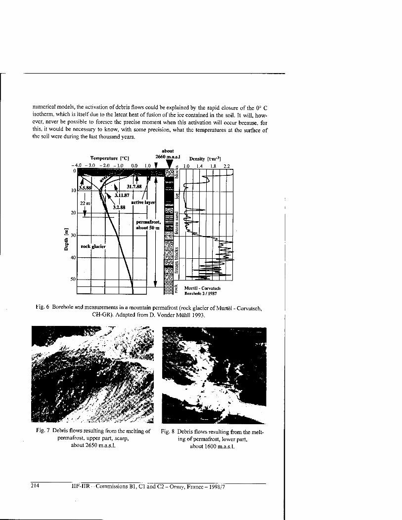
numerical models, the activation of debris flows could be explained by the rapid closure of the 0° C isotherm, which is itself due to the latent heat of fusion of the ice contained in the soil. It will, however, never be possible to foresee the precise moment when this activation will occur because, for this, it would be necessary to know, with some precision, what the temperatures at the surface of the soil were during the last thousand years.

-4.0 0|

Temperature [°C]

-3.0 -2.0 -1.0 0.0

about 2660 m.a.s.l Density [t-m"3)

1.0 1.4 1.8 2.2

Murtel - Corvatsch Borehole 2/1987

Fig. 6 Borehole and measurements in a mountain permafrost (rock glacier of Murtel - Corvatsch, CH-GR). Adapted from D. Vonder Miihll 1993.

Fig. 7 Debris flows resulting from the melting of permafrost, upper part, scarp,

about 2650 m.a.s.l.

Fig. 8 Debris flows resulting from the melting of permafrost, lower part,

about 1600 m.a.s.l.


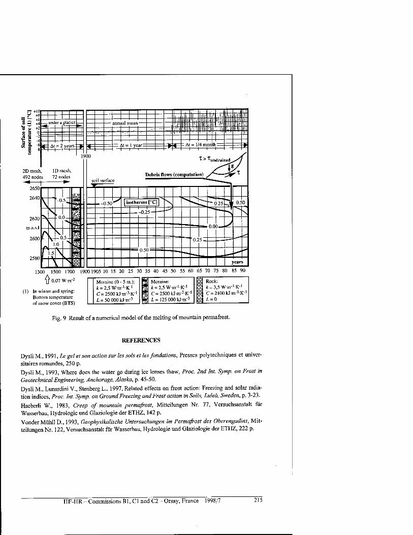
FT +101 Y +8

1300 1500 1700 19001905 10 15 20 25 30 35 40 45 50 55 60 65 70 75 80 85 90

{} 0.07 W-nr2

(1) In winter and spring: Bottom temperature of snow cover (BTS)

Moraine (0 - 5 m.): t = 2,5W-m-'-K-1

C=2500kJ-nr:,-K-1

L = 50 000 kJ-nv3

U J S Moraine: S * = 2,5W-m-|-K-1

% C = 2500kJm-3K-1

%| L=125 000kJ-m-3

Rock: jt = 3,5Wm-'-K-1

C=2l00kJ-m-3-K-' L = 0

Fig. 9 Result of a numerical model of the melting of mountain permafrost.

REFERENCES

Dysli M., 1991, Le gel et son action sur les sols et les fondations, Presses polytechniques et univer- sitäres romandes, 250 p. Dysli M., 1993, Where does the water go during ice lenses thaw, Proc. 2nd Int. Symp. on Frost in Geotechnical Engineering, Anchorage, Alaska, p. 45-50.

Dysli M., Lunardini V., Stenberg L., 1997, Related effects on frost action: Freezing and solar radiation indices, Proc. Int. Symp. on Ground Freezing and Frost action in Soils, Luleä, Sweden, p. 3-23.

Haeberli W., 1983, Creep of mountain permafrost, Mitteilungen Nr. 77, Versuchsanstalt für Wasserbau, Hydrologie und Glaziologie der ETHZ, 142 p.

VonderMühll D., 1993, Geophysikalische Untersuchungen im Permafrost des Oberengadins, Mit- teilungen Nr. 122, Versuchsanstalt für Wasserbau, Hydrologie und Glaziologie der ETHZ, 222 p.


PERTE DE PORTANCE AU DEGEL DES FONDATIONS DE ROUTES ET FORMATION DES LAVES TORRENTIELLES DANS LES PERGELISOLS ALPINS: UN MEME PHENOMENE

RESUME: La communication traite de la similitude entre la diminution de la portance au degel dans les sols gelifs d'infrastructure de routes et de voies ferrees et la formation de laves torrentielles dans les pergelisols alpins soumis ä un rechauffement du climat. Elle montre, en particulier, que sur le plan thermique comme sur le plan mecanique le phenomene est le meme et que la chaleur latente de fusion de la glace y joue un röle preponderant. Cela explique la brutalite de ces deux phenomenes destructeurs et coüteux.


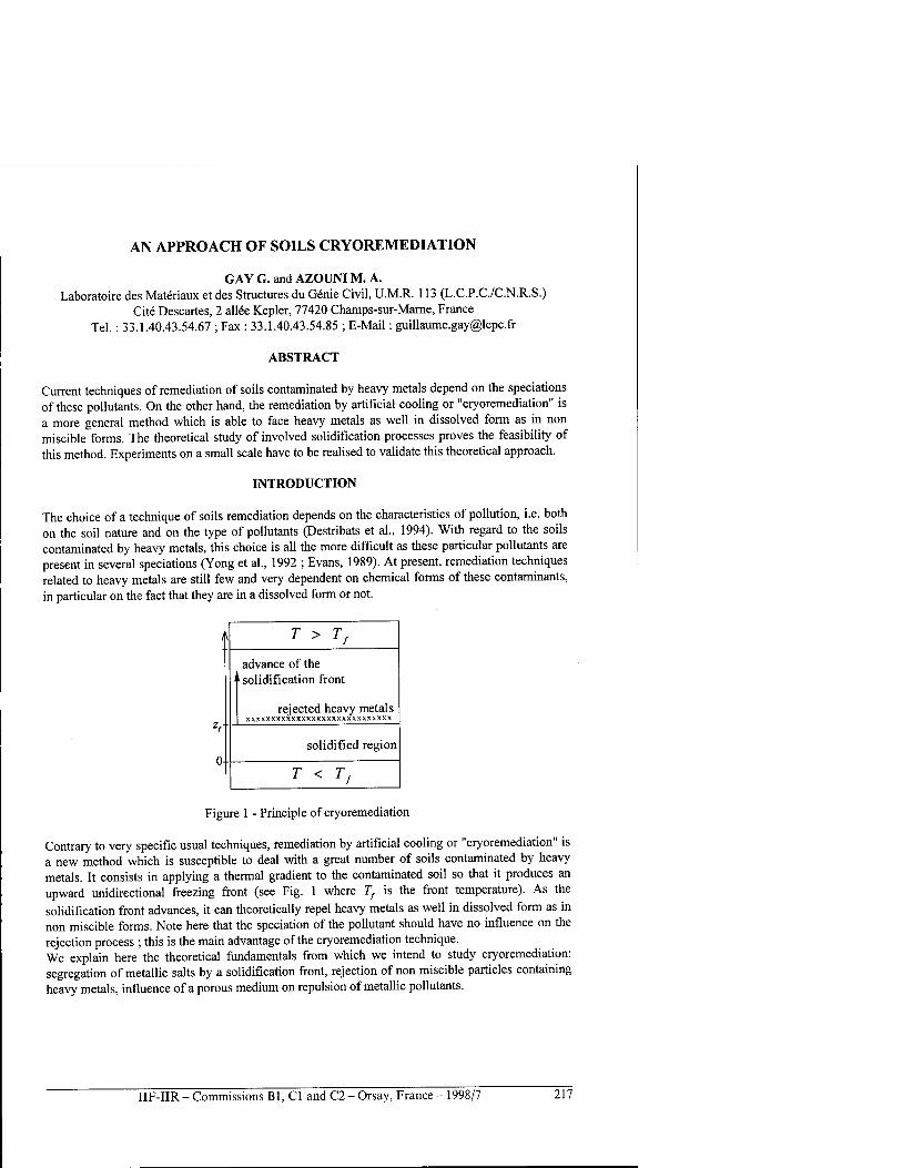
AN APPROACH OF SOILS CRYOREMEDIATION

GAY G. and AZOUNI M. A. Laboratoire des Materiaux et des Structures du Genie Civil, U.M.R. 113 (L.C.P.C./C.N.R.S.)

Cite Descartes, 2 allee Kepler, 77420 Champs-sur-Marne, France Tel. : 33.1.40.43.54.67 ; Fax : 33.1.40.43.54.85 ; E-Mail: [email protected]

ABSTRACT

Current techniques of remediation of soils contaminated by heavy metals depend on the speciations of these pollutants. On the other hand, the remediation by artificial cooling or "cryoremediation" is a more general method which is able to face heavy metals as well in dissolved form as in non miscible forms. The theoretical study of involved solidification processes proves the feasibility of this method. Experiments on a small scale have to be realised to validate this theoretical approach.

INTRODUCTION

The choice of a technique of soils remediation depends on the characteristics of pollution, i.e. both on the soil nature and on the type of pollutants (Destribats et al., 1994). With regard to the soils contaminated by heavy metals, this choice is all the more difficult as these particular pollutants are present in several speciations (Yong et al., 1992 ; Evans, 1989). At present, remediation techniques related to heavy metals are still few and very dependent on chemical forms of these contaminants, in particular on the fact that they are in a dissolved form or not.

0--

T > Tf

advance of the iL solidification front

rejected heavy metals xxxxxxxxxxxxxxxxxxxxxxxxxxxxx

solidified region

T < T,

Figure 1 - Principle of cryoremediation

Contrary to very specific usual techniques, remediation by artificial cooling or "cryoremediation" is a new method which is susceptible to deal with a great number of soils contaminated by heavy metals. It consists in applying a thermal gradient to the contaminated soil so that it produces an upward unidirectional freezing front (see Fig. 1 where Tf is the front temperature). As the solidification front advances, it can theoretically repel heavy metals as well in dissolved form as in non miscible forms. Note here that the speciation of the pollutant should have no influence on the rejection process ; this is the main advantage of the cryoremediation technique. We explain here the theoretical fundamentals from which we intend to study cryoremediation: segregation of metallic salts by a solidification front, rejection of non miscible particles containing heavy metals, influence of a porous medium on repulsion of metallic pollutants.


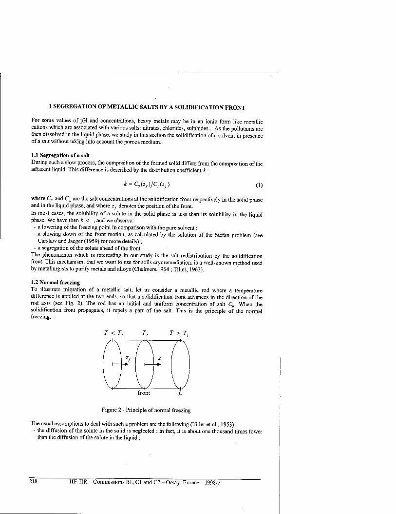
1 SEGREGATION OF METALLIC SALTS BY A SOLIDIFICATION FRONT

For some values of pH and concentrations, heavy metals may be in an ionic form like metallic cations which are associated with various salts: nitrates, chlorides, sulphides... As the pollutants are then dissolved in the liquid phase, we study in this section the solidification of a solvent in presence of a salt without taking into account the porous medium.

1.1 Segregation of a salt During such a slow process, the composition of the formed solid differs from the composition of the adjacent liquid. This difference is described by the distribution coefficient k :

k = Cs(zf)/CL(zf) 0)

where C, and CL are the salt concentrations at the solidification front respectively in the solid phase and in the liquid phase, and where zf denotes the position of the front. In most cases, the solubility of a solute in the solid phase is less than its solubility in the liquid phase. We have then k < , and we observe:

- a lowering of the freezing point in comparison with the pure solvent; - a slowing down of the front motion, as calculated by the solution of the Stefan problem (see

Carslaw and Jaeger (1959) for more details); - a segregation of the solute ahead of the front.

The phenomenon which is interesting in our study is the salt redistribution by the solidification front. This mechanism, that we want to use for soils cryoremediation, is a well-known method used by metallurgists to purify metals and alloys (Chalmers, 1964 ; Tiller, 1963).

1.2 Normal freezing To illustrate migration of a metallic salt, let us consider a metallic rod where a temperature difference is applied at the two ends, so that a solidification front advances in the direction of the rod axis (see Fig. 2). The rod has an initial and uniform concentration of salt C0. When the solidification front propagates, it repels a part of the salt. This is the principle of the normal freezing.

T < T,

front

T > T,

Figure 2 - Principle of normal freezing

The usual assumptions to deal with such a problem are the following (Tiller et al., 1953): - the diffusion of the solute in the solid is neglected ; in fact, it is about one thousand times lower

than the diffusion of the solute in the liquid ;


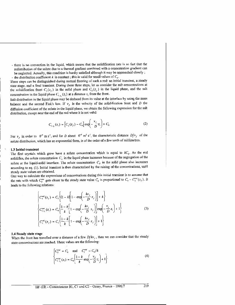
- there is no convection in the liquid, which means that the solidification rate is so fast that the redistribution of the solute due to a thermal gradient combined with a concentration gradient can be neglected. Actually, this condition is hardly satisfied although it may be approached closely ;

- the distribution coefficient k is constant; this is valid for small values of C0. Three steps can be distinguished during normal freezing of such a rod: an initial transient, a steady state stage, and a final transient. During these three steps, let us consider the salt concentrations at the solidification front Cs(zf) in the solid phase and CL{zf) in the liquid phase, and the salt concentration in the liquid phase C, 2/ (z,) at a distance z, from the front. Salt distribution in the liquid phase may be deduced from its value at the interface by using the mass balance and the second Fick's law. If vf is the velocity of the solidification front and D the

diffusion coefficient of the solute in the liquid phase, we obtain the following expression for the salt distribution, except near the end of the rod where it is not valid:

C,.,,(*,)' [QCz^-QJexpj-^-z, + C„ (2)

For v, in order to (T5 m s'1, and for D about 0"' m2 s"1, the characteristic distance D/vf of the

solute distribution, which has an exponential form, is of the order of a few tenth of millimetres.

1.3 Initial transient The first crystals which grow have a solute concentration which is equal to kC0. As the rod solidifies, the solute concentration CL in the liquid phase increases because of the segregation of the solute at the liquid-solid interface. The solute concentration Cs in the solid phase also increases according to eq. (1). Initial transient is then characterised by the raising of the concentrations, until steady state values are obtained. One way to calculate the expressions of concentrations during this initial transient is to assume that the rate with which Cj"' gets closer to the steady state value C0 is proportional to C0 - C™"{zf). It

leads to the following relations:

fi — jfcr f kvf CZW-CA— l-expl- —

A-k CT'(zf) = CA-r l-exp|- — zf

+ k

+ 1

exd-^-z, +1 D

(3)

1.4 Steady state stage When the front has travelled over a distance of a few D/kvf, then we can consider that the steady

state concentrations are reached. These values are the following:

cr = C0 and Cf = Cjk

c;:i,(z,) = Cc 1-Jfc exP|-^z/l + 1

(4)


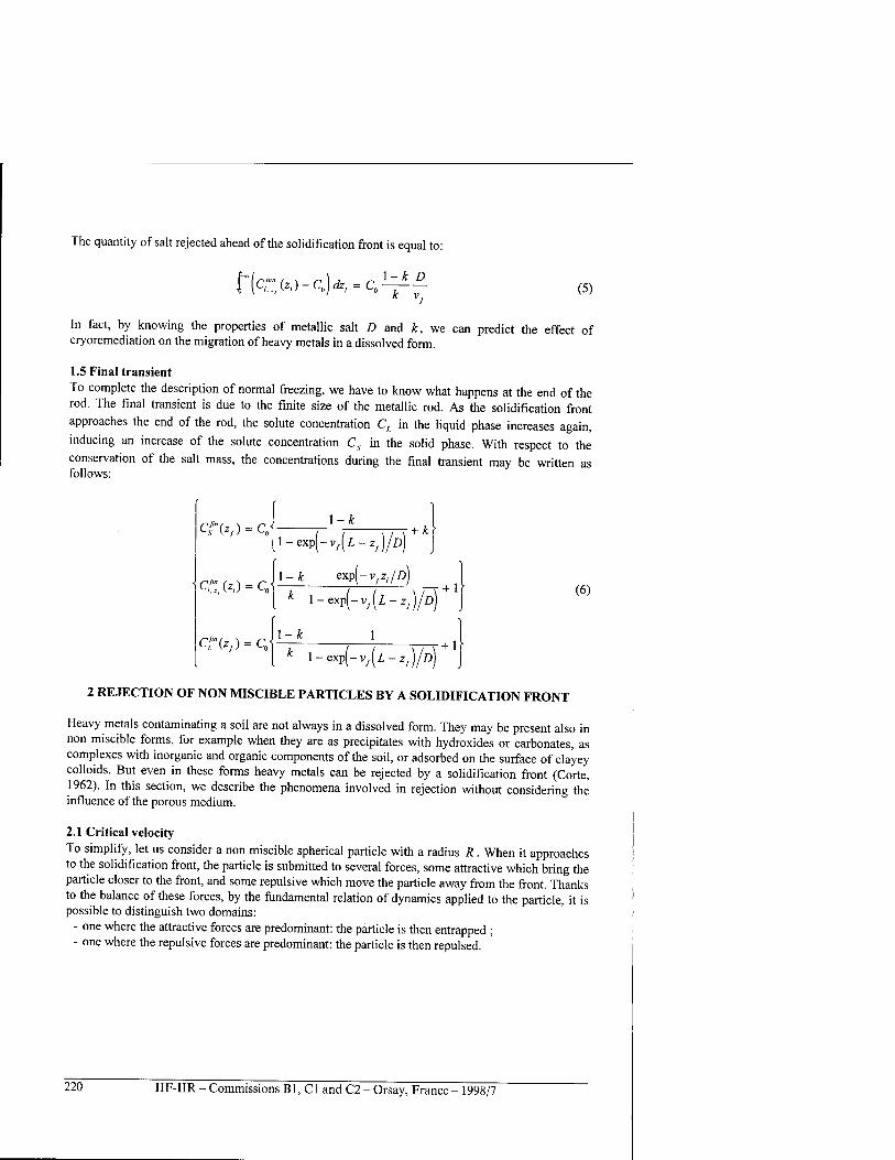
The quantity of salt rejected ahead of the solidification front is equal to:

r(qT,(*,)-c0)<fc; = c0- k D (5)

In fact, by knowing the properties of metallic salt D and k, we can predict the effect of cryoremediation on the migration of heavy metals in a dissolved form.

1.5 Final transient To complete the description of normal freezing, we have to know what happens at the end of the rod. The final transient is due to the finite size of the metallic rod. As the solidification front approaches the end of the rod, the solute concentration C, in the liquid phase increases again,

inducing an increase of the solute concentration Cs. in the solid phase. With respect to the conservation of the salt mass, the concentrations during the final transient may be written as follows:

C£,(z,) = Q

Cf"{zf) = C0-

\-k + k

[l-expj-v^l-*,)/*>) j

\-k exp(-v/Z;/£>) + 1

l-expj-vÎ-z,)//)) j (6)

1-fc + 1

l-expf-v^Z-z,)//)) J

2 REJECTION OF NON MISCIBLE PARTICLES BY A SOLIDIFICATION FRONT

Heavy metals contaminating a soil are not always in a dissolved form. They may be present also in non miscible forms, for example when they are as precipitates with hydroxides or carbonates, as complexes with inorganic and organic components of the soil, or adsorbed on the surface of clayey colloids. But even in these forms heavy metals can be rejected by a solidification front (Corte, 1962). In this section, we describe the phenomena involved in rejection without considering the influence of the porous medium.

2.1 Critical velocity To simplify, let us consider a non miscible spherical particle with a radius R . When it approaches to the solidification front, the particle is submitted to several forces, some attractive which bring the particle closer to the front, and some repulsive which move the particle away from the front. Thanks to the balance of these forces, by the fundamental relation of dynamics applied to the particle, it is possible to distinguish two domains:

- one where the attractive forces are predominant: the particle is then entrapped ; - one where the repulsive forces are predominant: the particle is then repulsed.


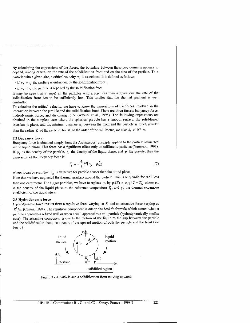
By calculating the expressions of the forces, the boundary between these two domains appears to depend, among others, on the rate of the solidification front and on the size of the particle. To a particle with a given size, a critical velocity vc is associated. It is defined as follows:

- if vf > vc the particle is entrapped by the solidification front;

- if v/ < vc the particle is repelled by the solidification front. It may be seen that to repel all the particles with a size less than a given one the rate of the solidification front has to be sufficiently low. This implies that the thermal gradient is well controlled. To calculate the critical velocity, we have to know the expressions of the forces involved in the interaction between the particle and the solidification front. There are three forces: buoyancy force, hydrodynamic force, and disjoining force (Azouni et al., 1995). The following expressions are obtained in the simplest case where the spherical particle has a smooth surface, the solid-liquid interface is plane, and trie minimal distance h0 between the front and the particle is much smaller

than the radius R of the particle: for R of the order of the millimetre, we take k0 < 10~5 m.

2.2 Buoyancy force Buoyancy force is obtained simply from the Archimedes' principle applied to the particle immersed in the liquid phase. This force has a significant effect only on millimetre particles (Yemmou, 1991). If p is the density of the particle, p, the density of the liquid phase, and g the gravity, then the

expression of the buoyancy force is: A

(7) F. = *'(P,- P, g

where it can be seen that Fg is attractive for particle denser than the liquid phase.

Note that we have neglected the thermal gradient around the particle. This is only valid for radii less

than one centimetre. For bigger particles, we have to replace p, by p,(T) = p,0y,[T - T„) where p,0

is the density of the liquid phase at the reference temperature T0, and y, the thermal expansion coefficient of the liquid phase.

2.3 Hydrodynamic force Hydrodynamic force results from a repulsive force varying as R and an attractive force varying as R2/h0 (Casses, 1994). The repulsive component is due to the Stake's formula which occurs when a particle approaches a fixed wall or when a wall approaches a still particle (hydrodynamically similar case). The attractive component is due to the motion of the liquid to the gap between the particle and the solidification front, as a result of the upward motion of both the particle and the front (see Fig. 3).

zA

motion motion

Figure 3 - A particle and a solidification front moving upwards


With the assumption that h0 «R, the hydrodynamic force is globally attractive. If p{r) is the pressure in the liquid film at a distance r from the particle axis, then we have:

Fn = %2nr{p(r)-p(R))dr (8)

If T| is the dynamic viscosity of the liquid phase, pv the density of the solidified phase, and v the

particle velocity, then the expression of the hydrodynamic force is:

F = -67ÜT1 .Piz£i.Vf f (9)

If we can make the approximation p; « pv (e.g. water-ice system), then the hydrodynamic force becomes: Fn = -6nr\vp R

2/h0.

2.4 Disjoining force Disjoining force is due to the molecular interactions that occur in the liquid film between the particle and the solidified phase. If the distance h0 is not too small (/z0 > 10"8 m) then the structural interaction is negligible in comparison with the van der Waals interaction. If the particle has no surface charges, then there is no electrostatic interaction (Debye interaction). According to Israelachvili (1985), the disjoining force is obtained by differentiating the non- retarded van der Waals interaction energy between the particle and the front with respect to h0:

dW

With the assumption that h0 «R, it leads to:

^ R

F^-^K (11)

The Hamaker constant fl. can be expressed in fonction of macroscopic properties of ice, water, and

particle by the Lifshitz theory (Israelachvili, 1985): fl. = /(w,e) where n is the reflective index and e the dielectric constant. In most cases, Hamaker constant is positive and the disjoining force is then attractive. Nevertheless in the particular case of a particle-water-ice system, the Hamaker constant is negative, of the order of -10~2' J. So the disjoining force is the only repulsive force acting on the particle. In the simple configuration we choose to study, the critical velocity is inversely proportional to the radius of the particle. For more complicated configurations, like a rough particle or an irregular front, see the works of Azouni and Casses (Ref. 1 and 5).

3 INFLUENCE OF POROUS MEDIUM ON THE REJECTION OF HEAVY METALS

In previous sections, we have described the rejection of heavy metals, whatever their speciations, in a solvent. So far we have not taken into account the part of the contaminated porous medium in this rejection. In this section, let us see how a soil solidifies.


3.1 General observations The most coarse soils, like sands or gravels, have little influence on the phenomena described above. At most they lead to a delay in the dynamics of the migration of metallic pollutants. Solidification of fine soils, like clays or silts, is more particular. It results in the formation of ice layers, and the quantity of ice in such layers is greater than the expected amount of ice which would be produced by the water present initially.

3.2 Qualitative explanation in the case of a fine soil As the pores are very thin, a part of water is adsorbed on their surface. The freezing temperature of water in a pore is not uniform any more. For a given negative temperature, there is still unfrozen water at the surface of the pore. Consequently there is not a well defined solidification front but rather a freezing region. The dynamics of this freezing region lead to a decrease of the pressure near this region (Vignes and Dijkema, 1974). This lowering of pressure results in the migration of water from the unfrozen region to the freezing one. This migration explains the important quantities of ice observed in layers. As the unfrozen region dries out, it consolidates and its freezing temperature decreases. So this region cannot be frozen at the same temperature as that of the freezing region. For this reason, solidification in a fine soil leads to the formation of ice layers. Taking into account the influence of this particular freezing process on the rejection of metallic pollutants by cryoremediation is still complicated. A set of experiments on a small scale with colloidal suspensions of clay contaminated by heavy metals will help us to answer some of the raised questions.

CONCLUSION

In theory, the technique of cryoremediation is a method very adapted to soils contamination by heavy metals because it is not very affected by the several speciations of these pollutants and because it is particularly efficient when it is applied to small particles. Now, we have to validate the various models and assumptions that we have retained in our theoretical approach by carrying out experiments on a small scale (at least at first). Thanks to these experiments, we hope to measure the efficiency and the energy cost of cryoremediation in several cases more and more complicated : water containing metallic salts, water with non miscible particles containing heavy metals, "sound" porous medium, porous medium contaminated by heavy metals.

REFERENCES

1. Azouni M. A. and Casses P., 1998, Thermophysical properties effects on segregation during solidification, Advances in Colloid and Interface Science, vol. 75: pp. 83-106.

2. Azouni A., Casses P. et Yemmou M., 1995, A propos de la rencontre d'une particule spherique et d'un front de solidification, Bulletin de la Societe Franqaise de Physique, vol. 99: pp. 3-6.

3. Carslaw H. C. and Jaeger J. C, 1959, Conduction of heat in solids, Oxford Science Publications, second edition, chapter XI "Change of state", pp. 282-296.

4. Casses P., 1994, Interactions particules-front de solidification : modelisation et experiences, These de doctorat en Physique des Solides, Universite Denis Diderot, Paris VII, 158 pages.

5. Casses P. and Azouni-Aldi M. A., 1994, A general theoretical approach to the behaviour of foreign particles at advancing solid-liquid interfaces, Advances in Colloid and Interface Science, vol. 50: pp. 103-120.

6. Chalmers B., 1964, Principles of solidification, John Wiley and Sons Inc., 319 pages.


7. Corte A. E., 1962, Vertical migration of particles in front of a moving freezing plane, Journal of Geophysical Research, vol. 67 (3): pp. 1085-1090.

8. Destribats J.-M., Prez E. et Soyez B., 1994, La depollution des sols en place - Techniques et exemples, Etudes et Recherches des Laboratoires des Ponts et Chaussees, serie Environnement et Genie Urbain EG10.

9. Evans L. J., 1989, Chemistry of metal retention by soils, Environmental Science and Technology, vol. 23 (9): pp. 1046-1056.

10. Israelachvili, 1985, Intermolecular and surface forces, Academic Press Inc., chapter 11 "van der Waals forces between surfaces", pp. 137-160.

11. Tiller W. A., 1963, Principles of solidification, In : Gilman J. J., editor, The art and science of growing crystals, pages 276-312.

12. Tiller W. A., Jackson K. A., Rutter J. W., and Chalmers B., 1953, The redistribution of solute atoms during the solidification of metals, Acta Metallurgica, vol. 1: pp. 428-437.

13. Vignes M. and Dijkema K. M., 1974, A model for the freezing of water in a dispersed medium, Journal of Colloid and Interface Science, vol. 49 (2): pp. 165-172.

14. Yemmou M, 1991, Etude des interactions particules-front de solidification, These de doctorat en Rheologie et Transfert de Masse et de Chaleur, Universite Denis Diderot, Paris VII, 189 pages.

15. Yong R. N., Mohammed A. M. O., and Warkentin B. P., 1992, Principles of contaminant transport in soils, Elsevier, collection "Developments in Geotechnical Engineering", n° 73, chapter V "Contaminant-soil interaction", pp. 143-180.

UNE APPROCHE DE LA CRYODEPOLLUTION DES SOLS

RESUME : Les techniques actuelles de depollution des sols contamines par des metaux lourds restent tres dependantes des speciations de ces polluants. La depollution par le froid, ou "cryodepollution", est en revanche une methode plus generate, capable de faire face aux metaux lourds aussi bien sous forme dissoute que sous des formes non miscibles. L'etude des bases theoriques des differents aspects concernes de la solidification montre la faisabilite de cette methode. Des experiences ä petite echelle restent ä mener afin de valider cette approche theorique.


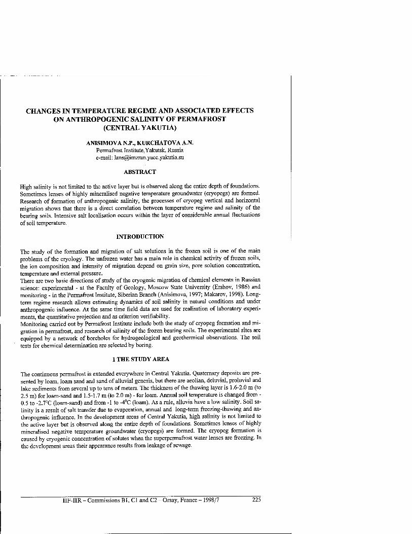
CHANGES IN TEMPERATURE REGIME AND ASSOCIATED EFFECTS ON ANTHROPOGENIC SALINITY OF PERMAFROST

(CENTRAL YAKUTIA)

ANISIMOVA N.P., KURCHATOVA A.N. Permafrost Institute,Yakutsk, Russia e-mail: [email protected]

ABSTRACT

High salinity is not limited to the active layer but is observed along the entire depth of foundations. Sometimes lenses of highly mineralised negative temperature groundwater (cryopegs) are formed. Research of formation of anthropogenic salinity, the processes of cryopeg vertical and horizontal migration shows that there is a direct correlation between temperature regime and salinity of the bearing soils. Intensive salt localisation occurs within the layer of considerable annual fluctuations of soil temperature.

INTRODUCTION

The study of the formation and migration of salt solutions in the frozen soil is one of the main problems of the cryology. The unfrozen water has a main role in chemical activity of frozen soils, the ion composition and intensity of migration depend on grain size, pore solution concentration, temperature and external pressure. There are two basic directions of study of the cryogenic migration of chemical elements in Russian science: experimental - at the Faculty of Geology, Moscow State University (Ershov, 1986) and monitoring - in the Permafrost Institute, Siberian Branch (Anisimova, 1997; Makarov, 1998). Long- term regime research allows estimating dynamics of soil salinity in natural conditions and under anthropogenic influence. At the same time field data are used for realisation of laboratory experiments, the quantitative projection and as criterion verifiability. Monitoring carried out by Permafrost Institute include both the study of cryopeg formation and migration in permafrost, and research of salinity of the frozen bearing soils. The experimental sites are equipped by a network of boreholes for hydrogeological and geothermical observations. The soil tests for chemical determination are selected by boring.

1 THE STUDY AREA

The continuous permafrost is extended everywhere in Central Yakutia. Quaternary deposits are presented by loam, loam sand and sand of alluvial genesis, but there are aeolian, deluvial, proluvial and lake sediments from several up to tens of meters. The thickness of the thawing layer is 1.6-2.0 m (to 2.5 m) for loam-sand and 1.5-1.7 m (to 2.0 m) - for loam. Annual soil temperature is changed from - 0.5 to -2.7°C (loam-sand) and from -1 to -4°C (loam). As a rule, alluvia have a low salinity. Soil salinity is a result of salt transfer due to evaporation, annual and long-term freezing-thawing and anthropogenic influence. In the development areas of Central Yakutia, high salinity is not limited to the active layer but is observed along the entire depth of foundations. Sometimes lenses of highly mineralised negative temperature groundwater (cryopegs) are formed. The cryopeg formation is caused by cryogenic concentration of solutes when the superpermafrost water lenses are freezing. In the development areas their appearance results from leakage of sewage.


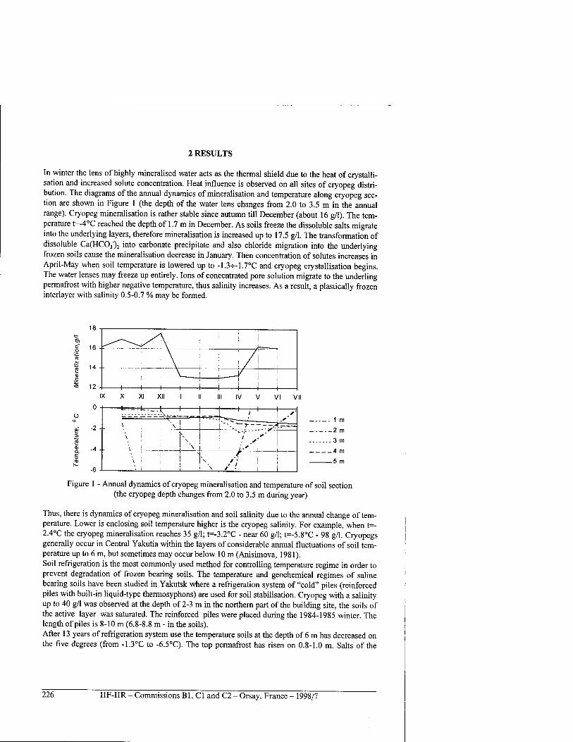
2 RESULTS

In winter the lens of highly mineralised water acts as the thermal shield due to the heat of crystallisation and increased solute concentration. Heat influence is observed on all sites of cryopeg distribution. The diagrams of the annual dynamics of mineralisation and temperature along cryopeg section are shown in Figure 1 (the depth of the water lens changes from 2.0 to 3.5 m in the annual range). Cryopeg mineralisation is rather stable since autumn till December (about 16 g/1). The temperature t=-4°C reached the depth of 1.7 m in December. As soils freeze the dissoluble salts migrate into the underlying layers, therefore mineralisation is increased up to 17.5 g/1. The transformation of dissoluble Ca(HC03')2 into carbonate precipitate and also chloride migration into the underlying frozen soils cause the mineralisation decrease in January. Then concentration of solutes increases in April-May when soil temperature is lowered up to -1.3-H-1.7°C and cryopeg crystallisation begins. The water lenses may freeze up entirely. Ions of concentrated pore solution migrate to the underling permafrost with higher negative temperature, thus salinity increases. As a result, a plastically frozen interlayer with salinity 0.5-0.7 % may be formed.

c 16 - ^^—^^^ S^\ \ i i

"CD

"55 14 - ■\: I/| \

03 \ ! ; / | '• § 12-

\ ! ! j 1 1 1 1 i 1 j 1 j

o Q

8? CO

0> a S CD

1 m

-2 m

. 3 m

-4 m

-5 m

Figure 1 - Annual dynamics of cryopeg mineralisation and temperature of soil section (the cryopeg depth changes from 2.0 to 3.5 m during year)

Thus, there is dynamics of cryopeg mineralisation and soil salinity due to the annual change of temperature. Lower is enclosing soil temperature higher is the cryopeg salinity. For example, when t=- 2.4°C the cryopeg mineralisation reaches 35 g/1; t=-3.2°C - near 60 g/1; t=-5.8°C - 98 g/1. Cryopegs generally occur in Central Yakutia within the layers of considerable annual fluctuations of soil temperature up to 6 m, but sometimes may occur below 10 m (Anisimova, 1981). Soil refrigeration is the most commonly used method for controlling temperature regime in order to prevent degradation of frozen bearing soils. The temperature and geochemical regimes of saline bearing soils have been studied in Yakutsk where a refrigeration system of "cold" piles (reinforced piles with built-in liquid-type thermosyphons) are used for soil stabilisation. Cryopeg with a salinity up to 40 g/1 was observed at the depth of 2-3 m in the northern part of the building site, the soils of the active layer was saturated. The reinforced piles were placed during the 1984-1985 winter. The length of piles is 8-10 m (6.8-8.8 m - in the soils). After 13 years of refrigeration system use the temperature soils at the depth of 6 m has decreased on the five degrees (from -1.3°C to -6.5°C). The top permafrost has risen on 0.8-1.0 m. Salts of the


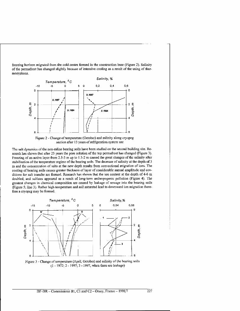
freezing horizon migrated from the cold centre formed in the construction base (Figure 2). Salinity of the permafrost has changed slightly because of intensive cooling as a result of the using of thermosyphons.

Salinity, %

-10 Temperature, °C

-5 0 5 0

E 2

Q.

Q

X.1997 / / t /

/ /

1 \

1 X.1984

/ 1

1 1

1 1

Figure 2 - Change of temperature (October) and salinity along cryopeg section after 13 years of refrigeration system use

The salt dynamics of the non-saline bearing soils have been studied on the second building site. Re- search has shown that after 25 years the pore solution of the top permafrost has changed (Figure 3). Freezing of an active layer from 2.5-3 m up to 1.5-2 m caused the great changes of the salinity after stabilisation of the temperature regime of the bearing soils. The decrease of salinity at the depth of 3 m and the concentration of salts at the new depth results from convectional migration of ions. The cooling of bearing soils causes greater thickness of layer of considerable annual amplitude and conditions for salt transfer are formed. Research has shown that the ion content at the depth of 4-6 m doubled, and sulfates appeared as a result of long-term anthropogenic pollution (Figure 4). The greatest changes in chemical composition are caused by leakage of sewage into the bearing soils (Figure 5; line 3). Rather high temperature and soil saturated lead to downward ion migration therefore a cryopeg may be formed.

-15

Temperature, C

-10 -5 0 5 0

Salinity,%

0,04 0,08

E 2

JE Q. <B Q

N X

7\, 1 / i 2 ■ I

,-/

\ / / , ' • s if:

\ f /•' \ • \ , 1 ' /' V \ ' /' \^

\ / / 3 \ ' /• / t \ \! : ( n \ \ : i: \ . !\ I '•'

Q.

Q

Figure 3 - Change of temperature (April, October) and salinity of the bearing soils (1 -1972; 2 -1997; 3 -1997, when there are leakage)


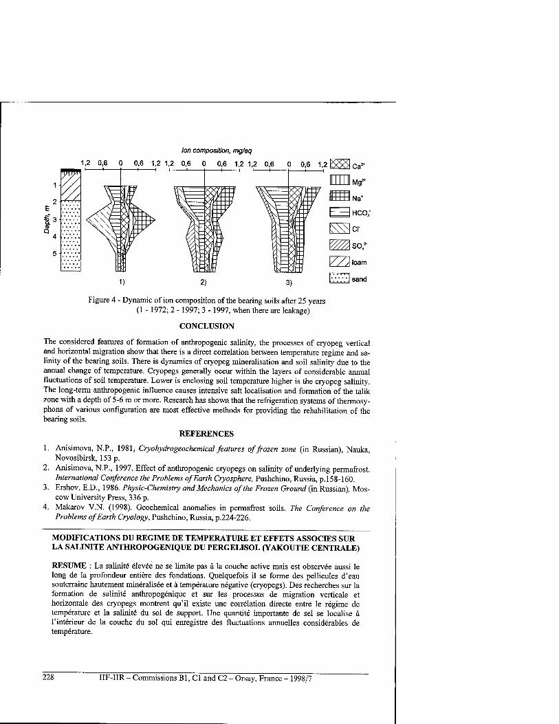
1

2 +

WJfll

r S4

5-

Ion composition, mg/eq

1,2 0,6 0 0,6 1,2 1,2 0,6 0 0,6 1,2 1,2 0,6 0 0,6 1,2 H 1 i ^ _i 1 i 1_

fl

Ca2*

iNa*

I HCO;

1) 2) 3)

EScr

Y/A loam

[•.•.•.'.•J sand

Figure 4 - Dynamic of ion composition of the bearing soils after 25 years (1 - 1972; 2 -1997; 3 -1997, when there are leakage)

CONCLUSION

The considered features of formation of anthropogenic salinity, the processes of cryopeg vertical and horizontal migration show that there is a direct correlation between temperature regime and salinity of the bearing soils. There is dynamics of cryopeg mineralisation and soil salinity due to the annual change of temperature. Cryopegs generally occur within the layers of considerable annual fluctuations of soil temperature. Lower is enclosing soil temperature higher is the cryopeg salinity. The long-term anthropogenic influence causes intensive salt localisation and formation of the talik zone with a depth of 5-6 m or more. Research has shown that the refrigeration systems of thermosyphons of various configuration are most effective methods for providing the rehabilitation of the bearing soils.

REFERENCES

1. Anisimova, N.P., 1981, Cryohydrogeochemical features of frozen zone (in Russian), Nauka, Novosibirsk, 153 p.

2. Anisimova, N.P., 1997. Effect of anthropogenic cryopegs on salinity of underlying permafrost. International Conference the Problems of Earth Cryosphere, Pushchino, Russia, p.158-160.

3. Ershov, E.D., 1986. Physic-Chemistry and Mechanics of the Frozen Ground (in Russian), Mos- cow University Press, 336 p.

4. Makarov V.N. (1998). Geochemical anomalies in permafrost soils. The Conference on the Problems of Earth Cryology, Pushchino, Russia, p.224-226.

MODIFICATIONS DU REGIME DE TEMPERATURE ET EFFETS ASSOCIES SUR LA SALINITE ANTHROPOGENIQUE DU PERGELISOL (YAKOUTIE CENTRALE)

RESUME : La salinite elevee ne se limite pas ä la couche active mais est observee aussi le long de la profondeur entiere des fondations. Quelquefois il se forme des pellicules d'eau souterraine hautement mineralisee et ä temperature negative (cryopegs). Des recherches sur la formation de salinite anthropogenique et sur les processus de migration verticale et horizontale des cryopegs montrent qu'il existe une correlation directe entre le regime de temperature et la salinite du sol de support. Une quantite importante de sei se localise ä l'interieur de la couche du sol qui enregistre des fluctuations annuelles considerables de temperature.


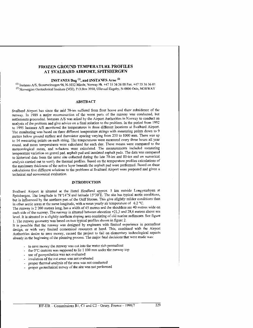
FROZEN GROUND TEMPERATURE PROFILES AT SVALBARD AIRPORT, SPITSBERGEN

INSTANES Dag(1), and INSTANES Arne <2)

(" Instanes A/S, Storetveitvegen 96, N-5032 Minde, Norway Ph. +47 55 36 36 00 Fax. +47 55 36 36 01 (2) Norwegian Geotechnical Institute (NGI), P.O.Box 3930, Ullevaal Hageby, N-0806 Oslo, NORWAY

ABSTRACT

Svalbard Airport has since the mid 70-ies suffered from frost heave and thaw subsidence of the runway. In 1989 a major reconstruction of the worst parts of the runway was conducted, but settlements proceeded. Instanes A/S was asked by the Airport Authorities in Norway to conduct an analysis of the problem and give advice on a final solution to the problem. In the period from 1992 to 1995 Instanes A/S monitored the temperatures in three different locations at Svalbard Airport. The monitoring was based on three different temperature strings with measuring points down to 9 metres below ground surface and thermistor spacing varying from 250 to 1000 mm. There was up to 14 measuring points on each string. The temperatures were measured every three hours all year round, and mean temperatures were calculated for each day. These means were compared to the meteorological mean, and n-factors were calculated. The measurements included measuring temperature variation on gravel pad, asphalt pad and insulated asphalt pads. The data was compared to historical data from the same site collected during the late 70-ies and 80-ies and on numerical analysis carried out to verify the thermal profiles. Based on the temperature profiles calculations of the maximum thickness of the active layer beneath the asphalt pad were performed. Based on these calculations five different solutions to the problems at Svalbard Airport were proposed and given a technical and economical evaluation.

INTRODUCTION

Svalbard Airport is situated at the Hotel Headland approx. 5 km outside Longyearbyen at Spitsbergen. The longitude is 78°14'N and latitude 15°30'E. The site has typical arctic conditions, but is influenced by the northern part of the Gulf Stream. This give slightly milder conditions than in other arctic areas at the same longitude, with a mean yearly air temperature of-6,2 °C. The runway is 2 200 metres long, has a width of 45 metres and the shoulders are 40 metres wide on each side of the runway. The runway is situated between elevation +21,3 and 28,6 metres above sea level. It is situated in a slightly northern sloping area consisting of old marine sediments. See figure 1. The runway geometry was based on two typical profiles shown in figure 2. It is possible that the runway was designed by engineers with limited experience in permafrost design, or with very limited economical resources at hand. This, combined with the Airport Authorities desire to save money, caused the project to fail on elementary technological aspects already in the beginning of the planning process. The major fatal decisions that were made was:

- to save money the runway was cut into the water rich permafrost - the 0°C-isoterm was supposed to lie 1 100 mm under the runway top - use of geosynthetics was not evaluated - insulation of the cut areas was not evaluated - proper thermal analysis of the area was not conducted - proper geotechnical survey of the site was not performed


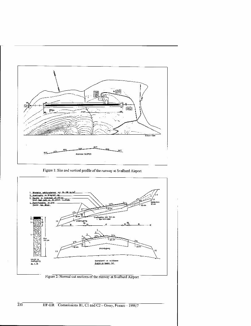
SCALE 1:100«

RUNWAY SLOPES

Figure 1: Site and vertical profile of the runway at Svalbard Airport

I Silnl.kke asfallorusbtlom Ann 16-130 kn/m' ? AvrMtinc*1<yi m Wkg/mi Ag 1 Rmr»lnn ™ nrrekinknlt M-ffllmm

fflfîlt mrf pikk «i IK-tOmm T = ?0cm

&_£PiStakningMfifl ov oru» Skyldm mm 30 em

■aVO

hoi Utsnitt ov Overbygning

M IX)

Normalprofil ov rutlebanen

.Ensidia QQ toidiq fall

Figure 2: Normal cut sections of the runway at Svalbard Airport


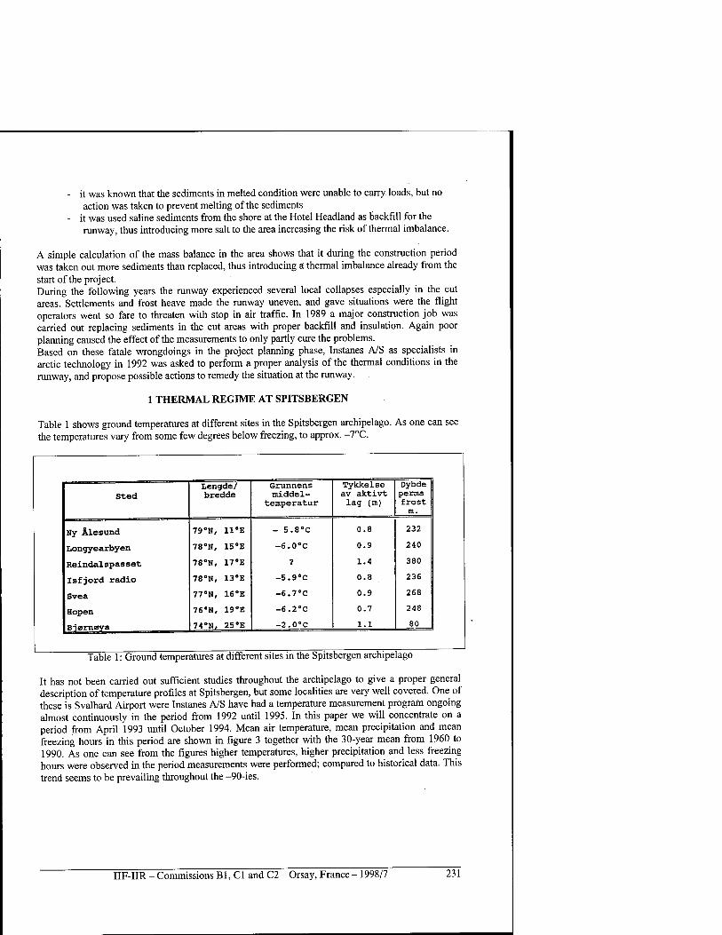
- it was known that the sediments in melted condition were unable to carry loads, but no action was taken to prevent melting of the sediments

- it was used saline sediments from the shore at the Hotel Headland as backfill for the runway, thus introducing more salt to the area increasing the risk of thermal imbalance.

A simple calculation of the mass balance in the area shows that it during the construction period was taken out more sediments than replaced, thus introducing a thermal imbalance already from the start of the project. During the following years the runway experienced several local collapses especially in the cut areas. Settlements and frost heave made the runway uneven, and gave situations were the flight operators went so fare to threaten with stop in air traffic. In 1989 a major construction job was carried out replacing sediments in the cut areas with proper backfill and insulation. Again poor planning caused the effect of the measurements to only partly cure the problems. Based on these fatale wrongdoings in the project planning phase, Instanes A/S as specialists in arctic technology in 1992 was asked to perform a proper analysis of the thermal conditions in the runway, and propose possible actions to remedy the situation at the runway.

1 THERMAL REGIME AT SPITSBERGEN

Table 1 shows ground temperatures at different sites in the Spitsbergen archipelago. As one can see the temperatures vary from some few degrees below freezing, to approx. -7°C.

Sted Lengde/ bredde

Grunnens middel-

temperatur

Tykkelse av aktivt lag (m)

Dybde perma frost m.

Ny Alesund 79"N, ll'E - 5.8°C 0.8 232

Longyearbyen 78°N, 15°E -6.0°C 0.9 240

Reindalspasset 78°N, 17"E ? 1.4 380

Isfjord radio 78"N, 13°E -5.9"C 0.8 236

Svea 77°N, 16"E -6.7"C 0.9 268

Hopen 76"N, 190E -6.2°C 0.7 248

Biarnaya 74°N, 25°E -2.0°C 1.1 80

Table 1: Ground temperatures at different sites in the Spitsbergen archipelago

It has not been carried out sufficient studies throughout the archipelago to give a proper general description of temperature profiles at Spitsbergen, but some localities are very well covered. One of these is Svalbard Airport were Instanes A/S have had a temperature measurement program ongoing almost continuously in the period from 1992 until 1995. In this paper we will concentrate on a period from April 1993 until October 1994. Mean air temperature, mean precipitation and mean freezing hours in this period are shown in figure 3 together with the 30-year mean from 1960 to 1990. As one can see from the figures higher temperatures, higher precipitation and less freezing hours were observed in the period measurements were performed; compared to historical data. This trend seems to be prevailing throughout the -90-ies.


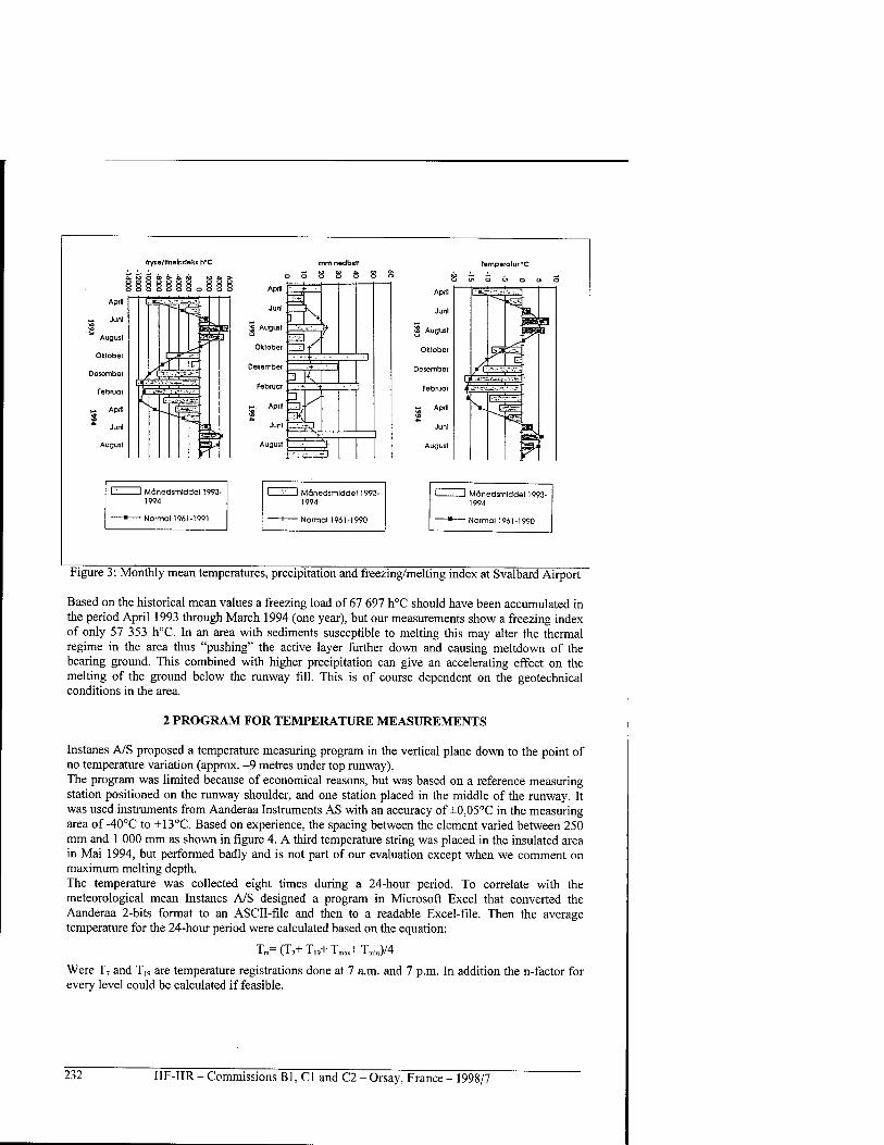
ftyje/Hnelndeki h'C

■ A- i. M ro ±k O-

mm nedb0r _ — w Ol a. w o o o o o o

temperafur *C

o 01 o u* o o> a

April

1'

[Tii~;---- .;;'^ ;..,n

Hk r*3

1

Junl

\ ■^

^

- *S S August «#*

^

Oktober |..'ji r-Vi

r^ I E Desember H |,'-!-V-"«".

..««TÄ^'i* .,,-■;«.

Februar i-E'^-iX.-»-**.:■>.-!

- April L-Tte- *o

Junl

August

I I Mdnedsmiddel 1993- 1994

- Normal 1961-1991

1 Mdnedsmiddel 1993- 1994

- Normal 1961-1990

J Mdnedsmiddel 1993- 1994

- Normal 1961-1990

Figure 3: Monthly mean temperatures, precipitation and freezing/melting index at Svalbard Airport

Based on the historical mean values a freezing load of 67 697 h°C should have been accumulated in the period April 1993 through March 1994 (one year), but our measurements show a freezing index of only 57 353 h°C. In an area with sediments susceptible to melting this may alter the thermal regime in the area thus "pushing" the active layer further down and causing meltdown of the bearing ground. This combined with higher precipitation can give an accelerating effect on the melting of the ground below the runway fill. This is of course dependent on the geotechnical conditions in the area.

2 PROGRAM FOR TEMPERATURE MEASUREMENTS

Instanes A/S proposed a temperature measuring program in the vertical plane down to the point of no temperature variation (approx. -9 metres under top runway). The program was limited because of economical reasons, but was based on a reference measuring station positioned on the runway shoulder, and one station placed in the middle of the runway. It was used instruments from Aanderaa Instruments AS with an accuracy of ±0,05°C in the measuring area of -40°C to +13°C. Based on experience, the spacing between the element varied between 250 mm and 1 000 mm as shown in figure 4. A third temperature string was placed in the insulated area in Mai 1994, but performed badly and is not part of our evaluation except when we comment on maximum melting depth. The temperature was collected eight times during a 24-hour period. To correlate with the meteorological mean Instanes A/S designed a program in Microsoft Excel that converted the Aanderaa 2-bits format to an ASCII-file and then to a readable Excel-file. Then the average temperature for the 24-hour period were calculated based on the equation:

Tm=(T7+T19+TmM+Tmi„)/4

Were T, and T19 are temperature registrations done at 7 a.m. and 7 p.m. In addition the n-factor for every level could be calculated if feasible.


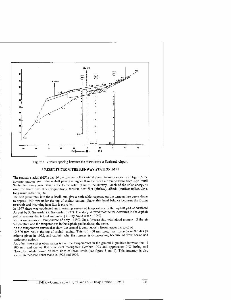
Figure 4: Vertical spacing between the thermistors at Svalbard Airport

3 RESULTS FROM THE RUNWAY STATION, MP1

The runway station (MP1) had 14 thermistors in the vertical plane. As one can see from figure 5 the average temperature in the asphalt paving is higher than the mean air temperature from April until September every year. This is due to the solar influx to the runway. Much of the solar energy is used for latent heat flux (evaporation), sensible heat flux (airflow), albedo (surface reflectivity), long wave radiation, etc. The rest penetrates into the subsoil, and give a noticeable response on the temperature curve down to approx. 750 mm under the top of asphalt paving. Under this level balance between the frozen reservoir and incoming heat flux is prevailed. In 1977 there was conducted an interesting survey of temperatures in the asphalt pad at Svalbard Airport by R. Saetersdal (R. Saetersdal, 1977). The study showed that the temperatures in the asphalt pad on a sunny day (cloud amount ~1) in July could reach +30°C with a maximum air temperature of only +14°C. On a forecast day with cloud amount ~8 the air temperature and the temperatures in the asphalt pad is almost the same. As the temperature curves also show the ground is continuously frozen under the level of -2 500 mm below the top of asphalt paving. This is 1 400 mm more than foreseen in the design criteria given in 1972, and explain why the runway is deteriorating because of frost heave and settlement actions. An other interesting observation is that the temperatures in the ground is positive between the -1 500 mm and the -2 000 mm level throughout October 1993 and approaches 0°C during mid November while frozen on both sides of these levels (see figure 5 and 6). This tendency is also shown in measurements made in 1992 and 1994.


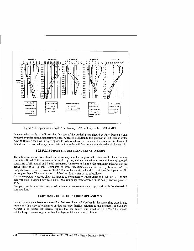
- Feb.93

- Man 1993

- Juni 1993

- JuD 1993

- Aug.93

- Sep.93

- Oktober 1993

- Nav.93

- Deiember 1993

-■— Jan.94

—x— Feb.94

—*— Mail 199a

—o— Apt.94

—&— Mall 994

- Junl 1994

- Ju( 1994

- Aug.94

~ Sap.94

Figure 5: Temperature vs. depth from January 1993 until September 1994 at MP1.

Our numerical analysis indicates that this part of the vertical plane should be fully frozen by end September under normal temperature loads. A possible solution to this problem is that there is water flowing through the area thus giving rise to water/ice lenses in the area of measurements. This will then disturb the normal temperature distribution in the soil. See our comments under ch. 2.4 and .5.

4 RESULTS FROM THE REFERENCE STATION, MP2

The reference station was placed on the runway shoulder approx. 40 metres south of the runway centreline. It had 12 thermistors in the vertical plane, and was placed in an area with natural ground consisting of silt, gravel and fluvial sediments. As shown in figure 6 the maximum thickness of the active layer is 2 100 mm. Compared to other measurements carried out by Instanes A/S in Longyearbyen the active layer is 500-1 200 mm thicker at Svalbard Airport than the typical profile in Longyearbyen. This can be due to higher heat flux, water in the subsoil, etc. As the temperature curves show the ground is continuously frozen under the level of-2 100 mm below the top of asphalt paving. This is 1 000 mm more than foreseen in the design criteria given in 1972. Compared to the numerical model of the area the measurements comply well with the theoretical computations.

5 SUMMARY OF RESULTS FROM MP1 AND MP2

In the summary we have evaluated data between June and October in the measuring period. The reason for this way of evaluation is that the only feasible solution to the problems at Svalbard Airport is to restore the thermal regime that the design was based on in 1972. This means establishing a thermal regime with active layer not deeper than 1 100 mm.


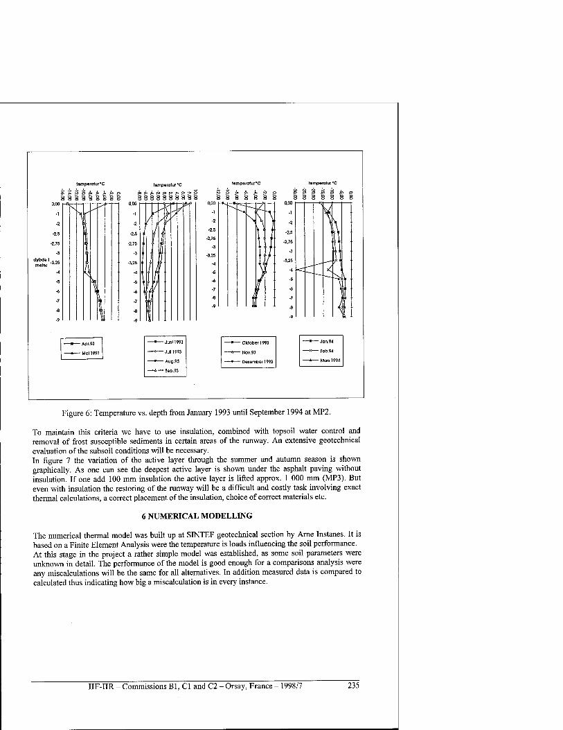
- Api.93

-Moll «3

-Juni 1993

-JUI1993

- Aug.93

- Sep.93

—>—Oktober 1993 —■— Jan.94

« Nov.93 —x— Feb.94

—•—- Desember 1993 —*— MOB 1994

Figure 6: Temperature vs. depth from January 1993 until September 1994 at MP2.

To maintain this criteria we have to use insulation, combined with topsoil water control and removal of frost susceptible sediments in certain areas of the runway. An extensive geotechnical evaluation of the subsoil conditions will be necessary. In figure 7 the variation of the active layer through the summer and autumn season is shown graphically. As one can see the deepest active layer is shown under the asphalt paving without insulation. If one add 100 mm insulation the active layer is lifted approx. 1 000 mm (MP3). But even with insulation the restoring of the runway will be a difficult and costly task involving exact thermal calculations, a correct placement of the insulation, choice of correct materials etc.

6 NUMERICAL MODELLING

The numerical thermal model was built up at SINTEF geotechnical section by Arne Instanes. It is based on a Finite Element Analysis were the temperature is loads influencing the soil performance. At this stage in the project a rather simple model was established, as some soil parameters were unknown in detail. The performance of the model is good enough for a comparisons analysis were any miscalculations will be the same for all alternatives. In addition measured data is compared to calculated thus indicating how big a miscalculation is in every instance.


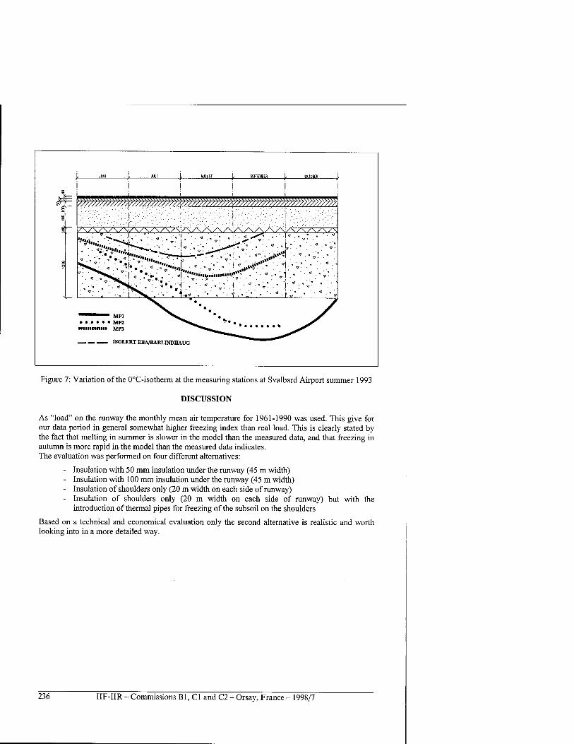
_4 StPTiUBE» jf_

I I

^ !?>?>>)?>>^

__ — ISOLERTEBA/BARLINDHAUG

Figure 7: Variation of the 0°C-isotherm at the measuring stations at Svalbard Airport summer 1993

DISCUSSION

As "load" on the runway the monthly mean air temperature for 1961-1990 was used. This give for our data period in general somewhat higher freezing index than real load. This is clearly stated by the fact that melting in summer is slower in the model than the measured data, and that freezing in autumn is more rapid in the model than the measured data indicates. The evaluation was performed on four different alternatives:

- Insulation with 50 mm insulation under the runway (45 m width) - Insulation with 100 mm insulation under the runway (45 m width) - Insulation of shoulders only (20 m width on each side of runway) - Insulation of shoulders only (20 m width on each side of runway) but with the

introduction of thermal pipes for freezing of the subsoil on the shoulders

Based on a technical and economical evaluation only the second alternative is realistic and worth looking into in a more detailed way.


PROFILS DE TEMPERATURE DU SOL GELE A L'AEROPORT DE SVALBARD, SPITSBERGEN

RESUME : Depuis le milieu des annees 70, on a note ä l'aeroport de Svalbard des soulevements du sol gele et un affaissement des pistes du au degel. En 1989, des travaux importants de reconstruction des parties les plus abimees des pistes ont ete conduits, mais les tassements ont continue. « Instanes A/S » a ete charge par les autorites aeroportuaires de Norvege d'analyser le probleme et de fournir des solutions. De 1992 ä 1995, « Instanes A/S » a enregistre les temperatures ä trois emplacements differents de l'aeroport de Svalbard. L'enregistrement a ete effectue avec trois bandes differentes comportant des points de mesure descendant jusqu'ä 9 metres de profondeur dans le sol et avec un espacement des thermistances variant de 250 ä 1000 mm. II y avait jusqu'ä 14 points de mesure sur chaque bände. Les temperatures etaient mesurees toutes les trois heures toute l'annee durant, et des temperatures moyennes etaient calculees pour chaque journee. Ces moyennes etaient comparees ä la moyenne meteorologique, et des facteurs n etaient calcules. On a egalement effectue des mesures des variations de temperature sur des revetements en gravier, des revetements en asphalte et sur des revetements d'asphalte isoles. Les donnees ont ete comparees avec des donnees historiques relevees sur le meme site, ä la fin des annees 70 et des annees 80 ; une analyse numerique a ete menee pour verifier les profils thermiques. En se fondant sur les profils de temperature, des calculs ont ete effectues sur l'epaisseur maximale de la couche active au-dessous d'un revetement d'asphalte, ce qui a permis de faire cinq propositions differentes visant ä resoudre les problemes de l'aeroport de Svalbard et de proposer une evaluation technique et economique.


APPLICATIONS OF REMOTE SENSING TO OIL CONTAMINATION OF FROZEN TERRAIN

MARCHAND Y., and REES G. Scott Polar Research Institute, University of Cambridge Lensfield Road, Cambridge CB2 1ER, United Kingdom

ABSTRACT

The world's most extensive ground oil pollution probably occurs in the rich oil-producing areas in Siberia where permafrost is often present. Growing concern has also been expressed over oil pollution sites in northern America. Yet very little research as been undertaken into effective monitoring and remediation procedures in cold regions. While appropriate predictive and monitoring strategies for terrestrial oil spills can probably be devised for some areas, they are currently likely to be heavily dependent on in situ measurements, and not therefore readily transferable to large, remote areas where access may be difficult or restricted. Remote sensing methods, especially when combined with an appropriate Geographic Information System (GIS), have substantial potential in this field. In this paper we describe the results of some preliminary investigations of remote sensing data from oil spill sites in high latitudes. We then use these results to begin the task of specifying an appropriate methodology for using remote sensing and GIS techniques for detecting and monitoring of high-latitude oil spills.

INTRODUCTION

Arctic oil developments during the 1970s have raised concerns about the possible ecological impacts of oil spills in Arctic lands. This had led to some studies of natural or accidental spills (Deneke et al., 1975) and also to some experimental studies of spills in Alaska (Collins 1983) and North-West Canada (Hutchinson 1984, Seburn and Kershaw, 1997). These were small-scale studies, heavily dependent on in situ measurements. Since then, very little research has been undertaken into a possible transferable strategy concerning effective monitoring, predicting and remediation procedures within cold regions (Williams et al., 1997). Nowadays, the world's most extensive ground oil pollution probably occurs in Siberia where permafrost is often present (Vilchek and Tishkov, 1995). In addition, polar environments are highly sensitive to pollution, with long regeneration times and short lifetimes for industrial structures. Oil spills in cold regions usually occur in remote places where access may be restricted. Monitoring such sites only by field work is difficult and expensive, especially in the long term. Thus, a remote sensing approach would be highly desirable (Rees, 1997). In this paper, we present the conclusions of a preliminary investigations into the potential of remote sensing approaches and the possibility of defining a common Geographic Information System (GIS), containing knowledge from experimental oil spills and spaceborne data. The aim would be to use it as a tool for predicting and monitoring the short- and long- term effects of high-latitude oil spills.

1. KNOWLEDGE TRANSFER FROM FIELD STUDIES TO REMOTE SENSING APPROACH

Previous experimental studies took place in North America and involved pouring oil, usually crude though sometimes refined, onto small patches of ground. Such sites are too small to be studied using spaceborne or even airborne remote sensing systems. However, the knowledge from these studies in situ is important and can potentially be used to define or validate a remote sensing application to the detection and monitoring of an oil spill. This issue has the following main


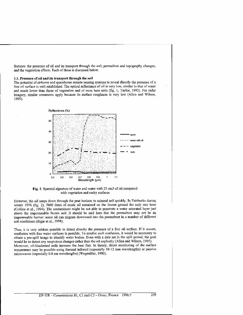
features: the presence of oil and its transport through the soil; permafrost and topography changes; and the vegetation effects. Each of these is discussed below.

1.1. Presence of oil and its transport through the soil The potential of airborne and spaceborne remote sensing systems to reveal directly the presence of a free oil surface is well established. The optical reflectance of oil is very low, similar to that of water and much lower than those of vegetation and of most bare soils (fig. 1, Taylor, 1992). For radar imagery, similar comments apply because its surface roughness is very low (Allen and Wilson, 1995).

Reflectance (%) . *-.—-:7Ä"^ ,

/ ""—• ~- -* *«. N 50 /

/ t

40

30

20 S*

* ■™:r ^

1

10 v' )

^^^ water

water with oil

• vegetation

■* ■ rock

0.4 0.5 0.6 0.7 0.8 0.9 1 1.1 Wavelength (um)

Fig. 1: Spectral signature of water and water with 25 cm3 of oil compared with vegetation and rocky surfaces

However, the oil seeps down through the peat horizon to mineral soil quickly. In Fairbanks during winter 1976 (fig. 2), 7600 litres of crude oil remained on the frozen ground for only one hour (Collins et al., 1994). The contaminant might be not able to penetrate a water saturated layer just above the impermeable frozen soil. It should be said here that the permafrost may not be an impermeable barrier: some oil can migrate downward into the permafrost in a number of different soil conditions (Bigar et al., 1998).

Thus, it is very seldom possible to detect directly the presence of a free oil surface. If it occurs, confusion with free water surfaces is possible. To resolve such confusion, it would be necessary to obtain a pre-spill image to identify water bodies. Even with a data set in the spill period, the goal would be to detect any suspicious changes rather than the oil explicitly (Allen and Wilson, 1995). Moreover, oil-blackened soils increase the heat flux. In theory, direct monitoring of the surface temperature may be possible using thermal infrared (especially 10-12 mm wavelengths) or passive microwaves (especially 0.8 cm wavelengths) (Wegmüller, 1990).


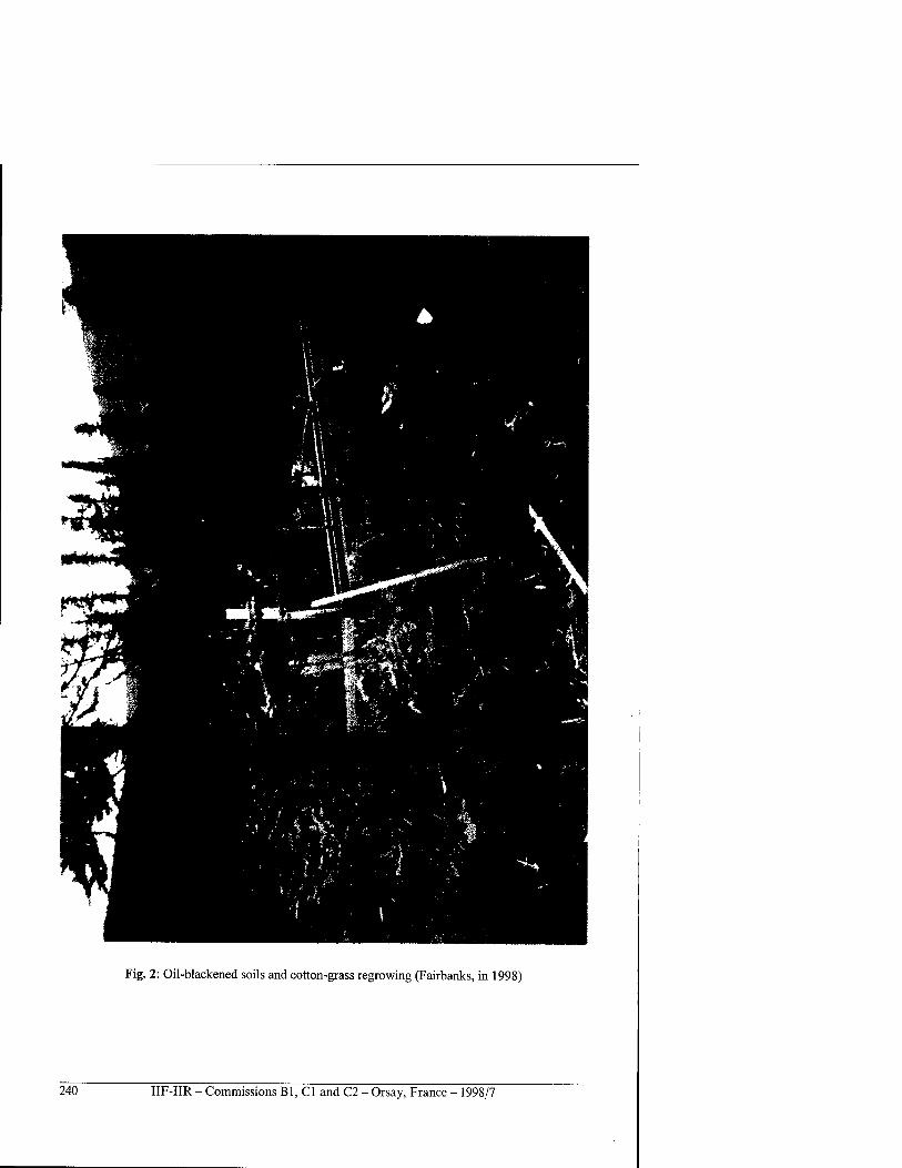
Fig. 2: Oil-blackened soils and cotton-grass regrowing (Fairbanks, in 1998)


However, the spatial resolution from spaceborne systems is fairly poor for these channels: 100m x 100m for the thermal infrared band of Thematic Mapper of the Landsat satellite and typically tens of kilometres for the microwave systems. In fact, very little research has been conducted in this area, and the results have been rather inconclusive. Nevertheless, temperature changes could lead to some modifications in the permafrost and topography.

1.2. Permafrost and topography changes A variety of responses to increase of the active layer depth has been reported: from little (Hutchinson and Freedman 1978, Mackay et al. 1975) to a lot (Collins 1983, Seburn and Kershaw 1997). It has been shown that this aspect is heavily dependent on the season rather than the oil concentration which is still important. In Fairbanks, the thaw depth was the greatest at the winter site: about 65 cm for the control ground, 120 cm in the summer site and 160 cm in the winter site recorded (Collins et al., 1994). Another important parameter is the type of the hydrocarbon contaminants. In Norman Wells, the active layer depth was raised up to 25% at the crude oil spill and 70% at the diesel spill. The latter contaminant had no significant impact on the permafrost at the tundra site (Hutchinson 1984). The previous disturbance also plays an important part in the oil spill impacts. In Tulita (N.W.T, Canada), an experimental crude oil spill was made during summer 1988 (Seburn and Kershaw, 1997). Three environments were considered: undisturbed black spruce forest; a simulated transport corridor where trees and shrubs were hand-cleared but ground cover left intact; and a severely disturbed trench for a simulated buried pipeline where all vegetation canopy and organic layer were removed, the area excavated and refilled. The mean of the maxima thaw depth was greater in the trench than anywhere else. The thaw of permafrost and the increase in active layer thickness cannot be detected directly by remote sensing methods, but the vegetation canopy, which is strongly dependent on it, can provide some information (Morrisey, 1988). On the other hand, subsidence may be caused by changes in the active layer depth. This occurred in the case of the winter spill at Fairbanks, where the subsidence increased to 60 cm. Although airborne or spaceborne stereophotography is not likely to be give a high enough vertical resolution to detect subsidence effects, it is possible that differential SAR interferometry could do so. This technique, which has been developed for (e.g.) monitoring volcanoes, has not yet been adequately investigated for monitoring subsidence.

1.3. Vegetation effects ., An oil spill generally produces long-term, possibly permanent, changes in vegetation cover. The first impacts may well be dramatic if the pollution event occurs in the growing season. If the vegetation is dormant at the time of the spill, the first impacts are less dramatic, but the long term effects are more severe. The Fairbanks case in 1976 is a good illustration as there were a summer spill and a winter spill in a black spruce forest (Collins et al., 1994). In the summer spill, the vegetation damage appeared almost instantaneously and was most extensive two years later. 22 years later, there is more vegetation here than on the winter site. At the latter, black spruce continued to die for over 15 years. This delay for the trees to die has been also observed at Norman Wells, where black spruce often to took up to 4 years to die, while some other plants took as long or longer before showing a sign of recovery (Hutchinson, 1984). These observations clearly indicate that the diversity and the association of species would change as a result of an oil spill. In general, tundra ecosystems show better recovery than taiga. However, regeneration of lichens and mosses is very weak although they are an important part of the Arctic and sub-Arctic flora. Shrubs like Labrador tea, birch and willow may have a good ability to recover despite deciduous usually show rapidly signs of damages. Cotton-grass (Eriophorum vaginatum) and horsetail have shown the greatest oil-tolerance. These


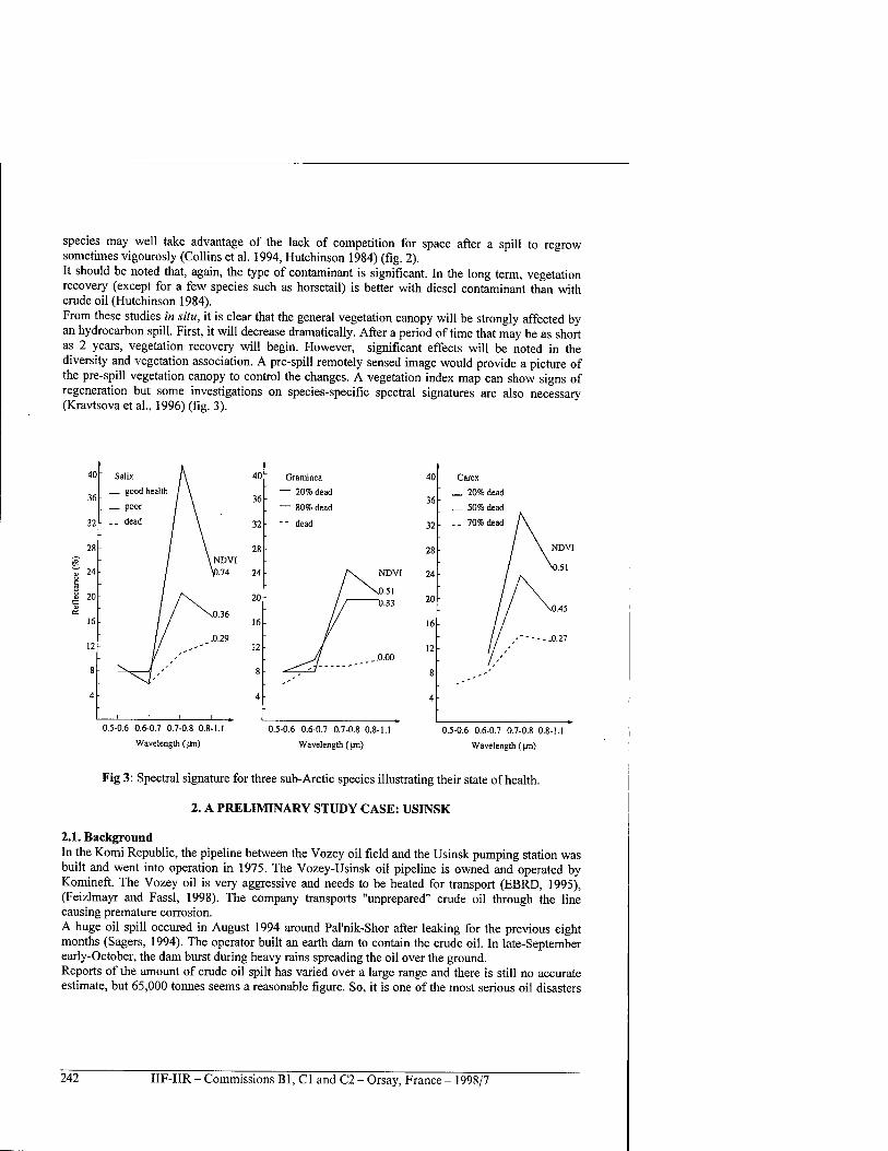
species may well take advantage of the lack of competition for space after a spill to regrow sometimes vigourosly (Collins et al. 1994, Hutchinson 1984) (fig. 2). It should be noted that, again, the type of contaminant is significant. In the long term, vegetation recovery (except for a few species such as horsetail) is better with diesel contaminant than with crude oil (Hutchinson 1984). From these studies in situ, it is clear that the general vegetation canopy will be strongly affected by an hydrocarbon spill. First, it will decrease dramatically. After a period of time that may be as short as 2 years, vegetation recovery will begin. However, significant effects will be noted in the diversity and vegetation association. A pre-spill remotely sensed image would provide a picture of the pre-spill vegetation canopy to control the changes. A vegetation index map can show signs of regeneration but some investigations on species-specific spectral signatures are also necessary (Kravtsova et al., 1996) (fig. 3).

28

24

0.5-0.6 0.6-0.7 0.7-0.8 0.8-1.1

Wavelength (jm)

Graminea

— 20% dead

— 80% dead

"" dead

NDVI

0.5-0.6 0.6-0.7 0.7-0.8 0.8-1.1

Wavelength (pn) 0.5-0.6 0.6-0.7 0.7-0.8 0.8-1.1

Wavelength ([m)

Fig 3: Spectral signature for three sub-Arctic species illustrating their state of health.

2. A PRELIMINARY STUDY CASE: USINSK

2.1. Background In the Komi Republic, the pipeline between the Vozey oil field and the Usinsk pumping station was built and went into operation in 1975. The Vozey-Usinsk oil pipeline is owned and operated by Komineft. The Vozey oil is very aggressive and needs to be heated for transport (EBRD, 1995), (Feizlmayr and Fassl, 1998). The company transports "unprepared" crude oil through the line causing premature corrosion. A huge oil spill occured in August 1994 around Pal'nik-Shor after leaking for the previous eight months (Sägers, 1994). The operator built an earth dam to contain the crude oil. In late-September early-October, the dam burst during heavy rains spreading the oil over the ground. Reports of the amount of crude oil spilt has varied over a large range and there is still no accurate estimate, but 65,000 tonnes seems a reasonable figure. So, it is one of the most serious oil disasters


in all history. The surface of the polluted area was at least 69 hectares. Pal'nik Shor was the most affected area, but the Khatayakha and Bezymiany areas were also contaminated. The first two are very swampy regions (fig. 4). Most of the cleanup was done at the end of 1995 and the oil was burnt. Some biorecultivation began in 1996. Many experiments to grow perennial long-life grasses were carried out in 1995 and 1996. Fertilizers were used. Among the 69 ha polluted, 60-64 had been cleared by April 1996.

2.2. First investigations on a SPOT image Fig. 4 shows a pre-spill view from the satellite SPOT on 17th July 1997. Usinsk lies at the northern margin of the forest in the basin of the Pechora river. The permafrost is sporadic and occurs in elevated places. The landscapes are half open with some hills covered by boreal forest. The low places are occupied by many uncrossable bogs. The vegetation is mainly composed of carex, mosses and grasses but also some forest patches, meadow and shrubs. This image was recorded by the satellite SPOT on 7th July 1994, before the main oil spill. Thus, it is a pre-spill view that shows the stage of the Palnik' Shor area before it became polluted. The vegetation is mostly low as this is a boggy area. Some (mainly coniferous) forest patches can be seen along the rivers and along the lakes. The Khatayakha area has similar features. This area was already damaged and could therefore be used to illustrate the expected spectral signature effects as a result of an oil spill (fig. 4).

CONCLUSION

It has been the aim of this paper to demonstrate how knowledge from experimental oil spills can be fruitful for developing a remote sensing application. It has been shown that remote sensing methods offer a considerable potential to characterise spill impacts in high latitude terrain. This potential includes airborne and spaceborne systems, optical, thermal infrared and radar. Some parameters appear already predominant to choose the remote sensing methods for monitoring. If the spill occurs in winter, it would be useful to investigate SAR interferometry or stereogrammetry analyses to detect possible subsidence. If it happens during the growing season, short-term investigations might be done with a short sampling interval of the remotly sensed data. Otherwise, efforts should rather be focused in the long-term. Field and remotely sensed data could be powerfully combined in a GIS. The latter would be used as a tool for predicting and monitoring the short- and long- term effects of an oil spill.

ACKNOWLEDGEMENT

Funding for this research is provided by the European Union with a Marie Curie Fellowship. Programme: Training and Mobility of Researchers-contract number: ERBFMBICT972600.

REFERENCES

1. Allen P., Wilson S., 1995.NRSC uses ERS-1 SAR data to monitor 1994 Komi oil spill. Earth Observation Magazin, no. April, p. 41-43.

2. Bigar K.W., Haidar S., Nahir M., Jarret P.M, 1998.Sites investigations of fuel spill migration into permafrost. Journal of Cold Regions Engineering, vol. 12, no. 2, p. 84-104.

3. Collins CM., 1983.Long-term active layer effects of the crude oil spilled, Interior Alaska. Proceeding of the fourth International Conference on Permafrost, Washington, p. 175-179.

4. Collins CM., Racine C.H., Walsh M.E., 1994.The physical, chemical and biological effects of crude oil spills after 15 years on a black spruce forest, Interior Alaska. Arctic, vol. 47, no. 2, p. 164-175.


5. Deneke F.J., McCown B.H., Coyne P.L., Rickard W., Brown J., 1975. Biological aspects of terrestrial oil spills - USA CRREL Oil Research in Alaska, 1970-1974, Cold Regions Research and Engineering Laboratory, Report 346, 66 p.

6. European Bank for Reconstruction and Development (EBRD), 1995. Russian Federation - Emergency oil spill recovery and mitigation project, April, 65 p.

7. Feizlmayr A.H., Fassl H.J., 1998.Inspection and Rehabilitation of Crude oil Pipelines in Eastern Europe and FSU. In Proceedings of the International Pipelines Conference, June, vol. II, p. 1005-1011.

8. Hutchinson T.C., Freedman W., 1978.Effects of experimental crude oil spills on subarctic boreal forest vegetation near Norman Wells, N.W.T., Canada. Canadian Journal of Botany, no. 56, p. 2424-2433.

9. Hutchinson T.C., 1984. Recovery of Arctic and sub-Arctic vegetation nine summers after crude and diesel oil spills. North of 60. Ottawa: Department of Indian Affairs and Northern Development, Environmental Studies, no. 22.

10. Kravtsova V.l., Lourie I.K., Ressle A.I., Touboubalina O.V., 1996. Method for computer classification of industrial impact on northern vegetation using space images. Earth Space Review, vol. 5, no. 2, p. 18-23.

ll.Mackay D., Charles M.E., Philips C.R., 1975. The physical aspects of crude oil spills on northern terrain. North of 60. Ottawa: Department of Indian Affairs and Northern Development, final report.

12. Morrisey L.A., 1988. Predicting the occurrence of permafrost in the Alaskan discontinuous zone with satellite data. In Proceedings ofthe fifth international permafrost conference, p. 213-217.

13. Rees W.G., 1997. Remote sensing of oil spills on frozen ground. Conference on Contaminants in Freezing Ground. Cambridge, UK, July, in press.

14. Sagers M.J., 1994. Oil spill in Russian arctic. Polar Geography and Geology, vol. 18, no 2, p. 95-102.

15. Seburn D.C., Kershaw G.P., 1997.Changes in the active layer of a subarctic right-of-way as a result of a crude oil spill. Canadian Journal of Earth Sciences, 34,12, pp. 1539-1544.

16. Taylor S., 1992. 0.45 to pi mm spectra ofPrudhoe crude oil and of beach materials in Prince Williams Sound, Alaska. Cold Regions Research and Engineering Laboratory, Special Report, 5.

17. Vilchek G.E., Tishkov A.A., 1995. Usinsk oil spill: environmental catastrophe or routine event. In Proceedings of Disturbance and Recovery in Arctic Lands - An Ecological Perspective, Crawford Ed.

18. Wegmüller U., 1990.The effect of freezing and thawing on the microwave signatures of bare soil. Remote Sensing of Environment, 33, p. 123-135.

19. Williams P., Rees W.G., Riseborough D.W., 1997. Strategies for development of cost effective amelioration procedures for oil spills in cold regions, in press

APPLICATIONS DE LA TELEDETECTION AU CONTROLE DE LA POLLUTION DUE AU PETROLE DANS DES TERRAINS GELES

RESUME : Dans le monde, la pollution du sol la plus importante est probablement celle se produisant dans les regions de Siberie oü Ton extrait de grandes quantites de petrole et oü le pergelisol est permanent. La pollution due aux sites d'extraction situes dans le nord du continent americain est aussi de plus en plus inquietante. Jusqu'ä ce jour, peu de recherches ont ete effectuees sur un contröle efficace dans ces regions froides et sur des procedures visant ä resoudre la pollution. Bien que les strategies de monitorage et les methodes predictives appropriees aux nappes terrestres puissent etre probablement appliquees ä certaines regions, elles dependent encore enormement de mesures in situ et ne sont done pas directement


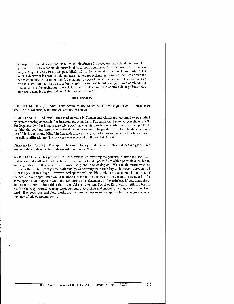
appropriees pour des regions etendues et lointaines oü l'acces est difficile et restreint. Les methodes de teledetection, de surcroit si elles sont combinees ä un Systeme d'information geographique (GlS) offrent des possibility tres interessantes dans ce cas. Dans 1'article, les auteurs decrivent les resultats de quelques recherches preliminaries sur des donnees obtenues par teledetection et se rapportant ä des nappes de petrole situees ä des latitudes elevees. Ces resultats sont done utilises dans le but de specifier une methodologie appropriee combinant la teledetection et les techniques dites de GIS pour la detection et le contröle de la pollution due au petrole dans les regions situees ä des latitudes elevees.

DISCUSSION

FUKUDA M. (Japan) - What is the optimum size of the SPOT investigation as to correlate of satellite? In last slide, what kind of satellite for analysis?

MARCHAND Y. - All small-scale studies made in Canada and Alaska are too small to be studied by remote sensing approach. For instance, the oil spills in Fairbanks that I showed you slides, are 3- 4m large and 30-40m long, meanwhile SPOT has a spatial resolution of 20m by 20m. Using SPOT, we think the good minimum size of the damaged area would be greater than lha. The damaged area near Usinsk was about 70ha. The last slide showed the result of an unsupervised classification on a pre-spill satellite picture. The raw data was recorded by the satellite SPOT.

CHENAF D. (Canada) - This approach is more for a partial characterisation rather than global. We are not able to delineate the contaminant plume - aren't we?

MARCHAND Y. - This project is still new and we are investing the potential of remote sensed data to detect an oil spill and to characterise its damages of soils, permafrost with a possible subsidence, and vegetation. In this way, this approach is global and ecological. We can delineate with no difficulty the contaminant plume horizontally. Concerning the possibility to delineate it vertically, I can't tell you at this stage. However, perhaps we will be able to give an idea about the increase of the active layer depth. That would be done looking at the changes in the vegetation association for some species could appear while the permafrost goes downwards. Nevertheless, if you think about an accurate figure, I don't think that we could ever give one. For that, field work is still the best to do. By the way, remote sensing approach could save time and money avoiding to do often field work. However, this and field work, are two well complementary approaches. You give a good instance of this complementarity.


Damaged area - bare soil

Town and industrial installations

Bright and/or dry soil with sparse vegetation

lI'Mm^l Short vegetation in swampy places

Deciduuus

Conifeiuus

Water

Pipeline Main asphalted road Earth road

Fig.4: Usinsk area before the oil spill (unsupervised classification, 17 July 1994).


SECTION V

RECHERCHES ET TECHNIQUES SUR LES ECOSYSTEMES

ET CRYOBIOLOGIE

RESEARCH AND TECHNIQUES ON ECOSYSTEMS

AND CRYOBIOLOGY

HIGH PRESSURE ASSISTED FREEZING IN BIOLOGICAL PRODUCTS

*OTERO L., °MARTINO M., °ZARITZKY N., *CARRASCO J.A., *De ELVIRA C. and *SANZ P.D.

*Instituto del Frio (CSIC). Ciudad Universitaria, 28040 Madrid, Spain °CIDCA, 47 y 116, 1900 La Plata, Argentina

ABSTRACT

Freezing biological products is one of the most interesting applications of High Pressure (HP) technologies. In this work, the effects of such process on the microstructure of large pieces of beef meat are analysed. For the study two points of interest have been chosen in the sample: the surface and the centre. In conventional freezing methods, thermal gradients reduce the freezing rate from the surface to the thermal centre and significant, differences are observed in the microstructure between these two regions. In HP assisted freezing, the supercooling reached after the release of pressure yields an instantaneous nucleation of water in all the volume of the sample at the same time. Microscopic observations show the existence of small intracellular ice crystals in the surface and in the centre of the product.

INTRODUCTION

Application of high pressures, HP, (100 MPa up to 900 MPa) to biological products is a new technique that can substitute high temperatures in many treatments. For example, in foodstuffs high pressures can reduce significantly the microbial population or can produce starch gelatinization at low temperatures. These effects have been observed using high temperatures which involve, at the same time, other undesirable consequences such as vitamin losses, colour changes, new flavours, etc. HP have also interesting applications in the low temperature field: freezing, thawing and sub-zero temperature non-frozen storage. High pressure assisted freezing process is based on the depression of the freezing point of water down to -21.995 °C at 209.9 MPa (Bridgman, 1912). The method consists in cooling the product under pressure in such conditions that it remains unfrozen at -20 °C, then pressure is released suddenly to atmospheric pressure. Due to the quasi-adiabatic expansion, temperature decreases according to the following equation:

0) AT T-V-a

where T: Temperature in K V: Specific volume (m3/kg) a: Thermal expansion coefficient (K" ) Cp: Heat capacity (J/kg-K)

bearing in mind that all thermodynamic properties of water are modified by pressure. Conditions in the sample after pressure release correspond to the solid state in the phase diagram of water. Then, just after the expansion and due to the isostatic pressure principle, a strong supercooling is produced in the whole volume of the product. According to Burke et al. (1975), for each degree K of supercooling there is an increase of about tenfold in the ice-nucleation rate. Freezing rate is one of the factors which determine the final quality of a frozen food (I.I.R., 1972). Slow freezing rates produce large extracellular ice crystals that can damage the original structure of the product, whereas high freezing rates involve the formation of small intracellular ice crystals that


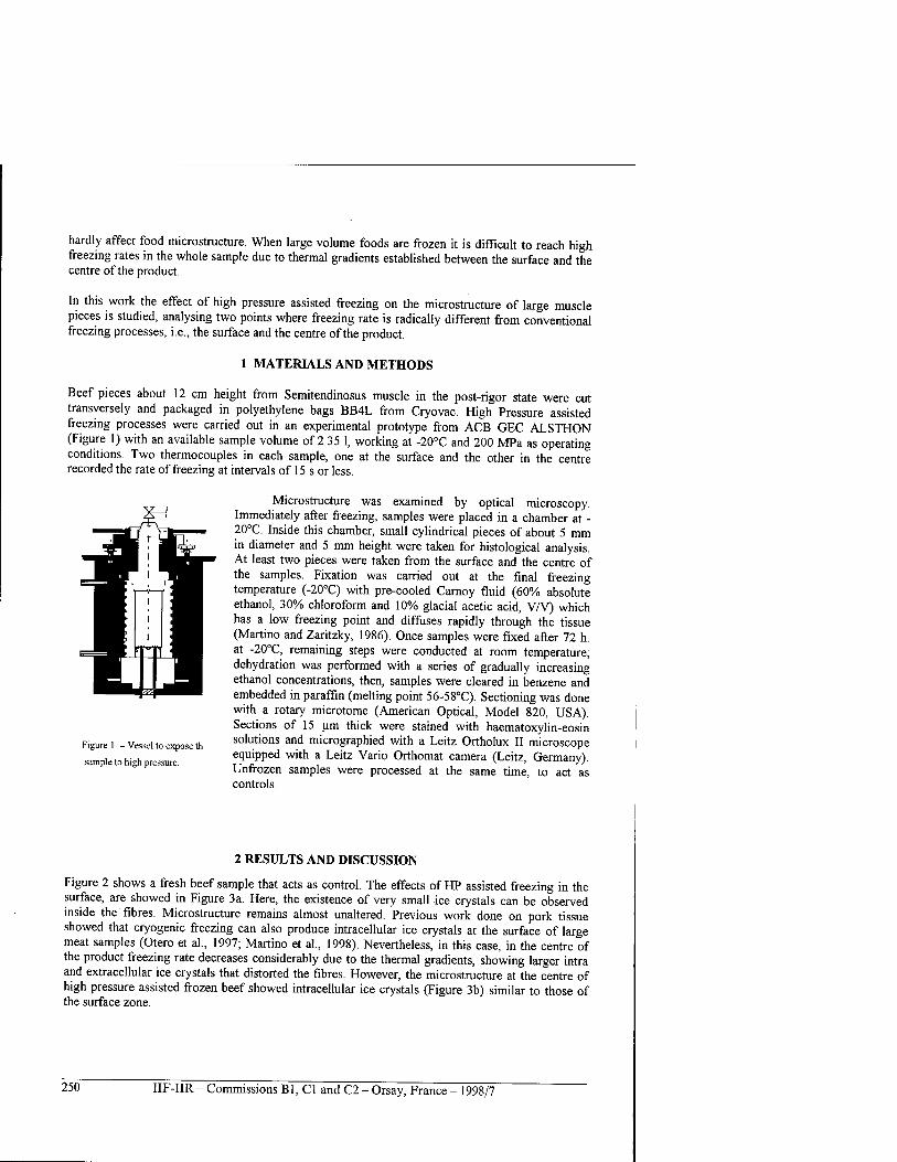
hardly affect food microstructure. When large volume foods are frozen it is difficult to reach high freezing rates in the whole sample due to thermal gradients established between the surface and the centre of the product.

In this work the effect of high pressure assisted freezing on the microstructure of large muscle pieces is studied, analysing two points where freezing rate is radically different from conventional freezing processes, i.e., the surface and the centre of the product.

1 MATERIALS AND METHODS

Beef pieces about 12 cm height from Semitendinosus muscle in the post-rigor state were cut transversely and packaged in polyethylene bags BB4L from Cryovac. High Pressure assisted freezing processes were carried out in an experimental prototype from ACB GEC ALSTHON (Figure 1) with an available sample volume of 2.35 1, working at -20°C and 200 MPa as operating conditions. Two thermocouples in each sample, one at the surface and the other in the centre recorded the rate of freezing at intervals of 15 s or less.

Microstructure was examined by optical microscopy. Immediately after freezing, samples were placed in a chamber at - 20°C. Inside this chamber, small cylindrical pieces of about 5 mm in diameter and 5 mm height were taken for histological analysis. At least two pieces were taken from the surface and the centre of the samples. Fixation was carried out at the final freezing temperature (-20°C) with pre-cooled Carnoy fluid (60% absolute ethanol, 30% chloroform and 10% glacial acetic acid, V/V) which has a low freezing point and diffuses rapidly through the tissue (Martino and Zaritzky, 1986). Once samples were fixed after 72 h. at -20°C, remaining steps were conducted at room temperature; dehydration was performed with a series of gradually increasing ethanol concentrations, then, samples were cleared in benzene and embedded in paraffin (melting point 56-58°C). Sectioning was done with a rotary microtome (American Optical, Model 820, USA). Sections of 15 um thick were stained with haematoxylin-eosin solutions and micrographied with a Leitz Ortholux II microscope equipped with a Leitz Vario Orthomat camera (Leitz, Germany). Unfrozen samples were processed at the same time, to act as controls.

Figure 1. - Vessel to expose th

-sample to high pressure.


Figure 2 shows a fresh beef sample that acts as control. The effects of HP assisted freezing in the surface, are showed in Figure 3 a. Here, the existence of very small ice crystals can be observed inside the fibres. Microstructure remains almost unaltered. Previous work done on pork tissue showed that cryogenic freezing can also produce intracellular ice crystals at the surface of large meat samples (Otero et al., 1997; Martino et al., 1998). Nevertheless, in this case, in the centre of the product freezing rate decreases considerably due to the thermal gradients, showing larger intra and extracellular ice crystals that distorted the fibres. However, the microstructure at the centre of high pressure assisted frozen beef showed intracellular ice crystals (Figure 3b) similar to those of the surface zone.


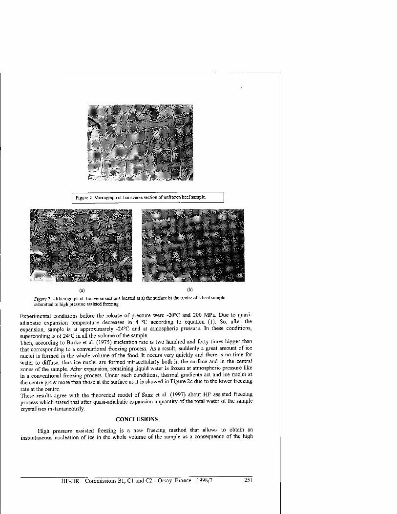
■MM ' l\

t l" ':

Figure 2. Micrograph of transverse section of unfrozen beef sample.

(a) (b) Figure 3. - Micrograph of tranverse sections located at a) the surface b) the centre of a beef sample submitted to high pressure assisted freezing.

Experimental conditions before the release of pressure were -20°C and 200 MPa. Due to quasi- adiabatic expansion temperature decreases in 4 °C according to equation (1). So, after the expansion, sample is at approximately -24°C and at atmospheric pressure. In these conditions, supercooling is of 24°C in all the volume of the sample. Then, according to Burke et al. (1975) nucleation rate is two hundred and forty times bigger than that corresponding to a conventional freezing process. As a result, suddenly a great amount of ice nuclei is formed in the whole volume of the food. It occurs very quickly and there is no time for water to diffuse, thus ice nuclei are formed intracellularly both in the surface and in the central zones of the sample. After expansion, remaining liquid water is frozen at atmospheric pressure like in a conventional freezing process. Under such conditions, thermal gradients act and ice nuclei at the centre grow more than those at the surface as it is showed in Figure 2c due to the lower freezing rate at the centre. These results agree with the theoretical model of Sanz et al. (1997) about HP assisted freezing process which stated that after quasi-adiabatic expansion a quantity of the total water of the sample crystallises instantaneously.

CONCLUSIONS

High pressure assisted freezing is a new freezing method that allows to obtain an instantaneous nucleation of ice in the whole volume of the sample as a consequence of the high


degree of supercooling obtained. Thus, a great number of very small intracellular ice crystals is obtained which does not affect beef microstructure. Only at the final phase of the process, at atmospheric pressure, thermal gradients are established. Improving the method involves the use of more powerful refrigerating systems. This freezing method can be especially useful to pieces of food of large volume in which, when conventional freezing methods are employed, thermal gradients are important.

BIBLIOGRAPHY

1. Bridgman, P. W. (1912). Proc. Am. Acad. Arts Sei. XLVII (13): 439-558. 2. Burke, M.J.; George, M. F. and Bryant, R. G. (1975) in Water Relations of Foods (Food Science and

Technology Monographs) (Duckworth, R. B., Ed.) 111-135, Academic Press. 3. I.I.R., (1972), Recommendation for the processing and handling of frozen foods. International Institute

of Refrigeration. Paris, 1972, p. 14. 4. Kalichevsky, MT., Knorr, D. and Lillford, P. (1995) "Potential food applications of high-pressue effects

on ice-water transitions. Trends in Food Science and Technology, 6,253-259. 5. Otero, L., Martino, M., Sanz, P., Zaritzky, N. (1997). " Histologie analysis of ice crystals in pork frozen

by liquid N2 and high pressure-assisted-freezing". Scanning, 19,3, 241,242- 6. Martino, M. and Zaritzky, N. (1986). Fixing conditions in the freeze substitution technique for light

microscopy observation of frozen beef tissue. Food Microstruct. 5, 19-24. 7. Martino, M, Otero, L., Sanz, P. and, Zaritzky, N. (1998). Size and location of ice crystals in pork frozen

by high pressure-assisted-freezing as compared to classical methods. Meat Science, 50, 3, 303-313. 8. Sanz, P.D., Otero, L., de Elvira, L., Carrasco, J.A. (1997). "Freezing processes in high-pressure

domains ".International Journal of Refrigeration., 20, 5, 301-307.

Acknowledgements

This research was supported from the "Plan Nacional de Investigaciön Cientifica y Desarrollo Tecnolögico" of Spain by the ALI97-0759 Project.

DISCUSSION

WILLIAMS P. J. (Canada) - 1/ In your diagram of freezing point against pressure, what equation did you use for ice? 2/ Some of most water in frozen soils (and many foodstuffs) is "bound", not "free". Does it mean that special forms of the Clausis-Clapeyron are relevant?

OTERO L- 1/ The equation is given by "Wagner, W. Saul, A. and Pruss A., 1994. International equations for the pressure along the melting and along the sublimation curve of ordinary water substance. J. Phys. Chem. Ref. Data 23(3), 515-525." 2/ We have used the corresponding to ordinary water substance.

CONGELATION A HAUTE PRESSION DES MILEEUX BIOLOGIQUES

RESUME : La congelation des produits biologiques est une des applications les plus interessantes de la technologie des hautes pressions. Dans ce travail, les effets de ce processus sur la microstructure de grands morceaux de viande de bceuf sont analyses. Pour l'etude, deux points d'interet ont ete choisis dans la geometrie de l'echantillon ; la surface et le centre. Dans les methodes de congelation traditionnelles, les gradients thermiques reduisent le taux de congelation du processus des la surface jusqu'au centre thermique et produisent des differences significatives dans la microstructure de ces deux regions. Dans la congelation aidee par haute pression, le fort sous- refroidissement obtenu apres la chute brutale de pression pour retrouver la pression atmospherique, produit une nucleation instantanee de l'eau de l'echantillon dans tout le volume en meme temps. Les observations microscopiques montrent l'existence de petits cristaux de glace intracellulaires ä la surface et au centre du produit.


THERMAL ACCUMULATORS WITH PHASE CHANGE BETWEEN -21 AND 40°C

DOMINGUEZ M., PINILLOS J.M., ARIAS J.M., GARCIA C. Instituto del Frio. Ciudad Universitaria 28040 Madrid Spain

1 INTRODUCTION

The importance of the accumulation of thermal energy, in the fields of refrigeration and air conditioning, has been recently appreciated, and hence, some countries have implemented solutions of compulsory compliance in the construction of large buildings and installations. The most practical way of accumulating heat or cold, is by taking advantage of the phase changes of the elements, considering that in a smaller volume and weight, it is possible to store a large amount of heat without any great changes in temperature. In general, the liquid-steam phase change is more energetic but presents greater technical problems, and therefore, there has been a trend towards the other phase change, the liquid-solid. Due to its many advantages, water has been most widely employed, and when accumulation of cold at temperatures close to 0 °C is desired, it has proven to have no competitors. At very low temperatures one encounters nitrogen which boils at -190 CC, and at intermediate ones there is dry ice which sublimes at -80 °C. For the high temperatures and as a consequence of the 1973' oil crisis, several hydrated salts were developed, such as Glaubert's, which accumulate heat at approximately 30 °C. In the field of transportation, the eutectic mixtures were developed and are still in use for specific applications in the field of the -25 to -10 °C. In heat or cold accumulation, there are two forms that require a different treatment, cyclic or closed installations and open ones with non-returnable products, as their problems are very different. In both cases problems arise in relation to heat transfer associated with phase change, as well as constructive problems which are mechanical or of handling in nature. It is important to bear in mind that new systems are only developed when the technical - economic solutions to the problems are found, and that the same principles must apply to the field of thermal accumulation. We shall analyse some energy related problems which are arising in the fields of refrigeration and air conditioning, and possible solutions will be provided by the use of heat accumulators. It is a well-known fact that there are two large groups in the field of food products, frozen products and refrigerated products. In the case of the transport of frozen products, being their commercialisation very widespread, there are very few problems and the temperatures are very well defined, being only some solutions required (1) in the final distribution, i.e. from the distribution centres of the large wholesalers to the small supermarkets. The commercialisation of refrigerated products is more complex, as the transport is more diverse and a greater effort is required. Among the refrigerated products we can mention, for example, "catering" food in airline companies, fresh fish, live crustaceans, and widening the scope to other perishable products, flowers, medicaments and blood, etc. All these products require to be transported at very different temperatures from 0 to 20 °C. In the case of many of the perishable products indicated the problem of weight loss, which requires moisture control, adds to the thermal problem itself, complicating the problem even further. In bulk transport, the most cost-effective means are: ships and trains, being it possible to consider the development of containers; in smaller scale transport: trucks and aeroplanes, the use of boxes or small containers is required (2) and (3). In the case of air conditioning there are several problems to solve, in which thermal accumulation can be very important: in large buildings, in single communication centres, in basic services centres, in exhibition halls and in houses in extreme environments. Two types of problems exist in these


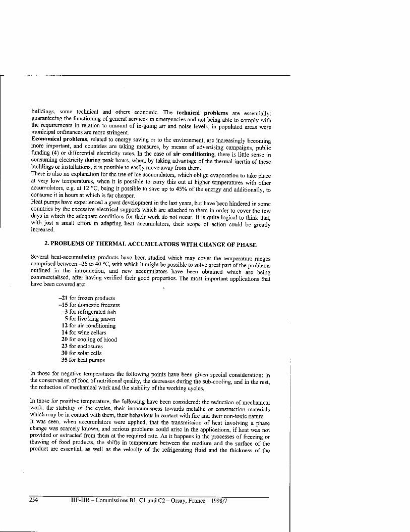
buildings, some technical and others economic. The technical problems are essentially: guaranteeing the functioning of general services in emergencies and not being able to comply with the requirements in relation to amount of in-going air and noise levels, in populated areas were municipal ordinances are more stringent. Economical problems, related to energy saving or to the environment, are increasingly becoming more important, and countries are taking measures, by means of advertising campaigns, public funding (4) or differential electricity rates. In the case of air conditioning, there is little sense in consuming electricity during peak hours, when, by taking advantage of the thermal inertia of these buildings or installations, it is possible to easily move away from them. There is also no explanation for the use of ice accumulators, which oblige evaporation to take place at very low temperatures, when it is possible to carry this out at higher temperatures with other accumulators, e.g. at 12 °C, being it possible to save up to 45% of the energy and additionally, to consume it in hours at which is far cheaper. Heat pumps have experienced a great development in the last years, but have been hindered in some countries by the excessive electrical supports which are attached to them in order to cover the few days in which the adequate conditions for their work do not occur. It is quite logical to think that, with just a small effort in adapting heat accumulators, their scope of action could be greatly increased.

2. PROBLEMS OF THERMAL ACCUMULATORS WITH CHANGE OF PHASE

Several heat-accumulating products have been studied which may cover the temperature ranges comprised between -25 to 40 °C, with which it might be possible to solve great part of the problems outlined in the introduction, and new accumulators have been obtained which are being commercialised, after having verified their good properties. The most important applications that have been covered are:

-21 for frozen products -15 for domestic freezers -3 for refrigerated fish

5 for live king prawn 12 for air conditioning 14 for wine cellars 20 for cooling of blood 23 for enclosures 30 for solar cells 35 for heat pumps

In those for negative temperatures the following points have been given special consideration: in the conservation of food of nutritional quality, the decreases during the sub-cooling, and in the rest, the reduction of mechanical work and the stability of the working cycles.

In those for positive temperature, the following have been considered: the reduction of mechanical work, the stability of the cycles, their innocuousness towards metallic or construction materials which may be in contact with them, their behaviour in contact with fire and their non-toxic nature. It was seen, when accumulators were applied, that the transmission of heat involving a phase change was scarcely known, and serious problems could arise in the applications, if heat was not provided or extracted from them at the required rate. As it happens in the processes of freezing or thawing of food products, the shifts in temperature between the medium and the surface of the product are essential, as well as the velocity of the refrigerating fluid and the thickness of the


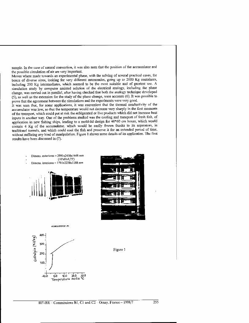
sample. In the case of natural convection, it was also seen that the position of the accumulator and the possible circulation of air are very important. Moves where made towards an experimental phase, with the solving of several practical cases, for boxes of diverse sizes, looking for very different autonomies, going up to 2000 Kg containers, including 200 Kg intermediates, which seemed to be the most suitable and of greatest use. A simulation study by computer assisted solution of the electrical analogy, including the phase change, was carried out in parallel, after having checked that both the analogy technique developed (5), as well as the extension for the study of the phase change, were accurate (6). It was possible to prove that the agreement between the simulations and the experiments were very good. It was seen that, for some applications, it was convenient that the thermal conductivity of the accumulator was low, so that the temperature would not decrease very sharply in the first moments of the transport, which could put at risk the refrigerated or live products which did not increase heat inputs in another way. One of the problems studied was the cooling and transport of fresh fish, of application in new fishing ships, leading to a mold-lid design for 40*60 cm boxes, which would contain 4 Kg of the accumulator, which would be easily frozen thanks to its separators, in traditional tunnels, and which could cool the fish and preserve it for an extended period of time, without suffering any kind of manipulation. Figure 1 shows some details of its application. The first results have been discussed in (7).

Dimens. exteriores = 2991x2438x1448 mm (10'x8'x4,75')

Dimens. interiores = 1791x2238x1188 mm

<?iK.

ACUMULAOORDE-3°C

4CO-

300

-a" 200-j i 100.

Figure 1

i—i—i—i—i—i—■—r- 40.0 0,0 10.0 20.0, 30.0

Temperatuva media "C


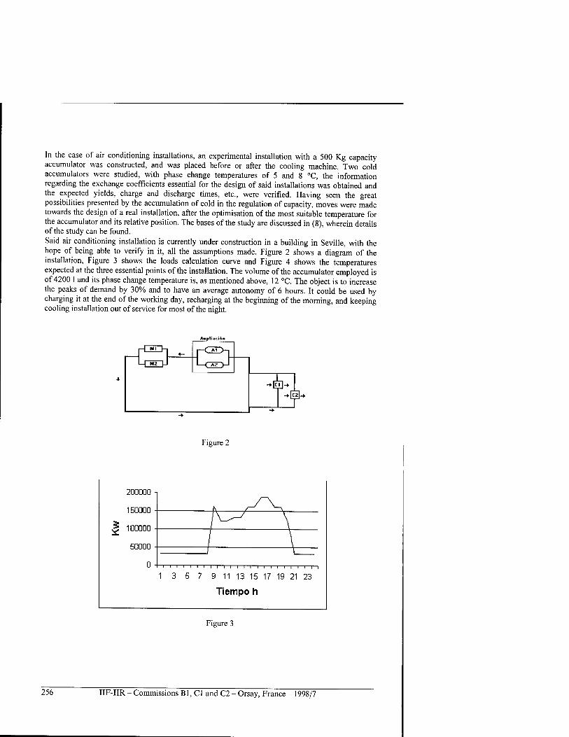
In the case of air conditioning installations, an experimental installation with a 500 Kg capacity accumulator was constructed, and was placed before or after the cooling machine. Two cold accumulators were studied, with phase change temperatures of 5 and 8 °C, the information regarding the exchange coefficients essential for the design of said installations was obtained and the expected yields, charge and discharge times, etc., were verified. Having seen the great possibilities presented by the accumulation of cold in the regulation of capacity, moves were made towards the design of a real installation, after the optimisation of the most suitable temperature for the accumulator and its relative position. The bases of the study are discussed in (8), wherein details of the study can be found. Said air conditioning installation is currently under construction in a building in Seville, with the hope of being able to verify in it, all the assumptions made. Figure 2 shows a diagram of the installation, Figure 3 shows the loads calculation curve and Figure 4 shows the temperatures expected at the three essential points of the installation. The volume of the accumulator employed is of 4200 1 and its phase change temperature is, as mentioned above, 12 °C. The object is to increase the peaks of demand by 30% and to have an average autonomy of 6 hours. It could be used by charging it at the end of the working day, recharging at the beginning of the morning, and keeping cooling installation out of service for most of the night.

<— J-QD-l ^ MI u

L<3E>r 1 «2 V

-*in -►[p

Figure 2

J 100000

—I I I I I I I I I I 1 I I I 1—I 1—I 1—I 1—I 1—I

1 3 5 7 9 11 13 15 17 19 21 23

Tiempo h

Figure 3


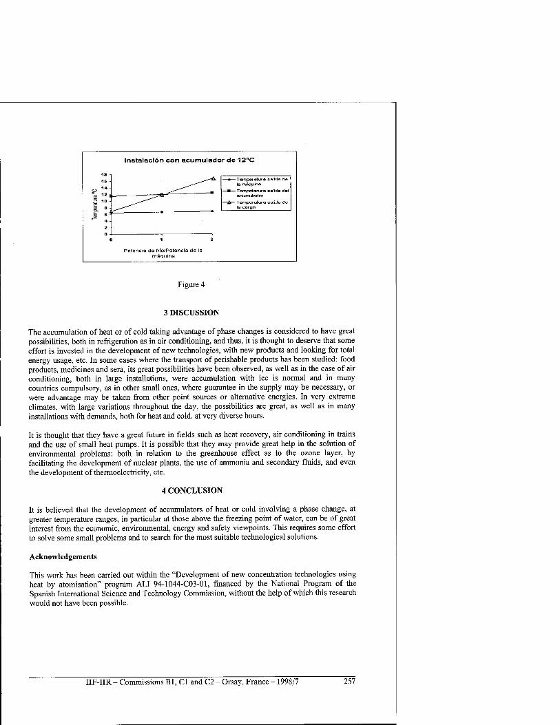
Instalaciön con acumulador de 12°C

- Temperatur« salida de la mäquina

- Tempetarura salida del acumulador

■ Temperature salida de la carga

Potencla de frfo/Potencia de la mäquina

Figure 4

3 DISCUSSION

The accumulation of heat or of cold taking advantage of phase changes is considered to have great possibilities, both in refrigeration as in air conditioning, and thus, it is thought to deserve that some effort is invested in the development of new technologies, with new products and looking for total energy usage, etc. In some cases where the transport of perishable products has been studied: food products, medicines and sera, its great possibilities have been observed, as well as in the case of air conditioning, both in large installations, were accumulation with ice is normal and in many countries compulsory, as in other small ones, where guarantee in the supply may be necessary, or were advantage may be taken from other point sources or alternative energies. In very extreme climates, with large variations throughout the day, the possibilities are great, as well as in many installations with demands, both for heat and cold, at very diverse hours.

It is thought that they have a great future in fields such as heat recovery, air conditioning in trains and the use of small heat pumps. It is possible that they may provide great help in the solution of environmental problems: both in relation to the greenhouse effect as to the ozone layer, by facilitating the development of nuclear plants, the use of ammonia and secondary fluids, and even the development of thermoelectricity, etc.

4 CONCLUSION

It is believed that the development of accumulators of heat or cold involving a phase change, at greater temperature ranges, in particular at those above the freezing point of water, can be of great interest from the economic, environmental, energy and safety viewpoints. This requires some effort to solve some small problems and to search for the most suitable technological solutions.

Acknowledgements



Bibliography

1. Dominguez M. El frio y la conservation de alimentos. Condiciones de almacenamiento. Instal Noticias n°23.sep.l997.5.

2. Dominguez M ; Pinillos J.M. ; Arias J.M Transporte de alimentos en contenedores con mezclas eutecticas: Generalidades Refrigeraciin Frial N° 39 . Jun. 35, 41.

3. Dominguez M ; Pinillos J.M. ; Arias J.M Transporte de alimentos en contenedores con mezclas eutecticas: Aplicaciones Refrigeration Frial n° 40 sep 1996.16,22.

4. Frial's work regarding transport. Applications. 5. Dominguez. M; Garcia C .Subvenciones para el ahorro energetico y la acumulaciön de calor . El

Instalador. In press. 6. Barragän V.M.; Arias J.M.; Dominguez M . Garcia C. Testing the computer assisted solution of

the electrical analogy in a heat transfer processes with a phase change which has an analytical solution, in press.

7. Barragän V.M.; Fuentes R. ; Dominguez M. ; Arias J.M. Testing the computer assisted solution of the electrical analogy in the temperature distribution on a square sheet with nonhomogeneous boundary conditions . in press.

8. Dominguez. ; Pinillos J.M. ; Arias J.M. ; Fuentes R. La acumulaciön de frio en el transporte de productos perecederos. Reclien 98. La Habana. Julio 1998.

9. Dominguez. M; Garcia C; Gutierrez P; Fuentes R.; Culubret J. La acumulaciön de calor en los sistemas de climatizaciön a temperaturas por encima de 0°C . Reclien 98. La Habana. Julio 1998.

10. Dominguez. M; Garcia C. Posibilidades de la acumulaciön del frio. Instal Noticias n°25. die. 1997. 5.


PERMAFROST AS MICROBIAL HABITAT: PALEONTOLOGY OF VIABLE ORGANISMS

GILICHINSKY D.A. Head of Soil Cryology Laboratory, Institute of Soil Science and Photosynthesis,

Russian Academy of Sciences 142292, Pushchino, Moscow Region, Russia Phone: 7 096 773 2604 - Fax: 7 096 779 0532 - E-mail: [email protected]

ABSTRACT

Numerous and various viable paleomicroorganisms have been isolated from the permafrost depths. The oldest (3Myr) were found in Siberian lowlands; the deepest (350m) in Canadian Arctic and preserved at the lowest temperatures (below -25°C) in Antarctica. They are the only known organisms, survived in situ over geological time and upon thawing resume the physiological activities. The presents of viable paleosystems is of interest from Earth and Life Sciences and forms the new basis for micro-, cryo-, paleo- and exobiology. Of special interest is the interaction of these knowledge to understand the planetary history, spatial and temporal limits of the cold biosphere. The fundamental problem is how long life may be preserved. No answer on this either by laboratory modeling and experiments, or calculations. From this point, the discovered phenomenon emphasizes the importance of the permafrost as a unique biological storage, where we can acquire from nature the key of the final result on the preservation of paleobiological objects.

CONCLUSIONS

Because of the unfrozen water and pore space, the frozen soils contain an abundance of viable cells, while in pure ice there are no more than a few dozen cells. The pure ice has insufficient cryoprotecting and transport abilities typical for soils. From the point of preservation of biological systems, this is the principal difference between ice and fine-dispersed frozen sediments. In Siberia the oldest continuously frozen permafrost in the North hemisphere dates back to 3Myr. In Antarctica it is possible that the permafrost exists during last dozens Myr, that is one order more than in Arctic. Here is possible to find out the oldest bacteria, which age can be greater by a factor of ten compared with the Arctic. We isolate here viable cells, at least, 3Myr old and plan to do the same in soils of 8.1Myr age. The limiting age, if one exists, within the Antarctic cores where the viable microflora were no longer present, could be established as the age limit for life preservation within permafrost. Positive results together with the Arctic data would give the background to establish the mechanisms of cell adaptation to permafrost conditions, which might work for billions years.

The keystone question is to detect whether the cells are viable but dormant or metabolically active, as well as to identify the boundary between these two states and to determine how long microorganisms can preserve viability according to these different ways and possibility of another forms of long-term preservation of viable ecosystems and vital activity in permafrost. This is why we call them only viable (culturable), not "living" cells. If the microbes are in anabiotic state in terrestrial permafrost, the latter is the best natural depository of paleolife. In any case, it may be used as a natural storage for the modern genetic pool.

Recent information suggests that permafrost microorganisms are not in the frozen resting state. Facts provide evidences that microorganisms can be metabolically active in the extreme nutritional and temperature regime of the cryolithosphere, where unfrozen water functions as a cryoprotector


and allows us to speculate on the possibility of bio(geo)chemical processes at supercooling state. This is why we hypothesize metabolism, although at a very low level, as unknown form and way of long-term preservation of viable ecosystems. Bacterial cells which were preserved during geological time didn't louse the ability to develop if a labile organic matter is available at subzero temperatures. If permafrost bacteria are active, their life is the unknown adaptive strategies, which could be speeded at the Universe.

Because the Cryosphere existence is a common phenomenon in Space, the terrestrial permafrost environment inhabited by microbes and their metabolically end products can be considered as a model of conditions of the other planets. Ancient microbial communities within the Earth permafrost provide a range of analogies for possible extraterrestrial ecosystems. Permafrost on these planets is an indicator of water presence. The main niche, where the microorganisms may survive, are the unfrozen water films enveloping cells and soil particles. This type of rigidly associated "liquid" water has not been sublimated and may be considered as a life indicator in extraterrestrial permafrost.

LE PERGELISOL EN TANT QU'HABITAT MICROBIEN : PALEONTOLOGIE DES ORGANISMES VIABLES

RESUME : De nombreux micro-organismes paleontologiques, varies et viables, ont ete isoles ä partir de plusieurs profondeurs de pergelisol. Les plus vieux (3Myr) ont ete trouves dans les plaines de Siberie, les plus profonds (350 m), dans la region arctique du Canada; d'autres, pouvant etre conserves ä basses temperatures (-25°C maximum) ont ete trouves dans l'Antarctique. Ce sont les seuls organismes connus qui survivent dans le temps et resistent au degel en recuperant leurs activites physiologiques. Ces systemes paleontologiques viables presentent un reel interet pour les sciences de la terre et de la vie et donnent de nouvelles bases ä la microbiologie, la cryobiologie, la paleontologie et la biologie. L'interaction entre ces diverses connaissances est particulierement interessante pour mieux comprendre l'histoire de la planete et les limites spatiales et temporelles de la biosphere froide. Le probleme fundamental est le suivant: combien de temps la vie peut-elle etre maintenue ? Aucune reponse n'a ete obtenue ä ce jour, ni par modelisation en laboratoire, ni par des experiences ou des calculs. De ce point de vue, les phenomenes decouverts soulignent l'importance du pergelisol comme unique milieu biologique de conservation, oü nous pouvons obtenir la cle du probleme de la conservation biologique dans le temps.


EFFET DE CONFINEMENT SUR LES PROPRIETES THERMIQUES DES SOLUTIONS CRYOPROTECTRICES

BAUDOT A.*, MAZUER J.*, ODIN J.*, DESCOTES J.L.** •C.R.T.B.T./C.N.R.S., B.P. 166, 38042 GRENOBLE Cedex, France.

«S.U.T.R./C.H.U, B.P. 217, 38043 GRENOBLE Cedex, France.

RESUME

La vitrification de tissus biologiques impose l'utilisation de solutions cryoprotectrices concentrees avec application de vitesses elevees pour eviter la formation de glace. Les vitesses minimales sont estimees par calorimetrie differentielle ä balayage. Elles ont ete determinees pour des elements biologiques prealablement impregnes de solution cryoprotectrice, et sont inferieures ä celle de la solution seule. Pour verifier l'effet de confinement, une etude plus systematique a ete realisee avec plusieurs systemes poreux inertes (pores de 2nm ä 100 um). Dans tous les cas, nous avons observe une diminution systematique des vitesses critiques que nous n'avons pu relier ä la taille des pores. Par ailleurs, nos mesures montrent une augmentation systematique de la temperature de transition vitreuse T en contradiction avec la plupart des recentes etudes sur le sujet dans des liquides purs. Nous souhaitons poursuivre et approfondir cette etude sur un materiau d'hydrophilie et de porosite contrölable et variable.

INTRODUCTION

La technique de vitrification (Fahy, 1988) apparait actuellement comme la solution d'avenir pour allonger les durees de conservation trop courtes des elements biologiques ä transplanter. Ce procede consiste ä eviter toute formation de cristaux de glace lors de l'abaissement en temperature, en piegeant toutes les solutions aqueuses dans un etat solide appele " etat vitreux ". La vitrification est un phenomene de nature cinetique qui se caracterise par une augmentation tres brutale de la viscosite ä la temperature de transition vitreuse Tg. Elle necessite des vitesses de refroidissement elevees qui sont abaissees en presence d'une quantite süffisante de " cryoprotecteurs " et deviennent accessibles techniquement. Les cryoprotecteurs interferent avec les processus de nucleation et de croissance des cristaux de glace (Storey et Storey, 1989). En plus de leur action protectrice au niveau biologique, ils ameliorent les conditions cinetiques de vitrification. Le rechauffement ä partir de l'etat vitreux pose lui aussi des problemes car il faut egalement eviter la cristallisation de glace dans l'etat liquide surfondu instable que Fon obtient ä la sortie de la transition vitreuse. Cette condition n'est remplie que pour des vitesses de rechauffement elevees. La connaissance des proprietes thermiques des solutions cryoprotectrices est done une information indispensable pour la cryopreservation par vitrification. La calorimetrie differentielle ä balayage est une methode largement utilisee dans le domaine de la cryopreservation (Sutton, 1992 ; Bryant, 1995). Elle permet de suivre les transitions de phase dans un echantillon de petite taille (quelques mg) en fonetion des vitesses de refroidissement et de rechauffement auxquelles il est soumis. Elle conduit ä une estimation des vitesses critiques necessaires pour vitrifier puis devitrifier l'echantillon sans l'endommager. Ce sont les vitesses au- delä desquelles le taux de cristallisation devient pratiquement nul. Nous determinons ces vitesses critiques ä partir d'un modele semi-empirique (Boutron, 1986 ; Boutron et Mehl, 1990) qui s'appuie sur la theorie classique de la cristallisation (Doremus, 1973). L'etude que nous presentons concerne l'effet des tissus biologiques sur les proprietes thermiques de solutions cryoprotectrices preparees ä partir de 1.2-Propanediol (1.2-PD) ou de 2.3-Butanediol (2.3- BD) ä 97% des isomeres dextro/levo. Apres une etude plus systematique des proprietes thermiques


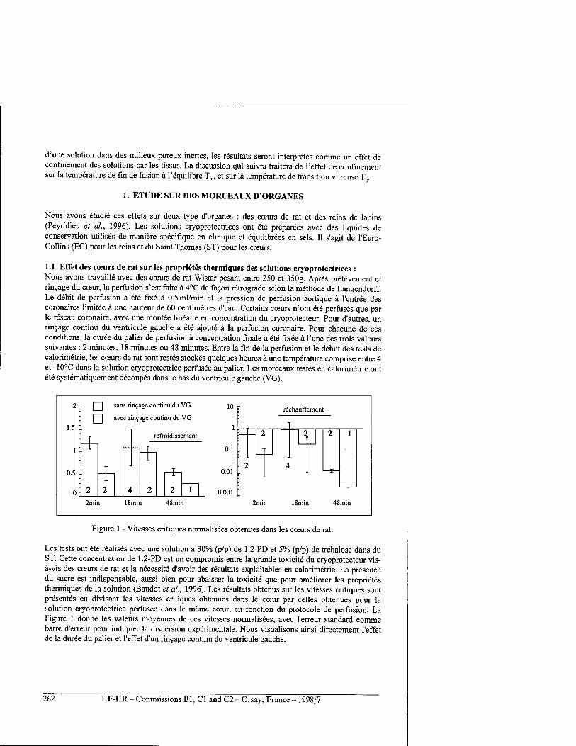
d'une solution dans des milieux poreux inertes, les resultats seront interprets comme un effet de confinement des solutions par les tissus. La discussion qui suivra traitera de 1'effet de confinement sur la temperature de fin de fusion ä l'equilibre Tm, et sur la temperature de transition vitreuse T,.

1. ETUDE SUR DES MORCEAUX D'ORGANES

Nous avons etudie ces effets sur deux type d'organes : des coeurs de rat et des reins de lapins (Peyridieu et al, 1996). Les solutions cryoprotectrices ont ete preparees avec des liquides de conservation utilises de maniere specifique en clinique et equilibrees en sels. II s'agit de l'Euro- Collins (EC) pour les reins et du Saint Thomas (ST) pour les coeurs.

1.1 Effet des coeurs de rat sur les proprietes thermiques des solutions cryoprotectrices : Nous avons travaille avec des coeurs de rat Wistar pesant entre 250 et 350g. Apres prelevement et rincage du coeur, la perfusion s'est faite ä 4°C de facon retrograde selon la methode de Langendorff. Le debit de perfusion a ete fixe ä 0.5 ml/min et la pression de perfusion aortique ä l'entree des coronaires limitee ä une hauteur de 60 centimetres d'eau. Certains coeurs n'ont ete perfuses que par le reseau coronaire, avec une montee lineaire en concentration du cryoprotecteur. Pour d'autres, un rincage continu du ventricule gauche a ete ajoute ä la perfusion coronaire. Pour chacune de ces conditions, la duree du palier de perfusion ä concentration finale a ete fixee ä l'une des trois valeurs suivantes : 2 minutes, 18 minutes ou 48 minutes. Entre la fin de la perfusion et le debut des tests de calorimetrie, les coeurs de rat sont restes Stockes quelques heures ä une temperature comprise entre 4 et -10°C dans la solution cryoprotectrice perfusee au palier. Les morceaux testes en calorimetrie ont ete systematiquement decoupes dans le bas du ventricule gauche (VG).

2

1.5

1

0.5

0

- □ D

sans rincage continu du VG 10

1

0.1

0.01

0.001

rechauffement avec rincage continu du VG

I 2 t 2 1 T reiroiaissement

-r

2

T

—. 1

2

r : 2 4 "i" 2 4

L

2

r 1

1 min 2min 18min 48min 2 mi n 18 mil l 48

Figure 1 - Vitesses critiques normalisees obtenues dans les coeurs de rat.

Les tests ont ete realises avec une solution ä 30% (p/p) de 1.2-PD et 5% (p/p) de trehalose dans du ST. Cette concentration de 1.2-PD est un compromis entre la grande toxicite du cryoprotecteur vis- a-vis des coeurs de rat et la necessite d'avoir des resultats exploitables en calorimetrie. La presence du sucre est indispensable, aussi bien pour abaisser la toxicite que pour ameliorer les proprietes thermiques de la solution (Baudot et al., 1996). Les resultats obtenus sur les vitesses critiques sont presentes en divisant les vitesses critiques obtenues dans le coeur par celles obtenues pour la solution cryoprotectrice perfusee dans le meme coeur, en fonction du protocole de perfusion. La Figure 1 donne les valeurs moyennes de ces vitesses normalisees, avec l'erreur standard comme barre d'erreur pour indiquer la dispersion experimentale. Nous visualisons ainsi directement l'effet de la duree du palier et l'effet d'un rincage continu du ventricule gauche.


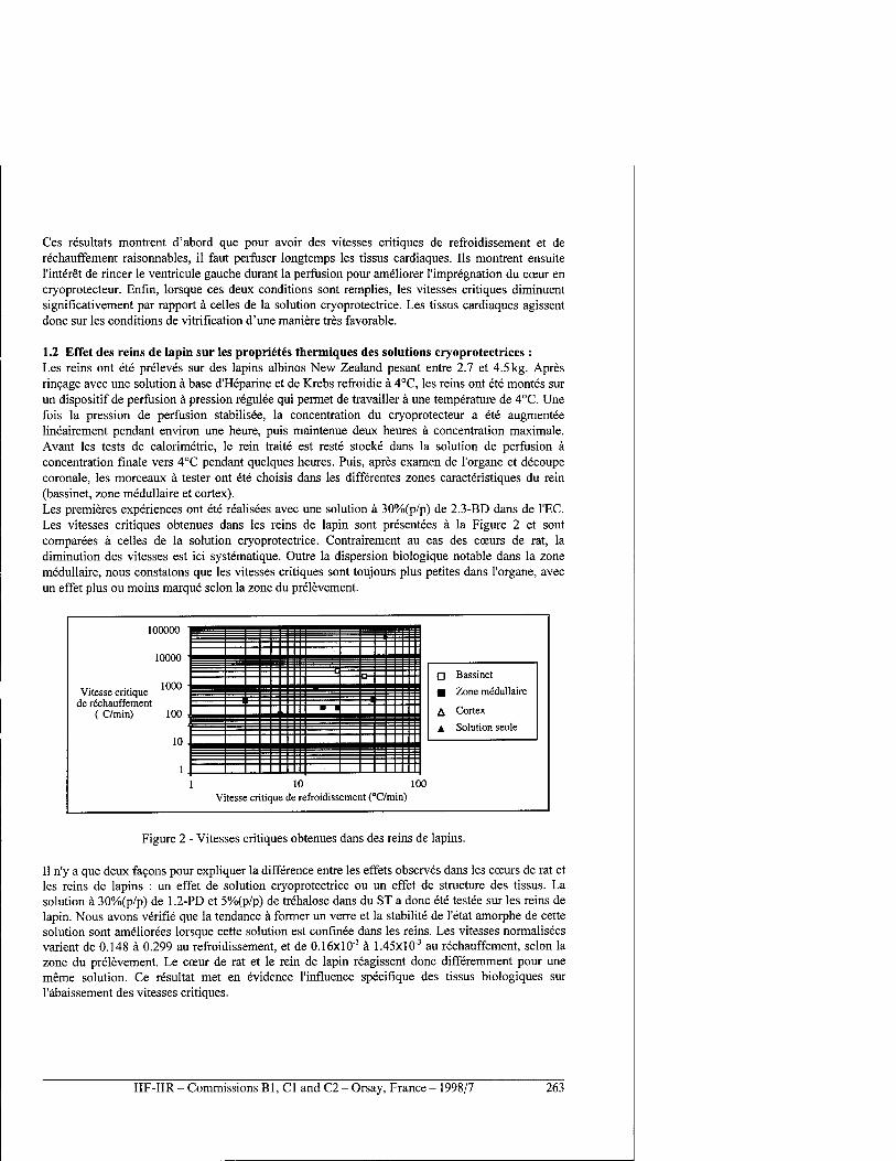
Ces resultats montrent d'abord que pour avoir des vitesses critiques de refroidissement et de rechauffement raisonnables, il faut perfiiser longtemps les tissus cardiaques. Ils montrent ensuite l'interet de rincer le ventricule gauche durant la perfusion pour ameliorer l'impregnation du coeur en cryoprotecteur. Enfin, lorsque ces deux conditions sont remplies, les vitesses critiques diminuent significativement par rapport ä celles de la solution cryoprotectrice. Les tissus cardiaques agissent done sur les conditions de vitrification d'une maniere tres favorable.

1.2 Effet des reins de lapin sur les proprietes thermiques des solutions cryoprotectrices : Les reins ont ete preleves sur des lapins albinos New Zealand pesant entre 2.7 et 4.5 kg. Apres rincage avec une solution ä base d'Heparine et de Krebs refroidie ä 4°C, les reins ont ete montes sur un dispositif de perfusion ä pression regulee qui permet de travailler ä une temperature de 4°C. Une fois la pression de perfusion stabilised, la concentration du cryoprotecteur a ete augmentee lineairement pendant environ une heure, puis maintenue deux heures ä concentration maximale. Avant les tests de calorimetrie, le rein traite est reste stocke dans la solution de perfusion ä concentration finale vers 4°C pendant quelques heures. Puis, apres examen de l'organe et decoupe coronale, les morceaux ä tester ont ete choisis dans les differentes zones caracteristiques du rein (bassinet, zone medullaire et cortex). Les premieres experiences ont ete realisees avec une solution ä 30%(p/p) de 2.3-BD dans de l'EC. Les vitesses critiques obtenues dans les reins de lapin sont presentees ä la Figure 2 et sont comparees ä celles de la solution cryoprotectrice. Contrairement au cas des coeurs de rat, la diminution des vitesses est ici systematique. Outre la dispersion biologique notable dans la zone medullaire, nous constatons que les vitesses critiques sont toujours plus petites dans l'organe, avec un effet plus ou moins marque selon la zone du prelevement.

100000 ]

10000 ■

1000 ■ Vitesse critique

de rechauffement ( C/min) 100 ,

10 .

1 .

_

I ■ Zone medullaire

B-l , A Cortex

A Solution seule

1 10 100 Vitesse critique de refroidissement (°C/min)

Figure 2 - Vitesses critiques obtenues dans des reins de lapins.

II n'y a que deux facons pour expliquer la difference entre les effets observes dans les cceurs de rat et les reins de lapins : un effet de solution cryoprotectrice ou un effet de structure des tissus. La solution ä 30%(p/p) de 1.2-PD et 5%(p/p) de trehalose dans du ST a done ete testee sur les reins de lapin. Nous avons verifie que la tendance ä former un verre et la stabilite de l'etat amorphe de cette solution sont ameliorees lorsque cette solution est confinee dans les reins. Les vitesses normalisees varient de 0.148 ä 0.299 au refroidissement, et de 0.16xl0"3 ä 1.45xl0"3 au rechauffement, selon la zone du prelevement. Le cceur de rat et le rein de lapin reagissent done differemment pour une meme solution. Ce resultat met en evidence l'influence speeifique des tissus biologiques sur l'äbaissement des vitesses critiques.


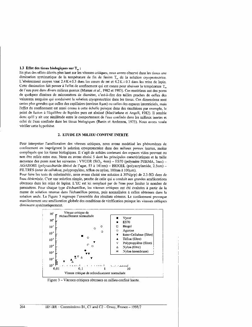
1.3 Effet des tissus biologiques sur Tra : En plus des effets decrits plus haut sur les vitesses critiques, nous avons observe dans les tissus une diminution systemafique de la temperature de fin de fusion T,„ de la solution cryoprotectrice. L'abaissement moyen vaut 2.4 K± 0.3 dans les coeurs de rat et 4.2 K± 0.3 dans les reins de lapin. Cette diminution fait penser ä l'effet de confinement qui est connu pour abaisser la temperature T„, de l'eau pure dans divers milieux poreux (Murase et al., 1982 et 1983). Ces materiaux ont des pores de quelques dizaines de micrometres de diametre, c'est-ä-dire des tailles proches de celles des vaisseaux sanguins qui conduisent la solution cryoprotectrice dans les tissus. Ces dimensions sont certes plus grandes que celles des capillaires (environ 8 um) ou celles des espaces intersticiels, mais l'effet du confinement est aussi connu ä cette echelle puisque dans des emulsions par exemple, le point de fusion ä l'equilibre de liquides purs est abaisse (MacFarlane et Angell, 1982). II semble done qu'il y ait une similitude entre le comportement de l'eau confinee dans les milieux inertes et celui de l'eau confinee dans les tissus biologiques (Banin et Anderson, 1975). Nous avons voulu verifier cette hypothese.

2. ETUDE EN MILIEU CONFINE INERTE

Pour interpreter l'amelioration des vitesses critiques, nous avons modelise les phenomenes de confinement en impregnant la solution cryoprotectrice dans des milieux poreux inertes, moins compliques que les tissus biologiques. II s'agit de solides contenant des espaces vides pouvant ou non etre relies entre eux. Nous en avons choisi 5 dont les principales caracteristiques et la taille moyenne des pores sont les suivantes : VYCOR (Si02, 4nm) - ES70 (polymere PHEMA, 3nm) - AGAROSE (polysaccharide derive de l'agar, 53 ä 141nm) - BIOGEL (polyacrylamide, 2.5nm) - FILTRES (ester de cellulose, polypropylene, teflon ou nylon, lOOnm ä lOOum). Pour faire les tests de calorimetrie, nous avons choisi une solution ä 30%(p/p) de 2.3-BD dans de l'eau desionisee. C'est une solution simple, proche de celle qui a conduit aux grandes ameliorations obtenues dans les reins de lapins. L'EC est ici remplace par de l'eau pour limiter le nombre de parametres. Pour chaque type d'echantillon, les vitesses critiques ont ete evaluees ä partir de la masse de solution retenue dans l'echantillon poreux, puis normalisees ä celles obtenues dans la solution seule. La Figure 3 regroupe l'ensemble des resultats obtenus. Le confinement provoque manifestement une amelioration globale des conditions de vitrification puisque les vitesses critiques diminuent systematiquement.

10'

10°

10-'

102

103

10"

10 =

10'6

io-'

Vitesse critique de rechauffement normalisee

o

o

o

D

■ Vycor • ES70 D Biogel O Agarose ▼ Ester-Cellulose (filtre) ▲ Teflon (filtre) V Polypropylene (filtre) A Nylon (filtre) ffl Nylon (membrane)

il_

0,01 0,1 1 10 Vitesse critique de refroidissement normalisee

Figure 3 - Vitesses critiques obtenues en milieu confine inerte.


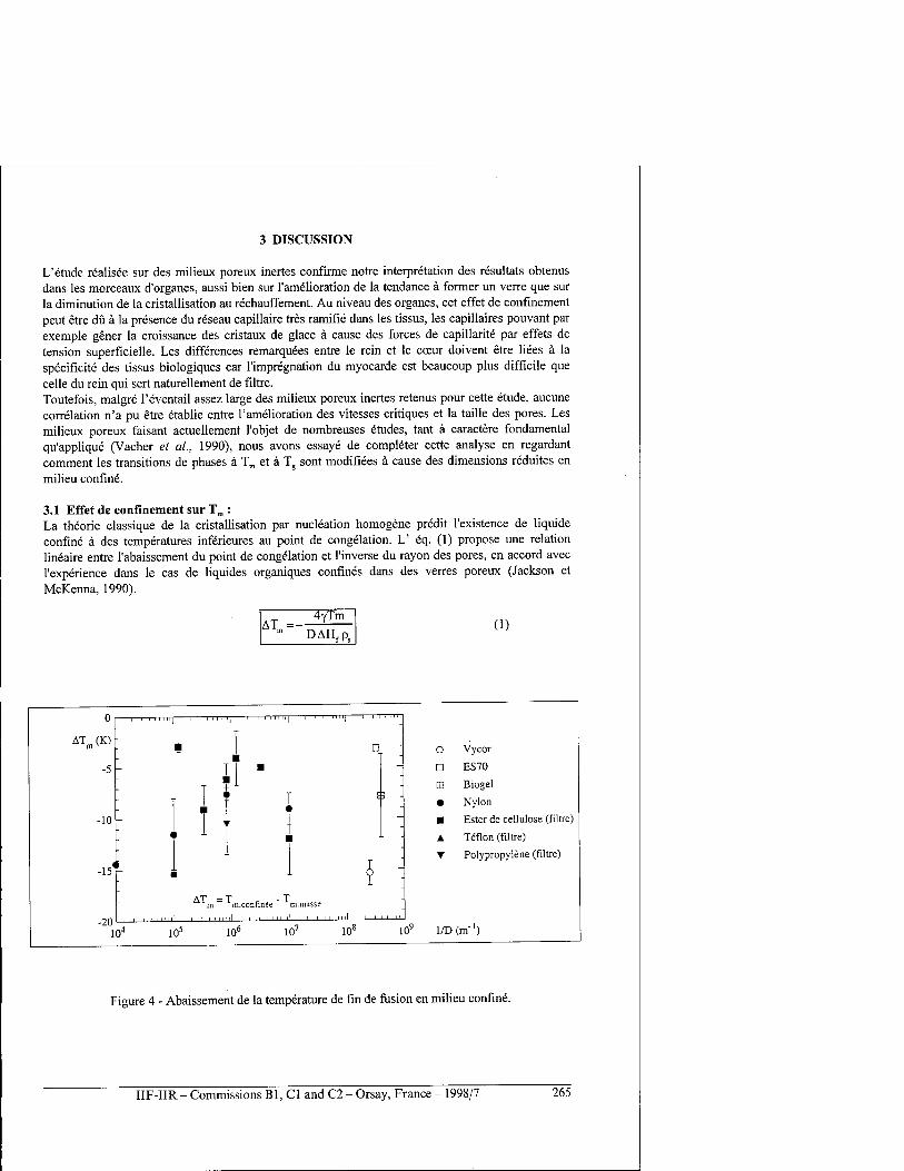
3 DISCUSSION

L'etude realisee sur des milieux poreux inertes confirme notre interpretation des resultats obtenus dans les morceaux d'organes, aussi bien sur l'amelioration de la tendance ä former un verre que sur la diminution de la cristallisation au rechauffement. Au niveau des organes, cet effet de confinement peut etre du ä la presence du reseau capillaire tres ramifie dans les tissus, les capillaires pouvant par exemple gener la croissance des cristaux de glace ä cause des forces de capillarite par effets de tension superficielle. Les differences remarquees entre le rein et le cceur doivent etre liees ä la specificite des tissus biologiques car l'impregnation du myocarde est beaucoup plus difficile que celle du rein qui sert naturellement de filtre. Toutefois, malgre l'eventail assez large des milieux poreux inertes retenus pour cette etude, aucune correlation n'a pu etre etablie entre l'amelioration des vitesses critiques et la taille des pores. Les milieux poreux faisant actuellement l'objet de nombreuses etudes, tant ä caractere fondamental qu'applique (Vacher et al., 1990), nous avons essaye de completer cette analyse en regardant comment les transitions de phases ä Tm et ä Tg sont modifiees ä cause des dimensions reduites en milieu confine.

3.1 Effet de confinement sur Tm : La fheorie classique de la cristallisation par nucleation homogene predit l'existence de liquide confine ä des temperatures inferieures au point de congelation. L' eq. (1) propose une relation lineaire entre l'abaissement du point de congelation et l'inverse du rayon des pores, en accord avec l'experience dans le cas de liquides organiques confines dans des verres poreux (Jackson et McKenna, 1990).

AT =- 4yTm

DAHfPs (1)

104

0 1 ' ' 1 i i i i

""1 "1 '''"

(K) I D -

-5

-10 1 1

1 T ■ + ■ • I

■

( 1

: i -

\ 1 1 1 1 1 L -

-15' i

< j * -

- AT m

= T m.confinê

T

m. masse

■ i

-

o Vycor

D ES70

H Biogel

• Nylon

■ Ester de cellulose (filtre)

A Teflon (filtre)

T Polypropylene (filtre)

105 10° 10' 10° 109 1/D(m"')

Figure 4 - Abaissement de la temperature de fin de fusion en milieu confine.


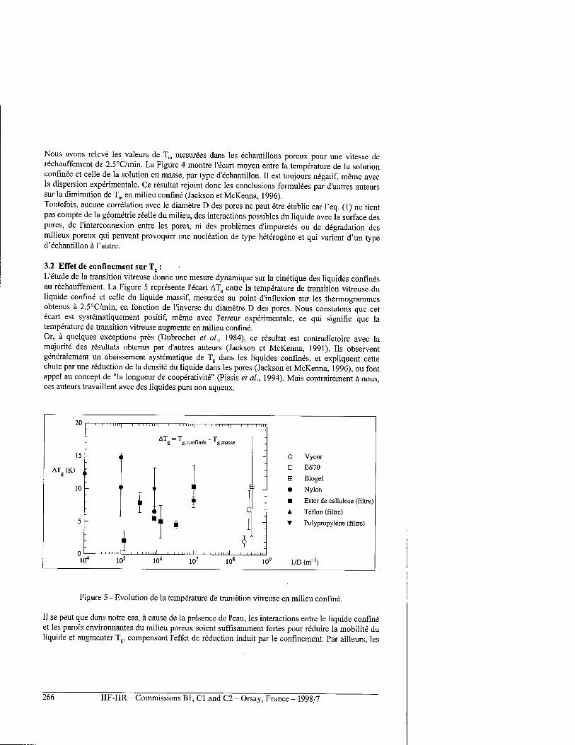
Nous avons releve les valeurs de Tm mesurees dans les echantillons poreux pour une vitesse de rechauffement de 2.5°C/min. La Figure 4 montre 1'ecart moyen entre la temperature de la solution confinee et celle de la solution en masse, par type d'echantillon. II est toujours negatif, meme avec la dispersion experimentale. Ce resultat rejoint done les conclusions formulees par d'autres auteurs sur la diminution de Tm en milieu confine (Jackson et McKenna, 1996). Toutefois, aucune correlation avec le diametre D des pores ne peut etre etablie car 1'eq. (1) ne tient pas compte de la geometrie reelle du milieu, des interactions possibles du liquide avec la surface des pores, de l'interconnexion entre les pores, ni des problemes d'impuretes ou de degradation des milieux poreux qui peuvent provoquer une nucleation de type heterogene et qui varient d'un type d'echantillon ä l'autre.

3.2 Effet de confinement sur Tg: L'etude de la transition vitreuse donne une mesure dynamique sur la cinetique des liquides confines au rechauffement. La Figure 5 represente 1'ecart ATg entre la temperature de transition vitreuse du liquide confine et celle du liquide massif, mesurees au point d'inflexion sur les thermogrammes obtenus ä 2.5°C/min, en fonction de l'inverse du diametre D des pores. Nous constatons que cet ecart est systematiquement positif, meme avec l'erreur experimentale, ce qui signifie que la temperature de transition vitreuse augmente en milieu confine. Or, ä quelques exceptions pres (Dubrochet et al, 1984), ce resultat est contradictoire avec la majorite des resultats obtenus par d'autres auteurs (Jackson et McKenna, 1991). Ils observent generalement un abaissement systematique de Tg dans les liquides confines, et expliquent cette chute par une reduction de la densite du liquide dans les pores (Jackson et McKenna, 1996), ou font appel au concept de "la longueur de cooperativite" (Pissis et al., 1994). Mais contrairement ä nous, ces auteurs travaillent avec des liquides purs non aqueux.

20

;

l| III Mill! 1

AT =T g g.confinee T

g.masse

-

15 i i - O Vycor

ATg(K) , i - D ES70

a Biogel 10 L ( 1 i ' 1 ( i • Nylon

I ( p - ■ Ester de cellulose (filtre)

5 I

i » 'l 1 i

i - ▲ Teflon (filtre)

T Polypropylene (filtre)

1 § - 0

1( | | , 1 , ,

)9 1/D(m_1) f 105 06 107 108 K

Figure 5 - Evolution de la temperature de transition vitreuse en milieu confine.

II se peut que dans notre cas, ä cause de la presence de l'eau, les interactions entre le liquide confine et les parois environnantes du milieu poreux soient suffisamment fortes pour reduire la mobilite du liquide et augmenter Tg, compensant l'effet de reduction induit par le confinement. Par ailleurs, les


modeles d'entropie de la transition vitreuse annoncent une diminution de 1'entropie pour un liquide confine dans des petits pores, ce qui deplace la transition vitreuse vers les hautes temperatures (Jackson et McKenna, 1991). Enfin, phenomenologiquement, la relation de Laplace combinee ä la relation d'Ehrenfest (Zhang et al., 1992) conduit ä :

„ Aoc4Ay Ay AT =v T note AT =4k—

8 "" s Ac D 8 D p

(2)

Or, Atake et Angell (1979) ont verifie pour de nombreuses substances que la pente des courbes de T, en fonction de la pression, qui correspond ä k (relation d'Ehrenfest), est toujours positive, avec toutefois une valeur plus faible dans le cas des alcools que pour des materiaux sans liaison hydrogene. Cela signifie que ATg est positif si Ay (difference entre les tensions de surface gaz/pore et liquide/pore) est positif, ce qui depend des proprietes de mouillabilite du liquide ä la surface des

pores. Enfin, nous remarquons que l'eq. (2) annonce un effet inversement proportionnel ä la taille des pores. Mais il depend beaucoup du milieu poreux ä cause de Ay. Nous ne pouvons done pas observer sur la Figure 5 une variation lineaire commune ä l'ensemble de nos experiences.

CONCLUSION

Nos mesures en milieu confine montrent que les contraintes geometriques changent les proprietes des solutions cryoprotectrices. Nous associons cet effet aux difficultes des mouvements moleculaires que rencontre la solution dans les pores, ou entre les pores, ä cause de la geometrie du milieu et des interactions possibles entre les molecules du liquide et les parois des pores. D'une part, elles abaissent les vitesses critiques et la temperature de fin de fusion Tm. D'autre part, elles augmentent la temperature de transition vitreuse Tg. Ce constat experimental est tres avantageux pour la cryopreservation car il signifie qu'il est plus facile de vitrifier un organe impregne de

solution cryoprotectrice que la solution seule. Actuellement, il nous est difficile d'analyser plus en detail les effets du confinement car dans nos milieux poreux inertes, les dimensions des pores ne sont pas toujours tres süres, la structure du reseau poreux est compliquee et il est difficile d'apprecier la qualite de 1'impregnation. Cette remarque rejoint en fait le probleme de la caracterisation des milieux poreux et de leur moderation geometrique. Pour approfondir notre etude, nous souhaiterions travailler de facon tres systematique avec un milieu poreux bien caracterise. L'ideal serait pour nous de trouver un materiau avec des pores de taille contrölable et variable sur une large gamme, dont nous pourrions faire varier les

proprietes d'hydrophilie et d'hydrophobie.

NOMENCLATURE

D . diametre des pores Aa variation du coefficient de dilatation isobare Ac variation de capacite thermique massique ä pression constante Ay difference des tensions de surface : ymi\im porel,x / Eaz - Ymiiieu poreux/ liquide

y tension de surface entre la glace et le liquide AHf chaleur latente massique de fusion de la glace au point de congelation

ps densite de la glace Tg temperature de transition vitreuse Tm temperature de fin de fusion ou temperature de congelation ä l'equilibre

vmas volume massique


BIBLIOGRAPHIE

1. Atake. T.. Angell. CA., 1979, Pressure dependence of the glass transition temperature in molecular liquids and plastic crystals../. Phys. Chem., vol. 83, no. 25 : p. 3218-3223.

2. Banin. A., Anderson, D.M., 1975, A similar law may govern water freezing in minerals and living organisms Xature, vol. 255 : p. 261-262.

3. Baudot. A. el ai. 1996, Effect of saccharides on the glass-forming tendency and stability of solutions of 2,3- butanediol, 1.2-propanediol, or 1,3-butanediol in water, phosphate-buffered saline, Euro-Collins solution, or Saint Thomas cardioplegic solution, Cryobiology, vol. 33, no. 3 : p. 363-375.

4. Boutron, P., 1986, Comparison with the theory of the kinetics and extent of ice crystallization and of the glass- forming tendency in aqueous cryoprotective solutions, Ctyobiology, vol. 23, no. 1 : p. 88-102.

5. Boutron, P., Mehl, P., 1990, Theoretical prediction of devitrification tendency : determination of critical warming rates without using finite expansions, Cryobiology, vol. 27, no. 4 : p. 359-377.

6. Bryant, G., 1995, DSC measurement of cell suspensions during successive freezing runs : implications for the mechanisms of intracellular ice formation, Cryobiology, vol. 32, no. 2 : p. 114-128.

7. Doremus, R.H., 1973, Glass science, John Wiley & Sons, New York, 349 p. 8. Dubrochet, J. et ai, 1984, Glass-forming microemulsions : vitrification of simple liquids and electron microscope

probing of droplet-packing modes,./. Phys. Chem. vol. 88, no. 26 : p. 6727-6732. 9. Fahy, G.M., 1988, Vitrification, In : McGrath, J.J., Diller, K.R., Low temperature biotechnology, The american

society of mechanical engineer, New-York, p. 113-146. 10. Jackson, C.L., McKenna, G.B., 1990, The melting behaviour of organic materials confined in porous solids, J.

Chem. Phys., vol. 93, no. 12 : p. 9002-9011. 11. Jackson, C.L., McKenna, G.B., 1991, The glass transition of organic liquids confined to small pores J Non Cryst

Solids, vol. 131-133 : p. 221-224. 12. Jackson, C.L., McKenna, G.B., 1996, Vitrification and crystallization of organic liquids confined to nanoscale

pores, Chem. Mater., vol. 8, no. 8 : p. 2128-2137. 13. MacFarlane, D.R., Angell, CA., 1982, An emulsion technique for the study of marginal glass formation in

molecular liquids,./. Phys. Chem., vol. 86, no. 11: p. 1927-1930. 14. Murase, N. et ai, 1982, Low-temperature calorimetric studies of compartmentalized water in hydrogel systems (I),

Cryo-Letters, vol. 3, no. 5 : p. 251-254. 15. Murase, N. et ai, 1983, Low-temperature calorimetric studies of compartmentalized water in hydrogel systems

(II), Cryo-Letters, vol. 4, no. 1 : p. 19-22. 16. Peyridieu, J.F. et ai, 1996, Critical cooling and warming rates to avoid ice crystallization in small pieces of

mammalian organs permeated with cryoprotective agents, Cryobiology, vol. 33, no. 4 : p. 436-446. 17. Pissis, P. et ai, 1994, The glass transition in confined liquids, J. Phys. : Condens. Matter, vol. 6 : p. L325-L328. 18. Storey, K.B., Storey, J.M., 1989, Comment les animaux surviventau gel, La Recherche, vol 20 no 208 • p 331-

341. 19. Sutton, R.L., 1992, Critical cooling rates for aqueous cryoprotectants in the presence of sugars and

polysaccharides, Cryobiology, vol. 29, no. 5 : p. 585-598. 20. Vacher, R. et ai, 1990, La structure fractale des aerogels, La Recherche, vol. 21, no. 220 : p. 426-435. 21. Zhang, J. et ai, 1992, Effects of confinement on the glass transition temperature of molecular liquids, J. Phys.

Chem., vol. 96, no. 8 : p. 3478-3480.

CONFINEMENT EFFECT ON THERMAL PROPERTIES OF CRYOPROTECTIVE SOLUTIONS

SUMMARY: Vitrification of biological tissues requires the use of highly concentrated cryoprotective solutions in conjunction with fast rates to avoid the formation of ice crystals. The lowest rates necessary are evaluated by differential scanning calorimetry. They have been calculated in several samples of biological tissue previously impregnated with a cryoprotective solution, and are lower than the corresponding rates of the bulk solution. To verify the confinement effect, we have conducted a more systematic study in a number of porous and inert materials (pore size from 2 ran to 100 urn). In each of these materials, we observed a systematic decrease of the critical rates, but did not find a correlation between this decrease and the size of the pores. In addition, our measurements also showed a systematic increase in the vitreous transition temperature TE, which contradicts most of the latest work on this subject involving pure liquids. We wish to continue this work with a more in-depth study on a porous material with which we can control and change the porosity and the hydrophilic characteristics.


CARTOGRAPHY GEOMORPHOLOGIQUE A L'AIDE DE BASES DE DONNEES GEOGRAPHIQUES EN HAUTE RESOLUTION :

L'EXEMPLE DU GLACIER LOVEN CENTRAL ET DE SON PIEMONT (SPITSBERG - 79°N)

BROSSARD T.*, JOLY D.*, NILSEN L.**

* Laboratoire THEMA, CNRS et Universite de Franche-Comte, 32, rue Megevand, F25030 BESANCON cedex. E-mail: [email protected]

** Institutt i Botani og Geologi, Drammensveien, N9000 TROMS0. E-mail: [email protected]

RESUME

Cette etude qui porte sur le front du Glacier Loven Central au Spitsberg repose sur l'utilisation combinee de donnees integrees dans un Systeme d'information geographique (S.I.G.). Elle vise ä proposer un outil de cartographie automatisee des formes geomorphologiques et des processus qui les sous-tendent. L'exemple des formes de gelifuxion a ete choisi pour ce test de mise au point. On a fait appel ä differents types de donnees en haute resolution (2 metres) : une image aerienne infrarouge numerisee, un modele numerique de terrain leve au G.P.S. et differentes couches d'information derivees 'comme la pente, l'exposition et les formes topographiques. D'un autre cote, des points d'observation disposes regulierement le long de transects ont servi ä l'echantillonnage du terrain et au recueil d'informations sur le sol, les microformes et la vegetation. Enfin, la procedure cartographique a requis les etapes suivantes :

• extraction des points de l'echantillon concernes par la gelifluxion, • recours ä une modelisation statistique pour etablir les relations entre loupes de gelifuxion et

facteurs retenus comme explicatifs et contenus dans le S.I.G. sous forme de couches d'information,

• utilisation du modele ainsi defini comme Operateur cartographique pour representer la distribution potentielle des formes de gelifluxion sur la zone test.

INTRODUCTION

L'image satellite est reconnue comme un auxiliaire puissant de la cartographie geomorphologique (Beshina et Taloskaia, 1981) surtout dans la zone arctique oü les coüts d'acquisition de 1'information sur le terrain sont eleves. Les systemes d'information geographiques qui integrent d'autres types de donnees comme les modeles numeriques de terrain et les couches d'information derivees (pentes, exposition, formes topographiques...) completent les moyens d'investigation utiles ä l'inventaire geomorphologique par la carte (Sidjak et Wheate, 1996). Les images satellites actuelles et les bases de donnees associees permettent de discriminer des objects et des situations en rapport avec les resolutions offertes qui sont d'ordre decametrique. Les domaines geomorphologiques qui structurent le paysage comme les moraines, les plaines d'epandage (sandurs) ou les eboulis peuvent etre reconnus et delimites de la sorte. En utilisant une base de donnees en resolution plus fine couplant une image aerienne infrarouge et un modele numerique de terrain leve au GPS differentiel, nous aborderons la reconnaissance d'elements geomorphologiques d'ordre metrique.

Au Spitsberg oü s'applique notre test, nous disposons de references relativement abondantes en matiere de cartographie geomorphologique. L'ensemble de la presqu'ile de Brogger a fait l'objet d'une couverture au 1/50 000 (Joly, 1970) Des leves topographiques par triangulation, au 1/10 000 ont servi de base ä une representation precise des faits geomorphologiques, notamment sur la partie


aval du glacier Loven Central qui nous interesse directement ici (Nationalkomitees für Geodäsie und Geophysik, 1962). Tolgensbakk et Sollid (1987) ont propose un mode de cartographie detaillee de la presqu'ile de Bragger qui s'appuie sur Interpretation d'image. La carte ou le croquis geomorphologique constituent un support documentaire essentiel pour beaucoup d'ouvrages ou articles (Andre, 1991 ; Brossard, 1991).

L'objectif de la presente etude est de completer les ressources existantes de l'analyse et de l'inventaire geomorphologiques par une methode qui met ä profit les capacites operatoires des S.I.G. (Denegre, 1992). II s'agit de croiser, par le biais de la modelisation statistique, donnees issues de l'observation et donnees numeriques resultant du traitement de l'image satellite et du modele numerique de terrain. Ainsi, sont mis en evidence les parametres environnementaux qui commandent, ä l'echelle metrique, la presence de formes et de processus remarquables comme la gelifluxion qui servira d'exemple ä notre application. Les modeles etablis selon cette procedure serviront ensuite d'operateurs cartographiques pour reconnaitre automatiquement les sites potentiellement favorables ä la manifestation du processus considere et pour en dresser la carte de distribution.

1. L'AIRE D'ETUDE

L'archipel du Svalbard dont le Spitsberg constitue File principale, est situe en bordure du bassin arctique ä pres de 80° N de latitude. II est couvert de glace ä environ 70%. La cöte ouest du Spitsberg est profondement decoupee par des fjords encadres de presqu'iles montagneuses comme celle de Br0gger oü se situe notre zone d'etude. Celle-ci se localise plus precisement au front du glacier Loven central ä 6 km de la station norvegienne de Ny-Älesund. Le glacier draine un bassin versant d'une dizaine de km2. II y a un peu plus d'un siecle, le Petit Äge de Glace a connu son paroxysme. A cette epoque, le glacier debordait assez largement sur son piemont ou strandflat. Avec le retrait qui a suivi et qui se poursuit aujourd'hui, un appareil morainique, bien delimite par Tare de son vallum, s'est construit et s'impose comme une forme majeure dans le paysage (Lefauconnier 1990). En avant de la moraine, on distingue la ligne rigide d'un affleurement calcaire qui sert d'appui ä plusieurs niveaux de plages glacio-marines (Forman, 1992), elles memes liees au soulevement glacio-isostatique post-wiirmien (ou post-weichselien). Une toundra bien venue recouvre ces niveaux relativement anciens et stables. En contrebas, les eaux de fonte proglaciaires ont construit une plaine d'epandage (sandurs) faite d'une succession de cones coalescents. Avec le recul glaciaire, le flux s'est concentre sur un exutoire tres instable, tandis que le reste de l'appareil de drainage est repris par la vegetation (Kergomard, 1984). Parmi les processus diffus qui commandent la dynamique des paysages, la gelifluxion prend un role important (Van-Vliet-Lanoe, 1992). Sur la moraine, le materiel, souvent riche en fines est apte ä la sursaturation. De plus, la presence de glace morte en profondeur favorise le glissement gelifluidal. Les chanfreins de raccordement entre les niveaux de plage constituent egalement des sites interesses par la gelifluxion.

2. DONNEES ET METHODE

Pour cartographier les sites potentiellement favorables ä la gelifluxion, la methode choisie requiert le croisement entre observations in situ et donnees exogenes contenues dans un S.I.G. sous la forme de couches. Les differents termes de notre approche demandent maintenant ä etre precises.

2.1. L'enquete de terrain L'ensemble du secteur d'etude a fait 1'objet d'un echantillonnage systematique par le biais de transects recoupant les principales unites bio-geomorphologiques que nous venons de decrire. Le


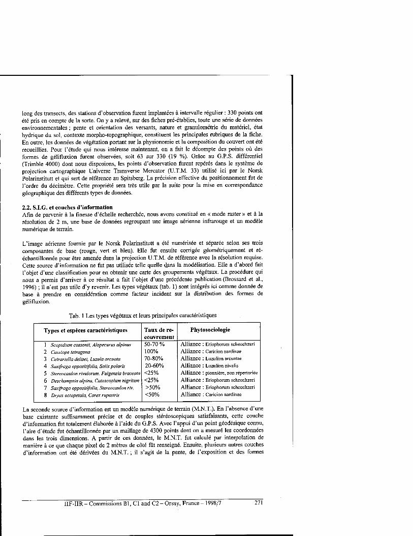
long des transects, des stations d'observation furent implantees ä intervalle regulier : 330 points ont ete pris en compte de la sorte. On y a releve, sur des fiches pre-etablies, toute une serie de donnees environnementales ; pente et orientation des versants, nature et granulometrie du materiel, etat hydrique du sol, contexte morpho-topographique, constituent les principales rubriques de la fiche. En outre, les donnees de vegetation portant sur la physionomie et la composition du couvert ont ete recueillies. Pour l'etude qui nous interesse maintenant, on a fait le decompte des points oü des formes de gelifluxion furent observees, soit 63 sur 330 (19 %). Grace au G.P.S. differentiel (Trimble 4000) dont nous disposions, les points d'observation furent reperes dans le Systeme de projection cartographique Universe Transverse Mercator (U.T.M. 33) utilise ici par le Norsk Polarinstitutt et qui sert de reference au Spitsberg. La precision effective du positionnement fut de l'ordre du decimetre. Cette propriete sera tres utile par la suite pour la mise en correspondance geographique des differents types de donnees.

2.2. S.I.G. et couches d'information Afin de parvenir ä la finesse d'echelle recherchee, nous avons constitue en « mode raster » et ä la resolution de 2 m, une base de donnees regroupant une image aerienne infrarouge et un modele numerique de terrain.

L'image aerienne fournie par le Norsk Polarinstitutt a ete numerisee et separee selon ses trois composantes de base (rouge, vert et bleu). Elle fut ensuite corrigee geometriquement et re- echantillonnee pour etre amenee dans la projection U.T.M. de reference avec la resolution requise. Cette source d'information ne fut pas utilisee teile quelle dans la modelisation. Elle a d'abord fait l'objet d'une classification pour en obtenir une carte des groupements vegetaux. La procedure qui nous a permis d'arriver ä ce resultat a fait l'objet d'une precedente publication (Brossard et al., 1996); il n'est pas utile d'y revenir. Les types vegetaux (tab. 1) sont integres ici comme donnee de base ä prendre en consideration comme facteur incident sur la distribution des formes de gelifluxion.

Tab. 1 Les types vegetaux et leurs principales caracteristiques

Types et especes caracteristiques Taux de recouvrement

Phytosociologie

1 Scopidium cossonii, Alopecurus alpinus 50-70 % Alliance : Eriophorum scheuchzeri

2 Cassiope tetragona 100% Alliance : Caricion nardinae

3 Celrariella delisei, Luzula arcuata 70-80% Alliance : Luzulion arcuatae

4 Saxifraga oppositifolia, Salix polaris 20-60% Alliance : Luzulion nivalis

5 Stereocaulon rivulorum, Fulgensia braceata <25% Alliance : pionniere, non repertories

6 Deschampsia alpina, Catoscopium nigritum <25% Alliance : Eriophorum scheuchzeri

1 Saxifraga oppositifolia, Stereocaulon riv. >50% Alliance : Eriophorum scheuchzeri

8 Dryas octopetala, Carex rupestris <50% Alliance : Caricion nardinae

La seconde source d'information est un modele numerique de terrain (M.N.T.). En l'absence d'une base existante suffisamment precise et de couples stereoscopiques satisfaisants, cette couche d'information fut totalement elaboree ä l'aide du G.P.S. Avec l'appui d'un point geodesique connu, l'aire d'etude fut echantillonnee par un maillage de 4300 points dont on a mesure les coordonnees dans les trois dimensions. A partir de ces donnees, le M.N.T. fut calcule par interpolation de maniere ä ce que chaque pixel de 2 metres de cote fut renseigne. Ensuite, plusieurs autres couches d'information ont ete derivees du M.N.T.; il s'agit de la pente, de l'exposition et des formes


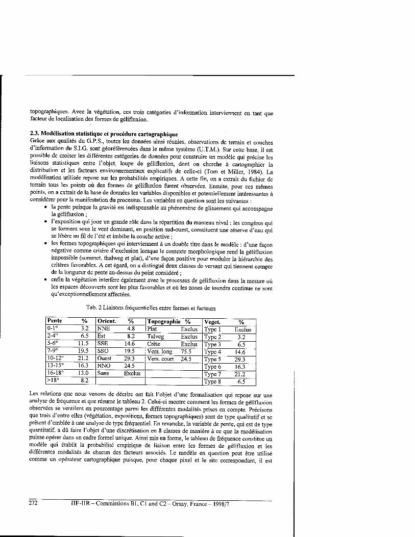
topographiques. Avec la vegetation, ces trois categories d'information interviennent en tant que facteur de localisation des formes de gelifluxion.

2.3. Modelisation statistique et procedure cartographique Grace aux qualites du G.P.S., toutes les donnees ainsi reunies, observations de terrain et couches d'information du S.I.G. sont georeferencees dans le meme Systeme (U.T.M.). Sur cette base, il est possible de croiser les differentes categories de donnees pour construire un modele qui precise les liaisons statistiques entre l'objet, loupe de gelifluxion, dont on cherche ä cartographier la distribution et les facteurs environnementaux explicatifs de celle-ci (Tom et Miller, 1984). La modelisation utilisee repose sur les probabilites empiriques. A cette fin, on a extrait du fichier de terrain tous les points oü des formes de gelifluxion furent observers. Ensuite, pour ces memes points, on a extrait de la base de donnees les variables disponibles et potentiellement interessantes ä considerer pour la manifestation du processus. Les variables en question sont les suivantes :

• la pente puisque la gravite est indispensable au phenomene de glissement qui accompagne la gelifluxion;

• l'exposition qui joue un grande role dans la repartition du manteau nival; les congeres qui se forment sous le vent dominant, en position sud-ouest, constituent une reserve d'eau qui se libere au fil de l'ete et imbibe la couche active ;

• les formes topographiques qui interviennent ä un double titre dans le modele : d'une facon negative comme critere d'exclusion lorsque le contexte morphologique rend la gelifluxion impossible (sommet, thalweg et plat), d'une facon positive pour moduler la hierarchie des criteres favorables. A cet egard, on a distingue deux classes de versant qui tiennent compte de la longueur de pente au-dessus du point considere ;

• enfin la vegetation interfere egalement avec le processus de gelifluxion dans la mesure oü les espaces decouverts sont les plus favorables et oü les zones de toundra continue ne sont qu'exceptionnellement affectees.

Tab. 2 Liaisons frequentielles entre formes et facteurs

Pente % Orient. % Topographie % Veget. % 0-1° 3.2 NNE 4.8 Plat Exclus Type 1 Exclus 2-4° 6.5 Est 8.2 Talveg Exclus Type 2 3.2 5-6° 11.5 SSE 14.6 Crete Exclus Type 3 6.5 7-9° 19.5 SSO 19.5 Vers, long 75.5 Type 4 14.6 10-12° 21.2 Ouest 29.3 Vers, court 24.5 Type 5 29.3 13-15° 16.3 NNO 24.5 Type 6 16.3 16-18° 13.0 Sans Exclus Type 7 21.2 >18° 8.2 Type 8 6.5

Les relations que nous venons de decrire ont fait l'objet d'une formalisation qui repose sur une analyse de frequence et que resume le tableau 2. Celui-ci montre comment les formes de gelifluxion observees se ventilent en pourcentage parmi les differentes modalites prises en compte. Precisons que trois d'entre elles (vegetation, expositions, formes topographiques) sont de type qualitatif et se pretent d'emblee ä une analyse de type frequentiel. En revanche, la variable de pente, qui est de type quantitatif, a du faire l'objet d'une discretisation en 8 classes de maniere a ce que la modelisation puisse operer dans un cadre formel unique. Ainsi mis en forme, le tableau de frequence constitue un modele qui etablit la probability empirique de liaison entre les formes de gelifluxion et les differentes modalites de chacun des facteurs associes. Le modele en question peut etre utilise comme un Operateur cartographique puisque, pour chaque pixel et le site correspondant, il est


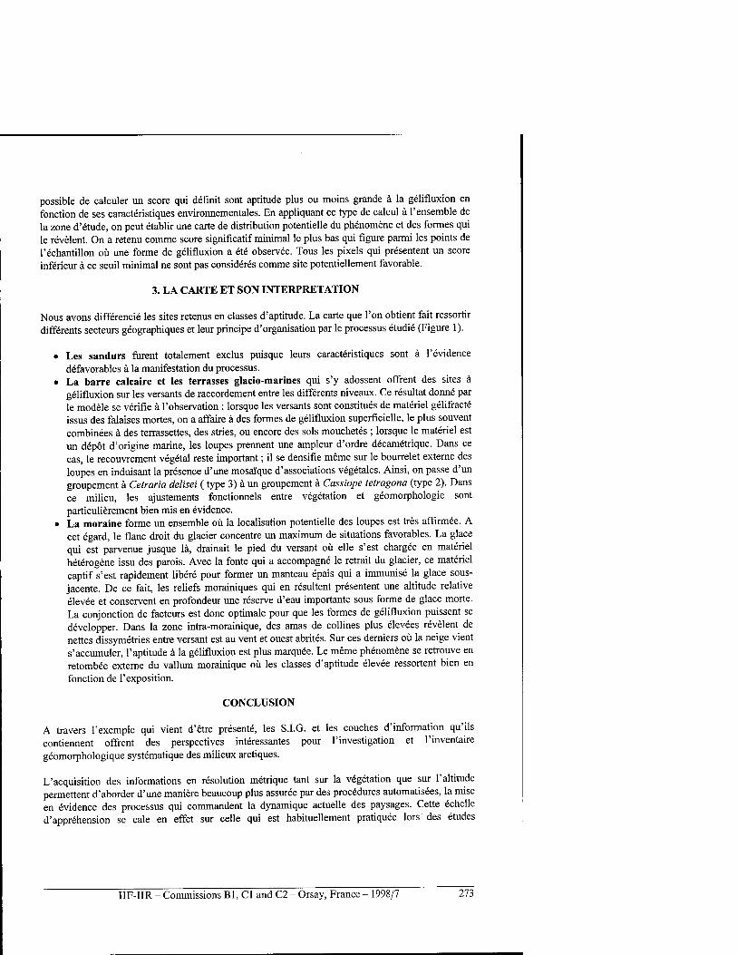
possible de calculer un score qui definit sont aptitude plus ou moins grande ä la gelifluxion en fonction de ses caracteristiques environnementales. En appliquant ce type de calcul ä l'ensemble de la zone d'etude, on peut etablir une carte de distribution potentielle du phenomene et des formes qui le revelent. On a retenu comme score significatif minimal le plus bas qui figure parmi les points de l'echantillon oü une forme de gelifluxion a ete observee. Tous les pixels qui presentent un score inferieur ä ce seuil minimal ne sont pas considered comme site potentiellement favorable.

3. LA CARTE ET SON INTERPRETATION

Nous avons differencie les sites retenus en classes d'aptitude. La carte que Ton obtient fait ressortir differents secteurs geographiques et leur principe d'organisation par le processus etudie (Figure 1).

• Les sandurs furent totalement exclus puisque leurs caracteristiques sont ä l'evidence defavorables ä la manifestation du processus.

• La barre calcaire et les terrasses glacio-marines qui s'y adossent offrent des sites ä gelifluxion sur les versants de raccordement entre les differents niveaux. Ce resultat donne par le modele se verifie ä l'observation : lorsque les versants sont consumes de materiel gelifracte issus des falaises mortes, on a affaire ä des formes de gelifluxion superficielle, le plus souvent combinees ä des terrassettes, des stries, ou encore des sols mouchetes ; lorsque le materiel est un depot d'origine marine, les loupes prennent une ampleur d'ordre decametrique. Dans ce cas, le recouvrement vegetal reste important; il se densifie meme sur le bourrelet externe des loupes en induisant la presence d'une mosaique d'associations vegetales. Ainsi, on passe d'un groupement ä Cetraria delisei (type 3) ä un groupement ä Cassiope tetragona (type 2). Dans ce milieu, les ajustements fonctionnels entre vegetation et geomorphologie sont particulierement bien mis en evidence.

• La moraine forme un ensemble oil la localisation potentielle des loupes est tres affirmee. A cet egard, le flanc droit du glacier concentre un maximum de situations favorables. La glace qui est parvenue jusque lä, drainait le pied du versant oü eile s'est chargee en materiel heterogene issu des parois. Avec la fonte qui a accompagne le retrait du glacier, ce materiel captif s'est rapidement libere pour former un manteau epais qui a immunise la glace sous- jacente. De ce fait, les reliefs morainiques qui en resultent presentent une altitude relative elevee et conservent en profondeur une reserve d'eau importante sous forme de glace morte. La conjonction de facteurs est done optimale pour que les formes de gelifluxion puissent se developper. Dans la zone intra-morainique, des amas de collines plus elevees revelent de nettes dissymetries entre versant est au vent et ouest abrites. Sur ces derniers oü la neige vient s'accumuler, l'aptitude ä la gelifluxion est plus marquee. Le meme phenomene se retrouve en retombee externe du vallum morainique oü les classes d'aptitude elevee ressortent bien en fonction de l'exposition.

CONCLUSION

A travers l'exemple qui vient d'etre presente, les S.I.G. et les couches d'information qu'ils contiennent offrent des perspectives interessantes pour l'investigation et l'inventaire geomorphologique systematique des milieux arctiques.

L'acquisition des informations en resolution metrique tant sur la vegetation que sur l'altitude permettent d'aborder d'une maniere beaucoup plus assuree par des procedures automatisees, la mise en evidence des processus qui commandent la dynamique actuelle des paysages. Cette echelle d'apprehension se cale en effet sur celle qui est habituellement pratiquee lors des etudes


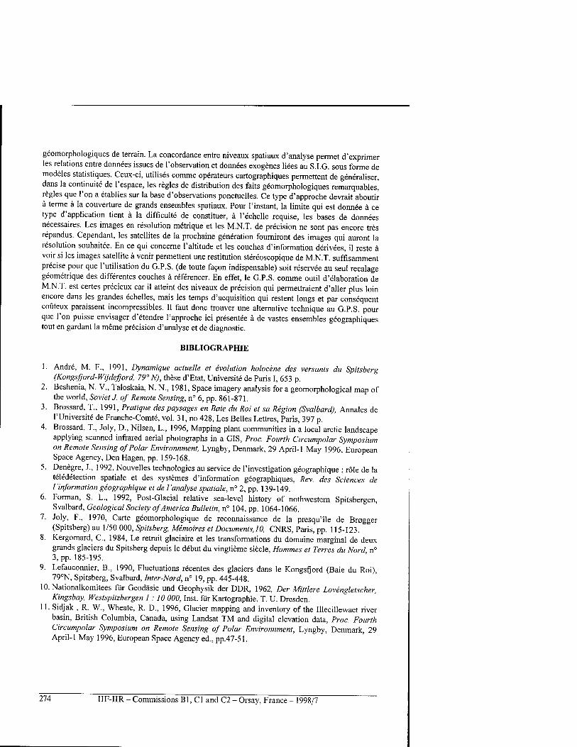
geomorphologiques de terrain. La concordance entre niveaux spatiaux d'analyse permet d'exprimer les relations entre donnees issues de l'observation et donnees exogenes liees au S.I.G. sous forme de modeles statistiques. Ceux-ci, utilises comme Operateurs cartographiques permettent de generaliser, dans la continuity de l'espace, les regies de distribution des faits geomorphologiques remarquables^ regies que Ton a etablies sur la base d'observations ponctuelles. Ce type d'approche devrait aboutir ä terme ä la couverture de grands ensembles spatiaux. Pour l'instant, la limite qui est donnee ä ce type d'application tient ä la difficult«: de constituer, ä l'echelle requise, les bases de donnees necessaires. Les images en resolution metrique et les M.N.T. de precision ne sont pas encore tres repandus. Cependant, les satellites de la prochaine generation fourniront des images qui auront la resolution souhaitee. En ce qui concerne l'altitude et les couches d'information derivees, il reste ä voir si les images satellite ä venir permettent une restitution stereoscopique de M.N.T. suffisamment precise pour que l'utilisation du G.P.S. (de toute facon indispensable) soit reservee au seul recalage geometrique des differentes couches ä references En effet, le G.P.S. comme outil d'elaboration de M.N.T. est certes precieux car il atteint des niveaux de precision qui permettraient d'aller plus loin encore dans les grandes echelles, mais les temps d'acquisition qui restent longs et par consequent coüteux paraissent incompressibles. II faut done trouver une alternative technique au G.P.S. pour que l'on puisse envisager d'etendre l'approche ici presentee ä de vastes ensembles geographiques tout en gardant la meme precision d'analyse et de diagnostic.

BIBLIOGRAPHIE

1. Andre, M. F., 1991, Dynamique actuelk et evolution holocene des versants du Spitsberg (Kongsfjord-Wijdefjord, 79° N), these d'Etat, Universite de Paris I, 653 p.

2. Beshenia, N. V., Taloskaia, N. N., 1981, Space imagery analysis for a geomorphological map of the world, Soviet! of Remote Sensing, n° 6, pp. 861-871.

3. Brossard, T., 1991, Pratique des paysages en Baie du Roi et sa Region (Svalbard), Annales de l'Universite de Franche-Comte, vol. 31, no 428, Les Belles Lettres, Paris, 397 p.

4. Brossard, T., Joly, D., Nilsen, L., 1996, Mapping plant communities in a local arctic landscape applying scanned infrared aerial photographs in a GIS, Proc. Fourth Circumpolar Symposium on Remote Sensing of Polar Environnment, Lyngby, Denmark, 29 April-1 May 1996, European Space Agency, Den Hagen, pp. 159-168.

5. Denegre, J., 1992, Nouvelles technologies au service de 1'investigation geographique ; role de la teledetection spatiale et des systemes d'information geographiques, Rev. des Sciences de Vinformation geographique et de I'analyse spatiale, n° 2, pp. 139-149.

6. Forman, S. L., 1992, Post-Glacial relative sea-level history of nothwestern Spitsbergen, Svalbard, Geological Society of America Bulletin, n° 104, pp. 1064-1066.

7. Joly, F., 1970, Carte geomorphologique de reconnaissance de la presqu'ile de Bragger (Spitsberg) au 1 /50 000, Spitsberg, Memoires et Documents, 10, CNRS, Paris, pp. 115-123.

8. Kergomard, C, 1984, Le retrait glaciaire et les transformations du domaine marginal de deux grands glaciers du Spitsberg depuis le debut du vingtieme siecle, Hommes et Terres du Nord n° 3, pp. 185-195.

9. Lefauconnier, B., 1990, Fluctuations recentes des glaciers dans le Kongsfjord (Baie du Roi), 79°N, Spitsberg, Svalbard, Inter-Nord, n° 19, pp. 445-448.

10. Nationalkomitees für Geodäsie und Geophysik der DDR, 1962, Der Mittlere Lovengletscher, Kingsbay, Westspitzbergen 1 : 10 000, Inst, für Kartographie, T. U. Dresden.

11. Sidjak , R. W., Wheate, R. D., 1996, Glacier mapping and inventory of the Illecillewaet river basin, British Columbia, Canada, using Landsat TM and digital elevation data, Proc. Fourth Circumpolar Symposium on Remote Sensing of Polar Environnment, Lyngby, Denmark, 29 April-1 May 1996, European Space Agency ed., pp.47-51.


12. Tolgensbakk, J., Sollid, J. L., 1987, Kvadehuksletta, Geomorphologi og kvatoergeologi 1: 10 000, Geografisk Institutt, Universitetet i Oslo.

13. Tom, C. H., Miller, L.E., 1984, An automated land-use mapping comparison of the Bayesian maximum likehood and linear discriminant analysis algirithms, Photogram. Eng Remote Sensing., n° 50, pp. 193-207.

14. Van-Vliet-Lanoe, B., 1992, Vitesses d'acquisition des differentes morphologies de solifluxion : comparaison entre l'Arctique et les Alpes Meridionnales, B.A.G.F., n° 3, pp. 274-278.

REMERCIEMENTS

Pour leur collaboration ä la constitution de la base de donnees : Societe de teledetection UNISFERE et Cabinet Breton-Desservy, Geometres Experts, Besancon. Pour leur soutien financier ä la Campagne de terrain : Norsk Polarintstitutt (Troms0), Institut Francais pour la Recherche et la Technologie Polaire (Brest), Fondation Franco-Norvegienne (Oslo).

MAPPING GEOMORPHOLOGICAL FEATURES BY MEANS OF A HIGH RESOLUTION DATA BASE : TEST IN FRONT OF LOVEN MIDDRE GLACIER (SPITSBERGEN -79°N)

SUMMARY: A delimited area in front of Loven Middre glacier was selected for this study. The G.I.S.-based techniques allow us to combine field observations and numerical data layers. They provide appropriate tools for geomorphological investigations and mapping. The example of solifluction lobes is taken for this test. With this aim in view, different types of high resolution data were collected and integrated into the G.I.S. technique with a resolution of 2 metres : a scanned I.R. aerial image, a digital elevation model made by using G.P.S. and sub-layers derived from the D.E.M. such as gradient, aspect and land forms. Moreover, observation points were positioned along transects. The observed categories concerned soil, grain size, microforms and vegetation. The proposed mapping method involves the following steps: • recognizing among sampled points, those having a solifluction lobe, • using a statistical model for establishing the relationships between solifluction features and data

layers stored in the G.I.S. • using the model obtained as an operator for mapping the potential distribution of solifluction

lobes.

DISCUSSION

ISHIZAKI T. (Japan) - What is the precision of positioning system GPS? What country produces that GPS system?

BROSSARD T. - L'imprecision donnee par le Systeme pendant les mesures sur le terrain etait inferieure au millimetre quand la configuration des satellites etait bonne. En pratique, les controles effectues par retour systematique sur des points connus ont montre que la variation des mesures tenait dans le decimetre. Au cours de nos missions, deux types d'appareils furent utilises : TRIMBLE (USA) et LEICA (Suisse) : la qualite des mesures etait equivalente pour Tun et l'autre.


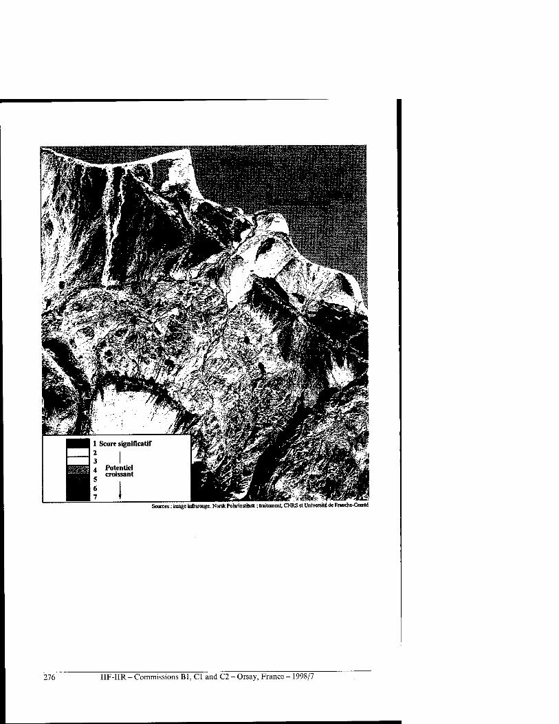
Sources: image jnfi-arougc, Norsk Potarinstitutt; traitement, CNRS et Univerefte de Franche-Comte


SECTION VI

PLANETOLOGIE

PLANETOLOGY

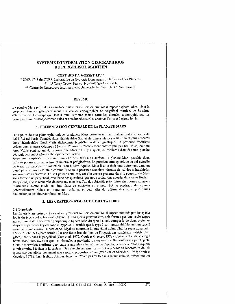
SYSTEME D'INFORMATION GEOGRAPHIQUE DU PERGELISOL MARTIEN

COSTARD F.*, GÖSSET J.P.** * UMR 1748 du CNRS, Laboratoire de Geologie Dynamique de la Terre et des Planetes,

91405 Orsay Cedex, France, [email protected] ** Centre de Ressources Informatiques, Universite de Caen, 14032 Caen, France.

RESUME

La planete Mars presente ä sa surface plusieurs milliers de crateres d'impact ä ejecta lobes lies ä la presence d'un sol gele permanent. En vue de cartographier ce pergelisol martien, un Systeme d'Information Geographique (SIG) reuni sur une meme carte les dormees topographiques, les principales unites morphostructurales et nos donnees sur les crateres d'impact ä ejecta lobes.

1. PRESENTATION GENERALE DE LA PLANETE MARS

D'un point de vue geomorphologique, la planete Mars presente un haut plateau craterise vieux de 4,6 ä 3,8 milliards d'annees dans l'hemisphere Sud et de basses plaines relativement plus recentes dans l'hemisphere Nord. Cette dichotomie Nord/Sud reste enigmatique. La presence d'edifices volcaniques comme Olympus Mons et d'episodes d'ecoulement catastrophiques (outflows) comme Ares Vallis sont autant de preuves que Mars fut il y a quelques milliards d'annees une planete geologiquement et geomorphologiquement active. Avec une temperature moyenne annuelle de -60°C ä sa surface, la planete Mars possede deux calottes polaires, un pergelisol et un climat periglaciaire. La pression atmospherique au sol actuelle de 6 mb lui empeche de maintenir l'eau ä l'etat liquide. Mais il en a etait tout autrement dans un passe plus ou moins lointain comme ratteste la presence d'anciens reseaux de vallees hierarchisees sur son plateau craterise. Ou est passee cette eau, est-elle encore presente dans le sous-sol de Mars sous forme d'un pergelisol, c'est l'une des questions que nous souhaitons aborder dans cette etude. Rappeions, que la recherche de cette eau constitue l'un des objectifs prioritaires des futures missions martiennes. Notre etude se situe dans ce contexte et a pour but le reperage de regions potentiellement riches en materiaux volatils, et ceci afin de definir des sites prioritaires d'atterrissage des futures robots sur Mars.

2. LES CRATERES D'IMPACT A EJECTA LOBES

2.1 Typologie La planete Mars presente ä sa surface plusieurs milliers de crateres d'impact entoures par des ejecta lobes du type coulee boueuse (figure 1). Ces ejecta peuvent etre, soit formes par une seule nappe mince munie d'un bourrelet peripherique (ejecta lobe du type 1), soit composes de deux systemes d'ejecta superposes (ejecta lobe du type 2). II semble que le type 3 soit vraisemblablement un type 2 ayant subi une erosion subaerienne, l'epaisse couronne interne etant aujourd'hui la seule apparente. L'aspect lobe des ejecta serait du ä une fönte brutale, lors de l'impact, des materiaux volatils (eau, glace) inclus dans le pergelisol (Carr et al. 1977, Gault et Greeley, 1978). Certains cliches Viking ä haute resolution revelent que les obstacles ä proximite du cratere ont ete contournes par l'ejecta. Cette observation confirme que, suite ä une phase balistique de l'ejecta, celui-ci ä l'etat visqueux aurait continue ä fluer ä la surface. Des chercheurs americains ont reproduit en laboratoire de tels ejecta sur des cibles contenant une certaine proportion d'eau (Wholetz et Sheridan, 1987; Gault et Greeley, 1978). Les resultats obtenus, bien que n'etant pas du tout ä la meme echelle, presentent une


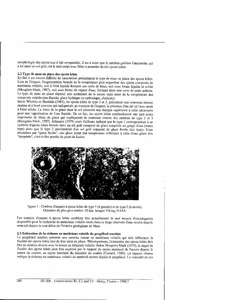
morphologie des ejecta tout ä fait comparable. II est ä noter que le satellite galileen Ganymede, qui a lui aussi un sol gele, est le seul corps avec Mars ä posseder de tels ejecta lobes.

2.2 Type de mise en place des ejecta lobes En fait il est encore difficile de caracteriser precisement le type de mise en place des ejecta lobes. Lors de l'impact, ['augmentation brutale de la temperature peut engendrer des ejecta composes de materiaux volatils, soit ä l'etat liquide formant une sorte de boue, soit sous forme liquide et solide (Mouginis-Mark, 1987), soit sous forme de vapeur d'eau, formant alors une sorte de nuee ardente. Le type de mise en place depend, non seulement de la nature mais aussi de la temperature des composes volatils (eau liquide, glace hydrique ou carbonique, clathrate). Selon Wholetz et Sheridan (1983), Ies ejecta lobes de type 2 et 3, presentent une couronne interne epaisse et ä bord convexe qui indiquerait, au moment de l'impact, la presence d'un sol oü l'eau serait ä l'etat solide. La fönte de la glace dans le sol necessite une energie superieure ä celle necessaire pour une vaporisation de l'eau liquide. De ce fait, les ejecta lobes contiendraient une part assez importante de blocs de glace qui expliquerait la couronne interne des crateres de type 2 et 3 (Mouginis-Mark, 1987). Johansen (1979) avait d'ailleurs indique que le type 1 correspondrait ä un Systeme d'ejecta lobes formes dans un sol gele compose de glace temperee ou gorge d'eau (water type) alors que le type 2 proviendrait d'un sol gele compose de glace froide (icy type). Nous entendons par "glace froide", une glace ayant une temperature inferieure ä celle d'une glace dite "temperee", c'est-ä-dire proche du point de fusion.

figure 1 : Crateres d'impact ä ejecta lobes de type 1 (ä gauche) et de type 2 (ä droite). Diametre du plus gros cratere: 30 km. Images Viking, NASA.

Les crateres d'impact ä ejecta lobes semblent etre actuellement le seul moyen d'investigation disponible pour la recherche de materiaux volatils situes dans ce large reservoir d'eau stocke dans le sous-sol depuis le tout debut de l'histoire geologique de Mars.

2.3 Estimation de la richesse en materiaux volatils du pergelisol martien Le pergelisol martien presente une certaine teneur en materiaux volatils qui doit influencer la fluidite des ejecta lobes lors de leur mise en place. Theoriquement, l'extension des ejecta lobes doit etre en relation directe avec la teneur en elements volatils. Selon Mouginis-Mark (1979), le degre de fluidite des ejecta lobes peut etre exprime par le rapport du rayon maximal de l'ejecta depuis le centre du cratere, au rayon maximal du diametre du cratere (Costard, 1989). Le rapport obtenu indique la richesse en materiaux volatils du materiel excave depuis le pergelisol. La viscosite de ces


ejecta varie en fonction de la teneur en eau mais aussi en fonction de la nature du materiel solide (Cave, 1993). Tout comme les coulees boueuses, la morphologie des ejecta lobes s'apparente ä un materiel ayant depasse la limite de liquidite. L'etalement (ou la mobilite) de l'ejecta depend de sa viscosite, c'est-ä-dire de sa teneur en eau. Des ejecta lobes relativement fluides seront plus rapides et s'etendront plus loin qu'une nappe visqueuse. La temperature de la glace contenue dans le pergelisol influence, dans une moindre mesure, sur la fluidite des ejecta lobes. Des etudes experimentales ont d'ailleurs confirme le role de la teneur en eau dans la fluidite et l'extension des ejecta (Gault and Greeley, 1978; Wholetz et Sheridan, 1987). Nous avons utilise cette methode pour des crateres d'impact k ejecta lobes ayant un diametre de cratere compris entre 1,2 km et 100 km. La mobilite des ejecta lobes est definie par le rapport E.M. du diametre maximal de l'ejecta au diametre maximal du cratere d'impact associe. Un rapport E.M. de 2 ou de 3 indique une faible extension de l'ejecta et done une faible fluidite. Un rapport E.M. de 5 ou de 7 indique une forte extension et une forte mobilite de l'ejecta.

3. LE SYSTEME D'INFORMATION GEOGRAPHIQUE (SIG)

L'objectif de cette etude est de proposer une analyse geomorphologique ä l'echelle globale du pergelisol martien ä l'aide d'un Systeme d'Information Geographique (SIG). Le but est de reunir sur une meme carte les recentes donnees topographiques (Smith et Zuber, 1996), les principales unites morphostructurales (qui font l'objet d'une redefinition) et nos donnees sur les crateres d'impact ä ejecta lobes. Pour cela nous utilisons le logiciel Arc Infos pour l'etablissement du SIG (Costard et Gösset, 1998). Notre base de donnees prend en compte 2561 crateres d'impact ä ejecta lobes distribues sur l'ensemble de la planete. Cette base de donnees comprend les coordonnees des crateres, et la mobilite des ejecta lobes (rapport entre l'extension des ejecta et le diametre du cratere). Rappelons pour memoire que les crateres d'impact ä ejecta lobes offrent de precieuses informations sur les caracteristiques du pergelisol au moment de l'impact.

Sur le SIG, le diametre des cercles est directement proportionnel ä la valeur du rapport EM. Le SIG (figure 2) revele que les ejecta de type 1 sont nettement concentres dans la zone equatoriale entre + 35° de latitude et ont une mobilite comprise entre 2 et 3,5. Par contre, les ejecta lobes de type 2 sont essentiellement concentres dans les moyennes et hautes latitudes (> 35°). On remarque que le type 2 se situe dans les moyennes et hautes latitudes, e'est-a-dire lä oü le pergelisol subaffleurant est compose de glace froide. Le type 1 se localise dans la zone equatoriale oü le pergelisol, situe en profondeur, est probablement compose de glace ä temperature relativement moins basse.

4 INTERPRETATIONS

Le rapport E.M. est done un indicateur de la richesse en materiaux volatils du pergelisol au moment de l'impact. Une teile observation comfirme le fait que les materiaux volatils sont essentiellement concentres aux moyennes et hautes latitudes (Barlow et Bradley, 1990; Kuzmin et al. 1988a, 1988b; Mouginis-Mark, 1979). Selon Fanale et al. (1986), les materiaux volatils se situent essentiellement aux latitudes superieures ä 40° car les temperatures sont constamment negatives et favorisent le maintien de la glace pres de la surface. Compte tenu de temperatures relativement plus elevees ä l'equateur et d'une pression atmospherique de 6 mb, la glace en surface a tendance ä se sublimer. Les hautes latitudes sont done particulierement propices au maintien d'elements volatils au sein du pergelisol martien, comme l'eau liquide ou la glace.


4.1 Le plateau craterise Le plateau craterise de l'hemisphere Sud correspond ä l'unite la plus craterisee de la surface de Mars. Nous sommes done en presence d'une unite morphostructurale ancienne mais presentant un pergelisol peu developpe, principalement pour deux raisons: 1. Un pergelisol situe en profondeur, puisque les crateres d'impact, inferieurs ä 1,5 km de

diametre, n'ont pas d'ejecta lobes, n'ayant pu atteindre le toit du pergelisol. 2. Un pergelisol discontinu, puisque dans certaines regions, des crateres d'impact ne presentent pas

d'ejecta lobes alors que d'autres, et de meme diametre, situes ä proximite en possedent. II existerait des regions ä pergelisol bien delimiters separees par des regions depourvues de pergelisol (Battistini, 1984). De fortes variations du gradient geothermique dans des regions bien localisees, comme par exemple les intrusions magmatiques, situees sous les grands crateres d'impact, pourraient modifier les caracteristiques thermiques de ce pergelisol. Une autre solution supposerait la circulation de nappes d'eau libre, en profondeur, et ayant gele suite ä un refroidissement climatique. Cette derniere hypothese pourrait s'expliquer par la presence de reseaux de vallees hierarchisees parcourant le plateau craterise et engendrant une infiltration des eaux. Une etude des eventuelles correlations spatiales entre ces vallees et l'aspect discontinu du pergelisol serait particulierement interessante ä cet egard.

Le plateau craterise date du Noachien (Scott et Tanaka, 1986): il s'est done forme lors de la periode du bombardement meteoritique intense entre 4,6 et 3,8 milliards d'annees. Le fort gradient geothermique (chaleur radioactive) ajoute ä l'intense degazage des roches a produit une atmosphere dense et relativement chaude, ayant tres probablement limite le developpement d'un pergelisol. Un pergelisol discontinu se serait developpe apres la formation du plateau craterise. Nous serions done en presence d'un pergelisol epigenetique.

4.2 La region volcanique de Tharsis La densite des crateres d'impact ä ejecta lobes est tres faible et s'expliquerait, d'une part par l'äge relativement recent de l'unite (Amazonien superieur, d'apres Scott et Tanaka, 1986) et d'autre part par la nature volcanique des terrains qui comportent des coulees de lave ä relativement faible porosite (Carr, 1981). La region de Tharsis se caracterise done par un pergelisol sec et d'äge recent. La richesse en elements volatils est aussi tres faible puisque le rapport E.M. n'atteint que 2,5. Les ejecta lobes sont tres faiblement developpes quelle que soit leur categorie dimensionnelle. Le pergelisol des plaines volcaniques de Tharsis se situe vers 1 km et 3 km de profondeur et n'est que tres pauvre en materiaux volatils.

4.3 Les plaines ridees Selon Thomas et Masson (1985), et Allemand et Thomas (1995) il existe une tres bonne correlation entre les plaines ridees et un pergelisol continu. En effet la carte 1, montrent une tres bonne correlation spatiale entre les crateres d'impact ä ejecta lobes de type 1 (typique d'un pergelisol ä glace temperee) et le developpement des plaines ridees. Dans la region de Lunae Planum.on remarque que tous les crateres d'impact, au-dela d'une certaine classe dimensionnelle, engendrent des ejecta lobes de type 1. Le pergelisol est done continu, permanent mais il se situe en profondeur puisque tous les impacts inferieurs ä 3 km de diametre sont depourvus d'ejecta lobes; ils n'ont done pas rencontre les couches superieures du pergelisol situe vers 300 m de profondeur. Ce pergelisol continu mais situe en profondeur est typique des terrains rides mais ne concerne qu'un nombre limite de regions comme celles de Lunae Planum, Coprates, Syrtis Major, Amazonis Planitia, Chryse Planitia, et le Sud d'Elysium. Cette distribution regionale implique une nature de terrain bien particuliere. Selon les indications apportees par les crateres d'impact ä ejecta lobes et selon les etudes de Scott et Carr (1978), de Thomas et Masson (1985), et de N. Mangold et al. (1998) et selon nos propres observations, les plaines ridees se composeraient de coulees de laves, ä faible teneur en glace, fossilisant une epaisse serie sedimentaire poreuse. Cette stratigraphie expliquerait l'absence d'ejecta lobes pour des crateres d'impact de petit diametre et la presence d'un pergelisol riche en


glace pour les terrains sous-jacents. L'absence ou la tres faible teneur en glace des couches superieures des plaines ridees semble confirmee par les caracteristiques des plaines volcaniques de Tharsis. D'apres Scott et Tanaka (1986), les plaines ridees datent de l'Hesperien inferieur (entre 3,7 et 3,1 milliards d'annees), c'est-a-dire juste apres la periode de bombardement meteoritique intense. Le refroidissement climatique aurait done ete süffisant pour autoriser la formation d'un pergelisol continu, probablement compose de glaces temperees en profondeur et qui s'est maintenu au cours du temps.

4.4 Le cas des plaines d'epandage aux embouchures des vallees de debacle Les regions d'Acidalia et d'Utopia Planitiae et la region Est d'Hellas Planitia presentent une concentration de crateres d'impact ä ejecta lobes ayant un rapport EM anormalement eleve. Ces trois regions ont en commun une latitude superieure ä 45°, une altitude de -2 km et se localisent aux embouchures des principales vallees de debacle. Ces trois facteurs, lorsqu'ils sont reunis, offrent des conditions particulierement favorables ä la presence de materiaux volatils, d'oü cette concentration en crateres d'impact ä ejecta lobes tres developpes (Costard and Kargel, 1995).

4.4.1 L'influence de l'altitude: Selon Mouginis-Mark (1979), la mobilite des ejecta lobes depend de l'altitude puisque le haut plateau craterise presente un E.M. faible alors que les basses plaines de l'hemisphere Nord ont un E.M. fort. L'analyse detaillee du SIG montre bien la forte mobilite des crateres d'impact ä ejecta lobes dans les plaines boreales d'altitude -4 km. Mais les bassins d'impact d'Hellas Planitia et d'Argyre Planitia, pourtant tous deux situes ä -4 km, ne presentent que des rapports E.M. de faible valeur qui ne depassent pas 3,5. En fait, cette correlation avec l'altitude est indirectement liee aux vallees. Seules les basses plaines situees aux embouchures des vallees de debacle presentent une forte richesse en materiaux volatils.

4.4.2 L'influence de la latitude: Aux latitudes inferieures ä 40°, les temperatures peuvent etre positives pendant une partie de la journee et engendrent une sublimation de la glace, d'oü un sol desseche pres de la surface. Selon les modeles de Clifford et Hillel (1983) et de Fanale et al. (1986), les conditions de pression atmospherique et de temperature permettent le maintien d'un pergelisol situe entre 150 m et 1 km de profondeur. Aux latitudes superieures ä 40°, aux embouchures des vallees de debacle, les temperatures sont constamment negatives tout au long de l'annee. La glace est en equilibre thermique pres de la surface et autorise le maintien d'un pergelisol subaffleurant (Fanale et al, 1986; Carr et al., 1977). La profondeur de la zone dessechee serait de quelques dizaines de metres.

4.4.3 L'influence des episodes d'ecoulement: Les profondeurs minimales du toit du pergelisol se situent dans Acidalia Planitia et Utopia Planitia; deux plaines d'epandage situees aux embouchures des vallees de Chryse Planitia et d'Elysium et dans lesquelles l'hypothese d'un pergelisol subaffleurant avait ete emise (Costard, 1989, Demura et Kurita, 1998). La forte densite des crateres d'impact ä ejecta lobes, impliquent necessairement un pergelisol ä la fois continu, subaffleurant et permanent. Dans ces deux regions, les ejecta lobes de type 2 presentent une forte mobilite puisque le rapport depasse tres souvent la valeur 5. Une teile observation confirme la presence d'un large depot de sediments depose par les episodes d'ecoulement (Lucchitta et al, 1986) et comportant un pergelisol particulierement riche en glace froide. Comme ces episodes d'ecoulement se sont etales dans le temps de l'Hesperien ä l'Amazonien (Scott et Tanaka, 1986), les plaines d'epandage des vallees de debacle ont maintenu un pergelisol sur environ trois milliards d'annees. Le pergelisol s'est done probablement mis en place plus ou moins en meme temps que la formation qu'il occupait et s'est


ensuite maintenu dans le temps. Les plaines sedimentaires comportent done un pergelisol syngenetique, continu et subaffleurant.

4.4.5 Le cas de Reull Vallis Dans l'hemisphere Sud, la region de Reull Vallis, situee au beau milieu du plateau craterise, presente un interet tout particulier. Par 41°S, 257°W, la vallee Reull Vallis se situe au niveau du rebord oriental du bassin d'impact de Hellas Planitia. Reull Vallis, de direction generate Est-Ouest, est une vallee calibree ä fond plat presentant un trace sinueux, parfois en baionnette et prenant sa source ä l'emplacement de profondes depressions bien localisees (Crown et al., 1992). Reull Vallis a une largeur de 5 km et une profondeur moyenne de 1 km. Certains crateres d'impact ont favorise l'elargissement de la vallee. Celle-ci se dirige vers le fond de Hellas Planitia situe plus ä l'Ouest, en entaillant une plaine craterisee composee de crateres d'impact ä ejecta lobes et de reliefs residuels allonges de 1,5 km de haut et aux versants intensement burines. A proximite immediate de Reull Vallis, le terrain presente des crateres d'impact ä ejecta lobes de type 2 qui indiquent un tres fort E.M. pouvant atteindre la valeur de 7. La presence dans la meme region de trois vallees (Harmaklis, Reull et Maadim Valles) peut expliquer la formation d'une plaine alluviale et ainsi de telles caracteristiques. Les buttes residuelles, aux versants inclines ä 35°, presentent en contrebas des depots de versant etale qui correspondent, vu leur tres faible pente, ä de vastes mouvements de fluage qui suggerent la presence de materiaux riches en elements volatils. De profondes depressions circulaires, ä la tete de certaines vallees, peuvent indiquer l'emergence, soit d'une nappe aquifere (Carr et Schaber, 1977), soit d'un talik. Une teile hypothese serait en accord avec les donnees fournies par les crateres d'impact ä ejecta lobes.

CONCLUSION

Cette cartographie offre une vue globale de la distribution spatiale et temporelle des reservoirs en materiaux volatils contenus dans le pergelisol martien et sur les grands traits de l'organisation du relief. Ce SIG est particulierement utile en prevision des futures missions martiennes, car il autorise l'identification de sites d'atterrissage potentiels pour de futures missions dediees ä l'exobiologie (recherche de l'eau et de la glace dans des regions oü eile peut etre encore subafleurante).

BIBLIOGRAPHIE

1. Allemand P. and Thomas P., 1995, Localization of Martian ridges by impact craters: Mechanical and chronological implications, J. Geophys. Res. 100, p. 3251-3262,

2. Barlow, N.G. and Bradley, TL., 1990, Martian impact craters: Correlations of ejecta and interior morphologies withi diameter, latitude and terrain, Icarus, 87, p. 156-179.

3. Carr, M.H., L.S. Crumpler, JA. Cutts, R. Greeley, J.E. Guest and H. Mazursky, 1977, Martian impact craters and emplacements of ejecta by surface flow. J. Geophys. Res., 82, p. 4055-4065.

4. Battistini, R., 1984, Morphology and origin of ridges in low-latitude areas of Mars, Earth, Moon and Planets, 31, p. 49-61.

5. Carr, M.H., 1981, The surface of Mars. Yale University Press, 232 p. 6. Carr, M.H. and Schaber, G.G., 1977, Martian permafrost features. J. Geophys. Res., 82, p. 4039-

4065. 7. Cave, J. A. 1993, Ice in the northern lowlands ans southern highlands of Mars and its

enrichment beneath the Elysium lavas. J. Geophys. Res. 98, p. 11079-11097. 8. Costard F., 1989, The spatial distribution of volatiles in the martiam hydrolithosphere. Earth,

Moon and Planets, 45, p.265-290. 9. Costard, F. and J. Kargel, 1995, Outwash plains and thermokarst on Mars. Icarus, 114, p. 93-

112.


10. Costard F. and Gösset J.P., 1998, Ground ice distribution on Mars based on GIS analysis, 29th Lunar Planet. Sei. Conf, Houston, abstract volume ( CD-Rom).

11. Crown, D.A., Price H.C. and Greeley R., 1992, Geologic evolution of the East rim of the Hellas Basin, Mars. Icarus, 100, p. 1-25.

12. Demura H. and Kurita K., 1998, A shallow volatile layer at Chryse Planitia, Mars 1998. Earth Planets Space, 50, p. 423-429.

13. Clifford, S.M. and Hillel, D., 1983, The stability of ground ice in the equatorial region of Mars. J. Geophys. Res., 88, p. 2456-2474.

14. Fanale, F.P., 1976, Martian volatiles: Their degassing history and geochemical fate. Icarus, 28, p. 179-202.

15. Fanale, F.P.; J.R. Salvail, A.P. Zent, and S.E. Postawko, 1986, Global distibution and migration of subsurface ice on Mars. Icarus, 67, p. 1-18.

16. Gault, D.E., and Greeley, R., 1978, Exploratory experiments of impact craters formed in viscous-liquid targets/ Analog for rampart craters, Icarus, 34, p. 486-495.

17. Johansen. L.A., 1979, The latitude dependence of martian splosh cratering and its relationship to water. NASA Tech. Memo. 80339, p. 123-125.

18. Kuzmin, R.O., N.N. Bobina, Zabalueva, E.V. and V.P. Shashkina, 1988a, Inhomogeneities in the upper levels of the martian cryolithosphere. (Abstract). Lunar and Planetary Science Conference, p.655-656.

19. Kuzmin, R.O., N.N. Bobina, Zabalueva, E.V. and V.P. Shashkina, 1988b, Mars: estimation of the relative ice content in upper layers of the permafrost. (Abstract). Lunar and Planetary Science Conference, p.657-658.

20. Lucchitta, B.K., Ferguson, H.M., and Summers C, 1986, Sedimentary deposits in the Northern lowland plains, Mars. Proc. Lunar Planet. Sei. Conf., J. Geophys. Res., 91, p.166-174.

21. Mangold N., Allemenand, P. And Thomas, P., 1998, Wrinkle ridges of Mars: Structural analysis and evidence for shallow deformation controlled by ice-rich decollements. Planet, and Space Sei. In press.

22. Mouginis-Mark, P.J., 1979, Martian fluidized crater morphology: Variations with crater size, latitude, altitude, and target material. J. Geophys. Res., 84, p.8011-8022.

23. Mouginis-Mark, P.J., 1987, Water or ice in the martian regolith?: clues from rampart craters seen at very high resolution. Icarus, 71, p. 268-286.

24. Scott, D.H. and Carr, M.H., 1978, Geologic map of Mars. U.S. Geol. Survey, Misc. Inv. Map I- 1083.

25. Scott, D.H. et Tanaka, K.L., 1986, Geologic map of the western equatorial region of Mars. U. S. Geol. Survey, Misc. Inv. Map I-1802-A.

26. Smith, D.E. and T. Zuber, 1996, Science, 271, p. 184-188. 27. Thomas, P.G. and Masson, Ph. L., 1985, Martian fluidized crater distribution: tectonic

implications. Earth, Moon and Planets, 34, p.169-176. 28. Wohletz, K.M. and Sheridan, M.F., 1983, Martian rampart crater ejecta: experiments and

analysis of melt-water interaction. Icarus, 56, p. 15-37.

GROUND-ICE DISTRIBUTION ON MARS BASED ON GIS ANALYSIS

SUMMARY: In order to quantify the spatial distribution of Martian ground ice, a global study of rampart craters was undertaken to determine their temporal and spatial relations with the surrounding morphostructural units. Rampart craters all over planet Mars have been systematically measured and mapped using a GIS database of geological and topographical information.


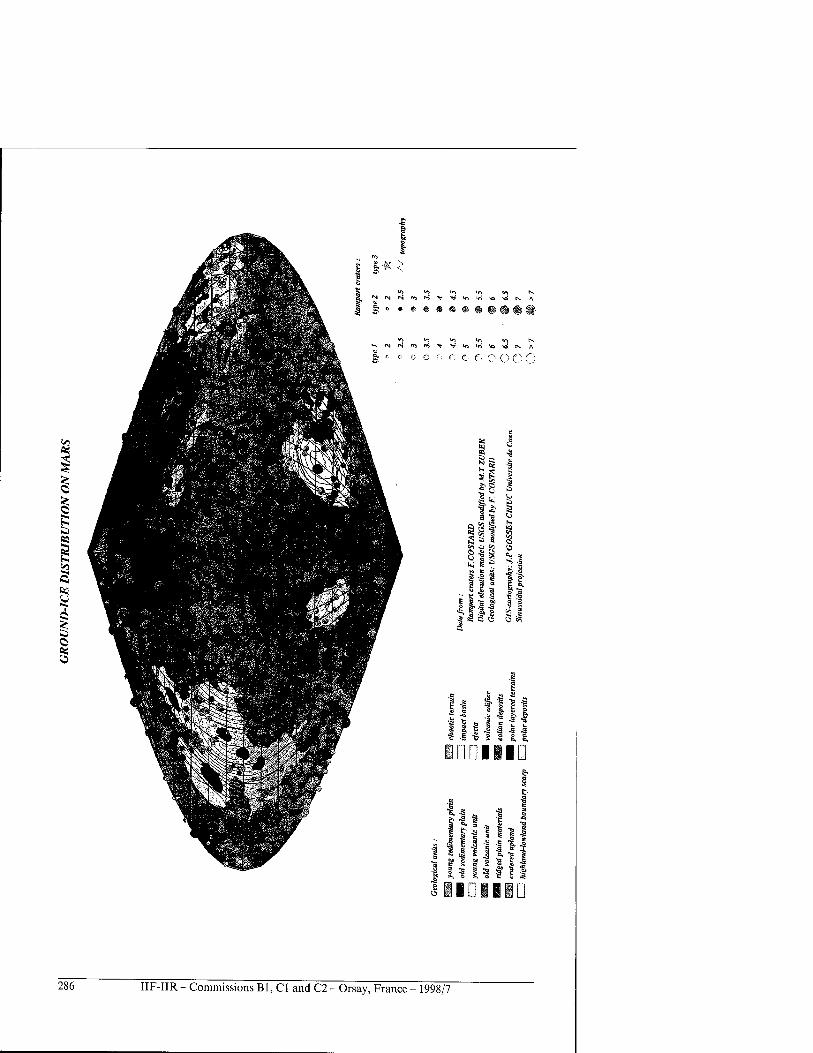
to

I I I 1

1^5 *) \C

• ®

e e G o COO

1* fa

SI g 15 ^ * S & 8 en ^j ^ Sill ö ? S «JE?

S.l|

sät 3 4 3 5 3

| I i J 3 -3 ^ M ■« w * <u ft, es,

BOnillD

*1

.11 to g

I 3

§ 1 ■s .s

•§ 1

J * ■» 1 si? S| ! ? t! I

lainu


EROSION THERMIQUE EN ZONE PERIGLACIAIRE : MODELISATION ET EXPERIMENTATION

MAKHLOUFIN.*, COSTARD F.** et AGUIRRE-PUENTE J.** * UPRES-A 6143, Centre de Geomorphologie, 14000 Caen, France.

** UMR 1748 du C.N.R.S., Universite Paris-Sud, bat. 504, 91405 Orsay, France.

RESUME

En zone periglaciaire, le processus d'erosion thermique le long des fleuves est tres efficace. A partir de l'etude des images satellitaires, on peut penser, par analogie, que certaines vallees martiennes se sont formees par l'action de ce processus. Pour confirmer cette hypothese, un modele a ete propose. Ce modele permet de determiner la vitesse d'erosion ä partir des caracteristiques du sol, des conditions thermiques et du type d'ecoulement. Cet article presente le dispositif experimental ainsi que le mode operatoire concus pour conduire les experiences de validation du modele. II s'agit d'un chenal hydraulique de petite dimension permettant d'etudier l'influence de certains parametres (nombre de Reynolds, temperature de l'eau, temperature initiale du pergelisol, teneur en glace) sur la vitesse d'erosion d'un bloc de materiau gele simulant un pergelisol. Des essais avec des blocs de glace pure et de sable congele ont ete effectues. Les resultats obtenus ont permis, d'une part, de montrer la bonne correlation entre le modele mathematique et l'experience et d'autre part, la hierarchisation de differents parametres influencant le taux d'erosion thermique.

INTRODUCTION

En zone periglaciaire, le processus d'erosion thermique est particulierement efficace le long des fleuves et rivieres. En effet, ce processus d'erosion est bien connu en Siberie oü la temperature moyenne annuelle du pergelisol est de l'ordre de -7°C (Pewe, 1991). Lors, des debacles de printemps, l'erosion thermique y est particulierement active et engendre un sapement des berges avec un recul pouvant atteindre 10 ä 25 m/an (Walker et Arnborg, 1963 ; Jahn, 1975 ; Are, 1983 et Walker, 1983). Par ailleurs, des etudes faites dans plusieurs disciplines laissent supposer que la planete Mars a connu, dans le passe, des climats du type periglaciaire en presence d'une grande quantite d'eau, avec probablement un sol gele permanent (pergelisol) en surface et en profondeur. La presence de ce pergelisol semble avoir exerce une influence non negligeable sur la morphologie de surface. L'origine des vallees martiennes a fait l'objet de nombreuses etudes. Differents types de processus ont ete proposes pour expliquer la nature de ces vallees qui ont ete successivement comparees aux chenaux de Scabland (Baker, 1982), aux chenaux sous-marins (Komar, 1979) et ä des vallees glaciaires (Lucchitta, 1982). A part l'erosion glaciaire, toutes les hypotheses font intervenir un episode d'ecoulement de type catastrophique. Mais, bien que l'existence d'un pergelisol soit admise par la plupart des auteurs, aucune de ces hypotheses, ä notre connaissance, ne prend en compte les inevitables echanges thermiques qui ont lieu entre un ecoulement d'eau et un pergelisol contenant une forte quantite de glace. Les analogies constatees entre la planete Mars et la Siberie, ä partir de l'imagerie satellitaire, nous permettent de penser que les vallees martiennes (outflow channels) ont du vraisemblablement se former sur un pergelisol subissant l'action de forts courants d'eau liquide en provenance de terrains chaotiques (Costard, 1989). Une modelisation a ete proposee afin de preciser le röle et l'efficacite relative du processus d'erosion thermique sur Mars. On dispose actuellement de deux modeles : un modele d'ablation (fönte du pergelisol et entrainement total et immediat des sediments) et un modele thermique fournissant


l'epaisseur de la couche degelee susceptible d'etre erodee (Aguirre-Puente et al, 1994 et Costard et al, 1995). Au für et ä mesure des progres realises, les resultats ont ete confrontes aux observations terrestres pour etre ensuite transposes aux conditions martiennes. Une etape intermediate concerne des verifications rigoureuses au Laboratoire. Pour cela, une experimentation a ete concue et mise au point pour valider le modele d'ablation. Elle constitue l'objet de cet article.

1 MODELISATION DE L'EROSION THERMIQUE : MODELE D'ABLATION

Le modele theorique etabli en 1994 (Aguirre-Puente et al, 1994)) permet de determiner la vitesse d'erosion ä partir des caracteristiques du sol et des conditions thermiques imposees au Systeme. On considere un probleme de changement de phase resultant d'un ecoulement d'une riviere, l'eau etant ä temperature Celsius positive, sur un sol gele ä temperature Celsius negative. Un flux thermique est transfere entre ces deux milieux creant ainsi une couche degelee definie par l'interface eau/sol et un front de degel qui se propage dans le sol initialement gele. Cette erosion est le resultat de ce degel associe ä l'enlevement des sediments. Ces phenomenes rendent complexe l'etude de ce processus. Pour simplifier le probleme, on a considere d'abord un modele d'ablation, supposant le retrait immediat de tous les sediments degeles et, par consequent, un contact permanent entre l'ecoulement de l'eau et le pergelisol. Ce modele correspond ä une erosion thermo-mecanique. Le transfert thermique entre l'eau et le pergelisol se fait par convection forcee. En considerant la loi de Newton, 1'equation de Fourier en regime quasi-stationnaire et le principe de conservation d'energie, la vitesse d'erosion est donnee par :

Va"pL{l + [cp(Tf-Ti)/L]} (1)

ou Te est la temperature de l'eau, Ts la temperature de surface du pergelisol, Tf la temperature de fusion, T; la temperature initiale, L la chaleur latente de fusion, p la masse volumique, cp la chaleur massique et h le coefficient de transfert de chaleur par convection. Le coefficient de transfert de chaleur h est determine de facon semi-empirique suivant les caracteristiques geometriques et hydrodynamiques du Systeme etudie.

2 EXPERIMENTATION

L'approche experimental, qui complete nos approches geomorphologique et theorique, consiste ä tester en laboratoire ä l'aide d'un modele reduit, le phenomene d'erosion thermique. Un chenal hydraulique de petite dimension (2.1m de longueur et 0.2m x 03m de section rectangulaire) a ete construit; il permet de simuler le phenomene d'ablation, de tester le modele et d'approfondir notre connaissance du phenomene de l'erosion thermique (figure 1). Ce chenal permet d'etablir un ecoulement d'eau destine ä etre en contact avec la surface d'un bloc de sol gele de caracteristiques connues telles que la composition, la porosite, et la dimension ( 0.2m x 0.1m x 0.22 m ). Le sommet du bloc gele est isole thermiquement et relie ä un cryostat. Le bloc etant place en haut du chenal, les sediments degeles tombent par l'effet de leur poids et sont directement evacues. Une pompe hydraulique assure le recyclage de l'eau de l'aval vers l'amont. Son debit est süffisant pour engendrer un ecoulement turbulent. La temperature de l'eau est constante et controlee. Le contact direct et permanent de cet ecoulement avec le pergelisol produira ainsi l'erosion thermique que les dispositifs de mesures permettront d'evaluer.


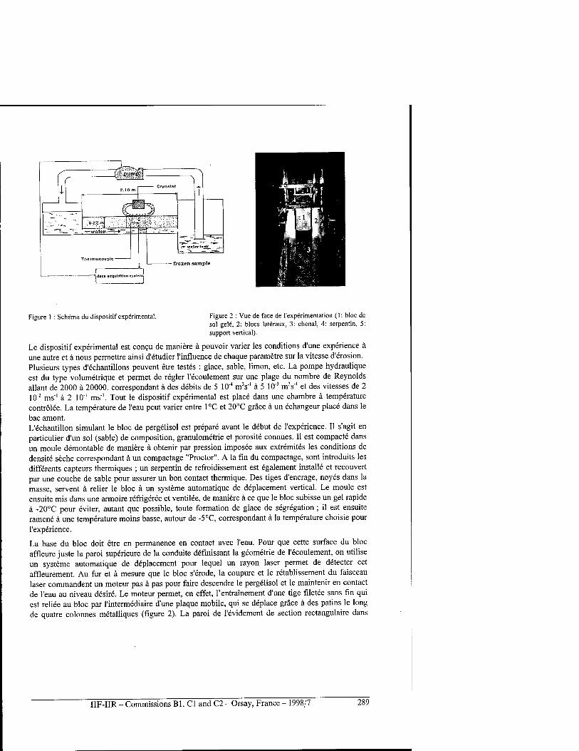
Figure 1 : Schema du dispositif experimental. Figure 2 : Vue de face de l'experimentation (1: bloc de sol gele, 2: blocs latiraux, 3: chenal, 4: Serpentin, 5: support vertical).

Le dispositif experimental est C0119U de maniere ä pouvoir varier les conditions d'une experience ä une autre et ä nous permettre ainsi d'etudier l'influence de chaque parametre sur la vitesse d'erosion. Plusieurs types d'echantillons peuvent etre testes : glace, sable, limon, etc. La pompe hydraulique est du type volumetrique et permet de regier l'ecoulement sur une plage du nombre de Reynolds allant de 2000 ä 20000, correspondant ä des debits de 5 10'4 m3s"' ä 5 10"3 mV et des vitesses de 2 10"2 ms"1 ä 2 10"' ms"1. Tout le dispositif experimental est place dans une chambre ä temperature contrölee. La temperature de l'eau peut varier entre 1°C et 20°C gräce ä un echangeur place dans le bac amont. L'echantillon simulant le bloc de pergelisol est prepare avant le debut de l'experience. II s'agit en particulier d'un sol (sable) de composition, granulometrie et porosite connues. II est compacte dans un moule demontable de maniere ä obtenir par pression imposee aux extremites les conditions de densite seche correspondant ä un compactage "Proctor". A la fin du compactage, sont introduits les differents capteurs thermiques ; un Serpentin de refroidissement est egalement installe et recouvert par une couche de sable pour assurer un bon contact thermique. Des tiges d'encrage, noyes dans la masse, servent ä relier le bloc ä un Systeme automatique de deplacement vertical. Le moule est ensuite mis dans une armoire refrigeree et ventilee, de maniere ä ce que le bloc subisse un gel rapide ä -20°C pour eviter, autant que possible, toute formation de glace de segregation; il est ensuite ramene ä une temperature moins basse, autour de -5°C, correspondant ä la temperature choisie pour l'experience.

La base du bloc doit etre en permanence en contact avec l'eau. Pour que cette surface du bloc affleure juste la paroi superieure de la conduite definissant la geometrie de l'ecoulement, on utilise un Systeme automatique de deplacement pour lequel un rayon laser permet de detecter cet affleurement. Au fur et ä mesure que le bloc s'erode, la coupure et le retablissement du faisceau laser commandent un moteur pas ä pas pour faire descendre le pergelisol et le maintenir en contact de l'eau au niveau desire. Le moteur permet, en effet, 1'entrainement d'une tige filetee sans fin qui est reliee au bloc par l'intermediaire d'une plaque mobile, qui se deplace grace ä des patins le long de quatre colonnes metalliques (figure 2). La paroi de l'evidement de section rectangulaire dans


lequel l'echantillon doit se deplacer est recouverte lateralement par une couche de caoutchouc mousse lubrifie qui permettra le glissement du bloc, son isolation thermique et empechera la remontee de l'eau.

Pour suivre revolution du champ thermique dans le bloc et par consequent l'eventuelle propagation du front de degel, des thermocouples sont places verticalement le long du sol gele. Pour cela, ä l'interieur d'un profile en carbone, introduit par pression dans l'echantillon, dix thermocouples cuivre-constantan de 0.2 mm de diametre ont ete places ä differentes profondeurs. Le taux d'erosion est determine ä partir de la mesure des hauteurs erodees ä des intervalles de temps donnes. Pour cela, on utilise deux methodes de mesure : d'une part, l'enregistrement du nombre de pas effectues par le moteur en fonction du temps et, d'autre part, l'utilisation d'un capteur de deplacement, solidaire du plateau superieur, qui se meut avec l'echantillon suivant sa vitesse d'erosion. Pour contröle, une sonde de platine plongee dans le chenal permet d'enregistrer la temperature de l'eau en fonction du temps. Tous ces capteurs sont relies ä une centrale d'acquisition de donnees. Par l'intermediaire d'un programme, un ordinateur commande l'asservissement du moteur et permet l'enregistrement des differentes mesures.

3 CONFRONTATIONS ET INTERPRETATION

On se propose de comparer le taux d'erosion donne par le Modele (Aguirre-Puente et al, 1994) et celui mesure par notre dispositif experimental. Pour l'application de ce modele on a considers; un ecoulement turbulent d'eau sur une plaque plane de longueur indefinie, et par consequent, applique

la formule semi empirique adaptee ä ce type d'ecoulement : Nu = % ; celle-ci permet de

determiner le coefficient de transfer! de chaleur h. Dans notre approche experimentale la veine d'essai utilisee pour tester les differents echantillons est assimilee ä une conduite fermee de section rectangulaire. Pour comparer la vitesse d'erosion theorique (modele) et celle mesuree (experience) il est necessaire d'evaluer dans ce cas le coefficient de transfert de chaleur h.

3.1 Determination semi empirique du coefficient de transfert de chaleur h On se propose de determiner empiriquement pour nos conditions experimentales la fonction qui relie les trois nombres adimentionnels : Le nombre de Reynolds, le nombre de Prandlt et le nombre de Nusselt oü apparait le coefficient de transfert de chaleur h dont il nous interesse de connaitre la valeur. A ses fins, on s'est inspire de l'approche de V.J. Lunardini et al (1986) On trace la courbe representative de l'equation Nu = f (Re,Pr). Sachant que cette equation est de la

forme : Nu = Prx x aReb, a et b sont determines graphiquement en procedant au lissage de la courbe.

Nu = 1.3434PrxRe0'491 (2)

La formule (2) caracterise notre chenal experimental, eile est adaptee ä sa geometrie ainsi qu'au degre de turbulence d'eau impose. Le coefficient de transfert de chaleur h ainsi determine est universel, il est valable pour tout type d'echantillon.

3.2 Confrontations avec le modele On se propose d'etudier les resultats obtenus pour differents types d'echantillons (glace pure, sable) en faisant varier plusieurs parametres tels que le nombre de Reynolds, la temperature de l'eau, la temperature initiale de l'echantillon et la teneur en glace, pour apprecier le degre d'influence de


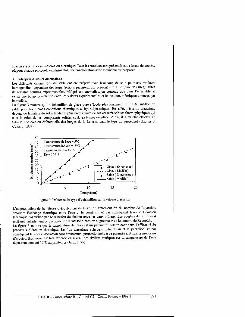
chacun sur le processus d'erosion thermique. Tous les resultats sont presented sous forme de courbe, oü pour chaque protocole experimental, une confrontation avec le modele est proposee.

3.3 Interpretations et discussions Les differents echantillons de sable ont ete prepare avec beaucoup de soin pour assurer leurs homogeneite ; cependant des imperfections persistent qui peuvent etre ä l'origine des irregularites de certains courbes experimentales. Malgre ces anomalies, on constate que dans l'ensemble, il existe une bonne correlation entre les valeurs experimentales et les valeurs theoriques donnees par le modele. La figure 3 montre qu'un echantillon de glace pure s'erode plus lentement qu'un echantillon de sable pour les memes conditions thermiques et hydrodynamiques. En effet, 1'erosion thermique depend de la nature du sol ä eroder et plus precisement de ses caracteristiques thermophysiques qui sont fonction de ses composants solides et de sa teneur en glace. Ainsi, il a pu etre observe en Siberie une erosion diferentielle des berges de la Lena suivant le type du pergelisol (Gautier et Costard, 1997).

50 45

B 40 B 35 a

'01 71 30 O s-

'4> 25

U S 20

V) 15 a a. 10

W 5 0

Temperature de l'eau = 5CC S^ Temperature initiale = -5CC yf Teneur en glace =16% /^ Re =14447 y

.-■'

.■k

..-'A ''Ä

A Glace (Experience) Glace ( Modele )

^ Sable (Experience) Sable (Module)

(^ 1 1 1

10 Temps(mn)

15 20

Figure 3: Influence du type d'echantillon sur la vitesse d'erosion

L'augmentation de la vitesse d'ecoulement de l'eau, ou autrement dit du nombre de Reynolds, ameliore l'echange thermique entre l'eau et le pergelisol et par consequent favorise l'erosion thermique engendree par ce transfert de chaleur entre les deux milieux. Les courbes de la figure 4 refietent parfaitement ce phenomene : la vitesse d'erosion augmente avec le nombre de Reynolds. La figure 5 montre que la temperature de l'eau est un parametre determinant dans l'efficacite du processus d'erosion thermique. Le flux thermique echangee entre l'eau et le pergelisol et par consequent la vitesse d'erosion sont directement proportionnelle ä ce parametre. Ainsi, le processus d'erosion thermique est tres efficace en niveau des rivieres arctiques car la temperature de l'eau depassent souvent 12°C au printemps (Jahn, 1975).


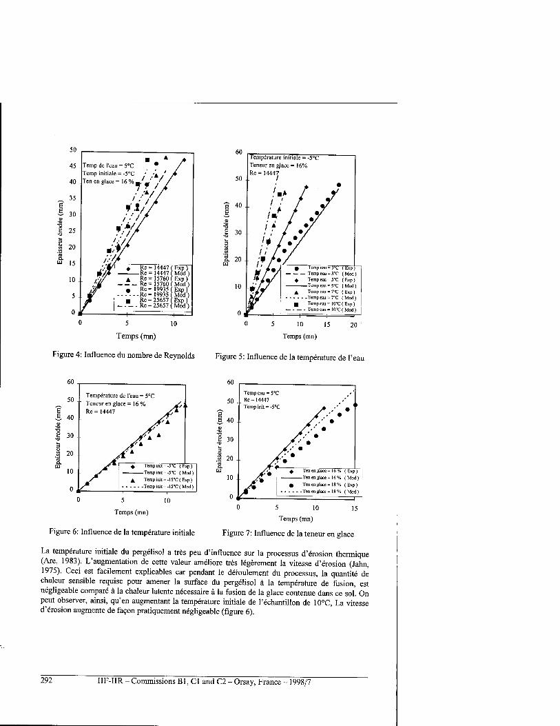
50

45

40

35

30

25

20

15

10

5

0

Temp de l'eau = 5°C Temp initiale = -5°C ' '^ ' Ten en glace = 16 % ■/«•' / '

» Re = 14447 (Exp) Re = 14447 ( Mod )

A Re =15760 (Exp) Re =15760 (Mod)

a Re =19935 (Exp) ..."... Re =19935 (Mod)

■ Re = 25657 (Exp ) Re = 25657 ( Mod )

60

50

40 ..

30

20

10

Temperature initiale = -5°C Teneur en glace = 16% Re = 14447

• /.A /

1 ■' / J

/V / / ■-'/•/

/* /•/ // / •/

/ 0 1 emp eau = rc (Exp) Temp eau = 3°C (Mod)

^ Temp eau = 5°C (Exp)

*JY Temp eau = 5°C (Mod)

A Temp eau -7°C (Exp) = 7=C (Mod)

JM pj Temp eau = IO°C(Exp)

\\ — - — - Temp eau

1 1-

■10°C(Mod)

10

Temps (mn)

10

Temps (mn)

15 20

Figure 4: Influence du nombre de Reynolds Figure 5: Influence de la temperature de l'eau

60

50

40

Temperature de l'eau = 5°C Teneur en glace = 16 % Re = 14447

^ Tempinit = -5°C (Exp) Temp init = -5°C (Mod) A Temp init --15°C( Exp) . . . -Tempinit = -15°C(Mod)

10

^ Ten en glace = 16 % { Exp) -Ten en glace = 16% (Mod)

Ten en glace =18% (Exp) -Ten en glace = 18% (Mod)

Temps (mn) 10 15

Temps (mn)

Figure 6: Influence de la temperature initiale Figure 7: Influence de la teneur en glace

La temperature initiale du pergelisol a tres peu d'influence sur la processus d'erosion thermique (Are, 1983). L'augmentation de cette valeur ameliore tres legerement la vitesse d'erosion (Jahn, 1975). Ceci est facilement explicables car pendant le defoulement du processus, la quantite de chaleur sensible requise pour amener la surface du pergelisol ä la temperature de fusion, est negligeable compare ä la chaleur latente necessaire ä la fusion de la glace contenue dans ce sol On peut observer, ainsi, qu'en augmentant la temperature initiale de l'echantillon de 10°C, La vitesse d'erosion augmente de facon pratiquement negligeable (figure 6).


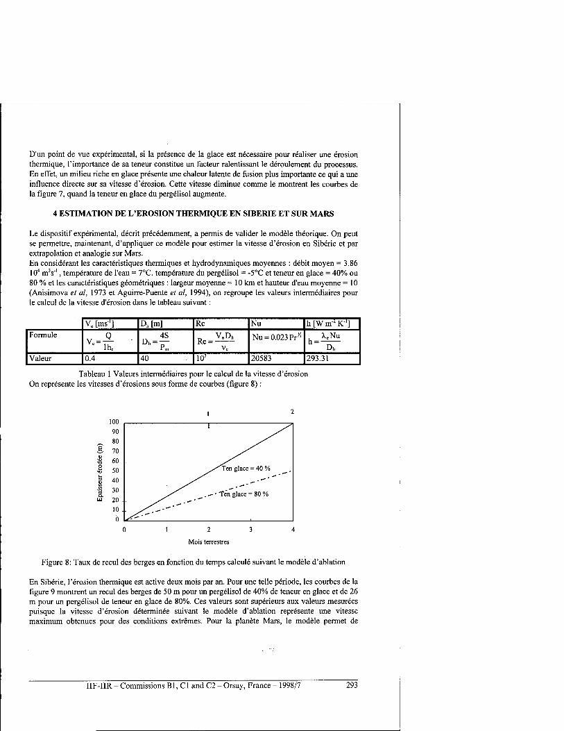
D'un point de vue experimental, si la presence de la glace est necessaire pour realiser une erosion thermique, 1'importance de sa teneur constitue un facteur ralentissant le deroulement du processus. En effet, un milieu riche en glace presente une chaleur latente de fusion plus importante ce qui a une influence directe sur sa vitesse d'erosion. Cette vitesse diminue comme le montrent les courbes de la figure 7, quand la teneur en glace du pergelisol augmente.

4 ESTIMATION DE L'EROSION THERMIQUE EN SIBERIE ET SUR MARS

Le dispositif experimental, decrit precedemment, a permis de valider le modele theorique. On peut se permettre, maintenant, d'appliquer ce modele pour estimer la vitesse d'erosion en Siberie et par extrapolation et analogie sur Mars. En considerant les caracteristiques thermiques et hydrodynamiques moyennes : debit moyen = 3.86 104 mV , temperature de l'eau = 7°C, temperature du pergelisol = -5°C et teneur en glace = 40% ou 80 % et les caracteristiques geometriques : largeur moyenne = 10 km et hauteur d'eau moyenne = 10 (Anisimova et al, 1973 et Aguirre-Puente et al, 1994), on regroupe les valeurs intermediaires pour le calcul de la vitesse d'erosion dans le tableau suivant:

Ve [ms"1] Dh[m] Re Nu h[Wm-2K-'] Formule v=^-

' lhe

4S

L m

Re=V<Dh

Ve

Nu = 0.023 Prx , A.eNu h= Dh

Valeur 0.4 40 10' 20583 293.31

Tableau 1 Valeurs intermediaires pour le calcul de la vitesse d'erosion On represente les vitesses d'erosions sous forme de courbes (figure 8) :

100

90

,-, 80

S 70

3 60 o 4 50

g 40 WD

■3 30 a. u 20

10

0

0 12 3 4

Mois terrestres

Figure 8: Taux de recul des berges en fonction du temps calcule suivant le modele d'ablation

En Siberie, l'erosion thermique est active deux mois par an. Pour une teile periode, les courbes de la figure 9 montrent un recul des berges de 50 m pour un pergelisol de 40% de teneur en glace et de 26 m pour un pergelisol de teneur en glace de 80%. Ces valeurs sont superieurs aux valeurs mesurees puisque la vitesse d'erosion determinee suivant le modele d'ablation represente une vitesse maximum obtenues pour des conditions extremes. Pour la planete Mars, le modele permet de

1

^/Ten glace = 40 % jr ^

s' *■■ Ten glace = 80 %

^— 1 1 1


supposer que le processus d'erosion thermique aurait ete tres efficace lors des episodes d'ecoulement. La morphologie de ses vallees peut etre expliquee, en partie par ce processus.

CONCLUSION

Une etude comparative ä partir de criteres geomorphologiques entre deux regions periglaciaires (la Siberie et la planete Mars) a donne naissance ä une hypothese de base. Pour comprendre et estimer l'efficacite du processus mis en question (erosion thermique), un modele theorique a ete etabli. Avant d'appliquer ce modele aux conditions reelles siberiennes et par analogies l'extrapoler aux conditions martiennes, une verification rigoureuse au laboratoire est proposee. La bonne correlation entre les resultats experimentaux et theoriques permet de valider notre modele. Cette etude experimental montre la hierarchisation de plusieurs parametres du point de vue de l'importance de leurs influence sur la vitesse d'erosion. On constate ainsi que la temperature de l'eau est le parametre le plus influent avant le nombre de Reynolds et bien avant la temperature initiale du pergelisol dont 1'influence peut etre negligee.

BIBLIOGRAPHIE

1. Aguirre Puente, J., Costard, F. and Posado Cano, R., 1994, Contribution to the study of thermal erosion on Mars. Journal of Geophysical research, 99 NO E3, p. 5657-5667.

2. Anisimova N.P., Nikitina N.M., Piguzova U.M. and Shepelyev V.V, 1973, Water source of Central Yakoutia-Guidbook, Second International Conference of Permafrost, National Academy Press, Washington, D.C, 47 p.

3. Are, F. E., 1983, Thermal abrasion of coasts. Proceedings of the Fourth International Conference on Permafrost, National Academy Press. Alaska, Washington, DC, p. 24-28.

4. Baker, V. R., 1982, The channels of Mars, University of Texax Press, Austin, 198 p. 5. Costard, F., 1989, Fluvio-thermal erosion on Mars: a Siberian analogy (abstract). Proceedings of

Lunar and Planetary Science Conference XX, Lunar and Planetary Institue, Houston, p. 189- 190.

6. Costard, F., Aguirre Puente, J. et Posado Cano, R., 1995, Erosion thermique sur Mars. Compte- rendus de l'Academie des Sciences, T.320 serie II, p. 151-155.

7. Gautier E. et Costard F., 1997, Erosion thermique et dynamique fluviale en Siberie Centrale - Resultats preliminaires, Environnement periglaciaire, n°4, p. 65-75.

8. Jahn, A., 1975, Problems oftheperiglacialzone, Washington, DC, Warzawa, 223 p. 9. Komar, P. D., 1979, Comparisons of the hydraulics of water flows in Martian outflow channels

with flows of similar scale on Earth, Icarus, 34, p. 156-181. 10. Lucchitta, B. K., 1982, Ice sculpture in the Martian outflow channels. Journal of Geophysical

Research, 87, p. 9951-9973. 11. Lunardini, V. J., Zisson ,J.R. and Yen, Y.C., 1986, Experimental determination of heat transfer

coefficient in water flowing over a horizontal ice sheet, Report, 86-3, CRREL. 12. Pewe, T. L., 1991, The heritage of engineering geology; The first hundred years, Permafrost

Proceeding, Vol. 3. Geological Society of America, Centennial special(ed. Kiersch G.A), Boulder, Colorado, p. 277-297.

13. Walker, H. J. and Arnborg, L., 1963, Permafrost and ice-wedge effect on river banks erosion. Proceedings of the First International Permafrost Conference.National Academy of sciences, Washington, DC, p. 164-171.

14. Walker, H. J., 1983, Erosion in a permafrost-dominated delta (abstract). Proceedings of the Fourth International Conference of Permafrost, Alaska, p. 1344-1349.


FLUVIAL THERMAL EROSION OF PERMAFROST IN PERIGLACIAL REGIONS: MODELLING AND EXPERIMENT

SUMMARY: In terrestrial Arctic regions, thermal erosion results from ground thawing produced by heat transfer from water flow to frozen ground. By analogy, a similar process could explain the Martian outflow channel morphology. A mathematical model has been proposed to estimate the efficiency and the rate of thermal erosion. Considering a constant heat transfer coefficient, the resulting thermal flux on the ground surface produces ground thaw, and the unfrozen sediments can be immediately removed by the water flux. To test our theoretical fluvial-thermal model (ablation model), an experimental hydraulic device has been built. We have investigated the effect of different parameters (Reynolds number, water temperature, sample of ground ice temperature) on the rate of thermal erosion. Results from experiments are in good agreement with theoretical estimates (mathematical model). This study shows hierarchy of parameters in terms of efficiency of fluvial thermal erosion.


INDEX DES AUTEURS AUTHORS INDEX

AGUIRRE-PUENTE I, 15, 154, 162, 171, 287 (Vice-President Bl)

ANISIMOVAN.P, 225 ARIAS IM, 149, 253 (Inst. delFrio. Benefactor Ass. Member)

AZOUNIM.A, 217 BARRAGÄN M.V., 149 BAUDOT A., 261 /Member CD

BENARD C, 188 BOREL S.,126 BROSSARD T., 269 BRZOSKAJ.B., 126 CAMPANONE LA, 180 CARRASCO J.A, 249 ßnst. delFrio. Benefactor Ass. Member)

CHEN X., 57, 104 CHERVINSKAYA OP, 120 CHUVUJN E.M, 34 COSTARD F., 162, 279, 287 CÖTE H, 95 De ELVIRA C, 15, 249 ßnst. delFrio, Benefactor Ass. Member)

DESCOTES J.L., 261 DJABALLAH-MASMOUDIN., 154 DOMINGUEZ M, 87, 149, 253 (Inst. delFrio, Benefactor Ass. Member)

DUPAS A, 195 DYSLI M., 208 ERCHOVED., 34 FEDUKIN I.V., 79 FREMOND M, 195 FROLOV A.D., 73, 79, 120, 139 FUKUDAM, 26, 112 GARCiA C, 149, 253 (Inst. delFrio, Benefactor Ass. Member)

GAY G, 217 GEOFFROY S., 188 GELICHINSKY DA., 259 GOBIN D., 188 GOLUBEV VN, 132, 139 GÖSSET J.P, 279 GUTIERREZ P, 87 (Inst. delFrio. Benefactor Ass. Member)

GUY B, 65 HORINO'H, 104 INAMURA T, 112 INSTANES D, 229 INSTANES A, 229 ISHIZAKI T, 41 JOLY D, 269 KIMH.K, 26 KURCHATOVA A.N., 225 LABBE L, 195 LAD ANY B, 205 LASSOUED R, 195 LOPEZ N, 87 (Inst. delFrio. Benefactor Ass. Member)

MAKHLOUFIN, 287 MARCHAND Y, 238 MARTINO M, 249 MASCHERONI R.H, 180 (MemberBl) MAZUERJ, 261 (Member CD

MERGUI S, 188 MITUNO T, 57 MURASHKO A.A., 34 NILSEN L, 269 ODIN J, 261 OTERO L, 249 PINILLOS IM, 87, 253 (Member Bl)

POSADO CANO R, 15, 162, 171 RAMOS M, 15, 171 REES G,238 SALVADORI V.O., 750 SANZ P.D., 15, 249 (Inst. delFrio, Benefactor Ass. Member)

SHENGY, 112 THIMUS J.F, 95 WHITE T.L, 46 WILLIAMS P.J., 46 ZARITZKYN, 249 (Member Dl)

ZYKOVY.D, 79, 120
