AD 704 600

PROCEEDINGS OF THE SYMPOSIUM ON SPACECRAFTATTITUDE DETERMINATION, SEPTEMBER 30, OCTO-BER 1-2, 1969. VOLUME I. UNCLASSIFIED PAPERS

L. J. Henrikson, et al

Aerospace CorporationEl Segundo, California

31 October 1969

."'p

S. . 0...'to.f:str, s

advancment.0eg0

a* ,6

NATONAL TECHNICAL INOCTONoSE

Thi s d n has .NAIOA TCNIA uIs.ORPARTMETNOFECMMERC

oo 50OS

55O

This document has been approved for public release and sal3.

AIR FORCE REPORT NO. AEROSPACE REPORT NO.SAMSO-TR-69-417.VOL I TR-0066(5306)-12. VOL I

PROCEEDINGS

OF THE

SYMPOSIUM ON

SPACECRAFT

SAT TI T U D E

DETERMINATIONSSeptember 30,

S~ October 1- 2, 1969

t ~VOLUME I

UNCLASSIFIED PAPERS

Cosponsored by AIR FORCE SYSTEMS COMMAND

Space and Missile Systems Organizationand THE AEROSPACE CORPORATION

Held at The Aerospace Corporation

2350 El Segundo Boulevard T s•

El Segundo, California I

69 OCT 31 :1< ;7, T

NATIONAL TECHNICALWNFORMATION SERVICE

THIS DOCUMENT HAS BEEN APPROVED FOR PUBLICRELEASE AND SALE; ITS DISTRIBUTION IS UNLIMITED

S. . . . I.

v!

Air Force Report No. Aerospace Report No.SAMSO-TR-69-417, Vol I TR-0066(5306)-12, Vol I

II

PROCEEDINGS OF ThE SYMPOSIUM ON

SPACECRAFT ATTITUDE DETERMINATION,

SEPTEMBER 30, OCTOBER 1-2, 1969

Volume I: Unclassified Papers

i

Cosponsored byAIR FORCE SYSTEMS COMMAND

Space and Missile Systems Organizationand THE AEROSPACE CORPORATION

Held atTHE AEROSPACE CORPORATION

2350 El Segundo BoulevardEl Segundo, California

69 OCT 31

:i(_') ,Pt

This document has been approved for public

release and sale; its distribution i. unlimited

.iI . .

PAGESARE

MISSINGIN

ORIGINALDOCUMENT

FOREWORD

These proceedings are published by The Aerospace Corporation, El Segundo,* California, under Air Force Contract No. F04701-69-C-0066. Any other

applicable contract number or company sponsorship is cited in a footnote onthe first page of the individual paper.

This document was submitted on 4 December 1969, for review and approval,to Captain D. Evans, SAMSO (SMTAE).

SHenrikson if fEans, aptain, USAFThb Aerospace Corporation SAMSO

" Cochairman C ochairman

2J. 'E. LesinskliThe Aerospace CorporationCochairman

The views expressed in each paper are those of the author. Publication ofthis report does not constitute Air Force or Aerospace approval of the report'sfindings or conclusions. It is published only for the exchange and stimulationof ideas.

Mhews V -vans, p Cn,

Director, Control and Sensor Projct OfJSystems Subdivision

Electronics DivisionEngineering Science OperationsThe Aerospace Corporation C

.1|

1.

PREFACE

held.The Symposium on Spacecraft Attitude Determination was

hold it The Aerospace Corporation, El Segundo, California, on

September 30 and October 1-2, 1969. It was cosponsored by~.: the Air Force Systems Command, Space and Missile Systems

Organization, and The Aerospace Corporation.

The symposium brought together 306 representatives from

44 industrial, governmental, and educational organizations con-

cerned with spacecraft attitude determination.

The purpose of the symposium was in general to present

a broad coverage of the spacecraft attitude determination prob-

lem andin particular to review the advances in sensing and data

processing techniques related to spacecraft attitude determina-

tion, to assess current capabilities, and to provide an exchange

, of ideas among people who have an active interest in thf. field.

The sponsors hope that the symposium has stimulated new ideas

and will lead to the advancement of spacecraft attitude deterrni-

nation potentials.

Symposium cochairmen were D. Evans, Captain, USAF,

L. 3. -enrikson, and J. E. Lesinski.

Hii

iii

ABSTRACT

These proceedings contain reproductions of the unclassifie.

papers presented at the Symposium on Spacecraft Attitude Deter-

mination, held at The Aerospace Corporation on September 30 and

October 1-2, 1969. Classified papers appear in Volume 11.

The symposium consisted of six sessions. A brief summary

of the material in each of these sessions follows.

Session I (Unclassified), Attitude Estimation Concepts, is de-

voted to papers surveying the general theory, modeling, and esti-

mation algorithm concepts of use in estimating spacecraft attitude.

Session II (Unclassified), Attitude Sensors and Sensing Tech-

niques, presents papers examining the current state of the art and

- future potential of some of the sensing techniques used in attitude

determination.

Session III (Unclassified), Attitude Determination Systems I,

comprises papers regarding attitude determination operational and

design experience for several different satellite systems.

Session IV (Secret), SPARS, contains papers that discuss the

hardware, algorithms, and system test results.

Session V (Secret), Attitude Determination Systems II, con-

cerns papers on United States attitude determination r( quirements

and classified applications,

Session VI (Secret) is the Panel Discussion. An edited tran-

scription of the panel discussion and audience participation appears

in Volume II of these proceedings.

Also included in the present volume are biographical sketches

of the chairmen andspeakers, and a list of the symposium attendees.

v

.•w- . . .. . . . . . .. . . . . . . . . . . . .. .

CONTENTS

FOREWORD ii

PREFACE 111

ABSTRACT v

Opening Session: 1KEYNOTE ADDRESS I

Session I:ATTITUDE ESTIMATION CONCEPTS 5

Seasion II:ATTITUDE SENSORS AND SENSING TECHNIQUES 113

Session III:ATTITUDE DETERMINATION SYSTEMS I 187

Session IV:SPARS 279

Session V-,ATTITUDE DETERMINATION SYSTEMS II 385

Session VI:PANEL DISCUSSION 415

BIOGRAPHIES 419

SYMPOSIUM ATTENDEES 427

" - "' vi

OPENING SESSION

KEYNOTE ADDRESS

Dr. Ivan A. GettingPresident

The Aerospace CorporationEl Segundo, California

KEYNOTE ADDRESS

Dr. Ivan A. GettingPresident

The Aerospace CorporationZI Segundo, California

It is my pleasure to welcome you to this Perhaps I ought to try to cefine what isSpacecraft Attitude Determination Symposium on meant by high accuracy. And if I may. I wouldbehalf of both the Space and Missile Systems like to fall back on a comment made in my intro-Orsanisation of the Air Force, and The Aerospace duction, regarding my involvement in high-accu.Corporation. We are pleased to be hosts to a racy radar. Indeed, during World War Ho whensymposium on a very timely subject, a symposium we went to industry to obtain high-accuracy gearwhich, we anticipate, will yield a useful exchange trains for driving antenna mounts, I found to myof ideas. amasement that although it was easy to get a

gear train with an accuracy of one angular milLot me define the topic of this symposium. about four minutes of arc), it was almost im-

A general definition of epacec.Jaft attitude deter. possible to improve this by a factor 10. In fact,mination to you could not specify shaft concentricity, bear.

ing concentricity, or diameters of gear trains,The estimation of the angular orientation and have them produced if you wanted a factorof a meaningful epasecraft-defined co. of four or five improvement in an accuracy ofordinate system. one mlu. Yet in the business of attitude specif-

ication of satellites we consider one mil as aS ofeIn earlier days. attitude determination was useful definition of where high accuracy begins.

often an implicit part of the attitude control eye- As a matter of reference, I seconds of arc ortam. As control system specifications became a twcatieth of a mil from synchronous altitudemore precise, the attitudb determination require. corresponds to about one mile on the earth atments became tighter, and the estimation of sat- the nadir.ellite attitude itself came to be recognieed as adifficult and important task, At the eame time, This is roughly the way in which attitudeexperimeAte on board spacecraft began to require determination requirements have evolved. It ishighly accurate knowledge of sensor pointing also important to note that thts evolution hasdirections. In the case of wide-field-of-view occurred very rapidly, and the requirements forsensors the requirements, in addition to or even more and higher-precision attitude determinationinstead of pointing, emphasined high-accuracy are mushrooming. Because the need is mush-knowledge of the line-of-sight direction. This rooming whereas the field is still relativelythen has led to the reed for precision attitude de- young, it seems very timely to bring togethertermination. Some examples of early attitude people from NASA, the Air Force, industry, anddetermination include many of the gravity-gradient- the universities who are interested in this area.stabilised satellites with such measurement de- It is felt that this is particularly appropriatevices as sun sensors and magnetometers. Also in because industry has expended considerablethis category are several of the early Air Force's effort in otudying the problem of satellite attitudeOVI series and such NASA satellites as the RAE. determination, much of which is not as yet avail-Examples of satellites with high-accuracy attitude able in the open literature.determination requirements are, for NASA, theOAO and, for the Air Force, the TACSAT, the Attitude determination as considered insynchronous communications satellite.-both of this symposium is of primary interest in thewhich will be discussed in this symposium. area of unmanned satellites. This can be readily

I

3

seen by noting the papers being presented, as or wholly in ground-based data-processingwell as the fact that this subjoct is of equal im- centers. In all cases the end result is an esti-portance to both NASA and to the Air Force. It mate of the ang.lar orientation of some frameis of course reasonable that "automatic" attitude associated with the spacecraft.dpterminatior. is most important for unmannedsatellites carrying experiments with sensors for In view of these considerations the firstwhich pointing directions need to be held and part of the symposium attempts to survey theknown with accuracy. Because of the importance state of the art of estimation, data, processing,to both NASA and the Air Force, it is hoped that and sensing concepts and techniques. Thesethis symposium will help to stimulate a reward- tools combined with the results of the design,ing and continuing cooperation between these two analysis, and hardware experience of manyagencies, associated contractors, and academic contemplated and flying systems presented inprofessionals. the next few sessions should help to define the

state of the art of attitude determination capa-In attitude determination systems the atti- bilities. From such a dissemination of existing

tude sensors may be any of a large variety: sun experience and knowledge in this collection ofsensors, magnetometers, horizon sensors, star related fields, it is hoped that the panel andtrackers, star scanners, gyro packages, com- a.udience discussion at the end of the five sessionshinations of these, and others. The estimation will not only be able to define the current statustechniques applied to the outputs of these sensors of attitude determination, but also determine itsmay vary from use of the outputs as direct mea- potential and discern the direction which It shouldsurements, to simple attitude deduction m.thods, go from here,to highly sophisticated estimation and data pro.cessing procedures. The data processing may Again, let me welcome you to the sympo-be entirely "on boardo or may be done partially slum,

)

4

J44

'I

i'

41

I .'5 • ''

SESSION I

ATTITUDE ESTIMATION CONCEPTS

Chairman:Prof. Harold Sorenson

University of California at San DiegoLa Jolla, California

Foundations of the Problem of AttitudeDetermination from a Spinning Gyrostat 7

A Limited Memory Attitude DeterminationSystem Using Simplified Equations of Motion 15

Modeling of Environmental Torques of aSpin-Stabilized Spacecraft in a Near-

Earth Orbit 29

A Least-Squares Attitude DeterminationAlgorithm Utilizing Starmapper and Sun

Sensor Time Pulses 53

Filtering Quantized Observations 71

Applications of Nonlinear Estimation Theoryto Spacecraft Attitude Determination Systems 89

5

(U) FOUNDATIONS OF THE PROBLEM OF ATTITUDE DETERMINATIONFROM A SPINNING GYROSTAT

Robert E, RobersonConsultant, Fullerton, California

andProfesior of Aerospace EngineeringUniversity of California, San Diego

La Jolla, California

ABSTRACT

(U) The foundation problem of attitude determination from a spinninggyrostat is to establish a relationship between a certain body frameand a-certain external reference frame. This work shows how thesensor frame and various celestial frames appear in a natural waya@ intermediaries and distinguish between the relationships that canbe considered known and those that must be obtained by observation,Modifications introduced by attitude control considerations also areincluded, The role of vehicle dynamics is described, and the natureof external and body frames likely to lead to simple predictivedynamic models are described for the casm of the gyrostat.

INTRODUCTION

(U) Consider two dextral orthonormal vector perhaps for the inclusion of a dissipative preces.bases that are in some way associated with a sion damper, The dynamical behavior of thespinning body: an "operational frame" O (0 latter is such that the axis of maximum momentand a ''sensor frame' S r [S_), Further, - of inertia, as well as the instantaneous angularlet G v (0 ) be an "orient--on reference frame' velocity vector, is kept almost coincident withwhose owvnncharacteristics are in some sense the body's angular momentum vector as the lat-known. In this work we examine the problem of ter slowly drifts under the action of the smalldetermining the orientation of 0 with respect natural external torque. Under Lheae conditionsto 0 using observations made in S. We shall there is no ambiguity about the meaning of "spinnot leave mnatters at this level of generality, of axis": it is simultaneously the principal axis, '

course, and will quickly focus on a inore con. the angular velocity vector, and the angularcrete situation. We shall find, however, that momentum vector. These vectors become temp.many of the ingredients of the specific problem orarily misaligned during the application of anyare brought out most clearly by considering it in control torques, but after sorme transient periodits more general framework. they again resume their alignment.

(U) In the case of spinning spacecraft, A well. (U) Because the traditional accuracy require.known method for determining the orientation of ments in astronautical engineering for this classthe body is based on the detection of the times of attitude determination problems have not beenat which the images of celestial bodies cross one extreme, it has not been customary or needful toor more body.mounted slits, refine the dynamical model further. All factors

considered, past problems of attitude determin.(U) As usually applied, the purpose of this kind ation from quasi. rigid spinning bodies have hadof attitude determination is to establish the iner- relatively straightforward -- though this is not totial direction of the "spin axis" of the body. The imply trivial - solutions,body normally is considered to be rigid, except

(U) Tho wituation becomes somewhat different ahbll be able to see how our implementation pathwhen th,.ie requiremento are changed as fol.lows: can bifurcate at various points and to get a clear

pernpective on the choices we face in finding our

I. The goal is to determine not just the way along it. Special emphasis is on the role oforientation of a "spin a.xls". in the body, the kinematios and dynamics of the ýgyrostaticbut of a prescribed-body.associated obse-Vationll base, If I accomplish nothing elsevector basis having no special dynam. in this work, I hope I will be able to demonstrateical characteristics of its own.; that a variety 'of -&lid routes exist which all lead'

to the same place. One place# the burden of2. The spinning body is not rigid, bux is a implementation here, another places it there,

quasi-rigid body containing sources of but which is "best"' is a pointless quibble until.angular momentum -- a quasi- r'gid each has been explored and perfected to a levelgyrostat. where quantitative comparisons can be made.

among their results.3. The requirement for accuracy in utti-

tude determination is extreme. THE GRAPH

With these changes the problem of attitude deter.. (U) Stripped to its fundamentals, the interrela-

ruination from a spinning body is more involved, tionships of our problem can be visualized beetIt is difficult and perhaps misleading -- even by introducing a system graph. The framesdargerous .- to extrapolate directly the concept: mentioned previously are represented by ver-the experience and engineering judgment, the tices, and the relative orientations between themvery terminology from the original to the modi- (as expressed by direction cosine matrices, forflied problem. example) by edges of the graph. The present

work specifically concerns attitude determination(U) There often is a temptation in engineering from slit crossing of star images, so it is con-

- practice to regard a problem that is new to us venient to introduce a celestial frame X withas a new problem. A moment's reflection, how. respect to which star lines of sight are defineever, tells us that the present problem .- as I itively known. (As one example, this might be ahove stated it in general terms .. is scarcely frame established by the mean equator and mean )new. For it is exactly the problem of the obser- equinox of 1950, 0, since star catalogs are avail.vational astronomer, who makes his observa- able in that frame. For definiteness in the die.tions: 1) from the surface of a quasi-rigid cussion, this "standard frame" X is assumedspinning body that almost certainly is nearly a in the sequel. ) Now refer to Fig. 1 in whichclassical gyrostat; 2) at an extremely high level the four frames -- the standard celestial Xof precision- 3) for purposes that include the the body-associated S and 0, and the externalability to establish the orientation of other earth. reference G- - are represented by points.fixed frames with respect to an external (real orvirtual) orientation reference frame. To besure, he may have fojnd it more convenient tometsure an angle than to measure slit crossing bow startimes; he may have found it more convenient touse methods of data reduction that are anienable ( " OtF,

to handling by desk calculator; he may havefound that the motions undergone by his base areboth slower and more regular than those under- 0 MOW

gone by a spinning spacecraft. But, in principl% *, ominy of the foundations of his problem are ex.sactly those of ours, an•d we should explicitlyrecognize the fact, I shall not pursue the anal-ogy further - -I am not an astronomer .. but Ibelieve it would be interesting, and perhaps pro-fitable, to do so, Fig. 1, Elementary System Graph

(U) The purpose of this note is to discuss sotne A typical star is shown, joined to the X -frameof the foundations of this kind of attitude deter- by a solid line to show that the relationgetip Ismina:ion problekn, foundations that are initially known through the star catalog. The connectionindependent of the specific application and the between the S.frame and the star is dashed todetails of how we may choose to implement an designate that the relationship has partial observ.attitude determination scheme, In this way we ability. The relationship between 0 and XS

can be presumed known in principle, once these (U) In any case, the establishment of the OS re-

frames have been explicitly defined, for the G. lationship is what an instrument engineer might

frame has been postulated as a reference frame call "boresighting. "1 We assume here that it canexternal to the body. As illustration, it might be done and is done -- that the missing link be-

be a frame fixed in the rotating Earth (to the tween 0 and S is filled in - and turn our

degree a frame can be fixed in a non-rigid blob) attention primarily to the chain of links between

or some celeesti-frame different from X . in 5 and G via X 8 .

any case, other. aspect, of the OX ielatioIehipare discussed later. (U) The situation at this point can be neatly

summarised by a paraphrase of Leopold(U) The relationship denoted by the line of KRONECKZER's famous epigram about the Ieal

crosses to the one desired. Presumably it is integers. The frames thus far introduced are

not amenable to direct observation, or we would the work of God; all else is the work of man,have no problemrto discuss. It follows8that to gofrom 0 to 0 it must be through the chain 0, SECONDARY REQUIREMENTS

8, star, X5, 0. (Naturally, there always are AND AUXILIARY FRAMESpossibilities of multiple sensors of the same• ordifferent types, with the corresponding possibil- (U) We first dispose of the path X 0 for a par.

ities of combining their outputs to make the in- ticular choice of .0. One can imagqe variousference, I assume here, however, that the ra- definitions of 0 that might arise in practical

tionals is to be developed fkr the single sensor.) problems. The case where 0 is embedded inthe Earth (modeled as a rigid body) is interesting

(U) The one link obviously missing in Fig. 1 is for illustrative purposes and does represent athat between 0 and S. How that gap is bridged situation of general interest. I shall not cite all

depends on the details of the application, but of the details that enter the X Q relationship,' basically there seems to be two ways. First, a but just enough to show that its complete specd-

direct observation might be possible under some fication might not be trivial in practice.conditions; for example, uoing autocollimatorsin the case of nearby stations on a sufficiently (U) An Earth-fixed frame could be either geo-rigid base when the frames can be dWfined ade- detic or astronomical in nature, and these do

. quately by accessible optical flats, or by some not necessarily coincide. The astronomer'ssimilar precision optical or mechanical link. pole in the "conventional pole" formalized by aThis option usually is not available in unmanned 1967 IAU resolution as the "CIO" or "Conven-spacecraft. Second. simultaneous or intermit. tional Origin. " It is implicitly defined by defin.tent observations on an external phenomenon in the latitudes of five stations near 38DN asfrom both stations, In particular, the common their average latitudes observed during the per.

external observable rmay be the star field Itself, Sod 1900-1905, The "true pole, ** in the sense ofthough it might conceivably be something else. the angular velocity vector departs somewhatWe assume the former for the purpose of die- from the conventional pole: the observed rela-cuesion. It might be asked, if direct observa- tionship, if required, can be found from the ra.tions can be made to relate 0 to a celestial ports of the Bureau International de l'Heure.frame .. If not X itself, at least one calcul. The prime meridian of this system is defined

Sable from X .. why the frame S ever enters from the conventional pole through the Green-the picture a&all. The answer is that S might wich sero of latitude. (This used to be thenot enter if the sensing capabilities from 0 mounting base of the Airey transit instrument,were fully equal to those from S. In practical but I have not troubled to verify whether this is

cases, however, it 'an happen that obsarvations still the case, I cite it merely to show that the

are possible from 0 only occasionally aud only choice '.s quite definite and explicit.)on some subset of stare, whereas it can be made

frequently nn a large star family from S. The (U) Geodetic frames, however, are based onastronomical analog might be a situation lnwhich best ellipsoidal fits to surface geodetic data.

O is a relatively cloudy site in a polar latitude Although the conventional pole probably will beequipped only with a senith transit (I paint the imposed as a constraint in the future, it has not

"picture black! ) whereas S is a well-equipped beon in the past. The only conventional con-desert observatory. Thu key is that the rola- straint on the various geodetic ellipsoids has

tionehip between S and 0 does not change boon that in each case there exists some axis ofrapidly, so the occasional observations from 0 rotational symmetry, Note also that there it nowill, after semu time, amaes enough data to fix assurance that the center of mass of the EarthSthe rilationship over a useful time period. On lies eithir on this axis or in the plane of thethe ith r hand, the relationship bhtween 0 and equator of a geodetic ellipsoid.G may chanmc rapidly and not very predictably.

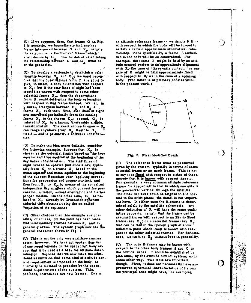
(U) If we suppose, then, that frame 0 in Fig. an attitude reference frame -- we denote it R -

I is geodetic, we immediately find another with respect to which the body will be forced toframe interposed between 0 and XNO namely satisfy a certain appro•imate kinematical rela-the astronomer's Earth-fixed frame which I tionship. More specifically, a frame B embed-shall denote by G . The burden of establishing ded in the body will be so constrained. Forthe relationship b 4 ween 0 and .GA must be example, the frame B might be held by an atti-on the #sodesist. tude control system to an apprnilmate alignent

-'.th Ai•,the case of "three.-axis control,"I or one(U) To develop a rationalo to establish a reol. axis of B might be held approximately fixedS ttonship between Xa and G0 jwe aut rep0| I with'•epc o••&i h e iasdnn

nise that the obser ~tlons froAm S are oing to body. (The latter is of primary considerationgive, in effect, a body orientation with respect in the pr'esent work..)to X but if the star lines of sight had beentreated as known with respect to some other - .celestial frame X , then the observationsfrom S.would detirmrn, the body orientation -with respect to that frame instetd, We can, in / $ - "6 .neral. interpose between 0 and X5 a . -

frame X such that: first, sAr lines of sight . bcare conveited periodically from the catalogframe X to the chosen X i second, 0 ts Xrelated t1 X. by a known. $referably sirtle,transformatigh, The exact choice is open .. XCcan range anywhere from X itself to 0 " k %itself .. and is primarily a loftware consiess.-

(U) To make thA idea more definite, considerthe following example, Suppose that X ischosen as the celestial frame based on the trueequator and true equinox at the beginning of the Fig. 2. First Modified Graph

sight have to be updated just once a day- typic. (U) The reference frame must be presumed

ally from X to a frame X based on the given by the system, typically in terms of somemean equatoi and mean equaox at the beginning celestial frame or an earth frame. This is not

to say it is fixed with respect to either of these,of the current p esselian year (applying cornes- merely that its known with respect thereto.tions for precession and proper mot-on), and For example, a very common attitude reference

t frame for spacecraft is that in which one axis isindependent •dav nur~oors which correct for pre- the geocentric vertical through the satellite.

cession, nutation, annual aberration and further The other two axes could be aligned in and nor-proper motion. On the other side, 0 is re.fated to X directly by Greenwich spirant Mill to the orbit plans: the detail is not import-.:sidereal ti: d obtained using the so-called ant hero. In either case the R-frame is doter-"equation of the equinoxes, s adned solely by the satellite ephemeris. Any

"other definition of R will have the same quali-

tative property, namely that the frame can beibl,(U) Otherf ourices but thpoint xamPlhas been arnd assumed known with respect to an Earth-fixedthat intermediary frames between X and sa frame (say 0 ) or a celestial frame (say X2 )

generally arise. The system graph now has the that can be tieA to the ( ystem graph at somegeneral charscter shown in Fig. 2. indefinite point which itself is known with res- Ipeact to the other celestial frames. For definite.

(U) This is not the only way auxiliary frames noes, we tie it to XS without loss in generality.

arise, however. We have not spoken thus farOf any requirements on the spacecraft body ex- (U) The body B-frame may be known with

cop tht i beuse asa bse or ttiudedetr- respect to the other body frames S and 0 inmtthation, Suppose that we now make the addi- the nominal sense, It could be established by.tona Supptios tht somekind of attitude con- plan axes, by the attitude control system, or insome other way. Two facts are important,

S trl requirement is imposed though. First, it does not necessarily have anynormally is dictated in practice by the opera- preferred dynamiial characteristics of its owntional requirements of the system. This,perfurce, introduces two new frames. One is (as principal axes might have, for example);

. '.I .. .... ... , . .. . . . . . . . . ..- . .., . ...•-. -. -- . - .. ,-, .--...-. .- -"- ."i

+Isecond, its true relationship to 0 or S would discussion that follows.) Let AX be the dir-

Shave to be estimated as a part of the attitude ection cosine matrix relatinithe a and Xdetermination process it there is any reason to frames according to S a AO'X. The star line• establish it more precisely than could be done of eight then resolves in the S-frame asfrom a priori nominal considerations. S SX X

X A X and the coordinates of that star(U) Figure 3 shows the system graph modified i1age in the SIS 3 .plane are closelyto talike account of the control relationship. Thetwo possible defnitioo sof R are depicted-by .1 8/S 3)",'a-dashed" and 'b-dasheod" lines, It it evident s (l 1 (1)that as a natter of logic it does not matter'which way R Ii defined, for given one defini, where c istionit. is easy enough (in principle) to define focal length of the sensor opti-

the elternative relationship usinj the known cal system.

X O link, It does mnake a difference in prac.tileAhowever, depending on how R. eventually (U) A star-imago is detected by the sensor when

finds its way int6 the attitude deterPnateon.t the coordates in the fo plne stify thehas not yet done so, at the stale of Fig. 3, but equation of , slit in tht plane. I r sray ang

if it does the definition should be used which re. inearinstpraeeti onuch alits are linsarl ayduces the burden of computation. For earmple, one has e teqution ax + be r 1a whorae x

it P were determined by the satellite sphem. aerie and if it were established that the "b. in the Sit,-plane When sI and s given by

E.(1) 6~if hsejaiA . , Atendashed" relationship were the more natural to Eq.use as a part of the attitude determination pro-cess@, it would just be good sense to ask for an S ) +S(c (.8(hephemeris with respect to . rather than . a(.c) ) + b(-a 3 u l(X2 ), (Za)and conversely, if the "&.dasfedo* relationshifwere the one directly needed. an event is detected, We can write this in L

matrix form by introducing the row matrix

S ---------------------------- a * ca ob 1).Sin which case, we can say that the tatrix equa-

-@ tion characteriuing a star sighting is

coo OX VASPA 1 0. (2b)

(If one takes account of such effects as slit devi-

ations from nominal location and shape, focal Iplane tilt, and optical distortion, the right hand

$A side may be a small nonlinear term in i,.S Theconceptual basis can be described just at well,

Fig. 3. Modification for Control however, if we set these deviation terms equalto sero,)

ROLE OF ROTATIONAL DYNAMICS (U) Recognize that Eq. (2) is satisfied at a

(U) I shall not go into detail about the observ- single sighting of a specific str in a specificables of our problem, but & few general state. slit. As the satellite rotates, many stars areaents are needed as , basis for dgecusains the sighted sequentially, generally in more than onerole of the nateleiteds rotational dyscun the slit, and a 4ifferent value of the time is attached

to each event. The total data stream from the

(U) Consider a star sensor in which the 5. sensor can be regarded as a collection of "sat-

frame is rigidly embedded. For definiteness, feed equations" having the same generalstructure, but different a.-natrices (perhapsvisualize the S axis as the optical axis of thesenior andrie 1

2 ,-plano as its focal pla.ne. Sdlcted from two possibilities) and different

Denote by )I thedirection cosine matrix of the X -matrices (selected from a star populationline of sight to a particular star resolved in the that depends on the sensor sensitivity, field ofXframe, ( yb n of the X.frmes view, satellite motion), Most importtnt for ourX-frame. (This may beanyofteXra sintroduced previously, without changing the present discussion, the data stream contains

0t.

• + .•, .... :' ... - . • ',- -• . -. + - --. ........ .-...... . ..-,

matrices A mp~ at different instants. (U) In short, the trure role of the dynamnicsThe matrix ASX is one possible character- and kinematics of satellite rotation is to estab-ization of satellite attitude, and it changes with Ugsh a time scale for the way the observedtime as the satellite rotates. events ought to occur if the satellite parameters

and rotational initial conditions have the values(U) Attitude. datermiuination is the use of thethtwtinteyav.Tobsrtosf

data-tr." to iierASX t'sos deiredwhatever det Ialled character, arias measure .oftime. the dliffrence between~the vehicle Is actual be-

havior and he way its "predictive mnodel", or(U) But suppose the star line of sight is known 1dy~namic tiodel' behaves.-Th deviations

t\ in the R-'framis instead, Equation (2b) be- occur from four soiarcomicomes

1. errors in the physical measurement,

CA ) 0 (3a) ... im~perfoletions in Eq. (2)

and the same attitude determiAnation process .3 rosi u siaeo eildetermines A$R instead. If the line of sight parameters and initial stateware known in the CL-frame, we would have 4. imperfections in the dynamic model

CA so X (b The deviations actually are used to revise ourestimate of vehicle parameters and initialstate, Obviously, if the revision is to be a

instead, and the attitude would be determined valid one, the errors and imperfections inas a relationship between. the 8-framne and the Items 11 Z and 4 must be reduced as far as0-frame, Figure 3 makei it clear that a&ny of possible to avoid contaminating the estimation,.these alternatives are equally acceptable as a

way satonto the ultimate, determnination of the (U) The characteristics we would like in thedsrdrelationship between 0 and 0. The dynamic model &rot firstly, that deviations in

point is that the data stream has the same struo. the observables be linearly related to devia-turn in all of these cases, so the same type of tions in the parameter family, for only in thisically provide the relationship between the S. theory as broad as we would likel secondly,frame and the frame in which the star locations that the model be complete enough to avoid get.are given, There is no special reason to regard ting substantial deviations simply from effectsa n X-frame as preferential in this regard ex. ignored in the model. The linearisation re-cept that the XX change much slower in it, and quirement implies, in effect, that a descriptionless frequent updating is required, of the rotation can be found which is in some

sense "simple, 11 and it is this subject that I(UT) In this discussion, I will focus only on a wish to address in the remrainder of the work,sequential estimation process, though this isnot the only way one might approach a deter. (U) The rotational behavior of any spinning -

mination of the A-type matrix from the condi. body is essentially nonlinear, and this is notions of slit crossing, less true for the spinning gyrostat that this work

views as the spacecraft. To linearize, one(U) Although the event on which the observa- must expand about some state of motion -.- pro.tion is based is a slit crossing, the actual ob. ferably, about some stu-te of stesd, motion ifservable is related to time. It might be the the resulting linear equations are to have con-slit crossing time itself, or the deviation of stant coefficients, The problent of complete.that time from a predicted value. In the former noess in ane that has to be examined separatelycase, the only way to tie all of the observed for each satellite system doeigai, but for manytimes together and to the instant at which the cases it is enough to consider the "natural,attitude io to be evaluated is by a knowledge of motion of an otherwiue rigid, torquedfrea gyro-.-the satellite rotationt more specifically, by a stat am a basic guide in the sense discussed be-knowledge of how the rotation depends on the low, and to assure completeness of ths modelpertinent parameters of the vehicle, In the by introducing other pertinent effects as per-latter case, exactly the same kind of knowledge turbations, '-

is required in order to predict a time of slit

crossing,

(U) The basic question we face in our formula.( ) tion of the dynamic model it "What motion is it X

natural to linearize with respect to?" Supposewe find that there is a set of "modeling axes." MM in the body whose motion with respect to aset of "kinematic reference axes" K is asimple motion, in the sense that it can be rep-resented as a small deviation frim a' state ofsteady rotation. Then it is natural 'to decomr.pose the direction cosine matrix in the middleof Eq.' (2b) so that equation becomes

(OAIM) AMK(AKX 0x1 (4)

The quantity X K a A XX is calculable, ofcourase, because the motion of K is known'.The quantity vAIM is subject to estimation in X-fromethe sae Way as a itself, or the matriceoABe A0B1 which Fig. $ suggee•ljight bedesired. The middle watrix, A , is theone whose behavio- is -linearly predictive.

R •MARKS ON OYROSTAT BEHAVIOR

(U) I shall conclude by remarking briefly on Fig. 4. Euler Angles for the Spinning Oyrostat

the major candidates for frames M and K,based on what it known of the unperturbed ma. (U) Howlver, the function of the attitude controlb o what snownoftheunpertubesystem is to keep a body, say B3 (close to M3,

( ) presurnably), in approximate alignment with a

(U) irst, how dose a spinning gyrostat look to corresponding axis R 3 of the .frgame, To the) rst, does a space-fiedbservert looksmuc lie aextent it does this successfully and efficiently, itai space-fixed observer. It looks much like ainy 8ldllymvetealli oetmvco

gradually moves the angular momentum vectorother spinning body. We picture its motion around in space until the natural precessional

with respect to inertial space by introducing motion tends to kee B3 cot to R3. Underthe usual Euler angles (Fig, 4) relating the t ircmtancs , te 13-frame ould serbody frame M to some inertial frame X, these circumstan.ps, the Rframe could serve

,Undecertain condetions, we find that thl a a kinematic reference fre with respect tojyrotatspin •vth amos contan flis •Which the dynamical description could be linear,

gyboutat apin with almost e constant rat*e uied. But if the 1.-frame itself were in a stateabout the body axis ("spin axis") a wle of steady rotation about 1.3 with respect to anwithat axis preces ses about X3 at An Almost ta -rm rCe X-frarne or the 0-frame, ta -VM rGconstant angle 9 at an almost constant rate X-frame would serve equally well as the K-frame.These conditions, basically, are that the bodybe not too asymmetric about M3 and that X3 (U) In conclusion, the kinematic referenceframebe normal to the invariable planet that is, it is sul be baseon the sysem anur m rmealigned with the total angular momentum of the should be based on the system angular men.

satellite. It seem@ reasonable, therefore, to tumn, but in cases of practical interest one mightbe able to select the ,s-frame, 0-frame or X.consider a kinematic reference (K) frame frame of rig. 3 A. equally valid approAimate

which is inclined to X3 at a certain anile 00 realisetions of that "most natural" choice,and which processes about X3 at a certainconstant rate $0, (It turns out the equations (U) As regards the body frame, a natural Choicecan be linearised whenever q0 is used, but e i it the b ot a e, osnatut hthe M3 body axis does not then closely follow exists if the gyrostat is not a gyrostat but athe corresponding K3 .aie, ) This K.frame simple rigid body, namely the choice of the M-is not precisely ainy of the frames depicted in frame as principal axes of inertia. These arei the axes about which the angular motion under.Fig. 3 Jgoes purely periodic excursions in the body, so

their choice effectively removes any secular part(*i) of the motion that would tend to make large

angles develop between K and M. For the truegyrostat there is a somewhat analogous set ofsimenvalue-like body axes, but unfortunately

13

" '. + v -+;• .~~~~~'AL• . "' ,."•. . . . . , ' ,

t~l e Iii I~ II I III| I d

K÷

their use does not result in an angular velocity (U) Thus, we have seen there are certainvector which, except for the component on M3, "natural" choices for the M and K frames tohas purely periodic components. It follows that use in the dynamic model, and that there are -

the M-frams inevitably drifts secularly with certain approximations to them which we wouldrespect to the K-frame, and lineariuation might have reason to believe might be acceptable.be invalidated if the drift is great enough, It to Perhaps most important, we have seen that apossible to choose a body fiame with respect to variety of path# to our problem would seemawhich there is purely periodic motion (no secu. riori to be equally acceptable. To decide

ardrift) on axes MI 'and Ma, However, the Li1onally which is "best" cannot be done with.frame is not an i nherent property of the body, out.pursuing each to the point where all, relevantbeing initWl a condition dependent. Most inves. software considerations are clearly understood.tigator's have a dislaste for working with thiskind of body frame.

144

I

I-) iI'KII

4

I• **

I .

'i. t";•2].

14

m,;; ~~~~~~~~~~~~ ~~~~~~~~~ ~~~.. ".. .-..... ....... . .. ) -Th ,..'i " .- ;., .... ,, ,.. .... ., ... .:• ...- ...

' • 4aim • , , ..- . .- .. .- . , r '•, o., ,

(1) A LIMITED MEMIORY ATTITUDEOETERMINATiON SYSTEMI USING SIMPLIFIED

EQUATIONS OF MO~TION*

by Edwin 0, PoudriastMarquette UnivirsityMilwaukee, Wisconsin

ANSTRACTI

A .sequential. limited memory attitude determination system Isdeveloped for a spinning spacecraft# The limited memory estimationsystem Is derived from the least-square procedure and employs. pastmossurs~entans both to delete'the old data from the covariance me-trix In order to maintain filter sensitivity and to augment +hemeasurement error term. The extrapolation of the spacecraft statesacross the memory Interval Is made practical by a set of simplifiedspaeocraft equations for which long computation time Intervals arepormi fted.

The report deveiops the simplified equatlons which employtime averaging of the first order parturbatioons and demonstratestheir accuracy In the are second range over a tlme Interval as longas 1000 sec. The concept of limited memory and the computationalC method for Incorporating It Into a Kl~aman filter computer prograftIs derlved. %eaulta Indicate that the limlted memory system Issuperior to the nonlinear Kalman filter to"h In 100e4 of conver-geonce and accuracy and that are second accuracy for a spacecraftoptical axis Is feasible with the limited memory filter. The do+*Indiaftes that a substantiai portion of the system capability Isdue to the augmentatlon of the measurement errors

It i wel kowntha thenoniner amenConcepts for alleviating the ninsnssitivityIt + beoms inellnowtnv toa stae andnli parKalmete problem for the Kalman flIiter, proposed by

filtr bcoms Ioonlfla, o sateandpor~or Schmiidt,El) and Jazwlnskl,EI3 and Le6,E4] hayeerrors if the state disturbance noise Is nopligi- been classed as Ilimited memory filters, oflie. CiI2)? This condition exists for the accu- these, Schmidt's procedura, W~*ch augments therats determination of attitude for a spinning Kalman 0ilter witlh an additiunci gain turm, Issateilite In an earth's field environment; In the only techniquo wniCh does not add consider-most cases the spacecraft motion Is disturbed by abie computelionsi conpiaxity to the filter. TheRiegnatic, gravity gradient, aerodynamic, soisr, maxim~um likelihood technlque of Jetwinski requirosand micrometeoroid torques. Usually In a wali- the batch processing of two Kalman filters *vondesigned astellitae In a near earth environment for the simple linear system.the aerodynamic, solar, and rterometeorold torquesare negligibie, while the0 magnetic and gravity The technique of Loe, based upon theqradiant torquoe should Us modeled if accuraCies I~ ihted haost-squars has bean extended to thein the arc second ran~ are desired. (Note athat mnlonlnar prob lem by ~the author.*3J The nonlinearonly +h* mic roffetordd torques can be considered version requires the axtrapoistlon of the8 6tat0random.) and state transition matrix across the memory

length at each measurement point, In general,this calcuiation Increases conslderebly the corn-puter saiution time end complexity and the sub- '

* Thi wor on e insequent filter Considered Impractical. However,Thi w thim s report Issponsored Inpart a Wa of equatlons of motion for the spinIng~m(7)by NASA grant NGF650400I-009 and In part by a body In an earth torqued environment have been

consultant agreement witm Honeywell, Inc. developed CGJ whereby exceptionallyý long Into-gration time intervals can be used. This sub-

stantially reduces the cocnutotoicn time for theextrapolation. Haence +he nonlinear weighted si*(

les;squares technique Is a fefaible filter forthe attitude determination problem. y

This paper will outline the approach used TSM0-T otodvlpthe simplified equations of motion + si - oaddemonstrate their accuracy for thul torquedr

spinning body. The nonlinear least squareslimited memory technique will be outllned, e ndthe equations for the Implementation of the fil- sin2 C05 co i p TV cot Ttor presented. Ftosulta of a Simulation Study. r +4demonstrating con .vorglince and accuracy cepabil L-LyWaes of this limited memory scheme willi bepresentoed

(T sin* + T Cosn 4) Cot I

The most commo~n method of determination oftespacecrAft orientation' Is +h~e soluion of I lt,2 062

eq~r§ uatfons, including those torque effects * r cow a .. ~... .. ~which may be signifiomit. If one requires aoly.Ltions over a long period of time Or neeldathelequation solutions as only Oon step In an anely- Tcm *+ os)*Ia (for exampie, the attitude determination Vproblem), than It Is of Interest to determine In r sin awhat manner the equations of motion may be eompu-tad accurately yet rapidly by elimfination of un-necessary terms end by Increase In the compute- where r w angular momentum magnitudeflonal speed.

T TT,T d torques appliedfto theOno of the mollt ineresting methods for x y 1 spacecraft aiong the angu-

analysis of spin stabilized matel "alte, developed lar momentum axes x, y,)primarily by V. V, Beletski isE17 uses the con. end a

* Copts of timse-aeraging of the torques In orderto determine the longer term motions In the sWt Lx, LV, L, spacecraft principalalt its orientation. Tme method Is similar to the inertia'nonilinear analysis concept of slowly varying phaseend amplitude discussed by lAcLachlln~Il. Usingthese techniques, iBelstskii has been able to pre- and where the angloasr, 4, *, 0, and ~'aredict the effects of aerodynamic, gravity, and defined In Figure 1.magnetic field torques on the stability and cr1-entatlon of a satellite over daily end monthly In order to have a consistent se of equa-time Intervals. tlons It is necessary todylpthetoqe

The oncet emloyd byUslosklIsequatonlos In terms of the State variables endThe oncet eployd byaeltawl isthe eartn's fields experienced during the orbit.

equally applicable to deriving the differential The thiree torques considered are the Interactionequation form for calculating thie Satellite mo- between the spacecraft and the earth's magnetiction. Using two sets of transformations, first, field, the edldy current torque resulting fromfrom inertial to angular momentum axes and currents Induced on the Spacecraft by the earth'sSecond, from angular momentum to princrpoi body magnetic field, and the gravity gradient torqueaxes the resultant differential equations E63 rosulting from Interaction between the mass dIe-become tribution and the gravIfttlonal field. Experi-

once has shown that the*e are the major torqueTx contributiono'for a high density spacecrafts

I However, the anaiytical procedures used are notlimited to these specific torques elid are equal-ly applicable to solar, aerodynamic,cand othersresulting from spacecraft motion or o lrientation.

The magnetic field interaction torque, Inrmny the angular momentum coordinate frame IS

jjM.VIMX a (2) *"

16

where . o earth's magnetic field vector where F'l and T are the transforms from localrvertical to Inertial frama and Inertial to anlu-.. M a - axdyixs residual magnotic dipole lot moetum from respectively. The forer

frome Involves the spscara•ft orbital elementsE a Euler angle transformltioln of while the letter involves i and t. The term

Figure I b, momentum to body axis Lr° can be written In angular momentum w -ordi-

Carrying the cross product, equation (2) b-ts as E-LEO so that equation (5) becomes

coffee(~)S T T 3u r! x (E1ILE) r' (7

Equatins (•.), (3) a, d (7).describe the three

•( V 8) a x torques In terms'of the stats variables andtheir ratesi, and the orbital elementsft, fl

where EI Is the Ith column vector of I" t* lad U *".

A set of-spproxlaftO differential eque-

The magnetic eddy current torques can b lone can be deveooped which are greatly 'simplI-

written as fled over the state equations (1) when*the "torques In equations (3), (3), and (7) are used.

-( 1 X ) In order to derive the simplifled set, timeaveroaing of the first order perturbation torqueIs used; thte Is, the fires order torques are

where K a magnetic eddy current loss constant obtained as functlons of time end then averaged.to eliminate those terms which are cyclic and

* total angular veloilty result In. no net.change over a period. This isIdentical to the method used by BeleSkll C70.,In contrast to mie'development, averaging here

Assuming the angular velocity of the angular Is carried out for the differential equations -

einsblan comprlson with Inatead of on the gonereilsed work function be-omentum axes Is nelgbei op t cause the torques which Influence all state mo-

the angular velocity of the body a&es, the eddy lions are required.current torques become

The derlvatlon procedure Is illustrtedoZ[ m K(BM T AT,_) - AS (STU)) for ea symmetrlI body, L x a L y 0 LE , Assulmng

the torques are first order small equations (I)b~ecome

where A a matrlx reltIlng angular veloclty ofbody axes ao the angular momentum C 0o O rO 0 ( ¶f resf

The gravity gradient torques, available Inmany references (e.go, 9) are given by b rOa 0 co

3W Qr1 x (Lrt)) -x

I'quation (3) can bo used to develop the firstorder torques by subs+ttutlon Into equations(3), (5), and (7). Since the torques becomefunctions of tima only, a set of first orderperturbitlon equations can be wr.Ittan. The

R v satellite radius from center of seit.h resultant equatlons are still vory complex.re local verical unit vector Since many of +the terms aer periodic with

S liperiods

L s Inertia diagonal matrix

T w Lx T2 , 2w L

The local vertical unit vector Is obtained In r0 0 Aangular momentum worolinotes by

rFo T FI (,0,0) the method of slowly varying amplitude end"phase (8) can be employed. For example, the

17 j

I2' . ",. -. '. .. : ''; I . ' . 1: - "I *.,\ • • -

torque term Y becomes2

T a JIM T ?Cr~O*d (9)

0 9

The use of equation (9) eliminat~es from the. '1-1right-hand side of equation (We ll those termswh~ich have net average of zero over the periodsT' or T2 6KoOK

4 INERTIAL. ANGULAR WANU4401 MOM90TUM-qaference 6 daVe lops the Gooerchenta for MOCNTUM AMI PRINC MAIL IOUT AX&S

the magnetic, eddy current, and gravity gradient i IAiSytstrCintorques of equations (3), (5), and (7) In terms IusIAiSytmfo Si-of the State variables, Using thoea results, Stabilized Satellite-equations (1) beosme

(3i B (I + bCsal a P' C al S 3 vLx(l 4 )(1? 3 sin2 0) r2r3Lx - r2p RrA

KRY1V1 (I .+ b ceS2 8) 1 ass Sa I i Lx(I a)(2T 3 vln 20 ) rlr 3LxSn sn 21113rOn I

* rK(5 2 2 - q12 )(I # D~ 00&' j

bK elm 2 6 (152 + 192)-- 4 LX

q (I+ h 052 'c+ 't 8 x 2 os c+ I oo

~uL~ 0 a) cot @ (r 2 + 3 s 2 - 2r3 )

4R3r p

br sn 0(6 u ~ ~1L 3o L Hl - )eoa 8 C,2 4 r2 2r 21; elm 0 (1 AV 2 3

LK P 2R 3r

T7 777777

whore 02 aT2W8000641rd body axis angu-L ~~~~w2 u 0.31415926 rad/seJ h ue

5md r1,r 2 and r3 rar components uf equation (6). 0 4 0

I t I s possi bl, to develop a simnilIar proco- .557Uuro for tho monsy'.etrlc Inertia body. lewover,the Initial solutions are In tho torrc uf elliptic r *20.61617134 # ft-sefunctions so :flat a closed form solution for allIterms of the differential equation similar to 99.999

equtio (1) I no~ovllols.It s'#howe ver,pos3i.J4 to. 2VIIII6+8thfth nnyf.rlr e tr:Ody O.qua- *314,41546ticnaswt;,(u grM'tdoo I of incroosc In com-ploxity and hnme* possible to employ the same fil for tnis comparison, both sets were pr0-ter procedures 'o.IUs presented #or either syrf.. cranmmed for digital computer Solution using IBM*tric. or nonsymmotnit body. ?040.' This sect ion presents the comparative re-

suits. Since the computer used wasn limited In.ACCRA AALYS F~nJUIstoragoemad computational speed was reduced be-

T I IAI0m cause a lare portion of the program was run Indubt a precsin It aseided to program the

Symrmetric body and l~clude only the magmatic fieldIn the precedlig section a set of time- effects$

averaged perturbation equations were developedwhich describe the motion of a spin-stabilized Using the above conditions, the true aqua-spacecraft in an earth orbital environment. Thi~s tions cuand approximate equations (10) wereset affords a marked slprpilifiction over the solved using a 4lth order Runge-Kutta Integrationexact equations and since the torques eae time- routine with a fixed Interval also of 0.1 sec4averaged It should be feasible to employ large Figures 2-5 compare the solutions, Figure 2integration stop Sizes for their Solution. Since shows the motions for the angles T and C over athese equations possess distinct advantages when 40 sec time period. This short time is used toemployed In the %;omputer mfodeling of the motion Illustrate the effsect of avrergIng, that Is, theof a Spinning satellite, an accuracy comparison exact Solution has oscellat+ions not present Inbetween the tilme-averaged Wo and the exact the averaged Solution. The averaged Solution,equations is6 Important, however, duplicaeos precisely the long term mo-

tlons of the exact set. Solutions over period&The true magnetic field experienced by a of 80(1 sec. indicate differenesm In magnitude to

Satellite Is rather complex. However, an ap- be of the order of 0.00010.proximate field can be generated by assumingthat the earth's flied results from a dipole Fig~ure 3 compares the cone angie, I , forTfned with its spin axls and the satellite; the exact and approximate solutions over a 600ima circular orbit, sec inerval. In this ease, the exact solution

he$ approximately a 20 sea period, which mak~esThe spacecraft used In the comparison alm- the exact motion difficult to representj hence

ulatIon wos the conceptual mechanization of a the envelope has been Indicated , Again the angu-horizon definitlon experiment by HoneywellI, Inc. lar differenceo Is of the order of 010001*0for the NASA Lang lay Research Canter [9j. Thenominal spacecraft uses a 500 km. Sun synchro- Figure 4 compares the angular momentum fornows orbit with tho foliowing parametes and the exact and approxifmate solutions. Again th4Iintial conditionst approximate solution (which closely approximates

the roan of the exact soiution) represents theLx a LY 0 56.66 slug-ft2 average change hut does not hove the oscillations.

Lz 65,62 slug-ft2 The error In the 1;ody angular spin poat-flin Is represented by the term

M x a !A y 4 d M 0a .51092 x ID'I ft-1/GaussK a 0,141739 x 10"4 ft-O-sec/GnuS&2 a -

0 inclination 0 97.360 This term Is a riore realistic representation ofu, er, oflblluw -the spin than the Individual Euler angles. Forergoof 611u-;"a 9.30example, at the conditions a * 0, the torque

terms in equation (1) are Infinlte although noN*long, of asecending node 00 aC' larity exists In the equations (10). SIMI- '

isly Grosch C103 shows, for small cone angle,woo orbital rate *.06346/86C 0, the sum and dIfferenoe of the spin and pro.( 2 cession angle ore more useful for system repro-

WxU 0seontalon. Figure 5 shows the spin positionerror overl a time Interval of 800 sec to be less

4 .--.-.... 19

whore x Uaugmented state vector model of114A954system Including any unknown

58 *a 51&T 'V Cparameters

X.(k) ameasurement equation

i4.43 f5 - -- (x) x measurement modelAV: - system noise

v~k) meriasur-ement noise

tie Itom

riguro 2 Comparison of Exact andAveraged ~atesolutionrs

than fl.00026, As shown In reference 6.furt*hrreductIon of this error should be possible by

* more accurate selection of the Initial angularm romentum for the approximate equations.

Figure 4 Exact and Avoreged AngularA Momentum¶ Solutions

It Is assumed that the noise Is white, gaussian.)WIth

11111150400 Yj - R(lk) i(t - k) (12)

Kigurs 3 Exec+ and Averaged Cone 1[!wTl a QM (t -~ +)Angie Comparison

In the attitude detarmination problem conal-The cor~uter soiution enmparlson indicates dared +he neqleated torques should not be repre-

that the approximate equations of motion are cap- sented as gaussian white noise, Hoens w Is zero,able of representing a sptnnin0 satellite In an-earth's field environment to within one o overlong time Intervals and hones should be adequatefor Precision attitude determination.

The general model fora dyn~jmlc system andIts measurement equations aer ANO 1m NV9L0P1

x W £ A k)t + yIk OAO NLp

Pijuro 5 Spin- Precession Angulargrrer Comparison K

so.

The weighted least-sguibro solution for In addition to +h~e update, +he state troanstienm mpovdesimt fr p), given an Initial atrix, *Ct,p) is needed to evaluate the terms

l$+m ved esi at -p,1 r(k) of equation (14); that Is,

esimt jp (p). isj

u~p as jo * (P -) +x (k)T

( WqQ~r'1 2 (k)(x.() -X (

where

;(k) 7 I4y -1,~e/2(k (1*4)8

IT"IEquation (13) assumes that only the measurementsJ

k,: atNXp are employed, and honce can be cloass- V T H~jk *(k,p)

To obtain a sequential limited memory filtero lgorithm It Is necessary to formulate a method Note thet In uveluating equation (10) atfor adding new deta nd eliminating old data as keng It Is necessary to intearate both state and

*the new measurements are taken. The mOt co~mmon state transition backwards from k a p+1. In thismethod uses the standard Inversion ism"e to hen- process I+ becmeas feasible to evaluate reasure-..die the matrix Inversion In equation (1,3). Adding Rant error portion, that Is, +he second term Ina new (p41) term, ths equation can be written as equation (13)

( ' P+l,q (k krn H~kTjo jkq1- k))

'~(k) T~k)* ~(pi) ~a+ all points within the Interval 0t which time(k Tk)+90+)ITR corresponds to a measurement point. These tarms)s cam be used to reinforce the error and haene

conceivably obtain the Improved convergence and* ~ accuracy$

pq - p,, ( T q ;p -Vp Po Tlil advantage of the simplified equationsdeveloped In the provious sections iDecotres ap-parent*.411th them It Is possible without a

Subtroctlnq tho qth term gives prohlItitve Incroass In computer time to evalu-ate the filter ouuntien at k - q bteause ox-

~Plql %+laqremly la~n- lnte'wation intorvois C At w 5010CI) sic) Ar fsaslble. 'e,*ne In a few cycles tltrou9h

+i) he 1%jnga-Kutta Integratlon ro-.tlno the Value Of

4. ;p,.;.Tp pI~q5ITp state and state traneitrlon can be obtained atp~iq'.'p i~'' P+4 k q and thc llolftod memo~ry filter IrpIefmmnod.

The filter algorithm requires a method for ax-trapolating the estimate and the covariance ATTITUCE DEF.TR'IUATIOl1 ":-AsrJVPEWNTmatrix to the new mosauraemen point, that Iscalculating jo (p+0) and P p~q(P*l) given jo (P) The pruvvous stctiona have developed aand p (p+I). For the nonilnear case (again least-squarqq limited remory filter and a sat of

p ,q simplified equations which are compuetloati llyan approximation from the Ilmner case) the compatible. The remaining foeture of any atti-equations developed by Cox [83 and others should tude determination systoii+11 th fe sureamont, W1Ill

be adequate. They are be discussed In this +1m

*~p i'i'"'*P The muasuremient Is based on star trenmsit0 (41)* *p41p)across a body mounted telosoope as amirloyed

p~q O nP1,P P T 4 8 origilnally for Project Scanner. The moasuremmnt+Is taken when the slilt piano of +ho telescope

(17) and the star are coicident. The tims of occur- '

+ O(P)rence of this event Is recorded and It Is this

2L

NA

tin which Is employed to determine the precise the additlvt noise term IsV H i nvehicle a"titude. 1k ~

Tho geoaletrIc condition satisfied Is Assuming E~N a I and uncorrelated with thnte16ueetnos oeineRKH(x(t) -t) a a. ETUs * 0 (19) given by

whrea thsl'normal vector H~~*EEY A n) 21 (22)

at II th star vector Assuming . tand tha e foirst I Ien' con

B~esides the measurement equation, the measure- equation (10) predon'inatu, themm ont gradient, vi~ k H(j,,k), Is required In RI E T E T DE Taequation (18). This Is *E il __'.I'Aýr

4 H~k SE 2(23)G1() T b coA2 *),2 ý

ax I(k)T !4~ Lx21 Mk

W T 3

a sif one furthur assumes, that the random, var-Ix2 it Iables Ilk) can be replaced by their present est!-

rates and +he covarlances are negligible In comn-1H(k) T purl son to +ho rvans, then

H~) a ET a (20) 2~k 2 (24)- ~ ~ -Ux T - ibcr

2 ei2L 2?

Tx4~~~ b os - j k

Lx-T69.1E*l lie It I aI Is rue that '.no roaasurom3nts noi se I nabove form Is corrvlateý, tnw aari of RIkI as toowuighfinr, maTrix Is mroe dazirajia then attao'ptinq

IH~k) o pjrocess an alt~irratg form~ of t, r% ,asunrvmnt3H 0 I kO, n Cruaflcn.

hu~ va uu jso(! for alIs jater-lncd re.-"

In add~oito I tho +n radient, +he covarianca w. crk c# '"btrc'4' ar' ;cac ý,czL. w7f. 12, ..r~oof tho additive noise In tr'e measuremnt equetirrn + ~ st~aocr _vIdalc- a, for Loitirv'~ne t..Is reoufrad. The 3ctuai massuroment aqua+ an (Hg) cimtbr cl ti s~nr, ccrruL,,cncs to tký c,,"arior,doos5 not contain time expl Icitly but time is the'luanti~y recoroad a+ each measurement event. /n',111 +Is ths act does net affect the m~easurementoquation, It creates a problem since the additive IL ? 00 I .n 1"i)noise termn In the measuremeunt equation Is notreadily available. An approximation to the addl- __

t:vo moise can ba made by cons~derIng 'Anlulr0 in +1 m~igltu itnr !m enjulmr ýrrorsd!I It' C 1,. Ver st'dmrc cbvirtico,, liuaticr. (251

I'(x(t+ I1 OI ii(xk)- (21) is A to 0aniwrat, t~it strmnaca~ delltc wscd

"hl, k reatured time ~1 nneln 1 4 ,E:~AI rb

t+ rue tir-o

ranoom~ tioero orputen simulation using the aboveJoti'it * 0so t,,tlem' Ins been developed for an IPM 7040 in order

'oI qta 31 1tthat to study the offectIveniss of t1he limited memoryTF procedures. The simlulation consist. of two pro-

dHgrams, *,%a first to generate star sighting and (VT,: the selconn to vemloy the noml Inver least+ squares

lI 'Itsd n'umory cstimation concept In detormrnIng

) 22

second of these proqrarre Is discussed In thIs mem~ory and the method by which new data Is added

report. and old deleted. DUO to the fact that the IBM7040 was I IrtIted to 16,000 words of storage, it

The computer flIow d Iagram for the uIImlted was decided to read a ieqmant of stars Into themermory estimation systenm Is shown In Fljure 6. memory from ta;a and process those stars. vhunThis program Is rolatIvely itralght-forward In the sequential fflter noodod a now star not Inthat It follfws a fairly standard pattern for the mwvmory t~an thmose otars no longer needed Insequentlal filtering with a few exceptioms. The the filter are elimlnated, the set of stare In

6. CLULATI 64AO114T* 60.110 DA:TA I4iTIAkILATI3l Fos ilOM 46UM.

Mil USMISSUI TANSTIO aitTRCAT POSmaisiw al's ~aTi

OL RAISI E t ~i W I

6. ACCUWA411 11SH11SELE4T 1011014 CMOM*NSTANT tA44IIiatfILi~IATtaIO S

itcal SMAOSNt DATA pi

INTH14ATS h STARSAESTAeTAIo

cocpaas aais ass SSTN1GLC m CAKIld II DTAX CAieTIISeCACiAIi P01115 TOki SAkTI ovv oOTAIN

IIIINSTIOW ACIISACY a. ISSISAI IIl ul

5045PM AW TA als 55 5.TI~dN STA S AN CALAIM $?lltiLULTI %IN S ISTL14ie1 TRANSITIO MARI uto Now ST

IOIC t PROR 6CU A~ie P'CY r ANipte Flow *12iagr F

the memory lout still required by the filter afe The placement of the stars shown in Table IshIfted, and no~w stars read In. The tape to then would be similar to those In a typical low aiii-

reinexe bac tothe ropr p~nt.tude orbit where earth blockage might eliminmate)

The ecod i th r~tod y wich~ ~stars wlttiln a 1400 portion of a revolution forThe ecod Isthemetod b whch saftcan a Vehicle with Its nominal spin axls normal tohe selected for processing within the noxt data Its orbital plane.cycle for trhe tesnts squares Ilmln~id memory sy-stem. Two altwrnetiven using randomi selection of TAO3LE Istars are available. The first uses an orderedsequence, end the second selects a ffxed step Star 14ag. Age Elevationalle end thmn selects a particular star with aband ot 5-10 stars about thet fixac point. This 1 +1,5 100 oletter technique leads to a aoinewhat more uniforrselection ot. store across filter memory len 'gth. 2 +2,5 -5' 70'

The integration of tho state and the solu- 3 +0 011 15tlon of the state transition matrix use a fourthorder Runge-kutta routine. The state transitlon 4~23matrix Is used to extrapolate the covarlance ma-trix but not e xactly in ldicated In equotion(17). Instead the PI Concept as reported in The star magnitudes were used to weigh the aecu-reference 13 Ia used. This latter procedure racy at the olghting data according to equationeliminates the need for double precision In the (25) with a +1.0 noMenl magnitude star assumedcalculation Of P ' wMI +tesm . Asurog + have a 10 W Rimtdws. The filtera positive deflnite covarianca matrix. assumed all stars wore + .0 rmagnitud*4

lar Theproessng t sar atafora prtlu-The capability ot least squares limitedTheaspen upateg if stardaigta-forwaprd. Tu- memory filter considering various factors such isnew eastutremis updoatIsa f sragt as in the Thlen memory length and number cf stars procossed attilter anda the itocthed least-sqars Imi+hedKl each estimatlon point Is comipsred with the Kalmannmemory procedure Is being used any additional filter In Figures 7-11,previously measured stars are processed until all A oe rvosy ti esbet nselected stors within the mfemory window have been Asrpr te within uly the tIt s addition le measur-Included. ments since the augmentation of the covariance

Once all star points within the window have metrix requires the Integration of the statebeen processed the new oovarisnce metrlx Is cal- back~wards to the qth measurement time. Equationculated. No to the fact that this solution may (13) con~slders the summnation fromr the time q+lcause difflicultes because of large subtractive to p+1 but the program Incorporates the qth Rea.changes In P, the computer augmens P In two srmn ro isado eia hsde oaddig te nw dta a~ ten ub-seem to be a serious alteration of the least-rctn th l aa eor h utato squares procedure. (It should be noted that thetoPt is +ce lheo d, its& Woeff he abtrased both qth measurement error ts always available but

equctionthe q~l may not.) This positive weighting ofequationthe qth measuremenmt Is different from the limitedj 4 w+ (26) memory scheme of Lee C4 who proposed that this

IPA measurement error should be subtrooted.#

I ~ ~ ~ ~ ~ ~ ~ 1 thscni4n sntstsie, i o ith these conold.cratloms In rind, Oigure,oummo ydeletion of the old date. 7-I1 presant tho Wsitie+on errors In tho x-z

augmened by ata.nertial plano orientt~ofl , annular rmvmurturn,Using the new P matrlx, the new estimate is 0, and K, ruspectIvely, (Nýota that the Inr-

Is obtained and1 at specific points, the accurecy tini plane orienstatin and spin anple are raarlyof+h e~l~oIscoarel+0+htof the aeact icantical, The former Is useful in assessinmgth

sof theetiaeiscfrpdtota accuracy for a hortiz'~ defmnition experiment.)soluion.Considered are estiratus with a memory length of100 and 200 stars and an Inclusion of either 5 or

SIMULTI REULTS8 stars within the mvemory band. These resultstL~~i~ 1U~fl.arv compired to the nonlinear Kalman filter. InThe imult~o resltsemplyeda apce-most cases the results are substantially ir~roved

Craft moeal similar to that used for the stdof the perturbetion equation accuracy. Only the ' Actual ly this study has not inveafligateeddy current torque was used In cordr to simplify the mehods used to "e +h the terms of aqua-modeling. This parameter was assumed to be un- tion (l3), When t'he =1~e and system are iden-known, and heceaumetd to the satat vetor, +tesat equ.ation (13) Is cortect but wihen model

inaddition , changes In Initaol Conditions were and true system differ, the mathod of weightigms&And for that matter the mehod for error Com- )

p~arisoen (I.e., what Is aman by best fiti are §Vno longer 9+relg#htforward6

both In terms of more rapid Convergence am wellas better accurecy. For example, the system, withmeimory length of 200 stars and 5 stars/sighting A4maintains am x-s Inertial plane orientation accu- aeracy of 10 sec: after 7! star slghtings and an " 0Aangular momryntum accurscy of M0f002 1-ft-sec I.r Aafter 114 star sightings. This latter Is a om-siderable Improvement over the Kalmaen filter lUPaWSwhich barely ruaches .00002 0-ft-sec at 399 btsightings. These results are disl aIeyed cons ia- eaA

tonlyoye te wole group of limited memory VAconditions with the possible eoxtosplo of cone IW~Sangle, In addtifon the esthutflom errors tend UAUto be more randomly distributed and rot subject __- Lto +h bias error caused by Ins~senitIvly which seoccurs In the Kalman syst'in. ame I

The system with 5 stars and 200 star memory anlength appears to give the best results. H4ow.iue7S~ nloEtmto roever, since a random selection of stirs withinthe memory window was Lused, the results may dif-fer depending upon the exact stars used. To show .006e1thv true ettects of differences In the number rot 0048stars and memory length a*Fwtone Carl'o simulati on a aamd a statistical analysis of the results wouldAa 0bo required. SOW a 0 0Q

I+toi poooible to siow separately the at tee--tivuesss of processing additional stars at eachAmoasurenant point In reducIng the state error, 90m4M.5AThis may be shown by considering the condition 04..e -01Twith moasurtront noise but with no data ellmlna- 6* T 50ITANtion for tme covoriance imatrix, Essentimlly the 5UMa~tsystem' uses the K~alman weighting gain but uses4nU 0 u

()more than the last measurements it each points is"e 4 w ie I

Figure 12 shows the effect of using one and I.five measurement stars mecrso a 100 star lengthbind om the precession angle error, *. Figure 13shows estimation erriors for the angular moffentumdirection angle for the same conditiors as above 9i3ur.- 8 A.gwlsr .'-mmanum Est'imation Errorexcept that two different maisuremant noisem-quences have been Included. In ill these casesIt cam be seen tihat the convergence and accuracy .0considering additional measurements Is greatlyImproved over the single MOSreasree COnditon. iThis result would Indicate that the considerable loo.Improvement of the less+ squares I imitad meMOrY 004.filter over tha K~alman filter Is Out to +he Inclu- om5AtMSsian of additional measuremrents, IIA 1 6 AA I

ihe results of the study have shown t4hat00the I IteI~d memory nonlineaor fIlt ar system when.01 Gk ITlvused In comnbination with the time averii~ed spin- 04e4 MAN 2TARIning satellite equations results In am excellent * A 0 apractical attitude determination algorithm, The *100 1second of arc accuracy of the equationkb permits10 1precisior to be maintalnad whila the imonsenit- &D Ivlty to tIme intervals used for computation &If~a se a.plifles the, intagration outroutims and still per-

nlita axtrapolationo of tho 6s0ateand o.tatt tran-sitium matrix across the nmwory length. PIsgure 9 T Angle ~Eslmatlom Errcr

The least-squarese mlmitd msmor'y f1iltar0onver r~ce snJ accuracy over t1hu nonil near -

mqm f1 tar for all stift veripbles. For the

totecnyorgenoe afld accuracy. 01

5..04.

I..' A7 ir A

I A ARA ~ a 1 %off.

a 0 a a

WISIYIWS *10STA

1.00. A 0 * Florurs 13 Effect of Added Mosmureftnts,a Joe I on t Error

to a0 £1

1. Wfld1t, S. F., "Com~pensation for Modelingr~gure In Cone Angle Ei1Iif9aflon Error * Errors Iin Orbit Determination Problemse,"

Analytical MvCharnlC3 ASSOC., Inc. Interim,11105 Rpt, '.0. 61-16 Contract' !AS5-l 048, Nov.

*0 110 1. 2. Smls .,I. tndih .J,9 n oslow?.No7., "DIvergence In them Kalman Fitier,

Aa -6 AIMA Journal Vol. 5, Not. e, June 1967,A me Ipp. 114-1121.

3. JsxwlnskI A H. "Linilted romry OptimailAm I Fltetng, 1*968 JAC Proc. pp. 383-389.

I D~bI___________________________ 4, Lee Q. C. Ko, "The 't~bvtrg Windowsu'

-Se e0 nd IdintlfcmIcatn,1 Aerospace flpto Ic.ftn OP sumu HSA%~X T WSTD1 (2301)-23, June 1q67.

rIjurs 11 'Torque Coe~ffnlenl Eustf~gtA So FuraE r. ~and" NaoP . Dvlpafm ofnnn pa cmtdleffryf, Fnilter Sstemogfor "recilson Altiud DetarmImatlon of

r~tNASA 1NGR"50-C0I-ooC, NJov. IM6.__________ 11____NSA& ______. Foudri at, E. C. , I'S tfplI #rod Equatloms of

A Motion for a Torq~ued Spin Itabflitzed100 !Afopc .: I

0 1 7. 'A I 4+11K'4-+I ain o f an Ar I f I IalI

-oeNASA Tach Trn. 7AAT -429, 1965.

FInure 12 Effm%4 of Added aMeeurei'n~s phyteliy a o d rols don , Aon Error Ind se i. I9UCh~.S

26

9. Tldwsl1I N. W., it al, "Conceptual 'achan- 12. Os*roff, A. J. &Famenczyk, K. C., "DulesignIzle/€o Studels for a Horizon Definition of an Electronically Scanned Star SensorSpicmcrot-At•ltude Control Subsystem," wlth DIgItal Output" NASA TN D-5281,NASA CR-66382, Contrect NASI-6010, Honey- June 1969.' well, Inc,, Vey 1967.wl Ic y 7 13. Belllntonl, . F'., & Dodge, K. W., "A Squira

10. Grosch, C. B., "Orlenttilon of a RIgid Foot Formulotion of the Kalman-SchmidtTorque Free Body by Urs of St+r Transits," Filter," AIM Jour., Vol. 5, No. 7, JulyJ. of Spacecraft, Vol, 4, No. 5, May 967, pp. 1309-1314.1967, pp. 562-566.

II. Cox, Hip "On +he Estimaiton of State Varl-nmces and Paramters for Noisy Dynimic

Systemio," IFEE rmas. on A.C. Vol. A.C,-90, 1o. I, Jan. 1964, pp. 5-11.

f

27

iV4 ~ .".,t

'1 .• .,• ,., .•..• • ;•, , , . _,." ,,,. ,,•. k. . 4•... .,P' '- . ' .. •. '• '.L. •. . .• " "'''• ". . .

MODELING OF ENVIRONMENTAL TORQUES OF A SPIN-STABILIZEDSPACECRAFT IN A NEAR-EARTH ORBIT I

N, W, TidwellHoneywell Inc.

Minneapolis, Minnesota

IABSTRACT

Passive stellar mapping attitude determination systems require, in lieu of a rategyro' package, an accurate vehicle model to meet continuous 14-arc-second attitudeaccuracy requirements, Such a vehicle model is used in the attitude determination data .reduction algorithm for propagation of vehicle state from one observation to the nextwithin the 14-arc-second accuracy. The accuracy requirement is met by identifying,modeling, and evaluating environmental diuturbances that perturb vehicle motion, andthereby establishing the torques to be included in the vehicle model, This paper is con-cerned with modeling disturbance torques experienced by spin-stabilized spacecraft,Several sources of torques are presented, and all but five eliminated due to constraintsand mission requirements. The five torques discussed are caused by induced eddy cur-rents, aerodynamic pressure, solar pressure, residual magnetic moment, and gravitygradient, A computer program developed to simulate the particular mission Was usedto evaluate the behavior of the torques, and a simulation was performed to determinethe attitude effect of each torque relative to the untorqued vehicle. The results of thesimulation are summarized in this paper, and the relative importance of each turque is( noted. Attitude prediction time for 14-arc-second accuracy in shown for various com-binations of torques used in the vehtcle model, Of the five torques, the magnetic inter-action torques were the most significant in terms of spin decay, Torques cauned byasolar pressure and gravity gradient were the next most significant, while the aero-dynamic torque was the least significant, The solar pressure and gravity gradienttorques had the greatest effect on precession (4e and b•), State propagation within 14arc seconds was possible for five minutes using only the residual magnetic momentand the eddy current torques in the vehicle model.

INTRODUCTION cient data reduction techniques are being devel-oped.

The need for infrared measurement researchand detection techniques is critical to the success Figure 1 is a schematic of an attitude deter-of U. S. space programs devoted to earth re- mination system designed to have s lifetime ofsources detection, military surveillance, andmeteorology research, An essential part of in- -7--frared measurement experimentation and detec-tion techniques is the determination of the expert- VAN I A [Ament axes atttude and, in turn, the experiment's L J LLIline of night at the time of the experiment mea.surement. In the evolution of infrared researchand Implementation the growing complexity of HitA~i~ .. C Hitthe missions ham demanded greater precision [ AI'EICG ý~i

attitude determination. Many missions are pre- IPA'ICAP , ,sently demanding a continuous time history of the , ' ,,experiment pointing direction of 1 to 30 arc sec-onds for periods of one year or more. To meetthese requirements, long life attitude measmure- Fig. 1. Schematic of Attitude Determinationment instrumentation and sophimtloated and effi- System

IThis work was performed under NASA contract NASI-801,

A '

. ... .;:', ,,.,, :. . - • -,, ... ,,!.• .•,•'• .,,.-,• ..,,.•.... .. .. . . . ..... . ,,., . ., .... : .• •-:,•, .:. :,,2.!

', ' . . . . 7A•.( I " •. J5 • ' '

one year and an attitude accuracy of 14 arc sec- diction time for various combinations of torqueends. This concept is the result of an Attitude- used in the model is given in this paper,Referenced Radiometer Study 2, conducted byNASA Langley Research Center. The require-ment is for continuous attitude estimation for Table 1. ARRS Mission Requirements14-arc-second accuracy in an inertial frame.The concept consists of a passive scanned star- Orbital Parametersmapper and sun mapper on a spin-stabilized - Altitude - 500 kmvehicle. The output of the attitude determinationsensor is transit times of.a celestial body. A - Eccentricity - zero (circular orbit)ground data reduction program uses the transit - Inclination - 97. 38' (near-polar suntimes to estimate the spacecraft attitude, In synchronous) 0ilieu of a gyro rate packaes, a vehicle model in-

sluding siificant environmental torque models - Phasing - 3:00 a. m. or 3:00 p. m, usedi used. - * 450 longitude of the ascending node

In developing a vehicle model for long-life aw"S A~t g.-fa fig-ral-mission, two requirements that must be met are: - Shape - see Fig. 2

(1) The model must propagate the vehicle - Inertia characteristics: Iy u 55 slug-ftd tare within 14 are seconds from colas-

tial observation to observation, This is Ix saimportant during daylxght operation be-cause stray light reduces the star- 1.mapper capability to detect stars, and, F jconsequently, times between observa-tions are lengthened. - Magnetic characteristics: M • M w M

(2) The soeed of data reduction must be Moment coofficients: M M y a5suff~ictent to prevent any backlogging *. 0 (+5 x l0"6) ft-lb/Gauss due to pre-

of data collected throughout the one- flight compensation uncertaintiesyear period, This requires simplifica- AM du to differen es in sunlight and darktion of the model and, at the Name time, x odi o 5r of14-arc-second propagation accuracy. conditions u 5%of MxOne example of aimpicati~o is mini- Eddy current coefficients:mization of the num er of parameters 1,4 x 0i"'required to be estimated because the 0number of differential equations in the - Experiment optical axis: lies in spin planeestimator increases according ton(n + 1)/2 where n is the order of the Onerational Characteristiqstate, - Spin rate: 3 revolutions per minuts

These two requizements led to an investiga- - Attitude: spin axis nominally perpendiculartion of the environmental disturbances for the to orbit plane within t5'. NoARRS mission requirements given in Table 1. control applied during instrumentIn the investigation, several sources of torques measurement period.were identified, and the torques due to eddy cur-rents, residual magnetic moments, solar pres-sure, aerodynamic pressure and gravity grad- The results of the investigation show that theient were modeled, residual magnetic moment and eddy currents

produce significant short-term spin decay andThe purpose of this paper is to present should be included in the vehicle model, The

the five sources of torque and to discuss the model for the eddy current torque has three co-various torque models that were used, Com- efficienti; however, simulations showed that aputer simulations performed during the investi- sing)e coefficient model is a pood substitute for

otion determined the attitude deviation resulting the three coefficient model.from each torque relative to an untorqued vehicle,Also, the validit of comparing each torque to The prediction time without attitude updatethe untorqucd case rather than to the five torque was shown to be approximately five minutes whencase was determined through the use of a torque eddy current and residual magnetic momentslin~earity simulation, Simplifications of the torque are included in the vehicle model, Simu-models were made where possible, and su gge- lations also showed that cyclic torque terms maytions for simplification were also noted, Pre- be deleted, thus improving the numerical evalua-

tion speed of the vehicle model. .

2 The Attitude-Referenced Radiometer Study (ARRS) was conducted by Honeywell Inc, for NASA& Langley Research Center under NASI-S801 contract, The purpose of the study was to advance the

technique for the design andfabrication of radiometric experiments for orbital application.

30

41.4

X energy is in one direction. The effect of this( torque iL i.gligible and is no longer considered,

Internal moving parts can be a large con-tributor to vehicle motion, but the present mis-sion does not require moving parts such Re taperecorders, gimbals, dithering mirrors, etc.therefore, no model is required.

Torques due to meteorites are extremelysmall which Bdletskii (Ref, 1) shol to be 4negligible, Based on Bsletskii'm work, mite=-

1f1 rite effects are not considere~d further.

Vehicle outgassing, (Ref. J), due to trappedair po,.kets has an exponential decay and is insig-

z niticant after several orbits. The effect of thistorque will not enter the attitude determinationproblem.

The five remaining souroes of torque areinvestigated and analysed in the following pages.xz PLAM IPL•.AW I The constraints given in Table I are used in theSPIN PLAIL NOMINALLY 1.115 INDRI IT PLANI* •8 derivation of the torques due to the sources. A

RADI0VTR O0PTICAL AXIS computer program wan devised to simulate the1l.3 IN XZ PLANE mission and compute the effects of the torques

on attitude, The vehicle model and equationsused in that simulation are given in Appendix A,

Fig, 2. Spacecraft Configuration while the coordinate frames used in the programare gliven in Appendix B.

The computer program computed the atti-tude for an untorqued vehicle and the attitudeand torque for the torqued vehicle, It then corn-uted the differences in the attitude and torque

Several sources that cause perturbation on for output, In all the simnulation runs, the orbitthe spacecraft are: parametern were identical, The true anomaly,

v, longitude of the ascending node, 4, and thhe0 Active attitude control torques inclination, I, are 157 degrees, 45 degrees, and

97. 83 degrees, respectively. The attitude4 Electromatic radiation from the space- angles, 4o, 0, and 6 are defined in Appendix A.

craftlResidual Mamnetio Moments

a Internal moving partsTorque •q•ustLon -- A torque will exist due

0 Meteorites to the interaction of current flow in the space-craft electrical circuits and induced momonts

a Vehicle outgassing with the earth's magnetic field, The magnitudeof the moment is expected to vary due to changes

a Eddy currents in spacecraft control modes and powesr usage.While the design of the spacecraft can reduce

R Residual magnetic moment the magnitude of the moment, k residual mag-netic moment will remain,

a Solar pressure The general equation for the torque due to

e Aerodynamic pressure the residual magnetic moment is

e Gravity gradient T "' xB (1

The mission plan requires that the attitude end in body axiscontrol torque be suspended during measurements.The attitude is maintained by the spin stability Tx 2 MB - I I Mof the spacecraft, and only periodic attitude cor- yreotions are required, thus eliminating the need T M B .for an active attitude control torque model. T

K• The electromagnetic radiation from the space- T3 • B - B B N1craft is due to a plannod 0, 5k-watt transmitter,which causes at moat 4 x i0" ft-lbs when the

•" + • ~~~~~.. " ... ',...'......... . . . . . . . .

orbit plane and thus give the largest cyclic#here variations. The y-component of torque is cyclic

M M me body ails residual meg- with a period of 20 seconds anid mean value of3enotic moments, ft-lb.IT sera, This component of torque is a function ofGauze, and B~Ma, M and B ,where M4 and Mv are con-

sk&nts and k, and Asare CYOlf1 in boc?y axesB B 12abody axis components of with a 20-second period due io the spacecraftD~ ~. the earth's magnetic field, spin. The x-component is asio cycli, with a

Gauss period of 20 secondis (3 rpm spin rate) and withthe mean varying with position in orbit. The

-wabta The residual mag- mean of the x-comp et of torque is nonseronetic omen trqM cig voas programmed because of the IM .) term, The cyclic portion

ada one-orbitsmato was mad* using the in due to the MId 3 Z rA,ing vluesThe Cyclic naturl of the torque does not

ft-lb/ create a cyclic variation in the attitude differ-M1 *7 h Il'U 786 0 6 tl/ ne A0. The deviation in S at 5700 seconds

Thisvale ofthemomet i repesetatie ti -75 arc seconds. Aft ho AO and Aip haveThi vaue f te mmen isrepesetatve spin rate cyclic variatioN l extent of the

of moment values experienced on the ear'.y Tiros variation to insignificant over the ful~l orbit,spacecrafts. Initial conditions were choken such approximately I arc sea variation of A 0 atthat a cone angle of 0. 61 dog was obtained and 5 a2. 4 seconds, These results suggest thatthe principal y-axis of the body was misaligned short-term variation of torque with a period ofto the orbit normal by approximately T. 5 dog 20 seconds and mean of sera may be deletedThe orbit parameters were chosen with the true from the torque modeL The difference, Alp,anomaly at the equator and a south heading, The has orbital variation on a mean drift of 40 arc

rightAscnuon of 45 dog represents a 3 a. me or seconds per urbit. The Aý has orbital varia-th Icrnurergaeob Fiuep. m. sn'launch condition, a d the inclination gives tion about the mean drift or t10 arc seconds.

sosth valu of the Tx, Tye and T an a func. EdUy Currentstion of time.

ducae Eagton- - Eddy currents are in-The peaks of the envelope in all three of the due nteaaeraft due to the spin motion

*torque plots represent the south and north pole of the spaceoraft. Vinti (Ref. 3), ihowed thatof the earth, respectively. At theme points, the the interaction of the generated eddy currents

*magnetic field components are greatest in the and earth's magnetic field produced. a torque.)

*It-

Fig.~~~~~ ., Toqu on Spccrf .u to ....

Fig . 3 . Toqeo pccaf u oRsda

that preocessed the spin axis of a spherical space- potential, 0, is determined by the boundarycraft in addition to causing spin decay. The work conditions; i. e, currents normal to the boun-of Vinti resulted in the following equation for the dary are zero, und LaPlace's equation. Thistorque on a spherical-conducting spacecraft: boundary valve problem is the Neurnann-type for

which very few closed-form solutions are known(K C x B) xB (3) (Ref. 5), Howover, for the two-dimensional caise

where with simply connected regions and the boundaryconditions satisfying Gauss's theoremS* spacecraft 1,pi vector

B a earth's magnetic field r d a 0 (int ral on tha boundary

f Icondition around the boun-K m a coefficient based on the spacecraft Idry)dimensions and conductivity

The appealing feature of this model is the wheresingle coefficient, In using this model the atti- a gtude determination estimation program need • gradient at the surfacesestimate only one coefficient, The subjectspacecraft configuration, however, is not a de v differer•ial olement along the boun-sphere and a new model was derived to deter- darymine i. more coefficients are necessary todescribe the eddy current effects, The Neumann problem can be reduced to the

Dirichlet problem by, using the Cauchy-RiemannThe general expression in Oausi1an units for conditions. The Cauchy-Riernann conditions

the torque on a spacenraft due to eddy current transform 0 into a stream function, %P, Follow-interaction is ing this procedure, slutions for the stream

functions are obtained, The torque integral is(J H)dV () rephrased in terms of the stream function be-

fore integration. The torque expression iswhere nbtamned by integration over the volume of each

vu edc e deipanul relative to a common body axis frame and-• volume eddy current density adding all torque due to each panel, Carrying

- rout the integration, the closed-form torque equtw * direction from the center of mass to tion i•*r the 'Hat" configuration is:

the element of volume

C a speed of light in vacuum Lx , "Pi (W xH y yHxHy)

H w earth's magnetic field strength z -p2 W(xH -.u H Hx )

a permeability a I for alumnnum m P3 a y(H 2 ) t H.2 H HP3 yHx2 x x y

The volume current density (Ref. 4) inclosed form is given by - MZHy (5)

a. 1 (xH) xr;+ V0 L WH2 HHL•m-pi(uzH -pHyHz)z P zy y yzwhere 'w h e tatic electrical conductivity -P 2 ("Ox w H H 2)

0 n potenitial that is required to satisfy where the p's are constants evaluated using thethe boundary condition and LaPlarc dimensions and conductivity of the cylinder panelsequation, 7-0 , 0 and solar panels,

For a sphere, the potential, 0, is a constant, The equations for the p's are.and 7 0 n 0. The solution is now easily obtainedfor the sphere by integrations over the volume,

For the "Hat" configuration, the eddy current . .1

L W"•" '.density was derived for the akin of the spacecraft, {,' r % '. -assuming that each solar panel and cylinder aidss .... ,i.... ; *are eleutrically isolated, and the skin was chosen . 'vto be thin# thus reducin, the eddy current volume 4 - L hL' "'"A.density to a two-dimensuinal problem, First, "'" ").(• the eddy current density in the rectangular panelmust be comnputed in closed form, This eddy c''-rent density ýs known once 0 is known. The

33... .. ,. . . . .. .

'4. .. •4, :.

t

* ,Jz~ , n ~The coefficient values are: )

S£ r P a 2.075 x 10- tbgo

Z2. 1 " (6) P2 7.20 x 10"' 5 Gt-lbo-se

0L I Po 6,226 10"•N.,," .•L . 9-r •.

m •./IV r.• (. - Corui~er Siuwlation Remult. -- The "Hat"aw jI. cnfiuraton odelwasprogrammed and evalua-

ted relative to an untorqued vehicle using the* .. computed coefficient. A oscond .imulation was.

, L c*j conducted to compare the spherical model and"the "Hat' model. in order to compare, the co-efficient P 3 wal chosen to be the same am the

where spherical model coefficient, K, and P, and P2a * static elrieoalca conductivity ratio kept the same a. the ratio of the above corn-

puted values. Figure 4 is a plot of the 'Hat" con- 9

r a thickneas of cylinder panels figuration torque using the computed coefficientsfor a one-half orbit simulation. The y-component

a thickness of solar panels of the torque variem only &a a function of orbitposition. However, the x-component of torque

W w width of cylinder panels exhibits variation at the spin frequency and thepin victor procession frequency (motion of u

L w length of cylindor panels in the body), The peak points of the torque occurat the polos because of the greater magnitude of

h a length of solar panels the field at the poles.

d a width of solar panoel The attitude deviation, A6, doem not possessa cyclic variation, but AIP and A possems a spin

2n-l, where n a, l , 3e , rate cyclic variation. The deviation in 46 at 2700s econds is 3500 arc see, and 4;0 and AVIhavea

peak-to-peak Variation uf 37.5 arc *uu. The ra-e • W ults mulgoet, for accurate propagation of mpace-

craft att tude, that the torquem due to eddy cur-rents be included in the model,

L1 L - L n distance from center ofmams sto enad of cylinder opposite It in of interest to reduce the number ofsolar panel end parameters required to be estimated by the algo-

rithm, Thus, comparison of the two eddy current 4-'is torque expression has three coefficients modes was made using the following coefficients

for the "Hat" configuration spacecraft as ecrn.-pared to the single coefficient for the spherical K z 0, 25 x 10' 4configuration. The three eoefflclentm were evalu- "ated using the baseline dimensions of the vehicleand a static conductivity of aluminum at 20*C(Ref. 3), The values used in the evaluation of the P 0, 80 x 10" j--ocoefficient are: 0

S W 0, 0254 cm

i a 0. 3 x , 20

W M 55.9•cm I0 t-lb-e

L * 101,1 cm -W -

h I 111. 8 cm A computer simulation was conducted corn-peking( the difference in attitude g-uierated by • .. :;

•' d S 5. 9am the two models. The differences of the twodL * 55,9 c m putid~ng the a~renc in attiud gemreed byk• ea((•'.','.,modele are for (AO) at 2700 seconds 1, 4 arc ,',,.,

L 43.1am sIoondand Ai are 0,4 arc second peak to peak'2C2 . 2, 83x iO~11 ~ about a P.ero mean at 2700 seconds, For the2C] ,8x -11 ie••ii,,

j ~ohm-cms

L* "x34 • ; -, ' '' " " :' .[

-7. 77-.7- ,

IU OHM~t ~ *U~Lk,~-

T7... . ... .. .. . .. .. ..:t4r

Ing 4. one~ 7dd Currnt Toqu o HlfOri

Fig.du.s. "liEdtyprurrert iorque on Hanfharged

stated vAlues of the oeofficients, the differences earth's atmosphere at a distance of one autro-: ay that the spherical model is adequate for the nomioal unitjrcm the sun is 1396 i1 percentattitude determination algorithm, watts . in r. c This towor density which pro-

Solar Radiation with high solar motivity. The rediation p~ressureP* acting on a nonreflectlve surface normal to

Interplanetary radiation or1ittates pri- th &Si ncoming radiation is given bytion, compred to solar radiation, contributeslittle to the total radiation pressure exerted an emiLafuritherdidedo int saecrsft.ronagti radiation wierafunithe diried ont aepaectraftagnotar radiation wherand particle r'adiation. Electromagnetic radia- Pe 11 pressut.re d`UW 10 tlffuti Wr RNMtettion consists of photons which propagate in wave rad~iationforms having wavelengths in the continuouc spec-trum. Photons have zero rest mass, no olec-E a molar constant (1396 w/rn 2)tricul charge, and no magnetic moment, butthey do pomiiess energy resulting in a force pro- C - velocity of light (2. 995 x 108 mn/S)ducing a pressure termed light pressure,1Prtial radiation consists goflectrons, protons, hence

nutrons, alpha and beta particle plasma and P6 N 4, 585 x 10's newton/mester 2

mayother subparticles,, These particles, whichhve a rest mass, are expsed from the sun at .

This particle radiation which sweeps throughout atclstajinterplanetary space in termed "solar wind.'' TatilRdit -'he solar atmosphere

of electrmgei aaint invreysoo- fo, hc ersnsa expansion of the solartional to the square of the distance from the sun, corona, is called the "solar wind. " Thp coronaAbout 99 percent of this solar energy lices in the is composed primarily of hydrogen; hence, thenarrow band from 3000 to 4000 angstroms, solar wind consists primarily of highly ionized(Ref, 6), with the remaining 1 percent distributed hydrogen particles (electrons and protons),

Cin the ultraviolet, infrared and radio frequencies. .ince the mass of the proton is 1837 times theThe incident electromagnetic radiation power mass of the electron, the energy of the molardensity (the solar constant) received outside the wind can be determined fromn the particle energy

.35

of the proton alone, which is about one Key during EuaAtione (Ref. 9) - The Oorque on a bodyquiet sun periods. During quiet sun periods, the due to solar pressure is computed from thevelocity of solar wind particles at one astronomi- following three formulae taken from Beletekiical is about 400 km per second with a density of (Ref. 0)about 10-100 particles per cubic centimeter + ;X(fef 8), The pressure, which equals the energy m d '( r1(n ') ds (7)density on a surface normal to the particle velo- lcity, is given by

m I V 22Wý X (n ;) d,(8)

where * P:(l-c) • + €o 2 (9)

Pp pressure due to solar particles 0

wherem * proton particle mass (1, e7 xl0 1' gm)

I a region of body in sunlight; do is anpmrticle density (10-100/1m ) area differential

V w particle velocity (400 km/sec) P1 • vector from body's C.aM, to do

Thus, the pressure on a surface normal to f a unit vector directed from sunsolar particle radiation during quiet sun period is u

Pp * 5.8 X 10"1 to 5.8xl l0 lb/ft2 n * unit outer normal to diP P v pressure exerted locally by sunlight

During active sun periods, however, the o N body's reflection coefficientsolar pressure due to particle radiation is greatly oraglnafied, Solar flares oause a rapid expansionof the corona, producing an increase in the velo- The integrations described in Eqs. (7) andcity and density of the solar plasma, (8) are performed over two distinct surfaces

the solar panels and end of the spacecraft (F16 5)Solar flares vary in magnitude and brightness and the aides of the spacecraft (Fig. 5). To

ad are classified according to their area (pe.r simplify the model, three assumptions are made:-cent of solar disk involved), Observations haveshown that the frequency and duration of solar 1) That the sun never shhies on the and offlares vary as a function of their class. Small the spacecraft opposite the solar panelsflares (class 1) occur every few hours and havedurations of about 10 to 40 minutes, 2) That the shadow of an outside end of a

solar panel never strikes any part ofConversely, the large flares (classes 3 and the spacecraft

3+) occur more rarely but have longer durations.As many am six or seven clams 3+ flares with 3) That the sides of the spacecraft (i.e.,mean durations of about three hours may be not the solar panels) constitute a circu-expected in one year during the active portion of lar cylinder rather than a hexagonal one,tho 11-year solar cycle,

As a result of a class 3+ flare, the solar XBplasma velocity may increase to about 1300 kmper second with particle density increasing toas high as 100 particles per cubic centimeter(Rof. 5 and 8), During this brief period, thesolar particle radiation pressure is

Pp * 7, 8 x 10' lb/ft2S•ZBBased on the forejuing estimates, the particle

radiation presmsure is at least an order of magni-tude less than the electromagnetic radiation pres-sure and may be neglected

In developing the solar pressure disturbancetorque model, a constant pressure

PaI x 10" lb/ft3

Fig. 5. Relatiun of Solar Panels and Endis uned for a surface normal to the sun line with of Spacecraft to the Body Axes,no variation due to solar activity, l i

I r,

S.... .. :

y This torque IN zero because sunlight does

( A not fall on this surface for this nilalon,

. -All comp utations in this seutikn are done inthu unprimadcoordinate eysLern of the cylindri-cal coordinate aystem, The body of the space-I ~craft is approxUmiated by a circular vylin 4cr of

'a/length L. Figure 8 shows the configuration in

thvy aprimied coordinate system (this system indear, In Appendix 3).

SyfigWur~he ando 4w tto beunit vector. along2

hend tq () The probl ectorhenT, , i s dbre toen from theo e dun, rt hae the memf components ae w, in body

p1cmta ourdedbymote cmiaino h blwn

i~o]S u n l g h t p a s i n g b e t e e n t w o s o l r p n e l l• b e

coFik. 8. Spacecraft in Unprimed Coordinate

s ystem f We deltne cynd v- to be unit vectors llonruwo ajaicent solar gnne, edTeli The sunlight bythese two edges will strike the cylinder,

The integratid n of h -q s. (7) and ( 8) over the The problem, then. will be to find the rer.on

end solar panel'i art quite mimple; the intogra- of lntegration, i. e., the re I~on on th, io ylindertione over the aides are considerdbly more com- where the sunlinht falls. ar area will ben bounded by some coombrntion ys the following

pliclted,Sunligthl passing between two solar panelsliesmay strike the spacecraft. If so, tb~e integration a) The circles forming the top and bottom. of E;qm. (7) and (8) must be performeod over theofteclnrmu~nlit reg[ion. The limitts of i'ntogafiior4, 1. e.,Oftectns

oeie• ounding (th), , ), n(l•$unlit re ..... are decie b) The shadows formed by the adjacent(edges of

Iwi solar panelsSince Was and of the sapcecraft is always c) The lines which border the sunlit and

fully illuminated, intpgration of Eqa. (7) and (9) dark sides of the cylinder.•s P rf o m ed to bta n • €] s ed or m fo rT he lines u nde r (c ) are m o st ea sily de sc ribe d•+ IC~b°'S 1in the cylindrick, coordinat~e systemn (depcr-ibedC 0 QLJin Appendix Bl), They are described by "T. n s 0.• [ 0 lor

-' .tan' 1 (co/ao)M00

To achieve the description of the Upvs un~er[hr (b0,we must consider the projection of V, and v 2"where

onto the cylinder, In the unprimed system,a b dirocUon co3ines of Pun i min 30- + k convector in the body frante The projection of ý onto thpcv liq es M nCoJ

plane which is oomtnon to v I und T, Call thisplane P1l P1 hae a non-zere normal,I * length from center mass of vehicle N * v1 Xto the m ouar pat;el endto• th

" lr a•l nbo

Gov 30' + •(s° con 30, - co sin 306)S a, area exposed to the sun bo sin 30 c

A point known to be on the plans is (0, 0, r3) wherew.hern, r3 ia the radius of the cylinder. Knowingthe normal to PV and a point an PI is anough to KI a r, bo (/3 &o co)determine the plane uniquely. The equation for (P 1 is found to be / K2 r"Sb 0 1/(/S +%c)

b /S sin6"00 +

3 2

3 b

the i" similar maner, Pa, the pl~. wt: 0JO(e) */3.inB4Q÷ 0SS 1-

Sth, ewi's pwo~.otin of vs, has, equationI

The cylindeY has the equation I

2 I

If Fqo. (10) and (13) are solved •imultane- Iously, the roeiult is a line which describes theprojection of vi on the cylinder (at least on thesunny side ot the cylinder). A similar explaaa-tion holds for the simultaneous solution ofFqa., (7) and (13). Theme mo|ulte are expr•ssedin Xqe. (14) anO (15) in the cylinderloal coor-dinate sys tem.

For viFri., 7. Both Shadows Intersecting Lott

Edge of Sunlit AreaY r 3 b0 /(/3 ao c 0 ) (Oaie -cote+ 1)

(14)

and for ;

y • r bo/(/3 ao+ ) (+c min +co A- 1)

The lines under(.) are described by

i ly • 03

L)( 11) I• Cy - -L)

Equntions (10), (14), (15) and (15) desoribethe lines on the surface of the e ylinder whichar'e candidates for the integration limits in Eql,(7) and (9). Depending on the direction fromwhich the sun in shining, differentlWr tlonlimits exist. They fell into six distin i c~ts-go.ies which arc shown in Figs, 7 through 12.

CrCase I t shown in Fig, 9. Both ,hadows I*.,:. j•a(sPw¢, t, 'C'

run off the left edge of the &unlit 'art of the ylin- Ki•le-der, I y,) ra lilowed to represent either

intogrand in Eqs. (7) or (8), then ftA, 8. 8had '!srMeoting Edp of SunlitAraLdEnd of Ipatiecraft

f~ f(y, dor3 K, irl) f (yoe) dy4d10

(l7

" - ' " - -- ' . . " - - - -. . . . . .'- - .... . . . ... ... . . .

This seemo s reasonable assumption. If the

solar panels are never shorter than the length gf

"the cylinder, the angle between the y-axils and rwould have to exceed 45 dogree. for this to occur.

- - This sort of thing is not expected.

In order to find som~e of the preceding inte-L I gpation limits, it is necessary to invert Eqs, (14)and (15). Their inversions are Eqs, (18) and(19), respectively.

'II

I.a iTOue.rs1 'e| I i J4

Fig. 9. Shadow@ Intersecting R•i ht Edge ofSunlit legion snd End of Spacocraft

IN)

e , Itch Shadow IntersectingNTearest Erdge of Sunlit Region .

Fi. 10 ohSadwInesetnIih

i 'U

E~dge of Sunlit Resgion g

44

Tre other five cases are shown in ri, 0 a eeýhrouAh 12. It is moAsmeo that the readjr -pv ie w i ,n g Oa o n g th e l i~ e o f T 0 , o th a t th e n , I 0 Orde-,e ) * ] , p . . 1.• " ' ! y e•

lines treo the rilht and left visible edges of the .

cylinder.tzibli.tty"t.Attthe spondin to th q (e7) hvt e been Fig. 12. Tkth Shadows Intersecting End of

omlulation car Sp~acecraft(•'•..' cLublttb for each %ýile, In six ,sethe Paoli--•e¢rt

• ]'• ~b•lity the~t the mh'1ndolw due to the• end Auf the solar

:'i •::•ir•panel m ay st •rike the splaX "r aft'e has b e tignored.

, 3,) may

S. . . . . . . . . . . . . . .: : -.- . .-. " . . Z. .... - -... . -'-,-, . " '. -.. ' : . • .• : " :... .'-. ,

Sin", r/3 (YiK 1 ) -1)4 For the k-component:: ,

K I IS1r1 2Am C1

Will .354@II - 01

It is important to check carefully to see that For the tc300mponent.* as yielded by Eqs. (1S) or (10) lion on thesunny halt at the spacecraft as defined by the two j *

*.0 lines. It niot, the coriect value will be

Any integral expressed as a solution to one of 4 it., III 'P fog I" 1

the six casses ron be written ts a linear zombina- N(#, i l e,-SRIition of some integrals of the following general KK~ ~.336~s~3

r3 of A-L f ya 0 dyde * 1 (20) 0 1 I'Ul

where 1116,111411 4, got6 *s 3I~

H(fl n d 3 sinG0 - 1ornS +1, "'"*6

and d can take on the value of ~tl For the aacomnponont:

and Ki . lISm- gi 1m 1 11 N~I.~/ . r') o et )

[K *L 12ifd. 1 1] . 6rI I

The general evaluation of I/ r3 CEq. (20)1 has been W .me I dow -j kit/ ie,. - .1 6i'e~,04-(1S 1~ &.3..parlormed for both fuinctions whic h fly, 86 re pre-sents, The result for g ' ~ 3 ~lE L

(I-jIL 1 coo -j6. AS A, 1 I L

-, KH(9ý- A148 -)~e a~~ coal(i'.3.ae,~' .~.

£This solvesa the problern in the untprimedasystem, To solve it for the~other five V-shaped

For the r-comnportnti a ream, we must trannformn I into the primed

* . ~ ~ ~I AT 11M~)

For teTcopnt, After finding ',the torque in the primeddl~system, we transform it back to body coo~rdinates

,, ,. ,..4..4a.~..a.,. uThe only rsrnaining~problem is to devise ameans for determining IrB anc a functionof t,~meandball orientation. The negative oftIS - mline in the ecliptic at an angle, 6, from the X01

if4C7

4 - -Sil-

z ~program is called at each time step. of theftume-ical integration of the.equations of motionof the spacecraft, and the torque at that timeond p )ace is computed, It should be emnphasizedithat the integrations of Eqs. (7) and (8) are notperformed numerically but are evaluated analy-

-Ye tically at each time step,

PI ulaion A imula-

Icompoftents both exhibit oyllo variation s. HoW.

ever the y-component to 20 times smnaller then~

simulation time, indicating very little dPenFcO8 s Gency on orbitgaoetion. The peak to Pe Kof the

I min a-component is symmetria about aero, butU 5rig,813 does not show this due to sampling

L oit being 4. S seconds apart, Fig. 14 shows3Hence, in body coordinates, thtorque is essentially osttovr the simu-

lation period at x. 10 a O ft-lb.

T The deviations in attitude relative to the;B Lo] *E(04,k )O 0 geI' untorqued vehicle exhibit only slight variation

at the spin frequency. Again, this suggests thatterms In the torque expression that are cyclic

L 0 J may be deleted from the model. The torucauses a spinup o1 the vehicle Which resut in

In the computer simulations of flights, real a devition, AS, of 100 arc seconds at 2700timo seldom exceeds two or three hours, and it seconds. The angles 0 and %P deviate positivel)will be assumed that 9 is a constant, from the untorqued case and are +6 5 and + 10

The secns revtosapertinearl, as a70 @unctordoA cmputer subprogram was written to cal- arhese odsi respearti nel rly at 2 a0 secnds,

culate solar pressure torque. The computer with time, 'excenpt for AS which is increasingnonlinearly,

00114

4 NNW WI

A P

Fig. 18. Torque on Spacecraft Due to Solar Pressure

1 4

p.~ 4 '= '

Ii•weem -'' ' ' ." , n I10 •

" , - -- '' :.. . ~. . - .- . . -• . ,iu . . .I.o . ,I $moo' Fig, 14, Torqm Reuluting fromn lolar Pressr E-ffect on Spacecrat•

'rho computer programJ of the icItr preisure myntem (principal body axes).

S torque wu. found to be yery s1ow in execution.Thin elowneei of executio Li due to evaluaiton The torque on a rigd body d•o to the gravity •over the npacecrift cylinder to acconit for the gradient inshadownl, and {i required at each integration - "step, Three approachen to remedy the execution Q • -• r x ' r.21

' time were coneiderdid (1) r~rnove the effect of S3cylinder torque and cornidedr ony torque due tosolar presnurs: (3) compu~te and store torque due annu~mnir that the earth is ephericlt, "to npacecraft shadowing for one or two npin pen|-

•' odni arid (3) com ute torque due to solar pan~ein Further,Snormally anld addcylinder torque based on the a Earth's gravitatiOna~l constantstorenri of torque data for IU Iublequent neaon, 1, 408I x 10t 'A 3 /oe.C

Approach I wali tried ulnnuccensfullyj r • Unit vector in direction; of earth'sSApproach 2.Was lu¢ceslful, radias- vector

Comparing� the reu.ts, the lttitude difference R S Distance from earth's center toforT he modified lar preosmre torque et 2700 body's center os mas.teconds is w Moment oft nerti dyadic of thtbody

AT • +97, s rf ecin In body coordinates the equtibons are g

ove the, spccrf ayidrc toeac on for the graieni

sh.a10,i0 arc ne with a equi arc atc ach integvsriation rmd t ec oi(

and tme correct modereli (I) rtmol rh e2c410 soo adconds of ar e du - r er t ,

odi and . () arp c sc toruwhere due to s r nd r t••,he direction cosiesno ra9, 0 arc ine with a 1, 25 arc ec of the ore bvedor from e eParth's l center of ma sst

variation a t the spin f1equency ComCmtar. Blmureiot Rth attt d. A completeafo ed on these result, the modified solar orbprt'rmulttoon Wa conduct27i Fidg' 1 cin a plot

sreciunrs is sufoicintly accurate iner siiuliaon of the torqueb odor ayymetric spacecraft as weper 60ds of 1/9 orbit, and2waued insubsequent have chnoen here, the y-comonequ t of torque ianilyatn, sero, The +7 arid Ta torque componentn am

cyclic and are the same except they are 90 degrees

_mt_y..___~ out of phasle, Twn sero torque points occur be- 0)caune the opaccraft principal moment of inertXi4- The equations for the graity 2a normal to u he orbit p'ane twict per orbit, The

|rid•nt •e variatio n at thedy-nfrequency

i.e on thm reslt, the modified;. solar ori Emlaio was. .odcd Fig, 1.iapoa.nal••.''::i, .'t',• 'seo- -, Th . .. ...... .and .... to qu co p ne t are ' ;• '

Im 4'I

4.-.

magnitude of the torque in 175 x 10"0 ft-lb, whioh The torque equation is then given byis about two orders of magnitude higher than the ~e,(x~d

ohrfive torques. C.Vx d

The attitude deviation due to thi torque doesposuesis variation at the spin frequecity but has v10only a peak-to-peak variation of 1. 5 are seconds + 0V'ýr](dXin 40 at 3500 seconds and is growintg with time, 2 Pa~ a~ c 0

4For the attitude accuracy of 14 are seconds, the JOf 5torque termsp that create the attitude variation at I )the spin frequency may be eliminated. The torque tw:Xr*) ;r dS (23)

Ldoes cauoe a nhegative deviation in attitude, and at S(n. e0 > o)3500 seconds th deviations in 6, 0, and *$ are-17, -69, -82 arc second@, reupectively. Thetorque affects precession of the spacecraft, 0 whereand , more than spin decay, 0. Even for the n*unit vector in direction of normal torelat ively large value of the torque magnitude, surface, dS,the deviation in attitude is not corres pondingly qlarger than the deviation due to the other torque. e av V0/1 unit vector in direction ofThis is due to the attenuation of cyclic torque atvspin frequencies, translationsI velocity of center of mass

relative to incident streamAeo ancTru i's 2 radius vector joining. surface element

center and spacecraft center of massEquations - - The torque produced consists

of aeoinaynimic ~essure torque due to the space- The first term of Eq. (33) represents torquecraft's center ,fms eoit,,y and a dissipative due to misal~ignatent of spacecraft center of masstorque due to the spacecraft's angular rate, The and center of pressures. The second term rep-tcurqus equation including theme two effects to resents dissipative torque due to spacecraft spin.taken from Beletskii's work (Rif, 1), The torque Upon oixaminirng the coefficient of each term, theequation is valid when the spactoraft's angular torque du to center of pressure ntisa3.inmentAvelocity is large compared with the rotation of is approulmatel~y a factor of 'to larger than thethe atmospitere (earth's ratio approxim ntely)l the dissipative torque coefficient when wr << Vlinear surface velocities due to lhe spiln of the For a 500 km-altitude orbit,Vo is S. 694 x ?j4 Esatellite is small compared with the epiaoscraft's ft/sec.center of massx velocityj sand the &agle of attackof each surface encountered is less than i13,

1.4

* * * -

VI

ii

Peiu nygalnesiated that,1/2 Stream

.4,:sMiliative turque in a factor of 10 leosng

thiin preasure torque and is sufficiently smaallsothat the second term of Eq. (23) will be nag-leeted, Then. the aerodynamic torquýe equationI

pa V. )(-Vfr )CIS (14)

v v I

V 0)The domain of integration is indicated by 40

5 M , 1v ) 0), This means the angle of attack of (mreach surface element in leas than r/1. The ARMFspacecraft surfacem consist of a hexalonal cylln-der and rectlngdar molar panels, "

StreamThe direuticon of the stream in in the orbit plane, veleeltyand fo~r this reason the spacecraft will present adifferent surface to the stream, depending on the mattitude of the vehicle, I

Fig. 18 illuetrates two orientations of thespacecraft that give two different domainx forIEq (24). Stream shadow.

The aerodynamic torque will be representedby two equations because of the different surfacespresented to the stream am shown in Fig. 18. InFig. 16b, the force along the y-axis due to the ystream in positive, Fig. 10a illustrates that the d )force along the y-axis is negative, y20

Derivation of Torque for Fv k 0 The comn-putatinn can be done on each atirface and summedover thu domain of integration, The spacecraft

, haI two basically different geometries -- a hex-* agqnal cylinder and solar panels, The hexagonal Fig, 1. Spacecraft Shadowing

cylinrer is comprised of six planes as shown inF .i o, The body coordinates are also shown

Torque on the cylinder is computed by in-*tograting over each of the surfaces (1.1, .... 8) The end of the cylinder nontributes a torqueand using only theqp torques on the surfaces whenwhicn matisfy ni *v**O, *v - (Jr 000.

Torque due to the solar panels to computed Derivation of Torque for cv, 3 0 or F £0:amsuming that the solar panelw can be approxi- Torque due to aerodnami pressure Is doferent F

;j. mated by a diek as shown in Fir, Ii, (Fig. 18a). The molar panels are not shadowed,The torque equation for the disk when Fdw, however, on the cylinder isbe alm ited

i~~~u t tYnb ohoevea h cylinder isa wn be limitedsaa given by due to the attitude control limits,V2 • ,,' (e" vxI) dci The shadow on the cylinder will affect the

Slimits of integration for the torque due to the

' S(T - cylinder.

The integration wiLl be performed over the In the derivation of the torque for the solarshuded area of F 1i. 18, and the results subtract- panels, we aain asseue a soli disk am before,ou from the intherlated dresult over the entire disk The torque an the 9IU4gder for , ,0 is de-defin.d between r 3 eAd r4. rived the same as low ly, 50, On ltheimlt

of Integration for LI to changed,

.'14 qi•.'t Li .V

_ _ _ _ _ .. .I: . . . ..• , ,,.. .. . .• •• • :.

1.1

rFig. 10, Shadowing on Cylinder Due tosotla Panels

A_ The limit of integration for Li a function

of the spaoeorat attitude relative Io the IteI nm.The new limit of integration is given by L.,

The torquA due to the disk for V. J >O isgiven by integrating over the disk of radius r4 .

C M id 1e4ir t Summarizi.ng te equations for the torque, on-ilihgIn t • b Nltl l~orswilatiye

Fig. 17. Spacecraft Hexagonal CylinderConfiguration .,',, • . , ..

whe re

L , ., . , .* ... .

L, * '|•i.1 .ie,

,'N -' ' ,I

, . ,,,, . ,d °,''

where

F i g . 1 8 . S h a d o w i n g o n S o l a r P a n e l D u e t o , ,, V , . . W t m ,,t , . . .. . . .. . .,, ,Sp a ce c r a ft C y lin d e r '" '.

45

AL' = 7 77'

means sum over the surfaces whose angle of The deviation of the attitude due to this tor-attack is positive, que in bounded over one orbit, The deviation of

AS reaches -5 are seconds at 1200 seconds andThe torque equation derived above is not an remains constant to 2200 seconds, and the do-

exact representation of the vehiole's aerodynamic viation then reaches +2. 0 saru seconds at 3900torque. Frictional or dissipative torques were seconds. The attitude angles are bounded withinneglected. +10 and -20 arc seconds for Ip and withlin +25 and

+5 arc seconds foi e. The a3rodynarmo torqueIn the derivation of pressure torque, the so- indicates greater effect on the precession of the

lar panels wert ussumedto be a solid disk, where angular momentum vector than •n the spin decay.in actuallty, six reotanguar panels are the solar The cia vailation at the spin frequency is atpanels (Neo Fig. 40), most , 5 arc seconds peak to poak, This mug-

Lct tatcyli terms of the trque model can• be ~dropped. "••

T~OR=tE MOA E ThARFor urposes of ,simplifying the vehicle model

used in an attitude estimation algorithm, pro-odition times for various combinations of torque

must be determined, A linearity analysis wasconducted to show that the efete of each of the

effect as the combined Live torques.

"- I KI"LI The analysis consisted of computing the atti-tude deviation due to the individual torques re&'&-tive to an untorqued spacecraft, computi the

- - attitude deviation due to the combined torques rol-ative to an untorqued spacecraft, and @u=mingtthe individual attitude deviations to oomparevwth-the combined attitude deviation. The initial con-ditions used for the analysis:

S• 0. 76 red.

. 20, Solar Panel Configuration * • 70 rae

Y 3, 2600 rad

n 0. 087 ridThe torque due to the solar panels in reality 9 a 3. 1 rad

Is varying with a frequency six t•ies the spin ratesaLI opposed to the result obtained in this analysis,The re-alt derived in this analysis is varying rol- * , 27 radative to the body axis only, but not the ma•i•itudeci the torque, In Fig. 20, the shaded area covers Zx " Zl " 56I 68 slug-ft2

only pi.rt of the two solar panels, and as the space- n 85. 62 slug-ft2

craft rotates, varying unounts of solar panel areaare shaded, Zt Is for this reason the magituds of * 0. 008674 red/seathe solar panel torques is varyin gsproximately xsix times the spin rate, The dilk-'h•apd panels w a 0, 314159 rad/seo 3 rpmgive a larger magnitude of torque but remain con- ystant in absolute value, P, 0,*0734 x 10". fti p.

Compute tinfl R411Ujl-- A simulationof one LI1 ori~t was made andtne t-quoe Is shown 0 79023In Fig. 21. The magnitude of the torque varies o4ft•lww.with positlon in orbit ranging in value from seroto 3,0 x IO" , ft-lb. The x-ocimpnont It .io .... -0. 6263 10" 5

at the spin frequeroy and possesses two nu•l over P3 *one orbit, The null point occurs when the aLui ofa ttack is serc. Because scoaraft Is Spu~in fai.14 y M .176 0ised, the angle of attaok wll baome mere twice,The y-componsnt of torque is mero. 0

_ ","".-.-...... . .. . . . . . . .-. .

4 '6 -.. ,; -• . , . .: : ,.. . . . . . . .

aI 4_

r'--~-- ~4 -49 4- 4.4

444

I

toqu re1tv to Lh r ~o ie c+e The Au

Belprod eascs raure conetant a * 1" 9b list at~titud e deviation frvros intheithercon of7 ~column in each table is the ~deviation due to the

ft predctompre tom, thbe las anrdetermowitatino theThe~~~ difee.e 5 (A),I 8 dictlon time is laes than 5 minutes when onlyarc sea after 45 minutes of orbit, This numbe a residual magnetic moment and eddy onurrmnt

could very well be attributed to roundcoff (10th and models are incOluded,I Ith descimal place). The differencte in A ( A 0)1i.at worst 0, 15 arc sacond over 45 milnutes, and Table 2. Summary of 60 Attitude Devia-A ( AO~ is at worst 0mB 5 ar second. Tha results tiOn DIe to Each Torque and thedemonstrate the linearity effet of the torques on Total Torquethe scecoraft attitude. The result allows one to

uit2vdetermine the prediction time allowed to-most apcfe 14car second accuracy i atoo. :.

tituds. It.

Tables 2 and 3 list each torque and show the m m 14 . a~effect on spin decasy ( 60) andi precegiulon(A O~ver a m~ tUm m, ad m m45 minute simulation. The resifual magnetic me- sa 0Am Anim. 'r .

ment and eddy currents cause the streatest spin j5 -A.. 11md 1 11in ý1 I..decIay. lolar presaure creates a spin-u which 44 -9.4 m0t a ,1 ý al -'reduces the total spin decay. Table 3 shows that 4k -4 6 .±.. masjI, r'4 ,. IAgravity gradient and solar pressure cause thegreatest effect on procession A) yadgsoaprsuetqetohe oe,

ATTT~fE P~flCTIN TM~the prediction time can be at least 10 minutoo,based an the five torque model total environment.

The prediction time in the time elapsed whenthe vehicle model attitudog oogton for differentcombination# of torque d esr from the five-torque

*attitude propagation by 14 are Seem Tables 4 and 5

Aooe t

Table 4. Comparison of the Effect of Dif-'Table 3, Summary of 60 Attitude Deviation ferent Combinations of Torque with

Due to Each Torque and the the Total Torque EffectTotal Torque

.. T Li-n 0 -, , W , sum,

-ni -f ar et-

I ' 0 * 19 I s. a 10 0 a og I l0ll a ,•..i .. 90 II 14 1 ISO. I 13 l, 1

I10 il I, I l I II 3,4 bkI

94 a i u 0 661 .61? .60644O 44 I ,S, 9.3 I 43 la I IkI II l, * Ila,?,• * Iu, I

. i. ll, mI a I .-,1 80 gogil, 1 . 1 •11l06I4 I1. i 4 4 i, I 14, 1 4i,i 3 "., I " li

It 9. 9'1. 11,1101.6 At. I

4, -1111, Msl.a 1 -1764,4

CONCLUSI ON S I L 4- - .Uol I 1 1l 1. i .ll14,4

D;)erivatitton of Modale 1l a Attitude deviation due to reialdull mnagneti

al 4 Altitude dovilin jug to randlula, remag icThe effects 3f five envtronmental disturbances mu AnAnt , eddy our, atl., And ieoa prllesurle

oc the spacecraft have been determined for the toruoes

given spacecraft mission, The torques due to the o.*lh8.49.hu Altitude devliiLon due to the five torqueseddy currents, solar presure, and aerodynamicpremlsure depend on the spaoecraft configuration1 Table 5. Comparlion of the Effect ofand were derived for the specific OpLOecratt con- Different Combinatlons offiguration. The torque due to eddy currents wu Torque on Precession (o)derived only for the ipacLOriIft skin because oflaco of definition mf components and pac0a11 Ie inthe i paoeor•ft, And in general, a .osed-formh I "'molutfon for the eddy currents is feasible only for T o re I t I Ii * I) II) * (I ) ( 1) . Pis N..)are• mmm*I l Ila ll le ) Car.il4'Il ( ar .)(lo l l). l

A, few special cases. It is oonoluded that an Ixact I

mudel for the entire source is not feaxible, The jji jj )torques due to molar pressure and aerodynamic 0 6,4 34, 1 0

Tpemeure were derived in lomed form, but due to , 40, i is. Itire-varying shadow@ in the spacecratt the cloned- I 41, 11? go, A

form equations are very com plex, The molar preo-lure torque model program executed four times (ie * il • Ailud. L1.4u dJ S ,il 1iia9ii1:lower than the other models because the shadow- MOlIll t11 ediy 16froel,

ing war varying and required additional numeriocl tl ,* I(3) • ti'•dion ova iQl n rts•,dll ,arlic* computation at each integration step, Consequent- mfrln3 l i , aid lir pr.llle,

ly, a modlfied version ofthe model war umed which ) • (1) • II( 1 Aliilade o.~inil dUE tM3I ,4.lJI mil.Pi71

proved to be accurate over a half orbit. ) M (3) (4) I AilnI A Idly Oviske1* due IQ ol. flvo iorquh ,

EffctonAttitud about 10 minutes using only the magnetLe andsolar pressure torques.

The torques due to sc dy currents and the resi-dual magnetic moments were found to hAve the simplificatlon of Modelgreatet lpmin decay effect. The gravity gradienttorque h the greatest effect on the procession The "Hit" eddy current model was found to(d, and ý), i.a., angular momentum precession, have nearly the anrre effect on attitude as the'T'he solar pressure created a ai p11-up and il third spherical model, Therefore, the spherical modelin its absolute effect on spi. And ithe aerodyna- ie odequate for the estimation algorithm, TrnI ad-mic torque had the least effect on the ipacecrLtt vantalg is tkat it has one coefficient, This re-attitude, The five torques were incorporated into ducem the number Ic parameters to be lrtimaeteda vehicle model that wu used in a mimulaion of and naturally speeds execution of the algorithm,the tr'ue attitude determination semlor output, which in important when one year of data must beRet. (10), For 5 minutes propegation timie be- processed, Purely cyclic terms in all of the tor-tween itell.•r observations, the torques due to ther ll d ~ 0~lll L qolil el h d~ u r n u l m a~y be rem oved w ithout loss of state props -, ..esidual magnetic moments and the eddy current gation aocuracy yet gain soeed in program execu-

are adequate for use in the attitude estimation al- tion, This warn shown byI.C, Foudriat, Ref, (LIL).gorithm, Ref. (10). Due to the slow execution time for the molar pres-aure torque, it was modified to compute the tor- ',:',t.J

By adding the solar pressure to the algorithm que due to the tme-varying shadowm over one p'l,

model, the spin decay over 45 minutes is well cycle and intsrwolated for the entire orbit. The spwithin the accuracy of 14 arc seconds, However, modified model was used in subsequent imulation,the precession error limits the prediotion time to Ref. (10). at

0..48 _L

'I

APPENDIX A body frame areSEICLE MoEL 1P about the ZI axis

The equations of motion used to analyze the 0 about the first displaced X axiseffect of the torques arei

C about the second displaced Y axisThe transformation equation is given in Appen-

y W (C-A) + -r dix B,(Y x a The equations of motion are written inCWM "•wy (A-1) + fsC termse of Euler syrnznotrio paramerter, Conver-

lion between Euler angles and the symmetric- 1 (.We •y . arameter by equating the transformation matrix

1 2 s) to E£ (a S,a2 ,Y1 V2).*3 " I (win 1 " WV l' The equations of motion were programmedto compute body rates and spacecraft Euler

S-•1 angle attitude for the untorqued case and thespecified torque came, The torque in body axes

I and the difference in Euler angle attitude wasý2 2 (Wex I" Wy1 3 " WRol) plotted,

whereA A•PPZ.'D?• B

A * •L• inertia ratioy COORDNATE SYSTEMS

Cm I/Iy • inertia ratio Ecliptic System (XE$ YE, Z)

An inertial coordinate sydtem with origin(x the center of the earth, The X&and YE axes a

in the ecliptic rlane (the plane •fthe earth's oraround the sun with the X axis directed along

y torques divided by Iy the vernal equinox (that point of intersection ofthe ecliptic and celestial equator where the sunScrosses the equator from mouth to north and tteapparent annual motion along the ecliptic), TheZ. axis is normal to the ecliptic and directedMaong the north pole of the ecliptic.

body ratios Equatorial System (XV, Y1 , Z1)

An inertial coordinate system with origin atua ) the center of the earth, The X, and Yj axes are

in the earth's equatorial plane with the Xr axisdirected along the vernal equinox. The ! andM X axes coincide Thm Z axis is directed parel-lef to the earth's polar axis towards the north

02 celestial pole,

Euler symmetric parameters Body Axes System (X,,Y], ZB)

A rotating coordinate system fixed in the")3 vehicle with origin at the vehicle center of mass,

The X ý,Y Y, ZB axes coincide with the principalaxes o- in irta with the YB axis directed along

The two major coordinate systems used in the nominal spin axi,this program are the inertial coordinate frameand the body-fixed coordinate frame, The in-ertial coordinate frame has its origin at the The coordinate system formed when the bodycenter of the earth with the X, axis directed to axis rnstem in translated without rotation a dis-the vernal equinox, and the ZI axis along th~e tenor l, (L3 0) along y-axis, ' •earth polar axis, The body frame has Its origin 2L

at the center of mass, and the axes defin4d bythe principal moment-of-inertia axes. The"ouler angle rotations from the inertial to the

!'' 'I __•"• ¢ .4" ,

-'• • --. ,_ _ • - - . . : : ,

.... . .. . . .... .. . .. . ' .' . . . . . . . . . . , ,, .' ,, , r .

The Cylindrical Syaten (r. . Y) Successive rotations (1, 0, ) define the orthogonaltransformation E (4, 0, 8) from the equatorial

The coodinate system formed by letting r inertial reference frame to the body axes refer-measure the radial distance in the A - z plane of once frame, The rotations are:the unprimed system, 0 measure the rotationabout the y-axis, and the y coordinate is thegame am on the unprimed system, (See sketch lp about the ZI axisbelow.

0 about the first displaced X axisY

G about the second dieplaced Y Axis

Y) *A vector 1h in equatorial inertial coordinatesis s neen body coordinates AN 2B,

X where

z E•6PAe) NIP co cip co Io•ocoe011po ee-;nce 86€-m cs , COCThe Primed System (x',zý (B2)

The coordinate system formed when the One translation defines the transformationunprimed systern is rotated an integral multiple from body axes to unpritmed Leamof ?T/3 abomt the y - axis, (See sketch below,)

y B L (B 3)

X B

The transformation from cylindrical coordinatesZo to unprimed coordinates it deoorlbod by the fol-lowing set of equationm

= X x ar smin 0

y a Y, (B4)x v r com 9

Coordinate Transformations A rotation of (i - 1) -", I a 1, 2, .8, defines

One rotation C defines the orthogonal trans- the orthogonal transformation MWi) from theformation 0 Wc) from the equatorial inertial oye- primed to the unpritned systm,.tern to the ecliptic inertial reference fraene,This rotation is Here, S

Cabout the a XI Axis col (1- 1) 0 sin. - 1)

where M(i) W 0 1 0 (B 5)is the obliquity of the eclipti-. Its mean -in- •( - 1) 0 cci (1 1)

value in 1960 to 2.3' 2I'40, 16' This im the a ]angle between the e0liptic and the celestial andequator. A vector 21 in the equatorial 4frame is seen ao the vector Ie in the ecliptic 3* M (i) R, (B 8)frame where "e G(c) I.

and1 0 0 1, Esletskit, V. V,, Motion of an Artificial

Satellite About Its Center of Mam, NASAC(€) • 0 cc 51 (El) TT F-429, 1968,0-IC cI ()• '.•,.

4. " +i1.:. -: , .-'•

0. . . .. . oo , , . • . . • + '

50' . . - ". . : • ,+• ' -P , . '• ' - . . . -: + •.• : - •'I ; " -

Tidwell, N, W., at al. Conceptual Mech- 7. "The Solar S atem," Vol. 1: 'The Sun,"'anization itudies for a Horizon Definition edited by 0. ;, Kuiper, University or

Sppcýcrai, Attitude Control Subsystem, NASA Chicago Press, 1953,CFR663B2, May 1967. 8. "The Physics of Solar Flares," AAS-NAFA

3, Vinti, John P., Theory of tho Spin of a Con- Symposium, NASA SP-50,(Goddard Space*Juctinq Satellite in the Magnetic Field of the Flight Center, 1963.Earth, Repor, No. 1020, Ballistic ResearchLabs, Aberdeen Proving Grotnd, Md., 9. Dandanell, E. A., Solar Torqae Model,July 1957. Honeywell internal memo, dte*i March 1,

1958. Tot D.D. James.

4. Smith, Louis 0. 6 A Theoretical Study of the Nan, 0.D., and Arnson, 0.R The Do-Torques Inoduced byea Magnetic Field~onvI-Atud

Rotating Cylinders and Spinning Thin-Wall opment and Performance of anAi

Cones, Cone Frustums, and General Body Determination Data'Reduction and Analysis

oiRevolution, NASA rR-R-129, 1962. System, Aerospace Corporation AttitudeDetermination Sym osium, September 30,ý5. Petrovsky, 1. G., Lectures on Partial Dif- 'October I ctd 2, UPS9.

S~foerntial Equations, Ilnterscience Pub-U.shers, 04, pp. 192.18. 11, Foudriat, E.LC. , the Limit Memory Attitude

Determination System Using Simnplified

6. "The Radiation Envirorment, Fourth Equation of Motion, Paper presented at

Weather C coup, United Statem Air Force, Awrospace Corp.oration Attitude Determina-4WGF-80-6-1, 1 JW, 1P65. tion Symposeium, September S0, October 1SIand

2, 1969.

II

i I

____ ... • '.• ". :, ,. ., __ _ __ _ _"_%

A LTA•T-SQUAR•S ATTITUDE DETERMINATION AiGOmnfl UTILU.ZING

STARMAPPD AND SUN SENSOR TIM• PULSEN3

D, L Icharmack "'

5yatem and iesearch Centerlioneywe ll Tao.It. Paul, Mineisota

A312".

This paper describes a feasibility •,udy of an attitudedetarmination schema for the Horiuon Definition osasiroment Program

(KW) satellite.

On-boo.d Instrumentation for attitude determination ipaludeda starmapper and sun sensor instruaent package. The instrumentu..tputl are time pulses, which occur whenever a stat (or the sua)enters an inerument field of view. A sequence of iuch pulsescan be interpreted as rotary motion unly through in,:ogration ofthe model equations.the The solution of the model differential aquationa man be

expressed as a function of the initial conditions• the model para-meters, and time. The problem, then, bocomie one of findirg thoseinitial conditionsa and parameters that bast euplain the observedstar and sun sighting time pulses.

The method of least squarei was chosen• to solve this problem.It is shown that the method produces an accurate attitude estimatefrom noisy suarmappor time rulsis, even though ts,o model equationeare quite different from reality. It is also shown that with aproperly designed sun aensor it is possible to d.teaimins all Lni-tial conditions and parametets except for one of the initial atti-tude Angles. Those facts determine an attitude determinationalgorithm thAt is suitable for astimating the attitude of the

* T mantation for attitude determination includeda stirmapper aud sun sensor instrument paciagi.

This paper descrihes a feasibility studyof an ertitude determination scheme for the or i- The haiiic method for determining the atti-son Definition •easurement Iftolram (UM) datcl, tude of a rotating velitale from starmapper timelite (Ref. 1). pulses is described by Orosch in Wef. ?. Ke

was the firi6 to display an equation (his con-The HK sitellite vat conceived to b; a It'aist equation) that must be true at star

spin-stabLlisod wheel configuration with the sighting instAnte. Hli problem udc that ofangular momantum vector nominally along the estimating the attitude of a spinlu rigid,spacecraft axis of syrmtry. On-board instru- torque-froee, symetric body. He wAs able to

This work was done under NASA Contract No. USA i-6O0O, May, 1967,

!53

do this 411-h th" knowe analytic solution fo the ..'baisof OmPUter simulation reOslts, that thevehiula ikamotion, the star sighting' time pulses method produces an accurate attitude estimate

Sfrom the starslpper, and tholconstraint equation. from noisy stirsaspper time pulses, even though Jits results are extended here to th-4 case of a the model equations are quite differcnt from thespinning, rigid body under the tufluenco of assumed reality.torques. A method for a-ilising sun sensor timepulses is also developed. A most intevreting part of the study is

that of determining what parameters and initialThe modal differential equetions for ealeL- conditions can be obtained from sun sensor data

lite rotary motion Are of preat importance in alona (viewing the sun as a fixed object in4dstetrmni4n attitude with the assumed instrument space). It is shown, on the basis of certain

pckaq. The inewrumnt uutplut are rime pulses, computer studies, that with a properly designedwhich 6isur whenever. s star (ao the suu) enters sun sensor it tI possible to determine all ini-

an intr;*wnt field of view., Assmulmn solution . ial conditions and parameters except for one of

of' the star-0plee matchinj ptobtl0, a eaquence t1hI initial Attitudea angles.

of such•puLleS 03A be iattrplsted a rontarymoteon 6pily'through intsgrlstioq 'a o the model Finally, an attitude determination also-equations. hater t00e6 Approximate reality, r ith is described that uses etarmpper -beerva-Sthe better the time polses car be itsvpvare.od is' tLoos during the dark part of the orbit and sun

.attituds, Monevor,'unprediosabe; orques, st:h sensor pulses during the daylight part. Thisas those h roduae4 bymetsqvoid Lipcts, produce algorithm is suitable for estimating the atti-uncartiuntte in the notion, so thar. l.ea limit tude of the HI satellite.to the accuracy of the knowledge of the otion.Moreover, thA iristument Lime pLolass thsAaalvesmay be in error by riManm amounts; aking itnecwisary to consider the bta•tltics of thetimin% pul.e error in the intirprocatipn of the Ij. VarYiablaesig{,nal. W iy Ias Vehicle angular rates along princi-

The chosen ipproaoh to the attitude deter- pal body axesminatifu problac is firat to set. up the modeldifZ." ttiel equations to icawrately as possible, *, 0, 3 Lulsr angles relating principal

in order that the solution approximate, am close- axes to inertial spacely as possible, ýhe motion of the vehicle. Themagnitudes of the torques in these equations are t Time (independent variable) )poorly known, ainse they depend or satellitecharacteristics that cannot be accurately detoe- x State vector with components ýWx,mined before launch. Addition•lly. the vehicle WY , a I? 0 )nmount of insrtia ratios charge slowly with ti•e,Tie magnitudes end ratios can be seswasd to be Subscript (o) on state variables indicetep ini-

constant way reasonably long time intsrvala, tial conditions, usually taken at to - 0.av'd they are inciu4ed as paremAters to be deter-

mined. The solution of the differential equa- Nol. Paireterstions cen be expressed as a function of the ini-tial attitude angles and angular velocities (the 110 Z12 J Vehicle moments of inertia aloaginitial conditions), the model paramter., and principal x, y, and a axes,time. The problem, then, beomes one of finding respectively Ithose initial oondttions and parameters that best

exlain the observed star and sun sighting tize A, C Mo• nt of inertia ratios, taken asFulsee, The attitude estimate is recmiered from II and 1,, respectively, divLdedintegration of the differentiel equations with b 'the determined set of initial conditions andparameters. X,, Mys M Vehicle magnetic mcaent coeffi-

ciouts with respect to principalThe method of least square@ was chosen to coirdiuehtesp t r

solve this problem, This was a prsctical choicebecause the data reduction was to be done as '

posteriori on the ground. The function to bo dividd byminimsesad i.* taken as thn sum of the squares of divided by Z2the observation eqquasto arrori, where the obser- K Vehle magntic eddy current""ation equation is a relatiouehip betwseu t01 cofficent"state variables that should equal sero at each coeficeobservation instant. Thus, the man error in the K' Miinacic eddy current ruefficientobaervation equation at each observation instant dJvlded by 12is minmised.

This paper details the development of the '1. 120 63 Veheile ofset anes ro pelatingleat squares data reduction algorithm and the experimental axes to principalresultP dertved therefrom, It is shown, on the coordinates

1' .

C. ,-Y I2--i-, .... . ". : ,,*,4,.:. -7-

k7

The vector %I' ' 3 A vector (usaually a u&nit vector)wi* ocmiponants along the mxpert-

Paramumter vector with components mental x, y, and a coordinate mtes,

y Complete ptara•eor vector wi.th XS A vector (usualy A unit victor)componets (xo, a, it) with components alone the slit

fr'kom* x, y, and z. coordiLnate &examOri PiaS T espectivtly,

Q Longitude of the ascending node sraneormaton Matrices

t Znclination s($, u) ule•r transformattion from inertialspace to principal body ooordinateo.

V True anomalyr.(hleR Iea3) Transformation from body coordi-

LSaL.Zazhar2 m4elee to IeprTIMental coor1ditatte.

01 light &scanaion of a given star A(Ply) Transformatton from eapart•entalwith respect tos inertial space coordinates to alit frame.

6 Declination of a given star with A.I(Oy pivot few vector in A,) repre.respect to inertial space mehning direotion cosines of the

normal to the sitt plane in expert-Coordinats frAms agd Veators mental coordinates,

~ ~' k~ Unit vectors in the inertial x, y, ~ aLarand a directions, respectively. thtj points toward the first point H(%ty) Observation for kt traaoit time

of5 A~es, kZ poitst coward te am a function of parameter vector

north pole, and J, Gompletes the Vector cf constraints for allright-handed triad. transit times in a liven interval,

o ko Unt \voctors defining the orbit of tism.1 Cmdinate treae. ia points •. M•ix of particle of 11 viLh

toward the vehils fro= the center respect to y.of the mith and a• to surJI to

the orbtI plans. towoetol the J a Leat-oluaros function to be

ritht, handed triad.

La, ja, k3 Unit vectors along the body princi-pal X) yo arnd a coordinate a"eS, A Ix ls Arth Magnetil field components inrespe; .ivel.y, y principal coordinate,

LIP J1 0 kS Unit vectors ailong the Linstrument I Torque components in Principalor exparimentcal x, y, and a coordi- x y coordinates divided by .Y"nato Axes, respeu1tively.

f Half field of view angle (Y7L. ),itL ) , kj Unit vectors along the slit frame

x, y, And a coordLnate "axem, ,) Time derivativeeaspsativzly.

(') he primaon a vector or a matrixi 4mp ka Unit vectors for ingaruediatf represents the transpose of the

cootdinars froves in the xa y, tid veotoy or the %atvix,s direciotis, a i 1,,.,,.

9z A vector (,,aulL) a unit veutor)with eo"Mrnenta altung the inertialx, y, and m afep respectively.

Xa , Vector (ua'lly e unit vector)v'ch coupments &Ion$ the prineipalbody X, yj Lad 4 eoerdinste "aes,relpattivaly,

V ;.

SMoment of inertia about the principal y axle.The malnetta field components of the earth, Bxp

The differential equations for the rilid Iy, and 3 are assumed to be in body ooordinates,vehicle rotary motion may be written (Rsf. 3) as y

The ordering of the rotation@ in Fig. I is1- somewhat different than that used in Ref. 3. The

that could occur if the precession angle were

SFXxW.(c.A + YI ON sro. Also, division of Sq. (1) by 1 2 eliminate@L a parsameter in the sections that follow. Nhis

-,, was poseible because the unknown coefficient.sJ Mx, My, W a and K are mulciplicative umnatants in

and the torque equations. Division by . 2 "erelyscdals them differently.

* s ix n + w ° 0Cos 6 .i k9 ]3

co 0W. aos I+ W a sing (2)

w siny

where w and wo are angular rates about the ebody principit axes and 1, 0, and I are Sulera ngle rlslating body and inertial coordinates(Fig. I), A and C are the inertia ratios

and -rx) Ty, and To are the disturbing torques 0

divided by 1i, 2' li ilnary studies showed that

agnetie mome•nt and eddy current torques were byfar the dominant torques acting upon the MW4vehiclke. For the piarposes of the feasibilitystudy, these torques were taken as

"{'[</+ 1.2)% + Ax(Iywv+ I a

y NIX " NIS + Ji4) J

A K'L*-(3.2 y A 2xii w,*)j (+a)

"K,[" (B /> SO° + "<""+x4 "" '}

The toeIfistseue No And N are magnetic

""omemnt cefficiente, I is the eddy current! ,' Ic o e f f i c i e n t ) a n t h e p i l e i n d i c a t e t h a t t h e i , 1 e i l n h p a ~ e l l l~ i l , .• "coeficiet, nd te piweeindiatethattheFig. 1. Ieiationehip of the Puincipal Axis C

coeffilients have all been divided by 2, the Coordine Fram io lertiel Ilie,

Cori. F e bl .

7

"W", , .4v , .,- . ... •, ,• .. .. . . .•,,,,.,'.- • -:'•. • • .. .. _ •. 4.,... .

O1ID.VATZOH !OUAT ZOE

The starmapper and the sun sensor instru- k, k

mints consist basically of a photocell and aip ~plane witlh a stra~ight narr'ow alit i.n it, The

alit and the photocell, viewsd am a line andpln aihasrih aro lti t hpoint, respectively, establish the "slit planes"'of the instrument. The length of the slit andthe distanos of the photooell behind the slitdetermine the instruient field of view in thealit plane, The instrument Li strapped to thesatellite, so the alit plane sveeps the heavensas the vehicle rotates, lach time a star,vlewed am a point source, enters the field of

view, the photcaell is triugered and an outputtime pulse is produced. (It La assumed that thealit plane is not normal to the vehicle angular4velocity vector, so that no star remains in thefield of view for a finite length of time.)

The observation equation is a relationship kjj kýthat should be true at timing pulse instants. IiAt such an instant, the line of aight to thestar lies in the instrument field of view, Thus,the equation states that the dot product of the a2slit plans normal and the line of eight to thestar Li sars, Now the star coordinates Treknown in inertial space, whereas the slit planeis tied to the rotating satellite coordinateframe. Thus, a series of rotations im requiredto get the two vectors into the same coordinate k6fr a•e.

The first rotation relates inertial spaceand the body principal coordinate frame. Thus,a vector x I in inertial lpauc m is seen in the J6, j*

body frame as x., and the transformation matrix

is I(Vi,,S), where

atriX I Ian be derived from Fig. 1 and it turnsouttos -''.3 rlF ov - s so ev ce a# + e so cv -me c 1

9 ev+ t 10@1 m ev- G 80 v G Go Fi. 2. Relationslhip oft he Instrument

e-I •CoornAtte irame to the Principal Axis

(5) Coordinate Frame

It is assmead that the instrument coordi- A vector,'x in the body from is seen as X1 innate fr•me is displaced from the body principal the experimental frame, wherecoordinate system, and that the relationshipbetween the two frame Li described by rotationsthrough the three angles ' 12P and ,3 e xTe Cx

order of these rotations is illustrated in Fig,2, and the transformation matrix ts C(g1 ja2,s3 )c

2 c( and a( are abbreviations for cos( and iLn( ) in the rotation metrices of this section.

jY .'". .. ?

57 1'

77. ,.

i4

and whet. 1I. Iteasule betw5e n th, Line of eightto the eat and the is axis (7rS. •). I

;4 o 8 ai a t~e 3 cZ t ai mla t 141+ 4 of tl a "-91 a @4;

2 1OI3I82.*.63S----" '3•'2(8)k'

A given slit coaordnate fruas of eitherth estavoippe: ort the sun seinor Li related tothe expewiuental corwdLnate ftram through tota-aion angles y and A. The ordor ot theme iota-

tlons is y about the expermlental x axis and A* about the new y axli (?its 3) ZI K La vieat-

tar Li the slit trame and x is the vector in theampmrimental fraw , then

whore

@0 C~y -my

so -0 my to ()

The combination of Zqo. (5), (7),and (9) is

Slit lansl kILet I be th e If• •tion slit)

cosne s o fam e sta in inertial space. If the mtar

-hias tl f ascension a an declina'tion 6 thie

"too 6 Go$ o"

x Gaswa 6 its a (1.2)I slit plane

The mitl plane is defined as the sIlit fIrais- It plans. If the star is in this planse atpartioular instant of time, thou xg cawrempondLin Itl, 3. IsilaioLmhip of the $lit Coordinate

IFro to the xpetimantal Coordinate irvan,to le is the vector showing the .i5t Plana and slit

'0 ,

R,* oGs (3)

min

Itp

Nmetrs are the set (A, 0, X;# X; 1'), M K'). Thusk SLIT PLANE the anles. (0, 0, *) Gan be exressed as functions

of time and these twelve parameters,

SLIT Oels fro Sqs. (6) and (8) that theobservation Eq, (•1) ia a function of the mismatchan•les (i1, i•, £3) end the attitude angles (*,

S• TAR 0, 9) evaluated at specific instant@ of time.

S since the attitude aniles depend on twelve pare-motors and the observation times) it to possible

S•• S to express Eq, (15) as a function of the fifteendimensiocual vector

a0 a

Is Sa (16)Is. . elationship of the Line of light to and the tims instant at vhich *4 0, and I area star to the slit Plane at the lighting evaluated, (The slit plane aniles A and yj and

Instent the star aniles Q and 6 are omitted in the yvector, since they ere assumed to be known qua.n

Equations (11) through (13) can thea betwritten Now consider a time Interval to a t i T.

Let N be the total number of obaurvations of the

0 co o tar through all the slits durin~g the time inter..val. (The star pulse matching problem is assumedI1

Ol i IJ O~fto be solved at this point) Lat t , k " l,..,N

L Jmapr, at which Eq. (15) is supposed to hold.In geninal, t is not thh osvci instan t thet sallcusoe ]q. (l) to be true. Moreover) the modal

which ts the vector reletionahip that must be Eqs. I) end (2) with torques (4) may differ fromatisfied the instant the star is in the slit the exact differential equations, so that Actual

plans, The observation equation to the first attitude may differ from the computed attitude.component of equation (l4), namely This eould cause Eq. (1t) to be violated, even if

tk were the exact transit time, Zn view of this,

rcos~osa~let 1i(t,) be the right-hand side of sq. (15)and consider the equations

0 A OR A C os L in (1,B)

L sin 6 Jfltkpy) w ILk k I,., (7

where A is the first raw of (10). This equation The least squares problem to be solved is that of

holds for each of the three assumed slits in the mimisinI the sumstarmapper (with appropriats values for A and N)and for each visible star in the field of view of H 2 (18)the stayrpper at the proper instants of time, h') : rIt is also used for the siLLs of the sun sensor h,,with n and a taken as coorditates of the sun.(The sun is assumed to be fixed in inertial spae with respect to the fifteen dimensional vector yin this feasibility study,) of 1q. I,6,

LZA5T4OIQUAZXS ~L�k t JTZ01AZ kz T The necessary condition for (18) to bs 0.minimum is

It is well known (lef. L) that system ofdifferential equations like Eqs. (1) end (2) withtorques (i) have solutions that can be expressed N____ti,_as functions of the model parameters, time, and l H(tklly) by, 0,initial conditions at some initial time, The

SIo 001 6') taken at time *t t and the pare-

S~~~59.'..k + • 1• '

Vf

where n is taken as 15. It Newton-kaphoon itera- hic)A~ L L~h +M A1tion (Rat. is) a applied to Eq. (19), there otklyb +ram Llti

S2H(t where ,, 0, 0 and their partials arm eval6ated at

BRn t ) _______ t 1 tk, b is one of (Wxo, W , Va ;o# 0o 9If 0,, k 0

jul A, c, M, X;, and Bi is the vector inN bHIt.,yl) Stq. (155), The partials of Oj aJ nd e coma from

+ C. X(tk y) "" 0) tell,, (20) solution of linearized versions of Nqs, (1) andkal•Y (R) with torques (,), For amonvonoe lo, %t( .90O )) and t a €, C ,

Thus, it the vector y ts close anolugh to the meiti-" Xp 1', mThen qs (1) land (0) with torques

mieing val.ue then the E co.uted from sq. (90) have the formI and added to y iteratitvely will oaisa the even-

tual satisfaiution of Sq. (19), k - e(t,x,&), K(to • X,The problem with Eq. (20). is the seonsda

partial derivative of K that occurs in the matrixto be invrted. ThiLe is difficult ind time son- And the correponding linear differential equa-A nLn to o~mput. Hosever, ts multiplier, from tions areq- (17), is emal, and the Newton-4.phson methodis known to be relatively ineensitive to errers

intematrix. Thsen ol uspect that the toA(~) zsecond partiala could be neglected in sq. (20) Bx x6x0 a' x 0and that aonvergence would still result. This 0

has always happened in practice, which justifiesthe truncated foL'u of the equationi Am AL AM+AL A (to) *0 (97)

N bH(tkY)r N(t where the partiale in Eqs. (26) and *71 are

evaluated along the solution of Eq. 9, Eque-

n hH(t%,Y) O~tkjy) tione (o) and (27) are solved emoultansoucly

--l . 06- withuEq. (),And values at t w*t are used tokL By, by j ovalute (at ).

,n suinury, the method proceeds as followsi

10 - o,, n. (01) 1. Am initial estimate for y a (xebaes) is

provided.

Zn matrix notation, this ti 2. Equations (in) through (97) are integrated.

QIH + a'04y * 0 (es) 3. At each Iter observation instant tk)k o l,.,K, the constraint H and its par-•tial are cp�uted Enq. (2+) and the remarkaswhere above this aquaticn and inserted into Sq. ,

=lb~yTt(t,') K(t;"Y)" 4. Ay is campacted graom Sq, (2) after the last

l 1 . 1 observation has been processed,

OX(ty) 6. steps 2-5 &te ropeoaed untLl 6y becomes

K( t negligible.H NtM Y)l by, by ' • n • l t t l ,ri'

"'""i4:"

L The matheatical flow diagram of this procees is() shown inig. 5.;.A

To determine the partial derivatives required in(23), notice first that 14(tiy) may be dtfferon-

ttated directly with respect to ýho mismatchangles ell a aohd e3. The other partials are

evaluated from the expression

60

-:7t

Y_ Z'

-i t:

effetsan the starmapper optics. Computerresults indicate that the solution gfta the darksidi oan be exeraplated over thib tim. periodwithin 10 arc seuconds of error.

I.nitial &uses 0, Y k V k•

(26, (27) to star

Sa:

obess.arvaig ttituentrmnto

lSt k N I+n

li8 vhlole Is aissued to be in a roulaGLr,•OO ts atbit about a epherleal rotatiu• earth,The date is tikGO au the fLirs day of oprtnS, so•i

Upat athe su i ot theInet a ainTh .

orb•t pramete2 s (see Vi, 6) at taken as

the sun and the orbit. Only the lbottom half ofthe olrbit I h ueid durins stmuliton ru•ns, N ine

th poblem Is fathmtil ssq.ri (22thlepu t to a poy +ala throu 11e J1lIh

ption. ý.XTherefore d low Diagram of theaslt riraqluu -s lya haf a Atbituof datermialson ln

Simiu~laton of a ooplete Orbit would have resul.

Sed in riassiv out sphericl•a ot sine eartilIntegsation Is used in the e•slmul , ,.o,

ro putei runs me st fi t d 0 in ths oenterof the dsur side ou the orbit (1a. 7 )s. The

oerbitspondsetor aG Fig 6uae tnakan as' 173

(VIL, 6)s The dsvodwnt paina beltien daylih.t

th snd ndas (twiiht) orit. apOulythei btomnalfut of Ln fSgtt et pcthn orbit lakued, duin ab mut at io r I uacns, sinean$oraeisp lect e t &p oithlver th rog I ter ea dayligt satelit

prseionds. Thues a daa pp of. about one ilnuite iintroducdIn t uhe ist dat to aimul for earhatmompherte refraton of sun sr ay an a rth cenl

of th d

Cl n.. ... . . .to a ue Anomaly of iV....I.. ........

S R aATA LAST SUN jDATA POINT

DARK SUN

I -

END OF STAR RUN

TWILIGHT

FIRST SUNDATA POINT

"TS. 7, Relationship of Orbit And iun Showing Those Portions of

the Orbit Over Which Star and Su n Data Are Used

An additional ties gap of one minute is magnetic field is known to about .h I percent of, allowed from the twilight point to the first sun the computed value, and (3) additiou•a torques

sighting data punt. ',is is ougfioient time for have been neglected, To simulate these offectsthe vehiole to rise above the au ch's atmosphere, tho magnetic field components (in lucal vorticidata is collected fez the reiinder of the half program (Ref. 1) by the amounts

orbit,

Initial conditions and parameter values at *(a sin WI) Ithe center of the darkt are taken asi XL K

W - ,V do&/eo 1V 0 54,8 slug - ftL VY L90 1X u s 0 (a, 3 in w3t) I

W a18 dog/see %2 65.62 slug - ft 2 L L 5 i ~)I

W 1 M z -4L.68 slug - ft2 The rates wl, w nv crepdtoeidsof

S 1/2, 1/3 and 1/5 of an orbit to simulate I on.

*a • 5 deg 41 a 0 deg period effects, end values for al, a2 and a are

0 w 190 deo '2 a 0 deg discussed beal.

60 * 180 deg 4 a 0 dog It is also known that the magnetic moment0Gl Ioeffiients N, Kand XI have different values

Val~ues for XXI Xy$ Xa d KM as discussied below, during the sunlight portion of the orbit thanthey do over the dark part, To simulate thiseootditiar and parameters, ffect in the data generatina program, the values

i rom the inithi a hil io symmetfric : the CoeffiQien6L are pertarled at the twilightit can be shOwn that the Veice is thrmountIs(11 Z3), that it epip. at roughly 3 rpm about poit by the amOuntsthe principle y mis, and that the com Angle isabout 0,7 degrees, Prom the orbit parameters, & - 05 Xthe spin vector ti mis4eigned with respect to theOrbit anorAl by about 2.6 degrees. MY - -,05 k

The torque Iqs. (+) may not represent the * .0" Meaiot tor•qus acting 0o the •eb•ile, Reassns forthis Are (1) that the forms of the torques mayonly approrimate the exaot forms r ,ugnatiatmoment a04 eddy current torquesl (2) th4 earth's

62

S.. ....... + ,.. ..... .. ......................................... -:r+!•.•:,t+• •.•+ •• , •,; + , . •, - , - + ,• •.'s +;•...V

-. L-41 [ +i"+++'1 "

The data generating program generates star Table 1. Itarmapper Parameters( •":cresolg ins tants for the starmapper over the dark- portion of the o-.bLt to the twi•lht point. Stare

down to 3,4 magnitude are used. The p -sn-ogrorSredlts re then used to gsernsir tiun dato for theresaitnder of the orbit i u rc

An edptinr routioe is peincluded qn the leist- 2 0 90mqurea attande datermi-tion prog*ram. stredsces the neubtr of star sightinr s to e given u wr itnlimber pit rLavoLuth on stad so)upts the a higttingt htimes with raise. The retinedd starw aee cosenle.on the basis of broghtnes eand the netder nt tht tr edetvnr of the hp ter sirhtin u

fars per revolution iq a specified quantilty. iobent. ) only one noise met var s uned. TheThe noise a s Thlmed to n e f ussithi withat r alngth of the set lan determined from the s tx

aolun fd m atrndrd devqat(o) of .p n x 10n• par per revosution th ee r hen tu wer ste n er oeicOnAli The redpet rou".tine troats the sun just r evo lution wars ilated pfour s aers and terlske as another c ol t. ct i p i) nois e values et the bottom oa the mat

t urinb rutn ot the a eis t-suael es alstotde a '8Lste.,deterlynation prograc it became ewhcdent that the several ot the computer run3 are discussedoffets angle c3 in 1q. (1,6) was difficult to below. All runs have 14 variables and c:onverged

dTtereslm. oh reason farcthrs is that the mast to soluixons,

column e ysiutrix so tha poor esias ofr- wir used utido the star s(3htengtlil s ith respetr during the runis desroibtey belo T firsetthend tu stars ptrhreouter of

@=me s the forl• d onter ining pirtsalese th in -fer used in the data generatind program are die-speer to 60. This 8 8especially true when aL played in the first colum of Table 2. Addition-

1.) h e- lly, the mesul eti e ield perturbation x onstentse

aipae in Tab. I, anis thee covre pars-eddtverae

t Rons aboft the lame axisq The vehicle is elssnearly eTustr da, (hsih a tgaevdte d the wituttion,.st ,, 2s - 3 agnetic o eThe dterlt oi these fattoro is tho menr the macrixdar nearly xintuelr os thait poor a te4tee o4O,. wore used during genratit of the ttai i-tingald pn3 are obtainedr. The angle awas uin •nable3coampantsr

ly seu to are durins thf The vdes ribed belowi erxr in orind ia o a txs. per revolution(lA method ior deternf ning j th presented in iAt. iere eoed in Cainstm a1xsd. IInstetctveld,"conditions rfsultih u exprti om prtncirrnpal axes er- a

displaeid in Table 3, and the converged par&-

Rtuns out th ast-sqcorp l doti prtoctesin star values bre ohff e angle, in Table 3Ns1program esu siplt inloe to parols onw ior th ruhce poa stare per revolufion fRie ah t bebtdark pert and oa e onsder s tunhli part of the raeduto, a nd that two stare per r ivoluLon R iveorbit. xueri etar deate iswLtaoly edited) ns ion d the worst. A-athe manetic momnt -oofi-to determine the at~titde from the center of the Cisnto differ Lhe Most from• their actual values.

dark to epproxiumately one minute before the ti-olbht poained Rsults obtainod from these comput. The angle differences in Table 3 compareer Tuns art discussed first. The converged term- errors in principal axes. The desired comparisonn e ve ronditlons or them e runs become the initile is errors in instriment axes. Instrucent (ndconditions for the sunlit portion of the orbtt, prinoa, pal axes are the same in the data genera.

at turns oft that asqamplers plptoaon to the atti- ting program, but the offset angls in Tabletude determination problem. anot be obtasned caue them to be different in the oeast squaresfrom sun sirhtinsalone, o problem o mith reduced program. *orrsctlon factors f cl and t2 to bedimsnieon pre ooni W ered er thise . The o the Thes to nd not afe ae s In R .ombpt, r xperiment to determhne the digieniion- ved uc sic and e0 e ue small. fo ',1elity of the problum p end the atqitudt seeclcu They are

obtained are disouin ed oa c p i bI?• 20]• IUi8 V E-1n0 € •cl God 9 si Jn 0] (29)

1U MUIA Cos A,

Several computer runs wars nmsde to test the 80 a I1 sin 0 + c• 2Cos e (30)adequacy of the leoc|t squares approach to the

attitude d'termin4.-Lea problem. The effects ofmodel partkirbations, residual magnetic moment and 80 - -61 sin 0 (31.)

eddy current torq•(i levels, and numb~er of strtesig~hted pot reveolution were examined, The star- These corrections do not affect Cases I and 11ma• pper parameters fort heme rutns &to given in very mucsh since8 PLed€ t u~aleL

•e~ a Lever , the effects a re quite spectacular for Case111, as shown in Taeble 4• (compare with Tab•le 2).

VV:"4.': .i. U

Table 2. Converged Parameter Valu•e for Cases 1, 11,and III

PARAWTIR ACTUAL CAR I CABI 11 CAS! III

A.83325 -833n .863420 .83356

C .83328 .83333 -83233 .83301

N f •t-lb/iauss 4. -6x . -3.48 x10" -6.422x.0" 1.7ixlo-

XY 5,16x40"6 3,874XI06 ,84xlO" 6 -9 ýSxlo'.

u 1,6xi0"6 ,174x0"3 i.61x1O'" 2.36xo 3

x ft-lbisec/lgUl52 1. 42 X10 1,O•*3, .x 1. L441.o" 1.}•4x1-0

41 degrees 0 .0021 • .0059 .036

C2 0 .0014 - .001 - .0193

Table 3. Ixtrem Irrorm in lIT Anglea Relating Principal Axss toInertila• pace at Itax ILihting Instant@

Cae AT, ar ea w4 arcse MAS, are Doea

Max Kin ax Mi nz Kin

1 • 3,04 -13M5 4.21. • 5.90 0,31 -3.7

it 9,-1 -16.83 20,23 8,-1 1.1.6 .6.,7

1%% 86.0 40.0 129.0 100.0 18.15 8.76

ZV 1.85 .1. ,99 - 9.96 3,44 -5,84

V 0.24+ 2.935 6.94 ' 13.56 57 6.608

Table 1. Ixtreme Irrors in Angles Relating Zxpe1menLi,1 AxOe toInertial loses Based on~ a Spat Cheeak of R~esult#

a, re got A0 lir ABC 48, arc see•

64

, I A" t1 . ,. . . .. . ... . . . . ... , ,

Typical errors in the pitch angle (sum of Cases IV and V examine the effects of model(31) and 66) are pottsd in Pit. 8 for Case 1. perturbations, residLI&I majneCtc momaint and eddyThe upper and loIe envelopes (dashed lnes) current torque levels. The difference between

represent the values of maximma and minimum the two cases is that In Case IV the magnetioerrors at ster stghtin instants. The cuves field perturbations arejoining the envelopso Isolid lines) are theerrors over star sighting intervals. Time . -between thml. curves represents the rest of the A a a3 3rotation period of the vehicle, over which nodata is available from this program, A similar whereas in Case V they are the negatives of these.pitch angle error curve for Case 11, although Six sre per revolution are used in both cases.with a somewhat larger spread between the dashedcurves, is shown in Ref. 1. The corresponding The actual parameter values used in genera-pitch angle error for Case III isa shown in It. ting the star sightingj are show in Table .9. Also shown is a possible worst case error The magnetic mo•ent coefficients are a factor ofbetween star Iighting instant. This was derived 10 larger than those used in the previous cases,by-assuming long term variations of the pitch to correspond with those estimated foi the earlyangle error to be within the error a nvel o•, end Tirm spacecraft. The eddy current coefficientthen ouperimposino the solution from tq.731). is twioe that used proviously, and this is theIn the actual situation, there are probably com- estimated value based on several satellites, Thepensating effects that lessen the overall error magnetic field perturbat 4 on is * pircentsomewhat. Kovevew, these results indicate that inead of the 2 perent of the pravtal oeiltwo stsrs per revolution do not yield sufficient no

S0acurc fr the I d~O sael ite ,*. mee~~em o

LI - 1. . -. . ._ .- .-..... - - ....--2

-0 4

(u -6 ....300 320 340 360 380 400 420 440

TIME, SEC

il, 8. LUperimantal Axes Pitch Angle rror for Case I

30~77

2 0 POSSIBLE VARIATION OF./ATTITUDE ERROR BETWEEN

10 DA'A POI TS

÷O S I , i

SI'I-30 '. '•

300 320 340 360 380 400 420 440

TIME, SEC

Fil. 9. Experimental Axes Pitch Angle Irror for Case III

•,... .. __ _,, . ,._;6 5" i ': :• t, ' . ........ . ' .. . . . " ... ,'" " ,"• -- = ' ,..... .

Table •. Converged Parameter Values forCases IV and V

PARAMER_ ACTUAL. CASE V CASE V

A .83328 .83296 .83291

C .83328 .83563 .83368YX W ft-lb/Sass 5. 16xio" -1.56xlo"5 -3.o6xlo"•

• i • 5.,16xio'5 4.gxL' 0+ xLO

5. • 16xio 5• 1 '•6xi 0 "4 1. O7xlO' • 4

K ft-lb-sec/gauss2 2, 6xio"5 2.96,xlO" 2.,"xlO'3

.a1 desiees 0 - .0031 - .0031

20 - .ooi1 - ,oo16

Table 3 shows that the extremum argular Aooordinrg to the implicit function theorem, theerrcrs compare favorably with those of CUes I matrix of partial derivatives to be examined forand It. Table 5 shouts h.jw senuitive WY K7 sinaulaity has elements given by the bracketed

a terms in (20). If the model and the •ranbi.tand K are t~o the magstic field perturbations. t.mas are perfect, then each H(tt y), k - li,,,. "

From the results of Cases IV and V, it is is care , The matrix then reduces to t'- :,.,,ductconcluded that a sids rangoe of parameter vaeri- . 0'G, where U Cis defined in Eq. (23), #--1 ' I.tions *an be tolerated in the vehicle and model eglected columns cf 0 have been omitted .- ace

with little effect of the accuracy of the atti - they correspend to the deleted variables. If thetude estimate (at least at star sighting Inatanl4 maetrix ti nonsingular, then the normal equations

can be solved for the oependent variables in termsThe conclusions drawn from the star sight- of the set of independent, or omitted, variAbles.

* in, results are:

The matrix can be examined for singularitye Peasibility of attitude determination In oniy the simplest of analytic problems. For

ty the method of least squares is the torqued case of interest, the matrix must beestablished, examined numerically. Consequently, a compiter

program was constructed for this purpose,0 Your stars per revolution give adequate

results, whereas two stare per revolu- The program starts with the complete l1 x lrLion do not see to be snough. matrix. The vector G'H of Eq. (22) is also in

memory. An input card specifies the rows and0 Large parameter variato.is car be columns to be deleted. Alter the matrix and

tolerated. vector have been condensed, the program performsthe four tests described below,

0 Numesrical integration uf the difforen-tial equations is too flow. I., The solution to Eq. (2) Is computed,

The pivot elements are output duringEUN SIHTf0 KASU•TIJ the Gauss-Jordan reduction as an aid tn

estimating %hich rows (or columns) areK 0no M dependent.

Thd first problwm to be solved is that of 2. The solution is multiplied by the con-det:irmiýiin which of the l. parameters in (16) densed uatrix and compared with thecan '.e found from observations of the sun. The condensed 0'N vector. This indicatesApproach to this proolem is to apply the implicit the quality of the solution.function theorem to tht normal: qs. (19), wheremore then one variable has been eliminated. (The 3. The minimum rank of the condensedelimination merely reduces both the numitr of matrix is determined. For each nuseri-equations and unknowns to, eay, m, where m z n. cal operation performed in the Gauss-ber, Eqs. (19) (23) iood with n replaced by i.) Jordan reduction, a parallel calculation

_ ..... . . ... . . . i.i.. .' . '._.': _ :,, "" • "-"'

of the maximum error in that compute-t~on i.s "od and utor ed, When the Eierrors in the elements of the working dmatrix bescne Sreater than ow equal to SUN-LJEthe elements yet to be processed, the PROJECTIONreduction 'a halted, and the rank is ON VECLEsald to bo q"l to the umber of roaw(aMd aol mmi) processed. The original. SURFACEmatrix is assumd to be peufect, Anmbt equialnt to 1/iof the leastsignlfican, bit in the aesutow istequired for the sotimate of roundoff kEerror.r,

6. The sigeivaluas of the mymemtria matrixare computed. The method ie a highlyaccurate one developed by SouseholdeSThe eLsgenvales are eamtined to see if SLITSthere are any close to sero, and to seeit they are all positive.

The above program wans used at various fig. 10. $lit Configuration forstages of the development to determine sete of the Bun $ensor Studiesparsaw"ers for the solution, The approach wasto generate the leant squares equations for agiven alit geometry, and then to examine the it ia recognised that other sun seieooiystem for several L.iely ujees. The parameter digaiaes may be more practical. The objectiveleats weeo slrected iron the results.

of the studLee was to drew conclusions about a

Conclusions from these atudies are geometry that would carry over to other alitconfig•imation., without necessitating a major

I The offset angle c should be deleted as reprogrameing effort on the data generating pro-3 gram,

in the ater sighting results, leaving aSx 14 matrix to be examined. TwLve end Thrten Variable BoLutiona

A oLngle too-alit sun sensor produces leveral runs were made assuming the stara least squares matrix with a maximum Case 11 terminal values to be the stsrtigl Lni-rank of 12. Thus, 12 variable solutions tiel conditions. Yout slits vere used, whichare possible, allowad aolutiona in terms of 13 variable.. The

results are womriaLsed in Table 6 in terms ofC Two, two-slit sun sensors (4. alits total) angular errors in principal coordtnates. All

produce a least squares matrix with rank runs except the lat one are for 1/2 the sunlit"13. Thus, 13 variable solutions are part of the half orbit. The deleted variablespoasible, (specified in the tahle) are held fixed at their

mlt£inated values from the star sighting relults."" Otte of the initial angles (to, 00 or B.)Run I assume a perfect modal and no nolse.

can always be deleted without reducing It was Included to show that a thirteen variablethe rank of the matrix. solution is obtained, Run 11 is the sam run,

SThe slit parameters vermi tiu so those of slits except :hat the model is no longer perfect

1 and 3 (Table 1) a' the staruapper during runs (&I - 2 - A3 " .02 in 1q. (28) as in the star

of the date generating program and the least- sightint results). The angular errors haveaquares attitude detebianetion proarm, bie lthough the spreads are very small. No

explanation for the bias was found. Run 1I%This slit configuration is illustrated in adds tos'.e to the sun transit times. It is seen

rig, 10, where the vehicle is pictured as a that the angular bias becomes lees and that thesphiical. body. (In• Pig. 10, the jZ axis is the spread .k extreme become larger.outward nor~l.) The slits join together on the In Run IV, anles # and o are hold fixed.kt axis. Ai thvehicle spins abouL the "S u asg a 0the traces the dotted line on the A somewhat better bias is obtained, but a ýLest

.Ž~~~. ~th sun-line tra werte dteted ine:: of thet~aiis i:TT.

spread Li found. Ividently it is Lost to allow

of te vhice, b th sigleas much freedom as possible to the least equares

sun sensor, the field of view is blocked off to process.the left of the IS - JR pla•n. In the four-alit

design, the field of yie" is widened out to 180 Angle to was hold fixed in the above runsso that thejg olAe. .. crons each slit twice per because an aurtos in t this quantity does not affectýA1-4t .. thu ,olutia, for 9 significantly (6.e., is a

'"i :;67

7 .7.I.71- " " .- --

,

Table 6. "ttrems frrors in Angles Relati,•gExperimental Axes to Inertial Ipace for 12 and 13 Variable Solutions

Rua Var ables hold ay, ea lec ar, ac ee a•cA arc see

fixed •N n Ma x ]Ki . - . --. __ - -

t $o O,•o0.•0 o0.1 0.41 0.1 0,08 .0,08

11 10.21 8.88 53.66 51..47 ~5.88 13.36

MII . , .21.39 -8.05 49.47 29-.6 38.04 31.30

IV to) 00 21.52 -.1.L. 98.07 8.94 RT.37 6.82

00V o 15.06 -15.0. 11.17 9.19 943 7 7.26

VI so 5.38 *7, 1ý 1.'19 *9.8J4 C.4 -11.58

socond-ordei error source). In fact, in the no obtained, The data appears to be fairly welltorque cast, the effect is to cause a btas in * bounded by these curves, as examination of thealone, without changing the rest of the solution, slopes of the connacting line segments yieldsHowever, the observation equation HI is sensitive flat slopes (maximsa nd minima) for at least oneto 1, so that poor results are obtained, even set of dat.,though the analytic solution to the no-torquecase does not show this effect. These results indicate how the sun data

should be merged with the star data to estimateSHowever, the vll of I0 is accuratel~y the vehicle attitude over the entire orbit: (1)t Star data should be used over the dark pert ofdetermined from star observations. Holding this the orbit; (2) the terminal estimated value of

consttant should result in more accurate results. the angLe a (at the twilight point) from (1)Runs V and VI dmonstrate that this is so, Run V should be used as the fixed initl vlue for theextends half way through the daylight part of the sunlit portion of the orlItj (3) the thirteenctraja tory, whereas Run V1 extends all the way. d imn stonal at titud e d eterm ina tion al go!ithm

It is seen rom Table 6 that the errors and the lshould he used with the sun data to estimate thespreads in # and 0 era smallAr for the longer run, attitude over the sunlit part of the orbit,AlthouSh the spread in the 6 error is lesi, thebias is larger in this case. A further coparl- This lgorithm appeas to be suitle forson of the two runs is made in Table 7. Without estimating the atttude of the D llite.exception, the parameter values are bettor for thelonger run. T'he reason for the butter accuracymay well be that twice as much data is processedto find the solution, resulting iL better smooth- The problem of estimating vehiGle ,ttittdging charecteristics, from starmappit and sun sensor instrumant timethe Figure 11 shows the pitch angle error for pulse measurements Vas considered, Star timethe experimental frame over a selected time pulses were used over the dark part of the orbit

piand sun sensor pulaeo alone were consldered fordadhed line represants the limiting values t"t i

Table 7. Additional Results for Runs V and V1

Run 61 42 A 16K

0iV •12 .0033 -83345 .83311 I. 0IXlO 4l0.4XO"6 6.26xlo'. i.46X-O..

VI .Oo4 .ooo6 .83323 .83334 4 9l1l0C 4.83XIl0 25OxI. " .,,x0o.5

, .. .,.. . ' J'I ' .

68 ____ . .

., :,

.. ..- i

S..... +,.-•+, .... • .,•++. t..., • .. ~~..• 7 ,'+.--"." .:"'- I ,

q0

I S

Yi. - 1' 7 , .w -, .... -=- --I:1-. - -

sic - k - pa- 1. W 7 _

tm Iu to nt

1-•[ ' ?0 " 3140 1360 13CC 1400 1420 44

toIME, SEC

No.' N y', Vram. Inc., Alstems,Jenior 1&LI VI

Mi a ,oeteriori .da~a proce~ssin algortthm .YR JI~iDili.The polapptrd cfhor f •oI• uion of t hhi pRMobc i s f

ilnea srlt-time towludge of preciI vehiclO atti- I. W. Th Voleang, J, A. Dstas, D. L4,tude is notL reqired, It expesaseo notemd tso thie 2•C.. Grosch , .tltiOnoa liL TorqueI-I

hnte initil on or tse insthemode paainsmente Bn

Th last-suvb onmwepoe s hto Noacat Vol, 1 40 No 5, Contr6a(967 t

terms of Acttes rlqinitil c mode•o os the vIa& llA

mossthrles sp~i aobsre sqet. 3 M.-5'5 Godsakn WAWAP YAp Let Addiso+n-:

The appriacth choten for sletioate of the 4 l.l3.Ah ivnIion, MiN.Lepovi ls, Theoy ofo

datrtisde efteru bint.on prolour ii the ; ethoevof •o•inarl Aro.utlorasalnd lpte Io .nisMcra-il•o.* I l wavt squlares. The fvluior fo the andela eqN0-:tofl, oft mott.•n PAin a, axpressed in terms of tim., 2. C. 5. Or'oech, "•Ovio.m:tetioi of a Mittld Torque-

pr ini..til condition., cond the model parst ter. ft•e Body by Use of tr TrerBie," .tThe least-suare wa p quhiler, fe r po end as thet of nlysoesft cawHilo. No York) (67).

1detstc innlesti ho in couid be ditleoa ad pabe-vaters thae Cist eAsin t sh tha observed •*0uetnc 3. K. oldste~n, gIIILI.L•JhalJ0.l Addison-efrtharmippr and beun eenao. tim pudees. Wesley, withisdproperly.

at e tttdte ang es ( 11e ily 8Tni•tled on the e. n, A CoddinPgtot¶, . irtson, Ta•uIO.a.L

4tM*1Wi-%fr 9ential datuatuons algorithm low

dark side of the .. i-ktt:, Dour staIPI prI revolu- Ordinary j.ftetLk.l~l•o~IN•I'W•L

tLon erlesulfficl.•t fo r this qurpose, and large orb . .psr.ta•r varititono could be tolerbtc<

The• situatiee yes quite d~ifierent on the •g~gg Mo~raw-HLL , y ¥ork L

s gn.lt .ide of mth orbdt, It yia not the ht o wmuch in+loti~on could be disanalUd dtroc sun obser-

vsatons aloge, toher wasiu ltlo a sihowed thatcvsryltnutg could 1is deteraind with o properl.ydlsslgneisu ss•o emssm•pt for one o• the tnit',al

aT titude anleLs (and t3), hkis led to a thirteen

t~he eunLit• port~on oft the orbt.i,,

tinaly•,y a Iethod for tying the two nt•Ltudk+ellsltnmle together was dlVle+tple and deacitbed,

" i ', ~~This algorithm a+++apsmr, t~o Ibw suitable for esgima-J

,( )} ttin$ t6 astLtid of the lH0 sateLLt•i.

69" " .......- **'~ - _- . -____,_____________ - ,

l•" J•'• q-" +-- " + •, .' . ,.. Lar •+.,• i.• ' L' . , t +' -•.... .,, \ ., - .-

I

I i

FILTERING QUAW IZKD OI$ERVATION$1S IJ. P. O'Malley

Systems Design DepartmentTRW Syste•s Oroup

Redondo Beach, Californli

Attitude sensor measurements may be forced t asAuIN evenlyspaced, quantized values, This cffeet ma• be caused by diitalencodor truncation on-board the spacecraft or by pecul antifls Insensor desagn. Before quantization, the observations may be errorfree or contaminated b normally distributed, additive noise. Themethod of maximum likelihood can be used to derive algorithms forprocessing such datai. The approach And assumptions resemble thoseused In spacecraft navigation. When noise is absent, the estimateminimizes the quadratic form in the a prior' normal density sub-ject to linear constraints imposed by the data. This is A 1inear"-rogrnmning problem, When noisy data are quantized, the maximumikelihood condition Is transcendental, Batch processing And

L sequential algorithms may be derived by linMIt~•M IS t

,nzatI vamtshes, both formulations approach the r more commonquivallnts, When the generality of the model Is restricted, the

usntited-norrml estimate is x2-minlmum, The deal n of softwaremn:•orpnting the%@ quamtled data algorithms i1 ds cussed, and

somesimle s lesaregiven to illustrate their accuracy ad-v anitaes over suboptimal normal filters.

I. 11IM T&ON for data processing algorithms which recognizethe existence of quantizatiom constraints in the

Most estimation algorithms assume that the sampling process. The computational proceduressenior observations art selected from a continuous most frequently used do not fulfill this reuire-statistical distribution. In manrj practical atti- Ment. In a geneoral sense we may( conceive otude determination problems, however, the measure- four combinatIons of models for the observationmonts will be noticeably quantized. The sample noise and the sampling limlitation. The observa-values will be taken from a discrete statistical tions may or may not contain normally distributed,distribution, In oml calls, the measurements are additive noise. Samples of these observationsI MAyconstraied by attitude senior resolution limita- or ray not be taken from a continuous set. Eithertions. In others, the analog output from the ien- of the two observation models may be combined withson is runcated, befWor comiutation and trans- either o" the two sampligmodels, Methods formlision In the downlink telemetry, by the analog processing unquantized data are relatively wellto.dlgital format zonversion process, The measure- known. We wish to develop feasible alg oithms forment separation, or quantization level, will be processing quantlzed data both with and withoutdetermined by the number of binary bits allocated normally distributed additive noise.to the senior reading and the Inca ing law employedfor Conversion to engineering Inits. The data pr•oceIng Ilgorithm must produce

an estimate of the state Yvrables: the attitude,When quantization is in appreciable part of pol1ibly attitude rate, and significant model

the total 7easurement error, there may be a need constants The sta l 411 be measured at so•e

1Thti work was company-sponsored.

U - -.- --- 71

f/

epoch time. In concept, at least, updating a conditions hold:previous state to the current time Is a trivial tinoperation, The estimate will satisfy soe cr1- ) the atenron, but the definition and exact nature of distri utedthe best criterion are topics of considerabledebate There are many camps in the field of e the observation noise Is additive andestimation theory, There are Sayesians, who use normally distributeda priori expectations, and non-Bayesians, who onlybelieve their data. There is a non-statistical e the sampling distribution is continuousleast-squares school and a partially statisticalwelghtid-least-squares school. The least-squares e the observations are linearly relatedadvocates minimize the sum of the squares of the to the state.residuals, the differences between the measureda and predicted sample values. The weighted-least. When the sampling distribution is discrete, thesquares group gives different weights to different probabillity densit is skewed towards the a priori.data'types, Taere is a non-parametric mini-max he maximum likelihood estimate will be closer toschool which believes in minimizing the maixmum the a priori than the expected state. This ten-error without making an hypotheses about the dency may be In accordance with en ineening

Sstatistical distribution on the simple values. judgemnts about the relative credibiliy of theThere Is a parametric mini-max school which would a priori and a posteniori information. Also,minimise the maximum covarience matrix of state the attitude senior and doat processing computerestimation uncertainties, There Is a maximum may both be included in the ottitude control loop,likelihood school which favors the estimate which The maximum likelihood estimate of attitude maymaximizes the probability densltýy function, be preferable to the maen, because in over cor-FInally, there Is an expected value school which rection for a return to the a priori costs moreadvocates cmputing the man of the conditional attitude control gas than an under correction,distribution defined by the a priori probabilitydenslity given the data. There are particular The scope of this analysis Includes theproblom which are more tractable Isolved one way derivation of specific conditions aitlified byrather than another. There are also special cases the maximum likelihood state estimate forwhich violate the rationalbehind some of these quantized data, the constructlon of feasiblecritirl. n many instances, several different ilgorithms for evaluating this state estimate,phlosoph will all yield the Fame answer. Each and the design of software incorporating these

school contributes something to our understanding algorithms. In addition, the relative moritsof the estimation process, The factors to be and demerits of such procedures will be examined,considered In selecting a criterion are the enaly- Cstic tractabilbity of the derivation, the computa- Certainly, there are simple, sub-opttmltional complexity of the algorithm, the accuracy algorithms which could be used to process quan-of the answer, and the engineering application, tized senior data, Complex techniques are justi-If we were faced with a drop-dead accuracy require- fiable only when the emphais is on accuracyment, we would lean towards a mini-mix criterion, enhancement. We can predict that attitude esti-If we lacked faith in our ability to model senior metion algorithms which recognize quAntization con-noise, we would adopt a non-parametric, a least- straints will be more comp'ilx, and rn)re accurate,squares, or a welghted-least-squares criterion, then those which do not.When the probility denslty function is sylmitril-Cal ahout its unique maximum, the mean and maximum The techniques considered should be appli-coincildoi either the man value approach or the cablo to any attitude detsrminat10n problem whichmaxmmum likelihood approach may be used, which might be encountered, The estimetion equationsever II sealer. Whom the density distribution should be expressed in a form explicitly indepen-exhibits several relative maxima, however, the dent of any particular dynamic model or sensor.method of maximum likelihood should be avoided. Exalmples'designed to guide the-analyst in making

preliminary decisions about the nec:ssity forI n developing algorithm for attiltude deter- mplementing these lgorithims, how•vr, should

minat~on, we shall use the maximum likelihood be as simple aI possible.criterion and adopt a Bayeslin outlook regardingthe Importince of a priori Information. BDigital 11. NORMAL FILTERSalgorithms are flexible And may be used for bothbatch processing and sequentila estimation, At A cursory review of prr.3dures for process-the list minute, a Bayeslin has the option of Ing contlnuous vilued observations contamitiedchanging his mind and de-wetghting the a priori, by normally distributed, additive noise will helpThe rat onale behind the selection of the maximum codify the notation and assumptions to be employedlikelihood method In preference to the mean value In deriving algorithms for processing quantizedmethod Is somewhat subjective. The use of the observations,expected value for the state estimate insures that

the variance or ascond moment of the probability Unless the attitude dynamics are badly un-distrnIbvtion Is minimized Ii a region near the stable or the analyst hs made a poor choice ofestimate. The maximum likelihood state optimizes coordinates, the propagated effect of imallthe probability of inclusion In a region near the initial state pertur a ions should be approxi-estimate, The expected state and nailamum likeli- mately linear in the neighborhood of a referencehood state coincide if oll four of the following solution to the dynamic equations of motion, even

---- - "".-,. - .4.

though the dynaminc model Itself Is non-linear, For samples taken from a continuous dim-Also, the effect of small deviations in~ the tribution, the logarithm of the joint density iscurrent state on the nominal observations definedby the reference state should be linear, eventhough the observations themselves are non-Iliear In L(tll,,;) *- ~ A(functions of the current tate nay cases, 70the observations will be linearze about the l*_A)4'(-ta priori, but the distinction between the refer- - Y-A)A(-ence and a priori will be maintained for gener-ality. + constant.

If a total of n Attitude sensor measure- The first variationments are available', their deviations y~o , - ., yfrom the observations computed using the refer~nce 6~;~~ T 1 .Estate may be arranged In an nxl column vector y, dr AI.~t T-1*A~

Also, the m unknown deviations between the trueand refereonce state parameters at some common must vanish at * for any choice of at. Thusepoch tire may bearranged in an mxl column vectorand denoted by i. The observation vector, than,Is given by (;+T'Am(; +T'j 1

Al + The state estimation errors are

where (A;~ I AA )[a(,+)AA1+A)

A Iso covarlince matrix of state estimation uncertain-ties Is

is an nx~n matrix of first order partial derivativesof the n observations with respc ote tt (A;'.T )E 1 ~-)~4 T A ~ -

components, and Is an nxl column vector ofmeasurement noise. The noise Is normally dis- + AT"_ymR7(_A7 A"'A](A;lATAm1A)-' (2. ~ tributed, and the measurement noise covariance 2

XTU By means of the matrix (Shur) identityI is priesumably known. All li nificant measurementbiases art included in the s &ovector. (E+80'C)4 lEBCEBDLE

In accoriance with our Bayesian philosogpnwihhldyhnteprdcsae.ole nthe deviation A of the A priori state f ho wht holnd s whae n b thsqae androduc s are defi ed mand i-reference statecamd the non-singular a priori and liareliboth square mand b non-s ngular the faxi-covariance matrix mmlklho siaemyb rte ntefr

A0 ~ ~ ~ ~ ~ ~ ~ + * ~.)~) 0 IAT(A.A AT4A)'.(;*,Al0 3

and the covariance matrix of estimation uncertain-are assumed to be knlown. Ities is

The maximun likelihood state estimate x*______Maji~i Z5P the joint probability density function RZIR(~4) N A0, 0AT(kA.aAT+A)I'AAO (4)

L~n 0. oftiea priori state and the measure-caes b n auso Ths menhd was used in particularCerltesae sim eisain r

ca~ y GusadIntroduced as a genaqral pro-Clayteste sim eisa inrcedure by R. A, Flihor. The value of I whCh function of the a priori and observations, and themaximizes L(;lx0,y) also "saximis $n io1 ) state estimation uncertainties are normally dis-Thus, the maximum likelihood estimate MAY be tributed, We shall never be this lcyaandefined by the non-trivial s olu tions to the 1likeli-hood aqua ion In some cases n may be on the order ofsevaial thousand ponmta, and m may includ from

six to sixty state variables. If Eqs. (11 and (3)I In L*10; were prograissed directly, the core storage require-

errors are statistically independent, so the' errors

73

_77777-27.777 .

in yi~ad yj art uncorrelated for i~j, than A and state may not have been close enough tj the trueA1w11be diagonal matricesl the Ith diagonal state to insure linearity. Thurefors, the maxi-

aliwant of A wil1 be i2 the variance in th aIth mum likelihood estimate Is added to the referenc6otr atin nd the h~ diagonal elewent of -state to define a new reference, and the calcula-A-wl be l/oj2. jjth ith row of A Is tions are repeated beginning with 1-1. This

denoted by itAratIva process does not converge until thetrue root-sum-square of the residuals

Al l yi('ti~t {T7a row vector with . elements, then

and the predicted root-sum-squere of the residualsATA-i U (AT/01ATJ T 2

- / . , An/an), 7ATA-i.m 1 ATYI/al, *f .;;TT.T~~*1

ATA'1A m~ ATA/ 0 agree well enough to satisfy the criterion

The expression for the estimate, Eq. (I) may be ý Nrwritten in the form For simplicity, the flow In Fig. 1 does not show

~logic for bounding the solution, for edit IAjAIVj)-(A;1.tiAIYI~t) 5) dtaor for printing residuals and stoate r

every Iteration. The reduction of non-linearaffects by iteration Is one of the advantages of1-'

and the estimation error covariance matrix is batch processing.

(A;1 AT J.1 ( ifEq. (3) were used to process all thef ~~~ (i.x)(*) A AiA/a3' 6 observations at one time , the core storelga1.1~ ''requirements would be gross, The di mensin

of the noise coveriaces matrix would ex pandIn the form mest cafluonly used for processing snes k tricks we can play with summlations tosatellite tracking data, A sin ao estimate of the alv iate this difficulty. For sequential pro-Equatio I 5) than isa'ac rcsig tteetmto oiinemtisaE is Qopted frosi all the data at once. coising agplications, however, A may be replacedal gorithm, A simplified functional flow diagram & ter -1 observations, the matrix A may beis shown In Fig. 1. The program begins by read- replac:d by, Ai the observation parti a s for theIng the a priori state and state covarlance matrix, ~ observation, the covariance matrix of ob-the reference state estimate, h pc ie h servation errors A may be replaced by al theobservation weights a.... v,a, ad'the nutmmber ofh variance on ths~ift observation, the

j observationt to be prtices sedn A. The program a priori state A may be replaced by x1.l thet cmutes A" , lots the scalar PoO, end computes state estimate diter procsiling i-I observations,x0,the dihtarence between the reference and Ud the a posteriori state may be replaced bya priori states estimates. The date processing ~ ''thl state estimate after Iobservations.loop Is initialized by setting the current obser- Wit these substitutions, Eqs. (3) and (4) arevatlon Index 1.1, the =Au matrix 001, the mxlmatrix MwO, end the scaler TmO. The observations T' Aand their time t ag are read off a tape or disc, * e -I Ai l A1 yi-Aixt 1 )the reference state Is used to compute thereference observation at the time tag, the dif- A? * .1Aference y i between thq actual and predictedobservatlon and the lxm row vector of observa-ent Ion partaiaf Aj, Next, the running sums ofan

AAj/a1. A'yi/.l. and yj/aj Ai4(t.i)

are comuted. After processing the nk observa- AW1 i- () iAtion, th state esimate is computed _va Eq. (5). a?*AiAiiATAt this point, we recognisa that the reference

744

REFERENCE0 A PRIORI

COMPUTE

SITIP O

READ -OMPUTN mO093,VAWKREFEENCAND 09I

I NI

NO I YES (A" +N)"

+

PRIN,OUTPUT

Fig. 1,N rm lBtc rcesn

The~nltyaJA11.l1 s sclamo ther. is and the setimation variance approachesstt.Nwvle fteeohsaeand epoch o2/n&2.

state colvariance putrix atcompued at er.l evtterteyxrem h a seiridt

A simplified functional fow diagram for the A h te xrm h otroidtestimation algorithm Isgive: n Fig. 2. One, May be tree of random "aise, but samp eM1B mayof the virtues of the sequential estimation be restricted to'a discrete set of'valies. Onlyprocedure Is Its ability to process and discard the a priori state errors are rindamt Aisthe data'as Vthyare accumulated. The observation normally distributed with coveriAMC* milrix A..and observatio tme tag are no longer needed For convenience, let us assume that the attitudeonce they have been Use5 to update the state. sensor data are rounded up or down to the near-However, the sequential term can not easily be ast allowed value:used to overcome non-linear effects byrepeatediteration without cou"romling its maln advan-tages.

The derivations iven here follow Solloway, where I Is an nxl column vector of elements aiRef. 1. and Cramer, Re . 2. The treatment of paecifying the uantization for the associatedcorrelated observations for batch processing is Nsraiono. ýases where the data are always3discussed by Milness and McGuire In Ref. 3. rounded up or always rounded down may ýe treatedMorrison, Ref. , describes convergence criteria In tlis format by modifying the observation vec-and bounds on the solution for non-linear itera- tor y,tion. Rtference 5 derives the effect of un-estimated biases on the ostimate and gives a The oint probability density of themethod foi, implicitl y solving for biases during a priori stoate estimate and a p ostriori data isbatch processing, Thea narl ogus atats reductionfor Kalran filters is outlined by Galles In L*f(~ 1CInRef. 6. Most authors giye the text by Shap iro, Lf(1, l(Il..m(lnRef. 71 as the original source for the applicationof batch processing methods tU trajectory pro. for this connbinaticjn of the continuous and dis-diction, Bucy and Joseph, Ref. It have recentlycrt dirbuon teadi Rf 2 TeTha text containsion anete exeniv biligrph onThauthored a book emphasizing sequential estimation, a priori distribution isthe theory and applications of Kalman flilters. .(10.1)T A;1(J, )T/2

Simpnle exo~pl es sometimes help explain 1 e1 , mr ope phenomena. In the one-dimesional (U).M/2 A, /

case where the partial of the obsorvation withres1PaCt to the state 11 a scalar constant a, for the m elements of the state vector 'A Tmethe maximum 1141lihood state estimate is given by dic1t prbblt0o h t bevlni

X* C x 0 ,J0 l, 4~/0) E y1 1 /61 4O if ~yi-A Il! Li/2piCllyl) -I-a ~0 if Hlyi Ajix'l -ai/2

where X i the a priori estimate of x, ag is the where Ai Is the I row of the observation par-a R p irivariance, a' Is the measuremment noise tiels matrilx A. Il~ constant l//Al normalizes

%p. ariance and n it the total nmbe~r of observe- the intoa nI of the distribution. The solutioni Ations. fhe estimation error variance is such thA1

n

If hea oserinidaa re of little value, the is not necessarily unique. By the somvewhat cim-parameters na'al /02 and laol/) Eyv ill be olified conditions of the problem, there mustmilli the a p~'ori will doelnate tesolution. sal at lesmn lto such that thin constraintAs the quantity of a posteriori data Increases, limits are satisfied for all the observations.the state estimate approaches Howaver there may actually be an Infinite number

of solutions satist lin these constraints. Theselection of the s to n which also minimizes

me Y

READ 'Ac, alipm

REFERENCEA PRIORI2

EPOCH

SET -I I.NrADy

inswres a unique estitat, When the sampling If n'm and the row veclore in A are linearlydistribution is continuous, Inclusion of a priori Independent, then AAoATis iMnvertible, In otherstatistics is a matter of enginearing Judgemnt. words, the nfter of Independent constraints canIf we want a unique solution when the data are not exceed the state dimension without overspecify-quantized, we Rist give up this option, Ing the solution, When n)m, as is most often the

case, thin diere will be a minimal subset withThe quantized maximwm likelihood estimate, observations Vcm such that the remaining nm-

then, will minimize the quadratic form observation constraints are satisfied automati-cally. If AX is a matrix with &Ap linearlyinnd4eodeat rem taken from the set A..",Anend y is the correspon4ing subset of obervationsfr J, lthan t Is an lxI vector given by

subject to the constraints* (A•^nA)- (A .AAk0 )

/ the optimal stte estimate is

Problems of this type have been solved by Whalen,Ref. h, using linear poraining And the "simplex *, .. A AT Trj1.+A1) (g)method developed by an lag In Aef. 10. The X X Aequltions required are • t a•ightforard in aforml sense. If is a "surplus/slacku end the quadratic criterion isvector satilfylng the quantiatlion constraintsIfi46•I/2, then -the raxium likelihood estimate

* n mias

Ao . (t-.AX+AX, 0) (AX A AX -yA 0) (10)

subject to the linear constraints Won I w., and AA Is invertmble

• (. ( ÷Al -0, y* ; ft

The saw solution minimiles the unconstrained , let us convert these foal rsultsinto a feasible algorithm, Given the a prioriscalar function state and no obtervaitons, our best aStNi~ma of

the state is the s priori state itself e *tm o

. ( ) + (t.;+g)IT We begin by tiating the attitude sMenor ob srva-Ilanoss ,.,,, Yg,, , As long ac the sensorconstetat

ere I Is a :aolum vector of Lagraneian milti-pliers. The first vuriation wit vanish at the

texrv l point, and the comente of' the first 1I yI-Ai1*fl 1, a/2variation 81 are arbitrary. Thus,

Are satisfied, 1* is an adequate state estimate,* - t-o.OAT , In general, each observation maps into two

"and parallel Phypelnlnes:

Al. l . (AAAT) .1 0Y 1-A 1 /2

Maifrom the constraint eWatienl,

If we want to solve for ai e •g01g Y.A •.i12to Save to ianWet tMh utris AAT ?WNTie are nobservatiios snd a statet pfrem'sl so thiswatrixi ei to the p ea of aa n Strix, A sketch of WI constraint boundaries is showns an "mm ltri o ted an ni w a r ti if Fig. 3 for a two dimnlsOnel Itat vector withprOdUCt ai singl anr. eU ,m Who Am, ith. copmmts 11 x iand origin at o, Only twopr!wct is Stn'l'r 0"kT 041 ( rA) A^is n"".observations are 111,utrated. Iach observation

here aps ito to parallel lines

sinAlA AT)"' (AT)_A'jA~ As sown as the nuimber of lir~arly Indepen- ((A.A 0 odent observatioos equals the dimmnalon of the

state spate, the region containing the optiwue L

.-- --------------

•".... ... ••:t."•.......- .................... ........................- , ,,:

x '

x 2

2/

0

+/

Fig. 3. Constraint Boundarie's A

Fig. 4. Constraint Boundaries B

x 2 4+2

4-

2+ 2+

rig. S. Constraint Boundaris C Fig, 6b Constralin Bo~tndariem D

i ' . ..

77>

'17

2A

estimate will be bounded, We could delete any At I7observations which lie outside the current boundstAM) K)by keeping track of the vertices. However, ifeach observatlon haippns to define now virtiles, •we might end up with more vertices than observe- ystions. A• such deletion scheme should be tai-lored to the data and d~ynamic model.

Eventually, we hope there will be an obser- (Mvation yj such that

andThe now estimate of the optimum state, as de-fined by Eq. (9) with AX AJ, eat., will lie at L i+l.the point of tangency betwien thviyolatid con- A sketch showing the optimum at a vertex isstraint boundary and an a priori equiprobability Included as Fig. 5. If the dimenilon of the can-ellipsoid, Figure 4 illustrates such an optimum hfor the third obiervltiont the sxes are scaled straint space t Is equal to the dimenslon m ofjo make the equtprobabilty ellipses centered at the state vector, then, by hypothesis, the ei-o appear circular, mate must sat•ify ll the constraints imposed by

observationl with IndIcas esis thin 1. If Ltm,The new candidat for the optimum estimate then I may not be large enough, There may be

A nconstraints which Are satitf ld by the oldmay vlolate some of the constraints Imposed b letimat)e I end not satisfied by AM, At thisthe old observations 11t.1., The matrices and point, we mus t return end beat ttstlig the firstVectors used to define t a candidate State mustbe saved. These parameters will be denoted by observion with the new ste e estimatei subscripts. The value of the index I which Eventually, we will either obtain a solution

causes Ill the other violations to be satisfied for sOme P-m which satisfies all the constraints,Ust maximize, for all violations computed using or we will Increase the dimenion of the can-

Wl, the minimum value of the quadratic criterionl Le Once we the on@ oalong the intersection boundary, For each value :treint space until o ns , Once we satisfy one ofof I asiociated with a violation, we must define thes conditions, w can begIn tsini,i " "

However, when one of the new observet onl n theset +.1,. , violates the observation constraint )defird by ', we have no guarantee that theoptnirim 1ýas on a vortex. This possibility isshown In Fit. 6. We must begin again with LEl,The :.om utalionel procedure outlined is sequen-tial, he observation base is expanded measure-ment by moasurement, end the current stateelstitnet Is either allowed to stand or recomputedto satisfy all the proceeding conctiraints mn.

A% AI , y _*I ' fortunately the bservAYton&, once processed, canS AI ~ y( not be discarded,

A Simplified logic flow diagram for aand seqjontial quantized f11ter is shown in Fig. 7.The most frequently used test loop is made as

.* ~Short as possible by settin 6g:%1 and 6j .0 eachtirme a new observation y I violatel c nstraints,For the same reason, a•fsm is Saved and An.0.The basic test on the observation Is suff clent

The number of constraints now i1 L+l. to detect the last observation In eithor case,lqwitlons (9) end (10) determine the now state and tests of I.J and Ion may be eliminated fromestimate ia and cr1tenon value c at the Inter- tnis most frequently used portion of the compute-section. When the criterion value c for soam tlonal log1c.observation exceeds the maximum criterion valu*

jfro prevlous violations, the current pare- A flow diagram for a batch version of caom-.ters should be slvel uling the notation puter program for processing quantized date Is

As vAolluons W lhay s been tested, we must violation w Ich maximizes the oriterion function ' ;

Increment the constralnt dimension count And does not produce an estimate satisfying all thereconstruct the optitnum solution by setting observation constraints, then the Solution lies 4 ,on a VY;texi the constraint dimension is expended,

end a new optimum Is computed. This process of ~altn nd expanding the constraints continues.'

until •h constraint and state dimensions are

V 8,, d

- .ji. -. *1*

-" -',• .• ,•,, , .. . ' . , ,. - *•, . . -•. - u•..., -*.. . , . , • ' :' : ' .: :'

11A,1 $17r r MAD

j"UCj cohm 013. VALL4

An -0 TIYA TAGA _,O.I

UT 0, 1 1

-1COMPUTEREFERENCE

014.yj AND Al

11, Ajrýl Y16

III I y1sMINI A piWTPjT

L01. YIS

NO 11,, - Ar; 11 y1s

NO -A4,1

A, JA*. At. AA,

+ At IASIN Y"t I A, I

r tY (A,,S Aý)

Ar

C rwr

y"I $ Al

No

YIS MINIA CLrPUT

NO C CM y1i

c A. vi7-7- Cm. C

No yps IrC

a Aj

Quantized Data Sequential Logic

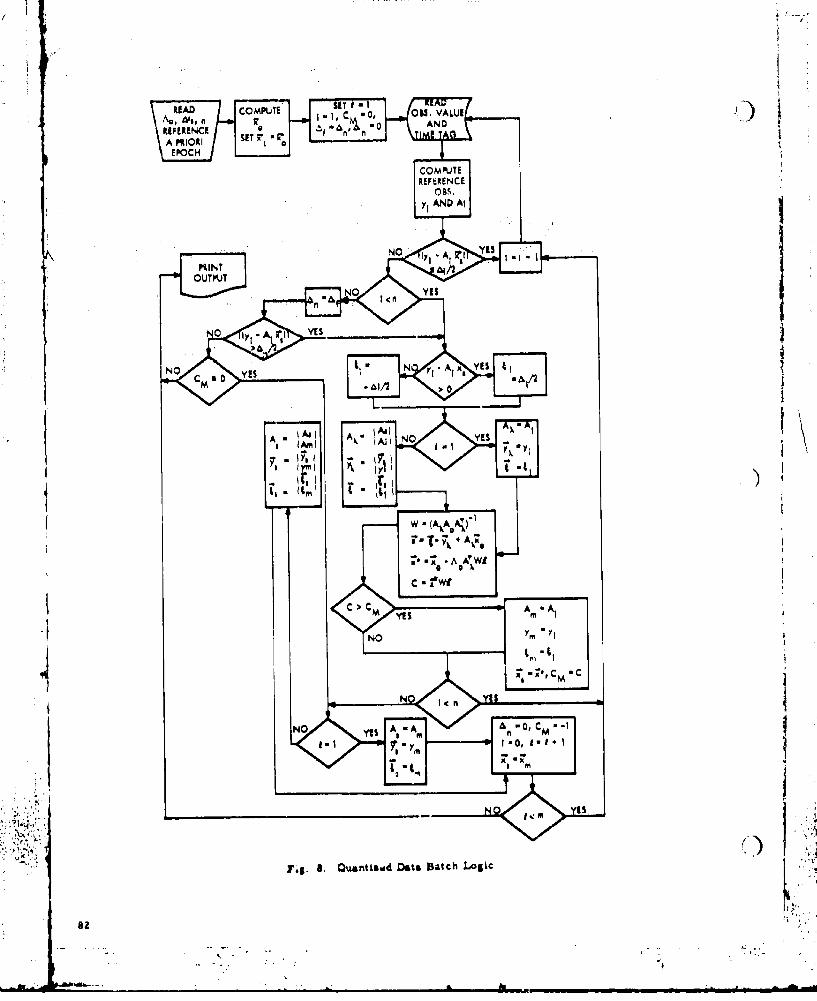
READ CC)MPUTf SIT IIIAvo AVito C -0, 015. VALUI

ANDRIFERINaA PRIORI SIT

EPOCH

COMPIUMREFERENCE

Olls.YI 4ND Ai

NO 1;e, -A rl YES

KINTOUTPUY

NO YIS

YES

ANO C 0 YES

L

A, I Ak-AlA, Aw I A NO YES

Arm (Aj Y,I yl I

W (AA.Aý)-'

+A

A,,IILWI

C

C CM YES Apm A

NO Y" "y,

I-C n

NO yjS A I Am Do Cm

yf"

ILK X,

ts

]rig. 8, Quantisled Data Batch Loogic

equal or until the observation constraints are and Is located 2.32cv units from the a priori.(satlified. The logic reqired for these batch The median, or 50% probability point, xsO mini-

computations is a subset of the logic for the mizes the first absolute momenteseqential algorithm.

In the general multi-dimensional casc, thereIs no simple way to determine the error In the F 5stA*e estimate. The a priori normal density must ten sasatesi tendi otd2.6abe integrated over ý.he area enclosed by the quann- uaknits fra stheat n Te estimate whis oaed22chtization constraints. The mage td 5f the error unt ro h apiri h un e sta mt hcIs bounded by the distance from the auto esimate minfmieso the maxi unetinty Is given byto the furthest constraint boundary around theteaih timanfteed itsndsregion of allowed estimates. A linear Mionte Carlo located 2.6vo units from the a priori. The roea-

aayi ypoietebsmenofdtmi- tivo virtues of each of these measures of centralIng estimation uncertainties, because of the location taken as a state estimate g* dependdifficulties which would be encountered in trying an what one wants to maximize and where one wantsto construct the bounding surface. the maximum to occur, The probability of In-

clusion In a oyimmstrIc intervalfor 4amon dimensionalP static model, the

sta'A and observation deviations are constant.' I,~~* 'xdThe maximum likelihood state estimate Is ¶ rlx.xlid -.0 j ~x' d x

(Y-A/Z)/a If Y.AxoiA/2 for each of these estimates Is shown In Fig. gas a function of d. As expected, the median is

X x0 If -A/2!y-ax 4a/2 then wbastm estimate for this criterion up to the0- point where the ynetric interval extends below

the break po tint tl!he density function. At(Y+6,/2)/& If y-ax0 -/ high probability levels, the mini-max aitimate

is best. because the lower half of the sywi-The robailiy desityfuntionIsnetric Interval does not contribute anthiný toThe robbiliy dnsit fuctio iathe probability Interval, the maximum 1 kel hood

estimate Is never best. On the other handI weif 11AIA2Is b more interested In maximizing the pro-

10 if1y-ax~A/ ility of Inclusion In an interval o? fixedf(X) lengtx cotinn heetmae2wt n ri

(l/v7 ( 0K x Pa trary mid-point. This probability4

otherwise. whlere P~xcl(x*,d)) ] f~x) dx

k * e(x- 01/xd is shown in Ni. 10 for our numerical example,

j dxTemid points eave been selected to maximizeth(y-A/2)/& prbability of inclusion for each of our estimates.

& ith Ithis performance criterion, the maximumnormalizes the density Integral, likelihood estimate is as good or better than any

other possible estimate.As a numierical example, suppose the qu&ati- 0f aalorithm for processilng data with* ~~~~~zation level 4/a is Wqa to the a priori standard nomal ianr ue roshd enue o u

deviation 0,, and the observation $y/a) occurs exrample h es-timate o ud r o nvherbe ven t usdfo1u2.o unts from x . Theadensity function, then, S pl thesiaewudcn erg vnualiosozro hni a is'en hn2Oouiso ra to (y/I$ - 2.6a.. The rate of convergence would

than3 Oounis frm x. medat estwiadepend on the ratio of the hypthetical measure-which ta izshe density is given by ment standard deviation a to the a priori stan-

max~~zesdard deviation a..

x'* ao IV. g2AjIZ1D-RQBML FILTMgbecause A comination of the two data types covered

In the preceding analyses occurs whem the atti-tudo sensor 11"1al is contaminated by normally

2.5o * (/a)-x~/ * os~.distributed, -JitOva nolise and then quantizedby/A diialei.1 iO This case is particularly44teresting In att tue determination prob!eMs

The mean T of the di stri butionm, taken at a itate because the sensors Aar usually noisy and desgestimate, minimizes the variance limitations on the satellite commnications sub-

insto usually preclude the use of leIngthy digitalwords for attitude sensor information.

83 A.~

-MF

0.0'.

0.4

INTIRVAL SIZE- IN UNITS

Fig. 9. Probability of Inclusion in an Asymmetric Interval

00

0, 2 ____

0.2 0.4_ ____0._____

rig. 10o. Probability of Inclusion in a Symmetric Interval

84

'I 7 7 T 7 , ---h- i;."

Them probability dnsity function for thejoint distribution on the a priori state end thequsntizid-normal sensor noiie is given by 106TA

L(*Xi~0 oS) - k ga (ýxIl* 0) gln (+x~ 5

where k is a normalization constant, -T *n

U T .'(y1+•1/'A1;)'/"o! ;1.y1/'A¢,'•)1 /2a

gives the functional dependence on the a prioriestimate, and

For the a Priori contribution,

i proportional to the probability that the popu.lation Rerameters defined by g assume the samplevalues y. The volume of integration V in n dimen-sional measurement space is bounded by g5 (•l•)

* + /2 Thus, the maximum likelihood condition

the quantization constraints. This is t a sinoacombnination of the continuous and discrete casesgiven in Ref. 2. If the sensor measurement error&s L(9A; ) g )are uncorrelated, then A is 4 diagonal matrixwith trace elements a', and *0

and the restriction that *• is arbitrar I Iythat the maximum likelihood stst, eltitl"y

! ÷/*,-A,1)2/2• di must satisfy the transcendental equation

y.tAi/2-

As before, in the derivation of the normal filter,the optimum can be found by equating the firstvariation of the density logarithm to ziro. For T .(ys+Ai/2.Ai;*)z/2oI .A 1 /2.A 1;*a,2atthe measurwaunt contribution. A1 T

yiyi+'i*zdVF I of 1A11 f/2a ,

8(xy) 61/2 (i~i) 2 2 yi-4 1/2 (1f +1 *2/2 For the take of brevity, this condition will be

e(*i'Aji)2/ O I written In the form

A+ r Aho#o• y 1'A 1/ 2 d• 1 -A•* 2• . C

/- M•ei(1*) -(yj-A/2%i*)1/2v1

_ _ _ _ __/ _A_1_/ 1 4 ( y 1* 1 i

I T _At__s _ -A I ' '

ft 1 i" A /J

fas

_______ .....�_,_.....___,_._�______-A. ,

On the surface, at least, Eq. (11) seem tobe amanable to solution by Newtonian iteration.We th-li denote the right-hand side of Eq. (11) W1 (0)A 1;x, - #1(;O)

by f(P), FroM a state vector astil P- wmy compute Z(x*w.), Expansion ofin ta •oemayt soimaute,~ Ine first oer series yelds replacing ylat In the numerator sunmmation.stteesfrs o r sA comutational procedure similar to the

+ -i= |.1( I Kalmen filter, Eqs. (7) and (8), is needed toa|= •-'1) * "~~ ;-comIlte the analoiy between normal and quantized-

I norma filters. A tar a large rmer of observa-tions have been taken, the state estlimte should

By differentlation of Eq. (11), be fairly stable. The state estimat#tIn after nmessurements and the state estimate XA.1 after

nT ) n-l leaiurlemnts should be nearly equal, After0IN1 A I A T-1mea n- ue ments, the transcendental mxnimur

1.1 likelihood condition Is given by

whereA

a ~ ~ -A/2A) (i I/2A*)h/20I~~ -A~d) ( ii)

t( L' "1'/ 10)2/20)S,[+A ./Z/,I24.Ai (y1 "^€/- ]^i*)2/2CI 2

a 1Y1 1 "0 J (12)

For n amasurements,

Thus, the Improved state estimate Isliven by T A n ( •.)Sn nA 1.1A In oide

""+ T,- + n,',t -T... .o . .n . .. . .. . .. . ,+ ' + . -, ,

[ - A W . (n.1"f, . )_ .1-A . A ,8~~~ ~~ ilLO )A 1*~13 L B -j" iu - n n

This eapreasion m be put in a more. convenientfarm~ Mirt of &lI we may let up u11.l bq for S;Iyieldreference state @stints, substitute for 1(i). uo rnyed

and perform saw algebraic manipylationst then, 4 ~ , qA ~ W(')~~

~' I ~ ~This expression is not what we want to sa".z TW(.A_.- *,1*] (14) BeKluse of computational difficiiti III we "a notwish(0)x to li edur andevalua itrMed WI1. oI

observtion.when~ 1 In the limit as Al hog qjhea *j, oeraIon Thajrror intoiducedml becu4aproac isa 1/od ) andl di ben torace I~f~~ ,i b.; toivt v,) )de

-( tlI/a Wi isal au "I 1aI4 fWWdeto ( EqIujto W (0 ) , replacng 110 1)In tdepend strongly on the state, the 1 nearitatiannormalI replacin andi t is Invalid Anyway, With this apoimaion we ()nov~~l matris and may defi nse I a ~ o a

86-'S I

and the normal filter estimate for a one dimin-ni .. stonel static model with a single observation

A;! A A .1) Atype approaches

an Y.~i-

A1 The quantized data may be brken Into groups.Each group will correspond to onm of the i1lowsd Iobservations Yk. The normal filter estimate will

Ny the Shur Identity, * at Pk Yk'

An " An'l . An'INAn'n'1 (16) where^n n.l n nq• m •.) yk+Al(

and the maximum likelihood state estimate is Pkgiven by Yk"4/2

4 A A T is the probability of being in the kh group.-" n n (16) Eich group has the se quentlzatlon-evel a end

AnA.nATw-;1(1*.I) the variance o' Is the san for all observations," n n If the samples are sy.mnetrical about their truemean, the normal filter will be asymptotically

These expressions are analogous to the normal exact. If the samples are not ,yVnetrical , asequential filter, Eqs. (7) end (8), nhe normal filter acting on quantlzed-normal datalimit as the quantization vanishes, W ( •I) will leave a bias error In the estimate. Numer- -'

in the donoiinator ipproaches on2 , wT Ishe ical calculations have been carried out for twoscaler rW- (iA•j)p(xg.l) in the numerator examilee: 6/o'l .0 with the man offset bypp r higs, n-Ann~ -0,2 a and A/a.4.0 with the mean offset by -l ,1.0n n-i For tme residual bias was 0,04 5, and,

In view of the similarl between the nor•ml for Oa-4.0, the residual bias was 0,37a,end quantized nor mal filters .1 h, b atch anid %@- The ostl matlon of p ar ameters In a dl stri-quential logics deoicribed in Figs. (1) and (2) bution of known form vie the xP-minimun methodwill be applicable In the quantized-mortal case is di~cuoiod by Chramr In Ref., 2, A priori

too Newtonian iteratlon using Eq. (11) should statistics are not used, the relationship betwp ib avo ided If po sii ble $ be c u se of th I co mput er the stat e ,end sim p le d at ai s s t atic( , and o n ly on etimecost if on-lpeartiesartsevere,thImplicist, daic non-ll1meirities ante ,s explicth data type is considered, Under these assumptions,

transcendental non-lnai•Itis and the explicit our tranicendental maximum likelihood conditionns the maximum my be written in the form

likelihood condition might be reducod simul-taneously using an Iterative batch logic, El[ ;(Yj+A./2"Ao1*)2/2c2 "-(Yj-6/2-AOi1)2/2,]

Estimation uncertaintles for the quantized- i. Ano~ral filter will not follow A normal distri-bution unless some simplifying assumptions are I+A/2 -(-ýA )made regarding the size of the quantization, In .general, a linear Konte Carlo analysis wouldseem to provide the most convenient means ofaccurtely evaluating filter perfovnce, where A. is the con€ n value of the Al. If the

sunmation is taken over k quantum groups, we haveAccording to Cramur, Ref, 2, the correction

to th mean for grouped data vanishes to termsof order four in a. This approximation Is no (Yk+A/-Ao)2/2Q2 -(y•-t/2.A )a/202longer valid when the quantization and measurement A a_ __kA_ __-

standard deviation are comparable in magnitude. Y-+AI? 0In theory, at least, the quantized-normal filter (will converge to the correct answer as the number f eof observatione increases. However, if the yk.AlI

/ normal filter were used to process quantized-mnormal data, the estimate might contain residualbiaie,, even when the number of observations I I where Yk is the number of obmervtilon, in the k~hInfinite. In the limit, the a priori Is swamped, group. The integral in the denominator Is

87

4 s--i... ~ - - - - -

bounding vertices, Theflogicproportional to the probability of Inclusion bound ;i nIn the group, and the product of' A with e peyfoh s t~m, 4aval-difference of the exponential terms in the num- able, could also be used tooirtor is proportional to the partial of the provide error bounds,probability Pk with respect to the state. Thus,the Condition on the estitmte may be written e Finally, the maximum likelihood

estimate may be the most detir-able in smae applications but not

P *k • O. in others. For quantized and-• quantized-normal data, algorithms

Vk 71* which compute the expected istator the state which minimlzei the

If there are m state components, this equation first absolute moment pra not yetprovides us with m condittions whi h the state available even though their po-\mwst satisfy. The quantity ipk/61* Is in xl tentill virtual are clear.row vector. This result is identical toEq. 30,3.3a of Ref, 2.

REFERENCESV. C 1. C. B. Solloway, L•I• a: the Theus r of

Orbit De ina _! ion, eit PopuIlsionWhen estimation accuracy is critical and Lao0ratory, EPD-.I5, Pasadena, California

the attitude sensor data are subject to quantiz. (9 December 1964),tion constraints, the errors introduced by pro-cessing quantized or quantized-normal data with a 2. Harold Cramer, Methods of Mathematicalsub-optimal normal filter may be Intolerable, On Statistics (Princeton Univen Ity Press,the basis of the prvceding analyses, there areitIspromising computational procedures for findingmaximum likelihood attitude state estimates in 3. T. A. ognes& and J. S. McGuire, Statisugjcases where quantization occurs but the data are of Orbit Determi•.•ion-Correlate-sieirvo-a otherwi• error free and in cases where the data 5L, Space TUc norogy Laboratoriesare quantized after being sampled from a normal ocumnt No. 897-6001 -RU-000population, These ilgorithms are comparable In (15 December 1961),generality and flexibility to the normal filtersconno•l used for trajectory or attitude estima- 4. David C. Morrison, 'Methods for Nor-Linear )tion. Unfortunately, they are also more complex, Least Squarei Problems and Convergence

Proofs,'.' ,Seminar Cclodingl, TrktngOne most significant conclusion is the Programs and Orbiliterm l ULe .

equivalence In form between the normal and FPU1610M LCalifOy, FiskoIna, •11fornia,quantized-normal logic flows. Any computer pro- 23-20 February 1960),gram deal nod to process normal data can beealy modified, if necessary, to handle quantized- S. T. A, Magness and J. B. Mc•uire, Sttistliisno1ýmel dtof Orbit OstormlnaltlOn-Wetghtld 6l.tV. ;

nradata. 39vorls SecT O airmii.giWi atostIj1Some potentially Interesting research topics, XscU pient No. 697Te6002lOyI

with practical applications, appear to have beendiscovered during this study. 6. W, B Galles Elrmlontion of Stieas due to

Bias in a UiAMan Filter, A. C. Electronics

o Although a linear Rcnte Carlo analysti 13T191:on, General motors Corp,, Memorandumdoes provide a way to evaluate astima- 48-480-m (8 July 1966),tion uncertainties, there may be others,less obvious but more satisfying, 7. drwin Ira Sh prro, The Pld•ctlin of

S s1l l 1 ;t • M I 1 1 1 1 T r lj iat or ; e U P~ T R a d ar

I Because of their complexity? the servaona kmcuraw-mi11, mew or,accuracy eIhancement capab 1ityof these ftters should be tested 8. R. S, lucy and P. 0. Joseph,for each new potential application, tar Stochjltt cIll wjthRD orlThe estimation accuracy requirements$ .0 i oriciari Publishers. 195).for the application In question may

not be stringent enough to warrant 9. Barry H. Whlan, Linler Itigrl Ind fortheir use, Mal it-lornal , Berkeley. D e ll n ,

a The conve ence properties of the 1962),proposed Algorithms should bestudied, 10. T C, Koopm ad,, ac$1U AnalsP ctio n twiey, New or,

a The munt of data procesmed by lgl) unapter XX], Q. a. 1Dntltg,'a quantized filter could posiblybe reduced by keeping track of the

IT:

II

APPLZCATIONS OF NONLINFAR ESTIMATION THEORYTO SPACECRAFT ATTITUDE DETERMINATION SYSTEMS'

D, B. Jackson

bpaoe Flight Systems, Aerospace DivisionHoneywell, Inc.

Office of Control Thuory and ApplicationNASA Fleotronics Research Center

Cambridge, MassachusettsA1STRACT

This piiper describes the application of some recent developmnents In stochastic

estimation theory to the mechanization of strapdown attitude reference systems forspacecraft. The attitude reference problem statement and the growing need for a non-linear formulation are briefly reviewed, along with some applicable elements of non-linear estimation theory, Seve'a1 alternate att4tude reference mechaniSations are out-lined, and then some state variable, state measurement, end noise modeling considera-tions, coupled with computational estimates, are shown to dictate a clear-cut preferencefor a particular mechanization. A typical configuration for an advanced spacecraftattitude reference system is then postulated, and some simulation results of the per-formance of this system are presented, The simulation results show that the moment-I approximating approach to nonlinear estimation results in better system performancethan several other approaches for the class of nonllnearities found In attitude refer-ence system equations.

IZ, NHTKDUCTZON neceemarn assumptions of linearity arevery good H However, for the more general

Linear optimal filtering theory class of spacecraft attitude reference(Refs. 1,3) has played an important role systems, assumptions of linearity breakin the field of spacecraft trajectory down. for:11l-attitude or 116:rg angledetermination since about 1962 (Ref. 3). maneuvering eystems, the equat one ofSine that time , linear filtering has had motion be am highly nonlinear. fon less

important a plicatione in the aerospace precise systems, amsumptions of small|areas of ueleostial spaoe nvavigation, agir- deviations from a nominal attitude tra-

craft navigation, reentry veh ile trajec- jectory break down. For gyroless a a-"eatory timation, orbit determination, tame, a nominal trajeoryt about which

launch vehicle ascent guidance, and dif- one can linearise coefficients is notferent types of system error analysis. available. Therefore, a universallyThere have been Important non-aerospace applicable attitude reference filteringapplications as well. Recently, the need mechanisation should be based on a non-for high precision spacecraft attitude linear formulation if possible. Thisdetermination has led to the application nonlinear torwulation should also haveof real-tims linear filtering in this the property that it reduces to thearea (Ref. 4). The latter use of linear classical linear mechanization in thefilteri.ng has been made possible by the limit. .

advent of the small, low power, flight-

weight general purpose digital computer. The estimation philosophy that isfollowed in this paper is based on entire-The Kalman-Buoy linear filtering I Bayesian models for the state and

theory works very well for small angle observation noise proceese, and the

precision attitude reference, since the estimation criteria will be minimum

IThis work was supported in part by the NASA Electronics Research Center's Senior( Residence Pron in the Off ie of Control Theory and Application (OCTA),

, ,9

varianoe with the best estimate defined ftogliqibls. Rather, only certainaa the conditional mean. Theoe are a plausible arguments about the shape ofnumber of other estimation criteria and the conditional probability den3itynoise models which have been studied in function Are necessary.the liter:atu:e. For instance, Kushner(Ref. 5) and Pfeiffer, at al. (Ref. 6) Based on this approach, the paperhave studied filters whose estimate is describes the formulation of a compre-the made of the conditional density hansive attitude reference meohaniaktionj

(maximur likelihood estimation), and capable of being implemented in real timeL&May (Ref. 7) and Schweape (Ref. 8) in a spacecraft cexputnr. The formula-have studied the propagation of possible tion is general enough to accoodate nnystate boundaries when the inputs are combination of discrete and contJnuousdescribable in a set-theoretic context attitude and angular rate measurements.instead of a probabilistic framework. A typical configuration for an advanced

spececraft attitude reference system isHowever, for the attitude reference then described. The perino ance of this

problem at hand, the Dayesian minimum system in the face of various levels ofvariance formulation is appealing Mor state and observation noise is demon-several reasons. Firet, it turns cut strated by showing a number of resultsthat most modern inertial component from a digital simulation of the system.erraor can be modeled nicely in terms of $ome non-theoretical questions are thendeterministic and probabilistic processes. briefly discussed relating to theAlso, the minimum estimation variance practicality of the system postulated.criterion leads to a formal filter whichinvolves expectationo of products ofprocese, observation, and state compo- 11. AMY¥|snents. When Euler's quaternion para-meters or direction cosines are used to A. Attitude Reference Problem Stotementdescribe the attitude state components, and Backgroundthis expectation operation leads tointegrals of products of state variables The fundaAkental point from which mostand marqii~al conditional densities that state-of-the-art precisicn spacecraft inever have to be integrated explicitly, attitude reference system syntheses

proceed is the assumption of three-axisWhen the attitude dynamics arq toy- body angular rate information, usually

resented by nonlinear differential squa- in the form ofa three-axis, strappedtione and nonlinear state measurements down, single de ree-of-freedom gyroare assumed, it can be shown that the package. Experlence on a number of pro-state probability density function, grams of this nature has indicated thatconditioned on all the ;a&t measurements, this is the best and uften the onlysatisfies A partial differential equa- method of achieving precision, wide band-tion similar to Kolmogorov's forward width attitude information in a benignequation. Using this result and the zt6 environment when the heavily weightedcalculus, it is possible to derive the parameters are simplicity, high precision,differential equations for all the and reliability. The output from thismoments of the conditional density. The triad will be continuous analog voltagesformal details are given in Kushner or trails of digital rebalance pulses.(Ref. 9). These output signals are then integrated

on a three-axis transformation basis toThe problem with implementing an obtain a continuous indication of inertial

attitude estimator based on this formu- attitude.lation is that expectations of functionsat least oubicly nonlinear in the state The basic problem whiuh must beare involved. Therefore, these expecta- solved in any attitude reference systemtion terms are functions of higher of this type is the bounding Qf the long-moments. in turn, the differential equa- turm attitude errors. These errors aretions for these higher moments involve caused primarily by gyro drift and scalestill higher moments, et., and the exact factor uncertainties and by integrationsolution would require an infinite number algorithm imperfeutivns. Therefore, someof differential equations. In most of method of periodically injecting directthe literature on nonlinear estimation, ettitude information into the attitudethe infinite dimensional problem is reference system is necessary. Toresolved by expanding nonl inear functions illustrate the dynamics of the situation,in Taylor series about the expected ionsider Pig. 1.value of the state and truncating theseries. However, for the attitude asti- The system illustrated in this figureS arionproblem at hand, it is unneoessary is a e sh as all theto invo e arguments about the higher salient error propagation features of more lw

S order terms of series expansion@ being sophisticated three-axis systems.

ssm

measurements are received only' at discexteyj. points in time, instead of on a continuous

basis. This type of system ha. an error 1NJ ~ dynamics mystoo th~at can be appiroximitted

N 1 as a mmmpled data control system. liach aErepresentation is shown in Pig., 4.

REAL A

Fig. 1. Singis-axla Attitude Fg .Attd ro rqecReference 3yotem RsceCercteito

True vehicle rate, 6Tj is corrupted by i -1tyo noise and~biales (N) and appears to lt

Uh ytma M This is integratedcontiytma Nnuously to obtain a running measureol true attitude, I I. To bound 0 Nm 9periodic or continuous measuremeni s aremade of attitude (IT) directly. Thesemeamurements are also corrupted by sensornoise (N') and the attitudo measurementsloappear to the system am S. * is thencompared to ON and the diliferelce isused to generate feedback signals to Fig. 4. Single-ax~s Black Diagram -

*An error block diagram correspend~ng to It is possible to analyse this typethe above system appears in Pig,* 2. of a system by s-transform and v-plane

techniques. This analysis yields error*e frequenc response charaoteristics that

*~~I haeprodic behavior at half the samp-ling 2requenoy for the sampled attitude

41~ sgnal. For the continuous attitudeeror signal in this systems modified s

transforms could be used to obtain the

Fig. 2. Single-axii Error Block Diagramreoneadtercaae-This discussion was simply included

The transfer function for systems of to indicate that a gi ver attitude refset-this type is once system mechanisation requires knowi1

edge not only of the magnitude of themeasured angular rate null offset and

0 /a noise, but also knowledge of its spectralA. Cl) characteristics in order to predict

e attitude ezror values of the system. It9 5 + is clear from Fig. 3 that a bounded2~aittitude reference system is loes sensi-

Thrfrthe effect of addinth tive to hi~jh-trequenoy noise than it isThereforeynose de o hattitude measurement sequence tNws to oilwhfrentmothng inoie due atoithdeitg

change the attitude error frequency re- raion.een Whn moth in the attitude itgspones characteristics tram those shown ratif.eren @yet= otisi anpe attitudein Fig. 3 (a) to those in Pig. 3 (b). reoernceqsystemofnhs mu t e bhe anowredIn other words, when attitude measurementi lwn usin utb nwrdare added the offset@ of low frequency Whtcmnesofgr ditand d-c rate measuzement errors are no rate and a~titude measurementlonger catastrophic. The situation isero inlnc th acucy fslightly more complicated when attitudeero inlncthacucy f

29

an updated attitude e dedrene d process wioheyqstM, Iad whatare the se- pc wimatical zelatioz'hipi'tht,!deocriL the dependence of my$- !CE(t)E'(•)] = 2(t)e(t=) (4)ta erro or, those comonentOT

where 6(.) in the Dirac delta. The came(2) Given the. answer to t.he first wher:e O depends explicitly an x(t) willquestion, how should the not be-itudied, as thin leads ao

attitude reference syst~em be lengthy and subtle argument about the. echeanud tL.o ninomiae om*e difference between the ItO calculus andLnoasure of , lyate error, l•., I ,tratonavica• alculus for the differen-how 4hou.d the' feedbqtck gains tiad e ~functions of solutions ofbe ch" eon as a 9aaftion of . stcohaitia diffarential equations. Any-Sinitial 6ondL Womti o rsand way, thLsgenerality will not be neededtime?. afor the problem at hand.

Ixtmnsivo.1pboratory tasting -adThe problem is to continuously euti-analyticl rModelingestudies have, been' mate the state •(t• from the corrupted

,P.orofind reatetly for predision inertial observations"sensors (Rut. 4),." The t:sults oftiae , t, , "se

stUdies indicate that in the frequency .(t) W z I (t), I + V(t) (()range of intiroct,'precision rate andattitude instruims toof the type being where X and are •x and v(t) is an txluaed,'in curtent syctema have randou error aere-mean whita Gaummian noime processoharaoteristics that can be modeled quite withaccurately am normally distributed whiterandom processes. This fortunate cir- [V W)V 1 (. 1 (t) (t'T)oumstanee allowe one to turn effectivelyto the extensive literature on linear • and R are amsumed to be real symmetricand nonlinear stochastic estimation positive definite (RIPD) matrices, and intheory to implement a system in come addition it is assumed that"optimal" gonie.

B. APNji¢•ll 1meentf of NonlinearXtma ~on ETx0)' t) *(B

Thui subsoetion will review briefly z[w(t)y' C)] a l: y t,o io (3)iome of the oon•epts of nonlinear elti-mntion theory that have a bearing on theattitulde referenoe problem. it should !(O) in a Gaussian procemI with maan 9Le viewed am a skimpy and nonrigorous andsummary. For extensive and mathematicallycotisfying expoiitioni of the subject,refer to XuIhnOr (Reifs. 10,11), Wonham ([x(O)-x o][(O)-x 1') A P(O) - '_ (10)(Ref. 12), Buoy (Ref. 13), No and Lee 0r(Ref. 14), and Pfeiffer, at al., (Ref. 5). wwhere p_ Im RIPO. under the ahoy.

Am stated in the introductLon, the ammwnpt'ons, it can be shown (Ref. 11)procems and observation noise models are that the probability denmity function,Dayeaian and the estimation criterion ia conditioned on all the pact measurements,minimum emtimation error variance, with which describec the distribution of x(t)the best state estimate therefore being matisfies the following partial differen-the mear, of the conditional probability tial equation:denmity function. Ipscifoiae Ily, thediffrerutial equation describing theevolution of the state of the dynami•£lsystem IN ~g~Qt~i

d!L N)/dt - [(EWt),t + 0t) W (t) (2)* Pa '( It• " Ii~ ff Hi ) ' I' l( t I (• ( U, - "[s.,-] I o ',

Em0 Ko (3)

where x and 7 are nxl, g is nxk, and v(t) where

is a k;'l sero-msan white Gaussian noile l

i .:: *:,. , ,.. . . .• 92•. : .. ,

4 I(12) 1 1x 9 x 1 ?(

(This partial differential equation with- x(.,out the last term (observation@) is tn e etc. tFokker-Plank-Xolmicgorov equation for theforward evolution of the unconditional However, for the estimation problemdensity,) Using this result and the It8 at hand, it will be unnecessary to invokecalculus, it is possible to derive the arguments about the higher order terms ofdifferential equations for all the series expansions being negligible.moments of P . The formal details are Rather, only certain plausible argumentsgiven in Xuefner (Ref. I), The results about the shape of the conditional proba-for the first twQ mcments can be ex- bility density function will be necessary.pressed in a ompact notation which is The reason this is iossble will becomesggested by JalAinski (Ref. 15). The apparent in what follows.conditional Aeon and covariance differ-ential eqetione are given by The equations for updating the state

estimate and covariance equations atdiscrete updates can be formulatsd from

SI"t,/,d. a ,ayes rule approach. Ho and Lee (Cef.I''a'' 11 ii'u'I *ii! 14) have a very readable account of this",At -* 1/.i, I w* g&,.msi-lk,[l - ,IW. and Jaswinski (Ref. 16) gives the results

u,,I |(,) .•e,* , .{, ~ of some further studies in this area.When the discrete observations turn out• to be linear in the Stat, which is often

* II {m. 2 l ~l ,Kll-lI• [Itl •the case in updated attitude r•efrence• l.I[mlti~ttLll. aIIr.,l't sllmywitems, the discrete xalman filter up-* 2amIuurLF~I' atI•Al~( ;date equations can be used to calculate

the state estimate and covariance matrixdiscontinuities at which occur at discretemeasurement time,

This filter reduces to the Kalman-Sucy C. hltrn' ts Atttud e ferln -l

continuous time filter when r and H arelinear in x. The problem wiEh impTement-ing the above estimator is that terms The ultimate output of any attitudelike EzxI') and (xLH') are involved. reference system is ome periodic orlince F and/or H is nonlinear in to these continuous measure of vehicle attitudeexpectation terms are functions a[ higher with respect to a reference coordinatemoments. In turn, the differential equa- system. Performance-orLented goals, whentions for these higher moments involve eachanising an attitude reference system,still highoe moments, etc., and the exact involve minimizing a functional measuresolutian would require a countable infin- of attitude error with fixed levels ofite number of differential equations. sensor error, or, conversely, maximioing

the acceptable levels of sensor errorIn most of the literature on nonlinear consistent with meeting a fixed level of

estimation, the infinite dimensional stem accuracy. There are a number ofproblem is resolved by expanding an f(x) alternate mathematical formulations for

n a Taylor's soeris about the expected the attitude reference problem which arevalue of X, formally equivalent. However, it will

be shown that the choice of a particularformulation has a profound influence onsuch things as the ease with which optimal

2 2 or suboptimal estimation theory can bef CA) + N-E) applied, computational loading, and accur-

" = acy.

The systems discussed in this report(15) are limited to those that derive an

attitude transformation matrix withrespect to a coordinate system fixed in

Then the various expected values take the inertial space. The basica ideas, however, Nform are easily carried over to more msecial-soed classes of system@# much cs$oal- |L' •:,•

2 ,x" =wvertical oriented systems.WW f(* + 1P16 2 x x0* For any arbitrary orientation of an

93

L _ . " •

attitude reference ayatet, there exists *2 ( sin (x 3 ) p + cos (x 3 )q) see (x1 )a unique real orthogonal transformation(1x3) Pi_(xmatrix T which inertial vectors *3 + 'n (x3) PSXz into-15dy vect"ors X Ie + coo (x3)Ql tan (x2) 2 r (22)

The Euler angle formulations have thestrong disadvantage that both the differ-

where ential equations and the direction cosineequations involve nonlinear (trigonometricand product) functions of the Suler angles.

L1' 13 Also, the differential equations have alI- L1a3 sin ularity at x. w/ /2. Xowever, Ruler

21 .23 parameter ttrans;ormation systems.j t3 t33. Mortenson (Ratf, 16) give a Very interest-

ing disoussion Of the no-alled Rodriques-Cayley parameter@, which have the distinct

The objective of the attitude rotor- advantage of differential and directiononce system is to acmt up with the most Cosine equations which haveonly quadraticaccurate running estimate possible for nonlinearities, which are comput ationallythis nine-element direction cosine matrix, much limpler than trio nometr i non-There are many parametric systems which linaritiesm.are comconly used to define uniquely thediaection cosine matrixt One of the most commonly used four- .

parameter systems is the Ru1c quatoenicnparameter system (oftun roferred to as

ti* a f(Xi'X32u''Xn)' (20) Euler'l :•sy•trical parameters), a die-CuBsion of which can be found in Mitchelland Rogers (Ref. 19). for quaternions,

The most Commonly used values of n are 3, the direction cosine element equations4, and 9. The smallest value of n have the formsufficient to define uniquely TJI is 3.The most commonly used three-parameter 2 2 2 2

systems, a discussion of which can befound in Ooldetein (ef. 17). ror an t a 2(x X +often-used spacecraft let of Ruler angles 12 2 3 1in the pi:ch-roll-yaw sequence, thedircttion cosine eheont equations have £13 2 2(x3x4 "the form

£21 " 2(x233 - xlx4 )

L Co - Gas ( (Y + CM1) XI @ ÷N2 - xN -+2 X

-13 - -. in (C16 oCe (A3) + aim (N) coo (X2 ) Bi' (n £33 * (232( 4 2+ lx2 )

433 " -c"s (xM) sin (N3) 4 It?% (X) sin (NJ) coo NM3 )

c22 - oo (XMC cog CM3) 131 2 2(x 2 x4 + XIx 3 )

L,3 , sin (•12) sin (X3 ) + aii (XN ) cog (NJ) coo M3 t3 2 (2•S(3X4 K1112

93 - Cos (XI) sin (192)

13 --sn K) X + 2 x2 (23)L|| ~~~21 • ln(133 1 4l 2 3l"X l.(3

L33 " cog (91) cog (NJ)In this case, the differential equa-

ticns relating the Euler quaternion para-

The differential equations relating the meters to the body-axis angular velocityEuler angles to the body axis components components "arepo q, and r of the total angular velocityvector are in this case Au 1 /2 (x4 P .,* x~r - x3 q) ,!'

1 oos N3) p -sin (x)q * 1/2 (x

94

K3 - 1/2 (x 4r + xlq - X2P) Notice that now all the equations arelinear in the attitude parameters. This,

*4 w -1/2 (xp + x2 q + xr). (24E however, came at the expense of increas-3r ing the number of parameters significantly.

Also, four- and nine-parameters are notall independent, and the resulting trans-

With this formulation, the direction formation matrix can boeome non-orthoqonalcosine equations bocme quadratic, non- because of computational errors. This islinear equations, and the quaternion not usually a practical problem though,differential equations are linear func- since an occasional orthonormalisationtions of the quaternions. (In the case procedure will siffice to pzevent degen-I of the Rodriques-Cayley parameters, the eration of T-81differential equations are quadraticallynonlinear.) There are nuerous other The only thing that remains in thefour-parameter set used to describe spcification of the attitude referencespatial rotations in quantum mechanics, such algorithm (exclusive of estimation) isas the Cayley-Xlein parameter set (Ref. the determination of the body angular17). Theme parameters are computationally rate components p, q, and r that driveunappealing for the spaceraft dynamics the attitude parameter differential equa-situation, however, since the parameters thons. ror a general torque-free rigidare omuplex variables, space vehicle (the only type considered

here) the 4ifferential equations for theThe most direct, and often the best body angular rate components are (Raf.

way to obtain the desired transfoymation 20)matrix is to deal with a non -paaaetersystem, i.e., the direction cosaaIes them-selves. The transformation matrix 131 - INY - Yis written directly in terms of theparameters, and the direction cosine Y . Cr- V%

* differential equations are

'In I Lr - 43 1 r (21) I-IY) ry, (11 t1 3where the Ii are the moments of inertia

L r t about the rte measurement coordinate* 12 " t22 3 2 q system axes and the Ii4 are the corres-

ponding products of in rtia. It is cleart 13 " -23r t 33q that these equations can be written as

the following quadratic first-order-1 .t 3 1 p -£.Llr vector nonlinear differential equationt

£22 " t 3 2p - 412 r ''

t 23w " 3 3p - 41 3r qrpr (29)

t31 •tllq - t 21 p p2

2~3 12q -*q•32 " t1q 22P .

' • r2£33 " t 1 3 q " (25)

These equations can also be written as where I is a constant UxS matrix which isa complicated, but constant, alqebraic

S(26) )function of the noments and products of- inertia. In this study, attention will

where 4 ia the 3x3 direction cosine matrix be focused on the simpler Principal axisand equational

I r -q &qr

n r0 p(27) ma 2 Prq -p 0 t = a 3pq (30)

S~95}4'4.

where This could represent a short-term attitudereference system, or a periodically up-

a I (I-Y / I dated attitude reference system duringthe period between updates. Suppose, forpurposes of illustration, that the only

a2 9 x y error component in the output of the gyrois a4ditive Gaussian white noise. In

a3 * (x-Iy)/Is (31) this came, the dynamical system is givenby

If the body angular rates are measured (t)l 1 (t)about a non-principal axis coordinate I F 8(t)system, they can easily be transformed L Iinto a principal axis system by a con- a2 t) 2 (32)stant 3x3 matrix transformation and thecomputations can take place in thatcoordinate frame, so there is no lose of and noisy cuntinuous observations aregenerality by the principal axis assump- antion. If external or attitude control takensystem torques are to be included in thedynamics, they must be modeled and [ 1inc)uded in the angular rate differential y(t) - tO 1L + v(t)equations. However, this is beyond the 2(t)intended scope of this study and willnot be included here. a H e(t) + v(t) (33)

it is well known (Ref. 17) that thesolutions of the principal axis angular where v(t) is a scalar sero-mean whiterate equations are elliptic integrals Gaussian noise process withof the second kind. When two of themoments of inertia are equal (disk-shaped, rod-shaped, or bodies of revolu- E~v(t)v(Tfl d 2 d(t-T) (34)tion) the elliptic integral solutionsdegenerate to sinusoidal solutions, andwhen all three moments of inertia are 81 is the attitude and 52 is the attitudeequal (inertial spheres) the differential rate component of the state vector 8.equations decouple, with constant eolu- Notice that the attitude dynamics aretions. However, these facts are irrele- modeled as those of a constantly rotatingvant to numerical integration mechanisa- untorqued vehicle.tions in real systems and are of noconsequence here. Normally an attitude estimate 1(t) is

derived from this type of symteam by simplyintegrating the gyro output y(t). In this

D. State-Variable, State-Measureent' came, it can be shown (Appen,.ix A) thatand Noise-Modeling Consideratione the attitude error variance diverges as

There is considerable latitude in the 2 2 2selection of state variables, attitude E[eI(tW-8ljt)] * E9I (0)-e 1Io)]2 treference dynamics, and component noisemodels for systems of the types consideredhere. This is a subject which can have In other words, the standard deviation ofa profound impact on systnm performance the attitude error diverges as the squareand often receives far too little atten- root of time. Consider, on the othertion. One of the dangers of optimal and hand, a mechanization based cn the Kalman-suboptimal estimation is that the effects Buoy continuous time linear filter. Inon system performance of noise and this came, the state estimate is the solu-dynamics modeling errors are subtle, hard tion ofto evaluate, and sometimes disastrous."Although some work has been done in thisarea for linear systems (Ref. 21), the di(t)/dt - F 0(t) + K(t) (y(t)-H e(t))impact on complex systems is essentially S(36)an open question, and can only beresolved in a particular situation by where K(t) - P(t) H'(t) a.2 (37)considerable simulation work.

andh Consider a simple example, namely, a

single-axis attitude reference system dP(t)/dt (38)whose only sensor is a rate gyro, operat- 2ing on a single axis, untarqued vehicle. F PWt + PWt E'- (t) H.a-2 H p~t)

with initial conditions 2p22(0)t 2SP~tt) -Pll() +(46)

i(0) - E[8(0)J - _(( (39) t) + P 2 2 (0)t

Thus, the behavior of the attitude errorP(0) a I{CeI0)-8(0)J (e(01-B(0)]'} variance for the filter system is quite

different from that of the conventional" PC (R8PD) (40) system. The time behavior of the two

variances is shown in Fig. 5.

Then Consider the beha-ior of the filtersystem performance in the face of adynamics model error such as a small,

P(t) unknown torque T I

z([{ ct (te t) ] it)-_(t)]1) (41)

For this simple case, this Riccati equa- (t) 0 e (t) Ttion, although nonlinear, can be solved le; 2 1 1 Ol [e2(t] [TJ 4analytically. After some tedium, thesolution is

where T. is not modeled in the filter.In this case, the transient behavior of

p1 1 (t) y1 2 (t) the estimate error is no longer given by"E(t) (42) the computed covariance matrix and is

t )difficult to analyze analytically. Pow-p 12(t P22(t ever, the steady-state behavior of the

error can be evaluated by examining thewhere steady-state filter gaini

,DNA

(, iPlll t) pll(0) (43) .Y11,

P2 2 (0) a2210t d

o2pl2 ()t 2 - 2 2 p 1 2 (O)t-p22 (O)t

o + p 2 2 (0)1t Fig. 5. Attitude Error Variancesvs, Tims

22 (0P121) + P 2 2 (0)t) K 1 im PP1 2 (t) (4 P2 2 (0)t trl 1 r-

P2 (t p(t)-lim ()J ['] a-

t-0(t 01(t p2 2 ()1Sp22~~(t) 0 2+ P22(01)15 .1 • .:

=+ p 2 (O)t L0oJThus

Consider the cam ir 0) 0i.e., that the initial at'itu•| and rate [01 ip (49) 'estimate errors are uncorrelated. This e. * A [y(t)-e2 owill be the case in most attitude refer- 0 8.2 0 " 1once syetams since attitude initialisa- 5'..'•.tion and rate information conb fromcompletely independent sources. Then the -6 + (y(t)-8 y(t)attitude error variance equation reduces 2lw 2to e2 -+ v(t), e2 w - ( 0)u

97mr

Therefore, it is clear that For the present, gyro uncertaintieswill be modeled as normally distributed

d W80 -810) 21 C 2 stationary white noise processes. Thea E( ~question of gyro biases (constant driftrates) will not be considered here,

which is the same steady-state behavior although it is an easy extension of whatas the conventional system and the follows. Essentially, the unknown biases"exaot" filter system. The transient become components of the augmented statebehavior certainly can be no better than with no dynamics or directthe "exact' filter system and for typical measurements. Thus, biases introduce novalues of system parameters (small model additional nonlinearities into the systemerrors) probably lies somewhere between or measurement equations and oomplicatethe exact and conventional system per- estimation only in the sense that theyformance curves. However, in certain increase the dimension of tCie state.instances it could be worse than the Therefore, since the main emphasis hereconventional system. is to explore the nonlinear estimation

aspects of attitude reference systems,An important point is that the con- biases will be assumed to be sero to keep

ventional system mechanization amounts things computationally reasonable.to considering that the noise is drivingthe plant rather than influencing the Let the state of the attitude referencemeasurement. in this case, after separ- system be described by a sufficient setating out the perfectly melaured portion of attitude pirameters and the three bodyof the system, the state equation is of angular rates. The state equation willthe form be written in the form

Ae1 - rbe I + Gw(t) with F n 0, Q * 1 and dx(t)/dt - Fix(t), tI (53)

E tw( *)] = o2 61t-.r) (51) where the explicit dependence of F on timeis to indicate that in the generaT casethe attitude dynamics could include known

Then the attitude variance is forcing terms (torques). Attention will )bo centered on Euler angles, Suler

2 pquaternion parameters. or directionP klt) (0) + V t (52) cosines for the choice of attitude para-meters. Zn this case,

for systems where rate dynamics are not c x, sin (x3)

taken into account, as it keeps thefilter qains from approaching sezo whenattitude measurements are included in T[x(t) = axI x6the system. &2x4x6

The poai;t of this oversimplified a3x 4 x 5example is that how one models attitudereference system dynamics, measurements,ad uncertainties plays just as important 12xx+a role in determining the performance of [ 4 5 2 x7 3x,an actual system as does the skill with .which one applies optimal filteringtheory. Unfortunately (or fortunately, or a Xfrom a job security standpoint) the 7modeling question is one which has nopat answer, and can be resolved in an a xindividual case only by extensive analy-tical and simulation studies. The queas-tion of modeling will not be broachedhear, since this is a more general studyof attitude reference systems. Rather,plausible models will be assumed forsystem, measurement, and noise phenomena, or alXllx,2 (54)and my stem performance will be evaluatedin this constrained situation withseveral approaches to state variable a x -estimation.

98 1

where [ c ln + V (t)- I " 1xlI~v~T

x2 0 t2 where the subscripts A and R refer toattitude and rate components, respectively.lines the attitude and rate components ofthe measurement are uncorrelated, R(t)

xn "n has the form

X +1• pn

xn+2 q R(t) - (60)n~ ~ a _R•t(t)Xn+3 r (55)n

so that R(t) in invertible asand -slm ' ""~~y 5 ' "~Fl) ';T; .'; 1"/- It) is I

x y 1WN-Ix - I L ! j((a 3 ig (6 - i

This fact will be ver useful in the

The t4 i - 1, n are the generalized &qasnetrsIk

attitude parameters. The problem will be -1formulated mc that continuous and dis- (I(aH(x,t)W)' A (t) (W by,(t)]crete attitude and/or rate observationscan be accommodated. The filter will bed rived so that the conditional mean and can be separated into the two terms

( covariance differential equations evolveincluding the effects of the continuousmeasurements and the effects of the {ERea,(xt)I)' • (t) (Elby.t)])discrete measurements are taken intoaccount by a separate calculation at themeasurement times. Consider only con- + (ECONR(XR~t)]Y' R (t) (ElbyR(t)])tinuous nonlinear measurements of theform

This fact will permit separation of theterms involving attitude and rate measure-

X(t) w HCX(t),tI + v(t) (57) ments 4.n the filter equationp and easyevaluation of the individual contributionsof thesw measurements,

where v(t) is a tero-mean continuouswhite 5aussian noise process with Consider now the impact of the choice

of the attitude parameter met on the ease(58) of mechanization of the nonlinear estimator.

EV(t)V' (•)3 * R(t)6(t-T), R is RSPD The Euler angle differeaitial equationsgiven earlier have terms on the righthand side like

Since in practically any attitudereference system the observations ofattitude and rate are performed by x 5tan (x1) coo Nx3)sensors that are sliearte physical on-tities with little in omoon (with thepossible exception of a oommon power Therefore, the mechanization of the non-supply), it is a very reasonable assump- linear estimator leads to terms liketion that the attitude and rate measure-ment errors are uncorrelated. This Elx tan (x com (xpermits a convenient partitioning of the x ta ,K)c:'x)measurement process and noise variancef f x5 tan (x 1 ) coo (x 3 )Nmatricesti ! - 7-13

[A(t)] PM(xl,x 3 ,xV ,t) dx 1 dx 3 dx 5 (62)

99

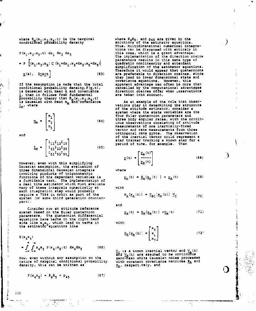
where P (x ,x ,x ,t) is the marginal where 905, and P4 5 are given by theconditional plobibility density solutions of the estimator equations.

Thus, multidimensional numerical integra-tions can be dispensed with entirely in

P(xlx 3 ,x, 1 t) dx1 dx 3 dx5 this case, which is a great advantage.The implementation of the direction cosine

r parameters results in this same type of•P L(XX 3 ,fX) C (Cl+dxlX 3+dx3 ,x +dx,)l quadratic nonlinearity and attendant

simplification of the estimator equations.Therefore it would appear that quaternions

y(s), 0<s<t (63) are preferable to direction cosines, sincethey lead to lower dimensional state andcovariance equations. However, this

If the assumption is made that the total apparent advantage can often be more thanconditional probability density,P(x,t), cancelled by the computational advantagesis Gaussian with mean m and covariance direction cosines offer when ,boervationsE, then it follows froid fundamental are taken into account.probability theory that P(x 1 ,X ,X ,t)is Gaussian with mean r~ §nd co ar ance As an example of the role that obser-E.. where vations play in determining the structure

of the attitude estimator, consider asystem where the state variables are thefour Euler quaternion parameters and

M" m3 (64) three body angular rates, with the contin-uous observations consisting of attitudemeasurements of one inertially-fixedvector and rate measurements from three

and orthogonal rate gyros. The observationof the inertial vector could represent a

F1 1 1 star tracker tracking a known star for a11 13 151 period of time, for example. Then

'M E31Z33r35 (65)

Y~). .. (68)However, even with this simplifying [R..](Gaussian assumption, the evaluation ofthree dimensional Gaussian integrals whereinvolving products of trigonometricfunctions of the dependent variables is YA(t) - HA[xA(t) + 4A(t) (69)a formidable task. The implementation ofa real time estimator which muct evaluatemany of these integrals numerically at witheach integration step would probablyrequire a 7094 in orbit as part of the HA[xA(t)] T3 1B[4(t)] V, (70)syetem (or some third generation counter-part).

andConsider now an attitude reference

system based on the Euler quaternion YR(t) - HR[XR(t)] +VR(t) (71)parameters. The qusternion differentialequations have terms on the right handside like x xb, which lead to terms in withthe estimatgr equations like x,.

E(x 4 xs) L7 ,

I f f XOxS P(XVx5 pt) dx 4dx 5 (66).. (4 )x( V is a known inertial vecto: and V (t)SvAd Vw (t) are assumed to be contindus

Now, even without any assumption on the Isro-Aean white Gaussian noise processesnature of marginal conditional probability with constant covariance matrices EA anddensity, this can be written aS n, respect.'vely, and

F(x 4x 5 ) " 4 P 4 5 (67)

100

and terms like E(xix 2 HAl) lead to termsr 2 X ! 1 1 like

12 2 2 IIýlx * '- 4 C2 2 X, 21 I(X~

S I 2 2 2 2 IIX 3 .2 , 2 E 2 (2x xXV 2 (xx X +X +l2x[. "114,.. , •'•" - 12 2(x•x "*" 2•..v € ÷

2 'X24 1

21X314 -12 1~ 4 - X2 ý 11 2 3 1' P 2

(73) ÷x 3pP1 2 2 1 2p2 3+ 2p 1 3Applying the formulas given previouslyfor the optimal nonlinear estimator +xlx3P22+2X2x3Pl2+P1223)V41yields equations for propagating thestate estimate, where one of thu typical (80)component equations is

The use of the rate and attitude decom-position mentioned earlier is apparent in

*d .- the above equations.

I E~j , ~I ~ rIILA) - When direction cosines are used asI " I ~.4 PI I •AI* | *'LA1 " ,lI I stats variables, the same form arises for•'jt3 7 • , I L "AI

1 4 K•L

1'.•j' K;(H, |j the mean and second moment equations, but

the expected value expansions are much(74) lose complex since in this case HA is

linear in the state instead of quadratiq.where Also, the highest order moments appearing

are third moments, whereas with quaternionsH l fourth moments appear in the second moment

H AT differential equations.A2 V 12 v75) There are 4 number of other types of

LHA3 vJ attitude measurements besides observa-tions of inertial vectors which areutilised in typical attitude reference

So E(HAl) involves terms like systems. For instance, if the attitudesensor has photoiansitive slits acrosswhich stars transit, then the observation

E(2x 2x 3 V1 2) 2VV12 (x 2x 3+P2 3 ) (76) equation describes the fact that the dotproduct between the star vector and thenormal to the slit plane vanishes.

and E(xlHAl) involves terms like Derivation of the estimator equations inthis and other t1ypical cases followsalong the lines indicated above for

-(2X 2Vi 2 (Xlx 2x 3 inertial vectors, and no new difficulties1x 2 3 1 2) 12123(77) are encountered.

+ x 1 P2 3 +x2Pl 3 +x3 PI 2+Pl 2 3 ) E. Computat- nal Considerations

One of the 49 resulting equations for In the previous sectiun Eular anglespropagating the second moment is were shown to lead to a computationally

infeasible nonlinear estimator, and. -r quaternion parameters and direction

dp cosines yielded equations which had someSrA [1 hope of being implemented in real time.

12"7H j *.I~2~2 Quaternions led to a state of dimensionIX-" A seven, whereas direction cosines led to

Y 7 P.37J L p'.'A 2'A3: A3l a state of dimension twelve. Now, certain""NiHIM 1 2

1-.- ' assumptions will be made on the nature of

- 2 Y A2 ' HA3 "Al the shape of the conditional probability

-lZM2XA• .a2(,•XA2F • 1 .2 I(M 3 density so that the mean and second(H, moment equations yield "sufficient statis-r~ 1 1 . r. 1 tics" to do estimation. In the case of"Ii� *P25 ;1 N'A•/ direction cosines, we will just have toL, LP a • ,'"2- xkENA2 J L '2

1"A2'J assume that the conditional density is

~' PaJ ' ' MA - A~A2~L

312

42 (78)~A sy~mmetric , whereas in the case of(78 / quaternions we will have to make the 3'

So terms like E(FIx 2 ) lead to terms like stronger assumption of normality. In iI A2 ^ other words, (see also Kushner (Ref. 15)),E(1/2 x2x~x5) 1 /2(x 2x 4 x5

A (79)

+X 2P4 5 +Xx4P 2 5+X5 P2 4+P2 4 5 )

4 i01

Direction Comineo: n = 0 C81) lightened by more than 70%. Thus, the"curse of dimensionality" of Bellman ist Pijk - 0 (82) not a global phenomenon. The reason for )

Quaternion Parameters: ~the simplification due to direction[ - pcosines is, of course, due to the factPijkl Pijpkl that the attitude observations are linear+ PikPJl in the state variables, instead of

quadratically nonlinear. This means thatPilPjk the highest moments found in the directionThe equations for the attitude estimator, cosine differential equations are thirdexamples of which were give inathe moments, whioh are ignored, whereas thee e which were gven in the quaternion equations include fourthprevious section, can be simplified and moments, which are approximated as sumsJudiciously manipulated by the applica- of products of second moments.tion of a number of useful identitiesthat exist between expectations of pro- It is emphasized that the foregoingducts of variables, and suma and pro- computational estimates are conservative,ducts of moments of these variables, in that only the most obvious commonSome of the more useful of these identi- terms between equations were computedties are given in Appendix S. once and stored. With judicious attention

to com•nonality, the numbers cited aboveAlso, due to the fact that the could be reduced at least by 30%. There-

covariance matrix initial condition is fore, theme computational estimates shouldsymmetric and the covariance differential be regarded an minimum memory estimates,equations are symmetric, pi * and and not maximum speed estimates.only the diagonal elements Id oAJ of thesets of strictly triangular elements needbe solved. Thus, the mean and covariance 1IZ. SITMLATION STUDYsolutions lead to 35 equations in thecase of quaternions and 00 equations in A. Rats Estimation Mochanisetionthe case of direction cosines.

It was desirable to first evaluateFor the present discussion, it will the performance of the foregoing types of

be assumed that R is a diagonal'matrix, filters without having to study the com-i.e., that all sinmor errors are uncor- plete attitude reference estimator.related. Again, this is a reasonable Therefore, a problem with similar dynam-assumption for random-type errors in ical and observational behavior of lowerisolated inertial components. (Anyay, dimension was studied, namely the esti-in practice, correlation data are impos- mation of body angular rates in the presencesible to obtain from hardware people), of noisy continuous observations. This

problem has been studied with differentWithin the constraints of all the approaches to estimation by Detchmandy

qualifications listed above, a computa- and Sridhar (Ref. 22) and Athens and Toetional count was performed to determine at MIT. This problem has identicalthe number of operations noeussury to characteristics to the complete directionevaluate the right-hand sides of the cosine formulation given earlier, e.g.,estimation equations at each integration quadratically nonlinear state and linearpoint. The result@ are sumiarised in measurements.Table 1 for the two formulations consid-ered. Briefly, the prublem is to estimate

the state of the noise-driven system ,

x.jlr (i X; ' 0 w20 t (83)

d , (t) 00x 0 0 w (t)

I - IIr~~~un(0 "o r m'n1.01Ln

rnr,ýIat~~Isy roix~i Lr" xs~ 3 a-. 3" 0aPw3

This is quite an amaing result. Dy I2 - -- Ix_2(increasing the dimension of the state and m athe numbe~r of differential equations from C )35 to 90, the computational load im (m4)

y0

LOZ ,

from the noisy continuous observations Yj mechanisations was coded in FORTRAN IVof one or more of the xi corrupted by for the 7094. The true angular rateadditive noise aMvi(t). The wi and v equations are obtained from a fourth-are unit variance zero-mean uncorre a ed order Runge-Kutta solution, with aGaussian white noise processes, and fixed 0.01-second step size. The esti-

mation first and second order statistics

are obtained from a rectangular into-Z{[x(lo)-x [x(0)-• ') i P(0) - P (65) qration, also with a 0.01-second step

- -size. All of the runs were made withthe following initial conditions, which

It will be Rsumed that all three moments are similar to those in the Detohmendy-of inertia are unequal, so that questions Iridhar paper (Ref. 22)eof state observability do not arise immed-iately when only one angular rate is ob-served. In this case, the estimator which x 1 (0) a 0,9 rad/secresults from applying the methods out-lines in the previous section is x 2 (0) - 0.5 rad/sec

A A A x (0) w 0.2 rad/secdx /dt * 3()*xsu/t

xl/dt = l[x 2 (t)x 3 (t)+p2 3 ]

+ - y 1(t) -x1 Ct)] (66) 1 2K slug/ft2

M I 4K slug/ft2

dx2/dt 2 [XIM(t)x 3 (t)+Pl 3 ) The other initial conditions for theestimator equations are givan in Table

+12 2. The assumed and actual values of+ -7- lY 1 V-/ J the moments of inertia, plant noise,

, and observation noise were the same inall oases, i.e. the effect of modeling

A A A errors war not studied. The ratedx /dt a * x ýt) ÷ estimation filters were studied in

3 3' 1 2 (t)+P 1 situations where one and three stateP1 3 Avariables were observed in the presence

+ [-T (Yjt)-xl(t)] (I8) of noise. Both the layesian minimumovariance moment-approximating methodand the Detchmendy-Iridhar invariant-imbedding method were simulated. When

- • only one state variable was observed,

s ome of the estimate. converged to solu-tions out of phase with the true solution.

........ ., . .... i. This behavior caused considerable con-: asternation until the following fact was

dt/t- SYN. :realisedi Rate estimation with only one

---------- .......... !, . state variable observed is an unobserv-. SYN.able problem, even if the moments of

inertia are all unequal!

P, ( in general, very little in known about-'i 1P, P":'1(, the observability of nonlinear differen-

tial equations. However, in this partic-"" P.IP1 J 013 ular case, it can be said conclusively

that the system is unobservable, i.e.,that y(t) for O<t<T does not uniquely

The form of the equations when two or define the stati 7(t) in the absenci ofThiise ForT the thleenia equationsi tw

three components of rate are measured is noise. For the differentil equionsmore complicated, but of the same generalform and will not be given here. Theequations are similar to those given by x1(t) a Ix 2 (t)X 3(t)etchmndy and Gridhar, but additional 1 1

covariance teors arise in the right-hand 2•(t) * a 2 x1 (tix 3 (t) (90)side of the mean equations with thebayernian minimum variance approach. x 3 (t) aL3xI(t)x 2 (t)

A simulation of these rate estimation

-~.--- J2

let the true solution be given by rather poor three-axis platform, unless )further a-priori information was avail-able about the other two orthogonal

X1(t) angular rates. Therefore, the runsreported in Table 2 had all three state

x(t) - x-(t) (91) variables observed.

x1(t) The estimation results for two selec-ted cases are given in Figs. 6 and 7.In plot contains the true and estimated

Consider the alternate solution xvalues of one of the three angular rates.given by - (Only one is shown to consorve space,)

The time historien of the true rates aremarked with a "plus" sign, and the

estimated rates are marked with circles.xt* (t) • x!(t) Next is a plot showing the evolution ofK *(t) M -xfCt) (92) diagonal elements of the covariance

matrix. The three time histories arexl*(t) - -xS(t) marked as follows

Now x**(t) clearly matinfism the differ- P11entill equation, and yet if only the first P22 a 0state variable in observed it results inexactly the same observation time history p3 -as x*(t), since

The off-diagonal elements of the cover-xt*(t) - x!(t) (93) iance matrix are also plotted. The

coding in

This explains the curious out-of-phase P12 ÷behavior of the second and third statevariables in some of the simulation runs, P1 3 =0 0since the cut-of-phase solution is justas likely a candidate given the observa- P23 "tions as the in-phase solution, giventhat 92(0) = 93(0) - 0. The solutionthat Zhe estimator "chooses" is simply a Fig. 6 is the minimum variance moment-function of the random observation noise approximating method, The case shownsequence. Thus, an inertial reference here is with large observation noise, tounit with only one gyro would make a illuninate the differences between the

Table 2, summary of Rate Estimation Run@

Run X (0) x (0) X3(0) Pi(0) Pi(0) Method 2 2 Three-Axis ErrorNo x1( 2(20 23(0 PiO 11 p ~M (10 Run Average)

A ,9 0 0 3 1 Mowent- 0 0.7 0.233 rad/secapprox-instmng

S .9 0 0 3 1 Invari- 0 0.1 0.278 rad/secant im-bedding

C .9 0 0 3 1 Moment- 0 1.0 0.659 rad/seo capprox-imating

D ,9 0 0 3 1 Invari- 0 1.0 Over half of theant im- runs divergedbedding ____"_"__

C

performance of the two filtering methodsconsidered. The estimate is fairly slowto converge (cautious), but it is stableand after 100 seconds is a faithfulreplica of the true state. Notice alsothat the covariance matrix elements arefairly smooth and well-belived.

rm

•,~ ~ ~ ~ ~ ~ ~~~r -• -,---,-W;T- ,-r ,T

Fig. 6c. Simulation Results forCase C-1 (con.)

Admittedly, the large values ofobserved rate noise tend to make thssomewhat of an unrealistic example, butit does give a good comparison of the

-r.--7 ....... l. U".= relative performances of the two approach-eo to estimation. Notice also that the

Fig, 6a. Simulation Results for estimation equations derived by theCase C-I invariant-imbedding method are the same

as those resulting from the so-calledextended Kalman filter approach.

'II el, ilS

• •: , , ,5,,, I T

FIg. 6b. Simulation Results for n.7

Case C-i (Corn.) Fig. 7a Simulation Results for

Fig.7 shows the invariant-imbedding Case D-I

method operating under the same condi-tions as the moment-approximating methodshown in Fig. 6, including the samepaedoradomnube eeueoeused to B. A•_.titude Reference Mechanization ipseudo-random number sequenceusdtderive the observation noise. The in- ,evariant-imbedding method seems to be more Based on the above experience, theeager to "Jump to the wrong conclusion." complete twelve dimensional direotionAlso, the estimate shown on Fig. 7 can colne attitude reference mechanlzationbe seen to be diverging, and the co- outlinedoin Section 2 washsimulated for

varincematix s gong egaivea "gyrolsess' system. This is the typsdefinite as indicated by the negative of system where continuous attitude

values of the diagonal elemente. Note reference information is necessary andthat the modes of the plant dynamics are only discrete attitude measurements are

much more dominant in the covariance available, with no rate information

Smatrix elements in this case. available in between attitude discretes.

system operating on a satellite in a 90 provide interesting results.) The starminute orbit whose primary motion is a sensor obB, rvat an noise variance inpitch motion at orbital rate. However, 0.25 x 10-0 rad', In Fig. SO, the truethe two transverse rates reach 201 of the attitude error OX is marked with a *plus"pitch nominal amplitude. Two six degree sign and the standard deviation es-imatefield-of-view strapdown star sensors 0 is marked with a circle. The varianctsweep thw sky, seeing down to +3.0 visual estimate in seen to portray quite accur-

* magnitude stars with three crossed-slit ately the behavior characteristics of the* detectors each. actual error. The three angular rate

est.mates are ihcn in rigs. 8b to Od,tracking the naimy true rates am bestthey can in the abisnoe of gyro data.

Vi

/ A[

4/ I-

b f,~ ~kft -U -U U -K 4- I

Fig, 8., Simulation Results for '%P'I1= M N" XUU AU" )Case 18A

Fig. Be, $imulation Results forCase 18A (cont.)

Fig, 8b. Simulation Results forCast 18A (cont.)

Fig. 8d. Simulation Results forThe unknown torque acting on the Case 18A (cont.)

spacecraft causes a white, Gaussian

angular acceleration. The angular ac!l-era~ion qpeatral density is 0.5 x 10,",.'red /seo '/Ms. (This is unrealisticallylarge to avoid olaif icat.on problems and

106S..... ... .. -.. . .... .. . .. . i.. ...-

I P

This type of a system has been used in The eqUations for up'iating the state

the past on spin-stabilized spauecraft and covariance matrix at observation time

with slit type star sensors and/or sun are simply the Kalman discrete equations,

because the observations are linear inthe stets for the dot product type ofobservation occurring with alit type

,,* ,m ridetectors.

Many attitude error requirementsspecified in the last few years are interms of the so-called three-axis e.rti-tude error. That is, small angular error@about almost orthogonal rotation axes ina small angle ruler set are treated asvectors and added, with the accuracyrequirement placed on the vector aum.Loet a true transfv.-maticn matrix and atransformation matrix slightly in errorbe denoted

T B , i 1, 9 (94)

VT BIz• i = 1, 91 (95)

Fig. 7b. Simulation Results forCase D-1 (cont.) respectively. Then it can be shown that

the three-axis attitude error e existing

,.,.,..between the two tried@ mapped 9E thesetwo transformations is given by

A(o i i +h eents o+ th iova) an2

- (1 4 12 +5 3

•-r•---•--•r.•--r•--(t .- • aeav Ialte it +s posil t

1 l 17 ~ 2 a8 3 91/

A (1 7 5. 1 8 £9 ^9

Also, if the elements of the covariancem~a trix

P E [(th-u (1H Ji t)] -(97)

WW C1as Wdare available, then it is possible toFig,7~. imuatio Reultsforderive the eastiated one sigma three-axisFig, 7c. Simulation Results for attitude error e , After applyingCast D-I (cont.) 2everAl transforgation matrix identities,

this error estimate can be shown to be

Nonlinear estimation approximations Il 1-)Pll + +.. 1-_t)P 9

are particularly attractive in this type

of system, for two reeascna

1, A nominal attitude history derived - I£2P1 -2 3l13-PI3 " 22P23

from measured rats, about whichone can linearize, is not avail- - t 415p4 5 - t416P46 - t15 1able.

2. The approximate nonlinear equa- - Z - _ t t8 9 P8 91 1/2

tions are almost as easy to solve a OP76 t7 9P79 (98)as a linear filtering solution,because all terms pertaining to Figure 8 shows the resuitm of the moment( continuous observations in the approximating method being used on astate and covariance equations simulated gyroless attitude referencevanish.

i 101

IV. CONCLUSIONS AND RECOMMENDATIONS Redondo Beach California (13 December1965).

An unified approach to the formalmechanization of nonlinear estimators 7. J. L. LeMay, "Recoverable and reachableapplicable to a wide clear of spacecraft zones for control systems with linearattitude reference systams has been plants and bounded controller outputs,"presented. In any given spaceborne situ- IEEE Trans. on Automatic Control,ation, it would probably be undesired to Vol. AC-9, No. 4, pp. 346-354implement the full detail of these equa- (October 1964).tions, particularly the covariance matrixequations. However, if one wants to look 8. F. C. Schweppe, "Recursive estimationtat fixed gain mechanizations, this pro- unknown but bounded errors and systemvides a performance level against which inputs" IEEE Trans. o,1 Automaticone can evaluate performance. If Control, Vol AC-13, No. 1, pp. 22-263.cheduled gain systems are to be considered, "Febr-uary 1968).the behavior of the covariance matrixelements provides insight into how the 9. H. J. Kushner, "Approximations toscheduling should be implementud. optimal nonlinear filters," IEEE

Trans. on Automatic Contrcl,#=. AC-12,No. 5, pp. 546-556 (October 1967).

ACKNOWLEDGEMENT10. H. J. Kushner, "Dynamic equations for

The considerable help and encourage- optimal nonlinear filtering," J.ment of Prof. Harold Kushner of Brown DifferentialEuations, Vol. 3,University and the staff of the Office of pp. 179-190 7 197 .Control Theory and Application ci NASA/ERCare gratefully acknowlegad, 11. H. J. Kushner, "On the differential

equations satisfied by conditionalprobability densities of Markov

REFERENCES processes," J. SIAM on Control,Vol. 2, No. 1, pp. 106-119 T7T64).

1. R. E. Kalman, "A new approach tolinear filtering and prediction 12. W. M. Wonham, "Some applications ofproblems," Trans. ASME, Series D. J. stochastic differential equations toBasic Engineeg, Vol. 2 optimal nonlinear filtering," J. SIAM.p. 35-45 (March 1960). on Control, Vol. 2, No. 3, pp.-O-

369 (IFM).,2. R. E. Kalman and R. S. Buoy, "New

results in linear filtering and 13. R. S. Bury, "Nonlinear filteringprediction theory," Trans. ASME, theory," IEEE Trans. on AutomaticSeries D., :. Basic E~ineerln , Vol. 83, Control (Correspondence), Vol. AC-IC,No. 1, pp. 95-108 [March 1961). No. 2, p. 198 (April 1965).

3. G. L. Smith, S. F. Schmidt and L. A. 14. Y. C. Ho and R. C. K. Lee, "A BayesianMcGee, "Application of statistical approach to problems in stochasticfilter theory to the optimal eastima- estimation and control," IEEE Trans.tiun of position and velocity on on Automatic Control, Vol, AC-9,board a circumlunar vehicle," NASA No. 4, pp. 333-339 (October 1964).TR-135 (November 1961).

15. A. H. Jazwinski, "Filtering for non-4. "Space Precision Attitude Reference linear dynamical system," IEEE Trans.

System (SPARS) Phase IA Final Report on Automatic Control (Corresondence),(U)," Lockheed Missiles and Space Co , Vol. AC-Il, No. 4, pp. 765-766Sunnyvale, Caltfornia (February 1969) (October 1966).(Secret).

16. A. H. Jazwinski, "Nonlinear filtering5. H. J. Kushner, "Nonlinear filteringi with discrete observations," Paper

the exact dynamical equatior,s satisfied 66-38, Third AIAA Aerospace Sciencesby the conditional mode," IEEE 'rans. Meeting, New York (January 1966).on Automatic Control, Vol. AC-n-T--. 3,pp. 262-267 (June 1967). 17. H. Goldstein, Classical Mechanics

(Addison-Wealey Publishing Company,6. C. G. Pfeiffer, et al., "Sequential In(., Rading, Mass., 1950) Chapt. 4.

processing techniques for trajectoryestimation," TRW Report No. 08542- 18. R. E. Mortenson, "On systems for6001-RC-000, TRW Systems Group, automatic control of the rotation of

LU8

a rigid body," unpublished technical causing drift in p:3Cision floated gyrospaper. are not sufficiently understood at present

to permit. lmodeling these errors as func-19. E. E. L. Mitchell and A. E. Rogers, tions of their sources.

"Quaternion parameters in the simula-tion of a spinning rigid body, "Simu- The effect on attitude error oflation, pp. 390-396 (June 1965). deterministic components suct, as conntants,

ramps, and discrete frequency sinusolds is20. Anon., "Dynamics of the Airframe," straightforward. Analysis of the effects

BU AER report AE-61-411, Northrop of random components of gyro drift usuallyAircraft, Inc. (September 1952). begins with the assumption that the random

process is stationary and ergodic. If the21. B. Friedlander, "The effect of incor- process has a rational power spectral

rect gain in the Kalman filter," density, it may be shown (Ref. A3) thatIEEE Trans. on Automatic Control, the autocorrelation function may be approx-Vol. AC-12, No. 5, p. 610 (October inated to any desired accuracy by a series1967). n

22. 0. M. Detchmendy and R. Sridhar, ýxx (A-1)

"Sequential estimation of states and kZlparameters in noisy nonlinear dynam-ical systems," Trans. ASME. SeriesD J. Basic Enqineering, Vl7.1T,7 Often, the process x(t) can be repre-No. 2, pp. 362-368 'June 1966). sented sufficiently by ths first term of

this series

APPENDIX A ( a & 2 exp(_cl) (A-2)

ATTITUDE ERROR DUE TO where 2 is th variance of the observedUNCORRECTED GYRO DRIFT process and c- is the "fundamental" time

constant of the autocorrelation functionPrecision strapdown gyro attitude of the observed process.

reference systems derive attitude by into-grating the torque necessary to rebalance On a single axis basis, the angularthe gyro gimbal angle to zero over the time error in the attitude reference system,puriod of interest. This is accomplished y(T), which is attributable to the randomby integrating a voltage proportional to process rate error is giventhe torquer current in an analog rebalanced Tgyro or by counting the rebalance pulsesin a pulse rebalanced gyro. The error y(T) - f xlt) dt (A-3)sources for attitude reference systems of fthis general class can be grouped as follows: 0

(1) Gyro rate measurement error The iitensity of the attitude error aftera time interval T,

(2) Integration errors2

This diecusuion is limited to the E"y (T}i - y (T) (A-4)

effects of the angular rate errors inherentin the gyro-rebalance loop combination, follows from the theory of Brownian motionIntegration errors, which involve such (Ref. A4) for particles whose velocitiesthings as integration algorithm truncation have an ex',onential autccorrelation fusc-and interval length, rebalance pulse tion. Harmon (Ref. A5), and later McAl-quantization, finite word length, and lister (Raf. A6) and Frclov (Ref. A7),initial condition errors, are discussed showed that for the gyro case the driftby Morgan (Ref. Al), Sullivan (Ref. A2), angle variance has the formand others.

202

Gyro rate errors are usually modeled T - cT * expf-cT)-l] (A-5some linear combination of constants, c

ramps, discrete frequency sinusnids, andweakly self-stationary random processes. It is clear that for times long with respect

model is that its properties can usually t thtbe made to Agree well with gyro rate errors jmeasured in the laboratory. The phenomena

in addition, environmentally induced errors (functions of vibration, acceleration, andtmmperature) and dynamically induced errors (e.g., rebalance loop frequency response)are present. These sources are not considered here.

- -109

72 -1 -1 2A6 ATAy7CT) 2C c T for T>>c y 2CT) . 2A_/ J2

Examination of Eq. (A-2) shuws that (A-5) (A-15)may also be written as

wherey-MT - T fexx (-) dT for T>>c'

(A-7) 1 - ar (A-16)

showing that the long period variance ofthe integral of any random process with a (A-15) then reduces torational spectrum is equal to the productof time and the area under the autocorrela-tion function for the process. It may also 2A2 2be shown that this relation is exact for y CT) - - T exp(-T ) d1the case of white noise at the input tothe integrator.

In this case _- A2T (A-17)

W (T) - A26(T) (A-8) which again verifies (A-7) . In this came,however, the relation is exact for all T.

where Relation (A-7) can be stated in a moreuseful form by considering the power

when - 0 spectral density of the exponentially) (A-9) correlated process x(t).

00 when T • 0

and Gxx • - sxx :)sxp(-J,..) dT

2c 2 c (A-l5) -6(- d- - 1 (A-10)

- '7 2(2÷ )

Hammon (Ref. AS) shows that (A-5) may bewritten as Note that

T 2-1_y (T) - 2 (T-T) :(T) dT (A-11) G x (0) --

0so that Eq. (A-6) may be written as

Let the autocorrelation function be re-written in terms of the Gaussian pulsefunction (see Davenport and Root (Ref. A9)) y (T) 2G () T

•xx ) - A2 lim ga(T) (A-12) In other words, the long period variance ofa• a the integral of an exponentially correlated

random process is proportional to thewhere product of the power spectral density at

zero frequency ard time. This result isalso derived by Newton (Ref. AB) in a more

g XP[-a2T2 (A-13) rigorous manner oy contour integrationa V7 meehods. Relation (A-19) also holds for

any random process with a rational spectrum,so that since in this case the autocorrelation

function can be represented as a sum of2 A2 (T- lim _ exp(a2.2 dT exponential autocorrelation functions, thg

y(T) -2 Fourier transform of which(spectral density)is equal to the sum of the Fourier trans-

forms of the individual elements.

Reversing the order of integration and 4,limiting, and changing variables yields

110

REFERENCES FOR APPENDIX A APPENDIX B

Al. A. A. Morgan, "Computational errors USEFUL MOMENT IDENTITIESin the generation of the dizectioncosine matrix in a strapdown system,' There are a number of useful identities

Journal of the Institute of Navi- relating the expectation of products of

gation, Vol. 14, No. 1 (1967). random variables to the sums of productsof moments of these variables. Judicious

A2, J. J. Sullivan, "A solution of the use of these identitis5 can result in con-

critical computational problems siderable simplification of the attitude

associated with strapdown navigation estimation equations. Some of the more

systems," AIA Guidance and Control useful identities are given here, Addition-

Conference (August 1966). al identities can ke easily derived from

theme.A3. J. H. Laiiing and R. H. Battin,

Random Processes in Automatic x pw. (B-1)Control "McGraw-Hill Book Company, I .. . . .!T7ew York, 1956.) ixK I ,xx * •w ÷ xpik " 'p) * Pi~k(B-2)

A4. G. E. Uhlenbeck, and L. S, Ornstein,"On the theory of the Brownian EKKK) xKx$ ,- 1 X j, X IPPI. •X * l I: Imotion,' Physical Review, Vol. 36(September i, 1930) . X* P :k • P . Kj'kP1 * lki I

AS. R. L. Hammnon, "An application of .. .. .

random process theory to gyro drift .x • ;P: PKwi (3-3)analysis,' IRE Transactions onAeronautical and NaviEational E±.Kw - •KK • r x X •• (B-4)

Electronics (September 1960). X I

A6. D. F. M,:Allister, 'Luinar and EarthOrbital Navigation," Journal of 2*L -k;, -:Ikp~

British Interplanetary sty (1964), . (B-5)

A7T. V. S. Frolov, "Error characteristics txx - xx k k (B-6)of a gyrostabilizer with floated- (3-6type gyroscopes," Avtomitiku i Tala-mekhanika, Vo. 26, No. 9 (SeptemberI195).

Ae. G. C. Newton, Jr., "Inertial-guidancelimitations imposed by fluctuationphenomena in gyroscopes," Proceedingsof the IRE (April 1960),

A9, W. B. Davenport, Jr. and W. L. Root,Random Signals and Noise (McGraw-HillBook Company, Inc., New York 1958.)

i ,4

S,.,'.,'.I

I

I1

- - -- . - -

Sl tI.

SESSION II

ATTITUDE SENSORS AND SENSING TECHNIQUES

Chairman:Mr. R. Lillestrand

Control Data CorporationMinneapolis, Minnesota

Two Approaches to the Star Mapping Problemfor Space Vehicle Attitude Determination 115

Sub-Arc Second Star Sensors, Design andFabrication 133

In-Orbit Startracker Misalignment Estimationon the OAO 143

Solar Attitude Reference Sensors 155

Accuracy of IR Horizon Sensors as Affectedby Atmospheric Considerations 161

Instrumentation for Infrared Horizon Sensing 169

113

A

4

TWO APPROACHES TO THE STAR MAPPINGPROBLEM FOR SPACE VEHICLE

ATTITUDE DETERMINATION

Mark Gorstein and James N. Hallock

NASA Electronics Research Center

and

Juri Valge

MIT Instrumentation Laboratory

ABSTRACT

The use of gimballed and strapped-down star trackers forspacecraft attitude determination is a well developed technology,but it presupposes some restricted degree of knowledge aboutthe star positions and usually requires a special maneuver toobtain a favorable vehicle attitude, The paper considers thegeneral problem of self-contained attitude determination in threeaxes without a priori knowledge of the star position-vehicleattitugderZlationehip and without the need for any xpecial maneuvers,Two approaches are discussed, The first approach concerns asearch for a simple and unique star pattern and an optimuminstrument geometry based upon the actual angular distribution ofthe stars, The second approach concerns the adaption of holographyto the problem of a recognition of a star field for attitude determina-tion,

I, INTRODUCTION

One of the quantities required by a space- distinction is made between star trackers andcraft for guidance is its attitude, Among the star mappers, as shown in Fig, 1. The starseveral methods now employed for inertial atti- tracker or monitor must have attitude informa-tude determination (horizon sensing, gravity tion sufficiently accurate to point at a star sogradient etc, ), inertial gyroscope packages aug- that thu star falls within its field of view, Themented by star tracking provide the most accur- star mapper' s primary function is star identif-

ato and versatile approach. The information for ication, and it needs no a priori attitude inform-determining inertial attitude is available in ation, It is well recognized that the area ofstellar positions, and only recently have efforts technology between theme extremes is well popu-been made to utilize it beyond tracking of known lated with mission oriented designs rind designsstars. Various attempts have been made in the geared to specific instrumentation configura-direction of fuller utilization of the stellar info- tions, Under consideration in this paper is thermation by development of star mapperm, general problem of self-contained attitude deter-

mination in three axes without a priori knowledge

At least for this discussion, a very clear of the star position-vehicle attitude .

115

their next step of development, However, moy- -RADIATION STAR PRECISE ing parts were still needed to generate informa-FROM MAPPER INERTIAL tion in two coordinates (Refs. 3 and 4), SomeSTARS ATTITUDE elimination of the moving parts in possible if the

vehicle motion is periodic and in sufficientlystable (Refs, 5 and 6). In all these cases, thepointing direction of the instrument coordinatesmust be known at least in one direction, Thisrequirement destroys the attainment of completeautonomy.

RADIATIONI STAR TRACK PRECISEFTROM O OTINERTIAL The state of the art stellar sensors of todaySTARS OR MONITOR ATTITUDE have the above described limitations, The inves-

tigations reported below take the final step toarrive at a completely autonomous star mapperfor stellar inertial attitude dotermination withoutAPPROXIMATE any a priori pointing information of the mapper,

INERTIALATTITUDE IU. FIRST APPROACH

Fig. 1, Definition of S'ar Tracking andStar Mapping, A, Description of the Problem

Men have used star patterns for visual iden-tification of stars for centuries, However, it is

relationship and without the need for any special difficult to achieve automated instrumentation onmaneuvers. Two approaches will be considered, the same level of sophistication as the decisionThe first approach uses star catalog information processes found inman, It is desirable there-for determination of a uniquely identifiable star fore to find ways for simplifying the identificationpattern which is available in all attitudes of so that it becomes a feasible task forpointing, Minimal detector parameters are problem,assumed from known state of the art hardware, state of the art instrumentation,

* The second approach concerns the adaptation ofholography to the problem of recognition of star The prolalem at hand consists of three partitfields. The primary objective is a device whichis completely autonomous and which will provide a. Find the type of pattern into which realthree..ajis attitude reference information umin stars can be arranged uniquely,

*; but a single device sampling a single star field.The star position data will be processed at theS speed of light without a computer, b, Determnine its availability in all atti~udess gaof pointing on the celestial sphere,

SI11. HISTORY,Oc, Prove with a simulation program that

* Autonomous space navigation has been a the pattern car be used for identification

desirable goal for a long time, and miscellan- of the stars that it contains,

sous approaches of stabilized attitude sensing, B, The Choice of an identifiable Star Patternaugmented by the use of star trackers, havebeen considered. There has been a continual The basic criter~onforidentifying star patt-evolution of devices, using stellar information Teh, and consequently individual stars making up

for the purpose of vehicle attitude cr position the star pattern, was that star position only wouladetermination. The classical star trackers be used for identification purposes, It was wellhave been plagued by gimbal readout uncertain- recogized that there are other properties of starqties and other accuracy limiting phenomena which may differ sufficiently from star to star and(Ref. i) as well as the power required to articu- thus aid in identification, Besides star position,late gimbals and activate the readout logic,thaplcbiyofhesrmgiud nse-the applicability of the star magnitude and spec-

tral energy content to the problem on hand will beAt first attempts were made to use star discussed,

trackers as area scanners, and in some cases d

speed of response was too low, while in all Star Magnitudecases at least two gimbals were used. Severalapproaches to reduce the number of gimbals Star magnitude is a complex quantity since itwere considered (Ref, 2) and some of those depends upon the net energy sensed by a particularwere evolved into star mapping schemes in detection system from a particular star, Its use

11I 6

I

for identification imposes an accurate calibration magnitude,requirement on the detection system, Calibra- --ttion of r&diometric sensors in practical mass- Star Positionsproduced detection systems is possible to anabsolute accuracy of 105 to 20%, Besides initial The star positions are recorded in a starcalibration, the stability of the entire detector catalog more accurately than are the star mag-system witi time and environment will be a pot- nitude and the spectral type, becausie astrometryential degrading factor on the detector system in angular measurements is more advanced thanperformance, Interference from a bright source in radiation measurement. This uniqueness is joften results in a false star detection in the dot- due to a relatively high accuracy of positionactor system and discrimination by magnitude measurement. Even if the star position is mess-alone is not at all possible in this case, Thus ured to an accuracy of only one arc minute, thethere is a whole group of stars which, according absolute accuracy on a 3800 circle is 0, 00484%.to their magnitude, fall into thi i region and there- This shows the potential of the angle criterion forfore no unique determination of the star identity identification, in contrast to the possibilities ofis possible. Finally, there is considerable un- the magnitude discrimination, Other factors ofcertainty about the actual spectral content of star concern are the stability of the calibration forradiation outside the earth' s atmosphere, The angle measurement and the angular distribution Ipresent-day knowledge of star radiation spectral of the stars.content is restricted to the atmospheric windowregions and has barely been explored even in Tne angular stability of star position meas-this limited region, This would restrict the urements in a strapped-down system is dependentmagnitude identifying sensor response to the upon the proper thermal and structural design ofatmospheric window regions even for operation the instrument, This is one of the factors whichoutside the atmosphere, is most often overlooked in instrument designsl

the radiometry and electrical shielding problemsSpectral Energy Content of Stars often overshadow in emphasis the most element-

ary structure and thermal design requirements,Another star identification scheme (Ref, 7) With appropriate care the influence of thermal

involves the use of the spectral energy content of and force loads upon the structure should not con-the wtars. Energy from a star is measured in tribute to the measurement system inaccuraciesseveral wavelength regions and the intensities in in excess of the above 0,00464%,each region for a given star are used as the iden-tification property, The greatest potential prob- A distinction should be made here betweenlem here is the basic incompatibility of detector detector stability in affecting the star measure-sensitivities and star energy availability. There- monts for pattern identification, and the inaccur-fore, independent 'spectral measurements over acies between mapper coordinates and the opera-restricted wavelength regions require proportion- tional support vehicle coordinates. Only the in-ally more time to complete the measmrements or accuracies affecting the identification of stars inneed physically larger detector systems, Stars a pattern are of interest in the current study,must be detected in an operational situation since the accuracy problems affecting coordinateduring a finite time period, The maximum allow- relationships have been adequately analyzed forable time period is very often related to the star trackers,libration rates and the libration amplitudes of thebass from which measurements are made, In Choice of az Identifiable Star Patternorder to overcome the effects of high libration k

rates, tightly controlled stabilization can be The method used here finds the stellar co-employed in some ca&es, but this requires aux- ordinates c(f the individual stars in the group byiliary attitude sensing, and somewhat defies the identifying the stars by their numbers and refer-purpose of the star mapper altogether. The ins- ring to the star catalog. The problem which istrumentation has the same problems with calibra- analyzed ývre is primarily concerned with ident-tion and stability as the problems inherent in the ification of stars in a pattern, and thereforesystems using only magnitude, If there were a factors affecting this process will be emphasised,radical improvement in the available energy(such as might be found after more measurements The uncertainties which affect the identifica-above the atmosphere) and a major improvement tion process involve the detector resolution and I "in detectors, the spectral identificition method the entire detection system dimensional stability.may be usable, from instrumentation viewpoint, The detector resolution caumes a certain numberbut results appear to remain plagued with amhig- of star positions to become indistinguishable from ' .uities because of radiometric calibration diffi- one annther, The dimensional instability of the ,

culties very much like mappers using the star detectoi system causes uncertainties in the size

117

of the field of view, The net result is that therewill be patterns composed of different stars that ,appear to have similar geometries and cannot bedistinguished from one another. If the number of 14

stars in the group forming the pattern is increas-ed, this problem will dirninish. The Increase inthe number of strra in the group, however, incr-eases the complexity of instrumentation andidentification time, FieeaUy, some compromisehas to be reached between the uniqueness of starpatterns and the complexity of information. 14

Another important criterion for determin-ing the type of an acceptable pattern is the comp-utational use of stars identified in the pattern, It ,eis necessary to distinguish the differences invol- isved in computational use of stars and the ability 4

to identify them ai a pattern. The magnitude ofangular separation of stars in a pattern recogni-tion problem should be sufficient to overcome the 14detector related problems described earlier, buthas no particular lower or upper bound in value.On the other hand, it is difficult to use star posi- totions for coordinate computations if their separa-tion angles are less than 100. The type of diffi- a Be go Is Go 1 IN uG LO 11 14'

cultiem and their severity depend upon the naviga- WA3LANOa,, U5 AULJ1 sI THR lLDG1 ,11OV UIII 1OMusstion or attitude control problem and are generally Fig, 2. Total number of star pairs plotted asrelated to the computational difficultice in estab- a function of star separation angleslishing coordinate system relationships with for two fields of view, for variousnearly collinear vectors. The difficulties also flelds-of-view diameters, using starsdepend upon how many stars are completely used of m 0 3, 8 and brighter,in the problem. For example, two star, give venough informatAon for a coordinate determination a, Angular position information only mayexcept for a 180 ambigiity, and no great preci- be used for searching for suitable starsion is required to resolve this ambiguity, There- patterns and for identifying stars fromfore, if two stars were separated by an angle measured information.larger than 100, the third star could be as closeto one of them as allowed by the detector resolu- b. The magnitude or spectrum of the starstion, However, if all other factors are not role- should not be used for the purpose ofvant, a larger than 100 separation of stars in the identifying the stars as a pattern, orpattern is desirable, If one of the separation individually,angles were near 900, the computation@ would besimplified. Another consideration is the availa- c. One of the separation angles in the starbility of star paare. For this purpose a study was pattern should be as close to 900 asmade around 90e separation angle, to determine possible.an optimum value, A• shown in Fig. 2, thevalue can be chosen as 90°. d, The measure of a star pattern useful-

nese in star mapper operation is thePractical optical systems with this field of comparison of the total number of

view are not availableb therefore two fields of pcslible patterns that can be formedview, separated by 90 center to center are used, with the number of patterns that cannotThe ilae of the field of view for the first tests be distinguished from each other,was estimated from Kleiman' a study (Ref, 8) tobe 20-0, and based on available data the sensor Operational Star Catalogresolution was chosen to be 1200 lines,

The Operatlonal Star Catalog for the starThe basic ground rules for the investiga- identification is a condensed format type catalog

tions to be reported here were established reflect- where as much information as possible is pro-ing the criteria discussed above, and can be processed on the ground for efficient on-board

uzrnmarized as follows: computations, TheOperational Star Catalog isformed from the General Star Catalog as

118

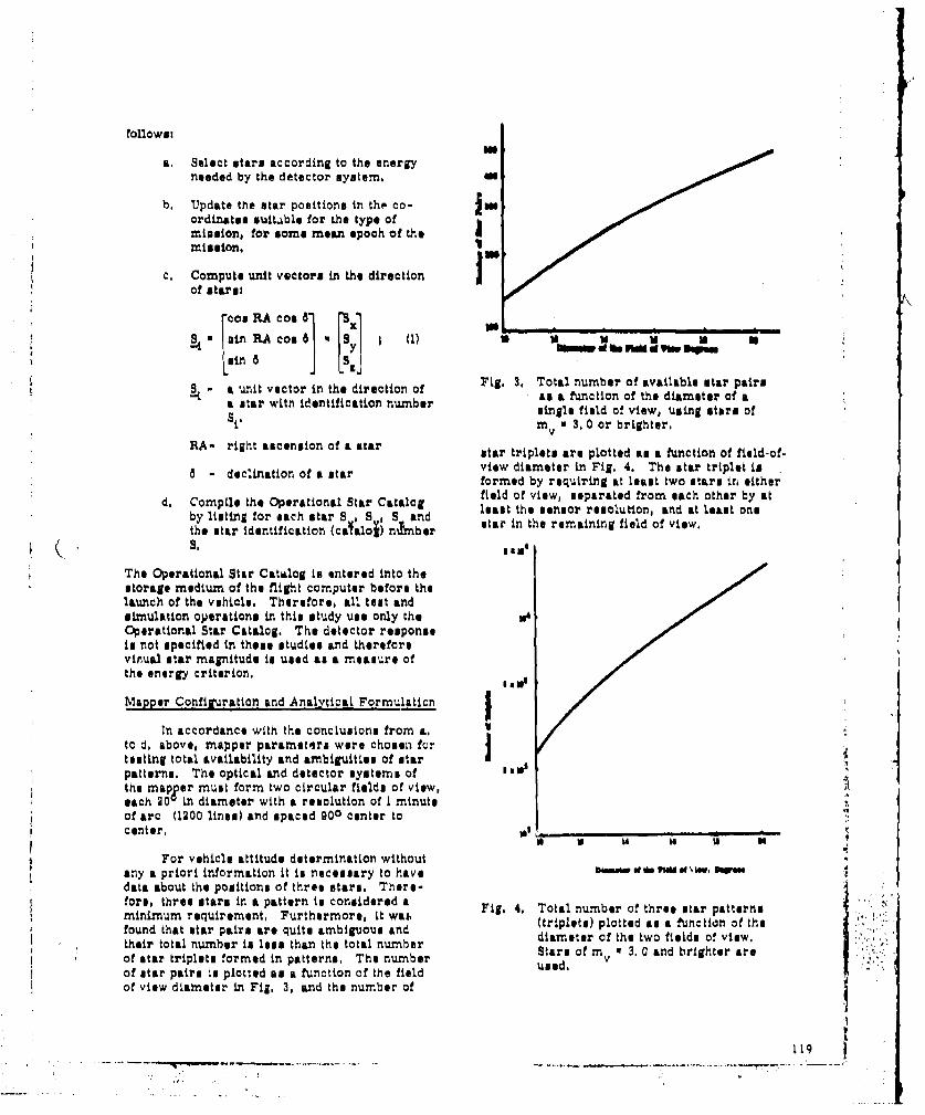
a, Select stars according to the energyneeded by the detector system,

b, Update the star positions in the cc- lossordinates suitable for the type ofmiasion, for some mean epoch of themission,

c, Compute unit vectors in the directionof stars•

~ og R.A cog: 81 ___________________*• in RA cos6 S 1 (1) "Mmi loli F.0 d W ' Is

sin J

Se- unit vector in the direction of Fig. 3, Total number of available star pairsas a function of the diameter of aa star with identification number single field of view, using stars ofSi. 3. 0 or brighter,

RA- right ascension of a star star triplets are plotted as a function of field-of-declination of a star view diameter in Fig, 4. The star triplet is

formed by requiring at least two stars in either

d. Compile the Operational Star Catalog field of view, separated from each other by at

by listing for oach star S I S , S and least the sensor resolution, and at least one

the star identification (casfaloa) nmnber star in the remaining field of view.

K m.S , ,

The Operational Star Catalog is entered into thestorage medium of the flight computer before thelaunch of the vehicle. Therefore, all test andsimulation operations in this study use only theOperational Star Catalog. The detector responseis not specified in these studies and thereforevirual star magnitude is used as a measure ofthe energy criterion, saI w

Mapper Configuration and Analytical Formulation

In accordance with ths conclusions from a,to d, above, mapper parameters were chosen fortesting total availability and ambiguities of star 5

patterns, The optical and detector systems ofthe maprer must form two circular fields of view, Aeach 20C in diameter with a resolution of I minuteof arc (1200 lines) and spaced 900 center tocenter, t __ _,._ _ _ _ ,

3 4 IS N

For vehicle attitude determination withoutany a priori information it is necessary to haveE=Peii,.IU. kerdata about the positions of three stars. There- 4fore, three stars in a pattern is considered a Fig, 4, Total number of three star patternsminimum requirement, Furthermore, it was (triplets) plotted as a unction of tefound that star pairs are quits ambiguous and ( l .a."

dimtars of mh tw f.eldandfbrigherwartheir total number is less than the total number diameter of the two fields of view,of star triplets formed in patterns, The number used.of star pairs is plotted as a function of the fieldof view diameter in Fig, 3, and the number of

11

Computations for determining the star the stars is described in Rot, S.triplets formed by the stars in the Operational

Catalog involve at first a text of all possiblepairs for a fit in one field of view:

cos (2 8- c S. S (2)

whi ereS - angular radius of each field of

view

s - accuracy of the field-of-viewAlocation with respect to theinstrument boresight,

The pairs that fit in a field of view are thentabulated, and the entire Operational Catalog is

aearched for third stars corresponding to eachpair. The search is carried out by performinga number of tests between the star pair and thestars in the Star Catalog in order to determinewhich stars could be in the second field of view.The first test consists of a comparison whicheliminates most of the unsuitable candidates byrequiring that both conditions below are atis-fiedi

cos (D00 - 26) ), . • > coS(GO0 4294 (3) Fig. 5, Goeomitry of third star determination,

and Ambigjuouti triplets are identified by actually

look•ng at earlier computations of star pairs am )cog (900 - 26) > S3 , S > cos(90 + 20)1(4) potentially ambiguous patterns, The actual amb-

3 Q - iguoue triplet test then merely compares theangles of the prospectively ambiguou• pair stare

- unit vector in direction of a star in with the conventionally found third stars. Thefirat field of view, star I, aambiguities arise because the accuracy of starunit vector in direction of another locations specified in the catalog is much highersta in u it rto fdirel tio of view, har 2than the resolution of the sensor. Therefore, the

sensor identifies star pairs with separation anile

-unit vector in the direction of the differences less than its resolution as being theiS3 ustar which is being tested to deter- same pair, The effect of the sensor resolution

mine wifh it ein seondtfield of voew, can well as the titar magnitude upon the number ofmine if it I in second field of view, ambiguities and available tripletm is shown inand therefore the third star in the Fig. 8.pattern.

A still clearer indication of the dependenceMore tests will follow only if equations 3 of the number of ambiguous triplets upon resolu-

and 4 are both satisfiedl otherwise the next tios is given in Fig, 7, where the ambiguousstar is considered for the first toot. For fur- triplets are plotted as a function of lines of res-ther tests the principle involved is that if on olution for several fields of view, Special atten-the celestial sphere a small circle of radius 0 tion in called to the case of a 200 diameter fieldcontains two stars and any part of a great circle of view, visual star 'nagnitude 3.0. and 1200 linedrawn with the s tar under test as its center, resolution. 7his corresponds to the median starS then the star under test can beoa third star, and mapper parameters assumed, The total

etnumber of triplets is equal to 16000 and of those,Referring to Fig, 5, it on the celesmtal 80 are ambiguous, meaning there are 80 pairs of

sphere, small circles are drawn about stars Sl triplets which cannot be distinguished from eachand S , the area common to both small circles ohrbohs atulrmpercniuainMust ihon be within angle I of a great circle ohrb hspriua aprcniuain(of radius 900 drawn about S . The method ofusing circles drawn about stirs on a celestialsphere for studying the angular relationship of

120

,, ~ ~ I,.', .

C. All Attitude Availability of Star Patterne

K ~TOTAL PUXMflor TIMRI rThere are numerous methods which may beused to investigate the distribution of identifi-able star patterns is a function of the orientationof the mapper coordinates with respect to cele.-tial coordinates. It ha. not been possible to findan accurate statistical description of star posi-tione on the celestial sphere, and therefore it isnecesslary to consider more deterministic &l-

I sinwunthough possibly laborious approaches to the mol-ution of the star pattern availabl~ity question. -I

A very simple scheme was used since theanalysis time was reasonable and from an esti-mate the computation machine time was not pro..

""I TlA IM hibitive (about 119, 952 individual mapper orient-O1214 I55OLUMU"M ations need to be investigated), and complete

explicit information for every position of a fieldof view can be found,

' Description of the Approach

vMAIL MAR ,•AUIT-•. Two circular fields of view, the celner of

each definable by two coordinates, result in aFig. 6. Total number of three star sets, and fouw-dimennsional description of the pattern ava*l-

similar three star sets plotted as a abLlity, In order to overcome Wes difficulty, thefunction of visual star magnituade, for following approach will be aueditwo sensor resolutions,

a. Designate the fields of view as I and 2,attaching no preference as to which iswhich, Both fields of view are circular,with radius 01 the cem ers sf the fieldsof view are separated by 90

W b, Letting one field of view (center of fieldof view 01) remain in place the othercenter tI moved in steps of V degreesthrough a complete great circle,

Sc, At first, field of view 01 is checked andflue if it contains two or more acceptable

stars, only one star is required in fieldUI of view #2 for each of its positions. Ifle field of view 01 contains only one star,* then field of view #2 is required to con-

EU*e tain two stars in each of its great circlepositions, If field of view #1 contains nostars, the next position is incrementedwithout searching field of view 02, At

the end of the great circle, the total num--a--- ber of positions in which a complete setS6 , mica'n01, of stars was available for pattern deter-

mination is counted and its ratio with thetotal number of steps, NP, will be

Fig. 7. The number of ambiguous star triplets cnmputediplotted as a function of the lines of 3.00resolution for various fields of view, NP 36-- (5)

C • l I1I

12O (

where Firure 10 show. the change in percent avail-ability of tatr sets with magnitude, Figure 11

C - an integer les then ten, or an shown the effect of the change in the field-of-view )asterisk showing in 10% amounts diameter upon the three star met availability.

the coverage of celestial sphere byuseful star patterns. 00

NPI - the number of risitiona where anidenti:lable star triplet was found,

Figure 8 is a schematic reprementation of thesearch routine for one point on display, Forthe next point field of view #1 is incremented byapproximately v degrees and the procedure Idepicted in Fig, 8 is repeated,

I!e ,, o- , V 136AT,1"0° '1R A 0h

INCREMENT MVM IVAL XA&UMN

P-g. 10, Percent availability of star sets plottedas a function of star magnitude, Field-of, view diameter is 200,

D coT 43rDCI FoV 42.

NO CON CONTAI OTAiNYNTWO STARI STR ON7 T~Nwo STARR

ON STR CA OE STAR

ICOONAI T T AIN

IAVAILABILITYrIR:c ORDER BY|ONE•

Fig. 8, Operations for availability determina-tion, Fig, 11, Percent of availability of three star sets

plotted as a function of the diameter of

Type of Display of tlie two fields of view for various itarmagnitudes,

the display of the computed informationconsists of symbols representing the value of C. At first it was anticipated that a markedThe number of symnbols in each line is the sarne change in percent coverage would result from

as the number of the field of view #1 incremented changing the test step siue y, However, at mag-positions, Four displays are incorporated into nitude 3. 0 and field of view diameter of 200, noFig, 2, Star mapper parameters and energy change at all in percent availability occurs if thecontent of stellar information were varied, to teot step size is varied from 30 to 100. Hence the Vdetermine the sensitivity of star set availability attained percent coverage with the 50 test step

to these parameter chaLnges. siue is correct and there is no need to decrease "13the step size (and therefore increase the analysis

122

inS~~.... Mi46 U& '"•

li•low "M • i

6IMVt PM !WAL MIMAT

Aillil I.-Wl N, -W~i .. i.Wt W . kiý-* iDil

II

'to

ii,.t. Ai.IA iiia A84 GSI 1 4lr

l I •ft ..�.W l • W I' l I Ma snIli . I Ift

Al ¶t SaN,. P1.14 ii . II !I fts .- I SIr l ft

0 lit w11 l4tl

R~~ ~ ~ ~ 2, RU, t: ,H

A. i =0' a.

varios ft of vn

,a-t5,. ,-l.......... I ftI[ ............... 1 I

,+Ii*ii~ ~l*,Il~.h l . nfl~ • i iiiflli i iI

Fig, 2. Four display. of star set avaiibility forvarious field of view diameters and ,,tar

magnitudes.

computer time), spectral band detectors with available extra-terrestrial star data for the purpo-e of generat-

In conclusion for this study, acceptable per- ing a more flexible Operating St,•r Catalog.cent coverage of the entire celestial sphere bystar sets can be obtained with fields of view D. Simulation of Star Mapping250 to 300 in diameter nnd with the requirementto detect stars of visual magnitude 3, 8 .nd The simulation of star mnapping on a comp-brighter. The use of visual magnitude implies uter has to be formulated in accordance withthe use of sonsors similar in reeronse to the actual operating procedures of an operationalhuman eye. This is not necessarily true, and star mapper system. As shown in Fig, 12,efforts are centinulnif in matching broad only the part concerned %,ith the identification

123

A-b

.Z A O ,T ni "separation angle between starsSwhich have unit vectors designated

07 rNPe~• IrR 5 ard ndVZCTOR -

For the identification of individual stars a com-parison of input separation angle cosines ismade with the separation angles computed from

COMPUTE ANOLES data in the Operational Star Catalog, This pro-BETWEFN cedure can beat be described as an operation of

steps for each computation,

K•s AR McAE AN'D i1, Compare cos F? to cosines of inputseparation anglUxa

cosi(a-a) > coso > coo(i+r) ; (B) a

cosV(12 -") > cos nj t coso (2 +) (0 )

----- ---- -L------.. coe(a 3 -U) > ccs 77, > cos(0 3 + a) 1 (10)

D!rnbuz owhereM,•PPX Oa - resolution of the sensor

COC•DttrNATtgIg

2, If cos nt meets any of the criteria ofFig, 12. Functions of an Operational Star I, ontl S i and S j into the appropriate

Mapper column in array 01.

algorithm has been simulated. 3. Find coo Y7 for all i and J, and repeatsteps I and J2 ,

The cosines of the separation angles bet- Now array 01 is ready for identification of ind-ween unit vectors to some known stars, desig- ividual stars and the following discussionsated here as `1 S9 and S3, were used as input attempts to reason a solution.information for this simulation, and the algor-ithm had to find these stars from the Operat- Choose the tirt Si S1 corresponding toLonal Star Catalog, This was accomplished cosol. There St and Si courd be tho same as S1tseveral times, using the process described and S2 used for input information generation,here. Next choose the S, Sj oorresponding to cosel2

which has ,ne of the star numbers in commonThe three input angle cosines are entered with those listed under cosill. If no such Si S$into computer storage media and are listed into corresponding to C02132 exists, the firstthe heads of colum ns in array #1, as coon , corresponding to coo, re prs ets, an ami g-cosf , osf Thesepraton nglecos~esof orrespondinij to cosfl 1 represents an ambig-hone , coslai The separation arngle coat log of uous angle, and the next Si Sj corresponding to

isar fome with aprtoa star Catalog aoarlatewthe r cost 1 is chosen and the same test is made. Thecomputed without regard to ordert test is then repeated until a Si Sj is found whichCOB nij Sin formed with a star common to at least twoScosn�'7ij . - pairs. The common star to both pairs is tenta-

* S + SiS 5 tively called S21 the other star in the cosil 1i • jx •"iyy ' Sizjz ()clumr. is called S11 and iii the coshl2 column,

S3.> i*1 I

-stbeAfter two pairs with one common star haveidentification number of i star been found, the remaining two stars are comp-

ith ared to the two star List for Si St correspondingsttar to coct 3, to see if a pair makini UP 31 S3 is

present, If two such stars are found, the stars

IZ4

are identified. If two stars corresponding to nature of the holographic process, the starthe two stars of the pair S1 S3 were not found field mapper will not require an attitude controlamong those corresponding to Si $l listed under system nor will it be dependent upon ground-coaL38, then search must be repeated for further based information,values of Si S. corresponding to coseil and afterexhausting this column repeat the operations Holography (9, 10, 11, 12) is a means forwith Si S corresponding to cosn3, then again recording a wave field on some photo-sensitivesearch tFe cosf33 column for SI S. Several medium (typically photographic film) with suff-star triplets were successfully identified by icient completeness that the wave field can bethis simulation, and no difficulties with the use regenerated from the record. The regeneratedof the algorithm were experienced, wave field cannot be distinguished from the

original and can be focused to form an image.E, Conclusions In the typical holographic experiment, a coher-

ent beam of light is split into two components.The basic question of availability of unique One component (the object beam) illuminates the

star patterns for all pointing attitudes, and the object and a portion of the Rayleigh scatteredability of the star mapper to identify the indiv- light from the object is then intercepted byidual stars, has been answered am shown in the photographic film, The other component (thetwo preceding sections, This means that comp- reference beam) it directed to the film, subjectletely autonomous stellar attitude determination to coherence length restrictions, and functionsby the use of a star mapper alone is possible, like the local oscillator signal of a superhetero-The mapper should have two fields of view, each dyne receiver to aid in recording the phase250 to 300 in diameter, and 900 apart center to information, To read out the recorded hologram,center, It should be sensitive enough to detect the developed photographic plate is returned tostars brighter than visual magnitude 3. 8; no the original recording position and illuminatedlimit in sensitivity need be imposed, with the reference beam, If the original object

position is viewed through the photographicThe autonomous capability does not hinder plate, an image of the object in three dimen-

operations, if indeed the approximate pointing sions will be seen.direction of the mapper is known, mainly from

( its own previous autonomous attitude determin- A holographic record of a particular staration, A priori knowledge of attitude reduces pattern can be made in the laboratory using athe computation time. Thus no limitations to a template (with back lighting) as the star pattern

present systems type operation are imposed by and the light from a point source (a pin hole syn-the star mapper but the ability for autonomous tern) as the reference beam. The star fieldattitude determination has become available, pattern may then be regenerated anywhere byThe autonomous capability allows the star map- presenting the point source reference beam toper to operate without a gyroatabilized system, the hologram. A reciprotal situation can alsoand can establish inertial attitude for such be demonstrated in which the star pattern it-systems when they are reactivated after shut- self is presented to the hologram, If the stardown, pattern is the same (or similar) as the recorded

pattern, the point source will be generated andcan be focused onto a detector. The presence

IV, SECOND APPROACH or absence of the regenerated point source is anindication of the presence or absence of the

A, Introduction original star pattern. This simple means ofstar pattern recognition is severely limited in

The second approach is the adaption of its use for practical reasons (alignment prob-holography to the problem of recognition of star lems) and one must introduce another level of 14

fields for attitude determination. A primary sophistication -- the use of a lens,objective is a device (hereafter to be called a

t star field mapper) which will be completely B, Fourier Transformation Property on Lenses

autonomous and which will provide three-axisinertial attitude reference information using a One of the most remarkable and usefulsingle device sampling a single star field. properties of a converging lens is its inherentOperation of the mapper essentially will be in ability to perform two-dL-nension Fourier trans-real-time and all the data processing required furmations (see Reference 13, page 83, for afor identifying a star field will be done optically. complete discussion), When an object is placedSuch a recognition device could be modified for in the front focal plane of a leno, ai exactacquisition and/or tracking, In addition to Fourier transform relation exists between thethese advantages gained due to the inherent object and the field amplitude across the back

S " i . . .. ... . .. " • " •'.. .2,

' • L " .- _ _•

focal plans of the lns (neglecting vignetting Fourier transform operationseffects caused by the finite lena aperture). TheFourier transforms are just images but the TT (a) m TA a a (15)images are defined in spatial Fourier space or,more commonly, in the spatial frequency dom- TT (b) x TB " b (18)ain.

(A theorem of Fourier transforms says that:The holographic system indicated in Fig. -1 -1

13 records the information (a. b) in the focal TT f(x, y) - T T f(x, y)plane of the lens. Because of the reciprocalnature of holography, either u or b may be con- - f(-x, -y) (17)sidered as the object and the oth.r 'as the refer-ence, Let T be the operatoe which generates a for all points of continuity of f(x, y). The co-Fourier transform -- then T represents the ordinate system is redefined in a reflectedaction of the lens. Ift geometry.) The field amplitude in the hologram

plane islA• T (a) (11)- •A (A + B) (A* + B,) i,3 T (b) (12)

"and in the image plane the field amplitude istthen the field amplitude in the back focal planeof the lens is T ((A + B) (A* + E*))

T (a+b) a A *B (13) T (A2A* +_A2 B*+ +AA*B+ABB*) (19)

by invoking the linearity of Fourier transforms. The term of interest is T (AA*B) which is theThe hologram is recorded on ilm which has a holographically generated M"Po' of b, Obvious-square-law characteristic (film is analogous to ly using b as the input would generate T(B*BA),a mixer) and thus the recorded information isl the holographic itnage of a, along with otffer

terms, If a were a given star pattern and b a(A.+ B) (A* .. B,) (14) point hource serving as a reference beam, then

presenting a to the hologram will generate thewhere * indicates complex conjugate, point source as long as a is identical (or simi-

lar) to the pattern whicli was used to make thehologram. Also, the desired term will be gen-erated oft-axis and will be separated from the

Oobject other three term,.

! Lens 10

:2•�H ologrom

CA,8(A*ý 47A B

S~(A-+ B) (4*,* 8*)

I I'* Fig, 13, A holographic system to record

(a, b) in the focal plane of a len,.

In Fig. 14 the symbol a is presented to thehologram and an aoditionarlenon in used to per-form another Fourier traaniformation. With an Fig. 14, A simple optical recognition system.appropriate choice of coordinate systems(Ref. 14), the second Fourier tranwformation Now, why introduce the lenses in the f-rotwill yield the same result as the inverse place? A hologrAm ronstructed without the

126__ _ ,-._____1

( ____

Aensee requires an accurate alignment between correct frequencies pass almost unattenuatedthe unknown pattern and the original recording while the other frequencies are largely supp-position of the stored pattern. The problem is ressed, The transmitted frequencies then aresimilar to trying to prove that a small section reconstructed to form a normal image whilecut from one of two identical photographic neg - the leakage of other frequencies reconstructs aatives will match some portion of the uncut neg- noise background. Since the memory unit wasative - a trial and e~'ror search may or miy not constructed holog: 1phically using a point refer-work. By transforming to the spatial frequency once, the output is a spot of light (a correlation)domain, an object can be "compared" anywhere whose coordinates in the output plane bear ain the field of view of the lens without precisely one-to-om correspondence with the location ofoverlaying the image,. No matter where in the the unknown star field in the optical memory,field of view of the lens the pattern im located, With a position sensitive detector, the coordin-the information (assuming a perfect lens) will ates of the unknown star field are obtainedpass through the focal region of the lens, The directly,information retained in this process is the reo-ative positions of a and b (see Fig, 13) in the D, Implementation of Star Mipperoutput plane, Thus, if tAe pattern a is movedabout in the input plans (just translations, not One possible means of implementing a starrotations), the reconstruction of b, the point field recognition system is indicated in Fig. 16,courcewill move correspondingly in the output The figure is intended on)y to depict the sevenplane. The prospect of tracking is meaningful major research and/or component areas.if a position senlitive detector (mosaic detectorfor instance) can be used to sense the presence Telescopeof the point source,

The telescope provides the star field imageSuppose that a pattern composed of the to be identified, In the laboratory, photographic

letters A through Y arranged in five rows of positives are used in place of the telescopicfive letters each is recorded in the focal plane system and the film transport system. An ideal?o a lens, A point source is used as the refer- star field rnrpper will have its angular resolu-

once wave, Assume the letter E is in the tion determined solely by the diameter of the"upper right-hand corner" of the input pattern, collecting aperture of the telescope via theIf just the letter E is presented to the optical Rayleigh criteria. For the ansuing discussionsystem (see Fig, 14), then the holographically it is assumed that diffraction limited collectingRenerated point source would appear in the optics will be available, About a 45 degreeupper right-hand corner" of the output plane, field of view (fourth magnitude stars being the

Alternatively, if the input is any one of the limiting magnitude) in anticipated (Ref. 0)1 ittwenty-five possible letters, an identification is known that Schrmidt-Cassegrain and Bouwers-can be realised by applying the input to a bank Makoutov systems have no field distortionsor memory of twenty-lve filters (each matched over wide fields and their field curvatures canto one of the possible input characters) and be improved,examining the output - ideally only one will re-construct the point source, Imaging Mediun

C. Star Field Mapper A film transport system is shown (Fig, 16O )as the means of presenting the Star field image

TVe star field mapper under development to the recognition system, An ultimate designwill use a memory compos,4d of optically #ener- would employ a reusable medium which couldated Fourier transforms of the "universe' (see store the input star image during the recogni-Fig. 15). A modified Rayleigh intorferometer tion phaps and he erasable and ready for useis used to record the diffracted images, Once when another attitude measurement in required.,the Fourier transform has been recorded, it is The optical recognition system in not able toplaced in a similar optical system (recognition operate directly on the temporally incoherentmnde of Fig, 15) to serve as a memory unit -- and mutually spatially incoherent star field, Ana matched filter in the spatial domain. The input medium would transfer the incoherent starstar mapper presents an unknown star field to field to a density or phase modulation whichthe optical memory which, in turn, modifies tho could be accepted by the optical system, Preo-star field' s spatial frequency spectruml the ently, various solutions to the recording prob-Uutput is an altered image of the star field, The lem are being examinedi rapidly developedtransform lens converts the optical signals to silver halide films, thermoplastics, photoplas-spatial frequencies by diffraction and they are tics, free radical films, dry silver films,then paased through the spatial filter. The photochromics, etc,

|--

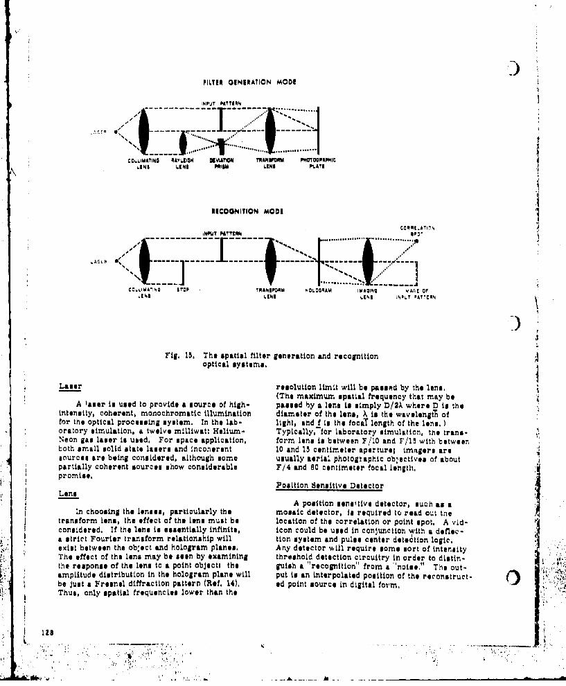
FILTER OENIERATION MODE

. .... . .........

CO.LIMATINO RAYKIIOH KVIATI "NAN O@5§M PWOT OO APMl'C

INSI 61NS PISM LINS PILA "I

I1ICOONITION MODI

C0PPC.ATi•4 .CNPU? P0??tW T mP 0 N

r .. .... ... .. ...........

CO.LIWAIN6 ?• TRANDPORM HOLOGRAM MAIA Y&l A6, OF6[Nl 6[NI a ;NP6T PATTCRN

- ,1

Fig, 15, The spatial filter generation and recognitionoptical systems,I'I

Laser resolution limit will be pasied by the lens,(The maximum spatial frequency that may be

A aser to used to provide a source of high- paused by a lens is simply D/2). where D it theintensity, coherent, monochromatic illumination diameter of the lens, X is the wavelengt'i offor the optical processing system, In the lab- light, sndf is the focaT length of the lens, )oratory simulation, a twelve milliwatt Helium- Typically, for laboratory simulation, the trans-Neon gas laser is used, For space application, form lens is between F/10 and F/I1 with betweenboth small solid state lasers and incoherent 10 and 15 centimeter aperture; imragers aresources are being considered, although some usually aerial photographic objectives of aboutpartially coherent sources show considerable F/4 and 80 centimeter focal length,promise.

Position Sensitive DetectorLens

SA position sensitive detector, much as aIn choosing the lenses, particularly the mosaic detector, is required to read out the

transform Lens, the effect of the lens must be location of the correlation or point spot, A vid-t considered, If the lena is essentially infinite, icon could be used in conjunction with a defle,-

a strict Fourier transform relationship will tion system and pulse center detection logic,exist between the object and hologram planes. Any detector will require some sort of intensityThe effect of the lens may be seen by examining threshold detection circuitry in order to distin- athe response of the lens to a point objecti the guish a "recognition" from a 'noise." The out-amplitude distribution in the hologram plane will put ti an interpolated position of the reconstruct-.be just a Fresnel diffraction pattern (Ref, 14), ed point source in digital form,Thus, only spatial frequencies lower than the

1284n i'

POSSIBLE IMPLEMENTATION

TELESCOPE

TRANSFORM IMAGING i4LENS LENS

HOLOGRAPHIC MOSAICMEMORY DETECTOR

FILM TRANSPORT SYSTEM( . •

Fig. 10, Schematic of a possible holographic starmapping syitem.,

Holographic Memory developed to superimpose a number of patternsin the same plane of a hologram with the ability

The holographic memory, its formation to uniq~uly dentify each individual pattern, Inand read-out, is the moat critical aspect of the contrast to prior techniques, the readout proc-recognition syatem. The concept of a bank of ess does not require any movement of parts,filters (one for each possible scene) with each e. g, , the hologram is not rotated through ascene stored on a separate hologram Implies a Bragg angle nor is the direction of the inputlot of equipment, For instance, if all the holo- beam changed in any manner, The solution isgrams were to be mounted on a filter wheel, an to introduce another Ions which comes to aadditional insano would be required to allow a focus before the photographic plate (see Fig. 17).rotation of the hologram for an angle iearch Mathem hceally, the hologram is:plus a means to record the angle (angle encoder). i(o + ax) e-iaix 1 2For any ganeral instrument to bo used in a space H (x) e + e (20)mission, the number of holograms could becomeimpractical, If equal ralius circular fields of where, fur simplicity, the reference beam hadview are stored, then 8n (n is an integer great- been assumed to be on-axis and the obliquitiesor than unity) circles are r;quired to complete- of the star pattern (amplitude S) and the thirdlyc OY a unit sphere with circles of radius beam are opposite and differ by the anglel ,G0/(2 1I7n) degrees (about 84/n degrees), In Expandingithe of eliminating moving parts in the 2, onpace environment, multiple storage techniques Wx) * (2 + S ) + (1 + So ) I +were investigated, -io-x -o ,.2ax

three-beam technique (Ref, 15) has been + So e (21)H

iig

formation of point Fi, and the angle of theplate P would indicate which of the stored patt-erns is matched by the input pattern, In thethree-beam technique, point F' will be presentwithout any movement of plate PI there willalso be another point of light 0' which is the"image of point 0 (Fig. 17), The position of

....... point G' indicates which of the stored patterns- ~matches the input pattern (if any), F' and GI'

come to a point focus in different planes whichis convenient for readout purposes, Thus, the

.T three-beam technique allows one to interrogate____ the stored patterns for a matching pattern in

one operation, without the previously requiredneed for moving the photographic plate.

Fi.1.Three-beam concept for the record-Ing of multiple star fields.

When the hologram ii illuminated by the starpattern (assume 0 to be small), the first and F1second order reconstructed beams consist of ---- I", ,', ..

the interferograms of the star pattern (or its . .......° = " " '- --------------------.--....conjugate) with the third beam and with the i' .

reference beam., y choosing appropriate si .," P "obliquities, the reconstructions of the third Abeam and the reference beam can be confined T 1

to well-defined regions of the output plane,

When a new- pattern is to be stored, thelocation of lIns B in changed in such a maienr Fig, 18, Readoul process of the three-beamas to keep constant the dietance from the center technique,of lens B to the axis 0-01 as well as the diet- 2anceS from the center of the plate P to point 0 It is now proposed to store the 6n patterns(the focal point of lens B) and from point 0 to required to cover the celestial sphere in each 4,the center of lens B (i. e., a rotation about the of the angular orientations needed to be sure0-01 axis), Now there are three beams inter- that a recognition is always obtained, Regen-fering aV the photographic plate P. The expos- eration of the point source will give the (x, y)ure time for each pattern varies roulhly as the coordinates of the center of the unknown starreciprocal of the total number of patterns to be field with respect to a stored pattern, A ringstored, The non-lineartty of the amplitude of photodiodes will be used to intercept the re-transmittance curve causes each pattern to be generation of the third beam and thus identifyrecorded in its entirety (Ref, 16), which of the many stored patterns correlates

with the unknown pattern, The voltage signalsThe distinct advantage of the three-beam can then be used directly to monitor and/or up-

technique can be seen in Fig, 18 which displays date a gyro inertial frame,the readout plocess of the images stored on thephotographic plate P. An unknown pattern in E, Laboratory Simulationplaced Wi a window formed by the stops S1 thetransform lIns performi the Fourier transform The apparatus for the star field mapper isof the pattern, and in the plane of the photo- in the development stage, At present, the holo-graphic plate the Fourier transform is multi- graphic memory is being constructed and stud-plied with the previously recorded Fourier ied, Tne three-beam technique and appropriatetransforms, Lens A then performs another bleaching techniques appear to have consider-Fourier transform and exhibits the cross cor- able potentilW for extending the holographicrelation of the input pattern with all the stored memory capability. At this writing, thirteen ,,patterns As a Pint of light F' Using just the patterns have been recorded and the crosstalkprior art, one would have to rotate the photo- is barely detectable witk an unshielded photo-

1 graphic plate in order to search for the multiplier. The sigunl-to-noise ratios have

130

S+, ?:i,'f l

always beeon better than 4011 and at times ne,.0y of speed in processing the information (due to1000l1, If an input medium can be found or decv- the elimination of the computer) and the .impli-eloped and if the three-bouin technique can be !el optical system is presently in the develop-extendel to map the universe, an autonomous ment stage, Although initial feasibility hasstar field mapper can become a practicality. If been demonstrated in the laboratory, the deter-a mission restricts the fields of view to only mination of the accuracy to which a star fieldselected stellar *reas or landmarks, a tracking can be located as a function of the spacecraftmode is certaiily feasible using the same stabilization and the size of the holographicoptical system, memory have yet to be determined, Also,

further development is needed for an erasableF, Conclusion Input medium exhibiting recognition capabil-

ities with signal-to-noise ratios of several hun-Optical mated filtering has a great poten- dred to one. It in expected, however, that

tial in the pattern recognition field, especially these problems can be solved within the nextwhen the objects are stars, Critical registra- few years and that modern optical methods willtion problems inherent In conventional recogni- be a demonstrated powerful technique for space-tion systems are eliminated in the spatial craft navigation and guidance,frequency domain. The star field mapper willbe a completely self-contained Automatic device Ackhnowledlementswhich will provide three-axis attitude referenceinformation in either analog or digital form, Constructive suggestions from Mr, J.The optical system processes the star condi- Bellantoni in designing the Operational Startions without a computer and at the speed of Catalog and the contributions of Dr, K, Soosnarlight, A holographic star mapper could provide and Mr, H, luszolino for tkhe analysis and pro-greater accuracy than known autonomous navi- gramming In Part III of this paper are grate-gation techniques, fully acknowledged.

V. SUMMARY REFERENC E~S

1.F, D. Grant, "Inflight Alignment Errors ofA more far reaching space voyages are Stable Member MIT Instrument-

undertaken and for future Earth-orbiting veh- tihe Laboratory Report E..148, December,

icles, the need for self-contained navigation 1903.systems based on electra-optical technique isdecidedly increased, The attitude information 2, R, C. Hutchiion, "Geometrical and Astro-provided by such systems is essential for the nomRi.Cl Aspucts of Employing a Star

proper reduction of meteorological, geophys- Tracker to Correct the Attstude of a Stable

ical, and many other types of data gathered by Platform," MIT Instr-mentation Laboratory 4

a space vehicle, Report R-323, Febru•ry 19111,

This paper has discussed two new approach- 3, P. Gevas, J, Abate and J. Gulbenkian,as to the problem of rapid determination of "Design, Fabrication and To:st of a Feas-directions in inertial space, Though both sys- ibility Model Relative Star Angle Compara-tems have the desirable property of being able tor,". Tchnical Documentary Report No,to perform the required star pattern matchwithout moving parts or spacecraft slewing ASD-TDR-63-585,

(i, e,, they both operate in the strapped-downmodel), the complement of equipment and the ,Resear ivision ontrsliDatao rpora -speed at which attitude is determined is mark- tng "el esti gation of a WidAngle different foernc the twoc appoaces

gation," Technical Report APAL-TR-86-l0,edly different for the two approaches, A~ngle Celehtical Refeecport Space-T a-8-0

The conventional approach employs a com- Aria 1968.

puter and is within the state of the art so that T, M. Walsh and R L, Kenirer,hardware miy be configured which will meet Any -sespace qualification, For precise pointing infor- of a Star Field Mapping Technique for Use Sin Determining the Attitude of a Spin Stab- -motion, the use of two sensing heads Is req- iliced Spacecraft," NASA TND-4837,uired, The two heads may have arbitrarilyskewed or orthogonal pointing axes.

( ,The desirable approach using the holo-graphic technique with its inherent advantage

71..

6. T. M. Waelsh, W. C, Dixon Jr,, D, E, 11, E. N. Leith and J. Upatnie&ý, J. 0. S. A.Hinton and J. A. Holland, "A Celestial 52, 1123, 1982,Attitude Measurement Instrument forProject Scanne., " NASA TN D-4742, 12. E. N, Leith and J, Upatnicke, J. 0. S. A.

54, 1295, 1964.7, AF Avionics Lab., R & TD Division AFSC,

Wright-Patterson AFB, Ohio, "Star 13. J. W. Goodman, '%Lntroduction to FourierIdentification by Optical Radiation Analy- Optics, , McGraw-Hill, 1968.sis, 11 TDA No. AL TDR 04-13, Janurary1 T64. 14, ", B, DeVelia and 0. 0, Reynolds, "Thnory

and Applicatitns of Holography, " Addison-8. L.A. Geizzar and R, A. Arehart, "An Wesley, 84, 1967.

Analytical Approach to the Determinetionof Stoller Fields of View, " NASA TR 15, J. N, Hallock, NASA Tech Brief 68-10347.R-257,

18, J, N. Hallock, Amer. J, of Physics 36,9. J. B. DeVelis and G, 0. Reynoldo, 782, 1968.

"Theory and Applications of Holography,Addison-Wesley, 1987,

10, 0. W. Stroke, "An Introduction to CoherentOptics and Holography " Academic Press,199,

)i

iI!

()

132t

SUB-ARC SECOND STAR SENSORS, DESIGN AND FABRICATI•O1

Joseph . CarrollControl Data Corporation

Idina Space and Defense SystemsMinneapolis, Minnesota

Current and future requiremsnts for star :ensota in the sub-arcsecnsd region favor |tarmappere over Star Trackers because of the

letter's mechanical complexity, Work at Control Data has concentratedsince 1961 tn Itarmappers in which star images transit slits in thefocal surface of a wide-angle optical syitem. The variety of spicevehicle motions causes &corresponding variety in star sensor designs,including the choice between an internally driven reticle and a no-moving-parts system which uses vehicle motion for sean Senaration,Inherently concentric optical systems (catadioptric or all mirror) arerequired to mainlain high quality i•mage throughout the field, Imagediameters will probably not become smaller than a few arc secondi,thereby necessitating interpolation of the star transit pulse from thephotodetector, Successful thermal deigln 1)1 the sensor avoids temper-ature gradients and permits operatiota over 4ide ambient ranges, ri-hally, the type of photodetector chosen significantly influences thedesign of the pulse processing electronics, Both solid state (photo-diode, Cd,, Cdie) and photoemissive (?MT) detectors are examined,

. 0790DU"•ION All of theme applications-.in space andground based--require the sensing of the direc-

Extremely precise star sensors can find use tion io a star relative to a coordinate framein a broad array of applications from scientific located within a star sensor, We consider inresearch to operational systemal from ground- this paper only those sensors capable of perform-based installations to spacecraft components, ing; him task in its most precise form--that is,

with errors from one or two arc seconds down toSpacecraft attitude detection is of most one- or two-tenths of an arc second, We thus

interest in the present conference, but there are intend to discuss sensor performance which wealso pomitioning requirements in space--location believe feasible in the 1970ts in the areas oftwithin the molar or satellite system via triangu-lation, distance from an extended body, and (a) operational spacecraft, anddirection to a target body, There are also a t shost of terrestrial tsoks which requi-c star (b) automated tools for astronomice ,'siensing astronomical surveye, north azimuth do- surveying and research,termination, polar motion and atmoerhuric tiltstudies, continental drift, star position deter- Zn addition to the requirement for sub.arominationj then on other planetas position fixing, second accuracy, we will treat only those sensors •,letermination of spin dynamics, studies of inter- vhich are automatic in the sense that no manualnal masi distributions (vertical deflection),-the intervention is required in their opprktion,posoibilities are almost endless, This eliminates such star sensors a4 observatory

telescopes, theodolites, photographic senithtubes, and similar squipme:, which use the eye or

SContrml Data Corporation has performed photography for the basic sensing element or isnumerous programs under Department of Defense, manually directed, even if aided by servos.NASA, and company sponsorship, The results ofthose programs are pertinent to the conclusions We have thus restricted ourselves to twodrawn in this paper, types of star sensoris Star Trackers and

133

Starmsppers, and the purpose of this paper will)be to cc pare theme two in terms of ultimateaccuracy (concluding that in some applications the AZIMUTH4 AXISlatter would be & better choice) and to reviewthose optical design and star detection (elec~--tronic) techniques employed in Starmapper symstma gII VPto maximize performance.,XI

We will not discuss system aspects in any NRO FOYdepth. Suffice it to say that sensors such aetheme are capeble-.through multiple measurementsand math modeling--of providing system accuracies 9gAINAIwhich improve upon individual star sightings by OPTIlCAL AXISas much as an order of magnitude (Refs. I and 2).

III STAN34AMU AND ST6A newICBThe two major categories of star sensors N1

(after telecopes, aet., ate eliminated as die- ICOI zcussed above) are the relatively conventional

* star Tracker--a 4escendent of the theodolite- Indthe never Starmappmr--an outgrowth (principally SUR~ MAWCKR

* at CDC) of early work in aetrome trios in Russiaand satellite cracking in this country. ,[ O

A. Sta IL acklE PAST SLITS CECAUSK

The Star Tracker, as shown in Fig. 1, is O CYMTOcomposed of a telescope gimbaled in two axes soOPIAthat it can point in any direction, (Practical SSIlimitatiuns usually limit this to one hemisphere.) R~C9AIt is very much like a theodolite except that theFOA UPCIvertical end horisontal circles haye been replac-

* ad by Angle encoders and the focal plane of the HTILCR DTTOtelescope contains photoelectric sensors for de- ~COLC~C~TCOtermining the location of the star within theoptical field of view, STARMAPPER

servos are also mounted on each axis forthe purpose of acquiring the star on command from Fig. 1. Schematic Diagrams ofthe computer and driving the star to the center Two Automatic Star sensorsof the field of view based on error signals fromthe telescope detection electronics. Thus, an%ppkoximate knowledge of the orientation of the The Itarmapper has no gimbals but is rigidlyvehicle is used to point the telescope in the attached to the vehicle, AS Lhe latter rotates,geub~ral direction of the desired sear (usually a theo star images are cerrted across the slitfew minutes of arc to one degree) from whence the pattern producing a saviss of pulses from theinternal control loop takes over to precisely photoelectric detector(s), This ptilas sequence

* point the telescope. When this is complete, the is then timed and relAyed to the computer whichangle encoders are read into the computer as a identifies the transiting stare end computes ameasurement. pointing direction An~d/or determines the velures

of various motion parameters (spin rate, proe-*Alternately, the photodetsetorl themselves cession, momenta of inertia, etc.).

can provide a vernier an the angle encoder reed-lings, thereby eliminating the need for precise There are two types of Itarmapperst one

control~~~~od fffnlpit .hvn or motiong pathru thdepsa il 1endiguo thecontrol~~~od offnlfoninhvign moviongtrog p the and r fepenin u and the

An extensive licerarure exists on Star other containing an internal reticle drive toTrackers, their application, limitations, con- scan the slits past star images which are rela-atructi,3n, aet. References 3, 4, and Iare per. tively stationery when body rotation is slow,hape representative of the current stats of theNart.* A number of articles (far less than for

Star Trackers) have been published concerningB~. LULU=na~ Starmappere and their antecedents, Zarly Russian

astromstric work involving star transit& is (Also iho~n in Figure 1 is a sketch of the reviewed in Ref. 6. The use of slits in the

major Itarmapper concepts. Briefly, a wide-angle Baker-Nunn satellite tracking camera is discussedcamera type of optical system images a field of in Ref. 7, Astronumical surveying applicationsstars onto a slit pattern at the focal surface, using theodolites are discussed in Res.s Op 9,

-- 7---T-

end 10. A Completely automatic u1eYing system parts is a definite advantage. Moving partseconis outlined in Refs. 2 and 11. latellita Atti- varying stresses, changes in lubrication films,tuda determinaion is discussed principally in slow wearing of the surfaces, and torques applied

Refs. 1, I1, 13, 14, 15, and 16. More detailed to other members of the system (altering perhapsreferences are cited later, the orientation ever so slightly) The requLire-

mente for mechanical balance and cancellationC. Tracker/lianoer CoOarisLona techniques is nearly unsurmountable, Constant

calibration becomes much more involved becauseThe fundamental differences between a Star of the many configurations of the sensor which

Tracker and a Starmapper are listed in Table 1. must be checked.Generally, the Starmapper is a much simpler In-stru•snt mechanically dut to the absence of servo In short, tiny systematic errors (a tooloops, gimbal axes, and angle encoders, But to large bell in the race, e.g) which refuse toaccomplish in esmentially similar task, it must relent to calibration, are present in all measure-possess a wide field of view (me asured in degrees ment systems but lot rapidly out of hand whoerather than minutes) in order to scan a sufficient moving parts are encountered,number of stars, and it is very important thatimage quality remain high over the entire field Thus it is the author's point of view thatsince stars can pass thWough the field at any for certain of the most precise applications.-point and must be detected with equal accuracy, in spec& or on the planets--the Starmapper posses-The Itar. Tracker need only have lood imale qual- @a an ultimate accuracy potential which the Starity near the center of the field aince it is Tracker lacks,only with the star cantered that the anile encod-rer are read. Another comparison between Itar Trackers

and Itlrmappls aind one faiLto •l ikely to gotthb authov boiled in oil) can be made on the

Table 1, Comparison of basis of body spin rate ae shown in fig. 2,Atar lensor Characteristics Vehicles with rapid rotation rates are ideally

ulited to Starmappers whereas those applicationstending toward inetially stable platforms are"more suitable for lStr Traclrie or require Star-mappers with intLernal oCan.

m9 I, 9 Sitll .1 11.14 .1

T (9 *.~.. ***s.. . ........i.. .II :

v ri r ela i v t o s I i I

appiabity to datmo ai, its moreM,

.9!, k l I I Iintuitive operat (lmt i icl .il.,i tte. i. Ap a I o rs

Wide Rings.... of Spin Rate-. 5o on 6 th one ha ndl , we ha, an i99 ilimil

SIi •.ili IO I ..elll I I .. , I 5. m . .l,1 *, I I

vestlt eaie o ta field ddnsity, itIlCtION O AI I dqise ll/l~.. IsEM 9app L'Iicability to ayime' operation, itsl morel'lu'i

W ideRne fSin Rsltel

of grcat mechanical simplicity (to the point of nomoving parts), aend, on the other hand, an intru-

Oent Of apparently more versatile usape and car-tainly one of lunger historic acceptance.

2However, when viewed in terms of system The above accuracy comments apply also to

a)ccuracy, and when that accuracy requirement ie internal scan Itarmoppers (though only one part( pecified in tenths of an arc second, then one is involved), ItZ could be that a body with nomust conclude---provided the particular applica- motion whatsoever relative to the star can havetion by itself does not favor One instrument form its orientation precisely measured (automatically)over the other--that the elimination of moving only with very great difficulty,

Lat..

II, STA•JPPIR DEIZGN curvature was by defintioiu completely fro* ofcomal, altigmatism, distortion, and chromatism a,

The Starmapper sensor achieves its sub-arc well as having a very nearly 180 degree field ofsecond performance through a combination of high view, Its disadvantages are spherical aberra-quality optics and electronic interpolation of tion, curvature of field, And a focal surface

the transit pulse, located within the optical system itself. Interms of Starmapper usage, curvature of field is

Analysis (Refs. 17 and 18), experiment circumvented by conforming the photodatector to(Ref. 19), and flight performance (Rief. 1 end the focal surface, (This is discussed later near20) demonstrate that the image of a star can be Fig. 9 .) An internal focal surface is detri.•n.

interpolated--that is, havs its center located to tal in that it blocks light entering the aperturewithin some fraction of the total image sise--by and it is relatively inaccessible, The lattera factor approximately equal to the signal to is no problem for electronic photodetac/ors sincenoise ratio, Thus, if, for example, individual access is required only for initial assemblystar transit. were desired to 0,3 arc second, and light blocking is one of the inevitable negatives

the aperture were such as to provide a $/N a 10, present in any design though it can usually bethen the dialeter of the optical image can be five kept to 25% or 30% of the total aperture,arc seconds. lurthermore, for 0.5 arc are endindividual transits, a system accuracy of 0,1 are Thus, the spherical mirror with centeredsecond or better can be achieved thrnugh over- aperture Ieoes well suited to the Starmapperdetermination, Thus, system accuracies are often concept if spherical Aberration can be eliminat-30 times better than optical image diameter! ead, During the i940' several publications--

most notably that of Makoutov (Ref. 22) and

Thiu complementary role--optics/detection-- Souweas (Ref. 23), demonstrated that a cancen-requires excessive performance from neither tric meniscus could correct the spherical aberra-component. The electronics need be stable only tion of the mirror without affecting any of theover the time duration of the transit and the other useful properties except for a small amount

optical image can be much larger than the final of color introduced by the meniscus itself. Thisdesired system performance. color is then reduced by using in achromatic

meniscus, also discussed by Maklutov, Bouwirl,

In the following two sections we examine and especially Taylor (Ref, 24). 7inally, aeach of these major components of the Itarmapper Schmidt-type aspheric corrector plate (Inventedsystem, illustrating various design techniques as early as 1929 (Ref, 25b can be located at theand pointlnl out their relative merits and penal- aperture to eliminate the residual sphericalties, Quite obviously we will not cover all aberration at the expense of slight off-axil )aspects of itarmApper design. The optical and degradation, The configuration recommended for

detection systems, however, have undergone con- a particular Starmapper depends on the requiredsiderable development over the past few years and field of view, f/number, and photodetector spec-

*thus merit special attention at the present time tral region,though iher@ should be no implication that thesedevelopments are complete, 1. Eiama -Desgn 4

* A, galiaij i~lu A numerical example will help to illustratethese features of the concentric optical system,

The optical system for a precislon Star- Let us start with the basic optical configura-mapper must have both a camera-type field of view tion shown in Figure 3, Let it be an f/2.0 my&-(from a few degrees to a few tens of degrees) and tem which we wish to design for an 9-.l detectoran image diameter of a few arc second; throughout response (3200 to 6200 Angstroms) which peaks atthis field, This combination is usually contra-dictory since image quality, in the classical

sense, is a strong function of off-axis angle, MENISCcs CORRECTORThe image diameter (arc seconds) for a single lons (DOUlL[T)increases As 0, where e is the off -xis angle, K'for a parabola, the dependence is ;

2. (Gee Ref.

21.) With gooo imagery over a wide field, how- -

ever, the sensor encounters a sufficient number 1

of stars and each is measured with aqual accuracy, A-The optical design possessing these properties,while at the same time remaining simple and easyto manufacture1 is the concentric optical system -- FOCAL lWlFA[

of Souwere and Malcsutov. 'A~

In the 1930'1 and 40's it was recognized by /a nuber of investigators that a spherical mirror l

with the Aperture atop placed at the center of , .U/YNtRO

This is the diffraction limit for a 1.6 in. Fig. 3, Illustrative Cross-Section of

diameter aperturo. Starmapper Concentric Design

136

4200 Angstroms, (For the moment we leave che max- this is normalized relative to the aperturq, theni-- off-axis angle unspecified,) f5 - f/no, w 2.0. Let us choose B1 - -4.5 for a

specific design. ThenLooking ahead to the correction for color,

we must first choose a pair oý glasses whose in-dicies cross near 4200 Angstroms. While not = = - 0.156966 (2)necessary, the advantage to this eelecticn is thatthe maniscus becomes, at the selected wavelength,a solid piece of glass whose radii can be varied The advantage of this equation lies in the factto optimise monochromatic performance. The that, while it is derived only for paraxial rays,correction fur color in the neighboring wave- it is a true relationship even for rays of largelengths then becmes eeaier because one 0, already aperture height. In the ray-trace program, aguaranteed good perormance for at least one wave- coý#entric element combinAtion of Rlj, R, RM, andlength. Systems have been designed for wave- meniscus index n is found to focus margSnal rayslength regions quite different from that at which at the point f, given by Eq. (1). Thus, for athe indiciae are equal. However, this considera- given f 5 , R14, and n (the parameters 63ually chos-bly complicates the decision process and is not as en ;irst), Eq. (2) reauces the design tack to theall-intuitive as designing near a "crossiLn" wave- systematic investigation of only one patamoter,length, not two,

A review of the Schott g•ass catalog (or To be @pecific, we merely choose a seriesany glass catalog having the requisite data) shows of R, values, Compute R3 from the above equationthat several glass pairs have indicies which are and perform a computer ray-trace on each result-equal near 4200 Angstroms.•4 Let us choose ZK5 ing syccem. For the numerical example, Fig, 5 isend LLP6, whose indicies are plotted in Figure 4. the outco- from which we i•mediately see that

•1 -1.6250, R3 • -2,l11l is the preterred

First order optical design then shows that F_-1 6250_R__________the pref rre

the system focal length fe (positive), mirror Booradius R: (negative), and meniscus radii R, and socRi (neative) of a concentric system are relatedat the design waviangth by 4oo

-L 4. (L W I-(I-L.)Sa M 0 1oo

where n is the (comn) index of refraction. if

a-so

I I v= iT:

'5, I I 5-•i t 4 I i ? 85 5

44 loti

Fig, 4. Glees Pairs are Chosen for the 45 5c 55 V 15 iTMeniscus Based upon Their Indices

bsing Equal at the Design WavelengthFig. 5. Monochromatic Meniscus Design

Such a review is beat carried out via a The closir RM comes to -2 x f the thinnercomputer program which uses the index coeffi- will be the menitcue,cients published in the catalog, At CDC a tableof all such glass pairs together with their dis- 7 The ray-trace progrum most used at CDC wasperiions and common indiciels has been publishod originally designed by S. Brewer of the Aerospacerum 3650 Angetrums to 8532 Angstroms. Corporation and adapted to our needs through fre-

Squent aOd-ons and revision&. This is a continu.Squ~tion (1) can be derived from any @tan- ous process, am is to be expected, and the pro-

dard optt..al text, e.g,, Ref. 26, p. 57 gram lends itself very nicely to these changes.

137

design which minimizes blur spot sie even though original design. That this is a very minor prob-all points in the figure satisfied Eq. (1) l ame with concentric syteso is shown by the spotthis is an excellent illustration of analytical diagrams of Figure 7,tools being used to reduce the computationalload.) 2. Aspherics

We have thus found a monochromatic design There is usually not such point in depress-wiuh very good imagery at any off-axis angle. ing the blur circle diameter below a few arcThe spherical aberration of the mirror alone second& since this is the diffraction limit foraounted to 1600 arc seconds, We have thus apertures of a few inches, The simple meniscusachieved a factor of 400 improvemcnt by the addi- discussed above is thus sufficient for opticaltion of the concentric mnniscus, The blur spot systems with f/no. , 2. Should the f/no. op-can be further reduced at this point (and at this proach one, the requisite Image quality becomeswaveleugth) by placing an aspheric corrector plate harder to achieve, as shown o Fig, 8 (taken fromat the aperture stop, (lee below,) However, page 453 of Raf. 21).the blur spot mise achieved in Figure 5 is suffi-cient for the present illustration, 00F \

A~KfTo extend this performance to other colors,

ve need to select an interface position and radius ('of curvature, This is a much more difficult task Of 0requiring Investigation of many wavelengths anddecisions whether to sacrifLice sove portion ofthe spectrum for another. The ray-trace programis run at 30 uniformly spaced wavelengths in therange 3150 Angstroms to 6200 Angstros. The max- 10" 0 0imum blur spot dimension ie automatically plottedas a fun'tion of wvovelenlth. Figure 6 show& some 10 roeof the results for several values of the radiusof curvature R2 of the meniscues interface. Adesign near R. a 7,5 and t1 w 0,2 would probably o.0he a good comlination producing imags diameters-under six arc seconds from 4000 Angstroms to 5000 "Angstroms.

The introduction of an interface into the L)meniscus destroys the pure concentricity of the .30 35 40 51 ,60

WAVILENGTH IN MICRONI

60 ,'/ Fig. 7, Off-axis end Color Performance ofExample DeSign

S// o -

Funcion of ONnisculSst Col.or Analysis asl a I . I

•uncionof Hnlaus nterface R~adius of Curvature

00 0. 0 1.0 3.5SA controlled method of evaluati•ng color •/ NUkiIllt

correction is to inteo~rate the product of t~hele tee.tor spect~ral responee and the maeimuam per-rant of blur spot Lnerly passing through the F•ig. S. Spot Diaemter is e Strong Yunction ofslit, The des~in task La t~hen to maxti.se t~his f/no, an~d Can Be Oreatls:' Reduced by Usi•ng anJintegral through manipulatiLon of the surfaces, Aepheric Correct~or

/300

P10

-i. 6. O i ,, C l ....

":" -' ;' . .... . .. " '" • :. .. ":.. ... •"" , ,: '. . . ;" •.... ,.i

Fnto of. Msisv Inefc Raiu of Curvature• • '

;,-~~~~~. 1. .1'- ,, .. . ... 5 .. 0 ,.15 '/., ".

An aspheric plate placed at the aperture temperature range as possible. For the concn-stop can significantly reduce image esia as also trio system the glass lands can be located inseen in fiR. I. The aperture in the proper place such a way that housing expansion is counteractedfor the e&pheric as it is there that. the least by meniscus expansion to produce a constant backeffect an off-axis images will occur. To under- focal length.stand this, note that the aspheric surface is de-signed to correct rays that are a given di•tance 4, Phycal istEradially from the aperture center. If the designis tailored to the on-axis bundle of rays, then a Narrow field, high resolution telescopes,bundle of rays arriving from soce other angla will such as used in Star Trackers, are usually ofstrike the aspheric .at slightly different post- quite long fooal Ien3th, The reason for this istionsi thereby undergoing slightly different (and that the photodetector (such u an array ofperhaps not optimam) corrections. With the diodes or an image dissector) has resolutionampheric somuwhere else, however, (e.g., on the uoually less than 1,000 lines/in, If each sunhmirror surface) the difference in correction ele*Mnt is to be, say, fiv are seconds, a focalwould be significant since the effective "hoilht" length of 10' 3/(Sx 5 X 10'a 40 in, is required,of a ray striking the surface at a given point To maintain reasonable physical size for meor-would vary with the off-axis angle. space epplications, folded and cassegrain systems

Zn sumacy, the use of any aspheric degrades a

the "concentricity" of the design. The least pen- Starmapper systeu, on the other hand, malkealty is paid, however, by locating this surface excellent use of short focal lengths for equally .at the aparture stop or the center of curvature of compelling reasonn, In the first place, the wide

the other elements, field of view would cresti an excessively largefocal surface for long feoal lengths. A 40 in.

Zn terms of color correction, the aspheric focal length and 200 field of view means that theappears to subtrsct an amount from the blur circle photodetector would be 13 in, in dismeter! Andiameter which is the seam for all wevelengths. order of magnitude smaller is desired, Further-Thus te degree of color correction provided by more, the resolution element ti defined as thethe meniscus interface is approximately preserved fiteness of the slit edge. This can be held towhen en aspheric is added, 20 to 40 microinohes which, over a one inch

surface, is s lines/inch equivalent of 23 to3. Optical System fabrication 50 thousand, Thu• , not only is tt desirable to

have short focal lengths in Starmappersl it isThe concentric optical systerm discussed quite possible Ilso,

here contains only three elsmntai two pieces ofglss and one mirror. All five surfaces are lince the barrel length of a concentricspherical, making thq fabrication task quite in- system in roughly two and one-half times theexpensive relative to the usual 9 to 11 element focal length, we have the lgneras result that therefractive systems., HMwevr, some new techniques folded or clsslgrain system is approxima•ely thefor measuring precisely the radius of cucvaturs same sise as a concentric system,

of the surfaces have had to be developed. Theseconsist of a combination of gauge blocks and large 3, 1. c.on and Imti Itlruolitondiamoetr spherometere to obtain accuracies ofbetter than one mil. Theoretical tolerance analy- As the star imago moves Scross the slit,sis shows that two and, for some surface.l three the photodetector output rises to a maximum andmils can be permitted without serious degradation falls back to its steady state value in a mannerin image quality, but a few critical parameters which is delayed and perhaps distorted from the(especially the entrance face of the meniscus) original light pulse. This original pulse is

should be within .0005 in. of the design value, highly symmetric due to the ýre taken in assign-ing the optical system and in arranging the slits.

fabrication of the &spheric ts a more diffi.- Tis symmetry is maintained if (a) the detectorcult task but is again aided by the computer and is fast (such as a PM or photod4ode), and (b)hy the fact that the iapheric is required only to the following elactronics is designed to preserve

perform very slight "corrections." Thus very the original shape, for slow detectors (in rela-little deviation from a plane is required which tion tn the star transit time), the output pulsemakes possible the use of interference fringes am will probably not be oymetric. In that case,a •mesuring technique. During the design of the detection must rely on a single side of the

&spheric, the computer can also produce the de- pulse, such as the leading edge,sired fringe pattern (via e.g. s Cal-Coop plotter).This pattern can then be used as a direct overlay Befors discussing specific electronic tech-

to check the work, niques used to cim the transit of a s3ar s¢•tos.Saslit, let us first co'ier the problem of mauching

The design and fabrication of the lens hous- a (generally flat) photodetector to a curveding is vitally important from the standpoint of focal surface,maintaining proper separation between the mirrorand the focal surface (mounted integrally with the . Cu'iried Focal Surfacemeniscus corrector), This distance--the backfocal ltnAth--must be held comistant over as wide a The wide field usually used in the conteen-

139

4 '-I•' : " ....... "-'-1'"•• -.---"" - -.-- 7;F- ' -"_--[ ,, ' ' ¾, + 5

.. .. . . ..4 • , , • -•. , ,,' + ++,.t -

tric sysLtm maces the focal surface curved, there- 2, Ditectol/AmolifierSby requiring that photodaesctorm or other defining

elem.ntS--luch as i]t--ult conform to this Figure 10 illultrates three detector/olec-curvature to remain in focus. tronics associatLons, Seoh has its own met of

advantzges, disadvantages, and special requiri-Approximating the curved surface by a plane ments. The classical photo•ulntiplier, of course,

severaly reRtricts the focussed field of vimu. If has the advanta•e of a built-in high-gain, Iow-an image size increase of or radians is allowable, noise amplifier which, in addition, is vary fast,

. then it can be shown that the focussed YOy is thereby preserving the pulse shape of the insom-Ing light. In sddition to this, and most impor-Isant for low-light-level work, the basic photo-

YOV 4.fl conversion process--the photoemissive surface.-is* essentially photon notese limited. That is, the

surface Itself contributes very little noise duewhere F is the f/no. fo r F a 2 end ct w I slec, to "dark" current. Against this arm sine AndYOV < 3/4 dog, Thus, for YOV values of several high voltage.degrees or more, some means mist be found toaffect physical curvature of the detection *'.a- both the CdU and photodioda detectors armMInts, quite small and requite only low voltages, but

their fabrication problems are not trivialFigure 9 iLustrates several methods of deal- (Ref. 27). Electrically, carefully designed am-

ing with a curved focal surface. Others can prob- plifiers must be added to (sch system, and noiseably be invented, lach requires careful consid- calciulations show that the detector itself is theeration of such things as the photodetector, primary source,detzator or slit pattern, fiber optic technology,and crystal deformation possibilities. A further concern with solid-state devices

is their high impedance which makes them especial-All of the methods shown in Figure 9 have ly susceptible to electromagnetic interference,

been tried, b and D have been most successful to The signals are so tiny that the least amount ofdate. A and C appea: promiming since for A, MKI Sets amplified along with the signal, there.:ractional deformation is usually small, and for by creating additional noise, To counteractC, the fibers are already part of a larger face- this, preamplifters are micro-packiaged and placedplate, thus eliminating the handling required in as close to the detecting element as possible.alternate 2. The net affect is to produce a package behind the

¶ DETECTOR FABRICATED DETECTOR FABRICATED(ETCHED, DIFFUSED) ON (ETCHED, DIFFUSED)ON

DEFORMED SURFACE GROUND,CURVED SURFACE FAT OPOTCSE T ACETO PLATE

FLAT PHOTODETECTOR

.1 FIBER OPTICS BUNDLES' \ ' , • l : i \ /I N D I V I D U A L, ,

AREA DETEC4OR (PMT, PIN) P T C

SDELINEATIN. MASK (DEPOSITED ON ROUND, CURVED SURFACE)

Fig, 9. Various Huthods of Hatching Fhotodetector to A Curved local Burfece

140 ~

are, of course, equally useful if the mystic, isPHOTOMULTIPLIER TRANSIT closely following the true attitude or after

TIME initial identification is achieved. The riasonA LT -E is obvioust the transits tho•em lvse are occurr-FILTER T TO TIMING ing at relatively widely separated times, thus

CIRCUITS making the occurrence of an ambiguity (two tran-LOW GAIN ,sits for one possible star or two start for oneAMPLIFIER LAVL transit) almost iwpommible,

-CdS PHOTODE)ECTOR DELAYED TRANSIT 3. Tranoit TiminaE-.ELECTRODES TIME A special requirement for timing the tran- -•

- TRIGGER-TO TIMING sit of a star in a Iltrmapper is the wide dynamicFILER ELY' RIGERCIRCUITS range requireg. If star magnitudes are desired

from +3m to 01 , this represents a factor of 100+V HIGH GAIN BIAS LEVEL in signal rasz'e. this can be out to About 16 if

LOW NOISE H-Ii- -.AK stars brighter than 2m are allowed to maturate the' AMPLIFIER f ib "ystem. This results in only a 2.7% loss of tar-2 sets,

STRANSIT A variety of timing me thods are poesibl, JPHOTODiOD . .. TIME aa iPHOTOD-.A - two of which are shown in Fig. 10--fixed and van-

"- TO TIMING able bias levels. For syo metric palsos, theFITRý ýRIE CiRCUITS times of the rise and fall of the pulse bear the

smie relationship to the peak and, therefore, can+be averaged to determine the time of the peak.

AMLWIIE L.V.L The significant advantage here is that no specialAMPLIFIER stability criteria need be applied to the biaslevel. Stability i, only required during thepulse Itself,

rig. 10. Three itar Detection Schemes To handle the dynamic range, several levelscould be established so that detection would occurnear enough to the pulse midpoint to encounter a

focal surface which is, in most cases, approxi- rapidly changing signal,mately the same else m ai a If the pulse is unsymmatric, the above

From a systems standpoint, the solid state scheme has to be abandoned because a fixed bias ,detection method cat% identify the slit which the level would give transit time which depended onstar crossed--tho P)T generally cannot. This pulse height (&me Fig, 11). luch a system could ¶identification can be of significant benefit-- be calibrated if the detector output were suffi-reducing computation load--when the approime ciently uniform, but for solid state devicesr e d~~~~ c~~ tLI~1 aop t t o o d =v i h p ~ m t " (e s p e i a~l l y n a r r ow - s i• t U Si) i t Li n o t ,attitude is only poorly known and when solutionsare desired quickly, If sufficient computingcapacity is available (either in volume or length ti o shos auch eme i n whi te pulseof time allowed) then such a benefit is of less tion in Pig. 10 showa scheme in which the pulseirtance. Ei, Sther solid state or PM detectors traverses two channealk one delayed and the

other which detects and holds the peak. A fixed

SIl61,1 LKVILI 1917!

II"ITAI INTRANClEo ouM lYSRR EXIT TIM91

I [b(4) Ao,4prlr slAs L•'I/ , ,(O)tMEDt SIAS L EVEL '";.:

141Si .- '(a"h'7XE ; A ... VEL

fraction of the peak value (e.g., one-half) is 12. R. L. Lillestrand and J. 3. Carroll, "Self..then used an a bias voltage for detection of the Contained System for Interplanetary Navila-delayed pulse. The pulse is then detected on its tion," Amer•can Astronautical Society, San"loading edge only and at a certain percentage of Francisco, August 1-3, 1961, Preprint 61-93.the peak regardless of this peak value. Such ascheme takes care of variations both from star 13. R. L, Lillaetrand it at., "Celestial Success-intensity and detector response by the introduc- or to Inertial Guidance," Sliect[ronico, Marchtion of a calibrstable delay, The accuracy of 21, 1966, Also, "Automatic Celestial Gui-such a scheme is dependent upon two characteris.- dance, pert 21 Noew Challenge to Designer'stics of the pu•asi consistency of shape indepen- Ingenuity," April 4, 1966,dent of height and reaching its peak when thestar image has a fixed relationship relative to 14. C. 3, Grosch, "Orientation of a Rkiid Torque.the alit. Free Body by Use of Star Transit, - I. AL

1BajcIri k&4JA RcLL, Vol. 40, no, 5, p. 562,

1. A, 1. Labonte, at at., "The SCNS Attitude Do- 15, T. Md. Walsh, 0. C. Keating, D, Minton, "Atti-termination Experiment on ATS-ZU1," presented tude Determination of a Spin-stabilixed .

at the Spacecraft Attitude Determination Sym- Project Scanner Spacecraf t,"1 NASA TND.4740,posium. The Aerospace Oorporation, E1 Segundo, August, 1968,Sept. 30-Oct.1-2, 1069.

16. R. Hertel and 1. Lowen, "Scanning Celestial2. J. 1, Carroll, "An Automatic Instrument for Attitude Determination System for a Stabilis-

the Determination of Astronomic Position," ed Satellite," presented at the lectro-alI,.z/uJn d RUd n.,ln. Sept. 1969, Optical Systems Design Conference, Now York,

September 16-18, 1969.3. R. deiJardins, "in-Orbit Star Trsaekr Misaliln-

mint Estimation on the OAO," presented at the 17. D, C, Harrington, "Noise Error Analysis of an FSpacecraft Attitude Det4rmination Symposium, Optical Star and Planet Scanner," NARCON,The Aerospace Corporation, E1 Segundo, Sept, IEZE, Dayton, May, 1963,30-Oct. 1.2, 1969. 18, 1. J, Farrell end C, D. Zimmrman, "Informs-

4, A, F. W. Parr and M. , Dah,"a/Night tion Limits of Scanning Optical Systems,"Shipborns Test Range Star Tracker, presented O M1A EiecrDAo l Zicol iQLgL nLQ Z--at the Electro- 'Optical systems Design Confer- galling, MIT Press, 1965once, Now York, Sept. 16-18, 1969.

19, Foacibility Investigation of a Wide Angle5,. G. Quaius and F, McCanle, Tracz k Z a, Ar A Celestial Riference for Space Navigation,

6yatoau haig, spart An Books, Washington, Technical Report AYAL-TR-66-lO, Control DataD, C,, 1966, Corporation, April, 1966,

6. Pavlov, N, N., "The Photoelectric Registration 20. Self-Contained Navigation Experiment, rinalof Star Transllts," Trudy GAO, Leningrad, Pub- Report, Contract No, NAiS-9683, Control Data

lications of the GOA, Series 11, Vol. LIX, Corporation, July 10, 1969.1946,

21. HMandboo gL Miliary, 1DAaua Tohnala~.7. A. P. Willmore, "A New Method of Tracking U. S, Oovernment Printing Office, Washington,

Artificial Earth Satellites," Nature, 128, D, C., 1965.

1008 (1955).22. D, 0, Makoutov, "Now Catsdioptri-ý Meniscus

8. Liang Tsiog-YunS, "Determination of Time, Sylstms," 2: 21L.k L". A=- Vol. 34, no, 5,Longitudes, Latitudes, and Asimuths by the p. 270, May, 1974.Photoelectric Method," GsJeodesy a" As "-toaraph,, 1, 32-38, 1963. 23, A, Bouwers, Optics Elsevier,

1950.9, R, L, Moreau, "Photoelectric Observations in

Geodetic Astronomy," Canada uryor 24, P. H. Taylor, "Reflecting Telescope," U, S.Vol. 20, no, 4, 282-291, 1966. Patent No. 2,558,593, June 26, 1931.

)0. D, 0, Abby, "Development of an Elactro-Optical 25, B, Schmidt, Mitt, Namb. Sternworte, Rergedorf,Theodolite," presented to the XI Pan American 7 (1932) 36.Consultation on Cartography, Washington,0. C,, 1969. 26. F. A. Jankini and H, E. White, Fudamentals

of Optics, McGraw-Mill, 1950, orl11, J. 3, Carroll, "An Automatic Instrument for

the Determination of Amtro-Asimuth," present- 27. R. 1. Scott and J, E, Carroll, "Developmented at the AIM Guidance, Control and Flight and Test of kdvanced Strapdown Components forHachanios Conference, Princ•ton, New Jersey, SPAME," presented at Spacecraft AttitudeAugust 18-20, 1969. Preprint No. 69-861. Determination Symposium, lept. 30-Oct, 1-2, 1969.

149

, ,, ,•: . ,, - __ ._:77 _.

rn-ORBrr STARTRACKER MISALIGNMENT EST24ATION ON THE OAO

R. desJardinsGoddard Ipaes Flight Cante

Oreenbelt, Maryland

The present Orbiting AtrouondioLl Observatory (OAO-AS) ti de-signed to point Its optical aLIs to may location on the celestial sphere,and then maintain that pointing withi minute o arc whle makingastronomical observations, This is acoomplished under oontrol of mixtwo-axie gimballed startrackers. In order to ensure this precision theitartraokers must be properly aligned relative to each other and to thespacecraft structure. Since this alignment oan change due to thermaland launch stresses, the alignment must be performed after the space-craft is in orbit,

Four misalignment parameters are modeled for each startrnokertthe throe rotational misaligaments about the coordinate axes, and anull shift in the inner gimbal, Then two procedures for estimating theseparameters from in-orbit telemetry are analysed. The special pro-ceaure, which applies when the spacecraft attitude is perfectly known,involves expressing the known true direction caines of the guide starin terms of the measured gimbal angles and the four unlnown misalign-ment parameters. The general procedure, which applies when thespaceoraft attitude is known only to be near nominal, involves con-sidering the trackers by pairs, For each pair, the known true anglebetween the pair of guide stars is expressed in terms of the measuredgimbal angles and the eight unknown misalignment parameters,

Some problems senountered in the use of these procedures arebriesly described, and the actual misalignment parameters estimatedin-orbit on the OAO-A2 are presented,

1, INTRODUCTON developed, Then iome problems peculiar to the OAOare discussed briefly, and actual misaligment param-

The OrLdtiq Astronomical Observatory (OAO) is eters estimated in-orbit on the OAO-A2 are presented,designed to maintain precise paintings in space withinone minute of arc under the control of sLx two-axis U, GENERtAL DIMCBSIONgimballed startrackers, luch precivion cannot bemaintained unless the startraokers are aligned relative The Orbiting Astronomical Observatory (OAO) wasto one another and to the spaeor.ft structure to the launched successfully on December 7, 1908, Two days"same order of magnitude. Launch vibration and thermal later, its six fimbelled startwackers were turned on,streesee cause alignment deviations which must be directed through a computer-oontrolled star searchcalibrated out while the spacecraft is in orbit, pattern, and successUlly aoquired their predetermined

guide stars. Tbus begin oub of the most complex con-In this paper, the mathematical analysis of tech- trol procedures ever attempted, as the Dupport Com-

niques for performing this calibration on the OAO is puter Program lystem (SC P) at Goddard Opaue Flight

143

],77..

. .; . L * - -,• • . l , , ' '

Center took on the 24-hour-a-day task of directing Lad M. MATHEMATICAL MDEL:maintaining the spacecraft pointin axis to preassignetargets within one minute of are, This is the design A, Notational Preliminaries-.1pointing aocuraoy in the coLree-pointIng mode, In whichcontrol Is derived from the gimballod startrackers, 1 The mLth@mAtios employed in the en•uing allye is

is almost exclusively the algebra of rotatiot•s, sir eAny desired attitude in spaoe oan in theory be abstraotly the problem is one of locating variouo three-

maintained simply by calculating the gimbal angles re- dimensional reotangular coordinate systems, with aquired to point two or mo:r stmrtraokers at predeter- oommon origin, with respect to ono another. 4A note-mined noncolliner guide stare. If the trackers are tion of ttm formthen directed at these guide stars Bad the actual gimbalangles ruguired to do this are observed, the error .angles between the observed &Wd oomputed gimbal angles .an be proocmsed to provide oontrol signals for re-storing the npaocraft to the nominal atibmd.

Many practical problems ise to oomplicate the will mean that a rotation a tnufoarms vectors frompicture. lack of control stability arises for soame track- some coordinate system i to some other ooordinateing configurations, especially near collinearity of two system 1, Computat•mally this mrans that if VI is antrackers, Occulting bodies are Uoublesome, specimi- ordered triple representing a fixed abstract vector V Inoaly the "effective" earth, which has a diameter of 164' some coordinate trame i, Lad j is some other coordinateat the 00-mile orbital altitude of the GAO, As seen frame, then 11 the mAtrli much that V J R l , Oh-from the spacecraft, the earth revolves about the OAO viously then V' 1 RT VJ, where the superscript T mig-once every orbital period (about 100 minutes). This nUloes the transpos, The Unotationmakes it necessary for the ICPU to provide alternatestartracker-star pairs, which are switched out of orinto the Control loop as vrlois guide stars becomeocult4od or unocoultod,

yThe practical problem being addressed in this

r paper is the post-launch alignment of the gimballedstartm okers. Prior to huch, the ftartoksrm are will mrAz that the transformation from the c coordinateprecisely aligned, in the sense that the directions of system to the c oordinate system is affected by rotatingtheir optical and gimbi axes are ftxed in the control the I coordinate system in fhe positive sens (right-coordinate system. The mlisaipmenta from nominal hand rule) about its y-axdn through an angle 91, h.,(erfect orthogonality) are than Entered into the com-putLtioWa model of the spacecraft in the ICPS, so thatcorrections to the gimbal commands can be computed Ce 0 -sewhich will ensure that the mtarteokers are acouratelypointed, Dring launch, however, violent stresses V 0 1 0 V'

"occur which change those misalipgments. On OAO-A2, (so 0 C6/"theme changes have been as large as five arominutee,Even in the orbital environmnt, thermal stressescause measuarble chaps in the misalignments. On where c v csm•9, m0 w sLne,.OAO-A2, a 180' roll about the spacecraft optical axiscauses cbanges groter than one arominute in amen S, Mathematical Model of Spaocraftmisalignimemats. It ti clear that such misalignment) discrepmanies are intolerable If the desired coarse The present application conoese only the relation-pointing accuracy of one arominute is to be maintained, ships among directions in mpsop l hemce the OAO space-Even if pointing aoo•rcy were not a problem, pointing craft wll be adequately modeled by considering onlyprecisiom is, Da quality is greatly degraded when its body-fixed axes, Ue "control' coordinate system

sanimli,,aod trackers, dropping out of or coming Into the . This l| a standard right-hand orthogonal triad ofcontrol loop as their stare become occulted or unoc- ones x,, y,, a, (7Ug. 1), The Wisconsin Experimentoulted, cause large movement of the spacecraft pointing Pckap PWP) pMeriment optics on OAO,,-A are

WE. nominally aligned to the Ix.-axiss the Smithsonian

I~h folowonspacecraft 0.40-B and OAO-C Will have a fine-pointing capability, in which control is derived 0>from the ,•xerimenter's sensor, T.e, e s a d p acriei t on .: range.

144

Astrophysical Obaervatory (SAO) oamneras are norni- ZNY(nally aligned to the -Me,&LIfus 5tI1O

The six startrackoer are oriented one at each endo.' the three ocoordinate axes, am shown in FII, 1. Iooa~l ZOXtracker coordinate systemsi xy, Y I 1 k -1, 2, ... O,

10

06

9.

/ *

C3 00, 00

009 OUrif 0IMLAL AXISlox OUT A 0MIAL ANOLI

'0 INNIft OIMIAL ANGLIN *NORMAL TO TP41 GIMSAL

PLANS (* Ag4F plaN deIAp~~d

/ P7H \ YAW ci

yAt r.I ai

00 V I Q0

0 00

0 1* 0 Aid /

land star Tracker QimbalI Loctions

azrs defined such that th. ae111th position of tracker )kc lies along the *x -axids, the inner gimbal aids at "fsenith2 coincides ;Ath the y -Wod, land the outergimbal aid coincides with Is 11 Whax. Witgi the Thi transformation is roproemnted by the followinglocal tracker kc coordinate system, the outer and co tamr dndarminner gimbal phasing is defined according to the codnt-rnfraindarmright asicension-deolization conventioni outer gimWamotion about the 11 W -xl is positive counterclock-wise, inner gimbal motion about the inner gimbal aits0is positive clockwise, 3 Theis relationships aret -shown in Fig. 2,

Henoce a star in the field of view of tracker kc As each of the six local coordinate systems is nom-with gfimbal angles al,f ", (outer, inner, roimp,) has inally aligned parallel to sorne control got of axes, thv

I~heimm gimbal, ridee in the outer gimbal, so that the Innr gimbal laids rotates with the outer gimbal. Henceas,~the Lmrw simbal axis coincides with the y4,-ads only for zero outer gimbal Lngie,

3PbaSLIW is defined in this way for the mathematical modell phasing in the physical spacecraft is slightly differ- -

ent from that definfed here,

145

4L..

ommial tuangormatlm 1k from the ooa al Wase c to gimbal axis is always parallel to the sk-,wds, Hewce nothe system k. has a Matrix Composed only of 0 0*11 separat parmeter is necessary to represet this aButt.

However, a aull ahift 4, in the iner gimbal oan1 0 00 0 be separated from a misssa mlnet about the tracker

U: 0 0 -1Yk,-axi by taking a large outer gimbal angle, siaoe thisR0R3 0 -1 ) separates the ,nr gimbal Wis from the yh-aLxs. (The0 1 0 0 LoziAr gimbal axis It parUllel to the y,-axs only when

the outer gimbal lii Is merao,)

/0 0 ecause dA, masquLerades am d04~ for mano outer-1 0 a .' gimbal angle, the monao.of d4. his beea taken a -that

1o d%, vim,, posit n the usual right-hand mae,

0 10 Th t gn o the sense of the iner gimbal angleItself, wIch is that of deolination (declination Is tegs-tive is the usual right-hand owes)~,

15 (0 0 i 0 0 a an~Teemilpet w esrddrn1 0 0 RI 0 1 There are of course some mrlsaligpments presemn

1 0/ 0 0/ pre-launch oalibration, and are included i the softwarein the llowing way, rirts, the initial rotational mii-

lUpzn te ar measured for each tracker and inoor-Each such transformation is represented by the follow- pioated as an IJitial constant imall-Logle rotationing diAgram: matrix I - dnlk, koond, the initial inner gimbal null

WAt is incorporated in such a way that the innwr gimbalcommand issued includes this null shift.

Dluminary

Thus we have defined the following ooordiate trans-formation model, for each tracker. ? the nominal cae, )

C. Mafthmatical Model of Mlsajlmmnpts the outer Land Iumner imbal angles a, , A , reap,, are- ocomputed based ca the known aSttu"e othe spacecraft

The miilgarments modeled wen, first, rotaonal and the kao•wn imisaligmenti dk Iminsalipameuta do , dV , 4 en positive In the con-

Nventional right-ha'Zi senee) abot each of the tracker kcoordinaOe anoik, yI , 1,, reip. Theae represent n a+n Carbitrary mlmallnpmu the trackse k gimbal plat-form relative to the specaraft mructure ao a whole,

Making the usual small-agle fI~rst-order) apprwodratiocu

~ ~ These gimbal aaglei would nominally point the star-(ci a tracker k Lme-o-sight directly at the target star. Dueto unkomm miallgnmetsd oI, h, however, add tothe fact at %oe tri spacecraft attitude could be some-

the rminaslnm4at can be reproeamod bY a sMnAU-agle what rovmqed from nominal, the tracker will not inroation matrix gemeral find Im target star at tbm angles

we have the followingmstuationi

secondrthe tht wo alsow -o'e shft of thlihtly, -3 , p.+; ,Z.d:o: '' ,d

poeition in the Inner a&W outer gimbale, A =11ll ihtInfathtsllpgnmet aothetracku r o s inc the oue t i"i " te that of h')Thud fora

- ...

given star being tracked by a given tracker, we have Now for an arbitrary Logle a and a small Lngle 6a, we( the followngi oan mak the first-order appo•cdmationa,

it sin m (a* 4\) :1 sin , a ýacoo a

kk The maulipMents d, do, 4i cA re assumed Small,

Y NW tnd eros bru , bo Must theirefore likewise be small.Henas the right-hand member of the above equaton canbe put In the fermiWhr i(! o o (I +, dnk) "

rv. MMALMM NtZT EQUAT12ON 1 0 0) 0 -ci, do

A. I~cwu beomrs~ Att/ime 0 1 0 ci, 0 -A.~~Lo Man Baon loed CO

pirst , consaider the situation whih wuld prevailif thr. spaoecraft attde were perfectly kom, 8up-

a ft e d S, t a r , ai t m m i u g i m b al a .l e ý, ( o u t e L o r s i n 0, C ai.mer, riop.), Due to mitlgllPamata, hb eowsl thestar is nsaolly found at measured gimbal angles 0 0 1

o In .a,-o oa 0

i• C os• 0 - Km g

Y 0 ,0

LAInM 0 CosM Ain cordinate system k the viewed star has coordi-Lilac (1,0,0); in coord~tst system k', the viewed starhamscome coordinates V, Working baokwards from sys-e- sin A 0 -cor 0 M) 1tern k' to system k' by either path should lead to the + (4u d03)"ame coordinates ý, Hence we have the sation, \

Co cA4 0 s rin A

a, a) si 0, I n0 )() w a0 (cinA 0 CoA ( Retain•i Only terms to first order in the malil angles,1 we haveI

C I -o-d e do a c

V I (

\ sLn •o "ln, /

/coom(a +W ) - rain (0 ÷ W ) 0 .kn I, in. 4

~sin (a + !) Coal("T + ) 0)/0d ca mk*00 0--

g 44" 0 Cal) (4 + b,, €0) \Ik~~~n (•' - d2) f €l cc(M ÷ A.•-dc,l3) /}

.V •

m in c corn M Then one can in t~eory direct any of the five remaining+ C C gimballed itartrackers to several starm as outlined in

+ ~ 05 ~ 05 ~the previous section, and determine the milsalignment&0 as demcribed, This procedure was actually used during

tho early orbital oheckout to identify any large mias-alignments present.

( - The assumptions made do not hold rigorously, ofSourse, and hene the method has limited precision,

COO AA

The first assumption, that the boresighted star-tracker im aligneld to thel +%-x.-Ltis, Is0 ntO mt'ooerou

which leads to for OAO-A2, for the axti of interest is the WJP opticalaxis, and the experimenter has the capability of mea-uring thW pitch and yaw deviations of his optio from the

0 min M - sin a coon , coa v sin A,\ boresighted startracker optics, Theme doviations cantrackners to artificial misaliugnment@ in such a way that

(mtoilccs -comecosM 0 COS A the expertmenter optics are propoerly pointed,

do The second assumption, that the particular side-S/ sin OCOS AA COs v sin AA locking tracker chosen accurately controls the roll co-

COB 0 CON AAos In sin sin ýordinate, is also not serious for the OAO-AI, for thedo ) ) experiment optics are not roll-senuitive, The roll co-

S-con /4 ordinate is used to maximloo solar paddle power outputby rolling so as to allga the solar paddle as nearlynorma) to the sunline as possible, But the power output

Thus if for a particular tracker, one reading of the te- varies like the cosine of the deviation from this optimumlemstry , M, •7, 4u is given, one can generate three roll angle, and hence is not semnitive to first-orderequations in that traoker's four uknown milsalignments variations,dz, d9. di, d0, if two roa•Ldiz are given repraesotingdifferent pointings (and in particular, different values The fizal assumption mentioned above, that theof a), on can generate mix equations In the four un., control system )Srldm the spacecraft fixed, creates aknownu , and in general four of theme will be independ- lower bound on the precision otainable with the method,ent, we that a unique solution may be obtained. if more of about 18 aroseconds, This order of precision hasthan four equations are available, one may obtain a actually been obtained under very tightly constrainedlemst-squares solution, operations,

B, Oirational Considerations C. Unknown Spacecraft Attitude

The situation described above prevails only under The design pointing accuracy of the OAO-A2 undervery artificial circumstances, On OAO-All the above gimballed startracker control was moe minute of arc,procedure was used to obtain initial rough estimates of To achieve this accuracy, gimbelled startracker mis-the post-launch mialignments am follows, There is Llignments must be known to at least the same order ofanother startracker, the boromighted startrackeo, in magnitude. Hance it is desired to Create an aligumentaddition to the glmbelled startrackers, mounted on the Witimatlor technique which does not depend on knowingspacecraft, Its optical axie is aligned nominally along the spacecraft attitude preoisoly,the -x,-axis. This startracker was directed at a suit-able star, themn commanded to hold the spacecraft in This is accomplished by considering the trackingpitch and yaw, while one of the side-looking gimballed startraokers by pairs. On th4 one hand, the anles be-startraokers was direoted at a suitable star and o0m- "atwe two stors individually being tracked by two cor-macdod to bold the spacecraft in roll. The following responding startraokers is known precisely from starassumptions ar mafdoe Catalogs, On the other hand, the a•nle between the

tracking startrackers as computed from the gimbal mess-I, The boresighteid strtraokor is aligned to the urommatm will differ from tIh true angle, and this dis-

+x ,-Il crepLnoy is assumed to be due to milclignmoents of thetrackers Involved, Cousider the following diagram, A'

U. The side-looking tracker is aligned in the roll- T (, "controlling gimbal Q -,.

iii. The control system holds the spacecraft fixedCD I;

148

• p. ,'. ____

The computed dot product betwleen the traokers i and j where the differe a. ooeff•clents are all evaluated inis given by the nominal state, i.e., assuming zero misalipmuens.

For any given data reading, the discrepancy Ab 2 b - b'Is computed from the known coordinates of the star.

b' jO and the data (the measured angles a<, ý.', •,' ,4,).The differential coefficients are almo computed from thedata, as followsi

where ij- are the measured () coordinates of stari(iI) in the control coordinate system (), From thediLagram b •b ,-b I ' '

0 )TT'd~ 0 b.. *

0 0 1

/ ~ 0 s~~' I /Now

\d4I -d ig T

IimLlarly for tracker J( I

Of the other hand, the true dot product between the ("he coordinate system I is that of the misaligned star-ltars ii knol i from the star catalog, and may be ex- tracker gimbal platform, Cf. Fig. 3.) Hencepressed as a function, of the N(unown) misalipmentsand the *known) measured anglemi

,/ I -d- d

R1d I' - (ddl 4,31~

m ~,~ ~ 1 ~ d 1 0 0IIý_aj0 0 1'- I

Fig. , ( 0 1 0/

Taking the dot product In the i' coordinate syltoml Evaluating I'l In the nominal Itat., this beoomes

(0 0 0)0 0 -1J ~

The difference 6b s b - b' is a function of the eight n- \0 1known mlsallpments do,, do,, d&, , c i I do , d9dp., dO) Iand hence may be expressed to first or er Indihere•aita form, 0 '

0~~' 0 laLICT•i 0 1", ...

46b 84b, do= =•,...,,3,

149

149

Hance At zero mnsalipments,

Li (-)) j'5Mi

0 - 0€ = k a

* / ' R ube computed usin1 th above formulas, due to th,

symm~etry Ioflw iand simly by intarbagt .m shing a)nd6eneratedA

in a ciefiar wey,

/ 0 66 \)a

\AA R ; t c a n b e <p • th -f u , (d) ,dj3do I I

0 -,,r\..,,re.) 4 o,cri CIL (14 't'-

Finally, Ca k' CI '1

0; MA v.C. c;10' )T cA, 0 1A) 0 C)C) 5, M

a)~ CM) C") 'i 0 C" J

Altogether In the system of the six gimballed star-trackers, there are 24 ulialmowls, Ind the above Eq, (1)

1 0 d.B0 may be regarded to one equation in 24 ujnknowns, Each0 1 0 0 pair of tracking startraokar. generates one much equa-:tion for each data reading, A met of three tracking Star- 0

d" 0 1 (0') trackers taken by pairs generates three such equations,and in gen•ral a met of n tracklng startrackers generates(J) such equations (some redundant)./ 1 d¶I'''+ ' '

d~l 1 - l ik') ferel lnt valuesl of o), lO. fo ll trakr,'*llil anld the equatilons .:i.

do / CM"i described above are geneirated, in this WaY R largeISO.. .l" ,:o• •

number rf equations in the 24 unknOWnl mlsalignments angles between p.irs of startrackers are involved, thereare genarated Ibis system of equations is than solved is no fixed reference in the budy axes to which all thein the .east-squarap sense. The solutions represent trackers can be aligned. Hence normally suartmoksrthe least-squares estimatae sought. #1, the forward-looking tracker, is chosen as a refer-

enoe and assigned zero rotational mlsaligzmentsThe quality cf the estimates obtained is controlled dt d5, 0 (it may still have a nonzero inner

b) processing several mete of data, so that the con- gimbal null shift d,31). Theo the remaining misalig-sistency of each estimate may be monitored. beveral meats are estimated by the procedure described. Theinteresting Otaraotaristics have appeared am a result of experimenter has the capability of determninLg the do-this quality evaluation. Some of these features are viation in pitch and yaw of his optics from the Star-discussed in the next section, tracker #1 line-of-sight. It has airsely boen noted that

the experiment is not roll-soesitive, cc from that pointV. SPECIAL FEATURES of view it is permissible to leave the roll reference

arbitrary.A. Tracker in or out of Control Loop

C. Separatlon of d•3 from dk•There are two trazkIng modes of startracker oper-

ation, In both modes, the startracher is locked onto a It has turned out to be more difficult than antici-star (Its Vide star), and continuously reads out its pated to separate 43 from d9 that is, to declue whaterror an&gles 'measus -14-minus-oommanded" in both portion of the error appearLug about the inner gimbalgimbals. axis in dun to null sh!t. dWl in the inner gimbal and what

portion is due to rotational misalignment dO %f the gim-In the usual operational mode, the Auto Track bal platform about the tracker y-axls.

Mode, these error aignal. are then resolved into com-ponents of error about each of the three spacecraft From iq, (1), assuming that the other misalign-control axes, and averaged with similar components ments have been determined, the pertivent equation forfror-i the other tracking startrackers, Th6 average some tracker I has the lora,•error signals then control the spinning up or down ofinerti, vheels to restore the spacecraft to its nominal(attitude, It is then clear that the error signals from a ii !tracker operating in the Auto Track Mode by themselves -give no information about the misalignments of that 0 d,tracker relative either to nominal or to any other \-C7tracke-'. The spacecraft takes on attitudes near nom-toal in response to all the errors seen by all the track-.ing startrackers in the control loopl those attitudes are /away from nominal and hence generute additional errors g-in all the trackers in the loop, including the perfectly * B/ I d;3, z constantaligned trackers. Hence it Is not possibt ` in the &-to -c_Track Modo to separate errors due to Misalignmentfrom errors due to other sources imply by observingthe errors from one startrAcker, When L 0, the inner gimbal axis and the y,-axis

coincidw:Another tracking mode of starcracker operation,

the Forced Track Mode, Is also available, If a star-tracker is tracking in this modn. its error sigwls are 1 , 0 0not mioed ýnto the control iop. (The 3pacecraft at-titude must be controlled by acome other moans, suchas by other gimballed start.-ckers, by the Rate andPosition Sensor (RAPS) accilerometer package, etc,) i0 dO ( d23, ) constantif attitude reference can be maintained in a ulfficientlyprecise way, then the gimbtl error signals read outwil! aceaally represent the rusaligtnments of the trackerwith respect to thv reference uoordlnatee being main- Thus only the sum d5, + d2 can be determined. To sep-tamned, If conditions are right, thia mode can be used orate di from d6,, it Is necessary to take large valuesto obtain gross misalignmen. ertimates iattrly quickly, of oa, so that the ooeffic.entsas discussed In Section IV. A

B. 1s=inmnt Reference

The 24 anmknown rni salitnmeents are not all deter-ritted by the estimation projedure, Sines only the \c•, C/

i{

and manner in which .he data are collected, 'his require-ment cannot be assured. For these reasons, It may be

/ necos.ary in the ,ontinuing de-.'elopmen of this estima-J/ Ntion system to perfco m minimsil variance estimation on

* nthe data .rather than Pimple least squares. Most of thej ~analysis for such a pi-wcodure can be found in Ref. 1.

Vi, RESU L'IB

are sufdlclently distinct. A, Launch-induoed Mi&lJignmants

If -- ' is small, then tee difference betwen thers Table 1 lists the misal Tnments estimated to have

coefficients can be approximated to firet-orderi been caused by launch stroeses. The figures given arethe differences between the pý.elaunch calibration meas-urements and the early in-orbit estimates. Theme

a,. £ values wex e determained by a vas lty of techniques and0 _ , data fits, &A are given relat.ve to startracker 01. 4

- J The entries :n Table 1 are given to the nearest 0, 2 arc-\-\ -c /minute slthou•th their accuracy is probably not better

than U. 4 arortinuts.

- -. s~.'Table 1. Launch-induced Misalignments (airominl

Misalignmment ParameterTracker -

" "~ ' f' .... (t )1 F-,4, (,1 1)27 d( o ~ oý o o1 ~ 0 0 00Lc-,' ,oIj,,o2 0,4 0.4 -1.0 1,4

which is first order in the small angle, If in addition, a -5.6 3.0 -1.0 0

is small, this becomes approximately

4 -1.6 -3,0 -2.8 0

5 -0.6 -0.2 1.0 0.8

6 -3.0 -0.8 -5.6 0

which is second ord.- in smmUl angles. Now in the These are significant misalignments. Allowing forcourse of collecting data, a considerable ,. ;rticn of the 0.4 araminute error in the cntries in Table 1, and even. data will have both gimbal angles small enough to cause assuming a complete inability to separate d- from d:ý,difficulty in separating these parameters, since the the rotational misalignment@ exceed 2, 2 arcminutes

procedure followed by the computer in selecting guide rms and 5 arominutes naximum.star patterns favors small gimbal angles.

B. Thernl-induoed Misalignents t

1). optimal EstimationThe misalignments given in Table I produced ex-

The above feature points out onu of the limitations ceptionally gcod pointings in the early orbits, withof least-squares estimation in this application. Func- gimbal errors consistently down in the 10-20 arcsicondtional dependenci between parm• ters is not taken into range, But when operations with the alternate exlmeri-account. Furthermore the data are assumed to be rep- mentor (SAO) commeiosd, the pointing. degradedresmentative of all the perameters equally. Due to the rmarke(ily, The dogrudation is due in some part to

A shift in the pointing of troker #I relative to the experiment optics has been removed from the misalignmentsreported in Table 1, although it is ircluded in the misalignment table for sp.aceoraft operations,

152

* - a-. -. ..... - :.. . ..

thernmal fluctuation. In the early orbits, the operations still represent rotational misallgnments in excess ofstaff was gingerly in their movomants of the spacecraft 0.6 arcrninute rms and 1.6 areminutes maximum.and tended to operate in a restricted region of the sky.Over a period of several orbits, the mrnsalignments C. Conclusionsstabilized at or near the values given in Table I above. ,

Significant gimballed startiacker misalignraentsThe SAO experimenter operates out of the opposito on the order of 2 to 5 arominutus due to launch stresses

end of the spacecraft from WEP, however, Since both and 0. 5 to 1. 5 arcraiutes due in part to thermalstay well away from Lhe sun, this tends to expose the stresses have bean estimated on the OAO-A2 usingopposite extremities of the Ppacecraft to the sun' rays, techniques described in this report, This magnitde ofThe thermal bending which then takes place is felt to misalIgnments, If uncorrected, would have representedcontribute substantial additional misalignment to that a substantial limitation to high-precisBion pointing utrdergiven in Table 1. Hence it was deem,d adviqable to gimbailed startracker control. Using rather crude datadevelop an additional (B) set of misaligtnments for SAD -olleotion and estimation techniques, however, mis-operations. The differences B-A between this modified alignment parameters have bees obtained of sufficientset and the original (A) set are given in Table 2, These precision to maintain (and in sums constrained opera-are considered to be in some part thermal-induced tioans, to improve ou) the OAO-A2 design pointing ao-misallgnmen's. curacy of one arominute, Using improved data collec-

tion techniques and optimal misalignment estimation, atheoretical pointing rapability under gimballed star-

Table 2. Misalignment Differences B-A (aromin) trFtaker control of close to one-half arcminute in con-strained operations is indicated.

'Misalignment Parameter VII. AC"OWLEDGMENTTracker si

dt d,! dd' Thiu paper would net be complete without aolmowl-edging the people who made ic possibles J, Howard

1 0,4 1,0 0 0,4 Wright, Sal Soecia, and especially Paul Davenport, whowere farsighted enough to recoguize the prnblem area,

2 -1.8 -0.2 -1.6 1.4 and who provided the sutpport and encouragement neededfor me to maP j a contribution,

3 0. -1. 2 -1. 8 0,4

REFERENCES4 0.2 3.0 0.6 -1.6

1. Specification of Computer Progpa=, for Determina-5 -0. 8 -0.8 0. 2 -1.8 tion uf 0AO Mtrtraoksr Bias Errors, Contract

No, NA85-9753-14, prepared by Westinghouse6 0 0,1 0.8 1. 2 Electric Corporation for Goddard Space Flight

- ,. Center, October 13, 1966.

2. 1, Report for OAO-OCCS Problem ol, "Matha-It ahould bc noted that these B nii.ahgnmaits have matical Modeling of Factors Causing Bias Errors

not Pucceaded in reducing the gimhal errors to thoso in Pointing of OAO-Al Spacecraft, Contract No.txperiottuo4 in the early orbits. The errors currently NAS5,9753-7, prbpared by Westinghouse Electricrun in tho 3Q-60 arsocond range. One explanation for Corporation for Goddard Space Flight Center,th: s may be thrt the experimenter is currently ranging M&4rq 1•, 1966,over a much laribr region of the celestial sphere dueto a Epacecraft problem which is not of concern here, 3, 'Mathematical Analysis of a Proposed TechniqjueIt mry be that the thermal fluotaations tue to this ac- for Calibrating O1mballed Startracker Msaltign-tivtty arc contributing substantial ",'arlation in the me.ts, Goddard Space }¶ght Center OAO-SCPSSmimalijnments, Technial Memorandum T-68-28, R, deeJardins,( October 28, 1968.

The misalignment dilfferenoes given In Tablo 2 maybt conservatively char'aoterized ; were t'ose in Table1. Allowing for an srroa of 0. E arcmLute in these

* entries, avd not srparkting ,I) from dt, the figures

5 The thermal inertia of the tpaceaft is such that light-dark variation cf misalignment. during one revolution

is Iegigibl'1.

• • .. • .• , .. ',i~4-

SOLAR ATTITUDE REFERENCE SENSORS1

D. A. Kouo and J, C. KollodgeHoneywell Radiation Center

Lexington, Massachusetts

ABSTRACT

The use of sun sersors for space craft attitude systems israviewed. Effects of solar activity and solar constant uncer-tainty are considered. It Ai shown that with proper design sunsensors with arc second aLcuracy can be built, However, toachieve high accuracy, thermal considotrations and physicaloptics considerations have to be introduced into sensor design.

A

I, INTRODUCTION

Solar Attitude Reference Sensors

(.• The problem 'of the selection of navigationalreferences is a complex one and the approachto its solution varies conpiderabLy with mission ,applications For some missions iiL i possible E ito find a 'natural' set of coordinate systems,

For example, for a synchronous attitudesattelite, an tarth sensor and polaris tracknrform a natural referenze For planetary ex-ploration, the sun and the Star Canopus form * .it natural reference am illustrated in Fig I.Most misrions, however, are flown in low Fig. I Sun Canopus Measurementearth orbit and it becomrut necessary to sense Geometry

various nravigational references during diff.rentparts of the mission. A general pictoriAl representation of the

sun is shown in Fig. 2. The first important

One possibility is the use of various guide factor is th.e diameter of the solar disc. In a

stars and planels. The latter are usually ex- 10 micro-radian sensor, the center of the solar

cluded, because their use requires additional disc hes to be determined to an accuracy of

ephemeris computation approximately I part in 1000, This can beachieved with proper selectinn of operating

The sun has been used as a navigationpl spectra because the sun is a rOisc of unitorm

reference for missions of this type. However, brightness However, since solar activity

due to its size, tracking of the sun carries with a-uses light emission outside of the solar disc,

it several problems, which have Lo be consider- and sun spots cause darkening of the solar disc

ed in detail, before accurate sun sensors can in various areas, as in most systems, careful

be designed. selection of operating wavelengths and curnpro-mises between linearity and null stability are

This work was performed at the Honeywell necessary.Radiation Center

A.

Sun Spot:

Fig. 2. Sun Activity ERROR SIGNAL TO CONTROL SYSTEM

II. DIFFERENCES BETWEEN THE STARSENSING AND SUN SENSING PROBLEMS

OFFSET CONIA• 0The star tracker designer has a very

serious problem with signal Levels, Mopt Fig. 3. Offset Poining Modetracker demigihs Are signal limited, requiringhigh sensitivity low noisu detectors, The In many cases all three approaches haveoptical rystems generaly are large to ,ollect the to be used to measure various aspecth of thenecesary stellar energy. sn sensor performance To overcome problems

The sun represents a source of interference of exact calibration systems are often designedtoto provide for simple automatic gain circuitrytothe differencebetstar tracker do nderstand to insure that the unknown& in the testing andthe difference between star tracker and sun calibration process do not contribute to syste-sensor design one has to realize that the energy matic errors of the sensorreceived from the sun is approximately 1010greater than the energy received from SirluL(1 ) In the following section, some generic N

Thus from the sinal processing standpoint, types of sun sensors are described, to indicateTheusu fenor dhesigncan wroreswith etredpoy approaches which have been taken in the donign

the sun sensor deAsigns, Ca n work with extremely process. The last section of the paper describesn,,all ape.-turem, As a matter of fact, the some of the properties of the aun and how these

signal - or really total erergy - from the sun properties rnlate to the design of high accuracyis no high, tiit severe thermal distortions sun sensors.within the structure can causu misalIgnment. s oand errors III. SENSOR CONFIGURATIONS

Very often sun sensors are used in an off- A Shadow Mask Sytemset po:nting mode as shown in Figure 3. This A Sd Mask System

type of a system requlires accurate knowledge One of the simplest sensor configurationsof the linearity of the sun sensor output and of

fthe lienety of the sunsorf is shown in Figure 4. The system consiststhe gradient of the seneor of two detectors, two maeks, and structure to

which the detector and mans't are attached AsFor star trac ~ers, measurements of this tht' pun moves through an angle 6, a larger por-

typneare atn ives faceay withthe sunblemr ofe-u tion of detector I ind a smaller portion of detectorsigner though :s faced with the problem of sun 2 are illuminated, The current generated by thesimulation. two detec~ors verges with incident sun angle;

The brightness of the sun is extremely thus an eror signnl is geierateddifficult to simulate. Thus the sun sensor The assembly can be divided along thedesigacr may sithLr test with a source which ve'tical demarcation line • .1 the two halvesprovidep. the correct total energy a, Lhu sonsor vcan bemou cteon eire a of the space-'. .

and thus subtends a larger angle than the actual can be mounted on separate areas of the s pace-ndcraft The field of view of the ,,nsor and "":•'i

sun, use a rource with the proper subtended linear range car be varied by the detector-maskai~gle and lower total energy. or actually go out-

sideendusethe ealsunspac~ng and by the size of the two detectors.1lde and use the real sun

156

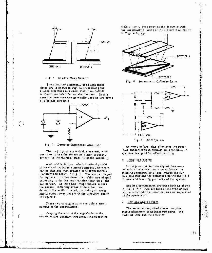
field of view, dioes prov~de the designer w~ththe possibili:y of using an AGC syster as Ehown

SUNLICHT

SDETECTOR 2

DETECTOR 2 DETECTOR I

Fig. 4. Shadow Mask Sensor V DETECTOR I

Fig. 6, Sensor with Cylinder LensThe circuitry commonly used with these

detectors is shown in Fig, 5. (A ssuming that ,silicon detectors are used, Cadmium Sulfideor Cadmium Selenlde can also be used. In this I '-ocase the detectors are generally used as two arma JrPof a bridge circuit.

"Fig, 7. AGC System

Fig. , Detector Difference Amplifier As noted before, this alleviates the prob-

lemas encounterea in simulation, especially inThe major problem with this system, when ibystemse defigned for offset po.nt-.ngone tries to use the sensor as a high accuracysensor, in the thermal stability of the asembly B IrmainToSýstem_

A second technique, which limit. the field In the prevous section approaches wereof v:ew and produces a more compact unit which conaiderea where either a mask formc thecan be shielded with greiter care from thermal defen gery or a le i ma thedefining geometry or a lens images the suntransients, is shown in Fig. 6. The sun is imaged on a de'.ector and the detectors define the fieldthrough a slit on two detectors, which are shaped of view and trac'xing geometry of the system.accordirg io th. desired transfer function of thesun sensor. As the solar image moves across Anoaher co bination provides both as shownthe sensor, differing areas of detector I and in Fig2. wo seniors of the type showndetector 2 are illuminated, providing an errorsignal output when used with the circuitry shown can be mounted on a common base or separated

on the spacecraftin Figure 5

These two configurations are only a small C. Critical Angle Prismsample of the ponaibflllies. The sensors described above require

Keeping the mum of the signals from the stable alignment of at least two parts: the

two detectors constant throughout the operating ma, or lens and the detector

157

i,. ." -, . ; " = • ; : _: -M o-

in a simple DC system, the detectors canbe mounted directly on the bac' surface of the-.critical angle prism as shown in Figure U., Itvariation in detector sensitivity is sufficientlycritical, a single detector and chopper as shownin Figure 12 can be used.

SRDOW MASK

Fig. 8. Imaging System with Shadow Mask

To reduce the number of pieces which have &••. .,to be controlled relative to thu reference surface,a critical angle prism can be used, In this casea single piece of glass (or quartz) controls the 0t(€null axis of the sensor. Light enters the sensorFi.1,D CasSseS as shown in Fig. 9, The backc surface of theFgLD asyse

S prism is cut at the critical angle. The trans- , , -e~~

near the critical angle the transmission is'j proportional to the square root of the angle and

passes througs, zero with an infinite slope. Thus "extremly high sensitivity cant be obtained in , • •'• •addition to the advantages mentioned above

ChopperSFig, 12. AC Caps System

'. ~D. .ig•.tal Sensors

Due to the high energy which is availablefrom the sun, it is possible to replace theanalog detectors shown in Figure 6! with a Greycoded set of detectors. This ty~e of systemsprovides direct readout of t•,e sun position

Fig.~. t ca Anle PismSince the solar diameter is approximately /20,Fig.•. Citicl Anle Pismthe system shown in Figure 13 is limited t, a

';• F'•"'•resolut.ion of 1/20. For certain miselons, •nd';•I especially during atti'.ude acquisition portions:' ot a mission, this type of a system can provide

It the required accuracy.

t^'" Since the positir.n output is carried as a.0e simple aind offset pointing is very easy.|

j o• If higher accuracy is required, it can be

Sobtained directly at discrete times, whan the stateof one of the dig',tal outputs is changing or by• ,•,.•0IC •0••, 0 either analog or digital interpolation |••!

18 Fig. 10. Critical Angle Prism Transmission ¾.•

15.. ... ... .. .....8.. .)i..,,

L9

Z I-SUN POSITION OFF NULL

SUN POSITION AT NULL

Fig. 13. Digital Sensor

IV, ERROR SOURCES IN SUN SENSORS Fig. 14, Error Sensitivity

The total field of view of the system isFirst lot us consider solar activity and e milli-radianu, The comparable width of the

the corona to determine whather or not high detector is *accuracy sun sensing is feasible,

At null the current from each detector isMost of the solar activity is photographed proportional to 9•/2 The change in the current

through very narrow filters, because very little for a 0. 01 milli-radian displacement Is . 0lx9t//activity is easily observable within the whitefoa0.1mil-danisac etis0 IVactvituum i eai observghbless wit the whitde ses Thus the fractional change in the detector currentcontinuum. The brightness of the sun decreases for a 10 micro-radian displacement is 0 02/9.very rapidly at the edge, with the white coronahaving a brightness of approxiMately 100(l) of

the un he oroa des eten toabot 3If it is assumed that the two detectors will" ./ the sun, The coron•, does extend to about 3 have a differential sensitivity drift of 156 aftier

solar radii, thus it Can contribute mit 0' of thehaeaifrntasnitvyditofatronerry compared to the sun, initial calibration, then the field of view of the

ep hnsor, 0, can be 0,2 milli-radians (consider-

Flares generally cannot be seen against ably smatler than the solar diameter). For athepotosre thoeragh cnnobe flaren (July 2,1) 1 degree (0' 20 mill-radian) field of view thethe photosphere though nne flare (July 2i, 1948) relative stability of the detectors has to be 0. 1

added 10% to the continuum but only in the 4000- reltv6000 AO region{l) per cent.

This relationship is independent of the munTypical flares provide less than 1% to the Ti ea~nhpi needn ftesaTypical flare( diameter and depends only on the total field

continuum output. eof view.

To avoid the regions of high solar activity, If one assumes that 0. 1% matching over anit is therefore necessary to choose a band of extended period is feasible, then the accuracyoporation in the red region of the spectrum looking and field of view limits of this type of systemat the red to near infrared spectrum of the sun. re set, If theme numbers are sol compatible,A spectral region choice of this type allows it becomes necessary to remove ; portion of theachievement of the highest accuracy within ener nuol.present knowledle of the sun. energy at nul

As a first approximation, assume a 9Let us now consider the error terms within milli-radian mask (essentially a complete mar'l-

the sun sensor shown in Fig. 6 The complete ing of the sun). The primary error source is nowimage of the sun falls on both detectors. Con- the corona.eider a displacernnnt of 10 micro-radians (thesun diameter is approximately 9 milli-radians) As a worst cae, assume thatch coronaas shown in Fig 14 extends to three meo the sola" radius ,nd

that it in all loc .ed on one aide of the solarr 1disc

"b15

A quick cal-ulation shows that errors intro- While one type of sun sencor was used to

duced by this factur are negligible for reasonable illustrate the design parameters, the same

(less than 180 degree) fields of view, analysis is required for imaging, shadow maskor critical angle prism systems,

Prominences which average 0, 5 arc min by2 arc sec also represent negligible sources of The designer haL to realize from the

error in a sun sensor system, beginning that he is working on a system withan expected accuracy of 1 or 2 arc seconds,

Thus, in conclusion, one can assume that The problems are not in the circuit design,

the sun ic an object with uniform brightness but in the mechanical, thermal and physical

in the 0,8 to I. O'micron range optics aspects of the system.

V. DESIGN CONSIDERATIONS REFERENCES

Due to the high energy which is available 1 G. P, Kuiper, The Sun (The University of

from the sun the apertures of solar attitude Chicago Press, Chicago, Illinois, 1953).

sensors are usually very small when comparedto the apertures used in star trac term. 2. Staff of Goddard Space Flight Cqnwer,

I cm 2 of solar energy is more than sufficient Orbiting Solar Observatory Satellite,

for very easy data processing, The Project Summary, NASA SP-57, 1985.

However, the Airy disc diameter of an 3 NASA Design Criteria Office, Sun Sensor

optical system with 1 cm aperture operating Design Criteria, NASA SP to be assigned.

at '. micron is approximately 50 arc sec. Thusthe order of magnitude approximatiuns used 4 H, Nagaoka, Diffraction Phenomena in

in the previous sicption require much more the Focal Plane of a Telescope with Circu-

detailed analysis(1) than is provided by simple lar Aperture, due to a Finite Source of

geometrical optics Arguments. Light, Ph~lTosophiTal Magazins, V. 45,no, 1898,

160

ACCURACY OF IR HORIZON S•80RS AS AFFECTED BY ATMMIMIC CONSIDERATION•"

John A. Dodgen and Howard J. Curfman, Jr.NABA Langley Research Center

HaptonJ Virginia

(U) The effects of amompherio variability on :R horizon sensors areillusetrated using expriaental data and analytical study results obtainedor supported by Langley Rescorch Center. It is shown that proper meled -tion of d •pc tral itaertva minimizeb horeson aens peoblpap e Letsd bylor-level famsphuric efeT•ese The bete spectral interval Ws a found t o '

de therin.s0i tron w6-ito batinde Assciated which Ch2angsorpitsaon.i Ith

atsshow , That band effecively shields a hensor nrom cloue hdeoCher lov- a ldica e effectse .ovex eri en es it sensitive t o relaoiively s;slowly voierng temereturee hanee in the atmphere ar oe i 0 ki therebyintroauci e vriations conuse d by teatotel and oeographit eflecofr Tf eirsults of a seo y of t•tsi e vbletons over orrecto•n sn shows thatidffermintil trind eih latitude existmi watich changey oi.h season, foris s|hown ahat t simslyc itlerentede itngle beam, horizon henbor tn theSC02 band can be uyo~ed to enerienee approximahely 3 km r ildom V swna-n)ion of the hpraion sbout yhe teterministie co anl primarnly s thehesrer lenehs en ea It is concluded thut the use of a three- or four-beahoholOr sensor with simle "oslesineng" aspe acmrantoof e foa uysemapicoffects) will provide attitude determination accuracy of 0.050 (la) for

cpatecrait et altisudor abose 100 deutecal miles.

o sOreJ ac.c atmospherc data eo prtr hs t horizon vanria -e amain by a horizon senior will be shown, and smoe

(U) Por the pabt swveral years, the Langley concluseions dra•wn as to the accuracy obtainale.R•esearch Center has been conducting resea~rch on

horizon• sensing a$ a •means Of Measuring space. BACK 0Ocraft attitudeo, This work Was directed priw,•rilytoward describing more Lacurately the input to (U) Early in t~his work, LRC decided to concen.

such horizon nsuors, nanely, the harison trate on the thermal infrared spectral region, inrAiance profile. The research includes both order to proyide "ful-time" horizon sensor use,wetprlmental measurements and analytical studies, in both surlit and dark portions of the orbit) aand covers a wide spectral range from the ultra. featuza not possible with cpectaol intervalsviolet to the far infrared (Refs. 1.12). We feel dependent on solar illumination. As a result ofquite strongly that the horison data being analytioal work by several investigatorsobtained wstablishes fundamental design considers- (Rife.,13, 14, and 15) we further concentrated or,tions for any future horizon senior developme4ntsl, two spectral intery•Iep nameiyo the 15-micron C02nis paper will review briefly parts of the b" and the rotational water vapor band beyond

Langley reiearch Including results. Data from the 20 microns, where the absorption characteristicsProject Soanner flight experiment will be used to of the atm•sphere move the apparent horizon todeonstrate the effects of spectral interval higher altitudes, thereby minimizing the effectsreelection and of geographical position. The of low-altitude phenomena such as clouds.results of an analytical stuCy utilitina available Project Boanner obtained experimental data in the

14-14 Cwh2c band ad in the 21-32u water vaporband which indicated the C02 bend to be more

This work wts done at NASA Langley Research promising from the standpoint of minimising theCenter, Hampton, Virginia effects of low-altitude atmospheric vagaries.

Figure I presents radiance profiles from Projeot

161

14-

12- - 21-32P H20 VAPOR

1---14-1611 C02

8 130 N

RADIANCE. Pw/2s 6 57 0N 0- 8

17 0 N

2

0 10 20 30 40 50 60 70

TANGENT HEIGHT, km(U) F11. 1. Meas.red Rsaianre Profiles Trom Project Scaner for

1-14A and 01-W pectral Urnd

Scanner (Reet, 6, illustrating a version of tho) c•ngs whtich oc our, it was found neeoosiry toso-c•lled 'ool-.clou•" pmoblm in the 21-J• develop a analytical. means of synthesizingprofile. The solid-lie wLter-•v•r profile r-Alance profiles frm available atmosphericmuaked 130 N vus obtained from an %rea known to be infoiation by solving the radiative transferclear, vwhe that uired 5TO @cme fras an ares problen. This was due to the lack of eperi-known to have high clouds. The radiance obseod inntally determined profiles having the requiredIn the cloudy area in sen to be roughly oin-half temorsl and geographic coverage. Homeywell, ZInc.,that in the clear szeae. The tvo dashed-line under eontract to LanL4 y, developed a modelourves ise C02 prof•• le from tWe se area aod (Ref. 10) which Included such factors as gasshow little or cons of the effect and indicate tbe mixing ratio, atmspasric transmittance, c'efrso-rLdiance levels ane governed only by the tempera, tioui, Doppler broadening, aod the absence ofture strujcture of the atosphiere. Tho effects that tharmodynmic equilibrium at higher altitudes.the tempeature structuft has oc the horimm are dbhle it waU reognised that Other bazly-tics.lIlluatmtm,4 On Fig. 2 vwhaT moineeied radia•ce notbds existid (Refs, 1A and 15), no single onef rofilen for both winter and munur conditions ppeeamd to incorporate s.l of the factors deemed

Ref. 7) ae shown fop three latitudes, The deae im*tmAnt. Profiles obtained from the developedprofiles are for sumr conditions, and a treAd of anal1ytical a~p- compared very favorab..j with

radiLi anen vm o with latitude is noted. The map o mental Project Scaterrusults, givi addedsldprofiles wnotie ntewno lgt cniee oteesl, nlsso topri

and s~how a more prominsnt, and opposite trend with effects on htor'ilon sensors,.,

latitude. The agmamet betvee the winter LeoIsu e r profiles at 170 N fa"ls within the experi. (U) A seond problem then arose, namely, how canmental masuremnct acouracy, so no seasonal we get the omputer to @ee" or "think" like aeffects are evident. Thu it Is sean that a horison •emor in order to determine the senisi-horison seneor operating in the lk C02 band is tivity to radsnin• profile chawgert Honeywelleffectively decoupled from cloud probhlis, how- developmed 4M% we call the "'locator" ococept forever, it would probsbly be sensitive to high- this pa•toee (Ref. 12). A "lucator" difines, inIlitUAl Atlspheric variations which occur as a a simple vwq how an idealised horison sensorfu.ntion of seson and the position on the earth, operates to detect (or locate) an altitude which

is characteristic of a radiance profile. Thisconcept is illustrated on Yi&. ., A horisonsernor having a wide field of view would, in

(U) in order to evaluate the sensitivity of effect, integrate the eners' under the Profile ashorison sensors to the geopraphical and seasonAl it is Bcannd down across t1' horison, The

located horison al 4 itude (h,) would be as shvvn

16Z

580 N 330 N 170 N - WINTER

6.0 - -SUMMER

5.0-

4.0\

RADIANCE, W/m2 sr 3.0

2.0

1.0

010 20 30 40 50 60 10 20 30 40 50 60

10 20 30 40 50 60TANGENT HEIGHT, km

(U) Fig. 2, Seasonal Variations of Meaeured CO2 Radiance ?roftles (Project Scanner)

6.0

5.0 - hII: C3 N (h)dh

5.04.0

RADIANCE, 3.0N, W/m 2-sr 2.0,-RA

1.0 - I•. -km/m 2-sr10

-30 -20 -10 0 10 20 30 40 150 60 70 80TANGENT HEIGHT, h, km

(U) Fig. 3. "located Horizon for a Threshuld Va'.ue on the Integral of Radimnce

for the specified threshold on the .alue of the can be generall.y described as the northern hu•-inteogral. A number of other "locators" have been sphere isar North America. A number of locatorsdevised, some ufing r&4i&nce level, others weir6 identified and applind to this body of data,oter4ng to normalize the profiles. The important and the variations of indicated altitudes were

thng Is that any profile, defined by season, examin#d. For practical horison sensor use) itlatitude, tims-of-dsy, and so forth, can be was de-wed boot to view anY syste8Mtic variationsreduWet to a single number, an indicated horison an a funotion of latitude for a specified season.eltiti.de, for a given 2ocator, In this way, This then constitutes an oblateness-typevariations due to the perturbing functions can correction which could be rather easil.ybe conveniently Lnelysed. Limplemnted.

(U) To examine the e•ffeOt of seaSonal. and a'geographioal changes, a body of atmospheric datafrom radiosondes and M rocket flights was (U) The method of analysis just described wascompiled (Ret. 9), aid used to synthesis@ used to examine the performance of a sensor whichrdiaLnee profilee for a number of synoptic situ". locetd the horizon at the altitude where ations (sefe, 16-18) coveorin various seasons aLd 3-waitt.meterI 2 ._rll radiance level exists. Ther.evra ,e•a.rse, for the geographical area which

S;I : ••" 'm " - . . . . .... . . . t.. . .. =,I m,-, gl d • I I I I I e I i II -In - • i- ll i/4

40- - UG.

35

LOCATED HORIZON 30ALTITUDE, km

25-

20- "" I , I I I I I J0 10 20 30 40 50 60 70 80 90

LATITUDE, deg NORTH(U) Fig. .. Variation of the 5 3-2-sr" Altitude Point With Latitude for No Seaaons (•D•t

Based on 5 Years)

results are ehown on Fig, a. The ordinate is single horizon sensor b@eam fror, 300 n, mi, miti-a.lt-,týe in kIn, the abscissa i3 north latitude in tude, thts locator is not too promisi.-g, 1f tIhedegrees, and data for july and ft' late November locator is modified tc noro•r•iue the prý;u'Lleare presented to shcw the sasornal change. The using peak radiance levels, consideraýtlcsolid liner represent the mean for alL data for i::provemenz is obtalned. For exarple, using thethe date, •a the shaded zone reprosents the tla helf-rsLldance level, or "half-po--er pýint•*"variation about the mean. The upper curve for loca:or moves the located eloititde to approx±-"the July dAta shows the summer trend and is a•en rately 40 k--, with an indicaed systeematic varla-to be relatively flat, but shows the tendency tion of 6 km and a a0 variance of !,,- km,"toward a higher altitude (greater radiance) at the resulting in an iiprovement of a,,out a factorupper latitudes seen earlier in the Scanner cur•es of 5.in Fig. 2, The winter data show a much m=repronounced trmnd (approx ii km deviation of the (U) T-.e data Iu..t dinuuised, hIle n.t.cre.ti.gmean) 'grich is ac.ompanied by a rw-ch 4Ider ran4vm frcr, a synoptoi view as to what ie happening,variation, ±5,5 km at the higher atitudes, It is do not represent uhat is felt to be a realisticinteresting to note, however, that the trend lines horizon sensor.appear to pivot about k latitude near 200 whichmight explain the close Lgreenont between the (U) roe craracrer atics of the mingle beam ofProje•t Scanner winter and eummer profiles at a more prctical sensor are eho'wn on Lg. 5,

170 N latitude. The data of Fig. - cover the An edge tracker 4..thering at 2 ':!z ie postuiated,5-year span 1964 to 19e7, and the variance for any utilizing a thermtistor boloreter in a 2-inch-single year is considerably reduced from that diameter opticaL system. This device t.ith a 10shown here. In fact, the November data for 1%5 vertical by 6C horizontuCl field of vteq Inte-and 1966 tended to agree, and averaged together grates the energy in the horizon profile as itprovided a systematic variation (or trend) of sweepe onto the earth, therefore operating on12 km and a maxinum I1 value of approximately an integral-of-radiance locator, The rlltur.eeS km, while 196. was a bland Year having a eyaeMY - sensitivity of the device correspond, toatic variation of ý,5 kcm with a !a value of slightly less than 2 k.7, indicated L.titude at-little more than 1.0 1c, We are not yet convinced the hortzcn, Addition of a sample-and-holdthat a deterministic biennial cycle exists which circuit .nd comparator will allow use of a-would allow some reduction in the random lo normalized inegrral locator.variance. When it is realized that 1.0 km at thehorizon corresponds to 0.020 displacement for a

5

1&A. "" - V - . . .

EDGE TRACKER - 50 x 2hz VERTICAL DITHER

DETECTOR : THERMISTOR BOLOMETER

OPTICS : 2 INCHES DIAMETER

FIELD OF VIEW : 10 x 40

RADIOMETRIC EFFICIENCY : 18%

DETECTION LOGIC : 1. THRESHOLD OF INTEGRATEDRAD lANCE

2. THRESHOLD OF NORMALIZEDINTEGRATED RADIANCE

W/2NER : -0.025 W/m sr

HORIZON SENSITIVITY : z2km, S/N - 10

(U) Ylg. . Sinrle-Bee.m Horizon Sensor D~eigr. Charc•oeristics

4342

41

40

39

38

LOCATED 37HORIZON 36

ALTITUDE, km

34-33 -

32 -

31-*I p 4 J_ I I I I I

0 10 20 30 40 50 60 70 80 90LATITUDE, deg NORTH

(u) Yij. 6. Varibtions of the Loeatd Altitude for a 20-Wxtt-ki-Mstsr"2.r" Thxr'eho on rZntegrated •a1tnce With Latitude for November T on

,,''

165

IfJil1 • I~ll"II~llI IIIIIIIIII llllll IIIIIl lllnlll NMI"lll~l

3)38

36 F35

34

LOCATED 33HORIZON 32I

ALTITUDE, km I

30 -

29f

28F

271

0 10 20 30 40 50 60 70 80 90LATITUDE, deg NORTH

(U) Flg. 7. Var-ationa uf the Located Al•t.tude for a Norwai1te4 integpa of Radidnee WitLZlAtitude for Noimynber (Data Uzod on Years)

1.0~

0.1

ATTITUDE UNCERTAINTY,d% ",% %% ' • CURRENT

deg ~ ~ .~ACCURACYNIS" RANGE

0.01 . N %. f,

IN \ 3km

\ 1.5km

100 1,00 10,000oSPACECRAFT ALTITUDE, n.m.

(U) Tig. 8, SnW1-B,, Horizon Sensor Angiular Un.,er~tanty Caused by Hoz'Agoi, RadianceVariations

166

(U) Repremertative ;erfo~rmnce for such a sensor does make the senior sensitive tc relativelyas described, during the Xovfmber season (3-year slowly varying temerature changes in the atmo.-average), as a simple threshold of integrated phere above 20 km and, coLsequently, introducesradiance device is shown on Fig. 6, Note that vsriL&ttons due to seasonal arO geographioalthe average trend vith latitudc i reduceOd to 6 c effects. A study of thee changes indicates thatwith a mxi=m la uncerteinty about the mean of a deterministic effe!t with latitude existsapproximately 3.5 km. The change in performance which varies with season. Based on a •tUdY ofdue to the approaeh used in "n lng" the atMospheric changes covering 3yar, a simplylocator is shown on Pig. 7. Th3 trend of the implemented, mingle-beam, horizon sensor in theaverage Wan reduced to about 4 kt, hoveyer, the C02 ban "m expect to expevience abai 3 kmranm vriatA~ion was reduced onl•y to aboutA 3 ke random variance of the noiison Pct higher latitudes.indicating the major advantae to o besuppression Use of a thre4- or four-bemma horison sensor ofof the systenatic effects, with %.ittle imroyeent he type discussed, and, ma•Ug "•blatoness typ-?in random scatter. These data should only be oorrections for the sy•tamatic horizorn eofects, jconeidered as illuatrative, and do not represent should prnvide attitude leter•ination accuracy toan attempt to optimize the normalization technique. 0 . 0 r (1a) or better. Wh1le the results of the

U) The significance of th esults st horison variance study showed a poesibilitm. of(U)sshed is ilustratednon 11g. •he * mfurther accuracy improvements, a4ditional high-discussed is illustrated on Fig. 8. The ordite resolution experimental measurements of theof this plot is the attitude uncertainty in horizon would be required to fully exploit thedegrees, Lad the abeluga sho ve the spa cecraft po ten tial .

a ltitude in naeutical miles. The curves show the ieffects of several values of horizon variance inkiloneters on the accuracy of a single-been,horizon sensor. The values of horizon varianceare near thosu which were obtained &. Ic values (U) The authorp gratefully acknowledge the work

of R. E. Davis, ct LAI4gl Research Center, whosein the earlier results. thr refearnce prrosem) analyses provided much of the data presented, andthe top zone rep resents the a&carac range A. Ja/l.l, Jr., for verifying the horizon sensor •reported by several users of horimon sensors. design choracterietitr.The line showing the ar4ulamr uncertainty for a3-km variation corresponds to the performance ofthe iingl•e-beam horizon sensor just presented,where correction has been made for latitude. If 1. Dodgen, J. A.; and Curftan, J., Jr,: •ui.S the atiudeer of Horizon Definition Studies Beingbeam .jorigon sensor, the effea.tive uncertainty bndertaken by Langley Research Center.would roughly correspond to the 1,5 km value Proceedings of the First 8ypsum on Infraredalso protted. For a spacecraft operating at Sensors for Spacecraft Guidance & Control,

~00r..ml. alitue, t i sen tit n alarBarnes Eng. Co., c. 196", pp. 233-239.accuracy of approximately e0.030 (ic) isindca~ted. 2. Dot'gen, J. A.) McKee, T. B.) and Jalink,

(U) .The results Just presented are bases on a A., Jr.: XASA-LRC Program to Define Zxperi-

study which utilized a model to wyntheseze mentally the Earth's IR Horizon. Proceedings

radiance profiles from apper at.mocpheric data. of the Second Smposium on Infrared Sensors

There are indications that somc further improve- for Spa ecrft Guidance & ConC.rol, Barne-

ment in :iorizon sensor accuracy may be available Eng. Co., c. 1968, pp. 113-L29.

if more othiestinated compensations are allowed, H. framkEy W. C.) a" Mc:ee, . B.: Radiance of Ahowever, the question arises as to thi vLlid•ty the Earth and Its LL~t in the Kiddle Ultra-of the synthesized data for purposes of 2.mproved violet. NASA dts D-2.5i , July 6id. U

acouracy. ProJect Scanner experimental datL usedto check the model were limited to approximately 4. McKee, T. L.; Whitman, R. I.) and Engle, C.l-2,0 )m resolution. Further s:,perimental. data Badiometric Obeervationo of the Earth'. Horizonof improved radiometr.c acc',racy, and wider From Altitudes Between •00 and 600 Kilometers.covera4e, would be necessary to verify, or FAmAltitdes Beteen 0a60.

replace, the model for purposes of improved Aaccuracy. 5. Jaink, A., Jr.) Davis, R. E.; wn Hinton,

NC D. .L: Radiometric Measurements of theCONCLUDING FJJAW Earth's IR Horizoii From the X-l1 in 1hree

(U) The work done at the fnegley Research Center Spect-.al Intervals. NASA T; DZ-6A4, July lg6b.on the variability of ~.he earth'd infrared horison 6. Mcee T. B. '"hI R.1)ad Davis R. E.

indicates that proper selection of spectral• • :nter-l can miniize horison sensor probleus due Infrared Horison Profiles for Su-er Conditions

tO low-level atmospheric effects. The best From Project Scanner. NASA TW D-4741,

choice of spectral inter a;. was found to be the August 16.1-.0- to i 6 ,.1..rcrcn band asooclated wit" CO-absorption in the atmnsphere. This band 7. WLitzAn, R. I.) McKee, T. B.) and Davis, R. H.:effectively shields a sensor from cl(ud problems Infrared Horizon Profiles for Winter Conditionsand vcivable souhces of straso ;omadia-icn. It lFrom Pvoject Scaaner. NASA T B-4905,

Derember 1968.

167

8. Kirk, R. J.h Watson, B. F.) Brooks, E. M., Lad 14. Hanel, R. A. Lndeen, W. R.) and Conrath,cmrpenter, N. 0. B.: Infrar•d Horizon S. J.3 The l-,rared ,orLson of the PlanetDefinition - A State-of-the-Art Report. E.arth. J. of the Atmospher±c sciences,XASA CR-722, Honeyvell, Inc., April 1967. Vol. 20, 'to. 2, March 196;% pp. 73-86.

9. Peterson, E. L.j Schustz, J.) Sheek. W. E.) 15. Wsrk, D. %.) Alishouac, J.) Lb4 Yaonamao,wnd Tang, Wen: Derivation of a Moteorological 0.: Calculationa of the k-th's SpectralBo6y of Deta Covering the No:thern Hemisphere Radiance for Large Zmnith Angles. U.S.in the Longitude Region Between 600 W and Department of Couseo e Weather Breau1600 w From March 1964 ThKr4cg February 1965. Ye~torologioal Satellite LaboratoryNASA CR-7M, Honeywell, Inc., April 1967. Repo•t No. 21, October 1963.

10. Bates, J. C.) Hanson) D. S.) Houae, F. B. 16. Honeywell, Ino. compilation of AtmosphericCarpenter, R. 0. B.; and Dille, J. C.i The Profiles and Synthesized 14 ZR HorisonSynthesis of 1•i Infrared c (orison Radia•n Radiance Profiles Covering the NorthernProf-es From. Meteorological •ata Inputs. Hemisphere in the Longitudc Region B•tweenNASA CR-724P Honeyell, Znr., April 19•7. 600 W and 1600 V From Maroh 1964 Thrxovu

February 196 - Part I. NASA CR.66184 ,11. Thomas, J. R.) ones, X. E.) Carpenter, october 1966.

R. 0. B.) and Ohring, 0.: The Analysis of1ý4 Infrared Horizon Radiance Prof.',e VLra. 17. Honeywell, Inc.: Compilation of Atmospherictione Ovur a Range of Meteorologic.l, Profiles mn Synthesized 1u I R HorizonGeographical, an Seasonal Conditions. Radiance Profiles Covering the NorthernNASA CR-725, Honeywell, Inc., April 1967. Hemisphere in the Longitude Region Between

600 W and 1600 W Prom MArch 1964 Throuh12. Thomas, J. R., Deriva.ion and S atistical February 1963 - Part Il. NASA CE-66185,

Comparison of Various Analytical Techniques 0-tober 1966.Which Defie the Location of ReferenceHrizons in the Zaurth's H••-son Radiance 18. BrAfteld, L. G.j and Nelson, 0. D.:Profile, NAaA CR-726, Honeywell, Inc., ocaated Horizon Vasrition Stuy - Fiz.alApril 1, 1967. Rey.rt, xASA CR-6674&, Honeyell, Inc.,

Janu..ry 1969.13. Xc;Gee, R. A.: An Analyticas. Infrared HAdia-

tion Model of the Earth, Applied Optics,Vol. 1, No. 3, September 1962, pp. 649-,. .)

164

S 168

INSTRUMENTATION FOR INFPARED HORIZON SENESNG

Robert W. AsthtimerDefense and Space DivisionBarnes Engir.sering Conmpany

Stamford, Connecticut

i

The chimrcteristics of the earth's horizon in vious infrai id s'octralregions are presented in einother paper. This pcs,er will dibcuF. theinstrumentation necessary for sensing this rdWa',or sign.t",e andprocessing it to p,'oduce an electrkoal ouiput indicative a! !he angulc"location of the hoeinon.

Basically, all horizon saiuning instrumeIet3 arA comprised of an opticalsystem includ'ng any opticl-mechanical awaoiing mechanisms, oneor more IR dstsctors, and pro;sising elsctronils. The most sensitii,,R detectors aro the cryogenica.ly cooled photodetectors. However,

these have been rurely used in ?iorlion sensors bec-Ule of the ;rac-tical difficulties of cc.oling, and because inmtrumrnnt accurmcy i.getisrally liited by 'actors other than detacto,' kensitivity. The de.-tectors commonly used ara '.h* immirsed thermistor boil.,neter on, the

thermopile, both of which ci,,c thermal detectors aid do not requtrecooling,

Usually the iniormotion desired is the pceition rf the local vertical,'rom which pitch Qnd rclA ittitu6e can be ('erived. Therefore, t 4o notnecesL.ary to locaite the oclual ground horizon but ruther aný level inthe ,tr,,;sphera bearlng a constant relation tu the ground hori.cn., Atlow altitudis the structure of the hnrizon profile beco'mee cf great im-portcnoD and the Iznstrument must contain logic to identify such an in-, ,ariant point on the pi 1.e. This logic is called a "locator" c:,d avariety of locator te:hr.queu have been studied and used. At highaltitudes where the angular &ubtense of the entire atmosphere is lessthan the ciccurccy dsirod, the horizon profile becmes unimportant.

Jo~izon sensing instruments can be classified into three types:wide aitgle scanneru, edge trackers, and radiance balancers . Thereliti,,e advantagec of such are discussed and typical instrumenttof each type described. The factor5 lin'iting cacuracy and the re-sults achievd in jractlice are discussed.

169

I. INTRODUCTION point, acquire the horizon. This may be ccoom-plshed by iome other system such as an inertial )

A number of methods nie been developed reference, or a seerch mode may he necessary.for determining the attitude of a spac, vehicle. Once the horizon is acquired, there are two poe-They oil rvquire some instrumenW foe sensing 'he sible modes of operation. The horizon sensorangu.lar oriertution of spacecraft coordinates with output may be used as an error indicator to con-r•iipjct to wome ext~rnal reference SuCo as the trol the spacecraft, in which case only a narrowsun, the store, the magnetic field oi a planet, or proportional range around the null position is re-an Liertial platform which stores the orientation quired. Alternately the sensor may be requiredof some extvrnal coordinate system. For orbiting to accurately read out the position of the localvehicles tie local vertical or horizon of the vertical independently of the spacecraft attitude,planet is a useful reference and in this paper, I in which case a wide linear or proportional rangewill discuss indt"uventation for sensing this id necesiary.hcriuon from the thermal discontinultv betweenthe planet and the essentially absolute zero The prinoipcl target parameters of interestspace background. The horizon can obviously be are the angular subtense, the temperature anddetected in other spectral regions much as thp entissivity of the planetary surface, and in thevisible during the daylight phase, but the infra- case of a planet with an atmosphere, the limbred ham proven to be the most useful since it is profile. Finally, the sensor parameters are theindependent of phase, so I will restrict my re- design decisions which must be made to con-marks to this type . Our general problam then is struct hardware to fulfill the system require-to design hardware that will measure hngles be- ments. In the following sections some of thesetween spacecraft coordin':tua and the planotcay factors will be considered in more detail,horizon at ý.everal points. Neglectin7 planetaryoblateness this amounts to sensing the position I1. CHARACTERISTICS OF THE INFRARFD HORIZONof the local vertical with respect to the space-craft. Fundamental to obtaining high accuracy are

the characteristics of the infrared horizon, ThisTne major factors entering into the design of is discussed in more detail in another papep but

a horizon smnsor are tabulated in Table 1 it is necessary at this point to indicate brieflyhow and why they affect the horizon sensor de- )sign and accuracy. The true or hard horizon of

Table 1 the earth can only rarely be seen from space, be-ing obscured by clouds, haze, and atmospheric

A. SMSTEM F 1fUIREMENTS absorption, Therefore, thn thermal horizon ap-pears as a radiance gradient fading into the space

1. Acquisition Capability backgruund, which can subtend as much as 21 at2. Accuracy low orbiting altitudes, This gradient has a dif-3. Linear Range ferent appearrance and stability in various spec-4. Response Time tral regions, From experimental and theoretical

studies of theme profiles, stable characteristicsB. HORIZON CHARACTERISTICS have been found which permit identification of a

pInt on the profile which is always a fixed alti-1. Angular Subtense (Altitude) tude 2boy the true horizon. A signal processing2. Radiance Variations technique to detect such a point has been called3. Horizon Profile a "locator." It has been shown that by spectral

filtering to the 14.5 - 15.5 micron band, and useC, bENSOR PARAMETERS of a suitable locator, an uccuracy of 0.020 can

be achieved from low orbiting altitudes.I. Detector Type2. Detector Field of View This problem is non-existent on the moon3. Aperture Requiremerrts because of the absence of an atmosphere; how-4. Scanning or Tracking Mechanisms ever, another and equallIy disturb!ng phenomenon5. Electronic Logic and Processing occurs, namely, thn large variation in horizon

radiance over the lunar disc. In practical sen-@sor|, a horizon "!caottr" is required to overcome .. ,'.j •First, we must consider the system require- this effect an well, ,,.,.?••

ments. This involves the type of Information we • ft \we,require from the horizon sensor and the use towhich it is to be put. The system must, at some

•0

We shall first consider the simpler problem spatial variutions ii, detector responslivity andof identifying the so-called "hard" horizon where optical aberrations. Alse the frequency responsethere is no gradient caused by the atmosphere, of the detector and associated electronics willThis is the situation with the moon, or the earth tend to round off the corners of the waveshace,at long distances where the angular subtense of which is a further limitation to use of a very lowthe atmosphere becomes negligibly small. The threshold.worst case in encountered on the moon where thesurface temperature range of 1201K to 3000K will When we consider the earth from low alti-produce a radiance range of 50/1 in the 14 - 354 tudem an added complexity develops; the infraredspectral region. A simple horizon location exam- horizon no longer appears sharp but is diffuseple for this case is iketohed in Figure 1. Con- because of the emission of the atmosphere. Theaider the field of view of an iwfrared detector plot of radiance seen from space vs. altitudescanning across the edge of the moon. The hori- above the earth's surfuce is called the horizonson will be identified as the angular position profile and is dependent upon the local atros-where the signal exceeds a pre-established pheria conditions, and the speatal region inthreshold level which, in this example, is taken which it is viewed. Figure 2 shows calculatedas 1/2 the full cold moon signal. If the field of profiles for the 8 - 12L atmospheric window. Theview Is Infinitesimally small, the correct horizon profiles are computd for different atmosphericposition P will be identified regardless of the structures dependent upon latitude, season andtemperature of the horizon. Howeve: if a wide weather conditions. Since clear air is fairlyfield is used as shown, the horizon will be iden- transparent in this region the horizon is deter-tifled at A on a hot horizon and at B on a cold mined by the surface, or clouds; -usually theone, which will produce an error equal to almost latter because of the long tangent slunt paLhhalf the field of view. Thus if the field were 21, through the atmosphere. The v=iations in cloudan errr up to 10 could result depending upon the height with different weather conditions stronglytemperature of the lunar horizon, affect the shape of the profiles and make this a

poor spectral region if high accuracy is desired.An obvious means of reducing the error is to

lower the threshold, since A and B approach P Figure 3 shows profiles for the same range ofas the threshold approaches zero. This is called atmospheric conditions in the carbon dioxide ab-a minimum threshold locator technique. In prac- sorption band between 14 and 164. The surfacetice, a limit is reached by the detector noise and and clouds are veiled in this r-gion by the opaquethe threshold must be placed well above the noise COZ in the upper atmosphere and consequentlylevel. The threshold can be made as low as de- the profiles are much more uniform. The differ-sired by increasing the optical collecting apertUre ences are almost entirely caused by the changeto improve the signal/noise ratio. in stratospheric temperature with latitude. If

these profiles are normalized with respect to theAnother technique is to adjust the threshold peak radiance, they almost perfectly overlayeach

to a fixed percentage- of the full edge radiance, other. This indicates that the no~rmalized thresh-This could be accomplished by using two detec- old locator technique described previously wouldtars separated so that the field of one was corn- identify a point a fixed dir,ance above the truepletely filled below the horizon before the second horizon, which is indep,.ndent of weather condi-reached the horizon. The signal developed by tions or latitude. For establishing attitude thisthe first detector would thwn be used to set the i, equivalent to sensing the true horizon.threshold for the second. In scanning systems,the edge radiance could be stored an one scan Because of the stability of the horizon pro..and used to adjust the detection threshold for the file and the uniformity of radiance over the sur-following scan - the process continuously updat- face, the 14 - 164 hand is the best spectral re-ing itself. For example, if the threshold were glonfor obtaining high accuracy attitude informa-always adjusted to 50% of the edge radiance the tion wi'h respect to re earth. By using suitablehcrizon would always be identified at point B far locator techniques, an accuracy of 0.6 krn can beany edge temperature. The true horizon position obtained which corresponds to 0.020 from a 300

P can then be determined since the displacement km altitude. However, use of this band providesB - P ts a known constant, in this "ose half the no advantage in attitude sensing against the moon,field of view e. This technique is called a nor- and the narrow spectral filtering only reduL.e; themalized threshold locator, radiation signal. Because of the low temperature

of the dark side of the moon, it is necessary toIn practice other factors enter to distort the collect as much radiation as possible. Thus it is

Idealized situation shown in Figure 1, and must desirable to use a wide spectral bandwidth ex-be considered. The sensitivity over the field of tending out to long wavelengths. The spectral

view will not be perfectly uniform because of band from 14 to 354 is a good compromise for

171

combined operation with the earth or the moon. Thermal detectors which depend upon a re-The short out-off at 144 reduoas the dynamic aistance change for signal generation, such as -range of lunar radiance from the hot to cold sides thermistor or metal bolometera, are much moreand also blocks the atmospheric window where subject to internal temperature effects than ther-cloud effects from the earth are most troublesome. mocouple types. The reason for this Is that InThe earth atmosphere is opaque in the 14 - 35ýL order to sanse the resistance change a bias cur- Lregion because of C02 and water vapor ab- rent must be usled to convert it to a voltage lig- Isorption. nal. The desired signal thus appecre as a vry,

smcll change superimposed on the much larger1Il. DETECTOR CHARACTERIBTIC8 bias voltage. Bridge arrangements of deteator

elements may be used to buck out the large biasAs has been mentioned, at least for the earth voltage, but it is practically impossible to main-

and moon, the range of apparent planetary tam- taln the degree of balance necessary over a wideperatures to be sensed extend@ from 120°K to ambient temperature range, Optical modulation,3806K, Detectorm sensitive to such thermal ra- of course, solves the problem since the d.c.diction must respond to long wavelengths from 8 bias voltage is filtered out, therefore these de-to 40 microns, Photoconductive detectors highly tectors are seldom uled without optical modu-sensitive in this region have been developed lotion,such as copper or zinc doped germanium, butthese all must be cooled to temperatures in the Thermocouple detectors do not require bias-neighborhood of liquid helium. Reliable cooling ing and are thus free of this problem. The onlyto these temperatures for long periods of time is voltage appearing is the thermoelectric EMF pro-difficult in space systems and the most suitable duced by the radiant heating of the junction, anddetectors are the thermal types, such as thermis- this I1 not superimposed on a biasing voltage,tor bolometers and thermopiles which do not re- Unmodulated optical systems are therefore fec-quire cooling. Of these the thermistor bolometer sible with thermocouple or thermopile detectors.is the most sensitive and has found greatest use, However, even with these detectors, care mustThey are usually immersed on a germanium lens be taken in the design to eliminate spurious sig-for increased detectivity. nals from internal temperature gradients and self-

emission of optical parts. Also thermocouple de-The thermal detectors operate by virtue of tectore sufficiently rugged for space application.

the heating effect when incident radiation is ab- are much slower and less sensitive than thermis-scrbed on the sensitive element. The very small tor detectors.temperature change resulting affects nome phys-ical parameter such as the resistance which can The elimination of optical chopping andbe read out electrically. An inherent difficulty scanning mechanisms is highly desirable forin the use of such detectori is the Identification space missions where very long life and lowor separation of the temperature change caused powLi are necessary. The spurious signals orby the desired radiation from the very much larger drifta, inhereat in unnmodulated systems, makeambient temperature variations. For example, in them relatively less accurate than opticallya typical horizon sensor the change in rudiation, scanned systems. Therefore, thermopile detec-when the field of vliw scans from space onto the tors are most suitable for applications where low

S earth, increases the detector element temperature power and long life are paramount, and where re-about 0.001'C. The spnsor must be designed so atrictions in other performance characteristicsthat this temperature differential may be detected can be tolerated,in spite of ambient temperature variations 10,000to 100,000 times greater, IV. SNS TECHNIQUES

The most common way cf separating the de- The detector must be employed in an opticalsired temperature change froes unwanted internal arrangement to provil'e information from which theeffects is by optical-mechanical scanning or coordinates of the center of the planetary discchopping. This modulates the external radiation can be determined to the degree of accuracy de-signal at a relatively high frequency, and spu- sired, A number of systems have been developed

• " rious signal% produced by the slowly changing for this purpose, These caxn all be shown to be

ambient temperature can ioe removed by capaci- versions of three general categories which wetance coupling to the electronic ampli'ier. It is shall designate at follows:

important to notice that such modulatio.i must bedone on the radiation signal before detection and (1) Wide Angle Scnnnin.; Systemsnot on the electrical output, Electronic chopping (2) Edge Tracking Systems . .will modulate both externdl and internal signals (3) Radiometric Balance Systems'1H in of nio value in this respect.

172

The detector field of view and scan pattern For equivalent optics and detectors, thisassociated with these techniques are shown in type of system will have a better signal-to-noiseFigure 4. In the conical scan, which is typ~nal ratio than the wide angle beanning types becauseof the wide angle scanning systems, the irhtan- of narrower electronic bandwidth. It leads to utaneous detector field is relatively small and is much more complicated system, however, be-caused to scan through a large cone whose apex cause separate search and edge tracking move-angle may be as much as 1801, although an apex mants must be provided on ouch sensing headangle between 50e to 120Q is more usual. The along with preclsion position readouts.detector signal generated will be an approxi-mately rectangular woveshape repetitive at the A high price is paid for this narrow band-scan frequency. This waveshape is usually width and consequent greater sensitivity. With-limited in some fashion to eliminate amplitude out the wide angle soan, the previously men-dependonce, and then position information is de- tioned space reference is lost, and there is norived by a phase or pulse width comparison tech- convenient way for the syster. to sense whethernique, Two sensors are used to generate pitch the signal is from the true horizon or some otherand roll attitude Information, discontinuity such as a cloud edge or terminator

which can be much greater than the horizon sig-Most horizon sensor systems flown to date nal. Various devices such as auxiliary detectors

have been of the conical scan type because it may be employed to prevent locking on falsepossesses a number of very significant advan- edges, but they further complicate the system.tages. It has excellent acquisition capability, The edge tracking type of system would appearattained without additional search modes because best suited for application where spectral filter-of the wide soan angle. The attitude information ing to a narrow atmospheric absorption band suchis derived from time characteristics of an ampli- as the 151A C02 band can eliminate radiance vy-tude limited waveshape and im therefore rela- riations over the planetary disc, The increasedtlively insensitive to radiance variations over the detectivity of this type system would compensatesurface of the planet. Another advantage is that for the large reduction in signal caused ýy thebecause of the wide field scanned it is certain spectral filtering.that some portion of the scan will leave the plan-et and view space. This provides an absolute The former two systems employ optical mod-zero radiance level against which any portion of ulation by mechanical means, It should beany planet M give a positive contrast. Use pointed out, however, that a itatiolury array ofcan be made of this reference in setting limiting detectors could be used whose outputs are elec-levels so as to prevent the system from confusing tronically sampled. Fcr example, in a conicalradiance discontinuities on the planetary surface, scan system, instead of mechanically causing asuch as may be produced by the terminator or small detector field to scan over a wide circle,clouds, with the true horizon, This can be a me- a stationary array of detector elements can berious problem with edge tracking systems, The placed to view the same circle, and the arrayprimary disadvantage of the conical scan sensor sequentially sampled electronically. Thermopile1,6 the need for high speed rotating elements detectors are particularly well suited for thiswhich restrict life and cause lubrication com- technique, and a system of this type has beenplication. in spaceborne applications, developed,

The basic concept of the edge tracking mys- The radiometric balance type sensor is atbm is shown in Figure 4-B, A small detector non-scanning system and operates by comparingfield of view is caused to lock onto the radiance the radiation received from opposite portions ofdiscontinuity at the edge of the planetary disc, the planet, Wide fields of view are necessary toThis is usually accomplished by oscillating the ichieve a proportioncl output. A possible or-detector field through a small angis normal to the -angement of detector fields is shown in Figurehorizon edge and moving the entire sensor or the 3C. Four wide angle stationary fields are em-oscillatinv field until a balanced waveshape is ployed designated a, b, c, and d; and attitudeob~tained. Multiple senisor heads may be used, information is obtained by the difference in ra-in which case at lealt three are necessary, or a diant power received from opposite fields, i.e.,single oscillating field may be caused to trace P0c " P and Pb - IPd' This obviously onli gives :around tne udge. In either case, the horizon pa- accurate results if the planet is uniformly ra-sition Is determined by reading out the position diant, and therefore this system is primarily .,.of the center ot the oscillating field with respect suited for use with planets of uniform radianc,to spacecraft coordinates, i.e., angles 01 62' such as Venus or where only coarse pointing in-

( •p 3 , and 64 in Figure 4-B. formation is necessary.

173* if,

The great virtue of this system is its extreme base structure. The other unit on tne base is ansimplicity and consequent high reliability. by Inertial refer-ence packcige,using thermopile detectors no moving parts arenecessary and very long life can be achieved. If a satellite is spin stabilited, the motionNon-uniform radiance effects can hometrnimes be of the vehicle itself can be used to generate aminimized by spectral filtering. wide angle moan, and the internal scanning mech-

anism can be eliminated. In this acme the sen-In the remainder of this paper, several sx- sor becomes very simple, consisting only of a

amples of operational sensors employing these lens, detector and processing electronics. Asprinciples are described, its field of view crosses the horizon a pulse is

gnnerated, thus such sensors are usually :ailedV. WIDE ANGLE SCANNING SYSTEMS horizon crossing indicators. They are used to

measure spin rate, inclination of the spin axis,The conical scanning horizon sensor has or to trigger other instruments when they arrive

been the most commonly used system of this at th'i proper position.type. A cross sectional view of a typical sensorof this type is shown in Figure S. The conical Figure 9 is a phctograpn of a horizoi. cross-scan is produced by a germanium prism mounted ing indicator used on the WNTELSAT and TACSATon a hollow barrel which is driven through gear- vehicles, The sensor is about 2' x 2' x 4" ining by a small motor, An internal phase reference overall dimensions.signal is developed by a semicircular iron vaneon the hollow barrel and a stationary magnetic VI. EDGE TRACKING 9ENSORpick-up, The detector is a germanium immersedthermistor detector, The sensor is filled with dry The horizon sensing system uied with theknitrogen and hermetically sealed to prevent eva- Orbiting Geophysical Observatory (Project OGO) *

poration of lubricants. A germanium front window isa good example of an ertge tracking system, AIs used with a multilayor interference filter to de- cross-sectional view of the basic sensor head isfine the spectral band, Overall dimensions are shown in Figure 10, A germanium immersed ther-approximately 3-1/2" diameter and 7' long. mistor bolometsr at the focal point of a fixed

tLlescope views the earth by a reflection from a )A typical scan geometry is shown in Figure mirror mounted on the rotor of an electro-magnse-

6. Two a•snor heads are usually used . In this tic actuator called a Positor, This is shown inconfiguration, pitch attitude is determined by ri:ure 11 and is esientially a permanent magnetphase comparison between the detector signal type torquer with a met of auxiliary coils excitedwhich is of a rectangular waveehape, and an in- at several kilocycles to accurately read out theternal square wave reference generated by a rotor position in a manner similar to a resolver.mcanetct plck-up, Roll ittituds is obtained by It permits the mirror to be positioned at any pointpulse width comparison between the detector over a 45 0 angle and also superimposes a smallsignals frome the two sensor heads. An alternate rapid sinusoidal oscillation or "dithrr" at a fre-arrangement is to direct one of the sehnor heads quency of 10 cps and a peak to peak amplitude ofalong the directiun of travel in which case, the 3 0, The rotor is mounted to the frame by a pairsame phase detection processing is used for both of flexure pivots Lo eliminate lubrication and wearpitch and roll. problems . The teloscope aperturn is 2 cm and the

instantaneous fi.eld of view of the deteutor is 1 I xFigure 7 shows a typical wave shape pro- 1I which can be positioned over a 900 angle by

duced by the conical scan. The earth pulse an'p- the Positor.litude is irregular because c! radiance var.ationsover the surface and is cleaned up by clipping, The sensor has two modes - search ana track,The sun may also appear in the scan and must be In the search made the instantaneous field of therejected, which can be done by several methods telescope is slowly soiineri ovye a 900 arc,such as pulse width or amplitude rejection, in- When the horizon Is reached a 3u cps signal willhibiting the output wheil ie threshold crossing be generated on the detector by the small 30 cp.rate is doubled, or trie use of an auaillary short dither oscillation ouperimposed on the Positorwavelength detector for identifying and rejecting mirror. The position of the horizon within thetne sun pulse. limits of the dither oscllctin amplitude is ind-i-

cated by the 2nd, harmonic content of the deeas-Figure 8 shows the component of i conical tar signal, which goos to zero when the horizon ,,,

scan horizon sensin/ system manufactured by is centered within the dither oscillation. The "

Barnes Engineering Company for use on the Agena Po~itor mirror is servoed by adjusting its aver-spacecraft. It eonsists of two sensor heads and age angle so that the 2nd harmoniu vanishes.an electronic processing box mounted ona common The angle to the ho:izon is thCn read out from

174

S -: .•.. , _ • .~~~ ~~~~~-Y ;.. .. , .. ... . . . . . . .

the average Positor-mirror position by the read- sensor heads are placed in such a manner that

out windings. their optical axis are normal to the surfaces of animaginary dodecahedron encompassing the vehicle

The complete system is comprised of four as shown in Figure 12. This produces an angularsuch sensor heads oriented 900 apart. These separation betw'en fieldm of 63 ° 26',measure the angles from a reference axis to fourpoints equally spaced around the horizon from The preaen.e or absence of earth signal with-which the attitude ot the reference axis with re- in the Twelve fields of view is used to establishspect to the earth is determined, Actually only the orientation of the vehicle relativo to thethree heads are required, the fourth giving re- earth. The syltem is only suitable for use atdundancy in case of a failure. Also if the sun lower altitudes such that at least one sensorappears within the field of view of any of the field will always view the earth. At an altitudefour sensor heads, that head is removed from the of 625 km (1300 subterise angle) a single inter-computation without any loss of performance. rogation will give an attitude readout accuracy ofPairs of heads are packaged together in a single i)00 about each axes. By successive interroga-casting, the entire system consisting of two such tions, the vehicuo tumbling motion can be deter-dual tracker head casting. und an electronic mined and the accuracy improved to about *I*package. Its total weight is 13.2 lbs. and itconsumes 8.5 watts of power (average). A photograph of one of the six sensor heads

is shown in Figure 13. Two inch diameter ger-The basic system has been extended and ap- manium objective lenses are mounted at opposite

plied by TRW Corpoiction to other sopcecraft. In ends of an optical tube focusing radiation onto aone version for synchronous altitude operation, pair of thermopilm detectors at the center of thethe Positor dither motion is increased such that tube. The thermopiles are connected in seriesthe sensor scans completely across the earth, In opposition so that a poaitive, negative, or zerothis mode the system is no longer an edge tracker signal will result depending upon whether thebut becomes a wide angle scanner, earth is seen in one field, the other, or neither.

Another ingenious edge tracking system has The long life capability of this type of sys-Sbeen developed by Qicntic Industries, In this tern has been amply demonstrated on this program

system the tracking mirror is mounted on crojoed since one of these spacecraft is still in orbit andthermostated bimetallic springs. The arrange- the earth altitude sensing system working afterment allows the mirror to rotate about the cross- about 4 years.over of the blmetal springs as if it were mountedon a shaft with hearings. Mirror position is con- In conclusion, it may be stated that infraredtrolled by heating one or the other of the bime- horizon sensors have and are being effectivelytallic springs, The mirror position is read out used on a wide variety of earth orbiting spaceoptically, The horizon is sensed by an crray of missions and it is expected that they will findthree thermopile detectors. Such detectors are additional use in the future on orbiting missionscapable of DC radiometric response as mentioned to the moon and other planets.previously and, therefore, no dither motion needbe superimposed on the tracking rmirror,

VII. RADIOMETRIC BALANCE SENSORS

Because of their basic inaccuracy ao dis-cussed previously, such systems hove found lit-tle application although several experimental sys-teom have been constructed . A unique system ufthis type has been used on the MicrometecroidMeasurement Capsule of Project Pegasus, Thisis an unstabilized spacecraft which very slowlytumbles in a random manner and the problem wasto read out its attitude with respect to the earthupon ground interrogation.

The attitude readout syatem employed con-10, rmists of six identical sensor heads, each having

"two narrow fields of view pointing in oppositedirections along the same optic axis, The fieldsof view are 2° x 20. On the space vehicle the

175

HOT MOON50

X

#I'//

THRESHOLD/

I! I

COLD MOON

I/a -

NOISE A 10 ANGLE

\DETECTOR FIELD OF VIEW Ce)

Flgure I, ERRORS CAUSED BY THRESHOLD LEVEL

.4 176

16,.

- - - - - - 14

.11

I IANARDC 10

25 ;i

S0 L.m-20-I0- 0 4+10 +'20 +30 +40 +'50 (Kin

( Figure 2. HORIZON PROFILES INTHE 8-1 2 M SPECTRAL BAND

I- 30 -.-

ARCTIC WUMMERI

(4)

5 A

254-

I.4

ARCTIC aUM -4

hoO h20 10 0 + 10 + 20 + 30 + 40 +50ChKm)

0 0.

Figure 3. HORIZON PROFILES IN THE I4-M SPECTRAL BANDA R T C AU M RD I

TRPCA 4 4 :

goo-I r o -

too -tho-O -10 0 + O 10 +20 ÷30 +40 +510 (km) •',,,

Figure 3. HORIZON PROFILES IN THE 14-16,u SPECTRAL BAND

177

-!

I

MOTION bSCAN M •

A 0dCCONICAL RADIOMETRIC

SCAN BALANCE

EDGE TRACKER

Figure 4, BASIC SENSING TECHNIQUES

A).,

- I-' - -. .. : , • I . . '. ,

A8L FILTER ON WINDOW MOTOR

OPTICAL MATERI'AL, GERMANIUMFOV, +.j X 34 AGNETIC PICKUPAPERTUREt I .ROTATIONAL RATE, 30 CPS

Figure 5, TYPICAL CONICAL SCANNER

179

i16

-DIR ECTI ON )OFTSCAN -\ i

Ki DRC 1 0NR JL I ETI

FSgur. 6. CONICAL SCAN GEOMETRY

SUN SNIDEAL: )

I

Fgr 6. COIA CNGOER

ACTUAL:

ABf EAR~~~TH I-----

A- RISE/FALL TIMEB- CONTRAST I 2C-SUN )

Figure 7. CONICAL SCAN WAVESHAPES

18O

Fgure 8. PHOTO OF COMPLET CONICAL SCAN HORIZON SENSOR SYSTEM

18

;aý

41

igure 9. PHOTOGRAPH OF HORIZON CROSSING INDICA m

6 SEALPIEIFEltOPTICAL

WINO-

2o6

Figure 10. 000 TYPE TRACKING SENSOR

183

(,!

i

ELECTRICAL VCONNECTION -- COILTO ROTOR COIL

LAMINATEDMIRRORIRON

C¢YLINDRICAL

FIELD COIL

PERMANENTMAGNET

Figure II POSITOR ASSEMBLY

184

low--I

). -IMAGINARY

-DODECAHEORON

1 001I, \ \ D

10, 1000r 00Figre12 OIETAIO OF -I SESO FIED

Figure 13. MVMC SENSOR HEAD

SESSION III

ATTITUDE DETERMINATION SYSTEMS I

Chairman:Dr. J. D. Gilchrist

The Aerospace CorporationEl Segundo, California

Development and Application of a Star-MappingTechnique to the Attitude Determination of the

Spin-Stabilized Project Scanner Spacecraft 189

The SCNS Attitude Determination Experimenton ATS-II 207

The Development and Performance of anAttitude Determination Data Reduction and

Analysis System 223

TACSAT Attitude Determination 235

The Attitude Determination System for theOrbiting Astronomical Observatory 249

Attitude Determination and Prediction for aClass of Gravity-Stabilized Satellites 257

Estimation and Prediction of the Attitude of aPassive Gravity Stabilized Satellite from

Solar Aspect Information 267

187

4 ii

MTYL.OPKW AND APl LCATOTq OF A 8TAP-•,APPIM 72CE!UZ TO THE AMTMM M XNA0 OF 0.

THE .PM-STAEMZ: FR: WCT SCA1WM SPACIRAk*

Thoma" M. Walsh and Dway'ne E. H~inton?"A Langley Research Center

Hamptonp Virginiai

(U) Determination of the positions of the infrared radiance profilesof the earth's horison mea•ured during tvo suborbital Project Soannerflights required that the instantaneous spacecraft attitude be determinedwith an accuracy () of 0,0160, This requirement led to the develop.sent of a celestial attitude determination prcedurse using a stsr-ma•per.This procedure was auocuesfu.Uly applied to flights on August A,~ 1966sent design and data processing techniques are discussed,

Q (U) A summary of flight results inocluding signal and noise character-istics, signal detection, time measurement accuracies, and examples ofattitude determination of selected axes is also presented.

ITOMrJC•N vwithin the field of view result in a star maythat io des criptive of spacecraft attitude

(U) A reseazah program at the Langley Research relative to the celestial sphere.Center, d1rented to defining the radiance signa-ture of the earth's horizon, has included several (U) The design of the star-mapper is discussedflight exeriments which obtained data in a wide and a description of its basic elemients such asspectral range, One of these experiments, called the optics, photomultiplier, reticle, electronics,Pioject Scanner, vhich utilized a spin-stabilized and sun shield Is included. A brief discussionspacecraft launched into a suborbital trejectory, of the techniques used for processing the Projectvas designed to obtain high-resolution Scanner star-mapper signals is aLso izcluded.msasurMent of the earth's horison radiance 1essulte from Ocanner flights I and 2 of August 16,profile in the carbon dioxide and water vapor 1966, and December 10, 1966, are sumarised,spectral regions and to position these measuwe.ments relative to the solid earth with a la STAR-HAPW CONCEPTaccuracy of 0,0220, Determination of thepositions of these profiles rquirets that the (U) The miasuremazts used to obtain attitudeinstantaneous spacecraft attitude be determined informatior were provided by a passively scannedwith an accuracy (1a) of 0.0160 (Ref, 1). This st.ar-apper, which is described in detail inrequirement led to the development of a celestial Ref. 2. A ,|chematic of the stLr-mapper is shownattitude measurement procedure using a star- in Ftg. 2. The instrument mounting positionedmapping technique. Figure 1 illustrates the the star-mapper optical axis normal to theapplication of this technique to the Project expected principal spin axis of the spacecraft.Scanner experiment. As shown in the figure, A coded retile, shown in rig. 2, was centered inspacecraft spin stion scans the field of view of the focal plane of the inst.raunt. A photo-an optical system about the celestial sphere, detector vks placed behind the reticle, which wasDetection aod identification of stars falling principally opaque end contained a pair of

This work was donv at MAA Langley ReearachCenter) Hampton, Virginia

189

Iq

S÷I

STAR MAPPER

RAD IOMETER ' 00

RADAR TRACKING

DA ýAhUIRY

(U) Mg. 1, Scanner Spacecraft Operational Schmatic

identically coded sequences of transparent sl~tt, number of detected stars by ad,~ustment of theone vertical1 group LMn one slanted group, Each threshold magnitude andi reduction of false detec.

squence of transparent slits in the Ltar-zapper tions due to spurious noise by Ldj~istment of the6.:sdesgne to eneatean utpu coe goupdetste-tion logic (Refs. 2 eamd 3). Limiting of the

indicating the passage of a tr across the number of detected etars and reluchio of falsereticle. The elapsed time (Lt,) between epi r of detin aed thire bl of Ident io n ofpulne groups produced by a single str in related the sighted staers. Spin motion of the spacecraftto the elevation r mzae of that star In the field caused star images t? travel across the reticleof viaw of the star-mapper. The elapsed time and produced two coded sequences of radiant(At2) between pulse groups produced by a pair of energ which were sensed by the photodetector andstars ti related to their azimuth angle sepsration. transmitted to a ground receiving station. The

gr."uz.i-received coded star signals were tape(U) The coding feature of the reticle was used recorded simultsetously with range time signals.to reduce the system response to InLtruent noise Processing if the 'ecorded stLr signals consistedand to backround noise due to the multitude of of four major operations: time detection ofstare dimmmr than a selected threshold visual apparent star sightings, manue.l pairing of starm..gnitudw. This feature permitted limiting of the sighting times to reduce the number of false star

190

(. SPIN AXIS

ISTA MOTION

RESOLUTION: O.O150 RETICLE: TRANSPARENT SLI1SSTAR60 0STAR -- FOV 60 BY 60

MAPPER FOV_ B *STAR A STAR B

At1 ELEVATION ANGLE

At2 AZIMUTH ANGLE -

"VEHICLE CONFIGURATION SI GNAL OUTPUT

(U) ig. 2. Btar-Mapper Conept

sightings, identification of detected stars, and diamr or nomprominent stars. This externalidentification of the parameters of the dynamical light wag assumed to be of a diffuse nature)

(aquati~ns of motion describing the spacecraft hence, the noise as sensed by the photamultiplier .attitude. A brief description of these operations is dependent upon the effective field of view of iis given in this paper. the telescope. Efective fitAld of view is

defined here as the total clear opening of theIN-mmI D=9zQ CONSDR.AONS reticle in the focal plane. The background light

may be considered as an equivalent signal in(U) Since the basic star-mappor measurement is terms of tot.l integrated starlight) d "the time a star image transits a reticle slit, the eapressed in effective number of tenth-magnitudeinstrument acouracy i determined by the resolu, stars psi, square desre of effective field of

tion of time detection of a star pulse. There- r1iew (Reft. h and 6). 'is •[qUivaleznt signalfore, in design, it is necessary to consider not can then be handled in a man ner similar to theonly the optical field aistorticn and retiole Star signal to determine the effective noiseinaccuraciel but also the optical image quaity level as sensed by the photomultiplier. Noise

and electronic system fidelity that affect the sources such as ';he electronic noise of the air.star-sign• l pulse shape. -1he optical and bnrne equipmert and radio frequency noise •reoleo.ronic design requirements are further negligibles, a compared with the other noiseconstrained by the specific flight requirements, sources mentioned here,On Project bcanner, these requirements werea 2700 per sec spin rate, a day or night (U) For pcoitive IL:Ai:fication of a scannoedoperation, a mechanical envelope of 40.64 by star field, it is nec'ssary to insure that an2ý.40 by ý,.61 ci, and a mass limitatior, of adequate nuaber of detectable stars will be18 kg. scanned in a given Ata field. It has eeon

determined ?at a 6 field of view scanned

(U) A major problem involved in a system of this through 360 of the celestial sphere will satisfytype is signmal detection in the presenoe of a t'ree-bo•y sighting requireent when thesystem and external noises. The signal levels are density of the stars contained within t1ie scannedprincipally a function of the number of required field of view approximates the star density ofstar sightings tor identification purposes. The the mean galautic latitude, as shown in Fig. Jnoise sO•rces investigated for the instrument (Ref. 3) . The launch windows for both flightsdesign woerei xternml nnise due to baokground were selected to insure that the density of starsstarlight, noiha of the phot~oultiplier tube, and viewed by the star-mypper would approximate thiselectronic noise of the system. The noise due to density for the brighter stars.

( starlight was considered to originate from the

191

500

GALACTIC EQUATOR

100-MEAN GALACTIC

50 ATITUDES.S

BRIGHTER THAN m

10-

5 GALACTIC POLE

1 - 1 1

0 1 2 3 4 5 6VISUAL MAGNITUDE, m

(11) Fig. 3. Spatial Density of Stare Per Revolution ofa 60 Vertical rield ot Viewi

(U) The stLir signals gvnerated by the photo- hotter (Refs. 4 end 5). in additico, themu.tiplier are dependent uptn the spectral radiant 'everage" source tomperltuAre of the myriad ofintensity of the star source and the spectral stari s • hich make up the sq bao4round Incharacteristics of the optics mid photamltiplier. 6,0000 K or colder (R~efs. 4 and 6). The rope-pThe speatrl radliant intensities of •4tar sources sentative source temperatures clearly indicatedwere determined by using equivalent source- that the peak pectrael response of the star-temperature approximations and assuming bla•kbod~y mapper should lie toward the short-vevelengthspectra for +3 visual mapditude and brighter stars, region relative to the visual spectrum. Based onA survey of the literatue indi'ated that the available glass for the optical system and photo.majority of stars of +3 visual magntude and multipliers, the mhort-wavelen•gth cutoff of thebrighter have source temperaturee of 6,0000 en instrment was selected to be 3,200 engtrs as

r9,

a design Zoal. The long-wavelengt~h cutoff oA the ranje-time measurement@ was expected to beizstz ont was selocted to be 6,000 angstroms to 10 microseconds or 0.000 when the spacecraftprovide a rafficiene swut of mar irradiance nomial spin rate of 2760 per "o was considered.intogatiou for tr-signal detection and to The lu error ini stlhting an individual star wa"reduce the reponse of the instrument to back- determined to be 0.0060 by comuting the root-ground light. ems= quare of the error du~ to rang-time

resolution an convolution of the optical resolu-(U) Tho Pro~ject Scanner eperiment required tion with the belio snlit. width,Ithat the spacecrsft attitudo be determinedcentizuous~l With an aoclurvcy (1Zr) of 0.0160. As (V) The design of a star-mLper wnit followed aa eas of insuring that the eperme•, et accuracy series of trade-offs betwen opticalrequirment was met, a lo accuracy of 0.0060 wu treaaission, detector Sensitivity, opticalestablished for sighting@ of individual stars. distortions reticle design or curvat'ure, back-Thin accuraoy of 0.006o includiA the effects of pound noise, electronic bandvidth# detectoroptical resolution, reticle alit widths, wt a dark-current note, vehi•i.e spin rate, resolution10-microsecond time resolution of rw4M-ti.me requirements, sizes aud weight (mss). In themeaaureuents. following section, the star-mapW? design is4

(U) Ineally, the optiel resolution pn ht moea-i tradefislit width wou~ld have been equal to achieve amatchsd-.ilter relationship. CWevelr, a possible 3I cm•MM Oneed arose for star-sipal amplitude mLuurem-ntsfor purposes of magnitude classification to aid (U) The final design layout of the st•ar-mapperthe star identification problem. Therefore, a is shown it Pig. ., As indicated in this figure,slit vidth of 0.01,0 aid an optical resolution of it was necessary to use folding mirrors to meet0.10 were selected as A compromise between the Scanner vehicle space limitation. •or thismatched-filter aharacteristics and amplitude- configuration, the rmerall optical efficiency,measurement requiremants. The resolution of using measured trasminisivity of all elemnts,

was computed to be approhimatel.y 60 percent.

LIGHT SHIELD CALI BRATION LENS GROUP NUMBER 3MIRROR NUMBER 3 • WITH FOCUSING MOUNT

FIELDFLATTENER

RET ICLE MIRRORI

FIL LENsSROUSMIRRORLESGOP

P TMBER 4 ýELECTRO CNUMBEROPT I CAL •- , IAD2;

REFERENCE I - MIRROR :MIRROR i• ' '{i ' NUMBER I

SUN-SH IELD 3 AXSU OT

BAFFLES •t)AI

PHOTOMULT! PLIER TU BE2- ELECTRONICS

(U) Tig. 4. Star-l.pIer Aaemb4 •ayout

193

*,

MU The refractive optical system chosen for the GAO test facility. A summ&W of the measured.the Projeot BSanmer star-mapper was a odified data indicated the mm-slield attenuation at 210Petsv•l design with a 38.1-c focal length off the optical uaie was .ppoxima•nly 4 X 10-10

Md a 12.7-c clear aperture, The lens layout rather than the required 10"12, Since the Scannerconsisted of a cemented doublet, a larg lens launoc could be changed to a dork-of-night flringwith an aperture stop located midway through without coeranising the eerient objectives,the lens, a second cemented doublet, ad a no attempt at a redesign was underU ,e.field flattener just in front of the reticle.Behi.d the retice were two field lenses whichspread the light to cover 7ý Percent of thephot~olmltipllier cathode surface. This design (U) Operational tests were performed before,provided a mian. blur circle ;f 0.010 over the duftqg and lafter enviromental stresses. Opticalfield of view, Since it was not possible to And alineme% degradlations were evaluated afterobtain a istortiom.free image plane, the Slits each enviro•Iental teat. The reulats of Severalon the reticle wore curved slightly to a&d~ut for systeA tests including field-of-view mappingNthis problem., The first trszsparent vert.ical Accuracy and photometric calibration are discussedslit wal 0.,03 wide, followed by am opaque slit briefly. A me detailed presentation may bewidth of 0.O50. The ecoMn transparent vertical found in Ref. •.slit wan 0.50 wide with am opaque slit width of0,0450 being nestj and the third trasparazn, (U) The field-of-view maping accuracy test wASvertical alit was 0. wide, This groing design"a to determine the effects of opticalprovided a tvo-leve eight-bit pseudo ra•oeMm code inaccuracies on Angular position measurements insequence of 1-1-0--0-0-0-1. The choice of this the field of view. The basic method employed tocode sequance was mae to provide a high determino these inaocuracies was a reconstructionprobability of discriminating stars of +3 visual of the reticle through star-maeper Ieasurmentsmagnitude Lan brighter against the expected back- and clomparison oý this reconstructed reticle withground (Refs, 1 an d) the reticle deuign, The results of this test

demonstrated that the reconstructed reticle agreed(U) A r•gedised photmultiplier tube having am with the theoretical retlcle within 0,010 at allapproximate 8-1.1 spectral response Was selected points.as the photod•etector. This tube had a darkcurrent of 1.5 x lol" azpoere, a reaponsivity of (U) The Ideal meau of calibration for a photo-63 mi•csampres per •umen, and used 14 dynodes to metric device of thin type would be exposure todevelop a gain o a nominal Supply voltage several ltari of different visual magnitudes Andof 2,800 volts do. The output of the photomulti- spectral classes. H{owever, present knowledge ofplier tube was amplified by a bandpasn amplifier atmospheric attenuation at wan particular timeto obtain the desired gain and pulse fidelity, And the presence of scintillation mak this msthodThe low-frequency cutoff was required because of questionable. Therefore, a star sisuLator wasslowly varying levels of spatial ba~kground noise. constructed to calibrate the Scanner star.r-apper.The hig-frequencr cutoff was a function of time Three spectral filters were used to match threeof star pa sage over the narrowest reticle slit, selected star spectral classes, The nelectedoptical reso1lution (blur circle), And telemetry classes were AO, 00, and M~, which were approxi-system filtering. The telemetry hystem required mated by blackbody temperatures of 11,000c, 6,0000,that the maximm output of the star-mLpper be and 3,1000 K, respectively. A study vwa performedSvolts. To remain within thin output level, P to estimte the response of the star-mapper to thedynamic range of 0.2ý6 to 4.0 volts was simulated stars And to the ideal blackbodies ofestablished for +3 to 0 visuAl magnitude stars of exact temperatures, The results of this studythe AO spectral cIlA (.U,0000 K), reosectively, showed that spectral errors inthe simulaitedAii~ in.-flight calibration lamp wan installed so blackbodies caused the output of the star-mapperthat a one-point calibration check could be made to be slightly less when viswl.ng Ia imulated. sa-rperiodisally throughout the flight to evaluate than when viewing true blackbodies of the samsthe system gAin stability. vieual effective irradi•nce, The iffererzes in

star-mapper output varied between 3 and IC portent,(U) :n order to assure recognition of a +3 depending on the star spectral class,visual magnitude AO star) it wae required that thesignal levels produced by stray light bo less thaz (U) The absolvte levels of the star simulatoror equal to the signal level produo4e by a +4 spectral output were adjuoted by use of neutralvisual magnitude AC star, For sunlight, this density filters, The transmission values of theApecifice.tion required an attenuation factor of neutral density filters were selected t• control10,12 for all rays entering at angles of 21O or thm effective vi'sible irradiance of the star iimu-greater from the optical axis, The Lun-shield lator when used with the test collimator. Correc-baffles were knife edged, with a 600 bevel, and tions wear made to the data to compensate forwere spaced 1.27 cm &part over the lenth of the irregularities in the flatness of the spectra.!sun shield,. All baffles were coated with a high. characteristics of the neutral density filters,quality black paint. The assiembled st&r-mapper Tests were performed to determine the attenuationflight unit is shown in Fig. 5. factors for each clams necesiiry to achieve an .

irradiLnCe value of 3.1 1"x wvtts/co- '•or t,(U) The effectiveness of ,,he nun-shield attenua- star with a visual magnitude of 0. These teatstion was evaluated for off-axis light saclrces using were performwd by using a standard photocell and

"''1 q4i• >.

(U) Fig. 5. Project Scanner Star Mapper

filter combination with a spectral response (U) A simplified diagram of the data processingequivalent to the human eye. For the AO star with procedure is shown in Fig. 7. The raw star-visual magnitude of 0, the system gain was mapper signals, range time, and two referenceadjusted until the star-mapper output signal frequencies of 1 kilohertz and 100 kilohertz werereached a value of 4 volts. For each spectral tape recorded. The 100-kilohertz signal was usedclass, the irradiance was varied from an equiva- as a 10-microsecond vernier during 1-millisecondlent star with mv = 0 to a star with my = +3 intervals. The raw star-mapper signals were,n half-magnitude steps. The signal-to-noise converted to a two-level digital pulse train byr.tio (exclusive of backgroulnd noise) was found use of an adjustable threshold. This two-levelto be approximately 13:1 for the stars with a coded-pulse sequence was compared in a correlatorvisual magnitude of 0 of the AO class. A summary with a reference pulse sequence consisting of anof the calibration of the star-mapper is shown in equal number of bits. Detection of a starFig. 6. An error analysis of this calibration transit across a sequence of transparent slitsmethod was performed, and results indicated that was acknowledged provided that comparison of thea variation of ±25 percent could be expected for reference code sequence with a given sequence ofIn-flight irradiance measurements. nine basic bits produced agreement of any two

ones and all five zeros or three ones and fourTAN, r1SIT-TIME DETECTION zeros. Acknowledgment of transit detection was

in the form of a gating signal which enabled(IJ) The data processing required to detect and digital recording of range time of detection,tdtentify the otLro sighted bý the instrument will threshold setting, and peak amplitude of thebe briefly d,-scribed. A detailed discussion of first pulse in a signal-pulse sequence. The'rf dLta rrocenlrg may be found in Ref. 1. peak-amplitude detector was reset to zero after

195

4.0 •STAR TYPE0 AO

2. GOS MO

1.0i

volts

.4

.2

I , 1 I I

0 ,. 1.0 13 2.0 2.5 30)VISUAL MAGNITUDE

(U) Fig. 6. Btar-Xapp•r Calibration

each code-mequence scognitio•n. T.he variable by pairing traneit-time differences betweenthreshold and the Uape recording feature permitted aLpprent-star signalp with the sid of the signal

manual selection of a limited number of stars per amplitude measurements. All trernuit-tinevehicle revolution. This capability reduced the differences that exceeded the constraints estab-number of possible amigulties in the subsequent lished by the geometry of the reticle slitsta.r identification progprm. Detection times configuration and estimated vehicle spin rte,were set for the trailing edge Of each code were rejected as false star indications, Thimsequence. Detection-time resolution was limited modified listing of star transit times was thenby the time duration of one semnt of the code used in the routine of star identification,sequence and rLage-time uncertaintins. The timeduration of eQah bit of the code aequance wascontrolled by a variable-clock pulse generator STAR IDENITIFCA1:ON AND PARAIMM ESTDMATIONwhich was adjusted for the beet estimate ofvehicle s)in rat.e a the ar fauls resolution of"the smallest transparent slit of the reticle. The (U) The two prnmary operations of the star-spin..rte estimate was rea••usted to attitude- mapper data processing procedure shown in Tig, 7determination results became available (Ref. 1). are the identification of the detected otars an

estimation of the parameters of the dvnamical(U) The results of the transit, time-detection equations of motion describing the spacecraftprocessing were stored in a digital listing of attitude. The listing of star transit-time pairsapparent-star transit times and amplitudes of each was operated upon in a star identificationa@ppvrvnt-star sigal. This listing was hand sorted progrx which prcouced a listing of identified

196

coded signals Telemestery Amzl.og tosa irllvl

Tims

Xtemeawie logice

Listingea of stttom

(u 11 Sta *ta-Aapaz raie Identificati n star ceVu11e

starl Tim ofei sightinlams.Te pita a Oeo h piayrq irens. o h poa

use asinut at tok araetr etiatinca5thlo t daetrasi ti @Uei ohbteronlosc

of mtio ofthespaecrft.A priori dt eacodn¶e ~terfrnesaeue nti

estmton prpan i te orm ofsesti yaes oyCRf )ad pae otes nearet 01fi d a ofmnomnalveicl tejetoy, ehilemomnt ofth time ffis tb s of thenast rmical

aprxiaio f eicespnrte bse onsta .1iten st rdue by G el ntof frotio

steal str ihenir igationg prmes. adThe listin etwa Oestablihe brmay reu emnso the programj~i~usda nu aat atmtrestimation wapharopsasi imsbei hrnl.ia

parameters~ ~ ~ ~~~~~(U Allc seie h dnmcleqaia ~i enrsof the redue str.Tefequatcelsuseinbtthstar Identification we aamtr ore m cosdrt obt caineid e fr or the transca til g4

estimation~ ~ ~ ~~~~~strs prona adinoa rhofstingetit of re-7)ndpLt othnalloe 0.1 eseo

(U) xiAto ofa vdehticlespin prats. bas ued tonC~~ starelstn was reduce in heliinto n ofa rtaomiucsiesgtnso dentifyea stras ite withed c stairs of of ngulaoraseparlsatro of ~ e thpair of vstarlifolloa ngi seti ons detect rinbte inecodingri ti the spacesrsmcad of is3.5 (Rf )Sh tar ldni a iotn g was

araf ittitde gomerythe athmatcal ode futherredcedby slecingall tar falin

assued or he yamial juaiots ofmotonwitin selcte b~A o theuslstil sher

principal•yj a process of finding a cataloged strs appear in the transit alit planes of the&aoguar separation wihich peaed to within a fixed star-mapper reticle, A simplifi.ed schematic oftolerance of an estimated angular separation of a the problem geometry Is shovn in 7%g. 8.pair of observed stars.

S~ae Ai~i~id..~2E~Z(U) The relationship between the coordinates of(U) The general probIle considered here is one an identified star in the celesti.al referenceof a geo--trioal formuation of the celestial frme Lad the coordinate of the star as sig•tedattitude of a reference frame fixed in a spinning, in a slit-plan reference frame my be determinedtorque.free, prolate, symmetrtcal rigid body. The by use of the defined Zuler angula rotationsproblem is further defined as one for which theorientation of the body-fixed reference is to bedetermined at instantI of time at which knownstars are observed and as a funtion of time for -()8()SC)e)e)v~~periods during which no stars are observed. Thebasic m*esurments which wre used to determinevehicle orientation are the %:Uw at which known

PR INC IPALAXIS OF BODY . -e

, , .)

- J3

,,0 7• VERTICAL SLIT/ °-- • ..• -•" •.,•/ ,SLANTED SLIT i;

3 4SCAN PLANE OF14 OPrlCAL AXIS -

(U) Pig. 8. Relationship of Vehicle Principal Axes tx InertialReference Frame ()

198

( Te pasramters * and * define the location of stars, t•e•r se1hting times, and leaut-SqAarethe an4glar omiesmt vector in celestial coordi- teahigues, -the pareemetrs of Eq. (1) werenates) 0 ., 8, a" * are the standard =ulr angle estimated.rotations for the Principal body ass) I and'2 repe eet Risalitm t rotatiAon of te tumjeer 31Matim noptical ai. relative to the principal spin axis)Lad and A are rotations which define the (U) In the develomnt of the spacecraftlocation of the oodod slits relative to the attitude detemiAna~ton g•matry Zq, (2)waoptical axis. derived to sghw the relationship betveen the

celestial codinates of am identified star sod(U) The vector I my also be written in the the coordinat s of the star in either thecelestial reference frme vertical or sAunted slit plans reference fraees.

Substituting 1qa. (2) and (3) into Eq. (1)T results in* a (co. C coo , min C •coo8, gin ) (2)

where n and b are the right ascension -n cdeclination of the identified star. The vector ecu 5 in8 (0)(9)()9C01(270 0r in the stax-mapper reference frume is defined u(ais sin -

r C ( no, ,, min n) (})

where n is defined as the elevation angle of The nine undetermined parameters of Eq. (8) arethe sat In a slit plane. ror the cLase of a *) 9, 0, 0, 'tP *p 91, and 42, An observedSpinning torque-free synaetricul rigid body, the star produced two equations such as Eq. (8), oneangles $ and of Eq. (1) are defined as each for the sla••od and vertical slit planes.

Since a large number of star observations wereexpected, a leastnsquares technique was selected

00 for estimation of the undetermined parameters.

MXQMM F_ D1A"A-nfCi7OI ACCtMACY

(U) Before appliCation of the attitude determi.and the rates and i are defined •s nation technique to flight data reduction, the

accuracy of the psruwter estimation method hadto be ascertained in order to establish expected

I U accuracies for the Iroject ScaLner flights. In3- c (6) addition, criteria had to be developed in order1o aseems the Ldequae y of any estimate as deter-

mined from flight data. To establish the* (I1 - iexpected acouraoy of spacecraft attitude deter-

mination, a simulation study was performed.Criteria for assessi•' the adequacy of estimateswere developed by using the results of this study.In this study, Sim•latld flight data were

where I is the moment of inertia about the generated ':y using the expected launch and flightprincip spin axi of the vehicle) hI is the corditioni of Project cLanner flight 1. 'nThe

moment of inertia about either one of a pair of mathematioal model of simulated spacecraftaxes which are =mtually orthogonal and orthogonal equations of motion 'as identical to that whichto the principal spin axis of the bodyl and W was assumed for the flight vehicle. Simulated

flight data were in the torm of a time list ofis the total spin velocity about the principal transited stars and the right ascsion adspin axis of the body. declination values of theiis stars updated to the

(U) if all Parameters of Eq. (1) were uniquely expected launch time .aTs* simulated data weredefined, the attitude of Lcy get of axes would be used to estimate the valust of the previouslyknown. However, Only the 7 and 0 angles of desoribed parameters in thi. same manner as for

. (2) were ued t be e nown efre flight data. These estimates were used toflight. Of the remaining parameters in Eq. (2), generate pointing direction time histoies ofi, *2, O, 0, and Vo were assumed to be selezted axes. The errord in these pointing

(un1,vn) eet.matee of 9 and 0 were available directions, specifica&ly the pointirg directionufrom launch data and estimates of w, 0, and 8 eaTore of the optical axis, were the basis ofwere available from preliminary examination of $sessaing the accuracy of the attitude determina-star-mapper data. With the use of identified tion solution.

199

(u) The accuracy of the attitude determination POS6 IGHT LVAJTJUA N 07 KTAR-MAPPM OQpMM gprocedure wan determined by calculating the standarddeviation ofthepointingdirection error 0 et (U) A check of the star-mappor calibration wasselected times from data representlngmultipýes Of a attempted by using two randomly selected identi.preces ionp eriod, number of star sightings per spin fied stare of flight 1. Photographs of the codedperiod, and anrgu2Lr displacement of stare within a star signals for the selected stari A•alad and

.spin period, The results oft•hee al.culaticons showed Alphhlo&. are shown in Fig, 9. This figure shownthat star placement within a spinperiodvas amajor star signal. generated by the vertical group offLctor, aiice with poorly laced stars (i. e. all slits for three different sighting times tostars in a spin period are placed within half a period) demonstrate the never* noise problem introducedprecession information i not welld efined. The by background and signal-generat&d noise. In allaccuracy of attitude determination increased as the cains, the coded pattern is clearly evident enddata-fit periodused int he least-squLren program indicates the advantages of coded reticles forincreased and an the number of star sighting& per spin star signal detection purposes, Alkaid andperiod increased for the one-precensoon- cycle came, AlpheCCL are +1.91 visual magnitude B3 and +2.31The one-half precession-cycle case also indicated visuAl map'itude AO Stars with predicted star.evidence of this trend, The one-and-one-half mapper sigal levels of 0.90 aLd 0.60 volt,precession-cycle CLEe shoved no p&rticular trend, respectively. Averaging 10 mightingi of eachand the results for this case were interpreted to star resulted in output mignal levels ofmean that the errors in the estimates of the 1.65 volts for Alkaid and 0.8 volt for Alyheoca.undetermined parameter yere in the noise level for Several other stars were examined in a similarany considered number of stars per spin period. manner and results indicated that the itar-.apperBased on thene calculations, the predicted ScLnner hbA a sensitivity which was 1.5 to 1.75 timessta~r-mapper acouraeW wan estimated to have a ma.i- greater than that expected from the preflightmum la value of approximately O.0040. The oalibration results. A Check of the star-mappervalues obtained in the simulation study give calibration over its dynamic range uas notassuraice that the attitude determination tech- possible, since ncne of the stars identifiednique would meet the experimental requirement of during the firot flight were predicted to produce0.0160 with a confidence level of 99 percent. outputs greater than I volt,

Relation gf Trilt•-iae Jrro to -jLOi.t- S (U) The average background noise was expected,ntional Relsdu&L to be approximately esqivaloent to the signal

produced by a +4 visual magnitude AO star. No(U) To evaluate the accuracy of attitude deter- attempt was made to verify this expected back-mination resulting from use of the estimates an groun noise because of the existence of numerouscomputed in the leuat-squLres propgam, tim errors low-intensity stars that were identifiable aswere added to the siulated star transit timel. star signals although not identified for attitudeThese errors had an equal probability of having determination purposes. Hnwveor, a rough.values of +26, 0, or -26 microseconds and a approximation of the pe3k-to-peak noise level duestandard deviation at of approximately 21 micro- to background noise may be determined from anseconds, Since it is not possible to measure a exsaination of iY.g, 9. In this figure, thefor flight data, It was necessary that some otheý average peek-to-peak background noise level Isparameter be used to estimate the magnitude of approximately 0.3 volt or a root-mean-square (ma)transit time errors. The ftnotionall residuals of value of 0,.1 volt, By using the signal andthe least-squares solutions resulting from simu- noise definitions, of Ref. 3, the ratio of averagelated data were eamned for this purpose. The signal level to rms bacLrounA level wuconvergence factor used in the least-squares predictec tu be in the range of 6.ýl to i3.ýilprogram was ad~justed unti: a least-square for an assumed +2.3 vtoual magnitude AO signaliteration resulted in tIme residual values which star and a backgound level equivalent to a rangeagreed with the time errors to within an accuracy of +3 to +4 visual mngnitude AC star,of 5 microseconds. In this study, the standard respactively. The average in-flight signal ofdeviation of the time residuals a Was calcu- 0.58 volt obtaineC Vcr Alpheoca ad the averagelated for each set of star mightin41 used in a rms background level of 0.11 volt indicate alest.squaLres solution and found to be approxi- signal-to-noise ratio of 8il. These values agreemately 20 microseconds for all cases in the study. favorably and indi.oto validity of the assumedFor at P 20 microeconds, the accuracy of the signal and noise models used in the design of thecomyAt•l vehicle attritude orien1taton was well ots~r-•maper, A listlin of all @•tars identifiedwithin the specified requttents. This parameter during Project Scanner flight I is given in

WE@ the factor which was used to assess the F71. 10. These stars are listed according toadequacy of a least-squLres solution for flight their Boss catalog number, star name, Bayer name,data. In the case of flight data, the convergence constellation, vidual magitude, arA spectralfactor was Qiuoted until Utr was near Its class. The lowest intenaity visual magnitudeminim value. When ctr van at an acceptable star identified from the star-m•pper data of theminimum value, a oeaLt.nsquares solution VLw first flight was a B8 star with a visual magnitudeaccepted ai an adequate one. of +3,01 the lowest intensity star, relative to

.?hn

"A is--1 msec 0- . 25 0. nsec

1_1 volt I volt

(a) Alkaid (b) Aiphecca

(U) Fig. 9. Typical Star Signals

the instrument spectral response, identified from positions of these stars (5 Orionis, • Ursaedata of the first flight, was an M3 star with a Majoris, and m Piscis Austrini) were cross%isual magnitude of +3.19. The results of checked with positions taken from the apparentProject Scanner flight 2 were very similar and a place tables (Ref. 9) and updated to the nearestlisting of all stars used to determine attitudes 0.1 day of the flight. Discrepancies of thefor both flights is shown in Fig. i1. order of 0.010 in the star positions taken from

the Boss catalog and updated to the nearest(U) The number of stars per spin period sighted 0.1 day of flight were found. When the stars'by the star-mapper during each data period varied positions determined from the apparent placefrom 3 to 14. Ambiguities in associating raw tables were used for these stars, the timedata with vertical or slanted slit transits and residuals for these stars dropped to acceptablein star identification were encountered when two limits.or more stars with small angular separations werepresent in the field of view of the star-mapper. (U) An analysis of all solutions of the nineSuch problems usually resulted in unusable data vehicle-motion parameters determined from flightfrom one or both stars, in which case the data showed a time residual ctr of approximatelyquestionable stars were eliminated from the star 30 microseconds. In the simulation studyidentification list. As a result, the number of described in an earlier section, star transitstars actually used for attitude determination of time errors having a standard deviation ofthe Scanner vehicles was considerably smaller approximately 21 microseconds were added to thethan the number identified, simulated star transit data. These time errors

resulted in a standard deviation of the time(U) Preliminary data revealed that several stars residuals ctr of approximately 20 microsecondsconsistently exhibited large time residuals. when data were fitted over an interval of 0.5 toSubsequent checking traced the cause of these high 1.50 precession cycles. The corresponding maxi-residuals to errors in the updated star positions mum standard deviation of the pointing directionbased on values listed in the Boss catalog. The error, ca, was found to be approximately 0.0040.

201

Boa ,aaog

Boes catalog Name Bayer name A f St Spectralnumber magnitude claus

*3584 Acarnar 6 Eridani 3.08 A26274 Curia B Eridani 2.92 A36668 Bellatrix -y Orionis 1.70 B26847 Mintaka 8 Orionis 2.48 098208 TeJat Posterior A Geminorum 3.19 M3

12407 Talitha I Ursae Majoris 3.12 A4

15145 Merak p Ursae Majoris 2.44 AO16268 Phekda vt Ursae Majoris 2.54 AO17518 Alioth e Ursie Majoris 1.68 AO

*16133 Mizar C Ursae Majoris 2.17 A2 I

18643 Alkaid 1 Ursae Majoris 1,91 B320947 Alphecca a Corona Borealis 2,31 AO22193 Kornephorom g Herculis 2.81 0825180 Kaum Borealis X Sagittarii 2.94 K025661 ( Sagittaril 3,30 B825941 Nunki , a Sagittarii 2.14 D3

*26161 Ascella C Sagittarii 2.71 A2 )30942 Alnair a Gruis 2.16 B5

*Double star.

(U) Flo. 10, Identified Stare of Project Scanner Flight 1

It can be shown that there is a linear relation- the vehicle aotua. been a esymetrica.1, rigid,ship bAtvwen , aLod ot. Since it has been torque-free opinnig body, the vehicle's motionshown that ant an cr have verY close agree- for an entire data period could have been repre-ment, it can be esid that there is approximately rented by a single set of nine vehicle mctiona lizear relationship between a. and a•r. parameters. Under this nomumption, the singleTherefore, the expeoted accuracy in point ig met of nine vehi:le motion parameters could havedirection determined from flight data is approxi- been determined by performing a least-equaresmately 0.0060. Although the time residuals were fitting of all the staa, transit times in ansomewhat larger tlan the transit time errors used entire data period. Preliminary evaluation ofin the simulation study, the accuracy of the data the results of the ittitude determinationstill remained within acceptable limits for the procedure for both flights indioat~te that someflight experiment. undefined inuroe produted small disturbing

torques during the data periods. Desired(U) On both flights, a oold-gas reaction jet accuraoies in the determination of vehiclecontrol aetm wr une to erect the vehicle to attitude were obtained with the assumed model bywithin ±2 of the local vertical at four definite reducing the time periods covered by a least-times during the flight in urder to maximise the squa.re solution to approximately th•zre-fourthsdata gathering of the primary horison definition of a precession cycle in order to minimise theexperiment. During the intervals between these effects of these torques wa possible vehicleerection times, the controls were turzmwd off and asrometries. For ezy. e, the second datathe spiL-stabili.ed vehicle was aesumed to be period of Scanner flight 1 was y diyided Into 12free of eternal and control torques Star- time interval and 12 sets of nine vehicle motionipper data for eanh of the two Scanner flights parameters were used to define the vehicle's

coneisted &f four sach da*A periods, each of which motion during that data period. eh disurepancywas approximately 2-1/12 minutes in duration. Had between the model issemed for the motion of the

Z02I

number j Name Bayer name viu Scnumermagnitude cleass

Scanner flight 1

*3584 Acamar e Eridanl 3.06 A2 I

6274 Curea 0 Eridani 2.92 A36688 Bellatrix I Orionis 1,70 B26847 Mintaka e Ursae Majoris 1.68 AO

15145 Merak 0 Ursae Majoria 2.44 A016268 Phekda v Ursae Maaoria 2.54 AO17518 Alioth e Ureae Majoeri 1.68 AO18643 Alkald • Ursas MaJoria 1.91 B3S20947 Alphecca a Coronae Borealis 2.31 AO22193 Kornephoros I Herculis 2.81 08

*26161 Ascella Sagilttarit 2.71 A2

Scanner flight 2

519 1 Anku a Phoenicia 2.44 059188 Adara e Canis Majoria 1.63 B19443 Weoen 0 Canis Majorim 1.98 03

(M 988 Aludra 77 Cenis Maioris 2,43 B5"13926 Regulus a 1 Leonia 1.34 B? I

*14177 Algieba y Leonia 2.61 KO18643 AlkLid 71 Ureas Majoris 1,91 B321466 Vega a Lyrae 0.14 Al30491 Deneb Algiedi 8 Capricorni 2.98 AB32000 Fomalhaut a Piacis Auetrini 1.29 A2

*Double star.

(U) Fi%. 11. Stare Usied to Determine Attitude of oanner Vehic2les

vehicle in the parameter identification program The spin rate obtained for the second data perioddescribed earlier and the actual vehile motions of flight 1 increased by 0.04 percent over thiswW be seen by observing the total angulAr spin time period. This percentage of increa•e for wrate w, which is defined by was approximately, the same for sll data periodsof both f~light, N~O A~ttWt Wasi mae tdio deter-

m thug source of this variation in the ai•med" cn+ Cox odal. A possible source af the semall disturbingtorques could have been inoomrlerte closure of thecontrol valves in the reaotion jet control system

For a y=metrical, rigid, spinning, torque-free during the data period.body, this angular spin rat* should reainconAtat. Spin rate determiued oy succeeding (U) To illustrate the use of the nine vehiclesolutions of approximately three-fourths of a motion parsmeters, a set of these yareea ters waspreceSsiOn cycle over an entire data period slowly selected from the second data period of Scannerbut constartly increased. This vgas characterist 4 a flighit I eand warn used to generate time hipitoriernof all four data periods of both Scanner flights, of the star-mapper optical axis (t) and the

203

.I -:• i I I | II

vehicle principal spin axis (26). The result@ c' CONCLUSIONStheme computations are Bhovu in Figs. 12 aznd l_in which the pointing directions of theme two (U) The star-mapper system and the usociatedaxe@ are plotted in terms of declination "nd data reduction techniques described prmvided aright ascension for selected time period@. highl.,y accurate method for dete ,mining theFigure 12 represents the pointing direction of instantaneous attitude of a spinning vehicle.the optical axis during one @pin period a•d ispersions in attitude angles determined by thiFiU. 13 represents the pointing direction of the method for Projeot Scanner were less than 0,010.vehicle principal opin axis during a precession The flight results also demonstrated that thecYCle. Also shown in Fig. 13 is the pointlng design Coal of detecting and identifying +Jdirection of the t axis during a procession visual magnitude stars was achieved and thecycle. -'his plot illustrates the effects of the laboratory photosetric calibration wasmismlinement an"les, 91 " 42- The eooplete sufficiently accurate to permit use of sign,'1listing of all tle sets of nine paraters for amplitudes for slit-to-slit and scan-to-sLaneach data period and for both flights VaU used in correlation of star transits to aid in the

similar =nner to generate time histories for identification pronedure. A significant problemthe ± axis. These results along with the that was not resolved was the design andpreflight measured angulLr relationship between construction of a sun shield having the requiredthe star-mapper 18 axis and each radiometer attenuation of stray sunlight to allow daylightoptical axis were used to determine the timn operation.history of each radiometer ortical axis incelestial coordinates.

0.!,Ch -a . 'S .,

- \ O..

(U). Fig 12 Pontn Dieto :fteSa-aprOtclAis(e o n eil 1Peio Based on teStoMi e Veil o toPamersSlcd owheeon

Auus 16 1966,•

Z04

! /, ÷: S w, .e '.. . '....

• e r , • 'o

Peid aedo th e fsne VhileMoio Paaetr Selec.ed Pro th Secnd

Auut l, 19,66

36.25 -STARTING POIWi( ~~6h• . 25S m 46.7s LUT )

36.05 -

DECLINATION, ENDING POINT

35.85-

35.65-

35.45 1 1345.85 346.05 346.25 346.45 346.65 346.85 347.05

RIGHT ASCENSION, deg

(U) Fig. 13. Pointing Dtrection of Vehicle Principa.1 Spin Axis 6 .nd the R Axiz for OnePrecession Cycle Bamed on the Set of Nine Vehicle Motion Parametere Seec d From theSecond Data Period of Project Scanner nighbt I for Time Beginn'nr 6h 2ým 46.71 tJ' onAugust 16, :.966

. Kauth, Ri±chardi Backgout4s, Handbook ofMilitary Infrared Technology, William L.

1. Walsh, T. X.) Keati~I, Jean C.j WAd Hinton, Woift, Pd., Offtev ftIav, Res., DM 'Tkvy,Dwayne E.: Attitude Determination of Spi-. 196ý, Ypp 9ý-173,Stabilized Project Scanner Epacecraft.NASA TIN D-4.0, 1968. 6. Roach, F. F.) and MeI.l1, Awrence Rt inte-

grated St&-light Over the Sky, Astropye,2, Walsh, T. .,) Dixon, William. C., Jr.1 Fiinton, J., Vol. 23, No. 1, • anuary 1961, pp•,228.2 42,

Dwayvne E.) and Holland, James A.i A CelestialAttitude ,easuuement Irstrument for Project 7. Boma) Benjamin: General Ca•tlogtue of 3 342Scaner. NXAA TN D-4742, 1968. Stare fo-' the Epoch 190, Pu•l, No. 468,

Vol., II-V, Carnegie Inst. of Washington,Walsh, T. M.) azA Kenizer, Robert Lo, AnaLy- 1937.sis of a Star-Field Mapping Technique for Usein Detemining the Attitude of a Spin- 8. Anon,: Explanatory Supplement to the Astro- ,Stabilised Spacecralt. NASA TN D-4637, 1968. nomical Ephemeris and the American Ephemeris

and Navtia• l Almanac. H. M. Nautical Almanac4. Chapman, R. M.) and Carpenter, R. 0,1 Effect Office, 1961,

of Night S Backgmrounds on Optical Measure-ment•. OCA Tech. Rep. 61-23-Aj Oeophys. Corp. 9. Anon. Apparent Places of vu•naaent•al Star.Amer., may 22, 1961,. 1966, Astron. Rechen-inst, oeid:elberg, l149,

I20I•

THE SCNS ATWITUDE DETV-01NATION EXPERIME•T ON ATS-171I

C. B, Grouch, A, E, LaBonts, and B. D. VannalliEdina Space and Defense Systems

Control Data CorporationMinneapolis, Minnesota

The attitude determination portion of the SCHS experimentflown on ATI-Z11 in traced from the original concept formulationthrough operational data reduction and interpretation of theattitude reasults, The basic concepts related to the deturmins-tion of spacecraft attitude from the stellar transit time infor-mation provided by a completely passive atrapped-down atarscanner are briefly reviewed. A kketch of the complete SCNSattitude determination syatem and its information flow is pro-vided. The effects of celestial noise sources--faint star back-ground, bright objecta, and hard radiation--are examined,Results of a detaaled evaluation of star detection performanceare also presented. Finally, the attitude results and estimatoeof their accuracy are discussed. In cases of good stellar targetgeometvy, the root sum square three-axie attitude error wasfound to lie in the range from 12 to 20 seconds of arc,

1. INTRODUCTION moon, sunlit Earth, and hard radiation yield asignificant number of recorded times. Moreover,

The characteristics of the stellar-based, statistical fluctuations in the radiant outputcompletely paesive, atrapped-down attitude deter- of any given star cause legitimate traneit@ to bemination system which was flown on ATS-111 are undetected with a significantly high frequency.described, The attitude motion of the satellite In addition, the recovery time duration followingcan be approximated in that of a spinning, torque- a bright soucre encounter causes a large portionfree, rigid symmetric body. The attitude deter- of the azirmuuhal directions to be lost to usablemination instrumentation employs three slits detections,which are loc&ted behind a lens system which inrigidly mounted to the estellite. The rotational Before examining the nature and solution ofmotion of the satellite causes the stars to sweep these various difficulties, a brief descriptionacross these slits, The brighter stars in the of the baeic method used to compute the ettitudeinstrument's field of view are sensed by a photo- from transit times of known etart will be given,multiplier located behind the slits and the time More complete discussion may be found in Refs. ,they transit each slit is recorded, These tran- and 2,sit times together with a description of theorientation of the slits with respect to the The general problem is to find the orients-satellite axes and a knowledge of the star which tioi of a coordinate system fixed in the space-produces each recorded transit tinA is sufficient craft with respect to a stationary coordinateto determine the attitude of the satellite as a system. The •asic input maeaurements whichfunction of time, yield this orientation, or attitude, are the A

times of transit of known staro across a slit.Unfortunately, not all recorded times are

produced by known stars. Celestial noise sources Consider a L:ansparent slit etched on thesuch As faint star background, the sun, sunlit otherwise opaque focal plane of an optical eye-

tem ea shown in Fig, 1. If the slit is a

l hie work was carried out for the 0oddarH streight line segment and the optical system isSpace Flight Center of NASA under Contract free of distortion, then a portion of a plane

No. NAio-9683o will be defined which contains the slit and the

207

Observe that since the optical system is

SLIT PLANE fixed within the aatellite, ; is aleo fixed with-in the satellite. Its components are thereforemoet easily written in a coordinate system fixedin the satellite. On the other hand, I ia moateasily written in a celestial coordinate system(a system in which the star directions are cata-

loed).2 In oider that these vectors may be

!OCAL SURflACE written in the some coordinate syatem, parametera(FIXEO IN SATELLITE) which specify the orientation of the coordinate

system fixed in the satellite with respect to the

"BICONVEX LENS celestial system must be introduced, However,EQUIVALENT TOOPTICAL lYSTEM these are precisely the unknown attitude model

F(IXED IN SATELLITE) parameters which are co be determined, Solutionfor these parameters yields a state vector, which,when inserted in the attitude model, results ina time history of the attitude over the interval

PHOTOETCHED SLIT spanned by the transit time data in Eqs. (2).

Fig. 1. The Relationship Between the Slit Two additional observations may be made.

Plane and the Target Star at First, each stellar target will yield two spatial-the Instant of Transit ly independent measures--e.g., azimuth and eleva-

tion--if more then one alit ia employed in thesenior. The bet of basic constraint equationa

nodal point of the lens system. Given a distant then takes the formbright point source, this source will be sensedby a detector behind the alit if, and only if, itlies on the plane defined by the slit and optical !•,(ct) 0i 0) (3)system, If a point source crosses the plane, themource traneitg the alit. T7he initant the pointsource lies in the plans is called the transit where j indexes the set of slits, The additionaltime, information per star which is gained from a multi-

slit systam may be exploited to reduce the num-For any transit time of a star, the follow- ber of required stellar targets or to increase

ing equation may be written the data sampling rate, Second, if the number ofindependent conditions in Eqs. (3) exceeds thedimensionality of the state vector, then this set

- 0 (1) of equations is redundant and may be solved in aleast-squares sense, The internal consistency ofthe resulting solution is a measure jointly of

where the adequacy of the attitude model end the accu-racy of the transit times.

n unit vector normal to the slit plane

at the instant of transit, end The remainder of the paper emphasiaes theimplementation of these concepts in the attiLude

- unic vector in the direction of the determination portion of the SCN9 (Self-Containedstar. Navigation System) experiment flown on the ATS-

III satellite, The oaiscusnion begins with aBut to specify the vehicle orientation at any brief description of the characteristics of ATS-specific instant requires three independent angles III which are pertinent to this problem,while Eq, (1) yields only one condition. Addi-tional equAtions are obtained as the vehicle 11. ATS-111motion causes the sensor to scan the celestialsphere and other stars are encountered. This re- The orbit of the ATS-111 satellite is cir-sulta in a set of conditions culer, equatorial, and synchronous. Hence, ca

viewed from the spacecraft, the earth subtends arelatively small angle (170). This implies thct

i•(t ) 't * OJ . (2) tho vehicle will be in the sunlight continuouslyexcept for very brief eclipses (of approximately

one hour duration) on orbits which occur aroundIf no further infornation is introduced, this the time of the Spring and Fall equinoxes, How-simply adds one equation and three unknown angles ever, the great altitude required for synchronousat each isolated transit time. however, the orbits also means that Earth-related torques onphysics which governs the motion of the satellite the satellite will be very smell,may be invoked to develop a rime-dependent charac-

terIzation of the attitude which involves just a 2 t 'few unknown parameters, This "attitude model" At this point it is a'suye thAt the star

may then be used to internally couple the condi- has been identified, although suc'h identifLcetiontions ir Eqs. (2). is not a trivial proble",

208

A pictorial view of the ATS-I1I wpatecraft effected. Second, much of the SCNS attitude dataitself is displayed in Fig. 2. Also shown is tre was collected in the brief eclipse periods and arelative location of the flight instrumentation positive acceleration of the vehicle rotation weafor the SCNS experiment. Although the satellite obaerved. This was attributed to the change inis quite massive, it is seen t' have a very com- the spacecraft thermal environment as the satel-pact shape which tend* to make it insensitive to lite passed out of direct sunlight and into theeven those small forces which are present. Fur- earth's shadow. As the spacecraft cc-,led, itther, the vehicle 4s spinning very rapidly--O00 shrank and consequently sped up to conserve angu-rpm--and thuu possesses a high degree of attitude lar momentum. A constant acceleration was found"stiffness." to provide an adequate description over a time

period of a few minutes (several hundred rota-tions). For longer periods, an accelerationwhich is linear V'. time was required. The cavia-ad attitude characterization (Model 2) assumedthat the satellite spins about a fixed axis witha rats which may bb a quadratic in time. Alongwith o and 8, the attitude parameters for Model 2enter as

aU' IN t 1 +0 23 6 smple spin

ang le.

Two additional features of ATS-i11 requiremention here. The nominal direction for thespin axis was very close to the South CelestialPole. Since a characterisation in tsrms of (a,6) has a singularity at that point, an alterna-tive pair of angles with the singularity at theFirst Point of Aries was used internal to thedata reduction to avoid possible convergence prob-lems. The final solution was, however, convertedto standard celestial coordinates before output.

S•The other teature relates to the ATS-IZI teleme-try. A wide band (5 ama) channel was availableso it was possible to transmit the analog starsignal froti the scanner directly to the ground

Fig. 2. The ATS-III Satellite Showing receiving station for pulse detection and digitalthe Location of SCNS Flight Instrumentation transit time encoding. This permitted signifi-

cant simplification of the flight instrument endprovided considerably more flexibility in system

As a .onsequence of the characteristics des- operation.cribed above, the dynamics of ATS-IZI were ini-tially assumed to correspond to the general case III. THE SCNS EXPERIMEtHof a rigid, torque-free, symmetric body. Thebasic attitode parameters in this description The SCNS experiment had two primary objec-(referred to henceforth as aodsl 1) &reo tives--demonstration of precision attitude deter-

mination capability and investigation of they, 6 - right ascension and declination, feasibility of a self-contained celestial naviga-

respectively, of the engular mo- tion system. Tie stellar attitude determinationmentum vector, system--the subject of this paper--is patterned

after the concepts outlined in the Introduction.e - nutation or half-cone angle, The nevibation system extends these concepts to

the detection of the apparent motion of a nearby"0 + 4t - spin angle, and bed" with respect to the fixed field of stellar

targets. This apparent motion is created both6 + It - precession angle. by the actual rotion of the target body--the moon

and/or a small probe ejected from the spacecraft--However, after gaining some experience witi. the and the motion of the spacecraft itself. Thus,actual operqtion of the satellite, two changes if data is gathered over a significant segmentwere made in the model. First, the precession of the orbital path, it may be reduced :a obtainand nutation damper on the spacecraft was found the orbits of both spacecraft and target or ofto be very effective; the half-cone angle e was the spacecraft elone if the target orbit isheld to less than 0.5 arc-minute. Thus, the spin known a priori. The latter case holds, of course,axis and total angular momentum vectors were if the target it the moon.essentially coincident. Under theme conditions,only the sum of a and 6 he significance; nosepar.,tion of the spin and precession can be

_9

A. Exoeriggir 042e2rL=jZn Fig. 3, some fundamental aspects of the

relative geometry of the experiment ore shown asa projection on the celestial sphere. The opti- 0IRCT;IO OF ANLARcal axis of the SCNS Instrument is nominally MOUSN|IU VECTORcanted away from the positive spin axis of thevehicle by an angle of 650 and the optical fieldof view is epproximately 300. Since the direr-tion of the ipacecraft spin axis lay very close to OPTCAL AXISthe South Celestial Pole, the scanning motionswept out an effective field of pisw coveringthe annulus between declinations -10° and -40o. FOCAL SURFACEThe large field of view and large cant an•glwere dictated primarily by the target acquisition IFIXED INrequirements of the navigation experiment. As INTIMAican be seen from Fig. 3, however, this leads to SPACEa configurarion in which the sun lies directly -in the path of the scan during the winter months.Figure 3 also illustrates the fact that the sunwill be eclipsed by the earth only for times ofthe year near the equinoxes and then only forspacecraft orbital positions such that the satel-lite nadir is near that same equin'ctal point. FIXED IN SATELLITENote finally that the sun is never more than 340from the edge of the annular field, even at sum-mer solstice. Fig. 4. Orientation of the Slits as Defined by

r a. and 0. The body fixed syltem(fS, •|g •) is such that the (fB, iB) planeINSTANTA•EOUS PORTION contains the point ol slit intersection.

OF CELESTIAL SPHEREUITENDIEC MY EARTH

intersection.

1AOIR The unit triad C•, 5n, and gB have defined

directions, which are Kixed in the spacecraft.------- -- n general, it would require six Anglas to de-

fine the orientetion of the three elit planes;S\ however, for the case here, only three angles

J~l are required as shown in Fig. 4. These threeangles cannot be considered known beforehand for

P1 0 10• VIE they depend upon the spacecraft's spin axis.This alignment cannot be accompliehed with theaccuracy to which it may be computed from startransits. Thus, the three angles r, t, and awhich define the orientation of the slits withrespect to a preferred coordinate system fixed

Din the spacecraft are pasasitic unknowns in thetotal problem.

The general state vectors for the two atti-tude models may now be uosarized as follows:

Fig. 3. Principal Geometric Relationships Model 1 Model 2of the SCNS Experiment as Projected on the precession simple accelerated spin I

Celestial Sphere

The SCNS slit configur;-tion as projected onthe celsstial sphere is shown in fig. 3. The lo-cation of these slits with respect to the satel-lite spin axis is critical and is pictured inFig. 4. The alits were fabricated to Intersectat a point to that the center slit bisects thengl1 formed by the outer slits. The unit vectorsi •S is in the direction of the spacecraft'sspin axis, while tB is fixed in the body of the ('

spacecraft such that the (dB, 9B) plane containsthe diec-ation which images at the point of slit

:10

B. •hes Seaer The rotational alit width of each of thethree photo-etched slits in the focal plane rati-

The on-board equipment pertinent to the ci. is approximately 7.6 arc-minutes. Here, "ro-attitude determination experiment consists of an tational alit width" is defined as the angleoptical system, detector, and analog electronics through which the satellite must rotate to causeassembly. A schematic section of the sensor a point image to pasc from the leading to thehead is presented in Fig. 5, Because of severe trailing edge of the alit. A constant rotationalexperiment space limitations, it was necessary to alit width along the length of each alit and

fold the optical system as shown. Furthermore, among the slits implies a constant stellar dwellonly a minimum light baffle sufficient to block time. This, in turn, simplifies specification ofstray scattered light from the adjac.ut space- the optimum signal filter electronics.craft structure could be provided. The absenceof an elaborate sunshade was partially offset The detector is an Electro-Mechanical Ro-by the experimental nature of the program which search Model 541-1-01-14 photomultiplier with anpermitted restriction of operation to favorable integral high voltage power supply. The lsec-configurations of the bright celestial sources-- tronics following the photowultiplier provide on-the sun, sunlit Earth, and moon. However, as board amplification and filtering of the analogwill be described below, the inatrument was oper- star pulse output. A combination of two highated with fair success when the satellite was voltage settings plus sight gain steps in thefully sunlit and with excellent results with the on-board amplification results in 16 levels ofmoon directly in the annular iiald of view. system sensitivity which can be selected by tale-

metry command. The overall range of these levels

corresponds to approximately five stellar magni-o\T`CTOR tudea, The final amplified star signal outputIlP4OTOMULTIPL{gN is then fed directly to the ground station overTUN) the wide-band telemetry link.

C. Data ZncodinaREF LICTON

F After the analog sensor signal is received

at the tracking station it is fed immiediately toan electronics complex which implements a vari-ety of signal processing steps. A copy of theanalog signal is recorded on a video tape unit.( This recording provides a back-up source in the

VI'W Ad event of a malfunction in the direct digital en-(SIcN coding of the star data; the signal can be replay-

CONDENSER LENS ad and digitized from the copy. The tape version51KI PLA E may also be replayed to a high speed chart

SJRC ~recorder to generate a visual display of the

aoRIATIuON INIELO signal for more detailed study. Another copy of

CONE (LIGoT BAFFLE) the signal is directed to the operator's real-time visual display. This unit is centeredaround en oscilloscope with trace storage caps-

Fig. 5. SCNS Optical Assembly and bility. It permits the operator to eatimate theDetector Schematic quality of the signal and provides him with infor-

mation on which to base his selection of a detec-tion threshold level.

The objective is an off-the-shelf Super-Farron lens assembly with a 300 nominal field of The primary path for live data, however, is

L view, a 76 in focal length, and an 88.5 mm saper- shown in the over-all chaart of SCHS informationture. Because of this wide field angle and very flow presented in Fig. 6. The sensor output issmall Z/number, the system exhibits rather strong fed directly into the threshold detection elec-vignetting. Further, computer ray traces based tronics and all analog pulses which exceed the

on the lens prescription indicate that the blur threshold level setting are detected. The three-spot diameter varies from 5 to 80 arc minutes as hold system initially employed a level which wasthe off-axis angle grows from 00 to 100. The operator sesectable but otherwise constant inefficiency for off-axis sources ia reduced even time. This approach proved entirely adequate formore by the optical complications inherent in the operation in the nearly dark-sky condiLiona offolded light collection system. The net effect the eclipses. However, the extreme changes in

of this pattern of attenuation is to reduce the the background light levels encountered duringuseful field for typical stellar detection$ to sunlit operation required development of baseline

about 120. This, however, remains ample for following circuitry. The threshold was then setattitude target acquisition for almost any orion- at a fixed level above the resultant time-varyingtation of the annular field on the celestial baseline.sphere. In addition, the full field is stillavailable for the bright lunar transit@ required icr either type of level, the output of the

. for moon navigation, threshold system is a new train of rectangularpulses. The leading edge of each rectangular

21

D. Data Reduction

VA ACUWS/TiON In the absence of a high incidence of )spurious transits, the stellar target identifice-

A?,5-- I... S'?I tion (and subsequent attitude determination)J.-,_ J_ process would be relatively simple and straight

"4400 so* .A forward. Almost every star detected would appear-- . as a unique triplet of star signals. Time sepa-

rations of triplet pulses for a liven star could,PA •be compared unambiguously to known separations

of candidate stIas, and a matching of triplets toDA fV Ecuorresponding stare accomplished.

--------------.-. Because of the positioning of the SCNS in-NASA ""-.• strumant on the ATS vehicle and the direction of

"the spin axis of the satellite, the optical fieldof view swept close to the earth and Earth-occulted sun on each scan. In addition, the ann-ular field of view crossed the Milky Way at two

I points. Consequently, the sensor picked up agreat deal of spatial noise which resulted in

l ....... I Of ...............- many spurious detections. This high incidence ofnoise necessitated the use of digital filteringtechniques which were applied as a pro-processing

PAU EOUC/€ON • - stop in the ground-based computer data reduction.

A computer program was written to perform4 me the necessary digital filtering, to identify

stare from their transit times, and to calculateF_ 4~8061 the attitude parameters. The principal opera-

tions in this program are outlined in the flowArMANW114V CONWO OfflOWN1 chart presented in Fig. 7. These operations are

•Ldi5 briefly described as follows:

Fig. 6. Principal Path of Information Flow 1. From the raw transit time data, de-Through the Complete SC•S Attitude termine the jgperod to w thin

Determination Experiment approximately one part in 10.This is accomplished by constructinga histogram of transit time differ-

pulse corresponds to transit "ingress"--the in- ences of all (reasonable) differences@tant at which the analog pulse just exceeds the near the approximate spin period (anthreshold. estimate of the aeriod good to one

part in about 10 was usually availa-Similarly, the trailing edge of the rectan- ble). Then all entries in the most

gular pulse corresponds to transit "egreaOs"--the heavily populated cell are averagedinstant at which the analog pulse just drops be- to obtain the spin period estimate.low the threshold.

2. Reduce all transit times within anThe train of rectangular pulses, in turn, interval covering approximately 20

is used to control the transfer of digital clock scans m the scan period estimatetimes. The basic clock is derived from NASA from Step 1. This "folds" all of the istandard time end is carried to a time encoding data back to the first scan interval,granularity of one microsecond. At the instant and a pulse count histogram is builtcorresponding to the leading edge of a rectangular up over the scan. Peaks in the histo-pulse, the contents of the clock and a tag indi- gram are then selected as correspondingcating transit ingress are transferred to a small to repeatable transits. In effect, adigital computer which serves as a data buffer at multi-scan correlation is performedthe trackIng site. In analogous fashion, the and used to reject tandom spurioustransit egress time and its tag are transferred detections. For each selected clusterat the occurrence of a rectanguler-pulse trailing of repeatable transits, the reducededge. Note that the star "transit time" as de- average transit time (in the firstfined above is taken as the mean of the ingress scan) is computed.and egress tines. The small computer then simplytransfers the data it has collected to digital 3. Search through the set of reducedmagnetic tape. The remaining series of steps in average transit times to locatethe attitude determination process may now be t of repeatable pulse clusters.implemented by reducing this transit data off- Triplet selection is based on theline in a large-scale digital computer. synmutry of the slit pattern about the

center slit; equal spacing from

212

firat-to-second and second-to-thirdpulses ia sought. The triplets which Jarise are then regarded as candidatestellar detections. This stop comn-

INPU RAWpletes the preprocessing phase.INPTRA NIT A star DdniicAoTpeainAn t

4. ldentlf as many triplets as possiblewith known stars. Thia is the "tblind"l

implementation may be illustrated byEXTRACT SCAN PERIOD reference to Fig. S. The apparent

TRANSIT TIMS PAYT9iN.STARI

INSTANTANEOUS

DEXTERATPULE TRIPLUETS

STARl Inrir RUdKNOWN

IR IFY~~A: [klPLIMS SCNTXIANCAF-7.Fig 8.% Gemer of thei "Blind" .11

(Pr~lStarr Identificatio

xis dirGectonmat y bfte "Binfrd"foSthe p Identifpic ataio oninera

andec t the Isytuknown sliceoeryaurhr

targes dirandio may be intrred from

the scan period and the reduced aver-

cianter slit transits. Once pi, p

a nd 6jare known, only a simple p;pli -

F ESTIMATE SOLUTION ERRORS 1ustion of spherical trigonometry isrequired to compute the angular sepa-ration, Pi ,on the celestial sphere

apparent separation on the celestial

OUTPUT ýATTITI SL N sphere between any two stare is an~T L S ~ r IONinivariant quantity independent of the

particular scan axis from which theyare s*ened. Thus, a s atlog listingstar pair separation is searched endall pairs which agree with pjto with-

Fig. 7. Flow Chart of the Majur Steps in some tolerance are listed as poten-in the SCNS Attitude Determinat ion tial matches with targets i and J.

Computer Program This procedure is also applied to

target paira (L. k) and (j, k). The attitude state veLtor and its estimatedlists of potential matches are then standard deviation.searched for a linkage of three sterejwhich closes on itself as followe: The background description is concluded

with a brief history of the operation of theTarget separation Pij Pjk 91k SCNS attitude 4xperiment.

Potential star-pair a-a b-c .- h 3. Ixoeriment Ooorationmatches (a, b, . JL d-m/p-ware star index q-s\h- /t-x ATS-II1 was launched in November of 1967.numbers) ......... However, operation of the SCNS experiment was not

attempted until 13 March 1968 when the satelliteThe corresponding targets are then was in the shadow of the earth and thus completti-identified with the stars in the ly shielded from direct lunlight for a brief sal-linkage. If additional triplets are ment of each orbit. Indeed, up to that time thepresent (such as 4 in Fig. 8), then spacecraft was continually sunlit and the sun'sconfidence in the identification is position lay directly in the SONS annular fieldgreatly strengthened by matching these of view.new triplets with catalog stars. forthe case shown in Pig. 8, the star Data wee then collected with the SCOSidentified with target J. must have equipment on 31 separate days over a periodthree matching separations with the spanning 205 days from 13 March 1968 throughcorreeponding three stars already 4 October 1968. The specific date& of expari-identified with i, j, and k. After as ment operation and key operational conditionsmany triplete are identified as possi- are summerised in Table 1 where the "Day" numberble, the identifications of both star is measured from the beginning of 1968. "1clipae"number and slit "umber are assigned to operation corresponds to the celestial configure-each original transit time which tion when ATS-III is in the earth's shadowl also,entered into the corresponding repeat- unless it is explicitly noted, the moon is notable pulse cluster, in the annular field of view.

5. Perform a seast squares solution of ,

the set of constraint equations CKqs. Table 1. History of SCNS(3)] associated with these identified Attitude Determination Experiment Operationtraneit times; the result is a prelim

iU=atthitudeL LMS vectoj3,r miaLna. ote tht t hd e components Day Date Operational ConditionsPJo.Note that the components of th astate vector enter Rqs. (3) in a non-linear manner to the equations are 73 13 March Spring Eclipsefirst linearized and an iterative solu- (preliminary cxperimenttisn is reqired, check)

6. Predict transit times for all possible 95-97 A-6 April Spring elipsetarget stars in the annular field of 131-135 10-14 May Spacecraft Sunlitview on the basis of the attitude eolu- Moon in Annular Fieldtion obtained in Step 5. (nR usehtl transit time

data obtained)7. UL•. the predicted times with indi,,id- 151 30 May Spacecraft bunlit

usl measured transit t.mes. This step 1test Selit

comprises the final detailed star tof bi neuior -identification operation, lowing circuitry)

170-171 18-19 June Spacecraft Sunlit8. Perform the least squares iterative

&ttitu dei nation on the final et 193 11 July Spacecraft Sunlit

of identified transit time data. Once Moon in Annular Field

the solution has converged, the resid- (moon detection taste)

uals for the individual transit times 201-204 19-22 July Spacecraft Sunlitare examined and data which fits the 249-250 5-6 September fall Eclipsesolution rather poorly is •J•O •". Moon in Annular FieldThis process tends to delete misidenti- (date for lunar naviga-fied or inaccurately detected transita. tion experiment)The attitude solution is then repeatedwith the restricted data set. 263 19 Septembor Fall Eclipse

.268-278 24 September Pall Eclipse-4 October Moon in Annular Fieldparameters from the internal consistency (date for lunar nevi-

(functional residuals) of the overdeter- gtion experiment)mined system of equations. The process a__._is than completed with the output of thego

""214

• 4

As noted in the table, no useful transit magnitude (visual). However, very few of thesetime data was obtained for the period covering added stars are near the center of the field andDays 131 through 135. However, oscilloscope ob- the strong off-axis optical attenuation makesservations of the analog signal from the sensor them appear effectively fainter. Further, thoserevealed that star pulses X present in the few fainter stars which ire near the center ofportion of the scan away from the sun or mnnn; the field are fairly red in colorl the spectralthey were not being adequately detected by the response differences between the relatively blue-fixed threshold level because of large baseline sensitive SCN8 instrument and the visual magni-fluctuations induced by the high light levels tude scale also make these stare effectivelyfrom the moon and scattered sunlight. The detec- fainter, Even so, many of these fainter targetstion electronics were modified to include a base- were detected with modest repestability,line following threshold level which was testedon Day 151 (30 May). This modification success- The first observation which strikes onefully solved the detection problem and useful upon examining a set of raw transit time data isstellar data was obtained under all following that there are many more apparent transits than 1operational conditions--with the spacecraft in can be accounted for on the basis of the poten-direct sunlight or in the earth's shadow and tial stellar targets--even if all of the moderate-with the moon in or out of the annular field of ly bright stare are considered. The results inview. The stellar detection performance of the Fig. 10 were derived after the problem of extrac-SCNS instrument is the subject of the next tint the stellar information from the spurioussection.

IV. DETECTION CHARACTERISTICS *2 $CAN DNI,,O

The locations and visual magnitudes of the " #ts ds.M# hi/MM PUS.iprincipal stellar targets in the SCNS annularifield of view are shown in Fig. 9. The two i Iclusters consisting of Sirius, Adhere, Wesen, andMiriam on one side and Antares, Nunki, and Dechub-be on the other correspond to the two regions inwhich the 8CNS annulus crosses the Milky Way. E \u '," • iL., 5A

The rematning bright star, omalhaut, is in a Irelatively sparsely populated region of the coles- P"I

tial sphere, In addition to these etghu bright(. stars, most of which are also very close to the

center of the optical field of view, the fullannulue contains 26 more stare down to third

6'• iC,0 15' 540' 500' lW~

NIGH AMN1014idepooo)OPTICAL AXIS 544MY 404IS411

fig. 10. Typical Noise Pulse Histogram forDark Sky Conditions (based on data

remaining after all ttansits from identifiedstellar targets have been removed).

transiL background had been solved with the pre-processing correlation described in Section 111-D.Nevertheless, these results illustrate thesources of the excess transits. The spurious de-

MS. if 141 taction race (in pulses per degree per lsan)- ,, 9o which is plotted in Fig. 10 was obtained in the

following series of steps:

1. Transit times from highly repeatabledetections were extracted from theno4sy raw date using multiscan corre-lotion.

2. These transit times were identifiedand then used to obtain a precise atti-tude determination on the basis ofModel 2.

3. This attitude solution was next used to( Fig. 9. Target Geometry of the 8CNS predict the transit times for all stare

Effective Annular Field of View Showing the which were in the annular field of viewEight Stars (Plus Visual Magnitudes) Which Were and brighter than fourth magnitude.

Regularly Detected Under Dark Sky Conditions

215

L,'."

4. The solution generated times were then the preprocessing techniques described here werccompared against the raw transit data found to be very effective in isclatinS the use- )and a match was accepted whenever the ful data. Indeed, it was found that the entirepredicted and measured times agreed to problem could be solved automatically in caseswithin a tolerance equivalent to the where there were five times as many spuriousrotational slit width. All data "iden- transits as roliable stellar detections!tified" in this manner was deleted fromthe list. The original transit times The no'-e environment becams significantlywhich remained after this matching worse for SCNS operation when the satellite wasprocess were assumed to be spurious, in full sunlight. Although the sun was some

distance from the annular field (but never more5. Finally, the distribution of this than 340 away at closest approach), sunlight was

noise data was found as a function of directly incident on the inner surface of theposition in the soan and normalized to minimal baffle over a significant fraction ofa noise frequency in spurious transits the scan. Light scattered directly into theper scan degree, optics under these conditions obliterated nearly

half the scan. In addition, the detector highFor the results in Fig. 10 (acquired on voltage supply and the following amplification

Day 96), the rate of spurious detections is quite electronics were saturated by this burst oflow over the right ascension range from 500 to light and required a time equivalent to approxi-3300 although there are clearly discernible in- mately 30 additional degrees of the scan to Icreases correlated with the two crossings of the recover after each solar encounter. Thus, aMilky Way. The noise sources in this region segment of the scan nearly 2100 long was lostappeer to be primar!.y the background of faint for data acquisition during sunlit operation.atars (supported by the Milky Way correlation) Nevertheless, those bright stare which lay inand random hard radiation events at the sensor, the remainder of the scan were regularly detectedIn particular, visual examination of Visicorder with only a small increase in the transit timechart recordings of the analog signal reveals variation. This latter decrease in accuracy isoccasional isolated pulses of very large ampli- attributed to the general increase of internaltude but short duration, These are thought to noise excitation in the detector and followingbe due to very compact showers of photoelectrons electronics; the spin period was sufficientlyproduced by a single hard radiation event, In- rapid so that the system was unable to returndeed, the narrow transit width of such pulses completely to a quiescent state tefore receivingwas used to delete them in the preprocessing another burst of scattered sunlight.phase of the data reduction. -

In addition to the significent level ofThe dominant noise detection rates for spurious transits just described, another problem

eclipse operation, however, are correlated with related to the selection of reliable stellar datathe position of the earth and the earth-occulted was encountered. The moderately bright stars insun relative to the scan (see fig. 10). Although the annular field--Wesen, Mirsam, Nunki, andthe body of the earth is dark and is not directly Dechubba--were not regularly detected in everyin the ICNI field, the edge of the annulus passes slit on every scan. Indeed, although each star-within 1.3 of the earth's south pole. Two slit combination was detected with significanteffects are significant here. First, because of frequency when considered alone, a complete trip-the great altitude of ATS-III in its synchronous lot of transits from any of these stars weeorbit, sunlight may be refracted and scattered observed only occasionally. The detectability ofto the spacecraft by the earth's atmosphere. The a particular star on a particular scan exhibitedearth will thus have a halo around it which can only weak correlation from slit to slit. Thesebe seen from the spacecraft. Further, even intrascan deectlion fluctuations imply, then,though direct sunlight is blocked by the earth, that much of the useful stellar data cannot bethe SCNI annulus will cross the zodiac very 'losa located by searching for individual triplets ofto the sun and the scan will sweep to within 100 uniformly spaced transits. Fortunately, however,of the solar position at closest approach. Thus, the multi-scan correlation technique first estab-the SCNS instrument will scan directly through a lishee the repestabilitv of individual star-slitregion of the sky where the background due to combinations and only teen seeks to locate trip-zodiacal light will be mere than an order of mag- late among these pulse clusters. Thus, thenitude brighter then the background of faint automatic preprocessing in the date reductionstars. These two sources, then, may account for deals simultaneously with the problems of extrathe tremendous increase in feloe detections near noise transits and missing stellar transits.the "dark" earth and occulted sun.

Before turning to the detailed resultsAs a concluding note to the discussion of characterising the detection performance of the

the level of spurious data acquired during system on individual stellar targets, a brief die-eclipse operation, it may be observed from cussion of effective or "instrument" stellarFig. 10 that on Day 96. Fomalhaut was embedded in magnitudes is needed. As noted above, both the"the edge of the band of sun- and earth-rilated SCNS spectral response and the vnrving off-axisnoise. Nevertheless, this star was regulerly optical attenuation affect the apparent magnitudesdetected and its transits were extracted from the of potential target stars. In order to obtain a ,background by the multi-scan correlation. Thus, reasonable spectral correction, the equivalent

216

black body temperature end intensity coefficient the identification may be missed. Precisely thiswere derived for each candidate star from the type of conflict arose between Sirius end Adhaervisual magnitude and B-V color index for that for one of the three transits of each; a detec-star. This black body characterization was then tion was regularly present near the expectedcombined with spectral information on the lens location but was paired with Sirius only 12% ofand photomultiplier to obtain a new relative mag- cha time and wee nevar associated with Adhere innitude. The zero point of this new cacle was the final star identification.chosen such that a star of zero visual ma&gnitudeand zero B-V index would transform to zero instru- Figure 11 illustrates the expected gradualment magnitude at the center of the optical field, detection cut-off as a function of magnitude.These color-corrected magnitudes were then modi- The three bright ltarl--4omalhaut, Adhere, andfied for off-axis attenuation using measurements Antares--all have nearly the same instrument mag-obtained during pro-fliSht tests. Here, all nitude and are detected very regularly. The fourcorrections were expressed iL, a manner such that stars of intermediate brightness are also some-the final "instrument" magnitudes were normali.- what clustered in instrument magnitude and aread to an equivalent magnitude for a star on the typically seen from 35% to 65% of the time. Theoptical axis. The specific attenuation correc- group of points beyond magnitude 2.5 and belowtions could be made, of course, only after the frequency 0.2 in Fig. 11 represents data fromattitude problem had been solved and the off- the fainter, marginally detectable stars in theaxis crossing angles were known. It may also be BCU annulus. Although the clustering of instru-observed here that the aide slit transits were mant magnitudes into three fairly distinct andfurther from the optical axis than the center cumpact sets precludes an unambiguous interpreta-slit transit; thus, the stars were effectively tion, the resulLs in the plot do suggest that thefainter in the side slits. A eumery of the in- cut-off extends over approximately one stellarstrument magnitudes for the eight principal tar- magnitude. This broad range of intermediate de-Set stars and for the specific attitude results tection frequencies nmay be attributed to a combi-on Day 263 is given in Table 2. nation of statistical variations in the additive

Table 2. Instrument Magnitudes of 1

SCHS Target Store

Visual Instrument Magnitude( Star Magnitude Center Slit Side Slits

Sirius -1.58 -0.68 -0,63Antares 1.22 1.60 1.75 ,7Fomalhaut 1.29 1.41 1,62 aAdhere 1.63 1.50 1.70Waeen 1.98 2.23 2.38.-Mirsam 1.99 2.37 2.43 aNunki 2.14 1.97 2.13 .sDechubbs 2.5A 2.28 2.39

.4There are two key indices of stellar detec- C

tion performance--the frowuenc i with which indi-vidual star-slit combinations are detected andthe transit "avariation within the set ofdetections for a particular star and slit. InFig. 11, observed detection frequencies are plot-ted as a function of star-slit instrument magni- atude for data taken on Day 263. Individual fre-quencies are simply the ratio of the number ofscans on which a particular star-slit wes detected 0and identified to the total number of scans in thedata set; the results in Fig. 11 correspond toapproximately 650 scans. Only "conflict-fres" STELLAR MAONITUOIpoints have been plotted here. A "conflict"arises when more than one potential target is inthe slit pattern (but not necessarily in the samn Fig. 11. Star Detection Frequency as aslit) at the same time. This can have two effects. Function of Iffecttve Stellar MagnitudeIt the targets are very nearly sjý.nred in the fox Typical Dark Sky Operation.slita simultaneously, then the apparent detection (The "effective" magnitudes have beenrate for each is artificially enhanced by the corrected both for the relative spectralother. On the other hand, if one target is Just response of the SCNS sensor and for varyingentering a alit as the other is leaving then the off-axis optical attenuation. The latterdetection frequency for the combined pulse is correction differq from slit to slit onenhanced but the transit time is distorted and the same star.)

217

a' - t I . . . . I 1

background noise and to fluctuations in the photon bright source--remains to be discussed in norearrival rate from the individual moderate-bright- detail. The effects of operation with the space-noss target stars. The rapid spin rate of the craft in full sunlight have already been brieflyATS-I1 spacecraft provides a very short "integra- described. However, much of the experiment opera-tion time" for the collection of stellar photons tion was carried out with the moon directly in theas each slit transits the star. annular field of view (see Table 1) and the asso-

ciated sensor behavior was extensively investi-Rasults for the complementary index of gated. In particular, during the data collection

stellar detection performance--via., transit operations on Days 249 through 250 and Sgain overtime accuracy--are ahcn in Fig. 12. Hart, the the entire period from Day 268 through 278, theRMS transit Lim residual for the center slit de- moon occupied a sequence of positions in thetections of each of the eight principal BCHS vicinity of Dochubba, Antares, Nunki, and Foeal-targets is plotted against the corresponding in- haut. Bach of these etare was completely oblit-a trumrnt magnitude. Again, the results are taken erated by the effects of the moon for some offrom Day 263 and involve several hundred detec- these configurations; the results are suemariledtions per star. Since each individual transit in Fig. 13. Here, the relative detectability oftime residual is a measure of the accuracy with each star is plotted as a function of its sei-which the associated transit time "fits" the muth separation from the moon. The "relativefinal least-squares attitude solution, the data detectability" values were obtained through twoin Fig. 12 demonstrates the rather strong corre- normalisation steps applied to the originai de-lation between target intensity and transit time tection frequencies for each star and each datavariation for stare in the vicinity of detection collection operation. On a given day, all ofcut-off. In terms of @oan aiimuth an&&*, the the detection frequencies for the four stars ofdetection variation ranges from 23 arc-seconds interest were divided by the detection frequencyfor transits of Sirius to 36 arc-seconds for tran- for the center slit of Adhara. This latter starsite of Fomalhaut and finally to 76 arc-seconds was well away from the location of the moon, andfor transit& of Mirsaa. Since tha rotational it was therefore used as a detection standard toslit width is 7,6 arc-minutes, these detection eliminate the effects of slight variations invariations correspond to effective slit interpola- threshold setting@ from day to day. The secondtion factors of 20, 12.5, and 6, respectively, normalisation consisted of dividing each of theThus, the use of a moderately wide slit to mo- detections for a particular star by the detectionprove the photon integration capabilities of the frequency observed for that star on Day 263 (eachsensor while still maintaining accuracy in the divisor was also normalized with respect to de-resulting detected transit times is clearly demon- tections of Adhara on Day 263). The moon wasstrated. completely out of the field on the latter date.

Thus, the frequencies for Day 263 were treatedOne aspect of detection performance--the essentially as measures of the intrinsic detects-

recovery of the system after an encounter with a bility of each star. From Fig. 13, it may beobserved that the scan prior to *he moon isaffected only when the moon has essentially enter-ed the optical field. Following the lunar en-

40 counter, however, the system sensitivity remainsdegraded over a larger animuth angle, This isattributed to the time required for the detector,Sits power supply, and the following electronics

-0 4 to raeovew from saturatian• the recovety angle issimilar to the value noted above for the recoveryfrom a strong burst of scattered sunlight. In

0 any event, the presenct of the moon directly in

19 0

*a•lO-O 0 Ml a

s 4U"I 0,xe

*01 ?5 0

SM 4W 4WiWlJ ? .3, -W OW ow

Fig. 12. Transit Uweiduals as a...

function of Instrument .*tgnitude--Data for Fig. 13. Relative Stellar Detectability as aCenter Slit Transits Only, Day 263. Function of the Asimuth Separation from the

One microsecond of tim corresponds to 2.3 Moon to the Target Star. In all cases, thearc-seconds of scan rotation, moon is tn the field of view,

216

-I8

the annular field appegrs to delete about 500 of tion to the next. Since they do not, it is con-azimuth from the useful scan (except, of course, cluded that thc precession and nutation damperfor moon transits) but to leave the remainder of is very effective and that the determination ofthe scan essentially unaffected. This is a e is in the noisel the effects of precession andremarkably short time for full recovery given the spin cannot be reliably separated. It may berapid spin rate of ATS-111. o~meryed, however, that the auto (to + ) and

(+ •) ALL well defined. Thus, the genirai pre.V, ATITU• RESULTS cession model was abandoned in favor of Model 2

which assumne that the satellite spine about aThe aspects of the system described up to fixed axis. This latter model was employed in

this point are all significant but subsidiary to all subsequent reductions of attitude date, andthe primary goa'.--precision determination of the its use was justified by the small residuals asso-time dependent spacecraft orientation. It was ciated with the solutions,anticipated that the spacecraft might exhibitsignificant precession so the preliminary data Typical solutions obtained ustng Model 2taken an Day 73 (13 Match 1968) was reduced using with data taken during the sprint eclipses areattitude Model 1. The results for four different presented iti Table 4. ?or these reductions, theintervals of data, each covering approximately 25 time interval over which the data was gathered

Srotations of the satellite, are muamri•sed in was sufficiently long to exhibit a non-negligihlTable 3. A number of features emerge. Plirt, the spin acceleration (a) due to the Ccolio and con-direction of the total angular momentum is seen traction of the spacecraft in the earth s shadow.to lie very close to the South Pole--within 14 The T term, however, was assumed to be identieal-

arc-minutes. Second, the results for the nuts- ly Baro.tion cone angle, e, are bounded by 0.5 arc-minute,.Also, Cases I and 2 (or 3 and 4) use a common Also showm in Table 4 are estimates of theinitial time mnd one would expect the values for standard deviations of the aight variable compa-both d. and #, to remain the same from one solu- rents in the state vector; these were obtained

Table 3. Solution for Precession Model (Day 73 Data, 10 Unknowna)

Half Cane Initial spin Initial Precession Angles Which Right Ascension

(Nutation) Spin Rate Precession Rate Define Location of & Declination ofAngle Angle Angle slits Angular Momentum

Came 8 * ar aNo. dog deo deS/sec de deg/asec dog dog dog deg deo

1* .008 -66.720 -21.935 -54.255 598,042 84.272 -11.057 ,122 64.81 -89.782

2* .003 51,419 -18,211 185.589 594.318 84.294 -11.170 .186 66.53 -89.768

3w* .005 106.187 -22.589 117.065 598.595 84,373 -11.122 .186 62.42 -89,772

4** .003 104.132 -22.445 119.117 594.451 84.391 -11.114 .184 60.43 -89.773

, indicate cases which had common initial times.

Table 4. Summary of Attitude Results from Data Taken on Days 73 end 96.

.(Simle Accelerated Spin Model with T' a 0, E a iNS Value of Residuals of Least Squares Solution (Ieoc))

Total

Dataa, a 2 r 6 No, of E IntervalDay deg deg/ec deg/leoc deg dog dog deg dog Transits esec sac

73 256.694 575.9005 .00012 -11.1688 .193 84.280 61.27, -89.748 444 31.8 104

96 47.497 576.3982 .:0010 -11.0834 .220 84.436 78.548 -89.5s50 867 34.9 84

Day sac sec/sec l•c/sc2

sac set Sac dog sIc

73 9.44 .446 .0078 32.26 29.33 54.17 .621 12.9396 11,92 .391 .0089 35.15 26.65 67.26 .211 10.62

219

& ."* ..* .:

from the residuals of the final solutions. It is declinatlon of the spin axis or, Days 269 throughseen that all parameters are quite accurately de- 277 is presented in Fig. 15. These results alsotermined except for -(the ce-elevation of the clearly demonstrate the small but significantslit vertex) and a (the right ascension of the systematic change in both * and 6.spin direction). The slit parameter, a, is

poorly determined because the angle between thecenter slit and each outer slit is relatively 014144)small (1101020) while the useful target starshave a very small spread in co-elevation withrespect to the spin direction. Por precisely IOthese same reasons, however, the other unknowns T AISIlON $P A95 telin the state vector are insensitive to errors \

in C, The large estimate for the standard devia- low. nT or f.t

tion in * arises simply from the fact that the . .-.

spin axis is close to the South Celestial Vole; m, /

the right ascension is poorly determined therebu. a large error in a results in a rather small /error in the pointing direction. $so - e 1, SfOMION. OF 60I1 AxIs (Si

One further observation may be made trom QO..'.' othe results in Table 41 the spin axis directionchanges significantly between Days 73 and 96..This change is attributed to a spacecraft manou- 1, 41 .. L.ver which was performed on Day 82. The entire ilio il I's I Sys #eINl A I Ihistory of the ATS-111 spin axis pointing direc- ?,,t MAIN1

tion as determined by the SCNS experiment istraced in Fig, 14. Noge that the spin axis wasnever further than 1,1 from the South Celestial Pig. 15, Direction of Satellite Spin AxisPole, but its right ascension varied by almost as a Function of Time on Days 269 to 277.1800 over the time interval from Day 73 to Day (Time measured from the beginning of 1968.)278. No spacecraft maneuvers were performedduring the period from Day 171 to 278 so thedrift in pointing direction must be attributed The attitude results as just described are

to small external torques acting on the satellite, of fundamental interest to the total operation )A more detailed plot of the right ascension and of the spacecraft. However, from the standpoint

of the experimental nature of SCNS, the attitudesolution error characteristics are more interest-

RIGHT AICttNIION Weoll' ing. Of course, an attitude reference of higher-a* precision than SCHS is not available on the

"0l spacecraft so error estimates can only be obtainedI0. by examining the internal consistency of the SCNS

S-ea A results. Two methods of obtaining such estimateswere used.

B00 500 The first approach exploited the fact thato.$,. /the least-squares solutions involved hundreds of

/tratieits from eight independent targets. Thus,-see.both the spatially independent variables (the

I P-IFspin axis direction, the azimuth at the referenceto. go.- time, and the slit parameters) and the time relat-

', \1 1 6 TM.l.l ,lad rates and accelerations were highly overditer-mined, Under these conditions, the residuals inthe least;-squares Io.,Itionl may be used to asti-mate the standard deaiationI in the determinations

0 1t00 of the state vector components. An example of/Wthis approach has already been exhibited in

\0, 1 Table 4 in connectica with results from operation

4 •4ýp in the spring eclipses. Note that when the fullol . scan is available, the target geometry is excel- '

lent (Fig. 9) and the errors in each of threeloom spacecraft axes is on the order of ten arc

seconds (Table 4).

During the summer months, when the satel-Fig. 14. Direction of the ATS-111 Spin Axis lite was in full sunlight, only two or three of,

as Determined by the SCNS Experiment for the stare were acquired from the sat consistingVarious Dates in 1968. No spacecraft of Dechubba, Antares, Nunki, and (occasionally)

maneuvers were performed from Day VS to 97, Fomalhaut. This resulted in significantly poorernor from Day 171 to 278, target geometry. Also, as has already been

220

".+ ,,., 'I "

mentioned, the variation in the transit times For operation in full sunlight, it wasfrom those star-alit combinations which were de- found th&t the sensor was able to recover fromtectud was increaced by the noise environment, t extenive solar encounter on each scan andUnder these circumstances, it was not possible to to detect two or three brijht stare within asolve for the slit parameters--they were treated narrow auimuth band. Iven, in this case of veryas known. Even aso, the estimate for the standard poor target geometry, the accuracy of the deter-dei-ation in the pointing direction determination mit,ation of the spin axis direction was on theis qnly 1.5 minutes of arc. order of 1.5 arc minutes. For an operational as

opposed to experimental system, however, moreFinally, the alternative approach to evalu- elaborate sun shielding would clearly be desir-

ating internal consistency in the attitudo solu- able and is reconmended. Finally, when thetions was applied to data obtained during the fall spacecraft was in the earthts shadow, both theeclipses. This method consist@ of separating number and distribution of useful stellar targetsthe original transit time data into subsets of improved and the full potential of the system wascompletely independent but interleaved detections, more nearly demonstrated. In these cases ofThe solutions based on these various subsets are good target geometry and reasonably dark sky con-then independent of one another and the spread Jitions, the root sum square three axis attitudein the determination of each unknown is a errors decreased to lie within the range frommeasure of the solution consistency. The re- 12 to 20 arc seconds.sults for a set of five such determinations fromthe data acquired on Day 263 aLe displayed in ACKNOWLEDOGENTTable 5. Here, a significant and reasonably re-peatable V term has been determined. Note also The authors wish to express their thanksthat spreads in the determinations of the three to Mr. Forrest H. Wainscott of the ATS Projrctspacecraft axes-.ASo, coo 8 &, and 66--are each Office, Goddard Space Flight Center, for hison the order of tan arc seconds. These values helpful insights and active participation duringare thus very consistent with the standard davia- the course of this effort.tion estimates described above. In conclusion,then, the root sum square three-axis attitude REFERENCESerrors appear to fall in the range of 12 to 20seconds of arc. 1. Final Reportt Self-Contained Navigation

Experiment, Contract No. NA85-9683,VI. CONCLUjZONO prepared by Control Data Corporation,( for NASA-Goddard, July, 1969,

The attitude determination portion of theSNS experiment on ATS-Z11 was successfully oper- 2. C, 3. Groach, "Orientation of a Rigidated on a number of different dates spread over a Torquo-Free Body by Use of Star Transits,"205 day period from 13 March to 4 October 1968, Jour lo IISpaecraft Aid Eockita, Vol. 4,Data was acquired both when the satellite was No, 5, pp. 562-566.within and out of the earth's shadow. This datawas reduced off-line but with an operationalcomputer program which fully automated the tosksof pre-processing data selection, star identifi-cation, attitude determination, and error eGIL-mation.

Table 5. Attitude Solutions for Completely Independent but Interleaved Sets of Data(Day 263, 9 Unknowns)

a, 3 r e 6group dog deg/saec deg/sec 2 deg/sec 3 del del deg dog deg I

(1) 266.170 637.0246 1,247x10" -2.485xlO' 8 -11.0964 0.463 84.205 216.351 -88.999(2) 266.168 637.0246 1.247x10" -2.379x10"8 -11.0904 0.408 84.220 216.668 -88.999

(3) 266.170 637.0246 1.247x10"4 -2,304x10 8 -11.0985 0.463 84.209 216.645 -68,999

(4) 266.169 637.0246 1.246x0"4 -1.92610" 8 -11.0916 0.458 84,213 216,604 -89.002(5) 266.167 637.0246 1.248x10" -2.566LU0 -11.0937 0.459 84.211 216.760 -89,000

Spread 0.003 -- 0.002x10" 0.640x10 8 0.0081 0.005 0.015 0.209 0.003

AA. ,., . ,

i zzI

THE DEVELOPMENT AND PERFORMANCE OF AN ATTITUDE DETERMINATIONDATA REDUCTION AND ANALYSIS SYSTEM'

0. R. Arneson and 0. D. NelsonHoneyweU Inc.,

Minneapolis, Minnesota

4

ABSTRACT

An Attitude Determination (A/D) data reduction and analysis system is described.The system' s basic capabilities are: The reduction of starmapper and sun sensordata to estimates of spacecraft state, generation of simulated starmapper and sunsensor data, and an on-line analysis capability. A nonlinear Kalman-type estima-tion algorithm Is used in the system to reduce sensor outputs to estimates of vehi-cle rates, attitude, and parameters. Conceptually, the spacecraft is spin sbabilizedand uncontrolled during data gathering with the spin axis nominally oriented normalto the orbit plane. A discussion of the spacecraft dynamics and estimation algorithmsis included, along with results which demonstrate attitude accuracy as a function ofsuch parameters as instrument noise and number of celestial sightings per vehiclespin period.

SINTODUCTION * General Applicability - The contractobjectives are to provide a simulation

For the purpose of this paper, the Attitude applicable to a cla0 s of applicationsDetermination problem is defined to be the rather than to a specific mission. Con-estimation of spacecraft rates, attitude, and sequently, a system treating a wideparameters by means of ground-based data pro- selection of parameters as variablescessing of starmapper and sun sensor data. for data reduction studies is required.Conceptually, the A/D system under considera-tion consists of a passive starmapper and sun 0 Display Capability - A computer eye-sensor instrument system fixed in the spacecraft, tom with a versatile display is neces-an on-board data handling and filtering subsystem, sary to enable the analyst to realize aand ground data processing of the starmapper and thorough standng of the opehtlonsun sensor outputs to yield estimates of space- and performance of the data reductioncraft attitude. Within this context, two topics are algorithms.discussed. First, the capabilities of an attitudedetermination system simulation are described. To satisfy these requirements the followingSecond, results of studies using the simulation features have been incorporated into the simula-are presented. tion:

The simulation is designed to sImultaneously 0 An accurate and computationally effi-satisfy several requirementsi cient mathematical model of the space-

craft dynamics and torques affecting9 Operational Requirement - Missaens of the spacecraft rotational dynamics.

a year0 s duration or longer are con- External disturbance torques due totemplated. Thus, to prevent backlog- eddy currents, residual magnetic mo-gins of data, the chosen estimation ment, gravity gradient, and solar andalgorithms must be capable of provid- aerodynamic pressure are included ining estimates of spacecraft state in the model to generate simulated star

Sinifivantly faster than real time on and sun sensor outputs. For the atti-xisting computers. tude determination data reduction thefirst two torques are included in the

spacecraft model.

1Thls work done under Contract NASI -8801, August 1989

223

" Kalman filtering of sensor outputs to Variwice of instrument noiseyield estimates of spacecraft rates, aattitude, and parameters. )B Denotes vector in body coordinates

" Identification of stars causing sensor ( )I Denotes vector in inertial coordinatesoutputs by using algorithm estimates ofattitude during the normal sequential 0 Optical axes of starmapper (sundata processing. sensor)

I An on-line analysis and control utilizing fov Field of view of starmapper (suncathode ray tube display to provide sensor)

access to any variable of interest and c1 , c 2 , s3 Angles parameterlaing the offset ofsimulation control functions, the experimental w. r. f. the space-

craft axesNOTATI9- Cant anglewith zero offset, the angle

t Time, independsunt parameter between the optical axis, and the ybody axis

t Star (or sun) transit times l otation angle of slit plane about the

Wx' y Spacecraft angular rates, principal optical axis

body axes a, 8 Right ascension, deelination of star

ip, , 0 Euler angles parameterizing the (sun)rotation from inertial to body co-ordinates SIMULATION DESCRIPTION

I1* I2& 13 Spacecraft moments of inertia Two major functions are performed by thesimulation. The primary function is the reduc-

A.,C Inertia ratios I1/12 and 13/12 tion of starmapper and sun sensor measurementsto spacecraft attitude estimates. Secondly, in

R1 Spacecraft residual magnetic moment lieu of actual transit data, simulated transit datacoefficient vector divided by 12 is generated. Thus the simulation, which exists

as a single operational computer program, en-KI Spacecraft eddy current coefficient, compasses both the major hardware and software

divided ,y 12 aspects of the problem. )

X Variable dimension estimation state Because of its simplicity and non-iterativevector structure, the nonlinear Kalman filter mechaniz-

Sunctional representation of ed to process trarsut data sequentially in time isused for the estimation algorithm. Sequential

P Covariance matrix processing of transit data, as opposed to batch

T processing, provides a distinct advantage whenDenotes matrix or vector transpose applied to an operational system. In such a sys-S Jacobian matrix, bl/ bx tem the identification of stars causing the trawsita a ais in itself a formidable problem and one that

€ Measurement error must be solved before the data can be used forattitude estimation. However, after an initial

H Measurement model period of convergence, the attitude estimates

I IH• generated by the sequential estimation provideH Ithe necessary information to perform the star

" n. identification in r trsllel with, rather than prior

2 to, the estimation. Two formulations of the 4a Measurement variance filter are mechanized in the simulation - a con-

ventional meehanisation and the so called "squaretM(k, k-i) State n x n transition matrix relating root" formulation in which all covariance computa-

linearizeJ state from time tk-l to tions are performed with the square root of thetime tk covariance matrix rather than with the covartance

T matrix itself. While tie conventlon(41 formulationW Square root of covariance PWWT and the square root are analytically equivalent If

()b( ) Denotes quantity before and after additive noise is not considered, numerical errorbapplication of corrections due to do not cause the covarlance matrin to hc'cme neg-measurement error ative definite in the latter. thus ,ircumventkng

one formidable problem in the t-actical appliha-0) Denotes unit vector tion of the filter.

U Unit normal to alit plane Estimation of vehicle rate,, Vuler angleN,inertia ratios, and magnetic moment and eddy ci.ur-

b Star (or sun) vector In inertial space rent coefficients is possible with the Nimul,,,lon.

The following paragraphs provide a detailed Figure 1 illustrates these rotations.description of the system.

Spacecraft Model

Vehicle motion and orientation are describedby the angular rates about the principal body axesand Euler angles parameterizing the rotationsequence from inertial to body coordinates. Ayaw, roll, pitch sequence given by rotations

Sabout the inertial z axis0 about the first displaced x axisa about the second displaced y axis

is used for the parameterization. A right-handinertial coordinate system defined by the x axis

P pointing towaid the first point of Aries and thex axis pointing toward Polaris is assumed.

These variables satisfy the first-order non-linear differential equations:

Cwx " w z (C -Ac) + ry, /

yy6z. " x wy (A -1) + rz] C,,,-,,, ...

and FIg. 1. Rotations from Inertial to

sin-W + in O cor 83 / con o Body Coordi-aates

(. 1) i co5o + w sin ex Since in practice the experimental frame,8 wy - * sin0 defined by the starmapper and sun sensor instru-

ments, may differ from the desired body axeswhere IFo represents the total external dlatur- frame, small displacements of this frame frombance t&rque acting upon the spacecraft and A the body frame are treated by the introductionand C are the inertia ratios I1/l2 and 13/12. of the following sequence of rotations

Distinct torque models are employed for the 1generation of simu)ated transit data and the atti- about the first displaced x axistude determination data reduction. For the latter, a tthe two most prominent torques, magnetic mo- C about the second displaced y axisment and eddy current (single coefficient) are 3included in the model. For the former, the gra- These relate a vector in body coordinates tovity gradient, solar pressure, aerodynamic the experimental frame bypressure, three coefficient eddy current andmagnetic moment torques are modeled. Ref. 1 "E " D (tl, e 2 1 13) rBcontains a detailed description oi these torques.

whereFrom the rotations described it is seen that

a vector in inertial space is given in body co-ordinates by the trinsformation l . , .Lv e a N I .... a i .

lJ ~ ~ ~ ~ ~ ~ $ sp -iiili 114 1 1 41i ImI

rC ( ®, 0. 6) L1

whereIt is noted that these rotations are identical to

I, those relating inertial to body coordinates.

.. *...*..L' + ,0,,,* .,.n ; Oriortation of each starmapper or sun son-.... ..... * "*' ...... ' ... "'J sor slit is specified with respect to the experi-

mental coordinate frame by the cant angle y andslit plane rotation angle 0 about the optical axis.

4 Fig. 2 illustrates the orientation of a given slit.

" lZ2____________________________________________- -.-- l-- - --- ** 7 .--

The geometry shows that in the experieptal pframis the alit normal U and optical axis O arethe first and second rows of the matrix, respec-tively.

o Cos isinsiny -" /inPcoo

ow -coo 0 sin Y coo A Cos Y

whereas the third row is a unit vector lying in thelit plant and normal to0.

Fig. 3. Orbital Geometry

states that the projection of the vector along, the

YE line of siht to the star on the vector normal to

V tpln the slit piane vanishes ana~lytica~lly,

where I is the normal to the slit plane and

U - sitr plant r.Ior the star vector, both In body axes. In viewof the coordinate transformations described, it

XF is seen that

Fig, 2. Slit Plane Orientatan and

The %enLith vector Z from the center of the E(t)S

earth through the spacecraft is specified by the

usual orbital parameters - longitude of the Thus, the measurement model which follows is

ascending node fl, inclination l4and true anomaly the scalar form

u. For the nominal case defined by the y body 3

axis normal to the orbital plane, the Euler angles H(t) W B1 D E(t)

k and 0would equal 0 and i-901, respectively.

The geometry is illustrated in Fig. 3. This provides a measurement error at a transit

time given by

Measurement Model

Starmapper and sun sensor transits provide ,t

the raw data from which spacecraft attitude is where t is the predicted, generally nonzeroo

deduced. The nonlinear estimation algorithms value of the measurement.used for attitude determination require that thesetransit measurements be modeled analytically to Alternately, the time at which a transit will

provide a measurement error at the time of occur can be predicted and the error term taken

transit. The error is computed as the difference to be the difference of the predicted and measuredbetween a predicted measurement value and the time. To first order such a measuremer.t model

•¢ . observed. Since at a transit time the line of

i•ght to the star lies in a plane defined by the slit

and optical axls of the instrument, a natural mein- H'(t) u -H(O)/H(t)

surement model to employ is the equation which

226 ; 2;[6 i"," "

S... . :? .. . +: -- :• •'. .. ,,,•, +_ +,• . .:, + - . , .

Both models are implemented since the latter is updated implicitly byexhihits ý nonzero sensitivity to the rate vari-ablei, whereas the geometric constraint H(t) Wa (a) a Wb (a) - c R idoes not. where

Beside the measurement error, the filtering T T()Talgorithms require the variance of the measure- g b xment. Thin is derived from an assumed instru- 2 T12mrnt noise a, For the time constraint model c - [I + CH ( + T)/2)-H '(t) the mesurement variance Le

2 • (e/II) with the gain given byH 0/ 2T T 2R • Wb (s) /l(adlt + CH)

while for the geometric constraint Wb

2 , 2 •)2 The oovartince is propagated from transit0 H ('H 'x to transit by

Estimation Algorithm Wb(s) •(s, S-i) Wa(s-l)where MW (s-l) is the "after' update covarianice '

Two formulations of the nonlinear Kalman wheret'e' (e-i)is then"afterd udate covahearicfilter are mechanized in the simulation - a con- itbfrom uepdae foruhecrrn transit andWb' ithventional formulation using additive noise anda "before" update for the current transit andaSa Oa, a-1) is determined by numerical soluition of :square root formulation. Both state estimation - dbotechniques are implemented to process transit i (k, k-i) • fx(tk) I (k, k-1), 1 (k. k) I.data sequentially in time and as such can beconveniently stated in two parts (Ref. 2). Be- It is noted that initial conditionstworn transit measurements, the state and con-variance are extrapolated by a numerical solu- a 0tion of the differential equations which describe,Pto" c(ign)in some sense, their motion. At a transit mea- P(t 0) P (di

surement, both the extrapolated state and co- 7variance are extrapolated by a numerical solution orof the differential equations which describe, in W(to) 45•some sense, their motion. At a transit measure- 0

"ment, both the extrapolated state and covaeiance are assumed.are updated using the Kalman estimation formulaappropriate to the formulation. For state extra- Trrasit Time Modelf olation, a variable time step, variable ordersecond, third, or fourth) Runge-Kutta numeri- In lieu of actual transit data, simulated

cal integration in used to solve hardware outputs in the !orm of a sequence of*• ?(X), •(ts) * Xa transit time pulses from the starmapper and

I sun sensor are employed in the data reduationCovariance extrapolation is accomplished by a algorithms.variable time step second-order Euler integra-tion. In the mechanization of the conventional The generation of simulated siarmapper andestimation formulation covariance is extrapolated sun sensor outputs requires a simulation of con-by a numerical solution of siderable complexity. Its outputs are a series

T of time values representing the times at whichPf + fxP+Q. P(ts) P Pa the images uf various stars or the sun cross

X slits in the focal planes of the respective instria- Vwhere Q is an n x n diagonal "noise" matrix, ments as the instruments are scanned acrossdetermined empirically to prevent the covariance the celestial sphere by the spacecraft' w motion.from becoming negative definite. At a transit The situation is illustrated in Lfi. 4. It is seenmeasurement the stato and covariance are up- that each transit is characterized by the follow-dated with ing conditions.

"Ta aTb + IC C The l'ne of night to the celestial body caus-and tini the transit lies in a plane defined bv the optictax a of the instrument anu the slit, orPa a Pb - 1 H Pb1•S 0

W*, where the gain vector K is

With the squars, root formulatinr (Ref. 3) thecovariancc

P WW T

ZZ L

STAR IN TRANSIT At * -

CIL I .~

Ibecomes sufficiently small for a solution U at atest. Am the reference solution is generatjd the

I orude time estimates are refined by the sameprocedure over shortuned time spans. Space--K . -SLIT M'ANK craft attitude is evaluated at each refined esti-

IAN mats and an ostimate is accepted as a transit on* the condition

CILITIALfor an arbitrary tolerance el .S? T NOOn-Line Analysisa

To expedite analytical studies with the simu-lation, an on-line analysis capability utilizing

Fig. 4. Transit Geometry the cathode ray tube (C RT) display is used, Thisfeature is mechanized so that all variables of

Pi ~interest are available for dis pýlay duringI a simu-which states that the normal to the slit pl.eo ~ lation. Beside the basic diep pay capability ccn-is perpendicular to the star (sun) vector 5 at siderable simulation control is exercised troughthe instant of transit, the CRT by light pen.

The celestial body must lie within the field Specific on-line control functions providedof view (toy) of the instrument, analytically btelight pen are: 1) initiation of a simulation,given by 2ftecapability to change variables for display

-fovsotio fro a diplayed directory of vail--fov 2 cs'l . fo a anames with the light pon, 8) the capabilityThisstaes tat he aglesqbtnde by he tar to interrupt the simulation at any time during theThisstaes tat he agles~jbendd b he tar course of a run whereupon all variables may bevector and the optical axis 0 is loes than half osre rprmtrcagsmyb nu

the fov of the sensor. The Jelestial body must nobsthed sirularmtio ern 4 changse-o-ase die-putnot e blcke by he arth orplay capability permitting the ouuprposition of

a 003 r variables fromi different simulation eases.This earth blocking condtign is expresu'ed in Fig. 5 illustrates the display format, showingterms of the zenith vector Z through the vehicle the display directory, plotted simulation variable,

and he arthUocin ngler, hichdefnemand 11 ht-pen control mechanization, Other fea-adthevsbe reat i~okng angclesta r, hich dfnes tures incorporated int the display are automaticth ued vsble r1ear n fthe. eeta shr o sealing and variable display window length for

obscred ythe eathmodifying the resolution of displayed variables.

Since the simulated sequence of transitPamerchnsncsayfo R100times must depict a "real world" situation, all Paa mettuder ohy bes inunec tessayse for ias-ofive torques deuoeribed in Ref. I are normall castye studies a begiutnintof th sysultemoviincluded in the spacecraft model. The resulting teee thebgnigoasmuto.

comlextyofcourse, precludes aclsdfrsolution of the equations and requiresa ierativaZe :xtroely verstie and pwrful : onlneaal

techiqu todetermine the times of transit. Iter- sis tool, enabling rapid engIneorinag decisionsatonisscomplished as follows -- a reference to be made on-line and allowing complete moni-soltio ofthespacecraft equations of motion isesabisedatevenly apaced time9 increments by toring of the entire simulation,

nmrclintegration. Fourth order Runge- SIMULATION RESULTSKuta i usd.Once per spacecraft rotation

cueestimates are made of all transit times In the following paragraphs oeimulation re-which will occur in the next spin period. The sults are presented which are intended to providecrude estimate is determined by solving the Insight into the performance of the attitude do-equation of motion of the slit normal triato ytmwihhsbe cc bdIII ratios are delineated and results given showing

assuming a constant r'ate i~l. This equation is attd cuaya ucino ubrocelestial sighitings per vehicle spin period, asintera~d nueriall by rapzoidl rlea function of instrument noise, and as a functionThe inmegrailon Is terminated when the NewtonRaphoon integration step ofinstrument noise uncertainty.

228

* "A

*1 *. . . ...

It is noted from the initial conditions thatCS-. CA2 TOTAL STAN TRNSITS uI/ the vehicle is spinning at approximately three"IKITA LAST STAR TRANSIT AT Ii.M rpm, is misaligned with respect to the orbit

CuRMNTI M plan* by approximately 2, 6 deg and has a coneMl IYX angleof0 5Sdeg.

2 .. aw11 The starniapper is characterized by theISMOA cant angle

*5L t- 110 dog

dL•;pL. and the slit plane rotations

-2 d-odg, 02 a 0ddg, 03 m20dog

the s•un sensor by

Was .WM 11010 801 .45 dog, a .- 20 dog, and P. 20 dogINPUT

',,,,. ",,./ TURN A 30-deg fovis assumed for each instru-ment. A star catalog consisting of the firstone-hundred brightest stars (limiting "visual"magnitude of 2. 74) is used.

Fig. 5. CRT Displey For the data reduction simulations initial

condition errors for rates and Euler angles aretaken as

Transit data for these simulations is do-scribed by the following spacecraft initial con- A * I (0. 2094 deg, -0.1 deg, -0. 1 dog)/secditions and parameter values?

k (0. 2094 dog, I dog, 0)/sec A *p a 0. 5dog

Ve I45dog AO a 1 deg

S190. deg ,e •-1dog

* *dgThese values are arbitrarily chosen since0 82 dog initial condition errors have a negligible effect

•54. 68 uiug-f 2 on the steady-state errors. Although the errorlimits from which convergence can be obtained

1 65. 62 2are not completely defined, convergence from12 slug-ft2 5-dog errors in pitch (0) is possible. Other

a 54, 2vehicle paramoeter values for the data-reduction*3 slug-ft 2 simulations are

M (0.S16G) 10" (t . 3 , )B ft-lb/a M * (0.,0. ,0)

K a (0. 143) 10"4 ft-lb-sec/O2 and

All five torques are included in the model. K a (0. 2)10"4 ft-lb-sec/0 2

Orbital parameters used are,0 a5Thus, for estimation purposes no knowledge of

a 45 dog the spacecraft magnetic moment characteristics

* a 07. 38 deg is assumet. and the oddy current coefficient isgrossly in error. Estimation of these param-

ae sters is possible with the system. However,vo 686 deg the accuracy to which it is possible to estimate

those paraernters is as yet an unresolved ques-sun "0 tion. Consequently, the above values are used,

( * with a circular orbit assumed.

229*1 - A . .

i ,; , 1,

Inertia Ratio Determination Fig. 6. Continued

In an operational environment, it can be

assumed that, initially at least, the spacecraftprincipal moments of inertia will not be knownwith sufficient precision to permit accurateextrapolation of the spacecraft equations ofmotion. Thus, estimation of the inertia ratioswill have to be performed using the algorithmsdiscussed. The following paragraphs describesimulation experiments undertaken specificallyto obtain estimates of these parameters.

Results of a first cut at the estimtation of

the inertia ratios are shown in Figure 6, where

the errors in A, 1p, 0, and 0 labeled DA, DPSI,DPHI, DTHETA, respectively, are plotted. Al-

though the errors are converging at the termi-nation of the simulation, these results are notsatisfactory for the mission being simulated.For this mission the spacecraft is in the earth'sshadow slightly less than 2000 seconds; conse-quently, it is desirable to obtain good conver-gence in this period of time. The poor perfor-mance exhibited by the filter in this simulationis due primarily to the relatively large updatesexperienced by the inertia ratios A and C at thefirst few transit measurements. As seen fromFigure 6, the update is not only large but incor-

rect in sign. This is not too surprising sincethe initial measurement error primarily reflectsthe large initial uncertainties in attitude and notthe uncertainty in inertias. Since the initial

corrections are proportional to the initial as-sumed variance values, this problem can becontrolled by suitably modifying the varianceson A and C. However, such an approach is un-desirable since it is initial condition dependent,and by reducing the initial variances on A andC the sensitivity of the filter to uncertaintiesin the inertias may be lost.

Fig. 6. First Cut Inertia Ratio Estimation

Results. (Euler Angle Units areArc Secondg)

Alternately, estimation of these parameterscan be initiated at some time later than the time

Fig. 6. First Cut Inertia Ratio Estimation at which estimation of the vehicle rates and atti-

Results. (Euler Angle Units are tude is initiated. With this approach, the objec-

Arc Seconds) -- Continued tive is to obtain convergence to a measurementerror which is primarily due to the uncertaintyin the inertia values. Results of two simulations

230

using this approach are shown in Figures 7 and 8where errors in A. q/, 0, 9 are plotted for two Fig. 7. Continued

values of initial uncertainty in A and C (notshown). The first 200 seconds of the simulationare not plotted to permit a better choice of scal- C T -21i 2

ing. The results indicate the virtue of thisapproach.

For comparative purposes, it is noted thatthe simulations illustrated in Figures 6 and 7 areidentical in every respect except for the time atwhich the estimation of the inertia ratios wasinitiatd

Fig. 7. Inertia Ratio Estimation Results,AAo - 0. 0025

Fig. 8. Inertia Ratio Estimation Results,Fig. 7. Inertia Ratio Estimation Results, AA = 0. 011 -- Continued

AA = 0. 0025 - - Continued 0

231

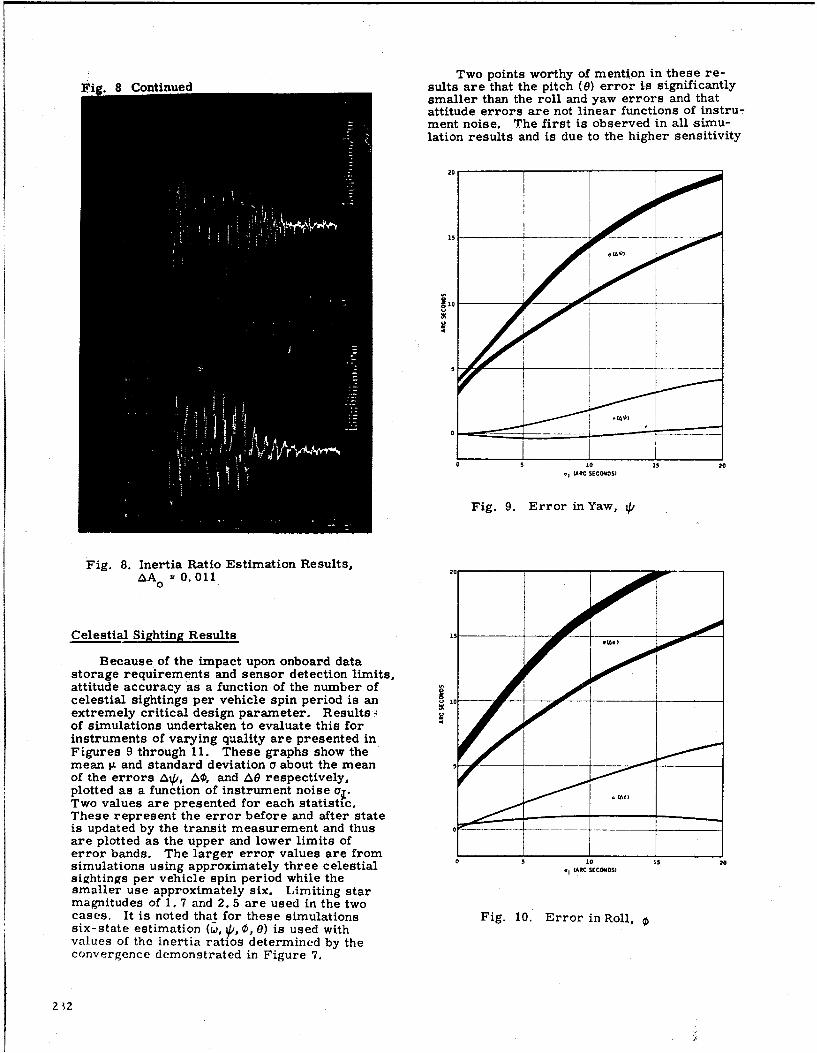
Two points worthy of mention in these re-lig. 8 Continued sults are that the pitch (0) error is significantly

smaller than the roll and yaw errors and thatattitude errors are not linear functions of instru-ment noise. The first is observed in all simu-lation results and is due to the higher sensitivity

15

20

0 1 5 20

1, 1ARC SECON$S)

Fig. 9. Error in Yaw, 4,

Fig. 8. Inertia Ratio Estimation Results,AA 0 = 0. 011 0

Celestial Sighting Results ___

Because of the impact upon onboard datastorage requirements and sensor detection limits,attitude accuracy as a function of the number ofcelestial sightings per vehicle spin period is an -

extremely critical design parameter. Results"of simulations undertaken to evaluate this forinstruments of varying quality are presented inFigures 9 through 11. These graphs show themean F and standard deviation a about the meanof the errors A/x, AO, and &e respectively,plotted as a function of instrument noise ao.Two values are presented for each statistic.These represent the error before and after stateis updated by the transit measurement and thus 0are plotted as the upper and lower limits oferror bands. The larger error values are fromsimulations using approximately three celestial .1 ,, CSECONDS,sightings per vehicle spin period while thesmaller use approximately six. Limiting starmagnitudes of 1. 7 and 2. 5 are used in the twocases. It is noted that for these simulations Fig. 10. Error in Roll, 0six-state estimation (w, V/, 0, 0) is used withvalues of the inertia ratios determined by theconvergence demonstrated in Figure 7.

212

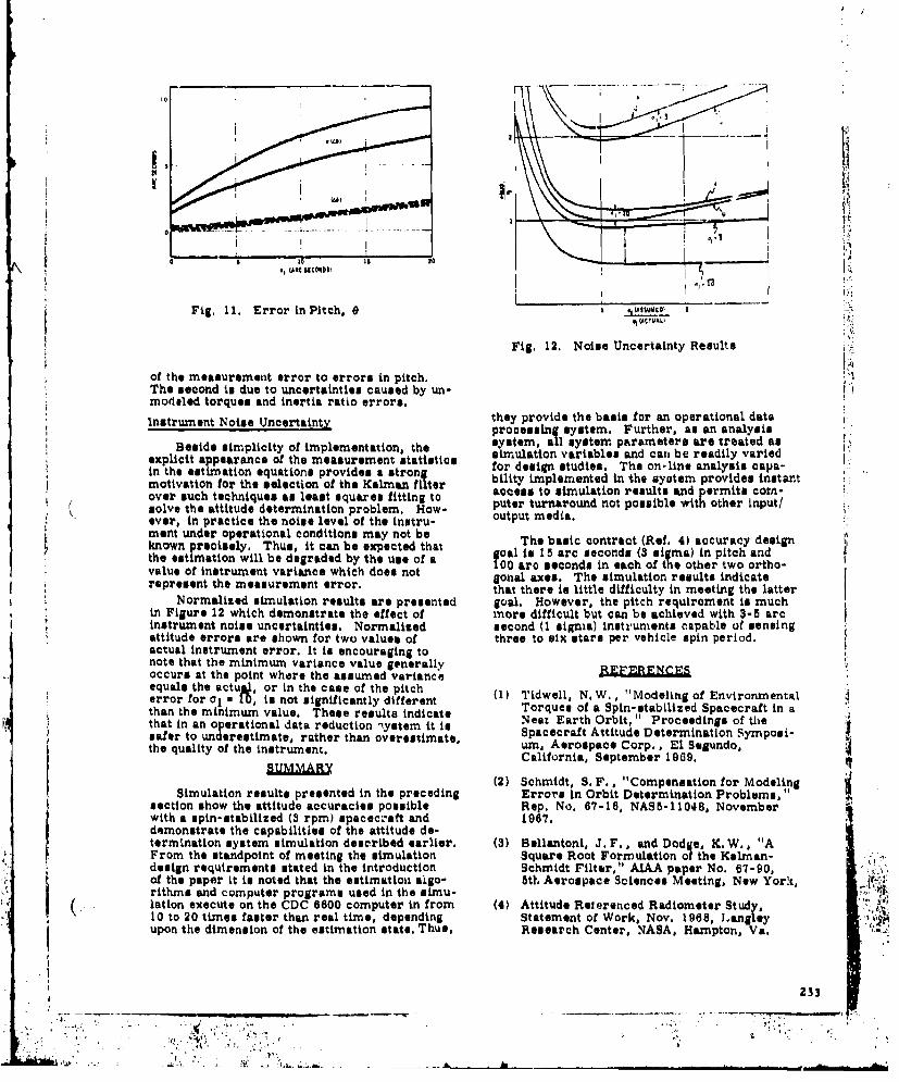
10

I I

Fig, 11. Error in Pitch, G .(l 0 , Io) 2

Fig. 12. Noise Uncertainty Results

of the measurement error to errors in pitch.The second is due to uncertainties caused by un-modeled torques and inertia ratio errors.

Instrument Noise Uncertainty they provide the basis for an operational dataprocessing system. Further, as an analysis

Beside simplicity of implementation, the system, all system parameters are treated ase simulation variables and can be readily variedexplicit appearance of the measurement statistics for design studies. The on-line analysis caps- }

in the estimation equations provides a strong for desimpeetudie the onlie pnlyis capt-motivation~~~~ ~~ fo h eeto fteKle ~r bility Implemented in the syatem provides instant

motivation for the selection of the Kalman filterat iuainrulsad riscmover such techniques as least squares fitting to access to simulation results and ermits cor-/~~~~~~ pue trronnopssible wit other input/,solve the attitude determination problem, How- puter turnaround not p ieever, in practice the noise level of the inutru- output media.ment under operational conditions may not be Teknown precisely. Thus, it can be expected that The basic contract (Ref, 4) accuracy designgoal to 15 arc seconds (S sigma) in pitch andthe estimation will be degraded by the use of a 00 arc seconds in each of the other two ortho-value of instrument variance which does not gonal axes. The simulation results indicaterepresent the measurement error, that there is little difficulty in meeting the latter

Normalized simulation results are presented goal. However, the pitch requirement is muchin Figure 12 which demonstrate the effect of more difficult but can be achieved with 3-5 arcinstrument noise uncertainties, Normalized second (1 sigea) instruments capable of sensingattitude errors are shown for two values of three to six stars per vehicle spin period.actual instrument error. It is encouraging tonote that the minimum variance value generallyoccurs at the point where the assumed varianceequals the actuk, or in the case of the pitcherror for ai w 10, is not significantly different (1) Tidwell, N.W., "Modeling of Environmentalthan the minimum value. These results indicate Torques of a Spin-stabilized Spacecraft in athat in an operational data reduction lyetem it is Neac Earth Orbit," Proceedings of thpesafer to underestimate, rather than overestimate, Spacecraft Attitude Determination Symposi-the quality of the instrument. urn, Aerospace Corp., El Segundo,California, September 1969.

(2) Schmidt, S.F., "Compensation for ModelingSimulation results presented in the preceding Errors in Orbit Determination Problems,"section show the attitude accuracies possible Rep. No. 67-16, NASB-11048, Novemberwith a spin-stabilized (3 rpm) spacecraft and 1967.I demonstrate the capabilities of the attitude de-termination system simulation described earlier. (3) Bellantoni, J. F., and Dod e, K. W., "AFrom the standpoint of meeting the simulation Square Root Formulation o0 the Kelman-Sdesign requirements stated in the introduction Schmidt F'ilter," AIAA paper No. 67-90,of the paper it is noted that the estimation aigo- 5th Aerospace Sciences Meeting, New York,rithms and computer programs used in the simu-lation execute on the CDC 6600 computer in from (4) Attitude Referenced Radiometer Study,10 to 20 times faster than real time, depending Statement of Work, Nov. 1968, Langleyupon the dimension of the estimation state, Thus, Research Center, NASA, Hampton, Va.

233I, *..

II

TACSAT ATTITUDE DETrRMINATION

Warren H. SistererStaff Engineer

Hughes Aircraft Company

Joseph Del RiogoMember Technical Staff

Hughes Aircraft Company

TACSAT M.ISSIONt GENERAL performance for correlation with field testresults. Support activities at Camp Parks are

The TACSAT Military Communications currently scheduled to extend through 3 yearsSatellite Is a large, spinning opocecraft built on of satellite orbital life,the Gyrostat stabilization principle. HughesAircraft Company designed and built the satellite SATELLITE CONFIGURATIONunder the auspices of the Air Force Cfor tacticalcommunications expeiments in both the UHF Figure I shows a cutaway view of the space -and SHP bands. Under contract to the Air Force, craft ilustrating aU primary subsystem hard- :,Hughes has supplied in-orbit control support ware. As indicated, the mission requiiementssince the successful launch in February 1969, have been implemented using a dual spin config-

uration utilizing the spinning rotor angularTACSAT is in synchronous, equatorial orbit momentum to stabilise the spacecraft in pitch

with its spin axis directed along the orbit normal, and yaw (axes normal to vertical cylinder axis)close to the direction of the earth's north polar and employing despin control to point a pro.axis. This orientation is critical to mission ferriiti axis in the despun section toward earth.performance; the despun communication anton. The satellite's communication antennas arerise have only east-west or asitnuth freedom mounted on the despun section, allowing-the(by virtue of the despun control system) and utilization of pencil-bearn (high-gain) antennadepend on control of spacecraft spin axis orien- patterns necessary to meet the very high com-tation for north-south control. munication power (ERP) and receive sensitivity

requirements associated with the experimentalThe spacecraft and its communications communication mission, Figure 2 is a repre-

repeater are designed to support an experimsn- sentation of the total spacecraft.tal military communication test program involv-ing small, low-performance ground stations for The design of the spacecraft's attitudeeventual triservice use. The primairy purpose sensorj (sun and earth) utilize the rotor spin toof these tests is to demonstrate the feasibility provit.e a built-in scan and allow the use ofof satellite communicationa using very small to simple fixed sensors with no maving parts. Simi-medium-sized terminals and to further define larly, the execution of all required propulsiveground station and spacecraft requirements for maneuvers can be accomplished using two fixeda future operational mission. jets (axial and radial) pulsed over a selected

(by command) segment of the rotor spin cycle.The experimental communication environ- In addition, the rotor spin provides an artificial

ment is characterised by several simultaneous, (centrifugal) gravity field maintaining the HOZdi:ect links to and from low-performance ground liquid propellant in the tanks at the orifice loca-stations operating in two radio frequency bands tion, which avolds the problems associated with(UHF and SHF). The large communication handling liquids in a sero I environment. Therepeaters required for this program are a direct arrangement of ihe attitude control and station.consequence of the multilink mission and limited keeping hardware is shown in Figure 3. Fourground station performance, earth sensors and two sun sensors are prt videdwhere one of each is sufficient to support all

In addition to the experimental ground critical functions. In addition, the RCS subsys.terminals, which will be operated under simu- tom incorporates two compietely independentlated field conditions, the communications experi, propulsion systems with the ,n-board H0a2mante are supported usi a lar a terminal with propellant in either jystem sufficient to completeboth UHF and SHF capability, Tis high- the mission orce station acquisition has boonperformance ground terminal (located at achieved, Figure 4 and 5 show the TACSAT sunCamp Parks, California) is used for quantita- s'oror and earth sensor units.tive measurements of satellite communicatfun

235

L _

HFMR-NUTAYION DAMPER)

ELECTRONIC EQUIPMENT DESPIN SUI$YSTEMSUPPORT ASSEMBLY

ELECTRONIC EQUIPMENT

REACTION CONTROL SPIN-UP SUBSYSTEM

DISPIN IIIARINGSUPPORT ASSEMBLY

Figure 1. Satellite Configuration

rigre .ACST iliar Co muncaion Stelitf)36

DESPINANNTNNA

ELECTRONICS

AXIALSPI ANTENN LAOTASTMASOT EAORTH' AT

DIRECTIO C45PI

3237

ATTITUDE CONTROL* precession rate vector. In this pulsed-jetmethod of generating torque, the vectors T. H,A dual-spin-stabilized spacecraft will and • are mutually perpendicular.

maintain its spin axis fixed with respect to

inertial space in the absence of external torques, It can be shown that the nutation induced by* in accordance with the law of conservation of the axial jet during the pulsing mode is small

angular momentum. Since detailed discussion for a reasonable rotor spin speed (-55 rpm) andof the dynamics of the dual-apin-stabilised con- the TACSAT inertia configuration. Thus, for allfiguration is not called for, only a brief descrip- practical purposes, the motion of the geometriction, with emphasis on the control aspect., is spin axis follows that of the angular momentumpreocented here for completeness. vector during the precession process.

The hydrogen-peroxide control system con- The reference signal for synchronous puls-sists of two sets of body-fixed axial and radial ing is obtained from the earth sensor. KnowledgeJets. The radial jets fire outward at an angle

of 2 dereesto he pin lan. Te spcecaft of the spacecraft orbital elements is sufficienti of 26 degrees to the spin plane. The spacecraft to generate spin phase information for the axial

center of gravity (cg) can be varied such that the gneratelsi phase i tiovfr the axialradil Jts my o ma notfir thoughthecg, and radial jets. Thus, with very simple space-radial jets may or may not fir* through the cg, craft sensor instrumentation and body-fixedts dictated by maneuver requirem, nts. The jets thrusters, both attitude and velocity control areare pulsed in synchronism with the spin speed, provided,which allows velocity only or simultaneous velo-city and Attitude corrections to be performed on TACSAT ATTITUDE DETERMINATIONthe vehicle (see Figure 6). REQUIREMENTS

The axial jets, aligned parallel to the spin Pointing errors directly affect communica-axis, are mounted near the periphery of the tion performance through a reduction of thespacecraft. In performing a reorientation earth coverage antenna gain, thereby loweringmaneuver, a precession torque is applied to the ERP -1/2 dBw per degree (Figure 8). Sincethe spinning spacecraft by one of the body-fixed the spacecraft is essentially in a circular syn-axial jets, which is pulsed in synchronism with chronous equatorial orbit, gointing errors maythe spin speed over a given sector of the spin be resolved into north-out (latitude) andcycle (Figure 7), In accordance with Newton's east-west (longitude) components (Figure 9).second law of (angular) motion, North-south errors are caused by the following:

"# Attitude measurement errorsT v. (d/dt)H s wXH AHI. const "I Antenna mirror to bearing and power

where T is the applied torque vector, H is the transfer assembly mechanical spin axisangular momentum vector, and w is the perpendicularity

11

I I ." -P•.• s,,,• •5•Locus oP ,cuisisJTON ROTO SPIN

:..4.

ANOLEOS fR TOR

TO EARTH iLIE

SISPIN AXIS

Figure 6. Radial Jet Firing Geometry Figure 7. Axial Jet Firing Geometry .,.,

238See R, ference 1. '

::';• .... .. • •, '-,-.LOCS O -.POSIBLE ,• ml,, iI i ±l i i i n ] [ u I i llI l l IlLO A IN in • i minii-i i 2 i a .3".. ? - 'I

LOSS CF HORIZON POWER COMPIUNICATIONSNI

XMIISTWATI C ON MNCTO

POINTING ERRO

AEARTH

SPAINFAlISIN HORIZON S

(POWER SLOURCE

ROONTORtO

ERROR ~ S NOMNAL ANCNNA NSPIGNIIOURO

( AA

Fiue8Ftitude E.rPorni Effscts on Stmuniady o Peratorn-A

N-1 POINTINi _ ERROR_<_I.

SPINAXIS

o Antenna electrical boresight It can be argued that the average directionof the mechanical spin axis ts along the angular

* Antenna bor'wsight variation momentum vector. Hence, in determining tieangular momentum vector direction, many

* Dynamic unbalance individual sensor readings will "average out" inthe least squares fit. This was demonstrated

a Bearing and power transfer assembly during periods of TACSAT nutation.mechanical axis wobble (runout)

Estimation of the angular mnomentum direc-* Attitude deadband tion alone is not enough however,% since other

unknowns enter the problem. Solar radiation9 Reaction control system execution errors pressure introduces a disturbance torque

resulting in a steady precession *f the spin axisError.4 in the east-west direction generally result direction. Thus, analogous to orbit determina-

from two sources: tion, the spin axis direction is estimated atsome point in time. Certain coefficients of the

. Inaccuracies in detection of despin point- solar torque equations of motion also must being error due to manufacturing tolerances estimated (similar to geopotential coefficients

in orbit determination). Finally, the attitude• Noise input to servo loop seusors may have constant biases in their

alignment and/or their electronic response whichIn addition to these efiects, the attitude of introduce data bias errors. These biases must

the spacecraft cannot be maintained so that the be estimated.angular momentum vector is always perpendicu-lar to the earth-satellite line. This is due to SUN SENSORStwo causes: 1) attitude measurement and controlinaccuracies, and 2) secular variations in the The TACSAT takes advantage of its rotorangular momentum vector due to solar torque spin (-35 rpm), which allows simple, n4,n.disturbances. articulated sensors to be scanned in a cone

about the spacecraft spin axis. Earth and sunTo meet platform pointing accuracy require- sensors are used that allow immediate deter-

ments of 0. 6 degree east-west and I degree mination of inertial orientation by measuringnorth-south, attitude determination accuracy on the co-elevation between the spin axis and thethe order of 0. 1 degree is required. In-flight two celestial reference bodies.data Indicates that this accuracy has been *easily achieved even under worst case gec- The sun sensors are identical to those flown

metrical conditions. on previous Hughes synchronous spacecraft(see Reference 2), The sensor is composeed of

ATTITUDE DETERMINATION PROBLEM two photo-voltaic elements, each mounted bohinda separate slit aperture (see Figure 4). Each

To this point, no distinction between the slit allows a fan-shaped fiekd of view. Thespacecraft mechanical spin axis (i. a. , despin primary slit is mounted such that the plane ofbearin,; ax' j) and the total spacecraft angular its field of view contains the spin axis, while theni'mentum vector has been made. The differ- second slit is twisted 35 degrees about a radialence is a subtle but very important one. The line through the first. Thus, the angular differ-average spacecraft spin vector lies along the once, t,_ between receipt a, & s9a pole. freomangulai momentum vector which may be regarded each slit is related to the coelevation of the sun,as constant in inertial space (over short periods 4,s, by the following spherical trigonometricof time). However, a multitude of effects may relationship (see Figure 10).cause the rotor mnechanical spin axis to deviatefrorm this direction, cot Ole a cot 4sin '. (1)

Nutation is the coning motion of the bearing whereaxis around the momentum vector caused by atransverse torque. A nutation damper is *5 a angle between sphii axis and sun linemounted on the antenna tower to cause suchtransient motion to decay. Wobble Is the spin 4' a angular separation of two slit crossingsfrequency coning caused by the center of gravitynot lying on the spin axis or by rotor cross v ' cant angle between slitsproducts of inertia. Higher frequency deviationsare ,:aused by bearing runout. For true three- While all Hughes' slit-type sun sensorsaxis difinition of spacecraft orientation, each of flown to date have been canted at I a 35 degrees,these effects, and others, m-st be considered in it is none the loes interesting to discuss thedetail. Howev.r, the magnitude of these effects tradeoffe made in selecting this anile. By inter-(<0. 02 degree) in steady-state operation is small secting the plane formed by each alit with 4 unitenough to be neglected for the earth coverage sphere centered at the spacecraft, the twoTACSAT mission. resulting great circles ma be drawn on a pro-

jection of the sphere, as shown in Figure 1 Ia.Neglecting sensor physical vrharacteristice and

240 -

* . , - - " -. . . . . . . . -- .. .. . . .. .* , . . . . ..

5P1.. AXISP

( 11, •bIfSCIION E

1IINSENSO" , SUNNINA

VEW PLANEI ANGLESPIN

.PULSe t I - Ii

-. 35./ UN1IN,-0?.110HT

TIME

it SUN SENSOR OUTPUTS ENIO VIEW PLANE

/ALIONMENT AXISOF SENSOR

Figure 10. Sun Sensor Characteristics

SUN DIAMETER'

'V INTERSECTION OP

SUNIT FAIE

U N IT i r JA ,, 0 + 1 i n

r 160 270 210

a) Projection of Sun Sensor Slit Geometry on b) Geometry of Sun's PathUnit Sphere Across 1 2 Slit

Figure 11. Sun Sensor Slit Geometry

mission requirements, 4 is to be chosen so ai Several physical characteristics of theto maximise the sensitivity of :he data, NV, to oeesor make the choice of 4 t s impractical.the coelevation angle, 46, That is, the deriva- FirsL, the slits do not have a total planar field oftive of %Zwith respect to 4. should be maxi- view, or even a half-plane, but are opticallymised with 4 as a parameter, Immediately, from limited to a total of about 90 deogsees, givingEquation 1, them the true fan-shaped field of view as shown

in Figure 10. Second, they have a finite angular

* 2 width, t ; and more important, the sun is not atan 4 sac T 3C 4C (2) point source, but has a finite diameter, 6. Thed#b aeffect of both these factors is to produce a

broader, less sharply oAfined voltage pulse toAs is expected intuitively, 4 - 4 maximizes be processed by spacecraft (or ground) electronics.

Equation 2 with the constraint that Equation I bephysically meaningful (sin T2 s 1); this con- Returning to Figure Ila, define "longitude',sttsint in equivalent to saying that fre; 4 > s as X•. Since the projection is sipacecraft c•intered,

the second slit will never pace through the sun, consider the sun to be moving leit to right atas is obvious in Figure II. The conclusion to some "latitudeo, Fp and at some angular ratew,be drawn is that if data sensitivity were the only the spacecraft rotor spin rats. It is required toconstraint, the sensor should be canted the maxi- determine the total angle 0 during which the sunmum amount consistent with the mission sun is visible in the slit as a function of +m, with

( , angle (**) history. as a parameter. Refnrring to Figure lip,

241

-. I:: - .. • •. . :,., .,.. . ..

recognize that tan o hae already been calculated errors on the order of 0. 10 degreei. Calibrationin Equation 2 as of these bias errors is discussed later,

d% EARTH SENSORtan a = (3)

as The earth sensor is a small telescope with aninfrared-sensitive chip mounted at the focal point.

which leads immediately to tle required equation The optics allow an effective bandpass of 14 to Ifor 0. 16 microns in the infrared band, the so-called CO?window. The earth sensor provides both leading

I dt 2 and traliling edge pulses, using derivative thresh-e 0 (4+6) sec (tan"'-4 (4) olding, with the leading edge pulse serving as a A

despin and control jet reference in addition toproviding attitude information. (By measuring

where the spin period as the time between successiveleading edge earth pulses, all other time interval

0 a total spin angle through which the sun is measurements can be converted to equivalentvisible in the canted slit angles. ) The earth sensors are mounted in pairs,

one 5 degrees above the satellite spin plane andt a slit width one 5 degrees below (or equivalently, 85 and

95 degrees, respectively, from the spacecraft6 a diameter of the sun spin axis). Two such pairs are included for

redundancy; however, only one is used at any(T20 ** as defined in Equation 1) time.

As expected, this relationship yields The basic information content from a single"earth sensor is the earth chord width observed

0• (+6) sec • at *. 90 degrees (5) as indicatid by the time interval between lead-Saing and trailing edge pulses (see Figure 12). Fora known &atellite position (hence, known radius),but more important, it shows 0 degenerating the earth chord width may be calculated from theco-elevation between the spacecraft spin axisand the earth center direction by the following

e0 at 415 (6) spherical trigonometric relationship, which isderived immediately from the law of cosines and

From a design point of view, Equation 4 chow@ is illustrated in Figure 13.that excessively long solar viewing by a slitmay be controlled by making the slit width, a, cos -o . c YCos n1as small as possible consistent with minimum cos of I sin y sin i (8)solar input energy requirements. Use ofEquations 2 and 4, along with sensor character-istics (signal-to-noise ratio, slit width, etc. )and mission constraints, allows proper selection whereof •. ai - one half the ang~ular chord width seen by .As a final not%, recognise that the longitudi- h f th e a l sensor

nal (k) intercept of the canted slit need notnecessarily be sero, but that the sensor will a = semidiameter of the earth's disk as seenfunction in an identical manner with an arbitrary 0 from the satellite

,, intercept longitude, X_. This results in a simplemodification of Equation 1 to V a co-oelvation of the spacecraft spin axis

and a line toward the earth's centercot u N cot 6 sin (*z" -). (7)

0i a angle betwfen the spacecraft spin axisweof canted and the optical axis of the ith sensor

where i the longitudinal intercept nte(85 and 95 degrees on TACSAT)sun sensor beam and * and * are aspreviously defined. While the sun sensor response it nearly

Data sensitivity and other functional linear over the range of sun angles encounteredduring TACSAT mission life (O a 90 623. 5 degrees),

properties are unaffected; however, proper earth sensor response is highly nonlinear, reflec-selection of X can prevent the two voltage pulses

frmeeroelapnwhc ayao smlr ting the relatively small earth vise (17. 8 degrees'• from ever overlapping, which may allow simpler

processing e!ectronics, diameter) seen from synchronous altitude. Ananalysis similar to that described for the sunsensors can be made for the earth sensors lead-

Ino failures in 40 satellite-years in orbit) but iug to an optimal selection of the mounting angles,/,nonj fllue rn 40t earlth-r sesos orbite thutrtyields data of only medium quality. TACSAT for both earth sensors. Since the earthexperience indicated random measurement sensor pulse is used additionally for a despin and

deviations of 0. 03 degree, but constant bias

Z42

-~ .2~2:, 7 ~- -

,II N TPAILINO 1oo1 PUL~I N LEADINO 1001 PULSE

NOITH SENSOI TRACK 0-

I $ RAILINO 1001 PULSEoEAT I

SOUTH SENSOR TRACK

Rol T SP IN | AU S LEADINO EDto PULSE

"AXIS I

SNORM L TO SIiN AXIS

S() Figure 12, Earth Senior Geometry

CIELSTIAL SPHERE

,,SPIN AXIS

SPACECRAFT

POJCIN OF ARTSAIELITION CELESTIAL SPHERE

SATELLITE

EARTH

" a) Angle Subtended by Earth at Satelte Altitude b) Earth Sensor Configuration

Figure 13. Earth Chord Width Calcalation

Z43

•. 7

jet control reference, these individual require- DATA FLOWany analysis. Figures 14, 15 show the attitude data flow

from the TACSAT vehicle to the Hughes DataTwo earth sensors used concurrently offer Processing Facility (HDPF).

several interesting variations in data processing.Instead of processing their measurements as The data is measured as a . equence of timetwo independent readings of earth co-elevation differences on-board, is digitised, and is thenangle, it is possible to difference their measure- telemetered to the ground. The remote trackingments and process the difference as a measure station (RTS) receives and preprocesses the rawof the angle between the spacecraft spin axis telemetry bit stream and records it on magnetic"and the plane orthogonal to the radius vector, tape. The RTS than converts the telemetry toThis concept can be likened to monopulse radar engineering units and edits it according to anyand has the similar advantage of doubling the of several processing modes. The edited telem-

- error sensitivity of the single measurement etry is then transmitted to the satellite testwhere error is interpreted as a deviation from center (STC) Bird Buffer,orthogonality to the radius vector, Anothervariation based on the same theme is that Of The STC Bird Buffer processes the editeddifferencing only the leading edge (or trailing telemetry to provide a printout of data for real-Sedge) pulses. This would trove effective where time monitoring, and generates history tapesthe accuracy of one type of pulse was in doubt, of the edited telemetry. The history tapes are

processed through the MUNCH program, whichNeither method can create information that produces paper tapes for taletype transmission

did not already exist in the data, and the authors directly to the HDPF, where the transmittedcontend that processing the two readings as data is automatically stored on magnetic tapeindependent co-elovation measurements utilizes by the OE 635 computer to await processing bythe data to its full advantage. Additionally, two the attitude determination program.important benefits are derivedi 1) data processing

algorithms work equally well whether data from THE ATTITUDE DETERMINATION PROGRAMS both sensors is available or not, hence, arevalid if either sensor fails or to off the earth, The attitude determination algorithm waswhile other schemes cannot handle this situation; implemented on the HDPF OE 635 large scale2) bias calibrations (described later) can be done digital computer, Program and data storage areon an individual sensor basis, allowing better on magnetic tape and are operated from thesensor performance analysis and utilization if TACSAT Operations Center via a remoteother sensors fail. terminal.

The TACEAT earth sensors returned data An attitude determination differential cor-of 0. 03 degree rme deviation, but with biases of rection algorithm was developed which handlesup to 0. 38 degree. These biases were determined up to nine parameters in its state vector: twoin the attitude determination least squares esti- attitude parameters (the equivalent* of right"mate and caused no significant problems. ascension and declination), three solar torque

coefficients, and four attitude sensor biases,SUN-EARTH SEPARATION Any subset of the total vector may be selected

for differential correction, the others beingA third, independent data type is available held constant.

""free of charge" by virtue of the sun and earthsensors: sun-earth separation angle, 1c. By The initial estimate of the state vector maytelemetering the time delay between receipt of be weighted with an a riori covariance matrix.the sun pulse (from the vertical slit) and the mid. The program itself wTouptut the covariancepoint between the leading and trailing edgs earth matrix of the final attitude state vector estimatepulses, the angular separation between the two on request at the and of each run. This previousbodies, as measured about the spacecraft spin covariance matrix may be used in conjunctionaxis, is available. with subsequent date., resulting in a stage-wise

estimate being built up as data is received,This data has unique properties and in often This capability reduces data storage and

overlooked as a pntential data source. The data reprocessing requirements.has its maximum sensitivity when the spin axis,the spacecraft-sun line, and the spacecraft- A straightforward least-squares estimatorearth line are coplanar and the two coelevation with a variety of data weighting and culling optionsangles, 0 and Y, are each as far from 90 degrees is used. The data can be shown to be uncorre-as possible. As described in Reference 3, lated, both between data types and betweenthis data can be particularly valuable during sequential readings of the same type, by virtuethe launch and ascent phase of a mission when of the way it is measured and tlemetered. A

S the spin axis may not be orthogonal to the orbit fixed point state estimate (based on work byplane. I. A, Our&, ase Reference 4) is obtained with all

*Right ascension and declination themselves are singular near the pole and hence unsuitable for differ-ential correction. A local coordinate system using the current estimate of the spin axis as the 3.axisis defined and the estimate is differentially corrected along the orthogonal I- and 2-axes.

244

-•'+ .. .• J, ..:•,. ,.' .-" : Y ,•. '*'h " . ' + ;- " "r+ 'I.• '+:+,' +" - " . 71!:7' 7+" " ,a +'.•+• .. .S, _- + + +.+= +. . .. • . .. •+. .. •: +

* OPEaATIS IN VARIOUS PROCESSING MODES

ANAYSI 44SENTATIO

SY1TM EORMTSDSIND SUPPERVAE6UINMD

I4IMOIYA

TAPEY AP

ANRVIEALSTITD NSRADCS TPRESENTATIO

P PLOID TUELEMETRYTLEMT

HISOR FOMTS1IMER RPPATP

)ECR PUNCTERY PAPE 00 MUACE FACI TLMERAM SISO

Figure 15. SC? On-.Lino Telemetry Processing System

TEETPCDC 10A 1 ATTIUDE ENIO

AN C TLMTR AIR.1

TA ;N

RESULTS OF IN-FLIGHT EXPERIENCE

the data related back to a single reference epoch Actual experience with flight data has beenof the state vector, As described in the Reference, quite successful. The earth and sun sensorsJthis technique is applicable to situations where have returned data with random noise of approxi-the differential equations describing the state mately 0. 03 degrees (Ior), but with larger thanvector are known and the system is not driven expected bias error@ of up to 0. 4 d,3gree onby "forcing noise", Forcing noise may be certain of the redundant sensors (see Table 1).described in this application as disturbance Atorques which are not modeled or are modeled These bias errors were determined quickly,incorrectly. A fixed point state estirmate can and caused no major concern in mission opera-be contrasted to a Kalman-type filter whire tions. The accurate determinati..r. of sensorcovariance matrix terms are increased to r.:flect biases is quite important. In theory, for a gaus-errors made in mapping the state vector fn, ,,sird, elan or purely random distribution of measure-

ment errors, the uncertainty in attitude shouldThe differential equations governing e*T-n decrease as N- 1 12 where N is the number of

axis motions due to solar torque were int~jented measurements, This assumption is implicit inanalytically after substitution of some a~n.,:lify. the weighted least-squares method of estimation.ing approximations. (These approxiniAval However, the biases in these measurementsintroduce a completely negligible error over dominates the certainty of the solution, so thatperiods of up to several months, ) The torque an accurate attitude solution is dependent onitself was modeled as a quadratic in solar aspect knowing the data biases with a high degree ofangle, 1s, with the three coefficients as terms confidence,in the state vector, The analytic integrals resultin a considerable saving in computation time over In light of modeling uncertainties, which area numerical integration scheme, felt to be the limitingt factor in attitude deter-

mination accuracy, the overall certainty intFour constant biases arise from the four attitude estimates is approximately 0. 03 degree.

data types available in each data vector: sunsensor, north earth sensor, south earth sensor, Several phenomena have become apparent.and sun-earth separation angle. The biases are Attitude determination accuracy does not aiffermodeled as sensor misalignments. It is con- significantly when data is taken during periodsceivable that the bias errors are, in fact, due to of spacecraft nutational activity (TACSAT haselectronic timing delays, atc., but it is impos- undergone random periods of nutation withsible to determine the source from the data amplitudes up to --1, 5 degrees), Though thealone. Hence, it makes no difference how they variation in sen.or output is actually sinusoidalare modeled as long as the end result - correct and regular in nature due to spacecraft nutation,determination of attitude - is achieved, the attitude estimator successfully treats this

sensor output variation as random noise andIn general, the algorithm has worked quite eliminates the effects on the solution almostwell. Convergence of the differential cirrec- completely. Larger data residuals result, buttioe iteration Is generally rapid (2 to 3 iterations) attitude determination results agree to withinand is not strongly initial -estimate dependent ..0, 01 degree of results obtained immediatelydue primarily to the relative linearity rof the before or after periods of nutation(after account-problem. Determination of biases is only possible ing for the effects of solar torque).when the data available meets certain geometriccriteria. The determination of solar torque An accurate orbit ephemeris generator iscoefficients requires that data be gathered over mandatory. In particular, a 1- to -I corres-a considerable time span (so as to allow the pondence exists between error in orbit normalmotion of the spin axis to be measurable in the direction (orbit inclination and right ascensiondata), of ascending node) and attitude determination

error. Operationally, orbit determinationThe program was developed with con- and/or updating must occur frequently enough so

siderable operating flexibility in mind and has that the orbital elements reflect the correctnot required any major modifications to respond orbital inclination and right ascension of theto attual mission situations, ascending node corresponding to the time at

TABLE 1. TACSAT ATTITUDE SENSOR BIASES

Sensor Bias, degrees Description

Earth sensorNorth A 0 38 * 0. 05 Toward equator (down)North B 0. 37 * 0, 05 Toward equator (down)South B -0. 06 m 0. 05 Toward equator (up)South A -0. 06 a 0. 05 Toward equator (up)

Sun sensor -0. 024 a 0. 05 Decreased asimuth_separation of sensor planes

246

.,l.l

which the data was taken. Correct inclination periods close to local (spacecraft) noon andis more important than correct in-track position midnight when the earth, sun, and spacecraft

- (mean anomaly). are essentially colinear, earth sensor data andsun sensor data are, to a large extent, redundant

The "strength" of the earth-sun-sensor and no longer provide separate attitude informa-geometrical relationships varies with time of tion. It is therefore advantageous to collect atti-day and time of year. The time of day and time tude data at times when the earth-spacecraft lineof •ear at which attitude data is taken is crucial, is as close to perpendicular to the sun-spacecraftClose to the equinoxes, the sun sensor data line as possible.becomes less sensitive to attitude changes. During

REFERENCES

1) M. J. Neufeld, and B. M. Ansel, "Synchronous Satellite Station Keeping," CommunicationSatellite System@ Technology, edited by R. 3, Marsten, Academic Press, New York, 1966.

2) W. H. Sisrer, and W. A. Snyder, "Attitude Determination and Control of Syncom, Early Bird,and Applications Tschnolo Satellites, " Journal of Spacecraft and Rockets, Vol. 6, No. 2,pp. 162-166, February 19 9.

3) "Hughes Multipurpose Synchronous Communications Satellite Study, " Vol. 2, Part III,August 1967.

4) 1. A, Oura, "Extension of Linear Estimation Techniques to Nonlinear Problems," ournal of1he_.Astronautica &Sciences, Vol. XV, No. 4, pp. 194-206, July-August 1968.

A N

'7

IJ:1

4(,

., ,: i[247

J6k i A..~ 1

THE ATTITUDE DETERMINATION SYSTEM FOeR THE ORBITINGASTRONOMICAL OBSERVATORY

Paul B. DavenportGoddard Space Flight Center

ABSTRACT

Various applicationl of attitude estimation an applied to the opera-tion of the Orbiting Astronomical Observatory are enumerated and ex-plained in some detaiL The techniques used, the results of these tobh-niques, and the problems eucountered during the first nine months of themission are delineated" The operatica of the Orbiting AstronomicalObservatory including the spacecraft and the supporting ground systemis briefly described.

INTRODUCTION feet across any two parallel sides of the octAgon. Thereis a hollow central tubular area four feet in diameter( On December 7, 1066 the NASA's Orbiting Astro- running the length of the spacecraft which is used to

nomical Observatory (OAO) was plaed into a near air- house the experimental equipment Two hinged sun-oular orbit Inclined 85 degrees from the equator by an shades approximately four feet square are attaohed toAtlas-Contaur booster. The OAO, orbiting 460 miles each end of the spacecraft to protect the expeoimentalabove the %arth's surface, doubled existing stellar data equipment from sunlight. Attached to each of two op.-clear of the earth's absorbing atmosphere in its first posits sides of the octagon at an angle of 84 degreesthirty days of operation. After nine months of sue- from the longitudinal (optical) axis ar four solar cellceOsful operations this first utronomioal observatory paddles whose combined dimensions are nearly elevenin space has ma& over 3000 observations of stellar feot by nine toot. Solar cells are mounted on both sidesobjects and hs attained some 8000 different attitudes of all eight paddles. The major subeyst'ms of thedistributed over the entire celestial sphere. OAO are stabilization and control, data prJoessing,

0orm0mmlwtln, nd power. Thrmal control Is pas-Two experiments are aboard the OAO spacecraft: sive. The entire spacecraft weighs over two tons

One designed by the University of Wisconsin and the which includes 10')0 pounds of experimental equipiment.other by the Smithsonian Astrophysical Observatory(RAO). The Wioonsin Ixperimentai Paokag (WUP) The primary mode of control is by utUllar guidanceincludes four stellar photometers, two scanning apes- so as to point eiiher of the experiments to within onetrometers, and one nebula photometer. The primary arc-minute of a specified target star. Control perpen-function of the WEP is to gather spectral energy dis- dioular to the optical ae is also required for mancu.tributions on selected stars and nebulae in the ultra- vering, power, taermal, and rhading considerations.violet range of 1000 to 4000 Angstrom (A). The SAO This three dimen.ional control is accomplished by us-experiment contains four 12-inch teolesc ps each of ing various oombinations of tix orthogonally mountedwhich image* a star field onto an ultraviolet sensitive gimballed startrackers each having a field of view ofphoto•tthode, The scientific objective of RkO is to one degree and an excursion of approximately forty

separate ultraviolet spectral bands ranisng between sighted with the optical axis, In also avalilble which;: 1100 A and 3000 A. Provides lin~le,10axis (optical) control. Averaged error

signals frn, the traeoorsl drive three orthogonally"THE SPACECRAFT AYD ITS CONTROL mounted "fine" momentum wheels whio• absorb the

extraneous torques tht would cause attitude errors.The OAO bpaocorait it an ootadnall) shaped The momeutum in the fine wheeld is oontinuously

aluminum structure ten feet long and six and two-t1i dr "d.anmpod" by a magJ.1tio unloading system consisting

,49

-,- . -" •- t f L '.,, . .. +:

of three flux gate magnetometers, three torquer coils other geometric considerations. From this, the num-(electromagnets), and a processor. The momentum In ber of turn& for each inertia wheel required to slewtho fine wheels may also be removed by a gas jet system. from the previous attitude to the present one is then

determined. The gimbal angles for each tracker andThe OAO may also be controlled by three rate their on-off schedule as a function of occultations by

gyros which actuate either the fine momentum wheels sun, moon, or earth are also generated. One of the(Hold On Wheels) or the gas system (Hold On Jets). final outputs of the SCPS Is the ordered liet of comn-The maximum drift rate for any one gyro as obtained mands in spaceoraft format which are to be executedfrom in-flight data is about 0,2 degree per hour. and their time of execution. Based upon the schedule

of ground contacts with the spacecraft, the number ofThe spacecraft is maneuvered from one attitude commands to be executed, and the current memory as-

(two axes) to another by means of three "coarse" Iner- signments the SCPS also determines when and wheresti wheels in an open loop manner. Two or more the commands are to be loaded into the spacecraft

trackers are required to track continuously during the memory.slew and aver d errors from preset gimbal anglessettle the spacecraft when the slew has terminated. The image of the 0AO command memory alongSlowing plus settling times vary with the axis and angle with certain ground procedures generated by the SCPSof rotation but is usually better than three dogreas per is then routed to the OA0 Operations Control Centerminute. Small closed loop slows (several degrees) may (OCC) which in turn transnots this "contact message"also be accomplished with the fine wheels by changin to one of five remote sites. These sites are: Tlosnian,the commanded gimbal anogs. North Carolina; Quito, Ecuador; Santiago, Chileo

Tansaarive, Madagasoarl and Orroral, Australia. AtThe OAO has two speulal modes uf controli "sun- the scheduled contact the remote station establishes

bathing' and "sun-pointing," In the former, sun sen- communications wilth the 0.40, loads new commands insore are used to actuate gas Jets which align the nor- memory (if necessary), and pthers telemetered datamal of the solar uell army to the sun when in sunlighL (real time and stored), The OCC monitors these con-Rate Syros then hold this position while in darkness, tacts (in the case of a Rosman contact it also roplacssSun-pointing is similar oxcept in this case the optical the remote station functions), and displays the return- -axis is pointed toward the anti-sun line, This is the ing telemetered data. During the contact, real Limepointing the spacecraft automatically obtains upon sep- commands already at the remote site may be executedaration from the launch vehicle, and real time commands from Goddard Space Flight )

Center (where the $CPO and OCC are located) can beIn addition to the sensors mentioned above there reo.ived by the site and relayed to the spacecraft.

are four tun sensors mounted so as to give solar as-peat data at any attitude. It is the purpose of these ATTITUDE ESTIMATION APPLICATIONSsensors 6o provide independent attitude Information

' while in sunlight. The applications for attitude estimation techniquesin the 0AO program ranp from coartw octimates

The data processing subsystem can accept led dLf- (several degrees) from the solar and magnetic sensorsforest control commands In addition to the gimbaL and to a proois attitude determination (seconds of arc)slewing commands. AU commands may be executed in from am many as six startracksrs.real time or stored (up to 956 commands) and executedat a specific time later as a function of an on-board A coarse attitude estimate is used as an Inter-clock, mediate step in obtaining stellar guidance. The transi-

tion between the coarse attitude estimate and stellarTHE GROUND SYSTEM control It obtained by geerating a sequence of star-

tracker gimbal angles consistent with a sequence ofFor the most part, the actual functions performed attitudes. This sequence of attitudes swoops out the

by the OAO are initiated by one of the eperimenters most probable region associated with the coarse atti-although soverL major elements of the ground system tude estimate. Stellar (?idanoe is then obtained whenlie between his request and the commands executed by twe or more trackers acquire their preassigned starsthe spacecraft. The experimenter specifies a sequence during the aearch maneuver.of target stare (pointings) and the associatod xpoeri-mental equipment commands necessary to obtain the The coarse estimate of the OAO'o attitude in ob- !

desired scientific objectives. This information (Expert- tained by placing the spacecraft in an attitude hold usingmentor's Target List) is pased on to the Mission the rate gyros and fins momentum wheels, Sun sensor -Computing Oroup where it and other inputs are entered and magnetometer data are then collected while theinto a complex computing system known as the •upport spacecraft is in contact with a ground station (approxi-Computer Program system (ScPC), The OCPS (which mately ten minutes). This data is then relayed, by highresides in a large sOale-high speed computer) deter- speed data links, to the control center whore it ismines the total attitude an a function of the target and passod to the SCPS. Since the attitude of the spaceraft

250

,ZO .mamma

is fairly stable during the collection of the data (rela- interpreting the results based on residual errors ,twltive to the aocuraey of the' , ta), it is assumed that all the anguhlr separation between the solar and magnetic( 'ihs data refers to the &am attitude and is thus used vectors. A technique has recently been developed whichcollectively to obtain a weighted leat squars estimate will determine from in-flight dtasay systemMtic errorsof that attitude. The star search commands, based upon caused by: the misallpmeWt of the manietometors,the attitude estimate, are then generated by the SICPS the permanent magnetic momewt of the spacecraft, andand transmitted (via the total ground system) to the the effects of the torquer coils on the magnetometers.spacecraft at some subsequent contact in real time. It is felt that this information will help eliminate the

present wide dispersion in the magnetic data.Even though the magnetometers were not calibroted

and give noisy data (their original purpose was solely THE ATTITUDE ESTIMATEto unload momenlum from the fine wheels) the above'procedure yields an adequate solution and has been used All of the attitude estimates referred to in theto place the OAO under stellar control approxtimately proceding sections are obtained from the same mathe-thirty times in a nine month period. The suocess of matical algorithm which yields a weighted least square$this teohaique has saved valuable time and eotedod the estimate of attitude. The only dtfferecue between thelife of the OAO's es supply since it is applicable at various applications is the selection of the weightlsany orientation whereas the original desig concept re- and/or the type of data to be used.quired a reorientation to align a particular axis withthe seun. 3ts~ar control wcukl then he acaomplished by The method (delineated in an appendix) is basedrolling about this axis until two or more startrackers upon two different vetor parametrlsations of three-simultaneously acquired stars. dimensional rotations, one vector has been referred

to ts the Gibbs vector and the other's components are-The OAO'I capability to hold an unknown attitude three of Euler's symmetrical parameters. The direc-under gyro control has also been used to derive an es- tioa of both vectors defntes the axis of rotation and

timate of attitude usinzg only magpetometer data. To their lengths are trigonometric functions of the angledate such rough estimates have had very limited appli- of rotation. One vector has a length equal to the tan-cation. However, on one occasion such an estimate was gent of the half-angle of rotation and is denoted as theused to verify that the telemetry from a sun sensor had Y vector, The other vector is denoted as Z end hasbeen misinterpreted. With calibrated magnetometers length equal to the sine of the half-angle of rotation.( this capability could provide useful attitude informationwhile the spacecraft is in darkness. The Z vector is used to obtain a vector expression

for the "smallest" rotation which will align an estimateWhen under stellar control, attitude determination of a rotated vector to its true value. A generalizedtechniques using startrwaokr data have been used for weighted least squares criterion is thus established byan independent verification of the commanded attitudes requiring the sum of squared lengths of all such Z'eand to determine the accuracy of the various sensors. (premultlplied by a symmetric weight matrix) to be aLeasnt squa•es solutions using all tracker data (usually minimum. The resulting equation is then simplifiedfrom two to four trackers) as at aggregate and In vare- by assuming that the weight matrix is the identity timersous combinations provides an excellent means for a soalar (this implies that the component errors ofevaluating the performance of each tracker and whether each Z vector are equal and independent).any misalignments exist between them.

The Y vector is used to express the least squaresMore sophisticated techniques have been employed condition In vector notation where the only variablesto determine the values of the tracker misalignments are the three components of the Y vector, The noses-from mnflight data. This has been necessary since eary conditions for an extremum are then applied toshifts due to launch stresses and other effects have this function and the result is a vector equation in termsbeen greater than expected. By use of this procedure of the Y vector. The luast squares solution can then bethe pointing accuracy has been better than the design obtained by findir4 tho largest zero cf a fourth degreespecification of one aro-minutb, polynominal and then solving a linear system of three

equations. In practioe, this approach is not taken sinceAttitude determination from tracker gimbal angies the vector equation is also amenable to a simple suo-is also performed in the processing of the uxperimental cosaive suhstitutions iteration which converges rapidly.

data. This allows a correlation of the data to a known Thus an approximate solution is constructed to startstar and aide in the evaluation of the scientifir results. the Iteration.

Stellar control has provided the opportunity to study When only two data vectors are given the least"the correlation between the errors of the sensors and squares rotation can be expressed as a product of twothe resulting error in attitude. In this manner a good rotations, each of which ia obtained by juxtaposing 'r"deal of experience has been obtained in the selection of vectors that are linsar combinations of the given vec-weighting factors for the various sensors as well as tors. The soalar coefficients of these linear combinations

*. .. . _ .'. :•'' ,.' i - .. .. " -V

are explilcitly given to functiona of the lengths end dot to improve th. overall accuracy. Since the minalign-products of the given vectors. This method yields the mente have been as good as thirty arc-secondu ove~r ex-atitMue eatimate whten only two data vectors are AV"i. tended periods It is felt that much of the variation can)able and provides the first approximation when more be accounted for with w~ditional pmaamtersiIn thethan two vectors have been mesautred. model.

-RESULTS AND RPRODLXIAB In the following table am, the results of fifteentypical attitude estimates using Only sun sensor amdAttitude error signals tram the experiments ane magnetometer data. Column one contains the numbernot available on1 the Present GAO. Therefore, it is dif- of data points used in the estimate-each datA point gives

ficult to ucertain the absolute error in attitude while two vectors (solar and magnetic). The second columnunider stellar control. However, attitude determination shows the anguar separation between the solar endusig telemetered gimbal angles from seversi trackers magnetic vectors. The length of time over which theover a tan minute interval usually yields resdal" or- data were taken is given In column three. Columnsrors of ame arc-minute or lees (the smpalest command four end five give the actual angular error of the solarIncrme~nt is twenty awo-seoonda), To min~tain this and msagntic data respectively (the attitude obtainedpProision, however, It baa been necessary to 'Goas"_ from tracker data serves. as the reference), The nextlocally re-evaluate the misaignments between the two columns diaplal the solar an magnetic errorstrackers. More elaborate misalignment models are using the solar-magnatic estimate as a reference. Thebeing considere .d to eliminate this minor problem end last column contains the angle of that rotation necessary

No. of Angular Duration Actual ?MAg. Error Residual Mag. Residual AttitudeDaIR PoiJnt Ue11"articn mint "ac. Ika Error Mean, Max. Bun Error Mean, Max, Error

6o StoasS 0:47 0.02 3.9,4.9 0.18 3.9.4.9 1.1

026 64 1:08 0625 6.4,8,.6 0.89 6.8, 8.0 1.1

10 39 44 1:850 0.14 3.6. 4.5 0.20 3.4, 4,4 1.2

11 37 99 9:42 0.06 2.6, 4.0 0.06 3.9. 3.3 1.8I11 86 49 2:21 0.06 4.7, 6.0 0.87 4.4,.5.9 1,8

14 81 89 4:11 0.08 7.1, 9.2 0.31 6.9, 9.9 2.8

14 40 s0 3:28 0.96 S.2, 3.5 0.18 9.3. 3.8 0,9

17 37 28 3156 0.06 3.4, 5.4 0.16 2.6, 8.3 3.3

18 47 98 8:23 0.02 1.4,.3.3 0.05 1.4, 3.3 0.5

24 89 45 7:82 0.06 4.8, 6,8 0.30 4.2, 6.0 0.3

25 s0 107 7:07 0.38 5.4, 6.4 0.81 a.4, 6.4 0.8

98 86 T8 7:52 0.09 6.1, 8.1 0.39 5.8, 8.1 1.0

25 29 41 6:49 0.22 1.7, 3.4 0.08 2.2,.4.0 1.5

28 6 46 6:34 0.21 6.1, 5,5 0.33 8,4, 8.4 1.9

to 74 61 6:49 0.26 5.5, 8.1 0.80 4.7, 7.6 2.1

All errors And angular soepration are in degreas.

tn all attitude estimates the sun sensor data was given a weight of 4 and the magnetometer data a weight of 1.

252 -____

to bring the solar-magnetic estimate In egreatnent with The ground system has been able to keep the satellitethe stellar determination, These figures clearly show productive around the clock nnd both experimentersthe dispersion in the magnetic data that was referred are continuing to receive valuable scientific data. Theto previously. The errors range from as good as our problems, thus far, have been minor and solved withcapability to predict the magnstio vector (the time of work-around proce&dres on the ground.the data is only known to within 16 scoonds) to a factorof five times worse. This makes it very difficult to With future OAO spaceoraft carrying much equip-determine the accuracy of the estimate in practice, ment as integrating as well as rate gyrom, ultra pre-especially when the angular separation is poor (less cision experiments, and an on-board computer it ap-than twenty degrees). In this case, small residual or- pears that the OAO program will continue to offerrors do not necessarily mean a good estimate. On the challenglng and exciting possibilities in the field of at-other hand, a separation of less than twenty degrees titude determination and control,mky yield a good estimate if the magnetic data aregsod. ACIKNOWLEDOMENT

It is rather apparent from the table that attitude I would like to take this opportunity to express myestimates bued upon the magnetic data only would be sincere thanks to the many hundreds of people who havequite poor in general. However, we made such an es- contributed to the success of the Orbiting Astronomicaltimate for what was considered to be the best case (the Observatory which has made this paper possible, Aone with eighteen data points) merely to see what type special "thank you" goes to Mr. and Mrs. Joseph Hen-of accuracy could be obtained by thiu method. The at- nossy for the computer programs associated with thistitude error in this case was 0,98 degree. Thus, if effort.the larger errors in the magnetic data can be elimi-

nated, useful attitude estimates could be obtained while REFERENCESthe spacecraft is in darkness.

1. Korn and Korui, Mathematical Handbook for Sol-Of the thirty some star searches attempted, only entists and iers (McOraw-Hill Book Coin-

three have failed due to poor attitude estimates, The pany, Inc., Now York, 1988), 2nd ad., chap. 14,

% present search capability, dite to a ground constraint, p. 479,is about 3.8 degrees which is the maximum error of thefifteen oases discussed earlier. However, in the fail- 2o P. B. Davenport, A Vector A roach to theure oases data was limited to a small interval of time Al bra of b oatione w caton.,where the angular separation was also small, Two TMEo Note, TN D-490O(Aug. 19-8).searches have also failed because one or more track-ere looked onto wrong stars (a bright neighbor of the 3. P. B. Davwnport, Mathematical Analysims for themsleoted star). Normally, logic aboard the OAO pro- Orientation and Control of The Orbit~iiJLAstronom-vents this by requiring simultaneous acquisition of ical Observatory Satellite, NASA Teoch. Note,stars, This logic which is set whenever all trackers TN*W' (,iJan. y),loss their stars, has been by-passed several times byground commands when it was apparent that stellar 4, J, L. Farrell, st al., "A Least Squares Estimatecontrol had been lost (only one tracker tracking). This of Satellite Attitude," SIAM Review, Vol. 8, No. 3.action Is justifiable In that It also prevents further lose p. 384 (1906).of control.

The occasional large errors in the magnetic datahave alerted us to a potential problem in estimating 4attitude from multiple data representing essentiallyonly two directions. When one direotion is weighedheavily over the other the solution is weak in one di-mansion geometrically and in another statistically, Thenet result is that there is another solution (a saddlepoint) to the necessary conditions for extremum nearthe desired least squares solution. This Is especiallytroublesome for small angular separations.

CONCLUSION

In every respect, the present OAG mission must be :.considered a resounding success. Although the OAO is

( , the most complex scientific satellite ever built it hasoperated almost flawlessly for nine continuous months.

253

• I . ... . . .. ... .. .d

APPE NDIX

A VECTOR APPROACH TO WEIGHTED LEAST SQUARES ATTITUDE ESTIMATION

Given the angle of a rotation, 9, and the rotation I Uaxis defined by the unit vector X it is well known that Z+ T.) T.

the matz ix, R, of the rotation can be expressed as

e ý Cox1 + (I 'cou9)XX T - sin4' where U =ul U, and T if T,. In other words, the

-X angle of the rutation is the angle between U and T,and the rotation axis is perpendioular to the pJane con-taining these two vectors. If U1I I T then U= RT.Here X denotes the sk(. -symmetric matrix formed Intparticular, if U toae'suIeme u (incuding e

from the components of X suoh that for any vector V, a measuremenL (includisg error)I iof vector components relative to a local right-handedXV : X x V ( I is the 3 x 3 Identity matrix and the super- othnraoornetsyemTi hean psil

scrit 1 deote trnspse).Purherore ~ ~~- orthonormal coordinate system, T is the san;; physicalscript T denotes transpose). Furthermore, any ortho-

gonal matrix with determinant equal to plus one can be vector but relative to a fixed reference system (alsoS expressed in the form of Eq. (1). Except when other- right-handed and orthonormal), and R is an estimateof the rotation (attitude) relating the two systems, thenwise stated, it is assumed that X has been seleoted so the veotoi error that can be corrected by a rotation is0 < 0 7. given by

If define the vectors Y and Z as

Y =tan (912) X Z = lin(0/2)x, F20 + U(,U .itT)Unf. t)

then we find, by standard trigonometric identities, that Thu quantity U - RT is the error in a true vector lonre-R may be written as it cannot be removwd, in general, by a rotation.

For each such measurement, U,, there correspondst - I [(I y ¥y) I + 2yyT -2 a AZ,. Thus, the weighted sum of "rotational errors"

•- squared is given by

or

f (R) "P \• ,/Z ,) TPtL , (J

R I(--27 Z)I + 2ZZT - 2 -T•,z. , ,

where m is the number of measured vectors and P, IsIn this manner, the vector components relative to a the weight matrix for ot if h measurement. if P, p, Isrotated system can be expresued, by vector relations, , Ias a funvtion of Y or Z and the components relative to a soalar) and equktion (2) is substituted ,nto equ-*a lixed system. For every rotation there uxiste a Z tion P1 we obtainvectcr, uniquely except for 180 degree rotatluon. A4nique Y vector exists for any rotatiouial matrix whosetrace Is different from minus one. 1(R) (W, ( -RV1 )2 (4

With the above definitions it then follows that IfT and U are any two vectors the rotation, R, whichwill align U and RT with the minimum angle of rotationcan he expressed by the Z rotation vector as

254

matrix AT A is symmetrio ard positive-semi-downrte. Lost d? denotes the I Ih ordered (d 2 _2a

0 ý 0) non-negative eigenvalue of AT A oorrespond-PI U1 '4gto the normalized eLienveoctor N1, The vestors

T U1 A "•" ( i" 1. 2, ,) then oottltute an orthogonal systemo~veotorswith IANl 1-" di. Thus, an orthonormtl syo-

tern of vectors T1 (1 2 1, 2, 3) can be constructedauchthat ANadTi. Ud, 2 UthenT, mybe amyarbi• ry unit vector; otherwise

ptTITIT

The ftuotion f(R), the weighted squared error-.aIs minit.rized when the function T2 and T. are then similarly constroted. Let N andT denote the orthogonal matrices obtained by juxtaposingthe vectors NI and TI respectively. Then from Lhe

oonstructions above it follows that T" AN r D, whereD is a diagonal matrix with entries d I (ordered). In-

g(R) W' RVi Lroduoing the orthoonL matrix M = N- I T (R is thele I desired least squares rotation) we find that the expres-

sion tr(RA) as a fnction of M becomes

is a maximum. This expression may be written as

tr(RA) : tr(NMT" A) : tr(MD) M11 d,

For M orthogonal and d .1 0, the maximum value oftr(R A) is obtained when M :I. Since IM', : INI RI iT'.iRR •n •willhbe arotation matrixwhenM z I if 'IN' IITi = 1.

t' r [R ViW T tr(RA) If INI ITI -1 - then the maximum value of tr(RA) for~R 1 • is obtained when

1l 0 0where tr denoteF "trees of' and

This latter case is equivalent to ohangbi the sip ofT. in the definition of T. Thus, R NTO, where

Hence, the least squares rotation is obtained by maxi- To = (T. T2, IN] I TI T3) is the desired solution to themizing the function gt(R) -" t r(RA) . lout &.qu~res condition. This solution can esilly be

goaL~temizd fcr vectors of arbitrary dimensions.Except for noLtacton, Eq. 4 is the same ans the equa-

tion In Ref. 4 to be minimized and the solutions there When only two measured vectors are given it canmay also be applied to Eq. 4. There Is, however, con- be shown thatsiderable difference in the defiittions of the vectorsused in the equations. As applied to attitude estimation, - W1 +the vectors in Ref. 4 are direction cosines (although the NJsolution also applies to unnormalized vectors) whereas IIW "YW2I N2 1w1 ' xW2here they are generated from the meae'urementa (nor-malized or not) so as to minimize the w.ighthd rotation XVt -Va yV1 + Verror. The following solution to minimiztng Eq. 4 is T VI - V 3 T2similar to that given in Ref. 4. - IYV 1 V21

Z51.4~~~~ h * ,-j*V

N N1 2N3 andT1 " Tt x T1 gives the lout squares If Eq. 4 Is written as a funotion of the Y rotation*solution If X AMd y gatisfy theo Condition X + Y 0 as vector and the onuditions for an axtiemum applied,

well a the lnmultaneous equations, the resulting three oa8lar equations oan be expressedby a single vector equation as

(v, v,) Wy ( (V *.V,) (K•.Y) - V3 V, a 0

.2 I(w, v .Y÷ (V, Y) (W, Y) +V i YThe solution to this pair of equations is given by

a4 (I+Y Y) [(Vi Y) W+ 01. Y) V1 +W1 MV]

Ref. 2 gives a solution of this equation which requires

obtaining the largest zero of a fourth order polyuonialand then solving a line system of three equations. It

with ham also been solved suoooesfully by a sucoessive sub-stitutionm iteration (divide both sides of the equation by

, (V. *V,) (, w) - (V, v,) (w,' w,) ,the oeffoient of Y on the left side). In this case, theM l -- 1 Vi are first rotated by an approximation of R. The

b - (VI 3) (W1 WI) W1 W2, ) ( V3) rotation corresponding to Y is then the correction tothe approximatiou neoessary to obtain the least squares

g (w, w, (vI V2) + (V1I v,) (W2 W2) solution.

Z5i

i

tII

0

S- 6

ATTITUDE DETERMINATION AND PREDICTION FOR A CLASS

OF GRAVITY -STABILA ZED SATELLITES

M. 0. Lyons and Z. D. Scott

Sunnyvale. California

ABSTRACTA relatively straightforward procedure for determining and

predicting the attitude of gravity- stabilized satellites from incompleteattitude informnation is presented, The sate~lltes considered were semi-passively stabilimed wit viscously damped control moment gyros.Closed form solutions for determinin- gyro parametera throuph flightdata processing and for obtaining vehicle yaw measurements from sunsensor data are given. Techniques for processing on-orbit flight dataand obtaining perturbed responses are described which pe.,mit ovalu-ation of the vehicle torque environment %sing mainimum squared errol'criteria. Finally, flight data from a recent series of gravity- stabilisedsatellites is presented with a comparison of on-orbit versus prelaunchparameters and a demonstration of the modelling accuracy and effective-

ness of the attitude prediction method.

SYMBOLS

MT Total external torque (3 x 1) H Time derivate, of H with respect tobody axes (3 x 1)

M4 External torque exclusive ofigravity torque (3 x 1) 1 Satellite's rigid body moment ofI inertia matrix (3 x 3)

MGravity- gradient torqueveoiyfboy3

M~u~~xI~r3 3xW Total time derivative of w withrespect to inertial space

HB Satellite's rigid body portion of .

agular momentum H. aLo(3 x 1) wW + W x W (3xl1)

H8 Total time derivative of H3 with R Ui aisvco 3x1

respect to inertial space r Magnitude of radius vector

H3 * W + wxlwt3xl) k Earth's gravity field constant

(Ij H Total angular momentum of the kU147 06t 3 eCMGs (3 x 1) (WK) Cross product matrix of w (3 x 3)

H Total time derivative of H with (ax) Cross product matrix of R (3 x 3)respect to inertial space

*A Direction cosine matrix relatingH uH +~ (Wx) H (3 x 1) the body frame relative to the orbital

reference frame (3 x 3)

"69 25

AD Relative angular velocity between I. INTRODUCTIONthe body frame and the orbital frame

(3 x The suocess of many satellite missionsD = W - AR ( )depends on how well vehicle attitude is control-

led or, at least, on how well it is known.W Angular velocity of orbital frame rmployina an attitude determination system is

WRT (Xo. Yo. Zo) (3 x 1) often, espeoially for passive and semi-passivecontrol systems, the most cost-offectiva way

(wDX) Cross product matrix of WD( 3 x 3) of performUng mission objectives. Over thepast year. such a system has been successfullyused to estimate and predict the attitude libra-wRX) Cross product matrix of R ( tions of a gravity-stabilised Agana satellite ina low altitude orbit. Satellite motion was con-

a Gimbal anile of CMOL trolled with a pair of viscouoly-damped controlmoment gyros placed in a vertical voe confl-

o of guration (Refs. 1, 2, and 3). Although fourSViscous gain o CMG gyroe were available for redundancy, two werenormally operated at one time, Attitude

K Spring constant of CMO sensing, in pitOh and roll. was provided by aduallbond horison sensor. and moms yaw infor-* Gimbal torque duo to torque mation was provided indirectly by three sun

generator and drift on CMG1 sensor units. All sensor outputs werecontaminated with noise from both on-board

t systems and down-link telemetry processingOi Transpose of the unit vector such that polatwise attitude readings were

reprosenting the output axis of unreliable, Furthermore, the sun was notCMO (1 x 3) always visible from the satellite which made it

impossible to calculate yaw directly from theI., Iy Is Principal moments of inertia sensor data throughout each orbit. Since

qualification of additional flight control hard-ware was neither feasible nor warranted, an

Wx. Wy, uo Components of w w. r.t. body axes attitude determination system, employingground data processing, was developed.SHx, Hy Hs Components of H w. r. t. body axes "

H o Although the solution to this problem,h. ha Magnitude of angular momentum of as posed, can be obtained in a very abstract

h ah M o ntsetting, it is the purpose of this paper to pro-sL gent a relatively straightforward method of

solution and to give results obtained fromA31 A, Al Components of A processing actual flight data. The contribution

Is not one of new theoretical work but rather

M M, Components of Mw, r, t. body one of interesting experimental results,Maxeaxes The attitude determination system to bd.

Ves angle - one half the total in- described employs a model, implemented witheluded angle between the spin axes a digital Qomputer simulation, of the gravity-of the two CMOb in the vertical stabilized satellite and the environmental dis-VCMO system turbances due to magnetic, solar, and aero,-

dynamic interactions. In order that the simu-Avera g orbital angular rate lation accurately portrays actual vehicle motion,

0 W 0 " $/Period (scalar) parameters describing the spacecraft must be0 determined, Usually, such parameters as

center of gravity, CMO angular momentum,C. a Abbreviation of cosine, sine and vehicle momnrts of inertia are accurately

known, Also, intensities of external distur-a Eccentricity of the orbit bances such as solar pressure, aerodynamic

effects, and magnt tic fields can e calculatedTrue anomaly for particular orbits of interest. What is

upirnow' aboeit the system are those parametersE Unit 3 x 3 matrix (3 x 3) describing the interaction of the vehicle with the

environment, e. g , area and magnetic moments,and drag cut Ificients, Once the satellite isplaced in orbit, however, observed vehiclemotion can be used together with the simulationto estimate these unknown parameters. Since

A-7

Y|.

ZSOa

S.. ••• s: - • , : . .- "T,. ... ° " " '•> r:;••

*4 /

S/ attitude motion for this type of satellite is a (0-)

somewhat periodic forced oscillation producedby complex environmental disturbance torques(Ref. 1), & digital simulation provides an INPUT AXIS 2appropriate solution; disturbance complexityis easily handled and convergence problems . (.)in the numerical integration are of little

cThe determination procedure is YB

organised into four main areas: flight attitude INPUT x Bdata is processed to remove telemetry channel AXIS 1noise, this data is used to compute closed FLform, equivalent on-orbit gyro parameters DIRECTIONand sun sensor yaw values; perturbed vehicle VEHICLEresponses are obtained ior variations in dis- BODY FRAMEturban"e torques to compute area momentsusing minimum squared error criteria; and,finally, a simulated response for past, present,and future satellite motion is generated.Relevant details of these techniques are dis.cussed in the sequel, beginning with systemmodelling and concluding with some actualresults and comments on system accuracy. EARTH

[U 31 ,Y3TEM MODELING4IOFig. 1. Roll Skewed VCMO System Oyro

Since the attitude determination Orientationtechnique depends on an accurate simulationmodel, some characteristics of the distur-bane* environment and a brief description ofthe non-linear vehicle dynamics are given for

- later reference, A similar derivation of the scissor motion provides pitch damping, whileequations of motion has been given in Ref. 1. cascade motion produces yaw damping and,

by toll-yaw cross coupling, damping in theM:Inetic, aerodynamic, and solar roll axis, The system e uations of motion

environmentf disturbances were incorporated are now briefly developed,into the simulation. The earth's magnetic From Euler'sfield was represented, for compttational obtaineution of motion oneefficiency, with a twelve offset dipole approx-imation to 1960 earth field data (Mef. 4. Thefitting error was loss than two percent for M M +M - H4low altitude orbits. Aerodynamic torques T 0 Bwere accounted for with a modified Pea Lt-

mosphere (Ref. %, incorporating solar bulge M 1 Wo + (Wx)Ileffects. Satellite position and relevant sunorientation were given with sun and satellite + H + (um)Hephemerides including second order earthkoblateness terms. Solar pressure disturbances . 3k-(Rx)IR,

were provided from structural models inoor- rporated as part of the simulation. Frequently,however, uncertainties in the reflectance andspeculaiity of structural components required The kinematics of attitude motion willthat additional solar torque components be be specified in terms of the direction cosineadded "open-loop, " matrix A. rather than moms of the more usual

kinematic representations (i.e. , Euler anglea,The roll-skewed VGMO control Euler parameters, Gibbs parameters, Caley-

system is a semi-passive system used to Kline parameters, etc. ) in order to minimizeconstrain vehicle libratione and is described notation and gcometic developments. Thein detail by numerous references, recently diroction cosine matrix A relates the bodyin (Ref. I) As shown in Fig. 1, the spIn vectors frame (X, Y. Z) roll, pitch, and yaw axes,of the gyros form a yes in the vertical plane respectively, relative to an orbital referencewith the pitch axis bisecting the vee. The frame. The orbital reference frame {X ,Yresulting angular momentum vector is no- Z) is established by the unit velocity 0 0

( minally aligned to the orbital angular velocity (f8r circular orbit), unit negative orbitalvector. Both gyros are electrically torqued angular velocity, and unit gravity vectors,to maintain the yes and prevent alignment of respectively. The time derivative of A canorbit rate and gyro angular momenta, Gyro be determined from Coriolis's law as

259

... ..... '..,...... • '

A - (WDX)A equation is scalar. The effect of the polarmoment of inertia of the gyro's gimbal can be

A * - (WX)A + (A) neglected, since the normal gimbal time con-RXstant is in the order of milliseconde while the

vehicle time constant I* in the order of ki4%.the second line of Eq. (2) comes about through second@, The equation of motion for the I'the similarity transformation of A on the cross- CMO (CMOL) inproduct matrix (waX), coordinating it in thebody frame rather than the orbit frame, Dl 07÷K i• i"O •)H 7

71+ -Q " ()Hi (7)

With the body frame selected to coincidewith the satellite's principal axes, the momentof inertia matrix is dia onal with elements Equations (3) and (7) can now be writtenI, I y, Is. so that q• 1 () can be written ae explicitly for the roll-skewed VCMOo9 stemr.

ror this system. the X-component of ZisM +, era, since the output axes of each gyro lie

.x -xwx - Is) "y", + Hx ÷Wy~," wary along the roll or X-axls. Assume that bothgyros are oriented symmetrically above andbelow the minue Y-axis, in the vertical plane,

3A by the angle A and CMOi has its output axis- a - 23 33 along negative X-sxls with its spin above the

horimontal planeoand CMO 2 has its output axisalong positive X-axis with~te spin below the

my Iy Wyy + (Ix * ia) WxWS + y +M X' x *Ha horisontal plane (Fig, I), The angular momen-

If the orbital motion i, that of the undtisturbed H2-a h2 [5(0 - 0•) Icent~ral force field two-body problem where theearth's oblatenees, atmospheric drag. sun andmoon effects are inored the anlr velocityis tha

ofteobtl eeec raebcmsdynamics of the roll-skewed VOMO system im

x L (. .y )In).A.

3 33

H- Wy h GO- ) a(D " 0)

SaE larW, + h 1c(y - 01) 4 +(p - oS)I

and1(y - I*))+ (A " I) A2 3 (3)

a/ :3 2 2 3(~e•)•(1 +3eOuot)' (6)My*yy x-1) xs

rr

'H ha SO - C,( -a l - z sl .

ceQdntalfor fiel tweo-beoderve problm wher'ethequaton effet motion ignored the agula vel€ocitrynd4 xh ( -0)-e•-0of rthte orbtly refeenc ftOrom* becomes dynumi thOe feutosta pcf h

whs + .w ai h am a) ̂i+ GO,+

' 260

(I _____(I-__A3__3

r~ y ~.

e Iaa+ (LI()9) Evaluating (11) at n discrete times, letting

J! ~~~~~~~+6I h a to - ) 2 ho(p - 07) J6c:w.l, .••~.ia ,"•"• '.m::l

-Q A13 A23

and weophting the parameters equally, (11) Jiinvertsd, for minimum squared error (Ref. 6)

and b1

Dla KZer&,a Wh 10;-02) - wobhop-02)

% -whop ,(10) t)sot)~)I t

where the eleotrical torque generator commands (FtF)"Ft Ion each Oh O, i , r r are adjusted to cause .the gyro gimbal Ic ojerato about its null, With ,these results., sime preliminary flight data Lt(t OF %(•-2(tprocessing rmay be accomplished. (13)

All quantities exoept TD , •, areknown functions of in A ion for

M, 1'1FORMATION OBTAINED DIRECTLY the unknown parameters is obtined when (11)FROM FLIOHT DATA is evaluated at four or more discrete time,.

With gyro characterietics determined, (10)A ro Parameters can be used to compute w*, wnenoo yaw followsby integration. The integration constant Is not

Before evaluatiou of the interaction of the known, however, so that the yaw obtained Isspacecralt and the environment can be acoom. only the oscillatory component, denoted T. Itpulshed, modeling for the control system must can be shown, in fact, that yaw motion is notbe made more preclis. Although the structural observable from juet horimon sensor and gyroproperties of the vehicle are usually known quite gimbal data. Both T and gyro parameters are

coourately prior to launch, the gyro parameters subjeot to errors in OMO modeling. Deviationsare subject to large uncertainty since accu.rate from an ideal gyro such to spring restraint andmeasurements in earth gravity are not valid for gimbal sticktion effecto could introduce appre-this type of gyro. Therefore, it Is advantageous ciable erro-r into the calculation. Furthermore,to calculate the damping coefficients and torque the gyros used for this particular system aregenerator biases for the CMO's installed in the known to possess Strongly temperature dependentspacecraft. The calculation proceeds by eli. damping cooefficients, D . The solution (13),minating we from Eq. (10), which yields for sero then, must be oonsiderAd to describe averagespring constant, K1 , system pa-amreters and not to gI'e v,,Ud poiAt-

, wise evaluation of go performance. The onlymethod for eliminati•n the bias error from *,

190!-01aa o-0ol). -o( ao3), .a( to -0 and honce, dota mine system yaw, i, to provideindependent yaw measurement at di.•creto tLnesthroughout the orbit. To this cuad, a sun sonsoris employed and the necerJiary data processing

W wyh s (01-oa] is now described.

(1261

)r

The oscillatory yaw component. T, discussed inB. Construction of Yaw.F.rom Sun Sensor the previous section, can now be combined withData the measured yaw, which may be provided only

infrequently throughout an orbit. To determinuBefore any sun drection sensor system the bias or constant yaw offset, # - V is made

can be used to determine yaw attitude, a sun small in the sense of minimum squared errorreference direction must be established. To fol.lowing Eq'. (13). The computed bias can thenthis *ad satellite and sun epheme~rides are con- be added to g iving a yaw time history valid

structed which are valid over the time span over the entire orbit.when sun sensor data is available. The sundirection can now be defined with respect to Although simple to implement, the sunorbit reference axes (X , % ,Z ) as shtown inorbit. referene Th es (X * Y a rshown Judensneor tochnique of yaw determination possessesFigd 2 This direction te, if curse, sndo- some serious shortcomings, Errors introducedpendent of vehicle attitude. Thi sun sensor data into the computations from inaccurate ephemerai-may now be introduced. For the experiments des are usually less than 0. 1 deg; the principalconsidered here, the sensor hardware-consisted errors are due to sensor quantlstion error andof three sensor heads, each with a pair of uncertainty In sensor alignment on the vehicle,orthogonAl recticles positioned over a grey coded For the present system, outputs ia 0. 5 dogliht sensitive surface, oriented at various increments with interpolation to 0. 25 dog wereangle* to the vehicle body frame, Attitude and available and the least squares estimation,azimuth readings from the reticles are converted between # and T,reduces .this error, Sensor mis-to direction cosines, the sun direction is then alignment uncertainty, the most serious error,transformed to the vehicle body frame(X1 Ym Z) must be determined on.orbit while the vehicle isthrough a set of Wuaer rotations specifiaopbvrne- stabilisod to a known attitude in three axes usingalignment of the appropriate sensor. Finally, a control system other than the CMOs, If suchthe sun direction in the body frame is trans- a calibration check cannot be made, there io noformed to a control frame (X , Y , Z ) defined way to determine actual sensor b adne, nt sinceas the body frame with pitch Ind iSoli rotatlon@ vehicle and sensor yaw iase are indiltinguish-removed, i. e., a reference frame including able. For the data given in Section V. no suchonly the yaw rotation about the local vertical, allgnment check was possible and alignmentThe relevant geometry Is shown in Fi. Z. The information from pre-flight measurements wasvehicle horison sensor pitch and roll time history employed, The errors observed are discusseddetermines this last transformation everywhere in Seotion V.in the orbit. The esu direction is now projectedonto the osculating plans of the orbit in bothorbit and control reference ax&e. If I and S IV. PERTURBATION METHODSdenote these projections then vehicle yE-&M issimply Once the characteristics of the Control

lIA \.l1/ Moment Gyros are obtained (Seotlon 111),itJ 5o-I' .tant remains to describe the interaction of the dis-

c an (14) turbance environment with the satellite, theeffects of solar pressure, aerodynamic drag,and the earth's magnetic field must be condsired.Thus, area moments and magnetic moments mustbe identified for each vehicle. If solar pressuredisturbances are not accounted for directly inthe dynamic model, additional external torquesmay have to be determined. The basic per-

SSUN turbation technique for accomplishing theseSDMRECTION tasks will now be described.

,, Flight data for the orbiting satellitegiving vehicle roll, pitch, and CMGO gitbalangles as functions of time over one complete

* B orbit in obtained. Some additional .¶etails ofB •N h FLIGHT the fight data procesging will be h.adn in the**4 FLGHT next section, Foar convenience in handling this

DINhtCTION data, these time functions are converted to thefrequency domain with a modified Fourier sariessuch that

; X(t) +as ÷ •, aicoaait

J~~~b:• ,,noi +,+,~~~ r 1•f-•;

rig. 1. Yaw Deterrmination Ceometry i;l (19)

. ,...~ry ~.. . . -+ ~b1 sinttit 4.. . . ..... ...... ___

SifA.

whereA

P aPf(t) is the flight data vector and t Is tiome. Pjusually taken from the ascending node.

The c.alculation is affected over a set of timeponts Ct j N by rewriting Eq. (Is): These parameters are set iW the si-

ii mulation and the vehicle response to all theperturbation@ is observed If this responsematches flight data within allowable limits,

•(t1)1 modelling is complete and estimation and pro-diction of attitude motion is accomplished by

y [ •a A x running the simulation. IU not, this motion,(tN)l (16) generated by P0. is used as a new x_, and the(16) procedure usin4 (18) is repeated un't! the saimu-

lated and actual motions agree to within anoacceptable error bound. Actual processing hasS~where x is the vector of coefficients &is bi, so

that - shown that more than one or two iterations pro-duce little improvement in the fit,

x•(At A%' I At Y V . SY3qTEM PERFORMANCE(17)

The flight data res&lts given belowinclude evaluation of the fitting and simulation

for an unweighted minimum squared error procedure for a four.hundred orbit time span,(Ret 6). The satellite motion due. to disturbances System parameters were initialised with thecan now be evaluated, fitting procedure for orbit 742, The flight data

and the simulated response using parametersPerturbations to satellite motion are obtained with the perturbation technique are

found using a dynamical simulation of the non- shown in Fig, 3. Table 1 gives a numericallinear equations of motion, System response evaluation of the errors between the flight andover the orbit represented by the flight data is simulated responses. Specific time points areconverted to a set of modified Fourier co- not shown for the flight data in thut this data

) efficients given by (17). Let the basic lib- has been proceosod to remove telemetry channelrations due to eccentricity be given by cc- noise, The most noticeable error in the fit toefficients x , for area moments @AXYA z' between processed flight yaw and simulatedand for magnetic moments MMXMyXMZ yaw. A bias on the order of 0. 5 deg can be

S! .observed, This ih principally due to the newThe coefficients, which will be referred to sensor misalignment uncertainty previouslygenerally as x,, are produced with a nominal discussed, Figures 4 and 5 illustrate theperturbation Ti, i', ares moment) tJ, repeated deterioration of the simulation over subsequentsimul..tion runs, and application of (17), If orbits 773 and 1142, a full 400 orbits beyondthe system is assumed linear, it ie the,' the initial fit, and Table 2 gives an evaluationpossible to write of the errors between simulation and flight 4

data.

M The deterioration in simulation accuracyas one moves away from the initial orbit is due"to errors in modelling the system. To examine

j(I8) this problem consider the comparison of systemparameters given in Table 3 for orbits 742 and1142, The first column gives the results of

where the as are to be determined, the fit on 742, and the second column presentsresults of a refit done on 1142. Notice there

Using a quadratic error criterion, is a substantial increase in gyro damping(18) Is solved in the presence of noise and coefficient. (four gyros were operating through-model inaccuracies by out this w4rk). The nominal damping coefficient,

based on ground measurements, is D a 1 67ft- lb- sec Oround measurements oi thisparameter cannot be made closer than 690%,

X( I 0) however, so that the results obtained for 742W X) x- - are not unreasonable, The gyro compartment

(19) was exposed to full sun on 742 and was partial-ly shaded on 1142 which would cause an in-crease in damping for the latter orbit. (The

( where the x are the columns of X, Hence, the temperature differential was ZOC, ) Additional-deie eceparameters are given by ly, al~ing on-orbit for this type gyro has been

263

Now-.

I"• .•-,•,! ? '.•.::',. :'!.::-'.; •,•...• ., .. -.. , "

- f-OCESSED FLIGHT DATA

Table 1. Errors in Initial Fit,

Rev 742 --- SIMULATED RESPONIE

,__ _ _ _ _ _ __ 2.50 '

Mean .Std Dev Max Error - 000"'-- .... . ---- "--'

Roll .0286 .0544 .3083 0.00

Pitch -. 0750 .1542 ., 729 5.00 t

Yaw -. 0373 .1141 -. 4919C M ,• I -. 0s ia 1 ,0734 -, 0 44 2o3CM12 *-.0073 1.0625 .Z3962-r

CMO3 .0186 .1133 .5985

CM04 .0127 O0965 .246 0,00 1

All errors in degrees. 2...

Response$• ~ ~~Table 2, Errors in Predicted 0,0., •m ,•1

Rev 773 0

Mean std Dav Max Error 2.50

R~oll .1031 0. 0818 ZZ30 *Pitch -. 3673 0, 3669 -. 1009011Yaw -2947 . 1302 -.6742`

C0MO -. 0104 0. 1756 -- 2.50

CM02 .0431 0. 1631 ,3Z42 2,30

CMO4 .14•3 0. 1630 ,4935 -- - -

Rev 1142 2.30r--- _ _-- -_

Roll 0.1 0.09 .'9

Pitch 0.05 1.09 -1.88 .0

Yaw 0,7 .76 -2.03 t 0.0

CMO1 -0.4 .80 .1.91CMOZ -0.,4 .74 .1.81

CMo0 -0.8 .46 .1,58 18.50

CM04 -1.2 .43 -1.87

observed to create severe stioktion problems. 0 .Since stioktion is not explicitly modeled,variations in damping will attempt to accountfor this effect. 177.50

For this satellite, closed-loop calculation 0 7 0 1 2 .of solar pressure disturbances was not avail- 1450 1530 1630 1750 1830 1930 2050

i able, and these torques were added open-loop TIME X 01Afor orbit rate and twice orbit rate terms as ,;

shown in Table 3. This modeling errorresults In the wide variation of the solar torques Fig. J. Flight Dta and Simulation for a it 'N

and, conseque.tly, of the magnetic torques. on Orbit 74ZAt the flight altitudes used, system responsewas quite insmnsitive to changes in yaw areamoments. Thus the deviation in this quantityis not unexpected.

264 _ _.

I , . ' I - Ii •I l i '.. a-- i* J.. I i .. . . • . t . . •.-

S1 ~ ; z iPROiSSED FLIGHT D, TA

2.50

250 0.

2.500

0.0 -25

2.5 .0 TIME(10 TI".00Fi

di0, c to onObt77 itof o Orit1j

1 2.3-2.50

IVI I-

2 70 150 15 05 10 20 25023600 30 30000 410 20

TIME1 00100EX 0

I 0.

Table 3. Vehicle Parameters for REFERENCESOrbits 742 and 1142

X. . D. Scott, and 3. J. Redden, "efrmanes of gravity- gradient VCM-3 systems.Proceedin s of the AIAA Guidance, Control

meter74d 1142h Mechanics Conference (Prini-roln,metr 42112 ew JerseInly, 15.20 August IVOV),

flbsc I332712. E. G. C. Burt, "On the attitude control ofD2. 03 2. 36 earth satellites, " zhhAnglo-American

1. 72 2.35Aeronautical Conferece tiiondon, sopit--61).D3 1.225

3. E. D. Scott, ''Control moment gyro gravityD1. 89 2. 35 stabilization, " Pr]ra nAtOAW

4 ~and AeronAutici-TKUT-iiciPress, 17R),Trad/mec .4, 03x10*4 -4. 09xl10 Vol,13, MIrace and Control -IL, p. 103.

.3. 8SX10 4 -3. 91x10 4 4, J3. J. Redden and E. D. Scott, "Dyadicrepresentation of the earth's magnetic

T-6. 8Zx10' 4 -6. 95x10'4 field, " DCA/ 2257/ 6221, Communication3 to Exotech, Inc, , Washington. D. C.,

7 4 -6. 60x104 -6. 80x10" 13 Nov. 1967.

roll torque.: 5. NASA Monographs on Space Vehicle Dou-constant 7.01 5 -0. 4x105 sign Criteria, Guidance and Control.ft-lb cwot -3. 0x10'5 -9. 8x10 9ccrf Aerodynamic Torqugs, to be

caw 0 t -1. 3x105 3. 2xl0 5 6. R. Deutsch, Estimation Theorx (Prentice-

0 1965). p. 58,saw t -0, Ux10" 0. BxlO,

moments: x 951 958ft3 .512 -227

magnetic MK x .OX 7. 4xl0 4

moments M y 0. 9x104 3, 3xI0 4

ft-lb/ M x0 4 -151 3

In conclusion, it has been seen that even forsimplified gyro and environmental mnodeling,the capability of the simalation in characteriaucby fitting mean errors loes than 0. 1 dog and byattitude prediction errors of loss than 1. 0 dogmesan over a four-hundred orbit span. Further-mo~re, gyro parameters determined during thefitting process agree with relatively inaccurxtemeasurements made in the earth's gravitationalfield, and exhibit behavior which can be at least 'qualitatively explained. For many missions ofinterest, such prediction and determinationCapability is of definite value. The results areespecially important if the vehicle hanisonsensurs should fail. For such an occurence,mission life might be greatly extended with theprediction system. More precise modeling ofcourse will improve the accuracy, and, In fact,prediction to the above accuracies was made fortime spans one order of magnitude larger than .,

those given here.

266

.4.k:

ESTIMATION AND PRUDICTION OF THE ATTITUDE OF A PASSIVE GRAVITY STABILIZED

SATELLITE FROM SOLAR ASPECT INFORMATION

Bruce E. Tinling and Vernon K. MerrickAmes Rwsearch Center, NASA

Moffett Field, Calif., 94035

ABSTRACT

Essential to the estimation and prediction technique is theselection of a simple observable set of satellite parameters which,if known, permits the disturbance torques to be approximated. Thevalues of the parameters were established by analysing a largenumber of imperfect observations and the attitude was subsequentlycalculated by integration of the equations of motion. A significantresult of the study is that the parameters can be estimated solely jfrom solar aspect information.

The technique was evaluated by a simulation study. Thesimulated satellite was assumed to be in a polar orbit at analtitude of 1400 km and to have solar aspect eonsors digitizedto have a sensitivity of 0,5* per digit. The results indicatedthat past attitude history could be estimated to within 0.1'.Application of the technique to long range prediction produced thes me orrors in earth pointing, but the yaw errors were approximatelydouhld.

I, INTROOLCTIUN scheme can be applied regardless of the type ofcontrol system in use, However, passive systems

The accuracy of any attitude determination are unique in that they are subject only to "orcesscheme depends upon the accuracy of the sotollite caused by interaction with the environment. Inattitude sensors and upon the technique employed contrast, active systems are subject to forcesto process their readings. *liesurements taken at caused by less predictable control activity.a given instant contain random errors, and con- Further, mince the disturbances to passive satel-siderably better accuracy can be achieved when litos are almost exclusively steady or periodic,some smoothing technique is applied. An efficient it should be possible to predict future attitudesmoothing, or attitude estimation, scheme can he motion based oin the analysis of past attitudebased on the premise tnert the steady-state motion history. If it is required that a satellitecan be computed when the variation of the external direct its sensors earthward, the natural choicedisturbrance torques with time is known. Success- of passive attitude control is gravity stabiliza-ful implementation requires that the satellite tion. In addition to long life, zero powerdynandcs and environment be known, and that suffi- consumption, and excellent reliability, thiscient information can be obtained from ohsorving stabilization technique provides a vibration-freethe attitude motion to deduce those remaining sensor platform with angular rates such lower thanunknown quantities, such as the residual magnetic its active counterparts.dipole, essential to the calculation of thedisturbance torques. Attitude estimation and prediction has

already been demonstrated by Scott and RoddenThe estlimation scheme is readily applied to (Ref. 1) who analyzed the motion of a gravity sta-

improving the knowledge of the attitude motion of hilized satellite that used control moment gyros( passively controlled satellites. In theory, the to provide damping and yaw stiffness. The present

267S,•.1.

flu

study was in'tia.ed to determine the feasibility Q covariance matrix of the observationsof applying estimation techniques to predict theattitude of a completely passive gravity stabi- q quantization of digital sensorslized satellite. The aims of prwsent study differsomewhat from those 3f Scott and Rodden. In par- r v~ctor function describing satelliteticular, major objectives of the present study are environmentto compare the estimation accuracy for varioussets of instruments and to determine the simplest t timeset of instrument sufficient to yield thenecessary information. v unit vectors defining orthogonal refer-

once frame coincident with principalMnre spacifically, the estimation technique inertia Axes of entire satellite; in

was applied to an inertislly coupled satellite oquilibr.,-A vj othat relies solely upon the gravitational fieldfor damping as well as restoring torque (Ref. 2). x unknown rarameters omposod of theIn the absence of suitable data from an actual e.ements oP, d,, andsatellite, it was necessary to analyze simulatedattitude motions. The simulation assumed the y(t) instrument readingssatellite to be in a polar orbit at an altitudeof 1400 km such as might be specified for metworo- z state vector composed of attitudes andlogical or earth resources missions. It is, of angular velocitiescourse, not possible to determine if the model ofthe steady-state disturbsnces used in the simula- A( ) incrementtion is adequate or if important errors will becaused from those nonsteady disturbances that are ( ) ensembleencountered in orbit, This type of study can,therefore, never prove that attitude estimation () estimated quantitywill be successful when applied to an actualsatellite. Converse)y, if attitude estimation is a unknown angles giving orientation ofinfeasible with a simulated satellite, it is cer- r. frame relative to V frametain to be infeasible for an actual satellite. J f

0 &cuts angle between boom axis and F3II. NOTATION axis

A(Q) time varying matrix of partial derivatives Y angle the sunline ir ,., ')ative to theof the attitude angles with respect to orbit normalthe unknown parameters

S aerror in the subscripted quantityunit vectors defining orthogonal refer- a

ence frame fixed in main satellite d bias of damper spring from zero positionbody; for zero attitude errors F • in absence of gravity torques

d components of the unknown vector from the X angle of the sunline relative to thecenter of mass to the geometrical center first point of Aries measured in theof the satellite; measured in the F ecliptic planeframe e

as variance of normally distributed errorse(t) instrum-nt errors in the edges of the region assigned to

each digit of sensorsH(t) timu varying matrix of partial derivatives

of the instrument readings with respect 0,O., Euler angle sequence relating 9 frameto the unknown parameters to 0 frame

ni ments and products of inertia of main r, longitude of the ascending node of thei satelilte body relative to the vj orbit measured from the first point of

frame Aries in the equatorial plane

S i,j 1, 2, 3 II. ESTIMATION AND PREDICTION TECHNIQUE

* mj components of the unknown magnetic dipole, The estimation technique is based on themoment; mesured in the bj framt premise that the dynamics of a gravity stabi-m mlized satellite and all of its disturbance0 unit vectors defining crthogcnal refer- sources are understood. The estimation technique

ence frame fixed at satellite orbit: seeks to establish the hitherto unknown values of03 is directed toward center of earth; certain quantities through analysis of theol is in the direction of motion observed attitude sensor readings, Once theunknowns are established, a complete model of the

p parateters describing physical character-istics of the satellite

268

.7

S . . . . . . . . . . . . . : : : + , , . . . .+ _ - .. , : . . . . . . . . .. .. . . .

dynamics and disturbance sources is available and in simulating the unknown motion to be analyzed.past and future attitude motion can be simulated. It is obvious, therefore, that the results of the

study can provide no conclusions concerningA. The Model whether or not the riaid-body equations are ado-

quate for use in the estimation procedure. SuchAll of the information, both known and conclusions must await application to a real,

unknown, that constitutes the complete model rather than to a simulated, satellite.required for the simulation can be placed inthree general categories: the equations of 2. The Environmentmotion, the physical characteristics of thesatellite, and the environment, These are The estiavtion procedure is based upon adiscussed in the following sections. perfect knowledge of the environment. Essential

to the knowledge of the envirosment is knowledge1. The Equations of Motion of the orbital parameters. This permits the

effects of eccentricity on the attitude motion toThe equations of motion must include all of be accounted for and establishes the relationship

the sign•lficant dynamical effects if precise between satellite-, solar.; and sarth-centeredestimation of future attitude notion is to be coordinates. This information along with theachieved. For this study, the dynamics were known onergy density of sunlight and a model ofassumed to be adequately represented by the the gomagnetic field, defines the solar pressuredynamics of a pair of connected rigid bodies, and magnetic environment of the satellite. ForFor some gravity stabilized satellites, rigid- near earth orbits, such as considered in thisbody dynamics are not an adequate representation study, the assumption that the magnetic field isbecause the flexural modes of boom motion couple known perfectly appears to be reasonable. Forsignificantly with the librational motion. This the purpose of this study the field was assumedis true, for Instance, in the analysis of the to be that due to a tilted dipole, although moremotion of the Radio Astronomy Explorer Satellite accurate models are available.which has boom lengths of the order of 200 moters(see Ref. 3). In other instances, the variation 3. Physical Characteristics of the Sstelliteof the mass distribution with time caused bythermal distortion may Invalidate the assumption The attitude behavior of the satellite canof rigid-body dynamics (see Ref. 4). These be calculated only if the set of parameters peffects will not be present if newly developed defining its physical characteristics are knownbooms are used which theoretically have no accurately. Many of those parameters, such asthermal distortion (Ref. 5), or if the satellite the mass distribution and geometry of the atabi-has a symmetrical arrangement of the boom. lized package, are known in the sense that they

can be measured accurately prior to launch andThe satellite considered in this study has are certain to remain constant thereafter.

symmetrically oriented booms whose lengths are Others, such as the residual magnetic dipole,such that their natural frequencies are large although they may be measured accurately prior tocompared with the libration frequencies. For launch, vary unpredictably during the period ofsuch a satellite the rigid-body equations are launch and deployment. Still others, such asconsidered to provide an adequate representation solar pressure torques, cannot be measuredof the steady-state dynamics. This represent&- adequately on the ground and must be estimated.tion requires an eiSht-dimensional state space:three coordinates each for the attitude and angu- Provided the model of the satellite systemlar velocity of the main satellite body, and two is adequate, errors in the calculated attitudecoordinates to represent the relative attitude will arise because of deviations in the measuredand angular velocity of the single degree-of- or estimated values of the unknown and poorlyfreedom damper body (see Rof. 2). The state known parameters. An obvious approcch to theequation is attitude estimation problem is to select all the

parameters whose value is uncertain and try toestimate bettor values using measured data. One

a fl[t, t, p, r(t)] (1) difficulty with this approach is that moasuromentsmay not permit all the parameters to be uniquelydistinguished from each other. Another diffi-

The form of f is known explicitly; p represents culty, of a more practical nature is that thethe parameters defining the particular physical mount of computation and numerical round offcharacteristics of the satellite; r represents errors increase rapidly with the number ofthe environment which reacts with the spacecraft parameters considered. A more realistic andto produce the external disturbances. The solu- certainly more practical approach is to limittioa of Eq. (1) for initial conditions z tzo the number of parameters to be estimated. Theand t m to, will be denoted by set of parameters selected mast have two proper-

Lies. First, the effect of each of the parameterson the attitude must be distinguishable from thez(t) . f 2 (t. to, zo, p. r) (2) effect of all the others. Second, it must bepossible to find a set of values for the param-eters that will produce an approximation to all( Equation (1) was used in generating the various the expected disturbance torques. For the partic-

quantities required by estimation procedure and ular low-altitude satellite under consideration,

Z69

lit - - ~. i.-2 - -~ . .

the par&'etcrs selected were the misalinement whereangles between the principal axes of inertia andthe reference axes, the distance between the 93(t, x) * g2(t,.g(lt, x)]center of mass and center of area, and the magni-tude and direction of the residual magnetic C, Estimation of Unknown Parametersdipole. A total of nine quantities is needed to

0 define these error sources, The estimation.procedure seeks to improvethe knowledge of the parameters assumed to be

The selection of the nine parameters to be imperfectly known. The process is similar toestimated implies that all other parameters and quasi-linearization described in Ref, 6. Asthe environment are assumed to be known perfectly, illustrated in Fig. 1, the process starts with anLet p • (x, p ) where x denotes the nine initial guess of the parameters x4 , From thisparameters to Ce estimated, and p0 denotes all estimate, an estimate of the subsequent instrumentthose assumed to be known. The motion of the sys- readings is calculated from the dynamic model oftem then only depends upon t and the unknown the satellite and its disturbancesq, and is com-parameters x, Thus: pared with the actual instrument readings from the

satellite, The difference between the Actual andestimated instrument readings is then used to

ztt) - glCt. x) - f 2 [t, too zoo (xi pc)# r] (3) improve the knowledge of the parameters xj. Thedesired quantities, the attitude angles, areobtained from the dynamic model of the satellite

B. Instrumentation and its disturbances. Knowledge of xj thereforeimplies that not only can past motion be estimated

Attitude instrumentation for earth oriented but future motion can be predicted.satellites is usually selected so that the atti-tude can be resolved from a set o! data taken ata given instant, Most earth oriented 3atelliteshave some combination of earth sensors magnetom-tters, and solar aspect sensors. Each sensor can 10LTtdetermine the coordinates of some line relative -

to the satellite reference system; thus two dif- I CTIMATION OF INMR5NT• Sy(t)ferent types are required to determine the atti- N VWWWN PAUWTCRItude at any given instant. With the introduction Lof the estimation procedure, the criterion forthe selection of instruments is different and ,less stringent. The only requirement is that theunknown parameters can be found from some set of 14 C [ ,• IAT..tTobservations taken at selected times. Using the OF D NAM'"•estimation procedure to determine attitude there- "L Lfore affords an opportunity to simplify the Iinstrument system. The identification of thesimplest set of instruments that would yieldsatisfactory attitude information was one of the Fig. 1. Block diagram of the ostimationgoals of the study. procedure.

The instruments considered were combinations The estimation technique relies upon makingof solar aspect sensors, a horizon scanner, and a a large number of imperfect observations to estab-damper 'joom angle indicator. Five solar aspect lish the value of the unknown parameters. Sincesensors are rqulred for spherical coverage, thK parameters are assumed to be invariant withrhree were placed 120" apart in the plane that time, the problem is tractable and consists innominally coincides with the orbital plane and the finding the minimum variance solution of a systemremaining two wore pointed In either direction of linear equations. The system of equations cannormal to the orbital plane. be expressed as

The general form of the equations character- * IA fx * 0 (6)lzing the set of instrument readings can beexpressed as; where

y(t) " 8 2 (t, z) * e(t) (4)

whore o represents instrument errors. Conse- \Ay(tn)/ilucntly, sensor outputs are related to the unknownparameters by the composite of Eqs. (3) aind (4).That is.

Y(t) 9 E3 (t, X) * ott) () n

270

VI

D --

e(t 1 )• by assuming random deviations of its physicalcharacteristics from a known satellite. -hecharacteristics of the known and the unknown

e -I I satellite are given in Table I. These deviationswere intended to simulate the unknown errore( n•) sources that might be present after the spaescraft

hau been launched and the booms erected. Thedeviations included the angle that the individual

ly(t) the deviation of the instrument readings boom make with the vertical reference axis, thefrom those corresponding to the atti- reflectivtty of the booms, the radius of curva-tude at time t given the prior ture due to thermal distortion, the erected boomestimate of the unknowns x length, the damper bias angle, and the residual

magnetic dipole.ax deviations in the unknown parameters

x eiifrom the prior estimate A complete simulation of a satellite wouldrequire that the relationship of the orbit to the

H(t) a matrix of partial derivatives relating sunline change slowly with the seasons and withAY(t) to Ax any motion of the line of nodes. For purposes of

simulation, the orbit was assumed to be polar,0(t) the instrument errors at time t and its relationship to the sunline was assumed

to be fixed for any one data sample, The effect

It was not feasible to calculate the of changes in the relationship of tho orbit toelesmets of the matrix H(t) analytically from the sunline on the estimation procedure was

the ronlinear equations of motion of the two-body studied through simulation of separate cases.

satellite. Instead, the elements of the matrix These were achieved by arbitrary changes in 0,

ware evaluated through simulation of the attitude the angle the line of nodes of the orbit makesmotion, A reference motion wu first obtained with the first point of Aries, and X, the angleassuming a prior estimate of the unknown param- meured in the ecliptic between the sunline toeters. A subsequent motion was then calculated the earth and the first point of Aries, The

following cases were studied:with an increment in one of the components of Ax. The magnitude of the increment was chosen tobe equal to the expected deviation. The deriv- -ative was then evaluated assuming the variation Case 0 1 Sun angle relative to orbitof the instrument reading with the chunge of state 0 0

to e inar Tus I 0: 0 Orbit plane contains sunlineto be linear, Thus, II 60' 0 Sunline 30' from orbit normalg)(t, x * lxi) - 13(t, x) III 30' 0 Sunline 60° from orbit normal( h IV 120' 90' Sunline .60' from orbit normal

The elements of the matrix H(t) therefore depend All the instruments were assumed to beon the prior estimate of x and the magnitudo of representative of those currently available.the increment Ax, as well as time. However, Their output readings were assumed to be digitalthe primary dependence is upon time which deter- and were simulated by calculating their exact

mines the orbital position and therefore the value and assigntng the appropriate digital value.relationship of the satellite to the sun ind the Each instrument was assumed to have some random-magnetic field. The dependence upon x arises neos in the location of the edges of the regionssolely from nonlinearities. assigned to each digit. This randomness can

arise from errors in the quantization (i.e.,The minimumi variance solation of Eq. (6) errors in the location of the edge of the region

for the deviation3 of the unknowns from the prior assigned to each digit), and from randomness inestimates, Ax, is well known (see, e.g., Ref. 7) the digit assigned by the .4ensor electronics whenand is given as the exact reading approaches the edge. In the

simulation, the errors were considered to be ofr? - (the latter type and were simulated by adding a_(7) random number to the exact reading prior to

assigning the digital value. If quantizationwhere Q is the covariancc of the instrument errors are present, the assumptions inherent inwhere ( isthe., co of Ithe instrsumed in tho the solution of Eq. (7) will be violated becausederivation o(i q. (?Y-*the t the instrument errors the erri-r distribution associated with a partic-drerivatin ofr thave thero instrument rer s ular digit will not have zero mean. Consequently,are unccrrelated, have zero mean, and are there will be a correlation between the sensorindependent of the measurementi. reading and its errors.

IV. SIMULATION The chareteristicS of each of the instru-mcis oimulait.:. 14 given In the following sketch

The unknown attitude motion and the and tsile. Note that the quantization of thecorresponding instrument readings were generated solar aapa•t sec.i.or is given as approximately 0,5".by a digital computer simulation. The character- The exact quantization of the solar aspect sensor(istics of the simulated satellite were obtained varies with the angles sensed. This variation,

27)

S .. . . . .•. * .," *, " . .

OIGTAL OUTPUT produce steady angular offsets that areindistinguishable from the variables, ai. The

" ",A oestimated values of either wet of parameters willtherefore produce both effects and one set could

- Ibe eliminated if the satellite orbit were to-remin normal to the sunline,

~NONALLY- • .hIsfmEOr• This particular orbit is also unique in

M LITY ORNAITY AUM N OF that solar aspect sensors alone do not providesufficient information to solve for even the

Sreduced list of unknowns. The reason is that asatellite with a steady attitude error will haveno change in its orientation relative to the sunas it moves along the orbital path. The sun sen-sors will yield information on two angles requiredto describe the orientation of the satellite rela-

as well as the edge errors, were taken into tive to the sun. Since it is required to evaluateaccount in calculating the instrument variances three variables to describe the-steady attitudefor use in Eq. (7), angle offset, no solution is possible. This dif-

ficulty could be resolved by using the damper boomV. RESULTS AND DISCUSSION angle for additional information if the bias of

. Othe damper from its nominal position, Oda, isA. Observabtlity known. Otherwise, the bias must be included in

the list of unknowns to be determined. In thisThe first result to be established is the event, one more unique equation and one more

identification of those sets of instruments that unknown are added to the system of equations and awill oermit a solution of Sq. (7) for the values solution does not exist.of the unknown parameters. A necessary conditionfor solving this equation is that all attitude Although the test for observability estab-angles must influence the readings of the sensors lishes that, with the above exception, solarat some time during a given orbit. As in the aspect sensors alone yield a unique solution for T

case of determining attitude at a given instant, the unknowns, it gives little insight into thethis rules out the possibility of using the accuracy of the estimation technique when ahorizon scanner alone, since yaw angle cannot be limited number of imperfect measurements are pro-sensed. The additional information possibly ceased. Therefore, estimation was attempted with

Scould be supplied by a damper boom angle indi- several instrument systems, These included solarcator if the damper boom responds to steady and aspect sensors alone, solar aspect sensors in com-oscillatory yawing motion, It will so respond biration with a damper boom angle indicator, andprovided that either the neutral position of the solar aspect sensors in combination with a horizondamper or the hinge axis does not lie normal to scanner,the yaw axis, However, the damper boom and thehinge axis of the satellite analyzed were located B, Short-Term Estimationin the horizontal plane. For this position, thedamper does not respond to a steady yaw, thereby The unknown parameters were estimated frompreventing tho evaluation of the steady yaw a date sample that covered about five orbits.offset, a. It follows that solar aspect sensors Typicel results showing the motion calculatedmust be included in any combination of the avail- given initial estimates of the unknowns are shownablu instruments ii Eq. (7) is to be solved, in Fig. 2. In this instance, the unknown param-

eter$ were initially estimated to be zero Cx v 0).* With the exception of a single orientation The first iteration then seoek to minimize the

of the orbit relative to the sunline, the solar variance of the difference between the actualaspect sensor measurements are influenced by all instrument readings and the exact instrument read-the attitude errors at some time during an orbit. ings corresponding ti motion when x m 0. As canThis is necessary, but not sufficient, to insure be seen from the results, integration of the equa-that a solution to Eq. (7) exists. To establish tions of motion with the now estimate of thethat a solution exists it is required that the unknowns results in reasonable agreement betweendeterminant of HHT be nonzero for some series of the estimated and the actual motion. Somemeasurements. With the exception of one situation improvement in the esti,•ated motion results if adescribed below, this condition was satisfied for second estimate of the unknowns is made. Insolar aspect measurements alone, Hence, except practice, this estimate would be based upon afor one condition, solar aspect measurements will subsequent data sample. For purposes of thisprovide sufficient information to solve for the study, ýhe same data were reprocessed.unknown increments in the unknown parameters,

The errors in ti.e second iteration of the

is normal to the sunline. Then the complete list data sample are shown in Fig. 3. The estimatedof unknowns is unobservable by any combination of motion matched the actual motion to within 0.1' 0instruments because the solar pressure torques except for A few points in yaw. This result wasthat result from the center-of-mass shift , obtained regardless of the instrument system in

p i *.,'.

272

__T *4 .. - - : - ~ rj7 1 ,.k Ic~

4a

solution for the unknowns. The observations wareI arbitrarily taken 0.3 of a radian apart along the

RLL, _ _ _ _11orbital path, and the maximum number of observe.4tions for any solution was limited to 100. Forthe set of 100 observations, the number of dis.crete instrument readings varied with the set ofinstruments in use and with whether or not the

- satellite passes through the earth's shadow,sen 1.%-< thereby eliminating solar &spect sensor readings,

-mTo test if 100 observations were sufficient4. to estimate the unknowns accurately, estimations

were madal with fewer observations and the vanrs-ACTUALII tion noted as thi nuumber of observations ýwas

99TWTIRDincreased. To eliminate the possible effects ofother sources of error, the data analysed corre-

-- sponded to a perfect linear model, Exact instru-sqW ment readings were generated by multiplying tw'omatrix H by an arbitrary met of values forunknowns. These readings were quantised as out-lined to the section on uindlation.

The error in estimating the unknown param-I-4 L~ *~* * : .term for various numbers of observations is0 .1.16 11 110 .11shown in Fig, 4. When the horizon scanner was

used, little change in the estimate of theunknowns occurred after about S0 observations,.4When the solar aspect sensors alone were used,Pig. 2. Typical results of the estimation ioosrain perdt emria nta

proceuresome of the unknowns were still changing. Note,however, that the errors for 100 observations

IMAASKOAldwere very' nearly the same for both instrumentationMICAIW KNM sytems The addition of horizon scanner measure---'-OAR iPSO KNMA yses~.sq'rments did nothing to improve the knowledr- of the(' .. C -.- ~ -c ..-. variables *2 and as which correspond to steady

I I roll and yaw, The horizon scanner would not be.1 expected to improve as since it does not sense

04 enoad-ýitlc"gMe yaw. The reason that no improvement in the esti-mate of al occurred is that the roll angle

Fig. 3 Typical errors in the estimation after '

two iterations over the entire period of thedata sample; nl - 0, 1 - 0.,7

use. As indicated by Fig. 3, no Improvement inF"the estimate bused on solar aspect sensors aloneresulted when horizon scanner measurements were f~1 flitfie Oincluded. A similar conclusion was reached con-.Icerning the addition of damper angle measurementsto the solar aspect sensor measurements.

An examination was made of various error Isources that can influence the accuracy of the 'estimation. These sources include: Insufficient Wobsrlo.t,egt X log

number of observations, nonlineanities in thevariation of the instrument readings with the

4' ~unknowns, imperfections in the model, and poor 'easo .easeIlk i~"4observability. These errors sources will be KMO OF DATA PolSdiscussed in turn.

o 50 '00 0 0~ ''*

1.Effect of Number of Observations JK0 OIVAIN

Ideally, sufficient observations should be Fg . Teefc fl.ndotaken to reach the point where additional observa- oigb4s rerv effoct of the a utieri ofthtions would cause little or no change In the state after one Iteration,

'JI

417

typically never exceeded 0.5'. All readings of practical purposes, as illustrated in rig. 5(b).the digital horizon scanner, accordingly were Figure 6 shows the expected result, that a thirdzero. Therefore, in effect, the horizon scanner estimate produced no further change in thecontributed infoumation only on the pitch motion, unknowns.

2. bffoct of Nonlinearities r

The matrix H was calculated with theassumption that the variation of the instrument ,2readings with each of the unknowns was linear,The fact that several iterations are necessa&ry to a,,dag 0 ,

got the bost fit to the actual motion indicates ...-

that the variation is not linear. This nonlinear- -ity is clearly demonstrated in Fig. $, Where a 4 0icomparison is made of the errors for the first . -.-and second estimates. Two curves are shown for *.L

each estimate. The curves designated as linearare the estimation arort.,when the attitude is:assumed to vary linearly with Ax and is given 0 0 -4

by A(t)Lx summed with the reference motion upon di Tes.which the estimate was based. The curve desig-nated as simulated, is the error incurred whenthe estimated unknowns are used as an input tothe integration of the equations of motion. The -3 ,4nonlinearity is evident in the first estimategiven in Pig. S(a). The second estimate elimi-nated the errors from nonlinearity, for all

d"ki iMllfMI311AU

"") 3 " 4 ie

Fig. 6. Convergence of the estimated parameterswith number of iterations to eliminatenonlineorities.

"d.q 3. Effect of Model Imperfections

Th. principal source of difficulty inapplying the estimation technique appears to be-- NIAA imperfections in the modes of the unknown dis-

I- MULATU N turbances. Thesa imperfections impair the accu-racy of the short-term estimation and degrade theprediction of future motions, particularly when

., 0 seasonal variations and orbital regression changeclg °'--m.-¶--- -- --. "' the relationship of the orbit to the sunline.oJ L

If the model is nerfect it should bepossible to estimate the unknowns precisely," oL • -"- • ,because the effects oe inztrument errors can be

0eq ' eliminated by taking a sufficiently long data-.1 sample, and the effects of nonlinearities can be

accounted for through an iterative procedure.However, consider the results shown in Pig. 6,"which gives the estimates of the parameters corre-

" " - -- - - sponding to an unknown motion generateJ by'- simulation of the satellite whose physicil charac-

-,1 teristics are listed as "Accual" in Table I, For• .•, this simulation, thu magnetic dipole is the only

oem's variable that elnters directly, Other sources ofattitude error, which are represented in the est)-

I ct, 5 (omparison of the errors in the first mation by the variables mi and di are unknownand second linear estimates with the cr'ora soler pressure torques and rotations of the princt-from simulations, pal axes relative to the instrument package. These

,';.'•T •G .v:•. ,'• • ??• •..... :' -- .* L .__,., .. . ,++ ++.,.= ,. . .. ; .• • -. ,+ • ; • :: -•..., (,+ • .. ... . . +A

torques and rotations are generated by errors in the relationship of the orbit to the sun changes,boom lengths, boom angles, surface reflectivities, thereby presenting some difficulty in the long-etc., rather than directly by changes in the term prediction of attitude motion.

K ) variables ai and di such as ved in computingthe I1 matrix. The results jidicate that the 4. Effect of Poor Observabilityestimated dipole is different from that known tobe present (see Fig. 6). The error in the estima- As has been previously noted, when thetion is not small, the largest component being orbit is oriented so that the susline lies alongunderestimated by roughly S0 percent. The corre- the orbit normal, three components of the statesponding errors in the attitude motion are those become unobservable by any set of instruments,shown in Pig. 1. These latter errors, however, When the sunline Lies close to the orbit normal,are small, being almost always less than 0.1'. all the elements of the staleare observable in

that the determinant of HHU is nonzero, How-The apparent contradictory results, that is, ever,.Sq. (1). becomes poorly conditioned and the

good estimation of the attitude motion, but poor states diffet wildly from those estimated forestimates of some of the unknowns, can arise from other orbits. This oondition was found to pro-two sources, One possibility is that the motion vail even when the orbit normal was as far as 309may be insensitive to change in a particular from the sunline. Typical results. of the firstunknown. The other possibility is imperfect estimate are shown in the table below. The datarepresentation of the attitude error sources by in the first column for estimates when the sunlinsthe model. The model used is an attempt to repro- was 30* from the orbit nomal (0 a 60', X a 0)sent all of the disturbances with a few distinct show results quite different from those obtainedvariables and is known to be an approximation. when the sunlins was in the orbital plane (n a 0,For instance, including the unknown distances, di, A v 0). This is particularly true of the valuesis an attempt to allow for unknown variations in of a3 and dl. These variables produce steadythe solar pressure torques. These variations are motions which are compensating so that the lineara consequence of variations in the geometry and fit to the unkn9wn trajectory obtained from thesurface properties as well as deviation of the product IA(t)|IAYI was comparable to othercenter of mass from its stated position. Even results of a first estimate of the unknowns.though deviations in the center-of-mass position Better definition of the state might be obtainedwill produce solar pressure torques with the same if the data sample were lengthened, therebyfrequencies as actually occur, it is unlikely reducing the effect of instrument errors. Evi-that a combination of the distances, di, will pro- dence of this type of improvement is given by theduce a solar pressure torque variation that would results shown for perfect solar aspect data.have the correct Fourier series representation() about all axes. Also, the use of Qj, to allow The fact that one unknown parameter isfor variations in the relationship between the poorly distinguished from another, or is poorlyprincipal axes of inertia and the instrument axes, observable, can be viewed as evidence that eachdoes not allow for changes in the magnitude of produces nearly the same effect on the motion,the principal moments of inertia. If the moments Insofar as short-term estimation is concerned, itof inertia are changed, the response of the satel- is expedient to eliminate one of the unknowns,lite to disturbance will be different from that Zn this instance, it was decided to eliminate allgiven by the calculated H matrix, three of the distance elements, di. The result-

ing short-term estimate (see thir column ofThe estimation proceduie will find the best table) yielded attitude estimation errors compare-fit to the data sample. In the example cited, ble to those chown in Fig. 2 for the case whenthe shortcomings of the model were compensated by the sun was in the orbit plane and all nineestimating a dipole different from that known to unknown parameters were estimated.be present. For short-term estimates this compen-sation is of little consequence. However, thecompensation required to yield the best estimateof the motion would be expected to be altered as

n a 60 , A a 0 n M , A 0

Variable Simulated Solar Perfect Solar Simulated Snlar Simulated SolarAspect Sensor, Aspect Data, Aspect Sensor, Aspect Sensor,

9 Variables 9 Variables 6 Variables 9 Variables

0,054 0.072 0.030 0.067-2 .,219 -,2$4 -. 230 -. 210

03 -S.45 -1.24 -. 227 -.575dl 3.94 .73 Not estimated -. 62d2 .07 .04 Not estimatod .04U3 .32 .51 Not estimated -. 66a1 -1.22w10" -1.21-10'4 -l.28xlO"6 .l,b7xl0"Sm2 .6710-6 .57010"6 .Sx10-3 .67M10"' m3 -2.02-10"6 -3.42.10"6 .3.49x10"6 -3.2885a0"

275

I W __ -itI%

C. Prediction interpolatiun or extrapolation, depending uponwhether one cycle of the variation of the sunline

The goal cf the estimation procedure ±5 to relative to the orbit has been completed. Anbe able !o predict attitude motion well into the alternative technique is to analyze data thatfuture so that the user of the satellite will encompasses the entire range of conditions thatknow, in advance,.the geocentric coordir.tes of have been encountered in the past, After one com-the center of the field of view of the sensors, plots cycle of these conditions has bten covered,The results discussed so far indicate that the the estimate will yield a set of paramsters for aunknown parameters can be evaluated from analysis best fit to All 6f the attitude motion. Thisof a short-data aegment such that simulation pro- possibility was explored in a rudimentary fashionvideos afit to the attitude motion to within 0.1', by analysing. a data segment composed of S0 obser-However, it is clear that the model is not per- vations when 6 a 60' and'S0 when n a 0. Thefact. There is', therefore, no assurance that the results are shown in Pig, 8. The estimation ofsame set of parameters will provide, satisfactory roll and pitch for either condition was equivalenteimulatinn of the motion for some future time when to the estimate when all 100 pieces of data wereorbital regression and seasonal variations havechanged the relationship between the solar, Seo-magnetic, and orbital coordinate AylteoMS. LN

Thi results of the short-term estimation '.were used in-an attempt to predict the motion forother orbits-with a different angle of the orbitnormal relative to the sunline. In particular, -it was attempted to predict the motion for the . -time of the vernal equinox (n a 0) from the param-stars evaluated when al a 60' and vice-versa, Theresults are shown in Flg 7. In each case, the . . .pointing error was predicted tc. within nearly 0,10,but the prediction of the yaw motion was poor. V/ / ,\Curiously, the predictions of yaw based on esti- -V/ \/ .\

nations when flu 60* were somewhat the better of " '

the two, even though three of the unknown is4parameters were not estimated.

,I Pi:, 8. Errors when the solar aspect measurements0 ' -- for two different orbit-sun relationships are

'IN. . N \ ./' analyzed as one data sample, A a 0.

to.• •-- /41>. taken from a single condition. The yaw error,.,£ y: • 1 •. •/:\ •though about doubled, was considerably smallerthan the error encountered under the condition ofFig. 9. The parameters estimated from a combina-

, 0" tion of the two data segments were used to predictthe motion for other orbits, Results of predic-

... I I .- q-- , : ations when the orbit-sun relationship was midwayU MTCliT I ONk•fl• between the two data samples are shown for 24-hour

- 1 to periods in Fig. 9. Two cases are shown, oneI'. dog WO 0 corresponding to the time of the equinox, and one

to the time of the tolstice. In each case, theurrors In pitch and roll are the same magnitude ascatinatod for a particular data sample, The error

"'i in yaw it roughly twice that estimated for ashort-term data sample and shows a 24-hour varis-

-. tion indicative of an error in estimation of theo components of the magnetic dipole.

Fig. 7, Errors when a short term ostimate of The results presented are limited in thatthe unknown parameters is used in the predic- they are based entirely upon simulation, rathertion of attitude for a different orbit-sun than flight results, an4 in that a single examplerel ationship. satellite confinedto a particular orbit was

studied, If the results can be considered to be

In practiue. satisfnctory long-term predic- typical, it is indicated that the pitch and roll

tion •ni.ht be achieved in •i variety of ways, The attitude can be predicted with an accuracy aboutmost obvious is to determine the time peiiod for five times better than the accuracy of a "inglewhich an 2stomdte of the unknown parameters measurement of an attitude sensor. For the partic-

yields satisfactory accuracy, The duration of ular satellite studied, the prediction, alon wilththis Ieriod will depeod upon the orbit and its an accurate satellite ephemeris, should yield theregression rate. After a number of successive geographic location of the earth irlented ingtri-evtimates of the parameters have been made, the ment axes to within 3 km. The errors in the long-estimation, frequency might be reduced through term prediction of the yaw errors war about twice

that for roll and pitch. Better yaw information

if ~~276 -A- -- ~_41 7?

N," . ;I ,• • • -.•-•• ... •...•' • •,s•!t, ,-. • . .... . ... .:

REFERENCES

'r 1. E. D. Scott, and J. J. Redden, "Performance A( • oe, ' • c' , _ r'7 of gravity gradient VCMG systems," Conferenceon Gravity Gradient Attitude Stabilization,(1968), sponsored by Air Force Syntems

[,.,• 4 A LA A1AA , i'.•.A/, Command Space and Missile Systems Organiza-tion and Tihe Aerospace Corporation.

1 ., 2. B. B. Tinling, and V. K. Nerrick, "Exploits-tion of inertial coupling in passive gravity

V VV,. gradient stabilized satellites," Jour'nal of0;1Spaoeoraft and Rooket*, Vol. 1, No. 4,S, • • • . . . .p p . 3 8 1 - 3 8 7 ( 1 9 6 4 •,.

0 a 4 I 6 10 it 14

? , I 3. D. L. Blanchard, at al,: "Design, simulation4, it S k' to to 24 is and flight perf.rrmance of the radio astronomy

explorer - A sjtellits," Confereneb on(a) nl* 300, X U0 Gravity Gradivnt Attitude Stabilization

(1968), sponsored by Air Force Systems•deq"J ... .... v*v- - v-v-v vCommand Space and Missile Systems Organiza-

,L ,tion and The Aerospace Corporation,

0.d , ,,AAAA ,Aa, A 4. G, Kanning, no rnftnoe of Thea

Distortion on the Performvance of Qravity-I Stabitiad Sats itese, NASA TN 1-S435 (1969).

5. P. C. Rushing, A. B, Simon, and C. I. Denton,EG Torsionally Rigid and Thermally Stable Boom,

Proseadinge of the Third Aerospaoc Mechanisms

S• • • , •o • n6. R. D. Schalow, and V. W. Eveleigh, "Quasi-o 4 a 6, linearization and parameter estimation

nationa Conferaoo on Sytem Sciences C1968),

( ) Fi, 9. Errors in attitude prediction whenSy.60" from parameters estimated from 7. G. L. Smith, On th Theory and Methodso[

*data when y a 90 and Y a 30*. Statistioal Inferenoe, NASA TR R-251 (1967).

might be obtained through estimation with advanceprediction limited to periods encompassing only asmall change of the orbit relative to the sunline.

VI, CONCLUDING REMARKS

The steady-state attitude of a passivegravity stabilized sitellito can be determined ifthe forces caused by the interaction of the satel-lite with the environment are known. It has beenshown that these forces can be adequately definedin terms of a small number of parameters, Fur-thermore, by applying the techniques of estima-tion, the value of these parareters can bedetermined froA solar aspect measurements only.

Simulatior studies have indicated that theattitude can be estimated to within 0.1* fromdata from digital solar aspect sensors having asensitivity of O.P. It must be recognized, how-ever, that it is not possible to determine fromthe study if the model of the steady-state dis-turbances is adequate or if important errors willbe caused by those nnnsteady disturbances thatare encountered in orbit. Final evaluation ofthe method therefore must await the launch of asuitable satellite to which the technique can be

C.; applied.

277

°-'.

TABLE I. CIARACTERISTICS OF ACTUAL AND ASSUMED SATELLITE* b

T0 4

V,C

*1!

'I

Actual Assumed

Total mass, kg 223 223Moments of inertia, kg-m 2

Main body, relative to V frame113005.0 3064.8

122 3774.0 S7M4.7133 780.0 705.5112 65.0 58,8

6.6 011s -.5 0

Damper, about hinge axis 122.3 172.3Boon systems

M4ain booms a b c d a b c dDiameter, cm 1.14 1.14 1.14 1.14 1.14 1.14 1.14 1.14Tip mnav, kg .727 .727 .727 .721 .727 .727 .727 .727SLength, i 30.7 I30.1 30.6 29.7 30.0 30.0 30.0 30.011" f le c t i v i t y . a s .9 6 .9 0 .8 6 .9 2 : .9 2 .9 2 .9 2

Minimum radius of curvature 366due to -olar radiation, m 305 261 f 261 457 457 457 457

Angle from verticalreference, B, dog 27.1 2S.0 28.2 27.3 26.7 26.7 26.7 26.7

Damper booms .....Length, m 15.0 15.0Tip mass, kg .178 .178Spring constant, Newton-m tad -. 000536 -. 000L36Dampink constant, Newton-m

rad/soc -119 1 119Bias, ed5 , deg .5 L

Lenter of mass of stabilizedpackage relative to zenter ofsphere, id .16 0

YIbody . 0hybodyhZbd . -. 04 0

A." ~~uncoapgRt~e d mgei ioeWeber 'm2

'jUnoWensrtm a magnetic dipole,

Am1 -. 13 1x1 0 "B 0

4m2 .066x'10 " 0A •m3 -. 227-10-5 0

276

d1

,,. * . .: ;.... -... •........ .......

:,' ...' . •. .,: • .(,! . .•., ; • ' . .,

SESSION IV

SPARS

Chairman:Dr. J. LeMay

The Aerospace CorporationEl Segundo, California

SPARS - A Completely Strapdown Concept forPrecise Determination of Satellite Vehicle Attitude 281

SPARS Algorithms and Simulation Results 293

Development and Test of Advanced StrapdownComponents for SPARS 319

Concepts and Mechanization for Evaluating SPARSin the Laboratory and in Orbit 343

SPARS: The System, Algorithms, and Test Results 361

Appendix

A Precision Strapdown Inertial Reference Unit -Hardware Mechanization and T-st Report

Laboratory Checkout and Testing of an AdvancedStellar Inertial Attitude Reference System 371

-:-Classified; published in Volume II

• a

(

SPARS - A COMPLETELY STRAPDOWN CONCEPT FOR PRECISE

DETERMINATION OF SATELLITE VEHICLE ATTITUDE1

William R. DavisLockheed MSC

Sunnyvale, California

and

Joseph A. MillerHoneywell Aero DivisionMinneapolis, Minnesota

S~ABSTRACT

This paper descrioes the, concept and development of a completely strapdownsystem for determination of satellite vehicle attitude to high precision. Known asSPARS for Space Precision Attitude Reference System, this system is the result ofa continuing effort on the part of the Air Force to improve attitude determinationaccuracy. The system described has been developed by Loukheed and Honeywellunder Air Force sponsorship over the last 2-1/2 years. The SPARS program is

4 described in terms of mission and mechanisation considsrations, the basic concept,the critical design considerations and tradeoffs, the r9esulting mechanization, andtest considerations and results in validating and evaluating the concept and specificmechanization. SPARS uses vehicle-fixed star sensors in a mode in which theymark the time of transit or epoch of a star as it crosses the sensor field of view.To provide essentially continuous attitude information from intermittent starsightings vehicle rate is integrated. Rate is determined by vehicle-mounted pre-cision rate integrating gyros. Parametric tradeoff studies in conjunction withcomplete system simulation on a OP computer are described. Results of thesestudies are reported along with results of precision laboratory tests of a prototypeISPARS hardware system which show that the SPARS performance requirementscan be achieved,

1TRODUCTION satellite attitude determination in support ofvprecision open-loop pointing requirements.Ever since man started throwingl rocks to

provide food and defense he has faced the prob- It in appropriate at this point to identifyism of hitting a tarpe. To hit a target, one must the acronym PEPSY for Precision Earthin some sense first point at it. In modern weapon Pointing System and its relation to SPARSsystems many types of pointing are required and (see Pig, l). Whereas SPARS is solely forused. Typically, however, one can distinguish determining vehicle attitude relative to inertialbetween two basic types of ointing. The first space, PFPSY is a more complex system whichand most familiar is identified here as closed utilizes SPARS information along with vehicleloop, in which one observes the target in real ephemeris and target ephemeris to provide anytime. The second, identified as open loop, uses combination of the following! vehicie attitudeknowledge about the relative target position not relative to local horisontal, pointing of a giM-derived from direct, real-time observation. baled sensor line of sight (LOS) at a specifiedThis paper discusses the development and labora- target, open-loop control of the LOS directiontory test of SPARS, a system for high-precision to high accuracy if necessary, knowledge of

( Thie work was supported by the Space and Miisile Systems Organize ion of the Air Force undercontract numbers: F04701-68-C-0069 and F04701-68-C-02327, F04701-89 C-0150

lei

LOS direction to an accuracy that is compatible direction (from knowledge of target and satellitewith SPARS accuracy, target ephemeris accu- positions) without target cooperation or tracking. )racy, and for earth targets, satellite ephemeris Other possible frames, such as those tied to theaccuracy. The major portion of this paper earth's magnetic or gravitational fields or to therelates to SPARS only. So. Ref. 1 for PEPSY earth's figure (horizon sensors), suffer fromdesign considerations. uncertainti'is on the order of an arc-min and

thus lack the required accuracy. Other possibleMirsion Conmiderationi reference or fix techniques have unacceptable

deficiencies; e. g., landmark tracking is not all-In modern systems, direct observation of a weather, radar requires active emissions, etc.

target can be quite difficult for reasona' such aslack of target identification or tracking obmerv- For the past two decades the traditional,ables. Indeed, the identification of observables and in most cases best, way of obtaining veryis often a specific mission objective. In such accurate continuous knowledge of the angularmissions, open-loop pointing is usually required. orientation of a moving vehicle has been toTypical of missions of this type that could be employ gyros and, where necessary, staraccomplished best by observation of locations or trackers on a gimbaled system in which one gim-targets on earth from satellite-based sensors if bal is fixed in inertial spaue, In applicationsadequate point accuracy were available arei such as airplane or missile accent guidanceautonomous navigation, laser pointing, earth where the vehicle motion can include significantresourcep location, absolute position determine- angular acceleration, this was, and in sometion for ABM, and missile test range calibration, cases still is, the best method. Implicit in thisThe desire to develop the basic technology for technique is the requirement to measure to thesuch missions has provided the major motivntion desired accuracy the absolute instantaneousfor SPARS development, orientation of the vehicle relative to the inertially

fixed gimbal. For high-accuracy systems, thisHigh angular resolution is a common measurement can be quite difficult and often is

requirement of thiii inissions, due mainly to the source of significant system error and com-the large satelliti-to-,tnrget distance, This plexity.implies narrow field -of-view (FOV) sensors andthus a capability for precise pointing control in In cases in which angular accelerations oforder to guarantee the target in the FOV. Even the moving system are insignificant othermore, it implies a requirement for precise methods are used. The earth's inertial orienta-pointing knowledge in order to effectively utilize tion, for example, can be ascertianed by thethe high resolution. It is important here to dis- simple measurement of time (clock) after atinguish between knowledge and control, For single star (inertial) fix since the earth's angular'losed-loop pointing, knowledge and control are velocity i known and its angular acceleration isusually intimately connected. Thus, in OAO insignificant.knowledge of telescope pointing relative to thestar being tracked is of the order of the tracking For SPARS' technology to be usable in aaccuracy, say 0. 1 arc sec. This is typically ton wide variety of missions it was important thattimes better than the knowledge of the location of the basic concept not include interaction with orthe strr relative to the rest of the fixed stars, be dependent upon the vehicle control system.

However, it was to be primarily for satellitesFor open loop pointing, knowledge and con- that were earth oriented, i.e., having a non-

trol have an arbitrary interreletion. Typically zero inertial angular velocity.though, one needs pointing control accuracy tosome fraction between one-third and one-tenth of The major considerations and concommitantthe FOV and pointing knowledge on the order of gross system outline that emerge from the lore-three to ten resolution elements. Since FOVs going includes high precision -- hence, digitalare of the order of 10 arc min and up, control to techniques for both measuring and computation;about 1 arc min could be adequjate, However, stellar reference -- hence stellar sensors; slowlythe need for resolution to a few feet range. from rotating vehicles with not insignificant angularvery desirable to mandatory, and mince an arc accelerations -- hence gyros; early availability--sec is about 0 fe.t at 200 nm, very accrmate hence state-of-the-art hardware at least forpointing knowledge is required. components, At this level of definition a major

decision was between strapdown and gimbeledImplementation Considerations star sensors, In support of the LMSC/HI deci-

sion to develop a strapdown concept are theIn order to provide open-loop pointing from following -•onsiderations: elimination of error

a base to a target, it is necessary to specify the sources from gimbal motion and readout; utilize-direction of base-to-target line of sight (LOS) tion of vehicle motici to provide star field scan:relative to the base. For pointing knowledge to ability to use time as the basic measurement;a high accuracy from an earth satellite base, the no requirement to point, i.e, , control, a vehicle-most practical method of specifying the LOS borne device in order to acquire attitude knowl-direction is to use a otellilr-inertial frame as the edge and hence no requirement for an on-board ..reference. This is because only in this frame is computer for SPARS-only information; increasedthere the possibility of knowing accurately both reliability from ,inmpler mechanization, mini-the satellite orientation and the desired LOS mum demand on vehicle mounting location due to

I 7' - :2Y4

I

small fixed vehicle window requirement -- thus LOW A"allowing the possibility of mounting the star jen- WA go$6,or(s) adjacent to critical payload(s); and finally,

minimum hardware development beyond existingcomponents and techniques. - .,

THE SPARS CONCEHT Ti

The LMSC/M SPARS concept conalsts of twostar sensors with a 3-gyro package operatin inconjunction with a digital computer. The orbitalgeometry of the concept is shown in Fig. 1.

ORSITALPA "M

SAR /Figure 2. SPARS Component Block/ Diagram

STAR SENSONS /i // SPARS

GYRO PACKI%% gyro drifts and thus -- in a bootstrappingfashion -- increase the accuracy for the eaaneinterval between star sightings. This process to

-- -GIMALE Implemented with Kalman recursive filtor tech-POINTING /r~ques.

To make the system Independent of specificcomputer I/O, star sensor and gyro outputs areprocessed by a special "interface and timing

COmPU'Tr unit." As a result the computer requirements"for SPARS aoinpu~ottioms are nominal and can bemet by any modern aerospace machine, and be-

N'o cause the sensors are all body mounted requiringTARGET no information about vehicle attitude to operate,

the computer can be either on board or on theground and the data processing can be either inreal time or delayed.

Figure 1. Precision Earth Pointing The .tar sensors are conceptually simpleSystem Concept instruments. They utilize concentric optics to

focus star energy onto a detector at the focalThe basic principle of operation of this sys- surface of the optical system. The detector con-

tern is that, in conjunction with the computer and mists of narrow strips of photosensitive elementsa stored star catalog, information from the star arranged in a spoke-like array. SpecificaUy.snsors provides a primary (long-term) refer- doped cadmium sulfide deposited as a thin filmence while the gyros provide a secondary (short- (.n a curved substrate is used &a the photosensi-temr) reference. Ihe computer will process tive element. The spokes are oriented so that(pulse) information from each of the sensing vehicle pitch, rotation causes the star image tosources to give continuous precision knowledge traverse the slits in a nominally transverseof vehicle inertial attitude. This information is direction. As the Jmage transits a spoke, aavailable at the compute, location, pulse of current is generated. The time of occur-

renoe of the pulse is the fundamental measure-As shown in Fig. 2, the gyros provide high ment used to determine attitude.

bandwidth attitude data with unbounded errors(drift), whereas the star sensor provides low Three ,ingle-degree-nf-freedom, gambandwidth data with !-i'uuded errors. The two bearing, pulse rebalance Vros are used fortypes of data ar c,.oined and filtered co that measuring vehicle rate. Pulss are summed inthey yield hi gh bandwidth attitude knowledge with the "timing' unit and associated with star

bounded errors. "tr'nsit pulses" for processing in the computer.

SPARS usts vehicle-fixed star sensors in a In the computer the vehicle attit' U- existingmode in which they mark the time of transit or at the time of an actuai star transit pulse Isepoch of a star as it crosses the sensor FOV. determined. This attitude is combined withTo prwvide essentially continuous attitude infor- knowledge of the transited star's position from amatios from intermittent star sighting3 vwhicle stored catalog of stars to estabUsh a measure ofrate is integrated. Rate is determined by vehicle- attitude error. This measure is then used tomounted precision rate integrathing iros. The make incremental corrections to the computedintermittent star transits are umed net only to vaiumaa of vehicle attitude and gyro drift.give perlolic attitude fixes but also to trim the

Fil. 3 Is a functional block diagram of SPA2 18.

777-7 77 --- .. _ -283

SENSORS

SJ H ... tOBSERVED CUP0PUITATVION1 AT | STANi STAR TIME; IMES -. TRANSIT TIME CATALOGSENSOR COUNTER TRANSIT TIMES

IINCREMENTAL STATE- RECURSIVE SYSTEM AND

SENSOR PR- ANCt c5 ORCINS FNTO FILTERING MEASUREMENTSENSOUNTER EQUATIONS -ERRORPACKAGE DONE •1 RIFT I ATTITUDE STATISTICS

.'ICORREGTCN I IOACTIONS I•

SBODY VEHICLECOMPNSAION TTIUDEINERTIAL

ATTITUDE

I "1 BODY ATlE V

Figure 3. SPARS Functional Block Diagram

This mechanization is identified as "implicit" would cause respectively either different stars toin that direct or explicit computation of attitude be transited or a sequence of two or more starsis not outputted in association with an external to be transited at still different times. With theevent suchas a specific star sighting. However, Implicit approach, the 60's of thre. or moresince a very accurate estimate of the vehicle successive transits are used to obtain a best-fitattitude state is always available, it is possible attitude estimate about all three axes.to relate the time of transit of any stored starto a measure of attitude error irrespective of Although a single detector slit can, inactual vehicle motion, principle, provide 3-axis information, tradeoff

studies have shown that higher system reliability,Oor this reason, in SPARS only time must better performance, and shorter acquisition time,

be measured in determining a vehicle's orienta- i.e., convergence, are realized by using twotion in space. Fig. 4 shows how this time dif- star sensors, each having six slits. A totalferential can be visualized. The projection of a failure of one star sensor will still permit excel-detector slit on the star field at the actual trans- lent system performance.it time is shown with solid lines (LOS I), andthe projection at the computed transit time is Additional insight into system operation isshown with dashed lines (LOS 2). The angle provided through consideration of a typical(time) difference between these projections is sequence of events. At the time of a star transitused to correct the computed attitude and rate. on a detector strip the following events occur:As shown, the difference 60 appears predomi-nately as a pitch error, Roll and yaw errors 1) A high-resolution timer is started and

continues until 'he computer somplesthe gyro output at the next samplingS= instant.

L081 2) A computed vehicle attitude and rateabout all three axes at the gyro

,- '% sampling time Is generated.3) Thic computed attitude and rate, alonk

with the elapsed time since the startransit (1), is used to gernratv a corn-puted attitude at the time of transit.

"A- ,At 4) The computed attitude at the startransit time is compared with starcatalog information (in the computer)to determine whether or not a star

,Figure 4. Time/Attitude Relationship transit should have occurred at about 0,in the lpliclt System that attitude.

284

5) If a transit should not have occurred, neither of these two additional cases was thethis false data is rejected and no fur- resulting system more attractive than the SDOFthea calculations are performed until gyro system, so the original recommendation

, the next star transit. was upheld.

8) If the computer acknowledges that a While PMT versus solid-state detectors andtransit should have occurred at about ESO versus SDOF Myuos were the pivotal designthe attitude that it did occur, then the decisions in the SPARS development, numeroussystem calculates system state cor- other tradooffs were performed before the sys-rections based upon a measure of tern was built and tested. In this, computerattitude error computed at the time of simulation was used to develop tradeoff infor-transit. mation in the areas of star-Neanor look angle,

star sensor separation, star sensor random7) Recursive filtering techniques utilize noise, star transit interval, gyro random noise,

the body attitude solution and known star sensor slit oonfigurationi attitude integra-system error statistics to generate tion step sie, attitude integration word length,a weighting function that minimizes and gyro pulse weight. These tradeoffs aresystem error. treated in detail in Ref. 2. From this tradeoff| ._____..._______._information, it was apparent that thw component

performasce dictated by system.performancewas reasaoably attainable asdthat the systemwas relatively insensitive to small vartation. It

The major critical design considration at component performance. One restworthy ekthe initiation of the SPARS program was the of the study was the nearly complete lack ofviability of the solid-state detector asd the sensitivity of system steady-stato performance•2advantage it had, if any, over a photomultiplier to the average interval between star crossings.tube (PMT). A limited amount of work had been Thus, if steady-state performance were the ondlydone In this solid-state area on t STAFF pro- consideration in selecting star transit interval,&:,,%m and it was largely due to the results oh- the star sensor FOV and sensitivity require-tamned on this program that the solid-state ments could have been greatly relaxed from thosedetector was viewed optimistically. that are now specified.

During the course of first phase of the The star trannit interval requirement thatSPARS program, three potential star senbor finally resulted grew out of a requirement forsuppliers conducted tests that indicated that acceptablc acquisition time. Considerations

I, either cadmium sulfide or cadmium selenide such as worst case. (i.e. a star power) orbits,could be uved successfully as the detector in the and acquisition convergnce recycling led to thestar sensor. One of these tests even included conclusion that approximately eight stars had tothe detection of actual 4th magnitude stars with be detected by each star sensor in each orbit.reasonably sized optics. Since the Air Force With eight stars per orbit identified as a star sensorhad expressed a desire for a solid-state device requirement, computer scans ofthe starcatalog wereand since solid-state devices tend to have greater run to establish the functional relationship betweengrowth potential than do vacuum tubes, the deci- FOV and star magnitude. It was by this functionalsion was made to go solid state. relationship between FOV and star magnitude, along

with accuracy requirements, that the star sensorA second major design decision involved the performance requirements were specified.

choice between an electrostatic gyro (ESO) andthe single-degree-of-freedom (SDOF) floated Four different star sensor configurationsgyro. A trade sttady was performed on thes two were considered during the course of the pre-approaches which carried through a paper design liminary design study. These four configura-to the point of determining computer require- tions included various values of FOV, sensitivityments, physical characteristics, cost, and and accuracy. No clear cut advantage for any ofdelivery. Surprisingly, neither of these systems the configurations emerged from the designdisplayed any significant advantage in any of the study. The decision to specify a sensor with atradeoff areas. Since the SDOF gyro was avail- relatively narrow 1.'OV was influenced by theable in the required configuration and the ESO following: the system analysis had been donerequired some ball pattern and readout develop- assuming a narrow FOV; the dimmer starsment, it was decided to use the SDOF gyro in associated with the narrow FOV telescope wereSPARS. expected tt have better uniformity than brighter

stars allowed by a wider FOV; and the off-axisIt was of interest in tl.e initial study that the accuracy of a narrow FOV sensor was believed

low drift rate characteristic of the ESO allowed to be inhere|itl better than the off-axis accuracysome operational advantages in the acquisition over a v ''er M.area that were very attractive. This was trueto such an extent that the ESO portion of the Son., additional design decisions that havetrade study was extended to include two gim- stood out in the program are: selection of pulsebaled and one strapdown configurations. In rebalance rather than analog rebalance gyros:

SThe staoy-state performance is, however, quite sensitive to the length of the longest intervalbetween star sightingo.

"2"5

selection of ratio detection on the leading edge (JTU) and a digital computer, see Ref. 3.of the star sensor pulse rather than leading edge Transits of known stars on the star sensorstrailng edge averaging; and the use of recursive provide precise attitude information of discrete )rather-han batch data processing for acquisition. times, The output of the star sensor is a single

pulse tt each star transit. The gyro assemblyMost practical experience with fractional provides continuous three-axis attitude informa-

arc sec measurement increments for gyro re- tion In the form of a digital word for motionbalance had been obtained using analog loops and about each axis. The ITU provides short-termvoltage-to-frequency converters. Some systems storage for the signals from the sensors andwere using pulse rebalance but their pulse converts them from asynchronous to synchronousweights were so large that it was difficult to signals before passing-them on to the computer.

acorreltthe- r capability with the requiredper- Finally, the computer determines the vehicleformance for SPARS. Special tests were con- attitude by processing star sensor and gyro dataducted to uncover any small pulse nonlnearities by means of recursive filtering.or pulse-induoed noise in the pulse rebalance

system. Significantly no-practical lower limIt T-he Star Sensorswas found to the pulse robal~nee pulse weight

and nouindication of pulse-induced noise was The two star sensors used in SPARS arefound during these tests, hence the deolson was physically identical. The design features a corn-made to use pulse rebalanced gyros in SPARS. pact, higha-resolution optical system in a

strapped-down, no moving parts configuration.p The star transit detector selection was Fig. 5 shows the sensor's simplicity.

sim~ilar in that the final approach selected wasbased upon empirical results. Wave shape andtime delay data of star crossings was obtainedin the laboratory with the final configurationdttector. This teot data indicated that the C0pfCT PMAleiding edge rise times of normalized star tran- .1. MIRO,sit pulses were independent of star brightness.This data also showed that the decay times of !the star transit pulses were so long and unpre- STARLIGHT

dictable that they were unusable for level switch-ing. In light of these findings a height-indepen-dent trigger (HIT) circuit which operated on the APIRTUre \ OTleading edge of the rtar sensor pulse was incor- SUN S141ELD PHOTODur. tZCporated into the star sensor electronics.

Initially it was thought that too many spacial-decision features were required for acquisition Figure 5. Star Sensorto be performed by the steady-state algorithm.A good deal of effort in the development of batchprocessor was expended with some successbeforjp the steady-state recursive approach wastried? and found to be superior.

Optical DesignThe steady-state algorithm was modified to

include among other thingt a provision for a r0 provide a good quality, bright circular-'ariable tolerance on what constituted a "good" star image over the entire FOV, SPARS utilizesIetar transit and a provision for recycling the a concentric optical system. Unlike conven-acquisition sequence if convergen1ce did not tional refractive systems which are large, heavy,occur. Simulation results demonstrated the and demand many elements to correct opticalacceptable performance of the recursive sys- errors or aberrations, the concentric opticaltern and the revised computer programs gave system is simple, small, and lightweight.evidence of the advantage of the recursive sys-tem from a computer requirement standpoint. The major element of the concentric opticalHence, further work on batch processing was system is the primary mirror shown in Fig. 8.dropped and the recursive approach to acquisition

was adopted as a part of the baseline system. Parallel rays of otar light entering theaperture are focused on a spherical focal surfaceSPARS MECHANIZATION[ (detector location). Since all optical surfaces

Aeshare a common center and every ray of light isSAs previously indicated (Fig. 2) the major on an axis, off-axis errors are normally eligS-

functional components of SPARS are! two strap- nated. Spherical aberration, the only on-axisdown star sensors, a three-axis strapdown gyro error, is minimized by employing a correctorreference assembly, an interface and timing unit lens, Because insertion of this refractive

",Suggested by Dr. J. L. LeMay.

286

V- ,..

APERIU STOP ,,ilauflioRICL Time of Transit Measurement

As a star image transits each slit, a pulse-type signal is generated. This signal risen to apeak as the 4ma~ moves-onta the slit and gradu-S,• L ally decays asth image moves off of the slit.A threshold detector is tripped by the leading

edge of the star signal and thereby generates adigital pulse -to the timing unit. The thresholdlevol is tied to the pulse height to compensatefor star pulse leading edge variations caused byvariations in detector response and/or star mag-"Jet.,n rutude and color (Fig. 8).

SFigure 6. Concentric Optical System .

corrector lens introduce# chromatic errors, themating surfaces of a dual element corrector lensare contoured for color correction.

The size of the star sensor is minimized by LI, I'A,,LAA, BIusing a small aperture and short focal length.The system is diffraction limited. The sun

shield reduces the risk of loss of the star fielddue to interference from brightt objects such asthe sun. moon, and earth. Damage to the starsensor from direct sunshine is avoided by a fast-response shutter.

Photosensitive Detector IThe SPARS star sensor employs a solid- TA -.S~state cadmium sulfide (CdS) detector (Fig. 7).

The detector is fabricated by depositing six nar-row strips or slits of CdS on a curved glass sub- Figure 8. Tim* of Transit Measurementstrate. The curved substrate is formed on thesame center of curvature as the star sensoroptics. Each detector slit is operated with a sepa-

V rate set of electronics using a matched, low-NOMINAL 51- noise preamplifier mounted near the detector toDIRECTION minimize noise pickup. The preamR output isOF STAR a-mn-plified and fed into an electronic filter (Fig. 9).MOTION j]The filter both delays the signal and processes itto enhance the sigfnal-to-noise ratio. The signal

is fed to a comparator with a variable thresholdlevel controlled by a peak signal detector which

0.35 SNSITIVEDIA SLITS

Figure 7. Solid-State Cadmium Sulfide .4A , JL• 11.'. •"Dete ctor • UP F.LTI, COUMM 1,,

Each slit is les than 111000 inch wide andjust approximates the star image diameter.30 Cadmium sulfide to a photoconductive material

which, with proper electrical as well as back-ground light bias, chan s its electrical risis- Figure 9. Time of Transit Detectiontance when illuminated by light in the .000k Electronics( region.

287

__ ___________d_

magnitude. Exceeding the thre6hold level trig- 0 High-vlscoulty, low pour point flota-gers a "one-shot" which provides a loical "one" tion fluid for improved g-insensitive .to the SITU which generates a word containing drift stability with nonoperative cool-alit identification as well as time of transit. down exposures

Performance The 002200 IRA to 0 by 9 by S. . in. high,and weighs approximately 16 pounds. The base s

The SPARS star spnsor can detect stars is aluminum honeycomb design, with the threedown to 4th magnitude* in the vislble spectrum. gyros located close to the base mounting pointsThis means that the sensor can detect more than for maximum rigidity.450 stare distributed throughout the celestialsphere. In a star-poor worsi-caso orbit, a Some of the significant construction featuresminimum of eight stars can b seen in one rove- used to keep the aims and weight of the IRA aslutlon. This is a sufficient nLmber to maintain small as possible are:\ desired accuracy.

a Many circuits are mechanized onTho SPARS Mtar sensor has the ability to ceramic substrates with deposited

detect stellar targets of varyingl brightness and resistors and conductors. Discretecolor in the presence of 1) random noise caused microelectrlc components such asby background and star radiation, and 2) noise integrated circuits, semiconductors,intrinsic to the detector itself. The sensor uses and capacitors are soldered to thea threshold level set above the normal noise level substrate.and below the minimum signal level x% that thetendency to either indicate false stars or to 9 Multilayer printed circuit boards aremiss stars is minimized, Design parameters used, especially where many inter-including slit width, transit time, and electronic connections are required between dis-filtering have been optimized to essentially crete components, integrated circuiteliminate false star occurrence while maintaining flatpacks, and ceramic substrates.a detection probability of 0.99. Error in deter-mining transit time is minimized by providing 0 Flexible printer, circuit tape is usedadequate signal to noise for those stars which for interconnecting circuit boards,are accepted by the system. gyros, and connectors. This tape

consists of a flat layer of conductiveThe Oyros material bonded between two sheets

of floxible Insulation,SPARS uses three identical gyros that are

mounted within a single package identified as the The 002200 IRA operates directly from theInertial Reference Assembly (IRA). The SPARS unregulated 29 vdc generating all required logicIRA Is identical to the Honeywell 002200, a unit and excitations internally including:currently fn production for Air Force Program467. This IRA contains three Honeywell 00334A6 0 Pulse rebalance electronics for each

bearing gyros in pulse rebalance loops, The gyro334A6 is a high-performance, single-degree-

of-freodom floated gyro designed explicitly to 0 Crystal oscillator and countdownmeet the demanding performance requirements electronicsof advanced strapdown systems. Salient featuresof the unit are: 0 D-C power supplies and EMI filters

0 Hydrodynamic, gas bearing spinmotor e Signal generator excitationfor maximum bearing life, reliability,and low gyro noise a Dual voltage spinniotor supply

e Precision, moving-coil, permanent- e Constant-current supply and precisionmagnet torque generator with very low reference voltagelinearity error, high-scale -factorstability, and two torque windings to 0 Tvmperature-control amplifiers forfacilitate testing each gyro and for oven

0 Pivot-jewel output axis bearing with a Telemetry signal-conditionlng circuitsmnicroinch bearing clearances forimproved output axis definition, andpiezoelectric mounting for low friction

4 A 4th magnitude star is just visible to an average observer on earth on a clear night.5 A "false star" is an indication of a star transit caused by 1) noise when no star is present.

or 2) repeated triggering of the one-shot caused by noise superimposed on a pulse from a singlevalid star transit.

ZP S

* - '.

The SPARS ITU computationail time ire required to perform allthe PFPSY computations.In order to reduce the demand on che com- TEST CONSIDERATIONS AND RESULTS

puter 1/0 and software, the sensor signals arebeing fed to the computer. This processing isperformed by the ITU. The ITU provides as Its From tebeginning of the dovelopment of

mainfuntio allof he n toutpat iroltsSPARS concepts and synthesis it was recognizednecessary to perform real-timo.Information that testing and evaluating SPARS would be a

trasfe frm te snsos te cmpuer.Th difficuIt task. The bsic reason is that thefunctional relationship of the ITU ios hown in desired laboratory performance is near the limitFigure 10. of measurement capability and of physical systemm

u/ cou"ner fo Ai gyro9 uTseM Cobs0 a oGMparison

pawn-1 4cuman PPSa~~~~~~~~~~ U-i cone o trn sa rni vns

a 3-it ecodr fo str sesor etetor den .~ ,.~.i',,~,,.,tifiatio. I addtionto his nputciruitr11h

ITU function A00

currentur t1ats heAR 1824 iucioa aoc geerl-arosram

sTohed prra ceonspissof tompuer with a in Cmue optbltore reptconertfoire sofr1ingle-adres ntranioeetios, 00000To evalutenther c tapabilityor thet1824tor SPARS, 8''. 0J .114 I0.

all fite qationsI adiind alorithmsinu crequiryed foro~.JEPt otests havfer btaeen orasycrnizedfrtisg clom- a PAm

an pae Thwer sompuy Aterpotal requirgaed for Ln2 1,oi 16..0 1-01.

As cansber slaeenthpe reqip ared oserations tre stIiits The prb 10s0w-od nta

wThin theR Ca mpabltyr ofR th4840pcfcly0tsigi ohlbrtoyadobtlevrn

Sthe t se resltsne showus that o nly a 61 2 pecnto the be r c niee d necssry if9notminds

avalaber reprtoir words 41 sige-drcent ofstheuavi-tons.rqi stoayoeaioa elyToeable at the wodcanda81iercen of the avai2bl for o SPARS,... 64 t - 0.

all f te eqatins ad agorthmsreqiredfo2H.9

PESYtetshve onognzdfrti o-IM

puer Th optrSpcyrqie o

thi outo ssmmr dinTbe1

Considerations for in-orbit testing andevaluation of SPARS were important in the evo-lution of the requirement for PENT with Its.opticl poinfal device subsrtoM. That Is tosay, pert of the motivation for developing a om-. sw[P spuo - i smc/oivplate PEPSY woo to provide in-Osbit observablemeasurements that would allow the evalustion @fSPARS.

Although in-orbit tests are generally 0on-ceded to present more'problems then equivalentlab toots, for. SPAR,:: in-orbit eon ent Figure 11. Observed Represontative Dimhas one very Important characteristic not easily am Trsit Detectonavailable In the lab and that is'the accuratelyknown absolute reference frame afforded by thefixed star•,.

However, th9 imple economics and logical -

Wte -• e d e velop am ent ot .' a o m ple system such

as S'ARU cell tor •labLtoUnL to precede In-orbittests and in faot suocess • b validatibn :Isprobably a r.ecessa rerequisito to Justifying

teexpense of &3 o91 fIoAs a ist stip in Implementing this philoso. DELAY 16 S

phy, lab tests on an enguneering model of SPARS STAR MAG .Swere performed In late 1908 and oerly 1969. Theresults of those tes.s on the LMUC/ 2-SPARE-,mochanisation were very encouragng and sup-ported previous analyses and =Ui 10t0ons In theconclusion that the moehanisation was capable ofelivering the desired acouracy,.

Two types of mutually supporting teats wereperformed. The first were component or subays-tem tests in which the offeqts of varying several:lpSctS of the environment were noted. Thesecond was a system test in which the external '-5environment was maintained nominally invariant 2and system parameters wore varied.

Subsystem Tests

Subsystem toeting on the gyro and timing unit wasstraight forward and will not be elaborated uponhere see Ref. 4). M.alor emhbasis wos on starsensor testing. Tests included operation onboth real stars outside and artificial (simulated)stars in the lab. They covered static and dyiiamioresponse of the detectors over a ran # of starintensity and color and background iumination.Two areas of major concern,, detector sensitivityand star epoch timing accuracy for dtfferent star 1 Mintensities, were studied in some depth. Resultsare summarized here. Illustrated in Fig# It arereal-star transits of Feb. 4, 1009 which show

I eal-to-noise ratios in excess oh Ot:1 with Figure 12. Epoch Timing Variation~with Star MagnitudeS S-ARS star transit on 6S Ursa Major (W1 44, Ab) (sweep speed. 60 ms/div.)

through moderately clear sky condition.interesting challenge in that SPARS perforrAsnoe

Figure 12 shows the variation in epoch would be determined b me suri the orientationn sheoi ath eof a v t ncision rate table, asit roeted at 240

witstar .e., tde This perforsnse Isade -fdea/r, by two dferent systems of comparablewith star ma pnitfde. This perormante is de- ccuracy-l-name y the lab bnstrumentateon andquate to e star epoch transits of a fro- a c mbi e ocy s~otet tosupprt SARS. SPARS. From this, only the difference betweenquency and aoccuracy sffl.iont to support SPARS. the two measurements is available and neither. t etmeasurement can be considered correct. Fur- ()Syste .m" Tests thermore tLe "lab measurement system" was

Systems testing of the SPARS presented an made up of several independent instruments in

9-0

Ij~;*Yj,,77

contrast to the SPARS which is an integrated CONCLUSIONmeasuring system. This is signifioant in that

itWsrecognized ahead of time that the mostdifil S ARSec wofl rbbyb establishing hetrfmaho was recognized that in order to achieve the

laoaof y tPA st w ould o po ably bet eata ing auf SPARS objective of improving attitude referencelaortrytstct~e~ n stP aIn " system performance significantly it would beGient accuracy to ntteSA prfmac# necessary to stretch technology a little, Small

The system tast program confirmed this increment pulse rebalance atrapdown gyros,prediction.. The measured d~ference between strapdown solid-state star sensors, recursive

th PASmeasiuremnent and the "laboratory" filtering real-tirbe on line data processing on-meSPARS otxhibited an exponential improve- the-fl lboratory autocollimator measurement

ment in performance with increased test time.* and stable laboratory stars all wore elements in4After c.orrection of initial astup mistakes, etc.,a this need to stretchessentially all Ii rovement c~me by gaininginsight into the 'fine struoture 'performance of As. a result of the program to date, a high

* level of confidence now exists both in the abUityprocss as S'AR Itslfperformance in orbit and in the ability to test

Figure 13 shows the final rvaults of mea- the system to this performance in'the laboratory.surin# table rotation, The ordinate "observation Ofte additional, somewhat subjective result oferror ist the difference between the SPARS mea- the program, has also become apparent. Theresurement and the lab instrument measurement of sooemsto have developed among the personnel

tai~~1.Th ascsa s abe ¶1 hih a~ssociated with the program a sense of satisfac- 7TtabeageThabcsaital anlowhcis scaled so that the ordinate values 0a attitude to nkoigtn ncnutn PRteerror for successive revolutions are shown at have grown a little in their search to do things

thsm-points. This plot suggests that a siabetrwynfcnpart of the ev'ror is systematic at tabl

period; i*e., note that the roll error for revolu- E RNC ,tion 3Isanoaarly on top of the roll e rror f or REFERENCES__revolution 2. The ESS of the error in all three 1 .R aia l U pc rcsoaxes averiged over four revolutions in the final Atitd Reernc Systvietml. (USPARSe Pheasionrun was 2. As an indication of the rate of tim-AtiueRfrceSsm(SRSPhe0

t rovemont in test performance, the RSS total Final Report SAMSO-TR-.68.217, Aprilerror dropped from about 7 to the final value of 19A(ece)2 in the course of about three iterations of thetest process that consisted primarily of facility 2. D. C. Paulson, D, B. Jackson, and C. D.calibration improvemnent. Browne (U) SPARS Algorithms and Simula-

tion Results, Spacecraft Attitude Deterrniin-ation Symposium, October 2, 1969 (Secret).

M5 REYLUT10M YAWND R~VOLU?,ON I ON 3. R.. T. Scott and J. E. Carroll, (U) Devel-

opment and Teot of Advanced Strapdown___ALZE Components for SPARS, Spacecraft Attitude

1550 0 ~TINSDetermination Symposium, Octuber Z, 1969W- Prrch ZaaOR (Confidential).

-10 LUIND KIVOLUTION I RLL4. . vchnyadF.YHouci

Concepts and Mechanization for EvaluatingFigure 13. SPARS Observation Error; SPARS In the Laboratory and in Orbit,Real-Time System Test Spacecraft Attitude Determination Sympos-

iurn, October 2, 1969.

Since there is no known error source in the 5. W, R.. Davis, et al.,. (U) Space PrecisionSPARS itself that ts systematic at table period, Attitude Reference System (SPARS) Phaseit Is considered appropriate to ascertain the 1A Final Report SAMSO-TR-69-72. Febru-SPARS performance by removing from the ary 190.~ (Secret).observation error the systematic error at tableperiod. Doing this gives a total random obser-vation error of 1. 1. Taking the probable labrandom error from this leaves 1 &as the probableSPARS error.

Thus, with actual hardware opyrating overa limited but representative net of "worst case"star interval conditions, the LMSC/HI SPARSconcept was shown to have the capability ofmeeting the SPARS performance requirements.

6Non-dimenslonal units normalized to the SPARS performance requirement.

291

d1

SPARS ALGORITIHMS AND SIMULATION RESULTS 1

D. C. Paulson, D. B. Jackson, and C, D. BrownAerospace Division

Honeywell Inc.Minneapolis, Minnesota

This paper describes data processing algorithms for the LMSC/HISpace Precision Attitude Reference System (SPARS), emphasizingthe application of discrete Kalman filter theory to the processingof data from the strapdown •'ros and passive star sensors. Thedescriptions are at a level o detail that reflects refinement in dig.ital simulaticn and real time system teat. A three degree-of-froe-dom digital uimulation, which includes the SPARS equations alongwith a "truth model" and dynamic error sources, is described. Re-sults of simulation runs are presented which show sensitivity ofattitude reference performance to star sensor geometry, measure-ment errors and detectability, to gyro drift and to computationalerrors. These resalts show that errors from the dynamic errorsources are well within the SPARS requirements. Results of a

. aseries of simulation runs to determine convergence of the attitudeerror from large initial values (acquisition) are ;,resented. Starsensor design parameters are shown to have a significant effect Ion convergence time. The paper concluces with a summary ofcomputational requirements, showing that the SPARS algorithmcan be implemented in a typical mndern aerospace con~puter.

INTRODUCTION a consequent overall reduction in hardware com-plexity and improvement in system performance.

The SPARS algorithms represent a new ap- In SPARS, the strapdown star sensors provideplication of recursiye filtering to strapdown discretes, and the nction of relating these tosensor data for precise determination of satellite one another to bound the drift of the strapdownattitude. This paper presents a detailed doscrip- gyro data is performed in the computer, Bytion of these algorithms in the form they wouldbe providing near-instnntaneous sensing of vehicleused in an orbiting vehicle with an on-board digi- non-linear dynamics, the yroe create a refer-tal computer, An all-digital simulation, with ence trajectory about which attitude errors be-which these algorithms have been analysed and have linearly, thus permitting use of linear re-refined, is presented along with some simulation cursite filtering without torque modeling. Theresults, As described in more detail in Ref. 1, recursive approach maintains a current and ac-these results have been verified, using theSPARS curate attitude reference without the difficultiesalgorithms in a slightly modified form, in a inherent in batch processing of large quantities

* dynamic system laboratory test, which consisted of data.of the real time determination of rate table atti-tude to high precision. The concept of reoursive filtering

to attitude determinat Ion was first proposed inThe coming of age of the high speed d'gital the SPARS Phase 0 proposal in early 1967 (Ref. 2),

flight computer permits a transference of certain In support of the proposal, a single degree-of-functions from the hardware to the software with freedom simulation was performed. Simulation

1The conception of the algorithms and the generation of the simulation program was Honeywell- V>sponsored in early 1967 The simulalion analysis effort was carried out under subcontract24-16582 to Lockheed Missileos and Space Company.

293

was expanded to a complete three degree-of- The relatively benign angular motion of thefreedom simalation (described herein) in the satellite enables this solution to be accomplishedmid-1967 eriod prior to co.menceme;it of the at a relatively low frequency without the usual )Phase 0 SPARS contract in December,. 1967. conoern for the "coning" considerations ofThe majority of the simulation effort was car- strapdown attitude computations,tied out tinder the Phase 0 contract (Rot,)_

duud( .. The two identical SPARS star sensors, alsoMost of the algorithm details, including the described in detail in Rft, 2, each utilises medi-

portions considered to he original, were devil- um field-of-view (< 104) concenttric optics toaped tn the mid-1967 time frame. - The exoep- image a portion of the celestial sphere on ation wac the extenuion of the recursive approach detector surface. The detector consists of ato acquisition , an approach which was taken in number of photoaens lye elements, hereinafterPhRase 0 shtei initial attemptr, touse a discrete denoted as mlits, arranged ina spoke-ike arraybatch processing approach had yielded poor re- to take advantage of the relative motion of thesults, Three noteworthy innovations devised for star field caused by the nominal pitch motion ofthe SPARS application and Incorporated into these the Earth-stabilisod vehicle. Fig, I shows thealgorithms are: 1) the particular use in the arrangement of the star sensor viewing direc-measurement calculation of the dot product be- tions and slit orientations with respect to thetween the star sensor detector slit normal and vehicle. The values of P arid. can be variedthe star vector, 2) the use of the dot product over a wide range to accommodate vehiclevariance, computed in the weighting function mounting constraints without significantly at-calculation, as a tolerance factor in the decision fecting attitude reference performance,making process for star identification, and 3)the formulation of the noise term in the covari- The basic star sensor measurement, re-ance matrix propagation using test-verified ferrdd to as a transit, is the epoch at which thewhite nolue drift, image of a star crosses one of the photo-sensi-

tive slits. This generates a current pulsewhichThese and the other SPARS algorithms, starts a counter that is terminated at the next

such as star catalog sorting, gyro rate calot- IRA precounter sampling time. The contents oflation and integration, and derivations of the the star sensor counter are stzrobed into the digi-geometry matrix and transition matrix equations, tal computer along with the IRA data, These dataare presented in a level of detail that is meant allow correction of the attitude state at the pre-to convey the great depth to which algorithm de- cise instant that the transit occurred.velopment has progressed in the SPARS simula-tion and test program. The descriptions of the The orientations of the star sensor slits aresimulation program and simulation reeults are precisely measured in a preflight calibration, Anot presented in the same level of detail. The single transit provides information of vehiclereader in referred to Ref. 3 for an in-depth orientation with respect to the measured star.treatment of these subjects. Coupled with the knowledge of star celestial co-

ordinates, a transit provides partial informationof vehich. inertial attitude, Multiple transits on

SENSOR CONCEPT different stars and on slits of varying angle withrespect to vehicle motion provide the necessary

The SPARS uses two complementing forms eata for complete attitude update,of sensor datal gyro data to provide an essen-tially continuous attitude reference, and starsensor data to bound the long term gyro drift.Strapped down machanizstions of both types of I

sencors are used, A brief descriptlon of these ;01JtCIWI .sensors follows, more detailed descriptions are of ,0V i---.O•Ct"/ -oFgiven in Refs. I and 4. \ I# -< --' 11Am UNIOR a

The inertial reference assembly (IRA), de- MOM J I.,,= '

frebedomrt intRef.ain gyestree moingled degeeoftheir input axes formning a nominally orthogonaltriad, A ternary pulse rebalance mnode ip usedto maintain good scale factor stability and mini- I,,

mize random drift, The IRA outputs are three OF Al€:,aonasynchronous pulse trains, each pulse repre- IOV. 1 OF.,,wm, ,u0"•

senting a fixed increment of the integral of rate 04"ClI A*g1MVexperienced by the vehicle abo'l the respectivegyrr input axis. Each pulse train is summod ina separate precouiter, the contents of which are Fig. I. Star Sensor-Vehicleperiodically strobed into a digital computer for 1noometrysoflution of attitude change over the sample period. ". ,

2,uggested by Dr. J. L. Lemay

2.94

DATA PROCESSING CONCEPT' The commutation error occurs only whenthere are simultaneous rates about two or more

The SPARS data processing can be dividied axes. The magnitude of a typical error termninto two major categorient gyro data processing per sample is roughly given by the product ofand star sensor data processing, Theme take the accumulated angle integrals (in radians)place at different frequencies) the gyro data is about two input axes over a sampling interval.4processed it a constant frequency of -several times For nominal body-rates and sampling-intervalsper second, and the star soensor data is processed in the SPARS application, the commutation

itir ntervals %a 'determined by star tran- error will introdu~ce an equivalent drift into theeiiii 198"4shows a block diagram with thene body -attitude solution that Is less than one tenth

functions further subdivided, the random gyro drift, However, for'worst case_________________body rates, tedrift becomes sufficiently large

QXEro 2ata Processn suc that a correction is desirable,

After. processing in tho precounters, the MA A straightforward method of correction isgyro data is inpu to the, computer for rate do- provided by fitting a polynomial to successiverivation, gyro bias compensation, gyro misalign- valueo; of a a~, then differentiating that functionzuent correction, and attitude (direction cosine) to obtain rate at the end points. This approach,solution, .Gyro data processing blocks are those has been taken, using a second order. curve fitin the lower half of -Fig. 2. (Ref. 5 ). An equivalent result Was obtained in

Ref. 0. The expression resulting for deriveda Qrjvt;PLe-Lt the sum of the gyro gyro rate (7, is (from Ref, 5 )1

puises~e dnated y A where Ia x, y, a.,Theme are measures of the integrals of rate a bout W g(t ).V (t 8 (()

intrev A irs orerapproximation for ratewoud ied wi.a $I/t ndthe so-called corn- where MOOtk is the precounter sum over themuatoneror wic aissfrom the fact that last samp ng inevl t, for the ith gyro

tingles are not vectors and thus do not commute. (I ax, y, or s) and AOi(tk. I) is the sum over the

F tb4omon INTWP ACE COMPUTER11

UNITF~~~g.~a 2.Bosenga o PR Cmuaiona Function

a"(mlalA

out MC""ty Maletiv

a i ' Trasi Time__ _

previous sampling interval for that same gyro. gyro-measured rates. Among these are EulerEquation (1) yields a second-order estimate of angles, direction cosines and symmetricalthe gyro sensed rates at the end of the most re- Euler parameters (a form of quaternions). Euler )cent sampling interval (tk). angles are undesirable in that a numerical solu-

tion of equations using thern involves time-con-Rates at the begirning of that interval are sumring trigoanometric functions, Direction co-

given by sines-involve only multiplications and additionsin the solution, but there are nine equations

(tk) r ei(tk)+ &0i(tk.Q) (2) which must be solved, Symmetrical Euler param-seter held some advantages in'that there are only

Both w (t ) and w (tk. 1) are used in the body four equations to be solved, again involving onlyattitudSit slution dUcribed in a later paragraph, multiplications and additions. However, sinceOnly Wgi(tk)is used for the rate output, the attitude output-of SPARS is to be used in

coordinate transformations for Earth targeting,Gyro Non- orhoaonalitv Corr#W.rk -- The direction cosines wilibe necessary in any case.

actual alignments of the gyro input axes are not This would require a special transformation fromcricital, but must be measured and compensated the four-parameter set to direction cosines, tak-for accurately. The equation for the compensa- ing extra computer storage as well as computa-tion isl tion time, Therefore, direction cosines have

been chosen for the SPARS body attitude solution,•o(tk) * ETon.J ")jtL) (3)CN [T oThe equations to be solved aresander uo(tk. ) Eixt) Tonal •g(tk" l) Xnltk) " )•n(tk'l)f +/tkt 1 'en•yndandk

j (t) • T (tD nt t(t k) n t(t k-i + [Wxzijn-uyvn]dt()where W W t k-1-

Wwnwnd (6)Wgy t) ý(tk $a (n~t- fd

and tk

ITon is a3x3 matrix, un(tk) n (tk-1) f Euy).n.Uxln~dt 3• '!

generally non-orthogonal, which is determined tk-1in a pro-flight calibration of the IRA. The re-sultant orthogonal rate vectors ZO(tk) and [o where >Xn, 'n, vn denote direction cosines betweenS (tk-1) represent the meauured rate components the body x, y, axeso, respectively, and the nth(tk 1 rereen th masredrae ompnets inertial axis (n •1, 2, 3). The time@ tk and tk.along the same three axes to which the star neta asensor photosensitive elements are referenced. denote present and last previous times at whicI

the gyro precounters were sampled,~ G~yro Drift Compensation -- Estimated ve-

yrrhicle ift- o-ae'oattn y adding the vyr- Equations (6) are solved numerically by a second

drift compensation vector, Bg, to the orthogonal order~mproved E.ylor integration scheme. Themennurmd rates rates iJ(tk-l) and w(tk) from Eqs. (4) and (,) rep-

resent the rates at the beginning and the end ofý(t ) (tk) ) the integration interval, and are substituted into

kt o g Eq. (6) for the w (i - x, y, z) as appropriate for

and the second order solution,

)(t k.1 Uo(tk. l) + B (5) The body attitude solution is incremental in- nature rather than absolute, and as such the gyro

which implies that the components ot' of are cor- precounters must be sampled and processed with-rection terms for drift about the orthognal body out losing any data. This implies use of an in-reference axes rather than the gyro input axes, terrupt in interfacing the gyro precounters withSince these corrections are for constant drift, the computer,there is no need to apply the compensation aboutthe.gyro input axes. Furthermore, the elements The nine direction cosines of Eqs. (6) re-of are updated periodically from star sights, ceive their initial conditions from and are updatedwh1h are all related to the orthogonal body ref- periodically by the star sights, which bound the

' erence axes. Use of gyro drift corrections in errors in attitude resulting from random gyrothese same axes saves one extra coordinate trans- drift and other lesser error sources. Amongformation. The updating of Bgis described in a these hsser error sources are the effects of.

later paragraph, computational roundoff and truncation as well as J,the commutativity effect mentioned earlier. The

t~oqyv Attitud•L.$9lu•Lg -- There are many computational errors will cause the directiontypes of parameters which can be used to Imple- cosines (hereinafter denoted collectively as Tmeat the numerical solutions of attitude from the 3 x 3 transformation from inertial to body1 3 1

296

I

coordinates) to become non-orthogonal. This For convenience in sorting, a special,iw rý.Drcected as part of the attitude updating temporary star catalog is periodical.y createdprocess once per star eight, as descr.bed in a in the computer from the inertial catalog des-later paragraph. The-overall effects of compu- cribed above. It is an orbit-oriented catalog,tational errors are described in a later portion for which right asoension, *0 , and declination,of this paper. 00 , with respect to a nominal orbit plane, are

computed for each star. The computation usedStar Sensor Data Processing a transformation, To0, relating orbital toS' inertial coordinates. It is defined asnj

The processing of data from the starsensor Is ,hown in the uppelr half of Fig, 2. [-cos Io min c• os io coso sin 1siBased on the input star sensor counter value, 0

the attitude matrix is interpolated back to the To, *-sin I~ min sin I,00cos% -gos 10 (70 0

star transit time, the star involved in the tran-elt is identified, a dot product is computed using L-con C -sin 00abberation corrected star catalog data, and the 0

attitude and gyro bita states are corrected using where lo and % arc the nominal orbit indin-a KalIzmn filter-generated weighting function, arion and nodal loigitu epciln• ation and nodal longitude, respectively, The

lAts rolatito of $thr Sensor Input Data -- equations for ao and 80 are:As deolorisd earlier, a star steior tranliff-Pules o=Irtu pe•)() "

ranltp*0 a arctan (JA0 /k0 (8)starts a counter in the interface and timing unit a 0

whinh is terminated at the next gyro sampling andInstant. The contents of the counter, termed thera (9interpolation interval, is input to the computer 8 r a .- () )

along with the gyru dat.. Also input to the V.-(V102computer at the same time is a coded word in- sdicating which alit was involved in the transit.This latter information Is not actually neces-

tsry during steady state operation when the rho s0 .O5iattitude uncertainty is sufficiently small to aOa cooI b

permit alit identification in the software, How- Iever, information is necessary for the acqui- [TO, in ( Cos 0 (10)sition process from largo initial attitude Js( 'Ij uncertainties, to will be explained later. 0.

The interpolation interval is added to thestar sensor time delay, which to predetermined Only those stars which are within a certainfrom a star sensor calibration, and the sum ts range of declinations are put in the temporarused to define the limits inat e. ao) for an into- catalog, The rjn e of declinations is deflnedbygration of the attitude mntrixbackward from tk the sensor field of view pl us an allowance forto the time of transit. Note that this calcu- limit cycle excursions. Those within the rangelation is performed only when a transit has form a "swath" of stare for which only the rightoccurred within the last gyro maiupling interval, ascension and an identification number (referringwhich in seldom, relative to frequency of to the permanent inertial catalog) are stored.solutions of Eqs. (6). A schematic of a swath in a portion of the ce-

lestial sphere is shown in Fig. 3. Only oneStar Catalog and Sortins Comiutation -- such swath is needed if the two star sensor tele-

Before the ititude matrix at tr-ii•t e can scope@ are mounted on the same side of thebe used to compute the star measurement, the vehicle at the same angle from the orbital plane,star involved in the transit must be identified. The swath must be updated periodically to ac-

count for orbital precession,The on-board star catalog consists of the

right ascension, or€ and declination, 8 in In addition to the above once per day sortingfixed inertial coordinates, of all stars to %e on declination, the number of candidate starsutilized in a givan mission. It iR nonceivable can be further reduced at the time of transit bythat this catalog could include only a segment sorting on right ascension. This Is done byof the celestial sphere covering a "swath" equal computing the right ascensions, oa, , andto the sensor field of view plus allowances for as• • of both star sensor telescope optical axeslimit cycle excursions and orbital precession, in the orbit coordinate frame, then retaining forHowever, this implies prior knowledge of the star identification, only those stare whose a'oorbit orientation in inertial space, which could are within a range of one of these two valuesbe changed considerably due to launch delays. (see Fig. 3). The sensor right ascensions inthe orbit frame are: -;'

Rather than require changes in the star '..T;catalog right up to the time of launch, it is o oSconsidered desirable to pay the small penalty a arctan V (U1)in computer storage necessary to store coordi- I I/riates of all detectable stare in the celestialsphere.

297

-7,

these velocities causes shifts in apparent starposition by several seconds of arc over an orbitand/or mission.

Only rough estimates of vehicle and Earthvelocity are needed to make adequate aberrationcorrections. To obtain the components of Earth

S,*A•40 -velocity around the Sun, the value of time, t, andMIT CYCLE) initial Earth angle in the Ecliptic, oE , (for

"4 t a 0) are required, Earth velocity It thenýEL• ilST IAL

STARNOT IN I roughly-0 CATALOG IOUT$,0t

SS W A T N) co o t + 0 . 1i • cANoiuAT STAR

/ TREI RAA O V•, vg OVc (coo iE) sin t + ( (14)

95'1' STA 04SO (sin i E ) sin j 8 1t + 0 E.ICp I'llx ," %-- _j

/11/ORRwhere Eaa is the average linear velocity ofOI ! 0q0•/the Earth sr 8und the Sun, iE is the inclination

of the eliptic to the equator, and t is in hours.

The vehicle velocity, Iv , may be providedfrom an external computation to SPARS, or itmay be estimated from body attitude as follows:

Fig. 3. Star-Telescope-Swath 17 a * Bl (15)Geometry i v

where S' is an average linear vplocity ofthe vehicrte"Iound the Earth and XB 1 is the )transpose of the first row in the body attitudematrix, TBI, i.e., X , X2, and X3 from Eqs.

a *arcan 0(12) (8). Equation (15) is valid when the vehicle isSLos (12) Earth-stabilized in a near-circular orbit.

where The aberration correction for both the abovevelocities is a simple vector adciition

SLOS 1S(,l,2) SkC O a ck + ck

LO -t, IT01]1 IT B1(t m)I T O (13ol ) 1 . V E + V a + 1min aCcos~c0 kI k c

IV LOSJ t sin J ck

: and where LOSi and LOS2B are the two vlctors where in the apparent pouition of the kth stardefining the star sensor telescope optical axes in in the Cartesian inertial frame. c is the speed ofthe body reference frame; these are stored con- light, and the terma in the brackets are the vec-stants. The transformation, TDI (tin), ia the tor components of ýhrs kth star in inertial co-body attitude solution interpolated back to the ordinates as calculated from the stored right 7time of measured transit. ascention a k and declination 8 ck. The result

F from Eq. (lU s not a unit vector; however, theEquations (11) and (12) are used, together deviation is so small (on the order of one part

with the temporary star catalog (stored in order in lO0) that normalization of 'kI is not necessary,of Increasing a0 to simplify sorting), to deter-mine those stars which are within the candidate For each star that is Identified as a transitrange for transit. Each such star is corrected candidate using the temporary, orbit orientedfor abberation and used in a final star star catalog, the correction of Eq. (16) is made £identification, prior to final stRr identification. The identifi-

cation number stored in the temporary catalog•b rrl•g Correction -- Correction for provides the means for referrin back to the

Abgrrt~ appren sta back tothration or the apparent star positions must inertial ac and 6c for use in Eq. (16).

be made for both vehicle velocity around the Earthand Earth velocity around the Sun. The cor- Dot Product Computation and Starrections are necessary because the effect of Identification The paratuter used In final

298

identification of the star involved in the transit The slit normal vector, lNi , is fixed inis the value of the star sensor measurement; body coordinates, whereas the star vector,i. e., the dot product between the star vector ,k , is fixed (except for aberration corrections)and the star sensor detector slit normal. in inertial coordinates. In order to evaluate

DOT, one of these vectors must be transformedFor a transit to occur, a star vector must into the frame of the other. The transformation

intersect one of the star sensor photodetector involved is that resulting from the body attitudeslits. As shown in Fig. 4, the photodetectors solution, TBi . If we choose to resolve thein. either telescope consist of six slits across star vector into body coordinates, Eq. (17) canthe field of view, It is assumed that each de- be written as:tector slit defines a single plane with the tole-scope optical axis. The jth slit plane is definedDOT m (18)Bb n a uit normal vector, rNj . Deviations Nalong any slit from the planar assumption rep- B 'resents one of the error sources in star measure- where the t Indicates that the speciallyments. Part of this error can be removed with evaluated at the transit time is used inappropriate calibration and software. 3 the soluion of Eq 18.the solutions of Eq. 18.

When a star vector intersects a alit plane, The procedure for finding the star causingthe dot product of the star vector and the nor- the transit is to evaluate DOT for each candidate,mal to that plane should be zero. That is, using the TNj for the slit identified by the inputDOT -. nidenttiication word, and compare the result with

.*N" •'•k 17) a preset threshold or toleranne. The latter isDOT -L(7 k a function of the system perform.%nce level,

determined by the KalmiAn filtering calculations,for the correct star, k. and is described in a later paragraph. DOT forthe correct star should be lebs than the toler-

LOS� ance; all other DOTS should be larger.

If more than one of the star candidateý,yield a IDOT I les than the tolerance (which isextremely unlikely during steady state operationwhen the tolerance level is very small), themeasurement is declared invalid and no statu

1"3 corrections are made. Similarly. if none of thecandidates yield a IDOT I less than the tolerance

(as would be the case when a star that is not in•nn 6 the catalog has caused the transit), the measure-

ment is disregarded. This technique eliminatesthe probability that uncatalogued stars, illumin-ated dust particles, or ambiguous transits canckuse improper state correc*.')nd to be made.Furthermore, it enables exercise of choice inselecting the on-board ltar catalog, in that alldetectable stars need not be catalogued. Inregions of the sry where stars are more closelyspaced, only selected stars would be catalogued,which reduces computer sterage without sacri-ficing overall system performance.

When a tingle valid transit ,Jandidate hasbeen identifiod, the value of DOT for that staris used for tne state correction. Note that fora perfect star sensor measurement DOT repre-sents the sine of the angle which is the projectionof the system attitude error onto a plane parallelto the star vector and perpendicular to the alitplane. Since DOT is small at a transit calcu-lation, a first order approximation can be madeequating DOT to the value of the above error

SFig. 4. Star-Telescope Geometry angle in redians. This is the quantity to beat Time of Transit multiplied by the Kalman weighting vector forSat Time O• Transitstate correction..,•,.:

State Correction -- The SPARS datat" roc-L1s=9g conce.pt makes use of linear recursive3 Six slits are used in SPARS. A larger num- fritering theory to correct state. Since the basicber of slits may be used with a correspondingly SPARS equations of attitude are non-linear, theylarger number of defining vectors, must be linearized to apply this theory. The

299

approach is valid if the system behaves linearly The Euler angles for this sequence arewhen perturbed about the non-linear solution, related to the direction cosines byobtained numerically in the on-board computer.This is true in the SPARS case.

Although the non-linear solution of attitude . ':" ....

utilizes direction cosines, it is undesirabLe to .. "*@ ... M. (. o u (21)

linearize these equations to define state. They -.f.in ." s smet J.. -

are nine parameters, and are not independent.Instead, three independent Euler angles areused, along with the three gyro bias correction where (TOI) is the inertial-to-orbit transfer-terms, as the variables frcmnvhich linearized matlon defined by Eq. (7) once per day. Fromstate is derived. The state, X, is defined as this arc defined the Euler angles

"80 o

8 *0 arctan (22)

a * X 8 (1)a a~rctan (vc/ vcC)

8By

B v arctan X 2 °/L 2 u

where the top three elements are linearized where x 2 0, 02° , V , and v 3 areEruer angles and the bottom three are Linaarized elements ofgyro bias corrections. The incremental cor- T

rection to state Is given by IT 0 tl*IB~~ ~ 1 I(3AR - ,(DOT) (20)

The computational functions of star catalogwhere It is a six-element weighting vector, theThcoptinafutosoftrctlg

geneatin ofwhih i desribd ina ltorsorting, aberration correction, and transit timegeneration of whi.,h is described in a later prediction may take as long as one or two gyroparagraph. precounter eam'oling ;ntervode to complete. It is

assumed that the linear correction to state canIn order to appy this state correction alter be made at that time rather than at the time of

a star transit, the direction cosines of the body measurement with negligible error, The lastattitude solution must first be converted to solution of TBI (tk) In thus used In Eqs. (23)Euler angles. The corrections of Eq. (2 Iý are and (22) to compute Euler angles. After thethen added, the first three elements of AX to corrections to state are applied by adding thethe Euler angles, and the last three to the gyro elements of 49 from Eq. (20) to the appropriatebias correction terms hx , By, and Bz [used Euler angles and gyro bias compensation terms,in Uqs. (4) and (5)1. Although this conversion the conversion back to direction cosines in made,to and from Euler angles would seem to require ujing Eq. (21). to obtain the updated attitude atextra computation time as well as storage rel*- the same time, tk . This becomes the new initialtive to performing all computations with Euler condition for the body attitude solution, Eq. (C).angles, overall time is actually reduced be-cause the high speed body attitude solution Weighting Function Generation -- As des-utilizes direction cosines, which are more ef- cribed3 in the preceding section, tWe SPARS dataficient, as discussed in a previous paragrkph. processing concept is an application of linearFurthermore, the procedure automatically recursive estimation theory. This theory isorthogonalizes the direction cosine matrix, thus well known and documented in the literature;no special function is needed for this purpose. Ref. 7 gives an over -all view with pertinent

The equations used to perform the trans- comments that will be 'eferenied herein.formations between direction cosines and Euler The essence of linear estimation theory isangles depend on the Euler angle sequence. To the solution of a (six element) weighting vector,avoid singularities involved in computing Euler K, which provides a means for correcting stateangles from direction cosines, the sequence Is in real time that minimizes the expectation ofdefined relative to the orbit-oriented coordinateframe. Use of a pitch-roll-yaw -- -error in a least squares sense. The weighting

"gimbal 8-f afunction is computed fronm a 6 x 6 covariancequence then avolda the "gimbal lock' problem matrix, P, which is a running estimate of sye- 4. .in that the roll and yaw angles are known to not tern •i'ror atattatics. As derived in Ref. 7, theexceed a few degrees. computation is (" ." "

300

T T -1 where peux, qv, r 0 , and , 6, l are theKZ = PH N-PH + R3* (24) Euler angles rela ing body attitude to the orbital

coordinate frame. The initial condition to Eq.wiwere HK i a geometry matrix of partial (29) is 0 (tk-l; tk-l) I(unit matrix). A"derivatives relating perturbations in state to rectangllar integration algorith for solution ofperturbations in measurement, and R is the Eq. (28) is adequate, since precision is notestimated measurement covariance matrix. For critical. The element:rsin*. *in0, cosip, etc.the SPARS oase, the measurement is a soalar, in F(t) can be derived from the attitude matrixhence R is the variance of the star sensor un- TM s. Eq. (203 by simple arithmetic oper-certainty in angular units. Eq. (24) is solved ations without inverse trigonometric functions.once per star transit and used in the state oor-rection. The geometry matrix (a I x 6 row At the tim of a valid transit, Eqs. (27),vector in this case), is derived in Appendix A (25), and (24) are &olved in that order. Theto be: weighting vector, T, is used to apply a state

H * H 1Icorrection according to Eq.. (20). The additionalH I T TO1 , (25) equation

P • P-KHP (30)The covarianoe matrix, P, in Eq. (24) is timevariant. In the SPARS application, its compu- must also be solved to update the covariance

tation can be discrete (see Ref. 7) since the matrix for error improvement resulting from thestar measurements occur relatively infrequently state correction. The result of this calculationwith respect to the high speed solution of state, is stored for propagation ahead by Eq. (27) atIn the discrete computation, the covariance the time of the next transit.

- matrix, P, is propagated from the time of onemeasurement to the next by means of a 6 x 8 Determinatio he "These Matrix." Uwt

* transition rmatrix, I (tk, tk-1 ), which is defined The matrix U(tk) in q. (27) must be somewhatas that matrix which relates linearized state, empirical inasmuch as it accounts for both knownj, from one time, tk.-, to the next, tk, by (statistically) and unknown plant noise, However,

if the assumption is made that the unknown plantt(tk).,( I tk~l g(t .L) (26) noise is small compared to the known, then an

approximate form for U(tk) can be derived. InTo ithis case, random gyro drift is the dominant

The propagation equation is: known plant noise. Assuming this to be a whitenoise process (evidence of this from test data is

P(tk) - # (tYi tk 1) P (tk)e Tt-.) 4 U (tk (27) givmn in a later paragraph) the form of U is de-rived in Appendix C to bei

where tk.1 and t k are times of the previous V2 AtT 0 0 0 0 0and present star transits, respectively, and 1 0U(tk) is a matrix representing the contributions 0 v 0 0 0to system errors, between measurements, of 2 tr

* unmodelod or Inacourwa:ely modeled system U(tk) 0 0 v 3 2t 0 0 0 (31)dynamics, i.e., plant noise. Included in thelatter are computational errors, and most im- 0 0 0 0 0 0portantly, random gyro drifts.

The transition matrix, t (tk; tk-l), is 0 0 0 0 0 0

* obtained by numerical integration of the equation 0 0 0 0 0 0

d Fit) (28) where 2 2 2 are the components of low(inc t k- It (t tkJ ] frequency gyro drift power l denity4

and 41T is the time since the last transit, ThisSince bF] is a matrix of time varying coefficients form is approximate in that the assumptions offrom the body attitude solution, this integration constant pitch rate and zero roll and yaw ratesof re neceusary to obtain a solutiozih The exact !Sm ust take place in parallel with the solution ofar ne s a y to b ai a s lu o . Th ex c

Eq. (6). The matrix [F) is derived un Appendix represencation of the effect of white noise gyroB, and in &s follows: drift could be handled by solving the linear sym-

metric mnatrix differential equation

0 ... -U- IJ • fAt [P(t)] - F(t) P(t)+ P(t)FT(t)+ Q(t) (32)dt

(29) in place of Eqs. (27) and (28). where Q(t) is the I00 °0 0 ° °0 • x p e c te d C O V ar ia n c e of th e n o ise ' (V ) in th e • •

"standard equation ,-

Sdt [•(t)[ • F(t)x(t) + V(t) (33)

4 Vl 2 v2 2 and v 33 are in units of (drift)2 /Hz.

301

That is, ýIMULATIQN AND MODELING

E 7t) v T (0 - Q(t~) 8(t-1) (34) The complexity and non-linearities of theSPARS problem necessitated the use of digital

for white noise, where 6 Is the Dirac delta simulation techniques for performan:e studies.function. Intoerrel ationship of error sources required the

use of a single, comprehensive digital simula-This approach is not taken in SPARS, pri- tion. As shown In Fig. 5, the simulation con-

marily because the solution of Eq. (32) is slightly mists of two main parts; a truth model, whichmore complex than solving Eqs. (27) and (28), simulates vehicle and mentor dynamics, and theand the performance obtained with the latter is SPARS algorithms. The latter are essentiallysatisfactory. those equations and logic discushed in the pre -

vious sections and need no further explanation.Equation (31) must be augmented in practical The remainder of this section describes the

application to account for the unknown plant noise truth model, I.e. the left-hand side of Fig. 5,(e. ~., computational errors). Experience in the and the error processing techniques.SPRS applic ationl has shown that use of theother three diagonal terms is sufficient. These The major elements of the truth model are theare determined by empirical means. Constant star transit calculations, the attitude andand time dependent terms have been tried with limit cycle solutions, and the sensor errorapproximately equivalent results. modelt.

SO; GE ONIE T RY

STARYSLIT IDENTIFIC.ATION TRU TANS~ Ir T MEASIURAO I7NTTE'RVOILATIO' ATTITUDE AT IFICATI N AND)

TRANSIT TIMESO TIT ERORAS CTR 1A IT TTIM DTUDE C

ERO OPERATITInS

IIFig. ~ ~ ~ ~ ~ ~ ~ ~ ~ ~ E1 VITreDgreo-reomSASEniltoi

E L Eo c k D i a g r am1 Y IA F I L T R I N

I, T RIFTCORRCTIO ANDSTAT"302 ODLCORCTO

ATTITUDTRNSTCORCTO

Sta" Transit Calculations attitude is used for star transit generation, atti-tude error calculation, and true rate generation.

A star transit prediction table is main- A modified vehicle limit cycle model changestained in the truth model for generation of true rate as though a reaction control jet fired when-transit times. Each time one of the imaginary ever an attitude deadband limit is exceeded.leading edges (which are a fixed angular distance Unlike a true vehicle attitude controller, theahead of the star sensors as shown in Fig. 6) simulated jet firings continue until the limitpasses a star, a linear prediction of transit cycle rate magnitude exceeds some minimum.time is computed, using true rates and attitudes, Thus, a worst case vehicle rate is simulated.and entered into the table. When the predictedtransit time is within 150 seconds of computed Sensor Error Modelscurrent time, the transit is re-predicted andthe table is updated. This is repeated 15 The star sensor error model consists ofseconds before estimated transit and for every fixed errors in the knowledge of star sensorAt thereafter until the transit occurs or until geometry and detector slit orientations, simu-the sensor passes by the star. Attitude is inter- lating calibration uncerl'inties, and randompolated within the last At using a Newton-Raph- errors to simulate variations in threshoid traii-son iteration on the dot product to define pre- sit time detection, non-planar slits, and noisecisely the true transit time. The logic employing in the star sensor processing electronics. Thisthe 150 and 15 second ranges was developed to additive random noise has a normal distributiongive accurate iteration near transit time yet with a variance equal to that expected of the starminimize the number of time consuming iteration sensors.between transits.

The gyro drift model simulates threecomponents. They are: Constant bias drift,sinusoidal drift, and random drift.

STAR V I In order to define an appropriate model,OPTICAL these components were measured usming available

AT'i , computer sampling and data reduction schemes/on test gyros. Less emphasis was placed on the

' >~first two components since SPARS corrects for,the bias as part of the algorithm, and sinusoidaldrifts typically occur only during gyro warmupor temperature tranuients. The latter are smallin SPARS due to the active gyro temperature con-trol. Considerable emphasis was given to themodeling of gyro random drift, however, becauseof its importance in performance evaluation. Itis shown in Ref. 4 that the random drift of theSPAFS gyros can very closely be represented bywhite noise over the frequency spectrum of in-

Fig. 6. 3 DOF Simulation Star Field terest. Thus, a model for white noise gyro driftGeometry was developed. The following are considerations

of this development.

For times much longer than the randomgyro drift cor'relation time (i.e., longer than

The above calculations are done for each star the longest gyro drift autocorrelation functionwithin transit range for each alit. At time of time constant, which is usually quite short), ittransit, the slit identification is tagged for use is shown in Ref. 8 that:in algorithm calculations, and the star identifi-cation is tagged for informational print out only. EEA (t) O (0)

Whenever the rates change due to limit cycle u(

control, the predictions are no longer accurate where A0(0) is the attitude error due to gyroand the entire table of transit times are repre- drift, Oxx(0 ) denotes power spectral density atdicted. Note that the above logic applies only to zero frequency, t is time and E denotes expec-the truth model; the SPARS algorithms do not tation. This shows that the long period variancepredict transits before they occur, but respond of the integral of exponentially correlated gyroonly after a transit signal is received from one drift is proportional to the product of the powerof the star sensors, spectral density at zero frequency and time. It i::I

is not possible to simulate this phenomenaAttitude and Limit Cycle Solution directly with white noise on a digital computer,

due to the fact that a finite integration step sizeThe truth model implements a highly accu- must be used. The method of introducing ran-

rate attitude solution by using a fourth order dom rate error Awl in the SPARS simulation canRunge Kutta integration of true rate. This true be represented by the block diagram of Fig. 7.

303

- - -. • ...... .... .

so

or

NORMALLY r4SIRIBUTED r2RATE ERROPR [.(w2 1/2 .P (42)

where fc w /2,. As an example, consider aone second truth model integration step slse andIfc I - D. 5 HM. These values yield the required

At standard deviation for the rate power spectraldensity:

I "ENO ORDERHOLD [E(Al 1/2 , (. PSD)112 (43)

SNotice that if the integration step mine were7 W changed to 0. 1 r1€onu, the rate power spectral

density would have to be changedto

INTEGRATION STEP - At

Fig. 7. Random uyro UriftSimulation to yield the vsme simulation results. Equation

(42) defnoes tls required standard deviation inputscaling oi the gaussiean random number generatorThe incremental aitude error incurred uised in the SPARS simulation for modeling gyroduring arty given period At in drift.

Aei - Au1 At (36) The simulated gyro d.*ift is added to true

rate t0 jive measured rate. This is thenand, since the individual rate error samples qucwtized into an integral number of weighted

are uncorrelated, the Central Limit Theorem pulses for input to the systersi and the remainder )can be invoked to give the error after a time after quantisation is added to measured rate int nAt: the next sampling interval.

n Error Processing Techniquee1(t) " i AG1

1.1 Attitude error is computed during the simu-(37) lation run and stored on magnetic tape with

n many other system variables for display -and

n E A input to the many analysif routines available..t1 A running RMS of the att, ude errors is also

generated in the simulal .n to indicate one

which leads to the variance equation sigma (over time) performande.

This simulation wan progremned using theECLA (t)0 n AtE(A &) (38) Honeywell-developed COMRADE (COMputer-

Aided-DEsign) system which operates on aEquations (35) and (38) lead to the following rela- hybrid computer. This is an extensive on-linetion which must be satisfied by the digital sim- executive system that provides the user with aulation man-machine comm-inication link, enabling the

engineer to control the computer through a(l/2 repertoire of simple commands. These com-

(2) /2 011(0)mands permit the user to control all of the[E(A2 ) )t J(39) input-output devices, run programs, adjust

input data, and graph data on a display scope.However, a gyro specification is not always Emphasis is placed on man-in-the-loop decisionwritten in terms of the ero -frequency power making at a modest sacrifice in computer utili-spectral density, but more often in terms of its sation efficiency. The SPARS simulation hasintegral to some frequency, wc' been incorporated within the framework of the

COMRADE system to allow simple and rapidS S'~c changes to system parameters, inmmediate dis -IPSD * J Oxx(o) dw 2 uc 0Gxx(0) (40) play of results, end evaluation of results using

c them as inputs to many other statistical and "'spectral analysis programs, A list (of Input

304N

parameters that can be varied in the simulation general error propagation characteristics ofto investigate system performance is given in the strapdown mechanization, and to evaluate theTable 1. effects of gross system parameter changes prior

to detailed computer simulation. In essence,More than 45 standard analysis routines are the steady state or quasi-steady state Riccati

available in the COMRADE program library, equation and related steady state stochasticSeveral of these which have been particularly equations can be manipulated to yield RMS dyna-useful to the analysis of SPARS system errors mic attitude error values for updated attitudeand gyro drift data are described in Table 2. reference systems, These equations can also be

manipulated to yield the required values of starsensor accuracy or star transit interval for a

Table 1. List of Simulateslo given level of system accuracy. This analysisInput Parameters is performed on a single-axis basis. Certain

plaurible multipliers can be introduced to obtain,.,,,1 i.t I Meo three -axis performance estimates.

I...' ,¢,e P.. , .) The steady-state performance of a osvtem rt:eIn y~.nI. .polo.i angles Ithr".0 with gyros can be bounded quite easily from

Altudo jo t * tsiid time cimstanh above and below. The lower bound is obtained

P., .no random error by assuming constant star transit intervals andI y- p~. -eiht an optimal linear filtering mechanization. Thefiyaomr.e.atir ~upper bound is obtained with a realistic star-".r p..... te. smping fa requency transit frequency distribution (zero-order Pols -FIird vint rthludt solution ..... d length son) and a particulai nonoptimal filtering solu-I, n', a•, .. ,I,,.tr tion; namely, an attitude gain of one. Let P beCy-. frd, .... the attitude error variance, Then between starIt., r, pr,-,n.,1,. ta. transits, the equation describing the buildup ofI ,..... Ii ,sita and .la t., ..: a r, ... the variance is

.................. Inn ... .. •yP-" nl tv(5p -p.. atrgrPrr n- "Pn-i+ + "~tAV (45)

h.1i ,'n•. I'ultipli a•1m, tW itn,

where Q is the zero-frequency power spectraldensity of the gyro drift and AtAV is the timebetween transits. At a transit. the optimalattitude gain is

Table 2. Useful COMRADELibrary Programs -T T -_____ _ _ __ _ _ Kn "PnH~HPnHT+R)' " n++ (46)

-n n- n- (46)

AUI tCOR Computes mean. variane, Intensity. linear trend,Ito.aacorrlaon Nrictiln. speCtral d..lt rtti..1te. where H- l for this single -axis system and Rand spectral den#sA oi ti*atr le Catvnlorv-d W theIlamnming ppeetril wmindow on a set it dasa smiplrs. is the star sensor error variance. The attitude

I tttlttFt Comrnpwta the Vr,.r .hna p..trn -. a., 0 d.,. variance update is then described byilmpl~e us 'n thp Co•ley and Tuk.iy I,'el t•ornT , i. o r. .. . as ( I K n ) P n

I III% 1 s,nP, ... . t, , lutnit I.raph".] -ilpy .r Pn+ H )P.,,.y. -y pat,.

P,11 .4 I mpm.taa ties.. Intensity -srtn.- prol.hItilllysestou~in(D)ed ti. pIMP inivlrul n" a .r n- P 47

art of dot. *anhplel. P +R " InWMIII. kitorat. a a ant .( data aamplrs tiy poý dNl y n-tt

iamplin Irnp.g n.m to I. anilogr atnllnia -l" Ipet e .ratP. P R

P +Rpn.+

ANALYSIS AND SIMULATION RESULTS Now, the crimial step is in recognizing that forLid" =tat operation and canstjt star transit

During the past two and a half years on the intervals.SPARS program, a large amount of analytical (48)and computer simulation results have been com- Pn-l+ "n+piled, in addition to the actual component andsystem testing efforts. This section will Thus, subwtituting Eq. (47) into Eq. (45) usingdescribe a few of the more interesting and unique (48),analysis and simulation results.

P RSingle-axis Analytical Results P n P + + QAtAV (49)

A single-axis analytical approach has beenused on SPARS to gain initial insight into the

3053Ot

* - ~ ~ - . -- -[

where the N have been dropped because they arunow redundant, Eq. (49) is a quadratic equation PAVN R + - (55))in P- INT,

2 . _ QAtAV" R 0 (50) Therefore, integrating over all possible intervallengths

Eq. (50) clearly has only one positive solution.The attitude error variance picture shown inFig. 8 can now be drawn. AV n - I

- (56)

,t (Notice that If the transit interval spacing wasAt AV uniform instead of Poisson, the average attitudevariance would be R + Q AtAv/2. This is an

important point, as it shows the effect of inter-val distribution. ) This is the single-axis attitude

Fig. 8. Attitude Error Variance Be- error upper bound. It is a conservative estimatehavior (Lower Bound) because of the nonoptimal filtering assumption,

Therefore:

The mean-square single-axis attitude -irror 1/4PAV is given by +RQAtAVA+ Q AtA4

(57)PAV P 2 (51) 1 (PAV)1/2 C (R + t AtV)1 /2

4 + R Q At AV Equations (51) and (56) are the equations ofinterest, a3 parametric curves can now be drawn

This is the single-axis attitude error lower for such things at star transit interve.l. Onebound. It is optimistic because of the *-qual star word of caution, For wide fields of view, moretransit interval assumption, slits will tend to smooth out the interval irreg-

ularities and the attitude accuracy will approachThe upper bound i. obtained by a quite dif- the lower bound, However for small fields of

ferent approachi by using the attitude gain a one view, this will not be true, since the intervalmechanization, and assuming that the star distribution will remain Poisson no matter howtransit interval spacing is Poision distributed, many slits are added, (Of course, AtAV will go(This is a pretty good assumption. Also note down though).that the star transit interval correlatinn playsno role in this discussion). In this case, the The above approach to parametric analysisattitude variance propagates after a transit like is valid only for a single-axis system. However,

to get a good idea of three axis pe or ce,P • R+Qt (52) multiply_.he answers by 3, e. ./ x\3- One

of the \13 factors comes from the fact that eachSince the star transit intervals are zero- of the single-axis erroes will be about the same

order Poisson distributed, the star transit in- ordeof magnitude. Thud the vector sum wouldterval probability density function is be 3 tinja any min le component, The other

factor of VW3 comes from the fact that thv aver-At age sensitivity (H) of 4 ttitude error in one axis

P(At) - At"L- (b3) to afven transit is not one, but a number like

where At is the same number as in the con- Tstant traiAYt interval discussion, Now, the This approach to determinina attitude refer-

probability density function for being !n the ence performance and the parametric impact of

transit interval whose length is between t and transit interval and Itar sensor accuracy, yieldst4...t at any particular time is the'i given by the a rapid inexpensive "ball-park" estimate which .first-orderyPoisson dintribumion defines the limits of system performance. In

problems where it is required to define a levelAt of performance in a short time, such as in pro-."

p( At • - (54) posal exercises, it allows the investigator to re-lA)y main in close contact with the essence of the

(AtAV) problem, rathe,, than becoming embroiled in com- .During any particular transit interval, the aver- pletely unrelated problems involved with gettingage attitude varianes is

306

a complex sinulation nmodified and operational in Dynarnic Attitude Error Resultsa short time, and minimizes the possibility oferror, since the answers are easily checked, The SPARS simulations have identified that

the SPARS dynamic error requirement is easilyThe method provided a guide in SPARS for satisfied with the proven performance of GG334A

selection of input parameters for the simu'ation gyros and state-of-the-art star sensors, Single-which was more complex and expensive to run, degree-of-freedom simulation results and the

more comprehensive three-dogree-of-freedomStar-Transit Interval .Study simulation have shown that there are two pri-

mary conttributors to the dynamic SPARS atti-A comprehensive computer study of the star- tude error; gyro random drift variance, and

transit interval characteristics of candidate SPARS star sensor error variance, It is possible -strapdown star sensors has been conducted to iden- with modest system complexity - to minimizetify parametric relationships and the extreme the effect of all other dynamic error sources,frequency variations possible. To establish such as star transit interval (as shown in Fig, i1),limits ,n potential system errors between star computational roundoff and integration algorithmsightings in the SPARS, which utilizes body-fixed truncation, gyro pulse weight, fixed drift, andstar sensors on a rotating vehicle with (drifting) gyro misalignment. Static errors caused by suchgy'ros for interpolation between sightings, it is things as optical misalignment., shifts, and is-important to know how the interval between star perfect calibration were analyzed separately.sightings may vary. To optimize sensor and_____________________system design, interval variation as a function 0,- CSR,3 •of star magnitude, sensor FOV, sensor orien- 0N , D

tationand orbt orienations ust be nown,-computer analysis on transit intervals was there-0,•'0,A0'.0,0,fore conducted early in the Phase 0 study (Ref. 3), • •

The analysis was made for a satellite in a

hr. Star data were obtained fron' the Smithson- - EV~,,ian star catalog (Ref. 9), To gain insight into the THR UGH CIN~TI ,effect of orbit orientation, si'o equally spaced line- • 400. INTIMIANOPt'

( rune were made for four limiting star magnitudes. , I0.. Since the initial objective was to bound the problem

and determine trends, a typical star sensor con- 10o

single slits, both pointed 30 degrees off vertical tA(,t~to the same side of the orbit plane and at an angle 40 '•TOof 60 degrees to each other in that plane, Rune v(swaths) were made with the sensors pointing in • .turn to both sides of the orbit plane, Sensor FOV .was varied from 2 to 10 degrees .... I 0

0.1 0.2 i,. 1.0 3.0 4.0 10 30 40 B0The analysis consisted of averaging the time 0.8 8.0

interval between star- slit transits over one orbit sTAR $CNS0R rIELD 0r V;tW (0(0!for one set of parameters. The summary results Fig, 9. Star Transit Intervals versus FOVof this analysis are given in Fig, 9. In Fig, 9the lower' and upper bounding lines represent thebest and worst star swath. found, respectively,(The worst swath is riot necessarily the same one •for different FOV's or limiting magnitudes). The 'lino in the center of each spread represents the The f.ffects of the t.wo primary error sourcesmean time between transits for all swaths at that on system• performance are shown in Figs. 10 ..magnitude. The spread indircates the range of through 12, The normalized three-axis, la •.values resulting from the six different line-of- attitude re ference sydtem dyanm~c error is •Inode orientations, If a larger number of swaths shown as a function of the empirical noise paras- .had been used, the r~ean points would fall more etar U, which is discussed in the SPARS dataexactly on a straight, 45-deg line for small processing section of this document, U is re- "FOV's, That is, for a sufficiently large static- lated to the forward loop gain of the recursivetical sample, as the FOV is doubled, the average filtering calculations durIng steady-state opera-time between star transits is halved, These re- tion. Tfhe figure. show that the optimum systemsulit show that for the baseline optical system accuracy is a very shallow function of U until a,ti,. averag•e time betwcen star transits for all relatively large value is reached. Th~s is inorbits is 210 sec. For the extreme orbits, this contrast to the results that were obttined earlyS~varies between 160 andl 340 seconds, in the study when a random-walk g'vro drift model( was used. In that case, optimal Hystem perfor-

mance was quite sensitive to U, However, thc

I . . ... . .. .. . ... . . . . . . . ... . .. 3 0 7

extensive gyro testing (Ref. 4) has shown conclu- The baseline system specified in Phase 0sively thst the random-process gyro model being hiad an ample margin of meeting the required oneused presently Is the correct representation in sigma accuracy. There were three main reasonsthe frequency range of iLitereat. for having this margin.

The uinkulation repults summarized in Figs. (1) The la errors shown we-c computed10 to 12 were used to create design curves for over many orbits to be truly repre-the Phase 0 star sensor epecifications. sentative, The system performance

statistics are somewhat variablefrom orbit to orbit due to fluctuations

A in the filtering equations and varia-AVRRAINTERTAL tions in the number of stars seen;

-2.0 ASU V the baseline mechanization provides7!'''AS!LIYN"'VdLU1 sufficient margin to comply with the

NASLINE 0, specified accuracy even for theworst orbit" condition,

(2) The primary intent of the la SPARSS1.0 - accuracy requirement is that the

system error never exceed threetimes this value. This is true re-

EMPIICA NOIE PRAMEE Ugardless of attitude error statistical(LOG SCALE, EACH DIVISION A FACTOR OF 10) distribution. In the case of SPARS.

the attitude error statistics areFig 1. Efet o Sar vanitInervl 1 seeer than Gaussian, and suf-Fig 10 Efec ofSta Trnst Iteralficient margin is provided to guar.k

antee 3a performance.

STAR r 'S .ML (3) Sufficient margin was almo allowedSEN IIIRI for static errors, shifts, etc. , whichERAS'I.T M\ were specified as design-to param-

V3A i LINEeters,AJXE OF0 The following significant conclusions have

.7 ERROR been reached:

aB AYLINE / 1'O (1) The system performance is notVALA sensitive to any nonuniform distri-

I's (2 bution of stars.

(2) The 0G334 gyro proven performanceis more than adequate for SPARS.

(3) The risk involved, if any, due to theI ~ development status of th~e star sensor0 is minimized, because the star sensor

IPRALNIEPARAMETEII U erri teutdi t fetO(LOG SCAPLE VAC DVIS3ION A FACT A OF 10)1ro satnaedI t feto

system error.

Fig. 11. Effect of Star Sensor Error Star Sensor Geometry Results

The SPARS three- degree- of -freedom simu-lation results have shown that the attitude refer-

I TIMES IIASELINE' once system error time history is relatively in-sensitive to the star sensor angular orientations

2.0. JAIRINK YROand detector geomnetr-os over a broad range of12 RINT values. Probably the t.iost useful function of the-RANDOM GYRO SPARS three degree- of -freedomn (3 DOF) simula-

DRIFT- 0 Ction at Honeywell has been the determination ofIWO the effect of various changes in star sensor geom-

etry and slit configuration. It would be extremelya -.0 difficult to obtain reasonable eatimate~i of these

1.0 sensitivities analytically, sinc, the pavamnetricI relationships involved are highly nonlinear andU . often not too intuitive. However, operating in an

o-iemode with the SPARS 3 DOF simulation,EMPIRICAL I011 PARAMETER, U(LOG0 SCALE, [ACI DIVISION AFACTOR OF 10) observing the performance characteristics forvarious parametric combinations, and making

of Gro Diftcorresponding changes resulted in a rapid deter-Fig. 11. Effect oGyoDitmination of the effects of sensor geometry on

svstenm performance. The significant conclusion,4 this study has beeni that star sensor geornetrv,othei than the FOV, does no. hav t strong effect _O_-_ 0_._____ __Z_______0

on system performance.

Telescope look-angle studies indicate thatIthere is no apparent performance advantage to h0MALUED ... IALULD,having the individual star telescopes cut different A,* , 0,r,,|.AAR __ Istar swaths in the celestial sphere. With this IftaO, I.o I

being the case, having the telescopes oriented0one behind the other eliminated 10 star simula- -1, I •tore in the lab test and minimized the star catalog Isize. The studies further indicated that the out- 4--.------" __ -,,of-orbit star swath angle and the angle betweenstar- telescopes have little effect on performiance 1NZTfor a wide range of angles. 'q I Y

Because performance is not a constraint and -. O .....

because there is a severe sun shield penalty forlook angles closer than 30 dog to the sun, the!etelescopes are oriented 60 deg apart. This sep-aration ensures that at least one of the two sen- P Msore can set stare at all times without the tele-scopes having to be oriented closer than 60 deg 7/

to the horizon. 0.01.14 I 0.!)

The salient results (normalized) of the star 7 I I •sensor slit studies are shown on Fig. 13 for the I .star sensor geometrical combinations considered, I IBoth ene and two sensor configurations werestudied, The first two-sensor configuration Ishown has a single slit in each sensor. The slits I.are canted at 45 deg to the direction of motion in I_ - - . ..an attemnpt to gain attitude information about bothaxes parallel to the focal plane. The resultingerror is seen to be relatively large. The addi-tion of a second slit more than doubles the numberof star transits and yields increased pitch axis Fig, 13, Effect of Star Sensorsensitivity, cutting the attitude error in half. Detector GeometryAlso shown are the performance results of anumber of two-sensor configurations with threeslits per sensor. For the first one shown, it isseen that the slit angle has little effect on systemperformance. The reason for this is that in-creasing the angle increases the sensitivity to Computational Error Studyattitude errors about an axis parallel to the di-rection of motion, but counteracting this is the Results obtained with the SPARS three-degree-fact that fewer stars are seen by the canted slits. of-freedom (3 DOF) simulation have demonstratedSeveral asymmetrical three-slit arrangements that the computational errors in attitude calcula-were also investigated, and very little change in tion are small with respect to other system errcrsystem performance was observed, contributors when the 1824 computer is used, and

that the design valh,' of gyro pulse weight is anOne additioral significant result of this study optimum value, There are three primary corn-

is that configurations with just one star sensor did putational contributors to the SPARS attitudenot perform as badly as might be expected. This error: integration algorithm truncation, roundoffresult has strong implications on system relia- of the numerical values of critical parametersbility considerations, since the failure of one of due to finite register length, and the quantizationtwo star sensot , would not be catastrophic and a of attitude changes due to the digital rebalancemodest performance degradation would be ex- electronics of the gyros, There is a tradeoffperienced. The reason one might expect a big between roundoff errors and truncation errorserror when using only one sensor is that the for a given word length and integration algorithm.sensitivity of one sensor to attitude errors about Longer integration step sizes result in a poorerIts optical axis is quite low. Fortunately, this is approximation of the algorithm to the kinematicscompensated for by the fact that this axis keeps of the Attitude relationships, whereas shorter stepchanging continually with respect to inertial Rizes result in more computer adds and multipliesspace, so that three-axis inertial information is per unit time, resulting in more rapid loss of ac-ultimately obtained. curac" in the least significant bitn of the attitude

variables.

3.309 •

The SPARS 3 DOF simulaticn was used toevaluate integration algorithms and computation 4. )step sizes, The first method investigated was afirst-order (rectangular) method with a step size logof 2. 0 sec. The resulting computational drift 3rate was approximately 0, 1 deg/hr. In an effort • 3.0to reduce this drift to an acceptable value, asecon6-order Runge-Kutta/improved Euler al- 4 2.0gorithm was ndded, resulting in a reduction ofthe computational drtft rate by three orders of 1.0 -

magnitude. Operating within the framework ofa typical system mechanization, it is important A 0 •j,

to know what effect this has on the attitude error 0.1 0.2 0.4 1.0 2.0 4.0 10 20

statistica. Fig. 14a shows the effect of second- ATTITUDE INTEGRATION S:EP SIZi (SEC)

order integration step size on SPARS perform-ance. The best performance occurs in the I-secadically for longer time, and also increasing in 1.

the 0. 1-sec region as roundoff errcr starts tccome into play. However, this study was done 1.--at 30-bit accuracy, and the optimum point willshift to the left for the baseline 48-bit integra-Vtion in the UNIVAC 1824. .IOS

The effect of gyro pulse weight is shown in

Fig. 14c. The dotted line ib the result that is .. . . . . .

obtained when the standard deviation of the 2A 28 32 36 40 44 48

quantization uncertainty for each gyro (1/V COMPUTER WORD LENGTH (BITS)times the pulse weight) is root .suWN-squaredIwith th. attitude error at a pulse weight of zero.The actual data are seen to roughly follow thisexpected trend, with some superimposed "beat 015 ' / j-*frequency" effects resulting from the interplay . ,

between pulse weight size and forced limit cycleamplitudes that vere used in thp simulation to (c) 1. -- REDICTED

maintain worst-case rates and maximum jet a RSS RELA-firingi. The baseline choice of pulse weight is TIONSIIIPsubstantiated by the data, 0.5

A.Q ITION STUDIES a 00.

Prior to steady-state operation, an acquisi- GYRO PULSE WEIGHT (NORMALI7ED)tion phase is necessary to t emove large attitudeuncertainties and residual gyro biases. A crucieinitial vehicle attitude relative to inertial spacemay be obtained from the orbital ephemeris data Fig. 14. Computational Effects

and assumed vehicle earth-oriented control. Theuncertainties in this computation are directlyproportional to the vehicle control system limit is clear from Fig. 15 that if only a single detec-cycle amplitude. These could be reduced if the table star were within the field of view, thereerror signals from the separate vehicle control would still be an ambiguity as to which detectorsystem were used in the initial calculation. Al- was involved in a transit. Thus, acquistion re-though not necessary, this would reduce acnuiui- quires a scheme to identify both star and detectortion time. at each trinsit before a state correction can be

computed. This it not necessary in steady-stateThe body attitude solution begins from the since the attitude uncertainties are extremely

initial condition using gyro data and preflight small and a small measurement tolerance willdrift compensation coefficients. Initial residual sort out the proper slit as well as star, Thus,gyro drift uncertainty may be a relatively large it is from acquisition that the requirement for aconstant bias. rhis is gradually reduced to the slit identification signal sent from the star sen-level of the random drift by the rate portion of sors to the computer originates,the state corrections as they are made at acceptedstar transits. As mentioned above, there may be several

stars at a transit time that are within the attitudeDue to the large initial attitude uncertainty, uncertainty of the identified detector plane. The

special logic is required during acquisition. At catalogued star which gives the smallest dot prod-a star transit, there may be more than one cata- uct (DOT from Eq. 18) is not necessarily the starlogued star within the attitude uncertainty of any causing the transi t . Applying a state correctiongivan detector slit and more than one slit within from a false star can cause rapid divergence ofthe attitude uicertainty of the transiting star, It the attitude error, since this constitutes a

310

Initially the values in the P matz ix are large/' •to represent initial condition uncertainties. These

/ ENGTH values diminish at each state correction, conais-LIMIT CYCLE

/"'. UtNaRAINT state performance is reached the covariance ma-- - --- trix tqrms are small and T approaches the level

- ,, ,*./ ", ! of Ri/2, resulting in acceptance of nearly everyTRANSIT10 J. valid transit. T will not tend to zero because ofS-TA t. ' the constant variance R and the plant noise term

,.UN..RTAIN1"., added to prevent the terms In P from diminishingRANGC •TANO4RI| ScIN-'q to zero.

RAOC\> K..I~ l/LIITS , I / An illustrative example of the dot product andLII N\ ". .,. tolerance convergence Is shown in Fig. 16. TheSTAINY \/ dot product and tolerance generally decrease at

"-. each state correction but the tolerance is always-\ "A¢CQmtIOR '. ACII$IITi0 0 greater than the correct dot product at each valid

I \ UNCERTAINTY •' .. UNCINTAINI -.V transit.ACQUIS11ON R ANGE FOR - " • RANG( FORUNCEPTAINTY 'CEICTOtO,,) O(tCTOR I /RANGE FOR -.- /OETECTOR 2A

S•)OF TAR

Fig. 15. Acquisition Uncertainty - JNSTSDetector Not Known T.M(NPHT R /Z

non-linearity in violation of the basic algorithmassumptions. To avoid this, the values of DOTfor all candidate stars are tested against a tol-erance which represents the maximum expectedvalue of DOT. If more than one star gives amagnitude of DOT within the tolerance, it can be Fig. 1 6. Example of DOT Product andinferred that the stars are spaced too closely for Tolerance Convergenceidentification and the transit must be neglected.Similarly, if none of the DOT magnitudes are Despite the logic to guard against false trans-within the tolevance, the transit must be diere- its, a small probability still exists that a transitgarded. The latter case may be due to transiting can be incorrectly identified. This results whenan uncatalogued star, an illuminated dust or pro- a transit from an uncatalogued star, dust particle,pellant particle, or noise in the detector electron- etc, occurs and a DOT from one and only oneice; in all of'these situations no state correction catalogued star is less than the tolerance at thatshould be made. time. The result is an incorrect state correction,

which usually causes increased system error; yetThe tolerance used in the candidate selection the covariance matrix and hence the tolerance for

nseeds to be large at the start of acquisition be- accepting future transits decreases as if the cor-cause of the large attitude uncertainty. As the rection were made on the correct star. Furtheruncertainty is reduced, the tolerance should also transits may be rejected or falsely identifiedbe reduced to minimize the number of rejected due to the correct star being outside the reducedtransits due to ambiguities, thus increasing the acceptability tolerance. In most cases thispercentage of accepted transits, causes the system error to increase rapidly as

shown in Fig. 17, due to gyro bias compensation1 The most appropriate time-variant tolerance errors. In a few cases the attitude error is ex-is cessive but not diverging, and is characterized

T 1 1/2 by continued rejection of future star transits.T - M HPHT + RI (58) Fig. 18 t. an example of this tolerance/dot prod-

uct relationship. System error could remainwhere the bracketed quantity is the variance of outside the tolerance without diverging if a meansDOT, and is computed in Eq. 24. The factor, M were not provid.d for sensing and correcting theis a constant multiplier. The quantity HPHT is situation.that portion of the variance in DOT due to attitudeuncertainties, and R is tnat portion due to mea- Two methods are used to test for excessivesurement uncertaintiew within the sensor itself, attitude error. The first is a comparison ofThe multiplier, M, boosts up the tolerance to systmrn Euler angles to a crude attitude based oncover the full range nf posisble measurement orbital .phemeris. If the difference for any onevalues since [HPHT + R] I is a one-sigma un- axis is greater than that ezpected from limit cyclecertainty and thus is often smaller than the and ephemeris uncertainties, the acquisitionactual error. process is restarted. Should the attitude error

311

NOMINAL STAR SENSOR AND OETE..TOR GEOMETRY

SFALSE

~ 1.0.25 & QOMIR

Fig. 17. Example of Attitude DivergenceAfter Acceptance of False Transit 4

0.i ir~ALSE TRANSIT0.r &CCtPT90

S• IDOTI

0 1 2 1/4INITIAL ATTITUDE ERROR (DE0) EACH AXIS

Fig. 18. Example of Excessive Attitude Fig. 19. Convergence versus InitialError After Acceptance of False Condition UncertaintiesTransit Simulation runs were made to investigate

two aspects of the effect of star sensor detectorbecome large enough to cause rejection of trans- lenlitivityl 1) the effect of the number of de-its on the basis ot tolerance, but not sufficiently tectable stars as established b., detector sensi-large as to cause restart by the above method, a tivity, and 2) the effect of a difference betweensecond method is used. It is a test on the number the number of catalogued stars and the numberof successive transits for which there are no of detectable stars. 4DOT's from catalogued stars within the toler-ances. A few such transits must be permitted to One would expect that as the number of de-allow for uncatalogued stars and false transit tectable stars increases, convergence time willsignals. Rejected transits based on more than decrease, simply because attitude measurementsone DOT within the tolerance should not be in- become rm ore frequent. However, as the numbercluded in the count to determine restart, since of detectable stars is further increased, a pointthis often occurs in the early stages of conver- will be reached where convergence time beginsgence in a fairly dense portion of the sky. How- to increase again due to rejections of multipleever, many zero candidate transits in succession transit candidates within the tolerance. Resultsindicate that the error estimates are lower than of oimulation runs indicated that this latter effectthe actual errors and the acquisition process vias not a significant factor over the rarge of de-must be restarted, tector sensitivities being considered. In fact, the

effect of the number of detectable stars was foundThe simulation program previously described to be much less important than the difference be-was used to study convergence time sensitivities tween the number of d,9tectable and cataloguedto initial conditions and system parameters. A ntars.

plot of convergence time versus initial conditionuncertainties is shown in Fig. 19. In general, The effect of such a difference is shown inthe convergence time increases as the initial Fig. 20. These data were obtained by varyingattitude errors increase. Sensitivity to changes the number of detectable stars while holdingin initial drift compensation errors was small fixed the number of catalogued stars. The re-except for the worst case 2-11'4 degree and 0. 5 suits, as expected, .ndicate that the better thAdegree/hour error condition, (Convergence time assessment of which stars the detector can "see",with zero initial errors was not zero because the the faster the acquisition process.

* initially large covariance matrix causes earlystate corrections to be excessive). Convergence Simulation data was also obtained to showS tinie.-, (n be further reduced when thn initial un- sensitivity of convergence time to star sensorrertaintleR are reduced if a corresponding re- field of view (FOV). The results, shown InFig.(duction is made in the Initial covariance matrix. 21, indicate that a large FOV is desirable from

312

S • --- - !Q 7 ; ., . , :,

problems of interrupts, which is a critical areain SPARS computations. That knowledge is cur-

NOMINAL SENSOR GEOMETRY rently being applied in Phase IB to program theSPARS algorithms for the UNIVAC 1824C flight

INITIAL ATTITUDE ERROR: 1 DEG computer. Laboratory tests will begin in earlyINITIAL GYRO DRIFT ERRORS: 1970 using the programmed 1824 with a complete

2 0.25 DEGA4R SPARS prototype (Ref. 10), The SPARS algor-ithms are also being pro rammed for a Honey-

* well DDP-516 computer for real time solutionin parallel with the 1824.

t0 ---.. An estimate of the computational require-ments for the 1824 computer is given in Table 3.

, • This shows that the SPARS algorithms requireless than halt of the capacity of this computer

_ _ _ __ from both a storage and speed standpoint. Thus._____..______ _ the SPARS can be implemented in a flight vehicle

0 0.5 1.0 1.5 with a typical aerospace general purpose com-puter with plenty of space and time remaining

NO. DETECTABLE STARS/NO. CATALOGUED STARS for other computational functions (e. g., vehiclecontrol, experiment pointing, etc. ).

Fig. 20. Contergence Time versus The simulation program described herein

Detector Sensitivity has been a powerful tool in analyzing SPARS

performance and delimiting design parameters.The simulation results presented have shownthat the SPARS dynamic errors are within the

_ _ _ _ _ _requirements of the SPARS program for state-

, NOMINAL SENSOR GEOMETRY of-the-art components. Needless to say, thesimulation data, as well as test data, have

INITIAL ATTITUDE ERRORS: proved the feasibility of the SPARS algorithms.1 DEC EACH AXIS

INITIAL GYRO DRIFT ERRORS: Table 3, SPARS Computational Requirements0.25 D.GtoR

460 STARSr1.0 - 0

""WO I - -, "... ... ,, , .1

p - 4 . CS MI . - C0

JL j0 4 8 12 2.. .

SENSOR FOV (DEG) ' .. ..

Fig. 21. Convergence Time versusSensor FOV

i APPENDIX A

DERIVATION OF GEOMETRY .UIan acquisition standpoint. However, this mustbe traded off against other considerations such The geometry matrix, K, is defined as theas ccuracy, the "window required in the space-as ansu n theflindow winhpe pace- matrix of partial derivatives relating perturba-crft, and sun baffling, ao l of which pose prob- tions in state to perturbations in measurement.lenna at large fields of view, Thus:

CONCLUSaON 8(DOT) C H 1 8 x (Al)

,0. The SPARS algorithms described herein wherehave been proven in digital simulation and realtime system test. During the tests performed H1 a (DOT) (i (A2)In P~hase IA, the algorithms were implernentedion an SIS-fl300 computer. Most of the algorithms a D B 0 [ ( (A 3)were programmed in Fortran, with the exception and DOT 1 31 (t)of input/output interrupt servicing routines. Con-siderable knowledge was gained in handling the

I313

, .. .. ... .... .. ,-~~~.. . ::..... . ,. . .

which is the dot product of the unit normal vec- The geometry matrix then becomes

tor to the detector lilt plane, I in body • aB 0 CT 0coordinates and the unit vector t'the star ray, H N (I i T0i•T i,

in the inertial coordicate frame transformed 0(A)to body coordinates thru [•T 3] The dot product 9[I V/'• l •

represents the one dimensinal angular error(smafl an le Ipproximation) in the transformationmatrix CTBi at the measured time of transit.

Evaluating (A2) yields DERWATION OF TRANSITION MATRIX

i The lirearized state vector elements naveboon defined an perturbations from the non linear

r T 3 solution value of three Euler angles and threeN 1". 3[BI ()]t 4 body rates

(i • 1-6)[H1

Operation on text Eq. (21) yields the partialderivatives: - " (BI)

*T-0 [TB1 ) - tGo0 [TO,] (A 5)

•1 sl•,2 slW"3sn,It is desired to define the fundam.ental ma-

n2 mine V I COO 1&2 Coe [ CTOI trLx, iF 1, in the solution of the linearized state

V2 sin - coo %)2 Cpropagation equation

." [F ] (B2)T ,31 D3 ET Oil (A 6) since that matrix is required for determinatLon

3 0 1 of the transition matrix, #.

03 0 -4 1 ETOp The Euler angles 0, 6, %P relate the angularposition of the body relative to an orbit oriented

V3 0 reference frame. Since the body rotates thru2 rradians in pitch and only very small angles inthe other two axes, a pitch-roll-yaw aequencewas chosen to avoid singularities.

(Tall co lk I EToi1 3 (AM) To obtain the relation between Euler ratesR "1 and body rates, consider the infinitesimal

1 •2 •3 rotation 8a" about some axI. This can be repre-I Xl .2 X 3 To sented with components:

0n*ej 80 1 + aiK (B3 + l

where a, J, and K are an orthogonal right handtriad fixed in the orbital reference frame,

(AS) 1, 1 and k are a similar triad fixed in the bodyb CTand the primes indicate convenient intermediate

B E B TBI] frames. The vectorse, 1, a&Id g, can be

represented in terms of i, J, and k as follows:where >'i, Iy and V1 are direction cosines -, . ,."i: ;,

between the body x, y, and z axes. respectively, J o* J s -0 Rin .and the t axis of the orbit oriented inertialcoordinate frame (I - 1, 2., 3), and 0, 9. and ip 1 "i,. i,, -- *inopare the inertial Euler angles roll, pitch, and •,, . I

yaw, respectively.

. . . , .cos + *.in .

3141.

Substituting these into Eq. (B3) gives Expanding Eq. (B8) in a Taylor series evaluatedOn 48 (j coo V4 cog 0+ sat a reference which includes limit cycling and

u=o +•in~cog 0 taking only first order terms- k sin 0)

+ 806 coo*k- joinVi) + dVI k -Psi ýý -*" pSf e~*asIP4o.*u "'+P . Bin j.Aq

(B5) i W(gi k-9co0 Au(418 in1P coso + 60coso1)i C 0 ""•o• (P co' 4 ,64ý sn *+,in kp ... ýaqý (T3 )+(coos1P coo 0 - 8a 0sin )'j 5. N coo 'k +P. $n A ,

+( -6 sin 0 + 84,) k- gin =,1... o

Dividing both sides of Eq. (B5) by 8t and taking thelimit as 6t goes to zero ".The linearized state equation Z [ EF] Z in

d (sin g/cos 0 + •cosg') r matrix form is then

+ ( Cos cos . s < o> r- sin ....

+ 4 sin 0 + 10, (W12"all - - I 0 4

But the to J, k components of dL are just the body 1 ;.Jrates p, q, and r rec'-ectively1

p a dsinP cos 0 + tcos 1PThe solution of the transition matrix, [I (t;to)J,q *w4coaco -c soo i (0ls) makesuse of this same matrix, [F) , and iswell known to be

r r - -6sin~ .0_ + [ (t;tV)o EF) * (tto)I ( B13)dtFinally solving Eq. (B7) the Euler rates are

where C I(to;t o )] - I. the identity matrix, whichdo p Cos t - q sin V4 is initialized at every star transit, By takingS(p sin i• + q cos advantage of the many zero elements of [F.(p 0 + Es, (B) q.IJ) can be written

v-," + tin 0(q co i4' + p umnm1) 1fj Fl, 3a 31 + F 1 ,4 +, j+F 1 15,j

Let i2.j - F2,I 1,3 + F2 3 03,J + F 2 ,14 4,j

P W Pm + Bx +F 2, 5 95,j (B14)

q o q* + B y (BR) ;3' j " F 3 1 1 *lj+ F 3 .3 03,j+F 3 , 4 14,jr B+F3 ,5 *5,j+ e9j i

r w rm + B. + ,

u4 j 5,j - iej - 0where pm q M, and rm are the measured rates j ,J ,J2, , N0and , 1B, and Bz are the compensation termsfor constant gyro bias, which are determined APPENDIX Cinitially In calibration but which aria desired to 'z':;LVATION OF THE "NOISE MATRI." U(t)be updated as part of the state vector.Then upon linearization The propagation of white plant noise in the

discrete case of linear recursive filtering canAp w 4Bxbe expressed in the following form

( * B~ BlO U(t * (t.) 'r ) (t. r) d¶ (Cl)

L~ r_

t..

S-- : ' i: .. .. . . ......... .. ..... 315.

(for example, see Ref. 11). The matrix is the sin qt qt, then:transition matrix given by Eq. (28) in the text,and Q('r) is the covariance expectation of the 1 0 -qt t 0 0plant noise, pln ol,0 1 0 0 t 0

i.e., #(t,r) U lt 0 1 0 0 t (CS)

E C;(t) ;(r):] a Q~t) 8(t-,r) (C 2) 0 0 0 0 0 0

where ;(t) is the plant noise vector in the 0 0 0 0 0 0canonical equation0 0 0 0 0 0

Substitution of Eq. (C5) and (C8) into (Cl) and- -F(t) • (t) + (t) (C3) integrating yields

2When random gyro drift is the only plant noise v" tT 0 0 0 0 0

2() v1(t 0 vo t,. 0 0 0

v 2(t) U;w * (CO) 3 t)* 0 0 0 0 (C9)

v3(t) 0 0 0 0 0 0

0 0 0 0 000

0 0 0 0 000

0 where At, a t-tk and the assumptions have

where vl(t) v 2 (t), and vjq(t) are the expected been made that:random drift components along the orthogonal vaxes, and are assumed to be white noise over 2 >>(v2 2 qtthe apectrum of interest. Substituting this in v 1 3Eq. (C2) yields and

v 0 0 0 0 0 v2 >v2 2 t2.

0 .2 0 0 0 0

Q(t) *0 0 v 3 0 0 0 (CB) REFERENCES

0 0 0 0 0 0

1. W. R. Davis and J. A. Miller, "SPARS -A Completely Strapdown Concept for Pre-

cise Determination of Satellite Vehiclet0 0 0 0 0 0_ Attitude," Presented to the Spacecraft

Attitude Determination Symposium. TheAerospace Corporation, September 30 to

In order to obtain a closed form solution for 9 October 2, 1969.fromn

S(t. •) [ F(t)J 0 (t, •) (CS) 2. "(U) Space Precislon Attitude Referencet System," Vol. I Technical Proposal,

function. If it In assumed that V/ - - o and 3. W. R. Davis et al., "(U) Space Precisionq •tconmt in F(t) b Eq. 29) of the toxtno, then Attitude Reference System (SPARS) Phase 1q ( ) becomes Final Report," VoSl I and U (SECRET),

LMSC B098019, SAIh.SO - TR - 68 - 219,.of 4t 0 -@in qt l t 0 -41 |-©oa April 1968.

0 0 0 t 0 4. R. T. Scott and 3. E. Carroll, "Develop-

f.l) ,q, 0 40uqt 0(|coa qt 0 •(at ment and Test of Advanced Strapdown0 o 0 (1o Components for SPARS,"' Presented to the ,.

SSpacecraft Attitude Determination SymposiumThe Aerospace Corporation, Septemier 30

U u 0 0 J to October 2, 1969.

5. John J. Sullivan, "A Solution of ithe Critical . "' 4

If it is further assumed that star transits occur Computational Problems Associnted witl.frequently enough that coo qt - I and Strapdown Navigation Systems," ALAA/JACC

3116d..

I.

- L, .

°:; . . • . . ..

Guidance and Control Conference, Seattle, 9. Smithsonian Astrophysical Observator• Star( Washington, August 15-17, 1966. Calo , Smitheonian Instite, Washington,k• D.C., 1966.

6. W. K. Clarkson, "Long Life Digital AttitudeControl System - Estimate of Computational 10. V. Hvoschinsky and F. Y, Horiuchi,Requirements," Aerospace Report No. "Concepts and Mechanization for EvaluatingTR-100i (2307)-13, Air Force Report No. PEPSY in the Laboratory and in Orbit:'SSD-TR-67-136, April, 1967. Presented to the Spacecraft Attitude Deter-

mination Symposium, The Aerospace7. Dr. Joseph L. LeMay, "Theory and Appli- Corporation, September 30 to October 2, 1969.

cation. of Linear Estimation Theory,"

Instrument Society of America Preprint . 1. . E. Brysonand Y. C. Ho, Cpid. Wathm,3.2-1-65, October 4-7, 1965. !Pn I(lidl ulsigC..WUm

Mass. 1989) Appendix A4.8. D. B. Jackson, "Applications of Nonlinear

Estimation Theory to Spacecraft AttitudeDetermination Systems," Presented to theSpacecraft Attitude Determination Symposium, IThe Aerospace Corporation, September 30to October 2, 1969.

; I.

LIii

40,

311

7 - - .... , . .. . ' *- - " .

DEVELOPMENT AND TEST OF ADVANCEDSTRAPDOWN COMPONENTS FOR SPARS 1

R.T. ScottSpace Flight Systoms, Aerospace DivisionSHNoneywell Inc.

Minneapolis, Minnesota

andEJ.E. CarrollEdina Space and Defense Systems

Control Data Corporation,• Minneapolis, Minnesota

r .

This paper describes the concepts and implementation of the design anddevelopment of the Honeywell SPARS components. The components describedare a strapdown Inertial Reference Assembly (IRA), a strapdown Star SensorAssembly (SSA), and a SPARS Interface and Timing Unit (SITU). Of these, theIRA is a flight qualified unit in production for another Air Force program, andas such the discussion in this paper consists of a description of the design and( •a presentation of test concepts and results pertinent to the SPARS application.The remaining components are undergoing development specifically for SPARS,and are presently In the second cycle of a development and teot program leadingto flight qualifinble hardware. The design, development and tests of the SPARSPhase IA ongineering models of the BSA and SITU are also described. Includedis a discussion for each device of the design, fabricatior and test considerationsof the current SPARS Phase IB program to develop prototypes of flightworthymodels, Included in these discussions are descriptions of subassembly develop-ment tests which played an important part in final component design definition.Examples of this are the series of tests to develop solid state cadmium sulfidedetectors for the SSA, and extensive testing of random drift characteristics ofthe gas bearing gyros in the IRA,

I. INTR UCTION SPARS. Test data is presented to illustratethe extreme precision attainable with state-

The SPARS components, consisting of an of-tho-art strapdown sensors. Supportinginertial reference assembly, star sensor, and information relative to the SPARS programinterface unit, provide extremely high precision is provided in Ref. 1, in -hich the devel-strapdown data for spacecraft attitude determin- opmsnt history of SPARS is traced from theation, These comporents are presently in a beginning of the Pha.,* 0 conceptual definitionsecond-generation devulopmernt program which in early 1967 through breadboard build andwill culminate in a SPARS laboratory system testing in Phase IA and into the currentStest in early 1970. These tests will be followed Phase 1B prototype development. Also de-by a qualification and an orbiting satellite flight scribed in Ref. 1 are the tradeoffsperformsdtest program, scheduled for completion in the to select the SPARS components and baselineearly 1970., design parameters, along with a functional•. description of how the components relate to

This paper presents the design concepts for each other to provide a precision inertialthese components, and emphasizes those aspects attitude reference. Reference 2 describesrelating to the critical design requirements of the details of processing the sensor data in

This work was supported by the Space and Missile S) stems Organization of the Air Force. theIRA under contract number F04701-68-C-0061 and the SSA and SITU under contract numbers F04701-68-C-0069, F04701-68.C-0227, and F04701-69-C-0150.

319

S",, ........ ..... ,

the computer, and Ref. 3 addresses the consid- inertial reference asbembly. The latter is theerations for testing SPARS as a system both on GG2200, a strapdown inertial reference assem- )the ground and in orbit. bly developed specifically for orbiting space-

craft on Air Force Program 467 %'ýtef. 7). ItIn the early phases of the space program is cur'rently in the final stages of flight qualifi-

strapdown inertial sensors were looked upon cation. The performancs characteristics ofstrictly as a means of implementing a simple this •ystem and the timeliness of its developmentreference and control system for short-term, have, in lark* part, been responsible for therelatively low accuracy applications. Strap- success of the LMSC-HoneyweU SPARS program.down gyros were used for missile and satellitebooster guidance in the late l1S0s and early 60. The development of a strapdown scanning-on such programs as Vanguard and Titan. type star sensor (sometimes referred to as aVibration and high angular rate environments Starmapper)represents an alternative to theLimited then, and still do, the ability to remove gimbaled star tracicer as a sensor suitable fordrift errors in a strapdown system, spacecraft attitude determination. The first

article appeared 1!1 1961 and considered bothApplications of strapdown gyros to orbiting navigation and attitude determination from a

vehicles (e. g., Agena) and interplanetary space spinning vehicle in interplanetary space (Ref.vehicle (e. g., Mariner), which began in the mid 8)f Two articles in 1966 discussed an internal1960s, took advantage of an environment in spinning roticle as a means of obtaining the starwhich isolation from vibration and high rates transits from an inertially stabilized vehiclethrough gimbals is not required in order to (Ref. 9). An article in this conference pre-achieve low drift rates. The development of sents the results of a Starmepper experimentimproved gas bearing gyros and pulme torquing aboard ATS-C (Ref. 10). The application oftechniques has led to strapdown systems which such an instrument to planetary surfaces toapproach the random drift performance of the determine astronomic position oi the motionmost sophisticated gimbaled systems, parameters of the body is discussed in Ref, 11.

Numerous other articles have been written onThe obvious advantage of strapdown is the more restricted facets of Starmapper design.

elimination of the complex gimbal assemblies. These four, however, illustrate well the de-An equally important advantage results when the volopmental history.gyros are to be used together with body-mounted, v p t orabsolute attitude sensors. In such a case, Application of the scanning-type star sensorstrapdown gyros provide necessary relative to SPARS was conceived during the Phase 0attitude change information directly, whereas a proposal period (Ref. 12). This represented aJgimbaled platform does so through the gimbal departure from the applications described abovereadouts, involving an additional error source, in that the motion of the star images across theThis advantage was dramatically emphasised in detector elements (caused in the SPARS casethe SPARS Phase 0 gyro tradeoffs between single by vehicle Earth-oriented rotation in orbit) isdegree-of-freedom strapdown and electrostatic considerably slower. This permitted use ofgyro (E30) concepts. The drift rate of the latter solid-state detectors, which have a somewhatis so low that star sensors would have to be em- slower response time thAn photomultipliur- 4ployed only for initial alignment with periodic type sensors but offer significant advantagesallgrunent every month or two, yet the basic in terms of size, power, reliability, and cost.limitations in the readout of a reasonably sized Consequently, development of the SPARS starESO (analogous to gimbal readouts on a platform) sensor has been most notable in two areas:were above SPARS error requirements. The optical design and detector development.higher random drifts of the mingle degree-of-freedom (SDOF) gyros ultimately selected for II. JERTIAL R.FERE•NCE ASSEMBLYSPARS were less important, since the resultantdrift in the attitude reference is bounded by the The Inertial Reference Assembly (IRA) used6iscrete star sensor measurements. in SPARS consists of three single-degree-of-

freedom gyros mounted with inpult axes in aThe concept of pulse torquing gyros was nominal orthogonal triad. The package shown

investigated in the mid IB00s. It was apparent in Fig. I and designuted the G02200 has beenthen that a digital, rather than an analog output under dtlvelopment on Air Force Program 467from strapdown gyros, offered advantages in since late 1007. Each axis employs a closed-scale factor stability and linearity, drift rate, loop pulse rebalanceI gyro. Digital data fromand compatibility with the digital computer, which each axis is provided on two output lines, oneat that time was in ita embryonic stage (Ref. 4). for each polarity of input motion. The pulsesStudies were made at Honeywell for implement&- appearing on these lines have a one-to-onetion of a strapdown attitude reference computa- correspondence with gyro torquer rehalancetion in a computer on the GAINS program by pulses and, therefore, represent an incrementalAnderson, et al. (Rot. 5). This work was ex- measurement of attitude.tended to development of the SIGN class ofguidance systems (Ref. 6) flown on the PRIME The G02200 consists of three functionalprogram. The present day version of this is the groups: inertial sensing, loop closure, and .JSIGN-III system, which uses the same basic gyros supporting functions. A discussion of the - ,and pulse rebalance techniques as the SPARS design of each group follows. Figure 2 shows

the IRA block diagram.

320

%.... . .. . .

The GO.134A gyro characteristics anid( environmental capability are shown in Table 1.

Table 1. 00334A Characteristics andEnvironmental Capability

Angt tar Momentumt I a 10' ITO-= /agooutput zIs Damping 106 io" -a.m-mataimba1 output Ama 111,1-cIftertiaChavatetristie Time 0.49 moo.WSWba Freedom .0.6 dogInput Axis Freedom all Ceg

01oT1ntor 1.6a voltsI tadian

Torepratunj1a'

Fig. 1. 002200 Inertial Rteference AsosemblyDiaeter 1,1M aftahas

Length 4.? 7inches

Wolot 1. 7 poundsI metuotr Power 4. g watto

Seal V ail r M)0ggft .Man ceotuwOu 1000 dsg eeTorquing Aste

A orquer 8cale 10 deglhrima

II ~ ~ ~ VLMI1 Go U~W 641 IM ~ nlGraifr 14 volts/radlim

11901411 anolel

woo (USISMICapability( )starerc .400 F minimumTsmperatuic 5000 F maulag..Riandom vibrtoune Is rota

AIM (80-1000 Mes)ROAVASUM 8 Vibrationt

9O"L0-400 Me a zearo to peakAwfia400-100 11

11CI 100-1100 so$ect1600-1000 dlearessing &I t 15 iboal

tram to to 10shook 80 1 peak. I mes

Figure 2. 002200 IRA Simplified Single-Axis Aecceleration It #IsBlock Diagram

A. Inria 1jjjjng

Inertial sensing is performed by three VMJ CIcvingle -de~gree-of-freedom gyros. Angular~ ma- %W9IAtions about an IRA axis are *snoed by the p~ro RINTIassociated with that Luis which outputs an e cca-tricaL ona proportional to the inpvut. A cutaway PVTAIview of ragyro, showing the primary mechan-ical features, Is shown in Fig. S. The gyroemploys a gas bearing spinusotor which affordslong life and lo~w-noise performance. Thisf-ailtates a low threshold and the determination,with minimum uncertainty, of input suds rate.The design also employs a permanent magnetTOtorquer fcor hioth torquling capability. Uaich gyro Iamploym four temperature sensors, one for tale-momr and three which function as references intemperature compensation or control circuits.

( Fig. 3. 00334A Gas Bearing Gyro

321

B. týoo•Closure Rectangular pulses are preferred because of th-simpler mechanization of the switching bridge

Closed-loop operation is effected with pulse and the constant-current supply.rebalancing, that is, discrete impulses of torqueare applied (fed back) to the gyro precession axis. 2. Dnlamic R•nge E1thn•sin -- In order toThese impulses are r. function of precession axis achieve a low rate uncertainty characteristic, adisplacement, which is a function of input axis relatively low pulse slie is employed. As amotion. The approach associated with generating consequence, the pulse rate requtied at highthese torque impulses is discussed in the follow- input rate conditions would generally be exces-ing paragraphs. sive in terms of attendant inaccuracies and

complexity, To obviate these difficulties, the1. TernSty TrSN"-- The loop employs loop employs a pulse weight change when the

ternary torquingl that is, at each allocated input rate reaches a prescribed range. Thespecific time slot provided by the timing refer- automatic increase in pulse weight is accom-once, either a positive pulse, a negative pulse, panied by a corresponding decreue in torwardor "no pulse" is fed to the gro precession axis loop gain in order to maintain the loop dynamictorquer, Ternary torquing is used because it characteristics. The increase in pulse weightaffords better performance than does binary is also accompanied with an output discrete thattorquing, In a binary torquing system, the loop identifies the output pulses as either high or lowcan provide only a positive or negative pulse. in value.The equivalent "no pulase" state with binarytorquing Is achieved by alternating positive and C. Supportins Functionsnegative pulses into the gyro torquer. Consid-erations associated with these two different ap- The supporting functions of the loop relateproaches are discussed below, to power, temperature control and compensa-

tion, timing references, telemetry, and test.At low input rates a difference between the The most notable among these functions is the

positive and negative pulse scale factors of the use of temperature compensation techniques toloop rebalance pulses will induce a gyro drift conserve power, In order to conserve power,proportional to this difference and to the fre- the temperature of the senaoru is allowed toquency of alternate pulse occurrence. The vary over a limited range and the resulting effectfrequency of occurrence for binar torquing is on output scale factor and loop gain is compen-equal to one-half the maximum rebalance fre- sated in the electronics.quency, about 5000 Hz. With ternary torquingthis frequency is generally less than 10 Hz. Loop scale factor variation with temperature )The corresponding induced drifts are, therefore, occurs primarily because of gyro tor quer scalein the ratio of 500:1, factor variation. This torquer variation is com-

pensated by controlling the precision currentTernary torquing generally involves a limit supply value as a function of gyro temperature.

cycle frequency that is two orders of magnitude This control is accomplished with a temperatureloss than that of a binary torquing system, The sensor that is physically located upon the gyroinherent rate determination capability with a and connected in the feedback loop of the currentternary system is, therefore, superior to that of supply.a binary system. This follows from examina-tion of the dictribution of net output pulse counts Loop gain variations with temperature occurthat would occur within a given sampling period; because of the change of gyro damping with tern-that is, the period that would be employed for perature. This effect is compensated with athe rate determination process. In general, a forward loop amplifier whose gain is controlledlower frequency limit cycle gives rise to less as a function of gyro temperature. This controlvariance in the net pulse count distribution. This is achieved with a gyro temperature sensor thatvariance is a direct measure of the "noise" or is connected in the feedback circuit around theuncertainty in the rate determination, amplifier. The variation of the gyro time con-

stant with temperature is not compensatedThe loop decision process associated with becauseb its effects are negligible.

generating a pulse consists of establishing apulse rate which it approximately proportional D, Electronic Circuit Paukauingto precession axis displacement. This pulserate function is achieved with a voltage-to-fre- State-of-the-art packaging techniques arequency converter, used for the IRA electronics. Most of the IRA

circuits are packaged on printed wiring board.,The loop employs interrupted constant- both two-sided and multi-layer. Mounted on

current type pulses. These pulses are nominally these boards are thick film assemblies, dis-rectangular in terms of current magnitude and crete components, and integrated circuits. Theduration. They are formed by the switching loop electronic assembly, shown in Fig. 4, isbridge operating in conjunction with a precision typical of the electronic circuit packaging. • J'.

current supply and the timing reference. Each of three identical assemblies consists of "multilayer printed wiring board (six copper

While there is virtually no restriction in layers) on which are mounted the discrete cor-,the form of a rebalance pulse, only the rectan- ponents and thick-film assemblies needed togular arid half sinusoido have common usage, provide the required functions.

322

S .. ... -,-,.. . .-.-..- , ... ; .

latter information is indicativo of initial con-dition uncertainties in drift rate for the SPARSacquisition proc.s.l.

1. Scale Factr.r linearity Tests -- Thetorquer linearity error was computed by themethod of least squares from analog torquingdata on a G0334A gyro. The results are pre-sented in Fig. 5, and show linearity errorsbelow 0. 01 percent to rates exceeding onerad/sec.

O .O 1•.CURIIIN'r MA

Fig. 4. Loop Electronics Assembly - b '.o0 . 010 so

E. 00226fl Ad~r'AUW~. POCCNT CIVIATION

The performance requirements of the Figure 5. G0334A Tor ue LinearityOG2200, the SPARS requirements, and the (Analog Data)acceptance test data taken on the Phase IA IRAare shown in Table 2. Of the drift parameters, TorquLng linearity tests have also been per-only random drift is important, since g- formed using pulse rebalance electronics. "Aeinsensitive (fixed) drift is corrected by star results are presented in Fig. 6 and again showsensor data in the SPARS optimal filtering linearity errors below 0. 01 percent to rates ex-

( calculations, and g-sensitivs drift is negligible coeding 40 dog/esc.in the orbital environment. Rate range of the002200 is more than adequate since the SPARS 2. &tAndom L oDrft Tests -- Extensivegyroe see orbital rate or less. Scale factor random gyo driftes-t were conducted on the

nearity Is important over the particular range 00334A gyro durnn the Phase 0 program. Inof rates seen by the gyros, since variations in thes tests, the gro is operated in a closedrate cause an apparent equivalent random drift analog loop, and the output signal is fed to ain the measured rate output. Frequency re- precision voltage-to-frequency converter. Thissponse is not critical in SPARS because of the rate signal is integrated with resetthble up-low frequency of input rate changes. down counters, which can be sampled and reset

Table 2. IRA Performance Requirements andPhase IA IRA Acceptance Teat Data

-- "t.0789L o , 0,,, aGt 0.,, ..00 L.480_,A

Uaa.aI*AA 1 0.10 0.60 0.00 907 0410- 010 3 40011mlt F "W/r

IrVU 11 is) O.. tiam 1a WNOW-lw+q•= lpI.41mo l, 0.1 0.01 0.001 0.000

we l• • o -I1*sr -1., .h.[, 1.00 PliOiIT OIVIAION

Nmin,,, diou, ASu0nmgi el,,,.j•o--,. Figure 6. 00S34A Torque Linearity

(Pulse R~ebalance Data)Since scale factor linearity and random

drift are the significant parameters affectingSPARS performance, testa were conducted tospacifically evaluate them for SPARS. Testswere also conducted to determine runup to runupand long-term (months) drift stability. The

3Z332=i

at any frequency of interest. The data was sub-sequently analyzed on a digital computer. Thedetails of theiae tests and the results are de- 0.54 S Ascribed in Appendix B. 0.4

0.3

3. p~-Lotunuand Long-Term

334A gyz~lr-Wliafri has been determined as a0function of spinmotor runup-to-runup. Figure .0.7A is a histogram of drift rate shifts with the in.put axis vertical (lAy) for 16 gyros..-.

Histograms showing the O0F cooldown drift 00334A_________1A____6_

rate stability of 24 G0334A gyros are shown in1 1 4 1 6Figs. 7B3, 7C, and 7D. The values in the his- lim ONYMItograms are the RMVS of the change in drift ratebetween successive cooldowns for each gyro.

Figure 8. GG334A 0-Sensitive TorqueIs. Stability

116 GV001J 14 lAH. .4

*M *h *M ejiCM 0.1.0i o;lj0: 0;0 41 1 a.69000 *4 1 MIIAAA, R~ip sh~imeoo OAV 5.coal Down. liability CRessiso,

t1 Mos Figure 9. 00334A 0-Sensitive Torque

0.61 a.M 9.04 Cl0.08 UD .11VNIMu lim*,a AMs

C. Cool OUR# stebiit3 Ui. C..l DOn, stalilty The output of the IRA alignment process is -

IMUIA) IOIURRA) a 3 x 3 tra~nsformnation matrix which in usad totranisform the three rates, derived from the

Figure 7. Error Torque Stability accumulated pulse sums from the three IRAgyros, into an orthogonal coordinate referenceframe. This orthogonal coordinate referenceframe would ideally be coincident with thenormals to the optical cube. If these cube sur-

The long-term drift rate stability measured faces are not normal to each other to the desiredon GG334A Wyos in shown in Figs. 8 and 9. degree of a~ccura, y, then the reference frame isDuring the timie period noted the gyoo were sub- formed by selecting threc vectors as follow.s:jected to 00 F cooldowns, long-term continuous 1) the no~rmal to one particular cube face-, 2)operation, and vsrious torquing tests, a vector that is 90 degrees from that normal and

in the plane of that normal and the normal to aF. SPARS TRA Gyro Input Axis Calibration second reference surface, and 3) the orthonortsiaa.

* On ofthenecssay caibrtios fr SARS This was the came in the Phase IA &ystem, rinceOperatofi the detessr airmitton of s the I PAgRo the surfaces on tho optical cube were not alignaed

opertio isthe etemintio of he RA yroas accurately as they could be measured. Theiput axis orientations with rempect to the same reference frame and the gyro input axes are

set of reference surfaces to which the star sen- shown in Fig. 10.more and ultimately the optical alignment link oroptical pointing device are aligned. These The accuracy requirement for determina-reference surfaces are three sides of an optical tion of gyro Input axes derives from the equiv-cube. alent drift associated with integration of attitude

324j

using rate about the wrong axes -- that is, a The misalignment angles of the two gyros arecross coupling error. It must be realized that directly obtained from the angle sums; then thecross coupling arising from body rates that are process is repeated twice more with the other twoessentially constant over many star sensor IRA axes parallel to the table spin axis. A totalmeasurements, such as is the orbital pitch rate, of six misalignment angles are obtained, whichwill create an equivalent bias drift that will be completely describe the misalignmenta of thecompensated for in the recursive filtering state three gyro lAs, with respect to the table Vpin axis.correction. Therefore, the rates which are tin-portant in specifyin gyro alignment accuracies In each of the three SPARS base orientationsare actually changes in rate which occur within on the rate table, the deviation of two optical cubeshort time periods. For the flight system, surfaces from the turntable spin axis must bevehicle Limit cycle rate changes are the domin- measured. Then the six desired alignmentant error source. The SPARS flight model errors, namely the angle between the gyro IAspecification value of gyro input axes calibra- and the optical cube norruals, can be calculated.tion accuracy is based on a maximum aLLowable The measurement of the gyro input axis relativeequivalent drift change of 10 percent of the to the optical cube normals is performed in twospecified gyro random drift level for typical parts: measurement of the mirror normalslimit cycle rate changes. relative to the turntable spin axis; and measure-

ment of the gyro input axis relative to the turn-table spin axis.

PMCH A With these two pieces of data, the desiredalignment errors of the gyro input axis relativeI2 to the mirror normals can be calculated. Thefirst of these measurements i0 made with atheodolite, using the local vertical as an inter-mediate transfer medium between several table

';E and theodolite positions. The gyro-to-spin-ORMAL y__'.S axis measurements are performed by rotating*OR 1 •• 0 .. the table at a high speed and counting pulses

'oil from the two gyros whose input axes are nom-3 -- inally normal to the table spin axis.

.-0 NORVAL, X-AXIS 2. MAjflj U9£j~L& t-•j•r "-- Once the gyroinput axes have been located relative to the cube

W 14 face normals, it is possible to transform ratesabout the gyro input axes into rates about the

.2 / orthogonal reference axes. The nonorthogon-all ality of the optical cube is measured before the

cube is mounted on the SPARS base. Thetransformation matrix is the inverse of a small-

Fig. 10. Gyro and Cube Coordinate Frames angle matrix which is calculated from the inputaxis alignment data and cube geometry data.

The orthogonal reference axes have been1. Gyro Input Axis Alirnment MeasureVnt defined as follows:

Frocedjurg -- The procedure requiresthat a fixture ba built to hold the SPARS base, X axis - normal to cube face "'D"mounting the IRA package and the optical cubesuch that each of the three gyro input axes can, Z axis - 90 degrees from the X axis in thein turn, be oriented along the vertical. The plane defined Ly normals to cubefixture is then mounted on a precision single- facus "D" and "C" and in theaxis rate table whose spin axis is nominally approximate direction of the "C"alligned to vertical. The rate table must have a face normal.

t precision constant-speed drive, excellent lowwobble characteristics, and accommodate the Y axis - normal to the plane of X and Z.weight of the IRA and frounting fixture. Rota- (Right hand system in X, Yp Z.)tion of the package on the table results In asaturated output rate from the gyro whose input Fir~ure 10 demonstrates rt lative positionsaxis (UA) is parallel to the table spin axis, and of the reference axes. cube face normals, andlow rates from the other two gyros. The angle gyro input axes. From this figure it is relativ-output from either of the two gyro. with IAs ely easy to resolve the three input axes into X,perpendicular to the table spin axis is proper- Y, and Z coordinates thus relating rates abouttional to the deviation from 90 degrees of the the reference axes to ratf s about the gyro inputangLte between that gyro's IA and the table ipin axes. This relatianship is shown in Eq. (1).axis. By rotating the table through precisely360 degrees at a constant rate, the effect of

i ( , earth's rate is canceled out. Wg -[TnoI Wr (1)

325

where:

eW is the rate vector about the g~ro input S ,W axesWr is the rate vector in the reference

frame, andI Tno] is the inverse of the transformation

matrix used in Ref. 2 to transformgyro data into the reference frame.

The transformation matrix,Tno, is computed

from the misalignment angles shown in Fig. 10as;

y E 2 l Y/2 X t Y2 Gyl

2 +e 2 Fig. 11. Phase IA IRA Electronics

The small angle approximation introduces lessthan 0. 2 arc second error for angles less thanone do8g"ee. surfaces to determine astronomic position or

0. Phase IA IRA the motion parameters of the body is discussedin (Ref. 11). Numerous other articles have been

The Phase 1A ERA was a modified breadboard written on more restricted facets of star sensorversion of the GA2200 IRA. The breadboard IRA design. Theme four, however, illustrate well the

vronoth0020IA ThbrdbadRA developmental history. m

electronics are shown in Fig. 11. This type ofconstruction allowed rapid assembly and test. In the following paragraphs we will firstThe separate gyro package was physically the ntsame else as the 002200, shown in Fig. 1. of all describe the SPARS star sensor in its

current design. Using this as a reference point,

The Phase IA IRA does not have dual rate we will then chronicle its development since 1967.range, provision for accepting an externaltiming reference, or dual voltage spinmotor A. Phase ID Stat Sensoroperation. In all other respects, it is func- The operation of the two star sensors in thetionally the same as the 002200. SPARS system has already been described.

Figure 12 shows some details of the lens elements,

II. TZhN& photodetector, and electronics. Each is deo-cribed separately below.

The developmental history of the SPARS 1. Ci Th ticalstar sensor is prinoelpally one of solid-state . ;- The o

photodetectors - or rather of their application fystem shown In g, s o e tye caledto star sensors, corrected rear concentric". That s, except

for the aspheric corrector plate at the apertureand the meniscus interface, all radii of curva-The development of the strtue (includin that o the focal surface) re

represents an alternative to the star tracker' concn g th the focal suce are

as a sensor suitable for spacecraft attitude concentric with tho aperture. Such a design is

determination. The first article (Ref. 8) appear- inherently free of coma, astigmatism, and th ei-

id in 1961 and considered both navigation and tertion in addition to possesmia theoreticalattitude9determinationefeombatspinning vehicle 180 dog. FOV. The meniscus interface is usedttintuerpdeteryination from o a rspinninvicles for color correction and is not concentric within interplanetary space. A pair of articles other surfaces. The aspheric surface provides(Ret.) in as aimeansed ofbain ingterna starning talmost perfect correction at the design w ave-retl~le as a means of obtaining the star transits lnt u s fcusas o ocnrc

from an inentially stabilined vehicle. An article lnt u s fcusas o ocnrcThese latter two surfaces thus reduce the usablein this conference (Rof. 10) presents the results FOV as well as introducing slight amounts of theof a star sensor experiment aboard ATS-IU. The ot aberratins.application of such an instrument to planetary

3Z6

... . -- -

¶ ..... from the design can be permitted. Element, .,i ... ......... ,..........centering should also be within 0. 001 in. in'1•"••i•" ........ ': ...... order that focus be maintained at the field edge.

! : A further consideration when such tolerances

are applicable is operation over a temperaturerange. It has been found that the back focallength (the axial distance from the mirror to the

"- '•focal surface) changes slightly with temperature.S.... i : : s.,0,Since the detector sensitivity was determined• empirically to be the major limiting parameter

"of the system, the fastest realizable opticssystem was designed to operate with it. Becauseof the low f/number (f/1. 14), the focal surface

.... IM must remain within microinches of its "best"k.• focus. To achieve this, the expansion of the

,.wI ..... loyer housing is counteracted by that of the=U,714t, meniscus in which the focal surface is mounted

by appropriately locating the lands for the opti-cal elements.

Figure 12. Phase EB SPARS Star SensorAs one would expect, thermal gradients are L"

of serious concern. A temperature differencefrom one side of the housing to the other of only

F will cause the mirror to tilt relative to theThe performance of this optical system is meniscus and, therefore, cause a pointing error

shown in Fig. 13 for both on-axis images and relative to the mounting flange that in significantfor two degrees off-axis (four-degree FOV). It relative to the SPARS accuracy requirement. Tocan be seen that there is almost identical per- prevent such gradients from occurring, a com-formance throughout the field which is a very bination of high conductance coatings, insulation,important criterion in star sensors. All of the and reflective paints is employed. Care will havestar sensor optics were manufactured by E & W to be exercised that such a gradient does not enter VOptics Inc., of Minneapolis, Minn. via the mounting flange. Finally, heat sources

within the star sensor electronics must be ade-quately analyzed to rmake sure gradients areminimized and those that remain are symmetrical.

2P . R....gc. -- The detector for the Phase IB( •~Qoo..Q f. SPARS star sensor has been developed by Allen-

Bradley Corporation of Milwaukee, Wisconsinand is composed of thin-film cadmium sulfide(CdS) deposited on a four-inch radius of.curvature

I •disk and overlaid with an electrode/slit pattern.-........... ' c' ""iThe configuration and construction techniquesare outlined in Fig. 14. The employment ofstretched wires of very small diameter (0. 0003i•. ) for the electrical mask has proven to be agood technique for solving the problems of sub-

i .,. O o 00... strate curvature and high length-to-width ratio(433). Photographic or other schemes have notbeen tried, but it is doubtful they could providethe necessary resolution under these conditionn.The definition of slit edge in of paramount im-

Figure 13. Star Sensor Optical System portance for accuracy. The stretched wirePerformance technique creates extremely smooth edges

(roughness less than 10 to 20 Pinches) withoccasional "chips" of 100 14 inches or no caused

The invention of the concentric system was probably by tiny dust particles which remain onthe simultaneous but unrelated work of Bouwers the wirt despite elaborate cleaning.(Ref. 13) and Makiuto (Ref. 14). The designsteps involved in these systems is outlined in Exactly how the (circular) star image inter-(Ref. 15) of the present conference. acts with the CdS material as it crosses the slit

is very difficult to analyze. Two characteristics

Unlike most optical designs, the allowable are clear, hownver, as Illustrate~d in the photo-tolerances on radius thicknesses, and separation@ graphs of Fig. 15:are very snall. Generally only 0. 003 in. ispermitted while for some dimensions (the radius (1) The output pulse from the detectorof the meniscus entrance face and the total men- contains a fast ( d0 m sec) leading edgeiscus thickness), no more than 0. 001 in. deviation followed by a slower decay (relaxation

327

A.____________________

of the material after light passage). constants of the materiel itself. For example,it typically reqadres 300 masee for the signal to

(2) Considerable variation in response rise to 63 percenteolf its ultimate height when 2occurs along the alit (Fig. 15 (b)) excited by a one -foot-candle stop function ofcaused by the star image passing over light sand operated with an optimum value of back-crystals or combinations of crystals ground light. A star image is past the slit in 60bavin varying sensitivities. m seec-for a vertical slit and 70 m @so for those

canted at 80 degreas. Neverthelems, sufficientstar detection signal io obtained from this free-

Calft= A-&* tion of peek value as will be discussed in the I(IIMARKAA next sectionsAsf

A considerabl amount of study and testingremain. to be done on the detector. Theose in-

[LL rV = _clude tests for the effect of star intensity andMAIS SWITIAI coorw on rise time, and the effects of tempera-s

*.~5 N~Ntore Raw humidity environment,METAL COWAGI

OST.CTaSI 3. Zaqbain - As shown in Vig. 12,the SPARS iWasarweno electronic. consists oftwo portlons: (a) the preemptiulra. mountedImmediael behind the detector,* and (b) themain amplfers detection and control circuitry,and or dMAribuZo aulw wound ther

4 WM RANMSS outsid of the seno oe

electronicstrm riom hog oe de o-tion. Each channel operates as shown Lit Fig

and occurs at a fixed fraction of the puls peak.Leading edge detection avoids problems caused

by puse aoymety Me. 15) anddet atinsa constant fraction (a. S. MaWl at the peak takescare of variation due to Acteator response aswell as ol.ar magnitude.U. L~IAI EL86 I Stu

INI~Di III.I INft\oIIId PULN 6009 M.

R~~ . .1 .1 .an i. . . . ho ev r .r at th .

rsiuat iona It es otate dsthe to SPRstar seansor

(App ==bara~ 140 of thloe beenipuorblithtakestin them USiga I hebeasth entrepe slisthose atue1.SarSno hs I lcrn

tes the 17 ad 1. Nourthoeerm re, o the akslit-- -

(apyassageisl mch0 ofater tanthep or ali tikes

326

Fractional peak or "adaptive" detection is VA $

achieved by sending the pulse through two chan-nels; one which delays the pulse, the other which SUBTRATE

stores the peak of the pulse. A fixed fraction ofthis peak value is then applied as a bias level to TRANSPARENT ELECTRODE

the detection circuit. The delayed pulse, when IL90IROKSait reaches the level detector. is thus detected ELECTRODE

(i.e., causes a logic level output to be sent tothe SITU) at a fixed value of its peak. W) ACTrV( 9 L9 .CNFIGURAVIOIN

Pulses which are below a minimum si &al- -Alto-noise (S/N) ratio are not processed at aACT ,A

thereby minimizing false transits from starsdimmer than the limiting detectable magnitude.Pulses which asturate the system also do notcause an output to the SITU because this state isdetected and blocks such output as well as dis- JRM I I

charging capacitors so as to arrive as quickly 0 7KC11"as possibleack in the operating range. Changesin the average detector dark current (due £principally to the sun) are eliminated by a base-line follower circuit which allows the average M TWOAPPROACHL; TOA CURVY0 SFAL IURFAC,

light level to increase by a factor of ten overthat normally supplied by the background lightin the aensor itself. Figure 17. Volume Effect CdS Fabrication

tu 4.WOW ro hs -- Besidesthe thin-flI, C dphotodete discussed above.,two alternate solid-state schemes are beinginvestigated for SPARS,

The second alternate approach to a SPARS6 A thin film, single crystal volume hotodetector-photodiodes is beLn pursued b

effect CdS lectro Nuclear Labs, Menlo Park, Califoria.The approach used is illustrated in Fig. 18.

0 A photodiode, A flat silicon disk has 0. 004 inch wide activeregions diffused in the desired radial pattern.

The first is being parsued by the Marquardt Not shown in Fig. 18 is a fiber-optic tacepl~teCorporation, Van Nu ya, California, and is flat on one side (which contacts the silicone)shown in Fig. 17, The unique feature here is and curved on the other side. The defining slitthat the substrate is a single cyrstal of sapphire mask ini deposited on thin curved face. (This isand the transparent electrode and CdS layers are one of the alternates shown in Fig. 17 b.) Starpitaxially grown as a single crystal. This imago light is then conducted by the fibers to the,. (i hould produce inherent uniformity of response active silicone regions.

•

are on either side of the CdS, the conduction is Very special photodiode characteristics arethrough the material rather than across its required for this application, the most demand-,surface as in the baseline approach currently Ing of which is that the NEP in the bandwidth of

in use. Tise should produce more efficient use intereop (below seven Hertz) must be in the 10"13of itcoming light since electrons released by to 10-I" W region in order to detect the signaleach photon quickly reach the electrodes. (about 10 watt ) with adequate SIN ratio.

Such a low NEP at low frequencies demands thatThe principal disadvantage lies In the par- the I1/f noise component have a break frequency-.

ticular geometry employed. The transparent below 100 Hertz.electrode, being on the substrate side of theCdS. forces the light to traverse the substrate. B. Development of the SPABS 5t"Sep.It is currently impractical to make the electrodeitself only 0. 0003 inch wide; thus, the defining 1. Ph-eg -- Star sensor studies at theslit must be on the other side of the substrate. beginning of Phase 0 were in the categories ofThis makes the light passing through the slit y sten. studieu, and capability and availabilityfan out considerably (about eau&I to the distance of detectors. In the system study or a, u

travelled at f /l), thereby applying much lower tions of slit geometry, number o5 slits, field offoot-candle ratings to the detector than would view, and number of sensors were addressed.have been the case had the light been focusseddirectly on the detector. For example, a one On the hardware side, the search for a suit-foot candle focussed spot fans out through 10 able photodetector rapidly converged on both CdSmile of substrate to a spot which is 10 mils in thin film and photodioda a.. the only promisingdiameter (up by a factor of 50 from 0.0003 inch). devices,The light level at the dotqctor is thum down by afactor of (50)2 to 4 x 10"4 foot candles.

32Q

A.A.

.• . , t , : ' • ; -"

; ¼

+•: F' '• +-• , +, ' ' .' t

&A. Phase IA opened. Results soon indicated,however. that stability was a very great problem.and it did not appear that the cause of the instab-

""~'~ ~ ility could be isolated without greatly improvinglaboratory conditions.

ACteli programiv crgesdap eam l

that ~~~ ~ ~ i Noiate crdiirt couldta beesabihe4ol

iii~104 memroetsmdoo bot thnf9 4dS001 OVPFcgar d 18 put-lmn hotodlode wit fireopi

lAdigso the Pli tora the detecto, Pigt bea0ceathat test reuty coul subaied etbinhe only1

Tbhois g daawsom suf ricienta r tesmomets Atin shotthatricsoltidcsate sytar secnstruwasefeasib. 19nanddeitionarments moad*a beomad than-tl a S half- t~ v(proued senso would woserch about on eq anly wen aawith eatherCdBoth photodioodt fbe. omptioent

lneadin deeor wher sitof tedcors, aniciae. 20. , *

Phise data was sufceto Larch, moment tohoeetht&sldsaestar sensors weebitwos usedsbe InthSPRbradbitonardumets conywllad obe rae thate at Fiue19 se0EufmnPoosize fenor deeworl twotrgk aoutsiequally ellwerhe ithroduce for the photodidetcr. Impovemeny

in eah deecto lbrato ourysest antipatued was -Di-.6D'v tdeelpd. o Ph nse de- Detlarigln theie peak-s oflih of thi sMtuton MU t was decided tou

satr sencircus wase develttope to circtven StepPoAbandeetrRroSxsin ednbedbcoard responsyel varia one retained atleiseretectormanufactrersuipmertPoussgetionsCDepenrdedoItctoe dtectiglortsdevelopmientwlrs ae eegthrdfo h P MCfirsbe dntscussed. HIr and CDCoetcr deecorpepl s el a foAle-rde¶ -labrtotevry test ftof Phase , aalbeltrtr.Ivsia~nltedetelope fefr iadnsid eUzn (d hud iis and the wekarnlgh ifthing sttof peifiwatns becamedt

depeded an betther detector lndeveomn wasl an nmeso weffor athdereng August, e l A, Theen

proveabetrdtco than UdS. TIsbis result was tat Allen-Bradley was selected inbecause of its faster reponse and broader aspec-tral region. Work thus proceeded in this direction

330

the CdS area and Unitel Detector Technology the original detectors received were responsivein the photodtode area. even to bright stars over only about five percent

of the sift lengths and even this five percent wasscattered along the slit. By early 1969, however,advances had been made to where 70 percent ofthe slit was adequately responding to a fourthmagnitude star wheau operating in a star sensor:with a three-inch aperture,

Ko•.aL~ • a) hpa.il,.nsa Cdl 4=-I=I REDPreterit"ll

- O*.d L

0-PA. Leads 04

__________________________________________

( d0. 0.19V 4

Head Assembly VIIUAL MAMNITUIDalada) aml hnitivity

m ~~.4 $''(a ortion orNaow lit , % IMP\ROVE( Overlaying single now , ,• tlISWT

i 01 oclM slptlel I( po+. ..i * * \ COLLE.CTION

- IOptI. endla at V0".3ho,--a .o ,a, NOWll a IW

0 8 1 5 4VIIUAL MAGNITUDE

bi Ihotodlode 8a5aletVIty

Figure 20. Detector Photos Figure 21, Phase 0 R~esults

Altogether, in the remainder of Ph•v' IA, b. A Sensors-- Figure 22 shows a32 detectors were received from Allen-Bradley photo of the Phase IA star sensor, three ofduring the course of a development which in- which were constructed during 1968. These werecluded doping changes, impedance variations, an approximttely half scale version of the Phaseendless discussions "s to how, exactly, the 0 experimental enisor except that enough glsdetector wu to function, similar discussions as was included for a 3 in. aperture (the design wasto correspondence between CDC& and A-Be test- for 2. 28 in.), and the FOV was 4 degrees asing procedures, variations in slit width, varia- finally decided upon from computer simulationstions in response time; a many other menaces at Honeywell and other considerations such aswhich al arid dvloping sub- sun shielding. The focal length was 4 inchestechnology. one €an summarize by saying that

( 2 UDT tried to produce narrow photodiodes on a curved substrate. A few were received but wereunable to detect the low liht levels presnt in the star sensor. Thus, no further mention is made ofthis effort,

l ~331

.. • +..~. .

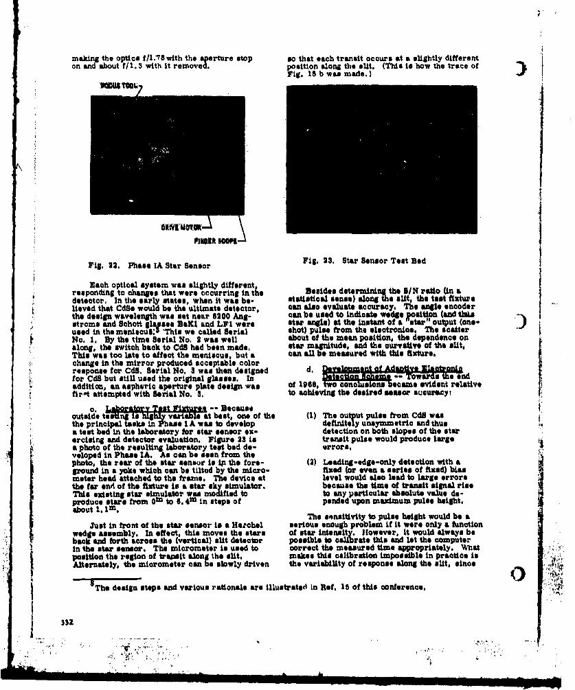
making the optics f/ 1.18 with the aperture stop so that each transit occurs at a slightly differenton and about f/1.3 with it removed, position along the slit. (This in how the trace of

Fig. 15 bwas made.)

IDAIVI MOIPN

FINUIR lOOps

Fig. 22. Phase IA Star Sensor Fig. 23. Star Sensor Test Bed

Each optioal system was slightly differentresponding to changes that were occurring in the Besides determining the S/N ratio (in adetector, In the early states, when it was be- stati•tical sensn) along the aut, the test fixtureliUved that CdSe would be the ultimate detector, can Malo evaluate accuracy. The angle encoderthe design wavelength was set near 6200 Ang- can be used to indicate wedge Rosltion (end tM&stroms end Schott glapsoes BKIl und LFl were star 41gle) at the instant of a tMar" output (one-used in the menisaul:3 'This we called Serial shot) pulse from the electronios. The scatterNo. 1. By the time Serial No. 2 was well about of the mean position, the dependence onalong, the switch back to CdS had been made, star magnitude, and the ourvaive of the slit,This was too late to affect the meniscus, but a can all be measured with this fixture.change in the mirror produced acceptable colorresponse for CdS. Serial No. 3 was then designed d. ow s sendfor CdS but still used the original glasses., In OA TowardsIU naddition, an aspheric aperture plate design was of 1968, two concus s came evident relativeftrit attempted with Serial No. 3. to achivinLg the desired sensor a1uecyt

a o. L�or-tITEtLE I•$M sL -- Becauseoutside tintinj i* hUhl y variale at best, one of the (1) The output pulse from Cdl wasthe principal tasks in P Ase I as to develop definitely uneymmnetric and thusa test bed in the laboratory for star sensor ex- detection on both slopes of the starercising and detector evaluation. Figure 23 is transit pulse would produce largea photo of the resulting laboratory test bed de- errors.veloped in Phase IA. As con be seen from thephoto, the rear of the star sensor is Ip the fore- (2) Leading-odge-only detection with aground in a yoke which can be tilted by the micro- fixed (or even a series of fixed) biasmeter head attached to the frame. The device at level would also lead to large errorsthe far end of the fixture is a star sky simulator. because the time of transit signal riseThis existing star simulator was modiLfied to to any particular absolute value de-produce stare from Om to 6. 4m in steps of pended upon maximum pulse height.abo~ut 1.,1m.

The sensitivity to pulse height would be aJust in front of the star senior is a Hezchel serious enough problem if it were only a function

wedge assembly. In effect, this moves the stars of st intar sty. However, it would always beback and forth across the (ver~ticl) liut detector possible to calibrate this nd lot the computerIn the star sensor, The micrometer iS used to correct the measured time appropriately. What 7,position the region of transit along the slit. makes this calibration impossible in practice isAlternately, the micrometer can be slowly driven the variebility of response along the slit, since

The design steps and various rationale are illustrated in Ref. 15 of this conference.

332

", ,4,. '...- +: 7.. -

no gradual function of alit uniformity would be The scope photos in Fig. 26 show some typicalapplicable. Errors in the many tens of arc results. Besides verifying overall sensor per-seconds were being created. formance against real stars (and through an at -

ooL.Tlbnr-), these tests substantiated the tVstsTo overcome this, the peak. ciorage (or performed under more controlled laboratory

adaptive) scheme shown back in ilg. 16 was conditions.developed. The rationale for this came fromnoticing that the loading edges of all the pulms.(regardless of ultimate height) differed onlyby a scale factor. Thus, If detection were to PTAR UNIN ACC• V

occur always at a fixed percentage of the pulsepeak, then it would also occur when the starimag bore a fixed relation to the slit (siUghtlypast it).

Some of the results obtained during the ;final Phase IA demonstration to the Air Forcein February, 1960 are shown In FigL. 34. Eachscopo trace uses a different star mag&ntd ad-is triggered by the anglc encoder onthe test , .fixture. Thus position along the sweep corre-lates with the lInus position on the star sensorfocal surface. One can see that the 50 percent -_,__,__,___._,,I _........jI_ ....... __point on each pulse Io within one or two arc 10 10 0 -.00seconds of the others. AK SIGNAL TO 55 501 N RATIO

Figure 25. Phase IA Star Sensor AccuracyDemonstration

Q-TOO NA ?M0ss901 18.04ILI

m -Fig. 24. Phane 1A Demonstration of HA 'Ra

50% Bias Level

The method chosen to achieve this fixed Figure 36. Representative Real Starpercentage or adaptive detection is to delay the Transitspulse in one channel while measuring its peakand sotting the trigger level in a second channel.The accuracy of this scheme, as demonstrated at Bome interesting insight into the thermalthe end of Phase 1, is shown in Fig. 25. stability of the sensor was also obtained by these

outside tests. Sinee hocus was established in thes t affIt -- At the end of Phase IA lob at roonj temperature and to ratures out-

(early 109) exensive testing was conducted side to _15"F did vot otie ably ct mnge ql-Safaist roea stars from the roof of Building IC ity, it was concluded that the sensor was relatvely

tho CDC headquarters complex in Minneapolis. insensitive to ambient temperature changes.

3w3

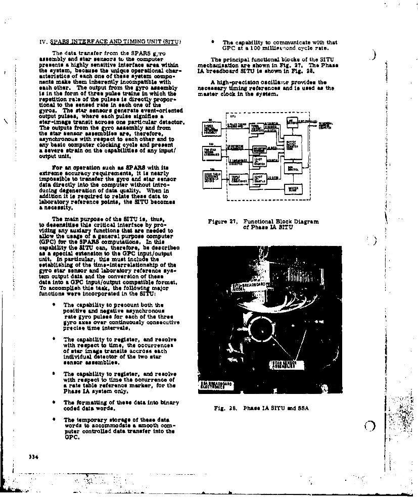
IV. SPARS INTERFACE AND TIMING UNIT (SITU) 0 The capability to communicate with thatGPC at a 100 millist,ýond cycle rate.

The data transfer from the SPARS g;roassembly and star sensors tW the computer The principal functional blacks of the SITUpresents a highly sensitive interface area within mechanization are shown in Fig. 27. The Phasethe system, because the unique operational char- IA breadboard SITU is shown in Fig. 28.acteristics of SlU& one of these system oompo-

nents make them inherently incompatible with A high-precision osciUa-tr provides theeach other. The output from the gyro assembly necessary timing references and is used as theIs in the form of three pulse trains in which the master clock In the system. 4repetition rale of the pulses is directly propor-tional to the sensed rate in each one of thegyros. The star sensors generate event-orientedoutput pulses, where each pulse signifies a -7star-image transit across one particular detector. goThe outputs from the g assembly and from0the star sensor assembies are, therefore,asynchronous with respect to each other and toany basic computer clacking cycle and present ' 'a severe strain on the capabilities of any input/output unit.

For an operation such as SPARS with itsextreme accuracy requirements, It Io nearly *impossible to transfer the gyro and star sensordata directly into the computer without intro- Fducing degeneration of data quality. When inaddition it is required to relate these data tolaboratory reference points, the SITU becomesa necessity.

The main purpose of the SITU is, thus, Figure 27. Functional Block Diagramto desensitise this critlcal interfasce by pro- f Phase IA SITUS vidin any auxiary functions that are needed toallow the usage of a general purpose computer(OPC) for the SPARS computations. In this "capability the SITU can, therefore, be describesas a special extension to the OPC input/outputunit. In particular, this must include theestablishin of the time-interrelationship of thegyro star sensor and laboratory reference sys-tem output data and the conversion of thesedata into a OPC input/output compatible format.To accomplish this task, the following major S

functions were incorporated in the SITU'

0 The capability to preoount both thepositive and negative asynchronousrate gyro pulses for each of the threegyro axes over continuously consecutiveprecise time intervals.

The capability to register, and resolvewith respect to time, the occurrencesof star image transits acoross eachindividual detector of the two starsensor assemblies.

C The capablity to register, and resolvewith respect o t ime the occurrence of -.a rate table reference marker, for the l J 0Phase IA system only.

• The formatting of theme data into binarycoded data words. Fig. a8. Phase IA SITU md BSA

e The temporary storege of these datawords to accommodate a smooth com- -)puter controlled data transfer into theoPC. . .

334

, ' •

The asynchronous gyro pulse trriris areaccumulated in conventional up/down countersover 100 millisecond periods and at the end ofeach period the contents of theme three counters MA

are strobed in parallel into their own specific I I ,,data word slots of a ten 5-bit word buffer output -. "register (BOR). After the strobing action thecounters are reset to zero for the next 100millisecond cycle. During the interval ofshifting gyro counts Into the BOR and the counter W,' . '"reset action, all the input circuits to the countersare inhibited from receiving gyro pulses. Anygyro pulses generated during this interval are I Aautomatically routed to individual holdingregisters from where they are strobed into the •counters after the inhibit is ited.

The star transit timer, the associated star L. .--.-.----- - --- --------.detector decoder and the reference marker timerare equipped with similar holding registers attheir inputs, so that the complete SPARS system Figure 29. Functional Block Diagram of Iis capable of running independent of computer Phase ilB SITU

cycle constraints.

The time referencing of the star transit andrate table position reference markers Is accom-plished with the use of ripple-up counter- wherethe discrete pulse generated by the sensors at The BOR format was changed to a five 12-the time of the event is used to gate in a 10 KHz bit word configuration and has a parallel wordclock for the remainder of the 100 millisecond entry capability to accommodate a shift throughtime interval in which the event occurred. The capability for facility information and data fromindividual star detector identification pulses other flight systems to the computer complexare coded in a hexadecimal coder. The contents via one common output bus.of theme time counters and the detector coder are Falso strobed into their indivioual slots in the A step-by-step, remotely addressable,BOR so that at the end of each 100 millisecond self-chsck system was incorporated for pre-period all the significant information about that system run verification purposes and failureperiod is stored in the correct binary format and isolatioyi in came of a system breakdown. This

word sequence and ready to be input into the self-check system can be automatically activatedcomputer, by the facility computer or manually by the

operator at the control station.A fixed delay after the BOR is filled, the

SITU sends a priority interrupt to the computerto indicate thtt it is ready to be interrogated. NThe dat& shift out operation from that point onIs under control of the computer, but must be EJtUT;N Alm ERROR ANALYSIS

completed before the end of the next 100-milli- T!'e actual input rate along the lA of one ofsecond cycle to prevent loss of valid data, the gyros being aligned In given by

In the Phase IB SITU the basic functionsfrom the Phase IA unit were preserved, butwere modified to present a closer approach to WIA to (WT + WE sin L) sin E

a flight worthy configuration, Fig, 29. Thegyro up/down counters were all made to haveequal capacity and the star transit time count + W. cos L cos E cos 8 (Al)and detector identification information are nolonger formattea as separate words but multi-plexed into a single data word, The basic clock where|

S frequency is increased from 100 KHz to 2MHzta allow faster strobe and reset operation, and WA is the gyro input axis rateart internal DC to DC power converter was added it ua tto allow operation from an unregulated 28 Vdc Tratesupply. WE is earth's rate

For simultaneous operational capability L is the latitude u the test sitewith a flight computer and a GPC, a more corn-plex BOR control and a dual buffered output were Ii the error angle between the gyro IA

added, and the table spin axis, and

335

_ _ _ _ _

e is the angle between the gyro IA and Table A-i. Summary of Uncertainties in I3Anorth Input Axis Calibration

Maximum Error.This equation assumes that the table spin NormalErore

axis is aligned with the local vertical, or that Error Source For ( er AxisL is the angle between the table spin axis and Gyro Pulse Weight 0. 120 0. 187the earth's spin axis. Rotation of the table Uncertaintythrough 360 degrees at a constant rate is pro-mented by the following integration of Eq. (Al): Gyro Drift 0.013 0.020

IRA Pulse Count 0.002 0,003Quantiuation

J'o WLA d9 o WT + WE sin L) sin E Table Encoder 0.007 0.013o AT EQuantisation

Table Bearing Wobble 0.333 0.467

+ WE coo L cos E cos BId9 (A2) Table Speed 0.007 0.013WEJ V.riatlons

Mirror to Spin Axis 0.200 0. 200T dt Measurement0 T d e* 2w (WT +W sinL) sinE Small Angle 0.067 0.093

Approximations -

(A3) Total one-a 0. 533

MeasurementUncertainty

where WT a d@/dt, and T is the time for one *Normalized to SPARS gyro input axis calibra-tion accuracy requirement.

revolution, T - 2f/WT. The integral I TW dt

is by definition the angular equivalent of theaccumulated pulses from the gyro being )PARS lNJW. AEpNfM ARILameasured.RADM RITESS)

This equivalent gyro input angle will be Gyros of the floated, air bearing, pulsedenoted by P wN, where P is the nyro pulse rebalanced rate integrating type with extremely

weight in radlbns per pulay. and N Is the low, stable drift rates are the candidates for theaccumulated pulse count. Solving for the mis- SPARS attitude reference system. The Honey-alignment, we have well G$334A is this type of gyro. One of the

major problems in determning system attitudeaccuracy is the accurate modeling of floated,

PwN ()ulse-robelanced fyro drift characteristics.sin E aW \ (A4) ýo'n t ro drit in unimportant in this appli-

2t 1 + E sin L cation because it gets calibrated out completelyW T in the SPARS recursive filtering equations.High-frequency gyro drift. on the other hand,

has such a low amplitude that it does not into-For misalignment angles of a degree or less, grate to an appreciable angle. The drift thatthe small-angle approximation affects system accurany the most is in the

0. 0001 to 0. 1 Hz range. Accurate power spec-tral density information on gyro drift in this

pwN region is somewhat difficult to isolate and ob-

E Pw(AS) tain. Long sampling times and a significantamount of data are involved. This appendix

2w I + !X sinL describes the resultn of C1G334A gyro driftSTtesting, statistical anlysis, and modeling.

can be used, where the approximation error Two primary methods were used by Honey-

is less than 0.2 are second well to gather gyro drift data during the SPARSG0334A drift testing program. The first method

Alignment Errors is to f rod the qero d rate output to precisionvoltage- to -frequacy converters. This rate

A number of uncertainties will result in the proportional a-c signal is then integrated with

data obtained from the above alignment pro- resettable up-down counters. The counters

codure. These are listed in Table Al. The can be sampled and reset to sero at any fre-

total uncertainty is well within the SPARS quenoy of interest, and the sampled counts are

requirement. then punched on paper tape or sent directly to

336

V-, . -

the SDS 9300 computer, with six-decimal digit Next, the intensity uf x is cuniputedaccuracy. This method is used to investigateF2 Nthe drift spectral characteristics out to half t Ex ) = (y -) 1•)the sampling frequency, timing the approxima- j Ntion that the rate error is constant over any one

sarple period, This test setup proved to be This intensity Is, of course, a measure of theextremely accurate, but unfortunately has the total average power.characteristic of exhibiting frequency folding Tneffects in the sampled data. i. e., drift at The autocorrelation function of the y processfrequencies greater than the sampling frequency is estimated byappears in the lower frequency part of theaampled spectrum. Nk-

To eliminate any frequency folding effects, N 1a second method of gathering data was employed.Here, the rate output is amplified with a high- where k m 0. 1, 2 .... m, € - kT, and T is theSgain, low-noise buffer amplifier right at the sample priod. Here, m in the specified numbertest setup to minimize noise pickup and trans- of lags maximum allowed is 2000).mission losses. The amplified signal is thenfed to a low-pass, seventh-order filter whose The variance of x, a measure of the aver-cutoff frequency can be varied between 2. 0 and age power associated with the a-c component,25 Hz. The voltage output from the filter can is given by R(O) sincebe read with an RMS reading meter, for com-parison with the standard deviation of the rateoutput computed in the computer facility from R(O) - E(y 2 ) a E (x (B5)the time history. This amplified and filteredsignal is then routed to the A/D convertersin the hybrid computer facility via coaxial An estimate of the power spectrum, sometimescable, The sample and hold amplifiers are referred to as the power spectral density. isinterrogated and reset by the computer at obtained from the Fourier spectrum of thi,any frequency of interest. The filter cutoff truncated autocorrelation function. Since R(r)frequency in the gyro lab in always adjusted 0 is an even function,that it is half the sampling frequency, toeliminate "folding" completely. rhis gives a( true picture of the drift power out to half the 2vsampling frequency. The signal flow through S (f) - J' R(i")eo2 f7. dr a 2 J R~r)thlb test setup is shown in Fig. El. .

42

'coo (2yr1,) dr (EU)irlt - -- *

,,;Z computed at intervals of f /2m over the range.. f'.., C. J f 2, where s thampling frequency.

l"..... A weighted average of ad)acent values ofS (f) iM obtained corresponding to a convolutionwith a spectral windowi in particular, theHamming window.

Figure Bl. Gyro Drift Test Configuration nfs (n-l)fsS [ "r . o. 23 S ._ a o. f

Once the gyro drift sample time history (u~l)f Ahas been obtained, the autocorrelation function + 0.23 S - - (B7)and the power spectral density (PSD) are com- 2m;puted. The mean is given by.

for n- 1. 2, ... , --l, and

x r E xj (Bl) .) (2

where N- 5000.

Once the mean has been computed, a new :0.46 S . + 0.54 S (138)

Y j "x , I X (EB 2)

' : , s' . .r s .... . ....... • .....

3. ..

"•.• . "- "7 -

The resolution is actually f /rm even though shows a typical not of data that was taken: 250the spectrum is computed ever/f / 2m cps se.zonds (out of 1250) sampled at 0. 25 sac withFinally, the area under the curve~(f) is comn- a 0. 1 Hz loop bandwidth. The scale factor for~uted, 0'a f a f / 2, and multiplied by a factor of these tests was 2, 7 volts/do g/hr..to obtain a lomparison between R(O) to QoeM- Tesaitclmdseta eut

spectrd easlieraned. assmuehrm h oeown for a 0. 1 Ka loop bandwidth gyro inspeoru stimted.Figs B3 E toEB5. Fig. ES shows that the drift

An alternate method of calculating the M~ autocorrelation time constant is well below 0. 1is also available, and gives results which agree seconds. The power spectral density peaks Invery well with the lagged products approach the 7 Hz range. The probability density functionsoutlined above. This computation involves (actually histograms) for the 20 nis and 0. 25 secevaluating the noefficients of the complex sampling rates are also shown in Fig. B3,. TheFourier series of a periodic p recess, y(t), which numerical values of the standard deviations foris identical to the Wroesms x(t) over sonme finite all this data are given in Table Bl.interval, 0 at a To. These coefficienis have theform

N-1 Jh T 6.1k C ~ U x(nT)a 'Jfk T,

km to, 1# 2# .,, N-1 (BO)

A computational algorithm due to Cooley and TMR(eaTukey' called the Fast Fourier Transform wasused, which reduces the computational require- 34meaits for evaluating these Fourier coefficientsenormously.

A number of samples were taken fordifferent gyro loop bandwidths, since the sensi- Ltivity of low-frequency gyro drift to loop band-width might have an important bearing on thisdesign parameter. Drift data was taken at 20 meaand 0. 25 sec, yielding spectral and statistical Woo IIdata out to 25 and 2. 0 Ht, respectively, Fig. 92

Figre 3.Autocorrelatlon Function, PSD,19,41Fiur E1'"JA.f$ and Statistics - 0. 1 Hr. Loop

Bandwidth

Table Bi. Gyro Drift Test Summary

0.-? A lov £0e 131

3.. C lI O G ." 463 8,131

3.3 C4 Im ' .Qv L 0.0 - -I

8.1 is0 gib 0.6 .6 L.6' 1.84 0.613II .$."0 Its 3 0 as ILO 3 .4 104 .341 0,

Figure B2. 03Vao Drift Below 2 Hz -0. 1 Ha -h A ndWat .6M 6ý& a 'Loop Bandwidth 00.mhfllIM

ME Transactions an Audio and E160troaocouatics Vol. AU-l1B. N~o. 2. (June 1967). C

338

0.014W

The upper left photograph ini Fig. B4 showsin more detail the spectrum out to 2.0 Hz, |which was obtained with the slower 0. 25 sec AIsampling and a 2.0 Ka filter cutoff frequency.To demonhtrate that no folding from higherfrequencies is present in this data. the spec-trum doriv*d from the higher sampling rateof 20 ms is overlaid ts a series of dots on thispicture, showing vyre close correlation. The S # 4WW I

envelope of the Fourier line spectrum, obtainedwith the Fast Fourier Transform ethibit aUshape nearly identical to the PSD. The photo-graph on the right shows an expanded pictureof PD out to 0. 1 Hz. This data is quiteflat and well-behaved, devoid of spikes ordiscontinuities.

oo

Fiaure Bb. Gyro Drift Power - 0. 1 HzLoop Bandwidth

An expansion of the data in the Cto 2 Hzrange is shown with the 0. 25 sec sampled data,and the 25 Hz data is overlaid as a dotted line,

F~ agin showing excellent oorr elation uAz a lackof frequency folding. A further expansion in the0 to 0. 1 Hz range is also shown.

; Figures D• through Bli show correspondingsets of data for 1. 0 and 10,0 Hz loop bandwidth,Krespectively. The main change in the data isthat the drift standard deviation grows largerwith increasing loop bandwidth as the powerspectral density grzows in the 1-25 Hz range.The question of importance, though, is howloop bandwidth affects gyro drift performancein the low frequency region. The upper photo-graph in Fig. B12 shows, from top to bottom.the power uut to 2 Hz for 10. 1. ant 0. 1 Hz loop

Figure B4. PSD Detail - 0. 1 Hz Loop bandwidth gyro loops, respectively. There is3ndwidth considerable difference at 2 Hz. but the lower

picture shows that in the region 0 to 0. 5Hz,the PSD integrals are practically coincident.Therefore, tho conclusion has been reached thatthe loop bandwidth can be selected using criteriaother tha= system performance.

It is also apparent from Fig. B12 that thePSD integral is very linear out to 0. 25 Hz.

The net result of all this is the plot of gyro which means that the PSD is esatantially flat, ordrift power (the integral of the PSD) versus 'white" out to this frequency. Based c i thesefrequency. This data for the 0. 1 Hz loop band- results, it appears that the most realistic maths-width gyro is shown in Fig. BS. The complete matical representation for floatod gyros of thepicture out to 25 Hz is shown on the left. The 00334A class in the low frequency range in adiscontinuity at 19. 1 Hz is due to a large spike random process whose variance is matched toin the PSD due to the natural resonance and the actual gyro drift varia.ice at the sample fro-motion of the toot pad at this frequency. That quency. This is a result that has far-reachingpart of thka integral, therefore. is not attributable implications In the design of bounded (e. g.,

gyr o drift but to actual measured angular celestial/inertial) attitude reference systems.motion at that frequency. The flattening of the In unbounded, strapped-down attitude referenceintegral zt 2.ý Hz indicates that nearly ell of the oysters, the critical gyro parameter is thedrift power is included below this frequency.

339

this short-term drift. Table BI summarizesgyr po drift test program that warn conductedin support of the Ph',ase 0 SPARS prograre. The :.

last six item& in this table summarize the testscoverer by Figs. B2 through B12.

•4 1dB I~l 9.1 "004•~t

and Stautptico - 1. 0 H0 Looppoam Te

Bandwidth am,.

Figure B8. Gyro Drift Power - 1.0 Hz

Loop Bandwidth

LO

IFigure B7. PSD Detail - . 0 Hz LoopBandwidth ,h .

absolute, long-term drift rate stablitty, since I

there is no capability for calibration while oper- = -atring. This long-term stability may very well •m, ,•.w,look like a random walk or damped random walkprocess. Figure B9. Autocorralation Function, PSD,

Sand Statistics - 10 Ha LoopSIn the design of bounded systsmL, this very Bandwidth

liong-term• stabiLity aissiumoa secondary impor-

NI I

tance and tho critical item become3 thz shorter-bterm drft. However, it tate sbilie than i

ipecotication of the amplitude of the short-termtdrift to determine the effect on aytmvery wlor-

lmookle (angular orrors verdua timed. Of oqumal Atiimportance the sepectal t marcterietics of

1 40

-,. -;•.• .... . ..-....- - --

4-- - --- m ~

Rik]

Figure BO. PSD Detail - 10 He Loop Figure B12. Comparison of Gyro DriftBandwidth Power at Different Loop

Bandwidths

"1. W.R. Davis and J.A. Miller. "SPARS -A Completely Strapdown Concept forPrecise Determination of Satellite VehicleAttitude," presented to theAttAtude Detegraination SymjDI-e_"n

Aerospace Corporauon. as 30 toOctober 2. 1969.

2. D.C. Paulson. D.B. Jackson, .nd C, D.Brown, "SPARS Algorithms and Simula-

L tion Results," presented to the m p uron Sacecraft Attitude Determinatio co-

sponsore by AFU.SMU and ThL Aerospace Corp., El Segundo, California,September 30, October 1-2, 1968.

"jou 3. V. Hvosohinsky and F. Horiuchi, "ConceptsNfn and Mechanization for Evaluating PEPSYin the Laboratory and in Orbit," presentedto the Spdcecraft Attitude f r etarmination

IL SiSmoosium, The Aerospoce" corporation,September 30 to October 2, 1969.

I,,,. 4. R. 0. Maze st a]., (U) Stuy and Develop-ment of Pulase Truma Wor WnetiaFigure Bi1. Gyro Drift Power - 10 He Loop AoD (CONFIDENTIAL,) -

Bandwidth £ednmcsl -IoposaL, Minneapolis Honey-wel1 Aero Document R -ED 5020,28 Jan'iary 1957.

5. J. E. Anderson at al., (U) The gmballjgseAnalvtle InertialNavihOURD 4ygetim(GURSe TCOFIDENTIAL), Minneapolis

HloiiyWe1l Acre Document R-ED-0029,August 2, 1957.

6. J.W. Minor. LoxCost stagdow Inetial!' I Sylili, presented to AIAA/ION Oidanoe

and Control Conferance, Minneapolis,'A Minnesota, August 18-18, 1985.

341 J'

I. lnertial Reference A.sernb.ly ouwers, Achieveeents in Optics,Part No. Ou 2200 AC), Utility, TechniMcal1. .Eevrowr,15.heemnsnOti,

Manua1, loneywell Documont 20973-UTM2, Elsevier, 1950.prepared under contract F04701-68-C- 14. D.D. Makmutov, "New Catadioptic Meniscus0061, 1 August 1059. System," J. Opt. Soc. Amer., Vol. 34,

8. R. L. Lillestrand and J. E. Carroll, 'Self No. 5, p. £ WAY 19y4.

Contained System for Interplanetary 15. J.E. Carroll. 'Sub-Arc Second StarNavigation,' &mrcnAtoat l1.J . arl,"u-r eodSa

iptonSan anceAstro nutiaSensors, Design and Fabrication," pre-Soci_ . San Francisco. Aug~ust 1961. sented at the Spacecraft Attitude Deter-mnination ;Symposiumn, Tihe Aerospac;_

9. R.L. Lillestrand, et al., "Celestial Corpratlon* El Segundo, September 30,Successor to Inertial Guidance," Yduto October'u-2, 19S9.tronic, Murch 21, 1966. Also, " A' -mic Celestlal Guidance, Part 2. New 16.. Richard H. Bube Poonsucini.,Challenge to Designers' Ingenuity," , Rihar John Wiley & hoonduI ••. oE, April 9, 1966. New York, 1960.

10. A. LaBonne, et al., "The SCNS Attitude 17. K. W. Boer, at al.. "'Properties of Re-Determination Experiment on ATS-4I," crystallized Evaporated CdS Layers,"presented at the Spacecraft Attitude Solid State Physics, Vol. 16, p. 697,Determingtion Symnposium, Th Aeospace 1986

Corporation, El 3egundo, September 30.October 1-2, 1969, 18. Physics and Chemistry of II-VI Comrnounds,

11. J.E. Carroll. "An Automatic Instrument edited by M. Aven and J. b. erener, North-'ot the DEo sroiHolland Publishing Company, Amsterdam,

tar the Determination of AstronomicPosition," Sirveving and Mtplona, to be 1967, especially Chapter 13 and 14.

publi-ihec.

12. (Uý Space Precisio Attitude ftefrqncby em, Vol. I Technical Proposal,

ONFIDENTIAL), LMSC 699615,15 May 1967.

I

0

342, -•4." :" -•-v"--'w,- • -, . : >

S• •. . . . . .. . . .. ' .,, '... . . - , ,• •

CONCEPTS AND MECHANIZATION FOR EVALUATING SPARS IN THE LABORATORY AND IN ORBIT 1

Vladimir Hvoechinsky and Fred Y. HortuchiLockheed Missiles & Space Company

Sunny~vale, California

This paper describes the concepts and mechanization for evaluating theSpace Precision Attitude Reference System (SPARS) as part of a PrecisionEarth Pointing System (PEPSY). Pertinent information is included con-coerning test installations, critical specifications, and error budget. Theseconcepts have been developed by Lockheed and Honeywell under Air Forcesponsorship over the last 2-1/2 years in an effort to improve the techniquesof attitude determoination and precision pointing front the spacecraft to aterrestrial target. The PEPSY hardware system presently is beingdesigned and built. Within the next year, complete end-to-end PEPSY per-formance will be evaluated iv test laboratories at Lockheed and at HollomanAir Force Base.

The orbital experiment with the PEPSY, known as PEPEX, is proposed asa followup phase of the present hardware development and evaluation pro-gram. The proposed concepts and mechanization for performing such anexperiment are presented.

2INTRODVTION EVOLUTION OF PEP$Yz

The intent of this paper is to present highlights Recognition of potential operational use for theof concepts and Wdes for evaluating an uxtremely extremely accurate attitude knowledge supplied byaccurate precision earth pointing system (PEPSY) in a SPARS was sufficient to motivate developing that tech-laboratory environment and in an operational satellite nology. However, it ,\as soon clear that to gain accept-environment. The authors would like to share with the saoe 10- operational aeployment of much a system itreaders basic difficulties and possible solutions to the would be necessary to prove its performance in a near-problems generated by such a task. It Is desired to operational situation. The realization that the onlypresent philosophically practical concepts exposing way one could accomplish an in-orbit check on themoetly the "happenings." and di-emphasizing maths- accuracy of satellite attitude determination suggestedmatical proofs and specialized statistical computations, making SPARS an element of a precision pointing aye-Such an approach is appropriate since during this ses- teza (PEPSY). This in effect closed the loop by usingsmoi several papers will be presented dealing with tlb attitude knowledge of SPARS in such a way that anryspecifies of algorithms, design, and testing for dif- deficiency would be reflected am a (major) deficiencyferent PEPSY subsystems and outlining the basic eye- In system performance. Since one of the mjtJor opera-tern concept and mission applications. (See Rafe, 1. tional uses proposed for SPARS was as a component2, 3. 4Q of a preci.ion pointing system, it was. therefore.

appropriate to synthesise R precision pointwig experi-In order to familiarize the reader with Whe eye- meet to test SPARS, Am this concept evolved. Ittent, and to help him with the acronym@ a synopsis of became evident that the mechanlsation of a precisionPEPSY is presented in the first section. Following the pointing experiment. particularly at an enrth target,synopsis, the next three sections will treat the evolu- was a worthwhile objective In its own right, Thus, inties of the basic test concepts. the mechaniatior. of spite of the fact that an expereimetit to point at star@ A7,the laboratory test, and thi proposed approach to the for attitude information only could have fewer errororbital experiment, sources and thus allow potentially narrower bowids oni

j ( t This report was prepared under Air Force Contract F04701-GD-C-01f0 on 23 September 1009.

343I .-.•''. -~ :.. .f-:*. . . .. -"....... .............- -. .- ,.--

establishing SPARS performance, the more complex and operates upon data contained in 512 24-bit words ofconcept of pointing at an earth target was retainea as destructive readout memory, Prime functions of thethe primary PEPSY test objective, computer in the PEPSY application are:

Ideal.l, one would specify that the test equipment • Perform attitude state computations (SPARS)(the pointing device) have an accuracy an order of mag-nitude better than the itesm to be evaluated (SPARS), a Generate pointing commands for OPDIt seemed unlikely that this could be achieved at areasonable cost In this case, Thus. for the purpose of * Store star catalog, calibration data, constants,evaluating SPARS, the PEPSY experiment as con- and initial conditions.ceived presents the problem of separating the errorsdue to SPARS from those due to the pointing device and In support of the above, a space-ground telemetry linkthe rest of PEPSY, sends information to, and receives Information from,

the on-board computer and/or sensors, This informa-Thus concepts for PEPSY testing with the objec- tion includes orbital parameters established by ground

Uve of SPARS evaluation had an impact on the synthe- tracking and errors in pointing commands.sis of PEPSY itself. The result Is the systemdescrlbed in the following sections. THE LABORATORY TEST CONCEPT

ELEMENTS OF PEPSY In Its entirety, the PEPSY system advances thestate-of-the-art in these flelds:

The Pracision Earth-Pointing System shown con-ceptually in Fig. 1 consists of a combination of four e Accurate determination of satellite attitude inmajor subsystems described briefly betow, real time or post flight (SPARS)

SPARS a On-orbit accurate evaluation and calibrationof SPARS

The Space Precision Attitude Reference Systemconsists of three orthogonally placed rate integrating e Accurate LOS pointing and knowledge in point-gyros and two star sensors mounted together in a strap- ing of a sensor from a vehicle to a grounddown configuration. The gyro package provides contin- target in open or closed-loop modes (OPD)usou three-axis wide-band attitude information, whiletime transits of known stars on the star sensors pro- e Ephemeris updating techniques (OPD)vide a precise attitude up-date at discrete times. ThisL subsyne~m, together with a computer, provides ex- a Extremely accurate, dynamic, three-axistreraely accurate real time satellite attitude knowledge angular alignment measuring device (OAL) )In an inertial reference frame,

The concept is good, but how can its performanceOPD be established? What accuracies are to be expected

and allocated to individual subsystems? How should theThe Optical Pointing Device consists of two main test of such a system be mechanized and what is the

elements, One Is a telesoope-asieor and the other is error budget?a two-waxs gimbal assembly, Two 720-pole 7-in. read-In Induotosyns mounted on the pitch and roll gimbals Clearly, accuracy is the name of the game. Theand used in conjunction with a high-gain closed-loop accuracy requirements of the SPARS subsyatem dictateservo point the telescope along a commanded line of the performance accuracy of the other subsystemssight. Telescope aiming is based upun Information which are to be used for its evaluation as well as thereceived trom SPARS, OAL, and the ephemerides of the maximum permissible error contribution of the testthe ground target and spacecraft. Any misalignment installation and instrumentation, To gain insight intobetween the satellite-target line of eight (LOS) and the the feasibility of synthewising a practical PEPSY, rela-OPD LOS is sensed by the teleocope-sensor. The OPD ULve error budgets were generated. These were basedIs capable of being commanded in both open-loop and on a trade-off between desired performance for SPARSclosed-loop modes, evaluation and the difficulty (cost) of the achieving a

precision OPD. Two configurations, remote and inte-OAL gral (corresponding to the relative mounting locations

of the OPD and SPARiwsrs considered, The budgetsThe Optical Alignment Link consists of optical for these oonfiguraticns are shown in Figs. 2 and 3.

transmitter and receiver assemblies which dynamicallymonitor relative angular displacements between the The eonnomios and step-by-step process for de-SPARS and OPD packages. Displacements detected by vuloping a sophiaticated system such as PEPSY call forOAL are fed to the computer for the generation of laboratory testing to precede in-orbit tests. Indeed.pointing commands to the OPD. suouessful laboratory validation is undoubtedly a noose-

sary prerequisite to justifying an oroital test. AlthoughAirbyrne Computer tn-orbit tests are usually more difficult than corros-

ponding laboratory tests, for PEPSY the in-orbit on-The UNIVAC 1bd4C selected for the airborne vironment has at least one advantage not available in

computer is a high-.performianco. generul-purpose, the laboratory, but important to precision evaluation,IWln-ry machine which can store up) to 12, 28b 16-bit and that is the accurately known absolute referenceinetructio,. words In its nondestructive readout memory frame created by the fixed starts. This brings up the

344

S+<

SPARS/

STAR SENSORSGYRO PACKAGE/

S//

LIN

OPTIAO

/ GO U A

Fig. 1 Precision Earth Pointing Concept

345

.V;7

"i • i . . .. . . ... .. .. .. I , ......... . .

, • -.. ,..;.,, . I. ,• .. I,

• "S•-..

i PEI•Y

1.O00

PITCH ROLL PITCH ROLL PITCH ROLL.37 .37 .57 .57 .34 .34

Fig. 2 Fractional Error for Main Subsystems of PEPSY in Remote Configuration

I -IPEPSY1.00

SPARS OPOD

PITCH ROLL PITCH ROLL.53 .53 .47 .47

Fig. 3 Fractional Error for Main Subsystem@ in Integral Configuration

question of the approach to be taken in the laboratory. To show the correspondenoe between the labora-Should one simulate whatever takes place in orbit and tory and orbital test geometry, Fig. 4, along with thethus compound the errors, or should one simplify the pointing Eqs. (1) and (2), are presented.laboratory mechanization in order to decrease the:error sources at the expense of the faithfulness of Line of sight vector to ground target in OPDsimulation? frame

The latter approach has been selected. Onlyessential dynamic and geometrioal conditions will be t T T V(simulated In order to establish as accurately as pos- S20 12(sible the hardware performance in the laboratory.

Figure 1 shows a satellite moving around the Line of sight vesto: to ground target in inertialearth end otating (pitching) to maintain a nominally frameoonstait u Litude relative to the local vertical. In thisattitude, the OPD is pointed toward the ground target .and maintains the required LOS during the experiment V TE21 T E (2)pass. The target with known earth coordinates is spointing at the known satellite position and continues topoint at It throughout the pass. The OPD is command-ed to point at the target on the basis of satellite attitude w. "determined by SPARS, satellite ephemeris com uted where.in the computer, ground target coordinaten, end OAL a iscretos fBig satellite ephemeris in the

initial frame

346

-•.-. . -.. ': -- . . . ....r ...- . ".'-

( I°''•.• POINTING

TCOMMAN[(L I TAR I TL SATELLITES (LAS) oPD

GROUND TARO EARH

C..

• ~INERTIAL-

(LAB TABLE \ ".-{TABLE ISN)

ROTATION) I INRTIAL (LABORATORY)

S~(XL) X1

(zL) z1

Ii'

( 715. 4 Laboratory and Orbital Geometry

347

.I, , .".' .-,.. ... "•- ... '..q • ,; ' ' ": -" •

F = Earth Target coordinates the OPD gimbal axis and will describe the angle -.which is identical to the angle a which OPD LOSvector goes through during the orbital overpass. This

T transformation from earth to inertial simplifiation requires only one precision rate table

frame and decreases the number of error sources.

For the laboratory end-to-end testing of PEPSY LABORATORY TEST FACILITYhardware, the following essential elements related to Tbeyorbital conditions are inoludedi The SPARS subsystem will be tested at Honeywell

Minneapolis and then shipped to LMSC Sunnyvale for

e Pointing line of sight vector from OPD to the integration with the Optical Pointing Device and other* ground target major PEPSY subsystems. At LMSC complete SystemAcceptance Test (SAT) will be performed. Final sys-

terns evaluation will take place at Holloman Air Force* Pointing vector maia~mum line of sight rate Bs pncmlto fSTfor the lowest orbit Base upon completion of SAT.

* Star distribution In angle *nd brightness In order to perform the SAT. three adjacent

factors representing nominal and worst case areas totaling 2500 sq ft are planned (See Figs, 3." 'orbits 6, and 8).

a Pitching and limit cycle motion of the e A clean room for the PEPSY test setupsatellite * An area for PEPSY control consoles, instru-

The elements encountered in orbit and contribu- mentation and control functionsting to the system error while testing in orbit but notnecessary for hardware evaluation in the laboratory t An air-flow bench area for assembly and main-are: tenanoe of PEPSY components and subsystemr.

e Ephemeris Ae (Eq. 2) computation obtained Cloan Roomby integratinf the equations of satellitemotion or ephemeris update from the ground The clean room is being built to approximate .station Federal Standard 209 for a 100,000 class installation.

Foreign particle stzc will not exceed 10 microns and

6 Earth target coordinates WT and earth-to- air lock passages and positive air preusure displace-inertial transformation T T ment will be incorporated. This room will house a

E2t seismic mass, upon which is located the Ooerz PrloL-

The elements present only the earth laboratory sion Rate Table with the PEPSY test specimen. Itenvironment whose error nontribution must be mini- will be light tight and painted a special color to reduce,mized and/or idnntifled are: unwanted light reflections. A diffused air conditioning

system will minimize air currents and thermal gradi-S Star field instabJll0 due to the thermal and ents in the vicinity of the test setup,mechanical stresses in the star simulatorsand their mountings The following environmental conditions will be

maintainedie Earth rotation which is sensed by gyros

Temperature 721F & 21F* Wobble in the rate table used to simulate

orbital rate Humidity 40% A 10'k RH

e Vibration and drifts of seismic mass on which A special overhead uable handling system will bePEPSY is to be mounted installed for completing the electrical connections be-

tweon the "PEPSY" setup on the rate table and equip-Gravity which is not present in orbital testing ment in the control room area. A servoed cable drumbut must be accounted for during laboratory may 4e used to follow the table rotation (plus and minustesting and preflight calibration of the system 2.3 turns), thereby unloading the cable torque from the(OPD) rate table,

()n important deviution from orbital geometry A seiamic mtss 15-ft long x 15-it wide x k-ftwus mudo for the laboratory test, From Fig, 4, itcan he soon that "ground target" will be mounted with thick will be made from reinforced Class K-I concrete

SPARS und OPD on a rate table simulating orbital rate, and instAiled 6 months prior to the test on a pneumatic

TiNs, of course, is not what will happen during the suspension system. Three main functions of this mase

orbital experiment. Why should on# do it in the labors- are:tory? A simplification can be made in the laboratory P.,Motup and atall achieve a me'mininfl end-to-end scaies- e Maintain stability in aximuth and tilt to within

tl,)n (if PEPSY. Thu only important requirement is to 0*'r-scns e asimuluto the polnting LOS vector T., from OPD to theutrgut. Thus. the targot in the laboratory T will e Maintain the relative motion between the testrotute around point 8. in lino with thu Intorsektion of equipment to lees than 0.5 seconds of are

, T

,... *..- -..- •. . . .',•

" ' , " i ',•~~~~~~~. . . .. . . -.. ! .. .. • ;

V

e Provide isolation from external vlbrations by a ter and 36 inches long. In the simulato', light from a

pneumatic support system having attenuation tungsten filament bulb li passed through two filters,Scharacteristics with a slope corresponding to a focused on a pinhole, and collimated by an achromatic

second order system with a resonanoe at 3 Hz. objective. By inserting different neutral density filters,stare from +1.0 to +5.0 visual magnitude can be simu-

A modified Goerz Model 800 aitr-bearing rate iated. Insertion of color correction filters permitstable will be installed on the seismic mass and used to stars of the A0, 05, M5 spectral classes to be simula-provide a rotational motion to the entire PEPSY spool- ted. Star imago size is smaller than 5 arc seconds=men, It will supply accurate (pitch) position readout while uniformity is better than * 0. 2 magnitudes.ditring pretest calibrations and test. The table will beoperated primarily in the rate mode using the synchron-ous drive system and will have a readout position Figure 7 shows star distribution for the selected

accuracy of less than 0.4 arc seconds RMS, and a resol- orbit, Stars A and B are used for the calibration of the

ution of 0.36 sec. The nominal angular velocity during OPD axis and yaw misalignment. Each simulator will

the test will be 4 degrees per minute. Peak-to-peak be mounted on a pier and enclosed by a protective cage

table wobble of the unmodified model was meusurod to to prevent accidental contact and misalignment. The

bo less than 0.6 see of arc pier-simulator spatial stability will be better than 1 arcsecond for a 12-hour period. The star field will be

Also mounted on the seismic mass are eight to calibrated before and after each run by the OPD and the

fourteen star simulators placed in a random pattern rate table, A provision in the star simulator mountarouihd the rotary table to simulate a llstatisticalLy nom- will be made to allow adjustment of the elevation angleInal" star field. Star simulators are 5 Inches in diame- by *2 degrees from the nominal "orbit plane."

F1P1 CLAN OOMCLIAN CLIANSPIPS'i CLIAN ROOM

A A

ACHICKOUT & 0

41111

PN LINL 23 OP

C-NITIOI, AIO5APOUIDANCI LAI

"LINI OF SIOMT

• _...._._.•OUTSI01N O RTH RI F A I SLII I LOD FN

ý NIII PLTFRMIOV-1114P OUILIT +

0---* RAILINO 0 IIOV-3 AMP OUItIT N

RIIIMVAtILE TRUOH COVIR 0 31V DC OULtt

Fig. 6 Tast Facility Floor Plan

34;,

. . .

WPROTECTIVE CAGE

M OVERHEAD CABLE RACKSSPECIMEN UNDER TEST

Fig. 8 PEPSY Test F~aility Perspeotive, LMBC Sunnyvale

350

3OIO ASA1MAAZ 3

*I -Np t 1 .0 .14 IL*0.* I

AS g. '7DsriuinofSa bmltr

ityai tucua lxrs ourn eX~n~eLAn twee PAS an OPDwhenmoIte in the

The PPSY cntrol Aresonitig ,wl rmte ofgrto

A4 0a~~~~~~~~~~~I AG6oh1nva2B4 opte h ES et pcmn ositn fSAS

theOPD te QL irorWne opuean nerau

a Tet dta cqusitin ed qickloo dislay an Tiing nttwiUbe ssebledon het recsio

A4:!4. a h ~ttP.1

The folwnFyialmsinoeaing. opitrbtical alowe StrSmltorstileinastefradesfo ra

anddynmi c onion nwllb siuatd hors No prenalo stuiurlfl b exrmted ocrin g th e -eroo eean fin A RS clbatind wi hen perormted anuthes

Th Nomina conrbitl areate shoawny Thi pi ,wlreot"cdfiureawintonlsaetm buwill~ ~~~~~~~ ~wl huetecnoeanrokofeupeta0Alsoopdereasethve lgoung-termet drifofthe testn

it Pwrando swathol fof"tr' varyin oeaion co eu Pmentin du of t pertoaure cha onge. ret

magitde aziuth the elevatineCmpteanontrfc

rai talo as shw.nFg, h o ttbewl

CONTROL AREAq

WINCREMENTAL TAPE RECORDERSSTRIP CHART RECORDER

~JPEPSY CONTROL CONSOLESPEPSY CONTROL RACK g.SPSYCQrIAe

M OOERZ TABLE CONTROLS (3 BAYS)Fi,8P SYCnrlAe

SULTRA CONSOLE (OPD)S1824 C AGE(3 BAYS) 1

M DDP-516 COMPUTER

4D SPANS STAR OlNlSN

OP11CMt PQ1N1iN0 DIVICI

COAL OilISCl 1, Omc

-. A10110INI COMPU111

0N11tIPACt AND I IMING UN.,

tMPICAt fAIQI 7

7 CAlt 110VO SUPPO01 U(.K

011C.ISON RAtIAL sIl

7'~T IPCA t VIA N ,NIALL&!1CN

11P Fig IIOV11jO

Fi. ISEP PSY rusit sutup

Mc'Nit intereslt•ng automatic calibjr'ations u-e: - af'ALT :. vector from the Ol'f) g, mhak r•ont t,,

- SPARS "a'itc cal" procedure determines the the target in target cordinatub.

orlent4auon in laboratory coordinates of the T transformation matriceM from jtwelle-star sensor detector alit normal j2K to k coordinatie frame.vectors.

0 ,,OPD;e 8 4'AR distrtbution is determined with the OPD

in elevation and with the OPD plus rate tableposition readout in azimuth. L lSoratory

e Calibration of OPD outer gimbal axis and yawmisalignment with the two additiorval itar TAB * tableSimulators "A" and "B" shown in Fig. 7.

TA =ground targetAll calibration data is computed and stored in the

"airborne" computer as well as in a laboratory compu-ter, It can be seen from Eqs. (4), 5j, and (6) that

OPD is pointed at a known• ta-get (r . ), by using aAll data to be recorded will be fed firit to the SPARS generated directiun cosine mafrix (TL2S)I and

laboretory computer fnr conditioning, For the OAL data rquick-look analysis the lab computer will calculate theEider Lngles at each star transit and subtract it from A special mechanism % ,ll be used to introducethe rate table position This information will provide dynamic disturbances between the bcses of SPARS anda real time indication uf the dalferenco- between the OPD) thorehy simulatiig vehicle flexure. At this point,SPARS and the rate table readouts it is intsiesting to observe the similarity betý.-en LOS

pointing vector equatiorns written for orbital and labor-The ground target simulator consists of a story oases In the OPD frame, One is Eq. (1) p.'rvious-

Cassegrainian optical collimating source witl an image ly indicated and sedond is Eq. (3) written in slightlysize of 3 arc seconds and a single gimbal structure with different form to underline the similarity.an Inductosyn readout accurate to 1. 5 arc sec andrepeatable to 0. 2 arc seconds. The target axis of rota- Orbition will he vertical and will pass through the intersec-tion o' tht OPD axes,

l.u Motion of the target will be programmed by the 3 T5 20 T12S L! (1)lau computer. It will be completely indepen-d;r.t of the PEPRY system and will be similar to the Laloratoryline-u.-sight-motion a1 in the orbital case (see Fig 4). = T TL (5

(- -o )V - [a Sin (0o1 - K) (4

Stan'1 ;n . (4) o-xis operathn of the OPD will be acoom-

R0 -g pushed by mounting the OPD pitch axis 30 degreesfrom vertica; and maintaining the target in the horizon-

h ta! ulane. The OPD can operate in the open-loop or.iE orbital constant cloved-l'wov modes. The airbornu computer generates

E outer and inner gimbel pointing commands by cunver'tingthe pointing vector L (Eq. 5)

0- 0 K - rate table pos~tion read out

-= 120 degrees per minute for 100-nm LýM JLx or lbit fi' .0 6 (7)

= range ,00* I J

The OPD will be Qonmmanded by the "airborne" Open loop:computer to point at and follow the giound target at aline-of-sight rate typical of that encountered In orbit.The pointing vector in OPD coordinate is given by L°Fq. 45) bolow. -Tane d (.8~Lo

T-TA5T S20 TTL28 T'rAB2L TTA2TAB L'TA 05-Lo

(ETA =LnV |1 Tan 7 " (8)

S. . ... ..... ...-- - - ,--- -, . .-- --

Closed loop! In order to obtain a larger sample of mutually

_Lo independent data points, the OPD and target will be=a zl _ AX exercised several times per table revolution, a altue-

- o o (10) tion corresponding to passing over several ground tar-

gets per orbit. Th;o is a technique for minimizIng thetime for data aooutindatleo. The STAR distribution

.0o pattern in azimuth will he changed from orbit to orbit toS= Ti• • + A (11) minimize systematic errors In table pario4icity exper-

I- Lensed in earlier testing. Data accumulated during they teso will be proo•sed r•ttistioally to ascertain SPARS

and PEPSY performanc., accuracy,

Where AX and &Y are the OPD telescope outputsfed back to the "airborne" computer, In the closed- The major error So-0,ce for the PEPSY test areloop mode, the measured OPD-target error is used to grouped in Fig. 10 acoordi! j to whether they are attri-track the target butable to the system or the laboratory.

E COMBINED

RF M TE TOST

POSYEQUIPMEN

I I ---- L I ..STAR GROUND GOERZ

SPARS LINK OPD SIMULATIONS TAROGN TABLEAND PIut AT

Fig. 10 Combined System Error B,.dget

End-to-end PEPSY perfoi mance can be summar- ORBITAL TEST (PFPEXI MECIIANIZATIONized by specifying the three quantities defined below:

The orbital evaluation of the SPARS. integratedwith an optical point ing device, will be implemented in

e Pointing Error, The angular deviation of the the Precision Earth-Pointing Experiment (PEPEX).OPD Telescope-Sensor (T-S) optical axis from The primary objective of the PEPP.X is to obtain thethe line of sigh. to the targnt. The pointing necessary quality ard ouantity of those measurementserror is indicated directly by the T-S output, from which statistically meaningful data on the SPARSTypically this must be kpt smaller than thL perfrrmi~nce may be derived in a post-flight a"alysit.T-S iield of view The experiment requires five major elements- The

PEPSY mounted on a satsilite; a cooperative grounde Pointinm Knowledge, The ability o ccnpute laser tqrget; a satellite gr(,und communication link; a

the line of sight to the target from post-test multi-station satellite tracking network; and auxiliarydata analysis. The Pointing knowledge is tracking systems.derived from knowledge of the puinting err.,'.the OPD servo error (inductosyn signaJ), anithe commanded OPD gimbal angle. Approach to the Experiment

Error in Pointing Knowledge. The angular For PEPEX, the SPARS/OPD combination willdeviation of the computed line of sight to the be mounted on an attitude-controlled satellite which istarget from the actual line of sight to the nominally orleetad in the local horizontsl plane as ittarget. The actual line of eight to the target traverses its orbital path about the earth. Th. result-is derived from a combination of the comn- ing pitching motion ol the satellite with respect tomanded target angle and the target servo error. inertial space provides the .motion enabling the SPARSIt is assuemed thet the error in pointing know- star sensors to sweep the celestial sphere and en-ledge obtained duriig; a lerte number of tests counter the star transit@ with which it will establishwill he normally distributed. the orientation of the inertial coordinate frame. ()

354

"' "<.' " ' -" -"

Typically, 'he PEPEX ,-IlI be con~ducted in the Present beam divergence will acoom'modate the two-following manner: After the sate~lltu is injected Into sigma, wcret-caoe ephemeris errors and allow aorbit and sufficient tim.a is "lowed for vehicle oUtffas- reasonable bt..am-pointing accuracy. In spite of this,sling to be completed, accurate orbit determnaotion will opea-looip pointing is preferable to closed-loop becausebegin Lidin; traotikng data from tW.. Air. Forip Satellite neither an onboard retro-r-Alector nlor a groundControl iFac4lity (SC F) System - After the List tracking receiver unit with its supporting; equipment is noese-paits prior to PEPEX operation, the beat (0)11; fit Is &aM. Beam pointing will be anoompllshed in open-loopmade by the ICF and an ephemeris -to generated and by driving a two-axsi gimbaled mirror that deflectsextrapolated through the experiment nose. A statei the light beam emnanating from a laser transmittervector from -this ephemeris In traxatmltted to the mtetl- fixed to a stationary base. Considering the requiredlite to be used to a set of initial oonditlone from which 4oCUraoy: pointing a small mirror is simpler thanthe flight oomputea' Woule generate an ephemeris painting the whole laser.throoigh the target pass. The flight aosavtitr, utiliz~ingthis on-board ephemeris, vehicle attitude data frem. Dtirinf the experiment pass, precisinn satellite,SPARS,:'vehlcleflowue data, frowthe OAL, and tbie tracking data will be gathered by mean. of a ballisticstored-target location, will then dotepmianet6) oom-ý oaizrera locatedwith tho'laser target (at Zdwowds APE),mind@ requi'red to point the OPO Teleaoope-Sansor , anti/or a com~plexof four geodetic DECOR ground sta-(T-6).at 'he cooperative ground target and to maintain tions (Fig. 11). These data will provide the high-that target in, the T-0 f1old of virw (TOy). priolplon satellite ephemeris necessary in the post-

flight a~.%dysai to determine the. portion of the target-The. ground target will1 be a high-intensity light Image error contributed by inaccuracies in the reaid

source gonerated by a continuouis-wave gas laser. This time ouboard ephemeris.leser operating in the TaMoo mode provides an outputbeam with a Gaussian cross-sectIonal Intansity funotnon. The ballistic owmera, with a pro-pa.. fixedThe beam dlvergeuicels ostabli %hed in such a way that setting, has the dealt able feature of providing a directfor the 2-sigma poorest beam-pointing aoaouraoy and a orientation meadurement of the OPD LOS in inertial2-aigma worst satellite -position prediction, the beam space. It will photograpo the vehicle in earth orbitwill Illuminate the PSPEX satellite at one-half the against a star reference background. The vehiole willmanximum laser output power, be equipped with a flashing Xenon light for locating

purposse. However, this approauh is limited In data-The baseline candidate for the laser is a gathering opportuinity to a short hegment of each night

stab~llzed 6-w argon io~n unit. Thisi laser features overpass and is subject to data loss due to oloud cover,a li Ihtweight head (80 lb) nd a comp at power aaUP- The magnitude of celestial segment observed i. depen-ply (250 lIU). At the 5145 Aline, chosen for its dent upon the field of view (FOV) of the camera. 1( ~simnilarity to starlight, the laser has a guaranteedpower output of 2. 5 w after 1 year of continuous The veraclity of any expaarinmantal result in-operation. ureasee with the quantity of the experimental data It.-

Jectod intoi the analysis. For this roason, the DECORFor a laier beam divorgenoe of e 550 arc so* at complex would offer %n advantage since additional ex-

the half-power points, and an atmoaphorle transmission perimental data could be gathered on iety Wlight. Thecomputed at a look angle of 30 dog up from the horizon, system will track a transponder-equipped satellitethe laser power deoneity is sever6U orders of magnitude over the full span (elevation angles greatsr than 15 doggreater than that from a isecond-magnitude star. For of any day or night overpass without rogiard to the extent*xample. at a 700-nm rang, laser power density is of cloud cover over any or all stations. An additional5 x 10-wAD2 , whereas the power density from a advantage of BECOR is its capability to provide a real-typical second-magnituds star Is 5 x 10" IOwhn2. time ephemeris urdate. An update is req~aired for open-Since the telesoope-sensor of the OPD is designed loop OPD pointing to be aoooir.~ltwhed without a loss ofto "see" a second-magnitude star, this design allows the target from the OVID field of view. The possible'.seeing" the laser under loee favorable conditions than magntude of the errors in the SCF extrapolated sphe-assumed ab~ove. Daylight detection of the laser against menum would no% proolude target acquisition due to thea sunlit earth is possible because of the mononchroma- wide T-8 aoquisltion FOV but could caus. the target totic nature of tbe laser and the narromw Instantaneous drift out of a high-acouracy narrow T-8 steady-statefield of view of the tole.43ope-sensor A spectral FOV. Since loves of target cannot be cocmpensated postfilter, a few angstrom. wide at 5146 X. eliminates flight, an Improved ephemeris must be provided to themost of the reflected solar spectrum. For the no- on-board computer.clotkd atmospheric conditions specified, the signal-to-noise ratio what observing the Waar against the sunlit A drawbaok to the DECOR system In that theearth is greater than 20 to 1. satellite ephemeris is determined relative to the earth-

fixed reference of the DECOR ground complex. TheTo enable the T-S to rsceive the laser signal, transformation to an inertial reference produces errors

the highly dlronticuaal laser beam must be precisely due to the uncertainty In the prorecse location af thepointed such that the satllte is Illuminated throughout ground complex. This error can be removed by adjust-the pass over the target station. These pointing com- Ing the ephomarin to incorporate the direct inertial

Wmwill be generated open-loop in ground computers orientation measurement of thr relative vehilel positionutillizing the best current satellite ephemerisa. Open- vector acquired by the ballistic camera.

A ~loop beam pointing demands a very accurate gimbal-( aligament and drive system. This accuracy minimizes The Space-round Link System (SOLD) station at

compounding of errors already present as a function of Vandenberg ATE will serve as the real-tine telometry,~4 Ibeam divergence and satellite position uncertainty, command, and experiment direction link between the

3155

ground rcontrol center and the vehicle. All PEPEX Contributors to Pointing Errortelemetry data wIll be transmitted to ground stations )via the SGLS on a real-time oasis during PEPEX oper- Open-loop pointing commands to the OPD areation or tape recorded for later readout. These data generated In the flight computer utilizing data from theinclude the tim6 variation of the target image error SPARS and OAL subsystems, stored information con-and all irputa and outputs to the on-board computer cerning geodetic location of the ground target, and thewbl,:h are neoessawy for the post-flight evaluation o satellite ephemeris as determined onboard in realPEPSY performance, time. The pitch (a) sad roll (P) commands to the

Inner sad outer gimbals respecti, ely were definedAfter an experiment pass is completed, a new in Eqs. (8) and (9) In terms of components of the

ephenmeris it generated in the ground computer center relative position vector between the satellite andand extrapolated to the next experiment pass. At the the ground target which was defined in Eqs. (1)conclusion of the flight. all accumulated telemetry aid and (2).trackitig data will be utilized in the post-flight analysisto establish the aocuraoy of pointing imowledge achievedby PEPSY.

tI

/ *1/// N IVAUA

: RANDII40

.9COR AkND TLM _;

5hECOa

i / V

\I

I Fig, I I Precision Tracking int PEPB'Y Evaluat~on Aooompliqhod With Operational Systems

J i 5, .

Pi, ii I Prciit tracing 11111 P1P11 Evlai N A Inmliehe With peaIonal System.Ii III ilmi 111Il

2The accuracy of the pointing commande must be tracking network being used, the quality, quantity, andsuch that the target remains within the narrow (high distribution of the tracking data, and the accuracy (ifaccuracy) field of view of the OPD telescope.-sonsor the mathematical gravitational and atmospheric densitythroughout the experiment pus. The extent to which models.the pointing accuracy Is achieved will be determined Tetikn aaerr aa to admerrby the accuracy with which the onhoard systems canThtrcigdaerosonstfrnomoruidetermine T128, TS20, compute the pointing oonmm~nds, and data biases peculiar to the equipment of the tracking

and xecte hor, Th T~~ wuldbe pate one a network being used. In addition, the tracking stationandt andut statio time oa21 aould be updte error Thday to reduce precession and mutaition errors, The loain bn stdtio time caAlsFeSCero.Fhelements not wholly within the control of the system trackding network to be uso consists of te FChardware are the accuracy of the target location and SOLS stations and the Satellite Test Center (STC) comn-the 6atillite ephemeris. Target location error is de- puter facility in iiiinnyvale. Errors In the gravitationalpendent upon geodetic survey accuracies and can be in model Include the inaoccuracies in the zonai ana tesseralexcess of 100 feot, The satellite ephemeris carried or coefficients and the earth's gravitational constant. Thecomputed on board would be the most significant con- atmospheric density model errors of interest during theA

tribtorto a exerimnt oining rro. Th nees- fitting and extrapolation intervals are those due to thesary ephtimerle accuracy Is a function of orbit altitude uncertainties in the contribution of actual geomagnetic

and he omial ffse anlesfro thelocl vrtbal. activity to the short period density fluctuations. These

On-Board Enhemyris Computation N EVTI I~Iit~hl TERMThe onboard ephemeris Is computed over a given I,. 'Itn

time interval utiing lnitIsLI-condltions input received Xfrom the ground. Two error sources come into play.IThe orror in the Initial conditions and the error in the ~c NI ~computed epheaneris. The former Is a function of the

ground tracking network, the traoking coverage, the /

atmosphericiand gravitational model erors, an teetntowihcufitted shemeris must be extrapoIa-2

ted forward from the last tracking pass. The latter Is-a function of the method of dompittation. This can beAAccomplished by. the closed form or numerical integra- '

* ~tion of the equations of motion. The selected methodare degree of complexity of the equations of motion to* C.be used was chosen on the basis of position accuracyIcomputation time, and computer capacity requirements , t'i.for the ran&e of orbitaltitudes and ovarpass time spans *

of interest. The timb history of position accuracies 1

for a 200-nm orbit utilizing the numerical integration Eof simplified equations of motion wad examined, S@0 00 400 300 4100 5111

Fig. 12. IV was found that at the end of a 8-minute TIM (SCovorpass the retention of only the J2 zoWa harmonicot the gravitational potential (Eq. )2) will result in aposition 20 feet from that determined when utilizing theJ and J imnale as well ts the tusseral harmonics,

and ,rotpresenting the ellipticity of the equator.Afir' drag ws, found to make a smaller contribution to dthe positi'rn error than those attributed to the tesseral ''

harmonics and was thus dropped from the oquationp ofmotion, This difference is more pronounced for higher I f Ja ), (12)orbit altitudoes. d

4 [\ / \ 1

Ujphoiris Determination With ground Tracking

The uncertainty in the on-board ephemeris, how- 6.. r-~ ~ l0 11 I 2ma,: 'ever, can never be less than that of the Initial condi- X 0 i2nh i1~ 2tions transmitted to the flight computer from the ground. PI (I HThese Initial conditions are derived from the best real- Where: x. y, r iiertlid positio~n vi.,ipononwetime prediction of the satellite ephemeris by a groundcomputer center fitting the orbital equaticns of motion - ItiLuvitationali constuntl

to observed data from anetwork of widely dispersed J24 e47x1- oa]hrnntracking stations. This real-time ephemeris is up-dated with each succeeding pass of tranking data.- The it-best fit just prior to an experiment pass will be exr- FU. 12 The Integration of the Equations of Motionpolated forward to a point just preceding predicted mtngalbtheJzalaroitrmftetarget acquisition. These Initial conditions are thenOmtigalbthe oalar nctr ftetransmitted to the satellite. The accuracy of thl 4 pro- Gravitatlonal Potential Results in Approdcmately a 20- F~tdiction Is dependent upon the characteristics of the Position Error Afti~r a 8-Mmn Integration Period

357

- ~A.

unter'talnties arc tunctions of the assumed variations preclude this possibility, a gross ephemeris correctionII tihe half-day averages of the geomagnetic index K-p. will be determined in tho ground computers by perform-Rlepresentative densit. variations are used simulating ing a least squares fit on the T-S detector data overminimum, moderate, and i4mnse levels of geomagnetic a short time span assuming that the total pointing errorheating based on observed Kp data correlated with ob- is due to satellite in-track position error, Fitting onlyserved density fluctuations, to a correction in the in-track position permits the

rapid calculation and transmittal of the correction toA comprehensive analysis of the accuracy of the flight computer. The ephemeris correction also

ephemeris determination and extrapolation can be made might be accomplished utilizing the SECOR data,only when the specifics of the available tracking net-work are known, However, for insight into the prob- Post-Flisht Analysislem, the accuracies obtained utilizing the AFSCFnetwork for a hypothetical 200-nm altitude orbit were The OPD pointing angle error data recorded andexamined. These results represent the maximum in- telemetered to the ground station during the flight willtrack position uncertainties assuming the availability be processed in the post-flight analysis to establish theof 11 passes of radar data over an interval of 16 hours. uncertainty in PEPBY pointing knowledge. The evalua-These data were processed in a weighted least-squares tion will be performed by an error-separation methodfit of all data at a rate of one point every 15 sec and utilizing a least squares fitting technique. The basicextrapolated forward for a maximum of 5 revolutions, premise in this method is that pointing angle errorsThe fitting parameters consist of the six-orbit 919- socuring due to errors in the vehicle and PEPSY statements and the vehicle ballistic parameter. vectors propagate in time in distinctive ways. In con-

trast the satellite ephemeris errors are assumed toAlthough for the case of maximum Rp activity remain constant over the short duration of any experi-

position uncertainties in the initial portion of the fitting meat pass. This approach requires that the time vari-interval were on the order of several miles, the fit for ation of the error parameteo a be accurately modeled.the 200-nm circular orbit converged after 8 hours of Error models for all of the system error sources willdata to a constant in-track position uncertainty. This be determined from previous test and calibration datasituation continues until the cessation of tracking. taken during the experiment. The parameters of theExtrapolation of the fitted orbital elements results in error models then become the fitting parameters in thethe predicted maximum RSS in-track position uncertain- least squares fitting equationities growing by a factor of four after five revolutions.The state of the art of ephomeriJ determination hasprogressed to the point where the errors in the extra- IQTW-1 q -11 -l (TW-1 40 (3pclrntion of an orbital fit for five revolutions under the AL - Q (QW)worst conditions will not impose excessive require- 0c

ments on minimizing the divergenoe of the target laserbeam to ensure acquisition of the target. The air drag where AL is the differential correction to the vector of1 unoertainties are the dominant error source. For low fitting parameters, Q is the matrix of partial deriva-

Kp activity periods, the station location and gravity tivs of the T-I detector data to the fiJting parameters,model uncertainties are the major error sources for W" is the data weighting matrix, 0o is a preloaded

t the extrapolation. Random data errors and data biases oovarianco matrix and q is the vector of residuals ofhave small effects compared to other sources. There- the observed detector data with respect to the computedfore, the use of more aocurate tracking data at the data based on the current best estimate of the fittingSOLS station locations will not noticeably affect the parameters. The time history of Q is determinedaccuracy of the predicted ephemeris. Improvements analytically based on the nominal trajectory for thein the air drag model, ground station survey, and experiment pass.gravity model are necessary to eignificautly reducethe ephemeris prediction error, The domination of The fitting parameters are varied in order tothe extrapolation by the air drag model errors in high yield a least squares fit of the total modeled pointingmagnetic heating periods leads to increasing ephemeris error to the actual error as determined from the tele-uncertainties at lower PEPEX orbit altitudes. This metered data. The PEPSY errors are then determinedoccurs due to the higher densities at the lower &a being the values of the PEPBY parameters whichaltitudes, gave the best fit, i.e. , the smallest residuals over the

pass of data being analyzed. The uncertainty In theknowledge of thee* PEPSY parametele, and thus the

Real-Time Euhemeris Update SPARS performanoo, will be dependent upon the qualityand quantity of test data, the validity of the error

The wide FOV incorporated in the OPD/Tr-S and models, and the accua.acy with which the fitting is

the narrow width of the ground laser beam have been accomplished.specified so that errors in the extrapolation of the pre-diotod satellite ephemeris under worst atmosphericconditions and the lowest anticipated orbit altitudes will A UNIVAC 1108 program simulating the post-not preclude the acquisition of the target by the T-. night error separation method has been developed,However, the gathering of acceptable test data requires coded, and partially choked out, The program requiresthat the target be maintained in the high-accuraoy the Input of radar tracking dat, two axis T-9 detectornarrow FOV of the T-S. While a large initial pointing data, nominal OPD pitch and roll gimbal angle histories,angle error can be removed by a compensating gimbal a beat estimate of the orbital initial condition, andbias, the causal large ephemeris error will soon move error model parameters. The program has beenthe target Image out of the narrow FOV. In order to checked out with noise-free simulated AFICF range

358

• - -. .... . .. ..,jT -7 . ... -. -. _._.,_.. .

• • ... '•t,,~ 1;.• ' ••- • :... ,,-

data, OPD detector data generated by the input of the fit has converged after seven iterations.six components of satellite position, velocity errorsand a set of SPARS pitch bias and drift-rate errors.The accuracy with which these eight parameters were Further work in checking out the fitting of thefitted is presented in Fig. 13. The errors in the fitted remaining error parameters, the determination of theparameters are the values obtained after nine iterations effects of noise on the data and the extent of the oorre-using the least squares method. As can be seen from lotion between parameters will be conducted In the nextthe table of the RMS detector and range data residuals, phase of the program,

I i . . arameterTrue Fit* Input Error Fit Correction* Error in Fit*

S-19149838 ft -19149535 -500 ft -500.16989 ft ,16959 ft

Y -348659.9 ft -3488658.9 -500 ft -499.00396 ft -. 99404 ft

ZI 10476490.1 ft 10476490 -500 ft -499.97058 ft -.02942 ft

)C 12091.4331 fps 12091.433 0 fps .18o9p x 10. fpa -. 0016898 fps

I18. 877193 fps 198.86730 0 fps -,98930 x 10' fps .0098930 fps

I;Z 1i• 29168.9497 fps 99168.943 0 fpa -. 30770 x 10.3 tpa .0003077 fpe

0 0 rad .1919 x 10"s -, 5 x10"5 red -. 4998 x 10"8 rad -000 x 10" rad

0 rid/sec -. 9718 x 10 -1 x 10 rad/seo -1.0003 x 10 rps .0003 x 10- rps

E MSData Residuals(. )~ ~ ~~No of Iterations T ___________No., arc-sec YT, arc-mco Rasg, ft

8 .887506 x 10" .216703 x 10' .44041 x 10'

7 .23614 x 103 .98930 x 10" .11310 x 10"3

9' .10980 x 10" .3696 x 10" .3298 : 10.

*Values given are after the 9th iteration

FIg. 13 Error Separation

A

REFERENCES

1. WR. Davis, t al. 4. W. R. Davis and J. A. Miller, a

9. U. 0. Paulms, D, B. Jaokson, and . D, Brown, 3. W.R. Davis, ot &I., (U) oiAitudtPe fa A PH I M• k eaa MV9 t ,

(O a t 1o 89 ). 4 i.

3. R. T. Scott and J. 1. Carroll, S

________________o WAR, .4...,'- I= (Oct lose).I

• '!3 9

TO"L"

SPARSt THE SYSTEM, ALGORITHNIS, AND TEST RESULTS1

N. r. Toda, J. L. tHels, and F. H. SohloeIBM Federal Bystoem Division

Owego, New YorktiSPARS - A Space Precision Attitude Reference System, has three major subsystems: an Inertial Reference

Unit, a Star Sensor Assembly, and a Digital Computer Subsystem. The MRU consists of three strapdown gyrosemploying pulse torque servo amplifiers for rebalancing, The star sensor assembly io a two-axis pitch withinroll gimbaled telescope. The computer subsystem Issues pointing commands to the telescope and processesmeasurement data from the star senior assembly and the Inertial reference unit to obtain an "optimal" estimateof spacecraft attitude, Th~s paper describes the IBM system configuration and the performance achieved during hlaboratory testing,

I. INRDUTO Quaternions or Wulr four parameters were"emloyed to represent atitude rather than direction

SPARS, a bacs pEnctsion Attitude Reference cosines or Euler angles. The attitude integration vlystem, consists oft an Inertial Reference Unit, a algorithm to particularly simple in this represents.-Star Sensor Assembly, and a Digital Computer Sub- tioni. The Kalman filter was employed to process thesystem. The ]partial jeference Vanlt (IRU) effectively star sensor data into "optimal" estimates of space-serves as the attitude memory between star sightings. craft attitude.It consists of three strapdown gyros employing pulsetorque servo amplifiers for re-balancing. The Star This paper describes the IBM SPARtS configura.-Sensor Assembly (M1A) to a two-axis, pitch within tion and the performance achieved during laboratoryroll gimbaled telescop",. Digital readout Is provided testing. Some quialtative data are included in theby incremental gimbal encoders and silicon digital main text; quantitative test results #Ad conclusionsdetectors. The latter measureis the pusition of the appear in the classified (SECRET) appendix to thisstar image within the field of view of the telescope. paper. Laboratory test equipment and proceduresThe computer subsystem issues pointing commands are discussed by Settlee and Nielsen in Raference (1).to the telescope and processes measurement data A description of the IRU usnd is given by Baum andfrom the SSA and IRU to obtain an "optimal" estimate Sheldon in Reference (3).of spacecraft attitude.

To demonstrate the accuracy of SPARS for aspacecraft that tis controlled to be nominally aligned The IBM SPARS configuration consists oft ato the local vertical, an extensive laboratory develop- strapdown Inertial Reference Unit (IRU), a gimbaledment program was undertaken to provide a very aoou- Star Sensor Assembly (81A), and an onboard compu-rate tost bed for the SPARS equipment. The principal ter which utilizes a software package omploytog Kal-laboratory subsystems were a precision rate table man fl~tetilng techniques.and star simulators. The IRU and fth MSA weremounted on the rate table which provided both a velo- The IRU ts ideally suited for orbital applicationscity environment and an independent measurement where relatively low angufar rates are experiencedi.of attitude. The gimbaled star sensor supplementst the Inertial

tWork doncrihud in this paper was performed under Contract F04701-88-C-02US.

.46

pakae by providing regular and frequent attitude cause the detailed description of the optical p~ro--updates via ceiestiai "fixes." High resolution of the scriptiun. the digital detectors, and their aaeuciutcd)strpsto Is realized by utilizing a gimobaled toel- signal processing circuits are of a proprietary nit-

scp ihasalIedof View (FOV). turin, they are ntIncluded In this paper. Tho over-all telescope FOV, which to defined by the optical

The IRU consists of three integrating gyroscopes prescription And the digital detector cell dirnenulon,operated in a forced limit cycle rebalanice loop. The to 600 arc soconds. An additional element existsoutput of the gyroscopes is In the form of pulse counts between the cylindrical lens and the detector cell toawhich are proportional to the nte~gral of the body provide star signal modulation.

anar rates, The overall gimbal asoembly employs a canti-*The BSA features gray-coded allir~on coordinate lever design rather than the conveational gimbal* readout devices combined with a pitch wIthin roll gim- design. Figure 1 shows the case of the roll -gim-

bal design. The purpose of the silicon coordinate bat serving as the mounthig fixture to the spacb-readout device, which is subsequently referred to as craft. The pitch gimbal assembly ts mounted ona digital readout, to to measure the X and Y ceordt- the roll gimbal shaft and the telescope assemblynotes of the star image within the telescope FOV. Is mounted on the pitch gimbal shaft, GimbalsThis provides a measurement of the star line of sight were free to rotate through at least So degrees, AIrelative to the telescope aixist orientation of the toel-scope relative to the SPARS base plate ts provided bythe pitch and roll gimbal encoders. The X 9m ICHGMAcoordinate measurements and the pitch and roll gim- ftsADOUT kbal angle measurements werti combined by the SPARSsoftware into pitch and-roll angles which defined thestar line of sight orientation relative to the SPARSL.aos plate. It is these angles which were input to the .

Kalman filter. * \'ujcp

The SM was designed to operate in a non-nulling *COPuIMm rCo,.%ND1o PICH ,4

mode, i.e. , the gimbal drive servos were not driven ROL)OI N 1so that the star image Ies@ in the center of the toel- kA- URO toioaits~oipeope rov. Instead, the telescope was driven so thatROLIMI ADUIthe star image remains within the IPOV and has norelative motion. Motion of the star image across the @ INITANTANSOUS 11111COP1MlIL.DOF VIMWdigital detector would smear the star image a&d would 10 Rc JAIN t 10 ARC MINresult in XC and Y coordinate readout errors. * TOTAL IIA MIILD Of 11

6Y GIMIAM~Y 90'Thw non-nulling approach was selected to permit

time of a rate servo rather than a position servo, Fig.l. BSAthereby minimising the gimbal servo design and tim-Ipr~oving star imago detection. Since the star image Beginning with warrmup and atar sensor aenrgi-remains motionless on the sensitive digital detector zation and self-test, an aperatlonal sequonce consist-grid, the image signal-to-nois, ratio can, be Increased Ing of star search and auquisition to performed.by lengthening the image exposure time~. SPARS to designed to determine precissly the rttitude

of a vehicle whose attitude iu already known to anTite BSA developed, fabricated, and demonstrated accuracy of *2-1/4 degrees per aLed. Thus the initial

during the SPARS Phase 1A effort Is physically made star acquisition probloin for the SPARS consists ofup uf two components: the gimbaLed telescope and the searching for a star within a cone having a half angleelectronics cabinet. Figure 1 shows the SSA. The of 2-1/4 degrees. Because the probability of the firstfunctional breakdown of these two compondints Is il three stars falling within the l0xiO arc mlnu'o. field-lustrated in Figure 2. of-view of the star sensor III very low, a search mode

Is implemented for acquisition. Following thu firstIIl. DIlTAL DETECTOR AND 'rELESC0P3 three star fixes, knowledge of the attitude io simproved

to the point that subsequent star sensor pointing com-The digital detectors are silicon photovoltaic mands will apsura that tltto star falls wiuhin the tole-

sensors employing a gray coded binary pattern which scope FOV. Subsequent star fixes at 30 second inter-produces a direct digital readout of a line image that vale then itre processed with the on-hoard filter toImpinges on the pattern. The line image to generated Improve the attitude estimate, t(, calibrate the mRUby the optics which include cylindrical elements, gyros, and to estimate star sensor misollgntrents.Pie-amplification electronics for digital detector out- Operational utilization of SPARAS requires only a sin-puts are contained In the telescope assembly. Be- gie Instantaneous snapshot of a star once every 30

362

SSA GIMIIALED TELESCOPE SSA ELICTRONICS CABINET

Dial-OPTICS D /0 PROCESSING 0/0 DATAI SDUDETECTORS APND0 11.C09ONICS &

IODI01MIL ANLE ECODE COMUTER

ENCODERS AND PROCESSING

I ATI IIA SERVO LOGIC RATE CMOS SDU

I FO

the ~ ~ ~ ~ Fg 2.iunc oSA earthsa raeinahegramro) n

tebsence. ofThe atiuerh furngtion intherval beaseen whereip deratel wholl vdibepe hihndeent onthpalb ate-

erior oav leon thlbrtn bity theo anPleS eae headanaaha:olytheToIR darc mints asadictaed bvey th23S teliescopeo toV paaetr AreTID reured, and TtediOavntaetapArovd Labreatorey was nosuc ethmateol ofe quarcer-fp h ieto oin arxadqenorft anobttwt rgritye Tfer e areemacn y sesq m ofinepanden for variabletes re-c

star ghtngs. owevr, tis aproxiaten b0 p emploedy b to haepthesadvntage thatd of thespacli earmIVw. tstR sufficient toPAN deonstrat crfuntio Th ost p. mnaeE nlstedrc

Thll o habit I labora tory imlmnalson waf pher-io csine employsan quaternions: To er~nhe kieart-c( fomed ith urin theaddlonal eqtations dof olb the bdreattivue to an inewritafme,

uthe rnuonce oearmsetihes ralledo tuhe tR yosr paraeen rCdyK aaees Tetu aaee

rePAReSentboationy was suin tht deivdly oequlartbefre Hton develoe direatrion csin. arxadqaeno

of a orit ouldbe ravrsedwit a egulrit ofre~rsenatin rsuls rns ad fur aramte363e

star alg.ige Hoevr thsapoiaey2.sedey u aeteavnaeta oalna

-itt test duainwssfiin odmntaefnto fp

The ruasons for employing quaternions (see Refer- whercences 3 and 4) are:

G f p, w) in linear In p G (t)k) (t-tk) (0I) 3

This formulation was an appropriate one to be* quaternione utilize only four parameters employed in SPARS since angular increments rather

to specify attitude In contrast to nine when than rates are the outputs of the gyros. The ele-direction cosines are used mOnts of G(t) are wi(t-tk), which is the angular

change about the ith body axis during the time inter-e the time history of spacecraft attitude Is vnl (tk, t) aesuming that rates are constant during

given by the integration of a vector differ- this interval. For the SPARS application, rAtes arcentlal equation instead of a matrix differ- almost constant except ,ttring short attitude controlontial equation resulting In fewer eompu- thrustlng intervals.

tations per Integration stepA hierarchy of Integration algorithms can be

"renormalliaation" of the quaternions Is developed by replacing the exponential by Its newer-much more simply accomplished then the, series expansion. Such a hierarchy has been con-corresponding operation for direction structed by Wilcox (4). in the SPARS application,cosines. The significance of the ronor- algorithms of higher than second order generallymalization operation will b- explained did not exhibit the accuracy predicted by theorotieRlsubsequently when the numerical Integra- analysis, This is because the gyro outputs are quun-tion of the attitude differential equation tl1 ud and therefore available only to limited ticcur-is discussed, acy, The accuracy of the second order algorithm

can be improved by replacing it by u "modifiedAn aid to understanding quaternions can be cc- second order" ulgorithm as bUgl•ontcd by Wilcox

rived from Euler's theorem which states that any (Iee eit). This modified second order algorithm cansequence of rotations utilized to bring two orthogonul be exprossud by the equation:reference frames Into coincidence is equivalent to aangle of rotation and let a (t), P (t) arnd y(t) be the dir- q(t) 4 I I- + C (ta)

ection cosines defining the fixed axis,

The quaternion elements 4,(t)m I 0 1, 2, 3,

CMt -"•wilt) dr

(t) coso(t sin (aa (t)/2) n~) • ,

q 2 (t) eone ý(tt sin (s(tt/2)

%(L) cos y (t) sin an(t)/2) and I Is the Identity matrix, In the development ofScon (/)(t)/2 ) ,l, use has been made of the relations

G M)2 -c(t)lThe quitternion representation of the kinematic

equations becomes The quaternion produced~ by the integration algorithm

4a iflq (2) ('iI will gradually depart from normality In the sensedt 2 that the scalar

wherefl is the skew symmetrix matrix 4

0 w3 -w2 W2 4-w w (3 will differ from unity, as the integration proceeds,

-I This effect can be compensated by periodic renor-I-.W -W 0j nialitation, I.e., by dividing the elements of the,'quaternion produce,' by (l61 by the scalar (6). By

and w1 Iinoten the spacecraft angular velocity in body utilizing the properties of quaternion norms It iscoordlnates. easy to show that nu accuracy Is lost by normalize-

tion at ewVcry Nth step rather than at every step.

The solution of (21 is approximately Therefore the normalizatitrn need be undertaken onlywhen attitude information is needed for calculation

q(t) 0 exp a(t) q(tk) external to the attitude integration. " ,

364

• ., .:,,*

The simplicity of the normalization correction components alung the true axes is

for quaternion Integration is quite In contrart to thecorresponding procedure for direction cosinesl. nlte- 41 *2'~ ' -1gration of the differential equations for the direction A, 4 * 3 A wIoosine representation of attitude requires not only a A) 2periodic renormalization of the rows (or columns) of "w2 31

the direction cosine matrix, but a ro-orthogonalita-J

tion of the rows (or columns). Rearrange terms to obtain

V1. FILTER FORMULATION~ 0: ' 3 A, I w~2 F - %Vl] , 0 W I ~ 2 zThe actual orientation of the SPARS attitude rot- 2 2 w - waernas f.rame differed from the estimateof ¢Its orlon- A, , 0W3-W

tation produced by the computer because of errorsin the initial estimate of attitude and because of drifts Although the gyros are physic||lly mounted along thein the gyro., The objective of the Kalman filter wtdi true body axes, they sense u combination of trueto estimate, by a sequence of sightings on selected rate w plus drift b and noise "7; the computer assignsstars, the attitude error and the bias components of the sensor outputs in the comnputed body frame; 1, o,,the gyro drift rates producing thehe errors. Estinia-tion began with initialization of the filter to the current Abest estimate of the body attitude reference frame and A - W• b 4 17,Sgyro drift biases. This estimate of attitude Was pro-pagated to the time of the first star sighting by the Assuiulng gyro drift is constant nad their input axesintegration of the quatorulon, At the tints of the first are perfectly aligned to the true body axes we obtainstar sighting, the estimates of the pitch end roll nng- the system equationleas of the line of sight to the star (computed on the"baoie of the oomp~tor's estimate of attitude) were conm- E 1 ":1pared with the measured pitch and roll angles. The d7) I IIdifferences were multiplied by the Kalman filter dt b L0 8b 0( weighting matrix to produce corrections to the estl-mantes of attitudu nnd gyro drift biases, t'tilizlng the whore a* denotec the upper (3x3) stibmatrix ofnew estinmates of attitude, the attitude quaternion was and 97 denotes gyro or process noise. Additionalre-initialized, tha gyro outputs were compensated by state variables could be added to include other dynam-the now estimates of gyro binses, and the attitude icnl biases and instrument bliases, (See Section 7.;, differential equations Integrated to the time of the

! next star sighting where the update procedure tol- The moasuromonts tire the roll 0 and pitch flowed at the first star sighting was repeated. This angles of the line of sight to a star. These -seudo-procodure continued as long as star sightings were measurements are the roll and pitch obtained by comb-taken. ing gimbal angle encoder and digital detector readings

into equi'/'alont roll and pitch angles of the LOS. TheTi:o usual formulation of a linear filter problem observation errot a are related to the statc variables

requirc.i a linoarisation of (2) about the beat current byestimate of the state, Straightforward apolication ofthis technique would result in at least seven statevwriables: four representing deviationt in the ela- [Ib]• v - H (H)monts of the quateenion and throe for the gyro drift ae 1J I b bJ

biates. The filer so designed would have to ineor- where Y reprebsnts the BSA instrument noise. Underporate a constraint on state variables since the suitable conditions on the etatistics of the state vurl-quatornion must have unit norm. able. at the initial time, the process noise 17 and the

instrument noisy i we have formulated i canonicalTo reduce the dimension of the state vector to linear filter problem in equations (7) and (S). In this

six elevnen.s and to remove the constraint on the formulation, the gyro readings ,rc not considered to* state vector, the very small attitude error wAus rep- be measurements in the usual filter sense minc( they

resented by three linfinlteslmal) angular rotations do not appeor in (9). If the dynamlonl equations ofI - 1, 2, 3 about the three body axes. motion describing spacecraft attitude were employed •

A A T to predict attitude, then gyroscope iutputp couid beLet. %T and w (w,, w 2^ AT:) employed as additional "filter" measuremente.

denote the-lingtlar velocities of the tmputed and truebody frames respectively. The circled subscript de- VII. FILTER IMPLEMENTATIONnotes the frame in which the components are evalu-ated. The angular velocity of the computed frame in The organization of the SIPARS on-boatad software,

365*~<---.

including the attitude filter, is shown in Figure 3. shown that if q((t) has a unit norm then 4(t+) Ohbo hauThe filter gain matrix computations were based on: unit norm. The gyro drift bias It updated by -)

Wi=Pi HT H HiPI(-)HT )R b(bI) I ) + ti I 1.11

The formula selected fcr the update of the filter

P, (+) " (I.Wili) Pi (-) (I-W 1Hl)T + WIRWT oooarianoe at star observation time differs from thecustomary formula which in

* P11.1 ()" .(t 1 1 ti)P1 ÷) €T(•.t~~t 1 ) " 1 Pt (t. ) - WtH.P (t,) - (I - WeiH) P (t,)

P(-) is the covarlanoe of the state vector immediately The selected formulation which can be foundbefore the ith observation, P1 (+) is the covariance In many references, e.go, In the taxt by Bryson andimmediately after the ith observation. Hj is the gradi- He (3) was chosen for Implementation in the filterent of the [I pitch and roll observation relative to the since it Is less sensitive to roundoff errors.filter states, R ie the oovarianae of the measurenmentnote,. Q1 is the oovartance of the noise acoumulented VIII. ERROR MODELin the interval (ti, t 1,,) due to random gyro noite.Finally, • Ct1, il is the transition matrix for the Errors in the measurements were characterizedsiate vector, ' either as a zero mean independent random sequence

or a zero mean random variable. The random se-The Kalman filter eatirrates a differential correc- quenoes combine to form the measurement and pro-

tion to the state, i.e., i cess noise errors which were represented in thefilter equations by the covarlanoe watrtces R and Q

i (ttiofi respectively. Biases were modeled as random varn-Al ables Certain bias errors can be included in the

Lb tJ- filter state. This is diicussed further in Seotirn VII tlJ - --, ^l- of Reference (1).%

where the tilde denotes measured values and the hat Bias errors were associated with alignment call-denotes estimates. The estimate *(ti) is transformed bration. SSA alignment errors occurred in the men- )Into an update of the quuternion by the formula cured (calibrated)alignment oft (1) the pitch and roll

- -gimbal aXes (yOX, YRZO ypX* Iypy) and (2) tole-vt 1 . -t 8(tt) q(t, ) scope (opic) axis with respect to the gima axes

tOy, YoZ ):v denotes the angular orientation, Thuwhere 8 (t) is a skew symmetrix matrix having same first subscrilat refers to cether the rnll, pitch or op-form asi•with w1 replaced by* (tl), It Is easily tie axis and the second subscript the axis of rotation.

t" GYROS

DIGITALDETECTOR GYROOUTPUTS " DRIFT •

ATTITUDE CORRECTIC'

IUPDATE Sq GYRO RATESG A LCATALOE

Sig 3 UO-oar S

ANLE ANGLE

CATTITUDE

• +.• .-. . ".. .. "

+ -• .- • .- - '

"'iv terrors consaist of: (1) biati crror in the inmtru- sisting of a series of pulses each representing anment :dlIginiment and ctlibration; (2) cyclic error in angular rotation about the input axis. The rerd-outih. it, odeling of repeatohblc bearing motion; (3) ran- error can have a maximum value ol on3 Pulse Weightdomi error in the form of non-repeatnble bea, ing me- (PW) and was assumed to be uniformly distributedthit and (4) thermal and gravity induced bending, between 0 and 1 PW.8SA thermal bending errors wore negligibly small inthe controlled laboratory environment. Gravity in- In addition to readout errors, the gyro outputsducod bending in the laboratory was assumed to be are In error due to gyro drift and angular noise in thenegligible except for the roll gimbal. However, test 3yro. Gyro drift was nharacterized as bias and wasresults indicate that this may have been n poor included in the filter state; angular gyro noise ap-issumptlon (Reference 1). The X, Y, and Z gyro pears in the filter equations as process noise, Be-input tcxes wore not perfectly aligned with the coor- cause a statistical description of gyro noise error did

U dinties defined by the IRL; optical cube. However, not exist, the MU vendor was requested to perform aSuncertainty in these ulignments had negligible effect series oi tests on an experimental version of theon SPARS performance. SPARS IRU. The data obtained from thcse tests were

used to establish an empirictl gyro noise model asThe noise-like random sequence error& are asic- described below.

elated with read-out and fabrication errors. Theradovt errors include resolution (quantization) and Single ahannel gyro pulse counts (incremental

fabrication of the readout devices, the gimbal encod- angles) were accumulated over an interval of time and

ers and the digital detectors, Resolution limitations the total number of pulse counts recorded, This was

impose uniformly distributed errors with maxima done for one millisecond and thirty second time inter-

cqun' to one-half the magnitude of the least sigrifi- vale, Analysis of the collected data indioatts that

cant bit readout. Fabriation errors arise from each gyro channel presents data containing a one sig-

imprecision in manufacture and the resulta,•t mnac- ma crror of leas than one rebalance pulse. Examina-

curacisa of extrapulation techniques. Fabrication tion of the data revealed a high correlation between

errors are for the most part repeatable at each read- millisecond samples and showed that a second har-•, ~monic of reduced magnitude to also present. The-•out position. However, the likelihood of a particular c.on fuced ma itd i also presen entreadout position rocurrirg with significant frequency correlation function implied a harmonc componenthduring a test run was sufficiently small to allow with a frequency of approximately .50 Hz, Thus the( modeling of fabrication error as a random phnonme- gyro noise (angle error) was modeled au a sum of nnon, sinusoid and a whita gauwsian sequence.

The digital detector error model includes: reso- The process noise covariance matrix Q thenlution (quantization) and fabriratiun, sorvo-induced becomesImage motion, and th._nrmal and gravity induced bhnd-ing of the telescope. 0Mor the long term, the doti:c- 2 -tor quantization error appers to be uniformly distri- F 0ibuted with standard deviation uf ,)D/v, where QD L 0

is the resolution of the detector, while the urn',ae where I Is a (3 x 3) identity matri and C is the standarderror duo to fabrication has magnitude of a'W . An deviation of gyro nobte,additional readout-type error source is imposed onthe digital detector by sorvo-induced image motinn Small ad hoc terms also were added to each of

across tho digital detectors. This image motion re- the six diagonal elements of Q primarily to increase

suits from servo rate following error and high fre- the elemuente of W relating to gyro drift bins updates.

quenvy rate oscillation (jitter). The servo errorsCiuse a smour of th-? star image on the detectors, IX. TEST RESULTS

reducing the signal-to-noise ratio and resulting Ina readout oa the mean image position. The gimbal en- Static and dynamic laboratory tests are described

coders are modeled by quantizing the gimbal angle in Reference (1). Qualitative test results are des-

plum fabrication noise. One-half of an encoder bit cribed in this section and quantativc results in the

(EW/2) is added (subtracted) to the gimbal encoder classified (Secret) appendix to this report.

reading for positive (negative) gimbal rates to reducequantization errors. After compensation, the encod- A. Convorgencg/Divorgncc

er causes errors which over the long term resembleit unutfrmly-distributcd source with a maxi mum val- Thu SPARS attitude filter should quickly reduce •"

ue of EW/2 combined with it normally-distributed large initial attitude errors, I.e., demonstrate ini- t ....-

source of magnitude WFE caused by fabrication tial convergence. Additionally, onve the error in the

errors, attitude estimate nonverges, it should not exhibit asecular growth as more and more observations are

Gyro quantization rnuses a readout error. rhe processed by the filter. This section discusses ini-IRVi is an angle measuring device with readout con- tint convergence and long-term divergence of the

-367

l-

filter. Since there was a comparatively long period The major unmodeled errorl were six SSA add starbetween receipt of the IRU and receipt of the BSA, ini- simulator alignment uncertainties. Provision was .tial convergence and long-term divergence were made in the test plan to estimate these biases in thebriefly studied by employing real iRU data and simu- SBA dynamic cnlibratio. test (il.* Theoreticallylated BSA data. these biases ore observable. l1owever, simulations

An econtrol syste was assumed which howed them to be poorly obqervable in the compara-An attitude htively short (twenty-minute) teat.

slaves the spacecraft to a losal vert.cal/orbit planeS coordinate sys' i. tc within ±2-1/4 degrees. Early, testing of the SPARS filter employing six

state variables, tlree representing attitude errorsFigure 4 shows the convergence of the attitude and three representing gyro drift, r'ses, indicated

estimate within about five minutes In the face of lni- thn. the unmodeled biaxer caused atwitude errors thattial aftltude errors of 2-1/4 degrees per %xis. The were slightly larger than would be predicted by thefirst few points are off scale, The dots ard asterisks filter' a estimate of the error oovaritnoo matrix.denote rospectively the attitude history just before and This behavior was attributed, at least in part, to thejust after a filter correction. unmodeled alignment biases. Furthermore, it was

felt that Ir orbital flight, calibration or estinmation ofLong-term divergence of the filter was not fully SSA biases might be required. Therefore, a twelve-

examined. There were no known significant, unmod- state variable SPARS filter was also designed for thesled, dynamical biases, a major oausa of filter div- laboratory testing.ergonee[r". It had been demonstrated in the SPARSPhase 0 effort that, if the gyro@ exhibited a drift An analysis showed that only ten of the twelvecomponent characterized by a random walk process, state variables or linear combinAtions of the statethe filter would diverge if the alogrithm assumed variable were estimable. The twelve state filterthe gyro process noise was white. Static gyro test was shown by simulation and error analysis to givedata did not reveal a random walk process. The fil- modest improvement in attitude over the normalter was, however, designed to account for a small twenty minute laboratory test.random walk component. The filter also employedsmall ad hoc terms in addition to moding and random Direct comparison of the six and twelve state fil-walk to keep the gyro drift components of the filter ters was made for one test. Actual SBA, tr* -.-. n

gain open. Figure 5 shows no apparent tendency of rate table data were recorded feom a SPAI: C ',noicthe filter to diverge for 6,300 seconds of operation. toL4 employing a six state filter. The recoravo sen-

sor data was then employed to drive a simulation ofB. Extended State Filter the twelve state filter. The mean attituoe error over

the last fifteen mintutes if testing showed an improve-The detailed analysis of SPARS and laboratory meat of 33 percent. Using the twelve state filter,

errors Indicated the desirability of adding more state 24 percent improvement In 67 percent point** wasvaiable- to the filter to reduce the effect of both sys- noted. Error analyses predicted a more significanttem and toe laboratory errors or, measured attitude, improvement for longer teats.

*x ýy *z0 , .0'". .

300.

41]1300 ;C." . ,

Fig. 4. Convcrgence from 2-1/4 Degrees Initial Error

' ton t es-"lo yTog only rite table and SSA data, i.e., no gyro data.

" By definition 67 percent of the measured attitude errors have wagnitude. smaller than the 67 percent point.

. 38...............- - - -, ..-

0,0

z

10 0

FigJ. 5. Long Term StIlbility of Attitude Accurac%

Best Available Copy

For orbitul appilict.ons, no morC than 11 state RJFFERENCI.Sv'ariables would be employed. Di.c to the unobserv-nbility of two state variables the filter could be de- [1] Schioe, [.. if., Neilsen, G., "Luhoratinrysigned for nine state variables without degrading Checkout and Testing of an Advancure Stullurattitude accuracy. Inertial Attitude Reference System," Spaco-

craft Attitude Determination Symposium,X. CONCLUSIONS Aerospace Corp., El Segundo, Calif.,

Sept. 30 to Oct. 2, 1969.This paper has described the oonfiguration, al-

gorithms and qualitative test results of a, precision [2] Baum, R.f, Sheldon, D., "A Precision Strap-attitude reference system. Quantitative results are down inertial Reference Unit -- Hardware

* given in the classified (Secret) appendix to this paper. Mechanization and Teat Report," Spgcocruft

Attitude Determination Symposium, AcrospaceThe outstanding feature of the IBM SPARS design Corp., El Segundo Calif., Sept. 30 to Oct. 2,

is the use of a gimbaled star sensor. The pointing 1909.freedom provided by a glinbaled star sensor resultsin a small star catalog consisting only of the bright- [3]t[3 Robinson, A. C., "On the Use of Quaternionseat and best located stars, With pointing freedom, in Simulation of Rigid-Body Motion," Wrighta star is almost always available and sighting ached- Air Development Center, USAF, Wright-ules can be adjusted to be as frequent as required to Patterson AFB, Ohio, Doe, 1958.optimize system performance. Furthermore, thegimbaled design can use a small telescopic FOV in [4] Wlcox, J. C.. "A Now Algorithm for Strapped-order to achieve high resolution with modern size own Inertial Navigation," IEEE Transactionsoptics. on Aerospace and Electronic Systems, Vol

: ~AES-3, No. 8, Selpt. 1967.The gimbaled star sensor's ability. to point to a

* star at any desired time is particularly significantduring the initial acquisition phase when frequent [5] Bryson, A, E., and He, Y. C., "Applied Op-sightings are desired to estimate attitude and drift timal Control," Blaisdell Publithing Coam-

* rate parameters. Such multiple sightings could be pany, pp. 364, 1969.used together with a suboptimal filter which is lesssensitive to convergence difficulties than the Kalman [6] Schlee, F. H., Standish, C. J., Toda, N. F.,filter. One possible technique Is the deterministic "Divergence in the Kalman Filter," AIAAfilter. Journal, Vol. 5, No. 6, June 1967.

I

0

370

A., .-• TT.,, 7. .. . .• . ,.,. -. -4~~'

" - • +"" " : .. .~~~~~~.I**'' •"fi. .. • -

,4'

+3

Al

(U) LABOHATORY CHECKOUT AND TESTING OF AN AADVANCED STELLAR INERTIAL ATTITUDE REFERENCE SYBTEM

F. H. Sabiee and G. NeilsenIMI Federal Systems Division

Owego, Now York

An advanced Atate-of-the-art sts11ar inertial attitude reference system has undergone laboratory testing by theIBM Federal Sy.tins Di~thAion for the flpace Preoision Attitude Reforetooe •y'stem (SPARM) program. Diseussud inthis paper are tho test laboratory configuration and the test sequence. The system tested conisted o1 a gimbaledi3ter trankero a three-gyro strapped-down Inertial refercoe unit, and associated data processing.

A hierarchy ei tests was perforrne4 upon the system and laboratory devices taken indivi dually and also in com-binatieo. This sequence oi tests was dosigned to isolate component and interface problems at the earliest possibletime. Tests proceeded fr~n simrple fanctional checkouts to 'nereasingly complex tests which exercised more andmore of the complete BPAAA/LABOPATORY system and which more closely resembled the final SPARS system test.

0 ,A short time schedule coupled with a sequential delivery of hardware required a flexible test philosophy in whichspecial purpose teats were configured as subclasses of the final SPARS system test.

This paper also discusses the laboratory instrumentation for calibration and alignment and its related monitor-Ing activit~es. laboratory facilities developed for these tests demotistrated short time stabilities of one and one-half aiv seconds and long time" alignment stabilities of approximately ten are seconds,

1. INTRODUCTION a common baseplate and tested in a benign environ-inent. The baseptate was mounted on a rate table

The IBM 8PARS Laboratory was specificaily de- which rotated past a set of fixed star simulators at asigned to test the attitude reference system of the rotatiunat vate characteristic of a low earth orbit.SPARS. This .yatem consisted of a 4imbaled star Superimposed on this orbit rate was a limit cyclesensor and strapped down inertial reference unit. simulating the oefects of the vehicle attitude controlmounted to a common base plate, The SPARS system system.wwat designed to estimate the Inertial attitude of a sat-ellite in an earth orbit. The satellite was to containan independent attitude reference Qnd oontro: iystem Th" star limulators were placed at fixed orien-maintaining the satellite in a rough local vertical orW- tations r'elitive to the rate table, and the SPARS starentation, The purpose of the SPARS cystem was to re- mensor assembly was made to slew from star to starfine the knowledge of alignment beyond the initial two following a realistic star pointing schedule. Vibra-and one half degree alignment ,ocura.y provided by tional and theernal dieturbanoeh were minimizedl nothe spacecraft attitude control system. stray light effects characteristic of sun, maon, or

earth aurona were simulated.The laboratorl test of the SPARS was desipiWd to ,

prove the system concept, A prototyte star sensor The toot was designed to %how the sccu.-aoy of theassembly ant. inertial reference unit were mounted to system under steady etu C con-ltions, that is, the

: Design characteristics of the SPARL software, the Ptar Sensor, and the Inertial Retore.nou Unit (IRU) and testdata mue given by N. F. Toda, et al., Reference (1),

371 :

",;. "' *,. - ,.',• ' , .-'-': + " "++',_,• _'•- +.++ + : • ,+,'•+? '~~~. . +.-. . . .:+i• +. ./ .'. . . . . . . . . . . . . ... .•...,. ., . ... •

ncc•jrnc that could be achieved once the initial attitude motion of the SPARS relative to the star simulatorserror had been reduced to a level near the steady state could be accurately modeled and accurately measured.upe-ating condr ,. Thus, the testing did not Includesearch and acquit•ztion of st-,,. The inertial reference unit meastirement of attitude

rate served the fur.otion of an attitude memory end en-rho principal Items of lhboratory equipment were abled the SPARS to combina many line of sight ieoss-

a ritte tOble tand ti set of four star simulators, The uroments into an accurate measurement of system at-purpose of the rate abile was twofold: first, to rotate titude and attitude rate.the SPARS at orbital rate past me set of fixed starsimulivtors, and second, to provide 2 measure of tie The rate table and star simulators were mountedangle through which the SPARS had been rotated, This upon a reinforced concrete pier isolated front groundungulhr road-out of the rate table wais used to generate vibration by pneumatic (air pad) supports. Numerousa lab( ratory measuremc nt of the SPARS attitude, which optical devices were used to monitor alignment of theis the measured direction cosine matrix relating a entire laboratory setup.coordinate frame fixed to the SPARS baseplate to alabortitory fixed coordinate frame. These two coor- Data processing was performed by a remotely lo-dinate frames were referred to as body and laboratory esaed IBM 7094 computer which executed the SPARSaxes, respectively. The measured attitude was then attitude estimation and sensor pointing functions. Inccmpared with the attitude sA computed by the SPARS an operational csue these estimation and star sensorsystem. The difference between these two attitudes pointing functions would be performed by an on-boardwas the measur d SPARS attitude error. This meas- computer. Test console@ for the inertial referenceured attitude error contained both laboratory errors unit and star sensor components and also data adapt-and SPARS orrors. That in, the laboratory misaliga- er& were located in the laboratory chamber proper.ment and rate table readout errors contrib@t4 lo the Two IBM 7094 computers were availables either onemeasurement of the SPARS errors. The effects of couldI he used to control the laboratory test. Exceptconstant and slowly varying misalikmoents were minin- for turn-on of equipment, these dynamic tests weremized by poriodio calibrations of the laboratory in- entirely under the control of the digital computer.strumentation. Howeveri short term Instabilltiew and Data processing was performed in real time and re-noise-like errors did affect the tests. These effects corded on tape. Offlins processing of this tape get-were additive and caused the tasi data presented in the orated printouts and plots of system and componentappendix to Reference (1) to be a pessimistic measure performance.of SPARS performance.

U. TS EOThe SPARS attitude reference system measured

the inertial rate of the baseplate using anasrrtial &ep- Four types of tests were performed to verifyerenae 1.nlt ORU) containing three orthogonallymounted that the star sensor assembly, the inertial referencegyroscopes. The system also measured the orientation unit, and laboratory test equipment performance metof the star line of sight relative to the baseplate using design spec Ificat Ions:a ftar &esor &psembly "1A). The basic principleused to estimate attitude was to compare the star line • Laborutory test equipment certificationof eight measured by the MSA with an estimated line ofsight. rhe letter was based upon a known orientation * IRU functic,,al, static, and dynamic testsaf the star line of sight and the current estimate ofsystem attitude. Residual differences between the ob- * Star sensor functional, static, and dynamicserved line of sight and the computed line cf sight were testsinput to a filter which corrected attitude %ad attituderate parameters so as to bettor fit these line of sight • Integrated SPARS testdifferences. This process relied on tracking a knownstar, I.e., a star whose Une of sight orientation wasknown in some suitable reference frame. Details of laboratory equipment, alignment, and

testing are given in Section III. Sections IV throughErrors in the calibration of the star simulator VI describe the [RU and SOA tests and the final

oriantation caused errors in the SPARS attitude and SPARS system test. Dynamic tests are further di-for a single star sighting had the same effect upon vided into open loop and closed loop tests. Closedsystem performance as an error in the rate table loop implies that a Kalman filter was used to pro-orientation, Rate table readout error had an additive aese line-of-sight residuals into improved estimateseffect upon system accuracy. Thus, the prime goal of of attitude and bias parameters. Open loop impliesthe laboratory configuration was to provide a stable that not filter was used. The purpose of the open loop 'i•and accurately measurable orientation of the star elm- tests was to ascertainthe effectiveneiss of previousulstoer relative to the rate table. A stable and uniform oalibration procedures. Open loop test@ were better for |

rate table rotation readout was needed so that the this purpose thanclosed loop teutA because bhe actitn of a

S 372

__.• • "'. ' ".. •'K " '. *'* .•

ny IL

K;l'1mian filter continuously correcting attitude and bias I1. LABORATOIAY CONI.I'IIATI()N( parameters masked the effects of misalignments or

gyro drift biases or other random system fluctuations. The SPARS laboratory, shown In Figure 1, was

situated in a 30 by 30 foot single-noored buildingTwo typos of closed loop dynamic tests were separated.from the main engineering bWtldings by

planned for both the BOA and the IRUt about 10 feet and located about 76 ftot from the com-

puter complex. The SPARS equipment wHs surrounded• Dynamic Calibration by the optical test equipment mounted on concrete nnd

steel structures referenced to the common pier, As-• Dynamic Sensitivity sociated electronios and a data adaptor were mounted

separate from the pier on a raised floor. Prior to

The Dynamic Calibration tests were designed primarily erection of the equipment in the room, the entire wallto calibrate a single component, either IRU or BSA, in and ceiling area was covered with an insulated drya dynamic environment which matched the subsequent wall finished with a low reflectivity black paint.SPARS test. These tests had the secondary goal ofdebugging the real time interfaces between the subsys- A dropped ceiling with perforated panels servedtern and the real time test control program, Dynamic as a pressurized distribution plenum providing aSensitivity tests were designed to show the sensitivity laminar down flow from the ceiling to the return grillsof the SPARS performance to the errors of one sub- located at floor level aOng the walls, Equipmentsystem. The iSA Dynamic Sensitivity test used a real cooling was accomplished through insulated ducts pro-SBOA mounted on the moving rate table but used simu- viding closed loops independent from the room uir

Isled IRU data, The IRL' Dynamic Sensitivity test used system. However, despite all the precautions takenreal IRV data but simulated BSA data. In both cases, to assure a minimum of air currents in the roorm, in-

the simulated data wis computed from rate table angle dividual shrouding was requred for most of the align-and angular rate data. meat optical paths.

Dynamic tests were scheduled to be performed for A. Stable Pierthe IRV first and the SBA second in the following order:

Since the task involved high precision optical1. Closed loop dynamic calibration alignments and measurements, the SPARS experiment

was conducted on an isolated pier measuring 21 feetA. Open loop long, 12 foot wide, and 2 feet thick, The pier was a

welded steel structure encased in concrete and floated3. Closed loop dynamic sensitivity on 10 pneumatic isolation mounts supported directly

by the reinforced concrete floor poured on the shaleThis sequential approach was motivated by the subsys- rook stratum. The pier attitude was servo controlledtorn delivery schedule and the short time available be- from three sensors measuring pier attitude In relation

tween delivery and the demonstration of the full SPARS to the floor at three strategic points under the pier.system test. By employing simulated SSA data in the An indication of the sensitivity of the pier suspensionX

t IRU dynamic tests, it was possible to debug real time system was demonstrated by a firm finger pressure

computer programs and test procedures. The BSA dy- impulse on the pier causing a momentary change innamic tests permitted greater error isolation by not attitude of up to one minute of arc followed by 1 cycleusing data from the IRU, in addition to studying the per second oscillations grpJually decreasing in ampli-effects of gyro noise models, the IRU Dynamic Sensi- tude,tivity test was designed to give an indication of antici-pated system performance well before delivery of the Adjustments on the pneumatic servo valves per-BOA. mitted releveling of the pier to compensate for atti-

tude changes caused by shifting or addition of equip-The SBA Dynamic Calibration test was also de- meat weight on the pier. A catwalk, straddling the

signed to calibrate a group of NSA and laboratory call- pier, permitted access to the pier-mounted equipmentbration parameters. This end-to-end cslibration tun- without Iamroducing attf .ude transients.der dynamic conditions was considered vital for thesuccess of the full SPARS test because preliminary B. Pier Monitoringerror analyses indicated that laboratory calibrationsand alignments could contribute significant error to The SPAR1E test was conducted less than fourthe SPARS test performance. months after the concrete pier was poured and pier

aging effects were expected. Moreover, since theAll of these tests were not actually performed in ability of the isolation system to maintain and return

the IBM-SPARS effort for rjasons disouesd in eec- to a constant attitude also was an unknown parameter,onas IV sad V. They are included here for their poe- two pier monitoring systems were implemented. One

etble application to other related test programs. system was a long-term manual system consisting of

373

31

SECON CONOLESVERTICAL ALIGNMENT AUTOCOLLIMATORS (2)

MIRROROUTSIDE THUODOLI TE-

HORIZONTAL ALIGNMENTAUTOCOLLIMATORS (2)

-PIER ALIGNMENTDATA MONITOR AUTOCOLLIMATORADAPTER SW STAR SIMULATOR

I ENO ALIGNMENT THEODOLITETAR SIMULATORS

.. ,AZIMUTH TRANSFERSI THEODOLITE

IA;

PIRALGM NTUAI IR ATCLIAON' 7 '* SUPPORTR(10)

FigKE 1.SPRITEtRt

two ato cllimtors ountd oninchidualconoete atedPIER. oeeIUclbaintai hc

tw ucollimatorswr mounted oionta Idvuat cnrig t e. iniated ther t piweer, moIon duliraingth tests whi chad

to each other and in line with three mirrora mounted erably lose than 1.53 arc seconds.permanently to the pier'. Two of the mirrors were atopposite end@ in the long direction of the pier and, C. Not eeecthrough a split collimator field, they provided pierazimuth as well as pier tilt Wn banding about the short Proper compensation of the ERU output required aaxis. The third mirror mounted at the middle of the knowlodge of Its orientation In relation to north. Thisfront long side provided tilt about the long aids plus w~as obtained In two steps. The first step involvedredundant azimuth Information. Pier bending as well transferring north Information from Polaris to a 16-as a gradual tilting of the pier in'the order of five arc inch diameter mirror onlled the second azimuth mir-seconds per three weeks was experienced, The mnean ror mounted on a concrete pedestal grouted to the pier.azimuth orientation changed back and forth a few are A transfer mirror, called the first azimuth mnivror,seconds, No provisions were made for monitoring the was used to establish the reference between polarisauto collirnatoral their individual pillars and mountings and the room, and for the subsequent transfer fromwere assumed to be fixed reforences, The standard the room to the pier.deviation for the collimator readings was . 16 are sec-ond. For Polaris observations, a theodolite was

mounted on at conortte pillar outside the lab and anThe second monitoring system was short term but ex~ternal reference mark two miles away facilitated

automatic, consisting of a two axis automatic autoool- observations as presoribed in the manual of Geodeticlimator receiving reflected light from a mercury pool Astronomy, special publications Number 237.

* mounted adjacent to one of the manual auto collimators.A fixture forming an Integral part of the Isolated pier The theodolite station was protected from weatherpositioned the automatic auto collimator one inch above and ambient light by a small shelter. An asbestos pipethe mercury surface, and the instantaLeous two-waL shrouded the optical path from the shelter intu theattitude information was continuously recorded during first azimuth mirror. Airflow and consequent image0the experiments. A random motion of *1. 5 arc see- jitter was reduced by a pellicle mounted at the insideonds represented the daily attitude motion of the Ise- end of the pipe.

374

* ,~.40.

The secona step Involved transferring the north duced disturbance torques upon the rate table. Rate

ruLrevnct, from the second azimuth mirror to the MU table angle readouts were calibrated by mounting aalignment cube. This was accomplished by an auto high accuracy angle divider on the table and counter-collimator mounted on a concrete structure and posl- rotating the divider to the same angular values as weretioned perpendicularly to the second azimuth mirror commanded to the rate ta'3lw. An autocollimator nilland in line with the cube. The auto collimatur was sensor was used to determine the return to zero corn-aligned and calibrated with the rate table turned to a parison of rate table and angle divider readouts, Thisposition permitting a clear line of sight to the 16 inch was done in one-degree increments. Rate errnr wasmirror. A parallel path was provided by a seond measured by two methods. One method utilized theauto collimator used in a similar manner for establish- rate table electronics and compared time intervalsing the orientation of the BSA alignment cube In rela- between one degree readout pulses when driving at ation to North. constant rate, The other method utilized the measured

angular errors between successive one-degree Mnore-Sightings on Polaris were made on three different ments and divided this by the average time for the

evenings with a total of 32 sightings resdlting in a given rate,standard deviation of the North angle in relation to thefirst atimuth mirror of a- 2,24 arc seconds. Trans- The resultu of the tests weresferring of the North angle from the first azimuth mir-mor to the second azimuth mirror was performed e Maximum peak'to-peak azimuth errorshortly after the equipment was assembled and a total 0,.55 arc sec, -0.5 arc secof 12 transfer checks were made, The standard devia-tion for azimuth transfers was or - . 8 arc second, e Worst case rate error = 0, 02 percent

A reading from the rate table, after it had been The rate table was driven at a nominal 16 earthadjusted to provide parallelism between the IU cube rates. Vehicle limit cycle effects were included byand second azimuth mirror, represented the north switching from 15 to 17 earth rates thereby simulatingreference angle, and the 111 collimator reading es- a d15 arc second per second limit cycle,tablished the relative azimuth angle between the twocubes. The standard deviation of the measurements E. Star Simulatorsfrom the second azimuth mirror to the cubes including

Sthe rate table setting was oan . 2 arc second. A simulated star field was produced by four starsimulators aligned in relation to the local vertical and

D. Hato Tabl. north. In order to minimize motion on the cablesleading to the rate table mounted units. distribution

"The IRV and BSA were rotated at controlled rates wa., kept within a horizontal sector of 110.' Theabout the local vertical by an air-bearing rate table tracking time for each star was optimized by placingwhose adjustable base was grouted to the isolated pier, the stars at 1201 down from the vertical. The StarA stress-relieved precision-machined casting, mounted Simulator had a 5, 5 Inch, diffraction limited refrac-directly to the rate table top, served as the mounting tive objective. The spectral bandwidth was fixed,base for the IRU and SSA. Pine and sloped surfaces ranging from . 62iA to 1. Op and peaking at. 85*. Thewore used for registration and the units were mounted objective was achromatized for 5893, 8521, andin a fixed manner to form an integral part of the rate 10140A. A constant current DC power supply ener-table top. Information on their relative position was gizer, a ribbon filament lamp, and a condenser relayobtained from the optical alignment cubes as described lens superimposed the ribbon image on a . 0007 inchearlier. Rate tnble air-bearing performance depended diameter pinhole. The angular subtense was 2.,6 arcon a balanced load achieved by careful counterbalane- seconds and counter rotating neutral wedges faoili-ing. Vertical alignment was monitored with an auto- tated adjustrment of the simulated stars to calibratedmatic autocollimator mounted to the overhead struc- star magnitudes.ture above the rate table axis. See Figure 1. Thisautocollimator was zero calibrated against a mercury Concrete pedestals grouted to the pier served aspool which was positioned during the calibration mode the fixed base for the stars and threaded etude per-on a three point adjustable mirror mounted on a fixture mitted alignment in azimuth and elevation. Critical,above the SPARS equipment, Proper adjustment of alignment'of the stars was not required, howeverthree variablest rate table vertical adjustment, knowledge of their final position was important andcounterweigtits, and the adjustable mirror resulted in was obtained by multiple surveys using the theodolitea moxtmunn total runout from the local vertical of one mounted on the rate table. Because of isolation pierarc socond. A firm finger pressure at the edge of the effects, the theodolite bubble readings were ignoredtable introduced a trnnsient in the order of one arc and zero position was established by autocollimation

V second. This deflection was minimized by special off the second azimuth mirror. The theodolite was

handling of the cables connectirg the SPARS and the read in direct as well as plunged povitiotia and the ratedata adapter. Use of slipringo would have further re- Lable was rotated In 90g intervals while the theodolite

375 •

* .•.4 , .. =-' .,.: - -•

-. ..'"- .' ":4: "" • '•i. .. t. . . . . J• , . . . . . . , ] . . . . • . . , ..

I { /

(

was counter rotated. Multiple readings were made at ure of the difference between attitude as mcksure.(i bythree different times. Each time the standard devia- the SPARS generated quaternion and nttitude as meub- )tion for star azimuth in relation to azimuth mirror ured by the laboratory instrumentation. The precisenumber one and elevation angle In rolation to rate table criteria used in this evaluation are discussed in Sectiuonaxis was 1. 5 are seconds. However, moan starposi- VIII.tion readings taken mix weeks apart indicated that star@

had shifted randomly on the order of 10 arc seconds. A. Functional TestIBSA Dynamic Calibration data indicated shifts on theorder of 4 arc seconds in a one-week period. The functional tests were only intended to be a re-These shifts were attributed to a combination of pier ceiving awnd inspection test on the BSA and I1tUI Thosewarping, star simulator aUgnment instability, und abbreviated tests wert performed upon receipt from

L possibly internal Instability of the star simulator, the vendor's facility and were designed to oxercinu ollsubsystem elements,

IV. TEST PLANB. BOA Functional Tests

This section discusses the teat plan outlined inFigure 2. Functional tests were primarily checks of The !unctional tests were requiled to check thatsystem operability while static tests were used to cal- the ISA Gimbal Telescope Assembly, &SA dijitnl do-lbratt certain aspects of subsystem performance. The tector, and the SOA Electronics Cabinet were opera-S1A and IRU dynamic tests had the same purpose a tional. These tests were performed upon receipt ofthe static tests, but were more like the SPARE test in the BSA and its associated teat equimoitt. The testistheir operational environment since they exercised the were performed manually to evaluate the operationalIRU or the BSA at operational rates and angles and pro- readiness of the BSA and not to check aAiInst precisecesased data using filters which were similar to the specifications. After these items proved to be opera-SPARS attitude filter. The dynamic tests aided in vail- iIonal, the BSA was integrated with the dnta adaptordating the SPARS filter software particularly in the and again functionally exeroised, this time under corn-checkout of sensor data handling techniques and systerr puter control, using the diagnostic programs.i nterfatces,

Ct. taU Functional tests

_______--______________ '_I_ 'The purpose of these tests were, to validate theTIIU EVALUATION IlU, and lIu console statusi to calibrate the gyro

,,VS.OSIlON ePIC, scale ftators and to deternine scale factor llnsarity.

1RU A 91AThe tests were performed upon Initial Integrationin the SPARS laboratory Knd as a diagnostic checkout,"The tests required the IRU console, test cable, stan-

NAM NAM, dard laboratory equipment and a high accuracy angleDYNAMIC DYNAMIC S* IVAUI.ATION indicator to allow positioning of the iRU in the ver-TESTS TESTS " VS. DESIGN SPIC. tical plane, After i visual inspection, the power-up

CLOSED LOOP CLOUD LOOP sequenoc was caecked and signol characteristics verL-DYNAMIC DYNAMIC fled to and tram the unit. A calibration of the gyroCAUSIATION CALIIEATION followed with data being rocorded for conditions oft

OPEN LOOP OPEN LOOP (Iý X-axis up, (2) X-axis down, (3) Y-axla up, (4,CLOUD LOOP CLOs.c LOOP Y-axis down and i0) Z-axis up.DYNAMIC DYNAMW,

SESI T I Rotation rates from three degrees per secvond tip

to five times earth rate were used in the detevtrninationSPARS UAL of gyro scale factur and linenrity. These teots %c'vTIME TEST performed manually and the datu was reduced using

an algorithm supplied by the IRt' vendor. After the,IRU proved to be iUnctiunal and the resultm obtained

I •tUATI were comparable to those of the vendor, the unit ,%osSPARS SYSTEM integrated with the data adaptor and func'tionaliy uexcr-

cised under computer control using diugnontic Ipo-Fig. 2. Test Sequence grams.

The goal of the SPARS laboratory teasts was to demon- V. STATIC AND CALIBIRATION TF'i'STSstrate the attitude estimation accuracy of the SPARSwhich included both hardware (gyros and star sensor) The iSA static tests and IltV calibration tests wereand software (the SPARS algorithm). Attitude occur- Intended to check the performance and accuracy ofacy had been intoepretod to mean a statistical mesa- each device while it was mounted on the rate toble in

376

.. " , .. . a, .•-_ _. -'- ,. ....., 1

VI. DYNAMIC TESTS SSA and laboratory calibration carriedi Out under Lirealistic dynamic environment. Thrt i~i, the raite ta-

The dyiAmic tests were inteuded to evaluate the big was turning und the BSA was following a rualimuiLperformance and accuracy of the BSA and IRX; sepa- star sighting schedule. Figure 4 shows the top leyalrately am' in combination (SPARS). These teutc were organization of the BOA Dynamic Calibration tuoit.IIntended to provide confidence In the performance Rate Table dat'q updated by filter oorroctivnm was usedevaluation of the respective units is viewed from a to generate BSA painting commands. The Kalman fil-system level. ter updated a group of laboratory alignment errorg

and WS alignment errors, The purpose in estimatingA. IRUDama'ot these errors was to calibrate the BSA oad thu labora-

tory in order to reduce the offsect of such arrorh uponThe 11W Dynamic Calibration test organization io the SPAR$ test.

sketched in Figure 3. .In this case, the IRV wasmounted on a rotating rate table and gyro pulse countswere processed intoesatimates of the three Wei sys- CWADtem attitude and the three gyri. drift btises. The pur- NIpose of this test was to generate gyro drift bias. esti- omates in a dynamic environment. Note that in dynsamictests, rate table speed errors caused the sam's effect IA CW 12

as the vertical gyro drift bias and could only be dis- =tinguished using an independent source of data such asthe static gyro calibration,

Calibration test without the filter. Such a tesosTeoUUOe optstt wsimya y amibetter indication of gyro drift stability thati the Dynamic Fig. 4. ISA Dynamic Calibrktiont Calibration test in which the Kalman filter is continu-

& ously adjusting attitude and drift rate compensation Analysis of the BSA Calibration teot Indicated thatpaaees the following nine parameteri were observable or en-

The IRV Dynamic Sensitivity test was similar to tiaal fro a~ comnglen ofa attnitderothe Dynamic Calibration test: the same filter was 1 P opnn fattd rousedt however, the treatment of rate table data wasdifferent. instead of simply comp~aring gyro derived 2, 1P y - Y component of attitude errorattitude with rate table derived attitude, as is done incalibration, the sensitivity teot used rate table diata 3. *~ Z -Z component of attitude errorto simulate the noisy outputs of the star mensor,These simulated star sonnor outputs were then proc- 4.* YHY + Y - Y component of base plate toso-sod in the same way as real star sensor data would rate table misalignment plus

have been processed In a full SPARS test. The IRU Y component of BOA pitch axisDynamic Sensitivity test was, In effect, a SPARS test misalignment,with a simulated star sensor. x vx -xcopntofbspaeo

DRIF NASIS71AT11rate table misalignment plusX component of SMA roll axis 5misalignment.

o110. copl CeePni iAXIS 8. YPX- X component of SSA pitch axisHIM misalignment

7. YOY Y component of BOA uptic axikATI misalignment

8. rOZ Z component of ISA optic axism~isalignment star

TEST IVA WATION

f a. S~ -Simulator azimuth difference.

Fig. 3. leC Dynamic Calibration Test The nth param~eter was the difference in azimuthB. 58A Dynamic Teso between the twn star simulators which were currently

being tracked. Star echedules used in this test involvedThe BOA Dynamic Calibration test provided an alternating between staris one and three during the firat

378',..

the SPARM9 laboratory. However, due to the com- star sensor upon a star simulator so that a zero digitalpressed MSA test schedule, the USA Gimbal and Servo reading was measured. One gimbal at a time was then

tests were deleted aud the associated computer pro- moved by small angular increments. At each Inre-grams were not generated. Instead, the diagnostic meat t'oth gkmbul angle and digital output,3 were re-program was used with an increased number of star corded. These recorded values were then comparrdllsightings and longer run time to generate UA sttic difforenoes in the digital reading and the gimbal angletest data. Increment were asoribed to errors in the gray-coded

digital device. This tout wias performad for both theA. 06 ttiu Tests pitch md the roll axes.

The basic USA static tests consisted of,

E. IRU ClUbrAtion Tests :

* Gimbal Test 'fe purpt@e of the IR tests was to give confi-

* Servo Test des and a d.ta bese for the IRU and $PARS dynantictest software and procedure. A stationary rate table

a Mapping Test Allowed intesmatlon, checkout, and debugging of theSePAIS/IRU software and hardare intorfaoe in an en-

B. 5iAfOlmhol Teat vtirometit which minimized the elmber of.errorsources and equipment synchronization problems.

This test was designed to ascertain gimbaling In-tegratlon and accuracy. The MA wea to be mouteds test also Was used to Istate and evaluateon the rate table at a preoieely known position. With the effect of IRU and test equipment error sources ongimbal rate command at zero, the proper gimbal poll- the SPARS filter performance, These Inoludeitice command would be ent to the MA to drive thetelesoope to the tarest star simulator. After the MAhad indicated star presence, the gimbal and digital do- o Gyro bias errorstector readouts were to be read. Several passeswould be made and the mean value of pitch ad roll e Oyro Mioding (high frequency noise)gimbal angles for each star would be uomputed, TheLOS to each star simulator would be determined by the e Pillar Convergence from error In Initial it-rmean values of pitch and roll sad then compared to the titude angle and ratekwn orlentation of each star simulator. The starseparation determined from MA measurement would e Pier mouseo+be compared to the known separation. This procedurewould be repeated for several precisely known rate In tis test the 1EV was mounted on a stationary ratetable positions. table positioned to one of the four cardinal poaltions

or to the initial starting position for the SPARS test.CA 1 t I1 outputs were then compared with the static ratw

The pur~ose of this test was to determine the table position to determine Mttitude error. Drift rateca epabilitpaosaca oft toot was toer no response was determined from attitude error and time measure-capabi1lity aind accuracy of the SSA servo In re pan"4

to a fixed rate command. This test alsa mdrod the ments. The drift rale mosured by this test was the

MSA to be mounted on a stoaiary rate table. 7 drift rate of the gyro plus a small error due to soft-

BSA would be driven to some arbitrary poittion near ware and Itoeration ariore.

its gimbal limits via a computer gimbal e"I*g positioncommand with the gimbal rate commands at tern. lata for this ts was stored On magnetic tapeWhen the SIA was settled into Ute comaui posltion, D or f line loe•reas l tome) by a Datac tp

the computer would ieam a gimbal rate command. Analysis Program. The IRU static test utilized theAfter allowing a period for the ISA servo to &aoaler- IRU Dyamic Calibratiou Program initialized for aate to the command raw, a sequoce of gimbal position static ease. Data exlmcho owuorred through the dstarmading would be shen and time tagged. Fronthis JAdapter Under dbutrol of the I!MM 7094 computer ad'data, the acftun servo rat would be determined asd was Stored on tape. The 1EV Date Analysis Programcompared to te commanded rate. then processed te d, % off-line allowing a common

set of data to be processed kW variqe pgro snd filterO. j m3delt. The Data Analyhis Program ompnted the eF-

timatoa of pyro drift rnts by comparing the atitude rate

A so-called mapping test was performed to deter- of dangs as determined by the Kamman filter with themisr westheArlre were an arey& in an gray-ooded lattitude rate of hange estimates found from rate table"dI"i, dtl dfd i whicb were of degraded auwmacy. dalt. An avrage of MA drift ratp errors was moThao tdiki *eoe performed by Initiall, Aligng dh puled bo- of ta o an --hannels.

377

-. " .... .- ,' i.riVA

," •' / + :, .e . . l . +.. .." '" • .. + - ., . ".: + • ' . t

-"-'. ... . . . ." ... ;' - • 'j" '-,. . • I'. " i • '

"i.

half of the test and nlternating between stnrs two and did, however, use the best estimates o! bias errorstowr duvclng the second half of the test. tUpdaltes in generated in preceding SSA Dynamic Calibration.

these ine' paramnetcrs were used to update 11 param- Note that both the Closed Loop Dynamic Calibration

eters nd follows: and the Open Loop SSA tests used rate table data tocompute an essentially error-free attitude and attitude

(YBA'i I I - (Y'BY) I + 1/2 8 (YBY + YPY) rate. The pitch and roll line of eight residuals werethen due only to BSA misalignment*, BSA random

(YPY) I + 1 - (YPY) I + 1/2 3 (YRY + )'PY) fluctuations, and star simulator misalignments. (Ratetable mlsaligunmanta were indistinguishable from star

(YBX) I + 1 a (Y HX) i - 112 8 (YBX + "MX) simulator misaligmentas rate table read out errorswere small). A Kl1man filter acted upon observed

(YRX) I + 1 - (YRX) i + 1/28 (77X - VMX) pitch and roll residual.i and attempted to adjust the set

of state variables so a# to minimize the observed(YPX) i + 1 - (YPX) I + 3 YPX residuals. To evaluate the BSA itself, the filter was

deactivated and uncompensated pitch and roll resi-(TOY) I+ - (YOY) I + 8 )TOY duals were analysed, This was the SEA Open L.a.op

test, It was performed after a series of BSA Dynamic(YOZ) I + 1 = (YOZ) I +8 YOZ Calibration tests in order to minimise the effect of all

observable bias errors,/

(WJ) i + 1 , (Yij i + 8 Yi (i is the number of obser-vations) The Closed Loop Dynamic Sensitivity SIA test was

similar to the Dyeramic Calibration in that the rate ta-- 1.2,3,4 ble data updated by a Kalman filter was used to point N

the SBA, However, the filter in this case was the regu-where lar SPARS filter rather than the special purpose BSA

Dynamico Calibration filter which was specifically do-biy I 8 Y When star simulator 1 signed to calibrate laboratory and BSA bias errors

provides the update Another difference is that rat,. iabl data was first8103 - - si data, processed to simulate noisy gyro pulse count data so

that the regular SPARS gyro processing software could( and be used. With these conditions, the BSA Dynamicsensitivity test was nothing more than a SPARS teot

ail - at, When the update is de- with a simulated gyro. The purpose was partiallyrived from tracking star validation of the SPARS software and partially evalua-

8i'3 8 ÷ Sv simulator 3, tion of BSA hardware in a realistic SPARS type 5nviron-Ment.

8Y SwB When star simulator 2provides the update The SPARA dynamic teat mentioned above was

8 1, - 8v data. similar to the BSA and the IRU Dynamic 3ensitivitytests, The fundamental difference was that all real

8v2 -- 3V When star simulator 4 sensors were used in the SPARS test. in this test,providcs the update rate table data had the primary function of test evalua-

8,, , + si data. tion. The $PARS dynamic test was the culmination ofall the preceding tests and was the prime means of

The updated estimates of attitude *X, 'Y, *Z demonstrating system concept feasibility.also were used to correct star simulator proition,Those attitude estimates were derived from a sequence VIi. COVMPUTFTR PROORAMN STRUCTUIEof star sighting@ in which rate table misalignmentswore indistinguishable from a rotation of the star A real time digital computer program was re-

pairs, I.e., a rotation of stars one and three for the quired not only to implement the SPARS atcitude filterfirst half of the test and a rotation uf stars two aud four but also to manage the collection and recording of test

for the second half of the test. It was decided to apply data. This was particularly true becau,.%o of the pre-the information contained in the estimates of *X, *Y, else tirn.e tagging requirements which resulted from*Z to correcting the estimuted star simulator azimuth the SPARS test performance goals. Every gyro pulse-and elevation angles, These corrections were, as count, every BSA angle reading, and every rate tablesuggested above, effectively a rotation of tho star output pulse had to be prec sely time tagged to main-pairs. With the addition of four star simulator eieva- tain attitude computati.n accuracy.tion ungles, the total number of parameters calibratedin the BSA Dynamic Calibration became 15. The BSA required pointing commands in real time

* and therefore required a real time test control pro-The Open Loop SBA test differed from the Dynamic gram. The only real time progrkm required for IRV

Calibration BSA test by virtue of not using a filter. It dyramic tests was a data collecting and recording pro-

379

",. .. - .'"-- ,. . 1... . , ,

....

granr. To achieve the simplest possible IRU dynamic the orientation of a body-mounted coordinate frr1me

test, the IRU Dynamic calibration and Open Loop tests relative to a laboratory-fixed coordinate frame. Ro-were designed as t; non-real time program which read tation of the rate table rotatcd the body frnme relativejn tnpe-iccording of the actual rate table and gyro test to the laboratory frame.outputs. There were only two real-time test pro- ji

l gram.: Attitude as measured by the laboratory instru- I"a SSA-SPARS Teat Program mentation was the direction cosine matrix DCLAB.

Attitude measured by the SPARS system was the di-

* Data Collection Program rcetion cosine matrix DCBPR, Each of these directioncosine matrices mapped a vector from the laboratory I

These programs were used to perform tests as out- to the body frame:

lined in Figure 5. The poist test PRINT programperformed tabular and plot formatting and some data VB u DCLAB VLprocessing functions. The diagnostic programschecked the data flow to and from the SPARS hardware,

the data adapter and the computer. Diagnomtic pro- where VB is a vector in the body frame and VL is thegrams were written for the rate table, IRU, and BSA. same vector in the laboratory frame. A similar rele-

tionship holds for DCSPR,

The matrix DCLAB is given by

lst DCLABis CA SA 0 0 - AY

SBA CA [ 0 1 - YM C0 0 1 V AX 1hON•O ?W OI

, ,,, /CAUIMATI0NI IIA 1 I I ON-40 I I I A AND"

001 "i PENNT Where CA and SA are the cosine and sine of the rateCONIoO I IAA Itable rotation angle respectively and YAX and YAY areI "°°uieaI .J AD IIA the X and Y components of the small angular tilt of the )

ORN LOOP IAU rate table axds with respect to the Z or vertical axis ofthe laboratory frame.

Fig. 6. Test Control Program StructureThe matrix DCSPR is given by:

The first stop in development of the real timelaboratory program was writing the real-time control 2 22progrmn, This executive program was married to at DCSPR (_q-q- 3 4 ) 2(qq2-•q3 q 4) 2(qlq3 -q 2 q4 )

! previously gonorotad equation simulation program .•2••

which !ncluded simulated IRU, BSA, and Rate Table 2(q 1 q 2 -q 3 q4 ) (-q 14q2-q 3 4q) 2(q 2 q3 -q 1 q4 )to produce a program that would operate in real time.| 2 2 2 2

As h: rihvare became available, the simulated equip- 2(q 1 q3 4q•2 q4 ) 2(q 2 q3 -q 1 q 4 ) (-q1 -q q 3 +q 4ment ' us replaced by real hardware. Output formatsof the real-ti no programs presented significant datain tabula: •i' or graphic display. These outputformatsi u Im /orgraphicdstpri y. o Thesatt e errorsu where ql, q2, q3, and .4 are the components of the at-form at s g uve o rno histories of the attitude e rrors , t t d u t r i n g n r t d b h P R y t mgyro drift bias estimates, pitch and roll residuals, titade quaterneon enerated by the SPARe system,etc., as well as performance summaries of each test The difference between the two direction cosin ma-run similar to that produced in the post tsat evalua- trices is given by the product DCLAB, DCSPRT where

tion program. The primary output even for real time T denotes the transposoe If both matrices are perfect

tests was geone voted by the post teat PRINT program. (have no errors) then the above product results In anidentity matrix. However, if there are small errorsIn either or both of the direction cosine matrices, the

VIII. Ej ,xATION OF ATTITUDE ERRORS product results in,

Attitude err'r was defined as the difference be-tween SPARR attitude measured by the laboratory DCLAB DCAPRT-{ 1 -*Z .*Y"instrumentation am,: t v'.A1 attitude as estimated by the *z 1 -X

SPAR@ system. Attitude in turn had been defined as -"iy +*X•X 1 C) ,

360

' . 4 ... ' :•' .' .*- .- . -. &T '. - .;

where JX', *Y. 4'7 are the X, Y, and Z components mntrix. L.nrgc ratlo criterin are symptomatic ofof the attitude error, - Plots of these component er- either Incorr'ect error mo(ele lending to tn Intcorrvctrors are shown at the end of this paper and in the up- covnrianco matrix or of improper system operation.pendix to Toda (IBID). .

DXC TEST RESULTS TAlso used to evaluate the attitude error are the

sample statistics, The msjoi system test err',r contributors wererate table readout error and star simulator line of

M 1 N sight instability. Rate table readout uncertainty wasSMean(i) on the order of .2 arc second one sigma and had the

1-1 same affect as an additive white noise in the Z (verti-cal)gyro. This effect Increased the apparent noise in

Where qi (i) Is a component attitude error at the Z gyro by .02 arc second per second using 30the Ith star sighting second sampling intervals. Rate table rate errors

were insignificant. Likewise, there was no perceptiblea Standard Deviation - instability of tho rate table axis orientation,

1/2 Star simulator lines of sight did exhibit instabilityt1 1 NIS)qsit over.aort dayIterva on the order of 10 arN- 1 =/ seconds were detected. Shifts of 4 arc seconds were

noted during a one week period. It was not possible to

a 67 percent point determine whether these shifts were due to instabilityof the star simulator itself or were caused by warping

The 6'1 percent point is the error leel which ex- of the concrete pier, and star simulator pedestal. Long

ceeds 67 percent of the component attitude errors in term pier orientation In azimuth and in level axes was

a given test, These three statistics were applied to the greater than five arc seconds but had no significant ef-

X, Y, and Z component attitude errors and also to a feet upon the accuracy of gyro compensation for earth rate.

so-called RSS error measurelAs diacussed earlier, calibration procedures mini-

SRSS (1) *X(l))2+(4Y(,))2 (Z(1))2 1/2 mixed the effects of slowly varying misalignments, butSi " high frequency noise-like laboratory error sources

caused the test results to be a pessimistic measure ofThe RSSB(i) term is the magnitude of the attitude SPARS performance. Some quantitative evaluation of

error at the ith star sighting. The mean of the RHS(i) this effect Is given by Toda (IBID).terms Is perhaps the must meaningful single errormeasure usedl th!s term gives the nvernge magnitude The Dynamic Calibration of the Star Sensor failed toof the attitude error in a given test. achieve satisfactory results, the Kalman filter did not

generate hias parameters corrections which reduced

Also used in the early stages of testing was a ra- line of sight residuals to the required levels. Subse-tio criterion given byt quent Open Loop SEA tests showed large residuals Indi-

cating Incorrect calibration parameters. This diffi-M crulty was at first attributed to large errors inthe ini-

R, Si Htial estimates of the parameters being calibrated, ItNI RMS(i) is known that a Kalman filter can fall to converge (see

Reference 3) under such circumstances. To avoid thisWhere RMS(i) is the square root of the estimation or- difficulty, it was decided to perform the Dynamic Coll-ror covarlance matrix immediately after the ith up- bration test using an Iterative least squares algorithm.date, The integer M Is the numblr of updates occur- The subsequent failure of this procedure was ascribedins in the two minutes Immediately preceding the ith to an incorrect error model. Review of the vendorupdute. The ratio criterion was computed at two min- calibration pronedures indicated that so called "gravityute intervals and plotted for the duration of a gtven droop" terms were not correctly utilized In the Dy-test, This parameter gave an Indication of the actual namnic Calibration test error model, Themegravity ...4error performance relative to the anticipated error droop terms were meant to compensate for the bendingperformance ns expressed by the error covarlance and twisting of the star sensor mounting caused by

'This definition of attitude error corresponds to the drift error described bv Koenke in Reference (2). In this pu-per, Koenke also defines a scale error and a skew error which are related to the fact that DCSPR may not be( orthonormal when the attitude Integrations are performed in a direction cosine matrix format. In the present case,attitude computations are perform ed In a quaternion format which Includes periodic normalitation of the quaternion,Given that the quarternion is a unit vector, the matrix DCSPR must be orthonormal virtually to the limit of word ' -length accuracy. Thus, ocale and skew errors are small and were not Pvaluated in the SPARS test.

381

gravity torques. The effective torque varies with tele- the face of small, 100 arc second, initial attitude er-scope orientatiot,, which In this cue is roll angle. Thus rote and with limit cycles of *k15 are seconds per sec- "the gravity droop terms were modeled um m!salignmonts ond,

which varied as a function of roll angle, •The table of compensation terms represented a

qPY = qPY1 ýPY2 sin • temporary measure which, given sufficient time andcalibration data, would have been replaced by an

+ *PY 3 cosn analytical solution of the bias calibration modeling andestimation problem. Such au analytical solution had

* *PY 4 sin 2 the clear advantage of not being limited to any particu-lar star or r•te table schedule.

*'4'P 5 con 2~Quantitative results of the SSA Open Loop and

Where YPY is the Y component of the small anglewhich SPAR• teats are given in the classified Appendix toexpresses the pitch axis misalignment. A similar ex- Reference (1) using both the table of compensationpreshion was used for VPX, the X component of mis- terms, referred to as empirical calibration, and thealignment oi the piton axis. At zero roll angle, the bias compensation terms derived from least squaresRSA pitch axis Is parallel to the Z or vertical axis, estimation. The latter is referred to as analytic com-1. t initia licorreoc error model applied gravity pensation. Figure 6 shows a typical time history ofdrt,.'p terms Lo YRX and YRZ, misallgnments of the E-A pitch residuals generated from a Dynamic Call-roll xis. Furthermore, droop terms were inithi.ly !.ration test using empirical compensations. Thepredicted to be on the order of 10 to 15 arc seconds, residual amplitude scale has been removed in order toDuring calibration it became apparent that droop ef- avoid classification.iocts were an order of magnitude larger.

Figure 7 shows gyro rate data from an Open LoopThe droop coefficiente were derived by curve fit- Dynamic Test.

S 1Ing to calibration data which were generated by thevendos. Because of the large magnitude of these co- A typical SPARS test result is shown in Figure 8.efficients, several are on the order of 100 to 200 arc This figure contains the time historl, of the RSS atti-seconds, oven small errors in the droop model can tude error. As discussed in Section VIII, the RSShave serious effects upon dynamic test perfoemance, attitude Is a measure ot the total three axis attitude )

error. Angle error scales have been removed toTime did not permit derivation of a satisfactory avoid classification. Quantitative data are ,iven by

bending mudel. *nstead, acceptable Open Loop SSA Toda in Reference 1.performance was achieved by using compensationterms which were in turn derived from an unratis- X.CONCLUSIONSfLctory Open Loop test. The procedure used was asfollows: an Open Loop test was performed and pitch This paper has described the philosophy and Im-and roll residuals were recorded for each star sight- plementation of a laboratory test program designeding, These residuals were then used to compensate specifically for evaluation of the SPARS attitude refer-the next Open Loop test which was run using the same ence system. In addition to functional and staticstar sighting schedule and the same rate table rate tests, a sequence of dynamic tests was used to evalu-and starting angle. The previously recorded residu- ate the system oompononts. Difficulties encountevedale were then uted to compensate the current obuer- in the Dynamic Calibration of the SSA were never

S cations. At each star sighting, the previously re- fully resolved due to test time limitations. However,corded pitch residual was subtracted from the cur- alternate calibratirn procedures allowed sucosi~ful

* rent pitel& residual. And similarly, the pr'vioualy demonstration of concept feasibility, and system ac-recorded roll residual was subtracted from the our- curacy.rent roll residual. This procedure wait repeated to

S reduce the effects of random noise-like errors. Resid- The Dynamic Sensitivity BSA test was not con-uals from the second Open Loop test were multiplied ducted. The long period between delivery of the IRUby a less than unity pin and added tr t previously and deliv# .y of the SMA resulted in a high degree ofrecorded compensation term. Between three and fc'ir confidence in the IRU perfermaneo prior to 6SA de-Iterations we-to required to achieve a stable set of com- )ivory. Given this confidence, it was deemed un-pensation terms, necessary to perform SPARS-like tests with simu-

lated IRU data, so real [RU data wes used instead.The resulting table of compensation terms was The Open Loop IRU test was dropped midway through

uniquely tailored to the run conuitions under which the test sequence in favor of a special output formatthey were derived, I ., they were appropriate to a in the post test PRINT program. This format wasparticular star 'chedule and rate table schedule. How- designed to monitor the open loop drift stability of .ever, this prooedure was found to give good results in each Syro.

382

%i. .__-_i .

IItCý dkICUbL iAN.1Coc.t SELL RISICI.AL 1ARC.11C.)

t.C41e11 01

1.4;Iftf C?

I.ill.t C I3.COIMIS C I4.1%IgOI C I

.S9CP C

1.419410 CO

Wp.idlfh C P&.l "'1" ' CO 1

I.C1143f C0I

1.1614SP 011.14141t 0)

*axC CI YGn zGR

AMCqio CICAI AM SII A4 AI

Fi. 7.~i CClopCyoTs

p*4lq4438C

7,'

"Gosy FRAME ASS (ARC.SECo}rIPE mS C.)

1.0998CE 01•

q.o0g9si Ci1.099"/|| c!

1.49q1SE C21. 1 V9941 C21.•59Wq• C22.3499!2e 02I.6qq9aI C?

1.94q4iu C2

,.M9%9E C23.4,a1ee C2* .ilqq l4p C2

* .4¶iql. 02

\o5.01ce6 CI5.31478f! C24*7961V6 C29.1$97B1 C2

.1, 41671 02/7.,1se C2

16C4|1621 C2 •

0.311t601[ 028.0?1901 C2

1,047SSI 0)k#071941! 03I, 10tq~t CIL1.1731g~ C).167q!e 03.7•14931 0C

ri g. 8 Typical SPARS Test Result

1, Norman F. Toda, Gerald L.. Heins, and !

Frank H. Schlee. "SPARS: The System.Algiorithms, and Test Results, " Spacecraft .Attitude Determination Symposium, Aero- •spac:e Corp. , El Segiundo, Calif. , Sept. 30to Cct. 2, 1969.

2. E. J. Koenke, "Attitude Computation for

Strapdown Navigation Syotems, " Oct 1969,Guidance and Control Reearch Directorate

NASA Electronics Research Center, Cam-bridge, Mass,

3. Norman F. Tod&, F"rank H. Schlee, andPaul Obeharsky. "The Region of KalmanFilter Convergence for Several Autonomous

Navigation Modes," AZAA Journal, April1969.

184

I.47 , ","0)••' "","

... 1

... Nran .,oda Gral L.Hesa,

Alritm.,a.d eatResl-,,'Spc.caf

SESSION V

ATTITUDE DETERMINATION SYSTEMS II

Chairman:Prof. R. C. K. Lee

University of California at IrvineIrvine, California

Space-Based Surveillance

Gyrostat Precision Attitude Determination andControl 387

High-Accuracy Real-Time Attitude and Line-of -Sight Determination for a U. S. Satellite

Attitude Determination PerformancePotential for a Yaw-Spin Satellite

Part One: Formulation of the EstimationEquations 397

Part Two: Performance of the AttitudeEstimator

Attitude Determination Schemes for a Varietyof Spacecraft Configurations

*Classified; published in Volume II

*41GYROSTAT PRECISION ATTITUDE DETERMINATION AND CONTROL*

3ohn.3, RibarichHughes Aircraft CompanyLos Angeles, California

ABSTRACT

A dual-spin (Gyrostat) vehicle attitude determination and control systemconcept that his the potential to attain 1. 0 arcsec pointing accuracy is pro-sented. Star sensor and bearing technology improvements, micro-g accel-erometers active rotor balancing, and onboard data processing are the keycontrol system elements. Preliminary analysis and simulation data supportthe feasibility of attaining the performance goal.

INTRODUCTION error has not been thoroughly investigated,Ref. 5 indicates that accuracy comparable to

Space missions being planned for the near the 1. 0 arceec goal can be achieved. The

future will involve sophisticated payloads such stationlceeping and periodic spacecraft attitudeas lasers and surveillance cameras that must corrections required to compensate for orbitalhave their primary functional axis determined drifts, solar and gravity gradient torques, and 4and controlled to within I arceec (30) or loess other environmental factors are assumed to beProgress toward this precision performance determined and applied independent of the con-goal is presently being achieved through the trol concepts presented in this paper and coam-Orbiting Astronomical Observatory Program patible with mission requirements. References

*)(Ref. 1) hardware technology improvemenits and 4 and 5 discuss recent approaches to thisexperimental efforts, and a variety of system problem,studies (Refs, 2 and 3). This paper presents

the results to date of a Hughes Aircraft The payload sensor must be pointed from oneCompany stv-'y that is considering the use of a nominal direction to another (slew) at variousdual-spinning vehicle (Gyrostat system) to a times during the mission, Once a nominalbus for precision performance payloads, The pointing direction has been attained, 1. 0 arcsecgeneral design guidelines and considerations pointing uncertainty must be achieved and main-are given first, followed by a state-of-the-art tained within and for a reasonable period ofGyrostat system performance and limitation time. In general, the shorter the slowing anddiscussion, precision Gyrostat system- design transition times, the better the payload dutya nd performance, hardware implications, and cycle. The payload motion will be provided by

,tetative conclusions and comments, the normal Gyrostat platform azimuth freedomand a payload elevation gimbal system attached

DESIGN GUIDE LIN4ES/ CONSXDERLATIONS to the platform.

A set of design guidelines has been formulated The payiload sensor nominal direction variesbased on Hughes studies to generate meaningful, continuously to correct for orbital motions, Itpractical results for a series of specific con- is assumed that these slowly varying rates canIcepts. Therefore, the information presented be programmed in an open-loop manner withwill be applicable to many particular systems periodic updating and that precision control willconceived during the 197 0's. not be degraded. Similar open-loop computa-

tions ot spacecraft orbital parameters will beA C yrostat configuration wit)' a platform- perform~ed to allow for a common reference

mounted precision payload is placed in a syn- system for the target and apacecraft.chronous stationary earth orbit with the generalrequirement to maintain payload pointing An inertial reference system is postulated toaccuracy to within 1. (0 arceec, The spacecraft enable the spacecraft to perform accurate point-is placed on station using present techniques inp computations usinga star measurements, Inwith an attitude uncertainty of 100 to 200 arceec addition, celestial references satisfy the desire(Ref 4). Although the orbit determination to deiuign a system which can be as independentuncertainty contribution to the total pointing of ground cooperation (i. e,., autonomous) as

practical,Company -sponsored precision pointing studies.

j 387

Although the prime function of the Gyrostat about the nominal desired spin direction at theplatform Is to support and control the payload spacecraft spin frequency (wobble).sensor, other items may be mounted on theplatform. The most likely candidate is a steer- The bearing runout phenomenon, which is aable communications antenna. Such systems deformation of the despin coupling mechanismare assumed to have independent control mech- producing an elliptical rather than a circularanisme and will not interfore with the precision bearing race, manifests itself as a 10-aresecpointing performance, wobble. This limitation is set by presenti machining technology.

The desire to generate an autonomous designleads to the inclusion of onboard computers into The residual nutation of 50 arceec is a resultthe control loop. Computer technology advances of the reaction torque acting on the spacecraftapplied to such applications appear promising during platform azimuth silewing. This figurenot only in terms of an autonomous control loop has been used as an upper bound rather than abut with respect to a complete autonomous 3-arceec figure associated with stoady-statedesign which, in cooperation with the ground, conditions. This limit is determined by presentcan adapt to many unexpected events. The use spacecraft mass properties and despin controlof an onboard computer, as in the case for all system design,components of the control loop, must also beevaluated with reference to reliability (3 to 5 The platform jitter of 40 arceec is the onlyyears), testability, weight, power, size, sinificant contributor to azimuth motions,schedules, and costs, This error is a function primarily of present-

* I day star sensor accuracy, platform rotorS5BASELINE GYROSTAT instrumentation, despin motor torque variations,and digital control quantization.

A state-of-the-art Gyrostat system will bediscussed to indicate present design technology The total stability errors are 59 and 40and performance limitations from which a pre- arcosec, 3 0. These totals do not include mis-cision concept is developed. This baseline is alignment of the payload sensor reference axisextracted from Hughes experience with the with respect to the common spacecraft, controlTACSAT, Intelsat IV, and various Company system, and measurement system axis, Suchefforts, Figure 1 illustrates the baseline with alignment errors are the largest contributors toa simplified payload sensor and key control the overall pointing accuracy budget.subsystem hardware items which must beimproved or added. Table I summarizes the The alignment of various spacecraft items is

* performance of the significant contributors to referenced to the Gyrostat platform-rotorthe total pointing budget. The errors are shown coupling, the BAPTA (bearing and power trans-as rotations normal to and about (azimuth) the for assembly), The items of concern includenominal spin-axis direction. Although the the rotor-mounted star sensors, which experi-actual payload sensor errors depend on its atti- ence initial laboratory installation and a-fieldtude with respect to the spacecraft, the total misalignments, boost phase deflections and

* res errors shown bound the sensor errors, varying in-orbit deflections due to thermalgradientI; BAPTA spin-despin mechanical

The rotor unbalance of 30 arceec is due to the deformatinns; and BAPTA azimuth uncertaintiespresent preflight balancing equipment and tech- between spinning-despun sections due to electro.niques utilized, The effect is to produce a mechanical instrumentation misalignment. The"coning motion of the spacecraft geometrical axis total error for each coordinate for this class of

errors is 100 arcsec.

MISSION Misalignment of the payload sensor coordi-SANONSOA nates with respect to the comnmon BAPTA

ACCILtOMITYR reference is caused by similar initial laboratorymisalignments, g-field, and boost deflections.Also, thermal deformations are significant

DISIRID "error sources, and this includes those withinLOS IIARINO(NAPTA) the payload itself, Another contributor is the

uncertainty in the elevation gimbal system.* which Includes bearing runout, repeatability

encoding, and other f&,ctore which revolve aboutMAI$ ULANSF.I, present technology status of the particular

T.OV design. The total payload misalignment erroralong each coordinate is 100 arceec. The 30totals of all the errors shown in Table I are I04and 147 arceec, which are interpreted as rea-

oATA onable state-of-the-art pointing accuracyP0IS limits.

W'S It should be recognized that the performancevalues given are representative only. Many of

SFigure 1. Precision Gyrostat the error sources could be reduced if the my@-

I.RA.... .

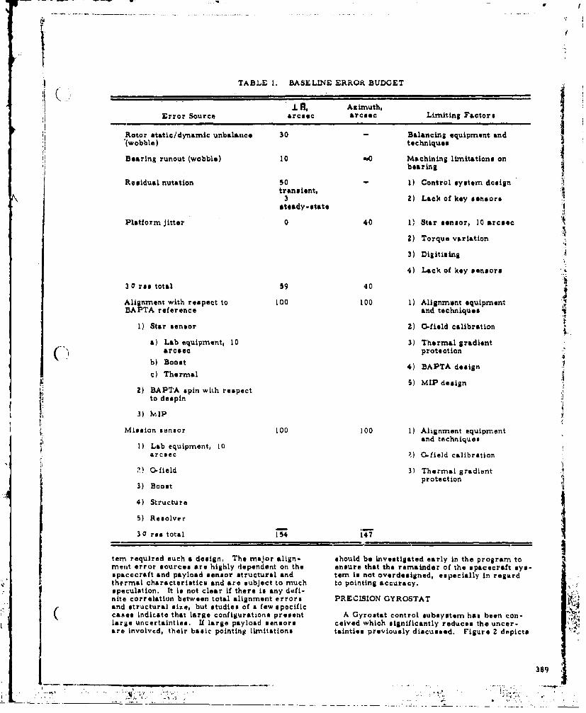
I

TABLE 1. BASELINE ERROR BUDGET

L H, Azimuth.Error Source arceec arc8ec Limiting Factors

Rotor static/dynamic unbalance 30 - Balancing equipment and"(wobble) techniques

Bearing runout (wobble) 10 '.0 Machining limitations on

Residual nutation 50 - 1) Control system designtransient.

3 2) Lack of key sensorssteady-state

Platform jitter 0 40 1) Star sensor, 10 arceec

2) Torque variation

3) Digitiming

4) Lack of key sensorsS3 0 roe total 59 40

Alignment with respect to 100 100 1) Alignment equipment

BAPTA reference and techniques

1) Star sensor 2) 0-field calibration

a) Lab equipment, 10 3) Thermal gradientarciec protection

b) Boost 4) BAPTA design

c) Thermal5) MIP design

2) BAPTA spin with respectto despin

3) MIP

Mission sensor 100 100 1) Alignment equipmentand techniques

I) Lab equipment, 10arcoec Z) 0-field calibration

,., C-field 3) Thermal gradientprotection

3) Boost

"4) Structure

5) Resolver

30 ras total 754 47

tern required such a design. The major align- should be investigated early in the program toment error sources are highly dependent on the ensure that the remainder of the spacecraft eys-spacecraft and payload sensor structural and tem is not overdesigned, especially in regardthermal characteristics and are subject to much to pointing accuracy.speculation. It Is not clear if there is any defi-nite correlation between total alignment errors PRECISION GYROSTATand structural size, but studies of a few spocificcases indicate that large configurations present A Gyrostat control subsystem has been con-large uncertainties. If large payload sensors calved which significantly reduces the uncerare involved, their basic pointing limitations tainties previously discussed. Figure 2 depicts

389

. . . . . . . . . .. .... . ... • :i +',

the control subsystem data flow from the son- The rotor-mnounted slar sensor provides datat sore to the onboard data processor to the final which allow inertial attitude determination and

controllers. The components shown in Figure 2, control to be accomplished. The accelorom-along with those shown in Frigure I which star cannot provide auch data, The-star datawere not diecusied previously, will be expLained are Used by the data processor to generatein this section. reference pointing directions for the platform

azimuth controlýand payload sensor loops.A micro-g accelerometer is mounted on the Also involved in these comp'utations are ground.

Gyrostat platform to mneasure inertial accel.. jonerated orbital and coordinate system data,orations in a tangential direction and plane target pointing data, and payload sensor eleva-normal to the spin axis. This orientation tion position (iresolver /encoder) dati;allows three major Componetnt3i Of aaceojxrationto be monitoredf 1) that due to wobble Produced,

by rtorunblane ad ~ATA earng unoSinlce the control system concept presented to2) induced nutations resulting. from platbornN thid point ha.i not accounted for the primarymotions and outside disturbances, and 3) tan-' acce.zrA¶y uncertainty due to deformationsgential Accelerations resulting from .platfprM btenh ala esrpiayad n

torqing ia he dspi conrol oto:~ ~ .. * the s..pacedra~i~ reference systems an additional *

accelerometer signal is operated on b9?.th*-dat4ý '" leaidz mst henZ4d tI swe hprocessor to remove the three, Rioter.tl~rtiI I .PAYload enn has star sensing capabilitiescomponents and estimate the wobble. nutatinvA antt can be usid rerlodically to view variousand despin torque. The wobble infoilnatiotA ,tare *nd tht'eby al)Low the system to be call-used to drive a mass transfer dfevic6-ivich 1i~'.Tedvain ewe h culsapositiline .nd estimated positions as seen by the* ~~~balances the rotor, thereby aeduclkil t?.s initia slgmnrotor unbalance and effective'rotor unl.alrnce pavle.ad sensor rllow for the mislgmndue to bearing runout, .. 'e a'tt'4rfen ra stoboetrn'ine.l an, ~eninto accoount. The effec-

t~yenow s' -dthe vulibraticik.proqedure depend.The nutation data are used by thet despin con- f'n milssioi ýconstrain'ts- spacec *raft particular -,trol motor to null the sparecraft nutatimn .4.la es n LfrexmltessPresent Gyrostat system desilas contrul nuta- -remj cylanw .~l.rd de'IT.2'ft~iexape enu he becastion via the despin motor but do not derivqiiii i~ o ontn uyccerqienutation data from accelegýomeate, measure- .tsrcia eo toi caUudbments. Instead, relative plotform-rot#)r posi- *~r'l~rdet. a 'eut necaie*tional data are the source data, master index ponin ntadiint&.r, ay''gesueral, adesignpulse (MIP). concept based on'the approach presented should

The platform tangential acceleration result. P .rovids -the on-orbit flo4bility to allow theVehicle characeristict to be evaluated duringing from despin motor torquing allows torque the initial misaian phases and then provide for

Jitter to be sensed immesdiately and damped bymdfcto ftemsinoeain n* the control loop. Present deeignas nre limited oiiaino h msinoeain n

in control accuracy by the jittur. pcratdsnprmer.

PROCO31NO .001 COTOLI CONTROL

CAAO STARIOS

LJI IISjL2AIJAM ION

MISIOSI.....2..... 5P LINK

(SAN SISO

MIigure 2.PeiinGrsttjnrlSse

~~VIf 39 - . .- . -- -- __ .I. .. 'YL11A'IA 10PRCCOS.

MIPp-- P~t~A.J4 ___

(In addition to the items discussed, Figure Z As discussed previously, the remaining errorindicates that the sensor complement includes sources are dependent on the particular Syetem 4earth and sun sensors which function in a con- design and may limit pointing accuracy unlessventional manner prior to the initiation of a spcial techniques are employed. The !, 0precision pointing phase, Also, the control arceec values listed assume that the payloadsubsystem must have provisions for accepting sensor can measure star direcd one periodically,ground commands and providing telemetry data. and these data are used to calibrate the system.

For exarple, if the star measurements wereThe evaluation of the precision pointing per- noise free, measurements would be required

formance and the feasibility of implementing the every 10 minutes, aseuning that the alignmentcontrol subsystem is being accomplished by error was due to a thermal gradient deforma-means of a variety of approaches. Table 2 is tion with a nominal rate of 60 arcoec/houran error budget for the precision Gyrostat per- estimated to within 10 percent. Since measure-formance using the same format as Table 1. ments are not perfect, the calibration interval iThe values presented were obtained primarily would be less than 10 minutes. Also, tvo orfrom the application of conventional determin- more stars with acceptable angular ispara-istic and stochastic servo loop analysis to the tions would probably be required, The signifi-anticipated attainable hardware performance canoe of such a calibration procedure isduring the next few years. st-ongly dependent on the payload sensor pri-

mary mission constraints.Rotor unbalance, 0. 1 arcesec, is dependent on

the estimation accuracy and mass transfer Aside from thermal gradient and star meas-device performance limits. The mass transfer urement errors, there are errors such as pay-device, based on a fluid transfer design being load elevation gimbal bearing performancedeveloped at Hughes, is judged to be the limit- uncertaintiep, payload structural bending anding factor, elevation angle measurement errors. These

errors are especially significant for largeBearing runout, 0. 1 arcesc, is based on the payload sensors.

assumption that the significant bearing runouterror occurs at the spin frequency and mani- Another important problem arises if the pay-festS itself as an "effectivo" rotor wobble, load cannot mense stars. One approach is toThis assumption it supported by past tests end autocollimate between the rotor-mounted starstudies plus current in-depth BAPTA studies. sensor and payload sensor, but this presents() Tests ire presently being conducted on BAPTA difficult, if not impossible, mechanizationunite which should provide bettur understanding problems because of the platform-rotor rela-of this error source. Therefore, within the tive motion, Mounting of star sensors on the -

correctness of this assumption, the uncertainty platform or, even more desirable, attachingis limited, as in rotor unbalance, to the per- star sensors d.rectlv to the payload sensor,formance of the mass transfer system. may be the solution. This also leads to the

possibility of eliminating the rotor-mountedAttainment of 0. 1 arcsec rosidual nutation star sensor if the 4eta rates and accuracy of

requires a significant platform product of the platform instrumentation are adequate.inertia to allow effective despin control system Tadamping of nutation. This requirement pre- The final values listed in Table 2 are the totalBents no significant problem in general; but, it payload sensor pointing accuracy values of 1.0u particular design cannot provide this feature, and 1.4 to 2.2 arcseo (301).other types of active nuta t ion control can beinvoked, STo obtain a high degree of confidence in pre-

Platform jitter, 1. 0 to 2. 0 arcaeL;, is a dicted system performance prior to total eys-resaeilt of incorporating accelerometer feedback tern preflight testing and actual inflight results,to directly damp random torques, and upgrading it is generally agreed that as detailed a com-star sensor measurement uncertainties to puter simulation as practical should bewithin 1 arceec or less. The confidence in developed. The simulation will allow the bestobtaining this performance is based on recent hardware dAta and their complex interaction tovendor discussions of flight proven micro-g be studied and evaluated. Toward this goal, aaccelerometers (Ref. 6) and star sensors and simulation is being developed which presentlyHughes hardware developments of similar utilises a l',nearized stochastic model of theitems. A reduction in the Gyrostat rotor spin Gyrostat and its control system (see Appendixspeed further improves the star sensor meas- for details), Presently, simulation results areurement accuracy. The performance also living added confidence to the precision pointingrequires digital control electronic imnpiovem nt control system concept presented being able to(finer quantization) which could be considered achieve the performance indicated in Table Z.state-of-the-art and therefore not requiring The system is assumed to begin operation at themajor advancements. The resultant 30 eta- completion of a somewhat coarse acquisitionbility error is 0. 18 arcmec and 1.0 to 2.0 mode. and estimate and control payload sensor/arcoec for the two coordinates defined spacecraft attitude through to a final regulatinpreviously, phase. All significant parameters are estimated

391. . ' + . . . 11 ' " '+ " + : " " ++ : .. .4 "•1 " "+-" ... . "S.. . .. ... . . "1. 4 " " :-1 , -. .4G 1

TABLE :1.. PRECISION GYROSTAT ERROR BUD'FT

r H, Azimuth,

Error Source arceec arceec Supporting Factors

Rotor static/dynamic unbalance 0. 1 - 1 ) Estimate wobble

(wobble) a) Studies

b) Simulations

2) Mass transfera) Fluid systemi

b) Mechanical devicesBearing runout (wobble) 0. 1 0 1) Hardware advances

2) Estimate wobble

3) Tests/studies

4) Mass transferResidual nutation 0. 1 "D 1) Estimate nutattion

a) Studies

b) Simulations

2) Despin control/platform product ofinertia

3) Active nutation rontrolPlatform jitter - 1,0 to 2.0 1) Accelerometer feedback

2) Star sensor, 1,0 arosec

3) Finer digital quantization

4) Studies / simulations30 rms total 0.18 1,0 to 2.0

Alignment with respect toBAPTA reference <1.0 <1.0 1) Star data every 10 rinutes, (10

1) Star sensor seconds accuracy, 60 sec/hrthermal deflection 10 percent

a) Lab equipment, 10 2) Position mission sensorarcaseCb) 0-field 3) Thermal protectiont blankets,

heaters, heat pipes, and mounting•) Boost 4) Upgrade alignment equipment andd) Thermal techniques

2) BAPTA spin with respect 5) 0-field compensationto despin

3) MIP

Mission sensor

1) Lab equipment, 10 arciec

2) O-field

3) Boost

4) Thermal

5) Structure _

6) Resolver

S30 rse total 1.0 1.4 to 2.2

39Z

. . . .. • , €.

and all controls exercised continuously in an and measurement noise components. The

acceptotbl s mannerc accelnrometer signal includes the three com-(cposseet previously dimcussed plus random proc-ess an* measurement noise.

Figures 3 and 4 are plote of the actual and It is anticipated that in actual operation theestimated spacecraft inertial transveise attitude controls would be exercised in steps: first,and platform azimuth, respectively, The trans. estimate and darnp the nutatlon; then, estimateverse attitude bias results from model errors the wobble and balance the system; and then, e m

which will be eliminated. The system shows operate the nutation and asimuth control loop.convergence to within'a few arceseconds in This approach may result in the use of a timeappcoximately 40 seconds. invariant estimator and controller, which

ghsimplifies data -rocessing. Also, the estima-Figisre 5 is a plot of the angular rate &aos- tion might only use accelerometer data prior

ciated with the single transverse axim attitude to controlling platform asimuth.history given in Figure 3. FIgure 6 is a plot ofthe unbalance in 'a single plane of the rotor. Although the simulation results give added

confidence to obtaining the desired precisionFigure 7 shows the basic accelerometer out- performance, much remains to be done in the

put signal with wobble, nutation, and process simulation area. Effort is presently-under wayto derive a complete detailed Gyrostat simula-

24 .. tion (includes nonlinearities) with a practicalestimator and controller mechanisation. In

6 - -- -addition, a star data processing algorithm, aT% k CTUALdetailed mission profile, and environmental

S1TI ATU disturbances will be incorporated.

- HARDWARE CONSIDERATIONS

- ... Although the analysis aspects of the precisionGyrostat concept are given major emphasis in

4 L this paper, they should not overshadow the0 5 10 13 2 25 30 3 40 43 0 formidable hardware technological aspects

TiMe, elCON01 i.volved in precision pointing in the 1-secondregion. The following ii a series of summary

Figure 3. Transverse Attitude Response

0000*0

1l , 6 A C T U A L'

12M- -- ISTIMAII"",- - -1i= Ii iJ

;:~. i i= • . . I,.

MEMSE 1000M 0 $ 10 I5 20 23 30 35 40 43 s00 5 10 13 2c 23 30 35 40 45 30 riMl, SECONMO

TIME, SCON•OS Figure 6. Rotor Unbalance

Figure 4. Platform Azimuth Reeponse

,o0 A ACýA --- 0o.• ,_i l. 0 A -0-00,1.. . ,L,. ,

, o+ ._ I J+: ' 1 -00 A_ I0 q ;0 13 30 7$ 30 3S 40 43 M 0 5r "10 13 20 21 30 35 40 45 30•; 1J•"i

t•?MAI•, SICONDS llI, MEI¢ONDI

Figuet S. Tralnsverse Rate Fiure7 Accelerometer Signal.,V.

393

- . ... .... .. ..I• ++ ,,,r,. - :.: +•. . .. L . . ..7. ".•,:A ..

comments for each of the key hardware itemrs les, but the same is not true of payloadof concern to the precision Gyrostat system sensor calibration, The calibration pro-design. cedure is highly dependent on milsion and

spacecraft design and will probably requireMicro-, Accelerometer an investigation phase early in the mis -hion. In general, payload sensor limits-

The platf o -mou-n•ted a Galsro etsr must be tions should be thoroughly understoodsensitive to a range of 0 to 10 'g and pro- before the control system design phase.vide a digital output. A micro-g accelerometersatisfying these gross requirements has been 9 Use of a payload senior with star sensingflown during the past few years (Ret. 6), Its capability reduces the calibration prob-measurement accuracy, weight, power, sine, lem and could simplify the Gyrostat con-and costs all satisfy tentative requirements. trol system (no rotor-mounted starIts reliability for a 3 to 5 year mission looks sensor),good but has yet to be demonstrated.

a Precision pointing designs will requireBearing and Power Transfer Assembly( BAPTA) many advances in technology and a

detailed investiox.tion of those effects thatAdvanced techniques are required to provide formerly have been considered as con-

a despin bearing joint that will result in motion tributing inesinificant effects on pointingerrors (wobble and noise) of the despun plat- accuracy. Also, complete system simu-form less than 1. 0 arcane in magnitude. lation based on hardware test data andHughes is currently developing a dospin bearing practical control system design areassembly which analysis indicates will result recommended.in motion errors no greater than 10.0 arcsec,Recent anallysis revealed that motion errors 'could be reduced to appronimately S. 0 arcticusing techniques similar to those employed in ACKNOWLEDGMENTthe referenced bearing assembly, but with abearing spacing of 20 inches. The study results presented in this paper

were provided by the efforts of many CompanyData Processor personnel. Special thanks are given to L.H.Grasshoff, Dr. T. Fong, Dr. C.P. Lu, T..

It is estimated that the star data processing Iaacce, and J. Yooum, who encouraged andestimater, controller, open-loop orbital and assisted in the study efforts.coordinate computations, and other controlsystem functions can be performed by anonboard general -purpose computer having 8,000to 10, 000 words of memory (A4 bits/word). The REFERENCESflight-proven Univac 1e24 appears to satisfythese and control loop rate computational N.A. Gunderson, "Princeton Experimentrequirements (Ref. 7). The weight, power, Package for OAO-C," Journal t Spce-siss, etc., are reasonable for incorporation craft and Rockets, April 1953.into an onboard system.

2. W..B. Chubb and D. N, Schultz, "AttitudeStar Sensors Control and Precision Pointing of ApolloTelescope Mount, " AIAA Journal of ;oAce-A slit-type star sensor has been developed at craft and Rockets, August 1963, p. 896.

Hughes for use on the Gyrostat system. It isestimated that a measurement accuracy of a 3. A.J. Iorillo, "Hughes Gyrostat System,"few arcseconds can be achieved through design Proadina. of h! o n Attitudeimprovements and rotor spin speed reductions gtablleat LnA Contra of Dual-Spn(20 rpm), Discussions with Control Data E , I - Z August 1967, AerospaceCorporation personnel also sup-ort these Corporation, El Segundo, California,conclusions. TR-0l58 (3307-01)-16. November 1967.SUMMARY/CONCLUSIONS 4. W.H. Sitrer and J. Del Riego, "TACSAT

Attitude Determination, " Spacecraft

The mechaisnatlon of a Gyrostat attitude Attitude Determination Symposium, Aaro-determination ad contral system to space Corporation. El Segundo, California,achieve 1.0 arcsec pointing accuracy 30 September, I - 2 October 1969.appears very promising. The designdepends on bearing and star sensor tech- 5. A. Braga - IIla, "Preliminary Report onnolgy improvements, platform-mounted the Orbital Operation of the Automaticmicro-g accelerameter, active rotor Itation-Keeping System of LES-6, " AIAAbalancing, and onboard data processing. Guidance, Control and Flight Mechanics

Conference, Princeton University, Augusta The orbit determination aspect of preci- 1969.sion pointing presents no critical prob-

3•94

_ _ .• .- ; .;.; ; ........... _ ..;.•: . .. .. . ,

6. E.H. Metzg,!r and M.[A. Meldrurn, "Mm- i V tz transverse moments oflature Electrostatic Acceleration (MESA), inertia of the entire fpace-Textron's Boll Aerosystem Company paper, craft about the spacecraftcg1967; also "]lectroestatic AccelerometerScores Firsts in Agena Flight. " Aerospac 13 . spin axis moment of inertiaTechnology, 28 August 1967. of rotor

7. Univac 1824 Computer Technical Descrip- 0 spin rate of rotortion, Univac Federal System Division,St. Paul, Minnesota. QIPQZ " unbalance parameters of the ,.

rotor which includes effec-8. AE. Brysort Jr., and Y.C. Ho, 61piji tive bearing wobble

Optimal Control. Blaisdell PublishingCo,Waltham, Moae$, id 1969.- T control torque about bearingWalthamMise,, 1969, Tm" axis

APPENDIXTb + w(t) - friction torque of bearing:

A digital computer simulation of a preeision b (T a unknown mean valueGyrostat system being developed at Hughes Air- aný w(t) w randomly vary-craft Company is described in this aLPPndLX. ing torque noi)e -assuredwhite) i•

a~n torque noiseon ofssMotion2zroetat Equations of,,Motion In order to completely describe vehicle

motior,, the following oequations are naeoesaryt ,

The linearised equations of motion for tia Gyrostat in inertial coordinates iare| eL • i (i y, a) (2)

t t 45 46 l x a a U 0 2) (3)

.146 156 161 j a

where %I are the rates of mass transfer in anactive balancing control system on the rotor.Equations (1) through (4), in general state space

0 13 C1 W are (Uming Ref. 8 notation):

I (1 0 0 W + x - Fx+Gu+i'w (5)

0 0 :z where

X 8 U Tm

Qcos rit + 0 si C y

01 sin 5t - Q cos 0 (C) C1 t

IQTm + Tb + w() y1

where 1n

1 145L I I spin inertia and cross prod- T6145 6'4 ucts of inertia of the despunbS~platform• about spacecraft cg

! 395

-- . . - - - '

pI

w - friction torqueLlois ae~ffectingu " t with u and w components

F, G,- a matrices derived from Eqs. (1) removedthrough (4) r a inertial components of accelerorn-

Measurement Function eter position

The rotor-mounted star sensor and platform- vx 1 o noise components associated with

rmounted accelerometer outputs are linear corn- xt yo ad tbinations of the system state plus additive imeaeurement noise formulated ass It is assumed that 8 are available once

X1 )1 2each spin period as the output from a star data

SHx +v (6) Processing aljorithm and that the accelerom-eter data are continuoue. His obtained from thisinformation and a substitution of Eq, (5) into the

where acceleration expression. It should be noted

the acceleration expression doss not presentlyV v x " include spacecraft cg misalignment with respect

X to the spin axis, Analysis has shown this termcan be incorporated in a linear sense.

e va Estimater/Controller (Ref. 8)

A Kalman filter has been mechanized for theLt i a estimater. A continuous representation is

L J used with proper provisions for sampled data.The controller is based on the use of a quad.

at r r is + r ratic performance index. This mechanizationyx xy as is suited to the time-varying characteristics ofthe system.

i4

12 .. *.':.

396

.. .. ... .. .

Ii

ATTITUDE DETERMINATION PERFORMANCE POTENTIAL FOR A YAW-SPIN SATELLITE

PART ONE: FORMULATION OF THE ESTIMATION EQUATIONS

J. E. LesinskiElectronics Division

The Aerospace CorporationLI Segundo, California 90245

, -

ABSTRACT

A computational algorithm is developed for precisely estimat-ing the attitude of an )rbiting spacecraft from data provided by abody-fixed star telescope. The algorithm is designed for applicationto a particular satelilte configuration -- namely, a spinning satellitethat has its spin axis nearly aligned with the local vertical and thathas an internally mounted reaction wheel which approximately can-cels its spin component of angular moment.

The paper is divided into two parts. Part One presents a"development of the attitude estimation equations. Particular atten-tion is given to the selection of an efficient set of coordinate systemsto define the problem. The philosophy underlying the algorithmdevelopment represents an attempt to obtain a potential for highattitude estimation accuracy by providing the estimator with accu-rate models of the problem. The attitude estimation algorithm isbased upon the Kalman filtering technique developed for linearsystems, but uses nonlinear state prediction equations and a non-linear measurement model. The dynamic characteristics of theparticular satellite configuration are exploited in the developmentof an approximate closed-form solution for the satellite motionwhich is utilized for the filter state prediction equations.

Part Two, a classified supplement, presents num-ericalresults assessing the attitude estimation performance potential.These results were obtained from a digital computer simulationthat contains a detailed simulation of the actual spacecraft motionas intluenced by the operation of the attitude control system andexternal torques, a simulation of the star sensor measurementprocess, and a simulation of the attitude determination algorithm.

1, INTRODUCTION vided to approximately cancel the spin axis co~m-

ponent of the total angular momentum so that theThis paper treats the implementation of an spin axis can ke precessed at orbital rate and

aligorithm to provide continuous "realtime" esti- maintained in close alignment with ti-e local ver-mates of the attitude of a particular satellite from tical. The satellite is designed for operation att measurement da•ta provided by a star telescope synchronous attitude.

. ixe'd to the satellite body. Star sensor measure-

msent data are transmitted in realtime via a te- An active attitude control system (ACS)lemetry link to be processed In a ground-based employing gats jets is utilized for spin axiscomputational facility, pointing conzrol and for trim of the residual an-

gular momentum, Attitude pointlng error signalsThe spacecraft configuration of interest is are obtained from a single horizon sensor which

ashown in Fig, I. This vehicle spins about its continuously scans over an angular region ofyaw axis at a nominal rate of 6 rprn. A constant space that contains the earth edge. Periodicalspeed, internally mounted reaction wheel is pro- "sampling" of the horizon sensor four times per

A 397

Vt'on problem, and thus are omitted from the die-cussion herein. The operation of the attitudecontrol syntem does, however, represent a ma-

SN SEN/SORlS of the attitude estimator. In order that the com-W PITCH AXIS putational algorithm can make some provision

CONTROL JETS -for the effects of ACS operations, the following(SPIN SPEED . __ datu are telemetered to the computational facility:AD.JUSTMENT AND- a=PITCH ATTITUDE) O ," 1. Control jet valve driver input pulses

STAN SENSOR SOM ROLL AXIS (jet on and off timem)

-4HORIZON SENSOR

2. Reaction wheel taciometer pulsesSI (reaction wheel speed information)

A body-fixed star sensor provides the basicmvaeurement data for attitude estimation, Thestar sensor optical system may be representedschematically as shown ir. F'ig. 3. The star sen-

'YAW AXiS sor consists of P. lens system, which produces astar image on the focal plane; a reticle containing

Fig. 1, Spacecraft Configuration three slits oriented as shown in the figure; and aphotomultipliter tube and associated electronics,which detect the time at which a star image falls

spin cycle yields two-axis pointing error infor- in the center of one of the slits. Photomultipliermation. A sun ,enbor provides a timing pulse outputs are sampled at a high rate and telemeter-

which is used to synchronize the horizon sensor ed to the ground. A p-eprocessor on the groundsampling times and the control jet firing times,Figure 2 illustrates the operation of the horizonsensor. The time to represents the synchron.- MAOE MOTIONzation pulse produced by the sun sensor. Thefigure illustrates the location of the horizon sen-sor scan regions at the four sampling times t 1

STAR IMAGE

through t. The r'itch control jet firing times

RETICLE )_________ I - -OPTCAL AXIS

SPIN FOCAL PLANE LUIGH RAYSRLOM STAR

• SUN LINE Fig. 3. Star Strssor Schematic

S(N

PACETRAFT

"EARTH A operates on the raw tetenmetry data to computeDISC the Lime rt whtih a star image crosses one of

the star sensor stits. This "measured" starcrossing time Is sent to the estimation algorithmto be used to update the c rrent attitude esti-

$AON SENSOR mates. For purposes herein, the details of thepreprocessor signrl processing are ignored, andit is assumed that these measured star crossing

Fig. 2. Horizon Sensor Operation times define the star sensor measurement output.Becau"eo=opticFl system limitations, back-ground noise, elertronic errors, and telemetry

are also synchronized with the horizon sensor limitations, this measured crossing time differssampling times to provide de-commutation of the from the true time at which a star image actuallycontrol torque in space. Thq spin jets, which crossed the 0lit. This error is assumed to beare used to adjust the satellite spin rate so as to characterized by a zero-mean Gaussian random 4

null the spin axis component of angular momen- sequence, uncorrelatrd from measurement totum, arit activated infrequently--about once per measurement. Typically, the standard deviationweek. of the star sensor measurement error is around

5 arc sec (expressed as the angular azimuthThe details of the attitude control logic are uncertainty in the stlur location .t the measured

not immediately relevant to the attitude estima- detection time'.

398

rI

The star telescope is mounted so that its vector x is comprised of the set of variables andoptical axis is approximately normal to the parameters eufficient to describe the spacecraftvehicle spin axis and the vertical alit shown in attitude motion and measurement processes,.Fig. 3 is approximately parallel to the spin axis. The evolution of the state over an arbitrary timeIn this manner, the field of view of the "vertical" interval from t to t it assumed to be governedslit scans a great circle band in the celestial by an equation Wf the formsphere as a result of the satellite spin (see Fig.4). In this way, stars are sensed as thair Imagescross the slit pattern in the telescope focal plane, x(t) = f[X(tN)I t, tN] + r(t, tN)v(tN) (1)The vertiral slit instantaneous field of view is3 deg.

where v(tN) denotes a vectnr-valued random see -quence which represents urknown disturbances

NORTH to the state; the function f(.) is a vector-valuedCELESTIAL function defining the trajectory of the state vectorPOLE In time. The scalar measurement process de-

noted Z(tN) can be represented as a function of

STAR SENSOR the state with additive measurement noise tN)

FIELD OF VIEW in the following form:

z(tN) e hfx(tN)J + u(tN) (2)

EARTHLOCAL It to assumed that the measurement noise isa aVERTICAL zero-mean, white noise sequence with k~nownvariance, Equations (1) and (2) constitute a de.

STLEscription o' the "real world" system motion and

SPIN measurement process, respectively. The func-tions f(- ) and h(- ) define the "predictable" portionof the system motion and measurement.

BAND OF STARS SEEN Simply stated, the estimation problem isIN ONE SPIN CYCLE to find some method of forming an estimate of

tht state, which is in some sense clove to theFig. 4, Star Sensor Scsn Geometry actual state, given a sequence of mreasurements

SF S o(tN). In particular, we are searching for anoperator that transforms the observation se-

II. CONFIGURATION OF ATTITUDF ESTIMATOR quence to an estimate of the state. The exactsolution to the optimal estimation problem with

In general, spacecraft attitude estimation nonlinear dynamics and/or measurements is notcan be defined as: known. However, the optimal estimation prob-

lem fur linear systems has been solved, andThe estimation of the angular orientation many different tec.hniques of forming an approxi-relative to some reference basis of a mate sulution to the nonlinear problem have beenmeaningful coordinate frame which is proposed in tht literature.embedded in the satellite body.

The estimation algorithm presented here is

The word "estimation' is uied because the de- developed heuristically on the basis that thesired information must be extracted from noisy problem can be considered "nearly' linear. Itsensor data. A meaningful coordinate frame is therefore postulated that the filter conifigura-refers to some coordinate frame attached to the tion that is optimal if the problcm were exactlyspacecraft which is useful to tht problem at hand, linear is a reasonable (but not necessarily best)In general, several possible choices exist for choice for tht actua! problem at hand. Further-this conrdinate frame, which defines the basis more, the filter ts st.,uctured so that the non-for definition of satellite attitude, an.1 its proper linearities that must be 'gnorad are higher-order,%election is imporlant tc attitud, estimation per- terms in the state estim Mtton error. If the fliterformince. This aspect of the problem is empha- design Is at all reasonable, the estimation errorsized in the next section, which discusses the will tend to become smailer with increasing filterImpl•mentatiton of the estimaition equations. time and thus increase the validity of the linear

approximations.In the present section, the general mathe-Matical struckure Of L~ U ttltude estimattiut prnb- The basic philosophy in developing the esti-.

lem is examined, and a ;,articular filter config- mation algorithm is first tn assume ik particularurition is postulated. filter configuration and then to find the set of

filter gains that are approximately the optimalLet x(t) denote ein n-vector that defines the gains for tht assumed configuration. In partiL-

rtAt,1 of the system under consider.ition. The ula,', it is assumed that the estimation algorithmcunsists or the following hasic stritcture:

399

. , .• \ t -' • -

ACTUAL R•, ' EINITIALIZE I(t'l] -- .

MEASUEiEMENT STATE,j(|NI1 N"I) PREDICT I0N

INI

MEASUREMENTPREDICTION •

Fig. 5. General Contfiguration of Attitude Estimator

State prediction1 tN~l t < t a. Prediction error:

^ A

Measurement prediction: brro+lterinN)ebyo(7

, itNtN1)• lxltNtNl)K 1) (t) + x~(tN) - (t) 7

Filtered state estimates•, The system dynamic equations as deie yEq,

(I) ar• expanded in a Taylor series about theA^,* point Xc(tN..l), the moat recent filtered statex(tN)• •(N ~ + K(tN)jz(tN)- •(tNitN~)] iS) estimate, to give the following result:

Equation (3) ii used to pred~ct the state between x [~Qtq) =t l] + e(t. tI.4 l)•(tN l)measurements i(tN.l),

the filtered state estimate at the last measure- + r(t,tN l)v(tNia )ment time. The measurement prediction ior"r:

"• ~based on the predicted state. Wheu• a measure-ment becomes available, the filtered etate estS- + higher-order terms in •(tN~l) )matE. is formed by ti'e addition of a correction '

•term to the predicted state, as seern in Eq. (5).': • The correction term consists of the difference '"r~et ~pdnts h ~ ata eia

Ahr ~,t•)dne the _~ partia dria

between the actual measuremont and the predtc- tie matrNi o1 the vector function fx (f1 f2 (6)S ted measurement multip red by a i ain matrix with respect to the st- be; that is,

S K(t ). Figlure 5 shows the mechanization of theattue estimt ateion inmatockdiasrarm form. as df, by Eq.

The fitter gain equations used here are the siJ' tN-l o ut

A A A point x~~~~(tN1, t hemo)eetflee tt

Kalman equations deuelope p for the case of b near Itxex(tN-)

system dynamics and a linear discrete measure-ment proce.s (Ref I), The steps leading up tothe application of these results to the present Similarly, Eq. (2), the measurement equation,nonlinear problem will now be examined to clar. can be e+panded in a - aylor oerm es about the•Qify the approximation involved. Let the following point (tNjtNl) to produce the following result.-0"notational come eniences be introducedor'ect.

The notation term denotes the e etimate of 1) " t,.;b the vector x t t given measurements up z(t) e hma (itx ) the + H(tNcP(tn 't I ..n)

to time sNho. Nh mehnz1o N -the

S 2 'rhe fltsred state estimate o(tN) is understood + higher-order terms in theto denote p(tNitN). prediction error 110)

tLpnotaionl coentncesbe ntrouce; N~N-1

The matrix H(t ) is a lxn matrix defining the which define the gain matrix sequence to producepartial derivatigves of the measurement function a minimum variance estimate of the st..te.h(-) with respect to the state; that is,

In the nonlinear problem here, none ofthese assumptions is strictly valid; nevertheless,

hix(tN) Eqs. (14)-(16) are used to compute the filter gainHlJf(tN) htN (11) matrix. Equations (9) and (11) are used to com-

SA pute the e and H matrices. Not* that these rnat-x NX(tINtN-l) rices are updated at each measurement time toreflect evaluation of the partial derivatives atthe most recent state estimate. For the non-

Now, neglecting the higher-order terms in Eqs, linear problem, the matrices M and P lose their(8) and (11) and using the results of Eqs. (3)-(5) significance as covarlance matrices and the gainyields the following linear approximation for the matrix is no longer optimal. The one justifica-propagation of the prediction error and filtering tion for use of these equations In the presenterror from one measurement tims to the next: nonlinear problem is that fairly accurate initial

estimates of the system state are available,Prediction error: This fact tends to give some degree of validity

to Eqs. (12) and (13) as representing the propa-gation of the actual filtering error, as the neg-

R(tNItNl)u S(tN~tN l)i(tN.1)+ r(tN. tNl)V(tNl) letted terms are higher.order terms in the stateestimation error multiplied by second-order and

(12) higher partial derivatives of the measurementfunction and dynamic equations. Under these con-

Filtering error: ditions, one might expect Eqs. (14) and (15) toapproximate the actual covariance matrices andEq. (16) to work rather well as a gain matrixfor the filter. In the attitude estimation problem

|(tN) O X(tNtN l) + N N NItN.1) + u(tN)J here, initial estimates of attitude are accurateto within I deg, owing to the operation of the at-

(13) titude control system. The higher-order termsdropped from Eqs. (12) and (13) are several or-

If a) the dynamic equations and measure- ders of magnitude smaller than the linear terms.ment equations are linear in the state variables,b) the random sequences v(tN) and u(tN) are III. IMPLEMENTATION OF ATTITUDEwhite, Gaussian, zero mean with coveriancesQ and R, respectively, and c) the initial guess ESTIMATORof the state vector is such that R(t?) is zero meanand Gaussian, then Eqs. (12) and 13) are exact The details of Implementing the attitudeand the piediction error and filtering error are estimation equations for the problem at hand willzero-mean, Gaussian, random sequences with now be examined, Then, the coordinate system3covariances M(tp) and P(tN), respectively, which that serve to define the problem are introduced,are found from (12) and (13), as follows: and the star sensor measurement functions are

obtained. Naxt, particular attention Is given tothe selection of a specific coordinate frame thkt

M (t ,(t t)P(t )e serves to define satellite attitude, and to theN N' N- N-I (tN, tN-1 development of an approximate closed-form solu-

tion for the iatellite motion. Finally, the specif-+ (tN, tN )Qr T(tN tN]) (14) Ic configuration of the attitude estimator is pre-

SNNsented,

P(t N) (I -K(t N)Hi(tN)IM(tN)II - K( tN )H(tN)i T A. Coordinate Systems

An inertial frame (I-frame), earth-centered

T and nonrotating in celestial space, is the funda-+ K(tN)RK (15) mental basis from which all orientations are

referenced, The unit vectors x7, Y, i1 are theorthonori'nal bases vectors for thisk.rame which

with P(t 0 ) a Etý(t 0 )i(t 0 )T!. Reference I shows are oriented as follows:

that the optimal gain matrix that minimizes thevariance of the filtering error is given by Z, points toward the first point of Aries

1" points toward the north celestial pole

K(tN) ' M(tN)HT (tN)IH(tN)M(tN)HT(tN) + R"l ý completes orthogonal right-hand set

(16) An intermediate attitude reference frame

(R-frame) is introduced as a convenience to aid

Thus, if assumptions a)-c) hold true, then Eqs, in defining attitude. The R-frame is an earth.(14)-(16) form a coupled set of matrix equations oriented reference frame that forms the basis

401

from which satellitc attitude angles ýre rneasured a subsequent paragraph discussing the star sen-and `is U"ned as follows: sor measurement functions.

Origin: satellite mass center The orientation of the Al-frame with respectto the 1-frame is determined by the satellite

Unit vectors: XR -'R' -"R ephemerls and is illustrated in Fig. 6.

- points Satellite attitude is defined in terms ofR center alto the earths geocenter mass three Euler angles OI' €. *3. which respectivelydefine the roll, pitch, and yaw attitude of the B-

XR points along the positive projection of frame with respect to the R-frame. The rotation

the satellite velocity vector on the plane sequence in going from the R-zrame to the B.frame is, first, pitch 02 about 7R; uext, roll 01normal to Z"R about the new 7 axis; finally, yaw 03 about the

7 o normal to the instantaneous orbit new r axis as illustrated in Fig. 7. The bodyplane completing an orthogonal right. attitude is then defined by the transformation

hand set

The body-reference frame (B-frame) Is a Xcoordinate system embedded in the satellite masssystem, which forms the basis to which the atti- (17)tude angles are measured. The spe"•"` c orien-tation of this coordinate system with respect tothe satellite it defined in a aubecquent paragraph. zBThe B-frame is here defined in the followinggeneral terms: where

Origin: satellite mass center [*] "03]z[0lxl0112y (18)

Unit vectors: -X ' ,B

7B defines the satellite yaw axis, positivetoward the end of the satellite whichis earth-pointed S,/ R

denotes satellite pitch axis

7B denotes satellite roll axis

Three star sensor coordinate systems SSI, ISSZ, SS 3 define the star sensor measurementgeometry. The orientation of these coordinatesystems in the vehicle is determined by the or- -entation of the reticle and the star sensor opticalcentar. These coordinate systems are defined in

IR(TO EARTH GEOCENTER)

TO flRNORTH ( '966 [RI

CELESTIAL \ \,POLE BR

Fig. 7. Definition of Satellite Attitude Angles

EQU- SATELLITE The subscript notation on rotation matrices willMASS be used throughout to denote the three fundamen-SCENTER tal rotation matrices:

1 0 0

Fig. 6, Definition of Attitude Reference I ox = coso sin,Frame Orientatton 0 -sin a cosaI

402

Lcos (1 0 -sin ni SS-3 Coorainate System

jyo 0 1 0 xSS 3 is identical to'sSZ

sin a 0 cos a .Is normal to Star Plane No. 3

The angles a ~' 1 '13 illustrated in Fig. 8rcOS a in a 0 define the orientation o the three stat planes.The orientation of the SS-2 and SS-3 coordinate

(aj = in a cos a frames relative to the SS-1 frame can be ex-0 1 pressed in terms of these angles as follows:

B. Star Sensor Measurement Process SSa /SIn the case of an ideal star sensor, the SS Ir. F 19)

measured star crossing time can be considered 2 2 1( ,to be that time when a unit vector to a star lies - -

in a particular plane fixed to ths star sensor. & z SFor the reticle configuration illustrated in Fig. 3 2S 1 Iwe can define thrte star planes to be the condi-tions for generation of a star crossing time sig- -,!

nal for each of the three slits. Each of these 7x x \"star planes" is the plane formed by the system 3 /SSoptical center and the center line of the corres- ..,ponding reticle slit. Figure 8 illustrates this 7SS 3 I Yss (20)star sensor geometry. Note that the three star ([O)plartes Intersect at a common point: the system 3-optical center. This point will be used to define /the origin of our star sensor coordinate systems. \ 3 i IThree star sensor coordinate frames, each hay- /ing the 7 unit vector pointing perpendicular to whereone of the star planes, are introduced as follows:

(- SS-l Coordinate System VZJx[-y 1 Jz (21)

lies in Star Plane No. I pointing out- 33: (22)ward along the projection of the line Jof intersection of Star 'lanes 2 and 3ont the plane

The orientation of the SS-1 frame with re-3Sis normal to Star Plane No. I spect to the B-frame is defined by two angles 1

- and 02 as illustrated in Fig. 9. Note that weýqSI :'es in Star Plane No. 1 completing have removed some of the generality in the def-right-hand set inition of the B-frame and have restricted 7B to

lie in Star Plane No. 1. The angle P3 designatesSS-Z Coordinate System the ing tar "twist' of the star sensor about 7B3

and p-, idicates the 'elevation'' of the star sen-.Sz points along the intersection of Star sor r: tive to the -7 plane. From the fig-

Planes Z and 3 urc, the orientation of the SS-l frame is express-ed as follows-

issz is normal to Star Plane No. 2S1IAR tE.'P (LI SV&',CI / 7/

$Iatn P Atit / z

-~~ 76 vJ B ('3)I'5, % - - j/ - I

,:, , {p--where [0 PlyiPi], (24)

Fig. 8. Star Sensor Optical Geometry

403

V

value for the predicted star crossing time. Theapproach it to de:in,, the measurement z as be-ing identical to"Mhe_'ot product in Eq. (20); that

1B is, we define the measurement z(tN) as

5i(tN) • !j.ss (tN) + a(tN) ; 0 (26,

where again tN designates the measured star de-tection time for Slit i. The measurement func-

Yss$ tion h(. ) in then defined as

STARPLANE NO. I

is hi[X(t N ))] I gj•' SSxtN) (27)

5ii where the subscript I designates the measure-litl ment function for Slit i. The quantity e(t ) In

Eq. (26) corresponds to the measuremenotniee

It, OU(N) in Eq. (2). In view of these definitions,the predicted value of the measurement is calcu-

Fig, 9. Orientation of Star Sensor lated asFrame Relative to Body Frame

S I t N, Y. (sit N) (28)In the case of an ideal star sensor, the

measured star crossing time produced by a starimage crossing a given slit is simply the time at wwhich the dot product of the unit star vector with vector os podeno tosl S[*.6d.un--he measure-the particular star plane normal (7S5ji vanishes. coprespondingBecause of optical aberrations, background ment residual z is simplynoise, and random errors in the generation ofthe star detection time, it is not possible to as- (t z j A (29)sign a unique location to the star vector in the i N -e i(tN) N f(t" (29) .body at its time of detection, The set of all poe-sible star vectors at the detection time for aparticular slit forms an ensemble of random vec- That is, the measurement residual is forinedtore in the satellite. For this case, the concept merely by means of computing the dot product inof the "star plane" is still useful if the star plane Eq. (29) and s it at the measured staris considered as that plane forming the beat crossing time, 7Th-iT an be done because themean sq~are fit over the field of view to this ran- actual measurement zi(tN) was explicitly defineddom ensemble of star vectors. In this situation, as being identically zero. This procedure isthe measured star crossing time tNproduced by computationally more efficient than explicitlyStar j crossing Slit i is defined implicitly by computing time residuals, and produces the same

information for the filter.

9.7S (tN) + e '= 0 (2s) The measurement functions for the three" I slits can be expressed in terms of the attitude

angles 01. 02, 03 and star sensor alignmentwhere ~ unt vector to Star J, And the error a, angles ,l' P2 by use of Eqs. (17).(24) to expressrepresle the random error in the detection the dot products to give the following results:process and genmetrically represents a smalldisplacement of the star vector normal to the h= • ,- i 0]f]](SjR (30)star plane. For purposes hereir., this error 1 jSS1 1shall be considered to be a zero-mean, Gaussian,

random variable.

The attitude estimator requires that the 2 J'S ',(measurement process be represented as a func-tion of the state variables in a form given Ly Eq. h . (0 1 o9.r~cl]lls (32)(2). Should the measurement variable s be de- h 3 TSS3 .1fined as being the star crossing time, some dif-ficulties can arise because of the implicit natureof Eq. (25) in generating a value for the predicted The quantity (Se t a column matrix composed Rtime. A different approach is used here that of the componeits of the star vector p In the R.avoids the necessity of computing an explicit frane; that is, •'

L740

Thus, from an operational standpoint, even'R• though the attitude of our B-frame is not of itself

(S '33) of primary interest, it is essential to choose aR ( 5B-frme whose attitude can be most accurately

determined. An additional consideration in the'r/ Tselection of the B-frame is the stability of its

alignment relative to the mission sensor, Incases where an on-orbit bore3ight of the missionsensor I@ not performed.

C. Selection of a Body-Reference FrameAt first glance, the most obvious choice

The R-frame up to this point has been con- for the B-frame would appear to be the star sen-cidered to be an arbitrary coordinate frame em- eor trame (SS-frime). However, this turns outbedded in the satellite body. From the stand- to be an undesirable choice for two reasons:point of the attitude determination problem, the First, the stability of the star sensor alignmentselection of a specific B-frame coordinate eye- relative to the mission sensor is poor. The

tern is an important consideration. nature of the effect of the thermal environment

on the structure is such that it causes largeThe primary consideration for selection of "twisting" deflectiot~s of the star sensor about its

a B-frame should be the accuracy to which its optical axis relative to the mission sensor.attitude can be determined. Mathematically, Second. even in the absence of these aliynmentthis question is one of the degree of "observa- variations, the observability of the attitude of thebility" of the attitude of the coordinate frame, star sensor coor inate frame is poor. This factgiven the particular set of a~titude measure- is a rtsult of the narrow field of view of the starments. Not all coordinate frames are equally sensor (*l. 5 deg) which makes it difficult toobservable. Speaking heuristically, the degree estimate the angle of rotation about the sensorof observability of a particular coordinate frame optical axis.

is associated with the extent that its attitude dis-placements affect the measurements, In order In view of these difficultiem, it becomesfor a particular frame to be observable, it is desirable to examine the vehicle dynamic char-thus necessary that its attitude directly affects acteristics in an attempt to select an alternatethe measurement process or indirectly affects it coordinate system whose attitude has sone par-by changing the dynamic motion of the attitude ticular significance in terms of the motion of thesensor. star sensor in space. It will be shown that a

Fzero-momentum satellite must spin about a par-From an operational standpoint, there ticular axis fixed in its body. This "spin axis"often exists a well-defined coordinate frarne is selected to define the I'axis of the B-frame,

"whose attitude we would like to obtain, namely,, a coordinate frame fixed to some mission sensor

whose pointinR direction in space is of primary Let the following notation be introduced:

"interest. This coordinate frame would be the f = the dyadic defining the moment ofmost desirable choice for a B-frame, but un- inertia of the total satellite massfortunately, such a frame it in general not ob- system with respect to its massservable, This is true because changes in align- centerment of the mission sensor relative to the satel-lite will have no effect upon the star sensor angular velocity of the B-frarewueasurements or upon the vehicle motion. In relative to inertial spaceorder to determine the pointing direction of thrmission senaor, one can rely on prelaunch mea- = total system angular momentumsurements defining the alignment relative to relative to its man@ centersome other frame (B-frame) whose attitude is rtobservable from the star sensor measurements. 3= "relative angular momentum or the

In cases where extremely accurate deter- contribution to the total angularmomentum R which is generated by

mination of the mission sensor pointi.ig direction elements of mass moving relative tois requir-d, prelaunch alignments may not pro- the B-frame

vide suflicient accuracy because of errors in-curred during boost and during the varying orbit- " . unit vector pointing along the reactionaL thermal environment. In these cases, on- w wheel bearing axisorbit calibration of the mission sensor alignmentrelative to the B-frame must by provided. This C w reaction wheel moment of inertiais often done by using the mission sensor to sight w about its wel mxis o

objects with known locations, and using the infor- bearing axis

mation together with the estimates of the attitude a reaction wheel angular velocityof the B-frame to update the knowledge of mis- relative to the satellitel.i.

lion sensor alignment relative to the B-frame.C Obviously, the acciracy of this 'boresight" pro-

cedure is related to the accuracy of the knowl- See Ref, 2 for a general development of theedge of the at.itude of the B frame. concept of "relative angular momentum."

4I 405

It is shown in Ref. 2 that the total angular hmomentum for a sdtellite of arbitrary configu- ,,ration can be expressed in the following form:

R I.•+ W (34) oz

Let (H), (w), (hi denote the 3X1 component ma- REACTION - Atrices of the v'actore R. U, Texpressed in an WE -

arbitrary coordinate frame (A-frame) embeddedin the satellite body, and let [I] denote the 3X3componer.L matrix of the dyadic I expressed inthis A-frame. The matrix form of Eq. (34) isas follows:

(H) I [1(w) + (h) (35) C• -' ,-

The angular velocity can be expressed in termsof (H) and (h) by inversion of Eq. (3S) to yield .

(W) = (H) - 11'(h) (36) 1p: 'YAW* PRINCIPAL AXIS OF TOTAL MOMENT OFINERTIA DYADICip : 'ROLL" PRINCIPAL AXIS OF TOTAL MOMENT OF INERTIA DYADIC

Let us further define A. 6, C aROLL, PITCH, YAW PRINCIPAL MOMENTS OF INERTIACOMPONENTS OF SPIN VECTOR IN PRINCIPAL AXES:

(6w) - [1) 1(H) (37) J- oineaW Cot a

W*. 0 Iona C

so that we can express the total angular velocity Fig. 10, Illustration of Spin Vector Orientation

as follows:

total angular momentum as required to maintainthe "residual' angular momentum less than 0, 2%

(W) - (6w) + (w*•) (39) of the wheel momentum; that is,

Equations (37) and (38) each define components <of a vector in the arbitrary A-frame. Equation < 0.002 I~' (41)(39) statee that the body angular velocity can beconsidered as the vector sum of two components Because of this fact, we find-- one component being the contribution of thetotal system angular momentum R. rnd the otherbeing the contribution of the relative angular c <i•l (4Z)momentum generated by moving parts.

If the satellite structure can be considered and the total angular velocity vector approximate-to be rig id, the relative angular momentum re-suits solely from the motion of the reaction wheel ly coincides with the vector -'relative to the satellite body. If the wheel hasmass eymmstry about its bearing axis, the rela- The vector is a by-fixed vector whosetive angular momentum vector is given as components were defined byTq.T38), and thus

has particular signifit.ance intermsof the motionof our satellite. This vector, which will be do- *1

C- CwR" (40) signated the "spin vector." represents the bodySwwangular velocity vector necessary to produce

sero-total angular momentum. Figure 10 illus-trates the orientation of the spin vecto'r for the

For the case of the vehicle configuration of in- case where the reaction wheelbearing axis isterest, the total angular momentum is a small mLsalignud with respect to the vehicle yaw prin-fraction of the wheel momentum owing to the cipal axis. In the idealised case of a vehiclesatellite outer structure spinning in space oppo- with a rigid structure and balanced reaction W,site to the internal spinning reaction wheel. At- wheel spinning abnut an axis fixed in the struc-titude control thrusters are used to "trim" the ture, one finds:

406ii . .

Or,,iitatiorn of the spin vector in thevehicle is fixed by virtue of Eq. (38)

2. The magnitude of the spin vector is /directly proportional to the wheel .relative speed wR .S1

3. If the spacecraft total angular mo-mentum remains identically zero,the satellite motion consists o'oT'pure spin about the vector -* whichis fixed both in space and In thesatellite body.

Thus, for the case of identically zero-total angu-lar momentum, the motion of the star sensor Isa pure spin about the vector w-*, which is located YSS,approximately 90 deg from the star sensor op-tical axis. The orientation of the spin vector inspace is of fundamental importance in determin-ing what the star sensor sees. For this reason,the T axis of the B-frame was chosen to lie alongthe spin vector, The 3'axis of the B-frame was

previously defined to lie in the star sensor ver- 'tical slit plane. This coordinate frame repre- , 2], [v], ,.gents the only alternate to the star sensor framewhich is observable from the star sensor mea-surements if total angular momentum is identi-cally zero. This is true because in this case, Fig. 11. Definition of Body Reference Framethe orientation of the vector C* relative to thestar sensor and relative to celestial space is theonly thing affecting the star sensor measurement D. Development of an Approximate Solutionprocess. The attitudes of the vehicle principalaxes or the wheel bearing axis are both unobserv- to the Vehicle Motionable in the zero-momentum came because, for The attitude of ths B-frame with respectany orientation of the principal axes, there existsa corresponding reaction wheel orientation that to the R-frame was defined in terms of the three

leaves the orientation of the spin vector invariant angles 1 , : 2 1 03' The vehicle kinematic equa.with respect to the star sensor, tions for therotation convention defined by Eq.

(18) were derived in Ref. 3, which pave theIf the total angular momentum is nonzero, following result-

the spin vettor still remains fixed in the body,but no longer remains fixed in space. The nextsection of the paper presents an approximate 1 0solution for the attitude motion of the B-frame,

It is desirable to restrict the B-frame to 2be fixed relative to the satellite structure. Lackof mass symmetry of the reaction wheel results @3in the vector E' "coning" in the vehicle at wheelspeed, resulting in a coning in the spin vector coo 03 -sin 03 O1/Wrelative to the structure, These effects are ex-tremely small, but for purposes of generality I o I0uany difficulties can be circumvented by defining + sin 0 3 fcos 01 cos 3 /cos 1 2the B-frame in terms of the average orientation I]iof the spin vector over one wheel spin cycle. sin 03 tan Ol cos 03 tan 0•1 . W

The vehicle B-frame which defines thebasis for definition of vehicle attitude Is thus de- (43) ,wfined in terms of the unit vectors sli pln wsoe• which are defined t s ofo t os where velo w3 represent components of theangular e ty of the B-frame expressed in the

•B lee n sar snso vetica slt paneB-frame, and w0 to the magnitude of the angularlie# in velocity of the R-frame (orbital rate). Equation

ZB n =*ll•*e (39) it used to expand the angular velocity vector,As a consequence of the definition of the B-frame

7 B completes an orthogonal riaht-hand set the spin vector may be expressed ai,

Figure II illustrhtes the orientation of our - 0'; + 0fl-framv relative to the SS-I star rensor frame. U4 0- 7B Y3 "+ ' TB

407

*~~~I At- A

The magnitude of the spin vector in proportional is the total angular excursion of the reactionto the reaction wheel rate of rotation with respect wheel relative to the spacecraft In the intervalto the spacecra.ft wR and may be expressed as (t, to.

The effect of finite total angular momentumIwel = KwR (45) produces a contribution to the motion which adds

to Eq. (48). An approximation to this contribu-tion Is now developed.

The constant of proportionality can be shown to The key to obtaining an approximate solu-be given by tion to Eq. (47) is to express the vector 6Cin

terms of the components of the total angular mo-

C 2 mentum vector exlpressed in the attitude refer-:_ 2 2 +2 Z once frame. Since the components of angular+ momentum in the B-frame are given in terms of

the components in the R-frame by the equation

+ coo2 L1 cos 2 aCL 1/2 (46)

1 HR

where A, B, C are the spacecraft principal totalmoments of inertia; a, and 42 are angles defining H 3y HR(the orientation of the wheel bearing axis with 2 Hrespect to the spacecraft yaw principal axis zp;and C is the wheel spin moment of inertia, JHB HRNow, Yetting 6B- 6w 6w denote the B-frame component& of t• vecto'• CZ as defined byEq. (37), and substituting the expanded angularvelocity vector into Eq. (43), we obtain and using Eq. (50) tn express Eq, (37) in the B-

frame, we can write

0 (HW B3 R I

+sI'll ;: 03/ .l -osi WB /cos l 0 W2where [TB] io the B-frame component matrix ofthe dyadic I. Note that for the vehicle of interest,

sin3 tan 0 Coe3 tan 0, 1the angles jl and 02 will be kept small by the

sin3 0 lJ\ 3 action of the attitude control system, f Eq. (51)is substituted into Eq. (47). and small angle ap-(47) proximations are made for i, and 02- the follow-

ing result is obtained:

Since 6u(a, 6W ' 6wB are &ach zero when thespacecrail tota•? ngula momentum is zero, Eq.(4?) has a rather simple solution for this case, *1 0 1"namely, (2 Jo](B]i

j2* 0 *1 0101("1 0.0(t) M 01(t 0 ) +3 -- €)(i3 .O 01 :] U0___e 2 (t) ' 02 (to ) + 'o(t - to) (48) 11 0 - l ( HR ) +

x 0 I O HR + W0

03(t) - O(to) + K R(9*) ̀ N (4)(2where 02 "0l \H R Kul

L 3.

tM(t) 00 f(o "-w R(' d, (49) •"L

408

In the absence of external torques, the The anlees i and t which are the angles be-total angular momentum vector is fixed in iner- tweenP andi53, are small fur the vehicle of

tial space. For circular orbits, the attitude interest. The moment of inertia matrix in the B-reference frame rotates at a constant rate w. frame is then given byFor these conditions, the cnmponents oi the totalangular momentum vector expressed in the atti-tude reference frame are given by the followingAclosed-form equation: [Ii] T I Txy B

H R ()B1" ZIx y1H~z~t} ,X[(,] ((,1~[,] (56)

SM The vehicle of interest is very nearly sym-

HR3(t) metric about the yaw principal axis such thatA x B. This fact can be usedto simplify the form jICos Wo(t *to) 0 sill Wo(t - to)' of the moment of inertia matrix still further.

c 0 Let the following quantities be defined:

S 1 0 A' = 2AB/(A + B,' (571

-sin .o(t to) 0 cos W 0(t - to) and

R 0 v "- (A - B)/(A + B) (S8)

XH 2 1(t0 ) In Ref. 3 a Taylor aerie expansion of the Vmoment of inertia matrix inverse in terms of 41,

ft /2, and v was made and the first-order termsR3 0 were substituted in Eq. (52). By so doing, we

tion to the attitude motion, which under worst-

where wo is the angular velocity of the R-frame case conditions had an amplitude of less than 0.5(orbitl rate). arc 3ec. An appreciable simplification results

if these terms are assumed to be zero and the

Equation (53) constitutes a first integral for "zeroth" -order approximation for the matrix in-the problem. The availability of the exact solution verse is used, which is given by

is the reason for selecting angular momentum inthe R-frame am one portion of the state vector. Fi/A' 0 0

One ,idditlonal step is required in the form- [I B1.1 0 iA|0(9ulation of equations for solutian: the simplifica- [ 0 01tion of the form of the moment of inertia matrix,L 0 0 1/CThe total moment of inertia tensor expressed in 0terms of its principal axes is in general given by

T Substitutinp Eq. (59) into Eq. (52), expanding,Vp 'A 0 0' 7and neglecling second-order termis in 01 and02

P we obtain the result

I X' •Y3 o 1C 0 0]

, •~2 : Y3 0Let the orientation of the principal axes [ - Y2 :J ( )

with respect to the B-frame be given by the fol-lowing transformation:

7P•v [,zl•,[,i.x'3]. 7B (55) Y3 + Kw R(zjP ( [B where

409

• I _.. j.

/H (t)/A ' e3 ý.~ b N~ a N t .tN ) 1 ] + CN sin a N it tNi) ,

/ A' (61) (66)

Y3aN = (C/A')Y3 (tN) (67)

Equttlun (60) is a linear time varying b 0 - A' (68)equation of th's form

S= F~t) ÷ u~t)cN : A /C)Yl(tN) (9

The coefficients of the matrix F(t) are functions 2 3of the "y" variables which vary slowly in time. U1 U Aty1 -. 7aNY " ya + Wu) (70)In the absence of external torques, an exact solu-

tion for the variation in the y variables is avail-able from Eq. (53). A closed-form solution to At 2 at 3 2Eq. (60) can be obtained if the coefficients oi the U2 = At(y 2 + w0 ) + 'T aNyl - .T~aNYZ (71)F matrix are treated as being stepwise constantover finite segments of time. It has been foundthat this can be done over lengtt.i of ýIme as at2long as several hundred seconds without compro- U 3 - K(a(t) - a(t N)] + Aty3 + -ylyzmising accuracy. We obtained results, whichare valid over one of these time Intervals, by 3 Isolving the constant coefficient differential equ- ( Y + (1 " CYZ " o (7.)ations; they are given as follows: + Y 1 I+ ' (

"l M/,,(tN) U ,t, tN) In Eqs. (70).(72), At denotes (t -. tN) and the yi

represent yi(tN). The functions Ul, 133, U3 areactually obtained as low-frequency trigonometry

(t2(t " tN)I@z(tN)} + U2 (t, tN) functions, but were expanded In a Taylor seriesin time and truncated after the cubic terms to

0 3 (t) !.3 (tN) U 3 (t, tN) give the resulte in Eqs. (70)-(72). This was doneto simplify the results. The uce of three terms

(62) in the series expansion to adequate If the timestep At is no greater than a few hundred seconds.

o . tThe method of including the effects of con-y1 (t) Yl(tN) coo y0t + y3(tN) sin w0At trol jet firings in the dynamic model to outlined

as follows. It is assumed that jet pulse durationis small, so that the control torque is assumed

y2 (t) = y 2 (tN) (63) to be applied impulsively. The basic idea i1 tomake a step change in the three components ofthe angular momentum vector in the attitude ref-

A' erence frame at the time of occurrence of the jety() YO(~) sin w.6t + YPN) cos w0 At pulse.

vwhere The following information is required fromthe attitude control subs)ystem:

coo aN(t tN) -sin aN(t - tN) 01t denoteu time of occurrence of theNF torque pulse '

t- tN) = sin aN(t- tN) cos aN(t - tN) 0t

031W tois equivalent rectangular pulsewidth

3MB) denotes components of control torque

(64) in the B-frame

Given this information, we can calculate the coam-0 =VIbN sinaN(t -tN) .CNfCOSaN(t -cN) . ponents of angular momentarn in the B-frame as

t65) (AHB(tF) B)Pw

410..

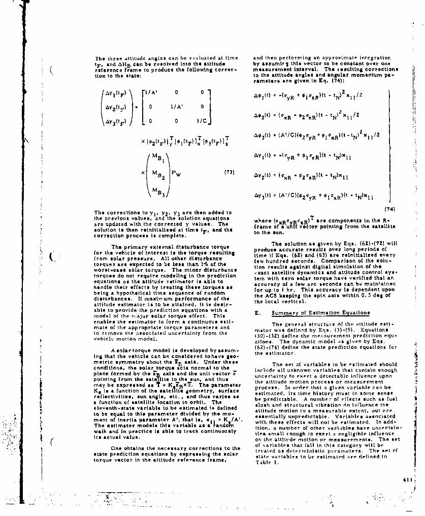
The three attitude angles can be evaluated at time and then performing an approximate integration

tF, and AHB can be resolved into the attitude by assumit S this vector to be constant over one

reference frame to produce the following correc- measurement interval. The resulting correctionstion to the state: to the attitude angles and angular momentum pa-

rameters are given in Eq. (74):

ayl(tF) I/A' 0 0 A60(t) "(qyR + • t(l~ 2 xl 1 /z

I~~ IIO

"a0 2 (t) q (xR *"z.R)it " tN)Xit/Z6y3 (t ) 0 0 I/C.

×[ezttr)1T[,lltF)T[0 3 (tF)1T A¢ 3 lt) a (A'/C)(02ZyR+xl xR)(t~tN)2Xll/Z

M ay3(t) "(IR + (i R ))(t -tN)xllayl I t ( y 1OzR N '

SMBz PW (73) AY(t) (axR " .zR)(t " tN)xl I

\MB3 "Y 3 (t) a (A'/C)(OZryR + 01ýxR)(t - tN)Xll

The corrections to yl, Y2 , Y3 are then added to (74)the previous valuer, and the solution equations where (7xR R0' R)

T are components in the R-

are updated with the corrected y values. The frame ofxaufRi vector pointing from the satellitesolution is then reinitialized at time tF, and the to the sun.correction process is complete.

The primary external disturbance torque The solution its given by Eqs. (62)-(72) willprouc accuraty erterlts disvrbnr lonorquedofor the vehicle of interest is the torque resulting produce accurate results over log periods of

* from solar pressure. All other disturbance time if Eqs. (62) and (63) are reinitialized everyt,.•fro solr pessre, ll the disurbncefew hundred second@. Comparison of the solu-

torques are expected to be less than l1f of the fion results against digital simulation of the

worst-case solar torque, The minor disturbance tion sults agin s al ationtof edo nt rquir trodeing n te prdicion xact satellite dynamics and attitude control sys.-

torques do not require modeling in the prediction tern with zero solar torque have verified that anequations as the attitude Tetimator is able to accuracy of a few arc seconds can be maiainedhandle their effects by treating these torques as for up to I hr. This accuracy is dependent uponbeing a hypothetical time sequence of random the ACS keeping the spin axis within 0.5 dog ofdisturbances, If maxirrum performance of the the aC eerin p weattitude estimator is to be attained, it is desir- the local vertical.able to provide the prediction equations with a E. Summary of Estimation Equationsmodel of the najur solar torque effect. Thisenables the estimator to form a continuous esti-mate of the appropriate torque parameters and Ths genera s t of th5 a tioto remove the associated uncertainty from the rrater was defined by Eqs, (3)-(5). EquationsSvehicle motion model. (30)-(3Z) define the mennurement prediction equ-• ations. The dynamic model as given by Eqs.

(62)-(74) define the state prediction equations forAsolar torque model to developed by assure- eetmtr

* in& that the vehicle can be considered tohave geo- tometric symmetry about the T, axis. Under these The set of variables to be estimated should

conditions, the solar torque acts normal to the Include all unknown variables that contain enoughplane formed by the 7B axis and the unit vector ~ uncertainty to exert a detectable influence uponpointing from the satellite to the sun, and thus the attitude motion pocess or measurementmay be expressed as T K The parameter process. In order that a given variable can beK, is a function of the satellite geometry, surface estimated, its time history must in some sensereflectivities, sun angle, etc. , and thus varies as be predictable. A numbs:" of effects such as fuela function of satellite location in orbit. The slosh and structural vibration do influence theeleventh-state variable to be estimated I0 defined attitude motion to a measurable extent, out 2reto be equal to this parameter divided by the mo- essentially unpredictable. Variables associatedment of inertia parameter A'; that is, x 1 - K /A'.The estimator models this variable as a landoq with these effects will not be estimated. In add-

ition, a number of other variables have uncertain-walk and In practice to able to track continuously ties small cnough to exert a negligible influence

its actual value. on the attitede motion or measurements. The set

of variables that fall in this category will beOne obtain@ the necessary corrections to the treated as deterministic parameters. The set of

state prediction equations by expressing the solar state variables to be estimated are defined intorque vector in the attitude reference frame, Ttble i.

411

,. 4. :-

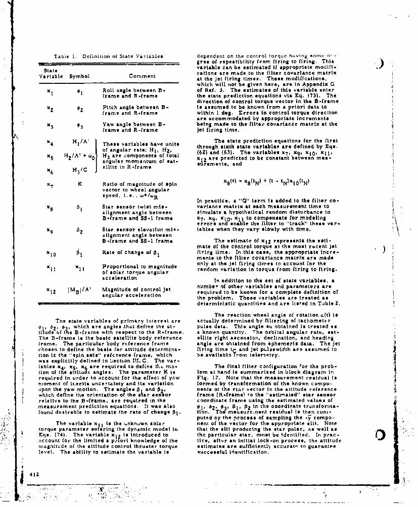
Table 1. Definition of State Variables dependent on the control torque having som( d.(-gree of repeatibility from firing to firing. This

State variable can be estimated if appropriate modifi-Varle Scations are made to the filter covariance matrix

at the jet firing times. These modifications,

which will not be given here, are in Appendix 0x I Roll angle between B- of Ref. 3. The estimates of this variable enter

frame and R-frame the state prediction equations via Eq. (73). Thedirection of control torque vector in the B-frame

x 2 Pitch angle between B- it assumed to be known from a priori data toframe and R-frame within 1 dog. Errors in control torque direction

are accommodated by appropriate incrementsx Yaw an•le between B- being made to the filtea cavariarce matrix at the

frame and R-frame jet firing time.x4 HI/A! T e The state prediction equations for the first

These variables have units through sixth state variables are defined by Eqs.

of angular rate; HI, H 2 , (62) and (63). The variables x 7 , x9, X1 0 , x 1 l,

x5 H 2 /A' + w0 H3 are components of total xlZ are predicted to be constant between mea-angular momentum of sat- surements, and

x H 3 /C J ellite in R-frame

x7 K Ratio of magnitude of spin x 8 (t) ' x,(tN) + (t - tN)xlO(tN)vector to wheel angularspeed, i~e., */twR In practice, a "Q" term is added to the filter co-

x 01 Star sensor twist mis- variance matrix at each measurement time toalignment angle between simulate a hypothetical random disturbance toB-frame and SS-I frame x 7 , x 9 , x 1 0 , xll to compensate for modelthg

errors and enible the filter to "track" these var-x 9 02 Star sensor elevation milt- tables when they vary slowly with time.

alignment angle between

B-frame and SS-l frame The estimate of xI 2 represents the esti-mate of the control torque at the most rwcent jet

1 l Rate of change of p, firing time. In this case, the appropriate incre-ments to the filter covariance matrix are madeonly at the Jet firing tines to account for the

Xo I xs Proportional to magnitude random v&riation in torque from firing to firing.of solar torque angular

acceleration In addition to the set of state variables, a

X IM /A' Magnitude of control Jet nuimbe- of other variables and parameters are12 BI arequired to be known for a complete definition of

angular acceleration the problem. These variables are treated as

deterministic quantities and are listed in Table 2.

The reaction wheel angle of rotation aft) isTne state variables of primary interest are actually determined by filtering of tachometer

0 o , which are angles ,that define the at- pulse data. This angle su obtained is treated astitude of the B-frame with respect to the R-frame. a known quantity. The orbital angular rate, sat-The B-frame is the basic satellite body reference ellite right ascension, declination, and headingframe. The particular body rtference frame angle are obtained from ephemeris data, The jetchosen to define the basis for attitude determina- firing time t and jet pulaewicith art assumedu totion ic the "spin axis" refcrence frame, which be availabltrom telerimtry.was explicitl7 defined in !5ection I1. C. The var-iables x4 , x 5 , x6 are required to define tl.* mo- The final filter corfiguration 'or the prob-tion of the attitu c angles. The parameter K is lem at hand is summarized in block diagram it'.required in order to account for the effect of ynw Fig. 12. Note that the measurement residual is

nmoment of inertia uncertainty and its variation formed by transformation of the known compo.upon the yaw motion. The angles p and 0 nents oi the rta. vector in the attitude referencewhich define the orientation of the slar senshor frame (R-frameO to the "estimated" star sensorrelative to the B-frame, are re4uired in the coordinate frame using the estimated valuea ofmeasurement prediction equations. It was also 01- 0z2 030 01, OZ in the coordinate trunsforma-found desirable to estimate the rate of change 0l. tion. The meusurc:nent residual is then com-

puted oy the process of sampling the -" compo-The variable Xll is the L.nknwn solar nent of the vector for the appropriate slit. Note

torque parameter entering the dynamic model In that the slit producing the star pulse, as well asEqe. (74). The variable xlzI nrdcdt the particular star, mitst be identified. In prac- •account for the limited a p:ron knowledge of the tice, aft-ir an initial lock-on process, the attitude

"magnitude of the attitude control thrueter torque estimates are sufficiently accurate, tn guaranteelevel. The ability to estimate the variable is successful i'entification.

41.

MEASURED SLITCROSSINJG TIME________

INRENTIALIZE CLSDFWMi?+1 JCLOSED

MEASUREMENT KNII STATE CORRECTIONS YNMCMOiESTIMATEDREIULREF FRAME To CS-RAME STATE

ES7IM!ATED UNIT STAR T F TI N

7 _07ý1ESTIMATES OF ATTITU'DE,$5 MISALIGNMENTS

[0 -101 5 UNIT STAR VECTOR IN REF FRAME

;S ss STAR

Fig, IZ, Filter Configuration

Table 2. Deterministic Ptirametere RLFERENCES

Varabl Comen L R. E. Kalman. "A New Approach to Linear____________________________________Filtering and Prediction Problems,

J. Basic Eng. , Trans. ASME 82, 35 (1960).A'/C 2AB/C(A +B) Moment of inertia param-

eter 2. Robert Robe.rson, Preliminar Report ontha Friundations of Atttd etmaI o

PCon~rol jet pulsewidth from a spinngOot, Aerojet !generalCorp. . Ileport3Mf 71-90 (6 Aug. 1968),

tTime of irditiation 3.ofLsne~ rcs tttd eiac~ontrol tovque pulse3. JELamk PeieAtudTsm-

Q~t)Reacion -hea ange oftion for an OrbitziZ pacecraft, Aerospaceo~t) eacton ~hee1 ngleof Cr-p7.,iepnrt TOR-O Dbbr5i7v-u1)-l

rotation (July 1969).

a~.b Satellite right ascension,declination, and headingangle

l'-'Z 1' 2'' 3 Star sensor sliL angles

0 ~Magr~itude of oriltal

_____ -413

SESSION VI

PANEL DISCUSSION

Chairman:Mr. Dennis F. Meronek

The Aerospace CorporationEl Segundo, California

Panel Discussion 417

Transcription *

Biographies 419

'Classified; published in Volume II

415

A

PANEL DISCUSSION

"The panel was chaired by Mr. Dennis F. Meronek of The

Aerospace Corporation. It comprised Major William Hartung

( of the Air Force (SAMSO) and the chairmen of the five previous

sessions: Professor Harold Sorenson, Mr. Robert Lillestrand,

Dr. James D. Gilchrist, Dr. Joseph LeMay, and Professor R.

C. K. Lee.

The discussion beganwith each chairman summarizing his

session, and Major Hartung examining possible future missions

requiring high-accuracy attitude determination. Atranscription

from the tape recordings of the entire discussion is published in

Volume II (classified) of these proceedings.

Brief biographies of the chairmen, speakers, and other

coauthors follow, if they were available at the time of printing.

01%

417

• ,. • • - . . . .. : :•, • - ,': .. - . ,:. •: .. ,p. .,1 -.' • -,. . 4

.4.In.h

BIOGRAPHIES

The Aerospace Corporation Representatives

The Aerospace Cnrporation, El Segundo, California, which cosponsored the symposium, was repre-sented by the following cochairmen and speakers. Each is a member of the Control and SensorSystemsSubdivision, Electronics Division, Engineering Science Operations. Dr. Henrikeon and Mr. Lesinski,together with Captain D. Evans, USAF (SAMSO), cochaired the symposium.

3. D. Oilchrist chairman of Session III, was born in Winnipeg, Canada. He received his BES and MS atthe university of Manitoba in 1959 and 1961, respectively, and his PhD in electrical engineering at theUniversity of Minnesota in 1965. From 1964 to 1968 he worked. at Honeywell, Ir.c., on various projects,including trajectory optimipiation, optimal guidance schemes, spacecraft attitude control systems, andattitude determination. At Aerospace he has been involved in attitude determination and sensor line-of-eight determination problems. Dr. Gilchrist also presented a paper during Session V of the symposium.

L. 3. Hsnrikson a cochairman of the symposium, received his AB from Harvard and his SM from MIT.h1a' 1ea0sching fellow at Harvard, and a research assistant at both Harvard and MIT. At Her-

yard, he obtained his PhD in control and estimation theory. While in graduate school, he was aesoci-ated with the Dynamics Research Corporation in Stoneham, Massachusetts. There he applied estimationtheory to the analysis of the Ship's Inertial Navigation System (SINS) for the Navy's Polaris submarineprogram, Since joining The Aerospace Corporation in 1967 he has been involved in spacecraft attitudeand line-of-sight determination problems. Dr. Henrikson has publinhed papers on correlated rmeasure-ment noise and nonlinear estimation.

•, chairman of Session IV, hails from Michigan, Ho earned his electrical engineeringversity of Detroit in 1957 and his MS at the California Institute of Technology in 1959.

From 1955 to 1959 he was a research engineer with General Motors Corporation, and from 1959 to 1962,a teaching fellow at the University of Michigan, where he received hie PhD in instrumentation engineer-ing, He has been with The Aerospace Corporation since that time, first as a section manager and now

as a program director. Dr. LeMay lectures on modern control theory at UCLA, is the author of nu-merous publications on control and navigation systems theory, and is a member of AIAA and IEEE,

J. E. Lesinski, a cochairman of the symposium, is a native of Michigan. He received his BS in aero-nautical engineering from the University of Michigan as well as his MS in instrum,%ntation engineeringin 1962, and has been with The Aerospace Corporation sinsce that time. His areas of specialiation areguidance control, estimation applications, and the sensitivity analysis of optimal filters. Most recentlyhe has been involved in a study of the implementation of optimal estimators for satellite attitude deter-mination, Mr, Leeineki also presented a paper in Session V of the symposium.

D. F, Meronek, chairman of Session VI, is a Wieconsonite, He obtained his BES and MS in electricalengineering at the University of Wisconsin, the latter in 1958. He has been at The Aerospace Corpora-tion since 1962, where he is head of the control systems department, which is involved in the design andanalysis of terminal guidance and spacecraft and reentry vehicle control systems, and in attitude deter-mination schemes.

SAMSO Representatives

The Space and Missile Systems Organisation, Air Force Systems Command, Los Angeles Air Force

StaLion, Los Angeles, California, a ro,,jonsor of the symposium, was represented by the followingchairm,.n and speaker.

David 3. Evans, Captain, USAF, a cochairman of the symposium, is a native of Pennsylvania, where her!ecevve a no in engineering physics at Lehigh University in Bethlehem in 1966. He graduated from theAir Force Institute of Technology in 1968 with an MS in space physics engineering. Since that time, hehas been aasignes to the Deputate for Technology, Exploratory Development Branch, Space and MissildSystems Organisation in Los Angeles.

419

. 1;':.:

William E. Hartunj, Major, USAF, received a BS in chemistry from the University of Santa Clara in1954. His BW S in aeronautical and astronautical engineering came from the University of Illinoisin 1963 and 1964, respectively, whence he was directl, assigned to Headquarters. Space Systems Divi- )sion. There he participated in the management of preliminary design studies for the Special DefenseProgram. After flying C-130s in the Philippines in support of South Vietnam, he was assigned to hispresent post at the Space and Missile Systems Organization. His mission analysis work last year wason the Surveillance of Objects in Space in the 1970s (SOS-70); currently, it is on the missile and spacedefense of the United States. Major Hartung presented a paper in Session V.

Other Representatives

Other session chairmen, speakers, and authors of symposium papers are listed below alphabeticallyunder the name of the organiziation each represents.

AEROJET -GENERAL CORPORA7iON

R. A, Lucas was born in Illinois, He received his BS ii mathematics, with honors, from Californiastate Polytechnic College in Pomona in 1966. Since that time, Mr. Lucas has been with the Aerojet-General Corporation in Asusa, California, working on attitude determination and simulation. He andhis coauthor presented their paper in Session V of the symposium. He volunteers that he has twobrilliant, beautiful children and is nice to cats, birds, and secretaries.

BARNES ENGINEERING COMPANY

Robert W, Astheimer, chairman of Session 11 of the symposium, received a BS in mechanical engineer-ing in 1944 &nd an Me[s in physics in 1949 at Stevens Institute of Technology. As an engineering traineewith the American District Telegraph Company, he develeped automatic fire detection systems andacomponents. From 1944 to 1946, he served in the Army Signal Corps on mobile radio equipment; thenuntil 1951 he was a physics instructor at Stevens where he did research on refractive index measure-ments and self-diffusion of metals, and electron microscope studies of metallic structure. At theNaval Ordnance Laboratory from 1951 to 1953 he investigated underwater explosion phenomena and -

, developed atomic and hydrogen bomb blast measurement instruments. When he joined Barnes Engineer-ing Company, Stamford, Connecticut, in 1953, he was concerned with infrared missile tracking, imag-ing units, and radiometers and spectrometersi portable and mobile IR pointing and scanningi satellite

: stabilization sensors, weather reconnaissance, and now thermal detectors. Later he became technicaldirector, responsible for the administration and technical direction of engineering, research, and do-velopment activities. He is now Vice President and Oeneral Manager of the Defense and Space ContractsDivision, Mr. Astheimer is a fellow of the Optical Society of America, and etuntributes extensively totechnical publications.

CONSULTANT

Robert E. Roberson received his BS in physics, his MS in mathematics, and a PhD itx mechanics, allfrom Washington Un versity in St. Louis by 1951. After 17 yeazs of experienct in government lab-oratories and industry, he became a consultant to industry in 1960 in aerospace vehicle dynamics andcontrol. In addition, in 1964 Dr. Roberson became a professor of engineering at the University ofCalifornia. Los Angeles, and has been with the University of California, San Diego, as profeseor ofaerospace engineering since 1967. Dr, Roberson presented the first paper o". the symposium.

CONTROL DATA CORPORATION

Joseph E. Carroll, a native of Wisconsin, attended St. Mary's College and then the University of Minnes-sots, wherein 1963 he received an MS in physics. He joined Control Data Corporation, Minneapolis,Minnesota, In 1961, and has been active in the design, analysis, f£aricatior, and testing uf spacecraftnavigation and attitude detection systems and their application to ground-based astronomical surveys.He is now technical director -)f the SPARS star sensor development. The author of numerous technicalpapers and holder of four patents, Mr. Carroll is a member of the Institute of Navigation, the ArcticInstitute of North America, and the American Congress on Surveying and Mapping. He authored thepaper he presented in the symposium's Session It, and coauthored a paper given in Session IV.

Charles B. Groech, a Chicagoan, obtained his BS in education and MS in mathematics from Iowa StateUniversity in 1955. He did graduate work in mathematics there and later at the University of Minnesota.He was in the mechanical division of General Mills from 1956 through 1962, and then did army duty forsix months. Later that year, Mr. Grosch joined Control Data Corporation in Minneapolis, where hehas been involved in the problems of applied mathematics directed primarily toward attitude determina-tion and celestial mechanics. Mr. Orosch is coauthor of a paper presented in Session I1I.

6 420

.• • , . :.-• .....

Anton E. LaBonte is a coauthor oi the paper he presented in Session III of the symposium. A native ofMinneapolis, he received his BS, MSEE, and PhD (in electrical engineering and mathematics) from theUniversity of Minnesota. While there, he did electrical engineering undergraduate teaching ind researchin the microrriagnetic characterization of ferromagnetic thin films. Upon receiving his PhD in 1966, hejoined the Control Data Corporation, Minneapolis, where his work has been 'a. star mapper attitude de-termination, its data reduction and evaluation, and systems engineering for scanning instrumentationand software for the analysis of photographic star plates.

Robert L. Lillestrand, chairman of Session II, served from 1945 to 1946 in the U.S. Navy. At theUniversity of Minnesota he achieved his BA and MA in physics in 1949 and 1951, respectively. He thenwent to General Mills, Inc. . where, until 1960, he was concerned with self-contained optical systemsfor space navigation based on star aberration only; precise IR search and track systems; error analysisof the ICBM impact prediction system; the design of the aberrascope; the monopulse radar antennapedestal for IRBM guidance and the precision automatic leveling platform. In 1960 Mr. LillestrandJoined Control Data Corporation in Minneapolis where he has been, successively, director of aerospaceresearch, staff consultant to the research division, and currently director of electro-optica research.He holds fie patents in the space navigation and detectionfield (including the stellar aberrasoope), andhas five pending. His papers have appeared in numerous journals such as Electronics, AP.S ournal,and the IEEE Transactions on Aerospace and Navigational Electronics. He has presented papers atnumerous symposia, and toa memoer ef tte American Physical Society, American Optical Society,American Astronautical Society, AlAA, and the Arctic Institute of North America. Mr. Lillestrand hasmade two expeditions to the North Pole and two to northern Oreenland; in the latter, in spring 1969, hediscovered the new northernmost point of land in the world,

Bruce D. Vannellt was born in St. Paul and received a BS in 1939 and an MS in 1963, both in mathematicsand ?rom the Univereity of Minnesota. He was with the Mitre Corporation in Boston in 1961 working ondisplay programs for ligh-altitude air traffic control. The following year, Mr. Vannelli wen' to ControlData Corporation, Minneapolis, as a programmer analyst on projects such as computer programs fo.attitude determinAtion devices, stellar pattern recognition, and satellite navigatimn using an ejectedprobe, Mr. Vannelli coauthored a paper given in Session I1l.

t HONEYWELL, INC.

Gerald R. Arneson received both his B5 and MS in electrical engineering from the Univeresty of Minn-L ( isot&, the latter in 1968. Since 1967 he has been involved in simulation problems in the computer

Ssciences section at Honeywell, Inc., Aerospace Division, Minneapolis. These have included a hybridsimulation of a VTOL aircraft to evaluate wind gust disturbance, d•gital simv;ulation of an attitude refer-ence using laser gyros, and a real-time data processing algorithin for SPARS, Mr. Arneaon recentlyhas been developing and implementing hybrid software for the Honeywell SD$ 9300 and Sigma V hybridcomputation facilities, In addition to these computers, he has worked with the CDC 1604-6600, andthe Honeywell H-2l and H-1800, Mr. Arneson is a coauthor of the paper he presented in Session 1II.

SD.Bron is coauthor of a paper given in Session IV of the symposium. Havirg received hisBIS nd ME at Purdue University by 1966, he 'oined Honeywell, Inc., Aerospace Division, as a

princm.pal development ergineer. In this capacity, he has made analysis tradeoff studies using theSPARS 3DOF computor simulation and was responsible for application of the SPARS algorithm to real-time software in Phile IA. Previous to his work on SPARS, Mr. Brown had worked on the verificationof a 13-foot air bearing test table and on an acceptance test program for a space vehicle motion simu-lator for NASA's Manned Spacecraft Center,

David B. Jackson received a BS in electrical engineering from the University of Minnesota in 1961, andlid a year of graduate study there in automatic control and digital computers. From 1962 to 1965 hewas with the Lockheed-California Company on a number of NASA and Air Force studies. Recently, herepresented Honeywell at the NASA Electronics Research Center at Cambridge, Massachusetts, wherehe worked on the application of stochastic estimation to the rnechaniration of strapdown attitude refer.once systems for spacecraft, and %here he prepared the paper he gave in Session I of the symposium.Previously, Mr. Jackson was involved in the three-degree-of-freedom computer program and simula-tion study in SPARS Phase 0 and in the Apollo Block 1I display coupler studies. He is presently withthe Aerospace Division of Honeywell, Inc. , in Minneapolis.

Jerome C. Kollod ae* is a coauthor of a paper in Session I1. He is with Honeywell, Inc., RadiationCenter, Loex nto,-' *a eachum etts.

"D. Alexander Koso,* coauthor of the paper he presented during Session Il of the symposium, is with"Honeywell, Inc., Radiation Center, Lexington, Massachusetts.

'(:1Biographical information not available.

I A

"I"I/. .- .t

J2seph A. Miller to coauthor of the paper he presented in Session IV of the symposium. He receivedh and MS in ele-trical engineering from MIT in 1953 and then joined Honeywell, Inc., Aero- )

space Division, where he id the SPARS project leader. He has supervised the concept and system re-quiremeits on the Block I Apollo SCS for four years, from concept definition to hardware verification.Mr. Miller has also been involved in its entry and Delta V operation and closed-loop system tests, aawell as directing the selection study of the attitude reference system for both Blocks I and II.

Gerald D. Nelson earned both his BS and MS at the University of Minnesota, in 1960 and 1968, respec-tivwly' Since 1963 he has been employed by the Aerospace Division of Honeywell, Inc,, as an analystin the computer sciences section. Mr. Nelson has been rusponsible for the design and implementetionof digital computer programs for a mult'sensor reconnaissance model, an Apollo tolerance analysisprogram, and a general-purpose program for the analysis of linear systems, known as VALUE. Hiswork has made him familiar with the IBM 7090-7094, the CDC .1600 and 6400-6600, and the HoneywellH-1800 computers. Mr. Nelson coauthored a paper given in Session In.

David C. Paulson received his BS and MSME at the University of Minnesota, the latter in 1960, Fromthen until 1'966'e was with the United Aircraft Corporation involved In conceptual design studies ofmissile, satellite, and space vehicle navigation and precision stellar-inertial attitude reference andpointing systems. Since 1966, he has been a staff engineer at Honeywell, Inc., Aerospace Division,where he is currently responsible for the Phase IS SPARS concept development, analysis, and testing.During Phases 0 and IA, he was work director for the system analysis, and responiible for the con-ceptual application of recursive filttring in the SPARS design. Mr. Paulson holds a pateot for an auton-omous orbital navigation mechanization, and is the coauthor of the paper he presented in Session IV.

David K. Scharmack, whose paper was presented in Session I, received his BSE and MS from the Uni-versity of Michigan, and worked for the Kuhlman Electric Company from 1957 to 1960. He is in theSt. Paul Systems and Resear'ch Division at Honeywell, Inc., which he joined in 1960, and is preparinigfor a PhD in control sciences at the University of Minnesota. His work has been largely in the field ofdigital computers, with his major research effort resulting in the "predictor method," a powerful toolfor determining optimal trajectories as functions of parameters. He has worked in the diverse areasof optical correlation and attitude determination, the latter being concerned with the orbital scanner.In addition to writing journal papers, Mr. Scharmack is the author of a chapter in Volume V ofAdvances in Control Systemse Theory and Practice, and has lectured on trajectory optimization in theU CLA sortha-course series.

Robert T, Scott earned his ESEE from Catholic University in 1950, and his MSEE from Purdue Univer-sity in 19 He has been with the Honeywell, Inc,, Aerospace Division since that time, and is current-ly the work director on SPARS Phase IS component design and development. This was preceded by hisefforts on the inertial reference assembly hardware requirements in Phase 0, and in the IRA buildingand testing in Phase IA. Prior to SPARS, he was involved in the rate gyro package for the MOL and in

S lguidance amplifiers for Gemini, Mr. Scott has specialized in inertial grade gyros, including the de-velopment and test of a rate gyro package for Sprint, and is the holder of two patents concerned withgyro temperature control. Mr. Scott coauthored the paper he gave in Session IV of the symposium.

N. W. Tidwell is a principal systems analyst at Honeywell, Inc., Aerospace Division, Minneapolis.He is also working toward his MS in electrical engineering at the University of Minnesota, having re-ceived his B8 in engineering physics at the University of Illinois in 1962. He is currently engaged inthe mathematical modeling of spacecraft perturbation torques and in a system parametric analysis todetermine spacecraft parameter sensitivity to the accuracy of attitude determination of a celestial map-per. Other areas of his experience relate to the orbital scanner spacecraft; horizon definition meas-urement program; F104 aircraft computer; the Electrically Suspended Gyro Monitor (ESGM), for whir.hhe developed optical alignment techniques; and the Advanced Orbiting Solar Observatory (AOSO), includ-ing sensor and solar simulation design and scheduling and testing on the six-foot air bearing table, Mr.Tidwell presented a paper in Session I of the symposium.

HUGHES AIRCRAFT COMPANY

posegh Del RItjo, currently in charge of the TACSAT attitude determinaeIon and control and station-epiin at Htug1h6s Aircraft Company in Los Angeles, received his BS in mathematics at Pennsylvania

State University in 1962. In the guidance and controls department at Hughes, Mr. Del Rie o is involvedin the design and analysis of trajectory and orbit shaping and on-orbit control of spin-stabilized space-craft. He has participated in the real-time launch and orbit phases of the Intelsat II, ATS, and theTACSAT. Mr. Del Riego coauthored a paper in Session III,

John :. Ribarich earned his BS in electrical engineering at the University of Minnesota. Mr. Ribarichpresented a paper in Session V of the symposium, He is with the Hughes Aircraft Company in LosAngeles, where he is section head in the guidance and control department. At present, he is involvedin precision pointing studies.

422

Warren H. Sierer is a staff engineer in the Space Systems Division of the Hughes Aircraft Company,Los Angeles. He went to work there in 1964, having received both his BS and MS in space physics atUCLA. Working in the area of attitude sensing and determination, he was a member of the team spe-cializing in this and in-orbit control during launch of ten spacecraft for NASA, Zomsat Corporation,and the Air Force. For the TACSAT. he developed the in-orbit control computer system and was chiefof orbital maneuvers during initial launch operations. Mr. Sisrer coauthored the paper he gave inSession I11.

IBM CORPORATION

. L HoI*s * coauthor of a paper presented in Session IV, is with the Federal Systems Division of15 fks, California.

W, C, Martin was awarded a BS in mathematics at Fresno State College in 1957 and Ln MS in engineer-ing at UCLA 'n 1968. He has worked extensively in the field of computer and control applications atthe U.S. Naval Ordnance Test Station. the Ford Motor Company, and The Aerospace Corporation. To-gether with his coauthor, he presented a paper in Session V of the symposium.

Gunnar Nielsen, coauthor of a paper presented during Session IV, received his BME at the OMT inDenmark in 1948. Joining IBM in 1951, he became a member of the medical engineering departmentof the physics laboratory and was assigned to heart, lungs, and artificial limbs. This led to work onperiscopes and precision optical and mechanical projection and measuring systems. Included were themap-match projection system, the photographic system for the AN/ASQ-3 -1-512) bombing navigationsystem, and the bombing navigation map-match system for the XB-70 aircraft, At present he is anadvisory engineer in the physical simulation department at IBM in Owego, New York, supporting thedesign and integration of opto-mechanical simulation equipment.

Frank H. Schlee graduated from Brooklyn Polytechnic Institute with a BS in aeronautical engineeringT 7;r i Athe University of Michigan, he received an MS in 1959 and a PhD in 1963, both in instru-

mentation engineering, a subject he also taught part time. He then joined IBM in the Federal SystemsDivision, Owego, New York, where he went to work on mission analysis for the standardised spaceguidance system. He then became involved in Gauss-Markov optimal estimation in autonomous space-craft navigation, the MOL, the Gemini navigation experiment, navigation systems for lifting reentryvehicles, and the test design and evaluation of SPARS. At present, Dr, Schle. is working on the designof the A7 navigatton and weapon delivery system. He coauthored two papers in Session IV, one ofwhich he also presented.

N. F. Toda was an instructor in the department of engineering mechanics at Cornell University from950 to 19'57. It was there that he earned his BME in 1950 and MME in 1953. After leaving Cornell,

he went to the Sperry Gyroscope Company where, until 1964, he was engaged in the development offloated gyros and the navigation and guidance of space vehicles, He then joined IBM in the FederalSystems Division at Westlake, California, where he is manager of the systems analysis department,At IBM, Mr. Toda has been involved in autonomous navigation, guidance of space vehicles, and theDefense Support Program attitude determination. He was also manager of the guidance analysis de.

partment for SPARS. His paper was given in Session IV.

LOCKHEED MISSILES AND SPACE COMPANY

William R. Davis, coauthor of a paper presented in Session IV, received hie BS in electrical engineer-Ing and NIS in physics from the California Institute of Tachnology. The latter was in 1947 after a stintat the U.S. Naval Academy in the USNR Officer Traini•g. In 1966, he received his PhD in electrical 4,engineering. From 1947 until 1956, he worked at several companies in the development of stable plat-forms, celestial navigation equipment, angle transducers, and high-speed commutators. He thenjoined Lockheed Missiles and Space Company at Sunnyvale, California, where he is project leader innavigation, guidance, and control, directing the SPARS program. While at Lockheed, Dr. Davis hasbeen involved in guidance and control, satellite drag makeup experiments, advanced technical planning,and advanced satellite and missile 4yetom synthessi-guid~nce and control. He also dtrected the initialsynthesis and development of the Agena ascent guidance and orbit a•titude control systems.

Fred Y. Hotiuchi received a BS and MS in aeronautical engineering from the University of Illinois, thelatter degree in 1958. After working in the Missile and Space Division of Douglas Aircraft Company,he joined Lockheed Missiles and Space Company, Sunnyvale, California, in 1960, where he is a researchspecialist in the guidance end flight mechanics department. Being responsible for the design of theprecision earth-pointing experiment of the SPARS program, Mr. Horiuchi Is concerned primarily withthe accurate determination of satellite orbits and drag lifetimes, and with atmospheric density analyces

* and satellite rendezvous studies. Mr. Horiuchi coauthored a paper presented in Session IV.

Biographical information not available.

4Z3

Vladimir Hvoschinsky received a Diploma Engineers degree from EPUL in Switzerland in 1954 and an70EE froi; the 7;liornia Institute of Technology In 1960. He designed wideband instrumentation forDynasoar at Ampex Corporation, and did research and development on electronic systems and servocontrols at Leach Corporation, Magnetic Research Corporation, Allen Bradley, and Brown-Bovery,Ltd., in Switzerland. In 1963 he joined Lockheed Missiles and Space Company and was project leaderfor the microwave radiometer terminal guidance and low-cost inertial guidance projects, includingflight and sled test experiments. He designed high-precision servos for the laser pointing commurica-tior. system for the special LOCAT satellite. Currently. Mr. Hvos:hintky directs the tests and ex-periment definition for PEPSY laboratory evaluation. He coauthored a paper which he presented inSession IV of the symposium.

ichael . L ione s a senior research engineer at the Lockheed Missiles and Space Company, Sunny-vale, ualifornia He received his BA in engineering physics at Cornell University in 1965 and his MAin electrical engineering at Stanford University in 1966. At Lockheed, Mr. Lyons' work includes thedesign and analysis of spacecraft attitude control, and estirmation techniques for attitude determination.He coauthored the paper he gave during Session II1.

E. D. Scott,* coauthor of a paper presented in Session I11. is with Lockheed Missiles and Space Comr-pany, Sunnyvale, California

MARQUETTE UNIVERSITY

E, C. Foudriat, author of the becond paper of the symposium, graduated from the University of IllinoisIn 1950 an3 went to Ohio State University where he earned both MS and PhD degrees by 1966. He hasworked for the Battelle Memorial Institute, North American Aviation, Inc., and NASA at Langley Re-search Center from 1957 through 1967, Dr. Foudriat then joined Marquette University, Milwaukee,Wilconsin, as an associate professor of electrical engineering.

MASSACHUSETTS INSTITUTE OF TECHNOLOGY

3urt Valae, * with MIT's Instrumentation Laboratory, Cambridge, Massachusetts, coauthored a papergriven linession II of the symposium,

NATIONAL AERONAUTICS AND SPACE ADMINISTRATION "S

Howard 3. Curfman, 3r,, a native of Norfolk, Virginia, graduated from the Virginia Polytechnic Insti-tude in 1945 with a A3 in aeronautical engineering. In 3anuary 1946 he went with NASA at tho LangleyResearch Center, Hampton, Virginia, where he is assistant head of the aerospace mechanics branch ofthe applied materials and physics division. His research has been in automatic stabilisation and controlof freely flying models of both aircraft and missiles. Mr. Curfman was manager of Project Scanner,

* is the author of 17 technical reports, and coauthored a paper presented in Session II of the symposium.

S. Paul B, Davenvort received his BA and MA in mathematics at the University of Delaware, the latterdegree in 195, rom then until 1962 he was with the computing facility of the Westinghouse DefenseCenter as a numerical analyst specialising in space applications. He then went to NASA's GoddardSpace Flight Center, Greenbelt, Maryland, where he is head of the mathematical and operations analy-sis section, Mr. Davenport's work has been mainly the mathematical modeling for the ground controlof the Orbiting Astronomical Observatory (OAO). His paper was given in Session III of the symposium,

Richard des3ardins received his BA in physics and his MA In mathematics from The Catholic Universityof America. He is a mathematics instructor there, at the same time working for NASA at the GoddardSpace Flight Center in Greenbelt, Maryland. For NASA, Mr. desiardins performs mathematical andoperations analysis for control of the Orbiting Astronomical Orservatory (OAO). He presented hispuiper in Session 11 of the symposium.

ohn A, oen, born in South Carolina, graduated from its Clemson College with a BME degree ine that time he has been employed at NASA's Langley Rvsearch Center, Hampton, Virginia, i

where he is head of the navigational instrumentation development section of the flight instrumentationdivision, His work in the areas of flight instrumentation and guidance and contr'ol has involved him inthe research aircraft flown at the Flight Research Center in California, Mr. Dod en supervised the

L early X-15 horason definition flight experiment, was experimenter on the Pro ect Scanner rocket, andparticipated in the early manned lunar mission studies. He is a coauthor of the paper he presented in"+- "+ Session 11.

Biographical information not available.

424

Daniel Sheldon* is a coauthor in Session IV. He is employed at Hamilton Standard Division, UnitedAircraft Corporation, Farmington, Connecticut,

Robert 3. Slabinski, born in Penn-ylvania, achieved his BS at the University of Hartford in 1964 andhis MS at the nUnersity of Connecticut in 1967, both in electrical engineering, where he is at presentpursuing a PhD in the same field. From 1960 through 1964, he woiked at the Royal McBee Corporationin the analysis and design of small high-speed mechanisms. At United Aircraft Cyrporation's HamiltonStandard System Center in Farmington since 1964, Mr. Slabinski has been active in sensor loop designand the dynamic performance analysis of strapdown inertial systenis. The paper that he coauthoredwas given in Session IV of the symposium.

UNIVERSITY OF CALIFORNIA

R. C. K. Lee is an associate professor of aerospace engineering st the Univeriity of California, Irvine,in Irvine, "alifornia. He received his BS, MS, and SoD degrees from MIT in aeronautics and astro.nautics. The next 12 years he spent first at Honeywell, Inc., and then at The Aerospace Corporation

working in the areas of space guidance and control, airborne vehicles, estimation theory, and adaptivecontrol systems. He holds several patents in these fields. Dr. Lee was uhairman of Session V of thesymposium.

Harold W, Sorenson, the chairman of Session I, received his BS at Iowa State University in 1957 andhis MS and mhD from the University of California, Los Angeles, in 1963 and 1966, respectively.During 1957 to 1962, he was a senior research engineer in the flight performance and guidance analysisEroup at General Dynamics/Astronautics. From 1963 to 1966, he was head of space systems in theElectronics Division of General Motors Corporation. The following year, he was a guest scientist at 4the Institut fdr Steuer-und-Regeltechnik, DVL, Oberpfaffenhofen in West Germany. Upon his return,Dr. Sorenson became an assistant professor in the system dynamics and control section of the depart-ment of the aerospace and mechanical engineering sciences at the University of California, San Diego,in La Jolla, California.

Biographical information not available,

(

ti

.4•

4Z6 -

'.

Mark Gorstein has been working for NASA at the Electronics Research Center in Cumbriage, Mass..-chusetts, since 1966. He received his BSEE at the City College of New York in 1958 and his MSAEfrom MIT in 1965, where he continues to work for his PhD in aeronautical engineoring. From 1958 to."'1960, Mr. Gorstein was employed at General Precision L.boratory on the circait design for Doppler inavigation systems. He then transferred to the Kollsman Instrument Company, first as a staff engineerin various star-tracking systems, and then as a resident at the MIT Instrumentation Laboritory.There he was responsible for the design and development of the Apollo horizon and star trackers, andsextant. At NASA, he is in applied research in electro-optical guidance systems in computer andguidance technology. His two pending patents include one for the quantasyn, an improved ultravioletdetector. In September 1968, Mr. Gorstein presented a paper at the EASCON conference, and, inSession II of the present symposium, he gave a paper which he coauthored.

3ames Nelson Hallock is coauthor of a paper liven in Session It. After receiving his BS in physics atMIT in 1963, he became a staff physicist there from 1964 to 1966. He was in the Apollo optics group,and also participated in the Gemini GT-7 and GT-10 experiments to measure landmark contrast, Hehas been w.th NASA since 1966 as a member of the computer and guidance technology branch at theElectronics Reseerch Center at MIT. There he obtained his MS in physics this year, and has completedhis course work. Mr. Hallock has written numerous intermal MIT and NASA reports, published in theAmerican Journal of Physcs, presented papers, and holds two patents. He belongs to the Optical So-ciety of Ame'rica, the A~erican Physical Society, the American Association for the Advancenient ofScience, and Sigma Xi.

Dwa~e E. Hinton was born in Louisiana and received his BS in physics from Kentucky Wesleyan Col-lege in 196Z. He has done graduate work at both the College of William and Mary and George Washing-ton University. Since February 1964 he has been with NASA at the Langley Research Center, Hampton.Virginia, in the navigation and guidance research branch. Mr. Hinton is primarily engaged in theattitude determination of spin-stabilized vehicles and experimental measurements in the IR of blackbodycavity emittance. He is coauthor of the paper he presented to begin Session III of the symposium.

Vernon K. Merrick, * a coauthor of a paper in Session III, is with NASA's Ames Research Center inM3offett Fie-d, Caiifornia,

B received his BS in mechanical engineering from the University of Texas in 1945 and hisv ring mechanics from Stanford University in 1947. Since that time he has been employed

at NASA's Ames Research Center, Moffett Field, California. Starting in 1962, he has specialized inthe past ve attitude control of satellites. Mr. Tinling and Vernon Merrick are the inventors of thepassive gravity stabilization system used on the ATS, DODGE, and RAE satellites, and coauthors ofthe paper Mr. TinlIng presented in Session III.

Thomas M. Walsh. coauthor of a paper presented in Session I11, ts a native of Pennsylvania. He re-cei7ved •hi';;Efrom Ohio University in 1953 and his MSE from the University of Akron in 1962. Heserved in the U.S. Army from 1953 to 1q55 at the Engineers Research and Development Laboratory,Virginia. Subsequently, he worked for the Westinghouse Electric and Goodyear Aerospace Corpora-tions and the Martin Company, primarily in the area of fire control systems. In 1962 he ,ýoined NASAat the Langley Research Center, Hampton. Virginia, in the fields of guidance and control and stellarrefe-ence systems, and the stability of various reentry spacecraft. At the University of Virginia'sextension division at Langley, Mr. Walsh has taught graduate control courses.

TRW, INC.

J. P. O'Mallejy attended the University of California, Berkeley, where he received his AB in physicsM74137. me was employed at North American Aviation's Space and Information Systems Division fromthat time to 1963, when he joined the TP.W Systems Group i.. Redond3 Beach, California. Mr. O'Malleyis a section head in the systems design department there. He presented a paper in Session I.

UNITED AIRCRAFT CORPORATION

Robert A. Baum was born in Pennsylvania, and received a BS in physics from th' Pennsylvania StateUniversity in 1962. From the Ronsselaer Polytechnical Institute in Hartford, Connecticut, he obtained6n MS in engineering science In 1965. He had already joined the United Aircraft Corporation's Hamil-ton Standard System Center in Farmington, Connecticut, in 1962, where he became active in the de-velopment, test, and analysis of strapdown inertial systems. At present Mr. Baum is a section engineerin the systems analysis group of the guidance and control department. He presented the paper that hecoauthored for the symposium in Session IV.

Biographical information not available.

425

SYMPOSIUM ATTENDEES

4 2 7

SYMPOSIUM ArTENDEES

The Aerospace Corpo~ration Attendees

R. M. Allman M. W. Jensen

Ralph Austin Paul Jorgensen

Barbara Ayotte D. L. Kleinbub

Gus Bartos G. F. Kuncir

Ray Berg R. C. LaFrance

P. G. Blandin W. C. Lawrence

John A. Bond A. Lasarus

A. F. Brigante E. A. Lee

Bruce Campbell R. C. K. Lee

Fred Campbell J. LeMay

Val Chobotov Carl Lonander

R. 0. Clabaugh Charles Leontis

T. Coffey J. E. Lesinski

P. R. Dahl R. Levinson

W. K. Davis C. S. Lorene

Vincent De Marco R. K. Luke

Marshall Earle L. E. Lundquist

I. Egashira A. S. Maser

D. D. Elliott S. Marcus

R. V. Erilane R. A. Marott

H. L. Ferger George Masters

N. Fismenco R. K. McClean

K. F. Fishback H. E. McDonnell

I. A. Getting N. Mendem

3. D. Gilchrist A. W. Merrill

L. J. Ginsberg Dennis Meronek

A. Gutman F. Morse

K. E. Hagen E. Nowacki

Roy Hammerand R. Olander

L. J. Henrikson Frank O'Leary

0. 1. Iwanaga Ray Papi-h

429

*A 4

.

C. L. Patterson W, r. Smith

K. C. Paulson H. Sokoloff

L. D. Roberts R.. L. Stewart

W. J. Russell M. Swrm

A. J. Schiewe T. C. Taylor

M. Schlessinger R. M. Terasaki

Bernard L. Shanks L. H. Wald

P. Sheldon M. T. Waeis

D. A. Shermerhorn R. W. Wheeler

R .. Skrlnska D. E. Whelans

P. L. Smith

SAMSO Attendees

0. E. Aichingftr Capt, James T. JonesSMBA SMT05

James E. Albert Capt. George LippincottSMT0S SMTOS

Lt. Col. K. R. Burns Lt. J. K. LyonsSMTGS SMTOS

Lt. Rodney Byler Lt. Cmdr. T. 3. MaguireSM T lNSbA- 50

Capt. L. A,. Deern Lt. V. MunnSMUB SMF T

Lt. D. E. Eagles Col. DW. PearsallSMAAS SMr

Capt. David Evans Lt. Col. D. D. RyderSMTAE SMGS

Maj, W. Glushko Lt. L. F. SendlinSMTGS SMTGS

Capt. T. E. Goodwvin Lt. Martin StoehrSMT SMAAS

Maj. W, Hartung Lt. Col. P. L. Suttler. Jr.SCL-6 SMAO-s

Capt. E. L. Heins Lt. Jam*, C. TrasgerSMABD SMTGS

Maj. F. J. Helltnis Maj. H. R. WitsigSMTCS SMUB

Joseph He Capt. Roger YeppSMT/CRZ SMAAS(AF Cambridge Research La,, )

Miaj. B. F. JohnsonSMGS

430

............• .

•, i~~~~....... . •.! .,.... . . .•...- - . .42 -- 7

Other .'ttendees

Krishin P. Abichandani Bernard H. Billik

Aerojet-General Corp. Hughes Aircraft Co.

t 100 W. Hollyvale St. Space Systems Div.

Ague&, Calif. 91702 Box 92426Los Angeles, Calif. 90009

Gerald J. AdamsHughes Aircraft Co. CraigD. BrownSpace Systems Div. Honeywell. Inc.

Box 92919 Aerospace Div.

Los Angeles, Calif. 90009 2600 K.!dgeway Rd.Minneapolis, Minn. 55413

Donald F. AdamekiNorth American Rockwell Herbert 0. Buolteman

12214 S. Lakewood Blvd, Lockheed Missiles and Space Co,SDowney, CaifL. 90241 Box 504Sunnyvale, Calif. 94088

William AdlerKollsman Motrument Corp. James W. Burns

575 Underhill Blvd. Lockheed Missiles and Space Co,

Syosset, N. Y. 11791 Box 504Sunnyvale, Calif. 94088

Joseph B. AlarioAerojet-General Corp. Joseph E. Carroll1100 W. Hollyvale St. Control Data Corp.Azusa, Calif. 91702 7200 France Ave. South

Minneapolis, Minn. 55435

Davinder K. AnandThe Johns Hopkins University James W. ChapmanA lied Physics Laboratory Control Data Corp.

Georgia Ave. 3101 E. 80th St.

Silvir Spring, Md. 20910 Minneapolis, Minn. 55420

Gerald R. Arneson Daniel J. ChiarappaHoneywell, Inc. General Dynamics ConvairAerospace Div. Box i1282600 Ridgeway Ad. San Diego, Calif. 92112Minneapolis, Minn. 55413

Thomas F. Clancy

Robert W. Astheimner IBM Corp.Barnes Engineering Co. Federal Systems Div.30 Commerce Rd. Box 780Stamford, Conn. 06904 Westlake Village, Calif. 91360

Jerry C. Bates Richard L. CleavingerHoneywell, Inc. Ball Brothers Research Corp.

Aerospace Div. Box 10622600 Ridgeway Rd. Boulder, Colo. 80303Minneapolis, Minn. 55413 Kenneth C. Coon

Robert A. Baum Control Data Corp.Hamilton Standard Div. 7200 France Ave. SouthUnited Aircraft Corp. Minneapolis, Minn. 55435Bradley International AirportWindsor Locks, Conn. 06096 Millard C. Crocker, Il

American Science & Engineering Inc.

Leo Beltracchi i I Carleton St.Avco Systems Dilp. Cambridge, MAss,. 02142

201 Lowell St.Wilmington, Mass. 01887 Paul B. Davenport

NASA

Thomas R. Bierma Goddard SpAce Flight Ctr.STRW Systems Group Spacecraft Control Prog.

One Space Park Branch (Code 542)

Redondo Beach, Calif. 90278 Greenbelt, Md. 20771

431

S...... •,+ . ::. :. .

L7

Dean C. EwaltJohn E. Davis IBM Corp.

Aerojet-General Corp. Federal Systems DIV.

9100 E. Flair Dr. Fdr S e D

El Monte, Calif. 91734 Box 780Westlake Village, Calif. 91360

Thomas D. Davis Robert L. FarrenrkopfLockheed Missiles awl Space Co. TRW Systems GroupBox 504 One Space ParkSunnyvale, Calif. 94088 Redondo Beach, Calif. 90278* Lokhed Mesies ad SaceCooSe dor BeCh af. 90278~

William R. Davis Seymour C. FordranLockheed Missiles and Space Co. Hughes Aircraft Co.S vBox a04 Research sad Development Div,S unnyvale, Calif. 94088 Centinela and Teals

Joseph Del Riego* Culver City, Calif. 90230

Hushes Aircraft Co. Arthur FishmanSpace Systmes Div. Barnes Engineering CO.,

Box 9A,9e9 2500 So. LaCientega Blvd.Los Angeles, Calif. 90009 Los Angeles. Calif. 90034

Richard L. desJardine ,

NASA 3. FlanneryNASA TRW Systems GroupGoddard Space Flight Ctr. One Space ParkSpacecraft Control Prog. Redondo Beach, Calif. 90278

Branch (Code 542)Greenbelt, Md. 20771 Franklin W. Floyd

James C. Devolitos Massachusetts Institute of

IBM Corp. Technology

Federal Systems Div. Lincoln Laboratory

Box780 Box 73

Westlake Village, Calif. 9360 Lexington, Mass. 02173

John A. Dodgen Herbert S. Fong )

Hushes Aircraft Co.

Langley Research CtrA Research and Development Diy.LengCeytineea andhTear,

Hampton, Va. 23365 ntinela and TealsCulver City, Calif. 90230

ADCOL Edwin C, FoudriatDept. of Electrical Engineering

Hugh J. Dougherty School of Engineering

Lockheed Missiles and Space Co. Marquette University

Box 504 is515W. Wisconsin Ave.

Sunnyvale, Calif. 94088 Milwaukee, Wisec. 53233

R. Edwards Glen H. Fountain

TRW Systems Group The Johns Hopkins University

One Space Park Applied Physics Laboratory

Redondo Beach, Calif. 90278 8621 Georgia Ave,Silver Spring, Md. 20910

Harold ElliottQuantic Industries, Inc. Allan M. Frew

999 Commercial St. TRW Systems Group

San Carloe, Calif. 94070 One Space ParkRedondo Beach, Calif. 90278

H. •-patein Rbr rnt

Hughes Aircraft Co. Robert Fnintsis

Research and Development Div. Hughes Aircraft Co.Continals, and Teals Space Systems Div.

Culver City, Calif. 90230 Box 9Z426Los Angeles, Calif. 90009

Erik M. Eriksen, Jr.Grumnann Aerospace Corp. Theodore B. Garber

Bethpage, N.Y. 11714 RAND Corp,1700 Main St.Santa Monica, Calif. 90406

*Unclassified sessions only.

412

4.....-

- -''A

• .m -• ----- -•.....

Darrell L. Gieseking Helen E. GustafsonMcDonnell Douglas Astronautics Quantic Industries, Inc.

Co. 999 Commercial St.3000 Ocean Park Blvd. San Carlos, Calif. 94070Santa Monica, Calif. 90406

Richard L. OutshallRonald W. Gillett Ball Brothers Research Corp.Hughes Aircraft Co. Box 1062Space Systems Div. Boulder, Colo. 80303Box 92919Los Angeles, Calif. 90009 Frederick W, Hager

NASARichard H. Ooodlin* Goddard Space Flight Ctr.TRW Systems Group Code 723One Space Park Code 72i

Redondo Beach, Calif. 90278 Greenbelt, Md. 20771

Edward P. Harris, IlIEdwardGordCon . Hughes Aircraft Co.Aers Jet-General Corp. Space Systems Div.1100 W. Holyvale St. Box 92919Anusa, Calif. 9702 Los Angeles, Calif. 90009

G. D. Gordon* Marcellus W. HauptCommunications Satellite Corp. Hughes Aircraft Co.COMBAT Laboratories Space Systens Div.Box 115 SaeSsesDvClir M 20734Box 90910SClarksburg. Md. 20734 Los Angeles, Calif. 90009

Mark Gorstein Jerald L. HeiseNASA IBM CorElectronics Research Ctr. Federal ystems Div,565 Technology Square Route 17CCambridge, Mass. 02139 Owego, N.Y. 13827

Richard J. Oran Richard L. HoldGrumann Aerospace Corp. TRW Sycteml GroupBethpage, N.Y. 11714 One Space Park

Eugene r, Grant lRedondo Beach, Calif. 90278Hughes Aircraft Co. Walter H. HiskelSSpace Systems Div.TR SytmGruBox 92919 One Space ParkLos Angeles, Calif. 90009 ofedondo Beachn Calf. 90278

' :Carlton R . GrayJa e A , H la James A. HillMassachusetts bistitute of North American Rockwell

Technology 12214 S. Lakewood Blvd.68 Albany St. Downey, Calif. 90241Cambridge, Mass. 02139

on n Dwayne E. HintonHughes Aircraft Co. Langley Research Ctr.

Space Systems Div, Hampton, Va, 23365Box 92919Los Angeles, Calif. 90009 Fred Y. Horiucht

Lockheed Missiles and Space Co.Charles B. Grosch Box 504Control Data Corp. Sunnyvale, Calif. 940887200 France Ave. SouthMinneapolis, Minn. 55435 Harold K. Hultner

General Dynamics ConvairMorgan A. Gunst, Jr. 5001 Kearny Villa Rd.Quantic Industries, Inc. San Diego, Calif. 92112999 Commercial St.San Carlos, Calif. 94070 William F. Hummell, Jr.

Hughes Aircraft Co.Space Systems Div.Box 92919

"Unclassified sessions only. Los Angeles, Calif 90009

433

Am

Vladimir Hvoschinaky William Kokot

Lockheed Missiles and Space Co. Perkin-Elmer Corp.Box 504 50 Danbury Rd.

Sunnyvale, Calif. 94088 So. Wilton, Conn. 06897

Sam S. Implombato Ralph W. Kordes

Perkin- Elmer Corp. Hughes Aircraft Co.

9800 So. Sepulveda Blvd.,Suite 2i4 Space Systems Div.

Los Angeles, Calif. 90045 Box 92919Los Angeles, Calif. 90009

John Irick

Lockheed Missiles and Space Co. Willi Kortib'"

Box 504 Dept of Applied Mechanics

Sunnyvale, Calif. 94088 School of EngineeringSSvaf4ord University

David B. Jackson Stanford, Calif. 94305

Honeywell, IncDAerospace Div. Dugan A. Koso2600 Ridgeway Rd. Honeywell. Inc.

Milneapolis. Minn, 55413 2 Forbes Rd.Lexington. Mass, 02173

Jack R. JenningsTRW Systems Group Walter H. Kroy

One Space Park McDonnell Douglas Astronautics

Redondo Beach, Calif. 90278 Co.3000 Ocean-Park Blvd.

William Jerkovsky Santa Monica, Calif. 90406

TRW Systems GroupOne Space Park Anton E. LaBonte

Redondo Beach, Calif. 90278 Control Data Corp.7200 France Ave. South

Jules I. Kanter Minneapolis& Minn. 55435

NASA Headquarters (RZO) ArWashington, D. C, 20546 Andrew S arsen, Jru' ~TRW systems Group

John E. Keigler One Space Park

RCA, Astro- Electronics Div, Redondo Beach, Calif# 90278

Box 800 Frederic LebowitzPrinceton, N. J. 08540 Hredericr boitHughes Aircraft Co.

George Kereter Research and Development Div.

Hughes Aircraft Co. Centinela and Teals

Space Systems Div. Culver City, Calif. 90230

Box 92919 o L

Los Angeles, Calif. 90009 Robert E. LeeHughes Aircraft Co.Research and Development Div. "

Gary H. Kindorf Centtnela and Teal*Hughes Aircraft Co.Cuv r it , alf 9 Z3

Research and Development Div. Culver City, Calif. 90230

Centinela and Teals

Culver City, Calif. 90230 Igor P. LeiiakovLockheed Missiles and Space Co.

Kenneth A. Klementis Box 504

IBM Corp, Sunnyvale, Calif. 94088

F e d e r a l S y s t e ,, is D iv , P e e r L k e s

Box 780 Peter LikensWestlake Village, Calif. 91360 University of California at

Los Angeles

Bernard Kleatidt Los Anreles, Calif. 90024

Hughes Aircraft Co.Space systems Div. Robert L. LillestrandBox 9291m DControl Data Corp.Box 92919 80 4hAe o

Los Angelis, Calif. 90009 8100 34th Ave. So.Minneapolis, Minn,. 55440

Sheldon A. KnightQuantic Industries. Inc. Robert A. Lucas

999 Commercial St. Aerojot-General Corp. ;,Jt

San Carlos, Calif. 94070 it0 W. Hollyvale St.9Azusa, Calif. 90702

Unclassified sessions only.

434

I . /

-'a4.'

>t~er P. Lundquist Rollin B. Mitchel)'i ney-well, Inc. IBM Corp.

i.osceDiv. Federal Systems Div.2600 R~dgeway Rd. Box 922Minneapolis, Minn. 55413 Azusa, Calif. 91702

Fran. E Lus~.Charles S. MorrisQuantic Induatries. Inc.- The Johns Hopkins University999 Comm~ercial St. A pplied Physics LaboratorySan Carlos, Calif. 94070 8621 Georgia Ave.

Silver Spring, Md. 20910

Michael 0. LyonsLockheed Missiles and Space Co. Plahard E. MortensenBox 504 Aarojet-Gefleral Corp.Sunnyvale, Calif. 94088 it100 W. Hollyvale St.

Azusa. Calif. 91702

Donald E. MaassCselB el 1

Martin Marietta Corp. Caghell AircraftCoBox 179HuhsArrfCoDenver, Colo. 8020t Space Systems Div.

Box 92919Victor Marshae Los Angeles, Calif. 90009Hughes Aircraft Co.Spac.s Systems Div. Dennis P. NellBox 92426 Hughes Aircraft Co.Los Angeles, Calif. 90009 Space Systems Div.

Box 92 919Robert H. Marsh Los Angeles, Calif. 90009Hughes Aircraft Co.Space Systems Div. Gerald D. NelsonBox 92919 Honeywell, Inc.Los Angeles, Calif. 90009 Aerospace Div.

2600 Ridgeway Rd.William C. Martin Minneapolis, Minn. 55413

( IBM Corp.Federal Systems Div. Murray J. NeufeldBox 780 Hughes Aircraft Co.Westlake Village, Calif. 91360 Space Systems Div.

Box 92919Kevin J. McAloon Los Angeles, Calif. 90009TRW System@ GroupOne, Space Park Vance D. NorumRedondo Beach, Calif. 90278 Aeroj st-General Corp.

I110 0W. Hollyvale St.Patrick D. McCarroll Azusa, Calif. 91702TRW Systems GroupOne Space Park John E. Notti, Jr.Redondo Beach, Calif. 90278 North American Rockwell

12214 S. Lakewood Blvd.Robert J. Mc~lvain Downey, Calif. 90241Hughes Aircraft Co.Space Systems Div. Gerald S. NurreBox 92919 NASALos Angeles, Calif. 90009 Marshall Space Flight Ctr.

Huntsville, Ala. 35812Vernon K. MerrickNASA Junas P. O'DonnellAmes Research Ctr. Hughes Aircraft Co.Moffett Field, Calif. 94035 Space systems Div.

Boxc 90919Joseph A. Miller Los Angdele, Calif. 90009Honeywell, Inc.Aerospace Div. Ezra 0. Ogletree2600 Ridgeway Rd. Massachusetts Institute of

- .. Minneapolis. Minn. 55413 TechnologyInstrumentation Laboratory68 Albany St.

~4. Cambridge. Mass. 02139

Unclassified sessions only.

435

Ronald V. Ogren Jh .RbrcTRW Systems Group Jh .Rbrc

One Space Park Hughes Aircraft Co.)Redondo B3each, Calif. 90273 Space Systems Div.

Box 90919Frank T. Ohgi Los Ang'les, Calif. 90009McDonnell Douglas Astronautics Rbr .RbroCo. Aerojet-Genezral Corp.5301 Bols& Ave. 10 .H~vl tHuntington Beach, Calif. 9Z647 Aius0, W a., 91702leSt

Joseph P. O'Malley Jh .RdeJohn J Rodd1TRW Systems Group Lockheed Missiles and Space Co.One Space Park

Redondo Beach, Calif. 90278Bo50948Sunnyvale, Calif.948

James R. Owena Roger L.. RollinsCommunications Satellite Corp. Philco-rord CorpCOMBAT Laboratories Sae&RetySsesDvBox 115Spc Renrclarksbur4, Md. 20734 3825 Fabian Way

Palo Alto, Calif. 94303David C. Paulson Richard K, RonaldHoneywell, Inc. Quantic Industries, Inc.Aerospace Div. 999 Cormmercial St.2600 Ridgeway Rd. SnCroClf 47Minneapolis, Minn. 55413 a aoClf 47

Paul Rupert'Harold Perkel North American R~ockwellRCA, Aetro - Electronics Div. Space and Info. Syst. Div.Box 800 12214 Lakewood Blvd.Princeton, N.J. 08540 Downey, Calif.90241

It. P. Pieper Williarn F. Sares., Jr.TRW Systems Group Massachusetts Institute ofOno Space Park TcnlgRedondo Beach, Calif. 90278 Lincholnaorator

Aeroet.enerl Crp.Box 73Aoroet-~nerl Crp.Lexington, Mass, 02173

Asusa, Calif. 91702 Aerojet-Goneral Corp.1 100 W. Hollyvale St.Keith 0. Powers

Aerojet-General Corp, Azusa, Calif. 917021 100 W.- Hol~yvalo at, Earl 0. SchallerAzusa, Calif. 91702 B Co.

Ralph Pringle, Jr. Federal', tm DvBell Telephone Laboratories Box 780Whippany Road Westlake Village, Calif. 91360Whippany, N. J. 07981 RgrT capl

Robert . ReidMartin Marietta Corp.4Lockhoood Missiles and Space Co. Denver, Cola. 80201Box 504Sunnyvale, Calif. 94088 DaviJ K. Scharmack

Rober 0. RnnieHoneywell, Inc.Systaims and Research Ctr.

Bethage N.Y L114 S. PulMinn. 55113Arthur L. Reynolds FakH.Shc

3ethpage,.Y.Frank4 H. Schloo*S1Hughes Aircraft Co. IBM Cor.

Space Systems Div. Federal lystems Div.

Eldon D. Scott Derle M. Solheir

Lockheed Missiles and Space Co. Hughes Aircraft Co.

Box 504 Research and Development Div.

Sunnyvale, Calif. 940S8 Centinela and TealsCulver City, Calif. 90230

Robert T. ScottHoneywell, Inc. David SonnabendAerospace Div. Ball Brothers Research Corp.

2600 Ridgeway Rd. Box 1062Minneapolis. Minn. 55413 Boulder, Colo. 80303

James Sebben' Harold W. SorensonTRW Systems Group Aerojet-General Corp.One Space Park I 100 W. Hollyvale St.Redondo Beach, Calif. 90278 Asusa, Calif. 91702

Richard L. Seibert Tom M. SpencerHughes Aircraft Co. Ball Brothers Research Corp.Research and Development Div. Box 1062Centinela and Teale Boulder, Colo. 80303Culver City, Calif. 90230

Fred W. StangRobert G. Seibert Barnes Engineering Co.McDonnell Douglas Astronautics 2600 So. LaCienega Blvd.

Co. Los Angeles, Calif. 900343000 Ocean Park Blvd.Santa Monica, Calif. 90406 Glenn T. Stabbins

Hamilton Standard Div. i-

Lt. KeiLmeth D. Senne United Aircraft Corp.Frank J. Seiler Re[,earch 8929 So. Sepulveda Blvd.

Laboratory (OAR) Los Angeles, Calif. 90045USAF Academy, Cola, 80840

Gunter SteinWarren H. Sierer Ball Broithers Research Corp.Hughes Aircraft Co. box 1062

Research and Development Div. Boulder, Colo, 80303"Ceontinela and Teals

Culver City, Cali. 90230 Walter W. StevensPerkin-Elmer Corp.

Kurt W. Simon 9800 So. Sepulveda Blvd., Suite 214TRW Systems Group Los Angeles, Calif. 90045One Space ParkRedondo Beach, Calif, 90278 Lincoln Teng

Optimal DataJohn 0. Simpson 6218 Madison PikeBall Brothers Research Corp. Huntsvilleo AlPi 3e806Box 1062 H ABoulder, Colo, 80303 Joe Thompson

System Development Corp.Bernard Sklar 2500 Colorado Ave.Air Force Weapons Laboratory Santa Monica, Calif. 90406Kirtland AFB, N. Mx. Norris W. Tidwell

Richard T. Skrarnstad Honeywell, Inc,Hughes Aircraft Co. Aerospace Div.Research and Development Div. 2600 Ridgeway Rd.Centinela and Teals Minneapolis, Minn. 5S413Culver City, Calif. 90230 Bruce E. Tinling

William A. Snyder NASAHughes Aircraft Co Ames Research Ctr.Space Systems Div. Moffett Field, Calif. 94035Box 92919Los Angeles, Calif. 90009 Norman F. Toda.

IBM Corp.Federal Systems Div. 3Route 17C

- "Owego, N.Y. t3d27

tUnclassified sessions only.

437

A . .•.I.

Norman R. Trudeau Phillip C. WheelerMassachusetts Lnstitute of TRW Systems Group

Technology One Space ParkLincoln Laboratory Redondo Beach, Calif. 90278Box 73Lexington, Mass. 02173 Eddy W. White

Hughes Aircralt Co.MaJ. Alvin R. Turner Space Systems Div.Hq. USAF Systems Command Box 90919

(SCTTI) Los Angeles, Calif. 90009Andrews AFB, Md. 20331

Franklin R. WiemannRichard S. Utter Honeywell, LInc.

Hughes Aircraft Co. Aerospace and Defense GroupSpace Systems Div. 650 No. Sepulveda Blvd.Box 90919 El Segundo, Calif. 90045Los Angeles, Calif. 90009

John S. WilliamsJuri Valge TRW Systerns GroupMassachusetts Institute of One Space Park

Technology Redondo Beach, Calif. 90278Instrumentation Laboratory68 Albany St. Paul Wong I'

Cambridge, Mass. 02139 Hughes Aircraft Co.Space Systems Div.

Bruce D. Vannelli Box 92426Control Data Corp. Los Angeles, Calif. 900097200 France Ave. SouthMinneapolis, Minn. 55435 John F. Yocum, Jr., '

Hughes Aircraft Co.Lyman B. Van Vliet, Jr. Space Systems Div.Hughes Aircraft Co. Box 929S9 Di\Research and Development Div. Los Angeles, Calif. 90009Centinela and TealsCulver City, Calif. 90230 Paul R. Yoder, Jr.

Perkin-.lmer Corp.Robert H. VanVooren 50 Danbury Rd.TRW Systems Group So. Wilton, Conn. 06897One Space ParkRedondo Beach, Calif. 90278 Richard T. Yoshida

Martin Marietta Corp.SCharles F. Vondra Box 179Honeywell, Int.. Denver, Colo. 80201

* Aerospace and Defense Group650 No. Sepulveda Blvd. Terry YuenEl Segundo, Calif. 90245 System Development Corp.

2500 Colorado Ave.James W. Watson Santa Monica, Calif. 90406TRW Systems GroupOne Space Park Tarry S. ZacconeRedondo Beach, Calif. 90278 Philco-Ford Corp.

Space and Reentry Systems Div.C. Robert Welti 3825 Fabian WayLockheed Missiles and Space Co. Palo Alto, Calif. 94303Box 504Sunnyvale, Calif. 94088 Walter S. Zukowsky__.___Perkin-Elmer Corp.

Unclasrified sessions only. 50 Danbury Rd.So. Wilton, -Zonn. 06897

438

"•Jr W ,. • " .': :• ,, :" - . .. . .'

.. ,. .: ,.• •• • "' . : . i" .

UNCLASSIFIEDSecurity Classification

( (Iesunty elatieffication of fit$*, 6od' of abstroct and ideaung wannotation muff 00 af1lC6ed ..AS" ON41 OvuIl'1 tP P t~o'a CI...di.d)

@I O11ATINA 0 ACTIgvg'Y (COF"Wee auth.,) A&. RISPOR? 4CURI7Y C LASSII~ibA NThe Aerospace Corporation UnclassifiedEl Segundo, California s4"u

PROCEEDINGS OF THE SYMPOSIUM ON SPACECRAFT ATTITUDEDETERMINATION, SEPTEMBER 30, OCTOBER 1-2, 1969; VOLUME I:

t\ AUMORM (Zes n~hatmea initial Symposu .m Mairmen:

* R91111 AT OATS 70 T@TA6 MD. OF Pilots or. M PnIps

69 OCT 31 425 224so. CONTRACT OR GRANT NO to *mR gIOI gus-1 "C00*1 N,.uumaffil)

F04701-69-C-0066 TR.0066(5306).12, Vol. I J

Sh as g 7." AnJ PONT NOMS (Any matstnunnb~ef Oat may 6* 4841i~e

SAMSO-TR-69-417, Vol. I10 A VA IL AILITY/61041tA TI@N .eOrgCgs

This document has been approved for public release arid sale; itsdistribution is unlimited.

Ii. SUPPL910ENTANY NOT18 I t, SPONSORING M161'1 ANY ACT IVITYSpace and Missile Systems OrganizationAir Force Systems CommandLos Angeles, California

I I A5SIT1ACTThese proceedings contain reproductions of the unclassified papers pre-

sented at the Symposium on Spacecraft Attitude Determination, held at TheAerospace Corporation on September 30 and October 1-2, 1969. Classifiedpapers appear in Volume II.

The symposium consisted of six sessions. A brief summary of thematerial in each of these sessions follows.

Session I (Unclassified), Attitude Estimation Concepts, is devoted topapers surveying the general theory, modeling, and estimation algorithm con-cepts of urse in estimating spacec~raft attitude.

Session II (Unclassified), Attitude Sensors and Sensing Techniques,presents papers examining the current state of the art and future potential ofsome of the sensing techniques used in attitude determination.

Session III (Unclassified), Attitude Determination Systems 1, comprisespapers regarding attitude determination operational and design experience forseveral different satellite systems.

Session IV (Secret), SPARS, contains papers that discuss the hardware,algorithms, and system test results.

Session V (Secret), Attitude Determination Systems 11, concerns papers( on United States attitude determination requirements and classified applications

Session VI (Secret) is the Panel Discussion. An edited transcription of

the panel discussion and audience participation appears in Volume II of theseproceedings. (over)

on FORM 1415 UNCLASSIFIED- - Security Classification

UNCLASSIFIEDSecurity Classification

KEY WORDS

Attitude Estimation Project ScannerAttitude Sensors ATS, Applications TechnologyOptimal Filtering Applications SatelliteNonlinear Filtering Applications TACSAT, Tactical CommunicationsSatellite Disturbance Torques SatelliteLeast Squares Estimation Applications OAO, Orbiting AstronomicalQuantized Data Filtering ObservatoryStar TrackersStar MappersSolar SensorsInfrared Horizon DefinitionInfrared Horizon SensorsSatellite Dynamic ModelingStrapdown Inertial Reference SystemsTesting of Inertial ComponentsAttitude Ditermination SystemsAttitude Determination AccuracyStrapdown AlgorithmsGravity-Gradient SatellitesOrbiting GyrostatsEstimation TheorySpin-Stabilized Satellites

Abutmct (Continued)

Also included in the present volume are biographical sketches of the Jchairmen and speakers, and a list of the symposium attendees.

lill

UNCLASSIFIEDSecurity Clessilfictlon

.''- t-