NUWC-NPT Technical Report 11,978 15 June 2010

Characterization of Nonlinear Systems with Memory by Means of Volterra Expansions with Frequency Partitioning Application to a Cicada Mating Call Albert H. Nuttall Adaptive Methods Inc.

Derke R. Hughes NUWC Division Newport

IVAVSEA WARFARE CENTERS

NEWPORT

Naval Undersea Warfare Center Division Newport, Rhode Island

Approved for public release; distribution is unlimited.

20100913314

PREFACE

This report was prepared under Project No. TD 1552, sponsored by the Defense Advanced Research Projects Agency (DARPA, D. Furey).

The technical reviewer for this report was Keith Peters (Code 1513).

Reviewed and Approved: 15 June 2010

David W. Grande Head, Sensors and Sonar Systems Department

REPORT DOCUMENTATION PAGE Form Approved

OMB No. 0704-0188 The public reporting burden for this collection of information is estimated to average 1 hour per response, Including the time for reviewing instructions, searching existing data sources, gathering and maintaining the data needed, and completing and reviewing the collection of information. Send comments regarding this burden estimate or any other aspect of this collection of information, including suggestions for reducing this burden, to Department of Defense, Washington Headquarters Services, Directorate for Information Operations and Reports (0704-0188), 1215 Jefferson Davis Highway, Suite 1204, Arlington, VA 22202-4302. Respondents should be aware that notwithstanding any other provision of law, no person shall be subject to any penalty for failing to comply with a collection of Information if It does not display a currently valid OPM control number. PLEASE DO NOT RETURN YOUR FORM TO THE ABOVE ADDRESS.

1. REPORT DATE (DD-MM-YYYY) 15-06-2010

2. REPORT TYPE 3. DATES COVERED (From - To)

4. TITLE AND SUBTITLE

Characterization of Nonlinear Systems with Memory by Means of Volterra Expansions with Frequency Partitioning: Application to a Cicada Mating Call

5a. CONTRACT NUMBER

5b. GRANT NUMBER

5c. PROGRAM ELEMENT NUMBER

6. AUTHOR(S)

Albert H. Nuttall Derke R. Hughes

5d PROJECT NUMBER

5e. TASK NUMBER

5f. WORK UNIT NUMBER

7. PERFORMING ORGANIZATION NAME(S) AND ADDRESS(ES)

Naval Undersea Warfare Center Division 1176 Howell Street Newport, Rl 02841-1708

8. PERFORMING ORGANIZATION REPORT NUMBER

TR 11,978

9. SPONSORING/MONITORING AGENCY NAME(S) AND ADDRESS(ES)

Defense Advanced Research Projects Agency 3701 North Fairfax Drive Arlington, VA 22203

10. SPONSORING/MONITOR'S ACRONYM

DARPA 11. SPONSORING/MONITORING

REPORT NUMBER

12. DISTRIBUTION/AVAILABILITY STATEMENT

Approved for public release; distribution is unlimited.

13. SUPPLEMENTARY NOTES

14. ABSTRACT This report introduces several new concepts to achieve some alleviation of the "curse of dimensionality" in determining the higher order kernels in a Volterra expansion. These concepts include: partitioning of the frequency scale(s), the fundamental region of formation, the diagonal strips in the two- dimensional frequency space, the second- and third-order basis functions, and filtering of the measured nonlinear output to the particular frequency band under investigation. The equations for the real basis functions at second- and third-order take some unexpected forms. These results are based on taking full advantage of symmetry and conjugate-symmetry frequency-domain relations that exist for real, symmetric, second-order and third-order, time-domain kernels. The inability to construct ideal bandpass filters requires the use of a frequency-overlap procedure, followed by discarding of the edge estimates with inherent errors, and retaining only the interior estimates of higher accuracy.

Application to a first- and second-order (noise-free) control example with a white broadband excitation gives excellent estimates of all the first- and second-order properties, such as the individual kernels, the individual Volterra waveforms, and the total estimated output waveform. Application to a cicada mating call with a distinctly non-white and non-Gaussian excitation gives good results for the estimated first- and second-order kernels and waveforms, considering the non-optimality of this type of excitation.

15. SUBJECT TERMS

Signal Processing Underwater Acoustics Time-Invariant Nonlinear Systems Volterra Expansions

Cicada Calls Frequency Partitioning Wiener Expansions

16. SECURITY CLASSIFICATION OF:

a. REPORT

(U)

b. ABSTRACT

(U)

c. THIS PAGE

(U)

17. LIMITATION OF ABSTRACT

SAR

18. NUMBER OF PAGES

58

19a. NAME OF RESPONSIBLE PERSON

Derke R. Hughes

19b. TELEPHONE NUMBER (Include area code)

401-832-5830 Standard Form 298 (Rev. 8-98)

Prescribed by ANSI Std Z39-18

TABLE OF CONTENTS

Section Page

LIST OF ILLUSTRATIONS ii

1 INTRODUCTION 1

2 BASIC VOLTERRA MODEL 3

3 FIRST-ORDER CONSIDERATIONS 7 3.1 Time-Bandwidth Product Problem 7 3.2 Alleviation of the TF Product at First Order 8 3.3 Sine and Cosine Expansion 9 3.4 Key Observation by Means of the Frequency Domain 10 3.5 First-Order Waveform Expansion 11 3.6 Elimination of Errors at Frequency Joints 12 3.7 Filtering the Nonlinear Response 12

4 SECOND-ORDER CONSIDERATIONS 15 4.1 Uniqueness Requirement 15 4.2 Properties of the Second-Order Frequency-Domain Kernel 15 4.3 Alternative Form for Second-Order Output V:(«A) 17 4.4 Alternative Derivation of Result (34) 19 4.5 Basis Functions in Two Dimensions 19 4.6 Second-Order Kernel Expansion 20 4.7 Second-Order Waveform Expansion 21 4.8 Discarding of Edge Strips at Second Order 22 4.9 Test Procedure for a First-Order and Second-Order Example 22 4.10 Interpretation and Usefulness 24

5 SECOND-ORDER NUMERICAL RESULTS FOR THE CONTROL EXAMPLE 25

6 THIRD-ORDER CONSIDERATIONS 29 6.1 Uniqueness Requirement 29 6.2 Properties of the Third-Order Frequency-Domain Kernel 29 6.3 Alternative Form For Third-Order Output yi{nA) 30 6.4 Basis Functions in Three Dimensions 31 6.5 Third-Order Kernel Expansion 33 6.6 Third-Order Waveform Expansion 33

APPLICATION TO A CICADA SONG 35 7.1 Waveforms and Spectra 35 7.2 First-Order Fit 40 7.3 Second-Order Idealizations 40

TABLE OF CONTENTS (Cont'd)

Section Page

8 SECOND-ORDER, TWO-INPUT, ONE-OUTPUT VOLTERRA MODEL 51

9 SUMMARY 53

LIST OF ILLUSTRATIONS

Figure Page

1 Measurement and Fitting Procedure 4 2 Diagonal Strips in/1/2 Plane 18 3 Test Procedure for Second Order 23 4 First-Order Kernels hu{b) h\(k) eh\(r) 26 5 Exact Second-Order Kernel hnik}^) 26 6 Model Second-Order Kernel Ii2(k\,k2) 27 7 First-Order Waveforms z\{b) y\(k) e\(r) 27 8 Second-Order Waveforms 22(b) \'2(k) e2(r) 28 9 Waveforms z(b) v(k) e(r) 28

10 Waveform L, 36 11 Waveform L2 36 12 Waveform M 37 13 Waveform L: (0.05-Second Segment) 37 14 Waveform L2 (0.01 -Second Segment) 38 15 Spectrum of Waveform L\ 38 16 Spectrum of Waveform L2 39 17 Spectrum of Waveform M 39 18 First-Order Kernel/? 1 (A:), |/j,(yt)|(:), and Envelope (r) 41 19 First-Order Kernel H\ 41 20 Smoothed Second-Order Kernel \h2\ (Observation Elevation Angle 35°) 43 21 Smoothed Second-Order Kernel |/?2| (Observation Elevation Angle 90°) 43 22 Second-Order Kernel H2 (Observation Elevation Angle 50°) 45 23 Second-Order Kernel H2 (Observation Elevation Angle 90°) 45 24 First-Order Waveform y\ 46 25 First-Order Spectrum Y\ 46 26 Second-Order Waveform^ 48 27 Second-Order Spectrum Y2 48 28 Total Waveforms z(k) y(r) 49 29 Waveforms z(k) yx{b) y2(r) (Laser L2 of Cicada Song SI 4) 49 30 Waveforms z(k) y\(b) y2(r) (Laser Lx of Cicada Song S9) 50 31 Waveforms z{k) y\(b) y2(r) (Laser L2 of Cicada Song S9) 50 32 Second-Order, Two-Input, One-Output Volterra Model 52

11

CHARACTERIZATION OF NONLINEAR SYSTEMS WITH MEMORY BY MEANS OF VOLTERRA EXPANSIONS WITH FREQUENCY PARTITIONING:

APPLICATION TO A CICADA MATING CALL

1. INTRODUCTION

The Wiener characterization of time-invariant nonlinear systems with memory utilizes an expansion involving kernels of various orders, typically limited to third order or less in practice. This limitation to third order is due to the "curse of dimensionality," that is, the fact that the required number of kernel coefficients increases exponentially with the order of fit adopted in the expansion. Also, great care must be taken in keeping the condition number of the very large relevant data matrix within reasonable bounds, so that its pseudo-inverse and Wiener expansion are accurate. This must be achieved even when the Gaussian excitation has a colored spectrum and, therefore, requires a special type of expansion of the kernel terms themselves. The end result of the characterization is a quantitative statement and breakdown of the exact amounts of each type of nonlinearity at the nonlinear system output. This information has obvious applications, including the underwater acoustic channel, by indicating the strength of the system nonlinearities and whether they can be ignored or whether they should be exploited for improved detection and/or classification purposes.

However, there are numerous instances where the excitation x(t) of the nonlinear system under investigation is not under one's control, but is instead dictated by the particular physical situation at hand. Such a situation arises in the case of a physical cicada mating call, where the excitation is the mechanical movement of the creature's tymbal(s), and the nonlinear system response z(t) is the audio pressure waveform received at a recording device some distance away. In such a case, appeal cannot be made to the Wiener expansion because the higher order moments of excitation x(t) are then unknown. Whereas all the odd-order moments of a stationary, zero-mean, Gaussian process are zero, and all the even-order moments are expressible in terms of just the correlation function Rx(r) of the Gaussian process x(t), none of the higher order moments of a non-Gaussian process are generally known, and are extremely difficult to estimate due to the need for an extreme amount of data about the excitation process x(t). For this reason, in the current cicada application, it is necessary to abandon the Wiener procedure for third order and above and, instead, revert to the Volterra expansion, which makes no assumptions about the statistics of the excitation .Y(/).

In an attempt to alleviate the curse of dimensionality, a frequency partitioning scheme was proposed in an earlier technical report.* However, it has been found that the non-overlapping square regions there, in the two-dimensional frequency space/1,/2, interact with each other, cross-contaminating each estimate. Also, off-diagonal frequency squares bring up the question

* Albert H. Nuttall, "Characterization of Nonlinear Systems with Memory, by Means of Volterra Expansions," Adaptive Methods Inc., Middletown, RI, 30 December 2009.

as to what frequency band to fit, the lower or upper or both. These problems have led to a very different partitioning of the two-dimensional frequency space, to be described here, that solves both problems and yields kernel and waveform estimates of both first and second order that are excellent for the control example used to test this new technique. Numerical results are presented to demonstrate the efficiency of this latest approach. An application to a cicada mating call is made that illustrates a very interesting second-order behavior.

2. BASIC VOLTERRA MODEL

Nonlinear system excitation x(t) is sampled at frequency/^ Hz, resulting in time-sampling increment A = \l fs seconds and sampled sequence {x(nA)\. For simplicity of notation, the A symbol will frequently be suppressed and the excitation sequence will be denoted simply by {x(n)\. At other times, A will be kept in order to stress the time dependence. Also, sequence {x(n)\ will frequently be referred to as a waveform.

Consider a time-invariant nonlinear system with actual sampled input sequence {x(n)\ and actual sampled output sequence \z(n)), both of which are sampled at the same rate /; and recorded simultaneously. The causal time-invariant Volterra model sampled output sequence {y(n)} is then given, to third order, by

AM A" 1 A' I

y(n) = /»„ + £/»,(*,) .r(n-*,) + £ Y. h2(ki'ki)x("-ki)x(n-k2) i,=0 A|=0i,=0

+ iiiM*i.^y x{n-kx) x(n-k2) x(n-ky) (1) t,«0 *,=()*,=0

= v„ + v, (n) + y2(n) + v, («),

where /?„, h], h2, hy are the zeroth-order through third-order (time-invariant) time-domain kernels

of the Volterra expansion. It is assumed that the Volterra kernels h^h2,hy are represented with

the same time-sampling increment A as used for the nonlinear system input and output waveforms x{n) and z(n). (The { } symbol around a sequence will be dropped from here on.) It is also assumed that the same "memory length" K in equation (1) is appropriate for all three orders of these kernels. This may not be the case in practice; if not, different sizes Kx,K^,Ky of

the summations in equation (1) may be required for a decent approximation of nonlinear system output z(n) by the model output y(n).

Although the input data x(n) appear in a nonlinear fashion in component model outputs

y2(n) and y^in) in equation (1), sequence x(n) is known, and the required second-order and

third-order input-data products in equation (1) can be easily calculated and stored. The unknowns in the Volterra expansion (1) are the four kernels hn,h],h^,hy, which appear linearly

in the model output y(n). This observation strongly suggests the use of a least squares approach in attempting to fit model output y(n) to the actual measured nonlinear system output z(n), through optimum choice of these Volterra kernels; see figure 1. Namely, the equations determining the best kernels h„, hx, h2, /?, will be the solutions of simultaneous linear equations

under the least squares philosophy. This is a very important consideration.

_x{n}_

^5*

NONLINEAR SYSTEM

WITH MEMORY

VOLTERRA MODEL

OF SYSTEM

z(")

V(n) ^

Figure 1. Measurement and Fitting Procedure

One major problem with this Volterra approach is the ill-conditioning of the very large data matrix that must be pseudo-inverted in the least squares processing approach. For a Gaussian excitation x(n), this ill-conditioning problem could be partially overcome by switching to a Wiener expansion with uncorrelated components (on an ensemble average basis); but that route is not available for third order and above in the current case of a non-Gaussian excitation x{n). However, a second-order Wiener modification is still applicable and is described below.

The additional problem of very large data matrices can be overcome by time-partitioning of the excitation x(n), accompanied by temporary storage on a hard drive. When particular sub- matrices are needed for computation in random access memory (RAM), these matrices can be recalled as needed from the hard drive. Of course, the tradeoff here is that the execution time can increase considerably.

However, the really major problem associated with both the Volterra and the Wiener expansions is the curse of dimensionality (COD), namely, the extreme number of coefficients (kernel values) required in equation (1). At first order, the number of coefficients that must be determined is A/, = K; at second order, the number of coefficients is approximately

M2 = K2/2; and at third order, it is approximately A/, = K~/6. The helpful denominator

factors of 2 and 6 come about through the judicious imposition of symmetry on the unknown kernels h2 and hy, without loss of generality.

The programming required for these tasks requires careful consideration in order to avoid ill-conditioning, storage limitations, and excessive execution time. Once available, the resulting program(s) can be utilized to determine the amounts and orders of nonlinearity in the cicada

mating call. If there is significant energy in the higher order nonlinear terms, this will indicate quantitatively just how important it is to determine exactly how the cicada can emit such strong signals from its small body. Practical applications of this information are of obvious importance in many fields, including underwater acoustics.

For an expansion limited to second order, the Wiener modification takes the form

K-l AM K-l

y(n) = w0 + £ w,(*, )i(fl-t,) + JJ w2(kltk2)[x(n-kt) x(n-k2)-Rx{kx-k2)]

A'-l A'-l

% -ZZ^M:)*,^,-*:) I A' I

A'-i

*,=0 A,=0

where w0, w,, w2 are the Wiener kernels. The subtraction of the excitation correlation function

/?,(£, -k2) in the first line of equation (2) makes the second-order (double-summation) term in

the top line uncorrelated with the zeroth-order term w0, regard/ess of the statistics of excitation

x(n). If x(n) has zero mean, then the zeroth-order term and the first-order term in the first line of equation (2) are also uncorrelated with each other. But that still leaves the cross-correlation between the first-order term and the second-order term unknown in the case of a non-Gaussian excitation x(n). Nevertheless, this Wiener modification in equation (2) is well worth considering and trying, when the expansion is limited to second order. It can lead to significantly smaller condition numbers for the large data matrix involved in the least squares procedure. Only the correlation function Rx(k) of the excitation x(n) needs to be estimated

from the available data; this is a very simple and quickly done task.

The interrelationships between the Volterra and Wiener kernels at second order are seen, from equations (1) and (2), to be

A I A' I

K = H0 - Z Z W"- (*I»*2)-Rjt(*l "M' h\ = VVM h2 = W2 • (3) ft, =0 *,=0

Thus, if the first line of Wiener model (2) is used to least squares fit the measured nonlinear output z(n), the corresponding Volterra kernels can then be determined from equation (3), and the corresponding Volterra waveforms can be determined from the last two lines of equation (2).

For completeness, the Wiener modification at third order for a Gaussian excitation would be

K-\ K-\ K-\

y{n) = wQ + YJw,(k,)x{n-k,) + YJ ^ w2(krk2)[x(n-k,)x(n-k2)-R^k, -k2)]

(4) A I A' 1 A 1

+ S X X w3(*i>*2>*3) W»-*i) *C»-*2) xfa-fcj)-3/?x(fc2-fc3) *(»-£,)], *,=0 A;=0 A,=0

using the assumed symmetry of Wiener kernel w3(kt,k2,k3), without loss of generality. The

corresponding Volterra kernels are then given by

AM K-\

K = w'o - X X M'2(*MM #,(*, -**)» *,=0 *,=0

*,(*,) = w,(*I)-3£ j w,(*,,it2,ifc3)^x(ifc2-*3), (5)

fc2 = w2, /?, = w3,

and would be computed q/Zer the least squares fit of Wiener model (4) to measured nonlinear system output data z(») was completed. Volterra waveforms y0,y1(n),y2(ri),yi(ri) are still

given by equation (1) in terms of the Volterra kernels.

3. FIRST-ORDER CONSIDERATIONS

3.1 TIME-BANDWIDTH PRODUCT PROBLEM

Corresponding to the first-order time-domain description ht (k) a //, (A:, A) in equation (1), it is useful to consider the equivalent frequency-domain descriptor, namely, the first-order frequency-domain kernel (discrete-time Fourier transform)

Hl(J\) = y£h](klA)exp(-i2xkiAf]). (6) *,=0

This relation can be inverted by means of the inverse Fourier transform to obtain

F

/r,(/r,A) = A \df\ #,(/,)exp(/2^^A/), for it, =0:K-\, (7) F

where the assumed band-limited character of the frequency-domain kernel //,(/,) has been

explicitly indicated as (-F,F). That is, F < l/(2A) = /v/2, the Nyquist frequency.

Suppose that first-order time-domain kernel h] (A, A) in equations (1) and (6) has a time extent of T seconds,

T = KA, (8)

and that the first-order frequency-domain kernel //, (/,) in equation (6) has a bandwidth (frequency extent) of F Hz, assumed lowpass about zero frequency, as indicated in equation (7). Then, to get a complete characterization of the continuous function /7, (r), it is necessary to

sample /;, (r) with time increment 1/(2F) seconds or finer. Since the time duration of /?, (r) is T seconds, a total of at least 277-" samples must be employed in order not to miss any significant information about /?, (r). This implies that the size K in equation (1) must be at least 2TF.

Although this value K = 2TF is usually manageable at first order, as far as least squares is concerned, the numbers of required coefficients for specification at second and third orders, given by

M2=(2TF)2/2 and M3=(27F)3/6, (9)

respectively, can quickly get out of hand. For example, if 2TF = 100, then

M, = K = 100, M2 = 5,000, and My = 167,000. (10)

In the normal equations that arise in least squares, the size of the data product matrix that must be inverted is M x M. The M2 x M2 case can often be solved with current-day computer RAM,

but the A/3 x M3 matrix will often not fit into RAM. If a simultaneous fit of all the components

in equation (1) to measured nonlinear system output z(n) were of interest, it can happen that nothing at all could be achieved, because of excessive storage requirements. Some method of addressing partitions of the various kernels is needed if meaningful useful estimates of the various kernels are to be obtained at higher orders.

3.2 ALLEVIATION OF THE TF PRODUCT AT FIRST ORDER

To see how a large TF product can be alleviated, recall equation (7). For a real first-order kernel /?,(£, A), develop it as

A,(*,A) = 2ARe {#, //,(fx)exp(i2n*,A/,) o

W 1W

= 2AReJ#,i/,(/I)exp(/2^A:iA/l) + 2ARe \dfx //,(/)exp(/2^1A/,) + - (11) 0 w

= h]n(k]A) + hu(k]A) + h]2(k]A) + --- + hu(klA), J = F/W-\.

Subscript \j denotes the/-//? band of the first-order kernel. This breakdown of kernel /i, (A:, A) is

not an approximation; it is exact. The frequency content of component kernel hw(kt A), namely,

its frequency-domain kernel //,„(/,), is limited to positive frequency band (0,W), while

H^ifi) for component kernel A,,(£,A) is limited to positive frequency band {jW,{j + \)W) for

/ = 0: J. This reduces the time-bandwidth product for each component kernel by a factor of

FfW. On the other hand, there are now J +1 = F/W narrowband kernels to be determined instead of just one broadband kernel. If one can evaluate (estimate) all the individual kernels hli(klA), j = 0:J, they can be added together to yield the total first-order time-domain kernel

/?, (k{ A), and thereby determine the entire first-order model output v, («) in equation (1).

The first-order model output sequence v, (n) in equation (1) can now be expressed as the sum of J + 1 narrowband components:

v, («) = v,0 (n) + v, ,(»)+••• + yu («), (12)

where

v„(«) = X /»„(*,)*(»-*,) =A \df, //,/(./;)A'(/l)exp(/2^./|/7A), (13)

and where

X(f) = Yde*P(-i2x JnA)x(nA) (14) n

is the Fourier transform of the discrete-time excitation x(nA). Regardless of the spectral content

X(f) of time-excitation x(nA), a band-limited, first-order, frequency-domain kernel //1;(/)

will limit the spectral content of model output component yu(n) to the frequency band

(jW,(j + \)W). If this particular model component ytJ (n) is to be separately fitted to the

measured system output z(ri), it makes sense to first filter the nonlinear system output z(n) to this same frequency band under consideration. Call this filtered version zt{n) for the/'-th band,

7=0: J.

If this pre-filtering of z(n) is not conducted, the least squares fit of bandpass sequence ytl(n)

to the original nonlinear system output sequence z(n) will result in the least squares procedure attempting to match out-of-band frequency components, which will be considered as noise or outliers to be fitted as well as possible. Therefore, it is mandatory to remove these contaminating out-of-band components in z(n) before attempting a least squares fit of yu(n) to the available

system output data. This eliminates out-of-band frequency components in z(n) that the model components can't possibly fit because of their intentionally limited frequency content. Even if this partitioning of the frequency scale were not adopted at first order, nonlinearity output process z(n) should still be filtered to the model's band of interest before doing any least squares fitting, because a model can't match frequency components outside its own band.

The breakdown of the first-order time-domain kernel in equation (11) is usually not necessary in practice because the TF product is typically not that large, and the corresponding least squares data matrix can be easily fitted into RAM. The real benefit of reducing the TF product is realized much more strongly when attempting second- and third-order least squares fits.

3.3 SINE AND COSINE EXPANSION

For the first-order kernel (waveform) hw(r) with duration Tand positive-frequency extent

(0,W), an attractive expansion (including negative frequencies) is afforded by the standard trigonometric form

m hw(ktA) = ^ a(/w)cos 2/r—k{A +^ b{m) sin 2n—£,A , (15)

m II V ' J ml V I J V I J

where M/T = W', the highest frequency in this particular low-frequency band, and the {a(m)\ and {b(m)\ coefficient sequences are real. The number of coefficients to be determined is about

2M = 2TW, not 2TF. Thus, the frequency-partitioning procedure achieves a worthwhile reduction in the sizes of the individual fitting procedures. There is no b(0) term in this usual harmonic expansion in equation (15); this is a trivial point at first-order, but will become significant at second-order. Similar harmonic expansions to equation (15) hold for the frequency bands (W,2W), (2W,3W),...,(F-W,F).

The first-order time-domain kernel /?,(&, A) is forced to be real. Therefore, the first-order

frequency-domain kernel //, (/j) defined in equation (6) satisfies a conjugate symmetry property:

H}(-fl) = Hl(fi)> (16)

If one specifies //,(/,) for positive frequencies /,, its values for negative frequencies are automatically fixed. This positive frequency range is called the "fundamental region" at first order.

A single positive-frequency elemental component of //,(£, A) in this fundamental region is

[a(m) - i b(m)] exp m

i2n—k, A V

m

) , a{m), b(m) real; /. =y^°- (17)

Upon addition of the conjugate contribution from the corresponding negative frequency - m/T,

the fundamental real basis function for this single frequency /„, is, after scaling by 1/2,

a(m) cos f m > 2n — k,A

T ' + b{m) sin

f m 2x—k,A

\ (18)

j

This is, of course, the same expression as already given in equation (15); however, this latter development serves to introduce the "fundamental region" concept, which will take on a much greater significance at second and higher orders. The basis functions are simply cosines and sines at first order.

3.4 KEY OBSERVATION BY MEANS OF THE FREQUENCY DOMAIN

The first-order component output time waveform y,; (nA) in equations (12) and (13) was

expressed in terms of frequency-domain quantities as

v,,(nA) = A { df exp(/ 2 n f nA) //,,.(/) X(f), (19)

where the excitation spectrum X(f) is generally broadband. The only place where time variable nA appears on the right-hand side of this expression is inside the exp( ) with the multiplier/ If waveform yt/(nA) on the left-hand side of equation (19) is to contain frequency

10

components only in frequency band {jW,{j + l)W), then frequency-domain kernel //,,-(/) must

be nonzero only in this same band. That is, one must have //,,(/) nonzero only for

jW<f<{j + \)W (20)

and the corresponding negative frequencies. This appears to be a trivial point here at first order; however, this observation will be of crucial importance at second and higher orders.

3.5 FIRST-ORDER WAVEFORM EXPANSION

When the trigonometric expansion for hl0(klA) in equation (15) is substituted into the first

equality on the left-hand side of equation (13), and the summations are interchanged, the result is

M M

yl0(nA) = ^a(m)xc(nA,m) + '£b(m)xs(nA,m), (21)

where

m=0 m=l

x.(nA,m) = V cos ' m In — kA

T v i J

m A-=0

K I

jrv(«A,m) = ^r sin 2n — kA x(nA-kA).

x(nA - kA),

(22)

These latter summations are convolutions of the trigonometric basis functions with the excitation x(nA). These waveform sequences {xc(nA,tn)\ and {xs(nA,m)\ can be precomputed for any m

values of interest and stored. According to the summation limit in equation (21), these waveforms are approximately band limited to (0,W) Hz, as desired, since M/T = W. Expansions similar to equation (21) can be developed for the other frequency bands {W, 2W),...,{F- W, F).

The expansion of first-order component waveform yw(nA) in equation (21) is linear in the

unknown real coefficients a(m) and b(m). These latter coefficients must now be chosen so that

yw(nA) approximates zt)(nA) as closely as possible in a least squares sense; see the discussion

following equation (13). The result of the least squares minimization will be a set of 2M- 1 simultaneous linear equations for the unknown real coefficients. (There will be 2M simultaneous linear equations for the real coefficients in all the other bands, j = \:J.)

Once the coefficients a(m) and b{m) have been determined from the least squares fit to

r0(«A), equation (15) is used to find the estimated kernel hw(ktA). Also, equations (21) and

(22) then yield the best-fitting waveform vl0(/?A) for the (0,^0 frequency band. This fitting

procedure must be repeated for all the other W-wide bands up to frequency F.

II

After accomplishing the fits for all the frequency bands up to frequency F, producing fitted first-order waveforms yi0 («A), yl, («A),..., yu («A), these waveforms are added together to get

the total first-order fit v, (nA) to the total nonlinear broadband measured response z(nA). Then, a total error waveform at first order can be computed according to

ei(nA) = yl(nA)-z(nA). (23)

3.6 ELIMINATION OF ERRORS AT FREQUENCY JOINTS

It has been found that the spectrum of error e, (nA) in equation (23) has peaks in the neighborhoods of frequencies W, 2W, 7>W, .... These latter frequencies are the locations of the "joints" of the frequency partitioning in equation (11). The reason for the errors at these frequency joints is the inability to do perfect bandpass filtering on output process z(nA). Every physical filter has to have a transition region in frequency, from its full response to its maximum attenuation level. Also, the finite-duration (gated) sines and cosines employed in expansion (15) always have side lobes in the frequency domain and will therefore have some nonzero response to frequency components outside their nominal "ideal" band.

A method for overcoming this problem is best explained by taking a numerical example. Let bandwidth W- 6 kHz. First, perform a least squares fit over (0:6) kHz. Retain the coefficients a(m) and b{m) only corresponding to the band (0:5) kHz. Discard the edge coefficients corresponding to (5:6) kHz, because they are expected to be in error.

Next, perform a separate fit over the (4:10)-kHz band. Retain only the coefficients pertaining to the interior (5:9)-kHz band. Discard both edge coefficients corresponding to bands (4:5) kHz and (9:10) kHz. Next, fit over (8:14) kHz. Retain only the coefficients for (9:13) kHz. The general procedure is now obvious.

In this manner, although 6 kHz is fit at a time, only the interior 4-kHz coefficients are retained, because these are the coefficients expected to be correct. The overlaps in frequency, for each successive fit, are necessary in order to be able to discard edge coefficients that are not considered trustworthy.

3.7 FILTERING THE NONLINEAR RESPONSE

By design, component waveform v1()(wA) has frequency content only in the frequency band

(0,WO; of course, this is only approximately true, as noted above. But nonlinear system output z(nA) is very broadband. As discussed in the sequel to equation (13), model output yw(nA)

cannot possibly match the frequency components of z{nA) that are outside the band (0,W0, whether they are signal or noise components. On the other hand, least squares is a greedy

12

procedure and will inherently attempt to fit out-of-band components to some extent. Therefore, filtering of z(/?A) is necessary before attempting any least squares fits.

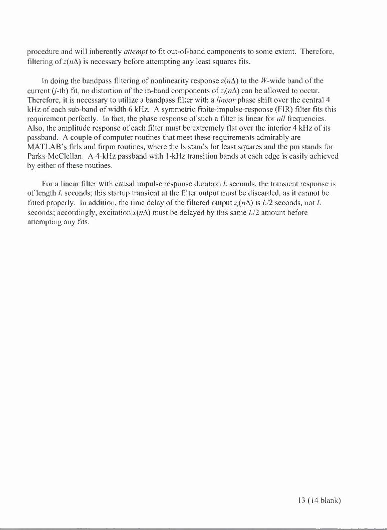
In doing the bandpass filtering of nonlinearity response z(nA) to the ^-wide band of the current (/-th) fit, no distortion of the in-band components of z7{«A) can be allowed to occur. Therefore, it is necessary to utilize a bandpass filter with a linear phase shift over the central 4 kHz of each sub-band of width 6 kHz. A symmetric finite-impulse-response (FIR) filter fits this requirement perfectly. In fact, the phase response of such a filter is linear for all frequencies. Also, the amplitude response of each filter must be extremely flat over the interior 4 kHz of its passband. A couple of computer routines that meet these requirements admirably are MATLAB's firls and firpm routines, where the Is stands for least squares and the pm stands for Parks-McClellan. A 4-kHz passband with 1-kHz transition bands at each edge is easily achieved by either of these routines.

For a linear filter with causal impulse response duration L seconds, the transient response is of length L seconds; this startup transient at the filter output must be discarded, as it cannot be fitted properly. In addition, the time delay of the filtered output z,{nA) is LI2 seconds, not L seconds; accordingly, excitation x(nA) must be delayed by this same LI1 amount before attempting any fits.

13 (14 blank)

4. SECOND-ORDER CONSIDERATIONS

4.1 UNIQUENESS REQUIREMENT

The second-order Volterra component waveform was given in equation (1) as

y2{n)=YdYdh1(kx,ki)x(n-kx)x(n-k2). (24) *,=o t2«o

It must be noted immediately that there can be no unique solution for the second-order time- domain kernel h2(&,,k2). Only the sum

M*l.*2) + *2(*2.*|) (25)

of symmetrically located kernel values (about the 45° line in kx,k2 space) affects output y2(n).

This is due to the symmetry of the product of the two x values in variables £, ,k-, in equation (24). To enable a unique solution for the second-order time-domain kernel, it is necessary to impose some condition. The condition adopted here is to take the second-order kernel to be real and symmetric:

h2(k2,kl) = h2(k],k2). (26)

There is no loss of generality in imposing this symmetry relation on the second-order time- domain kernel h2(kt>k2), because the output y2(n) of equation (24) depends only on the sum in equation (25), no matter what the excitation x(n) is. Also, significant advantage will be taken of this symmetry property, including a reduction in the number of unknown coefficients that must be determined, as well as avoidance of singular matrices.

4.2 PROPERTIES OF THE SECOND-ORDER FREQUENCY-DOMAIN KERNEL

The second-order frequency-domain (complex) kernel corresponding to h2(k]A,k2A) is

A' I K I

#:(/../:) = £ '£lh2(klA,k2A)aqp(ri2xflklA-i2xf2k1A). (27) It, -0 *2 =0

The inverse relation is

h2(klA,k2A) = A2 JJ#, df2 tf2(/1,/2)exp(/2>r/1*1A + /2;r/2*2A). (28)

15

Let the time duration of h2(klA,k2A) in each time dimension be ^seconds, and let the frequency

extent of H2(f],f2) in each frequency dimension be (-F,F) Hz. These limits are identical to

those used for the first-order situation. Then, using symmetry, approximately (2TF)2 /2 samples

are required to completely characterize the real second-order time-domain kernel h2(k]A,k2A). This rapid increase in the number of required coefficients for characterization, in progressing from first order to second order, is the COD.

Since h2(k]A,k2A) is forced to be real, it follows immediately from equation (27) that

H2(-f,-f2) = H2(f[,f2)*. (29)

And, from equations (26) and (27), there follows

H2{f2,fx) = H2(Jx,f2). (30)

That is, the complex second-order frequency-domain kernel H2(fx,f2) satisfies both a

symmetry relation about the +45° line in /,,/2 space, and a conjugate symmetry relation

through the origin of /,, f2 space.

These symmetry properties mean that complex frequency-domain kernel H2(fx,f2) needs

to be specified only in a 90° sector of fx,f2 space; it is then automatically fixed in the rest of the two-dimensional frequency plane. In particular, the "east" sector, composed of the 90° sector centered on the positive fx axis, is adopted as the "fundamental region" in /,,/, space. Mathematically, that is the region

/, >0, -/,</,</,. (31)

Advantage must always be taken of these symmetry properties because they afford a significant reduction in the number of unknowns that must be determined (estimated). Only the values of H2(fx,f2) in the fundamental region (31) need to be specified.

The area of the complete frequency space /,,/2, of extent (-F,F) in each dimension, is

(2F)2. On the other hand, the area covered by equation (31) is only

\dfx \ df2=F2=~(2F)2. (32)

The first factor of 1/2 is due to use of the conjugate symmetry relation (29), while the second factor of 1/2 is due to the symmetry relation of equation (30). These factors constitute a significant reduction in the number of complex coefficients that need to be determined at second order.

16

A seemingly "obvious" partitioning of /, ,/2 space is to take squares of size W x W. If

allowed, this would reduce the COD by the tremendous factor of (F/W)2. However, it is found that the outputs of these individual frequency squares interact and contaminate each other. In addition, it is not obvious how the off-diagonal squares in _/], f2, which cover different

frequency ranges in /, and f2, should be fit to a single band of frequencies of filtered output z(nA).

4.3 ALTERNATIVE FORM FOR SECOND-ORDER OUTPUT y2(nA)

Substitution of equation (28) into equation (24), and interchange of double summation and integration, leads to the relation

y2(nA) = A2 j|#, df2 exp[/2^(/, + /2)nA]H2(fl,f2)X(fi)X(f2). (33)

This is not a double Fourier transform; there is only one time variable on the right-hand side, namely, nA.

The key observation to make at this juncture is that the only place that time variable «A appears on the right-hand side of equation (33) is with the frequency combination f\ + f2. If

second-order Volterra output y2(nA) is to have frequency content only in the band (/„,.//,), for

purposes of fitting to a corresponding filtered version of z(«A), and if X(f) is broadband, then

second-order frequency-domain kernel H2(f\,/,) must be restricted to be nonzero only for

fa < ./', + f: < ft (34)

(and the corresponding negative frequencies). This condition allows the complex exponential in equation (33) to take on frequency variation only in the band (fa,fb ). The region in equation

(34) is definitely not square in /,,/2 space. Rather, see the blue and green regions in figure 2.

Equation (34) describes an infinite strip at angle -45° in the /,,/2 plane, with perpendicular

width (fh - fa)/V2 = W/-J2 . However, the fundamental region is limited to be below the +45°

line in the f,f2 plane; see the red-bordered 90° east region in figure 2. In addition, frequency

/, cannot exceed the limit F. The shape of this finite confined strip in the /,,/: plane is similar

to the shape of the state of Nevada. This is the restricted region of f,f2 space in which

M2(f,,f2) is allowed to be nonzero if y2(nA) in equation (33) is to contain frequency content

limited to the frequency range (fa,fh).

17

Figure 2. Diagonal Strips infjfo Plane

Frequency /,, can start at zero. Also, it is not necessary to let frequency fi, exceed F. It is assumed that there is no frequency content in nonlinearity output z(«A) beyond F. Thus, the fundamental (blue) strip can slide anywhere between the dashed red and black lines. The four yellow Xs represent the locations of the symmetry points of H1 (/,,/,) dictated by equations (29) and (30).

The length of the frequency strip (34) along the -45° line starts at value V2 F for/, = 0.

Therefore, the area covered by each strip is approximately V2 Fx WJ4l ~ FW, not F2 as it would be if frequency partitioning were not employed at all. Thus, the COD has been alleviated (not eliminated) by a factor of WjF through frequency partitioning, a very worthwhile and welcome reduction in many cases. Since the frequency "area" covered by each elemental

complex exponential in equation (17) is (1/71)", the number of unknown coefficients is about

FW/(\/T)2 = TF TW, not (TF)\

IK

4.4 ALTERNATIVE DERIVATION OF RESULT (34)

A Fourier transformation of equation (33) results in spectrum

Y2 (/) = \dfxH2 (/,, / -./;) X{fx )X{f- /,). (35)

In order for Y2(f) to be nonzero only in frequency band (/„,/,,), function H2(fl,f-f]) must

be nonzero only for fa < f < fh. Let f2 = f - /,. Then, / = /*, + f2, from which it then

follows that condition (34) must be satisfied.

4.5 BASIS FUNCTIONS IN TWO DIMENSIONS

The basis functions in one dimension (first order) were derived in equations (17) and (18), starting from an elemental complex exponential in the fundamental range. Here, in two dimensions (second order), the corresponding complex elemental starting function is

\_a{m^m-,) - i b(m{,m2)\ exp iln—-k^-viln—-k2A (36)

where coefficients \a(m],m2)} and {6(/w,,/w.,)} are real, and frequencies /, =mjT and

/: = mz/T are confined to the fundamental (blue) region in the /, ,/2 plane, as described

earlier. The total real function for expanding second-order time-domain kernel /7,(^,A,^2A), using the conjugate and reflective symmetries in equations (29) and (30), respectively, is then (with scaling 1/4=1/2*1/2!)

—[a(m],m2)-i b{m^m2)\ exp(/ A) +—[a(mt,m2)-i 6(/w,,/w2)] exp(/2?)

+ complex conjugate terms

= a(m.,nh) cos(^) + cos(5)

+ b(m.,m,) sin(A) + s'm(B)

where

A 2^A/ Ink, , A = (w, k] + m2 k2), a = (m2ki+mik2).

(37)

(38)

The two basis (bracketed) functions in the second line of equation (37) are obviously real and symmetric in kx,k2, upon use of equation (38), as expected and required. However, their forms are somewhat surprising and not easy to anticipate, without the construction utilized in equation (36) and the first two lines of equation (37).

19

It was pointed out in the sequel to equation (15) that the coefficient b(0) in the first-order case was absent because the corresponding sine term in the expansion was zero for m = 0. A more subtle but related property holds at second order. From equations (37) and (38), a typical term in the sine basis set is

1 . — sin 2

2TTA (m, k. +m^k^)

\ 1 + —sin

2 J (m2 A:, + mlk2)

T ' J (39)

This term is obviously zero for the point m[ = 0, m2 = 0 in fx,f2 space. But equation (39) is

also zero for m] +m2 = 0, even though neither term is zero. This latter condition yields a line in

the two-dimensional frequency plane /,,/,. All of the terms corresponding to this line,

w, + m2 = 0, must be eliminated from the sine basis set in order to avoid a singular matrix in a

second-order fitting process. None of the [cos(/l) + cos(Z?)]/2 terms in equation (37) is zero.

4.6 SECOND-ORDER KERNEL EXPANSION

Combine equations (37) and (38) to form the fundamental second-order basis functions:

c2(m],m2;ki,k2) = — cos

s2(m],m2,kl,k2) = — sin

K

In

K

(m] kt + m2 k2)

(/w, kt +m2k2)

+ — cos 2

1 . — sin 2

2£ K

"2/r

K

(w, k2 +m2ks)

(w, k2 +m2k\)

(40)

using T - KA. Both of these basis functions are symmetric in kf ,k2, and are symmetric in

/w,,/w2. Also,

c2 (0,0;/f, ,k2) * 0; s2(mt -m[;kx,k2) = 0 for all &, ,k2. (41)

For notational convenience, define

c(m,k) = cos In

K mk , A'(/w,&) = sin

In .\

K mk (42)

20

Then, equation (40) can be expanded as

c2(ml ,m2;kl ,k2) = - [c(w, ,kx) c{m2 ,k2) -s(ml ,ki) s(m2,k2)

+ c(m{,k2)c(m2,kl)-s{ml,k2)s(m2, *,)],

(43)

.v,(mx,m2;kl,k2) = -[s(m{,kx)c(m2,k2) + C(/H,,&,) s(/w2,£,)

+ s{mx,k2) c(w2 ,£,)+c(/», ,fc2) 5(m2,£,)].

Now, referring back to equation (37), the expansion for the second-order kernel is given by

h2(*,A,*,A) = - ^ a(w,,m2) [c(/w,,£,)c(m2,k2)-s(m{,k{)s(m2,&,)

+ C(/M, , A-2 )c(m2,kl)-s(m),k2) s(m2, *,)]

1

+ s{m],k2) c(m2,k]) + c{m^k2) s(m2,kx)],

where A/ and A/5 correspond to the particular two-dimensional region of frequency space

/,,/2 in figure 2 that is under investigation. Region Mv is smaller than Mr by virtue of the

comments following equation (39). Second-order kernel h2(klA,k2A) in equation (44) is

symmetric in kt,k2.

4.7 SECOND-ORDER WAVEFORM EXPANSION

As in equations (22) and (42), define sequences

K 1

x (n,m) = ^x(n-k)c{m,k\

(45) K I

xx (n,m) = Y, *(n ~ k) s(m,k). i ii

Sequence \xc(n,m)} is even in m, while {x^{n,m)\ is odd in m. Also, .rv(w,0) = 0 for all n.

These convolution sequences can be calculated just once and stored in two N x M arrays for further processing as needed. Substitution of equation (44) into equation (24), interchange of the double summations, and the use of equation (45) yields the second-order Volterra component in the form

21

^2 (w) = 2 fl^mi»,W2) [^ ("»"»,) jrr (w, m2) - JT, (», m,) x, (w, wi2)]

(46) + 2,b(tnvm2)[xs(n,mt) xc(n,m2) + xc(n,w,)xs(n,m2)],

where duplicate terms have been added together. Both bracketed terms are symmetric in w, ,m2.

This last equation for y2{n) is now in a form ready for use in a least squares fit to a filtered version of nonlinearity output z(n).

4.8 DISCARDING OF EDGE STRIPS AT SECOND ORDER

In an earlier first-order subsection, a method for the discarding of edge coefficients for the first-order fitting procedure was presented. That method can be generalized to second order as follows. The 1-kHz diagonal strip next to the bottom left edge of each 6-kHz diagonal strip in the /i, fa plane must be discarded. That particular 1-kHz diagonal strip in/1,/2 leads to the frequency components of y2(nA) at the lower edge of the {fa,fb) band, namely, to components in the band (fa,fa + 1 kHz).

Similarly, the 1-kHz diagonal strip next to the upper right edge of each 6-kHz diagonal strip must be discarded. Only the interior 4-kHz diagonal strip of each 6-kHz diagonal strip is retained. When the adjacent frequency band comes under investigation for fitting purposes, overlap will again be required. But the next analysis strip will be moved over by 4 kHz, not 6 kHz. Thus, two edge bands are discarded at first order, but two edge strips are discarded at second order. Third order will likely require discarding of edge volumes in the three- dimensional frequency space/1,/2,/3.

4.9 TEST PROCEDURE FOR A FIRST-ORDER AND SECOND-ORDER EXAMPLE

A nonlinear system with known first-order kernel hu,(k]A) and known second-order kernel

h2e(klA,k2A) was excited with stationary random process x{nA). The output z{{nA) of the

first-order kernel hu was computed and stored. Also, the output Z2(A?A) of the second-order

kernel h2e was computed and stored. Finally, the total nonlinear system output

z(«A) = z0 + z, (nA) + z2 (nA) (47)

was computed and stored, as was colored excitation x(nA). See figure 3.

22

NONIINFAR SYSTEM

z(n) 3

•"leW *,<">

SUM FILTER

<Vb>

x(n) zab<nl

hj.Os.y z2(n)

NONLINEAR MODEL (fa,(b)

Vo

1

W ^(n)

SUM V(n) ,

hjftj.y V2(n)

Figure 3. Test Procedure for Second Order

Working only with the recordings of excitation x(nA) and total nonlinear response z(/?A),

the object was to choose real coefficients a(m) and b(m) for first-order Volterra kernel /?, (A",A),

and to simultaneously choose real coefficients a(m[,m2) and b(mx,m2) for second-order

Volterra kernel h2(klA,k2A), such that the total Volterra model output

y(nA) = y0 + v, (nA) + y2(nA) (48)

fitted the filtered waveform zah(nA) as well as possible in a least squares sense.

Five checks can be conducted on the estimates obtained from this control example. Namely, one can compare: estimate A, with the exact hu,\ estimate h2 with the exact h2i,; estimate y{

with the exact z,; estimate y2 with the exact z2; and estimate v with the exact z. In an actual practical situation of an unknown nonlinear system under investigation, the only available comparison will be least squares model response v with nonlinearity response z. This comparison can also be conducted band-by-band in frequency.

23

4.10 INTERPRETATION AND USEFULNESS

The power in the total model output y(nA) relative to the power in total nonlinear output z(nA) measures the goodness of the fit. If only a small fraction of the z(nA) power is accounted for, there may be independent noise generated inside the nonlinear system that can't possibly be fit; the level of this internal noise can be determined by turning off input excitation x(nA) and observing the inherent power in output z(nA). Or the order of the Volterra (or Wiener) model may simply be inadequate and must be increased for a better fit. This would indicate that higher order nonlinearities are present in the system under investigation.

The relative levels of the powers in the total final fits v, (nA) and y2(nA) can be used as indicators of the relative amount of second-order nonlinearity in the system of interest. If the nonlinear power is significant in comparison with the linear power, it will behoove one to account for this nonlinearity in the system in the future.

Volterra kernel estimates /?,(£,A) and h2(k]A,k2A) can now be used to predict the performance of the investigated nonlinear system to different future inputs, without actually having to perform those experiments.

24

SECOND-ORDER NUMERICAL RESULTS FOR THE CONTROL EXAMPLE

The following results were accomplished by frequency partitioning. Figure 4 displays the results for the first-order kernel. The exact kernel hUi(ki) = hn(kl) is drawn in blue (b), and the

estimated model kernel /?, (k{) is drawn in black (k). The error eh] (kt) between them is drawn

in red (r). The estimate is a virtual overlay of the exact kernel; there is a small region at the far right where the red error curve deviates slightly from zero. The ratio of the energy in the error sequence to the energy in the exact kernel sequence is 0.000042.

The corresponding results for the second-order kernel h2(,(ki,k2) = h22(k],k-,) are given in

figures 5 and 6. The estimated model kernel in figure 6 is visually indistinguishable from the exact kernel in figure 5. The ratio of the energy in the error between the two functions to the energy in the exact kernel is 0.00023.

Figure 7 gives the results for a section of the first-order waveforms. The error waveform e,(«) between estimate >>,(«) and exact waveform zt(n) is extremely small and has a relative error energy of 0.000043, the same as for the first-order kernels in figure 4.

The corresponding comparison for the second-order waveforms is presented in figure 8. The variation with time of these second-order waveforms is much more erratic and quicker than for the first-order results in figure 7. This is not unexpected for a second-order nonlinearity. The ratio of error energy to exact energy is 0.00014.

Finally, the total waveform results for estimate y(n) and nonlinearity response waveform z(n) are given in figure 9. The error energy ratio is 0.000042 for this case. This last plot is the only comparison that can be constructed for the practical examples where only input excitation x(n) and nonlinear response z{n) are available.

Two new concepts have been introduced at second order in this investigation. They are the fundamental region (31) and the special basis functions (40) in two-dimensional time space k\, kz. These items are crucial in achieving a satisfactory second-order fit by means of least squares. Also, it was then necessary to eliminate any zero basis functions, and to use overlap and to discard edge estimates that were untrustworthy. The combination of all these items then led to a viable and accurate method of estimating the internal behavior of a second-order nonlinear system with memory.

25

2.5

2

1.5

1

•3 0.5

s o

-0.5

-1.5

j 1 •

i ! : ii • ! -AA Jji , Ik

| T:1 f\ y

| 1

I i I 1 1

1 ! 50 100 150 200 250

time delay index K, 300 350 400

Figure 4. First-Order Kernels hjj(b) hi(k) ehi(r)

n 045

0.4

0.35

0.3

0.25

102

100 2^^^-^r^^-^^^ 100 300 ^OT^T 30°

Figure 5. Exact Second-Order Kernel ht^kuk^

26

100 2m^--~^^r^—^^ 300 ^r^r 3o°

Figure 6. Model Second-Order Kernel Ii2(ki,k2)

4 01 4 02 4 03 4 04 4 05 4 06 4 07 4 08 4 09 4 1 time index n x 10

Figure 7. First-Order Waveforms zi(b) yi(k) e/(r)

27

25 r

20

15

• 10

a. £ 5

-10 _L _L

4.01 4.02 4.03 4.04 4.05 4.06 4.07 4.08 4.09 4.1 time index n x 10

Figure 8. Second-Order Waveforms 12(b) y>2(k) e2(r)

4.01 4.02 4 03 4.04 4.05 4.06 4.07 4 08 4 09 4 1 time index n .^

Figure 9. Waveforms z(b) y(k) e(r)

28

6. THIRD-ORDER CONSIDERATIONS

6.1 UNIQUENESS REQUIREMENT

The third-order Volterra component waveform was given in equation (1) as

v,(«) = Z Z Z *j(*i.*2.*a) *("-*.) x(n-k2) x(n-k3). (49) Ar,=0 A,=0 A,=0

It must be noted immediately that there can be no unique solution for the third-order time- domain kernel h3(kltk2,k3). Only the sum

A3(A:1,A2,*3) + A3(*3,*I,^2) + /j3(^2,^3,*l) + /j3(A:1,^3,*2) + /r3(*2,*,,A:3) + /»3(A:3,^2,^1) (50)

of six symmetrically located kernel values in k],k2,ki space affects output y}(n). This is due to

the symmetry of the product of the three x values in variables k{,k2,k3 in equation (49). To

enable a unique solution for the third-order time-domain kernel, it is necessary to impose some condition. The condition adopted here is to take the third-order kernel to be real and symmetric:

h3(k^k2,k3) = h3(k3,kt,k2) = *,(Jt2,*3,*,) = h,(k^k,,k2) = h3(k2,kltk3) = hy(k},k2,kf).(5\)

There is no loss of generality in imposing this symmetry relation on the third-order time- domain kernel h3{kx,k2,k3\ because the output y3(n) of equation (49) depends only on the sum

in equation (50), no matter what the excitation x(n) is. Also, significant advantage will be taken of this symmetry property, including a reduction in the number of unknown coefficients that must be determined, as well as avoidance of singular matrices.

6.2 PROPERTIES OF THE THIRD-ORDER FREQUENCY-DOMAIN KERNEL

The third-order frequency-domain (complex) kernel corresponding to h}(ktA,k-,A,k}A) is

H3(A,f2,f3)= Z Z Z th(kiA,k2A,k,A) exp(-i2x J\ k,A- i2x f2k2A- i2x j\ k,A).(52) A,=O *:=o A,=O

The inverse relation is

/7,U,A,*AM) = A3 \\\dU df2 df3 //,(/,,./;,/,) exp(;2/r/, k,A + i2jtf2 k2A + i2nf3 *3A).(53)

29

Let the time duration of h3(k{A,k2A,k3A) in each time dimension be T seconds. And let the

frequency extent of //_,(/,, f2,f}) in each frequency dimension be (-F,F) Hz. These limits

are identical to those used for the first- and second-order situations. Then, using symmetry, approximately (27Y7)3 /6 samples are required to completely characterize the third-order time-

domain kernel hy(k]A,k2A,k}A). This rapid increase in the number of required coefficients for

characterization, in progressing from first order to second order to third order, is the COD.

Since hi(klA,k2A,kiA) is forced to be real, it follows immediately from equation (52) that

#3 (-/; -fi -J\ >=#3 (./, Ji >/3) *• (54)

And, from equations (51) and (52), there follows

H3(fl>f2>f,) = H3(f2,fx,f1) = H3(f2,f3,fi)

(55)

= H3(fl,f3,f2) = H3(f2,fl,f3) = H3(J3,f2,fl).

Thus, the complex third-order frequency-domain kernel //_,(/, ,fi,f$) satisfies a conjugate

symmetry relation through the origin of three-dimensional f[,f2,fi space, as well as numerous

symmetry relations.

6.3 ALTERNATIVE FORM FOR THIRD-ORDER OUTPUT v?(«A)

Substitution of equation (53) into equation (49), and interchange of triple summation and integration, leads to the relation

y3 (nA) = A3 \\\df, dj\ df3 exp[i 2 n (./", + f2 + f3) »A] H3 (/,, f2, f3) X{fx) X(f2) X(J\). (56)

This is not a triple Fourier transform; there is only one time variable on the right-hand side, namely, nA.

The key observation to make at this juncture is that the only place that time variable «A appears on the right-hand side of equation (56) is with the frequency combination f{ + f2 + f3.

If third-order Volterra output yy(nA) is to have frequency content only in the band (fa,fh), for

purposes of fitting to a corresponding filtered version of z(nA), and if X(f) is broadband, then

frequency-domain kernel //3 (/,, /,, f3) must be restricted to be nonzero only for

fa </i+/a +A<f„ (57)

30

(and the corresponding negative frequencies). This condition allows the complex exponential in equation (56) to take on frequency variations only in the band (£„.//,). The lower bound in equation (57) describes a plane in three dimensions, while the upper bound describes a parallel plane. The in-between region in equation (57) is an infinite tilted slab in three dimensions.

The restricted frequency region at second order was given in equation (31). That result can be extended to third order by observing that only one of the six equal third-order frequency- domain values in equation (55) needs to be specified. In particular, one selects as the primary case that which satisfies the rule

\j\\<\j\\<\j\\. (58)

This limited three-dimensional frequency region is further reduced by application of equation (54), leading to the final restricted region

|./;|<|./;|<./-,, O<./;<F. (59)

If frequency/i is held fixed at a positive value, this allowed region in the /:,_/j plane consists of two 90° sectors, namely, the east and west sectors. Thus, the shape of the restricted volume in fufi>fi space is a pair of triangular pyramids with one common edge.

Advantage must always be taken of these symmetry properties because they afford a significant reduction in the number of unknowns that must be determined (estimated). Only the values of Hy{f\,f2,fi) in the limited region (59) need to be specified.

The volume of the complete frequency space/1,/2,/3, of extent (-F,F) in each dimension, is (2F) . On the other hand, the volume covered by equation (59) is only

\dj\ \ df2 \dj\=\df, }#22|/2|=J#12/12=|/'3=ii(2F)3. (60)

0 /, |/,| 0 -/, 0

The factor of 1/2 is due to use of the conjugate symmetry relation (54), while the factor of 1/6 is due to the symmetry relations of equation (55). These factors constitute a significant reduction in the number of complex coefficients that need to be determined at third order.

6.4 BASIS FUNCTIONS IN THREE DIMENSIONS

Corresponding to the two-dimensional development in equation (36), the complex elemental starting function in three dimensions (third order) is

tYi fti ni [a{m\,m2,my) -i b(m],m2,m7i)] exp /2;r—-kx/S. + i2n—=-A\A + i2n—-£,A

\ T T T ) (61)

31

(64)

where coefficients \a(m],m2,m})} and {6(W,,AW2,W3)} are real, and frequencies

fx=mjT, f2=m2/T, f3=m3/T (62)

are confined to the region in the /, ,f2 ,/3 plane described in equation (59). Let

a -In A/T = 27r/K, C = a{m^,m2,mi)-i b(m^,m2,m3). (63)

Then, using equation (61), the total elemental real function for expanding third-order time- domain kernel /7?(&,A,/r2A,&3A), using the conjugate and reflective symmetries in equations (54)

and (55), respectively, is, after expansion, simplification, and scaling by 1/12 = 1/2 * 1/3!,

•jy {cexp[/a (wijfc, +m2k2 + miki)] + c exp[ia (/w,£, +m]k2 +m2k})]

+ c exp[/a (m2k] + mik2 +m^ki)] + c e\p[ia (mlk] + w3&, + m,/r3)]

+ c exp[/'«' («?,£, +m]k2 +miki)] + c exp[/a (m}k] +m2k2 +/??,£,)]}

+ complex conjugate terms

= a(w,, m2, m3) va + 6(w,, m2, m3) vb,

where the real basis functions are

v, =| {cos[a(mikl +m2k2 + /w3£3)] + cos[ar(/?73£l + m^k2 + m2k})]

+ cos[a(m2k] + w3£2 +/Ml/r3)] + cos[or(/«lA-| + m^k2 + m-,ky)]

+ cos[a(m2kl + mtk2 + m^k^)] + cos[a(m3£, + m2k2 + mxky)]},

vh =| {sin[a(A?7lAl +m2k2 + w3£3)] + sin[a(/w3£, + m]k2 +w2/:3)]

+ s\n[a (m2k{ + mjk2 + w,A:3)] + sin[ar(w:Al + mik2 + m2k})]

+ sin[a(m2k] +w,/:2 +/w3A3)] + sin[ci'(/w3Al +m2k2 + m,£3)]}.

To minimize computer storage requirements, both functions in equation (65) must be expanded and expressed in terms of the quantities c(m,k) and s(m,k) defined in equation (42). The end results are

va = |[c(/w,,k])tl -sim^k^t, +c{my,k2)ti -s(mi,k2)t4 + c(w,,£3)/5 -.v(m,,^3) /fJ,

(66)

vh =j;[s(m],k])t[ +c(m],k[)t2 +s(mi,k2)ti +c(m[,k2)t4 + s(mx,k3)t5 + c(w,,/:3) t6],

(65)

32

where

(67)

, = c(m2,k2)c(mi,ki)-s(m2,k2)s(mi,ki) + c(m2,k})c(mi,k2)-s(m2,ky)s(m},k2),

2 =s(m2,k2)c(mi,ki) + c(m2,k2)s(mi,ki) + s(m2,ki)c(mJ,k2) + c(m2,ki)s(mi,k2),

3 = c(m2,k3)c(m3,kl)-s(m2,k3)s(m3,kl) + c(m2,kl)c(m3,k3)-s(m2,ki)s(m3,k3),

4 =\(/M2,^)c(/w1,Al) + c'(/??2,^J.9(w1,^l) + ^(w2,^l)c(mj,/:3) + c(w:,^l)5'(w3,A',),

5 =c(/w2,^)c(w1,/:2)-5(/?72,^l).v(/773,^2) + c(/w2,^2)c(/n,,Al)-.v(/w:,^2)5(m1,^,),

6 =i1ffl2,ii)c(ffl3,t) + ctm2,il)s(m,,i2)+5(ffl2^2)c(ffl,,*1) + c(/n,,A,).v(m,^1).

6.5 THIRD-ORDER KERNEL EXPANSION

Thus, from equation (64), the expansion for the third-order kernel is given by

h}(k],k2,ky) = Y, a(mi,m2,m,)vii+Y,b(m],m2,m})vh, (68)

where va and vh are given by equations (66) and (67). Region Mt. is constituted by those

ml,m2,my values in equation (62) that satisfy the conditions in equation (59). Region Mv is

identical to Mc except that the points m[ = 0, m2 + m} - 0 and m2 = 0, m] + m, = 0 and

my = 0, ml + m2 = 0 must be discarded because these particular basis functions v,, in equation

(65) are zero for all kt,k2,k^.

6.6 THIRD-ORDER WAVEFORM EXPANSION

The third-order Volterra component waveform is now given by substitution of equation (68) into equation (49). After expansion, simplification, and use of definitions (42), the result is

>'?(") = X fl('wp'w2i'w3)[^.(^'W|)C(w,/w2,/W3)-jrs.(«,/?7l)5(w,/n2,/w.,)]

+ V /?(wl,w1,w,)[.vv(«,wl) C(n,m2,m3)+xt (/7,w,) 5(n1m2,iR3)],

(69)

where sets of six duplicate terms have been added together, and

C(n, m2 ,m3) = x («, w2) xe (A?, m3) - xs («, m2) xs (n,/w3),

S(n,m2,m}) = x^(n,m2) xe(n,m3) + xc(n,m2) x,(w,/w3).

(70)

33

Both bracketed terms in equation (69) are symmetric in ml,m2,mi and involve only the known

stored arrays xc and xs. Equation (69) is now in a form ready for use in a least squares fit to a

filtered version of nonlinearity output z(n).

34

7. APPLICATION TO A CICADA SONG

7.1 WAVEFORMS AND SPECTRA

A time section of a cicada measurement (number SI 4) is displayed in figures 10 and 11. The data record is about 4 seconds long and the sampling frequency isfs = 96 kHz. The plots in figures 10 and 11 are of laser measurements L\ and Lz of the tymbal movements on both sides of the cicada's body. Figure 12 pertains to a microphone M located a few feet from the insect. The data segment to be analyzed here stretches from time index n = 2.5e5 to n = 3.5e5, which corresponds to approximately 1 second of data. From observation of the microphone data in figure 12, it is obvious that this is a noisy measurement. For example, although the two lasers are giving zero readings for n = 0.4e5 to n = 1.3e5, the microphone output is distinctly nonzero and noisy during this time interval. Therefore, it is expected that this noise continues during the 1-second analysis interval indicated above, and will constitute a portion of output data z(n) that cannot be fitted by a Volterra expansion. The laser measurements are considered as two inputs, x\(n) and x:(/?), to a nonlinear system with memory (the cicada body), while the microphone measurement is considered as the output z(n) of that same nonlinear system.

A blown-up section of duration 0.05 second of laser L2 is presented in figure 13. Although very noisy and jagged, there is obviously a "periodic behavior" of approximately 0.01 second. A sample time segment of 0.01 second is displayed in figure 14. The first-order probability density of the complete laser recording is approximately exponential, not Gaussian. Also, some very- high-frequency components are present in the input data.

The spectra of lasers L\ and Li are plotted in figures 15 and 16. The periodic low-frequency component shows up as a narrowband component centered at 96 Hz, as expected. Both spectra have a great deal of low-frequency content and are fairly flat almost all the way out to the Nyquist frequency of 48 kHz. It appears that the cicada is capable of generating some very-high- frequency components, all the way up to 50 kHz or so. If that is the case, the 96-kHz sampling rate may not have been large enough to avoid some aliasing. Recall that the laser time recordings themselves in figures 10 and 11 are very clean; that is, there is very little noise in these laser recordings. Thus, one has a non-Gaussian and non-white process to use for excitation x(n). This situation is not what one would choose for an excitation if the input were under one's control.

The spectrum for the microphone recording is given in figure 17. There are some pronounced humps at 6 kHz and 8 kHz that bear investigation. There is a strong (unexplained) very narrowband component centered at 39.472 kHz. And, again, the spectrum remains flat almost out to the Nyquist frequency of 48 kHz.

35

a) o

% -0 2

1.5 2 2.5 time index n x 10

Figure 10. Waveform Lj

0.15

0.05

B 0

| -0.051

-0 15 -

1.5 2 2.5 time index n :•: 10"

Figure 11. Waveform Li

36

0)

B

0.01

0 008

0 006

0 004

0 002

0

-0 002

-0 004

-0 006

-0 008

-0.01 0.5 1 1.5 2 2.5

time index n

Figure 12. Waveform M

3.5

x 10

008

2.55 2.555 2 56 2 565 2 57 2.575 2 58 2.585 2 59 2 595 2.6 time index n x 10

Figure 13. Waveform L2 (0.05-SecondSegment)

37

0.08

2.55 2.551 2552 2 553 2.554 2.555 2.556 2.557 2.558 2.559 2 56 time index n x 10

Figure 14. Waveform L2 (0.01-SecondSegment)

60

50

40

30

BO 20

10

0

-10 h

-20 10 15 20 25 30 35 40

frequency (kHz) 45

Figure 15. Spectrum of Waveform L1

38

S 20

5 10 15 20 25 30 35 40 45 frequency (kHz)

Figure 16. Spectrum of Waveform Li

20

10

£ -10

-20

-30

-40

l/V ill...; ;. uL**^dJujUU...

0 5 10 15 20 25 30 frequency (kHz)

35 40 45

Figure 17. Spectrum of Waveform M

39

7.2 FIRST-ORDER FIT

A combined least squares first- and second-order fit was conducted using laser L2 as excitation x(n) and microphone M as nonlinearity response z(n). The optimum first-order

kernel estimate h] is displayed in figure 18. The memory length K was taken as 336, giving a memory duration of 3.5 ms to both the first- and second-order kernels. This duration is apparently long enough to encompass the significant contributions of these kernels, because /?, has decayed by both ends of the fitting interval.

The corresponding estimate of the first-order frequency-domain kernel //, is shown in figure 19. The fitting procedure was limited to 32 kHz; the oscillations beyond this frequency are irrelevant side lobes. The major first-order response occurs between frequencies 4 kHz and 9 kHz. Thus, the high-frequency content observed in response z(n) in figure 17 is not due to a linear effect on input x(n), but is likely due to some nonlinear, higher order effect within the cicada's body itself.

7.3 SECOND-ORDER IDEALIZATIONS

To more easily understand some of the second-order results to be presented for this cicada investigation, it is worthwhile to first consider some idealizations of the second-order kernels, both in the two-dimensional time-delay domain r,, r2 and in the two-dimensional frequency

domain /,,/,. The examples will be taken in the continuous time-delay domain for simplicity; these cases have their direct counterparts in the discrete time-delay domain. The first case is

h2(T],T2) = w(T])S(rt -r2),

(71)

ff2(/i,/2) = ^(/.+/2)>

where w is a broad function, and W is its Fourier transform. This second-order time-domain kernel is a line-impulse function along the 45° line in T]tT2, with a slowly varying envelope w. The second-order frequency-domain kernel is a narrow mountain ridge centered along the -45° line in its domain. The height of the ridge is constant along any -45° line. Both functions in equation (71) are obviously symmetric in their respective domains. The output time waveform corresponding to equation (71) is

y2{t)=\dTMr)x\t-T). (72)

There is memory involved in this squaring device, but there are no "cross-terms" in which two delayed values of x are multiplied together, such as in equations (1) and (24).

40

0 025

E

100 150 200 time delay index k

Figure 18. First-Order Kernel h/(k), \hi(k)\ (:), and Envelope (r)

15 20 25 30 35 40 45 frequency (kHz)

Figure 19. First-Order Kernel H/

41

The second case is

h2(T.,t2) = J^—^ s(r,-r2),

(73)

H2(fl,f2) = W{f]+f2)S\ '/,-/:

The function 5 is a real, even, narrow function, in which case its Fourier transform S is a real, even, broad function. Function w is arbitrary but generally broad. Time-domain kernel h2 has a ridge concentrated near the 45° line but has a slowly varying amplitude governed by w. Frequency-domain kernel H2 is concentrated near the -45° line and has a slowly varying amplitude governed by S. The time-domain waveform corresponding to kernel (73) is

'r.+O y2 (t) = jj dxx dz2 w — s(r[ - r,) x(t - r,) x(t - r,), (74)

which has limited-extent cross terms, governed by the duration of s.

The third case is given by

ft2(r,,r2) = 2cos[2>r/t(r, +r,) + /?] w 'r.+O S(T, -T2),

H2 (/,, f2) = [exp(/ p) W(j\ + f2 - fL) + exp(-/ /?) W{fx +f2+ fL)] S\ fi-f2^ (75)

Frequency f) causes the ridge of Wlo move up and down in the /,,/2 plane by the value of /, and thereby creates two ridges parallel to the ^5° line. If s(0) = 0, then the time-domain kernel

//2(r,,r2) is zero for r2 = r,, which is the central +45° line. Combinations of different

functions w and s, along with different parameter values for f, and /? lead to a wide variety of

possibilities for the two second-order kernels h2 and H2.

The estimate of the second-order time-domain kernel h2 for laser L2 of cicada song S14 is displayed in figures 20 and 21. Since this kernel has a very-high-frequency behavior, it oscillates considerably in r, and r2. Accordingly, it has been rectified and smoothed so that it is easier to observe where its major contributions occur. Figure 20 is for an elevation observation angle of 35°, while figure 21 is a top (90° elevation) view. There is a pronounced contribution along two symmetrically displaced lines at +45° and a deep null along the main +45° line. These behaviors are consistent with those anticipated by equations (71), (73), and (75). The locations of the main energy are near the lines where |£2 -£,| = 220. At the sampling

frequency of 96 kHz, this corresponds to a time delay of 2.3 ms in the cross terms of y2(n).

42

0 0

Figure 20. Smoothed Second-Order Kernel |/r^| (Observation Elevation Angle 35°)

0 50 100 150 200 250 300

Figure 21. Smoothed Second-Order Kernel \h2\ (Observation Elevation Angle 90°)

43

The estimate of the second-order frequency-domain kernel H2 for laser L2 is displayed in figures 22 and 23, the former for an observation elevation angle of 50° and the latter for an elevation angle of 90° (top view). The strong response (red line in figure 23) centered at /, + f2 = 0 corresponds to a strong, low-frequency component in second-order model response

y2(n), while the two strong spread lines centered at /] + f2 = ±6 kHz correspond to the spectral hump for microphone waveform z{n) in figure 17. It can be seen from figure 23 that the

second-order frequency-domain kernel H2(fltf2) responds very well all the way up to 32 kHz, which was the highest frequency fitted. But that large response only takes place in the second and fourth quadrants of /,,/> space, which is the region where difference frequencies are created. There is very little response in the first and third quadrants; note that figures 22 and 23 are in dB. (The horizontal and vertical white streaks in figure 23 above 32 kHz should be ignored; they are due to a malfunction in producing the MATLAB .tif plots for inclusion in a Microsoft Word document. Several trials yielded these same results with streaks.)

It is not valid to compare the level of h2 with the level of A,; these two time-domain kernels don't even have the same dimensions; this can be seen from equation (1), where an extra .v multiplication takes place at second order. The same comment applies to attempting to compare the level of frequency-domain kernel H2 with the level of H]; these two quantities don't have the same dimensions either. The only valid comparison of levels is in terms of the Volterra model output waveforms y, (n) and y2(n), which always do have the same dimensions and which are the same as those of z{n).

A plot of a section of the fitted first-order waveform y, (n) is given in figure 24. It has no jagged behavior, as was present in microphone output z(«) in figure 12 or in laser input x(n) in

figures 13 and 14. This is consistent with the estimated first-order frequency-domain kernel //, in figure 19, which has its major response below 15 kHz.

The corresponding spectrum Yt (/) of y, (n) is displayed in figure 25. Its major contribution is in the frequency band from 5 to 9 kHz; this compares favorably with the result for the first-order frequency-domain kernel H{ in figure 19. It should be noted in figure 25 that the zero-frequency level is approximately the same as the major response level at 8 kHz. In contrast, in figure 19, the zero-frequency level is significantly below that at 8 kHz. This difference is due to the fact that the excitation x(n) of laser L2 has a much higher spectral level near zero frequency than at 8 kHz, as can be seen in figure 16.

44

20

frequency (kHz)

dff . 40.

m 20. .•!' MKJH L "J

•a ^^^•H^H iB 0.

-20. ' ^^H

4 D ^^

-20 -20

30

20

10

-40 frequency (kHz)

Figure 22. Second-Order Kernel H2 (Observation Elevation Angle 50°)

-40 -30 -20-10 0 10 20 30 40 frequency (kHz)

Figure 23. Second-Order Kernel Hi (Observation Elevation Angle 90°)

45

x1(T

0) •o

£ 0

401 4.02 4.03 4.04 4.05 4.06 4 07 4.08 4 09 41 time index n .^

Figure 24. First-Order Waveform yi

m -a

20 25 30 frequency (kHz)

Figure 25. First-Order Spectrum Y/

46

A section of second-order Volterra component waveform y2(n) is illustrated in figure 26.

It has a somewhat more jagged behavior than first-order waveform v, («) in figure 24. The

corresponding spectrum Y2(f) of v2(«) is given in figure 27. A pronounced spectral

contribution of Y2 is centered at 6 kHz with a peak value of 7 dB. The first-order spectrum Y] in figure 25 has a peak value of only -3 dB. This 10-dB difference is due to the second-order frequency-domain kernel results for H2 in figures 22 and 23. Namely, it is the ± 6-kHz ridges

of H^ in figure 23 that are creating difference frequencies in the neighborhood of 6 kHz. Here,

it is valid to make these quantitative comparisons of levels between F, and Y2, because the same

spectral estimation techniques and parameters were used on yt(n) and y2(n), which have the same dimensions.

The corresponding section of total Volterra fit y(n) is plotted (in red) in figure 28, superposed on the measured microphone response z{n) (in black). As can be seen, there are time segments where the total fit is especially good, and other time segments where the fit is poor. This is partially attributed to the fact that only laser L2 was used for this least squares fit.

There is the additional input from laser Lt that was totally ignored during this single-input least squares fit.

All the fitting results thus far have been for laser L, of cicada song S14 considered as the

input. For the fitting results in figure 29, laser I, was used instead as the input x(n). The

measured microphone output z(n) is plotted in black, fit yx(n) is plotted in blue, and fit y2(n) is plotted in red. For this segment of time, the first-order fit is extremely small, while the second-order fit does a decent job of mimicking output z(»). In fact, for this particular time

segment, the ratio of powers in v,(«) to z(n) is 0.036, while the ratio of powers in y2(n) to z(n) is 0.68. This example, along with figure 28, brings out the point that the cicada with two laser measurements and one microphone measurement should be considered as a /no-input, one- output nonlinear system with memory. That is, the block diagram in figure 1 is not general enough to encompass this generalization. More will be said on this observation below.

Results for a different cicada example (namely, song S9) are given in figures 30 and 31 for lasers L, and L2, respectively. Again, the measured microphone output z(n) is plotted in

black, fit y,(«) is plotted in blue, and fit y2(n) is plotted in red. The fractional power fit of total

waveform y{n) to output z(n) in figure 30 for laser L, is 0.25 at the left edge of the figure, but 0.92 at the right edge of the figure. By contrast, the fractional power fit of total waveform y(n)

to output z(n) in figure 31 for laser L2 is 0.78 at the left edge of the figure, but 0.24 at the right edge of the figure. This example serves to further support the fact that different tymbals (lasers) are contributing to different portions of the time waveform emitted from the cicada. The only way to properly calculate the relative strengths of these components is by way of a two-input, one-output Volterra model.

47

x 10-

4 4.02 4.0 4.04 4.05 4.06 4 07 4 0 4.09 4.1 -4 time index n

Figure 26. Second-Order Waveform y>2

x 10

10

-5 •

-10

§ -15

-20

-25

-30

-35

-40

iiii 1 T - |

J

\ ••;••

• •• • iMiUUl. • .i

i i i 1 1 iT

10 15 20 25 30 35 40 45 frequency (kHz)

Figure 27. Second-Order Spectrum Y2

48

x 10"

4 0 4.02 4 0 4 04 4.05 4 06 4 07 40 40 41 ,4 time index n

Figure 28. Total Waveforms z(k) y(r)

x 10

x10"

2.005 2.01 2015 202 2025 time index n x 10

2.03 4

Figure 29. Waveforms z(k) yt(b) y>2(r) (Laser L2 of Cicada Song S14)

49

x10J

607 6.08 609 6.1 6.11 6 12 6 13 6 14 6 15 6 16 6 17 time index n .rf

Figure 30. Waveforms z(k) yi(b) y2(r) (Laser L} of Cicada Song S9)

x10"'

6.07 6.08 609 6.1 6.11 6 12 6 13 6.14 6 15 6 16 6 17 time index n x 10

Figure 31. Waveforms z(k) yi(b) y2(r) (Laser L2 of Cicada Song S9)

50

8. SECOND-ORDER, TWO-INPUT, ONE-OUTPUT VOLTERRA MODEL

A Volterra model of a second-order, two-input, one-output system is given in figure 32. The two inputs are now labeled x{ (n) and x2 (n). There are now five required kernels that must all

be estimated from simultaneous recordings of laser inputs xt(n) and x2(n) and microphone

response z(n). The number of subscripts on the kernels h denotes their order, either first order or second order. A new type of kernel must now be employed, namely, a "cross-kemer hr(k],k2), which has tnv inputs and one output and which yields a second-order waveform

J'i:(") = X X M*i,k2)xx(n-kx) x2(n-k2)

(76)

= A2 JJ^#2exp[/2^(./l+/2)/7A]//12(./l,/2)^,(y;)A'2(/2).

However, time-domain cross-kernel hi2(kt,k2) need not be symmetric, because two different inputs X are multiplied in the first line of equation (76). Therefore, the only symmetry relation satisfied by its corresponding second-order frequency-domain kernel is

Hl2(-j\-f2) = Hl2(J\,f2)*, (77)

which follows from the imposed realness of h]2(k],k2).

If Volterra output v12(«) is to have frequency content only in the band (/0,/6), for

purposes of fitting to a band-limited version of z(n), and if X{{f) and X2(f) are broadband,

the second line of equation (76) reveals that one must have frequency-domain kernel Hn{fx,f2) nonzero only for

fu<\fl+fl\<A, •

just as in equation (34). Therefore, it will be necessary to let variables /,,/: in figure 2 range not only over the blue region, but, in addition, over its green extension into the second quadrant. The number of unknown (complex) coefficients for Hv will be equal to the sum of the number

of coefficients required for each of H',, and //-,,. This larger number of coefficients will significantly increase the effort required in the least squares procedure.

The basis functions for the h]2(k]A,k2A) kernel are given by one-half of equation (36) and its conjugate (but not using the symmetry property in the top line of equation (37)), namely,

O(/M,,/M2) cos(A)+ h(ml,m2) sin(A), (79)

51

where A is given by equation (38). The b(m] ,-w,) terms must again be dropped from the basis set.

Vn)

x,(n)

*,<•>)

Vn<n)

y12(")

y22(n)

y2(n)

Vo

1

SUM y(n)

Figure 32. Second-Order, Two-Input, One-Output Volterra Model

52

9. SUMMARY

Several new concepts have been introduced to achieve some alleviation of the curse of dimensionality in determining the higher order kernels in a Volterra expansion. These include: partitioning of the frequency scale(s), the fundamental region of formation, the diagonal strips in the two-dimensional frequency space, the second- and third-order basis functions, and filtering of the measured nonlinear output to the current frequency band under investigation. The equations for the real basis functions at second and third order take some unexpected forms that could probably not be anticipated. These results were based on taking full advantage of symmetry and conjugate-symmetry frequency-domain relations that exist for real, symmetric, second-order and third-order, time-domain kernels. The inability to construct ideal bandpass filters requires the use of a frequency-overlap procedure, followed by the discarding of edge estimates with inherent errors, and the retention of only the interior estimates of higher accuracy.

Application to a first- and second-order (noise-free) control example with a white broadband excitation gave excellent estimates of all the first- and second-order properties, such as the individual kernels, the individual Volterra waveforms, and the total estimated output waveform. Application to a cicada mating call with a distinctly non-white and non-Gaussian excitation gave good results for the estimated first- and second-order kernels and waveforms, considering the non-optimality of this type of excitation. However, if the design of the input excitation to a nonlinear system with memory is under the user's control, the ideal excitation to use is a white, Gaussian process. Better correlation properties ensue and smaller condition numbers prevail in this latter situation.

The reduction factor in the number of coefficients to be determined at each frequency partition is given by WIF, where Wis the bandwidth of the frequency interval under investigation, and F is the largest frequency of interest, typically near the Nyquist frequency. This factor applies at all orders and is helpful in alleviating the curse of dimensionality, but does not eliminate it.

53 (54 blank)

INITIAL DISTRIBUTION LIST

Addressee No. of Copies

Defense Advanced Research Projects Agency (Attn: D. Furey) 1

Center for Naval Analyses 1

Defense Technical Information Center 2

Albert Nuttall, Old Lyme, CT 10

Duncan Sheldon, Portsmouth, Rl 1

Martin Schetzen, Brookline, MA 1