Embed Size (px)
Citation preview

Soft Computing in Investment Appraisal
Antoaneta SerguievaDept. of Economics&Finance
Brunel UniversityUxbridge UB8 3PH, UK
John HunterDept. of Economics&Finance
Brunel UniversityUxbridge UB8 3PH, UK
Tatiana KalganovaDept. of Electronic&Computer Eng.
Brunel UniversityUxbridge UB8 3PH, UK
Abstract
Standard financial techniques neglectextreme situations and regards large marketshifts as too unlikely to matter. Suchapproach accounts for what occurs most ofthe time in the market, but does not reflectthe reality, as major events happen in therest of the time and investors are ‘surprised’by ‘unexpected’ market movements. Analternative fuzzy approach permitsfluctuations well beyond the probabilitytype of uncertainty and allows one to makefewer assumptions about the datadistribution and market behaviour.Fuzzifying the present value criteria, wesuggest a measure of the risk associatedwith each investment opportunity andestimate the project’s robustness towardsmarket uncertainty. The procedure isapplied to thirty-five UK companies tradedon the London Stock Exchange and a neuralnetwork solution to the fuzzy criterion isprovided to facilitate the decision-makingprocess. Finally, we suggest a specificevolutionary algorithm to train a fuzzyneural net - the bidirectional incrementalevolution will automatically identify thecomplexity of the problem andcorrespondingly adapt the parameters of thefuzzy network.
Keywords: Finance, Evaluating fuzzyexpressions, Neural networks, Evolutionaryalgorithms.
1 Introduction
Investment projects are typically chosen on the basisof a restricted information set, while the volatility
literature claims that stock prices are too volatile toaccord with simple present value models. Toapproach the problem, we model the restrictedinformation and incorporate price uncertainty intocalculations. Uncertain share prices and dividendyields, associated with a family of possible streamsof future cash flows, as well as uncertain discountrates are handled by the introduction of fuzzyvariables, whose values are restricted by possibilitydistributions. Alternatively, fuzzy numbers aresuggested with corresponding membershipfunctions. Increasing the range of uncertaintymodelled by the fuzzified data, we determine therobustness of the investment risk associated witheach project. Neural networks yield a mechanism tofacilitate the solution of the fuzzy criterion. Oncetrained to evaluate a project, a neural net providesinvestors with a simple re-evaluation tool when theinformation available is subject to change. Finally,as a direction for future research, we suggest a fuzzyneural net, as it will directly handle fuzzy marketdata, and recommend the bidirectional incrementalevolution as an effective training mechanism.
2 Net present value models
NPV evaluations are increasingly being used in theUK [14,17]. The technique is broadly adopted inpractice, managers are comfortable with it, and it isreasonable to consider the fuzzy alternative to takeaccount of more general forms of uncertainty. Fig. 1describes the interrelations between standard andsoft computing techniques as well as betweentheoretical and empirical research, all involved intothe process of formulating the fuzzy criterion.1
The standard NPV formula has been continuously
1 For a detailed discussion, see [19].
revised. It has been realised that the removal of anyof the perfect market assumptions destroys thefoundation and reduces the effectiveness of themethod. We do not attempt to cope with a specificdrawback of the technique but permit into the modelstructure as much uncertainty as the market couldpossibly suffer. The calculation based on thestandard criterion may be re-optimised due toinvestment irreversibility [8] and altered because ofthe effect of capital and labour market rationing [15]or impact of a project on the investor’s total risk[20]. Whatever reason one has for modifying theclassic result, the allowances provided by the fuzzycriterion will cover these specific circumstances andwill include the modified values. The outcome is aneffective method under restricted information,uncertain data and market imperfections.
Fuzzy net present value was first introduced in [2],then considered in a broader framework ofaccumulation and discount models in [6], andrecently modified with an alternative fuzzification ofthe project duration in [13]. All these studies aretheoretical. The major difference here is theemphasis we place on the empirical results - weevaluate 35 projects investing in UK companiestraded on the LSE. Concurrently, it is the analysis ofthe empirical results that facilitates the formulationof measures for the investment risk and the projectrobustness towards market uncertainty, and assiststhe definition of an alternative ranking technique.Thus the fuzzy criterion evolves into a considerablyinformative and advantageous to investors method.Further, we build a neural network to solve the fuzzyinvestment criterion. In result, investors are providedwith an effortless instrument for risk re-evaluation,any time they update a project. We also suggest afuzzy neural net and recommend an effectiveevolutionary training algorithm. In conclusion,
combining the advantages of various softmethodologies, the article balances empirical andtheoretical results, with the driving force being theinvestor's benefit.
3 Investment project evaluation using a fuzzycriterion with a constant discount rate
We apply two methods of evaluating fuzzy algebraicexpressions from [3]. First, if positive real triangularfuzzy numbers tP
~ , tYD~ and R
~ are substituted forthe share price Pt , dividend yield DYt and discountrate R, then FNVP
~ is the triangular-shaped fuzzynumber providing a set of values that belongs to thepresent value with various degrees of membership.Form the α-cuts of the price time-seriesP~
(α)= tP~
(α) and the dividend-yield time-series
YD~
= tYD~
for 1≤t≤N, and find FNPVΩ (α).
( ) [ ]( ) ∏
= î
≤α<α≥µ=α=α
N
1t tPtPt
tcta
10,P~
|x|x0,P,P
P~
(1a)
( ) [ ]( ) ∏
= î
≤α<α≥µ=α=α
N
1t tDYtDYt
tcta
10,YD~
|x|x0,DY,DY
YD~
(1b)
( )( ) ( )
( ) ( ) ( )α∈α∈α∈î
++
+=αΩ
××
=∑
R~
R,YD~
DY,P~
P|
|R1
PR1
DYP
N1N1
NN
N
1tttt
PVFN (1c)
Then the first solution is defined by µ( FNPVx | FNVP~
):
µ( FNPVx | FNVP~
)=sup α| FNPVx ∈ FNPVΩ (α) (1d)
Second, if tP
, tYD
and R
are positive real fuzzyvariables with triangular possibility distributionsPoss[ tP
=xPt]=µ(xPt| tP
~), Poss[ tYD
=xDYt]=µ(xDYt| tYD
~)
and Poss[ R
=xR]=µ(xR|R~
), correspondingly, thenFVVP
is the fuzzy variable, whose values are
possible solutions to the fuzzy present value criteria.Form the joint possibility distribution of share-pricetime-series and dividend-yield time-seriesπP=
Nt1min
≤≤ Poss[ tP
=xPt] =
Nt1min
≤≤µ(xPt| tP
~) (2a)
πDY=Nt1
min≤≤
Poss[ tYD
=xDYt] =Nt1
min≤≤
µ(xDYt| tYD~
) (2b)
and find the joint possibility distribution FVPVπ ,
FVPVπ =min πP,πDY,Poss[ R
=xR] (2c)
assuming that tP
, tYD
and R
are non-interactive.Then, the possibility distribution of the secondsolution is
Poss[ FVVP
=FVPVx ]=sup
FVPVπ |FVPVx =
( ) ( )NN
N
1tt
tt
R1P
R1DYP
++
+∑=
(2d)
The two solutions are identical but we present themboth, as the first provides the computational
Fuzzy LogicZadeh, 1965
NeuralNetworks
EvolutionaryAlgorithms
Soft Computing
Applications to Financial Eng.
Applications to Financial Eng.
Applications to Financial Eng.Financial
Engineering
StandardTechniques
theoreticalmodifications
[8,15,20]
Fuzzy Net Present Valuetheoretical [2,6,13]
NPV
empiricalstudies, [14,17]
Soft Computing inFinancial Engineering, [16]
Soft Computing in Present Value Criteriontheoretical and empirical studies,
[proposed paper]
Fig. 1: Interrelations in investment appraisal techniques standard and soft computing; theoretical and empirical studies
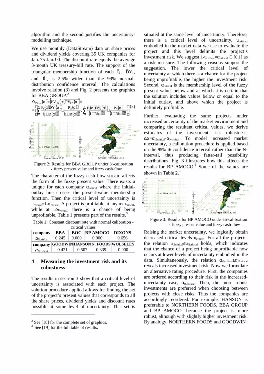
Figure 3: Results for BP AMOCO under t6-calibration fuzzy present value and fuzzy cash-flow
algorithm and the second justifies the uncertainty-modelling technique.
We use monthly (DataStream) data on share pricesand dividend yields covering 35 UK companies forJan.’75-Jan.’00. The discount rate equals the average3-month UK treasury-bill rate. The support of thetriangular membership function of each tP
~ , tYD~ ,
and R~ , is 2.5% wider than the 99% normal-
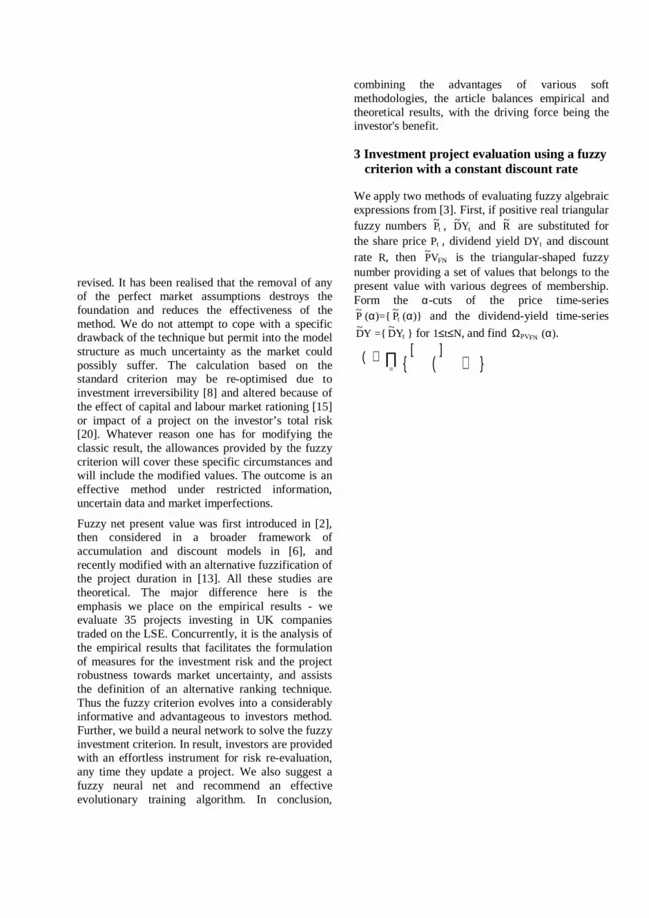
distribution confidence interval. The calculationsinvolve relation (3) and Fig. 2 presents the graphicsfor BBA GROUP.2
( ) ( ) ( )[ ]( ) ( )
( )( )( )( )( )
( ) ( )( )( )
( )( )( )
α+α+
α+αα
α+
α+
α+
αα=
=αα=αΩ
∑∑==
NN
N
1tt
ttN
NN
1tt
tt
FNFNPV
R1
P
R1
DYP,
R1
P
R1
DYP
PV,PVFN
(3)
The character of the fuzzy cash-flow stream affectsthe form of the fuzzy present value. There exists aunique for each company αcritical where the initial-outlay line crosses the present-value membershipfunction. Then the critical level of uncertainty isucritical=1-αcritical. A project is profitable at any u<ucritical,while at u≥ucritical there is a chance of beingunprofitable. Table 1 presents part of the results.3
Table 1: Constant discount rate with normal calibration -critical values
company BBA BOC BP AMOCO DIXONSαNcritical 0.245 0.000 0.000 0.656
company GOODWIN HANSON N. FOODS WOLSELEY
αNcritical 0.421 0.507 0.339 0.000
4 Measuring the investment risk and itsrobustness
The results in section 3 show that a critical level ofuncertainty is associated with each project. Thesolution procedure applied allows for finding the setof the project’s present values that corresponds to allthe share prices, dividend yields and discount ratespossible at some level of uncertainty. This set is
2 See [18] for the complete set of graphics.3 See [19] for the full table of results.
situated at the same level of uncertainty. Therefore,there is a critical level of uncertainty, ucritica,embodied in the market data we use to evaluate theproject and this level delimits the project’sinvestment risk. We suggest 1-ucritical=αcritical ∈ [0,1] asa risk measure. The following reasons support thesuggestion. The lower the critical level ofuncertainty at which there is a chance for the projectbeing unprofitable, the higher the investment risk.Second, αcritical is the membership level of the fuzzypresent value, below and at which it is certain thatthe solution includes values below or equal to theinitial outlay, and above which the project isdefinitely profitable.
Further, evaluating the same projects underincreased uncertainty of the market environment andcomparing the resultant critical values, we deriveestimates of the investment risk robustness,∆α=αt6critical-αNcritical. To model increased marketuncertainty, a calibration procedure is applied basedon the 95% t6-confidence interval rather than the N-interval, thus producing fatter-tail possibilitydistributions. Fig. 3 illustrates how this affects theresults for BP AMOCO.2 Some of the values areshown in Table 2.3
Raising the market uncertainty, we logically obtaindecreased critical levels ucritical. For all the projects,the relation ut6critical≤uNcritical holds, which indicatesthat the chance of a project being unprofitable nowoccurs at lower levels of uncertainty embodied in thedata. Simultaneously, the relation αt6critical≥αNcritical
reveals increased investment risk. Now we formulatean alternative rating procedure. First, the companiesare ordered according to their risk in the increased-uncertainty case, αt6critical. Then, the more robustinvestments are preferred when choosing betweenprojects with close risks. Thus the companies areaccordingly reordered. For example, HANSON ispreferable to NORTHERN FOODS, BBA GROUPand BP AMOCO, because the project is morerobust, although with slightly higher investment risk.By analogy, NORTHERN FOODS and GOODWIN
Figure 2: Results for BBA GROUP under N-calibration fuzzy present value and fuzzy cash-flow
! " # $ % & ' ( ) * *
+ ,-. ,/ 0
12 34 5
6782 96
←: ; < = >
← α ? @ A B A ? C D E F G H I J
K L M NO PQ R S T U NO V
Q R W NX YZ [ \ W NX O
] L ^ NV _` a b NV P
Z R c Nd d
efgX_ d_ edd h P _
i j k j l m n l o m p q r s p m t u v w x xy z| z~
¡ ¡
¢ £¤¥ £¦§¨© ª
« ¬®¯© °
←± ² ³ ´ µ
← α ¶ · ¸ ¹ ¸ ¶ º » ¼ ½ ¾ ¿ À Á
K L M NO PQ R S T U NO V
Q R W NX YZ [ \ W NX O
] L ^ NV _` a b NV P
Z R c Nd d
P_ d_ Pe de Pdd h P _
i j k j l m n l o m p q r s p m t u v w x xy z| z~

are preferable to BBA GROUP and BP AMOCO.
Table 2: Constant discount rate -investment risk robustness and project rating
company αt6critical rating ∆α robustness new ratingBBA 0.527 3rd 0.282 low 6thBOC 0.000 1st 0.000 high 1st
BP AMOCO 0.529 4th 0.529 none 7thDIXONS 0.713 8th 0.057 high 8th
GOODWIN 0.575 7th 0.154 medium 5thHANSON 0.573 6th 0.066 high 3rdN. FOODS 0.543 5th 0.204 medium 4th
WOLSELEY 0.000 1st 0.000 high 1st
Remember that the standard method will not quitedistinguish between the above projects, as they allhave a positive crisp net present value. The generallyaccepted technique will not tell us how to choosebetween projects with close crisp net present values.It will not reveal whether projects with higher NPVare less robust and less preferable. The standardresults are less informative and can be misleading.
5 Investment project evaluation using a fuzzycriterion with a time-varying discount rate
The assumption of time-varying returns transformsthe price-dividend relation into nonlinear and aloglinear approximation is required. We equate thelog present value lpv with the log share-priceestimation p at t=0. Then a project is profitable iflpv0= 0p >p0. The real fuzzy numbers to be substitutedfor the log share-price pt, log dividend-yield dyt andlog discount-rate rt, are correspondingly tp~ , tyd
~ , tr~ .The level-log data transformation causes triangular-shaped rather then triangular membership functionsfor tp~ , tyd
~ and tr~ . Now find the α-cut
( ) ( )( )[ ]( ) ( ) ( )α∈α∈α∈
î ρ+−++ρ−ρ=αΩ
×××
=
−∑r~r,yd
~dy,p~p|
|prkpdy1
N1N1N1
NN
N
1tttt
1tfnlpv (4a)
Then the first solution for the fuzzy log presentvalue is defined by its membership function,µ( fnlpvx | fnvp~l )=sup α| fnlpvx ∈ ( )αΩ fnlpv (4b)
By analogy with section 3, the triangular-shapedpossibility distribution of the second solution isPoss[ fvvpl
Â= fvlpvx ]=sup fvlpvπ =min πp,πdy,πr |
| fvlpvx = ( )( )[ ] NN
N
1tttt
1t prkpdy1 ρ+−++ρ−ρ∑=
− (5)
where the possibility distributions of the real fuzzyvariables tp
Ã, tyd
Ä and tr
Å are described by
Poss[ tpÆ
=xpt]=µ(xpt| tp~ ), Poss[ tydÇ
=xdyt]=µ(xdyt| tyd~
) and
Poss[ trÈ
=xrt]=µ(xrt| tr~ ), respectively. The two solutionsare identical, as
fnvp~l (α)= ( )αΩ fnlpv = fvlpvx |Poss[ fvvplÉ
= fvlpvx ]≥α ,0≤α≤1
and the calculations include
( ) ( ) ( )[ ] ( ) ( ) ( )( ) ( )[ ]( ) ( ) ( ) ( )( ) ( )[ ] ( )
αρ+α−+α+αρ−ραρ+
α−+α+αρ− ρ=αα=αΩ
∑
∑
=
−
=
−
NN
N
1tttt
1tN
N
ttt
N
1i
1tfnfnlpv
prkpdy1,p
rkpdy1lpv,lpvfn
We consider the t6-calibration and the assumption ofa time-varying discount rate enforces theemployment of N fuzzy numbers tr~ , 1≤t≤N. Table 3includes part of the results. We have not furtherincreased the uncertainty modelled in the t6-data,only introduced a variable discount rate. But acomparison between the t6 constant and time-varying results reveals characteristics similar toincreased market uncertainty: ulogcritical≤ut6critical≤uNcritical
and αlogcritical≥αt6critical≥αNcritical. Further, when projectsare assessed under t6 calibration and a time-varyingdiscount rate, real market conditions are approached,and this allows an improved evaluation of theinvestment risk and its robustness. Table 3 repeatsthe ranking procedure from the previous sectionwith the new results. The projects are first orderedaccording to the risk αlogcritical, then the order isrefined corresponding to the robustness indicator∆αlog=αlogcritical-αNcritical.
Table 3: Time-varying discount rate -risk robustness and project rating
company αlogcritical rating ∆αlog robustness new ratingBBA 0.696 5th 0.451 low 6thBOC 0.000 1st 0.000 high 1st
BP AMOCO 0.904 6th 0.904 none 7thDIXONS 1.000 u n p r o f i t a b l e
GOODWIN 0.925 7th 0.504 low 6thHANSON 0.673 4th 0.166 medium 3rdN. FOODS 0.656 3rd 0.317 low 4th
WOLSELEY 0.092 2nd 0.092 high 2st
6 Using neural networks to evaluate thefuzzy criterion
In this section, we apply a technique for evaluatingfuzzy expressions suggested in [4,5] and train aneural network to evaluate investment projectsaccording to the fuzzy present value criterion. Thetime-varying-rate case is considered and the three-layer feedforward neural net in fig. 4 is employed.For bias terms θj, sigmoidal transfer functionsg(x)=(1+e-x)-1 and weights wj i, uji, zji, vj , its output is
lpvnn= ( )∑ ∑= =
θ+++
m
1j
N
1ijijiijiijij dyzrupwgv . (6a)

Let us imply that the network is trained toapproximate the crisp log-present value:
lpvnn≈∑=
−ρN
1i
1i [(1-ρ)(dyi+pi)+k-ri]+ρnpn . (6b)
If we input the α-cuts of ip~ , ir~ , iyd~
, and performinterval arithmetic within the net to get thecorresponding α-cut of the fuzzy output nnvp~l , theresult is
( ) ( )[ ] ( ) ( )[ ] ( ) ( )[ ](( ) ( )[ ]) ) ( ) ( )(
( ) )) ( ) ( ) ( )( )
θ+α+α+αθ+α+
+α+α=θ+αα+
+αα+αα∗=αα
∑ ∑
∑ ∑
∑∑
= =
= =
==
m
1j
N
1ijijiijiijijjiji
m
1j
N
1iijiijijjiiji
N
1iiijiiiji
m
1jjnnnn
yd~
zr~up~wgv,yd~
z
r~up~wgvyd~
,yd~
z
r~,r~up~,p~wgvvp~l,vp~l
In order vp~l nn to be an approximation to the solution
fnvp~l described earlier and to provide that vp~l nn>0
for fnvp~l >0, the following sign restrictions areintroduced on the weights.wji≥0, uji<0, zji≥0, vj≥0, 1≤i≤N, 1≤j≤m, (6c)Then, if the net is trained to approximate (6b) under(6c), we get
( ) ( )[ ] ( ) ( ) ( )( ) ( ) ( ) ( ) ( ) ( )( ) ( ) ( )
αρ+α−+α+αρ−ραρ+
+α−+α+αρ−ρ≈αα
∑
∑
=
−
=
−
NN
N
1iiii
1iN
N
N
1iiii
1innnn
p~r~kp~yd~
1,p~
r~kp~yd~
1vp~l,vp~l(6d)
The problem is programmed using the neuralnetwork toolbox of Matlab4. We choose the trainingfunction trainlm based on the Levenberg-Marquarttechnique, as it is the fastest backpropagationalgorithm available. The toolbox allows functioncustomisation giving the user control over the
4 All programmes in Sections 3, 4, 5, 6 are written in Matlab.
initialising, simulating and training algorithms. Wehave modified trainlm to provide the satisfaction ofthe sign constraints. After training, the net issimulated using test vectors for each project, whileno element of the training set is included in the testset. For all companies, ss
setargtnetmax − ≤0.021 and
for most of them sss
etargtnetmax − ≤0.01, where s
stands for the s-th element of the test set. It is a goodapproximation and concludes that fnnn vp~lvp~l ≈ .
If an investment decision has to be taken within aperiod of time, we can first fuzzify the data using theinformation available at the beginning of the periodand then train a neural network to approximate thefuzzy log present value of the project. The decision-maker will be provided with the trained network andat any moment he or she acquires new information,the net will be simulated with modified inputs.
7 Future research
If one fuzzify the 3N-m-1 network structure fromFigure 4, it will handle fuzzy signals - fuzzy marketdata - at once instead of α-cut by α-cut. The fuzzynetwork takes fuzzy weights and fuzzy shift terms.The error of the approximation E is a distancemeasure D between the fuzzy log-present value
fnvp~l and the fuzzy neural net output fnnvp~l .
( )( ) ( )( )[ ]( )))2N,,1,N,,1,N,,1N
N
N
1i
N
1iiii
1iN
1i
2fnnfn
r~r~yd~
yd~
p~p~fnn,p~
r~kp~yd~
1DL1vp~l,vp~lD
LlE
ÊÊÊρ+
+−++ρ−ρ== ∑ ∑∑
= =
−
=
Evolutionary algorithms are the most promising toolin training FNN - they are well capable of searchingfor the optimal weights and shits while minimisingE. As N is very large, a scalability problem occurs.To solve it, we suggest a specific algorithm,bidirectional incremental evolution. The incrementalevolution is applied in training neural networks in[9], where a control problem in evolutionaryrobotics is approached. Unfortunately, it requiresadvanced knowledge of the complexity of theproblem. The bidirectional incremental evolutionallows us to overtake this problem. Its majoradvantages are the automatic identification of thecomplexity of the task, and the automatic change inthe parameters so that the system adapts to thecomplexity. Bidirectional incremental evolution hasbeen already applied in evolvable hardware [12] andthe experimental results have proved it to be apowerful technique for tuning systemsautomatically.
p1
r1
pN
rN
1
N
2N
N+1
w11
w1N
u11
u1N
w21w2Nu21u2N
1
2
m
wm1wmNum1
umN
1
v1
v2
vm
lpvnn
dy1 2N+1
3NdyN
z11
z1N
z21
z2N
zm1
zmN
Figure 4: Neural net architecture to solvethe fuzzy log present value problem

7 Future research
Our effort lies on the bridge towards a new paradigmof investment selection, where the perception ofconcepts inherent or surrounding the investmentprocess, whose character is not principallymeasurable, is best handled by ’nonnumeric’mathematics. [1] We presented some preliminaryideas in [11] and further develop here the technique,introducing fuzzy dividend yields and a second typeof calibration. We suggest measures of theinvestment risk and its robustness. Also neuralnetwork solution is worked out and the number ofcompanies is considerably extended. Finally apromising direction for future research is outlined.
The results reveal that there is a critical level ofuncertainty, ucritical, embodied in the market data weuse to assess a project and this level delimits theproject’s investment risk, αcritical. Evaluating thesame project under increased uncertainty of themarket environment, we derive an estimate of therisk robustness ∆α. Investment opportunities arefirst rated in correspondence with their risk and thenthe order is revised according to their robustness.The more robust investments are preferable whenchoosing between projects with close risks, and thissuggests an alternative ranking technique. It isimportant for investors to pick out projects havingnot only a small but also a highly robust investmentrisk. The fuzzy present value provides them with thenecessary information and facilitates their decision,while the crisp technique is less informative andeven misleading. Further, empirical tests haveconvinced financial analysts that stock returns aretime-varying rather than constant. In response, weintroduce fuzzy log present value. Finally, a trainedneural network provides investors with an effortlessinstrument for risk revaluation, any time they needto update and reconsider a project.
The mathematics underlying the standard financialtechniques neglects extreme situations and regardslarge market shifts as too unlikely to matter. Suchtechniques may account for what occurs most of thetime in the market, but the picture they present doesnot reflect the reality as major events happen in therest of the time. The soft computing approach allowsfor market fluctuations well beyond the probabilitytype of uncertainty, does not impose predefined dataor market behaviour, and efficiently works out asolution, producing better investment appraisal andallowing project revaluation.
AcknowledgementsThe authors are grateful to Prof. James Buckley forhis comments on the initial draft.
References[1] J. Aluja (1996). Towards a New Paradigm of Investment
Selection in Uncertainty. FSS, 84, 187-197.[2] J. Buckley (1987). The Fuzzy Mathematics of Finance.
FSS, 21, 257-273.[3] J. Buckley (1992). Solving Fuzzy Equations. FSS, 50, 1-14.[4] J. Buckley, E. Eslami, Y. Hayashi (1997). Solving Fuzzy
Equations Using Neural Nets. FSS, 86, 271-278.[5] J. Buckley, T. Feuring (1999). Fuzzy and Neural:
Interactions and Applications. Physica-Verlag,Heidelberg.
[6] M. LiCalzi (1990). Towards a General Setting for theFuzzy Mathematics of Finance. FSS, 35, 281-293.
[7] J. Campbell, A. Lo, A. MacKinlay (1997). TheEconometrics of Financial Markets. Princeton U. Press.
[8] Dixit, R. Pindyck, S. Sodal (1997). A MarkupInterpretation of Optimal Rules for IrreversibleInvestment. National Bureau of Economic Research WP,W5971.
[9] D. Filliat, J. Kodjabachian, J. Meyer (1999). IncrementalEvolution of Neural Controllers for Navigation in a 6-legged Robot. In Sugisaka and Tanaka, Eds., Proc. of the4th Int. Symp. on Artificial Life and Robots, Oita U.Press.
[10] F. Gomez, R. Miikkulainen (1997). IncrementalEvolution of Complex General Behaviour. AdaptiveBehaviour, 5, 317-342.
[11] J. Hunter, A. Serguieva (2000). Project Risk EvaluationUsing An Alternative To The Standard Present ValueCriteria. Neural Network World, 10, 157-172.
[12] T. Kalganova (2000). Bidirectional IncrementalEvolution In Extrinsic Evolvable Hardware. In J. John,A. Stoica, et al, Eds., Proc. of the 2nd NASA/DoDWorkshop on Evolvable Hardware, 65-74.
[13] D. Kuchta (2000). Fuzzy Capital Budgeting. FSS, 111,367-385.
[14] R. Pike (1996). A Longitudinal Survey on CapitalBudgeting Practices. J. Business Finance & Accounting,23, 79-92.
[15] M. Precious (1987). Rational Expectations, Non-marketClearing and Investment Theory Clarendon Press,Oxford U. Press.
[16] R. Ribeiro, H.-J. Zimmermann, R. Yager, J. Kacprzyk,Eds. (1999). Soft Computing in Financial Engineering,Physica-Verlag, Heidelberg.
[17] A. Sangster (1993). Capital Investment AppraisalTechniques: A Survey of Current Usage. J. BusinessFinance & Accounting, 20, 307-332.
[18] A. Serguieva, mimeo, Brunel University, 2001.[19] A. Serguieva, J. Hunter (2000). Investment Risk
Appraisal, Deprt. of Economics & Finance WP, 00-15,Brunel U.
[20] R. Stulz (1999). What is Wrong with Modern CapitalBudgeting? Address delivered at the Eastern FinanceAssociation meeting, Miami Beach.
[21] L. Zadeh (1965). Fuzzy Sets. Information & Control, 8,338-353.