COST-BENEFIT ANALYSIS FOR INVESTMENT DECISIONS,

CHAPTER 15:

COST-EFFECTIVENESS AND COST-UTILITY ANALYSIS

Glenn P. Jenkins

Queen’s University, Kingston, Canada and Eastern Mediterranean University, North Cyprus

Chun-Yan Kuo

Queen’s University, Kingston, Canada

Arnold C. Harberger University of California, Los Angeles, USA

Development Discussion Paper: 2011-15 ABSTRACT The capital expenditure appraisal process has so far been presented in the framework of a cost benefit analysis where all benefits and costs are expressed in monetary values. However, many projects or programs undertaken by governments produce benefits that may be considered to be highly desirable but whose quantification in monetary terms is difficult if not impossible. Common examples of such projects are the provision of elementary school education, improvements in the provision of health care services, investment in public security and the administration of justice. In such cases, a full cost benefit analysis may not be feasible for each individual project or program but a cost-effectiveness analysis (CEA) can be carried out. Such an analysis measures the quantities of benefits generated in terms of the number of units of the items produced, but no attempt is made to convert these into monetary values. This chapter outlines a methodology for conducting cost effectiveness analysis and discusses it usefulness and its limitations. Further extensions of cost effectives are made into topics of cost utility analysis, and the limitations of cost effectiveness. To be Published as: Jenkins G. P, C. Y. K Kuo and A.C. Harberger, “Cost-Effectiveness And Cost-Utility Analysis” Chapter 15.Cost-Benefit Analysis for Investment Decisions. (2011 Manuscript) JEL code(s): H43 Keywords: Cost Effectiveness, Cost Utility Analysis, Daly, Qaly, Marginal Cost Effectiveness.

CHAPTER 15:

1

CHAPTER 15

COST-EFFECTIVENESS AND COST-UTILITY ANALYSIS

15.1 Introduction

The capital expenditure appraisal process has so far been presented in the framework of a

cost benefit analysis where all benefits and costs are expressed in monetary values. However,

many projects or programs undertaken by governments produce benefits that may be

considered to be highly desirable but whose quantification in monetary terms is difficult if

not impossible. Common examples of such projects are the provision of elementary school

education, improvements in the provision of health care services, investment in public

security and the administration of justice. In such cases, a full cost benefit analysis may not

be feasible for each individual project or program but a cost-effectiveness analysis (CEA)

can be carried out. Such an analysis measures the quantities of benefits generated in terms of

the number of units of the items produced, but no attempt is made to convert these into

monetary values.

Cost-effectiveness analysis can be very useful at ranking the various activities that could be

undertaken by a government department when the alternatives address a common set of

objectives. For example, what is the most cost-effective way to generate electricity? Once

the spending priorities are defined between the broad functions of government, the scarce

budget funds can be allocated among projects within each of these functional areas based on

the results of a cost-effectiveness analysis. Projects with a lower priority and smaller positive

outcome are often shifted to the next budget period, when they can be considered again

along with the other options available at that time.

Section 15.2 lays out the concepts of cost-effectiveness. Section 15.3 discusses the

alternative ways of conducting the cost-effectiveness analysis, as well as its applications and

limitations. Section 15.4 describes the general methodology for using cost-utility analysis.

Sections 15.5 and 15.6 present the practical use of cost-utility analysis to education and

CHAPTER 15:

2

health projects, respectively. Conclusions are presented in the final section.

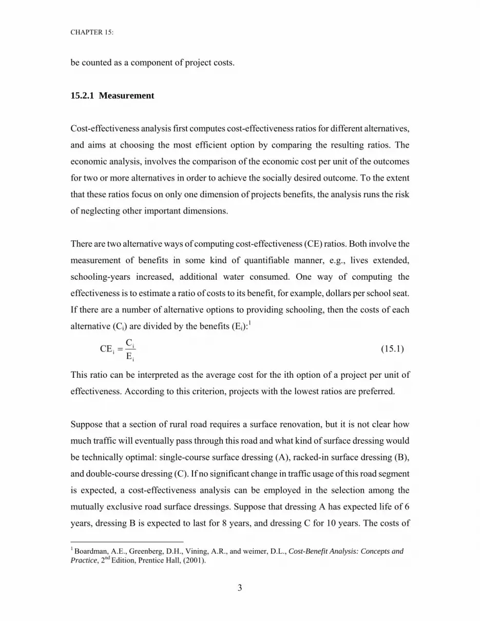
15.2 Cost-Effectiveness Analysis

When project benefits cannot be quantified in monetary terms, one can nonetheless choose

among the alternative options based on the one that achieves a given outcome at least cost. A

standard cost-effectiveness analysis in fact involves a series of steps similar to those of a

cost-benefit analysis. The main difference is that the outcomes of the project are measured in

physical units rather than be given monetary values. The focus is therefore on measuring the

costs of the alternatives.

When a project or program lasts for several years, it is important to include all relevant

capital and operating costs over the project’s life in the calculation. Capital costs include

expenditures on machinery, equipment and structure such as schools, hospitals and clinics,

equipment, vehicles, etc. Operating or recurring costs include office supplies, drugs, utilities,

wages and salaries of teachers, doctors, nurses and other staff. The cost-effectiveness of the

project should be calculated by dividing the present value of total costs of the option by the

present value of a non-monetary quantitative measure of the benefits it generates. The ratio is

an estimate of the amount of costs incurred to achieve a unit of the outcome from each of the

alternative options under consideration. For example, what are the costs (expressed in real

dollars) of adding a year to a person’s expected life when assessing different healthcare

interventions?

The analysis does not attempt to measure benefits in monetary terms, it is rather to find the

least-cost option to achieve a desired quantitative outcome. The costs should be measured at

their resource costs in the economic analysis. They should include not only direct costs but

also indirect and intangible costs. For example, in evaluating the impacts of alternative

higher education proposals one must include the forgone earnings of the individuals while

they are attending schools as part of the costs of obtaining a higher education in addition to

attendance fees, transportation costs and other project costs. In a project delivering medical

treatment, the time patients devote to waiting or traveling to hospitals or clinics should also

CHAPTER 15:

3

be counted as a component of project costs.

15.2.1 Measurement

Cost-effectiveness analysis first computes cost-effectiveness ratios for different alternatives,

and aims at choosing the most efficient option by comparing the resulting ratios. The

economic analysis, involves the comparison of the economic cost per unit of the outcomes

for two or more alternatives in order to achieve the socially desired outcome. To the extent

that these ratios focus on only one dimension of projects benefits, the analysis runs the risk

of neglecting other important dimensions.

There are two alternative ways of computing cost-effectiveness (CE) ratios. Both involve the

measurement of benefits in some kind of quantifiable manner, e.g., lives extended,

schooling-years increased, additional water consumed. One way of computing the

effectiveness is to estimate a ratio of costs to its benefit, for example, dollars per school seat.

If there are a number of alternative options to providing schooling, then the costs of each

alternative (Ci) are divided by the benefits (Ei):1

i

ii E

CCE = (15.1)

This ratio can be interpreted as the average cost for the ith option of a project per unit of

effectiveness. According to this criterion, projects with the lowest ratios are preferred.

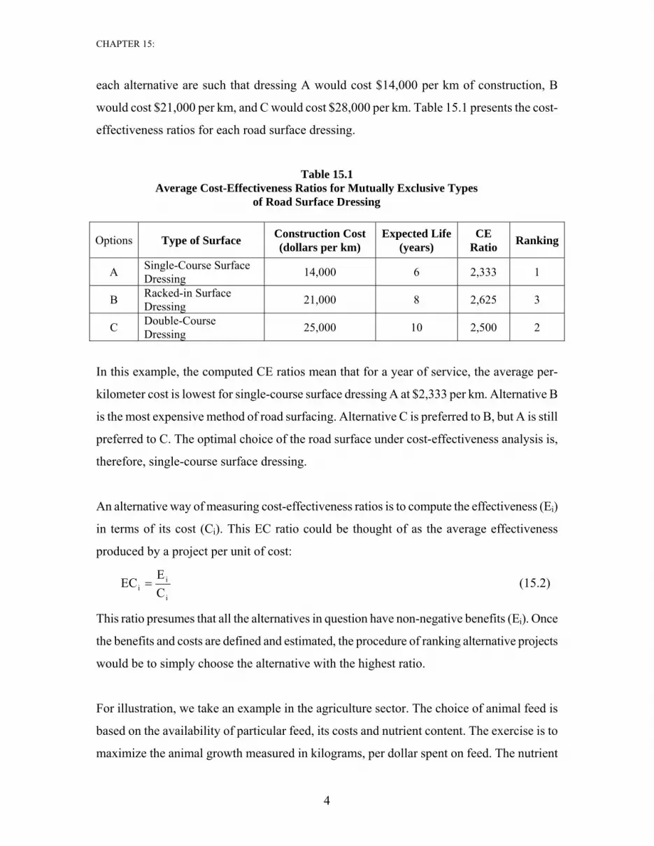
Suppose that a section of rural road requires a surface renovation, but it is not clear how

much traffic will eventually pass through this road and what kind of surface dressing would

be technically optimal: single-course surface dressing (A), racked-in surface dressing (B),

and double-course dressing (C). If no significant change in traffic usage of this road segment

is expected, a cost-effectiveness analysis can be employed in the selection among the

mutually exclusive road surface dressings. Suppose that dressing A has expected life of 6

years, dressing B is expected to last for 8 years, and dressing C for 10 years. The costs of

1 Boardman, A.E., Greenberg, D.H., Vining, A.R., and weimer, D.L., Cost-Benefit Analysis: Concepts and Practice, 2nd Edition, Prentice Hall, (2001).

CHAPTER 15:

4

each alternative are such that dressing A would cost $14,000 per km of construction, B

would cost $21,000 per km, and C would cost $28,000 per km. Table 15.1 presents the cost-

effectiveness ratios for each road surface dressing.

Table 15.1 Average Cost-Effectiveness Ratios for Mutually Exclusive Types

of Road Surface Dressing

Options Type of Surface Construction Cost (dollars per km)

Expected Life (years)

CE Ratio Ranking

A Single-Course Surface Dressing 14,000 6 2,333 1

B Racked-in Surface Dressing 21,000 8 2,625 3

C Double-Course Dressing 25,000 10 2,500 2

In this example, the computed CE ratios mean that for a year of service, the average per-

kilometer cost is lowest for single-course surface dressing A at $2,333 per km. Alternative B

is the most expensive method of road surfacing. Alternative C is preferred to B, but A is still

preferred to C. The optimal choice of the road surface under cost-effectiveness analysis is,

therefore, single-course surface dressing.

An alternative way of measuring cost-effectiveness ratios is to compute the effectiveness (Ei)

in terms of its cost (Ci). This EC ratio could be thought of as the average effectiveness

produced by a project per unit of cost:

i

ii C

EEC = (15.2)

This ratio presumes that all the alternatives in question have non-negative benefits (Ei). Once

the benefits and costs are defined and estimated, the procedure of ranking alternative projects

would be to simply choose the alternative with the highest ratio.

For illustration, we take an example in the agriculture sector. The choice of animal feed is

based on the availability of particular feed, its costs and nutrient content. The exercise is to

maximize the animal growth measured in kilograms, per dollar spent on feed. The nutrient

CHAPTER 15:

5

contribution of a particular feed to the process of growth of animal is measured in amount of

nutrient per unit of feed. A feed with a richer content is preferred to a type with lower

nutrition content. For each animal type, there are detailed programs stipulating a minimum

daily requirement of nutrition components for a healthy and rapid weight growth. The

alternatives are such that the necessary amount of daily nutrition component, for example

protein, could be secured through either an expensive fish-meal or by using cheaper

sunflower oilcake but in a larger volume.

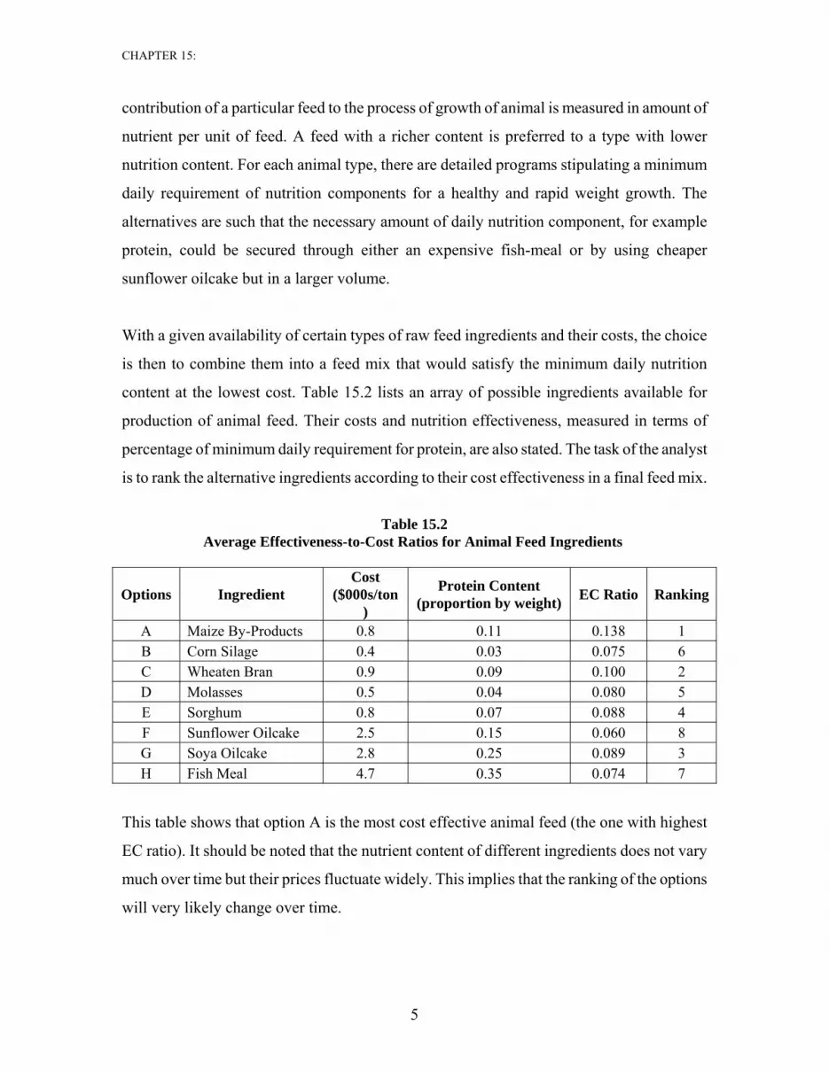
With a given availability of certain types of raw feed ingredients and their costs, the choice

is then to combine them into a feed mix that would satisfy the minimum daily nutrition

content at the lowest cost. Table 15.2 lists an array of possible ingredients available for

production of animal feed. Their costs and nutrition effectiveness, measured in terms of

percentage of minimum daily requirement for protein, are also stated. The task of the analyst

is to rank the alternative ingredients according to their cost effectiveness in a final feed mix.

Table 15.2

Average Effectiveness-to-Cost Ratios for Animal Feed Ingredients

Options Ingredient Cost

($000s/ton)

Protein Content (proportion by weight) EC Ratio Ranking

A Maize By-Products 0.8 0.11 0.138 1 B Corn Silage 0.4 0.03 0.075 6 C Wheaten Bran 0.9 0.09 0.100 2 D Molasses 0.5 0.04 0.080 5 E Sorghum 0.8 0.07 0.088 4 F Sunflower Oilcake 2.5 0.15 0.060 8 G Soya Oilcake 2.8 0.25 0.089 3 H Fish Meal 4.7 0.35 0.074 7

This table shows that option A is the most cost effective animal feed (the one with highest

EC ratio). It should be noted that the nutrient content of different ingredients does not vary

much over time but their prices fluctuate widely. This implies that the ranking of the options

will very likely change over time.

CHAPTER 15:

6

15.2.2 Marginal Cost-Effectiveness Ratio

When we evaluate several alternative options to the existing situation, we need to compute

incremental or marginal cost-effectiveness ratios. In the computation, the numerator refers to

the difference between the cost of the new and the existing alternatives (i.e., Ci and C0) while

the denominator shows the difference between the effectiveness of the new and the existing

alternatives (i.e., Ei and E0):

(15.3)

This ratio represents the incremental cost per unit of effectiveness. When there are several

alternatives available, the marginal cost-effectiveness ratio should be the one used to rank

the new measures versus the existing situation.

An illustration of this ratio is given below with a hypothetical example of the prevention of

deaths from traffic accidents. The ultimate goal is to minimize the number of traffic

accidents on the roads per year. Assume that there has been a program (A) in place that has

already reduced the number of accidents over past years. Now, an additional reduction in

accidents and resulting fatalities is desired, and this could be achieved in a number of

alternative ways. First, the system of tracking and prosecution of road speeder could be

enhanced, and this will involve more police officers on the roads (B). Second alternative is to

improve the roads condition, and to equip the roads with additional safety signs and

markings (C). Third way is to run a continuous public awareness campaign (D).

Let’s assume that the existing policy, which has been in place for years, costs $20.0 million

and it effectively prevents numerous accidents as well as some 500 related deaths a year.

Also assume that the alternative B would prevent another 100 deaths and cost $5.5 million

per year. Alternative C is estimated to cost $11.5 million and result in additional reduction of

500 fatalities every year. The third policy, alternative D, may reduce the road casualties by

additional 85 cases, and its costs are projected to be about $5.0 million a year. Table 15.3

illustrates the computation of marginal cost-effectiveness ratios and their ranking. The cost-

effectiveness ratio for options B, C, and D are marginal, since they represent an incremental

Oi

Oii EE

CCCE Marginal−−

=

CHAPTER 15:

7

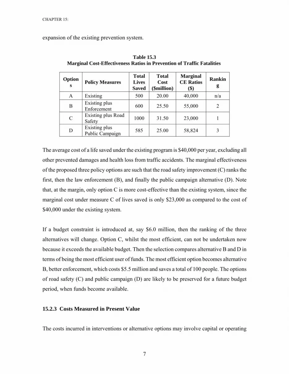
expansion of the existing prevention system.

Table 15.3 Marginal Cost-Effectiveness Ratios in Prevention of Traffic Fatalities

Options Policy Measures

Total Lives Saved

Total Cost

($million)

Marginal CE Ratios

($)

Ranking

A Existing 500 20.00 40,000 n/a

B Existing plus Enforcement 600 25.50 55,000 2

C Existing plus Road Safety 1000 31.50 23,000 1

D Existing plus Public Campaign 585 25.00 58,824 3

The average cost of a life saved under the existing program is $40,000 per year, excluding all

other prevented damages and health loss from traffic accidents. The marginal effectiveness

of the proposed three policy options are such that the road safety improvement (C) ranks the

first, then the law enforcement (B), and finally the public campaign alternative (D). Note

that, at the margin, only option C is more cost-effective than the existing system, since the

marginal cost under measure C of lives saved is only $23,000 as compared to the cost of

$40,000 under the existing system.

If a budget constraint is introduced at, say $6.0 million, then the ranking of the three

alternatives will change. Option C, whilst the most efficient, can not be undertaken now

because it exceeds the available budget. Then the selection compares alternative B and D in

terms of being the most efficient user of funds. The most efficient option becomes alternative

B, better enforcement, which costs $5.5 million and saves a total of 100 people. The options

of road safety (C) and public campaign (D) are likely to be preserved for a future budget

period, when funds become available.

15.2.3 Costs Measured in Present Value

The costs incurred in interventions or alternative options may involve capital or operating

CHAPTER 15:

8

expenditures that are spread over many years. Capital projects usually have large investment

outlays at the beginning and then recurrent costs and their benefits are spread over many

subsequent years. The costs and benefits should be both discounted to a common time period

in order to make a comparison of alternative options. Because the benefits are measured in

physical units, the effectiveness in quantity should be discounted by the same rate as the

costs. Thus, the proper cost-effectiveness ratio for the ith option can be expressed as follows:

i

ii ess EffectivenofPV

CostsofPVCE = (15.4)

After the cost-effectiveness ratios are computed for each of the alternative options, the

analyst can rank the alternatives and take a decision.

The question of what is the appropriate discount rate to use in the social projects or programs

is often raised, especially in the health projects. This will be addressed later.

15.2.4 Limitations of the Analytical Technique

There are some concerns of using cost-effectiveness analysis. These issues are discussed

below.

a) Does not Measure Willingness to Pay

Cost-effectiveness ratios are a poor measure of consumers’ willingness to pay. For example,

most of the taxpayers would probably be happy to pay for the prevention of an additional

number of deaths being caused by traffic accidents. But what is the willingness to pay for the

prevention of deaths of drug addicts? Furthermore, the number of addicts treated or the

number of lives saved through the treatment of drug addicts generally stands for the

effectiveness of a medical intervention. However, it may not be the best measure for which

people are willing to pay. In the case of a program to reduce drug addiction will both save

lives and also reduce the incidence of crime. It is likely the crime reduction impact that the

taxpayers are willing to pay most for. Faced with this kind of situation, the analyst must

make sure that the link is made to the ultimate impact valuable for which people are willing

to pay for to obtain an accurate assessment of the relative worth of the proposed

CHAPTER 15:

9

interventions.

b) Excludes Some External Benefits

Cost-effectiveness analysis excludes most externalities on the benefit side. It looks only at a

single benefit and all other benefits are essentially ignored. For example, an improvement in

education will not only increase life-time earnings of the students but also likely to

contribute to a reduction in the rates of unemployment and crime. In healthcare, there are

external benefits due to such treatments as the vaccination of children because the disease is

not spread to others. The analyst undertaking the evaluation should be careful not to exclude

important benefits arising from a particular project.

c) Excludes Some External Costs

As was pointed out earlier, while computing the cost-effectiveness ratio for a particular

project, attention should also be paid to the treatment of social costs beyond direct financial

costs. Different types of projects often have some of the costs in non-monetary value, such as

coping costs, enforcement costs, regulatory costs, compliance costs, and forgone earnings.

The economic cost-effectiveness analysis carried out for such projects must account for all

costs, measured at the resource costs rather than the financial costs of goods and services.

d) Does Not Account for Scale of Project

Scale differences may distort the choice of an “optimal” decision when a strict cost-

effectiveness analysis is employed. A project with smaller size but higher efficiency level

may get accepted, while another project may provide more quantity of output at a reasonable

cost. A complete cost benefit analysis does not have this problem because the present value

of net benefits already accounts for the difference in size among alternative projects.

15.3 Constraints in the Level of Efficiency and Budget

This section deals with the scale problem in cost-effectiveness analysis by introducing a

constraint, either on the maximum acceptable cost or on the minimum acceptable level of

CHAPTER 15:

10

effectiveness.2

a) Minimum Level of Effectiveness

When the objective is to achieve a minimum level of effectiveness, then the analysis simply

looks for the lowest cost solution (Ci) ensuring the minimum effectiveness level. That is,

Minimize Ci (15.5)

Subject to Ei ≥ Ē

This approach assumes that there is little value in exceeding the target effectiveness level.

Any additional units of effectiveness beyond Ē are not valued in the analysis, i.e., only the

total cost is minimized but not the cost per unit. This approach results in the selection of the

cheapest alternative that satisfies the minimum effectiveness criterion, even if there are other

alternatives that offer more units of effectiveness at lower per unit cost. This rule generally

favors projects with low total cost. Often, the lowest total cost does not constitute the best

project.

With the criterion (15.5), additional units of effectiveness may be still worth something but

not accounted for. Instead of selecting the cheapest alternative in terms of total cost, the

decision makers may like to select an alternative with the lowest per unit cost. Then, an

adjusted project selection criterion is used in which the minimum CEi ratio is chosen such

that the effectiveness is greater than the specified threshold level:

Minimize CEi (15.6)

Subject to Ei ≥ Ē

This new criterion (15.6) ensures a higher effectiveness level and likely to result in higher

costs than the unconstrained cost-effectiveness ratio (15.5). The project selected under this

rule is generally larger in size and more cost efficient.

2 Boardman, A.E., Greenberg, D.H., Vining, A.R., and weimer, D.L., Cost-Benefit Analysis: Concepts and Practice, Second Edition, Prentice Hall, (2001).

CHAPTER 15:

11

b) Maximum Budget Constraint

The other side of the same coin is the problem of maximizing the level of effectiveness

subject to a budget constraint. If the budget is fixed then the intuitive solution is to choose an

alternative that generates the most benefits. That is,

Maximize Ei (15.7)

Subject to Ci ≤ C

Under this rule, any cost savings beyond C are not accounted for, and selection only looks

for maximization of total efficiency, but not efficiency per dollar of spending, i.e.,

incremental cost savings are ignored. This fails to make a sensible choice in a situation when

two alternatives achieve exactly the same total efficiency but have different costs, both

below or equal to the minimum cost C . Because both alternatives have costs below the

budget limit, and both result in the same total efficiency, then the two alternatives would be

ranked the same.

An alternative solution to this problem is to do the project selection on the basis of the

lowest CEi ratio, which fits the budget constraint:

Minimize CEi (15.8)

Subject to Ci ≤ C

This rule (15.8) now effectively places some value on incremental cost savings. It selects the

most cost-efficient alternative, subject to a budget constraint.

15.4 Application: Olifants-Sand Water Transfer Scheme3

The growth in water demand over time by the various water users in Polokwane, Capricorn

District, and Sekhukhune Cross Border District in South Africa is rapidly using up all the

available water resources. Six groups of water users have been identified including, the

3 This section is extracted from the “Capital Project Selection Handbook for Department of Education”,

CHAPTER 15:

12

Provincial capital area, Polokwane, Lebalelo Water User Association (WUA), the mining

companies, smaller town centers, irrigation demands, and the rural communities.4

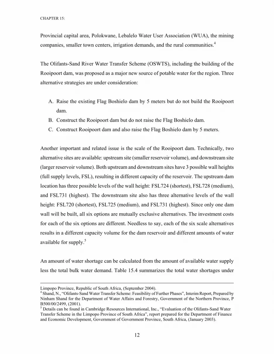
The Olifants-Sand River Water Transfer Scheme (OSWTS), including the building of the

Rooipoort dam, was proposed as a major new source of potable water for the region. Three

alternative strategies are under consideration:

A. Raise the existing Flag Boshielo dam by 5 meters but do not build the Rooipoort

dam.

B. Construct the Rooipoort dam but do not raise the Flag Boshielo dam.

C. Construct Rooipoort dam and also raise the Flag Boshielo dam by 5 meters.

Another important and related issue is the scale of the Rooipoort dam. Technically, two

alternative sites are available: upstream site (smaller reservoir volume), and downstream site

(larger reservoir volume). Both upstream and downstream sites have 3 possible wall heights

(full supply levels, FSL), resulting in different capacity of the reservoir. The upstream dam

location has three possible levels of the wall height: FSL724 (shortest), FSL728 (medium),

and FSL731 (highest). The downstream site also has three alternative levels of the wall

height: FSL720 (shortest), FSL725 (medium), and FSL731 (highest). Since only one dam

wall will be built, all six options are mutually exclusive alternatives. The investment costs

for each of the six options are different. Needless to say, each of the six scale alternatives

results in a different capacity volume for the dam reservoir and different amounts of water

available for supply.5

An amount of water shortage can be calculated from the amount of available water supply

less the total bulk water demand. Table 15.4 summarizes the total water shortages under

Limpopo Province, Republic of South Africa, (September 2004). 4 Shand, N., “Olifants-Sand Water Transfer Scheme: Feasibility of Further Phases”, Interim Report, Prepared by Ninham Shand for the Department of Water Affairs and Forestry, Government of the Northern Province, P B500/00/2499, (2001). 5 Details can be found in Cambridge Resources International, Inc., “Evaluation of the Olifants-Sand Water Transfer Scheme in the Limpopo Province of South Africa”, report prepared for the Department of Finance and Economic Development, Government of Government Province, South Africa, (January 2003).

CHAPTER 15:

13

alternative development strategies and project scales over the period 2002-2020 in terms of

present value of quantity of the shortage.6 The amount of water deficit, expressed in million

cubic meters, is discounted to year 2002, the starting point of the analysis.

Table 15.4 Present Value of Water Shortages under Alternative Development Strategies and Project Scales

(million m3 in 2002)

Rooipoort Site Upstream Downstream

Height of Rooipoort Wall FSL724 FSL728 FSL731 FSL720 FSL725 FSL731

A Flag Boshielo+5m (Rooipoort is not built) 85.7 85.7 85.7 85.7 85.7 85.7

B Rooipoort (Flag Boshielo is not raised) 56.4 31.9 19.7 56.4 28.7 15.6

C Flag Boshielo+5m and Rooipoort 12.2 3.6 1.7 12.2 2.8 1.7

The highest amount of water shortage is about 85 million m3 when only Flag Boshielo is

raised and Rooipoort is never built. The strategy that includes both raising the Flag Boshielo

and building the Rooipoort results in the lowest present value of water shortages of 1.7

million m3. If rule (15.5) were used to rank the three alternative water development

strategies, then strategy A would be excluded from further evaluation since it does not

provide enough water to users.

The analysis of such a project is to ensure the minimum cost effectiveness level of water

supply, in terms of alleviating water shortage over years, i.e., rule (15.6) is employed. Thus,

the criterion for selection of the best water development policy and scale of the projects is

the level of efficiency of the project to provide certain “basic needs” to the region, which are

essential for sustainable functioning of the economy. The CEi ratios are therefore computed

as the present value of all investment, operating and maintenance costs of each strategy and

each scale of the project, divided by the present value of water delivered to bulk users under

the corresponding alternative configuration of the OSWTS:

6 The discount rate used for both the costs and quantity of water shortage in this project was estimated at 11 percent real for South Africa. See Kuo, C.Y., Jenkins, G.P., and Mphahlete, M.B., “The Economic Opportunity Cost of Capital in South Africa”, South African Journal of Economics, Vol. 71:3, (September

CHAPTER 15:

14

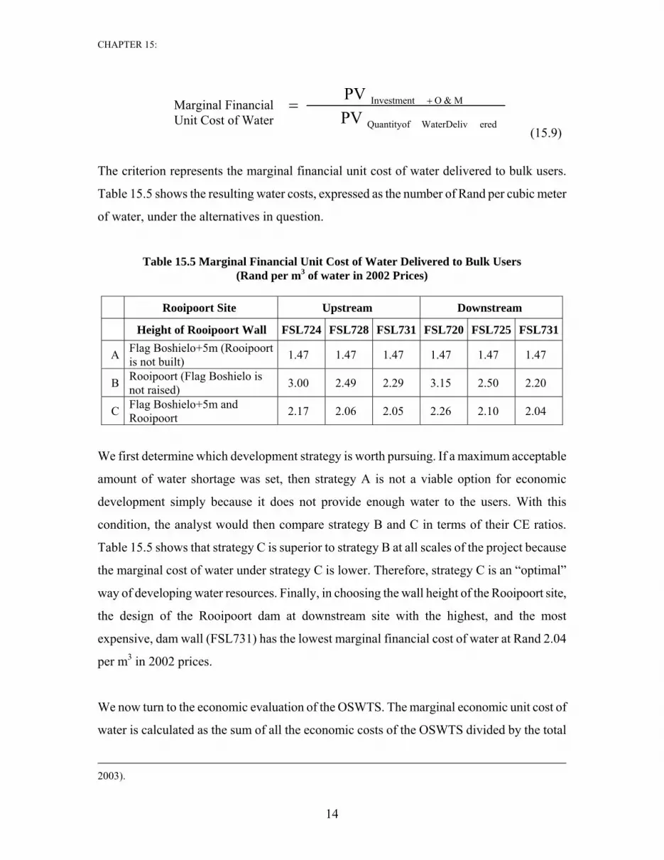
(15.9)

The criterion represents the marginal financial unit cost of water delivered to bulk users.

Table 15.5 shows the resulting water costs, expressed as the number of Rand per cubic meter

of water, under the alternatives in question.

Table 15.5 Marginal Financial Unit Cost of Water Delivered to Bulk Users (Rand per m3 of water in 2002 Prices)

Rooipoort Site Upstream Downstream

Height of Rooipoort Wall FSL724 FSL728 FSL731 FSL720 FSL725 FSL731

A Flag Boshielo+5m (Rooipoort is not built) 1.47 1.47 1.47 1.47 1.47 1.47

B Rooipoort (Flag Boshielo is not raised) 3.00 2.49 2.29 3.15 2.50 2.20

C Flag Boshielo+5m and Rooipoort 2.17 2.06 2.05 2.26 2.10 2.04

We first determine which development strategy is worth pursuing. If a maximum acceptable

amount of water shortage was set, then strategy A is not a viable option for economic

development simply because it does not provide enough water to the users. With this

condition, the analyst would then compare strategy B and C in terms of their CE ratios.

Table 15.5 shows that strategy C is superior to strategy B at all scales of the project because

the marginal cost of water under strategy C is lower. Therefore, strategy C is an “optimal”

way of developing water resources. Finally, in choosing the wall height of the Rooipoort site,

the design of the Rooipoort dam at downstream site with the highest, and the most

expensive, dam wall (FSL731) has the lowest marginal financial cost of water at Rand 2.04

per m3 in 2002 prices.

We now turn to the economic evaluation of the OSWTS. The marginal economic unit cost of

water is calculated as the sum of all the economic costs of the OSWTS divided by the total

2003).

Marginal Financial Unit Cost of Water eredWaterDelivQuantityof

M&OInvestment

PV PV +=

CHAPTER 15:

15

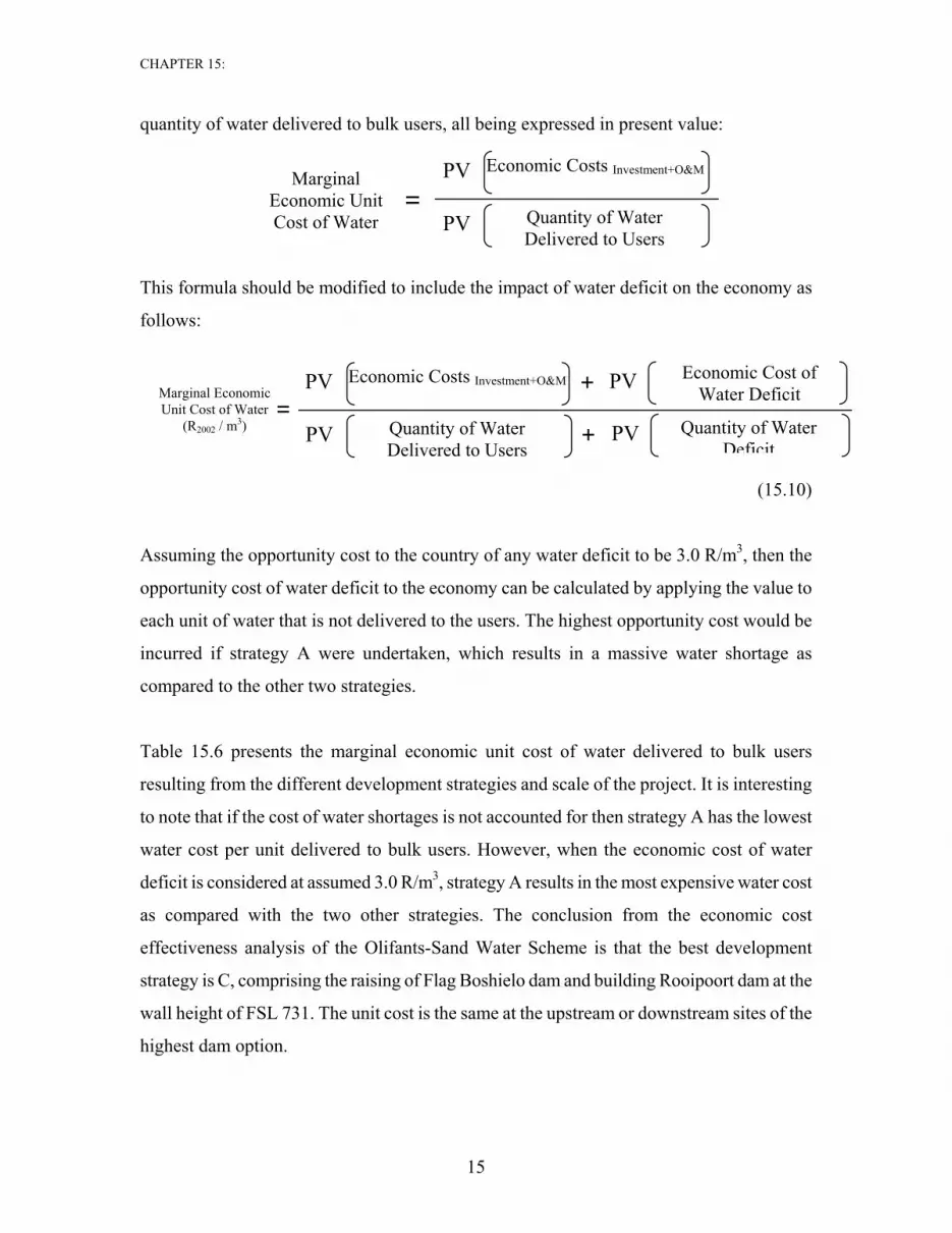
quantity of water delivered to bulk users, all being expressed in present value:

This formula should be modified to include the impact of water deficit on the economy as

follows:

(15.10)

Assuming the opportunity cost to the country of any water deficit to be 3.0 R/m3, then the

opportunity cost of water deficit to the economy can be calculated by applying the value to

each unit of water that is not delivered to the users. The highest opportunity cost would be

incurred if strategy A were undertaken, which results in a massive water shortage as

compared to the other two strategies.

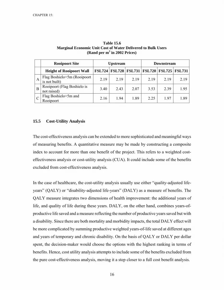
Table 15.6 presents the marginal economic unit cost of water delivered to bulk users

resulting from the different development strategies and scale of the project. It is interesting

to note that if the cost of water shortages is not accounted for then strategy A has the lowest

water cost per unit delivered to bulk users. However, when the economic cost of water

deficit is considered at assumed 3.0 R/m3, strategy A results in the most expensive water cost

as compared with the two other strategies. The conclusion from the economic cost

effectiveness analysis of the Olifants-Sand Water Scheme is that the best development

strategy is C, comprising the raising of Flag Boshielo dam and building Rooipoort dam at the

wall height of FSL 731. The unit cost is the same at the upstream or downstream sites of the

highest dam option.

Economic Costs Investment+O&M Marginal Economic

Unit Cost of Water (R2002 / m3)

= + Economic Cost of

Water Deficit PV

Quantity of Water Delivered to Users

PV

PV

Quantity of Water Deficit

PV +

Marginal Economic Unit Cost of Water

Economic Costs Investment+O&M PV =

Quantity of Water Delivered to Users

PV

CHAPTER 15:

16

Table 15.6 Marginal Economic Unit Cost of Water Delivered to Bulk Users

(Rand per m3 in 2002 Prices)

Rooipoort Site Upstream Downstream

Height of Rooipoort Wall FSL724 FSL728 FSL731 FSL720 FSL725 FSL731

A Flag Boshielo+5m (Rooipoort is not built) 2.19 2.19 2.19 2.19 2.19 2.19

B Rooipoort (Flag Boshielo is not raised) 3.40 2.43 2.07 3.53 2.39 1.95

C Flag Boshielo+5m and Rooipoort 2.16 1.94 1.89 2.25 1.97 1.89

15.5 Cost-Utility Analysis

The cost-effectiveness analysis can be extended to more sophisticated and meaningful ways

of measuring benefits. A quantitative measure may be made by constructing a composite

index to account for more than one benefit of the project. This refers to a weighted cost-

effectiveness analysis or cost-utility analysis (CUA). It could include some of the benefits

excluded from cost-effectiveness analysis.

In the case of healthcare, the cost-utility analysis usually use either “quality-adjusted life-

years” (QALY) or “disability-adjusted life-years” (DALY) as a measure of benefits. The

QALY measure integrates two dimensions of health improvement: the additional years of

life, and quality of life during these years. DALY, on the other hand, combines years-of-

productive life saved and a measure reflecting the number of productive years saved but with

a disability. Since there are both mortality and morbidity impacts, the total DALY effect will

be more complicated by summing productive weighted years-of-life saved at different ages

and years of temporary and chronic disability. On the basis of QALY or DALY per dollar

spent, the decision-maker would choose the options with the highest ranking in terms of

benefits. Hence, cost utility analysis attempts to include some of the benefits excluded from

the pure cost-effectiveness analysis, moving it a step closer to a full cost benefit analysis.

CHAPTER 15:

17

The estimation of benefit in CEA is limited to a single measure of effectiveness. This

simplification is often not acceptable and, instead, a cost-utility analysis is employed. In

principle, CUA could be used with multiple outcomes but as the number of dimensions

grows, the complexity of analysis also increases. CUA has been traditionally applied in

education and health projects, combining improvements in both quantity and quality.

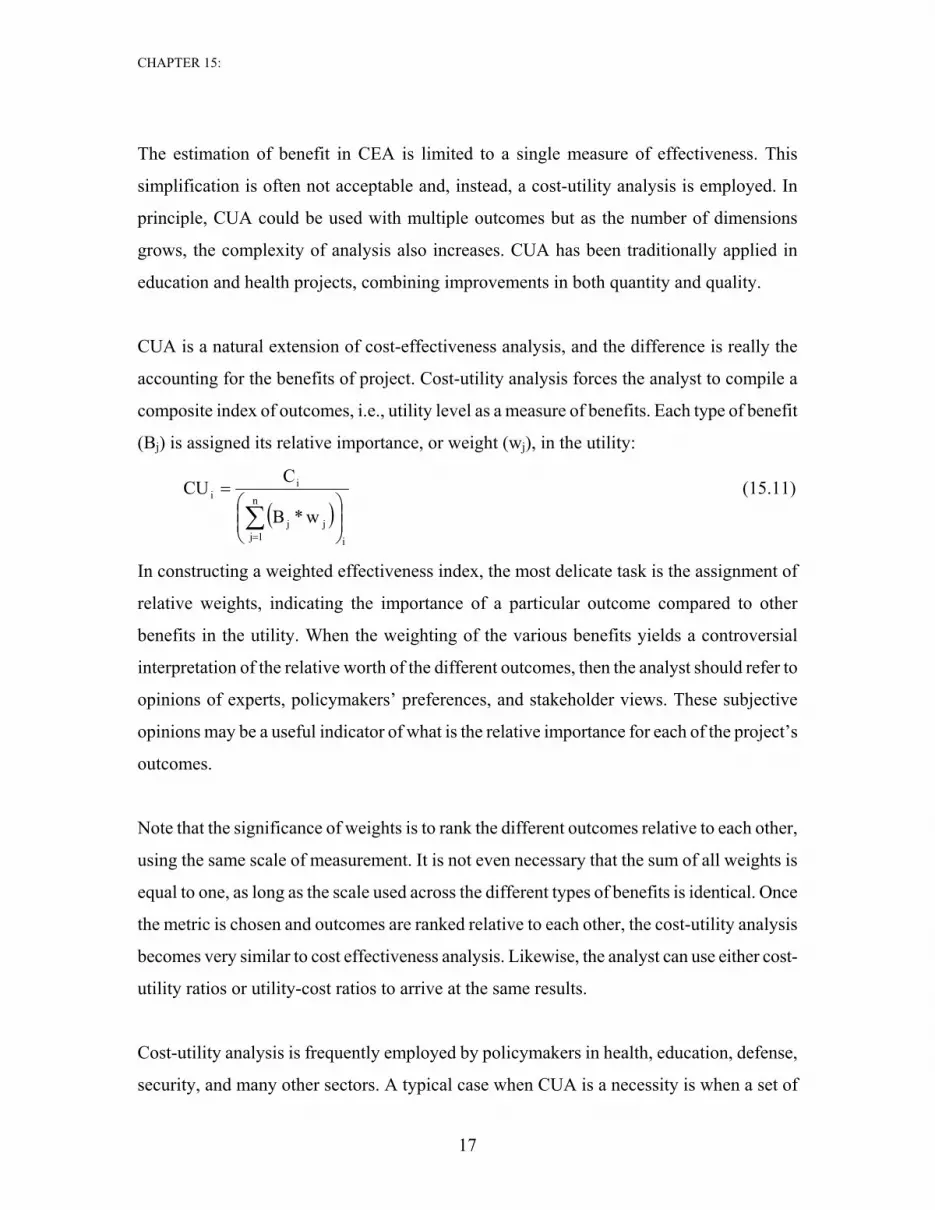
CUA is a natural extension of cost-effectiveness analysis, and the difference is really the

accounting for the benefits of project. Cost-utility analysis forces the analyst to compile a

composite index of outcomes, i.e., utility level as a measure of benefits. Each type of benefit

(Bj) is assigned its relative importance, or weight (wj), in the utility:

( )i

n

1jjj

ii

w*B

CCU

⎟⎟⎠

⎞⎜⎜⎝

⎛=

∑=

(15.11)

In constructing a weighted effectiveness index, the most delicate task is the assignment of

relative weights, indicating the importance of a particular outcome compared to other

benefits in the utility. When the weighting of the various benefits yields a controversial

interpretation of the relative worth of the different outcomes, then the analyst should refer to

opinions of experts, policymakers’ preferences, and stakeholder views. These subjective

opinions may be a useful indicator of what is the relative importance for each of the project’s

outcomes.

Note that the significance of weights is to rank the different outcomes relative to each other,

using the same scale of measurement. It is not even necessary that the sum of all weights is

equal to one, as long as the scale used across the different types of benefits is identical. Once

the metric is chosen and outcomes are ranked relative to each other, the cost-utility analysis

becomes very similar to cost effectiveness analysis. Likewise, the analyst can use either cost-

utility ratios or utility-cost ratios to arrive at the same results.

Cost-utility analysis is frequently employed by policymakers in health, education, defense,

security, and many other sectors. A typical case when CUA is a necessity is when a set of

CHAPTER 15:

18

alternative policy actions must be evaluated, each resulting in multiple outcomes and a cost-

benefit analysis is not possible. A simple cost effectiveness analysis is also not appropriate

because it ignores a host of important benefits.

15.6 Application of CUA in Education Projects

15.6.1 Nature of Education Projects

Acquiring an education can be viewed as a process of human capital formation. However,

education projects may have many types of outcomes with benefits measurable in monetary

and non-monetary terms. In broad categories, investment in education can generate various

in-school and out-of-school benefits. In-school benefits cover gains in the efficiency of the

education system, which may be intangible or difficult to quantify. In such cases, the

production of education services involves decisions of how one can select from alternative

investment strategies based on the lowest cost per unit of effectiveness.

Out-of-school benefits refer to improvement of earning capacity of the students and

externalities that accrue to society at large beyond the project beneficiaries. It generally

arises after the project’s beneficiaries finish a course of study or training. The most obvious

of such benefits is measured by the gain in productivity of the beneficiaries that is usually

reflected in the change in the earnings of the individuals between the with and the without

training situations.7 In evaluating an education project or program from society’s point of

view, the benefits will include the change in the gross-of-tax earnings including the value of

the fringe benefits such as value of health insurance, vehicles, housing allowances and

retirement benefits as a package. For example, in the case of evaluating a 4-year university

program, the present value of net benefits can be calculated over 40 years after graduation as

follows:8

7 See, e.g., Psacharopoulos, G., “Returns to Investment in Education: A Global Update”, World Development, Vol. 22, No. 9, (1994); Belli, P., Khan, Q., and Psacharopoulos, G., “Assessing a Higher Education Project: a Mauritius Feasibility Study”, Applied Economics, 31, (1999). 8 Belli, P., Anderson, J.R., Barnum, H.N., Dixon, J.A., and Tan, J.P., Economic Analysis of Investment Operations: Analytical Tools and Practical Applications, The World Bank, Washington D.C., (2001).

CHAPTER 15:

19

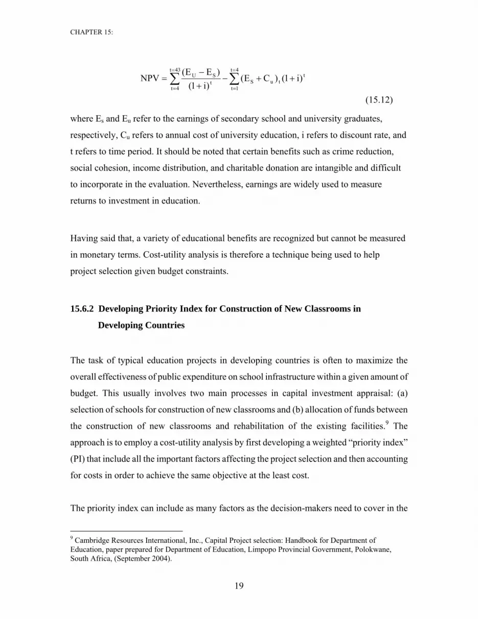
(15.12)

where Es and Eu refer to the earnings of secondary school and university graduates,

respectively, Cu refers to annual cost of university education, i refers to discount rate, and

t refers to time period. It should be noted that certain benefits such as crime reduction,

social cohesion, income distribution, and charitable donation are intangible and difficult

to incorporate in the evaluation. Nevertheless, earnings are widely used to measure

returns to investment in education.

Having said that, a variety of educational benefits are recognized but cannot be measured

in monetary terms. Cost-utility analysis is therefore a technique being used to help

project selection given budget constraints.

15.6.2 Developing Priority Index for Construction of New Classrooms in

Developing Countries

The task of typical education projects in developing countries is often to maximize the

overall effectiveness of public expenditure on school infrastructure within a given amount of

budget. This usually involves two main processes in capital investment appraisal: (a)

selection of schools for construction of new classrooms and (b) allocation of funds between

the construction of new classrooms and rehabilitation of the existing facilities.9 The

approach is to employ a cost-utility analysis by first developing a weighted “priority index”

(PI) that include all the important factors affecting the project selection and then accounting

for costs in order to achieve the same objective at the least cost.

The priority index can include as many factors as the decision-makers need to cover in the

9 Cambridge Resources International, Inc., Capital Project selection: Handbook for Department of Education, paper prepared for Department of Education, Limpopo Provincial Government, Polokwane, South Africa, (September 2004).

ttu

4t

1tS

43t

4ttSU )i1()CE(

)i1()EE(

NPV ++−+−

= ∑∑=

=

=

=

CHAPTER 15:

20

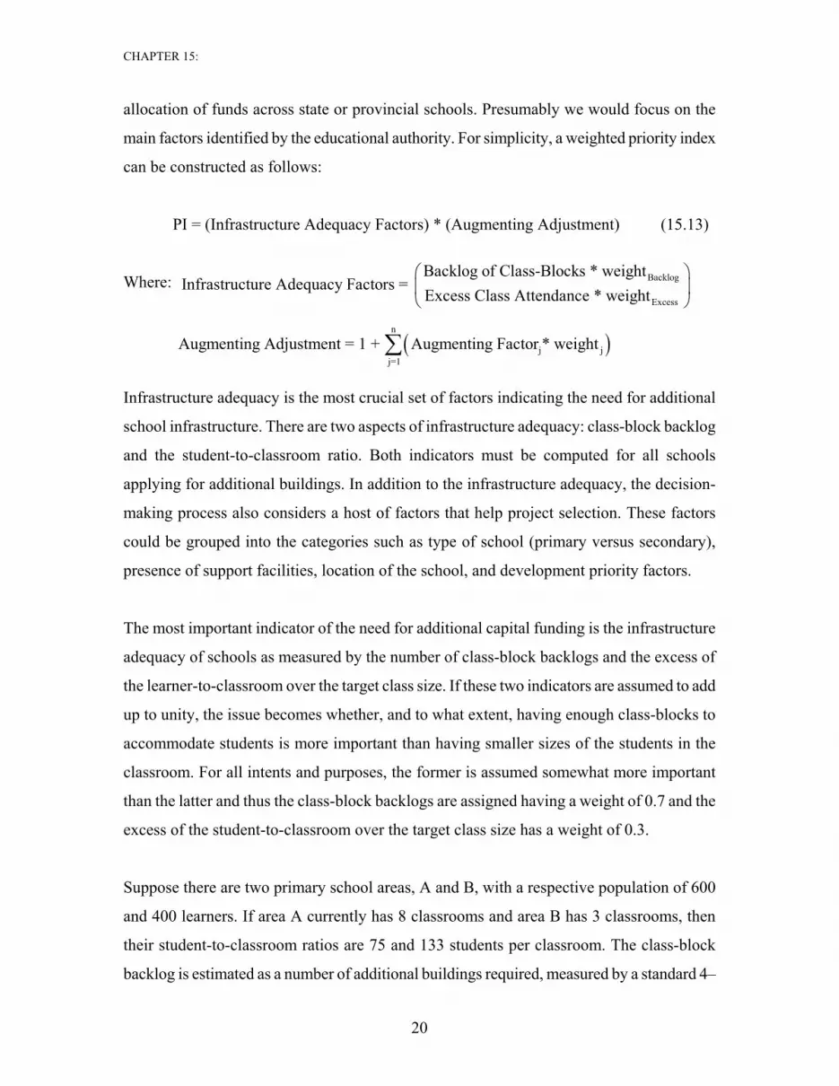
allocation of funds across state or provincial schools. Presumably we would focus on the

main factors identified by the educational authority. For simplicity, a weighted priority index

can be constructed as follows:

PI = (Infrastructure Adequacy Factors) * (Augmenting Adjustment) (15.13)

Where:

Infrastructure adequacy is the most crucial set of factors indicating the need for additional

school infrastructure. There are two aspects of infrastructure adequacy: class-block backlog

and the student-to-classroom ratio. Both indicators must be computed for all schools

applying for additional buildings. In addition to the infrastructure adequacy, the decision-

making process also considers a host of factors that help project selection. These factors

could be grouped into the categories such as type of school (primary versus secondary),

presence of support facilities, location of the school, and development priority factors.

The most important indicator of the need for additional capital funding is the infrastructure

adequacy of schools as measured by the number of class-block backlogs and the excess of

the learner-to-classroom over the target class size. If these two indicators are assumed to add

up to unity, the issue becomes whether, and to what extent, having enough class-blocks to

accommodate students is more important than having smaller sizes of the students in the

classroom. For all intents and purposes, the former is assumed somewhat more important

than the latter and thus the class-block backlogs are assigned having a weight of 0.7 and the

excess of the student-to-classroom over the target class size has a weight of 0.3.

Suppose there are two primary school areas, A and B, with a respective population of 600

and 400 learners. If area A currently has 8 classrooms and area B has 3 classrooms, then

their student-to-classroom ratios are 75 and 133 students per classroom. The class-block

backlog is estimated as a number of additional buildings required, measured by a standard 4–

Backlog

Excess

Backlog of Class-Blocks * weightInfrastructure Adequacy Factors =

Excess Class Attendance * weight⎛ ⎞⎜ ⎟⎝ ⎠

( )n

j jj=1

Augmenting Adjustment = 1 + Augmenting Factor * weight∑

CHAPTER 15:

21

class block required at school in order to maintain the maximum acceptable class size. With

the assumed target of 40 students per class in primary school, one can estimate the class-

block backlog at 1.75 blocks for area A and also for area B.10 In other words, if schools A

and B both have the same number of additional buildings required, but area B has a higher

student-to-classroom ratio, then this area should be given more priority.11

A composite index can be then estimated from these two indicators and associated weights

assigned to them. The score of school-area A would be equal to 1.79 (= 1.75 backlogs * 0.7

+ 1.875 excess ratio * 0.3). Similarly, the score of school-area B would be estimated as 2.22.

As a result, the priority of school-area B is higher than the priority of school-area A, based

on the two infrastructure adequacy factors. Such infrastructure adequacy composite score

can be computed for all schools concerned and a ranking of all schools based on purely

infrastructure adequacy can be made accordingly.

In addition to infrastructure adequacy factors, a number of additional aspects may be

considered. These factors may include type of school, presence of support facilities, location

of the school, and development priority. The objective is to develop an augmenting

adjustment index, ranging from unity to an additional number, say, 1.75, to account for

additional concerns by the educational authority and society as a whole. In other words, all

augmenting factors could introduce an upward shift in the index up to a limit of 0.75 taking

the infrastructure adequacy score as the base. Table 15.7, for example, presents a summary

of a tentative priority scores among the four identified groups of augmenting factors. The

actual weights could be further refined as needed.12

10 For school A, the backlog is estimated as 7 classrooms (= [600 students – (8 class-rooms * 40 students)] / 40 students-per-classroom), or 1.75 class-blocks. For school B, the same procedure yields 7 class-rooms (= [400 students – (3 class-rooms * 40 students)] / 40 students-per-classroom), or 1.75 class-blocks. 11 The excess ratio of learner-to-classroom over the target class size is 1.875 for area A and 3.325 for area B. These figures are estimated as the ratio of (75 students-per-classroom / 40 students-per-classroom) and (133 students-per-classroom / 40 students-per-classroom), respectively. 12 A positive augmentation factor for primary versus secondary schools could be based on the fact that generally the case that the rate of return from primary education is higher than for secondary education.

CHAPTER 15:

22

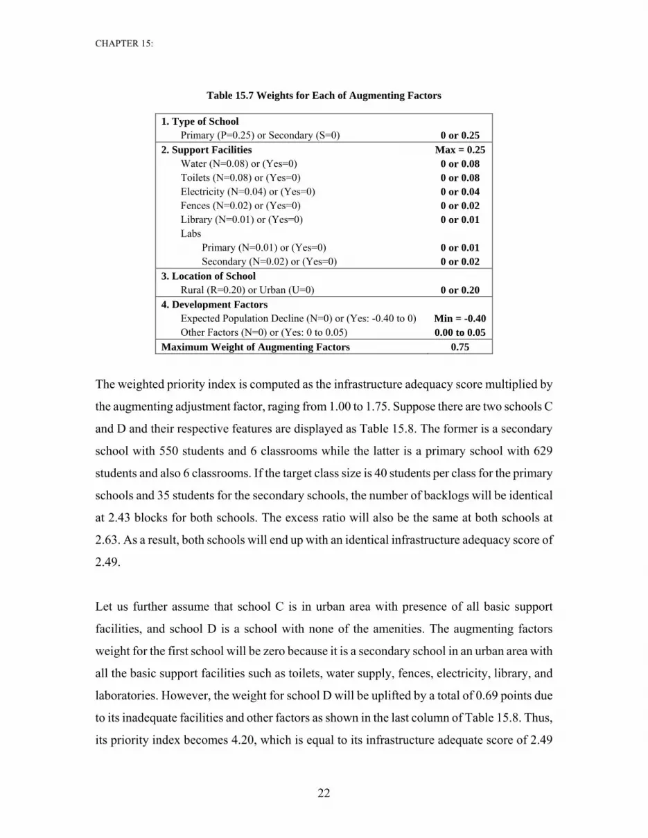
Table 15.7 Weights for Each of Augmenting Factors

1. Type of School

Primary (P=0.25) or Secondary (S=0) 0 or 0.25 2. Support Facilities Max = 0.25

Water (N=0.08) or (Yes=0) 0 or 0.08 Toilets (N=0.08) or (Yes=0) 0 or 0.08 Electricity (N=0.04) or (Yes=0) 0 or 0.04 Fences (N=0.02) or (Yes=0) 0 or 0.02 Library (N=0.01) or (Yes=0) 0 or 0.01 Labs

Primary (N=0.01) or (Yes=0) 0 or 0.01 Secondary (N=0.02) or (Yes=0) 0 or 0.02

3. Location of School Rural (R=0.20) or Urban (U=0) 0 or 0.20

4. Development Factors Expected Population Decline (N=0) or (Yes: -0.40 to 0) Min = -0.40 Other Factors (N=0) or (Yes: 0 to 0.05) 0.00 to 0.05

Maximum Weight of Augmenting Factors 0.75

The weighted priority index is computed as the infrastructure adequacy score multiplied by

the augmenting adjustment factor, raging from 1.00 to 1.75. Suppose there are two schools C

and D and their respective features are displayed as Table 15.8. The former is a secondary

school with 550 students and 6 classrooms while the latter is a primary school with 629

students and also 6 classrooms. If the target class size is 40 students per class for the primary

schools and 35 students for the secondary schools, the number of backlogs will be identical

at 2.43 blocks for both schools. The excess ratio will also be the same at both schools at

2.63. As a result, both schools will end up with an identical infrastructure adequacy score of

2.49.

Let us further assume that school C is in urban area with presence of all basic support

facilities, and school D is a school with none of the amenities. The augmenting factors

weight for the first school will be zero because it is a secondary school in an urban area with

all the basic support facilities such as toilets, water supply, fences, electricity, library, and

laboratories. However, the weight for school D will be uplifted by a total of 0.69 points due

to its inadequate facilities and other factors as shown in the last column of Table 15.8. Thus,

its priority index becomes 4.20, which is equal to its infrastructure adequate score of 2.49

CHAPTER 15:

23

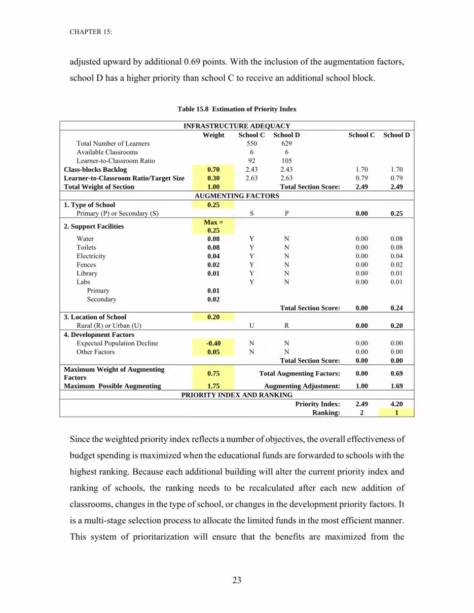
adjusted upward by additional 0.69 points. With the inclusion of the augmentation factors,

school D has a higher priority than school C to receive an additional school block.

Table 15.8 Estimation of Priority Index

INFRASTRUCTURE ADEQUACY

Weight School C School D School C School D Total Number of Learners 550 629 Available Classrooms 6 6 Learner-to-Classroom Ratio 92 105

Class-blocks Backlog 0.70 2.43 2.43 1.70 1.70 Learner-to-Classroom Ratio/Target Size 0.30 2.63 2.63 0.79 0.79 Total Weight of Section 1.00 Total Section Score: 2.49 2.49

AUGMENTING FACTORS 1. Type of School 0.25

Primary (P) or Secondary (S) S P 0.00 0.25

2. Support Facilities Max = 0.25

Water 0.08 Y N 0.00 0.08 Toilets 0.08 Y N 0.00 0.08 Electricity 0.04 Y N 0.00 0.04 Fences 0.02 Y N 0.00 0.02 Library 0.01 Y N 0.00 0.01 Labs Y N 0.00 0.01

Primary 0.01 Secondary 0.02

Total Section Score: 0.00 0.24 3. Location of School 0.20

Rural (R) or Urban (U) U R 0.00 0.20 4. Development Factors

Expected Population Decline -0.40 N N 0.00 0.00 Other Factors 0.05 N N 0.00 0.00

Total Section Score: 0.00 0.00 Maximum Weight of Augmenting Factors 0.75 Total Augmenting Factors: 0.00 0.69

Maximum Possible Augmenting 1.75 Augmenting Adjustment: 1.00 1.69 PRIORITY INDEX AND RANKING

Priority Index: 2.49 4.20 Ranking: 2 1

Since the weighted priority index reflects a number of objectives, the overall effectiveness of

budget spending is maximized when the educational funds are forwarded to schools with the

highest ranking. Because each additional building will alter the current priority index and

ranking of schools, the ranking needs to be recalculated after each new addition of

classrooms, changes in the type of school, or changes in the development priority factors. It

is a multi-stage selection process to allocate the limited funds in the most efficient manner.

This system of prioritarization will ensure that the benefits are maximized from the

CHAPTER 15:

24

allocation of capital budget for the construction of new class-blocks.

One can further extend the analysis to incorporate the physical condition of these

facilities and the rehabilitation costs required.13 In so doing, the priority for limited

budget may become the choice between building a new class-blocks and rehabilitation of

the existing facilities with a consideration of relative costs.

15.7 Application of CUA in Health Projects

15.7.1 Nature of Health Projects

There are many examples of market failures in the health sector. It is heavily regulated by

governments. The health services are generally subsidized at least at the primary care level.

In almost all situations in the field of health care patients do not pay a price or fee that

reflects the opportunity costs of the resources employed. Knowledge and information

between physicians and patients about sickness or disease is asymmetric. As a result, the

supply and demand for the services is not negotiable or as well defined as other goods or

services regularly bought and sold in markets.

The evaluation of a capital investment or a medical intervention in the health sector is

seldom subjected to a cost-benefit analysis because of the difficulty in measuring the

outcomes of the project in monetary terms. For example, the value of human life and the

value of improvements in human health are difficult to quantify in a satisfactory manner. So

far two approaches have been attempted by some researchers to measure these outcomes in

monetary value.14 The first is the human capital approach where improvements in health

status are considered as investments that will enhance productivity and increase incomes.

But this approach only focuses on earnings potential; the value of benefits is considered to

be biased downward because it ignores other benefits. The second approach is the

13 Zeinali, A., Jenkins, G.P., and Klevchuk, Andrey, “Infrastructure Choices in Education: Location, Build and Repair”, Queen’s Economics Department Working Paper, No. 1204, (April 2009). 14 Adhikari, R., Gertler, P., and Lagman, A., “Economic Analysis of Health Sector Projects – A Review of issues, Methods, and Approaches”, Economic Staff Paper, Asian Development Bank, (March 1999).

CHAPTER 15:

25

willingness to pay by consumers where one can assess the extra earnings demanded by

workers to undertake risky jobs or the additional safety expenditures made to reduce the

incidents of accidents. This may be considered an accepted measure of the implicit value of a

life of workers. Nevertheless, the empirical results cover a wide range of values. There are

also controversial issues such as the extent that younger persons are valued more than

seniors.

Due to the difficulty in measuring human life or other outcomes of health interventions in

monetary terms, cost-effectiveness analysis has become one of the most practical techniques

in evaluating alternative health projects or programs in order to achieve specific health

benefits at least cost. Given the benefits, the analyst should identify the incremental costs for

each alternative option. These include capital expenditures for hospital, clinic, computer,

medical equipment, etc. and operating costs for office supplies, administration expenses,

wages and salaries of physicians, nurses, laboratory technicians and other staff, and so on. In

the economic analysis, the cost should also include the opportunity cost of travel, waiting

and forgone earnings of patients or parents of sick children.

One area that is often faced by analysts is joint production of health services. For example,

some facilities and administration costs may be commonly used. The analyst should identify

and estimate incremental costs associated with each alternative intervention.

15.7.2 Unadjusted Measurement of Cost-Utility Analysis

Health projects or programs typically result in multiple benefits even if a single objective is

originally targeted. Using a simple cost-effectiveness analysis often omits some important

side benefits. Thus, the consequential choice of handling these problems is carried out

through a cost-utility analysis.

Suppose that the policymakers want to design an immunization program to maximize

CHAPTER 15:

26

improvement in health for a given budget in a particular region.15 Three alternative options

are identified to be evaluated. They are DPT (a combination of diphtheria, pertussis, tetanus

vaccines for children), BCG (Bacillus Calmette Guerin, used to prevent tuberculosis), and a

package of both DPT and BCG combined.

The effects of these alternative options can be obtained from simulations of an

epidemiological model that is devised and based on the number of vaccinations, the

efficiency of the vaccines, the incidence of fatality rates, duration of morbidity, and years of

life lost based on a life-table for the relevant population. The effectiveness of immunization

is measured by the reduction in morbidity and mortality rates, and both can be ultimately

translated into years of life. For instance, three individuals were saved with an immunization

program: the first individual has avoided a loss of 5 life-years, based on his life expectancy;

the second gained 8 life-years, and the third saved 3 life-years. The resulting total mortality

prevented by this program, as measured in life-years, is 16 years. A similar count goes for

morbidity, which presumes that a person with lower health status will eventually live a

shorter life, while an individual with higher health status will enjoy more years of life. The

epidemiological model makes a projection for the population in the particular region, and

reports the impact of an immunization program on total life-years gained. This is the

simplest type of cost-utility analysis as it accounts for mortality and morbidity both

measured in number of life-years saved.

Each of the three above alternative options will result in different additional numbers of life-

years gained. They are summarized in Table 15.9. The option of using DPT alone would

result in a reduction of total mortality by 209 years and reduction in total morbidity by

21,401 years. The cost of this option is $1.97 million. The second option, BCG alone, would

reduce mortality by 129 years and morbidity by 2,735 years, at a budget cost of $0.585

million. This option is not cost-effective in terms of total years of mortality and morbidity

gained. However, the BCG only program is more cost-effective in terms of mortality

15 This example is adopted from Belli, P., Anderson, J.R., Barnum, H.N., Dixon, J.A., and Tan, J.P., Economic Analysis of Investment Operations: Analytical Tools and Practical Applications, The World Bank, Washington D.C., (2001).

CHAPTER 15:

27

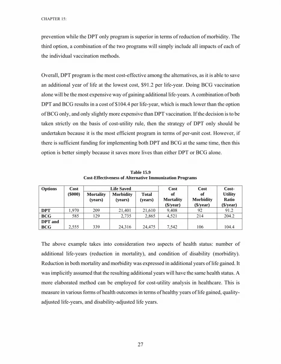
prevention while the DPT only program is superior in terms of reduction of morbidity. The

third option, a combination of the two programs will simply include all impacts of each of

the individual vaccination methods.

Overall, DPT program is the most cost-effective among the alternatives, as it is able to save

an additional year of life at the lowest cost, $91.2 per life-year. Doing BCG vaccination

alone will be the most expensive way of gaining additional life-years. A combination of both

DPT and BCG results in a cost of $104.4 per life-year, which is much lower than the option

of BCG only, and only slightly more expensive than DPT vaccination. If the decision is to be

taken strictly on the basis of cost-utility rule, then the strategy of DPT only should be

undertaken because it is the most efficient program in terms of per-unit cost. However, if

there is sufficient funding for implementing both DPT and BCG at the same time, then this

option is better simply because it saves more lives than either DPT or BCG alone.

Table 15.9 Cost-Effectiveness of Alternative Immunization Programs

Life Saved Options Cost

($000) Mortality (years)

Morbidity (years)

Total (years)

Cost of

Mortality ($/year)

Cost of

Morbidity ($/year)

Cost-Utility Ratio

($/year) DPT 1,970 209 21,401 21,610 9,408 92 91.2 BCG 585 129 2,735 2,865 4,521 214 204.2 DPT and BCG

2,555

339

24,316

24,475

7,542

106

104.4

The above example takes into consideration two aspects of health status: number of

additional life-years (reduction in mortality), and condition of disability (morbidity).

Reduction in both mortality and morbidity was expressed in additional years of life gained. It

was implicitly assumed that the resulting additional years will have the same health status. A

more elaborated method can be employed for cost-utility analysis in healthcare. This is

measure in various forms of health outcomes in terms of healthy years of life gained, quality-

adjusted life-years, and disability-adjusted life years.

CHAPTER 15:

28

15.7.3 Quality-Adjusted Life Years

Taking into account, but the distinction between fatal mortality and nonfatal morbidity

outcomes may be most objective to measuring the outcomes of health projects. QALY is the

measure that combines both the quantity, expressed in additional life-years, and their quality,

expressed through a health index. This has become a major tool in appraisal of many health

programs. In essence, QALY expresses a combined utility of both the additional years and

quality of life during these years. The basic idea is straightforward in which it takes one year

of perfect health-life expectancy to be worth one, a value of zero for death, and one year of

less than perfect life expectancy as less than one. For example, an intervention results in a

patient living for four years rather than dying within one year. The treatment increases three

years to the person’s life. However, if the quality of life falls from one to 0.8 after the

treatment, it will generate 2.4 QALY. QALYs can provide an indication of the benefits

gained from a variety of medical interventions in terms of quantity and quality of life for the

patient. Need less to say, there are problems associated with the technique. This is because

the index assigned to the state of health improvement may be subjective. Combining two

distinct variables -- mortality and morbidity -- into an index is mathematically convenient.

However, assigning appropriate weights and then ranking the choice among these

combinations has become a major challenge for decision makers in the medical sector.

DALY is another tool and considered to be an overall measure of disease burden on an

economy. It combines a years of life lost measure and a years-lived with disability measure.

The DALY index calculates the productive years lost from an ideal lifespan due to morbidity

or premature mortality. The reduction of productive years due to morbidity is a function of

the years lived with the disability and a weight assigned. The technique allows both

morbidity and mortality to be combined into a single measure. Moreover, DALY is age-

weighted healthy years of life gained. It has higher weights attached to productive years as

compared to a QALY where health weights are kept constant for a given health status.

A vast amount of effort has gone into research on defining a heath status. Usually, health

status is defined in terms of a composite index, covering most of the physical and

psychological conditions. Every health aspect included in the index is rated on some scale

CHAPTER 15:

29

from the worst to the best state. A single index can then be constructed from all the aspects.

For instance, one of the most comprehensive classifications is based on four dimensions:

physical function (mobility and physical activity), role function (ability to care for oneself),

social-emotional function (emotional well-being and social activity), and health problem

(including physical deformity).16

The usefulness of QALY index in cost-utility analysis depends on the reliability of the

methods used to define and to measure health status. There are three common methods of

deriving utilities of health status: the health rating method, the time trade-off method, and the

standard gamble method.17

15.7.4 Issues of the Analysis

Cost-utility analysis has overcome the limitation of taking account of only one type of

benefit under the cost-effectiveness analysis. There are some issues, however, that require

attention and further research.

First, although cost-utility analysis includes several key benefits, it relies on construction of

a composite utility index and their underlying relative importance in the index. Assignment

of relative weights to different types of benefits is usually based on a survey and consultation

with government officials, local community, experts in the field of project. Neverthelsss,

they are not based on market places nor consumers’ willingness to pay. Different methods of

utility derivation may result in different weights and generate different results.18

Second, caveats must be placed on the process of ranking of different types of benefits due to

the choice of scale on which the benefits are measured or the interaction among the

16 Torrance, G.W., Boyle, M.H., and Horwood, S.P., “Application of Multi-Attribute Utility Theory to Measure Social Preferences for Health Status”, Operations Research, 30, No. 6, (1982), pp. 1043-1063. 17 Froberg, D.G., and Kane, R.L, “Methodology for Measuring Health-State Preferences – IV: Progress and Research Agenda,” Journal of Clinical Epidemiology, 42, No. 7, (1989), pp. 675-685. 18 Hornberger, J.C., Redelmeier, D.A., and Peterson, J., “Variability among Methods to Assess Patients’ Well-Being and Consequent Effect on a Cost-Effectiveness Analysis”, Journal of Clinical Epidemiology, 45, No. 5, (May 1992).

CHAPTER 15:

30

outcomes. For instance, a program of drug-addicts treatment is likely to result not only in

their lower mortality and morbidity but also in reduction of street crime. Because different

types of benefits are often measured in different units, the choice of common ranking scale

should be compatible to all the benefits.

A second problem arises when different types of benefits are ranked. If one type of benefit is

ranked 80 on a 100-scale and another benefit is assigned a weigh of 40, it does not

necessarily mean that the first outcome is twice as preferable.

Another caveat lies in aggregation of individual preferences. A simple summation may seem

as the right way of combining individual choices into social preferences, but this procedure

is not appropriate if there are interactions among individuals such that would require another

method of compiling their total score.19

Third, concerns are often raised regarding discounting of health status and life-years in

healthcare applications. It is unquestionable that the costs should be discounted but concern

is sometimes expressed whether additional years and health status should be discounted too.

If costs are indeed discounted but health and/or years are not discounted, then the cost-

effectiveness ratio becomes smaller and smaller in the consequent years. Timing decisions

will be biased towards future dates because the ratios improve.20

When additional years and health quality are discounted, the rate used for discounting is

often debatable. The general consensus is necessary for discounting health improvement and

additional years gained in the future because individuals normally prefer having better health

now than the distant future as well as a life saved today is more valuable than a life saved

tomorrow. Nevertheless, there is still a considerable controversy over the theory, methods of

measurement, and the appropriate discount rate.21

19 Arrow, K.J., K.J., “Social Choice and Individual Values”, New York: Wiley (1963). 20 Keeler, E.B., and Cretin, S., “Discounting of Life-Saving and Other Nonmonetary Effects”, Management Science, 29, No. 3, (March 1983). 21 Gafni, A., “Time in Health: Can We Measure Individuals? Pure Time Preference?`”, Medical Decision Making, 15, No. 1, (1995).

CHAPTER 15:

31

Currently, a 3 or 4 percent rate is used by various institutions to discount the stream of

benefits and costs in health projects to compare alternatives. The rate is based on the rate of

time preference alone in terms of present versus future consumption. There is a serious

concern that such a discount rate does not fully capture the value that society forgoes in

terms of pre-tax returns of displaced investment. A rate of discount that takes into

consideration the opportunity cost of forgone investments will be much higher than the rate

of time preference of consumption. Note that in the case of most health interventions where

the costs are spread out the time of the intervention when the benefits are also being realized,

the discount rate may not be too critical. The size of discounting rates, however, would be

extremely important when capital expenditures such as construction of hospital and clinics or

purchase of expensive machines and other advanced equipments are incurred at the

beginning of the project. Hence, a reasonable approach to the discount rate is to use a

weighted average of the economic rate of return on private investment and the time

preference rate for consumption as outlined in Chapter 8.

15.8 Conclusion

Given the difficulties in quantifying the outcomes in monetary value for public security,

education, healthcare and other social projects, cost-benefit analysis cannot be used to

evaluate their alternative options. This chapter has presented alternative approaches, cost-

effectiveness and cost-utility analysis, to handle these types of projects. The general

procedure requires calculation of the incremental impacts of a particular project associated

with the incremental cost. The resulting marginal cost-effectiveness ratios are used to rank

the alternative measures or interventions.

When only one aspect of project benefits matters, cost-effectiveness analysis offers a handy

tool for selection of alternative options with technical efficiency. However, the approach

does not cover more than one single benefit; other benefits may also be important and should

be accounted for in the project selection.

CHAPTER 15:

32

A weighted cost-effectiveness or cost-utility analysis is generally used when multiple

benefits have to be included into assessment. It is measured by a composite index to include

all important factors affecting the project selection. The main advantage of this approach is

that it can capture a whole host of benefits in a single measure for ranking alternative

options. This is especially useful when applied to education or health projects because they

usually generate multiple benefits.

As regards the costs, they can be measured at both financial and economic prices. In the

economic analysis, they should be measured in resource costs over the life of the project or

program. Forgone earnings, for example, should be included in the economic evaluation of

secondary or higher educational programs. Likewise, travel and waiting time of patients

should also be accounted for in alternative interventions of health projects.

While both cost-effectiveness and cost-utility analysis offer practical methods of selection

among alternative projects or programs, both have limitations because their benefits cannot

be measured by a consumer’s willingness to pay at market prices. As a consequence, some

subjective judgments must be made in computing a composite index even though a survey

and consultation with experts in the field are frequently employed to minimize the possible

bias. Other questions such as the appropriate size of the discount rate are still contentious

issues, especially in health projects. Research continues in order to advance the methodology

for practical application in a wide range of fields.

CHAPTER 15:

33

REFERENCES

Adhikari, R., Gertler, P., and Lagman, A., “Economic Analysis of Health Sector Projects –

A Review of issues, Methods, and Approaches”, Economic Staff Paper, Asian

Development Bank, (March 1999).

Arrow, K.J., Social Choice and Individual Values, New York: Wiley (1963).

Arrow, K.J., Solow, R., Portney, P.R., Leaner, E.E., Radner, R., and Schuman, H.,

“Appendix I: Report of the NOAA Panel on Contingent Valuation”, excerpt from

”Natural Resource Damage Assessments under the Oil Pollution Act of 1990”,

Federal Register, Washington, D.C., (January 1993).

Belli, P., Anderson, J.R., Barnum, H.N., Dixon, J.A., and Tan, J.P., Economic Analysis of

Investment Operations: Analytical Tools and Practical Applications, Washington

D.C.: the World Bank, (2001), Chapters 7-9.

Belli, P., Khan, Q., and Psacharopoulos, G., “Assessing a Higher Education Project: a

Mauritius Feasibility Study”, Applied Economics, Vol. 31, No. 1, (January 1999), pp.

27-35.

Boardman, A.E., Greenberg, D.H., Vining, A.R., and Weimer, D.L., Cost-Benefit Analysis,

Concepts and Practice, Third Edition, Upper Saddle River, New Jersey: Pearson

Education, Inc. (2006), Chapter 17.

Cambridge Resources International, Inc., “Evaluation of the Olifants-Sand Water Transfer

Scheme in the Limpopo Province of South Africa”, report prepared for the

Department of Finance and Economic Development, Government of Government

Province, South Africa, (January 2003).

Froberg, D.G., and Kane, R.L, “Methodology for Measuring Health-State Preferences – IV:

Progress and Research Agenda,” Journal of Clinical Epidemiology, Vol. 42, No. 7,

(1989), pp. 675-685.

Gafni, A., “Time in Health: Can We Measure Individuals? Pure Time Preference?”, Medical

Decision Making, Vol. 15, No. 1, (1995).

Garber, A.M., Phelps, C.E., “Economic Foundations of Cost-effectiveness Analysis”,

Journal of Health Economics, Vol. 16, No. 1, (February 1997), pp. 1-31.

CHAPTER 15:

34

Hanemann, W.M., “Valuing the Environment through Contingent Valuation”, Journal of

Economic Perspectives, Vol. 8, No. 4, (Fall 1994).

Hornberger, J.C., Redelmeier, D.A., and Peterson, J., “Variability among Methods to Assess

Patients’ Well-Being and Consequent Effect on a Cost-Effectiveness Analysis”,

Journal of Clinical Epidemiology, Vol. 45, No. 5, (May 1992), pp. 505-512.

Keeler, E.B., and Cretin, S., “Discounting of Life-Saving and Other Nonmonetary Effects”,

Management Science, Vol. 29, No. 3, (March 1983), pp. 300-306.

Muenning, P., Designing and Conducting Cost-Effectiveness Analyses in Medicine and

Health Care, San Francisco: John Wiley & Sons, Inc., (2002).

Psacharopoulos, G., “Returns to Investment in Education: A Global Update”, World

Development, Vol. 22, No. 9, (September 1994), pp. 1325-1343.

Shand, N., “Olifants-Sand Water Transfer Scheme: Feasibility of Further Phases”, Interim

Report, Prepared by Ninham Shand for the Department of Water Affairs and

Forestry, Government of the Northern Province, P B500/00/2499, (2001).

Torrance, G.W., Boyle, M.H., and Horwood, S.P., “Application of Multi-Attribute Utility

Theory to Measure Social Preferences for Health Status”, Operations Research, Vol.

30, No. 6, (November-December 1982), pp. 1043-1069.

Viscusi, W.K., “The Value of Risks to Life and Health”, Journal of Economic Literature,

Vol. 31, No. 4, (December 1993), pp. 1912-1946.

Viscusi, W.K. and Aldy, J.E., “The Value of Statistical Life: A Critical Review of Market

Estimates throughout the World”, Journal of Risk and Uncertainty, Vol. 27, No. 1,

(August 2003), pp. 5-76.

Zeinali, A., Jenkins, G.P., and Klevchuk, Andrey, “Infrastructure Choices in Education:

Location, Build and Repair”, Queen’s Economics Department Working Paper, No.

1204, (April 2009).