Embed Size (px)
Citation preview
Investment Appraisal of an Animal Feed Plant in South Africa
Glenn P. Jenkins, Queen’s University, Kingston, Canada.
Eastern Mediterranean University, North Cyprus.
Andrey Klevchuk Cambridge Resource International Inc.
Development Discussion Paper Number: 2002-10
Abstract Limpopo Province of South Africa has been successful in recent years in attracting domestic and foreign investors. One of the priority sectors favored by the provincial development strategy is agriculture, and the proposed animal feed plant is a commercial project falling under the umbrella of projects encouraged by the Provincial Government. At the same time, this project is owned and financed by a foreign investor, hence, making it eligible for the direct foreign investment (FDI) support scheme provided by the National Government. This study completed an integrated financial, economic, stakeholder, sensitivity and risk analysis of the proposed animal feed plant in Polokwane Municipality of Limpopo Province. The plant is going to enter the existing industry where a number of domestic manufacturers already compete for the consumer. The most likely impact on the industry will be a reduction in the market share held by the existing feed producers.
Report prepared for: Department of Finance and Economic Development Limpopo Provincial Government Republic of South Africa. JEL code(s): H43 Key words: animal feed plant, foreign investment.
Investment Appraisal of an Animal Feed Plant in
Polokwane, Limpopo Province of South Africa
Prepared for:
Department of Finance and Economic Development Limpopo Provincial Government
Republic of South Africa
December 2002

PREFACE
As part of a program to strengthen the skills in the appraisal of public sector investments in
Limpopo Province, South Africa two projects that were under consideration in the Province were
evaluated in detail. They are the evaluation of the Olifants-Sands Water Transfer Scheme, and
appraisal of an Animal Feeds Plant in Polokwane, Limpopo Province, South Africa.
The first of these projects, the Olifants-Sands Water Transfer Scheme, is a pure public sector
infrastructure project, where issues of expansion strategy, location, scale and timing of the
investment were central to the financial and economic analysis.
The second project, an Animal Feeds Plant, is a commercial project, proposed by foreign
investors. It has requested financial assistance from the Government of South Africa for its
implementation. . It is to provide a domestic service, feed milling, and will operate largely in
competition with existing domestic suppliers. At the same time most of the inputs into the feed
milling and mixing process are internationally traded, as is the capital equipment used. This case is
a good illustration of the perils of the public sector subsidizing private foreign investments, when
the economic rational for the subsidy is not well defined.
This report has been written more as a teaching document than as a report of a feasibility study.
Each step in the analysis is described in detail so that it can be used as a practical guide by analysts
who are evaluating other investment projects. The report also frequently refers to the Manual for
the Appraisal of Investment Projects in South Africa (2003), or “Manual” from nowon. This
Manual contains a description of the methodology for the completion of an integrated financial,
economic, stakeholder and risk assessment of potential investment projects in South Africa.
2
EXECUTIVE SUMMARY
Limpopo Province of South Africa has been successful over the last years in attracting domestic
and foreign investors. One of the priority sectors favored by the provincial development strategy is
the agriculture, and the proposed animal feed plant is a commercial project falling under the
umbrella of projects encouraged by the Provincial Government. At the same time, this project is
owned and financed by a foreign investor, hence, making it eligible for the direct foreign
investment (FDI) support scheme provided by the National Government.
This study completed an integrated financial, economic, stakeholder, sensitivity and risk
analysis of the proposed animal feed plant in Polokwane Municipality of Limpopo Province. The
plant is going to enter the existing industry where a number of domestic manufacturers already
compete for the consumer. The most likely impact on the industry will be a reduction in the market
share held by the existing feed producers.
From the banker’s perspective, the feed plant would be an acceptable project to finance under
the proposed finance scheme. Debt service coverage ratios are above the 1.5 benchmark, and the
bank can further reduce its risk by negotiating collateral from the project. The feed plant is an
acceptable project from the banker’s point of view.
For the owners of this plant, the evaluation concludes that the “break-even” milling fee is 258.8
Rand2002/ton, under the given investment and operating costs. If the plant actually achieves or
exceeds this margin, the owners will have a profitable business, while a failure to maintain the
break-even milling fee would mean a financial loss.
The economic evaluation reveals that the project will have a negative impact on the economy.
The net present value of economic resource flows is –14.46 million Rand2002, which signifies a loss
in the economic welfare. This negative economic NPV is largely fueled by negative economic
externalities from the foreign exchange premium through additional usage of tradable inputs. The
project is not going to pay financially for this premium, and the economic costs are borne by all the
other economic agents in South Africa. The National Government should consider whether it
should support such projects, which tend to benefit the foreign owners and make the South African
residents to assume the economic costs.
3
The estimated present value of economic externalities generated by the project totals to –4.00
million Rand2002. The allocation of this negative externality is such that the domestic labor gains an
amount of 4.65 million Rand2002 in externalities, and the National Government incurs a loss
amounting to 9.04 million Rand2002.
The financial and economic model of the project is very sensitive to the following parameters:
change in cost of feed ingredients, change in milling fee, economic opportunity cost of capital,
foreign exchange premium, disturbance factor to real exchange rate, domestic inflation rate, tax
holiday duration, accounts receivable, accounts payable, composite demand elasticity for meat, and
supply elasticity of feed by other manufacturers.
The results of the risk analysis suggest that the project is likely to have even poorer financial
and economic performance than in the deterministic model. The expected values of the financial
and economic flows are lower than the computed net present values, and there is a 60% chance of
project failure for the owner’s point of view.
The National Government may reconsider its incentives policy towards foreign investment in
order to make the grant rules more flexible and to create a better selection shield against projects
harming the competitive domestic producers. The particular issue of whether the grant is the most
appropriate form of incentive for foreign investment is very questionable. It is also doubtful that
the Government’s true intention is to support foreign investors in the sectors where existing
domestic producers are competitive. Such a case does not justify for the direct government
intervention and, instead, is likely to create an artificial distortion to the market forces. The
economic will lose due to a cut back in the production by the existing domestic producers, while
the foreign investor could be the one enjoying the benefits.
4
CONTENTS
1. INTRODUCTION .................................................................................................................................................12 2. PROJECT DESCRIPTION....................................................................................................................................14
2.1 Location ...................................................................................................................................................14 2.2 Project Scope ...........................................................................................................................................14
3. ANIMAL FEED MARKET...................................................................................................................................16
3.1 Animal Feed Production ..........................................................................................................................16 3.2 Feed Ingredients.......................................................................................................................................17 3.3 Animal Feed Supply in Limpopo Province..............................................................................................17
3.3.1 Provincial Feed Industry ......................................................................................................19 3.4 Animal Feed Demand in Limpopo Province ...........................................................................................20
3.4.1 Game Farming......................................................................................................................20 3.4.2 Project’s Demand .................................................................................................................21
4. METHODOLOGY ................................................................................................................................................22
4.1 Objectives of Financial Analysis .............................................................................................................22 4.2 Objectives of Economic and Distributive Analysis .................................................................................23 4.3 Objectives of Sensitivity and Risk Analysis ............................................................................................24 4.4 The Method and Tools .............................................................................................................................24 4.5 Model Overview .....................................................................................................................................25
5. FINANCIAL ANALYSIS .....................................................................................................................................28
5.1 Scope of Financial Analysis.....................................................................................................................28 5.2 Model’s Assumptions: Table of Parameters ...........................................................................................29
5.2.1 Timing ..................................................................................................................................29 5.2.2 Capacity................................................................................................................................30 5.2.3 Financing..............................................................................................................................30 5.2.4 Foreign Exchange Premium.................................................................................................31 5.2.5 Discount Rates .....................................................................................................................32 5.2.6 Inflation and Exchange Rates...............................................................................................32 5.2.7 Taxation................................................................................................................................33 5.2.8 Working Capital ...................................................................................................................34 5.2.9 Labor ....................................................................................................................................35 5.2.10 Operating Costs....................................................................................................................37 5.2.11 Electricity .............................................................................................................................37 5.2.12 Water ....................................................................................................................................38 5.2.13 Inventory of Feed and Feed Ingredients...............................................................................38 5.2.14 Depreciation .........................................................................................................................39 5.2.15 Investment Cost Overrun Factor ..........................................................................................40 5.2.16 Maximum Grant Amount .....................................................................................................41 5.2.17 Feed Ingredients ...................................................................................................................42 5.2.18 Milling Fee ...........................................................................................................................42 5.2.19 Feed Production ...................................................................................................................44 5.2.20 Feed Prices ...........................................................................................................................45 5.2.21 Feed Market Parameters.......................................................................................................45
5.3 Table of Inflation Rates, Price Indices and Exchange Rate .....................................................................50 5.3.1 South African Rand..............................................................................................................50 5.3.2 US dollar ..............................................................................................................................52 5.3.3 Exchange Rates ....................................................................................................................52
5

5.4 Table of Investment Costs........................................................................................................................54 5.4.1 Land .....................................................................................................................................55 5.4.2 Construction Costs ...............................................................................................................55 5.4.3 Office Equipment and Vehicles ...........................................................................................56 5.4.4 Freight and Traveling...........................................................................................................56 5.4.5 Equipment ............................................................................................................................57 5.4.6 Summary of Investment Costs .............................................................................................62
5.5 Loan Schedule..........................................................................................................................................64 5.6 Schedule of Feed Ingredient Costs and Feed Prices ................................................................................70
5.6.1 Feed Ingredient Costs...........................................................................................................70 5.6.2 Feed Prices ...........................................................................................................................72
5.7 Capacity Utilization Schedule..................................................................................................................75 5.8 Inventory Schedule ..................................................................................................................................82
5.8.1 Feed Ingredients Inventory ..................................................................................................83 5.8.2 Feed Inventory .....................................................................................................................86
5.9 Table of Production and Feed Sales.........................................................................................................88 5.10 Depreciation Schedule .............................................................................................................................89
5.10.1 Tax Depreciation..................................................................................................................89 5.10.2 Economic Depreciation ........................................................................................................91
5.11 Schedule of Labor, Electricity and Water Expenses................................................................................93 5.11.1 Labor Expenses ....................................................................................................................93 5.11.2 Electric Power ......................................................................................................................94 5.11.3 Water Expenses....................................................................................................................96 5.11.4 Schedule of Other Operating Expenses................................................................................98
5.12 Working Capital Schedule .......................................................................................................................99 5.13 Projected Income Tax Statement ...........................................................................................................101 5.14 Banker’s Point of View.........................................................................................................................103
5.14.1 Projected Cashflow Statement from Banker’s Point of View ...........................................103 5.14.2 Debt Service Ratios as an Evaluation Criteria ..................................................................106
5.15 Owner’s Point of View ..........................................................................................................................111 5.15.1 Net Present Value...............................................................................................................111 5.15.2 Internal Rate of Return.......................................................................................................114
5.16 Financial Sensitivity Analysis................................................................................................................116 5.16.1 Change in Cost of Feed Ingredients ..................................................................................117 5.16.2 Change in Milling Fee.......................................................................................................118 5.16.3 Domestic Inflation Rate, 2003-2013 .................................................................................118 5.16.4 Foreign Inflation Rate, 2003-2013....................................................................................119 5.16.5 Disturbance to Real Exchange Rate, 2002-2013...............................................................119 5.16.6 Financing Method .............................................................................................................119 5.16.7 Loan Real Interest Rate .....................................................................................................120 5.16.8 Loan Grace Period.............................................................................................................121 5.16.9 Loan Repayment Period ....................................................................................................121 5.16.10 Tax Holidays .......................................................................................................................121 5.16.11 Investment Cost Overrun Factor .......................................................................................122 5.16.12 Accounts Receivable .........................................................................................................122 5.16.13 Accounts Payable ..............................................................................................................122 5.16.14 Labor Real Wage Growth .................................................................................................122 5.16.15 Electricity Real Charge Growth ........................................................................................123 5.16.16 Composite Demand Elasticity for Meat and Change in Cost of Feed Ingredients ............123 5.16.17 Composite Demand Elasticity for Meat and Change in Milling Fee.................................124 5.16.18 Supply Elasticity of Feed by Others and Change in Cost of Feed Ingredients..................124 5.16.19 Supply Elasticity of Feed by Others and Change in Milling Fee ......................................125
6
6. ECONOMIC ANALYSIS ...................................................................................................................................126
6.1 Scope of Economic Analysis .................................................................................................................126 6.2 Estimation of Project’s Economic Conversion Factors..........................................................................127 6.3 Basic Conversion Factors ......................................................................................................................129
6.3.1 Unskilled Labor.................................................................................................................129 6.3.2 Skilled / Semi-Skilled Labor and Local Management.......................................................131 6.3.3 Administration and Foreign Management.........................................................................134 6.3.4 Construction Labor............................................................................................................135 6.3.5 Operation and Maintenance Labor ....................................................................................136 6.3.6 Labor .................................................................................................................................136 6.3.7 Plant ..................................................................................................................................136 6.3.8 Materials............................................................................................................................137 6.3.9 Vehicles, Electricity, Water, Transportation and Storage, Administration, and
Transportation.............................................................................................................................138 6.4 Project Specific Conversion Factors ......................................................................................................139
6.4.1 Workshop, Awning, Unloading Car Canopy, Boiler House, Underground Pond/Pump House..........................................................................................................................................139
6.4.2 Assist Raw Material Warehouse, Finish Products Warehouse and Assisting House.........139 6.4.3 Steel Tank Warehouse........................................................................................................139 6.4.4 Gate House .........................................................................................................................140 6.4.5 Weighbridge.......................................................................................................................140 6.4.6 Parking and Toilet ..............................................................................................................140 6.4.7 Raw Material and Finish Products Laboratory...................................................................140 6.4.8 Construction .......................................................................................................................141 6.4.9 Freight and Traveling.........................................................................................................143 6.4.10 Mounting and Debugging Cost ..........................................................................................143 6.4.11 Assist Material....................................................................................................................143 6.4.12 Equipment ..........................................................................................................................144 6.4.13 Audit and Accounting Services..........................................................................................146 6.4.14 Advertising.........................................................................................................................147 6.4.15 Equipment Mechanic Service.............................................................................................147 6.4.16 Office and Transportation Services....................................................................................147 6.4.17 Business Travel ..................................................................................................................147 6.4.18 Feed Ingredients .................................................................................................................148 6.4.19 Change in Accounts Payable..............................................................................................149 6.4.20 Feed....................................................................................................................................150 6.4.21 Summary of Economic Conversion Factors.......................................................................154
6.5 Projected Economic Resource Flow Statement .....................................................................................155 6.5.1 Economic Benefits ............................................................................................................155 6.5.2 Economic Costs.................................................................................................................158 6.5.3 Economic Net Present Value.............................................................................................158
7. DISTRIBUTIVE ANALYSIS .............................................................................................................................160
7.1 Statement of Externalities ......................................................................................................................160 7.2 Reconciliation between Financial and Economic Analysis ...................................................................163 7.3 Allocation of Economic Externalities ....................................................................................................165 7.4 Growth Externalities vs. Net Externalities.............................................................................................167 7.5 Economic and Distributive Sensitivity Analysis....................................................................................169
7.5.1 Change in Cost of Feed Ingredients ..................................................................................169 7.5.2 Change in Milling Fee.......................................................................................................170 7.5.3 Domestic Inflation Rate, 2003-2013 .................................................................................170 7.5.4 Disturbance to Real Exchange Rate, 2002-2013...............................................................170 7.5.5 Tax Holidays .....................................................................................................................171 7.5.6 Investment Cost Overrun Factor .......................................................................................171 7.5.7 Composite Demand Elasticity for Meat ............................................................................171 7.5.8 Supply Elasticity of Feed by Others..................................................................................172
7
8. RISK ANALYSIS................................................................................................................................................173
8.1 Selection of Risk Variables and Probability Distributions.....................................................................173 8.1.1 Disturbance to South African Annual Inflation Rate .........................................................174 8.1.2 Disturbance to South African Real Foreign Exchange Rate ..............................................178 8.1.3 Disturbance to Cost of Feed Ingredients ............................................................................180 8.1.4 Investment Cost Overrun Factor ........................................................................................182
8.2 Results of Risk Analysis ........................................................................................................................183 8.2.1 Financial Module Results...................................................................................................183 8.2.2 Economic and Distributive Module Results.......................................................................185
9. CONCLUSIONS..................................................................................................................................................187
9.1 Financial Analysis..................................................................................................................................187 9.2 Economic Analysis ................................................................................................................................187 9.3 Distributive Analysis .............................................................................................................................188 9.4 Sensitivity Analysis ...............................................................................................................................188 9.5 Risk Analysis .........................................................................................................................................189 9.6 Overall Assessment................................................................................................................................189
BIBLIOGRAPHY AND REFERENCES.....................................................................................................................190 ANNEX A.......................................................................................................................................................................193
8
LIST OF FIGURES
Figure I: Locality Map of Animal Feed Plant.......................................................................................... 14
Figure II: Overview of Integrated Financial, Economic, Distributive and Risk Analysis of Animal Feed Project. ............................................................................................................................. 26
Figure III. Short- and Long-Run Excess Feed Demand from a New Plant................................................ 76
Figure IV. Probability Distribution of Disturbance to Annual Domestic Inflation Rate.......................... 177
Figure V. Probability Distribution of Disturbance to South African Real Foreign Exchange Rate. ...... 179
Figure VI. Probability Distribution of Disturbance to Cost of Feed Ingredients. .................................... 181
Figure VII. Probability Distribution of Cost Overrun Factor. ................................................................... 182
9
LIST OF TABLES
Table I. National Animal Feed Production from April 1999 to April 2000. ............................................ 16
Table II. Estimation of Economic Conversion factor for Feed Production Equipment. ............................ 62
Table III. Projected Cash Flow Statement: Banker’s Point of View, Rand, Real2002. ............................... 110
Table IV. Projected Cash Flow Statement: Owner’s Point of View, Rand, Real2002. ................................ 115
Table V. Estimation of Economic Conversion Factor for Feed Production Equipment. ......................... 145
Table VI. Estimation of Economic Conversion Factor for Equipment...................................................... 145
Table VII. Estimation of Economic Conversion Factor for Change in Accounts Payable. ........................ 149
Table VIII. Projected Economic Resource Flow Statement: Economy's Point of View, Rand, Real . ... 1572002
Table IX. Projected Externality Flows Statement: Economy's Point of View, Rand, Real2002.................. 162
Table X. Risk Analysis Results for Financial Module. ............................................................................ 183
Table XI. Risk Analysis Results for Economic Module............................................................................ 185
10
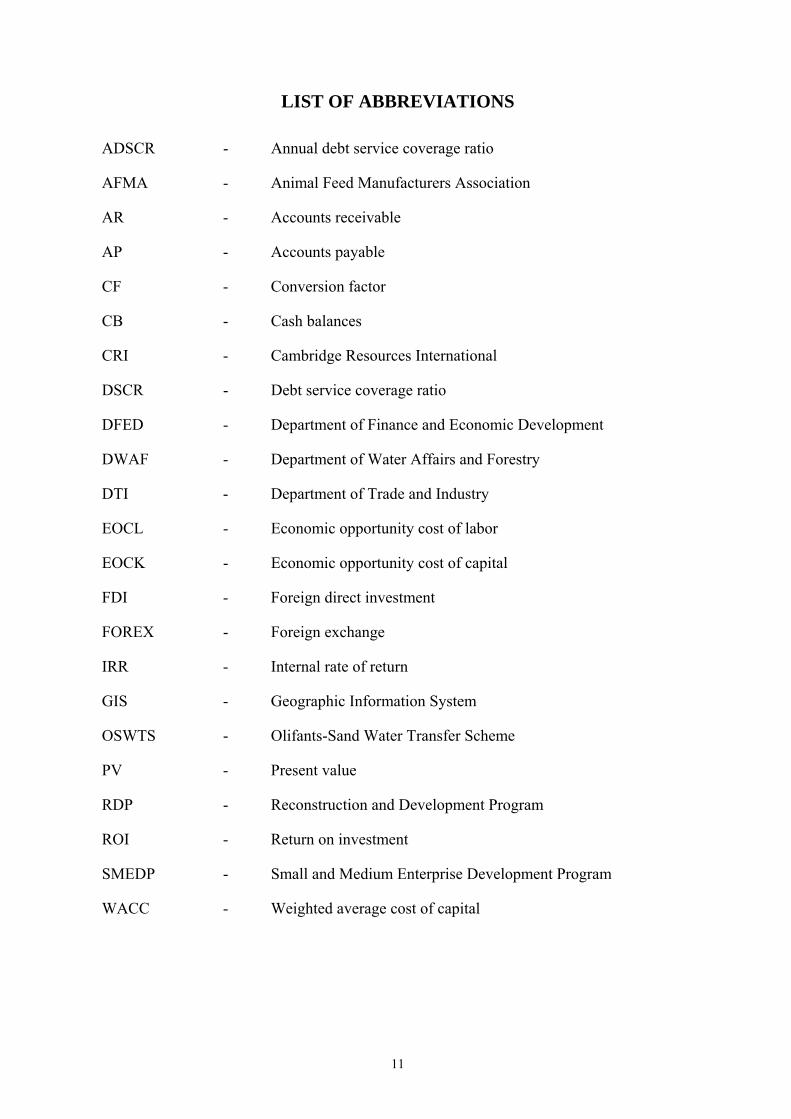
LIST OF ABBREVIATIONS
ADSCR - Annual debt service coverage ratio
AFMA - Animal Feed Manufacturers Association
AR - Accounts receivable
AP - Accounts payable
CF - Conversion factor
CB - Cash balances
CRI - Cambridge Resources International
DSCR - Debt service coverage ratio
DFED - Department of Finance and Economic Development
DWAF - Department of Water Affairs and Forestry
DTI - Department of Trade and Industry
EOCL - Economic opportunity cost of labor
EOCK - Economic opportunity cost of capital
FDI - Foreign direct investment
FOREX - Foreign exchange
IRR - Internal rate of return
GIS - Geographic Information System
OSWTS - Olifants-Sand Water Transfer Scheme
PV - Present value
RDP - Reconstruction and Development Program
ROI - Return on investment
SMEDP - Small and Medium Enterprise Development Program
WACC - Weighted average cost of capital
11
1. INTRODUCTION
It has been the task of the Department of Finance and Economic Development (DFED) to
identify and promote new promising projects in various sectors of the provincial economy. The
animal feed production was in the scope of the Limpopo Province Economic Development
Strategy.
This interest in animal feed production was amplified further by a report prepared in 2001 for a
foreign firm willing to invest into this industry. The foreign firm became interested in launching a
feed production plant in the Limpopo Province to serve the local market and, possibly, other
regions as well as neighbor countries.
Development of the agriculture sector is on of the top priorities in the Limpopo Province
Economic Development Strategy, and animal feed production falls under the range of activities,
being encouraged by the Government. In addition to that, the National Government has also
determined its support for fostering foreign direct investments (FDI) into the Province under its
“Small and Medium Enterprise Development Program” (SMEDP). According to this policy,
certain FDIs are eligible for a grant from the National Government, if the project in question is
expected to contribute substantially to the economic growth of the Province.
This project is of interest as an investment appraisal case study for two reasons. First, it is a
case of a foreign investment in an activity which is principally a domestically based service.
Although the service might be in great demand and highly valuable, it must be kept on mind, that it
is unlikely to generate substantial net foreign exchange earnings. At the same time, the economy
will need to incur investment costs in foreign currency. Hence, it is a type of foreign direct
investment that can not be considered to represent a net inflow of foreign investment funds into the
country.
Second, this project has applied for a capital subsidy from the Government and for other local
investment incentives. Hence, even if the project is highly worthwhile as a private investment, the
appraisal from the Government’s point of view needs to assess if the proposed feed project actually
generates sufficient economic externalities to justify the use of public sector resources to attract the
foreign investment into country.
12

Evaluation of the animal feed project was carried out with full cooperation of the firm’s
representatives. Department of Finance and Economic Development facilitated the logistical
support and was represented by Mr. D. M. M. Modjadji, Director of Planning and Research. Mr.
Andrey Klevchuk was appointed by Cambridge Resources International to conduct the evaluation
under overall supervision of Prof. Glenn P. Jenkins from CRI.
13
2. PROJECT DESCRIPTION
2.1 Location
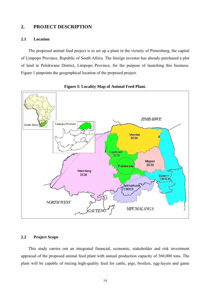
The proposed animal feed project is to set up a plant in the vicinity of Pietersburg, the capital
of Limpopo Province, Republic of South Africa. The foreign investor has already purchased a plot
of land in Polokwane District, Limpopo Province, for the purpose of launching this business.
Figure 1 pinpoints the geographical location of the proposed project.
Figure I: Locality Map of Animal Feed Plant.
2.2 Project Scope
This study carries out an integrated financial, economic, stakeholder and risk investment
appraisal of the proposed animal feed plant with annual production capacity of 360,000 tons. The
plant will be capable of mixing high-quality feed for cattle, pigs, broilers, egg-layers and game
14
animals. The inputs for animal feed include, but not limited to: maize and its by-products, corn
silage, wheaten bran, molasses, sorghum, fibber, feedlime, cotton seed, sunflower oilcake, soya
oilcake, fish meal, urea and possibly other ingredients.
The feed is expected to sell mostly to the local animal breeders, and probably also to other
regions within South Africa. It has been stated that export of feed may be feasible to the
neighboring countries if the product’s price is competitive. The possibility for exporting the feed to
Middle East (Saudi Arabia) was under close consideration, but this opportunity must be further
explored before making any quantitative projections.
There are many feed ingredients locally available in the Limpopo Province, but some of them
have to be purchased from other regions or neighboring countries. Thus, such ingredients as maze,
sunflower oilcake, soya oilcake, fish meal, and urea will have to be imported into the Limpopo
Province.
All the equipment and technology of feed production are to be replicated from an existing feed
plant abroad, which is already operated by the foreign investor. Given the fact that the plant in
Pietersburg will be an identical copy of its overseas counterpart, such a transfer of skills and
experience in this industry facilitates the planning for this project.
The foreign investor has purchased the land and initiated the transfer of the equipment from
the home country. The delivery of equipment and its on-site installation is expected to take 12
months or so. Thus, it is expected that the plant will start operation in the second half of 2003. It
will take another 12-18 months to reach its full capacity of 360,000 tons, if market conditions allow
this.
The foreign investor is planning to finance, build, operate and own the whole enterprise. Since
the project qualifies for the grant under SMEPD, it will receive a cash subsidy from the
Government, not exceeding Rand 3 million. This enterprise will also enjoy the other incentives
available for start-up companies in Limpopo Province. The expected lifespan of the project is 10
years from the commencement of operation.
15
3. ANIMAL FEED MARKET
3.1 Animal Feed Production
The demand for animal feed is a derived demand arising from the demand for meat. Feed
consumption is largely driven by commercial farms that typically need an additional food
supplement for the intensive raising of meat animals and poultry. Production of animal feed in
South Africa is an established industry. The main player has been the Animal Feed Manufacturers
Association (AFMA), with the market share of about 60% of the total feed sales.
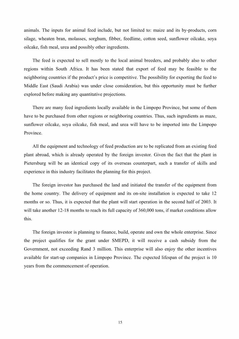
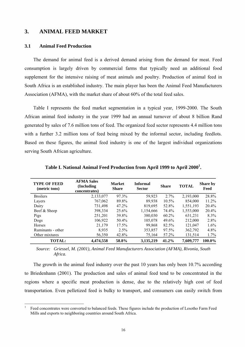
Table I represents the feed market segmentation in a typical year, 1999-2000. The South
African animal feed industry in the year 1999 had an annual turnover of about 8 billion Rand
generated by sales of 7.6 million tons of feed. The organized feed sector represents 4.4 million tons
with a further 3.2 million tons of feed being mixed by the informal sector, including feedlots.
Based on these figures, the animal feed industry is one of the largest individual organizations
serving South African agriculture.
Table I. National Animal Feed Production from April 1999 to April 20001.
TYPE OF FEED (metric tons)
AFMA Sales (Including
concentrates) Market Share
Informal Sector Share TOTAL Share by
Feed Broilers 2,133,077 97.3% 59,923 2.7% 2,193,000 28.8%Layers 767,062 89.8% 89,938 10.5% 854,000 11.2%Dairy 731,498 47.2% 819,695 52.8% 1,551,193 20.4%Beef & Sheep 398,334 25.6% 1,154,666 74.4% 1,553,000 20.4%Pigs 251,201 39.8% 380,030 60.2% 631,231 8.3%Dogs 106,922 50.4% 105,078 49.6% 212,000 2.8%Horses 21,179 17.5% 99,868 82.5% 121,047 1.6%Ruminants - other 8,935 2.5% 353,857 97.5% 362,792 4.8%Other mixtures 56,350 42.8% 75,164 57.2% 131,514 1.7%
TOTAL: 4,474,558 58.8% 3,135,219 41.2% 7,609,777 100.0%
Source: Griessel, M. (2001), Animal Feed Manufacturers Association (AFMA), Rivonia, South Africa.
The growth in the animal feed industry over the past 10 years has only been 10.7% according
to Briedenhann (2001). The production and sales of animal feed tend to be concentrated in the
regions where a specific meat production is dense, due to the relatively high cost of feed
transportation. Even pelletized feed is bulky to transport, and consumers can easily switch from
1 Feed concentrates were converted to balanced feeds. These figures include the production of Lesotho Farm Feed
Mills and exports to neighboring countries around South Africa.
16
one manufacturer to another if the differential in transportation cost makes it attractive. Mostly due
to this reason, only a little amount of animal feed is exported outside South Africa and where this
takes place, the producer is likely to be located close to the national border. Regional sales of
animal feed are quite frequent, and in the times of feed shortage customers may order feed from a
producer as far as 800 kilometers away. Nevertheless, the feed market predominantly serves the
domestic consumer and, hence, animal feed is classified as a “non-tradable” commodity.
3.2 Feed Ingredients
The essence of the feed production business is the mixing of various ingredients into different
types of feed with specific nutrition content. Thus, the availability of raw materials is a crucial
factor for the survival of a feed plant. The amount of raw materials available for local feed
production depends on the crop yields and human consumption of feed ingredients. The availability
of local raw materials determines the amount of imported ingredients to be imported from abroad
or other regions of South Africa.
Internationally over 500 raw materials are specified by their nutritional values for possible use
in animal feed, as Hasha (2002) suggests. However, the actual mix of ingredients used in the feed
production will depend on the availability and price of the ingredients, season of the year, and
foreign exchange rate, as well as other factors. The feed ingredients are close substitutes, their
prices tend to be correlated in the movements, and the analysts agree that maize prices directly
affect the prices of many other feed ingredients. In turn, the domestic maize prices in South Africa
are directly determined by world prices. In years where there is a maize surplus the domestic prices
will be derived from the prices of maize exports. Briedenhann (2001) points out that during years
of shortages the maize price will automatically switch to import (cif) parity. In other words, the
feed ingredients are largely “tradable” commodities, with their prices heavily influenced by the
international factors.
3.3 Animal Feed Supply in Limpopo Province
There are two ways to obtain animal feed in Limpopo Province for a farmer. The first is the
natural grazing, which is not available any time of the year, and/or production of an own-made feed
mix at the farm from ingredients purchased elsewhere. The second way is to purchase a complete
17

formulate feed from a branded manufacturer. As a matter of fact, most of the farmers in Polokwane
combine the two methods to ensure the needed nutritious content at the lowest possible cost. While
the commercial feed is definitely not the cheapest solution for the farmer, it does help the farmer to
save energy and time during bad grazing seasons. The problem with the natural grazing is that
there is less and less land suited for intensive grazing, and it is not always available when needed.
As our investigation suggests, many farmers indeed tend to mix the feed on site, or to purchase
semi-processed or raw by-products from the mills. This practice can be explained by a set of
factors affecting the process of animal breeding:
– need to change the vitamin and calorie content of the feed during the different stages of animal growth;
– quality of the feed;
– freshness of the feed, which tends to deteriorate if stored for long;
– lower transportation and handling costs if the farm is self-sufficient in feed production;
– full control over the process;
– lower labor costs, since the workers, already employed at the farm, can be used to handle the mixing.
On the other hand, the feed manufacturers offer a certified quality feed mixture at any time of
the year, and most of the commercial farmers increasingly use such feeds in order to ensure a stable
animal mass growth. The following four are the major suppliers used by animal production units in
and around Polokwane: Meadow Feeds in Randfontein and Delmas, Silgro Feeds (Genfood) in
Marble Hall and Silverton, OTK Feeds in Delmas, and ALZU Feeds in Middelburg. The two much
smaller local suppliers are Brenco in Louis Trichardt and Driehoek Voere at Vaalwater.
The analysts from the Department of Economic Planning and Research at the Provincial
Government have already considered the animal feed production to be a potent project in the
framework of the long-term provincial economic development. Annex D of “The Northern
Province Industrial Development Strategy 2000” (2000) conducted a pre-feasibility study on
animal feed production in the Province. One of the findings was that more than 80% of the
ingredients used in the production of animal feed are imported into the Province. The province is
currently not a major producer of maize, and research needs to be made to determine whether
18
maize can be grown commercially in the Province or if suitable substitutes are available to use
instead of maize for animal feed. Studies that have recently been conducted suggest that sorghum
could be an effective replacement for maize as the energy component in a feed formulation.
Comparisons between the nutrient value of sorghum and maize show that the feeding value of
sorghum is 85 to 97% of the equivalent value of maize.2
3.3.1 Provincial Feed Industry
It is quite cumbersome for a farmer to do own mixing of the feed, because the farmer will have
to procure a constant supply of ingredients at an affordable price level. The feed manufacturers
make life somewhat easier for the farmers by offering the ready made feed locally and there is no
need for the farmer to deal with the purchase, storage and processing of feed inputs. The
organizational structure of the feed market in Polokwane is a web of independent feed
manufacturers, each of them caring mostly to local consumers. The high transportation costs
enforce the consumers to compare the prices of the different manufacturers by including the
associated transportation and time costs.
In other words, an individual farmer faces a situation where he is free to choose between the
local and remote manufacturer, and the choice will depend on the two feed different prices as well
as time and transportation costs. When the total costs are equal, the farmer will be indifferent
between the two manufacturers but if one of them is lower, his preference will be definitely given
to the cheaper product, assuming that the feed quality and all other factors are identical:
PriceFeedLocal + CostTime
Local + CostTransportLocal = PriceFeed
Remote + CostTimeRemote + CostTransport
Remote
What is typical to observe is that the farmer is more likely to prefer the local manufacturer,
because the other feed producer faces the same input costs and any feed price differential is
typically absorbed by the higher transport costs. However, emergencies at the farm and feed
2 A wide range of other products that are suitable for inclusion in animal feed is available in the Northern Province.
These products currently have very little commercial value and require specific research into the nutrition implications and the economics of their inclusion in animal feed formulations. A list of these products is provided: citrus and other suitable fruit peels, cotton seed, spent grain (hops and sorghum), spent grain from mills, cassava starch, lucerne and roughage (production to be encouraged), under grade potatoes and potato peels, chicken manure, sickel bush, feather meal, fryer oil. Feather meal is a particularly interesting case in the sense that it is a valuable protein source and protein is the most expensive ingredient in any feed formula. There are large broiler and egg production facilities in Northern Province, but poultry feathers are being discarded.
19
shortage at the local producer do from time to time force the consumer to order feed from remote
manufacturers.
In other words, the market structure of the feed industry in Limpopo Province resembles a
monopolistic competition, where the nearest feed producer behaves as a local monopoly as long as
its feed price is competitive with the others’ price plus the time and transport costs. An important
implication of this market structure is that if a manufacturer is able to provide the feed at a lower
cost, the consumers will easily switch from the other brands to this manufacturer. Any new big
producer will definitely impact on the market share of the existing manufacturers.
3.4 Animal Feed Demand in Limpopo Province
The conclusion of “The Northern Province Industrial Development Strategy 2000” (2002) said
that there is a potential for the expansion of the animal feed production in the Province. There are
well-established cattle, pig and chicken commercial farms in the Province, as well as there are an
increasing number of smaller scale producers. The study conservatively estimated that the
provincial feed requirements in 2000 were approximately 230,000 tons, which included the major
beef feedlots, broiler and pork production, and egg layers. This figure did not include the numerous
small and farmers and game feed requirements.
3.4.1 Game Farming
What is special to Limpopo Province, compared to other regions of South Africa, is that it has
many game farms and their number is growing year by year as farmers find it more profitable to
care for the game animals. Eloff (2001) estimated that among the other provinces of South Africa,
Limpopo Province had the highest number of game units sold (6,377 units) and the biggest market
share (31.5%) in the industry in 2001. Unfortunately, there is no reliable statistics on the quantity
of feed consumed at game farms in Limpopo Province, but it is expected to be a substantial portion
of the total feed consumption.
Preliminary market research conducted by interviewing game farms indicated that they can be
a potentially lucrative segment of the feed market in Limpopo Province. Several factors contribute
to this. The lack of natural grazing for game animals comes about due to decreasing the territory of
areas suitable for grazing and due to decreasing availability of natural water. At the same time, the
number of game farms and variety of species bred there has been steadily increasing over the last
20
years, and this trend is expected to continue. This can be explained by the increasing tourism
demand for the sites situated in the province. Despite the promising expectations about demand for
game feed, there are no reliable estimates of the total amount of game feed demanded.
3.4.2 Project’s Demand
At present, there are no reliable estimates in regard to the total provincial animal feed
requirement. Using the results of the 2000 study as the basis, the feed total requirement, inclusive
of the game farms, can be conservatively assumed at 400,000 metric tons a year. An annual growth
rate of 3.0% allows to extrapolate this figure to year 2002 with a tentative estimate of 424,360
tons/year. This figure is likely to underestimate the real consumption of the animal feed.
Given the estimated size of the market, a feed production plant with a capacity of 360,000 tons
per annum will be a very big facility for Limpopo Province. Obviously, this feed plant will divert
some of the consumers from the existing producers and will force the less efficient manufacturers
either to quit the industry or to penetrate further to other regions.
In this situation, the new producer has to be flexible enough to offer the required variety of the
rations, as well as to be fast enough to deliver the product fresh to the farmers. There is a growing
concern about the safety of animal feed and as Speedy (2002) underlines that the feed industry
must ensure a safe and healthy diet for the meat animals. It is also important that the pricing of
commercially prepared feed be very competitive with the prices of the other manufacturers and
cost of doing the mix on-site. Of course, there must be a price difference to induce farmer to switch
from other producers or his own on-site mixing facility to purchase the feed from the new proposed
plant.
There is no guarantee that the project will be able to market all of the feed it can technically
produce because the provincial market is already supplied by other manufacturers. The
management can take an aggressive approach by artificially lowering the prices and by marketing
the products to other regions. However, the price reductions only can be a temporary measure to
fight for the market share, and the average break-even price must prevail in the long-run in order to
stay in the business.
21
4. METHODOLOGY
4.1 Objectives of Financial Analysis
Any project can be examined from several points of view, or “perspectives”, as Chapter 2 of
the Manual (2003) suggests. The project owner and operator are likely to be more interested in the
financial strength of the enterprise, and its ability to generate a sufficient return on investment. The
bank(s), who finance the project, wish to ensure a secure repayment of the funds loaned to the
project, and they look for the project’s ability to generate enough cash to meet the debt payments
over years. In respect to the financial analysis, this animal feed plant is a typical commercial
project, which can evaluated upon from the “banker’s point of view” (does not include loan
financing and loan repayment), and from “owner’s point of view” (including loan financing and its
repayment). Section 5 is devoted to the financial analysis of the proposed feed plant. Section 5.14
examines the project from the banker’s point of view, and the discussion of Section 5.15 reflects
the owner’s point of view.
The main questions on the agenda of financial analysis is to assess the financial viability of the
project with the given prices of raw materials and feed for both owner’s and banker’s points of
view. Another way to look at the financial performance of the project is to find the break-even fee
between the cost of raw materials and price of feed per ton, so that the net present value of the
project is equal to zero, since the National Government is involved in partially financing the
enterprise through an investment grant.
The Government should see whether the project is financially viable on its own, without the
Government’s support. If the proposed project is financially sound, then the question is whether the
National Government should give the investor any further incentives, which can be a harmful
disruption of the existing market mechanism. Also, the form of investment incentives is also
questionable, especially the cash grants to new foreign investment projects, which should be really
financially and economically justified. The Government must evaluate the project’s financial
impact on its revenues collections to see if the project’s net impact overweights the grant by higher
amount of tax collections.
22
4.2 Objectives of Economic and Distributive Analysis
The economic appraisal looks at the economic impact created by the project and Section 6
contains the economic analysis of the proposed feed plant. The economic analysis poses a
challenge for the evaluation of the project because many economic values are not observed in the
market place and, hence, adjustments need to be made to the financial values in order to arrive at
the economic values for the inputs and outputs of the project. Sections 6.2–6.4 deal with the
estimation of the economic conversion factors for the construction inputs and the economic value
of animal feed. The main objective of the economic analysis is to see if it is justified to provide a
grant for this type of business, and whether the grant is the most appropriate instrument to
stimulate growth in the sector.
The net present value of the economic benefits less economic costs, will indicate whether the
net economic benefits, measured in terms of year 2002, are greater than zero and project is a net
contribution to the country’s welfare. The flows of real economic resources associated with this
project must economically justify their employment at this project, since there are other sectors
where the resources can be successfully used. The modeling of economic recourse flows and
calculation of the economic NPV are discussed in Section 6.5.
Creation of the economic externalities is an inevitable consequence of any project, and their
estimation is an important component of the project evaluation. Section 7 is devoted to the
estimation of externalities and distributive analysis. The economic externalities are the difference
between the financial and economic values, which can be either negative or positive. Section 7.1
discusses the modeling of the externalities flows and computation of the present value of total
externalities. The reconciliation between the financial and economic analysis is done in Section
7.2.
The next logical step after economic analysis is the stakeholder impact assessment, which
actually looks at the distribution of the externalities amongst the different parties affected by the
project. The main question is who stands to win or lose from the introduction of this project and by
how much. The government may want to interfere and change the design of the project or the
pricing structure in order to obtain a more attractive set of the distributional impacts from the
project. Since the feed project is owned by a foreign company, the stakeholder analysis is essential
to distinguish between the benefits and costs incurred by the foreign owner and these accruing to
23
participants in the domestic economy. Section 7.3 looks after the task of allocation of the economic
externalities generated by the project.
The government needs to assess the economic impact of the project. It should evaluate the
direction and magnitude of the economic benefits and costs created by the project that may not
fully be reflected in the financial analysis. Section 7.4 examines these issues.
4.3 Objectives of Sensitivity and Risk Analysis
Sensitivity tests are performed on the financial, economic and distributive analysis results in
order to assess the degree of vulnerability of the project to various exogenous variables. Sensitivity
analysis is a convenient way to understand how to re-configure the structure of the project so that it
becomes less vulnerable to possible hazards. Sensitivity tests have been used throughout the
financial and economic analysis in order to detect the crucial project’s variables. Once such
parameters are located, the project’s owners and government may re-design the project to improve
its performance, if needed. There are two sections with sensitivity tests: Section 5.16 contains the
financial sensitivity tests and Section 7.5 has the economic and stakeholder impact sensitivity tests.
The risk analysis is carried out in Section 8, after identifying the risky and uncertain variables
of the project. The main objective is to test the behavior of the project under the most “realistic”
circumstances, generated under the risk simulation. A comparison between the “static” project
indicators and resulting risk “expected values” of these indicators reveals the likelihood of the
project to achieve the performance targets.
4.4 The Method and Tools
The methodological framework of this study follows the state-of-art investment appraisal
methodology developed by Jenkins and Harberger over the past 30 years and well-described in the
Manual (2003). The present study is an illustrative application of the methodology laid out in the
Manual.
The strong analytical framework is embedded into a computer-based mathematical model
constructed in the Microsoft Excel® spreadsheet processor. The actual modeling procedures and
formulas for project appraisal have been developed by Cambridge Resources International. The
24
risk simulation is modeled with the help of risk analysis software Crystal Ball®, developed by
Decisioneering Inc. The integrated financial, economic, distributive, sensitivity and risk analysis is
modeled into a single spreadsheet, and tabulated results are available in Annex A.
4.5 Model Overview
The analysis of the feed project is based on a mathematical model of the given and estimated
technical, financial and economic parameters. This analysis is done by using the Microsoft Excel
spreadsheet processor. All the relationships among the parameters are expressed in formulas, which
are constructed in such a way that any change in the basic parameters is automatically reflected in
all the consequent formulas, and final results are also adjusted. The model of the project is built in
steps, where “tables” are a set of links and relationships among variables, serving a specific
function in the model. Figure II outlines the steps in the feed project, and shows the tables used in
the model. A detailed description of each table will allow the analyst to replicate the model.
25
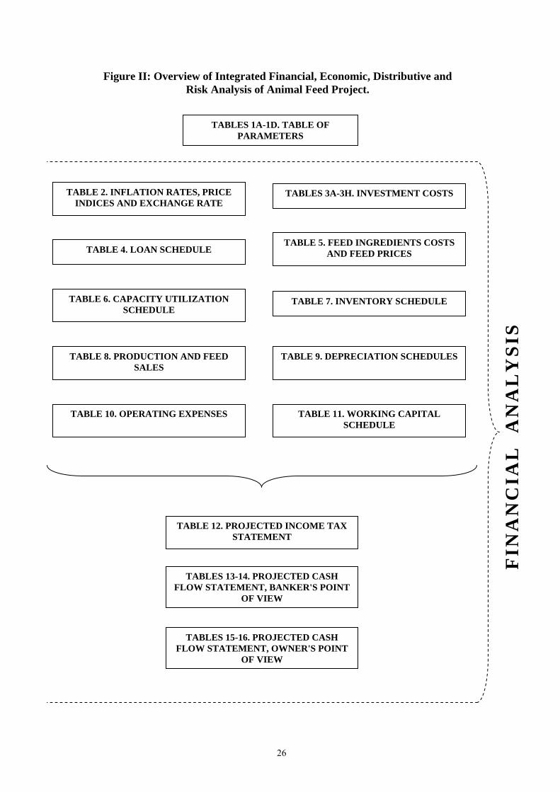
Figure II: Overview of Integrated Financial, Economic, Distributive and Risk Analysis of Animal Feed Project.
TABLES 1A-1D. TABLE OF PARAMETERS
TABLE 2. INFLATION RATES, PRICE INDICES AND EXCHANGE RATE
TABLES 3A-3H. INVESTMENT COSTS
TABLE 4. LOAN SCHEDULE TABLE 5. FEED INGREDIENTS COSTS
AND FEED PRICES
TABLE 6. CAPACITY UTILIZATION SCHEDULE
TABLE 7. INVENTORY SCHEDULE
TABLE 8. PRODUCTION AND FEED SALES
TABLE 9. DEPRECIATION SCHEDULES
TABLE 10. OPERATING EXPENSES TABLE 11. WORKING CAPITAL SCHEDULE
TABLE 12. PROJECTED INCOME TAX STATEMENT
TABLES 13-14. PROJECTED CASH FLOW STATEMENT, BANKER'S POINT
OF VIEW
TABLES 15-16. PROJECTED CASH FLOW STATEMENT, OWNER'S POINT
OF VIEW
FIN
AN
CIA
L
AN
AL
YSI
S
26
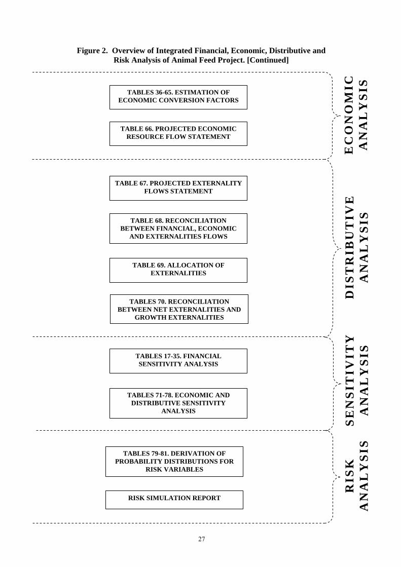
Figure 2. Overview of Integrated Financial, Economic, Distributive and
Risk Analysis of Animal Feed Project. [Continued]
TABLES 70. RECONCILIATION BETWEEN NET EXTERNALITIES AND
GROWTH EXTERNALITIES
TABLES 17-35. FINANCIAL SENSITIVITY ANALYSIS
TABLES 36-65. ESTIMATION OF ECONOMIC CONVERSION FACTORS
TABLE 66. PROJECTED ECONOMIC RESOURCE FLOW STATEMENT
TABLE 67. PROJECTED EXTERNALITY FLOWS STATEMENT
TABLE 68. RECONCILIATION BETWEEN FINANCIAL, ECONOMIC
AND EXTERNALITIES FLOWS
TABLE 69. ALLOCATION OF EXTERNALITIES
TABLES 71-78. ECONOMIC AND DISTRIBUTIVE SENSITIVITY
ANALYSIS
TABLES 79-81. DERIVATION OF PROBABILITY DISTRIBUTIONS FOR
RISK VARIABLES
RISK SIMULATION REPORT
RIS
K
AN
AL
YS
IS
SE
NS
ITIV
ITY
A
NA
LY
SIS
D
IST
RIB
UT
IVE
A
NA
LY
SIS
E
CO
NO
MIC
A
NA
LY
SIS
27
5. FINANCIAL ANALYSIS
5.1 Scope of Financial Analysis
Several objectives are pursued in the financial analysis of the animal feed production in
Limpopo Province. The central issue is the viability of commercial feed production under the
existing market conditions and the technology of the proposed plant. This financial analysis of the
proposed feed project is carried out from two alternative evaluation perspectives: “banker’s (or
total investment) point of view” and “owner’s point of view”. The main question here is to
determine if the proposed plant is a feasible investment. If not – then what are the factors, which
gravely affect the projected financial performance of the project.
The “banker’s point of view” evaluates the project without including any loan items into the
cashflows, in order to determine the overall financial potential of the project. Any grants and
subsidies which are not originating from the bank are included into the cashflow. If the project
seems to be performing well on its own then the project might be eligible for a loan. Annual debt
service coverage ratios (ADSCR) and debt service coverage ratios (DSCR) are calculated for
various financial schemes using the proposed plant configuration and prices of raw materials and
output. The analysis helps to determine if the amount of borrowed funds are likely to be repaid in
full with the given financial structure of the project. Section 5.14 contains the results of the
financial assessment from “banker’s point of view.”
The “owner’s point of view” is the second step of the analysis, and is simply the evaluation of
the proposed project as it is perceived by the project owner. Looking at the feed plant from this
perspective, the cashflows will include all grants/subsidies, as well as the cashflow items related to
external finance, i.e. loan funds and their repayment. The relevant measure of performance is the
net present value (NPV) of the cashflows, which signifies the overall financial performance of the
investment over years. The internal rate of return (IRR) criteria is also calculated, but it does not
play a role as a decision tool. Section 5.15 examines the proposed feed project from this evaluation
perspective.
In order to look at the project from different evaluation perspectives, a financial model should
be completed. Sections 5.2–5.12 are devoted to the discussion of the modeling procedures of such a
financial model. Section 5.13 prepares an income tax statement for the enterprise.
28
5.2 Model’s Assumptions: Table of Parameters
Construction of the Table of Parameters is the starting point of the modeling process. It is
really a set of fields in the spreadsheet, where all known parameters of the project are recorded. All
consequent formulas are built through links to the Table of Parameters and, therefore, it is
important to place all variables into this table, instead of scattering them in various locations in the
spreadsheet. Having all data in one place makes further references quick and ready. The Table of
Parameters is shown in Tables 1A–1D in Annex A.
It is useful to divide the available information about the project into logical sections, such as
timing, technical data, financing, taxation, economic parameters and etc. The parameters are
usually taken from preceding technical studies, or from experts, from the professional literature,
from market observations, or are assumed.
If an assumption is made, the analyst should make a reasonable estimate of the assumed
variable, and give an explanation why a certain value is chosen. Very often some data either are not
available or are costly to obtain, but a reasonable assumption is acceptable for the purpose of
conducting the analysis. A careful selection of the value for such cases is needed, because project
may be highly dependent on the variable in question. If it appears that the performance of the
project is indeed vitally linked with an assumed variable, then further sensitivity tests must be
performed to assess the impact of a change in the assumed variable on the project’s outcomes.
5.2.1 Timing
The timing section of the Table of Parameters contains the information about the start and
duration of the project. Thus, the operational life of the feed plant is taken as 10 operational years,
which is usually a sufficient period for a commercial project to pay back the initial costs and
compensate the owner(s). The starting point of the project, so-called “Year 0” concept, is year
2002 in which the physical construction of the plant takes place. Although that the construction
time is, at least, 12 months, the plant owner believes that the operation can be launched somewhere
at the end of year 2003. Therefore, year 2003 is the first operational year of the project, while the
last operational year is 2012.
29
After operating for 10 years, the plant is assumed to shut down and be “liquidated” in year
2013. In fact, the owner may like to continue the enterprise, but for the purpose of the analysis it is
assumed that all assets are liquidated for their “residual” value. Another way to look at it is to think
that the enterprise is sold as on-going concern and the owner gets paid for the remaining value of
the assets. Year 2013 is treated as a period in which the business is being liquidated and financial
accounts are settled among the feed plant and its suppliers and customers. No operational activities
take place in year 2013. A 45-hour working week is taken as the average labor work load at the
plant.
5.2.2 Capacity
The capacity section contains the technical data of the plant and management plans about
running it over time. The design capacity of the plant is 360,000 tons/year. Input/output conversion
ratio describes the proportion of raw feed ingredients (inputs) needed to manufacture 1 unit of
animal feed (output), which means that, on the average, it requires 1.1 metric ton of feed
ingredients in order to manufacture 1 metric ton of feed. This ratio accounts for technical losses
and shrinkage of the raw ingredients during the manufacturing process. Raw material requirements
of 396,000 tons/year are calculated as a product of plant capacity and the input/output conversion
ratio.
The planned capacity utilization factor is the “planned” production schedule for the plant.
However, actual production may be different from the “planned” path due to a number of reasons,
for instance, due to demand changes or/and changes in the cost of feed ingredients. Further analysis
will deal with such events, and meanwhile the “planned” utilization of the plant capacity is 50% in
year 2003, 70% in year 2004, 90% in 2005 and onwards, and 0% in year 2013.
5.2.3 Financing
This section contains parameters of the project financing, such as method of finance for
investment costs and terms of external finance. The investor has expressed its intention to finance
all the costs of equipment and its freight from equity funds of the company. According to the
company representative, the local costs will be financed by a combination of equity and a Rand
loan from a South African bank. The maximum amount of such a loan is about 50% of the local
costs.
30
Real vs. Nominal Interest Rate: For a project of this nature and size, a commercial Rand loan
can be drawn from one of South African banks. The underlying real interest rate for such kind of
commercial loan can be assumed 8.50%, which transforms into a nominal interest rate of 15.01%
in year 2003. As Chapter 4 of Manual (2003) suggests that the relationship between the real and
nominal interest rates and the expected rate of inflation can be expressed through formula:
i = r + R + (l + r + R) * gPe
Where, nominal interest rate is represented by (i), real interest rate by (r), country risk
premium by (R), and inflation rate by (gPe). Since the loan is drawn from a local bank, the country
risk (R) is set to zero, and with the expected inflation rate of 6.0% in year 2003, and with real
interest rate (r) of 8.50%, the resulting nominal interest rate is 15.01%.
Loan Terms: A likely, but not necessarily, set of conditions for such a loan would be a grace
period of 2 years from the start of the project, a repayment period of 5 years with equal nominal
annual installments. The actual nominal rate will be adjusted for the impact of the expected
inflation rate(s). Thus, the repayment of the loan will begin in year 2004 and the last repayment
will be made in year 2008. By definition, the ending balance of loan financing should be zero at the
end of year 2008.
5.2.4 Foreign Exchange Premium
A few economic parameters are used in the model. They are taken from other studies, for
instance, the foreign exchange premium on the traded goods is taken as 5.50% and on non-traded
goods as 2.0%, following Chapter 9 of Manual (2003).
In fact, there are more parameters for the economic analysis, but most of them are used only
once and tend to be too lengthy to be included into the Table of Parameters. For example, the
estimation of economic conversion factors requires a detailed break-down of cost shares for each of
the many commodities. Instead of placing these values in the Table of Parameters, they appear
directly in the conversion factor tables, marked as “assumed” values.
31

5.2.5 Discount Rates
There are two discounts rates used in the analysis: financial and economic. The financial
discount rate is the minimum rate justifying the use of private capital in this project. The required
return on investment rate can be used as the minimum acceptable financial discount rate. In other
words, the owner of funds will be willing to participate in a project only if the minimum return on
investment is assured at 10.0% in real terms. Adjusting to nominal rate, inclusive of inflation, give
us a nominal discount rate of 16.6%. This calculation follows the formula similar to the
relationship between real and nominal interest rates, and it can be expressed as:
DN = dr + (l + dr) * gPe
Where, the nominal discount rate is represented by (DN), real discount rate by (dr), and
expected inflation rate by (gPe). With the expected inflation rate of 6.0% in year 2003 and with real
discount rate (dr) of 10.0%, the resulting nominal discount rate is 16.6%. Both nominal and real
rate of return on investment may be used in financial analysis, representing the opportunity cost of
capital to the owners of the project. By definition, the net present value obtained by the discounting
the nominal net cash flow by the nominal discount rate must be identical to the net present value
obtained by discounting the real net cash flow by the real discount rate.
For the economic analysis, a different measure of cost of capital is needed, because this feed
plant is one among many alternative projects, where capital resources can be productively
employed. The relevant discount rate for economic analysis is the economic opportunity cost of
capital (EOCK) for South Africa. As reported in Chapter 8 of the Manual (2003), it has been
estimated that the real EOCK for South Africa is 11.0%. This figure is used in the economic
analysis as the discount rate for the stream of benefits and costs during the project’s lifespan.
5.2.6 Inflation and Exchange Rates
One of the core concepts of the financial modeling is tied up with the differentiation between
the “nominal” and “real” prices. “Nominal” prices are easily observed on the marketplace while the
underlying “real” prices are not. The difference between the two is the accounting for inflation
over time through change of the nominal prices are the real price level gross of the cumulative
effect of inflation, while real prices are net-of-inflation. This section of Tables of Parameters
contains information about expected inflation rate(s). Since there are two currencies involved into
32
this project, inflation rates have to be projected for both the US-dollar as well as for the South
African Rand. The US-dollar funds are used for purchasing the equipment and for freight and
transportation expenses while all other expenses are paid out in South African Rand.
Inflation Rates: The price quotations for the imported equipment date back to year 2000, and
that is why the inflation rates for years 2000 and 2001 are stated. The equipment prices of year
2000 have to be adjusted by the annual inflation rates, so that they reflect the present value of
equipment as of year 2002. Domestic average annual inflation rates adopted here are 6.0% for year
2000, 12.0% for year 2001, 9.0% is the expected average rate for year 2002, and 6.0% is the
expected average inflation rate for years 2003 and onwards. For the US dollar, the following rates
were taken as 5.0% for year 2000, 3.0% for year 2001, and 2.5% is the expected average inflation
rate for years 2002 and onwards. The assumption of constant inflation rates over 10 years of plant
operation will be relaxed later in risk analysis, and sensitivity tests will be done to assess the
impact of changes in the assumed inflation rates on the project performance.
Exchange Rate: The average exchange rates used in analysis prior to year 2002, are 7.57
Rand/US for year 2000, and 11.00 Rand/US for year 2001. Starting the year 2002, the expected
exchange rate will be modeled according to the relative inflation path of Rand and US dollar. An
additional disturbance term will be also included to represent all other factors influencing yearly
movements of the nominal exchange rate. It is also assumed that the underlying real exchange rate
between Rand and US dollar will remain constant over years.
One parameter artificially introduced into the model is the disturbance to the real exchange
rate, which is set to zero in the base case of the financial analysis to support the assumption of the
constant real exchange parity between the Rand and US dollar. However, the sensitivity and risk
analysis will use this parameter to simulate changes to the real exchange rate in order to test the
model’s responsiveness to this variable.
5.2.7 Taxation
Any project is subject to a few, if not many, taxes. It is convenient to place all tax related
parameters into one section. The general value added tax (VAT) rate in South Africa is currently at
14.0%, but feed ingredients and animal feeds are exempted from VAT, being a part of basic
agricultural produce. The corporate income tax rate is 30% on the income after depreciation and
interest expenses. A part of incentive package for start-up businesses, the tax code grants a 4-year
33
period of tax holidays, exempting any profits of the enterprise from the corporate tax liability.
After that, a full corporate income tax rate is applied on any profits. The rate of personal income
tax is currently 25%, and the amount of gross salary above the minimum wage is taxed at this rate.
5.2.8 Working Capital
Working capital section contains the expected average amount of accounts receivable (AR),
accounts payable (AP), and cash balances held (CB). Accounts receivable represents an average
annual delay in cash payments, or uncollected accounts arising from sales of the animal feed to
customers. It is often confused with the accounting concept of “accrual” record keeping, under
which income is reported as of the date of a sale regardless of whether the sale was paid for either
in cash or put on customer’s account. Opposite to this, in a cashflow analysis the sales receipts are
treated on an actual cash basis, and if any credit sale takes place, its proceeds are recorded in the
AR instead of being a part of actual cash sales. It is helpful to remember that any increase in AR
implies a reduction in actual cash inflows, relative to the total sales. Therefore, this positive
“change in AR" is actually deducted from the total sales to arrive at the amount of cash sales.
From interviews with the management of the firm, they plan to operate the business on cash
basis in order to prevent bad debts from customers, but it is unlikely that they will be able to
maintain such a strict policy. Under this policy, it is more reasonable to assume that the average
period payment from customers would be 14 days a year, or 2/52 weeks, or 3.85% of feed sales.
Accounts payable are treated in a similar fashion, since they are thought to represent the delay
in cash payments to the suppliers of the plant. It is assumed that the average delay in account
settlement would be 7 days a year, or 1/52 weeks, or 1.92% of total operating costs. It is beneficial
for the project operator to delay actual cash payment to the suppliers; as he has the flexibility of
using that cash during the period of payment delay.
Cash balances held is a cash fund, kept on hand facilitate making the necessary payments. It
has been assumed here that the average amount of cash balance held is 2% of the direct operating
costs.
34
5.2.9 Labor
Labor is a distinctive input of any project. Typically, labor parameters describe the number
and kind of employees, their wage rates, fringe benefits, insurance and social security payments,
expected real wage growth rates, etc. A few parameters will be also needed for the economic
analysis during the estimation of the economic conversion factors for the different labor types
employed by the project.
Unskilled Labor
The feed plant will need 12 full-time unskilled workers in year 2003, then 16 in 2004, and 20
people will be employed from year 2005 to 2012. No personnel will be needed in year 2013. The
gross monthly wage rate, inclusive of fringe benefits such as transportation, meals, and bonuses is
set at 2,100 Rand, and it is expected that this rate will grow, in real terms, by 0.5% per annum.
The people employed at the plant will come from other sectors, and given the labor market
situation in Polokwane, it is reasonable to assume that the two main sources of unskilled labor will
be the informal farming sector and quasi-voluntary unemployed. The average wage in the informal
sector (Wo) is taken as 651 Rand/month, and it is assumed the feed project will attract 10% of its
unskilled workers from the informal farming sector. The remaining 90% of the unskilled
employees will leave their quasi-voluntary unemployment, which earns the average income of
1,266 Rand/month. The stated parameters are enough to estimate the supply wage of unskilled
labor, which is the average wage rate of the informal sector and of and quasi-voluntary
unemployed, according to the Chapter 10 of the Manual (2003). The computed supply wage for
unskilled labor is 959 Rand/month.
There is no personal income tax on the income of unskilled labor because their salary is just at
the level of the official minimum wage of 1,266 Rand/month. But there are contributions, actually
paid by the employer, which accrue to the government-regulated agencies. Under the current law,
the social insurance contribution is set at 12.52% of the wage rate, from which 5.0% is thought to
be paid by the employee, but in reality it is paid by the firm. The compulsory contribution to the
workmen’s compensation fund is set at 2.55%, while the skills development fund requires an
additional payment of 1.5%, and the unemployment benefit fund takes another 2.0%. All the
contributions add up to 18.57% of the wage rate, which is a substantial amount and should not be
neglected.
35
Besides the contributions, a productivity bonus is usually paid to the worker at the end of the
year, and its monthly equivalent amounts to 65 Rand/month. Thus, the financial cost of unskilled
employee (gross wage) becomes 1,566 Rand/month, which is computed as the minimum wage of
1,266 Rand/month plus the productivity bonus of 65 Rand/month and plus the 18.57% in
contributions. All these parameters will be later used for the estimation of the economic cost of
unskilled labor in Section 6.3.1.
Skilled/Semi-Skilled Labor
Skilled personnel, such as technicians, will be employed on a permanent basis and the plant
will need 4 qualified employees starting from year 2003 till 2012. No skilled personnel are
expected to be employed in year 2013. The real wage rate to be paid by this project is set at 14,500
Rand per month, and it is expected to rise by 0.5% annually. These figures will be used for the
modeling project’s labor expenses on the skilled and semi-skilled labor.
A few parameters about the labor market are needed for estimation of the economic cost of the
skilled and semi-skilled labor. The prevailing market wage is taken as 12,830 Rand/month, which
converts to an annual salary of 153,960 Rand/year. It is assumed that the share of personnel
attracted from other sectors is 90%, and the remaining 10% are attracted from outside of the
unemployed pool. The annual income tax and site tax amount to 35,409 and 8,720 Rand/year
respectively, making the total amount of taxes equal to 44,129 Rand/year. A typical package of
fringe benefits for skilled and semi-skilled employees is estimated as 17.07% of the annual wage.
Local and Foreign Management
The tasks of supervision and administration of the plant operations fall on the shoulders of the
management. The analyst should differentiate between the local and foreign management because
each has its own opportunity cost and there are different income tax implications. There is a
substantial share of labor costs in the construction, and this is where the local management will be
used.
But the management of the plant must have enough expertise in running the production affairs,
and that is why three experienced people will be brought from the foreign country in order to
supervise the production. Their monthly wage rate is assumed to be 18,000 Rand per person,
subject to a real growth rate of 0.5% per annum. The management team will be employed full time
from year 2003 to 2012. The South African personal income tax rate is 25%, and foreign
employees are expected to repatriate 50% of their net-after-tax income back to the home country.
36
5.2.10 Operating Costs
There are a number of direct and indirect operating costs associated with the business.
Transportation and storage expenses are estimated at 2.0 million Rand/year at the full plant
capacity. Administration of the plant will be partially charged to an item of “office
accommodation” of 1.2 million Rand/year, and also to “telecommunication” expense, estimated at
0.6 million Rand/year. Audit and accounting services are expected to cost 10.0 million Rand/year,
while advertising is budgeted with 5.0 million Rand/year. Business travel and transportation
expenses are expected to be 1.0 and 1.5 million Rand/year respectively. Office and transportation
services will cost 0.5 million Rand/year. All the stated figures are expressed in the prices of year
2002, i.e. real prices. An inflation adjustment will be needed for the future projections in order to
maintain the same price level in real terms.
Equipment mechanic service is the expense for routine equipment maintenance, which
typically includes some spare parts and labor to maintain the machinery in a proper condition. It is
estimated that this service will cost, on the average, 2.5% of the real total equipment cost every
year. An adjustment should be made for the actual capacity plant utilization factor and inflation
rate.
5.2.11 Electricity
The site of the feed production is located in the vicinity of Polokwane Municipality and
electric power is supplied to the plant by Polokwane Municipality. A quote was obtained from the
Municipality on the conditions and tariffs applicable for such a connection. A fixed service fee of
90 Rand/month, in real terms, is charged on the connection regardless of the actual consumption. It
is expected that the plant will consume power of 200 KVA per month. A demand charge of 50
Rand/month, in real terms, is also applied on every KVA of energy consumed, in addition to the
following tariffs. The basic tariff of 0.20 Rand/kWh is charged for the first 100,000 KWh per
month, and a tariff of 0.18 Rand/kWh is charged for any energy above the 100,000 KWh/month
consumption. It is assumed that the tariffs will grow by 0.5% per annum in real terms, in addition
to the annual inflation adjustment.
37
5.2.12 Water
Water services are also provided by Polokwane Municipality, from which a quote was
obtained in regard to water tariffs. A step tariff rate system is used by the Municipality with the
first 30 m3/month being charged at 5.00 Rand/m3, the next 20 m3/month is charged 6.50 Rand/m3,
the following 50 m3/month is charged 7.50 Rand/m3, the next 19,900 m3/month is charged 8.00
Rand/m3, and any amount above that is subject to a tariff of 7.00 Rand/m3. Due to scarcity of water
in the region and raising costs of water provision, a real growth rate of 1.0% per annum is used in
the analysis, in addition to the annual inflation adjustment of the tariffs.
The designed water consumption for the plant is 60,000 m3/annum if it operates at the full
capacity. The actual water requirement in any year is calculated by multiplication of the 60,000
m3/annum water requirement and the actual plant capacity utilization factor in that year. For
instance, the water requirement for year 2003 is only 30,000 m3 because the plant is expected to
operate at 50% of its capacity.
5.2.13 Inventory of Feed and Feed Ingredients
The business of animal feed production requires input and output inventories in order to run
smooth. An inventory of feed ingredients is needed to ensure an interruptible availability of raw
materials, and to avoid frequent price fluctuations of the major ingredients, such as maize and
oilcake. Feed inventories are desirable to be able to serve any potential customer. The amount of
inventory is a choice of the management, and there is always a trade-off between the advantage of
having a plentiful stock at any time and the opportunity cost of keeping such inventories in the
working capital plus physical storage costs. A larger inventory implies higher opportunity and
storage costs and that is why, hence, any increase in inventory will have a negative impact on the
net cash flows of the enterprise. This will be reflected in increased purchases of inputs than
actually used in production in order to build up the input inventories, and an excess of production
over sales in order to accumulate the inventories of finished goods.
As experts from AFMA suggest, an “optimal” amount of raw materials inventory is a 2-month
stock of feed ingredients. It is assumed that at the end of year 2002, a 1-month stock of feed
ingredients needed for the operation in the next year will be purchased. During the period of 2003-
2012, a stock of 2-months feed ingredients will be maintained. Because there is no need for any
raw materials in year 2013, the ending stock in year 2012 should be zero.
38
Feed inventory is assumed to be a 3-week stock of manufactured feed in year 2002, while an
active advertisement campaign will be in action, and a 2-week stock from 2003 to 2012 during the
plant operational life. The feed inventory will still be a 2-week stock at the end of year 2012, and
this stock will be sold off during the liquidation year 2013.
5.2.14 Depreciation
Any physical asset, with exception of land, tends to depreciate over years. The financial model
of the project must account for the expected decline of the asset values, and a clear distinction must
be made between economic and tax depreciation of assets. It is important to understand how the
two types of deprecation enter into financial model.
Economic Depreciation
Economic depreciation is the physical process of aging of the equipment or any other asset,
and it attempts to estimate the actual loss of value of the asset over the years. The specific function
of economic depreciation is to estimate the salvage value, or also called “residual” value of assets,
which is the market value of the asset for which it could be sold for at the end of the project.
Economic depreciation aims at finding the liquidation value of the asset, which will be part of the
liquidation proceeds at the end of the project life.
It is expected that the feed plant equipment and vehicles will have a useful economic life of 15
years, which means that at the end of 10 operational years there will be some residual value left.
Also it implies that any equipment item depreciates at a rate of 1/15 or 6.67% per annum. The
construction assets, such as buildings and roads have a longer lifespan, and it is quite safe to
assume a 30-year economic life for them. This implies a 1/30 or 3.33% rate of annual depreciation,
and there will be a residual value at the end of the 10-year feed project life. The project owners will
have the option to recover the remaining value of the construction assets by selling the site and
buildings at the end of the project.
Tax Depreciation
Tax depreciation is different from economic depreciation. The rate of tax depreciation per year
is specified by the tax laws of the country. The purpose of tax depreciation schedule will be to
estimate the amount of the tax depreciation expense that can be deducted from the taxable income.
The tax laws around the world allow businesses to deduct a certain amount of tax depreciation
expense, based on the historical cost of the asset. It is not necessarily that the rate of tax
39
depreciation follows the physical aging of an asset, and also certain restrictions are often put on the
amount of depreciation expense for tax purposes, for example, in some countries it is possible to
depreciate either more or less than the full purchase value of an asset. It is typical that the rates of
tax depreciation are greater than the actual tear and wear of the company’s assets. This is favorable
for the business because more tax deductions are accumulated in the first years.
According to the current tax regulation in South Africa, the tax depreciation life for the
equipment and vehicles of the feed plant is taken as 5 years, allowing the full 100% depreciation of
the asset value. The rate of tax depreciation for equipment items is, therefore, 1/5 or 20.0% per
year, and after five years no further tax deduction is allowed. As we have seen above, the
equipment’s useful economic life is believed to be 20 years, but for tax purposes the whole cost of
equipment can be deducted from tax income in just 5 years, which is much faster than the actual
ageing of the assets. The tax depreciation rate in South Africa for the buildings and other
permanent constructions is set at 5% per annum and it is applied on the 100% of the historical cost.
The “historical cost” is the share of the initial costs eligible to be depreciated for tax purposes.
In certain cases, the tax code may allow the historical cost to be either more or less than the actual
cost. In this particular case the amount of the assets that is paid for by the Government grant is
deducted from the historical cost because this grant amount is not allowed to be depreciated for the
tax purposes. The tax cost base is applicable only for tax depreciation, because it has nothing to do
with the physical depreciation of the assets, captured in the economic depreciation. In the present
case, all assets are allowed to use the 100% of their historical value for the calculation of the tax
depreciation expense.
5.2.15 Investment Cost Overrun Factor
The investment cost overrun factor is a variable that represents the deviation in the actual
investment costs away from the design cost estimates. It is a very common for the actual
construction costs to rise due to unforeseen delays, technical difficulties or natural disasters. The
investment cost overrun factor expresses the change in the planned costs as a percentage. If there is
a positive deviation then the actual investment costs will increase, while a negative factor will
mean that the actual costs are lower than expected.
40
The correct way to incorporate the investment cost overruns into the spreadsheet is to apply it
on an existing value as an additional factor at the end of existing formula. For example, let’s
assume we have a cell with formula:
PNominal, YearX = PReal, 2002 * IDYearX
PNominal, 2003 = 100 * 1.06 = 106
Where the nominal price of an asset in 2003 is estimated as 106 Rand (PNominal) by multiplying
the 100 Rand, which is the real price of this asset in year 0 (PReal), by 1.06, which is the domestic
inflation index in year 1 (IDYear1 = 1 + Inflation RateYear1), assuming the rate of inflation equal to
6.0%. This simply says that the expected price of this asset in year 1 will be the price in year 0
adjusted for the domestic inflation. If investment cost overrun factor is incorporated into the above
formula, it should be added at the end of the formula:
PNominal, YearX = PReal, 2002 * IDYearX * (1 + Investment Cost Overrun Factor)
PNominal, 2003 = 100 * 1.06 * (1 + 0%) = 106
In the base-case, this factor is set to zero meaning that the costs are not biased either upwards
or downwards, and any change in investment costs is really unexpected. But any deviation from
zero will change the formula’s result.
This factor is later used in the sensitivity and risk analysis to test the viability of the project to
unforeseen changes in the investment costs. The investment cost overrun factor should be used
with a caution because it may not be reasonable to apply it on certain items, such as equipment, for
instance. There are no unexpected changes in the prices of equipment once the project signs a
contract with the supplier of equipment. Therefore, there should be no link to the investment cost
overrun factor for the equipment items and also for the land. Only the construction costs and
installation costs should be linked to this factor.
5.2.16 Maximum Grant Amount
This figure shows the maximum amount of grant that can be made available for a new project
as a part of the investment incentives package by the National Government. According to the
current regulations, SARS (2002), the maximum amount of cash grant is 3.0 million Rand to be
given in two annual equal parts.
41
5.2.17 Feed Ingredients
A variety of plants and agricultural by-products can be used as inputs for feed production. This
is an unrewarding task to enumerate all likely ingredients that can possibly be used in production.
Instead, a more general approach is used, assuming that whatever the actual mix of ingredients is,
the average cost of feed ingredients is 950 Rand2002/ton in year 2002. This figure is comparable
with the feed ingredients per-ton-cost estimates, stated in interviews by different farmers around
Pietersburg and by existing feed producers in Polokwane. The assumption is made that the average
cost of feed ingredients will remain constant at 950 Rand2002/ton, in real terms, over the project’s
life. Later this assumption can be relaxed in the sensitivity and risk analysis.
The change in the cost of feed ingredients is a variable created for the sole purpose of testing
the impact of cost changes on the project performance. What this variable does, is that it increases
(decreases) the feed ingredients costs if the value of variable is set to be positive (negative), and it
does not impact the ingredients costs at all if the variable value is zero. The mechanism through
which this variable influences the actual spending will be described in detail in Sections 5.6–5.7.
Most of the feed ingredients have a high traded content, because maize and protein sources are
internationally traded commodities and, therefore, a 50% share of tradable ingredients is assumed.
Non-tradable feed ingredients account for 40% of the total cost while transportation and handling
costs are assumed to be 8% and 2% respectively.
For the purposes of further economic analysis, assumptions must be made about the traded
content in each of the components of ingredients are needed. Thus, the traded content of tradable
ingredients is 100% because they are all internationally traded, while the traded content of non-
tradable ingredients is assumed to be only 20% of their value, and traded content of transportation
and handling costs are assumed to be 43% and 60% respectively. This detailed break-down of
traded content is needed in order to estimate the composite traded content of feed ingredients. This
is calculated as a weighted average of the cost shares and corresponding traded contents, and the
resulting figure is 63.7%. In other words, the total composite traded content of feed ingredients is,
on the average, 63.7%.
5.2.18 Milling Fee
The milling fee is the average real fee that must be charged per ton of feed in order for the
plant to break-even financially, i.e. to have the NPV of zero in the owner’s evaluation perspective.
42

In other words, this is the minimum milling fee that the plant must charge the customers per ton of
feed. The following equation holds true:
Price of Feed = Cost of Feed Ingredients + Milling Fee
The minimum milling fee shows how efficient this plant can be compared to other producers,
and if there are any economies of scale that help to reduce the overall production costs. Assuming
that all feed manufacturers face the same input costs and any individual producer is a price-taker,
then the ability of a plant to charge a higher milling fee means higher profits and greater flexibility
to lower its price tags, if needed.
Thus, for an individual producer, the break-even price of feed is a direct function of the
ingredients cost and milling fee. Any change in either of them should immediately translate into a
price movement. An implication of this fact is that the price of feed becomes an endogenous
variable, determined within the model. The two exogenous variables are the average feed
ingredients cost and average milling fee. In this case, we first want to know the value of milling fee
at which the project breaks-even, meaning that the net present value of the cashflows from owner’s
point of view is zero. In other words, the enterprise just covers all the investment and operating
costs, including the opportunity cost of capital.
Finding out the break-even point, which sets owner’s NPV to zero is an iterative process,
which can only be done after the financial model is complete and owner’s NPV is calculated. An
Excel’s function, called “Goal Seek” is used to set the owner’s NPV to zero by changing the value
of milling fee in the Table of Parameters. The resulting break-even value of the milling fee is 258.2
Rand2002/ton, and it is assumed to remain constant at this level, in real terms, over the project’s
lifespan in the base-case financial analysis. Thus, the average price of feed from the plant is
calculated as 1,208.2 Rand2002/ton, which is a sum of the average cost of feed ingredients and
milling fee.
The change in the milling fee is another variable, specially designed to trace the effect of
changes in the fee on the project performance. The value of this variable in the base case is zero,
meaning that no change is expected to the milling fee. Any deviation from zero is translated into
consequent effects on the price of feed, which should either rise or fall, but because the project is
said to be a price-taker then the ultimate impact will be on the quantity of feed sold, rather than the
price. The exact way of modeling this effect is described in Sections 5.6–5.7.
43
5.2.19 Feed Production
A number of parameters are used to describe and model the feed production. Typically a single
plant is able to manufacture different types of animal, aqua-feed and concentrates. It is also a safer
business strategy to diversify production by manufacturing feed for different animal and feed of
assorted dietary content. It is expected that the plant will produce feed for cattle, milk cows, layer
chicken, broiler chicken, pig feed, game feed and aqua feed. There could be also different kinds of
feed for the same animal, for example cattle feed can be formulated to support the nutritious needs
for each of the different stages of animal growth.
Faced with this variety of possible options, an analyst may find it difficult to be as precise in
projecting the future as he otherwise wants to be. It is impossible to foresee in advance what will
be the actual production mix of the different feed types during the 10-year life of the project. But
what is possible to do is that the analysis can be still carried out without sacrificing much of the
desired precision by making reasonable assumptions, based on the current observations and market
trends.
It is assumed that 30% of the feed production will be for cattle and milk cows, which are the
commonly bred animals in Limpopo Province. Other feed manufacturers also seem to have a big
portion of production in this type of animal feed. Since the actual mix of ingredient varies with the
type of feed, season of the year, current market prices, the average cost of raw materials for beef
feed is taken as 1,035 Rand/ton. The chicken layer feed and broiler feed are assumed to occupy
15% each in the total production of the plant. Their respective average ingredients costs are 1,096
and 1,046 Rand/ton. Pig feed is given a share of 15% in the total production, and its average raw
materials cost is taken as 894 Rand/ton. A lucrative and growing market in Limpopo Province is
the game feed for wild animals held in game reserves. This feed is often used to supplement
animals’ ration in the summer and to feed them in winter, when natural grazing might be scarce.
The average ingredients cost is assumed to be 743 Rand/ton, a figure consistent with information
obtained from interviews with the existing game feed manufacturers. Aqua feed is another potential
market niche, and the management of the project thinks that it is a direction they should go. The
aqua feed is easier to transport, and competition is less fierce, compared to other feed types. The
aqua feed is given a 5% share in the total production, and its raw materials cost is taken as 778
Rand/ton.
44
A number of feed types that this plant can manufacture are not, in fact, limited to the
mentioned above. The other possible types include sheep feed, feed for ostriches, feed for rabbits,
and so on. Again, it is impossible to foresee the actual combination of the production mix over the
project life, and that is why it is reasonable to limit the analysis to the selected feed types, which
are definitely going to be marketed.
5.2.20 Feed Prices
The price for each type of feed is calculated as a sum of its average ingredients cost and the
milling fee. For instance, the 1,366 Rand/ton price of chicken layer feed is a sum of its raw
materials, worth 1,096 Rand/ton, and the milling fee of 270 Rand/ton. The prices of the other feeds
are calculated in exactly the same way, reflecting the fact that the price is a direct function of the
raw materials cost and milling fee.
A weighted average cost of ingredients is calculated to cross-check the actual cost of the raw
materials in the production mix. The weighted average calculated as a summation of each feed’s
production share times its ingredients cost:
CW = ( )∑FeedM
FeedMFeedM CostIngrediets*%Production
The value of the weighted average cost of ingredients must be equal to the parameter of the
ingredients average cost, otherwise the feed prices will deviate from the expected levels, and the
relationship identity between the feed price, input costs and milling fee will not hold.
The weighted average price of feed is also computed by using a similar formula, applied on the
calculated feed prices:
PW = ( )∑FeedM
FeedMFeedX Price*%Production
The weighted average price of feed, derived from the formula above, is 1,220.1 Rand/ton, which is
simply the average cost of feed ingredients plus the milling fee.
5.2.21 Feed Market Parameters
Own-Price Elasticity of Demand for Feed
For the purpose of financial and economic modeling, a set of assumptions must be made about
the feed market in the Province. The very first target is to determine the value of the composite
45
demand elasticity for feed (ηFeed). A few methods can be used to derive this parameter, using both
direct and indirect ways to estimate the demand elasticity for animal feed. The direct approach
would use data on feed consumption on the farms and fit the actual data into an econometric
model; much like Tabeau (2001) did for the Netherlands. The problem with this approach is that it
requires a detailed set of data from the farms on their feed consumption and such data may not be
readily available. Given the fact that there is no data or primary study done in this respect for South
Africa, the analysis should turn to an indirect way to estimate the own-price demand elasticity for
animal feed.
The animal feed can only be used as an input into the meat production and the demand for feed
really depends on the requirements by meat producers. Therefore, the demand for feed is a derived
demand from the demand for meat by final consumers. As a consequence, in order to pursue this
approach, the analyst should first obtain the value of the composite demand elasticity for meat with
respect to its price.
The composite demand elasticity for meat (ηMeat) is a parameter describing the responsiveness
of the consumers’ demand for the meat to the meat price changes, as a composite commodity,
which consists of beef, chicken, pork, lamb and other meats. The reason for introducing such a
variable into the model is that the fact that the major driving force behind the feed demand is the
use of feed as an input for the meat production.
A number of econometric studies have been done on the estimation of the demand elasticity
for meat in various countries. Thus, Hanarahan (2002) finds on the example of Ireland that all the
meat goods are net substitutes. The own-price Marshallian elasticities are estimated as -1.52 for
beef, -0.49 for pig meat, -0.67 for poultry, and -0.61 for sheep meat. He also concludes that all the
meat goods are normal goods. Mbala (2002) in the article on the short-run demand for goat meat in
Cameroon finds that the own-price demand elasticity for goat meat is -0.85 if estimated by a linear
function, and -0.90 if estimated by a double-log function.
A study by CARD (1987) reported the own-price elasticities for all meat and dairy products
being between -0.97 and -1.05 in Indonesia. A report by Feuz (2002) states that previous national
research in the beef industry had estimated the own-price elasticity of demand for beef at -0.60 in
the United States. In a case-study of the pork import demand elasticity for Japan, Fabiosa and
Ukhova (2000) estimated that own-price Marshallian elasticity of the demand for domestic meats
was -1.11 for beef, -0.75 for pork, and -1.08 for poultry. Another paper by Workman, Kings, and
46
Hooper (1971) carried out research on the US beef demand in 1947-1967 and concluded that own-
price elasticity of demand for beef during that period was -0.67.
Faced with a lack of micro data on the meat market in South Africa, a seemingly reasonable
figure for the composite own-price elasticity for mead demand of –1.0 is used, which is consistent
with the international estimates. To explore the stability of the project performance to having the
meat demand elasticity different from unity, sensitivity tests are carried out in Sections 5.16.16–
5.16.17 and 7.5.7.
The share of feed cost in the meat production (αFeed) is yet another variable, which can be a
subject of debate, given the fact that different animals have different consumption of feed, and
shares of the feed cost in the total meat production costs are not the same. Ekermans (2001) states
that South African beef producers have feed costs as much as 80% of their total costs. But an
article in AFMA Matrix (2000) has a different assessment of the feed share in meat costs, and says
that feed costs are a 50-60 % variable component of the total operating expenses on most dairy or
feedlot enterprises. Thus, the present analysis assumes a 60% share of feed costs in the total costs
of meat production.
Looking at the feed as a composite item, comprising all types of feed, reveals that there hardly
is any other substitute for the feed input in meat production. This means, that the meat producers
should have an inelastic demand for animal feed, treated as a composite item. The following
relationship between output and input price elasticity of demand holds true for any commodity:
ηFeed = ηMeat * αFeed + βFeed / Other inputs * (1 – αFeed)
Where the demand elasticity of feed (ηFeed) is equal to the summation of the demand elasticity
for meat (ηMeat) times the share of feed costs in the meat production (αFeed), with the substitution
elasticity of the feed for other inputs (βFeed/Other inputs) times the share of all the other inputs in the
meat production (1 – αFeed). Thinking over this identity leads to a conclusion that, given the fact of
zero substitution between the composite feed input and any other inputs (δFeed / Other inputs = 0), it is
possible to estimate the composite demand elasticity for feed (ηFeed) by inserting the known
parameters into the identity:
ηFeed = –1.0 * 60% + 0 * 40% = –0.6
The resulting demand elasticity for feed is –0.6, which conforms to the prior expectation of it
being an inelastic parameter, since the meat producers have really no other substitute for feed as an
input.
47
Elasticity of Supply of Feed by Other Producers
The supply elasticity of feed by other producers is also a variable giving room for the analyst’s
judgment. Given the lack of research on the quantities estimates of the animal feed market
parameters, it is the task of this study to find an appropriate figure for the purpose of the analysis.
What is observed on the existing feed market in Polokwane, and was also confirmed in interviews
with the feed manufacturers, is that if the feed producer sees a real (inflation adjusted) increase in
the price of feed, with the cost of inputs remaining constant, he will be willing to expand the
production very fast. The feed manufacturing equipment can be used in almost a 24-hour cycle and
workers can be organized in shifts, if the plant faces an extra demand for its products. Placing a
numeric value on this variable is not easy, but keeping in mind that consequent sensitivity tests can
re-calculate the project results under different assumptions for this variable, a figure of 5.0 seems
to be a reasonable guess about the true value of the feed supply elasticity of other feed
manufacturers in Limpopo Province.
The share of ingredients in the total cost of feed, estimated as 0.88, is actually computed by
dividing the present value of feed ingredients costs by the present value of total investment and
operating costs. Such an operation will be possible only at the end of the financial model, and
Table 64 can be used for this purpose. Section 6.4.20 describes the modeling of that particular table
in detail.
It will be useful in the later financial analysis to measure the impact of a change in the cost of
ingredients on the demand for feed and, hence, production. The share of milling costs in the total
cost of feed is the proportion of the present value of the sum of all other costs except than the feed
ingredients to the present value of the total costs, or it can also be found by subtracting the share of
costs of ingredients in the feed from unity (1 – 0.88), since the sum of the two shares must add up
to one by definition.
The provincial production of feed by other manufacturers is an estimate of the quantity of the
feed supplied to the market. The quantitative assessment was done in DFED (2000) and it indicated
that approximately 400,000 tons of animal feed were produced in Limpopo Province in year 2000.
This figure, however, seems to underestimate the actual production because it does not account for
small farmers and alike. Also it does not take into consideration the provincial cross-boundary
movements, which is likely to reveal, if it was possible to trace, that the net provincial feed imports
are greater than feed exports to other provinces.
48
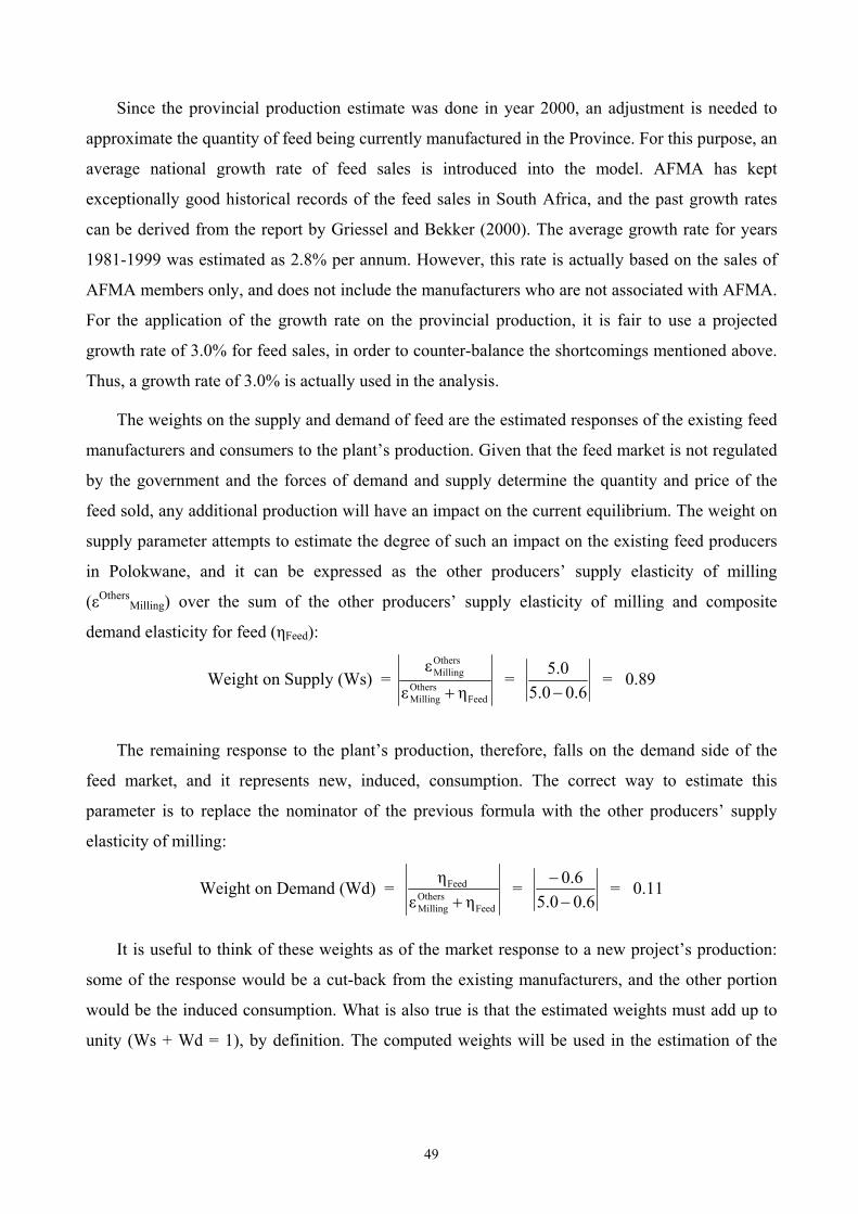
Since the provincial production estimate was done in year 2000, an adjustment is needed to
approximate the quantity of feed being currently manufactured in the Province. For this purpose, an
average national growth rate of feed sales is introduced into the model. AFMA has kept
exceptionally good historical records of the feed sales in South Africa, and the past growth rates
can be derived from the report by Griessel and Bekker (2000). The average growth rate for years
1981-1999 was estimated as 2.8% per annum. However, this rate is actually based on the sales of
AFMA members only, and does not include the manufacturers who are not associated with AFMA.
For the application of the growth rate on the provincial production, it is fair to use a projected
growth rate of 3.0% for feed sales, in order to counter-balance the shortcomings mentioned above.
Thus, a growth rate of 3.0% is actually used in the analysis.
The weights on the supply and demand of feed are the estimated responses of the existing feed
manufacturers and consumers to the plant’s production. Given that the feed market is not regulated
by the government and the forces of demand and supply determine the quantity and price of the
feed sold, any additional production will have an impact on the current equilibrium. The weight on
supply parameter attempts to estimate the degree of such an impact on the existing feed producers
in Polokwane, and it can be expressed as the other producers’ supply elasticity of milling
(εOthersMilling) over the sum of the other producers’ supply elasticity of milling and composite
demand elasticity for feed (ηFeed):
Weight on Supply (Ws) = Feed
OthersMilling
OthersMilling
ηεε
+ =
0.65.05.0−
= 0.89
The remaining response to the plant’s production, therefore, falls on the demand side of the
feed market, and it represents new, induced, consumption. The correct way to estimate this
parameter is to replace the nominator of the previous formula with the other producers’ supply
elasticity of milling:
Weight on Demand (Wd) = Feed
OthersMilling
Feed
ηεη+
= 0.65.0
0.6−
− = 0.11
It is useful to think of these weights as of the market response to a new project’s production:
some of the response would be a cut-back from the existing manufacturers, and the other portion
would be the induced consumption. What is also true is that the estimated weights must add up to
unity (Ws + Wd = 1), by definition. The computed weights will be used in the estimation of the
49
production forgone by the existing feed manufacturers, and also in the estimation of the economic
cost of feed.
5.3 Table of Inflation Rates, Price Indices and Exchange Rate
Having a complete Table of Parameters allows the analyst to start modeling the financial
profile of the project. The most logical thing to start with is the Table of Inflation Rates, Price
Indices and Exchange Rate, because all other tables will need the nominal prices and/or exchange
rates. A typical Table of Inflation Rates, Price Indices and Exchange Rate is shown in Table 2 in
Annex A, and it consists of the inflation indices of the currencies involved and the exchange rate(s)
projections for the future.
The feed project is financed by two currencies, the US dollar and South African Rand.
However, if more currencies are used then their inflation rates and price indices should be included
in the same manner as described here. For simplicity, it is useful to assume that the inflation rates
are the annual averages, but the exchange rates and price indices are the figures at the end of the
year.
5.3.1 South African Rand
The first line of the table is the projected inflation rate of the South African Rand (domestic
currency), which takes on the values stated initially in the Table of Parameters. As already
mentioned, the average annual inflation rates are 6.0% for year 2000, 12.0% for year 2001, 9.0%
for year 2002, and a rate of 6.0% is the expected average rate of inflation for the years 2003
onwards. Note that all the values in this table are “linked” to the Table of Parameters, and there is
no “typed” number. A failure to “link” the variables to the Table of Parameters will result in the
model being handicapped by the loss of relationship between the exogenous variables, i.e. inflation
rate in Table of Parameters, and the model’s outcomes.
Note that apart from having a direct link to the Table of Parameters, each year inflation rate
contains a factor for the “disturbance to the South African inflation rate” and modeled as:
iDYearX = iD
YearX (from Table of Parameters) * (1 + Disturbance to SA Inflation RateYearX)
iD2003 = 6.0% * (1 + 0%) = 6.0%
50
Where, the domestic inflation rate in year 2003 (iD
2003) already incorporates a factor, which
will account for unexpected changes or “disturbances” in the inflation rate in 2003. This
“disturbance to the South African inflation rate” is a special risk variable introduced into the model
for the purpose of risk analysis. This variable represents all possible forces affecting the projected
inflation rate of 6.0%, and these forces might be caused by unexpected domestic and international
events such as political and social crisis, war, terrorism, capital flight, etc.
In the base-case of the analysis, this variable is set to zero for every year of the project’s
operation indicating that, on the average, there is no expectations of the inflation rate to be
different from its long-run average rate of 6.0% per annum. The risk analysis software Crystal
Ball®, developed by Decisioneering, Inc., will generate a random disturbance factor in every year
of the project’s life, according to the specified probability distribution, based on the past and
expected inflation rate movements. Section 8.1.1 explains the way such a probability distribution is
derived.
The domestic price index is a computed index, which accounts for all accumulated inflation
since the year zero, year 2002. This index simply shows by how much the general level of prices
has risen since the beginning of the project. The way this index is computed allows for the
integration of both the expected inflation rate as well as the annual disturbances to it. The formula
describing this relationship is:
IDYearX = ID
YearX-1 * (1 + iDYearX)
ID2005 = 1.12 * (1 + 6%) = 1.19
Where the price index of the current year (ID2005) is calculated as a product of the previous
year’s price index (ID2004) times the factor for this year inflation rate (iD
2005). Since the current
inflation rate already includes the uncertainty factor, the above formula is flexible enough to
include the expected 6.0% rate of inflation as well as an element of uncertainty.
The future forecast of the real cost of inputs can be done on the assumption of an increasing,
declining, constant or a non-linear trend for the variable in question. If a cost of input, in real
terms, is expected to remain constant throughout the project life, let’s say Cnominal = 100 Rand2002,
then the nominal cost of this input in any given year is computed as a product of its real cost in
year zero prices times the current domestic inflation index in year X, ID2005 = 1.19:
CNominal, YearX = CReal, 2002 (Rand2002) * IDYearX
CNominal, 2005 = 100 * 1.19 = 119 (Rand2005)
51
This is a simple and convenient way to model the annual inflation increases. It should be kept
in mind that the year-zero price index is always unity, because the prices of this year are taken as
the starting point for further analysis. In fact, it does not matter which year is chosen to be the
starting point of the project, as long as all consequent analysis discounts the project benefits and
costs back to the same date in a consistent way.
5.3.2 US dollar
The US-dollar annual inflation rates are modeled in the same way as the domestic inflation
rates, taking into account the disturbance factor for the US dollar. The US-dollar price index
follows an identical modeling procedure to the one used for the South African Rand above. If a
project has to deal with more than one foreign currency then an additional set of variables
consisting of a price index, annual inflation rates, and disturbances to them are needed.
5.3.3 Exchange Rates
Exchange rate modeling is needed to convert any dollar-denominated cashflows into domestic
currency. Because all the financial statements and cashflow projections are typically done in the
domestic currency, any foreign revenues or expenses will have to be translated into their domestic
equivalents in a consistent way. The methodological framework of consistent modeling of price
indices and foreign exchanged rates is outlined in Chapter 4 of the Manual (2003).
A few facts are useful to remember at all times. The foreign exchange rate, no matter how
“stable” it may seem, is also subject to forces of the relative inflation rates of the two countries,
which must be reflected in the exchange rate projections. It is very common around the world to
express the value of certain goods in US dollar, or other “hard” currency to avoid frequent re-
labeling price tags due to domestic inflation. While this tactics is useful for such purposes, the US
dollar as any other currency also is subject to its own rate of inflation, which has in the recent years
been relatively modest as compared to inflation rates in some developing countries. It is also
necessary to express the equilibrium nominal exchange rate as a function of the price levels
between two countries, despite the fact that many other forces may influence the real exchange
rate. The changes in the exchange rate can be said to consist of the interaction of the two inflation
rates and a composite impact of all other factors. To keep analysis simple and manageable, it is
useful to assume that the real exchange rate remains, on the average, constant throughout the
52
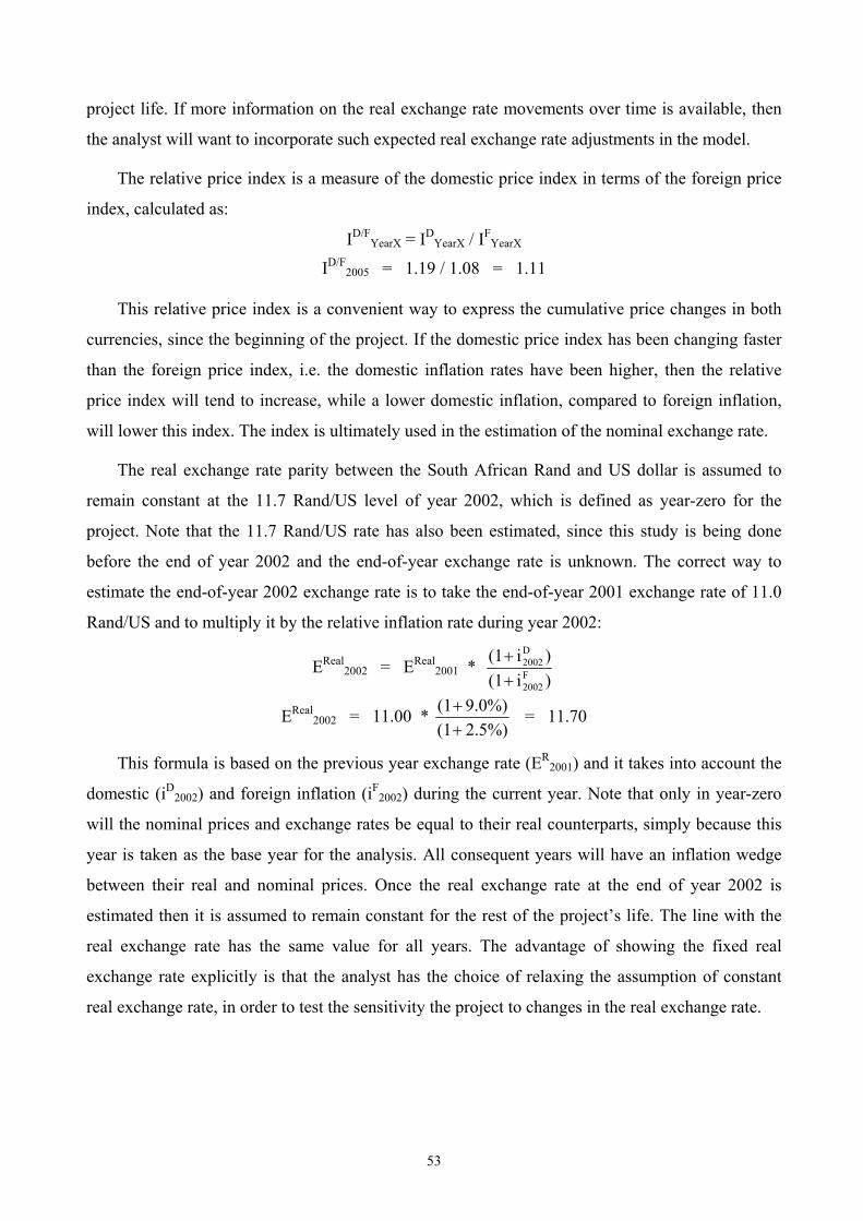
project life. If more information on the real exchange rate movements over time is available, then
the analyst will want to incorporate such expected real exchange rate adjustments in the model.
The relative price index is a measure of the domestic price index in terms of the foreign price
index, calculated as:
ID/FYearX = ID
YearX / IFYearX
ID/F2005 = 1.19 / 1.08 = 1.11
This relative price index is a convenient way to express the cumulative price changes in both
currencies, since the beginning of the project. If the domestic price index has been changing faster
than the foreign price index, i.e. the domestic inflation rates have been higher, then the relative
price index will tend to increase, while a lower domestic inflation, compared to foreign inflation,
will lower this index. The index is ultimately used in the estimation of the nominal exchange rate.
The real exchange rate parity between the South African Rand and US dollar is assumed to
remain constant at the 11.7 Rand/US level of year 2002, which is defined as year-zero for the
project. Note that the 11.7 Rand/US rate has also been estimated, since this study is being done
before the end of year 2002 and the end-of-year exchange rate is unknown. The correct way to
estimate the end-of-year 2002 exchange rate is to take the end-of-year 2001 exchange rate of 11.0
Rand/US and to multiply it by the relative inflation rate during year 2002:
EReal2002 = EReal
2001 * )i(1)i(1
F2002
D2002
++
EReal2002 = 11.00 *
2.5%)(19.0%)(1
++ = 11.70
This formula is based on the previous year exchange rate (ER2001) and it takes into account the
domestic (iD2002) and foreign inflation (iF
2002) during the current year. Note that only in year-zero
will the nominal prices and exchange rates be equal to their real counterparts, simply because this
year is taken as the base year for the analysis. All consequent years will have an inflation wedge
between their real and nominal prices. Once the real exchange rate at the end of year 2002 is
estimated then it is assumed to remain constant for the rest of the project’s life. The line with the
real exchange rate has the same value for all years. The advantage of showing the fixed real
exchange rate explicitly is that the analyst has the choice of relaxing the assumption of constant
real exchange rate, in order to test the sensitivity the project to changes in the real exchange rate.
53
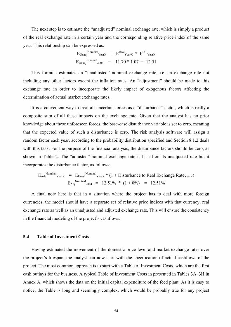
The next step is to estimate the “unadjusted” nominal exchange rate, which is simply a product
of the real exchange rate in a certain year and the corresponding relative price index of the same
year. This relationship can be expressed as:
EUnadjNominal
YearX = ERealYearX * II
D/FYearX
EUnadjNominal
2004 = 11.70 * 1.07 = 12.51
This formula estimates an “unadjusted” nominal exchange rate, i.e. an exchange rate not
including any other factors except the inflation rates. An “adjustment” should be made to this
exchange rate in order to incorporate the likely impact of exogenous factors affecting the
determination of actual market exchange rates.
It is a convenient way to treat all uncertain forces as a “disturbance” factor, which is really a
composite sum of all these impacts on the exchange rate. Given that the analyst has no prior
knowledge about these unforeseen forces, the base-case disturbance variable is set to zero, meaning
that the expected value of such a disturbance is zero. The risk analysis software will assign a
random factor each year, according to the probability distribution specified and Section 8.1.2 deals
with this task. For the purpose of the financial analysis, the disturbance factors should be zero, as
shown in Table 2. The “adjusted” nominal exchange rate is based on its unadjusted rate but it
incorporates the disturbance factor, as follows:
EAdjNominal
YearX = EUnadjNominal
YearX * (1 + Disturbance to Real Exchange RateYearX)
EAdjNominal
2004 = 12.51% * (1 + 0%) = 12.51%
A final note here is that in a situation where the project has to deal with more foreign
currencies, the model should have a separate set of relative price indices with that currency, real
exchange rate as well as an unadjusted and adjusted exchange rate. This will ensure the consistency
in the financial modeling of the project’s cashflows.
5.4 Table of Investment Costs
Having estimated the movement of the domestic price level and market exchange rates over
the project’s lifespan, the analyst can now start with the specification of actual cashflows of the
project. The most common approach is to start with a Table of Investment Costs, which are the first
cash outlays for the business. A typical Table of Investment Costs in presented in Tables 3A–3H in
Annex A, which shows the data on the initial capital expenditure of the feed plant. As it is easy to
notice, the Table is long and seemingly complex, which would be probably true for any project
54
having good data set on the investment costs. The feed project has a detailed set of itemized cost
estimates because its foreign counterpart plant was built in the same way. The total investment
expenditures can be broken down into several categories: land, construction, feed production
equipment, office equipment and vehicles. The land, construction costs, office equipment and
vehicles will be purchased with the South Africa Rand, but most of the equipment and its freight
costs will be paid for in US dollars.
5.4.1 Land
The land is already purchased by the foreign investor in Polokwane. The purchased plot of
land is actually a much larger area than needed for the feed plant. The investor wanted to have
spare space to be able to place any other of his future activities in the same location. The total
amount spent on the land was 7.0 million Rand in year 2002. The feed production is going to
occupy only about 1/6 of this area, and the project analyst should have a clear understanding how
to treat the land in this case. Since the feed plant will be using only a portion of the available land
while the rest will be associated with other project(s), then the true value of the resource used by
the feed plant is only 1/6 of the total cost, and not the full cost of the plot. For the purpose of the
analysis, a figure of 1.2 million rand is used as the land cost for this project. Since this is an asset
for which the investor already fully paid, no investment cost overruns are expected for this item.
5.4.2 Construction Costs
A few buildings have to be constructed, including the factory, warehouse, raw materials
warehouses, weight bridge, roads and various auxiliary structures. The full list of the items of the
construction costs are shown in the Table 3A in the Annex A. Note that a quote on the construction
costs was obtained in year 2001, and an adjustment for the inflation must be made in order to bring
the 2001-cost estimates to the price level of year 2002, year-zero in the analysis. It is often the case
with construction activities that there could be time and/or cost overruns, and the project model
must make a provision for such events. What it really means is that both time and cost overruns can
be expressed as a percentage deviation from the planned construction budget, because even time
delays imply business losses. Thus, the analyst should incorporate both the inflation adjustment
and provision for investment cost overruns in the estimation of the construction costs of year 2002.
The formula, which is capable of doing that, can be spelled out as:
CItemMRand
2002 = CItemMRand
2001 * (1 + iD2001) * (1 + Investment Cost Overrun Factor)
55
Knowing the actual circumstances of the project helps the analyst to make the right estimates
of the value for the variable. The question of whether to use the inflation rate of year 2001 or 2002,
can be resolved by knowing that the construction cost estimate was done at the beginning of the
year 2001, and actual construction of the plant takes place in the mid of 2002, which can be best
modeled with inflation rate of year 2001, not of 2002 because the construction starts before the end
of 2002. Let’s take the estimate of the construction cost of the workshop, and show that:
CWorkshopRand
2002 = 2,775,386 * (1 + 12.0%) * (1 + 0%) = 3,108,433 (Rand2002)
The cost of workshop in year 2001 (C2001) is adjusted for the inflation rate, and an additional
factor, describing the net effect of time/cost overruns from the Table of Parameters. In the base
case this factor is zero, meaning that no overruns are expected, but this parameter will be changed
in order to test the model’s responsiveness to this parameter in the consequent sensitivity and risk
analysis.
5.4.3 Office Equipment and Vehicles
In the 2001 application submitted by the investor for the grant incentives, the cost estimate for
the office equipment and furniture totaled to 946,000 Rand2001. The budget for vehicles was stated
as 400,000 Rand2001. These figures must be inflated to the price level of year 2002. No investment
cost overruns are expected for these two items.
5.4.4 Freight and Traveling
This section describes the costs of international and domestic freight of the equipment,
insurance, and traveling expenditures for the personnel transfer from the foreign country. The
freight cost estimates are taken from a quote obtained from international and domestic carriers in
2001. The international costs are paid in US dollar, and all local expenses in Rand. No investment
cost overruns are generally applied on such expenses.
The US-dollar expenses include the freight and statutory costs for machinery and equipment as
well as for certain imported raw materials. Another dollar expense is for the international travel of
the personnel. The column with total US-dollar expenses in year 2001 totals these expenditures but
further adjustment is needed in order to arrive at the price level of the year 2002. As mentioned
above, the US-dollar prices are also subject to inflation and the correct way to model this is to
inflate the past costs by the accumulated inflation (price index) of the US dollar. Since it is only
56
one year difference between the 2001 cost estimates and the 2002 project’s year-zero, then only the
adjustment is the US inflation rate for year 2001. For instance, the 2001 quote for the freight of the
machinery, equipment and raw materials is 252,500 US$2001, and then its year-2002 equivalent is
computed as:
CFreightUS$
2002 = 252,500 * (1 + 3.0%) = 260,075 US$2002
Thus, the required adjustment is made to include the US-dollar inflation of 3.0% in year 2001.
The same procedure is done for the traveling and statutory costs and their combined total, in real
US-dollar terms, is worked out at the bottom of Table 3A. At this point, a conversion of this US-
dollar total into Rand value is not needed, because this can be done in the summary of the total
investment costs later, as shown in Table 3H in Annex A.
The Rand costs of freight and traveling include local transport, offloading, agency charges,
insurance and VAT charges, and they are all grouped under the title of “local costs”. Again, their
values were taken from a 2001 quote and they have to be inflated to their 2002-year price level.
Thus, the 2001-Rand total of local costs for machinery, equipment and raw materials is 56,500
Rand2001, which has to be inflated by 12.0% of the 2001 year inflation rate in order to arrive at the
value of 63,280 Rand2002, at the year-zero prices. The same computation is performed for the
insurance and VAT charges. The total Rand requirements, in real terms, are stated at the bottom of
Table 3A.
5.4.5 Equipment
Tables 3B–3G contain a detailed account of equipment items, and that is why these tables
seem to be lengthy and complex. All equipment and machinery can be, in fact, divided into four
groups: raw material, drying and storage equipment; feed production equipment; feed briquetting
process equipment; and electronic and internet control system. There are sub-sections under most
of the groups:
Raw Material, Drying and Storage Equipment
– Section of Raw Material, Drying and Storage
Feed Production Equipment
– Section of Raw Material, Receive and Receiving Sieve
– Crush Section
– Dispensing and Mixture Section
– Pelletize Section
57
– Package Section
– Assistance Section
Feed Briquetting Process Equipment
– Assistance Section
Electronic and Internet Control System
– Weak Current Engineering and Internet Control System
– Electrical Machinery Control Centre (MCC)
– Work Field Material
This is the order in which these equipment items appear in Tables 3B-3G in Annex A. All the
equipment items are modeled in the same way, and instead of describing them section by section, it
could be more efficient to focus on the columns, which are somewhat complex to model.
Item and Description
Each item of the equipment and machinery has an order number according to the specifications
of the plant, as stated in the grant application by the investor. The item’s description and technical
specifications follow that, and these can be useful for anyone who is looking at the project from
technical view. The next column contains the number of units of a certain item to be used on the
feed plant.
The power requirements in kWh per unit and total for an item are stated in the following two
columns. A grand total of all power requirements will be done in the “summary” of the investment
costs for the purpose of estimating the total energy demand by the plant and electricity expense.
Prices and Grant Eligibility
Total US$2001: The original prices of all equipment items were obtained from a 2001 quote,
and this is the figure placed in the US-dollar “price per unit” column. Since some of the items are
used in multiple instances, a column with a total amount is needed, which is simply a product of
the 2001 US-dollar price and number of units used.
Note that even if all equipment costs are stated in US dollar terms, some of the actual spending
will done in Rand, because certain items are available locally, or they represent local costs.
Generally they are stated at the very end of each equipment section, and namely are the mounting
and debugging costs, assist and mount materials, electric control costs. Because of this fact that the
mechanical items and equipment are imported and paid for in US dollar, while the local costs are
covered from Rand fund, a separation is needed to keep track of the total foreign and local
expenses.
58
Thus, following the column with the US-dollar 2001-priced total there are three more columns,
which are: the total expense for an item expressed in year 2002 Rand; a total expressed in year
2002 US dollar, and amount of grant eligible expenses expressed in year 2002 Rand. Each column
serves its function in further analysis.
Total Rand2002: The column with the total expense for an item, expressed in year 2002 Rand,
will be needed to find the total expenditures in the investment costs. Because the cashflows are
generally reported in the domestic currency, all the imported items must be converted in their Rand
equivalents. Also, since the US dollar cost estimates are given in year-2001 prices, an adjustment
must be made to bring these costs up to the level of year 2002 prices. A formula, which serves both
these tasks, is:
CItemMRand
2002 = CItemMUS$
2001 * (1 + US Inflation Rate2001) * ENominal2002
What this formula does, is it starts with the year-2001 dollar cost of an item, then it inflates the
cost by year-2001 foreign inflation, and finally converts the result into Rand by applying the
nominal exchange rate of year 2002. An illustration of this can be shown on the “blanking die and
granular membrane”, order item #101:
CDie and Granular MembraneRand
2002 = 4,395.24 * (1 + 3.0%) * 11.70 = 52,956 Rand2002
The final year-2002 Rand value is the cost of the “blanking die and granular membrane” in
year-2002 prices, which can be used in further calculations. Note that there is no investment cost
overrun factor in the above formula. Each equipment item is processed in an identical way, and a
sub-total is computed beneath of every section. The feed production equipment as well as the
electronic and internet control system both comprise of many sections also contain grand-totals to
summarize the results from every internal section. The summary of investment costs table will
include all the costs of equipment items.
Total US$2002 Costs: This column is needed to show explicitly what are the actual expenses
made in US dollar, and what is the total requirement for US-dollar funds per item. It excludes all
locally made expenses such as the mounting and debugging costs, assist and mount materials,
electric control costs. The formula used to derive the year-2002 US dollar value from its year-2001
dollar cost quote is similar to the previous formula, except that it stops short of applying the
exchange rate:
CItemMUS$
2002 = CItemMUS$
2001 * (1 + US Inflation Rate2001)
CDie and Granular MembraneUS$
2002 = 4,395.24 * (1 + 3.0%) = 4,527.1 US$2002
59
Continuing with the example of the “section of raw material, drying and storage”, which is the
only section under “raw material, drying and storage equipment”, the US-dollar requirements is
stated for each item, except the very last articles of electrical control, mounting and debugging
cost, and other mounting material. These three items are to be expensed in Rand and are, therefore,
excluded. A total is computed for every section.
Grant Eligible, Rand2002: The purpose of this column is to show explicitly the items, which
costs are eligible to be included into the calculation of the basis for the grant. There are a number
of criteria, regulating the foreign investment incentives scheme, and according to them, only the
foreign costs of equipment are to be included into the base. International freight and transportation
expenses are also eligible, while domestic transport expenses are not. All the foreign costs have to
be expressed in their Rand equivalent.
The current regulation states that the amount of grant is the minimum of either 3.0 million
Rand, or 15% of the total grant eligible expenses3. The application for grant has been approved has
been approved, and for the purposes of the present analysis it is needed to find the total amount of
the grant eligible expenses.
The grant eligible column in the equipment and machinery costs simply shows the Rand year-
2002 value of an item, if the item is allowed to enter into the grant-base calculation. All items of
equipment are included, except the expenses such as the electrical control, mounting and
debugging cost, and other mounting material. At the end of each section, a total amount of grant
eligible expenses is calculated.
Share of Costs and Conversion Factors: The last few columns are needed for the estimation
of economic conversion factors (CFs). Since these economic conversion factors don’t have
anything to do with the financial analysis yet and the analyst may like to shift the calculation of the
investment items’ CFs down to the economic analysis. But given the length and detail of the
investment costs, it will be cumbersome to repeat the same sections once again only for the sole
purpose of assigning a conversion factor to them. Instead, the three columns last columns of the
investment cost tables are used to compute the conversion factors.
In the consequent financial and economic analysis, the expenditures on the equipment and
machinery are consolidated into sections of the equipment costs, and a single conversion factor is 3 Approved qualifying foreign entities may qualify for the Foreign Investment Grant (FIG) up to a maximum of 3.0
million Rand. The grant is available only to new qualifying investments, and offered only once to any foreign
60
required for each section to estimate its total economic cost. Given the numerous equipment items,
the analyst would generally like to keep all the investment costs data, and to compute a composite
conversion factor for the equipment as whole as for the each section. This can be accomplished by
taking a weighted average of the conversion factors of all items under a section through
multiplying their shares in the total cost of equipment by the individual conversion factors. This
can be formulated as:
CFSectionN = ( )∑ItemM
ItemMItemM CF*%Share
Note that the cost share of each item is based on the 2001 US-dollar values since it is the
“original” data and it does not exclude any non-eligible grant expenses or local expenditures. For
example, the cost share of the “blanking die and granular membrane” item (0.32%) in the “section
of raw material, drying and storage” is calculated as its cost (4,395.24 US$2001) over the total cost
of the section (1,373,437.1 US$2001).
The next column contains the conversion factor for each item. The conversion factors are
taken from the Electronic Database of Commodity Specific Economic Conversion Factors for
South Africa (2003), which is referred as “Database” from nowon, and calculated using the
methodology of as described in Chapter 6 of the Manual (2003). The very last column has a
description of the item in terms of the “harmonized standard code” and assumptions made about
this item. Continuing with the example of the “blanking die and granular membrane” item, its
description states that the South African Customs Authority would, most probably, treat all
equipment items as being a whole machinery for an agricultural processing, which can be best
described under one of the “harmonized code” items in Chapter 84.37 of the Database (2003). The
estimated CF for such machinery is estimated as 0.92544, and this is the value assigned to all
equipment items of the section. However, the last three expenses on the electrical control,
mounting and debugging cost, and other mounting material have their CFs calculated in the
economic analysis, because these three items do not fit into the description of the equipment.
The very last row of every section has either a “total” or “grand-total”, which sums up all the
computations done in each column. The conversion factor can be found there too. The CF for the
“section of raw material, drying and storage” is found to be 0.91937. All the consequent sections
follow the same format.
single entity. The FIG is the lower of the actual cost or 15% of the value of new machinery and equipment relocated from overseas. The FIG can not exceed 3.0 million Rand per project.
61
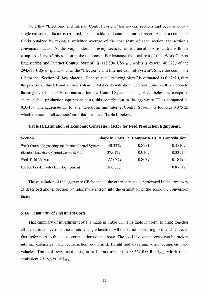
Note that “Electronic and Internet Control System” has several sections and because only a
single conversion factor is required, then an additional computation is needed. Again, a composite
CF is obtained by taking a weighted average of the cost share of each section and section’s
conversion factor. At the very bottom of every section, an additional box is added with the
computed share of this section in the total costs. For instance, the total cost of the “Weak Current
Engineering and Internet Control System” is 118,804 US$2001, which is exactly 40.32% of the
294,639 US$2001 grand-total of the “Electronic and Internet Control System”. Since the composite
CF for the “Section of Raw Material, Receive and Receiving Sieve” is estimated as 0.87810, then
the product of this CF and section’s share in total costs will show the contribution of this section to
the single CF for the “Electronic and Internet Control System”. Thus, placed below the computed
share in feed production equipment costs, this contribution to the aggregate CF is computed as
0.35407. The aggregate CF for the “Electronic and Internet Control System” is found as 0.87512,
which the sum of all sections’ contributions, as in Table II below.
Table II. Estimation of Economic Conversion factor for Feed Production Equipment. Section Share in Costs * Composite CF = Contribution
Weak Current Engineering and Internet Control System 40.32% 0.87810 0.35407
Electrical Machinery Control Centre (MCC) 37.01% 0.91624 0.33910
Work Field Material 22.67% 0.80270 0.18195
CF for Feed Production Equipment (100.0%) 0.87512
The calculation of the aggregate CF for the all the other sections is performed in the same way
as described above. Section 6.4 adds more insight into the estimation of the economic conversion
factors.
5.4.6 Summary of Investment Costs
That summary of investment costs is made in Table 3H. This table is useful to bring together
all the various investment costs into a single location. All the values appearing in this table are, in
fact, references to the actual computations done above. The total investment costs can be broken
into six categories: land, construction, equipment, freight and traveling, office equipment, and
vehicles. The total investment costs, in real terms, amount to 88,652,055 Rand2002, which is the
equivalent 7,578,679 US$2002.
62
The next two columns of this table explicitly state the Rand and dollar cash requirements per
each category of the investment costs, and their totals are computed below. Thus, Rand expenses
will amount to 53,600,002 Rand2002 and US-dollar costs are expected to be 4,066,378 US$2002. The
reason why such a separation is needed is that it is useful to reflect the actual cashflows, and also
for estimation of the loan requirements. Also, the owners of the plant will always need to know the
currency requirements for better cash management.
Grant eligible expenses are also stated per each category of investment costs, and the total
eligible amount is found as 86,574,444 Rand2002. However, the actual amount of grant is calculated
as the minimum of either the total eligible costs, or 15% of the total eligible costs if the project’s
total investment costs exceed 3,000,000 Rand, or the maximum grant ceiling of 3,000,000 Rand. A
function of MS-Excel, called “min” does such a comparison and in the case of this plant, the likely
amount of the grant will be the maximum 3,000,000 Rand. This is also the amount which has been
approved by the National Government as an incentive for this project. The regulation states that the
grant must be given in two equal installments over two years, on the condition that the project does
perform according to the approved application. If not, the second installment should not be given.
It has been assumed that the feed production will be awarded both installments, and then, the actual
grant inflow will be 1.5 million Rand in year 2002 and 2003.
At the very end of this table, there are three columns for tax depreciation of equipment and
machinery, whose existence here is needed to estimate a deduction from the investment costs due
to the government grant. The tax code of South Africa allows a tax deduction for the depreciation
of the capital costs; however, the total deductible investment costs must be reduced by the grant
amount, which is paid from the Government budget. Instead of consolidating all the investment
costs into a single item and then reducing its value by the grant amount, it is possible to find the
amount of grant per each eligible category of the investment costs, assuming that this grant
“spread” would follow the investment cost structure. This allows the analyst to work out a
consistent model with separate items under investment costs.
Thus, the Rand2002 equipment costs are taken into the first of these three columns, and their
total is computed at the bottom. Then the shares of each kind of equipment are calculated. Once the
shares are known, it is reasonable to assume that the base-value of each kind of equipment should
be reduced in proportion to its share in the 3.0 million grant. The very last column states that
amount per equipment kind, which is to be deducted from the base-value of equipment for
estimation of tax depreciation.
63
The item which has only been left behind is the total energy requirement of the feed plant. This
is simply a sum of all the energy requirements of the equipment and machinery. This monthly
power design consumption works out to be 2,248.23 kWh, using a 100% plant load factor.
5.5 Loan Schedule
A typical project finds it worthwhile to use a mix of financing sources. In addition to the
equity, the most common source of finance for start-up enterprises is a commercial loan from a
bank. This is a competitive finance option and the project owners have flexibility over the choice
of a particular bank and ability to negotiate and structure the deal. The financial model offers the
unique capability to test the performance of the project under various financing packages, and to
select the most “optimal” mix of funds. What is really extraordinary about financial modeling is
that a properly constructed model allows the analyst to change the proportions of the funds from
different sources, their interest rates and required rates of return, as well as the terms and
conditions of the financing, and much more. Table 4 shows the Loan Schedule of the project.
The intention of the feed plant management was to obtain a local loan to cover some of the
Rand expenses during the construction and starting phase. However, it has been stated that no plans
are made about reliance on such external finance, and during the interviews with are company
representative, a figure of about 50% of the local costs emerged as a preliminary estimate of
external borrowing. In other words, all the US-dollar expenses and the other half of the local costs
cash outlays that are to be financed by the equity contributions of the foreign investor.
It is relatively easy to obtain a loan of such amount on a commercial basis in South Africa, and
a set of typical conditions for such a loan was assumed. The Table of Parameters describes the loan
package in detail, and all the parameters used here can be referenced back to Section 5.2.3. The
purpose of Table 4 is to project the loan inflows and outflows in a flexible manner, to incorporate
all the loan parameters into the model. In other words, the Loan Schedule must automatically
adjust for any change in the interest rate, duration of grace period, and number of annual
installments. To model these desired properties into the financial model, a handful of formulas are
used.
Loan Receipts: The first line of the schedule is the loan receipts, stating the amount of loan
received in every year according to actual loan disbursements from the bank. All figures are
expressed in nominal domestic currency to reflect the actual cash flows. If a loan is drawn in a
64

foreign currency then the loan schedule must be carried out in that currency, assuming that the
repayment is also in the same foreign currency, and only nominal vales should be used. The
amount of the loan taken by the feed plant in year 2002 is 26.8 million Rand, which is the half of
all the local investment and preliminary costs.
Annual Interest Rate: The annual interest rate line is needed to reflect the changing nature of
the loan market, since any inflationary pressure is likely to increase the current nominal interest
rates. This is modeled in such a way that it incorporates the current inflation rate into the interest
rate computation. The function, linking the two can be expressed as:
iYearX = r + R + (l + r + R) * gPeYearX
i2003 = 8.5% + 0% + (l + 8.5% + 0%) * 6.0% = 15.0%
Where the annual nominal interest rate (iYearX) is based on the real interest rate (r) and country
risk premium (R), which is in the case of a domestic loan is commonly taken as zero, and then
adjusted for the expected rate of domestic inflation for the current year (gPeYearX). The real interest
rate is assumed to remain at the same level of 8.5%, but this assumption can be relaxed later in the
sensitivity and risk analysis. Note that the inflation rate already incorporates the unexpected
“disturbances” and if any exogenous factor causes the inflation rate to increase or decrease, then
the nominal interest rate will immediately change in the computed expected payment. The purpose
of this line in the loan schedule is to show explicitly what will be the nominal borrowing rate in
each year.
Repayment Installment: The next line of this table, named “repayment installment”, is used
to calculate the repayment installment based on the accumulated “outstanding debt balance at the
end of the year” and current nominal interest rate. There is a special function, called “PMT”, which
is built-in in MS-Excel to calculate the payment for a loan, based on constant payments and a
constant interest rate. Because the function returns a calculated payment as a negative number, a
minus sign is required in front of the function in order to keep all flows with positive signs. The
formula can be written as:
RINSTYearX = –PMT(iYearX, n, DebtBYearX)
For example, if the loan has to start repayment in year 2004 then the calculation of a fixed
annual repayment with the nominal interest rate (iYearX) of 15.0%, a repayment period (n) of 5
years, and an accumulated outstanding debt at the beginning of the 2004 year (DebtBYearX) of
30,822,681 Rand, would be:
65

RINST2004 = –PMT(15.0%, 5 years, 30,822,681 Rand2004) = 9,197,062 Rand2004
The value of the calculated repayment installment will be enough to compensate the bank for a
loan of 30,822,681 Rand, if 5 equal annual repayments are made. However, the loan repayment
does not start in this year, then a bigger amount of the accumulated debt (DebtBYearX) will have to
be repaid back by the project, and that is why each year has a different amount of the calculated
installment.
Outstanding Debt at the Beginning of Year: The outstanding debt at the beginning of the
year shows the opening balance of the debt flow. It is assumed that the loan account is “opened” at
the beginning of every year and “closed” at the end. Thus, the opening balance of the current year
is always equal to the ending balance of the previous year (DebtBYearX = DebtE
YearX-1) and the value
of the opening balance always takes on the value of the end balance of the previous year. For
example, the opening balance of year 2004 is the closing balance of year 2003. As a matter of fact,
the opening balance of year 2002 is zero, i.e. the loan has not been received.
The interest accrued line is meant to show the amount of annual interest accrued on the debt
balance during the current year. It is common for such loans to have a condition of “capitalization”
of accrued interest to the loan principle. Because the loan funds are tied up with this project, the
bank is in a position to charge the project for the use of capital and the relevant base for applying
the accrued interest is not the original loan principal but the current debt balance, which should
include all previous amounts of capitalized interest accrued. The formula, used to calculate the
current year interest accrued is:
INTAYearX = iYearX * DebtB
YearX
INTA2004 = 15.0% * 30,822,681 Rand2004 = 4,626,484 Rand2004
In other words, a debt balance of 30,822,681 Rand2004 will result in an amount of 4,626,484
Rand2004 in annual interest accrued, at the current interest rate of 15.0%. This does not mean that
this amount is actually paid back to the bank, but it does imply that this amount is definitely
included into the debt balance.
Annual Repayment Installment: The annual repayment installment line is needed to show
the actual amount of installment paid to the bank in a year. Note that there are no installments
made before and after the installment repayment period of 5 years, starting in 2004. The
installment is a sum of two parts: the payment of the current year interest accrued and the
66
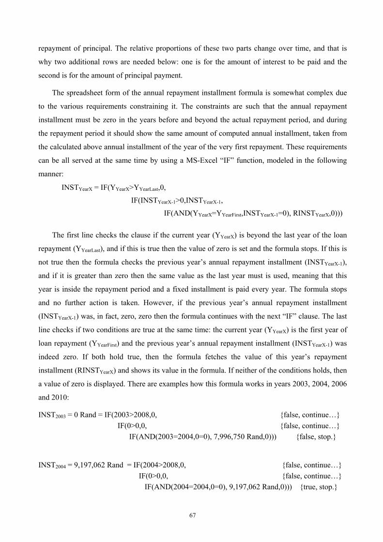
repayment of principal. The relative proportions of these two parts change over time, and that is
why two additional rows are needed below: one is for the amount of interest to be paid and the
second is for the amount of principal payment.
The spreadsheet form of the annual repayment installment formula is somewhat complex due
to the various requirements constraining it. The constraints are such that the annual repayment
installment must be zero in the years before and beyond the actual repayment period, and during
the repayment period it should show the same amount of computed annual installment, taken from
the calculated above annual installment of the year of the very first repayment. These requirements
can be all served at the same time by using a MS-Excel “IF” function, modeled in the following
manner:
INSTYearX = IF(YYearX>YYearLast,0,
IF(INSTYearX-1>0,INSTYearX-1,
IF(AND(YYearX=YYearFirst,INSTYearX-1=0), RINSTYearX,0)))
The first line checks the clause if the current year (YYearX) is beyond the last year of the loan
repayment (YYearLast), and if this is true then the value of zero is set and the formula stops. If this is
not true then the formula checks the previous year’s annual repayment installment (INSTYearX-1),
and if it is greater than zero then the same value as the last year must is used, meaning that this
year is inside the repayment period and a fixed installment is paid every year. The formula stops
and no further action is taken. However, if the previous year’s annual repayment installment
(INSTYearX-1) was, in fact, zero, zero then the formula continues with the next “IF” clause. The last
line checks if two conditions are true at the same time: the current year (YYearX) is the first year of
loan repayment (YYearFirst) and the previous year’s annual repayment installment (INSTYearX-1) was
indeed zero. If both hold true, then the formula fetches the value of this year’s repayment
installment (RINSTYearX) and shows its value in the formula. If neither of the conditions holds, then
a value of zero is displayed. There are examples how this formula works in years 2003, 2004, 2006
and 2010:
INST2003 = 0 Rand = IF(2003>2008,0, {false, continue…} IF(0>0,0, {false, continue…} IF(AND(2003=2004,0=0), 7,996,750 Rand,0))) {false, stop.}
INST2004 = 9,197,062 Rand = IF(2004>2008,0, {false, continue…} IF(0>0,0, {false, continue…} IF(AND(2004=2004,0=0), 9,197,062 Rand,0))) {true, stop.}
67
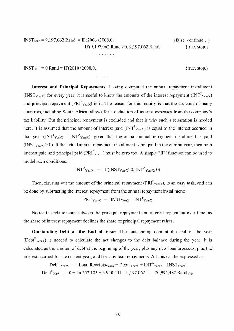
INST2006 = 9,197,062 Rand = IF(2006>2008,0, {false, continue…} IF(9,197,062 Rand >0, 9,197,062 Rand, {true, stop.}
…………
INST2010 = 0 Rand = IF(2010>2008,0, {true, stop.} …………
Interest and Principal Repayments: Having computed the annual repayment installment
(INSTYearX) for every year, it is useful to know the amounts of the interest repayment (INTPYearX)
and principal repayment (PRIPYearX) in it. The reason for this inquiry is that the tax code of many
countries, including South Africa, allows for a deduction of interest expenses from the company’s
tax liability. But the principal repayment is excluded and that is why such a separation is needed
here. It is assumed that the amount of interest paid (INTPYearX) is equal to the interest accrued in
that year (INTPYearX = INTA
YearX), given that the actual annual repayment installment is paid
(INSTYearX > 0). If the actual annual repayment installment is not paid in the current year, then both
interest paid and principal paid (PRIPYearX) must be zero too. A simple “IF” function can be used to
model such conditions:
INTAYearX = IF(INSTYearX>0, INTA
YearX, 0)
Then, figuring out the amount of the principal repayment (PRIPYearX), is an easy task, and can
be done by subtracting the interest repayment from the annual repayment installment:
PRIPYearX = INSTYearX – INTP
YearX
Notice the relationship between the principal repayment and interest repayment over time: as
the share of interest repayment declines the share of principal repayment raises.
Outstanding Debt at the End of Year: The outstanding debt at the end of the year
(DebtEYearX) is needed to calculate the net changes to the debt balance during the year. It is
calculated as the amount of debt at the beginning of the year, plus any new loan proceeds, plus the
interest accrued for the current year, and less any loan repayments. All this can be expressed as:
DebtEYearX = Loan ReceiptsYearX + DebtB
YearX + INTAYearX – INSTYearX
DebtE2005 = 0 + 26,252,103 + 3,940,441 – 9,197,062 = 20,995,482 Rand2005
68
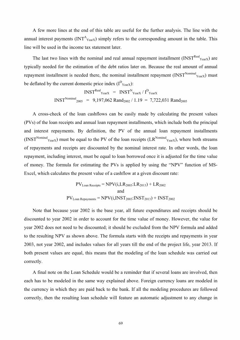
A few more lines at the end of this table are useful for the further analysis. The line with the
annual interest payments (INTAYearX) simply refers to the corresponding amount in the table. This
line will be used in the income tax statement later.
The last two lines with the nominal and real annual repayment installment (INSTRealYearX) are
typically needed for the estimation of the debt ratios later on. Because the real amount of annual
repayment installment is needed there, the nominal installment repayment (INSTNominalYearX) must
be deflated by the current domestic price index (IDYearX):
INSTRealYearX = INSTN
YearX / IDYearX
INSTNominal2005 = 9,197,062 Rand2002 / 1.19 = 7,722,031 Rand2005
A cross-check of the loan cashflows can be easily made by calculating the present values
(PVs) of the loan receipts and annual loan repayment installments, which include both the principal
and interest repayments. By definition, the PV of the annual loan repayment installments
(INSTNominalYearX) must be equal to the PV of the loan receipts (LRNominal
YearX), where both streams
of repayments and receipts are discounted by the nominal interest rate. In other words, the loan
repayment, including interest, must be equal to loan borrowed once it is adjusted for the time value
of money. The formula for estimating the PVs is applied by using the “NPV” function of MS-
Excel, which calculates the present value of a cashflow at a given discount rate:
PVLoan Receipts = NPV(i,LR2003:LR2013) + LR2002
and PVLoan Repayments = NPV(i,INST2003:INST2013) + INST2002
Note that because year 2002 is the base year, all future expenditures and receipts should be
discounted to year 2002 in order to account for the time value of money. However, the value for
year 2002 does not need to be discounted; it should be excluded from the NPV formula and added
to the resulting NPV as shown above. The formula starts with the receipts and repayments in year
2003, not year 2002, and includes values for all years till the end of the project life, year 2013. If
both present values are equal, this means that the modeling of the loan schedule was carried out
correctly.
A final note on the Loan Schedule would be a reminder that if several loans are involved, then
each has to be modeled in the same way explained above. Foreign currency loans are modeled in
the currency in which they are paid back to the bank. If all the modeling procedures are followed
correctly, then the resulting loan schedule will feature an automatic adjustment to any change in
69

the loan parameters. This enhances the ability of the analyst to evaluate the different financing
options for the project.
5.6 Schedule of Feed Ingredient Costs and Feed Prices
5.6.1 Feed Ingredient Costs
Table 5 contains the Schedule of Feed Ingredient Costs and Feed Prices. This table is needed
to project into the future the nominal costs of the feed ingredients and nominal feed prices. The
fluctuating nature of agricultural prices forces the analyst to apply a disturbance factor on the costs
of feed ingredients in order to imitate their likely behavior over years. As stated in the Table of
Parameters, the 950 Rand/ton cost of feed is made up of a few components: tradable (50%) and
non-tradable (40%) ingredients, transportation cost (8%), and handling cost (2%). The reason, why
it is necessary to look at the components separately, is that the different component are factors that
affect each in a distinct way, hence, it is more realistic to model them separately.
Tradable Ingredients: The tradable ingredients are assumed to be affected by the foreign
inflation because the international market will adjust to the US-dollar inflation. It is important to
differentiate the real cost changes from the inflation adjustments. The value of tradable ingredients,
in real US dollars, can be found as the real cost of feed ingredients, expressed in the 2002 prices,
times the share of tradable ingredients, and again times the percentage change in the real cost of
feed ingredients:
Tradable Value (US$Real2002) = CostIngredients
2002 * % Tradable * (1 + %∆CostIngredients2002) / EAdj
Nominal2002
Tradable Value (US$Real2002) = 950 Rand/ton * 50% * (1 + 0%) / 11.7 Rand/US$ = 40.6 US$2002/ton
This formula is needed only for year 2002, and in the consequent years this real value of
tradable ingredients will follow the foreign inflation rate, while its real price is assumed to remain
constant. In most circumstances the US-dollar price of tradable inputs would be known directly. In
this case, however, the initial costs of feed ingredients are known in the domestic Rand price. The
nominal US-dollar value of tradable ingredients for any year can be estimated as:
Tradable Value, US$NominalYearX = Tradable Value, US$Real
2002 * IFYearX
Tradable ValueNominal2004 = 40.6 US$2002/ton * 1.05 = 42.7 US$2004/ton
The resulting nominal US dollar price is a function of the foreign price index. In order to use
this price in further analysis, a conversion has to be made from nominal dollar prices to the
70
nominal Rand prices. This can be achieved by multiplying the value of tradable ingredients by the
adjusted nominal exchange rate of the current year:
Tradable Value, Rand/tonNominalYearX = Tradable Value, US$Nominal
YearX * EAdjNominal
YearX
Tradable ValueNominal2004 = 42.7 US$2004/ton * 12.51 Rand/US$2004 = 533.7 Rand2004/ton
Non-Tradable Ingredients: The projection of non-tradable ingredients, transportation and
handling costs is similar but they are all linked to the domestic rate of inflation, instead of foreign
inflation. The real value of non-traded ingredients for year 2002 can be estimated as a product of
the feed ingredient cost and the share of non-tradables in it, with a provision for the change in the
real cost of feed ingredients:
Non-tradable Value, Rand/tonReal2002 = CostIngredients
2002 * % Non-tradable * (1 + %∆CostIngredients2002)
Non-tradable ValueReal2002 = 950 Rand2002 /ton * 40% * (1 + 0%) = 380.0 Rand2002/ton
The assumption is taken that the calculated real values remain constant over time, but it will be
annually adjusted for the domestic inflation. Then, the nominal value of non-tradable ingredients in
any year can be found as a product of its real, year 2002 value, and the current domestic price
index:
Non-tradable Value, Rand/tonNominalYearX = Rand/tonNominal
2002 * IDYearX
Non-tradable ValueNominal2004 = 380.0 Rand2002/ton * 1.12 = 427.0 Rand2004/ton
The nominal cost projection for the transportation and handling costs are done in the same way
as for the nontradables ingredients. The unadjusted average nominal cost of feed ingredients is the
summation of the nominal projections of tradable, non-tradable ingredients, transportation, and
handling costs, and is computed as:
CUnadjNominal
YearX = Tradable + Non-Tradable + Transportation + Handling (RandYearX/ton) ValueNominal
YearX ValueNominalYearX CostNominal
YearX CostNominalYearX
CUnadjNominal
2004 = 533.7 + 472.0 + 85.4 + 21.3 = 1,067.4 Rand2004/ton
Adjustment for Unforeseen Cost Changes: However, an adjustment is needed in order to
model the unexpected annual fluctuations in the real price of the commodity, which originate
outside the model. Again, a “disturbance” factor is used for this purpose. The risk analysis will deal
with assignment of a probability distribution for this parameter, as will be discussed in Section
8.1.3. The adjusted average nominal cost of feed ingredients can be derived as:
CAdjNominal
YearX = CUnadjNominal
YearX * (1 + Disturbance Factor to Cost of IngredientsYearX)
CAdjNominal
YearX = 1,067.4 * (1 + 0%) = 1,067.4 Rand2004/ton
71
Thus, the adjusted nominal cost of feed ingredients incorporates the effect of both foreign and
domestic price movement, as well as a provision for any other exogenous impacts. This adjusted
cost projection can be readily used in the subsequent cashflows statements.
5.6.2 Feed Prices
This schedule is a part of Table 5 and it is required to project the feed prices into the future.
Because there are several kinds of feed to be produced by the plant, a separate forecast is done for
each type of feed. As already discussed in Section 5.2.20, the feed price is treated as a function of
the cost of ingredients and the milling fee. This follows from the competitive nature of the industry.
This relationship has a strong implication for the modeling of the feed prices since any change in
the cost of ingredients, either expected or totally unexpected, must immediately impact on the feed
prices. Such a relationship can be written as (given that the shares of the cost of ingredients and
cost of milling add up to one, i.e. αIngredients + αMilling = 1):
Price of Feed = Cost of Feed Ingredients + Milling Fee
%∆PFeed = (%∆CIngredients * αIngredients) + (%∆FeeMilling * αMilling)
Despite that the break-even milling fee is a feed price determinant, the 0.12 share of milling
costs is derived not from the milling fee share in the feed price but from the ratio of the PV of the
cost of milling in the PV of the total costs in Table 64, and described in Sections 5.2.21 and 6.4.20.
The very first line of the Schedule of Feed Prices deals with the change in the cost of feed
ingredients, while the second line shows the impact of the change in the milling fee, and the third
line combines the two and shows the net effect of changes on the real feed price. Note that the
changes in the feed price are changes to the real price, rather than to the nominal feed price.
Feed Price Adjustment due to Change in Cost of Ingredients: The price adjustment due to
change in cost of ingredients is the impact of changing ingredients cost on the feed price, while
keeping the change in the cost of milling constant. The computation of this adjustment can be done
by constructing the following formula:
Price Adjustment (C)YearX, %∆ = (%∆CIngredients + Disturbance to Cost of IngredientsYearX) * αIngredients
The change in cost of ingredients (%∆CIngredients) and share of the feed ingredients (αIngredients)
are explicit variables built into the Table of Parameters, and the annual disturbance to the cost of
feed ingredients is taken from the Schedule of Feed Ingredients Costs. In other words, any
expected or unexpected changes in the cost of ingredients will affect the feed price only to the
72
degree of the ingredients’ share in the feed, which is calculated as 0.88. Let’s assume that in a
particular year X, the percentage change in the real cost of ingredients is set as 10%, but the actual
disturbance factor in that year X for the ingredients is –5%, then the resulting price adjustment for
feed would be:
Feed Price Adjustment (CIngredients)YearX, %∆ = (10% + [–5%]) * 0.88 = 4.4%
This is an understandable outcome, meaning that since the net impact of the cost changes plus
5%, and then only 88% of this rise is translated into the feed price change, which is 4.4%.
Feed Price Adjustment due to Change in Milling Fee: Similarly, any change in the milling
fee is translatable into the feed price change only to the degree of the milling cost share in the feed
price, which is 0.12 as stated in Table of Parameters. It is assumed that the feed price estimated in
this schedule will adjust with a change in the milling fee, even if the charges for milling by other
feed producers do not change. But later, in Section 5.7, this price adjustment will be replaced by
the quantitative adjustment of plant’s production. There, the demand model will assume the plant
as being a price-taker and the only tool to achieve market equilibrium for the plant will be to alter
its production plans.
The milling fee is not a subject to unexpected annual fluctuation unlike the feed ingredients
market prices, and, therefore, no need exists for introducing a disturbance factor. The formulation
of this price adjustment can be presented as:
Feed Price Adjustment (FeeMilling), %∆ = %∆FeeMilling * αMilling
The percentage change in the milling fee and the share of milling costs in feed are parameters
defined in the Table of Parameters and they do not vary over time, i.e. the share of milling costs is
assumed to remain constant and the same change in the cost of milling is applied to all years’
milling fee. Let’s take a hypothetical situation when the percentage change in the milling fee is
10%, which means that the amount charged to cover processing costs has been raised by 10%.
Then, the following price adjustment will take place:
Feed Price Adjustment (FeeMilling), %∆ = 10% * 0.12 = 1.2%
The percentage increase in the feed price will be only 1.2%, because relatively small share of
the overall costs of producing feed is affected by this 10% rise in the milling fee.
Net Price Adjustment: The net price adjustment, as already stated above, is a sum of the two
separated price effects. Continuing with the previous examples, let’s estimate the net real price
73
adjustment in year X, where %∆CIngredients is 10%; disturbance factor in that year X is –5%; and
%∆FeeMilling is taken as 10%:
%∆PFeed, YearX = (%∆CIngredients * αIngredients) + (%∆FeeMilling * αMilling)
%∆PFeed, YearX = (10% + [–5%]) * 0.88 + 10% * 0.12 = 6.6%
This result came by as a product of the interaction of the annual change in the real ingredients
costs and change in milling cost. All the consequent real feed price forecasts use this annual real
net price adjustment to account for their annual fluctuations.
Feed Prices Forecast: There are forecasts for six types of feed, and all of them are done in the
same manner. Taking the beef feed forecast as an example, the projection is done for both the real
and nominal price of this feed. The reason for showing the real price explicitly is that it is
important to capture the movement of the real prices, and while the annual changes in the real price
are assumed to be zero here but the analyst can now easily model a change in the real price.
Thus, the real price of beef feed is simply referred to the corresponding figure in the Table of
Parameters, and no change of this price, is expected over the project life. However, the nominal
price will be annually adjusted for the domestic inflation in order to be consistent with the general
price level. The formula used to inflate the real beef feed price also incorporates the calculated net
price adjustment, and has a form of:
PNominalFeedN, YearX = PReal
FeedN, YearX * (1 + %∆PFeed, YearX) * IDYearX
Assuming that there is no change, either expected or unexpected, in the cost of feed
ingredients and in the milling fee, the forecast of nominal beef feed price for year 2004 is
calculated as:
PNominalBeef, 2004 = 1,333 Rand2002/ton * (1 + 0%) * 1.12= 1,498 Rand2004/ton
The forecasts for the other types of feed are done in exactly same way, based on their
respective real prices from the Table of Parameters, discussed in Section 5.2.20. Their common
average price in every year is worked out at the bottom of this table, as a weighted average of the
nominal prices and shares of different kinds of feed in the total production:
PFeedW, YearX = ( )∑
FeedN
NominalYearX FeedN,YearXFeedN, P*%Production
This nominal average price will be used in the valuation of the feed inventory, while
individual prices of the different types of feed will enter the calculation of annual feed sales.
74
5.7 Capacity Utilization Schedule
This schedule deals with the projections of the plant capacity utilization factor, which
describes the utilization of the plant’s capacity in any year. Table 6 shows the Capacity Utilization
Schedule. In any particular year, the plant’s installed annual capacity of 360,000 metric tons may
or may not be reached in full due to a number of reasons: market conditions for feed, feed
marketing effort, availability and cost of raw materials, technical factors, etc. The financial model
looks at the actual capacity utilization as an outcome of several forces: management’s effort in the
promotion of the feed sales and the market’s demand and supply of feed. Because there are a
number of other feed manufacturers in the Province, there is a constant competition pressure in this
market.
The capacity utilization factor combines the planned utilization of the plant with the current
market conditions, which impact on the sales of feed by this plant as well as by the other producers.
What is meant by the “current market conditions” is the frequent fluctuation in cost of feed
ingredients, which are the main input into feed production at any plant. Also, if this feed plant has
an ability to lower its overall milling costs, this should enable it to lower its feed prices and capture
a larger market share, keeping all other factors constant.
This situation is best described by the “excess demand” facing the new plant. While there is
equilibrium at the feed market right now, there is a range of prices at which the consumers will be
willing to purchase additional quantity of feed. Figure III illustrates this concept. At the present
equilibrium point E0 the consumers of feed purchase Q0 tons of feed a year at price Pm, and the
manufacturers produce the required amount Q0 tons/year. However, some of the consumers will
purchase more feed if its price were lower than Pm, but the existing producers would supply less
feed at such lower prices. Then, at any price below Pm there is a difference between the quantity
demanded (QD) and quantity supplied (QS) by the existing producers. The difference is nothing else
than the quantity of excess demand (QE = QD – QS) for any new producer who is able to operate at
a lower price range.
It is not surprising that the excess demand curve is more elastic than the original total demand
curve, because consumers would buy more and more feed at a successive lower price. In other
words, the new producer faces an excess demand for feed that is substantially more elastic than the
original market demand. The typical strategy by the industry entrants is to artificially lower their
price below the price of the existing producers in order to attract customers. This is done by
lowering the milling fee they charge as the ingredient costs are the same for everyone. Over time,
75

the competitive forces will determine who will survive among the existing and new producers, and
once the new entrant firmly establishes on the market, his price is likely to return to his long-run
equilibrium level.
Figure III. Short- and Long-Run Excess Feed Demand from a New Plant.
MARKET DEMAND AND SUPPLY
Once a new plant enters the industry with a lower price Pm, it faces an excess demand DSRExcess
with quantity demanded from the plant at price Pm equal to QSRPlant. If the new price level Pm is
sustained for a sufficiently long period, then some of the inefficient producers will have to shut
sown and leave the industry. In other words, the quantity of excess demand at Pm in the long-run is
greater than in the short-run, and the new plant will face an excess demand DLREscess with quantity
demanded equal to QLRPlant. Note that the long-run excess demand curve is more elastic than the
short-run curve due to the fact that the consumers will definitely prefer the feed producer with a
lower price.
The quantity of the feed demanded and sold by this plant can be characterized as a function of
its cost of inputs and the size of the milling fee. Under the assumption of fixed market feed price,
any change in the cost of ingredients or change in the cost of milling will affect the quantity of feed
produced and sold by the project:
QPlant = f (CIngredients, CMilling)
QSRE
EXCESS DEMAND FOR A NEW PLANT
Price (Rand/ton)
Price (Rand/ton)
SSRD0
SLR
E0Pm Pm
QD0
Quantity (ton/year)
0 Quantity (ton/year)
Q0
QLRS
QLRE
P1 P1
DLREXCESS
DSREXCESS
QSRE QSR
E
QLRE
QSRS QSR
Plant QLRPlant
76
In the analysis that follows, it is assumed that the changes in the total market that are caused
by the feed price movements due to changes in the cost of ingredients and changes in the cost of
milling happen only to the quantity of feed produced and sold by the plant, but not to the feed
price. In other words, the plant is assumed to be a price-taker, and the only tool to regulate the
optimal production in the short-run is the adjustment of its capacity utilization, i.e. quantity of feed
produced and marketed. Under this assumption of constant feed price, any changes in the cost of
feed production will directly impact on the quantity of feed manufactured by the plant. If the
quantity-price relationship expanded within the variables of this model, then a percentage change
in the quantity produced by this plant (%∆QPlant) can be approximated by a sum of the changes in
its cost of feed ingredients and the milling fee:
%∆QPlant = [ηFeed * αIngredients * %∆CIngredients] + [ηPlantMilling * αMilling * %∆FeeMilling]
Because, any price changes will alter the quantity of feed demanded, a detailed break-down of
the functional relationship is needed. The two exogenous variables in this formula are the
percentage change in the feed ingredients cost (%∆CIngredients) and the percentage change in the
milling fee (%∆FeeMilling), assuming that the cost of ingredients and milling fees of other producers
remain constant. All the other parameters are either assumed or determined within the model. The
shares of feed ingredients (αIngredients) and cost of milling (αMilling) were specified in the Table of
Parameters. Only the demand elasticity of feed (ηFeed) with respect to the price of feed and
elasticity of demand for feed from the plant with respect to the change in the cost of milling
(ηPlantMilling) have to be estimated.
The above relationship between the quantity demanded and its price implies, is that the change
in the quantity demanded facing the plant is both affected by the changes in the plant’s demand for
feed caused by changes in the cost of ingredients, which affect all manufacturers, as well as
changes in the plant’s milling fee, relative to the milling fees charged by other producers. What is
interesting here is that the price fluctuations of the feed ingredients have an effect on all feed
producers since they all purchase the same raw materials, but adjustments of demand due to the
changes in the milling fee shifts only the plant’s demand, without affecting other producers.
The value of own-price elasticity of demand for feed can be found from its relationship with
the own-price elasticity of demand for meat. It is actually a derived demand from the demand for
meat, where the own-price demand elasticity of demand for feed is the product of the feed share in
meat production times the own-price elasticity of demand for meat:
77
ηFeed = αFeed * ηMeat
–0.6 = 0.6 * (–1.0)
The share of feed in meat production (αFeed) and demand elasticity of meat (ηMeat) are taken
from outside sources, whose origin was already described in the Table of Parameters.
Feed Production in Province: The last variable missing in the formula is the demand
elasticity for feed facing the plant that arises from a change only in its own milling fee (ηPlantMilling).
The elasticity of demand facing the plant is a measure of the market response to the plant when it
alters its milling fee. Why this variable deserves attention here is because the overall costs of
milling and long-run break-even milling fee describe the efficiency of the plant as compared to
other producers, and if this plant possesses any economies of scale in production of feed, this will
be expressed in a lower milling fee needed to break-even, as compared to other producers.
The elasticity of demand for plant’s milling is the elasticity of excess demand facing the plant
and it can be expressed in terms of the feed’s overall price elasticity of demand, the plant’s share in
the total provincial feed production (QT/QPlant), and supply elasticity of other feed producers
(εOthersMilling):
ηPlantMilling, YearX = ηFeed * (QT
YearX/QPlantYearX) – εOthers
Milling * (QOthersYearX/QPlant
YearX)
The projections of the quantities produced and sold by the plant and other manufacturers are
made in Table 6, but the elasticity of supply for milling by other manufacturers is a parameter, not
readily observable. As it was already mentioned in Section 5.2.21, the supply elasticity of the feed
production in the Province is indeed elastic and a reasonable assumption of 5.0 is made. Later,
sensitivity tests will help to evaluate the full impact of this parameter on the model.
Thus, the only outstanding variables not specified at this point are the annual quantity of
production by other manufacturers and annual quantity of the total provincial production. The
production by other manufacturers can be found by subtracting plant’s production from the total
provincial feed sales. A future forecast of quantities produced for all years is necessary.
The planned plant production is based on the proposed “planned” capacity utilization in the
Table of Parameters, which can be easily achieved technically but require a sufficient marketing
effort. It is assumed that all the planned production can be sold on the market. The total provincial
feed production is an estimate of the feed consumed in the Province. This estimate is based on the
figure of 400,000 tons of feed consumption in the Province in year 2000. Because the feed
project’s starting point is year 2002, this provincial estimate has to be adjusted to its year 2002
78
level and further into the future. Since a 3.0% annual growth rate was taken as an estimate of the
provincial long-run trend in the demand for feed, then the projection of the total production and
consumption follows this rate, starting from year 2002. The estimate of the total provincial demand
in year 2003 would be:
QTYearX, tons/year = QT
YearX-1 * (1 + Growth Rate)
QT2003 = 400,240 * (1 + 3.0%) = 400,360 tons/year
Production Estimate by Other Manufacturers: The feed production by other manufacturers
is simply the difference between total provincial demand and this planned supply by the plant,
assuming that the plant is able to market all of its planned production. This arrangement implies
that these feed producers who have relatively high milling costs will have to either cut their fees, or
to go out the business. Of course, it is unrealistic to foresee the exact impact on the other
producers. Now, it is possible to figure out the production by others, by subtracting the planned
production by the plant from the total provincial feed sales:
QOthersYearX, tons/year = QT
YearX – QPlantYearX
QOthers2003, tons/year = 400,360 – 180,000 = 220,360 tons/year
Elasticity of Demand for Feed with Respect to Plant Milling: Returning back to the
estimation of the elasticity of demand for feed with respect to the plant’s changes in the cost of
milling, it is now easy to fill the missing parameters in the formula with the computed values:
ηPlantMilling, 2003 = (–0.6) * (400,360 / 180,000) – 5.0 * (220,360 / 180,000) = –7.5
Over years, this elasticity of demand facing the plant is declining due to the fact that the
market share of the plant, relative to other producers, is increasing. In other words, while the plant
is operating at low capacity levels, the responsiveness of the buyers of feed to any change in the
milling cost of any plant is very high.
Change in Cost of Ingredients and Change in Milling Fee: These two lines are useful here
to show explicitly what the annual changes in both variables might be. Note, while the change in
the milling fee refers directly to the Table of Parameters, the change in cost of ingredients is a sum
of the expected cost adjustment, which is taken from Table of Parameters, and its unexpected
annual disturbance, taken from the Schedule of Feed Ingredients Costs and Feed Prices. Thus, the
annual change in cost of ingredients combines two cost effects.
Change in Demand due to Change in Cost of Ingredients: It is assumed that the plant will
maintain its share in the total supply in the provincial feed market. Since the plant has been
assumed being a price-taker, any change in the cost of feed ingredients will translate into an
79
adjustment of the plant’s supply. A different quantity of feed would be supplied by the plant at
each point in the cost range of the inputs, assuming the feed price is kept constant. Having
estimated all the required parameters for modeling the percentage change of the feed production
enables the analyst to proceed with combining the different parts into a single formula. Again, it is
easier and more transparent to show the two effects separately.
Thus, there are two lines, one for the change in planned production due to changes in price due
to changes in the cost of ingredients, and the second for change in planned production due to
changes in the demand facing the plant due to changes in its milling fee. It is assumed that the plant
will adjust its production to match the demand for its feed as long as this demand does not exceed
the technical capacity of the plant.
The annual change in the planned production due to a change in the cost of feed ingredients
(%∆Q(CIngredients)) uses “IF” function of MS-Excel to filter out years when no operation takes
place. The form of the function is:
%∆Q(CIngredients)YearX = IF(QPlantYearX=0, , αFeed * ηMeat * αIngredients * %∆CIngredients, YearX)
Note that the percentage change in the cost of feed ingredients (%∆CIngredients) is taken as a sum
of the annual disturbance factor and the cost change parameter. This assures that both expected and
unexpected ingredients price fluctuations are modeled into the formula.
Change in Demand due to Change in Milling Fee: In a similar manner, the percentage
change in the demand due to a change in the milling fee (%∆Q(FeeMilling)) is computed on the
annual basis:
%∆Q(CMilling)YearX = ηPlantMilling, YearX * αMilling * %∆FeeMilling
Note that the annual component of this formula comes from the elasticity of the demand facing
the plant with respect to its milling fee (ηPlantMilling). The other two parameters are constant over the
life of the project, and they are taken directly from the Table of Parameters.
Net Change in Demand: The net percentage change is a summation of the two formulas,
representing the combined effect on the demand due to the changes in the cost of ingredients and
milling fee:
%∆QPlantYearX = %∆Q(CMilling)YearX + %∆Q(FeeMilling)YearX
Adjustment of Planned Capacity Utilization: The calculated percentage change in the
production is applied to the planned production. In order to model such a transition, an additional
80

line is used, named the “adjustment of planned capacity utilization”, which simply shows the
deviation of the planned capacity utilization from its expected path, or:
Adjustment of Planned Capacity UtilizationYearX (%) = 1 + %∆QPlantYearX
Actual Capacity Utilization: The adjustment factor really shows what is the shift in the
planned production due to the changes in quantity demanded due to changes in price, caused by
changes in the cost of ingredients and/or cost of milling. But another step is required to incorporate
this factor into the actual production schedule. The planned capacity utilization factor must be
multiplied by the computed adjustment in order to arrive at the “actual capacity utilization factor”:
Actual Capacity
Utilization FactorYearX (%)
Planned Capacity Utilization
FactorYearX (%)
Adjustment of Planned Capacity
UtilizationYearX (%) = *
Let’s demonstrate how this mechanism will work on the example of year 2004, assuming that
the expected percentage change in the cost of feed ingredients is 8.0%, while its unexpected rise
(disturbance factor) is 2.0%, the percentage change in the milling fee is –3.0%, and the planned
capacity utilization factor is 70.0%, which would result in planned production of 252,000
tons/year. The total consumption of feed in the Province is estimated to be of 400,360 tons. Thus,
the following system of equations would be set in motion:
%∆CIngredients, 2004 = 8.0% + 2.0% = 10.0%
ηFeed = 0.6 * (–1.0) = –0.6
%∆Q(CIngredients)2004 = (–0.6) * 0.88 * 10.0% = –5.28%
and
QOthers2004, tons/year = 400,480 – 252,000 = 148,480 tons/year
ηPlantMilling, 2004 = (–0.6) * (400,480 / 252,000) – 5.0 * (148,480 / 252,000) = –3.90
%∆Q(CMilling)2004 = –3.90 * 0.12 * (–3.0%) = 1.40%
then
%∆QPlant2004 = –5.28% + 1.40% = –3.88%
then
Adjustment of Planned Capacity Utilization2004 (%) = 1 + (–3.88%) = 96.12%
Actual Capacity Utilization Factor2004 (%) = 70.0% * 96.12% = 67.29%
Actual Production2004 = 360,000 * 67.29% = 242,232 tons/year
81
The actual capacity utilization factor can be readily used for further calculation of the
production quantities, sales, inventory, and production costs. All the relevant demand and supply-
side effects are already incorporated into the model.
The very last item of this table is a forecast of the production shares for the different kinds of
feed. Because it was assumed that their relative proportions will remain constant, the annual values
refer directly to the Table of Parameters.
5.8 Inventory Schedule
Since the business of this kind depends on the availability of raw materials, as well as its
ability to meet customers demand, an inventory of feed ingredients and feed are held on the plant
site. Because the amounts of inventory held are substantial, and it is expected that some minimum
inventory level will be maintained at all times, the project analyst must account for the capital tied
up with the inventory stocks. A useful way to look at such stocks is to remember that, although
they are needed for smooth operation of the business, but still the capital held in inventories always
has alternative uses and, therefore, has an opportunity cost. Table 7 presents the Inventory
Schedules.
There are two inventory stocks that a feed producer maintains. The input inventory typically
contains various feed ingredients used in the production and it is a precautionary stock, kept to
safeguard the producers from frequent fluctuations in the prices of agricultural commodities. The
second stock is the inventory of manufactured feed, kept to ensure a continuous availability of the
product for the customers.
The two inventories differ in the way they built into the financial model. The plant’s
management needs to know the quantity of both the input and output inventory stocks, and that is
the reason for constructing an explicit schedule of the feed ingredients and manufactured feed
inventory stocks. The ultimate use of the Feed Ingredients Schedule in the further analysis will be
estimation of the amount of purchased inventory in a year, which includes the ingredients for the
current production as well as the precautionary inventory stock. This amount of purchased
inventory is really the cost of inputs. It is assumed that any ingredients purchase is initially passing
through the inventory and only then channeled either into the production or kept as part of the
stock for the future use. The cost of purchasing the ingredients in a year will be used in the Income
Tax Statement and in the cashflow statements as the cost of feed ingredients.
82
In regard to the Feed Inventory Schedule, it should firstly be noted that there is often a
discrepancy between the quantity of feed produced during a year and quantity actually sold. The
difference is the net change in the stock of manufactured feed, not sold out to the customers for
whatever reason. In other words, the quantity of feed manufactured can be either sold or kept in the
inventory for the future. The cashflow statements should, therefore, include the sales of feed, which
are based on the quantity of feed actually sold, and should also include the change in the inventory
of manufactured feed, which represents the net addition to the inventory stock during a year. The
Feed Inventory Schedule calculates the quantity of feed sales and the net change in the feed
inventory stock held on hand.
5.8.1 Feed Ingredients Inventory
The feed ingredients inventory is a good illustrative example of modeling the inventory flows
into the financial analysis. The starting point of inventory schedule is to forecast the quantities held
in stock at the beginning and end of the year, and any additions and withdrawals from the stock
during a year. Only after the quantities of feed are calculated, their monetary valuation should be
done.
Opening Inventory: This is the stock of feed ingredients at the beginning of the year, and it is
assumed that this stock is the same at the end of the previous year, held in closing inventory.
Obviously, there is no inventory on hand at the beginning of year 2002, but there should be some
amount of feed ingredients already in stock by the end of this year, to ensure a smooth production
flow. Since the last operating year is 2012, then the plant will not need any raw materials for year
2013, and the opening inventory will be zero in 2013. For example, year-2003 opening inventory
takes the quantity of 16,500 tons from the closing inventory of year 2002.
Closing Inventory: The quantity of the closing inventory is determined by the production
requirement for the next year. Referring back to the Table of Parameters, feed ingredients
inventory requirements are stated for each year. This inventory of raw materials is set at 1 month in
year 2002, when the plant is still being launched, but starting from year 2003, this input stock is
kept for 2 months. The reason for storing such a large amount of feed ingredients is because of the
large price fluctuations in the ingredients prices, and the desire to ensure a constant availability of
the ingredients at the site. Thus, a typical quantitative estimation of feed ingredients inventory
stock at the end of the year becomes formulated as:
83
Actual Capacity Utilization
FactorYearX+1 = *
Design Annual
Requirement (tons/year)
Feed Ingredients *
InventoryYearX (months)
12 (months)
Closing InventoryYearX
(tons/year)
Closing Inventory2003 = 396,000 * 70.0% * (2 / 12) = 46,200 tons/year
This formulation implies that regardless of how much was the opening stock, additions and
consumption, the closing stock of feed ingredients must be a 2-month amount of the next year
production. The reason why the closing balance is based on the next year production, instead of the
current year production, is that the feed ingredients stock is kept for precaution reasons, and is
typically estimated while looking into the future production plans. Since this model already has
separated the planned production from actual production, it is now possible to step in with an
assumption that the computed actual production can serve the basis for inventory estimation.
Consumed Inventory: This is the quantity of inventory actually gone into production, and it
is simply the product of the design annual feed ingredients requirement from the Table of
Parameters and the actual capacity utilization factor in that year, but not the next year:
Design Annual
equirement (tons/year)
Feed Ingredients R
Consumed InventoryYearX
(tons/year)
Actual Capacity Utilization
FactorYearX (%) = *
Consumed Inventory2003 = 396,000 * 50.0% = 198,000 tons/year
Purchased Inventory: Because it is assumed that at the end of each year a certain quantity of
feed ingredients should be always kept in stock, purchases are needed in order to maintain the
desired level of inventories. Formulation of such purchases reveals that they are dependent on all
the three above inventory items. Purchases in a given year can be figured out as:
Purchased Consumed Closing Opening InventoryYearX = InventoryYearX + InventoryYearX – InventoryYearX
Purchased Inventory2003 = 198,000 + 46,200 – 16,500 = 227,700 tons/year
The valuation of the inventory stocks is the next step in modeling the inventory schedule. It is
assumed that the valuation of the feed ingredients inventory is carried on a first-in-first-out (FIFO)
basis. This means that the price of the oldest inventories (first in) is the value which is used to
determine the cost of the goods sold later in the Income Tax Statement.
84
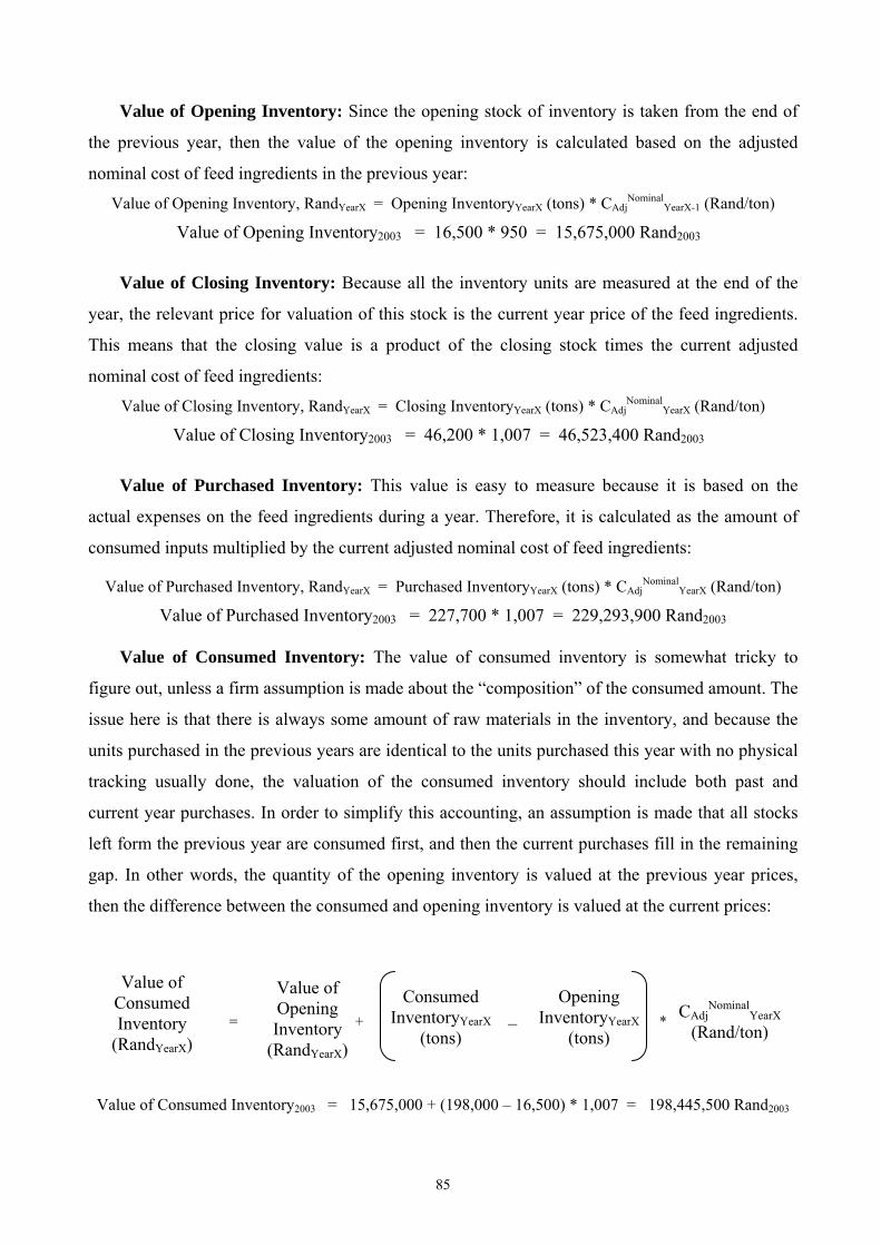
Value of Opening Inventory: Since the opening stock of inventory is taken from the end of
the previous year, then the value of the opening inventory is calculated based on the adjusted
nominal cost of feed ingredients in the previous year:
Value of Opening Inventory, RandYearX = Opening InventoryYearX (tons) * CAdjNominal
YearX-1 (Rand/ton)
Value of Opening Inventory2003 = 16,500 * 950 = 15,675,000 Rand2003
Value of Closing Inventory: Because all the inventory units are measured at the end of the
year, the relevant price for valuation of this stock is the current year price of the feed ingredients.
This means that the closing value is a product of the closing stock times the current adjusted
nominal cost of feed ingredients:
Value of Closing Inventory, RandYearX = Closing InventoryYearX (tons) * CAdjNominal
YearX (Rand/ton)
Value of Closing Inventory2003 = 46,200 * 1,007 = 46,523,400 Rand2003
Value of Purchased Inventory: This value is easy to measure because it is based on the
actual expenses on the feed ingredients during a year. Therefore, it is calculated as the amount of
consumed inputs multiplied by the current adjusted nominal cost of feed ingredients:
Value of Purchased Inventory, RandYearX = Purchased InventoryYearX (tons) * CAdjNominal
YearX (Rand/ton)
Value of Purchased Inventory2003 = 227,700 * 1,007 = 229,293,900 Rand2003
Value of Consumed Inventory: The value of consumed inventory is somewhat tricky to
figure out, unless a firm assumption is made about the “composition” of the consumed amount. The
issue here is that there is always some amount of raw materials in the inventory, and because the
units purchased in the previous years are identical to the units purchased this year with no physical
tracking usually done, the valuation of the consumed inventory should include both past and
current year purchases. In order to simplify this accounting, an assumption is made that all stocks
left form the previous year are consumed first, and then the current purchases fill in the remaining
gap. In other words, the quantity of the opening inventory is valued at the previous year prices,
then the difference between the consumed and opening inventory is valued at the current prices:
Value of Consumed Inventory
(RandYearX)
Consumed InventoryYearX
(tons) –
Opening InventoryYearX
(tons)
Value of Opening Inventory
(RandYearX)
CAdjNominal
YearX (Rand/ton) = + *
Value of Consumed Inventory2003 = 15,675,000 + (198,000 – 16,500) * 1,007 = 198,445,500 Rand2003
85
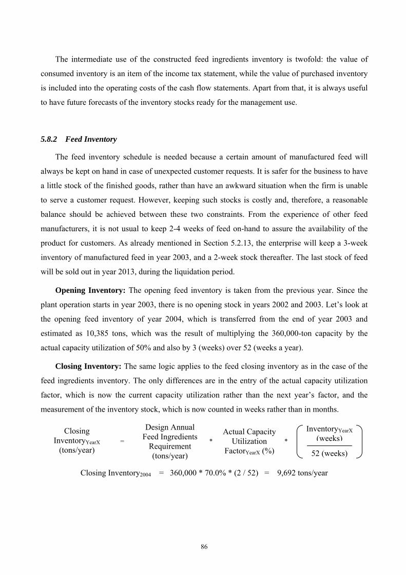
The intermediate use of the constructed feed ingredients inventory is twofold: the value of
consumed inventory is an item of the income tax statement, while the value of purchased inventory
is included into the operating costs of the cash flow statements. Apart from that, it is always useful
to have future forecasts of the inventory stocks ready for the management use.
5.8.2 Feed Inventory
The feed inventory schedule is needed because a certain amount of manufactured feed will
always be kept on hand in case of unexpected customer requests. It is safer for the business to have
a little stock of the finished goods, rather than have an awkward situation when the firm is unable
to serve a customer request. However, keeping such stocks is costly and, therefore, a reasonable
balance should be achieved between these two constraints. From the experience of other feed
manufacturers, it is not usual to keep 2-4 weeks of feed on-hand to assure the availability of the
product for customers. As already mentioned in Section 5.2.13, the enterprise will keep a 3-week
inventory of manufactured feed in year 2003, and a 2-week stock thereafter. The last stock of feed
will be sold out in year 2013, during the liquidation period.
Opening Inventory: The opening feed inventory is taken from the previous year. Since the
plant operation starts in year 2003, there is no opening stock in years 2002 and 2003. Let’s look at
the opening feed inventory of year 2004, which is transferred from the end of year 2003 and
estimated as 10,385 tons, which was the result of multiplying the 360,000-ton capacity by the
actual capacity utilization of 50% and also by 3 (weeks) over 52 (weeks a year).
Closing Inventory: The same logic applies to the feed closing inventory as in the case of the
feed ingredients inventory. The only differences are in the entry of the actual capacity utilization
factor, which is now the current capacity utilization rather than the next year’s factor, and the
measurement of the inventory stock, which is now counted in weeks rather than in months.
Actual Capacity Utilization
FactorYearX (%) = *
Design Annual
Requirement (tons/year)
Feed Ingredients *
InventoryYearX (weeks)
52 (weeks)
Closing InventoryYearX
(tons/year)
Closing Inventory2004 = 360,000 * 70.0% * (2 / 52) = 9,692 tons/year
86

Production: This is the actual amount of feed produced during a year. The correct way to
model this line is to multiply the design capacity of the plant by the actual capacity utilization
factor in the current year:
ProductionYearX (tons/year) = Design Capacity (tons/year) * Actual Capacity Utilization FactorYearX (%)
Production2004 = 360,000 * 70.0% = 252,000 tons/year
Sales: At this point, it becomes crystal clear that sales are not necessarily equal to the total
production in a year, simply because some portion of the feed produced should be kept on hands.
Thus, the sales can be found by subtracting the stock of closing inventory from the sum of the
opening inventory and current production:
SalesYearX (tons/year) = Opening InventoryYearX + ProductionYearX – Closing InventoryYearX
Sales2004 = 10,385 + 252,000 – 9,692 = 252,692 tons/year
Value of Closing Inventory: In the case of feed inventory, it is not needed to calculate the
values of opening inventory, production and sales. The only useful line here is the value of the
closing inventory, which is required to estimate the annual change in the stock of feed inventory.
At the end of the year, the relevant price to measure the inventory stock is the current weighted
average price of feed:
Value of Closing Inventory, RandYearX = Closing InventoryYearX (tons) * PFeedW, YearX (Rand/ton)
Value of Closing Inventory2004 = 9,692 * 1,281 = 13,164,279 Rand2004
The final use of the constructed feed inventory schedule is again twofold: the production and
sales quantities will enter into the Table of Production and Sales, and the values of closing
inventory is used for calculation of the “change in the feed inventory”. The change in the feed
inventory represents the cashflow equivalent of holding the feed inventory stock.
Change in Feed Inventory: The change in the feed inventory is the adjustment that reconciles
the quantity purchased and sold in a year, and it is computed as:
∆ Feed Inventory, RandYearX = Value of Closing InventoryYearX-1 – Value of Closing InventoryYearX
∆ Feed Inventory2004 = 13,306,212 – 13,164,279 = 141,933 Rand2004
87
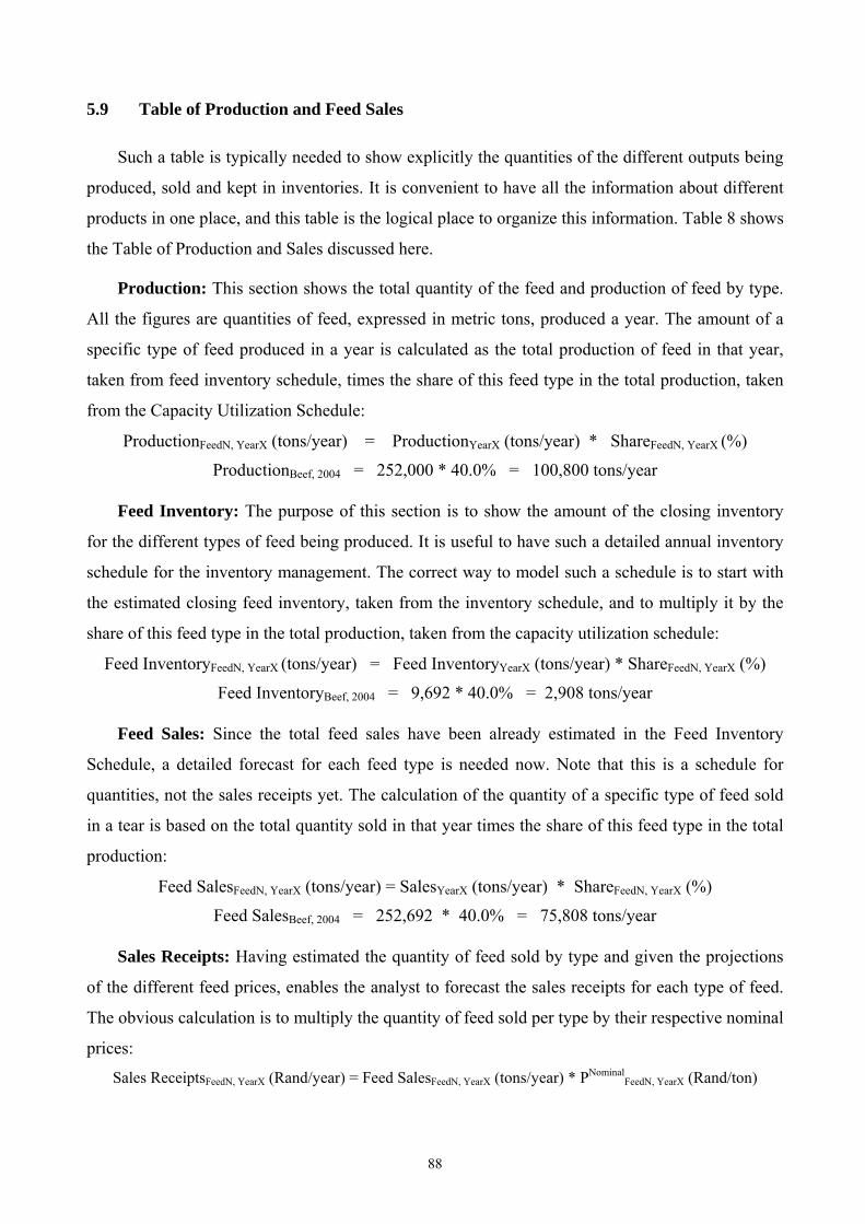
5.9 Table of Production and Feed Sales
Such a table is typically needed to show explicitly the quantities of the different outputs being
produced, sold and kept in inventories. It is convenient to have all the information about different
products in one place, and this table is the logical place to organize this information. Table 8 shows
the Table of Production and Sales discussed here.
Production: This section shows the total quantity of the feed and production of feed by type.
All the figures are quantities of feed, expressed in metric tons, produced a year. The amount of a
specific type of feed produced in a year is calculated as the total production of feed in that year,
taken from feed inventory schedule, times the share of this feed type in the total production, taken
from the Capacity Utilization Schedule:
ProductionFeedN, YearX (tons/year) = ProductionYearX (tons/year) * ShareFeedN, YearX (%)
ProductionBeef, 2004 = 252,000 * 40.0% = 100,800 tons/year
Feed Inventory: The purpose of this section is to show the amount of the closing inventory
for the different types of feed being produced. It is useful to have such a detailed annual inventory
schedule for the inventory management. The correct way to model such a schedule is to start with
the estimated closing feed inventory, taken from the inventory schedule, and to multiply it by the
share of this feed type in the total production, taken from the capacity utilization schedule:
Feed InventoryFeedN, YearX (tons/year) = Feed InventoryYearX (tons/year) * ShareFeedN, YearX (%)
Feed InventoryBeef, 2004 = 9,692 * 40.0% = 2,908 tons/year
Feed Sales: Since the total feed sales have been already estimated in the Feed Inventory
Schedule, a detailed forecast for each feed type is needed now. Note that this is a schedule for
quantities, not the sales receipts yet. The calculation of the quantity of a specific type of feed sold
in a tear is based on the total quantity sold in that year times the share of this feed type in the total
production:
Feed SalesFeedN, YearX (tons/year) = SalesYearX (tons/year) * ShareFeedN, YearX (%)
Feed SalesBeef, 2004 = 252,692 * 40.0% = 75,808 tons/year
Sales Receipts: Having estimated the quantity of feed sold by type and given the projections
of the different feed prices, enables the analyst to forecast the sales receipts for each type of feed.
The obvious calculation is to multiply the quantity of feed sold per type by their respective nominal
prices:
Sales ReceiptsFeedN, YearX (Rand/year) = Feed SalesFeedN, YearX (tons/year) * PNominalFeedN, YearX (Rand/ton)
88
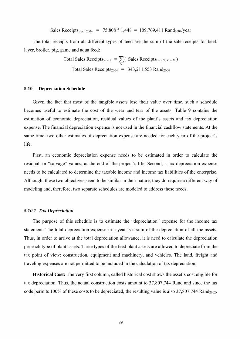
Sales ReceiptsBeef, 2004 = 75,808 * 1,448 = 109,769,411 Rand2004/year
The total receipts from all different types of feed are the sum of the sale receipts for beef,
layer, broiler, pig, game and aqua feed:
Total Sales ReceiptsYearX = ∑N
( Sales ReceiptsFeedN, YearX )
Total Sales Receipts2004 = 343,211,553 Rand2004
5.10 Depreciation Schedule
Given the fact that most of the tangible assets lose their value over time, such a schedule
becomes useful to estimate the cost of the wear and tear of the assets. Table 9 contains the
estimation of economic depreciation, residual values of the plant’s assets and tax depreciation
expense. The financial depreciation expense is not used in the financial cashflow statements. At the
same time, two other estimates of depreciation expense are needed for each year of the project’s
life.
First, an economic depreciation expense needs to be estimated in order to calculate the
residual, or “salvage” values, at the end of the project’s life. Second, a tax depreciation expense
needs to be calculated to determine the taxable income and income tax liabilities of the enterprise.
Although, these two objectives seem to be similar in their nature, they do require a different way of
modeling and, therefore, two separate schedules are modeled to address these needs.
5.10.1 Tax Depreciation
The purpose of this schedule is to estimate the “depreciation” expense for the income tax
statement. The total depreciation expense in a year is a sum of the depreciation of all the assets.
Thus, in order to arrive at the total depreciation allowance, it is need to calculate the depreciation
per each type of plant assets. Three types of the feed plant assets are allowed to depreciate from the
tax point of view: construction, equipment and machinery, and vehicles. The land, freight and
traveling expenses are not permitted to be included in the calculation of tax depreciation.
Historical Cost: The very first column, called historical cost shows the asset’s cost eligible for
tax depreciation. Thus, the actual construction costs amount to 37,807,744 Rand and since the tax
code permits 100% of these costs to be depreciated, the resulting value is also 37,807,744 Rand2002.
89
The same computation of eligible historical cost is performed for the equipment and vehicles,
but an additional action is needed to deduct the grant amount, which is deducted from the costs of
the equipment items but not deducted from the costs of office equipment, vehicles, freight and
traveling expenses. Recall that in the summary table of the investment costs, there was a section for
the equipment items with tax depreciation deduction, described in Section 5.4.6. Now it is time to
use the values from that section. The historical cost of every equipment item must be reduced by
the value of grant per that item, which can be taken from the summary table of the investment
costs:
Tax Base ValueItemN (Rand2002) = (Total CostItemN – Grant DeductionItemN) * %Historical CostItemN
Tax Base ValueFeed Production Equipment = (17,481,934 – 1,211,804) * 100% = 16,270,130 Rand2002
Annual Depreciation Expense: The total annual depreciation “expense”, which is not an
actual expense from cashflow point of view but it is treated as an expense for tax purposes, is a
sum of the annual depreciation of construction assets, equipment and vehicles. There is no
depreciation for land, which does not lose value but even tends to appreciate over time. The
treatment of land in financial and economic analysis will be discussed in the next section alongside
with the discussion of the economic depreciation.
A uniform formula is used to estimate the annual depreciation of each asset, which spells that
the amount of annual depreciation, in real terms, is equal to the initial cost of the asset (Historical
CostItemN) divided by the number of years of its tax life. Because the current tax regulation does not
provide for inflation adjustment of the tax depreciation expense, the resulting real annual value
must not be inflated4. The correct way to model the nominal tax depreciation expense is shown in
the formula below, which yields a fixed nominal value of depreciation expense in each year:
ADNominalYearX, ItemN (RandYearX) = Historical CostItemN (Rand2002) / Tax LifeItemN (years)
ADNominal2003, Construction = 37,807,744 / 20 = 1,890,387 Rand2003
The resulting nominal annual depreciation can be used in the Income Tax Statement. In order
to make the depreciation schedule adjustable to changes in the length of the tax life, a somewhat
complex MS-Excel function is used. This formula ensures that the annual depreciation appears
only in the years of asset’s tax life. If the current year is before or beyond the tax life period of a
certain asset, the value of zero is assigned to that year annual depreciation:
4 For a complete set of the regulations governing the tax treatment of depreciation expense, see SARS (2002).
90

ADNominal
YearX, ItemN = = IF(AND(YearX<(2003+Tax LifeItemN),YearX>2002), Tax Base ValueItemN / Tax LifeItemN * ID
YearX,0)
The annual depreciation expense adjusted for grant amount is a simple summation of the
results. This line will enter the income tax statement as depreciation expense of the feed plant.
5.10.2 Economic Depreciation
The purpose of this schedule is to estimate the residual values of the plant assets at the end of
the project’s life. The computational difference between the tax and economic depreciation
schedules is that the economic depreciation does not focus on the annual depreciation and, instead,
it estimates the residual value of an asset. The residual value of any asset can be found as:
Residual ValueItemN = Initial CostItemN – Accumulated DepreciationItemN
Initial Costs: To incorporate the above formula into the economic schedule, a few prior steps
should be taken. The very first column in this schedule contains the initial cost of the plant’s assets
to be depreciated over time. All assets are included and their cost values are taken directly from the
summary of the investment costs table with the exception of the freight and transportation expenses
which are excluded. Despite the fact that some of the equipment items had “mounting” expenses,
which are not physically present after the launch of the plant, it is assumed that such expenses
became embedded into the values of the corresponding assets.
Liquidation Values: Given that the initial costs are already established, now it is needed to
find the amount of accumulated deprecation for each asset, which is, in real terms, simply a sum of
all the annual depreciations over the project life:
Accumulated DepreciationItemN (Rand2002) = ∑X
( ADRealYearX, ItemN ).
The real annual depreciation is, in turn, calculated as the initial cost of the asset (Initial
CostItemN) divided by the number of years of its economic life. The resulting real annual value does
not need to be inflated because this annual depreciation is measured in real terms in order to reflect
the actual wear and tear of the asset. These transactions can be expressed as:
ADRealItemN (Rand2002) = Initial CostItemN (Rand2002) / Economic LifeItemN (years)
ADReal2002, Construction = 37,807,744 / 30 = 1,056,099 Rand2002
Accumulated DepreciationConstruction = ∑10
( 1,056,099 Rand2002) = 12,602,581 Rand2002
Residual ValueRealConstruction = 37,807,744 – 12,602,581 = 25,205,163 Rand2002
91
A residual value of such an amount is expected from the calculations because the economic
life of construction assets is taken as 30 years while the project operates only 10 years, which is
only one third of its useful life. Therefore, the residual value, in real terms, is simply a third of the
initial cost of construction. Because the cashflows are modeled in nominal rather than real prices,
the resulting real residual value must be inflated to the price level of the liquidation year:
Residual ValueNominalItemN (RandLiquidationYear) = Residual ValueReal
ItemN (Rand2002) * IDLiquidationYear
Residual ValueNominalConstruction = 25,205,163 * 1.90 = 47,846,924 Rand2013
The final destination of the calculated residual values is the revenue-side section of the
cashflow statements. The residual values are not included into the Income Tax Statement. A few
issues should be pointed for the analyst to reduce the number of questions that may arise.
The most common pitfall is related to the treatment of land. Most people agree that land does
not depreciate under usual circumstances, but the real issue is when the price of land increases over
time and the analyst has to decide whether to include this appreciation as a project benefit or not. A
good discussion on this issue is available in Manual (2003). What it means is that the analyst
should clearly see if the appreciation, or depreciation, in the real value of land is caused by the
project. If this is the case then such a real change in the value of the land should be included in the
residual value of the land. However, if the real appreciation (depreciation) of land takes place due
to the forces, external to the project, then the changes in the land value should not be included as a
part of the residual values.
The feed project is not a type of business that would substantially improve or spoil the land,
and therefore no real change in the value of land is expected over time. Thus, the annual
depreciation of land is also zero.
To calculate the residual value of land, the analyst should use the same formula as was utilized
for the estimation of the annual tax depreciation. This formula allows the analyst to have a flexible
economic depreciation schedule, with a provision for changing the length of the economic life.
Such a formula would have a form:
ADRealYearX, ItemN =
= IF(AND(YearX<(2003+Economic LifeItemN),YearX>2002), Initial CostItemN / Economic LifeItemN,0)
This approach will keep the residual values to a manageable detail, and should correspond to
the items of the investment costs. In the case of the feed project, the investment costs data are quite
lengthy and a reasonable consolidation can be reached by grouping similar items together. For
92
instance, the equipment items are consolidated in only four categories and further tables are based
on these category totals. Also, it can be useful to see the composition of the investment costs and
residual values, so it is advisable not to aggregate the data to a single cashflow item, unless
necessary.
5.11 Schedule of Labor, Electricity and Water Expenses
This schedule is constructed in order to forecast three operating expenses: labor, electricity and
water. In fact, each of them can be taken as a separate schedule but to keep the spreadsheet simple,
they are grouped together because their estimation is somewhat similar. Table 10 combines the
schedules for the labor, electricity, water and other operating expenses. The end product of each
section here is to have a forecast of annual nominal expenditure on labor, electricity and water.
5.11.1 Labor Expenses
Typically, a project employs a number of people that can be classified into three categories as
unskilled labor, skilled labor and management. The same division can be done for the employees at
the feed plant. Referring back to Section 5.2.9, let’s recall that the project will employ 12 unskilled
workers in year 2002, 16 workers in 2003 and 20 workers thereafter with a gross monthly salary of
2,400 Rand. Skilled and semi-skilled personnel will consist of four employees with a monthly
salary of 14,000 Rand. The permanent management team will be staffed with three professional
engineers, who will be transferred from the foreign country. Their monthly salaries are assumed to
be 18,000 Rand per person. All salaries are expected to grow by 0.5% a year in real terms, and also
to be adjusted for the annual rate of inflation.
Since all the three labor categories are modeled in an identical way, let’s take the example of
unskilled and semi-skilled labor to illustrate the computational techniques. The starting point here
is the data on the monthly salary, number of employees, and real wage growth rate. The final
product of labor schedule is the annual nominal labor expense, i.e. gross payroll.
Annual Salary: This column is created to convert the monthly salaries into annual equivalent
per employee, expressed in real 2002-year prices. This simple conversion takes the gross monthly
salary and multiplies it by 12 months a year, for example, this was done for unskilled and semi-
skilled labor:
Annual SalaryUnskilled & Semi-Skilled (Rand2002/year) = SalaryUnskilled & Semi-Skilled (Rand2002/month) * 12
93
Annual SalaryUnskilled & Semi-Skilled = 2,400 * 12 = 28,800 Rand2002/year
The resulting real annual salary is shown in the column, and it will serve as a base for the
estimation of the nominal annual payment in the consequent years.
Real Wage Index: Similarly to the price index in Table 2, a wage index is created in order to
show how the real wage, without inflation adjustment, would grow over years. Because all the
three labor categories are subject to the same real wage increase, it is convenient to build such an
index and use it for all labor projections. Since year 2002 is taken as year-zero for the feed project,
its index is set to one representing the starting point of the index. In all the consequent years, the
index is calculated by applying the defined growth rate to the value of the previous year index:
WIYearX = WIYearX-1 * (1+ Wage Growth RateReal)
WI2004 = 1.005 * (1+ 0.5%) = 1.010
Annual Nominal Payment: This is the nominal gross payroll for each labor category, and is
based on the calculated real annual salary, real wage index, domestic inflation, and number of
employees:
Annual PaymentNominalCategoryM, YearX (RandYearX/year) =
= Annual SalaryCategoryM, 2002 (Rand2002/employee) * WIYearX * nCategoryM, YearX (employees) * IDYearX
Annual PaymentNominalUnskilled & Semi-Skilled, 2004 = 28,800 * 1.010 * 16 * 1.12 = 522,945 Rand2004/year
The calculation of annual expenses for skilled labor and management is carried out in the same
way as for unskilled labor. The total labor expenditure a year is a sum of the unskilled, skilled and
management expenses.
5.11.2 Electric Power
The municipality tariffs for electric power were already stated in Section 5.2.11, and the total
power requirement for the feed equipment and machinery was worked out in the Summary of
Investment Costs, Table 3H. It is now possible to translate all the data into cash expenditures. The
only difficulties seen here are that the municipality bills industrial consumers monthly rather than
annual, and the billing is based on an increasing “step” tariff.
Tariff Index: Because it is expected that the real tariff will grow, on the average, by 0.5%
annually, such an index will be useful. The index value in year 2002 is one, and in the consequent
years it is computed in the same way as the real wage index:
TIYearX = TIYearX-1 * (1+ Tariff Growth RateReal)
94
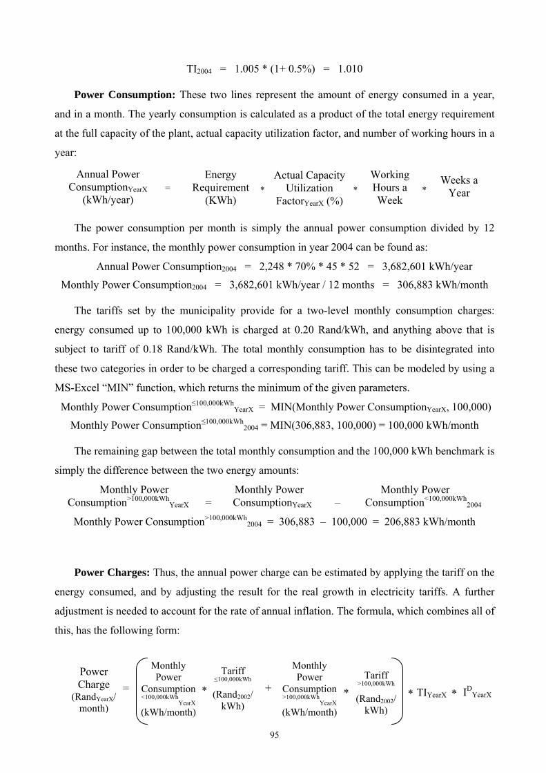
TI2004 = 1.005 * (1+ 0.5%) = 1.010
Power Consumption: These two lines represent the amount of energy consumed in a year,
and in a month. The yearly consumption is calculated as a product of the total energy requirement
at the full capacity of the plant, actual capacity utilization factor, and number of working hours in a
year:
Annual Power ConsumptionYearX
(kWh/year)
Energy Requirement
(KWh)
Working Hours a Week
Weeks a Year * *
Actual Capacity Utilization
FactorYearX (%) = *
The power consumption per month is simply the annual power consumption divided by 12
months. For instance, the monthly power consumption in year 2004 can be found as:
Annual Power Consumption2004 = 2,248 * 70% * 45 * 52 = 3,682,601 kWh/year
Monthly Power Consumption2004 = 3,682,601 kWh/year / 12 months = 306,883 kWh/month
The tariffs set by the municipality provide for a two-level monthly consumption charges:
energy consumed up to 100,000 kWh is charged at 0.20 Rand/kWh, and anything above that is
subject to tariff of 0.18 Rand/kWh. The total monthly consumption has to be disintegrated into
these two categories in order to be charged a corresponding tariff. This can be modeled by using a
MS-Excel “MIN” function, which returns the minimum of the given parameters.
Monthly Power Consumption≤100,000kWhYearX = MIN(Monthly Power ConsumptionYearX, 100,000)
Monthly Power Consumption≤100,000kWh2004 = MIN(306,883, 100,000) = 100,000 kWh/month
The remaining gap between the total monthly consumption and the 100,000 kWh benchmark is
simply the difference between the two energy amounts:
Monthly Power Monthly Power Monthly Power Consumption>100,000kWh
YearX = ConsumptionYearX – Consumption<100,000kWh2004
Monthly Power Consumption>100,000kWh2004 = 306,883 – 100,000 = 206,883 kWh/month
Power Charges: Thus, the annual power charge can be estimated by applying the tariff on the
energy consumed, and by adjusting the result for the real growth in electricity tariffs. A further
adjustment is needed to account for the rate of annual inflation. The formula, which combines all of
this, has the following form:
Tariff
≤100,000kWh
(Rand2002/kWh)
Monthly Power
Consumption <100,000kWh
YearX(kWh/month)
* *
Monthly Power
Consumption >100,000kWh
YearX(kWh/month)
Tariff >100,000kWh
(Rand2002/kWh)
+ Power Charge
(RandYearX/month)
= ID
YearXTIYearX * *
95
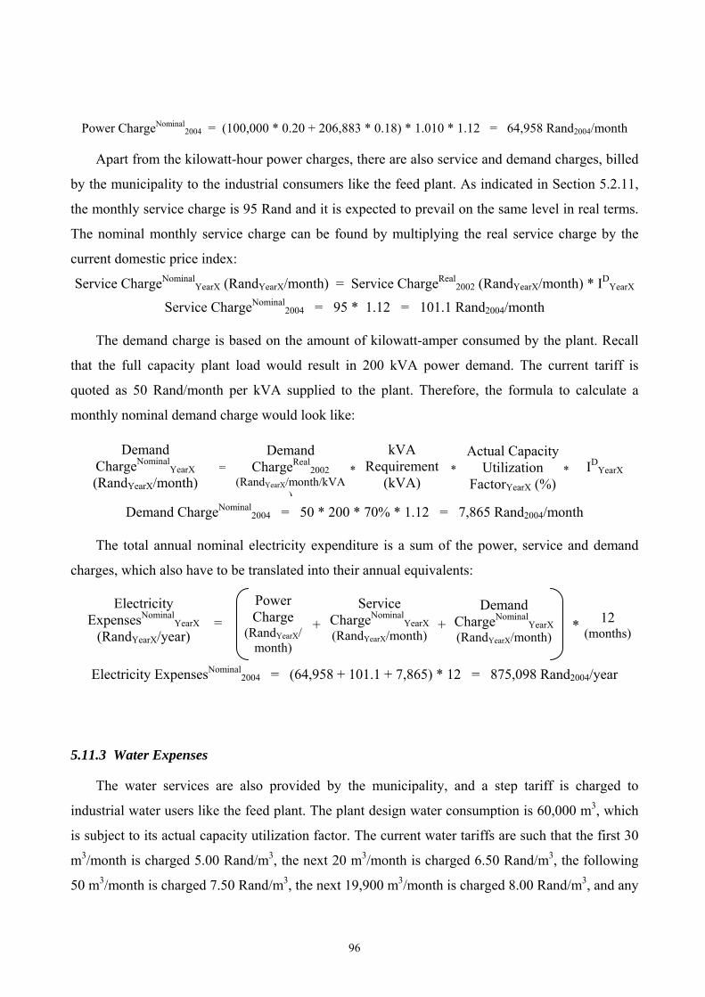
Power ChargeNominal2004 = (100,000 * 0.20 + 206,883 * 0.18) * 1.010 * 1.12 = 64,958 Rand2004/month
Apart from the kilowatt-hour power charges, there are also service and demand charges, billed
by the municipality to the industrial consumers like the feed plant. As indicated in Section 5.2.11,
the monthly service charge is 95 Rand and it is expected to prevail on the same level in real terms.
The nominal monthly service charge can be found by multiplying the real service charge by the
current domestic price index:
Service ChargeNominalYearX (RandYearX/month) = Service ChargeReal
2002 (RandYearX/month) * IDYearX
Service ChargeNominal2004 = 95 * 1.12 = 101.1 Rand2004/month
The demand charge is based on the amount of kilowatt-amper consumed by the plant. Recall
that the full capacity plant load would result in 200 kVA power demand. The current tariff is
quoted as 50 Rand/month per kVA supplied to the plant. Therefore, the formula to calculate a
monthly nominal demand charge would look like:
kVA
Requirement (kVA)
Demand ChargeNominal
YearX (RandYearX/month)
Demand ChargeNominal2004 = 50 * 200 * 70% * 1.12 = 7,865 Rand2004/month
Demand ChargeReal
2002 (RandYearX/month/kVA
)
Actual Capacity Utilization
FactorYearX (%) ID
YearX= * * *
The total annual nominal electricity expenditure is a sum of the power, service and demand
charges, which also have to be translated into their annual equivalents:
Power Charge
(RandYearX/month)
Demand ChargeNominal
YearX (RandYearX/month)
+ Service
ChargeNominalYearX
(RandYearX/month) +
Electricity ExpensesNominal
YearX (RandYearX/year)
12 (months)
= *
Electricity ExpensesNominal2004 = (64,958 + 101.1 + 7,865) * 12 = 875,098 Rand2004/year
5.11.3 Water Expenses
The water services are also provided by the municipality, and a step tariff is charged to
industrial water users like the feed plant. The plant design water consumption is 60,000 m3, which
is subject to its actual capacity utilization factor. The current water tariffs are such that the first 30
m3/month is charged 5.00 Rand/m3, the next 20 m3/month is charged 6.50 Rand/m3, the following
50 m3/month is charged 7.50 Rand/m3, the next 19,900 m3/month is charged 8.00 Rand/m3, and any
96
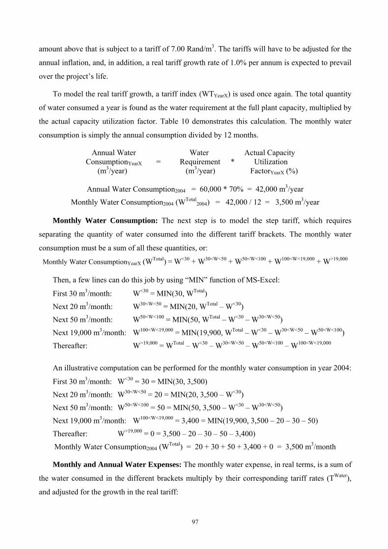
amount above that is subject to a tariff of 7.00 Rand/m3. The tariffs will have to be adjusted for the
annual inflation, and, in addition, a real tariff growth rate of 1.0% per annum is expected to prevail
over the project’s life.
To model the real tariff growth, a tariff index (WTYearX) is used once again. The total quantity
of water consumed a year is found as the water requirement at the full plant capacity, multiplied by
the actual capacity utilization factor. Table 10 demonstrates this calculation. The monthly water
consumption is simply the annual consumption divided by 12 months.
Annual Water Water Actual Capacity ConsumptionYearX = Requirement * Utilization (m3/year) (m3/year) FactorYearX (%)
Annual Water Consumption2004 = 60,000 * 70% = 42,000 m3/year
Monthly Water Consumption2004 (WTotal2004) = 42,000 / 12 = 3,500 m3/year
Monthly Water Consumption: The next step is to model the step tariff, which requires
separating the quantity of water consumed into the different tariff brackets. The monthly water
consumption must be a sum of all these quantities, or:
Monthly Water ConsumptionYearX (WTotal) = W<30 + W30<W<50 + W50<W<100 + W100<W<19,000 + W>19,000
Then, a few lines can do this job by using “MIN” function of MS-Excel:
First 30 m3/month: W<30 = MIN(30, WTotal)
Next 20 m3/month: W30<W<50 = MIN(20, WTotal – W<30)
Next 50 m3/month: W50<W<100 = MIN(50, WTotal – W<30 – W30<W<50)
Next 19,000 m3/month: W100<W<19,000 = MIN(19,900, WTotal – W<30 – W30<W<50 – W50<W<100)
Thereafter: W>19,000 = WTotal – W<30 – W30<W<50 – W50<W<100 – W100<W<19,000
An illustrative computation can be performed for the monthly water consumption in year 2004:
First 30 m3/month: W<30 = 30 = MIN(30, 3,500)
Next 20 m3/month: W30<W<50 = 20 = MIN(20, 3,500 – W<30)
Next 50 m3/month: W50<W<100 = 50 = MIN(50, 3,500 – W<30 – W30<W<50)
Next 19,000 m3/month: W100<W<19,000 = 3,400 = MIN(19,900, 3,500 – 20 – 30 – 50)
Thereafter: W>19,000 = 0 = 3,500 – 20 – 30 – 50 – 3,400)
Monthly Water Consumption2004 (WTotal) = 20 + 30 + 50 + 3,400 + 0 = 3,500 m3/month
Monthly and Annual Water Expenses: The monthly water expense, in real terms, is a sum of
the water consumed in the different brackets multiply by their corresponding tariff rates (TWater),
and adjusted for the growth in the real tariff:
97

Monthly Water ExpenseReal
YearX (Rand2002/month) = = (W<30*T<30 + W30<W<50*T30<W<50 + W50<W<100*T50<W<100 + W100<W<19,000*T100<W<19,000 + W>19,000*T>19,000) * WTYearX
Monthly Water ExpenseReal2004 =
= (30*5.0 + 20*6.5 + 50*7.5 + 3,400*8.0 + 0*7.0) * 1.020 = 28,415 Rand2002/month
This derived real monthly water expense has to be translated into its annual nominal
equivalent, which can be done by multiplying the result by the domestic price index and by the
number of months a year:
Annual Water ExpenseNominalYearX (RandYearX/year) =
= Monthly Water ExpenseRealYearX (Rand2002/month) * ID
YearX * 12 (months)
Annual Water ExpenseNominal2004 = 28,415 * 1.12 *12 = 383,124 Rand2004/year
5.11.4 Schedule of Other Operating Expenses
Apart from the labor, electric and water expenses, there are a number of the cash outlays.
Table 10 shows the future projections of the operating costs. The reason why these expenses are
grouped together is their similarity in estimation. Section 5.2.10 stated a number of annual
operating costs, and they are not expected to vary from year to year in real terms. However, an
adjustment for domestic inflation is necessarily. For the majority of the expenses here, the formula
below will be used, and if the calculation of some of the expenses involves more than that, an
explanation will be given. The basic formula is:
Annual Actual Capacity ExpenseNominal
ItemN,YearX = ExpenseRealItemN,2002 * Utilization * ID
YearX (RandYearX/year) (Rand2002/year) FactorYearX (%)
All expenses, except equipment mechanic service, are estimated by the formula stated above,
and an illustration of this can be done with the example of office accommodation, and
transportation and storage in year 2004:
Office AccommodationNominal2004 = 1,200,000 * 70% * 1.12 = 943,824 Rand2004/year
Transportation and StorageNominal2004 = 2,000,000 * 70% * 1.12 = 1,573,040 Rand2004/year
Equipment Mechanic Service: This expense can be estimated by using the main formula
with a little modification due to the fact that the cost of this service has to be derived from the
equipment cost:
Equipment Mechanic Total Equipment Share of Actual Capacity ServiceReal
2002 = Cost ServiceReal2002 * Mechanic * Utilization * ID
YearX
98

(Rand2002/year) (Rand2002/year) Service (%) FactorYearX (%)
Equipment Mechanic ServiceReal2002 = 47,566,700 * 2.5% * 50% * 1.00 = 630,259 Rand2002/year
Equipment Mechanic ServiceNominal2004 = 47,566,700 * 2.5% *70% * 1.12 = 935,304 Rand2004/year
5.12 Working Capital Schedule
Such a schedule is typically needed in order to model the annual changes in the working
capital, and Table 11 illustrates the modeling of working capital schedule. Usually, the working
capital includes accounts receivable, accounts payable and cash balance. The estimates of the
amount of such account were discussed in Section 5.2.8.
Accounts Receivable: These accounts represent the amount of cash outstanding from the
sales, and it is expected that accounts receivable will be equal to 2 week of the total sales, on the
average. Thus, the total amount of accounts receivable, which are always measured in the current
nominal prices, is found by the formula:
ARYearX (RandYearX/year) = Total Sales ReceiptsYearX (RandYearX/year) * [ARAdjusedYearX (weeks/year) / 52]
AR2004 = 343,211,553 * (2 / 52) = 13,200,444 Rand2004/year
Because the total feed sales are composed of several feed types, a further detailed separation is
also made in order to estimate the amount of accounts receivable per each feed type. It is computed
as the total accounts receivable multiplied by the share of the particular feed type in the production:
ARFeedN, YearX = ARYearX * %ShareFeedN, YearX
However, the estimated amount of accounts receivable is again a “stock” of cash sitting idle in
the accounting books, while the cashflow statements operate with “flows” of cash, which means
that the computed accounts receivable has to be converted into its cashflow equivalent, or “change
in accounts receivable”. Note that such a change is computed as the previous’ year accounts
receivable minus the current’s year accounts receivable, and any increase in their amount must
have a negative impact on the cashflows:
∆ARYearX = ARYearX-1 – ARYearX
∆AR2004 = 8,359,030 – 13,200,444 = –4,841,414 Rand2004/year
Again, a detailed break-down of the total change in accounts receivable is done per feed type,
by using a similar formula: ∆ARFeedN, YearX = ∆ARYearX * %ShareFeedN, YearX.
99
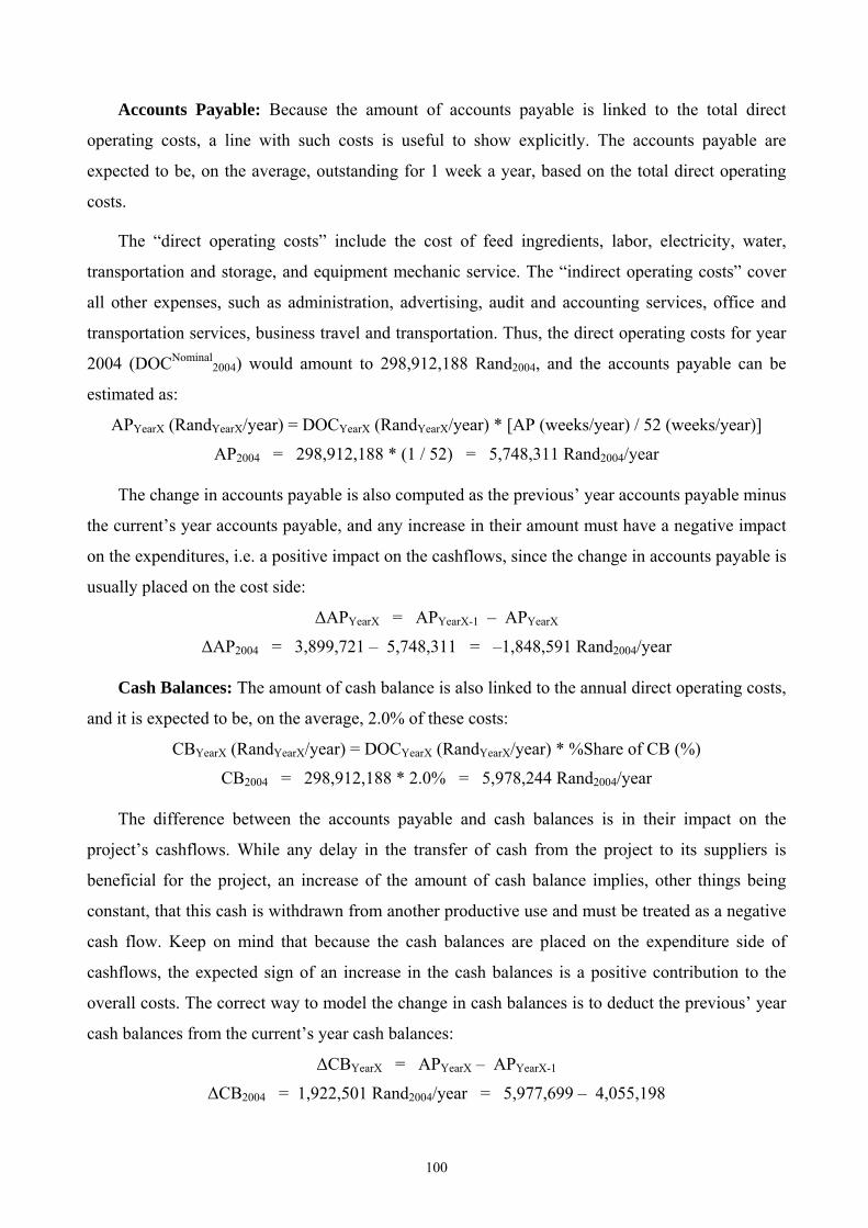
Accounts Payable: Because the amount of accounts payable is linked to the total direct
operating costs, a line with such costs is useful to show explicitly. The accounts payable are
expected to be, on the average, outstanding for 1 week a year, based on the total direct operating
costs.
The “direct operating costs” include the cost of feed ingredients, labor, electricity, water,
transportation and storage, and equipment mechanic service. The “indirect operating costs” cover
all other expenses, such as administration, advertising, audit and accounting services, office and
transportation services, business travel and transportation. Thus, the direct operating costs for year
2004 (DOCNominal2004) would amount to 298,912,188 Rand2004, and the accounts payable can be
estimated as:
APYearX (RandYearX/year) = DOCYearX (RandYearX/year) * [AP (weeks/year) / 52 (weeks/year)]
AP2004 = 298,912,188 * (1 / 52) = 5,748,311 Rand2004/year
The change in accounts payable is also computed as the previous’ year accounts payable minus
the current’s year accounts payable, and any increase in their amount must have a negative impact
on the expenditures, i.e. a positive impact on the cashflows, since the change in accounts payable is
usually placed on the cost side:
∆APYearX = APYearX-1 – APYearX
∆AP2004 = 3,899,721 – 5,748,311 = –1,848,591 Rand2004/year
Cash Balances: The amount of cash balance is also linked to the annual direct operating costs,
and it is expected to be, on the average, 2.0% of these costs:
CBYearX (RandYearX/year) = DOCYearX (RandYearX/year) * %Share of CB (%)
CB2004 = 298,912,188 * 2.0% = 5,978,244 Rand2004/year
The difference between the accounts payable and cash balances is in their impact on the
project’s cashflows. While any delay in the transfer of cash from the project to its suppliers is
beneficial for the project, an increase of the amount of cash balance implies, other things being
constant, that this cash is withdrawn from another productive use and must be treated as a negative
cash flow. Keep on mind that because the cash balances are placed on the expenditure side of
cashflows, the expected sign of an increase in the cash balances is a positive contribution to the
overall costs. The correct way to model the change in cash balances is to deduct the previous’ year
cash balances from the current’s year cash balances:
∆CBYearX = APYearX – APYearX-1
∆CB2004 = 1,922,501 Rand2004/year = 5,977,699 – 4,055,198
100
5.13 Projected Income Tax Statement
An income tax statement is the first set of results of the project evaluation. It statement
combines various technical, financial and market data into a single statement of the project’s
financial performance. This statement is needed to estimate the project’s annual tax liability, if any.
The projected income tax statement of the feed plant is presented in Table 12. While it follows
the standard format of an income tax statement, a few issues should be discussed about modeling
this statement.
Revenues: The revenues items all come from the sales of the different feed types, and their
values are taken directly from the Tale of Production and Feed Sales. Note that there are no
accounts receivable or the changes in accounts receivable here. All the figures are expressed in
nominal terms.
Cost of Goods Sold and Gross Margin: The cost of goods sold item was obtained from the
“value of consumed inputs” in the Schedule of Feed Ingredients Inventory. The gross margin
shows the difference between the total sales and cost of goods sold, or what is left for the producer
to cover all the current operating costs and to amortize the initial investment costs.
Expenses: All the expense items, with an exception of the depreciation expense, are taken
from the Schedule of Operating Expenses. All the figures are annual nominal expenses. The
depreciation expense is linked to the “grant adjusted annual depreciation expense” line from the
Tax Depreciation Schedule.
Income Before Interest and Taxes: This line is calculated by subtracting all direct and
indirect operating costs from the total revenues.
Income Before Taxes: This line is calculated by subtracting the interest expense from the
income before interest and taxes. Note that only the interest portion of the annual nominal
repayment is eligible to be deducted as an expense.
Cumulative Losses: In many countries, including South Africa, the tax code permits a
deduction of the corporate income losses from the previous years. If a business makes losses for a
few years in a row, their cumulated losses can be subtracted from the current taxable income to
arrive at the final corporate income tax for the current year. In South Africa, such losses can be
formally carried over indefinitely, since no restriction is set for the number of years to limit the
101
carry-over of losses. Thus, this line should show the total amount of the income losses accumulated
from the previous years. The cumulative losses can be zero, but usually they will have a negative
sign, the formula used here to do this task is:
Cumulative LossesYearX (RandYearX/year) = MIN(0, Income Before TaxesYearX + Cumulative LossesYearX-1)
Cumulative Losses2004 = MIN(0, 13,852,072 + [–6,192,673]) = 0 Rand2004/year
What the “MIN” function does here is the selection of the minimum value of either zero,
representing no loss, or summation of the current year’s income before tax and the previous year
cumulative losses. If this year income before taxes is negative, then this loss will be added to the
past accumulated loses, however if the current income before taxes is positive then it will reduce
the amount of accumulated loses. In the example above, the cumulative losses in year 2002 totaled
6,192,673 Rand while the income before tax is 13,852,072 Rand, which imply that the current
year’s income is sufficient to cover the amount of the past accumulated losses. At the same time,
the current income before taxes can be reduced by the amount of the accumulated losses for tax
purposes.
Taxable Income: This line is needed to show the amount of the taxable income, which can be
defined as the difference between the current income before taxes and the cumulative tax less carry
forward. The taxable income can be either positive or zero and the formula to model it takes the
form of:
Taxable IncomeYearX (RandYearX/year) = MAX(0, Income Before TaxesYearX + Cumulative LossesYearX-1)
Taxable Income2004 = MAX(0, 13,852,072 + [–6,192,673]) = 7,659,673 Rand2004/year
The cumulative losses from year 2003 are not zero and then the current 2004-year income
before taxes is reduced by the amount of the past cumulative losses. At the same time, if the
income before taxes was negative, then the function will return zero as the amount of taxable
income.
Income Tax: The amount of income tax is based on the current taxable income before taxes
and the corporate income tax rate. However, the tax law of South Africa envisages a 4-year tax-
holiday incentive for start-up business like the feed plant. Therefore, the “IF” function is used to
model the income tax calculation:
Income TaxYearX (RandYearX/year) = IF(YearX>(2002 + Tax Holiday), Taxable IncomeYearX * Tax Rate, 0)
Income Tax2004 = IF(2004>(2002 + 4), 7,659,673 * 30%, 0) = 0 Rand2004/year
Because the current 2004 year is still in the tax holiday period, no income tax is computed.
The formula automatically picks up any changes in the length of the tax holiday when the
102
parameter is adjusted in the Table of Parameters. If there are any other corporate taxes, they should
also be deducted at this point.
Income / Loss After Taxes: This is the bottom line of the income statement, indicating if the
enterprise is making or loosing money in a particular year from the point of view of tax authorities.
It is computed by deducting the taxes from the taxable income. The project’s income after taxes for
year 2004 is estimated as 7,659,673 Rand2004/year.
While the income statement gives a good idea about financial performance of the project, it
does not answer the question if the project is financially and economically feasible, and whether
the owners, financial institutions and government should be involved in it. A further analysis
needed, and the consequent sections look into the feasibility issue from different perspectives.
5.14 Banker’s Point of View
Following the construction of the projected income tax statement through time and estimation
of income tax liability, a projected cash flow statement from “banker’s point of view” is modeled,
based on the computed tables and schedules. The banker’s or total investment’s point of view is
first evaluation perspective, from which a typical project should be analyzed. Conceptually, this
perspective is needed to look at the project being without any external finance, like the project is
being run from the equity of the owners. The reason why it is important in order to look at the
project from this angle is that this really shows the strength of the project to repay its loans, if such
are taken.
5.14.1 Projected Cashflow Statement from Banker’s Point of View
The banker’s point of view is relevant for a person/institution, who is in a position to take part
in the debt financing of the enterprise. Before a banker approves any loan to be disbursed to the
project, he wants to make sure that the project is capable of repaying the loan in full and in a timely
manner.
Thus, the financial assessment of a project from the banker’s point of view is based on the
cashflow projections, excluding any items related to commercial bank loans, i.e. loan receipts and
loan repayments. A typical nominal cash flow statement for the banker’s point of view is presented
in Table 13. All figures are projected in nominal values.
103
Any cash flow statement consists of two parts: revenues and expenditures. At the very bottom,
the net cash flow is calculated, which is the difference between the annual revenues and
expenditures. What the figures of the net cash flow tell the analyst is whether a sufficient net
cashflow is available to service the debt financing undertaken by the project and to ensure a return
to the owners of the equity participation in the enterprise. While such a brief evaluation is very
illustrative and useful, a further analysis is needed to look into the relationship between the
projected net cash flow and proposed loan repayments. This is the core relationship to the banker’s
point of view, and it will be discussed in Section 5.14.2.
Revenues
Referring to Table 13, the revenues consist of the feed sales, change in the accounts
receivable, change in the feed inventory, liquidation values of the assets and the grant. The annual
nominal projections of feed sales by type are taken directly from the Production and Feed Sales
Schedule. The change in accounts receivable is linked to the computed values in the Working
Capital Schedule, and the change in feed inventory is referred back to the Feed Inventory Schedule.
The change in accounts receivable as well as the change in feed inventory in year 2003 are
negative figures, which can be explained by the fact that both the amount of the accounts
receivable and the stock of feed inventory are on rise in 2003, which means a negative cash inflow
for the enterprise.
The residuals values, in nominal terms, are taken from the Economic Depreciation Schedule.
Note that the only year when these residual values appear in the cashflows is the last 2013 year, at
the time “liquidation” of the business. The last item of the revenue side is the grant disbursements
in year 2002 and 2003. The total revenues line summarizes all the annual revenues, and its
projected amount of cash inflows during year 2003 is 197,169,549 Rand2003.
Expenditures
The expenditure side of this cashflow statement is lengthier, but it can be grouped into four
sections: investment costs, operating costs, working capital items and income tax. The investment
costs are all expressed in nominal domestic currency, and they are actually linked back to the
summary of the investment costs. The whole burden of capital investment, amounting to
88,652,055 Rand2002, is to materialize in year 2002, and there are no other capital expenditures in
the consequent years. Note that the annual depreciation of the assets is already captured in the
liquidation values, which are the difference between the initial value of the plant assets and
104
accumulated depreciation. Therefore, no annual depreciation expense is included into cash flows,
unlike the Income Tax Statement.
The operating costs can be further sub-divided into direct operating costs, and indirect
operating costs. The direct operating costs include feed ingredients, labor, electricity, water,
transportation and storage, and equipment mechanic service. The annual nominal cost of feed
ingredients is taken from the “value of purchased inputs” from the Feed Ingredients Inventory
Schedule. The projections of all the other operating costs come from the Schedule of Operating
Expenses. The total operating costs in year 2003 amount to 244,127,878 Rand2003.
The changes in accounts payable and cash balances are taken from the Working Capital
Schedule. Their signs in year 2003 conform to the expectation of the change in accounts payable
being negative, which reduces the costs, and of the change in cash balances being positive, which
does increase the costs.
The income tax amount is linked to the amount of income tax paid in the Income Tax
Statement. The total expenditures line sums up all the costs, and its projected amount in year is
244,283,867 Rand2003. This makes the estimated net cash flow in year 2004 to be –47,114,318
Rand2003, which is the difference between the total revenues and total expenses.
Nominal versus Real Cash Flows
The constructed nominal cash flow statement for banker’s point of view does reflect the cash
flows associated with the feed project; however, the analysis can not be based on the nominal
figures since they are distorted from the real values by inflation. The inflation impact must be
removed from the cashflows to enable the analyst to see the flows of real resources. At the same
time, the real cashflows, i.e. nominated in the fixed prices, will serve as a base for the economic
analysis later.
Such a conversion from the current prices to the real, year-2002, values can be made by
dividing all the figures of the nominal cash flow statement by the corresponding annual domestic
price index. Because the domestic price index incorporates all the inflation rates in the preceding
years, the resulting real value is expressed in the prices of the year-zero:
Cashflow ItemRealYearX (Rand2002/year) = Cashflow ItemNominal
YearX (RandYearX/year) / IDYearX
TransportationReal2004 = 1,179,780 / 1.12 = 1,050,000 Rand2002/year
This conversion should be performed for all cashflow items, year by year, in order to derive
the real, year-2002 valued, cash flow statement for banker’s point of view. Table 14 shows the
105
projected real cash flow statement from the banker’s point of view. Note that the same order of
items is maintained in the real statement, as was done in the nominal. Having obtained the real
cashflow statement, enables the analyst to step up with further inquiry into the financial
performance of the feed project.
5.14.2 Debt Service Ratios as an Evaluation Criteria
Neither NPV nor IRR are calculated for the banker’s point of view. The main criteria in the
assessment of the project’s ability to repay its debts is the annual debt service capacity ratio
(ADSCR), which simply compares the amount of current net cash flow to the current debt
obligations. If the net cash flow amount is greater than the debt repayment then the project can be
said capable of repaying its debt obligations on a year-to-year basis. Table III below shows the real
Projected Cash Flow Statement from the Owner's Point of View as well as the calculation of the
ADSCR and DSCR ratios.
ADSCR
Usually, the calculations of debt service ratios take place after the real projections from the
banker’s point of view, and Table 14 shows the computed debt ratios for the feed project. The
ADSCR ratios are calculated only for the periods in which repayments are made and “annual debt
repayment” includes both annual interest and principal repayment. The formula used for
calculation of ADSCR is:
ADSCRYearX = Annual Net Cash Flow before FinancingRealYearX / Annual Debt RepaymentReal
YearX
The annual net cash flow before financing is the net cash flow of the real cash flow statement
from the banker’s point of view, and the annual real debt repayment is taken from the Loan
Schedule. A negative ADSCR ratio implies that the project has a negative cashflow in a certain
year, and the inflows are not even enough to cover all the cash outlays. A positive ratio less than
unity means that the project is able to cover its expenditures, but there is not enough cash to make
the debt repayment in full to the bank. A ratio of unity infers that the project is just breaking even
in terms of covering its expenses and repaying the debt obligations but there is no cash available to
provide a return to equity. A positive ADSCR well above one implies that there is enough cash
generated by the business to repay both expenses and debt installments and give some return to the
equity owner(s).
106
An “IF” function of MS-Excel is used to compute the ADSCR, in order for it to be flexible
with the start and end dates of loan repayment. What the function does is that it shows a sign “-“ in
the years when there is no loan repayments made, instead of showing a division by zero error:
ADSCRYearX = IF(Annual Debt RepaymentRealYearX = 0, “-“,
Annual Net Cash Flow before FinancingRealYearX / Annual Debt RepaymentReal
YearX)
ADSCR2003 = IF(0 = 0, “-“, –44,447,470 / 0) = “-“
ADSCR2004 = IF(8,185,353 ≠ 0, “-“, 6,293,606 / 8,185,353) = 0.77
ADSCR2005 = IF(8,185,353 ≠ 0, “-“, 17,714,074 / 7,722,031) = 2.29
This is a usual cash profile of a commercial project to have an increasing ADSCR during the
first years of operation. As the project successfully establishes itself on the market and achieves its
capacity, the cash revenues stabilize and provide a sufficient amount of cash for both the financing
bank and the owner(s) of the business.
DSCR
Another related measure of project’s financial strength is the Debt Service Capacity Ratio
(DSCR), which is simply the accumulated annual debt service capacity ratio. The DSCR is
calculated only for periods in which debt repayments take place, and formula has the form of:
DSCRYearX = PV of Annual Net Cash FlowsRealYearX / PV of Annual Debt RepaymentReal
YearX
This ratio summarizes the project’s ability to repay its debt obligations over the remaining
years of the debt service, not for just a single year. While the ADSCR looks on this project strength
on a year-to-year basis, the DSCR ratio approaches the task from a wider angle and takes both
remaining net cashflow and remaining debt repayments into consideration. The debt service
capacity ratio is useful to examine how to obtain sufficient financial resources during questionable
financial periods, in which the annual capability of servicing the debt is doubtful. As a rule of
thumb, a DSCR ratios of 1.5 to 2.0 magnitude signify an “acceptable” coverage of the debt
obligations by the project and ratios less than that indicate either a poor financial design or/and a
bad business enterprise. In fact, such ratios are of rather subjective nature and it depends on the
industry standards and individual risk preferences what is really an “acceptable” ratio. Typically, a
bank has its own schedule of acceptable ratios for the different industries and project sizes. In a
more complete discussion of the use of this measure see Chapter 3 of the Manual (2003).
107
Net Cash Flow for Debt Repayment Function: Modeling the actual ratios can be complex
sometimes, and may involve several functions. The feed project DSCR computations need a few
extra lines in order to compute the DSCR ratios. The net cash flow for debt repayment function
(NCF for DRF) is one which is needed to show the amount of the net cash flow in a particular year
when a debt repayment is made in that year, and to show zero otherwise:
NCF for DRFYearX = IF(Annual Debt RepaymentRealYearX = 0, 0,
Annual Net Cash Flow before FinancingRealYearX)
NCF for DRF2003 = IF(0 = 0, 0, –44,447,470) = 0 Rand2002
NCF for DRF2004 = IF(8,185,353 ≠ 0, 0, 6,293,606) = 6,293,606 Rand2002
Present Value of Net Cash Flow: This line is also artificially created in order to compute the
present value of the annual net cash flow in the remaining years of the repayment period. Because
it is based on the computed above net cash flow for debt repayment function, instead of the original
net cash flow line, this PV includes only the years of actual debt repayment. The relevant discount
rate for such present value is the real interest rate (r), which will be also used for discounting the
annual real debt repayments. The function used here is the “NPV” function of MS-Excel:
PV of NCFYearX = NPV(r, NCF for DRFYearX+1:NCF for DRF2013) + NCF for DRFYearX
Note that the present value is estimated for each year, treating that year as the base year of
discounting. Therefore, the function excludes that year’s value from discounting NPV function,
simply because that value is already in its “real” form. For instance, here are examples of this
estimation for year 2003 and 2004:
PV of NCF2003 = NPV(r, NCF for DRF2004:NCF for DRF2013) + NCF for DRF2003
PV of NCF2003 = NPV(8.5%, NCF for DRF2004:NCF for DRF2013) + 0 = 68,929,060 Rand2002
PV of NCF2004 = NPV(r, NCF for DRF2005:NCF for DRF2013) + NCF for DRF2004
PV of NCF2004 = NPV(8.5%, NCF for DRF2005:NCF for DRF2013) + 6,293,606 = 74,788,030 Rand2002
Present Value of Debt Repayments: This line is needed to show the present value of the
repayment in the all remaining years of debt service. The same “NPV” function is used to compute
the present value of debt repayments (PV of DR):
PV of DRYearX =
= NPV(r,Annual Debt RepaymentRealYearX+1:Annual Debt RepaymentReal
2013)+Annual Debt RepaymentRealYearX
PV of DR2003 =
= NPV(8.5%, Annual Debt RepaymentReal2004:Annual Debt RepaymentReal
2013) + 0 = 29,078,001 Rand2002
108
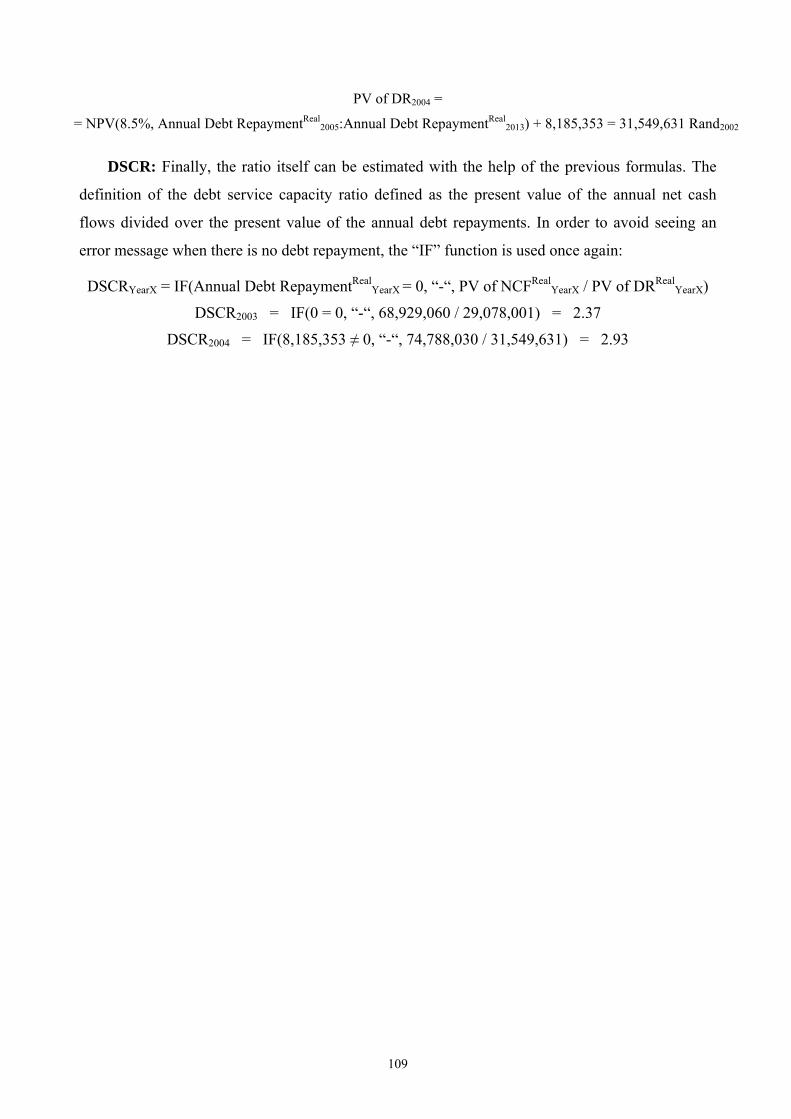
109
PV of DR2004 =
= NPV(8.5%, Annual Debt RepaymentReal2005:Annual Debt RepaymentReal
2013) + 8,185,353 = 31,549,631 Rand2002
DSCR: Finally, the ratio itself can be estimated with the help of the previous formulas. The
definition of the debt service capacity ratio defined as the present value of the annual net cash
flows divided over the present value of the annual debt repayments. In order to avoid seeing an
error message when there is no debt repayment, the “IF” function is used once again:
DSCRYearX = IF(Annual Debt RepaymentRealYearX = 0, “-“, PV of NCFReal
YearX / PV of DRRealYearX)
DSCR2003 = IF(0 = 0, “-“, 68,929,060 / 29,078,001) = 2.37
DSCR2004 = IF(8,185,353 ≠ 0, “-“, 74,788,030 / 31,549,631) = 2.93
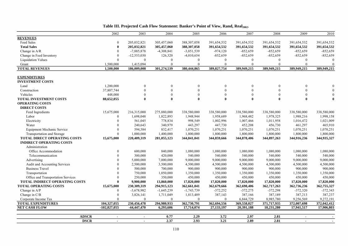
110
2002 2003 2004 2005 2006 2007 2008 2009 2010REVENUES
Feed Sales 0 205,032,821 305,457,060 388,307,058 391,654,532 391,654,532 391,654,532 391,654,532 391,654,532Total Sales 0 205,032,821 305,457,060 388,307,058 391,654,532 391,654,532 391,654,532 391,654,532 391,654,532Change in A/R 0 -7,885,878 -4,308,841 -3,851,539 -974,120 -852,659 -852,659 -852,659 -852,659Change in Feed Inventory 0 -12,553,030 126,320 -4,010,654 -852,659 -852,659 -852,659 -852,659 -852,659Liquidation Values 0 0 0 0 0 0 0 0 0Grant 1,500,000 1,415,094 0 0 0 0 0 0 0
TOTAL REVENUES 1,500,000 186,009,008 301,274,539 380,444,865 389,827,754 389,949,215 389,949,215 389,949,215 389,949,215
EXPENDITURESINVESTMENT COSTS
Land 1,200,000 0 0 0 0 0 0 0 0Construction 37,807,744 0 0 0 0 0 0 0 0Vehicles 448,000 0 0 0 0 0 0 0 0
TOTAL INVESTMENT COSTS 88,652,055 0 0 0 0 0 0 0 0OPERATING COSTS
DIRECT COSTSFeed Ingredients 15,675,000 216,315,000 275,880,000 338,580,000 338,580,000 338,580,000 338,580,000 338,580,000 338,580,000Labor 0 1,698,048 1,822,893 1,948,944 1,958,689 1,968,482 1,978,325 1,988,216 1,998,158Electricity 0 561,045 778,834 998,549 1,002,996 1,007,466 1,011,958 1,016,472 1,021,009Water 0 240,643 340,979 443,297 447,730 452,208 456,730 461,297 465,910Equipment Mechanic Service 0 594,584 832,417 1,070,251 1,070,251 1,070,251 1,070,251 1,070,251 1,070,251Transportation and Storage 0 1,000,000 1,400,000 1,800,000 1,800,000 1,800,000 1,800,000 1,800,000 1,800,000
TOTAL DIRECT OPERATING COSTS 15,675,000 220,409,319 281,055,123 344,841,041 344,859,666 344,878,406 344,897,263 344,916,236 344,935,327INDIRECT OPERATING COSTS
AdministrationOffice Accommodation 0 600,000 840,000 1,080,000 1,080,000 1,080,000 1,080,000 1,080,000 1,080,000Telecommunication 0 300,000 420,000 540,000 540,000 540,000 540,000 540,000 540,000
Advertising 0 5,000,000 7,000,000 9,000,000 9,000,000 9,000,000 9,000,000 9,000,000 9,000,000Audit and Accounting Services 0 2,500,000 3,500,000 4,500,000 4,500,000 4,500,000 4,500,000 4,500,000 4,500,000Business Travel 0 500,000 700,000 900,000 900,000 900,000 900,000 900,000 900,000Transportation 0 750,000 1,050,000 1,350,000 1,350,000 1,350,000 1,350,000 1,350,000 1,350,000Office and Transportation Services 0 250,000 350,000 450,000 450,000 450,000 450,000 450,000 450,000
TOTAL INDIRECT OPERATING COSTS 0 9,900,000 13,860,000 17,820,000 17,820,000 17,820,000 17,820,000 17,820,000 17,820,000TOTAL OPERATING COSTS 15,675,000 230,309,319 294,915,123 362,661,041 362,679,666 362,698,406 362,717,263 362,736,236 362,755,327
Change in A/P 0 -3,678,982 -1,645,239 -1,743,739 -372,252 -372,275 -372,298 -372,320 -372,343Change in C/B 0 3,826,141 1,711,049 1,813,489 387,143 387,166 387,189 387,213 387,237Corporate Income Tax 0 0 0 0 0 6,844,729 8,985,780 9,256,569 9,272,191
TOTAL EXPENDITURES 104,327,055 230,456,478 294,980,933 362,730,791 362,694,556 369,558,027 371,717,935 372,007,698 372,042,412NET CASH FLOW -102,827,055 -44,447,470 6,293,606 17,714,074 27,133,197 20,391,188 18,231,280 17,941,517 17,906,803
ADSCR - - 0.77 2.29 3.72 2.97 2.81 - - DSCR - - 2.37 2.93 3.21 2.89 2.81 - -
Table III. Projected Cash Flow Statement: Banker’s Point of View, Rand, Real2002.

5.15 Owner’s Point of View
The next logical step in the evaluation is to look at the project from the owner’s perspective,
as it would be relevant to the project owner(s). This point of view is distinctly different from the
other evaluation perspectives by inclusion of all loan and similar external finance items, as well as
the grant receipts. The idea is to assess the financial performance of the project with all the
supplementary external financing so that the owner could make his mind of whether this business
is worth investing into.
5.15.1 Net Present Value
The net present value (NPV) is an algebraic summation of the present values of the project’s
annual net cash flows over its lifetime. This is the main evaluation criteria to help the owner assess
the project’s net worth, compared with the owner’s alternative investment opportunity. Because a
typical investor has a variety of choices to invest the capital in, the investment into this particular
project must be justified by having a return higher than on the other alternatives, given the
riskiness of the proposed projects is the same. In other words, the investor usually has a
benchmark return-on-investment rate (ROI), which is the minimum acceptable return. Such a
benchmark is a subjective measure and it really depends on the availability and returns of the other
investment opportunities as well as on the owner’s risk preferences. Whatever the threshold rate is
chosen, it will be used to discount all the annual net cashflows to a single value in order to see if
this net present value is more or equal to zero. If the project’s net present value (NPV), discounted
by the chosen ROI rate, is zero then this implies that the project just breaks even and does not
make either profit or loss. A positive NPV implies that the project is capable of generating the
minimum required ROI as well as some additional profits. A negative NPV signifies the failure of
the project to ensure the minimum ROI, and the owner will, most probably, lose money in this
business under the given circumstances.
Table 15 presents the nominal Projected Cashflow Statement from the “Owner’s Point of
View”. Note that the order of the items is the same as in the cashflow from the owner’s point of
view with an exception that the annual nominal loan receipts are included on the revenue side and
annual nominal debt repayment is added to the expenditures. While almost all the cash flow items
are linked directly to the nominal cashflow from the owner’s point of view, only the loan receipts
111
and debt repayments are taken directly from the loan schedule. The resulting cashflow shows the
projected cash movements, valued at the current nominal prices.
Because the nominal cashflows are distorted by inflation, and it is not possible to discount
them straight away and they have to be deflated to the base-year price level. The same formula
used here as for the banker’s point of view:
Cashflow ItemRealYearX (Rand2002/year) = Cashflow ItemNominal
YearX (RandYearX/year) / IDYearX
The resulting real cashflows are shown in Table 16. They possess the property of being
expressed in the same price level of year 2002 and it is now possible to discount them and find the
net present value for the owner’s point of view. The “NPV” formula is based on the real cashflow,
and the relevant discount rate is the real return-on-investment rate:
NPVOwner (Rand2002) = NPV(ROIReal, Annual NCFReal2003:Annual NCFReal
2013) + Annual NCFReal2002
Once again, notice that because the net cash flow of year 2002 is already in its real equivalent,
it should not be included into the discounting bracket of the “NPV” formula and should be simply
added at the end of the formula. There is only a single NPV to be computed, placed in the year-
zero of the project. This net present value really summarizes all the cashflows of the feed project.
There are two approaches of using the NPV in the evaluation of a project. If all the parameters
of the project are known and can be reliably projected in the future, then it is easy to compute a
NPV, which is a performance indicator of the project built under the stated parameters. If any of
the project’s parameters are to change, the computed NPV will also be altered. With any given set
of parameters, the project will have its own NPV as a summary measure of its financial
performance. The computed NPV will tell the analyst whether the project is to profit, make losses
or just break even. The use of this approach is to evaluate the financial feasibility of the project.
Another approach to use NPV in the analysis of the project’s results is to select the value of
the most vital variable(s) so that the NPV is set to zero, meaning that the project just breaks even.
What this approach achieves is that it allows the analyst to find the critical level of the
parameter(s) at which the project just breaks even. Then, the break-even value of the critical
variable(s) is compared with the actual observations on these parameters and conclusions can be
drawn if the project’s revenues are realistically close to cover its costs.
In regard to the feed plant, it seems more appropriate to apply the second method. The logic
behind this is that the actual data does not contain enough information about what will be the
project’s cost of milling, or how economically the plant can process the raw materials. The
112
question is really over the economies of scale, if any, possessed by this feed plant. If the plant is
able to lower its cost of milling below the level of the other feed manufacturers, other things being
constant, then the project can derive more profit from the operations. From this perspective, the
size of the milling fee is really the key to the survival of the project because the other
manufacturers face the same costs of feed ingredients. In this situation, the approach of setting the
break-even NPV by changing the milling fee addresses this issue and allows to see if the computed
break-even milling fee is more or less competitive with the existing producers.
Thus, the computed NPV of the owner’s point of view is set to zero, and this result is
achieved by changing the size of the milling fee in the Table of Parameters. The mechanical
iteration and selection of the break-even milling fee value is left to the MS-Excel function “Goal
Seek”, which finds a specific value for a cell (NPV) by adjusting the value of one other cell
(Milling Fee). When goal seeking, MS-Excel varies the milling fee value in the specified cell until
the financial model of the feed plant returns the desired outcome of the NPV being zero.
The break-even value of the milling fee is 258.8 Rand2002/ton. What this means is that with the
given investment and operating costs, cost of capital, inflation level, the difference between the
average feed ingredients costs and average feed price must be, at least, 258.8 Rand2002/ton for the
project to survive. Any value below the benchmark milling fee will result in the NPV being
negative, which signifies an unfeasible project. At the same time, if the feed market prices allow
the plant to charge a higher price than the 258.8 Rand2002/ton fee then the project’s NPV will rise,
making it more attractive for investors.
The break-even value of the milling fee also tells about the technical efficiency of the plant, as
compared to other feed manufacturers. From an interview with an AFMA senior associate an
estimate of the typical milling margin was obtained, and the figure cited was 200 Rand2002/ton,
which is the difference between the cost of raw materials and the price of feed. The manufacturer
must fit into this tight margin with all its costs in order to stay competitive. The derived break-
even milling fee for the proposed plant seems to be above the stated AFMA average margin, and
this is a worrisome point.
However, looking at the resulting break-even feed prices from the project reveals that they are
a little bit lower than the typical feed prices in Limpopo Province. Because the feed prices are
expressed as a direct function of the feed ingredients cost and milling fee, the project seems to be
in the range of the average prices and it may have some room for price reductions, if needed. Thus,
the evidence here is not conclusive about whether the plant technical efficiency is significantly
113
114
different from the industrial average. For the purposes of further analysis, the value of the NPV
from the owner’s point of view is set to zero. Table IV below shows the real Projected Cash Flow
Statement from the Owner's Point of View.
5.15.2 Internal Rate of Return
The internal rate of return can be defined as the discount rate that sets NPV to zero. However,
this measure is not the main project evaluation criterion for the feed plant. Chapter 3 in the
Manual (2003) lists a number of reasons why the IRR fails to serve as a project evaluation
criterion. The most severe drawbacks of IRR are:
– IRR may not be unique, multiple IRR can be found, or not even a single IRR may exist,
– Wrong ordering of projects of different scales,
– IRR favors projects with shorter lives,
– IRR can be misleading for projects with different timing.
In other words, the IRR is not taken here as the main evaluation criterion and its computation
will serve only an illustrative function. Because the results can be deceptive, the project decisions
should not be based on the IRR.
The formula used to calculate the IRR is based on the real annual net cashflow of the project
from the owner’s point of view, and it has form of:
IRROwner (Rand2002) = IRR(Annual NCFReal2002:Annual NCFReal
2013)
What is true about the IRR is that its value is equal to the discount rate when the NPV is set to
zero. This is the definition of the IRR, which makes this identity to hold true, and it is not a
coincidence that the computed IRR is equal to 15.0%. The IRR will be useful as an indicator of the
relative impact of the variable in the sensitivity analysis, where the changes in various project
parameters will be tested on their impact on the project’s NPV, IRR and debt service capacity
ratios.
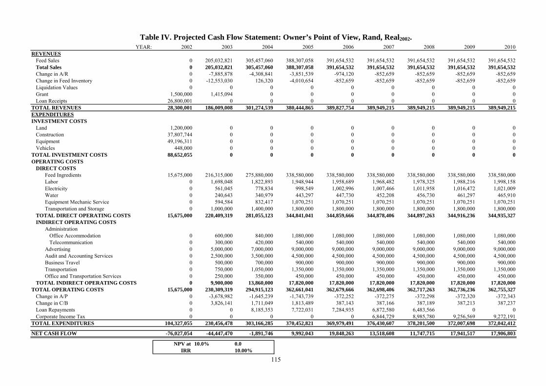
115
7 2008 2009 2010REVENUES
YEAR: 2002 2003 2004 2005 2006 200
Feed Sales 0 205,032,821 305,457,060 388,307,058 391,654,532 391,654,532 391,654,532 391,654,532 391,654,532Total Sales 0 205,032,821 305,457,060 388,307,058 391,654,532 391,654,532 391,654,532 391,654,532 391,654,532Change in A/R 0 -7,885,878 -4,308,841 -3,851,539 -974,120 -852,659 -852,659 -852,659 -852,659Change in Feed Inventory 0 -12,553,030 126,320 -4,010,654 -852,659 -852,659 -852,659 -852,659 -852,659Liquidation Values 0 0 0 0 0 0 0 0 0Grant 1,500,000 1,415,094 0 0 0 0 0 0 0Loan Receipts 26,800,001 0 0 0 0 0 0 0 0
TOTAL REVENUES 28,300,001 186,009,008 301,274,539 380,444,865 389,827,754 389,949,215 389,949,215 389,949,215 389,949,215EXPENDITURESINVESTMENT COSTS
Land 1,200,000 0 0 0 0 0 0 0 0Construction 37,807,744 0 0 0 0 0 0 0 0Equipment 49,196,311 0 0 0 0 0 0 0 0Vehicles 448,000 0 0 0 0 0 0 0 0
TOTAL INVESTMENT COSTS 88,652,055 0 0 0 0 0 0 0 0OPERATING COSTS
DIRECT COSTSFeed Ingredients 15,675,000 216,315,000 275,880,000 338,580,000 338,580,000 338,580,000 338,580,000 338,580,000 338,580,000Labor 0 1,698,048 1,822,893 1,948,944 1,958,689 1,968,482 1,978,325 1,988,216 1,998,158Electricity 0 561,045 778,834 998,549 1,002,996 1,007,466 1,011,958 1,016,472 1,021,009Water 0 240,643 340,979 443,297 447,730 452,208 456,730 461,297 465,910Equipment Mechanic Service 0 594,584 832,417 1,070,251 1,070,251 1,070,251 1,070,251 1,070,251 1,070,251Transportation and Storage 0 1,000,000 1,400,000 1,800,000 1,800,000 1,800,000 1,800,000 1,800,000 1,800,000
TOTAL DIRECT OPERATING COSTS 15,675,000 220,409,319 281,055,123 344,841,041 344,859,666 344,878,406 344,897,263 344,916,236 344,935,327INDIRECT OPERATING COSTS
AdministrationOffice Accommodation 0 600,000 840,000 1,080,000 1,080,000 1,080,000 1,080,000 1,080,000 1,080,000Telecommunication 0 300,000 420,000 540,000 540,000 540,000 540,000 540,000 540,000
Advertising 0 5,000,000 7,000,000 9,000,000 9,000,000 9,000,000 9,000,000 9,000,000 9,000,000Audit and Accounting Services 0 2,500,000 3,500,000 4,500,000 4,500,000 4,500,000 4,500,000 4,500,000 4,500,000Business Travel 0 500,000 700,000 900,000 900,000 900,000 900,000 900,000 900,000Transportation 0 750,000 1,050,000 1,350,000 1,350,000 1,350,000 1,350,000 1,350,000 1,350,000Office and Transportation Services 0 250,000 350,000 450,000 450,000 450,000 450,000 450,000 450,000
TOTAL INDIRECT OPERATING COSTS 0 9,900,000 13,860,000 17,820,000 17,820,000 17,820,000 17,820,000 17,820,000 17,820,000TOTAL OPERATING COSTS 15,675,000 230,309,319 294,915,123 362,661,041 362,679,666 362,698,406 362,717,263 362,736,236 362,755,327
Change in A/P 0 -3,678,982 -1,645,239 -1,743,739 -372,252 -372,275 -372,298 -372,320 -372,343Change in C/B 0 3,826,141 1,711,049 1,813,489 387,143 387,166 387,189 387,213 387,237Loan Repayments 0 0 8,185,353 7,722,031 7,284,935 6,872,580 6,483,566 0 0Corporate Income Tax 0 0 0 0 0 6,844,729 8,985,780 9,256,569 9,272,191
TOTAL EXPENDITURES 104,327,055 230,456,478 303,166,285 370,452,821 369,979,491 376,430,607 378,201,500 372,007,698 372,042,412
NET CASH FLOW -76,027,054 -44,447,470 -1,891,746 9,992,043 19,848,263 13,518,608 11,747,715 17,941,517 17,906,803
NPV at 10.0% 0.0IRR 10.00%
Table IV. Projected Cash Flow Statement: Owner’s Point of View, Rand, Real2002.
5.16 Financial Sensitivity Analysis
The purpose of the sensitivity analysis in project evaluation is to test the responsiveness of the
project’s outcomes to changes in the parameters of the model such as prices, quantities, growth
rates, elasticities and so on. The beauty of the sensitivity analysis is in its ability to reveal the
major hidden flaws and omissions in project financial design, and to enable the analyst to
realistically simulate possible real-life conditions into the financial model. The idea is to take a
single parameter and test the model over a range of the possible values of the selected parameter,
so that the model recalculates its final outcomes with each value of the parameter. In other words,
the spreadsheet computes a set of outcomes corresponding to the chosen range of values of the
parameter in question.
Technically, the MS-Excel spreadsheet program does not require the user to make multiple
copies of the same model in order to test the sensitivity of the model to changes in a parameter.
Instead, a special function called “Table” is designed to help the analyst to handle this task. This
function tabulates the defined projects outcomes under the various values of the tested parameter.
For the purpose of financial sensitivity analysis, the analyst should include the model’s
outcomes from the banker’s and owner’s points of view, which are typically the debt service ratios
for the banker’s perspective and the net present value for the owner’s perspective. Thus, for almost
all sensitivity tests made here, the following project’s performance criteria are considered: NPV
and IRR for owner’s point of view, ADSCR ratios for the first three years of loan repayment
(2004, 2005 and 2006), and DSCR for the whole period of loan repayment (2004).
Note, that the sensitivity analysis can test only one or, at most, two parameters at a time,
assuming that all other parameters remain constant. Thus, the only change in the project’s model
comes about from the tested parameter, and the model’s sensitivity measures only the specified
parameter(s). This allows the analyst to see the relative importance of each parameter to the
project’s performance. The parameters with the highest variability are indeed important while
some parameters that do not have a substantial impact on the project, are somewhat less crucial to
the project.
To make the comparison across the different tested parameters easier, the analyst may use a
scale of sensitivity, labeling the parameter as “high”, “medium”, “low” and “none” depending on
the responsiveness of the project’s outcomes to a change in the parameter. Such a scale is a
116
subjective assessment of sensitivity and it is the task of analyst to define the exact boundaries of
these benchmarks.
5.16.1 Change in Cost of Feed Ingredients
The feed ingredients cost is the most fluctuating variable, which changes on a daily basis and
its normal range of movements can be ±25%. Therefore, for the sensitivity test here, the change in
the cost of feed ingredients has been assigned a range from –25% to +25% with increments of 5%.
Table 17 shows the results of this test in a tabular form: the headline above contains the project’s
outcomes being the measures of the project’s performance, and the first column has the tested for
the change in the cost of ingredients. The first column presents the computed NPVs from owner’s
point of view, corresponding to each value of the parameter under the test. For instance, if the
change in the cost of ingredients remain –25% throughout the project life (i.e. the feed ingredients
are cheaper by 25%), then the financial net present value of the feed project from the owner’s
point of view would climb to 17.9 million Rand2002, instead of being zero as in the base case.
However, if the cost of feed ingredients rises by 10% and remains such throughout the project’s
lifespan, then the resulting NPV would be –6.7 million Rand2002. The pattern that can be traced
here is that a cost reduction makes the financial NPV grow, which is indeed a plausible
observation. The analyst can easily check whether the sensitivity table has been modeled correctly
by looking at the project’s outcomes at the base case value of the parameter. In the base case, the
change in cost of ingredients is zero and the corresponding NPV here must be zero too, which is
true.
The second column contains the computed values of the internal rate of return resulting from
the changes in the cost of feed ingredients. The same pattern of relationship between the tested
parameter and IRR is observed as in the case of NPV: a cost decrease causes the IRR to rise and
vice-versa. When the change in the cost of ingredients is zero (base case), the resulting IRR is
equal to the discount rate of 15%, which follows from the definition of the IRR.
The annual debt service coverage ratios also improve if the cost of feed ingredients decreases,
and they plunge down when the input costs rise. The ADSCR2004, which is the debt service ratio in
the very first year of debt repayment, is the lowest among the three, and this can be explained by
the fact that the plant is still operating under-capacity in this year, and as it increases its capacity
utilization the ADSCRs tend to rise too. The debt service coverage ratio tested here also shows a
117
negative relationship with the change in the cost of feed ingredients: when the cost raises – the
DSCR2004 declines and when the cost decreases – the DSCR2004 goes up.
Overall, the model is found to be “highly” sensitive to the tested parameter. Even a little, 5%
change in the cost of feed ingredients causes the project’s NPV to stray away by more than 3.4
million Rand2002. Given the unpredictable nature of the feed ingredients prices, this parameter can
be a good candidate for the risk analysis.
5.16.2 Change in Milling Fee
Although the milling costs are not expected to change substantially over the years, it is
important to test this parameter because this is the variable, which used as a tool to set the
project’s NPV to zero. A range from –25% to +25% with increments of 5% is taken for the change
in the break-even milling fee. The results, shown in Table 18, tell the analyst that the financial
model is “highly” sensitive to this parameter, and the change in the milling fee and project’s
financial performance are positively related. A decrease in the milling fee makes the NPV to
decline, but an increase in the milling fee causes the NPV to rise.
The IRR and debt service ratios follow the same relationship, and tend to improve due to an
increase in the fee. Note that a 5% change in this parameter causes even a greater response by the
NPV, as compared to the change in cost of ingredients. However, this parameter is not likely to
change over time and it does not qualify to be included into the risk analysis.
5.16.3 Domestic Inflation Rate, 2003-2013
The assumed rate of domestic inflation for years 2003-2013 was taken as 6.0% but it is very
likely that the actual inflation rate will deviate from this forecast. This sensitivity test shows the
response of the project to the different average inflation rates, ranging from 0% to 10% in
increment of 1%. Table 19 presents the results of this sensitivity test.
The base-case assumption of a 6.0% average inflation rate results in zero value of the NPV,
and if the average inflation rate declines below 6.0% then the NPV, IRR and debt service ratios all
improve, while any increase in the base-case inflation rate above 6.0% will deteriorate the
project’s performance. A single percentage-point change in the average inflation rate causes a 1.4
million Rand2002 adjustment in the NPV, which allows us to characterize this variable as a
118

“highly” sensitive parameter. The unpredictable nature of annual inflation rate makes it also a
candidate for the risk analysis.
5.16.4 Foreign Inflation Rate, 2003-2013
The foreign inflation rate has been used in the estimation of the foreign price index and
exchange rate, and also in the computation of the project’s investment costs. The base-case
inflation rate of the US dollar was assumed to be, on the average, 2.5% for years 2003-2013. This
sensitivity test, results of which are presented in Table 20, is used to determine the project’s
responsiveness to this parameter. A range of 0%-10%, in increments of 1%, is used for the US
dollar average inflation rate.
As the tabulated results of this test show, none of the project’s outcomes responds to changes
in the rate of foreign inflation. The net present value, internal rate of return, and debt service ratios
remain at the same level as in the base-case calculation, implying that the model has “none”
elasticity to this parameter. In other words, the project does not depend on the foreign inflation
rate and there is no need for any further inquiry into this variable.
5.16.5 Disturbance to Real Exchange Rate, 2002-2013
It has been assumed that the same real exchange rate between the South African Rand and US
dollar will prevail over the project life. However, the real exchange rate is exposed to various
domestic and international forces causing it to deviate from its long-run trend. A sensitivity test on
the disturbance to the real exchange rate was performed on the ±50% range of disturbance with a
10% increment, and Table 21 contains the tabulated output.
The model is “highly” sensitive to changes in the real exchange rate and the relationship
between this parameter and project’s indicators is such that a positive disturbance to the real
exchange rate decreases the NPV, IRR and debt ratios. This parameter is indeed a good candidate
for the risk analysis.
5.16.6 Financing Method
One of the exciting features of the sensitivity analysis is its ability to test various methods to
finance the project. Because a variety of sources are available to the project owners to fund the
119
project, a careful consideration is necessary in order to find an optimal combination of the
different finance options. Sensitivity tests allow to compare the different financial designs, and to
select one or another for further analysis.
For the feed project, the proposed intention of the plant management is to obtain a loan to
finance up to a half of the local investment costs. The company is going to use its own equity
funds to purchase the equipment and to cover the remaining local costs. A Rand-nominated loan
would be drawn on commercial terms from a South African bank. The sensitivity test here looks at
the financing of the project as coming either from outside as a loan or as being a part of the
owner’s equity contribution. A different combination of loan-equity shares are tested on their
impact on the project’s outcome. Table 22 displays the sensitivity analysis results.
Thus, a combination of 50% share of equity and 50% of loaned funds corresponds to the base-
case and makes the NPV to break-even. If the project decides to obtain a higher share of loan
finance, the NPV and IRR improve due to the fact that the cost of loan is lower as compared to the
cost of equity. On the other hand, if the actual finance mix contains less than 50% loaned funds,
the NPV and IRR decline.
The impact of the loan share being higher than 50% benchmark on the debt service ratios is
different from the NPV and IRR effects, because a higher loan share implies lower debt service
ratios, keeping all other things constant. Thus, any decision to increase the share of loan financing
will reduce the debt service ratios and vice versa.
The overall responsiveness of the model to changes in this parameter can be characterized as
“low”. The choice of financing mix is a one-time decision for this project, and because this
variable has a moderate impact on the performance a further risk analysis is not needed.
5.16.7 Loan Real Interest Rate
The sensitivity of the project to the real interest rate can be described as “low”, following the
tabulated results of such a sensitivity test in Table 23. The relationship between the real interest
rate and project’s performance is of a negative nature: if the real interest rate increases then the
project’s outcomes deteriorate. This can be explained by the fact that a higher real rate on the loan
would necessary imply higher real interest repayments, causing the net cash flows to decrease.
120

With a modest loan share in the total investment costs, the real interest rate impact is
somewhat limited and because the interest rate is typically negotiated by a contract, it is not
needed to include this variable into the risk analysis.
5.16.8 Loan Grace Period
The duration of loan grace period can be also tested on its impact on the project. Table 24
shows the results of the test with a clearly positive relationship between the duration of grace
period and the project’s performance. Any postponement in the start of loan repayment makes the
indicators to improve. Note that because the beginning of the loan repayment shifts the resulting
debt service ratios become zeros for years 2004-06. Overall, the sensitivity of the model to this
parameter is “low” and it is not eligible to be included into the risk analysis.
5.16.9 Loan Repayment Period
Obviously, any extended loan period should benefit the project, and Table 25 contains a proof
of this expectation. All the project’s indicators improve if the repayment period is prolonged by a
year or more, while any reduction from the base case 5-year period would cause a higher loan
payment each year and the NPV, IRR and debt service ratios will decline. The model’s
responsiveness to this parameter is rather “low” and it can be excluded from any further inquiry.
5.16.10 Tax Holidays
The existing tax regulation permits a 4-year tax holiday for the start-up businesses like the
feed plant. This is an investment incentive to the project and its financial benefits are estimated in
Table 26. Thus, any reduction of the tax holiday will reduce the NPV and IRR by making the
project pay the corporate income tax earlier, while any extension of the tax holiday would clearly
affect the NPV and IRR favorably. Note that the debt service ratios are less prone to changes in
this parameter. The overall sensitivity of the model to this parameter is “high” but because the
duration of tax holiday is fixed by the law, it is not needed to pursue the analysis of this variable
any further.
121
5.16.11 Investment Cost Overrun Factor
The expected effect of this parameter is to damage the project’s performance if there are any
cost overruns. As Table 27 confirms, this relationship holds true for all the project’s indicators and
a 5% unexpected rise in the amount of investment costs will lead to a negative change in the NPV
of about 1.3 million Rand2002.
However, the portion of the total investment costs affected by the investment cost overrun
factor is limited to the local costs of construction, and it is not applicable on the equipment, land
and transportation expenses. Therefore, its impact on the model is “medium” and is not of critical
importance as long as the cost overruns are moderate.
5.16.12 Accounts Receivable
For a cash-based business like the feed plant, it is important to test the project’s sensitivity to
the average amount of accounts receivable. Table 28 presents the results of this test with a clear
message to the project operator to keep the amount of AR as low as possible in order to maximize
the NPV, IRR and debt service ratios. Any delay in the time taken by customers to pay in cash or
any increase in the amount of AR will reduce the actual net cash flows and lead the business to
lose money. The model is “highly” sensitive to this variable and it is a matter of managerial effort
of keeping the AR at a minimum level.
5.16.13 Accounts Payable
In the same manner, a sensitivity test is performed for the amount of accounts payable by the
enterprise, with the results shown in Table 29. Again, this parameter has a strong impact on the
project’s performance and the model’s response is “highly” sensitive. Note that the relationship is
the inverse to the AR: a delay in the cash payment makes the project better off.
5.16.14 Labor Real Wage Growth
It can be argued that the real wage growth can be a bottleneck for some businesses; however
this is not a crucial factor for the feed plant, as Table 30 explains. While a higher wage growth
does cause harm to the project’s indicators, it does not really disturb the operations and can be
safely labeled being “low” in its importance. The NPV, IRR and debt service ratios all decline as
122
the average annual growth rate crawls up. But because the wage increases are sticky and
negotiable, i.e. contractual nature, this variable is not considered in further risk analysis.
5.16.15 Electricity Real Charge Growth
The real growth rate of electricity charges is tested in Table 31, and it is found to have a “low”
impact on the model. The relationship is such that any increase in the real growth rate causes the
project’s outcomes to deteriorate. Given the little impact on the model and low risk of sudden real
rate adjustments, this parameter is not included into the risk analysis.
5.16.16 Composite Demand Elasticity for Meat and Change in Cost of Feed Ingredients
The financial model has been using the parameter of composite demand elasticity for meat as
one of the determinants of the demand for animal feed. While the Table of Parameters assumes
this elasticity for meat to be equal to –1.0 in the base case, it is necessary to test the model’s
responsiveness to this parameter. Table 32 shows the result of this sensitivity test in a tabular
form.
Note that because there are now two variables being tested simultaneously on their impact on
the NPV, the table excludes all the other indicators. The reason why these two variables are to be
tested at the same time is that the base-case change in the cost of ingredients is zero and it does not
allow to see the impact of the composite demand elasticity for meat. However, when the change in
the cost of ingredient is different from zero, the NPV would adjust according to the value of the
demand elasticity being tested. Thus, in the top row there is a range of values of the demand
elasticity for meat, starting from –3.0 to –0.5 with increments of 0.25; and, at the same time, the
first column has a range of values for the change in the cost of ingredients from –25% to +25% in
steps of 5%.
At the base-case demand elasticity of –1.0, any change in the cost of feed ingredients causes
the NPV to go into the opposite direction by about 3.9 million Rand2002 per each 5% step. Thus,
the columns of the table tell about the model’s responsiveness to changes in the cost of
ingredients. Also, if the analyst looks across the rows rather than columns of this sensitivity table
then it becomes obvious that the rows show the sensitivity of the NPV to the value of the
composite demand elasticity for meat at every level of the change in the cost of ingredients. Thus,
if the ingredients cost change by –25%, the computed NPV at the base-case elasticity of –1.0 will
123
be raised to 17.9 million Rand2002, while if the elasticity is equal to –0.75 then the NPV would be
15.1 million Rand2002, and if the elasticity is equal to –1.25 then the NPV would be 20.7 million
Rand2002. In other words, if the true market composite demand elasticity for meat is more elastic
than the assumed value of –1.0, then the resulting NPV is underestimated, but if the composite
demand elasticity for meat is indeed inelastic than the project’s NPV is overestimated. The
financial model is, in fact, “highly” sensitive to this parameter.
5.16.17 Composite Demand Elasticity for Meat and Change in Milling Fee
Because the feed price determination mechanism is based on the both change in cost of
ingredients and change in milling fee, such a sensitivity test is needed to look at the impact of the
composite demand elasticity for meat on the NPV in the context of changes in the milling fee.
Table 33 shows the results of this test.
Note that this table is similar in its structure to the previous table. The top row is filled with
different values of the demand elasticity for meat, and the first column contains the values of the
change in the milling fee. At any given change in the milling fee there is a range of NPVs resulting
from the different demand elasticities. A ±0.25 deviation from the assumed –1.0 demand elasticity
causes the NPV to adjust by about 0.1 million Rand2002, which can be characterized as relatively
“low” response.
5.16.18 Supply Elasticity of Feed by Others and Change in Cost of Feed Ingredients
Another parameter deserving a sensitivity test is the supply elasticity of feed by other
producers, which was assumed to be equal to 5.0 in Section 5.2.21. The range of the values for this
parameter is taken from 1.0 to 8.0 in steps of 1.0 and the results are presented in Table 34.
As expected, there is “none” relationship between the feed supply elasticity by others and the
change in cost of feed ingredients, which is confirmed by the constant NPVs in the sensitivity
table. In other words, any value of the feed supply elasticity by others does not affect the project’s
performance as long as there is no change in the cost of feed ingredients.
124

5.16.19 Supply Elasticity of Feed by Others and Change in Milling Fee
This test measures the responsiveness of the NPV to the feed supply elasticity by others at a
certain change in the cost of ingredients. Table 35 presents the results of this sensitivity test. The
base-case assumes the supply elasticity of feed by others to be equal to 5.0, and the sensitivity
table shows that a unit-deviation from the assumed 5.0 elasticity would lead the NPV to adjust by
about 0.3 million Rand2002, which is relatively “low” impact.
125
6. ECONOMIC ANALYSIS
The main purpose of the economic evaluation of this project is to determine the economic
feasibility of such a feed production and desirability of grant support for this type of business in
Limpopo Province. The framework of the analysis includes the estimation of economic costs and
benefits, and comparing their net present values with the corresponding net present values from
the financial analysis. The economic NPV serves as an indicator of economic viability of the
project, and the estimated difference between the economic and financial NPVs, so-called
externalities, is the measure of the economic impact created by the project.
The roadmap of the economic analysis typically includes a section with estimation of the
economic conversion factors and modeling of the economic resource flow statement.
6.1 Scope of Economic Analysis
The economic analysis has its major objective to answer the question whether the project is
economically feasible in terms of generating a net addition to the country’s wealth, as measured by
the economic net present value. In order to achieve this objective, the analyst has to make a clear
distinction between the financial and economic flows associated with the project. For the financial
analysis, the cashflows represented the actual transactions of the project but the economic analysis
operates with the “flow of economic resources”. The equivalent of the financial revenues in the
economic analysis is the “economic benefits” created by the project and added to the economy.
The “economic costs” are the economic values of the resources forgone by other economic agents
in order to allow the project to use these scarce resources.
The financial cashflow statements do not include any externalities created by the project
because such externalities rarely materialize in the cash form. The economic analysis, by
definition, has to include all such externalities in order to portray the true picture of the economic
resource flows. The analyst must search and quantify any such externalities, even if they are not a
part of the financial items. The can generate positive as well as negative externalities. For example
investment in a rural road will lower the costs of normal transportation of goods and people but
also it will allow the passage of emergency vehicles such as police and ambulance that will
improve the level of security and will definitely benefit the local community.
126
In other words, the analyst should base the economic resource flows on the completed
financial model, but the financial cashflows must be converted into their economic equivalents and
any new items, i.e. externalities, must be quantified and included into the economic resource flows
too. The economic net present value the project, discounted by the economic opportunity cost of
capital (EOCK), will serve as the evaluation criterion for the project’s net contribution to the
economic welfare.
In order to use the projected financial cashflows for the economic analysis, so-called
“economic conversion factor” (CF) has to be estimated for each financial item, according to the
methodology of the economic analysis laid out in Chapter 5 of the Manual (2003). Thus, Sections
6.2–6.4 will be devoted to the estimation of the project’s conversion factors. Once all the cashflow
items are furnished with their economic CFs, the analyst will be able to construct the Projected
Statement of Economic Resource Flows and analyze it, as done in Section 6.5.
6.2 Estimation of Project’s Economic Conversion Factors
An economic conversion factor is a number, used to convert the financial value of a resource
into its true economic value. No doubt, most project analysts understand that the financial cost is
different from the economic cost by the amount of distortions such as taxes, subsidies, market
imperfections, and any other “externalities”. The conversion factor incorporates the amount of all
externalities and, thus, is a key element irreplaceable for the economic modeling because of its
simple and appealing nature. The methodological framework of using conversion factors is given
in Chapters 6 and 7 of the Manual (2003).
The conversion factor can be found as the economic value divided by the financial value. If
the calculated CF is greater than zero, this means that the economic value of this commodity is
greater than its financial value. When the commodity in question is the project’s output, a CF
greater than unity means that the project produces a good that has a higher economic value than
the financial price paid by the consumers. When the commodity is an input then the implication of
its CF being greater than unity is that the true economic cost of this input is higher than the amount
that the project pays for this input.
If the conversion factor of a commodity is smaller than unity and this commodity is a project’s
output, then the project is going to produce a good whose economic value is smaller than the
financial price paid by the consumers. When a commodity with a CF less than one is a project
input then the financial cost of the input paid by the project, is higher than its true economic cost.
127
A few basic economic parameters have to be introduced into the financial model in order to
carry out estimation of economic conversion factors. The necessary parameters are the economic
cost of capital (EOCK) in South Africa, and the economic cost of foreign exchange (FOREX). The
first represents the economic discount rate used in the analysis to discount the annual flows of
economic benefits and the costs of economic resources. Chapter 8 of the Manual (2003) concludes
that the EOCK for South Africa is, in real terms, 11.0%.
The economic cost of foreign exchange is used in the analysis to estimate the economic
conversion factors (CF) for most of the items used by the project. Given that even domestically
manufactured products have, in fact, certain proportion of imported content – the economic cost of
all products must account for the impact on the foreign exchange market on South Africa.
Considering the project as an incremental investment, any addition consumption of foreign
exchange by the project creates a distortion on the forex market in South Africa. The cost of
foreign exchange is actually the premium which is paid on forex transactions. Chapter 9 of the
Manual (2003) estimated the foreign exchange premium as 5.5% for the funds used to purchase
traded commodities and 2.0% for the funds used to purchase non-traded commodities.
Also, a number of assumptions have to be made about the cost structure of certain cashflow
items, and such assumptions are stated during the procedure of estimation of the economic
conversion factors. While most of the project parameters are usually placed in the Table of
Parameters, it is not unreasonable to keep certain non-repeating cost structure assumptions in the
tables with the actual estimation of the economic conversion factors.
The estimation of the conversion factors can be split into two broad categories: basic
conversion factors and project’s specific conversion factors. The reason for such separation lays in
the fact that many project’s CFs are “composite” conversion factors, derived from “basic”
conversion factors. Therefore, it is firstly needed to estimate all the basic CFs in order to proceed
with project specific conversion factors. The basic conversion factors for the feed project can be
listed as:
– Unskilled Labor – Skilled / Semi-Skilled Labor and Local Management – Administration and Foreign Management – Construction Labor – Operation and Maintenance Labor – Labor – Plant – Materials – Vehicles
128
– Electricity – Water – Transportation and Storage – Administration – Transportation
All the other conversion factors are derived from the basic CFs. Section 6.3 will deal with the
estimation of the listed basic CFs, and Section 6.4 will handle the rest of the project’s conversion
factor.
6.3 Basic Conversion Factors
6.3.1 Unskilled Labor
The conversion factor for unskilled labor is estimated in Table 36, in accordance with the
methodology outlined in Chapter 10 of the Manual (2003). The specific case of conversion factor
estimation relevant to the unskilled labor employed at the feed plant is the case of “urban project
hiring unskilled labor and paying above market wage”. All the necessary parameters were already
stated in Section 5.2.9, and now they are used to estimate the economic cost of unskilled labor
hired by the project.
EOCL: The financial cost of unskilled labor hired by a similar urban project was computed as
1,566 Rand/month, inclusive all taxes and social security contributions as well as bonuses. To find
the economic opportunity cost of labor (EOCL), a market equilibrium approach is used assuming
that the unskilled labor market was in equilibrium before this project begins demanding a certain
number of unskilled employees. Once the feed project employs addition workers, there will be an
impact on both the informal sector and quasi-voluntary unemployed group. As mentioned in
Section 5.2.9, the weights on the informal sector and quasi-voluntary unemployed are equal to
10% and 90% correspondingly. Their corresponding incomes are currently 651 Rand/month in the
informal sector and 959 Rand/month for the quasi-voluntary unemployed. The economic
opportunity cost of unskilled labor is, therefore, a weighted average of the two incomes forgone:
EOCLUnskilled = WInformal * WageInformal + WQuasi-Voluntary * WageQuasi-Voluntary
EOCLUnskilled = 10% * 651 + 90% * 959 = 928 Rand/month
Conversion Factor: By definition, the conversion factor for unskilled labor is the ratio of the
economic opportunity cost to the financial cost. Note that the resulting conversion factor is just a
number, and it does not have units assigned to it:
129
CF = Economic Value / Financial Value
CFUnskilled = 928 / 1,566 = 0.59240
Externality: The total labor externality is the difference between the economic cost of
unskilled labor and its financial cost, which can be found as:
Externality = Economic Value – Financial Value
ExternalityUnskilled = 1,566 – 928 = 638 Rand/month
It is useful to know the share of externality in the financial cost of labor (ρTypeH), which can be
easily obtained by dividing the computed externality by its financial value:
ρTypeH = ExternalityTypeH / Financial ValueTypeH
ρUnskilled = 638 / 928 = 40.8%
Thus, the share of total externality in the unskilled labor is 40.8% of its financial cost. In
further distributive analysis there will be a need to separate the total externality of labor of type H
into the portions accruing to the labor as benefit (ρTypeHLabor) and to the government in form of
taxes (ρTypeHGov). Such a division can be easily performed since all the necessary data were already
available in the Table of Parameters.
Share of Government Benefits: Referring to the section with unskilled labor, the analyst will
find that although there is no personal income tax on the minimum wage paid to the unskilled
employees, the government still is able to collect some 18.57% from the employer in the form of
social security payments and alike. Note also, that this amount is not to be reduced by any forgone
taxes because neither the informal sector nor the unemployed pay taxes. Thus, the amount of
government collections from the unskilled labor is 235 Rand/month, or 18.57% of the minimum
wage of 1,566 Rand/month. The share of the government benefits (ρUnskilledGov) in the total
externality of unskilled labor is the ratio of the computed government collections to the total
externality:
ρUnskilledGov = Government CollectionsUnskilled / ExternalityUnskilled
ρUnskilledGov = 235 / 638 = 36.8%
Share of Labor Benefits: By the same approach, the amount of labor benefits can be found
as the difference between the total externality and government collections, and the share of labor
benefits in the total externality is derived from the ratio of the labor benefits to the amount of total
externality:
Labor BenefitsUnskilled = ExternalityUnskilled – Government CollectionsUnskilled
Labor BenefitsUnskilled = 638 – 235 = 403 Rand/month
130
and
ρUnskilledLabor = Labor BenefitsUnskilled / ExternalityUnskilled
ρUnskilledLabor = 403 / 638 = 63.2%
By definition, the shares of the government benefits and labor benefits in the total externality
must add up to unity, and this is something useful the check:
ρUnskilledGov + ρUnskilled
Labor = 1
36.8% + 63.2% = 1
Thus, the analyst must have derived the following parameters: the economic CF for unskilled
labor (CFUnskilled), the share of the total externality in the financial cost of unskilled labor
(ρUnskilled), the share government benefits in the externality of unskilled labor (ρUnskilledGov), and the
share of labor benefits in the total externality of unskilled labor (ρUnskilledLabor). The conversion
factor will to be used to model the economic resource flow statement, and the other three
parameters will be helpful in the distributive analysis to differentiate between the labor and
government accrued externality.
6.3.2 Skilled / Semi-Skilled Labor and Local Management
For the purpose of economic analysis, the analyst has the full right to treat skilled labor, semi-
skilled labor and local management as three different types of labor, as each having its own
economic conversion factor. However, looking at the feed project closely reveals that these three
types of labor can be described by a single economic conversion factor. The reason for such
simplification is that all the three types here fall under the same category of “urban project hiring
skilled labor and paying above market wage”, according to Chapter 10 in the Manual (2003). The
implication of this similarity is that the feed project pays a higher than the market wage, and a
single conversion factor can be used. Of course, the base financial expenditures on each labor
type, on which the economic resource flows are built, are different from one another. Therefore,
the approach here is to derive a single economic CF, which can be used interchangeably for skilled
labor, semi-skilled labor and local management in the economic analysis of this project. Table 37
shows the derivation of this economic conversion factor.
Private Supply Wage: As stated in Section 5.2.9, the project will attract 90% of skilled
personnel from other sectors (Kd), where the average annual salary is taken as 153,960 Rand/year
(equivalent of monthly wage of 12,830 Rand/month). Because there are various fringe benefits,
131
which, on the average, account for 17.07% of the wage rate, the private supply wage of labor
attracted from other sectors is estimated as 180,241 Rand/year. This supply wage is actually the
average annual salary of 153,960 Rand/year, adjusted up by the 17.07% of fringe benefits.
Income Taxes: The amount of personal income taxes paid by a similar project can be found
as 44,129 Rand/year (TaxesMarket), which is a sum of the personal income tax of 35,409 Rand/year
and a site tax of 8,720 Rand/year. For the personnel attracted from the other sectors, some amount
of income taxes will be forgone. The amount of income taxes forgone can be estimated by
multiplying the amount of personal income taxes paid by this project (44,129 Rand/year) by the
share of the labor attracted from the other sectors (90%), which results in forgone annual taxes of
39,716 Rand/year.
EOCL: The EOCL for skilled labor can be approximated by the net-of-taxes market salary
plus the amount of income taxes forgone. The economic cost is the supply wage of labor,
decreased by the amount of taxes transferred to the government, plus the reduction in the tax
collections from the other sectors:
EOCLSkilled = Private Supply Wage – TaxesSkilledProject + TaxesSkilled
Forgone
EOCLSkilled = 180,241 – 44,129 + 39,716 = 175,828 Rand/year
Financial Cost of Labor: The resulting economic cost of skilled labor is the opportunity cost
of the skilled personnel employed by the feed plant. The actual net annual salary paid by the
project is 174,000 Rand/year, which is the annual equivalent of a 14,500-Rand monthly wage, and
this net annual salary is higher than the computed EOCL. In addition to the annual salary of
174,000 Rand/year, the project also pays to the skilled employees 17.07% in fringe benefits, thus
making the total financial cost of skilled labor equal to 203,702 Rand/year. Out of this amount, the
government gets 51,089 Rand/year in the form of personal income taxes (TaxesProject), as stated in
Section 5.2.9.
Conversion Factor: It is now easy to compute the conversion factor for skilled labor, which
is the ratio of the EOCL to the financial cost of skilled labor:
CFSkilled = EOCLSkilled / Financial Cost of LaborSkilled
CFSkilled = 175,828 / 203,702 = 0.86316
Externality: The total labor externality created by the existing structure of payments for
skilled labor can be found as the difference between the economic cost of labor and its financial
cost:
ExternalitySkilled = 203,702 – 175,828 = 27,874 Rand/year
132
The share of externality in the financial cost of skilled labor is a ratio of the computed
externality over the financial cost:
ρSkilled = 27,874 / 203,702 = 13.7%
Share of Government Benefits: To calculate the share of the government-accruing benefits
in the total externality, the analyst has to find the amount of taxes withheld by the government.
The income tax on the salary paid by the project is 51,089 Rand/year, while the amount of income
taxes forgone is 39,716 Rand/year, which means that the net tax collections are 11,373 Rand/year.
Therefore, the share of government benefits in the total externality is 40.8%:
ρSkilledGov = Government CollectionsSkilled / ExternalitySkilled
ρSkilledGov = 11,373 / 27,874 = 40.8%
Share of Labor Benefits: Given the fact that the government benefits are estimated and the
total externality is known, it is possible to find the amount of labor-accruing benefits as well as its
share in the total externality. The amount of labor externality is found as the financial cost of
skilled labor minus the private supply wage and plus the difference in the income taxes between
the prevailing market wage and project’s wage:
Labor BenefitsSkilled = Financial CostSkilled – Private Supply WageSkilled + (TaxesSkilledMarket – TaxesSkilled
Project)
Labor BenefitsSkilled = 203,702 – 180,241 + (44,129 – 51,089) = 16,501 Rand/year
therefore,
ρSkilledLabor = Labor BenefitsSkilled / ExternalitySkilled
ρSkilledLabor = 16,501 / 27,874 = 59.2%
Having completed this section, the analyst should be able to derive such parameters as the
economic CF for unskilled labor (CFSkilled), the share of the total externality in the financial cost of
unskilled labor (ρSkilled), the share government benefits in the externality of unskilled labor
(ρSkilledGov), and the share of labor benefits in the externality of unskilled labor (ρSkilled
Labor). Note
that the assumption is made about the conversion factor for skilled labor being equal to the
conversion factor for semi-skilled labor and also to the CF of local management:
CFSkilled = CFSemi-Skilled = CFLocal Management
133
6.3.3 Administration and Foreign Management
The administrative positions at the project will be filled with qualified professional who have
worked at the feed plant in the foreign country. There will be three permanent full-time managerial
posts. The company plans to bring the necessary people from abroad, and this labor type fits into
the case of “non-South Africans employed in South Africa”, according to Chapter 10 in Manual
(2003). Table 38 presents the estimation of the economic conversion factor for administration and
foreign management.
As mentioned in Section 5.2.9, the project will pay the foreign employees a wage of 18,000
Rand/month, and it is assumed that 50% of their net income will be expatriated outside of South
Africa. The personal income tax rate in South Africa is 25%. It is also assumed that the previous
wage rate for these individuals was 12,000 Rand/month.
EOCL and Conversion Factor: Because the foreign employees have not been a part of the
domestic labor force and they are not lured away from other sectors, the economic opportunity
cost of such labor is simply the net-of-tax salary, adjusted for the foreign exchange premium.
Since the personal income tax accrues to the government, it is not a cost component. The
adjustment for foreign exchange premium must be made in order to account for the fact that the
foreign individuals will transfer 50% of their incomes abroad, for which they will have to
exchange South African Rand for dollars, thus creating an additional demand for the US dollar.
The actual computation can be expressed as:
EOCLForeign = WageProject * (1 – Tax Rate) + WageProject * (1 – Tax Rate) * %Expatriated * FOREXTraded
EOCLForeign = 18,000 * (1 – 25%) + 18,000 * (1 – 25%) * 50% * 5.5% = 13,871 Rand/month
The estimation of the conversion factor is based on the project’s wage and computed
economic cost of foreign labor:
CFForeign = 13,871 / 18,000 = 0.77063
Externality: The total labor externality created by employing a foreign national at the feed
plant can be found as the difference between the project’s wage and EOCL:
ExternalityForeign = 18,000 – 13,871 = 4,129 Rand/month
The share of externality in the financial cost of foreign labor is a ratio of the computed
externality over the project’s wage:
ρForeign = 4,129 / 18,000 = 29.8%
134
Shares of Government Benefits and Labor Benefits: Since the foreign national have not
been in the domestic labor force, the government does not lose any taxes but it gains by the
amount of the personal income taxes withheld. At the same time, the amount of foreign exchange
losses due to the increased demand for dollars should be deducted from the government’ benefits:
Government CollectionsForeigh =
= WageProject * Tax Rate – WageProject * (1 – Tax Rate) * %Expatriated * FOREXTraded
Government CollectionsForeigh = 18,000 * 25% + 18,000 * (1 – 25%) * 50% * 5.5% = 4,129 Rand/month
What is appealing here is that the government benefits are equal to the total externality
(ρForeignGov = 1), meaning that there are no labor benefits (ρForeign
Labor = 0). In fact, the foreign labor
earns a higher wage rate than in the previous employment. The government collects full income
tax on the foreign nationals but it also loses the premium on the additional foreign exchange
demand if income repatriation takes place.
6.3.4 Construction Labor
The labor employed at the plant construction is treated as a separate item because this
construction labor is a mix of the labor types discussed above. Table 39 is used to derive the CF
for construction labor. The share of each labor type in the construction labor is obtained by using
data from a civil works construction project, done in Limpopo Province. The actual project was
hiring 370 people, 165 of whom were unskilled workers, 185 were skilled and semi-skilled
employees, and 20 professional were managing the project. Thus, the shares of the different labor
types are: 45% for unskilled labor, 50% for skilled and semi-skilled labor, and 5% for local
management.
The assumption for this plant construction is that this labor structure will prevail, and the
shares of the three labor types employed will be the same. This allows the analyst to derive a
composite conversion factor for “construction labor” as a weighted average of the CFs of the three
labor types:
CFConstruction Labor = ∑H
( %ShareTypeH * CFTypeH ) =
= %ShareUnskilled * CFUnskilled + %ShareSkilled * CFSkilled + %ShareLocal Management * CFLocal Management
CFConstruction Labor = 45% * 0.59240 + 50% * 0.86316 + 5% * 0.86316 = 0.74242
The CF for construction labor will be frequently used in the estimation of the conversion
factors for the different construction activities involving labor. Note that because the conversion
135
factors for skilled labor and management were assumed to be the same, a single CF is used for
both. Also, the construction labor does not include foreign management because it is usual for
such construction jobs to be done by a local firm.
6.3.5 Operation and Maintenance Labor
Table 40 estimates the conversion factor for operation and maintenance labor employed at the
project. The composition of the labor force employed for the operation and maintenance works is
different from the construction labor, and the assumed shares of the three basic labor types in such
works are: 15% for unskilled labor, 35% for skilled and semi-skilled labor, and 50% for foreign
management. The composite CF can be found as a weighted average of the basic labor conversion
factors:
CFO&Market Labor = ∑H
( %ShareTypeH * CFTypeH ) =
= %ShareUnskilled * CFUnskilled + %ShareSkilled * CFSkilled + %ShareForeign Management * CFForeign Management CFO&Market Labor = 15% * 0.59240 + 35% * 0.86316 + 50% * 0.77063 = 0.77628
6.3.6 Labor
The “labor” expense item corresponds to the total expenses on the plant’s employees, not
including the administration and management. An assumption is made that the unskilled workers
have a 70% stake in the total labor payment, while the skilled and semi-skilled personnel gets the
remaining 30%. Table 41 shows the computation of a conversion factor for labor expenses, and the
estimated CF for labor expenses can be found as:
CFLabor = ∑ %ShareH
( TypeH * CFTypeH ) = %ShareUnskilled * CFUnskilled + %ShareSkilled * CFSkilled
CFLabor = 70% * 0.59240 + 30% * 0.86316 = 0.67363
6.3.7 Plant
It is a commonly used term in the designing the civil works in Limpopo Province. The “plant”
is a mixture of commodities needed for construction, and while there is no precise listing of the
items comprising the plant, it is possible to assume its cost structure. Thus, the assumed
components and their shares in the “plant” are: steel - 50.0%, cement - 10.0%, stone - 15.0%, sand
136
- 10.0%, asphalt - 8.0%, and heavy equipment - 7.0%. If the analyst possesses a more
advanced knowledge of the plant components, they should be added to this list. Table 42 is used to
derive a conversion factor for plant.
The economic conversion factor for the plant is, again, a weighted average of the CFs of its
components. The individual CFs for all the plants components are obtained from the Database
(2003). An assumption is made that the freight and handling expenses from producer to port are
equal to the freight and handling costs from producer to this project.
The biggest part of the plant is steel, and this steel would fall into one of the items in Chapters
72 -76 of the Harmonized Code, which all have the same conversion factor of 0.92544. Note that
steel is an exportable item and the project uses steel as an input. Cement falls under the items of
Chapter 25.01-25.24, and it is treated as an importable commodity with a CF of 0.92544. Stone
and sand are non-traded items, and their conversion factor is taken as 0.95947. Asphalt is an
importable commodity, which can be described in terms of item 271490.1 in Chapter 27, with a
conversion factor of 0.84832. The heavy equipment used can be categorized as an importable
component, being an item of Chapter 84.29-84.30, with the resulting conversion factor of 0.92544.
Given the list of conversion factors and shares of the plant components, the estimation of the
CF for the plant becomes:
CFPlant = ∑H
( %ShareTypeH * CFTypeH )
CFPlant = 50%*0.92544 + 10%*0.92544 + 15%*0.95947 +
+ 10%*0.95947 + 8%*0.84832 + 7%*0.92544 = 0.92778
6.3.8 Materials
This is another commonly used term in civil works construction, to describe the various
materials consumed at the construction. Because the actual combination of such materials varies
from place to place, an assumed list of material items is used for the purposes of this study. The
following materials are taken: fuel - 30.0%, lubrication oils - 5.0%, wood - 20.0%, plastics -
27.0%, chemicals - 5.0%, electric supplies - 10.0%, and paint - 3.0%. An assumption is made that
the freight and handling expenses from producer to port are equal to the freight and handling costs
from producer to this project. Table 43 shows the results of conversion factor estimation.
Fuel is an internationally traded commodity, and actually imported into South Africa, the CF
for it is taken from the Database (2003) as 0.67805. Lubrication oils are also imported and can be
labeled with item 271011.52 of the Harmonized Code, with a conversion factor of 0.92544. Wood
137
is an exportable commodity for South Africa, and wooden materials for construction can be fit into
Chapter 44.01-44.18 of the Harmonized Code, with a conversion factor of 0.92544. Plastics are
importable and the best description for such materials is the item 391729.4 in the Harmonized
Code, with a conversion factor of 0.81439. Chemicals can be also said to be imported, and being a
part of Chapter 28.01-28.51, they have a conversion factor of 0.92544. The electric supplies are
importable items belonging to Chapter 84.01-84.14 listing of the Harmonized Code, with a
conversion factor of 0.92544. Paint is traded internationally and it can be fitted into the description
of the items in Chapter 32.08-32.09, with a conversion factor of 0.84832.
Integrating all the available parameters into the formula, the conversion factor for the
materials can be found as:
CFMaterials = ∑H
( %ShareTypeH * CFTypeH )
CFMaterials = 30%*0.67805 + 5%*0.92544 + 20%*0.92544 + 27%*0.81439 +
+ 5%*0.92544 + 10%*0.92544 + 3%*0.84832 = 0.81892
6.3.9 Vehicles, Electricity, Water, Transportation and Storage, Administration, and Transportation
Table 44 contains the conversion factors for vehicles, electricity, water, transportation and
storage, administration, and transportation. A number of items are taken directly from the
Database (2003). For instance, the vehicles expenses fall into the description of item 870210.8 of
the Harmonized Code, being importable and their conversion factor is equal to 0.78306.
Electricity and water are non-tradedable items, and according to the Database (2003), their
conversion factors are respectively 0.96813 and 0.92544. Administration expenses are associated
with the duties of the management, and the relevant conversion factor is the one for the foreign
management, 0.77063. Transportation is again a non-tradable item, which has a CF of 0.84749,
according to the Database (2003).
The transportation and storage expenses of the plant can be broken into the separate
transportation and storage expenses, assuming respective shares of 40% and 60%. The
transportation conversion factor has been estimated above, and storage can be assigned the non-
traded conversion factor for general building construction, which is stated as 0.88056. The
weighted average of the conversion factors for transportation and storage is equal to 0.86733,
which is indeed the conversion factor for the transportation and storage expenses.
138

6.4 Project Specific Conversion Factors
6.4.1 Workshop, Awning, Unloading Car Canopy, Boiler House, Underground Pond/Pump House
The workshop, awning, unloading car canopy, boiler house, underground pond/pump house
are all components of the construction costs, their conversion factors will be used to estimate a
single conversion factor for the construction. For simplicity, it is assumed that the workshop,
awning, unloading car canopy, boiler house, underground pond/pump house have the same cost
structure, which is: plant - 35%, materials - 10.0%, unskilled labor - 30.0% skilled and semi-
skilled labor - 15.0%, and local management - 10.0%. The corresponding conversion factors were
already obtained, and it allows the analyst to compute the composite conversion factor, as done in
Table 45:
CFWorkshop, etc. = ∑H
( %ShareTypeH * CFTypeH )
CFWorkshop, etc. = 35%*0.90747 + 10%*0.77422 + 30%*0.59240 +
+ 15%*0.86316 + 10%*0.86316 = 0.80012
6.4.2 Assist Raw Material Warehouse, Finish Products Warehouse and Assisting House
Table 46 estimates a conversion factor for the assist raw material warehouse, finish products
warehouse and assisting house. Again, a simplifying assumption is made about the assist raw
material warehouse, finish products warehouse and assisting house having the same cost structure,
and therefore the same conversion factor. The cost structure is taken as follows: plant - 20%,
materials - 15.0%, unskilled labor - 40.0% skilled and semi-skilled labor - 18.0%, and local
management - 7.0%. The conversion factor is a weighted average of the components’ conversion
factors:
CFAssist Raw Material Warehouse, etc. = 20%*0.90747 + 15%*0.77422 +
+ 40%*0.59240 + 18%*0.86316 + 7%*0.86316 = 0.76114
6.4.3 Steel Tank Warehouse
The same approach is used for the estimation of the CF for steel tank warehouse, whose
conversion factor is derived in Table 47. The assumed cost structure is: plant - 60%, materials -
139
5.0%, unskilled labor - 18.0%, skilled and semi-skilled labor - 7.0%, and local management -
10.0%. The conversion factor can be easily found:
CFSteel Tank Warehouse = 60%*0.90747 + 5%*0.77422 + 18%*0.59240
+ 7%*0.86316 + 10%*0.86316 = 0.85098
6.4.4 Gate House
Table 48 estimates a CF for the fate house. The components of the gate house are taken as:
plant - 45%, materials - 5.0%, unskilled labor - 40.0%, skilled and semi-skilled labor - 5.0%, and
local management - 5.0%. The conversion factor for the gate house is, therefore, computed by:
CFGate House = 45%*0.90747 + 5%*0.77422 + 40%*0.59240 +
+ 5%*0.86316 + 5%*0.86316 = 0.78172
6.4.5 Weighbridge
The calculation of a CF for the weighbridge is performed in Table 49, and it is based on the
following assumptions: plant - 50%, materials - 10.0%, unskilled labor - 20.0%, skilled and semi-
skilled labor - 10.0%, and local management - 10.0%. The conversion factor for the weighbridge
is, therefore, computed by:
CFGate House = 50%*0.90747 + 10%*0.77422 + 20%*0.59240 +
+ 10%*0.86316 + 10%* 0.86316 = 0.83689
6.4.6 Parking and Toilet
The costs of constructing the parking place and toilet are spread as follows: plant - 60%,
materials - 5.0%, unskilled labor - 20.0%, skilled and semi-skilled labor - 10.0%, and local
management - 5.0%. The computation of conversion factor is shown in Table 50, and can be found
by formula:
CFParking & Toilet = 60%*0.90747 + 5%*0.77422 + 20%*0.59240
+ 10%*0.86316 + 5%*0.86316 = 0.84557
6.4.7 Raw Material and Finish Products Laboratory
The last item of the plant construction costs is the Raw Material and Finish Products
Laboratory, which is assumed to have: plant - 30%, materials - 30.0%, unskilled labor - 15.0%,
140
skilled and semi-skilled labor - 15.0%, and local management - 10.0%. Its conversion factor is
computed in Table 51 as:
CFRaw Material & Finish Products Laboratory = 30%*0.90747 + 30%*0.77422 +
+ 15%*0.59240 + 15%*0.86316 + 10%*0.86316 = 0.82886
6.4.8 Construction
The construction expenses, as discussed in Section 5.4, are composed of a number of
components and, therefore, the estimation of a CF for the construction can be based on the cost
shares of these components and their respective conversion factors. In other words, a weighted
average approach to the estimation of the conversion factor can be successfully employed once
again. Table 52 shows the results of the estimation.
Expenditure and Share: The amount of expenditure on each component is linked to the
Table of Investment Costs, resulting in a total of 37,807,744 Rand2002. The cost shares of
individual components (αItemM) are easily calculated, for instance, the 3,108,433 Rand2002 expense
on the workshop corresponds to an 8.22% share of the total construction costs. Note that the sum
of the shares is equal to unity, by definition: 1 = ∑M
( αItemM ).
Conversion Factor: The individual CFs are referred to their appropriate conversion factors,
derived in the preceding sections. The composite conversion factor for construction, computed as
0.79199, is derived by taking a weighted average of the cost shares and their CFs:
CFConstruction = 0.79199 = ∑M
( αItemM * CFItemM )
Labor Benefit Share in Externalities: This is an additional column, needed to estimate the
share of labor externality for the distributive analysis. Later, in the stakeholder impact assessment,
the analyst may need to figure out the share of labor-accrued externalities from the total externality
of a cashflow item. For many construction expenses, there is a substantial portion of labor costs,
which generate an economic externality to the owners of the resource. Given the stated labor
parameters, it is possible to estimate the share of such labor benefits in the total externality.
The labor content in each construction item is a sum of the three types of labor: unskilled,
skilled and local management. The cost shares of the different labor types in each construction
component (βItemMTypeH
Labor) are also stated in the preceding sections. For example, the workshop
cost structure assumes that the cost shares are: βWorkshopUnskilled
Labor = 30%, βWorkshopSkilled
Labor = 15%,
141
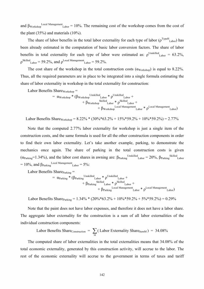
and βWorkshop
Local ManagementLabor = 10%. The remaining cost of the workshop comes from the cost of
the plant (35%) and materials (10%).
The share of labor benefits in the total labor externality for each type of labor (ρTypeHLabor) has
been already estimated in the computation of basic labor conversion factors. The share of labor
benefits in total externality for each type of labor were estimated as: ρUnskilledLabor = 63.2%,
ρSkilledLabor = 59.2%, and ρLocal Management
Labor = 59.2%.
The cost share of the workshop in the total construction costs (αWorkshop) is equal to 8.22%.
Thus, all the required parameters are in place to be integrated into a single formula estimating the
share of labor externality in workshop in the total externality for construction:
Labor Benefits ShareWorkshop = = αWorkshop * (βWorkshop
UnskilledLabor * ρUnskilled
Labor + + βWorkshop
SkilledLabor * ρSkilled
Labor + + βWorkshop
Local ManagementLabor * ρLocal Management
Labor)
Labor Benefits ShareWorkshop = 8.22% * (30%*63.2% + 15%*59.2% + 10%*59.2%) = 2.77%
Note that the computed 2.77% labor externality for workshop is just a single item of the
construction costs, and the same formula is used for all the other construction components in order
to find their own labor externality. Let’s take another example, parking, to demonstrate the
mechanics once again. The share of parking in the total construction costs is given
(αParking=1.34%), and the labor cost shares in awning are: βParkingUnskilled
Labor = 20%, βParkingSkilled
Labor
= 10%, and βParkingLocal Management
Labor = 5%:
Labor Benefits ShareParking = = αParking * (βParking
UnskilledLabor * ρUnskilled
Labor + + βParking
SkilledLabor * ρSkilled
Labor + + βParking
Local ManagementLabor * ρLocal Management
Labor)
Labor Benefits ShareParking = 1.34% * (20%*63.2% + 10%*59.2% + 5%*59.2%) = 0.29%
Note that the paint does not have labor expenses, and therefore it does not have a labor share.
The aggregate labor externality for the construction is a sum of all labor externalities of the
individual construction components:
Labor Benefits ShareConstruction = ∑M
( Labor Externality ShareItemM ) = 34.08%
The computed share of labor externalities in the total externalities means that 34.08% of the
total economic externality, generated by this construction activity, will accrue to the labor. The
rest of the economic externality will accrue to the government in terms of taxes and tariff
142
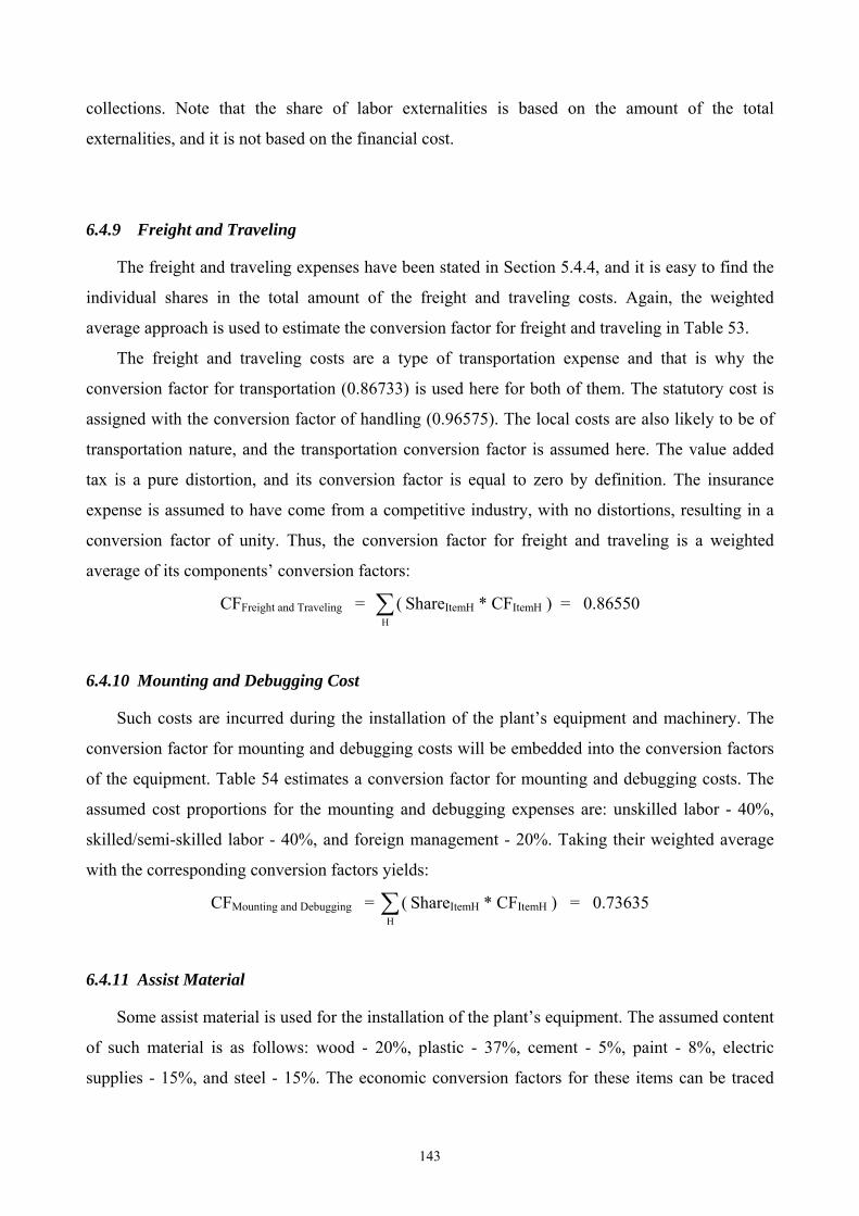
collections. Note that the share of labor externalities is based on the amount of the total
externalities, and it is not based on the financial cost.
6.4.9 Freight and Traveling
The freight and traveling expenses have been stated in Section 5.4.4, and it is easy to find the
individual shares in the total amount of the freight and traveling costs. Again, the weighted
average approach is used to estimate the conversion factor for freight and traveling in Table 53.
The freight and traveling costs are a type of transportation expense and that is why the
conversion factor for transportation (0.86733) is used here for both of them. The statutory cost is
assigned with the conversion factor of handling (0.96575). The local costs are also likely to be of
transportation nature, and the transportation conversion factor is assumed here. The value added
tax is a pure distortion, and its conversion factor is equal to zero by definition. The insurance
expense is assumed to have come from a competitive industry, with no distortions, resulting in a
conversion factor of unity. Thus, the conversion factor for freight and traveling is a weighted
average of its components’ conversion factors:
CFFreight and Traveling = ∑H
( ShareItemH * CFItemH ) = 0.86550
6.4.10 Mounting and Debugging Cost
Such costs are incurred during the installation of the plant’s equipment and machinery. The
conversion factor for mounting and debugging costs will be embedded into the conversion factors
of the equipment. Table 54 estimates a conversion factor for mounting and debugging costs. The
assumed cost proportions for the mounting and debugging expenses are: unskilled labor - 40%,
skilled/semi-skilled labor - 40%, and foreign management - 20%. Taking their weighted average
with the corresponding conversion factors yields:
CFMounting and Debugging = ∑H
( ShareItemH * CFItemH ) = 0.73635
6.4.11 Assist Material
Some assist material is used for the installation of the plant’s equipment. The assumed content
of such material is as follows: wood - 20%, plastic - 37%, cement - 5%, paint - 8%, electric
supplies - 15%, and steel - 15%. The economic conversion factors for these items can be traced
143
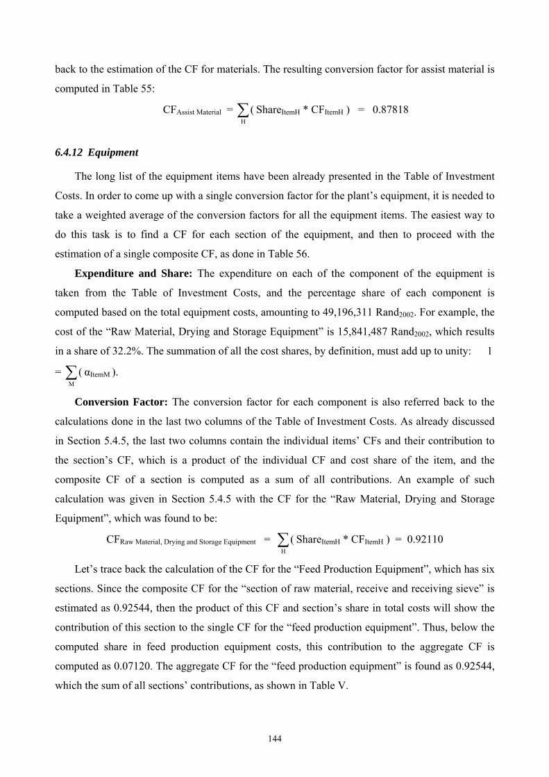
back to the estimation of the CF for materials. The resulting conversion factor for assist material is
computed in Table 55:
CFAssist Material = ∑H
( ShareItemH * CFItemH ) = 0.87818
6.4.12 Equipment
The long list of the equipment items have been already presented in the Table of Investment
Costs. In order to come up with a single conversion factor for the plant’s equipment, it is needed to
take a weighted average of the conversion factors for all the equipment items. The easiest way to
do this task is to find a CF for each section of the equipment, and then to proceed with the
estimation of a single composite CF, as done in Table 56.
Expenditure and Share: The expenditure on each of the component of the equipment is
taken from the Table of Investment Costs, and the percentage share of each component is
computed based on the total equipment costs, amounting to 49,196,311 Rand2002. For example, the
cost of the “Raw Material, Drying and Storage Equipment” is 15,841,487 Rand2002, which results
in a share of 32.2%. The summation of all the cost shares, by definition, must add up to unity: 1
= α∑M
( ItemM ).
Conversion Factor: The conversion factor for each component is also referred back to the
calculations done in the last two columns of the Table of Investment Costs. As already discussed
in Section 5.4.5, the last two columns contain the individual items’ CFs and their contribution to
the section’s CF, which is a product of the individual CF and cost share of the item, and the
composite CF of a section is computed as a sum of all contributions. An example of such
calculation was given in Section 5.4.5 with the CF for the “Raw Material, Drying and Storage
Equipment”, which was found to be:
CFRaw Material, Drying and Storage Equipment = ∑H
( ShareItemH * CFItemH ) = 0.92110
Let’s trace back the calculation of the CF for the “Feed Production Equipment”, which has six
sections. Since the composite CF for the “section of raw material, receive and receiving sieve” is
estimated as 0.92544, then the product of this CF and section’s share in total costs will show the
contribution of this section to the single CF for the “feed production equipment”. Thus, below the
computed share in feed production equipment costs, this contribution to the aggregate CF is
computed as 0.07120. The aggregate CF for the “feed production equipment” is found as 0.92544,
which the sum of all sections’ contributions, as shown in Table V.
144
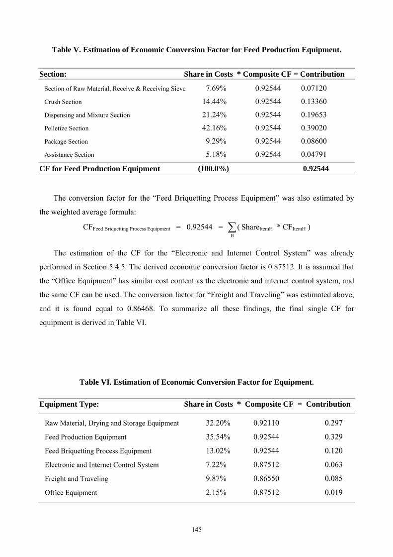
Table V. Estimation of Economic Conversion Factor for Feed Production Equipment.
Section: Share in Costs * Composite CF = Contribution
Section of Raw Material, Receive & Receiving Sieve 7.69% 0.92544 0.07120
Crush Section 14.44% 0.92544 0.13360
Dispensing and Mixture Section 21.24% 0.92544 0.19653
Pelletize Section 42.16% 0.92544 0.39020
Package Section 9.29% 0.92544 0.08600
Assistance Section 5.18% 0.92544 0.04791
CF for Feed Production Equipment (100.0%) 0.92544
The conversion factor for the “Feed Briquetting Process Equipment” was also estimated by
the weighted average formula:
CFFeed Briquetting Process Equipment = 0.92544 = ∑H
( ShareItemH * CFItemH )
The estimation of the CF for the “Electronic and Internet Control System” was already
performed in Section 5.4.5. The derived economic conversion factor is 0.87512. It is assumed that
the “Office Equipment” has similar cost content as the electronic and internet control system, and
the same CF can be used. The conversion factor for “Freight and Traveling” was estimated above,
and it is found equal to 0.86468. To summarize all these findings, the final single CF for
equipment is derived in Table VI.
Table VI. Estimation of Economic Conversion Factor for Equipment. Equipment Type: Share in Costs * Composite CF = Contribution
Raw Material, Drying and Storage Equipment 32.20% 0.92110 0.297
Feed Production Equipment 35.54% 0.92544 0.329
Feed Briquetting Process Equipment 13.02% 0.92544 0.120
Electronic and Internet Control System 7.22% 0.87512 0.063
Freight and Traveling 9.87% 0.86550 0.085
Office Equipment 2.15% 0.87512 0.019
145
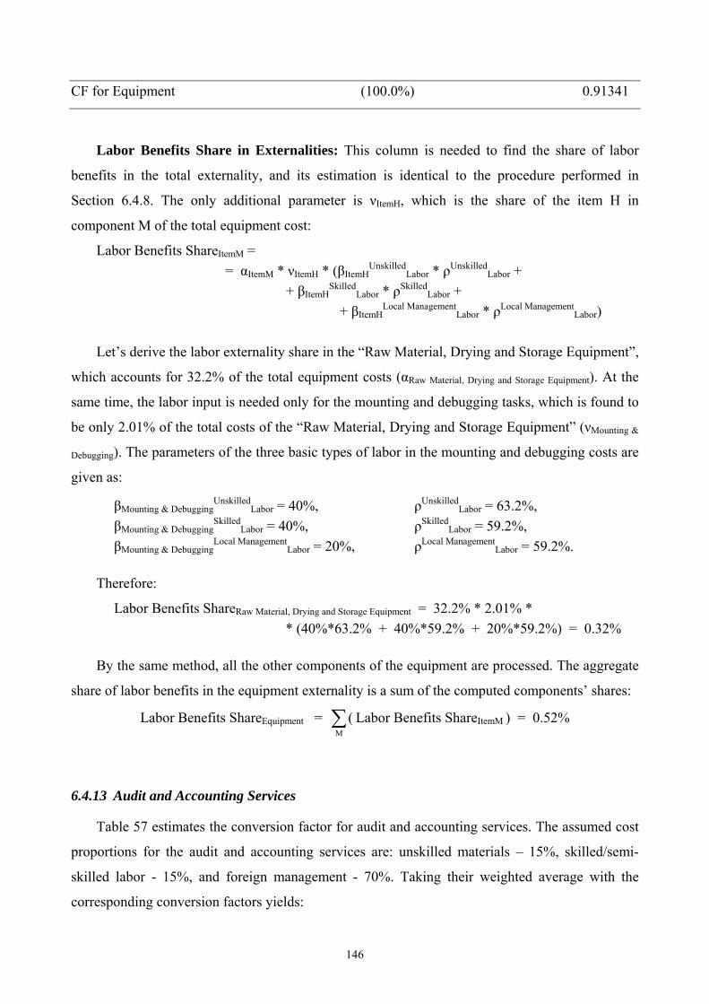
CF for Equipment (100.0%) 0.91341
Labor Benefits Share in Externalities: This column is needed to find the share of labor
benefits in the total externality, and its estimation is identical to the procedure performed in
Section 6.4.8. The only additional parameter is νItemH, which is the share of the item H in
component M of the total equipment cost:
Labor Benefits ShareItemM = = αItemM * νItemH * (βItemH
UnskilledLabor * ρUnskilled
Labor + + βItemH
SkilledLabor * ρSkilled
Labor + + βItemH
Local ManagementLabor * ρLocal Management
Labor)
Let’s derive the labor externality share in the “Raw Material, Drying and Storage Equipment”,
which accounts for 32.2% of the total equipment costs (αRaw Material, Drying and Storage Equipment). At the
same time, the labor input is needed only for the mounting and debugging tasks, which is found to
be only 2.01% of the total costs of the “Raw Material, Drying and Storage Equipment” (νMounting &
Debugging). The parameters of the three basic types of labor in the mounting and debugging costs are
given as:
βMounting & DebuggingUnskilled
Labor = 40%, ρUnskilledLabor = 63.2%,
βMounting & DebuggingSkilled
Labor = 40%, ρSkilledLabor = 59.2%,
βMounting & DebuggingLocal Management
Labor = 20%, ρLocal ManagementLabor = 59.2%.
Therefore:
Labor Benefits ShareRaw Material, Drying and Storage Equipment = 32.2% * 2.01% * * (40%*63.2% + 40%*59.2% + 20%*59.2%) = 0.32%
By the same method, all the other components of the equipment are processed. The aggregate
share of labor benefits in the equipment externality is a sum of the computed components’ shares:
Labor Benefits ShareEquipment = ∑M
( Labor Benefits ShareItemM ) = 0.52%
6.4.13 Audit and Accounting Services
Table 57 estimates the conversion factor for audit and accounting services. The assumed cost
proportions for the audit and accounting services are: unskilled materials – 15%, skilled/semi-
skilled labor - 15%, and foreign management - 70%. Taking their weighted average with the
corresponding conversion factors yields:
146

CFAudit and Accounting Services = ∑H
( ShareItemH * CFItemH ) = 0.79175
6.4.14 Advertising
The calculation of a CF for the advertising is performed in Table 58 and it is based on the
following assumptions: materials - 50.0%, skilled and semi-skilled labor - 20.0%, and local
management - 30.0%. The conversion factor for the advertising is, therefore, computed by:
CFAdvertising = ∑ ShareH
( ItemH * CFItemH ) = 0.84104
6.4.15 Equipment Mechanic Service
Table 59 is used to estimate the CF for the equipment mechanic service. The costs of
equipment mechanic service are assumed to be: lubrication oils - 15.0%, plastics - 10.0%,
chemicals - 10.0%, electric supplies - 10.0%, paint - 5.0%, unskilled labor - 10.0%, skilled and
semi-skilled labor - 35.0%, and foreign management - 5.0%. The conversion factor can be found
by formula:
CFEquipment Mechanic Service = ∑H
( ShareItemH * CFItemH ) = 0.84764
6.4.16 Office and Transportation Services
The office and transportation services expenses are assumed to consist of equal parts of
administration and transportation, therefore, its conversion factor is computed in Table 60 as:
CFOffice and Transportation Services = 50% * 0.77063 + 50% * 0.84749 = 0.80906
6.4.17 Business Travel
The business travel expenses are assumed to be 50% in the fuel costs, and the other 50% of
transportation, and the conversion factor is computed in Table 61 as:
CFBusiness Travel = 50% * 0.67805 + 50% * 0.84749 = 0.78819
147
6.4.18 Feed Ingredients
Section 5.2.17 described the feed ingredients content as having 50% of tradable components,
40% of non-tradable components, 8% of transportation costs, and 2% of handling expenses. Given
the high proportion of tradable components, the feed ingredients should be treated as tradable
input, according to the methodology laid out Chapter 6 of the Manual (2003). Table 62 carries out
the estimation of a conversion factor for feed ingredients. The starting point of the estimation is to
find the financial values of each feed ingredients component. The financial cost of feed ingredients
was set at 950 Rand/ton, which implies that the tradable components worth 475 Rand/ton, non-
tradable 380 Rand/ton, while transportation and handling costs account for 76 and 19 Rand/ton
respectively.
Unadjusted Conversion Factor: This is the economic conversion factor describing the
discrepancy between the financial and economic values of a commodity, but not adjusted for the
foreign exchange premium. In the absence of the conversion factor data for these components, and
given the fact that most basic agriculture commodities are VAT exempt, the unadjusted conversion
factors assumed for the tradable and non-tradable components are equal to one. The handling
expenses are subject to VAT, and therefore are assumed to have a CF of 0.93. The adjusted
economic conversion factor for transportation expenses was already estimated as 0.84749 in
Section 6.3.9, which already includes the adjustment for the foreign exchange premium, and that is
why the cells with the transportation calculations are skipped.
Unadjusted Economic Price: The unadjusted economic price (PeUnadj) is simply a product of
the financial price and the unadjusted conversion factor. For instance, the unadjusted economic
value of handling is only 17.7 Rand/ton, with the difference created by the VAT tax.
Traded Content: This states the percentage share of tradable inputs in each feed component.
Because even a purely non-traded commodity may, and usually does contain, some traded inputs,
and any additional consumption of these inputs will result in an additional foreign exchange
demand. It has been assumed that the traded content of the tradable feed ingredients components is
100%, non-tradable components have 30% of traded inputs, and handling has a 45% traded share.
Foreign Exchange Premium: As already mentioned, any additional consumption of traded
input will eventually impact on the country’s demand for the foreign exchange. Because South
Africa has a foreign exchange premium of 5.5% on tradable commodities and 2.0% on non-
tradable commodities, this premium must be included in the economic cost of a commodity. The
amount of the premium can be calculated as a product of the financial price times the share of
tradable content and times the corresponding foreign exchange premium:
148

FOREX Financial Tradable FOREX Premium Non-Tradable FOREX Premium PremiumItemM = PriceItemM * ContentItemM * on Tradable + ContentItemM * on Non-Tradable (Rand/ton) (Rand/ton) (%) (%) (%) (%)
FOREX PremiumHandling = 19.0 * (45%*5.5% + 55%*2.0%) = 0.7 Rand/ton
Adjusted Economic Price: This is the final economic value of a component (PeAdj), computed
as a sum of the unadjusted economic value and the amount of foreign exchange premium:
PeAdj
ItemM (Rand/ton) = PeUnadj
ItemM + FOREX PremiumItemM
PeAdj
Handling = 17.7 + 0.7 = 18.3 Rand/ton
For the transportation expenses, its adjusted economic value is derived by multiplying the
financial cost of transportation by its conversion factor.
The total of economic values of the feed ingredients components adds up to 969.9 Rand/ton,
which is a higher figure than the financial cost of feed ingredients. The conversion factor for feed
ingredients can be found as:
CFFeed Ingredients = Economic CostFeed Ingredients / Financial CostFeed Ingredients
CFFeed Ingredients = 975.5 / 950.0 = 1.02681
The calculated conversion factor implies that the economic cost of feed ingredients is greater
than the financial price the feed manufacturers pay for it. The difference is mostly attributed to the
foreign exchange premium on the traded components. In other words, the feed manufacturers do
not pay the full economic cost of the feed ingredients.
6.4.19 Change in Accounts Payable
Since the amount of accounts payable is assumed to follow the direct operating cost, then its
economic conversion factor can be rightly derived from the conversion factors of the direct
operating costs. Table VII below and Table 63 in Annex A both illustrate the procedure, and finds
a conversion factor of 1.02301 for the change in accounts payable.
Table VII. Estimation of Economic Conversion Factor for Change in Accounts Payable.
Direct Costs: PV of Costs Share * CF = Contribution
Feed Ingredients 1,934,038,122 98.2% 1.02681 1.008
Labor 11,911,257 0.6% 0.67363 0.004
149
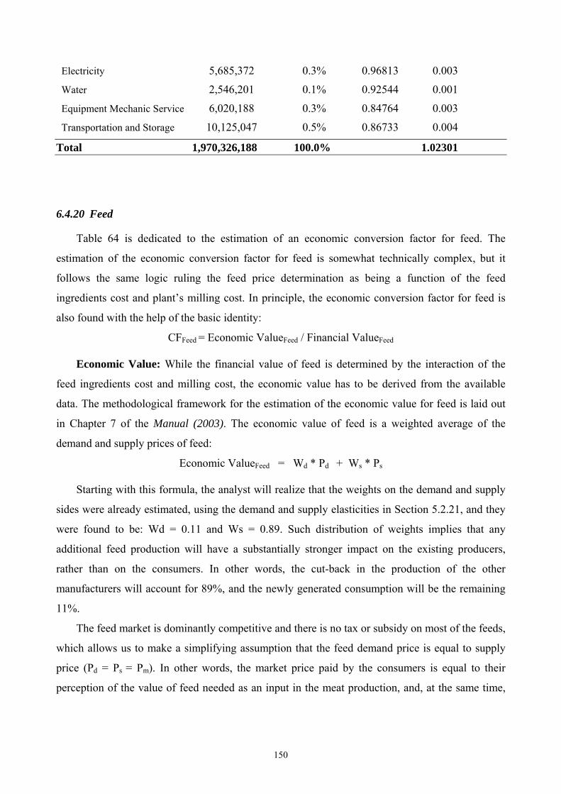
Electricity 5,685,372 0.3% 0.96813 0.003
Water 2,546,201 0.1% 0.92544 0.001
Equipment Mechanic Service 6,020,188 0.3% 0.84764 0.003
Transportation and Storage 10,125,047 0.5% 0.86733 0.004
Total 1,970,326,188 100.0% 1.02301
6.4.20 Feed
Table 64 is dedicated to the estimation of an economic conversion factor for feed. The
estimation of the economic conversion factor for feed is somewhat technically complex, but it
follows the same logic ruling the feed price determination as being a function of the feed
ingredients cost and plant’s milling cost. In principle, the economic conversion factor for feed is
also found with the help of the basic identity:
CFFeed = Economic ValueFeed / Financial ValueFeed
Economic Value: While the financial value of feed is determined by the interaction of the
feed ingredients cost and milling cost, the economic value has to be derived from the available
data. The methodological framework for the estimation of the economic value for feed is laid out
in Chapter 7 of the Manual (2003). The economic value of feed is a weighted average of the
demand and supply prices of feed:
Economic ValueFeed = Wd * Pd + Ws * Ps
Starting with this formula, the analyst will realize that the weights on the demand and supply
sides were already estimated, using the demand and supply elasticities in Section 5.2.21, and they
were found to be: Wd = 0.11 and Ws = 0.89. Such distribution of weights implies that any
additional feed production will have a substantially stronger impact on the existing producers,
rather than on the consumers. In other words, the cut-back in the production of the other
manufacturers will account for 89%, and the newly generated consumption will be the remaining
11%.
The feed market is dominantly competitive and there is no tax or subsidy on most of the feeds,
which allows us to make a simplifying assumption that the feed demand price is equal to supply
price (Pd = Ps = Pm). In other words, the market price paid by the consumers is equal to their
perception of the value of feed needed as an input in the meat production, and, at the same time,
150
the price of feed received by the manufacturers is equal to their long-term average production
costs, including the opportunity cost of capital.
While the financial prices on the demand and supply side can be said to be equal, there is an
foreign exchange effect and taxes impact on the supply side, due to the fact that the existing
producers will give up some of their production and release economic resources for other
productive use, which will have an influence on the input resources allocation within the economy.
Because there are economic externalities on the feed ingredients and milling cost, any re-
allocation of these resources will create distortions equal to the difference between the financial
cost of an input and its economic cost. A little modification of the economic value formula is,
therefore, required in order to account for this impact:
Economic ValueFeed (Rand2002/ton) = Wd*Pd + Ws*Ps – Ws*Input DistortionsFeed
The input distortions in the formula include all the distortions in the inputs used in the feed
manufacture process. Note that the input distortion is only applicable to the supply side of the
economic feed valuation. The negative sign of the net input distortions here represents the release
of resources, otherwise directed at the feed production by other producers. In other words, the
other producers will release economic resources previously used in the feed production, and the
value of input cost distortions must be deducted from the economic value of the feed produced by
this plant.
Distortions in Feed Ingredients: Now, the real issue is to estimate the amount of input
distortions. To simplify the matter, the analyst may think of the total distortions as being created
by the distortions in the feed ingredients and distortions in the cost of milling:
Input DistortionsFeed (Rand2002/ton) = Input DistortionsIngredients + Input DistortionsMilling
For the feed ingredients part, it is relatively easy to find the amount of distortions created by
the 0.9-weighted pull-back on the supply side. Since the cost of feed ingredients is 950.0
Rand2002/ton and the computed conversion factor of feed ingredients is 1.02681, then the amount
of distortions in the cost of ingredients can be approximated by formula:
Input DistortionsIngredients (Rand2002/ton) = CostFeed Ingredients * (1 – CFFeed Ingredients)
Input DistortionsIngredients = 950 * (1 – 1.02681) = –28.6 Rand2002/ton
What the minus sign implies here is that there is negative forex adjustment on the cost of
inputs going into the feed production, i.e. the economy suffers a loss, which is not reflected in the
financial cashflows, if there is an expansion of feed production. The loss comes about due to an
151
increased use of the feed ingredients, and consequent demand for the foreign exchange, which has
been determined as the major contributor to the feed ingredients economic conversion factor.
When this negative distortion is actually entered into the formula for estimation of the
economic value of feed, its sign will change to positive. This is explained by the fact that the 0.9-
weighted supply side adjustment implies a reduction of feed production by other manufacturers,
and a lower consumption of feed ingredients and a consequent release of the foreign exchange
previously used to purchase the feed ingredients. Thus, the input distortions on the ingredients side
will increase the economic value of feed, because foreign exchange is actually saved from being
used by the existing manufacturers in the feed production.
PV of Costs and Shares in Milling Cost: The estimation of input distortion in the milling
cost is more complex because the total cost of milling is actually composed of variety of items. By
definition, the milling cost includes all the other investment costs and operating expenses, with the
exception of the cost of feed ingredients which is excluded. To enlist all the individual
components of the milling costs, the analyst should exclude the cost of ingredients from the total
investment and operating costs.
The best way to do this task is to take the present value of each and every cost item, and then
exclude the present value of the feed ingredients. Examination of Table 64 can explain how the
present values are obtained. Each cashflow item has been computed with a present value,
according to the formula:
PVItemM (Rand2002) = NPV(EOCKReal, Annual CFItemMReal
2003:Annual CFItemMReal
2013) + Annual CFItemMReal
2002
PVLabor = NPV(11%, LaborReal2003:LaborReal
2013) + LaborReal2002 = 11,911,257 Rand2002
Note that the PV formula is based on the cashflow statement from the banker’s point of view,
where the loan items and grant are excluded. For the investment cost items, their liquidation values
are actually deducted from the corresponding investment costs to reflect the fact that the owners
will be able to recoup some of the initial investment costs by selling off useful assets.
As a result, the column with present values of project’s costs contains the PVs of all financial
costs, including the PV of the ingredients costs. The total present value of costs is computed as
2,187,324,982 Rand2002, which includes the present value of all investment and operating costs,
except for loan and grant items.
It is now possible to exclude the PV of ingredients costs from the listing, and the next column
performs this task. The total present value is now stands at 238,359,464 Rand2002, which is net of
the 1,934,038,122 Rand2002 feed ingredients cost. The new total is nothing else than the present
value of the milling costs, and using it as a base, the computation of the share of each individual
152
item is carried out. For example, since the present value of land is 768,191 Rand2002, its share in
the PV of the total costs is 0.32%. Thus, the share of land costs in the total milling costs is 0.32%,
and the analyst can figure out the actual land expenses per ton of feed produced by the plant.
Share of Feed Ingredients Cost in Feed: At this point, the actual share of the ingredients in
the feed production can be found as well as the share of the milling costs. The share of feed
ingredients is found as the PV of the ingredients costs over the PV of the total costs:
αIngredients = 1,934,038,122 Rand2002 / 2,187,324,982 Rand2002 = 0.88
Also, the share of the milling cost is simply the ratio of the PV of the milling costs over the
PV of the total costs:
αMilling = 238,359,464 Rand2002 / 2,187,324,982 Rand2002 = 0.12
By definition, the shares must add up to one which indeed holds true (αIngredients + αMilling = 1).
The derived parameters are used in the Table of Parameters (Section 5.2.21), in the Schedule of
Feed Ingredients and Feed Prices (Section 5.6) and in the feed demand determination model
(Section 5.7).
Values in Milling Cost: In order to find the value of each cost item, the computed cost share
should be multiplied by the share of milling, taken from the Table of Parameters. Thus, the value
of land costs would be 0.5 Rand2002/ton, which is a product of a cost share of 0.35% and milling
fee of 258.8 Rand2002/ton. The same action is performed for all the milling cost components, in
order to create an itemized cost structure of milling.
Distortion in Milling Cost: The amount of input distortion per item is computed on the basis
of the obtained earlier individual economic conversion factors. Because the conversion factors
already account for all the distortions such as taxes, tariffs, subsidies, foreign exchange premium
and so on, then the difference between the item’s conversion factor and unity is really the amount
of disturbances per unit. The formula used here utilizes the conversion factors found beforehand:
Input DistortionsItemM (Rand2002/ton) = ValueItemMMilling Costs * (1 – CFItemM)
Input DistortionsLand = 0.5 * (1 – 1) = 0 Rand2002/ton
Input DistortionsLabor = 7.1 * (1 – 0.67363) = 2.31Rand2002/ton
Having computed all individual cost items, a total amount of input disturbance in the cost of
milling can be found as a sum of their values. This amount adds up to 36.5 Rand2002/ton, which
represents the value of the resource externalities in the milling cost of feed released due to a
reduction in the production by other manufacturers. The net input distortion of the milling cost is a
positive figure here but when used in the formula for the economic value of feed it accrues a
153

negative sign there, which means that the economy loses some taxes and tariffs on the milling cost
components.
Conversion Factor for Feed: At this point, the estimation of the conversion factor for feed
becomes possible. First, let’s find the net amount of input distortion per ton of feed, which is the
sum of the distortions in feed ingredients costs and distortions in the milling cost:
Input DistortionsFeed = (–28.6) + 36.5 = 7.9 Rand2002/ton
Thus, the reduction in feed production by other manufacturers will release foreign exchange
worth 28.6 Rand/ton but, at the same time, such a reduction in the feed production by other
manufacturers will cause a reduction of taxes, tariffs collection as well as loss of labor
externalities worth 36.5 Rand per ton of feed. The net input distortion is an economic loss of 7.9
Rand per ton of feed, which is applicable on the 0.9-weighted supply-side response in the feed
market.
Then, the economic value of feed can be estimated as the weighted average of the supply and
demand prices minus the amount of net input distortions per ton. Note that the financial supply and
demand prices are assumed to be equal:
Economic ValueFeed (Rand2002/ton) = Wd*Pd + Ws*Ps – Ws*Input DistortionsFeed
Economic ValueFeed = 0.11 * 1,209 + 0.89 * 1,209 – 0.89 * 7.9 = 1,202 Rand2002/ton
With the computed economic value of feed being smaller than its financial price, the analyst
should expect the resulting conversion factor to be somewhat below unity:
CFFeed = 1,202 / 1,209 = 0.99415
This conversion factor has a strong implication for the economic analysis. The economic
value of the feed produced by this project is found to be smaller than the price charged to the
consumers. The reason for this, as we have seen, lays in the input distortion effect, which affects
the foreign exchange equilibrium, impact on the tax collections, and on labor externalities. A
further analysis will have to look at other economic resource flows in order to determine the net
economic impact.
6.4.21 Summary of Economic Conversion Factors
Table 65 is created to summarize all the estimated economic conversion factors and place
them in the same location for further reference. The table follows the same format of the cashflow
listing used in the Cashflow Statement from the Banker’s Point of View in order to make the
linking easy for economic modeling. This table also contains the per item summary of the labor
154
benefit share in externalities. Having all of these in the standard cashflow listing format helps the
analyst to keep the spreadsheet calculations consistent and transparent.
The change in accounts receivable is assigned with the same conversion factor as the feed,
assuming that the economic value of the accounts receivable, i.e. deferred payments, is equal to
the value of feed consumed right away.
The liquidation values of the plant’s assets are given the same conversion factors as their
corresponding investment cost items. The land is assumed to be freely traded and because no
substantial distortions exist, its conversion factor is equal to one.
The conversion factor for grant, tax, or any other financial transfer is always taken as zero, by
definition. The discussion of this issue is presented in Chapter 5 of the Manual (2003). Thus, the
stated conversion factors for grant in the revenues and income tax on the expenditure side are zero.
The change in accounts payable is assigned a weighted average CF for the direct operating
costs. The conversion factors for the change in cash balances is set to one, implying that this
cashflow item is assumed to be non-distorted, i.e. no taxes or subsidies are present.
6.5 Projected Economic Resource Flow Statement
As opposite to the cashflow statement, the economic resource statement operates with flow of
real resources rather than financial payments. It does include the economic externalities not
captured in the financial cashflows, which are typically generated by the project. The financial
revenues in this statement are replaced by a flow of economic benefits, and financial costs are
substituted for the flows of economic costs. All the economic flows are always expressed in fixed
real prices, reflecting the fact the true economic prices are not affected by inflation. Table VIII
below presents the Projected Economic Resource Flow Statement for the feed project, expressed
in the prices of year 2002.
6.5.1 Economic Benefits
It is important to model the economic resource statement in a consistent manner with the rest
of the spreadsheet. The typical approach is to take the financial cashflow statement from owner’s
point of view as a basis for the economic statement. The reason for this choice is that the owner’s
point of view does not include loan items, which are also excluded from the economic statement.
Also, it is useful to maintain the uniformity in the listing of the project statements’ items.
155

156
The mechanics of economic statement modeling is simple once the economic conversion
factors for all cashflow items are estimated. The economic values are obtained from the financial
cashflows by multiplying them by the estimated conversion factor, i.e. all the annual values of an
item are multiplied by the same economic conversion factor:
Economic ValueRealItemM, YearX (Rand2002/ton) = Financial ValueReal
ItemM, YearX (Rand2002/ton) * CFItemM
Economic ValueRealBeef Feed, 2003 = 91,371,705 * 0.99415 = 65,191,821 Rand2002/ton
Economic ValueRealBeef Feed, 2007 = 171,047,832 * 0.99415 = 124,529,683 Rand2002/ton
The financial value here is referred to the real cashflow statement form the owner’s point of
view. The underlying assumption is that the economic conversion factor does not change over the
project’s lifespan. While this assumption may hold for the 10-years life of the feed project, for
longer periods this may not be true due to the fact that the tax rates, tariffs and other distortions are
likely to change, thus, affecting the conversion factors. The analyst must address this issue when
working with a project with a longer lifespan.
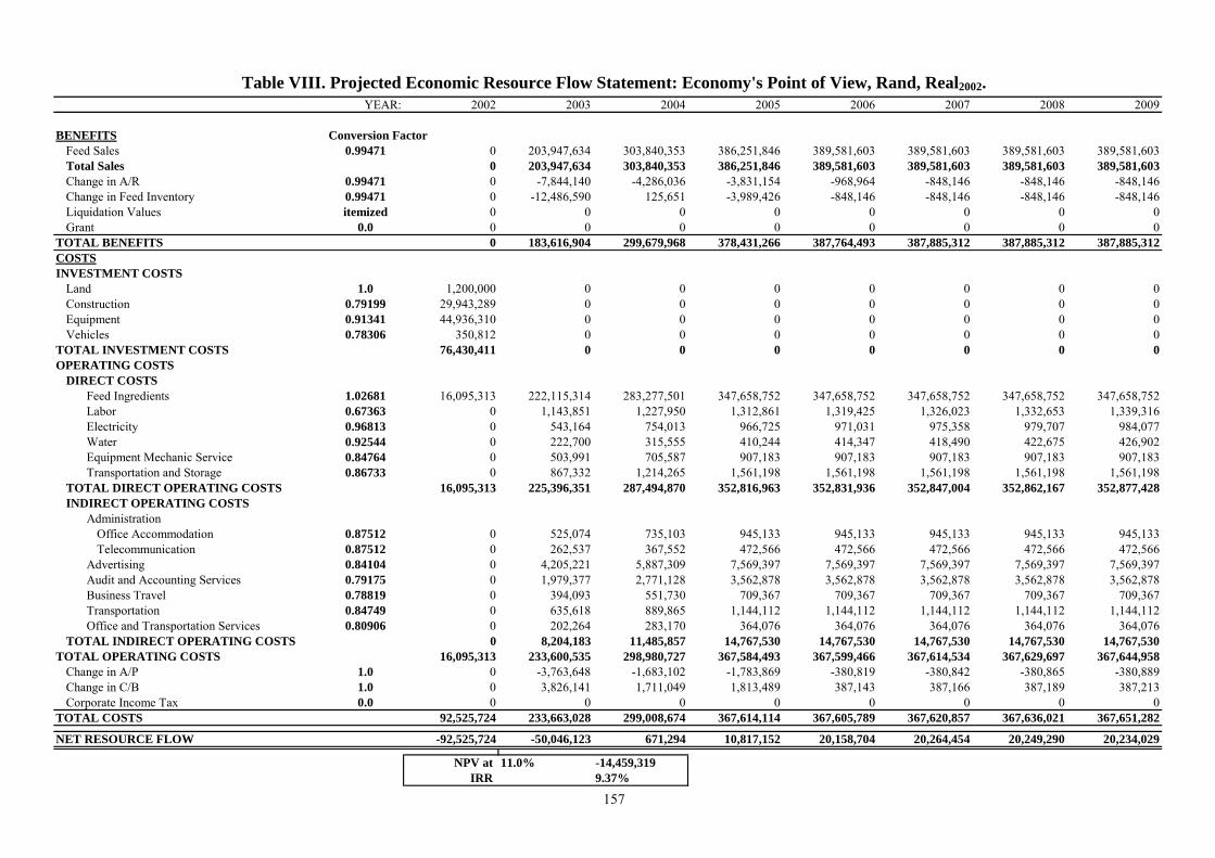
157
2008 2009
BENEFITS
YEAR: 2002 2003 2004 2005 2006 2007
Conversion FactorFeed Sales 0.99471 0 203,947,634 303,840,353 386,251,846 389,581,603 389,581,603 389,581,603 389,581,603Total Sales 0 203,947,634 303,840,353 386,251,846 389,581,603 389,581,603 389,581,603 389,581,603Change in A/R 0.99471 0 -7,844,140 -4,286,036 -3,831,154 -968,964 -848,146 -848,146 -848,146Change in Feed Inventory 0.99471 0 -12,486,590 125,651 -3,989,426 -848,146 -848,146 -848,146 -848,146Liquidation Values itemized 0 0 0 0 0 0 0 0Grant 0.0 0 0 0 0 0 0 0 0
TOTAL BENEFITS 0 183,616,904 299,679,968 378,431,266 387,764,493 387,885,312 387,885,312 387,885,312COSTSINVESTMENT COSTS
Land 1.0 1,200,000 0 0 0 0 0 0 0Construction 0.79199 29,943,289 0 0 0 0 0 0 0Equipment 0.91341 44,936,310 0 0 0 0 0 0 0Vehicles 0.78306 350,812 0 0 0 0 0 0 0
TOTAL INVESTMENT COSTS 76,430,411 0 0 0 0 0 0 0OPERATING COSTS
DIRECT COSTSFeed Ingredients 1.02681 16,095,313 222,115,314 283,277,501 347,658,752 347,658,752 347,658,752 347,658,752 347,658,752Labor 0.67363 0 1,143,851 1,227,950 1,312,861 1,319,425 1,326,023 1,332,653 1,339,316Electricity 0.96813 0 543,164 754,013 966,725 971,031 975,358 979,707 984,077Water 0.92544 0 222,700 315,555 410,244 414,347 418,490 422,675 426,902Equipment Mechanic Service 0.84764 0 503,991 705,587 907,183 907,183 907,183 907,183 907,183Transportation and Storage 0.86733 0 867,332 1,214,265 1,561,198 1,561,198 1,561,198 1,561,198 1,561,198
TOTAL DIRECT OPERATING COSTS 16,095,313 225,396,351 287,494,870 352,816,963 352,831,936 352,847,004 352,862,167 352,877,428INDIRECT OPERATING COSTS
AdministrationOffice Accommodation 0.87512 0 525,074 735,103 945,133 945,133 945,133 945,133 945,133Telecommunication 0.87512 0 262,537 367,552 472,566 472,566 472,566 472,566 472,566
Advertising 0.84104 0 4,205,221 5,887,309 7,569,397 7,569,397 7,569,397 7,569,397 7,569,397Audit and Accounting Services 0.79175 0 1,979,377 2,771,128 3,562,878 3,562,878 3,562,878 3,562,878 3,562,878Business Travel 0.78819 0 394,093 551,730 709,367 709,367 709,367 709,367 709,367Transportation 0.84749 0 635,618 889,865 1,144,112 1,144,112 1,144,112 1,144,112 1,144,112Office and Transportation Services 0.80906 0 202,264 283,170 364,076 364,076 364,076 364,076 364,076
TOTAL INDIRECT OPERATING COSTS 0 8,204,183 11,485,857 14,767,530 14,767,530 14,767,530 14,767,530 14,767,530TOTAL OPERATING COSTS 16,095,313 233,600,535 298,980,727 367,584,493 367,599,466 367,614,534 367,629,697 367,644,958
Change in A/P 1.0 0 -3,763,648 -1,683,102 -1,783,869 -380,819 -380,842 -380,865 -380,889Change in C/B 1.0 0 3,826,141 1,711,049 1,813,489 387,143 387,166 387,189 387,213Corporate Income Tax 0.0 0 0 0 0 0 0 0 0
TOTAL COSTS 92,525,724 233,663,028 299,008,674 367,614,114 367,605,789 367,620,857 367,636,021 367,651,282
NET RESOURCE FLOW -92,525,724 -50,046,123 671,294 10,817,152 20,158,704 20,264,454 20,249,290 20,234,029
NPV at 11.0% -14,459,319IRR 9.37%
Table VIII. Projected Economic Resource Flow Statement: Economy's Point of View, Rand, Real2002.
Note that the grant cash inflow is non-existent in terms of flow of real economic resources,
and it appears as having zero values. In fact, the grant is a financial transfer from the government
to the project and it has no underlying real resource movements.
The total economic benefits are computed each year to sum up all the economic benefit flows.
If any positive externality is generated by the project it must be added to the economic benefits.
The analyst must identify and quantify any such externalities in order to approximate the true
economic impact of the project.
6.5.2 Economic Costs
The economic costs are different from the financial expenditure of the project. The economic
costs include any externalities created by the project, and while the cashflow items have been
already furnished with a conversion factor, which describes the amount of externality, there could
be economic costs not associated with the financial expenditures. For instance, a chemical
processing plant may contaminate the project site and pose an environmental danger to the
surrounding areas. Even the most advanced pollution abatement methods do not ensure 100%
results, and the financial expenses directed on the prevention of such pollution are project’s
cashflow items but the remaining pollution is not usually accounted and represents a negative
economic externality created by the plant.
The modeling of the economic costs flows is identical in its mechanics to the formulation of
the economic benefits. The financial expenditures from the banker’s cashflow statement are
multiplied by the corresponding conversion factors to obtain the economic costs:
Economic ValueRealLabor, 2003 = 1,698,048 * 0.67363 = 1,143,851 Rand2002/ton
Economic ValueRealLabor, 2007 = 1,968,482 * 0.67363 = 1,326,023 Rand2002/ton
The same procedure applies to all the items in the investment and operating costs. As
mentioned above, the conversion factors for the change in cash balances is equal to one, and the
conversion factor for corporate income tax is zero. A total of all the economic costs is computed
every year.
6.5.3 Economic Net Present Value
The evaluation criteria for this project from the economy’s point of view is the net present
value, which is based on the net annual economic resource flow and discounted by the economic
158
opportunity cost of capital (EOCK). The idea is to sum all the annual net resource flows
(NRFYearX) into a single summary measure in order to see if the project is worthwhile for the
economy.
Table 66 contains the estimation of the economic NPV. Similarly to the financial NPV, a
negative economic net present value will imply a welfare loss for the economy, while a positive
net present value will mean that the feed project contributes to the country’s well-being. The
break-even, zero economic net present value signifies an acceptable project from the economy’s
point of view, since the project justifies its existence by compensating all the economic costs
associated with the re-allocation of resources due to the project. The formula to calculate the
economic net present value is:
NPVEconomy = NPV(EOCK, NRFReal2003:NRFReal
2013) + NRFReal2002 = –14,459,319 Rand2002
The computed economic NPV is a negative figure, which tells the analyst that the project will
make the country worse off with its existence. To make the matter severe, remember that the
financial NPV is set to zero, i.e. the project just breaks even financially.
The economic internal rate of return is also computed, but it is not considered being an
evaluation criteria. The calculated economic IRR of 9.37% shows that the economic performance
of the feed plant is far below the economic cost of capital attracted from the other sectors in order
to fund this project.
With such a result on hands, further insight into the project’s impact on the economy is
needed. The distributive analysis will look at the externalities created by the feed project as well as
their distribution among the stakeholders of this project.
159
7. DISTRIBUTIVE ANALYSIS
The distributive analysis looks into the issue of who will benefit from the project and who will
bear its costs. Since the National Government has approved a cash grant for this feed project then
it is important to identify the beneficiaries of the project to see if this is consistent with the
indented policy of promoting the foreign direct investment in Limpopo Province.
The distributive analysis is typically carried out in three consequent steps. First, the project’s
externalities have to be clearly identified. This task is undertaken in the Statement of Economic
Externalities in Section 7.1. Secondly, reconciliation between the financial and economic analysis
is necessary in order to ensure an error-free model, and this is done in Section 7.2. Thirdly, an
allocation of externalities should be performed to distribute the total generated externality among
the stakeholders and Section 7.3 addresses this issue in detail. Finally, the creation of “growth”
externalities is examined in Section 7.4.
7.1 Statement of Externalities
The statement of externalities is a statement combining all the project externalities into a
single location in order to display the per-item annual externality flows explicitly. According to
Chapter 11 of the Manual (2003), the economic externality can be defined as the difference
between the financial and economic value, provided that both values are real, inflation adjusted
figures:
ExternalityItemM = Economic ValueItemM – Financial ValueItemM
In practical terms, a statement of externalities can be compiled from the Statement of
Economic Resource Flows and real Cashflow Statement from the Banker’s Point of View.
Because the financial cashflows are expressed in real Rand, at the prices of year 2002, and the
economic resource flows are also measured in the year-2002 Rand, then the difference between the
two will yield the amount of economic externality, valued in the year-2002 Rand. The analyst
should link the financial and economic statements by item and by year in order to produce the
externality statement. Table IX presents the Projected Externality Flows Statement for the feed
project.
160

161
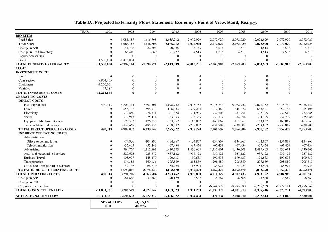
162
YEAR: 2002 2003 2004 2005 2006 2007 2008 2009 2010 2011BENEFITS
Feed Sales 0 -1,085,187 -1,616,708 -2,055,212 -2,072,929 -2,072,929 -2,072,929 -2,072,929 -2,072,929 -2,072,929Total Sales 0 -1,085,187 -1,616,708 -2,055,212 -2,072,929 -2,072,929 -2,072,929 -2,072,929 -2,072,929 -2,072,929Change in A/R 0 41,738 22,806 20,385 5,156 4,513 4,513 4,513 4,513 4,513Change in Feed Inventory 0 66,440 -669 21,227 4,513 4,513 4,513 4,513 4,513 4,513Liquidation Values 0 0 0 0 0 0 0 0 0 0Grant -1,500,000 -1,415,094 0 0 0 0 0 0 0 0
TOTAL BENEFITS EXTERNALITY -1,500,000 -2,392,104 -1,594,571 -2,013,599 -2,063,261 -2,063,903 -2,063,903 -2,063,903 -2,063,903 -2,063,903COSTSINVESTMENT COSTS
Land 0 0 0 0 0 0 0 0 0 0Construction -7,864,455 0 0 0 0 0 0 0 0 0Equipment -4,260,001 0 0 0 0 0 0 0 0 0Vehicles -97,188 0 0 0 0 0 0 0 0 0
TOTAL INVESTMENT COSTS -12,221,644 0 0 0 0 0 0 0 0 0OPERATING COSTS
DIRECT COSTSFeed Ingredients 420,313 5,800,314 7,397,501 9,078,752 9,078,752 9,078,752 9,078,752 9,078,752 9,078,752 9,078,752Labor 0 -554,197 -594,943 -636,083 -639,264 -642,460 -645,672 -648,901 -652,145 -655,406Electricity 0 -17,880 -24,821 -31,824 -31,965 -32,108 -32,251 -32,395 -32,540 -32,685Water 0 -17,943 -25,424 -33,053 -33,383 -33,717 -34,054 -34,395 -34,739 -35,086Equipment Mechanic Service 0 -90,593 -126,830 -163,067 -163,067 -163,067 -163,067 -163,067 -163,067 -163,067Transportation and Storage 0 -132,668 -185,735 -238,802 -238,802 -238,802 -238,802 -238,802 -238,802 -238,802
TOTAL DIRECT OPERATING COSTS 420,313 4,987,032 6,439,747 7,975,922 7,972,270 7,968,597 7,964,904 7,961,192 7,957,459 7,953,705INDIRECT OPERATING COSTS
AdministrationOffice Accommodation 0 -74,926 -104,897 -134,867 -134,867 -134,867 -134,867 -134,867 -134,867 -134,867Telecommunication 0 -37,463 -52,448 -67,434 -67,434 -67,434 -67,434 -67,434 -67,434 -67,434
Advertising 0 -794,779 -1,112,691 -1,430,603 -1,430,603 -1,430,603 -1,430,603 -1,430,603 -1,430,603 -1,430,603Audit and Accounting Services 0 -520,623 -728,872 -937,122 -937,122 -937,122 -937,122 -937,122 -937,122 -937,122Business Travel 0 -105,907 -148,270 -190,633 -190,633 -190,633 -190,633 -190,633 -190,633 -190,633Transportation 0 -114,383 -160,136 -205,889 -205,889 -205,889 -205,889 -205,889 -205,889 -205,889Office and Transportation Services 0 -47,736 -66,830 -85,924 -85,924 -85,924 -85,924 -85,924 -85,924 -85,924
TOTAL INDIRECT OPERATING COSTS 0 -1,695,817 -2,374,143 -3,052,470 -3,052,470 -3,052,470 -3,052,470 -3,052,470 -3,052,470 -3,052,470TOTAL OPERATING COSTS 420,313 3,291,216 4,065,604 4,923,452 4,919,800 4,916,127 4,912,435 4,908,722 4,904,989 4,901,235
Change in A/P 0 -84,666 -37,863 -40,129 -8,567 -8,567 -8,568 -8,568 -8,569 -8,569Change in C/B 0 0 0 0 0 0 0 0 0 0Corporate Income Tax 0 0 0 0 0 -6,844,729 -8,985,780 -9,256,569 -9,272,191 -9,286,569
TOTAL COSTS EXTERNALITY -11,801,331 3,206,549 4,027,742 4,883,323 4,911,233 -1,937,170 -4,081,913 -4,356,416 -4,375,771 -4,393,903
NET EXTERNALITY FLOW 10,301,331 -5,598,653 -5,622,312 -6,896,922 -6,974,494 -126,734 2,018,010 2,292,513 2,311,868 2,330,000
NPV at 11.0% -4,395,172IRR 40.72%
Table IX. Projected Externality Flows Statement: Economy's Point of View, Rand, Real2002.
The listing of items in this statement is identical to the cashflow Statement from Banker’s
Point of View as well as to the Statement of Economic Resource Flows. Note that items which
have conversion factor of one have the value of externality being zero, due to the fact that a unity
conversion factor represents undistorted commodities, whose transactions do not generate
economic externality. Such undistorted items are the land and the change in cash balances. All
the other items have been assigned a conversion factor different from one and, therefore,
economic externalities are induced throughout the project life.
The total externalities on the revenue items are computed for each year. The cost-side
externalities are also projected into the future, and their net externality flow (NEFYearX) is
calculated. The present value of the project’s externalities is based on the net externality flow,
being discounted by the economic opportunity cost of capital, and it can be found by MS-Excel
formula:
PVExternality = NPV(EOCK, NEFReal2003:NEFReal
2013) + NEFReal2002 = –4,395,172 Rand2002
What the computed result implies is that even the project covers its financial costs, it will
cause various stakeholders involved into this project to lose in the economic sense. This negative
externality makes the economic NPV go down to –14.5 million Rand2002. Now, it is important to
identify the cause(s) of such a negative impact, and allocate the resulting externality to the
project’s stakeholders.
7.2 Reconciliation between Financial and Economic Analysis
After constructing the Statement of Externalities, the analyst is advised to make a
reconciliation between the financial cashflows and economic resource flows to check the internal
consistency of the project’s model. Given the relationship between the financial and economic
values, the following identity must hold true, by definition:
Economic ValueItemM = Financial ValueItemM + ExternalityItemM
Starting with this equation, the analyst can substitute the present values of financial
cashflows and externality flows in order to check if their sum is indeed equal to the
corresponding present values of economic resource flows. Table 68 shows a typical example of
163
such reconciliation. For instance, let’s check the identity on the example of sales revenues for
beef feed:
PVEconomicItemM = PVFinancial
ItemM + PVExternalityItemM
PVEconomicBeef Feed = 662,300,722 + (–3,505,392) = 658,795,330 Rand2002
Note that the present values of the financial cashflows, economic resource flows and
externality flows are discounted by the same discount rate, which is the economic opportunity
cost of capital, not the financial discount rate. This is important to follow because if the financial
discount rate is used, the reconciliation will not work. The analyst must make sure that each and
every cashflow item does reconcile, signifying that the model has been built correctly.
Internal Reconciliation
A first cut can be already done on figuring out the main cause(s) for the externalities to be so
negative by analyzing the present values of cashflow items. On the benefit side, the negative
externality from the feed sales dominates the flows with about –11.0 million Rand2002 out of the
total benefits externality of –15.7 million Rand2002. On the cost side, there is no single item
winning the control over the net –11.3 million Rand2002 costs externalities, but the most
prominent items are the foreign exchange cost of the feed ingredients (49 million Rand2002),
corporate income tax (–25.6 million Rand2002), total investment costs (–12.2 million Rand2002).
The difference between the PV of benefits externalities and PV of costs externalities is the PV of
the total net externalities:
PVExternality = –15,659,635 + (–11,264,463) = –4,395,172 Rand2002
Looking at the magnitude of the figures in the externalities column of Table 68, the analyst
may notice that the big amount of externalities are generated by the following items: the feed
sales, investment costs, cost of feed ingredients, indirect operating costs, and corporate income
tax. Before an allocation of the estimated externalities is made to the project’s stakeholders, let’s
examine the forces that stay behind each of the identified group with sizeable externalities.
The feed sales externalities are generated by the distortions in the feed inputs and consist of
forex savings on the feed ingredients and foregone taxes, tariffs and labor externalities in the
production of feed by other producers. The externalities in the investment costs are primarily
caused by the foreign exchange premium and also by a creation of externality for labor. The
externalities in the cost of feed ingredients, as Section 6.4.18 explained, are caused by the foreign
exchange premium too. The items of the indirect operating costs have conversion factors less
than one, and the wedge between the financial and economic values is driven by the forex
164
premium and labor externalities. The corporate income tax is a pure transfer on the National
Government’s behalf.
7.3 Allocation of Economic Externalities
Any project affects a number of parties, either involved directly into the project or influenced
by it indirectly, and it is important to identify the main stakeholders affected by the project. The
issue here is to identify the gainers and losers from the project, and allocate the estimated
externality amongst the stakeholders. Remember that the financial return has been already
ensured by using the discount rate equal to the minimum acceptable rate of return on investment,
which means that the owners of the factors of production have been provided with the minimum
required financial reward for the employment of their resources. Therefore, only the project’s
externalities must be allocated to the affected parties but not the actual financial payments, since
all the payments have been already accounted for.
It is also important to understand that the externalities do not accrue to the project itself since
all the financial costs are already included into the evaluation, while other parties may either lose
or gain due to the project. Thus, the project analyst should exclude the project from being a
stakeholder in the distributive analysis and, instead, should allocate all the estimated externalities
to the affected parties.
The identification of the project’s stakeholders can be another hurdle on the way of the
analyst. A typical project evaluation refers to, at least, two stakeholders: government and labor.
In fact, there can be many stakeholders affected by the project and such stakeholders as the
environment, project’s suppliers, consumers, project’s competitors are often listed in investment
appraisal studies. The main criteria for distinguishing a stakeholder as having unique
characteristics to separate the externalities accruing to this particular stakeholder in a clear and
consistent manner. For instance, if the environmental impact is quantified, then the environment
can be treated as a “stakeholder” affected by the project. For more generic fiscal impacts such as
taxes, tariffs, subsidies, grants, and alike, the government is usually nominated into the position
of stakeholder standing to gain or lose from these externalities.
For the feed project in question, two stakeholders are considered in the distributive analysis:
labor and government. Both possess the required degree of detail to distinguish its own
externality from the total pool of generated externalities. In fact, only the labor externalities need
165
to be separated because the government is assumed to receive the remaining amount of total
externalities. Table 69 represents the Allocation of Externalities among the project’s
stakeholders.
Externalities: This column contains the present values of all the externality flows, so that
the project analyst can allocate all, or just a portion, of this value to the identified stakeholders.
Because the same item listing order has been kept in the model it is easy to navigate through it.
The total present value of externalities is found as –4,395,172 Rand2002.
Labor: The purpose of this column is to quantify the amount of labor externality per item.
The term “labor” here refers to all the three labor types combined into a single stakeholder. Note
that it is based on the computed share of labor benefits in the externality, calculated in the
Sections 6.3.1–6.3.3 and summarized in Table 65. The amount of labor externality for any item
M is simply the product of its labor benefits share and the present value of externalities for the
item:
Labor ExternalityItenM = Labor Benefits ShareItenM * PVExternalityItemM
Labor ExternalityLabor = 62.0% * –3,678,543 = –2,279,934 Rand2002
Labor ExternalityEquipment Mechanic Service = 27.0% * –865,638 = –234,039 Rand2002
Referring back to Table 65, many cashflow items don’t actually have any labor externality
and they are set to zero. Now, the calculation of labor externality is based on these shares and any
item having a zero share turns out to have a zero labor externality allocation in Table 65. The
total allocation of externalities to labor amounts to 4,648,522 Rand2002.
Government: The National Government is assumed to inherit all the remaining externalities
after deductions to the labor have been made. The total net amount of externality accruing to the
National Government is –9,043,694 Rand2002, and it is important to look at the composition of
this negative externality. The revenue side has a PV of the externality equal to –15,028,531
Rand2002, caused by the negative externality on the feed sales.
The costs side of the government externalities shows more variety in results. Thus, the
government collects taxes on the investment costs items (12,209,689 Rand2002) as well as taxes
on the indirect operating costs items (13,514,348 Rand2002) and corporate income tax (31,467,184
Rand2002). But the Government suffers a loss of foreign exchange due to the overall increased
consumption of feed ingredients, and the direct cost section amounts to a net externality of
35,388,355 Rand2002. The Government also collects corporate income taxes from the project
worth 25,592,658 Rand2002 in the present value. The resulting total of the cost-side is –6,048,935
166

Rand2002. Note that because the project’s cost items are negative flows for the project, they
become positive inflows to the Government.
The difference between the PV of benefits-side externalities and PV of cost-side externalities
is the present value of net externalities, and it is found as –4,395,172 Rand2002, which is exactly
the amount of externality computed in Tables 67 and 68. All the computed figures do reconcile,
implying that the model has been built correctly and no mechanical errors were made.
7.4 Growth Externalities vs. Net Externalities
The distributive analysis can be further expanded by examining the impact on of the project
on the “growth” externalities, and Table 70 presents the findings of this evaluation. The feed
project is assumed to generate a rate of return on private investment equal to the weighted
average cost of capital (WACC), so that the owner gets compensated for the opportunity cost of
his capital. Since the economic opportunity cost of capital in South Africa is 11.0% then the
average real return from the projects in the country is the estimated 11.0% rate. The difference
between the private WACC rate and economic EOCK rate entails a cost to the economic because
this capital, whether public or privately-owned, could have been invested into another sector with
the average return of 11.0%, in real terms. The cost is measured by “growth” externalities,
typically created by forgone tax and tariff collections, premium/loss on the foreign exchange
transactions, cost of inter-industry resource transfer and so on.
Net Cash Flow from Banker’s Point of View: The feed project is owned and financed, for
the most part, by a foreign investor, who does not cause a withdrawal of domestic capital from
other sectors, and the feed plant is not an incremental investment in this respect because the
source of funs is external to the economy. The foreign investor requires a 10.0% minimum rate of
return on investment (ROI), in real terms. The loan borrowed from a local bank carries a real
interest rate of 8.5%. Then, the WACC must be a rate between the 10.0% ROI and 8.5% interest
rate.
To make the computation of WACC easier, the analyst should remember that the WACC,
used as the discount rate in the computation of the NPV from the total investment’s (banker’s)
point of view, will make that NPV equal to zero. Therefore, the rate of WACC can be found by
using the “Goal Seek” function of MS-Excel by setting the NPV of net cash flow from banker’s
167

point of view (NPVF
WACC) to zero through changing the discount rate. The resulting rate of
9.85% ensures the break-even of the banker’s NPV.
Note that the net cashflow is taken directly from Table 14. The same financial cashflow can
be discounted by the economic discount rate. If the net cash flow from banker’s point of view is
discounted by the EOCK, then an NPV of –10,064,147 Rand2002 is obtained. This is net present
value of the financial flows discounted at the economic discount rate (NPVFEOCK).
Net Resource Flow from Economy’s Point of View: The net worth of the feed project from
the economy’s point of view is the net present value (NPVEEOCK) of the economic resource flows
associated with the project. The calculation of the economic NPV is identical to the procedure
described in Section 6.5.3. The economic net resource flow is taken directly from Table 66. The
resulting NPV is –14,459,319 Rand2002.
Net Externalities Flow from Economy’s Point of View: The present value of economic
externalities (PVExtEOCK) generated by the project can be estimated based on the net externalities
flow taken from Table 67. Section 7.1 has already discussed the computation of this present value
as –4,395,172 Rand2002.
Reconciliation: The net economic impact of the project should be equal to the project’s
financial impact from the total investment’s point of view plus the total externalities generated in
the economy and plus the capital market net impact, which is the difference between the project’s
financial NPVs discounted by the economic and private discount rates:
NPVEconEOCK = NPVFin
WACC + PVExtEOCK + NPVFin
EOCK – NPVFinWACC
0 + [–4,395,172] + [–10,064,147] – 0 = –14,459,319 Rand2002
In the above equation, the NPV from the total investment perspective is zero signifying the
fact that the feed plant breaks even financially. The net growth externalities can be approximated
by the difference between the project’s financial NPV at the economic opportunity cost of capital
and financial NPV at the private discount rate (WACC):
Net Impact on Capital Market = NPVFinEOCK – NPVFin
WACC
Net Impact on Capital Market = [–10,064,147] – 0 = –10,064,147 Rand2002
Because the underlying assumption was that the project does break even financially, the
NPV from the total investment perspective is zero, and the resulting net externalities are identical
to the present value of total externalities.
168
But this figure really measures the net effect on the tax collections and capital allocation. The
negative amount of net growth externalities here signifies a damaging impact on the economy
through lost taxes, tariffs and forex premium that would have been generated if the capital was
invested into a project where it would make the 11.0% return.
7.5 Economic and Distributive Sensitivity Analysis
Having built the complete financial and economic model of the project, it is useful to look at
the responsiveness of the model to changes in its parameters, and this section deals with this task
for the economic and distributive modules, done in a similar manner as it was for the model’s
financial module. The idea is to test the impact of a single parameter on the economic and
distributive outcomes by the means of re-calculating the model with different values of the
parameter in question. Again, the model’s response to the parameter is labeled as “high”,
“medium”, “low” and “none”.
For the economic and distributive sensitivity analysis, a different set of project’s indicators is
used. Because the financial NPV and debt service ratios do not represent the economic resource
flows they are excluded and, instead, the following indicators are employed: NPV of the
Economic Resource Flows Statement, total PV of the Statement of Externalities, PV of Labor
Externalities, and PV of Government Externalities. The economic NPV measures the economic
outcome of the project, while the total PV of Externalities shows the net amount of total
externalities generated by the project. The PVs of labor and government externalities are included
here to show the impact of a change in the tested parameter on each stakeholder.
In regard to the selection of parameters for the sensitivity test, it should be noted that not all
parameters examined in the financial sensitivity analysis are eligible for the economic sensitivity
test, because some of them are purely financial variables not affecting the real economic
fundamentals.
7.5.1 Change in Cost of Feed Ingredients
This parameter is tested in the economic sensitivity analysis with the same range of variation
from –25% to +25% with an increment of 5%. Table 71 shows the results of the sensitivity test in
a tabular form, and the analyst can mark this parameter’s impact on the model as “high”. The
economic NPV, PV of total externalities, PV of labor externalities and PV of government
169
externalities are all negatively related with the change in the cost of ingredients. Thus, if the cost
of feed ingredients is to rise, the impact would induce a deterioration of the economic NPV and a
decline in the positive externalities generated by the project.
7.5.2 Change in Milling Fee
The economic sensitivity test, results of which presented in Table 72, reveals that the model
is “highly” sensitive to this parameter. The economic NPV, PV of total externalities, and PV of
government externalities are positively linked with the change in the milling fee, but the PV of
labor externalities show a negative relationship with this parameter. This means that if the change
in the cost of milling is positive, then there is an increase in the values of economic NPV, total
externalities, and government’s externalities, but there is a decline in the amount of the labor
externalities. The negative relationship with the PV of labor externalities is explained by the fact
that the labor externality in the items is dependent on the actual capacity utilization, and labor
externality is reduced by a higher milling fee through the demand mechanism, affecting the
production schedule and operating costs.
7.5.3 Domestic Inflation Rate, 2003-2013
This sensitivity test shows the response of the economic module of the project to the
different average inflation rates, ranging from 0% to 10% in increment of 1%. Table 73 presents
the results of this sensitivity test, which allows us to characterize this variable as being a
“medium” sensitive parameter. This result is somewhat different from the financial impact of the
inflation rate, which was labeled “high”. The economic NPV, PV of total externalities, and PV of
government externalities are negatively correlated with the domestic inflation rate, while the PV
of labor externalities is not dependent on this parameter.
7.5.4 Disturbance to Real Exchange Rate, 2002-2013
The impact of this parameter on the economic and distributive outcomes of the project is
tested under the same ±50% range of disturbance to the real exchange rate. The model appears to
be “highly” sensitive to this parameter, as shown in Table 74. A positive disturbance to the real
exchange rate reduces the economic NPV but, at the same time, causes all externalities to rise.
170
7.5.5 Tax Holidays
The length of tax holidays will directly impact on the size of the total externalities and the
Government’s share of them. Table 75 displays the results of the test, which confirm the “high”
sensitivity of the model to this parameter. A longer duration of tax holidays will definitely
improve the project’s economic NPV but that will happen on the expense of the total externalities
and Government’s externalities. The present value of labor externalities is insensitive to the
duration of tax holidays.
7.5.6 Investment Cost Overrun Factor
The investment cost overrun factor affects only the amount of local construction costs, and
its impact on the project’s performance is not expected to be crucial from the economic
perspective. Table 76 confirms that expectation. The economic NPV and PV of labor externalities
are negatively related with the investment cost overruns, but the PV of total externalities and PV
of government externalities reveal a positive relationship with this parameter. Thus, if the
investment cost overruns increase, the impact would include a deterioration of the economic NPV
and PV of labor externalities, while the total externalities and government’s externalities would
increase. The positive relationship of the PV of total externalities and PV of government
externalities is explained by the fact that the Government will collect taxes on the construction
activities. The overall sensitivity of the model to this parameter is “medium”.
7.5.7 Composite Demand Elasticity for Meat
Following the financial evaluation, the economic sensitivity analysis puts this parameter
under test to find out the degree of the model’s dependence on this variable. Table 77 shows the
result of the sensitivity test, with an obvious negative relationship of this parameter with the
economic NPV, PV of total externalities and PV of government’s externalities. The PV of labor
externalities is not influenced by changes in this variable. The overall model’s sensitivity to this
parameter is “low”.
171

7.5.8 Supply Elasticity of Feed by Others
The supply elasticity of feed by other manufacturers deserves being tested for its impact on
the economic module of the project’s model, and the results of this test are presented in Table 78.
The relationship between this parameter and economic outcomes are such that the economic
NPV, PV of total externalities and PV of government’s externalities are negatively linked to the
supply elasticity of feed by others, i.e. a higher elasticity results in a lower economic NPV. The
present value of labor externalities is not related to changes in the feed supply elasticity by other
manufacturers. The overall impact of this parameter is “low”.
172
8. RISK ANALYSIS
Up to now an integrated financial and economic model of the feed project has been built
based on the assumptions of various parameters, and the results of the model are nothing else as a
unique combination of the proposed parameters. The issue is whether the parameters used in the
deterministic model, completed so far, really remain constant over the project’s lifespan. The
obvious answer is that most of the parameters will be either more or less than the used values, but
not exactly the same what is actually used in the model.
The sensitivity analysis has already addressed the need to identify the importance of the
project parameters, but the method of the sensitivity analysis falls short of assigning a probability
to the tested values in the parameter. For example, the probability of a little deviation from the
trend of the real cost of feed ingredients in a certain year is higher than the probability of a great
deviation from the trend. The sensitivity analysis is not equipped to test the project for such
changes while the risk analysis is able to handle this task.
The risk analysis allows the analyst to see what will be the likely effect of the interaction of
the various variables affecting the outcomes of the project. A risk simulation is carried out in
order to assess the sources and nature of the variability of the resulting financial and economic
water costs as well as the economic net present value of the project.5 A few steps are prerequisite
to running a simulation: a set of “input” risk variables has to be defined and assigned a
reasonable probability distribution for each variable; then the relationships among the risk
variables have to be specified; and the targeted “output” variables have to be selected.
Thus, Section 8.1 is devoted to the selection of the risk variables, which are chosen from the
parameters tested in the sensitivity analysis, and to the selection of an appropriate probability
distribution for each risk variable. The results of the risk analysis are discussed in Section 8.2.
8.1 Selection of Risk Variables and Probability Distributions
Not all the parameters tested in the sensitivity analysis are worth being included into the risk
analysis. The ones that are truly eligible to be risk variables typically possess two traits: the
model is very sensitive to this parameter and there is a great deal of uncertainty over the exact
5 A comprehensive description of the process of preparation and running a risk simulation with the Crystal Ball®
software is described in Decisioneering, Inc. (2000).
173
value of the parameter in question. If a parameter lacks either of these two characteristics, the
project analysts should reconsider the introduction of this parameter to the risk analysis.
If the project’s model is not sensitive to a parameter then it is not worth analyzing its impact
on the project in the risk analysis because the sensitivity analysis already estimated the strength
and direction of the relationship between this parameter and project’s outcomes. At the same
time, if the parameter has a strong impact on the project’s outcome but its future value is certain
and predictable, then it is does not make sense to model this parameter into the risk analysis.
Amongst the parameters already tested in the sensitivity analysis only four qualify to be
selected as risk variables in the risk analysis. The chosen parameters are the annual disturbances
to the domestic inflation rate, foreign real exchange rate, cost of feed ingredients, and the
investment costs overrun factor.
The first three risk variables are the annual disturbance to the corresponding parameters,
which were set to zero in the spreadsheet during the financial and economic analysis. They are to
be simulated annually, being assigned a different value in each year. The investment costs
overrun factor is rather a one-time risk variable, which does not recur annually. It was also set to
zero in the financial analysis. The next sections are devoted to developing an appropriate
probability distribution for each of the selected risk variables.
8.1.1 Disturbance to South African Annual Inflation Rate
The annual inflation rate is one of the macro-economic variables that are very difficult to
predict given the complexity of economic, financial and political forces influencing its
determination. Its annual movements are hardly predictable and because the model’s sensitivity
to this parameter was also “high”, the domestic inflation rate does qualify to be included into the
risk analysis.
Once a decision is made whether to include a parameter as a risk variable, an appropriate
probability distribution must be assigned to it. Unfortunately, the analyst will find just few cases
when the risk probability distributions are readily available for the project analysis. The typical
situation that the analyst faces is the need to derive a probability distribution from the raw
historical data on the variable in question. Table 79 presents the derivation of a probability
distribution for the disturbance to the annual domestic inflation rate from the 1971-1999
historical data on its movements, published by the IMF (2000).
174
Raw Data: Thus, the first two columns show the average annual inflation rate of the South
African Rand from 1971 to 1999. What is needed to do now is to carry out a regression on the
average annual inflation rate in order to separate the “predicted” inflation rate and “residual”, or
unexplained, inflation rate. While complex regression procedures can be successfully employed
here to mathematically model the actual behavior of the inflation rate, such a task can be
reasonably well by using a simple linear regression. The analyst has the choice whether to use a
more advanced formulation of the inflation rate behavior or to stay with the simple and appealing
method of the linear regression.
Predicted and Residual Values: The regression can be carried in MS-Excel by using the in-
built “regression” function, which generates two columns of output: “predicted” values and
“residual” values. The predicted values show the trend value of the domestic inflation rate
“explained” by the regression, which can be also called “expected” inflation rate. But because of
the unpredictable nature of the inflation rate movements, the actual historical values are typically
do not match their regression-predicted values and there is some amount of unexplained inflation,
called the “residual” value. This residual value really represents the risky unpredictable
component of the annual inflation rate movement.
By definition, the sum of the predicted inflation rate and residual inflation rate is equal to the
actual rate of inflation, for instance the record for the South African inflation rate in 1971
confirms that the actual 7.41% rate is equal to the sum of its predicted rate of 12.42% and a
residual of –5.01%. Thus, the column with the residual values contains the annual unexplained
deviation of the actual rate of inflation from its predicted trend.
Deviation from Predicted Value: The next step is to express the residual amount of
divergence as a percentage deviation from the predicted value. In other words, the predicted
value in each year is treated as 100% of what the inflation rate “should” be, and the residual
value is expressed as a percentage of that amount by using a formula:
% DeviationYearX = ResidualYearX / (PredictedYearX / 100) / 100
% Deviation1971 = –5.01% / (12.42% / 100) / 100 = –40.35%
In other words, there is a 40% negative deviation of the actual inflation rate from its
predicted trend value. This huge annual divergence between the predicted and actual inflation
rates is not explained by the regression, and represents the risk factors at work. Having completed
the computation of the percentage deviation for all the historical data records, the analyst has a
list of risk-related deviations of the parameter over a number of years.
175
Sorted Deviation: Since the computed percentage deviations still correspond to the
respective data records, the analyst should break this dependence and consider the percentage
deviations being a sample of the risk movements of this variable, independent from the original
data records. This sample set should be sorted from the lowest deviation to the highest in order to
see the range of risk movements of this parameter. The MS-Excel has a special function, called
“Sort”, to help the analyst making a list of percentage deviations in the ascending order. The
column named “sorted percentage deviations” contains the results of this procedure.
It becomes apparent that the risk movement in the annual South African inflation rate over
1971-1999 ranges from –58.17% to +58.35%. This means that, in any given year, the actual
inflation rate may fluctuate around its predicted trend value by about ±60% annually, which
indeed represents a substantial variation.
Unadjusted Probability Distribution: The probability distribution is simply a set of ranges
of variation of the parameter values with a probability assigned to each range. For instance, the
whole range from –60% to +60% deviation of the annual inflation rate can be broken into 11
brackets with a 10%-wide variation. The midpoint of each bracket is immediately computed. The
analyst has the freedom of selection for the brackets and their width. However, it is important to
select such intervals that each bracket has, at least, one observation in it in order to be
representative.
Now, the analyst should count the frequency of occurrence in each bracket, which counts the
number of observations inside each interval. For instance, the bracket from –60% to –50% has
two observations out of the total of 29 historical observations and, therefore, the percentage share
of this bracket is 6.9%, which is 2 over 29. Note that the frequency count should always add up to
the total number of observations, and the sum of percentage shares must be equal to 100%, by
definition. Thus, the unadjusted probability distribution is the set of chosen brackets and a
probability of occurrence of each bracket.
Unadjusted Expected Value: The legitimate question at this point would be about the
acceptance criteria of a probability distribution, which has just been derived from the raw date of
inflation rate movements over 1971-1999. An acceptance probability distribution is such that has
its “expected value” equal to zero. As a matter of fact, the expected value of a probability
distribution is the weighted average of the midpoints of the chosen brackets, or:
Expected Value = ∑M
( MidPointBracketM * ProbabilityBracketM )
176
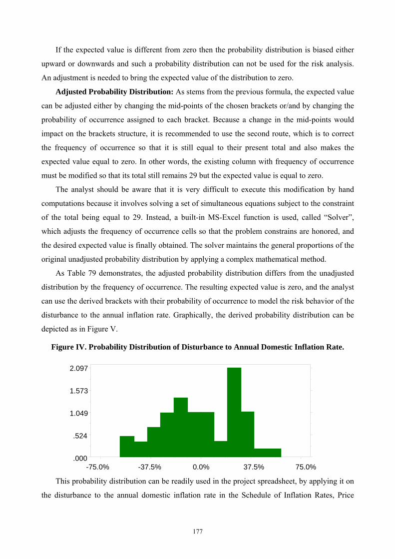
If the expected value is different from zero then the probability distribution is biased either
upward or downwards and such a probability distribution can not be used for the risk analysis.
An adjustment is needed to bring the expected value of the distribution to zero.
Adjusted Probability Distribution: As stems from the previous formula, the expected value
can be adjusted either by changing the mid-points of the chosen brackets or/and by changing the
probability of occurrence assigned to each bracket. Because a change in the mid-points would
impact on the brackets structure, it is recommended to use the second route, which is to correct
the frequency of occurrence so that it is still equal to their present total and also makes the
expected value equal to zero. In other words, the existing column with frequency of occurrence
must be modified so that its total still remains 29 but the expected value is equal to zero.
The analyst should be aware that it is very difficult to execute this modification by hand
computations because it involves solving a set of simultaneous equations subject to the constraint
of the total being equal to 29. Instead, a built-in MS-Excel function is used, called “Solver”,
which adjusts the frequency of occurrence cells so that the problem constrains are honored, and
the desired expected value is finally obtained. The solver maintains the general proportions of the
original unadjusted probability distribution by applying a complex mathematical method.
As Table 79 demonstrates, the adjusted probability distribution differs from the unadjusted
distribution by the frequency of occurrence. The resulting expected value is zero, and the analyst
can use the derived brackets with their probability of occurrence to model the risk behavior of the
disturbance to the annual inflation rate. Graphically, the derived probability distribution can be
depicted as in Figure V.
Figure IV. Probability Distribution of Disturbance to Annual Domestic Inflation Rate.
2.097
1.573
1.049
.524
.000 -75.0% -37.5% 0.0% 37.5% 75.0%
This probability distribution can be readily used in the project spreadsheet, by applying it on
the disturbance to the annual domestic inflation rate in the Schedule of Inflation Rates, Price
177
Indices and Exchange Rate. Note that this probability distribution can not be applied directly on
the annual inflation rate because it is rather expressed in terms of deviation from the expected
inflation rate. This way of modeling allows the analyst to be flexible to incorporate both the
expected trend of the variable as well as unexpected risk fluctuation around the trend:
iDYearX = iD
Expected, YearX * (1 + Disturbance to SA Inflation RateYearX)
Thus, annual inflation rate in year X is determined by the expected inflation rate and the
disturbance to it, to be generated during the risk simulation from the assigned probability
distribution.
8.1.2 Disturbance to South African Real Foreign Exchange Rate
The importance of this parameter has been marked as “high” in the sensitivity analysis and
because it is also fluctuates in an unpredictable manner from year to year; it becomes a candidate
for the risk analysis. The probability distribution of the foreign exchange rate movements can be
derived from the residuals of a regression made on the real exchange rate. Similarly to the
derivation of the probability distribution for the inflation rate, the procedure here starts with a set
of raw data, obtained from IMF (2000), which contains a historical record of the average annual
nominal exchange rate (Rand/US$) from 1970 to 1999. The same publication is the source of the
data for the South African consumer price index (CPI) during 1970-1999. Table 80 shows the
derivation of a probability distribution for the disturbance to South African real foreign exchange
rate.
Nominal vs. Real Exchange Rate: Most often the data on the exchange rates are stated in
their nominal form, rather than in real, and an additional transformation is needed to convert the
nominal exchange rates into the real rates, expressed in the same price level. This transformation
can be done through applying the following formula:
ERealYearX = ENominal
YearX * PIWorldYearX / CPISouth Africa
YearX
Where the real average exchange rate in year X is found as the nominal average exchange
rate (EReal) multiplied by the world price index (PIWorld) and then divided by the domestic
consumer price index (CPISouth Africa). While the nominal exchange rate and domestic price index
are usually available in the country macro-economic data, the world price index has to be
estimated by the analyst. The world price index used here was estimated by the Cambridge
Resources International and was based on the 1970-1999 forex data of the US dollar, UK pound,
178
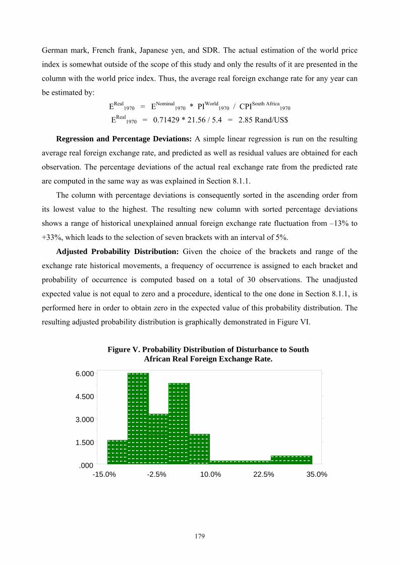
German mark, French frank, Japanese yen, and SDR. The actual estimation of the world price
index is somewhat outside of the scope of this study and only the results of it are presented in the
column with the world price index. Thus, the average real foreign exchange rate for any year can
be estimated by:
EReal1970 = ENominal
1970 * PIWorld1970 / CPISouth Africa
1970
EReal1970 = 0.71429 * 21.56 / 5.4 = 2.85 Rand/US$
Regression and Percentage Deviations: A simple linear regression is run on the resulting
average real foreign exchange rate, and predicted as well as residual values are obtained for each
observation. The percentage deviations of the actual real exchange rate from the predicted rate
are computed in the same way as was explained in Section 8.1.1.
The column with percentage deviations is consequently sorted in the ascending order from
its lowest value to the highest. The resulting new column with sorted percentage deviations
shows a range of historical unexplained annual foreign exchange rate fluctuation from –13% to
+33%, which leads to the selection of seven brackets with an interval of 5%.
Adjusted Probability Distribution: Given the choice of the brackets and range of the
exchange rate historical movements, a frequency of occurrence is assigned to each bracket and
probability of occurrence is computed based on a total of 30 observations. The unadjusted
expected value is not equal to zero and a procedure, identical to the one done in Section 8.1.1, is
performed here in order to obtain zero in the expected value of this probability distribution. The
resulting adjusted probability distribution is graphically demonstrated in Figure VI.
Figure V. Probability Distribution of Disturbance to South African Real Foreign Exchange Rate.
6.000
4.500
3.000
1.500
.000 -15.0% -2.5% 10.0% 22.5% 35.0%
179
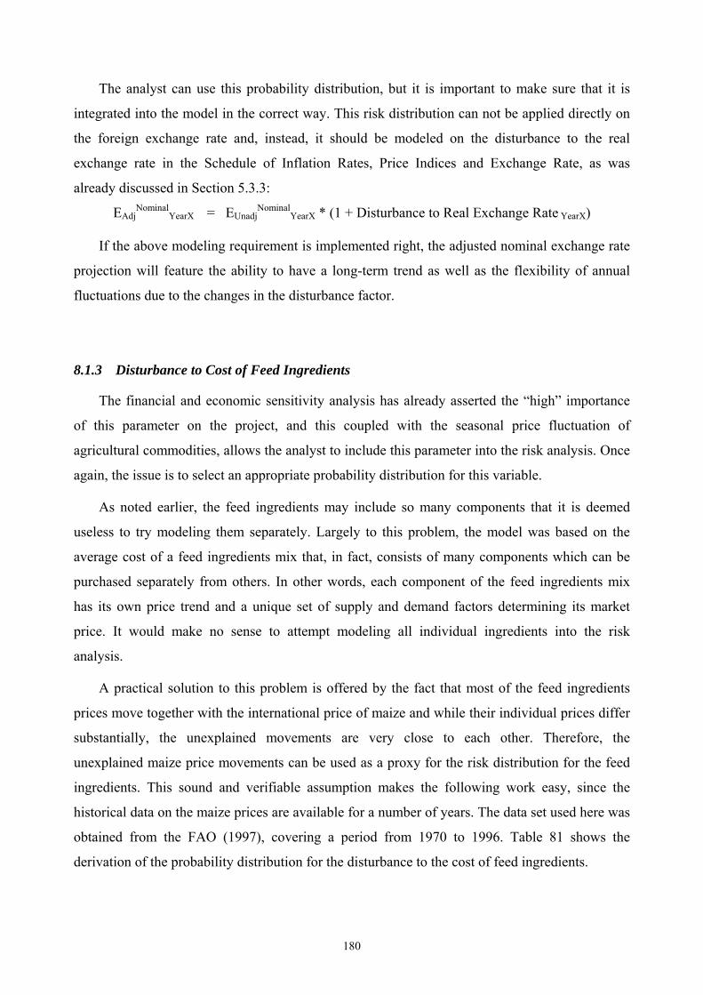
The analyst can use this probability distribution, but it is important to make sure that it is
integrated into the model in the correct way. This risk distribution can not be applied directly on
the foreign exchange rate and, instead, it should be modeled on the disturbance to the real
exchange rate in the Schedule of Inflation Rates, Price Indices and Exchange Rate, as was
already discussed in Section 5.3.3:
EAdjNominal
YearX = EUnadjNominal
YearX * (1 + Disturbance to Real Exchange Rate YearX)
If the above modeling requirement is implemented right, the adjusted nominal exchange rate
projection will feature the ability to have a long-term trend as well as the flexibility of annual
fluctuations due to the changes in the disturbance factor.
8.1.3 Disturbance to Cost of Feed Ingredients
The financial and economic sensitivity analysis has already asserted the “high” importance
of this parameter on the project, and this coupled with the seasonal price fluctuation of
agricultural commodities, allows the analyst to include this parameter into the risk analysis. Once
again, the issue is to select an appropriate probability distribution for this variable.
As noted earlier, the feed ingredients may include so many components that it is deemed
useless to try modeling them separately. Largely to this problem, the model was based on the
average cost of a feed ingredients mix that, in fact, consists of many components which can be
purchased separately from others. In other words, each component of the feed ingredients mix
has its own price trend and a unique set of supply and demand factors determining its market
price. It would make no sense to attempt modeling all individual ingredients into the risk
analysis.
A practical solution to this problem is offered by the fact that most of the feed ingredients
prices move together with the international price of maize and while their individual prices differ
substantially, the unexplained movements are very close to each other. Therefore, the
unexplained maize price movements can be used as a proxy for the risk distribution for the feed
ingredients. This sound and verifiable assumption makes the following work easy, since the
historical data on the maize prices are available for a number of years. The data set used here was
obtained from the FAO (1997), covering a period from 1970 to 1996. Table 81 shows the
derivation of the probability distribution for the disturbance to the cost of feed ingredients.
180
Nominal vs. Real Maize Prices: The first columns contain the annual observations of the
average yellow maize price delivered to the Maize Board in South Africa, and expressed in
nominal US dollars. These prices have to be converted into the real prices through dividing them
by the US producer price index, which was taken from the IMF [2000]. The resulting real
average yellow maize prices are expressed in the constant 1995 dollars, and can be used in a
regression.
Adjusted Probability Distribution: The mechanics of derivation of the adjusted probability
distribution for this parameter is the same as already demonstrated in the two preceding sections,
and its results are presented in Table 81. The adjusted probability distribution for disturbance to
cost of feed ingredients is graphically illustrated in Figure VII.
Figure VI. Probability Distribution of Disturbance to Cost of Feed Ingredients.
2.960
Once again, it should be noted that the correct way of introducing this parameter into the
model is to apply the derived probability distribution on the disturbance factor in the Schedule of
Feed Ingredients Costs and Feed Prices:
CAdjNominal
YearX = CUnadjNominal
YearX * (1 + Disturbance FactorYearX)
Thus, the adjusted nominal cost of feed ingredients in a certain year is a product of the
unadjusted nominal cost of feed ingredients and the annual disturbance factor, to be generated
during the risk simulation. The resulting adjusted nominal cost has both elements of the long-run
trend as well as an annual fluctuation around that trend.
.000
.740
1.480
2.220
-40.0% -17.5% 5.0% 27.5% 50.0%
181
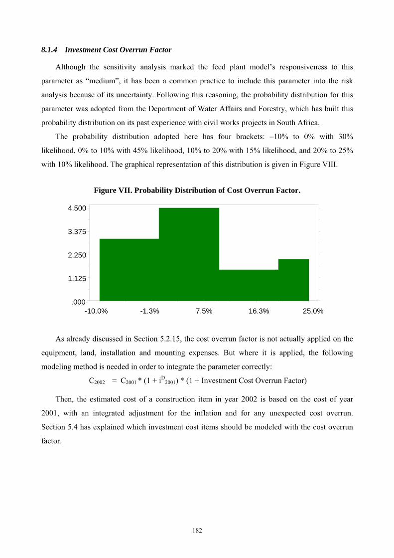
8.1.4 Investment Cost Overrun Factor
Although the sensitivity analysis marked the feed plant model’s responsiveness to this
parameter as “medium”, it has been a common practice to include this parameter into the risk
analysis because of its uncertainty. Following this reasoning, the probability distribution for this
parameter was adopted from the Department of Water Affairs and Forestry, which has built this
probability distribution on its past experience with civil works projects in South Africa.
The probability distribution adopted here has four brackets: –10% to 0% with 30%
likelihood, 0% to 10% with 45% likelihood, 10% to 20% with 15% likelihood, and 20% to 25%
with 10% likelihood. The graphical representation of this distribution is given in Figure VIII.
Figure VII. Probability Distribution of Cost Overrun Factor.
4.500
3.375
2.250
1.125
As already discussed in Section 5.2.15, the cost overrun factor is not actually applied on the
equipment, land, installation and mounting expenses. But where it is applied, the following
modeling method is needed in order to integrate the parameter correctly:
C2002 = C2001 * (1 + iD2001) * (1 + Investment Cost Overrun Factor)
Then, the estimated cost of a construction item in year 2002 is based on the cost of year
2001, with an integrated adjustment for the inflation and for any unexpected cost overrun.
Section 5.4 has explained which investment cost items should be modeled with the cost overrun
factor.
.000 -10.0% -1.3% 7.5% 16.3% 25.0%
182
8.2 Results of Risk Analysis
A Monte-Carlo simulation was performed with 10,000 runs. With each run a set of the
“input” variables was generated from their assigned probability distributions, and results of the
“forecasts” were recorded. The outcomes of the simulation can be described using a set of simple
statistics: mean, standard deviation, minimum and maximum values.
The mean of a set of outcomes is the expected value of the variable on which the risk
analysis is performed. If the mean of the simulated outcomes is too biased from the original
“static” value of the variable - then it tells us about a tendency that, in reality, the value of the
variable will be lower or higher than the original value. The standard deviation of a set of
outcomes describes the variability or dispersion of the outcomes around the expected value
(mean). A high standard deviation implies that it is more likely for an actual value of the variable
to be further away from the mean, i.e. outcome of project is more uncertain. The minimum and
maximum values specify the two extreme sides, up to which an actual outcome of a variable may
reach.
The risk analysis software simulates changes in the defined risk parameters and model’s
results are recorded as “risk forecasts”. The risk forecasts measuring the financial performance of
the project are the ADSCR ratios for years 2004, 2005 and 2006; the DSCR ration for year 2004;
the NPV of the real Cashflow Statement from the Owner’s Point of View. The risk forecasts
measuring the economic and distributive impacts of the project are: the NPV of the Statement of
Economic Resource Flows; the PV of total externalities as well as the PV of labor externalities,
and PV of government externalities from the Statement of Economic Externalities. Following this
division, Section 8.2.1 examines the risk results for the financial risk forecasts, and Section 8.2.2
evaluates the risk results for the economic and distributive modules.
8.2.1 Financial Module Results
The selection of the financial risk forecasts is not accidental, as they represent a specific
evaluation perspective on the feed project. Thus, the owner’s NPV represents the financial
performance of the project as perceived by the owner of this enterprise. The debt service ratios
are included to analyze the project’s performance from the banker’s point of view. The results of
Monte-Carlo risk simulation are displayed in Table X.
Table X. Risk Analysis Results for Financial Module.
183
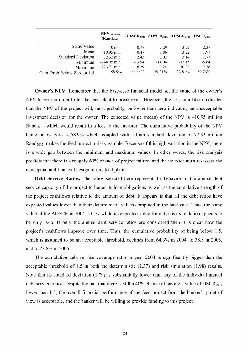
NPVOWNER(Rand2002)
ADSCR2004 ADSCR2005 ADSCR2006 DSCR2004
Static Value Mean
Standard Deviation Minimum Maximum
Cum. Prob. below Zero or 1.5
0 mln. -10.95 mln. 72.32 mln.
-244.95 mln. 223.71 mln.
58.9%
0.77 0.47 2.43
-13.54 6.29
64.44%
2.29 1.86 3.02
-14.04 9.24
39.21%
3.72 3.22 3.14
-13.15 10.92
23.81%
2.37 1.97 1.77
-5.64 7.38
39.76%
Owner’s NPV: Remember that the base-case financial model set the value of the owner’s
NPV to zero in order to let the feed plant to break even. However, the risk simulation indicates
that the NPV of the project will, most probably, be lower than zero indicating an unacceptable
investment decision for the owner. The expected value (mean) of the NPV is –10.95 million
Rand2002, which would result in a loss to the investor. The cumulative probability of the NPV
being below zero is 58.9% which, coupled with a high standard deviation of 72.32 million
Rand2002, makes the feed project a risky gamble. Because of this high variation in the NPV, there
is a wide gap between the minimum and maximum values. In other words, the risk analysis
predicts that there is a roughly 60% chance of project failure, and the investor must re-assess the
conceptual and financial design of this feed plant.
Debt Service Ratios: The ratios selected here represent the behavior of the annual debt
service capacity of the project to honor its loan obligations as well as the cumulative strength of
the project cashflows relative to the amount of debt. It appears is that all the debt ratios have
expected values lower than their deterministic values computed in the base case. Thus, the static
value of the ADSCR in 2004 is 0.77 while its expected value from the risk simulation appears to
be only 0.46. If only the annual debt service ratios are considered then it is clear how the
project’s cashflows improve over time. Thus, the cumulative probability of being below 1.5,
which is assumed to be an acceptable threshold, declines from 64.3% in 2004, to 38.8 in 2005,
and to 23.8% in 2006.
The cumulative debt service coverage ratio in year 2004 is significantly bigger than the
acceptable threshold of 1.5 in both the deterministic (2.37) and risk simulation (1.98) results.
Note that its standard deviation (1.79) is substantially lower than any of the individual annual
debt service ratios. Despite the fact that there is still a 40% chance of having a value of DSCR2004
lower than 1.5, the overall financial performance of the feed project from the banker’s point of
view is acceptable, and the banker will be willing to provide funding to this project.
184
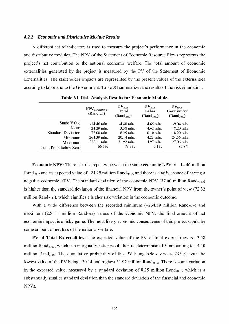
8.2.2 Economic and Distributive Module Results
A different set of indicators is used to measure the project’s performance in the economic
and distributive modules. The NPV of the Statement of Economic Resource Flows represents the
project’s net contribution to the national economic welfare. The total amount of economic
externalities generated by the project is measured by the PV of the Statement of Economic
Externalities. The stakeholder impacts are represented by the present values of the externalities
accruing to labor and to the Government. Table XI summarizes the results of the risk simulation.
Table XI. Risk Analysis Results for Economic Module.
NPVECONOMY(Rand2002)
PVEXTTotal
(Rand2002)
PVEXT Labor
(Rand2002)
PVEXT Government
(Rand2002)
Static Value Mean
Standard Deviation Minimum Maximum
Cum. Prob. below Zero
-14.46 mln. -24.29 mln. 77.00 mln.
-264.39 mln. 226.11 mln.
66.1%
-4.40 mln. -3.58 mln. 8.25 mln.
-20.14 mln. 31.92 mln.
73.9%
4.65 mln. 4.62 mln. 0.10 mln. 4.23 mln. 4.97 mln.
0.1%
-9.04 mln. -8.20 mln. -8.20 mln.
-24.56 mln. 27.06 mln.
87.8%
Economic NPV: There is a discrepancy between the static economic NPV of –14.46 million
Rand2002 and its expected value of –24.29 million Rand2002, and there is a 66% chance of having a
negative economic NPV. The standard deviation of the economic NPV (77.00 million Rand2002)
is higher than the standard deviation of the financial NPV from the owner’s point of view (72.32
million Rand2002), which signifies a higher risk variation in the economic outcome.
With a wide difference between the recorded minimum (–264.39 million Rand2002) and
maximum (226.11 million Rand2002) values of the economic NPV, the final amount of net
economic impact is a risky game. The most likely economic consequence of this project would be
some amount of net loss of the national welfare.
PV of Total Externalities: The expected value of the PV of total externalities is –3.58
million Rand2002, which is a marginally better result than its deterministic PV amounting to –4.40
million Rand2002. The cumulative probability of this PV being below zero is 73.9%, with the
lowest value of the PV being –20.14 and highest 31.92 million Rand2002. There is some variation
in the expected value, measured by a standard deviation of 8.25 million Rand2002, which is a
substantially smaller standard deviation than the standard deviation of the financial and economic
NPVs.
185
PV of Labor Externalities: The amount of labor-accruing externalities is not expected to
change much from the deterministic case, which results in the PV of 4.65 million Rand2002, to the
risk simulation expected value of 4.62 million Rand2002. There is a little variation recorded in the
expected value (0.10 million Rand2002), and the cumulative probability of the PV of labor
externalities is almost zero, i.e. the labor will definitely gain from the project.
PV of Government Externalities: A more complex picture is drawn on the externalities
allocated to the Government. The deterministic analysis resulted in an amount of –9.04 million
Rand2002 of externalities accruing to the National Government, and the risk simulation returned
an expected value of –8.20 Rand2002. The cumulative probability of the PV of Government’s
externalities being below zero is 87.8%, which means that while the expected PV of the
Government’s externalities is somewhat lower than in the deterministic case, there will be almost
a certain loss for the National Government.
186
9. CONCLUSIONS
This study has completed an integrated financial, economic, stakeholder, sensitivity and risk
analysis of the proposed animal feed plant in Polokwane. The plant is going to enter the existing
industry where a number of domestic manufacturers already compete for the consumer. The most
likely impact on the industry will be a reduction in the market share held by the existing feed
producers. The existing manufacturers will either have to exit the feed industry or to penetrate
further around Polokwane and, perhaps, even beyond. The findings of the analysis can be
summarized by sections, reflecting the structural organization of the study.
9.1 Financial Analysis
From the banker’s perspective, the feed plant would be an acceptable project to finance
under the proposed finance scheme. Because the lion’s share of the initial investment is financed
by the owners, the bank’s risk exposure is quite limited. The annual debt service ratios, except
the first loan repayment, are well above the 1.5 benchmark and the cumulative debt service ratios
are also pretty high. The bank can further reduce its risk by negotiating collateral in the form of
the title on the fixed assets of the plant. In short, this is an acceptable project from the banker’s
point of view.
For the owners of this plant, the evaluation is less conclusive in regard to actual profitability
of the enterprise, since the “break-even” approach was taken in order to find out the critical level
of the milling fee. But it is clear that with the given market feed prices and project’s cost
structure; the break-even value of the milling fee is 258.8 Rand2002/ton. If the plant actually
achieves or exceeds this margin, the owners will have a profitable business, while a failure to
maintain the break-even milling fee would mean a financial loss. A further insight into the
owner’s point of view is gained in the risk analysis.
9.2 Economic Analysis
The economic evaluation reveals that the project will have a negative impact on the
economy. The net present value of economic resource flows is –14.46 million Rand2002, which
means that the economic welfare will suffer a loss. This figure includes the financial cashflows
187
and estimated flows of externalities generated by the project. The largest amount of negative
externalities comes from the production of the feed, which causes an additional pressure on the
foreign exchange market through usage of tradable inputs. In other words, the negative
externalities are mostly caused by the premium on the additional foreign exchange transactions.
The project does not pay financially for this premium, and the economic costs are borne by all the
other economic agents in South Africa. Thus, the economic impact of the feed plant is negative,
and the National Government must consider whether it should support such projects.
9.3 Distributive Analysis
The estimated present value of economic externalities generated by the feed project amounts
to –4.00 million Rand2002, which is a considerable negative externality to the South African
economy. The allocation of this externality is such that the labor benefits by the estimated
amount of 4.65 million Rand2002, and the National Government incurs a loss amounting to 9.04
million Rand2002. The labor externalities are created by wages set at a higher level than the supply
price of labor. Most of the negative externality accrues to the National Government and this can
be again explained by the foreign exchange premium on the feed ingredients. The Government
does collect taxes on the investment and operating items of the project as well as the corporate
income tax, but the negative externality from the foreign exchange premium overweighs the tax
collections. Thus, the labor stands to enjoy some positive externalities due to the project, but the
National Government will suffer a much substantial loss.
9.4 Sensitivity Analysis
The model is very sensitive to the following parameters: change in cost of feed ingredients,
change in milling fee, economic opportunity cost of capital, foreign exchange premium,
disturbance factor to real exchange rate, domestic inflation rate, tax holiday duration, accounts
receivable, accounts payable, composite demand elasticity for meat, and supply elasticity of feed
by other manufacturers. Some parameters rather have a moderate impact on the project’s results
and such a list would include: investment cost overrun factor, method of finance, real interest
rate, and loan grace period. The model has a low responsiveness to changes in the following
parameters: foreign inflation rate, loan repayment period, labor real wage growth, and electricity
real charge growth.
188
9.5 Risk Analysis
The Monte-Carlo risk analysis, which was performed on the model, suggests that under the
risk simulation the project is likely to have even poorer performance than in the deterministic
financial and economic model. The expected values of the financial and economic flows are
lower than the computed net present values, and there is a 60% chance of project failure for the
owner’s point of view. Despite the fact that the model breaks even financially, the risk analysis
puts this under doubt. The expected value of the economic NPV and PV of total externalities are
also negative and it is unlikely to contribute a net benefit to the country’s welfare. The risk
analysis results confirm that labor is the net beneficiary of the project, while the National
Government will have to carry the burden of created negative externalities.
9.6 Overall Assessment
The overall evaluation of this project should warn the project owners about the substantial
degree of risk associated with the proposed feed plant, as the project may not be able to recoup
the capital invested. There could be ways to improve the project performance through skillful
management but the threat still remains, and all concerned parties must be aware of this.
The National Government may reconsider its incentives policy towards foreign investment in
order to make the grant rules more flexible and to create a better selection shield against projects
harming the competitive domestic producers. The particular issue of whether the grant is the most
appropriate form of incentive for foreign investment is very questionable. On the example of this
study, such a cash grant does not play a crucial role once the foreign investor is convinced to do
business in South Africa. This finding points out that some other business factors really shape the
investor’s decision to undertake a green-field project in the country, rather than the availability of
the grant itself.
It is also doubtful that the Government’s true intention is to support foreign investors in the
sectors where existing domestic producers are competitive. Such a case does not justify for the
direct government intervention and, instead, is likely to create an artificial distortion to the
market forces. The economic will lose due to a cut back in the production by the existing
domestic producers, while the foreign investor could be the one enjoying the benefits.
189
BIBLIOGRAPHY AND REFERENCES
AD-SC. (2002). Livestock Feed Requirements Study 1999–2000. Agriculture Division, Statistics Canada (AD-SC), Ottawa.
AFMA. (2000). National Feed Production in South Africa. Matrix AFMA, Animal Feed Manufacturers Association (AFMA), Rivonia, South Africa.
Aho, P. (2000). Outlook for Southeast Asia's Feed, Poultry and Livestock Industry. Poultry Perspective, Connecticut, USA.
Balakrishnan, V. (2002). Developments in the Indian Feed and Poultry Industry and Formulation of Rations Based on Local Resources. Department of Animal Nutrition, Madras Veterinary College, Chennai, India.
Balcombe, K.C. and Smith, L.E.D. (1999). “Redefining the Use of Monte-Carlo Techniques for Risk Analysis in Project Appraisal”. Journal of Development Studies, 36(2), December 1999, Pp. 113-135.
Briedenhann, E. (2000). South African Animal Feed Industry. EPOL, Centurion, South Africa.
Briedenhann, E. (2001). Raw Material Update for the South African Feed Industry. EPOL, Centurion, South Africa.
CARD. (1987). Evaluating Food Policy in Indonesia Using Full Demand Systems, Final Report, Centre for Agricultural and Rural Development (CARD), Iowa State University, Ames.
CAST. (1999). Animal Agriculture and Global Food Supply. Task Force Report No. 135, Council for Agricultural Science and Technology (CAST).
DA. (2001). Trends in the Agricultural Sector. Department of Agriculture, Pretoria, South Africa.
Decisioneering, Inc. (2000). Crystal Ball® 2000: User Manual. Decisioneering, Inc. Denver, Colorado, USA.
DFED. (2000). The Northern Province Industrial Development Strategy 2000. Department of Financial and Economic Development (DFED), Limpopo Provincial Government, Republic of South Africa.
DFED. [Manual] (2003). Manual for Economic and Financial Evaluation of Investment Expenditures in South Africa. Department of Financial and Economic Development (DFED), Limpopo Provincial Government, Republic of South Africa.
DFED. [Database] (2003). Electronic Database of Commodity Specific Economic Conversion Factors for South Africa. Department of Financial and Economic Development (DFED), Limpopo Provincial Government, Republic of South Africa.
190
DGA. (2002). Prospects for Agricultural Markets 2002 – 2009. Directorate - General for
Agriculture (DGA), European Commission, Brussels.
DSI. (2000). Abstract of Agricultural Statistics. The Directorate Statistical Information (DSI), Pretoria, South Africa.
Ekermans, L. (2001). Effect of the Free Market System on the Feed Industry. University of Stellenbosch, South Africa.
Eloff, T. (2001). The Economic Realities of the Game Industry in South Africa. Centre For Wildlife Economics, University of Potchefstroom, South Africa.
Fabiosa, J.F. and Ukhova, Y.S. (2000). New Aggregate and Source-Specific Pork Import Demand Elasticity for Japan: Implications to U.S. Exports. Working Paper 00-WP 253, Center for Agricultural and Rural Development (CARD), Iowa State University, Ames.
FAO. (1997). White Maize: A Traditional Food Grain in Developing Countries. International Maize and Wheat Improvement Center, Food and Agriculture Organization (FAO) of the United Nations, Washington, D.C.
Feuz, D. (2002). Improved Beef Demand Benefits Nebraska Cattle Producers. Panhandle Research and Extension Center, Institute of Agriculture & Natural Resources, Department of Agricultural Economics, University of Nebraska, Lincoln.
Gilbert, R. (2002). “Overview of World Protein Needs and Supply”, Paper Presented at the Expert Consultation and Workshop on Protein Sources for the Animal Feed Industry, FAO, Bangkok.
Griessel, M. (2001). Annual Sales of Animal Feed in South Africa: 1999-2000. Animal Feed Manufacturers Association (AFMA), Rivonia, South Africa.
Griessel, M. and Bekker, H. (2000). Historical Sales of Animal Feeds. Animal Feed Manufacturers Association (AFMA), Rivonia, South Africa.
Hasha, G. (2002). Livestock Feeding and Feed Imports in the European Union – A Decade of Change. Electronic Outlook Report from the Economic Research Service, United States Department of Agriculture.
Hanrahan, K.F. (2002). “A Fully Regular Model of Irish Meat Demand”, Paper Presented at the AES Annual Conference 2002, The University of Wales, Aberystwyth.
Jackson, M.E. (2001). Practical Aspects of Buying and Using Alternative Feed Ingredients. Chemgen Corp., Gaithersburg, USA.
Jooste, A. and Zyl, J. (1999). Regional Agricultural Trade and Changing Comparative Advantage in South Africa. Technical Paper No. 94, University of Pretoria, South Africa.
IMF. (2000). IMF Financial Statistics Yearbook 2000. International Monetary Fund (IMF), Washington, D.C.
Korman, V. (2001). A Willingness to Pay for Water Improvement in Famagusta, North Cyprus. Ph.D. Dissertation, Northeastern University, Boston, MA.
191
Loh, T.C. (2000). Livestock Production and Feed Industry in Malaysia. Animal Science
Department, Universiti Putra, UPM Serdang, Selangor, Malaysia.
Mbala, P.A. (2002). Short-Run Demand for Goat Meat in Cameroon. Institute for National Rural Development (INADER), University Centre of Dschang, Cameroon.
Nyirenda, D.B. (2000). Food Production in Sub-Saharan Africa: Opportunities for Feed and Food Production. School of Agricultural Sciences, University of Zambia.
Oanh, B.T. (2002). Description of Developments and Issues Relating to Livestock Production, Protein Supplies and the Feed Industries of Vietnam. Department of Agricultural and Forestry Extension, Ministry of Agriculture and Rural Development.
Safalaoh, A.C.L. (2002). “Livestock Production, Protein Sources and the Animal Feed Industry in Malawi”. Paper Presented at the Expert Consultation and Workshop on Protein Sources for the Animal Feed Industry, FAO, Bangkok.
SARS. (2002). Taxation in South Africa 2001/2 Tax Year. Law Administration, South African Revenue Service (SARS), Pretoria, South Africa.
Schroeder, T.C., Marsh, T.L. and Mintert, J. (2000). Beef Demand Determinants: A Research Summary. Agricultural Experiment Station and Cooperative Extension Service, Department of Agricultural Economics, Kansas State University.
Speedy, A.W. (2002). “Overview of World Feed Protein Needs and Supply”. Paper Presented at the Expert Consultation and Workshop on Protein Sources for the Animal Feed Industry, FAO, Bangkok.
Tabeau, A.A. (2001). Estimation of Feed Utilisation Matrices and Demand for Feed Using Farm Data. Report 8.01.01. Agricultural Economics Research Institute (LEI), The Hague.
Varley, R. (2000). Average Cost of Water to Rural Households. World Bank Development Papers, World Bank, Washington, D.C.
Wanapat, M. (2002). Current Livestock Production and Protein Sources as Animal Feeds in Thailand. Department of Animal Science, Faculty of Agriculture, Khon Kaen University, Thailand.
WB. (2001). World Bank Country Macroeconomic Data: South Africa (1971-2000). The World Bank, Washington, D.C.
Workman, J.P., Kings, S.L. and Hooper, J.F. (1971). Price Elasticity of Demand for Beef and Range Improvement Decisions, Department of Range Science, Utah University, Kansas.
192

ANNEX A
193